Embed Size (px)
Citation preview

EPA530-R-15-005
Industrial Waste Management Evaluation Model (IWEM) Version 3.1:
User’s Guide
June 2015
U.S. Environmental Protection Agency Office of Solid Waste and Emergency Response Office of Resource Conservation and Recovery

[This page intentionally left blank.]

IWEM User’s Guide Acknowledgements
iii
Acknowledgments Numerous individuals have contributed to the development of the IWEM software and documentation since IWEM version 1. At EPA, Mr. Taetaye Shimeles served as Work Assignment Manager for the current version of the model, providing directions and technical assistance, and is also a contributing author. Dr. Zubair Saleem, Ms. Ann Johnson, and Mr. David Cozzie had filled this role for the past versions. A variety of other EPA staff have provided additional technical guidance and suggestions, including Dr. Peter Grevatt, Dr. Lee Hofmann, Dr. Colette Hodes, Mr. Richard Kinch, Mr. Jason Mills, Mr. John Sager, Mr. Timothy Taylor, Ms. Shen-Yi Yang, and Ms. Janvier Young. The EPA has been assisted in the development of IWEM by several contractors: RTI International, HydroGeoLogic, and Resource Management Concepts, Inc.
.

IWEM User’s Guide Software Development History and Online Resources
iv
Software Development History The Industrial Waste Management Evaluation Model (IWEM 3.1) is the latest version of a ground water fate and transport developed by the U.S. EPA’s Office of Resource Conservation and Recovery (ORCR). IWEM, since its initial development in 2002, has undergone a number changes and revisions. Some of the changes were done to expand the scope of the model from modeling just waste management units, but also to evaluate potential contaminants releases from recycled industrial materials used in beneficial use applications. Additional revisions were also made to increase the usability the model, and allow greater control over the input parameters for the user. The changes and revisions made the model more flexible, user friendly as well as usable by various stakeholders. Brief descriptions of the major changes made to model since its initial release are presented below. The original IWEM 1.0 (U.S. EPA 2002a, b) was developed as part of the Guide for Industrial Waste Management (U.S. EPA, 2002c) to conduct two levels of screening analyses (Tier 1 and Tier 2) to determine the most appropriate liner design for several types of waste management units in order to minimize or avoid adverse ground water impacts. In Tier 1, the analysis reflected national distribution of waste management units and site conditions that affect the fate and transport of constituents in subsurface media. On the other hand, site-specific parameters were required for key parameters in the Tier 2 probabilistic analysis. This version was based on Version 2.0 of the U.S. Environmental Protection Agency’s (EPA’s) Composite Model for Leachate Migration and Transformation Products (EPACMTP) code (U.S. EPA, 2003a, b), which included the vadose-zone and aquifer modules developed under the Multimedia, Multipathway, Multireceptor Exposure and Risk Assessment (3MRA) framework (U.S. EPA, 1999).1
In 2006, building on version 1, IWEM 2.0 was developed by adding a module to simulate fate and transport from a new source type—a roadway constructed using recycled industrial materials (i.e., byproducts). The new source type was restricted to Tier 2 analyses. In addition to the new roadway source, IWEM 2.0 used the latest version of EPACMTP, Version 2.2, without modification. EPACMTP Version 2.2 includes non-science related changes to the input and output streams of EPACMTP Version 2.1 (U.S. EPA 2003c, d).
IWEM 3.0 enhanced the functionality of its predecessor, by introducing a more rigorous treatment of leaching through the roadway cross section by including ditches, drainage, and surface runoff as optional elements. The graphical user interface was also modified to accommodate the improved source type. In addition, two significant revisions were made to the model, which included the following:
Tier 1 analysis for waste management units was eliminated. The leachate concentration threshold values stored in the IWEM database and used for Tier 1 analyses were based on human health benchmarks (e.g., reference doses and slope factors) that were current as of 2002 when IWEM 1.0 was released. To avoid generating a “protective” liner
1 IWEM 1.0 and EPACMTP 2.0 were developed and tested concurrently, whereas the supporting documentation
for IWEM 1.0 was released prior to EPACMTP 2.0 documentation.

IWEM User’s Guide Software Development History and Online Resources
v
recommendation based on an out-of-date benchmark, the Agency opted to remove the Tier 1 analysis option from Version 3.0.
Built-in human health benchmarks, with the exception of maximum contaminant levels (MCLs), have been removed from the database.
This decision resulted in two significant changes to the model: (1) only Tier 2 analyses are now available in the software, so references to Tier 2 and the “tiered approach” were removed from the software and documentation; and (2) other than MCLs, the user is now required to provide human health benchmarks for the screening evaluation.
The current IWEM 3.1, replaces IWEM 3.0. IWEM 3.1adds a new module to simulate leaching from a structural fill to evaluate the beneficial reuse of industrial or combustion byproducts in the construction of the structural fill. Structural fills evaluated by IWEM include the use of industrial wastes and related byproducts as substitutes for the earthen materials to provide structural support for parking lots, roads, airstrips, tanks/vaults, and buildings; construction of highway embankments and bridge abutments; filling of borrow pits, and other landscape irregularities; and changing the landscape for development or reclamation projects.
Online Resources EPA’s Nonhazardous Industrial Waste Management tools web page (http://www.epa.gov/waste/nonhaz/industrial/tools/index.htm) provides links to the Guide for Industrial Waste Management, IWEM, and EPACMTP. The linked IWEM page provides links to the model itself as well as this User’s Guide and the Technical Background Document.

IWEM User’s Guide Format and Notation
vi
Format and Notation The main font for this document is 12-point Times New Roman font. The Industrial Waste Management Evaluation Model (IWEM) command buttons, icons, menu items and other action-controls are shown in 11-point Arial Narrow font, with small capitals style and with vertical bars at the beginning and end; for example, |FILE| and |EVALUATION| are two of the menu items contained in the IWEM menu bar. When referring to a sequential series of menu selections, such as “click on File, then click on Open,” this sequence of keystrokes is presented as |FILE|OPEN|.
IWEM screen and dialog box titles are presented in underlined text, and user-entry labels are using the same format as IWEM menu items and other action-controls.
The IWEM software is organized into screens and dialog boxes and, for easy reference, these components are labeled using a common numbering scheme. Within the main IWEM program window, there are a number of screens that are displayed one at a time as you move through an IWEM analysis. Each of these screens has a title that tells you what part of the IWEM software you are in; if the IWEM screen is stretched to fill the IWEM program window, then the title bar containing these titles is located directly beneath the IWEM toolbar. Additionally, within some of these screens there are several tabbed screens that resemble tabbed file folders. Each of these tabbed screens has a title (placed on the screen itself) that tells you more specifically what type of information is being requested or displayed on the screen. We refer to all screens and tabbed screens in this document simply as screens. Finally, when you use certain options on the Source Parameters (7), Infiltration (9), and Constituent List (10) screens, dialog boxes are displayed to allow entry of additional information. Each of these dialog boxes has a title (placed on the title bar at the top of the dialog box) that identifies the type of information requested.
Although there are other ways to navigate through the IWEM software, it is anticipated that most users will generally start at the beginning of an analysis and then move through the screens sequentially using the |NEXT| and |BACK| buttons. In order to facilitate the reporting of user comments and problems, EPA has organized all IWEM components into one common sequential numbering scheme according to the order in which they would be displayed in a typical analysis. Hence, a user will typically see the following sequence of screens and dialog boxes (however, there are some slight differences in this sequence depending upon the source type and infiltration option chosen by the user):
Input screen group (tabbed screens 6 through 13) EPACMTP Run Manager located on the Evaluation Screen (screen 14) Output tabs (tabbed screens 15 through 18) Evaluation Summary Screen (screen 19).
Please note that the screenshots presented in this User’s Guide reflect specific monitor and system settings. Your computer’s settings may be different, so you may need to use the sliders that appear as necessary on the right and bottom edge of the IWEM windows in order to see the entire screen.
IWEM User’s Guide Acronyms
vii
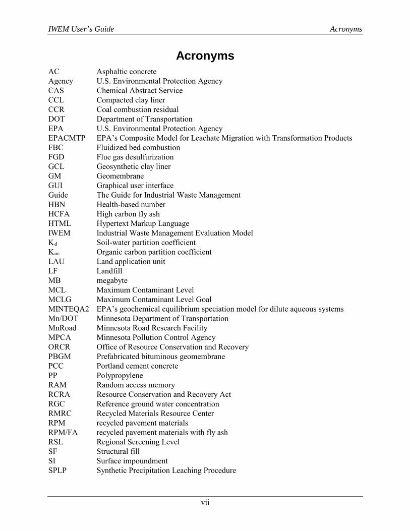
Acronyms AC Asphaltic concrete Agency U.S. Environmental Protection Agency CAS Chemical Abstract Service CCL Compacted clay liner CCR Coal combustion residual DOT Department of Transportation EPA U.S. Environmental Protection Agency EPACMTP EPA’s Composite Model for Leachate Migration with Transformation Products FBC Fluidized bed combustion FGD Flue gas desulfurization GCL Geosynthetic clay liner GM Geomembrane GUI Graphical user interface Guide The Guide for Industrial Waste Management HBN Health-based number HCFA High carbon fly ash HTML Hypertext Markup Language IWEM Industrial Waste Management Evaluation Model Kd Soil-water partition coefficient Koc Organic carbon partition coefficient LAU Land application unit LF Landfill MB megabyte MCL Maximum Contaminant Level MCLG Maximum Contaminant Level Goal MINTEQA2 EPA’s geochemical equilibrium speciation model for dilute aqueous systems Mn/DOT Minnesota Department of Transportation MnRoad Minnesota Road Research Facility MPCA Minnesota Pollution Control Agency ORCR Office of Resource Conservation and Recovery PBGM Prefabricated bituminous geomembrane PCC Portland cement concrete PP Polypropylene RAM Random access memory RCRA Resource Conservation and Recovery Act RGC Reference ground water concentration RMRC Recycled Materials Resource Center RPM recycled pavement materials RPM/FA recycled pavement materials with fly ash RSL Regional Screening Level SF Structural fill SI Surface impoundment SPLP Synthetic Precipitation Leaching Procedure

IWEM User’s Guide Acronyms
viii
STORET EPA’s Data Storage and Retrieval System, National Water Quality Database TBD IWEM 3.1 Technical Background Document (U.S. EPA, 2015a) TCLP Toxicity Characteristic Leaching Procedure WMU Waste management unit WSH Washington State Highway WP Waste pile
Units of Measure
This User’s Guide uses the following abbreviations for standard units of measures; these may be found in combination. In some instances, general units (e.g., length per time) may be used and in others, specific units (e.g., m/sec). Superscripts indicate the unit is squared (e.g., m2) or cubed (e.g., m3).
Specific units: µg microgram cm centimeter day day g gram ha hectare hr hour kg kilogram km kilometer L liter (if used with other specific
units, as mg/L) m meter mg milligram min minutes mL milliliter mm millimeter mo month sec second yd yard yr year
General units: L General unit for length (if used with
other general units, as M/L3) M General unit for mass M/L3 General unit for mass concentration
(mass per length cubed) M/M General unit for mass fraction (mass
per mass) T General unit for time Common Conversion Factors 1 acre = 4,047 m2 1 ha = 10,000 m2 1 ft2 = 0.093 m2 1 mile = 1,609 m 1 yd = 0.914 m 1 ft = 0.305 m 1 in = 0.0254 m 1 m/sec = 31,536,000 m/yr 1 cm/sec = 315,576 m/yr 1 ft/sec = 9,612,173 m/yr 1 ft/yr = 0.305 m/yr 1 in/yr = 0.0254 m/yr 1 gal/ft2/day = 14.89 m/yr
IWEM User’s Guide Table of Contents
ix
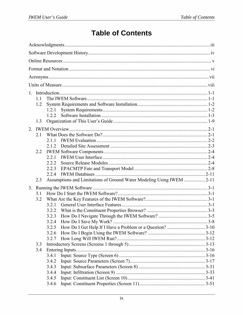
Table of Contents Acknowledgments .......................................................................................................................... iii
Software Development History ...................................................................................................... iv
Online Resources ............................................................................................................................ v
Format and Notation ...................................................................................................................... vi
Acronyms ...................................................................................................................................... vii
Units of Measure .......................................................................................................................... viii
1. Introduction ............................................................................................................................ 1-1 1.1 The IWEM Software ..................................................................................................... 1-1 1.2 System Requirements and Software Installation ........................................................... 1-2
1.2.1 System Requirements ........................................................................................ 1-2 1.2.2 Software Installation ......................................................................................... 1-3
1.3 Organization of This User’s Guide ............................................................................... 1-9
2. IWEM Overview .................................................................................................................... 2-1 2.1 What Does the Software Do? ........................................................................................ 2-1
2.1.1 IWEM Evaluation ............................................................................................. 2-2 2.1.2 Detailed Site Assessment .................................................................................. 2-3
2.2 IWEM Software Components ....................................................................................... 2-4 2.2.1 IWEM User Interface ........................................................................................ 2-4 2.2.2 Source Release Modules ................................................................................... 2-4 2.2.3 EPACMTP Fate and Transport Model ............................................................. 2-8 2.2.4 IWEM Databases ............................................................................................ 2-11
2.3 Assumptions and Limitations of Ground Water Modeling Using IWEM .................. 2-11
3. Running the IWEM Software ................................................................................................ 3-1 3.1 How Do I Start the IWEM Software? ........................................................................... 3-1 3.2 What Are the Key Features of the IWEM Software?.................................................... 3-1
3.2.1 General User Interface Features ........................................................................ 3-1 3.2.2 What is the Constituent Properties Browser? ................................................... 3-3 3.2.3 How Do I Navigate Through the IWEM Software? ......................................... 3-5 3.2.4 How Do I Save My Work? ............................................................................... 3-8 3.2.5 How Do I Get Help If I Have a Problem or a Question? ................................ 3-10 3.2.6 How Do I Begin Using the IWEM Software? ................................................ 3-12 3.2.7 How Long Will IWEM Run? .......................................................................... 3-12
3.3 Introductory Screens (Screens 1 through 5) ................................................................ 3-13 3.4 Entering Inputs ............................................................................................................ 3-16
3.4.1 Input: Source Type (Screen 6) ........................................................................ 3-16 3.4.2 Input: Source Parameters (Screen 7) ............................................................... 3-17 3.4.3 Input: Subsurface Parameters (Screen 8) ........................................................ 3-31 3.4.4 Input: Infiltration (Screen 9) ........................................................................... 3-33 3.4.5 Input: Constituent List (Screen 10) ................................................................. 3-41 3.4.6 Input: Constituent Properties (Screen 11) ....................................................... 3-51
IWEM User’s Guide Table of Contents
x
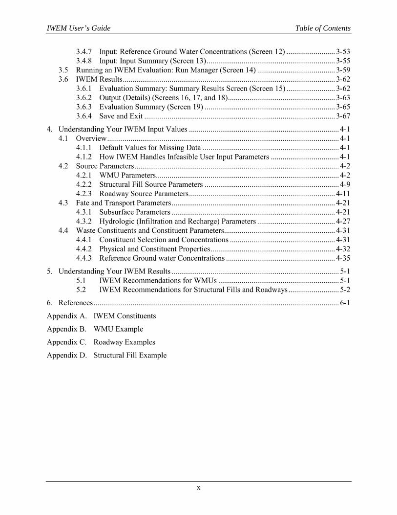
3.4.7 Input: Reference Ground Water Concentrations (Screen 12) ......................... 3-53 3.4.8 Input: Input Summary (Screen 13) .................................................................. 3-55
3.5 Running an IWEM Evaluation: Run Manager (Screen 14) ........................................ 3-59 3.6 IWEM Results ............................................................................................................. 3-62
3.6.1 Evaluation Summary: Summary Results Screen (Screen 15) ......................... 3-62 3.6.2 Output (Details) (Screens 16, 17, and 18) ....................................................... 3-63 3.6.3 Evaluation Summary (Screen 19) ................................................................... 3-65 3.6.4 Save and Exit .................................................................................................. 3-67
4. Understanding Your IWEM Input Values ............................................................................. 4-1 4.1 Overview ....................................................................................................................... 4-1
4.1.1 Default Values for Missing Data ...................................................................... 4-1 4.1.2 How IWEM Handles Infeasible User Input Parameters ................................... 4-1
4.2 Source Parameters ......................................................................................................... 4-2 4.2.1 WMU Parameters .............................................................................................. 4-2 4.2.2 Structural Fill Source Parameters ..................................................................... 4-9 4.2.3 Roadway Source Parameters ........................................................................... 4-11
4.3 Fate and Transport Parameters .................................................................................... 4-21 4.3.1 Subsurface Parameters .................................................................................... 4-21 4.3.2 Hydrologic (Infiltration and Recharge) Parameters ........................................ 4-27
4.4 Waste Constituents and Constituent Parameters......................................................... 4-31 4.4.1 Constituent Selection and Concentrations ...................................................... 4-31 4.4.2 Physical and Constituent Properties ................................................................ 4-32 4.4.3 Reference Ground water Concentrations ........................................................ 4-35
5. Understanding Your IWEM Results ...................................................................................... 5-1 5.1 IWEM Recommendations for WMUs .............................................................. 5-1 5.2 IWEM Recommendations for Structural Fills and Roadways .......................... 5-2
6. References .............................................................................................................................. 6-1
Appendix A. IWEM Constituents
Appendix B. WMU Example
Appendix C. Roadway Examples
Appendix D. Structural Fill Example
IWEM User’s Guide Table of Contents
xi
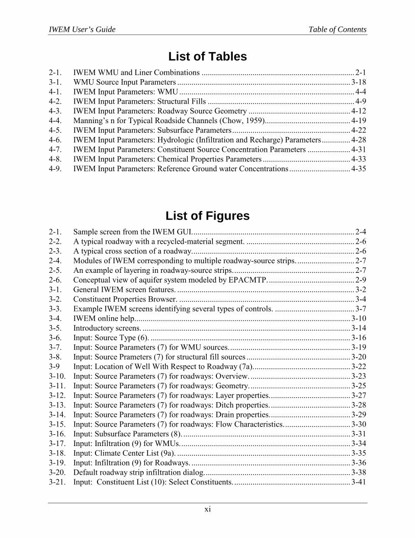
List of Tables 2-1. IWEM WMU and Liner Combinations ........................................................................... 2-1 3-1. WMU Source Input Parameters ..................................................................................... 3-18 4-1. IWEM Input Parameters: WMU ...................................................................................... 4-4 4-2. IWEM Input Parameters: Structural Fills ........................................................................ 4-9 4-3. IWEM Input Parameters: Roadway Source Geometry .................................................. 4-12 4-4. Manning’s n for Typical Roadside Channels (Chow, 1959) .......................................... 4-19 4-5. IWEM Input Parameters: Subsurface Parameters .......................................................... 4-22 4-6. IWEM Input Parameters: Hydrologic (Infiltration and Recharge) Parameters .............. 4-28 4-7. IWEM Input Parameters: Constituent Source Concentration Parameters ..................... 4-31 4-8. IWEM Input Parameters: Chemical Properties Parameters ........................................... 4-33 4-9. IWEM Input Parameters: Reference Ground water Concentrations .............................. 4-35
List of Figures 2-1. Sample screen from the IWEM GUI. ............................................................................... 2-4 2-2. A typical roadway with a recycled-material segment. ..................................................... 2-6 2-3. A typical cross section of a roadway. ............................................................................... 2-6 2-4. Modules of IWEM corresponding to multiple roadway-source strips. ............................ 2-7 2-5. An example of layering in roadway-source strips. ........................................................... 2-7 2-6. Conceptual view of aquifer system modeled by EPACMTP. .......................................... 2-9 3-1. General IWEM screen features. ....................................................................................... 3-2 3-2. Constituent Properties Browser. ...................................................................................... 3-4 3-3. Example IWEM screens identifying several types of controls. ....................................... 3-7 3-4. IWEM online help. ......................................................................................................... 3-10 3-5. Introductory screens. ...................................................................................................... 3-14 3-6. Input: Source Type (6). .................................................................................................. 3-16 3-7. Input: Source Parameters (7) for WMU sources. ........................................................... 3-19 3-8. Input: Source Prameters (7) for structural fill sources ................................................... 3-20 3-9 Input: Location of Well With Respect to Roadway (7a). ............................................... 3-22 3-10. Input: Source Parameters (7) for roadways: Overview. ................................................. 3-23 3-11. Input: Source Parameters (7) for roadways: Geometry. ................................................. 3-25 3-12. Input: Source Parameters (7) for roadways: Layer properties. ....................................... 3-27 3-13. Input: Source Parameters (7) for roadways: Ditch properties. ....................................... 3-28 3-14. Input: Source Parameters (7) for roadways: Drain properties. ....................................... 3-29 3-15. Input: Source Parameters (7) for roadways: Flow Characteristics. ................................ 3-30 3-16. Input: Subsurface Parameters (8). .................................................................................. 3-31 3-17. Input: Infiltration (9) for WMUs. ................................................................................... 3-34 3-18. Input: Climate Center List (9a). ..................................................................................... 3-35 3-19. Input: Infiltration (9) for Roadways. .............................................................................. 3-36 3-20. Default roadway strip infiltration dialog. ....................................................................... 3-38 3-21. Input: Constituent List (10): Select Constituents. ......................................................... 3-41

IWEM User’s Guide Table of Contents
xii
3-22. Input: Constituent List (10): Enter Leachate Concentrations for WMUs and structural fills. ................................................................................................................ 3-43
3-23. Input: Constituent List (10): Enter Leachate Concentrations for Roadway Strips. ........ 3-45 3-24. Input: Enter New Constituent Data (10a). ..................................................................... 3-47 3-25. Input: New Constituent Data (10b). ............................................................................... 3-48 3-26. Input: Add New Reference (10c). .................................................................................. 3-49 3-27. Input: Constituent Properties (11). ................................................................................. 3-50 3-28. Input: Reference Ground Water Concentrations (12). ................................................... 3-52 3-29. Input: Reference Ground Water Concentrations: Edit HBNs (12a). .............................. 3-53 3-30. Input: Input Summary (13): WMUs. ............................................................................. 3-55 3-31. Input: Input Summary (13) – Roadways. ....................................................................... 3-56 3-32. Evaluation: Run Manager (14). ...................................................................................... 3-58 3-33. Evaluation: EPACMTP dialog box displayed during model execution. ....................... 3-59 3-34. Output (Summary): Summary Results (15). .................................................................. 3-61 3-35. Output (Details): Results (16). ...................................................................................... 3-63 3-36. Evaluation Summary (19). ............................................................................................. 3-64 4-1. WMU types modeled in IWEM. ...................................................................................... 4-3 4-2. WMU with base below ground surface. ........................................................................... 4-6 4-3. Position of the modeled well relative to the WMU. ........................................................ 4-8 4-4. A typical roadway with a recycled-material segment. ................................................... 4-11 4-5. Sample road design cross-section. ................................................................................. 4-11 4-6. Diagrams used by IWEM to specify roadway geometry. ............................................... 4-14 4-7. Example roadway source diagram. ................................................................................ 4-15 4-8. Example of invalid receptor location after geometric transformation. .......................... 4-16 4-9. Locations of IWEM climate stations. ............................................................................ 4-29

IWEM User’s Guide Introduction
1-1
1. Introduction This document describes how to use the Industrial Waste Management Evaluation Model version 3.1 (IWEM 3.1). IWEM is a ground water screening model developed by the U.S. Environmental Protection Agency’s (EPA’s) Office of Resource Conservation and Recovery (ORCR)—formerly the Office of Solid Waste—for the management of non-hazardous industrial wastes. A companion document, the Industrial Waste Management Evaluation Model version 3.1: Technical Background Document (U.S. EPA, 2015a), provides technical background information. EPA strongly recommends that you take the time to understand the technical background of IWEM before using the model to make the best use of this program.
The objective of this User’s Guide is to provide the information necessary to perform an IWEM evaluation. The rest of this section provides an overview of the software (Section 1.1), system requirements and instructions for installing the software (Section 1.2), and the organization of the rest of the User’s Guide (Section 1.3).
If you have downloaded a copy of the User’s Guide, you can open and read it on-screen while the IWEM software is running on your computer. You may, however, find it easier to use IWEM’s online help or to print out a copy of the User’s Guide and refer to this hard copy while you are using the software.
1.1 The IWEM Software IWEM is a ground water screening model that uses hydrogeological settings, source characteristic, and leachate concentrations to evaluate and recommend the type of liner system that would be appropriate for industrial waste disposal facilities, or to evaluate the appropriateness of the beneficial use of industrial materials in structural fills and roadways. In the case of Waste Management Units (WMUs) – landfills, waste piles, surface impoundment, and land application units – this software helps you compare the ground water protection afforded by various liner systems for WMUs with the anticipated waste leachate concentrations, so that you can determine the minimum liner system required to be protective of human health and ground water resources. In the case of beneficial use of industrial materials in structural fills or roadways, it can help you determine whether or not the reuse of industrial materials in structural fills or roadways is appropriate.
The anticipated users of the IWEM computer program are managers of proposed or existing units, state regulators, interested private citizens, and community groups. For example:
Managers of a proposed unit could use the software to determine what type of liner would be appropriate for the particular type of waste that is expected at the WMU and the particular hydrogeologic characteristics of the site.
Managers of an existing unit could use the software to determine whether or not to accept a particular waste at that WMU by evaluating the performance of the existing liner design.
Managers of a structural fill or roadway project could use the software to determine an appropriate fill or roadway design incorporating industrial waste materials.

IWEM User’s Guide Introduction
1-2
State regulators could use the software in developing permit conditions for a WMU or deciding whether to allow the use of industrial materials in a particular structural fill or roadway design.
Interested members of the public or community groups could use the software to evaluate a particular WMU, a structural fill design, or a roadway design, and participate during the permitting process.
An IWEM analysis is a location-based screening analysis that uses a limited set of the most sensitive waste- and site-specific data to model the fate and transport of waste constituents through subsurface soils, ground water, and to a receptor well.1 The outcome of the analysis is a liner recommendation for WMU that protects human health and the environment, or a determination on the appropriateness of reusing industrial materials in a structural fill or a roadway. As with all modeling, the model outputs, interpretation of the results, and the recommendations should be taken with the consideration of the assumptions underlying the model and the adequacy of the input data. The user should familiarize themselves with the limitations and assumptions of the model (discussed in Sections 3 and 4 of the Technical Background Document) for appropriate use of the tool.
The unique aspect of the IWEM software is that it allows you to perform screening analyses and obtain recommendations with minimal data requirements. However, in some cases, this may not be sufficient, and a comprehensive and detailed site assessment will be needed. Such an assessment cannot be done using IWEM. If you are interested in conducting a more detailed analysis, you should consult with the appropriate state agency for information regarding the selection of an appropriate ground water fate and transport model.
1.2 System Requirements and Software Installation
1.2.1 System Requirements The IWEM software is designed to run under the Microsoft Windows operating system. The minimum system requirements for IWEM 3.1 are:
i586, Pentium, or compatible processor-based personal computer (Pentium III @ 500 MHz or greater is recommended)
128 MB of RAM At least 100 MB of available hard disk space A printer for generating hard-copy reports.
The IWEM 3.1 software and installation package are compatible with the following combinations of Windows operating system:
Windows XP Professional SP3 Windows Vista Pro (64-bit, 32-bit) Windows 7 Pro (64-bit, 32-bit) Windows 8 (64-bit).
1 In IWEM, the term “well” is used to represent an actual or hypothetical ground water monitoring well or drinking
water well, downgradient from a WMU or roadway source.

IWEM User’s Guide Introduction
1-3
If you encounter any problems installing or running IWEM installation, and you are using a version of Windows not on the list above (e.g., XP 2002), visit the Microsoft Support web site at http://support.microsoft.com, and click on the |RUN WINDOWS UPDATES| link and follow the prompts to download the latest updates to your version of Windows. IWEM may run fine on older versions of Windows, but has not been tested for compatibility with them.
If your operating system version is up-to-date and you still encounter problems installing or running the IWEM software, please contact the Resource Conservation and Recovery Act (RCRA) Information Center in any of the following ways:
E-mail: [email protected] Phone: 703-603-9230 Fax: 703-603-9234 In person: Hours: 8:30 am to 4:30 pm, weekdays, closed on Federal holidays Location: WJC West Building
1301 Constitution Avenue, NW Room 3334 Washington, DC 20004
Mail: U.S. Environmental Protection Agency
EPA Docket Center RCRA Docket, Mail Code 28221T 1200 Pennsylvania Avenue, NW Washington, DC 20460-0002
When contacting the RCRA Information Center, please cite RCRA Docket number: F1999-IDWA-FFFFF.
1.2.2 Software Installation To use the IWEM software, you must download the software from the EPA’s non-hazardous industrial waste website (http://www.epa.gov/industrialwaste/ – look for a link to Tools) and install it on your hard-drive. Depending on the security settings of your operating system, if your computer is connected to a network, this software may need to be installed (and any previous version uninstalled) by someone with administrator privileges. Instructions for installing and uninstalling the program are provided below. Any updates to these instructions are located on the website. If you have difficulty implementing the instructions below, please see your network administrator for help, or contact the RCRA Information Center as explained in Section 1.2.1, System Requirements.
The steps for installing and using IWEM 3.1 are as follows:
Step A – Uninstall Previous Installation of IWEM 1.0 or 2.0 Step B – Install IWEM 3.1.
If IWEM is not currently installed on your system, begin with Step B.
Step A – Uninstall Previous Installation of IWEM

IWEM User’s Guide Introduction
1-4
To ensure that the all of the supporting software components are up to date and compatible with IWEM 3.1, you must uninstall any previous installations of IWEM before installing the new version. To uninstall a previous installation (note that differences for Windows 7 are shown in parentheses):
1. Click on the Windows |START| button in the extreme lower left corner of your screen. 2. Select |SETTINGS|, and then select |CONTROL PANEL| (for Windows 7, select |CONTROL PANEL|
directly). 3. Double-click on |ADD/REMOVE PROGRAMS| (for Windows 7, select |PROGRAMS AND FEATURES|). 4. Select |IWEM|, and then click on the |CHANGE/REMOVE| button (for Windows 7, select the
|UNINSTALL| button at the top of the software list). 5. The IWEM Uninstall screen will appear. If IWEM is currently running, please close it
before proceeding. If you are ready to uninstall, click |NEXT|, otherwise click |CANCEL|. The uninstaller will begin removing IWEM. Click |Finish| when the process is complete. Note: A dialog box will appear during the uninstall process that will ask if you want to Remove Shared Components. These are system files that are specific to IWEM and can be deleted—select |YES TO ALL|.
6. If you do not encounter any un-installation problems, the IWEM program will be removed from the list of programs on the |ADD/REMOVE PROGRAMS| dialog box, and you can proceed to Step B, Install IWEM 3.1. However, if you do experience un-installation problems, please see your computer system administrator for help, or contact the EPA Docket Center, as explained in Section 1.2.1, System Requirements, of this document.
Step B – Install IWEM 3.1 The following steps provide instructions for installing IWEM 3.1:
1. Close all applications, such as word processing and e-mail programs. If you encounter any problems while installing IWEM 3.1, please contact your System Administrator for help. It is possible that a conflict with virus protection software may be responsible, or you may not have the correct user permissions to install software on your computer. If you do not have a System Administrator, and you choose to close or disable virus protection software, please do so ONLY after obtaining a copy of the setup file from the Internet. Once you have installed IWEM 3.1, restart or enable your virus protection software.
2. Download the IWEM 3.1 installation file. The file can be found here: http://www.epa.gov/epawaste/nonhaz/industrial/tools/iwem/index.htm. To download it, go to Download Model Files and User’s Guide, then click on the file name (IWEM_Installation.exe). If you are asked if you want to run or save the file, select Save. You may be able to specify a location to save it to (in which case, the Desktop is a convenient location) or it may be saved to a default download location.
3. Run the IWEM setup file. Navigate to where the file was downloaded and double click on the file IWEM_Installation.exe to run the installer. Don’t forget to be sure all other applications have been closed first.
IWEM User’s Guide Introduction
1-5
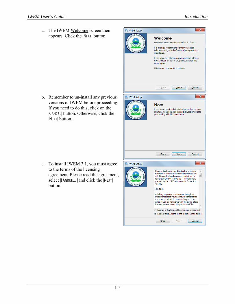
a. The IWEM Welcome screen then appears. Click the |NEXT| button.
b. Remember to un-install any previous
versions of IWEM before proceeding. If you need to do this, click on the |CANCEL| button. Otherwise, click the |NEXT| button.
c. To install IWEM 3.1, you must agree
to the terms of the licensing agreement. Please read the agreement, select |I AGREE…| and click the |NEXT| button.
IWEM User’s Guide Introduction
1-6
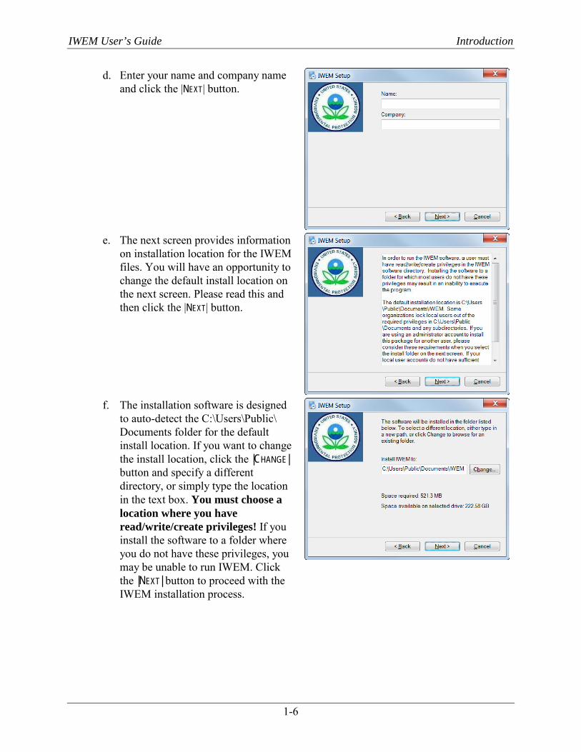
d. Enter your name and company name and click the |NEXT| button.
e. The next screen provides information
on installation location for the IWEM files. You will have an opportunity to change the default install location on the next screen. Please read this and then click the |NEXT| button.
f. The installation software is designed
to auto-detect the C:\Users\Public\Documents folder for the default install location. If you want to change the install location, click the |CHANGE| button and specify a different directory, or simply type the location in the text box. You must choose a location where you have read/write/create privileges! If you install the software to a folder where you do not have these privileges, you may be unable to run IWEM. Click the |NEXT| button to proceed with the IWEM installation process.
IWEM User’s Guide Introduction
1-7
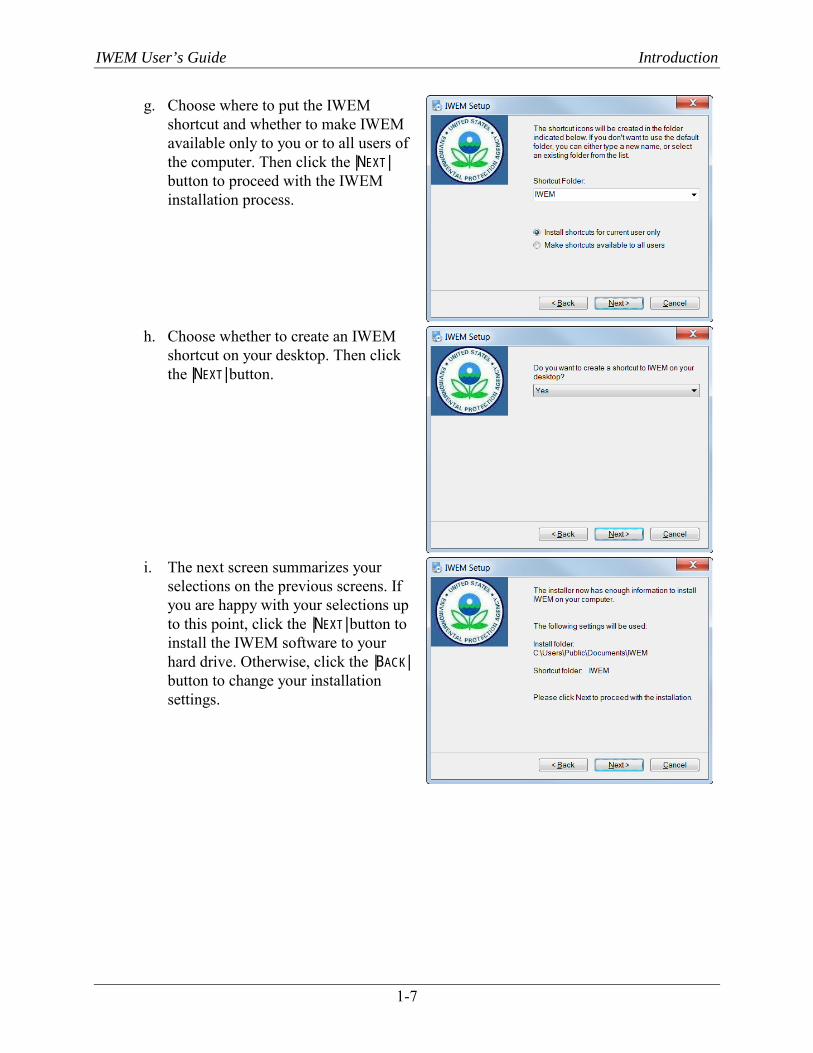
g. Choose where to put the IWEM shortcut and whether to make IWEM available only to you or to all users of the computer. Then click the |NEXT| button to proceed with the IWEM installation process.
h. Choose whether to create an IWEM
shortcut on your desktop. Then click the |NEXT| button.
i. The next screen summarizes your
selections on the previous screens. If you are happy with your selections up to this point, click the |NEXT| button to install the IWEM software to your hard drive. Otherwise, click the |BACK| button to change your installation settings.
IWEM User’s Guide Introduction
1-8
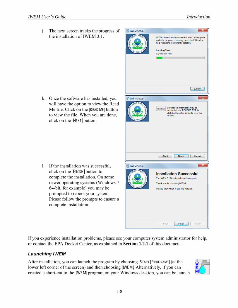
j. The next screen tracks the progress of the installation of IWEM 3.1.
k. Once the software has installed, you
will have the option to view the Read Me file. Click on the |READ ME| button to view the file. When you are done, click on the |NEXT| button.
l. If the installation was successful,
click on the |FINISH| button to complete the installation. On some newer operating systems (Windows 7 64-bit, for example) you may be prompted to reboot your system. Please follow the prompts to ensure a complete installation.
If you experience installation problems, please see your computer system administrator for help, or contact the EPA Docket Center, as explained in Section 1.2.1 of this document.
Launching IWEM After installation, you can launch the program by choosing |START| PROGRAMS| (at the lower left corner of the screen) and then choosing |IWEM|. Alternatively, if you can created a short-cut to the |IWEM| program on your Windows desktop, you can be launch

IWEM User’s Guide Introduction
1-9
IWEM by double-clicking the |IWEM| icon (shown at right) on your desktop.
1.3 Organization of This User’s Guide This User’s Guide is organized as follows:
Section 2 provides an overview of the IWEM software; Section 3 provides detailed instructions on how to run the IWEM software, and guides
you step-by-step through WMU and roadway evaluations; Section 4 presents background information to assist in understanding the input values;
how they affect the model evaluation; and how to obtain input values Section 5 presents background information to assist in understanding the IWEM results; Section 6 lists all references cited; Appendix A presents the list of waste constituents included in IWEM; Appendix B presents the example problem and reports for WMU evaluations; Appendix C presents the example problem and reports for roadway evaluations; and Appendix D presents the example problem and reports for structural fill evaluations.

IWEM User’s Guide Introduction
1-10
[This page intentionally left blank.]

IWEM User’s Guide IWEM Overview
2-1
2. IWEM Overview The IWEM software developed by the EPA provides a screening level analysis for the ground water pathway. Based on the user’s inputs and assumptions, the analysis produces recommendations on the type of liner to be used in a WMU that is protective, and/or whether the beneficial reuse of industrial materials in structural fills or roadways is appropriate or not. The model is a Windows-based program with a user-friendly interface, and will operate on any standard personal computer using windows operating system. This section describes the IWEM evaluation process (Section 2.1), the model structure and components (Section 2.2), and some of the key assumptions and limitations behind the model (Section 2.3).
2.1 What Does the Software Do? The IWEM software is consisted of six source modules to simulate the migration contaminants from a source location to a ground water well. Four of these modules are designed to help you identify a liner design for four different types of RCRA Subtitle D (non-hazardous) WMUs: landfills, waste piles, surface impoundments, and land application units. The remaining two modules are designed to help you determine whether the beneficial reuse of industrial material in a structural fill or roadway will be appropriate. IWEM arrives at these conclusions by comparing the model estimated ground water concentration at a well – calculated using the leachate concentration enter by the user for each waste constituent2 and a ground water fate and transport model – to a benchmark selected by the user. If the estimated ground water concentration is less than the benchmark, the modeled scenario is considered “protective” (or, “appropriate” in the case of beneficial use) with respect to that benchmark. These conclusions should be taken with the consideration of the underlying model assumptions and the adequacy of the input data.
For WMUs, IWEM will evaluate the protectiveness of ground water concentrations relative to your benchmark(s) for three standard liner scenarios: no liner, clay liner, and composite liner. Not all liner scenarios apply to all WMU types; Table 2-1 shows the combinations of WMUs and liners that are represented in IWEM. For land application units, only the no-liner scenario is evaluated because liners are not typically used at this type of facility.
Table 2-1. IWEM WMU and Liner Combinations
WMU Type
Liner Scenario
No Liner (in-situ soil) Single Clay Liner Composite Liner
Landfill Waste Pile Surface Impoundment Land Application Unit
= applies to WMU = does not apply to WMU
2 The estimated leachate concentration means the concentration, in milligrams per liter (mg/L), of each constituent of
concern that is expected to be present in the leachate after emplacement of the waste in a WMU or use of the waste in a structural fill or roadway. Typically this concentration is measured using a laboratory leachate test.

IWEM User’s Guide IWEM Overview
2-2
The IWEM user can save and retrieve evaluations so that they can be archived or retrieved later and modified. IWEM also has report generation capabilities to document in hard copy the input values and results.
2.1.1 IWEM Evaluation
An IWEM evaluation utilizes information on the source (WMU, structural fill, roadway) location and other site-specific data enabling you to perform an assessment that reflects key, sensitive site conditions. If appropriate, for site conditions (e.g., an arid climate), it may allow you to avoid constructing an unnecessarily costly WMU design. It may also provide an additional level of certainty that liner designs are protective of sites in vulnerable settings, such as areas with high rainfall and shallow ground water.
IWEM uses Monte Carlo analysis to handle the uncertainty associated with default values and other modeling parameters that are not user-specified. In a Monte Carlo analysis, a complete simulation (source modeling and fate and transport modeling) is run thousands of times, sampling input values from distributions for each iteration, to generate a probability distribution of expected ground water well concentrations for each waste constituent. For WMUs, well concentrations are calculated for each applicable liner alternative. IWEM then compares the estimated 90th percentile of the modeled ground water well concentration to a reference ground water concentration (RGC) value, which is either the regulatory maximum contaminant level (MCL) or a health-based number (HBN) provided by the user. For WMUs, it makes this comparison starting with the least effective liner scenario (no liner) and continuing through the more effective liner scenarios (clay, then composite) until it has identified the minimum liner design for which the 90th percentile of the estimated ground water concentration does not exceed the selected RGC for constituents considered.
For structural fills, the IWEM software calculates a distribution of expected ground water well concentrations for each leachable constituent present in the industrial material used in the structural fill. For each constituent, IWEM chooses a 90th percentile estimated exposure concentration for comparison to a benchmark selected by the user. Based on the result of the comparison, IWEM produces a recommendation on the appropriateness of using the industrial material in a structural fill. It is recommended that the user consults with the appropriate agency to ensure that the recommendation comply with state regulations.
In a similar manner, for roadways, which can include multiple structural components, IWEM calculates distributions of expected ground water well concentrations for all leachable constituents present in the reused industrial materials for each roadway strip containing leachable constituent mass. For each constituent, IWEM then sums the 90th percentiles of these distributions across all strips leaching that constituent to obtain the aggregate 90th percentile ground water exposure concentration for comparison to the benchmark for that constituent. Based on the result of the comparison, IWEM produces a recommendation on the
About Monte Carlo Analysis Monte Carlo analysis is a computer-based method of analysis developed in the 1940s that uses statistical sampling techniques to obtain a probabilistic approximation to the solution of a mathematical equation or model. The name refers to the city on the French Riviera that is known for its gambling and other games of chance. Monte Carlo analysis is increasingly used in risk assessments where it allows the risk manager to make decisions based on a statistical level of protection that reflects the variability and/or uncertainty in risk parameters or processes, rather than making decisions based on a single point estimate of risk. For further information on Monte Carlo analysis in risk assessment, see the EPA’s Guiding Principles for Monte Carlo Analysis (U.S. EPA, 1997).

IWEM User’s Guide IWEM Overview
2-3
appropriateness of using the industrial material in roadways. It is recommended that the user consults with the appropriate agency to ensure that the recommendation comply with state regulations.
IWEM is designed to allow varying levels of site-specific information and data, depending on what information you have available. IWEM allows you to provide site-specific values for the most important modeling parameters, but if you have limited site data available, IWEM will use default values or distributions for parameters for which you have no data. IWEM will also assist you in making the most appropriate use of the information you do have. For instance, if you know that a site has an alluvial aquifer, but you do not have site-specific values for ground water parameters such as hydraulic conductivity, IWEM will assign representative values for alluvial aquifers from its extensive built-in database of ground water modeling parameters.
IWEM contains a database with chemical properties and MCLs for more than 200 waste constituents (see Appendix A for a complete list of the constituents). You can also add waste constituents or modify constituent properties such as soil-water partition coefficient (Kd) or degradation coefficients in the database. You can also specify user-defined RGCs and the associated exposure durations.
2.1.2 Detailed Site Assessment If an IWEM evaluation does not adequately simulate conditions at a proposed site because the hydrogeology of the site is complex, i.e., the hydrogeologic conditions violate the assumptions fundamental to the formulation of the ground water pathway model supporting IWEM (See Sections 3.0 and 4.0 the EPACMTP Technical Background Document, U.S. EPA, 2003a) or the assumptions and limitations of the IWEM software (see Section 4.3 of the IWEM Technical Background Document, U.S. EPA, 2015a), you should consider conducting a comprehensive site- specific analysis. For example, if ground water flow is subject to seasonal variations, performing an IWEM evaluation may not be appropriate, because the IWEM model is based on steady-state flow conditions. Likewise, a highly heterogeneous, fractured, or tightly confined aquifer would not be appropriately represented by IWEM. A comprehensive site-specific ground water fate and transport analysis may be required to evaluate risk to ground water and alternative WMU liner designs or structural fill or roadway designs. This type of analysis is beyond the scope of IWEM. If appropriate, consult with your state agency and use a qualified professional, experienced in ground water modeling. EPA recommends that you talk to state officials and/or appropriate trade associations to solicit recommendations for a good consultant to perform the analysis.
It is important to use a qualified professional because:
Fate and transport modeling can be very complex; appropriate training and experience are required to correctly use and interpret models.
Incorrect fate and transport modeling can result in a liner system that is not sufficiently protective, or an inappropriate use of industrial materials in a roadway or structural fill.
To avoid incorrect analyses, check to see if the professional has sufficient training and experience in analyzing ground water flow and contaminant fate and transport.
IWEM User’s Guide IWEM Overview
2-4
2.2 IWEM Software Components IWEM consists of the following main components (or modules):
Graphical User Interface, which guides you through a series of user-friendly screens to perform an evaluation;
Source Term Modules that simulate releases from WMUs, roadways, and structural fills; Fate and Transport Model: EPA’s Composite Model for Leachate Migration with
Transformation Products (EPACMTP) is the computational engine with integrated Monte Carlo processor and ground water fate and transport simulator (U.S. EPA, 2003a,b,c,d); and
A series of databases of waste constituents and site-specific parameters.
Each of these components is discussed briefly in this section.
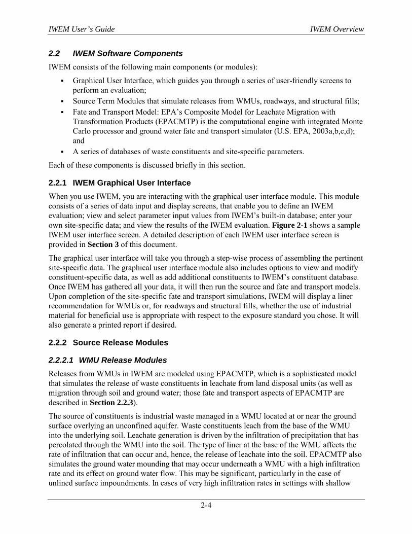
2.2.1 IWEM Graphical User Interface When you use IWEM, you are interacting with the graphical user interface module. This module consists of a series of data input and display screens, that enable you to define an IWEM evaluation; view and select parameter input values from IWEM’s built-in database; enter your own site-specific data; and view the results of the IWEM evaluation. Figure 2-1 shows a sample IWEM user interface screen. A detailed description of each IWEM user interface screen is provided in Section 3 of this document.
The graphical user interface will take you through a step-wise process of assembling the pertinent site-specific data. The graphical user interface module also includes options to view and modify constituent-specific data, as well as add additional constituents to IWEM’s constituent database. Once IWEM has gathered all your data, it will then run the source and fate and transport models. Upon completion of the site-specific fate and transport simulations, IWEM will display a liner recommendation for WMUs or, for roadways and structural fills, whether the use of industrial material for beneficial use is appropriate with respect to the exposure standard you chose. It will also generate a printed report if desired.
2.2.2 Source Release Modules
2.2.2.1 WMU Release Modules Releases from WMUs in IWEM are modeled using EPACMTP, which is a sophisticated model that simulates the release of waste constituents in leachate from land disposal units (as well as migration through soil and ground water; those fate and transport aspects of EPACMTP are described in Section 2.2.3).
The source of constituents is industrial waste managed in a WMU located at or near the ground surface overlying an unconfined aquifer. Waste constituents leach from the base of the WMU into the underlying soil. Leachate generation is driven by the infiltration of precipitation that has percolated through the WMU into the soil. The type of liner at the base of the WMU affects the rate of infiltration that can occur and, hence, the release of leachate into the soil. EPACMTP also simulates the ground water mounding that may occur underneath a WMU with a high infiltration rate and its effect on ground water flow. This may be significant, particularly in the case of unlined surface impoundments. In cases of very high infiltration rates in settings with shallow
IWEM User’s Guide IWEM Overview
2-5
ground water, EPACMTP may cap the infiltration rate to avoid having the modeled ground water mound rise above the bottom of the WMU.
Figure 2-1. Sample screen from the IWEM graphical user interface.
2.2.2.2 Structural Fill Release Module Releases from structural fills are modeled using EPACMTP as described in Section 2.2.2.1. The fill is configured as an unlined landfill with a user-specified fraction of leachable fill materials.
2.2.2.3 Roadway Release Module The roadway source module in IWEM is a stand-alone component that determines the pattern of leachate releases from reused industrial materials incorporated into a roadway structure. The output from the roadway source module consists of a time series of leachate fluxes and concentrations for each constituent identified in the reused material. If there are multiple, distinct components in roadway, each containing reused materials, leachate fluxes and concentrations will be generated for each component. The output is presented to EPACMTP, which uses the leaching information to conduct fate and transport simulations as it would for a WMU. If there is a single roadway component that generates leachate, then one Monte Carlo simulation is conducted for each constituent identified in the leachate. If multiple leaching components are defined, then EPACMTP will be executed for each constituent present in the leachate of each component. IWEM then sums the 90th percentiles of the resulting distributions across all roadway components leaching that constituent to obtain the aggregate 90th percentile ground water exposure concentration, which is used to determine if the ground water impacts are below or exceed the user-supplied benchmark.
IWEM User’s Guide IWEM Overview
2-6
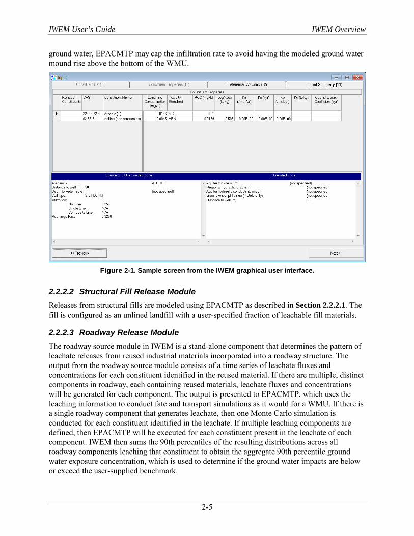
Figure 2-2 depicts a typical roadway with a segment constructed with byproduct materials. For the purposes of model simplicity, that segment is assumed to be nearly linear and thus can be approximated by the straight line segment AB. If the segment to be modeled is long and meandering, it must be subdivided into several nearly linear segments that can each be represented by a straight line.
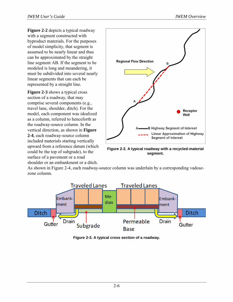
Figure 2-3 shows a typical cross section of a roadway, that may comprise several components (e.g., travel lane, shoulder, ditch). For the model, each component was idealized as a column, referred to henceforth as the roadway-source column. In the vertical direction, as shown in Figure 2-4, each roadway-source column included materials starting vertically upward from a reference datum (which could be the top of subgrade), to the surface of a pavement or a road shoulder or an embankment or a ditch. As shown in Figure 2-4, each roadway-source column was underlain by a corresponding vadose-zone column.
Figure 2-3. A typical cross section of a roadway.
Figure 2-2. A typical roadway with a recycled-material
segment.
IWEM User’s Guide IWEM Overview
2-7
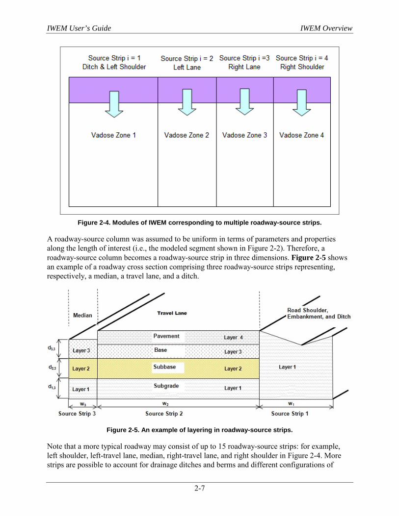
Figure 2-4. Modules of IWEM corresponding to multiple roadway-source strips.
A roadway-source column was assumed to be uniform in terms of parameters and properties along the length of interest (i.e., the modeled segment shown in Figure 2-2). Therefore, a roadway-source column becomes a roadway-source strip in three dimensions. Figure 2-5 shows an example of a roadway cross section comprising three roadway-source strips representing, respectively, a median, a travel lane, and a ditch.
Figure 2-5. An example of layering in roadway-source strips.
Note that a more typical roadway may consist of up to 15 roadway-source strips: for example, left shoulder, left-travel lane, median, right-travel lane, and right shoulder in Figure 2-4. More strips are possible to account for drainage ditches and berms and different configurations of
IWEM User’s Guide IWEM Overview
2-8
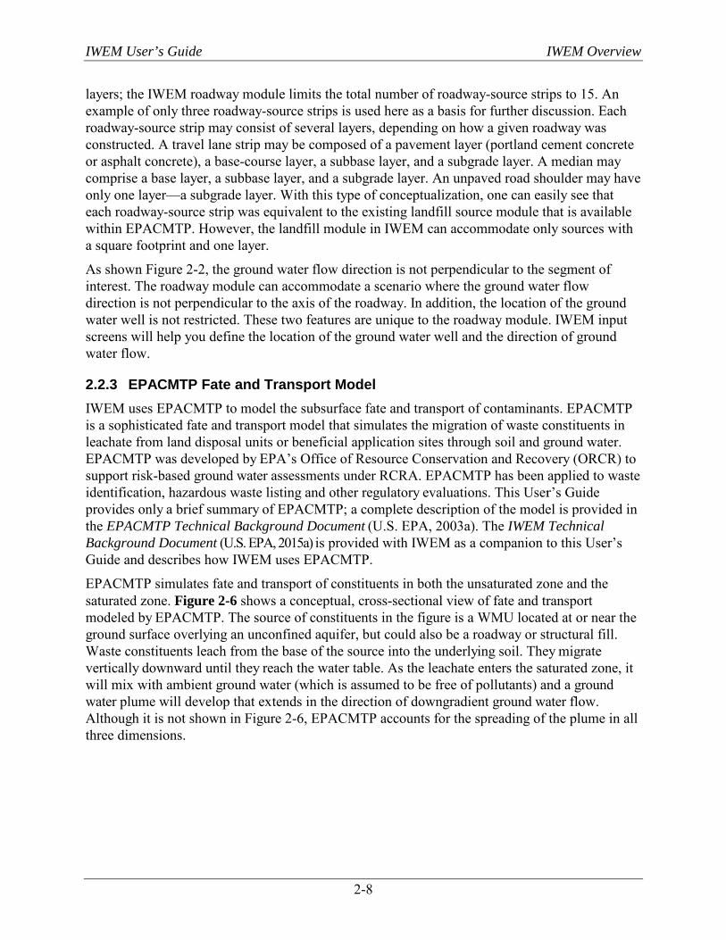
layers; the IWEM roadway module limits the total number of roadway-source strips to 15. An example of only three roadway-source strips is used here as a basis for further discussion. Each roadway-source strip may consist of several layers, depending on how a given roadway was constructed. A travel lane strip may be composed of a pavement layer (portland cement concrete or asphalt concrete), a base-course layer, a subbase layer, and a subgrade layer. A median may comprise a base layer, a subbase layer, and a subgrade layer. An unpaved road shoulder may have only one layer—a subgrade layer. With this type of conceptualization, one can easily see that each roadway-source strip was equivalent to the existing landfill source module that is available within EPACMTP. However, the landfill module in IWEM can accommodate only sources with a square footprint and one layer.
As shown Figure 2-2, the ground water flow direction is not perpendicular to the segment of interest. The roadway module can accommodate a scenario where the ground water flow direction is not perpendicular to the axis of the roadway. In addition, the location of the ground water well is not restricted. These two features are unique to the roadway module. IWEM input screens will help you define the location of the ground water well and the direction of ground water flow.
2.2.3 EPACMTP Fate and Transport Model IWEM uses EPACMTP to model the subsurface fate and transport of contaminants. EPACMTP is a sophisticated fate and transport model that simulates the migration of waste constituents in leachate from land disposal units or beneficial application sites through soil and ground water. EPACMTP was developed by EPA’s Office of Resource Conservation and Recovery (ORCR) to support risk-based ground water assessments under RCRA. EPACMTP has been applied to waste identification, hazardous waste listing and other regulatory evaluations. This User’s Guide provides only a brief summary of EPACMTP; a complete description of the model is provided in the EPACMTP Technical Background Document (U.S. EPA, 2003a). The IWEM Technical Background Document (U.S. EPA, 2015a) is provided with IWEM as a companion to this User’s Guide and describes how IWEM uses EPACMTP.
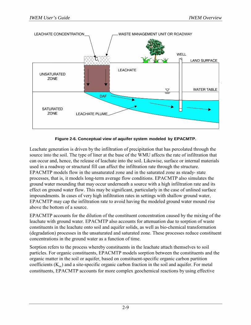
EPACMTP simulates fate and transport of constituents in both the unsaturated zone and the saturated zone. Figure 2-6 shows a conceptual, cross-sectional view of fate and transport modeled by EPACMTP. The source of constituents in the figure is a WMU located at or near the ground surface overlying an unconfined aquifer, but could also be a roadway or structural fill. Waste constituents leach from the base of the source into the underlying soil. They migrate vertically downward until they reach the water table. As the leachate enters the saturated zone, it will mix with ambient ground water (which is assumed to be free of pollutants) and a ground water plume will develop that extends in the direction of downgradient ground water flow. Although it is not shown in Figure 2-6, EPACMTP accounts for the spreading of the plume in all three dimensions.
IWEM User’s Guide IWEM Overview
2-9
Figure 2-6. Conceptual view of aquifer system modeled by EPACMTP.
Leachate generation is driven by the infiltration of precipitation that has percolated through the source into the soil. The type of liner at the base of the WMU affects the rate of infiltration that can occur and, hence, the release of leachate into the soil. Likewise, surface or internal materials used in a roadway or structural fill can affect the infiltration rate through the structure. EPACMTP models flow in the unsaturated zone and in the saturated zone as steady- state processes, that is, it models long-term average flow conditions. EPACMTP also simulates the ground water mounding that may occur underneath a source with a high infiltration rate and its effect on ground water flow. This may be significant, particularly in the case of unlined surface impoundments. In cases of very high infiltration rates in settings with shallow ground water, EPACMTP may cap the infiltration rate to avoid having the modeled ground water mound rise above the bottom of a source.
EPACMTP accounts for the dilution of the constituent concentration caused by the mixing of the leachate with ground water. EPACMTP also accounts for attenuation due to sorption of waste constituents in the leachate onto soil and aquifer solids, as well as bio-chemical transformation (degradation) processes in the unsaturated and saturated zone. These processes reduce constituent concentrations in the ground water as a function of time.
Sorption refers to the process whereby constituents in the leachate attach themselves to soil particles. For organic constituents, EPACMTP models sorption between the constituents and the organic matter in the soil or aquifer, based on constituent-specific organic carbon partition coefficients (Koc) and a site-specific organic carbon fraction in the soil and aquifer. For metal constituents, EPACMTP accounts for more complex geochemical reactions by using effective

IWEM User’s Guide IWEM Overview
2-10
sorption isotherms for a range of aquifer geochemical conditions, as generated using the MINTEQA23 geochemical speciation model.
By default, EPACMTP only accounts for constituent transformations caused by hydrolysis reactions. Hydrolysis refers to constituent decomposition that results from chemical reactions with water. However, you may also enter site-specific biodegradation rates. Biodegradation refers to constituent decomposition reactions involving bacteria and other micro-organisms. EPACMTP simulates all transformation processes as first-order reactions, that is, as processes that can be characterized with a half-life.
EPACMTP accounts for constituents that hydrolyze into toxic daughter products. In that case, the final IWEM results account for both the parent constituent and any toxic daughter products. For instance, if a parent waste constituent rapidly hydrolyzes into a persistent daughter product, the ground water exposure caused by the parent itself may be minimal (it has already degraded before it reaches the well), but the results would be based on the exposure caused by the daughter product.
For WMUs, IWEM makes liner recommendations by comparing ground water exposure concentration values estimated by EPACMTP against RGCs that are either regulatory MCLs or user-supplied benchmarks. For roadways and structural fills, IWEM makes the same comparison to determine if the beneficial reuse of industrial material in the design is appropriate (estimated ground water exposure concentration is less than the selected benchmark) or not. For an IWEM analysis, the ground water exposure concentration is evaluated at a hypothetical well located downgradient from the source. EPACMTP accounts for the finite life- span of WMUs, which results in a time-dependent ground water exposure concentration. The exposure concentration calculated by EPACMTP is the maximum average concentration during the time period in which the ground water exposure at the well occurs. The length of the exposure averaging period is adjusted to match exposure duration specified by the user. For instance, if the supplied benchmark assumes a 30-year exposure duration, the averaging period for calculating the average ground water exposure concentration is set to 30 years.
2.2.3.1 IWEM vs. EPACMTP As an IWEM user, you should understand the differences between IWEM and EPACMTP. EPACMTP is a full-featured ground water flow and transport model with probabilistic modeling capabilities; it is a sophisticated software program which requires a significant amount of computer and ground water modeling expertise to create the necessary input files, execute the model, and interpret the results.
In contrast, IWEM is a relatively simple and user-friendly program created specifically to conduct screening analyses of the ground water. Specifically, IWEM converts your input values into the required EPACMTP input files, executes a series of EPACMTP modeling runs, and then compiles and analyzes the results to produce a finding that is specific to your waste and your waste site or beneficial use. In addition, IWEM can print and save document-ready reports that include the results of an IWEM evaluation and the input data on which they are based.
3 MINTEQA2 (U.S. EPA, 1991) is a geochemical equilibrium speciation model for computing equilibria among
the dissolved, absorbed, solid, and gas phases in dilute aqueous solution.

IWEM User’s Guide IWEM Overview
2-11
In summary, IWEM can be thought of as an application of EPACMTP that is tailored specifically for use in non-hazardous industrial waste management decision- making. In order to make IWEM appropriate and easy to use in performing these analyses, not all of the EPACMTP functionality is available in IWEM; however, IWEM provides added capabilities to interpret results and develop reports, which are not available in EPACMTP.
2.2.4 IWEM Databases The final component of IWEM is an integrated set of databases that include waste constituent properties and other ground water modeling parameters. The waste constituent database includes 206 organic chemicals and 22 metals (25 for the Roadway Module). Appendix A provides a list of the constituents in the database. The constituent properties include physical and chemical data needed for ground water transport modeling, and regulatory MCLs
In addition to constituent data, IWEM includes a comprehensive database of ground water modeling data, including infiltration rates for different WMU types, liner designs, roadway materials, and structural fills for a range of locations and climatic conditions throughout the United States; and soil and hydrogeological data for different soil types and aquifer conditions across the United States. Details of these databases are provided in the EPACMTP Parameters/Data Background Document (U.S. EPA, 2003b,d) and in the IWEM Technical Background Document (U.S. EPA, 2015a).
IWEM uses these databases to perform evaluations. When site-specific data are available for an IWEM evaluation, they will override default database values. Conversely, when site-specific data are not available for an IWEM evaluation, IWEM will use default values or random sampling of values from distributions in its databases to augment the user-provided data.
2.3 Assumptions and Limitations of Ground Water Modeling Using IWEM IWEM uses sophisticated probabilistic techniques to account for uncertainty and parameter variability. To perform these evaluations, the mathematical models represent conditions that may potentially be encountered at waste management sites and beneath roadways or structural fills within the United States. Efforts have been made to obtain representative, nationwide data and account for the uncertainty in the data.
However, given the complex nature of the evaluations, a number of limitations and caveats must be delineated. These limitations are described in this section. Since IWEM relies on EPACMTP to model the source as well as fate and transport through the unsaturated and saturated zone, the discussion focuses on the limitations and assumptions inherent to EPACMTP. Before using this software, you need to verify that the model assumptions are appropriate for the site you are evaluating. The IWEM Technical Background Document (U.S. EPA, 2015a) provides additional information to assist you in this process.
EPACMTP represents WMUs, roadways, and structural fills in terms of a source area and a defined rate and duration of leaching. EPACMTP only accounts for the release of leachate through the base of the source and assumes that the only mechanism of constituent release is through dissolution of waste constituents in the water that percolates through the source. EPACMTP does not account for the presence of non-aqueous free-phase liquids, such as an oily phase that might provide an additional release mechanism into the subsurface. EPACMTP does not account for releases from the source via other environmental pathways, such volatilization or

IWEM User’s Guide IWEM Overview
2-12
surface run-off. EPACMTP assumes that the rate of infiltration through the source is constant, representing long-term average conditions; the model does not account for fluctuations in rainfall rate, or degradation of liner systems that may cause the rate of infiltration and release of leachate to vary over time.
EPACMTP does not explicitly account for the presence of macro-pores, fractures, solution features, faults or other heterogeneities in the soil or aquifer that may provide pathways for rapid movement of constituents. A certain amount of heterogeneity always exists at actual sites, and it is not uncommon in ground water modeling to use average parameter values. This means that the input values for parameters such as hydraulic conductivity, dispersivity, etc. represent effective site-wide average values. However, EPACMTP may not be appropriate for sites overlying fractured or very heterogeneous aquifers.
EPACMTP is designed for relatively simple ground water flow systems. EPACMTP treats flow in the unsaturated zone and saturated zone as steady state and does not account for fluctuations in the infiltration or recharge rate, either in time or areally. As a result, the use of EPACMTP may not be appropriate at sites with large seasonal fluctuations in rainfall conditions, or at sites where the recharge rate varies locally. Examples of the latter include the presence of surface water bodies such as rivers and lakes or ponds, and/or man-made recharge sources near the WMU. EPACMTP does not account for the presence of ground water sources or sinks such as pumping or injection wells.
Leachate constituents can be subject to complex biological and geochemical interactions in soil and ground water. EPACMTP treats these interactions as equilibrium sorption and first-order degradation processes. In the case of sorption processes, the equilibrium assumption means that the sorption process occurs instantaneously, or at least very quickly relative to the time-scale of constituent transport. Although sorption, or the attachment of leachate constituents to solid soil or aquifer particles, may result from multiple chemical processes, EPACMTP lumps these processes together into an effective soil-water partition coefficient. In the case of metals, EPACMTP allows the partition coefficient to vary as a function of a number of primary geochemical parameters, including pH, leachate organic matter, soil organic matter, and the fraction of iron-oxide in the soil or aquifer.
Although EPACMTP is able to account for the most important ways that the geochemical environment at a site affects the mobility of metals, the model assumes that the geochemical environment at a site is constant and is not affected by the presence of the leachate plume. In reality, the presence of a leachate plume may alter the ambient geochemical environment. EPACMTP does not account for colloidal transport or other forms of facilitated transport. For metals and other constituents that tend to strongly sorb to soil particles, and which EPACMTP will simulate as relatively immobile, movement as colloidal particles can be a significant transport mechanism. However given sufficient site-specific data, it is possible to approximate the effect of these transport processes by using a lower value for the Kd as a user-input.
EPA’s ground water modeling database includes constituent-specific hydrolysis rate coefficients for constituents that are subject to hydrolysis transformation reactions; for these constituents, EPACMTP simulates transformation reactions subject to site- specific values of pH and soil and ground water temperature, but other types of transformation processes are not explicitly simulated in EPACMTP. For many organic constituents, biodegradation can be an important fate mechanism, but EPACMTP has only limited ability to account for this process. The user must
IWEM User’s Guide IWEM Overview
2-13
provide an appropriate value for the effective first-order degradation rate. In the IWEM application of EPACMTP, the model uses the same degradation rate coefficient for the unsaturated and saturated zones if this parameter is provided as a user-input. In an actual leachate plume, biodegradation rates may be different in different regions in the plume; for instance in portions of the plume that are anaerobic some constituents may biodegrade more readily, while other constituents will biodegrade only in the aerobic fringe of the plume. EPACMTP does not account for these or other processes that may cause a constituent’s rate of transformation to vary in space and time.
Three of the four WMUs in IWEM and EPACMTP are considered temporary and their leaching durations are determined by the user-supplied value for operational life. Although these WMUs might be described as temporary, default values for their operational lives range from 20 to 50 years. EPACMTP was designed and fine-tuned to efficiently determine peak and average ground water concentrations at a well assuming that leaching durations would be long enough to capture the changing ground water concentrations in terms of years rather than days. Unless EPACMTP is appropriately modified, EPACMTP is not able to accurately capture peak concentrations at receptor wells for extremely short leaching durations of 1 year or less. A minimum value for operational life should be at least 5 to 10 years to ensure that EPACMTP accurately identifies a peak or average ground water concentration at the well.
IWEM allows the user to specify many key input parameters like the location of the ground water well where exposure concentrations are evaluated. Given the nature of these sensitive parameters, seemingly conservative choices can generate non-intuitive results that may lead the user to question the rigor of the model. It is very important, therefore, to be careful in selecting values for your inputs and understand how the remaining input parameters are related and how they are selected.
For example, in IWEM a user can specify where a ground water well is placed down-gradient of the source area but has no control over the depth of the well below the water table. The default depth of the ground water well in IWEM varies uniformly between 0 and 10 m or the thickness of the saturated zone, whichever is less. Consider a scenario where the well is placed very close to the source area. In Figure 2-6, the region of the saturated zone contaminated by leachate expands as the distance from the source increases. Very close to the source, the plume is relatively shallow and deepens at the distance from the source increases. There is reasonable likelihood that a random depth for a well very close to the source might actually be below the plume extent. Now, imagine that the source is small or very narrow (like a roadway). The plume depth is even shallower. The likelihood of the well missing the plume increases. This phenomenon could very well bias the estimated ground water exposure concentration to be lower, much lower than expected, causing the user to question the results of the analysis. Therefore, for such types of scenarios, IWEM is not an appropriate tool and the user should consider using a more site-specific analysis. More information on the limitations of IWEM on the down-gradient well distance is presented in Section 6.1.3 of the IWEM Technical Background Document (U.S. EPA, 2015a).

IWEM User’s Guide IWEM Overview
2-14
[This page intentionally left blank.]

IWEM User’s Guide Running the IWEM Software
3-1
3. Running the IWEM Software This section provides detailed instructions on how to run the IWEM software. Specifically, this section:
Instructs you how to launch the IWEM software; Explains the key features of the IWEM software; and Guides you step-by-step through IWEM evaluations.
3.1 How Do I Start the IWEM Software? To use the program for the first time, download it from EPA’s website (http://www.epa.gov/osw/nonhaz/industrial/tools/iwem/) to your hard-drive and install it. Section 1.2.2 gives detailed installation instructions.
The installation package will place an icon on your desktop unless you specify not to. You can launch IWEM by double-clicking the IWEM icon (shown at right) on your desktop. If you opt not to let the installation package place an icon on your desktop, you can launch the program by choosing |START|PROGRAMS| (at the lower left corner of the screen) and then choosing the |IWEM| program group and the program |IWEM|.
3.2 What Are the Key Features of the IWEM Software?
3.2.1 General User Interface Features The IWEM software has a user-friendly interface that is designed to operate in accordance with Microsoft Windows conventions. The first screen that appears after launching the program is the Start-Up screen (shown below), which will appear only while the program is loading.
The first time you run the IWEM software, it will display five Introductory screens. After reading them once, you can skip these screens in the future by editing the setting for Intro Screens under Options in the Menu Bar.
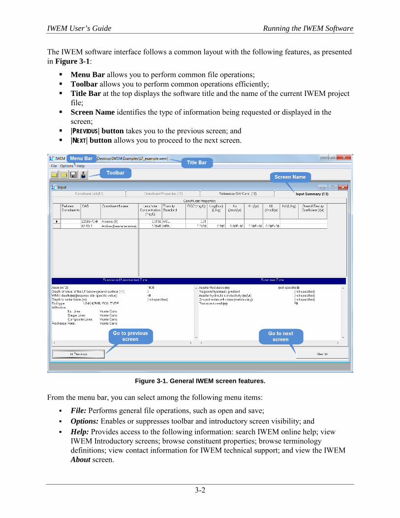
IWEM User’s Guide Running the IWEM Software
3-2
The IWEM software interface follows a common layout with the following features, as presented in Figure 3-1:
Menu Bar allows you to perform common file operations; Toolbar allows you to perform common operations efficiently; Title Bar at the top displays the software title and the name of the current IWEM project
file; Screen Name identifies the type of information being requested or displayed in the
screen; |PREVIOUS| button takes you to the previous screen; and |NEXT| button allows you to proceed to the next screen.
Figure 3-1. General IWEM screen features.
From the menu bar, you can select among the following menu items:
File: Performs general file operations, such as open and save; Options: Enables or suppresses toolbar and introductory screen visibility; and Help: Provides access to the following information: search IWEM online help; view
IWEM Introductory screens; browse constituent properties; browse terminology definitions; view contact information for IWEM technical support; and view the IWEM About screen.
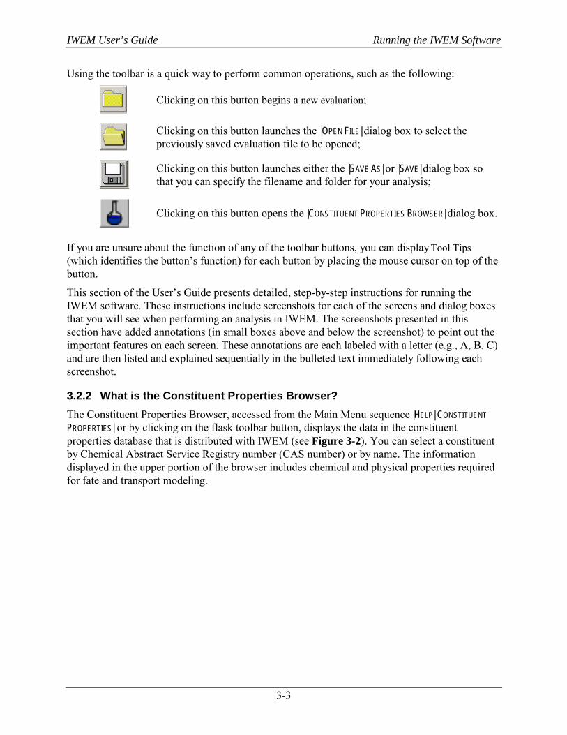
IWEM User’s Guide Running the IWEM Software
3-3
Using the toolbar is a quick way to perform common operations, such as the following:
Clicking on this button begins a new evaluation;
Clicking on this button launches the |OPEN FILE| dialog box to select the previously saved evaluation file to be opened;
Clicking on this button launches either the |SAVE AS| or |SAVE| dialog box so that you can specify the filename and folder for your analysis;
Clicking on this button opens the |CONSTITUENT PROPERTIES BROWSER| dialog box.
If you are unsure about the function of any of the toolbar buttons, you can display Tool Tips (which identifies the button’s function) for each button by placing the mouse cursor on top of the button.
This section of the User’s Guide presents detailed, step-by-step instructions for running the IWEM software. These instructions include screenshots for each of the screens and dialog boxes that you will see when performing an analysis in IWEM. The screenshots presented in this section have added annotations (in small boxes above and below the screenshot) to point out the important features on each screen. These annotations are each labeled with a letter (e.g., A, B, C) and are then listed and explained sequentially in the bulleted text immediately following each screenshot.
3.2.2 What is the Constituent Properties Browser? The Constituent Properties Browser, accessed from the Main Menu sequence |HELP| CONSTITUENT PROPERTIES| or by clicking on the flask toolbar button, displays the data in the constituent properties database that is distributed with IWEM (see Figure 3-2). You can select a constituent by Chemical Abstract Service Registry number (CAS number) or by name. The information displayed in the upper portion of the browser includes chemical and physical properties required for fate and transport modeling.
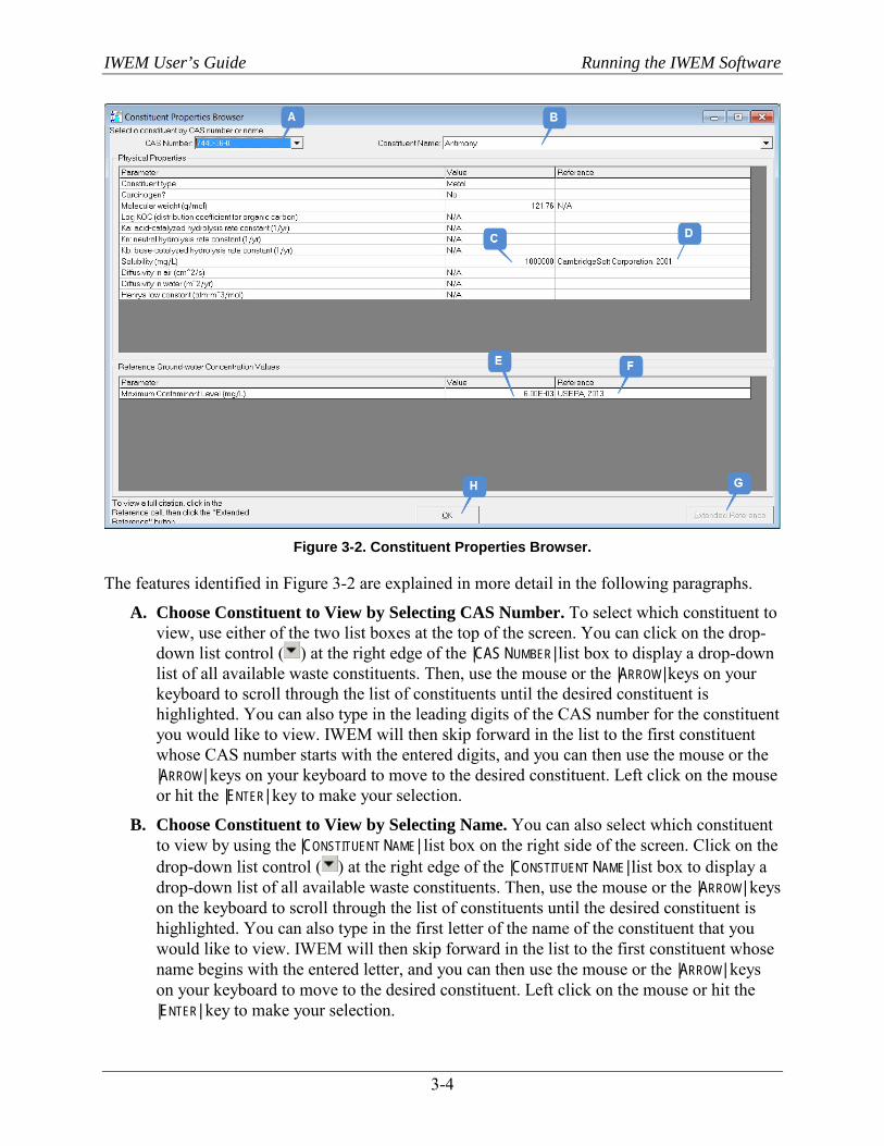
IWEM User’s Guide Running the IWEM Software
3-4
Figure 3-2. Constituent Properties Browser.
The features identified in Figure 3-2 are explained in more detail in the following paragraphs.
A. Choose Constituent to View by Selecting CAS Number. To select which constituent to view, use either of the two list boxes at the top of the screen. You can click on the drop-down list control ( ) at the right edge of the |CAS NUMBER| list box to display a drop-down list of all available waste constituents. Then, use the mouse or the |ARROW| keys on your keyboard to scroll through the list of constituents until the desired constituent is highlighted. You can also type in the leading digits of the CAS number for the constituent you would like to view. IWEM will then skip forward in the list to the first constituent whose CAS number starts with the entered digits, and you can then use the mouse or the |ARROW| keys on your keyboard to move to the desired constituent. Left click on the mouse or hit the |ENTER| key to make your selection.
B. Choose Constituent to View by Selecting Name. You can also select which constituent to view by using the |CONSTITUENT NAME| list box on the right side of the screen. Click on the drop-down list control ( ) at the right edge of the |CONSTITUENT NAME| list box to display a drop-down list of all available waste constituents. Then, use the mouse or the |ARROW| keys on the keyboard to scroll through the list of constituents until the desired constituent is highlighted. You can also type in the first letter of the name of the constituent that you would like to view. IWEM will then skip forward in the list to the first constituent whose name begins with the entered letter, and you can then use the mouse or the |ARROW| keys on your keyboard to move to the desired constituent. Left click on the mouse or hit the |ENTER| key to make your selection.

IWEM User’s Guide Running the IWEM Software
3-5
C. Physical Properties. For the selected waste constituent, the pertinent physical and chemical property values that are used in the IWEM analysis and their corresponding data sources are listed in the upper window on this screen.
D. Physical Properties Abbreviated Reference. Abbreviated references are listed for each value.
E. Reference Ground Water Concentrations. For the selected waste constituent, any MCL values in the IWEM database are listed in the lower table on this screen. User-entered Reference Ground Water Concentration (RGCs), such as health-based numbers (HBNs) and other user-defined RGCs are not displayed in the Constituent Properties Browser, but may be viewed and edited on the Reference Ground Water Concentration input tab.
F. Reference Ground Water Concentration Abbreviated Reference. Abbreviated references are listed for each value.
G. Click to Extended Reference for Selected Property. You can view the complete bibliographic citation of a constituent property (except constituent type, carcinogenicity, and molecular weight) by selecting the corresponding entry in the Reference column of one of the tables and clicking on the |EXTENDED REFERENCE| button on the lower right-hand side of the screen. Doing so will cause a message box to appear on-screen containing a complete bibliographic citation.
H. Close Constituent Properties Browser. Click the |OK| button at the bottom of the screen to close this screen.
3.2.3 How Do I Navigate Through the IWEM Software? The IWEM software consists of a series of screens containing controls for entering data and viewing results. This section describes in detail how to move from screen to screen and control to control, as well as how the various controls are used together to facilitate the use of the IWEM software. Although this guide assumes you will be using a mouse to navigate through the screens and features, you may also navigate using the keyboard exclusively.
Navigating with the keyboard involves the use of the following keys: the |TAB| key, the |BACK-TAB| key, the |ARROW| keys, the |ALT| key, and the |ENTER| key. The |TAB| key moves the cursor from one control to the next in a predefined order. The term cursor refers to either a vertical bar “|” that indicates the position of the next typed character, or the change in a control’s appearance from normal to a highlighted appearance, as shown here:
Normal
Highlighted (note the dotted line just inside the perimeter of the button).
When a control is highlighted, it is considered actively awaiting input from the keyboard or mouse. The |BACK-TAB| key (obtained by pressing the |TAB| key while holding down the |SHIFT| key) moves the cursor in the reverse order. When the cursor is on a command button, press the |ENTER| key to “click” the button. Radio buttons always appear in a set of two or more options; when the cursor is on any radio button, press the |ARROW-UP| or |ARROW-DOWN| key to select a different radio button. The |TAB| key moves you off the radio button group. The |TAB|, |BACK-TAB|, and |ARROW| keys

IWEM User’s Guide Running the IWEM Software
3-6
are also used to move from cell to cell in a data grid. A drop-down list displays the current choice of several possible choices; when the drop-down list is active (highlighted), use the |ARROW-UP| or |ARROW-DOWN| keys to display the desired choice.
The |ALT| key is used in combination with other key strokes to access controls or menu items quickly through pre-defined “hot-keys” that correspond to underlined characters on a control or menu item. For example, the underlined “O” on the |OK| button above indicates that pressing and holding down the |ALT| key and then pressing the |O| key would have the same result as a mouse click on the button. Similarly, the main menu system is activated by pressing the |ALT| key; the first letter of each menu item is underlined and can be accessed in the manner just described.
3.2.3.1 Screens The software is set up as a series of screens through which you can navigate to enter data and view results.
You can move through the program using three different methods:
Clicking on one of the toolbar buttons, or clicking on the Evaluation menu, Clicking on the |NEXT| or |PREVIOUS| buttons at the bottom of the screen, or Clicking on one of the labeled tabs located at the top of the data entry and results screens
(navigation among the tabbed screens is only allowed for those screens that are active).
Screens in IWEM appear as a single screen or as a group of screens with manila folder-like “tabs” along the top to differentiate between the individual screens. The Introductory screens are examples of individual screens that have |PREVIOUS| and/or |NEXT| command buttons along the bottom for navigating from screen to screen. The input screens consist of seven screens where you select a source or WMU type, identify the constituents in your waste, enter your leachate data, and specify the geometry and layout of the roadway, as well as other site-specific information. In addition to the navigational command buttons available on single screens, you can also move to adjacent screens by clicking on their corresponding tab.
3.2.3.2 Controls Various types of controls make the IWEM software easy to use. Examples of each of these controls from several IWEM screens are shown in Figure 3-3 and explained in more detail in this section. The letters in the figure correspond to the lettered bullets in the text. In general, a control is activated or selected by clicking on it with the mouse or by using the keyboard (e.g., using the |TAB| key to select the next control).
A. Text Boxes. Text boxes are used to display or accept information. In the screen shown in Figure 3-3, text boxes are used to accept the name or CAS number of a constituent. As you type characters or numbers into the text box, the list box cursor moves to the constituent in the list that best matches your input.
B. List Boxes. List boxes are used to display a list from which you can select one or many of the listed items. In Figure 3-3, the list box displays all of the constituents in the IWEM database that can be used in an analysis.

IWEM User’s Guide Running the IWEM Software
3-7
Figure 3-3. Example IWEM screens identifying several types of controls.

IWEM User’s Guide Running the IWEM Software
3-8
C. Radio Buttons. Radio buttons always appear in sets of two or more and are used when you can only choose one of the options listed. In the figure, you can choose to display all constituents, organics only, or metals only. If you make a different selection, the old selection is unselected. Select an option by clicking on it.
D. Data Grids. Data grids are like a spreadsheet within IWEM and are used to display data, accept data, or a combination of those; they can also contain items you select to affect other controls on a screen. The grid column widths and row heights can be manipulated with the mouse by moving the mouse cursor over the separators along the left side or top of the grid until the cursor changes to a horizontal or vertical bar. When the cursor changes, click and drag the mouse until you are happy with the new grid dimension, then release the mouse button. Moving from cell to cell can be controlled by mouse clicks or by the |TAB| or |ARROW| keys, as explained in Section 3.2.3. Select a particular row of the grid by clicking on the cell in that row or along the left border of the grid or using the |TAB| or |ARROW| keys to move to a particular row. In the screen in Figure 3-3, to remove a constituent from the list displayed in the data grid, select the grid row and then click the command button with the left-pointing arrow.
E. Command Buttons. Command buttons are used to execute an action, navigate from screen to screen, verify a choice, or acknowledge a message. Figure 3-3 shows a screen from IWEM where command buttons are used for various purposes: navigation (the |PREVIOUS| and |NEXT| buttons), moving information (the arrow buttons between the list box and data grid), and initiating some action (the |ADD NEW CONSTITUENT| button). Command buttons are activated by a mouse click or by pressing the |ENTER| key when the button is highlighted or active.
F. Drop-down Lists. Drop-down lists are used to make one selection from a list and then display only the selected item. In some cases, you may also be able to enter data in a drop down list—this type of control is usually referred to as “combo” box control: a combination of a text box control and drop-down box control.
G. Checkboxes. Checkboxes are similar to radio buttons, except you can check more than one in a set. Checking a checkbox turns on the listed option. Click on the box to check and uncheck it.
H. Dialog and Message Boxes. Dialog boxes appear throughout IWEM as additional data entry screens containing one or more of the controls mentioned above or as a way of informing the user. Data entry dialog boxes usually appear as a direct result of clicking on a command button, whereas message boxes appear as the result of an input or calculation.
3.2.4 How Do I Save My Work? You have several options within the IWEM software to save your analysis. After performing a new analysis, you can click on the |SAVE| button on the Toolbar or choose |FILE|SAVE| or |FILE|SAVE AS| from the Menu Bar to launch the standard Windows |SAVE AS| dialog box. Using the Windows |SAVE AS| dialog box, you can navigate to any folder location you prefer. The |SAVE AS| dialog will always default to the last location that you saved to. If you open a saved analysis, and then make changes to it, clicking on the |SAVE| button on the Toolbar or choosing |FILE|SAVE| from the Menu Bar will overwrite the contents of your original file with the current analysis settings; if you want

IWEM User’s Guide Running the IWEM Software
3-9
to save these changes to a new file, you must choose |FILE|SAVE AS| from the Menu Bar. If you forget to save before trying to exit IWEM or open a new file, a dialog box will automatically ask if you want to save your data before exiting the software or opening the new file. You will also be prompted to save your file after the run is complete to ensure that results are saved.
For each saved analysis, IWEM creates two project files in the location you specified in the |SAVE AS| dialog box:
*.wem file *.mdb file.
The combination of these two files completely describes the information you have entered (*.mdb) and any model-generated results (*.wem). The asterisk (*) is replaced by the name you assign to the project; the files will be saved in the project folder you specified.
Note that IWEM will not allow you to save both model inputs and results at a point where the inputs do not correspond to the model-generated results (e.g., when results have been generated, you return to an input screen, change an input, and attempt to save the project). If you do choose to save your work in a situation like this, only the inputs will be saved; that is, when you later open up this file, you will have to run the analysis to create the corresponding results.
You may open a previously saved IWEM analysis by clicking on any one of the following options:
|OPEN| button on the Toolbar |FILE|OPEN| selection from the Menu Bar.
Once the |OPEN| dialog box is displayed, highlight the appropriate file and click the |OPEN| button to open the desired file. IWEM comes with saved project files that correspond to the example problems in Appendices B, C, and D. Those files are installed to either
C:\Users\Public\Documents\IWEM\SampleData or C:\Users\[your user name]\Documents\IWEM\SampleData.
Note that IWEM 3.1 includes structural changes to the database that prevents some saved evaluation data from versions 1.0 and 2.0 of IWEM from being imported (e.g., HBNs were removed and must now be provided by the user). If IWEM detects that the saved scenario is out-of-sync with the current IWEM installation, IWEM will notify you with a message saying, “The version of the evaluation database ([path]) you are opening is different than the IWEM application database ([path]). Some saved evaluation data, including results, may not be imported. NOTE: You will have to re-enter any missing data and re-run the evaluation.” IWEM will load what information it can, however, you will need to review the scenario inputs, re-enter any missing data, and then re-run the evaluation.
You will then see a dialog box in which you can choose to view the input screens or cancel. If the file contains saved results and you want to view those, select |VIEW INPUT SCREENS| and keep clicking on |NEXT| at the bottom right; once you get to the Run Manager screen, clicking |NEXT| will take you to results.
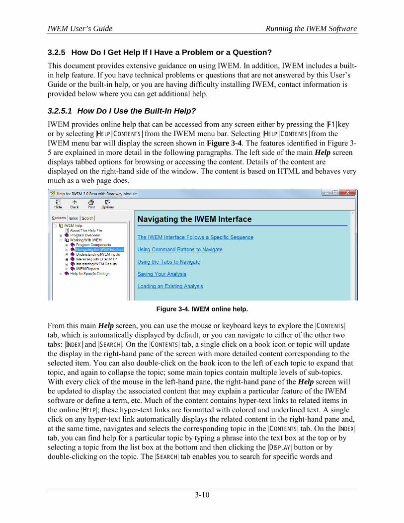
IWEM User’s Guide Running the IWEM Software
3-10
3.2.5 How Do I Get Help If I Have a Problem or a Question? This document provides extensive guidance on using IWEM. In addition, IWEM includes a built-in help feature. If you have technical problems or questions that are not answered by this User’s Guide or the built-in help, or you are having difficulty installing IWEM, contact information is provided below where you can get additional help.
3.2.5.1 How Do I Use the Built-In Help? IWEM provides online help that can be accessed from any screen either by pressing the |F1| key or by selecting |HELP| CONTENTS| from the IWEM menu bar. Selecting |HELP| CONTENTS| from the IWEM menu bar will display the screen shown in Figure 3-4. The features identified in Figure 3-5 are explained in more detail in the following paragraphs. The left side of the main Help screen displays tabbed options for browsing or accessing the content. Details of the content are displayed on the right-hand side of the window. The content is based on HTML and behaves very much as a web page does.
Figure 3-4. IWEM online help.
From this main Help screen, you can use the mouse or keyboard keys to explore the |CONTENTS| tab, which is automatically displayed by default, or you can navigate to either of the other two tabs: |INDEX| and |SEARCH|. On the |CONTENTS| tab, a single click on a book icon or topic will update the display in the right-hand pane of the screen with more detailed content corresponding to the selected item. You can also double-click on the book icon to the left of each topic to expand that topic, and again to collapse the topic; some main topics contain multiple levels of sub-topics. With every click of the mouse in the left-hand pane, the right-hand pane of the Help screen will be updated to display the associated content that may explain a particular feature of the IWEM software or define a term, etc. Much of the content contains hyper-text links to related items in the online |HELP|; these hyper-text links are formatted with colored and underlined text. A single click on any hyper-text link automatically displays the related content in the right-hand pane and, at the same time, navigates and selects the corresponding topic in the |CONTENTS| tab. On the |INDEX| tab, you can find help for a particular topic by typing a phrase into the text box at the top or by selecting a topic from the list box at the bottom and then clicking the |DISPLAY| button or by double-clicking on the topic. The |SEARCH| tab enables you to search for specific words and

IWEM User’s Guide Running the IWEM Software
3-11
phrases in online |HELP|, instead of searching for information by category. Just follow the on-screen prompts on the |SEARCH| tab to create and search a list of words in online |HELP|.
Pressing the |F1| key will automatically display an online Help screen that is appropriate for the current IWEM screen that you are using. This information is also available via the last topic listed on the |CONTENTS| tab: |HELP FOR SPECIFIC DIALOGS|.
Finally, you can access definitions of keywords or parameters used in IWEM by clicking on any underlined text in the WMU Data Requirements (3) or Roadway Data Requirements (4) introductory screens (see Section 3.3). These definitions can also be displayed at any time by choosing |DEFINITION WINDOW| from the |HELP| menu. Data requirements for structural fills are similar to those for landfills.
Once you find the information you need in online |HELP|, you can use the main menu or the command buttons at the top of the Help screen to skip to other sections of online |HELP| or to print out a particular topic.
3.2.5.2 Getting Additional Help If you have a technical question about installing or running IWEM, you should contact the EPA Docket Center. This information center is a publicly accessible clearinghouse that provides up-to-date information on RCRA rulemakings and responds to requests for regulatory publications and information resources. Please note that the EPA Docket Center cannot provide regulatory interpretations.
To get your technical questions about the IWEM software answered, please contact the EPA Docket Center in any of the following ways:
E-mail: [email protected] Phone: 202-566-0270 Fax: 202-566-9744 In person: Hours: 8:30 am to 4:30 pm, weekdays, closed on Federal holidays Location: WJC West Building 1301 Constitution Avenue, NW Room 3334 Washington, DC 20004 Mail: U.S. Environmental Protection Agency EPA Docket Center RCRA Docket, Mail Code 28221T 1200 Pennsylvania Avenue, NW Washington, DC 20460-0002
When contacting the RCRA Docket Center, please cite RCRA Docket number: EPA-HQ-RCRA-1999-0032.

IWEM User’s Guide Running the IWEM Software
3-12
For general support questions, please contact Taetaye B. Shimeles in any of the following ways:
E-mail: [email protected] Phone: 703-308-8729 Mail: OSWER/ORCR U.S. Environmental Protection Agency Mail Code 5305P 1200 Pennsylvania Avenue, NW Washington, DC 20460-0002
3.2.6 How Do I Begin Using the IWEM Software? The rest of this section provides a screen-by-screen tutorial that describes the data you are asked to enter at each screen and your data entry options (for instance, some input data are required and others are optional; Section 4 provides additional details on inputs). The guidance will assist you in performing an IWEM analysis for an industrial WMU to determine the minimum recommended liner design that will be protective of ground water given the RGCs you select or enter. In addition, this section will also help in conducting an IWEM beneficial use analysis using the structural fill and roadway modules. You will not need all the information provided here, because this document addresses all WMU liner designs, as well as structural fills and roadways, and several different levels of site-specific data. Follow only those subsections that are applicable to your particular waste and source. Section 4 provides additional details on inputs.
3.2.7 How Long Will IWEM Run? An IWEM evaluation can take anywhere from minutes to hours to complete, depending on the complexity of the source, the number of liner scenarios that must be run, and the number of constituents specified. Each combination of constituent and liner scenario or strip-layer configuration requires one probabilistic Monte Carlo modeling run consisting of 10,000 model realizations, and each of these realizations must run the computationally demanding fate and transport simulations. Approximate runtimes for 10,000 Monte Carlo realizations on a typical computer with a 2.5 GHz processor and 8 GB of RAM (this will differ on different computers) are as follows:
Land Application Units: about 4 minutes per constituent. WMUs with a single user-defined liner scenario: about 4 minutes per constituent. WMUs with three liner scenarios: 4 minutes per liner scenario per constituent, so up to
12 minutes per chemical depending on whether IWEM has to run one, two, or all three liner scenarios to find a scenario that is below the benchmark.
Structural Fills: about 4 minutes per constituent. Roadways: depends heavily on the complexity of the design and the properties of the
materials, but typically 3–12 minutes per constituent per strip.
These are only estimates, provided to give you an idea of what to expect. Many factors other than those noted above can affect runtime.

IWEM User’s Guide Running the IWEM Software
3-13
3.3 Introductory Screens (Screens 1 through 5) The text on Screens 1 through 5 provides a brief introduction to the IWEM software. Those screens are
Screen 1: IWEM Overview (Figure 3-5A) Screen 2: Use of IWEM (Figure 3-5B) Screen 3: WMU and Structural Fill Data Requirements (Figure 3-5C) Screen 4: Roadway Data Requirements (Figure 3-5D) Screen 5: Model Limitations (Figure 3-5E).
Specifically, these screens present an overview of IWEM statement regarding proper use of the model and coordination with regulatory agencies, a list of data input requirements, and a summary of model limitations.
By default, these screens are displayed when you start IWEM. You can turn that off by selecting OPTIONS|INTRO SCREENS from the Menu Bar, then clicking on SHOW AT STARTUP so that it is unchecked. You can also display these screens at any time from the OPTIONS|INTRO SCREENS menu by clicking on SHOW NOW. The key operational features of the introductory screens are described below.
A. Explanatory Text about IWEM. In this area of the screens, introductory text about IWEM is displayed.
B. Go to Previous/Next IWEM Screen. Click the|PREVIOUS| or |NEXT| button at the bottom left or right of the screen to return to the previous introductory screen or proceed to the next one.
C. Move Slider Down to View More Text. Depending upon your monitor settings, you may need to use the scroll-bar on the far right side of these screens to display more text if the complete text does not fit on the screen all at once.
D. Links. Click on any keyword displayed in blue underlined text to display a text box containing a definition or other information about the underlined item. After reading the definition, you can click on the |OK| button at the bottom of the dialog box to close the text box and return to the Introductory screen.
E. Start New Evaluation. Click on the |START NEW EVALUATION| button to begin an analysis for your leachate source type.
F. Open Saved Evaluation. Click on this button to open an evaluation you have previously saved. This will open a standard Windows File Open dialog box, allowing you to browse for your saved analysis. The file will have a .wem extension.
G. Close. This will close the introductory screens without starting or opening an evaluation.
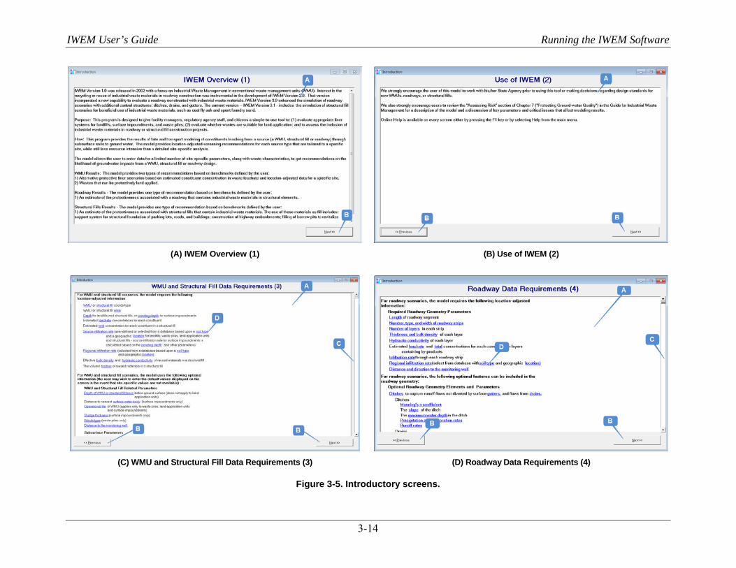
IWEM User’s Guide Running the IWEM Software
3-14
(A) IWEM Overview (1)
(B) Use of IWEM (2)
(C) WMU and Structural Fill Data Requirements (3) (D) Roadway Data Requirements (4)
Figure 3-5. Introductory screens.
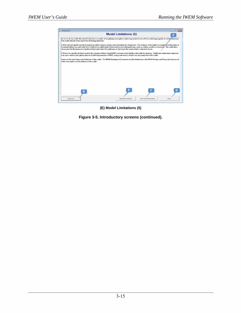
IWEM User’s Guide Running the IWEM Software
3-15
(E) Model Limitations (5)
Figure 3-5. Introductory screens (continued).
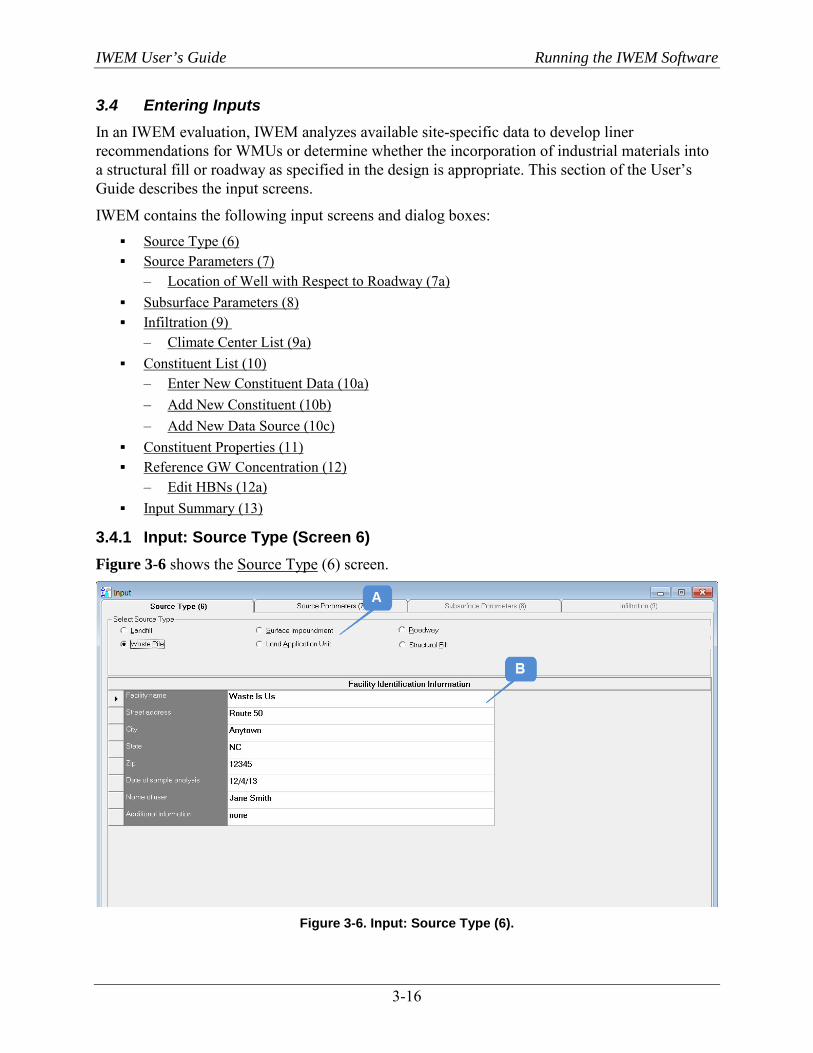
IWEM User’s Guide Running the IWEM Software
3-16
3.4 Entering Inputs In an IWEM evaluation, IWEM analyzes available site-specific data to develop liner recommendations for WMUs or determine whether the incorporation of industrial materials into a structural fill or roadway as specified in the design is appropriate. This section of the User’s Guide describes the input screens.
IWEM contains the following input screens and dialog boxes: Source Type (6) Source Parameters (7)
– Location of Well with Respect to Roadway (7a) Subsurface Parameters (8) Infiltration (9)
– Climate Center List (9a) Constituent List (10)
– Enter New Constituent Data (10a) – Add New Constituent (10b) – Add New Data Source (10c)
Constituent Properties (11) Reference GW Concentration (12)
– Edit HBNs (12a) Input Summary (13)
3.4.1 Input: Source Type (Screen 6) Figure 3-6 shows the Source Type (6) screen.
Figure 3-6. Input: Source Type (6).
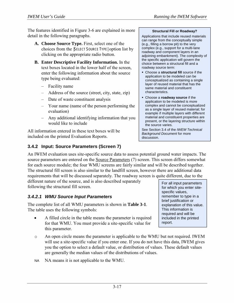
IWEM User’s Guide Running the IWEM Software
3-17
The features identified in Figure 3-6 are explained in more detail in the following paragraphs.
A. Choose Source Type. First, select one of the choices from the |SELECT SOURCE TYPE| option list by clicking on the appropriate radio button.
B. Enter Descriptive Facility Information. In the text boxes located in the lower half of the screen, enter the following information about the source type being evaluated:
– Facility name – Address of the source (street, city, state, zip) – Date of waste constituent analysis – Your name (name of the person performing the
evaluation) – Any additional identifying information that you
would like to include
All information entered in these text boxes will be included on the printed Evaluation Reports.
3.4.2 Input: Source Parameters (Screen 7) An IWEM evaluation uses site-specific source data to assess potential ground water impacts. The source parameters are entered on the Source Parameters (7) screen. This screen differs somewhat for each source module; the four WMU screens are fairly similar and will be described together. The structural fill screen is also similar to the landfill screen, however there are additional data requirements that will be discussed separately. The roadway screen is quite different, due to the different nature of the source, and is also described separately following the structural fill screen.
3.4.2.1 WMU Source Input Parameters The complete list of all WMU parameters is shown in Table 3-1. The table uses the following symbols:
• A filled circle in the table means the parameter is required for that WMU. You must provide a site-specific value for this parameter.
o An open circle means the parameter is applicable to the WMU but not required. IWEM will use a site-specific value if you enter one. If you do not have this data, IWEM gives you the option to select a default value, or distribution of values. These default values are generally the median values of the distributions of values.
NA NA means it is not applicable to the WMU.
For all input parameters for which you enter site-specific values, remember to type in a brief justification or explanation of this value. This information is required and will be included in the printed report.
Structural Fill or Roadway? Applications that include reused materials can range from the conceptually simple (e.g., filling a borrow pit) to the very complex (e.g., support for a multi-lane roadway and component layers in an adjoining embankment). The complexity of the specific application will govern the choice between a structural fill and a roadway source term: Choose a structural fill source if the
application to be modeled can be conceptualized as containing a single layer of reused material that has the same material and constituent characteristics.
Choose a roadway source if the application to be modeled is more complex and cannot be conceptualized as a single layer of reused material; for example if multiple layers with different material and constituent properties are present, or the layering structure within the source varies.
See Section 3.4 of the IWEM Technical Background Document for more discussion.
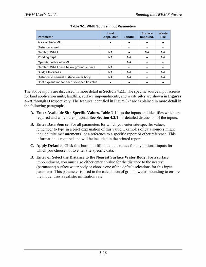
IWEM User’s Guide Running the IWEM Software
3-18
Table 3-1. WMU Source Input Parameters
Parameter Land
Appl. Unit Landfill Surface
Impound. Waste
Pile
Area of the WMU ● ● ● ● Distance to well ○ ○ ○ ○ Depth of WMU NA ● NA NA Ponding depth NA NA ● NA Operational life of WMU ○ NA ○ ○ Depth of WMU base below ground surface NA ○ ○ ○ Sludge thickness NA NA ○ NA Distance to nearest surface water body NA NA ○ NA Brief explanation for each site-specific value ● ● ● ●
The above inputs are discussed in more detail in Section 4.2.1. The specific source input screens for land application units, landfills, surface impoundments, and waste piles are shown in Figures 3-7A through D respectively. The features identified in Figure 3-7 are explained in more detail in the following paragraphs.
A. Enter Available Site-Specific Values. Table 3-1 lists the inputs and identifies which are required and which are optional. See Section 4.2.1 for detailed discussion of the inputs.
B. Enter Data Source. For all parameters for which you enter site-specific values, remember to type in a brief explanation of this value. Examples of data sources might include “site measurements” or a reference to a specific report or other reference. This information is required and will be included in the printed report.
C. Apply Defaults. Click this button to fill in default values for any optional inputs for which you choose not to enter site-specific data.
D. Enter or Select the Distance to the Nearest Surface Water Body. For a surface impoundment, you must also either enter a value for the distance to the nearest (permanent) surface water body or choose one of the default selections for this input parameter. This parameter is used in the calculation of ground water mounding to ensure the model uses a realistic infiltration rate.
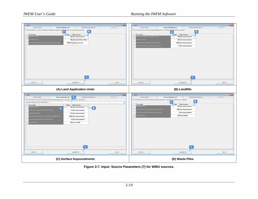
IWEM User’s Guide Running the IWEM Software
3-19
(A) Land Application Units (B) Landfills
(C) Surface Impoundments (D) Waste Piles
Figure 3-7. Input: Source Parameters (7) for WMU sources.
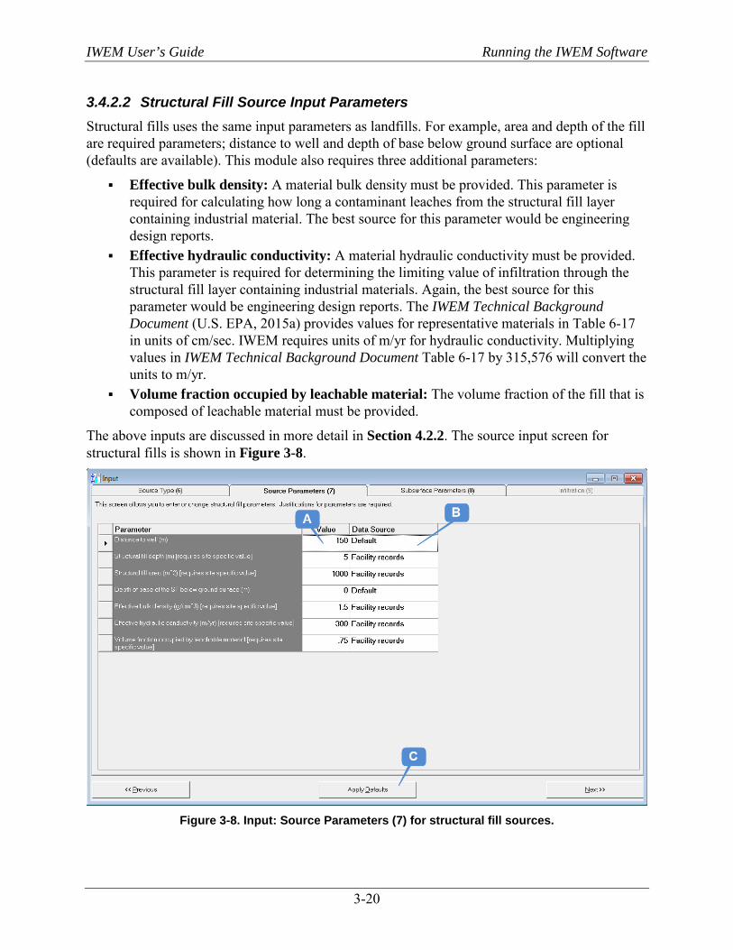
IWEM User’s Guide Running the IWEM Software
3-20
3.4.2.2 Structural Fill Source Input Parameters Structural fills uses the same input parameters as landfills. For example, area and depth of the fill are required parameters; distance to well and depth of base below ground surface are optional (defaults are available). This module also requires three additional parameters:
Effective bulk density: A material bulk density must be provided. This parameter is required for calculating how long a contaminant leaches from the structural fill layer containing industrial material. The best source for this parameter would be engineering design reports.
Effective hydraulic conductivity: A material hydraulic conductivity must be provided. This parameter is required for determining the limiting value of infiltration through the structural fill layer containing industrial materials. Again, the best source for this parameter would be engineering design reports. The IWEM Technical Background Document (U.S. EPA, 2015a) provides values for representative materials in Table 6-17 in units of cm/sec. IWEM requires units of m/yr for hydraulic conductivity. Multiplying values in IWEM Technical Background Document Table 6-17 by 315,576 will convert the units to m/yr.
Volume fraction occupied by leachable material: The volume fraction of the fill that is composed of leachable material must be provided.
The above inputs are discussed in more detail in Section 4.2.2. The source input screen for structural fills is shown in Figure 3-8.
Figure 3-8. Input: Source Parameters (7) for structural fill sources.
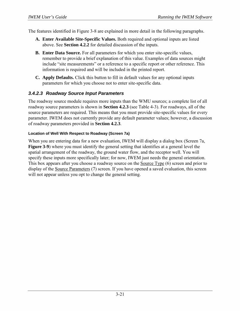
IWEM User’s Guide Running the IWEM Software
3-21
The features identified in Figure 3-8 are explained in more detail in the following paragraphs.
A. Enter Available Site-Specific Values. Both required and optional inputs are listed above. See Section 4.2.2 for detailed discussion of the inputs.
B. Enter Data Source. For all parameters for which you enter site-specific values, remember to provide a brief explanation of this value. Examples of data sources might include “site measurements” or a reference to a specific report or other reference. This information is required and will be included in the printed report.
C. Apply Defaults. Click this button to fill in default values for any optional inputs parameters for which you choose not to enter site-specific data.
3.4.2.3 Roadway Source Input Parameters The roadway source module requires more inputs than the WMU sources; a complete list of all roadway source parameters is shown in Section 4.2.3 (see Table 4-3). For roadways, all of the source parameters are required. This means that you must provide site-specific values for every parameter. IWEM does not currently provide any default parameter values; however, a discussion of roadway parameters provided in Section 4.2.3.
Location of Well With Respect to Roadway (Screen 7a)
When you are entering data for a new evaluation, IWEM will display a dialog box (Screen 7a, Figure 3-9) where you must identify the general setting that identifies at a general level the spatial arrangement of the roadway, the ground water flow, and the receptor well. You will specify these inputs more specifically later; for now, IWEM just needs the general orientation. This box appears after you choose a roadway source on the Source Type (6) screen and prior to display of the Source Parameters (7) screen. If you have opened a saved evaluation, this screen will not appear unless you opt to change the general setting.
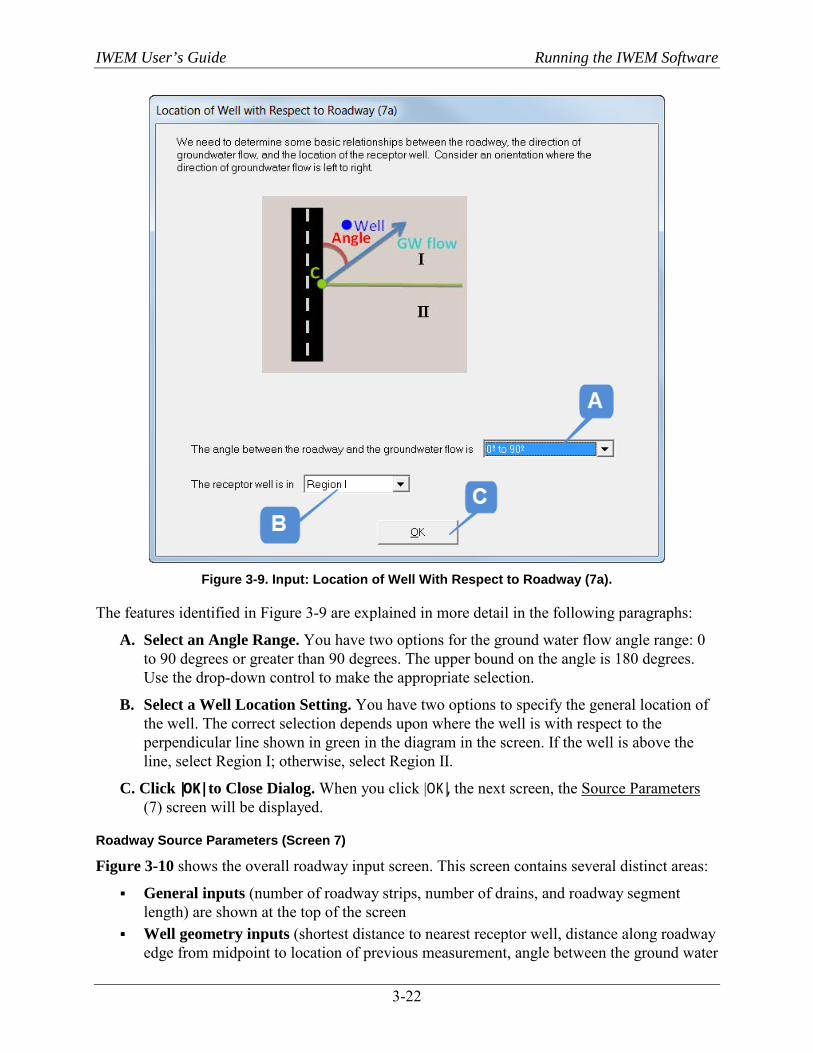
IWEM User’s Guide Running the IWEM Software
3-22
Figure 3-9. Input: Location of Well With Respect to Roadway (7a).
The features identified in Figure 3-9 are explained in more detail in the following paragraphs:
A. Select an Angle Range. You have two options for the ground water flow angle range: 0 to 90 degrees or greater than 90 degrees. The upper bound on the angle is 180 degrees. Use the drop-down control to make the appropriate selection.
B. Select a Well Location Setting. You have two options to specify the general location of the well. The correct selection depends upon where the well is with respect to the perpendicular line shown in green in the diagram in the screen. If the well is above the line, select Region I; otherwise, select Region II.
C. Click |OK| to Close Dialog. When you click |OK|, the next screen, the Source Parameters (7) screen will be displayed.
Roadway Source Parameters (Screen 7)
Figure 3-10 shows the overall roadway input screen. This screen contains several distinct areas:
General inputs (number of roadway strips, number of drains, and roadway segment length) are shown at the top of the screen
Well geometry inputs (shortest distance to nearest receptor well, distance along roadway edge from midpoint to location of previous measurement, angle between the ground water
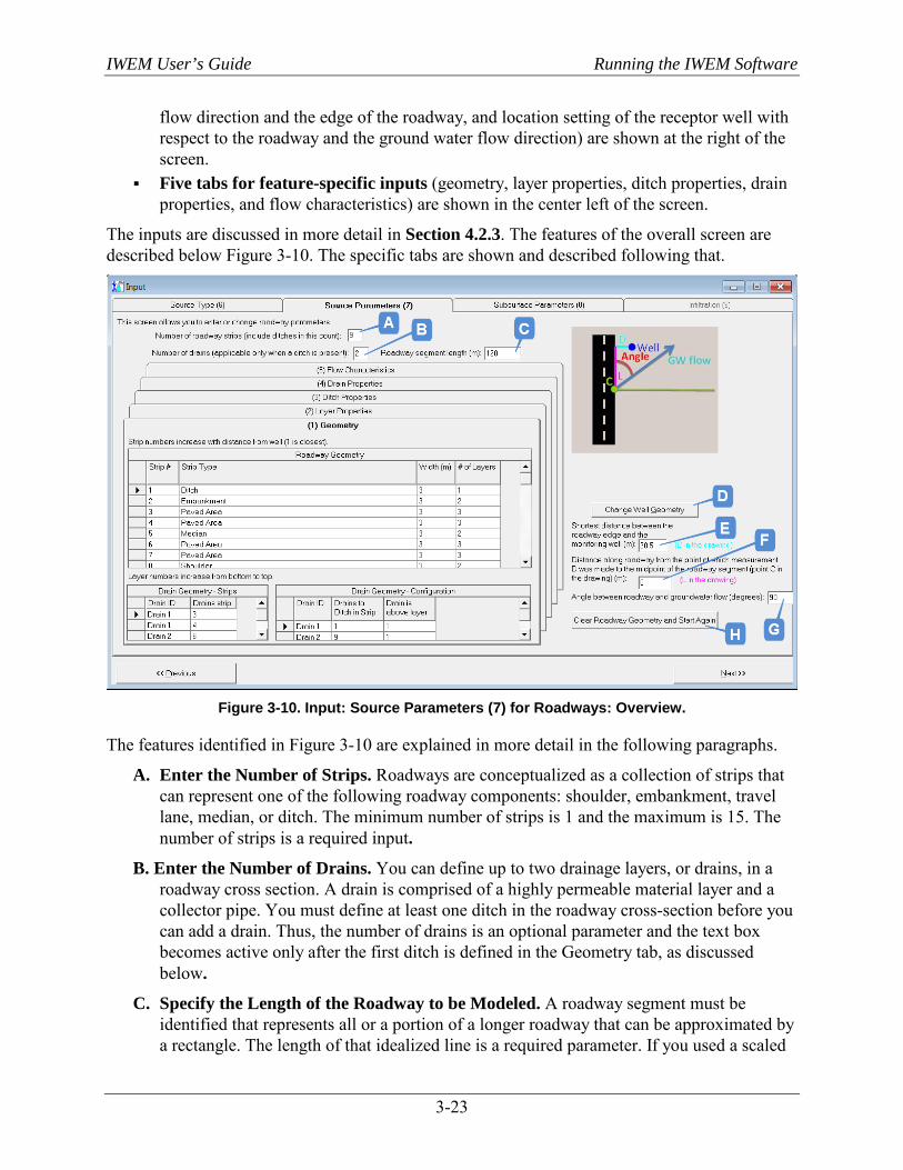
IWEM User’s Guide Running the IWEM Software
3-23
flow direction and the edge of the roadway, and location setting of the receptor well with respect to the roadway and the ground water flow direction) are shown at the right of the screen.
Five tabs for feature-specific inputs (geometry, layer properties, ditch properties, drain properties, and flow characteristics) are shown in the center left of the screen.
The inputs are discussed in more detail in Section 4.2.3. The features of the overall screen are described below Figure 3-10. The specific tabs are shown and described following that.
Figure 3-10. Input: Source Parameters (7) for Roadways: Overview.
The features identified in Figure 3-10 are explained in more detail in the following paragraphs.
A. Enter the Number of Strips. Roadways are conceptualized as a collection of strips that can represent one of the following roadway components: shoulder, embankment, travel lane, median, or ditch. The minimum number of strips is 1 and the maximum is 15. The number of strips is a required input.
B. Enter the Number of Drains. You can define up to two drainage layers, or drains, in a roadway cross section. A drain is comprised of a highly permeable material layer and a collector pipe. You must define at least one ditch in the roadway cross-section before you can add a drain. Thus, the number of drains is an optional parameter and the text box becomes active only after the first ditch is defined in the Geometry tab, as discussed below.
C. Specify the Length of the Roadway to be Modeled. A roadway segment must be identified that represents all or a portion of a longer roadway that can be approximated by a rectangle. The length of that idealized line is a required parameter. If you used a scaled
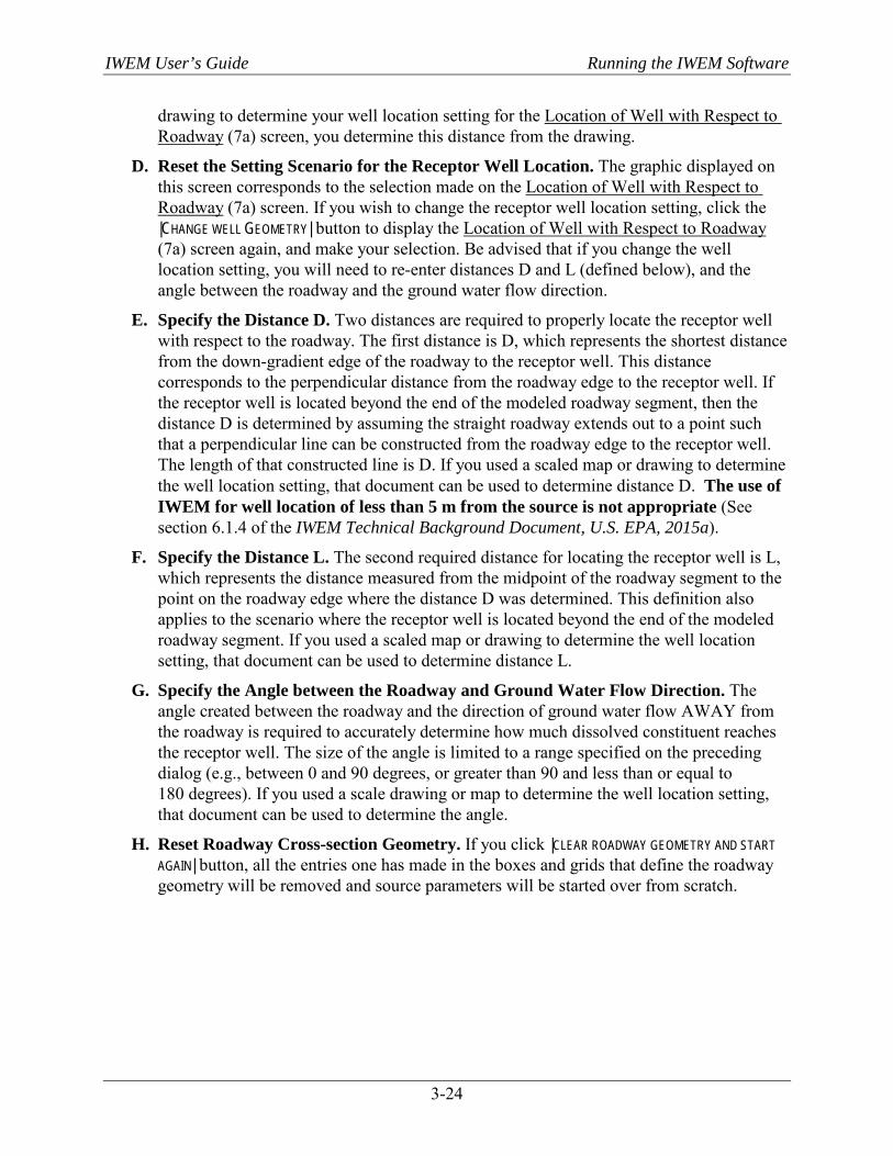
IWEM User’s Guide Running the IWEM Software
3-24
drawing to determine your well location setting for the Location of Well with Respect to Roadway (7a) screen, you determine this distance from the drawing.
D. Reset the Setting Scenario for the Receptor Well Location. The graphic displayed on this screen corresponds to the selection made on the Location of Well with Respect to Roadway (7a) screen. If you wish to change the receptor well location setting, click the |CHANGE WELL GEOMETRY| button to display the Location of Well with Respect to Roadway (7a) screen again, and make your selection. Be advised that if you change the well location setting, you will need to re-enter distances D and L (defined below), and the angle between the roadway and the ground water flow direction.
E. Specify the Distance D. Two distances are required to properly locate the receptor well with respect to the roadway. The first distance is D, which represents the shortest distance from the down-gradient edge of the roadway to the receptor well. This distance corresponds to the perpendicular distance from the roadway edge to the receptor well. If the receptor well is located beyond the end of the modeled roadway segment, then the distance D is determined by assuming the straight roadway extends out to a point such that a perpendicular line can be constructed from the roadway edge to the receptor well. The length of that constructed line is D. If you used a scaled map or drawing to determine the well location setting, that document can be used to determine distance D. The use of IWEM for well location of less than 5 m from the source is not appropriate (See section 6.1.4 of the IWEM Technical Background Document, U.S. EPA, 2015a).
F. Specify the Distance L. The second required distance for locating the receptor well is L, which represents the distance measured from the midpoint of the roadway segment to the point on the roadway edge where the distance D was determined. This definition also applies to the scenario where the receptor well is located beyond the end of the modeled roadway segment. If you used a scaled map or drawing to determine the well location setting, that document can be used to determine distance L.
G. Specify the Angle between the Roadway and Ground Water Flow Direction. The angle created between the roadway and the direction of ground water flow AWAY from the roadway is required to accurately determine how much dissolved constituent reaches the receptor well. The size of the angle is limited to a range specified on the preceding dialog (e.g., between 0 and 90 degrees, or greater than 90 and less than or equal to 180 degrees). If you used a scale drawing or map to determine the well location setting, that document can be used to determine the angle.
H. Reset Roadway Cross-section Geometry. If you click |CLEAR ROADWAY GEOMETRY AND START AGAIN| button, all the entries one has made in the boxes and grids that define the roadway geometry will be removed and source parameters will be started over from scratch.
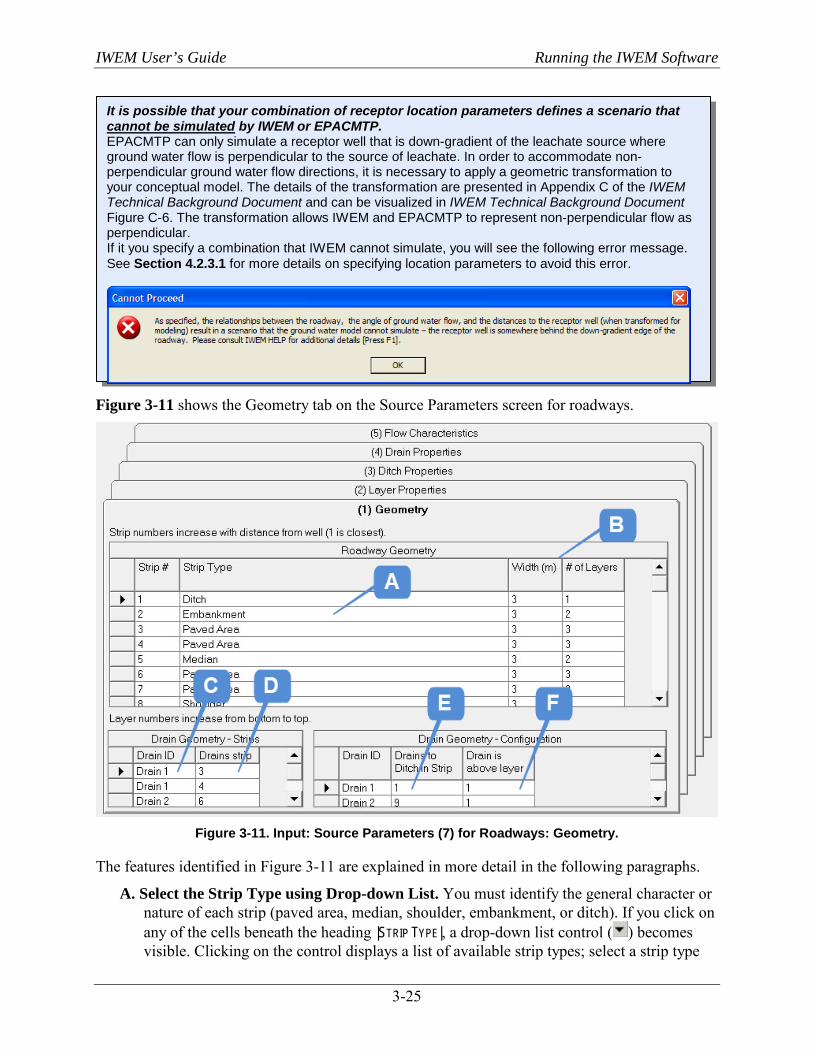
IWEM User’s Guide Running the IWEM Software
3-25
Figure 3-11 shows the Geometry tab on the Source Parameters screen for roadways.
Figure 3-11. Input: Source Parameters (7) for Roadways: Geometry.
The features identified in Figure 3-11 are explained in more detail in the following paragraphs.
A. Select the Strip Type using Drop-down List. You must identify the general character or nature of each strip (paved area, median, shoulder, embankment, or ditch). If you click on any of the cells beneath the heading |STRIP TYPE|, a drop-down list control ( ) becomes visible. Clicking on the control displays a list of available strip types; select a strip type
It is possible that your combination of receptor location parameters defines a scenario that cannot be simulated by IWEM or EPACMTP. EPACMTP can only simulate a receptor well that is down-gradient of the leachate source where ground water flow is perpendicular to the source of leachate. In order to accommodate non-perpendicular ground water flow directions, it is necessary to apply a geometric transformation to your conceptual model. The details of the transformation are presented in Appendix C of the IWEM Technical Background Document and can be visualized in IWEM Technical Background Document Figure C-6. The transformation allows IWEM and EPACMTP to represent non-perpendicular flow as perpendicular. If it you specify a combination that IWEM cannot simulate, you will see the following error message. See Section 4.2.3.1 for more details on specifying location parameters to avoid this error.

IWEM User’s Guide Running the IWEM Software
3-26
by clicking on the item in the list. Designating a Strip Type is required. If a strip is defined as a Ditch, the text box for the number of drains is enabled (see Item C above).
B. Enter Strip Width and Number of Layers. You must provide the width of that strip and the number of material layers used in constructing that strip. The best source for these parameters would be construction design drawings for roadways. In addition, maps, plan drawings, and area1 photos may also provide useful information.
C. Select a Drain Using Drop-down List. Assuming you have defined at least one drain, you will need to associate a drain with the one or more strips that contain that drain. The first step is to select a drain from the drop-down list that appears by clicking on the cell beneath the heading |DRAIN ID|. Clicking a cell will cause a drop-down list control ( ) to become visible. Clicking on the control displays a list of available drain IDs; select a drain ID by clicking on the item in the list.
D. Associate Strips with a Drain Using Drop-down List. This is second step to associate a drain and strip. Use the drop-down list beneath the heading |DRAINS STRIP|, to choose the strip number associated with the drain.
E. Identify the Ditch Strip Receiving Drainage Water. Each drain must be connected to a ditch. You may connect two drains to a single ditch, as long as the ditch is between the drains. Use the drop-down list beneath the heading |DRAINS TO DITCH IN STRIP|, to choose the strip representing a ditch that receives drainage from each drain.
F. Specify where Drain is in Cross-section. As mentioned above in Item C, the layering (and material) configuration beneath a drain must be identical across strips serviced by that drain. You locate the drain by specifying the layer number directly beneath each drain.
Figure 3-12 shows the Layer Properties tab on the Source Parameters screen for roadways.
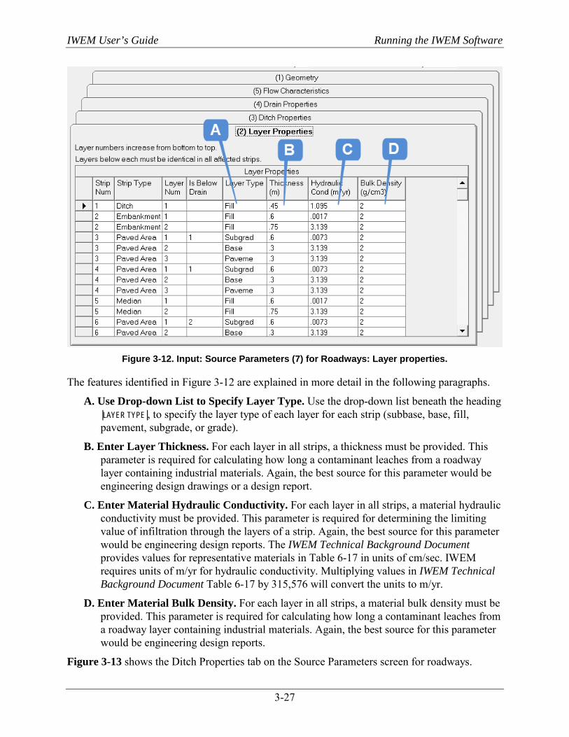
IWEM User’s Guide Running the IWEM Software
3-27
Figure 3-12. Input: Source Parameters (7) for Roadways: Layer properties.
The features identified in Figure 3-12 are explained in more detail in the following paragraphs.
A. Use Drop-down List to Specify Layer Type. Use the drop-down list beneath the heading |LAYER TYPE|, to specify the layer type of each layer for each strip (subbase, base, fill, pavement, subgrade, or grade).
B. Enter Layer Thickness. For each layer in all strips, a thickness must be provided. This parameter is required for calculating how long a contaminant leaches from a roadway layer containing industrial materials. Again, the best source for this parameter would be engineering design drawings or a design report.
C. Enter Material Hydraulic Conductivity. For each layer in all strips, a material hydraulic conductivity must be provided. This parameter is required for determining the limiting value of infiltration through the layers of a strip. Again, the best source for this parameter would be engineering design reports. The IWEM Technical Background Document provides values for representative materials in Table 6-17 in units of cm/sec. IWEM requires units of m/yr for hydraulic conductivity. Multiplying values in IWEM Technical Background Document Table 6-17 by 315,576 will convert the units to m/yr.
D. Enter Material Bulk Density. For each layer in all strips, a material bulk density must be provided. This parameter is required for calculating how long a contaminant leaches from a roadway layer containing industrial materials. Again, the best source for this parameter would be engineering design reports.
Figure 3-13 shows the Ditch Properties tab on the Source Parameters screen for roadways.

IWEM User’s Guide Running the IWEM Software
3-28
Figure 3-13. Input: Source Parameters (7) for Roadways: Ditch properties.
The features identified in Figure 3-13 are explained in more detail in the following paragraphs.
A. Enter Manning’s n for each Ditch. For each ditch strip, you must provide a value for Manning’s roughness coefficient, n. This parameter is required for estimating the ditch inflow/outflow rate calculated from cross-sectional average velocity along the ditch. Again, the best source for this parameter would be engineering design drawings or a design report. Representative values are provided in Section 4 (Table 4-4).
B. Enter Slope for each Ditch. For each ditch strip, slope of the ditch bed (dimensionless) must be provided. The slope can be calculated as the change in elevation of the ditch bed over its length divided by the length of the ditch. The slope should be set to zero if there is stagnant water in the ditch (no flow).
C. Enter the Maximum Water Depth for each Ditch. To safeguard against possible unrealistic values of water depth in the ditch, the estimated water depth is limited to this maximum water depth. The maximum water depth corresponds to the height from the ditch bed to the lowest cresting side.
D. Use Check Box to Indicate the Presence of a Gutter. Checking the box indicates that a surface gutter is present in the roadway cross-section and the gutter is associated with a specific ditch strip. A gutter is used to divert some or all of the runoff water from strips “above” the gutter, away from the associated ditch and out of the modeled system. You can specify how much of the runoff is not diverted in Item A of the Flow Characteristics grid, discussed below.
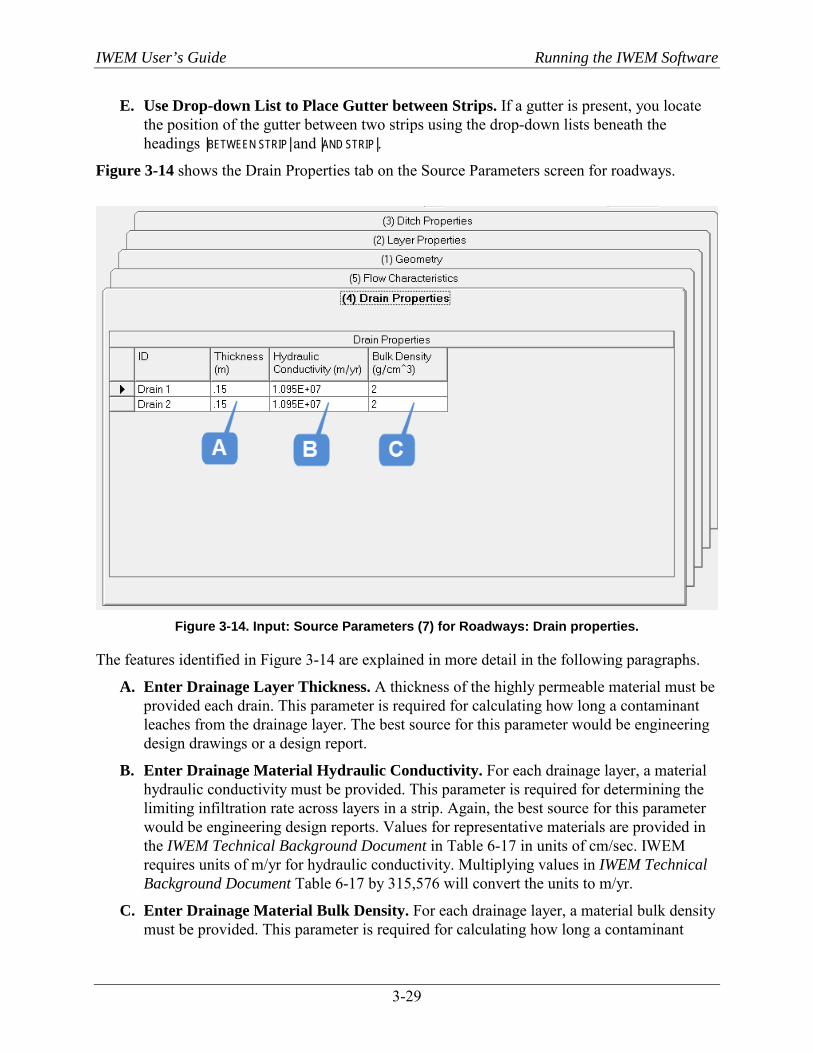
IWEM User’s Guide Running the IWEM Software
3-29
E. Use Drop-down List to Place Gutter between Strips. If a gutter is present, you locate the position of the gutter between two strips using the drop-down lists beneath the headings |BETWEEN STRIP| and |AND STRIP|.
Figure 3-14 shows the Drain Properties tab on the Source Parameters screen for roadways.
Figure 3-14. Input: Source Parameters (7) for Roadways: Drain properties.
The features identified in Figure 3-14 are explained in more detail in the following paragraphs.
A. Enter Drainage Layer Thickness. A thickness of the highly permeable material must be provided each drain. This parameter is required for calculating how long a contaminant leaches from the drainage layer. The best source for this parameter would be engineering design drawings or a design report.
B. Enter Drainage Material Hydraulic Conductivity. For each drainage layer, a material hydraulic conductivity must be provided. This parameter is required for determining the limiting infiltration rate across layers in a strip. Again, the best source for this parameter would be engineering design reports. Values for representative materials are provided in the IWEM Technical Background Document in Table 6-17 in units of cm/sec. IWEM requires units of m/yr for hydraulic conductivity. Multiplying values in IWEM Technical Background Document Table 6-17 by 315,576 will convert the units to m/yr.
C. Enter Drainage Material Bulk Density. For each drainage layer, a material bulk density must be provided. This parameter is required for calculating how long a contaminant
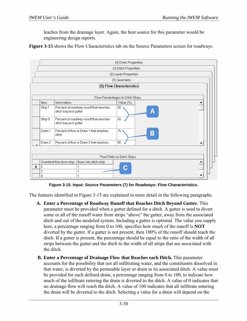
IWEM User’s Guide Running the IWEM Software
3-30
leaches from the drainage layer. Again, the best source for this parameter would be engineering design reports.
Figure 3-15 shows the Flow Characteristics tab on the Source Parameters screen for roadways.
Figure 3-15. Input: Source Parameters (7) for Roadways: Flow Characteristics.
The features identified in Figure 3-15 are explained in more detail in the following paragraphs.
A. Enter a Percentage of Roadway Runoff that Reaches Ditch Beyond Gutter. This parameter must be provided when a gutter defined for a ditch. A gutter is used to divert some or all of the runoff water from strips “above” the gutter, away from the associated ditch and out of the modeled system. Including a gutter is optional. The value you supply here, a percentage ranging from 0 to 100, specifies how much of the runoff is NOT diverted by the gutter. If a gutter is not present, then 100% of the runoff should reach the ditch. If a gutter is present, the percentage should be equal to the ratio of the width of all strips between the gutter and the ditch to the width of all strips that are associated with the ditch.
B. Enter a Percentage of Drainage Flow that Reaches each Ditch. This parameter accounts for the possibility that not all infiltrating water, and the constituents dissolved in that water, is diverted by the permeable layer or drain to its associated ditch. A value must be provided for each defined drain, a percentage ranging from 0 to 100, to indicate how much of the infiltrate entering the drain is diverted to the ditch. A value of 0 indicates that no drainage flow will reach the ditch. A value of 100 indicates that all infiltrate entering the drain will be diverted to the ditch. Selecting a value for a drain will depend on the
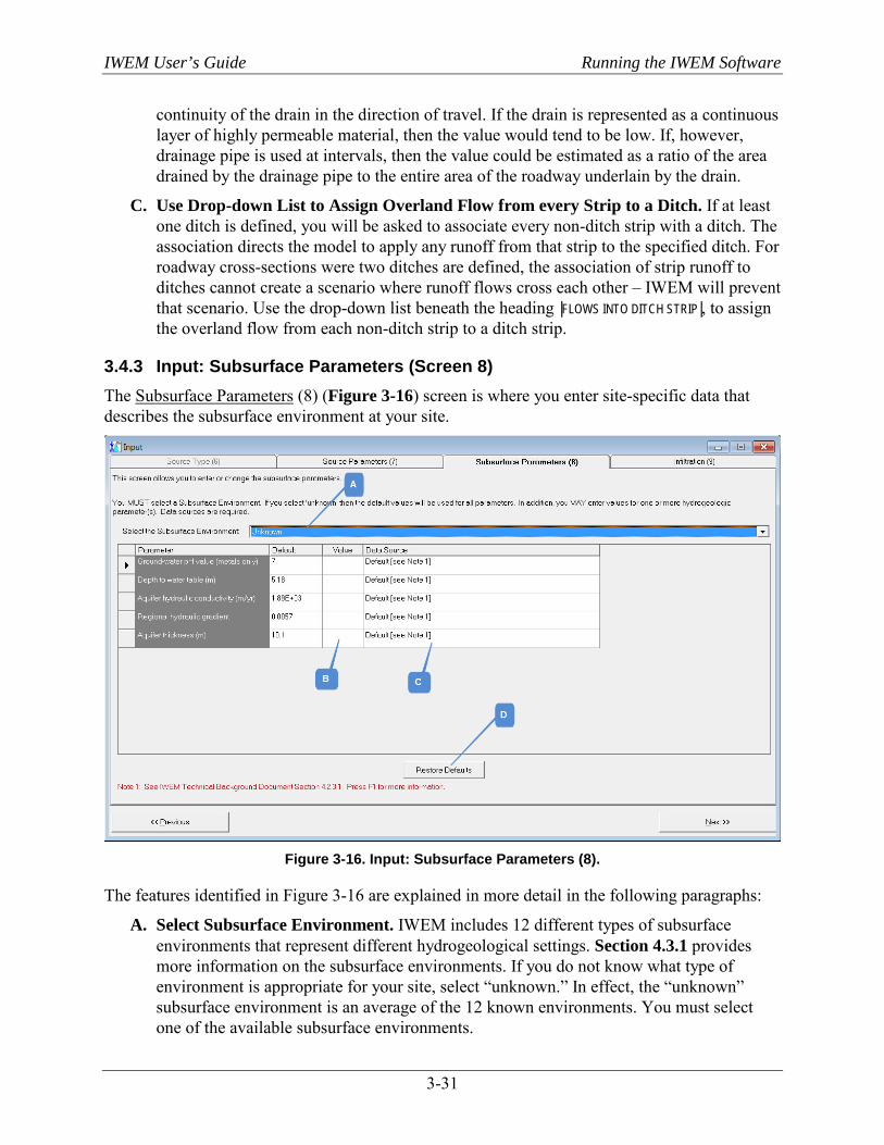
IWEM User’s Guide Running the IWEM Software
3-31
continuity of the drain in the direction of travel. If the drain is represented as a continuous layer of highly permeable material, then the value would tend to be low. If, however, drainage pipe is used at intervals, then the value could be estimated as a ratio of the area drained by the drainage pipe to the entire area of the roadway underlain by the drain.
C. Use Drop-down List to Assign Overland Flow from every Strip to a Ditch. If at least one ditch is defined, you will be asked to associate every non-ditch strip with a ditch. The association directs the model to apply any runoff from that strip to the specified ditch. For roadway cross-sections were two ditches are defined, the association of strip runoff to ditches cannot create a scenario where runoff flows cross each other – IWEM will prevent that scenario. Use the drop-down list beneath the heading |FLOWS INTO DITCH STRIP|, to assign the overland flow from each non-ditch strip to a ditch strip.
3.4.3 Input: Subsurface Parameters (Screen 8) The Subsurface Parameters (8) (Figure 3-16) screen is where you enter site-specific data that describes the subsurface environment at your site.
Figure 3-16. Input: Subsurface Parameters (8).
The features identified in Figure 3-16 are explained in more detail in the following paragraphs:
A. Select Subsurface Environment. IWEM includes 12 different types of subsurface environments that represent different hydrogeological settings. Section 4.3.1 provides more information on the subsurface environments. If you do not know what type of environment is appropriate for your site, select “unknown.” In effect, the “unknown” subsurface environment is an average of the 12 known environments. You must select one of the available subsurface environments.
IWEM User’s Guide Running the IWEM Software
3-32
B. Enter Available Site-Specific Values. You may enter values for any subsurface parameters for which you have site-specific data. You need not enter data for every parameter. If you do not enter site-specific data, IWEM will use a default or distribution, depending on the selected subsurface environment:
– For the unknown subsurface environment, IWEM will use the default value displayed (in the default value column). The value displayed on the screen will be input to the model as a constant value (no distribution of values is used). Each default value corresponds to the mean value of the available data for that parameter from all 12 subsurface environments. This value is representative of a national average. The displayed value in the data source column and the phrase “Default [see Note 1]” in the data source column indicate that IWEM will use the displayed default value for this input parameter in the analysis.
– For all other subsurface environments, IWEM will use a distribution of parameter values that corresponds to the specified subsurface environment to generate values. The word “Distribution” displayed in the default value column and the phrase “Monte Carlo [see Note 1]” in the data source column indicate that IWEM will randomly select values for this parameter from the appropriate distribution during the analysis. The distributions reflect the range of values that each parameter can have.
C. View or Edit Data Source for Each Value. You must document the data source or explain the value used for any site-specific values you enter. IWEM provides a default data source for all optional data. All data sources or explanations for default or user-specified data are included in the printed report.
D. Click to Restore Default Values. Clicking this button will clear any site-specific values and data sources you have entered and reset the default values.
For roadway sources, the information provided on screens 7, 7a, and 8 completely describe the roadway setting as required by IWEM. When you click |NEXT| on screen 8, IWEM will check your inputs to evaluate whether the setting you have described is physically possible and consistent with the EPACMTP model. Specifically, IWEM verifies that: the bottom of the roadway is above the water table, and the aquifer can support a typical drinking water well. If you do not specify the depth to ground water, IWEM will postpone this evaluation until the Infiltration (9) screen has been completed. IWEM will notify you if either of the above conditions is violated with a message box informing you of your options. If none of the suggested options is consistent with the conditions at your site, IWEM is not appropriate for your site, and you should consider a detailed, site-specific analysis. Consult Section 4.3, or the IWEM Technical Background Document, for more information on the assumptions built into the EPACMTP model which may make it unsuitable for a particular site.
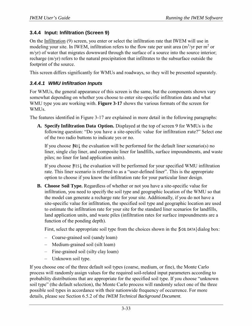
IWEM User’s Guide Running the IWEM Software
3-33
3.4.4 Input: Infiltration (Screen 9) On the Infiltration (9) screen, you enter or select the infiltration rate that IWEM will use in modeling your site. In IWEM, infiltration refers to the flow rate per unit area (m3/yr per m2 or m/yr) of water that migrates downward through the surface of a source into the source interior; recharge (m/yr) refers to the natural precipitation that infiltrates to the subsurface outside the footprint of the source.
This screen differs significantly for WMUs and roadways, so they will be presented separately.
3.4.4.1 WMU Infiltration Inputs For WMUs, the general appearance of this screen is the same, but the components shown vary somewhat depending on whether you choose to enter site-specific infiltration data and what WMU type you are working with. Figure 3-17 shows the various formats of the screen for WMUs.
The features identified in Figure 3-17 are explained in more detail in the following paragraphs:
A. Specify Infiltration Data Option. Displayed at the top of screen 9 for WMUs is the following question: “Do you have a site-specific value for infiltration rate?” Select one of the two radio buttons to indicate yes or no.
If you choose |NO|, the evaluation will be performed for the default liner scenario(s) no liner, single clay liner, and composite liner for landfills, surface impoundments, and waste piles; no liner for land application units).
If you choose |YES|, the evaluation will be performed for your specified WMU infiltration rate. This liner scenario is referred to as a “user-defined liner”. This is the appropriate option to choose if you know the infiltration rate for your particular liner design.
B. Choose Soil Type. Regardless of whether or not you have a site-specific value for infiltration, you need to specify the soil type and geographic location of the WMU so that the model can generate a recharge rate for your site. Additionally, if you do not have a site-specific value for infiltration, the specified soil type and geographic location are used to estimate the infiltration rate for your site for the standard liner scenarios for landfills, land application units, and waste piles (infiltration rates for surface impoundments are a function of the ponding depth).
First, select the appropriate soil type from the choices shown in the |SOIL DATA| dialog box:
– Coarse-grained soil (sandy loam) – Medium-grained soil (silt loam) – Fine-grained soil (silty clay loam) – Unknown soil type.
If you choose one of the three default soil types (coarse, medium, or fine), the Monte Carlo process will randomly assign values for the required soil-related input parameters according to probability distributions that are appropriate for the specified soil type. If you choose “unknown soil type” (the default selection), the Monte Carlo process will randomly select one of the three possible soil types in accordance with their nationwide frequency of occurrence. For more details, please see Section 6.5.2 of the IWEM Technical Background Document.
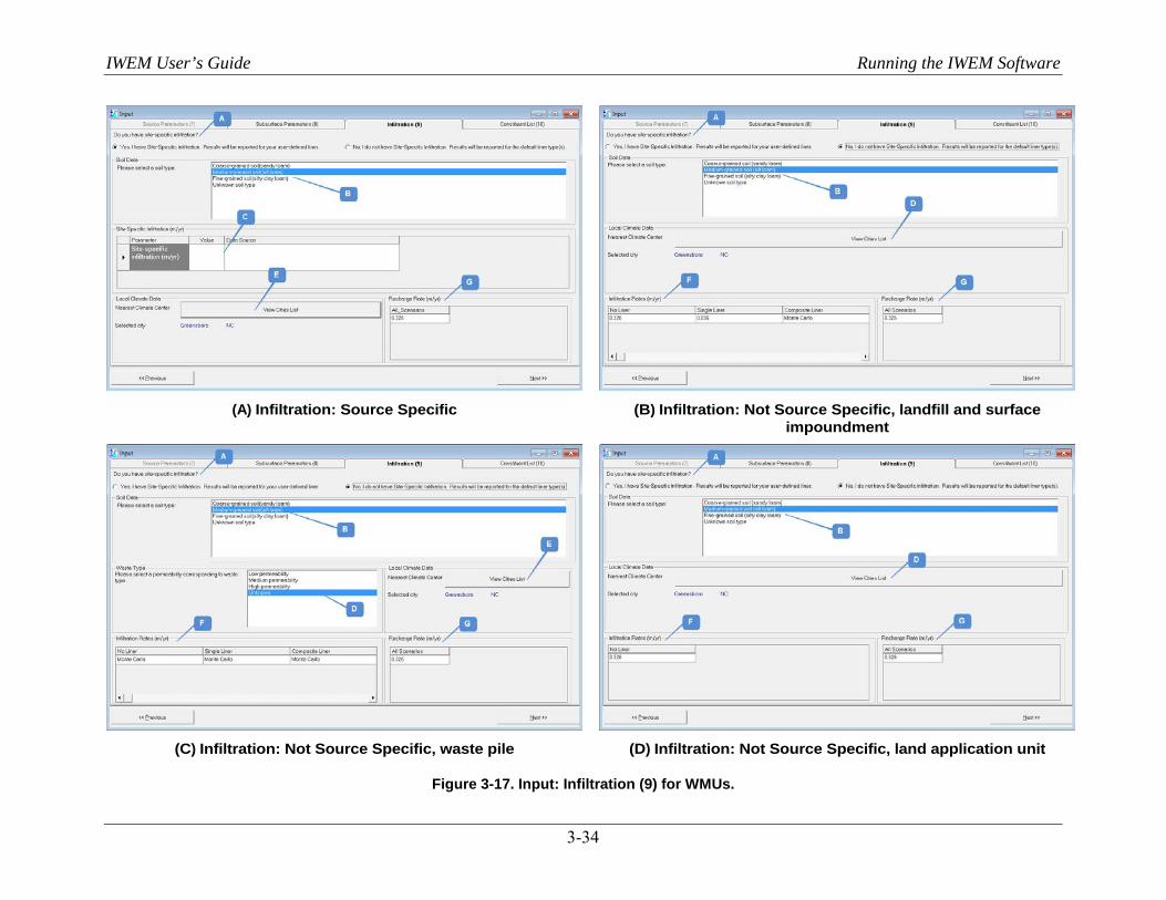
IWEM User’s Guide Running the IWEM Software
3-34
(A) Infiltration: Source Specific (B) Infiltration: Not Source Specific, landfill and surface
impoundment
(C) Infiltration: Not Source Specific, waste pile (D) Infiltration: Not Source Specific, land application unit
Figure 3-17. Input: Infiltration (9) for WMUs.
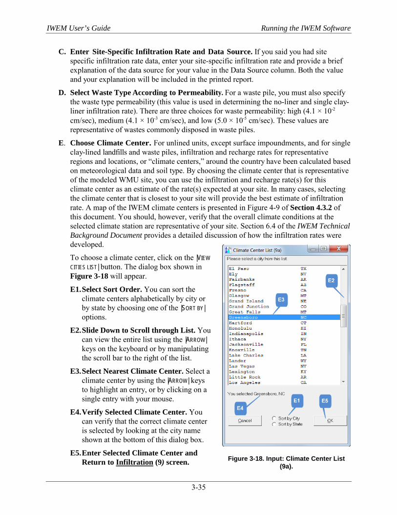
IWEM User’s Guide Running the IWEM Software
3-35
C. Enter Site-Specific Infiltration Rate and Data Source. If you said you had site specific infiltration rate data, enter your site-specific infiltration rate and provide a brief explanation of the data source for your value in the Data Source column. Both the value and your explanation will be included in the printed report.
D. Select Waste Type According to Permeability. For a waste pile, you must also specify the waste type permeability (this value is used in determining the no-liner and single clay-liner infiltration rate). There are three choices for waste permeability: high (4.1 × 10⁻²
cm/sec), medium (4.1 × 10⁻³ cm/sec), and low (5.0 × 10⁻⁵ cm/sec). These values are representative of wastes commonly disposed in waste piles.
E. Choose Climate Center. For unlined units, except surface impoundments, and for single clay-lined landfills and waste piles, infiltration and recharge rates for representative regions and locations, or “climate centers,” around the country have been calculated based on meteorological data and soil type. By choosing the climate center that is representative of the modeled WMU site, you can use the infiltration and recharge rate(s) for this climate center as an estimate of the rate(s) expected at your site. In many cases, selecting the climate center that is closest to your site will provide the best estimate of infiltration rate. A map of the IWEM climate centers is presented in Figure 4-9 of Section 4.3.2 of this document. You should, however, verify that the overall climate conditions at the selected climate station are representative of your site. Section 6.4 of the IWEM Technical Background Document provides a detailed discussion of how the infiltration rates were developed.
To choose a climate center, click on the |VIEW CITIES LIST| button. The dialog box shown in Figure 3-18 will appear.
E1. Select Sort Order. You can sort the climate centers alphabetically by city or by state by choosing one of the |SORT BY| options.
E2. Slide Down to Scroll through List. You can view the entire list using the |ARROW| keys on the keyboard or by manipulating the scroll bar to the right of the list.
E3. Select Nearest Climate Center. Select a climate center by using the |ARROW| keys to highlight an entry, or by clicking on a single entry with your mouse.
E4. Verify Selected Climate Center. You can verify that the correct climate center is selected by looking at the city name shown at the bottom of this dialog box.
E5. Enter Selected Climate Center and Return to Infiltration (9) screen.
Figure 3-18. Input: Climate Center List (9a).
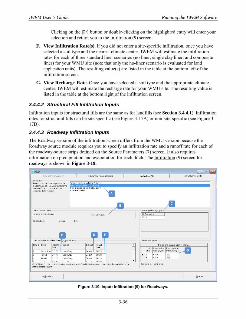
IWEM User’s Guide Running the IWEM Software
3-36
Clicking on the |OK| button or double-clicking on the highlighted entry will enter your selection and return you to the Infiltration (9) screen.
F. View Infiltration Rate(s). If you did not enter a site-specific infiltration, once you have selected a soil type and the nearest climate center, IWEM will estimate the infiltration rates for each of three standard liner scenarios (no liner, single clay liner, and composite liner) for your WMU site (note that only the no-liner scenario is evaluated for land application units). The resulting value(s) are listed in the table at the bottom left of the infiltration screen.
G. View Recharge Rate. Once you have selected a soil type and the appropriate climate center, IWEM will estimate the recharge rate for your WMU site. The resulting value is listed in the table at the bottom right of the infiltration screen.
3.4.4.2 Structural Fill Infiltration Inputs Infiltration inputs for structural fills are the same as for landfills (see Section 3.4.4.1). Infiltration rates for structural fills can be site specific (see Figure 3-17A) or non-site-specific (see Figure 3-17B).
3.4.4.3 Roadway Infiltration Inputs The Roadway version of the infiltration screen differs from the WMU version because the Roadway source module requires you to specify an infiltration rate and a runoff rate for each of the roadway-source strips defined on the Source Parameters (7) screen. It also requires information on precipitation and evaporation for each ditch. The Infiltration (9) screen for roadways is shown in Figure 3-19.
Figure 3-19. Input: Infiltration (9) for Roadways.

IWEM User’s Guide Running the IWEM Software
3-37
The features identified in Figure 3-19 are explained in more detail in the following paragraphs:
A. Choose Soil Type. Specify the soil type and geographic location of the roadway so that the model can generate a recharge rate for your site. First, select the appropriate soil type from the choices shown in the |SOIL DATA| dialog box:
– Coarse-grained soil (sandy loam) – Medium-grained soil (silt loam) – Fine-grained soil (silty clay loam) – Unknown soil type.
If you choose one of the three default soil types (coarse, medium, or fine), the Monte Carlo process will randomly assign values for the required soil-related input parameters according to probability distributions that are appropriate for the specified soil type. If you choose “unknown soil type” (the default selection), the Monte Carlo process will randomly select one of the three possible soil types in accordance with their nationwide frequency of occurrence. For more details, please see Section 6.5.2 of the IWEM Technical Background Document.
B. Choose Climate Center. Infiltration and recharge rates for representative regions and locations, or “climate centers,” around the country have been calculated based on meteorological data and soil type. By choosing the climate center that is representative of the modeled site, you can use the infiltration and recharge rate(s) for this climate center as an estimate of the rate(s) expected at your site. In many cases, selecting the climate center that is closest to your site will provide the best estimate of infiltration rate. A map of the IWEM climate centers is presented in Figure 4-9 of Section 4.3.2 of this document. You should, however, verify that the overall climate conditions at the selected climate station are representative of your site. Section 6.4 of the IWEM Technical Background Document provides a detailed discussion of how the infiltration rates were developed.
To choose a climate center, click on the |VIEW CITIES LIST| button. The dialog box shown earlier in Figure 3-18 will appear. See the bullets with that figure for instructions on navigating that box.
C. View Recharge Rate. Once you have selected a soil type and the appropriate climate center, the model will estimate the recharge rate for your site. The resulting value is listed in the table at the center right of the Infiltration (9) screen.
D. Enter Infiltration Rate(s). The roadway module requires the rate of water infiltration through each strip defined in your roadway. If you have estimates of these rates, then you may enter those values here, along with any supporting information in the next column to the right.
E. Select From Default Rates. If you do not have estimates of infiltration rates, you can use one of the available default roadway infiltration rates. Click on the "Select" button to display the dialog box shown in Figure 3-20.
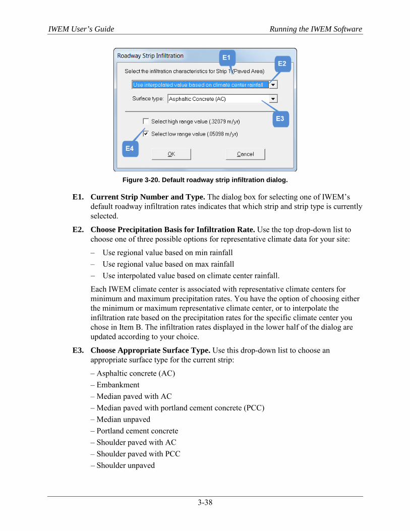
IWEM User’s Guide Running the IWEM Software
3-38
Figure 3-20. Default roadway strip infiltration dialog.
E1. Current Strip Number and Type. The dialog box for selecting one of IWEM’s default roadway infiltration rates indicates that which strip and strip type is currently selected.
E2. Choose Precipitation Basis for Infiltration Rate. Use the top drop-down list to choose one of three possible options for representative climate data for your site:
– Use regional value based on min rainfall – Use regional value based on max rainfall – Use interpolated value based on climate center rainfall.
Each IWEM climate center is associated with representative climate centers for minimum and maximum precipitation rates. You have the option of choosing either the minimum or maximum representative climate center, or to interpolate the infiltration rate based on the precipitation rates for the specific climate center you chose in Item B. The infiltration rates displayed in the lower half of the dialog are updated according to your choice.
E3. Choose Appropriate Surface Type. Use this drop-down list to choose an appropriate surface type for the current strip:
– Asphaltic concrete (AC) – Embankment – Median paved with AC – Median paved with portland cement concrete (PCC) – Median unpaved – Portland cement concrete – Shoulder paved with AC – Shoulder paved with PCC – Shoulder unpaved
IWEM User’s Guide Running the IWEM Software
3-39
The infiltration rates displayed in the lower half of the dialog box are updated according to your choice.
E4. Select High or Low Range Value. Select between infiltration rates that corresponds to ensembles of material property assumptions that result in an upper-bound value or lower-bound value for infiltration. Refer to Appendix E of the IWEM Technical Background Document for more details on material property assumptions.
F. Enter Runoff rates. If a ditch is defined, a runoff rate is required for each non-ditch strip.
G. Enter Precipitation and Evaporation Rates. If a ditch is defined, precipitation and evaporation rates are also required.
3.4.4.4 Probabilistic Screening Module The EPACMTP model used in IWEM to simulate ground water fate and transport incorporates certain constraints to ensure that the parameter values that are selected in the Monte Carlo process will represent physically realistic WMU or roadway settings. These constraints are as follows:
1. The base of a landfill, structural fill or waste pile must be above the water table, or the elevation of ponded water in a surface impoundment must be higher than the water table elevation. Land application units and roadways must be built on grade, so this constraint is not necessary.
2. Infiltration- and recharge-induced mounding of the water table cannot rise above the ground surface.
If either of these constraints is violated, EPACMTP will not run. Given the range of parameter values that may be generated in the Monte Carlo process, in combination with user-specified site-specific values, it is possible that IWEM might encounter a scenario where a constraint is frequently violated and IWEM is therefore unable to complete the Monte Carlo simulation process.
To prevent that occurrence, IWEM screens your input values and parameter distributions prior to performing the EPACMTP Monte Carlo simulation to ensure that an adequate number of Monte Carlo realizations can be conducted, based on the number of simulations selected.2 The Probabilistic Screening module of IWEM examines your inputs to determine if you have provided complete and valid information. If you specify a constant value for every parameter on screens 7 through 9 (i.e., Source Parameters (7), Location of Well with Respect to Roadway (7a), Subsurface Parameters (8), and Infiltration (9) screens), the screener routine will determine the magnitude of water table mounding (that is, IWEM will evaluate the constraints on hydraulic connections between the source type and the water table). If the screening is successful, suggesting sufficient Monte Carlo realizations can be conducted, IWEM will take you to the next input screen, Constituent List (10); otherwise, a message box will alert you to the most violated constraint and suggest potential remedies. If all proposed 2 IWEM defaults to 10,000 realizations. The user can change this value, but the Agency cautions that significantly
fewer iterations will impact the repeatability of the results.
Sec 5.2

IWEM User’s Guide Running the IWEM Software
3-40
remedies are inconsistent with site conditions, then IWEM is not appropriate for your site and a detailed site-specific analysis should be considered.
If you do not provide site-specific values for all possible inputs, the screener will generate values for the missing input parameters according to their appropriate distributions, and then evaluate the constraints. The screening process is usually very fast, unless it has trouble generating successful parameter sets. In that case, it could take as long as 2 minutes to complete. A progress bar is updated during the screening process.
As part of the screening process, IWEM will check that the aquifer that will be modeled has a sufficiently high transmissivity to supply enough water to a domestic drinking water well. A low transmissivity value corresponds to a combination of a low hydraulic conductivity in the saturated zone and a small saturated thickness. If this situation is encountered, IWEM will display a warning message dialog box that says “IWEM had determined that the aquifer system you have described is not likely to support a drinking water well. If this is inconsistent with your site conditions, you may wish to increase the value of aquifer thickness or aquifer hydraulic conductivity. If either of those changes are inappropriate for your site, you may still proceed with the analysis. Do you wish to proceed with this analysis?” If you click |YES|, IWEM will continue with the input parameters you provided; if you click |NO|, it will return you to the input screens to make changes.
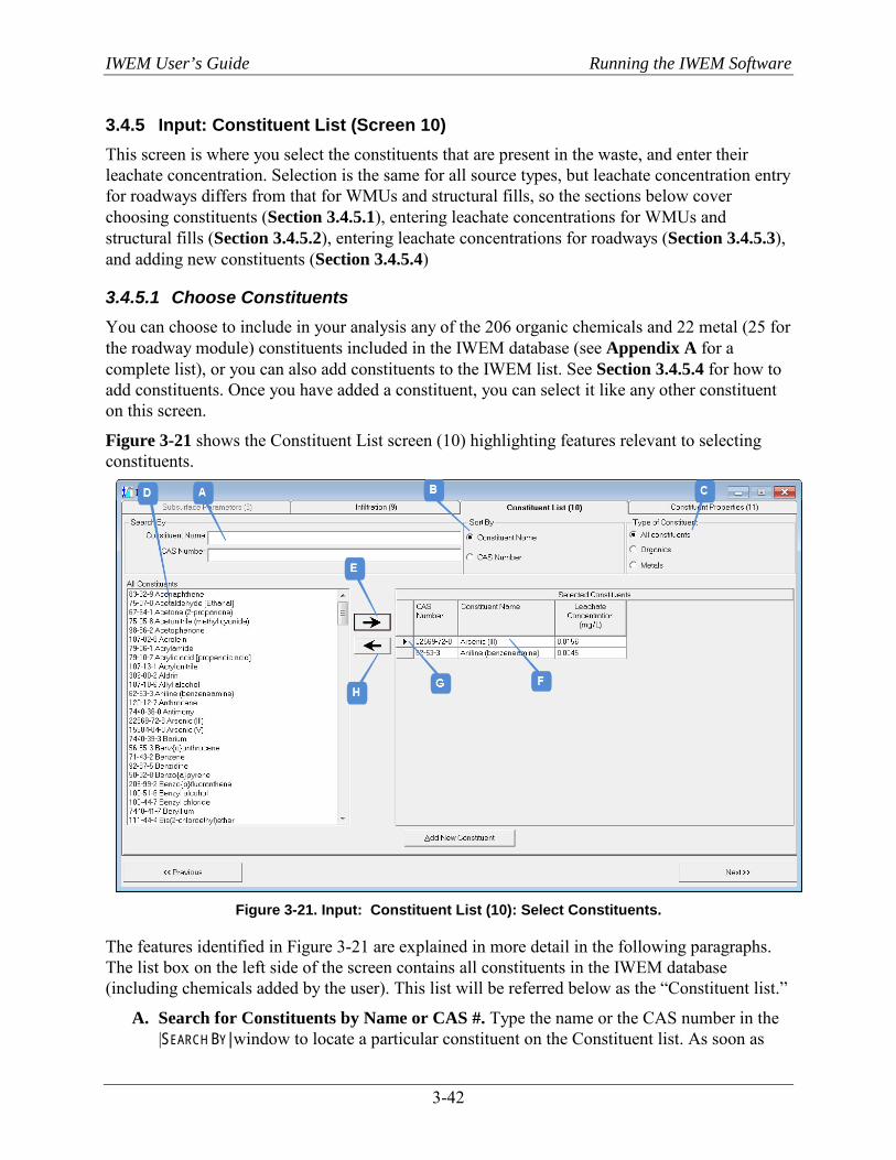
IWEM User’s Guide Running the IWEM Software
3-42
3.4.5 Input: Constituent List (Screen 10) This screen is where you select the constituents that are present in the waste, and enter their leachate concentration. Selection is the same for all source types, but leachate concentration entry for roadways differs from that for WMUs and structural fills, so the sections below cover choosing constituents (Section 3.4.5.1), entering leachate concentrations for WMUs and structural fills (Section 3.4.5.2), entering leachate concentrations for roadways (Section 3.4.5.3), and adding new constituents (Section 3.4.5.4)
3.4.5.1 Choose Constituents You can choose to include in your analysis any of the 206 organic chemicals and 22 metal (25 for the roadway module) constituents included in the IWEM database (see Appendix A for a complete list), or you can also add constituents to the IWEM list. See Section 3.4.5.4 for how to add constituents. Once you have added a constituent, you can select it like any other constituent on this screen.
Figure 3-21 shows the Constituent List screen (10) highlighting features relevant to selecting constituents.
Figure 3-21. Input: Constituent List (10): Select Constituents.
The features identified in Figure 3-21 are explained in more detail in the following paragraphs. The list box on the left side of the screen contains all constituents in the IWEM database (including chemicals added by the user). This list will be referred below as the “Constituent list.”
A. Search for Constituents by Name or CAS #. Type the name or the CAS number in the |SEARCH BY| window to locate a particular constituent on the Constituent list. As soon as

IWEM User’s Guide Running the IWEM Software
3-43
you have typed in enough information to identify the constituent, it will be highlighted in the Constituent list. You can then use the |ARROW| keys on the keyboard to move up or down in the list if the highlighted constituent is not exactly the one you intended to select.
B. Sort the Constituent List. You can sort the constituents by name or by CAS number by clicking one of the |SORT BY| radio buttons. By default, the list is sorted by name. Regardless of sort order, the list is always displayed with the CAS number first, followed by the name.
C. Filter the Constituent List. You can choose to display only organic constituents, or only metals, or a combined list of all constituents by clicking one of the radio buttons under |TYPE OF CONSTITUENT|. By default, all constituents are displayed.
D. Select Constituents to be Included in the Analysis. You can select constituents by using one of the methods below:
– To select an individual constituent, click on its name.
– To select multiple constituents that are listed in contiguous order (that is, one after another without any non-selected constituents in the middle), click on the first waste constituent, press down the |SHIFT| key, and then click on the last waste constituent. All waste constituents listed between the first and last chosen constituents should now be highlighted.
– To select multiple constituents that are not contiguous, click on the first waste constituent, and then hold down the |CTRL| key while selecting additional constituents using the mouse.
E. Add Highlighted Constituent(s) to the |SELECTED CONSTITUENTS| List. Once the appropriate constituents are highlighted in the Constituent list (on the left of the screen), click on the |ADD| ( ) button in the center of the screen to add it to your list of leachate constituents (on the right side of the screen; see item F). Note that a waste constituent can also be added directly to your list by double-clicking on it in the list on the left. Note that for roadways, there are multiple tabs and subtabs in the selected constituents area, for each of different roadway components (strips, ditches, drains). When you add constituents, they are added to all components; you can specify a zero leachate concentration later for constituents in specific roadway components if that roadway component does not use re-used materials or if you do not anticipate those constituents to occur in the materials used in that roadway component. See Section 3.4.5.4 for more on entering leachate concentrations for roadway sources.
F. View List of Constituents to be Included in Analysis. Once you have successfully added a constituent to your analysis, that constituent’s name and CAS number will appear in the |SELECTED CONSTITUENTS| window on the right side of the screen. If any of the selected waste constituents hydrolyze into toxic daughter products, the daughter products are also automatically added to the evaluation. You can modify constituent properties and toxicity standards of the daughter product(s) in the upcoming screens.
Navigating the List of Waste Constituents:
Use the scroll bar at the right of the display window
Use the |ARROW| keys on the keyboard (once one constituent in the list is selected)
Type in the constituent name or CAS number in the |SEARCH BY| box (see item B)
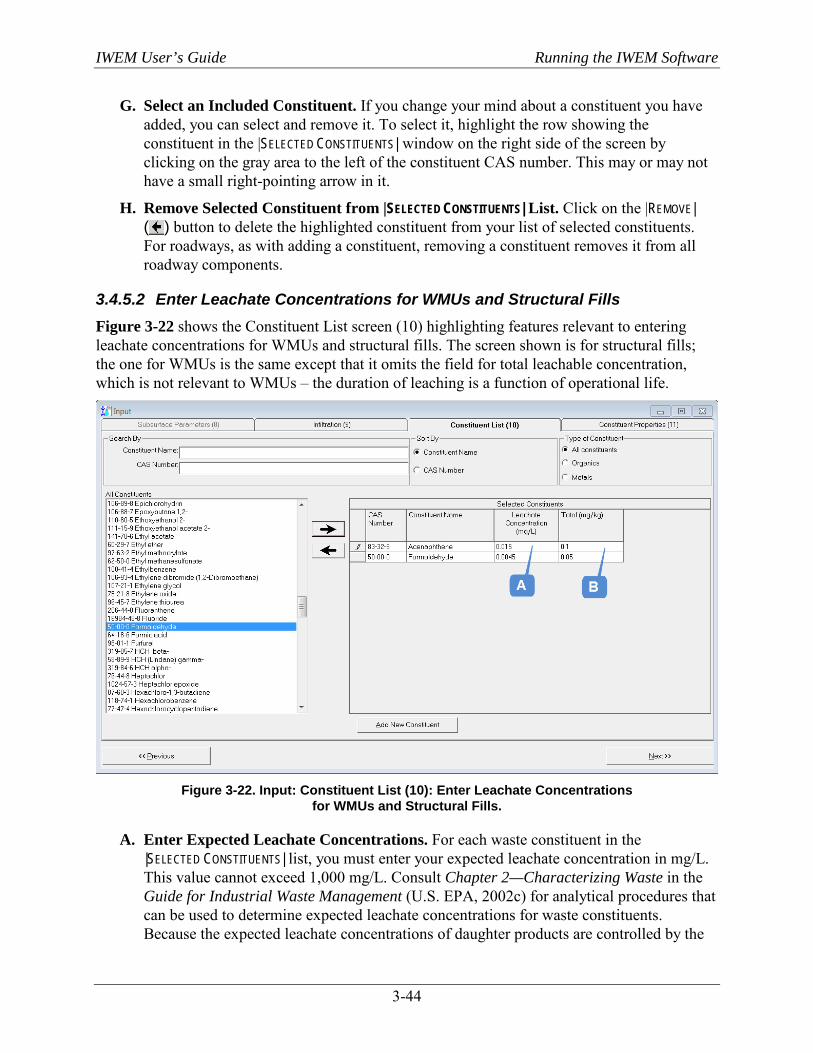
IWEM User’s Guide Running the IWEM Software
3-44
G. Select an Included Constituent. If you change your mind about a constituent you have added, you can select and remove it. To select it, highlight the row showing the constituent in the |SELECTED CONSTITUENTS| window on the right side of the screen by clicking on the gray area to the left of the constituent CAS number. This may or may not have a small right-pointing arrow in it.
H. Remove Selected Constituent from |SELECTED CONSTITUENTS| List. Click on the |REMOVE| ( ) button to delete the highlighted constituent from your list of selected constituents. For roadways, as with adding a constituent, removing a constituent removes it from all roadway components.
3.4.5.2 Enter Leachate Concentrations for WMUs and Structural Fills Figure 3-22 shows the Constituent List screen (10) highlighting features relevant to entering leachate concentrations for WMUs and structural fills. The screen shown is for structural fills; the one for WMUs is the same except that it omits the field for total leachable concentration, which is not relevant to WMUs – the duration of leaching is a function of operational life.
Figure 3-22. Input: Constituent List (10): Enter Leachate Concentrations
for WMUs and Structural Fills.
A. Enter Expected Leachate Concentrations. For each waste constituent in the |SELECTED CONSTITUENTS| list, you must enter your expected leachate concentration in mg/L. This value cannot exceed 1,000 mg/L. Consult Chapter 2—Characterizing Waste in the Guide for Industrial Waste Management (U.S. EPA, 2002c) for analytical procedures that can be used to determine expected leachate concentrations for waste constituents. Because the expected leachate concentrations of daughter products are controlled by the
IWEM User’s Guide Running the IWEM Software
3-45
leachate concentration of the parent constituent, the daughter product leachate concentrations are not IWEM inputs.
B. Enter Expected Total Leachable Material Concentration(s). For structural fills, you must also enter your expected total leachable material concentration in mg/kg for each waste constituent. Consult Chapter 2—Characterizing Waste in the Guide for Industrial Waste Management (U.S. EPA, 2002c) for analytical procedures that can be used to determine expected leachable materials concentrations for waste constituents. In addition, the user can also refer to the EPA’s SW-846 web site (http://www.epa.gov/epawaste/hazard/testmethods/sw846/new_meth.htm) to find newer validated methods to generate leachate data for industrial materials. Section 6.2.2 of the IWEM Technical Background Document provides additional guidance in determining or estimating appropriate input leachable materials concentration values specifically for industrial materials used in structural fills.
When both the leachate and total leachable concentrations are entered for a structural fill, EPACMTP will automatically calculate the time required to deplete the selected constituent from the fill.
If you enter an expected leachate concentration that exceeds the solubility of that constituent, IWEM will display a warning similar to this: “The leachate concentration specified for [constituent] is greater than the cited solubility value in the database of [value] mg/L. Do you want to change the leachate concentration?” If you accidentally entered the wrong value, click the |YES| button and correct the expected leachate concentration. If you want to proceed with the evaluation using your entered value, click the| NO| button. In this case, a similar warning message about your input leachate concentration will be included in the printed report.
3.4.5.3 Enter Leachate Concentrations for Roadways Figure 3-23 shows the leachate concentration portion of the Constituent List screen (10) highlighting features relevant to entering leachate concentrations for roadways.
The evaluation cannot be performed until both the expected leachate concentration and total leachable concentration are provided for a structural fill (or the expected leachate concentration for a WMU) for each selected waste constituent.
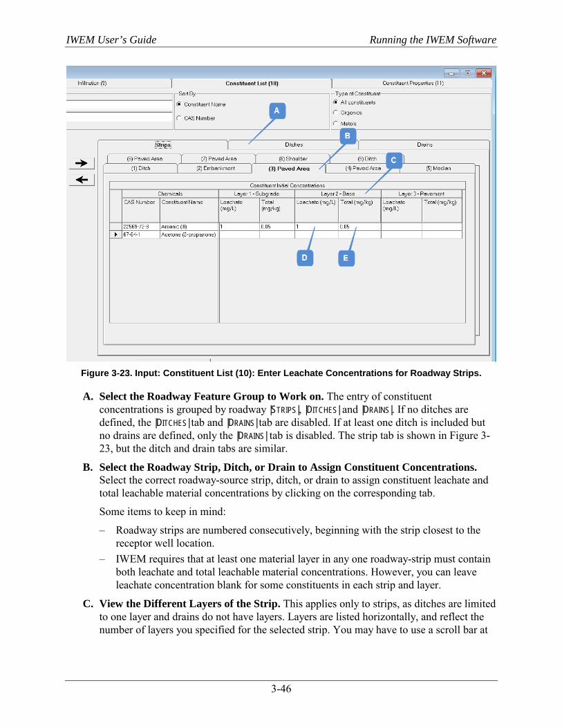
IWEM User’s Guide Running the IWEM Software
3-46
Figure 3-23. Input: Constituent List (10): Enter Leachate Concentrations for Roadway Strips.
A. Select the Roadway Feature Group to Work on. The entry of constituent concentrations is grouped by roadway |STRIPS|, |DITCHES| and |DRAINS|. If no ditches are defined, the |DITCHES| tab and |DRAINS| tab are disabled. If at least one ditch is included but no drains are defined, only the |DRAINS| tab is disabled. The strip tab is shown in Figure 3-23, but the ditch and drain tabs are similar.
B. Select the Roadway Strip, Ditch, or Drain to Assign Constituent Concentrations. Select the correct roadway-source strip, ditch, or drain to assign constituent leachate and total leachable material concentrations by clicking on the corresponding tab.
Some items to keep in mind:
– Roadway strips are numbered consecutively, beginning with the strip closest to the receptor well location.
– IWEM requires that at least one material layer in any one roadway-strip must contain both leachate and total leachable material concentrations. However, you can leave leachate concentration blank for some constituents in each strip and layer.
C. View the Different Layers of the Strip. This applies only to strips, as ditches are limited to one layer and drains do not have layers. Layers are listed horizontally, and reflect the number of layers you specified for the selected strip. You may have to use a scroll bar at
IWEM User’s Guide Running the IWEM Software
3-47
the bottom of the window to view all layers, depending on the number of layers and your screen settings. The scroll bar will appear if needed.
D. Enter Expected Leachate Concentration(s). For strips and ditches, you must enter your expected leachate concentration in mg/L for each waste constituent for each layer that contains constituents. The leachate concentration value cannot exceed 1,000 mg/L. However, it can be zero for some layers, if no leachable materials were used in that layer. Consult Chapter 2—Characterizing Waste in the Guide for Industrial Waste Management (U.S. EPA, 2002c) for analytical procedures that can be used to determine expected leachate concentrations for waste constituents. Section 6.3.9 of the IWEM Technical Background Document provides additional guidance in determining or estimating appropriate input leachate concentration values specifically for industrial materials used in roadways.
Because the expected leachate concentrations of daughter products are controlled by the leachate concentration of the parent constituent, the daughter product leachate concentrations are not IWEM inputs.
For drains, instead of leachate concentration, you will enter an optional concentration of water flowing into the upstream end of ditch. IWEM can accommodate pre-existing ditch flows that have initial dissolved concentrations of constituents of concern. The presence of constituents in existing ditch flows can have an impact on ground water concentrations down-gradient of the roadway and should not be ignored.
E. Enter Expected Total Leachable Material Concentration(s). For strips and ditches, you must enter your expected total leachable material concentration in mg/kg for each waste constituent for each layer that contains constituents. This concentration can be zero for some layers, if no leachable materials were used in that layer. Consult Chapter 2—Characterizing Waste in the Guide for Industrial Waste Management (U.S. EPA, 2002c) for analytical procedures that can be used to determine expected leachable materials concentrations for waste constituents. Section 6.3.9 of the IWEM Technical Background Document provides additional guidance in determining or estimating appropriate input leachable materials concentration values specifically for industrial materials used in roadways.
When both the leachate and total leachable concentrations are entered for a given layer, IWEM will automatically calculate the time required to deplete the selected constituent from that layer of the roadway.
If you enter an expected leachate concentration that exceeds the solubility of that constituent, IWEM will display a warning similar to this: “The leachate concentration specified for [constituent] is greater than the cited solubility value in the database of [value] mg/L. Do you want to change the leachate concentration?” If you accidentally entered the wrong value, click the
The evaluation cannot be performed until both the expected leachate concentration and total leachable concentration are provided for at least one layer in any roadway strip for each selected waste constituent. As long as this requirement is met, any incomplete entries will be reverted to blanks when the Constituent List (10) screen is left.
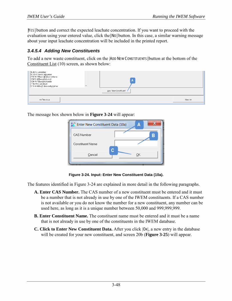
IWEM User’s Guide Running the IWEM Software
3-48
|YES| button and correct the expected leachate concentration. If you want to proceed with the evaluation using your entered value, click the| NO| button. In this case, a similar warning message about your input leachate concentration will be included in the printed report.
3.4.5.4 Adding New Constituents To add a new waste constituent, click on the |ADD NEW CONSTITUENTS| button at the bottom of the Constituent List (10) screen, as shown below:
The message box shown below in Figure 3-24 will appear:
Figure 3-24. Input: Enter New Constituent Data (10a).
The features identified in Figure 3-24 are explained in more detail in the following paragraphs.
A. Enter CAS Number. The CAS number of a new constituent must be entered and it must be a number that is not already in use by one of the IWEM constituents. If a CAS number is not available or you do not know the number for a new constituent, any number can be used here, as long as it is a unique number between 50,000 and 999,999,999.
B. Enter Constituent Name. The constituent name must be entered and it must be a name that is not already in use by one of the constituents in the IWEM database.
C. Click to Enter New Constituent Data. After you click |OK|, a new entry in the database will be created for your new constituent, and screen 20b (Figure 3-25) will appear.
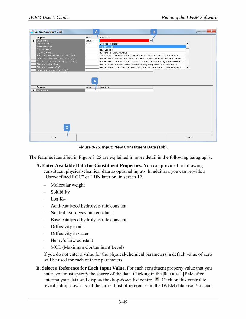
IWEM User’s Guide Running the IWEM Software
3-49
Figure 3-25. Input: New Constituent Data (10b).
The features identified in Figure 3-25 are explained in more detail in the following paragraphs.
A. Enter Available Data for Constituent Properties. You can provide the following constituent physical-chemical data as optional inputs. In addition, you can provide a “User-defined RGC” or HBN later on, in screen 12.
– Molecular weight – Solubility – Log Koc – Acid-catalyzed hydrolysis rate constant – Neutral hydrolysis rate constant – Base-catalyzed hydrolysis rate constant – Diffusivity in air – Diffusivity in water – Henry’s Law constant – MCL (Maximum Contaminant Level) If you do not enter a value for the physical-chemical parameters, a default value of zero will be used for each of these parameters.
B. Select a Reference for Each Input Value. For each constituent property value that you enter, you must specify the source of the data. Clicking in the |REFERENCE| field after entering your data will display the drop-down list control . Click on this control to reveal a drop-down list of the current list of references in the IWEM database. You can
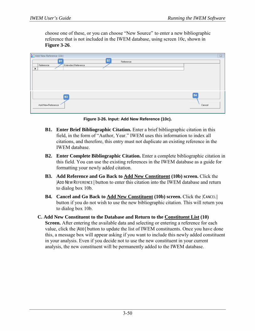
IWEM User’s Guide Running the IWEM Software
3-50
choose one of these, or you can choose “New Source” to enter a new bibliographic reference that is not included in the IWEM database, using screen 10c, shown in Figure 3-26.
Figure 3-26. Input: Add New Reference (10c).
B1. Enter Brief Bibliographic Citation. Enter a brief bibliographic citation in this field, in the form of “Author, Year.” IWEM uses this information to index all citations, and therefore, this entry must not duplicate an existing reference in the IWEM database.
B2. Enter Complete Bibliographic Citation. Enter a complete bibliographic citation in this field. You can use the existing references in the IWEM database as a guide for formatting your newly added citation.
B3. Add Reference and Go Back to Add New Constituent (10b) screen. Click the |ADD NEW REFERENCE| button to enter this citation into the IWEM database and return to dialog box 10b.
B4. Cancel and Go Back to Add New Constituent (10b) screen. Click the |CANCEL| button if you do not wish to use the new bibliographic citation. This will return you to dialog box 10b.
C. Add New Constituent to the Database and Return to the Constituent List (10) Screen. After entering the available data and selecting or entering a reference for each value, click the |ADD| button to update the list of IWEM constituents. Once you have done this, a message box will appear asking if you want to include this newly added constituent in your analysis. Even if you decide not to use the new constituent in your current analysis, the new constituent will be permanently added to the IWEM database.
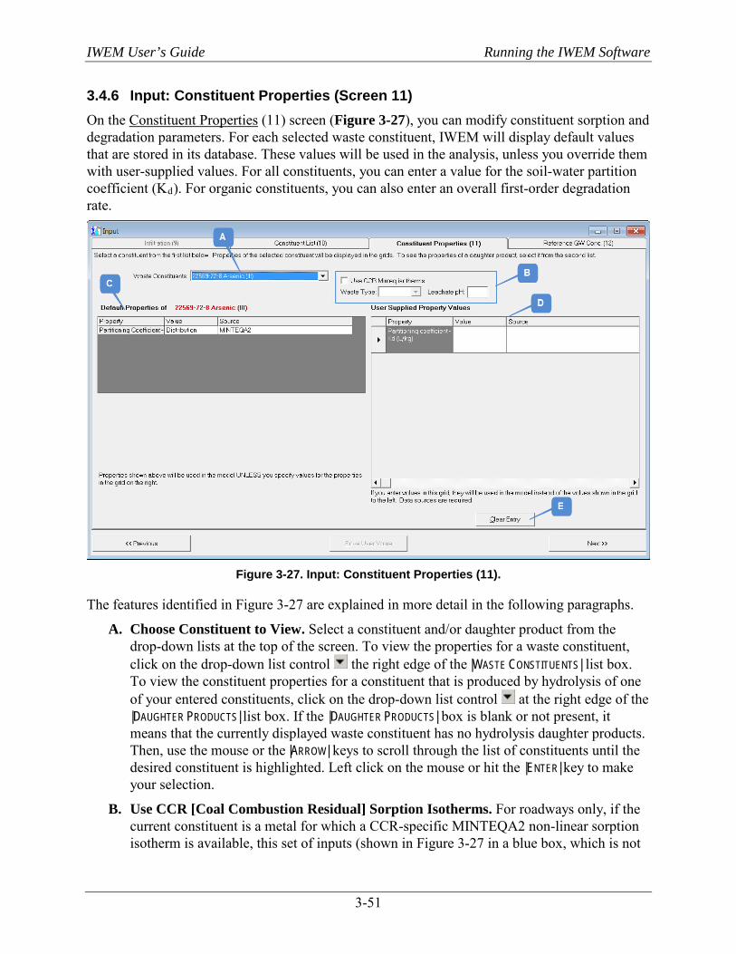
IWEM User’s Guide Running the IWEM Software
3-51
3.4.6 Input: Constituent Properties (Screen 11) On the Constituent Properties (11) screen (Figure 3-27), you can modify constituent sorption and degradation parameters. For each selected waste constituent, IWEM will display default values that are stored in its database. These values will be used in the analysis, unless you override them with user-supplied values. For all constituents, you can enter a value for the soil-water partition coefficient (Kd). For organic constituents, you can also enter an overall first-order degradation rate.
Figure 3-27. Input: Constituent Properties (11).
The features identified in Figure 3-27 are explained in more detail in the following paragraphs.
A. Choose Constituent to View. Select a constituent and/or daughter product from the drop-down lists at the top of the screen. To view the properties for a waste constituent, click on the drop-down list control the right edge of the |WASTE CONSTITUENTS| list box. To view the constituent properties for a constituent that is produced by hydrolysis of one of your entered constituents, click on the drop-down list control at the right edge of the |DAUGHTER PRODUCTS| list box. If the |DAUGHTER PRODUCTS| box is blank or not present, it means that the currently displayed waste constituent has no hydrolysis daughter products. Then, use the mouse or the |ARROW| keys to scroll through the list of constituents until the desired constituent is highlighted. Left click on the mouse or hit the |ENTER| key to make your selection.
B. Use CCR [Coal Combustion Residual] Sorption Isotherms. For roadways only, if the current constituent is a metal for which a CCR-specific MINTEQA2 non-linear sorption isotherm is available, this set of inputs (shown in Figure 3-27 in a blue box, which is not

IWEM User’s Guide Running the IWEM Software
3-52
part of the screen) will be enabled. If the material of interest contains CCR and you would like to use the waste-specific sorption data, make the following selections or entries:
– Check the Use CCR MINTEQ Isotherms checkbox – Select CCR Waste Type. IWEM provides MINTEQA2 non-linear sorption
isotherms for 25 metals across four generic CCR waste types. The waste types are: ash, ash & coal, flue gas desulfurization (FGD), and fluidized bed combustion (FBC) wastes. If the material of interest contains CCR and you would like to use the waste-specific sorption data, select a generic waste type that best represents your source material of interest.
– Enter Waste-Specific Value for leachate pH. In addition to selecting a CCR waste type, you must also provide a value for the pH of the leachate. Leachate pH is used to select appropriate MINTEQA2 sorption isotherms for your constituent and environmental conditions.
C. View Default Values and References. The constituent properties and their default values and references for the selected waste constituent are listed in the table on the left side of the screen. The screen shot in Figure 3-27 is for a metal; for an organic, this box would also show hydrolysis rates (acid catalyzed, neutral, and base-catalyzed).
D. Enter Site-Specific or Updated Values and References. For each constituent, IWEM assigns default values for Koc (Kd for metals) and hydrolysis rate constants (for organics only) (see constituent list in Appendix A); however, you can enter and use site-specific values for Kd (organics and metals) and overall decay rate (organics only) if these data are available. To enter site-specific values, just type them into the table on the right side of the screen. As noted, the screen shot in Figure 3-27 is for a metal; for an organic, fields for the value and source of the overall decay rate would also be displayed below the fields for Kd.
By default, IWEM accounts for degradation from constituent hydrolysis only. IWEM calculates the hydrolysis rate from constituent-specific values for the acid-catalyzed (ka), neutral (kn) and base-catalyzed (kb) hydrolysis rate constants. Biodegradation can also be an important process. However, biodegradation rates can vary greatly from site to site. You should only increase the overall decay rate above the value corresponding to the hydrolysis rate constants if there is clear evidence of biodegradation occurring at a site. For organics, the calculation of the overall decay rate from the hydrolysis rate constants and the calculation of Kd from Koc is given in Sections 6.6.1 and 6.6.2 of the IWEM Technical Background Document.
For each input parameter for which you enter a site-specific value, remember to type in a brief explanation of this value. This information is required and will be included in the printed report.
E. Clear All Entries. Clicking this button will clear any user selections or data entry for the current constituent.
Once your list of constituent properties is complete, click on the |NEXT| button to specify RGC values to be used in the evaluation.
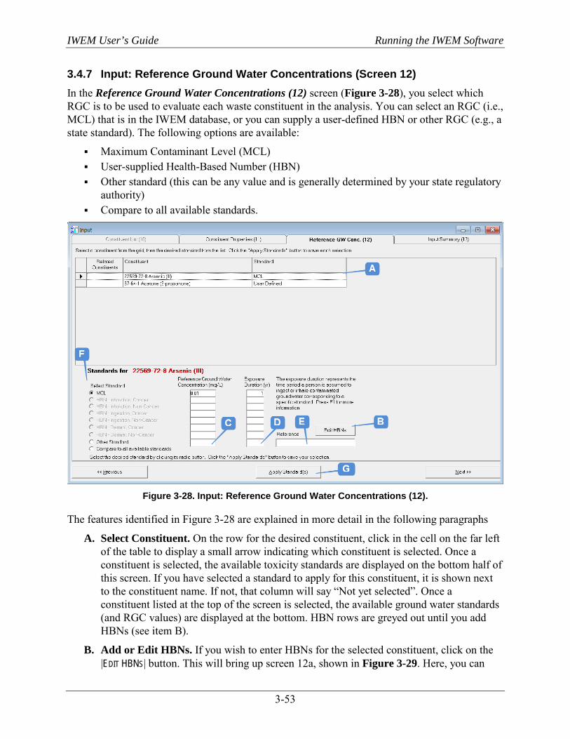
IWEM User’s Guide Running the IWEM Software
3-53
3.4.7 Input: Reference Ground Water Concentrations (Screen 12) In the Reference Ground Water Concentrations (12) screen (Figure 3-28), you select which RGC is to be used to evaluate each waste constituent in the analysis. You can select an RGC (i.e., MCL) that is in the IWEM database, or you can supply a user-defined HBN or other RGC (e.g., a state standard). The following options are available:
Maximum Contaminant Level (MCL) User-supplied Health-Based Number (HBN) Other standard (this can be any value and is generally determined by your state regulatory
authority) Compare to all available standards.
Figure 3-28. Input: Reference Ground Water Concentrations (12).
The features identified in Figure 3-28 are explained in more detail in the following paragraphs
A. Select Constituent. On the row for the desired constituent, click in the cell on the far left of the table to display a small arrow indicating which constituent is selected. Once a constituent is selected, the available toxicity standards are displayed on the bottom half of this screen. If you have selected a standard to apply for this constituent, it is shown next to the constituent name. If not, that column will say “Not yet selected”. Once a constituent listed at the top of the screen is selected, the available ground water standards (and RGC values) are displayed at the bottom. HBN rows are greyed out until you add HBNs (see item B).
B. Add or Edit HBNs. If you wish to enter HBNs for the selected constituent, click on the |EDIT HBNS| button. This will bring up screen 12a, shown in Figure 3-29. Here, you can

IWEM User’s Guide Running the IWEM Software
3-54
enter HBNs for inhalation, ingestion, and dermal pathways, for cancer and non-cancer endpoints.
Figure 3-29. Input: Reference Ground Water Concentrations: Edit HBNs (12a).
B1. Enter HBN. The HBN must be in mg/L. See Section 7 of the IWEM Technical Background Document for guidance on obtaining HBNs.
B2. Enter Exposure Duration. Each HBN must have an exposure duration, which corresponds to the time interval over which the average ground water concentration is calculated. All cancer HBNs for a particular constituent must have the same exposure duration, and all non-cancer HBNs must have the same exposure duration, although the non-cancer exposure duration can be different from the cancer exposure duration.
A note of clarification—the exposure duration does not control the time extent of a flow and transport simulation. An EPACMTP simulation will continue for as long as the receptor location is observing mass OR until the maximum simulation time is reached (10,000 years). The exposure duration specifies the time window used to compute the maximum time-averaged concentration.
B3. Enter Reference. You must enter a reference for each HBN-exposure duration pair you enter.
B4. Return to RGC Screen (12). Click on the |SAVE| button to return to the main RGC screen.
C. Enter Other Standard. If you wish to enter a state standard (e.g., one that is more stringent than the MCL) or any other RGC, you can do it here. Consult with the appropriate state regulatory agency for additional guidance on entering your own RGC value.
D. Enter Exposure Duration for Other Standard. Consult with the appropriate state regulatory agency for additional guidance on determining the exposure duration associated with the RGC value.
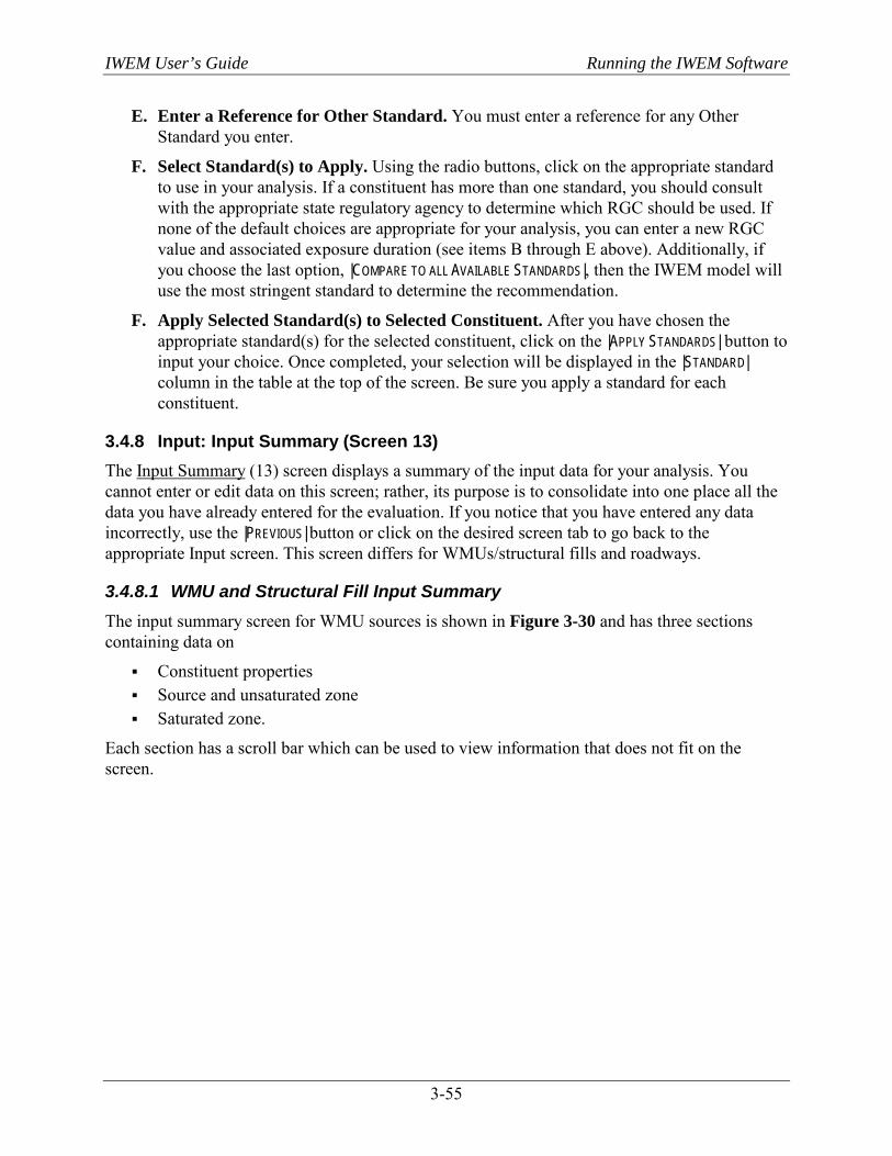
IWEM User’s Guide Running the IWEM Software
3-55
E. Enter a Reference for Other Standard. You must enter a reference for any Other Standard you enter.
F. Select Standard(s) to Apply. Using the radio buttons, click on the appropriate standard to use in your analysis. If a constituent has more than one standard, you should consult with the appropriate state regulatory agency to determine which RGC should be used. If none of the default choices are appropriate for your analysis, you can enter a new RGC value and associated exposure duration (see items B through E above). Additionally, if you choose the last option, |COMPARE TO ALL AVAILABLE STANDARDS|, then the IWEM model will use the most stringent standard to determine the recommendation.
F. Apply Selected Standard(s) to Selected Constituent. After you have chosen the appropriate standard(s) for the selected constituent, click on the |APPLY STANDARDS| button to input your choice. Once completed, your selection will be displayed in the |STANDARD| column in the table at the top of the screen. Be sure you apply a standard for each constituent.
3.4.8 Input: Input Summary (Screen 13) The Input Summary (13) screen displays a summary of the input data for your analysis. You cannot enter or edit data on this screen; rather, its purpose is to consolidate into one place all the data you have already entered for the evaluation. If you notice that you have entered any data incorrectly, use the |PREVIOUS| button or click on the desired screen tab to go back to the appropriate Input screen. This screen differs for WMUs/structural fills and roadways.
3.4.8.1 WMU and Structural Fill Input Summary The input summary screen for WMU sources is shown in Figure 3-30 and has three sections containing data on
Constituent properties Source and unsaturated zone Saturated zone.
Each section has a scroll bar which can be used to view information that does not fit on the screen.
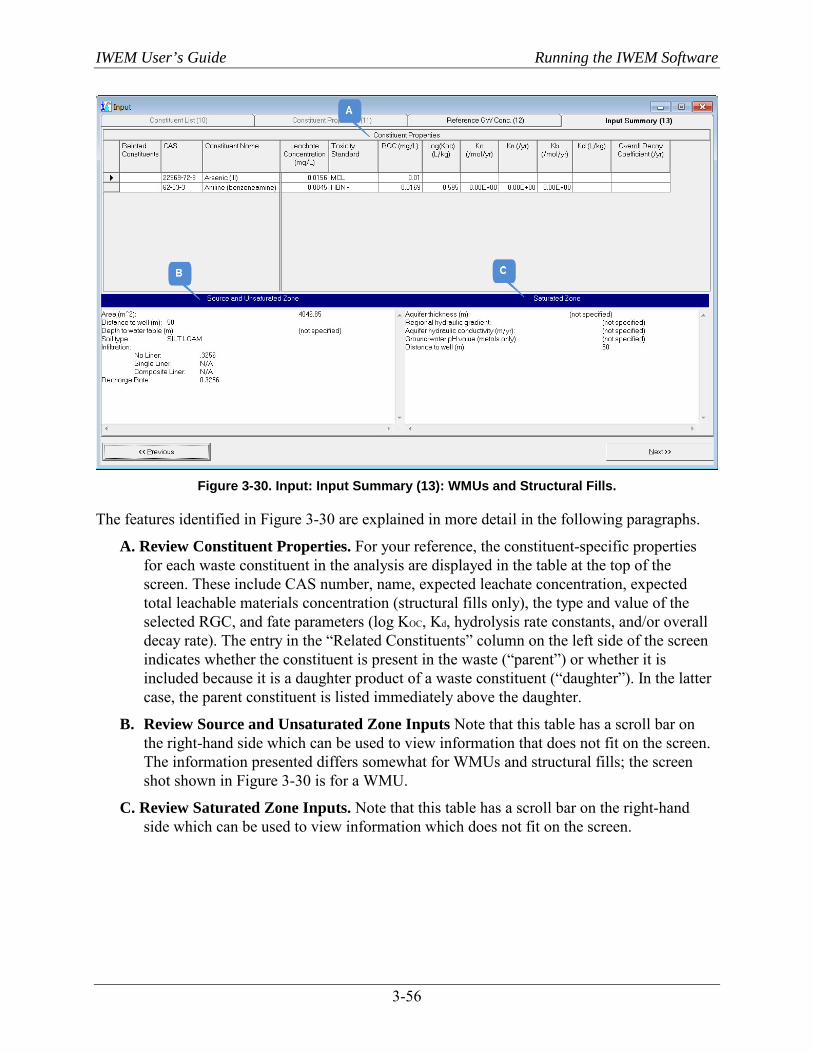
IWEM User’s Guide Running the IWEM Software
3-56
Figure 3-30. Input: Input Summary (13): WMUs and Structural Fills.
The features identified in Figure 3-30 are explained in more detail in the following paragraphs.
A. Review Constituent Properties. For your reference, the constituent-specific properties for each waste constituent in the analysis are displayed in the table at the top of the screen. These include CAS number, name, expected leachate concentration, expected total leachable materials concentration (structural fills only), the type and value of the selected RGC, and fate parameters (log KOC, Kd, hydrolysis rate constants, and/or overall decay rate). The entry in the “Related Constituents” column on the left side of the screen indicates whether the constituent is present in the waste (“parent”) or whether it is included because it is a daughter product of a waste constituent (“daughter”). In the latter case, the parent constituent is listed immediately above the daughter.
B. Review Source and Unsaturated Zone Inputs Note that this table has a scroll bar on the right-hand side which can be used to view information that does not fit on the screen. The information presented differs somewhat for WMUs and structural fills; the screen shot shown in Figure 3-30 is for a WMU.
C. Review Saturated Zone Inputs. Note that this table has a scroll bar on the right-hand side which can be used to view information which does not fit on the screen.
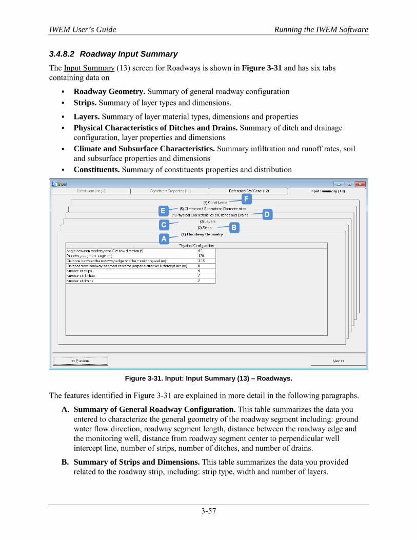
IWEM User’s Guide Running the IWEM Software
3-57
3.4.8.2 Roadway Input Summary The Input Summary (13) screen for Roadways is shown in Figure 3-31 and has six tabs containing data on
Roadway Geometry. Summary of general roadway configuration Strips. Summary of layer types and dimensions.
Layers. Summary of layer material types, dimensions and properties Physical Characteristics of Ditches and Drains. Summary of ditch and drainage
configuration, layer properties and dimensions Climate and Subsurface Characteristics. Summary infiltration and runoff rates, soil
and subsurface properties and dimensions Constituents. Summary of constituents properties and distribution
Figure 3-31. Input: Input Summary (13) – Roadways.
The features identified in Figure 3-31 are explained in more detail in the following paragraphs.
A. Summary of General Roadway Configuration. This table summarizes the data you entered to characterize the general geometry of the roadway segment including: ground water flow direction, roadway segment length, distance between the roadway edge and the monitoring well, distance from roadway segment center to perpendicular well intercept line, number of strips, number of ditches, and number of drains.
B. Summary of Strips and Dimensions. This table summarizes the data you provided related to the roadway strip, including: strip type, width and number of layers.

IWEM User’s Guide Running the IWEM Software
3-58
C. Summary of Layer Material Types, Dimensions and Properties. This table summarizes the layer properties and dimensions related data provided by the user, including: layer type, thickness, hydraulic conductivity and bulk density. Note that this table has scroll bars on the bottom and right-hand sides, which can be used to view information that does not fit on the screen.
D. Summary of Ditch and Drainage Configuration, Layer properties and Dimensions. For your reference, the roadway-strips where the ditch receives overland flow from, Manning’s n coefficient, slope, maximum water depth, initial flow rate, runoff percent not collected by the gutter, precipitation rate and evaporation rate are displayed in the table on the top of the data grid by each ditch. Drain location, thickness, hydraulic conductivity, bulk density and the percent of flow that reaches ditch are displayed on the bottom of the data grid by each drain.
E. Summary Infiltration and Runoff Rates, Soil and Subsurface Properties and Dimensions. This table provides summarized information related to soil type, aquifer type, nearest climate center, recharge rate, infiltration rates and runoff rates for each non-ditch strip. Note that this table has scroll bars on the bottom and right-hand sides, which can be used to view information that does not fit on the screen.
F. Summary of Constituents and Properties. This table summarizes the constituents’ proprieties and their respective leachate concentrations provided to the EPACMTP modeling. The information presented related to the constituents proprieties include, name of the constituent, fate and transport parameters (log Koc, Kd, hydrolysis rate constants, pH and overall decay rate), and value of the selected RGC. A section of this table also presents user-specified leachate and total leachable material concentrations by roadway-source strip and layer.
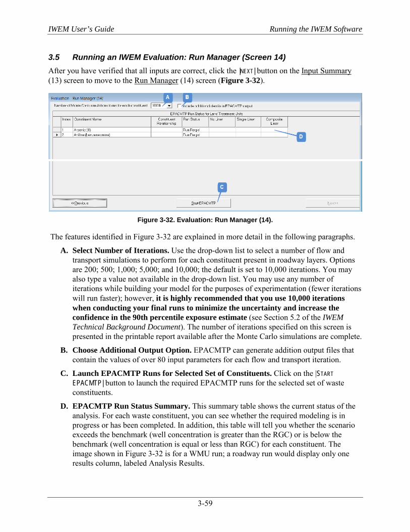
IWEM User’s Guide Running the IWEM Software
3-59
3.5 Running an IWEM Evaluation: Run Manager (Screen 14) After you have verified that all inputs are correct, click the |NEXT| button on the Input Summary (13) screen to move to the Run Manager (14) screen (Figure 3-32).
Figure 3-32. Evaluation: Run Manager (14).
The features identified in Figure 3-32 are explained in more detail in the following paragraphs.
A. Select Number of Iterations. Use the drop-down list to select a number of flow and transport simulations to perform for each constituent present in roadway layers. Options are 200; 500; 1,000; 5,000; and 10,000; the default is set to 10,000 iterations. You may also type a value not available in the drop-down list. You may use any number of iterations while building your model for the purposes of experimentation (fewer iterations will run faster); however, it is highly recommended that you use 10,000 iterations when conducting your final runs to minimize the uncertainty and increase the confidence in the 90th percentile exposure estimate (see Section 5.2 of the IWEM Technical Background Document). The number of iterations specified on this screen is presented in the printable report available after the Monte Carlo simulations are complete.
B. Choose Additional Output Option. EPACMTP can generate addition output files that contain the values of over 80 input parameters for each flow and transport iteration.
C. Launch EPACMTP Runs for Selected Set of Constituents. Click on the |START EPACMTP| button to launch the required EPACMTP runs for the selected set of waste constituents.
D. EPACMTP Run Status Summary. This summary table shows the current status of the analysis. For each waste constituent, you can see whether the required modeling is in progress or has been completed. In addition, this table will tell you whether the scenario exceeds the benchmark (well concentration is greater than the RGC) or is below the benchmark (well concentration is equal or less than RGC) for each constituent. The image shown in Figure 3-32 is for a WMU run; a roadway run would display only one results column, labeled Analysis Results.
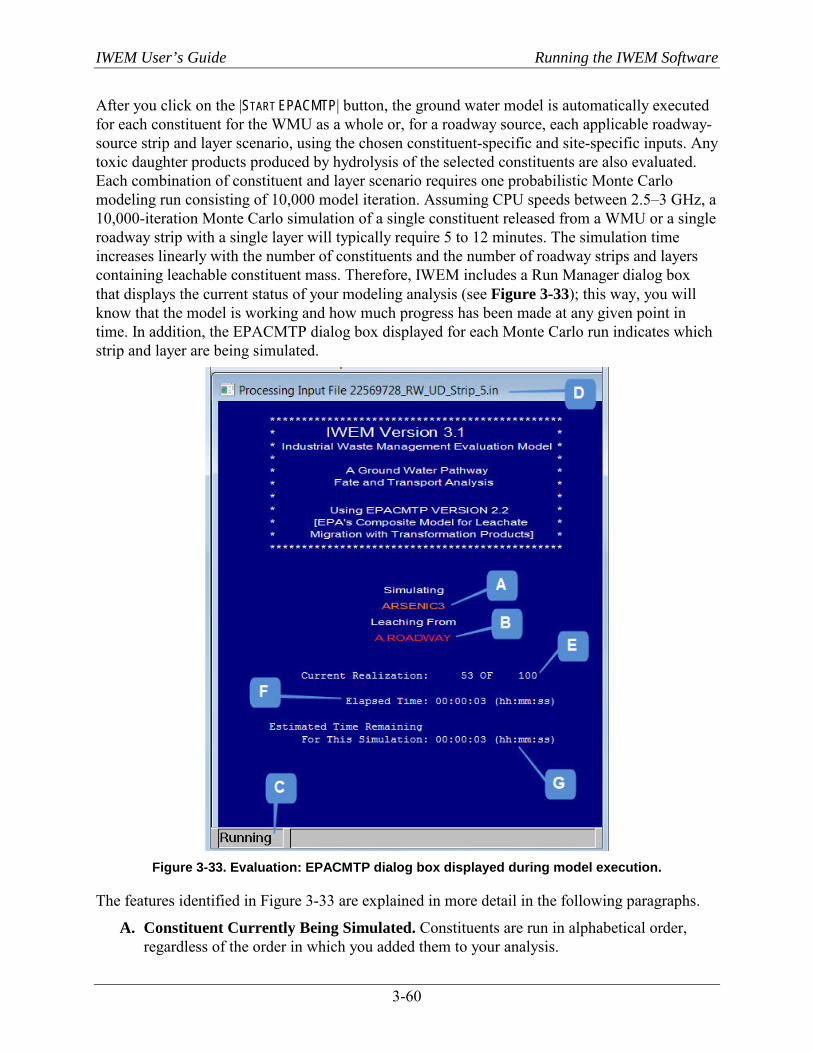
IWEM User’s Guide Running the IWEM Software
3-60
After you click on the |START EPACMTP| button, the ground water model is automatically executed for each constituent for the WMU as a whole or, for a roadway source, each applicable roadway-source strip and layer scenario, using the chosen constituent-specific and site-specific inputs. Any toxic daughter products produced by hydrolysis of the selected constituents are also evaluated. Each combination of constituent and layer scenario requires one probabilistic Monte Carlo modeling run consisting of 10,000 model iteration. Assuming CPU speeds between 2.5–3 GHz, a 10,000-iteration Monte Carlo simulation of a single constituent released from a WMU or a single roadway strip with a single layer will typically require 5 to 12 minutes. The simulation time increases linearly with the number of constituents and the number of roadway strips and layers containing leachable constituent mass. Therefore, IWEM includes a Run Manager dialog box that displays the current status of your modeling analysis (see Figure 3-33); this way, you will know that the model is working and how much progress has been made at any given point in time. In addition, the EPACMTP dialog box displayed for each Monte Carlo run indicates which strip and layer are being simulated.
Figure 3-33. Evaluation: EPACMTP dialog box displayed during model execution.
The features identified in Figure 3-33 are explained in more detail in the following paragraphs.
A. Constituent Currently Being Simulated. Constituents are run in alphabetical order, regardless of the order in which you added them to your analysis.
IWEM User’s Guide Running the IWEM Software
3-61
B. Source Being Simulated. This displays the source type (e.g., Landfill, Roadway). For WMUs, it also displays the current liner scenario being simulated (No Liner, Clay Liner, Composite Liner, or user-defined).
C. Running Indicator. This box displays “Running” to indicate that EPACMTP is running.
D. Input Filename to Track Simulation Progress. The currently executing EPACMTP input filename is displayed at the top of each EPACMTP dialog box to help you monitor the model’s progress in real time. The filename is formatted in the following way:
[CASID#]_[Source Type]_[Liner]_[Strip #].in
Where:
[CASID#] = Unhyphenated CAS number of current constituent [Source Type] = A 2 or 3 letter code for the type of source:
LAU = Land application unit LF = Landfill SI = Surface impoundment WP = Waste pile SF = Structural fill RW = Roadway
[Liner] = A 2 to 4 letter code for the current liner: NLin = No liner (WMUs and structural fills only) CLin = Clay liner (WMUs only) GM = Geomembrane (composite) liner (WMUs only) UD = User-defined (used for roadways or for WMUs for which you specified
a site-specific infiltration rate) [Strip #] = The roadway-source strip number assigned in the Source Parameters (7)
screen (e.g., Strip_1). This is displayed only for Roadway sources; for WMUs and structural fills, it is omitted
For example, the filename 7440439_RW_UD_Strip_1.in indicates that the EPACMTP input file represents cadmium (CAS 7440-43-9) released from strip 1of the roadway. The file name 7440439_SI_CLin.in represents cadmium released from a surface impoundment with a clay liner.
The EPACMTP runs proceed from the first to the last selected constituent. For WMUs, EPACMTP runs for a constituent are sequentially launched for the no-liner, single clay-liner, and composite-liner scenarios until a scenario that does not exceed the RGC is found. That is, if the single clay- liner scenario is determined to not exceed the RGC for a given constituent, the composite-liner scenario for that constituent is not modeled. For the land application unit and structural fills or user-defined liner/infiltration scenarios, only one liner scenario per constituent is evaluated. For roadway sources, EPACMTP runs for each constituent are sequentially launched for all strips and layers containing both leachate and total leachable material concentrations.
When the run is complete, this box will close and you will return to the Run Manager (14) screen. You will also be prompted to save your evaluation.

IWEM User’s Guide Running the IWEM Software
3-62
3.6 IWEM Results Once EPACMTP completes the fate and transport modeling, IWEM presents Summary Results (Screen 15), Detailed Results (Screens 16–18), and an Evaluation Summary (Screen 19). These are discussed in the following sections.
3.6.1 Summary Results (Screen 15) The summary results present a liner recommendation for WMUs or an assessment of whether the reuse of industrial materials in a structural fill or roadway design is appropriate. The result is based on a comparison of the estimated 90th percentile ground water exposure concentrations and the specified RGC. If the ground water exposure concentration of a constituent does not exceed the specified RGC, then the liner scenario is considered protective for that constituent; similarly, for a structural fill or a roadway scenario, the reuse of industrial material is considered appropriate. If the ground water exposure concentration exceeds the specified RGC, then the evaluated scenario is not protective (for liners) or inappropriate (for a roadway or a structural fill).
Figure 3-34 shows the summary results screen.
Figure 3-34. Output (Summary): Summary Results (15).
The features identified in Figure 3-34 are explained in more detail in the following paragraphs.
A. Recommendation for Each Constituent. For WMUs, this column is generally headed “Minimum Liner Recommendation” and it will display the minimum recommended liner. If you entered a site-specific infiltration rate, then the column is headed “User Defined Infiltration” and it will display whether or not the modeled infiltration rate will result in a ground water exposure concentration that is above or below the specified RGC. For structural fills and roadways, this column is headed “Results” and it will display whether or not the modeled structural fill or roadway design will result in a ground water exposure concentration that is above or below the specified RGC.
The no-liner, single clay-liner, and composite-liner recommendations are displayed in green text. If the composite liner exceeds the user-provided benchmark, then this message is displayed in red text. If the liner recommendation is “Not Applicable,” then this message is displayed in black text. Structural fill and roadway results are displayed in
IWEM User’s Guide Running the IWEM Software
3-63
green text if the ground water exposure concentration is below the RGC and in red text if it is above.
B. Overall Recommendation. For WMUs, the bottom of the screen displays an overall liner recommendation based on consideration of all waste constituents (and their daughter products). If EPACMTP estimates that the 90th percentile values of ground water well concentration for all constituents under the no-liner scenario are below their respective RGCs, then IWEM will recommend that no liner is needed to protect ground water. If the modeled ground water exposure concentration of any constituent under the no-liner scenario is higher than its RGC, then at least a single clay liner is recommended (or in the case of land application units, land application is not recommended) based on the inputs and assumptions you provided. If the estimated ground water exposure concentration of any constituent exceeds the RGC under the composite liner scenario, then consider pollution prevention, treatment, and more protective liner designs, as well as consultation among regulators, the public, and industry to ensure such wastes are protectively managed. For waste streams with multiple constituents, the least stringent liner design that is protective for all constituents is the overall recommended liner design.
This box is not shown for structural fills or roadways; for those, the design is only deemed acceptable if the ground water exposure concentrations for all constituents are below the specified RGCs.
C. Go to Detailed Results. Clicking on the |DETAILED RESULTS| button will take you to a detailed listing of the results (Screens 16–18), including the constituent-specific modeling results for all evaluated liner scenarios. See Section 3.6.2.
D. Go to Recommendations. Clicking on the |RECOMMENDATION| button will take you to the Evaluation Summary (19) screen, where you can choose to view the report or save your analysis and exit the IWEM software. See Section 3.6.3.
3.6.2 Output (Details) (Screens 16, 17, and 18) The detailed results present the data upon which the evaluation is based, by constituent. The expected leachate concentration is listed, along with the specified RGC type and value and the resulting 90th percentile ground water exposure concentration calculated by EPACMTP. These detailed results allow you to understand how the liner design recommendations were developed or the overall appropriateness of reusing industrial materials in a structural fill or roadway were determined.
If you directly enter a value for infiltration (for any of the four types of WMUs), EPACMTP will use this value of the infiltration rate in its fate and transport simulation, and IWEM will then compare the predicted ground water well concentration to each constituent’s RGC. In this case, the detailed results will consist of only one screen, labeled “Results –User-Defined Liner (18),” rather than the three that are shown below in Figure 3-35. Also, only one screen is displayed for roadways, labeled “Results – Roadway (18).”
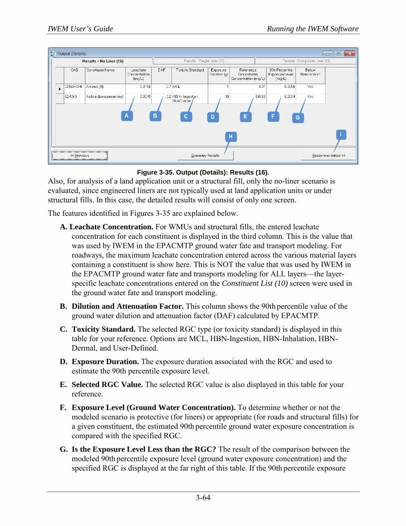
IWEM User’s Guide Running the IWEM Software
3-64
Figure 3-35. Output (Details): Results (16).
Also, for analysis of a land application unit or a structural fill, only the no-liner scenario is evaluated, since engineered liners are not typically used at land application units or under structural fills. In this case, the detailed results will consist of only one screen.
The features identified in Figures 3-35 are explained below.
A. Leachate Concentration. For WMUs and structural fills, the entered leachate concentration for each constituent is displayed in the third column. This is the value that was used by IWEM in the EPACMTP ground water fate and transport modeling. For roadways, the maximum leachate concentration entered across the various material layers containing a constituent is show here. This is NOT the value that was used by IWEM in the EPACMTP ground water fate and transports modeling for ALL layers—the layer-specific leachate concentrations entered on the Constituent List (10) screen were used in the ground water fate and transport modeling.
B. Dilution and Attenuation Factor. This column shows the 90th percentile value of the ground water dilution and attenuation factor (DAF) calculated by EPACMTP.
C. Toxicity Standard. The selected RGC type (or toxicity standard) is displayed in this table for your reference. Options are MCL, HBN-Ingestion, HBN-Inhalation, HBN-Dermal, and User-Defined.
D. Exposure Duration. The exposure duration associated with the RGC and used to estimate the 90th percentile exposure level.
E. Selected RGC Value. The selected RGC value is also displayed in this table for your reference.
F. Exposure Level (Ground Water Concentration). To determine whether or not the modeled scenario is protective (for liners) or appropriate (for roads and structural fills) for a given constituent, the estimated 90th percentile ground water exposure concentration is compared with the specified RGC.
G. Is the Exposure Level Less than the RGC? The result of the comparison between the modeled 90th percentile exposure level (ground water exposure concentration) and the specified RGC is displayed at the far right of this table. If the 90th percentile exposure
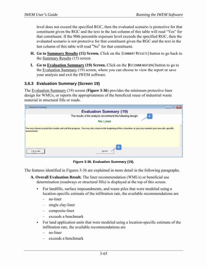
IWEM User’s Guide Running the IWEM Software
3-65
level does not exceed the specified RGC, then the evaluated scenario is protective for that constituent given the RGC and the text in the last column of this table will read “Yes” for that constituent. If the 90th percentile exposure level exceeds the specified RGC, then the evaluated scenario is not protective for that constituent given the RGC and the text in the last column of this table will read “No” for that constituent.
H. Go to Summary Results (15) Screen. Click on the |SUMMARY RESULTS| button to go back to the Summary Results (15) screen.
I. Go to Evaluation Summary (19) Screen. Click on the |RECOMMENDATION| button to go to the Evaluation Summary (19) screen, where you can choose to view the report or save your analysis and exit the IWEM software.
3.6.3 Evaluation Summary (Screen 19) The Evaluation Summary (19) screen (Figure 3-36) provides the minimum protective liner design for WMUs, or reports the appropriateness of the beneficial reuse of industrial waste material in structural fills or roads.
Figure 3-36. Evaluation Summary (19).
The features identified in Figures 3-36 are explained in more detail in the following paragraphs.
A. Overall Evaluation Result. The liner recommendation (WMUs) or beneficial use determination (roadways or structural fills) is displayed at the top of this screen.
For landfills, surface impoundments, and waste piles that were modeled using a location-specific estimate of the infiltration rate, the available recommendations are – no-liner – single clay-liner – composite-liner – exceeds a benchmark
For land application units that were modeled using a location-specific estimate of the infiltration rate, the available recommendations are – no-liner – exceeds a benchmark

IWEM User’s Guide Running the IWEM Software
3-66
For any WMU that was modeled using a user-specified site-specific value for the infiltration rate, the available recommendations are – below all benchmarks – exceeds a benchmark
For structural fills, the available results are – below all benchmarks – exceeds a benchmark
For roadways, the available results are – below all benchmarks – exceeds a benchmark
For WMUs, if your evaluation results in a recommendation of “exceeds a benchmark,” then the chosen liner design for managing the waste may not be appropriate at the selected site. In this case, consider pollution prevention, treatment, and more protective liner designs, as well as consultation among regulators, the public, and industry to ensure such wastes are protectively managed. See Chapter 4 of the Guide (U.S. EPA, 2002a) for further information.
For structural fills and roadways, if your evaluation results are “exceeds benchmark,” then the amounts and/or characteristics of industrial material included in the structural fill or roadway design may not be appropriate at the selected location. In this case, consider reducing the amount of material included in a particular layer or fill, or consider potentially eliminating the material altogether..
B. Display Reports. Clicking on the |REPORT| button displays the IWEM Report (examples can be found in Appendices B and C for WMUs and Roadways, respectively). The report functionality is a bit different for structural fills/roadways as compared to WMUs:
Structural Fills/Roadways. When you click on the |REPORT| button for structural fills or roadways, a printer setup dialog box will appear. Select your printer and click |OK|. A preview of the report will be displayed. From there, you can navigate pages by using |NEXT PAGE| and |PREVIOUS PAGE|, select |PRINT|, or |EXIT| the report. When you choose to print the report, a Windows print dialog box appears, where you can adjust printer settings or choose to print selected pages. You can save the report by printing it to a PDF file.
WMUs. When you click on the |REPORT| button for WMUs, a preview of the report will be displayed. These reports were designed using legacy software that provides different menu controls. Once the report is displayed on-screen, you can then use the following toolbar buttons to print, save, and scroll through the pages of the report:
Print the report. A Windows print dialog box appears, where you can adjust printer settings or choose to print selected pages. Note: The WMU reports can only be printed to your default system printer. To change printers, you will need to change your default printer from the Windows Control Panel.

IWEM User’s Guide Running the IWEM Software
3-67
Save (export) the report. A dialog box appears with several output file type options; however, most of these are no longer supported. Success with the export utility depends on what software you have installed on your PC. Most users will find that the best option for saving a document-ready report is to use the Print button (above) with a default printer set to a PDF driver.2
View the next page of the report
View the last page of the report.
View the previous page of the report
View the first page of the report.
Change the display size of the report.
3.6.4 Save and Exit At this point, you may want to save your results if you did not do so after the run finished. Click on the |FILE| menu and choose |SAVE| or |SAVE AS|. A dialog box will then open, which prompts you for the filename and directory location, as appropriate. Once you have provided a filename, the tool will save two files, automatically applying the “wem” and “mdb” extensions for you. The combination of these two files completely describes the data you have entered and any model-generated results. Click on the |SAVE| button on the toolbar. If you are editing a previously saved evaluation, the file will be automatically updated. If you have created a new evaluation, the |SAVE AS| dialog box will open, as described above.
Note that IWEM will not allow you to save both model inputs and results at a point where the inputs do not correspond to the model-generated results. If you do choose to save your work in a situation like this, only the inputs will be saved; that is, when you open this file at a later date, 2 If you do not have a PDF driver installed on your computer, many free PDF drivers are available online.
Functionality varies; CutePDF has good functionality and has been tested with IWEM. You can download it free from http://www.cutepdf.com/.
IWEM Report Includes Facility data entered on the Source Type (6) screen. List of selected constituents and their corresponding leachable concentrations entered on the
Constituent List (10) screen. List of input values and explanations of user-input data, as summarized on Input Summary (13)
screen. Summary results for each selected constituent, based on the user-specified RGC for each
constituent. Detailed results for each selected constituent, based on the user-specified RGC for each
constituent, and including an explanation of any appropriate caps or warnings about the presented results.
Constituent properties and RGCs for each selected constituent, including full references for the data sources.

IWEM User’s Guide Running the IWEM Software
3-68
you will have to perform an evaluation to create the corresponding results. Once you have completed an evaluation, you should save it under an appropriate file name. If you want to start a new evaluation by editing an existing IWEM file, you should first save the new evaluation under a different name to avoid losing the results of your original evaluation.
To exit IWEM, click on the |FILE| menu, and choosing |EXIT|. If you forget to save before trying to exit, a dialog box will ask if you want to save your data before exiting the software.

IWEM User’s Guide Understanding Your IWEM Results
5-1
5. Understanding Your IWEM Results After completing an analysis, IWEM provides a recommendation for a liner design for a WMU or on the appropriateness of reusing industrial materials in a structural fill or roadway design. As with all modeling, the recommendations should be taken with the consideration of the assumptions underlying the model and the adequacy of the input data that the user provided. This section provides guidance on how IWEM may assist you in answering the following questions:
For WMUs, – What kind of liner will be necessary to safely manage my waste in a landfill, surface
impoundment, or waste pile? – Is land application appropriate for my waste?
For structural fills and roadways, – Is the beneficial reuse of industrial materials in a structural fill or roadway design
appropriate? Should I consider a detailed site-specific assessment?
5.1 IWEM Recommendations for WMUs IWEM makes recommendations for landfills, waste piles, and surface impoundments by identifying the minimum liner design that is protective of ground water for all waste constituents, based your inputs and the RGCs selected. For land application units, IWEM determines whether land application of waste is considered appropriate (i.e., the ground water exposure concentrations of all constituents do not exceed their respective RGCs).
IWEM uses the EPACMTP fate and transport model to estimate the ground water exposure concentration that is expected for each waste constituent given the leachate concentration you specified. IWEM uses the technique of Monte Carlo analysis to develop a probability distribution of ground water well exposure concentrations for each constituent and liner scenario. IWEM uses the 90th percentile of the estimated ground water well exposure concentrations to make liner recommendations, or determine if a land application of waste is appropriate. IWEM arrives to these conclusions by comparing the 90th percentile estimated ground water exposure concentration to the RGC(s) for each constituent.
The Monte Carlo simulations required for an IWEM evaluation can be computationally demanding, and an evaluation of multiple liner designs for a single waste constituent can take several hours. In order to optimize the computational process, For all WMUs except land application units, IWEM will first perform the liner scenario evaluations sequentially: from least protective (no-liner) to most protective (composite liner) IWEM first makes this evaluation for the no-liner scenario. If the estimated ground water exposure concentration is less than the applicable RGC(s), then the no-liner scenario is protective of ground water for that constituent, given the RGC you entered. IWEM evaluates all waste constituents in this manner. If the 90th
percentile ground water exposure concentrations of all waste constituents are below their respective RGCs for the no-liner scenario, then IWEM recommends the no-liner scenario as being protective, given the RGCs, and the evaluation is complete. However, if the ground water exposure concentrations of one or more waste constituents exceed the RGC for the no-liner scenario, then IWEM will evaluate, sequentially, the single clay liner scenario and, if necessary,
Sec. 8.2

IWEM User’s Guide Understanding Your IWEM Results
5-2
the composite liner scenario to recommend the minimum liner design that is protective for all constituents, given the RGCs.
After conducting an IWEM evaluation, you can choose to implement the recommendation by designing the unit based on the liner recommendations given by the IWEM software, or you may choose to continue to a detailed site-specific analysis. If you choose to implement the IWEM recommendation, consultation with state authorities is recommended to ensure compliance with state regulations, which may require more protective measures than the results recommend.
If after conducting an IWEM evaluation, you are not satisfied with the resulting recommendations or if site-specific conditions seem likely to support the use of a liner design different from the one recommended (or suggest a different conclusion regarding the appropriateness of land application of a waste), then you may conduct a fully site-specific ground water fate and transport analysis.
5.2 IWEM Recommendations for Structural Fills and Roadways IWEM makes recommendations for structural fills and roadways by determining whether the reuse of industrial materials in a fill or roadway design you modeled is appropriate, given the RGCs you entered.
IWEM uses the EPACMTP fate and transport model to estimate the ground water exposure concentration that is expected for each waste constituent given the fill or roadway design and leachate and total concentrations you specified. IWEM uses the technique of Monte Carlo analysis to develop a probability distribution of ground water well exposure concentrations for the fill or each roadway strip containing leachable constituent mass. IWEM uses the 90th percentile of the estimated ground water well exposure concentrations to determine if the structural fill or roadway design is appropriate. If more than one roadway strip contains reused materials with a leachable constituent, IWEM will sum up the 90th percentile ground water well exposure concentrations for all strips leaching that constituent. IWEM compares the single or aggregate 90th percentile ground water exposure concentration to the RGC(s) for each constituent. If the estimated 90th percentile ground water exposure concentrations of all waste constituents are below their respective RGCs, then IWEM determines that the reuse of industrial materials in a structural fill or roadway design modeled is appropriate, given the RGCs. The recommendations should be taken with the consideration of the assumptions underlying the model and the adequacy of the input data that the user provided. The Agency also recommends that the user consults with the appropriate agency to ensure that the recommendation comply with state regulations.
Sec. 8.3 Sec. 8.4

IWEM User’s Guide Understanding Your IWEM Input Values
4-1
4. Understanding Your IWEM Input Values This section of the User’s Guide will assist you in understanding the source (WMU, structural fill, and roadway), waste constituent, and other fate and transport data that IWEM uses to evaluate the protectiveness of WMU liner design, as well as the appropriate reuse of industrial materials in structural fill, or roadway design.
The IWEM Technical Background Document provides additional detail on the input values. To assist you in cross-referencing the discussion on each input parameter to the corresponding section(s) of the Technical Background Document, specific cross-references are provided for each IWEM input. The cross-references are indicated pictorially as shown at right.
4.1 Overview This section provides a brief introduction to the general types of input parameters for which you can provide site-specific values. Those input parameters that are easily measurable and important to the model output are generally required inputs: you must provide site-specific values. The remaining input parameters are optional: use of site-specific data is strongly recommended for these parameters. However, if you do not have a value, the IWEM software will either allow you to select a default value if one is available, or you may choose from tables of suggested values that are representative of an array of site conditions or material properties. However, the more site-specific values you use, the less uncertain the results will be.
There are some optional features available in the roadway source type (e.g., ditches, gutters, embankments, and drains) that you may utilize in your conceptual roadway cross-section. There are additional required input parameters that you will need to specify if you elect to include one or more of these features in your analysis. The tables in this section give the allowable ranges and defaults (where applicable) for inputs. Section 6 of the Technical Background Document provides additional guidance in setting values in the absence of site-specific values.
4.1.1 Default Values for Missing Data Default values are generally obtained from IWEM’s internal ground water modeling and constituent property databases. IWEM is designed to help you make reasonable choices for default parameter values. For instance, if you do not know the specific values for ground water parameters, such as the thickness of the saturated aquifer zone and the hydraulic ground water gradient, but you do know the general hydrogeology of your site (e.g., you have an alluvial aquifer at your site), IWEM will use this information to select appropriate ground water values for alluvial aquifers. Depending on the parameter involved, IWEM may use either a single default value for a missing parameter, or it may use a probability distribution of values, to accommodate a range of possible values.
4.1.2 How IWEM Handles Infeasible User Input Parameters IWEM checks all entered data values. It verifies that only numeric data are entered in data fields and that values are non-negative. In addition, IWEM checks that values are all within feasible
Sec. x.y.z

IWEM User’s Guide Understanding Your IWEM Input Values
4-2
ranges. When a value is outside the feasible range, IWEM will display a warning and will not allow you to proceed until you change the entered value.
In addition to checking individual parameters, IWEM ensures that combinations of parameters will not lead to physically unrealistic results. This is particularly the case for parameter combinations which could cause an excessive degree of ground water mounding underneath a source. The extent of ground water mounding depends on source characteristics, the permeability of the unsaturated and saturated zones of the aquifer, the depth to ground water and the saturated thickness of the saturated zone. IWEM checks for infeasible parameter combinations after you have entered all parameters and alerts you if it has found a problem. If IWEM determines that the data you have provided will cause an excessive degree of ground water mounding, IWEM will reduce the allowed infiltration rate.
The following sections provide detailed descriptions of the individual parameters, including how you may obtain site-specific values. The parameters are organized in groups, according to the grouping in the IWEM software data entry screens:
Section 4.2: Source Parameters – WMU Source Parameters – Structural Fill Source Parameters – Roadway Source Parameters
Section 4.3: Fate and Transport Parameters – Subsurface Parameters – Hydrologic (Infiltration and Recharge) Parameters
Section 4.4: Waste Constituents and Constituent Parameters – Constituent Selection and Concentration – Physical-Chemical Properties – Reference Ground Water Concentrations
Note that parameter values must be entered in the units specified; a table of common conversions is provided in the front matter to assist you.
4.2 Source Parameters On the Source Type (6) screen, you will specify the type of source and information about the facility (e.g., name, address). The Source Parameters (7) screen will vary significantly depending on whether you selected a WMU source (landfill, waste pile, surface impoundment, or land application unit), structural fill source, or a roadway source. Therefore, inputs for these different source types are discussed separately in the following sections.
4.2.1 WMU Parameters IWEM address four different types of WMUs. Each of the four unit types reflects waste management practices that are likely to occur at industrial Subtitle D facilities. The WMU can be a landfill, a waste pile, a surface impoundment, or a land application unit. The latter is also sometimes called a land treatment unit. Figure 4-1 presents schematic diagrams of the different types of WMU’s modeled in IWEM.
Sec 3.1 Sec. 6.1
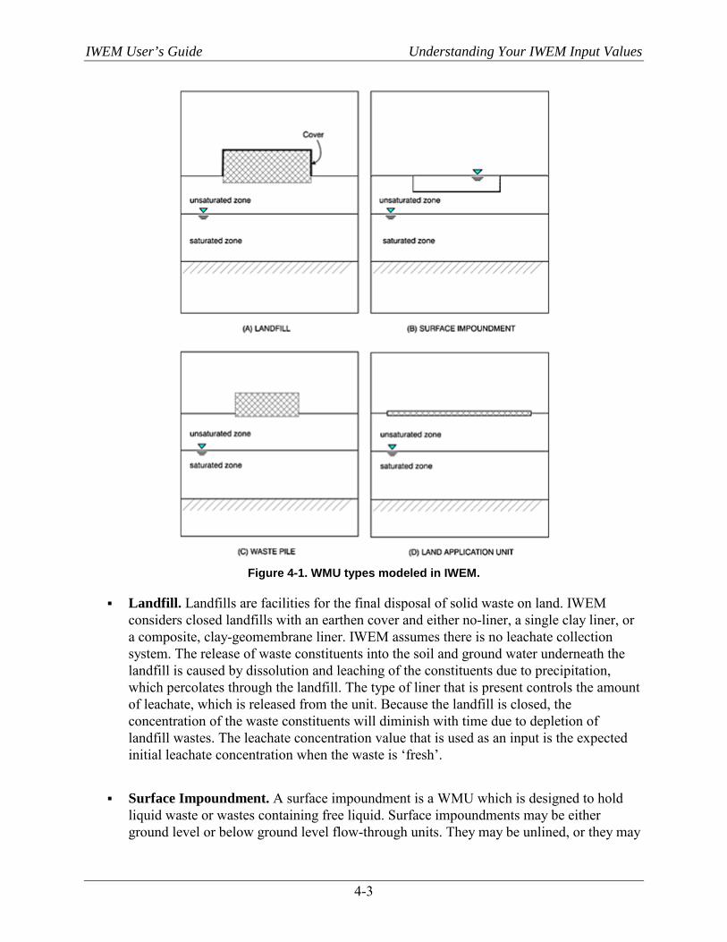
IWEM User’s Guide Understanding Your IWEM Input Values
4-3
Figure 4-1. WMU types modeled in IWEM.
Landfill. Landfills are facilities for the final disposal of solid waste on land. IWEM considers closed landfills with an earthen cover and either no-liner, a single clay liner, or a composite, clay-geomembrane liner. IWEM assumes there is no leachate collection system. The release of waste constituents into the soil and ground water underneath the landfill is caused by dissolution and leaching of the constituents due to precipitation, which percolates through the landfill. The type of liner that is present controls the amount of leachate, which is released from the unit. Because the landfill is closed, the concentration of the waste constituents will diminish with time due to depletion of landfill wastes. The leachate concentration value that is used as an input is the expected initial leachate concentration when the waste is ‘fresh’.
Surface Impoundment. A surface impoundment is a WMU which is designed to hold liquid waste or wastes containing free liquid. Surface impoundments may be either ground level or below ground level flow-through units. They may be unlined, or they may
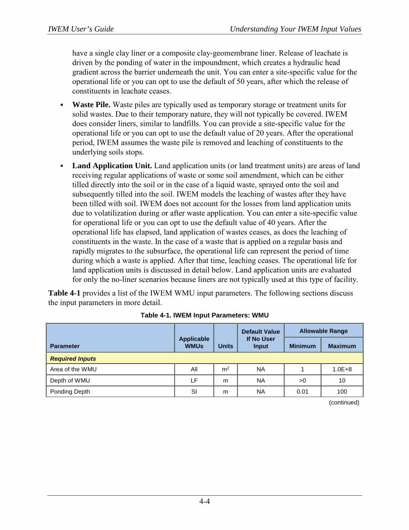
IWEM User’s Guide Understanding Your IWEM Input Values
4-4
have a single clay liner or a composite clay-geomembrane liner. Release of leachate is driven by the ponding of water in the impoundment, which creates a hydraulic head gradient across the barrier underneath the unit. You can enter a site-specific value for the operational life or you can opt to use the default of 50 years, after which the release of constituents in leachate ceases.
Waste Pile. Waste piles are typically used as temporary storage or treatment units for solid wastes. Due to their temporary nature, they will not typically be covered. IWEM does consider liners, similar to landfills. You can provide a site-specific value for the operational life or you can opt to use the default value of 20 years. After the operational period, IWEM assumes the waste pile is removed and leaching of constituents to the underlying soils stops.
Land Application Unit. Land application units (or land treatment units) are areas of land receiving regular applications of waste or some soil amendment, which can be either tilled directly into the soil or in the case of a liquid waste, sprayed onto the soil and subsequently tilled into the soil. IWEM models the leaching of wastes after they have been tilled with soil. IWEM does not account for the losses from land application units due to volatilization during or after waste application. You can enter a site-specific value for operational life or you can opt to use the default value of 40 years. After the operational life has elapsed, land application of wastes ceases, as does the leaching of constituents in the waste. In the case of a waste that is applied on a regular basis and rapidly migrates to the subsurface, the operational life can represent the period of time during which a waste is applied. After that time, leaching ceases. The operational life for land application units is discussed in detail below. Land application units are evaluated for only the no-liner scenarios because liners are not typically used at this type of facility.
Table 4-1 provides a list of the IWEM WMU input parameters. The following sections discuss the input parameters in more detail.
Table 4-1. IWEM Input Parameters: WMU
Parameter Applicable
WMUs Units
Default Value If No User
Input
Allowable Range
Minimum Maximum
Required Inputs
Area of the WMU All m2 NA 1 1.0E+8
Depth of WMU LF m NA >0 10
Ponding Depth SI m NA 0.01 100
(continued)
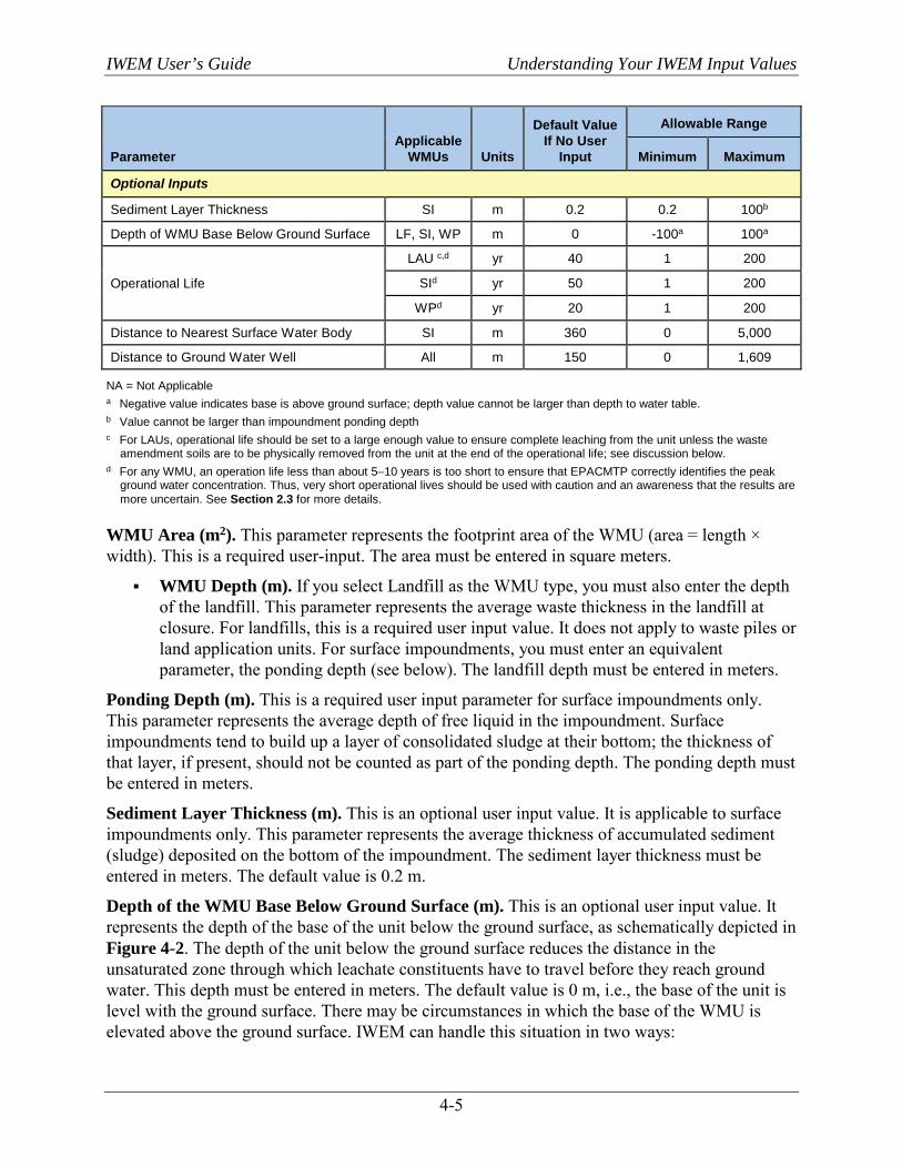
IWEM User’s Guide Understanding Your IWEM Input Values
4-5
Parameter Applicable
WMUs Units
Default Value If No User
Input
Allowable Range
Minimum Maximum
Optional Inputs
Sediment Layer Thickness SI m 0.2 0.2 100b
Depth of WMU Base Below Ground Surface LF, SI, WP m 0 -100a 100a
Operational Life
LAU c,d yr 40 1 200
SId yr 50 1 200
WPd yr 20 1 200
Distance to Nearest Surface Water Body SI m 360 0 5,000
Distance to Ground Water Well All m 150 0 1,609
NA = Not Applicable a Negative value indicates base is above ground surface; depth value cannot be larger than depth to water table. b Value cannot be larger than impoundment ponding depth c For LAUs, operational life should be set to a large enough value to ensure complete leaching from the unit unless the waste
amendment soils are to be physically removed from the unit at the end of the operational life; see discussion below. d For any WMU, an operation life less than about 5–10 years is too short to ensure that EPACMTP correctly identifies the peak
ground water concentration. Thus, very short operational lives should be used with caution and an awareness that the results are more uncertain. See Section 2.3 for more details.
WMU Area (m2). This parameter represents the footprint area of the WMU (area = length × width). This is a required user-input. The area must be entered in square meters.
WMU Depth (m). If you select Landfill as the WMU type, you must also enter the depth of the landfill. This parameter represents the average waste thickness in the landfill at closure. For landfills, this is a required user input value. It does not apply to waste piles or land application units. For surface impoundments, you must enter an equivalent parameter, the ponding depth (see below). The landfill depth must be entered in meters.
Ponding Depth (m). This is a required user input parameter for surface impoundments only. This parameter represents the average depth of free liquid in the impoundment. Surface impoundments tend to build up a layer of consolidated sludge at their bottom; the thickness of that layer, if present, should not be counted as part of the ponding depth. The ponding depth must be entered in meters.
Sediment Layer Thickness (m). This is an optional user input value. It is applicable to surface impoundments only. This parameter represents the average thickness of accumulated sediment (sludge) deposited on the bottom of the impoundment. The sediment layer thickness must be entered in meters. The default value is 0.2 m.
Depth of the WMU Base Below Ground Surface (m). This is an optional user input value. It represents the depth of the base of the unit below the ground surface, as schematically depicted in Figure 4-2. The depth of the unit below the ground surface reduces the distance in the unsaturated zone through which leachate constituents have to travel before they reach ground water. This depth must be entered in meters. The default value is 0 m, i.e., the base of the unit is level with the ground surface. There may be circumstances in which the base of the WMU is elevated above the ground surface. IWEM can handle this situation in two ways:
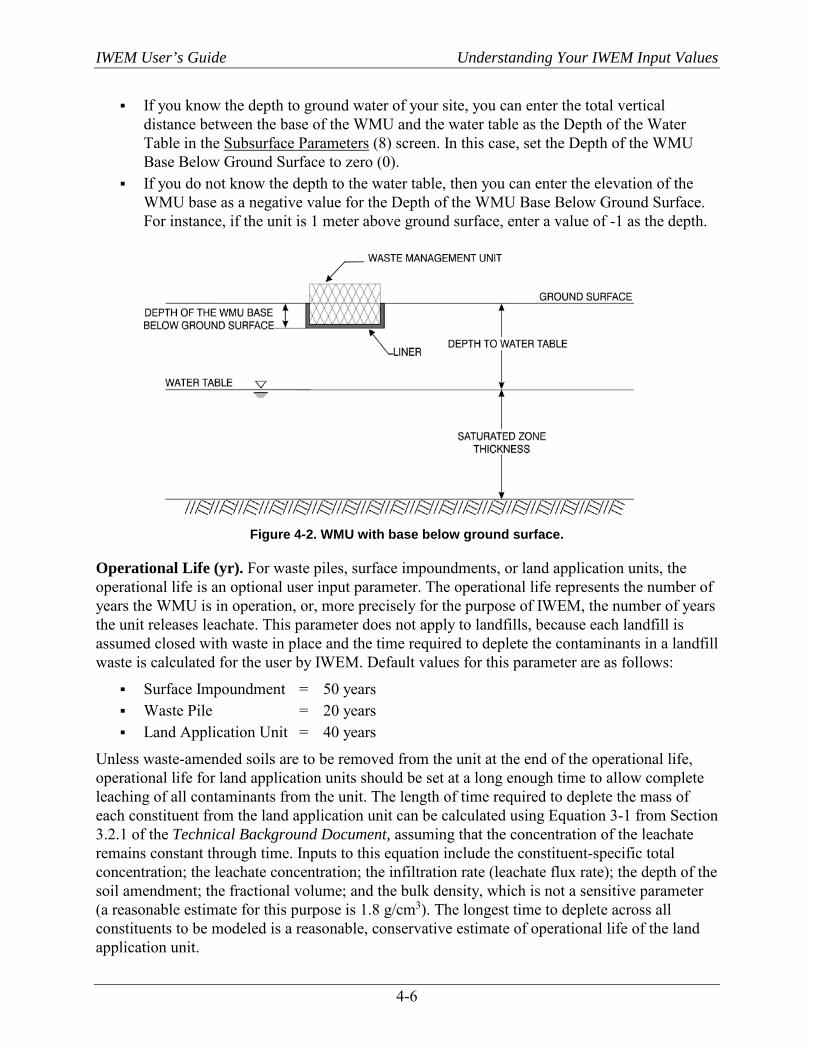
IWEM User’s Guide Understanding Your IWEM Input Values
4-6
If you know the depth to ground water of your site, you can enter the total vertical distance between the base of the WMU and the water table as the Depth of the Water Table in the Subsurface Parameters (8) screen. In this case, set the Depth of the WMU Base Below Ground Surface to zero (0).
If you do not know the depth to the water table, then you can enter the elevation of the WMU base as a negative value for the Depth of the WMU Base Below Ground Surface. For instance, if the unit is 1 meter above ground surface, enter a value of -1 as the depth.
Figure 4-2. WMU with base below ground surface.
Operational Life (yr). For waste piles, surface impoundments, or land application units, the operational life is an optional user input parameter. The operational life represents the number of years the WMU is in operation, or, more precisely for the purpose of IWEM, the number of years the unit releases leachate. This parameter does not apply to landfills, because each landfill is assumed closed with waste in place and the time required to deplete the contaminants in a landfill waste is calculated for the user by IWEM. Default values for this parameter are as follows:
Surface Impoundment = 50 years Waste Pile = 20 years Land Application Unit = 40 years
Unless waste-amended soils are to be removed from the unit at the end of the operational life, operational life for land application units should be set at a long enough time to allow complete leaching of all contaminants from the unit. The length of time required to deplete the mass of each constituent from the land application unit can be calculated using Equation 3-1 from Section 3.2.1 of the Technical Background Document, assuming that the concentration of the leachate remains constant through time. Inputs to this equation include the constituent-specific total concentration; the leachate concentration; the infiltration rate (leachate flux rate); the depth of the soil amendment; the fractional volume; and the bulk density, which is not a sensitive parameter (a reasonable estimate for this purpose is 1.8 g/cm3). The longest time to deplete across all constituents to be modeled is a reasonable, conservative estimate of operational life of the land application unit.
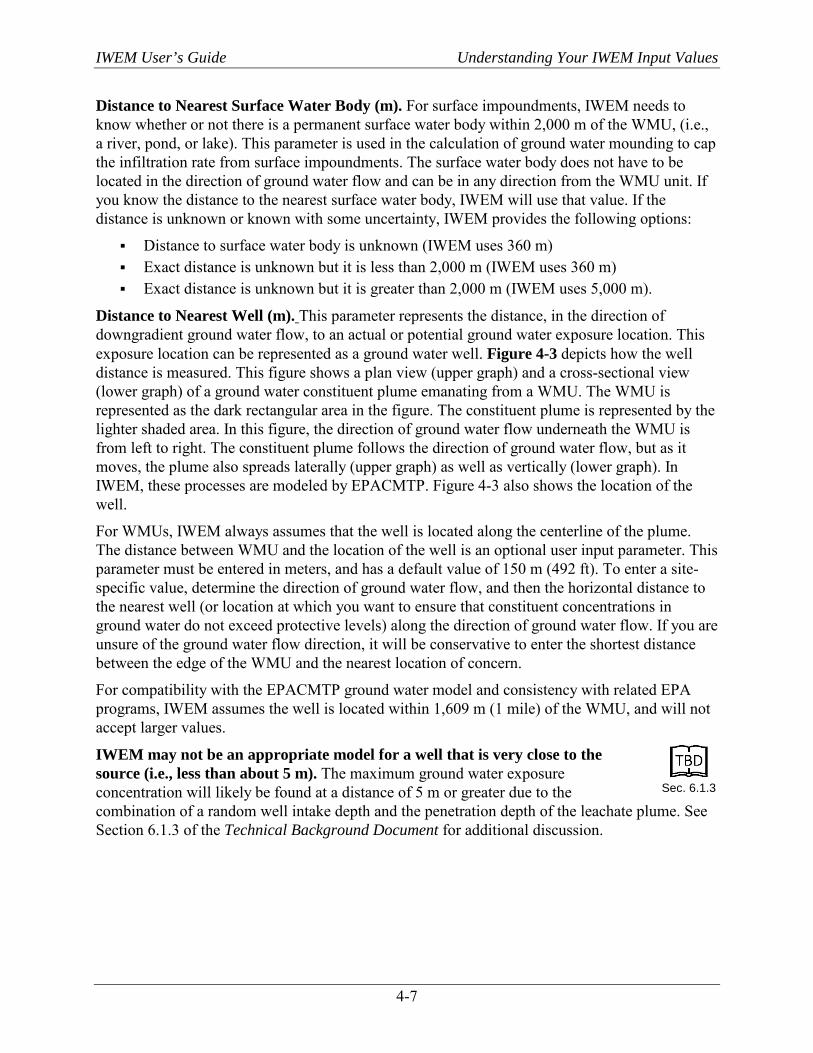
IWEM User’s Guide Understanding Your IWEM Input Values
4-7
Distance to Nearest Surface Water Body (m). For surface impoundments, IWEM needs to know whether or not there is a permanent surface water body within 2,000 m of the WMU, (i.e., a river, pond, or lake). This parameter is used in the calculation of ground water mounding to cap the infiltration rate from surface impoundments. The surface water body does not have to be located in the direction of ground water flow and can be in any direction from the WMU unit. If you know the distance to the nearest surface water body, IWEM will use that value. If the distance is unknown or known with some uncertainty, IWEM provides the following options:
Distance to surface water body is unknown (IWEM uses 360 m) Exact distance is unknown but it is less than 2,000 m (IWEM uses 360 m) Exact distance is unknown but it is greater than 2,000 m (IWEM uses 5,000 m).
Distance to Nearest Well (m). This parameter represents the distance, in the direction of downgradient ground water flow, to an actual or potential ground water exposure location. This exposure location can be represented as a ground water well. Figure 4-3 depicts how the well distance is measured. This figure shows a plan view (upper graph) and a cross-sectional view (lower graph) of a ground water constituent plume emanating from a WMU. The WMU is represented as the dark rectangular area in the figure. The constituent plume is represented by the lighter shaded area. In this figure, the direction of ground water flow underneath the WMU is from left to right. The constituent plume follows the direction of ground water flow, but as it moves, the plume also spreads laterally (upper graph) as well as vertically (lower graph). In IWEM, these processes are modeled by EPACMTP. Figure 4-3 also shows the location of the well.
For WMUs, IWEM always assumes that the well is located along the centerline of the plume. The distance between WMU and the location of the well is an optional user input parameter. This parameter must be entered in meters, and has a default value of 150 m (492 ft). To enter a site-specific value, determine the direction of ground water flow, and then the horizontal distance to the nearest well (or location at which you want to ensure that constituent concentrations in ground water do not exceed protective levels) along the direction of ground water flow. If you are unsure of the ground water flow direction, it will be conservative to enter the shortest distance between the edge of the WMU and the nearest location of concern.
For compatibility with the EPACMTP ground water model and consistency with related EPA programs, IWEM assumes the well is located within 1,609 m (1 mile) of the WMU, and will not accept larger values.
IWEM may not be an appropriate model for a well that is very close to the source (i.e., less than about 5 m). The maximum ground water exposure concentration will likely be found at a distance of 5 m or greater due to the combination of a random well intake depth and the penetration depth of the leachate plume. See Section 6.1.3 of the Technical Background Document for additional discussion.
Sec. 6.1.3
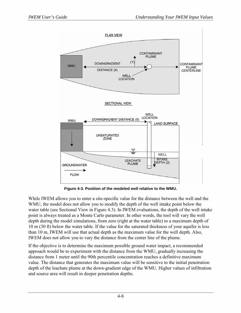
IWEM User’s Guide Understanding Your IWEM Input Values
4-8
Figure 4-3. Position of the modeled well relative to the WMU.
While IWEM allows you to enter a site-specific value for the distance between the well and the WMU, the model does not allow you to modify the depth of the well intake point below the water table (see Sectional View in Figure 4.3). In IWEM evaluations, the depth of the well intake point is always treated as a Monte Carlo parameter. In other words, the tool will vary the well depth during the model simulations, from zero (right at the water table) to a maximum depth of 10 m (30 ft) below the water table. If the value for the saturated thickness of your aquifer is less than 10 m, IWEM will use that actual depth as the maximum value for the well depth. Also, IWEM does not allow you to vary the distance from the center line of the plume.
If the objective is to determine the maximum possible ground water impact, a recommended approach would be to experiment with the distance from the WMU, gradually increasing the distance from 1 meter until the 90th percentile concentration reaches a definitive maximum value. The distance that generates the maximum value will be sensitive to the initial penetration depth of the leachate plume at the down-gradient edge of the WMU. Higher values of infiltration and source area will result in deeper penetration depths.

IWEM User’s Guide Understanding Your IWEM Input Values
4-9
4.2.2 Structural Fill Source Parameters Structural fills are modeled in IWEM as unlined landfills, with a few additional parameters (bulk density, hydraulic conductivity, and volume fraction occupied by leachable materials). Table 4-2 provides a list of the IWEM structural fills input parameters. The following sections discuss the input parameters in more detail.
Table 4-2. IWEM Input Parameters: Structural Fills
Parameter Units
Default Value If No User
Input
Allowable Range
Minimum Maximum
Required Inputs
Area of the structural fill m2 NA 1 1.0E+8
Depth of the structural fill m NA >0 10
Effective bulk density g/cm3 NA >0 2.1
Effective hydraulic conductivity m/yr NA >0 1×10⁸
Volume fraction occupied by leachable material
– NA >0 1
Optional Inputs
Depth of fill base below ground surface m 0 -100 a 100a
Distance to Ground water Well m 150 0 1,609 NA = Not Applicable a Negative value indicates base is above ground surface; depth value cannot be larger than depth to water
table.
Area of Structural Fill (m2). This parameter represents the footprint area of the structural fill (area = length × width). This is a required user-input. The area must be entered in square meters.
Depth of the structural fill (m). This parameter represents the average thickness of the fill material. This is a required user input value. The fill depth must be entered in meters.
Depth of the Fill Base Below Ground Surface (m). This is an optional user input value. It represents the depth of the base of the fill below the ground surface, as schematically depicted in Figure 4-2. The depth of the fill below the ground surface reduces the distance in the unsaturated zone through which leachate constituents have to travel before they reach ground water. This depth must be entered in meters. The default value is 0 m, i.e., the base of the unit is level with the ground surface. There may be circumstances in which the base of the WMU is elevated above the ground surface. IWEM can handle this situation in two ways:
If you know the depth to ground water of your site, you can enter the total vertical distance between the base of the fill and the water table as the Depth of the Water Table in the Subsurface Parameters (8) screen. In this case, set the Depth of the Fill Base Below Ground Surface to zero (0).
If you do not know the depth to the water table, then you can enter the elevation of the fill base as a negative value for the Depth of the Fill Base below Ground Surface. For instance, if the unit is 1 m above ground surface, enter a value of -1 as the depth.
Sec. 3.2 Sec. 6.2

IWEM User’s Guide Understanding Your IWEM Input Values
4-10
Distance to Nearest Well (m). This parameter represents the distance, in the direction of downgradient ground water flow, to an actual or potential ground water exposure location. This exposure location can be represented as a ground water well. Figure 4-3 depicts how the well distance is measured. For structural fills, IWEM always assumes that the well is located along the centerline of the plume. The distance between fill and the location of the well is an optional user input parameter. This parameter must be entered in meters, and has a default value of 150 m (492 ft). To enter a site-specific value, determine the direction of ground water flow, and then the horizontal distance to the nearest well (or location at which you want to ensure that constituent concentrations in ground water do not exceed protective levels) along the direction of ground water flow. If you are unsure of the ground water flow direction, it will be conservative to enter the shortest distance between the edge of the fill and the nearest location of concern.
IWEM may generate unreliable results for a well that is very close to the roadway (i.e., less than about 5 m). The maximum ground water exposure concentration will likely be found at a distance of 5 m or greater due to the combination of a random well intake depth and the penetration depth of the leachate plume. See Section 6.1.3 of the Technical Background Document for additional discussion.
For compatibility with the EPACMTP ground water model and consistency with related EPA programs, IWEM assumes the well is located within 1,609 m (1 mile) of the fill, and will not accept larger values.
While IWEM allows you to enter a site-specific value for the distance between the well and the fill, the model does not allow you to modify the depth of the well intake point below the water table (see Sectional View in Figure 4.3). In IWEM evaluations, the depth of the well intake point is always treated as a Monte Carlo parameter. In other words, the tool will vary the well depth during the model simulations, from zero (right at the water table) to a maximum depth of 10 m (30 ft) below the water table. If the value for the saturated thickness of your aquifer is less than 10 m, IWEM will use that actual depth as the maximum value for the well depth. Also, IWEM does not allow you to vary the distance from the center line of the plume.
Effective Hydraulic Conductivity of Fill Material (m/yr). The effective hydraulic conductivity of the fill material in meters per year. This parameter is required for determining the limiting value of infiltration through the fill. The best source for this parameter would be engineering design reports or material properties sheets. Values for representative materials are provided in Table 6-17 of Section 6.4.3.2 of the Technical Background Document in units of cm/sec. IWEM requires units of m/yr for hydraulic conductivity.
Effective Bulk Density of Fill Material (g/cm3). The dry bulk density of the layer material in grams per cubic centimeters. This parameter is required for calculating how long a contaminant leaches from fill containing industrial materials. The best source for this parameter would be engineering design reports or material properties sheets.
Volume Fraction Occupied by Leachable Material (Unitless). This parameter represents the portion of the fill containing leachable industrial materials. It must be greater than 0 and less than or equal to 1.
Sec. 6.1.3
Sec.
6.4.3.2
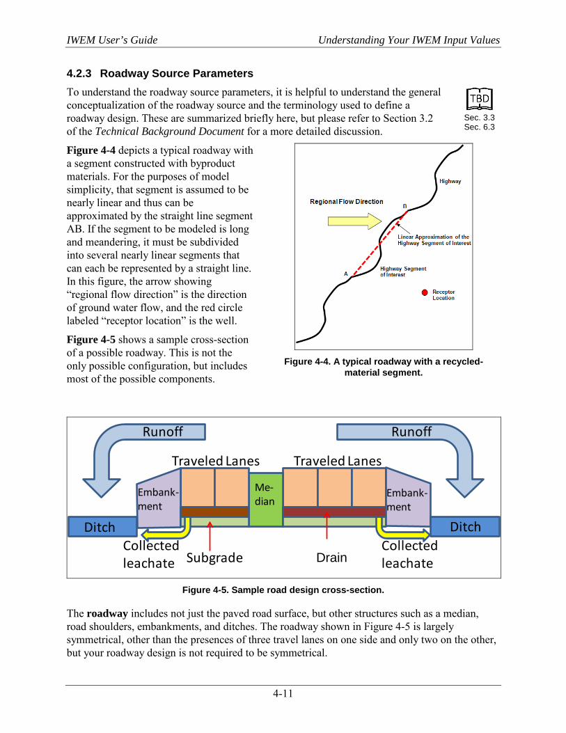
IWEM User’s Guide Understanding Your IWEM Input Values
4-11
4.2.3 Roadway Source Parameters To understand the roadway source parameters, it is helpful to understand the general conceptualization of the roadway source and the terminology used to define a roadway design. These are summarized briefly here, but please refer to Section 3.2 of the Technical Background Document for a more detailed discussion.
Figure 4-4 depicts a typical roadway with a segment constructed with byproduct materials. For the purposes of model simplicity, that segment is assumed to be nearly linear and thus can be approximated by the straight line segment AB. If the segment to be modeled is long and meandering, it must be subdivided into several nearly linear segments that can each be represented by a straight line. In this figure, the arrow showing “regional flow direction” is the direction of ground water flow, and the red circle labeled “receptor location” is the well.
Figure 4-5 shows a sample cross-section of a possible roadway. This is not the only possible configuration, but includes most of the possible components.
Traveled Lanes Traveled Lanes
Me-dian
Embank-ment
DitchDitch
Embank-ment
Permeable BaseSubgrade
RunoffRunoff
Collected leachate
Collected leachate
Figure 4-5. Sample road design cross-section.
The roadway includes not just the paved road surface, but other structures such as a median, road shoulders, embankments, and ditches. The roadway shown in Figure 4-5 is largely symmetrical, other than the presences of three travel lanes on one side and only two on the other, but your roadway design is not required to be symmetrical.
Sec. 3.3 Sec. 6.3
Figure 4-4. A typical roadway with a recycled-
material segment.
Drain
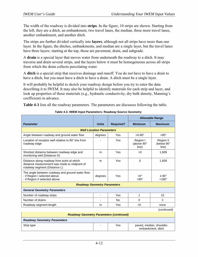
IWEM User’s Guide Understanding Your IWEM Input Values
4-12
The width of the roadway is divided into strips. In the figure, 10 strips are shown. Starting from the left, they are a ditch, an embankment, two travel lanes, the median, three more travel lanes, another embankment, and another ditch.
The strips are further divided vertically into layers, although not all strips have more than one layer. In the figure, the ditches, embankments, and median are a single layer, but the travel lanes have three layers: starting at the top, those are pavement, drain, and subgrade.
A drain is a special layer that moves water from underneath the roadway to a ditch. It may traverse and drain several strips, and the layers below it must be homogeneous across all strips from which the drain collects percolating water.
A ditch is a special strip that receives drainage and runoff. You do not have to have a drain to have a ditch, but you must have a ditch to have a drain. A ditch must be a single layer.
It will probably be helpful to sketch your roadway design before you try to enter the data describing it to IWEM. It may also be helpful to identify materials for each strip and layer, and look up properties of those materials (e.g., hydraulic conductivity, dry bulk density, Manning’s coefficient) in advance.
Table 4-3 lists all the roadway parameters. The parameters are discusses following the table.
Table 4-3. IWEM Input Parameters: Roadway Source Geometry
Parameter Units Required?
Allowable Range
Minimum Maximum
Well Location Parameters Angle between roadway and ground water flow degrees Yes >0-90° >90°
Location of receptor well relative to 90° line from roadway edge
- Yes Region I (above 90°
line)
Region II (below 90°
line)
Shortest distance between roadway edge and monitoring well (Distance D)
m Yes >0 1,609
Distance along roadway from point at which distance measurement was made to midpoint of roadway segment (Distance L)
m Yes 0 1,609
The angle between roadway and ground water flow: - if Region I selected above - if Region II selected above
degrees
Yes
>0°
>90°
≤ 90° <180°
Roadway Geometry Parameters
General Geometry Parameters
Number of roadway strips - Yes 1 15 Number of drains - No 0 2 Roadway segment length m Yes >0 none
(continued)
Roadway Geometry Parameters (continued)
Roadway Geometry Parameters
Strip type - Yes paved, median, shoulder, embankment, ditch
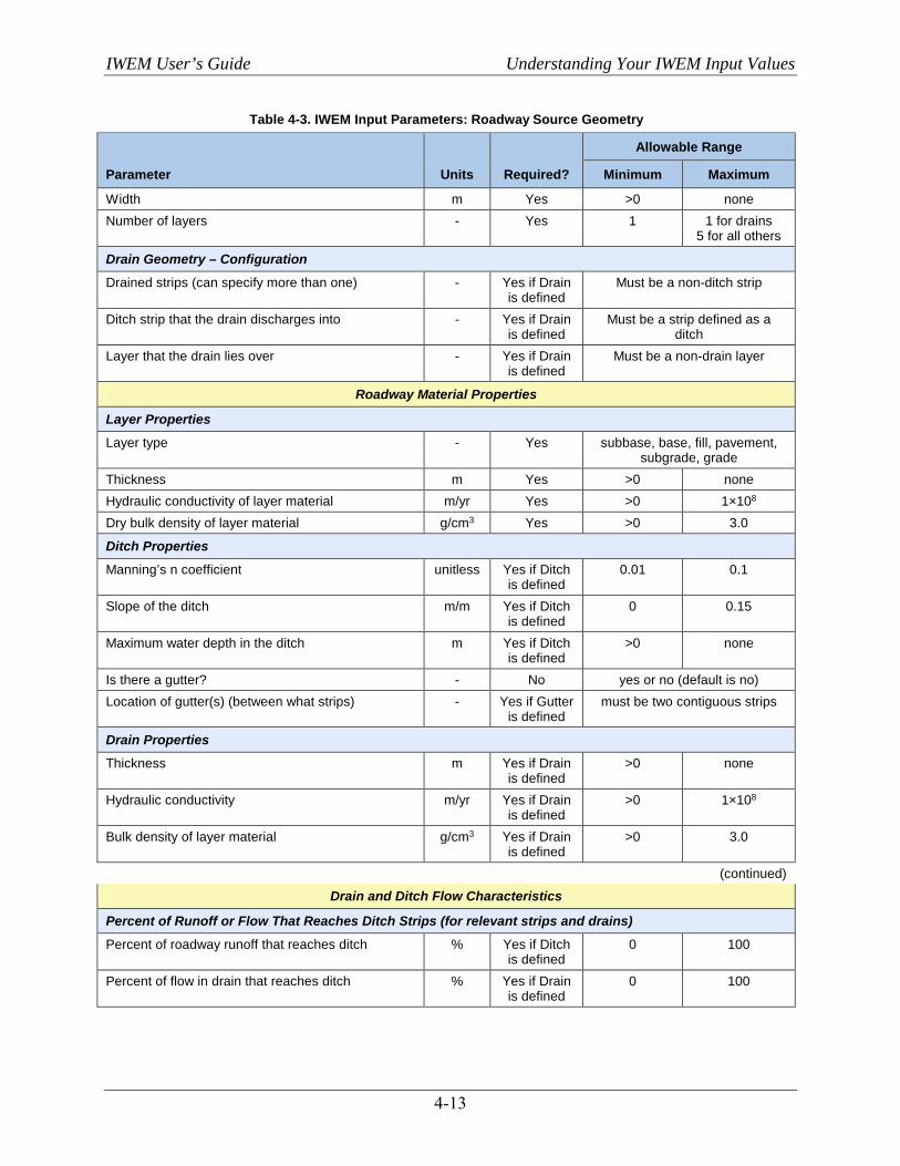
IWEM User’s Guide Understanding Your IWEM Input Values
4-13
Table 4-3. IWEM Input Parameters: Roadway Source Geometry
Parameter Units Required?
Allowable Range
Minimum Maximum
Width m Yes >0 none Number of layers - Yes 1 1 for drains
5 for all others
Drain Geometry – Configuration
Drained strips (can specify more than one) - Yes if Drain is defined
Must be a non-ditch strip
Ditch strip that the drain discharges into - Yes if Drain is defined
Must be a strip defined as a ditch
Layer that the drain lies over - Yes if Drain is defined
Must be a non-drain layer
Roadway Material Properties
Layer Properties
Layer type - Yes subbase, base, fill, pavement, subgrade, grade
Thickness m Yes >0 none Hydraulic conductivity of layer material m/yr Yes >0 1×10⁸ Dry bulk density of layer material g/cm3 Yes >0 3.0
Ditch Properties
Manning’s n coefficient unitless Yes if Ditch is defined
0.01 0.1
Slope of the ditch m/m Yes if Ditch is defined
0 0.15
Maximum water depth in the ditch m Yes if Ditch is defined
>0 none
Is there a gutter? - No yes or no (default is no) Location of gutter(s) (between what strips) - Yes if Gutter
is defined must be two contiguous strips
Drain Properties
Thickness m Yes if Drain is defined
>0 none
Hydraulic conductivity m/yr Yes if Drain is defined
>0 1×10⁸
Bulk density of layer material g/cm3 Yes if Drain is defined
>0 3.0
(continued)
Drain and Ditch Flow Characteristics
Percent of Runoff or Flow That Reaches Ditch Strips (for relevant strips and drains)
Percent of roadway runoff that reaches ditch % Yes if Ditch is defined
0 100
Percent of flow in drain that reaches ditch % Yes if Drain is defined
0 100
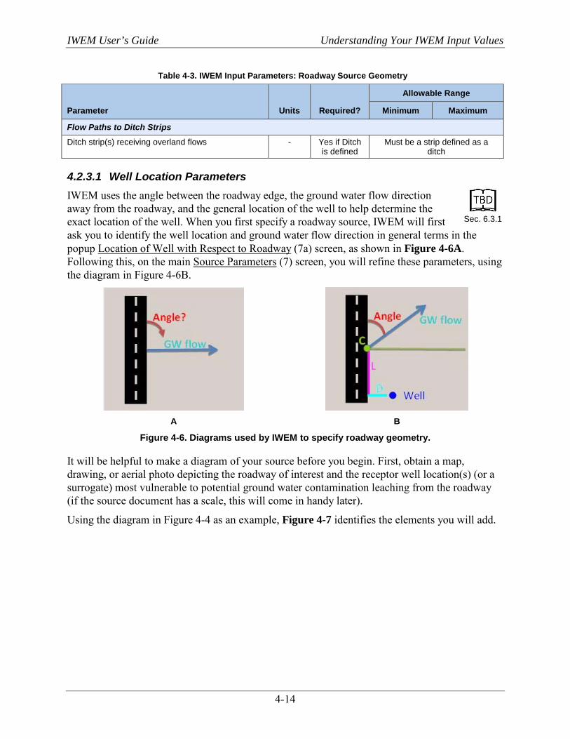
IWEM User’s Guide Understanding Your IWEM Input Values
4-14
Table 4-3. IWEM Input Parameters: Roadway Source Geometry
Parameter Units Required?
Allowable Range
Minimum Maximum
Flow Paths to Ditch Strips
Ditch strip(s) receiving overland flows - Yes if Ditch is defined
Must be a strip defined as a ditch
4.2.3.1 Well Location Parameters IWEM uses the angle between the roadway edge, the ground water flow direction away from the roadway, and the general location of the well to help determine the exact location of the well. When you first specify a roadway source, IWEM will first ask you to identify the well location and ground water flow direction in general terms in the popup Location of Well with Respect to Roadway (7a) screen, as shown in Figure 4-6A. Following this, on the main Source Parameters (7) screen, you will refine these parameters, using the diagram in Figure 4-6B.
A B
Figure 4-6. Diagrams used by IWEM to specify roadway geometry.
It will be helpful to make a diagram of your source before you begin. First, obtain a map, drawing, or aerial photo depicting the roadway of interest and the receptor well location(s) (or a surrogate) most vulnerable to potential ground water contamination leaching from the roadway (if the source document has a scale, this will come in handy later).
Using the diagram in Figure 4-4 as an example, Figure 4-7 identifies the elements you will add.
Sec. 6.3.1
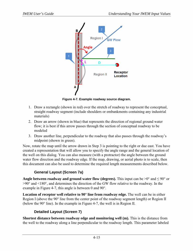
IWEM User’s Guide Understanding Your IWEM Input Values
4-15
Figure 4-7. Example roadway source diagram.
1. Draw a rectangle (shown in red) over the stretch of roadway to represent the conceptual, straight roadway segment (include shoulders or embankments containing any industrial materials)
2. Draw an arrow (shown in blue) that represents the direction of regional ground water flow; it is best if this arrow passes through the section of conceptual roadway to be modeled
3. Draw another line, perpendicular to the roadway that also passes through the roadway’s midpoint (shown in green).
Now, rotate the map until the arrow drawn in Step 3 is pointing to the right or due east. You have created a representation that will allow you to specify the angle range and the general location of the well on this dialog. You can also measure (with a protractor) the angle between the ground water flow direction and the roadway edge. If the map, drawing, or aerial photo is to scale, then this document can also be used to determine the required length measurements described below.
General Layout (Screen 7a) Angle between roadway and ground water flow (degrees). This input can be >0° and ≤ 90° or >90° and <180°, and determines the direction of the GW flow relative to the roadway. In the example in Figure 4-7, this angle is between 0 and 90°.
Location of receptor well relative to 90° line from roadway edge. The well can be in either Region I (above the 90° line from the center point of the roadway segment length) or Region II (below the 90° line). In the example in Figure 4-7, the well is in Region II.
Detailed Layout (Screen 7) Shortest distance between roadway edge and monitoring well (m). This is the distance from the well to the roadway along a line perpendicular to the roadway length. This parameter labeled
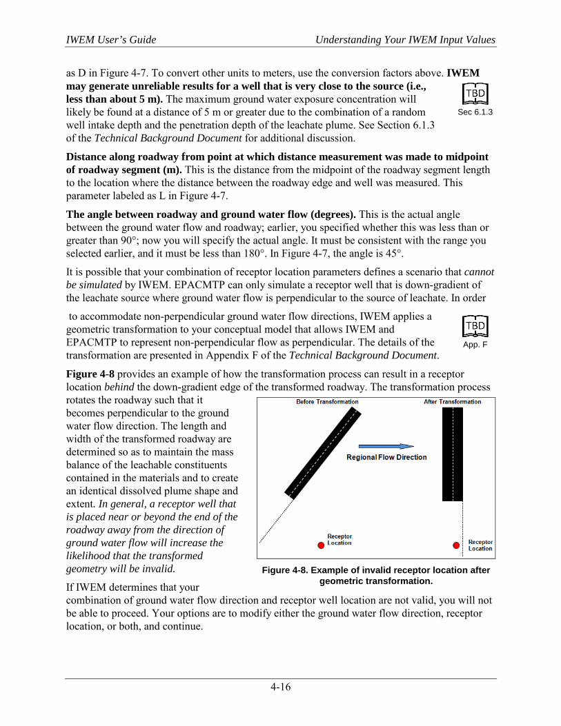
IWEM User’s Guide Understanding Your IWEM Input Values
4-16
as D in Figure 4-7. To convert other units to meters, use the conversion factors above. IWEM may generate unreliable results for a well that is very close to the source (i.e., less than about 5 m). The maximum ground water exposure concentration will likely be found at a distance of 5 m or greater due to the combination of a random well intake depth and the penetration depth of the leachate plume. See Section 6.1.3 of the Technical Background Document for additional discussion.
Distance along roadway from point at which distance measurement was made to midpoint of roadway segment (m). This is the distance from the midpoint of the roadway segment length to the location where the distance between the roadway edge and well was measured. This parameter labeled as L in Figure 4-7.
The angle between roadway and ground water flow (degrees). This is the actual angle between the ground water flow and roadway; earlier, you specified whether this was less than or greater than 90°; now you will specify the actual angle. It must be consistent with the range you selected earlier, and it must be less than 180°. In Figure 4-7, the angle is 45°.
It is possible that your combination of receptor location parameters defines a scenario that cannot be simulated by IWEM. EPACMTP can only simulate a receptor well that is down-gradient of the leachate source where ground water flow is perpendicular to the source of leachate. In order
to accommodate non-perpendicular ground water flow directions, IWEM applies a geometric transformation to your conceptual model that allows IWEM and EPACMTP to represent non-perpendicular flow as perpendicular. The details of the transformation are presented in Appendix F of the Technical Background Document.
Figure 4-8 provides an example of how the transformation process can result in a receptor location behind the down-gradient edge of the transformed roadway. The transformation process rotates the roadway such that it becomes perpendicular to the ground water flow direction. The length and width of the transformed roadway are determined so as to maintain the mass balance of the leachable constituents contained in the materials and to create an identical dissolved plume shape and extent. In general, a receptor well that is placed near or beyond the end of the roadway away from the direction of ground water flow will increase the likelihood that the transformed geometry will be invalid.
If IWEM determines that your combination of ground water flow direction and receptor well location are not valid, you will not be able to proceed. Your options are to modify either the ground water flow direction, receptor location, or both, and continue.
Sec 6.1.3
App. F
Figure 4-8. Example of invalid receptor location after
geometric transformation.
IWEM User’s Guide Understanding Your IWEM Input Values
4-17
4.2.3.2 General Geometry Parameters Number of roadway strips. As described above, a roadway strip is a portion of the width of the roadway you are modeling. Together, the strips make up the overall width of the roadway. Strips include both the actual road and strips along the side or down the middle that are not actual driving surface (such as shoulder or median). The number of strips is a required input.
Number of drains. A drain moves water from underneath the roadway to a ditch. Thus, you must define at least one strip as a ditch before you can add the number of drains. IWEM allows a maximum of two drains.
Roadway segment length (m). This is the length of the road segment you want to model.
4.2.3.3 Roadway Geometry Parameters Tab In this tab, IWEM displays a table with a row for each strip, up to the number of strips you specified above. The strips are automatically numbered from 1 to the number you specified. Strip 1 is the strip closest to the well, and the strip numbers increase with distance from the well. The following inputs must be specified for each strip:
Strip type. Choose a strip type from the dropdown box. Options are paved area, median, shoulder, embankment, and ditch.
Width (m). Enter the width of the strip in meters.
Number of layers. The number of vertical layers in each strip other than drains. You will specify the properties of these layers later.
If you defined any of the strips as a ditch, you will have the option to enter the number of drains above the table (see Section 4.2.2.2, General Parameters). IWEM allows a maximum of two drains.
If you specify a non-zero number of drains, IWEM will display two Drain Geometry tables.
Drain Geometry–Strips Table – Drained Strip(s). For each drain (drain 1 is the one nearest to the well), specify the
strip (or strips) that are drained by the drain. The strips drained by a drain must be located above the drain.
Drain Geometry–Configuration Table – Ditch strip that the drain discharges into. This is the strip number of the ditch that
the drain discharge into. It does not have to be on the same side of the roadway as the drain; you can specify two drains and one ditch and have both drains drain to the one ditch.
– Layer that the drain lies over. This is the layer number for the layer below the drain. Layers are numbered from 1 to the number of layers from the bottom up.
Note the following about drain layout:
Two drains can be connected to a single ditch
Sec. 6.3.2
Sec. 6.3.3
Sec. 6.3.4
Do not count drains in the number of layers!
IWEM User’s Guide Understanding Your IWEM Input Values
4-18
A drain can traverse one or more contiguous roadway strips, however, drains cannot overlap each other.
If a drain traverses multiple, contiguous strips: – The number of layers in each strip beneath the drain must be the same, and – The thickness and material properties of each like numbered layer beneath the drain
must also be same. Each drain requires values for the material hydraulic conductivity and dry bulk density.
4.2.3.4 Layer Properties Tab On this tab, IWEM displays a table containing a row for each strip-layer combination based on your inputs on the geometry tab. The strip number, strip type, and layer number columns are prepopulated. The Is Below Drain column is also prepopulated based on your entries in the Drain Geometry Configuration table on the Geometry tab. Remember that drains are not included in the layers; drain properties are specified on the Drain Properties tab. You must then provide the following inputs for each strip-layer:
Layer type. Choose a layer type from the dropdown box. Options are subbase, base, fill, pavement, subgrade, and grade.
Thickness (m). The thickness of the layer in meters. This parameter is required for calculating how long a contaminant leaches from the layer. To convert other units to meters, use the conversion factors above. The best source for this parameter would be engineering design reports.
Hydraulic conductivity of layer material (m/yr). The hydraulic conductivity of the layer material in meters per year. This parameter is required for determining the limiting value of infiltration through the layers of a strip. The best source for this parameter would be engineering design report or material properties sheets. Values for representative materials are provided in Table 6-17 of Section 6.4.3.2 of the Technical Background Document in units of cm/sec. IWEM requires units of m/yr for hydraulic conductivity.
Dry bulk density of layer material (g/cm3). The dry bulk density of the layer material in grams per cubic centimeters. This parameter is required for calculating how long a contaminant leaches from a layer containing industrial material. The best source for this parameter would be engineering design reports or material properties sheets.
4.2.3.5 Ditch Properties Tab In this tab, IWEM displays rows for each strip that you specified was a ditch.
Manning’s n coefficient (unitless). Manning’s n coefficient is a non-dimensional coefficient that reflects the hydraulic resistance induced from the roughness of the channel surface for open channel flow. A smooth channel generally has less hydraulic resistance and is represented by a lower coefficient value, resulting in higher velocity estimates. A rough channel is generally more hydraulically resistant and has correspondingly higher coefficient values. Chow (1959) compiled many values for Manning’s n for a wide range of channel
Sec. 6.3.5
Sec.
6.4.3.2
Sec. 6.3.6
Note that all layers below a particular drain must be homogeneous with respect to these properties – you must specify the same type, same thickness, same hydraulic conductivity, and same dry bulk density. If two layers that underlie the same drain are not the same, you will get an error
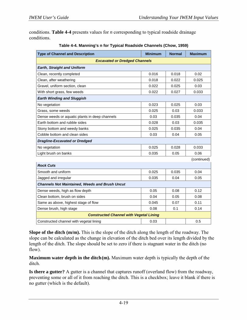
IWEM User’s Guide Understanding Your IWEM Input Values
4-19
conditions. Table 4-4 presents values for n corresponding to typical roadside drainage conditions.
Table 4-4. Manning’s n for Typical Roadside Channels (Chow, 1959)
Type of Channel and Description Minimum Normal Maximum
Excavated or Dredged Channels
Earth, Straight and Uniform
Clean, recently completed 0.016 0.018 0.02 Clean, after weathering 0.018 0.022 0.025 Gravel, uniform section, clean 0.022 0.025 0.03 With short grass, few weeds 0.022 0.027 0.033
Earth Winding and Sluggish
No vegetation 0.023 0.025 0.03 Grass, some weeds 0.025 0.03 0.033 Dense weeds or aquatic plants in deep channels 0.03 0.035 0.04 Earth bottom and rubble sides 0.028 0.03 0.035 Stony bottom and weedy banks 0.025 0.035 0.04 Cobble bottom and clean sides 0.03 0.04 0.05
Dragline-Excavated or Dredged
No vegetation 0.025 0.028 0.033 Light brush on banks 0.035 0.05 0.06
(continued)
Rock Cuts
Smooth and uniform 0.025 0.035 0.04 Jagged and irregular 0.035 0.04 0.05
Channels Not Maintained, Weeds and Brush Uncut
Dense weeds, high as flow depth 0.05 0.08 0.12 Clean bottom, brush on sides 0.04 0.05 0.08 Same as above, highest stage of flow 0.045 0.07 0.11 Dense brush, high stage 0.08 0.1 0.14
Constructed Channel with Vegetal Lining
Constructed channel with vegetal lining 0.03 0.5
Slope of the ditch (m/m). This is the slope of the ditch along the length of the roadway. The slope can be calculated as the change in elevation of the ditch bed over its length divided by the length of the ditch. The slope should be set to zero if there is stagnant water in the ditch (no flow).
Maximum water depth in the ditch (m). Maximum water depth is typically the depth of the ditch.
Is there a gutter? A gutter is a channel that captures runoff (overland flow) from the roadway, preventing some or all of it from reaching the ditch. This is a checkbox; leave it blank if there is no gutter (which is the default).
IWEM User’s Guide Understanding Your IWEM Input Values
4-20
Location of gutter(s) (between what strips). If you specified that the ditch does have a gutter, fill in here between what strips the gutter lies in. The specified strips must be contiguous, and they must both be strips for which runoff flows to that ditch, as specified in the Flow Paths to Ditch Strips table on the Flow Characteristics tab.
4.2.3.6 Drain Properties Tab IWEM displays rows for each drain you specified. Note that width of the drain is predetermined by the widths of the strips that it drains.
Thickness (m). The thickness in meters of the drain. This parameter is required for calculating how long a contaminant leaches through the drainage layer. Note that the drainage layer cannot be a source of leachate (so no leachate concentration may be assigned to it), but leachate from layers above the drain can leach through the drain material.
Hydraulic conductivity (m/yr). The hydraulic conductivity of the drain material in meters per year. This parameter is required for determining the limiting infiltration rate across layers in a strip. The best source for this parameter would be engineering design reports or material properties sheets. Values for representative materials are provided in Table 6-17 of Section 6.4.3.2 of the Technical Background Document in units of cm/sec. IWEM requires units of m/yr for hydraulic conductivity.
Bulk density of layer material (g/cm3). The dry bulk density of the drain material in grams per cubic centimeters. This parameter is required for calculating how long a contaminant leaches through the drainage layer. Note that the drainage layer cannot be a source of leachate (so no leachate concentration may be assigned to it), but leachate from layers above the drain can leach through the drain material. The best source for this parameter would be engineering design reports or material properties.
Each drain requires values for the material hydraulic conductivity and dry bulk density. Bear in mind that a drain is designed to be a permeable, transmissive layer; thus, it should have a relatively high hydraulic conductivity.
4.2.3.7 Flow Characteristics Tab Flow Percentages to Ditch Strips Table
IWEM displays rows for each drain and each ditch. Each will have one of the following two inputs that you must enter:
Percent of roadway runoff that reaches ditch beyond gutter (%).This parameter must be provided when a gutter defined for a ditch. A gutter is used to divert some or all of the runoff water from strips “above” the gutter, away from the associated ditch and out of the modeled system. The value you supply here, a percentage ranging from 0 to 100%, specifies how much of the runoff is not diverted by the gutter. A value of 0% indicates that no runoff water from strips above the gutter will reach the ditch. A value of 100% indicates that all runoff water from strips above the gutter will reach the ditch. If a gutter is not present, then 100% of the runoff should reach the ditch. If a gutter is present, the percentage should be equal to the ratio of the width of all strips between the gutter and the ditch to the width of all strips that are associated with the
Sec. 6.3.7
Sec.
6.4.3.2
Sec. 6.3.8
IWEM User’s Guide Understanding Your IWEM Input Values
4-21
ditch (See Section 3.4.2.3 under Ditch Properties and Flow Characteristics and the section below, Ditch strip(s) receiving overland flows).
Percent of flow in drain that reaches ditch (%).This parameter accounts for the possibility that not all infiltrating water, and the constituents dissolved in that water, is diverted by the permeable layer or drain to its associated ditch. A value must be provided for each defined drain, a percentage ranging from 0 to 100%, to indicate how much of the infiltrate entering the drain is diverted to the ditch. A value of 0% indicates that no drainage flow will reach the ditch. A value of 100% indicates that all infiltrate entering the drain will be diverted to the ditch. Selecting a value for a drain will depend on the continuity of the drain in the direction of travel. If the drain is represented as a continuous layer of highly permeable material, then the value would tend to be low. If, however, drainage pipe is used at intervals, then the value could be estimated as a ratio of the area drained by the drainage pipe to the entire area of the roadway underlain by the drain.
Flow Paths to Ditch Strips Table IWEM displays a row for each non-ditch strip specified.
Ditch strip(s) receiving overland flows. Specify which ditch strip receives runoff from each strip. You must specify a strip defined as a ditch. Note that if you placed a gutter between two strips on the Ditch Properties tab, runoff from both those strips must flow to the ditch associated with the gutter.
4.3 Fate and Transport Parameters Fate and transport parameters are divided into two tabs: subsurface parameters and hydrologic (infiltration and recharge) parameters.
4.3.1 Subsurface Parameters The subsurface parameters in IWEM comprise a group of the most important ground water modeling parameters. Unfortunately, these parameters are not easily measured. Obtaining site-specific values for these parameters requires a hydrogeological site characterization. Such information may be available from WMU planning and siting studies, environmental impact assessments, and RCRA permit applications. The United States Geological Survey (www.usgs.gov) and your local state geological survey may also be good sources of site-specific information.
To assist you in performing an IWEM evaluation, IWEM provides three options for entering subsurface parameters to assist you in making the best possible use of information you have. The more site specific parameters you can specify, the less uncertain the results. In order from most preferred (least uncertainty) to least preferred (most uncertainty), those options are as follows:
Use accurate site-specific values for all of the parameters, entering them directly in the appropriate data input screens.
If you have values for some, but not all, of the parameters , enter the parameter values that you know, and IWEM will make a best estimate of the missing values, utilizing information from IWEM’s national ground water modeling database about how the various parameters tend to be correlated.
Sec. 4
Sec. 6.5
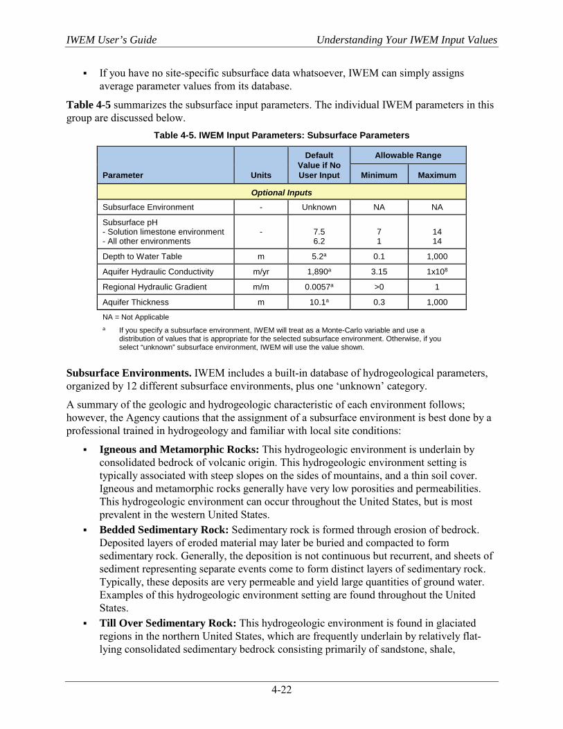
IWEM User’s Guide Understanding Your IWEM Input Values
4-22
If you have no site-specific subsurface data whatsoever, IWEM can simply assigns average parameter values from its database.
Table 4-5 summarizes the subsurface input parameters. The individual IWEM parameters in this group are discussed below.
Table 4-5. IWEM Input Parameters: Subsurface Parameters
Parameter Units
Default Value if No User Input
Allowable Range
Minimum Maximum
Optional Inputs
Subsurface Environment - Unknown NA NA
Subsurface pH - Solution limestone environment - All other environments
-
7.5 6.2
7 1
14 14
Depth to Water Table m 5.2a 0.1 1,000
Aquifer Hydraulic Conductivity m/yr 1,890a 3.15 1x10⁸
Regional Hydraulic Gradient m/m 0.0057a >0 1
Aquifer Thickness m 10.1a 0.3 1,000
NA = Not Applicable a If you specify a subsurface environment, IWEM will treat as a Monte-Carlo variable and use a
distribution of values that is appropriate for the selected subsurface environment. Otherwise, if you select “unknown” subsurface environment, IWEM will use the value shown.
Subsurface Environments. IWEM includes a built-in database of hydrogeological parameters, organized by 12 different subsurface environments, plus one ‘unknown’ category.
A summary of the geologic and hydrogeologic characteristic of each environment follows; however, the Agency cautions that the assignment of a subsurface environment is best done by a professional trained in hydrogeology and familiar with local site conditions:
Igneous and Metamorphic Rocks: This hydrogeologic environment is underlain by consolidated bedrock of volcanic origin. This hydrogeologic environment setting is typically associated with steep slopes on the sides of mountains, and a thin soil cover. Igneous and metamorphic rocks generally have very low porosities and permeabilities. This hydrogeologic environment can occur throughout the United States, but is most prevalent in the western United States.
Bedded Sedimentary Rock: Sedimentary rock is formed through erosion of bedrock. Deposited layers of eroded material may later be buried and compacted to form sedimentary rock. Generally, the deposition is not continuous but recurrent, and sheets of sediment representing separate events come to form distinct layers of sedimentary rock. Typically, these deposits are very permeable and yield large quantities of ground water. Examples of this hydrogeologic environment setting are found throughout the United States.
Till Over Sedimentary Rock: This hydrogeologic environment is found in glaciated regions in the northern United States, which are frequently underlain by relatively flat-lying consolidated sedimentary bedrock consisting primarily of sandstone, shale,

IWEM User’s Guide Understanding Your IWEM Input Values
4-23
limestone, and dolomite. The bedrock is overlain by glacial deposits which, consists chiefly of till, a dense unsorted mixture of soil and rock particles deposited directly by ice sheets. Ground water occurs both in the glacial deposits and in the sedimentary bedrock. Till deposits often have low permeability.
Sand and Gravel: Sediments are classified into three categories based upon their relative sizes; gravel, consisting of particles that individually may be boulders, cobbles or pebbles; sand, which may be very coarse, coarse, medium, fine or very fine; and mud, which may consist of clay and various size classes of silt. Sand and gravel hydrogeologic environments are very common throughout the United States and frequently overlie consolidated and semi- consolidated sedimentary rocks. Sand and gravel aquifers have very high permeabilities and yield large quantities of ground water.
Alluvial Basins, Valleys and Fans: Thick alluvial deposits in basins and valleys bordered by mountains typify this hydrogeologic environment. Alluvium is a general term for clay, silt, sand and gravel that was deposited during comparatively recent geologic time by a stream or other body of running water. The sediments are deposited in the bed of the stream or on its flood plain or delta, or in fan shaped deposits at the base of a mountain slope. Alluvial basins, valleys and fans frequently occupy a region extending from the Puget Sound-Williamette Valley area of Washington and Oregon to west Texas. This region consists of alternating basins or valleys and mountain ranges. The surrounding mountains, and the bedrock beneath the basins, consist of granite and metamorphic rocks. Ground water is obtained mostly from sand and gravel deposits within the alluvium. These deposits are interbedded with finer grained layers of silt and clay.
River Alluvium with Overbank Deposits: This hydrogeologic environment is characterized by low to moderate topography and thin to moderately thick sediments of flood-deposited alluvium along portions of a river valley. The alluvium is underlain by either unconsolidated sediments or fractured bedrock of sedimentary or igneous/metamorphic origin. Water is obtained from sand and gravel layers that are interbedded with finer grained alluvial deposits. The alluvium typically serves as a significant source of water. The flood plain is covered by varying thicknesses of fine-grained silt and clay, called overbank deposits. The overbank thickness is usually greater along major streams and thinner along minor streams but typically averages 1.5 to 3 m (5 to 10 ft).
River Alluvium without Overbank Deposits: This hydrogeologic environment is identical to the River Alluvium with Overbank Deposits environment except that no significant fine-grained floodplain deposits occupy the stream valley. The lack of fine-grained deposits may result in significantly higher recharge in areas with ample precipitation.
Outwash: Sand and gravel removed or “washed out” from a glacier by streams is termed outwash. This hydrogeologic environment is characterized by moderate to low topography and varying thicknesses of outwash that overlie sequences of fractured bedrock of sedimentary, metamorphic or igneous origin. These sand and gravel outwash deposits typically serve as the principal aquifers within the area. The outwash also serves as a source of regional recharge to the underlying bedrock.
IWEM User’s Guide Understanding Your IWEM Input Values
4-24
Till and Till Over Outwash: This hydrogeologic environment is characterized by low topography and outwash materials that are covered by varying thicknesses of glacial till. The till is principally unsorted sediment, which may be interbedded with localized deposits of sand and gravel. Although ground water occurs in both the glacial till and in the underlying outwash, the outwash typically serves as the principal aquifer because the fine grained deposits have been removed by streams. The outwash is in direct hydraulic connection with the glacial till and the glacial till serves as a source of recharge for the underlying outwash.
Unconsolidated and Semi-consolidated Shallow Surficial Aquifers: This hydrogeologic environment is characterized by moderately low topographic relief and gently dipping, interbedded unconsolidated and semi-consolidated deposits which consist primarily of sand, silt and clay. Large quantities of water are obtained from the surficial sand and gravel deposits which may be separated from the underlying regional aquifer by a low permeability or confining layer. This confining layer typically “leaks”, providing recharge to the deeper zones.
Coastal Beaches: This hydrogeologic environment is characterized by low topographic relief, near sea-level elevation and unconsolidated deposits of water-washed sands. The term beach is appropriately applied only to a body of essentially loose sediment. This usually means sand-size particles, but could include gravel. Quartz particles usually predominate. These materials are well sorted, very permeable and have very high potential infiltration rates. These areas are commonly ground water discharge areas although they can be very susceptible to the intrusion of saltwater.
Solution Limestone: Large portions of the central and southeastern United States are underlain by limestones and dolomites in which the fractures have been enlarged by solution. Although ground water occurs in both the surficial deposits and in the underlying bedrock, the limestones and dolomites, which typically contain solution cavities, generally serve as the principal aquifers. This type of hydrogeologic environment is often described as “karst.”
Unknown Environment: If the subsurface hydrogeological environment is unknown, or it is different from any of the twelve main types used in IWEM, select the subsurface environment as Type 13. In this case, IWEM will assign values of the hydrogeological parameters (depth to ground water, saturated zone thickness, saturated zone hydraulic conductivity, and saturated zone hydraulic gradient) that are simply national average values.
Subsurface pH. This parameter represents the alkalinity or acidity of the soil and aquifer. The pH is one of the most important subsurface parameters controlling the mobility of metals. Most metals are more mobile under acidic (low pH) conditions, as compared to neutral or alkaline (pH of 7 or higher) conditions. The pH of most aquifer systems is slightly acidic, the primary exception being aquifers in solution limestone settings. These may also be referred to as karst, carbonate, or dolomite aquifers. The ground water in these systems is usually alkaline.
IWEM assumes the subsurface pH value is the same in the unsaturated zone and saturated zone. The default pH value depends on the hydrogeologic environment you selected; if you selected “Solution Limestone” (Subsurface Environment 12), the default pH is 7.5. In all other hydrogeologic environments, the default pH value is 6.2. These default values represent median

IWEM User’s Guide Understanding Your IWEM Input Values
4-25
values from EPA’s Data Storage and Retrieval System, National Water Quality Database (STORET). If you do not know the hydrogeologic environment, IWEM will assume that the subsurface environment is of a non-solution-limestone type with the default pH of 6.2.
Depth to the Water Table (m). This parameter is the vertical distance from the ground surface to the water table as depicted in Figure 4-2. The water table in this case is meant to represent the natural water elevation, as it is or would be without the influence from the source. The presence of a WMU, particularly a surface impoundment, may cause a local rise in the water table called mounding. IWEM assumes that the depth to water table value you have entered does not include mounding. The tool will calculate the predicted impact of each liner, structural fill design, or roadway design on the ground water as part of the modeling evaluation.
If the water table elevation at your site shows seasonal fluctuation, it is best to enter an average annual depth to ground water value. Note that entering a smaller depth to ground water value will mean that constituents have less distance to travel before they reach the ground water, and IWEM will tend to estimate higher ground water exposure concentrations. It is also important to remember that in a WMU evaluation, the depth to ground water should be measured from the ground surface, not from the base of the WMU. If the base of the unit is lower than the ground surface and, therefore, closer to the water table, you should enter that value as the Depth of the WMU Base Below the Ground Surface (see Section 4.2.1 above).
The depth to ground water should be entered in meters. The default value for this parameter is a function of the selected subsurface environment. If you selected the “unknown” subsurface environment, IWEM will use the national average of 5.2 m. If you selected one of the 12 subsurface environments and do not specify the depth to the water table, IWEM will treat the depth to the water table as a Monte-Carlo variable: IWEM will use a distribution of values that is appropriate for the selected subsurface environment.
Hydraulic Conductivity (m/yr). This parameter represents the permeability of the saturated aquifer in the horizontal direction. The hydraulic conductivity, together with the hydraulic gradient, controls the ground water flow rate.
The hydraulic conductivity, together with the hydraulic gradient (see below), controls the ground water flow rate, in accordance with Darcy’s Law. The effect of varying ground water flow rate on contaminant fate and transport is complex. Intuitively, it would seem that factors that increase the ground water flow rate would cause a higher ground water exposure level at the receptor well, but this is not always the case. A higher ground water velocity will cause leachate constituents to arrive at the well location more quickly. For constituents that are subject to degradation in ground water, the shorter travel time will cause the constituents to arrive at the well at higher concentrations as compared to a case of low ground water velocity and long travel times. On the other hand, a high ground water flow rate will tend to increase the degree of dilution of the leachate plume, due to mixing and dispersion. This will in turn tend to lower the magnitude of the concentrations reaching the well. IWEM evaluations are based on the maximum constituent concentrations at the well, rather than how long it might take for exposure to occur, and therefore a higher ground water flow rate may result in lower estimated exposure levels at the well.
Siting a source in a low permeability aquifer setting is not always more protective than a high permeability setting. Low ground water velocity means that it will take longer for the exposure to

IWEM User’s Guide Understanding Your IWEM Input Values
4-26
occur, and as a result, there is more opportunity for natural attenuation to degrade contaminants. For long-lived waste constituents, it also means that little dilution of the plume may occur.
The hydraulic conductivity of aquifers is sometimes reported as a transmissivity value, which is usually denoted with the symbol T. Transmissivity is simply the product of hydraulic conductivity and saturated thickness. To back-calculate the hydraulic conductivity, you should divide the transmissivity by the value of the saturated zone thickness. The hydraulic conductivity parameter in IWEM must be entered in meters per year.
The default value of hydraulic conductivity in IWEM varies with the subsurface environment you have selected. If you selected the “unknown” subsurface environment, IWEM will use a nationwide average value of 1,890 m/yr. If you selected one of the twelve hydrogeologic environments and the hydraulic conductivity as “unknown,” IWEM will treat the hydraulic conductivity as a Monte-Carlo variable, and it will use a distribution of values that is appropriate for the selected subsurface environment.
Regional Hydraulic Gradient (m/m). For unconfined aquifers, the hydraulic gradient is simply the slope of the water table in a particular direction. It is calculated as the difference in the elevation of the water table measured at two locations divided by the distance between the two locations. In IWEM, this parameter represents the average horizontal ground water gradient in the vicinity of the source. The gradient is meant to represent the natural ground water gradient as it is, or would be, without influence from the source. The presence of a WMU, particularly a surface impoundment, or a structural fill or roadway may cause local mounding of the water table and associated higher local ground water gradients. IWEM assumes that the gradient value you have entered does not include mounding; rather the software will calculate the predicted impact on the ground water due to infiltration as part of the modeling evaluation.
For the same reasons as discussed above, assigning a low hydraulic gradient value will not necessarily result in lower estimated ground water exposures. The hydraulic gradient is a unitless parameter. Its default value depends on the subsurface environment you selected. If you selected the “unknown” environment, IWEM will use a nationwide average value of 0.0057. If you selected one of the 12 subsurface environments and did not specify the hydraulic gradient, IWEM will treat the hydraulic gradient as a Monte-Carlo variable, and it will use a distribution of values that is appropriate for the selected subsurface environment.
Aquifer Thickness (m). This parameter represents the vertical distance from the water table down to the base of the aquifer, as shown in the diagram in Figure 4-2. Usually the base is an impermeable layer, e.g., bedrock. This parameter is used to describe the thickness of the ground water zone over which the leachate plume can mix with ground water. If your site has a highly stratified hydrogeology, it may be difficult to precisely define the “base of the aquifer,” but in such cases, the stratification may effectively limit the vertical plume travel distance. In this case it may be appropriate to enter the maximum vertical extent of the plume as an “effective” saturated zone thickness in IWEM.
The parameter must be entered in meters. To convert from other units to meters, use the factors given in Section 4.2.1. The default saturated zone thickness is a function of the selected subsurface environment. If you selected the “unknown” subsurface environment, IWEM will use the national average of 10.1 m. If you selected one of the 12 subsurface environments and did not specify the saturated thickness, IWEM will treat the depth to the saturated thickness as a Monte-
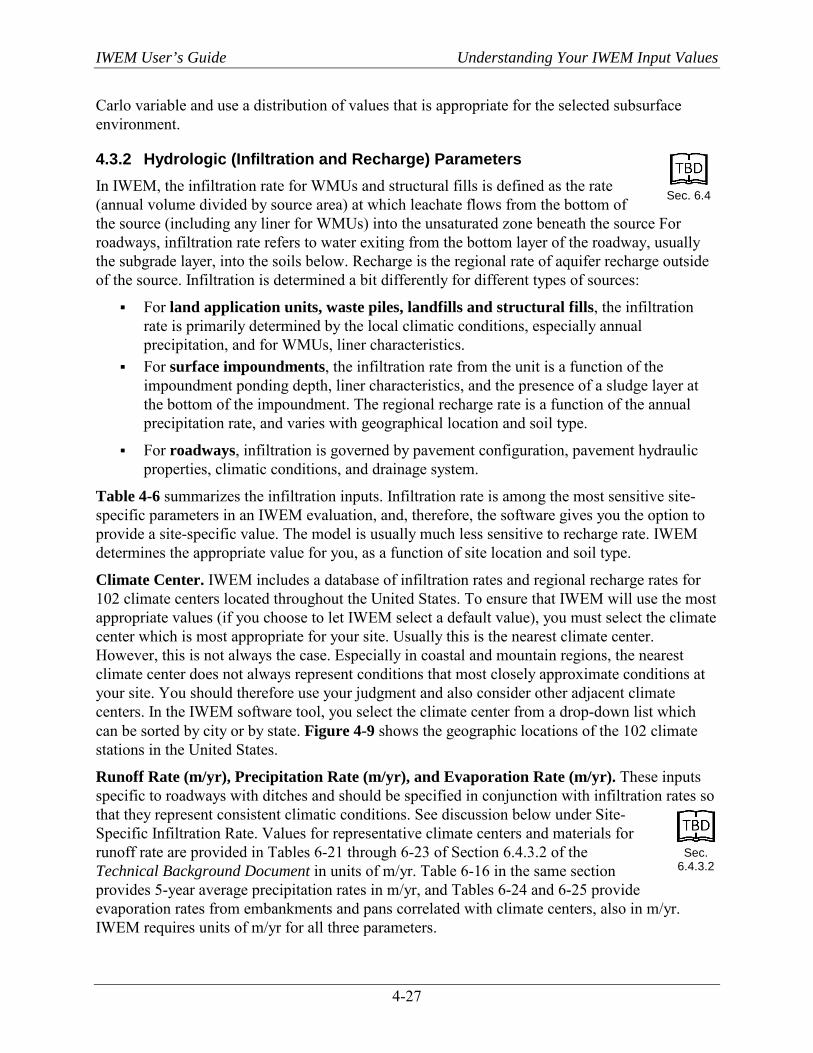
IWEM User’s Guide Understanding Your IWEM Input Values
4-27
Carlo variable and use a distribution of values that is appropriate for the selected subsurface environment.
4.3.2 Hydrologic (Infiltration and Recharge) Parameters In IWEM, the infiltration rate for WMUs and structural fills is defined as the rate (annual volume divided by source area) at which leachate flows from the bottom of the source (including any liner for WMUs) into the unsaturated zone beneath the source For roadways, infiltration rate refers to water exiting from the bottom layer of the roadway, usually the subgrade layer, into the soils below. Recharge is the regional rate of aquifer recharge outside of the source. Infiltration is determined a bit differently for different types of sources:
For land application units, waste piles, landfills and structural fills, the infiltration rate is primarily determined by the local climatic conditions, especially annual precipitation, and for WMUs, liner characteristics.
For surface impoundments, the infiltration rate from the unit is a function of the impoundment ponding depth, liner characteristics, and the presence of a sludge layer at the bottom of the impoundment. The regional recharge rate is a function of the annual precipitation rate, and varies with geographical location and soil type.
For roadways, infiltration is governed by pavement configuration, pavement hydraulic properties, climatic conditions, and drainage system.
Table 4-6 summarizes the infiltration inputs. Infiltration rate is among the most sensitive site-specific parameters in an IWEM evaluation, and, therefore, the software gives you the option to provide a site-specific value. The model is usually much less sensitive to recharge rate. IWEM determines the appropriate value for you, as a function of site location and soil type.
Climate Center. IWEM includes a database of infiltration rates and regional recharge rates for 102 climate centers located throughout the United States. To ensure that IWEM will use the most appropriate values (if you choose to let IWEM select a default value), you must select the climate center which is most appropriate for your site. Usually this is the nearest climate center. However, this is not always the case. Especially in coastal and mountain regions, the nearest climate center does not always represent conditions that most closely approximate conditions at your site. You should therefore use your judgment and also consider other adjacent climate centers. In the IWEM software tool, you select the climate center from a drop-down list which can be sorted by city or by state. Figure 4-9 shows the geographic locations of the 102 climate stations in the United States.
Runoff Rate (m/yr), Precipitation Rate (m/yr), and Evaporation Rate (m/yr). These inputs specific to roadways with ditches and should be specified in conjunction with infiltration rates so that they represent consistent climatic conditions. See discussion below under Site-Specific Infiltration Rate. Values for representative climate centers and materials for runoff rate are provided in Tables 6-21 through 6-23 of Section 6.4.3.2 of the Technical Background Document in units of m/yr. Table 6-16 in the same section provides 5-year average precipitation rates in m/yr, and Tables 6-24 and 6-25 provide evaporation rates from embankments and pans correlated with climate centers, also in m/yr. IWEM requires units of m/yr for all three parameters.
Sec. 6.4
Sec.
6.4.3.2
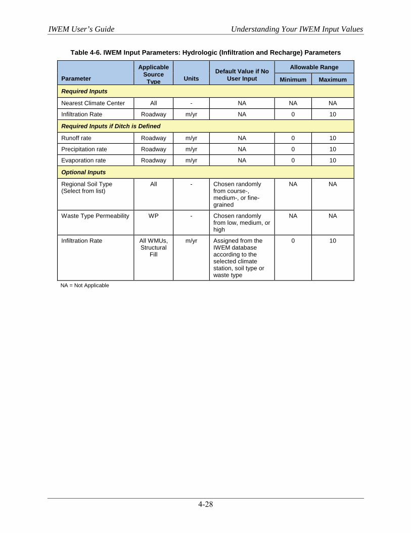
IWEM User’s Guide Understanding Your IWEM Input Values
4-28
Table 4-6. IWEM Input Parameters: Hydrologic (Infiltration and Recharge) Parameters
Parameter
Applicable Source
Type Units Default Value if No
User Input
Allowable Range
Minimum Maximum
Required Inputs
Nearest Climate Center All - NA NA NA
Infiltration Rate Roadway m/yr NA 0 10
Required Inputs if Ditch is Defined
Runoff rate Roadway m/yr NA 0 10
Precipitation rate Roadway m/yr NA 0 10
Evaporation rate Roadway m/yr NA 0 10
Optional Inputs
Regional Soil Type (Select from list)
All - Chosen randomly from course-, medium-, or fine-grained
NA NA
Waste Type Permeability WP - Chosen randomly from low, medium, or high
NA NA
Infiltration Rate All WMUs, Structural
Fill
m/yr Assigned from the IWEM database according to the selected climate station, soil type or waste type
0 10
NA = Not Applicable
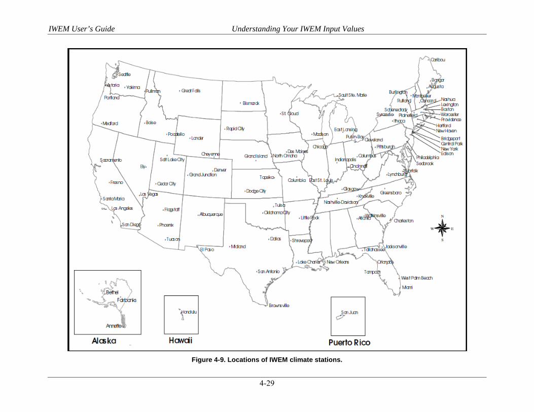
IWEM User’s Guide Understanding Your IWEM Input Values
4-29
Figure 4-9. Locations of IWEM climate stations.
IWEM User’s Guide Understanding Your IWEM Input Values
4-30
Regional Soil Type. To assign an appropriate recharge rate, IWEM needs to know the dominant, regional soil type near your site. IWEM provides a selection of three major soil types, which are representative of most soils in the United States:
Sandy Loam Silty Loam Silty Clay Loam.
IWEM also allows you to select the soil type “unknown.” In that case, IWEM will treat the soil type as a Monte-Carlo variable and randomly select from the three available soil types, in accordance with the relative frequency of occurrence of each type across the United States. By selecting the soil type, IWEM also assigns the soil parameters that are used in the modeling of fate and transport in the unsaturated zone of the aquifer.
Waste Type Permeability. This parameter is used only for waste piles. Waste piles are not typically covered and the permeability of the waste itself is a factor in determining the rate of leachate released due to water percolating through the WMU. For waste piles, IWEM recognizes three categories of waste permeability and their associated infiltration rate: high permeability (0.041 cm/sec); moderate permeability (0.0041 cm/sec); and low permeability (0.00005 cm/sec). The waste permeability is correlated with the grain size of the waste material, ranging from coarse to five-grained materials.
If you do not specify the waste type for waste piles, IWEM will default to randomly selecting between the infiltration rates for each of the three waste types in the Monte Carlo process, with each type having equal probability. That is, IWEM will use a uniform probability distribution.
Site-specific Infiltration Rate (m/yr). This parameter represents the actual annual volume of leachate, per unit area of the source, that flows from the bottom of the source into the unsaturated zone underneath.
For WMUs, the performance characteristics of a liner, if present, are among the most important factors controlling the infiltration rate, and therefore, the rate of leachate release. IWEM provides you the option to enter a site- specific infiltration rate to accommodate liner designs that are different from the standard liner designs (i.e., (1) no liner, (2) single clay liner, or (3) composite liner), and to evaluate extreme climatic conditions. IWEM provides default values for infiltration rate, which are a function of WMU type, liner design, and site location. These values are used as defaults. The default infiltration rates used in IWEM for landfills, waste piles, and land application units were developed using the Hydrologic Evaluation of Landfill Performance (HELP) model (Schroeder et. al., 1994). The infiltration rate from a WMU is difficult to measure directly; if you wish to determine site-specific WMU infiltration rates for use in IWEM, it is recommended to use a model such as HELP to estimate the rates.
For structural fills, infiltration is handled as for WMUs, but with no liner.
For roadways, subgrade infiltration is governed by pavement configuration, pavement hydraulic properties, climatic conditions, and drainage system. Nationwide, a multitude of combinations of those four factors are possible. At present, there are very little subgrade infiltration data. Section 6.4.3.2, Tables 6-18 through 6-20 of the Technical Background Document, presents some representative values correlated to climate center and
Sec. 6.4.1
Sec. 6.4.1.2

IWEM User’s Guide Understanding Your IWEM Input Values
4-31
pavement type. A procedure for estimating subgrade infiltration for different configurations, conditions, and settings is presented in Appendix E of the Technical Background Document. The procedure involves dividing the United States into 12 climatic zones. For each zone, pre-determined infiltration rates for major types of pavement configuration with a range of material properties and climatic conditions are given. If the roadway has a subsurface drainage system, please refer to those parts of the Technical Background Document for guidance on how to modify the selected default value. However, the Agency highly recommends consulting with a knowledgeable highway engineer/designer prior to determining a drainage system correction factor or a user-specified rate, in general. As a note, shoulders and embankments do not generally have subsurface drainage component systems The infiltration rate in IWEM must be entered in units of meter/year.
4.4 Waste Constituents and Constituent Parameters Constituent parameters are divided into three tabs: constituent selection and leachate/waste concentrations, chemical properties(e.g., sorption parameters, hydrolysis rate constants), and reference ground water exposure concentrations. The following sections discuss the IWEM constituent parameters.
4.4.1 Constituent Selection and Concentrations Constituents are identified in IWEM by either constituent name or CAS number. Whereas constituents may have multiple names, the CAS number is an industry-standard, unique, identification code. If you want to use the “Add New Constituent” option to assign different fate and transport parameters to an existing IWEM constituent, it is recommended to use the actual CAS number and enter a new constituent name.
Table 4-7 lists the parameters needed to specify constituent concentrations. Table 4-7. IWEM Input Parameters: Constituent Source Concentration Parameters
Parameter Units
Required User
Input?
Default Value if No User
Input
Allowable Range
Minimum Maximum
Leachate concentration (All sources) mg/L yes NA >0 1,000
Total concentration (Structural Fill and Roadway only)
mg/kg yes NA >0 1,000
Constituent Initial Concentration in Leachate (mg/L). You must provide the leachate concentration for each selected waste constituent that you expect in the leachate that will infiltrate into the soil underneath a source. For WMUs, this will be a single concentration for each constituent. For a roadway source, you must specify the leachate concentration of each selected constituent for each strip and layer. Note that IWEM does not allow the use of leachable materials in ditches, so you will not be able to enter leachate concentrations for strips designated as ditches.
Sec. 6.4.3.2
App. E
Sec. 6.1.2 Sec. 6.2.2 Sec. 6.3.9
IWEM User’s Guide Understanding Your IWEM Input Values
4-32
EPA has developed a number of tests to measure the leaching potential of different wastes and waste constituents in the laboratory. These include the Toxicity Characteristic Leaching Procedure (TCLP) and the Synthetic Precipitation Leaching Procedure (SPLP). Consult Chapter 2 of the Guide (Characterizing Waste) for analytical procedures that can be used to determine expected leachate concentrations for waste constituents.
Recently, new leaching test methods, EPA SW-846 Methods 1313, 1314, 1315, and 13161, were developed to support the evaluation of coal combustion residual materials. Leaching test results acquired from these new methods were also recently used in probabilistic fate and transport modeling of managed coal combustion wastes. These materials are typical materials used as adjuncts in roadways. These leaching methods are part of the Leaching Environmental Assessment Framework (LEAF) developed by a collaborative research effort between the U.S. EPA, Vanderbilt University, and Dutch and Danish partners (Kosson et al, 2002; U.S. EPA, 2010).
Constituent Initial Concentration of Total Leachable Mass (mg/kg). For structural fill and roadway sources, you must also specify total concentration of each selected constituent in the material used for the fill, or for roadways, each strip and layer. For roadways, you are only required to input both leachate and total concentrations for one layer in one strip.
Input values for source constituent parameters for recycled structural fill and roadway materials (i.e., leachate concentration and total leachable mass concentration) can be obtained from empirical testing data or field data. In practice, the producer of an industrial material would be the most likely resource for obtaining this data through engineering and environmental testing, both in the laboratory and in the field. The Recycled Materials Resource Center (RMRC; http://rmrc.wisc.edu/), a federal university–partnered research and outreach facility for the highway community, has developed the User Guidelines for Byproducts and Secondary Use Materials in Pavement Construction, available online.2 The online guidance document provides detailed information on many industrial materials commonly used in roadway and some structural fill construction.
4.4.2 Physical-Chemical Properties IWEM includes a built-in database with chemical properties data on 206 organic constituents and 22 metals (25 for roadway module). Appendix A provides a list of these constituents. (The default chemical properties are provided in Appendix B of the Technical Background Document.) To preserve the integrity of the database, IWEM gives you limited flexibility to modify these data. However, IWEM does give you the option of overriding some of those properties with user-specified values (see discussion below). IWEM also allows you to add new constituents to its database, which provides an indirect mechanism for assigning different constituent property values: by entering a constituent of interest as a new constituent in the database, you can assign it different parameter values.
The physical and constituent properties that affect subsurface fate and transport include sorption parameters and degradation parameters. These inputs are somewhat different for organics and metals; they are summarized in Table 4-8 and discussed below. 1 http://www.epa.gov/epawaste/hazard/testmethods/sw846/new_meth.htm 2 http://rmrc.wisc.edu/user-guidelines-2/
Sec. 6.6 App. B
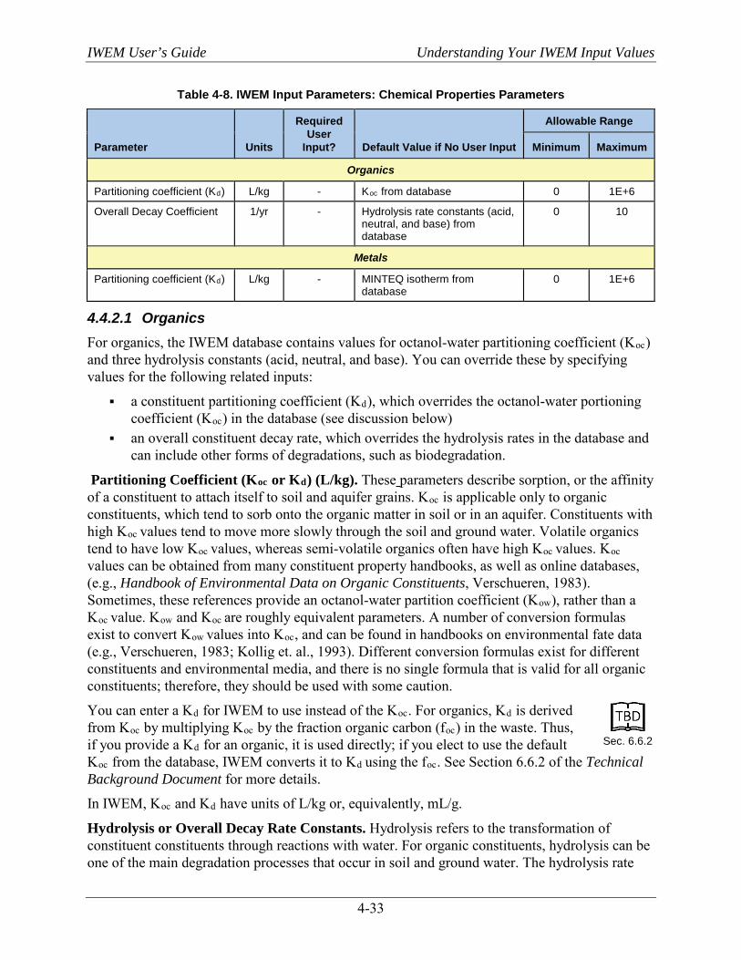
IWEM User’s Guide Understanding Your IWEM Input Values
4-33
Table 4-8. IWEM Input Parameters: Chemical Properties Parameters
Parameter Units
Required User
Input? Default Value if No User Input
Allowable Range
Minimum Maximum
Organics
Partitioning coefficient (Kd) L/kg - Koc from database 0 1E+6
Overall Decay Coefficient 1/yr - Hydrolysis rate constants (acid, neutral, and base) from database
0 10
Metals
Partitioning coefficient (Kd) L/kg - MINTEQ isotherm from database
0 1E+6
4.4.2.1 Organics For organics, the IWEM database contains values for octanol-water partitioning coefficient (Koc) and three hydrolysis constants (acid, neutral, and base). You can override these by specifying values for the following related inputs:
a constituent partitioning coefficient (Kd), which overrides the octanol-water portioning coefficient (Koc) in the database (see discussion below)
an overall constituent decay rate, which overrides the hydrolysis rates in the database and can include other forms of degradations, such as biodegradation.
Partitioning Coefficient (Koc or Kd) (L/kg). These parameters describe sorption, or the affinity of a constituent to attach itself to soil and aquifer grains. Koc is applicable only to organic constituents, which tend to sorb onto the organic matter in soil or in an aquifer. Constituents with high Koc values tend to move more slowly through the soil and ground water. Volatile organics tend to have low Koc values, whereas semi-volatile organics often have high Koc values. Koc
values can be obtained from many constituent property handbooks, as well as online databases, (e.g., Handbook of Environmental Data on Organic Constituents, Verschueren, 1983). Sometimes, these references provide an octanol-water partition coefficient (Kow), rather than a Koc value. Kow and Koc are roughly equivalent parameters. A number of conversion formulas exist to convert Kow values into Koc, and can be found in handbooks on environmental fate data (e.g., Verschueren, 1983; Kollig et. al., 1993). Different conversion formulas exist for different constituents and environmental media, and there is no single formula that is valid for all organic constituents; therefore, they should be used with some caution.
You can enter a Kd for IWEM to use instead of the Koc. For organics, Kd is derived from Koc by multiplying Koc by the fraction organic carbon (foc) in the waste. Thus, if you provide a Kd for an organic, it is used directly; if you elect to use the default Koc from the database, IWEM converts it to Kd using the foc. See Section 6.6.2 of the Technical Background Document for more details.
In IWEM, Koc and Kd have units of L/kg or, equivalently, mL/g.
Hydrolysis or Overall Decay Rate Constants. Hydrolysis refers to the transformation of constituent constituents through reactions with water. For organic constituents, hydrolysis can be one of the main degradation processes that occur in soil and ground water. The hydrolysis rate
Sec. 6.6.2

IWEM User’s Guide Understanding Your IWEM Input Values
4-34
values that are part of the IWEM database have been compiled by the U.S. EPA Office of Research and Development (Kollig, 1993). For each organic constituent, the database includes three hydrolysis rate constants: an acid-catalyzed rate constant, a neutral rate constant, and a base-catalyzed rate constant. However, other transformation processes can occur, such as biodegradation, and these processes are not considered in IWEM, nor are rate constants for them included in the constituent database. Biodegradation can be a significant attenuation process for organic constituents in the subsurface. However, this process is also highly site- and constituent-specific. It is not possible to provide reliable default biodegradation rates to be used in IWEM.
If you want to account for biodegradation or other transformation processes, you can enter a first-order constituent-specific overall decay rate (combining hydrolysis, biodegradation, and any other processes you wish to include). IWEM will use this rate instead of the hydrolysis rates in the database. This decay coefficient has units of 1/yr. The value of the decay coefficient is related to half-life as
Decay Coefficient (1/yr) = 0.693 / Half-life (yr)
IWEM stores user-defined decay coefficients in its constituent property database. You should, however, be careful in using a decay coefficient value which is appropriate for one site and not appropriate for others. Evidence of the significance of biodegradation should be carefully considered in accordance with EPA guidance, such as the OSWER Directive 9200.4-17P on Use of Monitored Natural Attenuation at Superfund, RCRA Corrective Action, and Underground Storage Tank Sites. A compendium of EPA bioremediation documents is available online at www.epa.gov/ORD/WebPubs/biorem.html.
4.4.2.2 Metals Metals Kd Isotherm Data. In the case of metals, sorption is expressed in the partition coefficient Kd. Kds for metals can vary significantly with ground water pH and other geochemical conditions. Thus, rather than using a single Kd value for each metal constituent, IWEM includes multiple sets of Kd values for each metal calculated using the MINTEQA2 geoconstituent speciation model to reflect the impact of variations in those conditions. Each set of Kd values is referred to as a sorption isotherm. The sorption parameters for metals in IWEM are part of the built-in database and they cannot be modified by the user. However, you can elect to use a different set of isotherms developed for coal combustion residuals by specifying waste type (ash, ash and coal, FGD, or FBC) and leachate pH. You can also specify a single Kd to use instead of the isotherms.
Further information on how the MINTEQ sorption isotherms were developed can be found in the Technical Background Document (Section 6.6.2.2) and the EPACMTP Parameters/Data Background Document (U.S. EPA, 2003b).
If you are adding a new constituent to the IWEM database, you can enter a single Kd value to model sorption for the constituent. The Kd must be entered in units of L/kg or, equivalently, mL/g.
Sec. 6.6.2.2

IWEM User’s Guide Understanding Your IWEM Input Values
4-35
4.4.3 Reference Ground Water Concentrations
The final set of constituent-specific parameters used by IWEM is RGCs, which reflect not-to-exceed exposure levels for drinking water ingestion, shower inhalation, and shower/bath dermal cancer risks and non-cancer hazards. RGCs include regulatory MCLs, other regulatory standards, and HBNs. Table 4-9 summarizes the RGCs used by IWEM, and they are discussed in more detail below.
Table 4-9. IWEM Input Parameters: Reference Ground Water Concentrations
Parameter Units Provided in IWEM
Database?
Allowable Range
Minimum Maximum
MCL mg/L Yes, for 59 constituents >0 NA
Other Standard mg/L No >0 NA
User-Specified HBN mg/L No >0 NA
Exposure Duration Associated with HBN yrs No >0 70
NA = Not Applicable
Note that only MCLs are provided in the database, and those are available for only 59 of the 231 constituents in the database. Thus, for constituents without an MCL, you will have to provide either an alternative regulatory standard or at least one HBN and associated exposure duration. Similarly, if you add a constituent to the database, you will have to provide at least one of these RGCs. IWEM imposes no restrictions on user-specified RGCs, other than that they should be expressed in units of mg/L. User-specified RGCs may represent either more or less stringent health-based values, or alternative regulatory standards. IWEM makes no assumptions about user-specified RGCs and, consequently, the software cannot check whether your value is correct or not.
Maximum Contaminant Level (MCL) (mg/L). Maximum Contaminant Levels (MCLs) are provided in IWEM for the 59 IWEM constituents for which values are currently available. MCLs are maximum constituent concentrations allowed in public drinking water and are established under the Safe Drinking Water Act. For each contaminant to be regulated, EPA first sets a Maximum Contaminant Level Goal (MCLG) at a level that protects against health risks. EPA then sets each contaminant’s MCL as close to its MCLG as feasible, taking costs and available analytical and treatment technologies into consideration. MCLs in the database cannot be changed. However, you can enter an alternative regulatory standard (see below).
Other Standards (mg/L). You may enter an alternative constituent-specific regulatory standard, such as a state regulatory standard, and IWEM will use it instead of the MCL. Alternative regulatory standards must be in units of mg/L.
Sec. 7

IWEM User’s Guide Understanding Your IWEM Input Values
4-36
User-Specified Health-Based Number (HBN) (mg/L). HBNs are the maximum constituent concentrations in ground water that would generally be expected not to cause adverse noncancer health effects in the general population (including sensitive subgroups), or not to result in an additional incidence of cancer in more than some specified fraction of (e.g., individuals exposed to the constituent (e.g., one in one million) via either ingestion, inhalation, or dermal pathways. HBNs are not provided in the IWEM database, but you can enter the following types of user-specified HBNs for use in an IWEM evaluation:
Ingestion, cancer Ingestion, noncancer Inhalation, cancer Inhalation, noncancer Dermal, cancer Dermal, noncancer.
The best source of HBNs is the Regional Screening Level (RSL) Generic Tables (U.S. EPA, 2015b), which provide HBNs for more than 700 chemicals under six scenarios. Consult the Technical Background Document (Section 7.2) for further details on obtaining HBN values from this source.
Exposure Duration (yrs). For each HBN you enter, you must also enter an associated exposure duration (in years) that is consistent with the way the RGC was derived.
Sec. 7.2
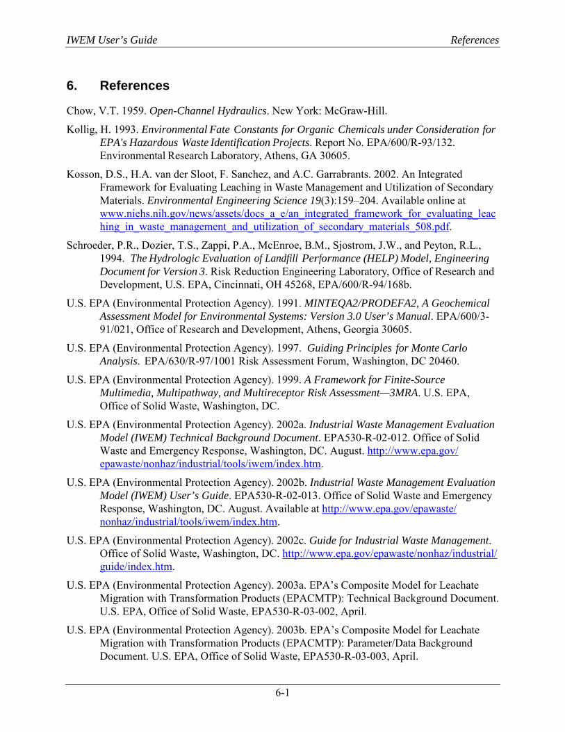
IWEM User’s Guide References
6-1
6. References
Chow, V.T. 1959. Open-Channel Hydraulics. New York: McGraw-Hill.
Kollig, H. 1993. Environmental Fate Constants for Organic Chemicals under Consideration for EPA's Hazardous Waste Identification Projects. Report No. EPA/600/R-93/132. Environmental Research Laboratory, Athens, GA 30605.
Kosson, D.S., H.A. van der Sloot, F. Sanchez, and A.C. Garrabrants. 2002. An Integrated Framework for Evaluating Leaching in Waste Management and Utilization of Secondary Materials. Environmental Engineering Science 19(3):159–204. Available online at www.niehs.nih.gov/news/assets/docs_a_e/an_integrated_framework_for_evaluating_leaching_in_waste_management_and_utilization_of_secondary_materials_508.pdf.
Schroeder, P.R., Dozier, T.S., Zappi, P.A., McEnroe, B.M., Sjostrom, J.W., and Peyton, R.L., 1994. The Hydrologic Evaluation of Landfill Performance (HELP) Model, Engineering Document for Version 3. Risk Reduction Engineering Laboratory, Office of Research and Development, U.S. EPA, Cincinnati, OH 45268, EPA/600/R-94/168b.
U.S. EPA (Environmental Protection Agency). 1991. MINTEQA2/PRODEFA2, A Geochemical Assessment Model for Environmental Systems: Version 3.0 User’s Manual. EPA/600/3- 91/021, Office of Research and Development, Athens, Georgia 30605.
U.S. EPA (Environmental Protection Agency). 1997. Guiding Principles for Monte Carlo Analysis. EPA/630/R-97/1001 Risk Assessment Forum, Washington, DC 20460.
U.S. EPA (Environmental Protection Agency). 1999. A Framework for Finite-Source Multimedia, Multipathway, and Multireceptor Risk Assessment—3MRA. U.S. EPA, Office of Solid Waste, Washington, DC.
U.S. EPA (Environmental Protection Agency). 2002a. Industrial Waste Management Evaluation Model (IWEM) Technical Background Document. EPA530-R-02-012. Office of Solid Waste and Emergency Response, Washington, DC. August. http://www.epa.gov/epawaste/nonhaz/industrial/tools/iwem/index.htm.
U.S. EPA (Environmental Protection Agency). 2002b. Industrial Waste Management Evaluation Model (IWEM) User’s Guide. EPA530-R-02-013. Office of Solid Waste and Emergency Response, Washington, DC. August. Available at http://www.epa.gov/epawaste/nonhaz/industrial/tools/iwem/index.htm.
U.S. EPA (Environmental Protection Agency). 2002c. Guide for Industrial Waste Management. Office of Solid Waste, Washington, DC. http://www.epa.gov/epawaste/nonhaz/industrial/guide/index.htm.
U.S. EPA (Environmental Protection Agency). 2003a. EPA’s Composite Model for Leachate Migration with Transformation Products (EPACMTP): Technical Background Document. U.S. EPA, Office of Solid Waste, EPA530-R-03-002, April.
U.S. EPA (Environmental Protection Agency). 2003b. EPA’s Composite Model for Leachate Migration with Transformation Products (EPACMTP): Parameter/Data Background Document. U.S. EPA, Office of Solid Waste, EPA530-R-03-003, April.

IWEM User’s Guide References
6-2
U.S. EPA (Environmental Protection Agency). 2003c. EPA’s Composite Model for Leachate Migration with Transformation Products (EPACMTP): Draft Addendum to the Technical Background Document. U.S. EPA, Office of Solid Waste. September.
U.S. EPA (Environmental Protection Agency). 2003d. EPA’s Composite Model for Leachate Migration with Transformation Products (EPACMTP): Draft Addendum to the Parameter/Data Background Document. U.S. EPA, Office of Solid Waste. April.
U.S. EPA (Environmental Protection Agency). 2010. Background Information for the Leaching Environmental Assessment Framework (LEAF) Test Methods. EPA/600/R-10/170. U.S. EPA, Washington, DC.
U.S. EPA (Environmental Protection Agency). 2015a. Industrial Waste Evaluation Model (IWEM) v3.1 Technical Documentation. Final. Office of Resource Conservation and Recovery, Washington DC.
U.S. EPA (Environmental Protection Agency). 2015b. Regional Screening Levels for Chemical Contaminants at Superfund Sites: Regional Screening Levels Generic Tables. Developed in cooperation with Oak Ridge National Laboratory. Available at http://www.epa.gov/reg3hwmd/risk/human/rb-concentration_table/Generic_Tables/index.htm. Accessed November 2013.
Verschueren, K., 1983. Handbook of Environmental Data on Organic Chemicals. Van Nostrand Reinhold Co., New York.
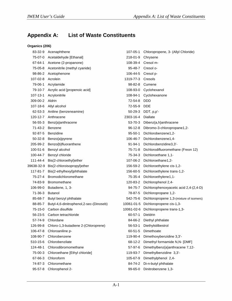
IWEM User’s Guide Appendix A: List of Waste Constituents
A-1
Appendix A: List of Waste Constituents
Organics (206) 83-32-9 Acenaphthene 75-07-0 Acetaldehyde [Ethanal] 67-64-1 Acetone (2-propanone) 75-05-8 Acetonitrile (methyl cyanide) 98-86-2 Acetophenone 107-02-8 Acrolein 79-06-1 Acrylamide 79-10-7 Acrylic acid [propenoic acid] 107-13-1 Acrylonitrile 309-00-2 Aldrin 107-18-6 Allyl alcohol 62-53-3 Aniline (benzeneamine) 120-12-7 Anthracene 56-55-3 Benz{a}anthracene 71-43-2 Benzene 92-87-5 Benzidine 50-32-8 Benzo{a}pyrene 205-99-2 Benzo{b}fluoranthene 100-51-6 Benzyl alcohol 100-44-7 Benzyl chloride 111-44-4 Bis(2-chloroethyl)ether 39638-32-9 Bis(2-chloroisopropyl)ether 117-81-7 Bis(2-ethylhexyl)phthalate 75-27-4 Bromodichloromethane 74-83-9 Bromomethane 106-99-0 Butadiene, 1, 3- 71-36-3 Butanol 85-68-7 Butyl benzyl phthalate 88-85-7 Butyl-4,6-dinitrophenol,2-sec-(Dinoseb) 75-15-0 Carbon disulfide 56-23-5 Carbon tetrachloride 57-74-9 Chlordane 126-99-8 Chloro-1,3-butadiene 2-(Chloroprene) 106-47-8 Chloroaniline p- 108-90-7 Chlorobenzene 510-15-6 Chlorobenzilate 124-48-1 Chlorodibromomethane 75-00-3 Chloroethane [Ethyl chloride] 67-66-3 Chloroform 74-87-3 Chloromethane 95-57-8 Chlorophenol 2-
107-05-1 Chloropropene, 3- (Allyl Chloride) 218-01-9 Chrysene 108-39-4 Cresol m- 95-48-7 Cresol o- 106-44-5 Cresol p- 1319-77-3 Cresols 98-82-8 Cumene 108-93-0 Cyclohexanol 108-94-1 Cyclohexanone 72-54-8 DDD 72-55-9 DDE 50-29-3 DDT, p,p’- 2303-16-4 Diallate 53-70-3 Dibenz{a,h}anthracene 96-12-8 Dibromo-3-chloropropane1,2- 95-50-1 Dichlorobenzene1,2- 106-46-7 Dichlorobenzene1,4- 91-94-1 Dichlorobenzidine3,3’- 75-71-8 Dichlorodifluoromethane (Freon 12) 75-34-3 Dichloroethane 1,1- 107-06-2 Dichloroethane1,2- 156-59-2 Dichloroethylene cis-1,2- 156-60-5 Dichloroethylene trans-1,2- 75-35-4 Dichloroethylene1,1- 120-83-2 Dichlorophenol 2,4- 94-75-7 Dichlorophenoxyacetic acid 2,4-(2,4-D) 78-87-5 Dichloropropane 1,2- 542-75-6 Dichloropropene 1,3-(mixture of isomers) 10061-01-5 Dichloropropene cis-1,3- 10061-02-6 Dichloropropene trans-1,3- 60-57-1 Dieldrin 84-66-2 Diethyl phthalate 56-53-1 Diethylstilbestrol 60-51-5 Dimethoate 119-90-4 Dimethoxybenzidine 3,3’- 68-12-2 Dimethyl formamide N,N- [DMF] 57-97-6 Dimethylbenz{a}anthracene 7,12- 119-93-7 Dimethylbenzidine 3,3’- 105-67-9 Dimethylphenol 2,4- 84-74-2 Di-n-butyl phthalate 99-65-0 Dinitrobenzene 1,3-
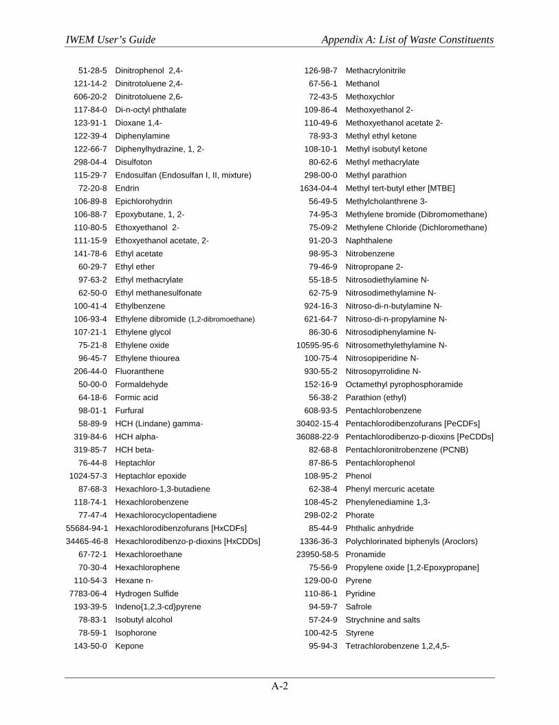
IWEM User’s Guide Appendix A: List of Waste Constituents
A-2
51-28-5 Dinitrophenol 2,4- 121-14-2 Dinitrotoluene 2,4- 606-20-2 Dinitrotoluene 2,6- 117-84-0 Di-n-octyl phthalate 123-91-1 Dioxane 1,4- 122-39-4 Diphenylamine 122-66-7 Diphenylhydrazine, 1, 2- 298-04-4 Disulfoton 115-29-7 Endosulfan (Endosulfan I, II, mixture) 72-20-8 Endrin 106-89-8 Epichlorohydrin 106-88-7 Epoxybutane, 1, 2- 110-80-5 Ethoxyethanol 2- 111-15-9 Ethoxyethanol acetate, 2- 141-78-6 Ethyl acetate 60-29-7 Ethyl ether 97-63-2 Ethyl methacrylate 62-50-0 Ethyl methanesulfonate 100-41-4 Ethylbenzene 106-93-4 Ethylene dibromide (1,2-dibromoethane) 107-21-1 Ethylene glycol 75-21-8 Ethylene oxide 96-45-7 Ethylene thiourea 206-44-0 Fluoranthene 50-00-0 Formaldehyde 64-18-6 Formic acid 98-01-1 Furfural 58-89-9 HCH (Lindane) gamma- 319-84-6 HCH alpha- 319-85-7 HCH beta- 76-44-8 Heptachlor 1024-57-3 Heptachlor epoxide 87-68-3 Hexachloro-1,3-butadiene 118-74-1 Hexachlorobenzene 77-47-4 Hexachlorocyclopentadiene 55684-94-1 Hexachlorodibenzofurans [HxCDFs] 34465-46-8 Hexachlorodibenzo-p-dioxins [HxCDDs] 67-72-1 Hexachloroethane 70-30-4 Hexachlorophene 110-54-3 Hexane n- 7783-06-4 Hydrogen Sulfide 193-39-5 Indeno{1,2,3-cd}pyrene 78-83-1 Isobutyl alcohol 78-59-1 Isophorone 143-50-0 Kepone
126-98-7 Methacrylonitrile 67-56-1 Methanol 72-43-5 Methoxychlor 109-86-4 Methoxyethanol 2- 110-49-6 Methoxyethanol acetate 2- 78-93-3 Methyl ethyl ketone 108-10-1 Methyl isobutyl ketone 80-62-6 Methyl methacrylate 298-00-0 Methyl parathion 1634-04-4 Methyl tert-butyl ether [MTBE] 56-49-5 Methylcholanthrene 3- 74-95-3 Methylene bromide (Dibromomethane) 75-09-2 Methylene Chloride (Dichloromethane) 91-20-3 Naphthalene 98-95-3 Nitrobenzene 79-46-9 Nitropropane 2- 55-18-5 Nitrosodiethylamine N- 62-75-9 Nitrosodimethylamine N- 924-16-3 Nitroso-di-n-butylamine N- 621-64-7 Nitroso-di-n-propylamine N- 86-30-6 Nitrosodiphenylamine N- 10595-95-6 Nitrosomethylethylamine N- 100-75-4 Nitrosopiperidine N- 930-55-2 Nitrosopyrrolidine N- 152-16-9 Octamethyl pyrophosphoramide 56-38-2 Parathion (ethyl) 608-93-5 Pentachlorobenzene 30402-15-4 Pentachlorodibenzofurans [PeCDFs] 36088-22-9 Pentachlorodibenzo-p-dioxins [PeCDDs] 82-68-8 Pentachloronitrobenzene (PCNB) 87-86-5 Pentachlorophenol 108-95-2 Phenol 62-38-4 Phenyl mercuric acetate 108-45-2 Phenylenediamine 1,3- 298-02-2 Phorate 85-44-9 Phthalic anhydride 1336-36-3 Polychlorinated biphenyls (Aroclors) 23950-58-5 Pronamide 75-56-9 Propylene oxide [1,2-Epoxypropane] 129-00-0 Pyrene 110-86-1 Pyridine 94-59-7 Safrole 57-24-9 Strychnine and salts 100-42-5 Styrene 95-94-3 Tetrachlorobenzene 1,2,4,5-

IWEM User’s Guide Appendix A: List of Waste Constituents
A-3
51207-31-9 Tetrachlorodibenzofuran, 2,3,7,8- 1746-01-6 Tetrachlorodibenzo-p-dioxin, 2,3,7,8- 630-20-6 Tetrachloroethane 1,1,1,2- 79-34-5 Tetrachloroethane 1,1,2,2- 127-18-4 Tetrachloroethylene 58-90-2 Tetrachlorophenol 2,3,4,6- 3689-24-5 Tetraethyl dithiopyrophosphate (Sulfotep) 137-26-8 Thiram [Thiuram] 108-88-3 Toluene 95-80-7 Toluenediamine 2,4- 95-53-4 Toluidine o- 106-49-0 Toluidine p- 8001-35-2 Toxaphene (chlorinated camphenes) 75-25-2 Tribromomethane (Bromoform) 76-13-1 Trichloro-1,2,2-trifluoro- ethane 1,1,2- 120-82-1 Trichlorobenzene 1,2,4- 71-55-6 Trichloroethane 1,1,1-
79-00-5 Trichloroethane 1,1,2- 79-01-6 Trichloroethylene 75-69-4 Trichlorofluoromethane (Freon 11) 95-95-4 Trichlorophenol 2,4,5- 88-06-2 Trichlorophenol 2,4,6- 93-72-1 Trichlorophenoxy)propionic acid 2- 93-76-5 Trichlorophenoxyacetic acid 2,4,5- 96-18-4 Trichloropropane 1,2,3- 121-44-8 Triethylamine 99-35-4 Trinitrobenzene 126-72-7 Tris(2,3-dibromopropyl)phosphate 108-05-4 Vinyl acetate 75-01-4 Vinyl chloride 108-38-3 Xylene m- 95-47-6 Xylene o- 106-42-3 Xylene p- 1330-20-7 Xylenes (total)
Metals (25) 7429-90-5 Aluminum (CCR waste only-Roadway) 7440-36-0 Antimony 22569-72-8 Arsenic (III) 15584-04-0 Arsenic (V) 7440-39-3 Barium 7440-41-7 Beryllium 7440-42-8 Boron (CCR waste only-Roadway) 7440-43-9 Cadmium 16065-83-1 Chromium (III) 18540-29-9 Chromium (VI) 7440-48-4 Cobalt 7440-50-8 Copper 16984-48-8 Fluoride
7439-89-6 Iron (CCR waste only-Roadway) 7439-92-1 Lead 7439-96-5 Manganese 7439-97-6 Mercury 7439-98-7 Molybdenum 7440-02-0 Nickel 10026-03-6 Selenium (IV) 7782-49-2 Selenium (VI) 7440-22-4 Silver 7440-28-0 Thallium 7440-62-2 Vanadium 7440-66-6 Zinc

IWEM User’s Guide Appendix A: List of Waste Constituents
A-4
[This page intentionally left blank.]

IWEM User’s Guide Appendix B: Example Problems for WMU Evaluation
B-1
Appendix B: Example Problems for WMU Evaluation
The purpose of this section is to provide the user examples on how to properly set up an IWEM evaluation for WMUs and execute the simulation. These examples are hypothetical scenarios to serve as tutorial; therefore, the user is cautioned from misconstruing both the scenarios and the results as real-life case studies. Project files corresponding to this example may be found in either
C:\Users\Public\Documents\IWEM\SampleData\ Appendix_B_WMU or C:\Users\[your user name]\Documents\IWEM\SampleData\ Appendix_B_WMU.
B.1 Land Application of Spent Foundry Sand in Home Gardens Spent foundry sands are ideal for manufactured soils because of their uniformity, consistency, and dark color in the case of green sands. The sands can be blended with soils and/or organic amendments (e.g., peat, composted yard waste, manures, biosolids) to develop manufactured soils suitable for horticultural, landscaping, and turfgrass applications (Jing and Barnes, 1993; Nayström et al., 2004; Lindsay and Logan, 2005; all as cited in U.S. EPA, 2009). However, the unencapsulated use of spent foundry sands is of particular concern because the application to land poses the potential for human and ecological exposure to chemical constituents found in the material. This example shows how IWEM can be used to evaluate the ground water impact from the use of spent foundry sands in manufactured soils containing spent foundry sands by home gardeners living in Madison, Wisconsin.
The following parameters were used within the model to define the use scenario:
Source Type: land application unit (i.e., unconsolidated application to land) Source Parameters:
– Area: 4,047 m2 (i.e., 1 acre) – Operating life: 40 years (default, determined to be long enough to ensure full
constituent leaching from waste amended soils) – Distance to drinking water well: 150 m (arbitrary model default distance)
Subsurface parameters were set to model defaults: – Subsurface environment: Unknown – Groundwater pH: 7 – Depth to water table: 5.18 m (IWEM default for a shallow aquifer) – Hydraulic conductivity: 1.89×10³ m/yr – Regional hydraulic gradient: 0.0057 m/m – Aquifer thickness: 10.1 m
Infiltration parameters were set based on the common soil type in Madison, WI: – Soil type: silt loam (medium grained soil) – Climate center: Madison, WI
Constituent List: – Arsenic (V) – Input leachate concentration: 0.015 mg/L. This concentration is the higher of the 95th
percentile leachate concentrations found by either Synthetic Precipitation Leaching

IWEM User’s Guide Appendix B: Example Problems for WMU Evaluation
B-2
Procedure (SPLP) or the American Society for Testing and Materials (ASTM) leachate methods.
Constituent Properties: – Chemical-specific decay rate: NA for metals – Soil-water partition coefficient: selected from isotherms generated by the
MINTEQA2 geochemical speciation model Reference Ground Water Concentrations:
– MCL (Maximum Contaminant Level): 0.01 mg/L (provided in IWEM) – Exposure duration: 1 yr.
This example results in a finding that land application is an appropriate management practice under this scenario (i.e., the estimated ground water concentration of arsenic under this scenario is below the MCL). The IWEM output report for this scenario is provided in Attachment B-1.
B.2 Landfill Example In developing a landfill unit to dispose industrial waste material, IWEM can be used to assist a unit manager or a design engineer to determine the most appropriate WMU design to minimize or avoid adverse ground water impacts by evaluating one or more types of liners, the hydrogeologic conditions of the site, and the toxicity and expected leachate concentrations of the anticipated waste constituents. The software can help compare the ground water protection afforded by various liner systems with the anticipated waste leachate concentrations, so that the manager/engineer can determine the minimum recommended liner system that will be protective of human health and ground water resources. The following example illustrates how IWEM can be used to determine the most appropriate liner design.
The following parameters were used within the model to define the use scenario:
Source Type: landfill Source Parameters:
– Depth of landfill: 6.5 m – Distance to drinking water well: 150 m (arbitrary model default distance) – Area: 12,300 m2 – Depth of the base of the landfill below ground surface: 0 (model default).
Subsurface parameters were set to model defaults: – Subsurface environment: Sand and gravel – Groundwater pH: default distribution – Depth to water table: default distribution – Hydraulic conductivity: default distribution – Regional hydraulic gradient: default distribution – Aquifer thickness: default distribution
Infiltration parameters: – Soil type: silt loam (medium grained soil) – Climate center: Greensboro, NC
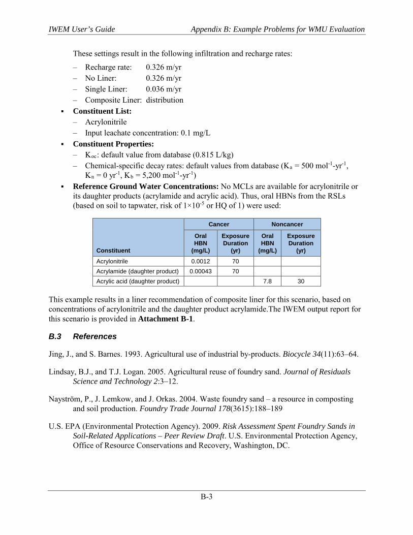
IWEM User’s Guide Appendix B: Example Problems for WMU Evaluation
B-3
These settings result in the following infiltration and recharge rates:
– Recharge rate: 0.326 m/yr – No Liner: 0.326 m/yr – Single Liner: 0.036 m/yr – Composite Liner: distribution
Constituent List: – Acrylonitrile – Input leachate concentration: 0.1 mg/L
Constituent Properties: – Koc: default value from database (0.815 L/kg) – Chemical-specific decay rates: default values from database (Ka = 500 mol-1-yr-1,
Kn = 0 yr-1, Kb = 5,200 mol-1-yr-1) Reference Ground Water Concentrations: No MCLs are available for acrylonitrile or
its daughter products (acrylamide and acrylic acid). Thus, oral HBNs from the RSLs (based on soil to tapwater, risk of 1×10⁻⁵ or HQ of 1) were used:
Constituent
Cancer Noncancer
Oral HBN
(mg/L)
Exposure Duration
(yr)
Oral HBN
(mg/L)
Exposure Duration
(yr)
Acrylonitrile 0.0012 70 Acrylamide (daughter product) 0.00043 70 Acrylic acid (daughter product) 7.8 30
This example results in a liner recommendation of composite liner for this scenario, based on concentrations of acrylonitrile and the daughter product acrylamide.The IWEM output report for this scenario is provided in Attachment B-1.
B.3 References
Jing, J., and S. Barnes. 1993. Agricultural use of industrial by-products. Biocycle 34(11):63–64.
Lindsay, B.J., and T.J. Logan. 2005. Agricultural reuse of foundry sand. Journal of Residuals Science and Technology 2:3–12.
Nayström, P., J. Lemkow, and J. Orkas. 2004. Waste foundry sand – a resource in composting and soil production. Foundry Trade Journal 178(3615):188–189
U.S. EPA (Environmental Protection Agency). 2009. Risk Assessment Spent Foundry Sands in Soil-Related Applications – Peer Review Draft. U.S. Environmental Protection Agency, Office of Resource Conservations and Recovery, Washington, DC.

IWEM User’s Guide Appendix B: Example Problems for WMU Evaluation
B-4
[This page intentionally left blank.]

IWEM User’s Guide Attachment B-1: Sample Reports from WMU Evaluation Example
B-1-1
Attachment B-1. Sample Reports from WMU Evaluation Examples
Example B1: Land Application of Spent Foundry Sand in Home Gardens ........................... B-1-3
Example B2: Landfill Example with Daughter Products ....................................................... B-1-7

IWEM User’s Guide Attachment B-1: Sample Reports from WMU Evaluation Example
B-1-2
[This page intentionally left blank.]
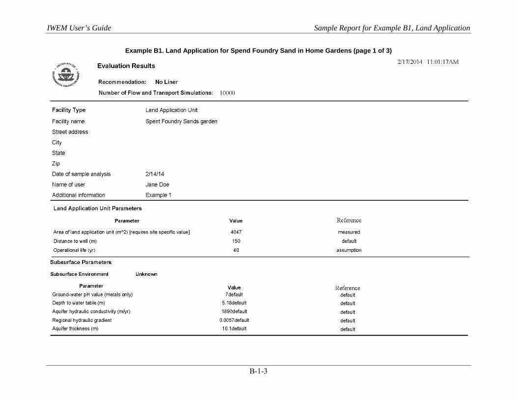
IWEM User’s Guide Sample Report for Example B1, Land Application
B-1-3
Example B1. Land Application for Spend Foundry Sand in Home Gardens (page 1 of 3)
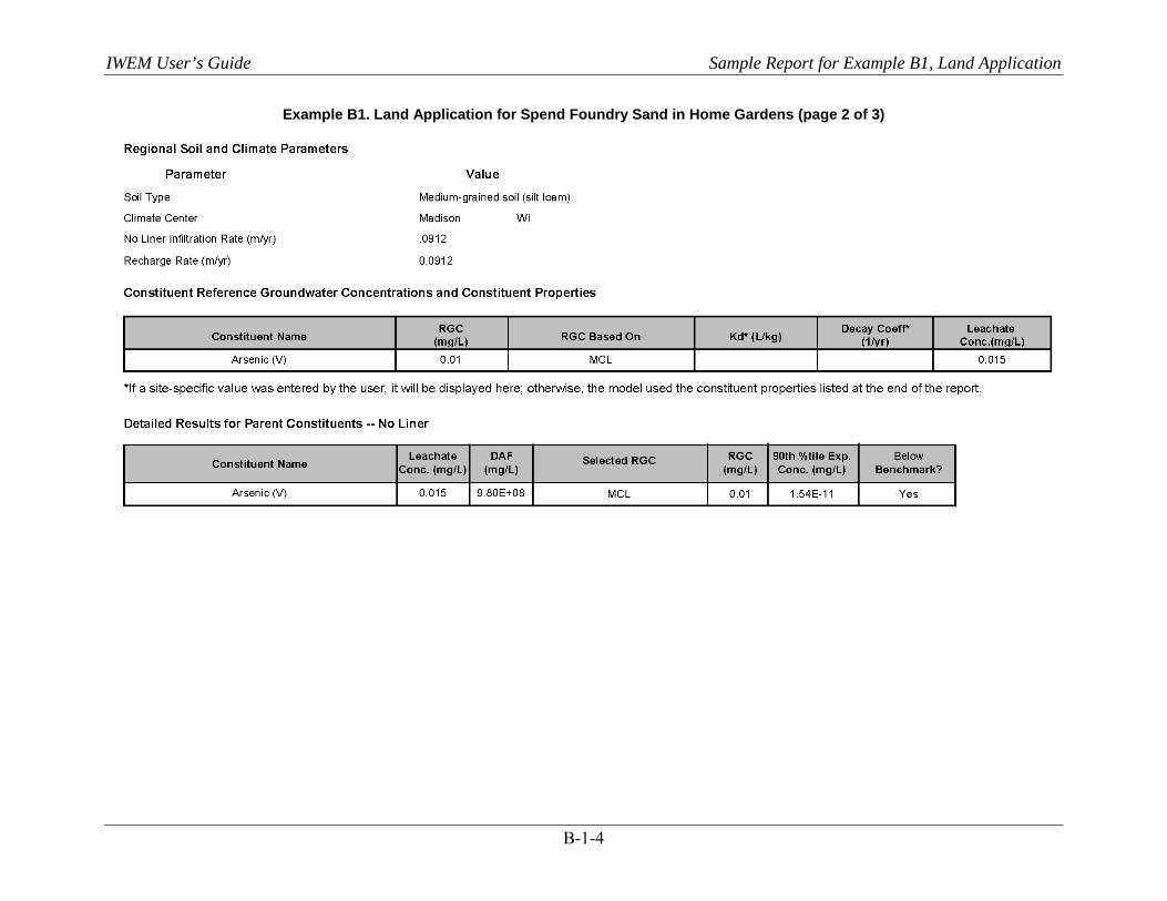
IWEM User’s Guide Sample Report for Example B1, Land Application
B-1-4
Example B1. Land Application for Spend Foundry Sand in Home Gardens (page 2 of 3)
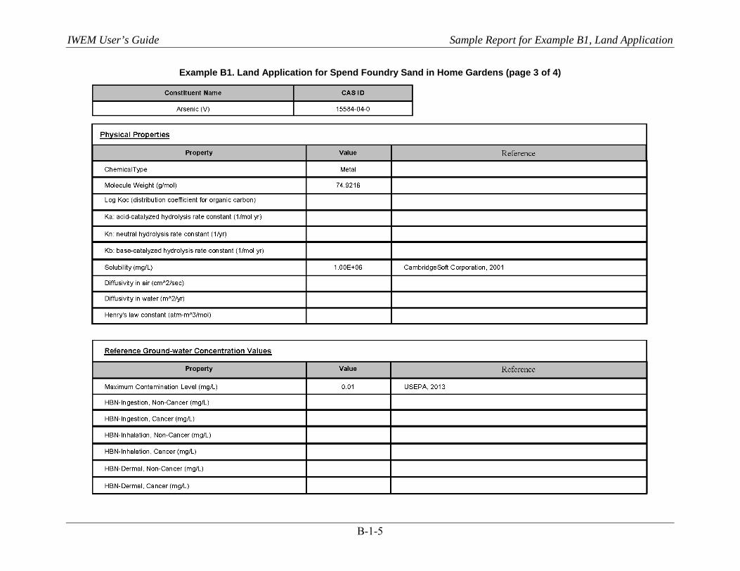
IWEM User’s Guide Sample Report for Example B1, Land Application
B-1-5
Example B1. Land Application for Spend Foundry Sand in Home Gardens (page 3 of 4)
IWEM User’s Guide Sample Report for Example B1, Land Application
B-1-6
Example B1. Land Application for Spend Foundry Sand in Home Gardens (page 4 of 4)
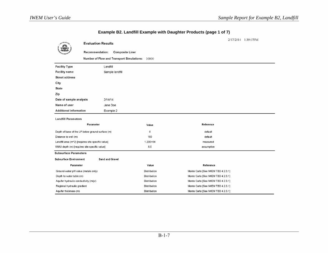
IWEM User’s Guide Sample Report for Example B2, Landfill
B-1-7
Example B2. Landfill Example with Daughter Products (page 1 of 7)
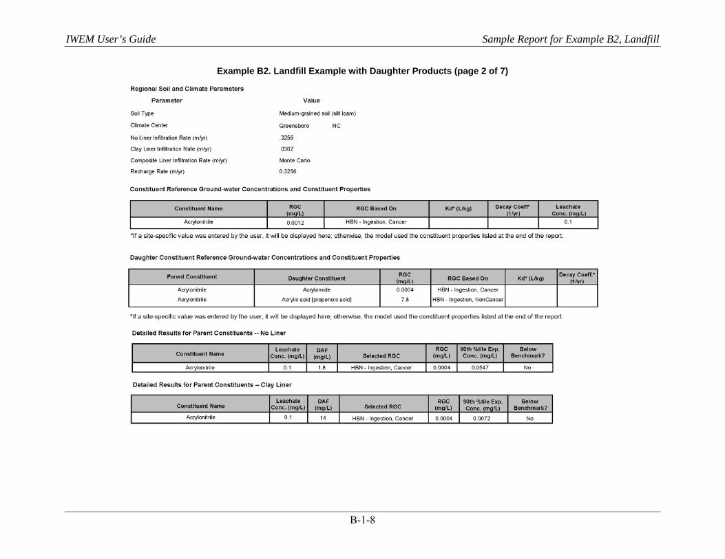
IWEM User’s Guide Sample Report for Example B2, Landfill
B-1-8
Example B2. Landfill Example with Daughter Products (page 2 of 7)
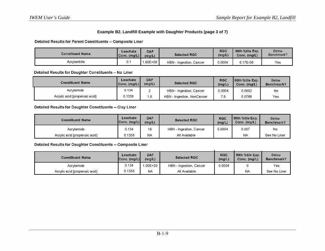
IWEM User’s Guide Sample Report for Example B2, Landfill
B-1-9
Example B2. Landfill Example with Daughter Products (page 3 of 7)
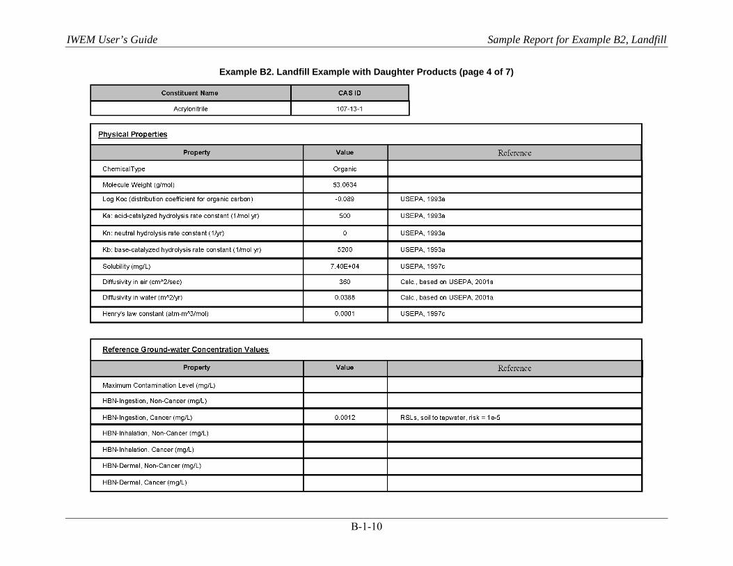
IWEM User’s Guide Sample Report for Example B2, Landfill
B-1-10
Example B2. Landfill Example with Daughter Products (page 4 of 7)
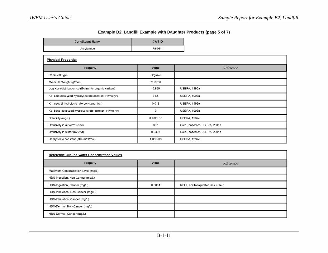
IWEM User’s Guide Sample Report for Example B2, Landfill
B-1-11
Example B2. Landfill Example with Daughter Products (page 5 of 7)
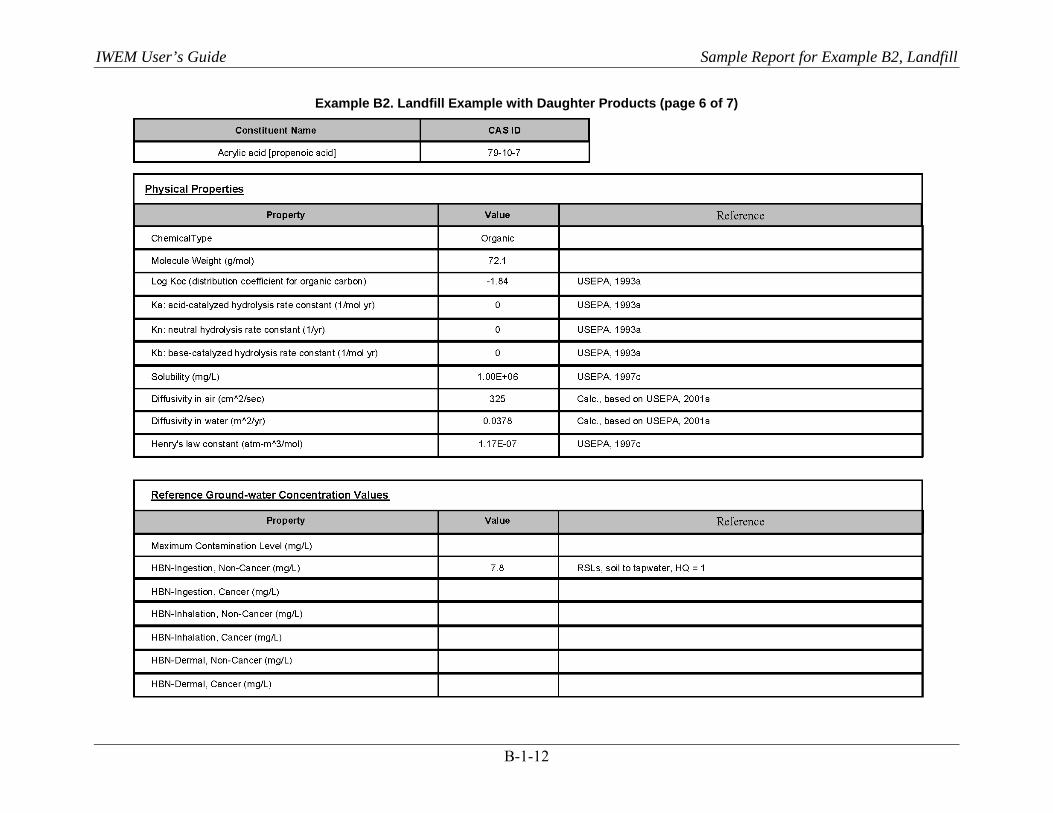
IWEM User’s Guide Sample Report for Example B2, Landfill
B-1-12
Example B2. Landfill Example with Daughter Products (page 6 of 7)
IWEM User’s Guide Sample Report for Example B2, Landfill
B-1-13
Example B2. Landfill Example with Daughter Products (page 7 of 7)

IWEM User’s Guide Attachment B-1: Sample Report for Example B2, Landfill
B-1-14
[This page intentionally left blank.]

IWEM User’s Guide Appendix C: Example Problems for Roadway Evaluation
C-1
Appendix C: Example Problems for Roadway Evaluation Project files corresponding to this example may be found in either
C:\Users\Public\Documents\IWEM\SampleData\Appendix_C_Roadway or C:\Users\[your user name]\Documents\IWEM\SampleData\Appendix_C_Roadway.
C.1 Introduction The following sections present five example problems applying IWEM Version 3.1 to three actual sites and one hypothetical site:
Example C1: A 152-m test section of Wisconsin State Highway (WSH) 60 near Lodi, WI
Example C2: A 1,829-m section of Highway 57, northbound lane, between Waldo and Random Lake, WI.
Examples C3 and C4: Minnesota Road Research Facility (MnROAD), Low Volume Road, near Monticello, MN.
Example C5: A hypothetical road segment including ditches, drains, and gutters located near Boston, MA.
The locations of the three actual sites are shown in Figure C-1. Each example includes a description of the problem and available data, a discussion of how values for the required input parameters were selected, screen shots of each IWEM screen showing the entered parameter values, and a brief discussion of the results.
Figure C-1. Map showing example sites: A–Lodi, WI; B–Waldo, WI; C–Monticello, MN
(map courtesy of Google Maps).
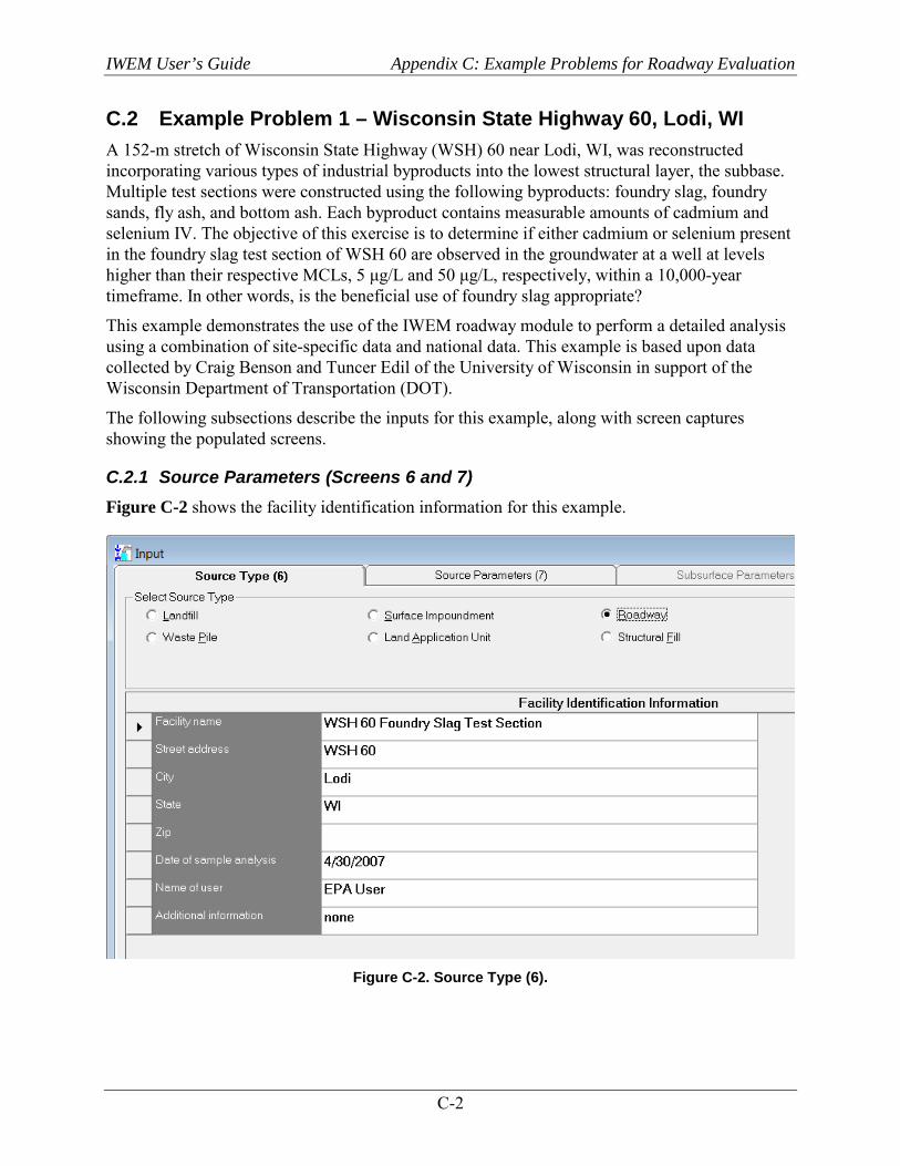
IWEM User’s Guide Appendix C: Example Problems for Roadway Evaluation
C-2
C.2 Example Problem 1 – Wisconsin State Highway 60, Lodi, WI A 152-m stretch of Wisconsin State Highway (WSH) 60 near Lodi, WI, was reconstructed incorporating various types of industrial byproducts into the lowest structural layer, the subbase. Multiple test sections were constructed using the following byproducts: foundry slag, foundry sands, fly ash, and bottom ash. Each byproduct contains measurable amounts of cadmium and selenium IV. The objective of this exercise is to determine if either cadmium or selenium present in the foundry slag test section of WSH 60 are observed in the groundwater at a well at levels higher than their respective MCLs, 5 μg/L and 50 μg/L, respectively, within a 10,000-year timeframe. In other words, is the beneficial use of foundry slag appropriate?
This example demonstrates the use of the IWEM roadway module to perform a detailed analysis using a combination of site-specific data and national data. This example is based upon data collected by Craig Benson and Tuncer Edil of the University of Wisconsin in support of the Wisconsin Department of Transportation (DOT).
The following subsections describe the inputs for this example, along with screen captures showing the populated screens.
C.2.1 Source Parameters (Screens 6 and 7) Figure C-2 shows the facility identification information for this example.
Figure C-2. Source Type (6).
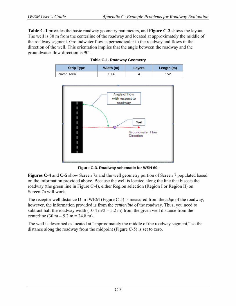
IWEM User’s Guide Appendix C: Example Problems for Roadway Evaluation
C-3
Table C-1 provides the basic roadway geometry parameters, and Figure C-3 shows the layout. The well is 30 m from the centerline of the roadway and located at approximately the middle of the roadway segment. Groundwater flow is perpendicular to the roadway and flows in the direction of the well. This orientation implies that the angle between the roadway and the groundwater flow direction is 90°.
Table C-1. Roadway Geometry
Strip Type Width (m) Layers Length (m)
Paved Area 10.4 4 152
Figure C-3. Roadway schematic for WSH 60.
Figures C-4 and C-5 show Screen 7a and the well geometry portion of Screen 7 populated based on the information provided above. Because the well is located along the line that bisects the roadway (the green line in Figure C-4), either Region selection (Region I or Region II) on Screen 7a will work.
The receptor well distance D in IWEM (Figure C-5) is measured from the edge of the roadway; however, the information provided is from the centerline of the roadway. Thus, you need to subtract half the roadway width (10.4 m/2 = 5.2 m) from the given well distance from the centerline (30 m – 5.2 m = 24.8 m).
The well is described as located at “approximately the middle of the roadway segment,” so the distance along the roadway from the midpoint (Figure C-5) is set to zero.
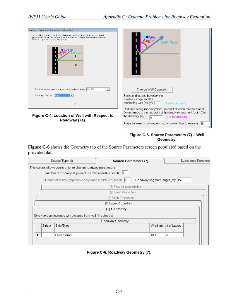
IWEM User’s Guide Appendix C: Example Problems for Roadway Evaluation
C-4
Figure C-4. Location of Well with Respect to Roadway (7a).
Figure C-5. Source Parameters (7) – Well Geometry.
Figure C-6 shows the Geometry tab of the Source Parameters screen populated based on the provided data.
Figure C-6. Roadway Geometry (7).
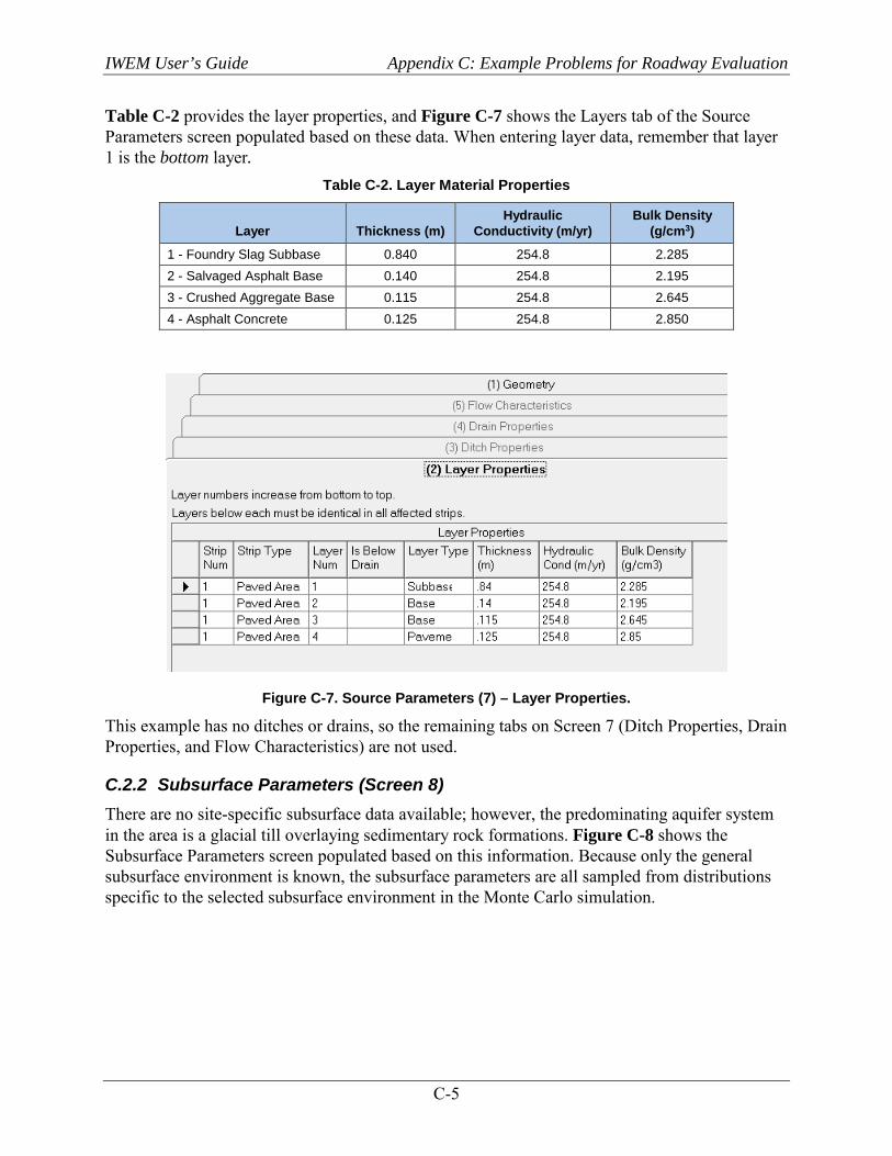
IWEM User’s Guide Appendix C: Example Problems for Roadway Evaluation
C-5
Table C-2 provides the layer properties, and Figure C-7 shows the Layers tab of the Source Parameters screen populated based on these data. When entering layer data, remember that layer 1 is the bottom layer.
Table C-2. Layer Material Properties
Layer Thickness (m) Hydraulic
Conductivity (m/yr) Bulk Density
(g/cm3)
1 - Foundry Slag Subbase 0.840 254.8 2.285 2 - Salvaged Asphalt Base 0.140 254.8 2.195 3 - Crushed Aggregate Base 0.115 254.8 2.645 4 - Asphalt Concrete 0.125 254.8 2.850
Figure C-7. Source Parameters (7) – Layer Properties.
This example has no ditches or drains, so the remaining tabs on Screen 7 (Ditch Properties, Drain Properties, and Flow Characteristics) are not used.
C.2.2 Subsurface Parameters (Screen 8) There are no site-specific subsurface data available; however, the predominating aquifer system in the area is a glacial till overlaying sedimentary rock formations. Figure C-8 shows the Subsurface Parameters screen populated based on this information. Because only the general subsurface environment is known, the subsurface parameters are all sampled from distributions specific to the selected subsurface environment in the Monte Carlo simulation.
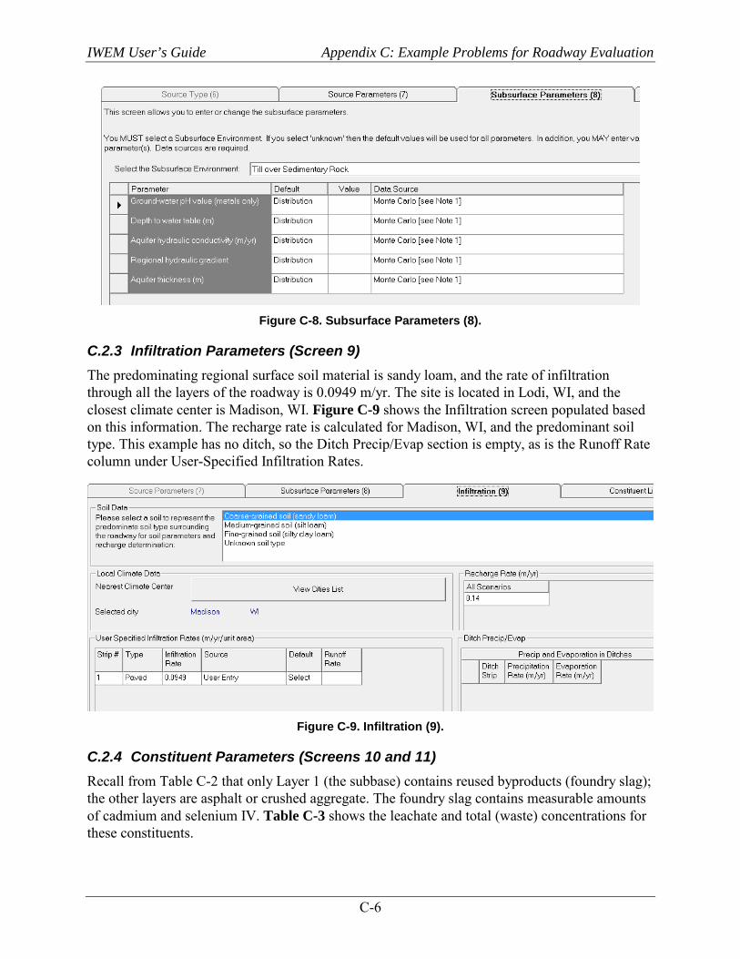
IWEM User’s Guide Appendix C: Example Problems for Roadway Evaluation
C-6
Figure C-8. Subsurface Parameters (8).
C.2.3 Infiltration Parameters (Screen 9) The predominating regional surface soil material is sandy loam, and the rate of infiltration through all the layers of the roadway is 0.0949 m/yr. The site is located in Lodi, WI, and the closest climate center is Madison, WI. Figure C-9 shows the Infiltration screen populated based on this information. The recharge rate is calculated for Madison, WI, and the predominant soil type. This example has no ditch, so the Ditch Precip/Evap section is empty, as is the Runoff Rate column under User-Specified Infiltration Rates.
Figure C-9. Infiltration (9).
C.2.4 Constituent Parameters (Screens 10 and 11) Recall from Table C-2 that only Layer 1 (the subbase) contains reused byproducts (foundry slag); the other layers are asphalt or crushed aggregate. The foundry slag contains measurable amounts of cadmium and selenium IV. Table C-3 shows the leachate and total (waste) concentrations for these constituents.

IWEM User’s Guide Appendix C: Example Problems for Roadway Evaluation
C-7
Table C-3. Constituent Concentrations for Layer 1 (Foundry Slag)
Constituent Leachate (mg/L) Waste (mg/kg)
Cadmium 0.0321 0.0397 Selenium IV 0.151 0.187
Figure C-10 shows the Constituent List screen populated based on this information. Note that the columns for Layers 2 and 3 (and Layer 4, off the edge of the screen) are empty, as there are no constituents present in those layers.
Figure C-10. Constituent List (10).
No site-specific information for constituent properties (Screen 11) is available, so the soil-water partitioning coefficient (Kd) will be sampled from a distribution.
C.2.5 Reference Ground Water Concentrations (Screen 12) Both cadmium and selenium IV have MCLs, which will be used for this example. Figure C-11 shows the Reference GW Conc. screen populated based on this information.
Figure C-11. Reference Ground Water Concentration (12).

IWEM User’s Guide Appendix C: Example Problems for Roadway Evaluation
C-8
C.2.6 Results As displayed on the Output Summary screen, IWEM determines that this roadway design with industrial materials is appropriate—the estimated 90th percentile cconcentrations for cadmium and selenium were below their respective MCLs. Empirical data collected at the site showed that field observations were less than the results predicted by IWEM for both metals; however, the predictions were correct with respect to the selected standards. By design, IWEM predictions based on the substitution of national data for key site-specific data (subsurface parameters and site-based partitioning coefficients) generate a conservative result; the result errs on the side of environmental and human health protection. The IWEM reports from this example are provided in Attachment C-1.
C.3 Example Problem 2 – Wisconsin State Highway 57, Waldo, WI A 1,829-m stretch of the northbound lane of WSH 57 between Waldo and Random Lake in Sheboygan County, WI, was undergoing reconstruction in 2001. A nearby manufacturing company, in Kohler, WI, generates spent foundry sands as part of its manufacturing process. In an effort to utilize this industrial material for beneficial reuse, the company had the material tested by a local engineering firm to see if it was structurally suitable for roadway fill. The firm determined that the material could be used as fill material beneath lightly loaded structural components (e.g., pavements) if kept at thicknesses between 0.6 and 1.2 m beneath the pavement at density of 1.89 g/cm3. In addition, the firm subjected the material to the following analytical tests: a total elemental analysis to determine what potentially hazardous constituents were present in the material and at what total leachable concentrations; and a water leach test [ASTM D3987-85 (WAC, 2006)] to estimate the potential leaching concentration of those constituents.
Although the results of the analytical tests did not identify any compounds at levels that exceeded standards for the material or leachate concentrations established by the State of Wisconsin (WAC Chapter NR 538), a modeling analysis was desired to confirm that the standards were in fact protective of ground water according to the MCL for the constituents of concern: arsenic and barium. The objective of this exercise is to confirm that the use of this foundry sand as a fill material in the reconstruction of WSH 57 will be appropriate, based on the MCLs for arsenic III and barium (0.01 and 2.0 mg/L, respectively).
We will demonstrate the use of the IWEM roadway module to perform a detailed analysis using a combination of site-specific data and national data. This example is based upon data provided to EPA by the Wisconsin DOT.
The following subsections describe the inputs for this example, along with screen captures showing the populated screens.
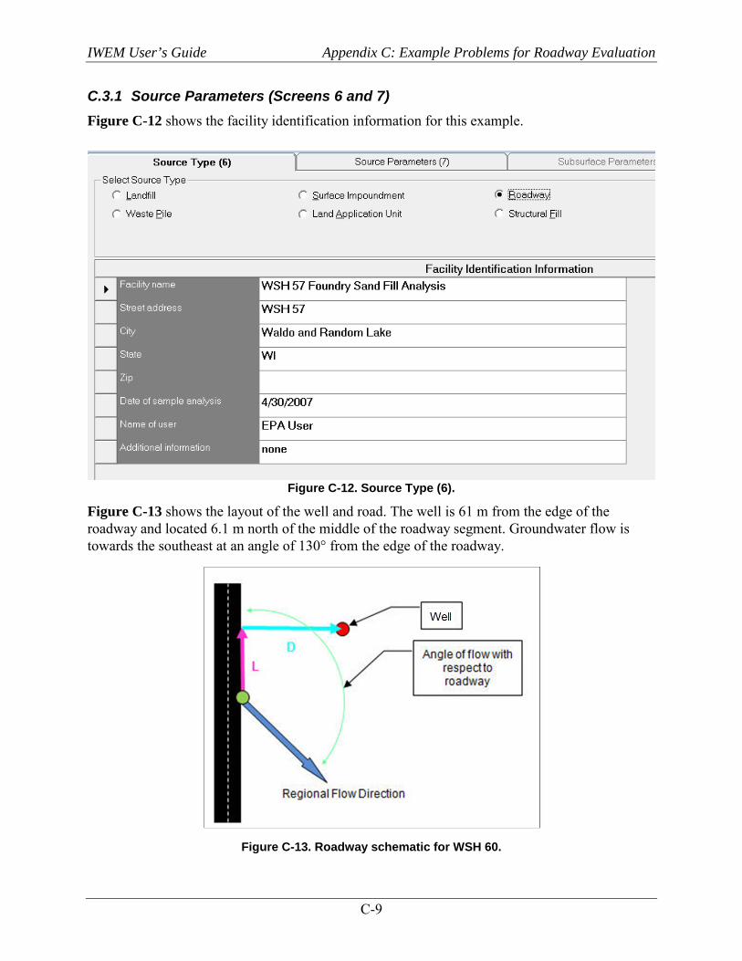
IWEM User’s Guide Appendix C: Example Problems for Roadway Evaluation
C-9
C.3.1 Source Parameters (Screens 6 and 7) Figure C-12 shows the facility identification information for this example.
Figure C-12. Source Type (6).
Figure C-13 shows the layout of the well and road. The well is 61 m from the edge of the roadway and located 6.1 m north of the middle of the roadway segment. Groundwater flow is towards the southeast at an angle of 130° from the edge of the roadway.
Figure C-13. Roadway schematic for WSH 60.
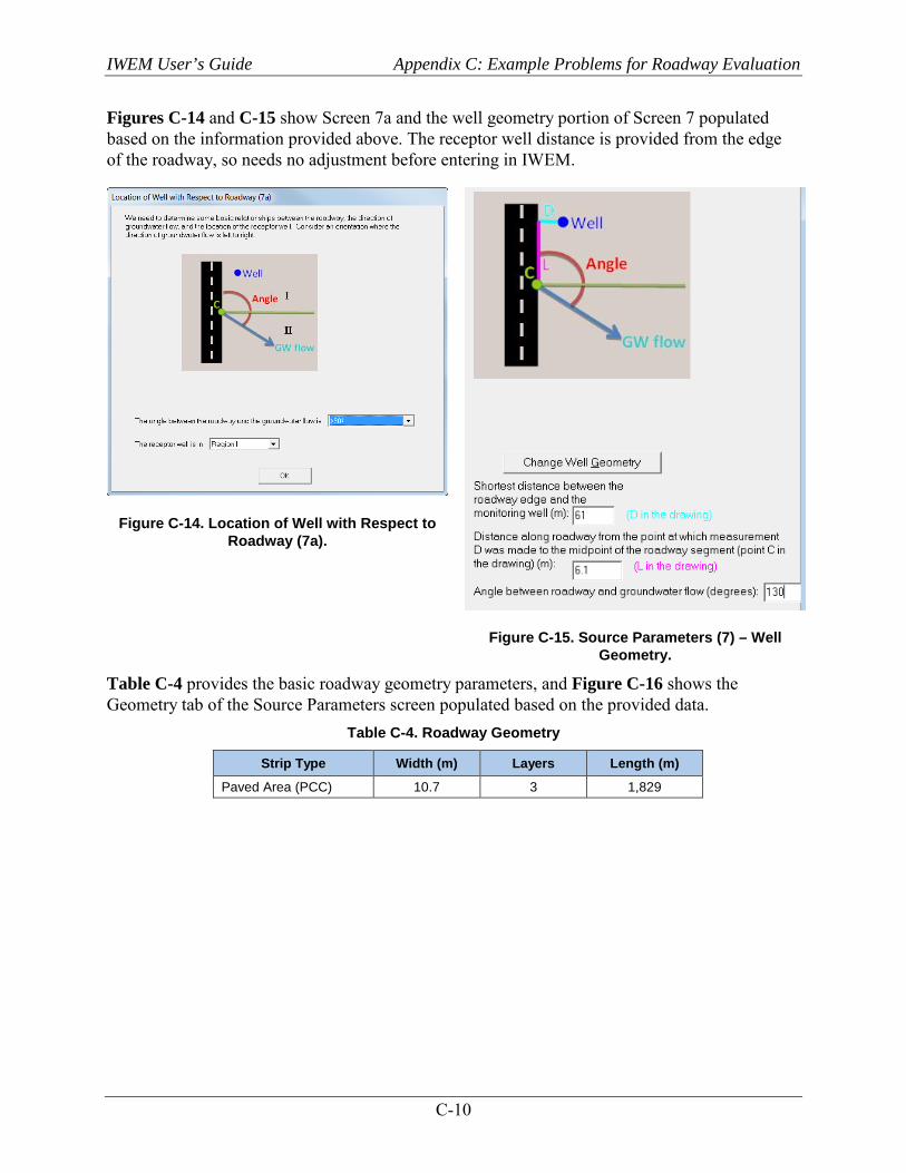
IWEM User’s Guide Appendix C: Example Problems for Roadway Evaluation
C-10
Figures C-14 and C-15 show Screen 7a and the well geometry portion of Screen 7 populated based on the information provided above. The receptor well distance is provided from the edge of the roadway, so needs no adjustment before entering in IWEM.
Figure C-14. Location of Well with Respect to Roadway (7a).
Figure C-15. Source Parameters (7) – Well Geometry.
Table C-4 provides the basic roadway geometry parameters, and Figure C-16 shows the Geometry tab of the Source Parameters screen populated based on the provided data.
Table C-4. Roadway Geometry
Strip Type Width (m) Layers Length (m)
Paved Area (PCC) 10.7 3 1,829
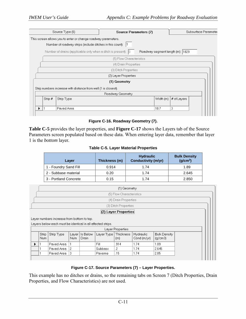
IWEM User’s Guide Appendix C: Example Problems for Roadway Evaluation
C-11
Figure C-16. Roadway Geometry (7).
Table C-5 provides the layer properties, and Figure C-17 shows the Layers tab of the Source Parameters screen populated based on these data. When entering layer data, remember that layer 1 is the bottom layer.
Table C-5. Layer Material Properties
Layer Thickness (m) Hydraulic
Conductivity (m/yr) Bulk Density
(g/cm3)
1 - Foundry Sand Fill 0.914 1.74 1.89 2 - Subbase material 0.20 1.74 2.645 3 - Portland Concrete 0.15 1.74 2.850
Figure C-17. Source Parameters (7) – Layer Properties.
This example has no ditches or drains, so the remaining tabs on Screen 7 (Ditch Properties, Drain Properties, and Flow Characteristics) are not used.
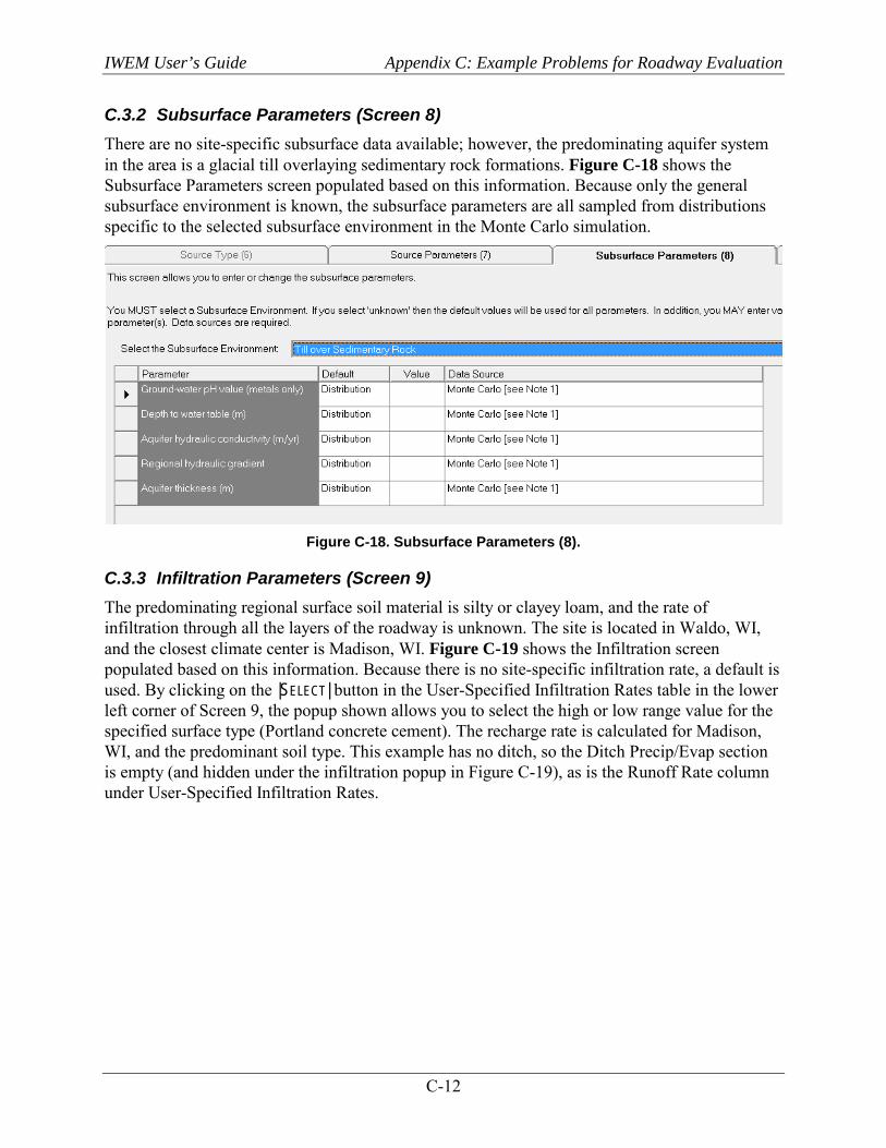
IWEM User’s Guide Appendix C: Example Problems for Roadway Evaluation
C-12
C.3.2 Subsurface Parameters (Screen 8) There are no site-specific subsurface data available; however, the predominating aquifer system in the area is a glacial till overlaying sedimentary rock formations. Figure C-18 shows the Subsurface Parameters screen populated based on this information. Because only the general subsurface environment is known, the subsurface parameters are all sampled from distributions specific to the selected subsurface environment in the Monte Carlo simulation.
Figure C-18. Subsurface Parameters (8).
C.3.3 Infiltration Parameters (Screen 9) The predominating regional surface soil material is silty or clayey loam, and the rate of infiltration through all the layers of the roadway is unknown. The site is located in Waldo, WI, and the closest climate center is Madison, WI. Figure C-19 shows the Infiltration screen populated based on this information. Because there is no site-specific infiltration rate, a default is used. By clicking on the |SELECT| button in the User-Specified Infiltration Rates table in the lower left corner of Screen 9, the popup shown allows you to select the high or low range value for the specified surface type (Portland concrete cement). The recharge rate is calculated for Madison, WI, and the predominant soil type. This example has no ditch, so the Ditch Precip/Evap section is empty (and hidden under the infiltration popup in Figure C-19), as is the Runoff Rate column under User-Specified Infiltration Rates.
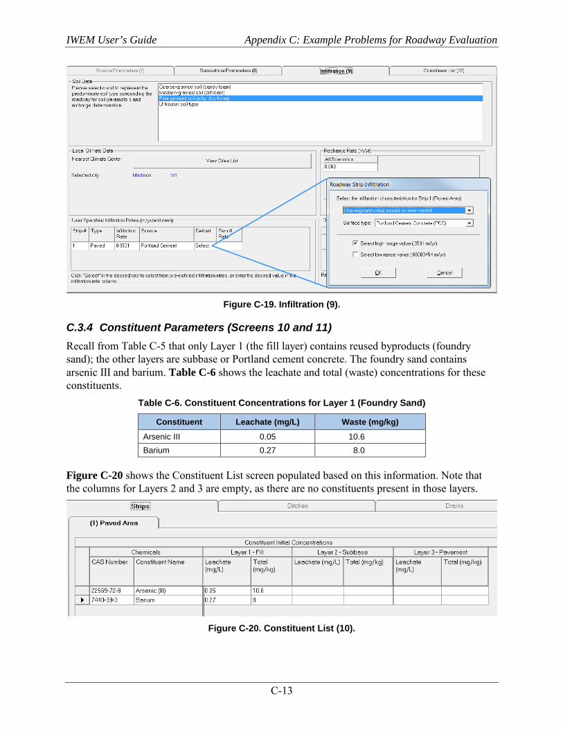
IWEM User’s Guide Appendix C: Example Problems for Roadway Evaluation
C-13
Figure C-19. Infiltration (9).
C.3.4 Constituent Parameters (Screens 10 and 11) Recall from Table C-5 that only Layer 1 (the fill layer) contains reused byproducts (foundry sand); the other layers are subbase or Portland cement concrete. The foundry sand contains arsenic III and barium. Table C-6 shows the leachate and total (waste) concentrations for these constituents.
Table C-6. Constituent Concentrations for Layer 1 (Foundry Sand)
Constituent Leachate (mg/L) Waste (mg/kg)
Arsenic III 0.05 10.6 Barium 0.27 8.0
Figure C-20 shows the Constituent List screen populated based on this information. Note that the columns for Layers 2 and 3 are empty, as there are no constituents present in those layers.
Figure C-20. Constituent List (10).

IWEM User’s Guide Appendix C: Example Problems for Roadway Evaluation
C-14
No site-specific information for constituent properties (Screen 11) is available, so the soil-water partitioning coefficient (Kd) will be sampled from a distribution.
C.3.5 Reference Ground Water Concentrations (Screen 12) Both arsenic and barium have MCLs, which will be used for this example. Figure C-21 shows the Reference GW Conc. screen populated based on this information.
Figure C-21. Reference Ground Water Concentration (12).
C.3.6 Results As displayed on the Output Summary screen, IWEM predicts that the roadway design exceeds the benchmark for arsenic III —the 90th percentile concentration for arsenic III is above its MCL. However, the 90th percentile concentration for barium was below the selected benchmark. The IWEM reports from this example are provided in Attachment C-1.
C.4 Example Problem 3 – Minnesota Road Research Facility (MNROAD), Low Volume Road, Monticello, MN
The MnROAD facility1 is operated by the Minnesota Department of Transportation (Mn/DOT), and is located in east-central Minnesota adjacent to Interstate 94 between Albertville and Monticello, MN, northwest of the Minneapolis/St. Paul metropolitan area. MnROAD is a cold-region testing laboratory with three instrumented test roadways used to track pavement performance over time. The 2.5-mile low-volume roadway, used to simulate conditions on rural roads, has several segments used for various experiments. One test segment uses high carbon fly ash (HCFA) to stabilize the base course beneath hot mix asphalt. This segment, along with control segments, has been instrumented with lysimeters to capture leachate from the stabilized base materials to evaluate the environmental performance of HCFA-stabilized bases. Most information used in this example comes from a Mn/DOT report (Wen, 2008), a construction drawing provided by Mn/DOT, and a master’s thesis (O’Donnell, 2009), submitted to the University of Wisconsin, which is a partner in the research project.
1 http://www.dot.state.mn.us/mnroad/
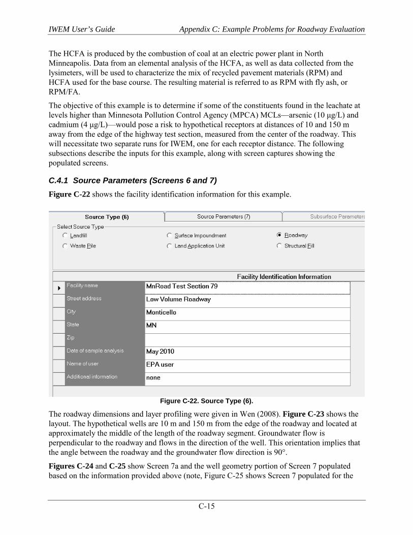
IWEM User’s Guide Appendix C: Example Problems for Roadway Evaluation
C-15
The HCFA is produced by the combustion of coal at an electric power plant in North Minneapolis. Data from an elemental analysis of the HCFA, as well as data collected from the lysimeters, will be used to characterize the mix of recycled pavement materials (RPM) and HCFA used for the base course. The resulting material is referred to as RPM with fly ash, or RPM/FA.
The objective of this example is to determine if some of the constituents found in the leachate at levels higher than Minnesota Pollution Control Agency (MPCA) MCLs—arsenic (10 μg/L) and cadmium (4 μg/L)—would pose a risk to hypothetical receptors at distances of 10 and 150 m away from the edge of the highway test section, measured from the center of the roadway. This will necessitate two separate runs for IWEM, one for each receptor distance. The following subsections describe the inputs for this example, along with screen captures showing the populated screens.
C.4.1 Source Parameters (Screens 6 and 7) Figure C-22 shows the facility identification information for this example.
Figure C-22. Source Type (6).
The roadway dimensions and layer profiling were given in Wen (2008). Figure C-23 shows the layout. The hypothetical wells are 10 m and 150 m from the edge of the roadway and located at approximately the middle of the length of the roadway segment. Groundwater flow is perpendicular to the roadway and flows in the direction of the well. This orientation implies that the angle between the roadway and the groundwater flow direction is 90°.
Figures C-24 and C-25 show Screen 7a and the well geometry portion of Screen 7 populated based on the information provided above (note, Figure C-25 shows Screen 7 populated for the
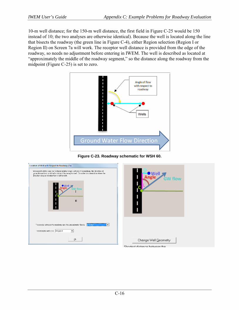
IWEM User’s Guide Appendix C: Example Problems for Roadway Evaluation
C-16
10-m well distance; for the 150-m well distance, the first field in Figure C-25 would be 150 instead of 10; the two analyses are otherwise identical). Because the well is located along the line that bisects the roadway (the green line in Figure C-4), either Region selection (Region I or Region II) on Screen 7a will work. The receptor well distance is provided from the edge of the roadway, so needs no adjustment before entering in IWEM. The well is described as located at “approximately the middle of the roadway segment,” so the distance along the roadway from the midpoint (Figure C-25) is set to zero.
Figure C-23. Roadway schematic for WSH 60.
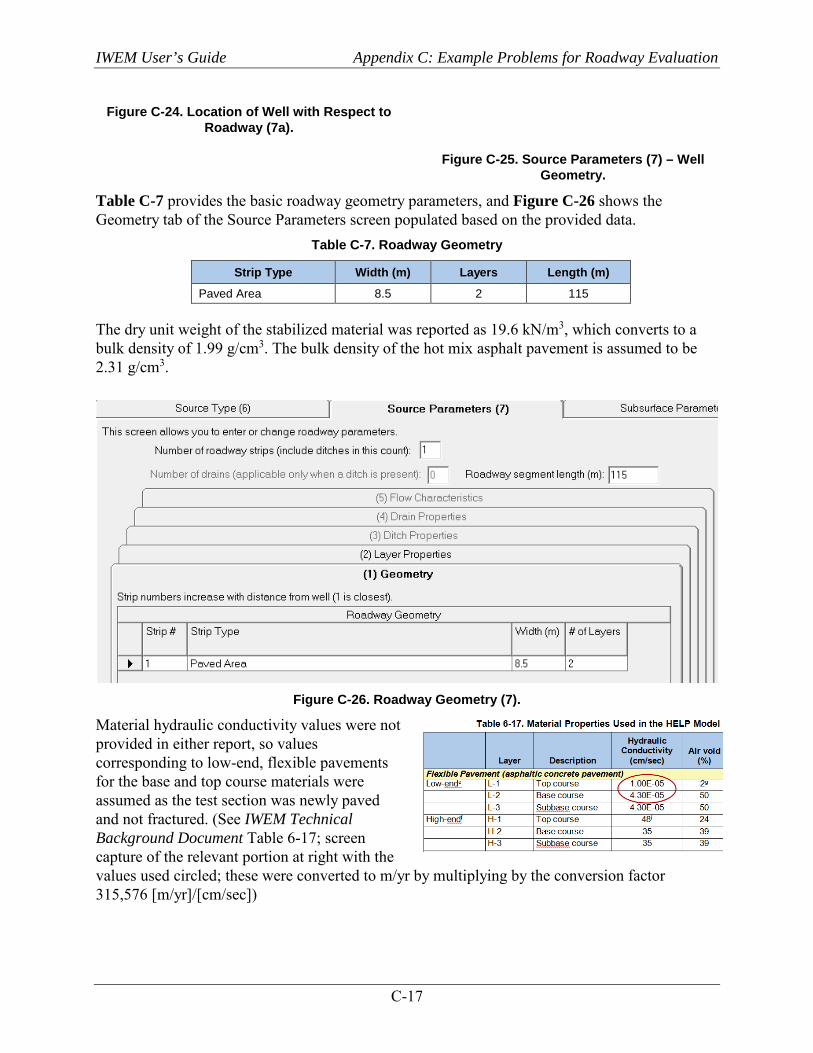
IWEM User’s Guide Appendix C: Example Problems for Roadway Evaluation
C-17
Figure C-24. Location of Well with Respect to Roadway (7a).
Figure C-25. Source Parameters (7) – Well Geometry.
Table C-7 provides the basic roadway geometry parameters, and Figure C-26 shows the Geometry tab of the Source Parameters screen populated based on the provided data.
Table C-7. Roadway Geometry
Strip Type Width (m) Layers Length (m)
Paved Area 8.5 2 115
The dry unit weight of the stabilized material was reported as 19.6 kN/m3, which converts to a bulk density of 1.99 g/cm3. The bulk density of the hot mix asphalt pavement is assumed to be 2.31 g/cm3.
Figure C-26. Roadway Geometry (7).
Material hydraulic conductivity values were not provided in either report, so values corresponding to low-end, flexible pavements for the base and top course materials were assumed as the test section was newly paved and not fractured. (See IWEM Technical Background Document Table 6-17; screen capture of the relevant portion at right with the values used circled; these were converted to m/yr by multiplying by the conversion factor 315,576 [m/yr]/[cm/sec])
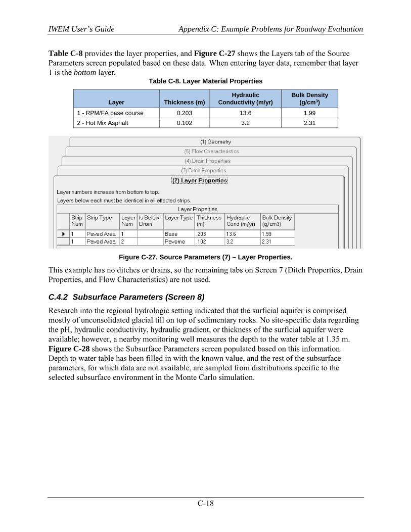
IWEM User’s Guide Appendix C: Example Problems for Roadway Evaluation
C-18
Table C-8 provides the layer properties, and Figure C-27 shows the Layers tab of the Source Parameters screen populated based on these data. When entering layer data, remember that layer 1 is the bottom layer.
Table C-8. Layer Material Properties
Layer Thickness (m) Hydraulic
Conductivity (m/yr) Bulk Density
(g/cm3)
1 - RPM/FA base course 0.203 13.6 1.99 2 - Hot Mix Asphalt 0.102 3.2 2.31
Figure C-27. Source Parameters (7) – Layer Properties.
This example has no ditches or drains, so the remaining tabs on Screen 7 (Ditch Properties, Drain Properties, and Flow Characteristics) are not used.
C.4.2 Subsurface Parameters (Screen 8) Research into the regional hydrologic setting indicated that the surficial aquifer is comprised mostly of unconsolidated glacial till on top of sedimentary rocks. No site-specific data regarding the pH, hydraulic conductivity, hydraulic gradient, or thickness of the surficial aquifer were available; however, a nearby monitoring well measures the depth to the water table at 1.35 m. Figure C-28 shows the Subsurface Parameters screen populated based on this information. Depth to water table has been filled in with the known value, and the rest of the subsurface parameters, for which data are not available, are sampled from distributions specific to the selected subsurface environment in the Monte Carlo simulation.
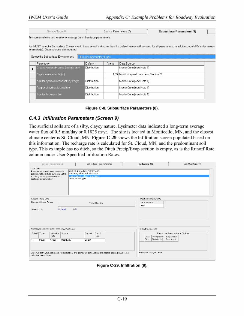
IWEM User’s Guide Appendix C: Example Problems for Roadway Evaluation
C-19
Figure C-8. Subsurface Parameters (8).
C.4.3 Infiltration Parameters (Screen 9) The surficial soils are of a silty, clayey nature. Lysimeter data indicated a long-term average water flux of 0.5 mm/day or 0.1825 m/yr. The site is located in Monticello, MN, and the closest climate center is St. Cloud, MN. Figure C-29 shows the Infiltration screen populated based on this information. The recharge rate is calculated for St. Cloud, MN, and the predominant soil type. This example has no ditch, so the Ditch Precip/Evap section is empty, as is the Runoff Rate column under User-Specified Infiltration Rates.
Figure C-29. Infiltration (9).
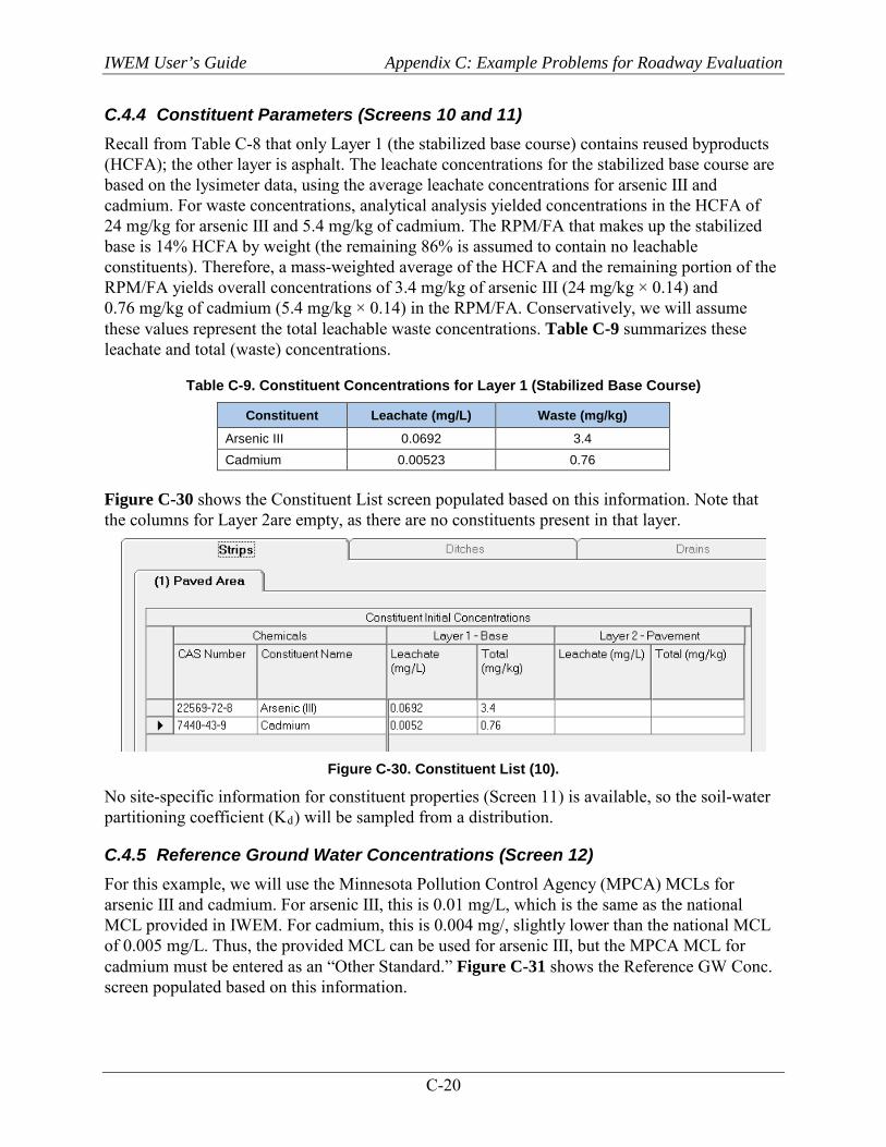
IWEM User’s Guide Appendix C: Example Problems for Roadway Evaluation
C-20
C.4.4 Constituent Parameters (Screens 10 and 11) Recall from Table C-8 that only Layer 1 (the stabilized base course) contains reused byproducts (HCFA); the other layer is asphalt. The leachate concentrations for the stabilized base course are based on the lysimeter data, using the average leachate concentrations for arsenic III and cadmium. For waste concentrations, analytical analysis yielded concentrations in the HCFA of 24 mg/kg for arsenic III and 5.4 mg/kg of cadmium. The RPM/FA that makes up the stabilized base is 14% HCFA by weight (the remaining 86% is assumed to contain no leachable constituents). Therefore, a mass-weighted average of the HCFA and the remaining portion of the RPM/FA yields overall concentrations of 3.4 mg/kg of arsenic III (24 mg/kg × 0.14) and 0.76 mg/kg of cadmium (5.4 mg/kg × 0.14) in the RPM/FA. Conservatively, we will assume these values represent the total leachable waste concentrations. Table C-9 summarizes these leachate and total (waste) concentrations.
Table C-9. Constituent Concentrations for Layer 1 (Stabilized Base Course)
Constituent Leachate (mg/L) Waste (mg/kg)
Arsenic III 0.0692 3.4 Cadmium 0.00523 0.76
Figure C-30 shows the Constituent List screen populated based on this information. Note that the columns for Layer 2are empty, as there are no constituents present in that layer.
Figure C-30. Constituent List (10).
No site-specific information for constituent properties (Screen 11) is available, so the soil-water partitioning coefficient (Kd) will be sampled from a distribution.
C.4.5 Reference Ground Water Concentrations (Screen 12) For this example, we will use the Minnesota Pollution Control Agency (MPCA) MCLs for arsenic III and cadmium. For arsenic III, this is 0.01 mg/L, which is the same as the national MCL provided in IWEM. For cadmium, this is 0.004 mg/, slightly lower than the national MCL of 0.005 mg/L. Thus, the provided MCL can be used for arsenic III, but the MPCA MCL for cadmium must be entered as an “Other Standard.” Figure C-31 shows the Reference GW Conc. screen populated based on this information.

IWEM User’s Guide Appendix C: Example Problems for Roadway Evaluation
C-21
Figure C-31. Reference Ground Water Concentration (12).
C.4.6 Results As displayed on the Output Summary screen, IWEM predicts that the roadway design exceeds the benchmarks for both arsenic III and cadmium at the well 10 m from the roadway. The 90th percentile concentration for arsenic III is 0.0524 mg/L (compared to an MCL of 0.01 mg/L). The 90th percentile concentration for cadmium is 0.0048 mg/L (compared to an MCL of 0.004 mg/L). Given that the initial leachate concentrations are 0.0692 mg/L for arsenic and 0.0052 mg/L for cadmium, the well concentrations are 76% and 92% of the initial concentrations for arsenic and cadmium, respectively. Therefore, clearly little dilution of the leachate occurs between the roadway and the 10-m receptor location.
In contrast, the 150-m well location provides sufficient dilution and attenuation to reduce the magnitude of the 90th percentile arsenic III and cadmium concentrations to 0.009 mg/L and 0.0009 mg/L, which are both below the MCLs (although, in the case of arsenic III, just barely below). The IWEM reports from this example are provided in Attachment C-1.
C.5 Example Problem 4 – Minnesota Road Research Facility (MNROAD), Low Volume Road, Monticello, MN
This example is a hypothetical problem to demonstrate how the Roadway module in IWEM could be used to approximate multiple sections of a road potentially impacting a single receptor. As mentioned in Section C.2.2.6 of the IWEM Technical Background Document (U.S. EPA, 2014), the approach presented here is only an approximation of the aggregate effects on a single receptor. The Agency highly recommends that a detailed, site-specific analysis be conducted for such a complex scenario, with the assistance of qualified and experienced personnel.
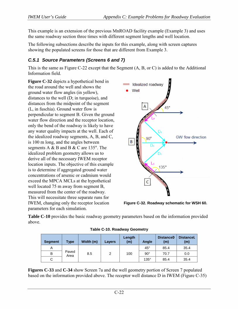
IWEM User’s Guide Appendix C: Example Problems for Roadway Evaluation
C-22
This example is an extension of the previous MnROAD facility example (Example 3) and uses the same roadway section three times with different segment lengths and well location.
The following subsections describe the inputs for this example, along with screen captures showing the populated screens for those that are different from Example 3.
C.5.1 Source Parameters (Screens 6 and 7) This is the same as Figure C-22 except that the Segment (A, B, or C) is added to the Additional Information field.
Figure C-32 depicts a hypothetical bend in the road around the well and shows the ground water flow angles (in yellow), distances to the well (D; in turquoise), and distances from the midpoint of the segment (L, in fuschia). Ground water flow is perpendicular to segment B. Given the ground water flow direction and the receptor location, only the bend of the roadway is likely to have any water quality impacts at the well. Each of the idealized roadway segments, A, B, and C, is 100 m long, and the angles between segments A & B and B & C are 135°. The idealized problem geometry allows us to derive all of the necessary IWEM receptor location inputs. The objective of this example is to determine if aggregated ground water concentrations of arsenic or cadmium would exceed the MPCA MCLs at the hypothetical well located 75 m away from segment B, measured from the center of the roadway. This will necessitate three separate runs for IWEM, changing only the receptor location parameters for each simulation.
Table C-10 provides the basic roadway geometry parameters based on the information provided above.
Table C-10. Roadway Geometry
Segment Type Width (m) Layers Length
(m) Angle DistanceD
(m) DistanceL
(m)
A Paved Area 8.5 2 100
45° 85.4 35.4 B 90° 70.7 0.0 C 135° 85.4 35.4
Figures C-33 and C-34 show Screen 7a and the well geometry portion of Screen 7 populated based on the information provided above. The receptor well distance D in IWEM (Figure C-35)
Figure C-32. Roadway schematic for WSH 60.
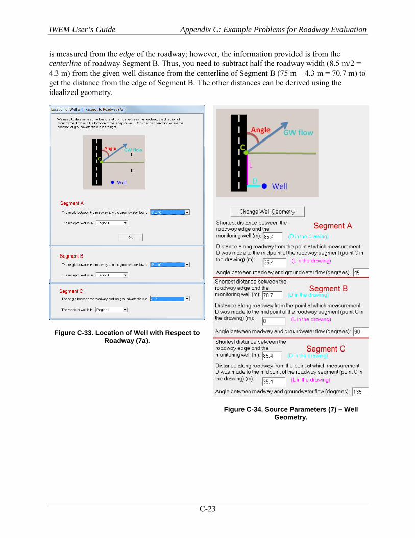
IWEM User’s Guide Appendix C: Example Problems for Roadway Evaluation
C-23
is measured from the edge of the roadway; however, the information provided is from the centerline of roadway Segment B. Thus, you need to subtract half the roadway width (8.5 m/2 = 4.3 m) from the given well distance from the centerline of Segment B (75 m – 4.3 m = 70.7 m) to get the distance from the edge of Segment B. The other distances can be derived using the idealized geometry.
Figure C-33. Location of Well with Respect to Roadway (7a).
Figure C-34. Source Parameters (7) – Well Geometry.
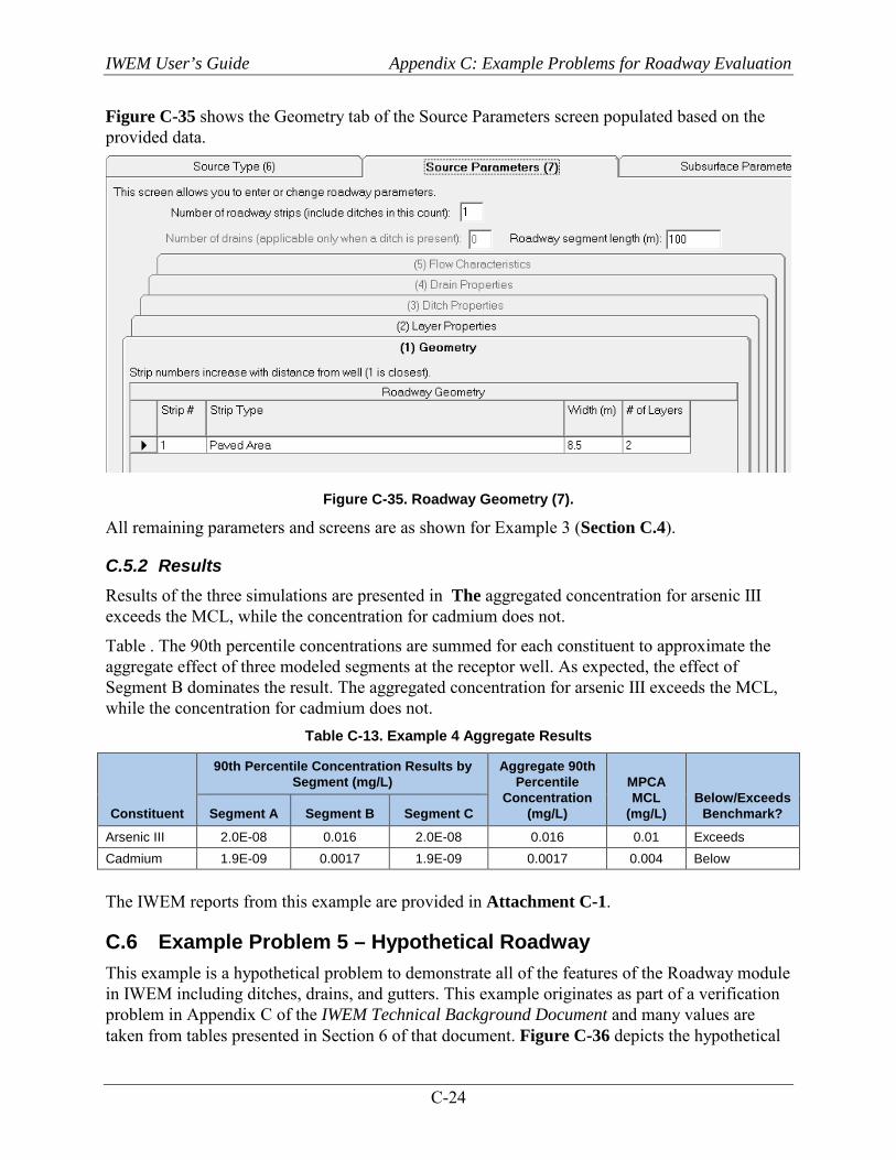
IWEM User’s Guide Appendix C: Example Problems for Roadway Evaluation
C-24
Figure C-35 shows the Geometry tab of the Source Parameters screen populated based on the provided data.
Figure C-35. Roadway Geometry (7).
All remaining parameters and screens are as shown for Example 3 (Section C.4).
C.5.2 Results Results of the three simulations are presented in The aggregated concentration for arsenic III exceeds the MCL, while the concentration for cadmium does not.
Table . The 90th percentile concentrations are summed for each constituent to approximate the aggregate effect of three modeled segments at the receptor well. As expected, the effect of Segment B dominates the result. The aggregated concentration for arsenic III exceeds the MCL, while the concentration for cadmium does not.
Table C-13. Example 4 Aggregate Results
Constituent
90th Percentile Concentration Results by Segment (mg/L)
Aggregate 90th Percentile
Concentration (mg/L)
MPCA MCL
(mg/L) Below/Exceeds
Benchmark? Segment A Segment B Segment C
Arsenic III 2.0E-08 0.016 2.0E-08 0.016 0.01 Exceeds Cadmium 1.9E-09 0.0017 1.9E-09 0.0017 0.004 Below
The IWEM reports from this example are provided in Attachment C-1.
C.6 Example Problem 5 – Hypothetical Roadway This example is a hypothetical problem to demonstrate all of the features of the Roadway module in IWEM including ditches, drains, and gutters. This example originates as part of a verification problem in Appendix C of the IWEM Technical Background Document and many values are taken from tables presented in Section 6 of that document. Figure C-36 depicts the hypothetical

IWEM User’s Guide Appendix C: Example Problems for Roadway Evaluation
C-25
roadway cross-section of nine strips and as many as three non-drainage layers. Other features included are two ditches, two drains, two gutters, and surface runoff. The objective of this example is to familiarize you with the various options available for simulating a more complex roadway scenario.
Figure C-36. Cross Section of a Roadway Segment in Verification Case 4 with Two Symmetric Drainage Systems [not to scale]
The following subsections describe the inputs for this example, along with screen captures showing the populated screens.
C.6.1 Source Parameters (Screens 6 and 7) Figure C-37 shows the facility identification information for this example.
Figure C-37. Source Type (6).
Figure C-38 shows the layout of the well and road. The well is 30.5 m down gradient from the roadway edge, and located at the midpoint of the roadway segment. Groundwater flow is perpendicular to the roadway.
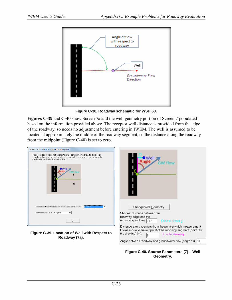
IWEM User’s Guide Appendix C: Example Problems for Roadway Evaluation
C-26
Figure C-38. Roadway schematic for WSH 60.
Figures C-39 and C-40 show Screen 7a and the well geometry portion of Screen 7 populated based on the information provided above. The receptor well distance is provided from the edge of the roadway, so needs no adjustment before entering in IWEM. The well is assumed to be located at approximately the middle of the roadway segment, so the distance along the roadway from the midpoint (Figure C-40) is set to zero.
Figure C-39. Location of Well with Respect to Roadway (7a).
Figure C-40. Source Parameters (7) – Well Geometry.
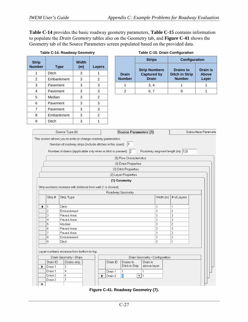
IWEM User’s Guide Appendix C: Example Problems for Roadway Evaluation
C-27
Table C-14 provides the basic roadway geometry parameters, Table C-15 contains information to populate the Drain Geometry tables also on the Geometry tab, and Figure C-41 shows the Geometry tab of the Source Parameters screen populated based on the provided data.
Table C-14. Roadway Geometry Table C-15. Drain Configuration
Strip Number Type
Width (m) Layers
Drain Number
Strips Configuration
Strip Numbers Captured by
Drain
Drains to Ditch in Strip
Number
Drain is Above Layer
1 Ditch 3 1 2 Embankment 3 2 3 Pavement 3 3 1 3, 4 1 1 4 Pavement 3 3 2 6, 7 9 1 5 Median 3 2 6 Pavement 3 3 7 Pavement 3 3 8 Embankment 3 2 9 Ditch 3 1
Figure C-41. Roadway Geometry (7).
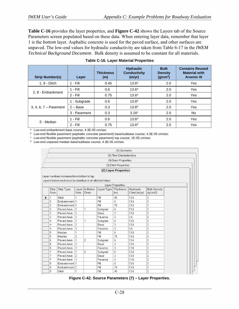
IWEM User’s Guide Appendix C: Example Problems for Roadway Evaluation
C-28
Table C-16 provides the layer properties, and Figure C-42 shows the Layers tab of the Source Parameters screen populated based on these data. When entering layer data, remember that layer 1 is the bottom layer. Asphaltic concrete is used for the paved surface, and other surfaces are unpaved. The low-end values for hydraulic conductivity are taken from Table 6-17 in the IWEM Technical Background Document. Bulk density is assumed to be constant for all materials.
Table C-16. Layer Material Properties
Strip Number(s) Layer Thickness
(m)
Hydraulic Conductivity
(m/yr)
Bulk Density (g/cm3)
Contains Reused Material with
Arsenic III
1, 9 - Ditch 1 - Fill 0.45 13.6a 2.0 Yes
2, 8 - Embankment 1 - Fill 0.6 13.6a 2.0 Yes 2 - Fill 0.75 13.6a 2.0 Yes
3, 4, 6, 7 – Pavement 1 - Subgrade 0.6 13.6b 2.0 Yes 2 – Base 0.3 13.6b 2.0 Yes 3 - Pavement 0.3 3.16c 2.0 No
5 - Median 1 - Fill 0.6 13.6d 2.0 Yes 2 - Fill 0.75 13.6d 2.0 Yes
a Low-end embankment base course; 4.3E-05 cm/sec b Low-end flexible pavement (asphaltic concrete pavement) base/subbase course; 4.3E-05 cm/sec c Low-end flexible pavement (asphaltic concrete pavement) top course; 1E-05 cm/sec d Low-end unpaved median base/subbase course; 4.3E-05 cm/sec
Figure C-42. Source Parameters (7) – Layer Properties.
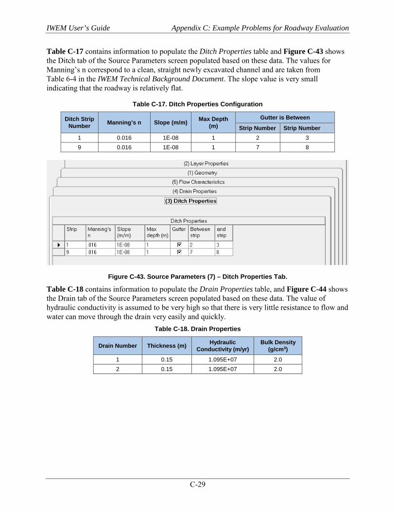
IWEM User’s Guide Appendix C: Example Problems for Roadway Evaluation
C-29
Table C-17 contains information to populate the Ditch Properties table and Figure C-43 shows the Ditch tab of the Source Parameters screen populated based on these data. The values for Manning’s n correspond to a clean, straight newly excavated channel and are taken from Table 6-4 in the IWEM Technical Background Document. The slope value is very small indicating that the roadway is relatively flat.
Table C-17. Ditch Properties Configuration
Ditch Strip Number Manning’s n Slope (m/m) Max Depth
(m) Gutter is Between
Strip Number Strip Number 1 0.016 1E-08 1 2 3 9 0.016 1E-08 1 7 8
Figure C-43. Source Parameters (7) – Ditch Properties Tab.
Table C-18 contains information to populate the Drain Properties table, and Figure C-44 shows the Drain tab of the Source Parameters screen populated based on these data. The value of hydraulic conductivity is assumed to be very high so that there is very little resistance to flow and water can move through the drain very easily and quickly.
Table C-18. Drain Properties
Drain Number Thickness (m) Hydraulic Conductivity (m/yr)
Bulk Density (g/cm3)
1 0.15 1.095E+07 2.0 2 0.15 1.095E+07 2.0

IWEM User’s Guide Appendix C: Example Problems for Roadway Evaluation
C-30
Figure C-44. Source Parameters (7) – Drain Properties Tab.
Table C-19 contains information to populate the Flow Characteristics table, and Figure C-45 shows the Flow tab of the Source Parameters screen populated based on these data. These values define how much runoff reaches a ditch and how much vertical flow through the strips underlain by drains is diverted to ditches. Runoff that does not reach a ditch is diverted by the gutter. The values were chosen arbitrarily. Finally, the arrows above the roadway in Figure C-36 indicate the direction and contributions of runoff from the roadway.
Table C-19. Flow Characteristics
Item Information Value (%)
Ditch Strip 1 Percent of runoff that
reaches this ditch
50
Ditch Strip 9 50
Drain 1 Percent of flow
through this drain that
reaches the ditch
50
Drain 2 50
Ditch Strip 1 Strips providing runoff to ditch
2, 3, 4, 5 Ditch Strip 9 6, 7, 8
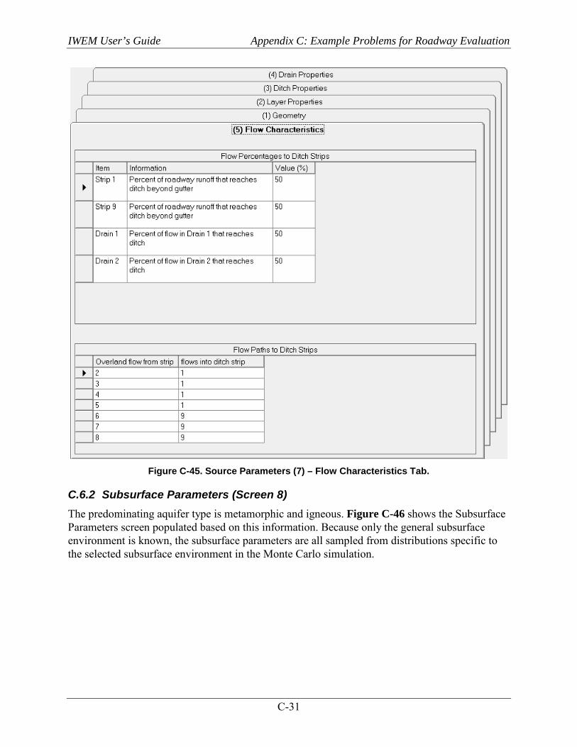
IWEM User’s Guide Appendix C: Example Problems for Roadway Evaluation
C-31
Figure C-45. Source Parameters (7) – Flow Characteristics Tab.
C.6.2 Subsurface Parameters (Screen 8) The predominating aquifer type is metamorphic and igneous. Figure C-46 shows the Subsurface Parameters screen populated based on this information. Because only the general subsurface environment is known, the subsurface parameters are all sampled from distributions specific to the selected subsurface environment in the Monte Carlo simulation.

IWEM User’s Guide Appendix C: Example Problems for Roadway Evaluation
C-32
Figure C-46. Subsurface Parameters (8).
C.6.3 Infiltration Parameters (Screen 9) Medium-grained soils are prevalent around the site. The site is located in Boston, MA. Table C-20 contains values used for infiltration, runoff, precipitation, and evaporation rates. Using Figure 6-7 from the IWEM Technical Background Document, Boston is located in climatic zone A1. Montpelier, VT was selected as the representative location for that zone and all rates in Table C-20 correspond to Montpelier, VT. A single rate was selected for each water flux type. The infiltration and runoff rates correspond to the low-end value for asphaltic concrete pavement. Evaporation rates are pan evaporation.
Table C-20. Rates for Infiltration, Runoff, Precipitation and Evaporation
Rate Value (m/yr) Table in TBD
Infiltration 0.12 6-18 Runoff 0.60 6-21
Precipitation 0.88 6-16 Evaporation 0.57 6-25
Figure C-47 shows the Infiltration screen populated based on this information. The recharge rate is calculated for Boston, MA, and medium-grained soils.
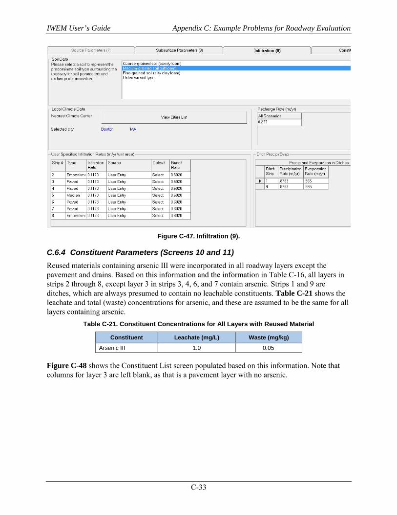
IWEM User’s Guide Appendix C: Example Problems for Roadway Evaluation
C-33
Figure C-47. Infiltration (9).
C.6.4 Constituent Parameters (Screens 10 and 11) Reused materials containing arsenic III were incorporated in all roadway layers except the pavement and drains. Based on this information and the information in Table C-16, all layers in strips 2 through 8, except layer 3 in strips 3, 4, 6, and 7 contain arsenic. Strips 1 and 9 are ditches, which are always presumed to contain no leachable constituents. Table C-21 shows the leachate and total (waste) concentrations for arsenic, and these are assumed to be the same for all layers containing arsenic.
Table C-21. Constituent Concentrations for All Layers with Reused Material
Constituent Leachate (mg/L) Waste (mg/kg)
Arsenic III 1.0 0.05
Figure C-48 shows the Constituent List screen populated based on this information. Note that columns for layer 3 are left blank, as that is a pavement layer with no arsenic.
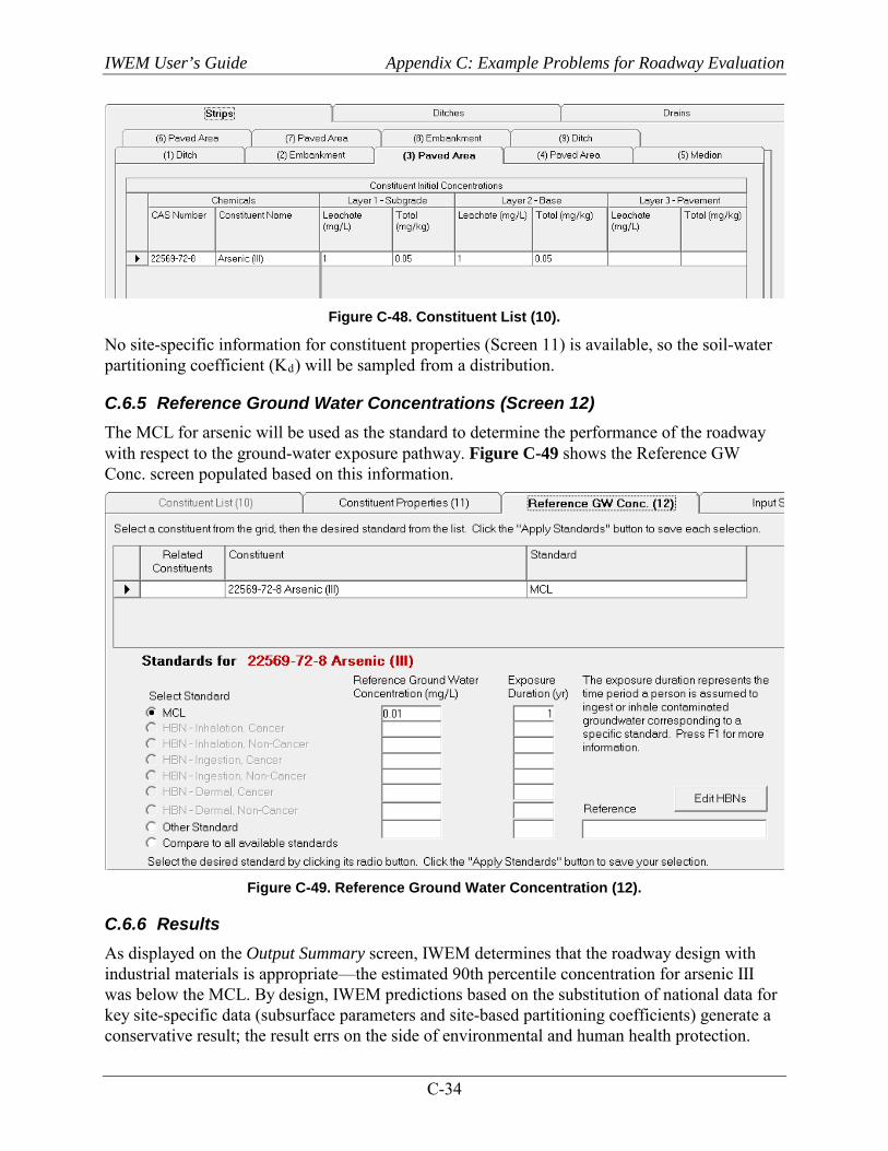
IWEM User’s Guide Appendix C: Example Problems for Roadway Evaluation
C-34
Figure C-48. Constituent List (10).
No site-specific information for constituent properties (Screen 11) is available, so the soil-water partitioning coefficient (Kd) will be sampled from a distribution.
C.6.5 Reference Ground Water Concentrations (Screen 12) The MCL for arsenic will be used as the standard to determine the performance of the roadway with respect to the ground-water exposure pathway. Figure C-49 shows the Reference GW Conc. screen populated based on this information.
Figure C-49. Reference Ground Water Concentration (12).
C.6.6 Results As displayed on the Output Summary screen, IWEM determines that the roadway design with industrial materials is appropriate—the estimated 90th percentile concentration for arsenic III was below the MCL. By design, IWEM predictions based on the substitution of national data for key site-specific data (subsurface parameters and site-based partitioning coefficients) generate a conservative result; the result errs on the side of environmental and human health protection.

IWEM User’s Guide Appendix C: Example Problems for Roadway Evaluation
C-35
The IWEM reports from this example are provided in Attachment C-1.
C.7 References
O’Donnell, J.B. 2009. Leaching of Trace Elements from Roadway Materials Stabilized with Fly Ash – Madison. Master’s thesis, University of Wisconsin-Madison.
U.S. EPA (Environmental Protection Agency). 2014. Industrial Waste Evaluation Model (IWEM) v3.1 Technical Documentation. Draft. Office of Resource Conservation and Recovery, Washington DC.
WAC. 2006. Wisconsin Administrative Code, Chapter NR 538.06(3). Industrial Byproduct Characterization.
Wen, H. 2008. MnROAD High Carbon Fly Ash Research Project. Annual Report Submitted to Minnesota Pollution Control Agency: Mn/DOT Office of Materials, 1400 Gervais Avenue, Maplewood, MN 55190. July 11. Available at http://www.mrr.dot.state.mn.us/research/pdf/2008MRRDOC026.pdf.

IWEM User’s Guide Appendix C: Example Problems for Roadway Evaluation
C-36
[This page intentionally left blank.]
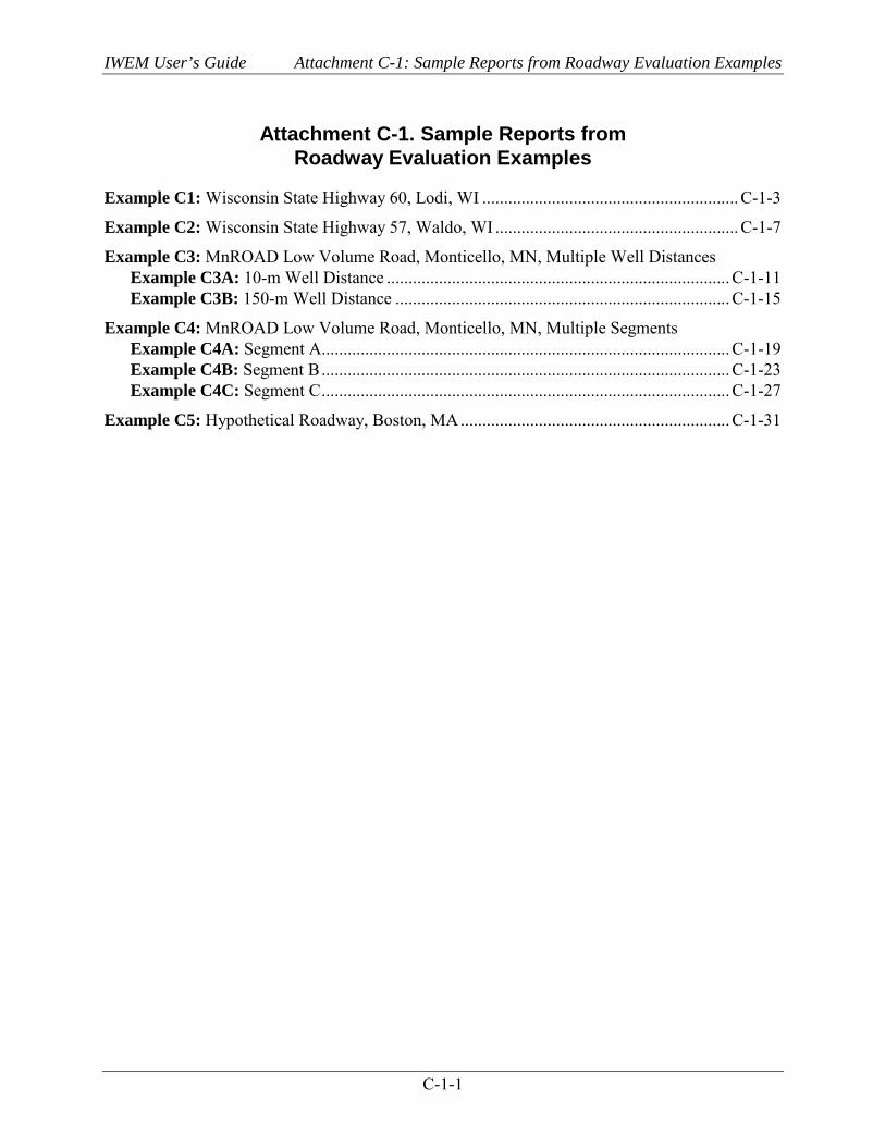
IWEM User’s Guide Attachment C-1: Sample Reports from Roadway Evaluation Examples
C-1-1
Attachment C-1. Sample Reports from Roadway Evaluation Examples
Example C1: Wisconsin State Highway 60, Lodi, WI ........................................................... C-1-3
Example C2: Wisconsin State Highway 57, Waldo, WI ........................................................ C-1-7
Example C3: MnROAD Low Volume Road, Monticello, MN, Multiple Well Distances Example C3A: 10-m Well Distance ............................................................................... C-1-11 Example C3B: 150-m Well Distance ............................................................................. C-1-15
Example C4: MnROAD Low Volume Road, Monticello, MN, Multiple Segments Example C4A: Segment A.............................................................................................. C-1-19 Example C4B: Segment B .............................................................................................. C-1-23 Example C4C: Segment C .............................................................................................. C-1-27
Example C5: Hypothetical Roadway, Boston, MA .............................................................. C-1-31

IWEM User’s Guide Attachment C-1: Sample Reports from Roadway Evaluation Examples
C-1-2
[This page intentionally left blank.]

IWEM User’s Guide Sample Report for Example C1, Wisconsin State Highway 60, Lodi, WI
C-1-3
Example C1. Wisconsin State Highway 60, Lodi, WI (page 1 of 4)
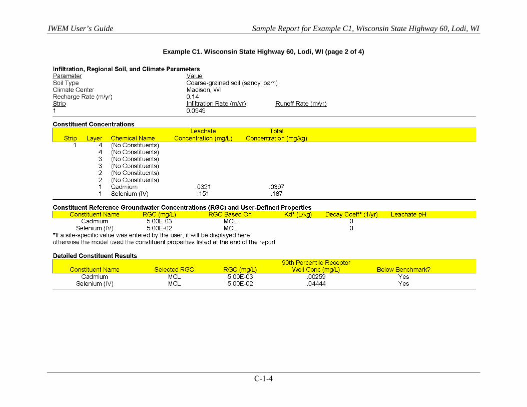
IWEM User’s Guide Sample Report for Example C1, Wisconsin State Highway 60, Lodi, WI
C-1-4
Example C1. Wisconsin State Highway 60, Lodi, WI (page 2 of 4)
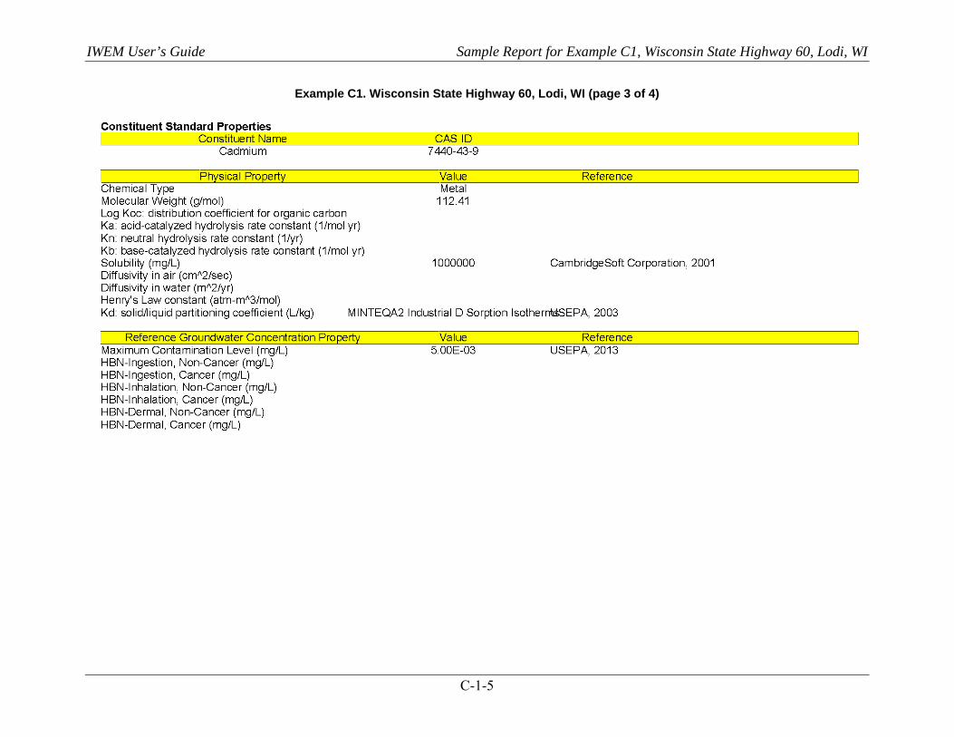
IWEM User’s Guide Sample Report for Example C1, Wisconsin State Highway 60, Lodi, WI
C-1-5
Example C1. Wisconsin State Highway 60, Lodi, WI (page 3 of 4)
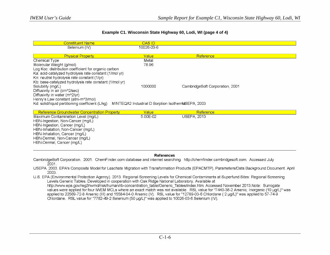
IWEM User’s Guide Sample Report for Example C1, Wisconsin State Highway 60, Lodi, WI
C-1-6
Example C1. Wisconsin State Highway 60, Lodi, WI (page 4 of 4)
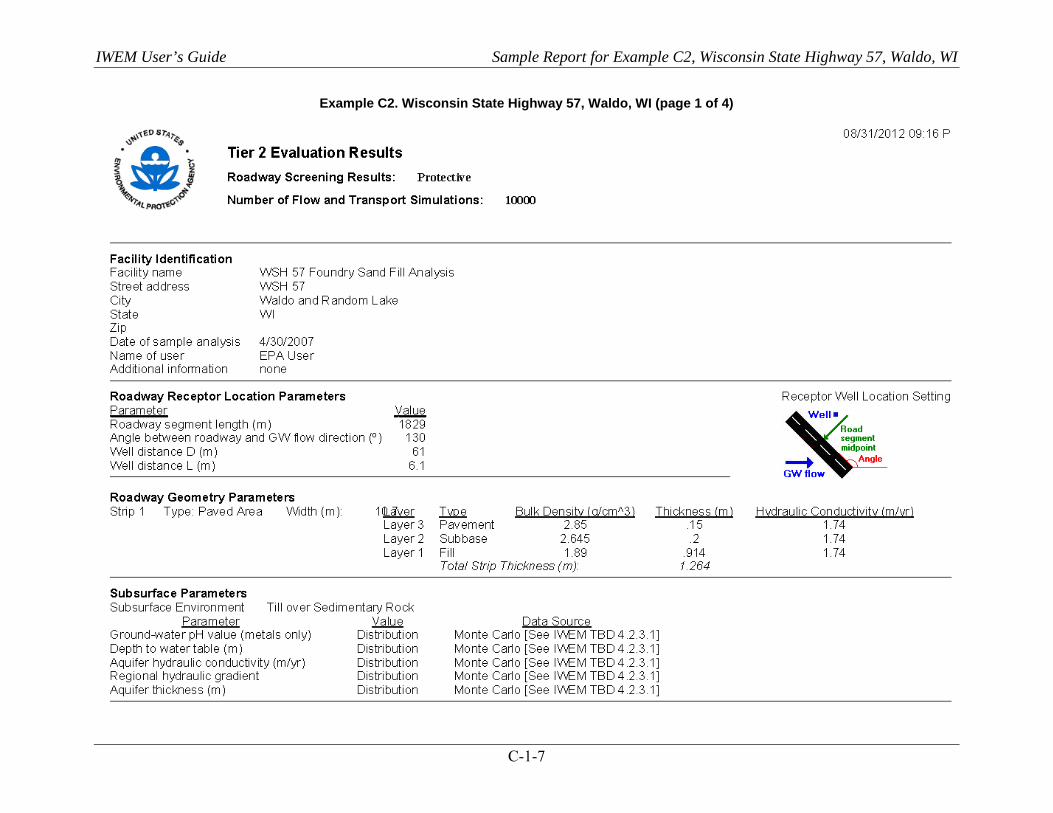
IWEM User’s Guide Sample Report for Example C2, Wisconsin State Highway 57, Waldo, WI
C-1-7
Example C2. Wisconsin State Highway 57, Waldo, WI (page 1 of 4)

IWEM User’s Guide Sample Report for Example C2, Wisconsin State Highway 57, Waldo, WI
C-1-8
Example C2. Wisconsin State Highway 57, Waldo, WI (page 2 of 4)
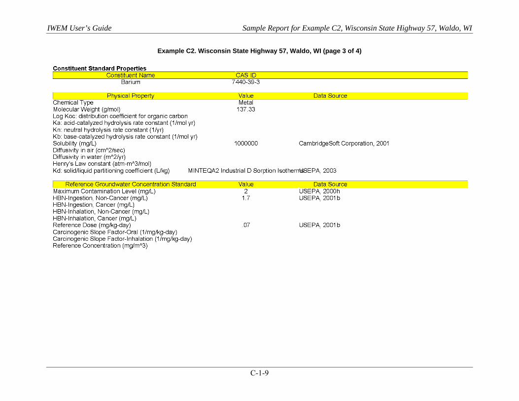
IWEM User’s Guide Sample Report for Example C2, Wisconsin State Highway 57, Waldo, WI
C-1-9
Example C2. Wisconsin State Highway 57, Waldo, WI (page 3 of 4)
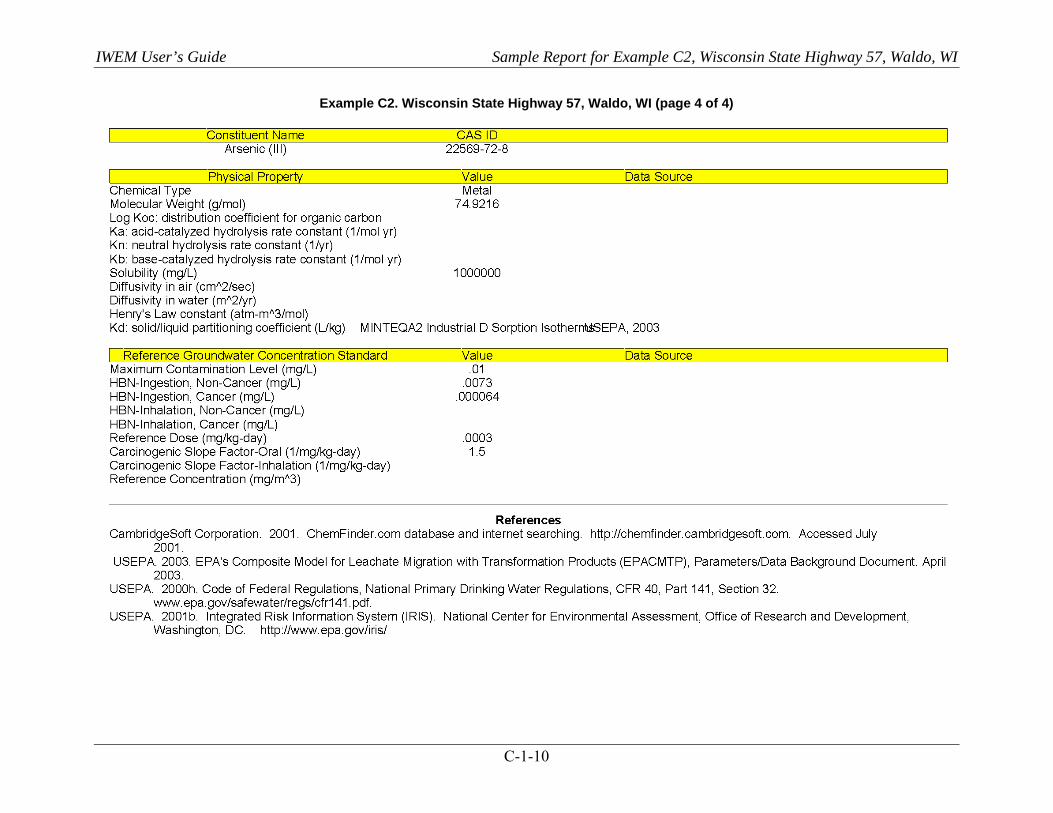
IWEM User’s Guide Sample Report for Example C2, Wisconsin State Highway 57, Waldo, WI
C-1-10
Example C2. Wisconsin State Highway 57, Waldo, WI (page 4 of 4)
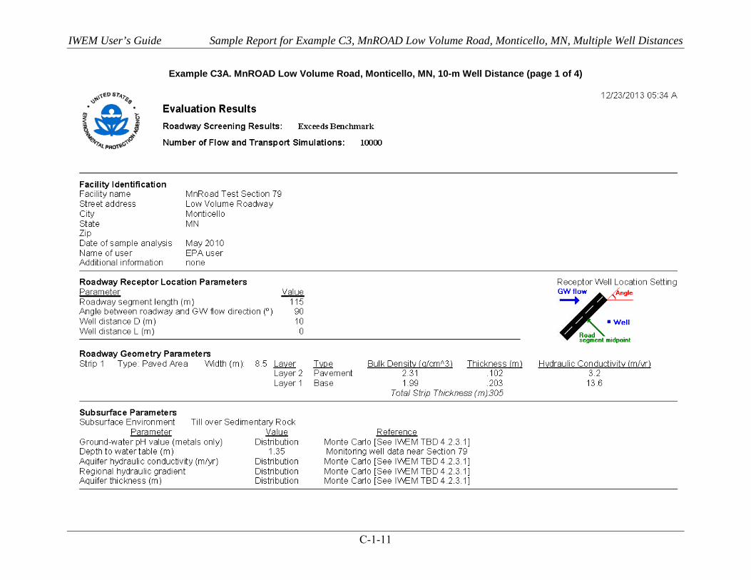
IWEM User’s Guide Sample Report for Example C3, MnROAD Low Volume Road, Monticello, MN, Multiple Well Distances
C-1-11
Example C3A. MnROAD Low Volume Road, Monticello, MN, 10-m Well Distance (page 1 of 4)
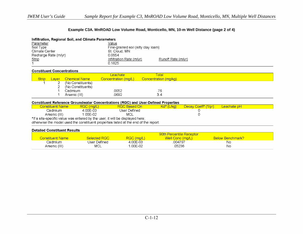
IWEM User’s Guide Sample Report for Example C3, MnROAD Low Volume Road, Monticello, MN, Multiple Well Distances
C-1-12
Example C3A. MnROAD Low Volume Road, Monticello, MN, 10-m Well Distance (page 2 of 4)
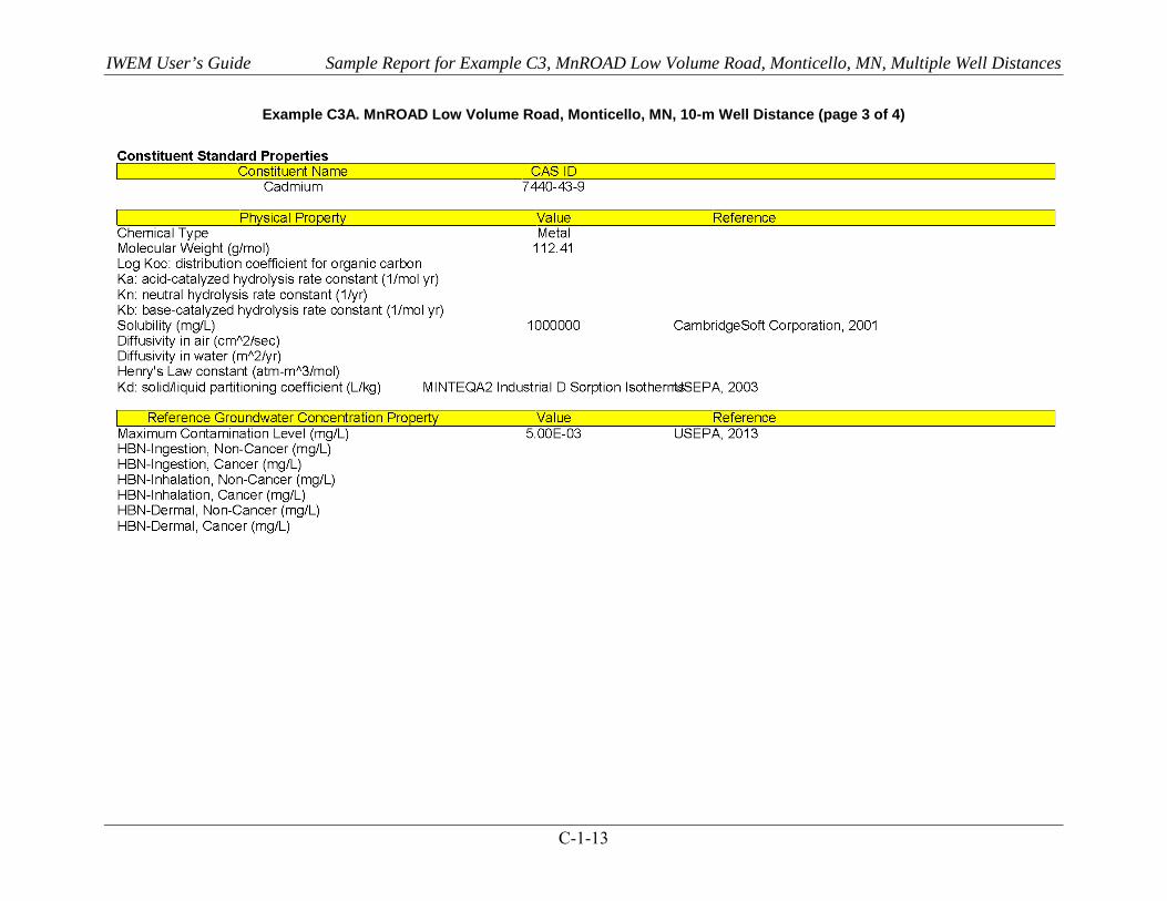
IWEM User’s Guide Sample Report for Example C3, MnROAD Low Volume Road, Monticello, MN, Multiple Well Distances
C-1-13
Example C3A. MnROAD Low Volume Road, Monticello, MN, 10-m Well Distance (page 3 of 4)
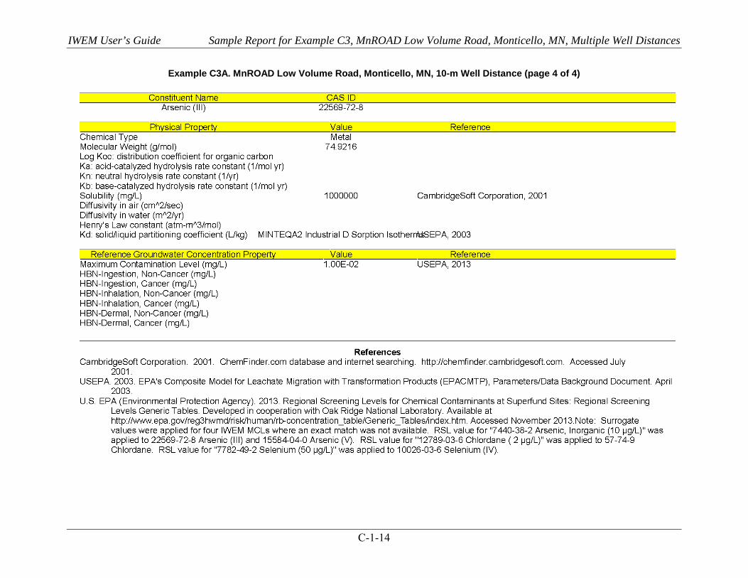
IWEM User’s Guide Sample Report for Example C3, MnROAD Low Volume Road, Monticello, MN, Multiple Well Distances
C-1-14
Example C3A. MnROAD Low Volume Road, Monticello, MN, 10-m Well Distance (page 4 of 4)
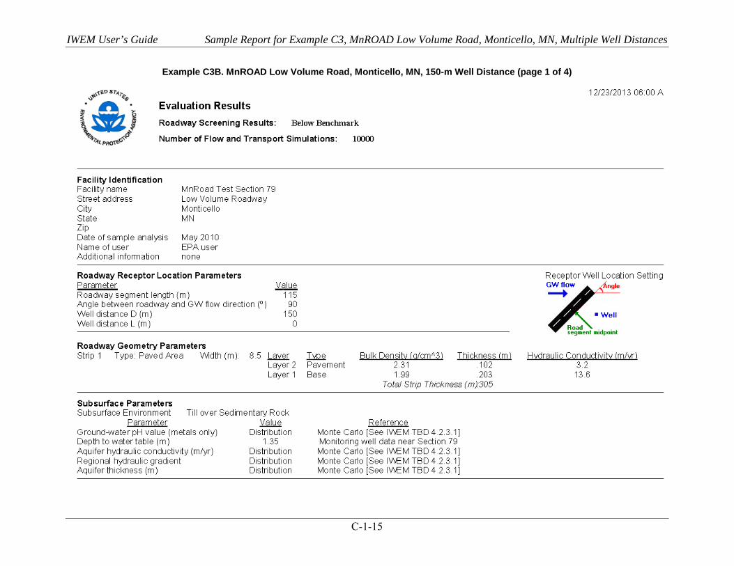
IWEM User’s Guide Sample Report for Example C3, MnROAD Low Volume Road, Monticello, MN, Multiple Well Distances
C-1-15
Example C3B. MnROAD Low Volume Road, Monticello, MN, 150-m Well Distance (page 1 of 4)
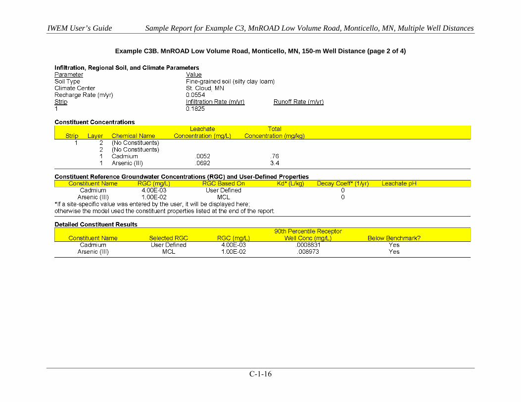
IWEM User’s Guide Sample Report for Example C3, MnROAD Low Volume Road, Monticello, MN, Multiple Well Distances
C-1-16
Example C3B. MnROAD Low Volume Road, Monticello, MN, 150-m Well Distance (page 2 of 4)

IWEM User’s Guide Sample Report for Example C3, MnROAD Low Volume Road, Monticello, MN, Multiple Well Distances
C-1-17
Example C3B. MnROAD Low Volume Road, Monticello, MN, 150-m Well Distance (page 3 of 4)
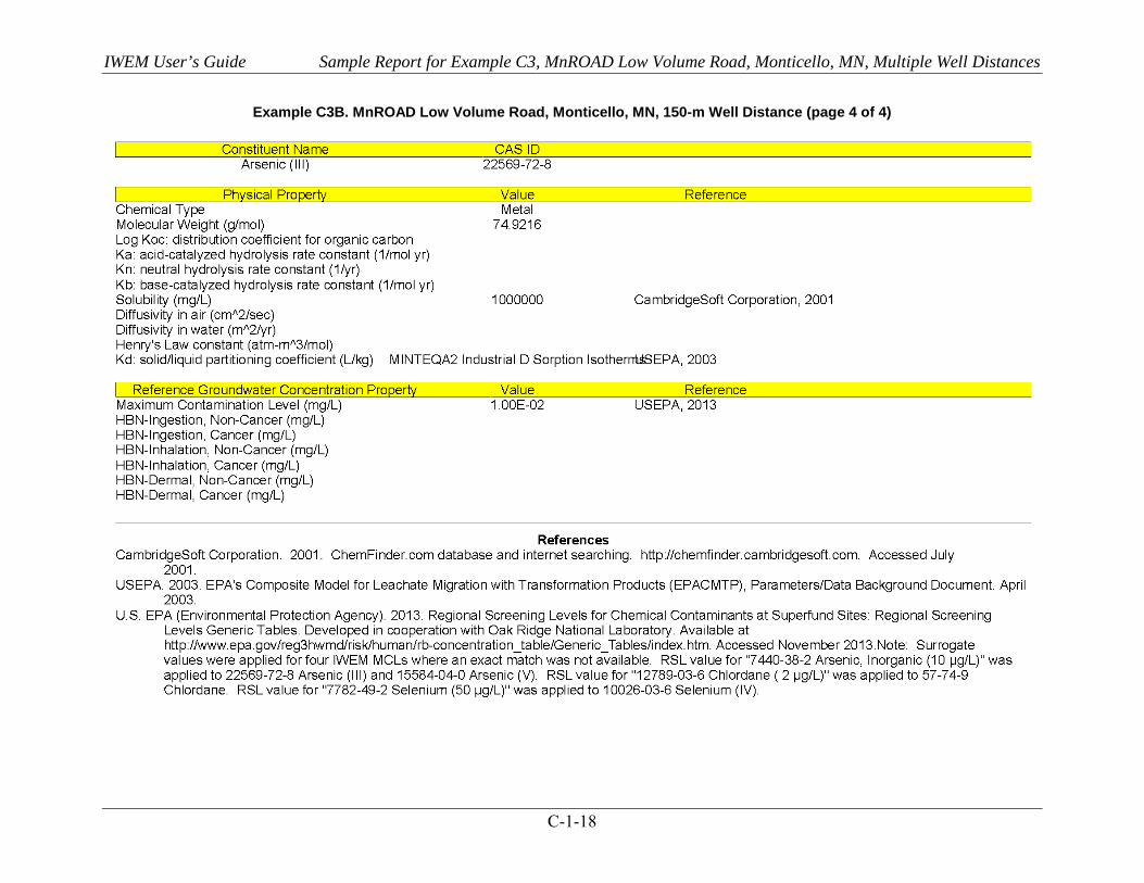
IWEM User’s Guide Sample Report for Example C3, MnROAD Low Volume Road, Monticello, MN, Multiple Well Distances
C-1-18
Example C3B. MnROAD Low Volume Road, Monticello, MN, 150-m Well Distance (page 4 of 4)
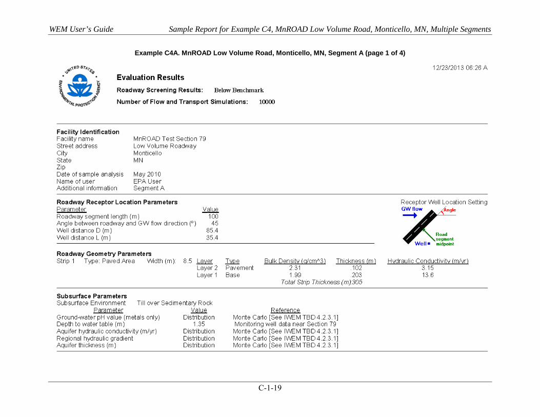
WEM User’s Guide Sample Report for Example C4, MnROAD Low Volume Road, Monticello, MN, Multiple Segments
C-1-19
Example C4A. MnROAD Low Volume Road, Monticello, MN, Segment A (page 1 of 4)
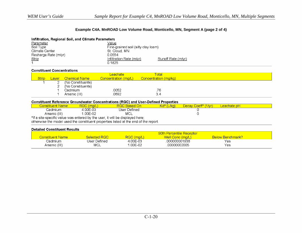
WEM User’s Guide Sample Report for Example C4, MnROAD Low Volume Road, Monticello, MN, Multiple Segments
C-1-20
Example C4A. MnROAD Low Volume Road, Monticello, MN, Segment A (page 2 of 4)
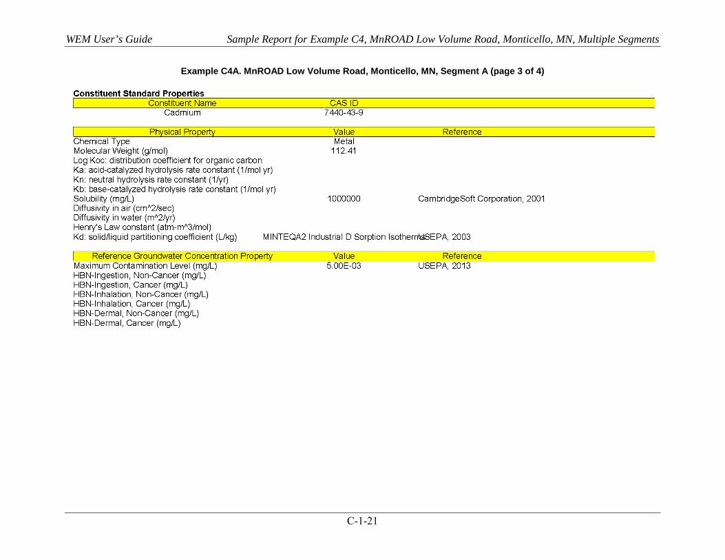
WEM User’s Guide Sample Report for Example C4, MnROAD Low Volume Road, Monticello, MN, Multiple Segments
C-1-21
Example C4A. MnROAD Low Volume Road, Monticello, MN, Segment A (page 3 of 4)

WEM User’s Guide Sample Report for Example C4, MnROAD Low Volume Road, Monticello, MN, Multiple Segments
C-1-22
Example C4A. MnROAD Low Volume Road, Monticello, MN, Segment A (page 4 of 4)

WEM User’s Guide Sample Report for Example C4, MnROAD Low Volume Road, Monticello, MN, Multiple Segments
C-1-23
Example C4B. MnROAD Low Volume Road, Monticello, MN, Segment B (page 1 of 4)
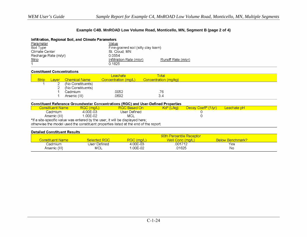
WEM User’s Guide Sample Report for Example C4, MnROAD Low Volume Road, Monticello, MN, Multiple Segments
C-1-24
Example C4B. MnROAD Low Volume Road, Monticello, MN, Segment B (page 2 of 4)
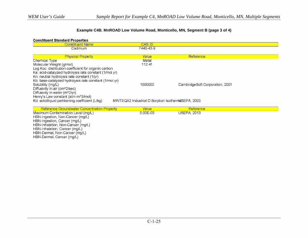
WEM User’s Guide Sample Report for Example C4, MnROAD Low Volume Road, Monticello, MN, Multiple Segments
C-1-25
Example C4B. MnROAD Low Volume Road, Monticello, MN, Segment B (page 3 of 4)
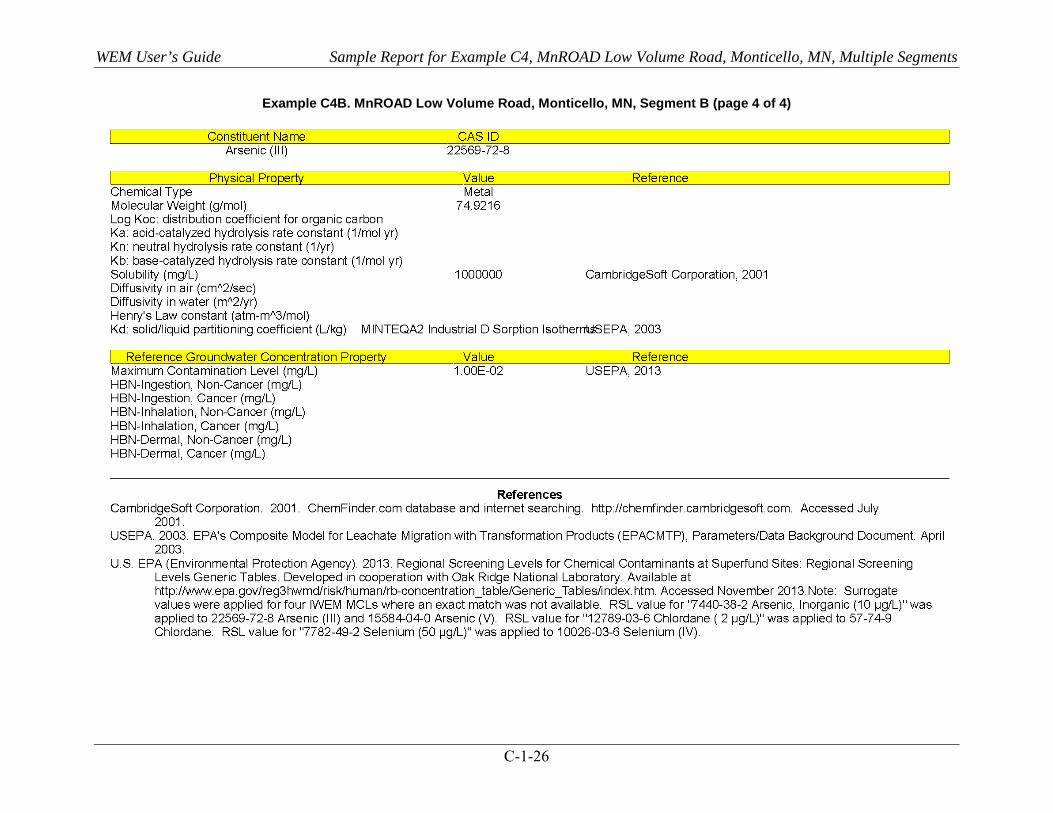
WEM User’s Guide Sample Report for Example C4, MnROAD Low Volume Road, Monticello, MN, Multiple Segments
C-1-26
Example C4B. MnROAD Low Volume Road, Monticello, MN, Segment B (page 4 of 4)
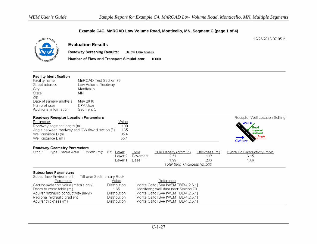
WEM User’s Guide Sample Report for Example C4, MnROAD Low Volume Road, Monticello, MN, Multiple Segments
C-1-27
Example C4C. MnROAD Low Volume Road, Monticello, MN, Segment C (page 1 of 4)
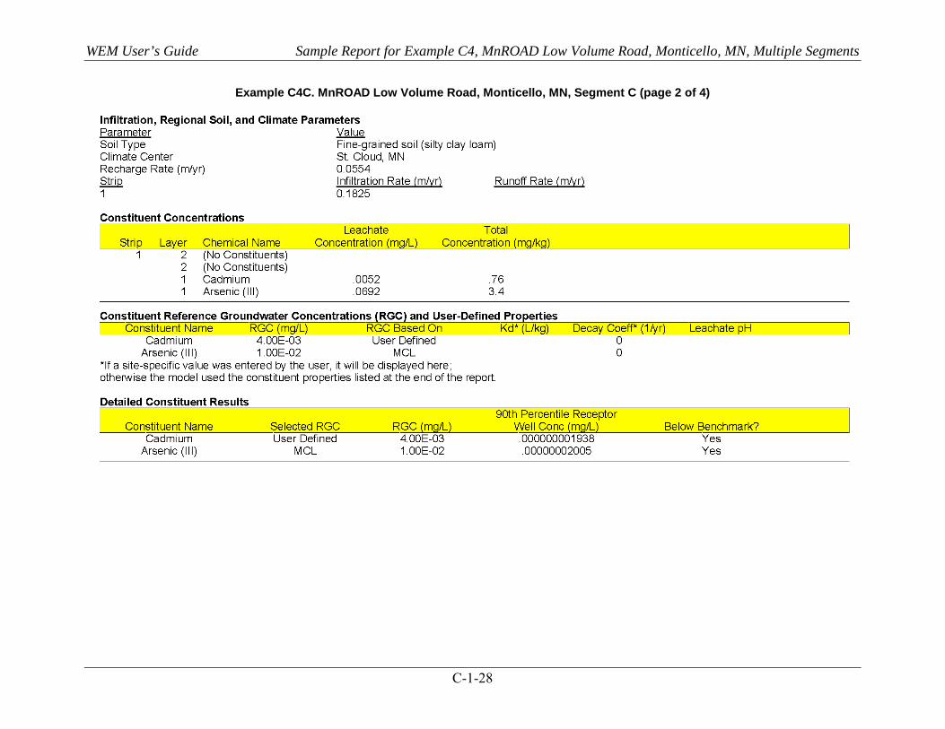
WEM User’s Guide Sample Report for Example C4, MnROAD Low Volume Road, Monticello, MN, Multiple Segments
C-1-28
Example C4C. MnROAD Low Volume Road, Monticello, MN, Segment C (page 2 of 4)
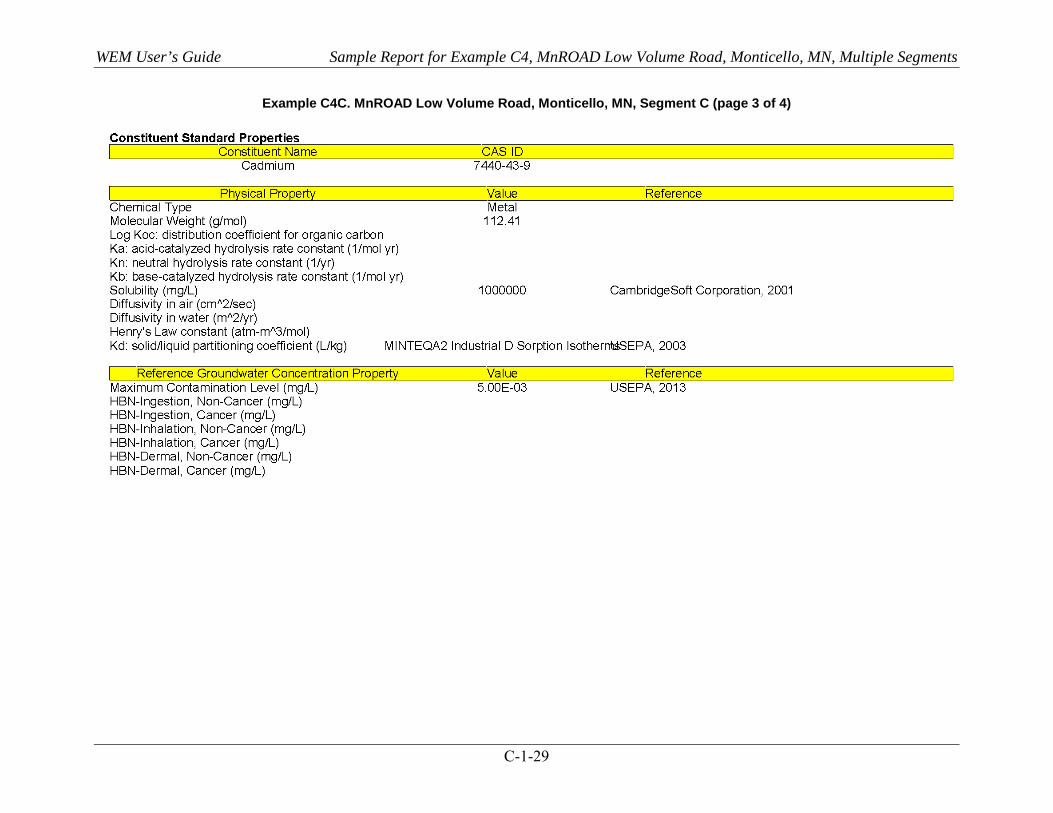
WEM User’s Guide Sample Report for Example C4, MnROAD Low Volume Road, Monticello, MN, Multiple Segments
C-1-29
Example C4C. MnROAD Low Volume Road, Monticello, MN, Segment C (page 3 of 4)
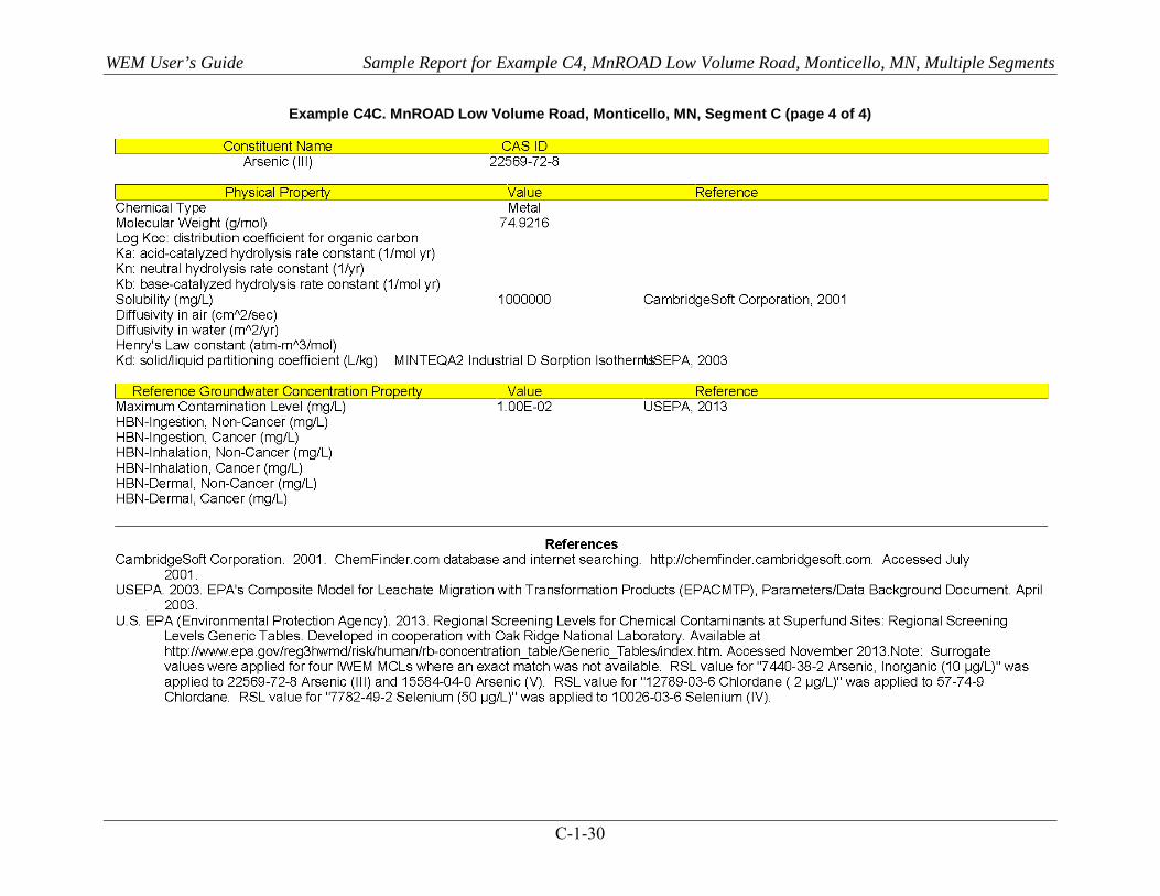
WEM User’s Guide Sample Report for Example C4, MnROAD Low Volume Road, Monticello, MN, Multiple Segments
C-1-30
Example C4C. MnROAD Low Volume Road, Monticello, MN, Segment C (page 4 of 4)
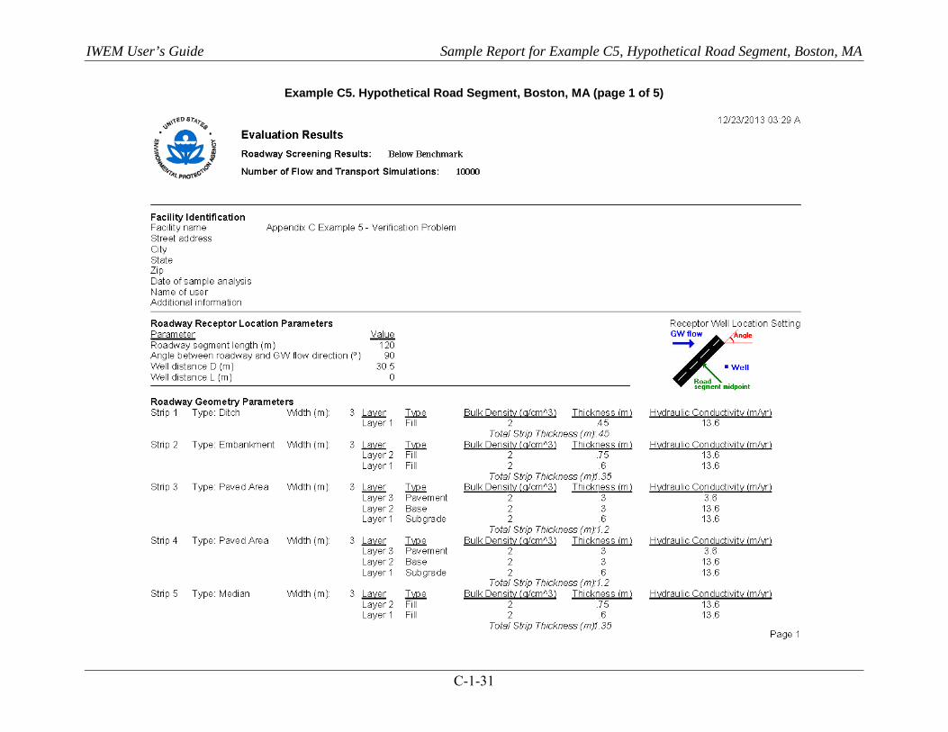
IWEM User’s Guide Sample Report for Example C5, Hypothetical Road Segment, Boston, MA
C-1-31
Example C5. Hypothetical Road Segment, Boston, MA (page 1 of 5)

IWEM User’s Guide Sample Report for Example C5, Hypothetical Road Segment, Boston, MA
C-1-32
Example C5. Hypothetical Road Segment, Boston, MA (page 2 of 5)
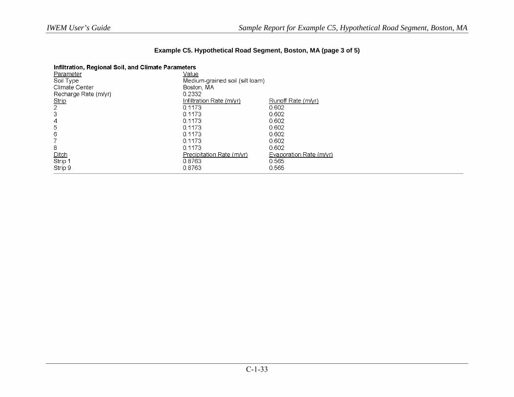
IWEM User’s Guide Sample Report for Example C5, Hypothetical Road Segment, Boston, MA
C-1-33
Example C5. Hypothetical Road Segment, Boston, MA (page 3 of 5)
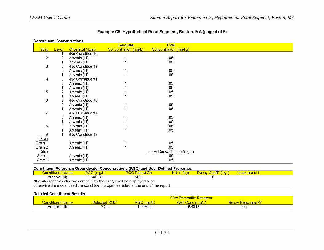
IWEM User’s Guide Sample Report for Example C5, Hypothetical Road Segment, Boston, MA
C-1-34
Example C5. Hypothetical Road Segment, Boston, MA (page 4 of 5)
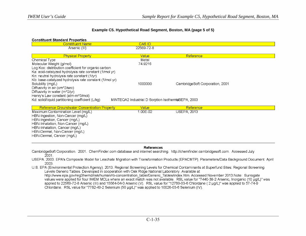
IWEM User’s Guide Sample Report for Example C5, Hypothetical Road Segment, Boston, MA
C-1-35
Example C5. Hypothetical Road Segment, Boston, MA (page 5 of 5)

IWEM User’s Guide Attachment C-1: Sample Reports from Roadway Evaluation Examples
C-1-36
[This page intentionally left blank.]

IWEM User’s Guide Appendix D: Example Problem for Structural Fill Evaluation
D-1
Appendix D: Example Problem for Structural Fill Evaluation
Project files corresponding to this example may be found in either
C:\Users\Public\Documents\IWEM\SampleData\ Appendix_D_Structural_Fill or C:\Users\[your user name]\Documents\IWEM\SampleData\ Appendix_
D_Structural_Fill.
D.1 Landscape Alteration Using Coal Ash as Compacted Fill Material This example was adapted and modified from the (EPRI, 1990) and evaluates an area near an industrial park north west of Minneapolis, MN, where ash fill is used to level an undeveloped section of the park. The area is approximately 15,000 m2 and was excavated to remove desirable soils for other uses. In order to prepare the site for possible future development, the area needed to be leveled. The excavated area was filled with about 40,000 m3 of coal ash from nearby coal-fired electrical generation stations over a two year period. Most of the ash fill, which has a fairly uniform thickness of 1.5–2.1 m after compaction, is covered by a thin layer of topsoil which aids in sustaining vegetation and preventing erosion.
The regional geology is dominated by a glacial end moraine. The surficial geology in the vicinity of the site is comprised of an undulating glacial outwash plain made up of mainly fine sand. Borings indicate that the surface stratum consists of light brown sandy loam and that the water table was approximately 4 m below ground surface beneath the fill area, and 2.1 m beneath the ash fill. Groundwater monitoring provides water table elevation in and around the site to establish an estimate of hydraulic gradient.
Physical properties of the ash and underlying soils were ascertained through laboratory test methods. Leaching concentrations were derived from lysimeters installed in the ash fill. Total concentrations were obtained from laboratory tests. The primary constituents of considered in this exercise are barium and molybdenum. The screening levels will be detection limits for both constituents. The following tables summarize the input parameters. No sorption data was available so default MINTEQA2 isotherms will be used. Detection limits will serve as the exposure standard and we assume a 1-year exposure duration. The following parameters were used within the model to define the use scenario (in order of entry):
Source Type: Structural fill Source Parameters:
– Distance to well: 30 m (hypothetical distance to compliance point) – Structural fill depth: 1.8 m (average depth of soil borings) – Structural fill area: 15,000 m2 – Depth of base of SF below ground surface: 1.8 m (fill is level with ground) – Effective bulk density: 1.47 g/cm3 (maximum value obtained in laboratory testing) – Effective hydraulic conductivity: 3.16 m/yr (compacted ash value obtained in
laboratory testing) – Volume fraction occupied by leachable material: 1 m3/m3 (entire fill is coal ash)
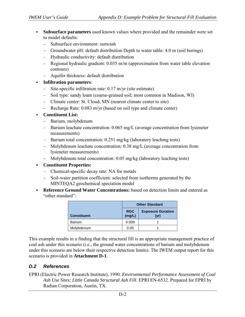
IWEM User’s Guide Appendix D: Example Problem for Structural Fill Evaluation
D-2
Subsurface parameters used known values where provided and the remainder were set to model defaults: – Subsurface environment: outwash – Groundwater pH: default distribution Depth to water table: 4.0 m (soil borings) – Hydraulic conductivity: default distribution – Regional hydraulic gradient: 0.035 m/m (approximation from water table elevation
contours) – Aquifer thickness: default distribution
Infiltration parameters: – Site-specific infiltration rate: 0.17 m/yr (site estimate) – Soil type: sandy loam (coarse-grained soil; most common in Madison, WI) – Climate center: St. Cloud, MN (nearest climate center to site) – Recharge Rate: 0.083 m/yr (based on soil type and climate center)
Constituent List: – Barium, molybdenum – Barium leachate concentration: 0.065 mg/L (average concentration from lysimeter
measurements) – Barium total concentration: 0.251 mg/kg (laboratory leaching tests) – Molybdenum leachate concentration: 0.38 mg/L (average concentration from
lysimeter measurements) – Molybdenum total concentration: 0.05 mg/kg (laboratory leaching tests)
Constituent Properties: – Chemical-specific decay rate: NA for metals – Soil-water partition coefficient: selected from isotherms generated by the
MINTEQA2 geochemical speciation model Reference Ground Water Concentrations: based on detection limits and entered as
“other standard”:
Constituent
Other Standard
RGC (mg/L)
Exposure Duration (yr)
Barium 0.009 1 Molybdenum 0.05 1
This example results in a finding that the structural fill is an appropriate management practice of coal ash under this scenario (i.e., the ground water concentrations of barium and molybdenum under this scenario are below their respective detection limits). The IWEM output report for this scenario is provided in Attachment D-1.
D.2 References EPRI (Electric Power Research Institute), 1990. Environmental Performance Assessment of Coal
Ash Use Sites: Little Canada Structural Ash Fill. EPRI EN-6532. Prepared for EPRI by Radian Corporation, Austin, TX.

IWEM User’s Guide Attachment D-1: Sample Report from Structural Fill Evaluation Example
D-1-1
Attachment D-1. Sample Report from Structural Fill Evaluation Example

IWEM User’s Guide Attachment D-1: Sample Report from Structural Fill Evaluation Example
D-1-2
[This page intentionally left blank.]

IWEM User’s Guide Sample Report from Structural Fill Evaluation Example
D-1-3
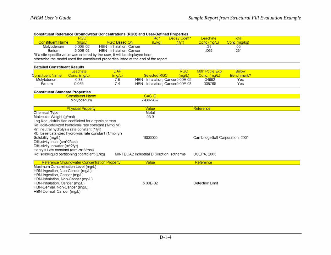
IWEM User’s Guide Sample Report from Structural Fill Evaluation Example
D-1-4

IWEM User’s Guide Sample Report from Structural Fill Evaluation Example
D-1-5