ISSN No. 2454 – 1427 

CDE April 2017

Industry Origins of Economic Growth and Structural Change in India

K L Krishna Email: krishna@econdse.org

Centre for Development Economics, Delhi School of Economics

Abdul Azeez Erumban Email: Abdul. Erumban@conference-board.org

The Conference Board, Brussels, Belgium & Faculty of Economics and Business, University of Groningen, the Netherlands

Deb Kusum Das Department of Economics, Ramjas College, University of Delhi, India

Suresh Aggarwal Department of Business Economics, University of Delhi, South Campus, India

Pilu Chandra Das Dyal Singh College, University of Delhi, New Delhi, India

Working Paper No. 273 http://www.cdedse.org/pdf/work273.pdf

CENTRE FOR DEVELOPMENT ECONOMICS DELHI SCHOOL OF ECONOMICS

DELHI 110007

1

Industry Origins of Economic Growth and Structural Change in India

K L KRISHNA Email: krishna@econdse.org

Centre for Development Economics, Delhi School of Economics

Abdul Azeez Erumban* The Conference Board, Brussels, Belgium & Faculty of Economics and Business,

University of Groningen, the Netherlands Abdul. Erumban@conference-board.org

Deb Kusum das Department of Economics, Ramjas College, University of Delhi, India

Suresh Aggarwal Department of Business Economics, University of Delhi, South Campus, India

Pilu Chandra Das Dyal Singh College, University of Delhi, New Delhi, India

Paper prepared for presentation at the India KLEMS Workshop December, 17, 2015, Delhi School of Economics, New Delhi

Abstract This paper is an attempt to document the evolution of India’s aggregate productivity, decomposed into the contributions of detailed industrial sectors and structural change during 1980-2011. Using the India KLEMS (K = capital, L = labor, E = energy, M = materials, and S = services) database version 2015, which provides comprehensive and consistent industry-level data on Indian economy, we decompose both labor productivity and total factor productivity growth (TFPG) into industry productivity contributions and resource reallocation effects. In general, the impact of static structural change on labor productivity has been positive, as workers moved to sectors of relatively higher labor productivity level. However, no positive dynamic reallocation effects—worker movement to fast growing sectors—have been observed. The industrial pattern of TFPG is not broad based, as several industries have contributed negatively to aggregate productivity growth. While the manufacturing sector did not see significant productivity gains in most part of the 1990s, it did see some revival in the recent years during which the relative importance of services as a major contributor to aggregate TFPG has declined. The structural transformation in India features the absorption of workers moving out of agriculture in the construction sector—a sector that has witnessed substantial deceleration in productivity growth—while employment creation in fast growing services has been slow and in the manufacturing sector rather stagnant. This makes India a unique place in the pattern of structural change, as compared to several of today’s advanced economies. The obvious question is whether India can sustain faster growth in the longer run if it does not focus on developing a solid manufacturing sector.

2

Key words: India; structural change; aggregate productivity growth; labor productivity; total factor productivity; industry origins; reallocation effects; manufacturing JEL classification: D24, L6, F43, O47, O53 ----------------------------------------------------------------------------------------------------- *Corresponding author: abdul.erumban@conference-board.org Views expressed in this paper are those of the authors and do not reflect the views of the organizations they belong to. The usual disclaimers apply.

1. Introduction

India’s GDP growth has increased consistently since the mid-1990s averaging from 6 to 7 percent, and

even reaching 9 to 10 percent in some years in the mid-2000s. There has been many studies discussing

several aspects of this growth process (Das et al., 2016; Bhagwati and Panagariya, 2013; Verma, 2012;

Balakrishnan, 2010; Eichengreen, Gupta & Kumar, 2010; Bosworth & Collins, 2008; Panagaria, 2008;

Kochar et al., 2006; Vaidyanathan & Krishna, 2007). One important aspect, which is less considered

from an overall economy perspective, is the role of productivity growth, which is essential in achieving

sustainable economic growth. Improving productivity and competitiveness was one of the objectives of

economic reforms initiated in the 1990s. The productivity literature in India is vast, but mostly confined

to formal1 manufacturing sector (see Goldar, 2015; Goldar, 2014; Kathuria et al., 2014; Das and Kalita,

2011; Goldar, 2004; Balakrishnan & Pushpangadan, 1994; Ahluwalia, 1991).2 Only a few studies have

attempted to analyze the aggregate economy productivity (Erumban & Das, 2016; Das et al., 2016;

Verma, 2012; Bosworth & Collins, 2008; Brahmananda, 1982). When looked from an aggregate

economy perspective, productivity growth can be achieved either by improving productivity growth at

industry level or by moving resources from low productive uses to high productive uses—often called

the process of structural transformation.

This paper makes an attempt to understand the role of industrial productivity growth and structural

change in determining aggregate productivity growth—both labor productivity and TFPG—in the Indian

economy during the last 30 years. Analysis of structural change and detailed sectoral productivity

dynamics, considering the entire Indian economy, is hardly available and has been constrained by lack

of data.3 Using the 2015 version of the India KLEMS database, we examine whether the observed

economic growth is broad-based, and whether it features the traditionally hypothesized structural

1 The two terms “formal” and “organized” are used synonymously in this paper. So are the terms “informal” and “unorganized.” 2 Goldar (2015) further underscores the importance of distinguishing between imported and domestic raw material inputs while accounting for manufacturing productivity growth, without which the estimated TFPG is underestimated. 3 Exceptions are de Vries, Erumban, Timmer, Voskobynikov and Wu (2012) and McMillan and Rodrik (2011). These studies suggest that the observed structural transformation in India so far has been growth enhancing. de Vries et al. (2012) further suggests that the growth enhancing effect of structural change disappears due to massive expansion of informal sector, as more jobs are created in the less productive informal activities.

3

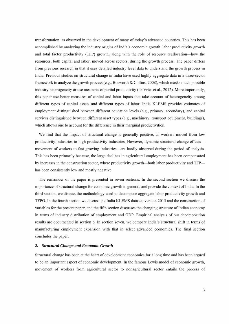
transformation, as observed in the development of many of today’s advanced countries. This has been

accomplished by analyzing the industry origins of India’s economic growth, labor productivity growth

and total factor productivity (TFP) growth, along with the role of resource reallocation—how the

resources, both capital and labor, moved across sectors, during the growth process. The paper differs

from previous research in that it uses detailed industry level data to understand the growth process in

India. Previous studies on structural change in India have used highly aggregate data in a three-sector

framework to analyze the growth process (e.g., Bosworth & Collins, 2008), which masks much possible

industry heterogeneity or use measures of partial productivity (de Vries et al., 2012). More importantly,

this paper use better measures of capital and labor inputs that take account of heterogeneity among

different types of capital assets and different types of labor. India KLEMS provides estimates of

employment distinguished between different education levels (e.g., primary, secondary), and capital

services distinguished between different asset types (e.g., machinery, transport equipment, buildings),

which allows one to account for the difference in their marginal productivities.

We find that the impact of structural change is generally positive, as workers moved from low

productivity industries to high productivity industries. However, dynamic structural change effects—

movement of workers to fast growing industries—are hardly observed during the period of analysis.

This has been primarily because, the large declines in agricultural employment has been compensated

by increases in the construction sector, where productivity growth—both labor productivity and TFP—

has been consistently low and mostly negative.

The remainder of the paper is presented in seven sections. In the second section we discuss the

importance of structural change for economic growth in general, and provide the context of India. In the

third section, we discuss the methodology used to decompose aggregate labor productivity growth and

TFPG. In the fourth section we discuss the India KLEMS dataset, version 2015 and the construction of

variables for the present paper, and the fifth section discusses the changing structure of Indian economy

in terms of industry distribution of employment and GDP. Empirical analysis of our decomposition

results are documented in section 6. In section seven, we compare India’s structural shift in terms of

manufacturing employment expansion with that in select advanced economies. The final section

concludes the paper.

2. Structural Change and Economic Growth

Structural change has been at the heart of development economics for a long time and has been argued

to be an important aspect of economic development. In the famous Lewis model of economic growth,

movement of workers from agricultural sector to nonagricultural sector entails the process of

4

development (Lewis, 1954). This model suggests that as the marginal productivity of workers in the

primary sector is zero, movement of workers from agriculture will not reduce productivity in the

aggregate economy. Rather as workers are released from less productive agricultural activities to more

productive industrial sector, industrialization happens, and overall productivity increases. Lewis model

was, however, a two-sector model, with no service sector being present. Fisher (1939) has already

suggested that as countries develop, a large service sector would emerge, following primary and

secondary sectors. This idea has been further developed by Clark (1940), suggesting that structural

change is essential for economic progress in capitalist economies, and at the height of development a

large number of workers will be engaged in the service sector. Similar arguments have been postulated

in Kuznets (1966) and Chenery & Syrquin (1975), with structural change—narrowly defined as a shift

of resources (inputs and output) from agriculture to manufacturing, and further from manufacturing to

services—features the process of development.4 Such structural change patterns featured prominently in

post-war economic growth across Western European countries, United States and Japan (Denison, 1967;

Maddison, 1987; Jorgenson & Timmer, 2011).

Recent literature on economic growth development reiterates the importance of the nature and the

speed of structural transformation in enhancing and sustaining economic growth (Lin, 2011; McMillan

& Rodrik, 2011). In the modern literature, structural transformation is viewed as the evolution of an

economy’s structure from low productivity activities to higher productivity modern activities (Naude et

al., 2015; Szirmai, 2013; Lin, 2011; McMillan & Rodrik, 2011). This would mean that structural change

could happen within the broadly defined manufacturing or service sectors, and does not have to be

necessarily between manufacturing and services. Workers could move from low productive agriculture

to high productive industries or services or from low productive manufacturing to high productive

manufacturing or from low productive service industries to high productive services. Moreover,

technological change typically takes place at the level of industries and therefore, patterns of industry

productivity could differ significantly (de Vries et al., 2012). Therefore, taking account of industry

heterogeneity at a more detailed level is of high importance in understanding structural change. Such

structural transformation is indeed desirable as a source of higher productivity growth and per capita

income. As workers and resources move from low productive activities to high productive activities,

overall productivity and growth accelerate. Such patterns have been observed not only in Western

countries, but also in developing countries such as Africa in the early post-independence years (de Vries

4 However, structural change might also involve a change in the scale of activities (e.g., mass production), and a shift from

self-employed jobs to more organized production. Structural change doesn’t have to be confined to economic, but it could also happen to institutions and policies, and often policy changes can stimulate economic structural changes (Naude et al., 2015, Szirmai, 2013).

5

et al., 2015). In addition, such movement of resources across sectors helps achieve greater diversity in

the economic structure of a country, reducing vulnerability to external shocks (Naude et al., 2015). It

requires suitable policies that facilitate the movement of resources from low productive to high

productive uses, and therefore understanding structural change and its implications are important for

countries like India.

Economic growth in India is often compared with that of neighboring China, despite substantial

differences between the two countries in the historical development path and institutional environment

(see for instance Eichengreen et al., 2010). A major difference between the observed growth process in

India and China is the importance of manufacturing in the aggregate growth in China and that of services

in India. While China’s development process appears to be more in line with the traditionally

hypothesized structural transformation, where resources have moved from primary sector to

manufacturing and now increasingly moving into services, India’s growth process seems to have

substantially bypassed the second stage in the structural transformation.

In general, from the conventional perspective, there are at least two reasons why the service sector

would emerge and dominate over the primary and secondary sectors in an economy’s development

process. The income elasticity of demand for services is in general high (e.g., financial services, business

services, tourism, etc.). As countries develop, and incomes rise, the demand for these services would

also increase, thus more resources would be allocated to services sector. Secondly, productivity growth

rate in the service sector compared to manufacturing sector is generally slower, as it is often difficult to

apply many new technologies in the services sector. As a consequence, prices of services would rise

relatively faster compared to nonservice sectors where prices would be lowered by technological

advancement. This traditional hypothesis, nevertheless, may not be valid in many modern services. For

instance many market services such as financial and business services benefit substantially from

information and communication technologies, helping them improve their productivity. Yet, in the

traditional sense, high income elasticity of demand and lower productivity leads to allocation of more

income and spending to the service sector of the economy. A third factor, which does not feature in the

conventional closed economy models, is the increased tradability of services activities. For instance,

software services, a segment of services India has been excelling since the 1990s, constitute about 45

percent of India’s export basket, and the factors that helped the growth of this sector includes

mathematical ability of Indian programmers, relatively lower labor costs, large English speaking

population, etc., (Erumban & Das, 2016).

Whatever the mechanism by which structural change takes place, an important insight from the

traditional development economic theory and the modern reemergence of the structural change

6

hypothesis (McMillan & Rodrik, 2011; Lin,2011; de Vries et al., 2012) is that growth and development

entails structural change. And analysis of structural change should consider more detailed industry data,

as technological change typically takes place at industry level, and there exists substantial heterogeneity

across industries within manufacturing and services sectors.

3. Methodology

In this section, we discuss the methodology used to construct aggregate estimates of productivity growth

and the contribution of individual industries and factor reallocation. We use decomposition methods to

understand the contributions of various sectors and structural change to aggregate labor productivity and

total factor productivity growth. The labor productivity decomposition is based on the canonical

decomposition method suggested in Fabricant (1942). Variations of this approach have been widely

used in the literature, where the basic idea is to decompose the growth rate of labor productivity into a

within industry productivity growth component and a between effect.5 The latter term – the reallocation

term – out of this decomposition is used as a measure of structural change (e.g., Bosworth & Collins,

2008; McMillan & Rodrik, 2011; de Vries et al., 2012; OECD, 2013; de Vries et al., 2014). The

methodology for total factor productivity decomposition is heavily drawn from Jorgenson et al. (2007),

further discussed and applied in the context of India in Erumban and Das (2016). We use the direct

aggregation method, in comparison with aggregate production possibility frontier approach, suggested

by Jorgenson et al. (2007), which are discussed in detail below.

Estimates of labor productivity growth, total factor productivity growth and output growth are

analyzed for 27 industries that cover the entire Indian economy for the time period 1985-2011. In

addition, in order to get a detailed picture of the pattern of observed productivity growth, we also provide

a graphical representation of the observed industry productivity growth, using the approach suggested

by Harberger (1998), and employed in Timmer et al. (2010).

3.1 Static and Dynamic Reallocation Effects—decomposition of labor productivity growth

The most common approach to measure aggregate economic growth and its sources is to assume an

aggregate production function. Assuming that there exists an aggregate production function (PF),6 we

can obtain aggregate value added (VPF) by summing value added across industries and, aggregate

employment (L) as the sum of the number of workers across industries. Then aggregate labor

productivity level in year t can be obtained as:

5 See de Vries et al. (2015) for a detailed discussion on different variations of this decomposition approach. 6 We discuss this assumption further in the next section.

7

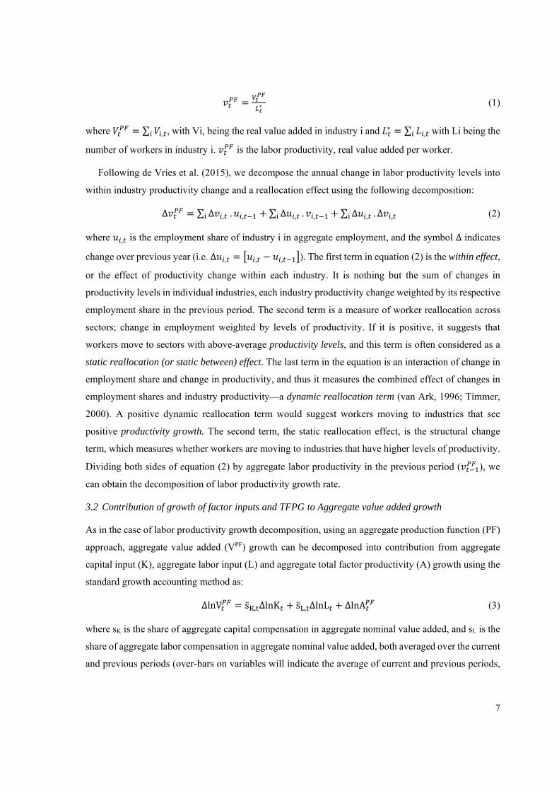
∗ (1)

where ∑ , , with Vi, being the real value added in industry i and ∗ ∑ , with Li being the

number of workers in industry i. is the labor productivity, real value added per worker.

Following de Vries et al. (2015), we decompose the annual change in labor productivity levels into

within industry productivity change and a reallocation effect using the following decomposition:

∆ ∑ ∆ , . , ∑ ∆ , . , ∑ ∆ , . ∆ , (2)

where , is the employment share of industry i in aggregate employment, and the symbol ∆ indicates

change over previous year (i.e. ∆ , , , ). The first term in equation (2) is the within effect,

or the effect of productivity change within each industry. It is nothing but the sum of changes in

productivity levels in individual industries, each industry productivity change weighted by its respective

employment share in the previous period. The second term is a measure of worker reallocation across

sectors; change in employment weighted by levels of productivity. If it is positive, it suggests that

workers move to sectors with above-average productivity levels, and this term is often considered as a

static reallocation (or static between) effect. The last term in the equation is an interaction of change in

employment share and change in productivity, and thus it measures the combined effect of changes in

employment shares and industry productivity—a dynamic reallocation term (van Ark, 1996; Timmer,

2000). A positive dynamic reallocation term would suggest workers moving to industries that see

positive productivity growth. The second term, the static reallocation effect, is the structural change

term, which measures whether workers are moving to industries that have higher levels of productivity.

Dividing both sides of equation (2) by aggregate labor productivity in the previous period ( ), we

can obtain the decomposition of labor productivity growth rate.

3.2 Contribution of growth of factor inputs and TFPG to Aggregate value added growth

As in the case of labor productivity growth decomposition, using an aggregate production function (PF)

approach, aggregate value added (VPF) growth can be decomposed into contribution from aggregate

capital input (K), aggregate labor input (L) and aggregate total factor productivity (A) growth using the

standard growth accounting method as:

∆lnV s̅ , ∆lnK s̅ , ∆lnL ∆lnA (3)

where sK is the share of aggregate capital compensation in aggregate nominal value added, and sL is the

share of aggregate labor compensation in aggregate nominal value added, both averaged over the current

and previous periods (over-bars on variables will indicate the average of current and previous periods,

8

throughout in this paper). Aggregate capital and labor compensation are derived from the identity that

total nominal value added is the sum of aggregate labor and capital compensation. ∆lnK is the aggregate

capital services growth rate and ∆lnL is the aggregate labor input growth rate. Aggregate capital and

labor inputs are also the sum of industry labor and capital inputs. ∆lnA is the growth of aggregate

total factor productivity, assuming an aggregate production function. Note that decomposition in (3)

uses log differences of output and input, whereas the decomposition in (2) use differences in levels,

which are later converted to percent changes. Therefore, they are not strictly comparable in terms of the

absolute magnitude.

The above approach is built on restrictive assumptions on the existence of an aggregate production

function, which requires identical industry value added functions. Jorgenson et al. (2005) use a less

restrictive production possibility frontier approach, which relaxes the restrictions on industry value-

added function. In this approach, the measurement of output differs from the aggregate production

function, but the measurement of inputs remains the same (see Jorgenson et al., 2007). Defining

aggregate value added growth as a translog index of industry value added growth, and keeping capital

and labor unchanged as in (3), we can express aggregate value added growth as:

∆lnV ∑ s̅ , ∆lnV , s̅ , ∆lnK s̅ , ∆lnL ∆lnA (4)

where Vi is the real value added in industry i. Note that ∆ in equation (4) is different from ∆

in equation (3), as equation (4) uses a translog aggregation of industry value added growth while

equation (3) is the growth rate of simply aggregated value added across industries. The difference

between the two is the reallocation of value added across industries.

In (3) and (4), aggregate capital and labor inputs are measured as the flow of services from these

inputs to the production process. Aggregate capital and aggregate labor inputs consists of different types

of capital assets (e.g., machinery, computers, buildings, etc.) and labor types (e.g., low-skilled, high-

skilled, old, young, etc.), with differing marginal productivities. Therefore, following Jorgenson (1963),

we define aggregate capital services and labor input as translog aggregates of heterogeneous types of

capital and labor.

∆lnK ∑ v , ∆lnK , ; and∆lnL ∑ v , ∆lnL , (5)

where vk is the share of each type of capital k in aggregate capital compensation, and vl is the share of

each type of labor l in total labor compensation, defined as:

v ,, , ,

∑ , , ,andv ,

, , ,

∑ , , , (6)

9

where PK,k is the rental price of capital type k, and PL,l is the price (wage rate) of labor type l. As before

v in (5) is the two-period averages of these shares. In our analysis, we distinguish between five types of

labor, and three types of capital assets (see section on data). They are respectively employees with

education 1) up to primary; 2) primary school; 3) middle school; 4) secondary and higher secondary

school; and above 5) higher secondary school and capital assets are transport equipment; machinery;

and construction.7 The above decomposition (equation 4) is used to obtain total factor productivity

growth for the aggregate economy. Aggregate economy productivity growth can be attained either by

improved productivity within industries or by moving labor and capital from low productivity to high

productivity industries.

3.3 Contribution of Industry TFPG and factor reallocation to Aggregate TFPG

In order to trace the industry origins of aggregate total factor productivity, and to quantify the relative

importance of various industries and factor reallocation (or structural change) in driving aggregate

productivity growth, we use the direct aggregation method suggested by Jorgenson et al. (2007). This

approach relaxes many assumptions on input and output measurement that exist in the aggregate

production function approach. In this approach, aggregate production function is a value added function

and the aggregate value added growth is measured as a translog index of industry value added, with

weights being the industry share in aggregate nominal value added (as in equation 4). The production

function at the industry level, however, is a gross output (Y) function, and therefore, industry output

growth can be decomposed into contributions from capital (K), labor (L) and intermediate input (X) as:

∆lnY , s̅ , , ∆lnK , s̅ , , ∆lnL , s̅ , , ∆lnX , ∆lnA , (7)

where sK, sL, and sX are respectively the shares of capital, labor and intermediate input in total nominal

output in industry i. Since nominal value of gross output is the sum of nominal value of industry value

added and nominal value of total intermediate inputs, the industry output growth can be obtained as a

weighted sum of industry value added growth and industry intermediate growth with the weights being

respectively the nominal share of value added in output and nominal share of intermediate inputs in

7 See Erumban and Das (2015) for a growth accounting analysis breaking machinery capital further into ICT and non-ICT

machinery.

10

output.8 Assuming that aggregate value added is a translog sum of industry value added, we can

decompose the aggregate value added growth as (see Jorgenson et al., 2007):

∆lnV ∑ s̅ , ∆lnV , ∑ s̅ ,, ,

, ,∆lnK , ∑ s̅ ,

, ,

, ,∆lnL , ∑ s̅ ,

, ,∆lnA ,

(8)

In equation (8), aggregate value added growth is sum of the weighted contribution of industry capital

input, industry labor input and industry TFPG. The weights on capital and labor consists of si, the share

of industry value added in aggregate value added, sK,i and sL,i, the share of industry capital and labor

compensation in industry gross output and svi, the share of industry value added in industry gross output.9

The first and last components of the input weights (si and svi) are also reflected in the TFPG weights.

In equation 4 we have the production possibility frontier – with aggregate value added growth being the

weighted sum of industry value added growth, and capital and labor inputs being the simple sum across

industries, whereas in equation 8, input growth rates are also weighted growth rates of industry capital and

labor. Therefore, the difference between the two is factor reallocation effects. Subtracting 4 (i.e. with the

simple summation of factor inputs) from 8 (i.e. the weighted aggregates of factor inputs), , and rearranging,

we obtain

∆̅ ,̅ , ,

∆ , ̅ ,̅ , ,̅ , ,

∆ , ̅ ∆ ̅ ,̅ , ,̅ , ,

∆ , ̅ ∆

∑ ,

, ,∆lnA , REAL , REAL , (9)

Equation (9) suggests that aggregate TFPG can be decomposed into weighted average of industry

TFPG and the capital and labor reallocation across industries. Note that the weight attributed to industry

TFPG in this setting is equivalent to the well-known Domar weight (Domar, 1961). The weight in

8 This implies that the real value-added of industry i can be derived as: lnVi, ∆lnYi,t.

1

s̅V,I,t∆lnXi,t

s̅X,i,t

s̅V,i,t, and

when combined with (7), it can be re-written as:∆lnVi, ,i,

s̅V,i,t∆lnKi,

,i,

s̅V,i,t∆lnLi,

1

s̅V,i,t∆lnAi, .

Combining this with (4) – the production possibility frontier –, we obtain lnV ∑ s̅ , ∆lnV ,

∑ s̅ ,, ,

, ,∆lnK , ∑ s̅ ,

, ,

, ,∆lnL , ∑ s̅ ,

, ,∆lnA , (i.e. equation 8)

9 These input weights are industry share of capital and labor compensation in aggregate value added, and the TFPG weight

is the industry output share in aggregate value added.

11

equation (9) is the ratio of si, or industry share in aggregate value added and svi or the industry value

added share in aggregate output, which approximates to the Domar weight, which is the ratio of industry

gross output to aggregate value added. These weights will be greater than one, as industry TFP

improvement can have a direct effect through industry output, but also an indirect effect through output

in other industries, by means of intermediate input sold to other industries (Jorgenson et al., 2012).The

difference between Domar-weighted TFPG and the aggregate TFPG is the sum of labor and capital

reallocation effects, which reflects the movement of these resources across industries.

4. Moving from aggregate to disaggregate industry analysis—the India KLEMS database version

2015

While there is significant amount of studies analyzing sources of growth and dynamics of productivity

in India’s organized manufacturing sector, which constitutes only less than 11 percent of total GDP

(National Accounts Statistics, 2014), analysis beyond this sector is constrained by lack of consistent

data on investment, employment and value added. The India KLEMS research project, with financial

assistance from the Reserve Bank of India, is a major initiative to fill this data gap. It facilitates research

on the relationship between labor quality (or educational composition), investment and productivity

growth in India. More importantly, since this data has been constructed keeping international standards,

ensuring comparability with other freely available KLEMS databases (EU KLEMS,10 Asia KLEMS,

and World KLEMS), researchers can compare performance of Indian economy with other developing

and advanced economies. While the data is completely consistent with national accounts, it provides

indicators which are often not publically available through national accounts.11 The India KLEMS

provides data on value added, gross output, intermediate inputs (all in both current and constant prices12)

employment by education levels, labor quality, wage share in GDP including estimates for self-

employed workers, capital investment and capital services by asset type along with indicators of labor

productivity growth and total factor productivity growth. All these data are available for 27 detailed

industries comprising the Indian economy over 1980-2011 period. As such the data is directly applicable

in growth accounting analysis to understand sources of output and labor productivity growth in India in

different time periods, and across industries, and also to compare with other countries, when combined

with other KLEMS databases. It can also be used for studies of inequality and wage setting, and to

10 See O’Mahony and Timmer (2009) for an elaborate discussion the KLEMS methodology, and also several uses of the

KLEMS type of data. 11We are thankful to CSO for providing detailed data on indicators such as asset wise investment, which is not available

publically. 12India KLEMS use a double deflation approach to construct constant price value added series (see Balakrishan &

Pushpangadan, 1994 for a first use of double deflation in Indian manufacturing).

12

understand the role of intermediate inputs in production. When combined with input–output databases

such as World Input–Output Database (WIOD), KLEMS type of data would facilitate in-depth analysis

of global value chains, which is of high significance in the context of increased fragmentation of

production (see Timmer et al., 2014). The KLEMS database is also useful for analyzing various policy

considerations including, tax, innovation, competition, and industrial policies.

The main source of data used in the India KLEMS is the National Accounts Statistics (NAS),

published annually by the Central Statistical Organization. This data is supplemented by Input–Output

tables, Annual Survey of Industries (ASI) and various rounds of National Sample Survey Office (NSSO)

surveys on employment & unemployment and unorganized manufacturing sectors. This section provides

a description of the data, their sources, construction of variables and the industrial classifications used

in the study. We require industry wise data on nominal and real value added, investment by asset type,

number of employees and labor compensation by type of workers and nominal and real values of

intermediate inputs. We briefly describe the source and construction of these variables in detail.13

Value added: India KLEMS provides estimates of Gross Domestic Product (GDP) by industry at both

current and constant prices, which are consistent with NAS 2004-2005 base series. For those industries

especially for some subsectors within the manufacturing sector, where detailed data are not available

from NAS, estimates have been made using the Annual Survey of Industries (ASI) for registered and

NSSO surveys for unregistered manufacturing industries. While the former source is used to split

aggregate value added data from NAS into subsectors in the organized sector, the latter is used for the

unorganized sector. The real value added data in NAS are single deflated, except for agriculture.

However, in our growth accounting analysis we use double deflated value added series, which are

derived using gross output, and intermediate input series obtained from the India KLEMS database.

Gross output: Estimates of gross output in India KLEMS for sectors agriculture, hunting, forestry and

fishing, mining and quarrying, construction and manufacturing sectors are directly obtained from NAS

at current and constant prices. For splitting some sectors, as in the case of value added, additional

information is used from ASI and NSSO. For other sectors, mainly service sectors, where there was no

output information available from NAS, input–output transaction tables, which provides output and

value added, are used. The ratio of these two is applied to value added in NAS to obtain consistent

estimates of gross output. The benchmark input–output tables for the years 1978, 1983, 1989, 1993,

1998, 2003, and 2007 are used for this purpose, and for the intermediate years the ratios are linearly

interpolated.

13 See Das et al. (2016) for a detailed discussion on the construction of these variables.

13

Intermediate inputs: Nominal values of intermediate input are basically the difference between nominal

value added and nominal output. The commodity inputs going into the production process of output

industries are aggregated into energy (E), material (M) and service (S) inputs. In this way, for each

benchmark year, estimates are obtained for material, energy and service inputs used to produce output

in the different industries. The time series of input proportions for industries are compiled for the

benchmark years and then linear interpolation is used to obtain the series for 1980 to 2011 at current

prices. To generate a price deflator for intermediate inputs, we use wholesale price indices published by

the Office of the Economic Advisor, Ministry of Commerce and Industry. We use weighted deflators

for materials, energy and service inputs for each of the industries (ala Balakrishnan & Pushpangadan,

1994).

Employment and labor composition: Employment data in India KLEMS is based on usual principal and

subsidiary status (UPSS) concept, and are obtained from the quinquennial rounds of Employment and

Unemployment Surveys (EUS) published by National Sample Survey Office (NSSO). The aggregate

labor input, used in this study is obtained as the weighted sum of employment growth rates of workers

of various educational levels using equation (5). Employment and wage data by educational categories—

up to primary school, primary school, middle school, secondary & higher secondary school, and above

higher secondary school—are also available from EUS. Since EUS does not provide self-employed

wage compensation, India KLEMS uses econometrically estimated compensation rates, using

demographic and socio economic characteristics of workers (see Aggarwal & Erumban, 2013). Capital

services: Capital services for the aggregate economy and for industries in India KLEMS are arrived at

using equation (5). In order to do this, it was essential to obtain investment data by asset type. Industry

level investment in three different asset types—construction, transport equipment, and machinery—are

gathered from NAS for broad sectors of the economy, the Annual Survey of Industries (ASI) covering

the formal manufacturing sector, and the National Sample Survey Office (NSSO) rounds for

unorganized manufacturing. These industry level data are used to construct capital stock using perpetual

inventory method, i.e.

, , 1 ,

where KK is the capital stock in asset K, K and IK is the real investment in asset K, and the subscript t

stands for year t. The assumed depreciation rates are 8 percent for machinery, 2.5 percent for

construction and 10 percent for transport equipment. The rental price of capital PK,k in (6) is measured

assuming an external rate of return (r), as

P , , P , , P , ,

14

where the external rate of return, r, is represented by a long-run average of real bond rate and market

interest rate, obtained from Reserve Bank of India.

5. Changing structure of Indian economy

As mentioned before, this study is conducted taking into account the significant industry heterogeneity

within the Indian economy and its consequences for aggregate economic growth using data on 27

industrial sectors of the economy. However, for expositional clarity, we aggregate the 27 industry groups

into different subsectors using appropriate aggregation procedures (see Table 1 for the industry groups).

In our industry discussions we will mostly follow these groupings. Since agriculture is a major

employment providing sector in Indian economy, which is often argued to be an important and key

sector for future sustainability of India’s economic growth (Balakrishnan, 2010), we keep it as a distinct

sector. Mining, utilities and construction are clubbed into one single sector, which we call as other goods

production. Manufacturing is divided into two broad groups, consumer and intermediate goods

manufacturing and investment goods manufacturing, where the latter includes machinery and transport

equipment manufacturing. Service sector is divided into five distinct sectors; trade and distributive

services, business services, financial services, all other market services and nonmarket services.14

Table 1: Industry groups and corresponding ISIC codes

sl Nr. Industry Group (Sector) ISIC Industries in the Group 1 Agriculture & allied

activities AtB Agriculture, hunting & fishing Goods Production Manufacturing 2 Consumer & intermediate

goods Mfg. 15to28+36to37

Mfg., excluding machinery, electrical & transport equipment

3 Investment goods Mfg. 29t35

Machinery, nec.; Electrical & Optical Equipment; Transport Equipment

4 Other goods production C+E+F

Mining & Quarrying; Electricity, Gas & Water; Construction

Services Market Services 5 Trade and distribution G+60t63 Wholesale & Retail trade; Transport & Storage 6 Finance services J Financial Services 7 Business Services 71t74 Renting of Machinery & Business services

14 Since investment in information and communication technologies is often considered to be an important driver of productivity change, an industry grouping based on ICT intensity will also be of high interest. However, this paper does not make that distinction. Such an attempt is made in Erumban and Das (2015), who document the growing importance of ICT using sectors in Indian economy

15

8 Other market services H+64+K+O+P

Hotels & Restaurants; Post & Telecommunication & all other market Services

9 Non-market services L+M+N Public Administration & Defense; Compulsory Social Security ; Education; Health & Social Work

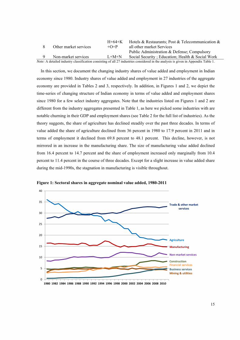
Note: A detailed industry classification consisting of all 27 industries considered in the analysis is given in Appendix Table 1. In this section, we document the changing industry shares of value added and employment in Indian

economy since 1980. Industry shares of value added and employment in 27 industries of the aggregate

economy are provided in Tables 2 and 3, respectively. In addition, in Figures 1 and 2, we depict the

time-series of changing structure of Indian economy in terms of value added and employment shares

since 1980 for a few select industry aggregates. Note that the industries listed on Figures 1 and 2 are

different from the industry aggregates presented in Table 1, as here we picked some industries with are

notable churning in their GDP and employment shares (see Table 2 for the full list of industries). As the

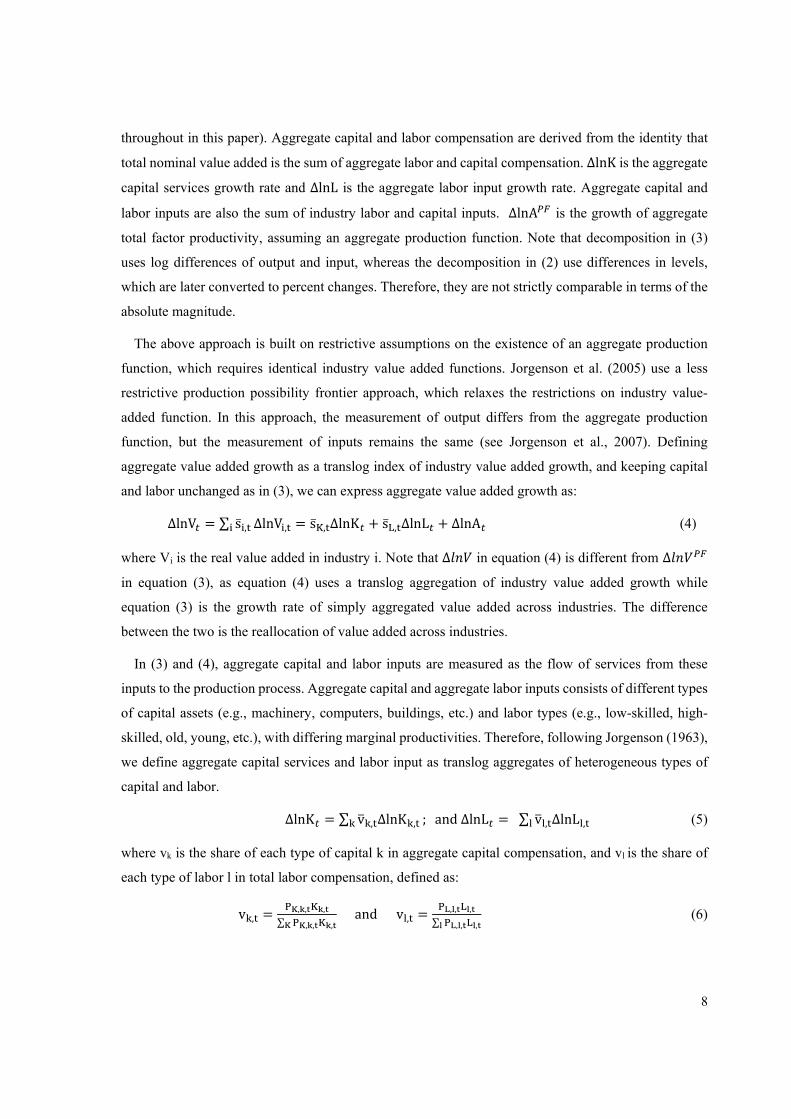
theory suggests, the share of agriculture has declined steadily over the past three decades. In terms of

value added the share of agriculture declined from 36 percent in 1980 to 17.9 percent in 2011 and in

terms of employment it declined from 69.8 percent to 48.1 percent. This decline, however, is not

mirrored in an increase in the manufacturing share. The size of manufacturing value added declined

from 16.4 percent to 14.7 percent and the share of employment increased only marginally from 10.4

percent to 11.4 percent in the course of three decades. Except for a slight increase in value added share

during the mid-1990s, the stagnation in manufacturing is visible throughout.

Figure 1: Sectoral shares in aggregate nominal value added, 1980-2011

Agriculture

Manufacturing

Construction

Mining & utilities

Financial services

Business services

Trade & other market services

Non‐market services

0

5

10

15

20

25

30

35

40

1980 1982 1984 1986 1988 1990 1992 1994 1996 1998 2000 2002 2004 2006 2008 2010

16

Notes: Trade & other market services include Trade, transport & storage, hotels and restaurants, post & communication and other services; Mining & utilities include mining, electricity, gas and water supply. Source: India KLEMS dataset, version 2015.

17

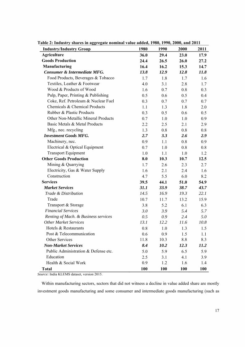
Table 2: Industry shares in aggregate nominal value added, 1980, 1990, 2000, and 2011

Industry/Industry Group 1980 1990 2000 2011 Agriculture 36.0 29.4 23.0 17.9 Goods Production 24.4 26.5 26.0 27.2 Manufacturing 16.4 16.2 15.3 14.7 Consumer & Intermediate MFG. 13.8 12.9 12.8 11.8 Food Products, Beverages & Tobacco 1.7 1.8 1.7 1.6 Textiles, Leather & Footwear 4.0 3.1 2.8 1.7 Wood & Products of Wood 1.6 0.7 0.8 0.3 Pulp, Paper, Printing & Publishing 0.5 0.6 0.5 0.4 Coke, Ref. Petroleum & Nuclear Fuel 0.3 0.7 0.7 0.7 Chemicals & Chemical Products 1.1 1.3 1.8 2.0 Rubber & Plastic Products 0.3 0.5 0.6 0.5 Other Non-Metallic Mineral Products 0.7 1.0 1.0 0.9 Basic Metals & Metal Products 2.2 2.5 2.1 2.9 Mfg., nec. recycling 1.3 0.8 0.8 0.8 Investment Goods MFG. 2.7 3.3 2.6 2.9 Machinery, nec. 0.9 1.1 0.8 0.9 Electrical & Optical Equipment 0.7 1.0 0.8 0.8 Transport Equipment 1.0 1.1 1.0 1.2 Other Goods Production 8.0 10.3 10.7 12.5 Mining & Quarrying 1.7 2.6 2.3 2.7 Electricity, Gas & Water Supply 1.6 2.1 2.4 1.6 Construction 4.7 5.5 6.0 8.2 Services 39.5 44.1 51.0 54.9 Market Services 31.1 33.9 38.7 43.7 Trade & Distribution 14.5 16.9 19.3 22.1 Trade 10.7 11.7 13.2 15.9 Transport & Storage 3.8 5.2 6.1 6.3 Financial Services 3.0 3.9 5.4 5.7 Renting of Mach. & Business services 0.5 0.9 2.4 5.0 Other Market Services 13.1 12.2 11.6 10.8 Hotels & Restaurants 0.8 1.0 1.3 1.5 Post & Telecommunication 0.6 0.9 1.5 1.1 Other Services 11.8 10.3 8.8 8.3 Non-Market Services 8.4 10.2 12.3 11.2 Public Administration & Defense etc. 5.0 5.9 6.5 5.9 Education 2.5 3.1 4.1 3.9 Health & Social Work 0.9 1.2 1.6 1.4 Total 100 100 100 100

Source: India KLEMS dataset, version 2015.

Within manufacturing sectors, sectors that did not witness a decline in value added share are mostly

investment goods manufacturing and some consumer and intermediate goods manufacturing (such as

18

petroleum refining, chemicals, rubber &plastics, nonmetallic minerals, basic metals &metal products).

Together these sectors constitute 67 percent of total manufacturing value added in 2011; an increase of

22 percentage points from 45 percent in 1980. The overall size of these sectors in the economy has,

however, increased only from 7 percent to 10 percent, not sufficient enough to offset the decline in the

share of other sectors. Textiles group has witnessed the highest decline in value added share within

manufacturing, from 4 percent in 1980 to 1.7 percent in 2011.

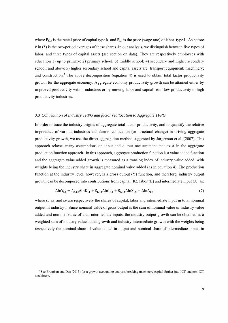
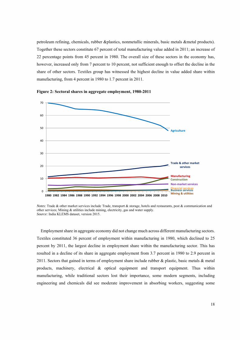
Figure 2: Sectoral shares in aggregate employment, 1980-2011

Notes: Trade & other market services include Trade, transport & storage, hotels and restaurants, post & communication and other services; Mining & utilities include mining, electricity, gas and water supply. Source: India KLEMS dataset, version 2015.

Employment share in aggregate economy did not change much across different manufacturing sectors.

Textiles constituted 36 percent of employment within manufacturing in 1980, which declined to 25

percent by 2011, the largest decline in employment share within the manufacturing sector. This has

resulted in a decline of its share in aggregate employment from 3.7 percent in 1980 to 2.9 percent in

2011. Sectors that gained in terms of employment share include rubber & plastic, basic metals & metal

products, machinery, electrical & optical equipment and transport equipment. Thus within

manufacturing, while traditional sectors lost their importance, some modern segments, including

engineering and chemicals did see moderate improvement in absorbing workers, suggesting some

Agriculture

ManufacturingConstruction

Mining & utilities

Financial servicesBusiness services

Trade & other market services

Non‐market services

0

10

20

30

40

50

60

70

1980 1982 1984 1986 1988 1990 1992 1994 1996 1998 2000 2002 2004 2006 2008 2010

19

positive structural transformation within the sector. Yes, the fact that manufacturing did not absorb the

workers released from agriculture defies the conventional structural transformation hypothesis.

A large part of the decline in agricultural employment is reflected in an increase in the construction

sector, which has increased from 2 percent in 1980 to 10 percent in 2011 and in trade and other market

services that increased from 12 to 21 percent. However, the output share of construction increased only

from 5 percent to 8 percent and in trade and other market services from 28 percent to 33 percent, thus

suggesting a decline in productivity levels.

Clearly, the emergence of service sector as the largest contributor to aggregate GDP is an important

feature of structural transformation of Indian economy. Service sector has been the single largest

contributor to value added in the post-1980 period. The share of the service sector in overall GDP

increased from 39.5 percent in 1980 to 54.5 percent in 2011. Within which market services15 constituted

31.1 percent of overall GDP in 1980, which increased more rapidly to 43.7 percent, with greater

acceleration since the 1990s. However, in terms of employment, the service sector is still less than one-

third of the economy, with the market services being at slightly below a quarter of overall employment.

The market services share in employment increased from 12 percent to 23.4 percent, and that of total

(including nonmarket sector) services increased from 16.9 percent to 29.2 percent.

Within the market services, business services increased its output share from half a percent to 5

percent, whereas its employment share increased from a trivial 0.2 percent to 1.6 percent. Financial

services doubled its output share from 3 percent to 6 percent; post &telecom increased from 0.6 percent

to 1.1 percent; trade sector from 11 percent to 16 percent; and transport and storage from 4 percent to 6

percent. However, the employment shares of these sectors did not increase in tandem with their output

shares. Employment share of financial services increased from 0.3 percent to nearly 1 percent, post

&telecom from 0.1 percent to 0.4 percent, trade from 6 percent to 10 percent and transport from 2 percent

to 4 percent.

15 Market services include trade, transport services, financial services, business services, post & telecom, and hotels & restaurants services.

20

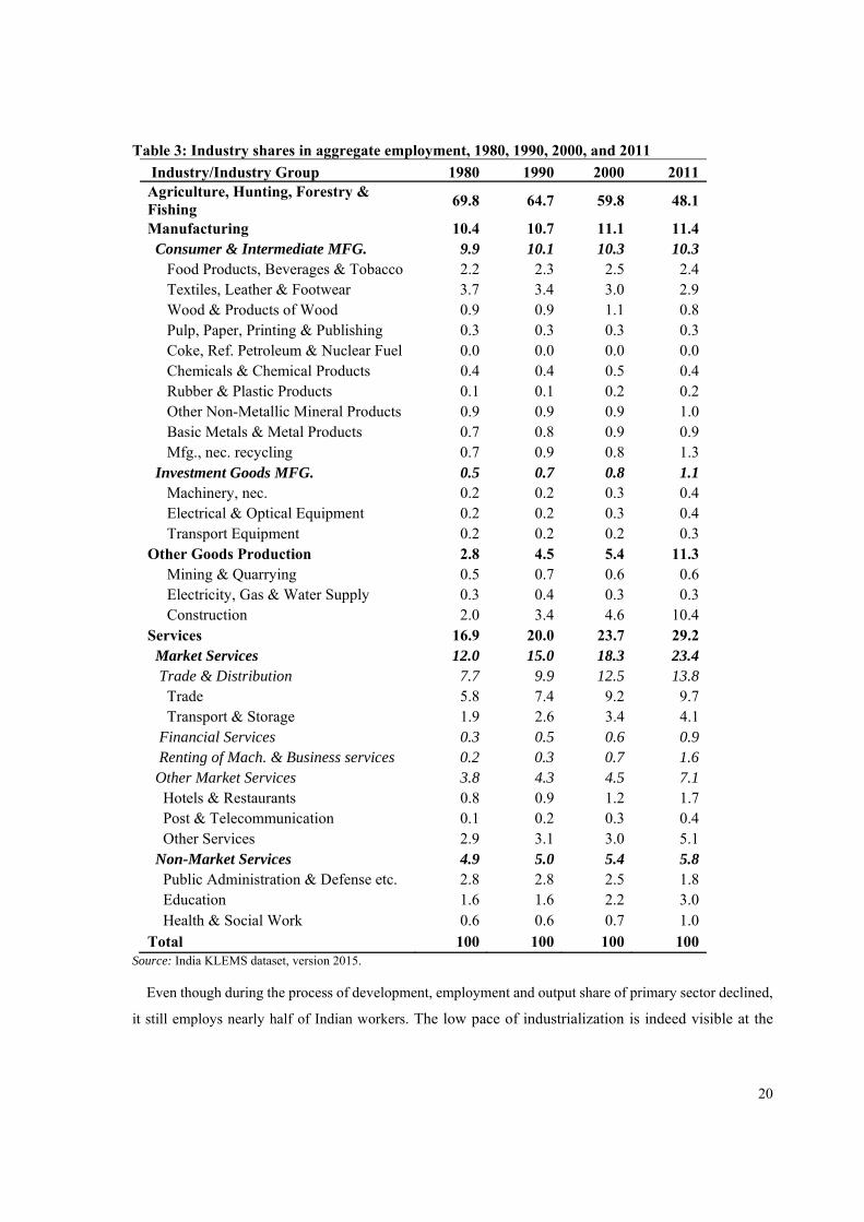
Table 3: Industry shares in aggregate employment, 1980, 1990, 2000, and 2011

Industry/Industry Group 1980 1990 2000 2011 Agriculture, Hunting, Forestry & Fishing

69.8 64.7 59.8 48.1

Manufacturing 10.4 10.7 11.1 11.4 Consumer & Intermediate MFG. 9.9 10.1 10.3 10.3 Food Products, Beverages & Tobacco 2.2 2.3 2.5 2.4 Textiles, Leather & Footwear 3.7 3.4 3.0 2.9 Wood & Products of Wood 0.9 0.9 1.1 0.8 Pulp, Paper, Printing & Publishing 0.3 0.3 0.3 0.3 Coke, Ref. Petroleum & Nuclear Fuel 0.0 0.0 0.0 0.0 Chemicals & Chemical Products 0.4 0.4 0.5 0.4 Rubber & Plastic Products 0.1 0.1 0.2 0.2 Other Non-Metallic Mineral Products 0.9 0.9 0.9 1.0 Basic Metals & Metal Products 0.7 0.8 0.9 0.9 Mfg., nec. recycling 0.7 0.9 0.8 1.3 Investment Goods MFG. 0.5 0.7 0.8 1.1 Machinery, nec. 0.2 0.2 0.3 0.4 Electrical & Optical Equipment 0.2 0.2 0.3 0.4 Transport Equipment 0.2 0.2 0.2 0.3 Other Goods Production 2.8 4.5 5.4 11.3 Mining & Quarrying 0.5 0.7 0.6 0.6 Electricity, Gas & Water Supply 0.3 0.4 0.3 0.3 Construction 2.0 3.4 4.6 10.4 Services 16.9 20.0 23.7 29.2 Market Services 12.0 15.0 18.3 23.4 Trade & Distribution 7.7 9.9 12.5 13.8 Trade 5.8 7.4 9.2 9.7 Transport & Storage 1.9 2.6 3.4 4.1 Financial Services 0.3 0.5 0.6 0.9 Renting of Mach. & Business services 0.2 0.3 0.7 1.6 Other Market Services 3.8 4.3 4.5 7.1 Hotels & Restaurants 0.8 0.9 1.2 1.7 Post & Telecommunication 0.1 0.2 0.3 0.4 Other Services 2.9 3.1 3.0 5.1 Non-Market Services 4.9 5.0 5.4 5.8 Public Administration & Defense etc. 2.8 2.8 2.5 1.8 Education 1.6 1.6 2.2 3.0 Health & Social Work 0.6 0.6 0.7 1.0 Total 100 100 100 100

Source: India KLEMS dataset, version 2015.

Even though during the process of development, employment and output share of primary sector declined,

it still employs nearly half of Indian workers. The low pace of industrialization is indeed visible at the

21

aggregate level, despite moderate increase in diversity and sophistication within manufacturing, causing

some positive dynamics within the sector. Much of the employment generated in nonagricultural sector

has been in construction, trade, and high-skilled services.

6. Industry origins of aggregate growth, and the role of structural change – empirical results

This section discusses the decomposition results for labor productivity growth rates for Indian economy

during 1980-2011. The period of analysis roughly covers the three phases of economic reforms in India,

say the pre (or partial) reform period, the transition period and the full reform period. For convenience

of analysis, we subdivide the entire period 1980-2011 into 3 subperiods that roughly tally with the pre-

and post-reform era—1981-1993, 1994-2002 and 2003-2011.

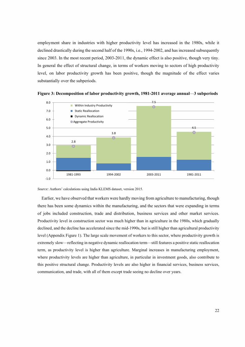
6.1 Industry decomposition of aggregate labor productivity growth

In this section, we look into the contribution of different sectors and structural change in terms of

workers’ movement across sectors, to aggregate labor productivity growth. The growth rate of labor

productivity, measured as output per worker, over 1981-2011 period, broken down to within industry

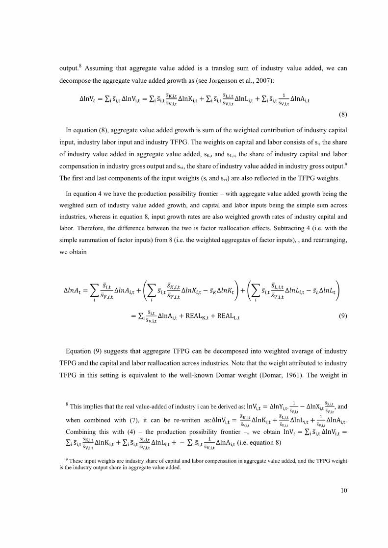
productivity growth, and static and dynamic reallocation is depicted in Figure 3. Labor productivity

growth increased from 2.8 percent during 1981-1993 to 3.8 percent during 1994-2002. In the mid-1990s

through early 2000s, labor productivity did further increase by more than 3.5 percentage point, reaching

at 7.5 percent.

The figure also provides the magnitude of the reallocation effects—both static and dynamic in relation

to the within industry productivity growth. If workers are moving into industries with above average

productivity levels, the static reallocation term will be positive, and if workers are moving to industries

that witness faster productivity growth, the dynamic reallocation term will be positive. In general, 50

percent to 80 percent of aggregate productivity growth is explained by within industry productivity

growth, and the rest can be attributed to structural change. Clearly, the impact of overall reallocation

has been positive throughout, which is also in accordance with the recent findings in McMillan and

Rodrik (2011) and de Vries et al. (2012). On average the structural change effect has been larger during

2003-2011 period, followed by first half of the 1981-1993, whereas it has been lower during the mid-

1990s through early 2000s.

When looked at static and dynamic effects separately, we observe that on average there have been

almost no dynamic reallocation effects throughout the period. It has been contributing less and mostly

negative in most of the years, suggesting that employment was hardly generated in sectors which were

witnessing faster productivity growth. The magnitude of the static reallocation effect has been lower

during 1994-2002 period as compared to the first and last periods of the analysis. Apparently, the

22

employment share in industries with higher productivity level has increased in the 1980s, while it

declined drastically during the second half of the 1990s, i.e., 1994-2002, and has increased subsequently

since 2003. In the most recent period, 2003-2011, the dynamic effect is also positive, though very tiny.

In general the effect of structural change, in terms of workers moving to sectors of high productivity

level, on labor productivity growth has been positive, though the magnitude of the effect varies

substantially over the subperiods.

Figure 3: Decomposition of labor productivity growth, 1981-2011 average annual—3 subperiods

Source: Authors’ calculations using India KLEMS dataset, version 2015.

Earlier, we have observed that workers were hardly moving from agriculture to manufacturing, though

there has been some dynamics within the manufacturing, and the sectors that were expanding in terms

of jobs included construction, trade and distribution, business services and other market services.

Productivity level in construction sector was much higher than in agriculture in the 1980s, which gradually

declined, and the decline has accelerated since the mid-1990s, but is still higher than agricultural productivity

level (Appendix Figure 1). The large scale movement of workers to this sector, where productivity growth is

extremely slow—reflecting in negative dynamic reallocation term—still features a positive static reallocation

term, as productivity level is higher than agriculture. Marginal increases in manufacturing employment,

where productivity levels are higher than agriculture, in particular in investment goods, also contribute to

this positive structural change. Productivity levels are also higher in financial services, business services,

communication, and trade, with all of them except trade seeing no decline over years.

2.8

3.8

7.5

4.5

‐1.0

0.0

1.0

2.0

3.0

4.0

5.0

6.0

7.0

8.0

1981‐1993 1994‐2002 2003‐2011 1981‐2011

  Within Industry Productivity

  Static Reallocation

  Dynamic Reallocation

Aggregate Productivity

23

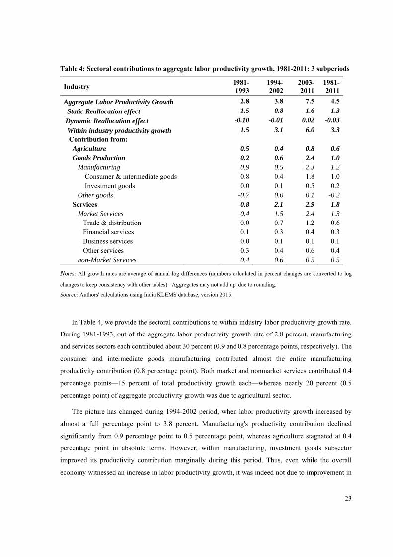
Table 4: Sectoral contributions to aggregate labor productivity growth, 1981-2011: 3 subperiods

Industry 1981-1993

1994-2002

2003-2011

1981-2011

Aggregate Labor Productivity Growth 2.8 3.8 7.5 4.5

Static Reallocation effect 1.5 0.8 1.6 1.3

Dynamic Reallocation effect -0.10 -0.01 0.02 -0.03

Within industry productivity growth 1.5 3.1 6.0 3.3 Contribution from: Agriculture 0.5 0.4 0.8 0.6 Goods Production 0.2 0.6 2.4 1.0 Manufacturing 0.9 0.5 2.3 1.2 Consumer & intermediate goods 0.8 0.4 1.8 1.0 Investment goods 0.0 0.1 0.5 0.2 Other goods -0.7 0.0 0.1 -0.2 Services 0.8 2.1 2.9 1.8 Market Services 0.4 1.5 2.4 1.3 Trade & distribution 0.0 0.7 1.2 0.6 Financial services 0.1 0.3 0.4 0.3 Business services 0.0 0.1 0.1 0.1 Other services 0.3 0.4 0.6 0.4 non-Market Services 0.4 0.6 0.5 0.5

Notes: All growth rates are average of annual log differences (numbers calculated in percent changes are converted to log

changes to keep consistency with other tables). Aggregates may not add up, due to rounding.

Source: Authors' calculations using India KLEMS database, version 2015.

In Table 4, we provide the sectoral contributions to within industry labor productivity growth rate.

During 1981-1993, out of the aggregate labor productivity growth rate of 2.8 percent, manufacturing

and services sectors each contributed about 30 percent (0.9 and 0.8 percentage points, respectively). The

consumer and intermediate goods manufacturing contributed almost the entire manufacturing

productivity contribution (0.8 percentage point). Both market and nonmarket services contributed 0.4

percentage points—15 percent of total productivity growth each—whereas nearly 20 percent (0.5

percentage point) of aggregate productivity growth was due to agricultural sector.

The picture has changed during 1994-2002 period, when labor productivity growth increased by

almost a full percentage point to 3.8 percent. Manufacturing's productivity contribution declined

significantly from 0.9 percentage point to 0.5 percentage point, whereas agriculture stagnated at 0.4

percentage point in absolute terms. However, within manufacturing, investment goods subsector

improved its productivity contribution marginally during this period. Thus, even while the overall

economy witnessed an increase in labor productivity growth, it was indeed not due to improvement in

24

manufacturing and agriculture, but alone from service sector. The service sector did see a significant

improvement in its productivity growth contribution—from 0.8 percentage point in the previous period

to 2.1 percentage point—with almost 70 percent of it coming from market services.

Indian economy achieved impressive labor productivity growth during the last period of our

analysis, 2003-2011, with improvement from 3.8 percent to 7.5 percent, nearly double the rate at which

it grew during the previous period. This improvement in productivity growth was reflected in almost all

segments of the economy, except in the nonmarket services. In absolute terms, agricultural sector

doubled its contribution from 0.4 percentage point to 0.8 points, whereas manufacturing improved

significantly from 0.6 points to 2.4 percentage points. Market services also contributed a similar

magnitude of 2.4 percentage point, thus both manufacturing and market services each constituted more

than 30 percent of aggregate labor productivity growth of 7.5 percent. Both consumer and investment

goods manufacturing did see improvement in productivity during this period, and within services, all

market service sectors, except the business services improved their productivity contribution.

Even though in absolute terms productivity contribution increased to 2.9 percentage point, an

increase of 0.8 percentage point from the previous period –, the relative importance of services sector

(market and nonmarket services combined) in overall productivity growth has declined from 55 percent

in the previous period to 39 percent, with market service declining from 40 percent to 30 percent

maintaining 32 percent, and nonmarket service losing massively to 7 percent. The relative contribution

of manufacturing improved from 13 percent to 31 percent, clearly suggesting a productivity surge in the

sector. The importance of agriculture for achieving higher aggregate labor productivity growth did not

fade away completely, as it maintained its relative contribution to aggregate productivity growth during

the last two subperiods.

6.2 Industry origins of aggregate TFPG

This section documents the contributions of industries and factor reallocation to aggregate total factor

productivity growth, aggregated using Domar weights (equation 9, page 10). Aggregate Domar-

weighted TFPG was small during 1981-1993, which includes the transition years of early 1990s,

compared to the latter periods. While it increased only marginally during 1994-2002 period, it has picked

up significantly during 2003-2011 (Table 5), when Indian economy witnessed more than 2 percent

annual average TFPG.

Among the three broad sectors—manufacturing, services, and agriculture—both manufacturing and

services contributed nearly equally to the aggregate TFPG whereas agriculture’s contribution was far

25

lower. Both manufacturing and services contributed respectively 65 and 68 percent (0.44 and 0.46

percentage point out of aggregate TFPG of 0.68%) of aggregate TFPG during 1981-1993. Agriculture’s

contribution was 0.17 percentage point, consisting a quarter of the aggregate TFPG. Among the broad

industry groups in Table 5, only trade and other goods production sectors had negative TFPG during

this period. Within manufacturing, out of 0.44 percentage point contribution to aggregate TFPG, 82

percent (0.36 percentage point) was due to consumer and intermediate goods, and within services 70

percent (0.32 out of 0.46) came from market services, despite seeing negative TFPG contributions from

trade and distribution services and no productivity gain in business services.

26

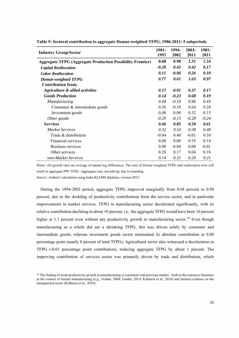
Table 5: Sectoral contribution to aggregate Domar-weighted TFPG, 1986-2011: 5 subperiods

Industry Group/Sector 1981-1993

1994-2002

2003-2011

1981-2011

Aggregate TFPG (Aggregate Production Possibility Frontier) 0.68 0.98 2.31 1.24

Capital Reallocation -0.20 0.43 0.42 0.17

Labor Reallocation 0.11 -0.06 0.26 0.10

Domar-weighted TFPG 0.77 0.61 1.63 0.97 Contribution from: Agriculture & allied activities 0.17 -0.01 0.37 0.17 Goods Production 0.14 -0.23 0.68 0.19 Manufacturing 0.44 -0.10 0.96 0.43 Consumer & intermediate goods 0.36 -0.18 0.64 0.28 Investment goods 0.08 0.08 0.32 0.15 Other goods -0.29 -0.13 -0.28 -0.24 Services 0.46 0.85 0.58 0.61 Market Services 0.32 0.54 0.38 0.40 Trade & distribution -0.04 0.40 -0.01 0.10 Financial services 0.08 0.00 0.35 0.14 Business services 0.00 -0.04 0.00 -0.01 Other services 0.28 0.17 0.04 0.18 non-Market Services 0.14 0.31 0.20 0.21

Notes: All growth rates are average of annual log differences. The sum of Domar-weighted TFPG and reallocation term will

result in aggregate PPF TFPG. Aggregates may not add up, due to rounding.

Source: Authors' calculation using India KLEMS database, version 2015.

During the 1994-2003 period, aggregate TFPG improved marginally from 0.68 percent to 0.98

percent, due to the doubling of productivity contributions from the service sector, and in particular

improvements in market services. TFPG in manufacturing sector decelerated significantly, with its

relative contribution declining to about 10 percent, i.e., the aggregate TFPG would have been 10 percent

higher at 1.1 percent even without any productivity growth in manufacturing sector.16 Even though

manufacturing as a whole did see a shrinking TFPG, this was driven solely by consumer and

intermediate goods, whereas investment goods sector maintained its absolute contribution at 0.08

percentage point (nearly 8 percent of total TFPG). Agricultural sector also witnessed a deceleration in

TFPG (-0.01 percentage point contribution), reducing aggregate TFPG by about 1 percent. The

improving contribution of services sector was primarily driven by trade and distribution, which

16 The finding of weak productivity growth in manufacturing is consistent with previous studies – both in the extensive literature in the context of formal manufacturing (e.g., Goldar, 2004; Goldar, 2014; Kathuria et al., 2010) and limited evidence on the unorganized sector (Kathuria et al., 2010).

27

increased its relative contribution from -6 percent (-0.04 percentage point out of 0.68 percent aggregate

TFPG) during 1981-1993 to 41 percent (0.4 percentage point out of 0.98 percent aggregate TFPG)

during 1994-2002. Out of 87 percent of service sector contribution to aggregate TFPG, market services

consist of 55 percent (0.54 percentage point) and nonmarket services consist of the remaining 32 percent.

In the last period, 2003-2011, the economy had a significant productivity growth surge. This was

achieved mainly because of the remarkable increase in the contribution of agriculture and manufacturing

whereas services contribution did see a decline. More than 40 percent of aggregate TFPG was from the

manufacturing sector (0.96 percentage point out of 2.31 percent aggregate TFPG), whereas contribution

of services shrunk to just a quarter (0.58 percentage point) compared to more than 85 percent

contribution during the previous period. Agriculture contributed more than 15 percent of (0.37

percentage point) of aggregate TFPG. Within manufacturing, consumer and intermediate goods

dominated at 28 percent (0.64 percentage point), but the investment goods sector gained substantially

reaching 14 percent (0.32 percentage point). Within services market services contributed 16 percent

(0.38 percentage point) and nonmarket services contributed 9 percent (0.20 percentage point).

Contribution of trade was negative, whereas financial sector gained significantly reaching 15 percent of

total TFPG (0.35 percentage point).

6.3 The industry pattern of Total Factor Productivity Growth

The results presented in Table 5 are summarizations of 27 disaggregate industry results into a handful

of industry groups, in order to provide an insightful discussion and for ease of analysis. To get a more

detailed picture of the pattern of productivity growth with meaningful interpretation, we use the

Harberger diagram (Harberger, 1998; Timmer et al., 2011). The Harberger diagram plots the cumulative

contribution of individual industries to aggregate growth, against the cumulative share of these industries

in aggregate output. It provides us a summary of how widespread or localized the productivity growth

and changes in growth are within an economy. If growth is widely spread across industries (or growth

takes place in many industries, thereby reflecting in aggregate economy) it is called as yeast-like growth,

and if the aggregate growth is driven only by the positive growth of a few industries, it is called

mushroom-like growth process.

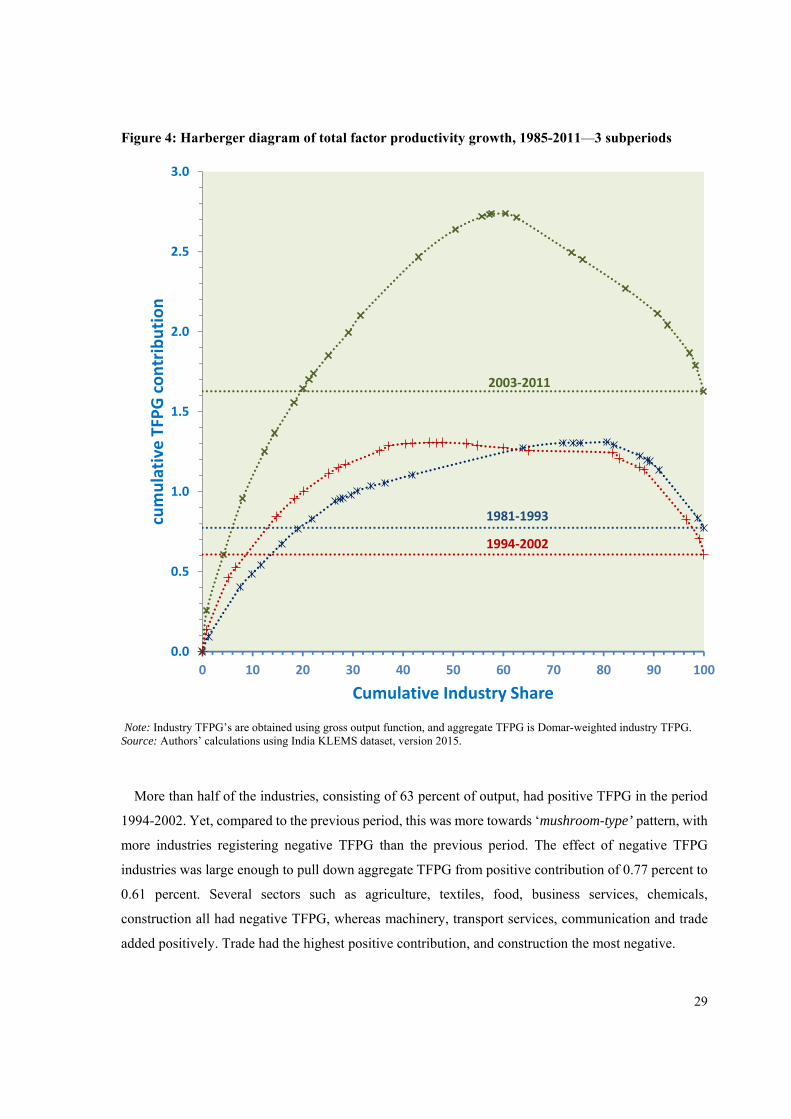
In Figure 4, we provide the Harberger diagram for the three time periods since 1981. The TFPG

presented in these graphs are the Domar-weighted aggregate (see Table 5). On the x axis of the graph,

we have cumulative industry output share, and on the y axis we have cumulative TFPG contribution.

The dotted horizontal lines show the aggregate Domar-weighted TFPG. In Table 6, we further provide

the detailed industry contributions that underlie the Harberger diagram.

28

During 1981-1993 period, there were more industries with positive TFPG (74%), but these industries

constituted only about 56 percent of output (also see Table 7). The pattern of TFPG was more “yeast-

like.” The positive contributions of industries aggregate to 1.3 percent, and the growth reducing effect

of negative TFPG industries brought the aggregate Domar-weighted TFPG down to 0.77 percent. The

largest contribution in the 1980s comes from other services sector followed by agriculture and public

administration, whereas construction registered the most negative contribution (Table 6). Other positive

contributing industries include electrical & optical equipment, financial services, food products and

chemicals. In addition to construction, industries that saw decline in TFPG during this period include

post &communication, transport services, and hotels & restaurants.

29

Figure 4: Harberger diagram of total factor productivity growth, 1985-2011—3 subperiods

Note: Industry TFPG’s are obtained using gross output function, and aggregate TFPG is Domar-weighted industry TFPG. Source: Authors’ calculations using India KLEMS dataset, version 2015.

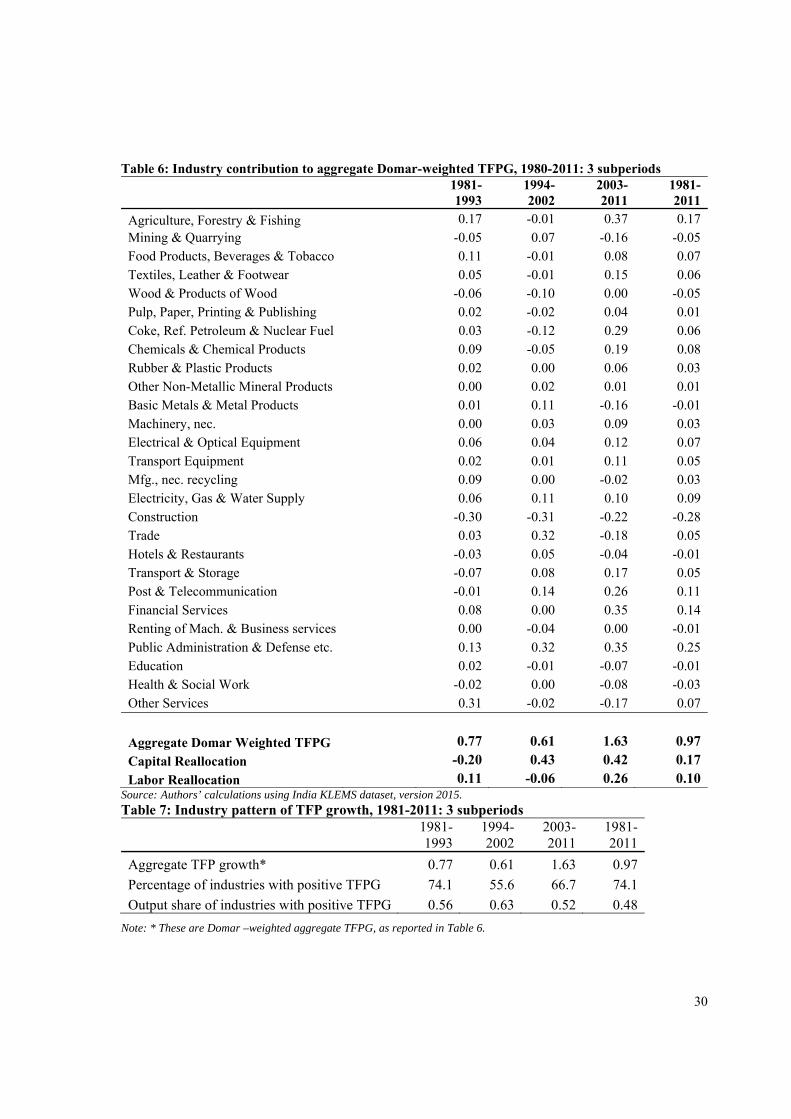
More than half of the industries, consisting of 63 percent of output, had positive TFPG in the period

1994-2002. Yet, compared to the previous period, this was more towards ‘mushroom-type’ pattern, with

more industries registering negative TFPG than the previous period. The effect of negative TFPG

industries was large enough to pull down aggregate TFPG from positive contribution of 0.77 percent to

0.61 percent. Several sectors such as agriculture, textiles, food, business services, chemicals,

construction all had negative TFPG, whereas machinery, transport services, communication and trade

added positively. Trade had the highest positive contribution, and construction the most negative.

2003‐2011

1981‐1993

1994‐2002

0.0

0.5

1.0

1.5

2.0

2.5

3.0

0 10 20 30 40 50 60 70 80 90 100

cumulative TFP

G contribution

Cumulative Industry Share

30

Table 6: Industry contribution to aggregate Domar-weighted TFPG, 1980-2011: 3 subperiods

1981-1993

1994-2002

2003-2011

1981-2011

Agriculture, Forestry & Fishing 0.17 -0.01 0.37 0.17 Mining & Quarrying -0.05 0.07 -0.16 -0.05 Food Products, Beverages & Tobacco 0.11 -0.01 0.08 0.07 Textiles, Leather & Footwear 0.05 -0.01 0.15 0.06 Wood & Products of Wood -0.06 -0.10 0.00 -0.05 Pulp, Paper, Printing & Publishing 0.02 -0.02 0.04 0.01 Coke, Ref. Petroleum & Nuclear Fuel 0.03 -0.12 0.29 0.06 Chemicals & Chemical Products 0.09 -0.05 0.19 0.08 Rubber & Plastic Products 0.02 0.00 0.06 0.03 Other Non-Metallic Mineral Products 0.00 0.02 0.01 0.01 Basic Metals & Metal Products 0.01 0.11 -0.16 -0.01 Machinery, nec. 0.00 0.03 0.09 0.03 Electrical & Optical Equipment 0.06 0.04 0.12 0.07 Transport Equipment 0.02 0.01 0.11 0.05 Mfg., nec. recycling 0.09 0.00 -0.02 0.03 Electricity, Gas & Water Supply 0.06 0.11 0.10 0.09 Construction -0.30 -0.31 -0.22 -0.28 Trade 0.03 0.32 -0.18 0.05 Hotels & Restaurants -0.03 0.05 -0.04 -0.01 Transport & Storage -0.07 0.08 0.17 0.05 Post & Telecommunication -0.01 0.14 0.26 0.11 Financial Services 0.08 0.00 0.35 0.14 Renting of Mach. & Business services 0.00 -0.04 0.00 -0.01 Public Administration & Defense etc. 0.13 0.32 0.35 0.25 Education 0.02 -0.01 -0.07 -0.01 Health & Social Work -0.02 0.00 -0.08 -0.03 Other Services 0.31 -0.02 -0.17 0.07

Aggregate Domar Weighted TFPG 0.77 0.61 1.63 0.97

Capital Reallocation -0.20 0.43 0.42 0.17

Labor Reallocation 0.11 -0.06 0.26 0.10 Source: Authors’ calculations using India KLEMS dataset, version 2015. Table 7: Industry pattern of TFP growth, 1981-2011: 3 subperiods

1981-1993

1994-2002

2003-2011

1981-2011

Aggregate TFP growth* 0.77 0.61 1.63 0.97

Percentage of industries with positive TFPG 74.1 55.6 66.7 74.1

Output share of industries with positive TFPG 0.56 0.63 0.52 0.48

Note: * These are Domar –weighted aggregate TFPG, as reported in Table 6.

31

Source: Authors’ calculations using India KLEMS dataset, version 2015.

During the last subperiod, 2003-2011, there were more than 65 percent of industries with positive

TFPG, covering only 52 percent of total output. It is important to note that most industries with positive

TFPG during this period had relatively high productivity growth compared to previous periods, adding

to 2.7 percent of aggregate TFPG. However, the negative contribution for remaining sectors reduced the

aggregate TFPG by more than 1 percent. Interestingly, Agriculture did contribute the highest TFPG

during this period. Public administration, a nonmarket sector, and financial services were the second

largest positive contributors, whereas construction remained to be the largest negative contributor to

aggregate TFPG. Post & telecom, electrical & optical equipment, textiles, chemicals and transport

services were among the sectors that had positive TFPG.

Thus the Harberger diagram reveals a mixed pattern of economic growth in India. Overall, it is

difficult to say whether Indian economy had a mushroom-like or yeast-like growth pattern. Clearly the

growth was not broad-based throughout the period. On average many industries contributed positively

to aggregate growth. However, often the negatively contributing sectors had a larger effect in terms of

their quantitative magnitude, leading to a substantial drop in the aggregate TFPG. Some sectors such as

electrical & optical equipment, chemicals and financial services had positive TFPG in most of the

periods, whereas construction had consistently negative TFPG.

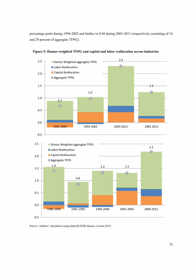
6.4 Capital and labor reallocation effects

In Figure 5, we consider the decomposition of aggregate TFPG obtained using aggregate production

possibility frontier, into contributions from within industry productivity growth, as discussed in the

previous two sections and the reallocation of capital and labor across sectors. Note that the factor

reallocation effects discussed here would be different from the labor productivity decomposition in the

previous section as the methodologies used in the two decompositions are significantly different. The

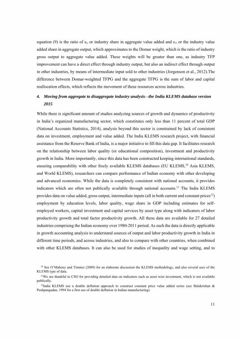
main observation that comes out from Figure 6 is that the aggregate TFPG is primarily a reflection of

TFPG in the underlying industries, or the within industry productivity change (Domar-weighted TFPG)

is significantly reflected in aggregate TFPG, particularly before 1994. It explains more than 100 percent

of aggregate TFPG in this period, whereas the overall reallocation effect was negative and therefore

dragged productivity growth down by 0.09 percentage point. The aggregate TFPG in this chart—TFPG

based on aggregate production possibility frontier—is the sum of Domar-weighted TFPG, presented in

Table 5 and the capital and labor reallocation terms (see equation 9). Overall the average reallocation

effect is about 0.27 percentage point, which however varies considerably over periods, with 1981-1993

being the only period with a negative overall reallocation effect. The reallocation term increased to 0.37

32

percentage point during 1994-2002 and further to 0.68 during 2003-2011 (respectively consisting of 16

and 29 percent of aggregate TFPG).

Figure 5: Domar-weighted TFPG and capital and labor reallocation across industries

Source: Authors’ calculation using India KLEMS dataset, version 2015.

0.7

1.0

2.3

1.2

‐0.5

0.0

0.5

1.0

1.5

2.0

2.5

1981‐1993 1994‐2002 2003‐2011 1981‐2011

Domar Weighted aggregate TFPG

Labor Reallocation

Capital Reallocation

Aggregate TFPG

1.4

0.8

1.3 1.3

2.2

‐0.5

0.0

0.5

1.0

1.5

2.0

2.5

1986‐1990 1991‐1995 1996‐2000 2001‐2005 2006‐2011

Domar Weighted aggregate TFPG

Labor Reallocation

Capital Reallocation

Aggregate TFPG

33

When looked at the reallocation effects of capital and labor separately, we see that, in general, the

capital reallocation term has been positive except in the first period. From a theoretical perspective, the

reallocation term quantify the deviation of the data from assumptions on capital and labor in the PPF.

For instance, a positive capital reallocation would suggest that prices of capital differ across industries,

and capital is moving to sectors with high capital prices. If prices are assumed to be proxies of

productivities, then it would suggest movement of capital to productive sectors. The large reallocation

of capital, particularly since the mid-1990s, therefore indicates that industries where capital was more

productive witnessed faster expansion of investment. It has been negative during 1981-1993, suggesting

that investment was taking place in industries which are relatively less productive. During the last

period, 2003-2011, there seem to have acceleration in investment in industries that have higher return

over capital, as reflected in a positive capital reallocation term. During this period, nearly 20 percent of

aggregate TFP growth was due to positive capital reallocation.

Labor also shows a positive reallocation term in the TFPG decomposition, except during 1994-2002

period, indicating a movement of labor from low wage to high wage sectors. Employment seems to have

been growing slowly in sectors with higher wages during the entire mid-1990s through early 2000s; the

labor reallocation during this period was negative. This is not in consistency with the labor productivity

decomposition, where we found positive, though relatively tiny, reallocation during this period. While

a strict comparison is hard to make, it might suggest that wages and productivity does not go hand in

hand. It is likely that wage levels in several consumer and intermediate goods manufacturing such as

food products, textiles and wood products, and services like trade and hotels and restaurants are not

higher, or even in some cases, lower than other sectors because of large presence of informal sector.

Also, the level of wages could be higher in sectors such as financial services, telecommunication

services, and some public sector services, where no substantial employment has been generated.17

Moreover, the labor reallocation in labor productivity was also lower during this period compared to

other periods. Since 2003, however, the reallocation again moved to positive territory. In general, the

trend in labor reallocation term in both labor productivity decomposition and TFPG decomposition are

quite comparable, except for the opposing signs during 1993-2002.

17 It would be interesting to examine the movement of real wages in comparison with labor productivity growth to see the

evolution of the gap between productivity growth and real wage (wages adjusted for consumer prices) growth. This could happen due to changing composition of capital and labor income share in GDP, which can be caused by, among other factors, the rapid expansion of informal sector, or the changes in workers’ terms of trade (relative price of goods that workers produce and they purchase). See Erumban and de Vries (2016).

34

7. Can India sustain a high long-run growth without manufacturing expansion?

Our analysis reinforces the fact that much of the growth in Indian economy in the post-reform period

has been driven by services sector, a pattern of structural change that defines the conventional hypothesis

of resource movement from primary to secondary sector and then to tertiary sector. However, what is

also evident from our analysis is that within the services sector, the largest contribution to aggregate

growth comes from market services with trade and distributive services dominating. Trade and

distribution service sector generates significant amount of informal jobs, perhaps indicating an

increasing in in-formalization of the Indian economy.18 Manufacturing sector has not gained significant

momentum either in terms of employment generation or output expansion, though its relative

contribution to productivity growth has improved. This poses an important question, whether India will

be able to sustain its service-led growth in the long-term and the observed structural transformation,

which has been growth enhancing in the past, is sustainable. Or should India reverse its structural change

dynamics to the conventional path, by focusing more on its manufacturing sector? We compare India’s

manufacturing share in employment and per capita GDP with that of select advanced economies, in

order to get a descriptive picture on how unique India India’s structural transformation is.

Manufacturing growth is often seen as a backbone of economic growth in several modern advanced

economies and is considered an important element in achieving growth enhancing structural

transformation in emerging economies (Szirmai, 2013). Many studies assert that for a developing

country like India, it is important to maintain a high manufacturing growth without which the pace of

growth of service sector cannot be sustained (Rodrik, 2013; Panagariya, 2008; Acharya et al., 2003).

Szirmai (2013) lists several reasons why manufacturing is important for a country’s development.

Empirically, it has been shown that GDP growth and manufacturing growth are highly correlated when

a country is at low level of income.19 Except for a few countries with abundant natural resources, almost

all countries that sustained a high growth did so with the help of manufacturing sector (Rodrik, 2013).

Structural change in most advanced economies has been such that after reaching an optimum peak,

employment generation in manufacturing has declined, and services sector continued its expansion.

18 Evidence points to an increasing informal sector in Indian economy (Moreno-Monroy, 2014), and the growth in

employment during the recent years is often argued to be driven by low-skilled informal jobs (Sasikumar & Thimothy, 2013) and informal jobs in small size nonagricultural firms (Mehrotra, 2014).

19 In addition to helping achieve higher GDP growth, manufacturing is also important in improving aggregate productivity. Since, productivity levels in manufacturing are generally higher than agriculture, reallocating workers from primary sector to manufacturing helps achieve higher productivity level for the aggregate economy. Moreover, manufacturing sector provides better opportunity for capital accumulation, technological change, economies of scale and scope, compared to agriculture or services (Szirmai, 2013; Naude et al., 2015).

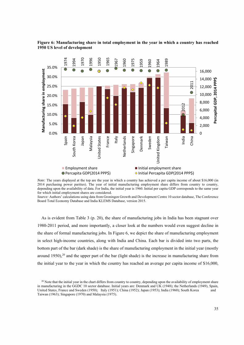
35

Figure 6: Manufacturing share in total employment in the year in which a country has reached 1950 US level of development

Note: The years displayed at the top are the year in which a country has achieved a per capita income of about $16,000 (in 2014 purchasing power parities). The year of initial manufacturing employment share differs from country to country, depending upon the availability of data. For India, the initial year is 1960. Initial per capita GDP corresponds to the same year for which initial employment shares are considered. Source: Authors’ calculations using data from Groningen Growth and Development Centre 10 sector database, The Conference Board Total Economy Database and India KLEMS Database, version 2015.

As is evident from Table 3 (p. 20), the share of manufacturing jobs in India has been stagnant over

1980-2011 period, and more importantly, a closer look at the numbers would even suggest decline in

the share of formal manufacturing jobs. In Figure 6, we depict the share of manufacturing employment

in select high-income countries, along with India and China. Each bar is divided into two parts, the

bottom part of the bar (dark shade) is the share of manufacturing employment in the initial year (mostly

around 1950),20 and the upper part of the bar (light shade) is the increase in manufacturing share from

the initial year to the year in which the country has reached an average per capita income of $16,000,

20 Note that the initial year in the chart differs from country to country, depending upon the availability of employment share

in manufacturing in the GGDC 10 sector database. Initial years are: Denmark and UK (1948); the Netherlands (1949), Spain, United States, France and Sweden (1950); Italy (1951); China (1952); Japan (1953); India (1960); South Korea and Taiwan (1963); Singapore (1970) and Malaysia (1975).

1974

1994

1970

1996

1950

1965

1967

1960

1975

1959

1960

1964

1989

2012

2011

0

2,000

4,000

6,000

8,000

10,000

12,000

14,000

16,000

0.0%

5.0%

10.0%

15.0%

20.0%

25.0%

30.0%

35.0%Sp

ain

South Korea

Japan

Malaysia

United

 States

Fran

ce

Italy

Netherlands

Singapore

Den

mark

Swed

en

United

 Kingd

om

Taiwan

India

China

Percapital GDP, 2014 PPP$

Man

ufacturing share in employm

ent

Employment share Initial employment sharePercapita GDP(2014 PPP$) Initial Percapita GDP(2014 PPP$)

36

measured in 2014 purchasing power parities. The average per capita income of the United States is

$16,000 in 1950, and therefore, the overall size of the bar represents the share of manufacturing

employment in a country in the year in which it has reached the US level of development in 1950. The

year in which each country has reached the US 1950 per capita income level is indicated near to the

circles representing their per capita income levels at the top of the chart.

Except for UK, Sweden and Taiwan, all the countries in the sample had nearly a quarter of their

workers employed in the manufacturing sector at the time they reached 1950 US level of development.

For instance, South Korea's level of per capita income in 1963 was $1,922—just 12 percent of the United

States per capita income in 1950—with 8 percent of its workers being employed in the manufacturing

sector. By 1994, South Korea reached the US' 1950 level of development. During these 31 years, Korea's

manufacturing share increased by 16 percentage point, reaching nearly a quarter of total employment.

Japan, another advanced Asian economy, reached the US 1950 level of development 20 years later in

1970—its per capita income increased from 26 percent of 1950 US level in 1953, with its manufacturing

share increased from 17 percent to 24 percent in the course of 17 years. Today both Korea and Japan

have their per capita incomes nearly 70 percent of US current per capita income level in 2015.

India's per capita GDP in 1960 was slightly above 50 percent of South Korea's per capita GDP in

1963. However, in 2011, the latest year for which we have employment share data in the India KLEMS

database, India's per capita GDP is only 29 percent of the US income level in 1950 (or South Korea’s

income level in 1994). Clearly the increase in per capita income in South Korea was staggering during

this period, along with remarkable increase in manufacturing jobs. From 1960 to 2011 India’s

manufacturing employment share increased only by 2.6 percentage point from 9.6 percent to 12.2

percent, clearly suggesting no significant structural change in India in terms of shift of workers from

agriculture to manufacturing. During this period, employment in market services increased from 7

percent to 24 percent, and nonmarket services declined from 10 percent to 6 percent. This suggests an

overall increase of service sector employment share by nearly 13 percentage point in half a century,

while manufacturing share increased by 2.6 percentage point only.

As is well known, China has focused significantly on low-cost, low-value added manufacturing,

increasing its employment share in manufacturing significantly over years. China's employment share

in manufacturing was 5.6 percent in 1952, at a time its per capita income level was below 4.9 percent of

the US level in 1950 (in fact, India’s per capita income in 1952 was slightly above that of China at 5.1

percent of US level in 1950), and by 2011 it has achieved a per capita income of 66 percent of US 1950

level. During these 60 years of time the share of Chinese manufacturing jobs increased by 13 percent.

Chinese achievement of nearly 20 percent manufacturing share in 60 years is still much lower in level,

37

and slower in pace, compared to what Korea has achieved during its development stage. Yet, today

China's per capita income is 22 percent of the US, which is double the size of India’s per capita income

in 2015 (The Conference Board Total Economy Database, 2015).

Clearly, the service sector surge has helped India achieve faster productivity growth in the aggregate

economy, but it has not been able to absorb workers from primary sector to the extent manufacturing

has been absorbing workers during structural transformation in many of today’s advanced economies.

Moreover, as is evident from our structural decomposition that the relative growth contributions of

services is declining in the recent periods, and many of the growth contributing services are high-skilled

or less labor-intensive (financial services, business services, communication services), or informal job

creating services (trade and distributive services). This along with the lack of job creation in

manufacturing has caused the absorption of workers in the construction sector that has been witnessing

massive decline in productivity growth. Over 1980-2011 period, there have been 187 million jobs

created in Indian economy, out of which 43 million (about 23%) has been in the construction sector.

The picture has got even more elevated since 2005. Almost half of the 43 million construction jobs

created during the course of 30 years has been added during 2005-2011 period, while agriculture has

lost 29 million jobs and textiles and wood each losing 1 million jobs. Overall 13 million jobs were added

during this period (with public administration and post &telecom also seeing an absolute decline in

employment). Clearly, most of the workers are absorbed in the construction sector.

It is hard to imagine that India can sustain a high GDP growth in the longer term, and achieve higher

level of per capita income, without focusing on developing a solid manufacturing sector and thereby

increasing opportunities for its young population. It is also unlikely that India will be able to climb the

development ladder faster, if India follows the Chinese style low-cost manufacturing, rather than

focusing on high-value added manufacturing. A Chinese style low-cost manufacturing is less feasible

for India, given that India will not have much labor cost advantage, as its fast growing ‘high-skilled’

services will put an upward pressure on overall wages, unless the economy is willing to accept a possible

increase in wage inequality, or is able to compensate wage escalation by improved productivity. Given

that nearly half of the workers in India are still employed in the agricultural sector, India still has large

potential for structural change. The speed of worker movement from agricultural sector was constrained

by lack of manufacturing expansion, and therefore more opportunities should be created in the

manufacturing. At the same time, to tap its demographic dividend more effectively, the country should

also focus on improving its human capital.

38

8. Concluding remarks

The importance of structural change for attaining higher levels of economic development was stressed

in the development economics literature as early as in the 1940s. The recent developments in this

literature reiterate the importance of workers and resources moving from less productive to more

productive sectors, in determining the speed of economic growth. This paper is an attempt to document

the evolution of India’s aggregate productivity growth, decomposed into the contributions of detailed

industrial sectors and structural change since the 1980s. Using the India KLEMS database, version 2015,

which provides comprehensive and consistent industry level data on Indian economy, we trace the

industry origins of labor productivity and total factor productivity growth (TFPG), along with the

contribution of factor reallocation. In the labor productivity decomposition, we examine both static—

movement of workers from low productive to high productive sectors—and dynamic—movement of

workers from slow growing to fast growing sectors—reallocation effects, in comparison with within

industry productivity growth.

Even though the relative shares of agriculture in total employment and output have diminished

substantially over time, agriculture still remains as the major employment provider in the Indian

economy. It appears that job losses in agriculture are largely absorbed in the construction sector,

followed by some increases in the employment share of market services, in particular, trade and

distributive services, financial services and business services. Manufacturing job creation has been very

low. Given the relatively higher productivity levels in these sectors compared to agriculture, the static

structural change—movement of workers to industries with higher productivity levels—has been

positive in India, whereas as the dynamic productivity gains—movement of workers to fast growing

sectors—has been limited or absent. Productivity growth in the construction sector, which has been

rapidly expanding in employment creation, has been consistently negative.

In general, the observed total factor productivity growth is not broad based. If the pattern of

productivity was more broad-based the aggregate productivity gain would have been much larger. There

are many industries that contributed negatively to aggregate productivity growth. While some industries

lost their relative importance as contributors to aggregate productivity, some industries emerged as

important contributors. The 1980s was a period of notable TFPG contribution from manufacturing, which

eroded in the second period, 1994-2002, when services dominated in terms of relative contribution to

aggregate TFPG. Yet manufacturing did witness a diversification during this period, with a shift in

productivity contribution towards investment goods from consumer goods production. This was also a period

of productivity acceleration in nonmarket services. In the last period, 2003-2011, however, manufacturing

39

revived significantly, breaking its own past record, and services lost its relative importance significantly in

contributing to aggregate TFPG.

The capital reallocation term in our TFPG decomposition has been positive since 1994, suggesting

expansion of investment in sectors with high returns from capital. Labor reallocation has, however, been

negative during 1994-2002 period; employment doesn’t seem to have expanded in sectors with relatively

higher levels of wages. This, which is in contrast with our static reallocation effect, seems to suggest

that wages and productivity does not go hand in hand.

Yet, India’s structural change, which defies the success story of several advanced economies, poses

major challenges. Evidence from several of today’s advanced economies both in Asia and elsewhere

suggests that no country has achieved a higher level of development without a solid manufacturing

sector. Even today, with the GDP growth being driven primarily by the services sector, nearly half of

India’s workers is employed in the primary sector, suggesting further potential for structural change. It

is hard to argue, particularly given the fact that the pace of job creation in high productive services has

been slow, India can sustain higher long-term growth rates without a solid manufacturing sector. Indeed,

India still has substantial catch-up potential in the manufacturing, and given its large pool of young

population and underdeveloped infrastructure, it can excel in manufacturing only if it focuses on

improving its human capital and infrastructure. However, poor quality of and accessibility to education,

hindering its human capital development, poor quality of infrastructure, slow pace of reforms, and the

co-existence of a modern formal and a traditional informal sector offers major challenges for further

positive structural change. Achieving growth-enhancing structural change requires adequate policies

that would ease the reallocation of resources from less productive to high productive sectors. The

reforms in the manufacturing sector are less complete, particularly from the perspective of formal job

creation, as the rigid labor market and weak infrastructure provided hardly any incentive for formal job

creation.

40

Bibliography

Acharya, S., I. J. Ahluwalia, K. L. Krishna, and I. Patnaik (2003), India: Economic Growth, 1950-2000, Global Research Project on Growth, Indian Council for Research on International Economic Relations, New Delhi.

Aggarwal, S. C., and A. A. Erumban, (2013), Labor input for measuring productivity growth in India: Methodology and estimates, Mimeo.

Ahluwalia, I. J. (1991), Productivity and Growth in Indian Manufacturing, Delhi New York: Oxford University Press.

Balakrishnan, P (2010) Economic Growth in India: History and Prospect, New Delhi: Oxford University Press.

Balakrishnan, P., and K. Pushpangadan (1994), Total factor productivity growth in manufacturing industry: A fresh look, Economic and Political Weekly, 29, 2028-2035.

Bhagwati, J., and A. Panagariya, (2013), Why Growth Matters: How Economic Growth in India Reduced Poverty and the Lessons for Other Developing Countries. New York: Public Affairs.

Bosworth, B., S. M. Collins (2008), Accounting for growth: Comparing China and India, Journal of Economic Perspectives, 22(1): 45-66.

Brahmananda, P. R. (1982), Productivity in the Indian Economy: Rising Inputs for Falling Outputs, Himalaya Publishing House, 1982.

Chenery, Hollis B. and Moises Syrquin (1975), Patterns of Development: 1950–1970, New York: Oxford University Press for the World Bank.

Clark, C (1940), The Conditions of Economic Progress, London: Macmillan. Das, D. K., and Kalita, G. (2011). Aggregate productivity growth in Indian manufacturing: An application of Domar aggregation, Indian Economic Review, 46, 2.

Das, D. K., A. A. Erumban., S. Aggarwal and S. Sengupta (2016), Productivity growth in India under different Policy Regimes, In Jorgenson, D., M. P. Timmer and K. Fukao (eds.),The World Economy: Growth or Stagnation?, Cambridge University Press.

De Vries, G. J., Erumban, A. A., Timmer, M. P., Voskoboynikov, I., and Wu, H. X. (2012), Deconstructing the BRICs: Structural transformation and aggregate productivity growth, Journal of Comparative Economics, 40(2), 211-227.

de Vries, G., M. P Timmer and de Vries, K (2015), Structural Transformation in Africa: Static Gains, Dynamic Losses, The Journal of Development Studies, 51(6).

Denison, Edward F., 1967. Why Growth Rates Differ. Brookings, Washington, DC.

Domar, E. D. (1961), “On the Measurement of Technological Change”, Economic Journal, 71.

Eichengreen, B., P. Gupta., and R. Kumar (2010), Emerging Giants: China and India in the World Economy, Oxford, Oxford University Press.

Erumban. A. A and D.K. Das (2016), Information and communication technology and economic growth in India, Telecommunications Policy, 40(5), 412–431, DOI: 10.1016/j.telpol.2015.08.006.

Erumban. A. A and K. de Vries (2016), Wage-Productivity Growth Gap: An Analysis of Industry Data, The Conference Board Working Paper, EPWP1601 https://www.conference-board.org/publications/publicationdetail.cfm?publicationid=7143

Fabricant, S. (1942). Employment in manufacturing, 1899–1939. New York: NBER.

Fisher, A. G. B (1939). Primary, Secondary and Tertiary Production, Economic Record. 15, 24–38.

Goldar, B. N (2004), Indian manufacturing: productivity trends in pre- and post-reform periods, Economic and Political Weekly, 39(46/47), 5033-5043.

41

Goldar, B. N (2014),"Productivity in Indian manufacturing in the post-reform period, in Kathuria, V. et al. (2014), Productivity in Indian Manufacturing- Measurements, Methods and Analysis, Routledge, New Delhi and UK.

Goldar, B. N (2015), Productivity in Indian Manufacturing (1999–2011) - Accounting for Imported Materials Input, Economic and Political Weekly, 40(35), 104-111.

Harberger, A. C (1998), A vision of the growth process, American Economic Review, 88(1) 1-32

Jorgenson D W & Mun Ho & Jon Samuels, 2011. "Information technology and U.S. productivity growth: evidence from a prototype industry production account," Journal of Productivity Analysis, Springer, vol. 36(2), pages 159-175, October.

Jorgenson, D., M. S.. Ho, and K. J. Stiroh, (2005), Information Technology and the American Growth Resurgence, Cambridge, The MIT Press.

Jorgenson, D.W (1963), Capital theory and investment behavior, American Economic Review, 53 (2), 247-259.

Jorgenson, D.W., & Timmer, M.P. (2011). Structural change in advanced nations: A new set of stylised facts. Scandinavian Journal of Economics, 113(1), 1-29.

Jorgenson, D. W., Ho, M. S., Samuels, J. D., & Stiroh, K. J. (2007). Industry origins of the American productivity resurgence. Economic Systems Research, 19(3),229–252.

Kathuria, V, S. N. R. Raj and K. Sen (2010), Organised versus unorganised manufacturing performance in the post-reform period, Economic and Political Weekly, 45(24), 55-64.

Kathuria, V., S. N. R. Raj., K.Sen (2014), Productivity in Indian Manufacturing- Measurements, Methods and Analysis, Routledge, New Delhi and UK.

Kochar, K., Kumar, U., Rajan, R., Subramanian, A., Tokatlidis, I. (2006). India’s patterns of development: What happened, what follows? Journal of Monetary Economics, 53 (5), 981-1019.

Kuznets, S. (1966). Modern economic growth: Rate, structure and spread. London: Yale University Press. Lin, J. (2011). New structural economics: A framework for rethinking Development. The World Bank research observer, 26 (2), 193-221.

Lewis, W. A. (1954). “Economic Development With Unlimited Supplies of Labour.” Manchester School of Economic and Social studies, vol. 22, pp.139-191.

Maddison, A. (1987). Growth and slowdown in advanced capitalist economies: Techniques of quantitative assessment. Journal of Economic Literature, 25 (2), 649–698.

Moreno-Monroy, A. I., J. Pieters , and A.A, Erumban (2014), Formal sector subcontracting and informal sector employment in Indian manufacturing, IZA Journal of Labor & Development, 3(22), 1-17.

McMillan, M., & Rodrik, D. (2011). Globalization, structural change, and productivity growth (NBER working paper 17143). Cambridge: NBER.

Naude W., A. Szirmai and N. Haraguchi (2015), Structural Change and Industrial Development in the BRICS, Oxford, Oxford University Press.

OECD (2013). “Structural Transformation and Natural Resources in Africa.” African Economic Outlook 2013: Structural Transformation and Natural Resources. OECD Publishing, pp.111-189.

Panagariya, A, (2008), India the Emerging Giant, New York: Oxford University.

Rodrik, D (2013), the past, present, and future of economic growth, Global Citizen Foundation Working Paper 1, https://www.sss.ias.edu/files/pdfs/Rodrik/Research/GCF_Rodrik-working-paper-1_-6-24-13.pdf

42

Szirmai, A (2013). Manufacturing and Economic Development, in A. Szirmai, W. Naude, and L. Alcorta (eds), Pathways to Industrialization in the 21st Century, New Challenges and Emerging Paradigms, Oxford, Oxford University Press.

The Conference Board (2014), The Conference Board Total Economy DatabaseTM, January 2014, https://www.conference-board.org/data/economydatabase/

Timmer, M. P. (2000). The Dynamics of Asian Manufacturing. A Comparison in the late Twentieth Century. Edward Elgar Publishers, Cheltenham.

Timmer, M. P., E. Dietzenbacher, B. Los, R. Stehrer, and G. J. de Vries (2015), An illustrated user guide to the World Input–Output Database: the case of global automotive production, Review of International Economics.

Timmer, M. P., G. J. de Vries, and K. de Vries (2014). “Patterns of Structural Change in Developing Countries.” GGDC research memorandum 149.

Timmer, M. P., R. Inklaar., M. O’Mahony and B. van Ark, B (2011), Economic Growth in Europe: A Comparative Industry Perspective, Cambridge, Cambridge University Press.

Timmer, M. P., R. Inklaar., M. O'Mahony and B. van Ark (2010), Economic Growth in Europe: A Comparative Industry Perspective, Cambridge University Press, 2010.

Timmer, Marcel P., Abdul Azeez Erumban, Bart Los, Robert Stehrer, and Gaaitzen J. de Vries (2014). "Slicing Up Global Value Chains." Journal of Economic Perspectives, 28(2): 99-118.

Vaidyanathan A. and K. L. Krishna, (2007) Institutions and markets in India's Development: Essays for K. N. Raj. Oxford University Press, New Delhi.

van Ark, B. (1996). “Sectoral Growth Accounting and Structural Change in Post-war Europe.” Chapter 3 in B. van Ark and N. Crafts (1996), Quantitative Aspects of Post-war European Economic Growth. Cambridge University Press.

Verma, R. (2012), Can total factor productivity explain value added growth in services? Journal of Development Economics, 99(1), 163-177.

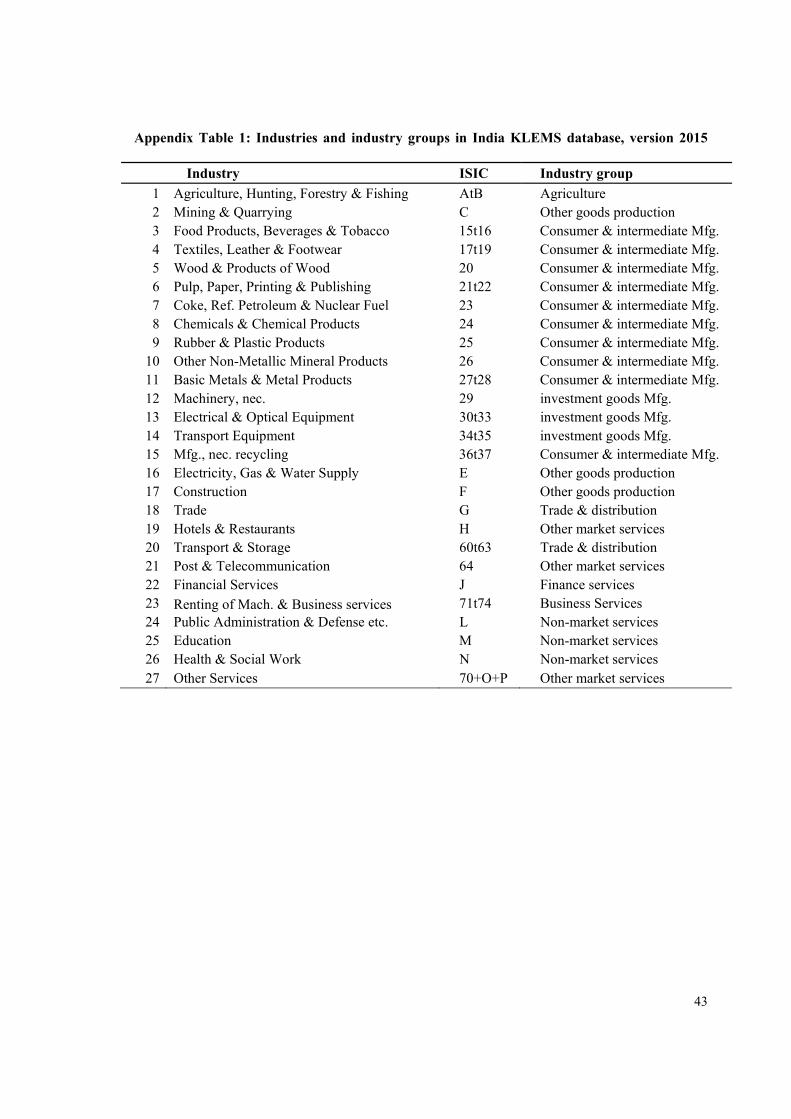
43

Appendix Table 1: Industries and industry groups in India KLEMS database, version 2015

Industry ISIC Industry group

1 Agriculture, Hunting, Forestry & Fishing AtB Agriculture 2 Mining & Quarrying C Other goods production 3 Food Products, Beverages & Tobacco 15t16 Consumer & intermediate Mfg. 4 Textiles, Leather & Footwear 17t19 Consumer & intermediate Mfg. 5 Wood & Products of Wood 20 Consumer & intermediate Mfg. 6 Pulp, Paper, Printing & Publishing 21t22 Consumer & intermediate Mfg. 7 Coke, Ref. Petroleum & Nuclear Fuel 23 Consumer & intermediate Mfg. 8 Chemicals & Chemical Products 24 Consumer & intermediate Mfg. 9 Rubber & Plastic Products 25 Consumer & intermediate Mfg.

10 Other Non-Metallic Mineral Products 26 Consumer & intermediate Mfg. 11 Basic Metals & Metal Products 27t28 Consumer & intermediate Mfg. 12 Machinery, nec. 29 investment goods Mfg. 13 Electrical & Optical Equipment 30t33 investment goods Mfg. 14 Transport Equipment 34t35 investment goods Mfg. 15 Mfg., nec. recycling 36t37 Consumer & intermediate Mfg. 16 Electricity, Gas & Water Supply E Other goods production 17 Construction F Other goods production 18 Trade G Trade & distribution 19 Hotels & Restaurants H Other market services 20 Transport & Storage 60t63 Trade & distribution 21 Post & Telecommunication 64 Other market services 22 Financial Services J Finance services 23 Renting of Mach. & Business services 71t74 Business Services 24 Public Administration & Defense etc. L Non-market services 25 Education M Non-market services 26 Health & Social Work N Non-market services 27 Other Services 70+O+P Other market services

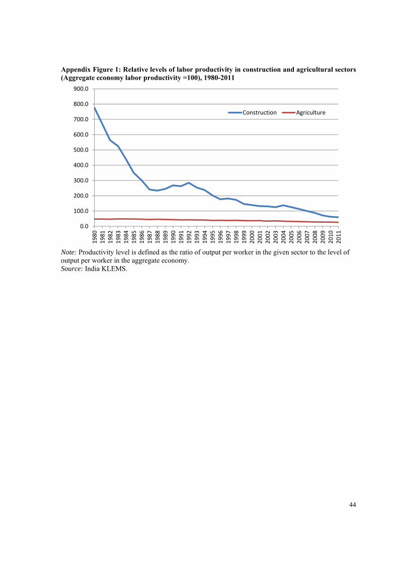
44

Appendix Figure 1: Relative levels of labor productivity in construction and agricultural sectors (Aggregate economy labor productivity =100), 1980-2011

Note: Productivity level is defined as the ratio of output per worker in the given sector to the level of output per worker in the aggregate economy. Source: India KLEMS.

0.0

100.0

200.0

300.0

400.0

500.0

600.0

700.0

800.0

900.01980

1981

1982

1983

1984

1985

1986

1987

1988

1989

1990

1991

1992

1993

1994

1995

1996

1997

1998

1999

2000

2001

2002

2003

2004

2005

2006

2007

2008

2009

2010

2011

Construction Agriculture