Embed Size (px)
Citation preview
Inequality: A hidden cost of market power 2017

This discussion paper should not be reported as representing the official views of the OECD or of its member countries. The opinions expressed and arguments employed are those of the author(s). Discussion papers describe preliminary results or research in progress by the author(s) and are published to stimulate discussion on a broad range of issues on which the OECD works. Comments are welcome and may be sent to the authors: [email protected]; [email protected]; and [email protected]. This document reproduces a paper circulated to OECD Competition Committee delegates for information with the reference number DAF/COMP(2015)10. This document and any map included herein are without prejudice to the status or sovereignty over any territory, to the delimitation of international frontiers and boundaries and to the name of any territory, city, or area. © OECD 2017
Please cite this work as: Ennis, S. et al. (2017) Inequality: A hidden cost of market power www.oecd.org/daf/competition/inequality-a-hidden-cost-of-market-power.htm
ABSTRACT
INEQUALITY: A HIDDEN COST OF MARKET POWER © OECD 2017 3
Inequality: A Hidden Cost of Market Power
by Sean Ennis, Pedro Gonzaga and Chris Pike OECD Competition Division *
This draft discussion paper explores the impact of competition on inequality by developing a new model to illustrate how higher profits from market power, and associated higher prices, could influence the distribution of wealth and income. It analyses data from eight OECD countries – Canada, France, Germany, Korea, Japan, Spain, the United Kingdom and the United States. Under this particular model, for an average country in the sample, market power increases the wealth of the richest 10% by between 12% and 21% for a range of reasonable assumptions about savings behaviour, while it reduces the income of the poorest 20% by between 14% and 19%. The results contribute to the economic literature on the origins of inequality, suggesting that competition may help to reduce economic inequality.
This paper contributes to OECD work on inclusive growth.
* This paper was written by Sean Ennis, Pedro Gonzaga and Chris Pike. OECD, 2 rue André-
Pascal, 75775 Paris Cedex 16, France. Corresponding author: [email protected]. Contact for other authors: [email protected], [email protected]. Special thanks to John Davies who instigated this work. Thanks for comments to Paul Atkinson, Walter Beckert, Adrian Blundell-Wignall, Marco Buti, Antonio Capobianco, John Davies, Steve Davies, Jens Høj, Morton Hviid, Bruce Lyons, Joaquim Oliveira Martins, Pierre Poret, Ana Rodrigues, Ania Thiemann, Catherine Waddams, and commenters from various competition agencies and seminars or conferences at the University of East Anglia, University College London and the World Bank.

TABLE OF CONTENTS
INEQUALITY: A HIDDEN COST OF MARKET POWER © OECD 2017 5
Table of contents
1. Introduction ....................................................................................................................................... 7
2. Model ................................................................................................................................................ 11
2.1 Assumptions ........................................................................................................................... 11 2.2 National income identity ........................................................................................................ 12 2.3 Consumption function ............................................................................................................ 13 2.4 Wealth dynamics .................................................................................................................... 14 2.5 Solving the model .................................................................................................................. 14
3. Data ................................................................................................................................................... 17
3.1 Market power indicator .......................................................................................................... 17 3.2 Wealth and income shares...................................................................................................... 18 3.3 Income share of labour ........................................................................................................... 19 3.4 Marginal propensity to save over average saving rate ........................................................... 19
4. Results............................................................................................................................................... 21
5.Conclusions ....................................................................................................................................... 23
Notes ..................................................................................................................................................... 25
References ............................................................................................................................................ 27
Annex A1. Tables and figures............................................................................................................. 31
Annex A2. Derivation of equation (6) ................................................................................................ 41
Annex A3. Derivation of equation (11) .............................................................................................. 43
Annex A4. Derivation of equation (15) .............................................................................................. 45
Annex A5. Derivation of equations (16) and (17) ............................................................................. 47
Annex A6. Estimating competitive mark-ups ................................................................................... 49
Annex A7. The marginal propensity to save ..................................................................................... 55

TABLE OF CONTENTS
6 INEQUALITY: A HIDDEN COST OF MARKET POWER © OECD 2017
Tables
Table 1. Data sources ......................................................................................................................... 31 Table 2. Summary data: distribution of net worth, income and consumption expenditures .............. 32 Table 3. Impact of market power on wealth shares ........................................................................... 33 Table 4. Impact of market power on the wealth of the richest 10% of households ........................... 34 Table 5. Impact of market power on income shares ......................................................................... 35 Table 6. Impact of market power on the income of the poorest 20% of households ......................... 36 Table A6.1. Mark-ups estimates: industry detail ............................................................................... 49 Table A6.2. Impact of market power on mark-ups and prices ........................................................... 50 Table A7.1. Marginal propensity to save (MPS) from a permanent shock in income ....................... 55 Table A7.2. Ratio of the marginal propensity to save to the average saving rate .............................. 56
Figures
Figure 1. Mark-ups across countries .................................................................................................. 36 Figure 2. Impact of market power on wealth distribution .................................................................. 37 Figure 3. Variation in wealth shares from a 1% mark-up reduction .................................................. 38 Figure 4. Variation in income shares from a 1% mark-up reduction ................................................. 39
INTRODUCTION
INEQUALITY: A HIDDEN COST OF MARKET POWER © OECD 2017 7
1. Introduction
While some degree of inequality is necessary for the operation of a market economy –by creating rewards for effort, achievement and innovation– recent economic research finds stagnation in median wages and an increased disparity between the incomes of different groups of the population.1 Understanding the contributing factors to inequality is important, if policymakers wish to reverse these tendencies. While there is much dispute about the origins of these tendencies, traditional explanations include a reduction in fiscal transfers from rich to poor, differences in human capital value or differences in demand for different types of workers. Increasingly, market power has also been identified as contributing to some extent to increased inequality. This has been noted by Ennis and Kim (2016), Furman and Orszag (2015), Rognlie (2015), Baker and Salop (2015), Creedy and Dixon (1999) and Comanor and Smiley (1975).
For the purpose of this work, market power is defined as the ability to drive prices and returns above competitive levels. The existence of market power has a dual effect on the income distribution, not only generating higher economic profits2 for business owners, but also imposing higher prices on consumers. The increased margins charged to customers as a result of market power will disproportionately harm the poor who will pay more for goods without receiving a counter-balancing share of increased profits. The wealthy, while paying more for goods, will at the same time receive higher profits from market power, due to their generally higher ownership of the stream of corporate profits and capital gains.
Further discussion of the role of market power in the distribution of wealth is exemplified by Baker and Salop (2015), who examine how competition law enforcement can complement other policy responses to concerns about rising inequality. Furman and Orszag (2015) identify mechanisms that may create a relationship between lack of competition and inequality. Another way in which competition can deliver benefits is by reducing the prices of goods consumed mostly by the poor (Hausman and Sidak, 2004), as there is some evidence that poorer consumers are more exposed to monopolisation. In particular, building on work by Creedy and Dixon (1999), Urzua (2013) shows how Mexican consumers from different income categories and from different parts of the country were exposed to monopoly power. They found that “the welfare losses due to the exercise of monopoly power are not only significant, but also regressive”.
While mechanisms by which market power can affect inequality are increasingly posited, the extent to which they may account for inequality is still open question. Little research has focused on the potential size of market power’s impact on inequality, with the exception of a study for the United States by Comanor and Smiley (1975), whose model has been updated and extended to other countries by Ennis and Kim (2016). The Comanor and Smiley (1975) model and assumed parameters for calibration have been suggested to contain substantial limits, though in our view the paper still provides a useful basis to obtain a notion of the dimension of the effect. Nonetheless, there is little analysis
INTRODUCTION
8 INEQUALITY: A HIDDEN COST OF MARKET POWER © OECD 2017
of the effects of competition on income or wealth distribution overall using more recent approaches.
Our paper helps to fill that gap by proposing a new steady-state model built up from fundamental economic relationships and addressing certain limitations that existed in prior work. By making a comparative static analysis between two different scenarios, one with existing levels of market power and another with competition enhanced, we model the potential impacts of market power on wealth distributions for eight OECD countries: Canada, France, Germany, Korea, Japan, Spain, the United Kingdom and the United States. The countries were selected to ensure coverage of a large share of the world’s wealth, in light of data availability. The wealth distribution data comes from the OECD Wealth Database or, in the two cases where the reported data are not at the required level of detail, from commonly cited alternative sources.3
While this paper focuses on the benefits of increasing competition, it does not suggest that all sources of economic market power should be eliminated. Some degree of product market power is desirable to provide sustained incentives to innovate. Patents, trademarks and brand differentiation, for example, often involve creation of market power accompanied by a positive impact on incentive to innovate. Similarly, some degree of market power is an essential spur to investment, which is why competition laws generally do not prohibit market power as such but rather its “abuse” to restrict competition. Indeed, some market power illegitimately arises from abusive behaviour by dominant companies or from cartels (illegal agreements between firms not to compete). Similarly, policy makers may be able to eliminate the scope for market power arising from government regulations that protect companies from competition.
Some observers may suggest that market power cannot play a significant role in creating inequality, as the effects of market power themselves may be modest. Indeed, only if market power is economically significant can it reasonably have major effects on inequality. There are reasons to consider the overall effects of illegitimate or undesirable market power as significant. Much anti-competitive behaviour by firms is hidden, because it is illegal. However, the business activities of discovered cartels already show a broad range of affected sectors. Accounting for both prosecuted and undiscovered cartels with a 20% discovery rate, and assuming comparable economic commerce of discovered and undiscovered cartels, Ennis (2014) suggests an estimate of the size of commerce affected by international cartels, between 1990 to 2013, at USD 48.5 trillion, while the mark-up found on typical discovered cartels is around 10% to 30%.4 Annualised over 24 years, this suggests about USD 2 trillion in cartel commerce per year, and anti-competitive price increases from cartels of USD 200-600 billion.
Similarly, it is very hard to estimate the total rents accruing to firms protected from competition by unnecessary anticompetitive regulation. However, a study carried out by OECD (Wolfl et al., 2010) found evidence that less restrictive product market regulations may have a significant impact on growth. In particular, the study estimates that reducing barriers to entrepreneurship (such as barriers to entry and antitrust exemptions) to a level consistent with the currently observed best practices among OECD members would allow an average OECD country to obtain a 0.35% to 0.4% higher annual growth rate of GDP per capita. Consequently, it seems reasonable to suppose that a significant proportion of the market power effect arises from ‘illegitimate’ or ‘excessive’ market power originating in sources that could perhaps be reduced through more effective competition policy.
Finally, while many modern commentators seek to distance competition law and policy from distributional concerns, it is worth noting that the origins of antitrust law lie
INTRODUCTION
INEQUALITY: A HIDDEN COST OF MARKET POWER © OECD 2017 9
very much in concerns about the concentration of wealth. In the United States, the antitrust laws were introduced explicitly to counter monopolisation of the economy not because of concerns about ‘efficiency’ but rather about undue political influence stemming from the wealth of the owners of the “trusts” (Baker and Salop, 2015). The results of this paper will add quantitative information to the debate over appropriate standards for evaluating competition law cases and weighing competition against innovation, with consumer surplus standards having more attractive features than total surplus standards for evaluating competition policies, because profits have much more unequal distributional consequences than consumption. The choice over which standard to adopt is important because it can have a direct result on competition law case outcomes and policies towards innovation.
This paper proceeds as follows: Section 2 derives and explains the steady state model that underlies the analysis, Section 3 discusses the data that can be fit to this model, Section 4 presents the results for all the countries in the analysis, Section 5 concludes and provides directions for future work.

2. MODEL
INEQUALITY: A HIDDEN COST OF MARKET POWER © OECD 2017 11
2. Model
The dynamic steady-state model that we propose is highly stylised, and intended to capture the most essential factors for the question at hand, but does not characterise all relevant phenomena. Based on actual income, wealth and consumption expenditure distributions, it models the potential effect that higher prices would have on different groups of the population.
For this purpose, we make a comparative static analysis between two alternative steady states: the first is the current state where business owners have market power and which is characterised by observed distributions of wealth, income and consumption expenditures; the second is a hypothetical steady state where markets are competitive and distributions of wealth, income and consumption expenditures are implied by the model and the reduction in mark-ups. We do not suggest that the economies examined are actually in steady state, but that the approach is a reasonable approximation to capture the essential features needed to compare situations with more or less competition.
2.1 Assumptions
The use of our steady-state model to measure the redistributive effect of market power implies four primary assumptions:
1. Market power for each country can be approximated by the difference between the average mark-up (across all sectors) in the country and a minimum mark-up that reflects the best-practices of most competitive economies.5 The method is further explained below and is designed to recognise that a significant level of mark-up is needed to cover necessary returns on investment and legitimate sources of market power such as patents and trademarks.
2. The marginal propensity to save (𝑠𝑠′) from increased income arising from lower prices is constant across wealth groups. This assumption simplifies the solution to the model, but does not prevent the average saving rate from varying across wealth groups.6 The assumption is a conservative one since accommodating a higher marginal propensity to save for the wealthier will only increase the magnitude of the redistributive effects that we identify.
3. Market power gains are distributed in proportion to the current net wealth distribution (later referred to as fi). This reflects the observations that corporate income and capital gains are distributed via business ownership, so that those with the largest wealth shares (whether in the form of corporate shares, bonds, pension fund entitlements, dwellings, land or others) will, in proportion, receive the largest share of the profits.7
4. The price of different baskets of goods will be inflated by market power in an equal percentage. This implies that products for the poor and products for the wealthy will be equally affected by market power.8 To the extent that the poor are more exposed to monopolisation, the model provides conservative, lower-bound estimates.
2. MODEL
12 INEQUALITY: A HIDDEN COST OF MARKET POWER © OECD 2017
Under these assumptions, we denote 𝑌𝑌 the total income in the economy, 𝐹𝐹 net wealth assets, 𝐶𝐶 the aggregate consumption expenditure, 𝑊𝑊 the labour income and 𝑅𝑅 the capital income. All variables are nominal and we will use the superscripts 𝑚𝑚 and 𝑐𝑐 to refer to the observed values in the monopolistic and competitive steady states, respectively. In addition, we consider 𝑔𝑔 the economic growth rate, �̅�𝑠 the average saving rate of the economy, 𝑠𝑠′ the marginal propensity to save, 𝛼𝛼𝐿𝐿 and 𝛼𝛼𝑘𝑘 the shares of labour and capital income in the monopolistic steady state, and 𝜇𝜇 the mark-up, defined as the price over estimated marginal cost.
As we want to isolate the redistributive effect of market power, we consider that the only impact of monopolies is to raise prices, while output remains constant. Thus, the difference between aggregate income, consumption expenditures and wealth in the monopolistic and competitive equilibrium is driven by the price increase. Given that under competition the aggregate price is equal to marginal cost, the following relations hold:
𝐹𝐹𝑚𝑚 = 𝜇𝜇𝐹𝐹𝑐𝑐 , 𝑌𝑌𝑚𝑚 = 𝜇𝜇𝑌𝑌𝑐𝑐 , 𝐶𝐶𝑚𝑚 = 𝜇𝜇𝐶𝐶𝑐𝑐 . (1)
While efficiency effects are outside the scope of the model, in reality we would also expect market power to reduce aggregate output, resulting in a deadweight loss. It is not clear though how deadweight loss affects inequality, since both business owners and consumers are harmed by lost transactions. Still, we should expect efficiency effects to impact particularly the poorest groups of the population, since the households that reduce consumption are those with lowest willingness to pay and that cannot afford monopoly prices. Likewise, supply contractions can be created by regulatory barriers that restrict the entry of small and medium enterprises, while reinforcing the market share of the largest incumbents.
2.2 National income identity
The national income identity defines aggregate output as the sum of income from labour and capital:
𝑌𝑌𝑗𝑗 = 𝑊𝑊 + 𝑅𝑅𝑗𝑗, 𝑤𝑤ℎ𝑒𝑒𝑒𝑒𝑒𝑒 𝑗𝑗 = 𝑐𝑐,𝑚𝑚. (2)
Note that the change in price when we move to the competitive steady state does not affect labour income, which we assume remains constant across the two steady states. In fact, if market power increased prices and wages in the same proportion, the redistributive effect of market power would likely be negligible, since workers and business owners would be affected in the same way. We also do not know a priori how capital income is affected by market power, since doubling prices does not necessarily double the return on capital. However, we can use the fact that 𝑌𝑌𝑚𝑚 = 𝜇𝜇𝑌𝑌𝑐𝑐 to obtain a relation between 𝑅𝑅𝑐𝑐 and 𝑅𝑅𝑚𝑚:
𝑌𝑌𝑐𝑐 = 𝑊𝑊 +1 − 𝜇𝜇𝜇𝜇
𝑊𝑊 +𝑅𝑅𝑚𝑚
𝜇𝜇���������𝑅𝑅𝑐𝑐
. (3)
2. MODEL
INEQUALITY: A HIDDEN COST OF MARKET POWER © OECD 2017 13
Using lower case letters to describe the shares of wealth and income of a particular population group, the income earned by a population group 𝑖𝑖 is, in each steady state, given by the following equations:
𝑦𝑦𝑖𝑖𝑚𝑚𝑌𝑌𝑚𝑚 = 𝑊𝑊𝑖𝑖 + 𝑓𝑓𝑖𝑖𝑚𝑚𝑅𝑅𝑚𝑚 (4)
𝑦𝑦𝑖𝑖𝑐𝑐𝑌𝑌𝑐𝑐 = 𝑊𝑊𝑖𝑖 + 𝑓𝑓𝑖𝑖𝑐𝑐 �1 − 𝜇𝜇𝜇𝜇
𝑊𝑊 +𝑅𝑅𝑚𝑚
𝜇𝜇 � . (5)
In the two equations above, 𝑊𝑊𝑖𝑖 is the labour income earned by each population group, whose nominal level is not affected by market power (just as aggregate labour income). Subtracting equation (5) from equation (4) and using the equalities in (1) and (2) (see Annex A2 for a complete derivation), we get:
𝑦𝑦𝑖𝑖𝑚𝑚 − 𝑦𝑦𝑖𝑖𝑐𝑐 = (𝜇𝜇 − 1)(𝑓𝑓𝑖𝑖𝑚𝑚 − 𝑦𝑦𝑖𝑖𝑚𝑚) + (1 − 𝜇𝜇𝛼𝛼𝐿𝐿)(𝑓𝑓𝑖𝑖𝑚𝑚 − 𝑓𝑓𝑖𝑖𝑐𝑐). (6)
Equation (6) implicitly defines income and wealth shares variations unleashed by market power, as a function of observable income and wealth shares, the mark-up and the income share of labour.
2.3 Consumption function
Next, we describe aggregate consumption expenditure using a linear consumption function with an independent term (autonomous consumption) and a constant marginal propensity to save, whose functional form can be derived from a linear expenditure model:9
𝐶𝐶𝑗𝑗 = 𝐶𝐶̅𝑗𝑗 + (1 − 𝑠𝑠′)𝑌𝑌𝑗𝑗, 𝑗𝑗 = 𝑐𝑐,𝑚𝑚. (7)
The particular functional form of the consumption function in equation (7) implies the following relation between the marginal propensity to save 𝑠𝑠′ and the average saving rate of the economy �̅�𝑠:
�̅�𝑠 = 𝑠𝑠′ −𝐶𝐶̅𝑌𝑌
, 𝑤𝑤ℎ𝑒𝑒𝑒𝑒𝑒𝑒 �̅�𝑠 =𝑌𝑌𝑚𝑚 − 𝐶𝐶𝑚𝑚
𝑌𝑌𝑚𝑚. (8)
The relation in equation (8) reflects the fact that, as long as autonomous consumption is positive, the average saving rate is lower than the marginal propensity to save, which is line with empirical evidence. Nonetheless, this relation also imposes that the ratio of autonomous consumption to income remains sufficiently small that the average saving rate is not negative.
Defining 𝑐𝑐𝑖𝑖 as the consumption share of a particular population group, the consumption expenditure of any population group can be described by the following equations:
𝑐𝑐𝑖𝑖𝑐𝑐𝐶𝐶𝑐𝑐 = 𝐶𝐶�̅�𝑖𝑐𝑐 + (1 − 𝑠𝑠′)𝑦𝑦𝑖𝑖𝑐𝑐𝑌𝑌𝑐𝑐 (9)
𝑐𝑐𝑖𝑖𝑚𝑚𝐶𝐶𝑚𝑚 = 𝐶𝐶�̅�𝑖𝑚𝑚 + (1 − 𝑠𝑠′)𝑦𝑦𝑖𝑖𝑚𝑚𝑌𝑌𝑚𝑚, 𝑤𝑤ℎ𝑒𝑒𝑒𝑒𝑒𝑒 𝐶𝐶�̅�𝑖𝑚𝑚 = 𝜇𝜇𝐶𝐶�̅�𝑖𝑐𝑐 (10)
where 𝐶𝐶�̅�𝑖𝑐𝑐 and 𝐶𝐶�̅�𝑖𝑚𝑚 are independent terms specific to the population group. Note that despite the simplifying assumption that all population groups react identically to a variation in income, the incorporation of group-specific independent terms allows average
2. MODEL
14 INEQUALITY: A HIDDEN COST OF MARKET POWER © OECD 2017
saving rates to vary across population groups, which is consistent with empirical evidence. Still, by equation (1), the average saving rate of the economy remains the same in the monopolistic and competitive scenarios, since market power affects consumption expenditure and income in the same proportion. Multiplying equation (9) by 𝜇𝜇 and subtracting it from equation (10), it is possible to show that (see Annex A3 for a complete derivation):
𝑐𝑐𝑖𝑖𝑚𝑚 − 𝑐𝑐𝑖𝑖𝑐𝑐 =1 − 𝑠𝑠′
1 − �̅�𝑠(𝑦𝑦𝑖𝑖𝑚𝑚 − 𝑦𝑦𝑖𝑖𝑐𝑐). (11)
Equation (11) describes how consumption shares react to a change in income share, an effect that intuitively depends on the saving behaviour characterised by the marginal propensity to save and the average saving rate.
2.4 Wealth dynamics
Finally, we describe aggregate wealth in steady state as the product of savings (aggregate income minus aggregate consumption expenditure) and a multiplier 1
𝑔𝑔, where
𝑔𝑔 can be interpreted as the growth rate of the economy:
𝐹𝐹𝑗𝑗 =𝑌𝑌𝑗𝑗 − 𝐶𝐶𝑗𝑗
𝑔𝑔, 𝑗𝑗 = 𝑐𝑐,𝑚𝑚, (12)
Equation (12) can be easily derived as the solution of a standard difference equation for wealth, by considering that in equilibrium wealth grows at the constant rate 𝑔𝑔.10 Moreover, in equilibrium, the same relation must be true for any particular population group:
𝑓𝑓𝑖𝑖𝑐𝑐𝐹𝐹𝑐𝑐 =𝑦𝑦𝑖𝑖𝑐𝑐𝑌𝑌𝑐𝑐 − 𝑐𝑐𝑖𝑖𝑐𝑐𝐶𝐶𝑐𝑐
𝑔𝑔 (13)
𝑓𝑓𝑖𝑖𝑚𝑚𝐹𝐹𝑚𝑚 =𝑦𝑦𝑖𝑖𝑚𝑚𝑌𝑌𝑚𝑚 − 𝑐𝑐𝑖𝑖𝑚𝑚𝐶𝐶𝑚𝑚
𝑔𝑔. (14)
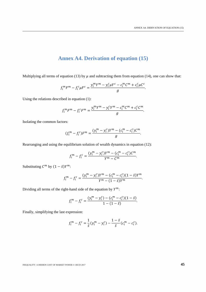
Multiplying all terms of equation (13) by 𝜇𝜇 and subtracting it from equation (14), one can show that (see Annex A4 for a complete derivation):
𝑓𝑓𝑖𝑖𝑚𝑚 − 𝑓𝑓𝑖𝑖𝑐𝑐 =1�̅�𝑠
(𝑦𝑦𝑖𝑖𝑚𝑚 − 𝑦𝑦𝑖𝑖𝑐𝑐) −1 − �̅�𝑠�̅�𝑠
(𝑐𝑐𝑖𝑖𝑚𝑚 − 𝑐𝑐𝑖𝑖𝑐𝑐). (15)
2.5 Solving the model
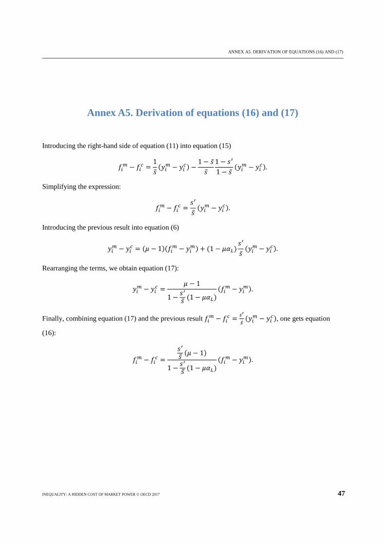
The system of equations (6), (11) and (15) characterise the equilibrium dynamics of wealth, income and consumption shares. Solving the system with respect to 𝑓𝑓𝑖𝑖𝑐𝑐 and 𝑦𝑦𝑖𝑖𝑐𝑐, we obtain our final measure of the redistributive effect of market power on wealth and income (see Annex A5 for a complete derivation):
𝑓𝑓𝑖𝑖𝑐𝑐 = 𝑓𝑓𝑖𝑖𝑚𝑚 +𝑠𝑠′�̅�𝑠 (𝜇𝜇 − 1)
1 − 𝑠𝑠′�̅�𝑠 (1 − 𝜇𝜇𝛼𝛼𝐿𝐿)
(𝑦𝑦𝑖𝑖𝑚𝑚 − 𝑓𝑓𝑖𝑖𝑚𝑚) (16)
2. MODEL
INEQUALITY: A HIDDEN COST OF MARKET POWER © OECD 2017 15
𝑦𝑦𝑖𝑖𝑐𝑐 = 𝑦𝑦𝑖𝑖𝑚𝑚 +𝜇𝜇 − 1
1 − 𝑠𝑠′�̅�𝑠 (1 − 𝜇𝜇𝛼𝛼𝐿𝐿)
(𝑦𝑦𝑖𝑖𝑚𝑚 − 𝑓𝑓𝑖𝑖𝑚𝑚). (17)
Equations (16) and (17) provide the simple result that the redistributive effects of market power on wealth and income depend on a few key variables that can be either observed or estimated: a market-power indicator (mark-up); the income share of labour; the ratio between the average saving rate and the marginal propensity to save; and the observed difference between income and wealth shares in the presence of market power.
If the marginal propensity to save were to equal the average saving rate, which is certainly a lower bound, equations (16) and (17) simplify to:
𝑓𝑓𝑖𝑖𝑐𝑐 − 𝑓𝑓𝑖𝑖𝑚𝑚 = 𝑦𝑦𝑖𝑖𝑐𝑐 − 𝑦𝑦𝑖𝑖𝑚𝑚 =𝐿𝐿𝛼𝛼𝐿𝐿
(𝑦𝑦𝑖𝑖𝑚𝑚 − 𝑓𝑓𝑖𝑖𝑚𝑚), (18)
where L is the Lerner index.11
This simple model has the advantage of deriving measures of the redistributive effects of market power from observed data that vary across countries and of having a steady-state solution emerging from dynamic relationships. These features distinguish the model from that used in the first paper known to have calibrated the impact of market power on wealth distributions, namely Comanor and Smiley (1975). While the new methodology has valuable improvements over this model and that of Ennis and Kim (2016) which followed the same methodology as Comanor and Smiley, the impact of market power remains substantial.

3.DATA
INEQUALITY: A HIDDEN COST OF MARKET POWER © OECD 2017 17
3. Data
This section describes the variables and data used to calibrate the model and their underlying sources. The eight countries considered have been selected both because of data availability and to ensure geographic breadth. To the extent possible, data sources have been used that are common across these countries to ensure comparability. Data sources are listed in Table 1 (Annex A1).
3.1 Market power indicator
The extent of market power is measured using mark-ups on average cost reported by Høj et al. (2007), who used the method developed by Roeger (1995)12 adapted from Hall (1988) to estimate sector-specific mark-ups for 17 countries, using the OECD-STAN database. The method includes a return on capital that is excluded from the calculation of the mark-up. The data used for these estimates covers the period 1975-2002 and is not purported to represent current mark-ups but rather average mark-ups over that time period in which wealth stocks have been built up. Mark-ups therefore may have changed since then, and the countries with higher mark-ups in these data are not necessarily those with the highest mark-ups now. Arguably, though, these historical mark-ups, which are certainly among the most detailed estimates available, would have played a role in establishing today’s wealth distribution.
Mark-ups are imperfect measures of competition, and the estimation method used by Høj et al. is recognised as providing only a first-order approximation. Measurement problems are also observed when working with input and output measures at the sectoral level. Nonetheless, mark-ups are commonly used to measure the strength of competition (Bresnahan, 1989, Schmalansee, 1989). Macroeconomic research in particular often relies on mark-up information to examine the impact of competition on economy wide factors, such as Aghion et al. (2005), Griffiths et al. (2006) and Thum-Thysen and Canton (2015). The figures used are in line with those of other authors (e.g., Griffiths et al., 2006) but have the feature of sector disaggregation.
While the mark-ups estimated by Høj et al. (2007) could be directly introduced into the model to measure the total impact of market power on the distribution of wealth, we do not believe that a complete eradication of mark-ups is a viable or desirable policy objective, as some sources of market power include beneficial factors, such as product differentiation and intellectual property rights. Instead, we attempt to compare actual mark-ups with the lowest sector specific mark-ups observed across countries, in order to estimate an unexplained or excess mark-up. The model can then simulate the effect of market power by calculating the wealth distribution that would exist if the excess mark-up does not exist.
The estimates of excess mark-up by country are calculated, for each sector, as the difference between the actual mark-up and the lowest observed mark-up across all countries in the sample. To illustrate, in the sector of wholesale and retail trade and
3. DATA
18 INEQUALITY: A HIDDEN COST OF MARKET POWER © OECD 2017
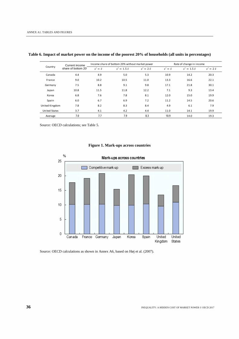
repairs, the mark-up observed in the UK is 16% and the minimum mark-up (found in Germany) is 12%. The UK excess mark-up for that sector is then calculated as the difference, i.e. 4.0%. Weighting across sectors by output, the average level of the excess mark-up in the UK is 3.9%, with the relevant average for other countries varying depending on the differences in sector mark-ups and output weights. The average mark-ups by country (across sectors) are shown in Figure 1 (Annex A1) and the exact numbers are provided in Annex A6, ranging between 3.9% and 10.6%.
This method of estimating market power focuses on finding likely cross-country differences in mark-ups, but it is not claimed to serve as a definitive measure of market power for any individual country. Moreover, these measures are not claimed to serve as a current indicator but instead as an approximation of long-run differences of market power across countries. It is possible that our estimates of excess mark-ups may exceed reported values on corporate profits, because not all profits are captured in corporate profit measures (e.g., partnership income from investment funds or professional service firms) and because a share of profit may be taken in income. Higher than minimal mark-ups, or the excess mark-up, may then be transferred into higher returns to shareholders (and profits), but also potentially into higher income for managers and other employees (e.g., from managerial profit-taking or collective bargaining that extracts part of a monopoly rent). Indeed, in some companies with high profits, such as financial firms, a great part of the income goes to a small, high-earning percentage of the employees, as shown in Denk et al. (2015).
3.2 Wealth and income shares
The difference between a population group’s share of total income and its share of total wealth is 𝑦𝑦𝑖𝑖 − 𝑓𝑓𝑖𝑖. This difference drives the accumulation of gains from market power for those with a share of business ownership (wealth) that exceeds their share of income, i.e., for fi>yi. In contrast, for those with shares of income that exceed their share of business profits, fi<yi, the impact of market power will be a net loss in both wealth and income. Intuitively, market power generates a transfer effect from consumers (in proportion to the income they earn) to business owners (in proportion to the wealth or capital they hold). This means that the families that lose the most from market power, in absolute as opposed to percentage terms, are likely to be those with a substantial income but low business ownership; this appears consistent with the observation that a “squeezed middle class” has experienced a sustained drop in real income.
Table 2 (Annex A1) presents summary statistics related to wealth, consumption expenditure and income by class, in the 8 countries of analysis. These are descriptive statistics, from previously identified sources or imputed from these sources. The less well-off groups are presented by quintile while the wealthiest groups are subdivided into smaller populations, including the top percentile (most wealthy 1%). Among the 8 countries studied here, wealth asset ownership of the top 1 percentile ranges from 6% to 37% of total wealth, while asset ownership of the bottom 80 percentiles ranges from 12% to 43% of total. We use wealth asset ownership by wealth group as our indicator of business ownership. The top percentile groups, particularly the 95th-99th percentile and the top 1 percentile have an income share of total income that is generally much lower than their percentage of wealth.
These findings support the point that the wealthiest households may receive disproportionately more of the profits from market power than others, while not being equally affected by price increases as other groups. Having said this, the impact of
3.DATA
INEQUALITY: A HIDDEN COST OF MARKET POWER © OECD 2017 19
competition on earnings is not unambiguous. Some work in labour economics finds that even some lower-skilled workers may share in supra-competitive rents earned by firms, as discussed in Furman and Orszag (2015). This effect is not considered in the model used here, but may be particularly important in heavily unionised sectors or for workers who can influence their own pay (such as CEOs and executive teams within weak corporate governance structures). In such cases, the profit transfers that are the basis of the model would be both to business asset owners and to those workers that are in a position to capture the rents earned by the business.
3.3 Income share of labour
The income share of labour corresponds to the fraction of total income or output that is earned from labour, usually in the form of wages. The specific measure we use is adjusted for self-employment, whose remuneration is not defined as wages, but which should still be considered as a part of labour income. The data was collected from the Ameco database and it is reported in Krämer (2011). The values are quite stable across countries and they range between 0.62 and 0.7.
3.4 Marginal propensity to save over average saving rate
The marginal propensity to save (𝑠𝑠’) is the proportion of a marginal increase in household income that is used for saving or, in other words, that is not allocated for consumption. Thus, the marginal propensity to save corresponds to 1 minus the marginal propensity to consume (MPC). The average saving rate (�̅�𝑠) is the share of the total income that is saved by the household, that is, it corresponds to the ratio of savings to income.
The ratio of the marginal propensity to save (MPS) to the average saving rate is one of the key parameters of our model. The ratio influences the scale of the impact that market power has on inequality. To ensure that we use the best available evidence for this parameter, we therefore surveyed the literature on savings rates (see annex A7 for more detail).
The issue here is the effect of a permanent and unanticipated reduction of market power on consumption and savings. Reputable studies of permanent and unanticipated changes in income are summarised in Annex A7. Among the studies considered, the average 𝑠𝑠′ is 0.16 but this varies across different countries and ranges between 0.11 and 0.23.
With respect to the average saving rate, we use data collected by national statistical offices for recent decades. The average of these savings rates is 0.11, and ranges between 0.08 and 0.12, with the exception of France whose saving rate was around 0.17. The average ratio between the marginal propensity to save (MPS) and the average saving rate for the four countries for which we were able to obtain estimates was 1.9, though this varied from 1.5 to 2.4. In order to capture a lower bound on the impact, we use a ratio of 1 of the MPS to the average savings rate. We then use two ratios that are closer to the calculated averages (1.5 and 2).


4. RESULTS
INEQUALITY: A HIDDEN COST OF MARKET POWER © OECD 2017 21
4. Results
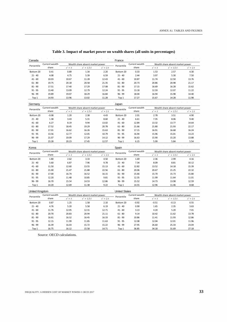
The main results are presented graphically in Figure 2 (Annex A1) and show the impact of market power.13 Each bar represents a share of wealth by population group. For each wealth group, actual wealth shares are in the bar on the left and shares absent market power are in the bar on the right. The range of results that is derived from different ratios of marginal propensity to save over average saving rate is indicated by a vertical line. The underlying data are provided in Table 3 (Annex A1).
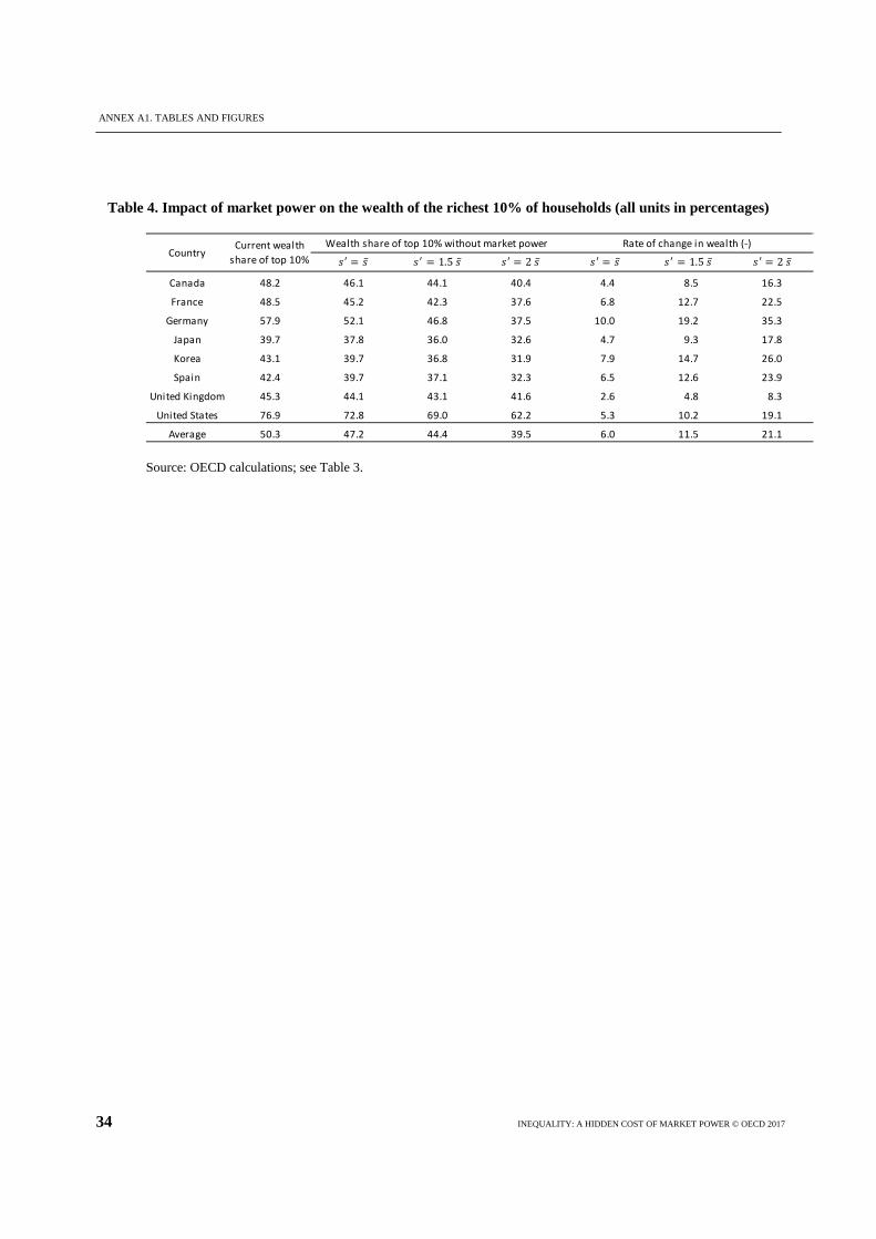
Overall, Figure 2 suggests that, in this model and for the countries studied, redistribution from eliminating market power would occur mainly from the wealthiest 10% of the population to the bottom 80%. Table 4 (Annex A1) summarises the percentage of wealth affected by the existence of market power across countries for the wealthiest 10%. For an average country in the sample, 12% to 21% of the wealth of the richest 10% of households (by wealth) reflects the presence of market power. This result is calculated by calibrating the ratio of the marginal propensity to save over the average saving rate between 1.5 and 2, the values of the ratio most consistent with the available data. Table 4 also reports a lower bound value for the unlikely scenario in which the marginal propensity to save is equal to the average saving rate. In that case the wealth attributed to market power would be 6%, showing a non-trivial share of wealth even under the most conservative assumption for the ratio. The differences in the impact of market power across countries arise from the differences in the distribution of wealth and income, observed mark-ups and income shares of labour.
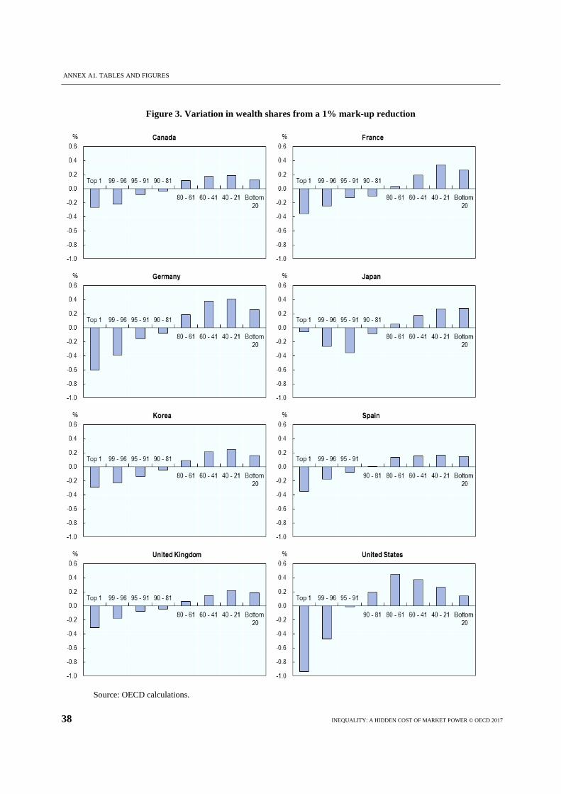
An alternative measure of how market power influences wealth distribution, which does not involve the assumption of a full elimination in market power, is the impact of a reduction in mark-ups by 1%, as shown in Figure 3 (Annex A1). As an example, the figure shows that a 1% reduction in mark-ups increases the wealth of the poorest 20% of the UK population by 0.19 percentage points. Their wealth therefore increases from 0.87% to 1.06% (an increase of approximately 22%). This marginal effect can be used as a ready reckoner to estimate the possible impact of reducing or eliminating anti-competitive market power for a given economy-wide price change. The extent to which middle income earners are squeezed by market power varies substantially across countries, as can be seen by focusing on the 20th to 80th percentiles.
In addition to looking at the impact on wealth, we also show in Table 5 (Annex A1) how market power affects the income shares of the population groups in each country, while Table 6 (Annex A1) summarises the percentage change in the income of the poorest 20% for all countries. In an average country in the sample, for a range of reasonable assumptions about saving behaviour, the income of the poorest 20% of households is expected to rise by between 14% and 19% in the absence of market power (11% in the unlikely lower-bound scenario).14 We note that these income effects are particularly meaningful for the poorest households, which often hold close-to-zero or even negative levels of wealth.

4. RESULTS
22 INEQUALITY: A HIDDEN COST OF MARKET POWER © OECD 2017
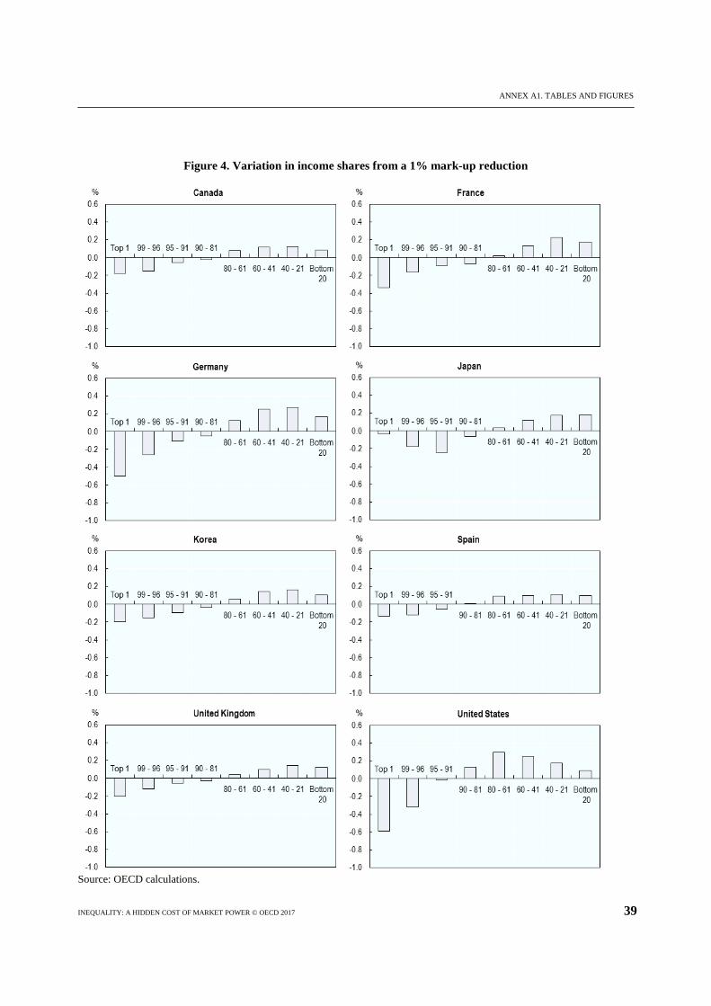
Finally, Figure 4 (Annex A1) shows the redistribution of income resulting from a reduction in mark-ups by 1%.15 Taking again the case of the United Kingdom, Figure 4 shows that a 1% reduction in mark-ups increases the income of the poorest 20% of the UK population by 0.12 percentage points. Their income therefore increases from 7.8% to 7.92% (an increase of approximately 2%).
5. CONCLUSIONS
INEQUALITY: A HIDDEN COST OF MARKET POWER © OECD 2017 23
5.Conclusions
Market power may contribute substantially to wealth inequality, augmenting wealth of the richest 10% of the population by 12% to 21% for an average country in the sample. The magnitude of the impact depends on the choice of key model parameters relating to saving behaviour and, even in an unlikely lower bound estimation would be 6%. Market power may also depress the income of the poorest 20% of the population by between 14% and 19% for an average country in the sample.
Sources of market power vary, and many are generally considered legitimate such as intellectual property protection for products, processes or brands. But violations of competition law, government-created barriers to entry or natural monopolies may be significant sources of market power. Policies that enhance competition –by reducing anti-competitive regulation or trade barriers, empowering consumer choice, fighting illegal cartels, empowering consumers through market studies, preventing mergers that create market power, or the abuse of market power– can therefore help reduce inequality.
Future research is needed to better understand these results. First, extending the analysis to developing countries would be interesting. This should be possible as data measuring inequality are rapidly becoming more easily available. Second, more work is needed to understand the likely scale of different sources of market power, ideally divided into at least three categories: legally obtained without government help, legally obtained with government help (e.g. due to competition-restricting regulations) and illegally obtained market power. Such figures would provide an underpinning for one of the key variables for this analysis. Third, relaxing the steady-state assumptions and developing a more complete model that includes variables on tax and inheritance would provide additional insight and realism. Fourth, using econometric techniques to regress wealth on measures of market power would be of substantial value, allowing one to conduct statistical inference and to obtain confidence intervals for these figures.
The results are nonetheless illustrative. They are based on a model, with accompanying variable and parameter estimates, in which the particular assumptions made are stated clearly and in which reasons and sources are provided for these conclusions. Alternative models and assumptions may yield different results. This research illustrates a mechanism by which market power can contribute to unequal economic outcomes. If this mechanism is correct, government action to reduce illegitimate market power can be an important component of a strategy for inclusive growth.
Importantly, we do not suggest that competition law and policy should specifically target inequality. Instead, we suggest that reduced inequality is a beneficial by-product of government actions and policies to reduce illegitimate market power. The analysis in this paper contributes to the debate on what standards to use when evaluating competition law cases or considering trade-offs between competition and innovation. In their seminal paper on horizontal mergers, Farrell and Shapiro’s (1990) central
5. CONCLUSIONS
24 INEQUALITY: A HIDDEN COST OF MARKET POWER © OECD 2017
conclusion is that if a total welfare standard is used for reviewing horizontal mergers, then under reasonable conditions, price-raising and profitable mergers necessarily increase total welfare. Implicit in their central result is that higher consumer prices may be counter-balanced for consumers by the fact that profits from such higher prices are distributed to shareholders. The analysis here suggests that the beneficiaries from higher profits from mergers may on average account for a rather small percentage of the population, selected from among the top 10% or less of the population, raising doubts about whether a total welfare standard is socially desirable, given the highly unequal distribution of a key factor of that standard, corporate profits, with the vast majority of citizens potentially being worse off as a result of such a merger. A consumer welfare standard avoids this pitfall. This analysis may thus contribute to the debate about whether consumer surplus or total surplus standards should be used.
The decision over which standard to use has a profound impact on the extent that effects of innovation are weighed into policy making, particularly as innovations tend to generate total welfare gains that include a large element of profit from intellectual property, as suggested by Shapiro (2012) and Katz and Shelanski (2005). Following this paper, more research would be valuable on this point.
This paper helps to reinforce the value of an alternative to standard policy solutions. To the extent that policymakers seek to reduce inequality in the distribution of wealth (or income), they often consider traditional tax and redistribution policies, even though these have potentially large impacts on incentives to earn and spend. Feldstein’s (1999) calculation suggests deadweight losses for high earners of 3.76 times the marginal tax revenue gained from higher tax rates and overall deadweight losses of twice the marginal tax revenue.16 As a result, there are potentially significant benefits for economies that reduce inequality through proactive policies that prevent illegitimate market power from regressively redistributing income and wealth in the first place. Distortions of competitive market outcomes might for example be pre-empted by investing in vigorous competition law enforcement and by removing regulations that protect companies from competition. Similarly, a competitive impact assessment might identify new rules and regulations that would increase inequality. Ultimately, this paper suggests that the standard redistribution policies ignore the potential role of competition policy in enhancing equality, which is a particularly worrisome omission because of pro-competitive policies’ attractive productivity and incentive features compared to alternatives. As a result, policymakers who focus on reducing inequality may wish to emphasise and enhance economic policies that favour competition.
5. CONCLUSIONS
INEQUALITY: A HIDDEN COST OF MARKET POWER © OECD 2017 25
Notes
1 See, for example, Piketty (2014), Piketty and Saez (2012), OECD (2015) and
Summers (2014). 2 That is, returns above the market return, which should be competed down to the
cost of capital. 3 For Korea and Japan, the sources are listed in Table 1. Other sources such as CSFB
report higher estimates of wealth and financial wealth for the top 1% in these two countries in particular.
4 The key assumption for this calculation is that commerce in discovered cartels is one fifth of total cartel commerce, which follows if one fifth of cartels are discovered. There is an active debate about the extent to which active cartels are discovered and prosecuted.
5 On the one hand, low mark-ups may indicate a declining industry with uneconomic return on capital. On the other hand, the lowest mark-ups in an industry may already be expected to include some market power, to the extent that sector-wide perfect competition is rare.
6 This assumption can be relaxed to yield marginal propensities to save that vary across wealth classes, but we note that this adjustment would actually imply higher shares of marginal savings for the highest wealth classes, further increasing the strength of the results reported below. The assumption is thus conservative, even if an over-simplification.
7 Market power may potentially be shared with employees, including lesser paid workers. If the workers, notably, receive a substantial increase in their incomes as a result of market power, the distribution of profits will not go not only to those with substantial net wealth but also those without, thus weakening the result of this paper. While this point is important to consider, to the extent that union negotiating power has declined over time, and that top management pay has substantially outpaced inflation, redistribution via labour income, to the extent it occurs, may be accruing increasingly to the wealthiest workers (i.e., management).
8 While the population of the top wealth decile and top consumption decile are not perfectly overlapping, the authors believe there is a high correlation between consumption shares of the income for those persons in the xth wealth decile and those in the xth income decile. This approximation is used because data on the consumption shares of the top wealth decile was unavailable to the authors at the time of writing. Note that for Korea, Japan and the U.S., the consumption of the top 1 percentile had to be calibrated based on consumption shares in known countries. Note: this footnote does not seem to belong to the place where it is in the main text.
9 In the linear expenditure model, households' utility from consumption and saving is described by the following equation: 𝑈𝑈(𝐶𝐶, 𝑆𝑆) = (1− 𝑠𝑠′)𝑙𝑙𝑙𝑙(𝐶𝐶 − 𝑎𝑎) + 𝑠𝑠′𝑙𝑙𝑙𝑙(𝑆𝑆). The maximisation of this utility function subject to the budget constrains yields the consumption function presented in equation (7).
10 Consider that the dynamics of wealth are described by the difference equation 𝐹𝐹𝑡𝑡+1 = 𝐹𝐹𝑡𝑡 + 𝑌𝑌𝑡𝑡 − 𝐶𝐶𝑡𝑡. That is, the wealth accumulated in any period of time is equal
5. CONCLUSIONS
26 INEQUALITY: A HIDDEN COST OF MARKET POWER © OECD 2017
to the wealth held in the previous period plus aggregate savings. Then, assuming that the economy grows at the exogenous growth rate 𝑔𝑔, the equilibrium solution of the difference equation is given by 𝐹𝐹𝑡𝑡+1 = 𝐹𝐹𝑡𝑡(1 + 𝑔𝑔) and, in steady state, equation (12) holds.
11 The Lerner index is equal to 𝑃𝑃−𝑀𝑀𝑀𝑀𝑃𝑃
, where P is the price and MC the marginal cost. 12 Prior work using Roeger’s approach has included Oliveira Martins et al. (1996) 13 The data from Japan have a different source which is listed in Table 1. 14 The income variations observed for the bottom quintiles of the population may
actually exceed the price change percentage from reduced market power. This follows from the fact that wealth is an endogenous variable in the proposed model, meaning that the real income increase from absence of market power enables the bottom quintile of the population to save more and subsequently receive extra returns on wealth. As an illustrative example, in a country where prices fall by 1% as a result of pro-competitive policies, a household that initially does not hold wealth obtains an immediate raise in real income by 1%, allowing it to save more, accumulate wealth and raise future real income.
15 Note that the figures for the top 10% in Japan are not comparable to those for other countries, perhaps suggesting that the data sources used, which are the most commonly cited, lead to a comparative under-reporting of wealth assets for the highest brackets compared to other countries.
16 See Feldstein (1999) which estimates for high-earning couples a $3.76 deadweight loss for each additional $1.00 in income tax revenue and that across all earners, the effect is about a $2.00 for each additional $1.00 in income tax revenue.
REFERENCES
INEQUALITY: A HIDDEN COST OF MARKET POWER © OECD 2017 27
References
Aghion, P., N. Bloom, R. Blundell, R. Griffith and P. Howitt (2005), “Competition and Innovation: An Inverted-U Relationship”, The Quarterly Journal of Economics, Vol. 120, No. 2, pp. 701-728, http://qje.oxfordjournals.org/content/120/2/701.short.
Autor, D. H., D. Dorn and G. H. Hanson (2016), “The China Shock: Learning from Labor Market Adjustment to Large Changes in Trade”, NBER Working Paper, No. 21906, http://www.nber.org/papers/w21906.
Baker, J. and S. Salop (2015), "Antitrust, Competition Policy, and Inequality", Working Papers, No. 41, http://digitalcommons.wcl.american.edu/fac_works_papers/41.
Bresnahan, T. (1989), “Empirical Methods for Industries with Market Power”, in R. Schmalansee and R. Willig (eds.), Handbook of Industrial Organisation, North-Holland, Amsterdam.
Comanor, W. S. and R. H. Smiley (1975), "Monopoly and the Distribution of Wealth", The Quarterly Journal of Economics, Vol. 89, No. 2, pp. 177-194, http://www.jstor.org/stable/1884423?seq=1#page_scan_tab_contents.
Conway, P., D. de Rosa, G. Nicoletti and F. Steiner (2006), “Regulation, Competition and Productivity Convergence”, OECD Economics Department Working Papers, No. 509, OECD Publishing, Paris, http://dx.doi.org/10.1787/431383770805.
Creedy, J. and R. Dixon (1999), “The Distributional Effects of Monopoly”, Australian Economic Papers, Vol. 38, No. 3, pp. 223-237, http://dx.doi.org/10.1111/1467-8454.00053.
Denk, O., S. Schich and B. Cournède (2015), "Why implicit bank debt guarantees matter: Some empirical evidence", OECD Journal: Financial Market Trends, Vol. 2014/2. DOI: http://dx.doi.org/10.1787/fmt-2014-5js3bfznx6vj.
Dynan, K. E., J. Skinner and S. P. Zeldes (2004), “Do the Rich Save More?”, Journal of Political Economy, Vol. 112, No. 2, pp. 397-444, http://www.journals.uchicago.edu/doi/pdfplus/10.1086/381475.
Elhauge, E. (2016), “Horizontal Shareholding”, Harvard Law Review, Vol. 129, No. 5, pp. 1267-1317, http://harvardlawreview.org/2016/03/horizontal-shareholding/.
Ennis, S. (2014), “Commerce Affected by Cross-Border Private Cartels”, OECD WP3 paper, DAF/COMP/WP3(2014)11.
Ennis, S. and Y. Kim (2016) “Market Power and Wealth Distribution” in OECD and World Bank, A Step Ahead: Competition Policy, Shared Prosperity and Inclusive Growth, World Bank Publishing, Washington, D.C.
Farrell, J. and C. Shapiro (1990) “Horizontal Mergers: An Equilibrium Analysis”, American Economic Review, 80(1), pp. 107-126.
Feldstein, M. (1999), “Tax Avoidance and the Deadweight Loss of the Income Tax”, The Review of Economics and Statistics, Vol. 81, No. 4 (Nov., 1999), pp. 674-680.

REFERENCES
28 INEQUALITY: A HIDDEN COST OF MARKET POWER © OECD 2017
Furman, J. and P. Orszag (2015), “A Firm-Level Perspective on the Role of Rents in the Rise in Inequality”, Presentation at A Just Society Centennial Event in Honor of Joseph Stiglitz at Columbia University.
Griffith. R., R. Harrison and H. Simpson (2006), “The Link between Product Market Reform, Innovation and EU Macroeconomic Performance”, European Commission Economics Papers, No. 243.
Hausman, J. A. and J. G. Sidak (2004), “Why Do the Poor and the Less-Educated Pay More for Long-Distance Calls?”, Contributions in Economic and Policy Research, Vol. 3, No. 1, pp. 1-26, http://dx.doi.org/10.2139/ssrn.296368.
Hall, R. (1988), “The Relation between Price and Marginal Cost in U.S. Industry”, Journal of Political Economy, Vol. 96, pp. 921-947.
Høj, J., M. Jimenez, M. Maher, G. Nicoletti and M. Wise (2007), “Product Market Competition in the OECD Countries: Taking Stock and Moving Forward”, OECD Economics Department Working Papers, No. 575, OECD Publishing, Paris, http://dx.doi.org/10.1787/108734233645.
Katz, M., and H. Shelanski (2005), “Merger Policy and Innovation: Must Enforcement Change to Account for Technological Change?" In Innovation Policy and the Economy, ed. Adam Jaffe, Joshua Lerner, and Scott Stern. Cambridge, Massachusetts: MIT Press.
Kitamura, Y., N. Takayama and F. Arita (2003), “Households Savings and Wealth Distribution in Japan”, in A. Borsch-Supan (Ed.), Life-cycle Savings and Public Policy: a Cross-National Study of Six Countries, Elsevier Science.
Krämer, H. (2011), “Bowley’s Law: The Diffusion of an empirical supposition into Economic Theory”, Cahiers d'Économie Politique ()Papers in Political Economy, vol. 61.
Leipziger, D. M. et al. (1992), “The Distribution of Income and Wealth in Korea”, EDI Development Studies, World Bank, Washington, D.C., http://documents.worldbank.org/curated/pt/1992/12/439352/distribution-income-wealth-korea.
Mendoza, R. U. (2011), “Why Do the Poor Pay More? Exploring the Poverty Penalty Concept”, Journal of International Development, Vol. 23, No. 1, pp. 1–28, http://dx.doi.org/10.1002/jid.1504.
OECD (2011), Divided We Stand: Why Inequality Keeps Rising, OECD Publishing, Paris, http://dx.doi.org/10.1787/9789264119536-en.
OECD (2014), OECD Competition Assessment Reviews: Greece, OECD Publishing, Paris, http://dx.doi.org/10.1787/9789264206090-en.
OECD (2015), In It Together: Why Less Inequality Benefits All, OECD Publishing, Paris, http://dx.doi.org/10.1787/9789264235120-en.
OECD and World Bank (2016), A Step Ahead: Competition Policy, Shared Prosperity and Inclusive Growth, World Bank Publishing, Washington, D.C.
Oliveira Martins, J. S. Scarpetta and D. Pilat (1996), “Mark-Up Ratios in Manufacturing Industries: Estimates for 14 OECD Countries”, OECD Economics Department Working Papers, No. 162, OECD Publishing. http://dx.doi.org/10.1787/007750682315.

REFERENCES
INEQUALITY: A HIDDEN COST OF MARKET POWER © OECD 2017 29
Piketty, T. and E. Saez (2003), "Income Inequality in the United States, 1913-1998", The Quarterly Journal of Economics, Vol. 118, No. 1, pp. 1-39, http://qje.oxfordjournals.org/content/118/1/1.abstract.
Piketty, T. (2014), Capital in the 21st Century, Cambridge, Massachusetts: Harvard University Press.
Rognlie, M. (2015), “Deciphering the Fall and Rise in the Net Capital Share”, Brookings Papers on Economic Activity, Brookings BPEA Conference, March, http://www.brookings.edu/about/projects/bpea/papers/2015/land-prices-evolution-capitals-share.
Roeger, W. (1995), “Can Imperfect Competition Explain the Difference between Primal and Duel Productivity Measures? Estimates for U.S. Manufacturing”, Journal of Political Economy, Vol. 103, No. 2. pp. 316-330.
Schmalansee, R. (1989), “Inter-Industry Studies of Structure and Performance”, in R. Schmalansee and R. Willig (eds.), Handbook of Industrial Organisation, North-Holland, Amsterdam.
Shapiro, C. (2012) “Competition and Innovation: Did Arrow Hit the Bull’s Eye”, in The Rate and Direction of Inventive Activity Revisited. Ed. Josh Lerner and Scott Stern. Chicago: University of Chicago Press.
Summers, L. H. (2014), “The Inequality Puzzle”, Democracy Journal, http://democracyjournal.org/magazine/33/the-inequality-puzzle/.
Thum-Thysen, A and E. Canton (2015), “Estimation of Service Sector Mark-ups Determined by Structural Reform Indicators”, European Commission Economic Papers, No. 547.
Urzúa, C. M. (2013), “Distributive and Regional Effects of Monopoly Power”, Economía Mexicana Nueva Epoca, Vol. 22, No. 2, pp. 279-295, http://www.scielo.org.mx/pdf/emne/v22n2/v22n2a2.pdf.
Wölfl, A., et al. (2010), "Product Market Regulation: Extending the Analysis Beyond OECD Countries", OECD Economics Department Working Papers, No. 799, OECD Publishing, Paris.


ANNEX A1. TABLES AND FIGURES
INEQUALITY: A HIDDEN COST OF MARKET POWER © OECD 2017 31
Annex A1. Tables and figures
Table 1. Data sources
Source: OECD.
Datasets Canada France Germany Spain UK USA Korea Japan
Total wealth shares
Leipziger et all (1992)
National Survey of Family Income and Expenditure, 1994
Consumption shares
Canada Survey of Household Spending 2013
USA Consumer Expenditure Survey, 2013
Statistics Korea: income and consumption 2014
Family Income and Expenditure Survey 2013, Japan
Income shares Canada Market, total and after-tax income of individuals 2011
USA Consumer Expenditure Survey, 2013
Statistics Korea: income and consumption 2014
Family Income and Expenditure Survey 2013, Japan
Income share of labour
Average saving rates
Statistics Canada
INSEE France
Deutsche Bundesbank
Eurostat Office for National Statistics
U.S. Bureau of Economics Analysis
Statistics Korea
Statistics Bureau of Japan
Marginal propensity to save
Mark-ups
OECD Datasets: Wealth Distribution Database
Eurostat: Mean Consumption Expenditure by Income Quintiles 2010
Eurostat: Distribution of Income by Quantiles 2014
Ameco's Adjusted wage share in selected OECD-Countries, 1990-2008 in Krämer (2011)
Literature sources in Annex A1.
Høj, J. et al (2007).

ANNEX A1. TABLES AND FIGURES
32 INEQUALITY: A HIDDEN COST OF MARKET POWER © OECD 2017
Table 2. Summary data: distribution of net worth, income and consumption expenditures (all units in percentages)
Source: OECD compilations.
Canada
Bottom 20 0.4 4.4 7.921 - 40 4.1 9.7 12.141 - 60 10.0 15.4 16.961 - 80 19.7 23.3 23.681 - 90 17.5 16.6 15.391 - 95 13.4 10.8 9.696 - 99 19.9 13.1 11.3Top 1 14.9 6.8 3.2
Percentile Net worth IncomeConsumption expenditures
France
Bottom 20 0.3 9.0 9.921 - 40 2.4 13.5 13.941 - 60 10.9 17.2 18.361 - 80 20.7 21.7 23.981 - 90 17.2 13.8 12.791 - 95 13.2 8.9 9.496 - 99 18.0 10.1 9.1Top 1 17.3 5.7 2.8
Percentile Net worth IncomeConsumption expenditures
Germany
Bottom 20 -0.1 7.5 8.621 - 40 1.4 13.5 13.141 - 60 6.3 17.6 17.861 - 80 17.5 23.0 23.981 - 90 17.0 14.7 14.791 - 95 13.6 8.9 9.696 - 99 21.1 9.4 9.5Top 1 23.3 5.3 2.9
Percentile Net worth IncomeConsumption expenditures
Japan
Bottom 20 2.0 10.8 11.821 - 40 6.6 15.1 16.341 - 60 12.8 18.3 18.661 - 80 21.7 23.2 22.781 - 90 17.2 14.4 13.991 - 95 16.9 5.7 6.696 - 99 16.6 8.3 7.6Top 1 6.2 4.3 2.5
Percentile Net worth IncomeConsumption expenditures
Korea
Bottom 20 1.8 6.8 9.921 - 40 5.6 13.3 15.941 - 60 11.5 18.2 19.961 - 80 21.0 23.9 23.281 - 90 17.0 15.4 13.991 - 95 12.2 7.8 7.096 - 99 16.7 9.6 7.8Top 1 14.2 5.0 2.6
Percentile Net worth IncomeConsumption expenditures
Spain
Bottom 20 1.7 6.0 10.121 - 40 7.3 12.2 14.441 - 60 12.8 17.3 18.761 - 80 20.1 24.0 23.281 - 90 15.7 15.9 15.191 - 95 12.4 10.0 8.196 - 99 15.5 10.4 7.6Top 1 14.6 4.3 2.7
Percentile Net worth IncomeConsumption expenditures
United Kingdom
Bottom 20 0.9 7.8 10.921 - 40 4.8 12.8 13.641 - 60 11.8 17.1 18.261 - 80 20.7 23.0 22.681 - 90 16.6 15.0 12.991 - 95 12.2 9.2 9.496 - 99 16.4 9.8 9.4Top 1 16.8 5.3 3.0
Percentile Net worth IncomeConsumption expenditures
United States
Bottom 20 -0.9 3.7 8.921 - 40 0.9 9.5 12.541 - 60 3.1 15.3 17.061 - 80 9.1 23.7 22.681 - 90 10.9 17.2 15.591 - 95 12.1 11.7 10.296 - 99 28.0 12.5 10.0Top 1 36.8 6.5 3.3
Percentile Net worth IncomeConsumption expenditures
ANNEX A1. TABLES AND FIGURES
INEQUALITY: A HIDDEN COST OF MARKET POWER © OECD 2017 33
Table 3. Impact of market power on wealth shares (all units in percentages)
Source: OECD calculations.
Canada
Bottom 20 0.41 0.89 1.34 2.2021 - 40 4.08 4.75 5.39 6.5941 - 60 10.03 10.67 11.28 12.4361 - 80 19.75 20.18 20.58 21.3581 - 90 17.51 17.40 17.29 17.0891 - 95 13.40 13.09 12.79 12.2496 - 99 19.89 19.07 18.29 16.84Top 1 14.93 13.96 13.02 11.28
Percentile Wealth share absent market powerCurrent wealth share 𝑠𝑠′ = �̅�𝑠 𝑠𝑠′ = 1.5 �̅�𝑠 𝑠𝑠′ = 2 �̅�𝑠
France
Bottom 20 0.33 1.53 2.57 4.3021 - 40 2.44 3.97 5.30 7.5041 - 60 10.87 11.74 12.50 13.7661 - 80 20.73 20.86 20.98 21.1781 - 90 17.15 16.69 16.28 15.6291 - 95 13.18 12.59 12.07 11.2296 - 99 18.04 16.94 15.98 14.40Top 1 17.27 15.67 14.28 11.98
Percentile Wealth share absent market powerCurrent wealth share 𝑠𝑠′ = �̅�𝑠 𝑠𝑠′ = 1.5 �̅�𝑠 𝑠𝑠′ = 2 �̅�𝑠
Germany
Bottom 20 -0.08 1.20 2.38 4.4321 - 40 1.38 3.43 5.31 8.6041 - 60 6.27 8.19 9.94 13.0261 - 80 17.52 18.45 19.29 20.7881 - 90 17.01 16.62 16.26 15.6391 - 95 13.56 12.77 12.05 10.7996 - 99 21.07 19.09 17.29 14.12Top 1 23.28 20.23 17.45 12.57
Percentile Wealth share absent market powerCurrent wealth share 𝑠𝑠′ = �̅�𝑠 𝑠𝑠′ = 1.5 �̅�𝑠 𝑠𝑠′ = 2 �̅�𝑠
Japan
Bottom 20 2.01 2.78 3.51 4.9021 - 40 6.61 7.35 8.06 9.4041 - 60 12.84 13.32 13.77 14.6461 - 80 21.66 21.80 21.93 22.1781 - 90 17.15 16.91 16.68 16.2491 - 95 16.94 15.96 15.01 13.2396 - 99 16.63 15.90 15.20 13.88Top 1 6.15 5.99 5.84 5.54
Percentile Wealth share absent market powerCurrent wealth share 𝑠𝑠′ = �̅�𝑠 𝑠𝑠′ = 1.5 �̅�𝑠 𝑠𝑠′ = 2 �̅�𝑠
Korea
Bottom 20 1.80 2.62 3.33 4.5021 - 40 5.60 6.87 7.96 9.7841 - 60 11.50 12.60 13.55 15.1361 - 80 21.00 21.47 21.88 22.5681 - 90 17.00 16.74 16.52 16.1591 - 95 12.20 11.48 10.85 9.8196 - 99 16.70 15.54 14.53 12.86Top 1 14.20 12.69 11.38 9.22
Percentile Wealth share absent market powerCurrent wealth share 𝑠𝑠′ = �̅�𝑠 𝑠𝑠′ = 1.5 �̅�𝑠 𝑠𝑠′ = 2 �̅�𝑠
Spain
Bottom 20 1.69 2.36 2.99 4.1621 - 40 7.34 8.09 8.81 10.1241 - 60 12.82 13.52 14.18 15.3961 - 80 20.06 20.67 21.25 22.3281 - 90 15.66 15.70 15.73 15.8091 - 95 12.35 11.99 11.64 11.0196 - 99 15.52 14.73 13.98 12.59Top 1 14.55 12.96 11.46 8.68
Percentile Wealth share absent market powerCurrent wealth share 𝑠𝑠′ = �̅�𝑠 𝑠𝑠′ = 1.5 �̅�𝑠 𝑠𝑠′ = 2 �̅�𝑠
United Kingdom
Bottom 20 0.87 1.25 1.58 2.1021 - 40 4.76 5.20 5.58 6.1941 - 60 11.76 12.05 12.31 12.7161 - 80 20.70 20.83 20.94 21.1181 - 90 16.61 16.52 16.45 16.3391 - 95 12.15 11.99 11.85 11.6396 - 99 16.39 16.03 15.72 15.22Top 1 16.75 16.12 15.58 14.71
Percentile Wealth share absent market powerCurrent wealth share 𝑠𝑠′ = �̅�𝑠 𝑠𝑠′ = 1.5 �̅�𝑠 𝑠𝑠′ = 2 �̅�𝑠
United States
Bottom 20 -0.92 -0.51 -0.13 0.5521 - 40 0.90 1.65 2.35 3.6341 - 60 3.13 4.20 5.20 7.0161 - 80 9.14 10.42 11.62 13.7881 - 90 10.86 11.41 11.93 12.8691 - 95 12.08 12.04 12.01 11.9696 - 99 27.95 26.60 25.33 23.04Top 1 36.85 34.18 31.69 27.18
Percentile Wealth share absent market powerCurrent wealth share 𝑠𝑠′ = �̅�𝑠 𝑠𝑠′ = 1.5 �̅�𝑠 𝑠𝑠′ = 2 �̅�𝑠
ANNEX A1. TABLES AND FIGURES
34 INEQUALITY: A HIDDEN COST OF MARKET POWER © OECD 2017
Table 4. Impact of market power on the wealth of the richest 10% of households (all units in percentages)
Source: OECD calculations; see Table 3.
Canada 48.2 46.1 44.1 40.4 4.4 8.5 16.3
France 48.5 45.2 42.3 37.6 6.8 12.7 22.5
Germany 57.9 52.1 46.8 37.5 10.0 19.2 35.3
Japan 39.7 37.8 36.0 32.6 4.7 9.3 17.8
Korea 43.1 39.7 36.8 31.9 7.9 14.7 26.0
Spain 42.4 39.7 37.1 32.3 6.5 12.6 23.9
United Kingdom 45.3 44.1 43.1 41.6 2.6 4.8 8.3
United States 76.9 72.8 69.0 62.2 5.3 10.2 19.1
Average 50.3 47.2 44.4 39.5 6.0 11.5 21.1
CountryCurrent wealth
share of top 10%Wealth share of top 10% without market power Rate of change in wealth (-)
𝑠𝑠′ = �̅�𝑠 𝑠𝑠′ = �̅�𝑠𝑠𝑠′ = 1.5 �̅�𝑠 𝑠𝑠′ = 1.5 �̅�𝑠𝑠𝑠′ = 2 �̅�𝑠 𝑠𝑠′ = 2 �̅�𝑠

ANNEX A1. TABLES AND FIGURES
INEQUALITY: A HIDDEN COST OF MARKET POWER © OECD 2017 35
Table 5. Impact of market power on income shares (all units in percentages)
Source: OECD calculations.
Canada
Bottom 20 4.39 4.87 5.01 5.2821 - 40 9.68 10.35 10.56 10.9441 - 60 15.37 16.01 16.21 16.5761 - 80 23.31 23.74 23.87 24.1181 - 90 16.56 16.45 16.41 16.3591 - 95 10.80 10.49 10.39 10.2296 - 99 13.09 12.27 12.02 11.56Top 1 6.80 5.83 5.53 4.98
PercentileCurrent income
shareIncome share absent market power
𝑠𝑠′ = �̅�𝑠 𝑠𝑠′ = 1.5 �̅�𝑠 𝑠𝑠′ = 2 �̅�𝑠
France
Bottom 20 9.00 10.20 10.50 10.9821 - 40 13.50 15.03 15.41 16.0341 - 60 17.20 18.08 18.29 18.6561 - 80 21.70 21.83 21.87 21.9281 - 90 13.80 13.34 13.22 13.0391 - 95 8.90 8.31 8.16 7.9296 - 99 10.10 9.00 8.73 8.28Top 1 5.70 4.10 3.70 3.05
PercentileCurrent income
shareIncome share absent market power
𝑠𝑠′ = �̅�𝑠 𝑠𝑠′ = 1.5 �̅�𝑠 𝑠𝑠′ = 2 �̅�𝑠
Germany
Bottom 20 7.50 8.79 9.14 9.7621 - 40 13.50 15.56 16.12 17.1141 - 60 17.60 19.52 20.05 20.9761 - 80 23.00 23.93 24.18 24.6381 - 90 14.70 14.31 14.20 14.0191 - 95 8.90 8.11 7.89 7.5196 - 99 9.40 7.42 6.88 5.93Top 1 5.30 2.25 1.42 -0.05
PercentileCurrent income
shareIncome share absent market power
𝑠𝑠′ = �̅�𝑠 𝑠𝑠′ = 1.5 �̅�𝑠 𝑠𝑠′ = 2 �̅�𝑠
Japan
Bottom 20 10.78 11.55 11.78 12.2321 - 40 15.09 15.83 16.06 16.4941 - 60 18.30 18.78 18.93 19.2161 - 80 23.21 23.34 23.38 23.4681 - 90 14.37 14.13 14.05 13.9191 - 95 5.66 4.68 4.37 3.8096 - 99 8.28 7.55 7.33 6.91Top 1 4.30 4.14 4.09 4.00
PercentileCurrent income
shareIncome share absent market power
𝑠𝑠′ = �̅�𝑠 𝑠𝑠′ = 1.5 �̅�𝑠 𝑠𝑠′ = 2 �̅�𝑠
Korea
Bottom 20 6.79 7.61 7.81 8.1421 - 40 13.33 14.59 14.90 15.4141 - 60 18.21 19.31 19.58 20.0361 - 80 23.88 24.35 24.47 24.6681 - 90 15.43 15.17 15.11 15.0191 - 95 7.78 7.06 6.88 6.5996 - 99 9.59 8.43 8.14 7.67Top 1 4.99 3.48 3.11 2.50
PercentileCurrent income
shareIncome share absent market power
𝑠𝑠′ = �̅�𝑠 𝑠𝑠′ = 1.5 �̅�𝑠 𝑠𝑠′ = 2 �̅�𝑠
Spain
Bottom 20 6.00 6.67 6.87 7.2321 - 40 12.20 12.96 13.18 13.5941 - 60 17.30 18.00 18.20 18.5861 - 80 24.00 24.61 24.79 25.1381 - 90 15.90 15.94 15.95 15.9791 - 95 10.00 9.63 9.53 9.3396 - 99 10.40 9.60 9.37 8.93Top 1 4.30 2.71 2.23 1.36
PercentileCurrent income
shareIncome share absent market power
𝑠𝑠′ = �̅�𝑠 𝑠𝑠′ = 1.5 �̅�𝑠 𝑠𝑠′ = 2 �̅�𝑠
United Kingdom
Bottom 20 7.80 8.18 8.27 8.4221 - 40 12.80 13.25 13.35 13.5241 - 60 17.10 17.40 17.47 17.5861 - 80 23.00 23.13 23.16 23.2181 - 90 15.00 14.91 14.89 14.8691 - 95 9.20 9.04 9.00 8.9496 - 99 9.80 9.43 9.35 9.21Top 1 5.30 4.67 4.52 4.28
PercentileCurrent income
shareIncome share absent market power
𝑠𝑠′ = �̅�𝑠 𝑠𝑠′ = 1.5 �̅�𝑠 𝑠𝑠′ = 2 �̅�𝑠
United States
Bottom 20 3.69 4.09 4.21 4.4221 - 40 9.45 10.20 10.42 10.8141 - 60 15.31 16.38 16.69 17.2561 - 80 23.69 24.97 25.34 26.0181 - 90 17.15 17.70 17.86 18.1591 - 95 11.70 11.67 11.66 11.6496 - 99 12.53 11.17 10.78 10.07Top 1 6.51 3.85 3.08 1.68
PercentileCurrent income
shareIncome share absent market power
𝑠𝑠′ = �̅�𝑠 𝑠𝑠′ = 1.5 �̅�𝑠 𝑠𝑠′ = 2 �̅�𝑠
ANNEX A1. TABLES AND FIGURES
36 INEQUALITY: A HIDDEN COST OF MARKET POWER © OECD 2017
Table 6. Impact of market power on the income of the poorest 20% of households (all units in percentages)
Source: OECD calculations; see Table 5.
Figure 1. Mark-ups across countries
Source: OECD calculations as shown in Annex A6, based on Høj et al. (2007).
Canada 4.4 4.9 5.0 5.3 10.9 14.2 20.3
France 9.0 10.2 10.5 11.0 13.3 16.6 22.1
Germany 7.5 8.8 9.1 9.8 17.1 21.8 30.1
Japan 10.8 11.5 11.8 12.2 7.1 9.3 13.4
Korea 6.8 7.6 7.8 8.1 12.0 15.0 19.9
Spain 6.0 6.7 6.9 7.2 11.2 14.5 20.6
United Kingdom 7.8 8.2 8.3 8.4 4.9 6.1 7.9
United States 3.7 4.1 4.2 4.4 11.0 14.1 19.9
Average 7.0 7.7 7.9 8.3 10.9 14.0 19.3
Country Current income share of bottom 20%
Income share of bottom 20% without market power Rate of change in income
𝑠𝑠′ = �̅�𝑠 𝑠𝑠′ = �̅�𝑠𝑠𝑠′ = 1.5 �̅�𝑠 𝑠𝑠′ = 1.5 �̅�𝑠𝑠𝑠′ = 2 �̅�𝑠 𝑠𝑠′ = 2 �̅�𝑠

ANNEX A1. TABLES AND FIGURES
INEQUALITY: A HIDDEN COST OF MARKET POWER © OECD 2017 37
Figure 2. Impact of market power on wealth distribution
Source: OECD calculations, results shown in Table 3.
ANNEX A1. TABLES AND FIGURES
38 INEQUALITY: A HIDDEN COST OF MARKET POWER © OECD 2017
Figure 3. Variation in wealth shares from a 1% mark-up reduction
Source: OECD calculations.
ANNEX A1. TABLES AND FIGURES
INEQUALITY: A HIDDEN COST OF MARKET POWER © OECD 2017 39
Figure 4. Variation in income shares from a 1% mark-up reduction
Source: OECD calculations.

ANNEX A2. DERIVATION OF EQUATION (6)
INEQUALITY: A HIDDEN COST OF MARKET POWER © OECD 2017 41
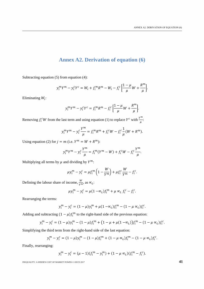
Annex A2. Derivation of equation (6)
Subtracting equation (5) from equation (4):
𝑦𝑦𝑖𝑖𝑚𝑚𝑌𝑌𝑚𝑚 − 𝑦𝑦𝑖𝑖𝑐𝑐𝑌𝑌𝑐𝑐 = 𝑊𝑊𝑖𝑖 + 𝑓𝑓𝑖𝑖𝑚𝑚𝑅𝑅𝑚𝑚 −𝑊𝑊𝑖𝑖 − 𝑓𝑓𝑖𝑖𝑐𝑐 �1 − 𝜇𝜇𝜇𝜇
𝑊𝑊 +𝑅𝑅𝑚𝑚
𝜇𝜇 �.
Eliminating 𝑊𝑊𝑖𝑖:
𝑦𝑦𝑖𝑖𝑚𝑚𝑌𝑌𝑚𝑚 − 𝑦𝑦𝑖𝑖𝑐𝑐𝑌𝑌𝑐𝑐 = 𝑓𝑓𝑖𝑖𝑚𝑚𝑅𝑅𝑚𝑚 − 𝑓𝑓𝑖𝑖𝑐𝑐 �1 − 𝜇𝜇𝜇𝜇
𝑊𝑊 +𝑅𝑅𝑚𝑚
𝜇𝜇 �.
Removing 𝑓𝑓𝑖𝑖𝑐𝑐𝑊𝑊 from the last term and using equation (1) to replace 𝑌𝑌𝑐𝑐 with 𝑌𝑌𝑚𝑚
𝜇𝜇:
𝑦𝑦𝑖𝑖𝑚𝑚𝑌𝑌𝑚𝑚 − 𝑦𝑦𝑖𝑖𝑐𝑐𝑌𝑌𝑚𝑚
𝜇𝜇= 𝑓𝑓𝑖𝑖𝑚𝑚𝑅𝑅𝑚𝑚 + 𝑓𝑓𝑖𝑖𝑐𝑐𝑊𝑊 − 𝑓𝑓𝑖𝑖𝑐𝑐
1𝜇𝜇
(𝑊𝑊 + 𝑅𝑅𝑚𝑚).
Using equation (2) for 𝑗𝑗 = 𝑚𝑚 (i.e. 𝑌𝑌𝑚𝑚 = 𝑊𝑊 + 𝑅𝑅𝑚𝑚):
𝑦𝑦𝑖𝑖𝑚𝑚𝑌𝑌𝑚𝑚 − 𝑦𝑦𝑖𝑖𝑐𝑐𝑌𝑌𝑚𝑚
𝜇𝜇= 𝑓𝑓𝑖𝑖𝑚𝑚(𝑌𝑌𝑚𝑚 −𝑊𝑊) + 𝑓𝑓𝑖𝑖𝑐𝑐𝑊𝑊 − 𝑓𝑓𝑖𝑖𝑐𝑐
𝑌𝑌𝑚𝑚
𝜇𝜇.
Multiplying all terms by 𝜇𝜇 and dividing by 𝑌𝑌𝑚𝑚:
𝜇𝜇𝑦𝑦𝑖𝑖𝑚𝑚 − 𝑦𝑦𝑖𝑖𝑐𝑐 = 𝜇𝜇𝑓𝑓𝑖𝑖𝑚𝑚 �1 −𝑊𝑊𝑌𝑌𝑚𝑚
� + 𝜇𝜇𝑓𝑓𝑖𝑖𝑐𝑐𝑊𝑊𝑌𝑌𝑚𝑚
− 𝑓𝑓𝑖𝑖𝑐𝑐 .
Defining the labour share of income, 𝑊𝑊𝑌𝑌𝑚𝑚
, as ∝𝐿𝐿:
𝜇𝜇𝑦𝑦𝑖𝑖𝑚𝑚 − 𝑦𝑦𝑖𝑖𝑐𝑐 = 𝜇𝜇(1 −∝𝐿𝐿)𝑓𝑓𝑖𝑖𝑚𝑚 + 𝜇𝜇 ∝𝐿𝐿 𝑓𝑓𝑖𝑖𝑐𝑐 − 𝑓𝑓𝑖𝑖𝑐𝑐 .
Rearranging the terms:
𝑦𝑦𝑖𝑖𝑚𝑚 − 𝑦𝑦𝑖𝑖𝑐𝑐 = (1 − 𝜇𝜇)𝑦𝑦𝑖𝑖𝑚𝑚 + 𝜇𝜇(1 −∝𝐿𝐿)𝑓𝑓𝑖𝑖𝑚𝑚 − (1 − 𝜇𝜇 ∝𝐿𝐿)𝑓𝑓𝑖𝑖𝑐𝑐 .
Adding and subtracting (1 − 𝜇𝜇)𝑓𝑓𝑖𝑖𝑚𝑚 to the right-hand side of the previous equation:
𝑦𝑦𝑖𝑖𝑚𝑚 − 𝑦𝑦𝑖𝑖𝑐𝑐 = (1 − 𝜇𝜇)𝑦𝑦𝑖𝑖𝑚𝑚 − (1 − 𝜇𝜇)𝑓𝑓𝑖𝑖𝑚𝑚 + �1 − 𝜇𝜇 + 𝜇𝜇(1 −∝𝐿𝐿)�𝑓𝑓𝑖𝑖𝑚𝑚 − (1 − 𝜇𝜇 ∝𝐿𝐿)𝑓𝑓𝑖𝑖𝑐𝑐 .
Simplifying the third term from the right-hand side of the last equation:
𝑦𝑦𝑖𝑖𝑚𝑚 − 𝑦𝑦𝑖𝑖𝑐𝑐 = (1 − 𝜇𝜇)𝑦𝑦𝑖𝑖𝑚𝑚 − (1 − 𝜇𝜇)𝑓𝑓𝑖𝑖𝑚𝑚 + (1 − 𝜇𝜇 ∝𝐿𝐿)𝑓𝑓𝑖𝑖𝑚𝑚 − (1 − 𝜇𝜇 ∝𝐿𝐿)𝑓𝑓𝑖𝑖𝑐𝑐.
Finally, rearranging:
𝑦𝑦𝑖𝑖𝑚𝑚 − 𝑦𝑦𝑖𝑖𝑐𝑐 = (𝜇𝜇 − 1)(𝑓𝑓𝑖𝑖𝑚𝑚 − 𝑦𝑦𝑖𝑖𝑚𝑚) + (1 − 𝜇𝜇 ∝𝐿𝐿)(𝑓𝑓𝑖𝑖𝑚𝑚 − 𝑓𝑓𝑖𝑖𝑐𝑐).

ANNEX A3. DERIVATION OF EQUATION (11)
INEQUALITY: A HIDDEN COST OF MARKET POWER © OECD 2017 43
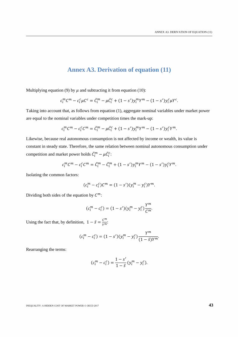
Annex A3. Derivation of equation (11)
Multiplying equation (9) by 𝜇𝜇 and subtracting it from equation (10):
𝑐𝑐𝑖𝑖𝑚𝑚𝐶𝐶𝑚𝑚 − 𝑐𝑐𝑖𝑖𝑐𝑐𝜇𝜇𝐶𝐶𝑐𝑐 = 𝐶𝐶�̅�𝑖𝑚𝑚 − 𝜇𝜇𝐶𝐶�̅�𝑖𝑐𝑐 + (1 − 𝑠𝑠′)𝑦𝑦𝑖𝑖𝑚𝑚𝑌𝑌𝑚𝑚 − (1 − 𝑠𝑠′)𝑦𝑦𝑖𝑖𝑐𝑐𝜇𝜇𝑌𝑌𝑐𝑐 .
Taking into account that, as follows from equation (1), aggregate nominal variables under market power
are equal to the nominal variables under competition times the mark-up:
𝑐𝑐𝑖𝑖𝑚𝑚𝐶𝐶𝑚𝑚 − 𝑐𝑐𝑖𝑖𝑐𝑐𝐶𝐶𝑚𝑚 = 𝐶𝐶�̅�𝑖𝑚𝑚 − 𝜇𝜇𝐶𝐶�̅�𝑖𝑐𝑐 + (1 − 𝑠𝑠′)𝑦𝑦𝑖𝑖𝑚𝑚𝑌𝑌𝑚𝑚 − (1 − 𝑠𝑠′)𝑦𝑦𝑖𝑖𝑐𝑐𝑌𝑌𝑚𝑚.
Likewise, because real autonomous consumption is not affected by income or wealth, its value is
constant in steady state. Therefore, the same relation between nominal autonomous consumption under
competition and market power holds 𝐶𝐶�̅�𝑖𝑚𝑚 − 𝜇𝜇𝐶𝐶�̅�𝑖𝑐𝑐:
𝑐𝑐𝑖𝑖𝑚𝑚𝐶𝐶𝑚𝑚 − 𝑐𝑐𝑖𝑖𝑐𝑐𝐶𝐶𝑚𝑚 = 𝐶𝐶�̅�𝑖𝑚𝑚 − 𝐶𝐶�̅�𝑖𝑚𝑚 + (1 − 𝑠𝑠′)𝑦𝑦𝑖𝑖𝑚𝑚𝑌𝑌𝑚𝑚 − (1 − 𝑠𝑠′)𝑦𝑦𝑖𝑖𝑐𝑐𝑌𝑌𝑚𝑚.
Isolating the common factors:
(𝑐𝑐𝑖𝑖𝑚𝑚 − 𝑐𝑐𝑖𝑖𝑐𝑐)𝐶𝐶𝑚𝑚 = (1 − 𝑠𝑠′)(𝑦𝑦𝑖𝑖𝑚𝑚 − 𝑦𝑦𝑖𝑖𝑐𝑐)𝑌𝑌𝑚𝑚.
Dividing both sides of the equation by 𝐶𝐶𝑚𝑚:
(𝑐𝑐𝑖𝑖𝑚𝑚 − 𝑐𝑐𝑖𝑖𝑐𝑐) = (1 − 𝑠𝑠′)(𝑦𝑦𝑖𝑖𝑚𝑚 − 𝑦𝑦𝑖𝑖𝑐𝑐)𝑌𝑌𝑚𝑚
𝐶𝐶𝑚𝑚.
Using the fact that, by definition, 1 − �̅�𝑠 = 𝑀𝑀𝑚𝑚
𝑌𝑌𝑚𝑚:
(𝑐𝑐𝑖𝑖𝑚𝑚 − 𝑐𝑐𝑖𝑖𝑐𝑐) = (1 − 𝑠𝑠′)(𝑦𝑦𝑖𝑖𝑚𝑚 − 𝑦𝑦𝑖𝑖𝑐𝑐)𝑌𝑌𝑚𝑚
(1 − �̅�𝑠)𝑌𝑌𝑚𝑚.
Rearranging the terms:
(𝑐𝑐𝑖𝑖𝑚𝑚 − 𝑐𝑐𝑖𝑖𝑐𝑐) =1 − 𝑠𝑠′
1 − �̅�𝑠(𝑦𝑦𝑖𝑖𝑚𝑚 − 𝑦𝑦𝑖𝑖𝑐𝑐).

ANNEX A4. DERIVATION OF EQUATION (15)
INEQUALITY: A HIDDEN COST OF MARKET POWER © OECD 2017 45
Annex A4. Derivation of equation (15)
Multiplying all terms of equation (13) by 𝜇𝜇 and subtracting them from equation (14), one can show that:
𝑓𝑓𝑖𝑖𝑚𝑚𝐹𝐹𝑚𝑚 − 𝑓𝑓𝑖𝑖𝑐𝑐𝜇𝜇𝐹𝐹𝑐𝑐 =𝑦𝑦𝑖𝑖𝑚𝑚𝑌𝑌𝑚𝑚 − 𝑦𝑦𝑖𝑖𝑐𝑐𝜇𝜇𝑌𝑌𝑐𝑐 − 𝑐𝑐𝑖𝑖𝑚𝑚𝐶𝐶𝑚𝑚 + 𝑐𝑐𝑖𝑖𝑐𝑐𝜇𝜇𝐶𝐶𝑐𝑐
𝑔𝑔.
Using the relations described in equation (1):
𝑓𝑓𝑖𝑖𝑚𝑚𝐹𝐹𝑚𝑚 − 𝑓𝑓𝑖𝑖𝑐𝑐𝐹𝐹𝑚𝑚 =𝑦𝑦𝑖𝑖𝑚𝑚𝑌𝑌𝑚𝑚 − 𝑦𝑦𝑖𝑖𝑐𝑐𝑌𝑌𝑚𝑚 − 𝑐𝑐𝑖𝑖𝑚𝑚𝐶𝐶𝑚𝑚 + 𝑐𝑐𝑖𝑖𝑐𝑐𝐶𝐶𝑚𝑚
𝑔𝑔.
Isolating the common factors:
(𝑓𝑓𝑖𝑖𝑚𝑚 − 𝑓𝑓𝑖𝑖𝑐𝑐)𝐹𝐹𝑚𝑚 =(𝑦𝑦𝑖𝑖𝑚𝑚 − 𝑦𝑦𝑖𝑖𝑐𝑐)𝑌𝑌𝑚𝑚 − (𝑐𝑐𝑖𝑖𝑚𝑚 − 𝑐𝑐𝑖𝑖𝑐𝑐)𝐶𝐶𝑚𝑚
𝑔𝑔.
Rearranging and using the equilibrium solution of wealth dynamics in equation (12):
𝑓𝑓𝑖𝑖𝑚𝑚 − 𝑓𝑓𝑖𝑖𝑐𝑐 =(𝑦𝑦𝑖𝑖𝑚𝑚 − 𝑦𝑦𝑖𝑖𝑐𝑐)𝑌𝑌𝑚𝑚 − (𝑐𝑐𝑖𝑖𝑚𝑚 − 𝑐𝑐𝑖𝑖𝑐𝑐)𝐶𝐶𝑚𝑚
𝑌𝑌𝑚𝑚 − 𝐶𝐶𝑚𝑚.
Substituting 𝐶𝐶𝑚𝑚 by (1 − �̅�𝑠)𝑌𝑌𝑚𝑚:
𝑓𝑓𝑖𝑖𝑚𝑚 − 𝑓𝑓𝑖𝑖𝑐𝑐 =(𝑦𝑦𝑖𝑖𝑚𝑚 − 𝑦𝑦𝑖𝑖𝑐𝑐)𝑌𝑌𝑚𝑚 − (𝑐𝑐𝑖𝑖𝑚𝑚 − 𝑐𝑐𝑖𝑖𝑐𝑐)(1 − �̅�𝑠)𝑌𝑌𝑚𝑚
𝑌𝑌𝑚𝑚 − (1 − �̅�𝑠)𝑌𝑌𝑚𝑚.
Dividing all terms of the right-hand side of the equation by 𝑌𝑌𝑚𝑚:
𝑓𝑓𝑖𝑖𝑚𝑚 − 𝑓𝑓𝑖𝑖𝑐𝑐 =(𝑦𝑦𝑖𝑖𝑚𝑚 − 𝑦𝑦𝑖𝑖𝑐𝑐)− (𝑐𝑐𝑖𝑖𝑚𝑚 − 𝑐𝑐𝑖𝑖𝑐𝑐)(1 − �̅�𝑠)
1 − (1 − �̅�𝑠) .
Finally, simplifying the last expression:
𝑓𝑓𝑖𝑖𝑚𝑚 − 𝑓𝑓𝑖𝑖𝑐𝑐 =1�̅�𝑠
(𝑦𝑦𝑖𝑖𝑚𝑚 − 𝑦𝑦𝑖𝑖𝑐𝑐) −1 − �̅�𝑠�̅�𝑠
(𝑐𝑐𝑖𝑖𝑚𝑚 − 𝑐𝑐𝑖𝑖𝑐𝑐).

ANNEX A5. DERIVATION OF EQUATIONS (16) AND (17)
INEQUALITY: A HIDDEN COST OF MARKET POWER © OECD 2017 47
Annex A5. Derivation of equations (16) and (17)
Introducing the right-hand side of equation (11) into equation (15)
𝑓𝑓𝑖𝑖𝑚𝑚 − 𝑓𝑓𝑖𝑖𝑐𝑐 =1�̅�𝑠
(𝑦𝑦𝑖𝑖𝑚𝑚 − 𝑦𝑦𝑖𝑖𝑐𝑐) −1 − �̅�𝑠�̅�𝑠
1 − 𝑠𝑠′
1 − �̅�𝑠(𝑦𝑦𝑖𝑖𝑚𝑚 − 𝑦𝑦𝑖𝑖𝑐𝑐).
Simplifying the expression:
𝑓𝑓𝑖𝑖𝑚𝑚 − 𝑓𝑓𝑖𝑖𝑐𝑐 =𝑠𝑠′
�̅�𝑠(𝑦𝑦𝑖𝑖𝑚𝑚 − 𝑦𝑦𝑖𝑖𝑐𝑐).
Introducing the previous result into equation (6)
𝑦𝑦𝑖𝑖𝑚𝑚 − 𝑦𝑦𝑖𝑖𝑐𝑐 = (𝜇𝜇 − 1)(𝑓𝑓𝑖𝑖𝑚𝑚 − 𝑦𝑦𝑖𝑖𝑚𝑚) + (1 − 𝜇𝜇𝛼𝛼𝐿𝐿)𝑠𝑠′
�̅�𝑠(𝑦𝑦𝑖𝑖𝑚𝑚 − 𝑦𝑦𝑖𝑖𝑐𝑐).
Rearranging the terms, we obtain equation (17):
𝑦𝑦𝑖𝑖𝑚𝑚 − 𝑦𝑦𝑖𝑖𝑐𝑐 =𝜇𝜇 − 1
1 − 𝑠𝑠′�̅�𝑠 (1 − 𝜇𝜇𝛼𝛼𝐿𝐿)
(𝑓𝑓𝑖𝑖𝑚𝑚 − 𝑦𝑦𝑖𝑖𝑚𝑚).
Finally, combining equation (17) and the previous result 𝑓𝑓𝑖𝑖𝑚𝑚 − 𝑓𝑓𝑖𝑖𝑐𝑐 = 𝑠𝑠′
𝑠𝑠̅(𝑦𝑦𝑖𝑖𝑚𝑚 − 𝑦𝑦𝑖𝑖𝑐𝑐), one gets equation
(16):
𝑓𝑓𝑖𝑖𝑚𝑚 − 𝑓𝑓𝑖𝑖𝑐𝑐 =𝑠𝑠′�̅�𝑠 (𝜇𝜇 − 1)
1 − 𝑠𝑠′�̅�𝑠 (1 − 𝜇𝜇𝛼𝛼𝐿𝐿)
(𝑓𝑓𝑖𝑖𝑚𝑚 − 𝑦𝑦𝑖𝑖𝑚𝑚).

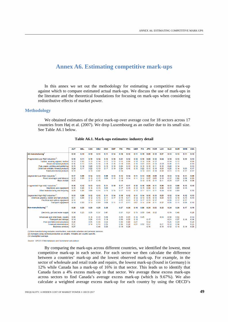
ANNEX A6. ESTIMATING COMPETITIVE MARK-UPS
INEQUALITY: A HIDDEN COST OF MARKET POWER © OECD 2017 49
Annex A6. Estimating competitive mark-ups
In this annex we set out the methodology for estimating a competitive mark-up against which to compare estimated actual mark-ups. We discuss the use of mark-ups in the literature and the theoretical foundations for focusing on mark-ups when considering redistributive effects of market power.
Methodology
We obtained estimates of the price mark-up over average cost for 18 sectors across 17 countries from Høj et al. (2007). We drop Luxembourg as an outlier due to its small size. See Table A6.1 below.
Table A6.1. Mark-ups estimates: industry detail
By comparing the mark-ups across different countries, we identified the lowest, most
competitive mark-up in each sector. For each sector we then calculate the difference between a countries’ mark-up and the lowest observed mark-up. For example, in the sector of wholesale and retail trade and repairs, the lowest mark-up (found in Germany) is 12% while Canada has a mark-up of 16% in that sector. This leads us to identify that Canada faces a 4% excess mark-up in that sector. We average these excess mark-ups across sectors to find Canada’s average excess mark-up (which is 9.67%). We also calculate a weighted average excess mark-up for each country by using the OECD’s

ANNEX A6. ESTIMATING COMPETITIVE MARK-UPS
50 INEQUALITY: A HIDDEN COST OF MARKET POWER © OECD 2017
STAN database to identify a country specific weight for each sector in each country (this reduces the excess mark-up in Canada to 7.58%).
In notation, the observed mark-up in sector o and country n (with whatever market power exists in a sector) is 𝜇𝜇𝑜𝑜,𝑛𝑛
𝑚𝑚 . The minimum (most competitive) mark-up found across all countries n (from n=1 to N) for sector o is:
𝑢𝑢𝑜𝑜𝑐𝑐 = 𝑚𝑚𝑖𝑖𝑙𝑙�𝑢𝑢𝑜𝑜,1𝑚𝑚 ,𝑢𝑢𝑜𝑜,2
𝑚𝑚 , … ,𝑢𝑢𝑜𝑜,𝑁𝑁𝑚𝑚 �.
That is, we take the most competitive mark-up for a sector to be the minimum observed for that sector across all countries in the sample. To the extent that a fully competitive situation is unlikely, except for commodity products, this minimum observed mark-up is a conservative (i.e., high) estimate of the competitive mark-up. The excess mark-up for a given sector o in a given country n is the difference between the observed mark-up for sector o in country n and the minimum mark-up for sector o in all countries:
𝜇𝜇𝑜𝑜,𝑛𝑛𝑒𝑒 = 𝜇𝜇𝑜𝑜,𝑛𝑛
𝑚𝑚 − 𝜇𝜇𝑜𝑜𝑐𝑐 .
To arrive at a figure representing a country’s overall excess mark-up, we weight the excess mark-up for each sector by the size of that sector (eo,n) in that country’s economy, yielding a weighted excess mark-up of:
𝜇𝜇𝑛𝑛𝑒𝑒 = ∑ 𝑒𝑒𝑜𝑜,𝑛𝑛𝜇𝜇𝑜𝑜,𝑛𝑛𝑒𝑒𝑂𝑂
𝑜𝑜=1 .
Since we use differences in the sector mark-ups between countries, we are able to ensure that the results are not driven by the variations in mark-ups across sectors. For example if mark-ups on average cost are higher in sectors with high fixed costs (e.g., telecoms) or lower in generally unprofitable sectors (airlines), we expect this would not be of a character to affect our overall results in a substantial way. What matters fundamentally for our results is whether mark-ups on average cost in the telecom sector in Canada are higher or lower than mark-ups on average cost in the telecom sector in Germany.
Results
Table A6.2. Impact of market power on mark-ups and prices (all units in percentages)
Source: OECD calculations, based on sector weights from STAN Database and sector-specific
mark-ups calculated in Høj, J. et al. (2007).
CountryAverage mark-up
(μm)Minimum mark-
up (μc)Excess mark-up
(μm-μc)
Impact of market power on prices
(
∝
)Canada 17.7 10.1 7.6 8.4France 19.2 10.2 9.0 10.0
Germany 20.9 10.3 10.6 11.8Japan 15.5 9.9 5.6 6.2Korea 20.5 10.0 10.5 11.7Spain 20.0 10.4 9.6 10.7
United Kingdom 13.5 9.6 3.9 4.3United States 16.7 11.0 5.7 6.4
Average 18.0 10.2 7.8 8.7

ANNEX A6. ESTIMATING COMPETITIVE MARK-UPS
INEQUALITY: A HIDDEN COST OF MARKET POWER © OECD 2017 51
Use of mark-ups in the literature
The European Commission (Thum-Thysen & Canton, 2015) identifies mark-ups as important indicators for measuring real frictions in goods markets and in capturing product market competition (Griffith and Harrison 2004). They report that according to Aghion (2002) mark-ups are a robust measure of competition and should be preferred to other indicators such as the Herfindahl index of market concentration (Griffith and Harrison 2004). They argue that country- and sector-specific mark-up estimates therefore provide valuable quantitative information about competition and rigidities in goods markets and changes in these mark-ups may be associated with reform measures (see also Blanchard and Giavazzi 2001 and Melitz 2003).
Høj (2007) looks at the level of profit mark-ups in different sectors and their relationship with indicators of product market regulation and examines whether more pro-competitive policies are related to stronger competition pressures as measured by lower mark-ups. They find a significant and positive correlation between product market regulations that can be characterised as less conducive to competition, such as removing trade barriers, facilitating market access or easing residency and nationality requirements for professional services, and mark-ups. However, Høj (2007) also cautions that mark-ups are an imperfect measure of competition and the estimation method used is only a first-order approximation to them.
Theoretical foundations: What is the redistributive effect of market power?
When producers exert market power over consumers, two economic effects are observed: (1) a deadweight loss in social welfare due to efficiency reasons and (2) a net redistribution of welfare from consumers to producers (see figure below).
The deadweight loss results from the fact that market power constrains the total
amount of output, imposing costs over all agents who would benefit with the additional transactions. On the one hand, where there is market power, consumers do not buy units of a good that they would be willing to purchase if the price was set at the competitive

ANNEX A6. ESTIMATING COMPETITIVE MARK-UPS
52 INEQUALITY: A HIDDEN COST OF MARKET POWER © OECD 2017
level. On the other hand, producers do not sell units of a good for which the competitive price would exceed the production cost. Therefore, the deadweight loss is shared by consumers and producers and leads to a net reduction of social welfare (which is why it is the common argument in favour of competition policy).
In contrast, the infra-marginal redistribution effect does not result from an output variation, but from the price increase that occurs because of market power. Indeed, when producers increase prices above the competitive level, the extra revenue they earn for the output sold comes directly from consumers who pay the higher price. Thus, while the redistribution effect has no net impact on social welfare, it leads to a transfer from consumers to producers, and therefore changes the distribution of wealth in the economy. This is the effect we want to measure to assess the impact of market power on the distribution of wealth.
How to measure the redistributive effect of market power using mark-ups?
In order to measure the total redistribution effect, we use mark-ups calculated from actual data (which reflect the existence of market-power), and we estimate the mark-ups that would hypothetically be observed in a competitive scenario, using the methodology previously described. Note that the “competitive mark-up” estimates are positive, reflecting the competitive rate of return that is required to cover the opportunity cost of capital. Then, from the “market-power mark-ups” and the “competitive mark-ups”, we obtain the price increase that is attributable to market power, which when multiplied by the aggregate consumption, gives the size of the redistribution effect (see figure below).
Naturally, the value estimated for the redistribution effect depends on our estimations of the “competitive mark-ups”. However, because these are estimated using the minimum mark-ups observed across countries, if anything they are overestimated (since no country is likely to have any sector level mark-ups below the competitive level). If competitive mark-ups are, in fact, overestimated, than the price change attributed to market-power is
ANNEX A6. ESTIMATING COMPETITIVE MARK-UPS
INEQUALITY: A HIDDEN COST OF MARKET POWER © OECD 2017 53
underestimated and the redistribution effect is also underestimated, meaning that our results are conservative.
Why not calculate the redistributive effect using excess profits?
Excess profits may appear to be another good measure of market power, as they reflect the extra gain earned by producers relatively to the competitive scenario. Nonetheless, they are not quite as good a measure of the redistributive effect of market power. This is because they include revenue losses from constrained output that are not redistributed to any other economic agent. In other words, excess profits are equal to the redistribution effect of market power minus producer’s deadweight loss, the last of which corresponds to an efficiency cost of market power.
In conclusion, if it is our aim to measure the redistributive impact of market power, we should focus on the redistribution effect that results from price variations. If it were our goal to measure the efficiency costs of market power, we should look at the deadweight loss which results from output changes. However, because excess profits combine the redistribution effect and part of the deadweight loss, they are not our preferred variable to study redistribution individually.

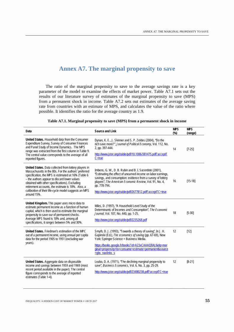
ANNEX A7. THE MARGINAL PROPENSITY TO SAVE
INEQUALITY: A HIDDEN COST OF MARKET POWER © OECD 2017 55
Annex A7. The marginal propensity to save
The ratio of the marginal propensity to save to the average savings rate is a key parameter of the model to examine the effects of market power. Table A7.1 sets out the results of our literature survey of estimates of the marginal propensity to save (MPS) from a permanent shock in income. Table A7.2 sets out estimates of the average saving rate from countries with an estimate of MPS, and calculates the value of the ratio where possible. It identifies the ratio for the average country as 1.9.
Table A7.1. Marginal propensity to save (MPS) from a permanent shock in income
Data Source and Link MPS (%)
MPS (range)
United States. Household data from the Consumer Expenditure Survey, Survey of Consumer Finances and Panel Study of Income Dynamics. The MPS range was extracted from the first column in Table 9. The central value corresponds to the average of all reported figures.
Dynan, K. E., J. Skinner and S. P. Zeldes (2004), “Do the rich save more?”, Journal of Political Economy, Vol. 112, No. 2, pp. 397-444.
http://www.jstor.org/stable/pdf/10.1086/381475.pdf?acceptTC=true
14 [7-25]
United States. Data collected from lottery players in Massachusetts in the 80s. For the authors’ preferred specification, the MPS is estimated at 16% (Table 6 – the authors appear to discard lower values obtained with other specifications). Excluding retirement accounts, the estimate is 18%. Also, a calibration of their life-cycle model suggests an MPS around 15%.
Imbens, G. W., D. B. Rubin and B. I. Sacerdote (2001), “Estimating the effect of unearned income on labor earnings, savings, and consumption: evidence from a survey of lottery players”, The American Economic Review, Vol. 91, No. 4, pp. 778-794.
http://www.jstor.org/stable/pdf/2677812.pdf?acceptTC=true
16 [15-18]
United Kingdom. This paper uses micro data to estimate permanent income as a function of human capital, which is then used to estimate the marginal propensity to save our of permanent shocks. Average MPS found is 18% and, among all specifications, it ranges between 5% and 30%.
Miles, D. (1997), “A Household Level Study of the Determinants of Incomes and Consumption”, The Economic Journal, Vol. 107, No. 440, pp. 1-25.
http://www.jstor.org/stable/pdf/2235268.pdf
18 [5-30]
United States. Friedman’s estimation of the MPC out of a permanent income, using annual per capita data for the period 1905 to 1951 (excluding war years).
Smyth, D. J. (1993), “Towards a theory of saving”, In J. H. Gapinski (Ed.), The economics of saving (pp. 67-69), New York: Springer Science + Business Media.
https://books.google.fr/books?id=A23xCAAAQBAJ&dq=marginal+propensity+to+consume+estimate+permanent&source=gbs_navlinks_s
12 [12]
United States. Aggregate data on disposable income and savings between 1959 and 1969 (most recent period available in the paper). The central figure corresponds to the average of reported estimates (Table 1-4).
Leabo, D. A. (1971), “The declining marginal propensity to save”, Business Economics, Vol. 6, No. 3, pp. 25-29.
http://www.jstor.org/stable/pdf/23480238.pdf?acceptTC=true
12 [8-21]
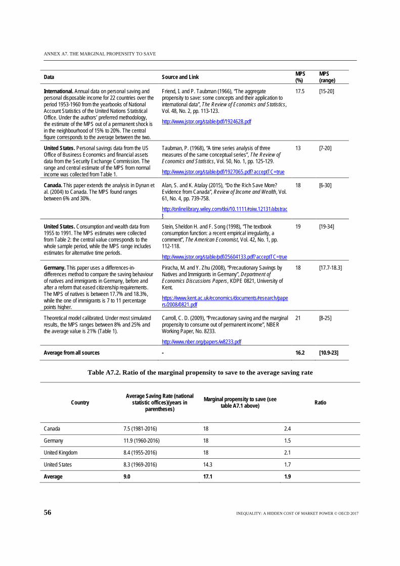
ANNEX A7. THE MARGINAL PROPENSITY TO SAVE
56 INEQUALITY: A HIDDEN COST OF MARKET POWER © OECD 2017
Data Source and Link MPS (%)
MPS (range)
International. Annual data on personal saving and personal disposable income for 22 countries over the period 1953-1960 from the yearbooks of National Account Statistics of the United Nations Statistical Office. Under the authors’ preferred methodology, the estimate of the MPS out of a permanent shock is in the neighbourhood of 15% to 20%. The central figure corresponds to the average between the two.
Friend, I. and P. Taubman (1966), “The aggregate propensity to save: some concepts and their application to international data”, The Review of Economics and Statistics, Vol. 48, No. 2, pp. 113-123.
http://www.jstor.org/stable/pdf/1924628.pdf
17.5 [15-20]
United States. Personal savings data from the US Office of Business Economics and financial assets data from the Security Exchange Commission. The range and central estimate of the MPS from normal income was collected from Table 1.
Taubman, P. (1968), “A time series analysis of three measures of the same conceptual series”, The Review of Economics and Statistics, Vol. 50, No. 1, pp. 125-129.
http://www.jstor.org/stable/pdf/1927065.pdf?acceptTC=true
13 [7-20]
Canada. This paper extends the analysis in Dynan et al. (2004) to Canada. The MPS found ranges between 6% and 30%.
Alan, S. and K. Atalay (2015), “Do the Rich Save More? Evidence from Canada”, Review of Income and Wealth, Vol. 61, No. 4, pp. 739-758.
http://onlinelibrary.wiley.com/doi/10.1111/roiw.12131/abstract
18 [6-30]
United States. Consumption and wealth data from 1955 to 1991. The MPS estimates were collected from Table 2: the central value corresponds to the whole sample period, while the MPS range includes estimates for alternative time periods.
Stein, Sheldon H. and F. Song (1998), “The textbook consumption function: a recent empirical irregularity, a comment”, The American Economist, Vol. 42, No. 1, pp. 112-118.
http://www.jstor.org/stable/pdf/25604133.pdf?acceptTC=true
19 [19-34]
Germany. This paper uses a differences-in-differences method to compare the saving behaviour of natives and immigrants in Germany, before and after a reform that eased citizenship requirements. The MPS of natives is between 17.7% and 18.3%, while the one of immigrants is 7 to 11 percentage points higher.
Piracha, M. and Y. Zhu (2008), “Precautionary Savings by Natives and Immigrants in Germany”, Department of Economics Discussions Papers, KDPE 0821, University of Kent.
https://www.kent.ac.uk/economics/documents/research/papers/2008/0821.pdf
18 [17.7-18.3]
Theoretical model calibrated. Under most simulated results, the MPS ranges between 8% and 25% and the average value is 21% (Table 1).
Carroll, C. D. (2009), “Precautionary saving and the marginal propensity to consume out of permanent income”, NBER Working Paper, No. 8233.
http://www.nber.org/papers/w8233.pdf
21 [8-25]
Average from all sources - 16.2 [10.9-23]
Table A7.2. Ratio of the marginal propensity to save to the average saving rate
Country Average Saving Rate (national
statistic offices)(years in parentheses)
Marginal propensity to save (see table A7.1 above) Ratio
Canada 7.5 (1981-2016) 18 2.4
Germany 11.9 (1960-2016) 18 1.5
United Kingdom 8.4 (1955-2016) 18 2.1
United States 8.3 (1969-2016) 14.3 1.7
Average 9.0 17.1 1.9


58 INEQUALITY: A HIDDEN COST OF MARKET POWER © OECD 2017
www.oecd.org/daf/competition