Inequality, Foreign Investment, and Imperialism

Thomas Hauner∗ Branko Milanovic† Suresh Naidu‡

This Draft: November 30, 2017

Abstract

We present an empirical restatement of the classical economic theory of imperialism andthe origins of World War I. Using recent data, we show 1) inequality was at historical highsin all the advanced belligerent countries at the turn of the century, 2) rich wealth holdersinvested more of their assets abroad, 3) risk-adjusted foreign returns were higher than risk-adjusted domestic returns, 4) establishing direct political control decreased the riskiness offoreign assets, 5) increased inequality was associated with higher share of foreign assets in GDP,and 6) increased share of foreign assets was correlated with higher levels of military mobilization.Together, these facts suggest that the classic theory of imperialism may have some empiricalsupport.

1 Introduction

The number of historical and political books and articles written on the origins of the Great War

(later called World War I) in all languages is enormous. Recently, around the centenary of the

outbreak of the War, there appeared many new historical books, some of which went on to became

international bestsellers. The discussion of the War thus appears endless and shows no signs of

abating.

But in one area, the discussion of the origins of the war, is strangely absent. This is economics.

The lack of recent economic works on the origin of the war is even stranger because it is economics

and not other social sciences that led the analysis in the past, arguing even before the hostilities

of 1914 began, that the war was almost inevitable, and then during the war continued with its

economically-driven “dissection” of the causes. We have in mind here the seminal work by John

∗Federal Reserve Bank of Minneapolis†CUNY Graduate Center, Stone Center for Socio-Economic Inequality‡Columbia University

The views expressed are the authors’ and do not necessarily represent those of the Federal Reserve Bank of Minneapolisor the Federal Reserve System. We thank Jannette Rutterford and Dimitris Sotiropoulos for sharing data on Britishprobate records with us and Thomas Piketty for sharing Parisian decedents data.

1

Hobson (1902), Imperialism: A Study, that in the next couple of decades led to several influential

works within the Marxist tradition that explained the imperialist origins of the war (Luxemburg,

Lenin, Bukharin). That line of analysis remained very active for a while among Marxist economists

(for example, Samir Amin (1974) in Accumulation on a World Scale). Paul Bairoch shared the same

view.1 It was recently restated by Branko Milanovic (2016) in Global Inequality where, focusing on

the role of high inequality before the conflict, he dubbed it an “endogenous” explanation of the war

meaning that internal logic of the highly unequal capitalist societies at the turn of the 20th century

predisposed them to imperialism2 which in turn caused the war. However, in the past fifty years,

interest in this type of explanation among economists and economic historians has been limited. It

is not exaggerated to say that theories of imperialism elicit today mostly an antiquarian interest,

and the empirical study of late 19th century international economy is largely subsumed under

“globalization”, which ignores the geopolitical concerns that loomed large in the early literature.3

Even Findlay & O’Rourke (2009), who are quite attuned to the complementary relationship between

force and trade, treat World War I as an exogenous shock to the well-managed globalization of

the previous 50 years. Tooze (2015) provides further historiography, highlighting the disconnect

between economic history literatures on 19th century globalization (who ignore geopolitics) and

political science literatures on international relations (which ignore economics).

Our objective in this paper is to revisit theories of imperialism in order to define them in a more

coherent manner, freeing them from reliance on irrelevant details, and to investigate whether the

mechanisms adduced by the authors can be empirically substantiated. However, while both the

modeling and the empirics are modern, in the sense that neither the tools of the analysis nor the

data were available to the authors who wrote a century ago, the main contours of the argument

are theirs.

They are relatively simple. According to Hobson, unequal distribution of income in advanced

1In his section on the causes of growth of foreign investments before 1914 (Chapter 13 of Volume 2 of his mon-umental Victoires et deboires, p. 320), Bairoch writes: “the increase in income inequality leads to an even fasterincrease in available funds (disponibilites) of the top classes. At that point the possibility emerges that there is a lackof profitable domestic investment opportunities. This is from 1840-50 apparently the case with the United Kingdom,and later with other European countries that have engaged in early industrializaton” (our translation).

2Imperialism in our paper will not be confined to direct colonization, but more broadly includes relationships ofinformal dependence. See Gallagher & Robinson (1953).

3The same is not true for historians where imperial pressures as determinants of World War I continue to play animportant role (e.g., Fritz Fischer and William Appleman Williams).

2

capitalist countries (more specifically, England) leads to secular underconsumption due to lack

of purchasing power of the poorer and middle classes. There is a glut of savings compared to

profitable investments that exist nationally (while Hobson did not have the language of domestic

financial frictions, his argument is consistent with modern formulations of uninsured idiosyncratic

returns, as our model in Appendix G formalizes). The owners of financial capital hence need to find

more profitable outlets for their investments and they can only find them in overseas territories

(where, one could say also, the marginal productivity of capital, due to its scarcity, is greater).

These investments are of two kinds: lending to foreign government in the form of purchase of their

bonds, or direct foreign investments. But neither form of investment is safe, once it is made so far

away from home and in the countries where property rights are much less secure than in the main

capitalist nations.4 In order to ensure security of their property, capitalists in advanced countries

resort to the use of state power, either to control the borrowing government and threaten it by

military force if it fails to pay the debt (e.g. Egypt, Turkey, Venezuela, Tunisia), or to conquer the

country in order to transform it into a colony where metropole rules (including those regarding the

security of property) apply.5

In Hobson’s view, imperialism is “vent for investments”. It is “the endeavor of the great con-

trollers of industry to broaden the channel for the flow of their surplus wealth by seeking foreign

markets and foreign investments to take off the goods and capital they cannot sell or use at home”

(p.85). And it is far from being class neutral, for the political and military power of the metropole

is used to ensure a superior return to the owners of foreign assets who are mostly the rich: “. . . if

I invest either in the public funds or in some private industrial venture in a foreign country for

the benefit of my private purse, getting specially favorable terms to cover risks arising from the

political insecurity of the country or the deficiencies of its Government, I am entitled to call upon

my Government to use its political and military force to secure those very risks which I have already

discounted in the terms of my investment. Can anything be more palpably unfair?” (Hobson, ibid,

4In fact, already Adam Smith (Wealth of Nations, Book IV, Chapter 2) had noticed that capitalists prefer toinvest close to home, in order to have their assets more easily controlled.

5Hobson (1902, p. 54) quotes the Italian economist Achille Loria: “France’s attempted conquest of Mexico duringthe second empire was undertaken solely with the view of guaranteeing the interest of French citizens holding Mexicansecurities. But more frequently the insufficient guarantee of an international loan gives rise to the appointment offinancial commission by the creditor countries in order to protect their rights and guard the fate of their investedcapital. The appointment of such a commission. . . amounts. . . to a veritable conquest.”

3

p. 358).

Having a colony (formal or informal) comes with other advantages like a cheap labor force that

can be exploited much more than domestic labor (where pro-worker regulations were already in

place), preferential access to raw materials (which can be denied to other imperialist competitors),

new monopolistic market for the products made or traded by the metropole (British textiles in India

or steel in the colonial United States, opium in China). In some cases (the sack of the Summer

Palace in Beijing), even outright plunder of the old-fashioned style was not excluded. Now, when

several major powers are involved in these actions, the struggle for colonies and for control of the

“unallocated” parts of the world rapidly ensues. It is this imperialistic competition that, after

several smaller conflicts (Fashoda, the two Moroccan crises) led to the outbreak of the Great War.

At the origin of the international conflict, however, was domestic maldistribution of income.

Empire was more than colonies, however. The literature has often focused on the difference

between colonial and non-colonial holdings, and a robust empirical fact is that colonial assets were

small relative to non-colonial assets.6 But as Saul (1960) shows, empire was a network of offsetting

trade balances, where for example British trade surpluses with North America and Continental

Europe were paid for with trade deficits with India and Turkey. Our argument is not about the

returns to colonies specifically, but rather the returns to empire broadly, including maintaining the

security and value of trade routes (and future trade routes). The large foreign asset positions held

by wealthy citizens of the metropoles could only be redeemed by future flows of income, whose

smooth realization would need to be guaranteed by naval power and expeditionary forces, secured

strategic routes such as Morocco and the Dardanelles, reliable prospects of future pan-African

trade linkages (Fashoda) or Asian markets (Tonkin), and extensive mutual defense treaties to deter

aggression.

This line of reasoning was, with small differences, held by most authors mentioned here. Lenin

(1917) (Imperialism: The Highest Stage of Capitalism) argued that the initial impetus to go in

search of foreign markets came from the tendency of the profit rate to fall in mature capitalism (a

point emphasized by Marx) rather than from Hobson’s “maldistribution” of income.7 Hilferding

6See Cain & Hopkins (1980) and Clemens & Williamson (2004), who show that less than 30% of British foreigninvestment was outside the white settler states.

7The idea is indeed contained in Marx. In Volume III of Das Kapital, in Chapter XV where he develops the “Law

4

(1910) (Finance Capital) has the richer and more nuanced version of this theory, where the declining

rate of profit leads to corporate consolidation and national cartels who earn profits by obtaining

protective tariffs over ever larger economic territories, generating a demand for empire. Rosa

Luxemburg (1913) (The Accumulation of Capital) thought that since capitalism suffered from the

permanent crisis of “realization of surplus value” (inability to sell all produced goods at profitable

rates) due to the lack of demand from the poorer classes, it needed to be in a permanent search

and conquest of external non-capitalist markets. She thus saw the parallel existence of capitalist

and pre-capitalist modes of productions (with the latter being gradually eroded by the capitalist

mode) as necessary for continuous capitalist expansion.

But the same view about the importance, for capitalists, of subjecting foreign territories to

their nations’ rule was not held only by Marxist economists. Max Weber (1922) in his Economy

and Society, written before World War I (and published posthumously), writes: “The safest way

of monopolizing for the members of one’s own polity profit opportunities which are linked to [con-

trol]. . . of a foreign territory is to occupy it or at least to subject the foreign political power to a

‘protectorate’. . . Therefore, this ‘imperialist’ tendency increasingly displaces the ‘pacifist’ tendency

of expansion, which aims merely at freedom of trade. . . The universal revival of ‘imperialist’ capi-

talism, which has always been the normal form in which capitalist interest have influenced politics,

and the revival of political drives for expansion are thus not accidental. For the predictable future,

the prognosis had to be made in its favor” (Volume II, Chapter IX, Section 4, “The economic

foundations of ‘imperialism’”).

In this paper, we do not take a position on the validity of either the maldistribution-cum-

underconsumption hypothesis or the “tendential decrease in the rate of profit” hypothesis. Our

argument is simpler but also less restrictive. We argue that the increase in income and wealth in-

equality in major countries has produced an increasing demand for financial assets, which could be

due to domestic credit market imperfections. The rich tended to invest overwhelmingly in foreign

assets because they were, adjusted for risk, more profitable than available domestic opportunities.

To protect such foreign assets, whether portfolio or direct, the countries, partially at the instiga-

tion of investors in foreign assets, increased military investments (naval dreadnoughts as well as

of the tendential fall in the rate of profit,” Marx writes that “the internal contradictions [of realization of surplusvalue] seek resolution by extending the external field of production” (p. 353).

5

territorial armies) and complemented it with geopolitical strategies, including both colonial con-

quests as well as extensive treaties. The value of securing Fashoda lay not only in the returns to

investment in Egypt, but also the prospect of integrating British/French African possessions (e.g.

a Cape-Cairo railway). We cite several more historical examples in Appendix E. The tensions

produced by all different countries pursuing similar goals led to conditions that made a Great War

more likely.

We cannot prove all these links empirically in this paper. Thus, the empirical part concentrates

on (i) the correlations between income/wealth inequality and the share of net foreign assets in

country’s GDP, and (ii) the relationship between the importance of foreign assets a country held

and the size of its military. We also present a case study of the Boer War, which Hobson publically

commented on extensively Hobson (1900) and which laid the groundwork for his subsequent theory

of imperialism, focusing on a very sharp change in colonial status as a clear instance of military

expansion lowering the risk premium for British investors.

In Appendix G we present a simple model of foreign asset markets. The demand for foreign

investment is horizontal at a risk-adjusted return r∗. The supply curve of foreign investment is a

function of the aggregate savings of the economy, but also the extent of domestic financial frictions.

The presence of domestic financial frictions is one mechanism for tying wealth inequality to foreign

investment, as large wealth owners, with low marginal product of capital can’t lend to poorer wealth

holders with higher marginal products, and hence invest abroad. This simple model shows how

the volume of foreign investment may not be a good measure of the economic surplus from empire,

and also offers a reinterpretation of Hobson (high inequality) and Hilferding/Lenin/Luxemburg

(low domestic returns) as emphasizing different forces shifting out the supply curve of foreign

investment.

We do not claim to explain the outbreak of the war, because that depended on numerous

contingencies, military alliances and not least importantly agency of principal actors. But we

do claim that the evidence given here shows that the key ingredients needed for the war were

present. Whether the war broke out in 1914 or not might have hinged on whether Franz Ferdinand’s

chauffeur mistakenly pressed the brake instead of the accelerator, but if the geopolitical tensions

and militarization favoring the war were not there, many royal drivers could have made similar

6

mistakes without the war breaking out.

The paper is organized as follows. In Section 2, we look at income and wealth inequalities in

the main capitalist nations on the eve of the conflict. In Sections 3–6, we study the importance

of foreign assets in the overall portfolio of the rich countries, look at whether foreign assets were

overwhelmingly owned by the rich, and whether their yield (adjusting for risk) was higher than

that of domestic assets. Finally, in Section 7 we assemble the empirical evidence to obtain esti-

mates of the relationships between the key variables (cross-country correlations between inequality,

foreign assets, and military capacity in the advanced countries prior to 1914). Section 8 presents

our conclusion. Appendices give information on the data we use and present a simple model of

supply and demand of foreign investments, where foreign investments provide a surplus (rent above

the compensation for asset riskiness) and where military force is used to ensure that the rent is

safeguarded.

2 An Overview of Income and Wealth Inequality in the Run-Up

to the Great War

Our data on inequality of income and wealth in the decades before the World War I are very

incomplete. Yet they are not inexistent, and a careful combination of all coeval sources and the

comparison of their movements over the 1860–1914 period allows us to form a picture of the

evolution of inequality in the major countries prior to the war. We shall look at three types of

measured inequality (based on three different sources of data), which although covering countries

and periods very unevenly can provide us with a general idea of the level and movement of inequality

in the half-century before the War. The first type of inequality is inequality in income that, in

principle, includes the entire population. Data for such estimates come principally from social

tables. The second type of inequality is concentration of income among the top 1% of income

earners. The data come from fiscal sources (i.e. tax records). The third type of inequality is

concentration of wealth among the top 1% of wealth holders. The data also come from fiscal

sources.

7

Income inequality, measured by the Gini coefficient, for the period 1860–1914 is shown in Table

1 and for a more limited sample of countries in Figure 1. Since the data are scarce, we present

them as decadal averages. We include major belligerent countries for which data are available, plus

the Netherlands that, while it mobilized the army, stayed neutral during the War, and was both

a significant international investor and a major imperial power. The data for the Central Powers

are limited to Prussia/Germany.8 More detailed discussion of the data for England/UK, United

States, and Prussia/Germany is provided in Appendix A.

Table 1: Inequality in major belligerent countries (Ginis of disposable per capitaincome)

Decade England/GreatBritain

USA Netherlands Japan Prussia Italy Russia

1860s 57 49 501870s 51 451880s 52 40 32 471890s 43 32 471900s 47 33 49 38a

1910–14 55 49 50 47 32 46

2005–15 35 41 29 32 31 36 35

GDP percapitaaround1914

4930 4800 3900 1330 3060 2200 1350

Sourceof pre-1914data

Social tables Socialtables

Fiscal datacombinedwith otherinformation

Fiscal datacombinedwith otherinformation

Fiscal datacombinedwith otherinformation

Householdbudgets

Socialtables

a Only European Russia.

Sources: For pre-1914 data see Appendix A. 2005–15 Ginis based on Luxembourg Income Survey per capita data. GDPs per

capita from the Maddison project, 2013 update.

Most of our information comes from social tables which give the list of salient socio-economic

groups with their estimated mean household incomes and population sizes. While social tables

are the best source that we have for the 19th century and early 20th century, they have many

shortcomings: the number of social groups may be small, the group averages may conceal large

8In the discussion, we treat Prussia as synonymous with Germany. According to the last pre-World War Ipopulation census in 1907, Prussia accounted for 62 percent of the German population (Wavell Grant, 2002, p. 11).

8

within-group variances (e.g. the average income of merchants may be representative of only small

fraction of merchants: many may be much richer, and many much poorer than the average) etc.

Social tables are the key source of the data for England/Great Britain where their origin goes back

to Gregory King’s 1688 social table, and also for the United States where Lindert & Williamson

(2016) have recently recreated very detailed social tables for the period 1774–1870. Compared with

the fiscal sources, social tables have the advantage of covering, in principle, the entire population,

from the poorest to the richest. Fiscal data, obviously, cover only the tax payers whose share may,

at times, be very low. Social tables are estimates of the “full distribution” although because of

their “compressed” nature, social tables, compared to standard modern household surveys that

interview thousands of individuals, tend to underestimate inequality.

Household budgets, used for Italy, are in principle similar to social tables because they too

cover the entire distribution. The approach consists in “post-sampling”, that is finding as many

as possible of household budgets from a given period and using information on location, household

size and profession of households obtained from such budgets, assigning to each observation its ex

post sampling weight. It is equivalent to treating whatever information exists (and is not random)

as having been derived from a stratified random survey. The method was pioneered by Brandolini

& Vecchi (2011) in their study of post-Unification Italy.

Finally, we show in Table 1 also estimates for Prussia and Japan that combine fiscal data with

other sources of information (e.g. agricultural wages, income distributions in individual cities etc.)

to produce a “full distribution”. Heterogeneity of sources makes comparison between the countries

more problematic but allows for (careful) within-country over-time comparisons.

From Table 1 and Figure 1 we can make three conclusions. First, on the eve of World War I,

Ginis of all countries lay in a rather narrow range between 46 and 55 Gini points with the exception

of Prussia (which is probably explained by the “piece-wise” construction of the Prussian data) and

Russia (which was covered only in part). It is also important to note that the richest county,

Great Britain was also a county with the highest level of inequality. Given that the social tables

are likely to underestimate inequality, the “true” British inequality might have been even higher,

approximately in the range of inequality levels in today’s Latin America.

9

Second, there is no general tendency toward rising or decreasing inequality during the 1860-1914

period. Only Japan shows a strongly increase in inequality. England/UK, United States, Italy, and

Prussia (in that order by their inequality levels) show high, but not rising, inequality.

Third, inequality then was much greater than inequality in the same countries today. In the

UK and the Netherlands, the difference is enormous: inequality is some 20 Gini points lower today,

that is, it is only about 60 percent of the Gini value before the Great War. The United States is

somewhat of an exception because today’s inequality is “only” 6 Gini points lower.

Figure 1: Estimated income inequality, 1860–1910

Table 2 shows income concentration data for a more limited sample of countries. These results

are based on fiscal data provided by the World Wealth and Income Database.9 Fiscal data, espe-

cially at the inception of the era of direct taxation in the US, UK, France and elsewhere covered only

the richest people, and thus they might provide reasonably good estimates of income concentration

(the share of total income received by the top 1%) but not estimates of the entire distribution.

In other words, they are a good measure of the importance of top income earners or wealth hold-

ers but are truncated and cannot be treated as a measure of inequality of the entire distribution.

However, they are valuable: top income share estimates combined with the “full-distribution” data

from Table 1 should give us a better hold on the evolution of inequality.

9The data for the Austrian part (Cisleuthania) of the Austro-Hungarian Empire come from Novokmet (2017).Austria accounted for close to 60 percent of the population of Austria-Hungary (30 out of 52 million).

10

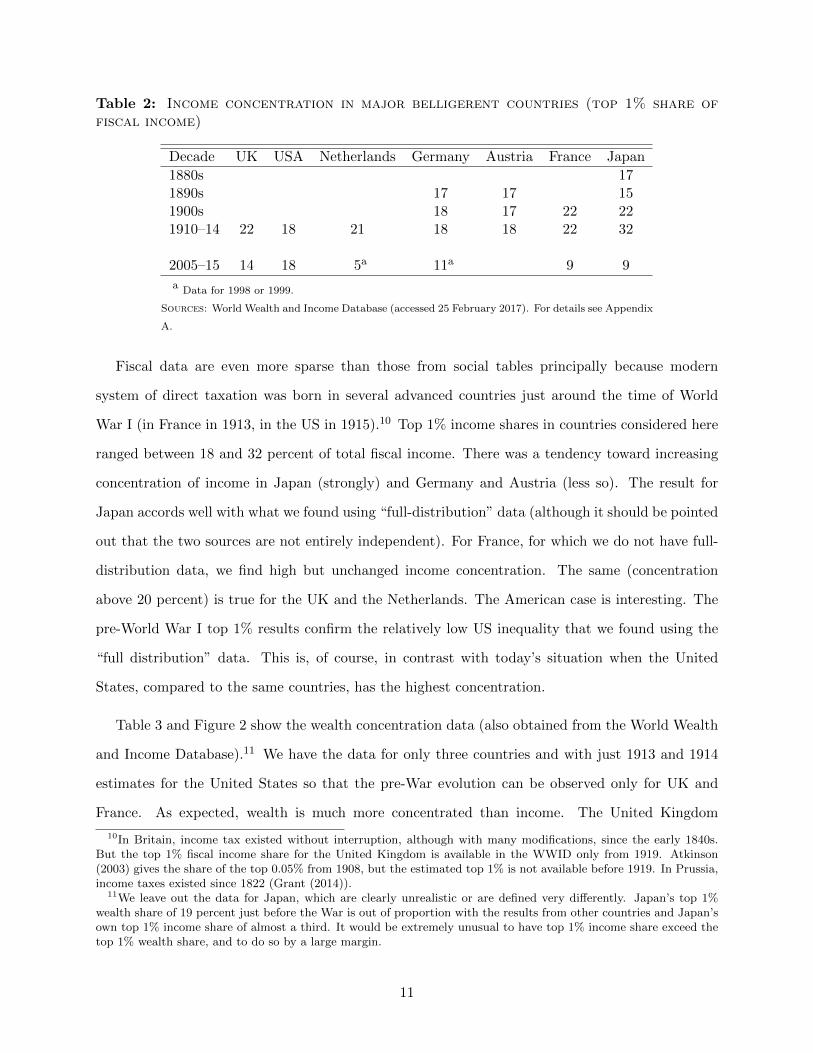
Table 2: Income concentration in major belligerent countries (top 1% share offiscal income)

Decade UK USA Netherlands Germany Austria France Japan

1880s 171890s 17 17 151900s 18 17 22 221910–14 22 18 21 18 18 22 32

2005–15 14 18 5a 11a 9 9

a Data for 1998 or 1999.

Sources: World Wealth and Income Database (accessed 25 February 2017). For details see Appendix

A.

Fiscal data are even more sparse than those from social tables principally because modern

system of direct taxation was born in several advanced countries just around the time of World

War I (in France in 1913, in the US in 1915).10 Top 1% income shares in countries considered here

ranged between 18 and 32 percent of total fiscal income. There was a tendency toward increasing

concentration of income in Japan (strongly) and Germany and Austria (less so). The result for

Japan accords well with what we found using “full-distribution” data (although it should be pointed

out that the two sources are not entirely independent). For France, for which we do not have full-

distribution data, we find high but unchanged income concentration. The same (concentration

above 20 percent) is true for the UK and the Netherlands. The American case is interesting. The

pre-World War I top 1% results confirm the relatively low US inequality that we found using the

“full distribution” data. This is, of course, in contrast with today’s situation when the United

States, compared to the same countries, has the highest concentration.

Table 3 and Figure 2 show the wealth concentration data (also obtained from the World Wealth

and Income Database).11 We have the data for only three countries and with just 1913 and 1914

estimates for the United States so that the pre-War evolution can be observed only for UK and

France. As expected, wealth is much more concentrated than income. The United Kingdom

10In Britain, income tax existed without interruption, although with many modifications, since the early 1840s.But the top 1% fiscal income share for the United Kingdom is available in the WWID only from 1919. Atkinson(2003) gives the share of the top 0.05% from 1908, but the estimated top 1% is not available before 1919. In Prussia,income taxes existed since 1822 (Grant (2014)).

11We leave out the data for Japan, which are clearly unrealistic or are defined very differently. Japan’s top 1%wealth share of 19 percent just before the War is out of proportion with the results from other countries and Japan’sown top 1% income share of almost a third. It would be extremely unusual to have top 1% income share exceed thetop 1% wealth share, and to do so by a large margin.

11

exhibits by far greater wealth concentration than France and the US: the top 1% controlled around

70 percent of British wealth and that share appears quite stable over the quarter century for which

we have the data. Data on French wealth concentration go back to the mid-19th century. They

show a significant increase in concentration, from around one half of all wealth being in the hands

of the top 1% to around 55–56 percent in the decades before the War. As mentioned, for the US

we have the data for only two years before the War (that is, if we treat 1914 as “before”) but it

is significant that the top 1% wealth share is much lower than in both European countries. These

extraordinary high wealth concentration shares are (by now) cut by more than half in France and

by more than two-thirds in the UK. The decline of the top 1% wealth share in the US was much

more moderate.

Table 3: Wealth concentration in major belligerent countries (top 1% share ofwealth)

Decade UK USA France

1860s 491870s 481880s 491890s 711900s 71 561910–14 68 44 55

2005–15 20 36 23Sources: World Wealth and Income Database (accessed 25 February 2017).

Overall, when we summarize the results obtained from the three indicators, they seem to point

to high but generally stable wealth and income inequalities. Japan alone exhibits increasing income

inequality and income concentration, France shows substantially rising wealth concentration and

England/UK stands out by extremely high levels of both income and wealth inequalities, but

without tendency towards their further increase. For both UK and France wealth concentration

was at, or around, its historical high in 1914.

12

Figure 2: Wealth concentration (share of total wealth owned by top 1% of wealthholders), 1860–1910

3 The Composition of National Financial Holdings

The premise of this paper is that acquisition of foreign assets between the United Kingdom, France,

and Germany (the countries from which we have the most data available), driven by historically high

levels of domestic inequality documented above, ultimately led to their expanding militarization

before 1914 as a means of securing and controlling foreign assets. In this section, we briefly discuss

trends in territorial expansion (the most obvious foreign asset) before focusing on net foreign asset

holdings in the core countries. Later, in Section 4, we will show that such assets were concentrated

amongst the wealthy, and finally, in Section 5, we will argue that the export of capital can be

explained by the superior relative rates of return enjoyed by investors.

3.1 Territorial expansion

Initial territorial claims for each of the three “core” countries (i.e. France, the UK, and Germany),

and their increases, are neatly summarized in Grover Clark’s 1936 aptly titled monograph, The

Balance Sheets of Imperialism. Some of his results are reproduced in Table 4, which documents

territorial control by square kilometers. In aggregate, 66 percent of the world’s total landmass was

considered independent in 1878—just prior to the final imperial push for colonial acquisitions. By

13

1913, not quite 54 percent was independent. Britain, already the largest empire in 1878, claimed

almost 19 percent of all square kilometers on the globe, and increased this to over 22 percent by

1913. Though France only held around four percent of global territories in 1878, it increased its

control by over 130 percent before the start of the war, to more than eight-and-a-half percent.

The before and after effects from the so-called scramble for Africa, as initiated by the Berlin

Conference of 1884–85, are remarkably acute: less than four percent of the continent’s landmass

remained independent after the scramble—compared to more than half in 1878. Britain nearly

tripled its territory, from just over five percent of the content to nearly 15 percent between 1878

and 1913.

Table 4: Share of square kilometers held by countries (%)

Total Worlda Africaa

1878 1913 Percent Change 1878 1913 Percent Change

Independent 66.19 53.66 -18.93 56.54 3.41 -93.97UK 18.86 22.27 18.08 5.13 14.46 181.9France 3.73 8.68 132.7 13.42 33.68 151.0Germany 0.36 2.61 625.0 . 9.15 .

a Data do not sum to 100 percent, leave out other imperial possessions.Source: Clark (1936), Table I

While the imperial hierarchy wasn’t dislodged, with Britain at the top, Germany made immense

gains over the period, going from a relatively small state with few, if any, colonial territories to

one with notable colonial dependencies (over nine percent of African territory). France more so.

She nearly tripled her territorial control over Africa, according to Table 4, though saw less total

expansion globally. British imperialism continued to expand, but at a clipped pace given the

increased competition.

3.2 Foreign asset holdings

Next, we trace the historical importance of foreign assets in the half century before the Great

War. The line graphs in Figure 3 (measured along the left-hand side axis) plot the evolution of

net foreign assets (NFA) relative to GDP before 1913 in the three core countries, using data from

Piketty & Zucman (2014). Somewhat surprisingly, the ratio of net foreign assets to total GDP was

larger in France in 1870 than in the United Kingdom—even though the UK controlled roughly six

14

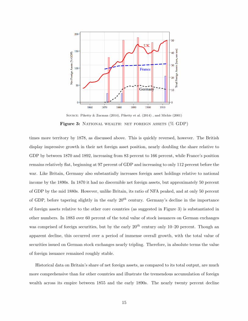
Source: Piketty & Zucman (2014), Piketty et al. (2014) , and Michie (2001)

Figure 3: National wealth: net foreign assets (% GDP)

times more territory by 1878, as discussed above. This is quickly reversed, however. The British

display impressive growth in their net foreign asset position, nearly doubling the share relative to

GDP by between 1870 and 1892, increasing from 83 percent to 166 percent, while France’s position

remains relatively flat, beginning at 97 percent of GDP and increasing to only 112 percent before the

war. Like Britain, Germany also substantially increases foreign asset holdings relative to national

income by the 1890s. In 1870 it had no discernible net foreign assets, but approximately 50 percent

of GDP by the mid 1880s. However, unlike Britain, its ratio of NFA peaked, and at only 50 percent

of GDP, before tapering slightly in the early 20th century. Germany’s decline in the importance

of foreign assets relative to the other core countries (as suggested in Figure 3) is substantiated in

other numbers. In 1883 over 60 percent of the total value of stock issuances on German exchanges

was comprised of foreign securities, but by the early 20th century only 10–20 percent. Though an

apparent decline, this occurred over a period of immense overall growth, with the total value of

securities issued on German stock exchanges nearly tripling. Therefore, in absolute terms the value

of foreign issuance remained roughly stable.

Historical data on Britain’s share of net foreign assets, as compared to its total output, are much

more comprehensive than for other countries and illustrate the tremendous accumulation of foreign

wealth across its empire between 1855 and the early 1890s. The nearly twenty percent decline

15

in foreign assets from the mid 1890s until the turn of the 20th century is likely attributed to the

material losses from the Second Boer war, after which foreign assets surpassed their previous peak

of 170 percent of GDP and rose to a new high of 181 percent by 1913.

The bar graphs in Figure 3 (measured along the right-hand side axis) document two additional

metrics of foreign asset growth, though only for France (blue bars) and Britain (red bars). The

French data represent the stock of foreign financial assets as a share of total assets held by Parisian

decedents between 1872 and 1912. (The data come from Piketty et al. (2014) and are reproduced

in greater detail in Appendix B; they include all financial assets, both foreign and domestic, as well

as the residual amount of non-financial assets.) They show a marked increase in the importance of

foreign assets in the estates of wealthy Parisians. Despite aggregate French net foreign assets as a

share of GDP not changing significantly overall in this same time period, foreign assets were still

becoming increasingly important amongst wealth holders.

The red bars in Figure 3 describe the total nominal value of foreign and British colonial securities

quoted on the London Stock Exchange’s official list. (A table providing asset class decompositions

of the Stock Exchange data from Michie (2001) is also provided in Appendix B.) It is unsurprising

that securities listed on the stock exchange in London mimic aggregate measures of net foreign

asset holdings, but it helps establish the clarity of the trends before the Great War.

The relative changes in the importance of all foreign assets as a share of total financial assets

between Paris and London (either held by estates, as in Paris, or quoted on the stock exchange,

as in London) are impressive. In Paris, between 1872 and 1913, foreign assets became more than

four times as large a component in decedent estates, increasing from only 13 percent to 40 percent.

Meanwhile on the London Stock Exchange, the importance of foreign assets grew as well. In 1873,

foreign (including colonial) assets were already a relatively larger component of total financial assets

(36 percent) in London than in Paris (13 percent). This increased to around 50 percent in London

by 1883 and fluctuated around this level until before the war.

Before addressing the rates of return on these foreign assets in Section 5 (and before our dis-

cussion of foreign asset holdings across the wealth distribution in the next Section), it is important

to consider what a typical portfolio allocation may have looked like so that we study returns on

16

the appropriate assets. The most detailed data available, also from Piketty et al. (2014), capture

only a subset of French investors, Parisian decedents. Piketty and his co-authors utilize estate tax

payments to glimpse into the portfolios of individual rich households (see Table B.1 in Appendix

B). Overall, bonds dominate both domestic and foreign financial asset portfolios. However, their

relative importance in foreign financial holdings increases over time, but less so in domestic finan-

cial holdings—though still outweighing equities three to one. There are also increasing shares in

foreign equity holdings over time, as territorial assets (and markets) grew. Throughout this period,

financial assets comprised a steady 62–63 percent of net estates, with the remaining third invested

in real estate and a marginal two-to-three percent in furniture. Though foreign assets accounted

for only seven-to-eight percent of total assets through 1882, by 1912 the share had jumped to over

20 percent.

Data from Bersch & Kaminsky (2008) reveal that over this same period foreign securities in the

leading German stock exchanges were also heavily biased towards bonds. Among foreign assets, 92

percent were bonds and only eight percent equities.

Disaggregated views of the London Stock Exchange securities data provide actual allocations in

the UK market by investment type (see Table B.2 in Appendix B). A notable increase in foreign

assets occurs in the decade between 1873 and 1883, but it tops out in 1893 at 42 percent of the

total nominal value of all securities. The bulk of equity investment was made in railroad securities.

The consistent increase observed in foreign railway equities is largely driven by listings from US

railroads, which accounted for over two-thirds of foreign railroad investment on the exchange by

1913. The nominal value of foreign securities in total plateaus around 40 percent by 1883, and

remains practically constant in the three decades before the Great War. As for the foreign asset

composition, while bonds are initially important their share declines from 62 percent to 37 percent.

At the same time, bonds play an increasing role in colonial securities, going from 29 percent of the

nominal value to over 55 percent.

We turn to one final source on British investment to ascertain the relative importance of bonds

in foreign investment. Data on 703 “high class” British securities studied by Edelstein (1982), and

utilized in Section 6, reveal that bonds consistently play the role of the dominant financial asset

amongst both colonial and foreign securities. (“High class” securities are defined as those that are

17

issued by governments or companies with secure reputations as market borrowers.)12 According to

the data, between 1870 and 1900, roughly 60 percent of foreign and colonial “high class” securities

were bonds. Between 1901 and 1906, 65 percent of foreign securities and half of all colonial securities

were bonds. And in the final years before the War, from 1907 until 1913, roughly two-thirds of all

foreign securities and 40 percent of colonial securities were bonds.

Bonds, therefore, are the key asset type we will use to compare domestic and foreign rates of

return since they are dominant within the clearly documented rise in aggregate net foreign asset

positions amongst the core countries.

4 Foreign Asset Holdings Across the Wealth Distribution

Our claim is that it is investors at the top of the wealth distribution who owned more foreign assets

and thus earned the lion’s share of the greater returns those assets produced (as we will show in the

next Section). This theoretical interpretation is supported by empirical evidence from the Parisian

decedent data, in Piketty et al. (2014), which shows that wealthier estates held more foreign assets

as a share of total assets than other parts of the distribution. It was also wealthy households, we

will argue, that had an incentive to politically support military expansion in order to enforce and

secure returns on these foreign assets.

Figure 4 gives evidence of not only the disproportionate share of foreign assets held by wealthy

estates (and only beginning in the 75th percentile of the wealth distribution), but also the large

increase in those foreign asset holdings between 1872 and 1912 across the top of the wealth distri-

bution.13 By 1912 there is roughly a tripling of foreign assets as a share of gross assets. This is

nearly entirely driven by the top 10% of Parisian estates, from around five percent of gross assets

among the richest households to almost 15 percent. However, the increase in foreign assets is likely

even greater for the top ventile. The skewness is biased downwards because the data in Figure 4

exclude the top 1% (withheld for anonymity).

Figure 5 presents data on wealthy households in the UK and their holdings of foreign assets. The

12See Edelstein (2010) for details on the selection criteria imposed in his sample selection.13Data also exist for 1882, but we do not include them as there is little discernible change from 1872. The magnitude

of foreign asset holdings remains the same, only the distribution becomes slightly more skewed towards the top.

18

1872 1912

Source: Piketty et al. (2014)

Figure 4: Distribution of Parisian decedents’ foreign assets bytype (% gross assets)

Notes: Only Parisian decedents with positive net estate values are included. The data alsoexclude the top 1% of estates.

1870–1902

Source: Rutherford & Sotiropoulos (2016)

Figure 5: Distribution of British probate gross wealth byquartile: foreign and imperial assets by type (% gross assets).

Notes: Quartiles are computed within probate sample, which begins at the 93th percentileof the overall distribution.

data are derived from probate records between 1870 and 1902—and thus miss the strong increase

in foreign assets by the British after the turn of the century. However, because they are probate

records, they capture estates left by elite households. The cutoff value in gross wealth for the bottom

19

probate quartile is 783 British pounds. Using British estate distribution data from Alvaredo et al.

(2017) over the same time period, we know this bottom probate quartile is approximately located

at the level of households just below the top 5% of the wealth distribution. The third quartile of the

probate data would fall just below the top 1% of the British wealth distribution. In other words,

Figure 5 is capturing only the wealthiest households, starting at roughly the top 7% and continuing

all the way to the top of the distribution. At the same time, it also captures the overwhelming

majority of British wealth. From Morelli, we know that the top 10% of estates owned 96 percent

of all wealth. The entire UK distribution in Figure 5 would essentially fit in the rightmost ventile

of the Parisian data in Figure 4—and it also includes the very top households, unlike the Parisian

data. Overall, rich British households have a similar investment portfolio composed of significant

but higher share of foreign assets than the French: the share is never less than 20 percent and

reaches almost a third.

What we have shown in the previous two sections is that the first era of globalization coincided

with three major trends in the half-century before the Great War: the enormous territorial expan-

sion of the UK, France, and Germany; significant increases in net foreign assets as a component of

national wealth; and the concentration of foreign asset holdings by the richest households. Next, we

provide evidence that returns on foreign assets, even when risk-adjusted, earned superior returns

over domestic assets.

5 Rates of Return on Foreign Assets

Was the export of domestic capital driven by a search for higher yields? That is, was Lenin correct in

ascribing capital export to “overripe” capitalism finding a “field for ‘profitable’ investment”(Lenin

(1917)[p.71])? We interpret “overripe” in pseudo-Marxist terms, equivalent to a decreasing domestic

rate of return relative to foreign rates, and document meaningful differences between domestic and

foreign rates of return for the “core” countries in this Section.14

14Of course, a precursor to the Lenin hypothesis, as discussed in Section 1, is Hobson’s conjecture that excesssavings, from high domestic inequality, led to overseas investment and imperialist tendencies. Edelstein (1982) findsconditional evidence of this in the UK between 1870 and 1913, arguing that the net foreign investment booms of1877–1890 and 1903–1913 were driven by the “disjuncture between desired savings and desired domestic investment”(p. 192).

20

A precondition for a difference in risk-adjusted rates of return is some type of capital market

failure. Importantly for generating a pattern that foreign rates of return are higher than domestic

rates of return, and foreign assets are held by the rich, is that domestic credit market failures

prevented rich agents from lending to poor agents at home, even though they could invest in

colonies abroad. It is not difficult to believe that standard information problems, such as collateral

constraints, in the domestic credit market might have plagued late 19th century core economies,

making the foreign investment margin seem more attractive than the domestic.

There exist a number of competing theories about why foreign, and in particular colonial, rates

of return might exceed domestic returns in the advanced economies of the late 19th century. One

is that advanced economies have a larger availability of capital and accumulated savings and thus

lower interest rates. Another is that colonies have cheaper labor and lower land rents.15 This

section will not point to one particular narrative over another, but instead present evidence for the

systematic superiority of foreign, relative to domestic, rates of return on bonds, which, as we have

seen, were the most common foreign asset type held by investors.

We are also not interested here in the composition of foreign investment across countries and

colonies. Clemens & Williamson (2004) analyze this for England, and document considerable

wealth bias: capital overwhelmingly went to the rich countries, where educated workers, secure

property rights, and abundant natural resources were available. But the rate of return to all foreign

investment, whether to Cairo or Canada, depended on pervasive British naval power. As Cain and

Hopkins put it: “peacetime British commerce derived competitive advantages from naval cruisers

stationed along mercantile shipping routes and serviced from such colonial stations as Gibraltar,

Malta, Singapore, Bermuda, Hong Kong and Alexandria”(Cain & Hopkins, 1980, pp. 191).

Given the preference for investing in bonds during the first era of globalization, how different

were foreign and domestic bond returns? To answer this we examine historic total bond return

15This difference in rates of return may belie an alternative investment motive: diversification. Some evidenceis provided by excerpts from contemporaneous financial publications in Chabot & Kurz (2009) that urge investorsto broaden their income flows and insulate themselves from domestic downturns. A covariance matrix of averagemonthly returns across eight categories of assets, calculated from a detailed dataset of 518,224 individual 28-daystock and bond returns between 1866 and 1907 by the authors, provides more evidence of the generally counter-cyclical behavior of domestic and foreign markets. For example, the correlation coefficients between American andBritish bonds, and foreign and British bonds is approximately 0.24. Averaging across 28-day mean returns in theirlarge dataset, Chabot & Kurz (2009) present the following hierarchy of bond return rates: BUS > BFor.Corp. >BFor.Gov′t > BUKCorp. > BUKGov′t, which broadly mirrors our own findings with respect to government bonds.

21

data from the Global Financial Data (GFD) database. The data are compiled from a wide array

of primary historical sources and are inclusive of reinvested interest and coupon payments, and

adjusted for inflation—however negligible in the 19th century. These real total returns on bonds

are separated into foreign bond portfolios by simply excluding the three belligerents, the UK, France

and Germany, and then calculating a straight arithmetic average of all the remaining country bond

returns. Ideally, these foreign bond returns would be weighted according to actual asset allocations

in each metropole’s aggregate foreign bond portfolio. These weights, however, change substantially

in our time window (as seen in the few available data points in Table B.2 Appendix B, for example)

and we only have snapshots of what this distribution may have looked for each of the core countries.

Thus we rely on a simple average of all foreign bond returns.

Our estimates of the return rate spread, or the difference in real rates of return between foreign

and domestic bonds, between 1870 and 1913 are summarized in Figure 6, below. The spreads in

real return rates are shown as five-year moving averages, where positive values indicate greater

foreign returns and negative values favor domestic returns.

Source: Global Financial Data, Total Return Bond Indices

Figure 6: Real return rate spread between foreign and do-mestic bonds

Notes: Estimated real rates of return on bonds are five-year moving averages. Foreign bondportfolios exclude the UK, France, and Germany, and consist of average real bond returnsof the following countries: Australia, Austria-Hungary, Belgium, Canada, Denmark, India,Italy, Japan, the Netherlands, Norway, Spain, Sweden, South Africa, and the US.

22

Examining Figure 6, two things are apparent. First, the spreads on real bond rates of return

exhibit strong cyclical behavior for each country—even when smoothed with a five-year moving

average. Fluctuations in British return rate spreads beginning in 1890, for example, coincide with

a brief bubble in Argentine investments, which crashed (the Baring Crisis), and a subsequent

expansion in 1893 fueled by Australian gold speculation, which suffered a steeper crash that spring

after no lender of last resort materialized.16 The increase in foreign bond returns relative to British

bond returns near the turn of the century is concurrent with the 1899–1902 (Second) Boer War

in South Africa. The relatively steep decline after the Boer war is examined in greater detail in

Section 6.3.

The second important takeaway is that the spreads in real rates of return are positive, on

average, for both the UK and Germany. Averaging the spreads in real return rates across the

entire time window, from 1870 until 1913, we find that British investors had nearly 1.9 percent to

gain by investing abroad (and 1.6 percent by investing in colonies only). Germans could expect,

on average, to earn 1.4 percent more by investing abroad.

In a recent working paper, Grossman (2017) utilizes the large, granular dataset of historic

security data from Investors Monthly Manual and digitized by the Yale University International

Center for Finance to study historic British financial returns. Though our data, in Figure 6, utilize

aggregated total return bond indices, Grossman’s results using individual security data mirror our

own, namely that non-British rates of return dominated for a period of 40 years, from 1869 until

1909. Grossman’s results also reveal a strong dip in the rate of return spread in the 1890s, though

it remains positive on average over that decade—as it does in our case. As a robustness check,

Grossman shifts his decades, which originally begin in 1869, to match the periods used by Edelstein

(1982). (We turn to the Edelstein securities data, below, in Section 6, to estimate risk-adjusted

return spreads.) With the exception of British returns dominating foreign returns during 6 years

between 1870 and 1876, Grossman’s data still reveal superior non-British returns for all other

periods until 1910.

Studying summary data from Esteves (2011), and calculating the difference in real rates of return

between “non-sovereign and non-colonial foreign securities” issued for sale on the Paris bourse and

16Kindleberger & Aliber (2005)

23

Source: Esteves (2011), Tables 5–7.

Figure 7: Real return rate spread between French foreignsecurities and domestic French bond

a domestic French bond, we find superior returns on foreign equities and bonds for French investors

as well. Figure 7 plots the spread in the real rates of return between the foreign security portfolio

relative to domestic French bonds. It is generally positive and increasing. The superior returns of

foreign equities are even greater than those of foreign bonds, beginning in the mid-1890s.

Note that although the values in Figure 7 are annual, and not moving averages as in the previous

graph, the vicissitudinous spreads observed for Germany and the UK also transpire in the French

data. For example, the enormous swing in the spread, from a local maximum of nearly four percent

in 1882 (and thus greater foreign returns) to over negative two percent for foreign equities by

1889, parallels a French foreign investment bubble into southeastern European bank stocks, fed by

short-term lending to brokers and bursting in 1882.17

The spread between foreign and domestic equity returns is also increasing, though the period

from 1886–1890 exhibits a negative advantage in foreign equities and 1887–1901 a negative advan-

tage in foreign non-sovereign bonds. Overall, the Esteves data suggest foreign equities of French

investors average a 2.2 percent higher real return than French domestic bonds over the entire time

period. Foreign bonds average 0.9 percent better.

It is worthwhile to compare the French result with the results of Parent & Rault (2004), another

17Kindleberger & Aliber (2005)[pp. 77–80]

24

source of historic French securities data and rate of return estimates. Over the period 1891–1913,

foreign bonds held by French investors outperformed domestic French bonds by an average of

0.6 percent—approximately the value that Parent & Rault’s estimated yield difference converges

to.

It could therefore be said that each of the three core countries exhibits “overripe” domestic mar-

kets in comparison to foreign alternatives in the 30 to 40 years before the war. France, in particular,

experiences an increasing spread on foreign rates of return in the 20 years before 1913.

6 Risk-Adjusted Rates of Return

We now consider the possibility that the impressive differences between foreign and domestic returns

in the previous Section could be attributable to risk. Financial models assume expected rates of

return are increasing in the level of risk. Therefore, foreign asset risk premia may be one important

reason for the observed average higher rates of return on foreign bonds (and equities, in the case of

France). One such risk is sovereign default, or severe price fluctuations of bonds more broadly. If

a country was more likely to default on its international obligations or fluctuate severely in prices,

investors would demand a higher rate of interest in order to consider the investment. (They may

also prefer a growing military to help decrease such risks, as we argue below.)

6.1 Empire or gold-standard effects?

Bordo & Rockoff (1996) provide evidence that precisely such a premium existed for interest rates,

specifically in countries not adhering to the classical gold standard before the First World War. By

lending only to countries operating on the gold standard, investors were guaranteed not only the

direct conversion to gold, and thus some essence of price stability, but also the presence of some

metallic reserves as collateral by borrowers. In contrast, lending to non-gold standard countries

required a higher interest rate. The authors estimate that Italy, which only briefly followed the

gold standard for a decade starting in 1884, faced higher interest rates than British bonds (the

presumed risk-free rate) by more than one percent. Interest rates in Spain, a country that never

25

followed the classical gold standard, were estimated to be more than two percent higher.

An alternative explanation for foreign risk premia is put forth by Ferguson & Schularick (2006),

who argue that lower interest rates were driven by British colonial political dependence, or an

“empire effect.” They claim the effect decreased interest rates by as much as 100 basis points for

colonial territories.

Our own data suggest both hypotheses could be true. Figure C.1 in Appendix C depicts the

difference in real rates of return between foreign bonds and British bonds. Again we use the

domestic bond’s rate of return as a yardstick to measure any advantage or disadvantage to investing

in foreign assets. Foreign bonds are grouped into three categories: colonies or dominions on the gold

standard (Australia and Canada); colonies not on the gold standard (India and South Africa); and

all other foreign countries that are neither colonies nor dominions. We again take five-year moving

averages. The data are volatile, inferring that no single effect can dominate other geopolitical

considerations or business cycles. However, non-colonial foreign bonds do generally exhibit the

higher rates of return, followed by colonies not on the gold standard. Average spreads across the

entire period obscure any noticeable trend: non-colonies averaged 1.8 percent higher returns than

domestic bonds, but colonies not on gold and colonies on gold both averaged 1.2 percent higher.

It seems Bordo & Rockoff’s gold standard effect and Ferguson & Schularick’s empire effect may

coexist.

6.2 British risk-adjusted rates of return

While both foreign bond and equity rates of return appear to dominate domestic British returns

(see Figures 6 and C.1 in Appendix C), we test whether or not higher foreign returns were actually

a reward for potential financial losses. That is, we ask if superior foreign returns were driven

by risk premia. Edelstein (1982) finds that, overall, average risk-adjusted non-domestic returns

between 1870 and 1913 generally outperformed domestic ones in Britain. His risk-adjusted return

represents the residual from a simple linear model between realized returns and the covariance

between a security’s return and the market’s.18

18See Edelstein (1982), Table 8.6.

26

In order to compare average rates of return between securities with varying risk profiles, we

calculate the Sharpe ratio. The ratio, a useful measure to compare relative returns as derived in

Sharpe (1964), can be written as

Skt =Rkt −Rft

σkt, (1)

where Rkt is the average realized rate of return for portfolio k in year t, Rf represents the risk-free

rate for the same time period, and σkt the standard deviation, or risk, of portfolio k’s returns in

year t. Using Edelstein’s data on the real realized returns of 703 British and foreign securities, we

compare domestic, foreign, and colonial risk-adjusted returns for both bonds and equities for each

year between 1870 and 1913.19 Figure 8 plots the results, showing the differences in Sharpe ratios

between foreign or colonial portfolios and domestic (British) ones, both for bonds and equities.20

Higher values in the spread indicate a superior foreign return relative to domestic returns after

accounting for both systematic and idiosyncratic risks faced by the portfolios, though the magnitude

is not comparable to our plots above.

Figure 8: Risk-adjusted return rate spread between foreignor colonial and British securities

Some revealing trends emerge. First, bonds and preferred equity shares (both forms of long-term

19Some British crown colonies within the sample became dominions between 1870 and 1913: Australia (1901), NewZealand (1907), and South Africa (1910). Each is counted as either a foreign country or colony for the relevant timeperiod in our analysis. Canada became a dominion in 1867 and is thus treated as a foreign country throughout.

20Five year moving averages are presented for all Sharpe ratios since the series are volatile and sensitive to businesscycles.

27

securities) earn better risk-adjusted returns than regular equities. (The number of equities versus

bonds in the overall dataset is comparable, 320 to 383.) Second, both foreign bond and colonial

bond realized returns dominate domestic returns after adjusting for risk. This is true in nearly

every period, except for the early–mid 1890s, the finding that parallels what we show in Figure

6 above. The superiority of foreign and colonial bond returns accelerates, reaching some of their

highest average levels in the late 1890s through 1913—the height of foreign competition for colonial

assets.

Equity returns, on the other hand, are less consistently dominated by colonial firms. While they

gain an advantage relative to domestic equity returns in the 1870s, the advantage regresses to zero

in the 1880s and early 1890s. It even becomes negative during the second Boer war. It is only

after the conclusion of the war that colonial equities earn a superior risk-adjusted return relative

to domestic ones. This supports our contention that military intervention positively contributed

to economic returns, thus incentivizing wealthy savers to support military expansion. Non-colonial

foreign equities, however, largely outperform domestic equities, with exceptions only at the very

beginning and end of our time window.

The aggregate trends outlined above in Figure 8 are generally consistent with those observed at

the sector level. That is, we estimate the spread in risk-adjusted rates of return using the Sharpe

ratio while specifically looking grouping by securities by financial equities, social overhead capital

bonds and equities (which are primarily railroad and telegraph firms), and government bonds.

Results are all presented in Appendix D, Tables D.1–D.4. The difference in risk adjusted returns

between foreign and colonial financial equities closely aligns with Edelstein’s periodizations. And

again, rates of return on bonds outperform those of equities across periods and countries.

6.3 The returns to imperial expansion: evidence from the Second Boer War

In this section we present evidence from the Boer War on rates of return. The Second Boer War was

both intellectually important for the development of the theory of imperialism and its most obvious

poster-child. It also generates a clean shock in imperial governance that can be used to isolate the

effect of incorporation into the British empire on investment risk. While general risk-adjusted

28

returns are higher abroad, this could be due to a large number of other factors. The Ferguson &

Schularick “empire effect” is likewise contaminated by many unobserved variables. In this section

we look at bond returns across South African provinces before and after the (Second) Boer war,

when two provinces went from Boer to British control. Our results here parallel the analysis in

Mitchener & Weidenmier (2005), who show that the 1905 Roosevelt Corollary, excluding Europeans

from the Americas, increased Central American bond prices by 74% in the subsequent year. They

attribute this to inclusion in the American sphere increasing the likelihood that debt disputes would

be resolved by American military power.

The intuition is similar: if we see the observed rate of return fall with imperial takeover of a

territory (particularly relative to neighboring already-colonies), it is likely because the risk-premium

(probability of reneging on repayment) falls. We use the same data from Ferguson & Schularick

(2006), but focus on the bond returns from the South African provinces. We look at the effect of

the British taking the Transvaal and Oranje from the Boers, and as Figure 9 shows, there is a clear

fall in the spread over British consols.

Figure 9: Changes in South African spreads: 1872Notes: Data from Ferguson-Shularick. Red line indicates end of Second Boer War.

In Appendix F, we show the relative fall shown in Figure 9 is, unsurprisingly, statistically

significant across a variety of regression specifications, and adjusting for arbitrary autocorrelation

within province (account for the few clusters with a wild-bootstrapped standard errors). The

29

relative impact of empire in this exercise is roughly 200 basis points, about double what Ferguson

& Schularick (2006) estimate for the whole empire sample.

The Boer war lasted between October 1899 and May 1902, following a breakdown in negotiations

over the disenfranchised status of English-speakers (Uitlanders) in the Boer provinces. But the

political claims of Uitlanders were tied up in financial and mining designs on the gold-rich and

poorly governed Boer lands. Indeed the 1895 Jameson raid that was the precursor to the war was

largely financed by De Beers mining magnates Cecil Rhodes and his employer Alfred Beit. Beit

contributed 400,000 pounds towards the raid. Among British greivances was the mid-1895 Boer

closing of trade routes that allowed Cape Colony (British) goods to avoid the high rates charged

by the Transvaal railway.

But beyond the specifics, British financiers broadly bemoaned the corruption and waste of

Paul Kruger’s government, and punished it with high borrowing rates which still did not deter

investment. (Smith, 1996, pp. 406) writes of pre-war Boer Transvaal: “The Transvaal, in turn,

was dependent on the City of London...This dependency was not just in terms of the investment,

long-term loans, and credits required by the capital-intensive gold mining industry...It extended

into that whole network of financial, shipping, insurance, and technical services ....which London

was uniquely well-equipped to provide. In 1898, a modest attempt by German financiers to divert

a small amount of gold from the Rand to Germany only served to show how uncompetitive Berlin

and Paris were ...in relation to London.”. While Smith concludes that British cabinet members

were not overly swayed by mining interests (contra Hobson), he acknowledges that “capitalists did

suffer from impositions at the at the hands of an inept and corrupt government.”

Anticipating World War I, the war was expected to be short and decisively won by the British,

but turned into a protracted conflict that wound up being the longest and costliest war fought by

the British between Napoleon and 1914. While the war began as a conventional war, it rapidly

became a counterinsurgency campaign against determined Boer guerrillas, with the British inno-

vating many tactics that would become staples of 20th century asymmetric conflict, most famously

the concentration camps for Boer families.

The conclusion of the war, and the resulting Treaty of Vereeniging, brought the Transvaal

30

and the Cape Colony under the British colonial office (with a promise of self-government after

a few years) and disarmed the Boers. The High Commissioner helped reorganize and improve

gold production, doubling output between 1903 and 1907. But as decisive was a British-controlled

government, unlikely to default on bonds held by British investors, likely raising the attractiveness

of bonds from these colonies. Imperial control here lowers the observed rates of return on bonds,

which we interpret as evidence that the risk-premium falls with integration in the empire, just as

in Ferguson & Schularick. The institutional effects are also similar to those identified by Ferguson

& Schularick: default risk fell substantially once a territory was brought into the empire. The

advantage of examining the Boer War is that it shows the impact of a direct military conquest of one

colony, within geographically proximate and similar areas, where the transition from independence

to colonial status was sudden and secured via a direct application of military force.

The increase in creditworthiness of the new South African additions to the British Empire was

noted at the time. This example shows, we believe, that the decrease of the risk premium was

compatible with a possible increase in the price of, and demand for, foreign assets.

7 The Pre-1914 Empirical Relationship Between Inequality, For-

eign Assets, and Militarization

Finally, we examine the cross-country correlations between inequality, foreign assets, and the mili-

tary, corroborating the economic origins of pre-war militarism. Given the severe endogeneity, sam-

ple selection, finite-sample, and measurement error problems, these correlations should be taken

as suggestive. While there is limited cross-sectional variation, the use of cross-country data still

allows us to see the broad patterns across countries: were the countries most involved in foreign

investments the ones who expanded their militaries the most. In conjunction with our evidence

above on the links between inequality and foreign assets, this correlation further supports the eco-

nomic theory of imperialism: high inequality begat high foreign assets, which begat incentives for

military control and protection, which begat armaments and militarization.

31

7.1 Were domestic wealth and income inequalities associated with accumulation

of foreign assets?

Perhaps the key idea which links high inequality (“misdistribution”) of income and wealth in late

capitalism and imperialism is decision of the rich to invest more in foreign assets, which we show

in the model (Appendix G) is a consequence of imperfect credit markets. In this section we show

that inequality was correlated with the NFA/GDP ratio in the pre-1914 period, using the patchy

and incomplete data that are available. We show the robustness of this correlation in regressions

presented in Appendix F, limiting ourselves to descriptive time-series graphs for the two countries

that we have the best data for, and which happen to be the most important belligerents, the United

Kingdom and Germany.

Our theory is primarily about wealth inequality. The wealth inequality data are overwhelmingly

from the UK and there the share of NFA has tended to move broadly together with concentra-

tion of wealth as shown in Figure 10 (as indeed argued, although without appropriate data, by

Hobson). But this relationship also appears in cross-country variation. In fact, the ranking by

wealth concentration (UK with approximately 92 percent in the hands of the top decile, followed

by France with 84 percent and the US with 78 percent) corresponds exactly to the ranking of the

three countries’ NFA/GDP ratios (UK between 150 and 180 percent, France with 112 percent and

the United States with -11 percent).

Consider now the use of income Gini coefficient instead of Top10 wealth. The most abundant

data here is from Germany. The German relationship between NFA/GDP and Gini is shown in

Figure 11, and displays a clear correlation. In Appendix F, we show that an increase in income

inequality of one Gini point across countries is associated, on average, with about eight percentage

points increase in the NFA/GDP ratio.

In the Appendix F we show a variety of specifications exploring this variation. The dependent

variable is throughout the ratio between the stock of foreign assets held by a country and its

GDP. We use two inequality variables (separately): Gini coefficient for income distribution, and

the share of wealth held by the top decile (that is, by the 10% of the richest wealth-holders). We

use top 10% in preference to top 1% because, by the end of the period we consider, significant

32

Figure 10: United Kingdom, 1855–1913: The ratio between net foreign assets andGDP, and top 10% wealth concentration

Figure 11: Germany, 1870–1913: The ratio between net foreign assets and GDP,and income Gini

wealth has spread beyond the top 1% and as the results of Piketty et al. (2014) on ownership of

foreign wealth by income groups in France discussed above show, investments in foreign assets were

not made only by the top 1%. We also use two controls: estimated level of democracy (Polity

IV variable “democracy” which is calculated as democracy–autocracy score and ranges from +10

(10–0) to -10 (0–10)) and GDP per capita in 1990 PPP dollars obtained from the 2013 update of

the Maddison project. For inequality variables we expect a positive correlation with NFA/GDP.

33

We also expect that richer countries will be more likely to have greater savings and to look for

investment opportunities abroad more, while we do not have a prior expectation for the role of

democracy.

Overall, we retrieve a highly significant positive association between inequality measures and

accumulation of net foreign assets, a borderline significant positive relationship in one case, and the

coefficients that are relatively high for cross-country regressions but (understandably) smaller when

we use country fixed effects. GDP per capita is generally (4 out of 6 cases) positively correlated with

greater share of foreign assets, but its effects are not statistically significant. This result may not

be very important per se, but acquires, we believe, greater significance when contrasted with the

results we obtain for the inequality variables. It is very clear that in a “contest” between GDP per

capita and inequality as to which one may be more strongly associated with greater accumulation

of foreign assets, it is the latter than wins. It is an outcome consistent with the Hobson-Lenin

hypothesis.

We turn next to testing the second part of the hypothesis: do countries that invest more in

foreign assets tend to have a larger military?

7.2 Was a greater share of foreign assets associated with more military?

The empirical evidence of the association between foreign assets and militarization is introduced

graphically and then supported with linear regression results. The data are assembled from a

variety of sources, beginning with the Piketty & Zucman (2014) data on historic national wealth

levels. This provides not only net foreign assets (as a percent of GDP) but also net aggregate

wealth-income ratios—which serve as a control variable. Our key dependent variable, military

personnel as a share of the total population (measured in logs), comes from the fourth version of

the collaborative Correlates of War Project database on National Material Capabilities.21 As in

the previous section, we utilize the historic GDP per capita data from the Maddison project as well

as the Polity IV project’s measure of democracy as additional controls.22

Figure 12 plots the relationship between military personnel and net foreign assets (again, as a

21See Singer (1987) and Sarkees & Wayman (2010).22See Maddison-Project (2013) and Marshall et al. (2015).

34

(a) Decade averages, no controls (b) Binned observations, with controls

Figure 12: Military personnel as share of total populationand net foreign assets: 1870–1913

share of GDP). All the core countries are included along with Denmark, Sweden, and the United

States. Thus our data sample captures not only belligerents but also neutral but wealthy observers

of the war. The data in this section is much less sparse than the inequality data in the previous

section, which means that we can rely more on formal econometric analysis.

The left panel, Figure 12a, displays the scatter plot of decadal averages of military personnel

and net foreign assets for each country and includes a linear fit but excludes any control variables.

Examining only the decade-long averages plotted, the relationship is clearly positively sloped. (The

slope of the regression line is significant at five percent.) While it appears this is mostly driven by

the low foreign asset values and militarization of the US observations, removing them retains the

significantly positive relationship. Both the French and German observations are clustered above

the average, while the British are below it, reflecting the below average size of the British military

given its very high level of net foreign asset holdings. If each of the three belligerent countries were

examined independently, each country exhibits the positive relationship between net foreign assets

and militarization individually.

Figure 12b groups the 183 observations into 20 bins, averaging the independent and dependent

variables for each bin, and displays the linear regression line across the binned observations. (Rather

than averaging within country and decade, the binned results average any country-year observations

within one of 20 bins.) It also residualizes military personnel and net foreign assets on the control

35

variables, net national wealth and GDP per capita, while also including country and year fixed

effects.23 The positive relationship of the regression line amongst the binned averages in Figure

12b is of identical slope as the fitted line in the left panel, Figure 12a. It is also significant at the

one percent level after the inclusion of these more robust econometric controls.

Table 5: Linear estimates of military personnel as share of total population

(1) (2) (3) (4)

Net Foreign Assets / GDP 0.005∗∗ 0.005∗∗ 0.005∗∗ 0.004∗∗

(0.002) (0.002) (0.002) (0.002)log GDP Per Capita (1990 GK USD) 0.201 0.523 0.280

(0.631) (0.787) (0.836)Wealth-Income Ratio 0.001 0.001

(0.001) (0.001)Democracy 0.020

(0.021)Constant -5.015∗∗∗ -6.496 -9.566 -7.756

(0.095) (5.204) (6.954) (7.305)

Country and Year FE Yes Yes Yes YesWithin-R2 0.412 0.413 0.431 0.439Countries 6 6 6 6Obs 184 184 183 183

Standard errors in parentheses∗ p < 0.1, ∗∗ p < 0.05, ∗∗∗ p < 0.01

Table 5 presents the regression results from a simple linear model with the dependent variable

military personnel as a share of the total population.24 Country and year fixed effects are used

in each model estimated—though the significance, magnitude, and sign of the association persists

without reliance on fixed effects. Our results support the finding of a positive and significant associ-

ation between a country’s net foreign asset holdings (as a share of GDP) and level of militarization

between 1870 and 1913. The effect holds while adding successive control variables, such as GDP per

capita, and a country’s aggregate wealth-income ratio. Only specification (4) is unique compared to

the graphical depiction in Figure 12b (itself equivalent to regression specification (3)), which adds a

country’s estimated level of democracy to account for any possible political regime effects. Though

it is convention to analyze net foreign assets (a stock) as a share of GDP (a flow), considering them

23The procedure is as follows: First the horizontal and vertical variables are each separately regressed on the controlvariables. Next, residuals are generated, which are then added to each sample bin’s average value.

24The estimation method applies Driscoll & Kraay (1998) standard errors, which account for heteroskedastic,autocorrelated, and cross-sectionally dependent disturbances.

36

as a share of total net wealth (and thus a stock divided by a stock) in the regression models in

Table 5 yields nearly identical results (not shown here). Net foreign assets remain significantly and

positively related to military size—in terms of personnel. These consistencies are also robust to

estimation methods, such as two-way fixed effects panel estimators.

The size of the coefficients in Table 5 suggests that a 10 percent increase in a country’s net foreign

asset holdings as a share of GDP would, on average, increase the number of military personnel

as a share of the country’s total population by 0.05 percent. Given the British average of 0.88

percent, French average of 1.54 percent, and the German average of 1.09 percent, the effect is

meaningful.

While we only have data on militarization, this should not be taken to be the only, or even

the primary mechanism by which foreign asset holdings, and ultimately domestic wealth inequal-

ity, inflame geopolitical tensions. The fraction of the population in the military is simply one

(measurable) consequence of the drastic increase in foreign asset exposure experienced by the core

countries in the late 19th century. Battleships to secure trade routes, treaties among minor and

major powers, colonial conquests both formal and informal, were all potentially consequences of

domestic political pressures to secure promised income streams from foreign assets.

8 Conclusion

In this paper we have presented empirical evidence for imperialist theories of the outbreak of

World War I, in particular the Hobson-Lenin thesis. We find that they stand reasonably well up to

scrutiny. The belligerent countries exhibited prior to the War very high levels of income and wealth

inequality (actually, in most countries inequalities were at their historical peaks); the holdings of

net foreign assets expanded absolutely and relatively; such assets were held almost entirely by the

rich; and foreign assets bore higher average returns than similar classes of domestic assets, even

adjusting for risk. We also find evidence that countries that owned more foreign assets (as a share

of their GDP) kept larger armies. Thus, all the ingredients for a war were present. This does

not mean that the war had to break out in 1914: it could have broken out at different date, or a

different place, or perhaps not at all. We simply argue that all prerequisites for a war were there,

37

and had clear economic rationales.

The theory we investigate here is different from the approaches that have recently been popular-

ized by Thomas Piketty (2014) in Capital in the 21st Century, and by Water Scheidel (2017) in The

Great Leveler. Both books highlight the role of modern warfare (in Piketty’s case explicitly World

War I) in effecting reductions in income and wealth inequalities. The mechanism is well-known:

destruction of physical assets, increased taxes to pay for the war, hyperinflation, nationalization of

property. These discussions focus on the effect of major wars on inequality. We were here however

concerned with the origin of the World War I and how high inequality might itself have led to

the war. This is why we consider imperialist theories of the war to be “endogenous”: they argue

that the seeds of wars exist within highly unequal capitalist societies themselves. As the classical

theorists of 19th century imperialism argued, domestic inequality can drive foreign war.

38

References

Allen, R. C. (2016). Revising England’s Social Tables Once Again. Discus-sion Papers in Economic and Social History Number 146, University of Oxford,http://www.economics.ox.ac.uk/materials/papers/14550/paper-146-july-2016.pdf.

Alvaredo, F., Atkinson, A. B., & Morelli, S. (2017). Top Wealth Shares in the UK Over More thana Century. Working paper, CEPR.

Amin, S. (1974). Accumulation on a World Scale: A Critique of the Theory of Underdevelopment ,vol. 1–2. Monthly Review Press.

Atkinson, A. B. (2003). Top Incomes in the United Kingdom Over the Twentieth Century.Http://www.nuffield.ox.ac.uk/users/atkinson/TopIncomes20033.pdf.

Benhabib, J., Bisin, A., & Zhu, S. (2015). The Wealth Distribution in Bewley Economies withCapital Income Risk. Journal of Economic Theory , 159 , 489–515.

Bersch, J., & Kaminsky, G. L. (2008). Financial Globalization in the 19th Century: Germany as aFinancial Center. George Washington University Working Paper.

Bordo, M. D., & Rockoff, H. (1996). The Gold Standard as a ”Good Housekeeping Seal of Ap-proval”. The Journal of Economic History , 56 (2), 389–428.

Brandolini, A., & Vecchi, G. (2011). The Well-Being of Italians. Economic History Working PaperNo. 19, Banca d’Italia.

Cain, P. J., & Hopkins, A. G. (1980). The Political Economy of British Expansion Overseas,1750–1914. The Economic History Review , 33 (4), 463–490.

Chabot, B., & Kurz, C. (2009). That’s Where the Money Was: Foreign Bias and English InvestmentAbroad, 1866–1907. The Economic Journal , 120 (547), 1056–1079.

Clark, G. (1936). The Balance Sheets of Imperialism: Facts and Figures on Colonies. ColumbiaUniversity Press New York.

Clemens, M. A., & Williamson, J. G. (2004). Wealth bias in the first global capital market boom,1870–1913. The Economic Journal , 114 (495), 304–337.

Driscoll, J., & Kraay, A. (1998). Consistent Covariance Matrix Estimation with Spatially DependentPanel Data. The Review of Economics and Statistics, 80 (4), 549–560.

Dumke, R. J. (1991). Income Inequality and Industrialization in Germany 1850–1913: KuznetsHypothesis Re-Examined. In Y. Brenner, H. Kaelble, & M. Thomas (Eds.) Income Distributionin Historical Perspective, (pp. 117–148). Cambridge and Paris: Cambridge University Press andEditions de la Maison des Sciences de l’Homme.

Edelstein, M. (1982). Overseas Investment in the Age of High Imperialism: The United Kingdom,1850–1914 . Columbia University Press New York.

Edelstein, M. (2010). The Realized Rate of Return to 703 UK Home and Foreign Equity, Preferenceand Debenture Securities, 1870-1913: Data Sources, Description and EXCEL Instructions.URL http://www.qc-econ-bba.com/facultypages/edelstein/

39

Esteves, R. (2011). The Belle Epoque of International Finance: French Capi-tal Exports, 18801914. Available at SSRN: https://ssrn.com/abstract=2024984 orhttp://dx.doi.org/10.2139/ssrn.2024984.

Ferguson, N. (1998). The Pity of War . Penguin Press.

Ferguson, N., & Schularick, M. (2006). The Empire Effect: The Determinants of Country Risk inthe First Age of Globalization, 1880–1913. The Journal of Economic History , 66 (02), 283–312.

Findlay, R., & O’Rourke, K. H. (2009). Power and Plenty: Trade, War, and the World Economyin the Second Millennium. Princeton University Press.

Gallagher, J., & Robinson, R. (1953). The Imperialism of Free Trade. The Economic HistoryReview , 6 (1), 1–15.

Grant, O. W. (2014). Does Industrialization Push Up Inequality? New Evidence on the KuznetsCurve from Nineteenth Cenutry Prussian Tax Statistics. Discussion Papers in Economic andSocial History Number 48, University of Oxford.

Grossman, R. S. (2017). Stocks for the Long Run: New Monthly Indices of British Equities,1869–1929. Economic Working Papers 2017-004, Wesleyan University, Middletown, CT.

Hilferding, R. (1910). Finance Capital: A Study of the Latest Phase of Capitalist Development .Routledge.

Hobson, J. A. (1900). The War in South Africa: its causes and effects. J. Nisbet.

Hobson, J. A. (1902). Imperialism: A Study . New York: James Pott and Company.

Kindleberger, C. P., & Aliber, R. Z. (2005). Manias, Panics and Crashes: A History of FinancialCrises. John Wiley & Sons, 5th ed.

Lenin, V. (1917). Imperialism: The Highest Stage of Capitalism. Petrograd: Zhizn i Znaniye.

Lindert, P., & Williamson, J. (1983). Reinterpreting British Social Tables 1688–1913. Explorationsin Economic History , 20 , 94–109.

Lindert, P., & Williamson, J. (2016). Unequal Gains: American Growth and Inequality Since 1700 .Princeton University Press.

Luxemburg, R. (1913). The Accumulation of Capital .

Maddison-Project (2013). http://www.ggdc.net/maddison/maddison-project/home.htm.

Marshall, M. G., Gurr, T. R., & Jaggers, K. (2015). POLITY IV Project: Political RegimeCharacteristics and Transitions, 1800-2014.URL http://www.systemicpeace.org/inscrdata.html

Michie, R. C. (2001). The London Stock Exchange: A History . Oxford University Press.

Milanovic, B. (2016). Global Inequality: A New Approach For the Age of Globalization. HarvardUniversity Press.URL https://books.google.com/books?id=ggnbCwAAQBAJ

Milanovic, B., Lindert, P., & Williamson, J. (2011). Pre-Industrial Inequality. The EconomicJournal , 121 (551), 255–272.

40

Mitchell, N. (1996). The Height of the German Challenge: The Venezuela Blockade, 1902–3.Diplomatic History , Spring , 185–209.

Mitchener, K., & Weidenmier, M. (2010). Supersanctions and Sovereign Debt Repayment. Journalof International Money and Finance, 29 , 19–36.

Mitchener, K. J., & Weidenmier, M. (2005). Empire, Public Goods, and the Roosevelt Corollary.The Journal of Economic History , 65 (3), 658–692.

Novokmet, F. (2017). The Long-Run Evolution of Inequality in the Czech Lands: Top IncomeShares 1898-2015. Ph.d. dissertation entre communisme et capitalisme: essais sur l’evolution desinegalites de revenus et patrimoines en europe de l’est, 1890-2015, Paris School of Economics.

Offer, A. (1989). The First World War: An Agrarian Interpretation. Oxford: Clarendon Press.

Parent, A., & Rault, C. (2004). The Influences Affecting French Assets Abroad Prior to 1914. TheJournal of Economic History , 64 (2), 328–362.

Piketty, T. (2014). Capital in the 21st Century . Harvard University Press.

Piketty, T., Postel-Vinay, G., & Rosenthal, J.-L. (2014). Inherited vs Self-Made Wealth: Theoryand Evidence from a Rentier Society (Paris 1871–1927). Explorations in Economic History , 51 ,21–40.

Piketty, T., & Zucman, G. (2014). Capital is Back: Wealth-Income Ratios in Rich Countries,1700-2010. The Quarterly Journal of Economics, 129 (3), forthcoming.

Platt, D. (1968). Finance, Trade, and Politics in British Foreign Policy: 1815–1914 . OxfordUniversity Press.

Rutherford, J., & Sotiropoulos, D. (2016). Putting All Their Eggs in One Basket? PortfolioDiversification 18701902. Accounting History Review , 26 (3), 285305.

Sarkees, M. R., & Wayman, F. (2010). Resort to War: 1816-2007 . Washington D.C.: CQ Press.

Saul, S. B. (1960). Studies in British Overseas Trade, 18701914 . Liverpool University Press.

Scheidel, W. (2017). The Great Leveler: Violence and the History of Inequality from the Stone Ageto the Twenty-First Century . Princeton, NJ: Princeton University Press.

Sharpe, W. F. (1964). Capital Asset Prices: A Theory of Market Equilibrium Under Conditions ofRisk. The Journal of Finance, 19 (3), 425–442.

Singer, J. D. (1987). Reconstructing the Correlates of War Dataset on Material Capabilities ofStates, 1816-1985. International Interactions, 14 , 115–132.

Smith, I. R. (1996). The Origins of the South African War, 1899-1902 . Longman PublishingGroup.

Smolensky, E., & Plotnick, R. (1992). Inequality and Poverty in the Unites States: 1900 to 1990”.Discussion Paper No. 998-93, University of Wisconsin-Madison, Institute for Research on Poverty,Available at http://www.irp.wisc.edu/publications/dps/pdfs/dp99893.pdf.

Tooze, A. (2015). Capitalist Peace or Capitalist War? The July Crisis Revisited. Cataclysm 1914:The First World War and the Making of Modern World Politics, (p. 66).

Weber, M. (1922). Economy and Society .

41

Appendices

A Income inequality in England/Great Britain, United States and Prussia/Germany

A.1 England/Great Britain

English/British income inequality data are more plentiful than for other countries, principallythanks to the social tables (a technique that was created in England by Gregory King). Englishdata are also important because they portray the evolution of inequality in the first industrializingcountry in the world, and they thus acquire an importance that goes beyond a simple countrystudy.

The key sources of English/British data are, as already mentioned, the social tables, and towardthe end of the 19th century national Censuses combined with wage, rent and other data. We usehere seven data sources, named after their authors: Gregory King’s for 1688, Joseph Massie’s for1759, Patrick Colquhoun’s for 1801–3, William Smee’s for 1841, Dudley Baxter’s for 1867 (bothSmee and Baxter estimates were based on Censuses), Arthur Bowley and Josiah Stamp’s for 1880,and finally Bowley, Stamp and Guy Routh based on the UK Census for 1911–3. The last threeestimates cover Great Britain and are the ones that we use here (to construct Table 1). However,to get a longer-term overview, it is useful to compare them with the earlier England and Walesestimates.

Figure A.1: English/British income inequality 1688–1913 (based on social tables)and top 1% wealth share (1895–1914)

Figure A.1 shows the estimates of English/British inequality over the period 1688–1911 bydifferent authors. They are using the same underlying social tables. The difference in results stemsfrom two types of adjustments that authors make to the original social tables. In order to ensuresocial group consistency over time (that is, to have the same social groups included over a longerperiod), some authors like Allen (2016) and Broadberry et al. (2016) recombine various socialgroups, sometimes taking several groups and combining them into one. This creates some (evenif often small) divergence between their Ginis and the Ginis calculated directly from the originaltables. The second type of adjustment made by researchers is an attempt to make the social tables

42

fit more closely the modern survey approach by adjusting for the average household size of differentgroups. In the original data, some social groups (e.g. the top income groups in Gregory King’stable: temporal lords, baronets, spiritual lords) have an average household size in double digits,significantly greater than the others. Once we move to a Gini calculated on a per capita basis,which gives a much more realistic idea of inequality (as in Milanovic et al. (2011)) the results willagain diverge from the original tables. This explains why different authors come up with differentinequality estimates while working with the same underlying “material.” These differences in resultsmay also imply a somewhat different reading of the evolution of English/British inequality in the18th and 19th centuries.

MLW results shown in Figure A.1 build on the Lindert & Williamson (1983) reworking of theBritish social tables. They display sustained increase in income inequality over almost two centurieswith a peak occurring in the last third of the 19th century, followed by a slight decline afterwards.25

In a recent paper, Allen (2016) took the same social tables, but reorganized the social groups, andGinis calculated from his tables are somewhat higher.26 More importantly, they show a high plateauof inequality lasting over the first half of the 19th century and the decline beginning earlier, perhapsalready by 1850. Although the differences in Gini levels between MLW and Allen estimates are notvery large, the interpretation of inequality movement is different. According to Allen, the IndustrialRevolution, which accelerated after the end of the Napoleonic Wars, just kept British inequalityat a very high level, but did not increase it as the MLW data imply. Finally for completeness, weshow the Broadberry et al. (2016) recent results which cover only the period up to 1800 and arebased on a yet a different reworking of the social tables.

As an additional check on income inequality data, we show in A.1 the annual data from 1895 to1914 of the top 1% wealth share. The top 1% possessed, as we have already seen, an extraordinaryhigh share of British wealth (around 70 percent), but that share displays, after the turn of thecentury a slight downward tendency. By the end of our period, it was down to 67 percent. In fact,after 1907, top 1% wealth share remained below 70 percent in all years, while before 1907, it wasalways at 70 percent or above.

A.2 United States

The situation with the United States is simpler because we have only one consistent series of socialtables (and one set of calculations based on them; Lindert & Williamson (2016)). According tothese data, US inequality steadily rises from Independence to about 1860–1870 when it reaches thepeak of 51 Gini points. It is worth mentioning that the US peak, calculated from the same type ofdata and from about equally detailed sources, is substantially lower than the British peak, whichoccurs around the same time and reaches, according to both Allen and MLW estimates, around 60Gini points.

By 1913, US income inequality was slightly less than in 1870 although one needs to be cautiousthere since the datum for 1913 is a regression estimate based on the long-run relationship betweenthe Gini, rate of unemployment, and the top 5% share of fiscal income (Smolensky & Plotnick

25The data are extremely sparse and we are talking here of changes as if they took place incrementally and overthe entire periods while in reality, had we had the data for all the years, we would have certainly found periodsof increases or declines. When we simply connect two data points, much separated in time, we obviously miss thechanges in the intervening years.

26Also, to keep comparability with the earlier social tables, Allen modifies Smee’s table to include only Englandand Wales (rather than the entire Great Britain).

43

(1992)) and thus methodologically quite different from the Lindert-Williamson social tables. Fi-nally, it is important to mention that Lindert-Williamson analysis includes slaves throughout (thatis, until the Emancipation in 1865) with their estimated received and imputed incomes.

Figure A.2: US income inequality 1774–1913 (based on social tables except 1913)and top 1% income share (1913–1917)

US fiscal data are available from 1913 and in Figure A.2 we show them up to 1917. There is notmuch variability there: the top 1% income share stays at 17–18 percent throughout. A comparisonwith Great Britain is difficult to make because the first equivalent estimate for the UK is from 1919and thus includes the effects of the war. However, for the top 1% wealth share, we do have oneestimate for the United States (1910) and the share there (44 percent) is much inferior to the onethat we find for Great Britain (around 70 percent). Thus, it seems that at the eve of World WarI, both income inequality and wealth concentration (and especially the latter) were much lowerin United States than in the Great Britain. Both countries also show steady and high incomeinequality and income or wealth concentrations with all of them being on a high plateau ratherthan either evincing a tendency to go up or down.27

A.3 Prussia

The data for Prussia come from fiscal sources studied by Grant (2014). Because of the changesin the fiscal rules (including the threshold income after which direct taxes are assessed), the databefore 1891 are not directly comparable with those after 1891. However, there is a consistentseries from 1891 until 1914. That series has been “augmented” by other information, such as ruralincomes, wages of low-skilled workers and the like, to generate an estimate of the overall incomedistribution. Based on such “augmented” data Wavell Grant calculates annual Ginis. What isstrikingly different from the results for Great Britain and the United States is a very low level ofinequality, staying throughout the period at under 35 Gini points and dropping as low as 32 on theeve of the War. This is less than two-thirds of the British level of inequality at the same time. Itis impossible to say whether the inequality level of Germany as a whole might have been greaterthan for Prussia alone, but even so, it is unlikely that it would have reached Ginis of above 50 thatwe find for the US and Great Britain.

27An exception to that may be decreasing wealth concentration in Great Britain.

44

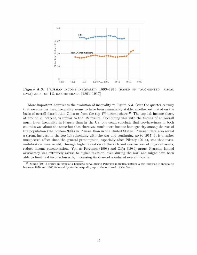
Figure A.3: Prussian income inequality 1893–1914 (based on “augmented” fiscaldata) and top 1% income share (1891–1917)

More important however is the evolution of inequality in Figure A.3. Over the quarter centurythat we consider here, inequality seems to have been remarkably stable, whether estimated on thebasis of overall distribution Ginis or from the top 1% income share.28 The top 1% income share,at around 20 percent, is similar to the US results. Combining this with the finding of an overallmuch lower inequality in Prussia than in the US, one could conclude that top-heaviness in bothcounties was about the same but that there was much more income homogeneity among the rest ofthe population (the bottom 99%) in Prussia than in the United States. Prussian data also reveala strong increase in the top 1% coinciding with the war and continuing up to 1917. It is a ratherunexpected effect since the general presumption, especially after Piketty (2014), was that mass-mobilization wars would, through higher taxation of the rich and destruction of physical assets,reduce income concentration. Yet, as Ferguson (1998) and Offer (1989) argue, Prussian landedaristocracy was extremely averse to higher taxation, even during the war, and might have beenable to limit real income losses by increasing its share of a reduced overall income.

28Dumke (1991) argues in favor of a Kuznets curve during Prussian industrialization: a fast increase in inequalitybetween 1870 and 1900 followed by stable inequality up to the outbreak of the War.

45

B Composition of Foreign Assets by Parisian Decedents and London StockExchange Securities

Table B.1: Financial asset portfolio composition: Parisiandecedents, 1872–1912 (%)

Financial Assets Non-Domestic Foreign Other Financial

EquitiesPriv. Gov.

Total EquitiesPriv. Gov.

TotalFinancial Assets

bonds bonds bonds bonds Assets(1) (2) (3) (4)

1872 16 19 11 46 1 2 4 7 10 371882 16 19 13 48 2 2 3 7 8 371912 13 14 5 32 7 5 9 21 8 39

Source: Piketty et al. (2014), Table B11

Note: Assets in columns (1)–(4) sum to 100 percent.

Table B.2: Total nominal values of securities quoted in Lon-don Stock Exchange official list (%)

British Colonial ForeignBonds Rail Other Equities Total Bonds Rail Total Bonds Rail Total

1873 38 17 9 63 2 5 7 18 11 291883 25 18 7 51 4 4 7 23 19 421893 18 17 11 47 5 5 10 15 27 421903 16 16 20 51 5 4 9 15 24 391913 14 13 22 48 4 5 9 15 26 41

Source: Michie (2001), Table 3.3

46

C “Empire Effect” vs. “Gold-Standard” Effects

Source: Global Financial Data

Figure C.1: Real return rate spread between foreign and British bonds

D Differences in Foreign (Colonial) and British Risk-Adjusted Rates of Re-turn

Figure D.1: Government bondsFigure D.2: Social overhead capitalbonds

47

Figure D.3: Social overhead capital equities Figure D.4: Financial equities

E Historical examples of sanctions or military force

Promotion of British free trade was historically independent of foreign policy decisions, shunningeconomic intervention in pursuit of laissez faire ideals. Earlier in the nineteenth century, civilservants even viewed commerce with contempt. France, historically, took a different tack. “Therefusal of a quotation on the Bourse was a weapon that the Government used with some frequency,and to this extent it was able to influence the nature and direction of French overseas investments,often along purely political lines,” D.C.M. Platt writes.29 By the twentieth century, however, moreaggressive displays of political power in support of economic agendas began to unfold. Here weexamine evidence in support of our thesis that increasing militarization by imperial powers wasa means of reducing foreign risk premier by eventually coercing debtor states through physicalenforcement of international financial contracts.

Before states imposed trade sanctions on defaulting governments, shareholder organizations likethe Corporation of Foreign Bondholders (formed in 1873) coordinated with each other to protect theinterests of foreign and colonial asset holders. Market signals, such as interest rate hikes on states indefault, were another mechanism, albeit one that proved largely ineffective and short-lived.

Supersanctions, the threat or implementation of financial “house arrest” by foreign administra-tors or the actual deployment or threat of gunboats, proved the most effective methods of enforcingcontracts, Mitchener & Weidenmier (2010) argue. For example, in 1876 the British Foreign Officesent a delegation to Egypt, along with French counterparts, at the behest of Khedive Ismail toexamine its finances. Fiscal control was the advised outcome. Resistance by Ismail proved futile ashe was soon forced to abdicate in favor of his son, and by 1883 British negotiators agreed to, andoversaw, a debt settlement with creditors. A similar financial junta, the Council of Administra-tion, took control of Turkey’s debt settlement in 1881 after economic and political problems beganthree years prior. It issued the Decree of Mouharrem, a fiscal package of tax increases and debtrepayments to bondholders, and remained in the country for the remainder of the gold standardera.

The decisive gunboat diplomacy episode played out between December 1902 and February 1903.Pitting Venezuela against the imperial triumvirate of Britain, Italy, and Germany, it established a

29Platt (1968), p. 6.

48

violent precedent for future threats—and tested the parameters of Roosevelt’s passive interpreta-tion of the Monroe Doctrine, the aged American policy of opposing European imperialism in theAmericas. As retold in Mitchell (1996), an assortment of “businessmen, imperialists, exporters,and right wingers called for intervention to collect outstanding claims.” In partnership with eightBritish ships, who coordinated the blockade, Germany began seizing Venezuelan navy boats onDecember 9, ultimately sinking two unseaworthy ships and shelling the town of Puerto Cabello.Eventually, with the US arbitrating, an agreement was signed on February 13. Each of the threeblockading powers received $27,500 and the Germans were to receive an additional $340,000 withinthree months.

In all, Mitchener & Weidenmier (2010) identify 12 episodes between 1870 and 1913 in whichso-called supersanctions were deployed by creditor nations. What was their combined effect? Theauthors claim ex-ante default probabilities on a security’s principal decreased by an average of 60percent after a country experienced supersanctions. Furthermore, their risk premium decreased byaround 200 basis points as a result of improved “fiscal discipline.” Not only is there an empiricallyconsistent relationship between the net foreign asset positions of imperial nations and levels ofmilitarization prior to the First World War, but there also exist historical examples of countriesusing force, or threatening to, in order to coerce debtor countries into making bond payments.

F Regression Results

F.1 Boer War Regressions

We explore this in a regression in Table F.1, with wild-bootstrapped standard errors. We estimatea regression of the form

spreadct = PostWart ×BoerControlc + δc + δt + εct, (2)

where c represents the South African colony and t the year.

Table F.1: Spreads Over UK Consols

(1) (2) (3) (4)

Post War × Boer Control -192.7∗∗∗ -201.1∗∗∗ -199.8∗∗∗ -254.3∗∗∗

(15.61) (13.66) (13.00) (15.38)Boer Control 138.3∗∗∗ 149.1∗∗∗

(9.457) (8.457)Post War -28.70∗∗

(10.01)Province FE No No Yes YesYear FE No Yes Yes YesControls No No No Yes

N 96 96 96 84

Standard errors, wild-bootstrapped by 4 province clusters, in parentheses.∗ p < 0.05, ∗∗ p < 0.01, ∗∗∗ p < 0.001

Notes:There are 4 provinces: Cape Colony, Natal, Oranje, and Transvaal. Controlsare log of exports per capita, trade balance, and public deficit (as share of GDP).

49

F.2 Inequality and Net Foreign Assets Regressions

We estimate specifications of the form:

NFAitGDPit

= β1Inequalityit + β2Democracyit + β3log(yit) + δi + εit (3)

The regressions are run in three formulations: pooled cross section and time regressions, country-fixed effects, and pooled regression over five-year averages. This is done because our data are verysparse and in some formulations we have only one subset of countries and years while in otherformulations we have another subset. The results are shown in Table F.2. Consider first the pooledregressions (columns 1 and 2 in Table F.2). Both income Gini and the share of wealth held by thetop 10% (Top10 wealth) are positively correlated with NFA/GDP and are statistically significantat less than 0.1% level. For example, increase in the concentration of wealth among the top 10% byone percentage point is associated by more than 12 percentage point increase in the ratio betweenNFA and country’s GDP (column 2). This result is driven however by the cross-country differencesbetween the three countries that are included in the regression.

Table F.2: Net foreign assets and inequality

(dependent variable: ratio between net foreign assets and GDP)

Pooled regressions Country fixed effects Pooled five-year averages(1) (2) (3) (4) (5) (6)

Gini 8.33∗∗∗ 5.87∗∗ 10.34∗∗∗

(0.00) (0.02) (0.00)Top 10% wealth 12.19∗∗∗ 0.77 15.12∗∗∗

(0.00) (0.07) (0.005)Democracy -21.84∗∗∗ 12.71 0.35 2.19 -25.51∗∗∗ 25.75

(0.00) (0.19) (0.84) (0.81) (0.005) (0.28)GDP per capita (log) 141.2∗∗∗ -112.3∗ 11.79 93.9 123.8∗ -153.5∗

(0.002) (0.06) (0.52) (0.33) (0.08) (0.06)Constant -1336∗∗∗ -122.4 -256.3 -728.9 -1267∗∗ -142.3

(0.001) (0.77) (0.11) (0.60) (0.03) (0.62)

R2 (within) 0.61 0.87 0.29 0.12 0.66 0.98F 12.0 38.8 2.8 0.7 5.9 71.4Countries Germany France Germany France Germany France

Britain Britain Britain Britain Britain BritainUSA USA USA USA USA USA

Obs 27 21 27 21 13 9∗ p < 0.1, ∗∗ p < 0.05, ∗∗∗ p < 0.01

Results for the five-year-average pooled regressions are shown in columns 5 and 6 (Table F.2).Although we now have a denser data set (since it suffices that a variable be available for one yearin a five-year period) the number of possible data points is obviously very much reduced, and thusthe overall number of observations becomes even smaller. Results for the five-year-average pooledregressions are very similar to what we obtained with the yearly data: both inequality statisticsare highly significant and the values of the coefficients are very close to the earlier results.

50

When we use country fixed effects (regressions 3 and 4 in Table F.2) income Gini remains positiveand statistically significant but its value becomes smaller: a Gini point increase is associated, onthe average, with 5.87 percentage point increase in the NFS/GDP ratio. This is not surprisingbecause the main variability in pooled regressions came from inter-country differences. Once theyare reflected in country intercepts, the effect of inequality within country on its accumulation offoreign assets, while still strongly positive, is less. For the Top10 wealth variable, the effect is alsopositive, again much smaller than in pooled regressions, and statistically significant only at the 7%level.

G A Simple Model of Imperialism

Imperialist countries invested in a variety of geopolitical strategies to defend the rents from foreignassets, in particular securing future trade balances. Here we show a simple partial equilibriummodel that generates the total surplus at stake from empire in terms of a simple supply anddemand diagram that includes the colonial and domestic rates of return, as well as the domesticwealth distribution and economic structure. This model deliberately simplifies, but builds on ideasfrom recent models in macroeconomics with incomplete markets and idiosyncratic rates of returnto capital, as in Benhabib et al. (2015).

G.1 Basic model

There exists one metropole, with unit measure of metropolitan citizens, with a foreign asset (subjectto aggregate risk only) yielding a risk-adjusted rate of return r∗ = R−ρ, where R is the “observed”rate of return and ρ captures the risk of foreign investments, which can be affected by state action:property rights, risk, transactions and transportation costs. Importantly, suppose the demand forinvestment from abroad is perfectly elastic.

Suppose there is also some fraction δ < 1 of capitalists, who control a share α > 12 of the

average income y, so that inequality is parameterized by αδ . Also, suppose capitalists save s of

their income while non capitalists save nothing, so that the economy-wide savings rate is s ≡ sα.However, citizens get idiosyncratic domestic rates of return which are distributed according toF (r), which for simplicity we suppose is uniform, supported on [rchoke, rchoke + Φ]. The supplycurve of foreign investment is Kf (r∗) = syF (r∗). The choke price rchoke is the lowest domesticreturn anyone can get, and positive, while Φ measures the dispersion in domestic interest rates (areduced form measure of financial frictions). The cdf of domestic rates of return is thus given byF (r) = r−rchoke

Φ .30

Figure G.1 shows the simplest version of this diagram. We define the surplus yielded by empireas

S(r∗) =

∫ r∗

−∞Kf (r)dr =

αsδ

2Φ(R− ρ− rchoke)

2 (4)

30In a standard lifecycle saving model with borrowing constraints, having stochastic idiosyncratic rates of returnyield endogenous fat-tailed wealth distribution, as shown in Benhabib et al. (2015), but the important thing for ourpurposes is domestic investment opportunities yield lower returns than foreign returns.

51

S(r∗)

I∗

r∗ = R− ρ

Kf (r)

rchoke

Figure G.1: Imperialism incidence curve

Many theories of imperialism can be built into determinants of the supply curve of foreigninvestment thus formulated, which predicts the level of rents generated from empire. Countrieswill be willing to expend up to the total surplus return when weapons both raise the return onforeign investment as well as secure the market. We show that this model nests the major economictheories of imperialism by channeling them into changes in the relative return from domestic vsforeign assets for investors. Importantly, the value of empire is not simply the level of foreigninvestment. It depends on the level of foreign investment and the gap between the counterfactualrate of return at home. This is captured by the shaded region in Figure G.1, the total surplus fromempire (denoted S), which is given by the area between the demand and supply curves for foreigncapital. If rchoke is very close to r∗ and Φ is small, then the value of empire could be low despiterelatively high foreign investment, and if rchoke is very low and Φ very high, then the value ofempire could be high despite low investment. The latter case is more likely, too, in the presence ofhigh inequality (so that e.g. the very rich face very low rates of return domestically) and financialfrictions that ensure a considerable dispersion of domestic rates of return via Φ.

We incorporate military mobilization in the simplest way. If the metropole can spend W onarmaments and military mobilization to decrease the risk premium ρ, so that ρ = ρ′(W ) < 0 andp′′ > 0. Then the metropole chooses W to maximize syF (r − ρ(W )) −W ,

−ρ′(W ∗)(R− ρ(W ∗) − rchoke)sy

Φ= 1 (5)

G.2 Comparative statics

The surplus from empire, and thus military mobilization, increases to the degree the supply offoreign investment shifts right or becomes less elastic, as well as to the degree the return on foreign

52

investment increases.

Hypothesis 1: Hobson The savings rate s increases, due to an increase in inequality α,without an increase in rchoke or Φ, so that the supply of investment abroad increases the supply offoreign capital and thus the overall surplus S from empire.

Hypothesis 2: Hilferding/Lenin/Luxemburg The domestic rate of return, e.g. rchoke, falls(due to either low domestic demand or cartelization of business) so that the supply of investmentabroad increases, along with S.

Hypothesis 3: Economic Determinants of Military Spending Military mobilization isincreasing in the value of the surplus from foreign capital, follows from ρ′(W ) < 0.

53