Embed Size (px)
Citation preview
113© The Author(s) 2017 L. Bértola, J. Williamson (eds.), Has Latin American Inequality Changed Direction?, DOI 10.1007/978-3-319-44621-9_6
Inequality, Institutions, and Long-Term Development: A Perspective from Brazilian Regions
Pedro Paulo Pereira Funari
1 Introduction
Inequality is a subject of intrinsic interest, in the sense that it is related to moral concepts such as justice and fairness.1 Notwithstanding, it is also important for its effects, for example, on the growth and educational attainments of a society. Ironically, it is one of the most hotly debated subjects within growth and develop-ment economics literature and one which is far from reaching a consensus.
A first wave of development literature (as characterized by Easterly 2007, p. 756) presents the idea that high inequality could promote growth by concentrating income in the hands of high-saving capitalists (Kuznets 1955; Kaldor 1956). As presented in Aghion et al. (1999b), the view that wealth inequality could be growth enhancing is based on three arguments: (1) the marginal propensity to save of the rich is higher than that of the poor; (2) investment indivisibilities; and (3) the trade- off between productive efficiency and equality. However, later works indicate a possible negative effect of economic inequality on growth, both theoretically and empirically.2 Several mechanisms were suggested as causes of this, such as political economy mecha-nisms (Alesina and Rodrik 1994; Persson and Tabellini 1994), imperfect capital markets (Banerjee and Newman 1991; Galor and Zeira 1993; Perotti 1992) and investment in human capital (Bourguignon and Verdier 2000; Galor et al. 2009; Galor and Zeira 1993; Perotti 1996), the composition of the aggregate demand (Murphy et al. 1989), and macroeconomic instability (Aghion et al. 1999a).3
P.P.P. Funari (*) University of California, Davis
1 These concepts and interrelations are investigated since the birth of philosophy in Ancient Greece. See the works of Plato (e.g., The Republic) and his disciple Aristotle (e.g., Politics).2 For comprehensive reviews, see Aghion (1999b) and Bénabou (1996).3 For the effects of redistribution on growth, see Easterly and Rebelo (1993), Perotti (1996), and Aghion (1999b).
114
Three important studies followed, casting doubt on the robustness of what were then considered consistent results, and finding no negative relationship between economic inequality and growth. Using new data and panel techniques, Forbes (2000) finds a positive relationship between economic inequality and growth. Barro (2000) and Banerjee and Duflo (2003) also present evidence against such a clear-cut negative relationship. However, Easterly (2007), using an insightful instrument, finds again a negative relationship between inequality and economic performance.
There are also important studies correlating political inequality and develop-ment. Acemoglu (2008) shows how political inequality may retard development due to the unwillingness of incumbent elites to allow the entry of new agents. Elites might also block the introduction of new technologies (Acemoglu and Robinson 2000). Bates (1981) shows how, in a politically concentrated environment, there might be little interest in the provision of public goods, including schooling. As noted by Acemoglu et al. (2008), political inequality will also tend to be associated with the absence of political competition and accountability, two factors that help to guarantee that political systems generate desirable outcomes.
Even more important for the present work are Engerman and Sokoloff’s compre-hensive series of studies on development of the Americas. Engerman and Sokoloff (1997, 2002) argued that factor endowments had a major influence on the coloniza-tion strategies throughout the American continent that, in turn, established different initial levels of inequality that account for the divergent institutional paths of American societies that resulted in the differential development standards of these regions today. Therefore, in Engerman and Sokoloff’s view, inequality had prejudi-cial effects on development in a cross-country framework.4
It is to this context of apparently contradictory evidence that Acemoglu et al.’s (2008) study belongs. Their study distinguishes empirically between economic and political inequality in their exploration of the effects of inequality. As the authors correctly note, economic inequality is probably endogenous in regressions without a political inequality variable, since we expect them to be linked, and this might bias the econometric evidence on the effects of economic inequality. The authors not only construct different variables for economic inequality (the land Gini) and politi-cal inequality (a political concentration index) but also deal with a constant de jure institutional environment, the region of Cundinamarca in Colombia, which, accord-ing to Pande and Udry (2005), might provide deeper insights into the specific chan-nels through which inequality affects development.
4 Two brief comments on Engerman and Sokoloff’s thesis: (i) Theories presented by North et al. (2000), which emphasize the importance of metropolitan objectives in contrast to local conditions, and Frankema (2010), which supports the role of precolonial institutions, are likely complemen-tary to the one by Engerman and Sokoloff (for a review of these theories, see Frankema 2009, Chap. 3); and (ii) we believe that the validity of Engerman and Sokoloff’s theory is in a cross-country framework, and, therefore, studies such as those by Nunn (2008), Acemoglu et al. (2008), and Dell (2010) do not necessarily oppose their views. Moreover, as shown by Nugent and Robinson (2010), there can be heterogeneities with Latin America.
P.P.P. Funari
115
The authors present intriguing evidence. Overall, they find a negative relationship between economic and political inequality for nineteenth-century Colombia and a positive association between economic inequality in the nineteenth century and development outcomes in the late twentieth century. These results are unexpected, as it is generally expected for Latin American countries to have high inequality, both economic and political, and that they are positively correlated (mutually reinforc-ing each other). The interpretation of the authors, based on Bates’ (1981) insights on Africa, is that in “weakly institutionalized” societies, where few constraints were imposed on the actions politicians could take, large landowners had the power to keep in check the rapacious tendencies of these politicians.5
We provide a similar investigation for the complex case of Brazil. With unique data from the beginning of the twentieth century—the Brazilian Economic and Demographic Census of 1920—we were able to construct from scratch unique indi-cators of economic inequality (the land Gini coefficient among landowners) and of political inequality (the proportion of individuals that were eligible to vote) at the municipal level in selected Brazilian states. However, we not only analyze how inequality (both economic and political) is related to long-term development, but we also go further into analyzing how inequality is related to long-term development within different de facto institutional environments while controlling for a constant de jure context (in line with Pande and Udry’s reorientation argument).
Therefore, we are able to integrate both the inequality literature and the recent insti-tutional literature (see, e.g., Acemoglu et al. 2001, 2002; Pande and Udry 2005; Banerjee and Iyer 2005).6 We calculate the respective inequality indicators for all the municipalities in four Brazilian states: Minas Gerais, São Paulo, Pernambuco, and Rio Grande do Sul. The states were carefully selected in order to capture how inequality is related to long-term development in different de facto institutional environments greatly influenced by the unique colonial experiences of these regions. Our analysis presents evidence of a heterogeneous relationship between inequality and long-term development indicators, broadly consistent with the colonial experiences of the states considered, likely a reflection of different de facto institutional environments.
Furthermore, our study intersects with an important recent literature on the Brazilian case. Naritomi et al. (2012) present evidence that colonial experiences indeed shaped different de facto institutional environments within the country. Summerhill (2010), exploring the state of São Paulo, does not find a negative effect of land inequality on long-term development.7 Moreover, and in line with our results, the author does not find a significant relationship between political inequality measured by the extent of the franchise and long-term economic growth. In a state-level analysis, Wegenast (2010) argues that Brazil’s different agrarian structures determined, in the long run, the educational outputs. His analysis suggests that in
5 The concept of “weakly institutionalized societies” is developed in Acemoglu et al. (2004).6 For a more systematic approach and review of the institutional literature, see Acemoglu et al. (2005).7 De Carvalho Filho and Colistete (2010), examining the same state of São Paulo at the beginning of the twentieth century, find a negative correlation between land concentration and supply of public education at that time.
Inequality, Institutions, and Long-Term Development…

116
states with higher land concentration, there were fewer incentives to invest in education. Moreover, for the Latin American context, Dell (2010), investigating the negative effects of the mita, suggests that land concentration would have been a beneficial factor, for it is hypothesized that the long-term presence of large-scale landowners in non-mita districts provided a stable land tenure system that encour-aged public goods provision.
The chapter is organized as follows. In the next section, we explore the Brazilian development process from a historical perspective. We then proceed to the data analysis. Next, we present the econometric results. The last section concludes.
2 The Brazilian Context
2.1 Some History
Brazil was first claimed by modern Europeans in 1500. The interest of Crown and settlers would soon turn to the production of sugar, which became the colony’s first major export. International prices were high and the supply, especially from Sicily, Atlantic islands such as Cape Verde and Madeira, and the East, was low and restricted. At the time, the main production centers were in Pernambuco and in Bahia. Brazil was the biggest sugar producer in the world until mid-seventeenth century—the heyday of the sugar enterprise in Brazil—when competition from Central American colonies and the Antilles became stronger (Prado Jr. 1956 [1945]).8
As expected, geographical characteristics were determinant for the success of this enterprise. Moreover, although there was no general overall plan for the sugar enterprise, potential problems were largely avoided thanks to favorable circum-stances. Production techniques, the creation and expansion of a consumer market, and financing were largely dealt with by the Dutch, who practically controlled the so-called Portuguese enterprise. Due to economies of scale, production was based on large land properties with a single owner, called latifúndios, characterized mainly by monoculture and slave labor. Prado Jr. (1956 [1945]) notes the absence of complex methods of production in colonial Brazil, both in terms of space and time, or even significant improvement in methods. Production expansion was based on the extension of land under cultivation and on slave population growth rather than on changes in the production process and increased productivity.9
8 The competition from the Antilles was a direct consequence of the Dutch experience with the sugar industry in Brazilian lands before their expulsion in 1654. After learning the technical and organizational aspects, they were able to implement a similar structure in the Caribbean territories and generate higher profits (Furtado 2006 [1959]).9 According to Prado Jr., Brazil’s development problems are a direct consequence of the dependence of the colony on exports of primary products produced in large properties with slave labor. However, Villela (2013) argues that none of these elements can explain for themselves Brazil’s lack of growth at the time, the lack of efficiency gains being the fundamental problem.
P.P.P. Funari
117
Furtado (2006 [1959]) argues that the high profitability of an economy with a high import coefficient tends to hinder investments in secondary activities, such as food production. The intense specialization of the sugar economy would be then associated with its high profitability (Furtado 2006 [1959], p. 93). As a result, cattle raising shifted to the countryside of the Northeastern region. This activity was radically different from the sugar industry, occupying extensive areas of land, and the impact of the dry seasons was reflected in the absence of permanent occupation. Not only was there no need for large initial capital investments, but also the large amount of land available hindered productivity increases.
In the early seventeenth century, sugar exports began to decline, mainly due to increasing competition from British, Dutch, and French colonies. Prices continued to fall throughout the eighteenth century. With the decline of the sugar industry, income fell also in the cattle farming sector, which then became mostly a subsis-tence activity, allowing a continued growth of the population since the activity could be easily expanded due to the availability of land. The growth of the share of the cattle farming sector in relation to the sugar industry brought with it a decline in the region’s average per capita productivity and income.
The problem was that the accelerated growth of the sugar enterprise had no struc-tural counterpart. The economic system, under which almost all the net income gen-erated stayed with the large landowners, often resorted to importing luxury goods, slaves, or machines for that same sugar industry, and underwent no significant change during this period. Therefore, the whole enterprise depended heavily on the external market. With the continued fall in prices and the increased opportunity costs due to the emergence of the mining regions, the sugar economy entered a “secular lethargy” (Furtado 2006 [1959], p. 91) that endured until the nineteenth century.
At the same time, economic enterprises in the Northeast did not completely stagnate with the decline of sugar production. The second half of the eighteenth century saw a rise in international demand for other agricultural products, particularly cotton, due mainly to the Industrial Revolution. The rural parts of the state of Pernambuco, being drier and, therefore, more suitable for the production of cotton rather than cattle raising, would also benefit.
During most of the sixteenth and seventeenth centuries, the southern part of the colony was relatively free of direct intervention from the Crown. With the main economic interest focused on sugar production, settlers in those other regions lived at the margin of the colonial enterprise. Soon after the fall of sugar prices after 1650, this geopolitical structure changed. In the last years of the seventeenth century, gold and other precious metals were discovered in the countryside of the Portuguese territory, especially in Minas Gerais. By the mid-eighteenth century, gold mining had reached its greatest land extent and highest levels of production. For almost a century (1675–1765) gold mining would be the focus of the attentions of the Crown (Prado Jr. 1956 [1945]). Migrants arrived from different parts of the country and new towns sprang up in the mining districts. Along with the shift of the colony’s economic center from the Northeast to the Southeast, there was also shift in the political center. As a consequence, Rio de Janeiro replaced Salvador (Bahia) as the capital of the colony in 1763.
Inequality, Institutions, and Long-Term Development…
118
Although mining also made use of slave labor, the social structure was less rigid than in the sugar-producing areas. Slaves were never the majority among the popu-lation. Gold mining led to greater social inclusion, for it was not necessary to have important amounts of initial capital. Possibilities were greater even for slaves, who could often work for themselves and buy their freedom. Therefore, although the average income in the gold economy was inferior to the average income at the apogee of the sugar economy (Furtado 2006 [1959]), income was more broadly distributed and the percentage of free people was higher. This influx of wealth led the Portuguese Crown to rapidly establish a bureaucratic apparatus to avoid tax eva-sion.10 The heyday of the Brazilian gold rush was in the 1750s, when exports reached 2.5 million British pounds (Furtado 2006 [1959]).11
However, the decline of the Brazilian gold rush came soon, due to its geographi-cal characteristics (alluvial), inferior extraction techniques, and a bureaucracy inca-pable of providing sustainable incentives to the enterprise. Denis (1911, p. 61) notes: “As the surface of the alluvial workings became exhausted by wasteful meth-ods, a great part of the population was gradually absorbed by agriculture and stock- raising. (…) During the nineteenth century the mining activities of Minas were not very notable: although it was discovered that the alluvial deposits had been merely scratched on the surface.” With the decline of the gold cycle and the persistent low international prices for sugar, the last years of the eighteenth century were charac-terized by economic difficulties in the colony. All in all, “the latifundium, slavery, and the export trade remained, as the historian Caio Prado Jr. has said, for more than 300 years the principal institutions of Brazilian society” (Dean 1971, p. 607).
Early in the nineteenth century, a major political event changed the development path followed by the colony. In 1808, by order of Prince Regent Dom João, fleeing from Napoleon’s troops, the Portuguese royal family is transferred to Brazilian lands.12 In 1822, in a country with approximately 3.9 million inhabitants (of which 1.2 million approximately were slaves), Dom Pedro—son of Dom João (who was then in Portugal), the colony’s regent at the time—declared independence and was proclaimed Constitutional Emperor, remaining in power until 1831. After a regency period (1831–1840) characterized by great social instability, his son, Dom Pedro II,
10 Examples of important administrative controls by the Portuguese Crown are the payment of one-fifth of the production (and their careful supervision through all stages of the mining activity), prohibition on individual negotiations, establishment of special trading monopolies, and tight control on local manufacturing.11 In 1780 the value of gold exports was less than one million British pounds (Furtado 2006 [1959]).12 According to Prado Jr. (1956 [1945]) this was effectively the end of the colonial period for Brazil. New economic measures were soon adopted. The first and probably the most important measure was a manifesto declaring that all Brazilian ports should be considered open to trade with the entire world, and that goods might be exported under any flag. At the same time, royal monopolies were abolished and import duties reduced, laws prohibiting the establishment of industries were repealed, a national press was established (Denis 1911), and new educational and financial institu-tions (such as the first Banco do Brasil, in 1808) were established as well.
P.P.P. Funari
119
became the new emperor in 1840. Finally, in 1889 the Republic was proclaimed and 1891 saw the implementation of a new constitution.
Notwithstanding the government’s intention of dealing with land concentration under the Empire, efforts would eventually fail, largely because the political system was dominated by a landed elite (Dean 1971). Furthermore, the positive effects on prices of the events at the end of the eighteen century and beginning of the nineteenth century were due to a confluence of particular circumstances.13 Once international markets returned to normal conditions, a new phase of difficulties began for the colony: conflicts with England, on which newly independent Brazil had become dependent, mainly due to the unilateral application of the liberal economy by the former (Furtado 2006 [1959]) and worries with the end of the slave trade, the scarcity of the government’s financial resources, and the increasing dissatisfaction in practi-cally every region led to a series of social rebellions. In the midst of these difficul-ties, a new source of wealth would emerge: coffee, which led to a new period of economic affluence in the country.14
Like Minas Gerais, the region that corresponds to what is today the state of São Paulo was only of marginal economic importance during the first centuries of colonization. Although São Paulo was not completely outside the great sugar enter-prise, it was coffee that made the region especially important. Coffee was introduced into the country in 1727 and large-scale production started at the end of the eighteenth century.15 However, it was at the beginning of the nineteenth century that Brazilian production became significant in international terms.16
It is around this time that the labor question became delicate. With the abolition of slavery it became clear that the country’s best option was to import foreign work-ers. After initial problematic experiences and with government’s generous interven-tion, it was possible, for the first time in the country’s history, to attract a massive influx of European migrants.17 The average numbers of non-slave immigration grew steadily from the 1860s to the end of the century.18
13 Important international events were beneficial for a colony whose main activity was the export of primary products: the Industrial Revolution, the American War (1775–1783), the French Revolution (1789–1799), the Napoleonic Wars (1803–1815), and the upheaval in many of the Spanish colo-nies had a significant impact on the supply and, therefore, prices of primary goods in which Brazil had an idle production capacity, such as sugar, cotton, and leather.14 According to Goldsmith (1986), we have the following figures for the average growth in GDP per capita: 1850–1860: 1.4 %; 1860–1870: 1.0 %; 1870–1880:−0.2 %; 1880–1890: 0.4 %; 1890–1900: −1.7 %. For a different view, see Leff (1997).15 The USA was the main market for the Brazilian product (Prado Jr. 1956 [1945]).16 Figures provided by Furtado (2006 [1959]) show that the production was of 3.7 and 5.5 million sacks in the periods 1880–1881 and 1890–1891, respectively, rising to 16.3 million between 1901 and 1902 (one sack was equivalent to 60 kg).17 For example, after several charges of abuse, Germany prohibited emigration to Brazil in 1859.18 The figures for the annual average numbers of immigrants, by decade, are 1860–1869: 9850; 1870–1879: 20,780; 1880–1889: 47,890; 1890–1899:118,170; and 1900–1909: 66,651 (Leff 1972).
Inequality, Institutions, and Long-Term Development…
120
As we have seen, the last years of the nineteenth century were extremely favorable for the production of coffee in the Brazilian lands, especially in Rio de Janeiro, São Paulo, and Minas Gerais regions. Not only were internal conditions conducive towards increasing production, but there was also the auspicious external circumstances of supply shortages.19 However, considering the inelasticity of international demand and the large availability of lands and relative production advantages, it was inevi-table that the coffee supply would continue to increase, with a consequent decline in prices. The response of the coffee planters and the government (tightly con-nected) to these adverse prospects was to implement valorization programs that consisted in buying and storing the excess coffee so as to control international prices.20 However, this mechanism for protecting the coffee economy was only “a process that transferred, to the future, the solution of a problem that would only become more and more serious” (Furtado 2006 [1959], p. 256). The policy was relatively successful until the 1920s, when the Great Depression brought Brazil into a new era of difficulties and political disruption.
Rio Grande do Sul would only become economically relevant in the second half of the eighteenth century. The region’s economy would be based on cattle farming. According to Prado Jr. (1956 [1945]), the cattle would reproduce rapidly due to the favorable natural environment, providing the region with the greatest concentration of cattle in the colony. Production of derivatives such as dairy products and leather was also of considerable importance. Agriculture would be developed only in a small sector near the coast (Prado Jr. 1956 [1945]). Initially, similar to the country side of the Northeast region, cattle farming developed as an extensive activity. Leather exports helped to maintain what was then a low-profitability activity afloat. It was only with the already mentioned discovery of gold that the activity faced a “true revolution,” being finally integrated with the rest of the colony (Furtado 2006 [1959], p. 121).
Following Prado Jr. (1956 [1945]) and Engerman and Sokoloff (1997, 2002), we can say that a different colonization method was structured. Variations in geographic characteristics such as climate and soil meant that the lands that today form the state of Rio Grande do Sul were not suited for the production of tropical products such as sugar. In order to protect the region from possible competitors such as Spain, the solution was to establish a settlement strategy similar to the one in the USA and Canada. Recruitment was made among poor and middle-class Portuguese families and peasants and considerable advantages were offered to those willing to emigrate (Prado Jr. 1956 [1945]).
Thus, the settlement of the South region of the country, especially Rio Grande do Sul, was unlike any others in Brazilian colonization. Land was more equally divided, slave labor was used in much smaller scale, and the population was rather homoge-neous (Prado Jr. 1956 [1945]).
19 Supply constraints in the main production centers, such as the Portuguese Ceylon—present-day Sri Lanka—encouraged the Brazilian production.20 Brazil had practically a monopoly on coffee production, being responsible, at its height, for producing more than three-quarters of the international supply (Furtado 2006 [1959]).
P.P.P. Funari

121
2.2 Political Aspects
In terms of political participation, Love (1970) states that the end of the Empire and the establishment of the Republic (1889) saw a democratization of the formal politi-cal process at three levels. The first is that the number of elective positions at all levels of government was increased (governors and the president and vice president of the Republic were now to be elected). Second, suffrage was expanded compared to the Empire. Under the first republican Constitution on 1891, all literate males 21 and older could vote. Finally, authority was decentralized.
There is some divergence between Love’s (1970) and Leal’s (2012 [1948]) views. Probably the reality was closer to Leal’s explicit exposition, which notes the great fragility and dependence of the municipal administration, despite some increase in revenues noted by Love (1970). As we will see in greater detail later, the introduc-tion of these liberal constitutional mechanisms of government, broader suffrage, and decentralization did not result in the type of de facto political structure that the members of the 1890–1891 constituent assembly had envisaged (Love 1970).
A central aspect of the Brazilian history for our study is the coronelismo, one of the most important characteristics of the First Republic (1889–1930). Leal (2012 [1948]) defines it as the result of a combination of the representative system of the time and an inadequate social and economic structure. In other words, coronelismo is a peculiar manifestation of the private sector, an adaptation through which resid-ual elements of old and excessive private power have managed to coexist in a politi-cal regime of (theoretically) broad representation. It is a commitment between the public sector, progressively strengthened, and the decadent influence of the local chiefs, mainly the landowners (Leal 2012 [1948]). “Without the requisite social and economic structures, universal suffrage could either produce long-term political sta-bility or strengthen traditional conservative elements against liberal reforms” (Love 1970, p. 4), and in the Brazilian case during the First Republic, “the official liberal ideology, on which the Constitution of 1891 was based, had outpaced the social and economic evolution of the country” (Love 1970, p. 10).
According to Leal (2012 [1948]), these manifestations of private sector power, especially in rural areas, are due to the agrarian structure of the country, characterized mainly by strongly concentrated land ownership.21 The vast distances and empty areas within the territory, as well as the scarcity of people, greatly influenced the situation (Carvalho 1946). Therefore, the public sector commitment is explained by the sufficiently broad franchise that makes the government dependent on the rural electorate. The essence of this commitment is that local chiefs provide unconditional
21 According to Love (1970), the nation remained 90 % rural in the early years of the Republic. Furthermore, Love (1970) argues that the critical role played by urbanization is based on three main points: (i) Brazilian rural society, owing to its historical roots, has a much stronger patriarchal tradition than its urban counterpart, and for this reason the rural vote was easier to control; (ii) the rural sector offered more opportunity for manipulation of the vote through fraud and violence, because the state and its mechanisms for guaranteeing free suffrage were less effective in the coun-tryside; and (iii) the access of the urban population to greater opportunities for education meant that a large percentage of urban dwellers would vote than their rural counterpart.
Inequality, Institutions, and Long-Term Development…
122
support to the “official” candidates in state and federal elections, and in return, the states give the local chiefs a free hand in almost all issues that concern the municipality, including the appointment of state positions at local level (Leal 2012 [1948]).
In an agrarian society with high land concentration, where the public sphere was largely absent in rural areas, the coronel was often responsible for improving local conditions, especially in terms of the provision of public goods and services: schools, roads, railroads, churches, and hospitals among others. It was, therefore, mostly with such improvements (some of which depend only on his political prestige while others might demand personal contributions or contributions from friends) that the munici-pal chief built and maintained his leadership position (Leal 2012 [1948]).
Leal’s (2012 [1948]) analysis stressed the importance of the reciprocity in the sys-tem. On the one side, the municipal chiefs and the coronéis who decided the choices of many voters and, on the other, the politically dominant situation in the state controlled the budget, the jobs, the favors, and the police force. The weakness of the municipali-ties was therefore a deciding factor in maintaining the coronelismo.
Just as coronelismo ruled relations between municipalities and states, the política dos governadores (“governors’ policy”) ruled relations between the states and the federal government.22 Leal (2012 [1948]) shows clearly the contradiction in the sys-tem: by arguing that there should be constraints placed on the powers of the munici-palities to avoid rule by local oligarchies, legislation gave the governors of the states every means for encouraging the very same local oligarchies, albeit to their benefit, creating state oligarchies and the consequent política dos governadores.23 Both the commitment between the governors and the coronéis and the one between the presi-dent and the governors were based on the inconsistency of the rural electorate, a direct consequence of the type of agrarian structure dominant in the country.
3 The Data24
3.1 The Census of 1920
The Census of 1920 is the fourth population census and the first agricultural and industrial census to have been conducted in Brazil. In accordance with the International Statistical Congress, which took place in Belgium in 1853, the purpose
22 It was a “system in which the president assured the governors of the states that their parties would always win elections in their respective jurisdictions in exchange for support of presidential policies in congress (which favored export agriculture) and electoral support of the president’s successor” (Love 1970, p. 9).23 The politics of the coronéis led to the strengthening of the state power in a much more effective way than the política dos governadores guaranteed the reinforcement of the federal power, especially in terms of the different possibilities of the use of violence (Leal 2012 [1948]).24 As we can see from Table 2, the number of municipalities has increased considerably between 1920 and 2000. In order to assess the effects of inequality on development in the long term, we had to match the municipalities in 2000 (2150 municipalities) to their counterpart in 1920 (512 municipalities). The construction of the comparable territorial units (CTU) was done manually using the reports of IBGE of each municipality’s origin. Table 2 presents the number of CTU for each state.
P.P.P. Funari
123
of an agricultural census is to “indicate the facts in which the complete knowledge of the conditions, process, and results of the agrarian statistics of each country at a specific time, depends” (IBGE 1923, p. v). Therefore, it is the first reliable survey of the agrarian conditions throughout the nation.
The Census contains detailed information on the quantity and average size of rural properties at the municipal level, which enables us to construct our measures of land inequality, which we use as proxy for economic inequality, for each of the four states of interest: Minas Gerais, São Paulo, Pernambuco, and Rio Grande do Sul.25
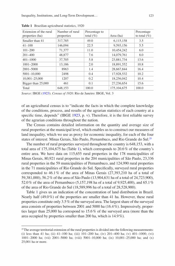
The number of rural properties surveyed throughout the country is 648,153, with a total area of 175,104,675 ha (Table 1), which corresponds to 20.6 % of the country’s entire area. We have data on 115,655 rural properties in the 178 municipalities of Minas Gerais, 80,921 rural properties in the 204 municipalities of São Paulo, 23,336 rural properties in the 59 municipalities of Pernambuco, and 124,990 rural properties in the 71 municipalities of Rio Grande do Sul. Specifically, surveyed rural properties corresponded to 46.1 % of the area of Minas Gerais (27,393,210 ha of a total of 59,381,000), 56.2 % of the area of São Paulo (13,904,631 ha of a total of 24,723,900), 52.0 % of the area of Pernambuco (5,157,198 ha of a total of 9,925,400), and 65.1 % of the area of Rio Grande do Sul (18,589,996 ha of a total of 28,528,900).
Table 1 gives us an indication of the concentration of land distribution in Brazil. Nearly half (49.0 %) of the properties are smaller than 41 ha. However, these rural properties constitute only 3.5 % of the surveyed area. The largest share of the surveyed area consists of properties between 2001 and 5000 ha (16.4 %). Impressively, proper-ties larger than 25,000 ha correspond to 15.6 % of the surveyed area (more than the area occupied by properties smaller than 200 ha, which is 14.9 %).
25 The average territorial extension of the rural properties is divided into the following measurements: (i) less than 41 ha; (ii) 41–100 ha; (iii) 101–200 ha; (iv) 201–400 ha; (v) 401–1000; (vi) 1001–2000 ha; (vii) 2001–5000 ha; (viii) 5001–10,000 ha; (ix) 10,001–25,000 ha; and (x) 25,001 ha or more.
Table 1 Brazilian agricultural statistics, 1920
Extension of the rural properties (ha)
Number of rural properties
Percentage to total (%) Area (ha)
Percentage to total (%)
Smaller than 41 317,785 49.0 6,115,158 3.5
41–100 146,094 22.5 9,593,156 5.5
101–200 71,377 11.0 10,454,242 6.0
201–400 48,877 7.6 14,079,761 8.0
401–1000 37,705 5.8 23,881,734 13.6
1001–2000 13,186 2.0 18,891,552 10.8
2001–5000 8963 1.4 28,667,844 16.4
5001–10,000 2498 0.4 17,928,532 10.2
10,001–25,000 1207 0.2 18,256,042 10.4
Bigger than 25,000 461 0.1 27,236,654 15.6
Total 648,153 100.0 175,104,675 100.0
Source: IBGE (1923). Census of 1920. Rio de Janeiro: IBGE, Vol. 3
Inequality, Institutions, and Long-Term Development…
124
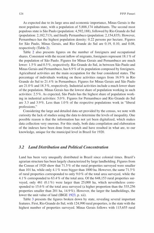
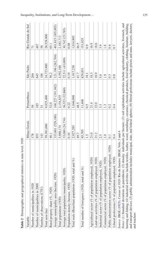
As expected due to its large area and economic importance, Minas Gerais is the most populous state, with a population of 5,888,174 inhabitants. The second most populous state is São Paulo (population: 4,592,188), followed by Rio Grande do Sul (population: 2,182,713), and finally Pernambuco (population: 2,154,835). However, Pernambuco has the highest population density: 0.22 persons per hectare. Figures for São Paulo, Minas Gerais, and Rio Grande do Sul are 0.19, 0.10, and 0.08, respectively (Table 2).
Table 2 also presents figures on the number of foreigners and occupational shares. Consistent with the recent inflow of migrants, foreigners represent 18.1 % of the population of São Paulo. Figures for Minas Gerais and Pernambuco are much lower: 1.5 % and 0.5 %, respectively. Rio Grande do Sul, in between São Paulo and Minas Gerais and Pernambuco, has 6.9 % of its population composed by foreigners. Agricultural activities are the main occupation for the four considered states. The percentage of individuals working on these activities ranges from 16.9 % in Rio Grande do Sul to 21.4 % in Pernambuco. Figures for Minas Gerais and São Paulo are 21.0 % and 18.3 %, respectively. Industrial activities include a much lower share of the population. Minas Gerais has the lowest share of population working in such activities: 2.5 %. As expected, São Paulo has the highest share of population work-ing in industrial activities: 5.0 %. Figures for Pernambuco and Rio Grande do Sul are 3.3 and 3.9 %. Less than 1.0 % of the respective populations work in “liberal professions.”
Considering the large and detailed data set provided by the census, we note with curiosity the lack of studies using the data to determine the levels of inequality. One possible reason is that the information has not yet been digitalized, which makes data collection very onerous. For this study, both data compilation and elaboration of the indexes have been done from scratch and have resulted in what are, to our knowledge, unique for the municipal level in Brazil for 1920.
3.2 Land Distribution and Political Concentration
Land has been very unequally distributed in Brazil since colonial times. Brazil’s agrarian structure has been largely characterized by large landholding. Figures from the Census of 1920 show that 71.5 % of the rural properties surveyed were smaller than 101 ha, while only 4.1 % were bigger than 1000 ha. However, the same 71.5 % of rural properties corresponded to only 9.0 % of the total area surveyed, while the 4.1 % corresponded to 63.4 % of the total area. Of the 648,153 rural properties sur-veyed, only 461 (0.1 %) were larger than 25,000 ha, which nevertheless corre-sponded to 15.6 % of the total area surveyed (a higher proportion than the 535,256 properties smaller than 201 ha, 14.9 %). However, the larger the landholdings, the lower the unit value of land (IBGE 1923, p. xii).
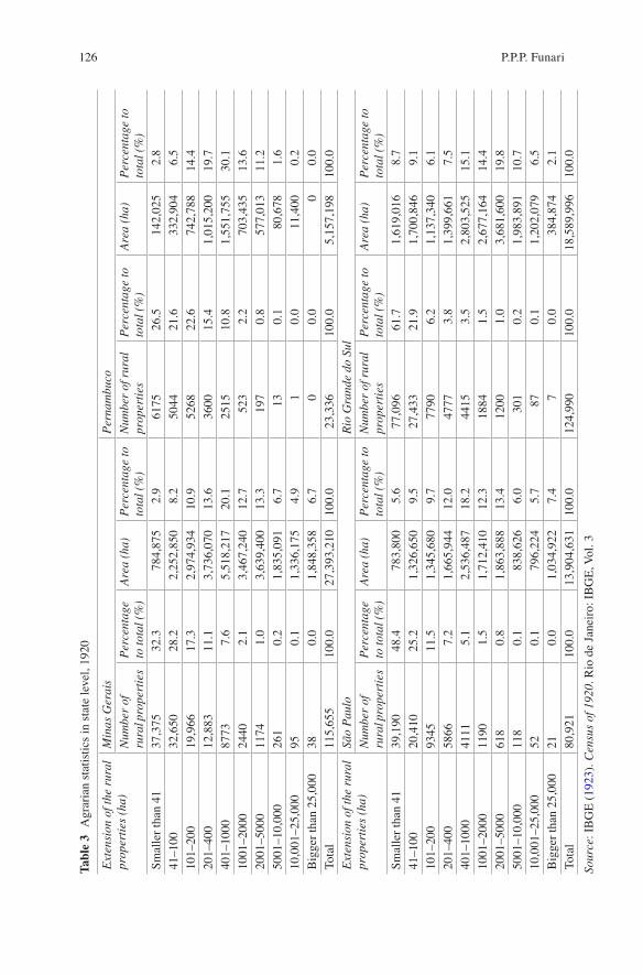
Table 3 presents the figures broken down by state, revealing several important features. First, Rio Grande do Sul, with 124,990 rural properties, is the state with the highest number of properties surveyed. Minas Gerais follows with 115,655 rural
P.P.P. Funari
125
Tabl
e 2
Dem
ogra
phic
and
geo
grap
hica
l st
atis
tics
in
stat
e le
vel,
192
0
Var
iabl
eM
inas
Ger
ais
Per
nam
buco
São
Pau
loR
io G
rand
e do
Sul
Num
ber
of m
unic
ipal
itie
s in
192
017
859
204
71
Num
ber
of m
unic
ipal
itie
s in
200
085
318
564
546
7
Num
ber
of o
bser
vati
ons
(CT
U)
143
5118
858
Tot
al a
rea
(ha)
59,3
81,0
009,
925,
400
24,7
23,9
0028
,528
,900
Rur
al p
rope
rty
shar
e (%
, 192
0)46
.152
.056
.265
.1
Ave
rage
mun
icip
alit
y ar
ea (
hect
are,
192
0)33
3,60
1 (5
29,1
80)
168,
227
(191
,942
)12
1,19
6 (2
62,7
04)
401,
815
(305
,885
)
Tot
al p
opul
atio
n (1
920)
5,88
8,17
42,
154,
835
4,59
2,18
82,
182,
713
Ave
rage
tot
al p
opul
atio
n (m
unic
ipal
ity,
192
0)33
,080
(24
,734
)36
,523
(32
,860
)22
,511
(43
,009
)30
,742
(23
,785
)
Pop
ulat
ion
dens
ity
(hec
tare
, 192
0)0.
100.
220.
190.
08
Tot
al m
ale
(Bra
zili
an)
popu
lati
on (
1920
, tot
al a
nd %
)2,
927,
285
1,04
6,09
81,
917,
238
1,01
4,90
5
49.7
48.5
41.7
46.5
Tot
al n
umbe
r of
for
eign
ers
(192
0, t
otal
and
%)
85,7
0511
,698
829,
851
151,
025
1.5
0.5
18.1
6.9
Agr
icul
tura
l se
ctor
(%
of
popu
lati
on e
mpl
oyed
, 192
0)21
.021
.418
.316
.9
Lan
d-us
e ac
tivi
ties
(%
of
popu
lati
on e
mpl
oyed
, 192
0)21
.222
.018
.918
.6
Indu
stri
al s
ecto
r (%
of
popu
lati
on e
mpl
oyed
, 192
0)2.
53.
35.
03.
9
Com
mer
cial
sec
tor
(% o
f po
pula
tion
em
ploy
ed, 1
920)
1.0
1.3
1.9
1.8
Pub
lic
adm
inis
trat
ion
sect
or (
% o
f po
pula
tion
em
ploy
ed, 1
920)
0.1
0.2
0.3
0.4
Lib
eral
pro
fess
ions
(%
of
popu
lati
on e
mpl
oyed
, 192
0)0.
40.
40.
80.
7
Sour
ce:
IBG
E (
1923
). C
ensu
s of
192
0. R
io d
e Ja
neir
o: I
BG
E, V
ols.
3 a
nd 4
Not
es:
(1)
Sta
ndar
d de
viat
ions
in
pare
nthe
sis;
(2)
den
sity
: in
divi
dual
s pe
r he
ctar
e; (
3) s
oil
expl
oita
tion
act
ivit
ies
incl
ude
agri
cult
ural
act
ivit
ies,
liv
esto
ck,
and
hunt
ing
and
fish
ing;
(4)
ind
ustr
ial
acti
viti
es i
nclu
de t
exti
les,
lea
ther
, w
ood,
met
allu
rgy,
cer
amic
s, c
hem
ical
pro
duct
s, f
ood
indu
stry
, cl
othi
ng,
furn
itur
e, b
uild
ing,
an
d tr
ansp
ort
devi
ces;
(5)
pub
lic
adm
inis
trat
ion
incl
udes
mun
icip
al, s
tate
, and
fed
eral
sph
eres
; (6
) li
bera
l pr
ofes
sion
s in
clud
e pr
iest
s an
d nu
ns, l
awye
rs, d
octo
rs,
and
teac
hers
Inequality, Institutions, and Long-Term Development…
126
Tabl
e 3
Agr
aria
n st
atis
tics
in
stat
e le
vel,
192
0
Ext
ensi
on o
f the
rur
al
prop
erti
es (
ha)
Min
as G
erai
sP
erna
mbu
co
Num
ber
of
rura
l pro
pert
ies
Per
cent
age
to to
tal (
%)
Are
a (h
a)P
erce
ntag
e to
to
tal (
%)
Num
ber
of r
ural
pr
oper
ties
Per
cent
age
to
tota
l (%
)A
rea
(ha)
Per
cent
age
to
tota
l (%
)
Sm
alle
r th
an 4
137
,375
32.3
784,
875
2.9
6175
26.5
142,
025
2.8
41–1
0032
,650
28.2
2,25
2,85
08.
250
4421
.633
2,90
46.
5
101–
200
19,9
6617
.32,
974,
934
10.9
5268
22.6
742,
788
14.4
201–
400
12,8
8311
.13,
736,
070
13.6
3600
15.4
1,01
5,20
019
.7
401–
1000
8773
7.6
5,51
8,21
720
.125
1510
.81,
551,
755
30.1
1001
–200
024
402.
13,
467,
240
12.7
523
2.2
703,
435
13.6
2001
–500
011
741.
03,
639,
400
13.3
197
0.8
577,
013
11.2
5001
–10,
000
261
0.2
1,83
5,09
16.
713
0.1
80,
678
1.6
10,0
01–2
5,00
095
0.1
1,33
6,17
54.
91
0.0
11,
400
0.2
Big
ger
than
25,
000
380.
01,
848,
358
6.7
00.
00
0.0
Tot
al11
5,65
510
0.0
27,3
93,2
1010
0.0
23,3
3610
0.0
5,15
7,19
810
0.0
Ext
ensi
on o
f the
rur
al
prop
erti
es (
ha)
São
Pau
loR
io G
rand
e do
Sul
Num
ber
of
rura
l pro
pert
ies
Per
cent
age
to to
tal (
%)
Are
a (h
a)P
erce
ntag
e to
to
tal (
%)
Num
ber
of r
ural
pr
oper
ties
Per
cent
age
to
tota
l (%
)A
rea
(ha)
Per
cent
age
to
tota
l (%
)
Sm
alle
r th
an 4
139
,190
48.4
783,
800
5.6
77,0
9661
.71,
619,
016
8.7
41–1
0020
,410
25.2
1,32
6,65
09.
527
,433
21.9
1,70
0,84
69.
1
101–
200
9345
11.5
1,34
5,68
09.
777
906.
21,
137,
340
6.1
201–
400
5866
7.2
1,66
5,94
412
.047
773.
81,
399,
661
7.5
401–
1000
4111
5.1
2,53
6,48
718
.244
153.
52,
803,
525
15.1
1001
–200
011
901.
51,
712,
410
12.3
1884
1.5
2,67
7,16
414
.4
2001
–500
061
80.
81,
863,
888
13.4
1200
1.0
3,68
1,60
019
.8
5001
–10,
000
118
0.1
838,
626
6.0
301
0.2
1,98
3,89
110
.7
10,0
01–2
5,00
052
0.1
796,
224
5.7
870.
11,
202,
079
6.5
Big
ger
than
25,
000
210.
01,
034,
922
7.4
70.
038
4,87
42.
1
Tot
al80
,921
100.
013
,904
,631
100.
012
4,99
010
0.0
18,5
89,9
9610
0.0
Sour
ce:
IBG
E (
1923
). C
ensu
s of
192
0. R
io d
e Ja
neir
o: I
BG
E, V
ol. 3
P.P.P. Funari
127
properties while São Paulo and Pernambuco had 80,921 and 23,336 rural proper-ties, respectively. However, the total area of the properties surveyed is larger in Minas Gerais (27,393,210 ha) than in Rio Grande do Sul (18,589,996 ha). This is consistent with our second feature: while all states present a similar pattern to the country as a whole by presenting a higher concentration of rural properties smaller than 101 ha, there are important variations within this pattern. Whereas only 26.5 % of the rural properties in Pernambuco are smaller than 41 ha (with 48.1 % smaller than 101 ha), a total of 61.7 % of the rural properties in Rio Grande do Sul are smaller than 41 ha (with 83.6 % smaller than 101 ha). The figures for São Paulo and Minas Gerais are 48.4 % (with 73.7 % smaller than 101 ha) and 32.3 % (with 60.5 % smaller than 101 ha), respectively. Third, of the total area surveyed, rural properties smaller than 101 ha represent only 9.2 % for Pernambuco (with 2.8 % of properties smaller than 41 ha) and 11.1 % for Minas Gerais (with 2.9 % of properties smaller than 41 ha). However, properties smaller than 101 ha make up 17.9 % of the sur-veyed area for Rio Grande do Sul and 15.2 % for São Paulo.
Another important aspect of the agrarian structure of the country is that the larg-est share of the surveyed area is usually composed of properties between 401 and 1000 ha: 20.1 % of the area of Minas Gerais, 30.1 % of the area of Pernambuco, and 18.2 % of the area of São Paulo. However, for Rio Grande do Sul properties between 2001 and 5000 ha occupy the largest relative area: 19.8 %. Finally, we highlight the impressive share of properties bigger than 25,000 ha in São Paulo and Minas Gerais: 7.4 % and 6.7 %, respectively.
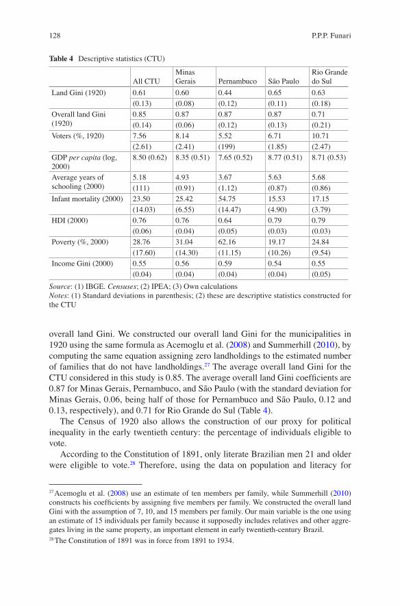
With the available information, we were able to construct two types of measures of economic inequality. The first one is the standard land Gini coefficient, which measures land inequality among landowners.26 The average land Gini considering all the comparable territorial units (CTU) from the four states was 0.61. The average coefficient was 0.60 for Minas Gerais, 0.44 for Pernambuco, 0.65 for São Paulo, and 0.63 for Rio Grande do Sul (Table 4).
Although widely used, the standard land Gini does not capture one important aspect of economic inequality: it does not take into account individuals who do not own land. If, for example, land is divided equally among 10 % of the individuals in a given society, while the other 90 % remain without land, the standard land Gini coefficient will indicate that this society is perfectly egalitarian. Therefore, if we want a proxy for economic inequality for the population as a whole, we need an
26 For each municipality we constructed the Gini coefficient using the same formula as Nunn
(2008): 1 12 1
1
1
+ ( ) -- +( )
=
=
å
ån
n i a
n a
i
n
i
i
n
i
, where n is the number of rural properties, ai is the farm size,
and i denotes the rank, where rural properties are ranked in ascending order of ai. The calculation is made using the Stata programs ineqdec and ineqdec0.
Inequality, Institutions, and Long-Term Development…
128
Table 4 Descriptive statistics (CTU)
All CTUMinas Gerais Pernambuco São Paulo
Rio Grande do Sul
Land Gini (1920) 0.61 0.60 0.44 0.65 0.63
(0.13) (0.08) (0.12) (0.11) (0.18)
Overall land Gini (1920)
0.85 0.87 0.87 0.87 0.71
(0.14) (0.06) (0.12) (0.13) (0.21)
Voters (%, 1920) 7.56 8.14 5.52 6.71 10.71
(2.61) (2.41) (199) (1.85) (2.47)
GDP per capita (log, 2000)
8.50 (0.62) 8.35 (0.51) 7.65 (0.52) 8.77 (0.51) 8.71 (0.53)
Average years of schooling (2000)
5.18 4.93 3.67 5.63 5.68
(111) (0.91) (1.12) (0.87) (0.86)
Infant mortality (2000) 23.50 25.42 54.75 15.53 17.15
(14.03) (6.55) (14.47) (4.90) (3.79)
HDI (2000) 0.76 0.76 0.64 0.79 0.79
(0.06) (0.04) (0.05) (0.03) (0.03)
Poverty (%, 2000) 28.76 31.04 62.16 19.17 24.84
(17.60) (14.30) (11.15) (10.26) (9.54)
Income Gini (2000) 0.55 0.56 0.59 0.54 0.55
(0.04) (0.04) (0.04) (0.04) (0.05)
Source: (1) IBGE. Censuses; (2) IPEA; (3) Own calculationsNotes: (1) Standard deviations in parenthesis; (2) these are descriptive statistics constructed for the CTU
overall land Gini. We constructed our overall land Gini for the municipalities in 1920 using the same formula as Acemoglu et al. (2008) and Summerhill (2010), by computing the same equation assigning zero landholdings to the estimated number of families that do not have landholdings.27 The average overall land Gini for the CTU considered in this study is 0.85. The average overall land Gini coefficients are 0.87 for Minas Gerais, Pernambuco, and São Paulo (with the standard deviation for Minas Gerais, 0.06, being half of those for Pernambuco and São Paulo, 0.12 and 0.13, respectively), and 0.71 for Rio Grande do Sul (Table 4).
The Census of 1920 also allows the construction of our proxy for political inequality in the early twentieth century: the percentage of individuals eligible to vote.
According to the Constitution of 1891, only literate Brazilian men 21 and older were eligible to vote.28 Therefore, using the data on population and literacy for
27 Acemoglu et al. (2008) use an estimate of ten members per family, while Summerhill (2010) constructs his coefficients by assigning five members per family. We constructed the overall land Gini with the assumption of 7, 10, and 15 members per family. Our main variable is the one using an estimate of 15 individuals per family because it supposedly includes relatives and other aggre-gates living in the same property, an important element in early twentieth-century Brazil.28 The Constitution of 1891 was in force from 1891 to 1934.
P.P.P. Funari
129
municipalities, we can easily calculate the percentage of the population of each municipality which was eligible to vote in 1920. The average percentage of indi-viduals eligible to vote considering all the CTU of our study is 7.6. In 1920, the average percentage of individuals eligible to vote was 8.1 for Minas Gerais, 5.5 for Pernambuco, 6.7 for São Paulo, and 10.7 for Rio Grande do Sul (Table 4). We see that Rio Grande do Sul appears to be more equal not only in an economic sense (overall land Gini coefficient), but in a political sense as well. Moreover, we see a higher level of political inequality in Pernambuco, where a high percentage of the population was illiterate at the beginning of the twentieth century.
4 Quantitative Analysis
4.1 Inequality and Long-Term Development
In order to explore the long-term consequences of land (economic) inequality and political inequality for development in Brazil, we exploit the cross-sectional vari-ation in the CTU for our four states of interest: Minas Gerais, Pernambuco, São Paulo, and Rio Grande do Sul.
We first estimate cross-sectional ordinary least squares (OLS) regressions of the form
y g p xi i i i i2000 1920 1920= + + +a b d e¢. . .
where yi2000 is a measure of development for the CTU i for the year 2000, xi is a vec-
tor of control covariates, and εi is an error term. The key variables in this equation are gi
1920 and pi1920, the (standard) land Gini coefficient for the CTU i in 1920 and the
constructed variable for political inequality (percentage of eligible voters) for the same CTU i in 1920, respectively.29 Therefore, our main interest is the consistent estimation of α and β.
The regressions will be estimated with all the observations and dummy interac-tions, allowing for differential statistical relationships for each state. We will there-fore be able to capture possible different de facto institutional environments, with such differences rooted in specific colonial experiences of each state. As dependent variables, we will first use what we call “main outcome variables,” which are GDP per capita, average years of schooling, and infant mortality.
As previously discussed, the inclusion of these specific states has a clear purpose. Each of these regions is representative of a particular colonial experience within a constant de jure environment. This likely led to different de facto institutional envi-ronments that might cause inequality to relate in heterogeneous ways with each
29 We note that there is no uniform framework in the literature for the econometric analysis of the effects of historical inequality. In this study, we follow mainly Acemoglu et al. (2008).
Inequality, Institutions, and Long-Term Development…
130
development indicator. Pernambuco is representative of the old agrarian structure, of great importance during the colonial era due to the sugar production that had far-reaching implications for the political, economic, and social structure of the region. Minas Gerais was the center of the gold cycle and later became an important producer of coffee and a center for the supply of goods for the domestic market. São Paulo was the main coffee producer, and in the late nineteenth century became Brazil’s most important economic center, a position that it still occupies today. Rio Grande do Sul had a later occupation with characteristics associated to those of North America (see, e.g., Engerman and Sokoloff 1997, 2002), and vast numbers of European immigrants (as in São Paulo) shaping its development path.
The main econometric concern with this specification is the possible endogeneity bias generated by omitted variables.30 In other words, if omitted factors in εi are cor-related with the explanatory variables, the estimation by OLS will generate inconsis-tent estimators. Easterly (2007), based on the extensive economic history developed by Engerman and Sokoloff, has argued that growing conditions (topography, climate, and soil) favorable to the production of cash crops contribute to higher inequality. Therefore, we will control for a rich set of covariates (included in the vector xi).
4.2 Contemporary Outcomes
We start by providing results of simple regressions (weighted correlations), using as independent variables the land Gini (as discussed, among landowners) and the per-centage of eligible voters (our franchise—political inequality—indicator) and one
30 The key condition for OLS consistency is the absence of correlation between the independent variables and the error term. A sufficient condition is the zero conditional mean assumption:
E xe /( ) = 0 , which means that the error term is not correlated with any function of the indepen-
dent variables. In applied econometrics, endogeneity arises in one of the three ways: (1) omitted variable bias; (2) measurement error; and (3) simultaneity (Wooldridge 2010). Our main concern is the omitted variable bias due to the inability to control directly for variables such as land quality.
The usual formula for analyzing the omitted variable bias is px q
xk kk
k
lim .b b g
= +( )( )
é
ëêê
ù
ûúú
cov ,
var
(Wooldridge 2010, p. 67). Our strategy in this study is to use a proxy variable solution. There are
two formal requirements for a proxy variable for the omitted variable q: (1) the proxy variable
should be redundant in the structural equation, E y x q z E x q| , , ,( ) = ( ) , where z is the proxy vari-
able; and (2) the correlation between the omitted variable q and each xj be zero once we partial out
z: L q x x z L q zk| 1, , , , | 1,1 ¼( ) = ( ) , where L(.) represents a linear projection (Wooldridge 2010).31 Technically, we have a simple regression when there is only one independent variable. In our case, we have at least four dummy interactions for each variable. Aiming to keep language as simple as possible, I will use the term “simple regressions” when there is only one independent variable of interest (irrespective of the number of interactions).
P.P.P. Funari
131
multiple regression, including both inequality variables.31 As dependent variables we will use our “main outcome variables,” namely (natural logarithm of) GDP per capita, (natural logarithm of) average years of schooling, and infant mortality.32
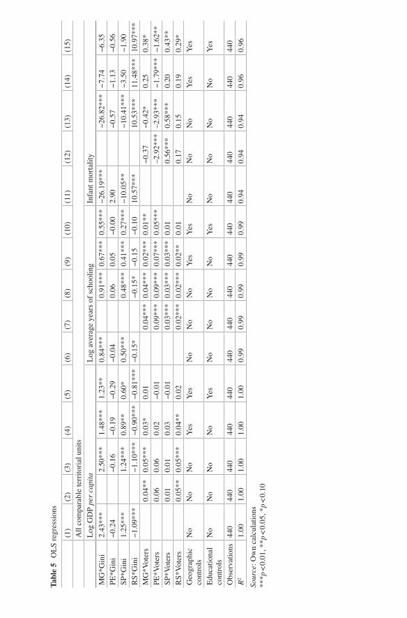
Table 5 presents the estimated coefficients. As we can see from Column 1, the bivariate relationship between the land Gini and GDP per capita is heterogeneous. The estimated coefficients for Minas Gerais and São Paulo are positive and highly significant (2.43 and 1.25, respectively). While the coefficient for Pernambuco is not significant, the estimated coefficient for Rio Grande do Sul is not only signifi-cant, but also negative (−1.09). The simple regression of GDP per capita on the percentage of eligible voters is presented on Column 2. Only for Minas Gerais and Rio Grande do Sul the estimated coefficients are significant. Nevertheless, they have the expected positive sign. When we regress GDP per capita on both inequality variables, the picture remains broadly the same, a reflection of the surprising low correlation between the land Gini and the percentage of eligible voters (0.09, considering all CTU).
Columns 6 and 11 suggest similar relationships between economic inequality in the early twentieth century and average years of schooling and infant mortal-ity. In other words, we estimated, for both dependent variables, positive and highly significant coefficients for Minas Gerais and São Paulo, a negative and significant coefficient for Rio Grande do Sul, and a nonsignificant coefficient for Pernambuco. Concerning the bivariate relationship between the percentage of eligible voters and average years of schooling, the coefficients are positive and highly significant (Column 7). There is, however, a surprise when we estimate the regressions with infant mortality as the dependent variable: the significant coefficient for São Paulo suggests a positive relationship between political equal-ity and infant mortality (Column 12). We discuss these results in greater detail below. Regressions including both inequality variables present similar results (Columns 8 and 13).
Although important in their own right, the results discussed above are only historical correlations. The natural concern with those correlations is the possible bias generated by the inconsistency of OLS estimation in the presence of omitted variables. We attempt to correct the estimation for this bias by controlling for a rich set of control variables. Another concern is that the positive correlation between the political inequality variable is being driven by the association of this variable with an educational indicator. In order to construct the franchise indicator, we took the number of literate males, which is likely to reflect the educational environment of that particular CTU. In order to control for this specific source of bias, we control for the educational variables in 1920.
We now discuss the extended results from regressions with GDP per capita as the dependent variable. The inclusion of educational controls reduces marginally, for Minas Gerais and Rio Grande do Sul, the significance of the estimated coefficients
32 For now on, when I mention “GDP per capita” or “average years of schooling” I will be referring to their natural logarithms.
Inequality, Institutions, and Long-Term Development…
Tabl
e 5
OL
S r
egre
ssio
ns
(1)
(2)
(3)
(4)
(5)
(6)
(7)
(8)
(9)
(10)
(11)
(12)
(13)
(14)
(15)
All
com
para
ble
terr
itor
ial
unit
s
Log
GD
P p
er c
apit
aL
og a
vera
ge y
ears
of
scho
olin
gIn
fant
mor
tali
ty
MG
*Gin
i2.
43**
*2.
50**
*1.
48**
*1.
23**
0.84
***
0.91
***
0.67
***
0.55
***
−26
.19*
**−
26.8
2***
−7.
74−
6.35
PE
*Gin
i−
0.24
−0.
16−
0.19
−0.
29−
0.04
0.06
0.05
−0.
002.
90−
0.57
−1.
13−
0.56
SP
*Gin
i1.
25**
*1.
24**
*0.
89**
0.60
*0.
50**
*0.
48**
*0.
41**
*0.
27**
*−
10.0
5**
−10
.41*
**−
3.50
−1.
90
RS
*Gin
i−
1.09
***
−1.
10**
*−
0.90
***
−0.
81**
*−
0.15
*−
0.15
*−
0.15
−0.
1010
.57*
**10
.53*
**11
.48*
**10
.97*
**
MG
*Vot
ers
0.04
**0.
05**
*0.
03*
0.01
0.04
***
0.04
***
0.02
***
0.01
**−
0.37
−0.
42*
0.25
0.38
*
PE
*Vot
ers
0.06
0.06
0.02
−0.
010.
09**
*0.
09**
*0.
07**
*0.
05**
*–2
.92*
**–2
.93*
**−
1.79
***
−1.
62**
SP
*Vot
ers
0.01
0.01
0.03
−0.
010.
03**
*0.
03**
*0.
03**
*0.
010.
56**
*0.
58**
*0.
200.
43**
RS
*Vot
ers
0.05
**0.
05**
*0.
04**
0.02
0.02
***
0.02
***
0.02
**0.
010.
170.
150.
190.
29*
Geo
grap
hic
cont
rols
No
No
No
Yes
Yes
No
No
No
Yes
Yes
No
No
No
Yes
Yes
Edu
cati
onal
co
ntro
lsN
oN
oN
oN
oY
esN
oN
oN
oN
oY
esN
oN
oN
oN
oY
es
Obs
erva
tion
s44
044
044
044
044
044
044
044
044
044
044
044
044
044
044
0
R2
1.00
1.00
1.00
1.00
1.00
0.99
0.99
0.99
0.99
0.99
0.94
0.94
0.94
0.96
0.96
Sour
ce:
Ow
n ca
lcul
atio
ns**
*p <
0.0
1, *
*p <
0.0
5, *
p <
0.1
0
133
for the percentage of eligible voters (Column 4). We note that, while this is not the case for average years of schooling (Column 9), the picture is similar when infant mortality is the dependent variable (Column 14). When geographic and educa-tional controls are included, we have a clearer picture. Column 5 shows that the results for Minas Gerais and São Paulo, of economic inequality in 1920 being posi-tively and significantly correlated to GDP per capita in 2000, are robust. For Pernambuco, economic inequality appears to be non-correlated with income in the long run. For Rio Grande do Sul, economic inequality in 1920 remains negatively (and highly significant) correlated to GDP per capita in 2000. Moreover, all esti-mated coefficients for our political inequality variable become insignificant with the inclusion of geographic variables.
However, the results for average years of schooling and infant mortality are dif-ferent. First, economic inequality in 1920 is only significantly related to average years of schooling in 2000 for Minas Gerais and São Paulo, the states in which the coefficients are positive (Column 10). In other words, only positive relationships between economic inequality and educational attainments in the long run are sig-nificant. Considering infant mortality, we have the opposite picture: only negative relationships, as the case of Rio Grande do Sul, between economic inequality and development in the long run are significant (reflected in a positive estimated coef-ficient, Column 15). The percentage of eligible voters does not appear to have had important effects on development in the long run. Either the coefficients lose their significance or they present small magnitudes (Columns 10 and 15).
We now expand our analysis by introducing the overall land Gini calculated index. This variable, as already mentioned, shows the inequality of land distribution across the whole population. Extending the analysis in this direction provides fur-ther insights into the relationship between inequality and long-term development.
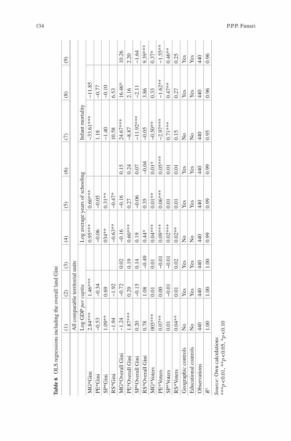
Table 6 presents the regression results. Several noteworthy aspects emerge. First, when including both Gini variables and the percentage of eligible voters in regres-sions with no controls and GDP per capita as the dependent variable, the land Gini among landowners remains significant for Minas Gerais and São Paulo, while the overall land Gini is significant for Pernambuco (Column 1). The inclusion of con-trols makes all overall land Gini coefficients become insignificant (Column 2). Moreover, regressions with the overall land Gini as the only economic inequality variable (and with control variables) show no significant relationship (Column 3). Regressions with average years of schooling as the dependent variable present simi-lar results (Columns 4–6), somewhat more favorable to the standard land Gini (the coefficient for Rio Grande do Sul is significant, Columns 4 and 5). Coefficients for the overall land Gini remain broadly insignificant as well in regressions with infant mortality as the dependent variable the inclusion of the control variables (Columns 8 and 9). Notwithstanding, the comparison of regressions with the standard land Gini (Table 5, Columns 5, 10, and 15) with regressions with the overall land Gini (Table 6, Columns 3, 6, and 9) indicates a stronger effect of the standard land Gini.
Therefore, our empirical results suggest that the effects of land inequality among landowners would possibly dominate over the effects of the inequality of land distribution across the population as a whole.
Inequality, Institutions, and Long-Term Development…
134
Tabl
e 6
OL
S r
egre
ssio
ns i
nclu
ding
the
ove
rall
lan
d G
ini
(1)
(2)
(3)
(4)
(5)
(6)
(7)
(8)
(9)
All
com
para
ble
terr
itor
ial
unit
s
Log
GD
P p
er c
apit
aL
og a
vera
ge y
ears
of
scho
olin
gIn
fant
mor
tali
ty
MG
*Gin
i2.
84**
*1.
46**
*0.
95**
*0.
60**
*−
33.6
1***
−11
.85
PE
*Gin
i−
0.53
−0.
34−
0.06
−0.
051.
18−
0.77
SP
*Gin
i1.
09**
0.69
034*
*0.
31**
−1.
40−
0.10
RS
*Gin
i−
1.94
−1.
92−
0.63
**−
0.47
*10
.58
6.53
MG
*Ove
rall
Gin
i−
1.24
−0.
720.
02−
0.16
−0.
160.
1524
.67*
**16
.46*
10.2
6
PE
*Ove
rall
Gin
i1.
87**
*0.
290.
190.
60**
*0.
270.
24−
8.87
2.16
2.20
SP
*Ove
rall
Gin
i0.
20−
0.15
0.14
0.19
−0.
060.
07−
11.9
2***
−2.
11−
1.64
RS
*Ove
rall
Gin
i0.
781.
08−
0.49
0.44
*0.
35−
0.04
−0.
053.
869.
39**
*
MG
*Vot
ers
005*
**0.
010.
010.
04**
*0.
01**
0.01
*−
0.50
**0.
330.
37*
PE
*Vot
ers
0.07
**0.
00−
0.01
0.09
***
0.06
***
0.05
***
−2.
97**
*−
1.62
**−
1.55
**
SP
*Vot
ers
0.01
−0.
01−
0.01
0.02
***
0.01
0.01
0.71
***
0.47
**0.
46**
RS
*Vot
ers
0.04
**0.
010.
020.
02**
0.01
0.01
0.15
0.27
0.25
Geo
grap
hic
cont
rols
No
Yes
Yes
No
Yes
Yes
No
Yes
Yes
Edu
cati
onal
con
trol
sN
oY
esY
esN
oY
esY
esN
oY
esY
es
Obs
erva
tion
s44
044
044
044
044
044
044
044
044
0
R2
1.00
1.00
1.00
0.99
0.99
0.99
0.95
0.96
0.96
Sour
ce:
Ow
n ca
lcul
atio
ns**
*p <
0.0
1, *
*p <
0.0
5, *
p <
0.1
0
P.P.P. Funari
135
4.3 De Facto Institutional Environments and Structural Change
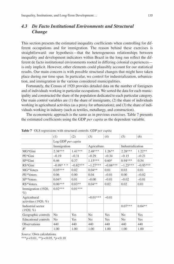
This section presents the estimated inequality coefficients when controlling for dif-ferent occupations and for immigration. The reason behind these exercises is straightforward: our hypothesis—that the heterogeneous relationships between inequality and development indicators within Brazil in the long run reflect the dif-ferent de facto institutional environments rooted in differing colonial experiences—is only implicit. However, other elements could plausibly account for our statistical results. Our main concern is with possible structural changes that might have taken place during our time span. In particular, we control for industrialization, urbaniza-tion, and immigration in the various considered municipalities.
Fortunately, the Census of 1920 provides detailed data on the number of foreigners and of individuals working in particular occupations. We sorted the data for each munic-ipality and constructed the share of the population dedicated to each particular category. Our main control variables are (1) the share of immigrants; (2) the share of individuals working in agricultural activities (as a proxy for urbanization); and (3) the share of indi-viduals working in industry (such as textiles, metallurgy, and construction).
The econometric approach is the same as in previous exercises. Table 7 presents the estimated coefficients using the GDP per capita as the dependent variable.
Table 7 OLS regressions with structural controls: GDP per capita
(1) (2) (3) (4) (5) (6)
Log GDP per capita
Immigration Agriculture Industrialization
MG*Gini 2.38*** 1.41*** 2.48*** 1.26** 2.28*** 1.22**
PE*Gini −0.19 −0.31 −0.29 −0.34 −0.15 −0.21
SP*Gini 0.46 0.37 1.15*** 0.60* 0.94*** 0.54
RS*Gini −0.99* * * −0.82*** −1.27*** −0.88*** −1.25*** −0.95***
MG*Voters 0.05*** 0.02 0.04** 0.01 0.03 0.01
PE*Voters 0.06 0.00 0.04 −0.01 0.00 −0.02
SP*Voters 0.04* 0.01 −0.00 −0.01 −0.02 −0.01
RS*Voters 0.06*** 0.03** 0.04** 0.02 0.02 0.01
Immigration (1920, %)
0.02*** 0.01***
Agricultural activities (1920, %)
−0.01*** −0.01
Industrial sector (1920, %)
0.07*** 0.04**
Geographic controls No Yes No Yes No Yes
Educational controls No Yes No Yes No Yes
Observations 440 440 440 440 440 440
R2 1.00 1.00 1.00 1.00 1.00 1.00
Source: Own calculations***p < 0.01, **p < 0.05, *p < 0.10
Inequality, Institutions, and Long-Term Development…
136
An interesting picture emerges. When controlling for the share of individuals working in agricultural activities, we still have a positive and significant relation-ship between economic inequality and GDP per capita in the long run for Minas Gerais and São Paulo, even when geographic and educational controls are included; for Pernambuco, coefficients remain largely insignificant; as for Rio Grande do Sul coefficients remain negative and highly significant (Columns 3 and 4).
However, controlling for immigration the economic inequality coefficient for São Paulo is no longer significant even in regressions without further controls (Column 1). Although the remaining coefficients maintain similar properties as the above-made discussion, this analysis suggests that the effects of land inequality in São Paulo might be reflecting the positive effects of immigration. Moreover, when controlling for the percentage of individuals in industrial activities São Paulo’s land Gini coefficient remains significant only in regressions without geographic and edu-cational controls (Columns 5 and 6). Finally, we note that, with the exception of agriculture in regressions with the usual controls (Column 4), all coefficients of structural controls are highly significant and have the expected sign.
Thus, we have presented a robustness check for our hypothesis that the heteroge-neous relationships between economic inequality and development within Brazil are due to the different de facto institutional environments. Several regression spec-ifications show that controlling for variables proxying structural changes nonethe-less maintains the heterogeneous results within the country. This evidence is in accordance with the hypothesis.
4.4 Inequality Yesterday and Inequality Today
Finally, we present a natural extension of our investigation: the relationship inequal-ity in the past and inequality today. This is an especially interesting question in the Brazilian context, for Brazil is one of the most unequal countries in the world, often portrayed as an example of high structural and persistent inequality.
Using a framework similar to previous investigations, we econometrically exam-ine the relationship between the (standard) land Gini in 1920 and inequality today, measured by the income Gini in 2000. Again, our units of analysis are the CTU. Results are in Table 8.
Results are broadly the same across specifications. For Minas Gerais the esti-mated coefficient for economic inequality in 1920 is not significant in regressions with no controls (Column 1) and with the full set of controls (Column 3). Moreover, we find no significant relationship between political inequality in 1920 and eco-nomic inequality today. For São Paulo, although the estimated coefficient changes its sign (it is negative in regressions with no controls, Column 1), the land Gini estimated coefficient is never significant. The estimated coefficient for the percent-age of eligible voters is only significant without the inclusion of the controls and is very small across specifications. Therefore, we find no statistical significance for the relationship between economic or political inequality in the early twentieth century and economic inequality in 2000 in Minas Gerais and in São Paulo.
P.P.P. Funari
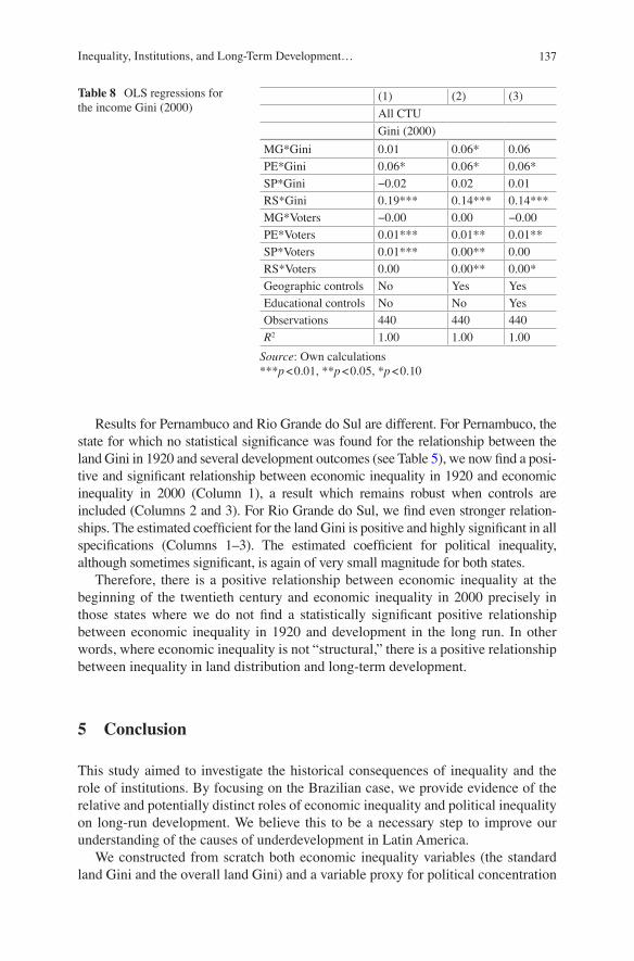
137
Results for Pernambuco and Rio Grande do Sul are different. For Pernambuco, the state for which no statistical significance was found for the relationship between the land Gini in 1920 and several development outcomes (see Table 5), we now find a posi-tive and significant relationship between economic inequality in 1920 and economic inequality in 2000 (Column 1), a result which remains robust when controls are included (Columns 2 and 3). For Rio Grande do Sul, we find even stronger relation-ships. The estimated coefficient for the land Gini is positive and highly significant in all specifications (Columns 1–3). The estimated coefficient for political inequality, although sometimes significant, is again of very small magnitude for both states.
Therefore, there is a positive relationship between economic inequality at the beginning of the twentieth century and economic inequality in 2000 precisely in those states where we do not find a statistically significant positive relationship between economic inequality in 1920 and development in the long run. In other words, where economic inequality is not “structural,” there is a positive relationship between inequality in land distribution and long-term development.
5 Conclusion
This study aimed to investigate the historical consequences of inequality and the role of institutions. By focusing on the Brazilian case, we provide evidence of the relative and potentially distinct roles of economic inequality and political inequality on long-run development. We believe this to be a necessary step to improve our understanding of the causes of underdevelopment in Latin America.
We constructed from scratch both economic inequality variables (the standard land Gini and the overall land Gini) and a variable proxy for political concentration
(1) (2) (3)
All CTU
Gini (2000)
MG*Gini 0.01 0.06* 0.06
PE*Gini 0.06* 0.06* 0.06*
SP*Gini −0.02 0.02 0.01
RS*Gini 0.19*** 0.14*** 0.14***
MG*Voters −0.00 0.00 −0.00
PE*Voters 0.01*** 0.01** 0.01**
SP*Voters 0.01*** 0.00** 0.00
RS*Voters 0.00 0.00** 0.00*
Geographic controls No Yes Yes
Educational controls No No Yes
Observations 440 440 440
R2 1.00 1.00 1.00
Source: Own calculations***p < 0.01, **p < 0.05, *p < 0.10
Table 8 OLS regressions for the income Gini (2000)
Inequality, Institutions, and Long-Term Development…
138
(the percentage of eligible voters) at the municipal level for the states of Minas Gerais, Pernambuco, São Paulo, and Rio Grande do Sul. The states were specifi-cally chosen for their different colonial experiences, which probably shaped their de facto institutional environment. Our selection was made on the basis of the abundant data provided by the 1920 Census, a source which, surprisingly, had not yet been exploited for this purpose.
The results are surprising. First, we find almost no correlation between the land Gini and the percentage of eligible voters in Brazilian municipalities in 1920. Second, and somewhat unexpectedly, we find a positive relationship between eco-nomic inequality in early twentieth century and development outcomes in 2000 for the states of Minas Gerais and São Paulo, both from the Southeast region. Pernambuco, a Northeastern state, presents no evidence of a significant relation-ship between economic inequality and long-term development outcomes, while the evidence for the South, the state of Rio Grande do Sul, is that the relationship is negative. Third, we find no robust significant relationship between political inequality, measured by the percentage of eligible voters, and long-term develop-ment outcomes. Fourth, the effects of economic inequality are largely due to the concentration of land among landowners, as shown by the insignificance of the overall land Gini.
These are interesting results, for they appear to contradict the general view that economic inequality would always be costly for a society and that greater political participation would foster development. The answer to part of this riddle might lie in the fact that political participation was very low in early twentieth-century Brazil, and a marginal increase (the econometrically captured effect) might have given more irrelevant votes to a captured political system, leaving the economic outcomes unchanged. In other words, greater franchise might not have given the population more political participation. With regard to the effects of economic inequality, when considering the land Gini in an agrarian structure, these are likely to be strongly linked to collective action problems. In a captured political system such as Brazil in the Old Republic, land concentration might have differing effects, especially when taking into account that, in some regions, landowners were largely responsible for the provision of public goods.
Further important analyses were conducted. First, we find evidence that there is almost no correlation between economic (land) inequality in the early twenti-eth century and recent income inequality in states where there is a positive rela-tionship between economic inequality and long-term development (Minas Gerais and São Paulo). In other words, the positive effects of inequality are associated with a particular structural organization at a specific time, in contrast to a more structural inequality, which, as exemplified by the cases of Pernambuco and Rio Grande do Sul, would have either negative or no significant effects on long-term development.
Finally, our hypothesis that different de facto institutional environments are associated with different relationships between inequality and long-term devel-opment was, initially, only implicit in our analysis. Important structural changes that occurred during this time span might be responsible for the heterogeneous
P.P.P. Funari
139
relationships found previously between inequality and long-term development. Three elements were our main concern: (1) immigration; (2) industrialization; and (3) urbanization. After controlling for these variables, our main results were main-tained, strengthening our hypothesis.
It is important to note that we do not argue that inequality is conducive to devel-opment in general. We present evidence that inequality might be associated with better development outcomes in the long run in a particular political context in a within-country framework. It is possible that the theoretically harmful effects of inequality are better reflected in a cross-country framework, in which the mecha-nisms are related to the different de jure institutional environment. In other words, relative equality would be better for a particular country, but within an unequal country (with certain sociopolitical and economic characteristics) more inequality would be associated with better outcomes.
Much work remains to be done. We mention some possible extensions. First, there are few works that attempt to control for different de facto institutional envi-ronments. Further employment of this strategy likely will provide beneficial insights in order to better understand the development paths of societies. Second, empirical and theoretical studies that offer a differentiation between within-coun-try and cross- country effects of variables are largely welcome.33 Third, models attempting to capture the within-country effects of variables such as inequality in politically captured environments are lacking. Finally, the external validity of our results remains questionable. Comparative studies within Latin America are a logical next step.
Acknowledgment I would like to thank my Masters’ supervisor Renato Colistete for his guid-ance and support. I have benefited from conversations with William Summerhill, Luis Bértola, Alfonso Herranz, Ewout Frankema, Leonardo Weller, Mauro Rodrigues, Pedro Duarte, Rodrigo Soares, Gilberto Lima, Thales Pereira, and Gabriel Corrêa, as well as comments from participants at the 4th Southern Hemisphere Economic History Summer School at Universidad de la Republica, 42nd National Economic Meeting (ANPEC), Latin American Inequality Conference, IV CLADHE, 10th Conference of the EHES, and the FEA-USP Workshop on Economic History. Financial support from FAPESP and CAPES is gratefully acknowledged.
Open Access This chapter is distributed under the terms of the Creative Commons Attribution 4.0 International License (http://creativecommons.org/licenses/by/4.0/), which permits use, duplica-tion, adaptation, distribution and reproduction in any medium or format, as long as you give appro-priate credit to the original author(s) and the source, a link is provided to the Creative Commons license and indicate if changes were made.
The images or other third party material in this chapter are included in the work's Creative Commons license, unless indicated otherwise in the credit line; if such material is not included in the work's Creative Commons license and the respective action is not permitted by statutory regu-lation, users will need to obtain permission from the license holder to duplicate, adapt or reproduce the material.
33 See, for example, Robinson (2006).
Inequality, Institutions, and Long-Term Development…
140
References
Acemoglu, D. (2008). Oligarchic versus democratic societies. Journal of the European Economic Association, 6(1), 1–44.
Acemoglu, D., Johnson, S., & Robinson, J. A. (2001). The colonial origins of comparative devel-opment: An empirical investigation. American Economic Review, 91(5), 1369–1401.
Acemoglu, D., Johnson, S., & Robinson, J. A. (2002). Reversal of fortune: Geography and institu-tions in the making of modern world income distribution. Quarterly Journal of Economics, 117(4), 1231–1294.
Acemoglu, D., & Robinson, J. A. (2000). Political losers as a barrier to economic development. American Economic Review: Papers and Proceedings, 90, 126–130.
Acemoglu, D., Robinson, J. A., & Verdier, T. (2004). Kleptocracy and divide and rule: A theory of personal rule. Journal of the European Economic Association, 2, 162–192.
Acemoglu, D., Johnson, S., & Robinson, J. A. (2005). Institutions and the fundamental cause of long-run growth. In P. Aghion & S. Durlauf (Eds.), Handbook of economic growth. North- Holland: Amsterdam.
Acemoglu, D., et al. (2008). Economic and political inequality in development: The case of Cundinamarca, Colombia. In E. Helpman (Ed.), Institutions and economic performance. Cambridge, MA: Harvard University Press.
Aghion, P., Banerjee, A., & Piketty, T. (1999a). Dualism and macroeconomic volatility. The Quarterly Journal of Economics, 114(4), 1359–1397.
Aghion, P., Caroli, E., & García-Peñalosa, C. (1999b). Inequality and economic growth: The per-spective of the new growth theories. Journal of Economic Literature, 37, 1615–1660.
Alesina, A., & Rodrik, D. (1994). Distributive politics and economic growth. Quarterly Journal of Economics, 109(2), 465–490.
Banerjee, A., & Duflo, E. (2003). Inequality and growth: What can the data say? Journal of Economic Growth, 8, 267–299.
Banerjee, A., & Iyer, L. (2005). History, institutions, and economic performance: The legacy of colonial land tenure systems in India. American Economic Review, 95(4), 1190–1213.
Banerjee, A., & Newman, A. (1991). Occupational choice and the process of development. Journal of Political Economy, 101(2), 274–298.
Barro, R. (2000). Inequality and growth in a panel of countries. Journal of Economic Growth, 5, 5–32.Bates, R. (1981). Markets and states in tropical Africa. Berkeley, CA: University of California
Press.Bénabou, R. (1996). Inequality and growth. NBER working paper, no. 5658.Bourguignon, F., & Verdier, T. (2000). Oligarchy democracy, inequality and growth. Journal of
Development Economics, 62, 285–313.Carvalho, O. (1946). Política do Município. Rio de Janeiro: Livraria AGIR Editora.De Carvalho Filho, I., & Colistete, R. P. (2010). Educational persistence: Was it all determined
100 years ago? Evidence from São Paulo, Brazil. MPRA paper, no. 24494.Dean, W. (1971). Latifundia and land policy in nineteenth-century Brazil. The Hispanic American
Historical Review, 51(4), 606–625.Dell, M. (2010). The persistent effects of Peru’s mining mita. Econometrica, 78(6), 1863–1903.Denis, P. (1911). Brazil. New York: Chas. Scribner’s Sons.Easterly, W. (2007). Inequality does cause underdevelopment: Insights from a new instrument.
Journal of Development Economics, 84, 755–776.Easterly, W., & Rebelo, S. (1993). Fiscal policy and economic growth: An empirical investigation.
Journal of Monetary Economics, 32, 417–458.Engerman, S., & Sokoloff, K. (1997). Factor endowments, institutions, and differential paths of
growth among new world economies: A view from economic historians of the United States. NBER working paper series on historical factors in long run growth, no. 66.
Engerman, S., & Sokoloff, K. (2002). Factor endowments, inequality, and paths of development among new world economies. Economía, 3(1), 41–88.
P.P.P. Funari
141
Forbes, K. (2000). A reassessment of the relationship between inequality and growth. American Economic Review, 90(4), 869–887.
Frankema, E. (2009). Has Latin America always been unequal? A comparative study of asset and income inequality in the long twentieth century. Global economic history series (vol. 3). Boston, Leiden: Brill.
Frankema, E. (2010). The colonial roots of land inequality: Geography, factor endowments, or institutions? Economic History Review, 63(2), 418–451.
Furtado, C. (2006 [1st ed. 1959]). Formação econômica do Brasil (34th ed.). São Paulo: Companhia das Letras.
Galor, O., Moav, O., & Vollrath, D. (2009). Inequality in landownership the emergence of human- capital promoting institutions, and the great divergence. Review of Economic Studies, 76, 143–179.
Galor, O., & Zeira, J. (1993). Income distribution and macroeconomics. Review of Economic Studies, 60, 35–52.
Goldsmith, R. W. (1986). Brasil 1850–1984: Desenvolvimento financeiro sob um século de infla-ção. São Paulo: Harper and Row.
IBGE – Instituto Brasileiro de Geografia e Estatística. (1923). Censo demográfico de 1920: População (Vol. 3). Rio de Janeiro: IBGE.
Kaldor, N. (1956). Alternative theories of distribution. Review of Economic Studies, 23(2), 83–100.Kuznets, S. (1955). Economic growth and income inequality. American Economic Review, 45(1),
1–28.Leal, V. N. (2012 [1st ed. 1948]). Coronelismo, enxada e voto: O município e o regime represen-
tativo no Brasil. São Paulo: Companhia das Letras.Leff, N. (1972). Economic retardation in nineteenth-century Brazil. Economic History Review,
25(3), 489–507.Leff, N. (1997). Economic development in Brazil, 1822–1913. In S. Haber (Ed.), How Latin
America fell behind. Stanford: Stanford University Press.Love, J. (1970). Political participation in Brazil, 1881–1969. Luso-Brazilian Review, 7(2), 3–24.Murphy, K., Shleifer, A., & Vishny, R. (1989). Income distribution, market size, and industrializa-
tion. Quarterly Journal of Economics, 104(3), 537–564.Naritomi, J., Soares, R., & Assunção, J. (2012). Institutional development and colonial heritage
within Brazil. Journal of Economic History, 72(2), 393–422.North, D., Summerhill, W., & Weingast, B. (2000). Order, disorder and economic change: Latin
America versus North America. In B. Mesquita & H. Root (Eds.), Governing for prosperity. New Haven: Yale University Press.
Nugent, J., & Robinson, J. A. (2010). Are factor endowments fate? Journal of Iberian and Latin American Economic History, 28(1), 45–82.
Nunn, N. (2008). Slavery, inequality, and economic development in the Americas: An examination of the Engerman–Sokoloff hypothesis. In E. Helpman (Ed.), Institutions and economic perfor-mance. Cambridge, MA: Harvard University Press.
Pande, R., & Udry, C. (2005). Institutions and development: A view from below. In R. Blundell, W. Newey, & T. Persson (Eds.), Proceedings of the 9th World Congress of the Econometric Society. Cambridge: Cambridge University Press.
Perotti, R. (1992). Fiscal policy, incomes distribution, and growth. Columbia University working paper, no. 636.
Perotti, R. (1996). Growth income distribution, and democracy: What the data say. Journal of Economic Growth, 1, 149–187.
Persson, T., & Tabellini, G. (1994). Is inequality harmful for growth? American Economic Review, 84(3), 600–621.
Prado, C. Jr. (1956 [1st ed. 1945]). História econômica do Brasil (4th ed.). São Paulo: Brasiliense.Robinson, J. A. (2006). Equity institutions, and the development process. Nordic Journal of
Political Economy, 32, 17–50.Summerhill, W. (2010). Colonial institutions, slavery, inequality, and development: Evidence from
São Paulo, Brazil. MPRA paper, no. 22162.
Inequality, Institutions, and Long-Term Development…
142
Villela, A. (2013). O desenvolvimento econômico no Brasil Pré-1945. In F. Veloso, P. Ferreira, F. Giambiagi, & S. Pessôa (Eds.), Desenvolvimento econômico: Uma perspectiva Brasileira. Rio de Janeiro: Elsevier.
Wegenast, T. (2010). Cana, café, cacau: Agrarian structure and educational inequalities in Brazil. Journal of Iberian and Latin American Economic History, 28(1), 103–137.
Wooldridge, J. (2010). Econometric analysis of cross section and panel data (2nd ed.). Cambridge, MA: The MIT Press.
Pedro Paulo Pereira Funari holds a Master of Science in Economics and a Bachelor of Science in Economics from the School of Economics, Business and Accounting of the University of São Paulo. He is currently a Ph.D. candidate at the University of California, Davis. His main interests are economic history, institutions, and development.
P.P.P. Funari