Embed Size (px)
Citation preview
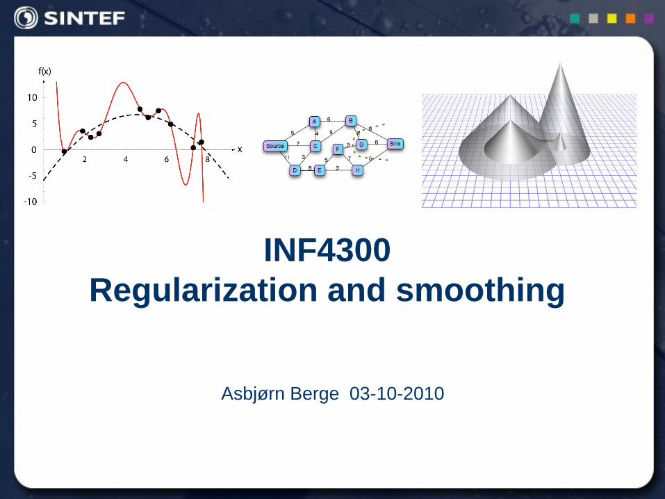
INF4300
Regularization and smoothing
Asbjørn Berge 03-10-2010

Readings for this lecture
Morphology
R.C. Gonzales and R.E. Woods: Digital Image Processing, 3rd ed,
2008. Prentice Hall. ISBN: 978-0-13-168728-8. Chapter 9, 9.4,9.5
very cursory
Graph cuts and other regularization approaches
Exercise/tutorial text
Cursory reading for interested students
http://www.cs.cornell.edu/~rdz/graphcuts.html
Classic paper: What Energy Functions can be Minimized via
Graph Cuts? (Kolmogorov and Zabih, ECCV '02/PAMI '04)
2
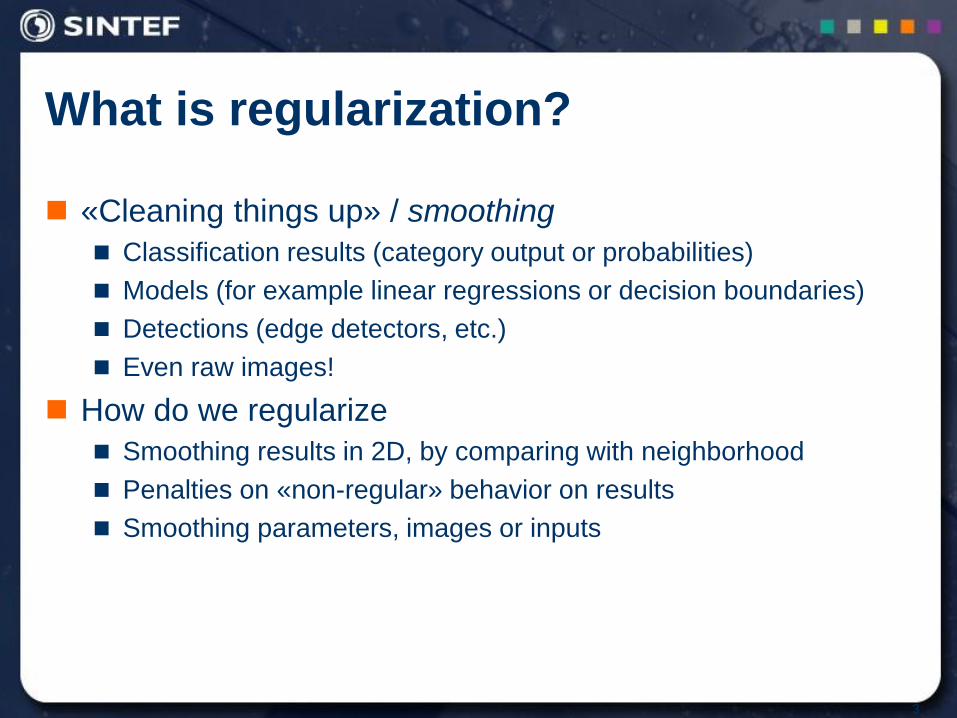
What is regularization?
«Cleaning things up» / smoothing
Classification results (category output or probabilities)
Models (for example linear regressions or decision boundaries)
Detections (edge detectors, etc.)
Even raw images!
How do we regularize
Smoothing results in 2D, by comparing with neighborhood
Penalties on «non-regular» behavior on results
Smoothing parameters, images or inputs
3

What will this lecture cover?
General terminology on regularization
The regularization inherent in Support Vector Machines
Morphology
Graph cuts
4
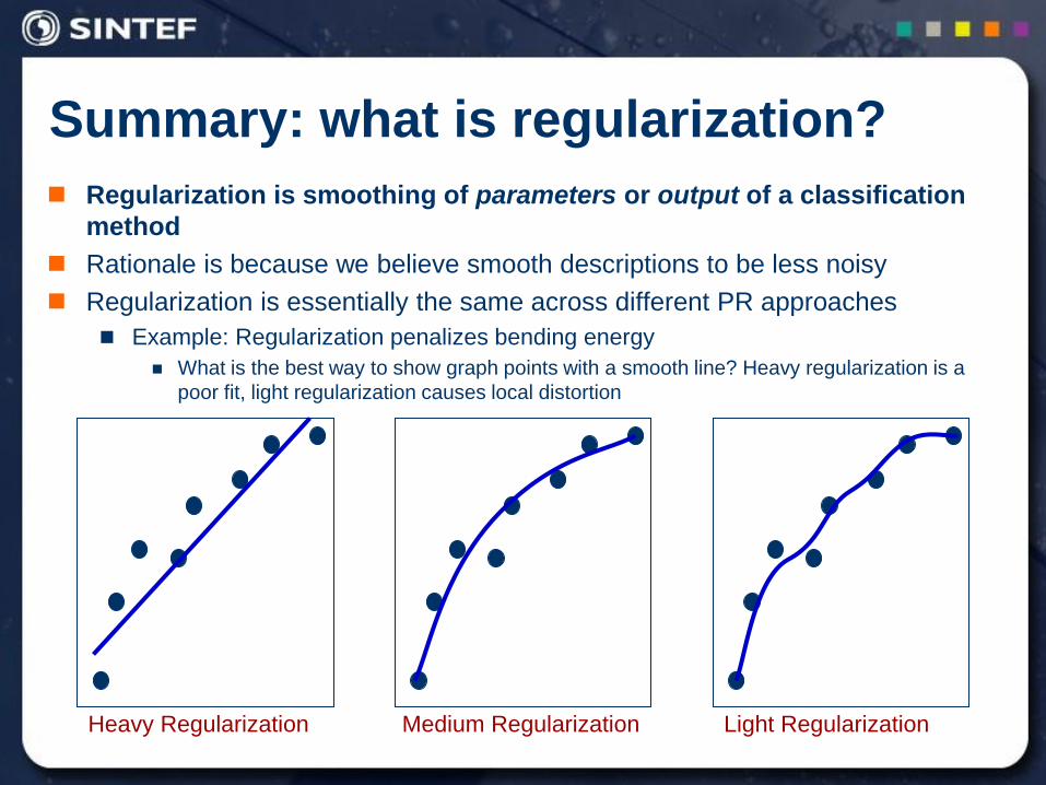
Summary: what is regularization?
Regularization is smoothing of parameters or output of a classification
method
Rationale is because we believe smooth descriptions to be less noisy
Regularization is essentially the same across different PR approaches
Example: Regularization penalizes bending energy
What is the best way to show graph points with a smooth line? Heavy regularization is a
poor fit, light regularization causes local distortion
•Regularizatio
n works by
restrictions on
possible
solutions or by
using simpler
estimates
explicitly or
indirectly.
Medium Regularization Heavy Regularization Light Regularization
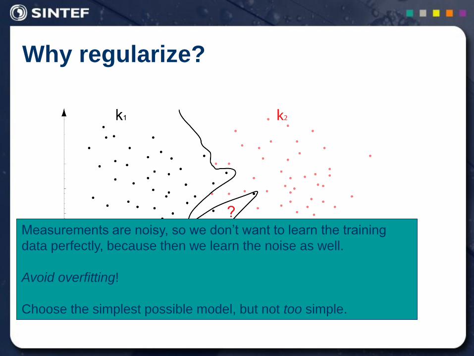
Why regularize?
Measurements are noisy, so we don‟t want to learn the training
data perfectly, because then we learn the noise as well.
Avoid overfitting!
Choose the simplest possible model, but not too simple.
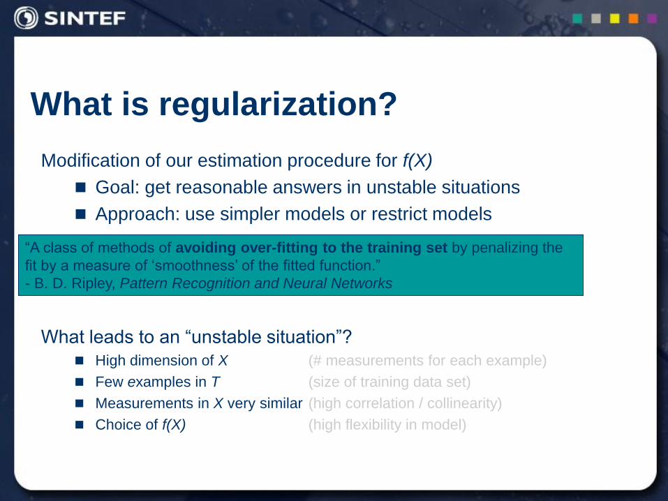
What is regularization?
Modification of our estimation procedure for f(X)
Goal: get reasonable answers in unstable situations
Approach: use simpler models or restrict models
What leads to an “unstable situation”?
High dimension of X (# measurements for each example)
Few examples in T (size of training data set)
Measurements in X very similar (high correlation / collinearity)
Choice of f(X) (high flexibility in model)
“..regularization methods, express our prior belief that the type of functions we
seek exhibit a certain type of smooth behavior…”
– Hastie & al : The Elements of Statistical Learning
“A class of methods of avoiding over-fitting to the training set by penalizing the
fit by a measure of „smoothness‟ of the fitted function.”
- B. D. Ripley, Pattern Recognition and Neural Networks
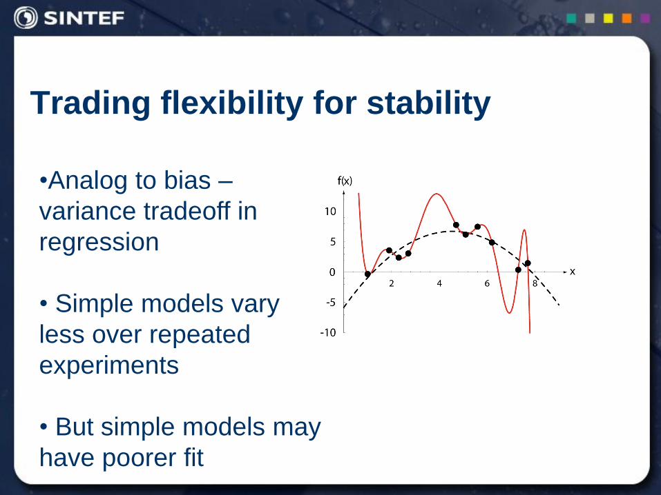
Trading flexibility for stability
•Analog to bias –
variance tradeoff in
regression
• Simple models vary
less over repeated
experiments
• But simple models may
have poorer fit
Examples of regularization in a
classification context
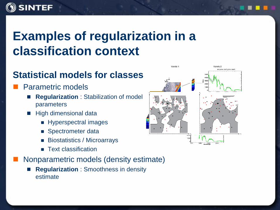
Statistical models for classes
Parametric models
Regularization : Stabilization of model
parameters
High dimensional data
Hyperspectral images
Spectrometer data
Biostatistics / Microarrays
Text classification
Nonparametric models (density estimate)
Regularization : Smoothness in density
estimate
# word combinations
>>
# example documents
Examples of regularization in a
classification context
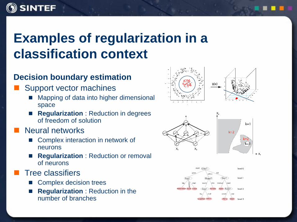
Decision boundary estimation
Support vector machines Mapping of data into higher dimensional
space
Regularization : Reduction in degrees of freedom of solution
Neural networks Complex interaction in network of
neurons
Regularization : Reduction or removal of neurons
Tree classifiers Complex decision trees
Regularization : Reduction in the number of branches
Examples of regularization in a
classification context
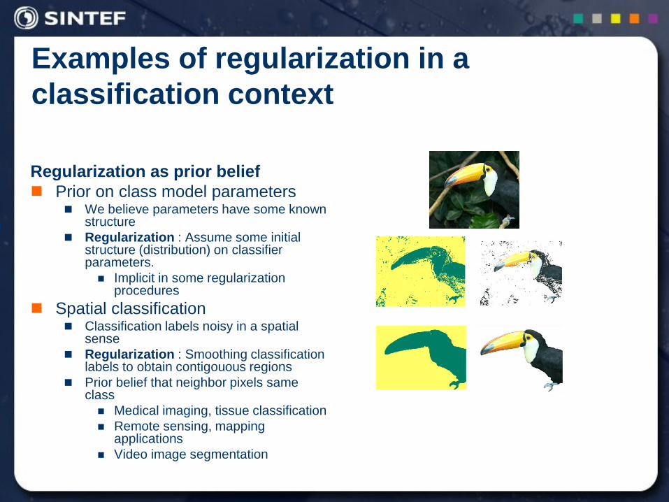
Regularization as prior belief
Prior on class model parameters We believe parameters have some known
structure
Regularization : Assume some initial structure (distribution) on classifier parameters.
Implicit in some regularization procedures
Spatial classification Classification labels noisy in a spatial
sense
Regularization : Smoothing classification labels to obtain contigouous regions
Prior belief that neighbor pixels same class
Medical imaging, tissue classification
Remote sensing, mapping applications
Video image segmentation
pi μi
X Yi
i
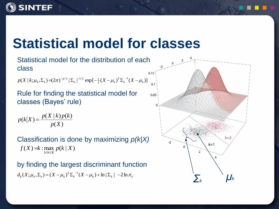
Statistical model for classes
)|(max:)(1
XkpkXfKk
)]()(exp[||)2(),;|(1
212/12/
kk
T
kk
p
kk XXkXp p
Statistical model for the distribution of each
class
Rule for finding the statistical model for
classes (Bayes‟ rule)
Classification is done by maximizing p(k|X)
by finding the largest discriminant function
)(
)()|()(
Xp
kpkXpXkp
μk Σk kkkk
T
kkkk XXXd p ln2||ln)()(),;(1
Covariance matrix stabilization
p
i ik
T
ikikk
p
i
T
ikikik
T
kkkk
a
dd
ddaDAD
1
1
1
k
p
i
ik
p
i ik
k
T
ikk a
a
XdXd p
ln2)ln(
)]([)(
11
2
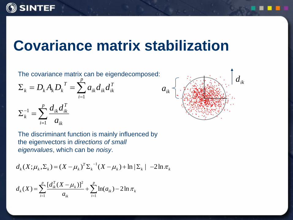
The covariance matrix can be eigendecomposed:
The discriminant function is mainly influenced by
the eigenvectors in directions of small
eigenvalues, which can be noisy.
Correlation increases => the ratio between
the smallest and the largest eigenvaue increases
ikaikd
kkkk
T
kkkk XXXd p ln2||ln)()(),;(1
A short example of the variability in the
discriminant function
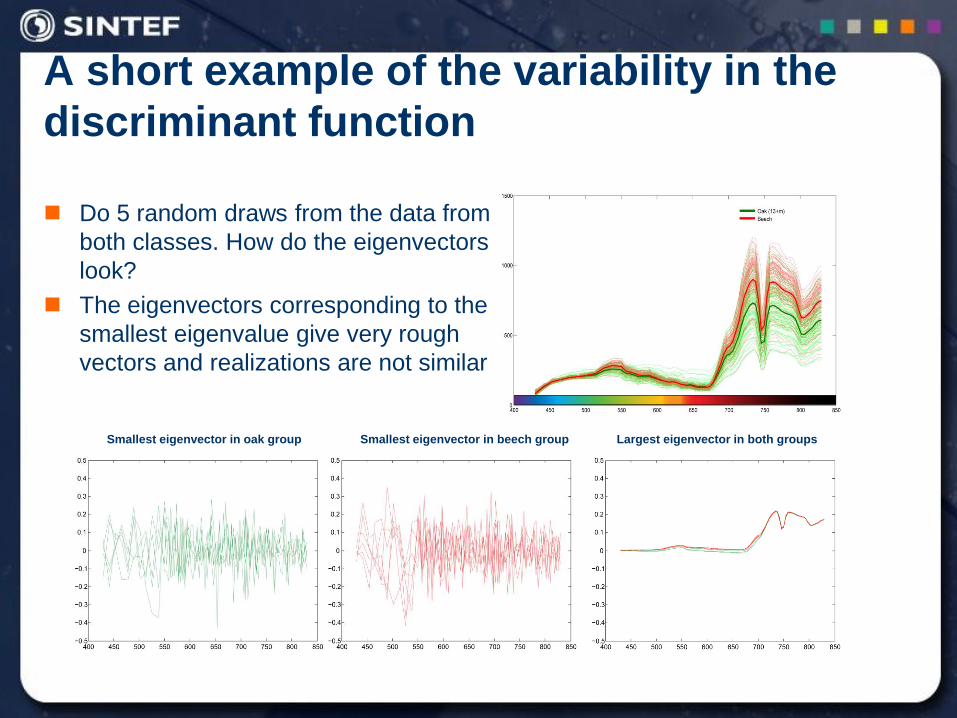
Do 5 random draws from the data from
both classes. How do the eigenvectors
look?
The eigenvectors corresponding to the
smallest eigenvalue give very rough
vectors and realizations are not similar
Smallest eigenvector in oak group Smallest eigenvector in beech group Largest eigenvector in both groups
Covariance matrix stabilization
• Truncate or adjust eigenvalues in the distance
measure
•Spectrometry approaches such as SIMCA, DASCO
and ZVD
•Add a diagonal matrix (“ridge regression”)
•Flexible discriminant analysis (Legg til en omega,
fex den andrederiverte)
• Use simpler estimates or a combination of simpler
estimates
•LDA (!)
•RDA /LOOC and variants, eigendecomp
•Naïve bayes, STIC-like
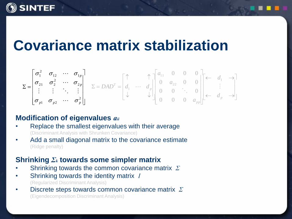
Modification of eigenvalues aii • Replace the smallest eigenvalues with their average
(Discriminant Analysis with Shrunken Covariance)
• Add a small diagonal matrix to the covariance estimate (Ridge penalty)
Shrinking Σk towards some simpler matrix • Shrinking towards the common covariance matrix Σ
• Shrinking towards the identity matrix I (Regularized Discriminant Analysis)
• Discrete steps towards common covariance matrix Σ
(Eigendecomposition Discriminant Analysis)
2
21
2
2
221
112
2
1
ppp
p
p
p
pp
p
T
d
d
a
a
a
ddDAD
1
22
11
1
000
000
000
000
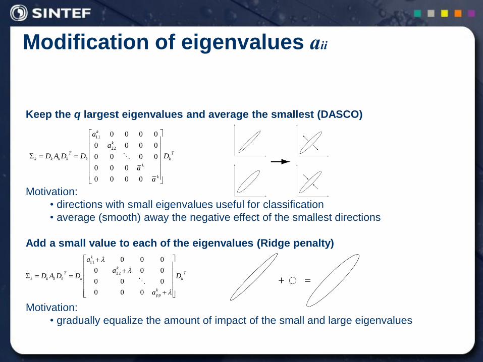
Modification of eigenvalues aii
Keep the q largest eigenvalues and average the smallest (DASCO)
Motivation:
• directions with small eigenvalues useful for classification
• average (smooth) away the negative effect of the smallest directions
Add a small value to each of the eigenvalues (Ridge penalty)
Motivation:
• gradually equalize the amount of impact of the small and large eigenvalues
...,
0000
000
0000
00000
00000
11
aD
a
a
DDDA TT
T
k
k
pp
k
k
k
T
kkkk D
a
a
a
DDAD
000
000
000
000
22
11
T
k
k
k
k
k
k
T
kkkk D
a
a
a
a
DDAD
0000
000
0000
0000
0000
22
11
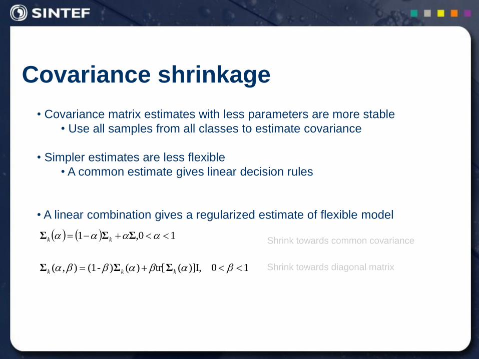
Covariance shrinkage
10]I,)(tr[)()-(1),(
10,1
kkk
kk
ΣΣΣ
ΣΣΣ
• Covariance matrix estimates with less parameters are more stable
• Use all samples from all classes to estimate covariance
• Simpler estimates are less flexible
• A common estimate gives linear decision rules
• A linear combination gives a regularized estimate of flexible model
Shrink towards diagonal matrix
Shrink towards common covariance
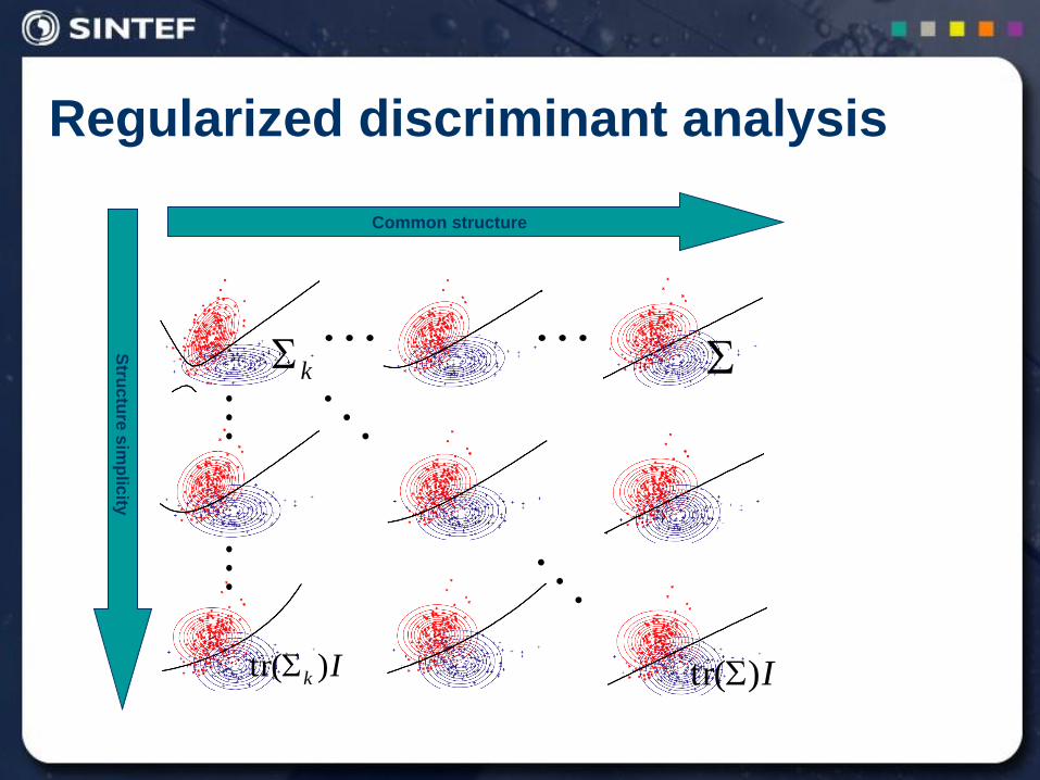
Regularized discriminant analysis
Common structure
Stru
ctu
re s
imp
licity
Ik )(tr
k
I)(tr
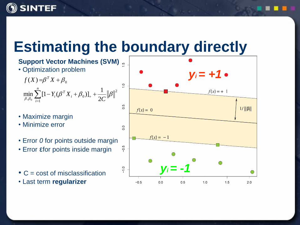
Estimating the boundary directly Support Vector Machines (SVM)
• Optimization problem
• Maximize margin
• Minimize error
• Error 0 for points outside margin
• Error εfor points inside margin
• C = cost of misclassification
• Last term regularizer
2
1
0,
0
2
1)](1[min
)(
0
CXY
XXf
n
i
i
T
i
T
yi = +1
yi = -1
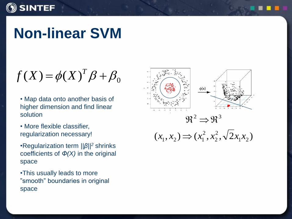
Non-linear SVM
0)()( TXXf
)2,,(),( 21
2
2
2
121
32
xxxxxx
• Map data onto another basis of
higher dimension and find linear
solution
• More flexible classifier,
regularization necessary!
•Regularization term ||β||2 shrinks
coefficients of Φ(X) in the original
space
•This usually leads to more
”smooth” boundaries in original
space
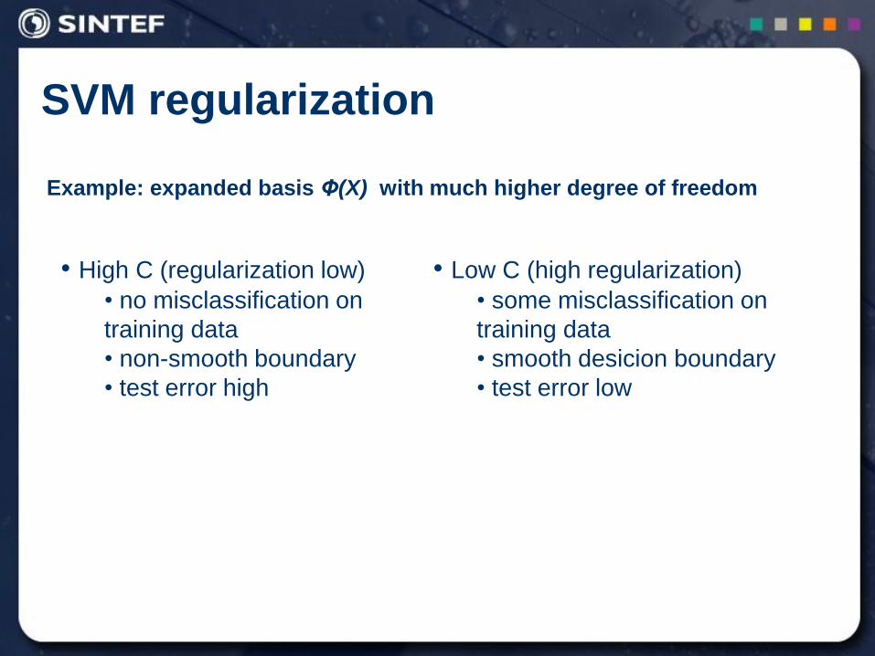
SVM regularization
Example: expanded basis Φ(X) with much higher degree of freedom
• High C (regularization low)
• no misclassification on
training data
• non-smooth boundary
• test error high
• Low C (high regularization)
• some misclassification on
training data
• smooth desicion boundary
• test error low
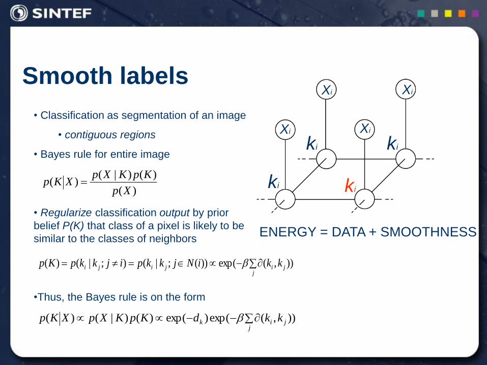
Smooth labels
• Classification as segmentation of an image
• contiguous regions
• Bayes rule for entire image
• Regularize classification output by prior
belief P(K) that class of a pixel is likely to be
similar to the classes of neighbors
•Thus, the Bayes rule is on the form
)),(exp())(;|();|()( j
jijiji kkiNjkkpijkkpKp
Let πk vary over the image
)(
)()|()(
Xp
KpKXpXKp
ki
ki ki
ki
Xi
Xi
Xi
Xi
ENERGY = DATA + SMOOTHNESS
)),(exp()exp()()|()( j
jik kkdKpKXpXKp
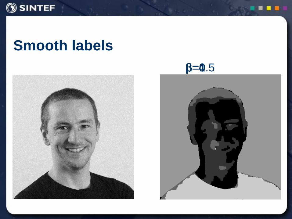
Smooth labels
β=0 β=0.5 β=4 β=1
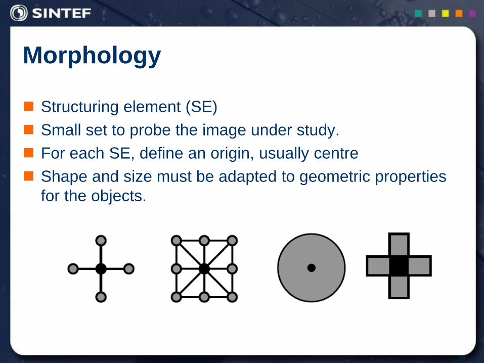
Morphology
Structuring element (SE)
Small set to probe the image under study.
For each SE, define an origin, usually centre
Shape and size must be adapted to geometric properties
for the objects.
28
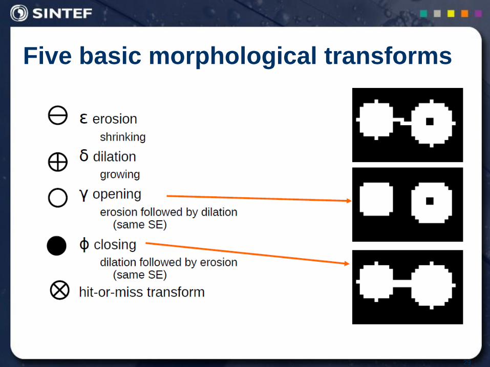
Five basic morphological transforms
29
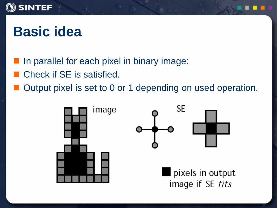
Basic idea
In parallel for each pixel in binary image:
Check if SE is satisfied.
Output pixel is set to 0 or 1 depending on used operation.
30
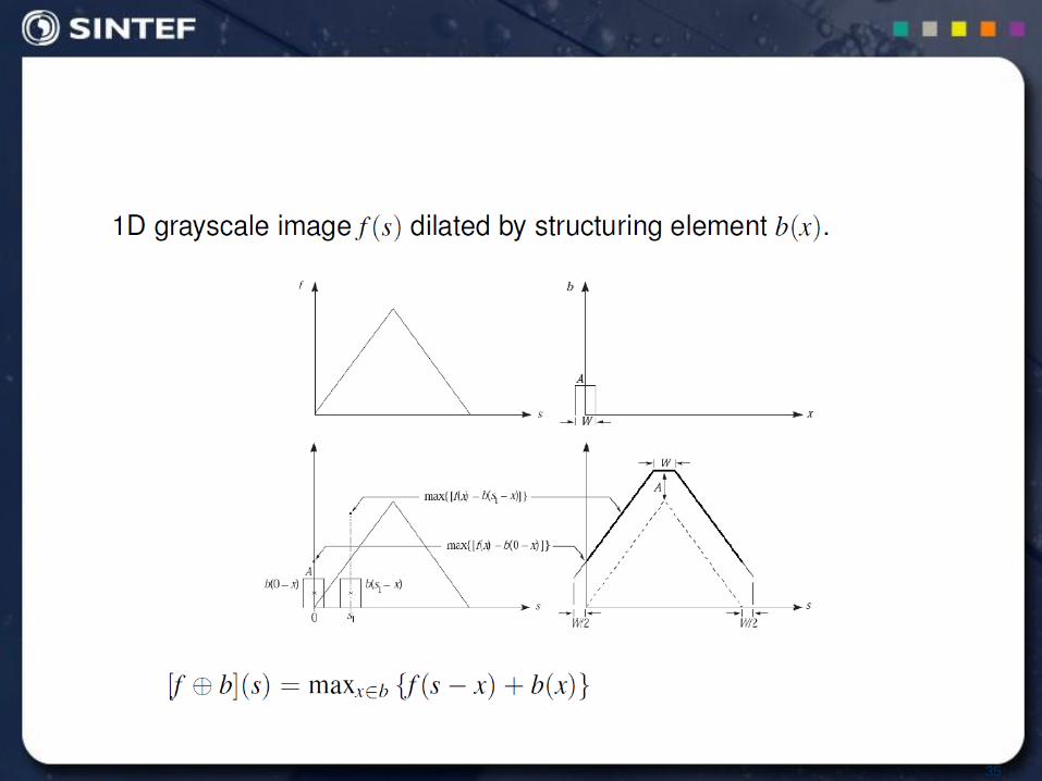
35
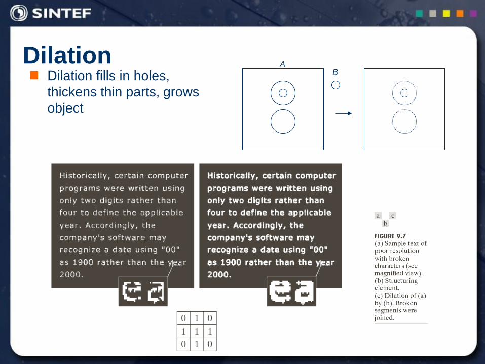
Dilation Dilation fills in holes,
thickens thin parts, grows
object
B A
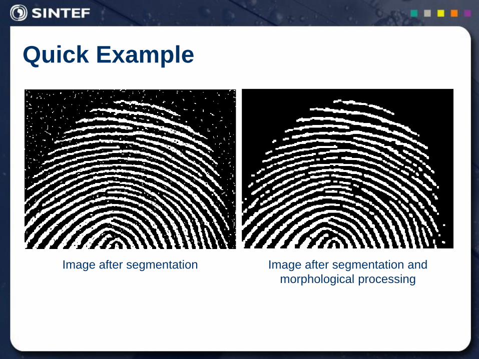
Quick Example
Image after segmentation Image after segmentation and
morphological processing
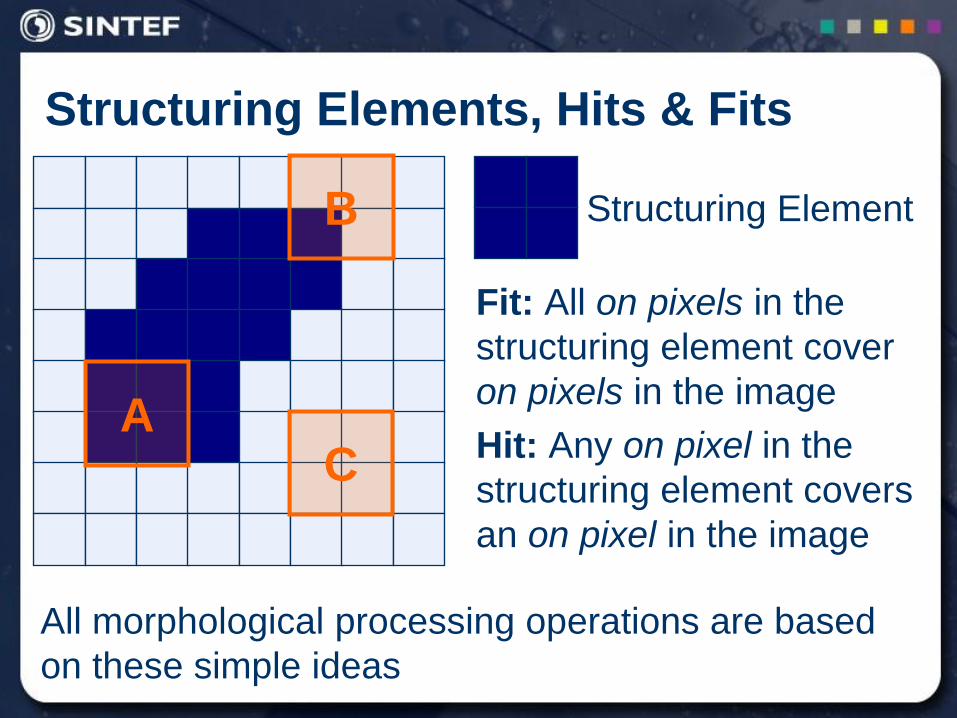
Structuring Elements, Hits & Fits
B
A C
Structuring Element
Fit: All on pixels in the
structuring element cover
on pixels in the image
Hit: Any on pixel in the
structuring element covers
an on pixel in the image
All morphological processing operations are based
on these simple ideas
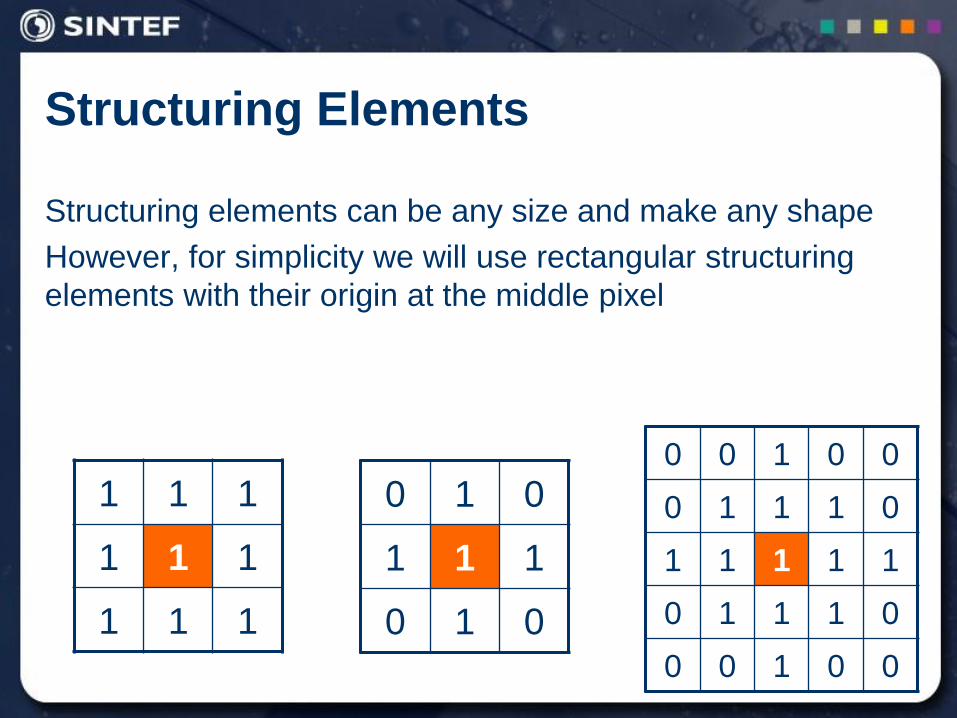
Structuring Elements
Structuring elements can be any size and make any shape
However, for simplicity we will use rectangular structuring
elements with their origin at the middle pixel
1 1 1
1 1 1
1 1 1
0 0 1 0 0
0 1 1 1 0
1 1 1 1 1
0 1 1 1 0
0 0 1 0 0
0 1 0
1 1 1
0 1 0
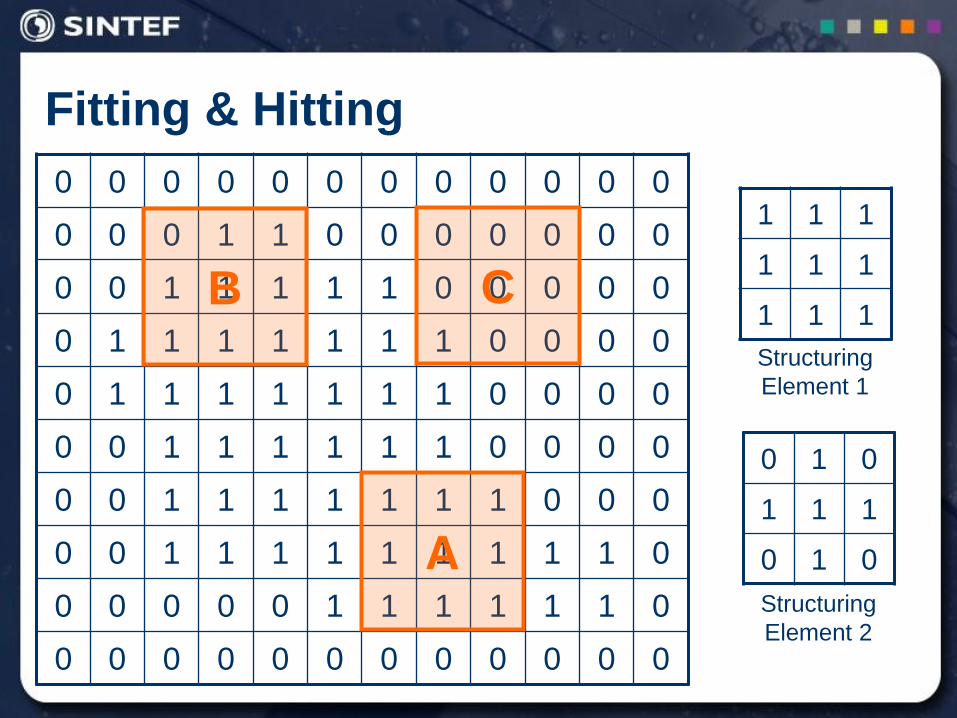
Fitting & Hitting
0 0 0 0 0 0 0 0 0 0 0 0
0 0 0 1 1 0 0 0 0 0 0 0
0 0 1 1 1 1 1 0 0 0 0 0
0 1 1 1 1 1 1 1 0 0 0 0
0 1 1 1 1 1 1 1 0 0 0 0
0 0 1 1 1 1 1 1 0 0 0 0
0 0 1 1 1 1 1 1 1 0 0 0
0 0 1 1 1 1 1 1 1 1 1 0
0 0 0 0 0 1 1 1 1 1 1 0
0 0 0 0 0 0 0 0 0 0 0 0
B C
A
1 1 1
1 1 1
1 1 1
Structuring
Element 1
0 1 0
1 1 1
0 1 0
Structuring
Element 2
Fundamental Operations
Fundamentally morphological image processing is very like
spatial filtering
The structuring element is moved across every pixel in the
original image to give a pixel in a new processed image
The value of this new pixel depends on the operation
performed
There are two basic morphological operations: erosion and
dilation
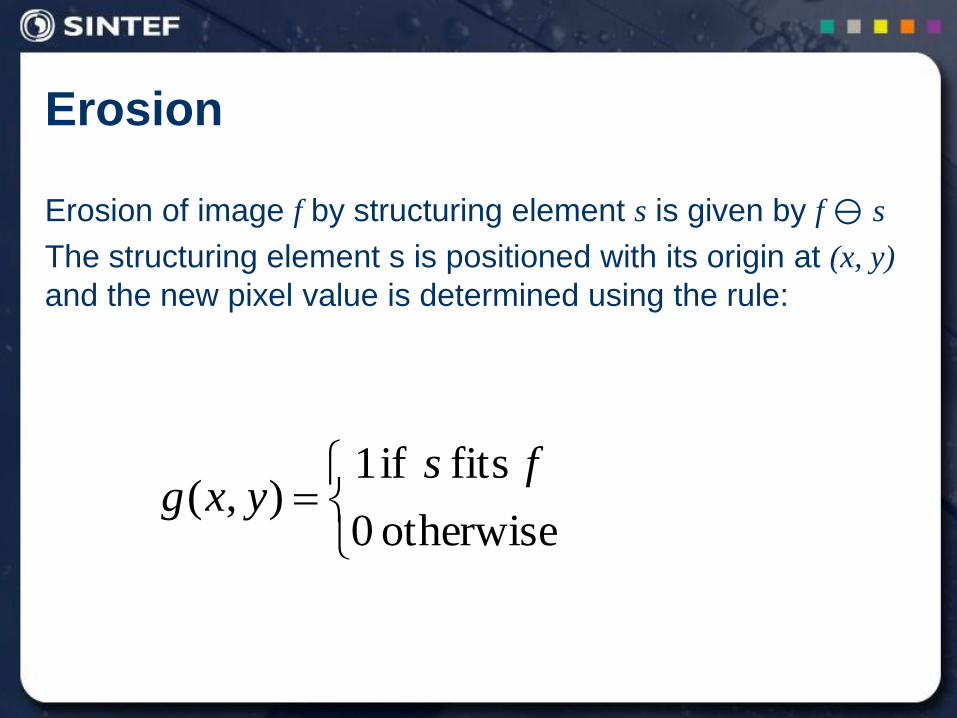
Erosion
Erosion of image f by structuring element s is given by f s
The structuring element s is positioned with its origin at (x, y)
and the new pixel value is determined using the rule:
otherwise 0
fits if 1),(
fsyxg
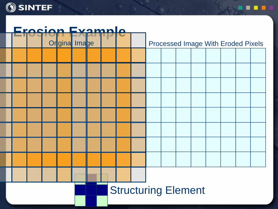
Erosion Example
Structuring Element
Original Image Processed Image With Eroded Pixels
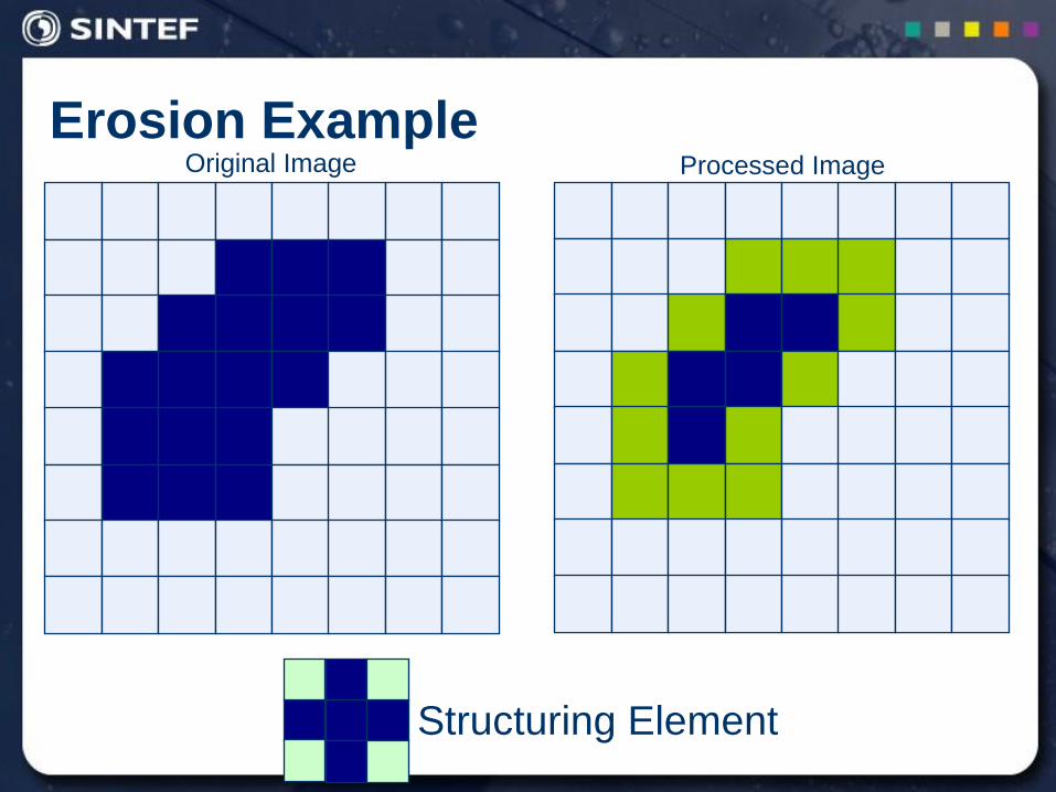
Erosion Example
Structuring Element
Original Image Processed Image
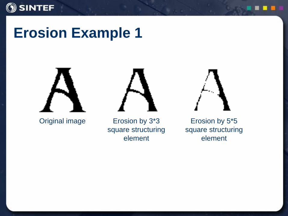
Erosion Example 1
Original image Erosion by 3*3
square structuring
element
Erosion by 5*5
square structuring
element
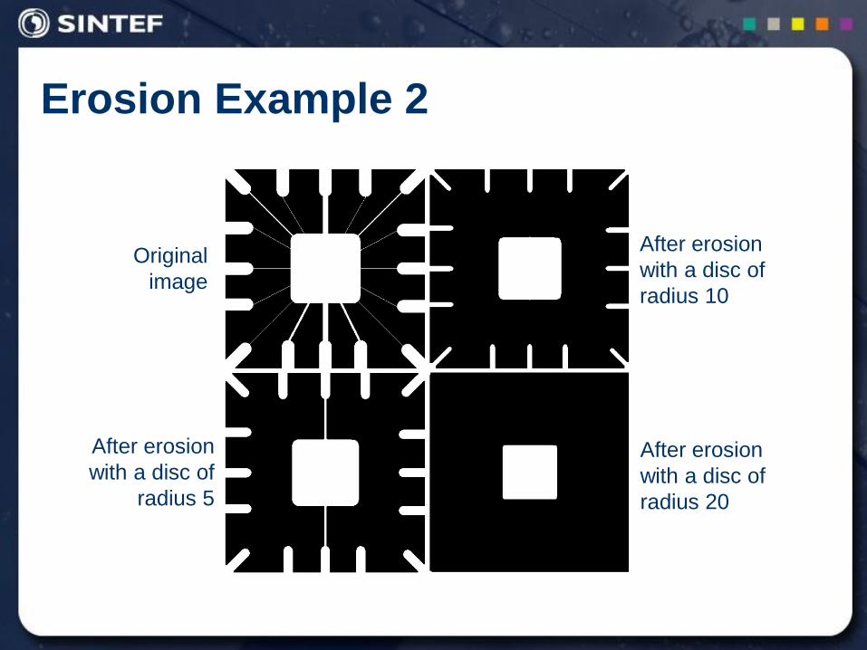
Erosion Example 2
Original
image
After erosion
with a disc of
radius 10
After erosion
with a disc of
radius 20
After erosion
with a disc of
radius 5

Dilation
Dilation of image f by structuring element s is given by f s
The structuring element s is positioned with its origin at (x, y)
and the new pixel value is determined using the rule:
otherwise 0
hits if 1),(
fsyxg
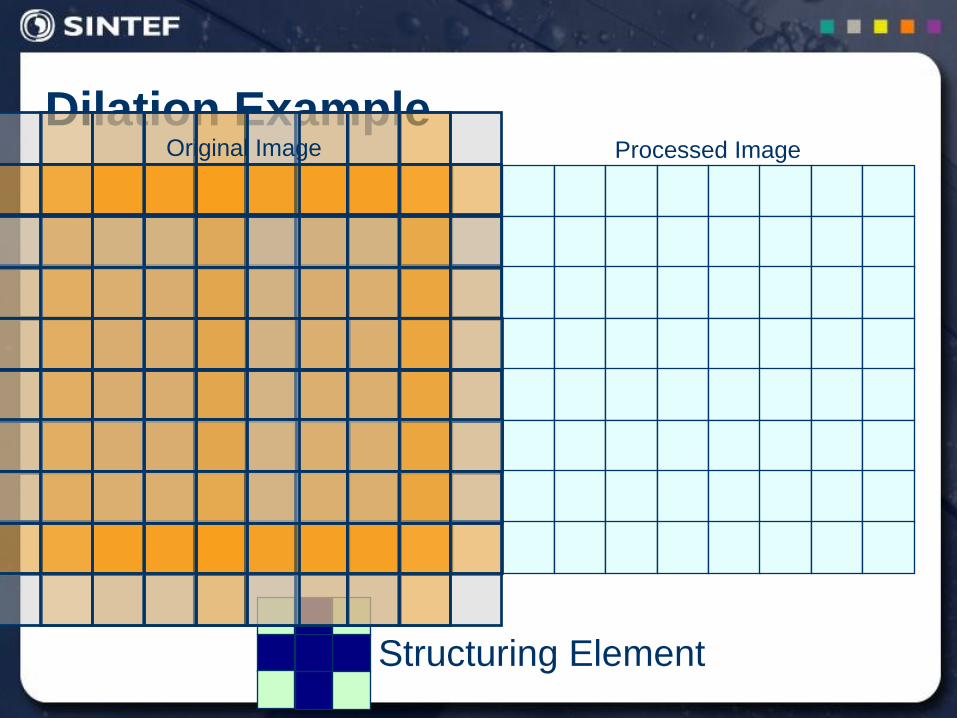
Dilation Example
Structuring Element
Original Image Processed Image
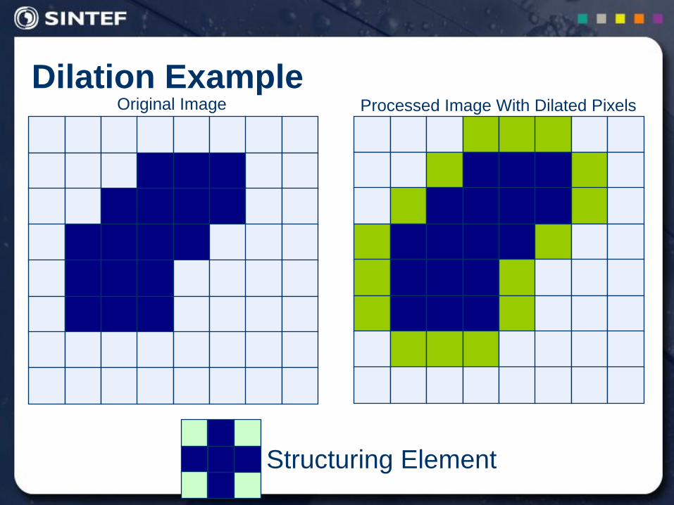
Dilation Example
Structuring Element
Original Image Processed Image With Dilated Pixels
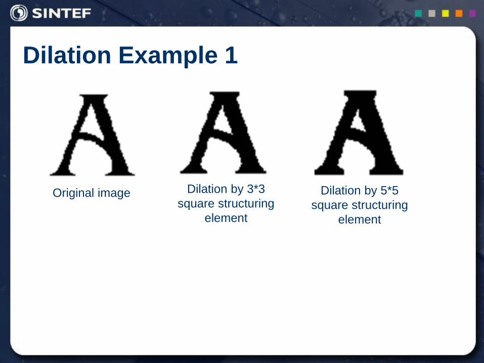
Dilation Example 1
Original image Dilation by 3*3
square structuring
element
Dilation by 5*5
square structuring
element
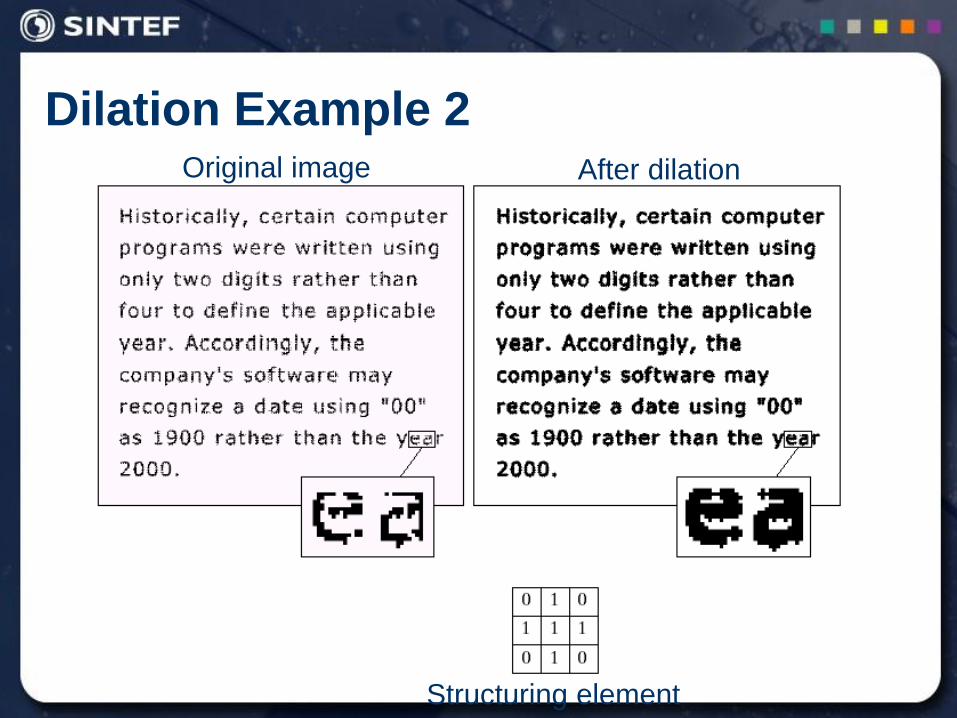
Dilation Example 2
Structuring element
Original image After dilation
Compound Operations
More interesting morphological operations can be performed
by performing combinations of erosions and dilations
The most widely used of these compound operations are:
Opening
Closing
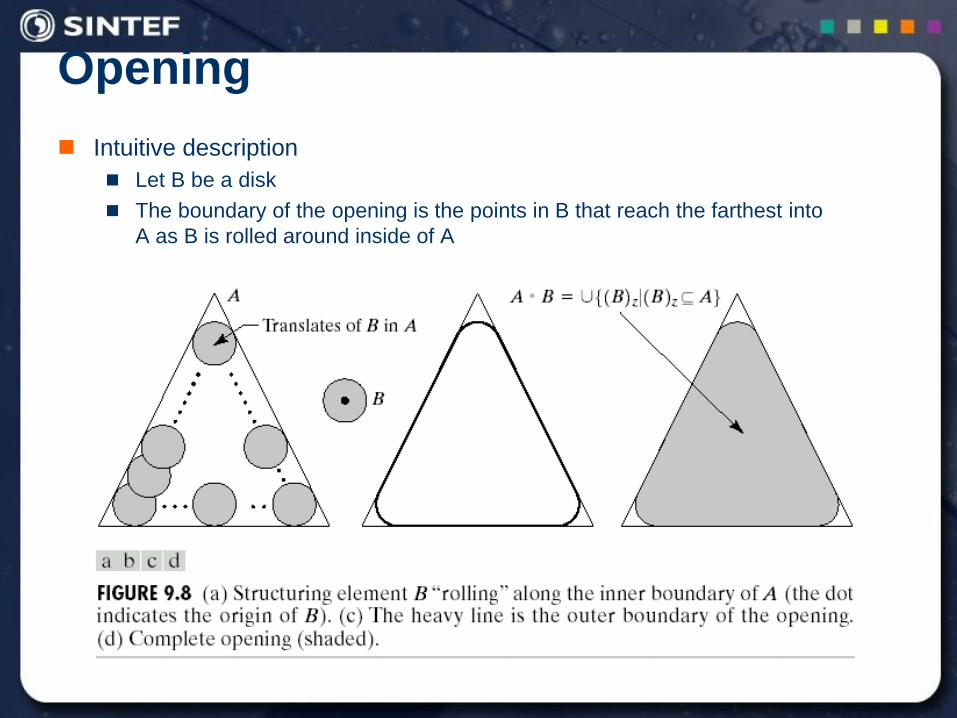
Opening
Intuitive description
Let B be a disk
The boundary of the opening is the points in B that reach the farthest into
A as B is rolled around inside of A
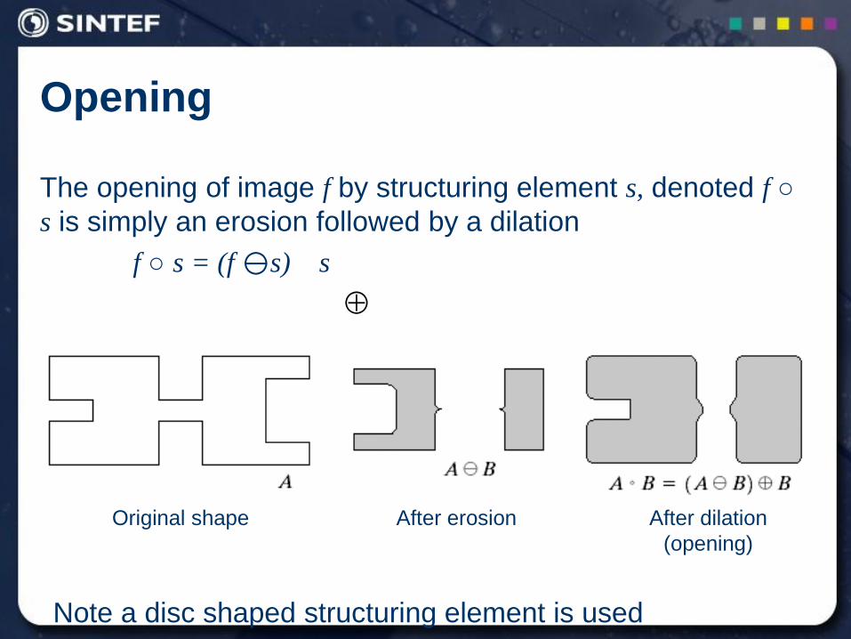
Opening
The opening of image f by structuring element s, denoted f ○
s is simply an erosion followed by a dilation
f ○ s = (f s) s
Original shape After erosion After dilation
(opening)
Note a disc shaped structuring element is used
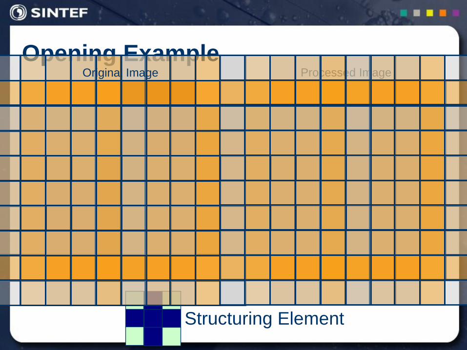
Opening Example
Structuring Element
Original Image Processed Image
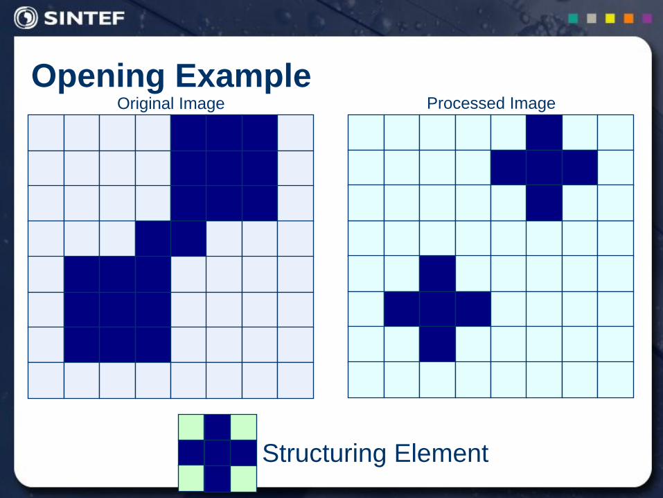
Opening Example
Structuring Element
Original Image Processed Image
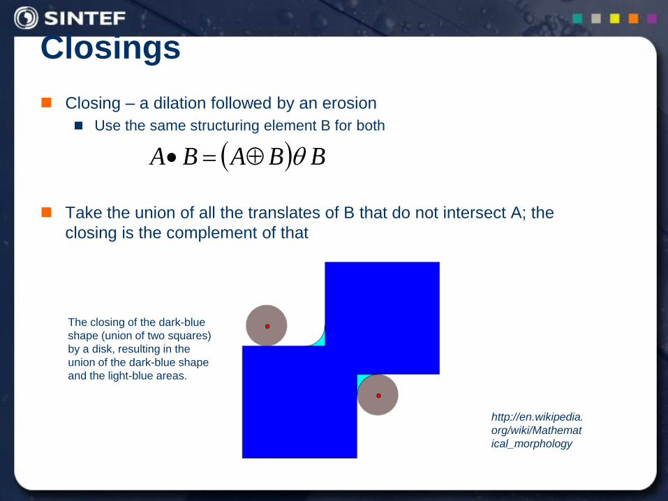
Closings
Closing – a dilation followed by an erosion
Use the same structuring element B for both
Take the union of all the translates of B that do not intersect A; the
closing is the complement of that
BBABA
The closing of the dark-blue
shape (union of two squares)
by a disk, resulting in the
union of the dark-blue shape
and the light-blue areas.
http://en.wikipedia.
org/wiki/Mathemat
ical_morphology
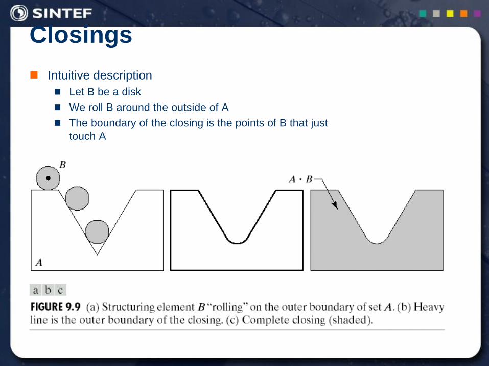
Closings
Intuitive description
Let B be a disk
We roll B around the outside of A
The boundary of the closing is the points of B that just
touch A
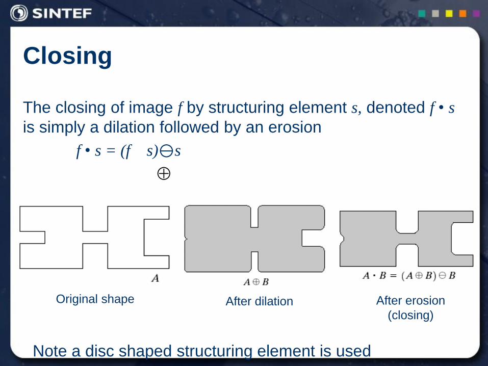
Closing
The closing of image f by structuring element s, denoted f • s
is simply a dilation followed by an erosion
f • s = (f s)s
Original shape After dilation After erosion
(closing)
Note a disc shaped structuring element is used
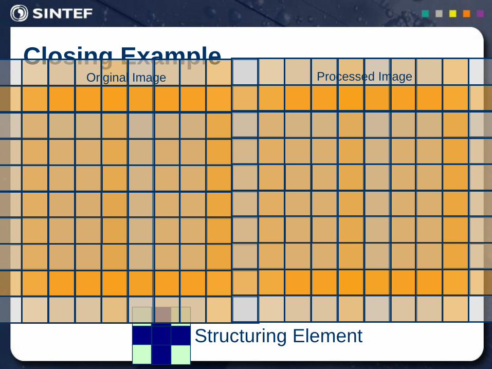
Closing Example
Structuring Element
Original Image Processed Image
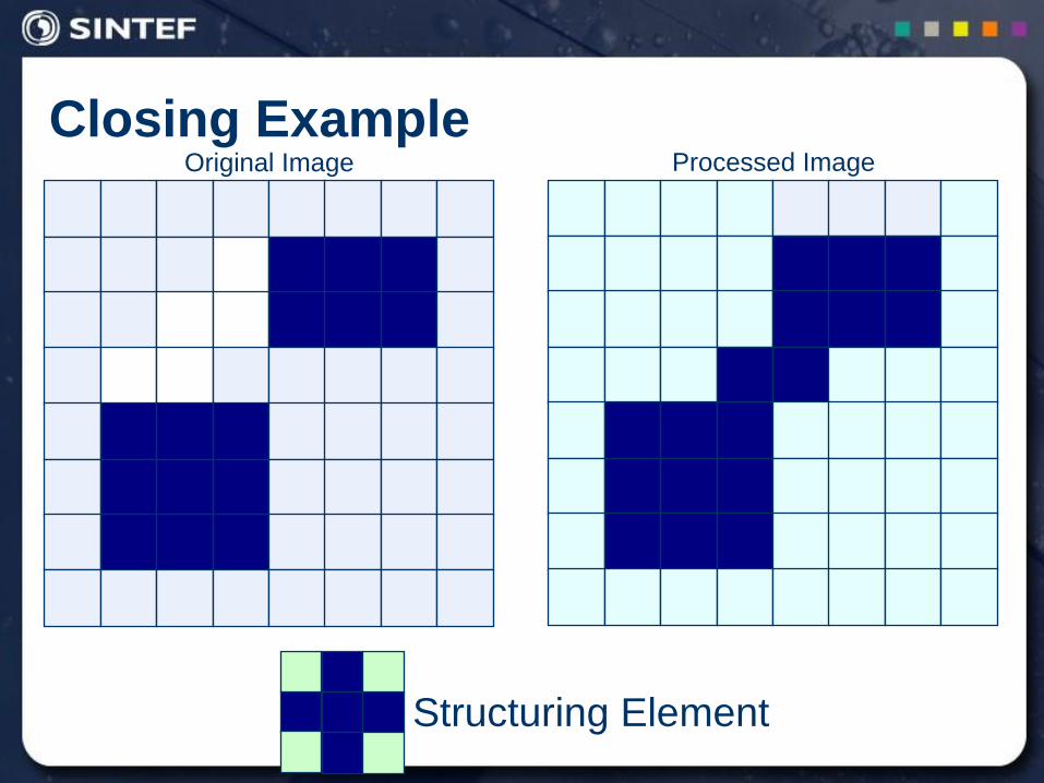
Closing Example
Structuring Element
Original Image Processed Image
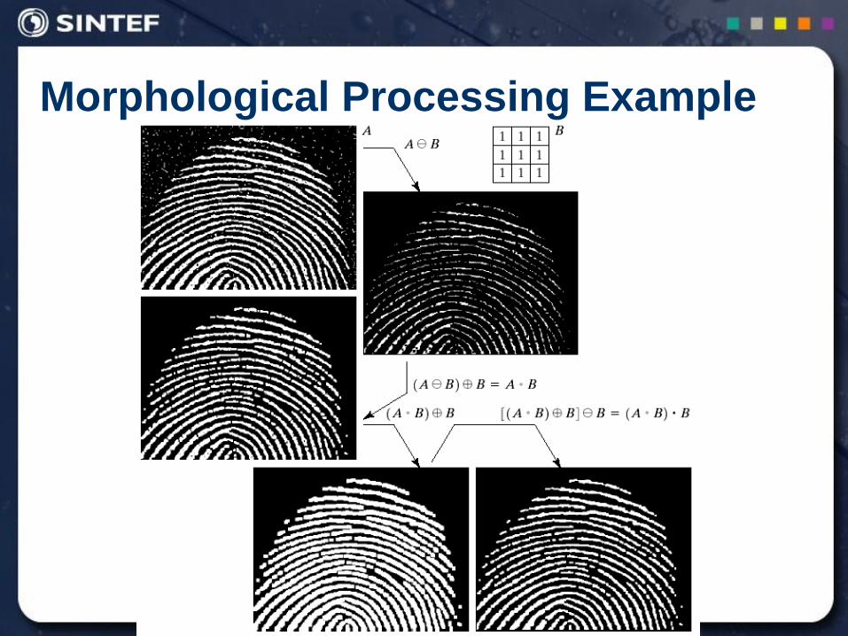
Morphological Processing Example
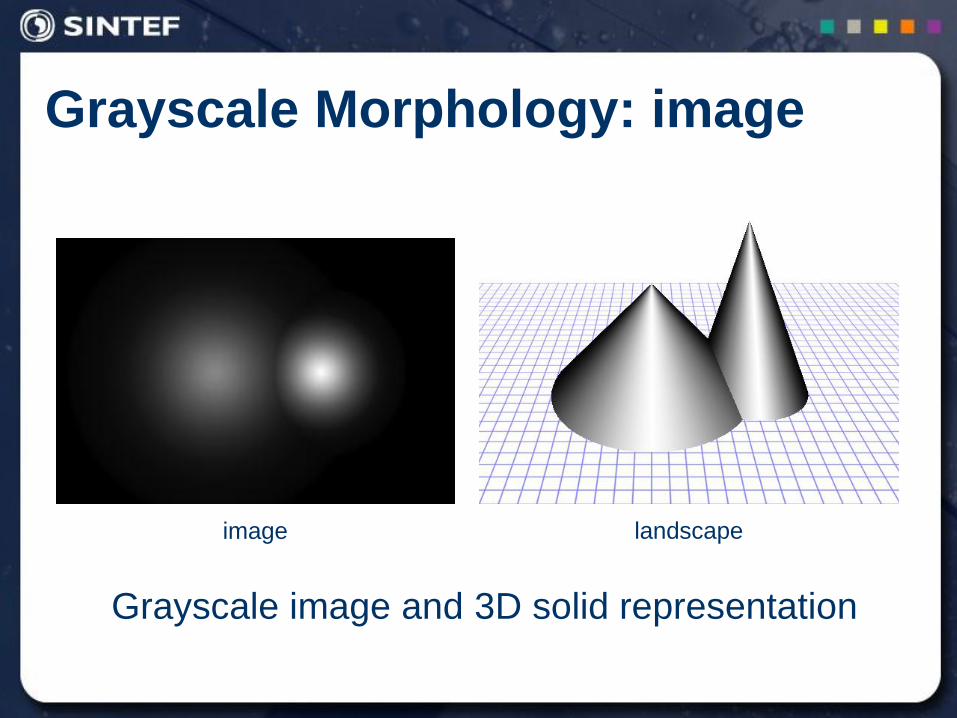
Grayscale Morphology: image
Grayscale image and 3D solid representation
image landscape
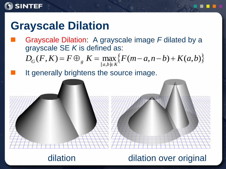
Grayscale Dilation
dilation dilation over original
Grayscale Dilation: A grayscale image F dilated by a grayscale SE K is defined as:
It generally brightens the source image.
),(),(max),(],[
baKbnamFKFKFDKba
gG
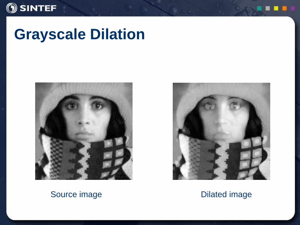
Grayscale Dilation
Source image Dilated image
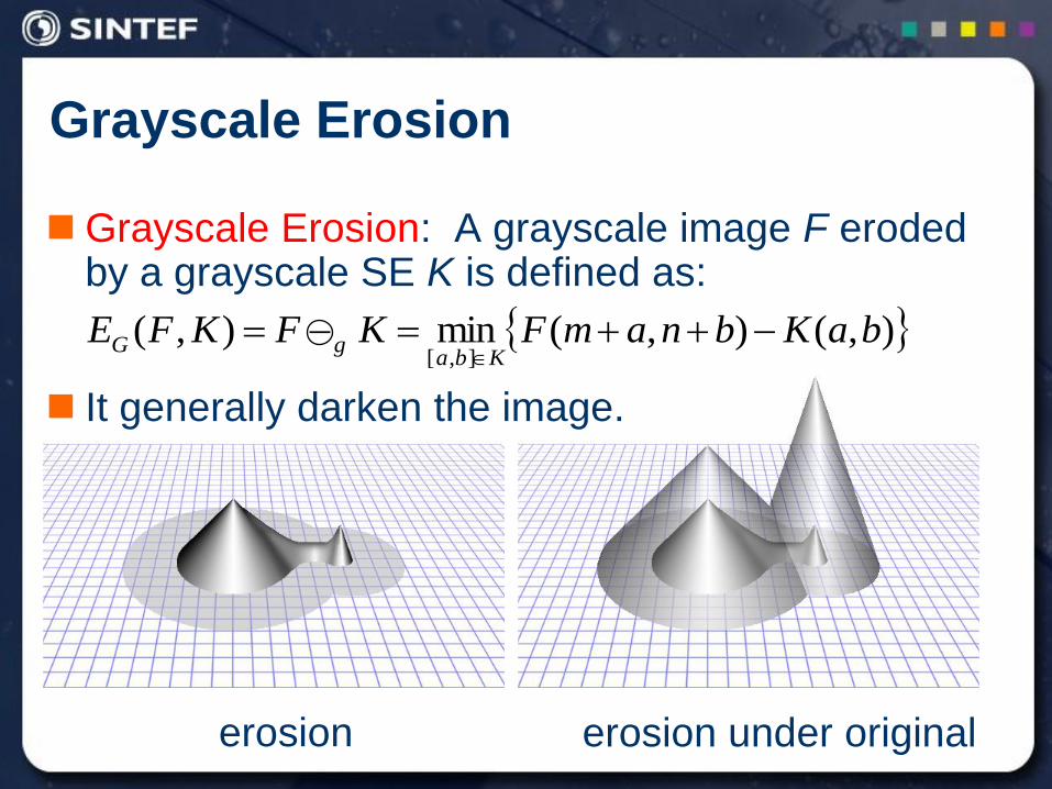
Grayscale Erosion
erosion erosion under original
Grayscale Erosion: A grayscale image F eroded by a grayscale SE K is defined as:
It generally darken the image.
),(),(min),(],[
baKbnamFKFKFEKba
gG
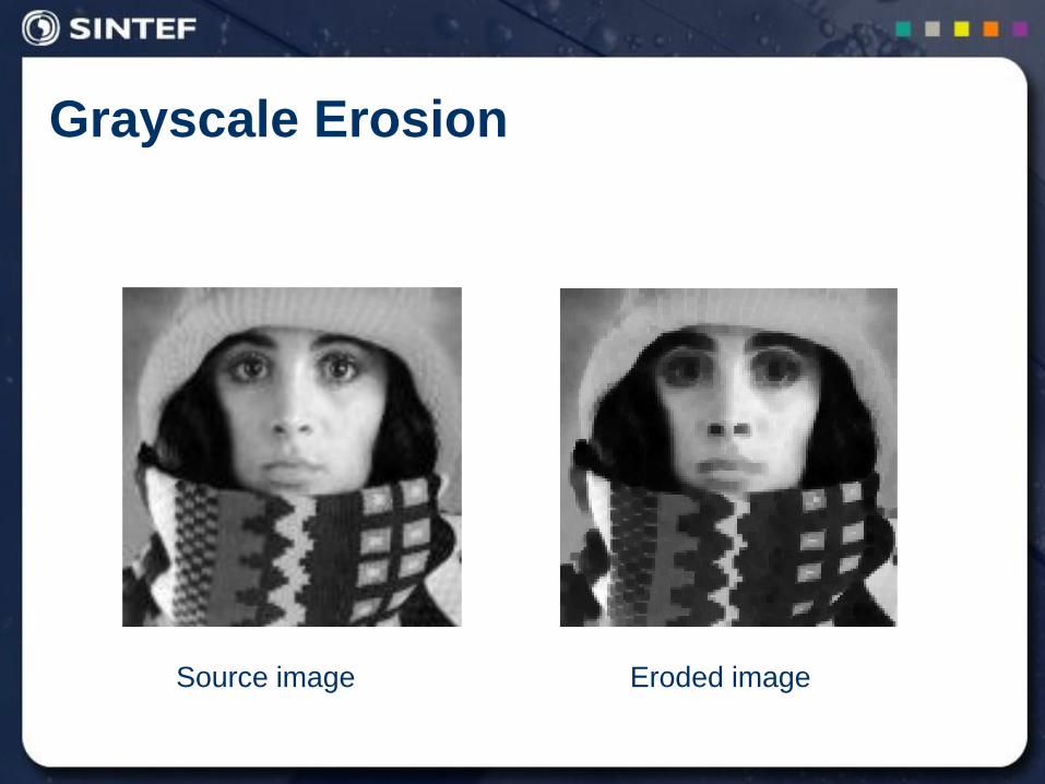
Grayscale Erosion
Source image Eroded image
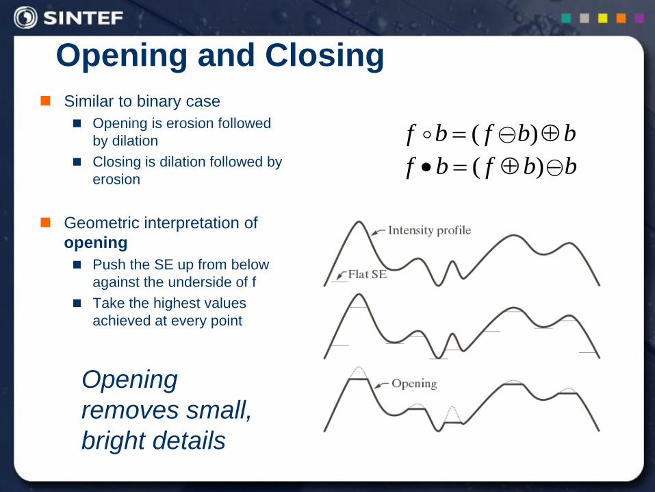
Similar to binary case
Opening is erosion followed
by dilation
Closing is dilation followed by
erosion
Geometric interpretation of
opening
Push the SE up from below
against the underside of f
Take the highest values
achieved at every point
Opening and Closing
Opening
removes small,
bright details
bbfbf )(
bbfbf )(
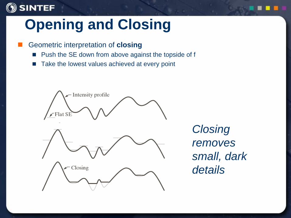
Opening and Closing
Geometric interpretation of closing
Push the SE down from above against the topside of f
Take the lowest values achieved at every point
Closing
removes
small, dark
details
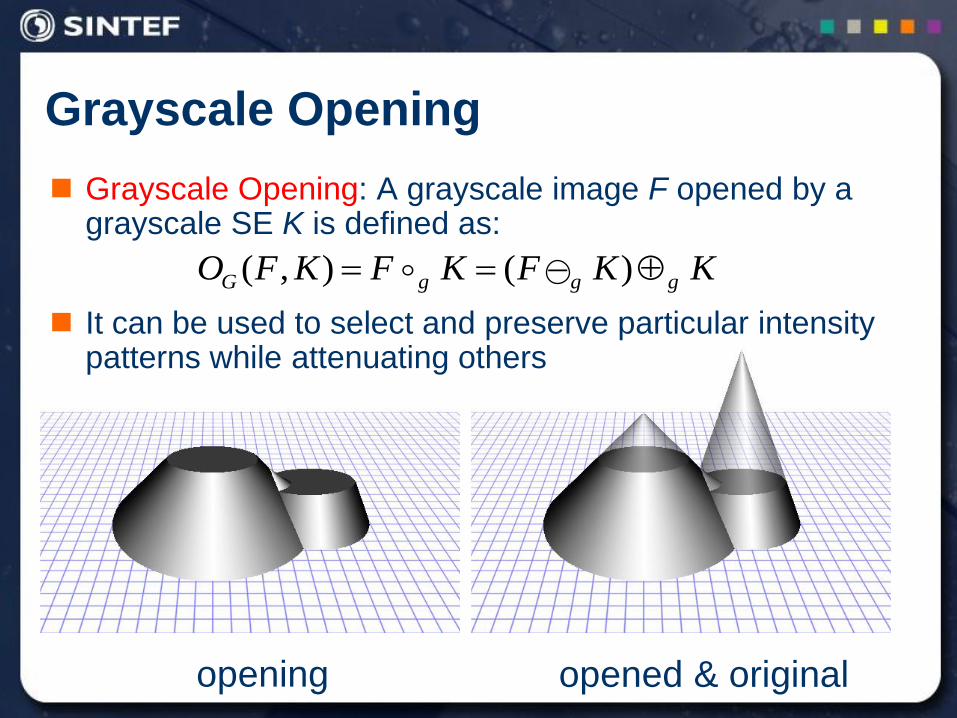
Grayscale Opening
opening opened & original
Grayscale Opening: A grayscale image F opened by a grayscale SE K is defined as:
It can be used to select and preserve particular intensity patterns while attenuating others
KKFKFKFO gggG )(),(
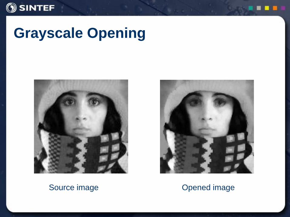
Grayscale Opening
Source image Opened image
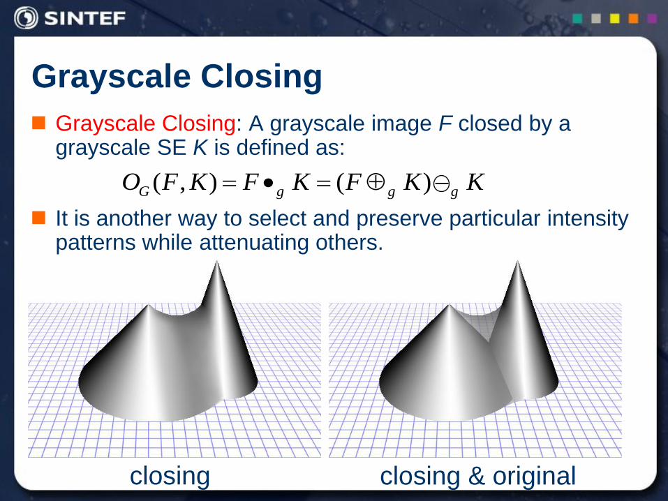
Grayscale Closing
closing closing & original
Grayscale Closing: A grayscale image F closed by a grayscale SE K is defined as:
It is another way to select and preserve particular intensity patterns while attenuating others.
KKFKFKFO gggG )(),(
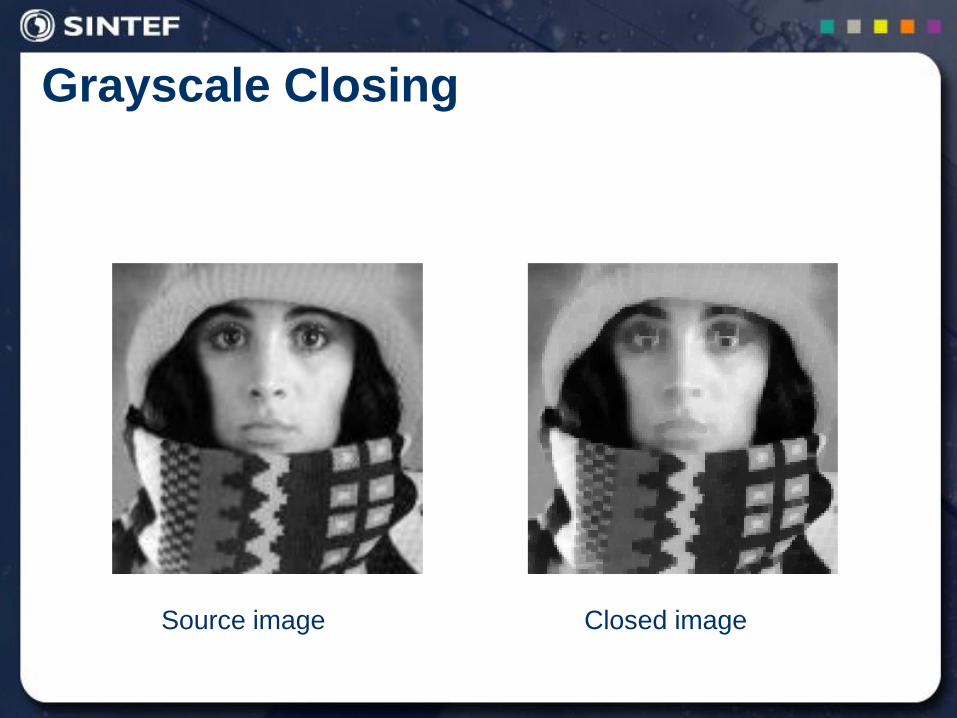
Grayscale Closing
Source image Closed image
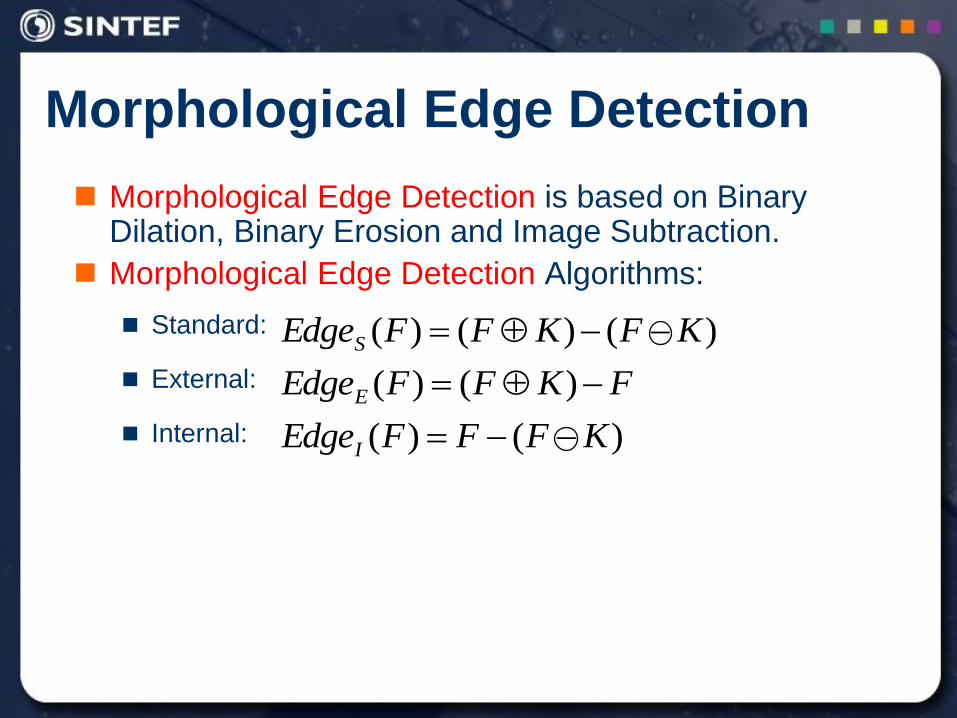
Morphological Edge Detection
Morphological Edge Detection is based on Binary Dilation, Binary Erosion and Image Subtraction.
Morphological Edge Detection Algorithms:
Standard:
External:
Internal:
)()()( KFKFFEdgeS
FKFFEdgeE )()(
)()( KFFFEdgeI
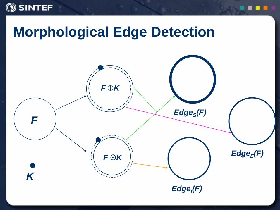
Morphological Edge Detection
F
K
F K
F ΘK EdgeE(F)
EdgeS(F)
EdgeI(F)

Morphological Edge Detection
F
EdgeS(F) EdgeE(F)
EdgeI(F)
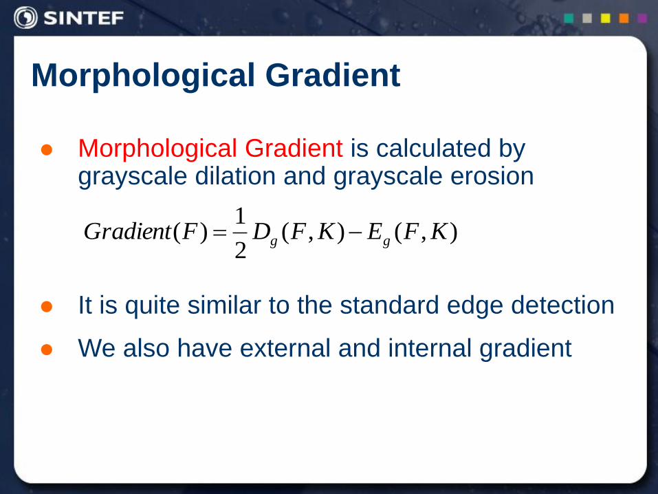
Morphological Gradient
Morphological Gradient is calculated by grayscale dilation and grayscale erosion
It is quite similar to the standard edge detection
We also have external and internal gradient
),(),(2
1)( KFEKFDFGradient gg
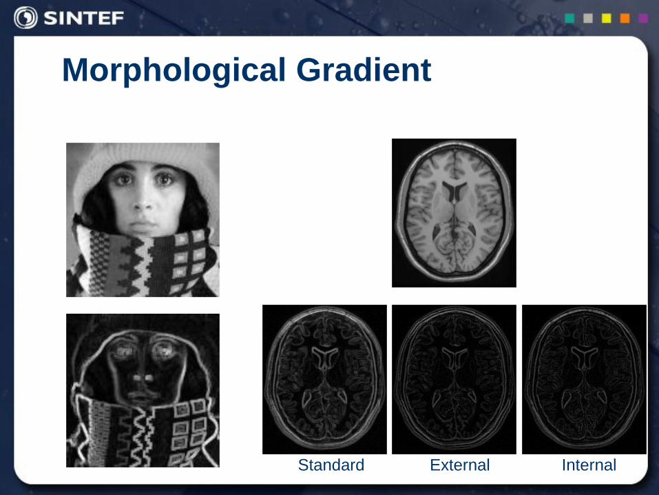
Morphological Gradient
Standard External Internal
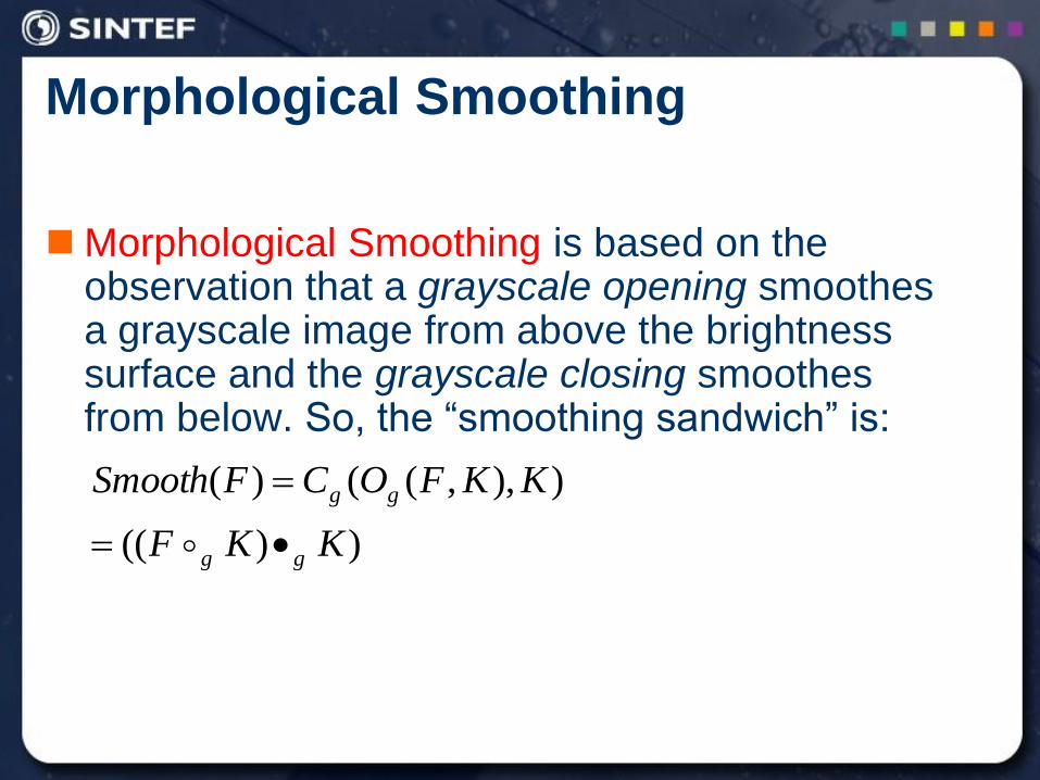
Morphological Smoothing
Morphological Smoothing is based on the observation that a grayscale opening smoothes a grayscale image from above the brightness surface and the grayscale closing smoothes from below. So, the “smoothing sandwich” is:
))((
)),,(()(
KKF
KKFOCFSmooth
gg
gg
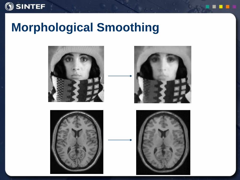
Morphological Smoothing
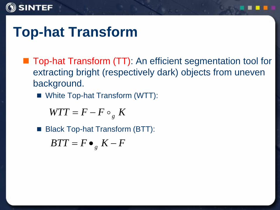
Top-hat Transform
Top-hat Transform (TT): An efficient segmentation tool for
extracting bright (respectively dark) objects from uneven
background.
White Top-hat Transform (WTT):
Black Top-hat Transform (BTT):
KFFWTT g
FKFBTT g
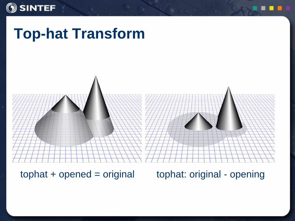
Top-hat Transform
tophat + opened = original tophat: original - opening
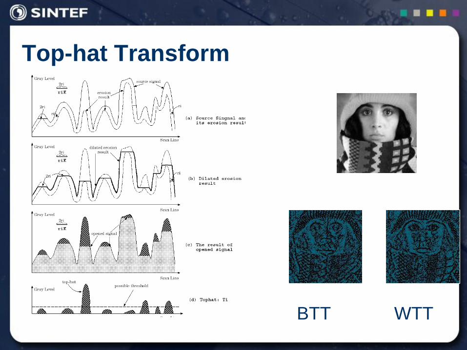
Top-hat Transform
BTT WTT
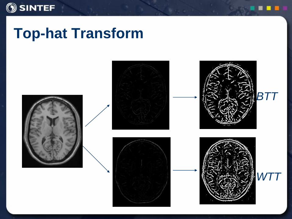
Top-hat Transform
BTT
WTT
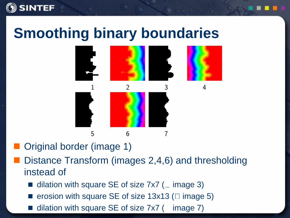
Smoothing binary boundaries
Original border (image 1)
Distance Transform (images 2,4,6) and thresholding
instead of
dilation with square SE of size 7x7 ( image 3)
erosion with square SE of size 13x13 ( image 5)
dilation with square SE of size 7x7 ( image 7) 90
Energy Minimization Problems
In general terms, given some problem, we: Formulate the known constraints
Build an “energy function” (aka “cost function”)
Look for a solution that minimizes it
If we have no further knowledge: The problem can be NP-Hard (requires exponential solution
time)
Use slow, generic approximation algorithms for optimization problems (such as simulated annealing)
EM in Computer Vision
Consider a broad class of problems called Pixel Labeling
Given some images we want to “say something about the pixels”
For each pixel p, give it a label fp from a finite set of labels L,
such that we minimize some energy function.
Many applications
Image Segmentation
Image Restoration
Stereo and Motion
Medical Imaging
Multicamera Scene Reconstruction
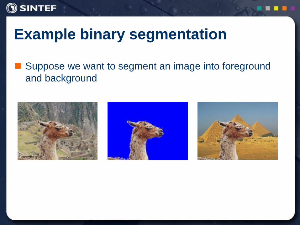
Example binary segmentation
Suppose we want to segment an image into foreground
and background
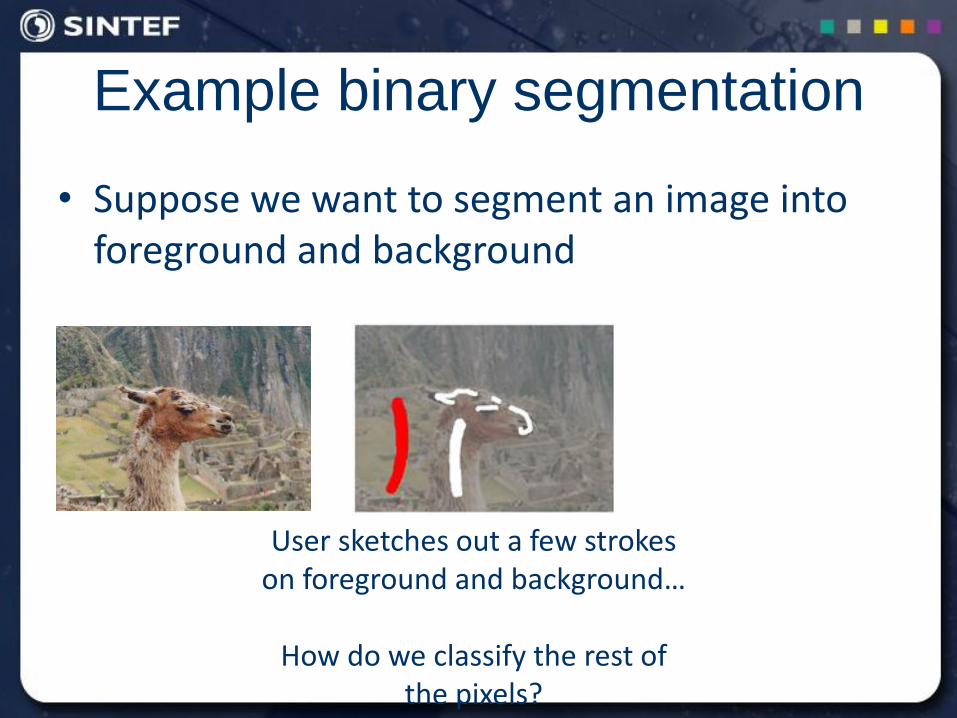
Example binary segmentation
• Suppose we want to segment an image into foreground and background
User sketches out a few strokes on foreground and background…
How do we classify the rest of
the pixels?
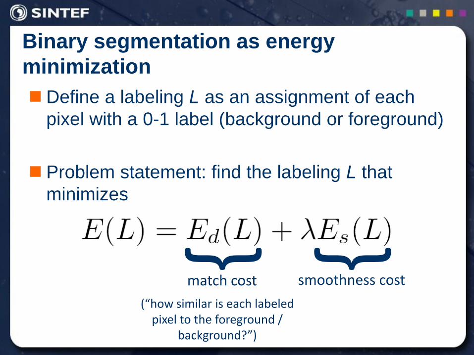
Binary segmentation as energy
minimization
Define a labeling L as an assignment of each
pixel with a 0-1 label (background or foreground)
Problem statement: find the labeling L that
minimizes
{ {
match cost smoothness cost
(“how similar is each labeled pixel to the foreground /
background?”)
EM in Computer Vision
Consider a specific family of Energy Functions Powerful enough to formulate many useful problems
Can be reduced to solving a graph min-cut problem
Problems defined with these functions: Can be solved quickly (using max-flow algorithms)
In many cases – optimal solution or within a known factor of the optimum
Nqp
qpqp
p
pp ffVfDfE,
, ,
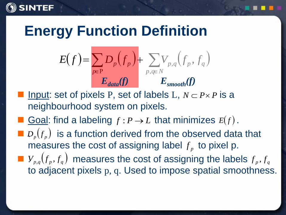
Input: set of pixels P, set of labels L, is a
neighbourhood system on pixels.
Goal: find a labeling that minimizes .
. is a function derived from the observed data that
measures the cost of assigning label to pixel p.
. measures the cost of assigning the labels
to adjacent pixels p, q. Used to impose spatial smoothness.
Energy Function Definition
PPN
LPf : fE
pp fD
qpqp ffV ,, qp ff ,
pf
Esmooth(f)
Edata(f)
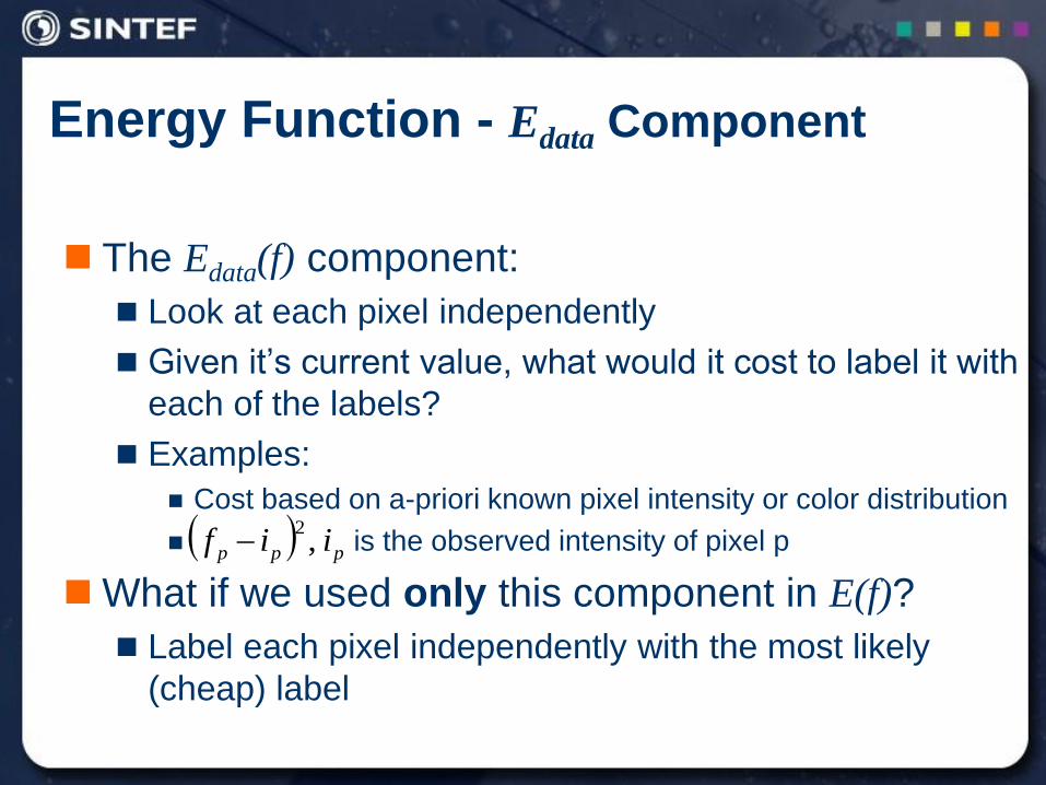
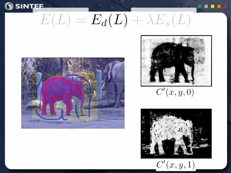
The Edata(f) component:
Look at each pixel independently
Given it‟s current value, what would it cost to label it with
each of the labels?
Examples:
Cost based on a-priori known pixel intensity or color distribution
is the observed intensity of pixel p
What if we used only this component in E(f)?
Label each pixel independently with the most likely
(cheap) label
Energy Function - Edata Component
ppp iif ,
2
Yevgeny
Doctor, March
2008, IDC
99
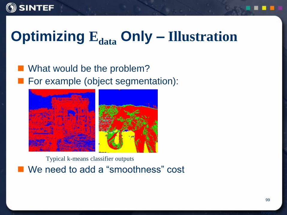
What would be the problem?
For example (object segmentation):
Typical k-means classifier outputs
We need to add a “smoothness” cost
Optimizing Edata Only – Illustration
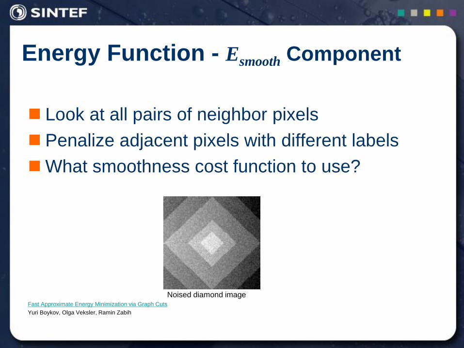
Energy Function - Esmooth Component
Look at all pairs of neighbor pixels
Penalize adjacent pixels with different labels
What smoothness cost function to use?
Noised diamond image Fast Approximate Energy Minimization via Graph Cuts
Yuri Boykov, Olga Veksler, Ramin Zabih
Yevgeny
Doctor, March
2008, IDC
102
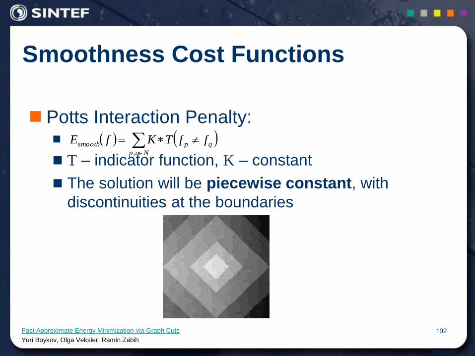
Potts Interaction Penalty:
T – indicator function, K – constant
The solution will be piecewise constant, with
discontinuities at the boundaries
Smoothness Cost Functions
Nqp
qpsmooth ffTKfE,
Fast Approximate Energy Minimization via Graph Cuts
Yuri Boykov, Olga Veksler, Ramin Zabih
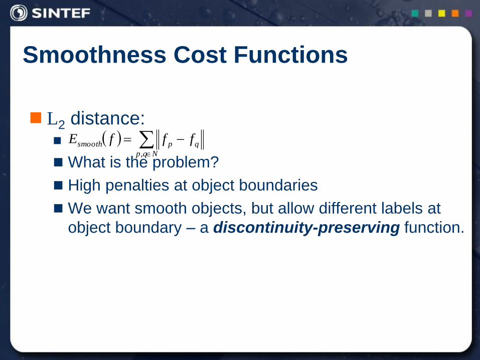
L2 distance:
What is the problem?
High penalties at object boundaries
We want smooth objects, but allow different labels at
object boundary – a discontinuity-preserving function.
Smoothness Cost Functions
Nqp
qpsmooth fffE,
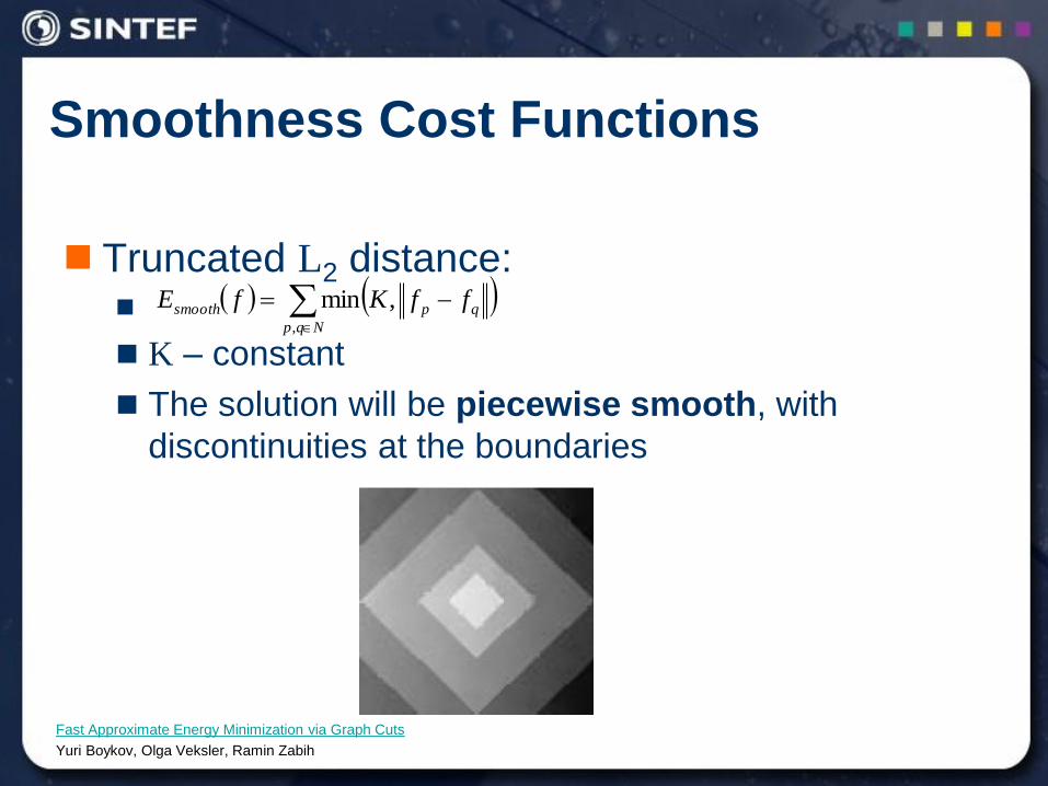
Truncated L2 distance:
K – constant
The solution will be piecewise smooth, with
discontinuities at the boundaries
Smoothness Cost Functions
Fast Approximate Energy Minimization via Graph Cuts
Yuri Boykov, Olga Veksler, Ramin Zabih
Nqp
qpsmooth ffKfE,
,min
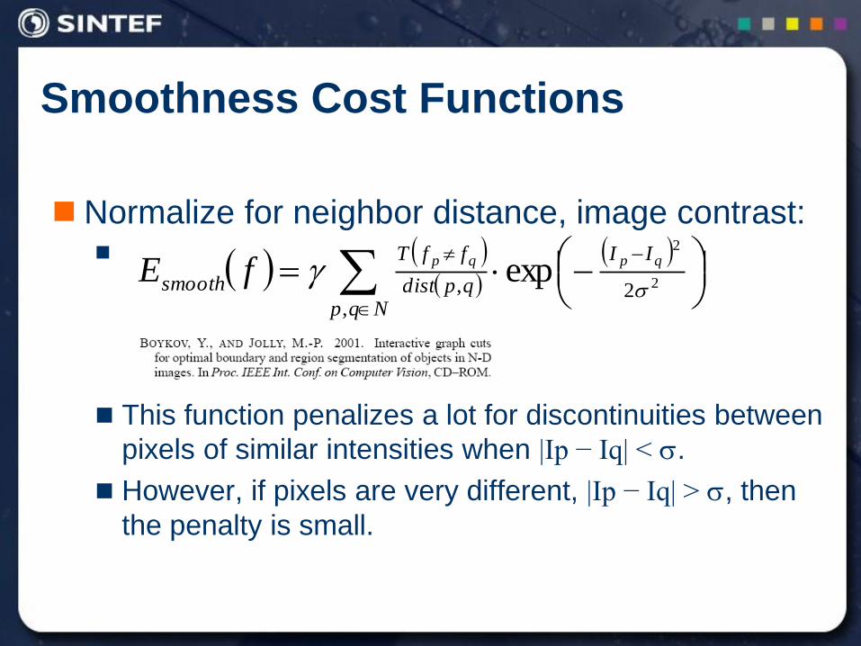
Normalize for neighbor distance, image contrast:
This function penalizes a lot for discontinuities between
pixels of similar intensities when |Ip − Iq| < .
However, if pixels are very different, |Ip − Iq| > , then
the penalty is small.
Smoothness Cost Functions
Nqp
II
qpdist
ffT
smooth
qpqpfE,
2, 2
2
exp
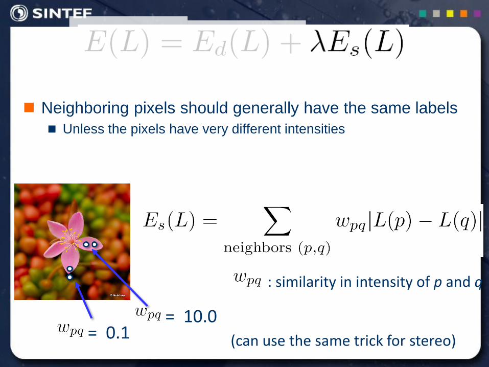
Neighboring pixels should generally have the same labels
Unless the pixels have very different intensities
: similarity in intensity of p and q
= 10.0 = 0.1 (can use the same trick for stereo)
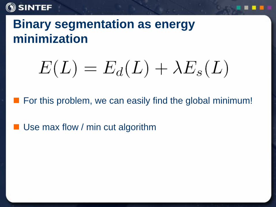
Binary segmentation as energy
minimization
For this problem, we can easily find the global minimum!
Use max flow / min cut algorithm
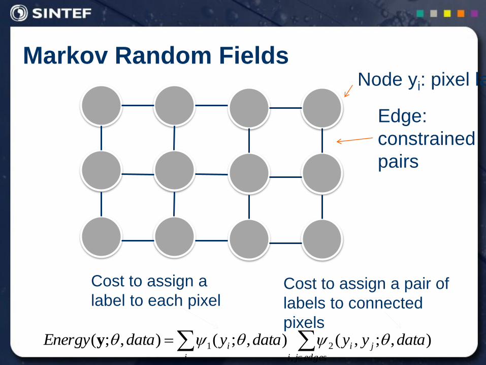
Markov Random Fields
edgesji
ji
i
i datayydataydataEnergy,
21 ),;,(),;(),;( y
Node yi: pixel label
Edge:
constrained
pairs
Cost to assign a
label to each pixel Cost to assign a pair of
labels to connected
pixels
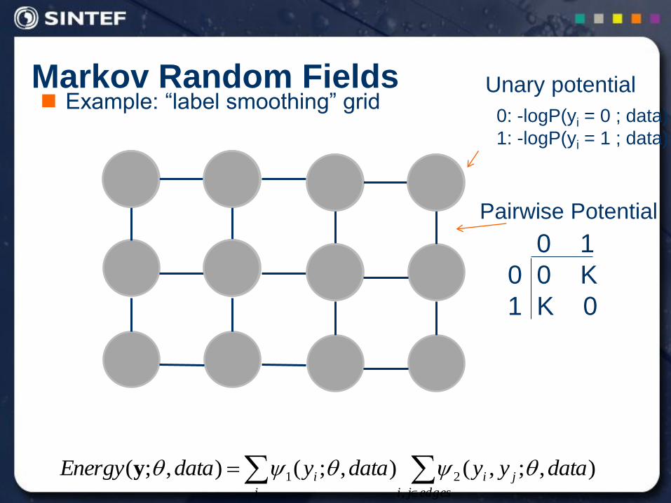
Markov Random Fields Example: “label smoothing” grid
Unary potential
0 1
0 0 K
1 K 0
Pairwise Potential
0: -logP(yi = 0 ; data)
1: -logP(yi = 1 ; data)
edgesji
ji
i
i datayydataydataEnergy,
21 ),;,(),;(),;( y
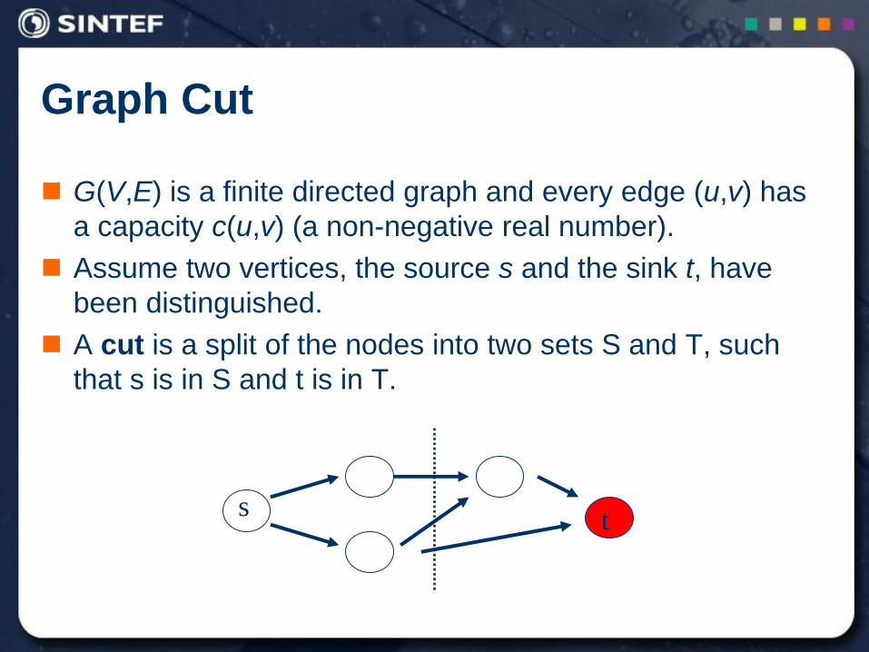
Graph Cut
G(V,E) is a finite directed graph and every edge (u,v) has
a capacity c(u,v) (a non-negative real number).
Assume two vertices, the source s and the sink t, have
been distinguished.
A cut is a split of the nodes into two sets S and T, such
that s is in S and t is in T.
t s
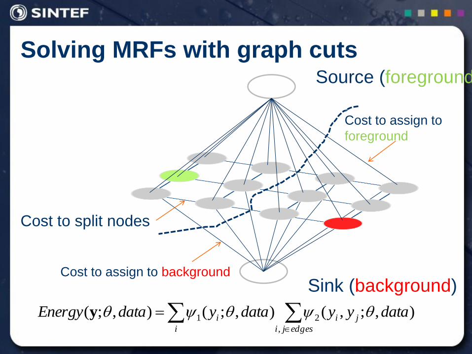
Solving MRFs with graph cuts
edgesji
ji
i
i datayydataydataEnergy,
21 ),;,(),;(),;( y
Source (foreground)
Sink (background)
Cost to assign to
foreground
Cost to split nodes
Cost to assign to background
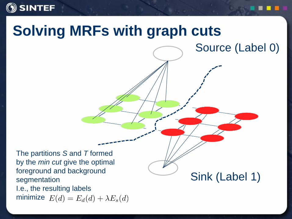
Solving MRFs with graph cuts Source (Label 0)
Sink (Label 1)
The partitions S and T formed
by the min cut give the optimal
foreground and background
segmentation
I.e., the resulting labels
minimize
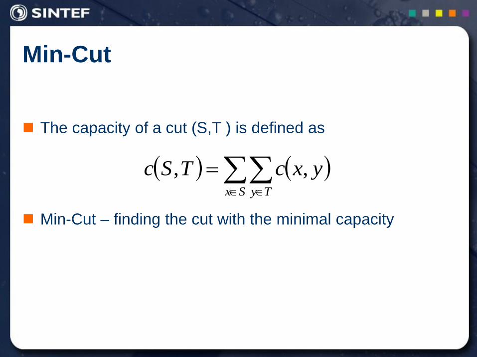
Min-Cut
The capacity of a cut (S,T ) is defined as
Min-Cut – finding the cut with the minimal capacity
Sx Ty
yxcTSc ,,
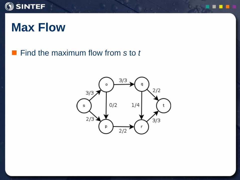
Max Flow
Find the maximum flow from s to t
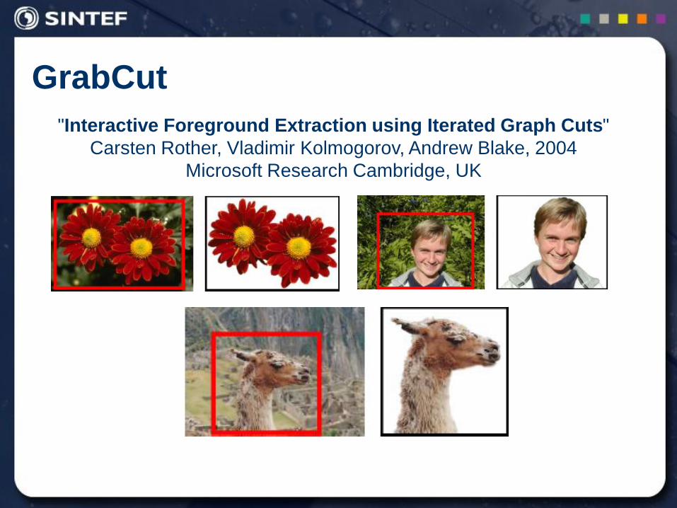
GrabCut
"Interactive Foreground Extraction using Iterated Graph Cuts"
Carsten Rother, Vladimir Kolmogorov, Andrew Blake, 2004
Microsoft Research Cambridge, UK
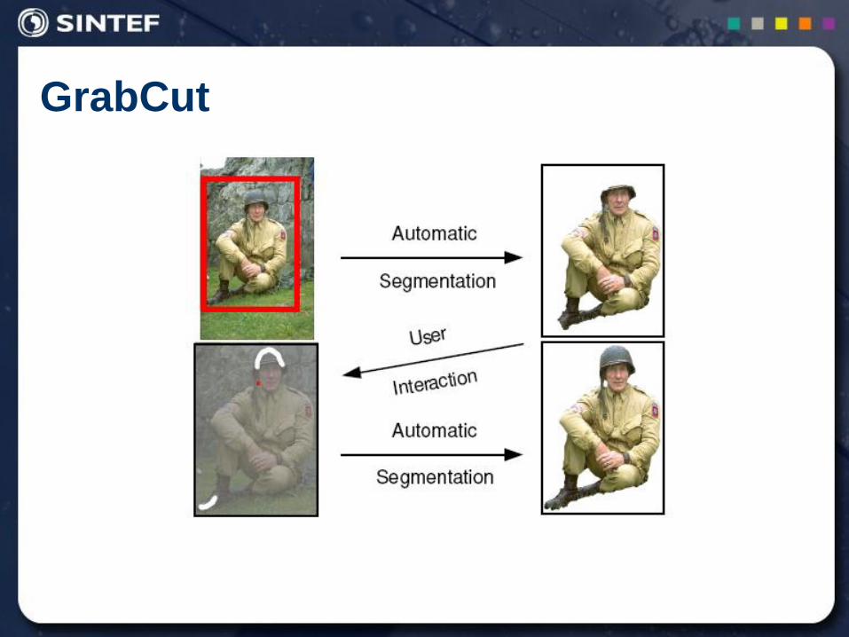
GrabCut
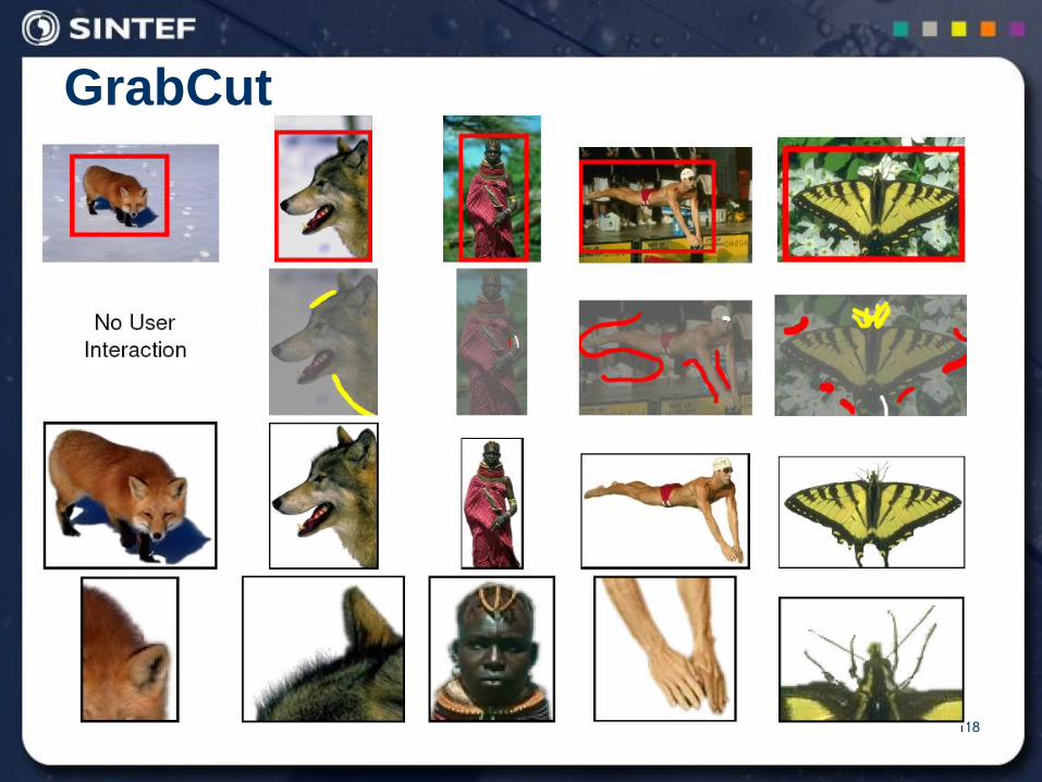
118
GrabCut
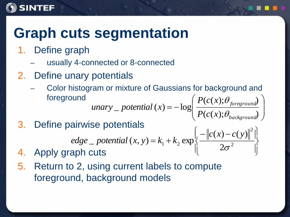
Graph cuts segmentation 1. Define graph
– usually 4-connected or 8-connected
2. Define unary potentials
– Color histogram or mixture of Gaussians for background and
foreground
3. Define pairwise potentials
4. Apply graph cuts
5. Return to 2, using current labels to compute
foreground, background models
2
2
212
)()(exp),(_
ycxckkyxpotentialedge
));((
));((log)(_
background
foreground
xcP
xcPxpotentialunary
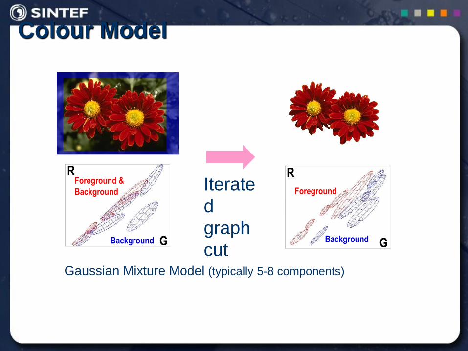
Colour Model
Gaussian Mixture Model (typically 5-8 components)
Foreground &
Background
Background
Foreground
Background G
R
G
R Iterate
d
graph
cut
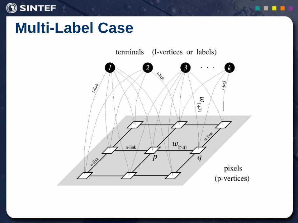
Multi-Label Case
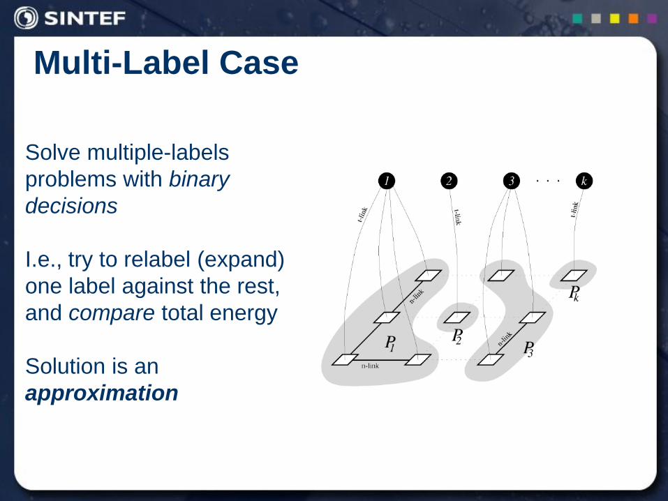
Multi-Label Case
Solve multiple-labels
problems with binary
decisions
I.e., try to relabel (expand)
one label against the rest,
and compare total energy
Solution is an
approximation
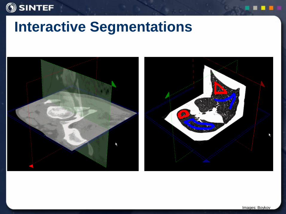
Interactive Segmentations
Images: Boykov