Inference for stochastic volatility models using time - LSE Statistics

The Annals of Statistics2010, Vol. 38, No. 2, 784–807DOI: 10.1214/09-AOS702© Institute of Mathematical Statistics, 2010

INFERENCE FOR STOCHASTIC VOLATILITY MODELS USINGTIME CHANGE TRANSFORMATIONS1

BY KONSTANTINOS KALOGEROPOULOS, GARETH O. ROBERTS

AND PETROS DELLAPORTAS

London School of Economics and Political Sciences, University of Warwickand Athens University of Economics and Business

We address the problem of parameter estimation for diffusion driven sto-chastic volatility models through Markov chain Monte Carlo (MCMC). Toavoid degeneracy issues we introduce an innovative reparametrization de-fined through transformations that operate on the time scale of the diffusion.A novel MCMC scheme which overcomes the inherent difficulties of timechange transformations is also presented. The algorithm is fast to implementand applies to models with stochastic volatility. The methodology is testedthrough simulation based experiments and illustrated on data consisting ofUS treasury bill rates.

1. Introduction. Diffusion processes provide natural models for continuoustime phenomena. They are used extensively in diverse areas such as finance, bi-ology and physics. A diffusion process is defined through a stochastic differentialequation (SDE),

dXt = μ(t,Xt , θ) dt + σ(t,Xt , θ) dWt, 0 ≤ t ≤ T ,(1.1)

where W is standard Brownian motion. The drift μ(·) and volatility σ(·) reflectthe instantaneous mean and standard deviation, respectively. In this paper we as-sume the existence of a unique weak solution to (1.1) which translates into someregularity conditions (locally Lipschitz with a linear growth bound) on μ(·) andσ(·) (see [31], Chapter 5 for more details).

The task of inference for diffusion processes is particularly challenging andhas received remarkable attention in the recent literature (see [32] for an exten-sive review). The main difficulty is inherent in the nature of diffusions which areinfinite-dimensional objects. However, only a finite number of points may be ob-served and the marginal likelihood of these observations is generally unavailablein closed form. This has stimulated the development of various nonlikelihood ap-proaches which use indirect inference [18], estimating functions [6], or the efficientmethod of moments [14] (see also [13]).

Received October 2007; revised December 2008.1Supported by the EPSRC Grant GR/S61577/01 and by the Marie Curie fellowships.AMS 2000 subject classifications. Primary 65C60, 60J60, 91B84; secondary 62M99, 62F15.Key words and phrases. Imputation, Markov chain Monte Carlo, diffusion processes.

784

http://www.imstat.org/aos/

http://dx.doi.org/10.1214/09-AOS702

http://www.imstat.org

http://www.ams.org/msc/

INFERENCE FOR SV MODELS USING TIME CHANGE 785

Most likelihood-based methods approach the likelihood function through thetransition density of (1.1). Denote the observations by Yk , k = 0, . . . , n, and withtk their corresponding times. If the dimension of Yk equals that of X (for each k) wecan use the Markov property to write the likelihood, given the initial point Y0, as

L(Y, θ |Y0) =n∏

k=1

pk(Yk|Yk−1; θ,�), � = tk − tk−1.(1.2)

The transition densities pk(·) are not available in closed form but several approxi-mations are available. They may be analytical (see [1, 2]) or simulation based (see[9, 28]). They usually approximate the likelihood in a way so that the discretiza-tion error can become arbitrarily small, although the methodology developed in[4] succeeds exact inference in the sense that it allows only for Monte Carlo error.A potential downside of these methods may be their dependence on the Markovproperty. In many interesting multidimensional diffusion models, the observationregime is different and some of their components are not observed at all.

A famous such example is provided by stochastic volatility models, used ex-tensively to model financial time series such as equity prices [19, 20, 33] or in-terest rates [3, 8, 15]. A stochastic volatility model is usually represented by atwo-dimensional diffusion,(

dXt

dαt

)=

(μx(Xt ,αt , θ)

μα(αt , θ)

)dt +

(σx(αt , θ) 0

0 σα(αt , θ)

)(dBt

dWt

),(1.3)

where X denotes the observed equity (stock) log-price or the short-term interestrate with volatility σx(·) which is a function of a latent diffusion α. Note that theobserved process X in (1.3) is not Markov; the distribution of a future stock pricedepends (besides the current price) on the current volatility which in turn dependson the entire price history. Nevertheless, since the two-dimensional diffusion isMarkov, state space approaches are possible and may be implemented using se-quential Monte Carlo techniques [12, 29]. While such approaches allow for onlineestimation of the volatility, various implications arise regarding inference for thediffusion parameters [25, 34].

An alternative approach to the problem adopts Bayesian inference utilizingMarkov chain Monte Carlo (MCMC) methods. Adhering to the Bayesian frame-work, a prior p(θ) is first assigned on the parameter vector θ . Then, given theobservations Y , the posterior p(θ |Y) can be explored through data augmenta-tion [35], treating the unobserved paths of X (paths between observations) as miss-ing data. Note that the augmented diffusion satisfies the Markov property irrespec-tively of the observation regime. Hence data augmentation approaches are moregeneral.

Initial MCMC schemes following this program were introduced by [21] (seealso [10, 11] and [22]). However, as noted in the simulation-based experimentof [10] and established theoretically by [30], any such algorithm’s convergenceproperties will degenerate as the number of imputed points increases. The problem

786 K. KALOGEROPOULOS, G. O. ROBERTS AND P. DELLAPORTAS

may be overcome with the reparametrization of [30], and this scheme may beapplied in all one-dimensional and some multidimensional contexts. However, thisframework does not cover general multidimensional diffusion models. Chib, Pittand Shephard [7] and Kalogeropoulos [23] offer appropriate reparametrizationsbut only for a class of stochastic volatility models. Alternative reparametrizationswere introduced in [17] (see also [16] for a sequential approach).

In this paper we introduce a novel reparametrization that, unlike previousMCMC approaches, operates on the time scale of the observed diffusion ratherthan its path. This facilitates the construction of irreducible and efficient MCMCschemes designed appropriately to accommodate the time change of the diffusionpath. Being a data augmentation procedure, our approach does note rely on theMarkov property and can be applied to a much larger class of diffusions than thoseconsidered in [1] and [4]. Moreover, it may be coupled with the approaches of [30]and [7] to handle more general models, that is almost every stochastic volatilitymodel used in practice. The paper is organized as follows: Section 2 elaborateson the need for a transformation of the diffusion to avoid problematic MCMC al-gorithms. In Section 3 we introduce a class of transformations based on changingthe time scale of the diffusion process. Section 4 provides the details for the cor-responding nontrivial MCMC implementation. The proposed methodology of thepaper is tested and illustrated through numerical experiments in Section 5, and onUS treasury bill rates in Section 6. Finally, Section 7 concludes and provides somerelevant discussion.

2. The necessity of reparametrization. A Bayesian data augmentationscheme bypasses a problematic sampling from the posterior π(θ |Y) by introduc-ing a latent variable X that simplifies the likelihood L(Y ; X , θ). It usually involvesthe following two steps:

1. Simulate X conditional on Y and θ .2. Simulate θ from the augmented conditional posterior which is proportional to

L(Y ; X , θ)π(θ).

It is not hard to adapt our problem to this setting. Y represents the observationsof the price process X. The latent variables X introduced to simplify the likeli-hood evaluations are discrete skeletons of diffusion paths between observations orentirely unobserved diffusions. In other words, X is a fine partition of multidimen-sional diffusion with drift μX(t,Xt , θ) and diffusion matrix

�X(t,Xt , θ) = σ(t,Xt , θ) × σ(t,Xt , θ)′

and the augmented dataset is Xiδ, i = 0, . . . , T /δ, where δ specifies the amount ofaugmentation. The likelihood can be approximated via the Euler scheme,

LE(Y ; X , θ) =T/δ∏i=1

p(

Xiδ|X(i−1)δ

),

Xiδ|X(i−1)δ ∼ N(

X(i−1)δ + δμX (·), δ�X (·)),


which is known to converge to the true likelihood L(Y ; X , θ) for small δ [28].Another property of diffusion processes relates �X (·) to the quadratic variation

process. Specifically we know that

limδ→0

T/δ∑i=1

(Xiδ − X(i−1)δ

)(Xiδ − X(i−1)δ

)T =∫ T

0�X (s, Xs, θ) ds a.s.

The solution of the equation above determines the diffusion matrix parameters.Hence, there exists perfect correlation between these parameters and X as δ → 0.This has disastrous implications for the mixing and convergence of the MCMCchain as it translates into reducibility for δ → 0. This issue was first noted by [30]for scalar diffusions and also confirmed by the simulation experiment of [10]. Infact the convergence time is of O(1

δ). This problem is not MCMC specific as it

turns out that the convergence of its deterministic analogue, EM algorithm, is alsoproblematic when the amount of information in the augmented data X stronglyexceeds that of the observations. In our case, X contains an infinite amount ofinformation for δ → 0.

The problem may be resolved if we apply a transformation so that the algo-rithm based on the transformed diffusion is no longer reducible as δ → 0. Robertsand Stramer [30] provide appropriate diffusion transformations for scalar diffu-sions. In a multivariate context this requires a transformation to a diffusion withunit volatility matrix (see, for instance, [24]). Aït-Sahalia [2] terms such diffu-sions as reducible and proves the nonreducibility of stochastic volatility modelsthat obey (1.3). The transformations introduced in this paper follow a slightly dif-ferent route and target the time scale of the diffusion. Since the construction obeysthe same principles of [30] the convergence time of the algorithm is independentof augmentation level controlled by δ. Another appealing feature of such a repara-metrization is the generalisation to stochastic volatility models.

3. Time change transformations. For ease of illustration we first provide thetime change transformation and the relevant likelihood function for scalar diffusionmodels with constant volatility. Nevertheless, one of the main advantages of thistechnique is the applicability to general stochastic volatility models.

3.1. Scalar diffusions. Consider a diffusion X defined through the followingSDE:

dXt = μ(t,Xt , θ) dt + σ dWXt , 0 < t < 1, σ > 0.(3.1)

Without loss of generality, we assume a pair of observations X0 = y0 and X1 = y1.For more data, note that the same operations are possible for every pair of succes-sive observations, and these pairs are linked together through the Markov property.We introduce the latent “missing” path of X for 0 ≤ t ≤ 1, denoted by Xmis, so thatX = (y0,X

mis, y1). In the spirit of [30], the goal is to write the likelihood for θ , σ


with respect to a parameter-free dominating measure. Using Girsanov’s theoremwe can get the Radon–Nikodym derivative between the law of the diffusion X,denoted by P

X , and that of the driftless diffusion dMt = σ dWXt which represents

Wiener measure and is denoted by WX . We write

dPX(X)

dWX= G(t,X, θ, σ ) = exp

{∫ 1

0

μ(t,Xt , θ)

σ 2 dXt − 1

2

∫ 1

0

μ(t,Xt , θ)2

σ 2 dt

}.

Consider the factorization,

WX = W

Xy × Leb(y1) × f (y1|y0, σ

2),(3.2)

where y1 is a Gaussian random variable, y1|y0 ∼ N (y0, σ2), and Leb(·) denotes

Lebesgue measure. This naturally factorizes the measure of X as the Lebesguedensity of y1 under the dominating measure multiplied by the conditional domi-nating measure W

Xy . We can now write

dPX(Xmis, y0, y1)

d{WXy × Leb(y)} = G(t,X, θ, σ )f (y1|y0, σ ),

where clearly the dominating measure depends on σ since it contains WXy which

represents a Brownian bridge with volatility σ .To remove this dependency on the parameter σ we consider the following time

change transformation. Let a new time scale be

s = η1(t, σ ) =∫ t

0σ 2 dω = tσ 2(3.3)

and then define the new transformed diffusion U as

Us =⎧⎨⎩

Xη−1

1 (s,σ ), 0 ≤ s ≤ σ 2,

Mη−1

1 (s,σ ), s > σ 2.

The definition for t > σ 2 is needed to ensure that U is well defined for differentvalues of σ 2 > 0 which is essential in the context of a MCMC algorithm. Usingstandard time change properties (see, for example, [26]), the SDE for U is

dUs =⎧⎨⎩

1

σ 2 μ(s,Us, θ) dt + dWUs , 0 ≤ s ≤ σ 2,

dWUs , s > σ 2,

where WU is another Brownian motion at the time scale s. Applying Girsanov’stheorem again, the law of U , denoted by P

U , is given through its Radon–Nikodymderivative with respect to the law W

U of the Brownian motion WU at the time


scale s:

dPU(Umis, y0, y1)

dWU

= G(s,U, θ, σ )(3.4)

= exp{∫ +∞

0

μ(s,Us, θ)

σ 2 dUs − 1

2

∫ +∞0

μ(s,Us, θ)2

σ 4 ds

}

= exp{∫ σ 2

0

μ(s,Us, θ)

σ 2 dUs − 1

2

∫ σ 2

0

μ(s,Us, θ)2

σ 4 ds

}.

By applying the factorization of (3.2) on WU at the new time scale s, the likelihood

can be written as

dPU(Umis, y0, y1)

d{WUy × Leb(y)} = G(s,U, θ, σ )f (y1|y0, σ ).

The dominating measure still depends on σ as it contains WUy which reflects a

Brownian bridge with conditioning event Uσ 2 = y1. We therefore introduce a sec-ond transformation which applies to both the path and the time scale of the diffu-sion process U . Consider a new time scale

u = η2(s, σ ) = s

σ 2(σ 2 − s)or s = η−1

2 (u, σ ) = uσ 4

1 + uσ 2

and define a new diffusion Z through

Us = (σ 2 − s)Zη2(s,σ ) +(

1 − s

σ 2

)y0 + s

σ 2 y1, 0 ≤ t < σ 2.(3.5)

Note that this transformation is a bijection. In the case of y0 = y1 = 0 its inverse isgiven by

Zu = 1 + uσ 2

σ 2 Uη−1

2 (u,σ ), 0 ≤ u < +∞.

Applying Itô’s formula and using time change properties we can also obtain theSDE of Z based on another driving Brownian motion WZ operating at the timescale u:

dZu ={μx(t, ν(Zu,σ ), θ)

1 + uσ 2 + ν(Zu,σ )

}dt + dWZ

u , 0 ≤ u < +∞,(3.6)

where ν(Zu,σ ) = Us . This operation essentially transforms to a diffusion that runsfrom 0 to +∞ preserving the unit volatility. A third attempt to write the likelihood,now based on Z, again uses the Girsanov theorem and the factorization of (3.2) tocondition the dominating measure on y1. This writes

dPZ(Z,y0, y1)

d{WZy × Leb(y)} = G(u,Z, θ, σ )f (y1|y0, σ ),(3.7)


where PZ denotes the law of Z and W

Zy reflects the law of the driftless diffusion

Z conditioned on y1. The integrals in G(Z, θ, σ ) run up to +∞); however, theexpression is finite being a bijection of the Radon–Nikodym derivative betweenP

U and WU given by (3.4). Using the following lemma, we can prove that W

Zy is

the law of the standard Brownian motion and hence the likelihood is written withrespect to a dominating measure that does not depend on any parameters.

LEMMA 3.1. Let W be a standard Brownian motion in [0,+∞). Considerthe process defined for 0 ≤ t ≤ T

Bt = (T − t)Wt/{T (T −t)} +(

1 − t

T

)y0 + t

Ty1, 0 ≤ t < T .

Then B is a Brownian bridge from y0 at time 0 to y1 at time T .

PROOF. See [31], Section IV.40.1, for the case y0 = 0, T = 1. The extensionfor general y0 and T is trivial. �

COROLLARY 3.1. The process Z is standard Brownian motion under thedominating measure. In other words W

Zy is standard Wiener measure.

PROOF. Note that WUy reflects a Brownian bridge from y0 at time 0 to y1 at

time T and we obtained WZy by using the transformation of Lemma 3.1. Since

this transformation is a bijection, U is a Brownian bridge (under the dominatingmeasure) if and only if Z is standard Brownian motion. �

The likelihood, given by (3.7), allows the construction of an irreducibleMCMC scheme that alternates between updating the parameters and the diffusionprocess Z. For the path updates we may use the fact that

dPZy

dWZy

(Z|y0, y1) = G(t,Z, θ, σ )f (y1|y0, σ )

f P (y1|y0, θ, σ )∝ G(t,Z, θ, σ ),(3.8)

where PZy is the law of Z conditioned on y1 and f P (·) is the density of y1 un-

der PZ . Both P

Zy and f P (·) are generally unknown but their calculation may be

avoided in a MCMC algorithm which essentially only uses (3.7) and (3.8). Sincethese expressions only require the evaluation of f (·) and G(·), which are eitherknown or may be approximated using the augmented diffusion path, the task ofBayesian inference is feasible. Details are presented in Section 4.

3.2. Stochastic volatility models. We will first demonstrate how the case ofstochastic volatility models may be brought to a similar and equivalent form to thatof the previous section. Consider the general class of stochastic volatility modelswith SDE given by (1.3) for 0 ≤ t ≤ t1. Without loss of generality, we may assume


a pair of observations (X0 = y0, X1 = y1) due to the Markov property of the two-dimensional diffusion (X,α). The likelihood can then be divided into two parts:the first contains the marginal likelihood of the diffusion α, and the remaining partcorresponds to the diffusion X conditioned on the path of α

Pθ (X,α) = Pθ (α)Pθ (X|α).

Denote the marginal likelihood for α by Lα(α, θ). To overcome reducibility issuesarising from the paths of α one may use the reparametrizations of [7] or [23]. Therelevant transformations of the latter are

βt = h1(αt , θ),∂h1(αt , θ)

∂αt

= {σα(αt , θ)}−1,

γt = βt − β0, βt = h2(γt ),

and the marginal likelihood for the transformed latent diffusion γ becomes

Lγ (γ, θ) = dP

dW(γ ) = Gγ (t, γ, θ),(3.9)

where W denotes Wiener measure. By letting αt = gθ,γt = h−1

1 (h2(γt ), θ), theSDE of X conditional on γ becomes

dXt = μx(Xt , gθ,γt , θ) dt + σx(g

θ,γt , θ) dBt , 0 ≤ t ≤ 1.

Given the paths of the diffusion γt , the volatility function σx(gθ,γt , θ) may be

viewed as a deterministic function of time and θ . The situation is similar to that ofthe previous section. We can now introduce a new time scale

s = η(t, γ, θ) =∫ t

0σ 2

x (gθ,γω , θ) dω.

Let T be the transformation of the ending time t1, T = η(t1, γ, θ). We can thendefine U on the new time scale s as in (3.3):

Us ={

Xη−1(s,γ,θ), 0 ≤ s ≤ T ,Mη−1(s,γ,θ), s > T .

(3.10)

The SDE for U now becomes

dUs ={μx(Us, g

θ,γ

η−1(s,γ,θ), θ)

σ 2x (g

θ,γ

η−1(s,γ,θ), θ)

}dt + dWU

s , 0 ≤ s ≤ T .

We obtain the Radon–Nikodym derivative between the distribution of U with re-spect to that of the Brownian motion WU ,

dP

dWU= G(s,U,γ, θ)


and introduce WUy as before. The density of y1 under W

U , denoted by f (y1|y0,

γ, θ), is just

f (y1|y0, γ, θ) ≡ N(y0, T ).

The dominating measure WUy reflects a Brownian motion conditioned to equal

y at a parameter depended time T = η(t1, γ, θ). To remove this dependency weintroduce another time scale,

u = η2(s) = s

T (T − s)or s = η−1

2 (u) = uT 2

1 + uT,

which defines a second time change similar to (3.5)

Ut = (T − s)Zs/{T (T −s)} +(

1 − s

T

)y0 + s

Ty1, 0 ≤ s < T .(3.11)

The SDE for Z, in the case of y0 = y1 = 0 is given by

dZu = T

1 + uT

{μx(u, ν(Zu), γk(u,γ,θ), θ)

σ 2x (γk(u,γ,θ), θ)

+ ν(Zu)

}dt + dWZ

u ,

0 ≤ u < ∞,

where k(u, γ, θ) denotes the initial time scale of X, t , and ν(Zu) = Us .Conditional on γ , the likelihood can be written in a similar manner as in (3.7)

dP

d{WZy × Leb(y)}(Z|y0, y1, γ ) = G(u,Z,γ, θ)f (y1|y0, γ, θ).(3.12)

By using the exact same arguments of Section 3.1, we can show that WZy reflects a

standard Wiener measure and therefore the dominating measure is independent ofparameters. To obtain the full likelihood we need to multiply the two parts givenby (3.9) and (3.12).

3.3. Incorporating leverage effect. In the previous section we made the as-sumption that the increments of X and γ are independent, in other words we as-sumed no leverage effect. This assumption can be relaxed in the following way: inthe presence of a leverage effect ρ, the SDE of X conditional on γ can be writtenas

dXt = μx(Xt , gγ,θt , θ) dt + ρσx(g

γ,θt , θ) dWt

+√

1 − ρ2σx(gγ,θt , θ) dBt , 0 ≤ t ≤ t1,

where W is the driving Brownian motion of γ . Note that given γ , W canbe regarded as a function of γ and its parameters θ . Therefore, the termρσx(g

γ,θt , θ) dWt can be viewed as a deterministic function of time, and it can

be treated as part of the drift of Xt . However, this operation introduces additional


problems as the assumptions ensuring a weakly unique solution to the SDE of X

are violated. To avoid this issue we introduce the infinitesimal transformation

Xt = H(Ht , ρ, γ, θ) = Ht +∫ t

0ρσx(g

γ,θω , θ) dWω,

which leads us to the following SDE for H :

dHt = μx{H(Xt , ρ, γ, θ), gγ,θt , θ}dt +

√1 − ρ2σx(g

γ,θt , θ) dBt , 0 ≤ t ≤ t1.

We can now proceed as before, defining U and Z based on the SDE of H in asimilar manner as in (3.10) and (3.11), respectively.

3.4. State dependent volatility. Consider the family of state dependent sto-chastic volatility models where conditional on γ , the SDE of X may be writtenas

dXt = μx(Xt , gγ,θt , θ) dt + σ1(g

γ,θt , θ)σ2(Xt , θ) dBt , 0 ≤ t ≤ t1.

This class contains, among others, the models of [3, 8, 11, 15]. In order to ap-ply the time change transformations of Section 3.2, we should first transform X

to Xt , through Xt = l(Xt , θ) so that it takes the form of (1.3). Such a transforma-tion, which may be viewed as the first transformation in [30], should satisfy thefollowing differential equation:

∂l(Xt , θ)

∂Xt

= 1

σ2(Xt , θ).

The time change transformations for U and Z may then be defined on the basisof X that will now have volatility σ1(g

γ,θt , θ). The transformation l(·) also applies

to the observations y0 = l(X0, θ) and y1 = l(X1, θ) which may now be functionsof the parameters in σ2(·). These parameters enter the reparametrized likelihood intwo ways: through the density f (y1|γ, θ) which now should include the relevantJacobian term, and through the function ν(Zu) in the drift of Z which accordingto (3.11) would depend on the transformed endpoints.

3.5. Multivariate stochastic volatility models. We may use the techniques ofSection 3.3 to define time change transformations for multidimensional diffusions.Consider a d-dimensional version of the SDE in (3.1) where σ now is a 2 × 2matrix ([σ ]ij = σij ). As noted in [24], the mapping between σ and the volatilitymatrix σσT should be 1–1 in order to ensure identifiability of the σ parameters.A way to achieve this is by allowing σ to be the lower triangular matrix that pro-duces the Cholesky decomposition of σσT . For d = 2, the SDE of such a diffusionis given by

dX{1}t = μ

(X

{1}t ,X

{2}t , θ

)dt + σ11 dBt ,

dX{2}t = μ

(X

{1}t ,X

{2}t , θ

)dt + σ21 dBt + σ22 dWt .


The time change transformations for X{1} will be exactly as in Section 3.1. ForX{2} note that given X{1} the term σ21 dBt is now a deterministic function of timeand may be treated as part of the drift. Thus, we may proceed following the routeof the Section 3.3.

Similar transformations can be applied for diffusions that have, or may be trans-formed to have, volatility functions independent of their paths. For example, wemay assume two correlated price processes with correlation ρx :

[σ ]11 = σ {1}x (g

γ,θt , θ),

[σ ]21 = ρxσ{2}x (g

γ,θt , θ),

[σ ]22 =√

1 − ρ2xσ {2}

x (gγ,θt , θ).

We may proceed in a similar manner for multivariate stochastic volatility modelsof general dimension d .

4. MCMC implementation. The construction of an appropriate data aug-mentation algorithm involves several issues. We focus on describing how to updatethe latent diffusion paths and the parameters that drive the time change transfor-mations. The updates of the remaining parameters include standard MCMC stepsand are thus omitted. The change in the time scale introduces three interesting fea-tures: the presence of three time scales; the need to update diffusion paths that runfrom 0 to +∞; and the fact that time scales depend on parameters. In this sectionwe present the details of a MCMC scheme that addresses the above. For ease ofillustration, we start with the simple case of a univariate diffusion with constantvolatility

dXt = μ(t,Xt , θ) dt + σ dBXt , 0 ≤ t ≤ 1,X0 = y0,X1 = y1,

and build up to the case of stochastic volatility models (1.3). Note that such exten-sions are not hard to implement since the time change transformations need onlybe applied to the paths of the observed diffusion process X. The updates of thetransformed diffusion process γ , which drives the volatility, may be carried outusing an overlapping scheme as in [23].

4.1. Three time scales. We introduce m intermediate points of X at equidistanttimes between 0 and 1, to give X = {Xi/(m+1), i = 0,1, . . . ,m+1}. In addition, wemake the assumption that m is large enough for accurate likelihood approximationsand any error induced by the time discretization is negligible for the purposes ofour analysis. This assumption introduces no implications as the value of m may beset to an arbitrarily large value prior to the analysis.

Given a value of the time scale parameter σ , we can get the U -time points byapplying (3.3) to each one of the existing points X so that

Uσ 2i/(m+1) = Xi/(m+1), i = 0,1, . . . ,m + 1.


Note that it is only the times that change, the values of the diffusion remain intact.In a stochastic volatility model we would use the quantities∫ (i+1)/(m+1)

i/(m+1)σ 2

x (·) ds

for each pair of consecutive imputed points.The points of Z are multiplied by a time factor which corrects the deviations

from unit volatility. The times of the diffusion Z may be obtained by

tZi = σ 2i/(m + 1)

σ 2(σ 2 − σ 2i/(m + 1)), i = 0,1, . . . ,m.

Clearly this does not apply to the last point which occurs at time +∞. The pathsof X or U are thus more convenient for likelihood evaluations as they only containfinite time points. They may be used instead exploiting the fact that the relevanttransformations are bijections. However, the component of the relevant Gibbs sam-pling scheme should be the diffusion process Z.

4.2. Updating the paths of Z. The paths of Z may be updated using an in-dependence sampler with the reference measure as a proposal. Here W

Zy reflects

a Brownian motion at the Z-time scale u which is fixed given the current valuesof the time-scale parameters and the paths of γ in the case of stochastic volatilitymodels. An appropriate algorithm is given by the following steps:

• Step 1: Propose a Brownian motion on the Z-time, say Z∗. The value at theendpoint (time +∞) is not needed.

• Step 2: Transform back to X∗ using (3.5).

• Step 3: Accept with probability min{1, G(X∗,θ,σ )G(X,θ,σ )

}.

4.3. Updating time scale parameters. The updates of parameters that definethe time scale, such as σ , are of particular interest. In almost all cases, their con-ditional posterior density is not available in closed form, and Metropolis steps areinevitable. However, every proposed value of these parameters will imply a differ-ent Z-time scale u. In other words, for each potential proposed value for σ thereexists a different set of Z-points needed for accurate approximations of the like-lihood the Metropolis accept–reject probabilities. In theory, this would pose noissues had we been able to store an infinitely thin partition of Z, but of course thisis not possible.

We use retrospective sampling ideas (see [27] and [5] for applications in differ-ent contexts). Under the assumption of a sufficiently fine partition of the time scaleof Z, all the nonrecorded intermediate points contribute nothing to the likelihoodand they are irrelevant in that respect. The set of recorded points is sufficient forlikelihood approximation purposes. In other words, their distribution is given bythe likelihood dominating measure W

Zy which reflects a Brownian motion. Hence,


they can be drawn after the proposal of the candidate value of the time scale pa-rameter. To ensure compatibility with the recorded partition of Z, it suffices tocondition on their neighboring points. This is easily done using standard Brown-ian bridge properties. Suppose that we want to simulate the value of Z at time tbwhich falls between the recorded values at times ta and tc, so that ta ≤ tb ≤ tc.Denote by Zta and Ztc the corresponding Z values. Under the assumption that Z

is distributed according to WZy between ta and tc we have that

Ztb |Zta ,Ztc ∼ N

{(tb − ta)Ztc + (tc − tb)Zta

tc − ta,(tb − ta)(tc − tb)

tc − ta

}.(4.1)

We describe the algorithm for the case of more than two observations; denoteby X0 = y0, Xt1 = y1, . . . ,Xtn = yn. The time change transformations should beapplied to each pair of successive observations thus giving n separate Z diffusionprocesses. As mentioned earlier, the diffusion processes X and U are bijectionsof this collection of Z diffusion processes and may be used instead in a MCMCscheme. Our proposed algorithm for the σ -updates may be summarized throughthe following steps:

• Step 1: Propose a candidate value for σ , say σ ∗.• Step 2: Repeat for each pair of successive points:

– Use (3.3) and (3.5) to get the new times associated with it.– Draw the values of Z retrospectively at the new times using (4.1).– Transform back to X∗ (which corresponds to the time between the pair of

successive points), using (3.5).• Step 3: Form the entire path X∗ by appropriately joining the bits between suc-

cessive observations.• Step 4: Accept with probability

min{

1,G(t,X∗, θ, σ ∗)∏n

i=1 f (yi |yi−1, σ∗)

G(t,X, θ, σ )∏n

i=1 f (yi |yi−1, σ )

}.

In a stochastic volatility model the updates of the paths of the transformed diffu-sion γ may be implemented using overlapping blocks. Note that these paths drivethe time u, of the diffusion process Z, and therefore a similar algorithm as aboveshould be embedded in their updates. For simplicity consider blocks of γ pathsthat correspond to times between nonsuccessive observations. Each block is thenfurther split into sub-blocks containing intervals between successive observations,thus providing a number of separate Z diffusion processes. Details are presentedbelow:

• Step 1: Propose γ ∗ between the times of two nonsuccessive observations, yA

and yB , by a Brownian bridge connecting the relevant endpoints of γ .• Step 2: Repeat for each pair of successive points between (and including) yA

and yB :


– Use (3.10) and (3.11) to get the new times associated with it.– Draw the values of Z retrospectively at the new times using (4.1).– Transform back to X∗ (which corresponds to the time between the pair of

successive points), using (3.11).• Step 3: Join the bits of X∗ to form its path between yA and yB .• Step 4: Accept with probability,

min{

1,Gγ (t, γ ∗, θ)G(t,X∗, γ ∗, θ)

∏ni=1 f (yi |yi−1, γ

∗, θ)

Gγ (t, γ, θ)G(t,X,γ, θ)∏n

i=1 f (yi |yi−1, γ, θ)

}.

5. Simulations. As discussed in Section 2, appropriate reparametrizations arenecessary to avoid issues regarding the mixing and convergence of the MCMCalgorithm. In fact, the chain becomes reducible as the level of augmentation in-creases. This is also verified by the numerical examples performed in [23] evenin very simple stochastic volatility models. In this section we present a simulationbased experiment to check the immunity of MCMC schemes to increasing levelsof augmentation, as well as the ability of our estimation procedure to retrieve thecorrect values of the diffusion parameters despite the fact that the series is par-tially observed and only at a finite number of points. We simulated data from thefollowing stochastic volatility model:

dXt = κx(μx − Xt) dt + ρ exp(αt/2) dWt +√

1 − ρ2 exp(αt/2) dBt ,

dαt = κα(μα − αt) dt + σ dWt,

where B and W represent independent Brownian motions, and ρ reflects the corre-lation between the increments of X and α (also termed as leverage effect). A high-frequency Euler approximating scheme with a step of 0.001 was used for the sim-ulation of the diffusion paths. Specifically, 500,001 points were drawn and onevalue of X for every 1000 was recorded, thus forming a dataset of 501 observa-tions of X at 0 ≤ t ≤ 500. The parameter values were set to ρ = −0.5, σ = 0.4,κx = 0.2, μx = 0.1, κα = 0.3 and μα = −0.2.

The transformations required to construct an irreducible data augmentationscheme are listed below. First α was transformed to γ through

γt = αt − α0

σ, 0 ≤ t ≤ 500,

αt = gγ,σt = α0 + σγt .

Given γ , and for each pair of consecutive observation times tk−1 and tk (k =1,2, . . . ,500) on X, the following transformations were applied: first, we removedthe term introduced from the leverage effect

Ht = Xt −∫ t

tk−1

ρ exp{gγ,σt /2}dWs, tk−1 ≤ t ≤ tk,


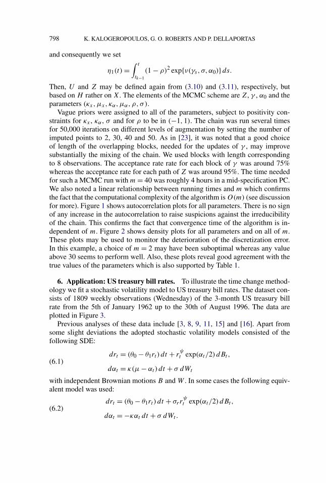
and consequently we set

η1(t) =∫ t

tk−1

(1 − ρ)2 exp{ν(γs, σ,α0)}ds.

Then, U and Z may be defined again from (3.10) and (3.11), respectively, butbased on H rather on X. The elements of the MCMC scheme are Z, γ , α0 and theparameters (κx,μx, κα,μα,ρ,σ ).

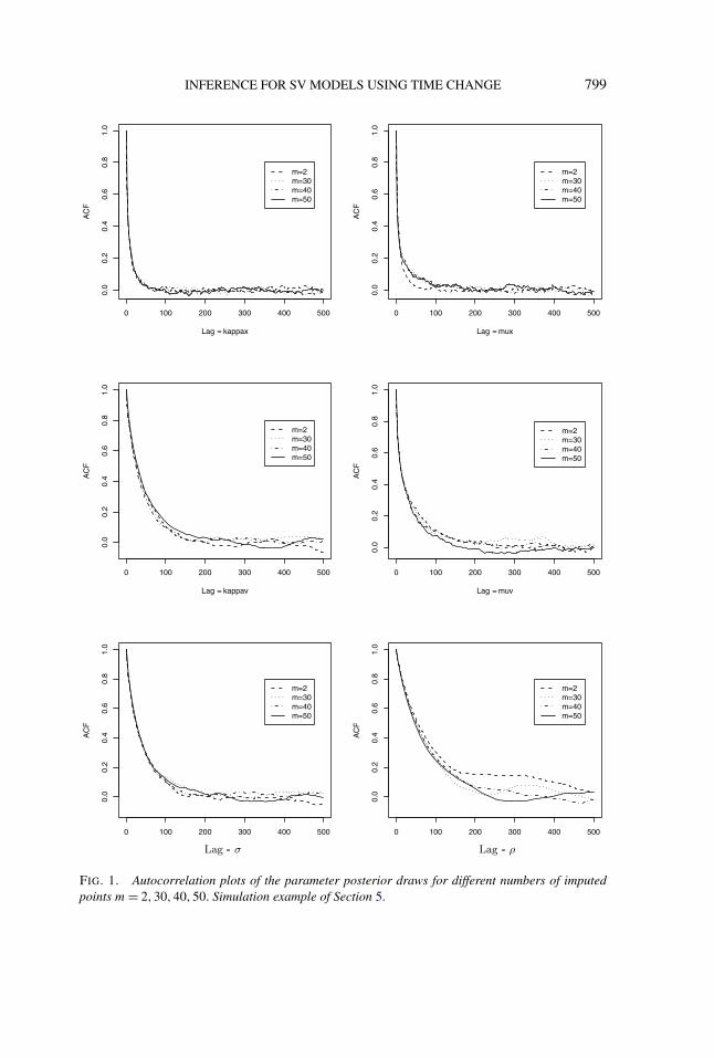
Vague priors were assigned to all of the parameters, subject to positivity con-straints for κx , κα , σ and for ρ to be in (−1,1). The chain was run several timesfor 50,000 iterations on different levels of augmentation by setting the number ofimputed points to 2, 30, 40 and 50. As in [23], it was noted that a good choiceof length of the overlapping blocks, needed for the updates of γ , may improvesubstantially the mixing of the chain. We used blocks with length correspondingto 8 observations. The acceptance rate rate for each block of γ was around 75%whereas the acceptance rate for each path of Z was around 95%. The time neededfor such a MCMC run with m = 40 was roughly 4 hours in a mid-specification PC.We also noted a linear relationship between running times and m which confirmsthe fact that the computational complexity of the algorithm is O(m) (see discussionfor more). Figure 1 shows autocorrelation plots for all parameters. There is no signof any increase in the autocorrelation to raise suspicions against the irreducibilityof the chain. This confirms the fact that convergence time of the algorithm is in-dependent of m. Figure 2 shows density plots for all parameters and on all of m.These plots may be used to monitor the deterioration of the discretization error.In this example, a choice of m = 2 may have been suboptimal whereas any valueabove 30 seems to perform well. Also, these plots reveal good agreement with thetrue values of the parameters which is also supported by Table 1.

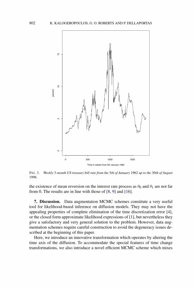
6. Application: US treasury bill rates. To illustrate the time change method-ology we fit a stochastic volatility model to US treasury bill rates. The dataset con-sists of 1809 weekly observations (Wednesday) of the 3-month US treasury billrate from the 5th of January 1962 up to the 30th of August 1996. The data areplotted in Figure 3.

Previous analyses of these data include [3, 8, 9, 11, 15] and [16]. Apart fromsome slight deviations the adopted stochastic volatility models consisted of thefollowing SDE:

drt = (θ0 − θ1rt ) dt + rψt exp(αt/2) dBt ,

(6.1)dαt = κ(μ − αt) dt + σ dWt

with independent Brownian motions B and W . In some cases the following equiv-alent model was used:

drt = (θ0 − θ1rt ) dt + σrrψt exp(αt/2) dBt ,

(6.2)dαt = −καt dt + σ dWt .


FIG. 1. Autocorrelation plots of the parameter posterior draws for different numbers of imputedpoints m = 2,30,40,50. Simulation example of Section 5.


FIG. 2. Kernel densities of the posterior draws of all the parameters for different numbers of im-puted points m = 2,30,40,50. Simulation example of Section 5.


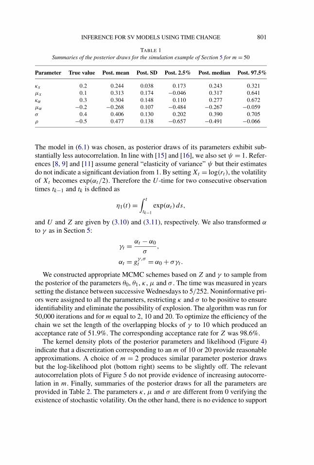
TABLE 1Summaries of the posterior draws for the simulation example of Section 5 for m = 50

Parameter True value Post. mean Post. SD Post. 2.5% Post. median Post. 97.5%

κx 0.2 0.244 0.038 0.173 0.243 0.321μx 0.1 0.313 0.174 −0.046 0.317 0.641κα 0.3 0.304 0.148 0.110 0.277 0.672μα −0.2 −0.268 0.107 −0.484 −0.267 −0.059σ 0.4 0.406 0.130 0.202 0.390 0.705ρ −0.5 0.477 0.138 −0.657 −0.491 −0.066

The model in (6.1) was chosen, as posterior draws of its parameters exhibit sub-stantially less autocorrelation. In line with [15] and [16], we also set ψ = 1. Refer-ences [8, 9] and [11] assume general “elasticity of variance” ψ but their estimatesdo not indicate a significant deviation from 1. By setting Xt = log(rt ), the volatilityof Xt becomes exp(αt/2). Therefore the U -time for two consecutive observationtimes tk−1 and tk is defined as

η1(t) =∫ t

tk−1

exp(αt ) ds,

and U and Z are given by (3.10) and (3.11), respectively. We also transformed α

to γ as in Section 5:

γt = αt − α0

σ,

αt = gγ,σt = α0 + σγt .

We constructed appropriate MCMC schemes based on Z and γ to sample fromthe posterior of the parameters θ0, θ1, κ , μ and σ . The time was measured in yearssetting the distance between successive Wednesdays to 5/252. Noninformative pri-ors were assigned to all the parameters, restricting κ and σ to be positive to ensureidentifiability and eliminate the possibility of explosion. The algorithm was run for50,000 iterations and for m equal to 2, 10 and 20. To optimize the efficiency of thechain we set the length of the overlapping blocks of γ to 10 which produced anacceptance rate of 51.9%. The corresponding acceptance rate for Z was 98.6%.

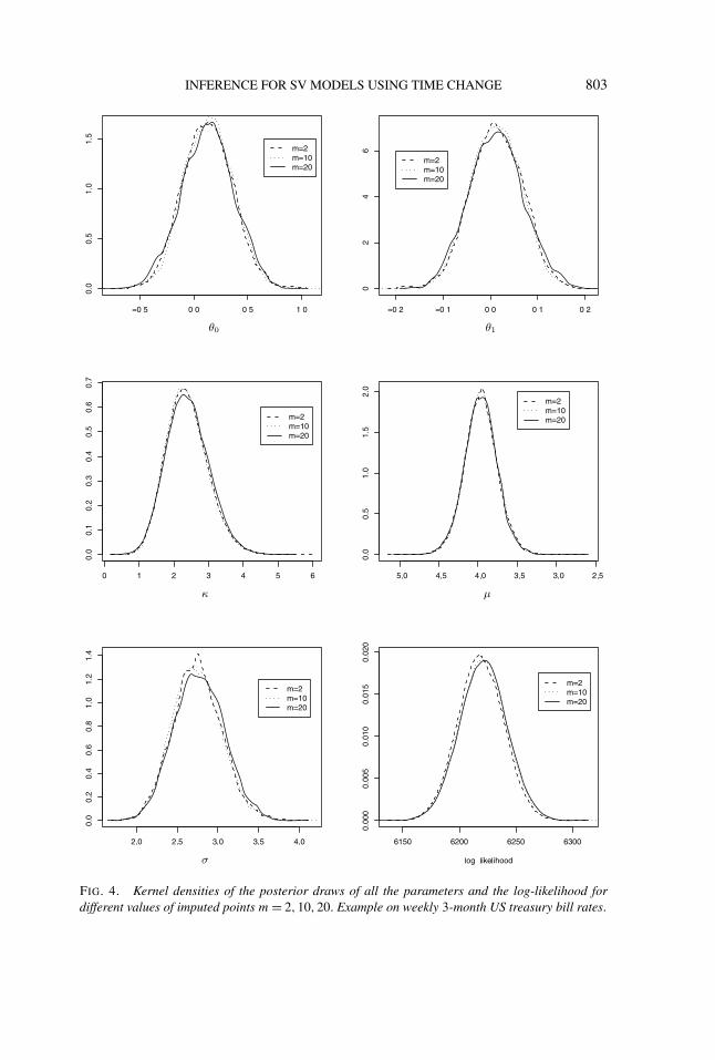
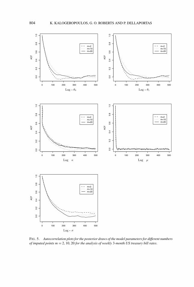
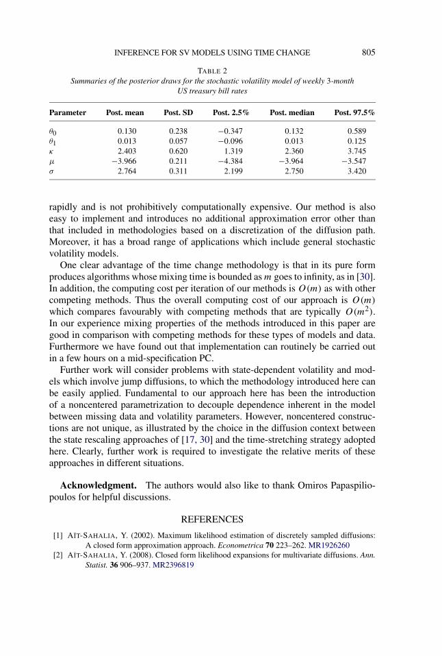
The kernel density plots of the posterior parameters and likelihood (Figure 4)indicate that a discretization corresponding to an m of 10 or 20 provide reasonableapproximations. A choice of m = 2 produces similar parameter posterior drawsbut the log-likelihood plot (bottom right) seems to be slightly off. The relevantautocorrelation plots of Figure 5 do not provide evidence of increasing autocorre-lation in m. Finally, summaries of the posterior draws for all the parameters areprovided in Table 2. The parameters κ , μ and σ are different from 0 verifying theexistence of stochastic volatility. On the other hand, there is no evidence to support


FIG. 3. Weekly 3-month US treasury bill rate from the 5th of January 1962 up to the 30th of August1996.

the existence of mean reversion on the interest rate process as θ0 and θ1 are not farfrom 0. The results are in line with those of [8, 9] and [16].

7. Discussion. Data augmentation MCMC schemes constitute a very usefultool for likelihood-based inference on diffusion models. They may not have theappealing properties of complete elimination of the time discretization error [4],or the closed form approximate likelihood expressions of [1], but nevertheless theygive a satisfactory and very general solution to the problem. However, data aug-mentation schemes require careful construction to avoid the degeneracy issues de-scribed at the beginning of this paper.

Here, we introduce an innovative transformation which operates by altering thetime axis of the diffusion. To accommodate the special features of time changetransformations, we also introduce a novel efficient MCMC scheme which mixes


FIG. 4. Kernel densities of the posterior draws of all the parameters and the log-likelihood fordifferent values of imputed points m = 2,10,20. Example on weekly 3-month US treasury bill rates.


FIG. 5. Autocorrelation plots for the posterior draws of the model parameters for different numbersof imputed points m = 2,10,20 for the analysis of weekly 3-month US treasury bill rates.


TABLE 2Summaries of the posterior draws for the stochastic volatility model of weekly 3-month

US treasury bill rates

Parameter Post. mean Post. SD Post. 2.5% Post. median Post. 97.5%

θ0 0.130 0.238 −0.347 0.132 0.589θ1 0.013 0.057 −0.096 0.013 0.125κ 2.403 0.620 1.319 2.360 3.745μ −3.966 0.211 −4.384 −3.964 −3.547σ 2.764 0.311 2.199 2.750 3.420

rapidly and is not prohibitively computationally expensive. Our method is alsoeasy to implement and introduces no additional approximation error other thanthat included in methodologies based on a discretization of the diffusion path.Moreover, it has a broad range of applications which include general stochasticvolatility models.

One clear advantage of the time change methodology is that in its pure formproduces algorithms whose mixing time is bounded as m goes to infinity, as in [30].In addition, the computing cost per iteration of our methods is O(m) as with othercompeting methods. Thus the overall computing cost of our approach is O(m)

which compares favourably with competing methods that are typically O(m2).In our experience mixing properties of the methods introduced in this paper aregood in comparison with competing methods for these types of models and data.Furthermore we have found out that implementation can routinely be carried outin a few hours on a mid-specification PC.

Further work will consider problems with state-dependent volatility and mod-els which involve jump diffusions, to which the methodology introduced here canbe easily applied. Fundamental to our approach here has been the introductionof a noncentered parametrization to decouple dependence inherent in the modelbetween missing data and volatility parameters. However, noncentered construc-tions are not unique, as illustrated by the choice in the diffusion context betweenthe state rescaling approaches of [17, 30] and the time-stretching strategy adoptedhere. Clearly, further work is required to investigate the relative merits of theseapproaches in different situations.

Acknowledgment. The authors would also like to thank Omiros Papaspilio-poulos for helpful discussions.

REFERENCES

[1] AÏT-SAHALIA, Y. (2002). Maximum likelihood estimation of discretely sampled diffusions:A closed form approximation approach. Econometrica 70 223–262. MR1926260

[2] AÏT-SAHALIA, Y. (2008). Closed form likelihood expansions for multivariate diffusions. Ann.Statist. 36 906–937. MR2396819

http://www.ams.org/mathscinet-getitem?mr=1926260



[3] ANDERSEN, T. G. and LUND, J. (1997). Estimating continuous-time stochastic volatility mod-els of the short term interest rate. J. Econometrics 77 343–377.

[4] BESKOS, A., PAPASPILIOPOULOS, O., ROBERTS, G. and FEARNHEAD, P. (2006). Exactand computationally efficient likelihood-based estimation for discretely observed diffu-sion processes (with discussion). J. R. Stat. Soc. Ser. B Stat. Methodol. 68 333–382.MR2278331

[5] BESKOS, A. and ROBERTS, G. O. (2005). Exact simulation of diffusions. Ann. Appl. Probab.15 2422–2444. MR2187299

[6] BIBBY, B. and SORENSEN, M. (1995). Martingale estimating functions for discretely observeddiffusion processes. Bernoulli 1 17–39. MR1354454

[7] CHIB, S., PITT, M. K. and SHEPHARD, N. (2007). Efficient likelihood based inference forobserved and partially observed diffusions. Submitted.

[8] DURHAM, G. B. (2003). Likelihod based specification analysis of continuous time models ofthe short term interest rate. Journal of Financial Economics 70 463–487.

[9] DURHAM, G. B. and GALLANT, A. R. (2002). Numerical techniques for maximum likelihoodestimation of continuous-time diffusion processes. J. Bus. Econom. Statist. 20 297–316.MR1939904

[10] ELERIAN, O. S., CHIB, S. and SHEPHARD, N. (2001). Likelihood inference for discretelyobserved non-linear diffusions. Econometrica 69 959–993. MR1839375

[11] ERAKER, B. (2001). Markov chain Monte Carlo analysis of diffusion models with applicationto finance. J. Bus. Econom. Statist. 19 177–191. MR1939708

[12] FEARNHEAD, P., PAPASPILIOPOULOS, O. and ROBERTS, G. O. (2008). Particle filters forpartially observed diffusions. J. R. Stat. Soc. Ser. B Stat. Methodol. 70 755–777.

[13] GALLANT, A. R. and LONG, J. R. (1997). Estimating stochastic differential equations effi-ciently by minimum chi-squared. Biometrika 84 125–141. MR1450197

[14] GALLANT, A. R. and TAUCHEN, G. (1996). Which moments to match? Econometric Theory12 657–681. MR1422547

[15] GALLANT, A. R. and TAUCHEN, G. (1998). Reprojecting partially observed systems withapplications to interest rate diffusions. J. Amer. Statist. Assoc. 93 10–24.

[16] GOLIGHTLY, A. and WILKINSON, D. (2006). Bayesian sequential inference for nonlinear mul-tivariate diffusions. Stat. Comput. 16 323–338. MR2297534

[17] GOLIGHTLY, A. and WILKINSON, D. (2007). Bayesian inference for nonlinear multivariatediffusions observed with error. Comput. Statist. Data Anal. 52 1674–1693. MR2422763

[18] GOURIÉROUX, C., MONFORT, A. and RENAULT, E. (1993). Indirect inference. J. Appl.Econometrics 8 S85–S118.

[19] HESTON, S. (1993). A closed-form solution for options with stochastic volatility. With appli-cations to bonds and currency options. Review of Financial Studies 6 327–343.

[20] HULL, J. C. and WHITE, A. D. (1987). The pricing of options on assets with stochastic volatil-ities. Journal of Finance 42 281–300.

[21] JONES, C. S. (1999). Bayesian estimation of continuous-time finance models. Unpublishedpaper, Simon School of Business, Univ. Rochester.

[22] JONES, C. S. (2003). Nonlinear mean reversion in the short-term interest rate. Review of Fi-nancial Studies 16 793–843.

[23] KALOGEROPOULOS, K. (2007). Likelihood based inference for a class of multidimen-sional diffusions with unobserved paths. J. Statist. Plann. Inference 137 3092–3102.MR2364153

[24] KALOGEROPOULOS, K., DELLAPORTAS, P. and ROBERTS, G. (2007). Likelihood-based in-ference for correllated diffusions. Submitted.

[25] LIU, J. and WEST, M. (2001). Combined parameter and state estimation in simulation-basedfiltering. In Sequential Monte Carlo Methods in Practice (A. Doucet, J. F. G. De Freitasand N. J. Gordon, eds.). Springer, New York. MR1847793














[26] OKSENDAL, B. (2000). Stochastic Differential Equations, 5th ed. Springer, Berlin.MR2001996

[27] PAPASPILIOPOULOS, O. and ROBERTS, G. (2008). Retrospective MCMC for Dirichlet processhierarchical models. Biometrika 95 169–186. MR2409721

[28] PEDERSEN, A. R. (1995). A new approach to maximum likelihood estimation for stochas-tic differential equations based on discrete observations. Scand. J. Statist. 22 55–71.MR1334067

[29] PITT, M. K. and SHEPHARD, N. (1999). Filtering via simulation: Auxiliary particle filters.J. Amer. Statist. Assoc. 94 590–599. MR1702328

[30] ROBERTS, G. and STRAMER, O. (2001). On inference for partial observed nonlinear diffusionmodels using the Metropolis–Hastings algorithm. Biometrika 88 603–621. MR1859397

[31] ROGERS, L. C. G. and WILLIAMS, D. (1994). Diffusions, Markov Processes and Martingales,2, Itô Calculus. Wiley, Chicester. MR1331599

[32] SØRENSEN, H. (2004). Parametric inference for diffusion processes observed at discrete pointsin time: A survey. Int. Stat. Rev. 72 337–354.

[33] STEIN, E. M. and STEIN, J. C. (1991). Stock price distributions with stochastic volatility: Ananalytic approach. Review of Financial Studies 4 727–752.

[34] STROUD, J. R., POLSON, N. G. and MULLER, P. (2004). Practical filtering for stochasticvolatility models. In State Space and Unobserved Component Models 236–247. Cam-bridge Univ. Press, Cambridge. MR2077640

[35] TANNER, M. A. and WONG, W. H. (1987). The calculation of posterior distributions by dataaugmentation. J. Amer. Statist. Assoc. 82 528–540. MR0898357

K. KALOGEROPOULOS

LONDON SCHOOL OF ECONOMICS

AND POLITICAL SCIENCES

DEPARTMENT OF STATISTICS

HOUGHTON STREET, WC2A 2AELONDON

UNITED KINGDOM

E-MAIL: [email protected]

G. O. ROBERTS

UNIVERSITY OF WARWICK


CV4 7AL, COVENTRY

UNITED KINGDOM


P. DELLAPORTAS

ATHENS UNIVERSITY OF ECONOMICS

AND BUSINESS


76 PATISSION STREET, 10434 ATHENS

GREECE










mailto:[email protected]



Documents

Inference for stochastic volatility models using time - LSE Statistics