Inferences on the source mechanisms of the 1930 Irpinia ...geo.mff.cuni.cz/vyuka/seismologie/seis1/cele/2004-AnnGeophys-Emolo...of the 1930 Irpinia (Southern Italy) earthquake from

1

Inferences on the source mechanisms

of the 1930 Irpinia (Southern Italy) earthquake

from simulations of the kinematic rupture process

Antonio Emolo1*, Giovanni Iannaccone2, Aldo Zollo1 and Antonella Gorini3

1 Dipartimento di Scienze Fisiche, Università degli Studi “Federico II”, Napoli, Italy 2 Istituto Nazionale di Geofisica e Vulcanologia, Osservatorio Vesuviano, Napoli, Italy 3 Dipartimento della Protezione Civile, Servizio Sismico Nazionale, Roma, Italy

* Author for correspondence:

Antonio Emolo

Dipartimento di Scienze Fisiche

Università degli Studi “Federico II”

Complesso Universitario di Monte S. Angelo

Via Cintia

80126 Napoli, Italy

E-mail: [email protected]

Tel.: +39-081-2420317

Fax: +39-081-2420334

Antonio Emolo, Giovanni Iannaccone, Aldo Zollo and Antonella Gorini

2

Abstract

We examine here a number of parameters that define the source of the earthquake that occurred on

23rd July, 1930, in Southern Italy (in the Irpinia region). Starting from the source models proposed

in different studies, we have simulated the acceleration field for each hypothesised model, and

compared it with the macroseismic data. We then used the hybrid stochastic-deterministic technique

that was proposed by Zollo et al. (1997) for the simulation of the ground motion associated with the

rupture of an extended fault. The accelerations simulated for several sites were associated to the

intensities, using the empirical relationship proposed by Trifunac and Brady (1975), before being

compared with the available data from the macroseismic catalogue. A good reproduction of the

macroseismic field is provided by a normal fault striking in Apenninic direction (approximately

NW-SE) and dipping 55° toward the SW.

Key words 1930 Irpinia earthquake, ground motion simulation, kinematic source model

Inferences on the source mechanism of the 1930 Irpinia (Southern Italy) earthquake

3

Introduction

At 00:08 UTC on 23rd July, 1930, a seismic event completely destroyed several villages (Villanova

del Battista, Trevico, Aquilonia and Lacedonia) in the Campania Region of Southern Italy, which

caused the loss of about 1,500 lives. The earthquake was felt over a wide area of about 36,000 km2,

that covered the Campania, Puglia and Basilicata Regions of Southern Italy (Alfano, 1931). The

maximum estimated intensity for the earthquake was X MCS (Gruppo di lavoro CPTI, 1999). The

damaged area had an elliptical trend that stretched in the Apenninic direction (NW-SE) and that

showed a weak concavity toward the SW (Fig. 1).

In modern seismology, ground motion simulation techniques aim to provide more exact

predictions of the ground shaking than those obtained, for example, from conventional

seismotectonic analyses and/or from the use of empirical peak attenuation relationships. These can

be realised through the calculations of reliable earthquake scenarios. On this basis, the simulation of

a seismic wave field has a fundamental role in any predictive estimation of the ground motion

parameters that are of engineering interest (ground motion peak parameters, signal spectral content,

etc.). Simulation methods are also important in studies of past earthquakes where the instrumental

data were poor or completely absent. As shown by the present study, simulation of the seismic

radiation can be considered as a useful approach in the validation of a source model proposed on the

basis of seismological, geological and geophysical data.

In the present study, we first reviewed the source parameters of the 1930 Irpinia earthquake,

and then we applied a hybrid stochastic-deterministic model of earthquake rupture (Zollo et al.,

1997) to assess the acceleration field associated with a number of source models that have been

proposed for this earthquake. We also compared the simulated acceleration maps with the

macroseismic field, to gain insights into the 1930 Irpinia earthquake source parameters. Finally, we

propose a new model for this earthquake source.


4

Epicentre location of the 1930 Irpinia earthquake

The international seismic bulletins list more than 100 stations that reported P- and/or S-wave arrival

times following the 1930 Irpinia earthquake, which were mostly from Italian and European

observatories. The arrival times are given with an accuracy within some seconds, with large

inaccuracies that depend from the mechanical clocks that were used in the seismological

observatories at that time. The residuals of the P arrival times reported for some close seismic

stations in the bulletin amount to several tens of seconds. Using these data, various authors have

estimated the epicentre location for the 1930 Irpinia earthquake using different methodologies

(Oddone, 1930; Karnik, 1969; CNR-PFG, 1985; NEIS catalogue; Boschi et al., 1995), as reported

in Table I and Figure 2. All of the proposed epicentre locations are close to the maximum intensity

area. However, and as discussed in the following, the epicentre area and the maximum-damage area

should not coincide, as the latter is associated with the geometric and dynamic characteristics of the

rupturing source as well as the quality of the constructions.

Magnitude and seismic moment

The seismic intensity data were broadly used in the estimation of the magnitude of the 1930 Irpinia

earthquake. Empirical relationships using the maximum intensity in the epicentre area, Io, were

applied to obtain a value of the magnitude. For example, Postpischl (1985) assigned a magnitude of

7.0 using an empirical relationship between the maximum intensity and magnitude proposed by

Karnik (1969).

Westaway (1992) revised the source parameters for the large historic Italian earthquakes, and

determined the relationships among the radii of greater value isoseismal curves and the magnitudes.

Applying this to each isoseismal from I = VI to I = X, Westaway (1992) deduced a mean value of


5

M = 6.3 ±0.2 for the 1930 Irpinia earthquake. This thus showed that the magnitude scale that was

obtained was equivalent to the surface wave magnitude, MS.

Using a uniform methodology, Margottini et al. (1993) analysed about 500 bulletins from

seismological observatories to estimate the magnitudes of 647 earthquakes that occurred in Italy in

the period of 1900-1986. For each earthquake, they used the values of the maximum amplitudes of

the recorded ground motion according to the characteristics of the recording instruments, and the

period that was associated with them. Moreover, in order to account for the effects of crustal

structure, they determined a correction factor for each station. In particular, for the 1930 Irpinia

earthquake, they used the amplitude of surface waves recorded at 41 seismic stations, thus obtaining

a surface wave magnitude MS = 6.6 ±0.3.

Gasperini et al. (1999) proposed a method that used the macroseismic intensity data to assess

the location, geometry and magnitude of the source of large historic earthquakes. Based on a dataset

of 75 instrumental magnitude values for Italian earthquakes, they calibrated a regression law to

obtain the equivalent moment magnitude Me using the epicentre intensity Io and the radii of areas of

different intensity levels. The estimated equivalent moment magnitude for the 1930 Irpinia

earthquake was Me = 6.7.

The seismic moment was estimated by Jiménez (1988), who analysed the records of the 1930

Irpinia earthquake obtained at the seismic station of Jena, Germany. This study proposed a method

for the retrieval of the focal mechanism parameters and the seismic moment for intermediate sized

earthquakes from the surface waves recorded at a single seismic station located at a regional

distance. Jiménez (1988) performed a dispersion analysis on the regional Love and Rayleigh wave

data in the period range of 30-100 s, and used this to infer the focal mechanism. An analysis of the

spectral content of the fundamental modes of the surface waves was then used to calculate the

seismic moment. The value obtained for the 1930 Irpinia earthquake was M0 = 2× 1018 Nm.

Table II summarises the proposed magnitudes and seismic moment values for the 1930 Irpinia

earthquake.


6

The focal mechanism

There have been several studies of the geometry of the fault-plane of the 1930 Irpinia earthquake

that have evaluated the focal mechanisms by P-wave polarities or that have applied semi-empirical

relationships to macroseismic data. Martini and Scarpa (1983) used the P-polarities that were

reported in the seismic bulletins or taken from the original seismograms. They assumed the

epicentre given by Karnik (1969), with a depth of 13 km. The solution proposed by Martini and

Scarpa (1983) shows a normal fault mechanism with a moderate strike-slip component, with nodal

planes oriented approximately in the ESE and WSW directions and dipping 40°-60° (Fig. 3).

Jiménez (1988) obtained a fault mechanism with a large strike-slip component with nodal

planes oriented in the N-S and E-W directions (Fig. 3). Gasperini et al. (1999) analysed

macroseismic data and proposed an azimuth of N109°W ±11° for the fault plane, with a fixed mean

dip of 45°.

In the present study, independent estimations of focal mechanism were obtained using two

different methods on the same dataset as that used by Martini and Scarpa (1983). The data that were

used are reported in Table III. The first approach was based on a search for the two planes that

optimise the polarities distribution on the focal sphere (FPFIT algorithm, Oppenheimer et al.,

1988). The second method was that proposed by Zollo and Bernard (1991), and it is based on the

probabilistic evaluation of the maximum likelihood model. The fault plane solutions obtained are

given in Figure 3 and summarised in Table IV. These are similar to those proposed by Martini and

Scarpa (1983), and are consistent with the azimuthal value of 109° for the fault plane that was given

by Gasperini et al. (1999).


7

Fault dimensions and mean value of slip

The length, L, and the width, W, of a fault that has generated an earthquake of magnitude M can be

calculated by the relationships provided by Wells and Coppersmith (1994):

MLLog 59.044.2 +−=

MWLog 32.001.1 +−=

Where the fault dimensions are expressed in km. Gasperini et al. (1999) inferred a source

dimension of 32.6 × 13.6 km2 using these Wells and Coppersmith (1994) relationships. Applying

the Wells and Coppersmith (1994) relationships to the magnitude value M = 6.1 proposed by

Jiménez (1988), the fault plane dimensions that are obtained are about 14.5 × 9 km2.

Once the seismic moment is known, it is possible to estimate the fault dimensions and the

mean final slip value for the earthquake under consideration. Using the relationship between

seismic moment and fault length for intraplate earthquakes provided by Scholz et al. (1986), we

obtained a fault length of about 10-15 km. Moreover, through studying the seismic fracture in

conditions of uniform static stress release, Madariaga (1977) established that:

µ

SCWDD >=<

Where <D> is the mean slip value; W is the fault width; DS is the static stress release; µ is the

rigidity; and C is a factor that depends on the geometry of the fractured area and that assumes a

value of 0.7 for a circular surface and 1.6 for a rectangular fault characterized by a width that is

negligible with respect to its length. Combining this relationship with the definition of seismic


8

moment ( ><= DLWM µ0 ), we obtain a fault width of about 5-10 km. The mean value of the final

slip is then between 0.4 m and 1.3 m.

Table IV summarises the proposed source parameters for the 1930 Irpinia earthquake.

Ground acceleration field simulation

The goal of our simulation study was to determine the reliabilities of the proposed source models

for the 1930 Irpinia earthquake through a comparison of the simulated acceleration field with the

macroseismic map. With this in mind, we simulated the ground acceleration field associated with

the four source models reported in Table IV. For each of the source models considered, we

performed simulations of 100 different rupture processes, with each of them based on parameters

defined by different positions of the rupture nucleation point (randomly chosen in the lower half of

the fault) and by different heterogeneous final slip distributions (calculated according to the k-

square model proposed by Herrero and Bernard, 1994). For each rupture process, we calculated the

ground acceleration at a regular grid of 121 receivers located in an area of 60 × 60 km2 (the red

shaded area in Fig. 1). The spacing between adjacent receivers was 5 km. The maximum frequency

content of simulated accelerograms was 5 Hz. For each receiver, the ground motion parameters of

interest (e.g., the mean values of peak ground acceleration [PGA]) were evaluated assuming that the

simulated peak accelerations were log-normally distributed. In our modelling, we simulated 100

different rupture processes for each fault model considered, after having verified that a larger

number of simulations did not produce substantial differences in the estimation of the mean values

of PGA for each receiver.


9

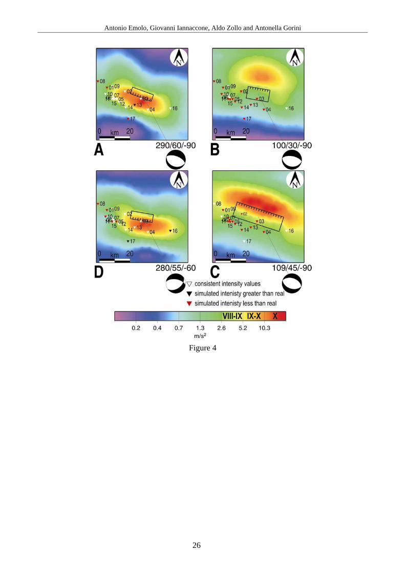
Figure 4 shows the maps of the PGA (mean values calculated from the 100 simulated rupture

processes) for the four source models of Table IV. As can be clearly seen, the spatial distribution of

the accelerometric field depends on the orientation and dimension of the ruptured surfaces.

The PGAs can then be converted in macroseismic intensities using empirical relationships. In

Figure 4, the colour scale was created so that the acceleration ranges for yellow and red correspond

to macroseismic intensities in the range IX-X, according to the relationship proposed by Trifunac

and Brady (1975):

986.13.0 −>=< IPGALog .

In this way, we can compare qualitatively the isoseismal curves of Figure 1 for the highest

intensity degrees with the yellow and red areas of Figure 4.

We also compared the macroseismic intensity data available from the NT4.1 catalogue

(Camassi and Stucchi, 1998) with the theoretical intensity values estimated from the simulated

accelerations by the Trifunac and Brady (1975) relationship for several towns. In Figure 4, the

white triangles mean that the expected intensity is consistent (within the range of one statistical

standard deviation) with the actual intensity data, whereas the black and red triangles mean that the

theoretical intensities are greater than and less than the actual data, respectively. Since we do not

take in account either site effects or the quality of the constructions, which can strongly influence

macroseismic data, we believe that this comparison is not completely satisfactory.


10

Results: a new source model

Seismological and macroseismic observations agree on the azimuth of the causative fault of the

1930 Irpinia earthquake, and they suggest an Apenninic orientation (approximately ESE-WNW) for

the fault plane. There are some uncertainties in the definition of the dipping direction of the fault

plane (towards the SW or the NE). This ambiguity also remains after the analysis of the fault plane

solution because we have found two possible solutions with the same probability. However, in

general the concave shape of the macroseismic field can be associated with a fault plane dipping in

the direction of maximum concavity. In the case of the 1930 Irpinia earthquake, the isoseismal

curves of Figure 1 show a weak concavity toward the SW, and this suggests a plane probably

dipping towards the SW. The results from the simulations for source models B and C in Table IV

(Fig. 4B, C), which are characterized by fault planes dipping toward the SW, show an acceleration

field characterized by a concavity in the fault dipping direction. On this basis, we chose a fault

plane oriented in the Apenninic direction and dipping towards the SW.

From Figure 4A, D, it appears that the lateral extension (i.e. in the anti-Apenninic direction) of

the peak acceleration field reproduces well the analogue extension of the isoseismal curves (Fig. 1).

On the other hand, through comparing the results for source models A and B in Table IV (Fig. 4A,

B), we note that when the seismic moment and fractured area are the same, the dip angle is smaller,

and the lateral extension of higher PGA area is larger. In comparison with the macroseismic field,

this observation allows us to exclude a sub-horizontal fault plane for the 1930 Irpinia earthquake,

and to consider a fault plane with a dip angle of between 40° and 70°.

The effects of a relevant strike component in the focal mechanism on the acceleration field

can be inferred through comparing the PGA maps for source models A and D of Table IV (Fig. 4A,

D); this produces a larger extension in the ESE direction that is not so evident in the macroseismic

field (Fig. 1).


11

While we were able to quite closely reproduce the lateral extension of the isoseismal curves

corresponding to the highest intensity levels, the longitudinal extension (i.e., in the Apenninic

direction) of the highest acceleration areas for source models A, B and D of Table IV appear to

underestimate the analogous extension of the isoseismal curves (i.e., the area corresponding to the

intensities of IX-X). As a consequence, we can conclude that the fault dimensions associated with

source models A, B and D are too small. On the other hand, in the case of source model C, which is

characterized by the largest fault dimensions among the models considered in this study, we found

an acceleration field that greatly overestimates the macroseismic field extension corresponding to

the highest intensity levels.

On the basis of the above-mentioned observations, we propose the source model reported in

Table V for the 1930 Irpinia earthquake. This model is characterized by dimensions which are

intermediate to those of models A, B and D, and model C, of Table IV. The magnitude of about 6.5,

which was evaluated according to the Wells and Coppersmith (1994) relationships, corresponds to a

seismic moment of 5.6× 1018 Nm.

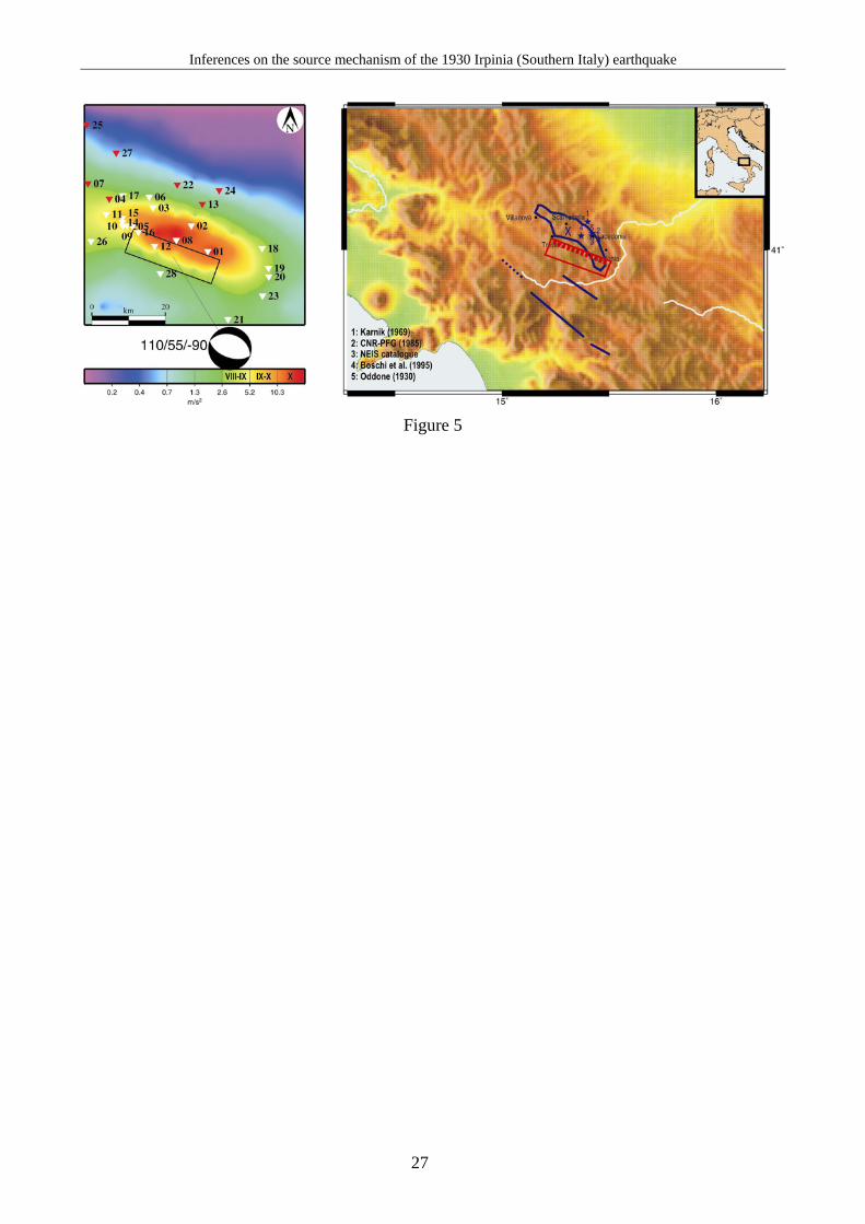
To validate our proposed source model, we calculated the mean PGA field associated with

100 possible rupture processes occurring on this fault. We then converted the PGA estimated for the

28 towns in the area under consideration into macroseismic intensities through the Trifunac and

Brady (1975) relationship, and searched for the fault position that was able to minimise the

differences between the estimated and observed macroseismic data available from the NT4.1

catalogue (Camassi and Stucchi, 1998). The final results are shown in Figure 5. The synthetic

acceleration field reproduces the characteristics of the macroseismic field well. Moreover, the fault

moves about 10 km in a SW direction as compared to the proposed epicentre locations shown in

Figure 2. As can be seen, the fault position does not coincide with the maximum area where it was

felt.

In the “Database of potential sources for earthquakes larger than M=5.5 in Italy” (Valensise

and Pantosti, 2001), the source parameters and location proposed by Gasperini et al. (1999) are


12

adopted. These are based only on the analysis of macroseismic intensity data. However, as pointed

out by Basili and Burrato (2001), the 1930 Irpinia earthquake did not generate clear surface faulting

and this makes it difficult to determine the exact position of the causative fault.

In conclusion, we propose that the fault associated with the 1930 Irpinia earthquake is located

in the central part of the Southern Apennine chain, and that dips in a SW direction, which is similar

to the eastern segment associated with the 1980 Irpinia earthquake.


13

Appendix

This appendix is devoted to the description of the methods that were used in this study for

simulating the seismic ground motion associated with an extended fault, as proposed by Zollo et al.

(1997).

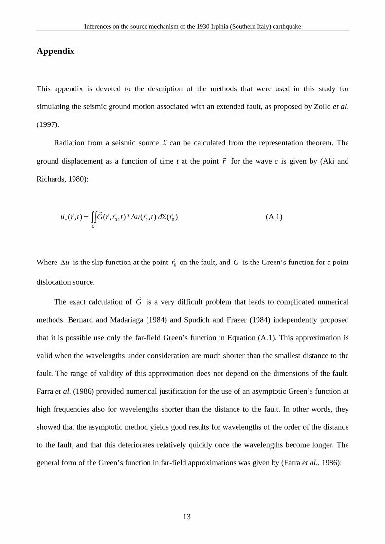
Radiation from a seismic source Σ can be calculated from the representation theorem. The

ground displacement as a function of time t at the point rr for the wave c is given by (Aki and

Richards, 1980):

∫∫Σ

Σ∆= )(),(*),,(),( 000 rdtrutrrGtrucrrrrrrr (A.1)

Where u∆ is the slip function at the point 0rr on the fault, and G

r is the Green’s function for a point

dislocation source.

The exact calculation of Gr

is a very difficult problem that leads to complicated numerical

methods. Bernard and Madariaga (1984) and Spudich and Frazer (1984) independently proposed

that it is possible use only the far-field Green’s function in Equation (A.1). This approximation is

valid when the wavelengths under consideration are much shorter than the smallest distance to the

fault. The range of validity of this approximation does not depend on the dimensions of the fault.

Farra et al. (1986) provided numerical justification for the use of an asymptotic Green’s function at

high frequencies also for wavelengths shorter than the distance to the fault. In other words, they

showed that the asymptotic method yields good results for wavelengths of the order of the distance

to the fault, and that this deteriorates relatively quickly once the wavelengths become longer. The

general form of the Green’s function in far-field approximations was given by (Farra et al., 1986):


14

[ ]⎭⎬⎫

⎩⎨⎧

−∆Π= )(Re4

),0,( 000

300

0, rTtFcJc

ctrG cc

cFF r&rrrr

ρρ

πρµ (A.2)

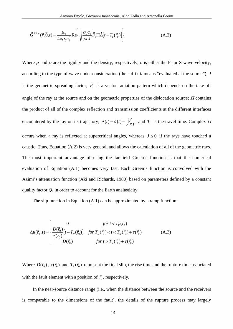
Where µ and ρ are the rigidity and the density, respectively; c is either the P- or S-wave velocity,

according to the type of wave under consideration (the suffix 0 means “evaluated at the source”); J

is the geometric spreading factor; cFr

is a vector radiation pattern which depends on the take-off

angle of the ray at the source and on the geometric properties of the dislocation source; Π contains

the product of all of the complex reflection and transmission coefficients at the different interfaces

encountered by the ray on its trajectory; titt πδ −=∆ )()( ; and cT is the travel time. Complex Π

occurs when a ray is reflected at supercritical angles, whereas 0≤J if the rays have touched a

caustic. Thus, Equation (A.2) is very general, and allows the calculation of all of the geometric rays.

The most important advantage of using the far-field Green’s function is that the numerical

evaluation of Equation (A.1) becomes very fast. Each Green’s function is convolved with the

Azimi’s attenuation function (Aki and Richards, 1980) based on parameters defined by a constant

quality factor Qc in order to account for the Earth anelasticity.

The slip function in Equation (A.1) can be approximated by a ramp function:

[ ]⎪⎪⎩

⎪⎪⎨

⎧

+>

+<<−

<

=∆

)()()(

)()()()()()(

)(0

),(

000

00000

0

0

0

rrTtforrD

rrTtrTforrTtrrD

rTtfor

tru

R

RRR

R

rrr

rrrrr

rr

r

τ

ττ

(A.3)

Where )( 0rD r , )( 0rrτ and )( 0rTR

r represent the final slip, the rise time and the rupture time associated

with the fault element with a position of 0rr , respectively.

In the near-source distance range (i.e., when the distance between the source and the receivers

is comparable to the dimensions of the fault), the details of the rupture process may largely


15

influence the high frequency seismic radiation. On the other hand, the heterogeneous final slip and

rupture velocity distributions of the fault are rather complex, as can be seen from near-source strong

motion data (Hartzell and Heaton, 1983; Heaton, 1990). This complexity can be related to the

variable rock strength and/or applied stress field along the faulting surface. Thus, to sum up, in the

near-source range, the high frequency seismic radiation is controlled by the complexity and

heterogeneity of the rupture processes that dominate the character of the signals when the site

effects can be considered as being weak or negligible.

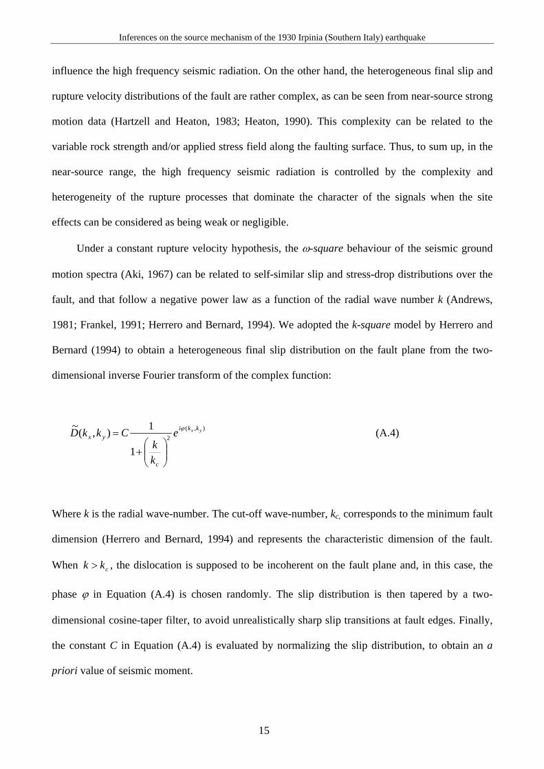
Under a constant rupture velocity hypothesis, the ω-square behaviour of the seismic ground

motion spectra (Aki, 1967) can be related to self-similar slip and stress-drop distributions over the

fault, and that follow a negative power law as a function of the radial wave number k (Andrews,

1981; Frankel, 1991; Herrero and Bernard, 1994). We adopted the k-square model by Herrero and

Bernard (1994) to obtain a heterogeneous final slip distribution on the fault plane from the two-

dimensional inverse Fourier transform of the complex function:

),(2

1

1),(~ yx kki

c

yx e

kk

CkkD ϕ

⎟⎟⎠

⎞⎜⎜⎝

⎛+

= (A.4)

Where k is the radial wave-number. The cut-off wave-number, kc, corresponds to the minimum fault

dimension (Herrero and Bernard, 1994) and represents the characteristic dimension of the fault.

When ckk > , the dislocation is supposed to be incoherent on the fault plane and, in this case, the

phase ϕ in Equation (A.4) is chosen randomly. The slip distribution is then tapered by a two-

dimensional cosine-taper filter, to avoid unrealistically sharp slip transitions at fault edges. Finally,

the constant C in Equation (A.4) is evaluated by normalizing the slip distribution, to obtain an a

priori value of seismic moment.


16

If a constant rupture velocity is used, the far-field seismic radiation is dominated by the slip

heterogeneity instead of the irregularities in the rupture velocity distribution. This approximation

may not be valid for highly discontinuous fracture phenomena, but it is reasonable when the rupture

velocity varies smoothly along the fault.

The rise time value in Equation (A.3) is generally chosen as the cut-off frequency of the low-

pass filter that is applied to the synthetic seismograms. In this case, the onset of slip appears to be

instantaneous with the passage of the rupture front. This choice maximizes the expected amplitude

of the ground motion in the far-field approximation.

The representation integral in Equation (A.1) is evaluated numerically by dividing the fault

into discrete sub-faults, and then summing up their contributions. A fine fault grid is needed to

calculate the representation integral up to high frequencies, to avoid undesired numerical effects due

to the fault dividing (e.g., spatial aliasing). Zollo et al. (1997) suggested characteristic sub-fault

dimensions of about 20-30 m.

This simulation method can be used to obtain predictive estimates of strong ground motion

parameters of engineering interest (peak parameters and spectral ordinates) in seismically active

areas. Paleoseismic evidence of the occurrence of repeated rupture episodes along the same fault (or

fault system) suggest that some characteristics, like fault geometry, source mechanism, and average

slip, depend on the direction and intensity of the regional stress field, and it is reasonable to

consider these constant on a large time scale. This concept is supported by several paleoseismic

studies that were performed on active faults in different tectonic environments (e.g., Pantosti and

Valensise, 1990; Pantosti et al., 1993; Meghraoui et al., 2000). However, numerical simulations of

fracture development suggest that the fracture process may not repeat the same style of nucleation,

propagation and arrest in successive rupture events along a given fault (e.g., Rice, 1993; Nielsen et

al., 1995; Nielsen et al., 2000). On this basis, a massive calculation of synthetic seismograms

produced by a large number of possible rupture processes occurring on the same a priori known

fault is performed. Assuming a constant rupture velocity, the history of each rupture is built from a


17

heterogeneous final slip distribution and a rupture nucleation point randomly chosen over the fault

plane. Considering that the source effects are dominant at near-source distances, the variability of

the synthetic strong motion records should account for the a priori unknown rupture complexity.

The range of expected variations of typical strong-motion parameters for a given seismogenetic

fault (or fault system) can therefore be estimated by statistical analysis. For these reasons, Zollo et

al. (1997) defined their simulation method as a hybrid stochastic-deterministic technique.

This simulation approach was used by Zollo et al. (1997) to estimate the strong ground motion

parameters for the Friuli earthquake (1976, M = 6.5), and by Zollo et al. (1999) to calculate the

ground motion scenario associated with a hypothetical earthquake occurring on the Ibleo-Maltese

fault system in South-Eastern Sicily. It has also been recently validated by Emolo and Zollo (2001),

who simulated the two main shocks of the Umbria-Marche seismic sequence (26th September, 1997;

the MW = 5.5 and MW = 6.0 events).

Acknowledgments

We thank L. Improta for helpful discussions. We would also like to thank G. Cultrera, an

anonymous reviewer, and M. Cocco for their constructive comments.


18

References AKI, K. (1967): Scaling law of seismic spectra, J. Geophys. Res., 72, 1217-1231. AKI, K. and P.G. RICHARDS (1980): Quantitative Seismology, Theory and Methods (W.H. Freeman

and Co., San Francisco, USA), vols. 1 and 2, pp. 932. ALFANO, G.B. (1931): Il terremoto irpino del 23 luglio 1930, Pubbl. Osservatorio di Pompei, 1031,

3-57. ANDREWS, D.J. (1981): A stochastic fault model, 2. Time-independent case. J. Geophys. Res., 86,

10821-10834. BASILI, R. and P. BURRATO (2001): Operating manual, Ann. Geophys., 44, suppl. 1, 835-888. BERNARD, P. and R. MADARIAGA (1984): A new asymptotic method for the modelling of near-field

accelerograms, Bull. Seism. Soc. Am., 74, 539-555. BERNARD, P. and A. ZOLLO (1989): The Irpinia (Italy) 1980 earthquake: detailed analysis of a

complex normal fault, J. Geophys. Res., 94, 1631-1648. BOSCHI, E., G. FERRARI, P. GASPERINI, E. GUIDOBONI, G. SMRIGLIO e G. VALENSISE (1995):

Catalogo dei forti terremoti in Italia dal 461 A.C. al 1980, ING-SGA, Bologna. CAMASSI, R. e M. STUCCHI (1998): NT4.1, un catalogo parametrico di terremoti di area italiana al

di sopra della soglia del danno, http://emidius.itim.mi.cnr.it/NT/home.html. CNR-PFG (1985): Atlas of isoseismal maps of italian earthquakes, Quad. Ric. Scient., Pubbl. 114. EMOLO, A. and A. ZOLLO (2001): Accelerometric radiation simulation for the September 26, 1997

Umbria-Marche (Central Italy) main shocks, Ann. Geophys., 44, 605-617. FARRA, V., P. BERNARD and R. MADARIAGA (1986): Fast near source evaluation of strong ground

motion for complex source models, in Earthquake Source Mech., Geophys. Monogr., Am. Geophys. Un., 37, 121-130.

FRANKEL, A. (1991): High-frequency spectral falloff of earthquakes, fractal dimension of complex rupture, b value, and the scaling of strength on fault, J. Geophys. Res., 96, 6291-6302.

GASPERINI, P., F. BERNARDINI, G. VALENSISE and E. BOSCHI (1999): Defining seismogenic sources from historical earthquake felt report, Bull. Seism. Soc. Am., 89, 94-110.

GRUPPO DI LAVORO CPTI (1999): Catalogo parametrico dei terremoti italiani, ING, GNDT, SGA, SSN, Bologna.

HANKS, T.C. and H. KANAMORI (1979): A moment-magnitude scale, J. Gephys. Res., 84, 2348-2352.

HARTZELL, S. and T.H. HEATON (1983): Inversion of strong ground motion and teleseismic waveforms data for the fault rupture history of the 1979 Imperial Valley, California, earthquake, Bull. Seism. Soc. Am., 73, 1553-1583.

HEATON, T.H. (1990): Evidence for and implications of self-healing pulses of slip in earthquake rupture, Phys. Earth Planet. Inter., 64, 1-20.

HERRERO, A. and P. BERNARD (1994): A kinematic self-similar rupture process for earthquakes, Bull. Seism. Soc. Am., 84, 1216-1229.

JIMENEZ, E. (1988): Etude des mécanismes au foyer à partir d’une station unique: application aux domaines Euro-Méditerranéen et Sud-Ouest Pacifique, Ph.D. thesis, Université L. Pasteur, Stasbourg.

KARNIK, V. (1969): Seismicity of the european area, Kluwer, Dordrecht. MADARIAGA, R. (1977): Implications of stress-drop models of earthquakes for inversion of stress-

drop from seismic observations, Pure Appl. Geophys., 115, 301-315. MARGOTTINI, C., N.A. AMBRASEYS e V. PETRINI (1993): La magnitudo dei terremoti italiani del XX

secolo, Rapporto tecnico ENEA. MARTINI, M. and R. SCARPA (1983): Earthquakes in Italy in the last century, in Earthquakes:

observation, theory and interpretation, edited by H. Kanamori and E. Boschi, Scuola Italiana di Fisica “E. Fermi”, 85th course, Bologna, pp. 479-492.


19

MEGHRAOUI, M., T. CAMELBECK, K. VANNESTE, M. BRONDEEL and D. JONGMANS (2000): Active faulting and paleoseismology along the Bree fault, lower Rhine graben, Belgium, J. Geophys. Res., 105, 13809-13841.

NEIS CATALOGUE. National Earthquake Information Service of USGS. http://neic.usgs.gov/neis. NIELSEN, S.B., L. KNOPOFF and A. TARANTOLA (1995): Model of earthquake recurrence: role of

elastic wave radiation, relaxation of friction, and inhomogeneity, J. Geophys. Res., 100, 12423-12430.

NIELSEN, S.B., J.M. CARLSON and K.B. OLSEN (2000): Influence of friction and fault geometry on earthquake rupture, J. Geophys. Res., 105, 6069-6088.

ODDONE, E. (1930): Studio sul terremoto avvenuto il 23 luglio 1930 nell’Irpinia, Relazione a S.E. il Ministro dell’Agricoltura e Foreste, in La meteorologia pratica, Regio Ufficio centrale di Meteorologia e Geofisica.

OPPENHEIMER, D.H., P.A. REASENBERG and R.W. SIMPSON (1988): Fault plane solution for the 1984 Morgan Hill, California, earthquake sequence: evidence for the state of stress on the Calaveras fault, J. Geophys. Res., 93, 9007-9026.

PANTOSTI, D. and G. VALENSISE (1990): Faulting mechanism and complexity of the November 23, 1980, Campania-Lucania earthquake, inferred from surface observation, J. Geophys. Res., 95, 15319-15341.

PANTOSTI, D., D. SCHWARTZ and G. VALENSISE (1993): Paleoseismicity along the 1980 surface rupture of the Irpinia fault: implications for earthquake recurrence in the Southern Apennines, Italy, J. Geophys. Res., 98, 6561-6577.

POSTPISCHL, D. (1985): Atlas of isoseismal maps of Italian earthquakes, Quaderni Ricerca Scientifica, 114, 2A, Roma.

RICE, J.R. (1993): Spatio-temporal complexity of slip on fault, J. Geophys. Res., 98, 9885-9907. SCHOLZ, C.H., C. AVILES and S. WESNOUSKY (1986): Scaling differences between large intraplate

and interplate earthquakes, Bull. Seism. Soc. Am., 76, 65-70. SPUDICH, P. and L.N. FRAZER (1984): Use of ray theory to calculate high-frequency radiation from

earthquake sources having spatially variable rupture velocity and stress drop, Bull. Seism. Soc. Am., 74, 2061-2082.

TRIFUNAC, M.D. and A.G. BRADY (1975): On the correlation of seismic intensity data in California and western Nevada, Bull. Seism. Soc. Am., 65, 139-162.

VALENSISE, G. and D. PANTOSTI (2001): Database of potential sources for earthquakes larger than M=5.5 in Italy, Ann. Geophys., 44, suppl. 1, with CD-Rom.

WELLS, D.L. and K.J. COPPERSMITH (1994): New empirical relationships among magnitude, rupture length, rupture width, rupture area, and surface displacement, Bull. Seism. Soc. Am., 84, 974-1002.

WESTAWAY, R. (1992): Seismic moment summation for historical earthquakes in Italy: tectonic implications, J. Geophys. Res., 97, 415-437.

ZOLLO, A. and P. BERNARD (1991): Fault mechanism from near source data: joint inversion of S polarizations and P polarities, Geophys. J. Int., 104, 441-451.

ZOLLO, A., A. BOBBIO, A. EMOLO, A. HERRERO and G. DE NATALE (1997): Modelling of the ground acceleration in the near source range: the case of 1976 Friuli earthquake (M=6.5), northern Italy, J. Seism., 1, 305-319.

ZOLLO, A., A. EMOLO, A. HERRERO and L. IMPROTA (1999): High frequency strong motion modelling in the Catania area associated with the Ibleo-Maltese fault system, J. Seism., 3, 279-288.


20

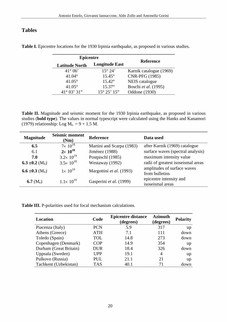
Tables Table I. Epicentre locations for the 1930 Irpinia earthquake, as proposed in various studies.

Epicentre

Latitude North Longitude EastReference

41° 06’ 15° 24’ Karnik catalogue (1969) 41.04° 15.45° CNR-PFG (1985) 41.05° 15.42° NEIS catalogue 41.05° 15.37° Boschi et al. (1995)

41° 03’ 31” 15° 25’ 15” Oddone (1930) Table II. Magnitude and seismic moment for the 1930 Irpinia earthquake, as proposed in various studies (bold type). The values in normal typescript were calculated using the Hanks and Kanamori (1979) relationship: Log Mo = 9 + 1.5 M.

Magnitude Seismic moment (Nm) Reference Data used

6.5 7× 1018 Martini and Scarpa (1983) after Karnik (1969) catalogue 6.1 2× 1018 Jiménez (1988) surface waves (spectral analysis) 7.0 3.2× 1019 Postpischl (1985) maximum intensity value

6.3 ±0.2 (MS) 3.5× 1018 Westaway (1992) radii of greatest isoseismal areas

6.6 ±0.3 (MS) 1× 1019 Margottini et al. (1993) amplitudes of surface waves from bulletins

6.7 (Me) 1.1× 1019 Gasperini et al. (1999) epicentre intensity and isoseismal areas

Table III. P-polarities used for focal mechanism calculations.

Location Code Epicentre distance (degrees)

Azimuth (degrees) Polarity

Piacenza (Italy) PCN 5.9 317 upAthens (Greece) ATH 7.1 111 downToledo (Spain) TOL 14.8 273 downCopenhagen (Denmark) COP 14.9 354 upDurham (Great Britain) DUR 18.4 326 downUppsala (Sweden) UPP 19.1 4 upPulkovo (Russia) PUL 21.1 21 upTachkent (Uzbekistan) TAS 40.1 71 down


21

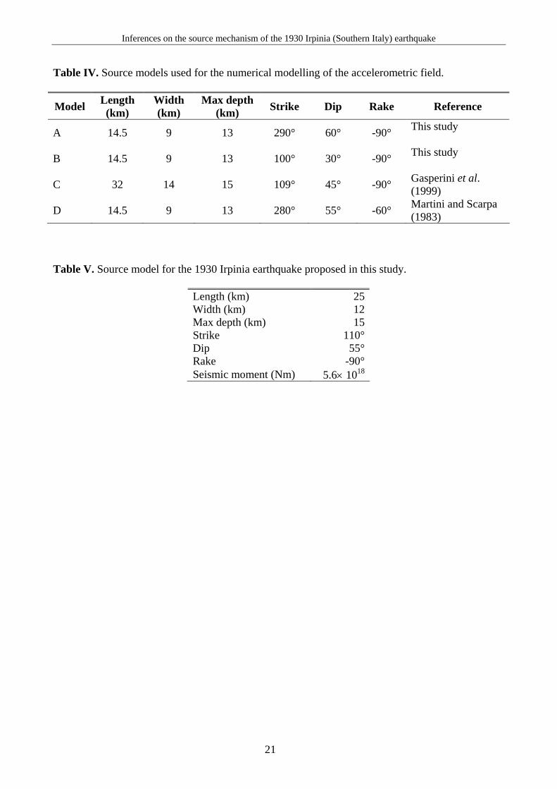
Table IV. Source models used for the numerical modelling of the accelerometric field.

Model Length (km)

Width (km)

Max depth (km) Strike Dip Rake Reference

A 14.5 9 13 290° 60° -90° This study

B 14.5 9 13 100° 30° -90° This study

C 32 14 15 109° 45° -90° Gasperini et al. (1999)

D 14.5 9 13 280° 55° -60° Martini and Scarpa (1983)

Table V. Source model for the 1930 Irpinia earthquake proposed in this study.

Length (km) 25Width (km) 12Max depth (km) 15Strike 110°Dip 55°Rake -90°Seismic moment (Nm) 5.6× 1018


22

Figure legends

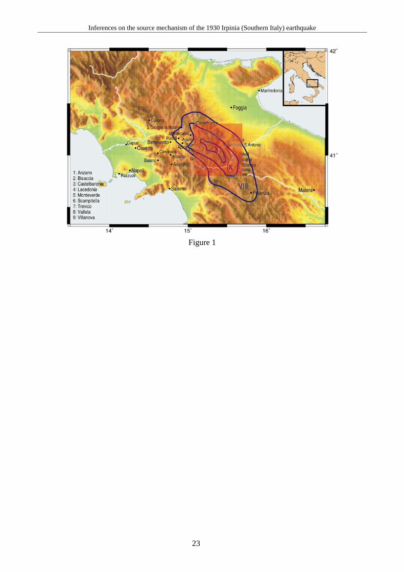
Figure 1. Isoseismal curves for the 1930 Irpinia earthquake (after CNR-PFG, 1985). Only the

curves corresponding to the degrees VIII, IX and X are reported. The red shaded area corresponds

to the region used for this simulation study.

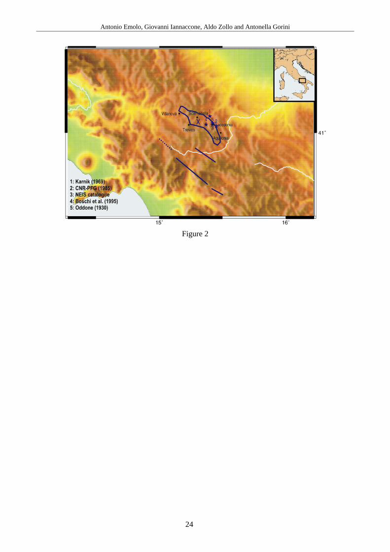
Figure 2. Epicentre locations for the 1930 Irpinia earthquake that have been proposed from

different studies. The isoseismal curve for degree X is also reported. The blue lines are the fault

traces for the 1980 Irpinia earthquake (after Bernard and Zollo, 1989).

Figure 3. Fault plane solutions for the 1930 Irpinia earthquake.

Figure 4. Peak ground acceleration field simulations for the four source models of Table IV. The

rectangles represent the surface projection of the fault. The dipping directions of the fault planes

and the focal mechanism are also shown. The numbered triangles represent towns (01: Aquilonia;

02: Lacedonia; 03: Scampitella; 04: Villanova; 05: Trevico; 06: Anzano; 07: Ariano Irpino; 08:

Bisaccia; 09: Carife; 10: Castel Baronia; 11: Flumeri; 12: Monteverde; 13: Rocchetta S. Antonio;

14: S. Nicola Baronia; 15: S. Sossio Baronia; 16: Vallata; 17: Zungoli; 18: Melfi; 19: Barile; 20:

Rionero; 21: San Fele; 22: S. Agata; 23: Atella; 24: Candela; 25: Castelfranco; 26: Frigento; 27:

Savignano; 28: Andretta).

Figure 5. Final sketch of the 1930 Irpinia earthquake. Left. Map of the simulated peak ground

acceleration field. The rectangle represents the surface projection of the fault. The dipping direction

of the fault plane and the focal mechanism are also shown. The triangles represent towns (see

legend to Fig. 4). The white triangles represent towns for which the actual intensity data are

consistent with that simulated; the red triangles represent towns for which the actual intensity data

are greater than simulated.


23

Figure 1


24

Figure 2


25

Figure 3


26

Figure 4


27

Figure 5

Documents

Inferences on the source mechanisms of the 1930 Irpinia ...geo.mff.cuni.cz/vyuka/seismologie/seis1/cele/2004-AnnGeophys-Emolo...of the 1930 Irpinia (Southern Italy) earthquake from