Embed Size (px)
Citation preview
Inferential Statistics
Predict and generalize
results to the general
population
Analyze, test
hypotheses, and answer
research questions
using math & logic
Allow the testing of
hypotheses using data
obtained from
probability and non-
probability samples
Used to draw
conclusions
1
What is Statistical Significance?
When Statistical Significance is found
It indicates that the observed relationship between
independent variable (predictor) and dependent
variable (outcome) from the data is likely to be
real, not by chance
Statistical Significance can be determined via
p-values
Confidence intervals
2
3
Statistical vs. Clinical Significance
A statistically significant result means that the
finding was unlikely to have occurred by chance.
Does not necessarily imply clinical relevance
Results may still be clinically relevant even when no
relationship appears from statistical analysis
Need to consider that factor in findings when
evaluating an article for use
4
What is Probability?
When conducting a statistical analysis, we have to ask
ourselves:
What are the chances of obtaining the same result from a study
that can be carried out many times under identical conditions?
The probability of an event is its long-run relative
frequency of occurring (0% to 100%) in repeated trials
and under similar conditions.
By chance, there is a risk that the characteristics of any
given sample may be different from those of the entire
population.
What is Probability?
Represented by the p value
What it represents
The probability that a difference exists based
on the statistical test performed
5
What is Probability?
Probability is based on the concept of
sampling error.
Even when samples are randomly selected,
there is always the possibility of some error
occurring.
Remember: The characteristics of any given
sample may be different from those of the
entire population.
6
7
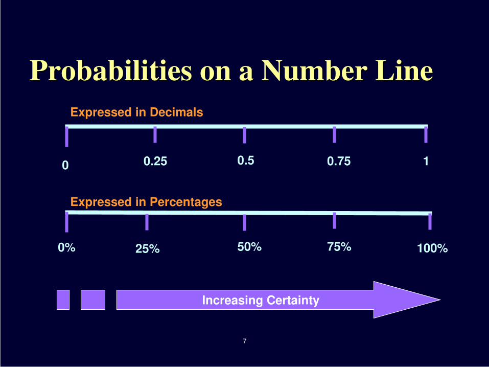
Probabilities on a Number Line
0% 100% 50% 25% 75%
0 1 0.5 0.75 0.25
Increasing Certainty
Expressed in Decimals
Expressed in Percentages
8
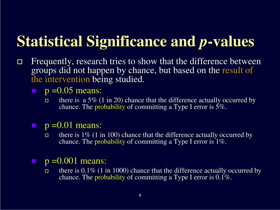
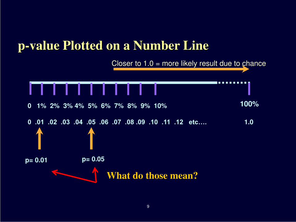
Statistical Significance and p-values
Frequently, research tries to show that the difference between groups did not happen by chance, but based on the result of the intervention being studied.
p =0.05 means: there is a 5% (1 in 20) chance that the difference actually occurred by
chance. The probability of committing a Type I error is 5%.
p =0.01 means: there is 1% (1 in 100) chance that the difference actually occurred by
chance. The probability of committing a Type I error is 1%.
p =0.001 means: there is 0.1% (1 in 1000) chance that the difference actually occurred by
chance. The probability of committing a Type I error is 0.1%.
9
p= 0.01
0 .01 .02 .03 .04 .05 .06 .07 .08 .09 .10 .11 .12 etc…. 1.0
0 1% 2% 3% 4% 5% 6% 7% 8% 9% 10% 100%
p= 0.05
Closer to 1.0 = more likely result due to chance
p-value Plotted on a Number Line
What do those mean?
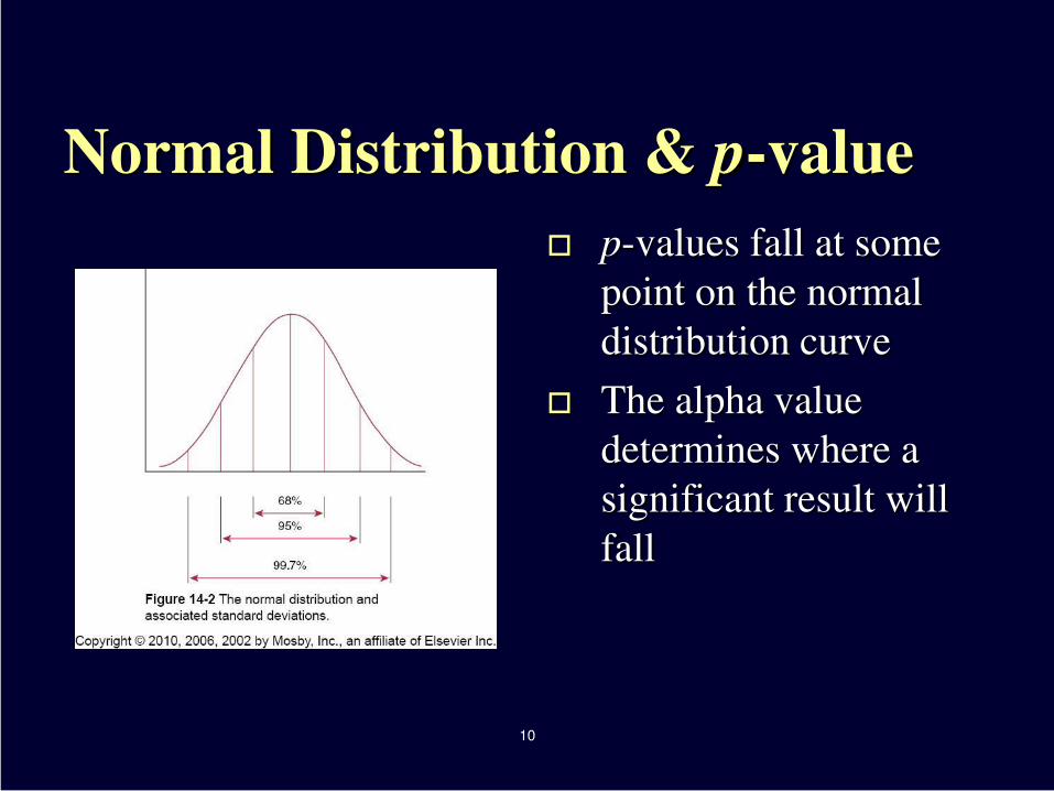
Normal Distribution & p-value
p-values fall at some
point on the normal
distribution curve
The alpha value
determines where a
significant result will
fall
10
11
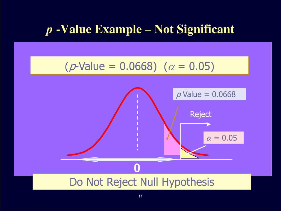
p -Value Example – Not Significant
0
Reject
(p-Value = 0.0668) (a = 0.05)
p Value = 0.0668
a = 0.05
Do Not Reject Null Hypothesis
12
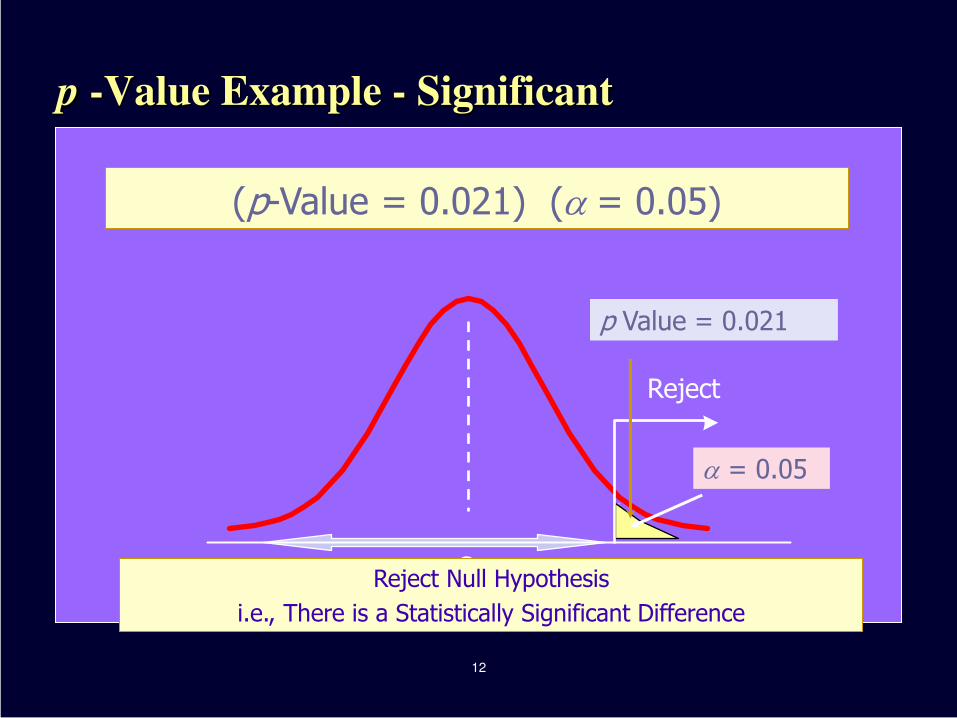
p -Value Example - Significant
0
Reject
(p-Value = 0.021) (a = 0.05)
p Value = 0.021
a = 0.05
Reject Null Hypothesis
i.e., There is a Statistically Significant Difference
13
Hypothesis Testing: The Why
Why do we do hypothesis testing? To determine:
How much of this effect is a result of chance
How strongly are these two variables associated
What is the effect of the intervention
Two hypothesis are tested
Research or scientific hypothesis
Null hypothesis
14
Hypothesis Testing: The What
Hypothesis is a statement about a research question.
Commonly hypotheses are statements about
A distribution parameter
Is the average birth weight greater than 5.5lbs?
Relationship between parameters
Is obesity rate higher among Blacks than Whites?
Relationship about probability distributions
Is smoking associated with CVD?
15
Null Hypothesis &
Alternative Hypothesis
Null Hypothesis (Statistical Representation: H0) Assumption that there is NO difference between groups
Alternate Hypothesis (Statistical Representation: HA) Statement that declares that there IS a difference between
groups
a.k.a. Study hypothesis
May be expressed as directional hypothesis e.g., the patient’s weight will decrease as a result of increased
exercise
16
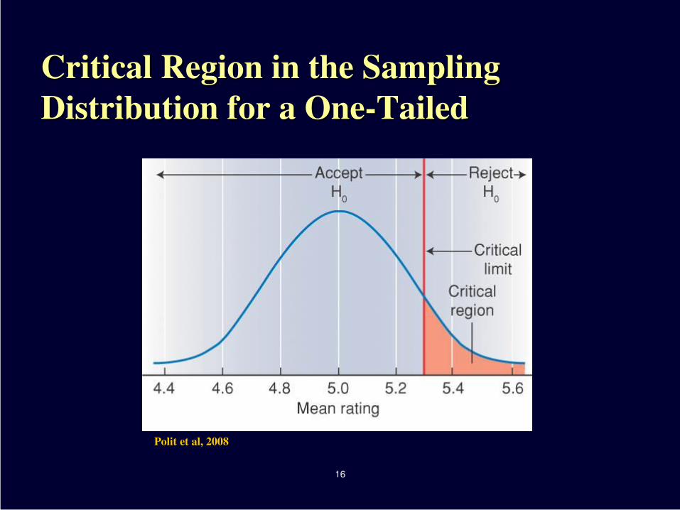
Critical Region in the Sampling
Distribution for a One-Tailed
Polit et al, 2008
17
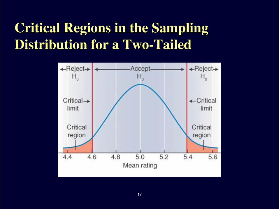
Critical Regions in the Sampling
Distribution for a Two-Tailed
18
Mosby items and derived items © 2009 by Mosby, Inc.
Level of Significance
Level of significance: alpha level (α)
Probability of making type I error
0.05 or less
Means that when you see the p value equal 0.05 or
less, the chance that a type I error occurred was
reduced.
The pre-determined cut off point at which you
will reject the null hypothesis
Level of Significance
Another way to think about it:
If the probability is = .01, this means that the
researcher is willing to accept the fact that if the
study was done 100 times, the decision to reject
the null hypothesis would be wrong 1 time out of
those 100 trials.
If alpha is 0.05, then the decision to reject the null
hypothesis would be wrong 5 times of those 100.
19
20
Hypothesis Testing, p-values, & Alpha Levels
For any p-value less than 0.05 (i.e. between 0 and 0.05) you will reject the null hypothesis.
This means that a difference exists i.e., the result NOT due to chance.
For any p-value greater than 0.05 (i.e., between 0.05 and 1.0) you will not reject the null hypothesis.
This means that no difference exists, i.e, the result may be due to chance.
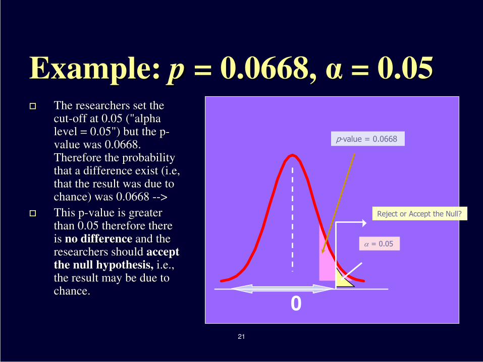
Example: p = 0.0668, α = 0.05 The researchers set the
cut-off at 0.05 ("alpha level = 0.05") but the p-value was 0.0668. Therefore the probability that a difference exist (i.e, that the result was due to chance) was 0.0668 -->
This p-value is greater than 0.05 therefore there is no difference and the researchers should accept the null hypothesis, i.e., the result may be due to chance.
21
0
Reject or Accept the Null?
p-value = 0.0668
a = 0.05

Example: Comparing Groups
The following slides provide examples of tables
from a research study that studied two different
types of arterial bypass surgery through a
randomized controlled trial. It also compared costs.
Link to actual study: http://jama.ama-
assn.org/content/291/15/1841.full.pdf+html?sid=3bae3b7d-0a0d-4152-babf-cbe9d6a2b0e4
22
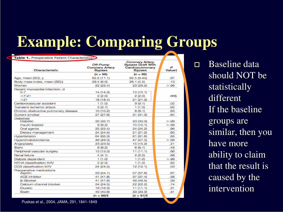
Baseline data
should NOT be
statistically
different
If the baseline
groups are
similar, then you
have more
ability to claim
that the result is
caused by the
intervention
Puskas et al., 2004, JAMA, 291, 1841-1849
23
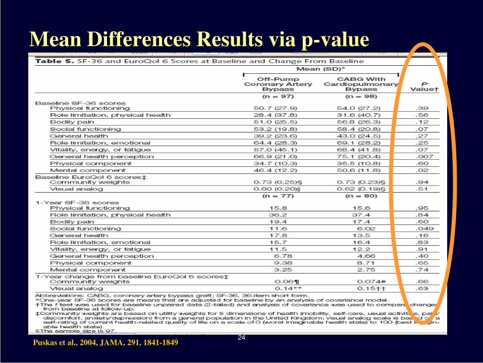
Example: Comparing Groups
24
Mean Differences Results via p-value
Puskas et al., 2004, JAMA, 291, 1841-1849
25
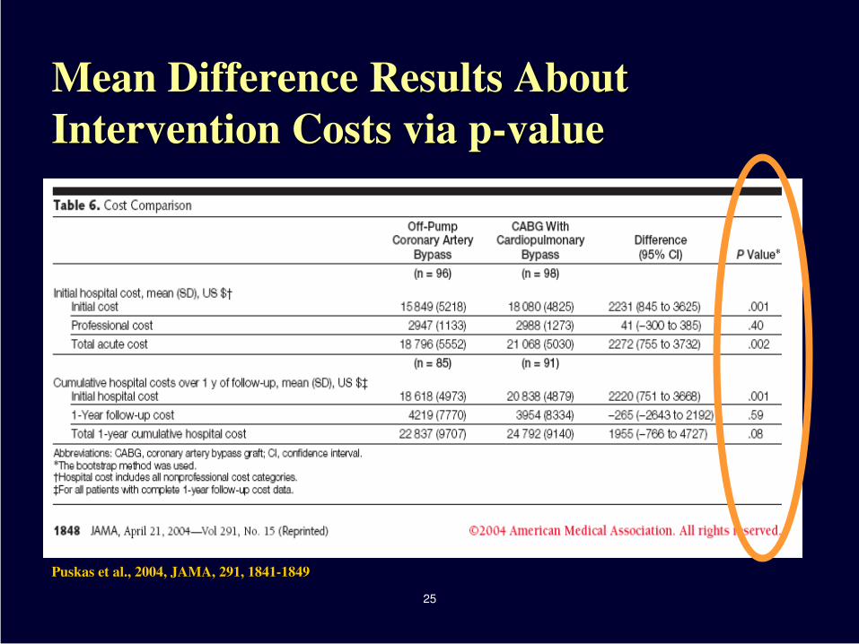
Mean Difference Results About
Intervention Costs via p-value
Puskas et al., 2004, JAMA, 291, 1841-1849
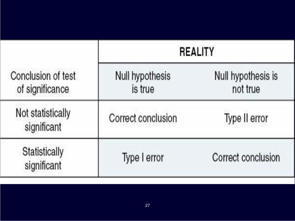
Types of Statistical Errors
Sampling error
The tendency for statistics to fluctuate from one
sample to another
Type I
Type II
26
27
28
The Power Analysis:
A Prevention Intervention for Errors
(1- β) is called the power of the test (or the
statistical power for the test/study).
It is the probability to find the difference between
groups in a sample when there is a difference.
To reduce likelihood of error, sometimes the
researcher needs to perform a priori power analysis.
Confidence Intervals
Method to describe the precision of an estimate
95% CI indicates that you are 95% confident that the results would fall between the high and low if you repeated the study
Shown as a range in publications The more narrow the range between the numbers the more
precise the result
Example: 95% CI (A, B)
Example: 99% CI (C – D)
29

Confidence Intervals
To describe the precision of the estimate: Narrow confidence intervals = more precise
Wide confidence intervals = less precise
Two types of measurement level data work with CI when determining statistical significance Continuous
Discrete/Ratio
30
31
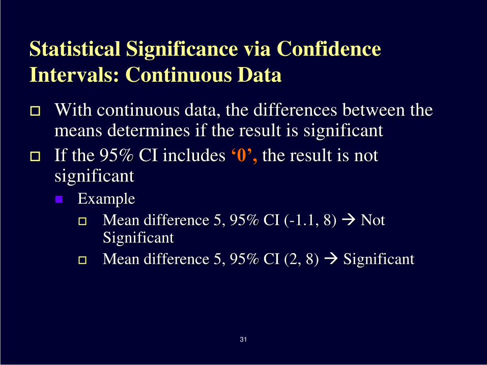
Statistical Significance via Confidence
Intervals: Continuous Data
With continuous data, the differences between the means determines if the result is significant
If the 95% CI includes ‘0’, the result is not significant Example
Mean difference 5, 95% CI (-1.1, 8) Not Significant
Mean difference 5, 95% CI (2, 8) Significant
32
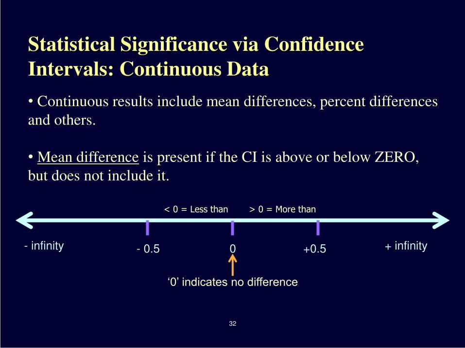
Statistical Significance via Confidence
Intervals: Continuous Data
• Continuous results include mean differences, percent differences
and others.
• Mean difference is present if the CI is above or below ZERO,
but does not include it.
0 - 0.5 +0.5 - infinity + infinity
‘0’ indicates no difference
< 0 = Less than > 0 = More than
33
Statistical Significance via Confidence
Intervals: Continuous Data
More about results with continuous data
Show outcome differences between groups
If the 95% CI includes ‘0’, the result is not significant 0 = no difference between groups
> 0 = outcome 1 is more likely in group 1 than in group 2
< 0 = outcome 1 is less likely in group 1 than in group 2

34
Statistical Significance via Confidence Intervals: Example – Cost Differences Between CABG Procedures
How it
appears
in a
journal
article
A B
C
35
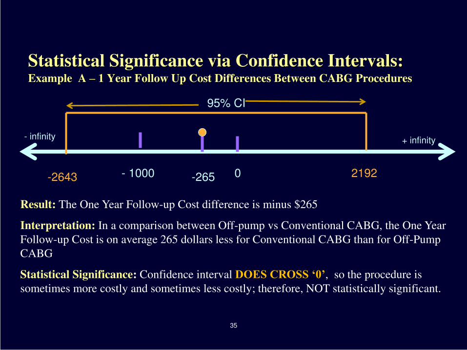
Statistical Significance via Confidence Intervals: Example A – 1 Year Follow Up Cost Differences Between CABG Procedures
- infinity + infinity
95% CI
0 - 1000 -265 2192 -2643
Result: The One Year Follow-up Cost difference is minus $265
Interpretation: In a comparison between Off-pump vs Conventional CABG, the One Year
Follow-up Cost is on average 265 dollars less for Conventional CABG than for Off-Pump
CABG
Statistical Significance: Confidence interval DOES CROSS ‘0’, so the procedure is
sometimes more costly and sometimes less costly; therefore, NOT statistically significant.
36
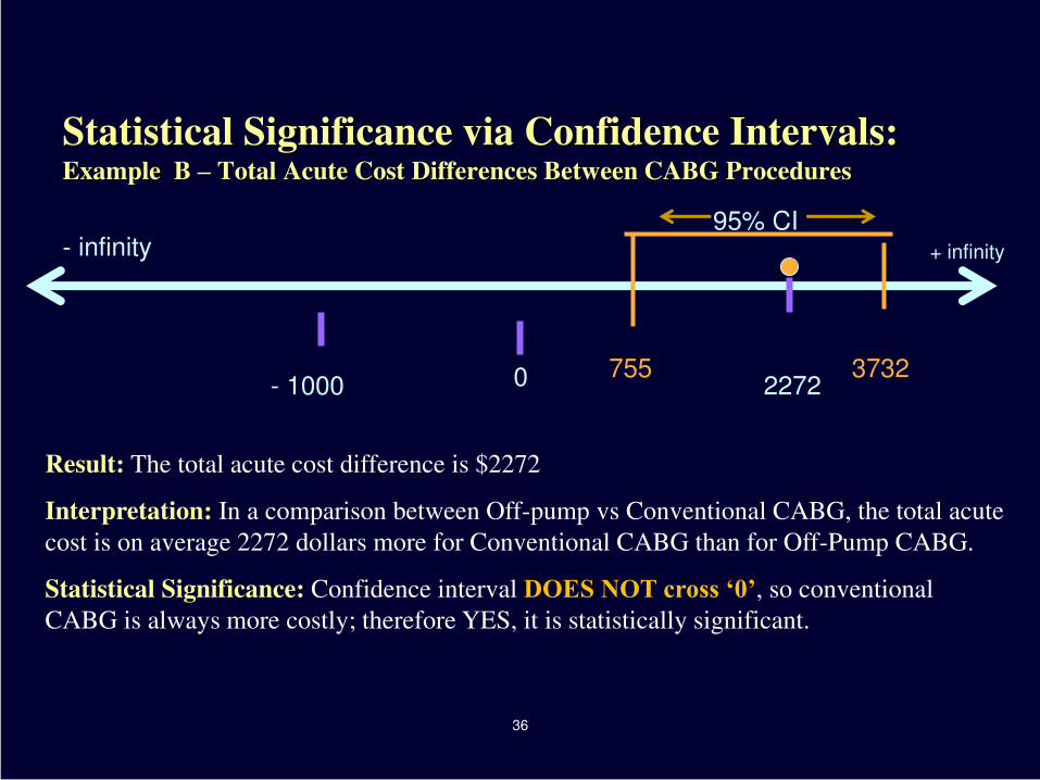
Statistical Significance via Confidence Intervals: Example B – Total Acute Cost Differences Between CABG Procedures
0 - 1000 2272
- infinity
3732 755
+ infinity
95% CI
Result: The total acute cost difference is $2272
Interpretation: In a comparison between Off-pump vs Conventional CABG, the total acute
cost is on average 2272 dollars more for Conventional CABG than for Off-Pump CABG.
Statistical Significance: Confidence interval DOES NOT cross ‘0’, so conventional
CABG is always more costly; therefore YES, it is statistically significant.
37
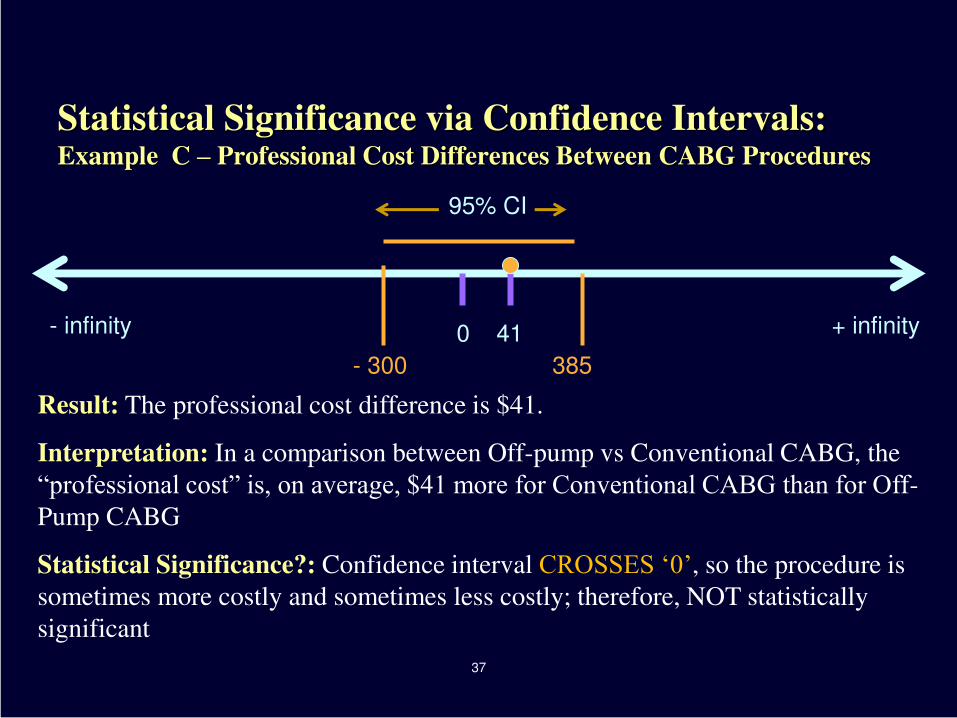
Statistical Significance via Confidence Intervals: Example C – Professional Cost Differences Between CABG Procedures
95% CI
0 41 - infinity + infinity
- 300 385
Result: The professional cost difference is $41.
Interpretation: In a comparison between Off-pump vs Conventional CABG, the
“professional cost” is, on average, $41 more for Conventional CABG than for Off-Pump CABG
Statistical Significance?: Confidence interval CROSSES ‘0’, so the procedure is
sometimes more costly and sometimes less costly; therefore, NOT statistically
significant
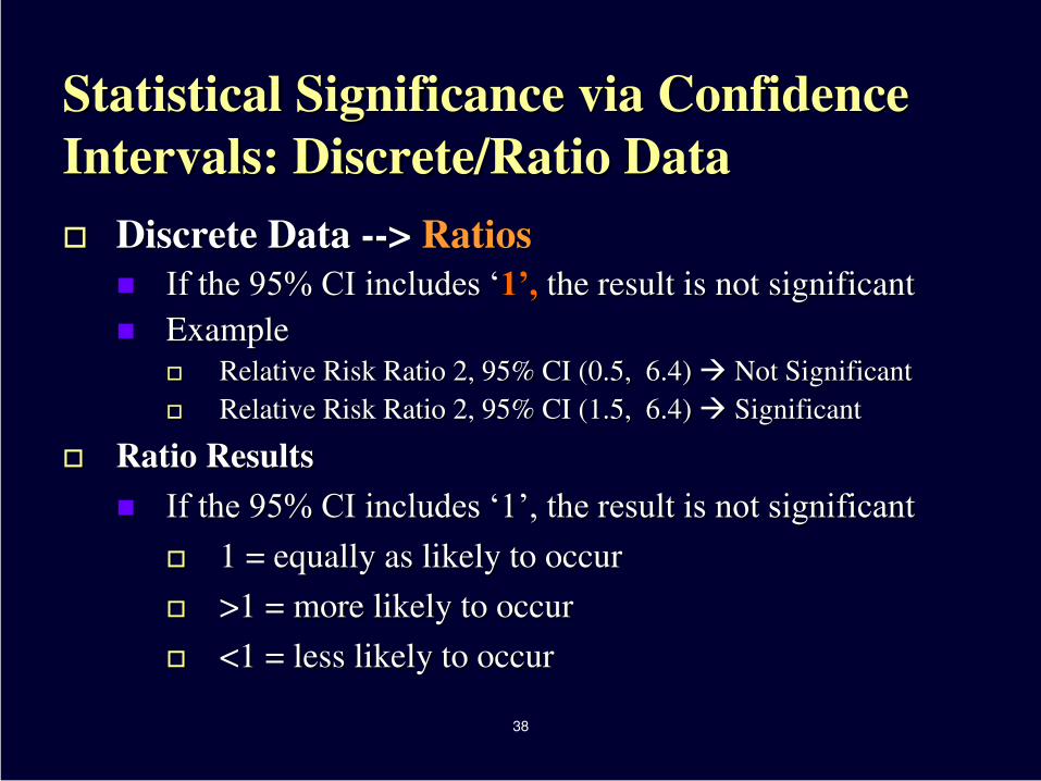
Statistical Significance via Confidence
Intervals: Discrete/Ratio Data
Discrete Data --> Ratios
If the 95% CI includes ‘1’, the result is not significant
Example Relative Risk Ratio 2, 95% CI (0.5, 6.4) Not Significant
Relative Risk Ratio 2, 95% CI (1.5, 6.4) Significant
Ratio Results
If the 95% CI includes ‘1’, the result is not significant 1 = equally as likely to occur
>1 = more likely to occur
<1 = less likely to occur
38
39
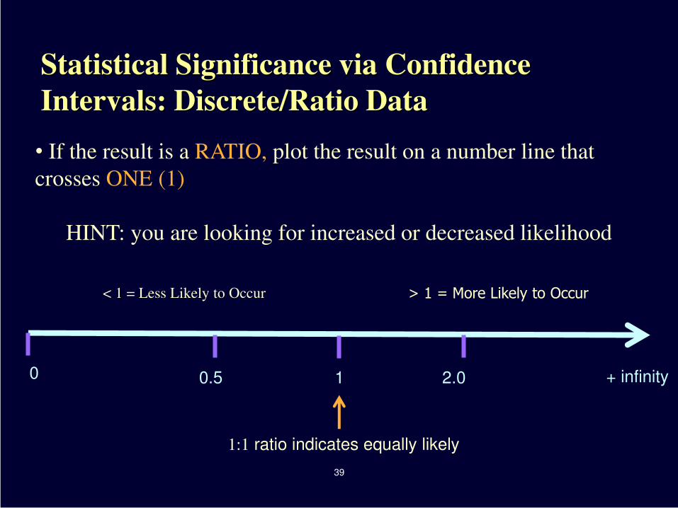
Statistical Significance via Confidence
Intervals: Discrete/Ratio Data
• If the result is a RATIO, plot the result on a number line that
crosses ONE (1)
HINT: you are looking for increased or decreased likelihood
1 0.5 2.0 0 + infinity
1:1 ratio indicates equally likely
< 1 = Less Likely to Occur > 1 = More Likely to Occur
40
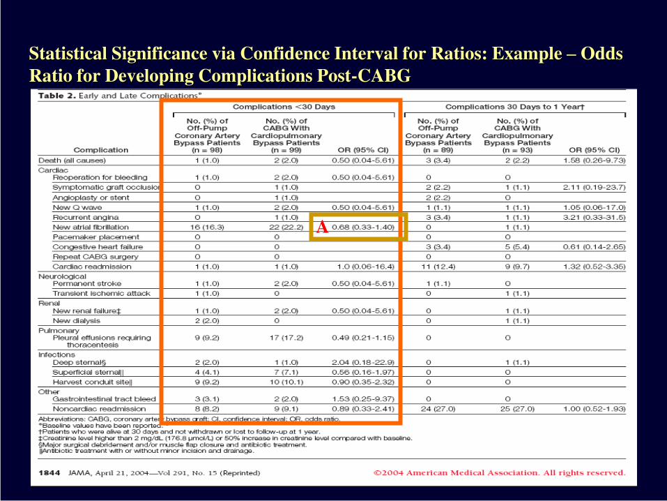
Statistical Significance via Confidence Interval for Ratios: Example – Odds
Ratio for Developing Complications Post-CABG
A
41
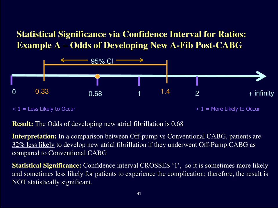
Statistical Significance via Confidence Interval for Ratios:
Example A – Odds of Developing New A-Fib Post-CABG
1 0.33 0.68 0 + infinity
95% CI
1.4
Result: The Odds of developing new atrial fibrillation is 0.68
Interpretation: In a comparison between Off-pump vs Conventional CABG, patients are
32% less likely to develop new atrial fibrillation if they underwent Off-Pump CABG as
compared to Conventional CABG
Statistical Significance: Confidence interval CROSSES ‘1’, so it is sometimes more likely and sometimes less likely for patients to experience the complication; therefore, the result is
NOT statistically significant.
< 1 = Less Likely to Occur > 1 = More Likely to Occur
2

42
Statistical Significance via Confidence Interval for Ratios: Example B –
Odds of Readmission Post-CABG
B
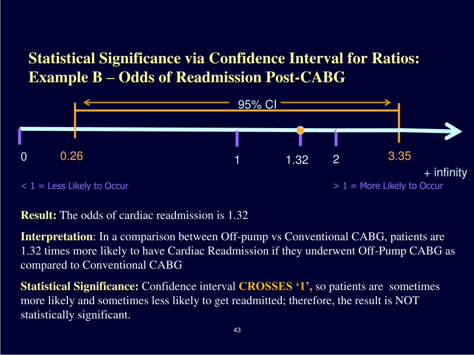
43
Statistical Significance via Confidence Interval for Ratios:
Example B – Odds of Readmission Post-CABG
1 0.26 1.32 0
+ infinity
95% CI
3.35
Result: The odds of cardiac readmission is 1.32
Interpretation: In a comparison between Off-pump vs Conventional CABG, patients are
1.32 times more likely to have Cardiac Readmission if they underwent Off-Pump CABG as
compared to Conventional CABG
Statistical Significance: Confidence interval CROSSES ‘1’, so patients are sometimes
more likely and sometimes less likely to get readmitted; therefore, the result is NOT
statistically significant.
< 1 = Less Likely to Occur > 1 = More Likely to Occur
2

Statistical Significance via Confidence
Interval for Ratios: Gauging Risk
Odds ratios can also determine the relative
risk for getting a complication or condition
Can help aid decision making by:
Healthcare professionals
Patients
44
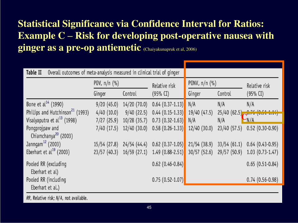
45
PONV = Post Op Nausea & Vomiting
C
Statistical Significance via Confidence Interval for Ratios:
Example C – Risk for developing post-operative nausea with
ginger as a pre-op antiemetic (Chaiyakunapruk et al, 2006)
46
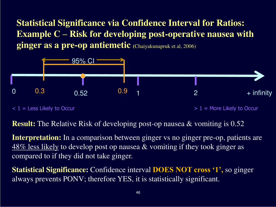
Statistical Significance via Confidence Interval for Ratios:
Example C – Risk for developing post-operative nausea with
ginger as a pre-op antiemetic (Chaiyakunapruk et al, 2006)
1 0.3 0.52 0 + infinity
95% CI
0.9
Result: The Relative Risk of developing post-op nausea & vomiting is 0.52
Interpretation: In a comparison between ginger vs no ginger pre-op, patients are
48% less likely to develop post op nausea & vomiting if they took ginger as
compared to if they did not take ginger.
Statistical Significance: Confidence interval DOES NOT cross ‘1’, so ginger
always prevents PONV; therefore YES, it is statistically significant.
< 1 = Less Likely to Occur > 1 = More Likely to Occur
2

Statistical Significance via Confidence
Interval for Ratios: The Forest Plot
A Forest Plot is:
A graphical display designed to illustrate the
relative strength of treatment effects in multiple
quantitative scientific studies addressing the same
question
Frequently used with meta-analyses
47
Statistical Significance via Confidence
Interval for Ratios: The Forest Plot
The left-hand column lists the names of the studies
The right-hand column is a plot of the measure of
effect (e.g. an odds ratio) for each of these studies
(often represented by a square) incorporating
confidence intervals represented by horizontal lines.
The area of each square is proportional to the study's
weight in the meta-analysis.
48
49
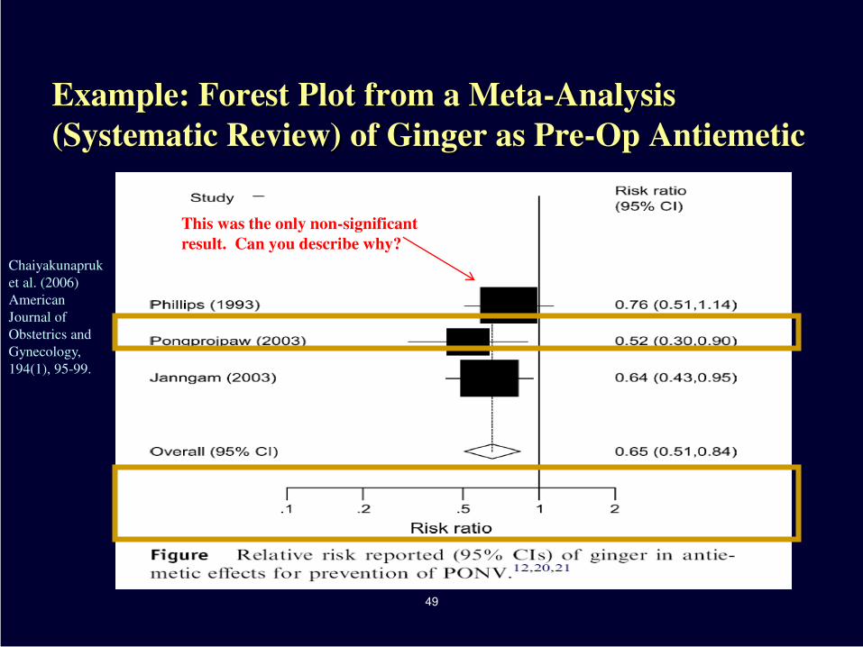
Example: Forest Plot from a Meta-Analysis
(Systematic Review) of Ginger as Pre-Op Antiemetic
Chaiyakunapruk
et al. (2006)
American
Journal of
Obstetrics and
Gynecology,
194(1), 95-99.
This was the only non-significant
result. Can you describe why?
50
Caveat
Statistical significance does not mean clinical
significance and vice versa
Size of the p-value does NOT indicate importance of the
result
If statistically significant, results might not be practical
e.g., Treatment could be effective, but might involve costly or
inaccessible procedure
Even if not statistically significant, results might be very
important
e.g., if sample size were increased, might see statistical
significance
Inferential Statistics
Tests of Difference(s)
Evaluating the degree of the relationship
between variables
51
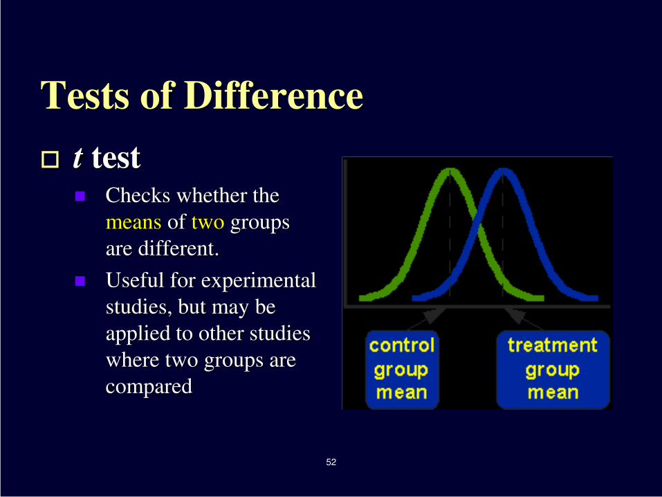
Tests of Difference
t test Checks whether the
means of two groups
are different.
Useful for experimental
studies, but may be
applied to other studies
where two groups are
compared
52
Testing Difference through Variation
Analysis of variance (ANOVA)
Tests whether more than two group means differ
Considers the variation between groups and within groups.
Analysis of variance (ANOVA)
Tests whether more than two group means differ
Considers the variation between groups and within groups.
Multiple analysis of variance (MANOVA)
Also is used to determine differences in group means, but when there
is more than one dependent variable.
53
Tests of Difference
Chi-square (2)
Uses nominal data to determine whether groups
are different.
A nonparametric statistic used to determine
whether the frequency in each category is
different from what would be expected by
chance.
54
Correlation (r)
The correlation coefficient is a simple
descriptive statistic that measures the strength
of the linear relationship between two
interval- or ratio-scale variables (as opposed
to categorical, or nominal-scale variables), as
might be visualized in a scatter plot.
55
Tests of Relationship
Most common test of correlation: Pearson
product-moment correlation Correlation coefficients can range in value from -1.0 to
+1.0 and also can be zero.
A zero coefficient means that there is no relationship
between the variables.
A perfect positive correlation is indicated by a +1.0
coefficient.
A perfect negative correlation by a -1.0 coefficient.
56
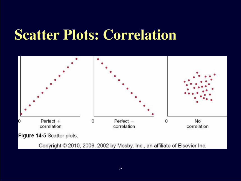
Scatter Plots: Correlation
57
Caution with Correlation
Correlation and Causality
One common mistake made by people
interpreting a correlational coefficient refers to
causality.
Example: When we see that depression and low
self-esteem are negatively correlated, we often
surmise that depression must therefore cause the
decrease in self-esteem.
58
Evaluating the Degree of Relationships
Between Variables: Regression
A correlation tells you IF a relationship exists
between variables
A regression tells you:
How strong a relationship is between the dependent and
two or more independent (explanatory) variables
How much of the dependent variable the independent
variable (or combination of variables) explains or predicts
How the dependent variable changes when the
independent variable is present or not
59
Common Types of Regression Analyses
Used in Health Research
Linear regression (also multiple linear regression)
Uses ordinal or ratio data
Logistic regression
Uses categorical (nominal) data
Frequently seen with odds ratios
Regression results are represented by r2 and look like
the example below in publications
Example: r2 = .7 (p=.0001)
60
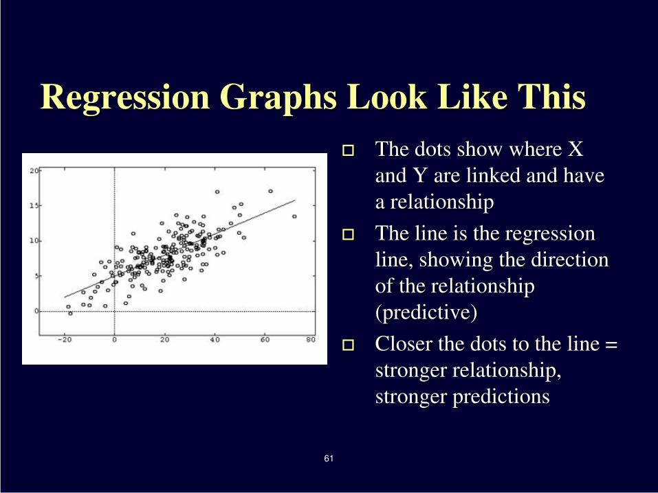
Regression Graphs Look Like This
The dots show where X
and Y are linked and have
a relationship
The line is the regression
line, showing the direction
of the relationship
(predictive)
Closer the dots to the line =
stronger relationship,
stronger predictions
61

Regression Tables Look Like This
Average education and the
kinds of hospitals where
nurses could work were
significant predictors of the
nurse-to-population ratio
Those two variables
combined explain 70% of a
nurse-to-population ratio in
a state in Mexico.
62
Variables Coefficient p
value
Median Income 0.0001 .582
Average
Education 0.6000 .000
# Children/Family 0.104 .662
Total Nursing
Schools -.0004 .410
Ratio of Public:
Private Hospitals -1.685 .001
Squires & Beltran-Sánchez (2009): This study sought to investigate macro-level
socioeconomic predictors of the nurse-to-
population ratio in Mexico.