Inferring High-Level Behavior from Low-Level Sensors

Donald J. Patterson, Lin Liao, Dieter Fox, and Henry Kautz

University Of Washington,Department of Computer Science and Engineering,

Seattle, WA, USA{djp3,liaolin,fox,kautz}@cs.washington.edu

Abstract. We present a method of learning a Bayesian model of a traveler mov-ing through an urban environment. This technique is novel in that it simultane-ously learns a unified model of the traveler’s current mode of transportation aswell as his most likely route, in an unsupervised manner. The model is imple-mented using particle filters and learned using Expectation-Maximization. Thetraining data is drawn from a GPS sensor stream that was collected by the au-thors over a period of three months. We demonstrate that by adding more externalknowledge about bus routes and bus stops, accuracy is improved.

1 Introduction

A central theme in ubiquitous computing is building rich predictive models of humanbehavior from low-level sensor data. One strand of such work concerns tracking andpredicting a person’s movements in outdoor settings using GPS [1–4]. But location isonly one small part of a person’s state. Ideally we would want to recognize and predictthe high-level intentions and complex behaviors that cause particular physical move-ments through space. Such higher-order models would both enable the creation of newcomputing services that autonomously respond to a person’s unspoken needs, and sup-port much more accurate predictions about future behavior at all levels of abstraction.

This paper presents an approach to learning how a person uses different kinds oftransportation in the community. We use GPS data to infer and predict a user’s trans-portation mode, such as walking, driving, or taking a bus. The learned model can predictmode transitions, such as boarding a bus at one location and disembarking at another.We show that the use of such a higher-level transportation model can also increase theaccuracy of location prediction, which is important in order to handle GPS signal lossor preparing for future delivery of services.

A key to inferring high-level behavior is fusing a user’s historic sensor data withgeneral commonsense knowledge of real-world constraints. Real-world constraints in-clude, for example, that buses only take passengers on or off at bus stops, that cars areleft in parking lots, and that cars and buses can only travel on streets, etc.. We present aunified probabilistic framework that accounts for both sensor error (in the case of GPS,loss of signal, triangulation error, or multi-path propagation error) and commonsenserules.

Although this work has broad applications to ubiquitous computing systems, ourmotivating application is one we call the Activity Compass, a device which helps guide

a cognitively impaired person safely through the community [5]. The system notes whenthe user departs from a familiar routine (for example, gets on the wrong bus) and pro-vides proactive alerts or calls for assistance. The Activity Compass is part of a largerproject on building cognitive assistants that use probabilistic models of human behavior[6].

Our approach is built on recent successes in particle filters, a variant of Bayes fil-ters for estimating the state of a dynamic system [7]. In particular we show how thenotion of graph-constrained particle filtering introduced in [8] can be used to integrateinformation from street maps. Extensions to this technique include richer user trans-portation state models and multiple kinds of commonsense background knowledge. Weintroduce a three-part model in which a low-level filter continuously corrects systematicsensor error, a particle filter uses a switching state-space model for different transporta-tion modes (and further for different velocity bands within a transportation mode), anda street map guides the particles through the high-level transition model of the graphstructure. We additionally show how to apply Expectation-Maximization (EM) to learntypical motion patterns of humans in a completely unsupervised manner. The transitionprobabilities learned from real data significantly increase the model’s predictive qualityand robustness to loss of GPS signal.

This paper is organized as follows. In the next section, we summarize the derivationof graph-based tracking starting from the general Bayes filter, and show how it can beextended to handle transportation mode tracking. Then, in Sect. 3, we show how tolearn the parameters of the tracking model using EM. Before concluding in Sect. 5,we present experimental results that show we can learn effective predictive models oftransportation use behavior.

2 Tracking on a Graph

Our approach tracks a person’s location and mode of transportation using street mapssuch as the ones being used for route planning and GPS-based car tracking. More specif-ically, our model of the world is a graph G = (V,E) which has a set V of vertices anda set E of directed edges. Edges correspond to straight sections of roads and foot paths,and vertices are placed in the graph to represent either an intersection, or to accuratelymodel a curved road as a set of short straight edges. To estimate the location and trans-portation mode of a person we apply Bayes filters, a probabilistic approach for estimat-ing the state of a dynamic system from noisy sensor data. We will now briefly describeBayes filters in the general case, show how to project the different quantities of theBayes filter onto the structure represented in a graph, and then discuss our extensionsto the state space model.

2.1 Bayesian Filtering on a Graph

Bayes filters address the problem of estimating the state xt of a dynamical system fromsensor measurements. Uncertainty is handled by representing all quantities involvedin the estimation process using random variables. The key idea of Bayes filters is torecursively estimate the posterior probability density over the state space conditioned

on the data collected so far. The data consists of a sequence of observations z1:t and theposterior over the state xt at time t is computed from the previous state xt−1 using thefollowing update rule (see [7, 9] for details):

p(xt |z1:t) ∝ p(zt |xt)

∫p(xt |xt−1) p(xt−1 |z1:t−1)dxt−1 (1)

The term p(xt | xt−1) is a probabilistic model of the object dynamics, and p(zt | xt)describes the likelihood of making observation zt given the location xt.

In the context of location estimation, the state, xt, typically describes the positionand velocity of the object in 2D-space. When applying Bayesian filtering to a graph, thestate of an object becomes a triple xt = 〈e, d, v〉, where e ∈ E denotes on which edgethe object resides, d indicates the distance of the object from the start vertex of edge e,and v indicates the velocity along the edge [8]. The motion model p(xt |xt−1) considersthat the objects are constrained to motion on the graph and may either travel along anedge, or, at the endpoint of the edge, switch to a neighboring edge. To compute theprobability of motion from one edge to another, the graph is annotated with transitionprobabilities p(ej | ei), which describe the probability that the object transits to edgeej given that the previous edge was ei and an edge transition took place. Without otherknowledge, this probability is a uniform distribution over all neighboring edges of ei.

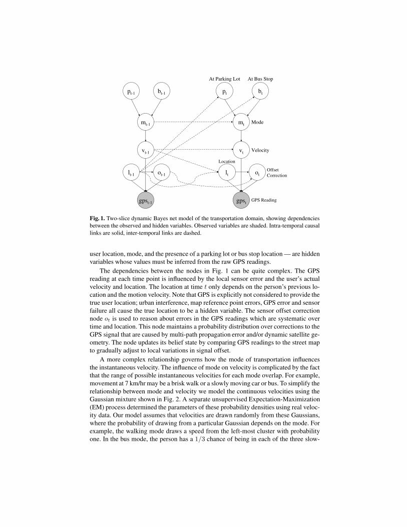
Our work builds on graph-based Bayesian tracking by hierarchically extending thestate model. We add a higher level of abstraction which contains the transportationinformation and a lower level sensor error variable. The resulting state xt consists ofthe variables shown in Fig. 1. The presence of a bus stop near the person is given bythe binary variable bt, and the presence of a parking lot is modeled by ct. The mode oftransportation, denotedmt, can take on one of three different values

mt ∈ {BUS, FOOT,CAR}.

vt denotes the motion velocity, and the location of the person at time t is representedby lt = 〈e, d〉. ot denotes the expected sensor error, which in our current model com-pensates for systematic GPS offsets. Finally, at the lowest level of the model, raw GPSsensor measurements are represented by gpst.

Tracking such a combined state space can be computationally demanding. Fortu-nately, Bayes filters can make use of the independences between the different parts ofthe tracking problem. Such independences are typically displayed in a graphical modellike Fig. 1. A dynamic Bayes net [10, 11], such as this one, consists of a set of vari-ables for each time point t, where an arc from one variable to another indicates a causalinfluence. Although all of the links are equivalent in their causality, Fig. 1 representscausality through time with dashed arrows. In an abstract sense the network can beas large as the maximum value of t (perhaps infinite), but under the assumption thatthe dependencies between variables do not change over time, and that the state spaceconforms to the first-order Markov independence assumption, it is only necessary torepresent and reason about two time slices at a time. In the figure the slices are num-bered t − 1 and t. The variables labeled gps are directly observable, and represent theposition and velocity readings from the GPS sensor (where a possible value for thereading includes “loss of signal”). All of the other variables — sensor error, velocity,

gpst GPS Reading

vt Velocity

mt Mode

pt

At Parking Lot

bt

At Bus Stop

lt

Location

otOffsetCorrection

gpst-1

vt-1

mt-1

pt-1 bt-1

lt-1 ot-1

Fig. 1. Two-slice dynamic Bayes net model of the transportation domain, showing dependenciesbetween the observed and hidden variables. Observed variables are shaded. Intra-temporal causallinks are solid, inter-temporal links are dashed.

user location, mode, and the presence of a parking lot or bus stop location — are hiddenvariables whose values must be inferred from the raw GPS readings.

The dependencies between the nodes in Fig. 1 can be quite complex. The GPSreading at each time point is influenced by the local sensor error and the user’s actualvelocity and location. The location at time t only depends on the person’s previous lo-cation and the motion velocity. Note that GPS is explicitly not considered to provide thetrue user location; urban interference, map reference point errors, GPS error and sensorfailure all cause the true location to be a hidden variable. The sensor offset correctionnode ot is used to reason about errors in the GPS readings which are systematic overtime and location. This node maintains a probability distribution over corrections to theGPS signal that are caused by multi-path propagation error and/or dynamic satellite ge-ometry. The node updates its belief state by comparing GPS readings to the street mapto gradually adjust to local variations in signal offset.

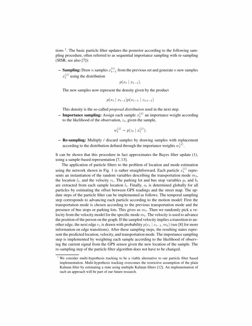
A more complex relationship governs how the mode of transportation influencesthe instantaneous velocity. The influence of mode on velocity is complicated by the factthat the range of possible instantaneous velocities for each mode overlap. For example,movement at 7 km/hr may be a brisk walk or a slowly moving car or bus. To simplify therelationship between mode and velocity we model the continuous velocities using theGaussian mixture shown in Fig. 2. A separate unsupervised Expectation-Maximization(EM) process determined the parameters of these probability densities using real veloc-ity data. Our model assumes that velocities are drawn randomly from these Gaussians,where the probability of drawing from a particular Gaussian depends on the mode. Forexample, the walking mode draws a speed from the left-most cluster with probabilityone. In the bus mode, the person has a 1/3 chance of being in each of the three slow-

0 18 37 55 73 91 110 1280

200

400

600

800

1000

1200Transportation Speed Modeling

Freq

uenc

y C

ount

Instantaneous Speed of a GPS Reading (km/hr)

Foot, Bus and Car SpeedsBus and Car SpeedsBus and Car SpeedsCar Speeds

Fig. 2. Gaussian mixture model for the dependency of transportation mode on velocities. TheGaussians were learned using EM based on previously collected velocity data. The frequenciesof the raw velocity values are indicated by the bins. Different transportation modes are modeledby sampling with different probability from the four Gaussians.

est velocity clusters. In our current approach, the probabilities for the Gaussians in thedifferent transportation modes were set manually based on external knowledge. Learn-ing the weights of the mixture components depending on the transportation mode (andeventually location) is left for future research.

In our model, the motion mode at time t only depends on the previous mode and thepresence of a parking lot or bus stop. For example, the person can only get on a bus ifthe node bt indicates the presence of a bus stop. The values of the bus stop and parkinglot nodes depend on the location of the person, as indicated by the arrows in the modelshown in Fig. 1. Learning mode and location transition probabilities is an importantaspect of our approach and will be discussed in Sect. 3.

2.2 Particle Filter Based Implementation

Particle filters provide a sample-based implementation of general Bayes filters [7].They represent posterior distributions over the state space with temporal sets, St, ofn weighted samples:

St = {〈x(i)t , w

(i)t 〉 | i = 1, . . . , n}

Here each x(i)t is a sample (or state), and the w(i)

t are non-negative numerical factorscalled importance weights, which sum up to one. Like Kalman filters, particle filtersapply the recursive Bayes filter update to estimate posteriors over the state space, butunlike Kalman filters, particle filters are not restricted to unimodal posterior distribu-

tions 1. The basic particle filter updates the posterior according to the following sam-pling procedure, often referred to as sequential importance sampling with re-sampling(SISR, see also [7]):

– Sampling: Draw n samples x(i)t−1 from the previous set and generate n new samples

x(j)t using the distribution

p(xt | xt−1).

The new samples now represent the density given by the product

p(xt | xt−1)p(xt−1 | z1:t−1)

This density is the so-called proposal distribution used in the next step.– Importance sampling: Assign each sample x(j)

t an importance weight accordingto the likelihood of the observation, zt, given the sample,

w(j)t = p(zt | x

(j)t ).

– Re-sampling: Multiply / discard samples by drawing samples with replacementaccording to the distribution defined through the importance weights w(j)

t .

It can be shown that this procedure in fact approximates the Bayes filter update (1),using a sample-based representation [7, 13].

The application of particle filters to the problem of location and mode estimationusing the network shown in Fig. 1 is rather straightforward. Each particle x(i)

t repre-sents an instantiation of the random variables describing the transportation mode mt,the location lt, and the velocity vt. The parking lot and bus stop variables pt and btare extracted from each sample location lt. Finally, ot is determined globally for allparticles by estimating the offset between GPS readings and the street map. The up-date steps of the particle filter can be implemented as follows. The temporal samplingstep corresponds to advancing each particle according to the motion model: First thetransportation mode is chosen according to the previous transportation mode and thepresence of bus stops or parking lots. This gives us mt. Then we randomly pick a ve-locity from the velocity model for the specific modemt. The velocity is used to advancethe position of the person on the graph. If the sampled velocity implies a transition to an-other edge, the next edge et is drawn with probability p(et | et−1,mt) (see [8] for moreinformation on edge transitions). After these sampling steps, the resulting states repre-sent the predicted location, velocity, and transportation mode. The importance samplingstep is implemented by weighting each sample according to the likelihood of observ-ing the current signal from the GPS sensor given the new location of the sample. There-sampling step of the particle filter algorithm does not have to be changed.

1 We consider multi-hypothesis tracking to be a viable alternative to our particle filter basedimplementation. Multi-hypothesis tracking overcomes the restrictive assumption of the plainKalman filter by estimating a state using multiple Kalman filters [12]. An implementation ofsuch an approach will be part of our future research.

3 Parameter Learning

One of the advantages of modeling the world with a graph is the ability to record be-havioral data about edge transitions. The discrete nature of such transitions facilitatesunsupervised learning of hierarchical model parameters. We have an intuitive prior ex-pectation of how state transitions occur between and within edges: edge transitionsoccur uniformly among the edge’s neighbors, and mode transitions vary according tothe presence of a bus stop or parking lot.

Learning in this context means adjusting the model parameters to better fit the train-ing data, typically to better model an individual user or the environment. Learning pa-rameters for specific individuals captures idiosyncratic motion patterns — the move-ments the user commonly makes, as opposed to the logically possible set of movements.Since our model also includes transportation mode, learning also means changing ourprior expectations about which edges mode transitions occur on. Bus stops and park-ing locations are conceptual locations where mode transitions may occur. Our modelenables learning of the commonly used subset of these locations, to highlight wherea user frequently parks her car, for example. The learned model supports better track-ing and prediction than the prior model, and is the foundation upon which high-levelunderstanding of the user’s behavior is built.

We now describe how to learn the parameters of our graph model using data col-lected by a person moving through the community. Our motivating application of theActivity Compass forces us to learn the transportation modes in an unsupervised man-ner. When deployed, Activity Compass users must not be required, for example, to keepa diary for several weeks of their transportation modes in order to create a supervisedtraining set. Hence, the most obvious difficulty is that we have to learn the motion modelbased solely on a map and a stream of non-continuous and noisy GPS sensor data.

A general approach for solving such learning problems is the well-known Expectation-Maximization (EM) algorithm [14, 15]. In our application, EM is based on the obser-vation that learning the model parameters would be easy if we knew the person’s truelocation and transportation mode at any point in time. Unfortunately, location and trans-portation mode are hidden variables, i.e. they cannot be observed directly but have tobe inferred from the raw GPS measurements. EM solves this problem by iterating be-tween an Expectation step (E-step) and a Maximization step (M-step). In a nutshell,each E-step estimates expectations (distributions) over the hidden variables using theGPS observations along with the current estimate of the model parameters. Then in theM-step the model parameters are updated using the expectations of the hidden variablesobtained in the E-step. The updated model is then used in the next E-step to obtain moreaccurate estimates of the hidden variables. EM theory tells us that in each iteration theestimation of the parameters will be improved and it will eventually converge to a localoptimum. In the following we give a more detailed description of how to apply EMtheory in our domain.

3.1 E-step:

Let Θ denote the parameters of the graph-based model we want to estimate and Θ(i−1)

denote the estimation thereof at the i − 1-th iteration of the EM algorithm. The model

parameters contain all conditional probabilities needed to describe the dynamic systemshown in Fig. 1. The E-step estimates

p(x1:t | z1:t, Θ(i−1)), (2)

i.e. the posterior distribution over the trajectories of the person given the observationsand parameters updated in the previous iteration. Here x1:t and z1:t are the states andobservations, respectively. Since it is not possible to find a closed-form solution forthe posterior over x1:t, we have to resort to an approximate approach [16]. Observe thatwhen we do particle filtering using the motion model with parameterΘ(i−1), the particledistribution at each time t along with the history of particles is an approximation forp(x1:t | z1:t, Θ

(i−1)). Hence, the desired expectation can be computed using the graph-based particle filter described in Sect. 2.2. Before we give implementation details forthe E-step, let us take a closer look at the M-step.

3.2 M-step:

The goal of the M-step is to maximize the expectation of log p(z1:t, x1:t | Θ) overthe distribution of x1:t obtained in the E-step by updating the parameter estimations.Because the distribution of x1:t is represented by the history of particles, the estimationof the parameters at the i-th EM iteration is computed by summing over all trajectories:

Θ(i) = argmaxΘ

n∑j=1

log p(z1:t, x(j)1:t | Θ)

= argmaxΘ

n∑j=1

(log p(z1:t |x(j)1:t ) + log p(x

(j)1:t |Θ)) (3)

= argmaxΘ

n∑j=1

log p(x(j)1:t | Θ) (4)

Here, n is the number of particles, x(j)1:t is the state history of the j-th particle, and

(3) follows from the independence condition

p(z1:t | x(j)1:t , Θ) = p(z1:t | x

(j)1:t ),

i.e., observations are independent of model transition parameters if the state trajectoryis known. For simplicity, we assume that all the particles have equal weight, i.e. afterthey are resampled. It is straightforward to extend our derivation to the case of differentweights.

Our approach is in fact a direct extension of the Monte Carlo EM algorithm [17].The only difference is that we allow particles to evolve with time. It has been shown thatwhen the number of particles n is large enough, Monte Carlo EM estimation convergesto the theoretical EM estimation [16].

3.3 Implementation Details

Even though EM can be used to learn all parametersΘ of the model described in Sect. 2,we are mostly interested in learning those parts of the model that describe the typicalmotion patterns of a user. All other parameters are fixed beforehand and not adjusted toa specific user. An advantage of this approach is that it requires much less training datathan learning all parameters at once.

The motion patterns of a specific user are described by the location transitions onthe graph and the mode transitions at the different locations. For the learning process,we have to initialize these probabilities to some reasonable values:

p(et | et−1,mt−1) is the transition probability on the graph conditioned on the modeof transportation just prior to transitioning to the new edge. This conditional prob-ability is initialized to a uniform distribution across all outgoing edges, with theexception of bus routes which have a strong bias forcing buses to follow the route(bus routes can be obtained from GIS sources such as [18]). With this exception,our model has no preference for a specific path of the person.

p(mt | mt−1, et−1) is the mode transition probability. This probability depends on theprevious mode mt−1 and the location of the person, described by the edge et−1.For example, each person has typical locations where she gets on and off the bus.Mode transitions are initialized with commonsense knowledge (e.g., one may notswitch from a bus to a car without first being on foot), and with knowledge of busstops. Parking lots are uniformly distributed across our map with no biases towardactual parking lots.

A straightforward implementation of the E-step given in (2) is to generate the expecta-tion over state trajectories by storing the history of each particle (see [7] for a discus-sion). To do so, at each re-sampling phase, the history of old samples needs to be copiedto the new samples 2. Then at the last time step, we have a set of samples with their his-tories. At the M-step, we update the model parameters simply by counting over theparticle histories. For example, to get p(ej | ei, BUS), we count the number of timeswhen a particle inBUS mode transits from edge ei to ej and then normalize the countsover all edges following ei and BUS. This approach, although easy to implement, suf-fers from two drawbacks. First, it is not efficient. When the data log is fairly long, savingthe histories for all the particles needs a large amount of space and history replicationbecomes slow. Second, and more importantly, since the number of samples is finite, therepetition of the re-sampling will gradually diminish the number of different historiesand eventually decrease the accuracy of the particle based approximation [7].

We can overcome these problems by observing that we are only interested in learn-ing the discrete transitions between edges and modes, e.g., the probability of transitingfrom edge ei to edge ej in BUS mode. The discreteness of these transitions allowsus to apply the well-known Baum-Welch algorithm [15], an EM algorithm for hiddenMarkov models (HMM). The Monte Carlo version of the Baum-Welch algorithm [19]performs at each iteration both a forward and a backward (in time) particle filtering

2 Unnecessary copy operations can be avoided by using tree data structures to manage pointersdescribing the history of particles.

step. At each forward and backward filtering step, the algorithm counts the number ofparticles transiting between the different edges and nodes. To obtain probabilities forthe different transitions, the counts of the forward and backward pass are normalizedand then multiplied at the corresponding time slices.

To show how it works, we define:

αt(et,mt) is the number of particles on edge et and in modemt at time t in the forwardpass of particle filtering.

βt(et,mt) is the number of particles on edge et and in mode mt at time t in the back-ward pass of particle filtering.

ξt−1(et, et−1,mt−1) is the probability of transiting from edge et−1 to et at time t− 1and in mode mt−1.

ψt−1(mt,mt−1, et−1) is the probability transiting from mode mt−1 to mt on edgeet−1 at time t− 1.

A short derivation gives us [15, 19],

ξt−1(et, et−1,mt−1) ∝ αt−1(et−1,mt−1)p(et | et−1,mt−1)βt(et,mt−1) (5)

and

ψt−1(mt,mt−1, et−1) ∝ αt−1(et−1,mt−1)p(mt | mt−1, et−1)βt(et−1,mt) (6)

After we have ξt−1 and ψt−1 for all the t from 2 to T , we update the parametersas: 3

p(et | et−1,mt−1) =expected number of transitions from et−1 to et in mode mt−1

expected number of transitions from et−1 in mode mt−1

=

∑Tt=2 ξt−1(et, et−1,mt−1)∑T

t=2

∑et∈Neighbors of et−1

ξt−1(et, et−1,mt−1)(7)

and similarly

p(mt | mt−1, et−1) =expected number of transitions from mt−1 to mt on edge et−1

expected number of transitions from mt−1 on edge et−1

=

∑Tt=2 ψt−1(mt,mt−1, et−1)∑T

t=2

∑mt∈{BUS,FOOT,CAR} ψt−1(mt,mt−1, et−1)

(8)

The complete implementation is depicted in Table 1. As the number of particlesincreases, the approximation converges to the theoretical EM estimation. Fortunately,our approach is very efficient in this regard, since our model parameters are associatedwith the number of edges and modes in the graph, not the number of particles.

In addition to the user specific parameters our model requires the specification ofother parameters, such as motion velocity and the GPS sensor model. The motion ve-locity is modeled as a mixture of Gaussians from which velocities are drawn at random.

3 Usually we also need a prior number for each transition. We will not discuss how to set theprior value in this paper.

Table 1. EM-based parameter learning algorithm

Model Initialization: Initialize the model parameters p(et|et−1,mt−1) and p(mt|mt−1, et−1).E-step:

1. Generate n uniformly distributed samples and set time t = 1.2. Perform forward particle filtering:

(a) Sampling: generate n new samples from the existing samples using the current param-eter estimation p(et|et−1, mt−1) and p(mt|mt−1, et−1).

(b) Importance sampling: reweight each sample based on observation zt.(c) Re-sampling: multiply / discard samples according to their importance weights.(d) Count and save αt(et,mt)(e) Set t = t+ 1 and repeat (2a)-(2d) until t = T .

3. Generate n uniformly distributed samples and set t = T .4. Perform backward particle filtering:

(a) Compute backward parameters p(et−1|et,mt), p(mt−1|mt, et) fromp(et|et−1,mt−1) and p(mt|mt−1, et−1)

(b) Sampling: generate n new samples from the existing samples using the backward pa-rameter estimation.

(c) Importance sampling: reweight each sample based on observation zt.(d) Re-sampling: multiply / discard samples according to their importance weights.(e) Count and save βt(et,mt)(f) Set t = t− 1 and repeat (4b)-(4e) until t = 1.

M-step

1. Compute ξt−1(et, et−1,mt−1) and ψt−1(mt,mt−1, et−1) using (5) and (6) and then nor-malize.

2. Update p(et|et−1,mt−1) and p(mt|mt−1, et−1) using (7) and (8).

Loop Repeat E-step and M-step using updated parameters until model converges.

The probabilities of the mixture components depend on the current motion mode andcan be learned beforehand using data labeled with the correct mode of motion. We usea standard model to compute the likelihood p(zt | xt) of a GPS sensor measurement zt

given the location xt of the person [1].

4 Experiments

Our test data set consists of logs of GPS data collected by one of the authors. The datacontains position and velocity information collected at 2-10 second intervals duringperiods of time in which the author was moving about outdoors. This data was handlabeled with one of three modes of transportation: foot, bus, or car. This labeling wasuseful for validating the results of our unsupervised learning, but was not used by theEM learning process.

From this data set, we chose 29 episodes representing a total of 12 hours of logs.This subset consists of all of portions of the data set which were bounded by GPS sig-nal loss, i.e. had no intermediate loss of signal of more than 30 seconds, and which

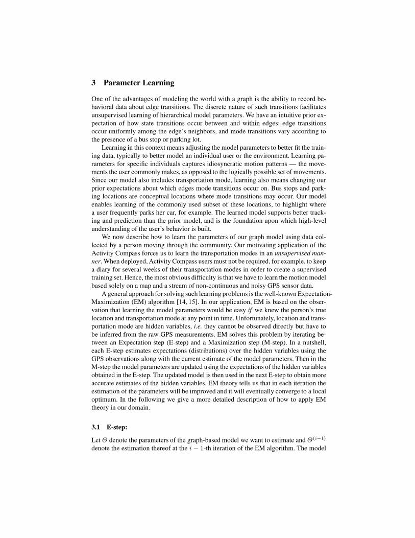
Fig. 3. Car (left), Foot (middle), and Bus (right) training data used for experiments. The black dotis a common map reference point on the University of Washington campus.

contained a change in the mode of transportation at some point in the episode. Theseepisodes were divided chronologically into three groups which formed the sets forthree-fold cross-validation for our learning. Fig. 3 shows one of the cross-validationgroups used for training. The street map was provided by the US Census Bureau [20]and the locations of the bus stops come from the King County GIS office [18].

4.1 Mode Estimation and Prediction

One of the primary goals of our approach is learning a motion model that predicts trans-portation routes, conditioned on the mode of transportation. We conducted an experi-ment to validate our models’ ability to correctly learn the mode of transportation at anygiven instant. For comparison we also trained a decision tree model using supervisedlearning on the data [21]. We provided the decision tree with two features: the currentvelocity and the standard deviation of the velocity in the previous sixty seconds. Usingthe data annotated with the hand-labeled mode of transportation, the task of the decisiontree was to output the transportation mode based on the velocity information. We usedthree-fold cross-validation groups to evaluate all of the learning algorithm. The resultsare summarized in the first row of Table 2. The first result indicates that 55% of the timethe decision tree approach was able to accurately estimate the current mode of trans-portation on the test data. Next, we used our Bayes filter approach without learning themodel parameters, i.e. with uniform transition probabilities. Furthermore, this modeldid not consider the locations of bus stops or bus routes (we never provided parkinglocations to the algorithm). In contrast to the decision tree, the Bayes filter algorithmintegrates information over time, thereby increasing the accuracy to 60%. The benefitof additionally considering bus stops and bus routes becomes obvious in the next row,which shows a mode accuracy of 78%. Finally, using EM to learn the model parameters

increases the accuracy to 84% of the time, on test data not used for training. Note thatthis value is very high given the fact that often a change of transportation mode cannotbe detected instantaneously.

Table 2. Mode estimation quality of different algorithms.

Model Cross-ValidationPrediction Accuracy

Decision Tree with Speed and Variance 55%Prior Graph Model, w/o bus stops and bus routes 60%Prior Graph Model, w/ bus stops and bus routes 78%

Learned Graph Model 84%

A similar comparison can be done looking at the techniques’ ability to predict notjust instantaneous modes of transportation, but also transitions between transportationmodes. Table 3 shows each technique’s accuracy in predicting the qualitative change intransportation mode within 60 seconds of the actual transition — for example, correctlypredicting that the person got off a bus. Precision is the percentage of time when the al-gorithm predicts a transition that an actual transition occurred. Recall is the percentageof real transitions that were correctly predicted. Again, the table clearly indicates thesuperior performance of our learned model. Learning the user’s motion patterns signifi-cantly increases the precision of mode transitions, i.e. the model is much more accurateat predicting transitions that will actually occur.

Table 3. Prediction accuracy of mode transition changes.

Model Precision RecallDecision Tree with Speed and Variance 2% 83%

Prior Graph Model, w/o bus stops and bus routes 6% 63%Prior Graph Model, w/ bus stops and bus routes 10% 80%

Learned Graph Model 40% 80%

An example of the modes of transportation predicted after training on one cross-validationset is shown in Fig. 4.

4.2 Location Prediction

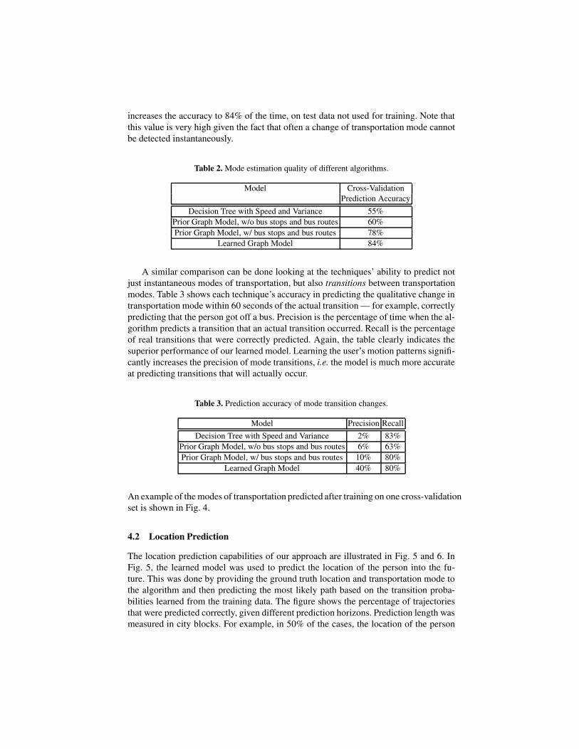
The location prediction capabilities of our approach are illustrated in Fig. 5 and 6. InFig. 5, the learned model was used to predict the location of the person into the fu-ture. This was done by providing the ground truth location and transportation mode tothe algorithm and then predicting the most likely path based on the transition proba-bilities learned from the training data. The figure shows the percentage of trajectoriesthat were predicted correctly, given different prediction horizons. Prediction length wasmeasured in city blocks. For example, in 50% of the cases, the location of the person

Fig. 4. This map shows the learned transportation behavior based on one cross-validation set containing nineteen episodes. Shown are only those edges and modetransitions which the learned model predicts with high probabilities. Thick gray linesindicate learned bus routes, thin black lines indicate learned walking routes, and cross-hatches indicate learned driving routes. Circles indicate parking spots, and the trianglesshow the subset of bus stops for which the model learned a high probability transi-tion on or off the bus. There are four call-outs to show detail. (A) shows a frequentlytraveled road ending in three distinct parking spaces. This route and the parking spotsindicate the correctly learned car trips between the author’s home and church. (B) showsa frequently traveled foot route which enters from the northeast, ending at one of thefrequently used bus stops of the author. The main road running east-west is an arterialroad providing access to the highway for the author. (C) shows an intersection at thenorthwest of the University of Washington campus. There are two learned bus stops.The author frequently takes the bus north and south from this location. This is alsoa frequent car drop off point for the author, hence the parking spot indication. Walk-ing routes extend west to a shopping area and east to the campus. (D) shows a majoruniversity parking lot. Foot traffic walks west toward campus.

0 10 20 30 40 50 60 70 80 90 1000

0.1

0.2

0.3

0.4

0.5

0.6

0.7

0.8

0.9

1

City Blocks

Prob

abili

ty o

f cor

rect

ly p

redi

ctin

gx

or m

ore

bloc

ks in

to th

e fu

ture

Predicting Future Location Given Transportation ModeBUSCARFOOT

Fig. 5. Location prediction capabilities of the learned model.

0 10 20 30 40 50 60 70 80 900

0.1

0.2

0.3

0.4

0.5

0.6

0.7

0.8

0.9

1

City Blocks

Prob

abili

ty o

f cor

rect

ly p

redi

ctin

gx

or m

ore

bloc

ks a

nd tr

ansp

orta

tion

mod

esin

to th

e fu

ture

Predicting Future Location and Transportation Mode

Fig. 6. Location and mode prediction capabilities of the learned model.

was predicted correctly for 17 blocks when the person was on the bus. In 30% of thecases, the prediction was correct for 37 blocks, and 75 blocks were predicted correctlyin 10% of the cases. Note that the linear drop in bus route prediction probability is dueto the fact that the data contained several correctly predicted episodes of a 92 block longbus trip. Obviously, long term distance prediction is much less accurate when a personwalks. This is due to the higher variability of walking patterns and the fact that peo-ple typically do not walk for many city blocks, thereby making a long term predictionimpossible.

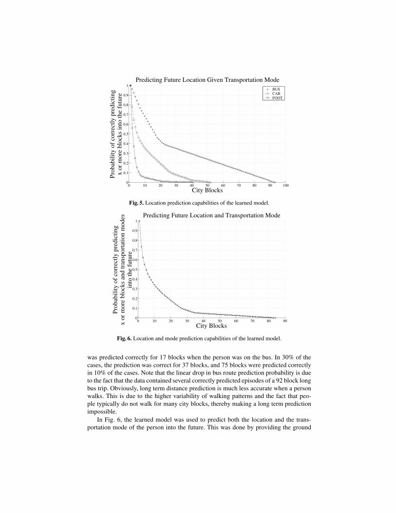
In Fig. 6, the learned model was used to predict both the location and the trans-portation mode of the person into the future. This was done by providing the ground

truth location to the algorithm and then predicting the most likely path and sequenceof transportation mode switches based on the transition probabilities learned from thetraining data. The graph shows that in 50% of the cases, the model is able to correctlypredict the motion and transportation mode of the person for five city blocks. This re-sult is extremely promising given that the model was trained and tested on subsets of29 episodes.

5 Conclusions and Future Work

The work presented in this paper helps lay the foundation for reasoning about high-leveldescriptions of human behavior using sensor data. We showed how complex behaviorssuch as boarding a bus at a particular bus stop, traveling, and disembarking can berecognized using GPS data and general commonsense knowledge, without requiringadditional sensors to be installed throughout the environment. We demonstrated thatgood predictive user-specific models can be learned in an unsupervised fashion.

The key idea of our approach is to apply a graph-based Bayes filter to track a per-son’s location and transportation mode on a street map annotated with bus route infor-mation. The location and transportation mode of the person is estimated using a particlefilter. We showed how the EM algorithm along with frequency counts from the parti-cle filter can be used to learn a motion model of the user. A main advantage of thisunsupervised learning algorithm is the fact that it can be applied to raw GPS sensordata.

The combination of general knowledge and unsupervised learning enables a broadrange of “self-customizing” applications, such as the Activity Compass mentioned inSect. 1. Furthermore, it is straightforward to adopt this approach for “life long” learning:the user never needs to explicitly instruct the device, yet the longer the user carries thedevice the more accurate its user model becomes.

Our current and future research extends the work described in this paper in a numberof directions, including the following:

1. Making positive use of negative information. Loss of GPS signal during trackingcauses the probability mass to spread out as governed by the transition model. Wehave seen that learning significantly reduces the rate of spread. In some cases, how-ever, loss of signal can actually be used to tighten the estimation of the user’s loca-tion. In particular, most buildings and certain outdoor regions are GPS dead-zones.If signal is lost when entering such an area, and then remains lost for a significantperiod of time while the GPS device is active, then one can strengthen the proba-bility that the user has not left the dead-zone area.

2. Learning daily and weekly patterns. Our current model makes no use of absolutetemporal information, such as the time of day or the day of the week. Includingsuch variables in our model will improve tracking and prediction of many kindsof common life patterns, such as the fact that the user travels towards his place ofwork on weekday mornings.

3. Modeling trip destination and purpose. The work described in this paper segmentsmovement in terms of transitions at intersections and between modes of transporta-tion. At a higher level of abstraction, however, movement can be segmented in

terms of trips that progress from a location where some set of activities take place(such as home) to a location where a different class of activities take place (suchas the office). A single trip between activity centers can involve several shifts be-tween modes of transportation. By learning trip models we expect to be able toincrease the accuracy of predictions. More significantly, trip models provide a wayto integrate other sources of high-level knowledge, such as a user’s appointmentcalendar.

4. Using relational models to make predictions about novel events. A significant lim-itation of our current approach is that useful predictions cannot be made whenthe user is in a location where she has never been before. However, recent workon relational probabilistic models [22, 23] develops a promising approach wherepredictions can be made in novel states by smoothing statistics from semanticallysimilar states. For example, such a model might predict that the user has a signifi-cant chance of entering a nearby restaurant at noon even if there is no history of theuser patronizing that particular restaurant.

Acknowledgment

This work has partly been supported by the NSF under grant numbers IIS-0225774 andIIS-0093406, by AFRL contract F30602–01–C–0219 (DARPA’s MICA program), andthe Intel corporation.

References

1. Hightower, J., Borriello, G.: Location systems for ubiquitous computing. Computer 34(2001) IEEE Computer Society Press.

2. Bonnifait, P., Bouron, P., Crubille, P., Meizel, D.: Data fusion of four ABS sensors andGPS for an enhanced localization of car-like vehicles. In: Proc. of the IEEE InternationalConference on Robotics & Automation. (2001)

3. Cui, Y., Ge, S.: Autonomous vehicle positioning with GPS in urban canyon environments.In: Proc. of the IEEE International Conference on Robotics & Automation. (2001)

4. Ashbrook, D., Starner, T.: Learning significant locations and predicting user movement withgps. In: International Symposium on Wearable Computing, Seattle, WA (2002)

5. Patterson, D., Etzioni, O., Fox, D., Kautz, H.: The Activity Compass. In: Proceedings ofUBICOG ’02:First International Workshop on Ubiquitous Computing for Cognitive Aids.(2002)

6. Kautz, H., Arnstein, L., Borriello, G., Etzioni, O., Fox, D.: The Assisted Cognition Project.In: Proceedings of UbiCog ’02: First International Workshop on Ubiquitous Computing forCognitive Aids, Gothenberg, Sweden (2002)

7. Doucet, A., de Freitas, N., Gordon, N., eds.: Sequential Monte Carlo in Practice. Springer-Verlag, New York (2001)

8. Liao, L., Fox, D., Hightower, J., Kautz, H., Schulz, D.: Voronoi tracking: Location estimationusing sparse and noisy sensor data. In: Proc. of the IEEE/RSJ International Conference onIntelligent Robots and Systems. (2003)

9. Bar-Shalom, Y., Li, X.R., Kirubarajan, T.: Estimation with Applications to Tracking andNavigation. John Wiley (2001)

10. Dean, T., Kanazawa, K.: Probabilistic temporal reasoning. In: Proc. of the National Confer-ence on Artificial Intelligence. (1988)

11. Murphy, K.: Dynamic Bayesian Networks: Representation, Inference and Learning. PhDthesis, UC Berkeley, Computer Science Division (2002)

12. Bar-Shalom, Y., Li, X.R.: Multitarget-Multisensor Tracking: Principles and Techniques.Yaakov Bar-Shalom (1995)

13. Del Moral, P., Miclo, L.: Branching and interacting particle systems approximations ofFeynman-Kac formulae with applications to non linear filtering. In: Seminaire de Proba-bilites XXXIV. Number 1729 in Lecture Notes in Mathematics. Springer-Verlag (2000)

14. Bilmes, J.: A gentle tutorial on the EM algorithm and its application to parameter estima-tion for Gaussian mixture and hidden Markov models. Technical Report ICSI-TR-97-021,University of Berkeley (1998)

15. Rabiner, L.R.: A tutorial on hidden Markov models and selected applications in speechrecognition. In: Proceedings of the IEEE, IEEE (1989) IEEE Log Number 8825949.

16. Levine, R., Casella, G.: Implementations of the Monte Carlo EM algorithm. Journal ofComputational and Graphical Statistics 10 (2001)

17. Wei, G., Tanner, M.: A Monte Carlo implementation of the EM algorithm and the poor mansdata augmentation algorithms. Journal of the American Statistical Association 85 (1990)

18. County, K.: Gis (graphical information system). http://www.metrokc.gov/gis/mission.htm(2003)

19. Thrun, S., Langford, J., Fox, D.: Monte Carlo hidden Markov models: Learning non-parametric models of partially observable stochastic processes. In: Proc. of the InternationalConference on Machine Learning. (1999)

20. Bureau, U.C.: Census 2000 tiger/line data. http://www.esri.com/data/download/census2000-tigerline/ (2000)

21. Mitchell, T.: Machine Learning. McGraw-Hill (1997)22. Anderson, C., Domingos, P., Weld, D.: Relational markov models and their application to

adaptive web navigation. In: Proceedings of the Eighth International Conference on Knowl-edge Discovery and Data Mining, ACM Press (2002) 143–152 Edmonton, Canada.

23. Sanghai, S., Domingos, P., Weld, D.: Dynamic probabilistic relational models. In: Pro-ceedings of the Eighteenth International Joint Conference on Artificial Intelligence, MorganKaufmann (2003) Acapulco, Mexico.