Embed Size (px)
Citation preview
Infinite dimensional Lapiacianand spherical harmonics
By
Yasuo UMEMURA and Norio KONO
Summary
The purpose of the present paper is to discuss the properties of
the Gaussian measure and the Lapiacian operator in infinite dimensions
as limits of finite dimensional analogues. In the limit of n->w, the
uniform measure on the ^-dimensional sphere, the spherical Lapiacian
operator, and Gegenbauer polynomials (spherical harmonics) tend re-
spectively to an infinite dimensional Gaussian measure, the infinite
dimensional Lapiacian operator, and Hermite polynomials. We also
discuss the addition formula and integral representation formula of
Hermite polynomials in this limit procedure.
Introduction
In the previous paper [6], one of the authors discussed the infinite
dimensional Gaussian measure on the dual space of a nuclear space,
for instance, on the space G$'), regarding it as a limit measure of
finite dimensional Gaussian measures. It can be also regarded as a
limit measure of uniform measures on spheres, as was shown by Hida-
Nomoto [3] : their measure is defined on the projective limit space &
of the n-dimensional sphere Qn, but it is equivalent to our measure
on (cSO, since there exists a measure-preserving one-to-one mapping
from Q into (£')•
These two different interpretations reflect the fact that the infinite
dimensional Gaussian measure is ergodic with respect to translations
like the finite dimensional ones, and also ergodic with respect to
Received October 20, 1965.
164 Yasuo Umemura and Norio Kono
rotations like the uniform measures on spheres.
Next we shall discuss the Laplacian operator. The Laplacianoperator An on Qn generates all rotationally invariant, symmetricoperators on Z,JCft,,dfito). On the other hand, the infinite dimensionalLaplacian operator Ac defined in [7] also generates all rotationallyinvariant operators on L2(Sf
yjuc). (c.f. §1). Hence, a question arises:
does An tend to Ac in some sense? In this paper we shall answer it,
namely we shall show that An/n tends to Ac as n-^w.
P. Levy defined the infinite dimensional Laplacian operator in [5]as the limit operator of An/n. Therefore Levy's definition turns outto be just the same as ours given in [7].
This fact implies the convergency of the eigen values and theeigen functions of An to those of Ac. Therefore Gegenbauer poly-nomials tend to Hermite polynomials. This has been known as aformula concerning special functions, for instance see [1]. However,we get here a new interpretation of this formula: finite dimensionalspherical harmonics tend to infinite dimensional ones.
Similar new interpretations are possible also for the additionformula and the integral representation formula concerning Hermitepolynomials. Especially, we shall show that the density function ofthe integral representation of the ^-dimensional zonal spherical functionconverges to that of the integral representation of Hermite polynomialin the sense of D(Sr
s /jc). The latter representation is equivalentwith the Gauss transform.
Our standpoint will make clear some aspects of Hermite poly-
nomials as infinite dimensional eigen functions.
We should also remark that the addition formula played an im-portant role in S. Kakutani's discussions on Brownian motions [4].
In this paper, after preliminary discussions in §1, we shall showrather intuitively in §2 and more exactly in §3 that the projectivelimi tof the uniform measures on spheres is just the infinite dimensionalGaussian measure. In §4, we shall establish the relation between finite
Infinite dimensional Laplacian and spherical harmonics 165
dimensional and infinite dimensional Laplacian operators, and theninvestigate how this relation reflects on their eigen functions; for
zonal ones in §5 and more generally in §6= In this point of view,
we interprete the integral representation formula in §7 and the addition
formula in §8.
We would like to thank Prof. H. Yosizawa of Kyoto University
and Prof. N. Ikeda of Osaka University for their suggestions of varioususeful ideas.
§1. Preliminaries (For details, see [6] and [7]).
Let L be a real nuclear space, and H be its completion by acontinuous Hilbertian norm |[ |U» Then, we have a relation;
where H* and L* are the dual spaces of H and L respectively.
Now, define a function %(<?) on L as follows
(1)
It satisfies the conditions of positive definiteness, continuity in thenorm |( \\H, and %(0)=1. So, by the theorem of Bochner-Minlos,%(<?) is the characteristic function of a probability measure JUG on L*\
(2)
Here, < T, £> means the value at f of the linear functional T. //c is
defined on the 6- algebra 33 (L*) which is generated by the family of
all Borel cylinder sets of L*. We call juc a Gaussian measure with
variance c2.
Definition 1. An unitary operator u on H is called a rotation
of L, if it satisfies]
i) u maps L onto L,
ii) u is homeomorphic on L.
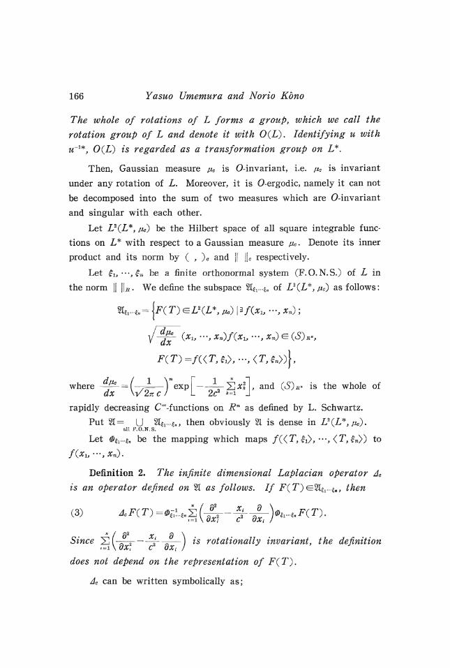
166 Yasuo Umemura and Norio Kono
The whole of rotations of L forms a group, which we call the
rotation group of L and denote it with O(L). Identifying u with
u~1*, O(L) is regarded as a transformation group on Z,*.
Then, Gaussian measure /JLC is O-invariant, i.e. p.c is invariant
under any rotation of L. Moreover, it is O-ergodic, namely it can not
be decomposed into the sum of two measures which are O-invariant
and singular with each other.
Let L2(L*, &} be the Hilbert space of all square integrable func-tions on L* with respect to a Gaussian measure juc . Denote its innerproduct and its norm by ( , )c and j| ||c respectively.
Let ?i, • • • , & » be a finite orthonormal system (F.O.N.S.) of L in
the norm (I ||a. We define the subspace SI^...^ of U(L* , /*c) as follows:
where -&- = ( * VexpT— —£xl\, and (<S)a. is the whole ofdx \Y2n c I L 2c2 *-i .1
rapidly decreasing C°°-functions on R" as defined by L. Schwartz.
Put §1= U Sl^-j., then obviously SI is dense in L\L*,tic).all F.O.N.S.
Let <%...§„ be the mapping which maps /«T, &>, • • • , <T, fra» to
Definition 2. TA0 infinite dimensional Laplacian operator AG
is an operator defined on §1 #s follows. If F(T) e§l?1...^B, then
(3)
Since ^[ z — — -^-— — ) fs rotationally invariant, the definitioni=l \ C/^i C (/#,- /
o^ depend on the representation of F(T).
Ac can be written symbolically as;
Infinite dimensional Laplacian and spherical harmonics 167
c - lim Jw -
where An is the usual ^-dimensional Laplacian operator on l?(Rn, dnx),n
rl = ̂ xl and / is the identity operator.
For an example of a nuclear space, we have the space (<5), thewhole of rapidly decreasing C"-functions on the real line. (cS) isnuclear because its topology is defined by countable Hilbertian norms;
In the above discussions, considering the case that L=(<S) and
H=L2(R1), we see that we can define a Gaussian weasure /JLC on OS')*and the infinite dimensional Laplacian operator Ac on L2(Sf,jmc).
§2. A limit property of uniform measures on spheres
Let Pn be the uniform probability measure on an ^-dimensional
sphere Qn of radius i/n + lc and center at the origin.
Qn : xl + xl+ — +xl+1= (n + l}c\
For this Pn, consider the joint distribution Pn,m (nS>ni) of (xl9 X2,
-•, Xm), namely for EdRm,
Proposition 1.
C4)M->oo
where p.G,m is the m-dimensional Gaussian measure with variance
c2. The convergence is uniform for all Borel subsets E of Rm.
Proof Decompose Rn+1 into the sum R^ + Rl~m+\ where
RI = {(Xi,Xs, ~',Xm,0, • - • , 0)},
and Rl-r"l^= {(o, --,o, xm+i, xm+2, • • • , xn+J} .
Let ^;= (#!, Jic2, • • • , ^n+i) be a point on J2ra, then the distance be-

168 Yasuo Umemura and Norio Kono
tween x and R™ is i/(^ + l)£2 — (x\-\ hri) , while the angle d
between the normal of Qn at x and the space Rl~m+l is given by
cos 6
Hence, clearly Pn,m is given by
f .x^"dxm for
0 for
where ^m is the normalization constant. Putting &w,
as £i,TO, we have
/ -r2 4- . . -4- T2
(5) dPnfm=krnym (I-* y .7"**
\ (n + ]Jc
where r+ means Max (r, 0) . From this, we see that
-+*2*1
2c2 J°
It is easily seen that the convergence is uniform with respect to(#1, •••, Xm)- This proves the proposition 1.
§3. The projective limit space Q
In order to make the situation in Proposition 1 clearer, we shall
construct the projective limit space & of Qn, and show that the limitmeasure P of Pn is isomorphic with an infinite dimensional Gaussian
measure juc defined in §1.
First, for any m<n, we shall define a projection fn,m from Qn
onto J2m as follows;
fn,m maps (0™= (x[n\ • • • , tfJSO
where
Infinite dimensional Laplacian and spherical harmonics 169
(6) ^ (ft) 2
Then, fn, m is a measurable mapping defined almost everywhere on Qn.(The exceptional set is {o>Cn) e £ra | xf = • • • = x%li = 0}).
(Remark-, If we use the polar coordinates, /w,m is defined as a map-
ping which maps
(0i, "•, 6m, • • • , 0n) on J2W to (0i, -•, dm) on $m.
This expression was used in [3]).
The projection fn,m satisfies the following conditions;
0 fl,n=fl,m°fm,n
ii) Pm(A)=Pn(f-
for m<n and a Borel subset A of J2TO.
Therefore, according to a theorem due to Bochner, we can constructthe projective limit probability space (Q, $8, P). It satisfies the follow-
ing properties:
PI) QCLl\.Qnn = l
P2) fm=fm,nQfn fOT Wl<M.
Here, fn is the restriction of nn on Q, where nn is the projection
from lLQn onto tin.n=i
P3) 93 is generated by Uf^&n), where $3n is the whole of
Borel subsets of Qn.
P4) P(f-\A^=Pn(A) for A&^n.
Since the coordinate #(/° (l^^w-t-1) is a function on Qn, it can
be regarded as a function on J2. We denote this function by JOM)(a)),
then for any w^ti,
(7) /„(») - W°(a>), -, JfSiCo);) ea*.Jf^^ft?) is a measurable fucntion on Q because of PS).
170 Yasuo Umemura and Norio Kono
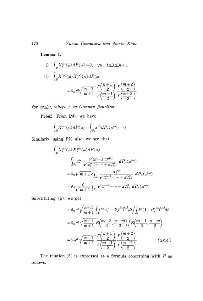
Lemma 1.
i) \ XI":>(o))dP(o)') =0, VnyJ£
ii)
for m<M, where r is Gamma function.
Proof From P4), we have
x™dPn(af»>) =0
Similarly, using P2) also, we see that
dp
W + l
Substituting (5), we get
m + l Jo o
n — m\ fm + l n — m
The relation (5) is expressed as a formula concerning with P asfollows.
Infinite dimensional Laplacian and spherical harmonics 111
For any ri^m, and for any Borel subset E of Rm, we have
(8)
Lemma 2. W°(aO; » = i, i-fl, i + 2, ...... } forms a Cauchy
sequence in L?(fi, P).
Proof From the previous lemma, we get
\ 2 / \ 2 /
\ 2 \ 20 as n,m~> w,
because we have asymptotically
, 1
From lemma 2, X(tn} converges to a function X{ in L2(j2, P).
Then, Xi(oi) is denned for almost all w.
Evidently,
rl(fl,)dP(a,)=0 and
Next, we shall imbed ^ into the space L*, the dual space of a
nuclear space L. (c. f. §1).
Since L is nuclear, there exist a complete orthonormal system {ft}
of L in the norm |] \\H and a square summable sequence {fa} such
that the norm:
(9)ti
is continuous in the topology of L.
Then, we see that for P-almost all
172 Yasuo Umemura and Norio Kbno
is defined and continuous on L. Because
where #(a)) = l/XUf^Gw)2 is finite for P-almost all CD.
Consider the mapping 2F : o;ej2-»TweZ,*. ^ zs one-to-one except
on a suitable null-set of ti, because if Tu(?) = To/(f) for any f, we
have Xk(a)) = Xk(a)r} for any A. This implies (o = cof, since for P-almost
all a), we get from (6)
cXi
thus for any m we have fm(<*>)=fm(<or)>
Next, we shall discuss the measurability. From P3), the proba-
bility measure P is defined on the smallest ^-algebra S3 which makes
all X\n\cD) measurable. From (11), this is equivalent to say $S is
the smallest <r-algebra which makes all X^co) measurable. Therefore,
the image W (S3) is the smallest c;-algebra which makes all < T, $ >
measurable regarding f as a linear functional on L*. In other words,
¥(9B) is the smallest ^-algebra which makes all Borel cylinder sets
of L* measurable. This means that 2F(33) is equal to S(L*) defined
in §1.
Finally, we shall show that the measure P on Q is mapped to
a Gaussian measure jutc on L*. Because of (8), we get
(12) Pt^K^W,...,^^)
- - e x pn c
____ Lr 2 l+x* \dXl2c2 J
So that if f = S <**£*, we have from (10)
Infinite dimensional Laplacian and spherical harmonics 173
Since the characteristic function of a measure on L* must be conti-
nuous on L, we have for any
(13)
This means that P is mapped to p.c, because of one-to-one corres-
pondence between measures and characteristic functions. So far, we
have proved:
Proposition 2. The projective limit space (J2, 93, P) is isomor-
phic with (Z,*, 93(L*), Ate).
Namely, there exists a measure-preserving one-to-one mapping
from a suitable subset tt of J2 onto a suitable subset L* of L*
where P(2»)= jUc(L*)=l.
Remark L* is a vector space, while & is not.
§4. Laplacian operators
In this section, we shall prove that the Laplacian operator on Qn
tends to the infinite dimensional Laplacian operator on L*.
On L2(Rn+1, dn+lx), the Laplacian operator is defined by Jw+1 =
r. Using polar coordinates, it is expressed as follows;S1=1
n/n /f 3* . n 9(14) Jw~n+i dr2 ' r dr r2 ~n'
Here An is the Laplacian operator on the unit sphere;
£)2
(15) 4 = 4-
- ml ^ ^~-""80w ' sinX ^
In order to show that the operator JK/(^ + l)c2 tends to AG in
some sense, we shall first give a rough discussion, and later formulate
it in an exacter way.
We shall operate zf«/(n+l)c2 and Ac on a function
). We have

174 Yasuo Umemura and Norio Kono
Here, we substitute
®L^^®L 82 /_^n xtx, 92/8r f=i r dxt' dr* ,.£i r2 9«,-8^
then we get
(n
thus in the limit of n->oo, we see that the right side converges to
Now, we shall give an exacter expression, regarding both An and
Ac as operators on L3(L*, #c).For a fixed C. O. N. S. {<?*} of L, the projective limit space J2 is
imbedded into Z,* as shown in §3. For this {?*}, we consider thespace §1 .̂..̂ , following the definition in §1, and denote it by SIn. The
union §Lo=LJ2L is a subspace of SI defined in §1. 3L is also dense«=iin D(L*, fjk).
On the other hand, consider an n-dimensional ball Bn of radius
•]/n + lc and center at origin.
Then, the Hilbert space L*(Bn, /*„,„), where the measure Pn,n is definedby (5), is isomorphic with L\@*,2P^), where 2Pn is the uniformprobability measure on the hemisphere &%•
l^ = (n
L2(tin,2Pn) is a subspace of L*(Qn,P^) which consists of all suchfunctions that satisfy
X
Infinite dimensional Laplacian and spherical harmonics 175
So, the Laplacian An is defined on Z,2(£,T, 2POT), hence on U(Br,,
Pn,B) also.
Define the mapping Qn from Lz(Rns #.,„) into U(Bn, Pw,w) as
follows;
QM maps any polynomial on J?OT to its restriction on Bn.
Since a polynomial on Bn is uniquely extended on Rn, Qn is one-
to-one on the set **$„ of all polynomials of ^-variables. Remark that
^n is dense in L\Rn, juc,^ and Qn^n is dense in L2(£„, PB,«)-
Now, define an operator Jw on ^3W as follows;
We shall express An as a differential operator on R71.
On the hemisphere £,t:
•2, ^w+1>0,
^i, "',^n can be regarded as coordinates. Namely, Xi,-~,xn are inde-
pendent variables on Q*, and xn+l=y/(n+l)c2 — x\ xl is a func-
tion of them. Using such coordinates, we have.
(17) Jn=
This expression is obtained in the following way: In the operator
An+i we change variables from (x^ -~,xn, xn+i) to (<*i, • • • , a», r), where^2 n d
r=yxl-\ l-xl+i and al = xi/r, then subtract -7^^ + ^— from it,dr2 r dr
and finally put r = Vn -\-lc.
So, for jfe$pw we have
(18) Z/(^ -.., *„) = (
_^ 82/ _n^,T 8/i y=i ' ^ 0Jr • 0JC • f^i ' dX •
Thus An is continuous in the topology of OS)*-. Namely, for a sequence
176 Yasuo Umemura and Norio Kono
{fk} cSft., if /*(#i, • • - , #w) y-J*-(xl9 ••• ,#„) tends to 0 in the topology
of (£)*„, then C ^ / 0 - tends also to 0 in (£)*.. Therefore, Jw
can be extended continuously on 2IW.
Consider the mapping %...$„ from 3L into L2(Rn,j^C)n) following
the definition in §1, and denote it by <Dn. Furthermore, put An = 0ZlQ
An°®n. An is an operator on 3IW. Namely, for F(T) =/«T, f i>, • • • ,
where \X. = /T g,-> means that after the calculation of the right hand
side we replace x{ by <T, f,->.
Since 2IwZ)SIm for n>m, An is defined also on §lm. So that on
the space SLo^USIm, we can consider symbolically the limit of
Now, we want to prove;
Proposition 3.
(20) Iim7 — ̂ Y^-^J, strongly on 3L.«-*oo ^
Namely, for any
(20) ; lim ^ ,F=ACF in L2(L*? ̂ ).
Proof Since §ITO can be regarded as a subspace of
it is sufficient to show that
in m , ^ m -If the function / does not depend on xm+1 • • • , #„ , the sum in the
Infinite dimensional Laplacian and spherical harmonics 177
right hand side of (18) is sufficient to take from 1 to m. Therefore,
dividing the both hand sides of (18) by (^ + l)c2, and taking thelimit of »-»oo, the wanted relation (21) is easily obtained.
Moreover, it is clear that in (20)', we can take the limit not
only in the norm of Z,2(L*, /*c), but also in pointwise way as functions
on L*. Indeed (20)' holds in any meaning of the limit, provided that
it makes the space 3L a topological vector space.
§5. Zonal spherical functions
From the result of §4, we can expect that spherical functions on
Qn tend to Hermite polynomials which are eigen functions of Ae. In
this section, we shall assure this for zonal spherical functions.
On Qn, eigen functions of An are called spherical functions.
Especially, a spherical function dependent only on Xi is called zonal.
It is given by Gegenbauer polynomial as explained below.
From (18), An is written on ^ as follows;
(22) JM = {(
Its eigen values are — l(l + n — 1), 7 = 0, 1, 2, • • • , and the correspondingeigen functions are
(23) f
Here, Cf(#) is Gegenbauer polynomial. It is defined as the solutionof
(24)
which satisfies Cf (1) = (2p + / - 1) ! // ! (2p - 1) ! .
On the other hand, Ac is written on ^ as follows;
(25) 4.1*
178 Yasuo Umemura and Norio Kono
Its eigen values are — //£2, / = 0, 1, 2, • • • , and the corresponding eigenfunctions are
(26) /.GO -«
Here, H,(x~) is Hermite polynomial. It is denned as the solutionof
(27)
whose coefficient of ^(^the highest degree) is 2'.
Therefore, on ^ the result in §4 means that
d d2/, x\ \ <P __ nxi\ (» + l)cV<teJ (» + l
strongly on ^.
Corresponding to this, the eigen values Ahn=— , ^ a tend to
^=— — — , and the eigen functions //,»(^0 also converge to //CO
except the normalization constants.
The latter result is easily verified by comparing the coefficients
in the polynomial //(#0 whih those in //,n(#i). But, we can regard
it as a direct result of the fact - - Ty""""*2'"
More exactly speaking, let ^l9t be the set of all polynomials ofone variable with degrees at most /. $P1?/ is an (/ 4- 1) -dimensional
vector space. Both the operators An and Ac keep -ft,/ invariant, sothat they are represented as matrices on ^i,/.
Lemma 3. If a kx k-matrix A has k different eigen values,
and if kxk-matrices An tend to A, then for sufficiently large n.
An also has k different eigen values. Moreover, eigen values and
eigen vectors of An tend to those of A respectively,
Proof is omitted.
Infinite dimensional Laplacian and spherical harmonics 179
Since Ac has 7 + 1 different eigen values on ?&,/, we have the
following proposition. The ratio of the normalization constants is
determined by comparing the coefficients of x1.
Proposition 4.
(28)l/2
Our new interpretation of this formula is that n-dimensional
zonal spherical functions tend to infinite dimensional ones.
§6. Spherical functions of many variables.,
In this section, generalizing the result in §5, we shall establish
the relation between finite dimensional and infinite dimensional sphe-
rical functions which are not necessarily zonal.
As we have discussed in [7], the infinite dimensional Laplacian
operator Ac on L2(L*?/«C) has eigen values — 7/c2, 7 = 0, 1, 2, • • • . For
the fixed C. O. N. S. {gk} of L, the eigen space £>/ is spanned by
(29) F/4 „...„... (T) s
where Ii + I2~i t-7*H—=1, Consequently, except for 7 = 0, each eigen
value — l/c2 has infinite multiplicity.
In order to resolve this multiplicity, let us consider the partial
Laplacians A{C
R\ Let R be a finite dimensional subspace of L, and
suppose that some elements of a C.O.N.S. {£*} of L, say &, fa, • • • , fv,
form a C.O.N.S. of J?.
Then, for F(T) eSIfl|2...^, (n>v), we put
(so) //;
Jf} is defined consistently by (30), independent from the choice of
a C.O.N.S. {£,} provided that its first v members form a C.O.N.S. of
R.
Now, we shall consider the fixed C.O.N.S. {£*} of L. We shall
180 Yasuo Umemura and Norio Kono
denote A^ instead of A(C
R\ when the subspace R is spanned by ?!,
Then, it is evident that
(31) A»Ftl „...,.... ( T) = - ^ i + « + - " j p l i ,,...„
Therefore, F/1/2...^...(T) is a simultaneous eigen function of the family
of operators A?\ v=0, 1,2, • • - . (We put ^0)=JC). Furthermore, each
simultaneous eigen value is simple.
Namely, for any decreasing sequence {/U} of non-negative integers
which tend to zero;
(32) /JoS^iS^S^ ---- *0, each Av is an integer,
there exists the unique simultaneous eigen function of A^ whose eigen
value is —Xv/c*. It is given by F/1/2.../fe...(T) where Av = lv+1 + lv+i-i — ,
or lk = Ak-i— Ak.
Next, we shall consider the partial Laplacians on spheres. Usually,
they are expressed in terms of polar coordinates, but here we shall
adopt the coordinates used in §4.
Namely, we regard Xi, • • • ,#„ as independent variables on J2*, and
x\ xl as a function of them. Then, using
this coordinates the partial Laplacians on the hemisphere Qn is defined
by:
(33) 2'°
Remark that Ji0) = i.
It is well known that the simultaneous eigen function of A^
(v=0,1, • • • , n — 1) is given by a product of Gegenbauer polynomials.
Regarding Xi, • • - , #„ as independent variables on Q», it is written as
follows;
Infinite dimensional Laplacian and spherical harmonics 181
(34) Fm,;i „...,. (Xl, ••-,xn)^n{(n + l')c*-xl ----- *U"/2
k = l
r\^-k^xk(_ _ Xk \
VOU-DC"-*? — *i_r/ 'where ^ = /*+1H ----- !-/„.
This function satisfies;
(35) Jly) rWi/1 „.../„ = -^a + ̂ -v-l)FWi/1 „...,„.
The set {Fn,/1/2.../s; /, = (), 1,2, •••} forms a C.O.S. of U(f£,2PJ.
In the same way as in §4, the operators A™ are defined on
U(Rn, jucyn). A(n} is also given by the right hand side of (33), sothat regarding YnJll2...in as a polynomial on Rn, it is a simultaneous
eigen function of A™. The operators A^ are also defined on L2(Z,*, ^c),and their simultaneous eigen function Fn,ili2...ln(T^ is obtained by
substituting x{ = (T, § ,-) in the right hand side of (34) .
It is easily seen that on the space 3ITC defined in §4, the operator
tends strongly to A¥ as ^->°o. Corresponding to this
fact, the former's eigen value _ ~^"~ tends to t^e latter's
eigen value —Av/c2.
The space ^pm,/, the whole of polynomials of m variables with
degrees at most /, becomes a vector space. Its dimension is dm,i =
Regarding ^3W?/ as a subspace of Sim, we see that on ^SWJ/ the set
of the partial Laplacians Af\ A{?\ • • • , A^'^ has ^/-different sets ofeigen values { — ̂ */c2; 0<v<m — 1} ;
So that, generalizing Lemma 3 in §5 to the case of simultaneous
eigen values, we can show that a suitable spherical function tends to
For ri^m>v, the operator A%} is defined on 5POT,/, and in thelimit of 72-^00 it tends strongly to A^. Therefore, we get the follow-ing proposition. The ratio of the normalization constants is obtained
182 Yasuo Umemura and Norio Kono
00
by comparing the coefficients of II xlkk.
k=i
Proposition 5e
(36)
where 1 = 1^ + 1^ ----- h / n H — <°o8
Though this formula is obtained directly from Prop, 4, we
have its new interpretation; the simultaneous eigen function of
the partial Laplacians on the n-dimensional sphere tends to the
infinite dimensional one.
Remark In general, for a sequence of C.O.N.S. {Sf }} , even if
lim {?iw)} = <?* strongly for any k, the limit O.N.S. {?*} is not always«-5»00
complete.
But in our case, a finite dimensional subspace ^3W,, is invariant
both under Jiv) and A?\ and U^m,/ is dense in L2(Z,*, ^). Therefore,M,/ = l
from the completeness of the system {Yn,ilt2...iH} in L2(@2, 2PW)? we
(oo / /• XT« £• \ \ )
UHlk( ^ ,2**' } ; /i + /a+-"<oo[ isfe=i \ i/2c / >
complete in L2(L*,^C).
§7. Integral representation formula
For Gegenbauer polynomial, we have the following formula, (c.f.
[2] page 177)
(37) c?/2 ̂ =We can obtain this formula in a natural way, if we express the right
side as an integral on the sphere Qn.
It is evident that if a\ = a\-\ ----- [-al, the polynomial //,ao-«,,(#i, "•>
Xn+i) = (a* %i —iai%2 ----- ian xn+i) l is homogeneous and harmonic on
Rn+1. Thus, regarding it as a function on £„, it is a spherical
harmonics with degree /. Namely, it satisfies

Infinite dimensional Laplacian and spherical harmonics 183
4»//,.0-..= -/ (/ + »-!)//, .,,....„ .
This is also true for any linear combination of //,«„...,..Let o/=(*I, ••• ,#i) be a point on Qn.l9 then being #fH
= nc2, the polynomial of Xi, --,xn defined as
(38) \ (i/wc*! - i*J #a ----- ix'n #«+i) l dm (<»')
is a spherical function on £n, where w(o/) is a measure on £n-i-
Especially if we consider the uniform measure Pw_i(o/) on J2n_i,the integral (38) depends only on Xi because of rotationally invarianceof Pn_i, therefore the obtained polynomial becomes zonal. This must
«-!/ ^ \
be a constant multiple of C, 2 [-, 1 — ).VT/W + IC/
(39) CT^f-/^^) - ( (Vncxi -ixiXi ----- ix'n *n+1) '\ V W + l C / J-0**-!
Putting #i/T/n + lc = ̂ and replacing w — 1 by n, we have
From this, comparing the value at M = l, we get (37).Thus the integral representation formula (37) takes a more natural
form by rewriting it into;
(39)' C, (w + 1} ,
X
The right hand side is also written as an integral on Q as follows:
(39)"(n
X
184 Yasuo Umemura and Norio Kono
Letting n->w in both sides of (39)' we shall obtain the integralrepresentation formula of Hermite polynomial. As we have shown
in §5,
- 7 = = - tends to ,Vn+lc) \V2
On the other hand, the integrand of (39) " converges to (#1 — iX1(ct)')y
in Z,2(£, P). This comes from the fact that (^iw)(o)))* converges to(X^o)))* in Z,2(J2, P) for any &. The latter is proved using a gene-
ralization of Lemma 1 in §3.
Lemma 1'.
r(j±k+m±l\r /' V—2 ) l \ 2
and jjrk = even. In the limit of n, m~^^>, the right hand
side tends to 1-3-5 — (j + k~l*)cj+k.
Proof of Lemma 1' is omitted.By the isomorphism between Z,2(J2, P) and L2(L*, ^c), the function
XL (<a?) corresponds to <T, fx> therefore from (39)" we have
(40) 1
We obtain so called Gauss transform rewriting (40) into the form;
So far we have proved;
Proposition 6. The density of the integral representation of
the zonal spherical function on n-dimensional sphere tends to that
of Hermite Polynomial in the sense of L2(Z,*, //c).
Infinite dimensional Laplacian and spherical harmonics 185
Remark Since a Gaussian measure is rotationally invariant, forany ?eL such that ||f|| = l, we have;
(40)' 1\cl c1
In other words
(40)" 1
§8. Addition formula
From (40)", if we put <? = ft cos 0 -f ft sin 0, we get
The integrand is written as
S ([ W0 sin<-*0< T- iS, f !>* < r- f S, ft)1-*fe = 0\«/
Moreover the distributions of <5, ft) and <5, ft) are mutually inde-pendent. Thus after the integration we get
1 1 1\(41) Hi (Xi cos 0 + ̂ 2 sin 0) = S U cos*0 sinl~k0Hk (x^ Ht-k (xj) .k=Q\K/
This is the addition formula of Hermite polynomial. As we haveseen here, it is obtained very easily if we regard Hermite polynomialas an infinite dimensional spherical function.
Putting
(41) is written as
H,(u + V,*=o
This is the formula of S. Kakutani [4] which plays an essential rolein his paper.
186 Yasuo Umemura and Norio Kono
Similarly, from the relation;
I,
*,= S , * • ( - 1) " cos*-'+«0 sin'-+'-2i0.~
c
we shall have an addition formula of a product of Hermite polynomials.Since it is too complicated, we present the case m = 2:
(42) Hi (Xi cos 0 + #2 sin o}Hk( — x± sin 6 + #2 cos 0)
where
Remark that this is not obtained directly from (41).For Gegenbauer polynomial, we can not derive the addition for-
mula directly from its integral representation. However, it is seenthat the addition formula of Gegenbauer polynomial tends term by
term to that of Hermite polynomial. The meaning of this fact iswell understood if we regard the addition formula as a transformationof an orthogonal base in L2(Z,*, #c).
REFERENCES
[1] Appell et Kampe de Feriat, Fonctions hypergeometriques et hyperspheriques.Especially page 335(6). Gauthier-Villars (1926).
[2] Bateman and others, Higher transcendental functions, vol. II Chap X, XI.McGraw-Hill (1953).
[3] T. Hida and H. Nomoto, Gaussian measure on the projective limit space ofspheres. Proc. Japan Acad. vol. 40 No. 5 (1964) 301-304.
[4] S. Kakutani, Determination of the spectrum of the flow of Brownian motion.Proc. Nat. Acad. Sci. U.S.A. 36 (1950) 319-323.
[5] P. Levy, Problemes concrets d'analyse fonctionnelle. Troisieme partie.Gauthier-Villars (1951).
[6] Y. Umemura, Measures on infinite dimensional vector spaces. Publ. of ResearchInstitute for Mathematical Sciences, Kyoto University, vol. 1 No. 1 (1965) 1-47.
[7] Y. Umemura, On the infinite dimensional Laplacian operator. J. Math. KyotoUniv. vol. 4 No. 3. (1965) 477-492.


![Notes on Spherical Harmonics and Linear …cis610/sharmonics.pdfChapter 1 Spherical Harmonics and Linear ... The reader will nd the above formulae in Fourier’s famous book [12] in](https://img.pdfslide.net/doc/110x75/5af1620f7f8b9ad0618f5829/notes-on-spherical-harmonics-and-linear-cis610-1-spherical-harmonics-and-linear.jpg)