Embed Size (px)
Citation preview
Bayesian Hidden Markov Models and Extensions
Zoubin GhahramaniDepartment of Engineering
University of Cambridge
joint work with Matt Beal, Jurgen van Gael,
Yunus Saatci, Tom Stepleton, Yee Whye Teh
Friday, 16 July 2010
2
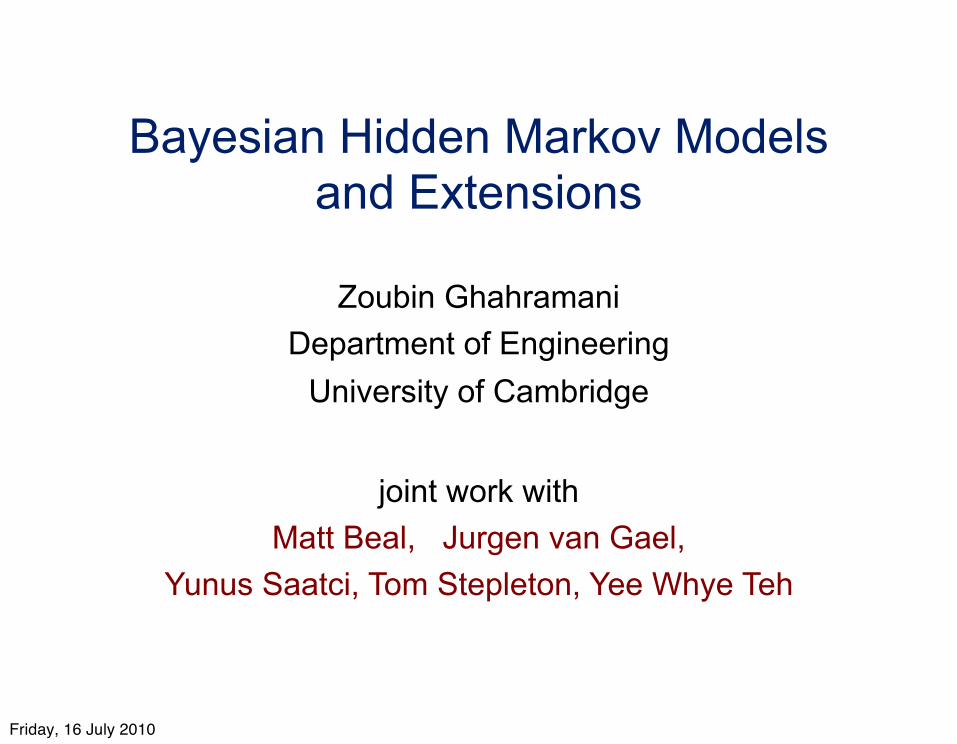
Modeling time series
Sequence of observations:y1,y2,y3, . . . ,yt
For example:
• Sequence of images
• Speech signals
• Stock prices
• Kinematic variables in a robot
• Sensor readings from an industrial process
• Amino acids, etc. . .
Goal: To build a probilistic model of the data:something that can predict p(yt|yt! 1,yt! 2,yt! 3 . . .)
Friday, 16 July 2010
3
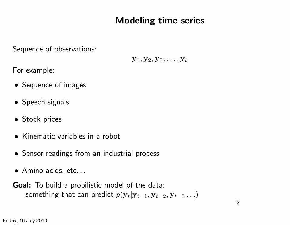
Causal structure and “hidden variables”
X 3
Y3
X 1
Y1
X 2
Y2
X T
YT
Speech recognition:
• x - underlying phonemes or words
• y - acoustic waveform
Vision:
• x - object identities, poses, illumination
• y - image pixel values
Industrial Monitoring:
• x - current state of molten steel in caster
• y - temperature and pressure sensor readings
Two frequently-used tractable models:
• Linear-Gaussian state-space models
• Hidden Markov models
Friday, 16 July 2010
4
Graphical Model for HMM
S 3
Y3
S 1
Y1
S 2
Y2
S T
YT
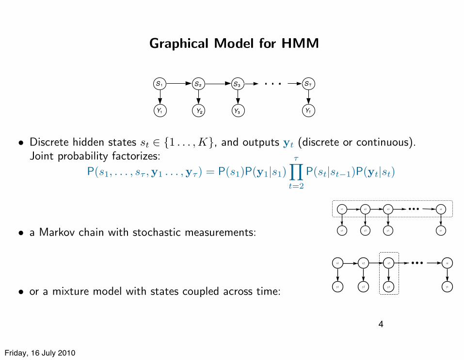
• Discrete hidden states st ! {1 . . . , K}, and outputs yt (discrete or continuous).Joint probability factorizes:
P(s1, . . . , s! ,y1 . . . ,y!) = P(s1)P(y1|s1)!!
t=2
P(st|st!1)P(yt|st)
• a Markov chain with stochastic measurements:
x1
y1 y2
x2 x3
y3
xt
yt
• or a mixture model with states coupled across time:
x1
y1 y2
x2 x3
y3
xt
yt
Friday, 16 July 2010
Hidden Markov Models
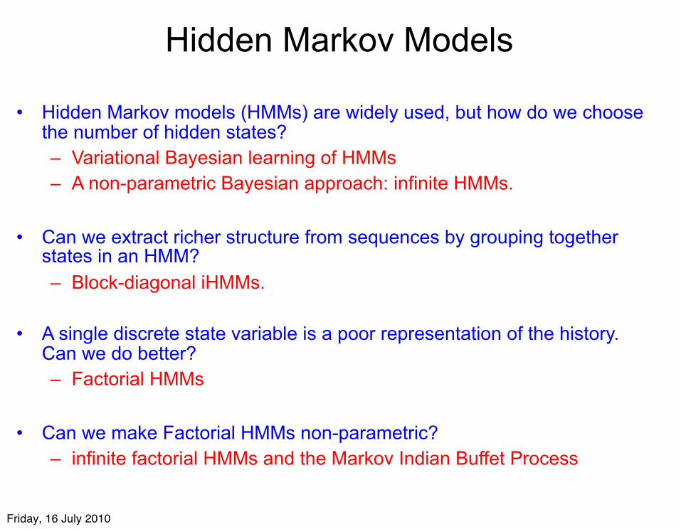
• Hidden Markov models (HMMs) are widely used, but how do we choose the number of hidden states?– Variational Bayesian learning of HMMs– A non-parametric Bayesian approach: infinite HMMs.
• Can we extract richer structure from sequences by grouping together states in an HMM?– Block-diagonal iHMMs.
• A single discrete state variable is a poor representation of the history. Can we do better?– Factorial HMMs
• Can we make Factorial HMMs non-parametric?– infinite factorial HMMs and the Markov Indian Buffet Process
Friday, 16 July 2010
Part I:
Variational Bayesian learning of
Hidden Markov Models
6
Friday, 16 July 2010
Bayesian Learning
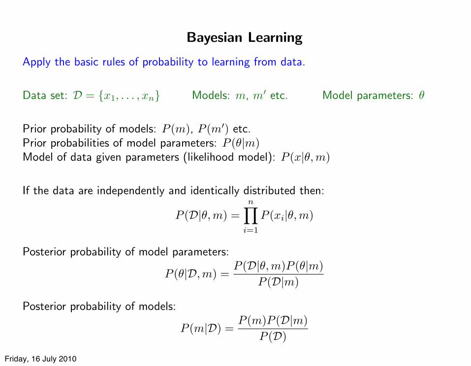
Apply the basic rules of probability to learning from data.
Data set: D = {x1, . . . , xn} Models: m, m! etc. Model parameters: !
Prior probability of models: P (m), P (m!) etc.Prior probabilities of model parameters: P (!|m)Model of data given parameters (likelihood model): P (x|!, m)
If the data are independently and identically distributed then:
P (D|!, m) =n!
i=1
P (xi|!, m)
Posterior probability of model parameters:
P (!|D,m) =P (D|!, m)P (!|m)
P (D|m)
Posterior probability of models:
P (m|D) =P (m)P (D|m)
P (D)
Friday, 16 July 2010
8
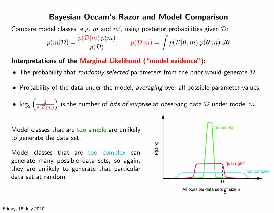
Bayesian Occam’s Razor and Model Comparison
Compare model classes, e.g. m and m!, using posterior probabilities given D:
p(m|D) =p(D|m) p(m)
p(D), p(D|m) =
!p(D|!,m) p(!|m) d!
Interpretations of the Marginal Likelihood (“model evidence”):
• The probability that randomly selected parameters from the prior would generate D.
• Probability of the data under the model, averaging over all possible parameter values.
• log2
"1
p(D|m)
#is the number of bits of surprise at observing data D under model m.
Model classes that are too simple are unlikelyto generate the data set.
Model classes that are too complex cangenerate many possible data sets, so again,they are unlikely to generate that particulardata set at random.
too simple
too complex
"just right"
All possible data sets of size n
P(D
|m)
D
Friday, 16 July 2010
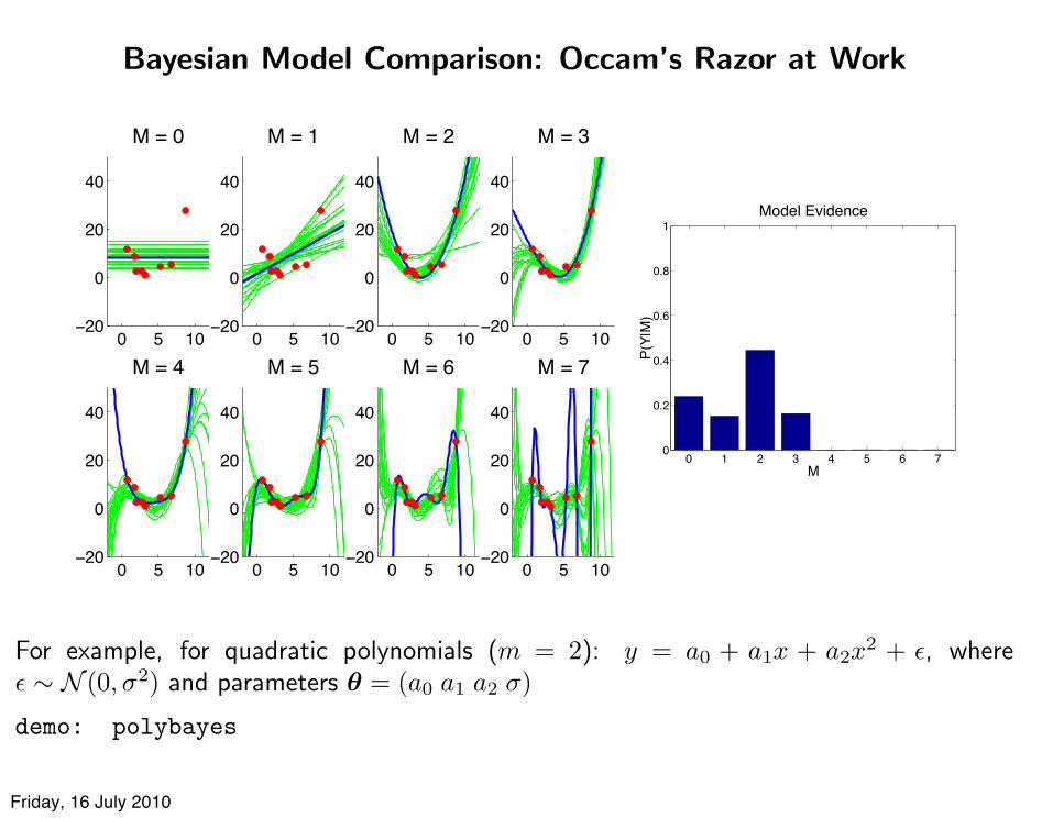
Bayesian Model Comparison: Occam’s Razor at Work
0 5 10!20
0
20
40
M = 0
0 5 10!20
0
20
40
M = 1
0 5 10!20
0
20
40
M = 2
0 5 10!20
0
20
40
M = 3
0 5 10!20
0
20
40
M = 4
0 5 10!20
0
20
40
M = 5
0 5 10!20
0
20
40
M = 6
0 5 10!20
0
20
40
M = 7
0 1 2 3 4 5 6 70
0.2
0.4
0.6
0.8
1
M
P(Y
|M)
Model Evidence
For example, for quadratic polynomials (m = 2): y = a0 + a1x + a2x2 + !, where! ! N (0,"2) and parameters ! = (a0 a1 a2 ")
demo: polybayes
Friday, 16 July 2010
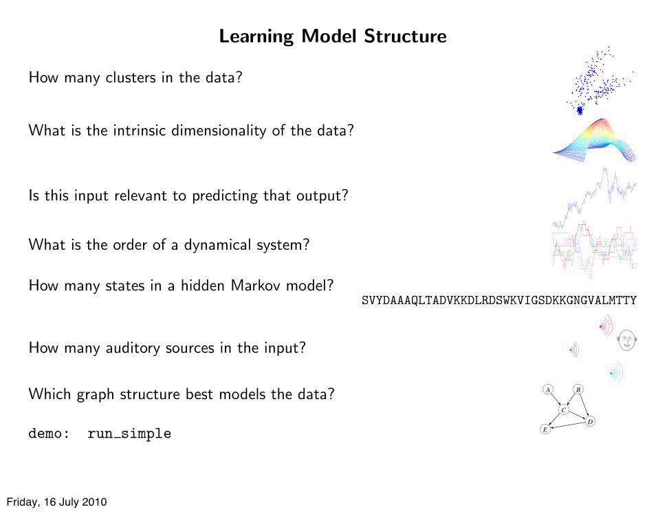
Learning Model Structure
How many clusters in the data?
What is the intrinsic dimensionality of the data?
Is this input relevant to predicting that output?
What is the order of a dynamical system?
How many states in a hidden Markov model?SVYDAAAQLTADVKKDLRDSWKVIGSDKKGNGVALMTTY
How many auditory sources in the input?
Which graph structure best models the data? A
D
C
B
Edemo: run simple
Friday, 16 July 2010
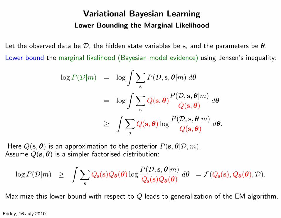
Variational Bayesian LearningLower Bounding the Marginal Likelihood
Let the observed data be D, the hidden state variables be s, and the parameters be !.
Lower bound the marginal likelihood (Bayesian model evidence) using Jensen’s inequality:
log P (D|m) = log! "
s
P (D, s,!|m) d!
= log! "
s
Q(s,!)P (D, s,!|m)
Q(s,!)d!
!! "
s
Q(s,!) logP (D, s,!|m)
Q(s,!)d!.
Here Q(s,!) is an approximation to the posterior P (s,!|D,m).Assume Q(s,!) is a simpler factorised distribution:
log P (D|m) !! "
s
Qs(s)Q!(!) logP (D, s,!|m)Qs(s)Q!(!)
d! = F(Qs(s), Q!(!),D).
Maximize this lower bound with respect to Q leads to generalization of the EM algorithm.
Friday, 16 July 2010
12
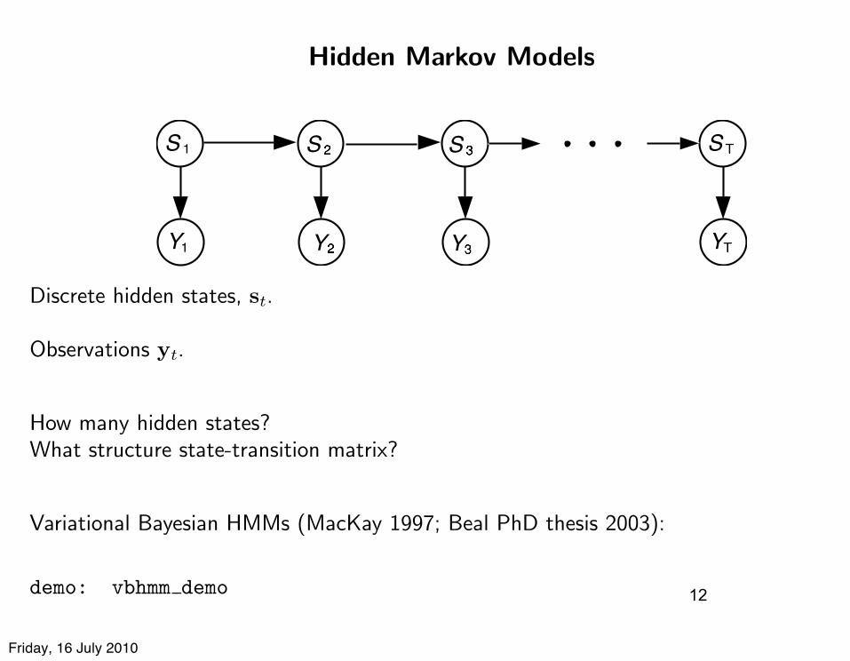
Hidden Markov Models
S 3
Y3
S 1
Y1
S 2
Y2
S T
YT
Discrete hidden states, st.
Observations yt.
How many hidden states?What structure state-transition matrix?
Variational Bayesian HMMs (MacKay 1997; Beal PhD thesis 2003):
demo: vbhmm demo
Friday, 16 July 2010
Summary of Part I
• Bayesian machine learning• Marginal likelihoods and Occam’s Razor• Variational Bayesian lower bounds• Application to learning the number of
hidden states and structure of an HMM
13
Friday, 16 July 2010
Part II
The Infinite Hidden Markov Model
Friday, 16 July 2010
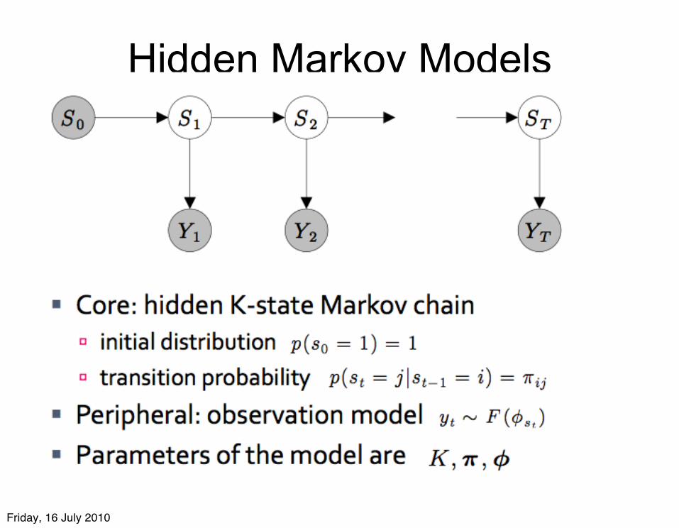
Hidden Markov Models
Friday, 16 July 2010
Choosing the number of hidden states
• How do we choose K, the number of hidden states, in an HMM?
• Can we define a model with an unbounded number of hidden states, and a suitable inference algorithm?
Friday, 16 July 2010
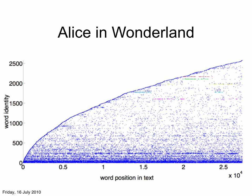
Alice in Wonderland
Friday, 16 July 2010
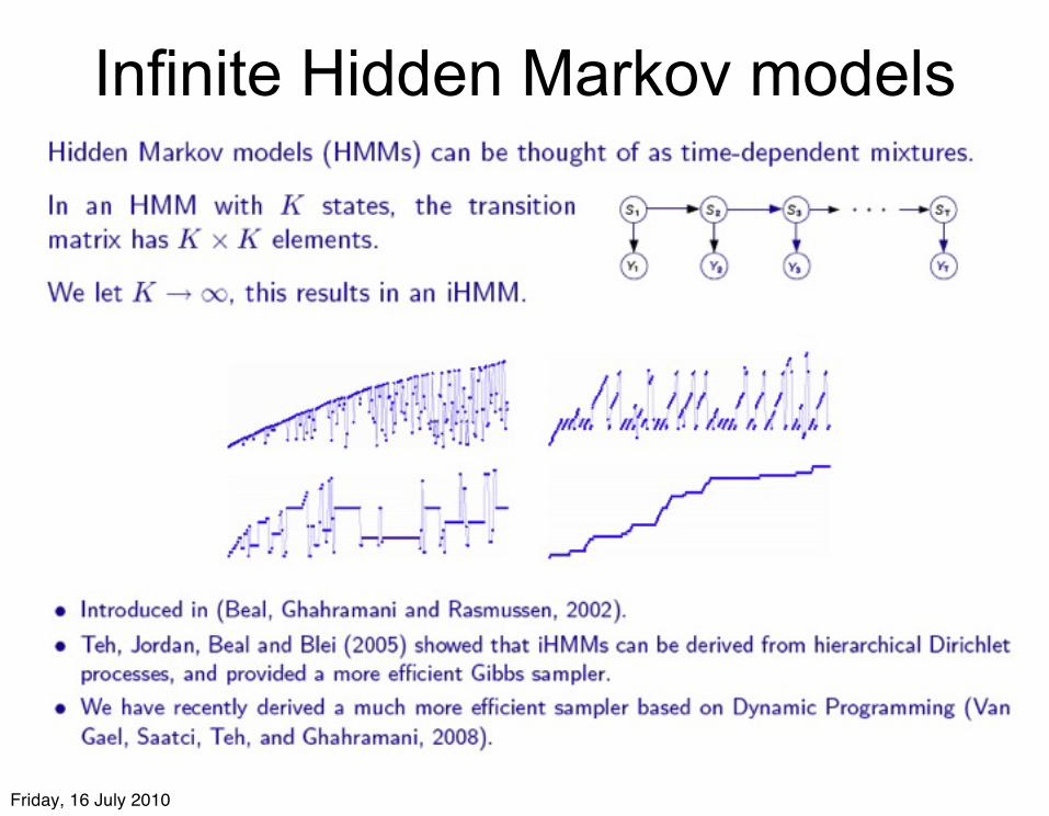
Infinite Hidden Markov models
Friday, 16 July 2010
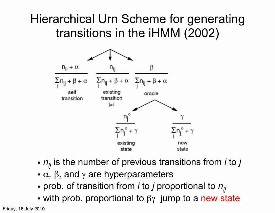
Hierarchical Urn Scheme for generating transitions in the iHMM (2002)
• nij is the number of previous transitions from i to j• α, β, and γ are hyperparameters• prob. of transition from i to j proportional to nij • with prob. proportional to βγ jump to a new state
Friday, 16 July 2010
Relating iHMMs to DPMs
• The infinite Hidden Markov Model is closely related to Dirichlet Process Mixture (DPM) models
• This makes sense: – HMMs are time series generalisations of mixture models.– DPMs are a way of defining mixture models with countably
infinitely many components.– iHMMs are HMMs with countably infinitely many states.
Friday, 16 July 2010
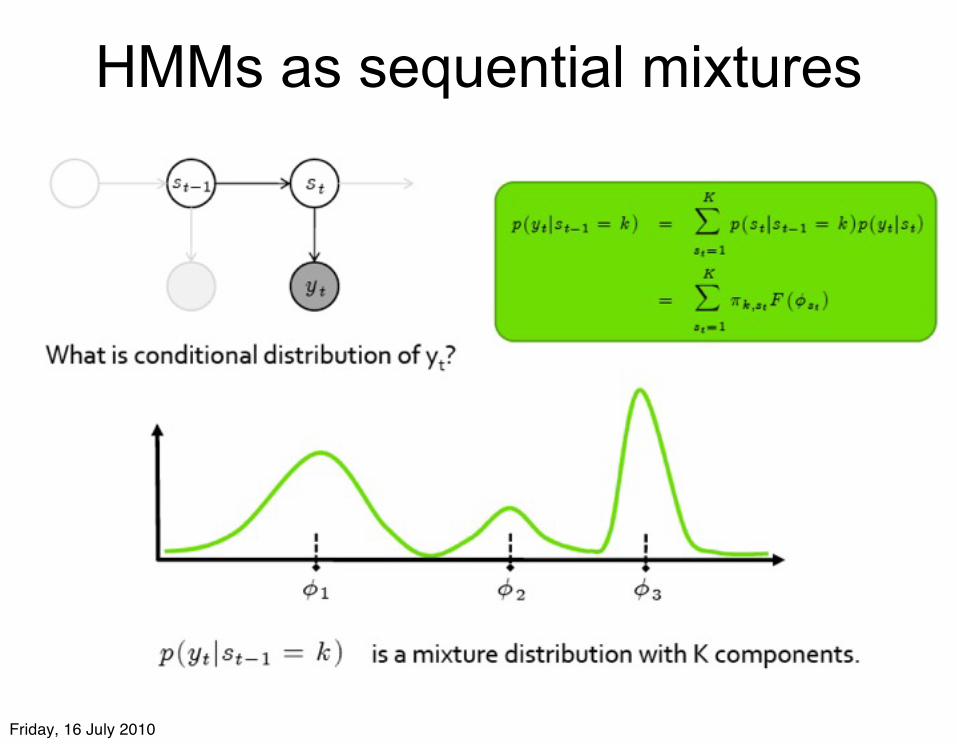
HMMs as sequential mixtures
Friday, 16 July 2010
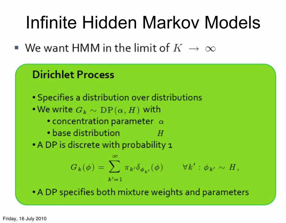
Infinite Hidden Markov Models
Friday, 16 July 2010
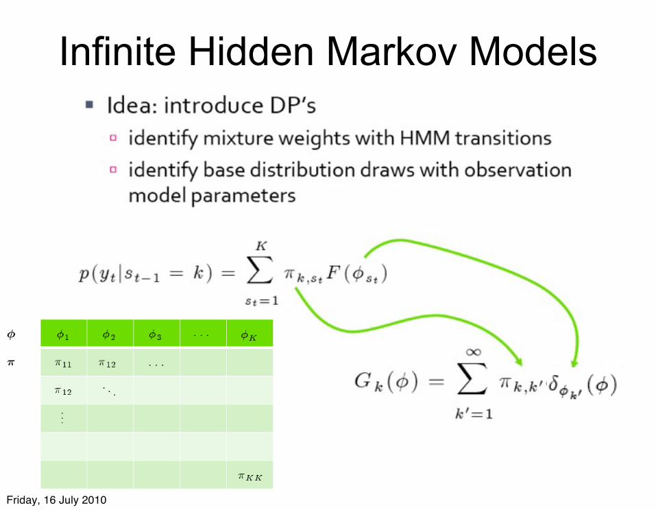
Infinite Hidden Markov Models
Friday, 16 July 2010
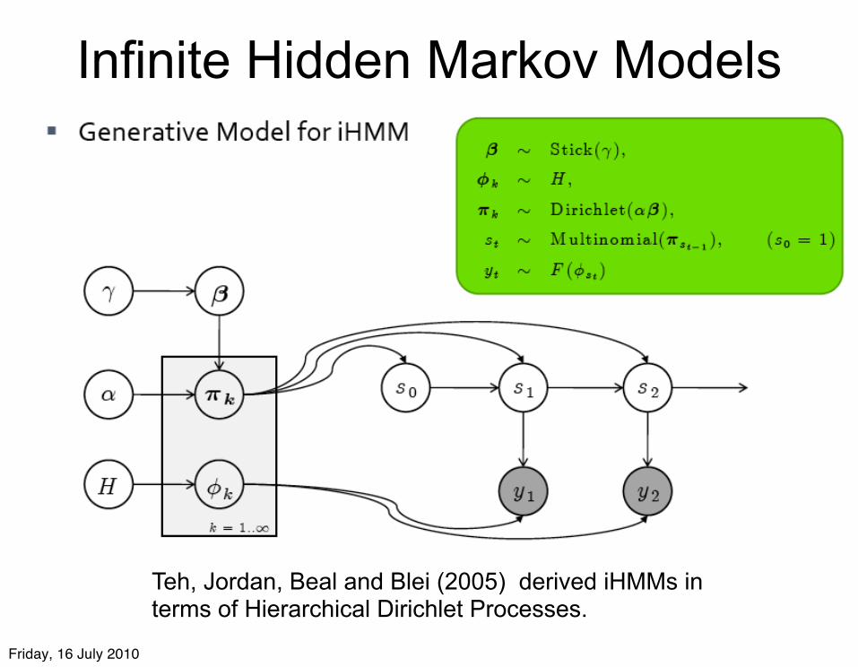
Infinite Hidden Markov Models
Teh, Jordan, Beal and Blei (2005) derived iHMMs in terms of Hierarchical Dirichlet Processes.
Friday, 16 July 2010
Efficient inference in iHMMs?
Friday, 16 July 2010
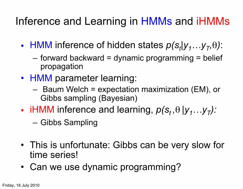
Inference and Learning in HMMs and iHMMs
• HMM inference of hidden states p(st|y1…yT,θ):– forward backward = dynamic programming = belief
propagation • HMM parameter learning:
– Baum Welch = expectation maximization (EM), or Gibbs sampling (Bayesian)
• iHMM inference and learning, p(st ,θ |y1…yT):– Gibbs Sampling
• This is unfortunate: Gibbs can be very slow for time series!
• Can we use dynamic programming?
Friday, 16 July 2010
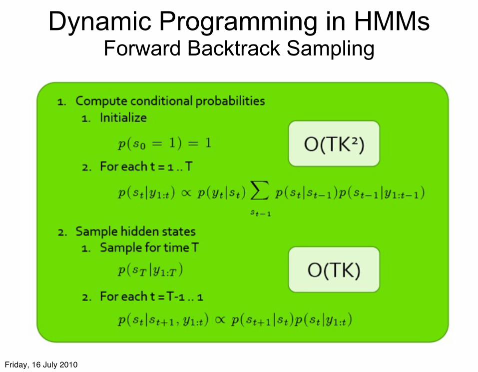
Dynamic Programming in HMMs Forward Backtrack Sampling
Friday, 16 July 2010
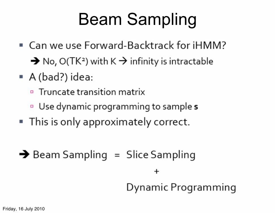
Beam Sampling
Friday, 16 July 2010
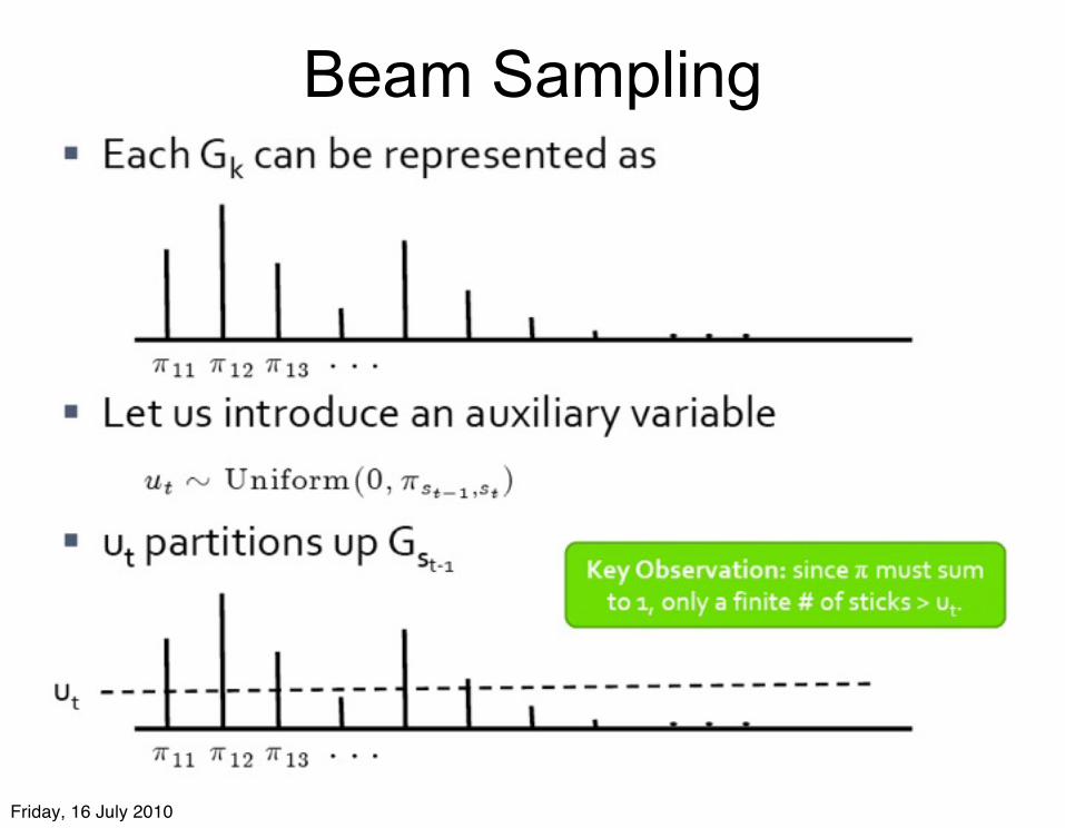
Beam Sampling
Friday, 16 July 2010
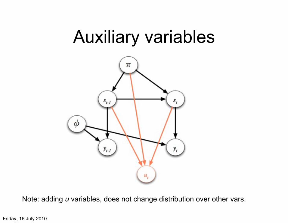
Auxiliary variables
Note: adding u variables, does not change distribution over other vars.
Friday, 16 July 2010
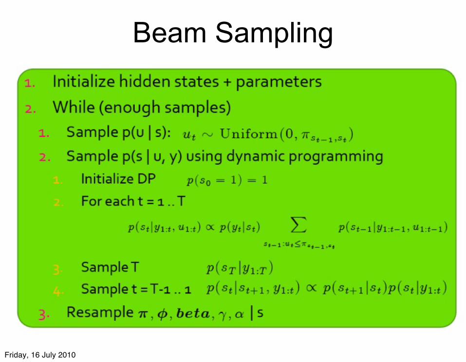
Beam Sampling
Friday, 16 July 2010
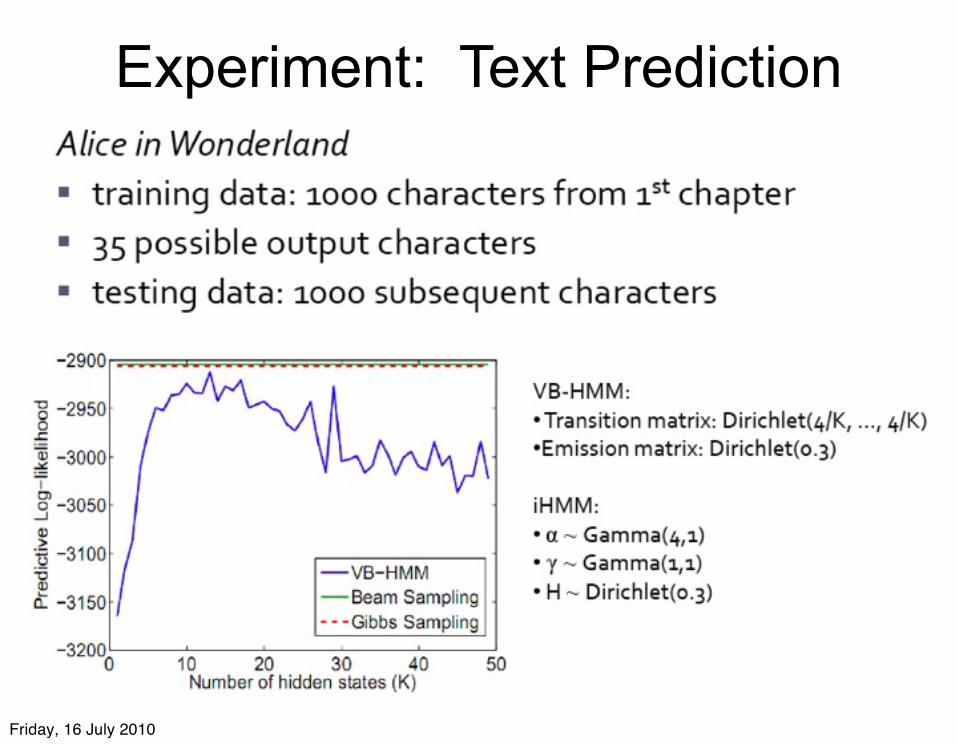
Experiment: Text Prediction
Friday, 16 July 2010
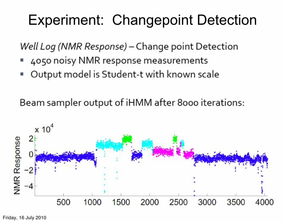
Experiment: Changepoint Detection
Friday, 16 July 2010
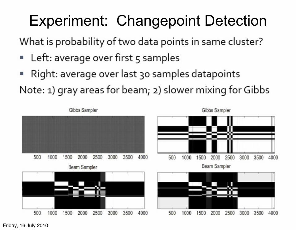
Experiment: Changepoint Detection
Friday, 16 July 2010
Parallel and Distributed Implementations of iHMMs
• Recent work on parallel (.NET) and distributed (Hadoop) implementations of beam-sampling for iHMMs (Bratieres, Van Gael, Vlachos and Ghahramani, 2010).
• Applied to unsupervised learning of part-of-speech tags from Newswire text (10 million word sequences).
• Promising results; open source code available for beam sampling iHMM: http://mloss.org/software/view/205/
35
Friday, 16 July 2010
Part III: iHMMs with clustered states
• We would like HMM models that can automatically group or cluster states.
• States within a group are more likely to transition to other states within the same group.
• This implies a block-diagonal transition matrix.
36
Friday, 16 July 2010
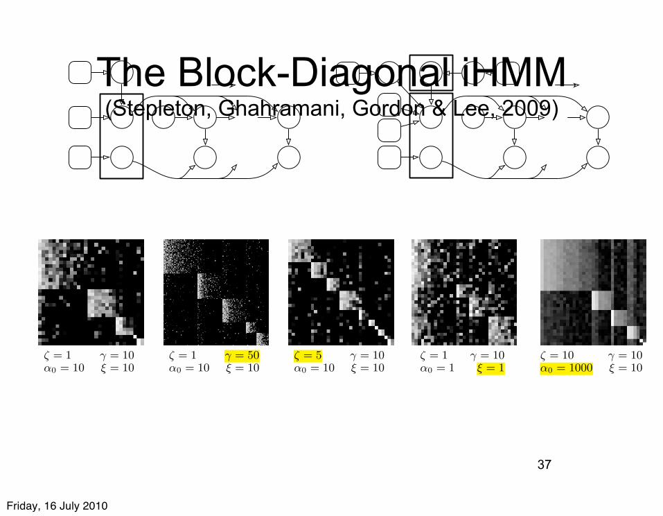
The Block-Diagonal iHMM(Stepleton, Ghahramani, Gordon & Lee, 2009)
37
546
Stepleton, Ghahramani, Gordon, Lee
!
!
"!
#!
$!
"
#! #"
$%
#%
$"
!
%
!
!
!
!
"!
#!"
#! #"
$%
#%
$"
!
%
!
$!
&
&! '
#$% #&%
'(!) '(!)
!
Figure 1: Graphical model depictions of (a) the IHMM as described in (Teh et al., 2006) and (b) the BD-IHMM.
! = 1 " = 10#0 = 10 $ = 10
! = 1 " = 50#0 = 10 $ = 10
! = 5 " = 10#0 = 10 $ = 10
! = 1 " = 10#0 = 1 $ = 1
! = 10 " = 10#0 = 1000 $ = 10
Figure 2: Truncated Markov transition matrices (right stochastic) sampled from the BD-IHMM prior with variousfixed hyperparameter values; highlighted hyperparameters yield the chief observable di!erence from the leftmostmatrix. The second matrix has more states; the third more blocks; the fourth stronger transitions betweenblocks, and the fifth decreased variability in transition probabilities.
! is a non-negative hyperparameter controlling priorbias for within-block transitions. Setting ! = 0 yieldsthe original IHMM, while giving it larger values makestransitions between di!erent blocks increasingly im-probable. Figure 3 depicts the generation of transitionprobabilities !m described by Equation 4 graphically,while Figure 2 shows some ! transition probability ma-trices sampled from truncated (finite) versions of theBD-IHMM for fixed ", #0, $, and ! hyperparameters.
3 INFERENCE
Our inference strategy for the BD-IHMM elaborateson the “direct assignment” method for HDPs pre-sented in (Teh et al., 2006). Broadly, the techniquemay be characterized as a Gibbs sampling procedurethat iterates over draws from posteriors for observationassignments to hidden states v, the shared transitionprobabilities prior ", hidden state block assignmentsz, and the hyperparameters $, ", #0, and !.
3.1 HIDDEN STATE ASSIGNMENTS
The direct assignment sampler for IHMM inferencesamples assignments of observations to hidden statesv by integrating the per-state transition probabilities!m out of the conditional distribution of v while condi-tioning on an instantiated sample of ". Since the BD-IHMM specifies sums over infinitely large partitions of
" to compute the "!m, we employ a high-fidelity ap-proximation via truncating " once its sum becomesvery close to 1, as proposed in (Ishwaran & James,2002). With these steps, the posterior for a given vt
hidden state assignment invokes a truncated analog tothe familiar Chinese Restaurant process for Dirichletprocess inference twice, once to account for the transi-tion to state vt, and once to account for the transitionto the next state:
P (vt = m | v\t,",z,#, yt, #0, !) !
p(yt | %m)!cvt!1m + #0&
!vt!1m
"
·
#cmvt+1 + #0&
!mvt+1
+ '(vt"1 =m)'(m=vt+1)
$
cm· + #0 + '(vt"1 =m), (5)
where cmn is the count of inferred transitions betweenhidden states m and n in v\t, and the · index in cm· ex-pands that term to
%Mn=1 cmn. The delta functions in-
crement the transition counts in cases where self tran-sitions are considered. Note: for simplicity of notation,we will reuse cmn for the count of m " n transitionsthroughout v in all forthcoming expressions.
When H is conjugate to P (yt | %m), explicit instantia-tion of the %m emission model parameters is not neces-sary. For brevity, this paper omits further discussionof the emission model inference, which is no di!erent
Friday, 16 July 2010
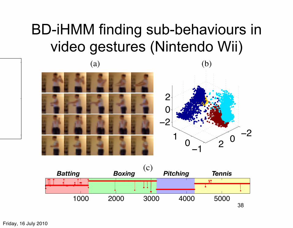
BD-iHMM finding sub-behaviours in video gestures (Nintendo Wii)
38
549
The Block Diagonal Infinite Hidden Markov Model
0
0.5
1
!!"#""
!!""""
!$#""
!$"""
!%#""
!%"""
!&#""
!&"""
!!"#""
!!""""
!$#""
!$"""
!%#""
!%"""
!&#""
!&"""
(a) (b) (c)
Figure 5: Test-set log probabilities for the 100 syn-thetic datasets for models learned by (a) the BD-IHMM and (b) the IHMM; these were not significantlydi!erent for this task (two sample t-test, p = 0.8).In (c), adjusted Rand index scores comparing sub-behavior labels inferred for the training data withground truth (c.f. Fig. 4(d)); over half have scoresgreater than 0.95. Scores of 0 typically correspond tocomplete undersegmentations, i.e. all data associatedwith just one cluster.
Well after su"cient Gibbs sampling iterations for bothmodels to converge, we simply stopped the inferenceand selected the last-sampled models for evaluation.We “froze” these models by computing the maximumlikelihood transition probabilities and emission modelparameters from these draws. We then applied stan-dard HMM techniques to these to compute the like-lihood of test-set process data, conditioned on therestriction that inferred trajectories could not visitstates that were not visited in the inferred training-set trajectories. IHMM evaluation in (Beal et al.,2002) is more elaborate: it allows the IHMM to con-tinue learning about new data encountered during test-ing. We chose our simpler scheme because we con-sider it adequate to reveal whether both models havelearned useful dynamics, and because our approach fa-cilitates rapid evaluation on many randomly-generateddatasets. Figure 5 shows that, overall, both the BD-IHMM and the IHMM are able to model the dynam-ics of this data equally well. Nevertheless, as shown inFigure 4(b), the IHMM could be “tricked” into conflat-ing states belonging to separate sub-behaviors, whilethe BD-IHMM inferred the proper structure.
Given the state labels v1, . . . , vT inferred for sequences,we can assign block labels to each observation aszv1 , . . . , zvT . If each block corresponds to a di!erent“sub-behavior” in the generative process, this new la-beling is an inferred classification or partitioning of thedata by the behavior that created it. The partitionsmay be compared with the true pattern of behaviorsknown to generate the data. We employ the adjustedRand index, a partition comparing technique, in thistask (Hubert & Arabie, 1985). Numerous index scores
!!"
! !#"
#
!#
"
#
1000 2000 3000 4000 5000
Batting Boxing Pitching Tennis
(a) (b)
(c)
Figure 6: (a) Selected downscaled video frames for(top to bottom) batting, boxing, pitching and tennisswing gestures. (b) First three dimensions of videoframes’ PCA projections, colored by gesture type.(c) Sequences of sub-behaviors executed in one set oftraining data: inferred by one of the model runs (redline) and ground truth (background shading). Eachsub-behavior actually comprises numerous video clipsof the same gesture.
near 1 in Figure 5 indicate frequent close matches be-tween the inferred classification and ground truth.
4.2 VIDEO GESTURE CLASSIFICATION
We collected multiple video clips of a person execut-ing four di!erent gestures for a motion-activated videogame (Figure 6). After downscaling the color videoframes to 21! 19 pixels, we projected the frames ontotheir first four principal components to create data forthe IHMM and BD-IHMM algorithms.
For inference, parameters were similar to the artifi-cial data experiment, except here the emission modelswere 4-D spherical Gaussians (! = 0.275). We re-peated a 9-way cross-validation scheme three times tocollect results over multiple trials; training sets con-tained around 6,000 observations. Subjecting theseresults to the same analysis as the artificial data re-veals similar compared test-set likelihoods and favor-able training-set sub-behavior labeling performance(Figure 7). Both models allocated around 45 hiddenstates to describe the training data (combined mean:44.5, ! = 5.0). We note that since both the BD-IHMMand the IHMM use multiple states to describe each ges-ture, inferred hidden state trajectories do not usefullyidentify separate sub-behaviors in the data: adjustedRand indices comparing the IHMM’s inferred trajec-tory labeling to ground truth sub-behavior labeling arepoor (µ = 0.28, ! = 0.036).
Friday, 16 July 2010
Part IV
• Hidden Markov models represent the entire history of a sequence using a single state variable st
• This seems restrictive...
• It seems more natural to allow many hidden state variables, a “distributed representation” of state.
• …the Factorial Hidden Markov ModelFriday, 16 July 2010
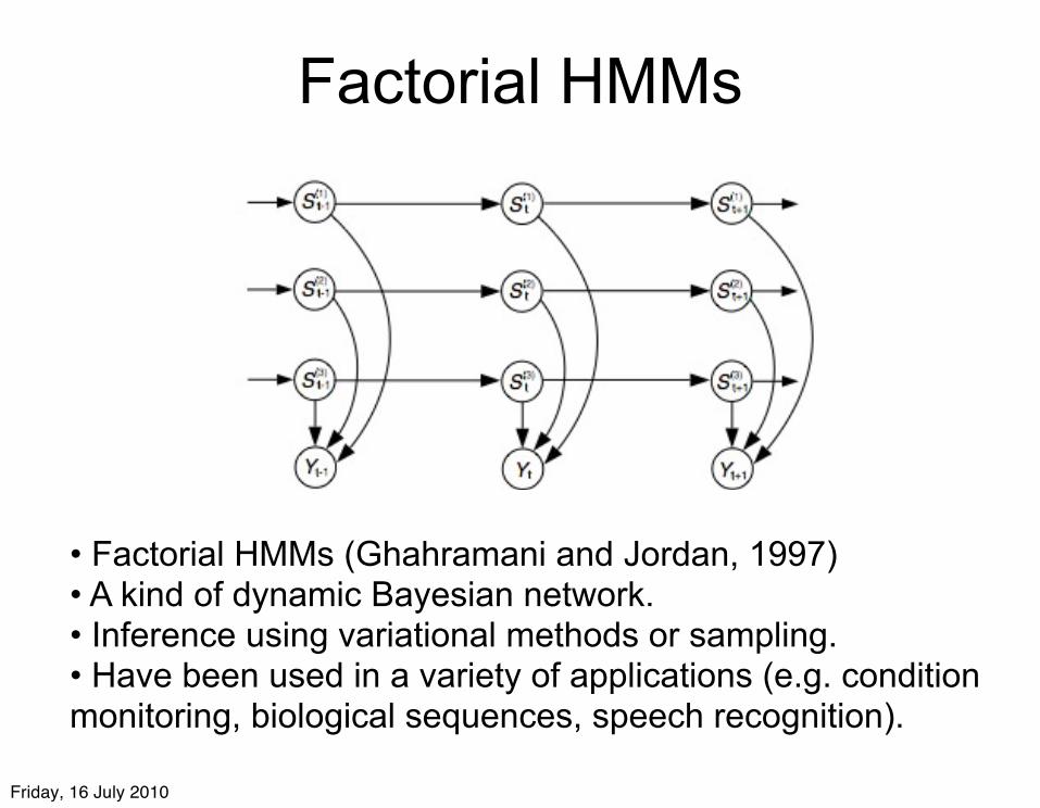
Factorial HMMs
• Factorial HMMs (Ghahramani and Jordan, 1997)• A kind of dynamic Bayesian network.• Inference using variational methods or sampling.• Have been used in a variety of applications (e.g. condition monitoring, biological sequences, speech recognition).
Friday, 16 July 2010
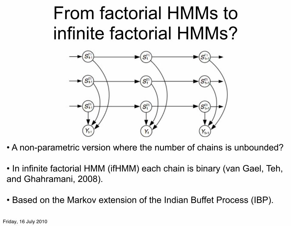
From factorial HMMs to infinite factorial HMMs?
• A non-parametric version where the number of chains is unbounded? • In infinite factorial HMM (ifHMM) each chain is binary (van Gael, Teh, and Ghahramani, 2008).
• Based on the Markov extension of the Indian Buffet Process (IBP).
Friday, 16 July 2010

Bars-in-time data
Friday, 16 July 2010
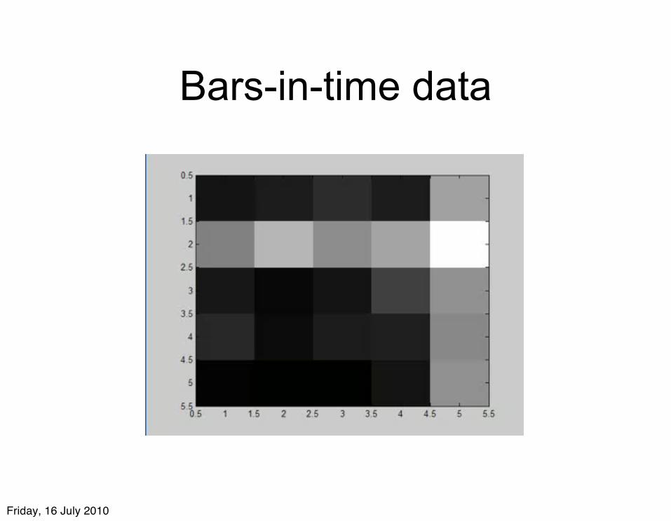
Bars-in-time data
Friday, 16 July 2010
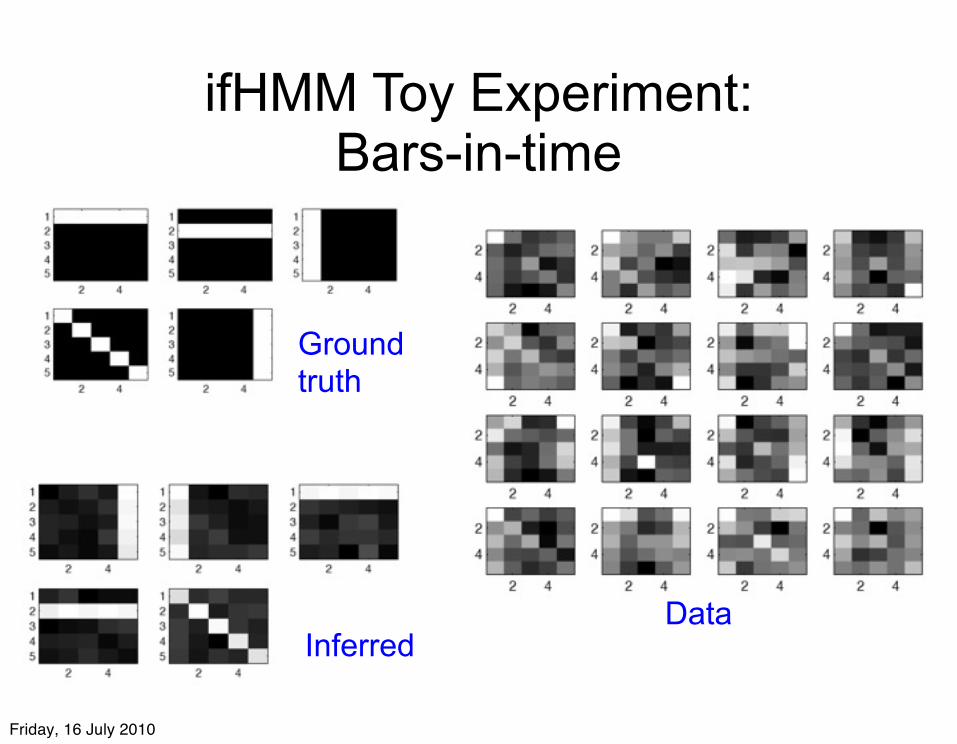
ifHMM Toy Experiment: Bars-in-time
Data
Ground truth
Inferred
Friday, 16 July 2010
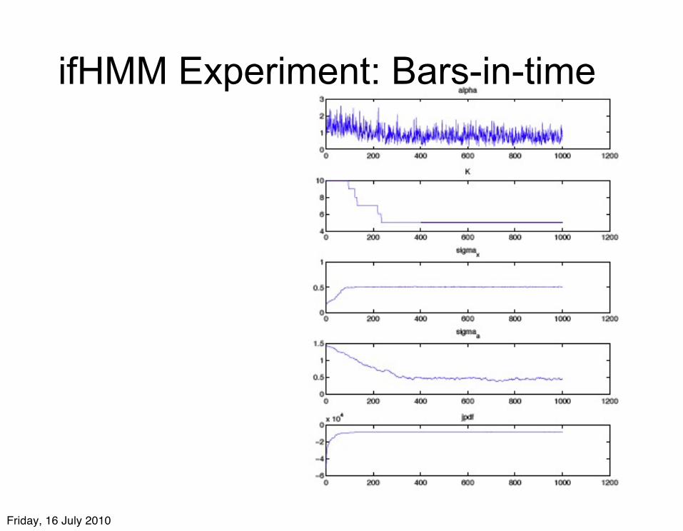
ifHMM Experiment: Bars-in-time
Friday, 16 July 2010
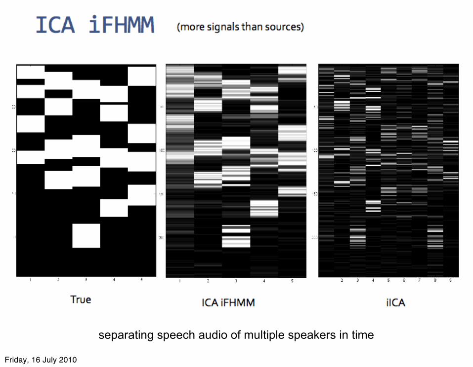
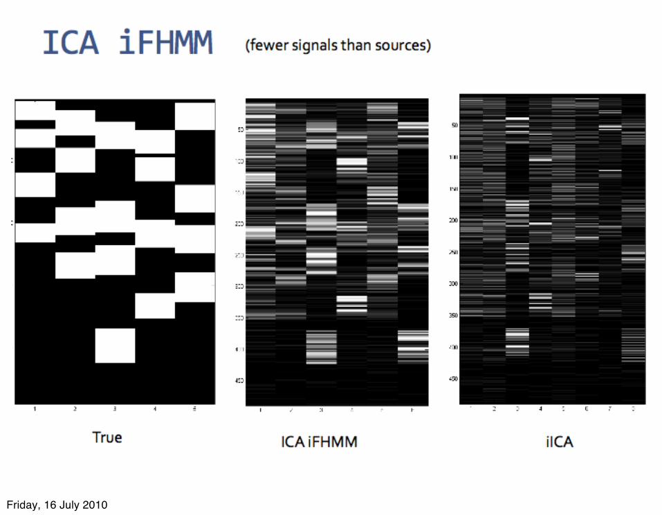
separating speech audio of multiple speakers in time
Friday, 16 July 2010
Friday, 16 July 2010
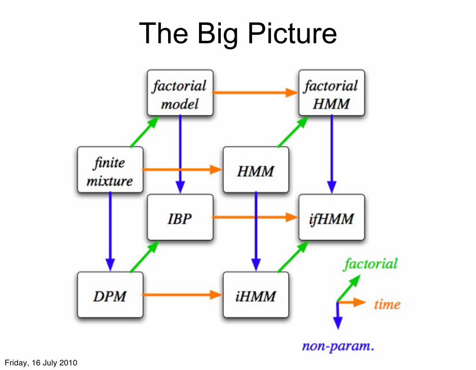
The Big Picture
Friday, 16 July 2010
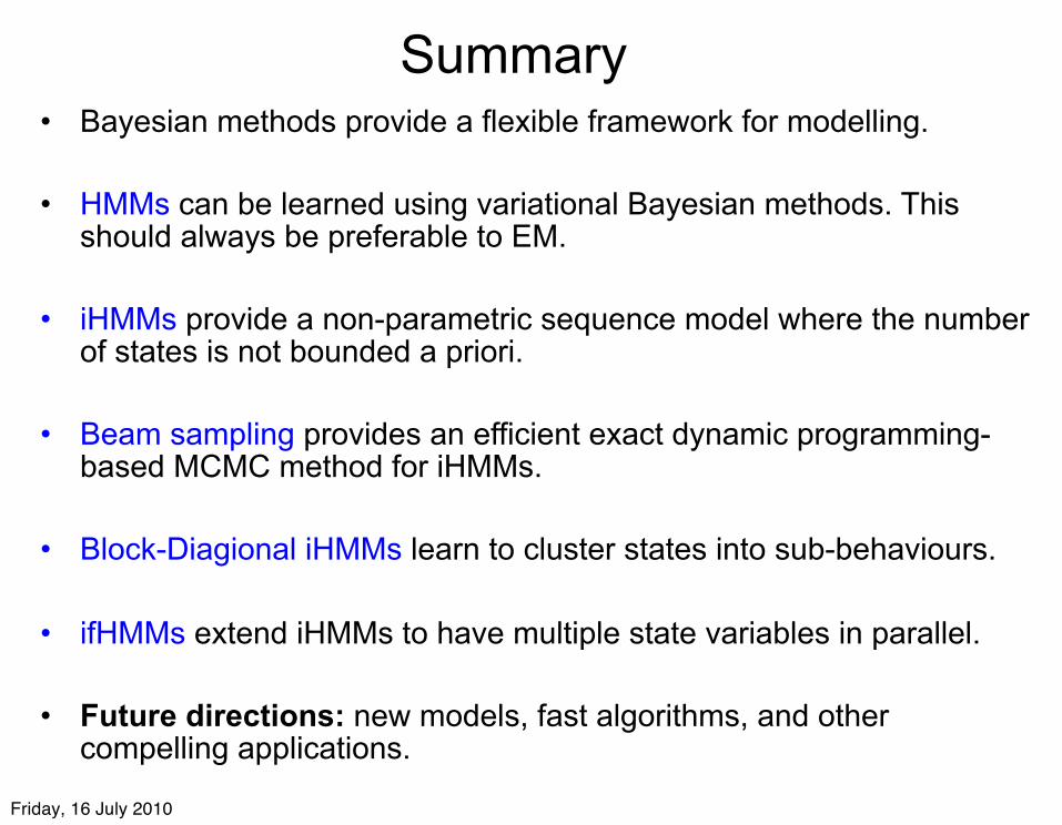
Summary• Bayesian methods provide a flexible framework for modelling.
• HMMs can be learned using variational Bayesian methods. This should always be preferable to EM.
• iHMMs provide a non-parametric sequence model where the number of states is not bounded a priori.
• Beam sampling provides an efficient exact dynamic programming-based MCMC method for iHMMs.
• Block-Diagional iHMMs learn to cluster states into sub-behaviours.
• ifHMMs extend iHMMs to have multiple state variables in parallel.
• Future directions: new models, fast algorithms, and other compelling applications.
Friday, 16 July 2010
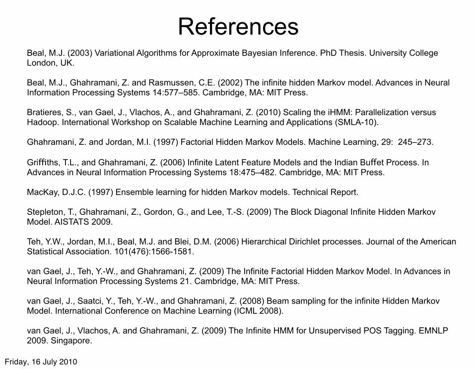
ReferencesBeal, M.J. (2003) Variational Algorithms for Approximate Bayesian Inference. PhD Thesis. University College London, UK.
Beal, M.J., Ghahramani, Z. and Rasmussen, C.E. (2002) The infinite hidden Markov model. Advances in Neural Information Processing Systems 14:577–585. Cambridge, MA: MIT Press.
Bratieres, S., van Gael, J., Vlachos, A., and Ghahramani, Z. (2010) Scaling the iHMM: Parallelization versus Hadoop. International Workshop on Scalable Machine Learning and Applications (SMLA-10).
Ghahramani, Z. and Jordan, M.I. (1997) Factorial Hidden Markov Models. Machine Learning, 29: 245–273.
Griffiths, T.L., and Ghahramani, Z. (2006) Infinite Latent Feature Models and the Indian Buffet Process. In Advances in Neural Information Processing Systems 18:475–482. Cambridge, MA: MIT Press.
MacKay, D.J.C. (1997) Ensemble learning for hidden Markov models. Technical Report.
Stepleton, T., Ghahramani, Z., Gordon, G., and Lee, T.-S. (2009) The Block Diagonal Infinite Hidden Markov Model. AISTATS 2009.
Teh, Y.W., Jordan, M.I., Beal, M.J. and Blei, D.M. (2006) Hierarchical Dirichlet processes. Journal of the American Statistical Association. 101(476):1566-1581.
van Gael, J., Teh, Y.-W., and Ghahramani, Z. (2009) The Infinite Factorial Hidden Markov Model. In Advances in Neural Information Processing Systems 21. Cambridge, MA: MIT Press.
van Gael, J., Saatci, Y., Teh, Y.-W., and Ghahramani, Z. (2008) Beam sampling for the infinite Hidden Markov Model. International Conference on Machine Learning (ICML 2008).
van Gael, J., Vlachos, A. and Ghahramani, Z. (2009) The Infinite HMM for Unsupervised POS Tagging. EMNLP 2009. Singapore.
Friday, 16 July 2010


![Particle Gibbs for Infinite Hidden Markov Modelspapers.nips.cc/...particle-gibbs-for-infinite-hidden-markov-models.pdf · The original Gibbs sampling approach proposed inTeh et al.[2006]](https://img.pdfslide.net/doc/110x75/5ed7b8dc498700329150e329/particle-gibbs-for-infinite-hidden-markov-the-original-gibbs-sampling-approach-proposed.jpg)