Embed Size (px)
Citation preview
Department of Economics
School of Business, Economics and Law at University of Gothenburg
Vasagatan 1, PO Box 640, SE 405 30 Göteborg, Sweden
+46 31 786 0000, +46 31 786 1326 (fax)
www.handels.gu.se [email protected]
WORKING PAPERS IN ECONOMICS
No 478
Inflation Dynamics and Food Prices in Ethiopia
DICK DUREVALL
JOSEF L. LOENING
YOHANNES A. BIRRU
University of Gothenburg and
Gothenburg Centre for
Globalization and
Development
World Bank National Bank of Ethiopia
November, 2010
ISSN 1403-2473 (print) ISSN 1403-2465 (online)
Inflation Dynamics and Food Prices in Ethiopia*†
DICK DUREVALL
JOSEF L. LOENING
YOHANNES A. BIRRU
University of Gothenburg and
Gothenburg Centre for Globalization
and Development
Email: [email protected]
World Bank National Bank of
Ethiopia
November 2010
Abstract
During the global food crisis, Ethiopia experienced an unprecedented increase in inflation, among
the highest in Africa. Using monthly data over the past decade, we estimate models of inflation to
identify the importance of the factors contributing to CPI inflation and three of its major
components: cereal prices, food prices, and non-food prices. Our main finding is that movements
in international food and goods prices, measured in domestic currency, determined the long-run
evolution of domestic prices. In the short run, agricultural supply shocks affected food inflation,
causing large deviations from long-run price trends. Monetary policy seems to have
accommodated price shocks, but money supply growth affected short-run non-food price
inflation. Our results suggest that when analyzing inflation in developing economies with a large
food share in consumer prices, world food prices and domestic agricultural production should be
considered. Omitting these factors can lead to biased results and misguide policy decisions.
Keywords: Ethiopia, Exchange rate, Food prices, Inflation, Money demand
JEL classification: E31, E37, O55, Q17.
*This is a substantially revised and updated version of Loening, Durevall and Birro (2009) available as World Bank
Policy Research Working Paper, No. 4969, and Scandinavian Working Papers in Economics (S-WoPEc), No. 347,
University of Gothenburg.
† We would like to thank Philip Abbott, Hashim Ahmed, Arne Bigsten, Robert Corker, Astou Diouf, Paul Dorosh,
Karen Mcconnell-Brooks, Jiro Honda, Deepak Mishra, Paul Moreno-Lopez, Rashid Shahidur, Eleni Gabre-Madhin,
Francis Rowe, Steven O’Connell, Cristina Savescu, Patricia Seex, Emily Sinnott, and Zaijin Zhan, as well as
participants of the 2009 Economists’ Forum, for useful comments and discussions. The views expressed in this paper
are the authors; they do not necessarily represent the views of the National Bank of Ethiopia, the International Bank
for Reconstruction and Development/World Bank and its affiliated organizations, or those of the Executive Directors
of the World Bank or the governments they represent.

1
1. Introduction
During 2004–2008, global commodity prices rose to record levels.1 As a result,
several low-income countries are still experiencing high price levels, trade deficits, and
unstable macroeconomic environments. High commodity prices, particularly for food,
also have adverse effects on poverty in countries with large fractions of net food-
buyers (Wodon and Zaman, 2010). Although food and fuel prices have fallen
substantially since August 2008, they continue to be high by historical standards, and
in mid-2010 several grain prices started to rise again, creating a fear of a new period of
food-price hikes.
Several studies have attempted to address the underlying causes of the global
price rise, typically identifying a combination of factors – ranging from long-term
economic and demographic trends combined with short-term problems, such as bad
weather, speculation, high oil prices, and export bans in a number of countries.2 At the
same time, we know less about how world food prices affect domestic food prices in
individual developing countries; particularly in Sub-Saharan Africa (see Minot, 2010).
One of the most affected countries is Ethiopia, which, with the exception of
Zimbabwe and some small island economies, had the strongest acceleration in food
price inflation in Sub-Saharan Africa (IMF, 2008a, 2008c; Minot, 2010). At the peak
of the global food crisis, in July 2008, annual food price inflation surpassed 90 percent.
This was an historically unprecedented rise, which began in 2006.
There is no consensus on why Ethiopia experienced such dramatic price rises.
The increase in inflation coincided with relatively favorable harvests, whereas in the
past inflation had typically been associated with agricultural supply shocks due to
droughts. World food price increases are believed to have small effects in Ethiopia
because of the limited size of food imports, which amounts to about five percent of
agricultural GDP. Minot (2010), for example, finds that out of the three stable food
prices analyzed, one is affected by world market prices (wheat), but that the
transmission from world prices is negligible. Instead, the chief explanations have
1 The price increases vary across commodities and data sources. The annual Commodity Food Price
Index of the World Bank‘s Development Prospect Group rose by 13.2 percent in 2004, declined
somewhat in 2005, and then rose by 10.0, 25.6 and 34.2 percent in the following three years. In the
middle of 2008, the index started to decline and by March 2009, it was at the same level as in mid-2007,
which is almost twice as high as the average value in 1999–2003.
2 Baffes and Hanioti (2010) provide a survey and extensive list of references.
2
focused on domestic demand, expansionary monetary policy, a shift from food aid to
cash transfers, and structural factors due to reforms and investments in infrastructure
(Ahmed, 2007; IMF, 2008b; Rashid, 2010).
Nonetheless, few studies, if any, attempt to identify the relative importance of
the factors driving inflation. The purpose of this paper is to fill this gap of information
by estimating a model of inflation for the period January 2000–December 2009, with a
focus on food prices. We use general-to-specific modeling and estimate single-
equation error correction models (ECMs) for the Consumer Price Index (CPI) and
three of its major components cereal, food and non-food prices. The reduction of the
general model is carried out with Autometrics, a computer-automated general-to-
specific modeling approach that tests all possible reduction paths and eliminates
insignificant variables, while keeping the chosen significance level constant (Hendry
and Krolzig, 2005; Doornik, 2009).
By developing error correction terms that measure deviations from equilibrium
in the money market, external sector, and agricultural market, we evaluate the impact
on inflation of excess money supply, changes in food and non-food world prices, and
domestic agricultural supply shocks. Agricultural markets can thus affect inflation both
through the transmission of international food commodity prices and through changes
in domestic food supply and demand. This approach can be viewed as a general
(hybrid) model that embeds other models of inflation, allowing us to test various
hypotheses, and account for the specific circumstances of developing economies with a
large agricultural sector.
Our results show that overall inflation in Ethiopia is closely associated with
agriculture and food in the economy, and that the international food crisis had a strong
impact on domestic food prices. The external sector largely determines inflation in the
long run (about three to four years). Specifically, domestic food prices adjust to
changes in world food prices, measured in local currency (birr), and non-food prices
adjust to changes in world producer prices. There are large deviations from long-run
equilibrium food prices, mainly due to the importance of the domestic market for
agricultural products; domestic food supply shocks have a strong effect on inflation in
the short run (about one to two years). These findings, however, do not imply that
domestic and world food prices are always close to each other. They show that prices
do not drift too far apart, which is consistent with observed price fluctuations of
domestic prices between import and export parity bands. The evolution of money
3
supply does not affect food prices directly, though money supply growth significantly
affects non-food price inflation in the short run.
A major contribution of the paper is that it takes into account specific
circumstances of a developing country with a large agricultural sector. Most studies on
inflation ignore domestic agriculture, and very few studies, if any, include international
commodity markets in their analysis. In turn, studies on the transmission of world food
prices to domestic food prices usually focus on individual prices and ignore the
macroeconomic context. Finally, almost all previous studies on inflation in Africa
model the CPI only, even though the weight of food in CPI is often over 50 percent,
and the dynamics of food and non-food prices can differ considerably.
Section 2 gives a short description of Ethiopia‘s recent macroeconomic
performance, and then outlines popular hypotheses of the causes of Ethiopia‘s inflation
trajectory. Section 3 provides the theoretical framework, formulates the empirical
model, and discusses how various hypotheses are tested. Section 4 describes and
analyzes the money market, external sector, and agricultural market, with the purpose
of formulating explanatory variables for the inflation models. Section 5 develops the
final models. Section 6 discusses major findings, and Section 7 concludes the paper.
2. Inflation in Ethiopia: Background and Previous Studies
2.1 Economic Performance and Inflation
In recent years, Ethiopia‘s economy has expanded rapidly: according to official
data, GDP growth averaged 11 percent between 2003/04 and 2008/2009. Agriculture,
which accounts for close to 50 percent of GDP and nearly 85 percent of employment,
grew even faster. In spite of this, about 38 percent of Ethiopia‘s 77 million people
lived below the official poverty line in 2005, but it is likely that an even larger
proportion have experienced extended periods of poverty due to shocks (Bigsten and
Shimeles, 2008). The rise in food inflation, for instance, is likely to have increased
urban poverty.
Historically, Ethiopia has not suffered from high inflation. The annual average
was only 5.2 percent from 1980/81–2003/04, and major inflationary episodes have
occurred only during conflict and drought. Annual average inflation reached a record
of 18 percent during 1984/85 because of drought, 21 percent in 1991/92 at the peak of
war with Eritrea, and again 16 percent during the 2003 drought.

4
Figures 1 and 2 depict the major trends in inflation during the current decade,
January 1999–July 2010, by showing the annual growth rates of the CPI and its major
components: food, cereals, house rents, construction, materials, energy and other non-
food prices. Table 1 gives a list of the CPI weights.
[Figures 1 and 2 here]
[Table 1 here]
The importance of fluctuations in food prices for the overall CPI is clearly
visible in Figure 1. The deflation in 2001–2002 was due to good harvests and
significant amounts of food aid inflows. There is a rapid increase in inflation induced
by the 2003 drought, another increase around 2005, and an almost exponential price
outburst in 2008. There was also a hike in non-food inflation during 2005–2007.
Overall, it is evident that food and non-food inflation behave very differently,
indicating that they should be analyzed separately.
As food accounts for 57 percent of total household consumption expenditure,
low food and CPI inflation are associated with adequate rainfall and good crop
harvests. However, this link seems to have been absent during 2004/05–2008/09, since
food inflation continued to accelerate despite good weather and an agricultural
production boom. It is notable that annual food inflation, measured in simple growth
rates, rose from 18.2 percent in June 2007 to a peak of 91.7 percent in July 2008. Food
inflation then started to decline, and during the latter half of 2009 there was even
deflation.
Figure 2 depicts food price inflation divided into its various components.
Despite a short hike of spice inflation in 2007, it is obvious that cereal price inflation
accounts for most of the fluctuations in food prices. It is also the most important
component of the food-price index; its weight in the CPI is close to 23 percent. The
two graphs thus give an early indication of the key role played by food prices in
general, and by cereal prices in particular, in Ethiopia‘s overall inflation dynamics.
5
2.2 Review of Studies on Inflation in Ethiopia
A few studies have emerged in the light of Ethiopia‘s food price crisis, drawing
mainly on logical deductions and descriptive analysis. We subsequently review the
most important ones.
The Ethiopian Development Research Institute (EDRI), a government think-
tank, has put forward several hypotheses, summarized by Ahmed (2007). Increases in
aggregated demand should a priori put pressure on demand for food, resulting in
acceleration of food inflation. Yet, the puzzle is that agriculture has been leading the
fast growth in the economy, and crop production has seen substantial growth during
the period. This seems to undermine the role of aggregate demand in explaining
Ethiopia‘s recent food inflation.
Changes in the structure of the economy, following a sustained development of
the infrastructure network, are viewed as a potentially better explanation for the price
increases. These include behavioral changes leading to increased commercialization of
crop production and reduced distress selling by peasants, equipped with better access
to credit, storage facilities and marketing information system, which might have
significant implications for aggregate demand and prices.
Ahmed (2007) also lists various other domestic and external factors, including
money supply and world commodity prices. In addition, housing shortages in urban
areas and speculation have affected inflation, where a lack of regulation might have
played a role in the surge in housing prices, particularly in Addis Ababa.
The International Monetary Fund (IMF, 2008b) suggests that inflation is being
led by rapidly rising food prices. However, since inflation is higher in Ethiopia than in
neighboring countries, domestic factors, including demand pressure and expectations
should be important. Some supply-side factors may also explain part of the rise in food
prices, such as reduced distress selling by farmers and the switch from food to cash
aid. The Fund thus recommends addressing macroeconomic imbalances, and forcefully
tightening monetary and fiscal policies. Rising global commodity prices may be
important, but the transmission mechanism is not clear because the amount of non-aid
food imports is relatively small. IMF (2008a) notes that there might be a process of
convergence to world food prices driven by high food prices in neighboring countries,
though there is a lack of empirical evidence.
6
Rashid (2010) also argues that domestic food price increases were the result of
general demand, except in 2007–2008 when cereal production was much smaller than
shown by official statistics. General demand in turn, was driven by excess money supply;
and accordingly, strict monetary policy brought inflation under control in 2008–2009.
Among the few empirical studies are Ayalew Birru (2007) and Wolde-Rufael
(2008). Ayalew Birru (2007) develops a macroeconometric model for the National
Bank of Ethiopia, the country‘s central bank, using annual data from 1970–2006. The
chief claim is that supply shocks, inertia, and the consumer prices of major trading
partners are among the most important determinants of inflation. Nevertheless, the use
of annual data and the need to correct for major developments in Ethiopia‘s turbulent
history limit the model‘s applicability, as does the fact that the analysis does not cover
the period of rapid inflation, 2007–2008. Wolde-Rufael (2008) also uses annual data
covering 1964–2003. In line with traditional inflation analysis, he ignores agriculture
and international prices completely.
In the context of Ethiopia, two microeconometric studies are important.
Osborne (2004) analyzes the role of news in the Ethiopian grain market. Although the
focus is on generalizing the neoclassical storage model, it throws light on the micro-
determinants of the inflation process because of the large weight of cereals in CPI.
Osborne reports that there have been several occasions of sharp rises or falls in
seasonal prices. For instance, in 1983/84, 1990/91 and 1993/94 maize prices rose by
over 100 percent during periods of six months. She attributes these to the role of news
of future harvests and forward-looking expectations. Thus, it is possible that the almost
doubling of grain prices that took place between February and September 2008 is a
similar phenomenon. Tadesse and Guttormsen (2010), using a rational expectations
model and threshold regression, find evidence of speculative storage during periods of
high prices over 1996–2006.
To conclude, while acknowledging the role of international prices, a key claim
is that expansionary monetary policy has been the major cause for high inflation, and
world food prices have played a minor, or no, role. However, there is little evidence of
the relative importance of their contribution to inflation in Ethiopia.

7
3. Modeling Inflation in an Agricultural Economy
In this section, we present an empirical inflation model that embeds different
models of inflation. It allows us to test various hypotheses rather than imposing
restrictions on the models, and can account for the specific circumstances of
developing economies with a large agricultural sector. The Phillips curve and the
quantity theory are the two traditional approaches used to model inflation, which we
first review briefly.
The Phillips curve stipulates that high aggregate demand generates
employment, which first leads to wage increases and later to rising prices. Although
sometimes applied to Sub-Saharan Africa, as in Barnichon and Peiris (2008), it may
not be an adequate approach for Ethiopia. Extensive self- and underemployment, large
informal markets, and a low degree of labor-market organization all make the link
between aggregate demand, unemployment and wage increases very weak or even
non-existent. Moreover, there is a strong negative correlation between business cycles
and inflation, since positive agricultural supply shocks increase GDP growth and lower
inflation, and vice versa. Disentangling the Phillips curve effect, if it exists, is a
challenging task since only annual GDP data is available.
Most studies on Sub-Saharan African economies thus use the quantity theory
and focus on the role of money supply and demand, assuming that inflation is due to
excess money supply. Nowadays, foreign prices are often added to the models to
account for imports or internationally traded goods. Some recent examples are: Blavy
(2004) on Guinea; Moriyama (2008) on Sudan; Olubusoye and Oyaromade (2008) on
Nigeria; and Klein and Kyei (2009) on Angola. Studies in this tradition usually neglect
agricultural markets and food supply, even though food makes up more than half of the
consumer basket. In fact, when food has a large weight in CPI, as in Ethiopia, food
supply is bound to impact strongly on domestic inflation, at least in the short run. This
seems to be the case in Kenya and Mali, as shown by Durevall and Ndung‘u (2001)
and Diouf (2007).
Following Juselius (1992), this paper takes the view that inflation mainly
originates either from price adjustments in markets with excess demand or supply or
from price adjustments due to import costs. The focus is on markets in three sectors:
the monetary sector; the external sector, including the markets for tradable food and
non-food products; and the domestic market for agricultural goods. Specifically, we

8
postulate that changes in the domestic price level are affected by deviations from the
long-run equilibrium in the money market and the external sector, represented by food
and non-food products, giving three long-run relationships,
0 1 2m p y R (1)
1pnf e wp (2)
2pf e wfp (3)
where m is the log of the money stock, p is the log of the domestic price level, y is the
log of real output, R is a vector of rates of returns on various assets and other sources
of money demand, pnf and pf are the log of domestic non-food and food prices, e is the
log of the exchange rate, wp and wfp are the log of world non-food and food prices,
and τ1 and τ2 are potential trends in the relative prices.
Equilibrium in the monetary sector is spelled out in (1). Demand for real money
is assumed to be increasing in y, where 1 = 1 for the quantity theory. In economies
with liberalized and competitive financial markets, the relevant rates of returns are
usually the interest rate paid on deposits and Treasury bills discount rates. However, in
Ethiopia interest rates are unlikely to influence money demand due to heavy market
distortions (Ayalew Birru, 2007). Earlier studies have mentioned various factors, such
as returns to holding goods, foreign currency and coffee (Sterken, 2004; Ayalew Birru,
2007; IMF, 2008b).
Equations (2) and (3) can be viewed as the long-run equilibrium in the external
markets for non-food and food products. For Ethiopia, they are probably best described
as relationships between prices of goods sold in the domestic market and imported
goods. This is because strictly speaking, all imports, except capital goods, can be
treated as intermediate products, since value, and probably mark-ups, are added in the
domestic market to final products by wholesalers and retailers.
As Figure 1 shows, there is a substantial difference in the behavior of the non-
food and food prices, motivating the use of price-specific formulations of the external
sector. In the empirical analysis, domestic non-food prices and international producer
prices are used when modeling non-food prices, and domestic and international food
prices are used when modeling food prices. The trend terms in (2) and (3) are included

9
because there might be trends in relative prices (real exchange rates) due to differences
in productivity growth or changes in measurement.
The domestic market for agricultural goods affects food inflation in the short
through supply shocks. To model the agricultural market, we estimate a measure of the
agricultural output gap (ag). The output gap is obtained by calculating the trend in
agricultural production with the Hodrick-Prescott filter, then removing the trend. There
are other methods to estimate the gap, but the swings in agricultural production are so
large that the choice probably does not matter much.
In the short run, several other factors might affect inflation as well. Thus, we
also consider money growth, exchange rate changes, imported inflation, oil-price
inflation and world fertilizer-price inflation.
Ideally, we would analyze all the variables in a single system. However,
because of the small sample with 132 monthly observations (January 1999 to
December 2009), we adopt an alternative strategy. We estimate the equations (1)–(3)
separately first. Then, to examine the relative importance of the three relationships and
the agricultural output gap in determining prices, we develop single-equation ECMs
for each of the four price series. The specifications vary but a representative ECM is of
the form:
1 1 1 1 1
1 2 3 4 5
1 0 0 0 0
1
6 7 1 1 1 2 1
0
2 1 1 3 2 81
( )
( ) ,
k k k k k
t i t i i t i i t i i t i i t i
i i i i i
k
i t i t t
i
t t tt
p p m R e wfp
wp ag m p y R
e wp pnf e wfp pf D v
(4)
where all variables are in logs, is the first difference operator, t is a white noise
process, Dt is a vector of deterministic variables such as constant, seasonal dummies,
and impulse dummies. To anticipate some of the findings: only one lag of agricultural
output gap, ag, enters the model because the series is highly persistent. Moreover,
output only enters in log-levels since monthly observations are not available.3
3 We interpolate annual GDP and cereal production to obtain the monthly observations for y and ag. The
series measure nicely the long-run trends in GDP and agricultural production, which are of primary
interest for the analysis of the monetary sector and calculation of the agricultural output gap. However,
the interpolation does not provide any information on monthly changes, so we do not include the
monthly growth rates in our regressions.
10
The long-run part of (4) consists of the three error correction terms, which
allow for discrepancies between the log-level of the price and its potential
determinants to impact on inflation the following period. Their coefficients, α1, α2 and
α3, show the amount of disequilibrium (or strength of adjustment) transmitted in each
period into the rate of inflation. The inclusion of variables in first differences and the
agricultural output gap variable accounts for the short-run part of the model. Since (4)
can be solved to get pt on the left-hand side, it determines both the log-level of the
price, as well as the rate of inflation.
It is possible to view (4) as a general model that embeds other models of
inflation within which we can test some of the hypotheses discussed in Section 2. A
fundamental one is that excess money supply drives inflation. In the pure monetarist
version, only variables entering the money-demand relationship should be significant.
Since this implies assuming a closed economy, or a floating exchange rate and no
imported intermediate goods, it is reasonable to allow imported inflation to influence
domestic inflation or assume that the law of one price holds for tradable goods
(Hanson, 1985; Jonsson, 2001). In the open economy version, a truly fixed exchange
rate would make money supply endogenous. However, this case does not seem
relevant for Ethiopia, which is considered as having a managed float during our study
period.
An alternative interpretation is that inflation occurs when world prices rise or
the exchange rate depreciates, while money supply is partly endogenous, as in Nell
(2004), or that the monetary transmission mechanism mainly operates through the
exchange rate channel, as Al-Mashat and Billmeier (2007) find to be the case in Egypt.
Since capital flows are restricted in Ethiopia, the mechanism at work in the latter case
would be through the impact of credit supply on imports and availability of foreign
reserves, and not the traditional exchange rate channel where interest rates affect
capital flows, which in turn affect the nominal exchange rate.
Another possibility is that domestic goods are made up of nontradables,
exportables and importables, and that relative prices change due to an increase in
export prices, for example. This leads to an improvement in terms of trade and
disequilibrium in the external sector. As a result, either the nominal exchange rate has
to appreciate, or the prices of nontradables have to increase, for equilibrium to be
restored. Decreases in terms of trade, on the other hand, require a depreciation of the
nominal exchange rate or a decline in domestic prices. It is quite possible that the
11
consumer price rises in both cases. This occurs if the nominal exchange rate is not
allowed to appreciate enough when terms of trade improve, and ‗devaluations‘ push up
prices through feedback effects when terms of trade deteriorate. Money supply would
in this case be demand determined, or solely influence domestic prices through its
effects on their proximate determinants (Dornbusch, 1980, chap. 6; Kamin, 1996).
Our specification also allows us to evaluate the importance of food prices for
inflation in two ways. First, the specification of (4) makes it possible to estimate the
impact of world food inflation on both Ethiopian food prices, as well as overall
inflation. Second, the inclusion of the agricultural output gap allows domestic food
supply to have an effect on inflation.
It is also possible to shed some light on the importance of structural change in
agricultural markets, although a microeconomic analysis would be preferable. If the
reforms have had a substantial influence on prices, the change in the relationship
between agricultural output and inflation, noted above, can be expected to show up in
the form of unstable coefficients and a structural break, particularly in the cereal price
model.
Another issue of interest is the degree of inflation inertia, measured by the
coefficient on lagged inflation. It is usually interpreted as measuring the effects of
indexation or inflation expectations. When there is no inertia, the parameters on lagged
inflation should be zero. In the other extreme, when the level of inflation is only
determined by inertia, the parameters on lagged inflation should sum to unity and all
others should be zero. In Ethiopia, indexation has not been common and government-
administered price setting, which was widespread before, has almost been abolished
(IMF, 2008b). Therefore, inertia would probably capture expectations.
4. The Monetary, External, and Agricultural Sectors
In this section, we formulate the error correction terms for the monetary and
external sectors and calculate the agricultural market output gap. We primarily use
cointegration analysis to test for the presence of long-run relationships, but we also use
the Hodrick-Prescott filter to obtain estimates of deviations from equilibrium. The use
of the Hodrick-Prescott filter is common in the literature on the P-Star model of
inflation when analyzing money and foreign exchange markets, and can be viewed as
12
an alternative to the cointegration analysis which is especially suitable when data is
scarce.4
The analysis focuses on the period January 2000–December 2009 but data from
January 1999 is used to allow for lags. Although a nationally representative CPI is
available from 1997, extending the sample further back in time is challenging: there
were significant data revisions of the National Accounts and the CPI methodology in
2000, and the Ethiopia and Eritrea war during 1998–2000 created economic instability.
Moreover, data on the euro exchange rate, which we prefer to use, is available from
January 1999. Appendix A describes the data sources, methods, and definitions of the
variables used.
4.1 The Monetary Sector
Modeling money demand in Ethiopia is less straightforward than in many other
countries because of its small financial sector and government regulation. Interest rates
are only partially liberalized: the National Bank of Ethiopia sets the minimum bank
deposit rate, while banks are free to set all lending rates and deposit rates beyond the
minimum. The minimum interest rate was adjusted only twice between January 1999
and December 2009, and the averaged deposit rates changed only a few more times in
spite of the rise in inflation. For instance, the saving rate was four percent in 2008
while inflation rose to over 60 percent. Moreover, the banking system is characterized
by excess liquidity: banks hold about twice as much in reserves in the National Bank
of Ethiopia as required (NBE, 2010). Since no interest is paid on excess reserves,
banks buy over 80 percent of the treasury bills: the capital account of the balance of
payments is closed, so domestic investors are not allowed to use international capital
markets. Subsequently, the Treasury bill rate is very low; it has been negative in real
terms since mid-2002, and the nominal rate has even been below one percent during
recent years. It is thus clear that interest rates are unlikely to be good measures of the
costs or returns of holding money.
Another challenge to estimating money demand is the lack of monthly
observations on income: only annual data on GDP are available. The annual GDP
4 Loening et al. (2009) provide an outline of the P-Star model and derivation of the measures. See also
Belke and Polliet (2006) on money markets, and Kool and Tatom (1994) and Garcia-Herrero and
Pradhan (1998) on foreign exchange markets.
13
series, measured in millions of birr at 1999/2000 prices, thus had to be interpolated.5
Although the interpolation does not create any useful information about short-run
fluctuations in income, it produces a monthly series that measures the trend in GDP,
which is the relevant variable for long-run money demand analysis.
As a first step, Figure 3 shows the log of velocity, y-(m-p), to highlight the
long-run relationship between income, price level and money stock.6 Velocity declines
continuously from 1999 to 2002 and then rises until 2008; the increase is almost
explosive during 2008. Then, as inflation starts to decline in mid-2008, velocity
declines as well, first sharply and then slowly. Thus, velocity is not a stationary series;
nor is any other linear combination of real money and output. Appendix B provides
Augmented Dickey-Fuller unit root tests.
[Figure 3 here]
We use the Johansen procedure to test for a long run relationship in the money
market, i.e., cointegration.7 Apart from interest rates, several variables might influence
money demand (Sterken, 2004; Ayalew Birru, 2007).8 However, prior tests indicated
that only the annual change in the parallel US dollar exchange rate, 12 ,eus
cointegrates with real money and output. Thus, currency substitution seems to be
important. Even though there are restrictions on capital flows in Ethiopia, some people
hold foreign currency as an alternative to broad money. In fact, US dollars could easily
5 The interpolation was done with the program RATS using the random walk option. To reduce end-
sample problems when applying the Hodrick-Prescott filter, forecasts for 2010 and 2011 were added to
the series. They were based on the IMF‘s forecasts (IMF, 2010).
6 Money demand was modeled using both M1 and broad money. The results were very similar so only
the results for broad money are reported. Broad money is the intermediate target for the National Bank
of Ethiopia (NBE, 2009) 7 See Juselius (2006) for a detailed description of the Johansen approach.
8 The Treasury bill and deposit rates move too little to explain money demand, so the only standard
candidates are inflation, which measures the expected cost of holding money instead of goods, and the
rate of change of the value of foreign currency, which measures the expected cost of holding domestic
currency instead of foreign currency. A few unconventional variables have been shown to influence
money demand in earlier studies. Sterken (2004) finds that food shortages increase money holdings
during 1966–1994. Moreover, coffee prices also affect money demand since people store coffee for
illegal exports; when real coffee export prices increase, money demand declines. Yet another
explanatory variable is international trade. Ayalew Birru (2007) argues that it influences demand for
deposits, and finds that real imports enter the demand function for deposits in Ethiopia during 1970–
2006. Among these variables, only the change in the value of foreign currency was found to enter long-
run money demand during our study period.

14
be purchased in a semi-official parallel foreign exchange rate market during the study
period, except for the period March 2008–June 2008 when the authorities had closed it.
Table 2 shows the test results for m-p, y, and 12 .eus9 The cointegration tests
with the other variables are not reported.10
There is strong evidence for one
cointegrating vector, 12( ) 0.88 1.88 ,m p y eus as the null of one cointegrating
vector (rank = 0) is clearly rejected. The long-run relationship is also evident in Figure
4, which depicts the cointegrating vector. Since the real money stock is endogenous, as
indicated by the significant adjustment parameter, 1, reported in Table 2, we assume
that the cointegrating vector represents long-run money demand. This is a valid
interpretation even if the adjustment parameter for 12eus
also is significant,
indicating a possible feedback effect. The significance also implies that 12eus is not
weakly exogenous, so we use the system estimates of the cointegrating vector when
developing single-equation ECMs. Moreover, we note that almost the same
cointegrating relationship is obtained using single-equation cointegration tests (see
Ericsson and Kamin, 2008, and references therein on this issue).
[Table 2 here]
The coefficient on income is 0.88. Although consistent with economic theory,
it is lower than expected since there is a belief that Ethiopia is going through a process
of monetization, which would imply a coefficient greater than unity. Yet, Mathieu
(2010) argues that Ethiopia has experienced demonetization during the last decade,
which is consistent with our result.
It is surprising that inflation does not enter money demand, but widespread
poverty might make the population so dependent on non-durable goods, such as food,
that buying durables as a protection against inflation is uncommon. Yet, adding
inflation to the cointegrating vector reduces its volatility after 2007, when inflation
rose to over 30 percent, so inflation seems to matter when it is sufficiently high. In
9 The observations for the four months when the official parallel market was closed, March–June 2008,
were interpolated. This does not seem to affect the findings, the long-run results hold also for the period
before the closure.
10 In order not to overburden the reader with tables, we do not report all results. The cointegration tests
with the other variables are available on request.
15
principle, we pick up this effect by adding lags of inflation in the ECMs, but in the
section with robustness checks (5.5) we also test if a cointegrating relationship that
includes inflation enters any of the models.
As mentioned earlier, we also derive an alternative measure of excess money
supply based on the P-Star model. It amounts to calculating the difference between the
actual real money stock and the long-run equilibrium levels of output and velocity,
( ) * *m p y v (see Belke and Polliet, 2006). We use the Hodrick-Prescott filter to
estimate y* and v*.11
The measure obtained is often denoted as the monetary overhang
(Gerlach and Svensson, 2003). Figure 5 depicts the monetary overhang. It is similar
but not the same as the cointegrating vector in Figure 4.
[Figures 4 and 5 here]
4.2 The External Sector
We begin by estimating the long-run relationship for food, equation (3), using
the CPI for cereal prices, pc, and the World Bank grain commodity price index for
world prices, wfp.12
The choice of cereal prices instead of food prices is made to get a
reasonably good match between domestic and world food prices, although the
differences between the CPI index for food and cereals are small as evident from
Figure 2. World market prices were converted to local currency using the birr-euro
exchange rates. We also tested the birr-US dollar, but the euro works better in the
models of inflation, especially for non-food prices, though there are no major
differences since the birr fluctuates much more that the euro-US dollar exchange rate.
The reason the euro works better is probably that a large part of Ethiopia‘s trade is
with Europe, about 40 percent of exports and 30 percent of imports (IMF, 2007).
Figure 6 depicts pc and e wfp for January 1999−December 2009. The two
series follow each other over time, and as Figure 7 shows, the relative price,
,e wfp pc appears to be a stationary series, although the swings around the mean
are very large. The trace test and the estimated eigenvalues, reported in Table 3,
11 We set to 6,400 to obtain a very smooth and slowly changing trend.
12 The components of the grain commodity index are wheat (25%), maize (41%), rice (30%), barley and
sorghum (4%). The index does not cover teff, a local grain only produced and mainly consumed in
Ethiopia and Eritrea, though the teff price closely mirrors movements in major cereal prices. Although it
would have been better to have indexes with very similar weights, we preferred to use world grain prices
for transparency reasons.

16
indicate that there is one cointegrating vector, and the likelihood ratio test for imposing
the restrictions 1, -1, -1 on the vector is insignificant. Moreover, domestic cereal
prices seem to be adjusting while the exchange rate and world food prices are weakly
exogenous, as shown by the estimates of the adjustment parameters and their standard
errors. We thus conclude that e wfp pc is a cointegrating vector.
[Table 3 here]
[Figure 6 and 7 here]
It is important to keep in mind that the relative price series is calculated with
indexes (set to unity in 2006:12), and that cointegration does not say anything about
the actual price levels. Moreover, the stationarity of the relative price series does not
imply that world and domestic prices will converge, only that domestic food prices
adjust when relative prices drift far apart.
The log of the non-food relative price is depicted in Figure 7. It is measured
with non-food CPI, pnf, the birr-euro exchange rate, e, and the European Union (EU)
producer prices, wp. This relative price is easy to calculate, transparent, and works well
empirically. We also tested alternative specifications, the birr-US dollar exchange rate,
US wholesale prices and the real trade weighted (effective) exchange rate, calculated
with weights for the 10 largest trading partners. The real effective exchange rate is in
principle the most adequate one, but it works very much like the birr-euro exchange
rate. Although there are some differences in the series, they nonetheless provide the
same information for our purposes.
Figure 8 shows that e wp pnf is not stationary for at least half of the study
period, which is also shown by the Johansen cointegration test (not reported). Adding
terms of trade does not produce a cointegrating vector. We follow Kool and Tatom
(1994) and Garcia-Herrero and Pradhan (1998), because of this, and use the Hodrick-
Prescott filter to remove the non-stationary component of the real exchange rate. We
thus assume that the trend obtained is the long-run real equilibrium exchange rate, or
that it at least captures the long-run level that is relevant for the adjustment of prices in
the goods market. Figure 9 shows the variable obtained.
[Figures 8 and 9 here]
17
4.3 The Agricultural Sector
Only annual data is available for agricultural output, so one option is to use the
amount of rainfall, as Diouf (2007) does, and another option is to use wholesale prices
of agricultural commodities, following Durevall and Ndung‘u (2001). We use the
annual series for the volume of cereal production, interpolated to monthly
observations: the available rainfall data do not work well, and wholesale prices are
influenced by many other factors than agricultural supply.
Including the growth rate of agricultural production in the models is not a good
idea, since it affects income, which in turn affects demand for food. Therefore, the
Hodrick-Prescott filter is used to obtain deviations from the long-run trend in
agricultural production. The resulting series can be viewed as a measure of the output
gap. It is thus assumed that demand grows along with average increases in agricultural
production, and that deviations, mainly due to supply shocks, result in price changes.13
Figure 10 shows the output gap and annual inflation for January 1999–
December 2009. The counter-cyclical pattern is clearly visible, and there is little doubt
that variations in agricultural production affected inflation during the study period. It is
also evident that other factors influence inflation, particularly since early 2005 when
prices continued increasing while output gap remained positive. Moreover, the rapid
rise in inflation in 2008 is not explained by the output gap.14
[Figure 10 here]
5. Determinants of Inflation in Ethiopia
In this section, we develop single equation ECMs for cereal, food, non-food
and overall CPI inflation. The models are estimated with OLS for the period January
2000 (excluding lags) to December 2009. We use general-to-specific modeling,
starting with general models that include error correction terms and the agricultural
13 We also used value added in agriculture instead of cereal production, but the results are virtually the
same. Note that there is some controversy over the data on agricultural output (Rashid, 2010). Hence,
we calculated two series, one with the official estimates, and one with estimates for 2008/09 and
2009/10 provided by FAO (2010), but the difference is small (see data appendix for details). The
observation for 2010/11, needed for the Hodrick-Prescott filter, is a forecast-based average growth. The
series used is the regressions reported is based on data from FAO (2010).
14 The estimated output gap works well in the regressions. However, we cannot rule out that official data
overestimate agricultural production (see Rashid 2010 for a critique of official agricultural statistics in
Ethiopia).
18
production output gap, and variables in first differences. The reduction of the general
model is carried out with Autometrics, a computer-automated general-to-specific
modeling approach. In principle, Autometrics tests all possible reduction paths and
eliminates insignificant variables while keeping the chosen significance level constant.
A great advantage of Autometrics is that it can handle models with many variables and
few observations.15
We report results based on models with 12 lags in the general ECMs. The
constant and seasonal dummies are forced to remain in all models, i.e., they are fixed.
By having a fixed constant we avoid erroneous inclusion of variables when the mean
of the dependent variable is different from zero. The seasonal dummies are fixed
because we do not have a variable measuring within-year changes in output. The
general models contain many parameters, so we use the one percent significance level;
the risk of rejecting the null hypothesis and including variables erroneously increases
substantially with a five percent significant level in models with many lags. Moreover,
since misspecification tests of the general models, as well as Figure 1 and 2, indicate
the presence of some extreme values, we start by using dummy saturation, a procedure
in Autometrics that tests for outliers and unknown structural breaks by including a
dummy for each observation (Santos, 2008; Castle and Hendry, 2009). We then form
indexes of the impulse dummies with weights based on their coefficients in the general
models to avoid distorting misspecification tests (Hendry and Santos, 2005). The
standard options in Autometrics are then used to reduce the general models, with
indexes of impulse dummies when required, to specific models. When reporting the
results, some variables of interest are included in the specific models for illustrative
purposes, even though their coefficients are not significant. Moreover, as a robustness
check, we report some omitted variables tests and estimates of some of the models
without dummies but with heteroscedastic and autocorrelation consistent (HAC)
standard errors.
5.1 Cereal Prices
The general model for pc includes the money market and foreign sector error
correction terms 12( ) 0.88 1.88m p y eus and ,e wfp pc and the agricultural
15 See Hendry and Krolzig (2005) and Doornik (2009) for a description of the methodology of
Autometrics, and Ericsson and Kamin (2008), Castle and Hendry (2009) and Ericsson (2010) for
applications.
19
production output gap, ag, lagged one period. The variables in first differences are
broad money, ,m world food prices, ( ),e wfp non-food prices, ,pnf and cereal
price inflation, .pc Moreover, a constant and seasonal dummies are included. We
later report omitted variables tests for international fertilizer and energy prices, since
they might affect cereal prices but turned out to be insignificant. The dummy
saturation procedure found outliers in January 2001 and during the period of extreme
volatility, May 2008–July 2008. These are added to the general model in the form of
an index. The January 2001 outlier is due to an unexplained jump in the food CPI,
which was created by the revision of CPI in 2006; there is no jump in the old series.
The other outliers are due to the almost explosive rise in cereal prices before harvest.
We interpret them as a consequence of forward-looking expectations, or speculative
storage, as outlined in the microeconometric work of Osborn (2004) and Tadesse and
Guttormsen (2010). When the index of dummy variables is added to the general
model, the misspecification tests for serial autocorrelation, autoregressive
heteroscedasticity, heteroscedasticity, normality and non-linearity are all
insignificant.16
Table 4 reports the specific model as Model 1, and Table 5 reports R2, residual
standard error, and misspecification tests. The external sector error correction term is
highly significant (t-value = 9.2), while the money market error correction term is
insignificant. This means that world food prices, measured in domestic currency, seem
to determine the evolution of domestic cereal prices: one percent increase in world
prices raises the domestic price level by one percent in the long run, given the
exchange rate. When there is disequilibrium in the external sector for food, about 12
percent of the disequilibrium is removed every month by changes in domestic prices,
again assuming the exchange rate is constant, so it takes approximately six months for
half of the disequilibrium to disappear.
[Tables 4 and 5 here]
The agricultural output gap is also important. Its coefficient is −0.2 (t-value =
−5.3). It explains most of the swings in cereal prices away from long-run equilibrium.
16 Due to space limitations, the general models are not reported. They can be obtained from the authors
on request.
20
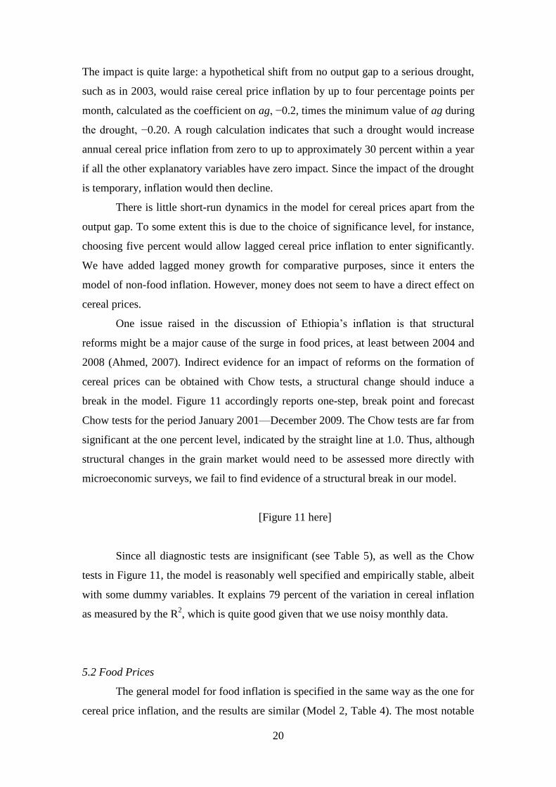
The impact is quite large: a hypothetical shift from no output gap to a serious drought,
such as in 2003, would raise cereal price inflation by up to four percentage points per
month, calculated as the coefficient on ag, −0.2, times the minimum value of ag during
the drought, −0.20. A rough calculation indicates that such a drought would increase
annual cereal price inflation from zero to up to approximately 30 percent within a year
if all the other explanatory variables have zero impact. Since the impact of the drought
is temporary, inflation would then decline.
There is little short-run dynamics in the model for cereal prices apart from the
output gap. To some extent this is due to the choice of significance level, for instance,
choosing five percent would allow lagged cereal price inflation to enter significantly.
We have added lagged money growth for comparative purposes, since it enters the
model of non-food inflation. However, money does not seem to have a direct effect on
cereal prices.
One issue raised in the discussion of Ethiopia‘s inflation is that structural
reforms might be a major cause of the surge in food prices, at least between 2004 and
2008 (Ahmed, 2007). Indirect evidence for an impact of reforms on the formation of
cereal prices can be obtained with Chow tests, a structural change should induce a
break in the model. Figure 11 accordingly reports one-step, break point and forecast
Chow tests for the period January 2001—December 2009. The Chow tests are far from
significant at the one percent level, indicated by the straight line at 1.0. Thus, although
structural changes in the grain market would need to be assessed more directly with
microeconomic surveys, we fail to find evidence of a structural break in our model.
[Figure 11 here]
Since all diagnostic tests are insignificant (see Table 5), as well as the Chow
tests in Figure 11, the model is reasonably well specified and empirically stable, albeit
with some dummy variables. It explains 79 percent of the variation in cereal inflation
as measured by the R2, which is quite good given that we use noisy monthly data.
5.2 Food Prices
The general model for food inflation is specified in the same way as the one for
cereal price inflation, and the results are similar (Model 2, Table 4). The most notable
21
difference is that the coefficients for the external-sector error correction term and the
output gap are smaller in the food price model. This is because cereal prices fluctuate
more than other prices in the food price index (see Figure 2). The adjustment process
towards the long-run equilibrium is eight percent instead of 12 percent per month, so it
takes about eight months before 50 percent of shock has been removed. Moreover, the
coefficient of the agricultural output gap is −0.12, instead of −0.20. Another difference
is that the rate of change of food imports enters lagged eight months with a negative
coefficient. This is counterintuitive and probably a coincidence; its coefficient is also
small and the t-statistic is just significant at the one percent level.
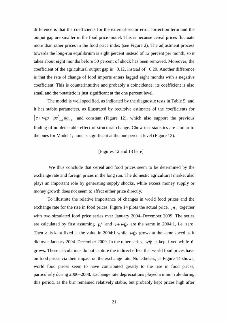
The model is well specified, as indicated by the diagnostic tests in Table 5, and
it has stable parameters, as illustrated by recursive estimates of the coefficients for
11 tte wfp pc ag
and constant (Figure 12), which also support the previous
finding of no detectable effect of structural change. Chow test statistics are similar to
the ones for Model 1; none is significant at the one percent level (Figure 13).
[Figures 12 and 13 here]
We thus conclude that cereal and food prices seem to be determined by the
exchange rate and foreign prices in the long run. The domestic agricultural market also
plays an important role by generating supply shocks, while excess money supply or
money growth does not seem to affect either price directly.
To illustrate the relative importance of changes in world food prices and the
exchange rate for the rise in food prices, Figure 14 plots the actual price, ,pf together
with two simulated food price series over January 2004–December 2009. The series
are calculated by first assuming pf and e wfp are the same in 2004:1, i.e. zero.
Then e is kept fixed at the value in 2004:1 while wfp grows at the same speed as it
did over January 2004–December 2009. In the other series, wfp is kept fixed while e
grows. These calculations do not capture the indirect effect that world food prices have
on food prices via their impact on the exchange rate. Nonetheless, as Figure 14 shows,
world food prices seem to have contributed greatly to the rise in food prices,
particularly during 2006–2008. Exchange rate depreciations played a minor role during
this period, as the birr remained relatively stable, but probably kept prices high after
22
the decline in world food prices during 2008. Re-drawing the figure with the official
US dollar exchange rate does not alter these conclusions.
[Figure 14 here]
5.3 Non-food Prices
The specification of the general model for non-food inflation includes the
money market term 12( ) 0.88 1.88 ,m p y eus
and the external sector error
correction term 1,e wp pnf
where
1 is obtained with the Hodrick-Prescott
filter. The other explanatory variables are the agricultural output gap, 1tag , the rate of
change of broad money, ,m imported inflation, ( ),e wp food price inflation, ,pf
and non-food price inflation, .pnf Since no misspecification test of the general
model are significant (not reported), no dummies are included.
The parsimonious model is well specified (Model 3 in Table 5). Nevertheless,
modeling non-food inflation is a challenge, as indicated by the R2; it is only 0.46,
compared to 0.82 for food prices. Moreover, the t-values are clearly lower than in the
two previous models.
The error correction term for the external non-food sector is significant, and the
monthly adjustment back to equilibrium after a shock is 11 percent. The money market
error correction is, as before, not significant, but money growth lagged nine months
has a t-value of 2.75. Its coefficient is 0.19, so money growth seems to affect non-food
inflation in the short run. There is also some inertia, since lagged non-food price
inflation enters the model, the coefficient is 0.51. Contemporaneous imported inflation,
( ) ,te wp also enter significantly. However, this is only due to changes in the
exchange rate; world market prices have no significant short-run impact.
5.4 CPI Inflation
We combine variables in the models for food and non-food price inflation
when formulating the general model for CPI inflation, except that lagged food and
non-food inflation are not included. This means we have two error correction terms for
the external sector, 1e wp pnf and .e wfp pc Dummy saturation indicated
two more outliers during 2008 than the ones obtained for food prices, March 2008 and
23
December 2008, so these were added to the dummy index. The resulting parsimonious
model, Model 4, is well specified as shown in Table 5.
The only significant error correction term is e wfp pc (t-value = 10.7).
Moreover, the agricultural output gap is highly significant (t-value = −6.9). This
indicates that inflation in Ethiopia during the study period was primarily food inflation,
and that long-run price increases were determined in the foreign food sector. The
adjustment after disequilibrium in the international food sector is five percent per
month, which is slow. In fact, it is an indication that better models are obtained when
analyzing food and non-food prices separately.
The coefficient on the output gap is −0.7, which makes sense: it is about one-
quarter of the coefficient in the model for cereal prices, and the weight of cereal prices
in CPI is 22.54 percent. Hence, using the same hypothetical example as above for
cereal prices, a shift from no output gap to a serious drought would raise monthly CPI
inflation from zero to over one percentage point, and by about eight percent per year.
Money does not seem to matter in the long run, but lagged money growth is
significant, as in the model for non-food inflation. There is also some inflation inertia,
but as in the non-food inflation model, it is small, 0.16.
5.5 Robustness Checks
In this section, we first carry out omitted variables tests and then re-estimate
the models without dummy variables to check the strength of the results
The omitted variables test statistics are reported in Table 6. The alternative
measure for the money market, the monetary overhang of the P-Star approach, is
clearly insignificant in all models. This is also the case for the long-run money
relationship expanded with annual inflation. We also tested the rate of change of
money, measured by broad money to reaffirm the results from the analysis in the
previous section, and by reserve money, which is the operational target of the National
Bank of Ethiopia (NBE, 2009). Both variables were entered with eight lags. None of
the tests is even close to significant at the 10 percent level.
Finally, we entered world fertilizer and energy price inflation, measured in birr,
but failed to find any impact. In the case of fertilizer, this is probably because of the
small use by the majority of rural households. Alternatively, an index specified for
Ethiopia might provide more information, but unfortunately the monthly data on the
value and volume of fertilizer imports is not detailed enough to allow sensible
24
calculations of unit values. The lack of significance of energy price inflation might be
because we capture the cost of fuel through other world market prices, or that
government controlled fuel prices during a large part of the study period (until October
2008), making the link highly non-linear.
Table 7 reports estimates of Model 1, 2 and 4 without dummy variables but
with HAC standard errors. The regressions provide the same message as the ones with
dummies: the coefficients are similar, and the error correction term for the external
food sector and the agricultural output gap are highly significant in all three models,
while the error correction term for the monetary sector is insignificant. The only
substantial difference is that the rate of change of lagged import food prices is
insignificant (at the five percent level) in the model for food prices.
[Table 6 and 7 here]
6. Discussion
In this section we discuss three of our key findings: (i) How do we explain that
global food prices matter in Ethiopia? (ii) How do we explain the limited role of
monetary policy? (iii) And how do we explain the volatility during 2008, which could
not be modeled with standard variables.
(i) The prevailing view in Ethiopia is that international trade in food is too
limited to allow world market prices to be transmitted to domestic prices. Moreover,
there are large deviations from the law of one price of, for example, maize and wheat,
so traders do not seem to exploit business opportunities (Ahmed, 2007; Dercon, 2009;
Rashid, 2010). In contrast to this view, we find that the long-run evolution of food
prices in Ethiopia is determined in the external sector.
To evaluate transmission mechanisms from world to domestic food prices, we
highlight a few issues. First, the finding of a strong link between domestic food and
world food prices is consistent with the observed large fluctuations of prices above or
below import or export parity bands. Domestic food supply shocks have a strong effect
on food inflation in the short to medium run, causing large deviations from long-run
equilibrium. This occurs because there are substantial market distortions. Restricted
access to foreign exchange, limited credit availability, and general uncertainty in the
private sector about government interventions, seem to inhibit traders from taking
25
advantage of significant business opportunities that arise when there are large
differences in domestic and foreign prices.
Second, the food price error correction term measures excess supply and
demand in the market for cereals, where not only the private sector, but also the
government and donors are important actors. Since both the government and donors
have responded to variations in harvests, at least since the mid-1990s, by increasing or
decreasing exports and imports of grain and food aid, they probably have limited the
impact of local supply shocks on food prices and prevented them from moving far
away from world market prices. Thus, private sector arbitrage as typically understood
might not be the only mechanism behind the price transmission.
Third, the authorities liberalized the domestic market for cereals in the
beginning of the 1990s, so domestic prices are market determined. An important
feature in this regard is the centralized wholesale grain market structure and improved
information flows due to public investments in infrastructure. For example, Getnet,
Verbeke and Viaene (2004) find that the wholesale market exhibits large concentration
power and transmits price signals into the local producer markets. Furthermore, their
results show – taking the example of white teff – that wholesale prices in Addis Ababa
seem to determine both short- and long-run prices in local supply markets. To this
should be added that brokers in Addis Ababa handle a very large fraction of the grain
trade in Ethiopia, making the city a de facto clearing house for the country. These
brokers are typically well-informed and have information about both domestic and
international food prices. As shown by Stephens et al. (2008) for Zimbabwe, there can
be price transmission even without trade.
Finally, although Ethiopia‘s international trade in food items is very tiny
relative to total agricultural production, it is not that small when compared to the total
volume of marketed products. In quantity terms, the share of marketed crops from total
agricultural production is about one-third, and the share of agricultural exports from
total marketed agricultural production, which includes coffee, may reach up to 30
percent. To this should be added that there is some unofficial trade with neighboring
countries, although little is known about its size. In other words, prices may matter at
26
the margin, and a few internationally marketed products may transmit price signals
into the subsistence sectors.17
(ii) We do find a short-run impact from lagged money growth on non-food
price inflation. However, excess money supply does not seem to have a direct impact
on inflation in the long run. The lack of significance of excess money could be due to
the use of a small sample (11 years of monthly data). However, as many other
variables are highly significant, insignificance is probably an indication of a relatively
weak impact.
In our view, the main reason for not finding that excess money causes long-run
inflation is that monetary policy may have been ineffective due to excess liquidity in
the banking system. Ethiopia has very large excess reserve ratios even by Sub-Saharan
African standards; according to Saxegaard (2006), only Equatorial Guinea had a higher
ratio in 2004. In an environment with large holdings of excess reserves, the monetary
transmission mechanism is likely to be weakened or even interrupted completely
(O‘Connell, 2005). This is because banks can easily adjust excess reserve ratios when
money demand changes, making the link between base money, which the central bank
controls, and the money stock unstable. Moreover, banks can themselves generate
money supply shocks. In Ethiopia, the link between base money and broad money was
very weak during the study period, as evident from a visual inspection of their
trajectories during the last decade.
Another reason is that money demand could be unstable, as a large part of the
Ethiopian economy is not monetized, particularly the rural areas, and there is a great
deal of barter trade. Movements of trade in and out of the monetized sector could
affect the coefficients in the money demand function. Moreover, most Ethiopians have
very limited options to shift from money to other assets. This is probably the reason
why the parallel US dollar exchange rate is the only opportunity cost variable that
enters our long-run money demand equation.
(iii) We need to use dummy variables to capture the explosive price increases
in the cereal market in the mid-2008. Our interpretation is that once passed a certain
threshold, the current food-price hike also raised forward-looking expectations
substantially. News about future harvests and rainfall can set a self-enforcing cycle in
17 For example, Ulimwengu, Workneh and Paulos (2009) find significant short-term price effects
between the world maize market and Ethiopian regional markets bordering Sudan.

27
motion where farmers withhold supply in expectation of higher prices, thus causing
prices to rise until harvesting begins (Osborne, 2004). This interpretation is supported
by microeconometric evidence of speculative storage (Tadesse and Guttormsen, 2010).
7. Conclusions
We analyze the determinants of inflation in Ethiopia by estimating error correction
models for cereal, food and non-food consumer prices and CPI using monthly data
from January 1999 to December 2009. The resulting models are highly parsimonious
and appear robust to standard misspecification tests.
Our results show that inflation in Ethiopia is heavily associated with the
dominant role of agriculture and food in the economy. In fact, Ethiopia‘s inflation was
practically synonymous with food price inflation during the study period. In the long
run, food prices seem to be determined in the external sector, i.e., the exchange rate
and international food prices explain the evolution of Ethiopia‘s food prices. In the
short run, domestic agricultural supply shocks, as well as inter-seasonal fluctuations,
which probably are induced by expectations about future harvests, cause large
deviations from the long-run relationship between domestic and foreign food prices.
Non-food prices are also determined by international prices in the long run. In contrast
to food prices, money supply matters, though only in the short run through changes in
money growth. The rise in world food market prices thus explains the presence of both
food price inflation and high growth rates in agricultural production after 2004–2008.
Since the weight of food prices in the CPI is 57 percent, transmission of global food
prices into the domestic market has been the major inflation factor in Ethiopia.
Although not analyzed in the paper, the reason for the passive role of money is
probably the structure of the financial system and the existence of large excess
reserves, which thwart the National Bank of Ethiopia‘s control of money supply. In
other words, the money stock has not played the role of a nominal anchor tying prices
down.
We fail to find evidence that structural change in the agricultural sector have
had a substantial impact on food price inflation. This finding is based on the stability
of the empirical models and their coefficients. The test is indirect, but in our view, the
finding is plausible because structural change is unlikely to generate high inflation
over several years. Moreover, world-energy price inflation does not seem to have a

28
direct effect on domestic inflation. This is partly because we indirectly capture oil
price inflation through its effect on world food and non-food prices. Another
explanation is that the authorities subsidized fuel until October 2008, keeping domestic
prices low.
Two medium-term policy conclusions emerge from the analysis. To make
monetary policy more effective, the functioning of the financial sector should be
improved. With control over money supply, world market price hikes and domestic
supply shocks can be managed better, reducing second-round feedback effects and
rises in inflation. Moreover, measures to boost and stabilize domestic agricultural
supply and productivity, particular for major food staples, are of cardinal importance
because negative supply shocks raise food prices sharply.
Our analysis should be viewed as what Hendry (1995) calls a ―progressive
strategy‖ where models and knowledge can improve over time. Nevertheless, we
believe that our results highlight the need to consider a country‘s specific institutional
and macroeconomic context when analyzing world food price transmission. And for
developing economies with a large food share in consumer prices, world food prices
and domestic agricultural production should be considered when analyzing domestic
inflation. Omitting these factors can lead to biased results and misguide economic
policy decisions.
29
References
Ahmed, H.A. 2007. Structural Analysis of Price Drivers in Ethiopia. Mimeo, Addis Ababa:
Ethiopian Development Research Institute.
Al-Mashat, R. and A. Billmeier. 2007. ―The Monetary Transmission Mechanism in Egypt.‖ IMF
Working Paper WP/07/285.
Ayalew Birru, Y. 2007. Explaining the Current Sources of Inflation in Ethiopia: A Macro-
Econometric Approach. Mimeo, Addis Ababa: National Bank of Ethiopia.
Baffes, J. and T. Haniotis (2010) ―Placing the 2006/08 Commodity Price Boom into Perspective‖
Policy Research Working Paper 5371, The World Bank.
Barnichon, R. and S.J. Peiris. 2008. ―Sources of Inflation in Sub-Saharan Africa.‖ Journal of African
Economies 17(5):729-746.
Belke, A. and T. Polliet. 2006. ―Money and Swedish Inflation Reconsidered.‖ Journal of Policy
Modeling 28(8): 931-942.
Bigsten, A. and A. Shimeles. 2008. ―Poverty Transition and Persistence in Ethiopia: 1994-2004.‖
World Development 36(9): 1559-1584.
Blavy, R. 2004. ―Inflation and Monetary Pass-Through in Guinea.‖ IMF Working Paper WP/04/223.
Castle, J.L. and D.F. Hendry. 2009. ―The Long-run Determinants of UK Wages, 1860–2004.‖
Journal of Macroeconomics 31(1): 5-28.
Dercon, S. 2009. ―Rural Poverty: Old Challenges in New Contexts‖ The World Bank Research
Observer 24(1) 1-28.
Diouf, M.A. 2007. ―Modeling Inflation for Mali.‖ IMF Working Paper WP/07/295.
Doornik, J. (2009) ―Autometrics‖ Chap. 4 in Eds. Castle, J., and N. Shephard, The Methodology and
Practice of Econometrics - A Festschrift in Honour of David F. Hendry. Oxford: Oxford
University Press.
Dornbusch, R. 1980. Open Macroeconomics. New York: Basic Books.
Dridi, J. and K. Zieschang. 2002. ―Compiling and Using Export and Import Price Indices‖ IMF
Working Paper WP/02/230.
Durevall, D. and N. Ndung'u. 2001. ―A Dynamic Model of Inflation of Kenya, 1974-96.‖ Journal of
African Economies 10(1): 92-125.
Ericsson, N.R 2010. ―Empirical Model Selection: Friedman and Schwartz Revisited‖ unpublished,
available at http://www.gwu.edu/~forcpgm/NeilEricsson-FSGets-March2010.pdf
Ericsson, N.R. and S.B. Kamin. 2008. ―Constructive Data Mining: Modeling Argentine Broad
Money Demand.‖ International Finance Discussion Papers 943. Board of Governors of the
Federal Reserve System.
FAO. 2010. Crop Prospects Crop Prospects and Food Situation, No. 2, May, Rome: Food and
Agricultural Organization of the United Nations.
Garcia-Herrero, A. and M.V. Pradhan. 1998. ―The Domestic and Foreign Price Gaps in the P-STAR
Model: Evidence from Spain.‖ IMF Working Paper WP/98/64. Gerlach, S. and L.E. Svensson. 2003. ―Money and Inflation in the Euro Area: A Case for Monetary
Indicators?‖ Journal of Monetary Economics 50(8): 1649-1672.
Getnet, K., W. Verbeke, and J. Viaene. 2005. ―Modeling Spatial Transmission of the Grain Markets
of Ethiopia with and Application of ARDL Approach to White Teff.‖ Agricultural Economics
33(3): 491-502.
Hanson, J. A., 1985. ―Inflation and Imported Input Prices in Some Inflationary Latin American
Economies‖ Journal of Development Economics 18(2-3) 395-410.
Hendry, D. F. 1995. Dynamic Econometrics. Oxford: Oxford University Press.
Hendry, D. F. and H.-M Krolzig. 2005. ―The Properties of Automatic Gets Modelling‖, Economic
Journal 115(502), C32-C61.
Hendry, D.F. and C. Santos. 2005. ―Regression Models with Data-based Indicator Variables‖
Oxford Bulletin of Economics and Statistics, 67(5), 571-595.
Hendry, D. F. and B. Nielsen. 2007. Econometric modeling: a likelihood approach. Princeton:
Princeton University Press.
IMF 2007. Statistical Appendix, Prepared by the Ethiopian Authorities (In Conjunction with the IMF
Staff Report for the 2007 Article IV Consultation) Washington DC: International Monetary
Fund
IMF. 2008a. ―Federal Democratic Republic of Ethiopia: 2008 Article IV Consultation Staff Report.‖
IMF Country Report 08/264. Washington DC: International Monetary Fund.
IMF. 2008b. ―Federal Democratic Republic of Ethiopia: Selected Issues.‖ IMF Country Report
08/259. Washington DC: International Monetary Fund.
30
IMF. 2008c. Food and Fuel Prices: Recent Developments, Macroeconomics Impact, and Policy
Responses. Fiscal Affairs, Policy Development and Review, and Research Departments, June
30, Washington DC: International Monetary Fund.
IMF. 2010 ―Ethiopia: 2010 Article IV Consultation and First Review of the Arrangement under the
Exogenous Shocks Facility—Staff Report; Staff Supplements; and Press Release on the
Executive Board Discussion.‖ Country Report No. 10/175, Washington DC: International
Monetary Fund.
Jonsson, G. 2001. ―Inflation, Money Demand, and Purchasing Power Parity in South Africa.‖ IMF
Staff Papers 48(2): 243-265.
Juselius, K. 1992. ―Domestic and Foreign effects on Prices in an Open Economy: The Case of
Denmark.‖ Journal of Policy Modeling 14(4) 401-428.
Juselius, K. 2006. The Cointegrated VAR Model: Methodology and Applications. Oxford: Oxford
University Press.
Kamin, S. 1996. ―Real Exchange Rates and Inflation in Exchange Rate-Based Stabilizations: An
Empirical Examination.‖ International Finance Discussion Papers 554.
Klein, N and A. Kyei 2009. ―Understanding Inflation Inertia in Angola‖ IMF Working Paper
WP/09/98.
Kool, C.J. and J.A. Tatom. 1994. ―The P-STAR Model in Five Small Economies.‖ Federal Reserve
Bank of St. Louis Review 76(2) 11-29.
Loening, J., D. Durevall and Y.A. Birru (2009) ―Inflation Dynamics and Food Prices in an
Agricultural Economy: The Case of Ethiopia‖ World Bank Policy Research Working Paper
Series, No. 4969..
Loening, J. and T. Masato. 2010. ―Decomposing Terms of Trade Fluctuations in Ethiopia.‖ Applied
Economic Letters, forthcoming.
Mathieu, P. 2010. ― For Sustained Growth, Ethiopia Needs to Promote Remonetization‖ IMF Survey:
Countries and Regions, June 22, 2010
Minot, N. 2010. ―Transmission of World Food Price Changes to African Markets and its Effect on
Household Welfare‖ Paper to be presented at the Comesa policy seminar ―Food price
variability: Causes, consequences, and policy options" on 25-26 January 2010 in Maputo,
Mozambique under the Comesa-MSU-IFPRI African Agricultural Markets Project (AAMP).
Moriyama, K. 2008. ―Investigating Inflation Dynamics in Sudan.‖ IMF Working Paper WP/08/189.
NBE. 2009. ―Monetary Policy Framework of Ethiopia‖, National Bank of Ethiopia.
NBE. 2010. Quarterly Bulletin, 24(4) Addis Ababa: National Bank of Ethiopia.
Nell, K.S. 2004. ―The structuralist theory of imported inflation: an application to South Africa‖,
Applied Economics 36(13) 1431-1444.
O‘Connell. S. 2005. ―Note on Excess Liquidity.‖ Mimeo, International Monetary Fund. Processed.
Olubusoye, O. and R. Oyaromade. 2008. ―Modelling the Inflation Process in Nigeria‖ AERC
Research Paper 182, African Economic Research Consortium, Nairobi
Osborne, T. 2004. ―Market News in Commodity Price Theory: Application to the Ethiopian Grain
Market‖ The Review of Economic Studies, 71(1) 133-164.
Rashid, S. 2010. Staple Food Prices in Ethiopia. Prepared for the Africa Agricultural Market
Program for the COMESA policy seminar ‗Variations in staple food prices: Causes,
consequences and policy options‘ Maputo, Mozambique, 24-25 January, 2010. Document
prepared for the Africa Agricultural Market Program.
Santos, C. 2008. ―Impulse Saturation Break Tests.‖ Economic Letters 98(2) 136-143.
Saxegaard, M. 2006. ―Excess Liquidity and the Effectiveness of Monetary Policy: Evidence from
Sub-Saharan Africa.‖ IMF Working Paper WP/06/115.
Stephens, E., E. Mabaya, S. von Cramon-Taubadel, and C. B. Barrett. 2008. ―Spatial Price Adjustment
with and without Trade.‖ Department of Applied Economics and Management Working Paper.
Cornell University.
Sterken, E. 2004. ―Demand for Money and Shortages in Ethiopia.‖ Applied Economics Letters
11(12): 759-769.
Tadesse, G. and A. Guttormsen. 2010. ―The Behavior of Commodity Prices in Ethiopia‖ forthcoming
Agricultural Economics.
Ulimwengu, J.M., S. Workneh, and Z. Paulos. 2009. ―Impact of Soaring Food Price in Ethiopia:
Does Location Matter?‖ IFPRI Discussion Paper 846.
Wodon, Q. and H. Zaman. 2010. ―Higher Food Prices in Sub-Saharan Africa: Poverty Impact and
Policy Responses.‖ World Bank Research Observer 25(1): 157-176.
Wolde-Rufael. Y. 2008. ―Budget Deficits, Money and Inflation: The Case of Ethiopia.‖ Journal of
Developing Areas 42(1): 183-199.
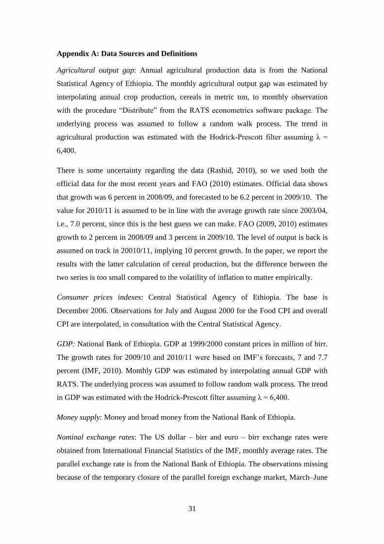
31
Appendix A: Data Sources and Definitions
Agricultural output gap: Annual agricultural production data is from the National
Statistical Agency of Ethiopia. The monthly agricultural output gap was estimated by
interpolating annual crop production, cereals in metric ton, to monthly observation
with the procedure ―Distribute‖ from the RATS econometrics software package. The
underlying process was assumed to follow a random walk process. The trend in
agricultural production was estimated with the Hodrick-Prescott filter assuming λ =
6,400.
There is some uncertainty regarding the data (Rashid, 2010), so we used both the
official data for the most recent years and FAO (2010) estimates. Official data shows
that growth was 6 percent in 2008/09, and forecasted to be 6.2 percent in 2009/10. The
value for 2010/11 is assumed to be in line with the average growth rate since 2003/04,
i.e., 7.0 percent, since this is the best guess we can make. FAO (2009, 2010) estimates
growth to 2 percent in 2008/09 and 3 percent in 2009/10. The level of output is back is
assumed on track in 20010/11, implying 10 percent growth. In the paper, we report the
results with the latter calculation of cereal production, but the difference between the
two series is too small compared to the volatility of inflation to matter empirically.
Consumer prices indexes: Central Statistical Agency of Ethiopia. The base is
December 2006. Observations for July and August 2000 for the Food CPI and overall
CPI are interpolated, in consultation with the Central Statistical Agency.
GDP: National Bank of Ethiopia. GDP at 1999/2000 constant prices in million of birr.
The growth rates for 2009/10 and 2010/11 were based on IMF‘s forecasts, 7 and 7.7
percent (IMF, 2010). Monthly GDP was estimated by interpolating annual GDP with
RATS. The underlying process was assumed to follow random walk process. The trend
in GDP was estimated with the Hodrick-Prescott filter assuming λ = 6,400.
Money supply: Money and broad money from the National Bank of Ethiopia.
Nominal exchange rates: The US dollar – birr and euro – birr exchange rates were
obtained from International Financial Statistics of the IMF, monthly average rates. The
parallel exchange rate is from the National Bank of Ethiopia. The observations missing
because of the temporary closure of the parallel foreign exchange market, March–June
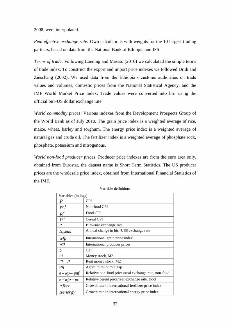
32
2008, were interpolated.
Real effective exchange rate: Own calculations with weights for the 10 largest trading
partners, based on data from the National Bank of Ethiopia and IFS.
Terms of trade: Following Loening and Masato (2010) we calculated the simple terms
of trade index. To construct the export and import price indexes we followed Dridi and
Zieschang (2002). We used data from the Ethiopia‘s customs authorities on trade
values and volumes, domestic prices from the National Statistical Agency, and the
IMF World Market Price Index. Trade values were converted into birr using the
official birr-US dollar exchange rate.
World commodity prices: Various indexes from the Development Prospects Group of
the World Bank as of July 2010. The grain price index is a weighted average of rice,
maize, wheat, barley and sorghum. The energy price index is a weighted average of
natural gas and crude oil. The fertilizer index is a weighted average of phosphate rock,
phosphate, potassium and nitrogenous.
World non-food producer prices: Producer price indexes are from the euro area only,
obtained from Eurostat, the dataset name is Short Term Statistics. The US producer
prices are the wholesale price index, obtained from International Financial Statistics of
the IMF.
Variable definitions
Variables (in logs)
p CPI
pnf Non-food CPI
pf Food CPI
pc Cereal CPI
e Birr-euro exchange rate
12eus Annual change in birr-US$ exchange rate
wfp International grain price index
wp International producer prices
y GDP
m Money stock, M2
m p Real money stock, M2
ag Agricultural output gap
e wp pnf Relative non-food prices/real exchange rate, non-food
e wfp pc Relative cereal price/real exchange rate, food
fert Growth rate in international fertilizer price index
energy Growth rate in international energy price index
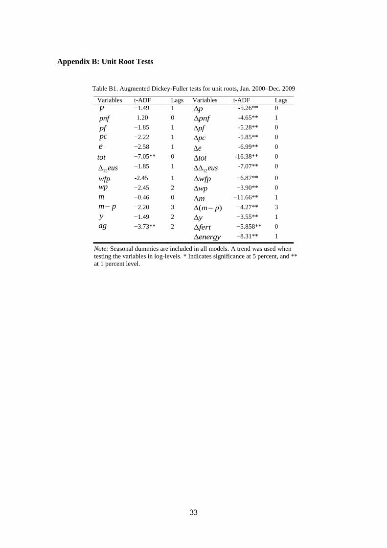
33
Appendix B: Unit Root Tests
Table B1. Augmented Dickey-Fuller tests for unit roots, Jan. 2000–Dec. 2009
Variables t-ADF Lags Variables t-ADF Lags p −1.49 1 p -5.26** 0
pnf 1.20 0 pnf -4.65** 1
pf −1.85 1 pf -5.28** 0
pc −2.22 1 pc -5.85** 0
e −2.58 1 e -6.99** 0
tot −7.05** 0 tot -16.38** 0
12eus −1.85 1 12eus -7.07** 0
wfp -2.45 1 wfp −6.87** 0
wp −2.45 2 wp −3.90** 0
m −0.46 0 m −11.66** 1
m p −2.20 3 ( )m p −4.27** 3
y −1.49 2 y −3.55** 1
ag −3.73** 2 fert −5.858** 0
energy −8.31** 1
Note: Seasonal dummies are included in all models. A trend was used when
testing the variables in log-levels. * Indicates significance at 5 percent, and **
at 1 percent level.
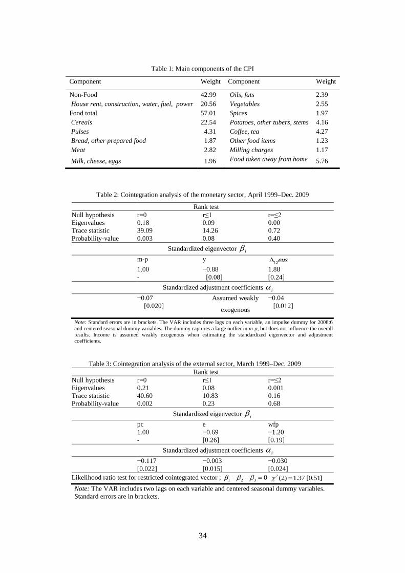
34
Table 1: Main components of the CPI
Component Weight Component Weight
Non-Food 42.99 Oils, fats 2.39
House rent, construction, water, fuel, power 20.56 Vegetables 2.55
Food total 57.01 Spices 1.97
Cereals 22.54 Potatoes, other tubers, stems 4.16
Pulses 4.31 Coffee, tea 4.27
Bread, other prepared food 1.87 Other food items 1.23
Meat 2.82 Milling charges 1.17
Milk, cheese, eggs 1.96 Food taken away from home 5.76
Table 2: Cointegration analysis of the monetary sector, April 1999–Dec. 2009
Rank test
Null hypothesis r=0 r≤1 r=≤2
Eigenvalues 0.18 0.09 0.00
Trace statistic 39.09 14.26 0.72
Probability-value 0.003 0.08 0.40
Standardized eigenvector i
m-p y 12eus
1.00
-
−0.88
[0.08]
1.88
[0.24]
Standardized adjustment coefficients i
−0.07
[0.020]
Assumed weakly
exogenous
−0.04
[0.012]
Note: Standard errors are in brackets. The VAR includes three lags on each variable, an impulse dummy for 2008:6
and centered seasonal dummy variables. The dummy captures a large outlier in m-p, but does not influence the overall
results. Income is assumed weakly exogenous when estimating the standardized eigenvector and adjustment coefficients.
Table 3: Cointegration analysis of the external sector, March 1999–Dec. 2009
Rank test
Null hypothesis r=0 r≤1 r=≤2
Eigenvalues 0.21 0.08 0.001
Trace statistic 40.60 10.83 0.16
Probability-value 0.002 0.23 0.68
Standardized eigenvector i
pc e wfp
1.00
-
−0.69
[0.26]
−1.20
[0.19]
Standardized adjustment coefficients i
−0.117
[0.022]
−0.003
[0.015]
−0.030
[0.024]
Likelihood ratio test for restricted cointegrated vector ; 1 2 3 0 2 (2) 1.37 [0.51]
Note: The VAR includes two lags on each variable and centered seasonal dummy variables.
Standard errors are in brackets.

35
Table 4: Parsimonious inflation models for Ethiopia, January 2000–December 2009
Explanatory variables Model 1:
Cereals
Model 2:
Food
Model 3:
Nonfood
Model 4:
CPI
pc
pf
pnf
p
EC-Monetary sector 12( ) 0.86 1.85 .m p y eus
0.006
(0.28) −0.017
(−1.21)
0.003
(0.30)
−0.006
(−0.83)
EC-External food sector 1t
e wfp pc
0.125**
(9.22)
0.081**
(11.2)
0.047**
(10.7)
EC-External non- food sector 1t
e wp pnf trend
0.108**
(5.30)
Agricultural output gap 1tag −0.197**
−(6.34) −0.125**
(−7.35)
−0.070**
(−6.90)
Lagged inflation 10tp
0.16**
(4.24)
Lagged non-food inflation
1tpc ,
Lagged non-food inflation 4 5( ) 2t tpc pc
0.514**
(4.35)
Exchange rate change te
0.146**
(4.03)
Lagged money 9tm
0.072
(0.37)
0.107
(1.02)
0.191**
(2.75)
0.167**
(2.85)
Food imports 8twfp
−0.095**
(−2.73)
Indicator for Food CPIa) 2000:1=1, 2008:5=1,
2008:6=1.5, 2008;7=1 0.119**
(9.34)
0.069**
(10.0)
Indicator for CPIa) 2000:1=1, 2008:3=1,
2008:5=1, 2008:6=1.5,
2008;7=1, 2008:12=−1
0.048**
(14.1)
Constantb)
−0.004
−(0.01)
0.066
(1.54)
−0.008
(−0.29)
0.025
(1.20)
Seasonal dummiesb)
Yes Yes Yes Yes
Note: t-values in parenthesis. * indicates significance at 5 percent level and ** significance at 1 percent level.
a) The indexes for the dummies were constructed by running the dummy saturation procedure in Autometrics. The
weights are based on the coefficients from the general models. b)
The constant and seasonal are fixed when running Autometrics and thus remain in the models by force.
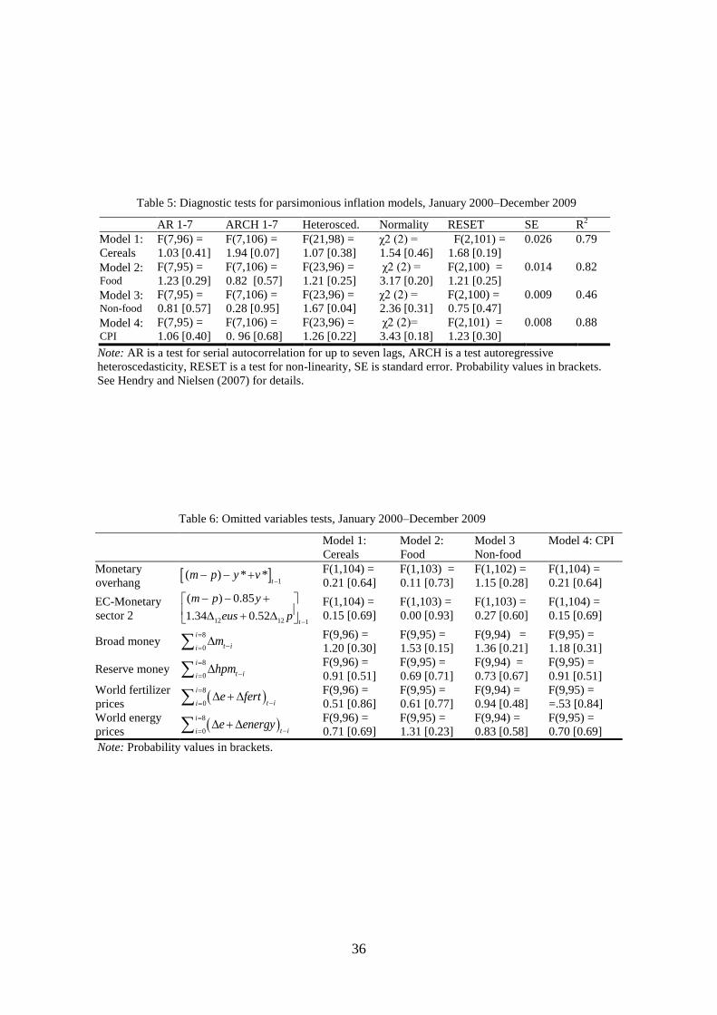
36
Table 5: Diagnostic tests for parsimonious inflation models, January 2000–December 2009
AR 1-7 ARCH 1-7 Heterosced. Normality RESET SE R2
Model 1:
Cereals
F(7,96) =
1.03 [0.41]
F(7,106) =
1.94 [0.07]
F(21,98) =
1.07 [0.38]
χ2 (2) =
1.54 [0.46]
F(2,101) =
1.68 [0.19]
0.026 0.79
Model 2: Food
F(7,95) =
1.23 [0.29]
F(7,106) =
0.82 [0.57]
F(23,96) =
1.21 [0.25]
χ2 (2) =
3.17 [0.20]
F(2,100) =
1.21 [0.25]
0.014 0.82
Model 3: Non-food
F(7,95) =
0.81 [0.57]
F(7,106) =
0.28 [0.95]
F(23,96) =
1.67 [0.04]
χ2 (2) =
2.36 [0.31]
F(2,100) =
0.75 [0.47]
0.009 0.46
Model 4: CPI
F(7,95) =
1.06 [0.40]
F(7,106) =
0. 96 [0.68]
F(23,96) =
1.26 [0.22]
χ2 (2)=
3.43 [0.18]
F(2,101) =
1.23 [0.30]
0.008 0.88
Note: AR is a test for serial autocorrelation for up to seven lags, ARCH is a test autoregressive
heteroscedasticity, RESET is a test for non-linearity, SE is standard error. Probability values in brackets.
See Hendry and Nielsen (2007) for details.
Table 6: Omitted variables tests, January 2000–December 2009
Model 1:
Cereals
Model 2:
Food
Model 3
Non-food
Model 4: CPI
Monetary
overhang
1( ) * *
tm p y v
F(1,104) =
0.21 [0.64]
F(1,103) =
0.11 [0.73]
F(1,102) =
1.15 [0.28]
F(1,104) =
0.21 [0.64]
EC-Monetary
sector 2 12 12 1
( ) 0.85
1.34 0.52t
m p y
eus p
F(1,104) =
0.15 [0.69]
F(1,103) =
0.00 [0.93]
F(1,103) =
0.27 [0.60]
F(1,104) =
0.15 [0.69]
Broad money 8
0
i
t iim
F(9,96) =
1.20 [0.30]
F(9,95) =
1.53 [0.15]
F(9,94) =
1.36 [0.21]
F(9,95) =
1.18 [0.31]
Reserve money 8
0
i
t iihpm
F(9,96) =
0.91 [0.51]
F(9,95) =
0.69 [0.71]
F(9,94) =
0.73 [0.67]
F(9,95) =
0.91 [0.51]
World fertilizer
prices
8
0
i
t iie fert
F(9,96) =
0.51 [0.86]
F(9,95) =
0.61 [0.77]
F(9,94) =
0.94 [0.48]
F(9,95) =
=.53 [0.84]
World energy
prices
8
0
i
t iie energy
F(9,96) =
0.71 [0.69]
F(9,95) =
1.31 [0.23]
F(9,94) =
0.83 [0.58]
F(9,95) =
0.70 [0.69]
Note: Probability values in brackets.
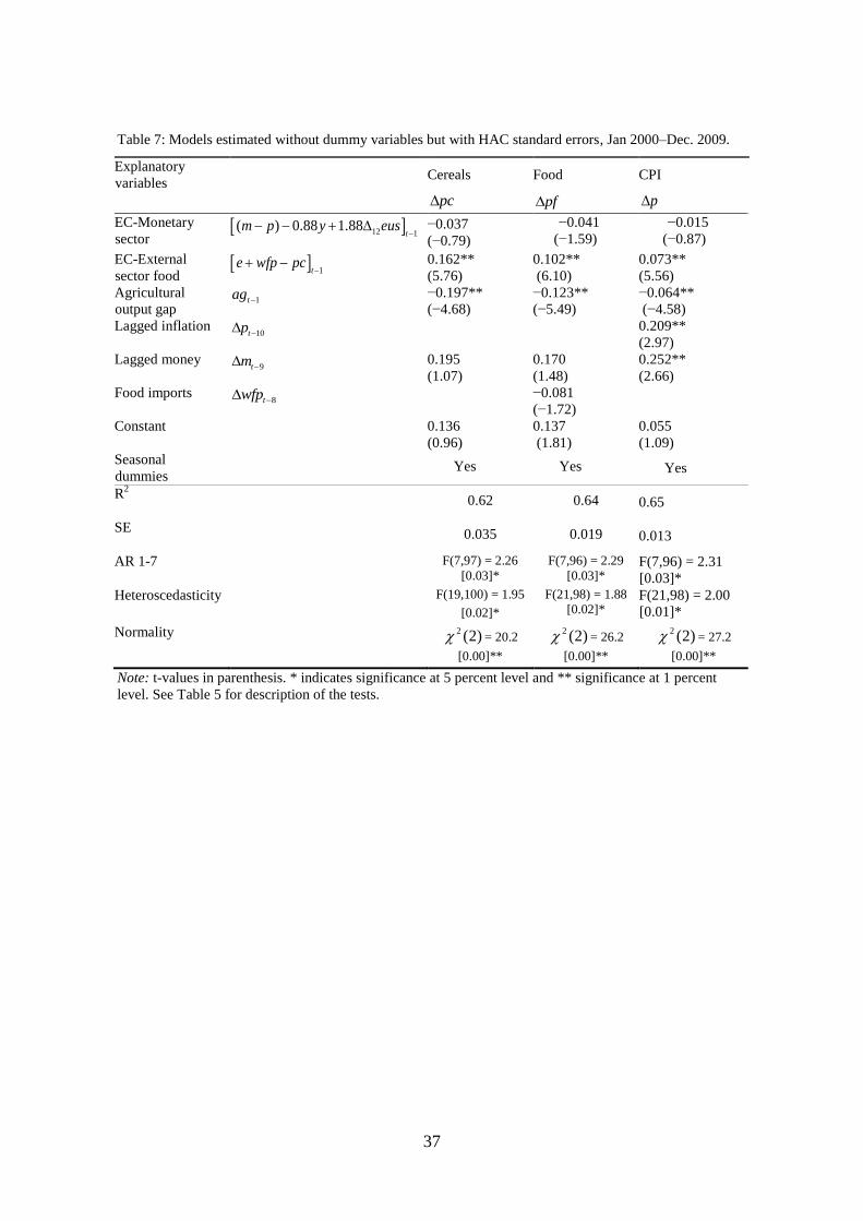
37
Table 7: Models estimated without dummy variables but with HAC standard errors, Jan 2000–Dec. 2009.
Explanatory
variables
Cereals Food CPI
pc
pf
p
EC-Monetary
sector 12 1( ) 0.88 1.88
tm p y eus
−0.037
(−0.79)
−0.041
(−1.59)
−0.015
(−0.87)
EC-External
sector food
1te wfp pc
0.162**
(5.76)
0.102**
(6.10)
0.073**
(5.56)
Agricultural
output gap 1tag
−0.197**
(−4.68)
−0.123**
(−5.49)
−0.064**
(−4.58)
Lagged inflation 10tp
0.209**
(2.97)
Lagged money 9tm
0.195
(1.07)
0.170
(1.48)
0.252**
(2.66)
Food imports 8twfp
−0.081
(−1.72)
Constant
0.136
(0.96)
0.137
(1.81)
0.055
(1.09)
Seasonal
dummies Yes Yes Yes
R2
0.62 0.64 0.65
SE 0.035 0.019 0.013
AR 1-7
F(7,97) = 2.26
[0.03]*
F(7,96) = 2.29
[0.03]* F(7,96) = 2.31
[0.03]*
Heteroscedasticity
F(19,100) = 1.95
[0.02]*
F(21,98) = 1.88
[0.02]* F(21,98) = 2.00
[0.01]*
Normality
2 (2) = 20.2
[0.00]**
2 (2) = 26.2
[0.00]**
2 (2) = 27.2
[0.00]**
Note: t-values in parenthesis. * indicates significance at 5 percent level and ** significance at 1 percent
level. See Table 5 for description of the tests.
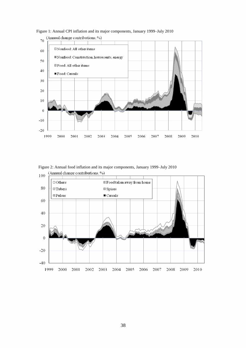
38
Figure 1: Annual CPI inflation and its major components, January 1999–July 2010
Figure 2: Annual food inflation and its major components, January 1999–July 2010
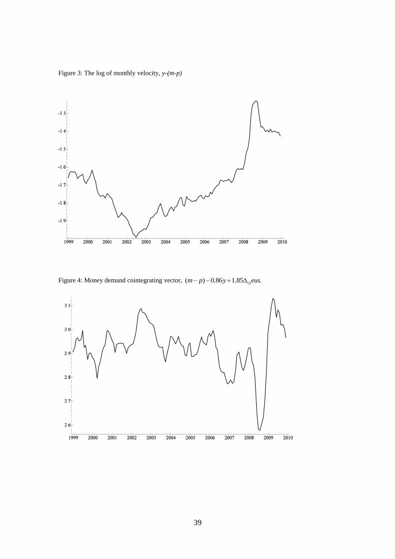
39
Figure 3: The log of monthly velocity, y-(m-p)
Figure 4: Money demand cointegrating vector, 12( ) 0.86 1.85 .m p y eus
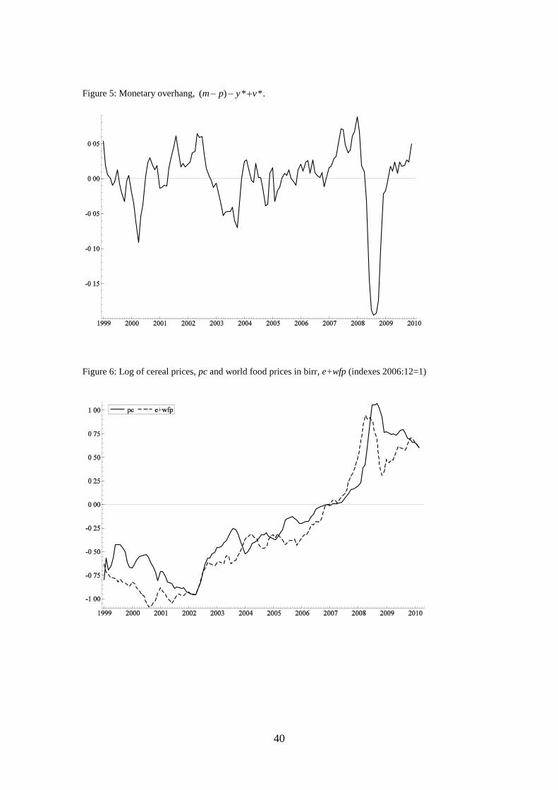
40
Figure 5: Monetary overhang, ( ) * *.m p y v
Figure 6: Log of cereal prices, pc and world food prices in birr, e+wfp (indexes 2006:12=1)

41
Figure 8: Log of relative price indexes for non-food, e wp pnf
Figure 7: Log of relative price indexes for food, e wfp pc
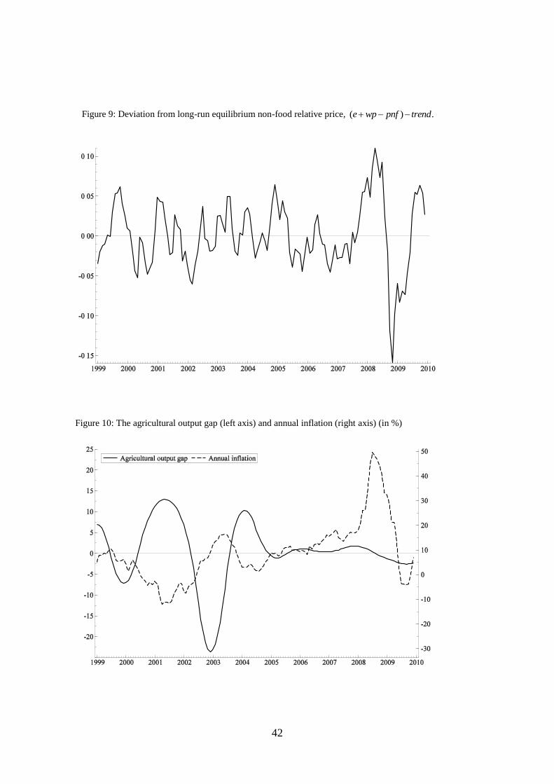
42
Figure 9: Deviation from long-run equilibrium non-food relative price, ( ) .e wp pnf trend
Figure 10: The agricultural output gap (left axis) and annual inflation (right axis) (in %)
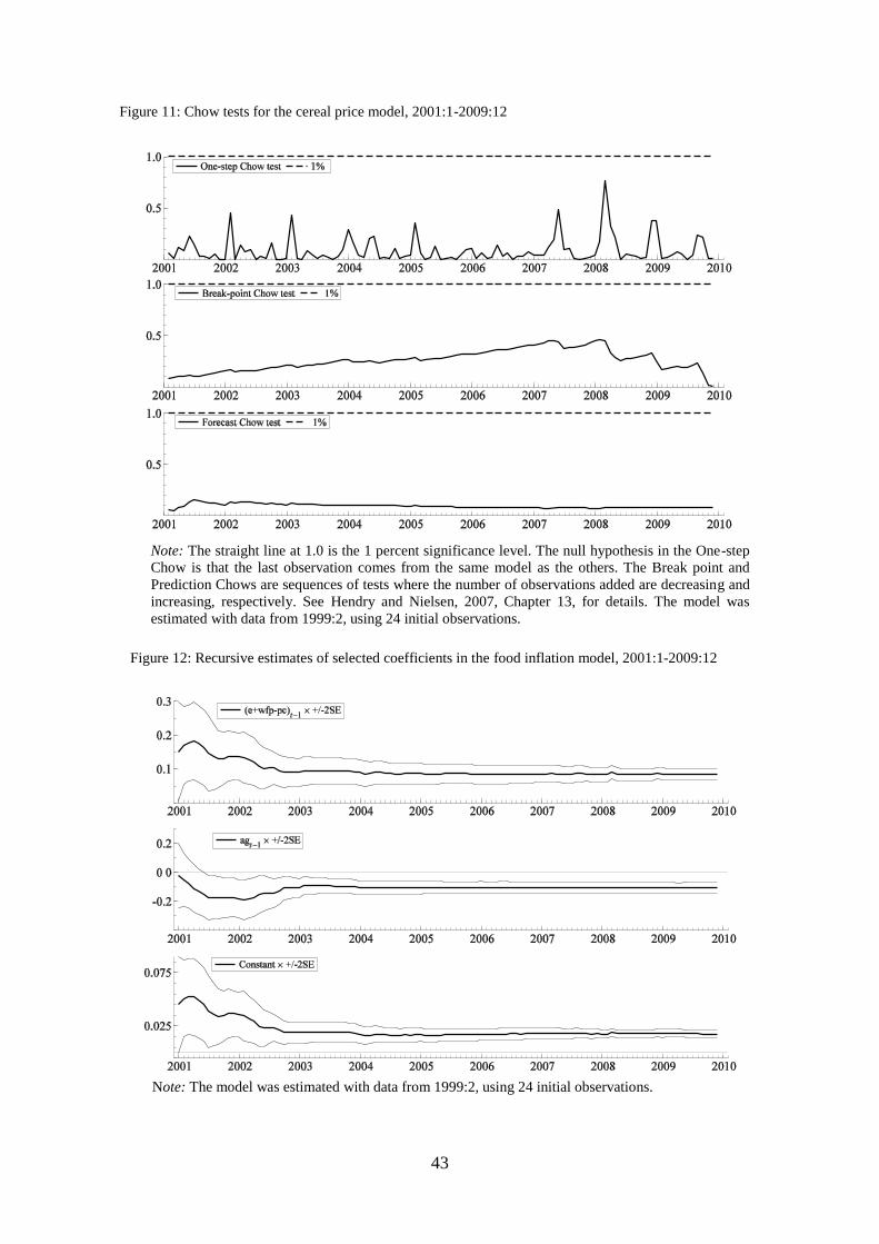
43
Figure 11: Chow tests for the cereal price model, 2001:1-2009:12
Note: The straight line at 1.0 is the 1 percent significance level. The null hypothesis in the One-step
Chow is that the last observation comes from the same model as the others. The Break point and
Prediction Chows are sequences of tests where the number of observations added are decreasing and
increasing, respectively. See Hendry and Nielsen, 2007, Chapter 13, for details. The model was
estimated with data from 1999:2, using 24 initial observations.
Note: The model was estimated with data from 1999:2, using 24 initial observations.
Figure 12: Recursive estimates of selected coefficients in the food inflation model, 2001:1-2009:12
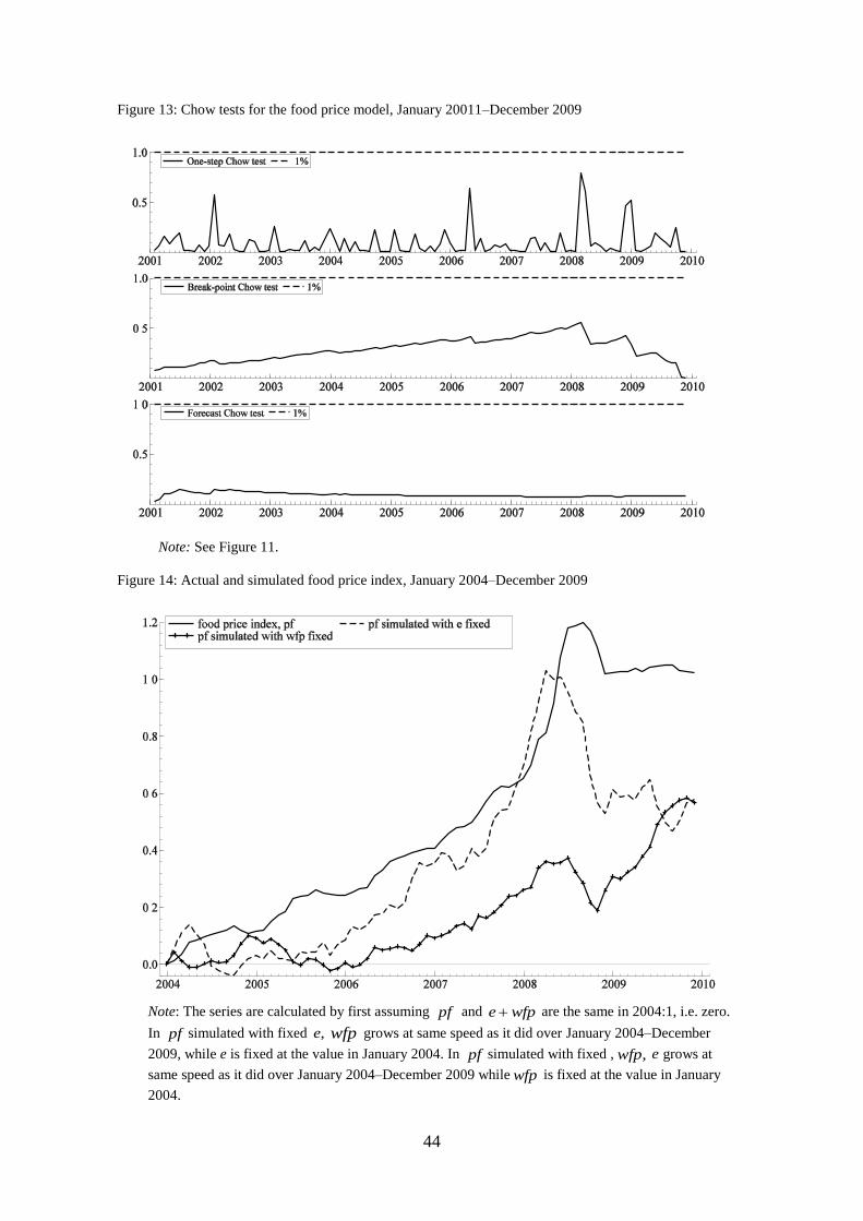
44
Figure 13: Chow tests for the food price model, January 20011–December 2009
Note: See Figure 11.
Figure 14: Actual and simulated food price index, January 2004–December 2009
Note: The series are calculated by first assuming pf and e wfp
are the same in 2004:1, i.e. zero.
In pf simulated with fixed ,e wfp grows at same speed as it did over January 2004–December
2009, while e is fixed at the value in January 2004. In pf simulated with fixed , ,wfp e grows at
same speed as it did over January 2004–December 2009 while wfp is fixed at the value in January
2004.