Inflation Targeting and Business Cycle

Synchronization

Robert P. Flood, IMF

Andrew K. Rose, UC Berkeley

1  

Few Monetary Strategies exist

• Fixed exchange rates

• Money growth targets

• Hybrid/Ill-defined strategies

• Inflation Targets; focus here

2  

Inflation Targeting

• Popular, swiftly-spreading, durable monetary institution

• Much studied

o Theoretical work on normative properties

Ex: Benigno and Benigno, Obstfeld and Rogoff

o Empirical work on domestic aspects of IT

Ex: Ball and Sheridan: does IT matter for inflation?

Ex: Siklos: did inflation process change?

• Little empirical work on international aspects of IT

3  

Focus Here: Monetary Sovereignty • Does IT provide insulation from foreign shocks?

o Mundell’s “Trinity” insulation: Yes!

• Focus is on domestic real phenomena

• Are business cycles less synchronized for countries that target

inflation?

o Natural comparison is countries that fix exchange rates or

are in monetary union

4  

Should Business Cycles be less synchronized for ITs? • IT countries all float (mostly pretty cleanly)

• Compare “Insulation” properties of fixed and floating regimes:

o Negative foreign shock hits with nominal rigidities

Requires fall in real exchange rate

o Faster, less costly to adjust nominal exchange rate

Alternative is wait for excess supply in labor, goods

markets to push nominal wages, prices down

But that implies decline in output, employment

5  

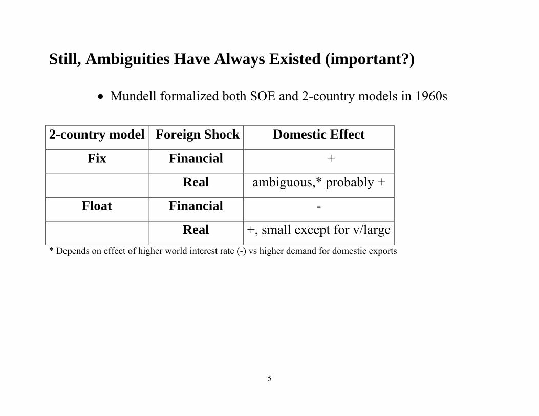
Still, Ambiguities Have Always Existed (important?)

• Mundell formalized both SOE and 2-country models in 1960s

2-country model Foreign Shock Domestic Effect

Fix Financial +

Real ambiguous,* probably +

Float Financial -

Real +, small except for v/large* Depends on effect of higher world interest rate (-) vs higher demand for domestic exports

6  

But Easy to Motivate Opposite Finding Theoretically

• We develop a small theoretical model of an open

economy with conventional blocks:

 

Lucas-style Aggregate Supply

tutpt

Etpty +−

−= )1

(β

7  

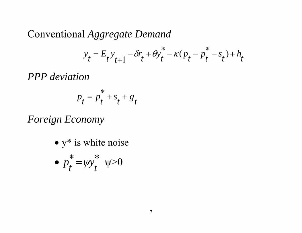
Conventional Aggregate Demand

thtstptptytrtytEty +−−−+−+

= )*(*1

κθδ

PPP deviation

tgtstptp ++= *

Foreign Economy

• y* is white noise

• **tytp ψ= ψ>0

8  

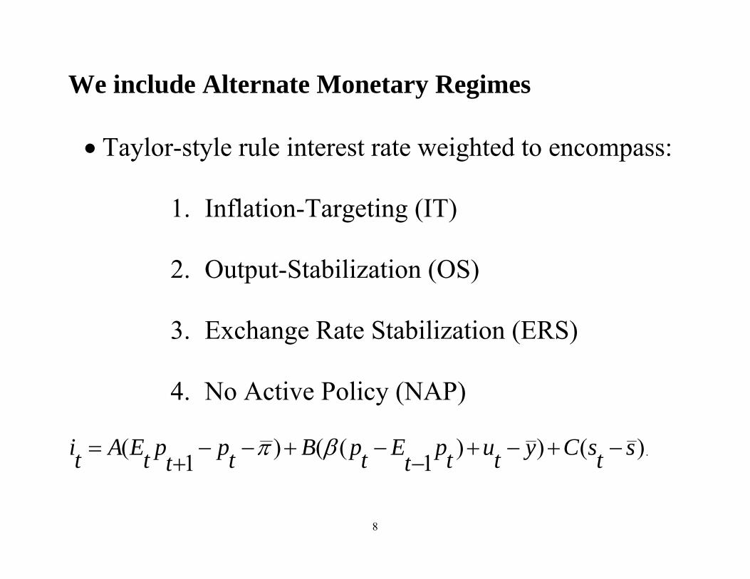
We include Alternate Monetary Regimes

• Taylor-style rule interest rate weighted to encompass:

1. Inflation-Targeting (IT)

2. Output-Stabilization (OS)

3. Exchange Rate Stabilization (ERS)

4. No Active Policy (NAP)

)())1

(()1

( stsCytutpt

EtpBtpt

ptEAti −+−+−

−+−−+

= βπ . 

9  

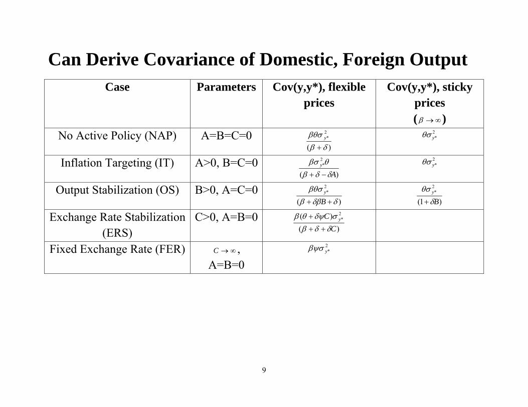
Can Derive Covariance of Domestic, Foreign Output Case Parameters Cov(y,y*), flexible

prices Cov(y,y*), sticky

prices ( ∞→β )

No Active Policy (NAP) A=B=C=0 )(

2*

δββθσ+

y 2*yθσ

Inflation Targeting (IT) A>0, B=C=0)(

2*

Ay

δδβθβσ−+

2*yθσ

Output Stabilization (OS) B>0, A=C=0)(

2*

δδβββθσ

++ By

)1(

2*

By

δθσ+

Exchange Rate Stabilization (ERS)

C>0, A=B=0)(

)( 2*

CC y

δδβσδψθβ

++

+

Fixed Exchange Rate (FER) ∞→C , A=B=0

2*yβψσ

 

10  

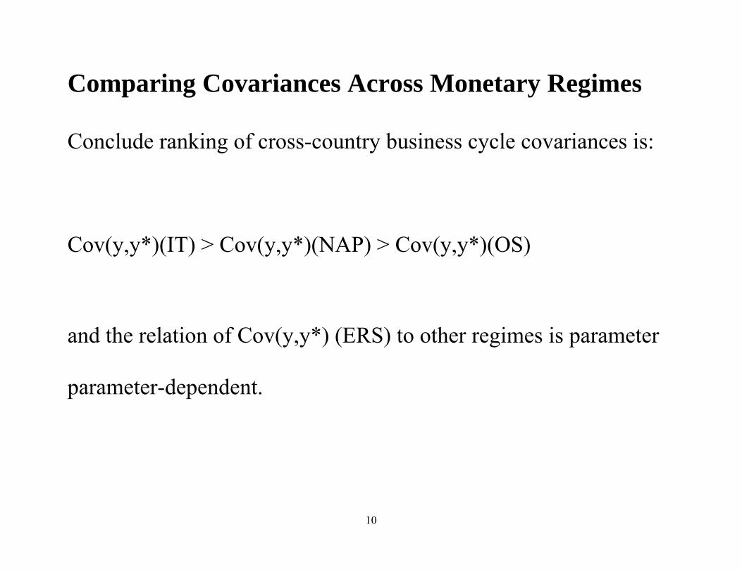
Comparing Covariances Across Monetary Regimes

Conclude ranking of cross-country business cycle covariances is:

Cov(y,y*)(IT) > Cov(y,y*)(NAP) > Cov(y,y*)(OS)

and the relation of Cov(y,y*) (ERS) to other regimes is parameter

parameter-dependent.

11  

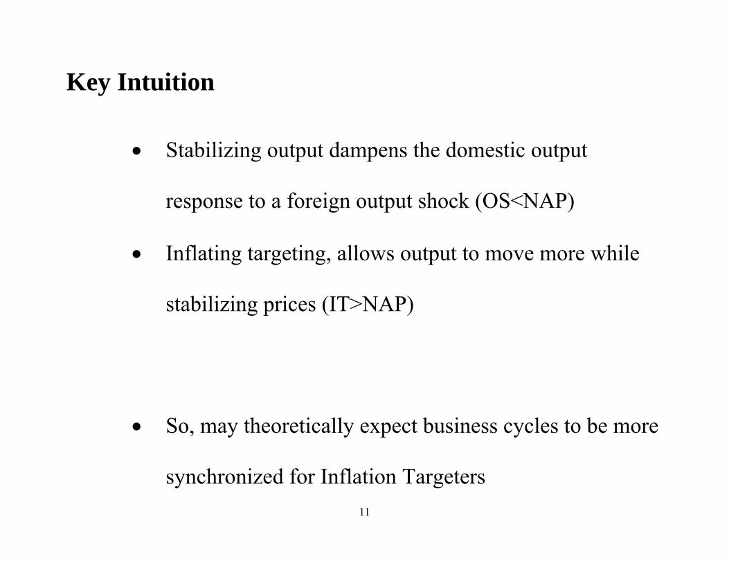
Key Intuition

• Stabilizing output dampens the domestic output

response to a foreign output shock (OS<NAP)

• Inflating targeting, allows output to move more while

stabilizing prices (IT>NAP)

• So, may theoretically expect business cycles to be more

synchronized for Inflation Targeters

12  

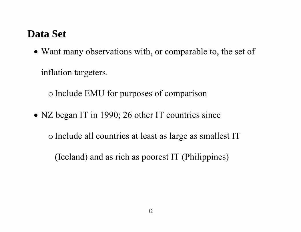
Data Set • Want many observations with, or comparable to, the set of

inflation targeters.

o Include EMU for purposes of comparison

• NZ began IT in 1990; 26 other IT countries since

o Include all countries at least as large as smallest IT

(Iceland) and as rich as poorest IT (Philippines)

13  

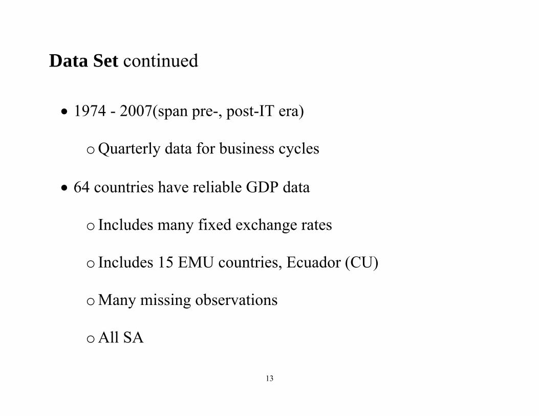
Data Set continued

• 1974 - 2007(span pre-, post-IT era)

o Quarterly data for business cycles

• 64 countries have reliable GDP data

o Includes many fixed exchange rates

o Includes 15 EMU countries, Ecuador (CU)

o Many missing observations

o All SA

14  

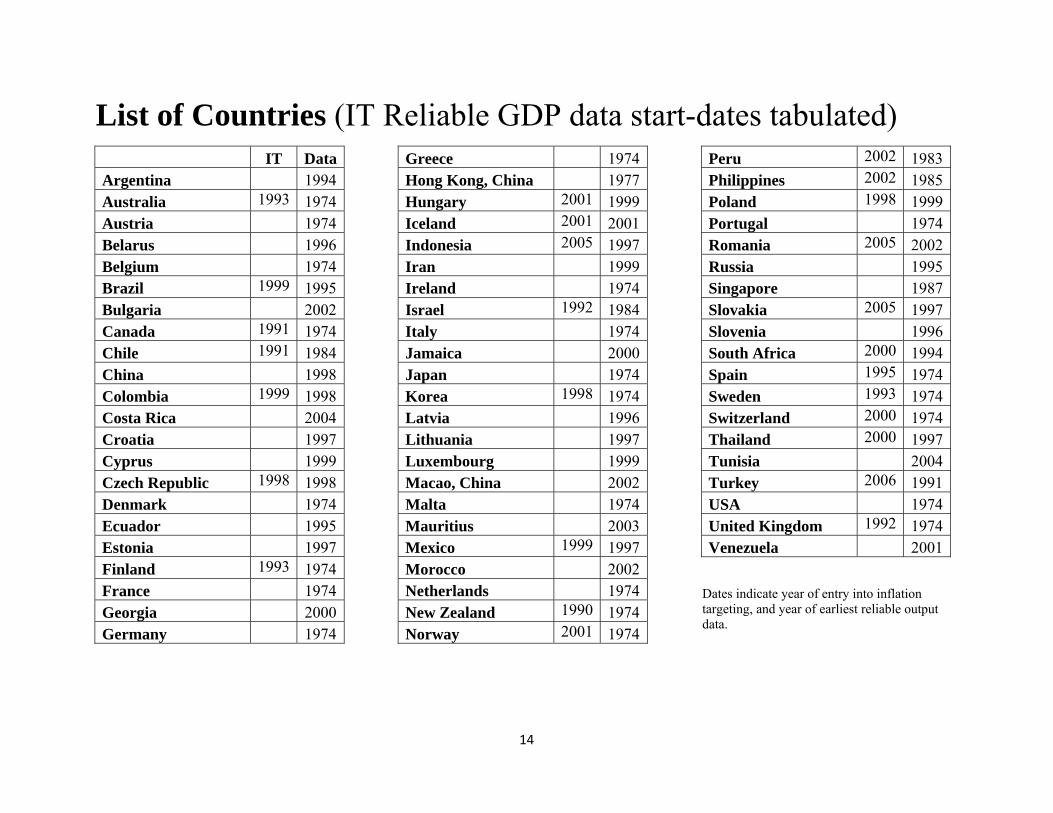
List of Countries (IT Reliable GDP data start-dates tabulated)IT Data

Argentina 1994Australia 1993 1974Austria 1974Belarus 1996Belgium 1974Brazil 1999 1995Bulgaria 2002Canada 1991 1974Chile 1991 1984China 1998Colombia 1999 1998Costa Rica 2004Croatia 1997Cyprus 1999Czech Republic 1998 1998Denmark 1974Ecuador 1995Estonia 1997Finland 1993 1974France 1974Georgia 2000Germany 1974

Greece 1974 Hong Kong, China 1977 Hungary 2001 1999 Iceland 2001 2001 Indonesia 2005 1997 Iran 1999 Ireland 1974 Israel 1992 1984 Italy 1974 Jamaica 2000 Japan 1974 Korea 1998 1974 Latvia 1996 Lithuania 1997 Luxembourg 1999 Macao, China 2002 Malta 1974 Mauritius 2003 Mexico 1999 1997 Morocco 2002 Netherlands 1974 New Zealand 1990 1974 Norway 2001 1974

Peru 2002 1983Philippines 2002 1985Poland 1998 1999Portugal 1974Romania 2005 2002Russia 1995Singapore 1987Slovakia 2005 1997Slovenia 1996South Africa 2000 1994Spain 1995 1974Sweden 1993 1974Switzerland 2000 1974Thailand 2000 1997Tunisia 2004Turkey 2006 1991USA 1974United Kingdom 1992 1974Venezuela 2001

Dates indicate year of entry into inflation targeting, and year of earliest reliable output data.

15  

Sources for GDP Data • IMF’s International Financial Statistics

• IMF’s World Economic Outlook

• OECD

o Many checks for mistakes, errors

o Also construct analogues for G-3 and G-7

Weights from sample averages of PPP-adjusted

aggregate GDP from PWT 6.2

16  

De-Trending Techniques

• Focus here is business cycles, deviations from trend

• Four Models for Underlying Trends:

• Hodrick-Prescott filter (smoother = 1600)

• Baxter-King band-pass filter (6-32 quarters)

• Fourth-Differences (growth rates)

• Linear Regression Model (linear, quadratic trends,

quarterly dummies)

17  

Create Business Cycle Deviations

• , , ,

• , , ,

• , , ,

• , , , , ,  

• Natural Logarithms throughout

18  

Measures of Business Cycle Synchronization (BCS)

• Conventional Pearson Correlation Coefficient

, ,   , , , ,

o Estimated over time (from 20 quarterly observations/5

years) for a pair of countries (“dyad”)

19  

Determinants of BCS

• Follow Baxter-Kouparitsas “BK: (2005) in using four robust

conventional variables:

1.Trade between i and j at τ

• Most important, only time-varying

2.Log distance between i and j

3.Dummy for both i and j developed countries

4.Dummy for both i and j developing countries

20  

Trade Measure

• Measured a la BK (bilateral trade of i,j over aggregate of i's

trade and j’s trade)

o Computed with IMF DoT data

o Frankel-Rose (1998)

• Sometimes add financial analogue with CPIS data

o Imbs (2006)

o Stocks, not flows, for 2002-2006

21  

First Look at the Time Series

• Look for:

o Evidence of “Decoupling” of business cycles over time?

(Few; and BCS often rises!)

o Lots of volatility over time

22  

 

The Entire Data Distribution: Is that a Downward Trend?

Bivariate GDP CorrelationsMean, +/-2 standard deviations of mean

HP Detrending

1980 1990 2000 20070

.25

.5

BK Detrending

1980 1990 2000 20070

.25

.5

Growth Detrending

1980 1990 2000 20070

.25

.5

Linear Detrending

1980 1990 2000 20070

.25

.5

23  

 

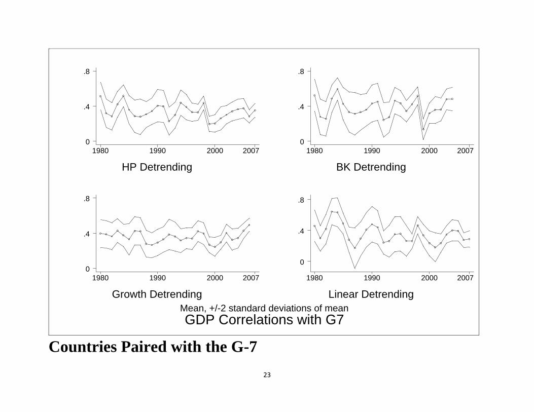
Countries Paired with the G-7

GDP Correlations with G7Mean, +/-2 standard deviations of mean

HP Detrending

1980 1990 2000 20070

.4

.8

BK Detrending

1980 1990 2000 20070

.4

.8

Growth Detrending

1980 1990 2000 20070

.4

.8

Linear Detrending

1980 1990 2000 2007

0

.4

.8

24  

 

Industrial Country-LDC Pairings

Bivariate GDP Correlations, Industrial-LDC pairsMean, +/-2 standard deviations of mean

HP Detrending

1980 1990 2000 2007

0

.25

.5

BK Detrending

1980 1990 2000 2007

0

.25

.5

Growth Detrending

1980 1990 2000 20070

.25

.5

Linear Detrending

1980 1990 2000 2007

0

.25

.5

25  

 

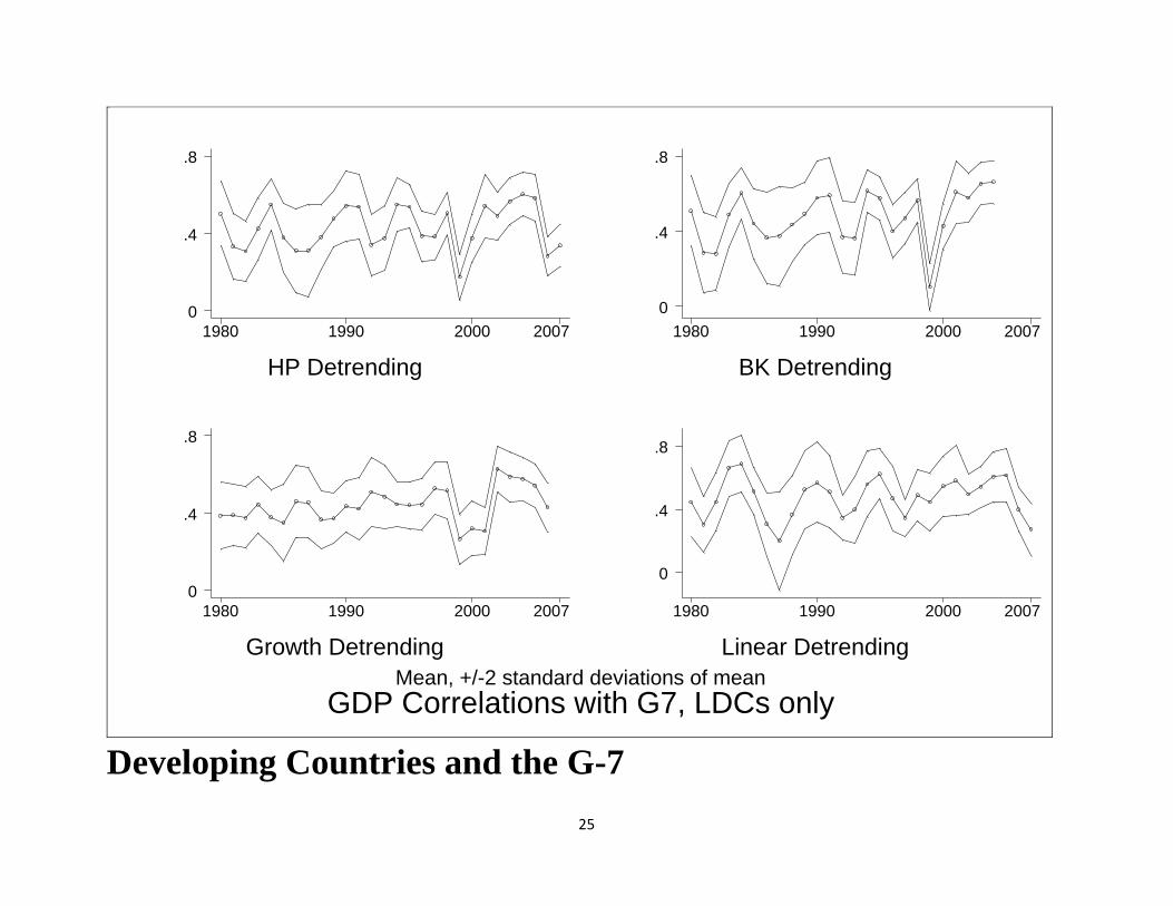
Developing Countries and the G-7

GDP Correlations with G7, LDCs onlyMean, +/-2 standard deviations of mean

HP Detrending

1980 1990 2000 20070

.4

.8

BK Detrending

1980 1990 2000 20070

.4

.8

Growth Detrending

1980 1990 2000 20070

.4

.8

Linear Detrending

1980 1990 2000 2007

0

.4

.8

26  

 

Developing Countries and the US

Bivariate GDP Correlations, US-LDC pairsMean, with (5%,95%) Confidence Interval

HP Detrending

1980 1990 2000 2007-1

-.5

0

.5

1

BK Detrending

1980 1990 2000 2007-1

-.5

0

.5

1

Growth Detrending

1980 1990 2000 2007-1

-.5

0

.5

1

Linear Detrending

1980 1990 2000 2007-1

-.5

0

.5

1

27  

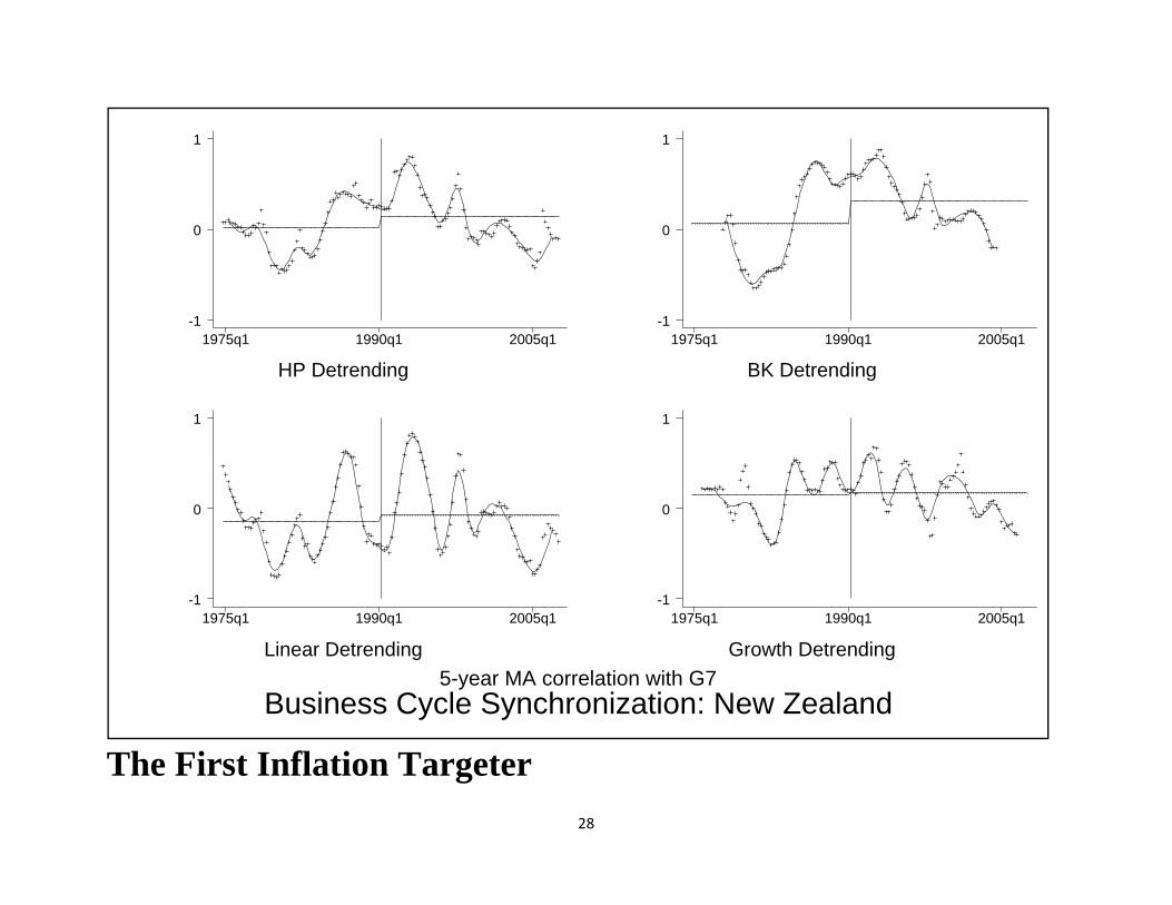
A Further Look at the Time Series

• Look for:

o Breaks at onset of inflation targeting?

(Few; and BCS often rises!)

28  

 

The First Inflation Targeter

Business Cycle Synchronization: New Zealand5-year MA correlation with G7

HP Detrending

1975q1 1990q1 2005q1

1

0

-1

BK Detrending

1975q1 1990q1 2005q1

1

0

-1

Linear Detrending

1975q1 1990q1 2005q1

1

0

-1

Growth Detrending

1975q1 1990q1 2005q1

1

0

-1

29  

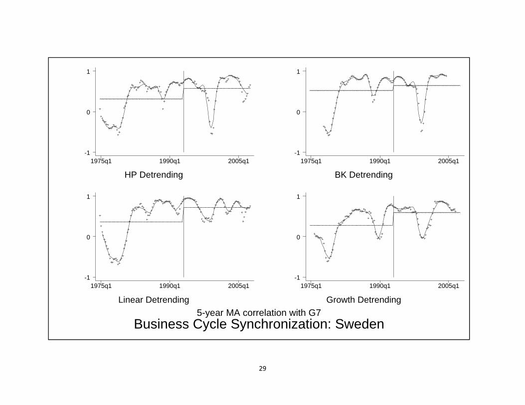
Business Cycle Synchronization: Sweden

5-year MA correlation with G7

HP Detrending

1975q1 1990q1 2005q1

1

0

-1

BK Detrending

1975q1 1990q1 2005q1

1

0

-1

Linear Detrending

1975q1 1990q1 2005q1

1

0

-1

Growth Detrending

1975q1 1990q1 2005q1

1

0

-1

30  

 

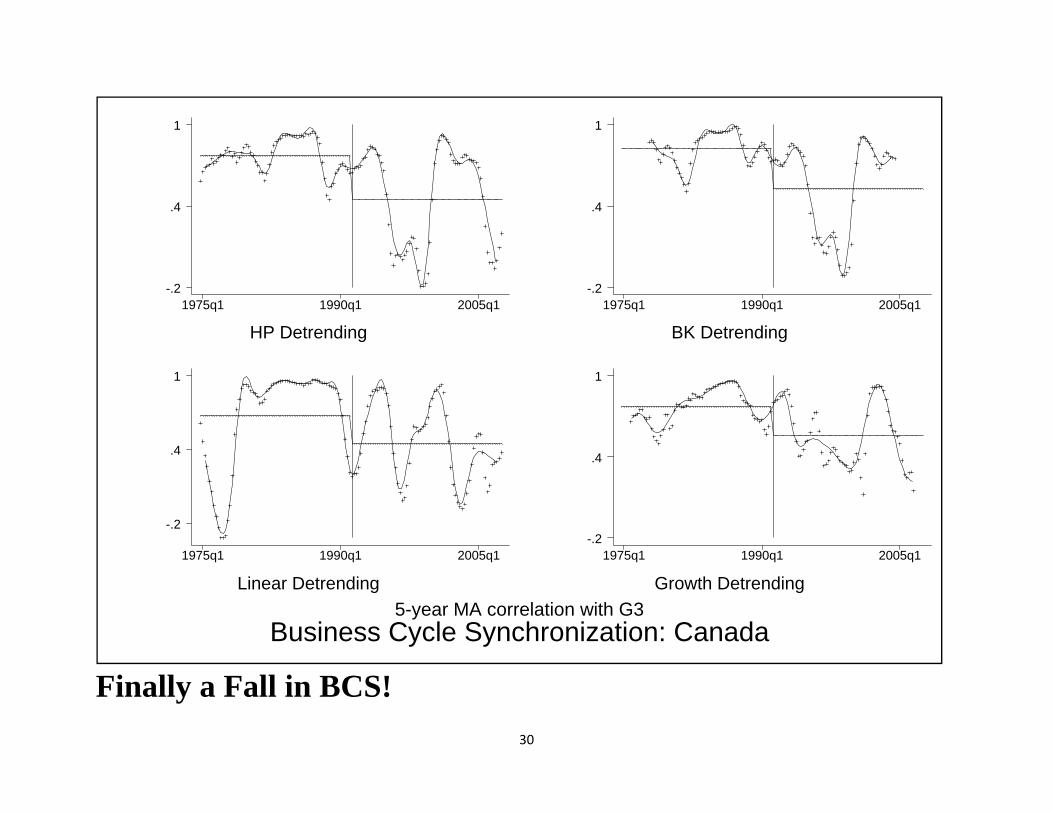
Finally a Fall in BCS!

Business Cycle Synchronization: Canada5-year MA correlation with G3

HP Detrending

1975q1 1990q1 2005q1

1

.4

-.2

BK Detrending

1975q1 1990q1 2005q1

1

.4

-.2

Linear Detrending

1975q1 1990q1 2005q1

1

.4

-.2

Growth Detrending

1975q1 1990q1 2005q1

1

.4

-.2

31  

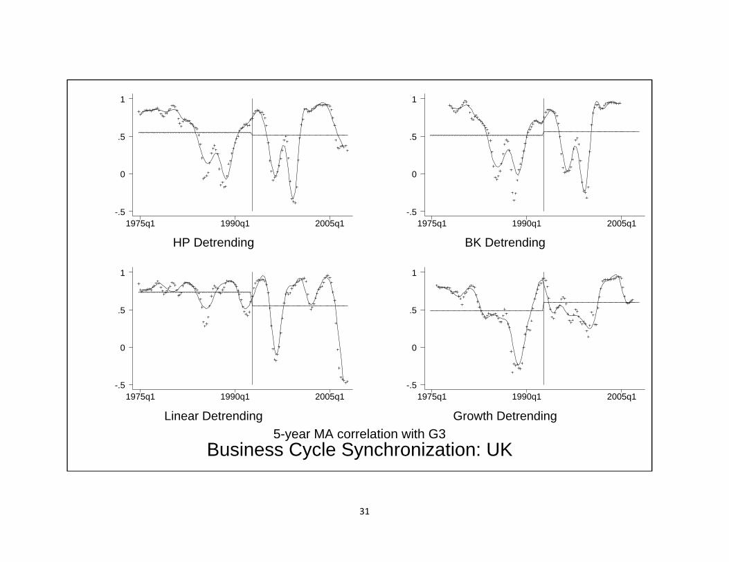
Business Cycle Synchronization: UK5-year MA correlation with G3

HP Detrending

1975q1 1990q1 2005q1

1

.5

0

-.5

BK Detrending

1975q1 1990q1 2005q1

1

.5

0

-.5

Linear Detrending

1975q1 1990q1 2005q1

1

.5

0

-.5

Growth Detrending

1975q1 1990q1 2005q1

1

.5

0

-.5

32  

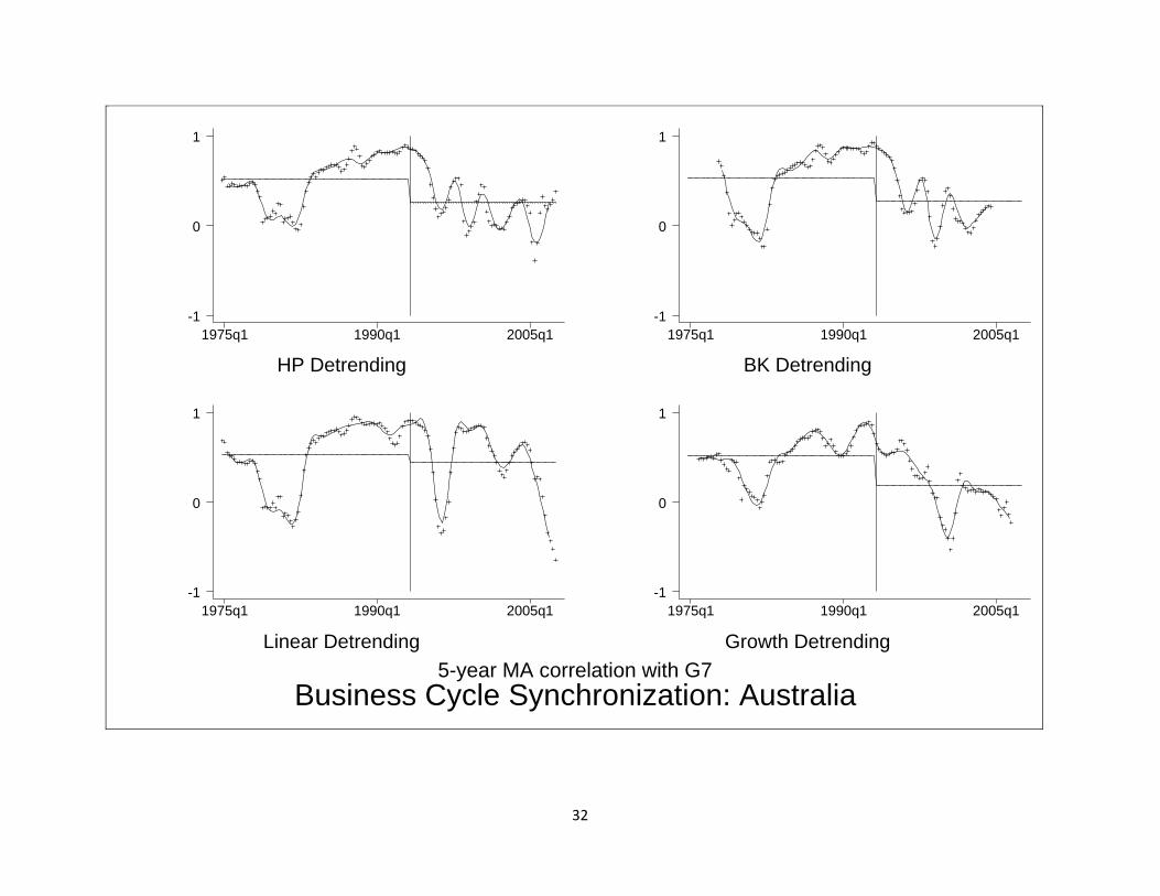
Business Cycle Synchronization: Australia5-year MA correlation with G7

HP Detrending

1975q1 1990q1 2005q1

1

0

-1

BK Detrending

1975q1 1990q1 2005q1

1

0

-1

Linear Detrending

1975q1 1990q1 2005q1

1

0

-1

Growth Detrending

1975q1 1990q1 2005q1

1

0

-1

33  

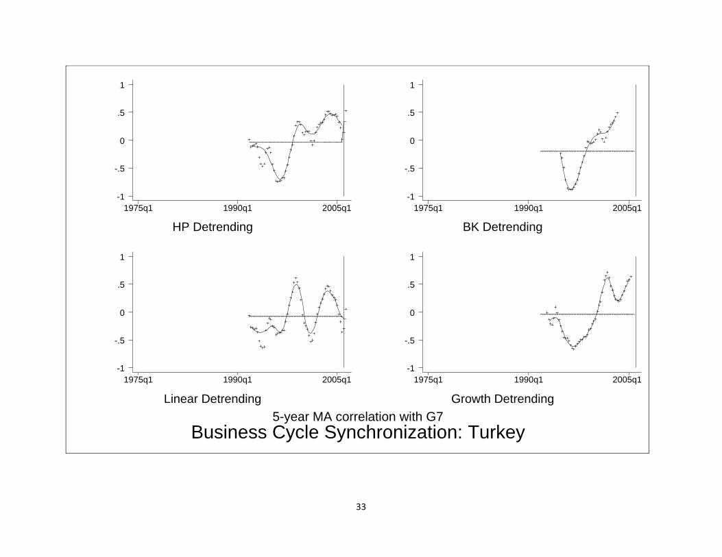
Business Cycle Synchronization: Turkey5-year MA correlation with G7

HP Detrending

1975q1 1990q1 2005q1

1

.5

0

-.5

-1

BK Detrending

1975q1 1990q1 2005q1

1

.5

0

-.5

-1

Linear Detrending

1975q1 1990q1 2005q1

1

.5

0

-.5

-1

Growth Detrending

1975q1 1990q1 2005q1

1

.5

0

-.5

-1

34  

 

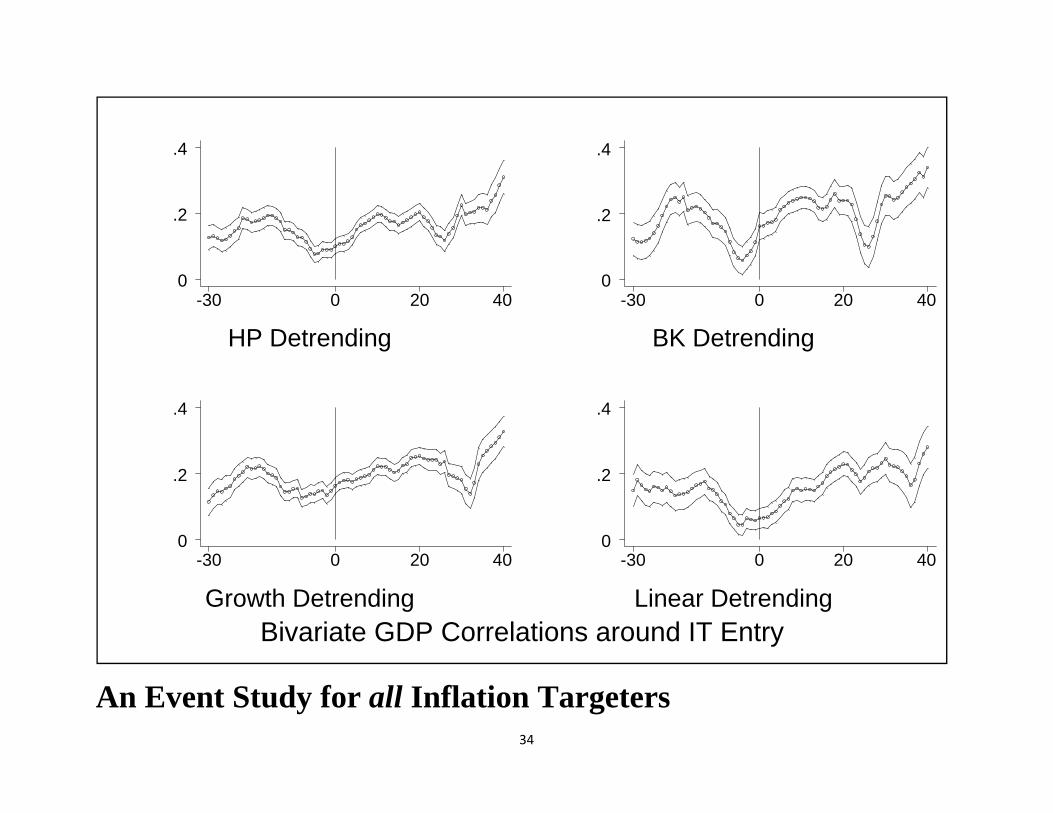
An Event Study for all Inflation Targeters

Bivariate GDP Correlations around IT Entry

HP Detrending

-30 0 20 400

.2

.4

BK Detrending

-30 0 20 400

.2

.4

Growth Detrending

-30 0 20 400

.2

.4

Linear Detrending

-30 0 20 400

.2

.4

35  

 

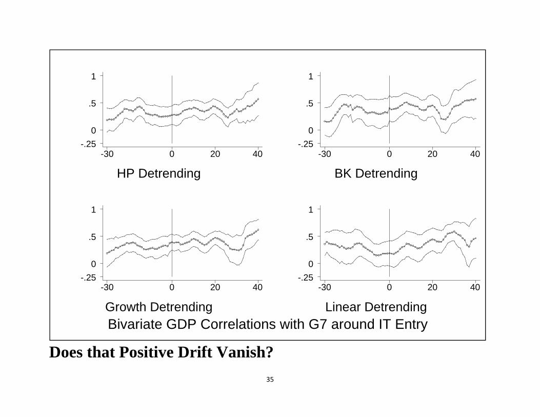
Does that Positive Drift Vanish?

Bivariate GDP Correlations with G7 around IT Entry

HP Detrending

-30 0 20 40-.25

0

.5

1

BK Detrending

-30 0 20 40-.25

0

.5

1

Growth Detrending

-30 0 20 40-.25

0

.5

1

Linear Detrending

-30 0 20 40-.25

0

.5

1

36  

 

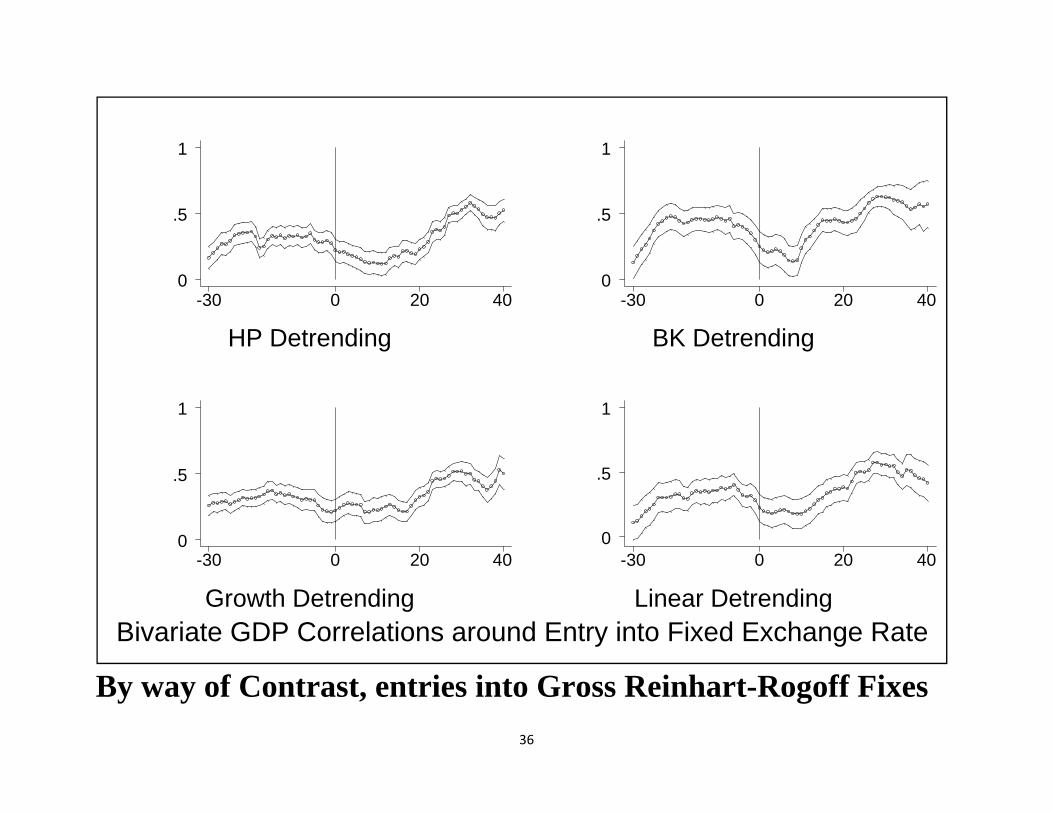
By way of Contrast, entries into Gross Reinhart-Rogoff Fixes

Bivariate GDP Correlations around Entry into Fixed Exchange Rate

HP Detrending

-30 0 20 400

.5

1

BK Detrending

-30 0 20 400

.5

1

Growth Detrending

-30 0 20 400

.5

1

Linear Detrending

-30 0 20 400

.5

1

37  

 

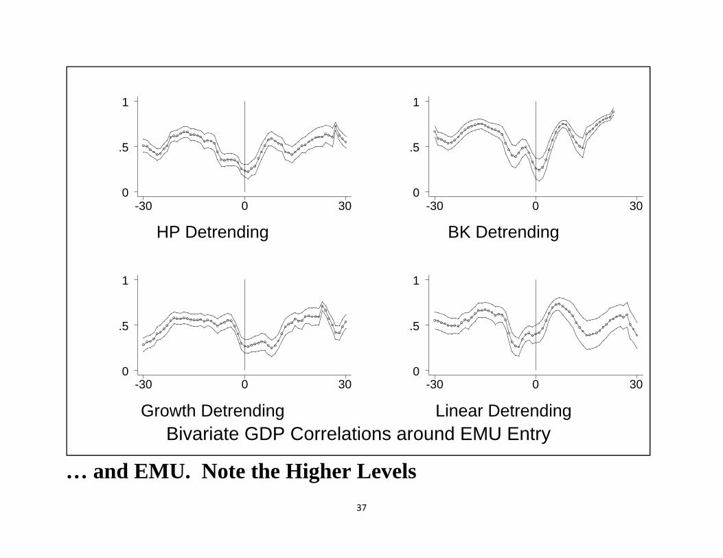
… and EMU. Note the Higher Levels

Bivariate GDP Correlations around EMU Entry

HP Detrending

-30 0 300

.5

1

BK Detrending

-30 0 300

.5

1

Growth Detrending

-30 0 300

.5

1

Linear Detrending

-30 0 300

.5

1

38  

Regression Analysis

• Event studies intrinsically univariate; do not control for other

reasons why BCS might vary across countries / time

o Also use limited data

• Remedy both problems with standard regression techniques

39  

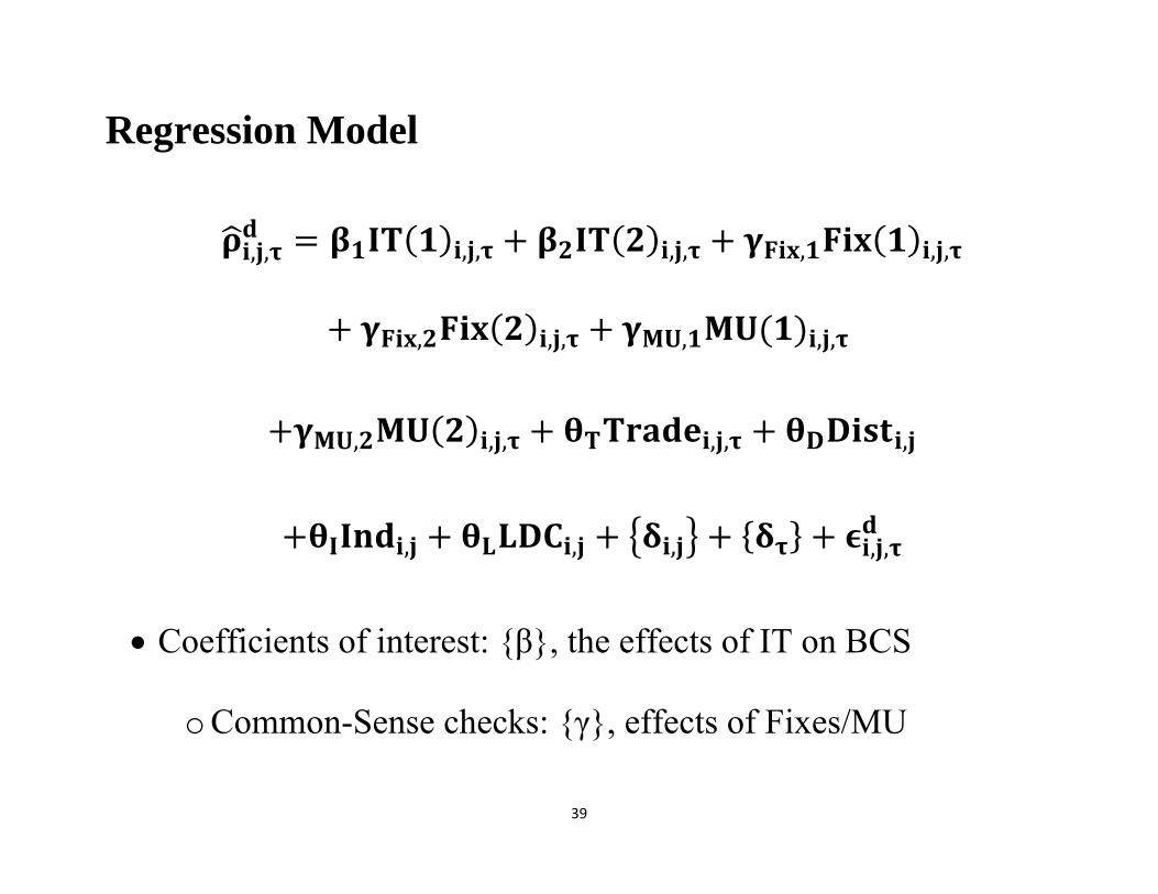
Regression Model

, , , , , , , , ,

, , , , , ,

, , , , , ,

, , , , ,

• Coefficients of interest: {β}, the effects of IT on BCS

o Common-Sense checks: {γ}, effects of Fixes/MU

40  

Controls from Baxter-Kouparitsas

• Bilateral Trade (normalized by multivariate aggregates of both

countries)

o Also, log distance, dummies for both countries being both

industrial/developing

• All four of the robust effects on BCS

41  

Estimation Technique

• Least Squares

o Time Effects

o With and without dyadic fixed effects

• Sample data every 20th observation (avoid dependence, since

BCS measure is moving average)

42  

One

IT

Both

IT

Fixed

ER

Both

MU

One

IT

Both

IT

Fixed

ER

Both

MU

HP

Detrending

.03

(.02)

.05*

(.02)

.27**

(.05)

.41**

(.03)

.03

(.02)

-.04

(.03)

.14**

(.05)

.08

(.05)

BK

Detrending

.02

(.04)

.06

(.04)

.21

(.12)

.59**

(.01)

.03

(.04)

.02

(.06)

.04

(.07)

.11*

(.05)

Linear

Detrending

.05*

(.02)

.07

(.04)

.34**

(.07)

.55

(.22)

.14**

(.03)

.01

(.05)

.24**

(.07)

.18**

(.06)

Growth

Detrending

.03

(.02)

.01

(.05)

.20*

(.07)

.23**

(.01)

.00

(.03)

-.10*

(.04)

.10*

(.05)

-.02

(.05)

Fixed

Effects Time Time Time Time

Time,

Dyads

Time,

Dyads

Time,

Dyads

Time,

Dyads

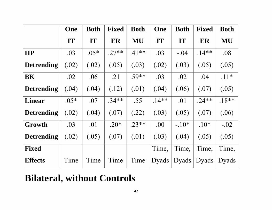
Bilateral, without Controls

43  

One

IT

Both

IT

Fixed

ER

Both

MU

One

IT

Both

IT

Fixed

ER

Both

MU

HP

Detrending

.03

(.02)

.05

(.02)

.22**

(.05)

.29**

(.03)

.03

(.02)

-.03

(.03)

.14**

(.05)

.11*

(.05)

BK

Detrending

.04

(.02)

.07

(.03)

.09

(.10)

.40**

(.03)

.03

(.04)

.02

(.06)

.01

(.09)

.15**

(.05)

Linear

Detrending

.06**

(.01)

.07

(.04)

.28**

(.05)

.41

(.18)

.14**

(.03)

.02

(.05)

.26**

(.07)

.22**

(.06)

Growth

Detrending

.02

(.02)

.01

(.05)

.12

(.06)

.06*

(.02)

.01

(.03)

-.10*

(.04)

.07

(.05)

-.03

(.06)

Fixed

Effects Time Time Time Time

Time,

Dyads

Time,

Dyads

Time,

Dyads

Time,

Dyads

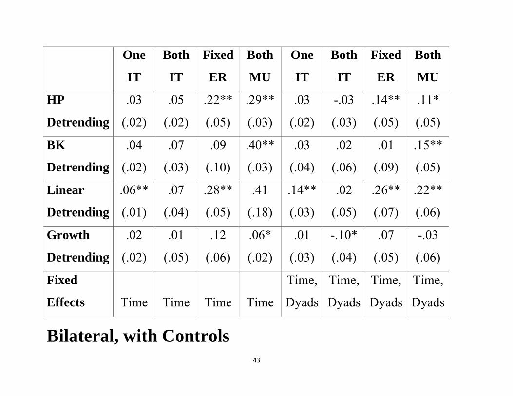
Bilateral, with Controls

44  

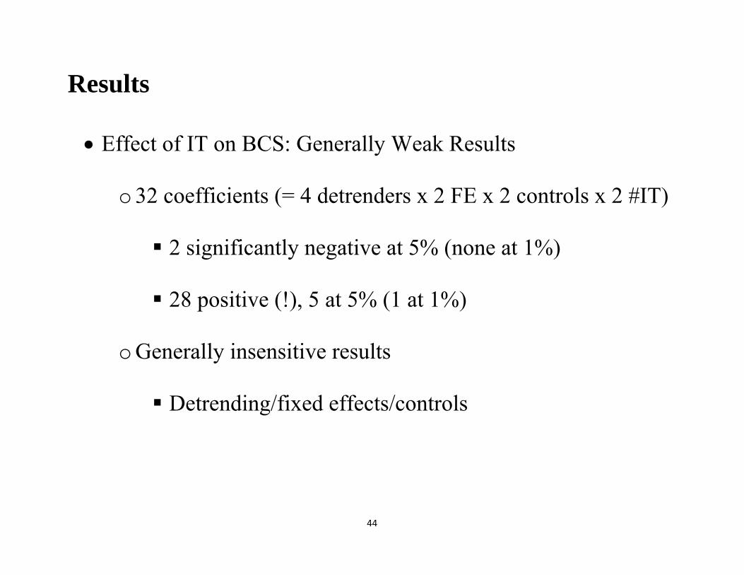
Results

• Effect of IT on BCS: Generally Weak Results

o 32 coefficients (= 4 detrenders x 2 FE x 2 controls x 2 #IT)

2 significantly negative at 5% (none at 1%)

28 positive (!), 5 at 5% (1 at 1%)

o Generally insensitive results

Detrending/fixed effects/controls

45  

Strong Signs that Fixing/Monetary Union Raise BCS

• 11 of 32 coefficients positive at 1%; 5 more at 5%

o 2/32 negative, neither significantly

• So data/methodology able to reveal significant, sensible results

• Analogues for BCS with G-7 deliver similar results

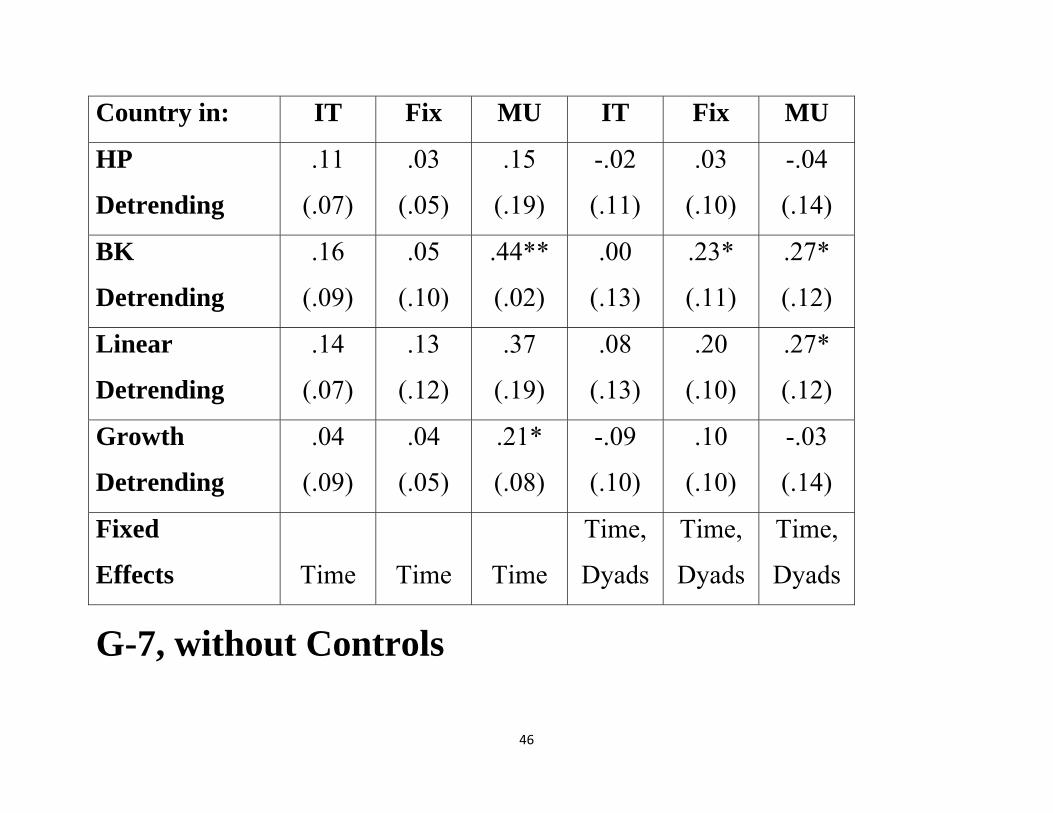
46  

Country in: IT Fix MU IT Fix MU

HP

Detrending

.11

(.07)

.03

(.05)

.15

(.19)

-.02

(.11)

.03

(.10)

-.04

(.14)

BK

Detrending

.16

(.09)

.05

(.10)

.44**

(.02)

.00

(.13)

.23*

(.11)

.27*

(.12)

Linear

Detrending

.14

(.07)

.13

(.12)

.37

(.19)

.08

(.13)

.20

(.10)

.27*

(.12)

Growth

Detrending

.04

(.09)

.04

(.05)

.21*

(.08)

-.09

(.10)

.10

(.10)

-.03

(.14)

Fixed

Effects Time Time Time

Time,

Dyads

Time,

Dyads

Time,

Dyads

G-7, without Controls

47  

Country in: IT Fix MU IT Fix MU

HP

Detrending

.07

(.05)

.01

(.03)

.02

(.15)

.01

(.11)

.07

(.10)

-.03

(.14)

BK

Detrending

.12

(.07)

.03

(.10)

.20**

(.04)

.05

(.13)

.27*

(.11)

.29*

(.14)

Linear

Detrending

.09

(.06)

.13

(.10)

.20

(.12)

.13

(.12)

.26**

(.10)

.28*

(.12)

Growth

Detrending

.00

(.07)

.02

(.04)

-.00

(.06)

-.07

(.11)

.13

(.10)

-.03

(.14)

Fixed

Effects Time Time Time

Time,

Dyads

Time,

Dyads

Time,

Dyads

G-7, with Controls

48  

Adding Financial Integration

One

IT

Both

IT

Fix MU One

IT

Both

IT

Fix MU

HP

.07*

(.01)

.02

(.02)

.25

(.07)

.29*

(.01)

.19**

(.06)

.06

(.07)

-.39**

(.05)

n/a

BK n/a n/a n/a n/a n/a n/a n/a n/a

Linear

.11*

(.004)

.05

(.04)

.26

(.02)

.39

(.17)

.40**

(.06)

.19

(.12)

-.22**

(.06)

n/a

Growth

.02

(.05)

-.02

(.09)

.07

(.03)

.05

(.04)

.23**

(.07)

-.01

(.13)

-.14

(.15)

n/a

Fixed

Effects Time Time Time Time

Time,

Dyads

Time,

Dyads

Time,

Dyads

Time,

Dyads

• Little effect (little data!)

49  

Problems with OLS

• Many potentially serious problems with LS

o Most important: monetary regimes not chosen randomly

Fixes, currency union chosen to affect BCS

Perhaps countries target inflation to insulate themselves

So worry about exogeneity

o IT countries may not be random sample

Special features which linear controls may not capture

50  

Treatment Methodology

• Consider relevant observations (dyad x period) as “treatments”

(IT participation), compare treatments to “controls” (non-IT)

• Match treatments to controls using propensity score,

conditional probability of assignment to treatment given vector

of observed covariates

51  

Methodological Details

• Since {ρ , ,τ} constructed from MA of 20 observations, only use

every 20th observation

• Use Baxter-Kouparitsas vector of 4 variables for covariates

o Check by adding financial integration (2002-2006 data)

• Initial estimator: nearest neighbor (5 matches)

o Check with 4 different estimators

52  

Initial Choice of Treatment/Control

• Treatment: dyads with one IT country (1,041 obs.)

• Control: observations since 1990 without IT (5,038 obs.)

o Check with 6 other treatment/control combinations

53  

Treatment

IT,

any (1041)

IT,

any

(30)

IT,

any (1041)

IT,

any (1041)

IT,

any (1041)

IT,

any (1041)

IT,

Fix/MU

(276)

Control

Any

(5038)

G-7

(532)

Fix or MU

(469)

Fix

(267)

Fix or

MU*

(3185)

No fix or

MU

(1853)

Fix or MU

(478)

HP

.08**

(.01)

.08

(.07)

-.03

(.05)

-.08

(.06)

.09**

(.02)

.06**

(.02)

.08*

(.04)

BK

.14**

(.03)

.11

(.10)

.03

(.07)

-.04

(.08)

.15**

(.03)

.12**

(.03)

.17**

(.06)

Linear

.10**

(.02)

.07

(.09)

.02

(.07)

-.02

(.08)

.12**

(.02)

.08**

(.02)

.01

(.06)

Growth

.13**

(.02)

.14*

(.06)

.03

(.05)

-.06

(.06)

.15**

(.02)

.11**

(.02)

.11**

(.04)

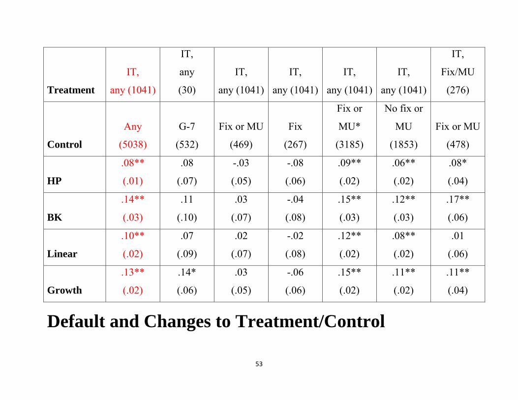
Default and Changes to Treatment/Control

54  

NN

(5)

NN

(1)

NN

(5) Strat. Kernel Radius

HP

.08**

(.01)

.08**

(.02)

.07**

(.02)

.06**

(.01)

.07**

(.02)

.08**

(.01)

BK

.14**

(.03)

.12**

(.03)

.16**

(.04)

.08**

(.02)

.10**

(.02)

.12**

(.02)

Linear

.10**

(.02)

.10**

(.03)

.12**

(.03)

.11**

(.02)

.11**

(.02)

.12**

(.02)

Growth

.13**

(.02)

.13**

(.02)

.17**

(.02)

.13**

(.01)

.13**

(.01)

.13**

(.01)

PS Standard Standard Augment Standard Standard Standard

Effect Average Average Average Treated Treated Treated

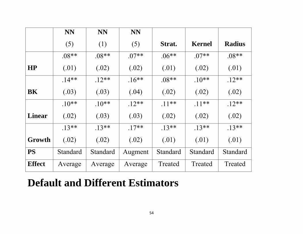
Default and Different Estimators

55  

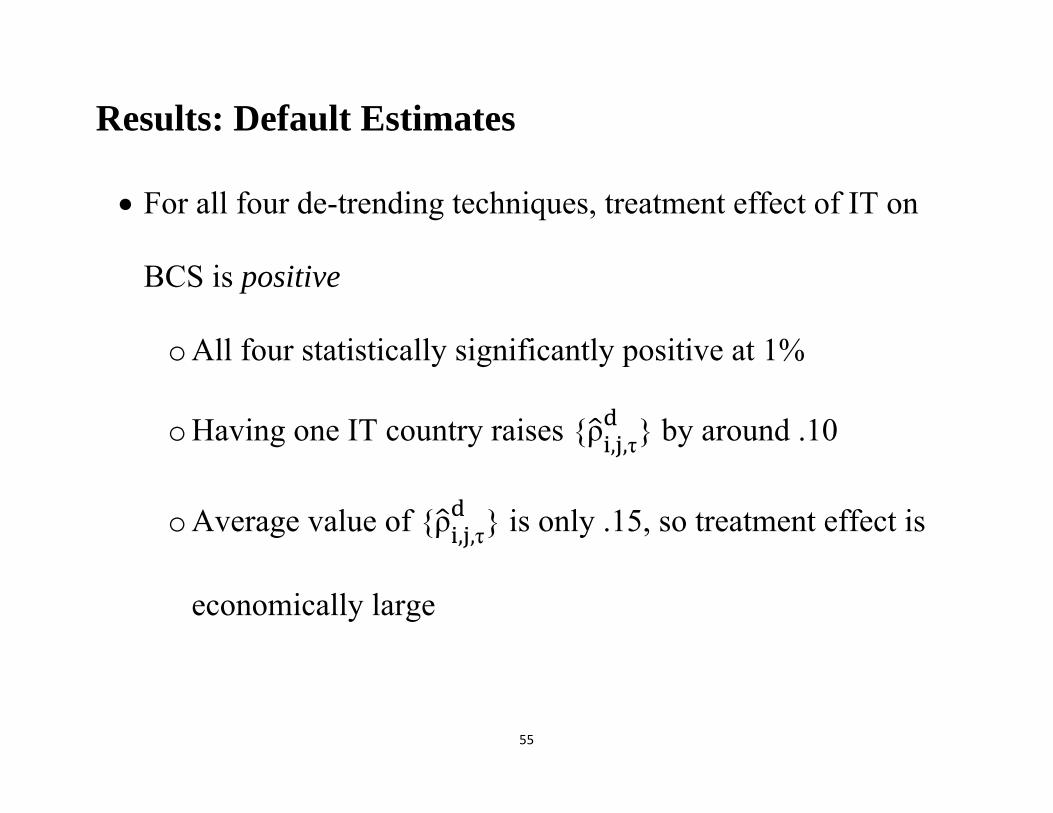
Results: Default Estimates

• For all four de-trending techniques, treatment effect of IT on

BCS is positive

o All four statistically significantly positive at 1%

o Having one IT country raises {ρ , ,τ} by around .10

o Average value of {ρ , ,τ} is only .15, so treatment effect is

economically large

56  

Sensitivity

• IT seems to increase BCS with G-7!

o Statistically insignificant effects though

• Effect of IT “treatment” on BCS close to that of fixing

exchange rate/monetary union!

o Smaller effects, but statistically insignificant differences

• Difference estimators make little difference to economic or

statistical significance

57  

Natural Contrast to IT: EMU

Estimator NN, (5) NN (2) NN (5) Strat. Radius Kernel

Model standard standard augmented standard standard standard

HP

Detrending

.171*

(.077)

.161

(.107)

.139

(.090)

.077

(.046)

.147**

(.042)

.108**

(.036)

BK

Detrending

.240**

(.093)

.219

(.128)

.376**

(.080)

.096

(.052)

.194**

(.051)

.146*

(.064)

Linear

Detrending

.275**

(.099)

.234

(.149)

.247*

(.126)

.122*

(.052)

.206**

(.054)

.156**

(.051)

Growth

Detrending

.101

(.069)

.107

(.095)

-.029

(.088)

.139**

(.037)

.179**

(.040)

.154**

(.037)

• Positive, bigger effects than those of IT (methodology works!)

58  

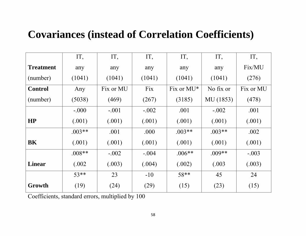
Covariances (instead of Correlation Coefficients)

Treatment

(number)

IT,

any

(1041)

IT,

any

(1041)

IT,

any

(1041)

IT,

any

(1041)

IT,

any

(1041)

IT,

Fix/MU

(276)

Control

(number)

Any

(5038)

Fix or MU

(469)

Fix

(267)

Fix or MU*

(3185)

No fix or

MU (1853)

Fix or MU

(478)

HP

-.000

(.001)

-.001

(.001)

-.002

(.001)

.001

(.001)

-.002

(.001)

.001

(.001)

BK

.003**

(.001)

.001

(.001)

.000

(.001)

.003**

(.001)

.003**

(.001)

.002

(.001)

Linear

.008**

(.002

-.002

(.003)

-.004

(.004)

.006**

(.002)

.009**

(.003

-.003

(.003)

Growth

53**

(19)

23

(24)

-10

(29)

58**

(15)

45

(23)

24

(15)

Coefficients, standard errors, multiplied by 100

59  

Quick Summary

• Little evidence of “Decoupling in Practice

• Inflation Targeting associated in theory and empirics

with greater business cycle synchronization across

countries

60  

Conclusion

• Advent of IT coincided with “Great Moderation”

• Long Unresolved debate: coincidence? did policy matter?

o Typically addressed empirically with domestic macro

phenomena (inflation, growth)

• But IT strongly linked with greater BCS

o Nudges us towards view that IT effect causal, not luck