INFLATIONARY PRESSURES IN SOUTH ASIA · INFLATIONARY PRESSURES IN SOUTH ASIA ... as India and Pakistan, experienced double-digit inflation rates. ... To identify the underlying causes

Asia-Pacific Development Journal Vol. 17, No. 2, December 2010

1

INFLATIONARY PRESSURES IN SOUTH ASIA

Ashima Goyal*

The similarities yet differences across South Asian countries, and theirdifferential response to recent food and oil price shocks, providesa useful opportunity to better understand the structure of inflation inthese economies. Analysis of the internal goods market and externalbalance of payments equilibrium and evidence on demand and supplyshocks suggests that output is largely demand determined butinefficiencies on the supply side perpetuate inflation. Pro-cyclical policyamplifies the negative impact of supply shocks on output. Inflationsurges are reduced at high output cost while propagation mechanismsand well-intentioned administrative interventions turn relative priceshocks into chronic cost-push inflation. The analysis brings out theimportance of food prices for the inflationary process. It is necessaryto protect the poor from inflation and especially food inflation. But thismust be done effectively. The paper concludes with an analysis ofeffective short- and long-run policy options.

JEL Classification: E31, E52, O11.

Key words: Inflation, South Asia, food price policy, demand and supply shocks.

I. INTRODUCTION

Countries in South Asia have common features that affect macroeconomicpolicy choices, outcomes and stability. These include high population density, lowper capita incomes, a large share of population in agriculture and relatively high

* Professor, Indira Gandhi Institute of Development Research, Gen. Vaidya Marg, Santosh Nagar,Goregaon (E), Mumbai-400 065 [email protected], http://www.igidr.ac.in/~ashima. The author isgrateful to Nagesh Kumar and Aynul Hasan for the invitation to write on this topic, to Ashfaque Khanand other participants of the ESCAP expert group meetings for comments, Mahendra Dev fordiscussions on food price policy, Sanchit Arora for research assistance and Reshma Aguiar forsecretarial assistance.


2

saving ratios.1 Also, food comprises a large part of the average consumption basketand the economies depend on oil imports, making these countries vulnerable toterms of trade and other supply shocks.

The region initiated liberalizing reforms in the 1990s. The reforms broughton shocks to the economies but, over time, they created greater diversity anddeeper markets that paved the way for reduced volatility. Controls may repressvolatility, but they create a fragile situation. Effective liberalization, however, isgradual. The smaller South Asian countries, Bhutan, Nepal and Maldives, aremore strongly affected by external shocks as they tend to be more open with lessmarket development and capital account controls, and more burdened withgovernment and international debt.

Similar features should lead to convergence in macroeconomic policies,but differing political systems are a potential factor causing divergence. Low percapita income democracies have a tendency to set short-term populist policiesand face persistent and chronic inflation, while governments not so dependent onpopular vote can allow higher inflation and volatility. These differential responses,under similar basic conditions and shocks, are used in this paper to understandcauses of inflation and suggest better policy design.

Spikes in food and fuel prices prior to the global financial and economiccrisis resulted in high inflation rates in most countries in Asia and the Pacific. Withthe onset of the crisis itself, inflationary pressure subsided sharply in all subregionsof Asia and the Pacific except South Asia. Major economies of South Asia, suchas India and Pakistan, experienced double-digit inflation rates. Food prices grewat even higher rates. Given the high incidence of poverty in the region, high foodand overall inflation rates disproportionately impact the poor. Moreover, a sustainedrise in food prices tends to raise wages and ultimately boost inflation.

To identify the underlying causes of high inflation, both food and overall,in countries of South Asia, mainly India, Pakistan, Bangladesh, Sri Lanka, Nepaland Maldives, and possible policy responses, potential causative factors areclassified into the generic categories of demand and supply. The former includesdomestic and external demand, monetary and fiscal policies. The latter includessectoral price shocks and capacity constraints. Government interventions, whichmay moderate a price spike but raise costs over time, aggravate supply shocks sothat a relative price change turns into inflation. Government policies for agricultureand speculative behaviour affect food inflation, and are also examined. The policies

1 There are, of course, variations across countries. In Pakistan and Nepal the savings to GDP ratiostruggles to reach 20 per cent while in India it has crossed 30 per cent.


3

include minimum price support, buffer stock, trade and public distribution schemes.More openness changes the inflationary dynamics.

Does high economic growth in some countries imply that infrastructuraland other capacity constraints are contributing to inflationary pressures? Data andanalysis suggest the macroeconomic dynamics is such that output is largely demanddetermined but inefficiencies on the supply side cause inflation. For example, thepower shortages that most South Asian countries suffer from are a failure in theprovision of public goods. These power shortages lead to higher costs sinceexpensive substitutes have to be used.

The structural features outlined above help explain the patterns identifiedin the response of select South Asian countries to the severe food and oil priceshocks of this decade. The analysis is used to assess the effectiveness of policyresponses and interventions, and to suggest alternatives, including some arisingfrom more openness.

Although the Reserve Bank of India has always emphasized the importanceof money supply as the cause of inflation, the sustained food inflation has recentlyspurred some analysis of supply side factors (Gokarn, 2010; Mohanty, 2010). Joshiand Little (1994) have long argued that supply-side responses have been neglectedin Indian macroeconomic policy.

The structure of the paper is as follows: Section II presents data on thecauses of inflation and draws out some stylized facts from the data. Section IIIderives an analytical framework. Section IV explores the political economy of foodprices. Section V presents evidence supporting the analysis. Section VI drawsout policy implications. Section VII concludes the paper.

II. CAUSES OF INFLATION

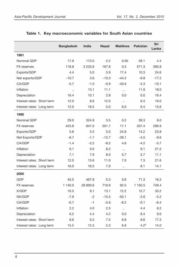
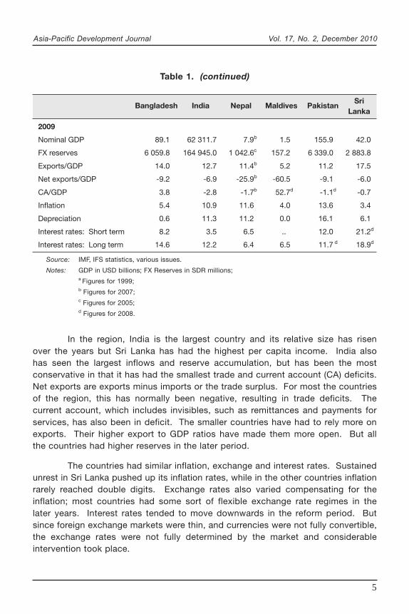
Relevant macroeconomic data are displayed in tables and figures for 5South Asian countries.2 Table 1 gives a comparative macroeconomic picture of thecountries and shows how this has changed at ten-year intervals from 1981 to2009. Apart from nominal gross domestic product (GDP) and reserves, it providescritical balance of payment ratios, long- and short-term interest rates, inflation andchanges in exchange rates.

2 The data source is the IFS (IMF). The advantage of using this data set is that the definitions usedare consistent for comparative purposes. But there are gaps in the data. The Maldives data are sopatchy and erratic they cannot be graphed.


4

Table 1. Key macroeconomic variables for South Asian countries

Bangladesh India Nepal Maldives PakistanSri

Lanka

1981

Nominal GDP 17.9 173.0 2.2 0.05 28.1 4.4

FX reserves 118.8 3 233.8 167.8 0.5 571.3 260.8

Exports/GDP 4.4 5.0 5.9 17.4 10.3 24.6

Net exports/GDP -10.7 3.6 -10.3 -44.2 -9.8 -17.2

CA/GDP -5.7 -1.0 -0.9 -40.6 -3.3 -10.1

Inflation .. 13.1 11.1 .. 11.9 18.0

Depreciation 16.4 10.1 2.8 0.0 0.0 16.4

Interest rates: Short term 12.0 8.6 12.0 .. 9.3 19.0

Interest rates: Long term 12.0 16.5 5.0 6.0 9.4 15.6

1990

Nominal GDP 29.0 324.9 3.5 0.2 39.3 8.0

FX reserves 423.8 847.0 201.7 17.1 207.4 296.9

Exports/GDP 5.8 5.5 5.0 24.8 14.2 23.8

Net Exports/GDP -6.7 -1.7 -12.7 -39.1 -4.5 -9.6

CA/GDP -1.4 -2.2 -8.2 4.6 -4.2 -3.7

Inflation 6.1 9.0 8.2 .. 9.1 21.5

Depreciation 7.1 7.9 8.0 5.7 5.7 11.1

Interest rates: Short term 12.0 15.6 11.0 7.0 7.3 21.6

Interest rates: Long term 16.0 16.5 7.9 .. 8.1 14.1

2000

GDP 45.5 467.8 5.3 0.6 71.3 16.3

FX reserves 1 140.0 28 600.6 719.9 92.5 1 150.5 749.4

X/GDP 10.5 9.1 13.1 12.2 12.7 33.2

NX/GDP -7.9 -2 -15.5 -50.1 -2.6 -5.2

CA/GDP -0.7 -1 -5.6 -8.2 -0.1 -6.4

Inflation 2.2 4.0 2.5 .. 4.4 6.2

Depreciation 6.2 4.4 4.2 0.0 8.4 9.0

Interest rates: Short term 8.6 9.3 7.5 6.8 8.6 17.3

Interest rates: Long term 15.5 12.3 5.3 6.9 4.2a 14.0


5

In the region, India is the largest country and its relative size has risenover the years but Sri Lanka has had the highest per capita income. India alsohas seen the largest inflows and reserve accumulation, but has been the mostconservative in that it has had the smallest trade and current account (CA) deficits.Net exports are exports minus imports or the trade surplus. For most the countriesof the region, this has normally been negative, resulting in trade deficits. Thecurrent account, which includes invisibles, such as remittances and payments forservices, has also been in deficit. The smaller countries have had to rely more onexports. Their higher export to GDP ratios have made them more open. But allthe countries had higher reserves in the later period.

The countries had similar inflation, exchange and interest rates. Sustainedunrest in Sri Lanka pushed up its inflation rates, while in the other countries inflationrarely reached double digits. Exchange rates also varied compensating for theinflation; most countries had some sort of flexible exchange rate regimes in thelater years. Interest rates tended to move downwards in the reform period. Butsince foreign exchange markets were thin, and currencies were not fully convertible,the exchange rates were not fully determined by the market and considerableintervention took place.

2009

Nominal GDP 89.1 62 311.7 7.9b 1.5 155.9 42.0

FX reserves 6 059.8 164 945.0 1 042.6c 157.2 6 339.0 2 883.8

Exports/GDP 14.0 12.7 11.4b 5.2 11.2 17.5

Net exports/GDP -9.2 -6.9 -25.9b -60.5 -9.1 -6.0

CA/GDP 3.8 -2.8 -1.7b 52.7d -1.1d -0.7

Inflation 5.4 10.9 11.6 4.0 13.6 3.4

Depreciation 0.6 11.3 11.2 0.0 16.1 6.1

Interest rates: Short term 8.2 3.5 6.5 .. 12.0 21.2d

Interest rates: Long term 14.6 12.2 6.4 6.5 11.7 d 18.9d

Source: IMF, IFS statistics, various issues.

Notes: GDP in USD billions; FX Reserves in SDR millions;a Figures for 1999;b Figures for 2007;c Figures for 2005;d Figures for 2008.

Table 1. (continued)

Bangladesh India Nepal Maldives PakistanSri

Lanka


6

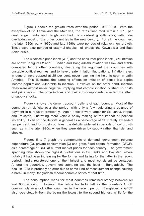
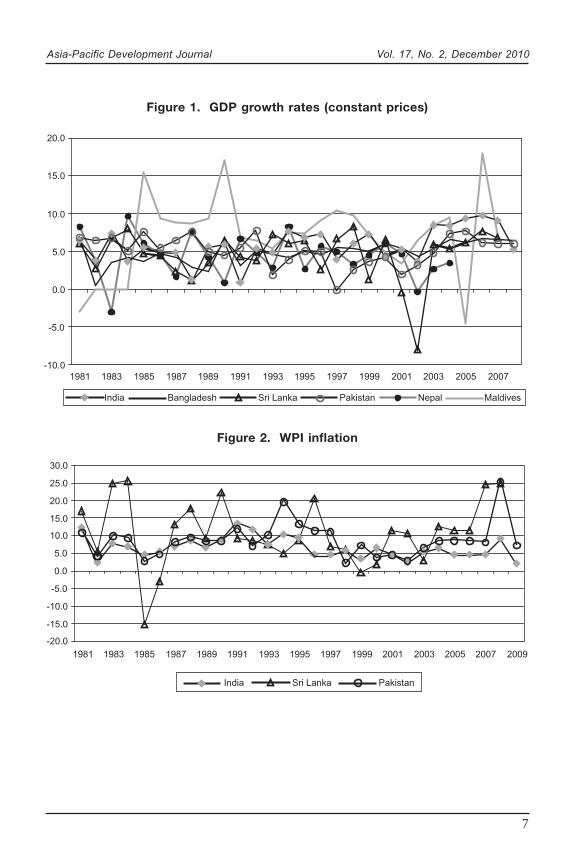
Figure 1 shows the growth rates over the period 1980-2010. With theexception of Sri Lanka and the Maldives, the rates fluctuated within a 0-10 percent range. India and Bangladesh had the steadiest growth rates, with Indiaovertaking most of the other countries in the new century. For all the countries,the late 1980s, early 1990s and late 1990s were periods of relatively low growth.These were also periods of external shocks: oil prices, the Kuwait war and EastAsian crisis.

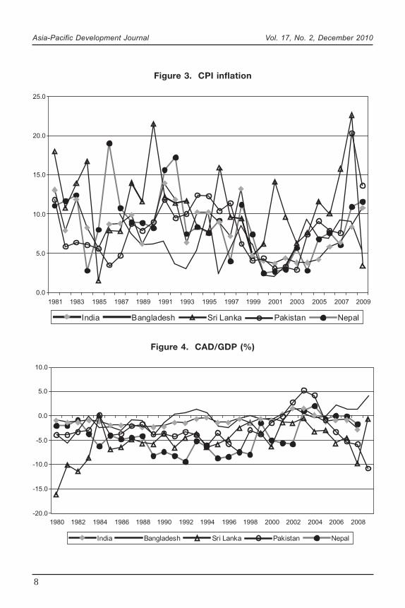
The wholesale price index (WPI) and the consumer price index (CPI) inflationare shown in figures 2 and 3. Indian and Bangladeshi inflation was low and stablecompared to the other countries, illustrating the argument that countries withunstable political regimes tend to have greater inflation fluctuations. Inflation rates,in general were capped at 25 per cent, never reaching the heights seen in LatinAmerica. This illustrates the damping effects on inflation of dense low capitaincome populations vulnerable to inflation. However, on the other hand, inflationrates were almost never negative, implying that chronic inflation pushed up costsand price levels. The price indices and their sub-components reflected the effectof supply shocks.

Figure 4 shows the current account deficits of each country. Most of thecountries ran deficits over the period, with only a few registering a balance ofpayment in surplus intermittently. Again deficits were larger for Sri Lanka, Nepal,and Pakistan, illustrating more volatile policy-making or the impact of politicalinstability. Even so, the deficits in general as a percentage of GDP rarely exceededten per cent, and for most countries, the deficits widened in periods of low growthsuch as in the late 1990s, when they were driven by supply rather than demandshocks.

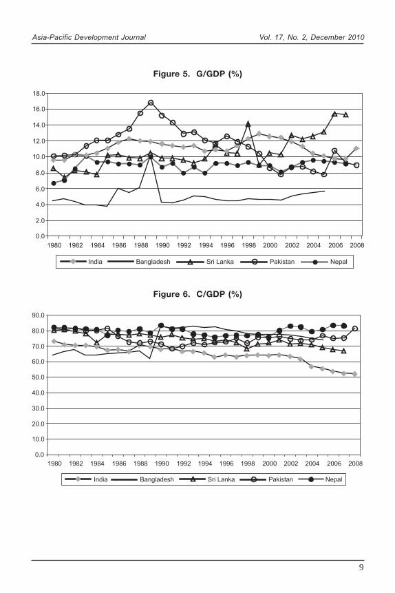
Figures 5 to 7 graph the components of demand, government revenueexpenditure (G), private consumption (C) and gross fixed capital formation (GFCF),as a percentage of GDP at current market prices for each country. The governmentspending ratio shows the highest fluctuations in Sri Lanka and Pakistan, wherenotably it had been increasing for the former and falling for the latter in the recentperiod. India registered one of the highest and most consistent percentages.Among the countries, government spending was the least in Bangladesh. Thepeak in 1988 is probably an error due to some kind of measurement change causinga break in many Bangladesh macroeconomic series at that time.

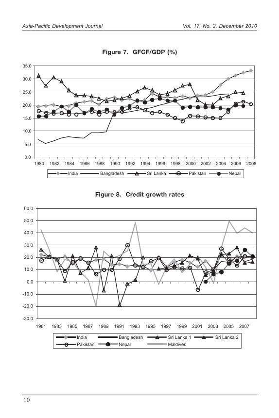
The consumption ratios for most countries remained steady between 60and 80 per cent. However, the ratios for India fell as the country’s GFCFconvincingly overtook other countries in the recent period. Bangladesh’s GFCFalso rose steadily from the being the lowest to the second highest, while for the


7

-20.0

-15.0

-10.0

-5.0

0.0

5.0

10.0

15.0

20.0

25.0

30.0

1981 1983 1985 1987 1989 1991 1993 1995 1997 1999 2001 2003 2005 2007 2009

India Sri Lanka Pakistan

-10.0

-5.0

0.0

5.0

10.0

15.0

20.0

1981 1983 1985 1987 1989 1991 1993 1995 1997 1999 2001 2003 2005 2007

India Bangladesh Sri Lanka Pakistan Nepal Maldives

Figure 1. GDP growth rates (constant prices)

Figure 2. WPI inflation


8

-20.0

-15.0

-10.0

-5.0

0.0

5.0

10.0

1980 1982 1984 1986 1988 1990 1992 1994 1996 1998 2000 2002 2004 2006 2008

India Bangladesh Sri Lanka Pakistan Nepal

Figure 3. CPI inflation

Figure 4. CAD/GDP (%)

0.0

5.0

10.0

15.0

20.0

25.0

1981 1983 1985 1987 1989 1991 1993 1995 1997 1999 2001 2003 2005 2007 2009



9

Figure 5. G/GDP (%)

Figure 6. C/GDP (%)

0.0

2.0

4.0

6.0

8.0

10.0

12.0

14.0

16.0

18.0

1980 1982 1984 1986 1988 1990 1992 1994 1996 1998 2000 2002 2004 2006 2008


0.0

10.0

20.0

30.0

40.0

50.0

60.0

70.0

80.0

90.0

1980 1982 1984 1986 1988 1990 1992 1994 1996 1998 2000 2002 2004 2006 2008



10

Figure 7. GFCF/GDP (%)

Figure 8. Credit growth rates

0.0

5.0

10.0

15.0

20.0

25.0

30.0

35.0

1980 1982 1984 1986 1988 1990 1992 1994 1996 1998 2000 2002 2004 2006 2008


-30.0

-20.0

-10.0

0.0

10.0

20.0

30.0

40.0

50.0

60.0

1981 1983 1985 1987 1989 1991 1993 1995 1997 1999 2001 2003 2005 2007

India Bangladesh Sri Lanka 1 Sri Lanka 2

Pakistan Nepal Maldives


11

other three countries, the rates fluctuated in a 5-10 per cent band. Among thedemand components, consumption ratios and GFCF held steady, G showedrestrained fluctuations. Output levels and growth rates fluctuated, and demandcomponents largely fluctuated synchronously. So demand categories might nothave been major independent sources of shocks.

Figure 8 shows that with the exception of Maldives, credit growth ratesnever exceeded 30 per cent. Pakistan, Sri Lanka and Maldives experienced periodsof negative credit growth. In general, this is a relatively good record for emergingmarkets as it indicates there was stability in the financial systems which, in turn,prevented large credit fuelled demand booms.

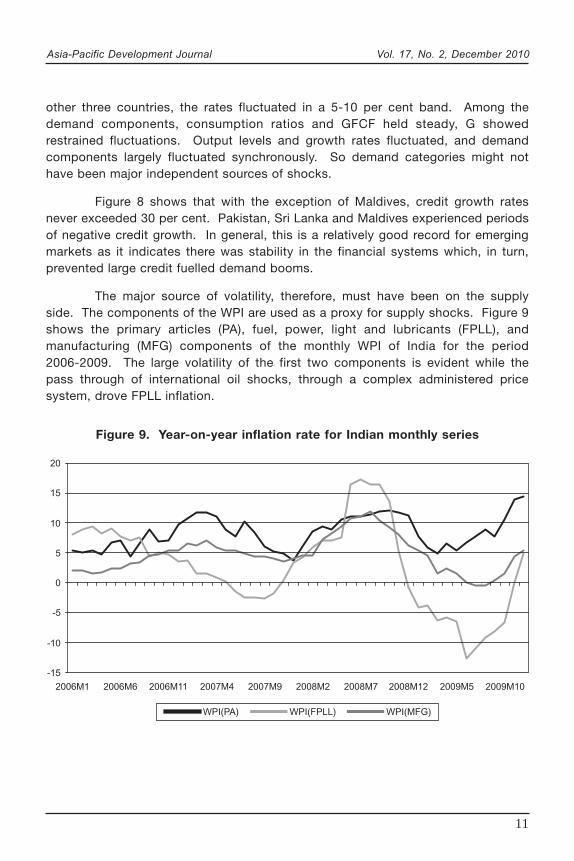
The major source of volatility, therefore, must have been on the supplyside. The components of the WPI are used as a proxy for supply shocks. Figure 9shows the primary articles (PA), fuel, power, light and lubricants (FPLL), andmanufacturing (MFG) components of the monthly WPI of India for the period2006-2009. The large volatility of the first two components is evident while thepass through of international oil shocks, through a complex administered pricesystem, drove FPLL inflation.

Figure 9. Year-on-year inflation rate for Indian monthly series

-15

-10

-5

0

5

10

15

20

2006M1 2006M6 2006M11 2007M4 2007M9 2008M2 2008M7 2008M12 2009M5 2009M10

WPI(PA) WPI(FPLL) WPI(MFG)


12

A. Stylized Facts

Some stylized facts can be extracted from the initial data analysis aboveas well as from results of Goyal (2011) on correlations and volatilities of timeseries, in which a smooth trend is extracted using the Hodrick Prescott filter.3

Frequent shocks, and less ability to smooth shocks, imply that output, consumption,investment and growth rates are more volatile than in mature economies. Lessfinancial sector development, lower per capita incomes and low wealth imply thatconsumption of a large proportion of the population is limited by income. Inaddition, since the frequent supply shocks are largely temporary, savings adjustrather than consumption. Therefore, the correlation of consumption (C) andinvestment (I) with output is higher, making ratios of C, and of I to output stable(Figures 6 and 7). C and I vary in response to output variation, but do not driveincome volatility.

During the period, net exports, or the trade surplus, was procyclical,meaning output rose with net exports. This could be due to export-driven growthor to a deflationary rise in commodity prices. The latter raises the import bill andreduces output and net exports together. The current account then becomesa source of shocks. This contrasts with standard behaviour in emerging marketsin which rising consumption and imports in good times make the current accountcountercyclical — the deficit rises in good times. Consumption is procyclical andmore volatile than in developed countries. In Asia, income shocks affect savingsrather than consumption.

Supply side or terms of trade shocks are to be expected in economiesthat are still agriculture dependent, have severe infrastructure bottlenecks, and aredependent on oil imports.

III. ANALYSIS

A. Aggregate demand and supply

It is difficult to find unemployment estimates on South Asia but the numbersare believed to be very large. Output in developed countries is regarded as belowpotential because the crisis left 22 million unemployed. In South Asia, the morethan 300 million people living below the poverty line are not meaningfully employed.In India alone, given the youthful demographic profile, 10-12 million are expectedto enter the labour force every year. The Planning Commission estimates it would

3 This is commonly used to separate the trend from fluctuations in macroeconomic time series.


13

take economic growth of 10 per cent per annum together with an employmentelasticity of 0.25 to absorb them. Capital, as a produced means of production, isno longer a constraint because of high domestic savings and capital inflows.Therefore, that 10 per cent rate of growth should be regarded as the potentialoutput.

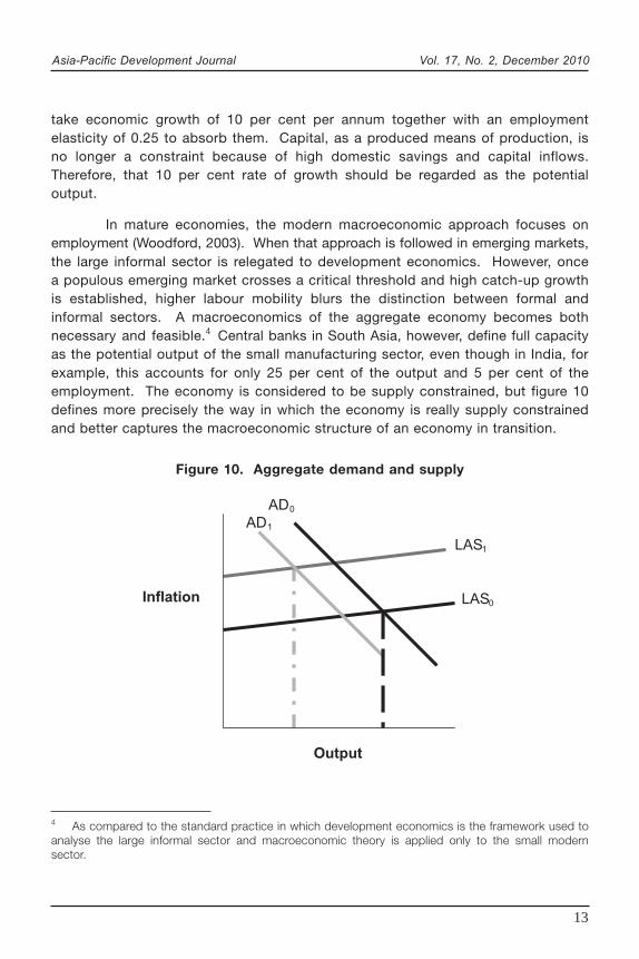
In mature economies, the modern macroeconomic approach focuses onemployment (Woodford, 2003). When that approach is followed in emerging markets,the large informal sector is relegated to development economics. However, oncea populous emerging market crosses a critical threshold and high catch-up growthis established, higher labour mobility blurs the distinction between formal andinformal sectors. A macroeconomics of the aggregate economy becomes bothnecessary and feasible.4 Central banks in South Asia, however, define full capacityas the potential output of the small manufacturing sector, even though in India, forexample, this accounts for only 25 per cent of the output and 5 per cent of theemployment. The economy is considered to be supply constrained, but figure 10defines more precisely the way in which the economy is really supply constrainedand better captures the macroeconomic structure of an economy in transition.

Figure 10. Aggregate demand and supply

4 As compared to the standard practice in which development economics is the framework used toanalyse the large informal sector and macroeconomic theory is applied only to the small modernsector.

LAS0

AD0

Inflation

Output

AD1

LAS1


14

The longer-run aggregate supply (LAS) is elastic (figure 10). Butinefficiencies, distortions and cost shocks push aggregate supply upwards, overan entire range, rather than only at full employment, since that is not reached atcurrent output ranges and output can increase. The LAS becomes vertical only asthe economy matures and full productive employment is reached. With sucha structure, demand has a greater impact on output and supply on inflation. Thisis the sense in which the economy is supply constrained.5

The food price wage cycle is an important mechanism propagating priceshocks and creating inflationary expectations. Monsoon failures or international oilprice shocks have been dominant inflation triggers. A political economy of farmprice support, consumption subsidies and wage support, with built-in waste,inefficiencies and corruption, contributes to chronic cost push inflation. Poortargeting of consumption subsidies imply that nominal wages rise with a lag pushingup costs and generating a second round of inflation stemming from a temporarysupply shock. The political economy indexes wages informally to food priceinflation. If the rise in average wages exceeds that in agricultural productivity,prices rise, propagating inflation. Other types of populist policies that giveshort-term subsidies but raise hidden or indirect costs also contribute to cost pushinflation. For example, neglected infrastructure and poor public services increasecosts.

Rigorous empirical tests based on structural vector autoregression (VAR),time series causality, generalized method of moments (GMM) regressions ofaggregate demand (AD) and aggregate supply (AS), and calibrations in a dynamicstochastic general equilibrium (DSGE) model for the Indian economy support theelastic longer-run supply and the dominance of supply shocks (Goyal, 2009b, 2008,2005).

Shocks that have hit the Indian economy serve as useful experiments inhelping reveal its structure. Consider, for example, the summer of 2008 when theeconomy was thought to be overheating after a sustained period of more than9 per cent growth. During that period food and oil spikes had contributed to highinflation. Sharp monetary tightening, which sent short-term interest rates above9 per cent during the summer, and the fall of U.S. investment bank Lehman Brothers,which froze exports, were large demand shocks that hit the economy. Industrialoutput declined sharply in the last quarter of 2008, but WPI-based inflation onlyfell after the drop in oil prices at the end of the year while CPI inflation remained

5 The analysis draws on and extends earlier work. See Goyal (2011). References not givenbecause of space constraints are available at www.igidr.ac.in/~ashima.


15

high.6 Demand shocks with a near vertical supply curve, should affect inflationmore than output. But the reverse happened. Output growth fell much more thaninflation.

The V shaped recovery, which set in by the summer of 2009, also indicatesa reduction in demand rather than a leftward shift of a vertical supply curve. Adestruction of capacity would be more intractable and recovery would take longer.Since labour supply ultimately determines potential output for the aggregateeconomy, the potential is large in the region.

The impact of a sustained high CPI inflation on wages possibly explainsthe quick resurgence of WPI inflation in November 2009 when industry had barelyrecovered. The manufacturing price index fell for only for a few months beforerising to its November 2008 value of 203 by April 2009. A booming economy doesadd pricing power, but supply side shocks also can contribute to manufacturinginflation.

Such outcomes are possible only if inflation is supply determined, butdemand determines output. Components of demand such as consumer durablespending and housing are interest-rate sensitive. During the crisis, the lag frompolicy rates to industry was only 2-3 quarters for a fall and one quarter for a sharprise. Policy rates have affected output growth since 1996. Nevertheless, theeconomy is supply constrained.

Since the recent inflationary episodes in South Asia have included a sharprise in food prices, based in part on international food, oil and commodity shocks,the next section develops a simple analytical structure that opens the closedeconomy analysed above to bring in international shocks. Both it and section IVon political economy identify some of the mechanisms that convert a relative priceshock into inflation.

B. Open economy

The AD-AS apparatus in the section above depicted the internal balanceof an emerging market. Internal balance holds when aggregate demand for domesticoutput equals aggregate supply at full employment of resources, with inflationremaining low and stable. An open economy must also be concerned with externalbalance or equilibrium in the balance of payments. The current account surplus or

6 Indian data show industrial growth slumped to 0.32 per cent over October-December 2008, butWPI inflation remained at 8.57 per cent and CPI inflation at 10 per cent. WPI inflation began fallinggradually from January 2009.


16

the net balance of trade (exports minus imports) must be financed by sustainablecapital flows. Adjustment to full internal and external balance normally requiresa combination of a change in relative prices (real exchange rates) and in demandor expenditure (Goyal, 2009a, 2004).

The real exchange rate (Z), is a relative price comparing the worldpurchasing power with the purchasing power of the domestic currency. It is givenby the ratio of the nominal exchange rate (E), multiplied by the foreign price leveland divided by the domestic price level (Z = EP*/P). If there is perfect purchasingpower parity, Z should equal unity.

A key conceptual distinction for a small country is that it must takeinternational prices as given. If markets are competitive, traded goods (exportablesand importables) can be combined into a single category because in a perfectlyelastic world, demand for exports and a perfectly elastic world supply of importsmakes their prices independent of domestic variables. But this means that theterms of trade, or the ratio of export to import prices, cannot change to help makethe adjustment to full equilibrium or balance. Therefore, the distinction betweentraded and non-traded goods is required. Since trade equalizes the domestic tothe border price of the traded good, the real exchange rate is given by the ratio ofthe prices of traded to non-traded goods (Z = EP

T/P

N). This is the dependent

economy model7 in which the real exchange rate and domestic absorption (A =C+G+I) are the two means of reaching internal and external balance. Exchangerate policy, which changes the nominal exchange rate (E), and fiscal policy whichchanges government expenditure (G), are the two policy instruments, affecting Zand A respectively. The first is an expenditure-switching policy. It changes thedirection of demand and supply. Demand shifts between domestic output andimports, and domestic resources shift between sectors producing traded and non-traded goods. The second is an expenditure-changing policy. It changes the levelof total demand.

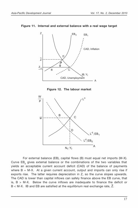
Figure 11 reproduces the Swan diagram and Figure 12 the underlying labourmarket equilibrium. The curve IB gives internal balance or the combinations of Zand A at which output demand equals full employment output, Y

f. The curve is

downward sloping because depreciation and a rise in demand both raise output.As domestic absorption rises, Z must appreciate to reduce foreign demand forexports, and total demand, to the full employment output level. Values above thecurve generate inflation, as a more depreciated exchange rate and higher absorptionraise demand. Those below the curve generate unemployment.

7 The dependant economy model was first applied to Australia (see Swan, 1960 and Salter, 1959)but has been used extensively and generalized to other times and countries. Trevor Swan developeda convenient diagrammatic representation known as the Swan Diagram.


17

Figure 11. Internal and external balance with a real wage target

Figure 12. The labour market

CAD, Inflation

CAD, Unemployment

;IB Yf

1EB

A

D

Z

Z~

wZB

0EB

C

D

BC

P

W

w

sL

1d

EB;L

0d EB;L

ff Y;NA

For external balance (EB), capital flows (B) must equal net imports (M-X).Curve EB

0 gives external balance or the combinations of the two variables that

yields an acceptable current account deficit (CAD) of the balance of paymentswhere B = M-X. At a given current account, output and imports can only rise ifexports rise. The latter requires depreciation in Z, so the curve slopes upwards.The CAD is lower than capital inflows can safely finance above the EB curve, thatis, B > M-X. Below the curve inflows are inadequate to finance the deficit orB < M-X. IB and EB are satisfied at the equilibrium real exchange rate, Z.

~


18

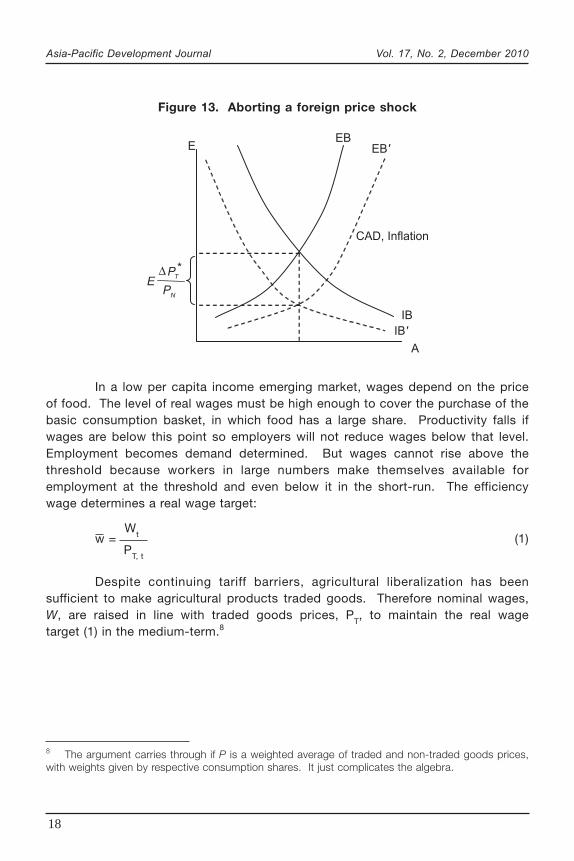
In a low per capita income emerging market, wages depend on the priceof food. The level of real wages must be high enough to cover the purchase of thebasic consumption basket, in which food has a large share. Productivity falls ifwages are below this point so employers will not reduce wages below that level.Employment becomes demand determined. But wages cannot rise above thethreshold because workers in large numbers make themselves available foremployment at the threshold and even below it in the short-run. The efficiencywage determines a real wage target:

w = Wt (1)

Despite continuing tariff barriers, agricultural liberalization has beensufficient to make agricultural products traded goods. Therefore nominal wages,W, are raised in line with traded goods prices, P

T, to maintain the real wage

target (1) in the medium-term.8

Figure 13. Aborting a foreign price shock

CAD, Inflation

EBEB'E

N

TP *

PE

∆

IB'

IB

A

PT, t

8 The argument carries through if P is a weighted average of traded and non-traded goods prices,with weights given by respective consumption shares. It just complicates the algebra.


19

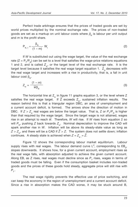
Perfect trade arbitrage ensures that the prices of traded goods are set byworld prices multiplied by the nominal exchange rate. The prices of non-tradedgoods are set as a markup on unit labour costs where β

N is labour per unit output

and m is the profit share.

PN, t

= β

N Wt

(2)

If W is substituted out using the wage target, the value of the real exchangerate (Z = P

T/P

N) can be set to a level that satisfies the wage-price relations equations

1 and 2, and is called Zw, or the target level of the real exchange rate. It is the

target level because it satisfies the real wage target equation 1. Zw

decreases withthe real wage target and increases with a rise in productivity, that is, a fall in unitlabour cost β

N.

Zw =

(1 – m)(3)

The horizontal line at Zw in figure 11 graphs equation 3, or the level where Z

satisfies the real wage target. If Z exceeds Zw, sustained inflation results. The

reason behind this is that a triangular region DBC, an area of unemployment anda current account deficit, is formed. The arrows show the direction of motion inDBC. If Z > Z

w real wages are below the target value. That is, Z or P

T/P

N is higher

than that required by the wage target. Since the target wage is not attained, wagesrise in an attempt to reach w. Therefore, W will rise. If W rises from equation 2 sowill P

N, pushing Z back towards Z

w. Nominal depreciation to improve the CAD will

spark another rise in W. Inflation will be above its steady-state value as long asZ > Z

w, and there will be a CAD if Z > Z. The system does not settle down; inflation

continues. A steady state is achieved when Z = Zw -

= Z.

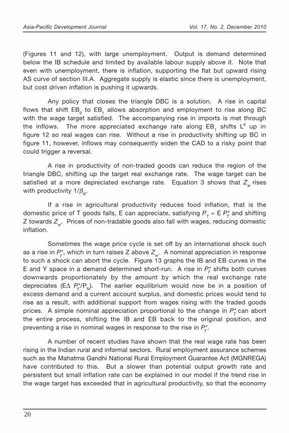
Figure 12 shows the corresponding labour market equilibrium. Laboursupply rises with real wages. The labour demand curve Ld, corresponding to EB

0,

slopes downwards. It shows how, for a given current account, employment rises asthe real wage falls, with absorption adjusted to achieve the given current account.Along EB, as Z rises, real wages must decline since as P

T rises, wages in terms of

traded goods must be falling. Even if the consumption basket includes non-tradedgoods and the prices of these goods hold steady, aggregate price will still rise withP

T.

The real wage rigidity prevents the effective use of price switching, andcan keep the economy in the region of unemployment and a current account deficit.Since a rise in absorption makes the CAD worse, it may be stuck around B,

(1 – m)

wβN

~~

~


20

(Figures 11 and 12), with large unemployment. Output is demand determinedbelow the IB schedule and limited by available labour supply above it. Note thateven with unemployment, there is inflation, supporting the flat but upward risingAS curve of section III.A. Aggregate supply is elastic since there is unemployment,but cost driven inflation is pushing it upwards.

Any policy that closes the triangle DBC is a solution. A rise in capitalflows that shift EB

0 to EB

1 allows absorption and employment to rise along BC

with the wage target satisfied. The accompanying rise in imports is met throughthe inflows. The more appreciated exchange rate along EB

1 shifts Ld up in

figure 12 so real wages can rise. Without a rise in productivity shifting up BC infigure 11, however, inflows may consequently widen the CAD to a risky point thatcould trigger a reversal.

A rise in productivity of non-traded goods can reduce the region of thetriangle DBC, shifting up the target real exchange rate. The wage target can besatisfied at a more depreciated exchange rate. Equation 3 shows that Z

w rises

with productivity 1/βN.

If a rise in agricultural productivity reduces food inflation, that is thedomestic price of T goods falls, E can appreciate, satisfying P

T = E P* and shifting

Z towards Zw. Prices of non-tradable goods also fall with wages, reducing domestic

inflation.

Sometimes the wage price cycle is set off by an international shock suchas a rise in P*, which in turn raises Z above Z

w. A nominal appreciation in response

to such a shock can abort the cycle. Figure 13 graphs the IB and EB curves in theE and Y space in a demand determined short-run. A rise in P* shifts both curvesdownwards proportionately by the amount by which the real exchange ratedepreciates (E∆ P*/P

N). The earlier equilibrium would now be in a position of

excess demand and a current account surplus, and domestic prices would tend torise as a result, with additional support from wages rising with the traded goodsprices. A simple nominal appreciation proportional to the change in P*

can abort

the entire process, shifting the IB and EB back to the original position, andpreventing a rise in nominal wages in response to the rise in P*.

A number of recent studies have shown that the real wage rate has beenrising in the Indian rural and informal sectors. Rural employment assurance schemessuch as the Mahatma Gandhi National Rural Employment Guarantee Act (MGNREGA)have contributed to this. But a slower than potential output growth rate andpersistent but small inflation rate can be explained in our model if the trend rise inthe wage target has exceeded that in agricultural productivity, so that the economy

T

T

T

T

T

T


21

is caught in the inflationary triangle. The analysis underlines the importance ofa rise in agricultural productivity to allow higher real wages without a rise in inflation.

IV. CHRONIC COST PUSH INFLATION: THE POLITICALECONOMY OF FOOD PRICES

In section III.A, it is argued that ill-designed government interventions mayinitially provide short-term benefits but lead to chronic cost-push inflation overtime. Because of the importance of food prices in South Asia, a good example ofthis is illustrated through actions by the Indian Government with regard to foodeconomy,9 which shows the doubtful short-term benefits and longer-termsupply-side inefficiencies.

As such, multiple government interventions were designed to ensure foodsecurity in this populous country where a large number of inhabitants lived belowthe poverty line. Consumers needed food availability at affordable prices andfarmers had to be motivated to increase production to feed the growing population.An elaborate procurement system guaranteed a market and price support for keyfoodgrains. This supported a public distribution scheme that provided subsidizedfoodgrains to the poor. Buffer stocks and trade policy (taxes and tariffs)complemented these objectives. Additional incentives for farmers came fromsubsidized inputs and total exemption from income taxes. Also, some restrictionswere placed on the movement and marketing of some agricultural goods to restrainspeculative hoarding, and on exports to ensure domestic supply.

The Indian Government sets procurement prices based on recommendationsfrom an independent regulator, the Commission for Agricultural Costs and Prices(CACP). Multiple agencies are involved in the process. The Food Corporation ofIndia (FCI) is responsible for procurement and buffer stocks. The Ministry ofAgriculture has a say in policies that affect agricultural pricing and marketing. TheMinistry of Consumer Affairs is concerned with prices consumers pay. Sinceagriculture is a State subject, State policies also affect outcomes, especially in theproduction, marketing and movement of commodities across borders.

In such a setup, the interests of farmers were pitted against those ofconsumers. There was limited coordination among the multiple agencies, which

9 Other countries in the region had similar programmes. For Bangladesh see Rahman and others(2008). Most net food importers such as Asian developing countries intervene to ensure affordablefood. Bangladesh and Sri Lanka are among the top ten global food importers. India is a marginalnet exporter (Nomura, 2010).


22

tended to be insular. Vested interests developed and enforced status-quoism inlarge programmes. As argued below, the greater opening out entailed in the 1990sreforms aggravated dysfunctional parts in the system. It created additional shocksthe system could not adapt to.

Border prices became a focal point for the farmers’ lobby. Althoughagricultural liberalization was slow and fractional, it meant a closer link betweendomestic and border prices. Agricultural exports grew from $4 billion when reformsbegan to $17 billion in the period 2008-2009. The comparative figures for importswere only $1 billion to $5 billion. Sharp rises occurred in exports of meat, dairy,rice, vegetables and fruits, sugar, animal feeds and vegetable oils. Therefore,border price changes could be expected to have a large impact. The World TradeOrganization (WTO) permissible aggregate measure of support was 10 per centand in this case, it was considered to be negative to the extent border pricesexceeded domestic prices. WTO compatible tariff rates are much higher at100 per cent compared to the 30 per cent that are actually applied on agriculturalimports.

Since some agricultural exports were restricted, farmers could argue theywere discriminated against, in order to ensure food security and supply the PublicDistribution System (PDS). Thus, when the gap between border prices and domesticprices rose, there was strong pressure to raise domestic procurement prices. Thiscreated a clear pattern in procurement price increases, changes in stock, anddomestic inflation impulses.

Higher procurement prices were set in the 1970s, when the green revolutioncommenced, as incentives to farmers to adopt new techniques. The distinctionbetween the procurement and support price was lost after the 1970s, and thesupport price, at which farmers could make assured sales, approached the marketprice. In the 1990s, it had overtaken the latter. In the 1980s, meanwhile, the rateof increase was kept low to share the gains of better productivity with consumers.In the 1990s, as productivity growth slowed more rapid price increases were granted.A double devaluation of the exchange rate contributed to upward pressures bywidening the gap between domestic and border prices. The steady increase instocks held by the Government indicated that prices were set too high. Theaverage level rose from 10.1 million tonnes in the 1970s to 13.8 in the 1980s and17.4 in the 1990s (Goyal, 2003). In July 2002, it peaked at 63 million tonnes, thenfell. But in 2010, there was another peak. This cyclic movement in stocks wasa new feature after the reforms.


23

Table 2. Price policy and its consequence

Wheat Wheat

Yearstocks inflation Unit value MSP +/- Agricultural(million (base: (Rs./Qtl) (Rs./Qtl) overmspa growthtonnes) 81-82)

1989-1990 .. .. .. .. .. 2.1

1990-1991 5.6 13.9 223.2 215 8.2 3.8

1991-1992 2.2 15.5 219.3 225 -5.7 -2.0

1992-1993 2.7 10.3 278.2 275 320.0 4.2

1993-1994 7.0 10.4 525.0 330 195.0 3.8

1994-1995 8.7 7.1 488.9 350 138.9 5.8

1995-1996 7.8 -0.5 579.9 360 219.9 -2.5

1996-1997 3.2 18.4 609.5 380 229.5 8.7

1997-1998 5.0 0.6 679.8 475 234.8 -5.1

1998-1999 9.7 9.0 750.0 510 240.0 7.9

1999-2000 13.2 13.1 650.0 550 100.0 -1.8

2000-2001 21.5 1.1 510.3 580 -69.8 -6.0

2001-2002 26.0 -0.7 502.1 610 -107.9 7.6

2002-2003 15.7 0.2 479.4 620 -140.6 -13.2

2003-2004 6.9 3.1 584.0 620 -36.0 21.0

2004-2005 4.1 1.5 727.5 630 97.5 -2.7

2005-2006 2.0 3.9 755.5 640 115.5 4.7

2006-2007 4.7 11.5 757.9 700 57.7 4.3

2007-2008 5.8 4.1 946.0 850 96.0 4.6

2008-2009 13.4 5.8 1 041.0 1 000 41.0 1.6

2009-2010 16.1 9.7 .. 1 080 .. ..

2010-2011 32.1 .. .. 1 100 .. ..

Source: GOI (2010).

Note: a overmsp is the excess of unit export value over minimum support price (MSP).


24

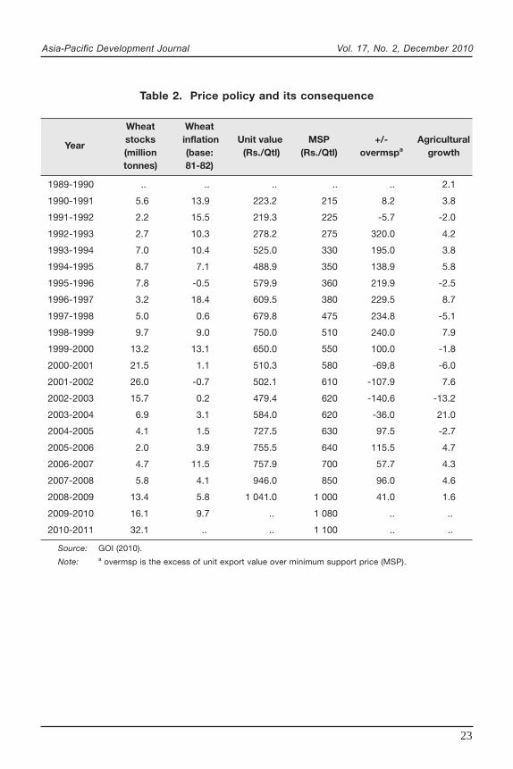
Table 2 gives details for wheat, in the post-reform period. It clearly showshow minimum support price (MSP) responds to the excess of export pricerealizations (unit value) over the MSP, and wheat stocks tend to peak with the risein MSP. Domestic wheat inflation is higher in periods of large exchange ratedepreciation.

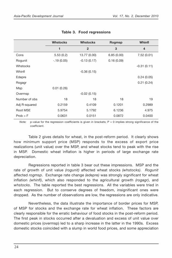
Regressions reported in table 3 bear out these impressions. MSP and therate of growth of unit value (rogunit) affected wheat stocks (whstocks). Rogunitaffected rogmsp. Exchange rate change (edepre) was strongly significant for wheatinflation (whinfl), which also responded to the agricultural growth (rogagr), andwhstocks. The table reported the best regressions. All the variables were tried ineach regression. But to conserve degrees of freedom, insignificant ones weredropped. As the number of observations are low, the regressions are only indicative.

Nevertheless, the data illustrate the importance of border prices for MSP,of MSP for stocks and the exchange rate for wheat inflation. These factors areclearly responsible for the erratic behaviour of food stocks in the post-reform period.The first peak in stocks occurred after a devaluation and excess of unit value overdomestic prices (overmsp) led to a sharp increase in the latter in the 1990s. Excessdomestic stocks coincided with a slump in world food prices, and some appreciation

Table 3. Food regressions

Whstocks Whstocks Rogmsp Whinfl

1 2 3 4

Cons 5.53 (0.2) 13.77 (0.00) 6.85 (0.00) 7.52 (0.01)

Rogunit -.19 (0.05) -0.13 (0.17) 0.16 (0.09)

Whstocks -0.31 (0.11)

Whinfl -0.36 (0.15)

Edepre 0.24 (0.05)

Rogagr 0.21 (0.24)

Msp 0.01 (0.26)

Overmsp -0.02 (0.15)

Number of obs 18 18 18 19

Adj R-squared 0.2159 0.4109 0.1201 0.2989

Root MSE 5.9754 5.1792 6.1236 4.975

Prob > F 0.0631 0.0151 0.0872 0.0400

Note: p-value for the regression coefficients is given in brackets; P = 0 implies strong significance of thecoefficient.


25

144 blank

of the Indian rupee. Some stocks had to be exported at a loss; MSP did notdecrease but only minor increases were registered in those years. As a result,domestic inflation was low. MSP was increased again substantially since stockshad hit a low and unit value again exceeded MSP in the period 2006-2007 afterthe international food price shocks. Price increases in India were staggered,preventing the prices from peaking in tandem with international prices. However,they did not fall even after international food prices fell.

Stocks built up again dramatically even as domestic food inflation continuedin double digits. Steep depreciation and volatility of the Indian rupee contributedto price pressures. The Government was unable to sell its stocks since their costprice exceeded the market price and it was reluctant to offer the stock at a lowprice on concerns that the commodity would be sold back to the Government.So, the State became the biggest hoarder, helping keep prices high.

In retrospect, is appears that the post-reform Government intervention wasdysfunctional. It neither protected the consumer nor was able to induce higherproduction from the farmer. Policies that meant to help the situation resulted in highstorage costs and wastage of grain. These costs, together with the pervasive inputsubsidies, diverted investment for rural infrastructure. Productivity remained low andsupply-side bottlenecks persisted. With regard to the analysis in section III.A, thepolicies contributed to a chronic upward crawl of the AS curve. Low agriculturalproductivity and the shocks from MSP kept the economy in the triangular regionDBC of figure 11 in section III.B. The analysis illustrates the point that directsubsidies can create indirect costs.

V. EVIDENCE ON INFLATION DRIVERS

This section presents some evidence on demand and supply shocks, therole of policy and the pressures creating chronic inflation.

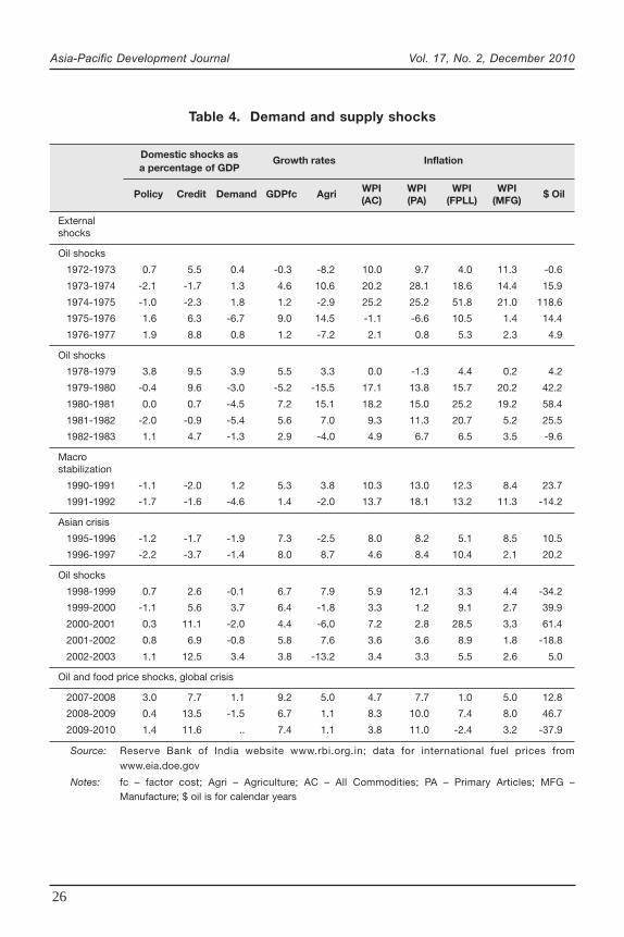
Table 4 gives Indian aggregate and sectoral growth and inflation rates,and calculates policy responses and macroeconomic outcomes for periods ofexternal shocks. The dollar oil price inflation and the FPLL component of the WPIcapture oil price shocks. Agricultural growth and WPI (PA) capture supply shocksemanating from agriculture. For the first three oil price shock episodes, policy andoutcome variables starting from one year before and continuing for one year afterthe price spike are given. Each period saw about a 100 per cent rise in internationaloil prices, but the pass through to Indian prices was a policy decision.


26

Table 4. Demand and supply shocks

Domestic shocks as Growth rates Inflationa percentage of GDP

Policy Credit Demand GDPfc Agri WPI WPI WPI WPI $ Oil(AC) (PA) (FPLL) (MFG)

Externalshocks

Oil shocks

1972-1973 0.7 5.5 0.4 -0.3 -8.2 10.0 9.7 4.0 11.3 -0.6

1973-1974 -2.1 -1.7 1.3 4.6 10.6 20.2 28.1 18.6 14.4 15.9

1974-1975 -1.0 -2.3 1.8 1.2 -2.9 25.2 25.2 51.8 21.0 118.6

1975-1976 1.6 6.3 -6.7 9.0 14.5 -1.1 -6.6 10.5 1.4 14.4

1976-1977 1.9 8.8 0.8 1.2 -7.2 2.1 0.8 5.3 2.3 4.9

Oil shocks

1978-1979 3.8 9.5 3.9 5.5 3.3 0.0 -1.3 4.4 0.2 4.2

1979-1980 -0.4 9.6 -3.0 -5.2 -15.5 17.1 13.8 15.7 20.2 42.2

1980-1981 0.0 0.7 -4.5 7.2 15.1 18.2 15.0 25.2 19.2 58.4

1981-1982 -2.0 -0.9 -5.4 5.6 7.0 9.3 11.3 20.7 5.2 25.5

1982-1983 1.1 4.7 -1.3 2.9 -4.0 4.9 6.7 6.5 3.5 -9.6

Macrostabilization

1990-1991 -1.1 -2.0 1.2 5.3 3.8 10.3 13.0 12.3 8.4 23.7

1991-1992 -1.7 -1.6 -4.6 1.4 -2.0 13.7 18.1 13.2 11.3 -14.2

Asian crisis

1995-1996 -1.2 -1.7 -1.9 7.3 -2.5 8.0 8.2 5.1 8.5 10.5

1996-1997 -2.2 -3.7 -1.4 8.0 8.7 4.6 8.4 10.4 2.1 20.2

Oil shocks

1998-1999 0.7 2.6 -0.1 6.7 7.9 5.9 12.1 3.3 4.4 -34.2

1999-2000 -1.1 5.6 3.7 6.4 -1.8 3.3 1.2 9.1 2.7 39.9

2000-2001 0.3 11.1 -2.0 4.4 -6.0 7.2 2.8 28.5 3.3 61.4

2001-2002 0.8 6.9 -0.8 5.8 7.6 3.6 3.6 8.9 1.8 -18.8

2002-2003 1.1 12.5 3.4 3.8 -13.2 3.4 3.3 5.5 2.6 5.0

Oil and food price shocks, global crisis

2007-2008 3.0 7.7 1.1 9.2 5.0 4.7 7.7 1.0 5.0 12.8

2008-2009 0.4 13.5 -1.5 6.7 1.1 8.3 10.0 7.4 8.0 46.7

2009-2010 1.4 11.6 .. 7.4 1.1 3.8 11.0 -2.4 3.2 -37.9

Source: Reserve Bank of India website www.rbi.org.in; data for international fuel prices from

www.eia.doe.gov

Notes: fc – factor cost; Agri – Agriculture; AC – All Commodities; PA – Primary Articles; MFG –Manufacture; $ oil is for calendar years


27

The table captures the monetary and fiscal response in the “Policy” variable.This is calculated as the rate of change of reserve money, Central Governmentrevenue, and capital expenditure, each as a percentage of GDP. That is, period tgives the total of the three variables each minus their respective values in periodt-1. A negative value implies policy contraction exceeding that in GDP. The tableshows this to be negative in years when the GDP growth rate fell due to an externalshock. Thus policy amplified the shocks.

The “credit” variable does a similar calculation for broad money M3, bankcredit to the commercial sector and total bank credit, capturing outcomes of policytightening. This was more severe in the earlier shocks. The availability of morefinancial substitutes and of external finance reduced the impact of policy tighteningon credit variables. Policy was now acting more through prices (interest ratechanges) than quantities. The world over, as financial markets deepen, centralbanks switch to targeting short-term interest rates, as nominal money targetsbecome difficult to achieve with unstable money multipliers. Quantitative responseis moderated since it becomes less effective.

Finally, the “demand” variable is the sum of changes in C, G, GrossDomestic Capital Formation (GDCF),10 and CAD as a percentage of GDP. Thus,each shock plus the policy response imparted a considerable negative impulse toaggregate demand. While the supply shock pushed up the As of section III.A, thepolicy response shifted the AD leftwards. The general perception is that demandand supply factors cause inflation (Mohanty, 2010). But the analysis suggests thatif demand falls when supply side shocks are pushing up inflation, demand cannotbe contributing to inflation.

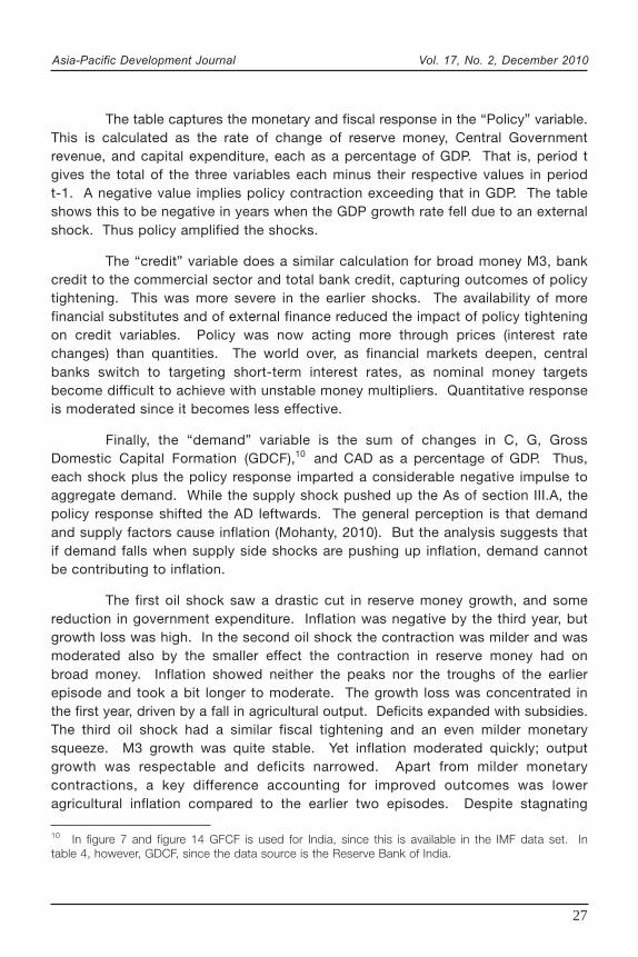
The first oil shock saw a drastic cut in reserve money growth, and somereduction in government expenditure. Inflation was negative by the third year, butgrowth loss was high. In the second oil shock the contraction was milder and wasmoderated also by the smaller effect the contraction in reserve money had onbroad money. Inflation showed neither the peaks nor the troughs of the earlierepisode and took a bit longer to moderate. The growth loss was concentrated inthe first year, driven by a fall in agricultural output. Deficits expanded with subsidies.The third oil shock had a similar fiscal tightening and an even milder monetarysqueeze. M3 growth was quite stable. Yet inflation moderated quickly; outputgrowth was respectable and deficits narrowed. Apart from milder monetarycontractions, a key difference accounting for improved outcomes was loweragricultural inflation compared to the earlier two episodes. Despite stagnating

10 In figure 7 and figure 14 GFCF is used for India, since this is available in the IMF data set. Intable 4, however, GDCF, since the data source is the Reserve Bank of India.


28

domestic agriculture, falling international prices in a more open regime had counteredpolitical pressures to ratchet up procurement prices.

The crude price shock during period 2002-2005 was equivalent to earlierepisodes but the world, including India, bore it better than past episodes. Thereasons behind this were openness, cheap imports, rising productivity that lowercosts, less dependence on oil and more credible anchoring of inflation. There wasalso the absence of other adverse shocks.

But falling international food prices reversed in 2003, and the rise wasparticularly steep in 2007 (45.28 per cent) and 2008 (12.5 per cent), as competitionfrom biofuels intensified. After being almost stationary from 1999, Indianprocurement prices also jumped in the period 2006-2007, and inflation in primaryarticles reached 7.8 per cent. Crude oil rose sharply: more than 100 per centduring the period 2002-2005, and another 100 per cent since then. The oil poolaccount and administered price mechanism created in 1974 was dismantled in2002 but administered prices were retained for petrol, diesel, kerosene and gas.The Government did not fully pass on these shocks. However, it was unable tosubsidize the sheer magnitude of the rise and finally raised prices in 2008. Sincefuel prices neither rose nor fell as much as in the international market, cumulativeIndian fuel inflation had exceeded international fuel inflation until 2005; after that itwas less. In 2010, petrol prices were also deregulated. As in the case of foodpolicy, intervention did not lead to the price rises seen in the international market,but prices did not fall with the international market, so that costs moved in only anupward direction.

The global financial crisis followed the oil shock. Oil prices crashed butlarge liquidity made available by stimulus programmes fuelled inflation incommodities. For the first time, counter cyclical macroeconomic policy, enabledby the coordinated global stimulus, created a demand stimulus, although the overalldemand shock was still negative. But high food price inflation led to a rapidresurgence of inflation, and a delayed exit failed to anchor inflation expectations.

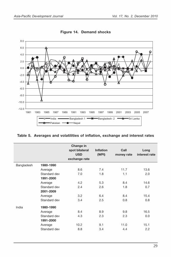
Figure 14 graphs the demand shocks for the countries of South Asia. Thepolicy aggravation of supply shocks was even higher in other countries. Theseries in the graph are calculated leaving out the CAD. A large CAD impliesdomestic resources are less than domestic requirements, but it is a consequenceof domestic demand, rather than an additional demand component. A CAD alsoimplies domestic demand is leaking abroad. Including it in the calculation ofdemand shock reduces demand even more as it widens during downswings. Thetwo series for Bangladesh accommodate the data break that leads to an outlier in1988.


29

Figure 14. Demand shocks

Table 5. Averages and volatilities of inflation, exchange and interest rates

Change inspot bilateral Inflation Call Long

USD (WPI) money rate interest rateexchange rate

Bangladesh 1980-1990Average 8.6 7.4 11.7 13.6Standard dev 7.0 1.8 1.1 2.01991-2000Average 4.2 5.3 8.4 14.6Standard dev 2.4 2.6 1.8 0.72001-2009Average 3.2 6.4 8.4 15.4Standard dev 3.4 2.5 0.8 0.8

India 1980-1990Average 8.4 8.9 9.8 16.5Standard dev 4.3 2.3 2.3 0.01991-2000Average 10.2 9.1 11.0 15.1Standard dev 8.8 3.4 4.4 2.2

-12.0

-10.0

-8.0

-6.0

-4.0

-2.0

0.0

2.0

4.0

6.0

8.0

1981 1983 1985 1987 1989 1991 1993 1995 1997 1999 2001 2003 2005 2007

India Bangladesh 1 Bangladesh- 2 Sri Lanka

Pakistan Nepal


30

2001-2009Average 1.0 5.7 5.9 11.9Standard dev 6.1 2.5 1.5 0.9

Maldives 1985 0.7 .. 9.0 9.12001 4.0 .. .. 7.02009 .. .. .. 6.5

Nepal 1980-1990Average 9.5 10.2 5.4 12.6Standard dev 4.9 4.1 0.9 1.91991-2000Average 9.5 9.1 6.6 10.5Standard dev 7.9 4.6 3.0 1.82001-2009Average 1.1 6.4 3.8 6.1Standard dev 6.0 3.3 1.4 0.4

Sri Lanka 1980-1990Average 9.3 12.4 18.7 12.7Standard dev 4.1 5.8 3.8 2.41991-2000Average 6.8 9.7 22.6 14.7Standard dev 2.9 3.3 7.7 2.02001-2009Average 4.7 11.2 15.9 12.7Standard dev 5.4 5.7 7.8 4.5

Pakistan 1980-1990Average 8.3 7.0 7.8 9.0Standard dev 6.0 2.5 1.3 0.91991-2000Average 9.5 9.2 9.8 10.6Standard dev 3.4 3.2 7.7 3.92001-2009Average 5.1 8.4 7.6 7.4Standard dev 8.3 5.6 3.6 2.9

Source: Calculated from IMF, IFS data.

Table 5. (continued)

Change inspot bilateral Inflation Call Long

USD (WPI) money rate interest rateexchange rate


31

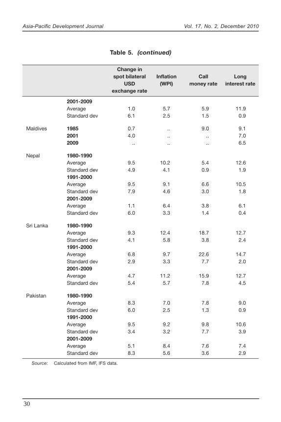
Table 5 reports averages and standard deviations in exchange ratedepreciation, inflation, and short- and long-term interest rates for South Asiancountries during the pre-reform decade, the decade when reforms commencedand one post-reform decade. In the pre-reform decade, administered price andquantitative interventions repressed markets and kept volatilities low, but as theequilibrium was fragile, this led to a large impact of external shocks. Countries inthe region lifted controls and liberalized markets in the 1990s. Initially volatilityincreased. Openness was itself a source of shocks as it increased diversity, whichtogether with the deepening of markets reduced volatility. India shows an initiallow, then rise fall pattern in volatility. Deeper markets are able to absorb shockswithout high volatility in prices. In smaller, more open countries, volatility remainshigh. In Pakistan and Sri Lanka internal unrest and political instability also vitiatedthe pattern. But all the countries in the table adopted more flexible exchangerates, resulting in a drop in average levels of inflation and interest rates.

During the period 1996-2003, average interest rates rose sharply and theirvolatility exceeded that of exchange rates, partly due to the East Asian crisis andthe use of interest rate defence, explaining the large fall in credit and demandduring the Asian crisis (table 4). Exchange rate movements were restricted at thecost of higher interest rate movements. During the recent global financial crisis,the fall in credit and demand was much lower partly because more exchange rateflexibility allowed interest rates to target the domestic cycle.

The current consensus is that a managed float is one of the best exchangerate regimes for an emerging market (Corden, 2002). Svensson (2000) emphasizesthat the exchange rate is an important tool of monetary transmission for a smallopen economy, with the lowest lag for the consumer price index. In line with theconsensus, exchange rates in the region have moved to greater flexibility, but theyare still managed.

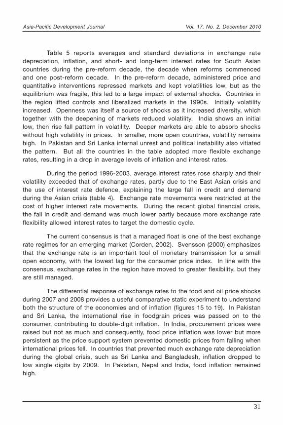
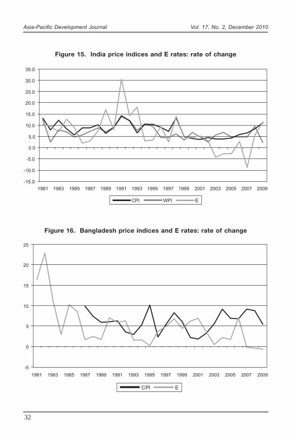
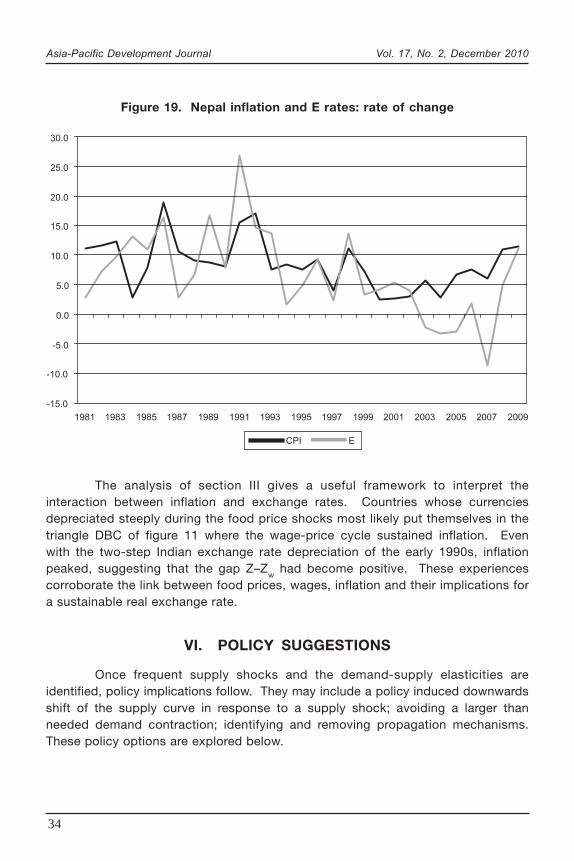
The differential response of exchange rates to the food and oil price shocksduring 2007 and 2008 provides a useful comparative static experiment to understandboth the structure of the economies and of inflation (figures 15 to 19). In Pakistanand Sri Lanka, the international rise in foodgrain prices was passed on to theconsumer, contributing to double-digit inflation. In India, procurement prices wereraised but not as much and consequently, food price inflation was lower but morepersistent as the price support system prevented domestic prices from falling wheninternational prices fell. In countries that prevented much exchange rate depreciationduring the global crisis, such as Sri Lanka and Bangladesh, inflation dropped tolow single digits by 2009. In Pakistan, Nepal and India, food inflation remainedhigh.


32

Figure 15. India price indices and E rates: rate of change

Figure 16. Bangladesh price indices and E rates: rate of change

-15.0

-10.0

-5.0

0.0

5.0

10.0

15.0

20.0

25.0

30.0

35.0

1981 1983 1985 1987 1989 1991 1993 1995 1997 1999 2001 2003 2005 2007 2009

CPI WPI E

-5

0

5

10

15

20

25

1981 1983 1985 1987 1989 1991 1993 1995 1997 1999 2001 2003 2005 2007 2009

CPI E


33

-10.0

-5.0

0.0

5.0

10.0

15.0

20.0

25.0

30.0

1981 1983 1985 1987 1989 1991 1993 1995 1997 1999 2001 2003 2005 2007 2009

CPI WPI E

Figure 18. Pakistan price indices and E rates: rate of change

Figure 17. Sri Lanka price indices and E rates: rate of change

-20.0

-15.0

-10.0

-5.0

0.0

5.0

10.0

15.0

20.0

25.0

30.0

1981 1983 1985 1987 1989 1991 1993 1995 1997 1999 2001 2003 2005 2007 2009

CPI WPI E


34

The analysis of section III gives a useful framework to interpret theinteraction between inflation and exchange rates. Countries whose currenciesdepreciated steeply during the food price shocks most likely put themselves in thetriangle DBC of figure 11 where the wage-price cycle sustained inflation. Evenwith the two-step Indian exchange rate depreciation of the early 1990s, inflationpeaked, suggesting that the gap Z–Z

w had become positive. These experiences

corroborate the link between food prices, wages, inflation and their implications fora sustainable real exchange rate.

VI. POLICY SUGGESTIONS

Once frequent supply shocks and the demand-supply elasticities areidentified, policy implications follow. They may include a policy induced downwardsshift of the supply curve in response to a supply shock; avoiding a larger thanneeded demand contraction; identifying and removing propagation mechanisms.These policy options are explored below.

Figure 19. Nepal inflation and E rates: rate of change

-15.0

-10.0

-5.0

0.0

5.0

10.0

15.0

20.0

25.0

30.0

1981 1983 1985 1987 1989 1991 1993 1995 1997 1999 2001 2003 2005 2007 2009

CPI E


35

A. Temporary shocks

Examples of temporary shocks that raise domestic prices are monsoonfailures and international oil or other commodity shocks that raise border prices.These have been dominant inflation triggers. Mild monetary tightening after a costshock can prevent inflationary wage expectations from setting in and further shiftingup the supply curve. But a sharp tightening that shifts aggregate demand leftwardswould have a large output cost with little effect on inflation. Reasonable interestrates encourage the supply response. A first round price increase from a supplyshock should be allowed, but a second round wage-price increase should beprevented from setting in.

If the nominal exchange rate rises11 (falls) with a fall (rise) in world foodgrainprices, domestic prices stay unchanged.12 This applies similarly for oil price shocksin South Asia as the region is heavily dependent on oil imports. An oppositechange in the nominal exchange rate in response to a temporary shock can preventdistorting administrative interventions that affect the food and oil sector.

There are short-term fiscal policies that shift down the supply curve, suchas tax-tariff rates, and freer imports. Trade policy works best for individual countryshocks that are not globally correlated. Nimble private trade can defeat speculativehoarders.

These short-run policies work only for a temporary shock. A permanentshock requires a rise in productivity to successfully prevent inflation. This isexamined in sections B and C below.

B. Preventing chronic cost-push inflation

Food prices play a major role in propagation mechanisms, since they raisenominal wages with a time lag. A fundamental reason for chronic supply sideinflation is that target real wages exceed labour productivity, so the solution is toraise worker productivity. Higher agricultural productivity is especially necessaryto anchor food price inflation.

11 Goyal (2003) simulated such a policy using wheat prices. It led to a coefficient of variation of 0.2for the nominal exchange rate, and removed the high wheat inflation of the 1990s.12 Shifting to winter daylight savings time in the United States of America saves thousands of firmsfrom having to change their working hours. However, changing one exchange rate prevents thousandsof nominal price changes that then become sticky and persist, requiring a painful prolonged adjustment.


36

With some liberalization, farm produce become traded goods andconsequently, border prices begin to affect domestic food prices. A target real wagein terms of food prices then implies a target real exchange rate or ratio of traded tonon-traded goods prices. In this case, the exchange rate contributes to inflationpropagation mechanism. If the real exchange rate required to satisfy a real wagetarget rate appreciates above the rate required for equality of aggregate demand andsupply, wages rise, raising the prices of non-traded goods. A nominal depreciationto increase demand helps sustain the cycle of continuous inflation. Higherproductivity of non-traded goods can shift up the target real exchange rate, sothe wage target can be satisfied at a more depreciated exchange rate, breakinga potential wage-price chain.

A rise in agricultural productivity allows the nominal exchange rate toappreciate, bringing the real exchange rate closer to the target real exchange rateand closing the inflationary gap between them, even while agricultural pricescontinue to equal border prices.

Inflows appreciate the exchange rate and remove chronic inflation. Thewage target is reached and the accompanying rise in imports met through theinflows. But it involves a risky widening of the current account deficit as appreciationencourages imports. Rising productivity increases the level of inflows that can besafely absorbed since the target exchange rate is more depreciated, encouragingexports. The CAD then still allows investment to exceed domestic savings butdoes not become too large.

C. Governance

Better governance and delivery of public services is necessary to improveproductivity. Reform of food policy is urgent given the relentless food inflation.East Asian countries were careful to moderate food price increases and focus ona rise in agricultural productivity as long as food budget shares remained high.Food prices and the nominal rate of protection in agriculture was allowed to riseonly after the food budget shares fell (Goyal, 2003). In addition, agriculture wastaxed to fund development. Nevertheless, low food prices did not preventagricultural incomes from rising, since at low per capita income levels demand forfood is elastic. When development proceeded sufficiently to lower budget sharesbelow 50 per cent, farm incomes began falling and governments turned from taxingto subsidizing agriculture. Since the share of the population in agriculture wasnow small, this was not a burden. In this period, food prices began to rise. Sincefood was now a small part of the budget, prices could rise without putting pressureon wages and inflation. As food budget shares fall agriculture must shrink.


37

In India, the move to subsidize agriculture came when food budget shareswere still high. Food still accounted for more than 50 per cent of householdexpenditure among 95 per cent of rural households and 80 per cent of urbanhouseholds in the 1990s (Goyal, 2003). More than 70 per cent of the populationwas still in rural areas even in the 2000s. The weight of the food group is48.46 per cent in the new CPI-Industrial Workers base 2001. For low-incomegroups the share exceeds this while for high-income groups, it is lower.

Although the increase in the absolute agricultural price level was lower inthe 1980s, output growth was more rapid. India is still in the range where incomeelasticities of demand for agriculture are high,13 so that agricultural incomes risemore with increases in output, even after correcting for the effect of buffer stockand public food distribution policy. A more moderate nominal price increase enablesbetter agricultural output and income growth.

Rising agricultural price levels do not guarantee favourable agriculturalterms of trade, as nominal wages and industrial prices also increase. Over time,stable prices provide better incentives for farmers. If the procurement price wereto become a true support price, foodstocks would reduce in a bad agriculturalseason when market prices rise, and increase as market prices fall in a good year.Farmers would get some assured income support even as the removal of restrictionson the movement and marketing of agricultural goods and better infrastructureallows them to diversify crops. Since price support can also use the option of justpaying the difference between market and support prices, stocks need not risewhen they are already high.

In reaction to the lower average stocks, public distribution schemes shouldfocus on remote places where there are no private shops, or on very poor areas.Food coupons or cash transfers to women can provide support to those below thepoverty line14 while allowing them to diversify their food basket, as recent studiesindicate. Foodgrains, for which the elaborate food policy structure is designed,now account for only 25 per cent of agricultural output. Thorough supply-sidereform is required.

But such reform may take time to achieve. The analysis in this sectionhas brought out the focal role of the unit value, which acts as a trigger for multipleinterest groups to force undesirable policies such as a rise in MSP. Political jostling

13 Nomura (2010) puts $3,000 as the per capita income level after which income elasticities ofdemand fall.14 Basu (2010) has argued for such a policy redesign. Cash transfers to women are effectivebecause women are more likely to apply them for family needs.


38

focuses on the short-term, ignoring negative long-term effects. Poor coordinationamong multiple agencies means they do not factor in each other’s costs. Theyalso neglect the big picture. Until thorough food policy reform occurs, a possibleappreciation of the nominal exchange rate can prevent a sharp rise in border pricesfrom triggering multiple interest group action and resulting in complex domesticdistortions.

D. International

Emerging markets must find non-distortionary ways to respond to spikesin food and commodity prices, but large global spikes imply macro distortionsbeyond supply shocks (Gilbert, 2010), which should also be prevented. Policiessuch as quantitative easing that aim to drive up prices across asset categoriesshould be implemented sparingly if at all. Excess liquidity creation in the West andpoor real sector response are sending funds into commodities, and this may becontributing to price spikes. Investors have turned to commodity markets forspeculation or for portfolio diversification.

What is the role of futures markets? A large number of studies of the 2008commodity spike, surveyed in Irwin and Sanders (2010), have on balance not foundevidence that the large-scale entry of index funds in commodity derivatives droveup prices. A correlation did occur but the correlation does not necessarily implycausality. Time series tests on the whole reject causality but they have their ownflaws. Lack of convergence between spot and futures prices in certain marketsalso suggest problems in the working of these markets. A price spike aboveequilibrium levels in a storable commodity should raise its stocks, but stocks weredeclining in most commodity markets during that period. Moreover, prices ofagricultural commodities without futures markets also rose at the same time. AnIndian committee was set up to examine the effect of commodity futures marketsas agricultural inflation rose (GOI, 2008). It found no unambiguous evidence of theeffect of futures trading on inflation. For some commodities, inflation hadaccelerated after the introduction of futures, for others it had slowed down.Commodities where futures were banned such as sugar, tur and urad dals hadhigher inflation.

When inventories of a storable commodity are low, a demand or supplyshock can result in a sharp price rise for that particular commodity. This is becauseit takes time for supply to increase. In such conditions, trading sends the priceshigher merely because the market expects the prices to increase. Buying futuresdoes not have the same effect as hoarding a commodity. Opposite paper positionscan be generated in deep and liquid markets. As long as informed traders dominate


39

the markets, values are unlikely to deviate far from fundamentals. But herdbehaviour, momentum trading and overreaction, make price discovery in financialmarkets flawed. Since futures markets serve the purpose of helping producersplan future output and to hedge risks, the answer is not to ban them, but toimprove their operations.

Restricting participants in the market is counterproductive to creatingliquidity. However, position limits can be used to reduce the share of speculativetransactions. Contracts can be designed to encourage hedging over speculationby distinguishing between hedgers and speculators with differential margins anddiscounts in fees or taxes for each category. Margins that increase with pricecould reduce momentum trading. Since spot and futures markets around theworld are becoming tightly integrated, convergence to common regulatory standardsis necessary. One region with lax standards can affect others, especially duringirrational periods of fear or hype. For example, most regulators impose positionlimits. The U.S. regulator finally proposed position limits in four energy commoditiesin 2010, but the European Union and a few other markets still do not have them.In 2009, a U.S. Senate subcommittee suggested a position limit of 5,000 contractsper wheat trader. The practice of giving position limit waivers should bediscontinued. Arbitrage occurs in response to selective or regional regulatorytightening. Coordinated improvements in financial regulation are required to reduceglobal commodity price spikes.

VII. CONCLUSION

The similarities yet differences across South Asian countries, and theirdifferential response to the severe food, oil price and other external shocks, providesa useful opportunity to better understand the structure of inflation in theseeconomies. The analysis and evidence in this paper implies output is largely demanddetermined but inefficiencies on the supply side cause inflation. Since outputvolatility exceeded that of demand components, the latter were not an independentsource of shocks. Procyclical policy, however, amplified the negative impact ofsupply shocks on output. Reduction in inflation was achieved at a high outputcost. But well-intentioned administrative interventions turned relative price shocksinto chronic cost-push inflation. The analysis shows why food price shocks canaggravate inflation. It is very important to protect the poor from inflation, especiallyfood inflation. But it must be done effectively.

Controlling inflation is important for the very survival especially ofdemocratic governments in the region. But complex and counterproductive schemesprovide temporary respite, only to pass the problem on to the future. Onions are


40

widely consumed by the poor; so when the prices of onions shot up in 1998, theanger of the electorate almost brought down the Indian Government. A cartoonpictured Amartya Sen, who had recently been awarded the Noble prize in economics,talking on the phone: “Yes Minister, thank you Minister, no, I do not have a theoryto bring down the price of onions”. The year 2010 again saw a sharp 600 per centrise in onion prices. The problem continues to be as urgent as it is unresolved.Knowledge of structure and behaviour makes successful anticipation and preventionpossible. Structural features and supply-side policies offer additional instrumentsto reduce inflation.


41

REFERENCES

Basu, K. (2010). “The economics of foodgrain management in India”, Ministry of Finance WorkingPaper No. 2/2010-DEA.

Corden, W.M. (2002). Too Sensational: On the Choice of Exchange Rate Regimes (CambridgeMA, MIT Press).

Gilbert, C.L. (2010). “How to understand high food prices”, Journal of Agricultural Economics,vol. 61, No. 2, pp. 398-425.

Gokarn, S. (2010). “The price of protein”, Inaugural Address at Special Conference in honour ofDr. Kirit Parikh at IGIDR, Mumbai on October 26.

Goyal. A. (2011). “Exchange rate regimes and macroeconomic performance in South Asia”, inRaghbendra Jha (ed.) Routledge Handbook on South Asian Economies, forthcoming.

Goyal, A. (2009a). “Swan diagram”, in Ramkishen S. Rajan, Kenneth A. Reinert (eds.) PrincetonEncyclopedia of the World Economy, (Princeton, New Jersey, Princeton University Press).

Goyal, A. (2009b), “The natural interest rate in emerging markets”, in Bhaskar Dutta, Tridip Roy,and E. Somanathan (eds.), New and Enduring Themes in Development Economics, (WorldScientific Publishers).

Goyal, A. (2008). “Incentives from exchange rate regimes in an institutional context”, Journal ofQuantitative Economics, January & July, vol. 6, No. 1&2, pp. 101-121.

Goyal A. (2005). “Exchange rates, food price stabilization & inflation”, in M. Sharma (ed.), LeadingIssues in Indian Economy, (Delhi, Atlantic Publishers and Distributors).

Goyal A. (2004). “The impact of structure and openness on the causal ordering of interest,inflation and exchange rates”, Journal of Quantitative Economics, Special Issue in Memoryof M.J. Manohar Rao, July, vol. 2, No. 2, pp. 223-242.

Goyal A. (2003). “Agriculture and industry: enhancing mutual gains”, Decision, July-December,vol. 130, No. 2.

Goyal A. and A.K. Pujari. (2005). “Identifying long-run supply curve in India”, Journal of QuantitativeEconomics, July, vol. 3, No. 2, pp. 1-15.

GOI (Government of India) (2010). Reports of the Commission for Agricultural Costs and Prices:for the crops Sown During 2009-10 Season. Commission for Agricultural Costs andPrices (CACP).

GOI (Government of India) (2008). Report of the Expert Committee on Commodity Futures, May.

Irwin, S.H. and D.R. Sanders. (2010). “The impact of index and swap funds on commodityfutures markets: preliminary results”, OECD Food, Agriculture and Fisheries WorkingPapers, No. 27, OECD Publishing.

Joshi, V. and I.M.D. Little. (1994). India: Macroeconomics and Political Economy 1964-1991,(Delhi, Oxford University Press).

Mohanty, D. (2010). “Perspectives on inflation in India”, Speech given at the Bankers Club,Chennai, 28 September.

Nomura. (2010). The Coming Surge in Food Prices. Nomura Global Economics and Strategy.

Rahman, M., D. Bhattacharya, W.B. Shadat, and U. Deb. (2008). “Recent inflation in Bangladesh:trends, determinants and impact on poverty”, Centre for Policy Dialogue: Dhaka.


42

Salter, Walter E. (1959). “Internal and external balance: the role of price and expenditure effects”,Economic Record, August, vol. 35, Issue 71. pp. 226-238.

Swan, Trevor W. (1960). “Economic control in a dependent economy”, Economic Record, March,vol. 36, Issue 73, pp. 51-66.

Svensson, L.E.O. (2000), “Open-economy inflation targeting”, Journal of International Economics,vol. 50, pp. 155-183.

Woodford, M. (2003). Interest and prices: Foundations of a Theory of Monetary Policy, (NewJersey, Princeton University Press).

Data sources

International Monetary Fund, International Financial Statistics, various issues.

India, Central Bank and Government of India (GOI) websites.

India, RBI Handbook of Statistics on the Indian Economy, Reserve Bank of India.

For crude oil: www.eia.doe.gov.

Documents

INFLATIONARY PRESSURES IN SOUTH ASIA · INFLATIONARY PRESSURES IN SOUTH ASIA ... as India and Pakistan, experienced double-digit inflation rates. ... To identify the underlying causes