Effect of Volume of Heat Sink on Process and Physical Properties of Parts Built by Welding Based SFF

Z. Jandric, J. H. Ouyang and R. Kovacevic

Research Center for Advanced Manufacturing

Department of Mechanical Engineering, Southern Methodist University 1500 International Pkwy. Ste. 100, Richardson, TX 75081

Abstract A new numerical simulation of the effect of the volume of the heat sink on the welding–based deposition process is performed. For this purpose, the ANSYS parametric design language (APDL) is applied. Due to the complex internal and/or external shapes of the designed three-dimensional (3D) part, different heat transfer conditions are met during the building process. The influences of the different heat transfer conditions on the physical part properties are also investigated. The influence of the volume of the heat sink on the process and on the physical properties is significant and can not be neglected. Extensive experiments are designed and executed in order to verify the conclusions derived from the finite elements model results and to investigate the material properties of the built part. Introduction The majority of the solid freeform fabrication (SFF) techniques use non-metallic materials for building parts. SFF based on welding is technique capable of making the 3D metallic parts. Any weldable metal can be used as a material for deposition. Also, several research-teams [1 – 9] have shown that this technique is capable of making diverse part shapes. Spencer et al. made a vertical wall and a hollow box. Ribeiro et al. made a ‘chimney’ shape, a ‘bow tie’ shape, and a ‘pint glass’ shape. Kovacevic et al. also made a thin vertical wall, cylinders, cubical 3D parts with straight channels, a 3D part with complex geometry and a 3D network of the cooling/heating conformal channels. The biggest challenge for this process is to control the process parameters. Namely, during the deposition process, it was apparent that process parameters cannot remain constant since the deposited layers were not smooth. In some instances, the beads were flat and wide, but in others they were tall, and looked like the heat input was insufficient. We looked for possible reasons for such huge fluctuations, and the influence of the geometry of the previously deposited layers was the only answer. This phenomenon is further investigated by modeling it with finite element method (FEM). For this purpose, the ANSYS parametric design language (APDL) is applied. A substantial amount of research has been documented for modeling and understanding the welding process. Rosenthal [10] and Rykalin [11] developed a solution to the heat equation for point and line heat sources on idealized geometries such as infinite plates. Because of computational difficulties encountered when attempting to include inelastic strains in an analysis in which rapid temperature changes take place, some analytical work was carried out that goes beyond Tall’s one-dimensional analysis of longitudinal stress [12].

331

A determination of the complete thermo-mechanical response due to welding requires a full three-dimensional inelastic analysis of mechanical behavior, accompanied by a computation of the three-dimensional transient temperature distribution. In the last decade, models for nonlinear transient finite element heat transfer analyses of the welding process have been developed [13 - 15]. Numerical modeling requires, at the beginning, considerable time and effort, but once the model is obtained, it is easy to change any welding parameter, welding conditions, type of the material, etc. The objective of this research is to numerically simulate the welding process during the deposition process and to evaluate the physical characteristics of the deposited material as a function of heat sink volume. Finite Element Model In this study, the commercial finite element software (ANSYS) was employed. It provides a convenient means of numerically modeling the welding process. The model is discretized into individual finite elements that collectively approximate the shape of the model. A 3D thermal solid element type with a 3D thermal conduction capability is used. The element has eight nodes with a single degree of freedom, temperature, at each node. The element is applicable to a three-dimensional, steady-state or transient thermal analysis. In our model, we mostly used a ‘mapped’ mesh so that the mesh has a regular pattern with obvious rows of elements (Fig. 1). Also, we used transition-mapped hexahedral meshing, by specifying line divisions on the side edges of the volume such that the divisions permit a transition-mapped hexahedral mesh, i.e. the elements at the top layer of the substrate are defined with a significantly smaller height than the elements at the very bottom of the substrate, since the temperature gradients in the vicinity of the top surface, where a heat flux is applied, is much higher. For this model, the thermal fields and thermal history is required, so a transient thermal analysis must be performed. This requires an integration of the heat conduction equation with respect to time. The basic FEM equation for the thermal problem can be derived from the thermal equilibrium equation:

( ) { } ( ) { } { } { }C T T K T T V Q+ + = � (1)

where

[ ] [ ][ ]T

VC c N N dVρ= ∫ is the heat capacity matrix

[ ]N = the shape function matrix

[ ] [ ][ ]T

T VK k B B dV= ∫ is heat conduction matrix

{ }T and { }T� are nodal temperature vector and nodal

temperature rate vector, respectively, and { }Q = the heat flux vector

Modeling Results The isotherms obtained with the 3D thermal analyses for different time intervals are given in Fig. 3a – 3f. Points of interest are located, where the surrounding mass of the material varies between

Fig. 1 Meshed model.

332

12% and 100% of the maximum possible (points are marked with the letters A – F, see Fig. 2). The heat input is kept constant and moves across the top surface at a steady rate. In the model, heat flux travels at speed of 23 cm/min. That is the actual speed that was used during depositon of material in welding-based SFF.

From these figures, it can be observed the change of temperature with different heat transfer conditions. Consequently, the size of the molten pool and the size of the heat affected zone alter as well. The central temperature contour in each image represents a critical temperature of 1530°C as the melting temperature. Hence, this contour denotes the

Fig. 2 Geometry of the model.

boundary of the molten pool. In Fig. 4 is shown a 45° corner together with the molten pool and the heat affected zone.

a) b) c)

d) e) f)

Fig. 3 Temperature fields as a function of volume of heat sink.

In Fig. 4a the heat input is far from the corner (45°), so that the volume of heat sink is half of the maximum possible one. At this instant, there is barely enough heat to melt material and consequently a small molten pool is formed. In Fig. 4b, the heat input is closer to the corner, the volume of the heat sink is decreased, and, the amount of the melted material is enlarged. In the Fig. 4c, the heat input is placed above the corner itself. The volume of the heat sink is four times smaller than in the first case, and as a result, the molten pool and heat affected zone are much larger.

a) b) c)

Fig. 4 Influence of the geometry on the size of the molten pool and the heat affected zone.

333

Although the difference between these three cases is obvious, it is not easy to quantify it through the numerical values. For this purpose, the temperature history was used. Temperature history from the model is verified experimentally by employing the thermocouples (see Fig. 5). For each thermocouple a hole is drilled in the appropriate edge. Each hole is drilled vertically from the bottom toward the top of the sample. The depth of the each channel is for 1.5 mm less than the height of the sample. To isolate thermocouples from noise that originates from the arc, in the bottom of each channel, thermally conductive and electrically insulating high temperature cement is placed. The thermocouples and thermally conductive cement are inserted together,

and left for the cement to cure. In order to compare the temperature history from the model with experimental results, nodes 1.5 mm beneath the top surface, from each corner, are selected. The temperatures from the model, for all angles, are recorded in time (Fig. 6). It could be seen that smaller heat sinks achieve a much higher temperature, and accordingly the molten pool enlarges. These results are also in good standing with the results obtained by Kamala et al. [16], where they also showed that the temperature increases when the heat flux is approaching a smaller heat sink. Direct comparisons of experimental and modeling results, for angles of 45° and 90° are shown in Fig 7. a) and b), respectively. It is evident that the experimental results are lower than those from the model. There could be several reasons for this difference: the model has several assumptions (such as the heat input remains constant during the process while in reality fluctuations in the current and voltage cannot be avoided, so, to minimize the error, the mean value is used; the workpiece is at a uniform temperature before the deposition starts; the body is exposed to a uniform forced convection; the surface-to-surface contact between the workpiece and ‘holding plate’ beneath is ideal, so that heat is transferred by conduction throughout the whole contact area; the effect of gas diffusion in the weld pool was not considered), as well as a

Fig. 5 Embedded thermocouples. Fig. 6 Temperature history.

a) 45° angle c) 90° angle

Fig. 7 Experimental vs. modeling temperature history.

Model

Experiment Experiment

Model

334

difference in the conductivity of the cement and mild steel, the fact that readings from thermocouples are too slow to capture the temperature peak, etc. In general, we can conclude that results of the model are in good standing with the experimental results. This proves that the model is set properly and that can rely on its results. This difference in the temperature leads to the well known fact: if the same material is heat treated in different way, a different microstructure is to be expected. Influence of the different volume of the heat sink on the material properties To investigate the influence of the volume of the heat sink on the material properties of the 3D part built by welding-based SFF, several experiments are designed and conducted. Material is deposited on the 3D pre-machined parts, which are of the same shape and size as the finite element model (shown previously). This shape simulates different heat transfer conditions by altering the size of the heat sink. Thus, the size varies from 100% for the bead placed at the flat top surface to the 12.5% for the bead placed at the 45° corner. During each experiment, the process parameters are kept constant. Overall, nine experiments are performed, while current is changed from 80 A to 160 A, with increments of 40 A, and wire feeding speed is changed from 40 cm/min to 120 cm/min, with increments of 40 cm/min. Mild steel welding wire with a diameter of 0.9 mm is used.

After depositing beads, they are cross-cut along the lines A-A, B-B, C-C, D-D, E-E and F-F (see Fig. 2) in order to obtain information about the weld bead geometry. After polishing and etching the cross-sections, all beads are measured and the averaged values for bead width, bW, bead build-up, bB, and depth of penetration, dP, are shown in Fig. 8. While bead width and depth of penetration decreases with increasing the volume of the heat sink (from 45° to 360°) 2.15 and 2.06 times, respec-

tively, bead build-up remains the same.

Images of the whole bead cross-sections at 45°, 270° and 360° are shown in Fig. 9. Enlarged images of the beads are shown in Fig 10. We chose to show only the two most extreme cases (45°- Fig. 10a and 360°- Fig 10 c ) and one at the angle of 270° (Fig. 10 b). Images are scaled equally, and they can be compared directly. Images of the cross sections are taken in the middle

a) 45° b) 270° c) 360°

Fig. 9 Cross-sections of the bead at different angles.

0

2

4

6

8

0 45 90 135 180 225 270 315 360

Angle

Bw

, Dp,

Bb

[mm

]

B w

D p

B b

Fig. 8 Geometry of the bead vs. angle.

335

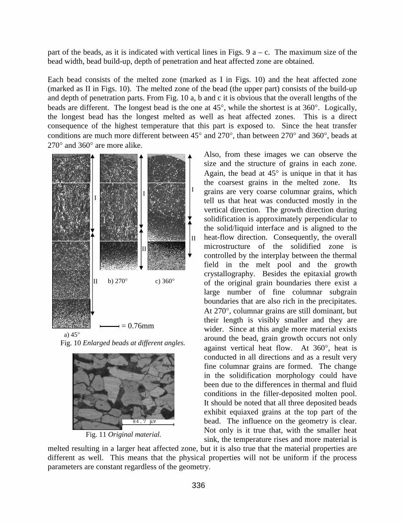
part of the beads, as it is indicated with vertical lines in Figs. 9 a – c. The maximum size of the bead width, bead build-up, depth of penetration and heat affected zone are obtained. Each bead consists of the melted zone (marked as I in Figs. 10) and the heat affected zone (marked as II in Figs. 10). The melted zone of the bead (the upper part) consists of the build-up and depth of penetration parts. From Fig. 10 a, b and c it is obvious that the overall lengths of the beads are different. The longest bead is the one at 45°, while the shortest is at 360°. Logically, the longest bead has the longest melted as well as heat affected zones. This is a direct consequence of the highest temperature that this part is exposed to. Since the heat transfer conditions are much more different between 45° and 270°, than between 270° and 360°, beads at 270° and 360° are more alike.

Also, from these images we can observe the size and the structure of grains in each zone. Again, the bead at 45° is unique in that it has the coarsest grains in the melted zone. Its grains are very coarse columnar grains, which tell us that heat was conducted mostly in the vertical direction. The growth direction during solidification is approximately perpendicular to the solid/liquid interface and is aligned to the heat-flow direction. Consequently, the overall microstructure of the solidified zone is controlled by the interplay between the thermal field in the melt pool and the growth crystallography. Besides the epitaxial growth of the original grain boundaries there exist a large number of fine columnar subgrain boundaries that are also rich in the precipitates. At 270°, columnar grains are still dominant, but their length is visibly smaller and they are wider. Since at this angle more material exists around the bead, grain growth occurs not only against vertical heat flow. At 360°, heat is conducted in all directions and as a result very fine columnar grains are formed. The change in the solidification morphology could have been due to the differences in thermal and fluid conditions in the filler-deposited molten pool. It should be noted that all three deposited beads exhibit equiaxed grains at the top part of the bead. The influence on the geometry is clear. Not only is it true that, with the smaller heat sink, the temperature rises and more material is

melted resulting in a larger heat affected zone, but it is also true that the material properties are different as well. This means that the physical properties will not be uniform if the process parameters are constant regardless of the geometry.

Fig. 11 Original material.

= 0.76mm a) 45°

Fig. 10 Enlarged beads at different angles.

c) 360°

II

I I

I

II

II

b) 270°

336

An image of the original material is given in Fig. 11. In addition, each of these beads is observed with the larger magnification. Results can be seen in Fig. 12 (45°), Fig. 13 (270°) and Fig. 14 (360°). All three beads consist of the build-up zone, the penetration zone and the heat affected zone. Although the grain-size shown in the figures is much different, the phase constituents at different angles are similar. The heat affected zone exhibits fine martensite and α-ferrite. The penetration zone is composed of coarse columnar dendrites. Some fine cementite precipitate at the grain boundaries along a certain crystal plane as shown in Figs. 12-14 (b). The segregation of carbon atoms at the grain boundaries leads to the precipitation of carbides, which may distinctly affect the mechanical properties of the beads.

New Experimental Set-up

All of the aforementioned experiments are performed on our new experimental set-up (shown in Fig. 15) where a 6-axis robot is added. A new torch and a wire feeding mechanism are designed to accommodate the robot’s specifications. This set-up allows us ‘more freedom’ in parts design, since robot can handle more advanced geometry. Thus, we built a turbine blade (see Fig. 16e). In Fig. 16 we can see the procedure of making the part – from designing the part in CAD software (Fig. 16 a), then generating the cross-section (Fig. 16b) and the torch path (Fig. 16c) with the new software “Success”, which is also

recently developed by our research team, and at the end, depositing material (Fig. 16d) and obtaining the final accuracy by milling the top and side surfaces (Fig. 16e).

a) a) a)

b) b) b)

c) c) c)

d) d) d)

≡ 84.7µm e) Fig. 12 45° Fig. 13 270° Fig. 14 360°

Fig. 15 Experimental Set-up.

337

Conclusions A three-dimensional finite element model of the transient, temperature-dependent heat transfer problem has been developed. This model affords a better understanding of the fluctuations that appear when a constant heat input is applied during the deposition process. The temperature fields are shown for the ‘critical’ angles. For these angles temperature history from the model is recorded and verified with the experimental results obtained from embedded thermocouples. Differences in the temperatures for the different angles cause different heat treatment of the deposited material and the material in the vicinity of the deposited material, i.e. the heat affected zone. Although the different grain sizes are observed for different angles, the phase constituents at different angles are similar. A new experimental set-up is designed and a 3D part is built. Acknowledgment The authors wish to acknowledge the financial support provided by the THECB, Grants No. 003613-0022001999 and 003613-0016-2001, NSF, Grants No. DMI – 9732848 and DMI – 9809198, and the U.S. Department of Education, Grant No. P200A-80806-98. References: (1) Spencer, J.D., Dickens, P.M., and Wykes, C.M., (1998). Rapid prototyping of metal parts by three-dimensional

welding, ImechE Proc. Part B, Journal of Engineering Manufacture, Vol. 212, pp. 175-182. (2) Dickens, P., Cobb, R., Gibbson, I., and Pridham, M., (1993). Rapid Prototyping Using 3D Welding, Journal of

Design and Manufacturing, Vol. 3, No. 1, March, pp. 39 - 44

a) 3D CAD model b) Cross-section c) Path planning

d) Turbine blade before milling e) Turbine blade after milling

Fig. 16 Procedure for making turbine blade by SFF based on welding.

338

(3) Merz, R., Prinz, F., Ramaswami, K., Terk M., and Weiss, L., (1994). Shape Deposition Manufacturing, Proceedings of the Solid Freeform Fabrication Symposium, University of Texas, Austin, Texas, August 8-10.

(4) Karunakaran, K., Shanmuganathan, P., Roth-Koch, S., and Koch, K., Direct Rapid Prototyping Tools, Proc. of the SFF Symposium, University of Texas, Austin, TX, August 1998, pp. 105-112.

(5) Ribeiro, A. F. M., Norrish, J., (1996). Rapid Prototyping Process using Metal Directly, Proceedings of Solid Freeform Fabrication, Symposium, 12-14 August, Austin, pp. 249-256, ISSN 1053-2153.

(6) Kovacevic, R., (2001). Rapid Manufacturing of Functional Parts Based on Deposition by Welding and 3D Layer Cladding, Proc. of the MoldMaking Conference, April 3-5, Rosemont, IL, presented by the MoldMaking Technology Magazin, pp. 263-276.

(7) Kmecko, I., Hu, D., and Kovacevic, R., (1999). Controlling Heat Input, Spatter and Weld Penetration in GMA Welding for Solid Freeform Fabrication, Proceedings of the 10th Solid Freeform Fabrication, Symposium, August, Austin.

(8) Kmecko, I.S., Kovacevic, R., and Jandric, Z., (2000). Machine Vision Based Control of Gas Tungsten Arc Welding for Rapid Prototyping, Proceeding of the 11th Solid Freeform Fabrication, Symposium, August, pp. 578-584.

(9) Jandric, Z. and Kovacevic, R., (2001). New Way of Process Parameters Optimization in SFF Based on Deposition by Welding, The Proceedings of the 12th Annual Solid Freeform Fabrication Symposium, Austin 6-8, Texas, pp. 110 – 119.

(10) D. Rosenthal (1946), Trans. ASME, Vol. 68, p 849-865. (11) N.N. Rykalin (1960), Calculation of Heat Process in Welding, Moscow, U.S.S.R. (12) E. Friedman (1975), Journal of Pressure Vessel Technology, p 206-213, August. (13) J.L. Beuth and S.H. Narayan (1996), Int. Journal of Solid Structures, V.33, N.1 p 65-78. (14) Z. Hu, M. Labudovic, H. Wang, R. Kovacevic (2001), Int. Journal of Machine & Manufacture V.41 p 589-607. (15) E.A. Bonifaz (2000), Welding J., May, p 121s–125s. (16) V. Kamala and J.A. Goldak (1993), Welding Journal, September, p 440-s – 446-s.

339