Embed Size (px)
Citation preview

Influence of Soil Plug on Pipe Ramming Process
N. I. Aleksandrova
Chinakal Institute of Mining, Siberian Branch, Russian Academy of Sciences,
Novosibirsk, 630091 Russia
e-mail: [email protected]
Abstract—Different modes of advance of a pipe with a soil plug under rectangular impulse
are investigated numerically and analytically with regard to dry friction between the pipe and
plug and between the pipe and external stationary medium. The two model solutions are
compared with and without regard to the pipe and plug elasticity. It is shown that elasticity
of the pipe and plug is neglectable in case of a long-duration impulse.
Keywords: Dry friction, impulsive loading, nonlinear dynamics, numerical modeling,
analytical solution.
INTRODUCTION
One of the main objectives in trenchless laying of underground utilities by percussive
pushing steel pipes in soil is the analysis of influence exerted on the wave process by friction
between the pipe and soil inside and outside the pipe. Dry friction plays an important part in
many mechanical systems with displacement of dry bodies. The issues of interaction between
solids with regard to dry friction are addressed in many scientific publications [1–24]. The first
to study the laws of dry friction were Leonardo da Vinci (1452–1519), Amonton (1663–1705)
and Coulomb (1736–1806) [1]. A review of dry friction model can be found in [11, 19, 24].
Various aspects of numerical solution of problems connected with the nonlinear laws of dry
friction were considered in [7–9, 15, 16, 21, 22, 24]. The analytical solutions for one degree of
freedom systems with dry friction are given in [4, 6, 10, 13, 14, 17, 18, 20]. Stead-state motion
of one or two bodies with dry friction described the Coulomb law [1] was analyzed in [2–4, 9,
12–14, 17], and nonsteady motion — in [9, 10, 18, 20–24]. Most of these studies are focused on
the stick/slip change under harmonic driving force. Influence of impulse on the system of two
bodies with dry friction remains yet to be investigated.
This study is focused on interaction between a cylindrical pipe, immobile external
environment and a soil plug under the action of a single impulse. External and internal friction of
the pipe is described by the classical Coulomb law [1].
1. ANALYTICAL SOLUTION FOR RIGID PIPE AND SOIL PLUG
We analyze joint motion of a steel cylindrical pipe in nondeformable soil and a soil plug
inside the pipe under transient load Q(t) directed along the pipe axis (Fig. 1). The pipe and soil
plug are rigid, i.e. modeled by concentrated masses. The equations of motion with regard to the
Coulomb law of constant dry friction at the inside pipe face and plug interface and at the outside
pipe face and immobile soil interfaces (model I) have the form:
2222111111 )()( kLPkLPtQtUM , (1)
222222 )( kLPtUM , (2)
,0,1
,0,0
,0,1
sign
1
1
1
11
U
U
U
Uk
.0,1
,0,0
,0,1
)(sign
21
21
21
212
UU
UU
UU
UUk
(3)

Fig. 1. Schematic representation of the problem formulation.
Here, U1, U2 are the displacements of the pipe and plug; τ1, τ2 are the limit shearing stresses at
the outside and inside faces of the pipe; P1, P2 are the inner and outer perimeters of the pipe; L1,
L2 are the pipe and plug lengths; M1, M2 are the pipe and plug masses; t is the time. It is assumed
in (1) and (2) that the dry friction force is applied over the whole outside pipe surface
(proportional to L1) and over the pipe and plug interface (proportional to L2). It is hypothesized
that all displacements and velocities are zero at the initial time )0()0()0()0( 2121 UUUU .
The further analysis is carried out in terms of the action of single rectangular impulse with
the amplitude Q0 and duration t0:
)–()()( 00 ttHtHQtQ , (4)
where Н is the Heaviside step function.
Integrating of (1), (2) in view of (3), (4) and zero initial conditions yields:
)()(
1)( 22110
11
kktQtI
MtU
, (5)
tM
kQt
M
LPktU
2
220
2
22222 )(
where
11
0*
LP
Q ,
11
22
LP
LP , )]–()–([)()( 0000
0
ttHtttHtQdttQtI
t
.
The difference of the pipe and plug velocities is given by:
)()(
1)()( 22110
1
21
kktQtI
MtUtU
where 21 /1 MM .
In as much as the function 12 k when 021 UU , we have the inequality to determine
the time interval where 12 k :
0/]/)()–()–([)()( 1211000021 MtkttHtttHtQtUtU . (6)
Similarly, we obtained the inequality to find the time interval with 11 k :
0/]/)()–()–([)( 122100001 MtkttHtttHtQtU
a) Let 21 . Then 2121 as far as . The task is to find a
time interval in which 12 k and 11 k . Let 1t and 2t satisfy the equalities 0211 )( tt
and 0212 )( tt . This implies 02101 )/( ttt and 012102 )/( tttt .
When 21 , 01 tt . In the time interval ],0[ 1tt , we have 12 k and 11 k .
Consequently, the solution takes the form of:
)–(]/)()–()–([)( 121000
1
01 ttHtttHtttHt
M
QtU ,
)–()( 1
2
202 ttH
M
tQtU
.
The values of 1U , 2U at the time 1t :
)()(
212
20012
M
tQtU ,
)()(
212
20011
M
tQtU .
In this manner, until the time 1t , the pipe and plug have different velocities (the plug slips
in the pipe) while at the time 1t their velocities level (stick) and when 21 / ( = const),
become the same:
)(2
00
M
tQU
irrespective of the specific values of 1 , 2 .
Let 1tt . Then inequality (6) is valid and, accordingly, 11 k . The function 2k at 1tt
can assume two values: 12 k and 02 k .
Suppose that 12 k . From (5) we obtain the solution for the pipe in the time interval
31 ttt , where the time 3t is found from the inequality 0)( 31 tU :
)–()–())((
)( 13
1
21301 ttHttH
M
ttQtU
, 1
21
2113
)(
)2(ttt
.
In the time interval 41 ttt , where 14 2tt is estimated from the equality 0)( 42 tU , we
have the solution for the soil plug velocity:
)–()–()(
)( 41
2
2402 ttHttH
M
ttQtU
.
When 3tt , 01 k and, consequently, 0)(1 tU ; when 4tt , 0)(2 tU .
Let us find the values of the parameters to satisfy the inequality 0)()( 21 tUtU in the
time interval 31 ttt , i.e. 12 k . The inequality:
0)())((
)()(2
24
1
213021
M
tt
M
ttQtUtU
is only valid when 12 . As a result, for 1tt , we have 12 k in case that 12 ,
otherwise 02 k if 12 .
The ensuing solution at 12 and 21 is given by:
)–()–())((
)–()(
)(1
)( 13
1
21301
210
1
1 ttHttHM
ttQttH
tQtI
MtU
,
)]–()–()()–([)( 41412
202 ttHttHtttttH
M
QtU
.
Let 1tt and 12 . Then 02 k and 11 k . In as much as the function 02 k in case
that 0)()( 21 tUtU , then то )()( 21 tUtU , i.e. the pipe and plug stick and move jointly. Their
total mass is 21 MM . The joint motion is described by the formula:
tt
MM
QtUtU 1
0
21
021 )()( .
They move together until the time 105 / tt , if 01 :
)–()(
)()()( 5
21
15021 ttH
MM
ttQtUtU
.
When 01 then at 1tt we have )/()()( 210021 MMtQtUtU .
Thus, when 21 and 12 , the solution is given by:
)–()–()(
)()–(
)()(
1)( 51
21
1501
210
1
1 ttHttHMM
ttQttH
tQtI
MtU
,
)–()–()(
)()–()( 51
21
1501
2
202 ttHttH
MM
ttQttH
M
tQtU
.
In case that 021 , 11 /)()( MtItU and 0)(2 tU .
b) Let 12 . In the same way as above, there are two possible variants: 12 k
and 02 k .
It is supposed initially that 12 k and 11 k . In this case, for 0tt , it is valid that:
0)–(1)( 021
1
01
ttHM
tQtU
.
This inequality is fulfilled if 21 .
Let us calculate the plug velocity in the interval 0tt :
)–()( 0
2
202 ttH
M
tQtU
and the relative pipe and plug velocity:
)–(1)()( 012
1
021 ttH
M
tQtUtU
.
The inequality 0)()( 21 tUtU holds true when 21 .
On the plane 2 , 1 , the inequalities 21 , 21 , 21 define three
domains with the single intersection point ),0(),( 12 . Finally, we have that 12 k and
11 k at 21 and 0tt never exist.
Let 02 k and 11 k . In this case, the pipe and soli plug move jointly:
)–(1)()( 01
21
021 ttH
MM
tQtUtU
.
We calculate their velocities at the moment 0tt :
1
21
000201 1)()(
MM
tQtUtU .
Let 0tt . We check the possibility of the situation when 12 k . It is assumed that
12 k . In this case, the inequality below should be fulfilled:
0)(
))((1)(
0
0211
21
001
t
tt
MM
tQtU
.
It is only valid when 1 .
Let at 6tt , 0)( 61 tU . Then, we have:
))((
)(1
21
106
tt , )()(
))(()( 06
1
12601 ttHttH
M
ttQtU
.
We calculate the plug velocity at 0tt :

)()(
1)(
)()( 0
0
021
21
00
2
020022 ttH
t
tt
MM
tQ
M
ttQtUtU
and relative velocity of the pipe and plug:
)())((
)()( 0
1
012021 ttH
M
ttQtUtU
.
When 12 , we have 0)()( 21 tUtU and 12 k is realizable. Notice that for
12 , 12 and 6t is determined.
Let 0)( 72 tU at 7tt . We calculate this time:
0
2
127 tt
.
As a result, in case that the inequalities 21 and 12 are satisfied, we have the
plug velocity solution:
)()()(
)–(1)( 7072
01
21
02 ttHttH
ttttHt
MM
QtU
.
Then, at 02 k ( 12 ), the joint velocity of the pipe and plug is given by:
ttMM
Q
MM
ttQtUtUtU
10
21
0
21
0100121
)(
)()()()( .
Here, 0)(1 tU if 1 .
c) Let 1 , then 21 , 21 . Consequently, the pipe and plug remain
motionless for the whole time interval:
0)()( 21 tUtU , 0t .
Fig. 2. Domains of solution in the plane 1 , 2 .
To sum up the results, we divide the plane 1 , 2 into domains I, II, III, IV and V (Fig. 2).
For each domain, we write expressions for the velocities of the pipe and plug and their
displacements obtained from time integration of the pipe and plug velocities.
Solution in domain I ( 12122 ,,0 ):
)()())(()()()(
13123112
01
01 ttHttHttttHt
Q
tI
M
QU
, (7)

],)()()()([ 1441
2
202 ttHttHtttttH
M
QU
,)}(]2)()2([
)()()])(2()()()2([
)(])()–()2()–([{2
31
2
121
2
3001
3112311
2
121001
1
2
210000
2
1
01
ttHttttt
ttHttHttttttttt
ttHtttHtttttHtM
QU
)](4)()()46()([2
4
2
114
22
111
2
2
202 ttHtttHttHttttttHt
M
QU
,
14
21
1123
21
01 2,
])2[(, tt
tt
tt
.
Solution in domain II ( 12211 ,,0 ):
)()())((
)()()(
1551
121
01
01 ttHttH
ttttHt
Q
tI
M
QU
, (8)
,)()()(
)( 15
2
511
2
202
ttHttHtt
tttHM
QU
,)()()(
)()2(
)()())(2()(
)()2(
)(])()–()2()–([2
5
2
1
2
512
121001
1511512
121001
1
2
210000
2
1
01
ttHtt
tttt
ttHttHttttt
tttt
ttHtttHtttttHtM
QU
.,)()(
)()())(2(
)(2
1
055
2
1
2
1
2
52
1
51
2
11152
11
2
2
202
ttttHtt
t
ttHttHttttt
tttHtM
QU
Solution in domain III ( 12211 ,,0 ):
)()()(
))(()()(
)(06
12601
21
01 ttHttH
ttttHt
MM
QU
, (9)
)()()(
)()(
)(07
2
2700
21
102 ttHttH
M
ttQttH
MM
tQU
,
)()()(2
01
2
21
01 ttHt
MM
QU
)()()(
))(2)(()( 06
126001
2
0 ttHttHttttt
t
)(
)(
))(()( 6
21
2
0
2
61
2
0 ttHtt
t
,

)},(])()([
)()(])2)(()([)()({2
72
2
0
2
71
2
0
0720701
2
001
2
2
02
ttHttt
ttHttHttttttttHtM
QU
0
2
1270
21
16 ,
)(
))((1 tttt
.
Solution in domain IV ( 12211 ,, ):
])()()()()([)(
055101
21
021 ttHttHttttHt
MM
QUU
, (10)
.)},()]()([)()(
)()()])(2()({[)(2
1
055
2
0
2
511
2
001
2
0500511
2
0
21
021
ttttHtttttHt
ttHttHttttttMM
QUU
Solution in domain V ( 12 ,0 ): 021 UU , 0t .
2. ALGORITHM FOR SOLVING FINITE DIFFERENCE EQUATION WITH REGARD
TO DRY FRICTION
The system of equations (1)–(3) with zero boundary conditions was solved in terms of a
unit impact using the explicit finite difference scheme:
111112222
21
11
1
1 /)(2 MkLPkLPQUUU nnnn ,
22222
21
22
1
2 /2 MkLPUUU nnn .
Here, τ is the step of the finite difference grid with respect to the time t; )(11 nUU n ,
)(22 nUU n are the displacements of the pipe and plug at nt ; )( nQQn is the amplitude
of external impact at nt .
The algorithm of solving with dry friction is described below. As far as direction and force
of friction are unknown beforehand, the pipe velocities are first calculated for two possible signs
of 1k ( 01 k and 01 k ) at the assumption that 02 k :
a) in the first case ( 01 k ), a fictitious velocity is introduced: /)( 101
01
nUUU where
111121
101 / MPLUU n ;
b) in the second case ( 01 k ) another fictitious velocity is introduced:
/)( 101
01
nUUU , where 111121
101 / MPLUU n .
In both cases, 11nU is calculated from the difference equation for the pipe without regard
to friction: 121
111
1 /2 MQUUU nnnn .
The two possible situations in this case are:
1. If the velocities 01U and 0
1U have the same sign, the true value 11nU out of 0
1U , 01U
is chosen such 101
kU that can reach the minimum:
)]abs(),abs(min[)abs( 0
1
0
1
0
11 UUU
k .
2. If the velocities 01U and 0
1U have different signs or one of them vanishes, then, based
on the assumption of passive friction, the real pipe velocity equals zero.
Then, we calculate the pipe and plug velocities for two possible signs of 2k ( 02 k and
02 k ) at the assumption that the value of 1k is chosen at the previous step:

a) in the first case ( 02 k ) fictitious velocities are introduced: /)( 11111 nkk
UUU ,
/)( 222nUUU , where 12221111
2111 /)(1 MPLkPLUU nk
, 1
22
nUU
2222
2 / MPL ;
b) in the second case ( 02 k ), the other fictitious velocities are introduced:
/)( 11111 nkk UUU
, /)( 222nUUU , where 12221111
2111 /)(1 MPLkPLUU nk ,
222221
22 / MPLUU n . The value 12nU is found from the difference equation for the plug
without regard to friction: 122
12 2 nnn UUU .
In the same way as before, two situations are possible:
1. If the velocities 21
1 UUk and
211 UU
k have the same sign, then the true values 1
1nU , 1
2nU out of 1
1k
U ,
2U and 11
kU
, 2U , are chosen as the pair 12
1kkU , 2
2k
U which can reach
the minimum:
)]abs(),abs(min[)abs( 21212111212 UUUUUU kkkkk .
2. If the velocities 21
1 UUk and
211 UU
k have different sings, or one of them
vanishes, then, based on the assumption of passive friction, the real relative velocity of the pipe
and plug equals zero. The pipe and plug stick and move together, consequently, friction between
them is absent.
Thus, the problem of calculating the times of transition of the pipe from standstill (relative
standstill of the pipe and plug) to motion (relative motion of the pipe and plug), constituting the
main difficulty in analytical solutions, reduces to the revealing of points where 01U and 0
1U
211( UU
k and 21
1 UUk ) have different signs, or one of them becomes zero. As far as the
calculations unambiguously determine the value and direction of the friction force, under solving
in each time level is the linear problem in which the friction force is already determined and
inserted on the right-hand side of the equation.
3. GRAPHIC PRESENTATION OF NUMERICAL AND ANALYTICAL SOLUTIONS
Figures 3–6 show the velocity–time relationships obtained for the pipe and plug using the
finite difference method and analytically from the formulas (7)–(10) at varied limit shearing
stress coefficients 21, . The values of the other parameters of the problem are: pipe and plug
lengths 121 LL m, pipe and plug densities 78001 kg/m3, 18002 kg/m3, pipe thickness
003.01 h m, Inner pipe radius 035.01 R m, impulse duration 500 t ms, effective force
amplitude 000230 Q N, difference grid time step 2.0 ms. These values conformed with the
pipe and plug masses 37.51 M kg, 93.62 M kg. The analytical and numerical solutions in
Figs. 3–6 coincided up to the error of plotting; for this reason, the method by which the velocities
are calculated is not mentioned in what follows. In Figs. 3–6, the solid lines show the functions
)(1 tU , the dash-and-dot lines — )(2 tU and the vertical dashed lines — the times
7654310 ,,,,,, ttttttt .
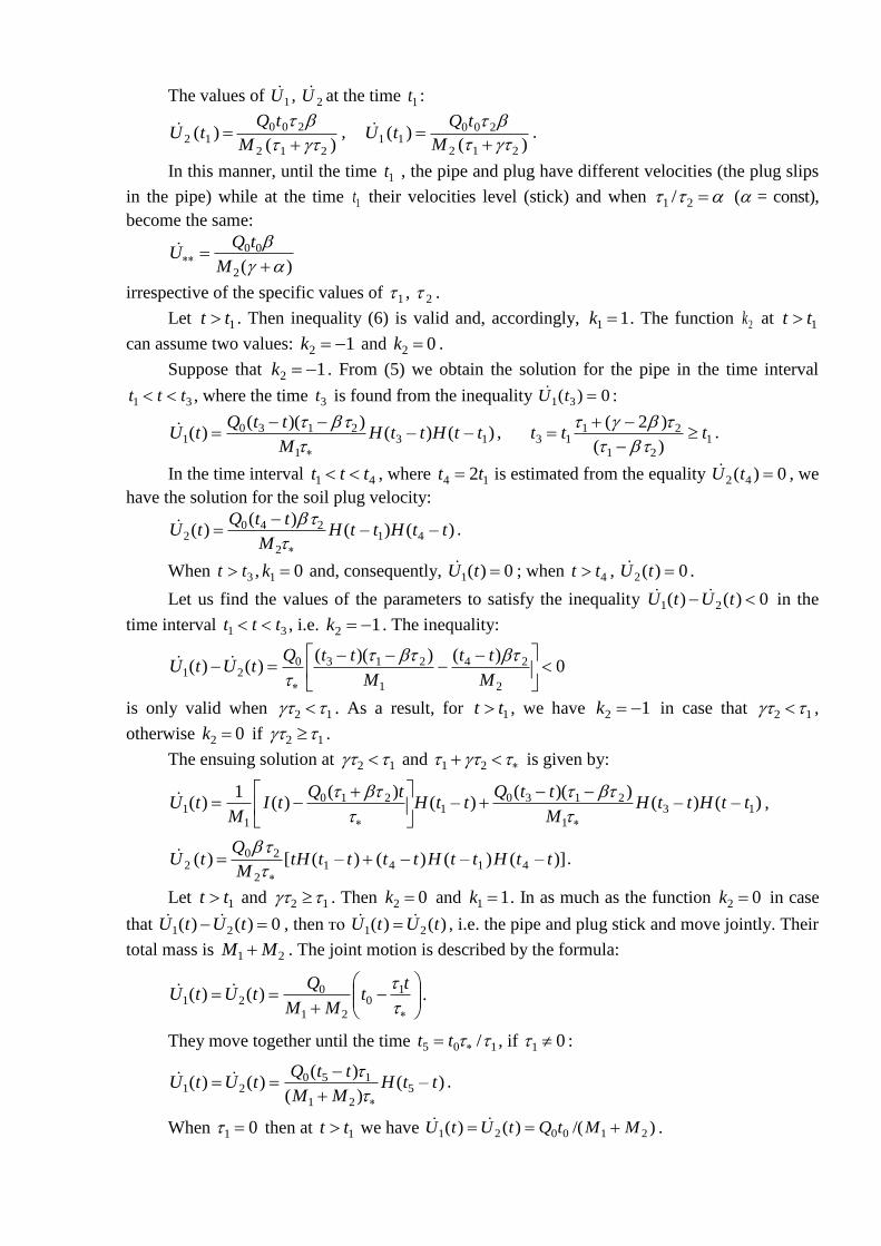
The velocities of pipe and plug in Fig. 3 are calculated from model I at
036564.0)1/(1 MPa. The problem parameters for curves 1 and 2 fit solution domain
I; for curves 3—domain IV. The analysis of the solutions at )1/(1 shows that at 02 ,
the plug is immobile while the pipe is advanced; when )1/(0 2 , the pipe and plug
move at different velocity up to the time of arrestment; as )1/(2 the pipe and plug stick
and move together until stoppage.
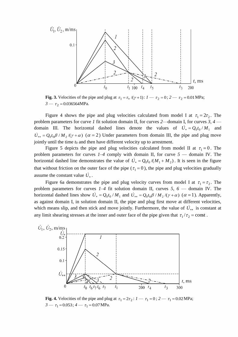
Fig. 3. Velocities of the pipe and plug at )1/(1 : 1 — 02 ; 2 — 01.02 MPa;
3 — 036564.02 MPa.
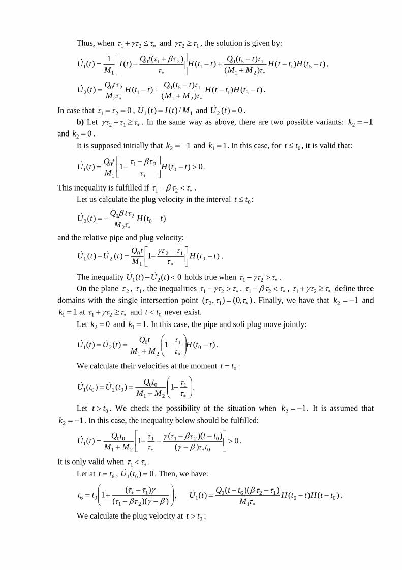
Figure 4 shows the pipe and plug velocities calculated from model I at 21 2 . The
problem parameters for curve 1 fit solution domain II, for curves 2—domain I, for curves 3, 4 —
domain III. The horizontal dashed lines denote the values of 100 / MtQU and
)/(/ 200 MtQU ( 2 ) Under parameters from domain III, the pipe and plug move
jointly until the time t0 and then have different velocity up to arrestment.
Figure 5 depicts the pipe and plug velocities calculated from model II at 01 . The
problem parameters for curves 1–4 comply with domain II, for curve 5 — domain IV. The
horizontal dashed line demonstrates the value of )/( 2100 MMtQU . It is seen in the figure
that without friction on the outer face of the pipe ( 01 ), the pipe and plug velocities gradually
assume the constant value U .
Figure 6a demonstrates the pipe and plug velocity curves from model I at 21 . The
problem parameters for curves 1–4 fit solution domain II, curves 5, 6 — domain IV. The
horizontal dashed lines show 100 / MtQU and )/(/ 200 MtQU ( 1 ). Apparently,
as against domain I, in solution domain II, the pipe and plug first move at different velocities,
which means slip, and then stick and move jointly. Furthermore, the value of U is constant at
any limit shearing stresses at the inner and outer face of the pipe given that const/ 21 .
Fig. 4. Velocities of the pipe and plug at 21 2 : 1 — 01 ; 2 — 02.01 MPa;
3 — 053.01 ; 4 — 07.01 MPa.
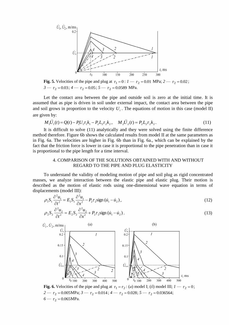
Fig. 5. Velocities of the pipe and plug at 01 : 1 — 01.02 MPa; 2 — 02.02 ;
3 — 03.02 ; 4 — 05.02 ; 5 — 0589.02 MPa.
Let the contact area between the pipe and outside soil is zero at the initial time. It is
assumed that as pipe is driven in soil under external impact, the contact area between the pipe
and soil grows in proportion to the velocity tU . The equations of motion in this case (model II)
are given by:
2222111111 )()( kLPkUPtQtUM , 222222 )( kLPtUM . (11)
It is difficult to solve (11) analytically and they were solved using the finite difference
method therefore. Figure 6b shows the calculated results from model II at the same parameters as
in Fig. 6a. The velocities are higher in Fig. 6b than in Fig. 6a., which can be explained by the
fact that the friction force is lower in case it is proportional to the pipe penetration than in case it
is proportional to the pipe length for a time interval.
4. COMPARISON OF THE SOLUTIONS OBTAINED WITH AND WITHOUT
REGARD TO THE PIPE AND PLUG ELASTICITY
To understand the validity of modeling motion of pipe and soil plug as rigid concentrated
masses, we analyze interaction between the elastic pipe and elastic plug. Their motion is
described as the motion of elastic rods using one-dimensional wave equation in terms of
displacements (model III):
)(sign 21222
1
2
112
1
2
11 uuPx
uSE
t
uS
, (12)
)(sign 21222
2
2
222
2
2
22 uuPx
uSE
t
uS
. (13)
Fig. 6. Velocities of the pipe and plug at 21 : (а) model I; (б) model III; 1 — 02 ;
2 — 005.02 MPa; 3 — 014.02 ; 4 — 028.02 ; 5 — 036564.02 ;
6 — 065.02 MPa.

Fig. 7. Velocities of pipe: dash-and-dot line is model I; solid line is model III.
Here, 1u , 2u are the displacements of the pipe and plug; 2 is the limit complex stress between
the pipe and plug; 2P is the inner perimeter of the pipe; 1S , 2S are the cross section areas of the
pipe and plug; 1E , 2E are Young’s moduli of the pipe and plug; 1 , 2 are the densities of the
pipe and plug; t is the time; x is the axial coordinate. The initial conditions are zero. The
coordinate system is chosen such that its origin coincides with the pipe end subjected to
impacting and the axis x is directed in parallel to the pipe axis (refer to Fig. 10). The longitudinal
load )–()()( 00 ttHtHQtQ is applied at the cross section 0x . At the ends of the pipe and
plug, the boundary conditions are set:
)(0
111 tQ
x
uSE
x
, 0
1
111
Lxx
uSE , 0
0
222
xx
uSE , 0
2
222
Lxx
uSE . (14)
The problem was solved by the cross-type explicit finite difference scheme. The algorithm
to calculate dry friction in the numerical solution for a rod-like pipe is described in [21, 22].
Figure 7 shows fragments of the pipe velocities. The solid line shows the velocity in the
middle section of the pipe (x = L1 / 2) in case of model III for elastic bodies. For the rigid masses
in model I, the velocity is denoted by the dash-and-dot line. The full plot for model I is depicted
in Fig. 5 by curve 1. The problems parameters are: 61 10195 E , 6
2 106.0 E MPa, 01 ,
01.02 MPa, 002.0 ms, the difference grid step along the longitudinal coordinate is
01.0h m, the other parameters are the same as in Figs. 3–6.
It is seen in the figure that the behavior of the solutions in the elastic and rigid models of
interaction is qualitatively the same. Differences are oscillations that arise in the elastic model
solutions due to reflection of waves from the pipe ends. The error of the maximum pipe velocity
amplitude in simpler model I is less than 0.25% relative to elastic model III. The comparison of
the solutions obtained by the two models shows that in case when the impulse duration is much
longer than the time of to and fro travel of wave along the pipe at a rod velocity, the pipe and
plug motion can be described using the simplified model (1), (2).
CONCLUSIONS
The analytical solutions to describe ramming of pipe with a soil plug are obtained. Various
modes of the pipe and plug system motion are studied depending on the values of the limit
shearing stresses at the outer and inner faces of the pipe. The finite difference algorithms are
developed for different models of the pipe and plug with a view to dry friction. It is shown that
the numerical and analytical solutions match together at a high accuracy. It is found that in case
of a sufficiently long impulse, the influence of elasticity of the pie and plug can be neglected and
the pipe and plug motion can be modeled as concentrated masses.
ACKNOWLEDGMENTS
This study was supported by the Russian Science Foundation, project no. 17-77-20049.

REFERENCES
1. Coulomb, C.A., Theorie des Machines Simples, Bachelier, 1821.
2. Meskele, T. and Stuedlein, A.W., Static Soil Resistance to Pipe Ramming in Granular
Soil, J. Geotechnical and Geoenvironmental Engineering, 2015, vol. 141, issue 3.
DOI:10.1061/(ASCE)GT.1943-5606.0001237.
3. Danilov, B.B., Kondratenko, A.S., Smolyanitsky, B.M., and Smolentsev, A.S.,
Improvement of Pipe Pushing Method, J. Min. Sci., 2017, vol. 53, no. 3, pp. 478–483.
DOI: 10.1134/S1062739117032391.
4. Hundal, M.S., Response of a base excited system with Coulomb and viscous friction, J.
Sound Vib., 1979, vol. 64, pp. 371–378. DOI: 10.1016/0022-460X(79)90583-2.
5. Pratt, T.K. and Williams, R., Nonlinear Analysis of Stick/Slip Motion, J. Sound Vib.,
1981, vol. 74, pp. 531–542.
6. Pielorz, A. and Nadolski, W., Criterion of Multiple Collisions in a Simple Mechanical
System with Viscous Damping and Dry Friction, Int. J. Non-Linear Mech., 1983, vol. 18,
pp. 479–489.
7. Martins, J.A.C. and Oden, J.T., A Numerical Analysis of a Class of Problems in
Elastodynamics with Friction, Comput. Meth. Appl. Mech. Eng., 1983, vol. 40, pp. 327–
360.
8. Oden, J.T. and Martins, J.A.C., Models and Computational Methods for Dynamic
Friction Phenomena, Comput. Meth. Appl. Mech. Eng., 1985, vol. 52, pp. 527–634. DOI:
10.1016/0045-7825(85)90009-X.
9. Oertel, Ch., On the Integration of the Equation of Motion of an Oscillator with Dry
Friction and Two Degrees of Freedom, Ing.-Arch., 1989, vol. 60, no. 1, pp. 10–19. DOI:
10.1007/BF00538404.
10. Makris, N. and Constantinou, M.C., Analysis of Motion Resisted by Friction. I. Constant
Coulomb and Linear Coulomb Friction, Mech. Struct. Mach., 1991, vol. 19, no. 4, pp.
477–500. DOI: 10.1080/08905459108905153.
11. Olsson, H., Аström, K.J., Canudas deWit, C., Gäfvert, M., and Lischinsky, P., Friction
Models and Friction Compensation, Eur. J. Control, 1998, vol. 4, pp. 176–195.
12. Krivtsov, A.M. and Wiercigroch, M., Dry Friction Model of Percussive Drilling,
Meccanica, 1999, vol. 34, no. 6, pp. 425–435. DOI: 10.1023/A:1004703819275.
13. Hong, H.-K. and Liu, C.-S., Coulomb Friction Oscillator: Modeling and Responses to
Harmonic Loads and Base Excitations, J. Sound Vib., 2000, vol. 229, no. 5, pp. 1171–
1192. DOI: 10.1006/jsvi.1999.2594.
14. Hong, H.-K. and Liu, C.-S., Non-Sticking Oscillation Formulae for Coulomb Friction
under Harmonic Loading, J. Sound Vib., 2001, vol. 244, no. 5, pp. 883–898. DOI:
10.1006/jsvi.2001.3519.
15. Renard, Y., Numerical Analysis of a One-Dimensional Elastodynamic Model of Dry
Friction and Unilateral, Comput. Methods Appl. Mech. Eng., 2001, vol. 190, pp. 2031–
2050.
16. Bereteu, L., Numerical Integration of the Differential Equations for a Dynamic System
with Dry Friction Coupling, Facta Univ., Ser. Mech. Autom. Control Robot, 2003, vol. 3,
no. 14, pp. 931–936.
17. Lopez, I., Busturia, J., and Nijmeijer, H., Energy Dissipation of a Friction Damper, J.
Sound Vib., 2004, vol. 278, no. 3, pp. 539–561. DOI: 10.1016/j.jsv.2003.10.051.
18. Yang, S.P. and Guo, S.Q., Two-Stop-Two-Slip Motions of a Dry Friction Oscillator, Sci.
China, Technol. Sci., 2010, vol. 53, no. 3, pp. 623–632. DOI: 10.1007/s11431-010-
0080-x.
19. Al-Bender, F., Fundamentals of Friction Modeling. ASPE Spring Topical Meeting on
Control of Precision Systems, 2010.
20. Rao, S.S., Mechanical Vibrations, Addison-Wesley Longman Incorporated, USA, 1995.

21. Aleksandrova, N.I., Numerical-Analytical Investigation into Impact Pipe Driving in Soil
with Dry Friction. Part I: Nondeformable External Medium, J. Min. Sci., 2012, vol. 48,
no. 5, pp. 856–869. DOI: 10.1134/S1062739148050103.
22. Aleksandrova, N.I., Numerical-Analytical Investigation into Impact Pipe Driving in Soil
with Dry Friction. Part II: Deformable External Medium, J, Min. Sci., 2013, vol. 49, no.
3, pp. 413–425. DOI: 10.1134/S106273914903009X. 23. Sumbatov, A.S. and Yunin, E.K., Izbrannye zadachi mekhaniki sistem s sukhim treniem
(Selected Problems on Systems with Dry Friction in Mechanics), Moscow: Fizmatlit,
2013.
24. Pennestrì, E., Rossi, V., Salvini, P., and Valentini, P.P., Review and Comparison of Dry
Friction Force Models, Nonlinear Dyn., 2015, vol. 83, no. 4, pp. 1785–1801. DOI:
10.1007/s11071-015-2485-3.
This paper was originally published in Russian in the journal “Fiziko-Tekhnicheskie Problemy
Razrabotki Poleznykh Iskopaemykh”, 2017, No. 6, pp. 114–126. An English translation was
published in the “Journal of Mining Science”, 2017, Vol. 53, No. 6, pp. 1073–1084.
DOI: 10.1134/S1062739117063138