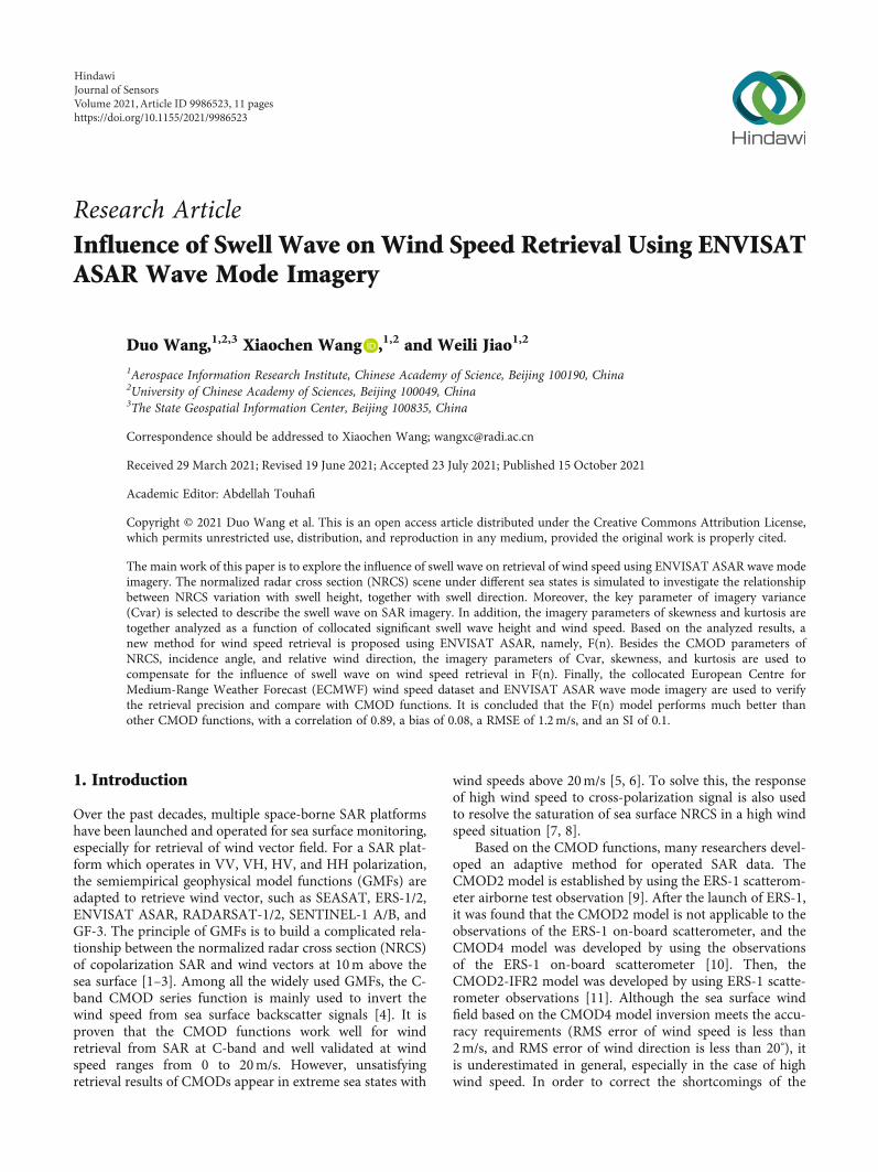
Research ArticleInfluence of Swell Wave on Wind Speed Retrieval Using ENVISATASAR Wave Mode Imagery

Duo Wang,1,2,3 Xiaochen Wang ,1,2 and Weili Jiao1,2

1Aerospace Information Research Institute, Chinese Academy of Science, Beijing 100190, China2University of Chinese Academy of Sciences, Beijing 100049, China3The State Geospatial Information Center, Beijing 100835, China

Correspondence should be addressed to Xiaochen Wang; wangxc@radi.ac.cn

Received 29 March 2021; Revised 19 June 2021; Accepted 23 July 2021; Published 15 October 2021

Academic Editor: Abdellah Touhafi

Copyright © 2021 Duo Wang et al. This is an open access article distributed under the Creative Commons Attribution License,which permits unrestricted use, distribution, and reproduction in any medium, provided the original work is properly cited.

The main work of this paper is to explore the influence of swell wave on retrieval of wind speed using ENVISAT ASAR wave modeimagery. The normalized radar cross section (NRCS) scene under different sea states is simulated to investigate the relationshipbetween NRCS variation with swell height, together with swell direction. Moreover, the key parameter of imagery variance(Cvar) is selected to describe the swell wave on SAR imagery. In addition, the imagery parameters of skewness and kurtosis aretogether analyzed as a function of collocated significant swell wave height and wind speed. Based on the analyzed results, anew method for wind speed retrieval is proposed using ENVISAT ASAR, namely, F(n). Besides the CMOD parameters ofNRCS, incidence angle, and relative wind direction, the imagery parameters of Cvar, skewness, and kurtosis are used tocompensate for the influence of swell wave on wind speed retrieval in F(n). Finally, the collocated European Centre forMedium-Range Weather Forecast (ECMWF) wind speed dataset and ENVISAT ASAR wave mode imagery are used to verifythe retrieval precision and compare with CMOD functions. It is concluded that the F(n) model performs much better thanother CMOD functions, with a correlation of 0.89, a bias of 0.08, a RMSE of 1.2m/s, and an SI of 0.1.

1. Introduction

Over the past decades, multiple space-borne SAR platformshave been launched and operated for sea surface monitoring,especially for retrieval of wind vector field. For a SAR plat-form which operates in VV, VH, HV, and HH polarization,the semiempirical geophysical model functions (GMFs) areadapted to retrieve wind vector, such as SEASAT, ERS-1/2,ENVISAT ASAR, RADARSAT-1/2, SENTINEL-1 A/B, andGF-3. The principle of GMFs is to build a complicated rela-tionship between the normalized radar cross section (NRCS)of copolarization SAR and wind vectors at 10m above thesea surface [1–3]. Among all the widely used GMFs, the C-band CMOD series function is mainly used to invert thewind speed from sea surface backscatter signals [4]. It isproven that the CMOD functions work well for windretrieval from SAR at C-band and well validated at windspeed ranges from 0 to 20m/s. However, unsatisfyingretrieval results of CMODs appear in extreme sea states with

wind speeds above 20m/s [5, 6]. To solve this, the responseof high wind speed to cross-polarization signal is also usedto resolve the saturation of sea surface NRCS in a high windspeed situation [7, 8].

Based on the CMOD functions, many researchers devel-oped an adaptive method for operated SAR data. TheCMOD2 model is established by using the ERS-1 scatterom-eter airborne test observation [9]. After the launch of ERS-1,it was found that the CMOD2 model is not applicable to theobservations of the ERS-1 on-board scatterometer, and theCMOD4 model was developed by using the observationsof the ERS-1 on-board scatterometer [10]. Then, theCMOD2-IFR2 model was developed by using ERS-1 scatte-rometer observations [11]. Although the sea surface windfield based on the CMOD4 model inversion meets the accu-racy requirements (RMS error of wind speed is less than2m/s, and RMS error of wind direction is less than 20°), itis underestimated in general, especially in the case of highwind speed. In order to correct the shortcomings of the

HindawiJournal of SensorsVolume 2021, Article ID 9986523, 11 pageshttps://doi.org/10.1155/2021/9986523

COMD4 model, the CMOD5 model was developed basedon ERS-2 scatterometer observations, which improves theapplicability to high wind speed [12]. In order to get theneutral wind rather than the real wind, the coefficient ofthe CMOD5 model is refitted and the CMOD5.N modelis obtained [13]. Moreover, a modified CMOD5.H modelby using ASCAT scatterometer high wind speed observa-tions is also proposed [14]. Then, the CMOD5.N modelwas further modified by using ASCAT scatterometer obser-vations to develop the CMOD6 model, and it has beenproven that the model is applicable to all C-band satellitescatterometer observations such as ERS and ASCAT [15].Finally, the CMOD7 model was developed based oncross-calibrated ERS and ASCAT scatterometer data, andits overall performance is better than that of the CMOD5.Nmodel [16].

Considering that CMOD functions were mainly derivedfrom space-borne scatterometer measurements, moreCMOD functions directly derived from SAR measurementsare proposed for wind speed retrieval. Due to the globalmassive collection of ENVISAT ASAR data, an initial SARGMF, denoted CSARMOD, was derived from collocatedENVISAT ASAR-measured NRCS and wind speed anddirection data acquired by ASCAT [17]. However, CSAR-MOD is not applied to any SAR wind speed retrieval dataand is limited to wind speeds up to 20m/s. Therefore, anew GMF, denoted CSARMOD2, was developed to exploreSAR-measured NRCS and wind vector data [18]. Scenes ofRADARSAT-2 and Sentinel-1A SAR data are collocatedwith wind speed and wind direction measurements providedby NDBC buoys. Moreover, when Chinese Gaofen- (GF-) 3SAR was launched, a good consistency of retrieved SARwind speed and buoy in situ measurements is present usingCMOD5.N, COMD7, and others. Several methodologies ofwind retrieval are also developed using GF-3 copolarizedand cross-polarized SAR data [19–21].

Although a series of wind speed retrieval algorithms areproposed in the past decades, the new algorithm is still aresearch highlight in retrieval processing. In particular, theempirical relationship between NRCS and wind speed wasconstantly revised using different operated SAR measure-ments. However, the sea state factor also influences theradar echo of the sea surface. It is known that the seasurface roughness caused by local winds contributes to theNRCS. Besides, the modulation of wind-generated small-scale roughness by swell waves can also modify the distri-bution of the sea surface slope, thereby, influencing thetotal NRCS of the sea surface. So, the influence of swellon NRCS would accordingly impact wind speed. In orderto acquire a precise wind field, it is significant to furtherdiscuss and compensate for the influence of a swell wavein retrieval processing.

The paper is organized as follows. The collocated dataset,as well as the CMOD series functions, is briefly introducedin Section 2. In Section 3, the influence of pure swell on atwo-dimensional sea surface slope and NRCS are demon-strated, together with a new strategy for wind speed retrieval.Then, the discussion and conclusion is given in Sections 4and 5, respectively.

2. Materials and Methods

2.1. ENVISAT ASAR Data. About 1647 scenes of ENVISATASAR Single Look Complex (SLC) imagery were collectedfrom January of 2011, and were further matched withECMWF data and buoy data. The parameters of used SLCdata details are listed in Table 1. Among all of the operationmodes of ENVISAT ASAR, the wave mode data wereacquired with a fine resolution of 10m and can provide con-tinuous images of the sea surface within each 100 km. Morethan 2500 scenes of wave mode imagery are acquired every-day, which provides benefits for sea surface wind vector fieldretrieval. The used ENVISAT ASAR wave mode imagery isshown in Figure 1.

2.2. Buoy and ECMWF Reanalysis Data. The buoy andECMWF reanalysis data are widely used as validationsamples for sea surface remote sensing retrieval. The buoymeasurements are provided by the National Data BuoyCenter (NDBC), and the valid scope of a buoy is usuallyset as 30min in time and 50 km in distance. The ERA-Interim reanalysis data are provided by European Centrefor Medium-Range Weather Forecasts (ECMWF). It isnoticed that the temporal and spatial resolutions are 6 hand 0:125° × 0:125°, respectively. Considering the occasionalabsence of buoy in situ measurements, the provided windfield (u10, v10) and other ocean dynamic parameters fromthe above two kinds of data sources can be used together asvalidation samples for sea surface remote sensing retrieval.

Figure 2 shows the wind vector comparison of buoy andECMWF reanalysis data. The correlations between buoy andECMWF data were 0.82 and 0.97 for both wind speed andwind direction, respectively. It can be seen that trustworthyresults are present between buoy measurement and ECMWFreanalysis data. To use buoy and ECMWF reanalysis data isreliable for processing the in situ wind vector field [22].

2.3. CMOD Function. CMOD functions are originallyderived from scatterometers, and the sea surface backscattersignals from space-borne measurements are related withincidence angle, wind speed, and wind direction [23]. Ageneral type of CMOD function is presented as follows:

σ0 = b0 θ, vð Þ 1 + b1 θ, vð Þ cos ϕw + b2 θ, vð Þ cos 2ϕw½ �n, ð1Þ

where σ0 represents the space-borne measured NRCS of the

Table 1: Parameters of ENVISAT ASAR wave mode SLC imageryused in this paper.

Parameters Values

Band C (5.3 GHz)

Polarization VV

Incidence angle θ 23°

Azimuth spacing 4.0m

Range spacing 7.0m

Swath width 5 km

2 Journal of Sensors

sea surface, θ represents the incidence angle, v represents thewind speed, ϕw represents the relative wind directionbetween real wind direction and radar antenna pointingdirection. b0, b1, and b2 represent the functions of θ and v,which are recalculated by collocated ECMWF reanalysiswind data, NDBC buoy in situ wind measurements, andspace-borne scatterometers (SAR). n represents the functionpower variable, which usually takes the value of 1.6. Actu-ally, the wind speed and wind direction, as a couple ofunknown terms, cannot be resolved on a basic set of inci-dence angle and NRCS. So, a general method of wind speedretrieval is to use external wind direction data as input,together with incidence angle, to acquire wind speed. TakingCMOD5.N, COMD-IFR2, and CSARMOD2, for example,the NRCS variation with an increase in wind speed and winddirection are shown in Figure 3.

In Figure 3(a), the incidence angle is set to 23°, and therelative wind direction is set to 0° (upwind direction). Itcan be seen that different CMOD functions behave in a sim-ilar curve characteristic, which increases as the wind speedincreases. However, as the wind speed increases, the gapbetween the NRCS of CMOD5.N, COMD-IFR2, and CSAR-MOD2 becomes more and more remarkable, especiallywhen the wind speed goes beyond 15m/s. It has been veri-fied that the COMD-IFR2 function behaves much better

than others in the case of low and medium wind speeds(below 20m/s). Besides, CMOD5.N presents a good perfor-mance in high wind speed cases (above 20m/s), and CSAR-MOD2 seems to be comprised of something betweenCMOD-IFR2 and CMOD5.N in terms of NRCS.Figure 3(b) shows the azimuth distribution of the NRCS ofCMOD5.N, COMD-IFR2, and CSARMOD2. The incidenceangle is set to 23°, and the wind speed is set to 5m/s. Anapproximate cosine shape is presented as an increase of rel-ative wind direction. No matter if it is in an upwind, down-wind, or cross-wind direction, the NRCS of CMOD5.N isstill below that of COMD-IFR2 and CSARMOD2. And theNRCS of CMOD-IFR2 greatly exceeds that of CSARMOD2in the up- and downwind directions, and it stays the samein the cross-wind direction. Although the CMOD5.N,COMD-IFR2, CSARMOD2, and other CMOD functionshave been explored, it still remains arguable in wind speedretrieval using space-borne scatterometers or SAR data.

3. Results

3.1. NRCS Simulation under Different Sea States. For windspeed retrieval from C-band SAR imagery at VV polariza-tion, the empirical relationship between NRCS and windspeed, wind direction, and incidence angle is established in

160°W 120°W 80°W 40°W 0°0°

12°N

24°N

36°N

48°N

60°N

N = 1647

Figure 1: Map of collected ASAR WV imagery and buoy location.

0 5 10 15 20 25 300

5

10

15

20

Buoy

win

d sp

eed

(m/s

)

25

30

ECMWF wind speed (m/s)

10

20

30

40

50

60Correlation: 0.82Bias: -0.05 mRMES: 1.78 mSI: 0.13

(a) Wind speed

Buoy

win

d di

rect

ion

(°)

10

20

30

40

50

60

0 45 90 135 180 225 270 315 3600

45

90

135

180

225

270

315

360

ECMWF wind direction (°)

Correlation: 0.97Bias: 0.37 mRMES: 21.43 mSI: 0.12

(b) Wind direction

Figure 2: Comparison of ECMWF wind vector with buoys.

3Journal of Sensors

0 5 10 15 20 25 30–16

–14–12–10

–8–6

–4–2

024

Wind speed (m/s)

Incidence angle = 23°Relative wind direction = 0°

CMOD5NCMOD-IFR2CSARMOD2

Nrc

s (dB

)

(a)

CMOD5NCMOD-IFR2CSARMOD2

0 45 90 135 180 225 270 315 360–16

–15

–14

–13

–12

–11

–10

–9

Relative wind direction (°)

Incidence angle = 23°Wind speed = 5 m/s

Nrc

s (dB

)

(b)

Figure 3: CMOD function backscattering characteristics: (a) CMOD function variation with wind speed; (b) CMOD function variation withwind direction.

Diffx

Range direction64 128 192 256 320 384 448 512

Range direction64 128 192 256 320 384 448 512

64

128

192

256

320

384

448

512

Diffy

64

128

192

256

320

384

448

512

Azi

mut

h di

rect

ion

Azi

mut

h di

rect

ion

(a) Wind wave

Range direction64 128 192 256 320 384 448 512

Range direction64 128 192 256 320 384 448 512

Diffx

64

128

192

256

320

384

448

512

Diffy

64

128

192

256

320

384

448

512

Azi

mut

h di

rect

ion

Azi

mut

h di

rect

ion

(b) Wind wave + swell wind

Figure 4: Two-dimensional sea surface slope: (a) wind speed = 5m/s, wind direction = 45°; (b) wind speed = 5m/s, wind direction = 45°,swell height = 2m, swell direction = 45°, swell peak wavelength = 200m.

4 Journal of Sensors

CMODs. However, the influence of sea state is usuallyneglected in processing SAR imagery due to sea surfacelarge-scale statics. Actually, the sea state consists of windwave caused by wind, and pure swell wave caused by exter-nal propagation. CMODs directly use the NRCS of the seasurface as the total sea surface backscatter signal to retrievewind speed, without consideration of the influence of a pureswell wave on NRCS. That is why the retrieval accuracy ofwind speed deteriorates in some sea zones. Here, the NRCScharacteristics under different sea states are simulated toassess the influence of a pure swell. According to the com-posite Bragg scattering model, the total ocean surface NRCSconsists of the Bragg scattering component of σp

br and thequasispecular scattering component of σsp [24]. It is notedthat the influence of breaking waves are neglected, whichhas outstanding performance in high incidence angles [25].

σp0 = σpbr + σsp: ð2Þ

According to the Bragg resonance scattering mechanism,the Bragg scattering componentσp

br is presented as follows: [26]:

σpbr = 16πk4 Gp θð Þ�� ��2Fr kbr, φð Þ, ð3Þ

where k represents the radar wavenumber, Gp represents theBragg scattering coefficients, θ represents the incidence angle,Fr represents the two-dimensional wave spectrum, kbr repre-sents the Bragg wavenumber kbr = 2k sin ðθÞ, φ represents theazimuth direction, p represents the polarization status.

The quasispecular scattering component σsp domi-nates in small incidence angles, which can be presentedas follows [27]:

σsp = Reffj j2π sec4θp ζx, ζy� �

, ð4Þ

where Reff represents the effective reflection coefficient, prepresents the slope probability density distribution func-tion of specular points, ζx = tan θ cos φw and ζy = − tanθ sin φw are downwind and upwind slopes, respectively.The sea surface slope in range and azimuth directionare presented in Figure 4.

Figure 4(a) shows the two-dimensional sea surface slopein the case of a wind speed of 5m/s and a wind direction of45°, and Figure 4(b) shows the two-dimensional sea surfaceslope in the same wind field, together with a swell heightof 2m, a swell direction of 45°, and a swell peak wavelengthof 200m. It can be seen that the wind-induced sea surfaceslope in range and azimuth direction in Figure 4(a) is clearlydistinguished from the wind and pure swell comodulated seasurface slope in Figure 4(b). The waves, especially the pureswell wave, modify the sea surface slope distribution whichfollows a Gaussian shape. It is noticed that wave breakingis neglected in this section, which induces the high-orderno-Gaussian terms [28, 29]. Figure 5 shows the differencebetween simulated NRCS and sea state.

As shown in Figure 5(a), the NRCS increased as windspeed increased, showing a similar tendency with theCMODs in Figure 3. However, an approximate constant ofNRCS appears with the influence of the swell wave, and apositive correlation relationship between an NRCS

0 5 10 15 20 25 30–25

–20

–15

–10

–5

0

Wind speed (m/s)

Nrc

s (dB

)

Incidence angle = 23°Relative wind direction = 0°Wind speed 5 m/s wind direction = 45°

Swell height 0 m

Swell height 4 mSwell height 6 m

(a)N

rcs (

dB)

0 45 90 135 180 225 270 315 360–16.5

–16

–15.5

–15

–14.5

–14

–13.5

–13

–12.5

Azimuth (°)

Incidence angle = 23°Wind speed 5 m/s wind direction = 45°

Swell height 0 m

Swell height 2 m direction 45°Swell height 2 m direction 135°

(b)

Figure 5: NRCS variation with wind speed and relative wind direction. (a) NRCS curves of upwind direction with swell heights of 0m, 4m,and 6m, respectively. (b) NRCS curves of upwind direction with a swell height of 0m, a swell height of 2m, a swell direction of 45°, a swellheight of 2m, and a swell direction of 135°, respectively.

5Journal of Sensors

increment and swell height is present. The influence of swellon azimuthal NRCS is shown in Figure 5(b). It is obviousthat a positive effect is investigated on sea surface NRCS inan upwind direction, which is opposite a cross-wind direc-tion. As a conclusion, the influence of the swell wave onthe modulation of sea surface wind-induced NRCS is clearlyin our simulation. With the aim to improve the retrievalaccuracy of wind speed, it is significant to consider the swellmodulation in wind-induced NRCS in CMODs [30].

3.2. Influence of Swell on Wind Speed Retrieval. Due tothe absence of straight swell wave measurement in realityfor wind speed retrieval, an imagery parameter of image

variance (Cvar) is set to describe the influence of a swellwave [31]:

Cvar = std I − Ih iIh i

� �� �2, ð5Þ

where hIi present the average value of the SAR intensityimagery. In order to evaluate the sensitivity of Cvar on swelland wind wave height, the Elfouhaily spectrum is suggestedto simulate the wind wave and swell wave spectrum and fur-ther explore the correlation between Cvar of correspondingsimulated SAR imagery and sea state [32]. Figure 6 showsthe variation of swell wave and wind wave height with an

1 1.5 2 2.5 3 3.50

Swel

l hei

ght (

m)

1

2

3

4

5

6

7

8

9

Cvar

Incidence angle = 23°Relative wind direction = 0°

Wind speed 1 m/sWind speed 5 m/sWind speed 10 m/s

(a)

Win

d-w

ave h

eigh

t (m

)

1 1.5 2 2.5 3 3.5Cvar

Wind speed 1 m/sWind speed 5 m/sWind speed 10 m/s

-0.5

0

0.5

1

1.5

2

2.5

3Incidence angle = 23°Relative wind direction = 0°

(b)

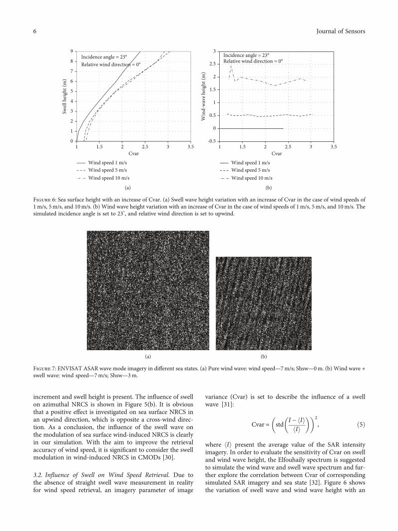
Figure 6: Sea surface height with an increase of Cvar. (a) Swell wave height variation with an increase of Cvar in the case of wind speeds of1m/s, 5m/s, and 10m/s. (b) Wind wave height variation with an increase of Cvar in the case of wind speeds of 1m/s, 5m/s, and 10m/s. Thesimulated incidence angle is set to 23°, and relative wind direction is set to upwind.

(a) (b)

Figure 7: ENVISAT ASAR wave mode imagery in different sea states. (a) Pure wind wave: wind speed—7m/s; Shsw—0m. (b) Wind wave +swell wave: wind speed—7m/s; Shsw—3m.

6 Journal of Sensors

increase of Cvar. Both Figures 6(a) and 6(b) are simulated inan upwind direction and at an incidence angle of 23°. Clearly,a quasilinear curve between the simulated swell wave heightand Cvar is found, which means that Cvar can be performedas an imagery characterization for swell information. On the

contrary, the wind wave height cannot represent any remark-able variation as an increase of Cvar.

To further assess the influence of swell wave on NRCS,the ENVISAT ASAR wave mode imagery is calibrated andgeometric. Collocated with ECMWF data, the wave streak

1 1.1 1.2 1.3 1.4 1.50

1

2

3

Shts

(m)

4

5

6

Cvar

10

20

30

40

50

60

(a)

Ws (

m/s

)

1 1.1 1.2 1.3 1.4 1.5Cvar

10

20

30

40

50

60

0

5

10

15

20

(b)

0

1

2

3

Shts

(m)

4

5

6

10

20

30

40

50

60

4 6 8 10 12Skewness

(c)

10

20

30

40

50

60

Ws (

m/s

)

0

5

10

15

20

4 6 8 10 12Skewness

(d)

0

1

2

3

Shts

(m)

4

5

6

10

20

30

40

50

60

10 15 20 25 30Kurtosis

(e)

10

20

30

40

50

60

Ws (

m/s

)

0

5

10

15

20

10 15 20 25 30Kurtosis

(f)

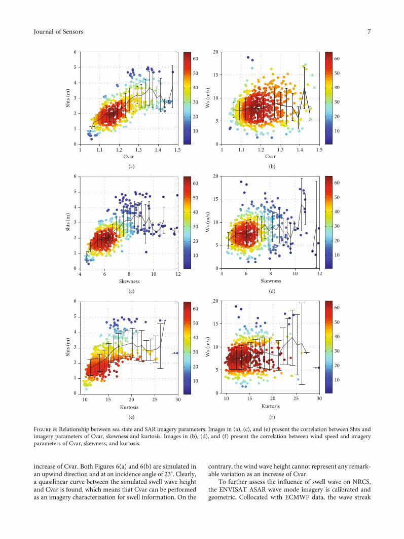
Figure 8: Relationship between sea state and SAR imagery parameters. Images in (a), (c), and (e) present the correlation between Shts andimagery parameters of Cvar, skewness and kurtosis. Images in (b), (d), and (f) present the correlation between wind speed and imageryparameters of Cvar, skewness, and kurtosis.

7Journal of Sensors

of SAR imagery under different sea states are shown inFigure 7. It can be seen that the swell wave is clearly distin-guished from Figure 7(b), which is under a sea condition of3mof significant height of swell wave (Shsw) and a 7m/swindspeed. In Figure 7(a), there is a pure wind wave with the samewind speed of 7m/s, but the wave streak is not recognizablewith the swell wave. It is concluded that the Cvar imagerycan be used to assess the Shsw directly from SAR imagery.

With the aim of investigating the influence of swell stateon wind speed retrieval without any external data, the swellgeography parameters, especially the significant swell wave

height, need to be parameterized from SAR imagery first.Besides Cvar, the higher-order features are also consideredby skewness and kurtosis of the radar cross section [33].The imagery parameters of Cvar, skewness, and kurtosisare together analyzed as a function of significant swell waveand wind speed, and the empirical relationship is fitted for agiven incidence angle shown in Figure 8.

Figure 8 shows the relationship between sea state andSAR imagery parameters. Colors represent the density ofscattering points, and the black line represents the error esti-mation. It appears that the performance of correlation

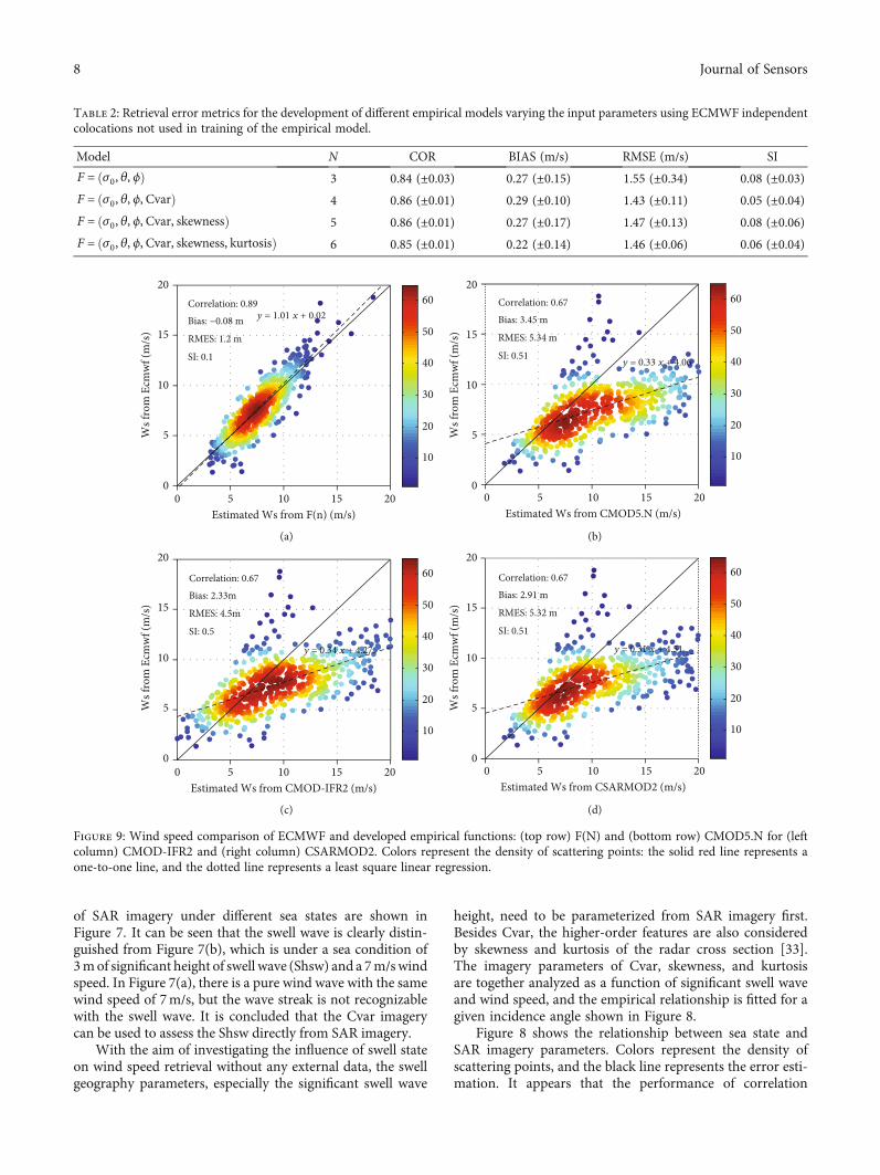
Table 2: Retrieval error metrics for the development of different empirical models varying the input parameters using ECMWF independentcolocations not used in training of the empirical model.

Model N COR BIAS (m/s) RMSE (m/s) SI

F = σ0, θ, ϕð Þ 3 0.84 (±0.03) 0.27 (±0.15) 1.55 (±0.34) 0.08 (±0.03)F = σ0, θ, ϕ, Cvarð Þ 4 0.86 (±0.01) 0.29 (±0.10) 1.43 (±0.11) 0.05 (±0.04)F = σ0, θ, ϕ, Cvar, skewnessð Þ 5 0.86 (±0.01) 0.27 (±0.17) 1.47 (±0.13) 0.08 (±0.06)F = σ0, θ, ϕ, Cvar, skewness, kurtosisð Þ 6 0.85 (±0.01) 0.22 (±0.14) 1.46 (±0.06) 0.06 (±0.04)

10

20

30

40

50

60

Ws f

rom

Ecm

wf (

m/s

)

0

5

10

15

20

0 5 10 15 20Estimated Ws from F(n) (m/s)

Correlation: 0.89Bias: –0.08 mRMES: 1.2 mSI: 0.1

y = 1.01x+0.02Correlation: 0.89Bias: −0.08 m

RMES: 1.2 m

SI: 0.1

y = 1.01 x + 0.02

(a)

10

20

30

40

50

60

Ws f

rom

Ecm

wf (

m/s

)

0

5

10

15

20

0 5 10 15 20Estimated Ws from CMOD5.N (m/s)

Correlation: 0.67Bias: 3.45 mRMES: 5.34 mSI: 0.51

y = 0.33x+4.06

Correlation: 0.67Bias: 3.45 m

RMES: 5.34 m

SI: 0.51y = 0.33 x + 4.06

(b)

10

20

30

40

50

60

Ws f

rom

Ecm

wf (

m/s

)

0

5

10

15

20

0 5 10 15 20Estimated Ws from CMOD-IFR2 (m/s)

Correlation: 0.67Bias: 2.33 mRMES: 4.5 mSI: 0.5

y = 0.34x+4.27

Correlation: 0.67Bias: 2.33m

RMES: 4.5m

SI: 0.5

y = 0.34 x + 4.27

(c)

10

20

30

40

50

60

Ws f

rom

Ecm

wf (

m/s

)

0

5

10

15

20

0 5 10 15 20Estimated Ws from CSARMOD2 (m/s)

Correlation: 0.67Bias: 2.91 mRMES: 5.32 mSI: 0.51

y = 0.31x+4.51

Correlation: 0.67Bias: 2.91 m

RMES: 5.32 m

SI: 0.51

y = 0.31 x + 4.51

(d)

Figure 9: Wind speed comparison of ECMWF and developed empirical functions: (top row) F(N) and (bottom row) CMOD5.N for (leftcolumn) CMOD-IFR2 and (right column) CSARMOD2. Colors represent the density of scattering points: the solid red line represents aone-to-one line, and the dotted line represents a least square linear regression.

8 Journal of Sensors

between imagery parameters of Cvar, skewness, kurtosis,and Shts behaves much better than wind speed. Comparedwith skewness and kurtosis, Cvar is more responsive to thecharacteristics of a swell. In terms of wind speed retrieval,it is suggested to add parameters of Cvar, skewness, and kur-tosis to compensate for the loss of the influence of a swellwave on NRCS.

3.3. New Method for Wind Speed Retrieval. A quasilinearrelationship is observed in the relationship with Shts, asshown in Figures 7(a), 7(c), and 7(e). In consideration ofthe influence of a swell wave on wind speed retrieval, anew empirical model is proposed, taking a unique formula-tion as follows [34, 35]:

Ws = A0 + 〠n

i=1Ai × Si + 〠

n

i,j=1Ai,j × Si × Sj, ð6Þ

where Si denote the SAR-derived parameters, Ai denote thetuning coefficients. Using the empirical relationship estab-lished by the training dataset, the rest of the verificationdataset is used to assess the model precision. As shown inTable 2, the retrieval error metrics for the development ofdifferent empirical models varying the input parametersare compared. It appears that the model precision of F(n)improved as the model parameters increase. When Cvar isused as input, there is a significant improvement comparedto the other functions that use three input parameters.Besides, as the parameters of skewness and kurtosis are usedas input, the performance of function robustness behavesmuch better than others.

3.4. Validation with CMODs. The CMOD model is widelyused for wind speed retrieval no matter if it is for a scatte-rometer or SAR. In this section, the F(n) model is comparedwith CMOD functions using collocated SAR and SWH data-set. Figure 9(a) shows the wind speed comparison between

the F(n) model and collocated ECMWF data. Figures 9(b)–9(d) show the retrieval precision of CMOD5.N, CMOD-IFR2, and CSARMOD2 using the same dataset, respectively.Colors represent the density of scattering points. The blacksolid line represents the one-to-one line, and the dotted linerepresents the least square regression line. It appears that theleast squares regression line agrees nicely with the one-to-one fit in Figure 9(a). The F(n) model performs much betterthan other CMOD functions, with a correlation of 0.89, abias of 0.08, an RMSE of 1.2m/s, and an SI of 0.1. An under-estimation is present for models of CMOD5.N, CMOD-IFR2, and CSARMOD2 in conditions where wind speed isgreat than 5m/s.

4. Discussion

Another important issue of the influence of swell peak wave-length on NRCS is also investigated in this session.Figure 10(a) shows the NRCS variation with an increase ofwave peak wavelength in the case where wind speed is setto 5m/s, 10m/s, and 15m/s, respectively. Barely no changeof NRCS is shown in a fixed wind speed. A similar relation-ship is also shown in Figure 8(b). The NRCS grows with anincrease of wind speed under different wave peak wave-lengths. It can be noticed that a minimum bias of NRCScan be found between different swells of peak wavelengths.

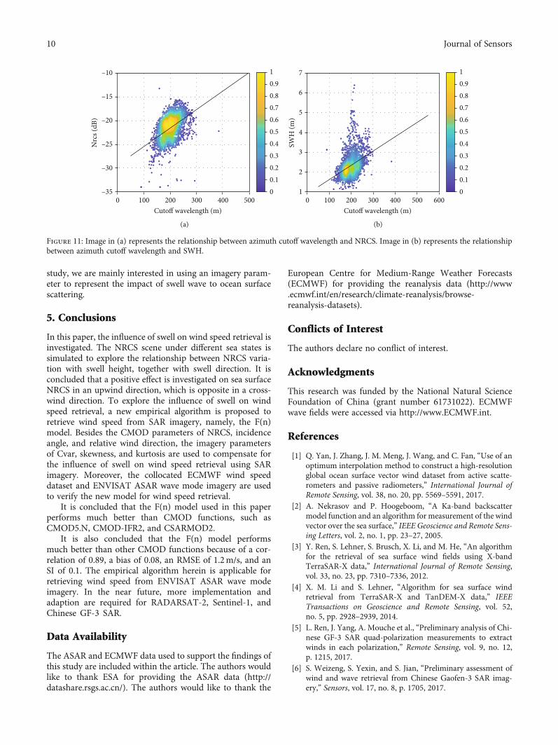
It has been noticed that the azimuth cutoff wavelengthwas also regarded as the imagery features caused by movingthe sea surface. To explore the impact of azimuth cutoffwavelength on NRCS, the correlation between azimuth cut-off wavelength and NRCS is shown in Figure 11. As shownin Figure 11, there is a high correlation between azimuthcutoff wavelength and SWH.

Unfortunately, an azimuth cutoff wavelength still cannotdistinguish SWH from a swell wave and a wind wave. Fornow, few studies are focused on the impact of azimuth cutoffwavelength on swell-wind wave interaction. So, in a future

150 200 250 300 350 400 450 500–20–18–16–14–12N

rcs (

dB)

–10–8–6–4–2

0

Peak wavelength (m)

Incidence angle = 23°Relative wind direction = 0°Swell height = 2 m

Wind speed 5 m/sWind speed 10 m/sWind speed 15 m/s

(a)

Nrc

s (dB

)

Swell wavelength 200 mSwell wavelength 300 mSwell wavelength 400 m

0 5 10 15 20 25 30–25

–20

–15

–10

–5

0

Wind speed (m/s)

Incidence angle = 23°Relative wind direction = 0°Swell height = 2 m

(b)

Figure 10: Influence of wave peak wavelength on NRCS.

9Journal of Sensors

study, we are mainly interested in using an imagery param-eter to represent the impact of swell wave to ocean surfacescattering.

5. Conclusions

In this paper, the influence of swell on wind speed retrieval isinvestigated. The NRCS scene under different sea states issimulated to explore the relationship between NRCS varia-tion with swell height, together with swell direction. It isconcluded that a positive effect is investigated on sea surfaceNRCS in an upwind direction, which is opposite in a cross-wind direction. To explore the influence of swell on windspeed retrieval, a new empirical algorithm is proposed toretrieve wind speed from SAR imagery, namely, the F(n)model. Besides the CMOD parameters of NRCS, incidenceangle, and relative wind direction, the imagery parametersof Cvar, skewness, and kurtosis are used to compensate forthe influence of swell on wind speed retrieval using SARimagery. Moreover, the collocated ECMWF wind speeddataset and ENVISAT ASAR wave mode imagery are usedto verify the new model for wind speed retrieval.

It is concluded that the F(n) model used in this paperperforms much better than CMOD functions, such asCMOD5.N, CMOD-IFR2, and CSARMOD2.

It is also concluded that the F(n) model performsmuch better than other CMOD functions because of a cor-relation of 0.89, a bias of 0.08, an RMSE of 1.2m/s, and anSI of 0.1. The empirical algorithm herein is applicable forretrieving wind speed from ENVISAT ASAR wave modeimagery. In the near future, more implementation andadaption are required for RADARSAT-2, Sentinel-1, andChinese GF-3 SAR.

Data Availability

The ASAR and ECMWF data used to support the findings ofthis study are included within the article. The authors wouldlike to thank ESA for providing the ASAR data (http://datashare.rsgs.ac.cn/). The authors would like to thank the

European Centre for Medium-Range Weather Forecasts(ECMWF) for providing the reanalysis data (http://www.ecmwf.int/en/research/climate-reanalysis/browse-reanalysis-datasets).

Conflicts of Interest

The authors declare no conflict of interest.

Acknowledgments

This research was funded by the National Natural ScienceFoundation of China (grant number 61731022). ECMWFwave fields were accessed via http://www.ECMWF.int.

References

[1] Q. Yan, J. Zhang, J. M. Meng, J. Wang, and C. Fan, “Use of anoptimum interpolation method to construct a high-resolutionglobal ocean surface vector wind dataset from active scatte-rometers and passive radiometers,” International Journal ofRemote Sensing, vol. 38, no. 20, pp. 5569–5591, 2017.

[2] A. Nekrasov and P. Hoogeboom, “A Ka-band backscattermodel function and an algorithm for measurement of the windvector over the sea surface,” IEEE Geoscience and Remote Sens-ing Letters, vol. 2, no. 1, pp. 23–27, 2005.

[3] Y. Ren, S. Lehner, S. Brusch, X. Li, and M. He, “An algorithmfor the retrieval of sea surface wind fields using X-bandTerraSAR-X data,” International Journal of Remote Sensing,vol. 33, no. 23, pp. 7310–7336, 2012.

[4] X. M. Li and S. Lehner, “Algorithm for sea surface windretrieval from TerraSAR-X and TanDEM-X data,” IEEETransactions on Geoscience and Remote Sensing, vol. 52,no. 5, pp. 2928–2939, 2014.

[5] L. Ren, J. Yang, A. Mouche et al., “Preliminary analysis of Chi-nese GF-3 SAR quad-polarization measurements to extractwinds in each polarization,” Remote Sensing, vol. 9, no. 12,p. 1215, 2017.

[6] S. Weizeng, S. Yexin, and S. Jian, “Preliminary assessment ofwind and wave retrieval from Chinese Gaofen-3 SAR imag-ery,” Sensors, vol. 17, no. 8, p. 1705, 2017.

Nrc

s (dB

)

0–35

–30

–25

–20

–15

–10

100 200 300Cutoff wavelength (m)

400 50000.10.20.30.40.50.60.70.80.91

(a)

SWH

(m)

01

2

3

4

5

7

100 200 300Cutoff wavelength (m)

400 60000.10.20.30.40.50.60.70.80.91

500

6

(b)

Figure 11: Image in (a) represents the relationship between azimuth cutoff wavelength and NRCS. Image in (b) represents the relationshipbetween azimuth cutoff wavelength and SWH.

10 Journal of Sensors

[7] B. Zhang, S. Fan, A. Mouche, G. Zhang, and W. Perrie, “Syn-ergistic measurements of hurricane wind speeds and directionsfrom C-band dual-polarization synthetic aperture radar,” in2019 IEEE International Geoscience and Remote Sensing Sym-posium, Yokohama, Japan, 2019.

[8] G. Zhang, X. Li, W. Perrie, P. A. Hwang, B. Zhang, andX. Yang, “A hurricane wind speed retrieval model for C-band RADARSAT-2 cross-polarization ScanSAR images,”IEEE Transactions on Geoscience & Remote Sensing, vol. 55,no. 8, pp. 4766–4774, 2017.

[9] A. E. Long, “Towards a C-band radar sea echo model for theERS-1 scatterometer,” in First ISPRS Colloquium on SpectralSignatures in Remote Sensing, pp. 29–34, International Societyfor Photogrammetry and Remote Sensing, Les Arcs, 1985.

[10] A. Stoffelen and D. Anderson, “Scatterometer data interpreta-tion: estimation and validation of the transfer functionCMOD4,” Journal of Geophysical Research: Oceans, vol. 102,no. C3, pp. 5767–5780, 1997.

[11] A. Bentamy, P. Queffeulou, Y. Quilfen, and K. Katsaros,“Ocean surface wind fields estimated from satellite active andpassive microwave instruments,” IEEE Transactions on Geosci-ence and Remote Sensing, vol. 37, no. 5, pp. 2469–2486, 1999.

[12] H. Hersbach, A. Stoffelen, and S. D. Haan, “An improved C-band scatterometer ocean geophysical model function:CMOD5,” Journal of Geophysical Research: Oceans, vol. 112,no. C3, pp. 225–237, 2007.

[13] A. Verhoef, M. Portabella, A. Stoffelen, and H. Hersbach,CMOD5.n—The CMOD5 GMF for Neutral Winds, KNMI,De Bilt, The Netherlands, 2008, Ocean Sea Ice SAF Tech. NoteSAF/OSI/CDOP/KNMI/TEC/TN/3.

[14] L. Ricciardulli, T. Meissner, and F. Wentz, “Towards a climatedata record of satellite ocean vector winds,” in Geoscience andRemote Sensing Symposium (IGARSS), 2012 IEEE Interna-tional, pp. 2067–2069, New York, 2012.

[15] S. Soisuvarn, Z. Jelenak, P. S. Chang, S. O. Alsweiss, andQ. Zhu, “CMOD5.H—a high wind geophysical model functionfor C-band vertically polarized satellite scatterometer mea-surements,” IEEE Transactions on Geoscience and RemoteSensing, vol. 51, no. 6, pp. 3744–3760, 2013.

[16] A. Elyouncha, X. Neyt, A. Stoffelen, and J. Verspeek, “Assess-ment of the corrected CMOD6 GMF using scatterometerdata,” in Remote Sensing of the Ocean, Sea Ice, Coastal Waters,and Large Water Regions, no. article 963803, 2015SPIE, Tou-louse, 2015.

[17] A. Stoffelen, J. A. Verspeek, J. Vogelzang, and A. Verhoef, “TheCMOD7 geophysical model function for ASCAT and ERSwind retrievals,” IEEE Journal of Selected Topics in AppliedEarth Observations and Remote Sensing, vol. 10, no. 5,pp. 2123–2134, 2017.

[18] A. Mouche and B. Chapron, “Global C‐Band Envisat,RADARSAT‐2, and Sentinel‐1 SARmeasurements in copolar-ization and cross-polarization,” Journal of GeophysicalResearch Oceans, vol. 120, no. 11, pp. 7195–7207, 2015.

[19] H. Wang, J. Yang, A. Mouche et al., “GF-3 SAR ocean windretrieval: the first view and preliminary assessment,” RemoteSensing, vol. 9, no. 7, p. 694, 2017.

[20] L. Wang, B. Han, X. Yuan et al., “A preliminary analysis ofwind retrieval, based on GF-3 wave mode data,” Sensors,vol. 18, no. 5, p. 1604, 2018.

[21] W. Shao, S. Zhu, X. Zhang et al., “Intelligent wind retrievalfrom Chinese Gaofen-3 SAR imagery in quad polarization,”

Journal of Atmospheric and Oceanic Technology, vol. 36,no. 11, pp. 2121–2138, 2019.

[22] L. Ren, J. Yang, A. A. Mouche et al., “Assessments of oceanwind retrieval schemes used for Chinese Gaofen-3 syntheticaperture radar co-polarized data,” IEEE Transactions on GeoS-cence and Remote Sensing, vol. 57, no. 9, pp. 7075–7085, 2019.

[23] W. Yong, “Exploitable wave energy assessment based on ERA-interim reanalysis data—a case study in the East China Sea andthe South China Sea,” Acta Oceanologica Sinica, vol. 34, no. 9,pp. 143–155, 2015.

[24] W. Shao, X. Li, and X. Yang, “Retrieval of winds and wavesfrom synthetic aperture radar imagery,” in Remote Sensing ofthe Asian Seas, V. Barale and M. Gade, Eds., pp. 285–303,Springer, Cham, 2019.

[25] P. A. Hwang, B. Zhang, J. V. Toporkov, and W. Perrie, “Com-parison of composite Bragg theory and quad-polarizationradar backscatter from RADARSAT-2: with applications towave breaking and high wind retrieval,” Journal of GeophysicalResearch: Atmospheres, vol. 115, no. C8, pp. 246–255, 2010.

[26] V. Kudryavtsev, D. Hauser, G. Caudal, and B. Chapron, “Asemiempirical model of the normalized radar cross-section ofthe sea surface 1. Background model,” Journal of GeophysicalResearch: Oceans, vol. 108, no. C3, pp. FET 2-1–FET 2-24,2003.

[27] G. R. Valenzuela, “Theories for the interaction of electromag-netic and oceanic waves–a review,” Boundary-Layer Meteorol-ogy, vol. 13, no. 1-4, pp. 61–85, 1978.

[28] D. E. Barrick, “Rough surface scattering based on the specularpoint theory,” IEEE Transactions on Antennas and Propaga-tion, vol. 16, no. 4, pp. 449–454, 1968.

[29] L. Wetzel, “On microwave scattering by breaking waves,” inWave Dynamics and Radio Probing of the Ocean Surface,pp. 273–284, Springer US, New York, 1986.

[30] P. H. Y. Lee, J. D. Barter, K. L. Beach et al., “Scattering frombreaking gravity waves without wind,” IEEE Transactions onAntennas and Propagation, vol. 46, no. 1, pp. 14–26, 1998.

[31] H. Li, A. Mouche, and J. E. Stopa, “Impact of sea state on windretrieval from Sentinel-1 wave mode data,” IEEE Journal ofSelected Topics in Applied Earth Observations and RemoteSensing, vol. 12, no. 2, pp. 559–566, 2019.

[32] D. Gao, Y. Liu, J. Meng, Y. Jia, and C. Fan, “Estimating sig-nificant wave height from SAR imagery based on an SVMregression model,” Acta Oceanologica Sinica, vol. 37, no. 3,pp. 103–110, 2018.

[33] T. Elfouhaily, B. Chapron, K. Katsaros, and D. Vandemark, “Aunified directional spectrum for long and short wind-drivenwaves,” Journal of Geophysical Research: Oceans, vol. 102,no. C7, pp. 15781–15796, 1997.

[34] V. Kerbaol, B. Chapron, and P. W. Vachon, “Analysis of ERS-1/2 synthetic aperture radar wave mode imagettes,” Journal ofGeophysical Research, vol. 103, no. C4, pp. 7833–7846, 1998.

[35] C. Fan, X. Wang, X. Zhang, and D. Gao, “A newly developedocean significant wave height retrieval method from EnvisatASAR wave mode imagery,” Acta Oceanologica Sinica,vol. 38, no. 9, pp. 120–127, 2019.

11Journal of Sensors