Embed Size (px)
Citation preview
Influences of transition
in age-education structure
and internal migration
on the labor market in Brazil
Ernesto Friedrich de Lima Amaral
Political Science Department (DCP)
Federal University of Minas Gerais (UFMG)
Funded by the Brazilian Institute of Applied Economics Research (IPEA)
1
Demographic transition
and economic development
Part of a larger project to look at the relationship between
changes in the age distribution and economic development
at the local level in both Brazil and Mexico (PI: Professor
Joseph Potter, UT).
Motivated by results for Asia and their relevance to Latin
America (Bloom, Canning, Williamson, Mason and others).
Awareness that the heterogeneity that prevails in Brazil and
Mexico could work to our advantage.
Figuring out how to take advantage of this heterogeneity led
us to look at studies that had been done on another major
demographic shock... the “baby boom” in the US.
2

“Baby Boom” and US Labor Market
Large literature on age-education shifts in the US (Freeman
1979; Welch 1979; Berger 1985; Triest, Sapozhnikov e Sass
2006).
Exceptionally large cohorts born during the “baby boom”
entered the American labor market in the 1970s with higher
levels of education.
Studies suggest that large cohorts depressed earnings.
Negative effects increase with education.
“Baby boomers” will still affect income structure after their
retirement.
3
The case of Brazil
Might such compositional changes have influenced earnings
in a large Latin American country such as Brazil?
As in other developing countries, age-education
transitions in Brazil provide a lot of variation in
demographic structure:
Fertility decline varied in timing and speed across states
and municipalities.
Educational enrollment increased substantially from very
low levels, but with much regional variation.
Our idea was to use this regional variation to analyze who
gains and loses from these compositional shifts, with a
cross-section time series approach.
4
Data
Microdata from the 1970-2000 Brazilian Censuses.
Census long forms are available for 25% (1970 and 1980)
and 10% or 20% (1991 and 2000) of households.
Long forms contain information on age, sex, education,
income, occupation, and migration.
We aggregate municipalities to the micro-region level,
yielding 502 comparable areas across the four censuses.
5

Categories
Time (census years): 1970, 1980, 1991, and 2000.
Age is categorized in four groups:
Youth population (15-24).
Young adults (25-34).
Adults (35-49).
Mature adults (50-64).
Educational attainment was classified in three groups
according to years of schooling completed:
No further than the first phase of elementary school (0-4).
Second phase of elementary school (5-8).
At least some secondary school (9+).
Earnings in main occupation: converted to January 2002.
6
0.0
3.0
6.0
9.0
12.0
15.0
18.0
21.0
24.0
27.0
30.0
15–24
years,
0–4
educ
15–24
years,
5–8
educ
15–24
years,
9+
educ
25–34
years,
0–4
educ
25–34
years,
5–8
educ
25–34
years,
9+
educ
35–49
years,
0–4
educ
35–49
years,
5–8
educ
35–49
years,
9+
educ
50–64
years,
0–4
educ
50–64
years,
5–8
educ
50–64
years,
9+
educ
Age-education Group
Perc
en
t
1970 1980 1991 2000
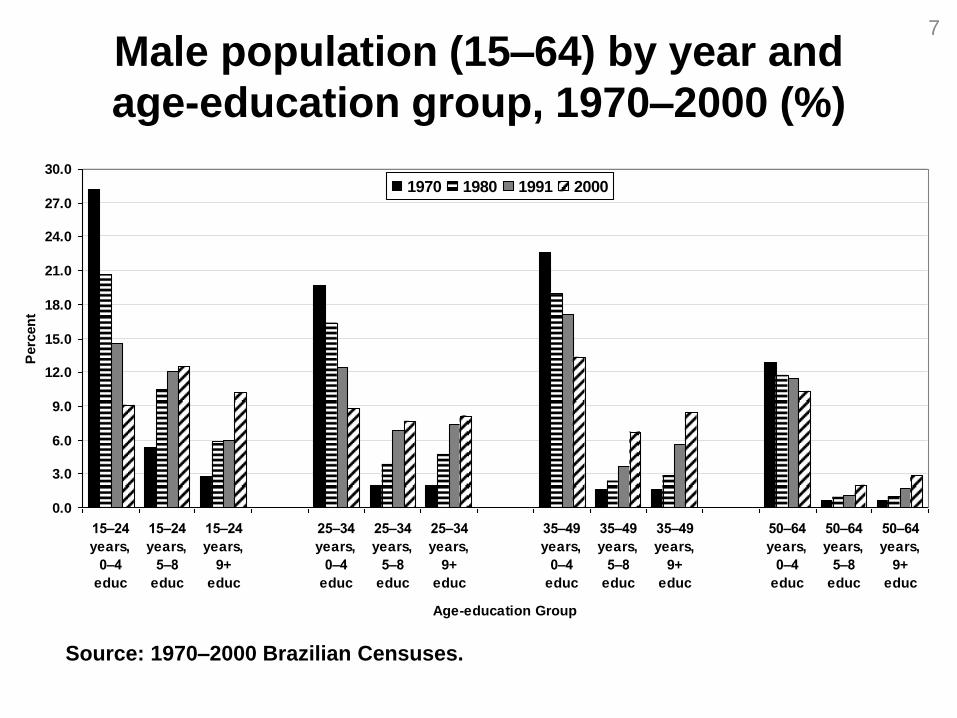
Source: 1970–2000 Brazilian Censuses.
Male population (15–64) by year and
age-education group, 1970–2000 (%)
7
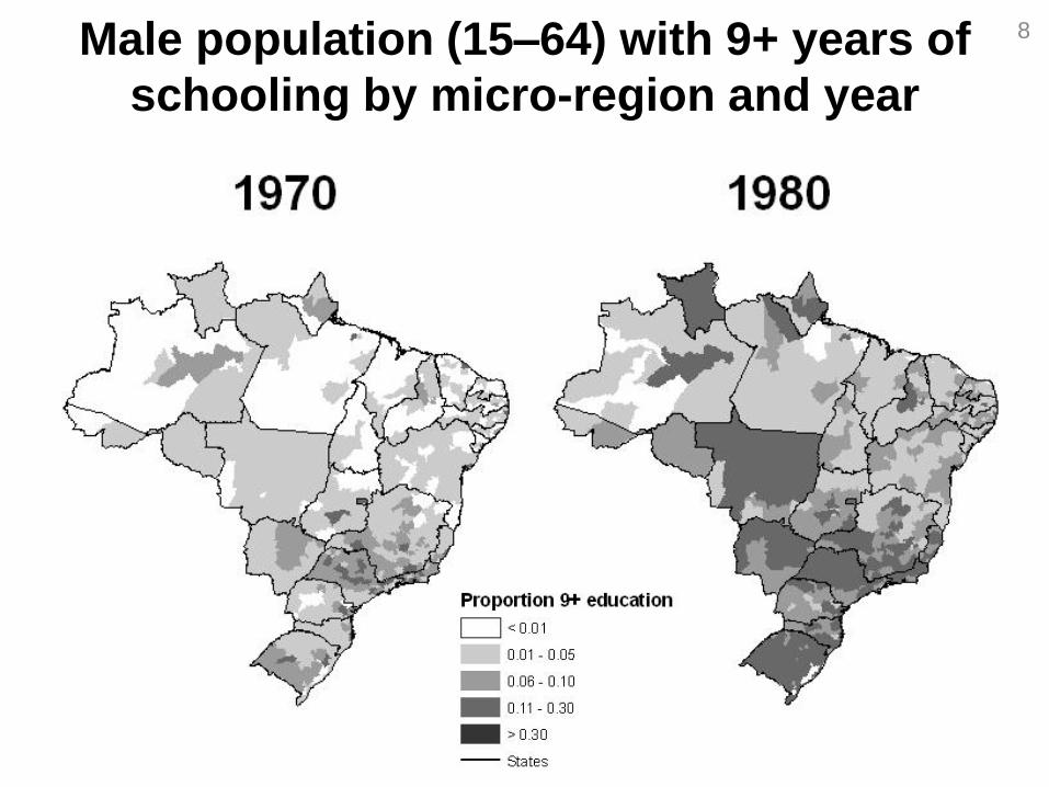
Male population (15–64) with 9+ years of
schooling by micro-region and year
8
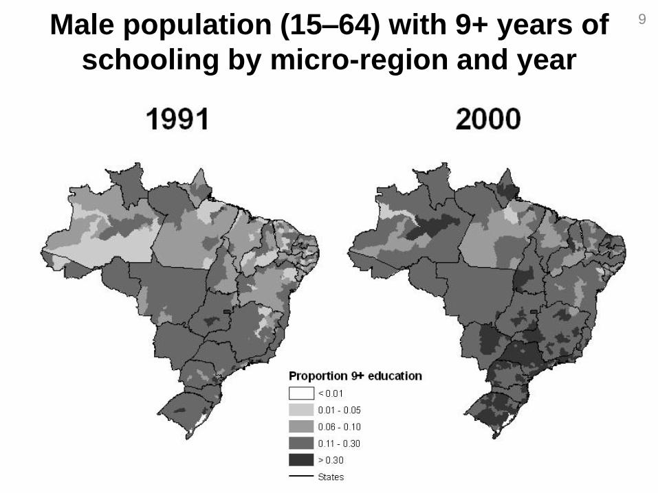
9 Male population (15–64) with 9+ years of
schooling by micro-region and year
0.00
250.00
500.00
750.00
1,000.00
1,250.00
1,500.00
1,750.00
2,000.00
2,250.00
2,500.00
15–24
years,
0–4
educ
15–24
years,
5–8
educ
15–24
years,
9+ educ
25–34
years,
0–4
educ
25–34
years,
5–8
educ
25–34
years,
9+ educ
35–49
years,
0–4
educ
35–49
years,
5–8
educ
35–49
years,
9+ educ
50–64
years,
0–4
educ
50–64
years,
5–8
educ
50–64
years,
9+ educ
Age-education Group
Ea
rnin
gs
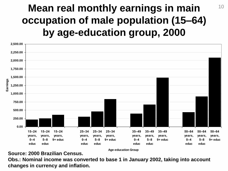
Mean real monthly earnings in main
occupation of male population (15–64)
by age-education group, 2000
Source: 2000 Brazilian Census.
Obs.: Nominal income was converted to base 1 in January 2002, taking into account
changes in currency and inflation.
10
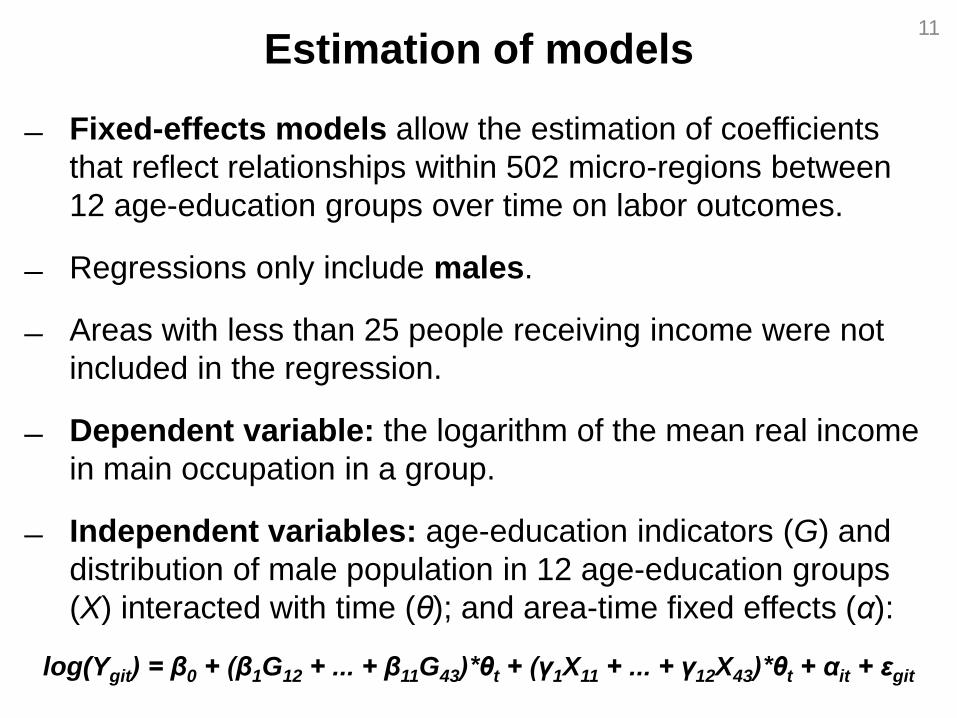
Estimation of models
Fixed-effects models allow the estimation of coefficients
that reflect relationships within 502 micro-regions between
12 age-education groups over time on labor outcomes.
Regressions only include males.
Areas with less than 25 people receiving income were not
included in the regression.
Dependent variable: the logarithm of the mean real income
in main occupation in a group.
Independent variables: age-education indicators (G) and
distribution of male population in 12 age-education groups
(X) interacted with time (θ); and area-time fixed effects (α):
log(Ygit) = β0 + (β1G12 + ... + β11G43)*θt + (γ1X11 + ... + γ12X43)*θt + αit + εgit
11
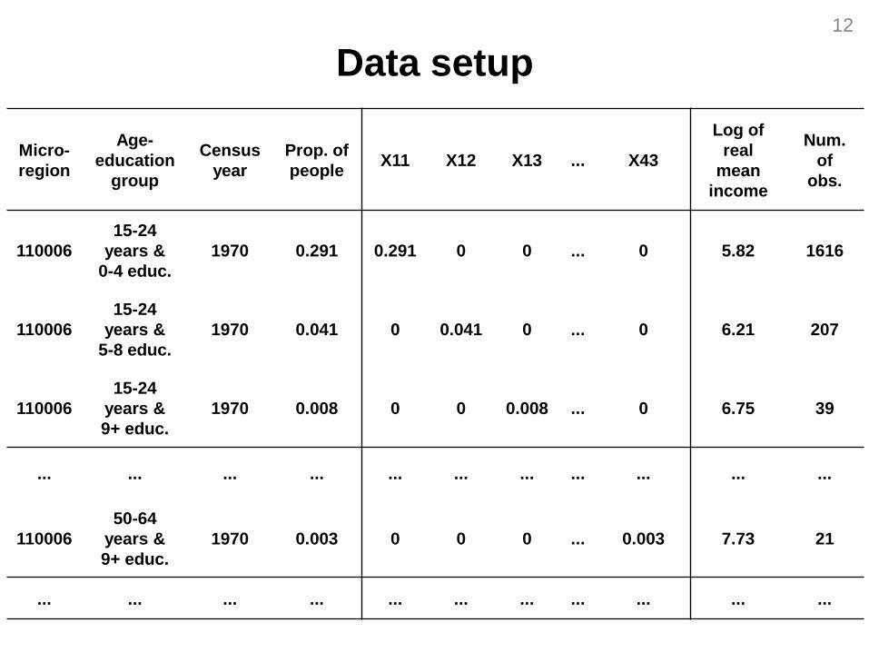
Data setup
Micro-
region
Age-
education
group
Census
year
Prop. of
people X11 X12 X13 ... X43
Log of
real
mean
income
Num.
of
obs.
110006
15-24
years &
0-4 educ.
1970 0.291 0.291 0 0 ... 0 5.82 1616
110006
15-24
years &
5-8 educ.
1970 0.041 0 0.041 0 ... 0 6.21 207
110006
15-24
years &
9+ educ.
1970 0.008 0 0 0.008 ... 0 6.75 39
... ... ... ... ... ... ... ... ... ... ...
110006
50-64
years &
9+ educ.
1970 0.003 0 0 0 ... 0.003 7.73 21
... ... ... ... ... ... ... ... ... ... ...
12

1.0
1.8
2.7
4.9
8.8
2.3
5.5
9.4
2.3
3.4
1.5
6.0
0.0
1.0
2.0
3.0
4.0
5.0
6.0
7.0
8.0
9.0
10.0
0-4
educ
5-8
educ
9+
educ
0-4
educ
5-8
educ
9+
educ
0-4
educ
5-8
educ
9+
educ
0-4
educ
5-8
educ
9+
educ
Exp
on
en
tial
of
co
eff
icie
nt
15-24 years 25-34 years 35-49 years 50-64 years
13 Effects of age-education indicators
(G11-G43) on earnings, 1970–2000
Source: 1970–2000 Brazilian Censuses.
1000
1375
1750
2125
2500
Earn
ings
0 .05 .1 .15Proportion
Predicted 1970 Predicted 2000
400
650
900
1150
1400
Earn
ings
0 .05 .1Proportion
Predicted 1970 Predicted 2000
300
340
380
420
460
Earn
ings
.05 .1 .15 .2 .25 .3Proportion
Predicted 1970 Predicted 2000
500
875
1250
1625
2000
Earn
ings
0 .05 .1 .15Proportion
Predicted 1970 Predicted 2000
400
550
700
850
1000
Earn
ings
0 .05 .1 .15Proportion
Predicted 1970 Predicted 2000
250
275
300
325
350
Earn
ings
0 .1 .2 .3Proportion
Predicted 1970 Predicted 2000
25–34 years
5–8 education 0–4 education 9+ education
35–49 years
5–8 education 0–4 education 9+ education
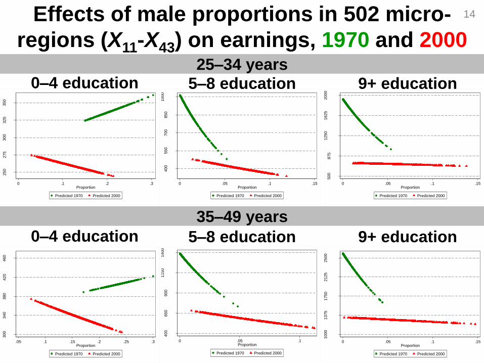
14 Effects of male proportions in 502 micro-
regions (X11-X43) on earnings, 1970 and 2000
New considerations
Objective is to develop methodological procedures to
include information of internal migration in the previous
models.
If there was no migration flows, the sending areas (which
already have lower relative earnings) would have even
lower earnings, and the receiving areas (which already have
higher relative earnings) would experience raises on
earnings.
By not controlling for migration in the models, results are
underestimating the negative effect of group size
(cohorts) on earnings.
The hypothesis is that, by controlling for migration flows,
the negative impacts of age-education-group proportions will
be even more negative than previous estimates.
15
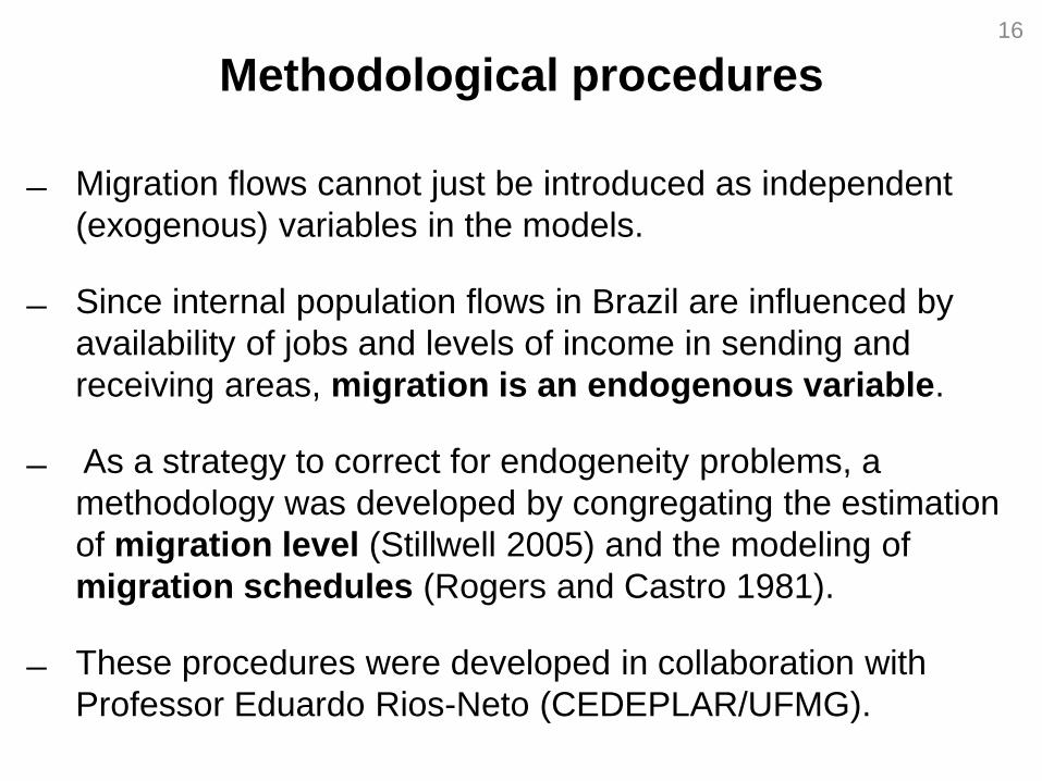
Methodological procedures
Migration flows cannot just be introduced as independent
(exogenous) variables in the models.
Since internal population flows in Brazil are influenced by
availability of jobs and levels of income in sending and
receiving areas, migration is an endogenous variable.
As a strategy to correct for endogeneity problems, a
methodology was developed by congregating the estimation
of migration level (Stillwell 2005) and the modeling of
migration schedules (Rogers and Castro 1981).
These procedures were developed in collaboration with
Professor Eduardo Rios-Neto (CEDEPLAR/UFMG).
16
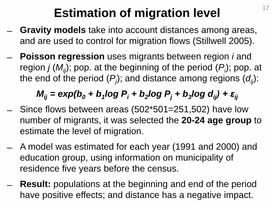
Estimation of migration level
Gravity models take into account distances among areas,
and are used to control for migration flows (Stillwell 2005).
Poisson regression uses migrants between region i and
region j (Mij); pop. at the beginning of the period (Pi); pop. at
the end of the period (Pj); and distance among regions (dij):
Mij = exp(b0 + b1log Pi + b2log Pj + b3log dij) + εij
Since flows between areas (502*501=251,502) have low
number of migrants, it was selected the 20-24 age group to
estimate the level of migration.
A model was estimated for each year (1991 and 2000) and
education group, using information on municipality of
residence five years before the census.
Result: populations at the beginning and end of the period
have positive effects; and distance has a negative impact.
17
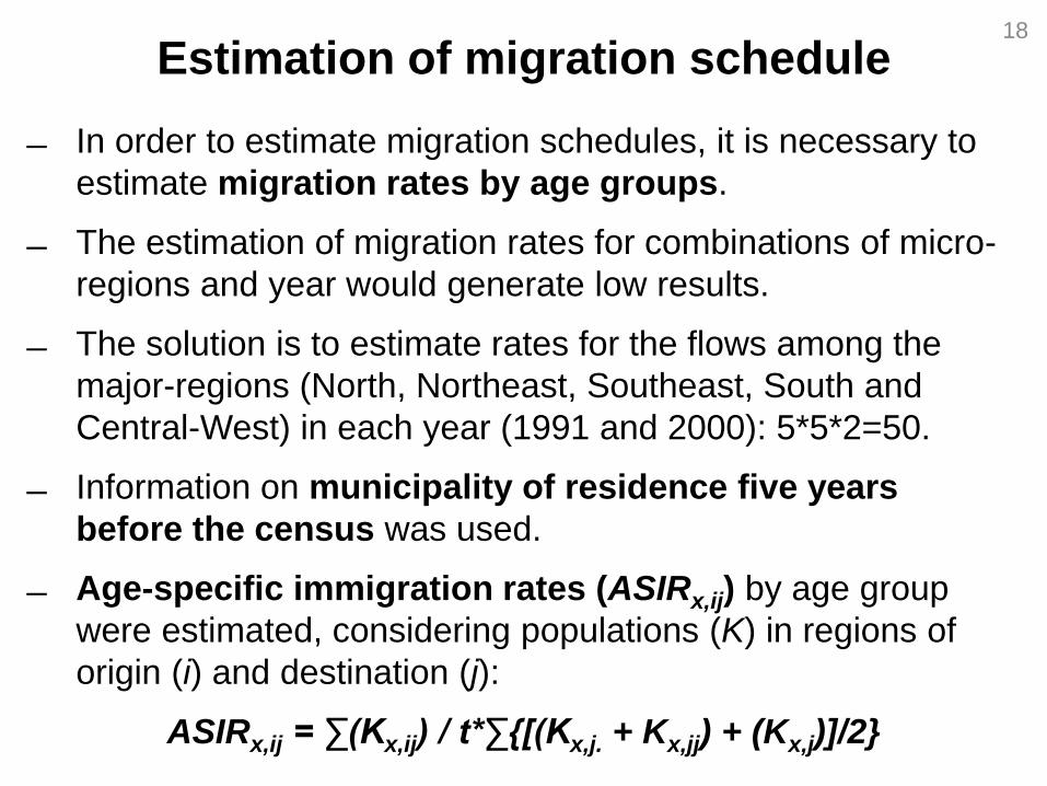
Estimation of migration schedule
In order to estimate migration schedules, it is necessary to
estimate migration rates by age groups.
The estimation of migration rates for combinations of micro-
regions and year would generate low results.
The solution is to estimate rates for the flows among the
major-regions (North, Northeast, Southeast, South and
Central-West) in each year (1991 and 2000): 5*5*2=50.
Information on municipality of residence five years
before the census was used.
Age-specific immigration rates (ASIRx,ij) by age group
were estimated, considering populations (K) in regions of
origin (i) and destination (j):
ASIRx,ij = ∑(Kx,ij) / t*∑{[(Kx,j. + Kx,jj) + (Kx,j)]/2}
18
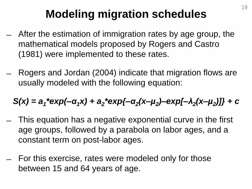
Modeling migration schedules
After the estimation of immigration rates by age group, the
mathematical models proposed by Rogers and Castro
(1981) were implemented to these rates.
Rogers and Jordan (2004) indicate that migration flows are
usually modeled with the following equation:
S(x) = a1*exp(–α1x) + a2*exp{–α2(x–µ2)–exp[–λ2(x–µ2)]} + c
This equation has a negative exponential curve in the first
age groups, followed by a parabola on labor ages, and a
constant term on post-labor ages.
For this exercise, rates were modeled only for those
between 15 and 64 years of age.
19
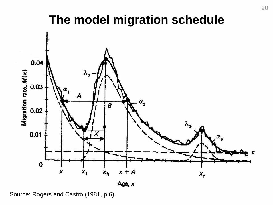
The model migration schedule
Source: Rogers and Castro (1981, p.6).
20
21
.05
.07
.09
.11
.13
.15
Pro
port
ional A
SIR
15 20 25 30 35 40 45 50 55 60Age Group
Observed, 1991 Observed, 2000
Estimated, 1991 Estimated, 2000
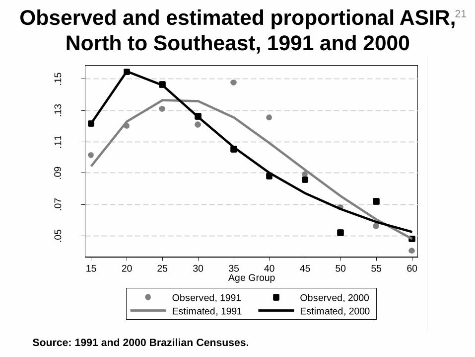
Observed and estimated proportional ASIR,
North to Southeast, 1991 and 2000
Source: 1991 and 2000 Brazilian Censuses.
22
0
.06
.12
.18
.24
.3
Pro
port
ional A
SIR
15 20 25 30 35 40 45 50 55 60Age Group
Observed, 1991 Observed, 2000
Estimated, 1991 Estimated, 2000
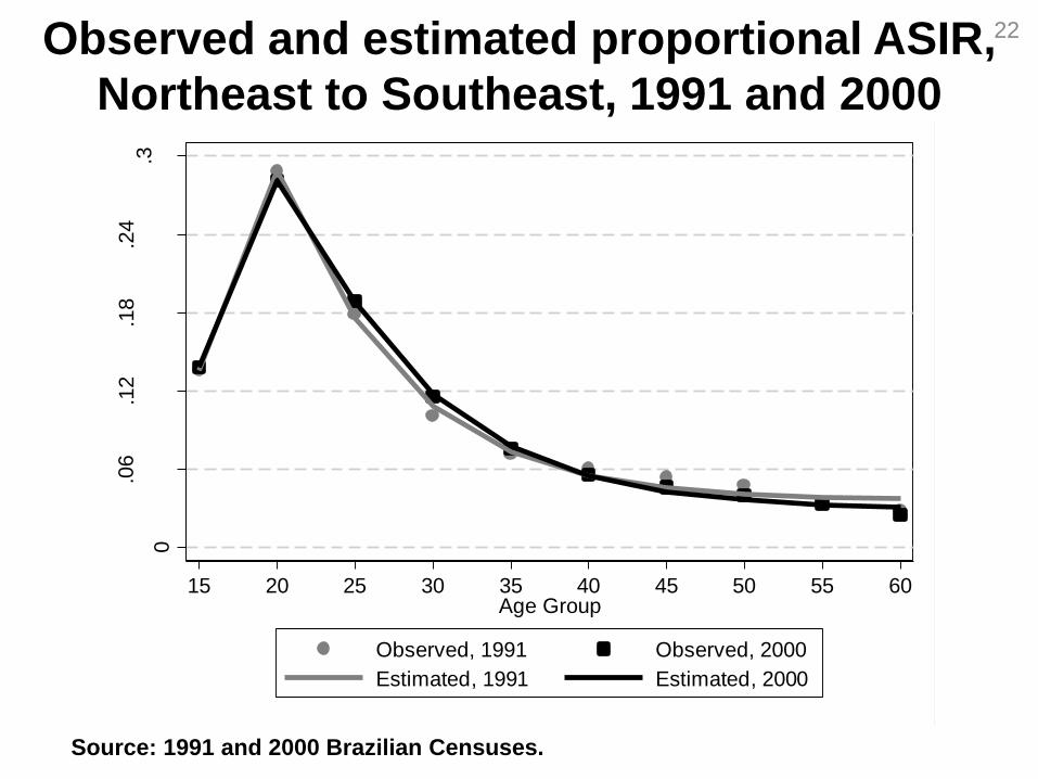
Source: 1991 and 2000 Brazilian Censuses.
Observed and estimated proportional ASIR,
Northeast to Southeast, 1991 and 2000
23
.06
.075
.09
.105
.12
.135
Pro
port
ional A
SIR
15 20 25 30 35 40 45 50 55 60Age Group
Observed, 1991 Observed, 2000
Estimated, 1991 Estimated, 2000
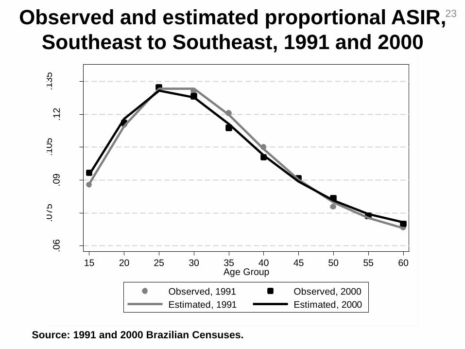
Source: 1991 and 2000 Brazilian Censuses.
Observed and estimated proportional ASIR,
Southeast to Southeast, 1991 and 2000
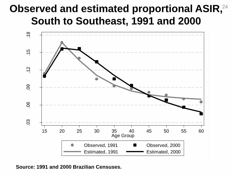
24
.03
.06
.09
.12
.15
.18
Pro
port
ional A
SIR
15 20 25 30 35 40 45 50 55 60Age Group
Observed, 1991 Observed, 2000
Estimated, 1991 Estimated, 2000
Source: 1991 and 2000 Brazilian Censuses.
Observed and estimated proportional ASIR,
South to Southeast, 1991 and 2000
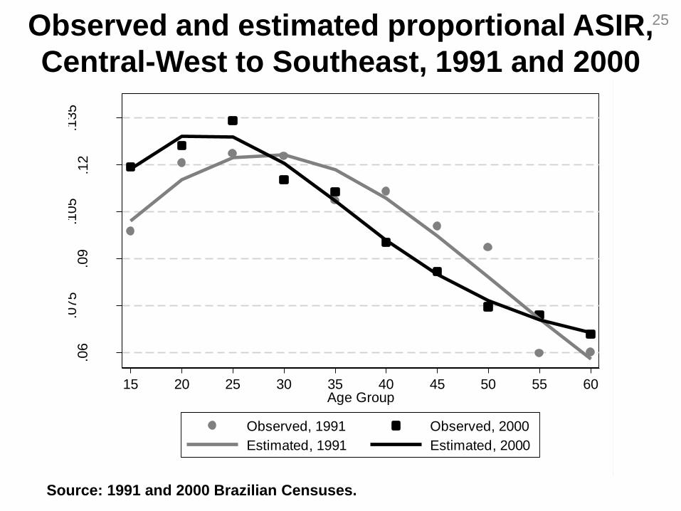
25
.06
.075
.09
.105
.12
.135
Pro
port
ional A
SIR
15 20 25 30 35 40 45 50 55 60Age Group
Observed, 1991 Observed, 2000
Estimated, 1991 Estimated, 2000
Source: 1991 and 2000 Brazilian Censuses.
Observed and estimated proportional ASIR,
Central-West to Southeast, 1991 and 2000
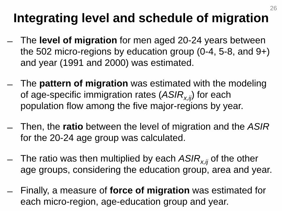
Integrating level and schedule of migration
The level of migration for men aged 20-24 years between
the 502 micro-regions by education group (0-4, 5-8, and 9+)
and year (1991 and 2000) was estimated.
The pattern of migration was estimated with the modeling
of age-specific immigration rates (ASIRx,ij) for each
population flow among the five major-regions by year.
Then, the ratio between the level of migration and the ASIR
for the 20-24 age group was calculated.
The ratio was then multiplied by each ASIRx,ij of the other
age groups, considering the education group, area and year.
Finally, a measure of force of migration was estimated for
each micro-region, age-education group and year.
26
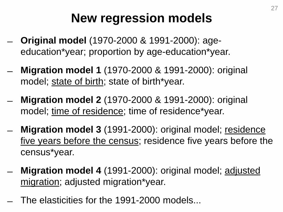
New regression models
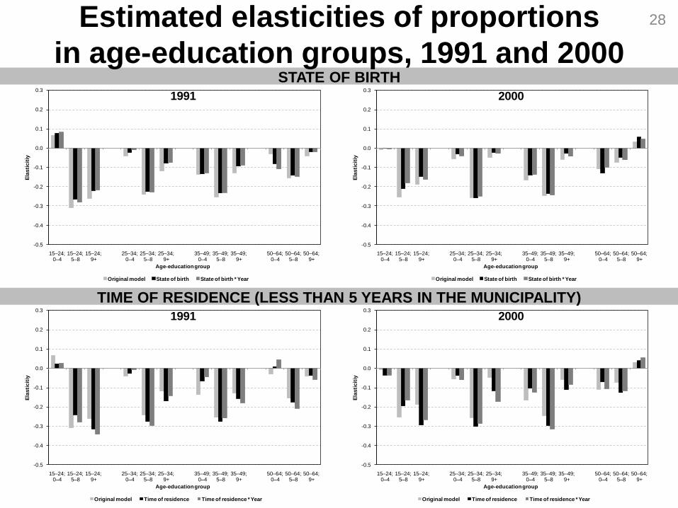
Original model (1970-2000 & 1991-2000): age-
education*year; proportion by age-education*year.
Migration model 1 (1970-2000 & 1991-2000): original
model; state of birth; state of birth*year.
Migration model 2 (1970-2000 & 1991-2000): original
model; time of residence; time of residence*year.
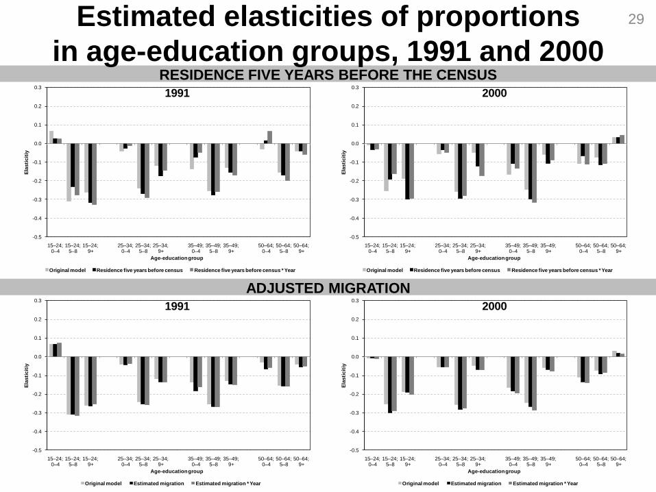
Migration model 3 (1991-2000): original model; residence
five years before the census; residence five years before the
census*year.
Migration model 4 (1991-2000): original model; adjusted
migration; adjusted migration*year.
The elasticities for the 1991-2000 models...
27
-0.5
-0.4
-0.3
-0.2
-0.1
0.0
0.1
0.2
0.3
15–24; 0–4
15–24; 5–8
15–24; 9+
25–34; 0–4
25–34; 5–8
25–34; 9+
35–49; 0–4
35–49; 5–8
35–49; 9+
50–64; 0–4
50–64; 5–8
50–64; 9+
Ela
sti
cit
iy
Age-education group
1991
Original model State of birth State of birth * Year
-0.5
-0.4
-0.3
-0.2
-0.1
0.0
0.1
0.2
0.3
15–24; 0–4
15–24; 5–8
15–24; 9+
25–34; 0–4
25–34; 5–8
25–34; 9+
35–49; 0–4
35–49; 5–8
35–49; 9+
50–64; 0–4
50–64; 5–8
50–64; 9+
Ela
sti
cit
iy
Age-education group
2000
Original model State of birth State of birth * Year
28
-0.5
-0.4
-0.3
-0.2
-0.1
0.0
0.1
0.2
0.3
15–24; 0–4
15–24; 5–8
15–24; 9+
25–34; 0–4
25–34; 5–8
25–34; 9+
35–49; 0–4
35–49; 5–8
35–49; 9+
50–64; 0–4
50–64; 5–8
50–64; 9+
Ela
sti
cit
iy
Age-education group
1991
Original model Time of residence Time of residence * Year
-0.5
-0.4
-0.3
-0.2
-0.1
0.0
0.1
0.2
0.3
15–24; 0–4
15–24; 5–8
15–24; 9+
25–34; 0–4
25–34; 5–8
25–34; 9+
35–49; 0–4
35–49; 5–8
35–49; 9+
50–64; 0–4
50–64; 5–8
50–64; 9+
Ela
sti
cit
iy
Age-education group
2000
Original model Time of residence Time of residence * Year
STATE OF BIRTH
TIME OF RESIDENCE (LESS THAN 5 YEARS IN THE MUNICIPALITY)
Estimated elasticities of proportions
in age-education groups, 1991 and 2000
-0.5
-0.4
-0.3
-0.2
-0.1
0.0
0.1
0.2
0.3
15–24; 0–4
15–24; 5–8
15–24; 9+
25–34; 0–4
25–34; 5–8
25–34; 9+
35–49; 0–4
35–49; 5–8
35–49; 9+
50–64; 0–4
50–64; 5–8
50–64; 9+
Ela
sti
cit
iy
Age-education group
1991
Original model Residence five years before census Residence five years before census * Year
-0.5
-0.4
-0.3
-0.2
-0.1
0.0
0.1
0.2
0.3
15–24; 0–4
15–24; 5–8
15–24; 9+
25–34; 0–4
25–34; 5–8
25–34; 9+
35–49; 0–4
35–49; 5–8
35–49; 9+
50–64; 0–4
50–64; 5–8
50–64; 9+
Ela
sti
cit
iy
Age-education group
2000
Original model Residence five years before census Residence five years before census * Year
29
-0.5
-0.4
-0.3
-0.2
-0.1
0.0
0.1
0.2
0.3
15–24; 0–4
15–24; 5–8
15–24; 9+
25–34; 0–4
25–34; 5–8
25–34; 9+
35–49; 0–4
35–49; 5–8
35–49; 9+
50–64; 0–4
50–64; 5–8
50–64; 9+
Ela
sti
cit
iy
Age-education group
1991
Original model Estimated migration Estimated migration * Year
-0.5
-0.4
-0.3
-0.2
-0.1
0.0
0.1
0.2
0.3
15–24; 0–4
15–24; 5–8
15–24; 9+
25–34; 0–4
25–34; 5–8
25–34; 9+
35–49; 0–4
35–49; 5–8
35–49; 9+
50–64; 0–4
50–64; 5–8
50–64; 9+
Ela
sti
cit
iy
Age-education group
2000
Original model Estimated migration Estimated migration * Year
RESIDENCE FIVE YEARS BEFORE THE CENSUS
ADJUSTED MIGRATION
Estimated elasticities of proportions
in age-education groups, 1991 and 2000
Final considerations
Findings follow the initial hypothesis, which addressed
that, by controlling for migration flows, negative impacts of
cohort size on earnings are even more negative than
estimates that did not take into account population flows.
The inclusion of internal migration has consistent results
only with the adjusted level and pattern of flows.
These strategies were designed in such a way that they can
be used in further studies, when new date become
available, as well as in the context of other countries with
the availability of migration data.
30