Embed Size (px)
Citation preview

The Pennsylvania State University
The Graduate School
Department of Meteorology
INFLUENCES ON SALINITY VARIABILITY AND CHANGE IN THE
DELAWARE ESTUARY
A Thesis inMeteorology
byAndrew C Ross
Submitted in Partial Fulfillmentof the Requirementsfor the Degree of
Master of Science
August 2013

The thesis of Andrew C Ross was reviewed and approved* by the following:
Raymond NajjarProfessor of MeteorologyThesis Adviser
Michael MannDistinguished Professor of Meteorology
Johannes VerlindeProfessor of MeteorologyAssociate Head, Graduate Program in Meteorology
*Signatures are on file in the Graduate School.
ii

Abstract
In estuaries, salinity has a strong influence on both the physical properties of the estuary
and the health of the estuarine ecosystem. In this work, statistical models are applied to
establish the response of salinity in the Delaware Estuary to environmental and climatic in-
fluences including streamflow, sea level, and wind stress. Unlike some statistical approaches,
the models used here are semi-parametric and are robust against autocorrelated and het-
eroscedastic errors. After using the models to adjust for the influence of streamflow and
seasonal effects on salinity, several locations in the estuary show significant upwards trends
in salinity. Replacing time with sea level in the models produces salinity-sea level relation-
ships that match those predicted by dynamical models, which suggests that sea-level rise
is causing increased salinity in the estuary. Alongshore wind stress also appears to play
some role in driving salinity variations, consistent with the associated Ekman transport
between the estuary and the ocean. Future changes in streamflow and the associated effects
on salinity are uncertain. However, the results suggest that continued sea-level rise in the
future will cause salinity to increase regardless of any change in streamflow.
iii

Contents
List of Figures vi
List of Tables viii
List of Symbols x
Acknowledgments xi
1 Introduction 1
2 Methods 6
2.1 Study Area and Data . . . . . . . . . . . . . . . . . . . . . . . . . . . . . . 6
2.2 Statistical models . . . . . . . . . . . . . . . . . . . . . . . . . . . . . . . . . 14
2.2.1 Distributions . . . . . . . . . . . . . . . . . . . . . . . . . . . . . . . 18
2.2.2 Smoothing functions . . . . . . . . . . . . . . . . . . . . . . . . . . . 19
2.2.3 Fitting and testing . . . . . . . . . . . . . . . . . . . . . . . . . . . . 21
2.2.4 Final models . . . . . . . . . . . . . . . . . . . . . . . . . . . . . . . 22
3 Results 24
iv

4 Discussion 40
5 Conclusion 45
Bibliography 46
v

List of Figures
1 Map of the Delaware Estuary. Salinity was measured at Ship John Shoal,
Reedy Island, Chester, Fort Mifflin, and Ben Franklin Bridge (Philadelphia).
Sea level was measured at Atlantic City, NJ. Streamflow was measured at
Trenton, NJ and near Philadelphia. . . . . . . . . . . . . . . . . . . . . . . . 7
2 Map of the approximate locations of the oyster beds where the Haskin Shell-
fish Research Lab made salinity measurements. . . . . . . . . . . . . . . . . 10
3 Time series of monthly mean salinity (first five panels) and time series of
monthly mean streamflow (bottom right panel). . . . . . . . . . . . . . . . . 26
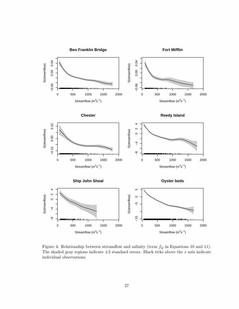
4 Relationship between streamflow and salinity (term fQ in Equations 10 and
11). The shaded gray regions indicate ±2 standard errors. Black ticks above
the x axis indicate individual observations. . . . . . . . . . . . . . . . . . . 27
5 Seasonal variations in salinity. For the oyster beds, the smooth plots the
relationship between salinity and decimal day of year (term fDD in Equation
11). For the USGS data, the smooths show the relationships between salinity
and month of year (term fM in Equation 10). The gray shaded regions
indicate ±2 standard errors. . . . . . . . . . . . . . . . . . . . . . . . . . . . 29
vi

6 Observed salinity values versus modeled salinity at Reedy Island. The blue
line indicates a 1:1 relationship between observed and modeled values. The
red line is a loess smooth of the actual relationship between observed and
modeled values. . . . . . . . . . . . . . . . . . . . . . . . . . . . . . . . . . . 30
7 Tensor product smooth of the combined effect of streamflow and axial dis-
tance on salinity in the oyster beds. The contours and color shading indicate
salinity. Points closer to the top of the plot are farther upstream. . . . . . . 32
8 Raw residuals (observed minus fitted) for the model in Equation 10 at Reedy
Island (black dots) and the trend that results when a term for time is added
to this model (blue line). . . . . . . . . . . . . . . . . . . . . . . . . . . . . . 33
9 Atlantic City, NJ sea level anomaly (top) and Philadelphia, PA sea level
anomaly (bottom) versus alongshore wind stress anomaly in the Delaware
Bay area (left) and cross-shore wind stress in the bay area (right). Black
lines indicate a linear fit; gray lines are loess smooths. . . . . . . . . . . . . 37
vii

List of Tables
1 Name, river kilometer (distance from Trenton, NJ), mean salinity, and per-
cent of non-missing monthly means during 1964-2011 for the five USGS salin-
ity stations in the estuary. Mean salinity was calculated from all available
monthly means. . . . . . . . . . . . . . . . . . . . . . . . . . . . . . . . . . . 9
2 ID, approximate axial and lateral distance, and mean of all available bottom
salinity measurements for each oyster bed. Axial and lateral distances are
approximated based on distances from a line from 39.182923, -75.139872
to 39.099661, -75.395070 and from 39.348973, -75.428746 to 39.283887, -
75.347674 respectively. . . . . . . . . . . . . . . . . . . . . . . . . . . . . . . 11
3 Location, trend in salinity per decade determined using a GAMM, p-value
for the trend component of the mixed model, and p-value for the trend using
a non-parametric Mann-Kendall test with autocorrelation (Hamed and Rao,
1998). Note that the different between the tests is likely due to the different
autocorrelation orders included in the models. Bold indicates locations where
both tests are significant at the 95% confidence level. . . . . . . . . . . . . . 25
viii

4 Location, trend in streamflow-adjusted salinity per decade, and p-value. Bold
indicates locations where the results are significant at the 95% confidence level. 34
5 Location, slope of the response of salinity to sea level, and p-value. Bold
indicates locations where the results are significant at the 95% confidence level. 35
6 Location, slope of the response of salinity to alongshore wind stress, and
p-value. Alongshore wind stress is defined as positive when it has a south-
southwest to north-northeast component. Negative slopes indicate that salin-
ity is lowered when the alongshore wind stress is from this direction. Bold
indicates locations where the results are significant at the 95% confidence level. 36
7 Location, slope of the response of salinity to cross-shore wind stress, and
p-value. Cross-shore wind stress is defined as positive when it is from the
east-southeast to west-northwest. Positive slopes indicate that salinity is in-
creased when the cross-shore wind stress is from this direction. Bold indicates
locations where the results are significant at the 95% confidence level. . . . 38
8 Location, slope of the response of salinity to wind stress magnitude, and p-
value. Bold indicates locations where the results are significant at the 95%
confidence level. . . . . . . . . . . . . . . . . . . . . . . . . . . . . . . . . . . 38
9 Location, slope of the response of salinity to the Gulf Stream Index, and
p-value. . . . . . . . . . . . . . . . . . . . . . . . . . . . . . . . . . . . . . . 39
ix

List of Symbols
E Expected value.
g Link function.
y Regression response variable.
f(x) A smooth function of variable x.
X A model matrix for fixed, parametric model terms.
β A parameter vector for fixed, parametric model terms.
Z A model matrix for random effects.
b A parameter vector for random effects.
ε Regression model errors or residuals.
N(µ, σ2) A normal distribution with mean µ and variance σ2.
Λ An error covariance matrix.
φ Lag-1 autocorrelation parameter.
S Salinity.
Q Streamflow.
x

Acknowledgments
I would like to thank my advisor, Ray Najjar, and my committee members Ming Li and
Michael Mann for the guidance and advice that they provided throughout this research
project. I thank Susan Ford and John Kraeuter for providing access to the Haskin Shellfish
Research Laboratory data punch cards and Mike Loewen for assisting in reading the punch
cards. Brandon Katz conducted an unpublished, preliminary analysis of the Reedy Island
salinity data, which provided a helpful background for this study. Support for this research
was provided by the National Science Foundation Physical Oceanography Program (award
#0961423) and Pennsylvania Sea Grant.
xi

Chapter 1
Introduction
Many estuaries are homes to rich, diverse, and productive ecosystems. Salinity influences
both the physical properties of an estuary and the characteristics of the estuarine ecosystem.
Even small changes in the salinity of an estuary can have a significant impact on the estuary’s
ecosystem; for example, salinity levels are often implicated in in oyster disease (Powell
et al., 1992), ammonia-oxidizing bacteria (Bernhard et al., 2005), and phytoplankton blooms
(Gallegos and Jordan, 2002). Understanding and mitigating the impacts of changing salinity
is particularly important because many estuarine ecosystems have already been stressed by
climate change and other human activities (Kennish, 2002).
A number of climatic and oceanic factors, including streamflow, sea level, oceanic salin-
ity, and wind stress, have an influence on the salinity and water quality of an estuary.
Streamflow determines the amount of fresh water entering the estuary; elevated stream-
flows are typically associated with fresher water in the estuary, and lower streamflows are
associated with increased salinity in the estuary. Higher sea levels increase salinity by bring-
1

ing more salt water into the estuary. The effect of sea level on salt intrusion is expected to
be proportional to the square of water depth (Savenije, 1993; Hilton et al., 2008). Varia-
tions in oceanic salinity alter the salinity of water circulating into the estuary. For example,
Lee and Lwiza (2008) found that quasi-decadal oscillations in oceanic salinity were linked
to similar oscillations in bottom salinity in the Chesapeake Bay. Finally, wind stress may
influence salinity through a variety of mechanisms including vertical mixing and Ekman
transport.
Changes in climate have the potential to cause changes in all of these variables. Precip-
itation amounts, frequencies, and intensities are expected to change in many areas, and the
associated effects on streamflow may be complicated by land use and evaporation changes
(Krakauer and Fung, 2008). Global mean sea level has risen significantly during the twen-
tieth century, and this increase is expected to continue through the twenty-first century
(Rahmstorf, 2007; Vermeer and Rahmstorf, 2009; Meehl et al., 2007). Meanwhile, wind
speeds have been declining over many regions in the Northern Hemisphere as a result of
land use changes and slowing large-scale circulations (Jiang et al., 2009; Vautard et al.,
2010).
Regardless of the cause, salinity change could be detrimental to many estuaries. This
study focuses on the salinity of the Delaware Estuary in the Eastern United States. Over 8
million people live within the Delaware River basin (Sanchez et al., 2012), and the Delaware
River and Estuary provide a significant amount of freshwater to nearby areas including
New York City and Philadelphia. High salinities are associated with salt intrusion into the
Philadelphia area water supply (Hull and Titus, 1986). In addition, a number of species
2

in the estuary are sensitive to salinity. Oysters, for example, cannot tolerate low salinities;
however, the oyster disease MSX (Haplosporidium nelsoni) becomes widespread in more
saline water (Haskin and Ford, 1982; Ford, 1985). The estuary is also the largest freshwater
port in the United States (Kauffman et al., 2011).
Because of the importance of the estuary and river for shipping, freshwater, and fishing,
a number of studies have examined the dynamic properties of the estuary. Tides in the
estuary are dominated by the M2 component (Wong, 1995). Sea level varies significantly
on the subtidal time scale primarily as a result of wind forcing, and winds can influence
subtidal fluctuations in circulation (Wong and Garvine, 1984). Salinity is higher in the
center of the estuary and lower near the shores; this lateral salinity difference is typically
larger than the vertical difference, which makes the estuary weakly to partially stratified
(Wong and Münchow, 1995; Wong, 1995).
The potential effects of climate change and sea-level rise on the the salinity of the
Delaware Estuary are significant both because of the importance of the estuary and because
of the large influence of sea level on the estuary. Garvine et al. (1992) found that the change
in salinity in the estuary produced by tidal advection was larger than the change in salinity
caused by streamflow. The response of salinity to sea-level rise has been examined in several
modeling studies (Hull and Tortoriello, 1979; U.S. Army Corps of Engineers, 1997; Kim and
Johnson, 2007), which generally found that salinity increases in response to sea-level rise.
This result has also been identified in other estuaries, including the Chesapeake Bay (Hilton
et al., 2008) and San Francisco Bay (Cloern et al., 2011).
Although numerical model simulations can be informative, they are subject to error as
3

a result of the numerous assumptions they make. For example, all studies to date assume
that sea-level rise has no influence on bottom topography, even though it is likely that sea-
level rise causes increased shoreline erosion, which increases sediment deposition (Cronin
et al., 2003). Thus, independent and empirical methods are essential for determining the
effects of climate change and sea-level rise on salinity. The Delaware Estuary is an ideal
site for applying empirical methods because salinity has been measured extensively in the
estuary. Previous efforts to model salinity in the Delaware Estuary and elsewhere focused
on least squares linear regression; for example, Garvine et al. (1992) and Wong (1995) used
linear regression with salinity and streamflow data to model the response of salt intrusion
length to streamflow in the Delaware Estuary. Marshall et al. (2011) used multiple linear
regression to build predictive models of salinity in the Florida Everglades. Other efforts
have focused on two different techniques: autoregressive models and generalized additive
models. Autoregressive models are an improvement over traditional linear regression models
because they take advantage of the highly autocorrelated nature of most water quality data.
Using autoregressive models, Gibson and Najjar (2000) predicted the response of salinity in
the Chesapeake Bay to future changes in streamflow, and Hilton et al. (2008) used similar
models to test whether sea-level rise has caused significant changes in Chesapeake Bay
salinity. Saenger et al. (2006) used autoregressive models to predict river discharge from
salinity observations and to reconstruct Holocene discharge and precipitation conditions.
A generalized additive model (GAM) is a different statistical model that has recently
become popular in many fields including water quality and hydrology. GAMs expand on
the traditional linear regression model by enabling the response variable to be a smooth,
4

nonparametric function of one or more predictor variables. The smooth functions can
include cubic splines, thin plate splines, loess smooths, or any number of other smoothing
functions. GAMs can also accommodate any error distribution in the exponential family
including the Poisson and gamma distributions. Both of these features are advantageous
over autoregressive models, which assume Gaussian errors and are fully parametric.
Several authors have recently applied generalized additive models to studies of salinity
and other water quality measures. For example, Jolly et al. (2001) and Morton and Hender-
son (2008) used GAMs to model changes in river salinity. Letcher et al. (2001) used GAMs
to model the response of catchment streamflow to precipitation. Autin and Edwards (2010)
showed how GAMs can be used to extract tidal variations from salinity, dissolved oxygen,
and temperature data and found that GAMs performed better than traditional harmonic
regression.
Although the nonparametric smoothing functions and the ability to handle multiple dis-
tributions makes GAMs advantageous over many other regression models, GAMs are not
typically robust against correlated or heteroscedastic errors. Generalized additive mixed
models (GAMMs) are a modification that enable GAMs to handle correlated and het-
eroscedastic errors. In this work, GAMMs are applied to perform a data-driven analysis of
the effects of streamflow, sea level, wind stress, and oceanic salinity on the salinity of the
Delaware Estuary and to predict future changes in salinity.
5

Chapter 2
Methods
2.1 Study Area and Data
Salinity in the Delaware Estuary has been measured through a number of different moni-
toring programs including surveys, automated sensors, and boat sensors. The goal of the
analysis was to determine which variables have an influence on salinity over long time peri-
ods. In addition, the statistical models that were applied perform significantly better with
larger amounts of data. As a result, of the many salinity datasets that are available, the
automated sensor data from the United States Geological Survey (USGS) and bottom salin-
ity measurements from the Haskin Shellfish Research Laboratory (HSRL) were selected for
statistical modeling. Both datasets include a large number of measurements and together
cover the period from the 1950s to the present.
The United States Geological Survey has measured salinity at five locations in the
Delaware Estuary since the 1960s (Table 1, Figure 1). The measurements from Reedy
6

PA
MD
DE
NJ
Figure 1: Map of the Delaware Estuary. Salinity was measured at Ship John Shoal, ReedyIsland, Chester, Fort Mifflin, and Ben Franklin Bridge (Philadelphia). Sea level was mea-sured at Atlantic City, NJ. Streamflow was measured at Trenton, NJ and near Philadelphia.
Island Jetty are the primary focus of the analysis because this series contains the least
amount of missing data. Measurements at Ship John Shoal were discontinued in 1986.
Chester, Fort Mifflin, and Ben Franklin Bridge contain a large amount of missing data.
Furthermore, the data from these three stations are not necessarily missing randomly; in
some cases, data recording was discontinued during winter months.
The USGS has officially approved the accuracy of salinity measurements through 2011,
so values from the earliest possible date through 2011 were used. To relate the salinity
measurements with other variables, any available data were used (in other words, pairwise
deletion of missing values was applied). The accuracy of the USGS measurements should be
sufficient for statistical analysis. The earlier USGS measurements were made with a flow-
7

through monitor. The accuracy stated by the official USGS documentation for electrical
conductivity (salinity) measurements from the flow-through monitor is ±3% of the full scale
(Gordon and Katzenbach, 1983). The USGS also issues an annual water data report for
each location, which classifies the measurements into four accuracy categories. During recent
years, the measurements have typically been rated good or fair, which indicates an accuracy
of ±3− 10% and ±10− 15% respectively. As a simple example, if the error in the electrical
conductivity measurements is assumed to be ±10% of the mean daily electrical conductivity
value at Reedy Island, this results in a salinity error of ±0.47 relative to a mean salinity
of 4.5. A ±3% error in electrical conductivity is equivalent to a ±0.14 error in salinity.
Even ±3% may be too large of an estimate, however, as Katzenbach (1990) determined
that the flow-through monitor was more accurate than the alternative mini-monitor and
packaged-sensor systems and that the flow-through monitor performed better than the
stated USGS accuracy. Furthermore, some USGS locations, including Reedy Island, have
recently switched to a YSI Incorporated sonde that has a stated salinity accuracy of 0.1 or
1%, whichever is greater (Mark R. Beaver, personal communication, March 5, 2007).
Although the measurement error is not explicitly included in the statistical models in
this study, it should be a random error that is generally absorbed in the variance of the
residual term without otherwise affecting the analysis. The analysis could be affected by
relocations. The USGS station at Chester moved 0.8 km upstream in April 1981. The Ben
Franklin Bridge station moved 0.09 km upstream in July 1988. Despite the relocations,
these data have been approved for use by the USGS, so no attempt was made to correct for
the effects of the relocations.
8
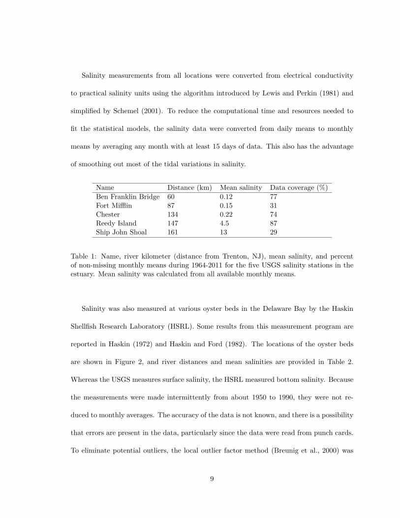
Salinity measurements from all locations were converted from electrical conductivity
to practical salinity units using the algorithm introduced by Lewis and Perkin (1981) and
simplified by Schemel (2001). To reduce the computational time and resources needed to
fit the statistical models, the salinity data were converted from daily means to monthly
means by averaging any month with at least 15 days of data. This also has the advantage
of smoothing out most of the tidal variations in salinity.
Name Distance (km) Mean salinity Data coverage (%)Ben Franklin Bridge 60 0.12 77Fort Mifflin 87 0.15 31Chester 134 0.22 74Reedy Island 147 4.5 87Ship John Shoal 161 13 29
Table 1: Name, river kilometer (distance from Trenton, NJ), mean salinity, and percentof non-missing monthly means during 1964-2011 for the five USGS salinity stations in theestuary. Mean salinity was calculated from all available monthly means.
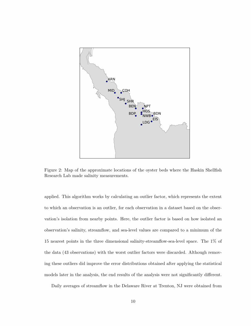
Salinity was also measured at various oyster beds in the Delaware Bay by the Haskin
Shellfish Research Laboratory (HSRL). Some results from this measurement program are
reported in Haskin (1972) and Haskin and Ford (1982). The locations of the oyster beds
are shown in Figure 2, and river distances and mean salinities are provided in Table 2.
Whereas the USGS measures surface salinity, the HSRL measured bottom salinity. Because
the measurements were made intermittently from about 1950 to 1990, they were not re-
duced to monthly averages. The accuracy of the data is not known, and there is a possibility
that errors are present in the data, particularly since the data were read from punch cards.
To eliminate potential outliers, the local outlier factor method (Breunig et al., 2000) was
9
ARN
BEN
BDNBDP
COH
EIS
HGS
LDG
MID
NPT
NWB
SHJ SHR
Figure 2: Map of the approximate locations of the oyster beds where the Haskin ShellfishResearch Lab made salinity measurements.
applied. This algorithm works by calculating an outlier factor, which represents the extent
to which an observation is an outlier, for each observation in a dataset based on the obser-
vation’s isolation from nearby points. Here, the outlier factor is based on how isolated an
observation’s salinity, streamflow, and sea-level values are compared to a minimum of the
15 nearest points in the three dimensional salinity-streamflow-sea-level space. The 1% of
the data (43 observations) with the worst outlier factors were discarded. Although remov-
ing these outliers did improve the error distributions obtained after applying the statistical
models later in the analysis, the end results of the analysis were not significantly different.
Daily averages of streamflow in the Delaware River at Trenton, NJ were obtained from
10

ID Axial distance (km) Lateral distance (km) Number of observations Mean salinityARN 31.34 -1.82 409 11.50MID 25.18 -0.93 303 13.57COH 24.08 -2.98 643 13.85SHJ 22.56 -0.44 178 14.82SHR 18.76 -1.07 596 14.95BEN 14.94 -2.82 491 17.01NPT 13.70 -5.11 120 16.33HGS 12.29 -3.45 193 16.95BDP 11.86 -0.50 105 17.45NWB 11.58 -2.91 572 17.48BDN 8.95 -5.91 240 17.85LDG 7.16 0.41 226 19.64EIS 6.73 -3.89 316 19.11
Table 2: ID, approximate axial and lateral distance, and mean of all available bottomsalinity measurements for each oyster bed. Axial and lateral distances are approximatedbased on distances from a line from 39.182923, -75.139872 to 39.099661, -75.395070 andfrom 39.348973, -75.428746 to 39.283887, -75.347674 respectively.
the USGS. At this location, the flow is approximately 58% of the total discharge into
the estuary from land (Sharp et al., 1986). Measurements were also obtained from the
Schuylkill River near Philadelphia, PA, which accounts for an additional 15% of the total
flow. The Schuylkill River gauge is upstream of the entrance of the river into the Delaware
River; the Schuylkill gauge drains 4903 km2 of the total 4952 km2 in the watershed. To
approximate the actual flow into the Delaware River, the Schuylkill gauge measurements
were multiplied by the ratio of the total drainage area to the gauged drainage area. This
estimate was then added to the corresponding day’s average streamflow at Trenton (except
when analyzing the salinity at the Ben Franklin Bridge, which is upstream of the Schuylkill
River). No other river or stream contributes more than 1% to the total discharge (Sharp
et al., 1986). To relate monthly mean salinity at the five USGS stations to streamflow,
11

the daily total streamflows were converted to monthly means for any month with at least
15 days of streamflow data. To relate the instantaneous oyster bed salinity measurements
to streamflow, an exponential moving average of the form Qt = KQt + (1 − K)Qt−1 was
applied (where t is in days). Using the root mean square error in the resulting model fits,
the optimal K was determined to be 1/15. The exponential moving average accounts for
the slower response of the downstream estuary to the streamflow upstream at Trenton and
Schuylkill. The exponential moving average produced better results than other methods
such as a simple lag.
Monthly averages of sea level at Atlantic City, NJ were obtained from the Permanent
Service for Mean Sea Level (Woodworth and Player, 2003). Atlantic City was selected
because it is near but not in the Delaware River and therefore should not be influenced by
the flow in the river. Monthly averages of sea level at Philadelphia were also obtained to
supplement the results. To relate the oyster bed salinities to sea level, the long-term trend
was extracted from the Atlantic City sea level record using seasonal-trend decomposition
with loess (Cleveland et al., 1990). The resulting trend was then interpolated to the day of
each oyster bed salinity measurement.
The trend component accounts for long-term fluctuations in sea level. Because the oyster
bed salinities were measured instantaneously near high and low tide, it is also necessary to
also account for tidal fluctuations in sea level. However, measurements of sea level with
sufficient temporal resolution are not available for most of the time period of the oyster bed
salinity measurements. Instead, predicted sea levels for Ship John Shoal were obtained from
the National Ocean Service. Although the time difference between a high or low tide and
12

the corresponding salinity measurement is provided in the HSRL data, the actual time of
measurement is not included. Therefore, to match the salinity measurements with a water
level, the sea level predictions were offset by the provided time difference. Then it was
assumed that salinity measurements would have only taken place during the day (8AM-
8PM), so the appropriate offset high or low water level in this range was selected. In the
event that measurements could have occurred at either 8AM or 8PM, the two water levels
were averaged.
The Gulf Stream Index (Taylor, 1995), which represents the first principal component
of the latitude of the north wall of the Gulf Stream, was used as a proxy for oceanic
salinity. Lee and Lwiza (2008) determined that the use of the index as a proxy for salinity
in the Mid-Atlantic Bight is appropriate. The monthly data were obtained from http:
//www.pml-gulfstream.org.uk/. The data cover 1966 through 2011.
Wind speed and direction were obtained from the North American Regional Reanalysis
(Mesinger et al., 2006). Reanalysis data are advantageous because they contain no missing
data or instrument biases and because they provide complete coverage over water (although
the data may be based on parameterizations). 3-hourly wind speed and direction from the
reanalysis were converted to wind stress using the equation τ = C10ρU210, where C10 is a
drag coefficient, ρ is the density of air, and U10 is the wind speed or component at 10 m. C10
was calculated using the equation from Wu (1982) with constant density. After calculating
the wind stress, the data were averaged over space and time to produce a time series of
monthly mean wind stress magnitudes and meridional and zonal components. Finally,
alongshore and cross-shore wind stresses were calculated using an alongshore direction of
13

south-southwest to north-northeast and a cross-shore direction of east-southeast to west-
northwest. The alongshore component should be associated with Ekman transport and sea
level fluctuations over the shelf near the Delaware Bay. The cross-shore component should
be associated with setup and setdown directly in the bay and estuary. The reanalysis data
only cover 1979 through the present. When relating salinity to wind stress, any salinity
measurements before 1979 were dropped.
Wind data were taken from all of the reanalysis grid points that are over water in two
regions: over the Delaware Bay between 38.8− 39.6◦, 74.9− 75.6◦ (the “local” region) and
over the shelf between 37.5− 39.8◦, 73.0− 75.0◦ (the “remote” region). At the monthly
time scale, these data are almost identical (aside from larger magnitudes in the remote
region), so the remote region was discarded and only the effects of winds in the local region
were considered.
2.2 Statistical models
Generalized additive mixed models can be derived by beginning with a traditional, linear
model and expanding the model to incorporate features such as non-Gaussian distributions,
correlated errors, random effects, and smooth functions of covariates. A traditional linear
model with n observations predicts the ith value of the n× 1 vector of response variables y
as
yi = Xiβ + εi (1)
14

where β is a p×1 vector of parameters associated with the n×p matrix of predictor variables
X (often called the model matrix or design matrix). Xi indicates the ith row of the matrix.
In this model, εi is typically assumed to be an independent, Gaussian random error with
mean 0 and variance σ2, i.e., εi ∼ N(0, σ2). As a result, the model can also be written as
E(yi) = Xiβ, yi ∼ N(Xiβ, σ2) (2)
Additive models are an extension of the linear model that include additive, smooth
terms in the model formula. The smooth terms can be cubic regression splines, thin plate
regression splines, loess smooths, or any number of other smooth functions. With one
smooth term f of a covariate x included, Equation 2 becomes
E(yi) = Xiβ + f(xi), yi ∼ N(Xiβ, σ2) (3)
To make the model algebraically possible to fit, the mean value of any smoothing function is
set to 0 (Wood, 2006); therefore, the distribution for yi is unchanged. Additional smoothing
terms can be added to this model. Smooths of multiple variables, such as f(x1i, x2i), can
also be included in the model.
Additive models can be easily modified to handle any distribution for yi that is in the
exponential family including the Gaussian, gamma, and Poisson distributions. With this
modification, Equation 3 becomes
g(E(yi)) = Xiβ + f(xi), yi ∼ an exponential family distribution. (4)
15

where g is known as a link function such as the identity, inverse, or natural logarithm
function. This model is known as a generalized additive model (GAM). Equation 3 is
a special case of this model where g is the identity function and yi follows a Gaussian
distribution.
One problem with applying any of the previous regression models to time series data is
that the errors are assumed to be independent and identically distributed. This is often an
invalid assumption for many hydrological and climatological variables (Hirsch and Slack,
1984). A modification known as a linear mixed model enables Equation 2 to handle serial
correlation and heteroscedasticity. A linear mixed model also includes both fixed and ran-
dom effects. Fixed effects are model parameters that apply to the entire population being
sampled. The previous models have been composed entirely of fixed effects. Random effects
are model parameters that apply to an individual unit or group that was randomly taken
from the population.
Assuming the simple case of one level of grouping, the random effects for group i are
represented with a parameter vector bi similar to how fixed effects are represented with a
parameter vector β. However, unlike the fixed effects, the random effects bi are assumed to
have a mean of zero and some simple variance structure ψ, so that bi ∼ N(0, ψ). The linear
mixed model is therefore
yi = Xiβ + Zibi + εi (5)
The convention for mixed models is to use the subscript i to denote the ith group rather
than the ith observation. If the number of observations in group i is ni, yi = yij =
(yi1, yi2, . . . , yini)ᵀ. As in the ordinary linear model, β is the p × 1 vector of fixed effects
16

associated with the ni × p model matrix Xi. The new random effects bi are a k × 1 vector
unique for group i and with an associated ni × k model matrix Zi. In the absence of
autocorrelation and heteroscedasticity, the within-group errors εi ∼ N(0, σ2I). To handle
autocorrelation and heteroscedasticity, the errors can be generalized to εi ∼ N(0, σ2Λi),
where Λi is positive definite and typically determined by a small set of parameters (Pinheiro
and Bates, 2000).
Finally, a generalized additive mixed model (GAMM) is a combination of the linear
mixed model and the generalized additive model that retains all of the unique advantages
of both models. GAMMs are derived by inserting the smooth functions and generalization
from the GAM into the linear mixed model. This is accomplished by splitting the smooth
functions into fixed and random effects (Lin and Zhang, 1999; Wood, 2004). The final model
structure then resembles
g(E(yi|bi)) = Xiβ + Zi1bi1 + Zi2bi2 + . . . (6)
Xiβ includes the intercept and any parametric component of the model as before; now, it
also includes the smooth portions of the smoothing functions. Each smooth term in the
model has an additional, separate random effect Zibi ∼ N(0, Iτ), where τ is the reciprocal
of the smoothing parameter λ, which controls the smoothness of the smooth (Wood, 2006).
These random effects represent the wiggly portions of the smooths. For convenience, the
models can also be written before splitting the smoothing functions:
g(E(yi|bi)) = Xiβ + f(x1i) + f(x2i) + . . .+ Zibi (7)
17

where the random effects terms that are not associated with smoothing functions Zibi are
optional.
2.2.1 Distributions
Two possible distributions could be assumed to apply to the salinity data: the normal
distribution and the gamma distribution. The gamma distribution may seem like the best
option since it only supports values greater than zero and salinity has a lower bound of
zero. However, tests comparing the distribution of the residuals indicated that the normal
distribution was by far the best choice for modeling salinity. Of the possible link functions
(identity, log, and inverse), the identity function produced the best results. Thus, the models
that were applied do not take advantage of the generalized modifications and are technically
additive mixed models, although they will continue to be referred to as generalized additive
mixed models. One consequence of this choice is that the models can predict negative
salinities. In practice, however, this rarely occurred, and the superior fits obtained using
the normal distribution and identity link make this issue negligible.
For the Gaussian and identity link case of Equation 7, the distribution for the residuals
in group i is εi ∼ N(0, σ2Λi). Any autocorrelation or heteroscedasticity is included in the
within-group error covariance matrix Λi. To do so, following Pinheiro and Bates (2000), Λi
is decomposed into
Λi = ViCiVi (8)
where Vi is diagonal and Ci is positive definite. Given this formulation, the variance of the
jth residual in the ith group is σ2[Vi]2jj and the correlation between two residuals j and k in
18

the same group i is [Ci]ijk. In other words, Vi determines the within-group error variance
and Ci determines the within-group error correlation. For both the USGS and HSRL
salinity data, the variance was assumed to depend on a power function of streamflow such
that var(εij) = σ2|Qij |2δ (Pinheiro and Bates, 2000). Other variance structures including
homoscedastic errors and variances proportional to power and exponential functions of the
fitted values were considered. Experiments indicated that the power function of streamflow
produced the highest likelihoods for most models. Furthermore, not including the fitted
values in the variance function allows the use of exact procedures to find the parameter δ
(Pinheiro and Bates, 2000).
In addition to heteroscedasticity, temporal autocorrelation is also present in the USGS
data. A first-order autoregressive (AR1) error process was assumed for the USGS data such
that the correlation between two errors spaced k months apart is φk (Pinheiro and Bates,
2000). φ is the lag-1 correlation and was also estimated by the model fitting algorithm.
There was typically enough time between successive observations in the HSRL data that
both spatial and temporal autocorrelation were assumed negligible.
2.2.2 Smoothing functions
The functions f in GAMs and GAMMs can be any number of smoothing functions. Among
those typically used are cubic regression splines, thin plate regression splines, and loess
smooths. In this work, thin plate regression splines (Wood, 2003) were applied to model
salinity as a smooth function of streamflow. These splines are considered optimal for use
in GAMs and GAMMs (Wood, 2006). A thin plate spline has a basis dimension k, which
19

is typically chosen as part of the model specification. In the GAMM fitting algorithm, the
specified basis dimension is considered an upper bound on the final basis dimension. Wood
(2006) provides recommendations on specifying the basis dimension. Because it is expected
that the relationship between salinity to streamflow is not overly complicated, the maximum
basis dimension for the streamflow smooth was set to 10 for all of the models in this work.
Instead of thin plate regression splines, cyclic cubic regression splines were used to model
seasonal effects. Any cubic spline consists of a number of knots and is continuous to the
second derivative at each knot. To make a cubic spline a cyclic cubic spline, the value,
first derivative, and second derivative of the spline at the first and last knots must also be
equal. This makes the cyclic spline useful for modeling data where the response should be
similar at the boundaries of the predictor variable. For example, a cyclic cubic spline could
be used to smooth a variable as a function of hour by placing knots at hours 0 and 24. In
the models used here, a cyclic cubic spline was used to model the response of salinity to
the current month (for the USGS monthly averages) or to the decimal day of the year (for
the HSRL instantaneous measurements). To do so, knots were placed at months 1 and 13
or decimal days 0 and 1, which causes the spline to smooth continuously from December to
January. The remaining knots were automatically placed with even spacing by the model
fitting algorithm.
Finally, tensor product smooths were used to relate the combined influence of axial
position in the estuary and streamflow to salinity in the oyster beds. These smooths are
appropriate for smoothing two variables with different units (Wood, 2006).
20

2.2.3 Fitting and testing
The models can be fit using maximum likelihood estimation (MLE) methods provided that
the Gaussian distribution and identity link are used (Wood, 2006). However, MLE produces
biased estimates of variance in many situations. A modification to MLE known as restricted
maximum likelihood estimation (REML) solves this problem. However, REML makes model
selection difficult because two models that have been fit with REML can only be compared
based on likelihood (for example, by comparing the Akaike information criterion or applying
a likelihood ratio test) when the fixed effects in both models are identical (Pinheiro and
Bates, 2000; Wood, 2006). To resolve this issue, the significance of the fixed effects was
tested using models fit with MLE. The resulting best model was then re-fit with REML to
produce the final results.
Likelihood ratio tests were applied to determine the significance of the fixed effects.
The likelihood ratio test works under the assumption that twice the difference of the log-
likelihoods of two nested models is χ2-distributed:
LRT ≡ 2 (la − l0) ∼ χ2k (9)
where la is the log-likelihood of the alternative model (which includes the fixed effects being
tested), l0 is the model under the null hypothesis which does not included the fixed effects
being tested, and the degrees of freedom k for the χ2 distribution is equal to the number of
fixed effects being tested in the alternative model (Wilks, 1938; Pinheiro and Bates, 2000).
The models for bottom salinity in the oyster beds also include random effects. REML
21

is necessary to obtain accurate estimates of the variance of the random effects. Model
selection for the random effects was performed by including all possible fixed effects terms,
fitting with REML, and using likelihood ratio tests to determine which random effects to
include. Finally, the fixed effects were tested using MLE as above and the final best model
is re-fit using REML. These methods indicated that including a random intercept for each
oyster bed significantly improved the model. However, including other random effects, such
as a separate trend for each oyster bed, did not significantly improve the model.
2.2.4 Final models
The final, basic model used to test the influence of sea level, oceanic salinity, and wind
stress on surface salinity at each USGS station is
Si = β0 + fQ(Qi) + fM (Monthi) + εi (10)
where Si is the ith salinity value, β0 is a constant intercept equal to the mean salinity
value, fQ(Qi) is a thin plate spline that relates salinity to streamflow and is evaluated at
the streamflow value Qi, and fM (Monthi) is a cyclic cubic spline that relates salinity to
calendar month and is evaluated at the ith month. fM captures seasonality in salinity that
is not explained by the other independent variables. It is assumed that εi ∼ N(0, σ2Λi),
where Λi includes autocorrelation and heteroscedasticity as previously discussed. For the
oyster bed bottom salinity data, the basic model is
Si = bi + β0 + β1Hi + β2xi + β3yi + fQ(Qi) + fDD(DDi) + εi (11)
22

where Si = Sij = (Si1, Si2, . . . , Sini)ᵀ and ni is the number of measurements at oyster bed
i, bi is a random effect with an expected value of zero that represents a unique intercept for
each oyster bed, β0 is a constant intercept that applies to every location, β1 gives the slope
of the response of salinity to sea level and Hi is the National Ocean Service predicted sea
level, β2 is equivalent to the axial salinity gradient and xi is the relative axial distance for
the ith oyster bed, β3yi is the same for the lateral gradient and distance, fQ(Qi) is a smooth
function of exponential moving averaged streamflow, and fDD(DDi) is a cyclic cubic spline
that relates salinity to decimal day. It is assumed that εi ∼ N(0, σ2Λi), where Λi includes
only heteroscedasticity.
To test the influence of sea level, oceanic salinity, and wind stress on the salinity measure-
ments, additional terms representing these variables were added to these two basic models.
For example, to test the influence of sea level on the USGS salinity data, an additional term
β1Hi was added to Equation 10.
23

Chapter 3
Results
Before analyzing the response of salinity to various factors, the monthly mean salinity data
were tested for trends in the raw data. This was done with a simple generalized additive
mixed model of the form Si = β0 + β1t+ s(Monthi) + εi. This model includes only a time
trend and seasonal cycle. In addition to testing the significance of the trend component
β1 with a likelihood ratio test, the raw salinity data were also evaluated with a Mann-
Kendall test for trend (Mann, 1945; Kendall, 1938) including autocorrelation (Hamed and
Rao, 1998). Whereas the GAMM test assumes AR(1) autocorrelation, the Mann-Kendall
test is more flexible and includes as many orders as are significant. Using these methods,
significant trends in salinity were found at Ship John Shoal (Table 3). Ship John Shoal has
a shorter record than the other time series, and it appears that the record coincidentally
covers a period when salinity was increasing (Figure 3). Significant trends were not found
at any of the remaining locations.
Streamflow is often one of the primary influences on estuarine salinity. The effect of
24

Location Trend (decade−1) Mixed model p Mann-Kendall pBen Franklin Bridge -8.2×10⁻³ 8.5×10⁻³ 0.45Fort Mifflin 7.1×10⁻³ 0.13 5.3×10⁻²
Chester -3.9×10⁻² 2.9×10⁻² 0.77Reedy Island -5.5×10⁻² 0.72 0.97Ship John Shoal 2.2 4.2×10⁻² 3.4×10⁻³
Table 3: Location, trend in salinity per decade determined using a GAMM, p-value for thetrend component of the mixed model, and p-value for the trend using a non-parametricMann-Kendall test with autocorrelation (Hamed and Rao, 1998). Note that the differentbetween the tests is likely due to the different autocorrelation orders included in the models.Bold indicates locations where both tests are significant at the 95% confidence level.
streamflow on the salinity of the Delaware Estuary can immediately be seen in Figure 3,
which plots the five monthly mean salinity time series and the time series of streamflow
for comparison. Salinity values hit record highs during the period of drought and low
streamflows in the mid 1960s. During the following period of increased precipitation and
streamflow in the 1970s, salinities dropped dramatically.
The basic relationships between salinity and streamflow, plus residual seasonal varia-
tions, are included in Equations 10 and 11. These models relate salinity to smooth functions
of streamflow and time of year. The fitted smooth functions fQ are shown in Figure 4. As
expected, salinity and streamflow are negatively correlated. The magnitude of the marginal
response of salinity to streamflow is larger under low-flow conditions. The benefit of using
a GAM or GAMM is also shown here, as a linear regression model is clearly inappropriate
and even a log transform or log linear model may not be valid.
25

●
●
●
●●●●
●
●
●
●
●●
●
●
●●●●
●
●
●
●●
●●
●
●
●●●
●●
●●●●
●●
●
●●●
●
●
●●
●
●
●●●●
●●
●
●●
●
●
●
●
●●●●●
●
●●
●
●●●
●
●
●●
●●
●
●
●
●●●
●●●
●●
●●
●●
●
●
●
●
●
●
●
●
●●●
●
●
●●
●
●
●●
●●●●
●
●●●
●
●
●
●●●●
●
●●●●
●
●●●
●
●●●
●●●●
●
●
●
●
●●●
●●
●
●●●●●
●
●
●●●●●
●
●
●
●
●
●●
●●
●
●
●
●
●
●
●
●●
●
●●
●
●
●●●●
●●●
●●●
●
●●●
●
●●●●
●
●
●●
●●●●●●
●
●●
●●●●
●●
●●
●
●
●
●
●
●●
●●●●
●●●
●
●●
●●
●●●●●
●●●●
●●●●
●●●●●●
●
●●
●●●●
●●
●●
●
●
●
●
●●●●●●
●
●
●
●●●●●
●
●●●
●●●
●
●
●●●
●●●●
●●●●
●●●●●
●●●●
●
●●●●
●
●●●
●●
●
●
●●●
●●●
●●
●●●
●
●●
●●●●
●●●●
●
●●●
●
●
●
●
●●●
●
●●
●●●
●●●●
●●●●
●
●●●
●
●
●
●
●●●
●
●●
●●
●
●●●●●
●●●
●●●
●
●●
●●●●
●●
●
●
●
●●
●
●●
●●
●
●●
●
●●●
●●
●
0.0
0.2
0.4
0.6
1960 1970 1980 1990 2000 2010
Sal
inity
Ben Franklin Bridge
●●
●
●
●
●●
●
●
●●
●
●
●
●
●
●
●●
●
●
●●
●
●
●●
●
●●●
●
●
●
●
●●●
●
●
●
●●
●
●●
●
●
●
●
●
●
●
●●
●●●●●●●
●
●
●
●
●
●●●
●●
●●●●
●●
●●●●
●
●●
●
●●
●●
●
●
●
●
●
●●●
●●
●●
●●
●
●
●
●
●
●
●
●
●
●
●
●●
●●
●
●
●
●●●●●●
●
●
●
●●●
●●●
●
●
●●
●●
●
●
●
●
●
●
●●
●
●
●
●
●
●
●
●
●
●
●
●●
●
●
●
●
●
●
●
●
●
●●
●●
●
●
●
0.0
0.1
0.2
0.3
1960 1970 1980 1990 2000 2010
Sal
inity
Fort Mifflin
●
●
●
●
●
●
●
●
●
●
●
●
●●
●●●●
●
●
●
●
●
●●●●●●●●●●
●
●●●●●●●●
●
●
●
●
●●●
●
●●●●●●
●●
●●●●●●●●●●●
●●●●●●●●
●●●●●●●●●●●●●●
●
●●●●●●●
●●●●●●●
●●●●
●●●●●●●●●●●●●●●●●
●
●●●●
●
●●●
●
●●●
●●●●●●●●●●
●
●
●●●●●●●●●
●●
●●●
●●●
●
●
●
●
●●●●
●
●●
●●●
●
●
●
●
●●●●●
●
●
●●●●
●●
●
●●●●●●●●
●●
●
●●●●●●●●●●●●●
●
●●
●
●
●●●●●●●●●●●●●
●●●●
●●●●●●●
●●
●
●●●●●●●●
●●
●
●●●
●
●
●
●●●●●●●●●●●
●●●●●
●
●
●
●●●●●●●●●●
●
●●
●
●
●
●●●●
●
●●
●
●
●
●●●
●
●
●
●●●●●●●●●
●
●●●●
●
●
●
●
●
●
●●●●●
●
●
●
●●●●●●●●●●●●●●●●
●●●●●
●
●
●●●●●●
●●●●●
●●●●
●
●
●●●●●●●
●●
●●●●●●●●●●●●
●●
●
●
●●●●●●●●
0.0
0.5
1.0
1.5
2.0
1960 1970 1980 1990 2000 2010
Sal
inity
Chester
●
●
●
●
●
●
●
●
●
●●
●
●
●
●
●
●
●
●
●
●
●
●
●
●●
●●
●●
●
●●
●
●
●
●●
●
●
●
●
●
●
●
●
●
●
●
●●
●
●
●
●
●
●
●
●
●
●
●
●
●
●
●
●
●
●●
●●●
●●
●
●
●
●
●●
●
●
●●●
●
●
●
●
●
●●
●
●
●
●●
●
●
●
●●
●
●
●
●
●
●●
●
●
●
●
●
●
●●
●
●
●●
●
●
●
●
●
●
●
●
●
●
●
●
●
●
●
●
●
●
●
●●
●
●
●
●
●●●
●
●
●
●
●
●
●
●●●
●
●●
●
●
●
●
●
●
●●
●
●
●
●
●
●
●
●
●
●
●●
●
●
●
●
●
●
●●●
●
●
●
●
●
●
●●
●
●●
●
●●
●
●
●
●
●
●
●
●●
●
●
●
●
●
●
●
●
●
●
●●●
●●
●
●
●
●
●
●
●
●
●
●
●
●
●
●
●
●
●
●
●
●
●
●
●
●
●
●
●
●
●●
●
●●
●●
●
●
●
●
●
●
●
●
●
●
●
●
●
●
●
●
●
●
●
●
●
●
●
●
●
●
●
●
●
●
●●●
●
●
●
●
●
●●
●●●
●
●
●
●
●
●
●
●
●●
●●●
●
●
●
●
●●
●
●
●
●
●
●●
●
●
●
●●●
●
●
●
●●
●●
●
●
●
●
●
●
●
●
●
●
●
●●
●
●●
●●
●
●
●
●
●
●●
●●
●
●
●
●
●
●
●
●
●
●
●
●
●
●●
●
●
●
●
●
●
●
●
●●
●
●
●
●
●
●
●●
●
●
●
●●
●●
●●
●
●
●
●
●●
●
●
●●
●
●
●
●
●
●
●
●
●
●
●
●
●
●
●
●
●
●
●
●
●
●
●
●
●●
●
●
●
●
●
●
●
●
●
●
●
●
●
●
●●
●
●
●
●
●
●
●
●
●
●
●
●
●
●
●
●
●
●
●
●
●
●
●
●
●●
●
●
●●
●0
5
10
1960 1970 1980 1990 2000 2010
Sal
inity
Reedy Island
●
●
●
●
●
●
●
●
●
●
●
●
●●
●
●
●
●
●
●
●
●
●●●●
●
●
●●
●
●●
●●
●
●
●
●
●
●
●
●
●
●
●
●●
●●
●●●
●
●
●●
●●
●●
●
●
●
●
●
●
●
●●
●
●●
●
●
●
●
●
●
●●
●
●
●
●
●
●●
●
●
●
●
●
●●
●
●
●
●
●
●
●
●
●●
●
●
●
●
●●
●●●
●
●
●
●
●
●
●●
●
●
●
●
●
●
●●
●●●
●
●●
●
●
●
●
●
●
●
●
●●
●
●
●
●
●●
●●
●
●●
●●
●●
●
●
●
●
●
●
0
5
10
15
20
25
1960 1970 1980 1990 2000 2010Year
Sal
inity
Ship John Shoal
●
●
●
●
●●
●●
●
●●●●
●
●●
●
●●●
●●
●●
●
●
●
●
●
●●●●
●
●
●●●
●
●
●
●●●●●
●
●
●
●
●
●
●
●●●●●●
●●
●
●●
●
●●●●●●
●●
●
●
●
●
●
●●●●●
●
●
●
●
●●
●●
●
●●
●
●
●
●
●
●
●
●
●
●●●
●●
●●
●
●
●●
●
●
●●
●
●
●
●
●
●
●
●●●●
●
●
●●
●
●
●
●
●
●
●●
●
●
●
●●
●
●
●
●
●
●●●
●●
●●
●
●
●
●●
●
●●●
●
●
●
●
●
●
●
●●
●
●●
●●
●
●
●●●●
●
●
●●
●
●
●
●
●●
●●●
●
●
●
●
●
●
●
●
●
●●●
●
●●
●
●
●
●
●●
●
●●
●●●
●
●
●
●
●●
●
●●
●
●
●
●
●
●
●
●
●
●●●●●●●●
●
●●
●
●●
●●●●●
●
●●
●
●
●
●
●●●●●●
●
●
●
●
●
●●●●
●
●
●
●
●
●
●
●●
●
●●●
●●●●
●●
●●●
●●
●●
●
●
●
●
●●
●
●
●●
●
●
●
●
●
●
●
●●
●
●
●●
●
●
●●
●
●
●●
●●●
●
●●●
●
●
●
●
●
●
●
●
●
●
●
●
●●
●
●
●●
●
●
●
●
●
●
●
●
●
●●●●●
●
●
●●
●●
●
●
●●●●
●●●
●
●
●
●
●●●●●
●
●
●
●
●●
●
●●
●
●●
●
●●
●
●
●
●●●
●●
●
●
●
●
●●
●
●
●
●
●●
●
●
●
●●
●●
●
●●●●●
●●
●
●
●
●●
●
●
●●●●●
●
●
●
●
●
●●●
●
●●
●
●
●
●
●
●●
●
●
●●●
●
●
●
●
●
●
●
●●●●●●●
●
●
●
●
●
●●●
●
●
●
●
●
●
●
●
●
●
●
●
●
●
●
●
●
●●
●
●
●
●
●
●●
●●
●
●
●
●
●●
●●
●
●
●
●
●
●
●●
●
●
●
●●
●
●
●
●
●
●
●
●●●
●
●
●
●●
●
●
●
●
●●
●●
●
●
●
●
●
●●●
●
●
●
●
●●
●
●
●
●
●
●
●●●●
●
●
●
●
●
●
●
●
●
●
●
●
●
●
●
●
●
●
●
●
●
●●●
0
500
1000
1500
2000
2500
1960 1970 1980 1990 2000 2010Year
Str
eam
flow
(m
3 s−1)
Total streamflow
Figure 3: Time series of monthly mean salinity (first five panels) and time series of monthlymean streamflow (bottom right panel).
26
0 500 1000 1500 2000
−0.
060.
000.
04Ben Franklin Bridge
Streamflow (m3s−1)
S(s
trea
mflo
w)
0 500 1000 1500 2000
−0.
060.
000.
04
Fort Mifflin
Streamflow (m3s−1)
S(s
trea
mflo
w)
0 500 1000 1500 2000
−0.
100.
000.
10
Chester
Streamflow (m3s−1)
S(s
trea
mflo
w)
0 500 1000 1500 2000
−8
−4
02
4
Reedy Island
Streamflow (m3s−1)
S(s
trea
mflo
w)
0 500 1000 1500 2000
−8
−4
02
4
Ship John Shoal
Streamflow (m3s−1)
S(s
trea
mflo
w)
0 500 1000 1500 2000
−15
−5
05
Oyster beds
Streamflow (m3s−1)
S(s
trea
mflo
w)
Figure 4: Relationship between streamflow and salinity (term fQ in Equations 10 and 11).The shaded gray regions indicate ±2 standard errors. Black ticks above the x axis indicateindividual observations.
27

The seasonal variation appears similar at all locations (Figure 5). Some of this similarity
may be due to the use of cyclic cubic repression splines, which place knots at equally-spaced
intervals. In general, after accounting for the influence of streamflow, salinity is lowest in
May and June and highest in October and November. Because there is a seasonal cycle in
streamflow, there is the potential for some concurvity issues when including both streamflow
and month as predictors in the model. However, the month term significantly improves the
model fits, and excluding it from the models results in a seasonal pattern in the residuals.
The adjusted R2 value for the model fit to Reedy Island salinity is 0.74. Farther down
the estuary, the adjusted R2 value for the fit to salinity is 0.57 at Ship John Shoal and
0.81 at the oyster beds. Upstream at Chester, Fort Mifflin, and Ben Franklin bridge, the
adjusted R2 values are 0.18, 0.60, and 0.54 respectively. The reduced performance at these
upstream locations is a result of difficulty in determining the salinity-streamflow relation-
ship under low-flow conditions (particularly during the 1960s drought). At all locations, the
models often, but not always, underpredict when salinity is high. This can be seen in Figure
6, which plots the relationship between the observed and modeled salinity values at Reedy
Island. One concern was that these difficulties may be caused by the use of smoothing
splines to approximate the sharply nonlinear response to streamflow under low-flow condi-
tions. However, experimental results not shown indicated that the modeling methods were
reasonable even when approximating exponentials. Furthermore, other smoothing methods
did not perform better at correctly predicting low salinities.
28

2 4 6 8 10 12
−0.
060.
000.
04Ben Franklin Bridge
Month
S(m
onth
)
2 4 6 8 10 12
−0.
060.
000.
04
Fort Mifflin
Month
S(m
onth
)
2 4 6 8 10 12
−0.
100.
000.
10
Chester
Month
S(m
onth
)
2 4 6 8 10 12
−8
−4
02
4
Reedy Island
Month
S(m
onth
)
2 4 6 8 10 12
−8
−4
02
4
Ship John Shoal
Month
S(m
onth
)
0.0 0.2 0.4 0.6 0.8 1.0
−15
−5
05
Oyster beds
Decimal day
S(D
ecim
al d
ay)
Figure 5: Seasonal variations in salinity. For the oyster beds, the smooth plots the relation-ship between salinity and decimal day of year (term fDD in Equation 11). For the USGSdata, the smooths show the relationships between salinity and month of year (term fM inEquation 10). The gray shaded regions indicate ±2 standard errors.
29

●
●
●
●
●
●
●
●
●
●●
●
●
●
●
●
●
●
●
●
●
●
●
●
●●
●●
●
●
●
●●
●
●
●
●
●
●
●
●
●
●
●
●
●
●
●
●
● ●
●
●
●
●
●
●
●
●
●
●
●
●
●
●
●
●
●
●●
● ●●
●●
●
●
●
●
●
●
●
●
●
●●
●
●
●
●
●
●
●
●
●
●
●●
●
●
●
●●
●
●
●
●
●
●●
●
●
●
●
●
●
●●
●
●
●●
●
●
●
●
●
●
●
●
●
●
●
●
●
●
●
●
●
●
●
● ●
●
●
●
●
●
●●
●
●
●
●
●
●
●
●●
●
●
●
●
●
●
●
●
●
●
●●
●
●
●
●
●
●
●
●
●
●
● ●
●
●
●
●
●
●
●
●●
●
●
●
●
●
●
●●
●
● ●
●
●●
●
●
●
●
●
●
●
● ●
●
●
●
●
●
●
●
●
●
●
●●
●
●●
●
●
●
●
●
●
●
●
●
●
●
●
●
●
●
●
●
●
●
●
●
●
●
●
●
●
●
●
●●
●
●●
● ●
●
●
●
●
●
●
●
●
●
●
●
●
●
●
●
●
●
●
●
●
●
●
●
●
●
●
●
●
●
●
●●●
●
●
●
●
●
●●
● ●●
●
●
●
●
●
●
●
●
●
●
●●
●
●
●
●
●
●●
●
●
●
●
●
●
●
●
●
●
●●
●
●
●
●
●
●
●●
●
●
●
●
●
●
●
●
●
●
●
●●
●
●●
●●
●
●
●
●
●
●
●
●
●
●
●
●
●
●
●
●
●
●
●
●
●
●
● ●
●
●
●
●
●
●
●
●
●●
●
●
●
●
●
●
●
●
●
●
●
●●
●●
●●
●
●
●
●
●●
●
●
● ●
●
●
●
●
●
●
●
●
●
●
●
●
●
●
●
●
●
●
●
●
●
●
●
●
●●
●
●
●
●
●
●
●
●
●
●
●
●
●
●
● ●
●
●
●
●
●
●
●
●
●
●
●
●
●
●
●
●
●
●
●
●
●
●
●
●
●●
●
●
●●
●0
3
6
9
12
0 3 6 9 12Modeled salinity
Obs
erve
d sa
linity
Figure 6: Observed salinity values versus modeled salinity at Reedy Island. The blue lineindicates a 1:1 relationship between observed and modeled values. The red line is a loesssmooth of the actual relationship between observed and modeled values.
30
At all locations, the addition of other terms to the model such as sea level and wind
stress often improved the fit and the R2 values, but any improvements were typically mi-
nor. As a result, this indicates that streamflow and an additional unknown seasonal effect
predominantly influence salinity.
In addition to influencing salinity values, streamflow may also influence the axial salinity
gradient in the estuary. Because the oyster beds cover a number of locations within a small
region of the estuary, the oyster bed data can be used to test the effect of streamflow on the
salinity gradient. To do so, the separate flow and distance terms in Equation 11 are replaced
with one tensor product smooth that models salinity as a 3D surface that smooths over
both streamflow and distance. The result is shown in Figure 7. This result has two similar
physical interpretations: first, the axial salinity gradient in the oyster beds is slightly larger
during high-flow conditions than during low-flow conditions. Second, locations upstream
in the estuary have a larger range of salinity in response to streamflow than downstream
locations except during very high flows. This result contradicts Wong (1995), who found
that streamflow and the axial salinity gradient of the Delaware Estuary were inversely
correlated. However, Wong (1995) studied the gradient between Reedy Island and Ship
John Shoal, whereas the majority of the oyster beds are located downstream of Ship John
Shoal. Wong (1995) proposed that the inverse correlation between streamflow and axial
salinity gradient may be a result of the salt intrusion ending downstream of Reedy Island
during low flow conditions. The salt intrusion limit is consistently upstream of the oyster
beds, which may explain why an inverse correlation was not found there.
Studies of water quality typically look for trends in variables after adjusting for the
31

−10
−5
05
10
S(streamflow, distance)
Streamflow (m3s−1)
Axi
al d
ista
nce
(km
)
4
6
8 10
12 14
16
18
20
250 500 750 1000 1250 1500
EISLDG
BDN
NWBBDPHGS
NPT
BEN
SHR
SHJ
COH
MID
ARN
Oys
ter
bed
Figure 7: Tensor product smooth of the combined effect of streamflow and axial distance onsalinity in the oyster beds. The contours and color shading indicate salinity. Points closerto the top of the plot are farther upstream.
influence of streamflow. To check for trends in salinity after adjusting for streamflow, a
parametric time term can be added to Equations 10 and 11. The resulting trends, likeli-
hood ratio test statistics, and p-values are provided in Table 4. Significant upwards trends
in streamflow-adjusted salinity are found at the oyster beds and Reedy Island. Upwards
32

●
●
●
●
●
●
●
●
●●
●
●
●
●
●●
●
●●
●
●
●
●
●
●
●
●
●
●
●●●
●
●
●●
●
●
●
●
●
●●
●
●
●
●
●
●
●
●●
●
●
●
●
●
●
●
●
●
●
●
●
●
●
●
●
●
●●
●
●
●
●
●
●●
●
●●
●
●
●●
●
●
●
●
●
●
●
●
●●
●
●
●
●●
●
●
●
●
●
●
●
●
●
●
●
●
●
●
●
●
●●
●
●
●●
●●
●
●
●
●
●
●
●
●
●
●
●●
●
●
●●
●
●
●
●
●
●
●●●
●
●
●●
●
●●●
●●●
●
●
●
●
●
●
●
●
●●
●
●
●●
●
●
●
●
●
●
●
●
●●
●
●●
●●
●
●
●●
●●
●●
●
●
●
●
●
●
●
●
●
●●
●
●
●
●
●
●●
●
●●
●
●
●●●●
●
●
●
●
●●
●
●
●
●
●
●
●
●
●
●●
●
●
●●
●
●
●
●
●
●
●●
●
●
●●●
●
●
●
●●
●
●
●●
●
●
●
●●
●
●
●
●
●
●
●
●●
●●
●
●
●
●
●
●
●
●
●
●●
●●
●
●
●●
●
●
●
●
●
●
●
●
●●
●
●
●
●
●
●
●
●●
●
●
●
●
●
●
●●
●
●●
●
●●
●
●
●
●
●
●
●●
●●
●
●●
●
●
●
●
●
●●
●
●●
●
●
●
●
●
●●
●●
●
●
●
●
●
●
●
●
●
●●
●
●
●
●●
●
●
●
●
●
●●
●
●
●
●
●
●
●
●
●
●
●●●
●
●
●
●
●
●
●
●
●
●●
●
●
●●●
●
●
●
●
●
●
●
●
●
●●
●
●
●
●●
●
●●
●
●
●●
●
●
●
●
●
●
●
●
●
●
●
●
●
●
●
●
●
●
●
●
●
●●
●
●
●
●
●
●
●
●●
●
●●
●
●
●
●
●
●
●
●
●
●
●●
●●
●
●
●
●●●
●●
●
●
●●●●●●●●●●●●●●●●●●●●●●●●●●●●●●●●●●●●●●●●●●●●●●●●●●●●●●●●●●●●●●●●●●●●●●●●●●●●●●●●●●●●●●●●●●●●●●●●●●●●●●●●●●●●●●●●●●●●●●●●●●●●●●●●●●●●●●●●
●●●●●●●●●●●●●●●●●●●●●●●●●●●●●●●●●●●●●●●●●●●●●●●●●●●●●●●●●●●●●●●●●●●●●●●●●●●●●●●●●●●●●●●●●●●●●●●●●●●●●●●●●●●●●●●●●●●●●●●●●●●●●●●●●●●●●●●●
●●●●●●●●●●●●●●●●●●●●●●●●●●●●●●●●●●●●●●●●●●●●●●●●●●●●●●●●●●●●●●●●●●●●●●●●●●●●●●●●●●●●●●●●●●●●●●●●●●●●●●●●●●●●●●●●●●●●●●●●●●●●●●●●●●●●●●●●
●●●●●●●●●●●●●●●●●●●●●●●●●●●●●●●●●●●●●●●●●●●●●●●●●●●●●●●●●●●●●●●●●●●●●●●●●●●●●●●●●●●●●●●●●●●●●●●●●●●●●●●●●●●●●●●●●●●●●●●●●●●●●●●●●●●●●●●●
●●●●●●●●●●●●●●●●●●●●
−2
0
2
4
1970 1980 1990 2000 2010Year
Res
idua
l
Figure 8: Raw residuals (observed minus fitted) for the model in Equation 10 at ReedyIsland (black dots) and the trend that results when a term for time is added to this model(blue line).
trends are also found at all of the remaining locations; however, none of these trends are
significantly different from zero at the 95% confidence level. It should also be noted that
each location covers slightly different time periods. These trends can also be found in the
residuals of the previous models with only streamflow and residual seasonal effects (Figure
8).
Despite the insignificant trends in raw salinity, statistically significant trends in streamflow-
adjusted salinity were detected. In addition, streamflow increased at a rate of 36 m3s−1/decade
during the study period (p =1.4×10⁻³ and 3.1×10⁻² using likelihood ratio and Mann-
Kendall tests respectively). This suggests that another factor, such as sea-level rise, is
acting to negate any salinity decreases caused by increasing streamflow.
The influence of sea-level rise can be tested by including a parametric term for sea level
33

Location Trend (decade−1) p-valueBen Franklin Bridge 8.3×10⁻⁴ 0.35Fort Mifflin 2.5×10⁻³ 0.31Chester 2.2×10⁻⁴ 0.92Reedy Island 0.19 8.7×10⁻³
Ship John Shoal 1.6 6.3×10⁻²
Oyster beds 0.38 <1.0×10⁻⁵
Table 4: Location, trend in streamflow-adjusted salinity per decade, and p-value. Boldindicates locations where the results are significant at the 95% confidence level.
in Equation 10. Due to the significant multicollinearity between sea level and time, the
time term that was previously inserted is now excluded. Note that sea level (high and low
tide water level, without sea-level rise) is already included in the oyster bed model to allow
observations from both high and low tide to be combined.
The resulting coefficients for the response of salinity to sea level are provided in Table
5. Due to the significant upwards trends in streamflow-adjusted salinity already detected,
any time series with a significant trend would likely be modeled as having a significant
effect on salinity. However, the results here are reasonable, as there is a physical reason to
expect increasing salinity with increasing sea level. Furthermore, the sea level term generally
improves the models more than the time term as evidenced by the higher likelihood ratio
test statistics. Finally, using numerical models, several studies examined in the discussion
have arrived at similar responses of salinity to sea level.
Theoretically, the response of salinity to sea level should not be a simple linear function
but rather a power function (Savenije, 1993; Hilton et al., 2008). A simple way of testing
this non-parametrically is to replace the parametric relationship between salinity and sea
34

Location Slope (m−1) p-valueBen Franklin Bridge 5.2×10⁻³ 0.60Fort Mifflin 3.3×10⁻² 0.17Chester 3.0×10⁻² 0.23Reedy Island 3.5 3.0×10⁻⁵
Ship John Shoal 4.6 2.5×10⁻²
Oyster beds 5.8 <1.0×10⁻⁵
Table 5: Location, slope of the response of salinity to sea level, and p-value. Bold indicateslocations where the results are significant at the 95% confidence level.
level with a smooth term. Using likelihood ratios to test the null models with parametric
sea level versus the models with smoothed sea level terms indicated that the null model was
never rejected. This does not necessarily mean that the response of salinity to sea level can
be represented by a straight line; however, it does indicate that any other form of response
is not detected in the current data.
The effects of wind stress may interact with sea level and circulation to affect the salinity
of the estuary. Because of the potential interaction between wind stress and sea level, the
sea level terms in the previous models are dropped and replaced with a term for wind stress.
The individual wind stress components (alongshore, cross-shore, and magnitude) are also
tested separately to avoid any potential multicollinearity. Parametric terms are used to
represent all of the wind stress terms because, like sea level, smooth relationships between
salinity and wind stress were never significantly better.
Alongshore wind stress from the south-southwest to the north-northeast should induce
Ekman transport away from the Estuary and lower sea level and salinity. Alongshore wind
stress from the north-northeast to the south-southwest should have the opposite effect. The
35

effect of alongshore wind stress anomalies on sea level anomalies can be detected at both
Atlantic City and Philadelphia (Figure 9). Using generalized least squares (Pinheiro and
Bates, 2000) with an AR(2) error covariance, the linear fits are −4.0 m/N m−2 at Atlantic
City and −2.3 m/N m−2 at Philadelphia (p < 1×10⁻⁵). The resulting effects of wind stress
on salinity were detected at Reedy Island and Ship John Shoal(Table 6). The values at the
remaining locations were not significantly different from zero.
Location Slope (N−1m2) p-valueBen Franklin Bridge 8.5×10⁻² 0.53Fort Mifflin 9.2×10⁻⁴ 1.0Chester -0.42 0.41Reedy Island -31 1.2×10⁻³
Ship John Shoal -64 3.0×10⁻²
Table 6: Location, slope of the response of salinity to alongshore wind stress, and p-value.Alongshore wind stress is defined as positive when it has a south-southwest to north-northeast component. Negative slopes indicate that salinity is lowered when the alongshorewind stress is from this direction. Bold indicates locations where the results are significantat the 95% confidence level.
Cross-shore wind stress may also affect salinity and sea level by directly inducing set-
up in the estuary. This effect is seen at both Atlantic City and Philadelphia, although the
effect on Atlantic City sea level is relatively small (Figure 9). Using the same methods as for
alongshore wind stress, the coefficients are 1.8 m/N m−2 at Atlantic City and 4.5 m/N m−2
at Philadelphia (p <1×10⁻⁵). With the alongshore component in the previous regression
models replaced by the cross-shore component, the effects of cross-shore wind stress are only
detected at Fort Mifflin (Table 7). As expected, the slope of the relationship indicates that
wind stress from the east-southeast to west-northwest is associated with higher salinities.
36

●●
●
●
●
●
● ●
●
●
●●
●●
●
●
●
●
●
●
● ●●
●
●
●
●
●
●
●●●
●
●
●
●
●
●
●
●
●
●
●
●
●
●
●
●●
●●
●
●●
● ●●
●
●
●
●
●
●
●
●
●●
●
●
●
●
●●
●
●●
●
● ●
●
●
●
●
●●●
●
●
●●●
●
●
●
●
●●
●
●●
● ●
●●
●
●
●
●
●
●
●
●
●●
● ●● ● ●●
●●●
●
●
●●
●
●●
●
●●
●
● ●
●
●
●
●
●
●●
●
●
●●● ●
●
●
●●
●
●
●●
●
●
●●
●
●
●● ●
●
●
●
●
●
●
●
●
●
●
●
●
●
●
●
●●
●
●
●
●
●
●●
●
●●
●
●
●
●● ●
● ●
●
●●
●
●
●
●
●
●●
●
●
●
●
●
●●●
●
●
●
●●
●
●
●
●
●
●
●
●
●
●●● ●
● ●
●
●
●
●
●● ●●
●●
●●
●
●
●
●
●
●
●
●●
●●
●
●
●
●
●
●
●
●
●
●
●
●
●
● ●●
●
●
●
●●
●
●
●
●
●
●
●
●
●
●
●
●
●
●
● ●
●
●
●
●
●
●
●
●
●
●
●
●●
●
●
●
●
●
●
●
●
●
●
●●
●
●●
●
●
●
●
●
●
●
●
●●
●
●
●
●
●
●
●
●
●
● ●●
●●
●
●
●
●
●
●●●
●
●●
●
●
●
●
●
●
●
●
●
●●
●
●
●
●
●●
●
●●●
●
●
●
●●
●●
● ●●●
● ●
6.8
6.9
7.0
7.1
7.2
7.3
7.4
−0.02 0.00 0.02
Alongshore wind stress (Nm−2)
Atla
ntic
City
sea
leve
l (m
)Atlantic City vs. alongshore
●●
●
●
●
●
●●
●
●
●●
●●
●
●
●
●
●
●
●●●
●
●
●
●
●
●
●●●
●
●
●
●
●
●
●
●
●
●
●
●
●
●
●
●●
●●
●
●●
● ●●
●
●
●
●
●
●
●
●
●●
●
●
●
●
●●
●
●●
●
● ●
●
●
●
●
●● ●
●
●
●●●
●
●
●
●
●●
●
●●
●●
●●
●
●
●
●
●
●
●
●
●●
●●●●●●
●● ●
●
●
●●
●
●●
●
●●
●
●●
●
●
●
●
●
●●
●
●
●●●●
●
●
●●
●
●
●●
●
●
●●
●
●
● ●●
●
●
●
●
●
●
●
●
●
●
●
●
●
●
●
●●
●
●
●
●
●
●●
●
●●
●
●
●
● ●●
●●
●
●●
●
●
●
●
●
●●
●
●
●
●
●
●●●
●
●
●
●●
●
●
●
●
●
●
●
●
●
● ● ●●
● ●
●
●
●
●
● ● ●●
●●
●●
●
●
●
●
●
●
●
●●
●●
●
●
●
●
●
●
●
●
●
●
●
●
●
●●●
●
●
●
●●
●
●
●
●
●
●
●
●
●
●
●
●
●
●
●●
●
●
●
●
●
●
●
●
●
●
●
●●
●
●
●
●
●
●
●
●
●
●
●●
●
●●
●
●
●
●
●
●
●
●
●●
●
●
●
●
●
●
●
●
● ●●
●●
●
●
●
●
●
●● ●
●
●●
●
●
●
●
●
●
●
●
●
●●
●
●
●
●
●●
●
●●●
●
●
●
●●
●●
● ●●●
● ●
6.8
6.9
7.0
7.1
7.2
7.3
7.4
−0.02 0.00 0.02
Cross−shore wind stress (Nm−2)
Atla
ntic
City
sea
leve
l (m
)
Atlantic City vs cross−shore
●
●
●
●
●●● ●
●●●
●
●
● ●
●
●
●
●●
●●
●
●
●
●
●
●●●
●
●
●
●
●
●
●
●
●
●
●●
●
●
●●
●
●
●
●●
●●
●
● ●●
●
●
●
●
●●
●●
●
●
●●
●
●
●●
●●
●●
●●
●
●
●
●
●
●
●
●
●●
●
●
●
●
●
●
●●
●
●
●●
●
●
●
●
●
●
●
●●
● ● ●
●●
●
●
●●●
●
●
●●
●● ●
●
●
●
● ●
●
●
●
●
●●
●
●
●
●
●
●
●●
●
●
●
●●
●
●●
●●
●
●●
●
● ●
●●
●
● ●
●
●
●
● ●
●● ●
●
●
●
●
●
●●
●●
●
●
●
●
●
●
●
●
●
●
●
●
●●
●
●
●
●
●
●●●
●●
●●
●
●
●
●
●
●
●
●
●●
●
●
●
●
●
●
●
●
●
●
●
●
●
●●
●
●
●
●
●
●
●
●
●
●
●
●
●
●
●
●
●
●
●
●
●
●
●
●
●●
●
●●
●●●
●
●
●●
●
●
●
●●
●
●
●●
●
●
●
●
●●
●
●
●
●
●●
●
●
●●
●
●
●
●
●
●
● ●
● ●
●
●
●
●
●
●
●
●
●
●
●
●
●●
●
●
●
●
●●
●●
●
●
●
●●
●
●
●
●
●
●
●
●
●
●●
●
●
●
●
●●●
●
●● ●
● ●
●●
●
●
●
●●
●
●
●
● ●
●
●
●
●●
●
●
●
●
●
● ●
●
●
●
●●
●
●
●
●
●
6.8
6.9
7.0
7.1
7.2
7.3
7.4
−0.02 0.00 0.02
Alongshore wind stress (Nm−2)
Phi
lade
lphi
a se
a le
vel (
m)
Philadelphia vs alongshore
●
●
●
●
●●●●
●● ●
●
●
● ●
●
●
●
●●
●●
●
●
●
●
●
● ●●
●
●
●
●
●
●
●
●
●
●
●●
●
●
●●
●
●
●
●●
●●
●
●● ●
●
●
●
●
●●
●●
●
●
●●
●
●
● ●
●●
●●
●●
●
●
●
●
●
●
●
●
● ●
●
●
●
●
●
●
●●
●
●
●●
●
●
●
●
●
●
●
●●
● ●●
●●
●
●
●● ●
●
●
●●
●●●
●
●
●
●●
●
●
●
●
●●
●
●
●
●
●
●
●●
●
●
●
●●
●
●●
● ●
●
●●
●
●●
●●
●
● ●
●
●
●
● ●
● ● ●
●
●
●
●
●
●●
●●
●
●
●
●
●
●
●
●
●
●
●
●
●●
●
●
●
●
●
●●
●
●●
● ●
●
●
●
●
●
●
●
●
●●
●
●
●
●
●
●
●
●
●
●
●
●
●
●●
●
●
●
●
●
●
●
●
●
●
●
●
●
●
●
●
●
●
●
●
●
●
●
●
●●
●
●●
●●●●
●
● ●
●
●
●
●●
●
●
●●
●
●
●
●
●●
●
●
●
●
●●
●
●
●●
●
●
●
●
●
●
●●
●●
●
●
●
●
●
●
●
●
●
●
●
●
●●
●
●
●
●
●●
●●
●
●
●
●●
●
●
●
●
●
●
●
●
●
●●
●
●
●
●
●●●
●
● ● ●
●●
●●
●
●
●
●●
●
●
●
●●
●
●
●
●●
●
●
●
●
●
●●
●
●
●
●●
●
●
●
●
●
6.8
6.9
7.0
7.1
7.2
7.3
7.4
−0.02 0.00 0.02
Cross−shore wind stress (Nm−2)
Phi
lade
lphi
a se
a le
vel (
m)
Philadelphia vs. cross−shore
Figure 9: Atlantic City, NJ sea level anomaly (top) and Philadelphia, PA sea level anomaly(bottom) versus alongshore wind stress anomaly in the Delaware Bay area (left) and cross-shore wind stress in the bay area (right). Black lines indicate a linear fit; gray lines areloess smooths.
The expected sign for this relationship is also found at all of the remaining locations;
however, the results at these locations are not significantly different from zero.
The magnitude of wind stress may also have an effect on salinity, for example by increas-
37

Location Slope (N−1m2) p-valueBen Franklin Bridge 0.21 0.10Fort Mifflin 0.93 4.7×10⁻⁴
Chester 0.74 0.14Reedy Island 12 0.21Ship John Shoal 1.9 0.98
Table 7: Location, slope of the response of salinity to cross-shore wind stress, and p-value.Cross-shore wind stress is defined as positive when it is from the east-southeast to west-northwest. Positive slopes indicate that salinity is increased when the cross-shore windstress is from this direction. Bold indicates locations where the results are significant at the95% confidence level.
ing or decreasing vertical mixing in the estuary. To test this, the cross-shore component in
the previous regression model was replaced with a component for wind stress magnitude.
A statistically-significant positive relationship between salinity and the magnitude of wind
stress was only found at Ben Franklin Bridge (Table 8). This result indicates that stronger
winds are associated with higher salinities. This would be expected in a stratified system.
Similar signs are found at Reedy Island, Chester, and Fort Mifflin; however, these results
are not significantly different from zero.
Location Slope (N−1m2) p-valueBen Franklin Bridge 0.25 2.6×10⁻²
Fort Mifflin 0.43 7.7×10⁻²
Chester 0.34 0.40Reedy Island 16 7.7×10⁻²
Ship John Shoal -7.2 0.89
Table 8: Location, slope of the response of salinity to wind stress magnitude, and p-value.Bold indicates locations where the results are significant at the 95% confidence level.
Finally, variability in oceanic salinity may also influence the salinity of the estuary. How-
38

ever, when a parametric term for the Gulf Stream Index is included in Equation 10, there is
no detectable relationship between surface salinity in the estuary and oceanic salinity (Table
9). It is possible that oceanic salinity may have an influence on bottom salinity. However,
the Gulf Stream Index is a relatively noisy monthly time series, so it was not regressed with
the instantaneous bottom salinity measurements at the oyster beds. Furthermore, vertical
salinity variations in the Delaware Estuary are typically small, so any influence of oceanic
salinity should propagate to the surface.
Location Slope p-valueBen Franklin Bridge -4.0×10⁻⁴ 0.44Fort Mifflin 1.9×10⁻⁴ 0.90Chester 3.4×10⁻⁴ 0.82Reedy Island 6.8×10⁻² 8.6×10⁻²
Ship John Shoal -9.0×10⁻⁴ 0.96
Table 9: Location, slope of the response of salinity to the Gulf Stream Index, and p-value.
39

Chapter 4
Discussion
Although the statistical models generally performed well and produced reasonable results,
there were several possible issues. One issue is that the models often underpredicted ex-
tremely high salinities. One hypothesis was that this issue may have been caused by the
use of smoothing splines to fit the roughly exponential salinity-streamflow relationship.
However, the smoothing spline method appears to work reasonably well. Several simula-
tions were conducted in which exponential functions were first fit to the observed salinity-
streamflow relationship. Next, various levels of random noise were added to the exponential
fits. Finally, the ability of the GAMM smoothing splines to accurately capture the exponen-
tial salinity-streamflow relationships was tested. In all cases, the splines were remarkably
close to the actual exponentials. In addition, trying other smoothing splines, increasing
the maximum degrees of freedom in the splines, and manually setting the spline knots did
not improve the model fits. Since it otherwise appears to work well, fitting splines to the
raw quasi-exponential relationship is advantageous over applying a log transform to salinity
40

because it preserves the additive nature of the model. An additional issue with that results
from assuming a Gaussian distribution with identity link and not applying a log transform
is that it is possible for the model to predict negative salinity values. In practice, however,
this rarely occurred.
Assuming that the statistical models are reliable, the results demonstrate that after
accounting for the effects of streamflow, a long-term upward trend in salinity is present.
This upward trend provides evidence that rising sea level may be causing salinity to also
rise. Firmly establishing causation is difficult, however, since any time series with an upward
trend would appear to be significantly related to the increasing salinity in the Estuary.
Additional evidence for causation can be extracted from other studies that have modeled
the response of salinity in Mid-Atlantic estuaries to sea-level rise.
Using numerical models, Hull and Tortoriello (1979) determined that a sea-level rise of
0.13 m resulted in a maximum increase in salinity of 0.38 near Reedy Island. This translates
to a 2.9 m−1 sensitivity of salinity to sea level, which is slightly less than the 3.5 m−1
determined using the statistical models in this study. At a location 23 km upstream of
Reedy Island, the U.S. Army Corps of Engineers found that a 0.3 m increase in sea level
resulted in a 0.3 increase in surface salinity, which translates to a sensitivity of 1 m−1 (U.S.
Army Corps of Engineers, 1997). However, they also found that bottom salinity in the lower
oyster bed area would actually decrease by 0.2 for a 0.3 m sea-level rise (a sensitivity of
−0.7 m−1), which contradicts the 5.8 m−1 sensitivity determined by the statistical models
in this study. The Army Corps hypothesized that the negative sensitivity of salinity may
be a result of flow diversions such as the C&D canal linking the Chesapeake and Delaware
41

Bays; flow diversions may have been introduced in the model by their approximation of
sea-level rise in the Chesapeake. In the area upstream of Reedy Island, Kim and Johnson
(2007) used numerical models to simulate the response of salinity under 1965 flow conditions
and 1996 consumptive use (a worst-case scenario) to a 0.1667 m sea-level rise. They found
that chlorinity would increase by 0.1377 ppt at Chester and 7 ppm at Ben Franklin Bridge.
When converted to salinity in parts per thousand, this results in a sensitivity of 1.5 ppt m−1
at Chester and 7.1× 10⁻² ppt m−1 at Ben Franklin Bridge. This is much larger than the
sensitivities identified by the statistical models in this study, which may be a result of the
imposed low-flow conditions.
Recent studies have also identified the implications of sea-level rise for salinity in other
estuaries. In the nearby Chesapeake Bay, Hilton et al. (2008) applied statistical and nu-
merical models and found that salinity has a sensitivity to sea level of 2− 7 m−1, which is
similar to the 3.5− 5.8 m−1 sensitivity identified in this study (albeit for a different loca-
tion). Similarly, using a 3D numerical model, Hong and Shen (2012) determined that the
salt content of the Chesapeake Bay will increase by 1.2-2.0 if sea level rises by 1 m. With
the same numerical model, Rice et al. (2012) found that, during typical flow conditions, a
1 m sea-level rise caused salinity to increase by nearly 10 in the James River at the mouth of
the Chickahominy River. During a simulated dry year, a 1-m sea-level rise causes a salinity
increase of slightly more than 4, which is more in line with the estimates by Hilton et al.
(2008).
Given that sea level and streamflow both influence the salinity of the estuary, how will
future changes in sea level and streamflow affect salinity? Streamflow is the dominant
42

influence on the salinity; however, changes in streamflow are difficult to project. In the
Eastern United States, streamflow is primarily determined by precipitation. Many studies
have projected that precipitation amounts will increase, both globally (Meehl et al., 2007)
and over the Eastern United States (Najjar et al., 2009). However, any change in streamflow
will also be determined by land use changes, increased plant water use efficiency as a result of
increased CO2, and increased evaporation as a result of higher temperatures (Krakauer and
Fung, 2008). Using global climate models, Najjar et al. (2009) projected that precipitation
changes will cause streamflows in the Mid-Atlantic region to change by 15±20% by the
end of the twenty-first century under the A2 emissions scenario. However, Najjar et al.
(2009) also found that warming-induced evapotranspiration changes could cause a 15-40%
decrease in streamflows in the region. If sea level is held constant at the 1964-2011 mean,
the statistical model for Reedy Island predicts that salinity will change from the 1964-2011
mean value of 4.5 to 5.7 for a -40% decrease in mean streamflow or to 3.5 for a 35% increase
in mean streamflow.
Rising sea levels should drive a significant increase in salinity. The Intergovernmental
Panel on Climate Changes’s Fourth Assessment Report (AR4) predicts that global mean
sea level will rise by 0.23− 0.51 m during the twenty-first century under the moderately-
high A2 emissions scenario (Meehl et al., 2007). Recent studies suggest that the AR4
may severely underestimate sea-level rise, with global average sea level possibly rising 1 m
or more above the 1990 mean by 2100 (Rahmstorf, 2007; Vermeer and Rahmstorf, 2009).
The East Coast of the United States is an area of particular concern because sea-level rise
there has been accelerating (Sallenger et al., 2012). Using statistical models, Vermeer and
43

Rahmstorf (2009) project that global mean sea level will increase 1.24 m above the 1990
mean level by the end of the twenty-first century under the A2 emissions scenario (the
models range from 0.98− 1.55 m). Using the modeled sensitivity to sea level of 3.5 m−1 at
Reedy Island, this amounts to a 4.3 increase in mean salinity by the end of the twenty-first
century with a range of 3.4-5.4. If streamflow is unchanged, this will raise the mean salinity
at Reedy Island to 8.8 (7.9-9.8). Using the possibly conservative IPCC estimates of sea-level
rise still results in an increase of 0.80-1.8, bringing the mean salinity at Reedy Island to
5.3-6.2. Thus, only the extreme range of a 35% increase in mean streamflow due to warming
will be able to offset the salinity increase caused by a conservative amount of sea-level rise.
Although streamflow, sea level, and wind stress probably account for most of the ob-
served variability in streamflow, other factors that are difficult to model, such as the deep-
ening of the navigation channel, may also influence the salinity of the Delaware Estuary. In
numerical model simulations performed by Kim and Johnson (2007), a increase in channel
depth from 40 feet to 45 feet would have caused a 4.03% increase in mean salinity at the
Delaware Memorial Bridge (near Wilmington, DE) and a 6.33% increase at Chester under
1965 drought conditions. From 1910 to the 1990s, the actual channel depth increased from
20 feet to 40 feet, which may have significantly increased salinity (DiLorenzo et al., 1993).
However, most of this increase occurred before the 1950s, so the effects on salinity during
the period of this study were likely negligible.
44

Chapter 5
Conclusion
The statistical models show that salinity in many areas of the estuary is actually increasing
after removing the effects of streamflow and seasonal variations. This increase in streamflow-
adjusted salinity may be caused by sea-level rise or other factors including the deepening of
the navigation channel. If the trend in streamflow-adjusted salinity is in fact being caused
by sea-level rise, the models project that salinity will increase significantly in the future as
sea level continues to rise. Any increase in streamflow caused by warming will likely be
unable to balance the increase in salinity caused by sea-level rise.
Although the statistical models used in this study appear to have worked well, additional
investigation into the ability of the methods to handle the salinity-streamflow relationship
may be beneficial. In addition, the comparison of the statistical model results with results
from numerical models would benefit from modern numerical model simulations forced with
the full range of possible streamflow conditions (rather than only low-flow conditions).
45

Bibliography
Autin, M. and D. Edwards, 2010: Nonparametric harmonic regression for estuarine water
quality data. Environmetrics, 21, 588–605.
Bernhard, A. E., T. Donn, A. E. Giblin, and D. A. Stahl, 2005: Loss of diversity of ammonia-
oxidizing bacteria correlates with increasing salinity in an estuary system. Environmental
Microbiology, 7, 1289–1297.
Breunig, M., H.-P. Kriegel, R. T. Ng, and J. Sander, 2000: LOF: Identifying density-
based local outliers. Proceedings of the 2000 ACM SIGMOD International Conference on
Management of Data, 93–104.
Cleveland, R. B., W. S. Cleveland, J. E. McRae, and I. Terpenning, 1990: STL: A seasonal-
trend decomposition procedure based on loess. Journal of Official Statistics, 6, 3–73.
Cloern, J. E., et al., 2011: Projected evolution of California’s San Francisco Bay-Delta-River
system in a century of climate change. PLoS ONE, 6, doi:10.1371/journal.pone.0024465.
Cronin, T., L. Sanford, M. Langland, D. Willard, and C. Saenger, 2003: Estuarine sedi-
ment transport, deposition, and sedimentation. A Summary Report of Sediment Processes
46

in Chesapeake Bay and Watershed, M. Langland and T. Cronin, Eds., U.S. Geological
Survey, chap. 6, 61–79.
DiLorenzo, J. L., P. Huang, M. L. Thatcher, and T. O. Najarian, 1993: Dredging impacts
on Delaware Estuary tides. Estuarine and Coastal Modeling.
Ford, S. E., 1985: Effects of salinity on survival of the MSX parasite Haplosporidium nelsoni
(Haskin, Stauber, and Mackin) in oysters. J. Shellfish Res, 5, 85–90.
Gallegos, C. and T. Jordan, 2002: Impact of the Spring 2000 phytoplankton bloom in
Chesapeake Bay on optical properties and light penetration in the Rhode River, Mary-
land. Estuaries and Coasts, 25, 508–518.
Garvine, R. W., R. K. McCarthy, and K.-C. Wong, 1992: The axial salinity distribution in
the Delaware Estuary and its weak response to river discharge. Estuarine, Coastal and
Shelf Science, 35, 157–165.
Gibson, J. and R. G. Najjar, 2000: The response of Chesapeake Bay salinity to climate-
induced changes in streamflow. Limnology and Oceanography, 45, 1764–1772.
Gordon, A. B. and M. Katzenbach, 1983: Guidelines for use of water quality monitors.
Tech. Rep. Open-File Report 83-681, U.S. Geological Survey, 93 pp.
Hamed, K. H. and A. R. Rao, 1998: A modified Mann-Kendall trend test for autocorrelated
data. Journal of Hydrology, 204, 182–196.
Haskin, H., 1972: Delaware River flow-bay salinity relationships. Tech. rep., Delaware River
Basin Commission.
47

Haskin, H. H. and S. E. Ford, 1982: Haplosporidium nelsoni (MSX) on Delaware Bay seed
oyster beds: A host-parasite relationship along a salinity gradient. Journal of Invertebrate
Pathology, 40, 388–405.
Hilton, T. W., R. G. Najjar, L. Zhong, and M. Li, 2008: Is there a signal of sea-level rise
in Chesapeake Bay salinity? J. Geophys. Res., 113, doi:10.1029/2007JC004247.
Hirsch, R. M. and J. R. Slack, 1984: A nonparametric trend test for seasonal data with
serial dependence. Water Resour. Res., 20, 727–732.
Hong, B. and J. Shen, 2012: Responses of estuarine salinity and transport processes to po-
tential future sea-level rise in the Chesapeake Bay. Estuarine, Coastal and Shelf Science,
104–105, 33 – 45.
Hull, C. and J. Titus, 1986: Greenhouse effect, sea level rise, and salinity in the Delaware
Estuary. United States Environmental Protection Agency and the Delaware River Basin
Commission.
Hull, C. H. and R. C. Tortoriello, 1979: Sea-level trend and salinity in the Delaware Estuary.
Tech. rep., Delaware River Basin Commission.
Jiang, Y., Y. Luo, Z. Zhao, and S. Tao, 2009: Changes in wind speed over China during
1956–2004. Theoretical and Applied Climatology, 99, 421–430.
Jolly, I. D., et al., 2001: Historical stream salinity trends and catchment salt balances in
the Murray-Darling Basin, Australia. Mar. Freshwater Res., 52, 53–63.
Katzenbach, M. S., 1990: Comparison of accuracy and completeness of data obtained from
48

three types of automatic water-quality monitors. Tech. Rep. Water-Resources Investiga-
tions Report 89-4198, U.S. Geological Survey, 65 pp.
Kauffman, G., A. Homsey, A. Belden, and J. Sanchez, 2011: Water quality trends in the
Delaware River Basin (USA) from 1980 to 2005. Environmental Monitoring and Assess-
ment, 177, 193–225.
Kendall, M. G., 1938: A new measure of rank correlation. Biometrika, 30, 81–93.
Kennish, M., 2002: Environmental threats and environmental future of estuaries. Environ-
mental conservation, 29, 78–107.
Kim, K. W. and B. H. Johnson, 2007: Salinity re-validation of the Delaware Bay and River
3-D hydrodynamic model with applications to assess the impact of channel deepening,
consumptive water use, and sea level change. Tech. rep., U.S. Army Research and Devel-
opment Center, Vicksburg, MS.
Krakauer, N. and I. Fung, 2008: Mapping and attribution of change in streamflow in the
coterminous United States. Hydrol. Earth Syst. Sci, 12, 1111–1120.
Lee, Y. J. and K. M. Lwiza, 2008: Factors driving bottom salinity variability in the Chesa-
peake Bay. Continental Shelf Research, 28, 1352–1362.
Letcher, R., S. Y. Schreider, A. Jakeman, B. Neal, and R. Nathan, 2001: Methods for
the analysis of trends in streamflow response due to changes in catchment condition.
Environmetrics, 12, 613–630.
49

Lewis, E. and R. Perkin, 1981: The practical salinity scale 1978: conversion of existing
data. Deep Sea Research Part A. Oceanographic Research Papers, 28, 307–328.
Lin, X. and D. Zhang, 1999: Inference in generalized additive mixed models by using
smoothing splines. Journal of the Royal Statistical Society: Series B (Statistical Method-
ology), 61, 381–400.
Mann, H., 1945: Nonparametric tests against trend. Econometrica, 13, 245–259.
Marshall, F., D. Smith, and D. Nickerson, 2011: Empirical tools for simulating salinity in
the estuaries in Everglades National Park, Florida. Estuarine, Coastal and Shelf Science,
95, 377–387.
Meehl, G., et al., 2007: Global climate projections. Climate Change 2007: The Physical
Science Basis. Contribution of Working Group I to the Fourth Assessment Report of the
Intergovernmental Panel on Climate Change, S. Solomon, D. Qin, M. Manning, Z. Chen,
M. Marquis, K. Averyt, M. Tignor, and H. Miller, Eds., New York and Cambridge:
Cambridge University Press.
Mesinger, F., et al., 2006: North American Regional Reanalysis. Bulletin of the American
Meteorological Society, 87, 343–360.
Morton, R. and B. L. Henderson, 2008: Estimation of nonlinear trends in water quality:
An improved approach using generalized additive models. Water Resour. Res., 44, doi:
10.1029/2007WR006191.
50
Najjar, R., L. Patterson, and S. Graham, 2009: Climate simulations of major estuarine
watersheds in the Mid-Atlantic region of the US. Climatic Change, 95, 139–168.
Pinheiro, J. and D. Bates, 2000: Mixed Effects Models in S and S-Plus. Statistics and
Computing Series, Springer-Verlag.
Powell, E. N., J. D. Gauthier, E. A. Wilson, A. Nelson, R. R. Fay, and J. M. Brooks, 1992:
Oyster disease and climate change. Are yearly changes in Perkinsus marinus parasitism
in oysters (Crassostrea virginica) controlled by climatic cycles in the Gulf of Mexico?
Marine Ecology, 13, 243–270.
Rahmstorf, S., 2007: A semi-empirical approach to projecting future sea-level rise. Science,
315, 368–70.
Rice, K. C., B. Hong, and J. Shen, 2012: Assessment of salinity intrusion in the James
and Chickahominy Rivers as a result of simulated sea-level rise in Chesapeake Bay, East
Coast, USA. Journal of Environmental Management, 111, 61 – 69.
Saenger, C., T. Cronin, R. Thunell, and C. Vann, 2006: Modelling river discharge and
precipitation from estuarine salinity in the northern Chesapeake Bay: application to
Holocene palaeoclimate. The Holocene, 16, 467–477.
Sallenger, A. H., K. S. Doran, and P. A. Howd, 2012: Hotspot of accelerated sea-level rise
on the Atlantic coast of North America. Nature Climate Change, 2, 1–5.
Sanchez, J., G. Kauffman, K. Reavy, and A. Homsey, 2012: Watersheds & landscapes. Tech-
51

nical Report for the Delaware Estuary & Basin, Partnership for the Delaware Estuary,
chap. 1, 14–47.
Savenije, H. H., 1993: Predictive model for salt intrusion in estuaries. Journal of Hydrology,
148, 203–218.
Schemel, L., 2001: Simplified conversion between specific conductance and salinity units for
use with data from monitoring stations. 2 pp.
Sharp, J., L. Cifuentes, R. Coffin, J. Pennock, and K.-C. Wong, 1986: The influence of
river variability on the circulation, chemistry, and microbiology of the Delaware Estuary.
Estuaries, 9, 261–269.
Taylor, A., 1995: North-South shifts of the Gulf Stream and their climatic connection with
the abundance of zooplankton in the UK and its surrounding seas. ICES Journal of
Marine Science, 52, 711–721.
U.S. Army Corps of Engineers, 1997: Chapter 5: Hydrodynamic and salinity modeling.
Delaware River main channel deepening project: supplemental environmental impact
statement, 5–1–5–62.
Vautard, R., J. Cattiaux, P. Yiou, J.-N. Thepaut, and P. Ciais, 2010: Northern Hemisphere
atmospheric stilling partly attributed to an increase in surface roughness. Nature Geosci,
3, 756–761.
Vermeer, M. and S. Rahmstorf, 2009: Global sea level linked to global temperature. Pro-
52

ceedings of the National Academy of Sciences of the United States of America, 106,
doi:10.1073/pnas.0907765106.
Wilks, S. S., 1938: The large-sample distribution of the likelihood ratio for testing composite
hypotheses. The Annals of Mathematical Statistics, 9.
Wong, K.-C., 1995: On the relationship between long-term salinity variations and river
discharge in the middle reach of the Delaware estuary. J. Geophys. Res., 100, 20 705–
20 713.
Wong, K.-C. and R. W. Garvine, 1984: Observations of wind-induced, subtidal variability
in the Delaware Estuary. Journal of Geophysical Research: Oceans, 89, 10 589–10 597.
Wong, K.-C. and A. Münchow, 1995: Buoyancy forced interaction between estuary and
inner shelf: observation. Continental Shelf Research, 15, 59–88.
Wood, S. N., 2003: Thin plate regression splines. J. R. Statist. Soc. B, 65, 95–114.
Wood, S. N., 2004: Stable and efficient multiple smoothing parameter estimation for gen-
eralized additive models. Journal of the American Statistical Association, 99, 673–686.
Wood, S. N., 2006: Generalized additive models: an introduction with R. Chapman & Hall.
Woodworth, P. and R. Player, 2003: The permanent service for mean sea level : An update
to the 21st century. Journal of Coastal Research, 19, 287–295.
Wu, J., 1982: Wind-stress coefficients over sea surface from breeze to hurricane. J. Geophys.
Res, 87, 9704–9706.
53