INFORMAL MEMO FROM USGS LUMINESCENCE DATING LAB

MARCH 15, 2007

REPORT TO SANDI DOTYAND GREG TUCKER ON BUTTERMILK CREEK

WATERSHED, WEST VALLEY, NY (DOE WASTE DISPOSAL SITE).

U.S. Department of the Interior U.S. Geological Survey

This report contains the data and final luminescence ages generated from this data

on samples WV-OSL-1A through sample WV-OSL-10A. These samples were collected

via transect by Greg Tucker and Sandi Doty near Buttermilk Creek (WV-OSL-1A

through WV-OSL-6A, WV-OSL-8A and 9A), and a sample apiece from Cattaraugus

Creek (WV-OSL-7A) and Connoisarauley Creek (WV-OSL-10A). The samples were

primarily composed of either sandy silt with pebbles (WV-OSL-2, -3, -5, -7, -8 and -9) or

gravelly sand (WV-OSL-1, -4, and -10; 10 had no pebbles, unlike the rest), although no

detailed particle size analyses was performed. The preferred size for optically stimulated

luminescence (OSL) dating is between 250 and 90 µm (60 mesh to 170 mesh). I obtained

large quantities of sand size grains of quartz for most of the samples after the first pass

through wet sieving. The samples had field moistures of 3% to 19% and total saturation

moistures of 14% to 37% (consistent with a sandy gravel sample material). Saturated

water content was obtained by weighing dry bulk soil material in a centrifuge tube,

saturating and mixing, centrifuging, suctioning off the supernatant and weighing the

resulting saturated soil.

Since the mountainous part New York state is classified as an Inceptisol regime

(soils with pedogenic horizons of alteration or concentration but without accumulation of

translocated material other than carbonates or silica; usually moist, or moist for 90

consecutive days during a period when temperature is suitable for plant growth) (Miller

and Donahue, 1995), I constructed a simple model to estimate average moisture content

for the samples. This model assumed moisture contents between 15% and 10%, even

though it was obvious some samples would be more saturated (or below a high water

table) than would others (specifically WV-OSL-2, -5).

OSL analyses were carried out in subdued orange-light conditions. Two and a

half centimeters of sediment were removed from one of the openings of the OSL sample

tube to prevent the possibility of light-contaminated sediments being dated. This left a

large quantity of sample for OSL analyses, as the PVC tubes were about 30 cm long. All

luminescence measurements were made on the central sections of sediment that were

least likely to have been exposed to sunlight during sampling.

Samples were treated with 10% HCl and 30% H2O2 to remove carbonates and

organic matter, and then sieved to extract the 250-180 µm-size fractions (60 to 80 mesh

size apertures), which was by far the largest size fraction between the 250-90 µm-size

fractions). Quartz and feldspar grains were separated by density using Li-Na tungstate

(ρ=2.58 gcm-3 and (ρ=2.67 gcm-3). The quartz fraction was etched using 40% HF for 45

min followed by 4N HCl for 10 min to remove the outermost layer affected by alpha

radiation and to remove feldspar contaminates. The quartz grains were mounted on

stainless steel discs using Silkospray, generally about 150-200 grains centered in the

middle of the 9.6 mm diameter disc in a single aliquot (called a “small” single-aliquot).

Light stimulation of the quartz was achieved using a RISØ array of blue LEDs centered

at 470 nm. Detection optics comprised of Hoya 2×U340 and Schott BG-39 filters

coupled to an EMI 9635 QA Photomultiplier tube. Measurements were taken with a

RISØ TL-DA-15 reader. β radiation was applied using a 25 mCi 90Sr/90Y in-built source.

The single-aliquot regenerative dose (SAR) protocol (Murray and Wintle, 2000)

was used to determine the equivalent dose (see Appendix A for more detail). A five-

point measurement strategy was adopted with three dose points to bracket the equivalent

dose, a fourth zero dose and a fifth repeat dose point. The test dose is used to correct for

sensitivity change - the repeat point is used to assess whether this correction is working

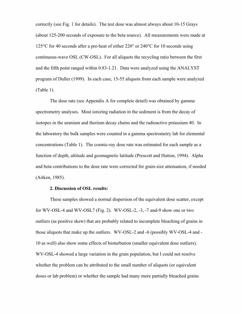
correctly (see Fig. 1 for details). The test dose was almost always about 10-15 Grays

(about 125-200 seconds of exposure to the beta source). All measurements were made at

125°C for 40 seconds after a pre-heat of either 220° or 240°C for 10 seconds using

continuous-wave OSL (CW-OSL). For all aliquots the recycling ratio between the first

and the fifth point ranged within 0.83-1.21. Data were analyzed using the ANALYST

program of Duller (1999). In each case, 15-55 aliquots from each sample were analyzed

(Table 1).

The dose rate (see Appendix A for complete detail) was obtained by gamma

spectrometry analyses. Most ionizing radiation in the sediment is from the decay of

isotopes in the uranium and thorium decay chains and the radioactive potassium 40. In

the laboratory the bulk samples were counted in a gamma spectrometry lab for elemental

concentrations (Table 1). The cosmic-ray dose rate was estimated for each sample as a

function of depth, altitude and geomagnetic latitude (Prescott and Hutton, 1994). Alpha

and beta contributions to the dose rate were corrected for grain-size attenuation, if needed

(Aitken, 1985).

2. Discussion of OSL results:

These samples showed a normal dispersion of the equivalent dose scatter, except

for WV-OSL-4 and WV-OSL7 (Fig. 2). WV-OSL-2, -3, -7 and-9 show one or two

outliers (as positive skew) that are probably related to incomplete bleaching of grains in

those aliquots that make up the outliers. WV-OSL-2 and -6 (possibly WV-OSL-4 and -

10 as well) also show some effects of bioturbation (smaller equivalent dose outliers).

WV-OSL-4 showed a large variation in the grain population, but I could not resolve

whether the problem can be attributed to the small number of aliquots (or equivalent

doses or lab problem) or whether the sample had many more partially bleached grains

(geological problem). WV-OSL-7 showed a similar large variation in equivalent dose.

However, some of the samples exhibited a tighter than normal distribution (WV-OSL-1,

5, and 8) and look like they were very well bleached at deposition (perhaps having been

exposed at the surface for some time before burial??).

In general, the older the sample, the more dispersion it displays. Samples that

have a brief or turbid fluvial depositional history (i.e. terrace or reworked glacial

deposits) or short transport path, also display more dispersion than will a sample

composed of mainly eolian grains or grains that were sub aerially exposed before burial

(point bar deposits). A set of “individual value plots” from all accepted equivalent doses

generated for each sample are shown in Fig. 2. Histograms for the luminescence samples

were also generated (Figs. 3, 4, 5). Please note that the thick curve over the histograms

bins is the normal distribution curve generated for that data set and that the simple mean

is shown for the equivalent dose, not the weighted mean as was used in Table 1.

The bin width of the histograms can be determined for the samples by defining it

as the value of the standard deviation (see Figs. 3, 4, 5; Lepper and McKeever, 2002). I

have attempted to come close to these standard deviation values while retaining a clear

data presentation of multiple graphs in one group for comparison purposes. Histograms

are unable to display the precision, from which each De value is obtained, but the

standard deviation generated for each sample is shown and I have also shown some radial

plots (Figures 6, 7, 8, and 9) to enable you to see the spread in the precision for the

samples.

A comparison of equivalent doses (Fig. 2) shows tight clusters for samples WV-

OSL-1,-5, and -8, which attest to their well-bleached characteristics. Except for the

above mentioned outliers, samples WV-OSL-2, -3, -6, and -9 also showed generally well-

bleached behavior as well, although the plateaus show a much broader distribution (and

larger standard deviations), more like that of sediment from a fluvial environment or

sediment that contains a strong component of partial bleaching. For this reason the mean

on some samples was weighted such that those grains that exhibited lower equivalent

doses and more precise errors (i.e. well-bleached grains) would control the total

equivalent dose (i.e. WV-OSL-2: 48.7Grays weighted vs. 44.9 Grays). WV-OSL-4, -7,

and -10 also had outliers that probably should have been removed, but the outliers to the

right and left of the fit were nulled by weighting the data. The other samples (WV-OSL-

1, -5, and -8) did not really require a weighted mean, but nonetheless were reported in

this way. This weighted mean affected the ages generated in only a minimal way,

however (see subtitles in histogram figures for variations against Table 1).

I did not attempt to calculate beyond any standard measures of central tendency

(mean, standard deviation), although t least two analytical tools have been developed that

address this issue and attempt to objectively determine a representative dose; including

the "zero age model" (Galbraith et al., 1999) and the "leading edge method" (Lepper, et.

al, 2000). The raw data will be required for those calculations and I will supply that data

if requested.

There were no difficulties with the samples returning reliable ages. I’m not sure

of the expected age range for these samples (i.e. Holocene floodplain vs. glacial

Interstade?), but there were no problems using the laboratory applied SAR protocol. The

samples did not show monotonic (saturating) behavior, did not show a lack of

proportionality between the regenerative and test-dose signals and there was no

difference in sensitivity corrections between the natural and the regenerative cycles. The

excessive scatter and high standard deviations for some of the samples are instead

attributed to problems in the geology of the sediment. The dispersion on the equivalent

doses obtained in the samples simply represents the variety of equivalent doses seen in

each sample (remember we analyzed 150 to 200 grains per aliquot). It was impossible to

tell whether young equivalent doses (WV-OSL-2, -4, -6, -10) were a result of

bioturbation or true burial ages. The older equivalent doses could represent varying

degrees of partial bleaching, clay migration or true burial ages and could not be separated

out into those that were a result of non-bleaching (residual luminescence held) via short

transport paths, partial bleaching or true burial ages.

Material used to calculate the dose rates did not vary significantly in any way for

the U and Th, except for WV-OSL-6, although there was no change in K for any sample

(Table 1). It is unclear what this increase means, but it did not seem to point to any

disequilibrium problems in the bulk samples. Maybe localized groundwater flow through

the sampled sediment??

3. Conclusion:

The samples showed a remarkably limited age range between ~15 ka to 17 ka

(one outlier at 21 ka), with associated errors of 5 percent (tight equivalent dose

distributions) to 12-13 percent (broad equivalent dose distributions). A comparison of

equivalent doses (Fig. 2) shows tight clusters for samples WV-OSL-1,-5, and -8, which

are attributed to their well-bleached characteristics. WV-OSL-2, -3, -7 and-9 show one

or two outliers (as positive skew) that are probably related to incomplete bleaching of

grains in those aliquots that make up the outliers, consistent with a fluvial or glacio-

fluvial origin.

WV-OSL-2 and -6 (possibly WV-OSL-4 and -10 as well) also show some effects

of bioturbation (smaller equivalent dose outliers). WV-OSL-4 and WV-OSL-7 showed

the largest variation in the age of the grain population. All the histograms look

acceptable and the samples responded in a normal fashion to the SAR protocol of OSL.

If the sample ages seem to too old in the context of your sampling program, I suggest

applying for further analyses to a single-grain OSL dating lab.

4. References

Aitken, M.J. (1985). Thermoluminescence Dating. Academic Press, London, 359 pp. Aitken, M.J. (1998). An Introduction to Optical Dating: The dating of Quaternary sediments by

the use of photon-stimulated luminescence. Oxford University Press, New York, 267 pp. Friedman, J.M., Vincent, K.R., and Shafroth, P.B. (2005) Dating floodplain sediments using tree-

ring response to burial, Earth Surface Processes and Landforms, 30 (9), p. 1077-1091. Galbraith, R.F., Roberts, R.G., Laslett, G.M., Yoshida, H. and Olley, J.M. (1999). Optical dating

of single and multiple grains of quartz from Jinmium rock shelter, Northern Australia: Part I, Experimental Design and Statistical Models. Archaeometry, 41 (2), 339-364.

Lepper, K. (2001). Development of an objective dose distribution analysis method for

luminescence dating and pilot studies for planetary applications. Ph.D. Thesis, Oklahoma State University, Stillwater, OK, 288 pp.

Lepper, K. and McKeever, S.W.S. (2002). An objective methodology for dose distribution

analysis. Radiation Protection Dosimetry, 101, 349-352. Miller, R.W., Donahue, R.L. (1995). Soils in our Environment (7th edition). Prentice Hall, New

Jersey, 649 pp. Murray, A. and Wintle, A.G. (2000). Luminescence dating of quartz using an improved single-

aliquot regenerative-dose protocol. Radiation Measurements, 32, 57-73. Murray, A.S., Olley, J.M. and Caitcheon, G.G. (1995). Measurement of equivalent doses in

quartz from contemporary water-lain sediments using optically stimulated luminescence. Quaternary Science Reviews, 14, 365-371.

Olley, J., Caitcheon, G. and Murray, A. (1998) The distribution of apparent dose as determined

by optically stimulated luminescence in small aliquots of fluvial quartz; implications for dating young sediments. Quaternary Science Review, 17 (11), 1033-1040.

Prescott, J.R. and Hutton, J.T. (1994). Cosmic ray contributions to dose rates for luminescence

and ESR dating: large depths and long-term time variations. Radiation Measurements, 23, 497-500.

Wallinga, J. (2002). Optically stimulated luminescence dating of fluvial deposits: a review.

Boreas 31 (4), 303-322.

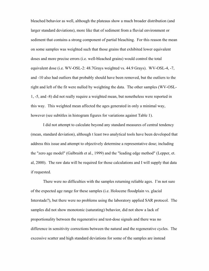
Figure 1a. OSL decay curve for WV-OSL-6, showing quartz signal as measured with blue-light wavelength emitting diodes. Time is measured in seconds (s) and OSL is measured in photons counts/second. Figure 1b. WV-OSL-6 growth curve, with the natural plotted on the Lx/Tx axis near 1.5 as a gray line). Regeneration proceeded “normally”, with a recycle within 18% of the first measurement and increases in responses to increasing beta radiation. Dose is measured in seconds x 100 (not / by 100) and OSL is measured in normalized OSL sensitivity measurements (Lx/Tx).

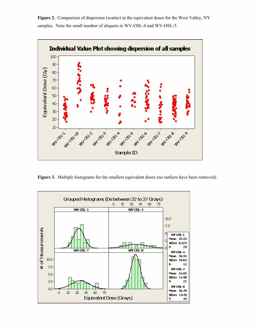
Figure 2. Comparison of dispersion (scatter) in the equivalent doses for the West Valley, NY

samples. Note the small number of aliquots in WV-OSL-4 and WV-OSL-5.

Figure 3. Multiple histograms for the smallest equivalent doses (no outliers have been removed).

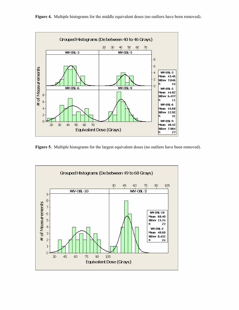
Figure 4. Multiple histograms for the middle equivalent doses (no outliers have been removed).

Figure 5. Multiple histograms for the largest equivalent doses (no outliers have been removed).

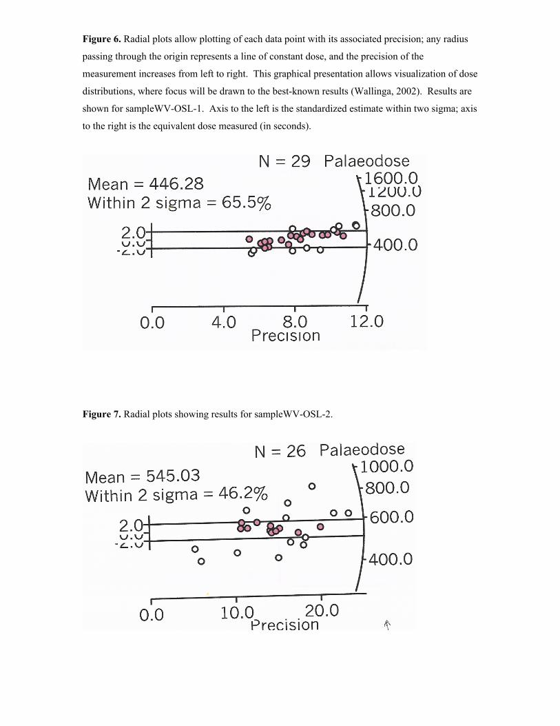
Figure 6. Radial plots allow plotting of each data point with its associated precision; any radius

passing through the origin represents a line of constant dose, and the precision of the

measurement increases from left to right. This graphical presentation allows visualization of dose

distributions, where focus will be drawn to the best-known results (Wallinga, 2002). Results are

shown for sampleWV-OSL-1. Axis to the left is the standardized estimate within two sigma; axis

to the right is the equivalent dose measured (in seconds).

Figure 7. Radial plots showing results for sampleWV-OSL-2.

Figure 8. Radial plots showing results for sampleWV-OSL-6.

Figure 9. Radial plots showing results for sampleWV-OSL-8.

Appendix A:

General Concepts of Luminescence Dating:

Most minerals react to ionizing radiation by essentially gaining energy at the electron

level, which accumulates through time if that energy is not released (as light) by some

outside stimuli (sunlight or intense heat over 200°C). Thus, sediment grains can record

their exposure history to ionizing radiation, which can then be “read” in the laboratory

and used as a clock. This procedure is referred to as luminescence geochronology

(Aitken, 1998), the goal of which is to establish the timing of the burial of mineral grains

in sedimentary deposits. If the mineral grains were transported at night, in turbid fluvial

conditions or in those deposits generally considered to be deposited in massive, sudden

discharge events (i.e. debris flows, colluvium, etc.) however, luminescence dating may

produce depositional ages that are too old because the luminescence clock was not reset

to “zero” just prior to burial.

Luminescence dating is based on solid-state dosimetric properties of natural

mineral grains. Minerals react to ionizing radiation, which is generated by radioactive

isotopes found in minor quantities in most terrestrial sediments and by cosmic radiation.

Specifically, ionizing radiation creates charge pairs/carriers (e-, h+) in mineral crystals.

The charge carriers are mobile within the crystals, but can become localized, or trapped,

at lattice defects and held there over geologically significant time scales. Over time, the

number of segregated, or trapped, charge carriers builds up in a way that can be described

by a saturating exponential function.

Exposure to heat, light, or high pressures can release charge carriers from trapping

sites and permit recombination, during which light is emitted from the mineral grains.

This detrapping resets the system within the mineral grains. In terrestrial environments

exposure to sunlight during sediment transport resets the clock and it is also why a

luminescence age is considered a burial age. In the laboratory, sediment is stimulated to

emit light, which is measured. The sediment is stimulated by exposure to light of specific

wavelengths (optically stimulated luminescence, OSL), or heat (thermoluminescence,

TL), in proscribed manners. The intensity of emitted light measured in the laboratory is

proportional to the trapped charge population, which is proportional to the total absorbed

radiation dose (De) that the sedimentary deposit experienced, and that relation is

proportional to the time elapsed since burial.

The simplest form of the OSL age equation is:

tOSL =De

′ D

where tOSL = age

De = total absorbed radiation dose,

D’ = natural environmental dose rate.

The accuracy of OSL ages is primarily dependent on the intensity and duration of

the sediment grains’ exposure to sunlight during transport, often referred to as “resetting”

or “bleaching”. Traditionally, sediments deposited from fluvial systems have been

among the most challenging to date using OSL methods because the grains were not fully

bleached prior to burial. Bleaching problems arise from the light filtering effects of

water, particularly water turbid with high suspended-sediment concentrations, and from

transport at night. A review of studies that used OSL to date fluvial sediments can be

found in Wallinga (2002). Unfortunately, many of these studies met with mixed results,

yet luminescence dating has important potential because fluvial deposits often lack the

foreign objects (charcoal, potsherds, living trees) that are essential for alternative dating

methods (e.g. Friedman et al., 2005).

Fortunately, modern luminescence dating equipment and experimental procedures

show promise. For example geochronological measurements can be made on small

collections of grains, termed single aliquots, or even single grains. This in turn permits

hundreds or even thousands of absorbed doses to be determined for individual field

samples. These data sets or dose distributions can then be visualized and statistically

interrogated. Numerous studies have now documented that “incomplete resetting” or

“partial bleaching” manifests itself as positive asymmetry in a sample’s dose distribution

( Murray et al., 1995; Olley et al., 1998; Lepper and McKeever, 2002). In these cases,

standard measures of central tendency (mean, standard deviation) do not represent the

true depositional age of the sediment. At least two analytical tools have been developed

that address this issue and attempt to objectively determine a representative dose;

including the "zero age model" (Galbraith et al., 1999) and the "leading edge method"

(Lepper, 2001).

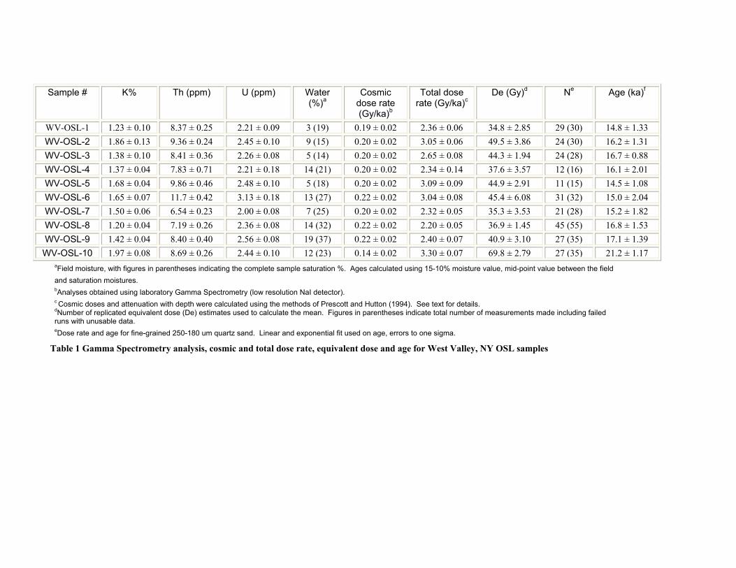
Sample # K% Th (ppm) U (ppm) Water (%)a

Cosmic dose rate (Gy/ka)b

Total dose rate (Gy/ka)c

De (Gy)d Ne Age (ka)f

WV-OSL-1 1.23 ± 0.10 8.37 ± 0.25 2.21 ± 0.09 3 (19) 0.19 ± 0.02 2.36 ± 0.06 34.8 ± 2.85 29 (30) 14.8 ± 1.33 WV-OSL-2 1.86 ± 0.13 9.36 ± 0.24 2.45 ± 0.10 9 (15) 0.20 ± 0.02 3.05 ± 0.06 49.5 ± 3.86 24 (30) 16.2 ± 1.31 WV-OSL-3 1.38 ± 0.10 8.41 ± 0.36 2.26 ± 0.08 5 (14) 0.20 ± 0.02 2.65 ± 0.08 44.3 ± 1.94 24 (28) 16.7 ± 0.88 WV-OSL-4 1.37 ± 0.04 7.83 ± 0.71 2.21 ± 0.18 14 (21) 0.20 ± 0.02 2.34 ± 0.14 37.6 ± 3.57 12 (16) 16.1 ± 2.01 WV-OSL-5 1.68 ± 0.04 9.86 ± 0.46 2.48 ± 0.10 5 (18) 0.20 ± 0.02 3.09 ± 0.09 44.9 ± 2.91 11 (15) 14.5 ± 1.08 WV-OSL-6 1.65 ± 0.07 11.7 ± 0.42 3.13 ± 0.18 13 (27) 0.22 ± 0.02 3.04 ± 0.08 45.4 ± 6.08 31 (32) 15.0 ± 2.04 WV-OSL-7 1.50 ± 0.06 6.54 ± 0.23 2.00 ± 0.08 7 (25) 0.20 ± 0.02 2.32 ± 0.05 35.3 ± 3.53 21 (28) 15.2 ± 1.82 WV-OSL-8 1.20 ± 0.04 7.19 ± 0.26 2.36 ± 0.08 14 (32) 0.22 ± 0.02 2.20 ± 0.05 36.9 ± 1.45 45 (55) 16.8 ± 1.53 WV-OSL-9 1.42 ± 0.04 8.40 ± 0.40 2.56 ± 0.08 19 (37) 0.22 ± 0.02 2.40 ± 0.07 40.9 ± 3.10 27 (35) 17.1 ± 1.39 WV-OSL-10 1.97 ± 0.08 8.69 ± 0.26 2.44 ± 0.10 12 (23) 0.14 ± 0.02 3.30 ± 0.07 69.8 ± 2.79 27 (35) 21.2 ± 1.17

aField moisture, with figures in parentheses indicating the complete sample saturation %. Ages calculated using 15-10% moisture value, mid-point value between the field and saturation moistures. bAnalyses obtained using laboratory Gamma Spectrometry (low resolution NaI detector). c Cosmic doses and attenuation with depth were calculated using the methods of Prescott and Hutton (1994). See text for details. dNumber of replicated equivalent dose (De) estimates used to calculate the mean. Figures in parentheses indicate total number of measurements made including failed runs with unusable data. eDose rate and age for fine-grained 250-180 um quartz sand. Linear and exponential fit used on age, errors to one sigma.

Table 1 Gamma Spectrometry analysis, cosmic and total dose rate, equivalent dose and age for West Valley, NY OSL samples