Embed Size (px)
Citation preview

Information Aggregation Failure
in a Model of Social Mobility∗
Avidit Acharya†
October 16, 2016
Abstract
I study a model in which high and low income voters must decide between con-
tinuing with a status quo policy or switching to a different policy, which is more
redistributive. Under the status quo policy, low income voters may get an oppor-
tunity to become high income earners. Such opportunities are expected to arise
infrequently, so in expectation these voters prefer the more redistributive policy.
Nevertheless, there is an equilibrium in which the vast majority of them cast their
ballots in favor of re-electing the less redistributive status quo. Although these vot-
ers are fully strategic and correctly assess their chances for upward mobility, they
vote exactly as if they are naive voters who over-estimate their chances of becoming
rich. As the size of the electorate grows, the status quo policy can be re-elected
with certainty, and the election fails to fully aggregate information.
JEL Classification Codes: D72, P16
Key words: redistributive politics, social mobility, strategic voting, information
aggregation
∗This paper is revised from a chapter of my dissertation. I would like to thank my adviser, AdamMeirowitz, for his comments and encouragement. I also thank Sourav Bhattacharya, John Duggan, TimFeddersen, Edoardo Grillo, Faruk Gul, Vijay Krishna, David Myatt, Juan Ortner, Wolfgang Pesendorfer,Kris Ramsay, Brian Roberson, Tom Romer, Erik Snowberg and participants at the 2012 EconometricSociety Meeting in New Delhi and the 2013 Midwest Political Science Association Conference in Chicagofor discussions and comments. The usual disclaimer applies.†Assistant Professor of Political Science, Stanford University, Stanford CA 94305 (email:
1
1 Introduction
This paper demonstrates the failure of elections to aggregate private information in an
environment where strategic voters have redistributive preferences and get opportunities
for social mobility. This result stands in contrast to existing results by Feddersen and
Pesendorfer (1997) and much of the subsequent literature in which elections were shown
to fully aggregate private information.
The model in which I derive this result has two groups of voters—high and low
income—who must collectively decide whether to re-elect a status quo policy or switch
to an alternative policy, which is more redistributive. Under the status quo policy, low
income voters may get an opportunity to become high income earners, but will succeed
in climbing the economic ladder only if they are talented. Low income voters do not
know whether or not they are talented unless they receive the opportunity, in which case
they learn about their talent from either their success or failure. Low income voters are
uncertain about the probability with which they can expect to receive the opportunity for
social mobility under the status quo, but they expect it to be low. Consequently, these
voters prefer the more redistributive policy to the status quo. The status quo policy is in
effect for one period, after which an election is held to decide whether to continue with it
in the next period or to switch to the more redistributive policy.
I characterize the set of equilibria of the model in the limit as the number of voters
grows to infinity. If the probability that a voter is talented is high, then in this limit
there are generically three equilibria. One of these is a pure strategy equilibrium in which
several low income voters, who are fully strategic and correctly assess their chances of
upward mobility, cast their ballots exactly as if they were naive (sincere) voters who hold
mistakenly optimistic beliefs about their mobility prospects. The voters who behave this
way are precisely the vast majority of low income voters who did not receive the economic
opportunity in the first period. All of these voters vote to re-elect the status quo policy
despite knowing, at the time they vote, that the more redistributive policy gives them a
strictly higher expected payoff.
The logic behind this result is as follows. In any equilibrium of the model, high
income voters (including those low income voters who climbed the economic ladder in the
first period) vote to re-elect the status quo policy, while low income voters who got the
opportunity and learned that they are untalented vote for the more redistributive policy.
If all low income voters who did not receive the economic opportunity in the first period
vote en masse to re-elect the status quo, then the election should not be close: the status
2
quo should win almost surely when the size of the electorate is large. But if the election
is close, and a low income voter is pivotal, it can only be because nearly half of the
electorate consists of low income voters who received the economic opportunity, learned
that they were untalented, and voted for the more redistributive policy. For so many low
income voters to learn that they are untalented, it must be that economic opportunities
are plentiful under the status quo. When this is the case, and low income voters believe
that they are likely enough to be talented, it is optimal for them to vote for the status
quo. The status quo is re-elected almost surely.
Under such behavior, the election fails to fully aggregate information. This means
that there is a positive ex ante probability that in a complete information version of the
same voting game—i.e., one in which all voters knew the likelihood of getting the economic
opportunity—the status quo policy would not be re-elected in limit as the number of voters
gets large. This happens precisely when the likelihood of getting the economic opportunity
is low, in which case the low income voters who did not get the opportunity in the first
period would want to elect the more redistributive policy. With complete information,
the law of large numbers implies that status quo policy wins almost surely as the size of
the electorate gets large. Instead, in the model with incomplete information, there is an
equilibrium in which the status quo policy wins with strictly positive probability in the
large electorate limit, implying that the election fails to fully aggregate information.1
The observation that strategic voters may not vote sincerely goes back to the seminal
papers of Austen-Smith and Banks (1996) and Feddersen and Pesendorfer (1997). This
paper uses their approach to address the classical political economy question of whether
it could be rational for the poor to vote against redistribution, thereby creating a link
between the classical political economy literature on redistributive politics and the strate-
gic voting literature that studies models in which voters are privately informed. I answer
the classical political economy question in the affirmative, and show that the seemingly
irrational behavior of low income voters can in fact be rationalized without adding issue
dimensions, such as social issues, or assuming that voters have non-material (ideological)
interests. Voters in my model are fully rational and strategic, but their behavior is ob-
servationally indistinguishable from that of naive voters who are overly optimistic about
their social mobility prospects.
1The described result holds in an equilibrium that exists when the probability that any given voter istalented is high, but in this case there also exists an equilibrium that fully aggregates information. Onthe other hand, if the probability that a voter is talented is low, then there is a unique equilibrium thatfully aggregates information, while if this probability is in an intermediate range then there is a uniqueequilibrium that fails to fully aggregate information.
3
2 The Political Environment
There are two periods and two policies. In the first period, a status quo policy is in effect.
Then, an election is held to decide whether to continue with it in the next period, or to
switch to a different policy, which is more redistributive. The policy that gets a majority
of votes is implemented in the second period.
There are 2n + 1 voters. At the start of each period, each voter’s income is drawn
independently. With probability λ ∈ (0, 12) a voter has a high income, and with remaining
probability 1 − λ he has a low income.2 Under the more redistributive policy, each high
income voter receives a payoff ψh, where ψ < 1 and h > 0, while each low income voter
receives a payoff of 0. Under the status quo policy, each high income voter has payoff h,
while each low income voter has probability δ of receiving an opportunity to become a high
income voter. If a low income voter receives the opportunity to climb the economic ladder
and he is talented, then he becomes a high income voter and receives the payoff h. If he is
not talented or if he does not receive the opportunity, then his payoff is −l < 0. Each low
income voter has prior probability p ∈ (0, 1) of being talented. If a voter becomes a high
income earner in the first period, he remains a high income earner in the second period.
Voters who receive an opportunity to become high income earners in the first period and
are unsuccessful learn that they are untalented, and would be unsuccessful also in the
following period. Voters who do not receive the opportunity in the first period do not
learn whether or not they are talented.
All voters know the success rate p, but they are uncertain about δ. This uncertainty
can be taken to reflect uncertainty about whether the status quo policy “works well:” if
δ is high, then opportunities for social mobility are plentiful and the status quo policy
works well, whereas if δ is low then opportunities are scarce and the policy does not work
well. In particular, if the status quo policy is re-elected, then the value of δ in the second
period is the same as in the first. Each voter experiences the consequences of the first
period policy only for himself; thus, each voter is uninformed about who (and how many
others) received the opportunity to climb the economic ladder, and whether or not they
succeeded.
2This assumption implies that in a large electorate (i.e., as n→∞) high income voters are a fractionλ of the population and are outnumbered by low income voters—a common assumption. In a finiteelectorate, on the other hand, the fraction of high income voters is random, and with positive probabilitythe rich will outnumber the poor. Since all of the main results are about large electorates, I maintain theassumption that each voter’s income-type is an independent random draw, which simplifies the analysis.A pervious working paper version of this paper (Acharya 2013) analyzed the case in which the share ofeach income-type is fixed even in finite electorates.
4

Let F denote the distribution of δ. I assume that F has a continuous density f , and
f(δ) ≥ ν for some ν > 0 and all δ ∈ [0, 1]. This assumption serves the same role in my
analysis as Feddersen and Pesendorfer’s (1997) Assumption 2 does in theirs.3 It ensures
that as the electorate grows, pivotal beliefs about the state get concentrated on the value
that brings the probability of drawing a vote for either alternative closest to 12. Let E[δ]
denote the expected value of δ according to the prior F .
Given δ, the expected payoff from the status quo policy for a low income voter is
y(δ) = −(1− δp)l + δph = −l + δp(l + h) (1)
which is linear and increasing in δ. Therefore, the unconditional expected payoff to re-
electing the status quo policy for a low income voter who did not receive the economic
opportunity is simply y(E[δ]). I assume that
y(E[δ]) < 0 < y(1) (2)
which says that low income voters do not expect the status quo policy to work well,
and therefore they prefer the more redistributive policy; however, if they thought that
the status quo policy did work well, then they would prefer that policy to the more
redistributive one.
Since y(δ) is strictly increasing in δ, there is a cutoff
δ =1
p
(l
l + h
)(3)
such that a low income voter who does not yet know whether or not he is talented would
prefer the status quo policy if the expected value of δ were above δ, and would prefer the
more redistributive policy if it were below δ. Note that the assumption 0 < y(1) made in
(2) implies p > l/(l + h), which means that δ < 1.
3 Voting Behavior and Information Aggregation
A type-contingent strategy for a voter maps his type to the probability with which he
votes to re-elect the status quo policy. To analyze the model, I study type-symmetric
Bayes Nash equilibrium in weakly undominated strategies, which I refer to simply as
3Feddersen and Pesendorfer (1997) also assume that the density of the state is bounded above.
5
“equilibrium” (Feddersen and Pesendorfer 1997). A type-symmetric equilibrium is one
in which all voters of the same type use the same type-contingent strategy. There are
four types of voters in the model: (i) high income earners, H, (ii) low income earners
that became high income earners in the first period, L+, (iii) low income earners that got
the opportunity in the first period but did not succeed, L−, and (iv) low income earners
that did not get the opportunity in the first period, L0. Note that H and L+ voters have
a weakly dominant strategy to vote to re-elect the status quo, while L− voters have a
weakly dominant strategy to vote for the more redistributive policy.4
In equilibrium, the L0 voters must vote as if they are pivotal; that is, they condition
on the hypothetical event that apart from their own vote, the election is tied (see, e.g.,
Austen-Smith and Banks 1996). Since our equilibrium is type-symmetric all of these L0
voters vote for the status quo with the same probability. Call that probability x. The
probability of drawing a vote for the status quo policy from a random voter, conditional
on δ, is then
π(δ, x) = λ+ (1− λ)[δp+ (1− δ)x] (4)
The probability of a voter being pivotal is
β(δ|x, n) =
(2n
n
)(π(δ, x))n(1− π(δ, x))n. (5)
For an L0 voter, the distribution of δ conditional on his type and the pivotal event is
fpiv(δ|x, n, L0) =β(δ|x, n)(1− δ)f(δ)∫ 1
0β(δ|x, n)(1− δ)f(δ)dδ
, (6)
which is well-defined because 0 < π(δ, x) < 1 for all (δ, x). Therefore, conditional on
being pivotal and being an L0 type, the expected value of δ is
Epiv[δ|x, n, L0] =
∫ 1
0
δf piv(δ|x, n, L0)dδ. (7)
In equilibrium, L0 voters vote to re-elect the status quo policy if Epiv[δ|x, n, L0] > δ and
vote for the more redistributive alternative if Epiv[δ|x, n, L0] < δ. They mix between
the two only if Epiv[δ|x, n, L0] = δ. I use these facts to establish the existence of an
4In a Poisson game formulation a la Myerson (1998) these types of voters would have strictly dominantstrategies. I do not adopt the Poisson game formulation so as to make my results more directly comparableto those of Feddersen and Pesendorfer (1997).
6
equilibrium for all values of n. The following proposition records this result, along with
the equilibrium behavior of voters of type H, L+ and L−.
Proposition 1. For every finite n, an equilibrium to the voting game exists. In every
equilibrium voters of type H and L+ vote for the status quo policy, while voters of type
L− vote for the more redistributive policy.
Proof. See Appendix A. �
Given that the behavior of types H, L+ and L− is fixed for all n, I will henceforth
abuse terminology and identify an equilibrium with the probability x with which each L0
type voter votes to re-elect the status quo policy.
3.1 Analysis of Large Electorates
To understand the behavior of the L0 types of voters, it helps to understand the prop-
erties of Epiv[δ|x, n, L0]—in particular, when is this conditional expectation of δ below
the threshold δ defined in (3) and when is it above? Proposition 2 below shows that
even though Epiv[δ|x, n, L0] is a complicated object for finite n, it is straightforward to
characterize its limit in n for every value of x. This makes it possible to characterize the
behavior of the L0 voters in large electorates.
Fix any x 6= p, and note that the probability π(δ, x) that a randomly drawn voter
votes for the status quo is strictly monotonic in δ, so there is a unique value of δ that
minimizes |π(δ, x) − 12|. Denote this value by δ∗(x). This is the value of δ that brings
the probability of drawing a vote for either alternative closest to 12, i.e., the value that
is most likely to deliver a tied election. The proposition below then states three facts:
(i) Epiv[δ|p, n, L0] = E[δ], (ii) Epiv[δ|x, n, L0] converges to δ∗(x) for all x 6= p, and (iii) if
x 6= p, then Epiv[δ|·, n, L0] can be made arbitrarily close to δ∗(x) in a neighborhood of x
by choosing n large enough and the neighborhood small enough.
Proposition 2. If x = p then Epiv[δ|x, n, L0] = E[δ] for all n. If x 6= p, then for all ε > 0,
there exists ρ > 0 and a number N such that n ≥ N implies
∣∣Epiv[δ|x, n, L0]− δ∗(x)∣∣ ≤ ε ∀x ∈ Bρ(x) := {x ∈ [0, 1] : |x− x| ≤ ρ}.
Proof. See Appendices B and C. �
The proof of the proposition in Appendix C relies on a general result presented in Ap-
pendix B. I show that if x 6= p, then the conditional distribution fpiv(·|x, n, L0) converges
7

to a Dirac mass at δ∗(x) as n gets large. In this sense, Proposition 1 belongs to a class
of results that trace their origins to an argument in statistics by Bayes (1763) himself,
and to a result in the voting literature by Good and Mayer (1975) and Chamberlain and
Rothschild (1981).5 Various extensions and applications of these results appear in several
more recent papers, including Feddersen and Pesendorfer (1997), Mandler (2012) and
Krishna and Morgan (2012). There are many ways to prove Proposition 2. I adopt the
approach of Feddersen and Pesendorfer (1997).
3.2 Graphical Analysis
Although Epiv[δ|·, n, L0] is a complicated object, Proposition 2 suggests that when n is
large, we can study the properties of Epiv[δ|·, n, L0] by studying the properties of δ∗(·),which is a much less complicated object. I now solve explicitly for δ∗(·) and use it to
provide some graphical intuition for the formal equilibrium analysis that follows.
Since π(·, x) in (4) is a linear function of δ with slope (1 − λ)(p − x), it is strictly
increasing in δ for x < p, strictly decreasing in δ for x > p, and constant in δ for x = p.
Also, note that π(1, x) = λ + (1 − λ)p, which is independent of x, and consider first the
case where π(1, x) = λ+ (1− λ)p > 12. If x >
12−λ
1−λ then π(δ, x) remains above 12
for all δ.
In particular, if12−λ
1−λ < x < p then π(δ, x) is upward sloping so π(δ, x) gets closest to 12
at
δ = 0; thus δ∗(x) = 0 for12−λ
1−λ < x < p. Similarly, if p < x ≤ 1 then π(δ, x) is downward
sloping so π(δ, x) gets closest to 12
at δ = 1; thus δ∗(1) = 1 for p < x ≤ 1. On the other
hand, if 0 ≤ x ≤12−λ
1−λ , then π(δ, x) does intersect 12
meaning that |π(δ, x) − 12| takes a
minimum value of 0. Thus, solving π(δ, x) = 12
for δ gives us δ∗(x) in the case where
0 ≤ x ≤12−λ
1−λ . The solution is
δ∗(x) =1
p− x
( 12− λ
1− λ− x)
(8)
Therefore, as Figure 1(a) depicts, δ∗(x) is strictly and continuously decreasing from
δ∗(0) = 1p
12−λ
1−λ to 0 on the interval [0,12−λ
1−λ ], constantly equal to 0 on the interval (12−λ
1−λ , p),
and constantly equal to 1 on the interval (p, 1]. Analogously, if we consider the case
where π(1, x) = λ+ (1− λ)p < 12, then we find that δ∗(x) is constantly equal to 1 on the
5Good and Mayer (1975) and Chamberlain and Rothschild (1981) used Bayes’s original argument
to show that if F is a distribution on [0, 1] with continuous density f , then limN→∞N∫ 1
0
(2NN
)αN (1 −
α)NdF (α) = 12f( 1
2 ). I thank David Myatt and Vijay Krishna both for telling me about this.
8
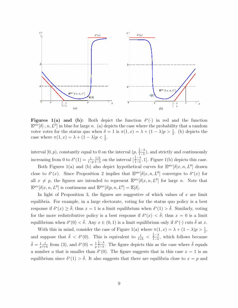
Figures 1(a) and (b): Both depict the function δ∗(·) in red and the functionEpiv[δ|·, n, L0] in blue for large n. (a) depicts the case where the probability that a randomvoter votes for the status quo when δ = 1 is π(1, x) = λ + (1 − λ)p > 1
2. (b) depicts the
case where π(1, x) = λ+ (1− λ)p < 12.
interval [0, p), constantly equal to 0 on the interval (p,12−λ
1−λ ), and strictly and continuously
increasing from 0 to δ∗(1) = 11−p
1/21−λ on the interval [
12−λ
1−λ , 1]. Figure 1(b) depicts this case.
Both Figures 1(a) and (b) also depict hypothetical curves for Epiv[δ|x, n, L0] drawn
close to δ∗(x). Since Proposition 2 implies that Epiv[δ|x, n, L0] converges to δ∗(x) for
all x 6= p, the figures are intended to represent Epiv[δ|x, n, L0] for large n. Note that
Epiv[δ|x, n, L0] is continuous and Epiv[δ|p, n, L0] = E[δ].
In light of Proposition 3, the figures are suggestive of which values of x are limit
equilibria. For example, in a large electorate, voting for the status quo policy is a best
response if δ∗(x) ≥ δ; thus x = 1 is a limit equilibrium when δ∗(1) > δ. Similarly, voting
for the more redistributive policy is a best response if δ∗(x) < δ; thus x = 0 is a limit
equilibrium when δ∗(0) < δ. Any x ∈ (0, 1) is a limit equilibrium only if δ∗(·) cuts δ at x.
With this in mind, consider the case of Figure 1(a) where π(1, x) = λ+ (1− λ)p > 12,
and suppose that δ < δ∗(0). This is equivalent to ll+h
<12−λ
1−λ , which follows because
δ = 1p
ll+h
from (3), and δ∗(0) = 1p
12−λ
1−λ . The figure depicts this as the case where δ equals
a number a that is smaller than δ∗(0). The figure suggests that in this case x = 1 is an
equilibrium since δ∗(1) > δ. It also suggests that there are equilibria close to x = p and
9
to x = x∗ where
x∗ :=
[ 12− λ
1− λ− l
l + h
]/[1− 1
p
l
l + h
](9)
which is calculated by solving δ∗(x) = δ for x, knowing that δ is given by (3) and δ∗(x)
is given by (8) when x ∈ [0,12−λ
1−λ ]. The reason that the figure suggests that there are
equilibria close to these points is because these points are close to the intersection points
of Epiv[δ|x, n, L0] with δ when δ = a. Similarly, if δ equals a number b that is higher than
δ∗(0) = 1p
12−λ
1−λ , then Figure 1(a) suggests that x = 0 and x = 1 are equilibria, and that
there is also an equilibrium close to x = p.
Now examine Figure 1(b). Suppose that δ equals a number a that is smaller than
δ∗(1) = 11−p
1/21−λ . That is, suppose that
p >
[l
l+h
][1−λ1/2
]1 +
[l
l+h
][1−λ1/2
] (10)
Then again there appear to be three equilibria, one at x = 1, one close to x = p, and
another close to x = x∗, where x∗ is again given by (9). Note that these are the same
values of x as in the case of Figure 1(a) above when δ < δ∗(0). If δ equals a number b
larger than δ∗(1) so that (10) holds with reverse inequality, then there appears to be only
one equilibrium close to x = p.
3.3 Limit Equilibria
I now formalize the graphical analysis of the previous section, and provide a full charac-
terization of the equilibrium set for large values of n. First, I review two familiar concepts.
I say that x is a large electorate equilibrium if there exists N such that n ≥ N implies
that x is an equilibrium of the voting game when the population parameter is n. I say
that x∞ is a limit equilibrium if it is an accumulation point of a sequence of equilibria
corresponding to a sequence of games indexed by n.6 Note that when the size of the
electorate is large, every equilibrium to the game has to be close to a limit equilibrium.7
6More formally, denote the game by Gn. For every sequence of voting games {Gn} there exists asequence of equilibria {xn} where each xn denotes the probability with which the L0 voters vote for thethe status quo policy in game Gn. x∞ is an accumulation point of such a sequence {xn} if the sequencehas a subsequence that converges to x∞. Since {xn} ⊂ [0, 1], the existence of limit equilibria follows fromthe existence of equilibria for games Gn, established in Proposition 1.
7Suppose, for the sake of contradiction, that a sequence of equilibria {xn}, each corresponding to thegame with population parameter n, has a subsequence that remains bounded away from all of the limitequilibria. That subsequence would in turn contain a sub-subsequence that converges to a limit that is
10
Also, note that every large electorate equilibrium is a limit equilibrium, but the converse
is not true.
Proposition 3. Suppose that λ+ (1− λ)p > 12
holds, or λ+ (1− λ)p < 12
and (10) both
hold. Then, there are generically three limit equilibria: (i) x∞ = max{0, x∗}, where x∗ is
defined in (9), (ii) x∞ = p, and (iii) x∞ = 1. When x∞ ∈ {0, 1} is a limit equilibrium,
it is also a large electorate equilibrium. If λ + (1 − λ)p < 12
and (10) holds with reverse
inequality, then x∞ = p is the unique limit equilibrium.
Proof. See Appendix D. �
The key result in Proposition 3 is that x∞ = 1 is a limit equilibrium (and also a
large electorate equilibrium) when λ + (1− λ)p > 12, or when λ + (1− λ)p < 1
2and (10)
both hold, which means that the probability of being talented, p, cannot be too small.
If p > 12, meaning that individuals are more likely to be talented than untalented, then
λ + (1− λ)p > 12
and we are in a case where x∞ = 1 is a limit equilibrium. In this case,
if the electorate is large, then a large fraction of low-income voters are poor not because
they are intrinsically untalented, but because opportunities are scarce.
The right hand side of inequality (10) has the following comparative statics. It is
increasing in l and decreasing in h and λ. In particular, as l increases, all else the same,
then the redistributive policy becomes more attractive, and the inequality is harder to
satisfy since the right hand side of the inequality increases. As h increases, the redistribu-
tive policy becomes less attractive, and the inequality becomes becomes easier to satisfy
since the right hand side decreases. As λ decreases, the right hand side of the inequality
increases, making it harder to satisfy.
I now provide some additional intuition for the pure strategy large electorate equilibria
mentioned in Proposition 3. If x∞ = 0, then none of the L0 voters cast their ballots for
the status quo policy. Therefore, the election is not likely to be close unless many low
income voters received the economic opportunity, became rich, and voted for the status
quo. This means that an L0 type’s expectation of δ, conditional on being pivotal, cannot
be small. When δ is larger than this conditional expectation of δ, the L0 voters are happy
to vote for the more redistributive policy. But when it is smaller, they would actually like
to switch their votes to the status quo policy.
bounded away from each limit equilibrium. But since this sub-subsequence is also a subsequence of {xn},its limit would have to be a limit equilibrium. Contradiction. Thus, when n is large, every equilibriumof the game has to be close to one of the limit equilibria.
11
Now consider the case of x∞ = 1. If p is large and all voters in L0 vote to re-elect the
status quo policy, the election is unlikely to be close: the status quo policy should win by
a large margin. But if the election does turn out to be close, then a large fraction of the
electorate must have voted for the redistributive policy. Since only the untalented voters
in L− vote for this policy, it must be that a large number of voters discovered that they
are untalented. They could only discover this by receiving the economic opportunity. In
other words, for so many voters to discover that they are untalented, it must be that δ is
large. Therefore, in this case, it makes sense—from the perspective of the L0 voters—to
vote for the status quo policy. On the other hand, if p is small, then the election is close
when not as many low income voters get the opportunity. In this case, the L0 voters may
want to switch their votes from the status quo policy to the more redistributive one.
3.4 Information Aggregation
I now study the information aggregation properties of the limit equilibria characterized
in the previous section. I say that a limit equilibrium x∞ aggregates information if for
almost every possible realization of δ, every subsequence of equilibria that converges to
x has a limiting distribution over electoral outcomes that equals a limiting distribution
over equilibrium outcomes of an otherwise identical subsequence of games, but in which
δ is common knowledge in all of the games in this sequence. A more formal definition is
given in Appendix E. The following proposition identifies which limit equilibria aggregate
information and which do not.
Proposition 4. If λ+ (1−λ)p > 12, then of the three possible limit equilibria mentioned
in Proposition 3, x∞ = max{0, x∗} aggregates information, while x∞ = p and x∞ = 1 fail
to aggregate information. If λ+ (1−λ)p < 12
and (10) holds, then none of the three limit
equilibria mentioned in Proposition 3 aggregates information. If λ + (1 − λ)p < 12, and
(10) holds with reverse inequality, then the unique limit equilibrium, x∞ = p, aggregates
information.
Proof. See Appendix E. �
Proposition 4 covers three cases. In the first case, where p is large, there is a limit
equilibrium, namely x∞ = max{0, x∗}, that aggregates information. But the two other
limit equilibria, namely x∞ = p and x∞ = 1, fail to aggregate information. Alternatively,
there is a case where all limit equilibria fail to aggregate information. This is the case
where λ + (1 − λ)p < 12
and (10) both hold. Finally, when p is very small so that
12
λ + (1− λ)p < 12
and the reverse of (10) holds, there is a third case in which the unique
limit equilibrium aggregates information.
The existence of equilibria in which information fails to aggregate is noteworthy given
the many positive results on information aggregation beginning with the seminal work of
Feddersen and Pesendorfer (1997). Nevertheless, the findings of a few other recent papers
also suggest that aggregation failure may be a more common phenomenon than was ini-
tially suspected. Bhattacharya (2013), for example, shows that having voters with diverse
preferences, as in this model, can lead to the existence of equilibria that fail to aggregate
information, but typically there will exist at least one equilibrium that aggregates infor-
mation.8 Bhattacharya (2013) studies a jury-type setting with two states of the world,
and shows that if voter preferences fail to satisfy a condition he calls “strong preference
monotonicity,” then there exists an equilibrium that fails to aggregate information. Al-
though Bhattacharya (2013) studied a model with binary states, and the current paper
has a continuum of states, an analogue to his strong preference monotonicity condition
fails in my model when λ + (1 − λ)p > 12.9 In contrast to these results that show the
existence of some equilibria that fail to aggregate information, I show that in the case
where λ+ (1− λ)p < 12
and (10) holds, all equilibria fail to aggregate information.10
Models in which information aggregation failure takes place with a continuum of signals
include Mandler (2012), Gul and Pesendorfer (2009) and Section 6 of Feddersen and
Pesendorfer (1997). However, the source of information aggregation failure in these models
is not preference diversity. Instead, these models share the common feature that there is
second order uncertainty, i.e. uncertainty about the the distribution of voter preferences.
Therefore, the source of aggregation failure in these models is qualitatively different from
the one here.
8Kim and Fey (2007) also study a model with preference diversity and show that there are equilibriathat fail to aggregate information. However, they also allow voters to abstain as in Feddersen andPesendorfer (1996).
9Strong preference monotonicity fails here because π(δ, 0) = λ + (1 − λ)δp is increasing in δ whileπ(δ, 1) = λ+ (1− λ)(δp+ 1− δ) is decreasing in δ, and x = 0 is the optimal value of x in the case wherethe state is known to be any δ < δ while x = 1 is the optimal value of x in the case were the state isknown to be any δ > δ.
10In this case, McLennan’s (1998) sufficient condition for information aggregation fails: there is nofeasible symmetric strategy profile that aggregates information.
13
4 Discussion
4.1 A “Behavioral Equivalence” Interpretation
In the x∞ = 1 limit equilibrium, the expected value of δ conditional on being pivotal
is nearly 1. In other words, conditional on being pivotal, low income voters who did
not receive the opportunity to climb the economic ladder in the first period believe that
they are nearly certain to receive the opportunity in the next period, so they vote to
re-elect the status quo policy. A naive voter who does not behave strategically, but has
overly optimistic beliefs about his chances for upward mobility (e.g. one who incorrectly
estimates the unconditional expectation of δ to be nearly equal to 1) would vote exactly
in the same way as the strategic L0 voter who conditions his vote on the pivotal event.
In fact, the observable behavior of these two kinds of voters is identical, since conditional
on being pivotal, the strategic L0 voter also believes that δ is nearly 1. This “behavioral
equivalence” is noteworthy considering the wide skepticism that much of the empirically
observed behavior of the American electorate could be consistent with voter rationality.11
It implies that if one had to draw inferences only from data on the voting patterns of
low income individuals who appear to overestimate their chance of climbing the economic
ladder and vote naively, one could not rule out the possibility that these are individuals
who actually correctly assess their chances for upward mobility and vote strategically.
It is also worth noting that in the x∞ = 1 equilibrium, conditional on being pivotal
an L0 voter believes not only that δ is large in expectation, but also that half of the
electorate—specifically, those who support the redistributive policy—are untalented. The
fact that this voter votes as if he simultaneously believes that he lives in a land of plentiful
opportunities, and in which there are several untalented other voters who voted for the
left wing redistributive policy, is an ironic but perhaps realistic feature of the model.
11See, e.g., Bartels (2008a), Achen and Bartels (2004), Healy, Malhotra and Mo (2010) and Wolfers(2002), among others. For example, Bartels (2008a) writes: “At the individual level ... psychologicalpressures produce unrealistic optimism about one’s own prospects, and an illusion of control over uncon-trollable events.” And in response to Shenkman’s (2008) accusation that “The consensus in the politicalscience profession is that voters are rational,” Bartels (2008b) writes, “Well, no. A half-century of schol-arship provides plenty of grounds for pessimism about voters’ rationality.” In response to this skepticism,the behavioral equivalence result of this paper shows that seemingly unsophisticated behavior may in factbe observationally identical to equilibrium behavior. Moreover, when δ < δ∗(0), it is the case that in alllimit equilibria the low income voters who did not receive the economic opportunity in the first periodvote for the status quo policy with positive probability. So, despite the existence of multiple equilibria,there is a strong sense in which the model rationalizes the behavior of agents who know that the moreredistributive policy is better for them, but nevertheless end up voting for the less redistributive policy.
14
4.2 Equilibrium in Pure Strategies
A feature of the model that sets it apart from other voting models with private information
is the fact that when p is large enough, there always exists a large electorate equilibrium
in pure strategies: x = 1 is an equilibrium of the voting game when the electorate is large.
In fact, in the case where λ+ (1−λ)p > 12
and δ < δ∗(0) (so that the redistributive policy
is still better for low income voters than the status quo, but not that much better) or
when λ+ (1− λ)p < 12
and δ < δ∗(1) (which is equivalent to (10)), this is the only strict
equilibrium. The other limit equilibria are in totally mixed strategies and are not strict.
4.3 Probability of Being Talented
When (10) holds, the assumption that p 6= 1 is crucial for generating the result that x = 1
is an equilibrium of the model for large electorates, as well as for generating the result
that there is an equilibrium that fails to aggregate information. In particular, under the
assumption that p = 1, all low income voters are certain to be talented, and the model has
a unique limit equilibrium, x∞ = x∗, which aggregates information. Therefore, the model
requires uncertainty both about the probability of getting the economic opportunity and
whether or not a given voter is talented.
However, it is also interesting to investigate the case where the parameter p is also
unknown to the voters, in addition to the parameter δ being unknown. That is, voters are
not only uncertain of how well the status quo policy works, they are also uncertain of how
likely any given one of them is to be talented. Assume that p and δ are independently
distributed, and suppose that the distribution of p has a continuous density g on the
support [p, 1]. Further, suppose that there is a number µ > 0 such that g(p) ≥ µ for all
p ∈ [p, 1]. Then we have the following result.
Proposition 5. If
p×min
{1,
1
1− p
(1/2
1− λ
)}>
l
l + h
then x∞ = 1 is a limit equilibrium (and a large electorate equilibrium) that fails to
aggregate information. In the limit as λ → 12, the unique limit equilibrium (and large
electorate equilibrium) is x∞ = 0, which aggregates information.
Proof. See Appendix F. �
15
4.4 Redistributive Policy First
The results of the model also hinge on the assumption that the status quo policy is less
redistributive than the alternative. If the more redistributive policy is implemented first,
or if there is only one period and voters must choose between the two policies without first
experiencing either policy, then the more redistributive policy always wins the election.
In light of this, one may think that the model is one of “status quo bias” rather than
“right wing bias.”
Meltzer and Richard (1978) have suggested that it may be difficult to separate status
quo bias from right wing bias. They argue that in the past century, the United States
progressively adopted left wing policies to replace status quo policies that were defended by
right wing politicians. Meltzer and Richard point to Roosevelt’s New Deal and Johnson’s
Great Society—both examples of policies that saw intense opposition when they were first
introduced, but whose programs, such as Social Security and Medicare, enjoy popular
support today. In light of these facts, the assumption that the right wing policy comes
first is consistent with the political competition over policies in recent American history.
Consequently, it may be quite challenging to distinguish status quo bias from right wing
bias not just in this model, but also in reality.12
4.5 Mobility Under the More Redistributive Policy
It is worth noting that I have not assumed that the more redistributive policy does not
give low income voters a chance for upward social mobility. In particular, one can take
the payoff to low income voters from the redistributive policy (here, normalized to 0) to
be an expected payoff, arising from an underlying assumption about the extent to which
the redistributive policy produces opportunities for upward mobility. It is sufficient for
the conclusions of the model that the probability of receiving opportunities for upward
mobility under the status quo policy is independent of the probability of receiving op-
portunities for upward mobility under the more redistributive policy. In this case, one
can treat the payoff to low income voters under the redistributive policy as a constant
12Another model of status quo bias is that of Fernandez and Rodrik (1991), who argue that if a policyreform creates winners and losers and it is not possible to ex ante identify who the winners and loserswill be, then even if it is ex post in the interest of a majority, it may be opposed by a majority. Boththis paper and theirs builds upon the intuition that since voters do not know how a policy affects themindividually, they may support or oppose it even when doing the opposite would be better for them.However, in Fernandez and Rodrik, the wedge is between ex ante and ex post welfare, while in this papervoters may strategically vote against a policy that they know is worse for them in expectation.
16
across all possible realizations of δ in the first period, since the voter cannot obtain any
information about whether or not the redistributive policy works well from experiencing
only the status quo policy.13
4.6 Other Works on Social Mobility and Redistribution
Where does this paper sit in the literature on social mobility and redistribution? Two
prominent contributions are those of Piketty (1995) and Benabou and Ok (2001).
Piketty (1995) develops a model in which individuals use their and their ancestors’
social mobility experiences to make inferences about the relative importance of luck and
effort in determining economic success. He shows that some dynasties converge to the
right wing belief that luck is relatively unimportant in determining success, and come
to oppose redistribution, while other dynasties converge to the left wing belief that luck
is important, and come to support redistribution. Piketty’s rational agent is not purely
individualistic; instead, his preferences also contain an ideological component. On the
other hand, all agents in my model are purely individualistic, caring only about their
material payoff.
Benabou and Ok (2001) address the question of whether purely self-interested low
income voters with rational expectations about their mobility prospects could vote against
redistribution. They show that if the income transition function between periods is strictly
concave, then such behavior is possible. However, Benabou and Ok’s story is considerably
different from the one in this paper. While in my model, there is a tension between a
voter’s true (naive) preferences and his equilibrium behavior, no such tension exists in
the Benabou-Ok model. Relatedly, the Benabou-Ok model does not exhibit information
aggregation failure, which is one of the important features of my model.14
13Actually, the results of the model only rely on the existence of a threshold δ < 1 such that L0
voters prefer the status quo policy when they expect δ to be greater than δ. In particular, this conditioncan be satisfied even when the probability for receiving an opportunity for upward mobility under theredistributive policy is perfectly correlated with the same probability under the status quo policy. Forexample, if the probability of receiving the opportunity under the more redistributive policy is κδ, thenthe critical threshold δ < 1 exists when κ < l+h
ψh −1plψh .
14In addition, Benabou and Ok also allow for downward social mobility. They take their model to data,and argue that their findings indicate that the “[mobility] effect is probably dominated by the demand forsocial insurance.” So, they conclude by issuing some skepticism that opposition to redistributive policiescan be explained by beliefs concerning social mobility.
17
5 Conclusion
Many low income voters oppose increased redistribution even when they stand to gain
from it. A longstanding question in political economy asks whether such opposition could
ever be rational.
This paper developed a model of social mobility and redistribution in which numerous
low income voters who care only about their economic payoff may, in a particular equi-
librium, vote with certainty for a right wing status quo policy that they believe is worse
for them than a competing left wing alternative. This occurs because voters are strategic,
so they condition their vote on being pivotal: In the event that every vote for the wining
policy matters, these voters believe that the status quo policy gives them a greater chance
of upward mobility than it actually does. An important consequence of their behavior is
the failure of the equilibrium to aggregate information.
These results are particularly relevant to democratic theorists who are concerned that
a lack of voter sophistication causes democracy to fail on many dimensions, including
preference– and information– aggregation. The aggregation failure result of this paper
shows that even when voters behave rationally, they may collectively fail to elect the
policy that is in the interest of the majority. In particular, these results imply that for
democracy to succeed, we might have to place some peculiar demands on voters: that
they not be overly optimistic and naive, but that they also not be fully rational.
One important issue that the paper does not address is what would happen if strategic
candidates could strategically choose the left and right wing policies to win the support of
voters. To my knowledge, there are few papers that study models of strategic voting with
strategic candidates. One paper by Gul and Pesendorfer (2009), for example, analyzes
such a model but they have only one strategic candidate choosing policy in an economic
environment that is sparser than the one here. The study of strategic voting with two
strategic candidates remains an open and fruitful area for future research.
Another question that the paper leaves unanswered is whether the equilibrium be-
havior of the voters in this model can be sustained over time. In particular, it would be
interesting to study an infinite horizon extension of the model and ask whether there is
an equilibrium path in which the behavioral equivalence between rational strategic voting
and optimistic naive voting holds through the long run. I conjecture that it may not,
because the optimistic voter has the potential to eventually learn that his beliefs were too
optimistic. On the other hand, the rational voter has less to learn: his expectations were
18
correct to begin with. Thus, aggregation failure may continue to hold in the long run if
voters are fully rational, but not if they are optimistic and naive.
Appendix
A. Proof of Proposition 1
Note that Epiv[δ|x, n, L0] is continuous in x, and recall that (3) defines the threshold
δ that determines whether an L0 voter prefers the status quo policy or the more re-
distributive policy. In particular, if Epiv[δ|0, n, L0] ≤ δ then x = 0 is an equilibrium; if
Epiv[δ|1, n, L0] ≥ δ then x = 1 is an equilibrium; and if Epiv[δ|0, n, L0] > δ > Epiv[δ|1, n, L0]
then the intermediate value theorem implies that there is a number x ∈ (0, 1) such that
Epiv[δ|x, n, L0] = δ, making x an equilibrium.
B. Feddersen-Pesendorfer Approach in Multiple Dimensions
Consider a majoritarian election where voters have private information about an uncertain
state variable. Feddersen and Pesendorfer (1997) proved that as the size of the electorate
grows to infinity, pivotal beliefs about the state must get concentrated around certain
“critical values.” These are values of the state that bring the probability of a vote for
either alternative closest to 12
(see their Lemma 1). Their result was for the case where
the state is one-dimensional. However, in Proposition 5 of the main text of this paper, we
allow for uncertainty about both δ and p, which makes the state (δ, p) of this extension
to our model two-dimensional. Therefore, to analyze the model and this extension, I
generalize the Feddersen-Pesendorfer result to multiple dimensions.
The notation of this section of the Appendix is independent of the rest of the paper.
There are 2n + 1 voters who must each vote in a majoritarian election for one of two
alternatives, 0 or 1. Each voter has a privately known type drawn from a common
type space Θ = {θ1, ..., θT}. There is an underlying state variable s that determines the
distribution over types
q(s) = (q1(s), ..., qT (s)) (11)
Here, qt(s) represents the probability of a voter being type θt when the state is s. (So∑Tt=1 qt(s) = 1 for all s.) I assume that s is distributed by the probability measure ϕ over
19

a set S ⊂ RZ that is the product of K intervals and Z −K finite sets
S = [a1, b1]× ...× [aK , bK ]× {d1K+1, d2K+1, ...} × ...× {d1Z , d2Z , ...} (12)
where K ∈ {1, .., Z}. (By allowing K = Z, I allow S to be the product of only intervals.)
A generic state is denoted s = (s1, ..., sZ). Let ||·|| denote the box-distance, i.e. ||s−s′|| < ε
if and only if |sz − s′z| < ε for all z = 1, ..., Z. Then, for ε > 0 and s ∈ S, define
Eε(s) = {s′ ∈ S : ||s− s′|| < ε} (13)
to be an ε-neighborhood of s. I say that a subset S ′ ⊆ S is admissible if the first L
component sets are nonempty intervals. I then make the following assumptions.
Assumption A.1: q(s) is continuously differentiable in (s1, ..., sK).
Assumption A.2: For all t = 1, ..., T , and every admissible S ′ ⊆ S there is an
admissible subset S ′′ ⊆ S ′ such that infs∈S′′ qt(s) > 0.
Assumption A.3: All components s1, ..., sZ of the state s ∈ S are independent.
Assumption A.4: The marginal distribution of ϕ on the kth interval [ak, bk] has a
continuous density fk, k = 1, ..., K. Moreover, there exists a number ν > 0 such that
fk(sk) > ν ∀sk ∈ [ak, bk] ∀k = 1, ..., K
Assumption A.5: Let γz(sz) denote the marginal probability of a point sz ∈ {d1z, d2z, ...}.Then γz(sz) > 0 for all sz ∈ {d1z, d2z, ...}, z = K + 1, ..., Z.
Consider a type-symmetric strategy profile, and let xt denote the probability that
voter type θt votes for alternative 0. Let x = (x1, ..., xT ) denote the profile of voting
probabilities. The probability of casting a vote for alternative 0 when the state is s is
π(s, x) = x · q(s) (14)
The probability that a voter is pivotal, given n and the profile of voting probabilities x
can be viewed as a function of s. That probability is
β(s|x, n) =
(2n
n
)(π(s, x))n(1− π(s, x))n (15)
20
For each t = 1, ..., T , define
Xt =
{x ∈ [0, 1]T
∣∣∣∣∣∫S
β(s|x, n)qt(s)dϕ(s) > 0 ∀n
}(16)
If x ∈ Xt, then the distribution of the state s = (s1, ..., sZ), given that a voter is pivotal
and is of type θt, is well-defined. That distribution is given by
fpiv(s|x, n, θt) =β(s|x, n)qt(s)dϕ(s)∫Sβ(s|x, n)qt(s)dϕ(s)
=β(s|x, n)qt(s)f1(s1) · · · fK(sK)γK+1(sK+1) · · · γZ(sZ)∫
Sβ(s|x, n)qt(s)dϕ(s)
(17)
which follows from Assumption A.3. Because Assumption A.1 implies that q(s) is con-
tinuous in s, π(s, x) is continuous in its arguments. Therefore, for all x, the following
problem has a solution:
mins∈S
∣∣π(s, x)− 1
2
∣∣ (18)
Let S∗(x) denote the set of solutions to this problem. For all ε > 0, define
S∗ε (x) =⋃
s∈S∗(x)
Eε(s) (19)
Let Bρ(x) := {x ∈ X : ||x− x|| < ρ} be the ρ-neighborhood of x. We then have:
Theorem A.1: Assume A.1-A.5. For every type θt, t = 1, ..., T , every x ∈ Xt, and every
ε > 0 there is number ρ > 0 for which
limn→∞
∫S∗ε (x)
fpiv(s|x, n, θt)ds = 1 ∀x ∈ Bρ(x) (20)
Proof. Define the function h : [0, 1]→ R by
h(π) = (π)12 (1− π)
12 (21)
and note that h is a continuous, strictly concave function that is maximized on any
compact set Y ⊆ [0, 1] by the value of π that minimizes |π − 12| on Y . Since h and π
are continuous, h(π(·, x)) is continuous on the compact set S, so it has a nonempty set of
21
maximizers S∗(x) ⊆ S. Let h∗ = h(π(s, x)) for any s ∈ S∗(x) so that h∗ = h(π(s, x)) for
all s ∈ S∗(x).
Now fix a type θt, x ∈ Xt and ε > 0. If S∗ε (x) = S then the result is trivially true,
since∫Sfpiv(s|x, n, θt) = 1. So assume S∗ε (x) ( S. Since h ◦ π is continuous, there exists
η ∈ (0, 1) such that
h∗ − 2η > sups/∈S∗ε (x)
h(π(s, x)) (22)
Since Assumption A.1 says that q(·) is continuously differentiable in (s1, ..., sL), h ◦ π is
uniformly continuous, which implies that there exists α > 0 such that
|h(π(s, x))− h(π(s, x))| < η ∀(s, x) ∈ S × Bα(x) (23)
This implies that
η ≥ sups/∈S∗ε (x)
|h(π(s, x))− h(π(s, x))|
≥ sups/∈S∗ε (x)
h(π(s, x))− sups/∈S∗ε (x)
h(π(s, x)) ∀x ∈ Bα(x) (24)
Combining (22) with (24), we have
h∗ − η = (h∗ − 2η) + η
> sups/∈S∗ε (x)
h(π(s, x)) + η ≥ sups/∈S∗ε (x)
h(π(s, x)) ∀x ∈ Bα(x) (25)
Now, for the η fixed above, define
A∗ε(x) := {s ∈ S∗ε (x) : |h∗ − h(π(s, x))| ≤ η/2}
A∗∗ε (x) := {s ∈ S∗ε (x) : |h∗ − h(π(s, x))| ≤ η/4} (26)
Since h ◦ π is uniformly continuous, there exists α′ > 0 such that
|h(π(s, x))− h(π(s, x))| < η/4 ∀(s, x) ∈ S × Bα′(x) (27)
So for all s ∈ A∗∗ε (x),
|h∗ − h(π(s, x))| ≤ |h∗ − h(π(s, x))|+ |h(π(s, x))− h(π(s, x))|
≤ η/4 + η/4 = η/2 ∀x ∈ Bα′(x) (28)
22
This proves that A∗∗ε (x) ⊆ A∗ε(x) for all x ∈ Bα′(x). Since every maximizer of h(π(·, s))is in A∗∗ε (x), this implies that it is also in A∗ε(x) for every x ∈ Bα′(x). Fix any such
maximizer s∗ = (s∗1, ..., s∗Z) and let
B∗ε = [s∗1 − ε, s∗1 + ε]× ...× [s∗K − ε, s∗K + ε]× {s∗K+1} × ...× {s∗Z} (29)
Collecting these facts, we have
∅ 6= A∗ε(x) ∩B∗ε ⊆ S∗ε (x) ( S ∀x ∈ Bα′(x) (30)
By the uniform continuity of h ◦ π, there are intervals I1, ..., IK that contain s∗1, ..., s∗K
respectively such that
R(x) := I1 × ...× IK × {s∗K+1} × ...× {s∗Z} ⊆ A∗ε(x) ∩Bε, ∀x ∈ Bα′(x) (31)
Since R(x) is an admissible subset of S for all x ∈ Bα′(x), Assumption A.2 implies that
there is an admissible set
R∗(x) := I∗1 × ...× I∗K × {s∗K+1} × ...× {s∗Z} ⊆ R(x) ⊆ A∗ε(x) ∩B∗ε (32)
such that qt(x) := infs∈R∗(x) qt(s) > 0. Let µ(x) denote the length of the shortest interval
I∗1 , ..., I∗K that are the first K components of R∗(x).
Now, for all x ∈ Bmin{α,α′}(x), s ∈ S\S∗ε (x) and s′ ∈ A∗ε(x) ∩B∗ε , we have
β(s|x, n)
β(s′|x, n)=
(h(π(s, x))
h(π(s′, x))
)2n
≤(
h∗ − ηh∗ − η/2
)2n
≤(
1− η1− η/2
)2n
(33)
The first inequality follows from (25) and the definition of A∗ε(x) in (26). The second
follows from the fact that the left side is increasing in h∗.
We also have∫A∗ε (x)∩B∗ε
qt(s)dϕ(s) ≥∫R∗(x)
qt(s)dϕ(s)
≥ qt(x)
(γK+1(s
∗K+1) · · · γZ(s∗Z) ·
∫I∗1
f1(s1)ds1 · · ·∫I∗K
fK(sK)dsK
)≥ q
t(x) · γK+1(s
∗K+1) · · · γZ(s∗Z) ·
(µ(x) · ν
)K> 0 (34)
23
The first inequality follows from (32). The second follows from the definition of qt(x)
above, the fact that s1, ..., sZ are independent by Assumption A.3, and the definition of
R∗(x) in (32). The third inequality follows from Assumption A.4 and the definition of
µ(x) as being the length of the shortest interval I∗1 , ..., I∗K . The last inequality follows
from Assumption A.5 and the fact that qt(x), µ(x) and ν are all positive.
To prove the theorem, we have for all x ∈ Bmin{α,α′}(x)
∫S\S∗ε (x)
fpiv(s|x, n, θt)ds =
∫S\S∗ε (x)
β(s|x, n)qt(s)dϕ(s)∫Sβ(s|x, n)qt(s)dϕ(s)
≤
∫S\S∗ε (x)
β(s|x, n)qt(s)dϕ(s)∫A∗ε (x)∩B∗ε
β(s|x, n)qt(s)dϕ(s)
≤sups∈S\S∗ε (x) β(s|x, n)
infs∈A∗ε (x)∩B∗ε β(s|x, n)
∫S\S∗ε (x)
qt(s)dϕ(s)∫A∗ε (x)∩B∗ε
qt(s)dϕ(s)
≤(
1− η1− η/2
)2n1
qt(x) · γK+1(s∗K+1) · · · γZ(s∗Z) ·
(µ(x) · ν
)K(35)
The first inequality follows from A∗ε(x)∩B∗ε ( S in (30). The second follows from applying
the appropriate bounds to the numerator and denominator on the left side. The third
follows from (33) and (34), and the fact that∫S\S∗ε (x)
qt(s)dϕ(s) ≤ 1. The result then
follows from choosing ρ = min{α, α′} and because (35) implies that for all x ∈ Bρ(x),
limn→∞
∫S\S∗ε (x)
fpiv(s|x, n, θt)ds = 0
C. Proof of Proposition 2
The proof of Proposition 2 follows from Theorem A.1, presented Appendix B, for the case
where Z = K = 1, s1 = δ and [a1, b1] = [0, 1]. The assumptions are satisfied because
0 < π(δ, x) < 1 for all (δ, x). For x 6= p and all ε > 0, the set S∗ε (x) is a neighborhood of
δ∗(x). Therefore, for all x in some neighborhood Bρ(x) of x, write
Epiv[δ|x, n, L0] =
∫δ /∈Sε(x)
δf piv(δ|x, n, L0)dδ +
∫δ∈Sε(x)
δf piv(δ|x, n, L0)dδ (36)
24
and observe that for n large enough, this quantity is bounded above by ε+ (δ∗(x) + ε) =
δ∗(x) + 2ε and bounded below by (δ∗(x) − ε)(1 − ε) > δ∗(x) − 2ε, both of which follow
from Theorem A.1. Thus for all x in some neighborhood Bρ(x) of x, the conditional
expectation Epiv[δ|x, n, L0] is within 2ε of δ∗(x).
D. Proof of Proposition 3
Consider the case where λ + (1 − λ)p > 12. Since π(δ, 1) is strictly decreasing in δ and
π(1, 1) = λ + (1 − λ)p > 12, we have δ∗(1) = 1. By the assumption in (2) that 0 < y(1)
we know that δ < 1. Thus if n is large enough then Proposition 2 implies that x = 1
is an equilibrium, making it a large-electorate equilibrium. Similarly, π(δ, 0) is strictly
increasing in δ and ranges from λ to λ + (1 − λ)p on the interval [0, 1]. Therefore, if
δ∗(0) < δ then for n large enough, Proposition 2 implies that x = 0 is a large electorate
equilibrium. Similarly, if λ + (1 − λ)p < 12, then because π(δ, 1) is strictly decreasing in
δ, Proposition 2 also implies that for n large enough, x = 1 is an equilibrium if and only
if δ∗(1) > δ, i.e. if and only if 11−p
1/21−λ >
1p
ll+h
, which rearranges to make (10).
We have completed the cases where x∞ = 0, 1 are large electorate equilibria. Therefore,
we must prove the following three claims: (i) p is always a limit equilibrium, (ii) x∗ is
a limit equilibrium if λ + (1 − λ)p > 12
and δ < δ∗(0) hold, or if λ + (1 − λ)p < 12
and
δ < δ∗(1) hold, and (iii) there are no other limit equilibria.
(i) Define δ∗(p) = E[δ] and fix ε > 0. Proposition 2 implies that {Epiv[δ|·, n, L0]}nconverges pointwise to δ∗(·). Consider first the case where λ+(1−λ)p > 1
2. Then Epiv[δ|p−
ε, n, L0] converges to 0 while Epiv[δ|p + ε, n, L0] converges to 1. Since Epiv[δ|x, n, L0] is
continuous in x for all n and since δ ∈ (0, 1), there is a number n large enough such that
Epiv[δ|p − ε, n, L0] < δ/2 and Epiv[δ|p + ε, n, L0] > (1 + δ)/2. But since Epiv[δ|x, n, L0] is
continuous in x for all n, the intermediate value theorem implies that for n large enough,
there exists a number x ∈ [p− ε, p+ ε] such that Epiv[δ|x, n, L0] = δ. This number x is an
equilibrium if n is large enough.
Now start with ε > 0 very small, and consider the sequence {ε/k}∞k=1. By the procedure
above, we can associate with each ε/k, a number Nk such that for all n ≥ Nk, there is an
equilibrium xn to the game with population parameter n that is within ε/k of p. Moreover,
we can use the procedure to construct a sequence of equilibria {xn}N for an increasing
index set N ⊆ N, where the kth element of this sequence is an equilibrium xn of a game
with population parameter n ≥ Nk and is within ε/k of p. Then, by construction, this is
25
a subsequence of equilibria of a sequence of games, and this subsequence converges to p
since the sequence {ε/k} converges to 0. Therefore, p must be a limit equilibrium.
The case where λ+(1−λ)p < 12
is exactly analogous, except that in this case Epiv[δ|p−ε, n, L0] converges to δ∗(p − ε) = 1 and Epiv[δ|p + ε, n, L0] converges to δ∗(p + ε) = 0 for
small ε > 0. Nevertheless, since δ ∈ (0, 1) the intermediate value theorem applies to
establish the existence of a number x ∈ [p− ε, p+ ε] such that Epiv[δ|x, n, L0] = δ. Then,
the above procedure can be applied again to show that p must be a limit equilibrium.
(ii) The proof that x∗ is also a limit equilibrium if λ + (1 − λ)p > 12
and δ < δ∗(0),
or if λ + (1 − λ)p < 12
and δ < δ∗(1), is exactly analogous to the argument above, and
omitted.
(iii) Finally, there are no other limit equilibria besides the ones reported in the propo-
sition. Indeed, suppose that there were another limit equilibrium, and call it x∞ = z.
Consider the case where λ + (1− λ)p > 12
and δ > δ∗(0), so that z ∈ (0, 1), z 6= p. Since
δ ∈ (δ∗(0), 1), we know that δ∗(z) is bounded away from δ; in particular, for some ε > 0
small enough
|δ∗(z)− δ| > 2ε. (37)
Since z is a limit equilibrium, there is a sequence of equilibria {xn} that has a subsequence
that converges to z. Denote that subsequence by {xk}K, where K ⊆ N is an infinite set.
Then, by Proposition 2, there exists ρ > 0 and N such that n ≥ N implies
∣∣Epiv[δ|x, n, L0]− δ∗(z)∣∣ ≤ ε ∀x ∈ Bρ(z). (38)
The inequalities (37) and (38) imply that for all n ≥ N
∣∣δ − Epiv[δ|x, n, L0]∣∣ > ε ∀x ∈ Bρ(z). (39)
This in turn implies that there is an index k ∈ K, k ≥ N , such that xk ∈ (0, 1) and∣∣δ − Epiv[δ|xk, k, L0]∣∣ > ε. But then xk cannot be an equilibrium to the game with
population parameter n = k, establishing the contradiction. We can use an analogous
argument in the other cases as well.
E. Information Aggregation and Proof of Proposition 4
Denote the game described in the main text by Gn, where n is the population parameter.
Consider all of the assumptions of this game, except that now suppose that the realiza-
26
tion of δ is publicly revealed to the voters. Call this modified game G◦n. Then, in any
equilibrium to the game G◦n, all voters not in L0 vote exactly as before. In particular,
members of H and L+ vote to keep the status quo while members of L− vote for the more
redistributive policy. Members of L0, however, vote for the more redistributive policy if
δ < δ and for the status quo policy if δ > δ. As with the equilibria of the game Gn, we
can identify an equilibrium of the game G◦n with the probability x◦(δ) that a voter in L0
votes for the status quo policy, written as a function of δ. Then, for all sequences of games
{G◦n}, and all realizations δ 6= δ, there exists a unique sequence of equilibria {x◦n(δ)} corre-
sponding to the sequence of games {G◦n}. Denote by {E◦n(δ)} the corresponding sequence
of equilibrium distributions over the two possible electoral outcomes.
Now, suppose that x∞ is a limit equilibrium of a sequence of games {Gn} in which δ
is not revealed to the voters. This means that corresponding to this sequence of games,
there is a sequence of equilibria {xn} that has a subsequence {xk}K⊆N that converges to
x∞. Associated with every such subsequence is a sequence of equilibrium distribution
functions {Ek(δ)}K over the two electoral outcomes, again viewed as functions over possi-
ble realizations of δ. If, for every such subsequence of every sequence of voting equilibria,
and almost every realization of δ, we have
limk→∞
E◦k(δ) = limk→∞
Ek(δ)
then the limit equilibrium x∞ is said to aggregate information. (Here, I am taking both
limits along the index set K.) In words, x∞ aggregates information if in large electorates
where voters do not know δ, and play equilibria close to x∞, the distribution over electoral
outcomes is almost surely the same as it would have been had δ been publicly revealed.
Proof of Proposition 4. The proof relies on an application of the law of large numbers.
Suppose {xk}K⊆N is a subsequence of equilibria that converges to limit equilibrium x∞.
Consider first the case where λ + (1 − λ)p > 12
so that max{0, x∗}, p and 1 are limit
equilibria. Suppose that x∞ ∈ {p, 1}. Then, we have limπ(δ, x∞) > 12
for all δ. Therefore,
for all δ, the status quo policy wins the election almost surely in the game Gk as k →∞.
But for all δ < min{δ∗(0), δ}, the redistributive policy wins almost surely in the game G◦kas k →∞. (When δ < min{δ∗(0), δ} and k →∞, all L0 voters vote for the redistributive
policy in the game G◦k and the votes of high income voters in L+ and H are almost surely
insufficient to re-elect the status quo.) Therefore, as k →∞, the equilibrium distribution
27
over electoral outcomes in the games Gk and G◦k are different when δ < min{δ∗(0), δ}. So
the limit equilibrium x∞ ∈ {p, 1} fails to aggregate information.
Next, let x∞ = max{0, x∗}. Begin with the case where π(δ,max{0, x∗}) < 12. In this
case, δ < δ. So, in both games Gk and G◦k, the redistributive policy wins almost surely as
k → ∞. Now consider the case π(δ,max{0, x∗}) > 12, where δ > δ. If δ < δ∗(0) then in
both gamesGk andG◦k, the status quo policy wins almost surely as k →∞. If, on the other
hand, δ > δ∗(0) then max{0, x∗} = 0, so δ > δ > δ∗(0) implies π(δ, 0) = λ+(1−λ)δp > 12.
In this case, for both games Gk and G◦k just the L+ and H votes are sufficient to guarantee
that the status quo policy wins almost surely as k →∞.
Now consider the case where λ + (1− λ)p < 12. Suppose that δ > δ∗(1). Note that if
δ < δ then only the H and L+ types vote for the status quo policy in games G◦k, so the
limiting share of votes for the status quo is almost surely λ+ (1−λ)δp < 12. On the other
hand, if δ > δ then the H, L+ and L0 type voters vote for the status quo policy in these
games, so the limiting share of votes for the status quo is almost surely λ+(1−λ)(δp+1−δ).This share of votes is larger than 1
2if and only if δ < 1
1−p1/21−λ = δ∗(1), which is not possible
under the hypothesis that δ > δ > δ∗(1). Therefore, the redistributive policy wins almost
surely in the game G◦k as k → ∞ for all values of δ. When δ > δ∗(1), the unique limit
equilibrium of the gameGk is x∞ = p. Then as k →∞ the share of votes for the status quo
policy in this game is almost surely λ+(1−λ)δp < 12. Therefore, the redistributive policy
wins almost surely in the game Gk as k → ∞. This implies that the limit equilibrium
x∞ = p aggregates information.
Now suppose that λ+ (1− λ)p < 12
and δ < δ∗(1). In this case, if δ > δ then only the
H, L+ and L0 type voters vote for the status quo policy in the games G◦k, so the share of
votes for the status quo policy as k → ∞ is almost surely λ + (1 − λ)(δp + 1 − δ). The
status quo wins almost surely in this limit if this share of votes is larger than 12, or in other
words if δ < 11−p
1/21−λ = δ∗(1). If, on the other hand, δ > δ∗(1), then the redistributive
policy wins almost surely in the same limit. If δ < δ then only the H and L+ type voters
vote for the status quo policy in the game G◦k so the share of votes for the status quo
policy in this game is almost surely λ + (1 − λ)δp < 12
as k → ∞. This means that the
redistributive policy wins almost surely in the limit. Thus, to summarize, for realizations
of δ smaller than δ or larger than δ∗(1), the redistributive policy wins almost surely in
the game G◦k as k →∞; otherwise, for realizations of δ ∈ (δ, δ∗(1)) the status quo policy
wins almost surely in the limit.
If x∞ = x∗, then the status quo policy wins almost surely in the game Gk as k →∞ if
π(δ, x∗) > 12, which holds when δ < δ; and the redistributive policy wins almost surely in
28
the limit if δ > δ. Thus, this limit equilibrium fails to aggregate information. If x∞ = p
then π(δ, p) = λ+(1−λ)p < 12
so the redistributive policy wins almost surely in the game
Gk as k → ∞. So again this limit equilibrium fails to aggregate information. Finally, if
x∞ = 1 then the status quo policy wins almost surely in the game Gk as k → ∞ when
π(δ, 1) > 12, i.e. when δ < δ∗(1), and loses almost surely in this limit when δ > δ∗(1).
Therefore, this limit equilibrium also fails to aggregate information.
F. Proof of Proposition 5
Again in this case, the H and L+ voters have a weakly dominant strategy to vote for
the status quo policy while the L− voters have a weakly dominant strategy to vote for
the redistributive policy. Let Epiv[δp|x, n, L0] denote the expectation of δp conditional
on being an L0 voter in an electorate of size 2n + 1 when each L0 voters vote for the
status quo policy with probability x ∈ [0, 1] and the other types of voters play their
equilibrium strategies. Note that Theorem A.1 in Appendix B applies with Z = K = 2,
(s1, s2) = (δ, p), [a1, b1] = [0, 1] and [a2, b2] = [p, 1]. A straightforward implication of the
theorem is that
∀ε > 0 ∃N s.t. n ≥ N ⇒ min(δ,p)∈S∗(x)
δp− ε < Epiv[δp|x, n, L0] < max(δ,p)∈S∗(x)
δp+ ε (40)
where S∗(x), defined in Appendix B, is the set of states s = (δ, p) that minimize the
difference |π(x, s)− 12|.
Consider the case of x = 1 and first suppose that p <12−λ
1−λ so that 11−p
1/21−λ < 1. Then
S∗(1) = {(δ, p) : p ≤ p ≤12−λ
1−λ , δ = 11−p
1/21−λ} so min(δ,p)∈S∗(1) δp =
p
1−p1/21−λ . Therefore, by
(40) and the assumption made in the statement of the proposition, for all n large enough
we have Epiv[δp|1, n, L0] > ll+h
, which implies that x = 1 is a large electorate equilibrium.
Now, on the other hand, if p >12−λ
1−λ then 11−p
1/21−λ > 1 so min(δ,p)∈S∗(x) δp = p. Therefore,
again (40) and the assumption of the proposition imply that Epiv[δp|1, n, L0] > ll+h
for all
n large enough. This again establishes that x = 1 is a large electorate equilibrium.
To see why this limit equilibrium does not aggregate information, note that in the
limit of a sequence of games indexed by n the status quo policy wins almost surely if
λ+(1−λ)(δp+1− δ) > 12, i.e. if δ(1−p) < 1/2
1−λ , and loses almost surely if δ(1−p) > 1/21−λ .
In the limit of a corresponding sequence of games where δ is common knowledge, the status
quo wins almost surely if δp > ll+h
and δ(1 − p) < 1/21−λ , or if δp < l
l+hand δp >
12−λ
1−λ .
It loses almost surely in the limit if δp > ll+h
and δ(1 − p) > 1/21−λ , or if δp < l
l+hand
29
δp <12−λ
1−λ . Therefore, if the realization of (δ, p) is such that p ≥ p and δp < min{
ll+h
,12−λ
1−λ
}then the status quo wins almost surely in the limit of the sequence of games with private
information but loses almost surely in the limit of the sequence of corresponding games
with complete information. Note that these inequalities define a set of positive measure.
Thus, the limit equilibrium x∞ = 1 fails to aggregate information.
Now consider the case of x = 0. If p <12−λ
1−λ then S∗(0) ={
(δ, p) :12−λ
1−λ ≤ p ≤ 1,
δ = 1p
12−λ
1−λ
}. On the other hand, if p >
12−λ
1−λ then S∗(0) ={
(δ, p) : p ≤ p ≤ 1, δ = 1p
12−λ
1−λ
}.
In either case, the set{δ : (δ, p) ∈ limλ→ 1
2S∗(0)
}, which is the set of values of δ such that
(δ, p) belongs to the set S∗(0) in the limit as λ approaches its upper bound, is a singleton
containing δ = 0. This implies that limλ→ 12
max(δ,p)∈S∗(0)(δp) = 0. This together with (40)
implies that for all n large enough Epiv[δp|0, n, L0] < ll+h
, making x = 0 a large electorate
equilibrium.
To see why this equilibrium aggregates information, note that in a sequence of games
indexed by n, the status quo wins almost surely in the limit if λ+ (1− λ)(δp) > 12, i.e. if
δp >12−λ
1−λ , and loses almost surely if δp <12−λ
1−λ . As above, in the limit of a corresponding
sequence of games where δ is common knowledge, the status quo wins almost surely if
δp > ll+h
and δ(1 − p) < 1/21−λ , or if δp < l
l+hand δp >
12−λ
1−λ . It loses almost surely in the
limit if δp > ll+h
and δ(1 − p) >12
1−λ , or if δp < ll+h
and δp <12−λ
1−λ . But as λ → 12, we
know that12−λ
1−λ < ll+h
. Therefore, the limiting electoral outcomes of the two sequences
of games coincide for almost all values of (δ, p), which means that the limit equilibrium
x∞ = 0 aggregates information.
30
References
[1] Acharya, Avidit (2013). “Equilibrium False Consciousness,” University of Rochester,
mimeo.
[2] Achen, Christopher and Larry Bartels (2002). “Blind Retrospection: Electoral Re-
sponses to Drought, Flu, and Shark Attacks,” Paper presented at the Annual Meeting
of the American Political Science Association.
[3] Austen-Smith, David and Jeffrey Banks (1996). “Information Aggregation, Ratio-
nality and the Condorcet Jury Theorem,” American Political Science Review, 90, 1,
34-45.
[4] Bartels, Larry (2008a). Unequal Democracy: The Political Economy of the New
Gilded Age, Princeton, NJ: Princeton University Press.
[5] Bartels, Larry (2008b). “The Irrational Electorate,” The Wilson Quarterly, Woodrow
Wilson International Center for Scholars, Washington DC.
[6] Bayes, Thomas (1763). “An Essay Towards Solving a Problem in the Doctrine of
Chances,” Philosophical Transactions of the Royal Society, 53, 370-418.
[7] Benabou, Roland and Efe Ok (2001). “Social Mobility and the Demand for Redistri-
bution: the POUM hypothesis,” Quarterly Journal of Economics, 116, 2, 447-487.
[8] Bhattacharya, Sourav (2013). “Preference Monotonicity and Information Aggrega-
tion in Elections,” 81, 3, 1229-1247.
[9] Chamberlain, Gary and Michael Rothschild (1981). “A Note on the Probability of
Casting a Decisive Vote,” Journal of Economic Theory, 25, 152-162.
[10] Feddersen, Timothy and Wolfgang Pesendorfer (1997). “Voting Behavior and Infor-
mation Aggregation in Elections with Private Information,” Econometrica, 65, 5,
1029-1058.
[11] Fernandez, Raquel and Dani Rodrik (1991). “Resistance to Reform: Status Quo Bias
in the Presence of Individual-Specific Uncertainty,” American Economic Review, 81,
5, 1146-1155.
[12] Feddersen, Timothy and Wolfgang Pesendorfer (1996). “The Swing Voter’s Curse,”
American Economic Review, 86, 3, 408-424.
31
[13] Good, I.J. and Lawrence Mayer (1975). “Estimating the Efficacy of a Vote,” Systems
Research and Behavioral Science, 20, 1, 25-33.
[14] Gul, Faruk and Wolfgang Pesendorfer (2009). “Partisan Politics and Election Failure
with Ignorant Voters,” Journal of Economic Theory, 144, 1, 146-174.
[15] Healy, Andrew, Neil Malhotra and Cecilia Mo (2010). “Irrelevant Events Affect Vot-
ers’ Evaluations of Government Performance,” Proceedings of the National Academy
of Sciences, 107, 29, 12804-12809.
[16] Kim, Jaehoon and Mark Fey (1997). “The Swing Voter’s Curse with Adversarial
Preferences,” Journal of Economic Theory, 135, 1, 236-252.
[17] Krishna, Vijay and John Morgan (2012). “Majority Rule and Utilitarian Welfare,”
working paper.
[18] Mandler, Michael (2012). “The Fragility of Information Aggregation in Large Elec-
tions,” Games and Economic Behavior, 74, 257-268.
[19] Meltzer, Alan and Scott Richard (1978). “Why Government Grows (and Grows) in
a Democracy,” Public Interest, 52, 111-118.
[20] McLennan, Andrew (1998). “Consequences of the Condorcet Jury Theorem for Ben-
eficial Information Aggregation by Rational Agents,” American Political Science Re-
view, 92, 2, 413-418.
[21] Myerson, Roger (1998). “Population Uncertainty and Poisson Games,” International
Journal of Game Theory, 27, 3, 375-392.
[22] Piketty, Thomas (1995). “Social Mobility and Redistributive Politics,” Quarterly
Journal of Economics, 110, 3, 551-584.
[23] Shenkman, Rick (2008). Just How Stupid Are We? Facing the Truth about the Amer-
ican Voter, New York, NY: Basic Books.
[24] Wolfers, Justin (2002). “Are Voters Rational? Evidence from Gubernatorial Elec-
tions,” Stanford GSB Working Paper #1730.
32