INFORMATION ASYMMETRIES: THREE ESSAYS IN MARKETMICROSTRUCTURE

INAUGURAL-DISSERTATIONZUR ERLANGUNG DES GRADES EINES DOKTORS

DERWIRTSCHAFTS- UND GESELLSCHAFTSWISSENSCHAFTEN

DURCH DIERECHTS- UND STAATSWISSENSCHAFTLICHE FAKULTÄT

DER RHEINISCHEN FRIEDRICH-WILHELMS-UNIVERSITÄTBONN

VORGELEGT VONLARS SIMON ZEHNDER

AUS KÖLN

BONN 2015

DEKAN: PROF. DR. RAINER HÜTTEMANNERSTREFERENT: PROF. DR. HENDRIK HAKENESZWEITREFERENT: PROF. DR. ERIK THEISSEN

TAG DER MÜNDLICHEN PRÜFUNG: 16TH NOVEMBER 2015

Contents

I. Estimation of trading costs: Trade indicator models revisited 8

1. Introduction 9

2. Data 10

3. Trade indicator models 113.1. The model by Madhavan, Richardson and Roomans . . . . . . . . . . . . . . . . . 12

3.1.1. Structural model . . . . . . . . . . . . . . . . . . . . . . . . . . . . . . . . . 123.1.2. Estimation of basic model . . . . . . . . . . . . . . . . . . . . . . . . . . . . 153.1.3. Statistical model . . . . . . . . . . . . . . . . . . . . . . . . . . . . . . . . . 153.1.4. Estimation of covariances . . . . . . . . . . . . . . . . . . . . . . . . . . . . 173.1.5. Estimation of VAR model . . . . . . . . . . . . . . . . . . . . . . . . . . . . 18

3.2. The model by Huang and Stoll . . . . . . . . . . . . . . . . . . . . . . . . . . . . . 203.2.1. Estimating the basic model . . . . . . . . . . . . . . . . . . . . . . . . . . . 203.2.2. Statistical model . . . . . . . . . . . . . . . . . . . . . . . . . . . . . . . . . 203.2.3. Estimation of covariances . . . . . . . . . . . . . . . . . . . . . . . . . . . . 213.2.4. Estimation of VAR model . . . . . . . . . . . . . . . . . . . . . . . . . . . . 22

4. Conclusion 22

Appendices 24

A. Tables 24

II. Bayesian estimation of the probability of informed trading 39

1. Introduction 40

2. Econometric methodology 422.1. Model . . . . . . . . . . . . . . . . . . . . . . . . . . . . . . . . . . . . . . . . . . . . 422.2. Mixture likelihood and complete-data likelihood representation for the compressed

EKOP model . . . . . . . . . . . . . . . . . . . . . . . . . . . . . . . . . . . . . . . . 432.3. Posterior, prior, and hyperprior distributions . . . . . . . . . . . . . . . . . . . . . 452.4. Gibbs sampling and Bayesian point estimates . . . . . . . . . . . . . . . . . . . . . 47

ii

3. Results 493.1. Simulation Results . . . . . . . . . . . . . . . . . . . . . . . . . . . . . . . . . . . . 503.2. An algorithm to choose a best estimator . . . . . . . . . . . . . . . . . . . . . . . . 61

4. Conclusion 65

Appendices 67

A. Derivations 67A.1. Derivation of posterior distributions . . . . . . . . . . . . . . . . . . . . . . . . . . 67A.2. Derivation of the posterior Gamma distribution . . . . . . . . . . . . . . . . . . . 69

B. Algorithms 70B.1. MCMC algorithm . . . . . . . . . . . . . . . . . . . . . . . . . . . . . . . . . . . . . 70B.2. Bias-reducing algorithm . . . . . . . . . . . . . . . . . . . . . . . . . . . . . . . . . 71

C. Tables 72

III. The probability of informed trading on U.S. corporate bond markets:Conclusions from a fragmented market 82

1. Introduction 83

2. Market structure and literature 842.1. Trading on secondary markets . . . . . . . . . . . . . . . . . . . . . . . . . . . . . . 85

2.1.1. Electronic quotation systems . . . . . . . . . . . . . . . . . . . . . . . . . . 862.1.2. Market participants . . . . . . . . . . . . . . . . . . . . . . . . . . . . . . . . 862.1.3. Introduction of TRACE . . . . . . . . . . . . . . . . . . . . . . . . . . . . . 89

2.2. Related literature . . . . . . . . . . . . . . . . . . . . . . . . . . . . . . . . . . . . . 90

3. Data 92

4. Estimation and results 954.1. Cross-sectional regressions . . . . . . . . . . . . . . . . . . . . . . . . . . . . . . . . 964.2. Comparison of PINs between corporate bond and corresponding equity markets 102

5. Conclusion 105

Appendices 109

A. Cleaning the enhanced TRACE data set 109

B. Tables 111

iii

Acknowledgements

In preparing this thesis, I received support from many people to whom I am grateful to. Firstof all I wish to express my sincere gratitude to my supervisor Erik Theissen for his enduringand patient support. I learned so much from him in countless, interesting discussions aboutfinancial markets and financial modeling. Without his abiding inspiration and his willingnessto challenge, this thesis would not have attained its current level. The year 2010 determined awatershed in my doctoral studies where I had to decide between giving up or starting all over.Erik Theissen supported me more than one can expect a doctoral supervisor to, and I could nothave imagined a better supervisor for this dissertation.

I further want to thank Hendrik Hakenes who agreed on short notice to act as reviser and Iappreciate his unselfish commitment, guidance, and valuable comments.

Furthermore, I want to thank Jörg Breitung for his support. In 2004, I started working in hisinstitute and his dedication to research inspired me. I was able to learn a lot from him abouteconometric modeling and as a result, got my foundation for research in general. He advocatedfor my application to the doctoral studies program for economics at the University of Bonn andI am very thankful for his trust in my aptitude. Moreover, I also want to thank Joel Hasbrouckfor being my sponsor at the Stern School of Business (NYU). He enabled me to make some of mymost important personal and professional experiences which allowed for my extensive growth.

In addition, I owe many thanks to Christian Pigorsch for his countless comments and helpfuldicussions. His advice leading to finite mixture distributions and their Bayesian estimation asthe central modeling approach in my thesis, was especially crucial. Furthermore, this workprofited from discussions with and comments from Joachim Grammig, Oliver Randall, MartinSchletter, and Larissa Bauer. I thank Elizabeth C. Romero for her unselfish support in editingthis thesis. I want to express my special thanks to Christoph Wagner to whom I became closeto during my studies in the doctoral program at the University of Bonn. Our discussions havebeen very worthful and motivating for the long way to go. I am very thankful for his honestopinions of my ideas and I was able to learn a lot from him about microeconomics. Finally, I amvery indebted to my brother Jens Oliver Zehnder. With his continuous support in reading mythesis and giving his honest opinions and ideas on how to improve it, the quality of my thesisundoubtedly improved. He assisted me when he had more important things to do and I thankhim very much for this.

Crucial to the process of developing my thesis was the financial support I received. TheFriedrich-Naumann-Stiftung für die Freiheit (FNST) provided both, financial support and anexcellent program for political-ethical education. Particularly, I would like to thank my fellowscholars and the administration team of the FNST. I also want to thank my godfather KarlStamm. Without your constant financial and ideational support, my research would not have

iv

become what it is today. Thank you for always being there for me.As my research demanded much programming, I want to further thank Steffen Schuler for

introducing me to object-oriented programming. He was my best teacher and gave me an un-budgeable understanding of programming. Furthermore, I would like to thank the R commu-nity and its core team and package developers’ constant efforts, in providing one of the beststatistical software to researchers for free. Special thanks goes out to the R-package develop-ers Dirk Eddelbuettel, Romain Francois, Doug Bates, Matthew Dowle, and Arunkumar Srini-vasan, for their endless input and patience. I thank the federal state North Rhine-Westphaliafor providing me with access to the high-performance cluster at the RWTH Aachen. At thehigh-performance computing center of the RWTH Aachen, I would like to add my thanks toChristian Terboven, Tim Cramer, Hristo Iliev, Paul Kapinos, Frank Robel, Dirk Schmidl, andSandra Wienke, for all the great workshops and their patience. I was able to learn so much fromthem about high-performance computing.

Most importantly, I would like to thank my family. Without you I would never have beenable to be where I am right now. I am especially grateful to my parents for giving me so muchlove and freedom to pursue my goals. You taught me to value education by every act you didand the devotion to your children is endless. Next, I would also like to thank my grandmother,Annemarie Laqua, for her loveful support. Finally, I want to thank my siblings: Anne NicolaZehnder for being there for me in my lonely moments and for pulling me right back into lifewhen I needed it the most, Meike Cornelia Zehnder for her unconditional love and her trusti-ness and Ines Zehnder, as the peaceful and balanced woman she is, for showing me to valueeach moment without a haste.

Finally, I am greatly indebted to my friends. Especially to Lisa Ehlers for the great momentswe had together and for her caring, emotional support. To Katrin Blüthner, for her endlessfortitude, humor, patience and all she has shared with me. To Jenny Rubio-Braun, for her cordialand enduring friendship. To Michael Jin-Yob Kim who always believed in me and shattered allmy doubts. I am very thankful to Tobias Kuhl, for our funny adventures together and for hisimmovable and unconditional succor in so many aspects of my life. Adriana Romero and CarlosRubio helped me to settle down in New York City during my research at NYU and I thank themvery much for their caring help and their loveful company. Furthermore, I would like to thankElizabeth, Tania, and Gabriel Romero, and Amaru Landrón-Romero for their cultural-emotionalsupport and for having been a second family to me during my stay in New York City. I am alsothankful to Lea Maria Brandes, for our valuable dicussions concerning professional visions andher care. Finally, I would like to thank all of my friends who cared for and thought of me. Ithank you for the special moments and the lots of laughter we had together. I am especiallythankful for all the helpful and releasing conversations we had. Thank you for you acceptingme as I am and always being there for me in your generous and caring ways, even when Imight have been too much of a strain in these last years. I am eternally grateful for all of yournurturing and much needed support.

v

Introduction

Incipient models of economic interaction generally assumed perfect information among theinteracting agents. Especially neoclassical economics contain perfect information as a key as-sumption in their approaches to describe the determination of prices, and income distributionsin markets through supply and demand. Therein, market participants are considered to actindependently on the basis of full and relevant information. As all market participants haveidentical information about the value of an asset and as their demand functions depend onthe price of the asset, there exists a price at which the market clears and no participant regretstrading afterwards.

Since the seminal papers of Spence (1973), Akerlof (1970) and Rothschild and Stiglitz (1976)we know that information asymmetry can change the outcome of an economic game entirely.In particular, Akerlof (1970) demonstrates that a market might fail altogether from informationasymmetry. For these reasons regulatory authorities have a special interest in monitoring mar-kets for information asymmetries, like for example insider activities. In this thesis I reconsid-erate several market microstructure models that measure information asymmetries on financialmarkets.

In the market for ‘lemons’ in Akerlof (1970) one party knows the true value of a good whereasthe other party must act on an expectation of this value. The resulting situation can be deter-mined by a total market breakdown through adverse selection: High-value assets have van-ished from the market and low-value assets are offered but not traded, because uninformedparticipants would always regret trading since they would generally pay too much for a low-value asset.

Stiglitz (2002) characterizes in his nobel prize lecture the sources of information asymmetries.Some of the information asymmetries are inherent for as an insider naturally knows more abouta financial asset than any other market participant. Further information evolves from the eco-nomic processes. For example: In trading a professional trader or a trading house might tradefor years or even decades in certain securities and has acquired special knowledge about a com-pany or is able to collect information from orderflow. Stiglitz (2002) points out that "[w]hile suchinformation asymmetries inevitably arise, the extent to which they do so and their consequences dependon how the market is structured [...]" This hypothesis is actually considered as a chief argumentin the debate about governmental intervention on security markets. Moreover, it defines thefoundation for the field of market microstructure.

"[M]arket microstructure", as O’Hara (1995) states it, "is the study of process and outcomes of ex-changing assets under explicit trading rule[s]." Whereas the rational expectations literature focusesexclusively on the analysis of equilibria by solving for an equilibrium price, market microstruc-ture is interested in the processes in an economy that coordinate the desires of demanders and

1

suppliers, so that a price emerges and trade occurs. Furthermore, "[u]nderlying much of the re-search in market microstructure is a shared focus on the information implicit in market data, and on thelearning process that translates this information into price[s]." (O’Hara (1995))

While former research in economics considered the price forming process most times as aWalrasian auction, Demsetz (1968) analyzed trading behavior and its consequences on pricesin security markets and thereby set the stage for the formal study of market microstructure.The main contribution of Demsetz (1968) is the notice of time dimension in the trading process.Buyers and sellers rarely arrive at the same time at a market due to heterogeneity in their needs.This makes it impossible to find a market clearing price at a given point in time. Demsetz’ ideais to introduce a cost for immediacy: Some traders wish to trade immediately, and as long asthese traders cannot find a counterpart they must offer a better price. This results in two andnot one price characterizing the equilibrium at each point in time: A price to sell and a price tobuy. The difference between these two prices is called the ‘bid-ask spread’. On most of today’ssecurity markets liquidity gets provided through traders and market makers who are willingto offer a free trading option in form of a so-called ‘limit order’, and it is considered that theyprovide this option only in exchange for an appropriate premia.1 2

If some market participants are better informed, then trading with them results in a certainloss for an uninformed trader. Starting with an insightful paper by Bagehot (1971), a new theoryemerged to model price processes that did not depend on transaction costs (e.g. cost of imme-diacy), but postulated an important role for information. As a result, this theory finds a spreadto exist, even in the absence of transaction costs. Main contributions to this branch of marketmicrostructure theory are Copeland and Galai (1983), Glosten and Milgrom (1985), and Easleyand O’Hara (1987).

The one-period model of Copeland and Galai (1983) assumes a monopolistic market maker (aliquidity providing intermediary who is in the middle of all trades) and order arrival processesdetermined by an exogeneous probabilistic framework. There exist informed and uninformedtraders in the market. Uninformed (or liquidity) market participants trade on both sides ofthe market for reasons left unspecified in the model and informed traders only trade, if theyhave information, and only on the market side specified by their private information. Sincethe market maker cannot know which type of trader she encounters, she weights her expectedgains and losses by the probabilities of uninformed and informed trading. The bid and askprices of the market maker then emerge from an optimization over these expected gains andlosses.

The market maker’s decision problem in Copeland and Galai (1983) is a static one: Tradinghappens only once, and hence, the market maker simply has to balance gains and losses. In-troducing dynamics changes the nature of the order arrival process. This process cannot beexogeneous anymore, as now a single order itself may contain information which should beconsidered in the price-setting decision of the market maker. Furthermore, the information un-

1The free trading option was first noted by Copeland and Galai (1983).2A limit buy order is an order to buy a certain amount of shares at a price not higher as indicated in the

order’s limit. A limit sell order is defined analogously.

2

derlying the orderflow can be extracted by uninformed traders during trading. This concept ofinferring information from orderflow is developed in Glosten and Milgrom (1985).

To understand the contribution of the paper by Glosten and Milgrom (1985) it is importantto see that an extension from the one-period to the multi-period case cannot be accomplishedby merely accumulating gains and losses from the one-period solution in Copeland and Galai(1983). What is missing in this framework is that trades themselves could reveal the underlyinginformation and thereby influence the price process.

Glosten and Milgrom (1985) consider the trade direction to be information revealing for thefollowing reason: Informed traders buy the asset in the event of good news and sell it in casethey have bad news about it. Therefore, selling to the market maker happens either, becausea trader needs liquidity, or, because he received bad news about the asset. The market makercannot tell which is the reason and minimizes her risk by adjusting her beliefs about the asset’svalue, conditional on the trade direction. During market hours the market maker receives tradesand infers from their direction information, which causes her to permanently update her beliefs,and this causes prices to change. By time, the market maker eventually learns the informationcontained in trades, and her prices converge to the asset’s true value. O’Hara (1995) writes:"[T]his focus on the learning problem confronting the market maker was a new, and important, directionin market microstructure. [...] This linkage of price setting to underlying asset values meant that theprocess by which information was impounded into prices could be addressed. This issue, long the focus ofboth the efficient markets and the rational expectations literature, could now be addressed in the context ofthe actual mechanisms used to set prices in security market[s]." In regard to the topic of this thesis, Ilike to emphasize that the model of Glosten and Milgrom (1985) also describes how informationasymmetry dissolves through market participants learning the information contained in thetrades of the informed.

Another important result from the Glosten and Milgrom model is that the adverse selec-tion problem, induced by informed traders, can lead to a total market shutdown, similar tothe breakdown of the market for ‘lemons’ in Akerlof (1970). As already mentioned above, theamount of informed trading is related to the size of the spread. The market maker sets a largerspread, if she beares a higher risk of trading with better-informed market participants. In caseof a very high amount of informed traders, the spread is chosen so high that it precludes tradingat all.

From the theoretical model of Glosten and Milgrom (1985) several approaches evolved toempirically measure information asymmetry and to estimate its influence on security prices.Such empirical testing can be found among others in Hasbrouck (1988), Glosten and Harris(1988), Madhavan et al. (1997), and Huang and Stoll (1997), and is summarized under the term‘trade indicator models’.

In the first part of this thesis I reconsiderate trade indicator models in a joint work with ErikTheissen. More precisely, we reconsiderate the models of Madhavan et al. (1997) and Huangand Stoll (1997). Trade indicator models divide the spread into an adverse selection component

3

and remaining components.3 As a byproduct an estimate of the spread becomes available. It is astylized fact that trade indicator models (e.g. Madhavan, Richardson, and Roomans (1997) andHuang and Stoll (1997)) underestimate the bid-ask spread. We argue that this negative bias isdue to an endogeneity problem, which is caused by a negative correlation between the arrivalof public information and trade direction. In our sample (the component stocks of the DAX30 index) we find that the average correlation between these variables is -0.193. We developmodified estimators and show that they yield essentially unbiased spread estimates.

The second and third part of the thesis build an entity and consider another way to mea-sure information asymmetries on financial markets. In a seminal paper Easley et al. (1996)proposed a sequential trade model to estimate the probability of informed trading (PIN). Theirmulti-period model assumes a market with risk-neutral and fully competitive market makers,informed traders and uninformed liquidity traders. The order arrival processes of informedtraders and uninformed traders are described by Poisson processes. Nature chooses betweennews days and no-news days. In case of a news day, the news can be either bad or good. Liquid-ity traders trade for reasons exogeneous to the model and therefore on both sides of the market.Informed traders only trade on news days. If the news are bad, they sell the asset, and if thenews are good, they buy the asset, i.e., they trade only on one side of the market. The empiricalmodel of Easley, Kiefer, O’Hara and Paperman (from hereon EKOP model) relies on the theo-retical ideas presented in Glosten and Milgrom (1985) in that the market maker is assumed toinfer information from orderflow and to adjust his beliefs accordingly.

Information asymmetry in the EKOP model is measured differently from information asym-metry in the trade indicator models: The trade indicator models consider the adverse selectioncomponent in the spread and thereby follow the assumption that information asymmetry al-ways gets priced. In contrast, the EKOP model estimates order arrival processes and computesthe market makers beliefs (see Easley et al. (1996, p.1407)), i.e., the probability of informed trad-ing as derived from the Poisson intensity rates.

In the second part, I present a collective paper with Joachim Grammig and Erik Theissen.We propose a methodology to estimate the probability of informed trading (PIN) that onlyrequires data on the daily number of transactions (but not on the number of buyer-initiated andseller-initiated trades). Because maximum likelihood estimation of the model is problematicwe propose a Bayesian estimation approach. We perform extensive simulations to evaluate theperformance of our estimator. Our methodology increases the applicability of PIN estimation tosituations, in which the data necessary for trade classification is unavailable, or in which tradeclassification is inaccurate.

In the third part of this thesis, I apply the Bayesian estimation framework from the secondpart to market data of the U.S. corporate bond market. The U.S. coporate bond market is ahighly fragmented market while Easley et al. (1996) base their model on a centralized marketstructure. My results might resemble this discrepancy.

I use transaction data from the Trade Reporting and Compliance Engine (TRACE) for con-

3The remaining component in the Madhavan, Richardson and Roomans model is simply the transitorycomponent. Huang and Stoll also add a component for inventory holding costs.

4

stituents of the S&P 500 in the first half-year of 2011. As a measurement of information asym-metry I employ the probability of informed trading (PIN) proposed by Easley, Kiefer, O’Hara,and Paperman (1996). In a cross-sectional regression of 4,155 fixed income securities on bondcharacteristics, market variables, and stock statistics I find that nearly 50% of the variation inPINs is explained. All estimated coefficients conform to expectations. While a comparisonof PINs in bond and corresponding equity markets confirms prior findings of lower PINs onmore active stock markets, it indicates the reverse for fixed-income securities: Less-frequentlytraded bonds exhibit lower PINs. These findings accord with there being lower transactioncosts on less active bond markets as found by Goldstein, Hotchkiss, and Sirri (2007). However,as news probabilities for bonds from the same issuer and bonds and corresponding stocks dif-fer significantly, I question the appropriateness of traditional models for measuring informationasymmetries. The probability of informed trading might not be a suitable measure for highlyfragmented markets such as the U.S. corporate bond market.

Understanding the sources of information asymmetries on markets is important for severalreasons: First, a general understanding for the creation of information asymmetries has beenalready emphasized in Stiglitz (2002) and is one of the main goals of economic sciences. Sec-ond, any governmental intervention in the structure of financial markets should be based on anunderstanding of mechanisms and third, as has been demonstrated by Han and Zhou (2013),information asymmetries appear to be priced in interest rates by investors, and therefore anunderstanding of main influence factors in control of the issuer might help issuers to design afixed security with bearable costs.

Bibliography

Akerlof, G. A., 1970. The market for ‘lemons’: quality uncertainty and the market mechanism.Aug 84 (3), 488–500.

Bagehot, W., 1971. The only game in town. Financial Analysts Journal 27 (2), 12–14.

Boehmer, E., Grammig, J., Theissen, E., 2007. Estimating the probability of informed trading—does trade misclassification matter? Journal of Financial Markets 10 (1), 26–47.

Copeland, T. E., Galai, D., 1983. Information effects on the bid-ask spread. the Journal of Finance38 (5), 1457–1469.

Demsetz, H., 1968. The cost of transacting. The Quarterly Journal of Economics 82 (1), 33–53.

Dias, J. G., Wedel, M., 2004. An empirical comparison of em, sem and mcmc performance forproblematic gaussian mixture likelihoods. Statistics and Computing 14 (4), 323–332.

5

Easley, D., Kiefer, N., O’Hara, M., Paperman, J., 1996. Liquidity, information, and infrequentlytraded stocks. Journal of Finance 51, 1405–1436.

Easley, D., O’Hara, M., 1987. Price, trade size, and information in securities markets. Journal ofFinancial economics 19 (1), 69–90.

Frühwirth-Schnatter, S., 2001. Markov chain Monte Carlo estimation of classical and dynamicswitching and mixture models. Journal of the American Statistical Association 96 (453), 194–209.

Frühwirth-Schnatter, S., 2006. Finite Mixture and Markov Switching Models. Springer Series inStatistics. Springer.

Glosten, L., Harris, L., 1988. Estimating the Components of the Bid-Ask Spread. Journal of Fi-nancial Economics 21 (1), 123–142.

Glosten, L. R., Milgrom, P. R., 1985. Bid, ask and transaction prices in a specialist market withheterogeneously informed traders. Journal of financial economics 14 (1), 71–100.

Han, S., Zhou, X., 2013. Informed bond trading, corporate yield spreads, and corporate defaultprediction. Management Science 0 (0), 1–20.

Hartigan, J. A., Hartigan, P., 1985. The dip test of unimodality. The Annals of Statistics, 70–84.

Hasbrouck, J., 1988. Trades, quotes, inventories, and information. Journal of Financial Eco-nomics 22 (2), 229–252.

Huang, R., Stoll, H., 1997. The components of the bid-ask spread: A general approach. Reviewof Financial Studies 10 (4), 995–1034.

Kokot, S., 2004. The Econometrics of Sequential Trade Models: Theory and Applications UsingHigh Frequency Data. Springer.

Lee, C., Ready, M. J., 1991. Inferring trade direction from intraday data. The Journal of Finance46 (2), 733–746.

Madhavan, A., Richardson, M., Roomans, M., 1997. Why do security prices change? Atransaction-level analysis of NYSE stocks. Review of Financial Studies 10 (4), 1035–1064.

McLachlan, G., Peel, D., 2000. Finite mixture models. Vol. 299. Wiley-Interscience.

O’Hara, M., 1995. Market microstructure theory. Vol. 108. Blackwell Cambridge.

Redner, R. A., Walker, H. F., 1984. Mixture densities, maximum likelihood and the EM algo-rithm. SIAM review 26 (2), 195–239.

Rothschild, M., Stiglitz, J., 1976. Equilibrium in competitive insurance markets: An essay on theeconomics of imperfect information. The Quarterly Journal of Economics 90 (4), 629–649.

6

Spence, M., 1973. Job market signaling. The quarterly journal of Economics 87 (3), 355–374.

Stiglitz, J. E., 2002. Information and the change in the paradigm in economics. American Eco-nomic Review, 460–501.

7

Part I.

Estimation of trading costs: Trade indicator models revisited

It is a stylized fact that trade indicator models (e.g. Madhavan, Richardson, and Roomans (1997) andHuang and Stoll (1997)) underestimate the bid-ask spread. We argue that this negative bias is due to anendogeneity problem which is caused by a negative correlation between the arrival of public informationand trade direction. In our sample (the component stocks of the DAX 30 index) we find that the averagecorrelation between these variables is -0.193. We develop modified estimators and show that they yieldessentially unbiased spread estimates.

8

1. Introduction

For more than 30 years researchers have developed measures of the bid-ask spread and itscomponents. Trade indicator models (as proposed by Glosten and Harris (1988), Huang andStoll (1997) and Madhavan et al. (1997)) are a very important and popular class of models. Thebasic intuition of these models is that (1) because of bid-ask bounce the time series of transac-tion prices contains information on the size of the spread (as in Roll (1984)) and (2) suppliersof liquidity will adjust their bid and ask prices in response to the information content of tradesthey observe (as in Glosten and Milgrom (1985)). The data required to estimate a trade indi-cator model are a sequence of transaction prices and a trade indicator variable which indicateswhether a trade was buyer-initiated or seller-initiated.1

It is well known that trade indicator models underestimate the actual bid-ask spread. Mad-havan et al. (1997) report that their implied spread estimate obtained from their trade indicatormodel underestimates the spread by approximately one third. Grammig et al. (2006) estimatethe Huang and Stoll (1997) trade indicator model for a sample of German firms and find thatthe implied spread is approximately 20% lower than the actual spread. We perform a similaranalysis (using data from Germany) and confirm these results.

In this paper we analyze why trade indicator models underestimate the spread. We focus onthe models proposed by Madhavan et al. (1997) and Huang and Stoll (1997). We hypothesize,and confirm empirically, that the trade indicator models suffer from an endogeneity problem.New public information is negatively correlated with the trade indicator variable. This negativecorrelation, in turn, results in a downward bias in the estimated spread and adverse selectioncomponent. We propose a modified estimator that accounts for this negative correlation. Ap-plication of this estimator largely eliminates the bias. The primary advantage of the modifiedestimator is that it allows us to identify the source of the bias in implied spreads estimated fromtrade indicator models. The modified estimator also lends itself to application in empiricalresearch. However, it requires additional data, namely, a time series of quote midpoints.2

The bias we document suggests that the results of trade indicator models should be inter-preted with care. The importance of our findings derives from the widespread use of tradeindicator models in the empirical literature.3 For example Weston (2000) uses the Huang and

1The model proposed by Glosten and Harris (1988) allows the transitory and permanent components ofthe spread to depend on transaction size. Consequently, data on transaction volume is required forestimation of the model.

2In many applications the trade indicator variable is constructed by applying the Lee and Ready (1991)algorithm to trade and quote data. In this case quote data is needed anyway, and the additional datarequirement of our modified procedure is not a cause for concern.

3We do not intend to provide a complete list of papers that apply trade indicator models. When selectingthe papers referred to in the text we confined ourselfes to research published in major journals.

9

Stoll (1997) model to analyze whether the (then) new Nasdaq order handling rules affectedthe components of the bid-ask spread. Green and Smart (1999) base their analysis of how anincrease in noise trading affects the components of the spread on the Madhavan et al. (1997)model. Hatch and Johnson (2002) use the Madhavan et al. (1997) model to analyze whethermergers among NYSE specialist firms affect the spreads (and its components) of the stocks inwhich the specialist firms make a market. Chakravarty et al. (2012) compare the bid-ask spreadsof trades triggered by intermarket sweep orders and trades triggered by other orders using theMadhavan et al. (1997) model. Brockman and Chung (2001) find that the adverse selection com-ponent of the spread, measured by the Huang and Stoll (1997) estimator, increases in periodsduring which firms repurchase shares.

The application of trade indicator models is not confined to the equity market. Green (2004)uses the Madhavan et al. (1997) model to analyze the impact of trading on bond prices aftereconomic news announcements. Bessembinder et al. (2006) and Han and Zhou (2014) adaptthe Madhavan et al. (1997) model to the corporate bond market while Bjønnes and Rime (2005)apply the Huang and Stoll (1997) model to the foreign exchange market.

Trade indicator models are not only used in market microstructure research but also in otherareas of finance. Odders-White and Ready (2006) analyze the relation between credit ratingsand stock liquidity. One of the liquidity measures they use is the Huang and Stoll (1997) esti-mator of the adverse selection component. Heflin and Shaw (2000) and Brockman et al. (44) usethe Huang and Stoll (1997) model to analyze how block ownership of shares affects the spreadand its components. Da et al. (2011) analyze the stock selection ability of fund managers. Theyfind that fund managers are more likely to benefit from trading stocks that are more heavilyaffected by information risk. One of the measures of information risk that the authors use isthe adverse selection component as estimated by the Madhavan et al. (1997) model. Cao et al.(2004) use the Madhavan et al. (1997) model to analyze how lockup expirations after IPOs affectliquidity.

The remainder of the paper is organized as follows. In section 2 we describe our data andpresent descriptive statistics. The effective spread and price impact we estimate directly fromthe data serve as benchmarks against which the implied spread and adverse selection compo-nent obtained from the trade indicator models are evaluated. In section 3 we present the tradeindicator models (both the structural and the corresponding statistical models), explain the en-dogeneity bias and derive our modified estimator. In this section we also present empiricalevidence which supports the presence of the endogeneity bias, and evidence which suggeststhat the modified estimator can largely alleviate this problem. Section 4 concludes.

10

2. Data

Our data set includes intraday data on the constituent stocks of the DAX-30 index.4 Thesestocks are traded in Xetra, an electronic open limit order book. The sample period is the firstquarter of 2004. The data set contains time-stamped transaction prices, the bid-ask spread in ef-fect immediately prior to the transaction, and a trade indicator variable which indicates whetherthe trade was buyer-initiated (trade indicator = 1) or seller-initiated (-1). Note that the trade in-dicator variable was provided by the exchange. We thus did not need to apply the Lee andReady (1991) algorithm to classify trades.

Table A.1 lists the 30 sample stocks. Even though they are the 30 most liquid German stocks,they cover a wide range in terms of market capitalization, trading volume, and transaction fre-quency. The largest stock (Deutsche Telekom) has more than 20 times the market capitalizationof the smallest stock (TUI). Similarly, the most actively traded stock (Deutsche Telekom whentrading activity is measured by volume and Allianz when it is measured by the transactionfrequency) has more than 27 times the trading volume and more than 6 times the transactionfrequency of the least active stock (Fresenius Medical Care). The last column of table A.1 showsthe average effective spread measured in Euro-Cent. Spreads range from 1.12 Cents (DeutscheTelekom) to 6.51 Cents (Adidas-Salomon).

Table A.2 shows the average price impact for each stock. The price impact of a transactiont is measured by the product of the trade indicator and the change in the quote midpoint afterthe transaction. We estimate three alternative versions of the price impact measure. The first(which we denote the immediate price impact) is based on the change in the quote midpointbetween transaction t and transaction (t + 1), the second (third) is based on the change in thequote midpoint between transaction t and the first transaction recorded at least one minute (fiveminutes) after transaction t. The immediate price impact is smaller than the 1- and 5-minuteprice impact in all 30 cases. The 5-minute price impact is larger than the 1-minute price impactfor almost all stocks, but the increase is much smaller than the increase from the immediate tothe 1-minute price impact. These results suggest that it takes at least one minute for the priceimpact of a trade to be fully reflected in the quote midpoint.

4Grammig et al. (2006) use the same data set.

11

3. Trade indicator models

As noted in the introduction we consider the trade indicator models proposed by Madhavanet al. (1997) (henceforth MRR) and Huang and Stoll (1997). The main difference between thesemodels is that MRR assume that the trade indicator variable follows a Markov process. Theresulting first-order serial correlation of the trade indicator variable is explicitly included in themodel. Huang and Stoll (1997), in contrast, implicitly assume that the trade indicator variableis serially uncorrelated.5 We start with the richer MRR model.

3.1. The model by Madhavan, Richardson and Roomans

3.1.1. Structural model

We consider a market in which suppliers of liquidity (who may be limit order traders ormarket makers) post bid and ask prices at which other traders can buy or sell assets. We developthe model with an electronic open limit order book (such as Xetra, the trading system fromwhich we draw our sample) in mind. Therefore, we do not allow transactions at prices withinthe quoted spread. Put differently, we assume throughout the paper that the parameter λ isequal to zero.6

The model ticks in transaction time. Every time t a trade occurs, pt denotes the transactionprice and the trade indicator variable qt ∈ 1,−1 denotes trade direction. qt is 1 for a buyer-initiated trade and −1 for a seller-initiated trade. Buys and sells are assumed to occur with thesame (unconditional) frequency, i.e. the unconditional probability of the events qt = 1 andqt = −1 equals 1

2 . Consequently, the unconditional expected value of qt is E[qt] = 0 and thevariance is V[qt] = 1.

Denote byµt the expected value of the security conditional upon public information. Changesin µt depend on (i) new public information arrival modeled by the white noise process ut and(ii) (private) information contained in the order flow. In the spirit of Glosten and Milgrom (1985)the surprise in the order flow, (qt − E[qt | qt−1]), reveals some of the private information heldby informed traders. The information content of the surprise component of the order flow iscaptured by the parameter θMRR ≥ 0. Thus, θMRR(qt − E[qt | qt−1]) is the permanent impact ofthe order flow surprise on the expected value µt of the security. µt evolves according to

µt = µt−1 +θMRR(qt −E[qt | qt−1]) + ut . (3.1)

5This statement holds for their basic model (equation (5) in Huang and Stoll (1997)). In their three-waydecomposition of the spread they allow for serial correlation in the trade indicator variable.

6MRR denote by λ the probability that a transaction occurs at a price inside the quoted spread.

12

Note that this process is a martingale and reduces to a simple random walk, if there were no in-formed traders (in which case θMRR = 0). Suppliers of liquidity post quotes which are assumedto be ex-post rational (or regret-free). Consequently, the bid and the ask price are set conditionalupon the next trade being seller-initiated (qt = −1) and buyer-initiated (qt = 1), respectively.Further, the liquidity providers require a compensation for their service. This compensation isassumed to be a constant amount φMRR ≥ 0 per share. The parameter φMRR models the transi-tory effect of order flow on prices.7 The ask and bid prices evolve as

pat = µt−1 +θMRR(1−E[qt | qt−1]) +φMRR + ut , (3.2)

pbt = µt−1 +θMRR(−1−E[qt | qt−1])−φMRR + ut . (3.3)

The resulting transaction price is

pt = µt +φMRRqt + ηt , (3.4)

where ηt is a white-noise error process which, among other things, captures rounding errorscaused by the existence of a discrete minimum tick size.8 Combining equations (3.1) and (3.4)yields

pt = µt−1 +θMRR(qt −E[qt | qt−1]) +φMRRqt + ut + ηt . (3.5)

Next we specify the process for the trade indicator variable qt. Like Madhavan et al. (1997) weassume a general Markov process for trade direction. However, as already noted above, we donot allow for transaction at prices within the quoted spread. The process is characterized by thefixed transition probability P[qt = qt−1 | qt−1] = γ. If traders split up larger orders into severalsmaller trades we expect γ > 1

2 . Similarly, price continuity rules, trade reporting practices, andother institutional factors may cause γ to deviate from 1

2 .With this specification the conditional expectation E[qt | qt−1] in eq. (3.5) is

E[qt | qt−1 = 1] = P[qt = qt−1 | qt−1 = 1](1) + P[qt 6= qt−1 | qt−1 = 1](−1) (3.6)

= γ − (1−γ) ,

E[qt | qt−1 = −1] = P[qt 6= qt−1 | qt−1 = −1](1) + P[qt = qt−1 | qt−1 = −1](−1) (3.7)

= (1−γ)−γ .

The first-order autocorrelation of the trade indicator variable is ρMRR = E[qtqt−1 ]V[qt ]

= γ − (1− γ)and therefore eq. (3.6) and eq. (3.7) can be summarized by

E[qt | qt−1] = ρMRRqt−1 . (3.8)

7As also pointed out by Madhavan et al. (1997),φMRR may cover order processing costs, inventory hold-ing costs, and possibly also rents earned by the suppliers of liquidity.

8Ball and Chordia (2001) proposes a model that takes the rounding of prices onto the tick grid explicitlyinto account.

13

Inserting eq. (3.8) into eq. (3.5) and recognizing that (from the first lag of eq. (3.4)) µt−1 =

pt−1 −φMRRqt−1 − ηt−1 yields the expression

∆pt = (φMRR +θMRR)qt − (φMRR + ρMRRθMRR)qt−1 + ut + ∆ηt . (3.9)

This equation is identical to equation (4) in Madhavan et al. (1997) and is the basis for theempirical analysis.

Effective spread The expected effective spread implied by eq. (3.9) is 2(φMRR +θMRR). To seethis, start from the definition of the effective half-spread,

sMRR

2= qt(pt −mt) , (3.10)

where mt denotes the quote midpoint at time t,

mt =pa

t + pbt

2. (3.11)

Inserting the ask and bid prices eq. (3.2) and eq. (3.3), respectively, and conditioning on qt−1

yields

mt|qt−1=1 =pa

t |qt−1=1 + pbt |qt−1=1

2=

2µt−1 − 2ρMRRθMRR + 2ut

2= µt−1 − ρMRRθMRR + ut , (3.12)

mt|qt−1=−1 =pa

t |qt−1=−1 + pbt |qt−1=−1

2=

2µt−1 + 2ρMRRθMRR + 2ut

2= µt−1 + ρMRRθMRR + ut . (3.13)

which impliesmt = µt−1 − ρMRRθMRRqt−1 + ut . (3.14)

This expression reflects the fact that the suppliers of liquidity take the serial correlation in theorder flow into account when setting their quotes. The effective half-spread conditional on qt−1

is

sMRR

2|qt−1=1 = qt(pt −mt) (3.15)

= qt(µt−1 +θMRRqt −θMRRρMRR +φMRRqt + ut + ηt −µt−1 + ρMRRθMRR − ut)

= (φMRR +θMRR + ηt) ,sMRR

2|qt−1=−1 = qt(pt −mt) (3.16)

= qt(µt−1 +θMRRqt +θMRRρMRR +φMRRqt + ut + ηt −µt−1 − ρMRRθMRR − ut)

= (φMRR +θMRR + ηt) ,

14

from which it immediately follows that the expected effective spread implied by the MRR modelis

sMRR = 2(φMRR +θMRR) . (3.17)

3.1.2. Estimation of basic model

The basic model (3.9) is nonlinear in its parameters (φMRR ,θMRR ,ρMRR)′. To estimate these pa-rameters we follow Madhavan et al. (1997) and use the generalized method of moments (GMM)with moment conditions

E

qtqt−1 − q2tρMRR

ξtqt

ξtqt−1

= 0 , (3.18)

whereξt = ∆pt − (φMRR +θMRR)qt + (φMRR + ρMRRθMRR)qt−1 (3.19)

is the residual.We estimate this model for the 30 stocks in our sample. Table A.3 reports, for each sample

stock, the structural parameters (φMRR ,θMRR ,ρMRR)′ and the implied effective spread, sMRR =

2(φMRR +θMRR). The last three columns show the actual spread (taken from Table A.1), the dif-ference between the implied spread and the actual spread in Cents, and the percentage differ-ence between implied and actual spread. We report Newey-West standard errors to accountfor serial correlation and heteroskedasticity. The results are consistent with those reportedby Madhavan et al. (1997) and Grammig et al. (2006). The spread implied by the trade indi-cator model is systematically lower than the actual spread measured directly from the data,s = 1

N ∑Nt=1 2qt(pt −mt) where N is the number of trades. The last column reveals that the bias

amounts to approximately 20%. The objective of this paper is to analyze why such a bias oc-curs. We argue that there is an endogeneity problem in eq. (3.9), that is, one of the regressors (qt

and/or qt−1) is correlated with the error term (ut +∆ηt). Our argument is best explained in thecontext of the statistical model corresponding to eq. (3.9) which we derive in the next section.

3.1.3. Statistical model

We search for a statistcal model that corresponds to our structural model (3.9). As pointedout in Hasbrouck (2007) the corresponding statistical model must be able to generate the fulljoint distribution of the variables under consideration (i.e. price changes and the trade indicatorvariable). The trade indicator model assumes a zero mean and stationary autocovariance for thestochastic processes ∆pt and qt. For models of this kind Wold’s theorem (see e.g. Brockwelland Davis (2009) and the application to the Roll (1984) model in Hasbrouck (2007)) states that acorresponding moving average (MA) process exists and is of the form

xt =∞∑j=0δ jεt− j +κt , (3.20)

15

where εt is a white-noise process, δ0 = 1 (a normalization), and ∑∞j=0 δ j < ∞. κt is a linearly

deterministic process which, in this context, means that it can be predicted arbitrarily well by alinear projection on past observations of xt. For a purely stochastic process κt = 0, and we areleft with a moving average representation.

The structural model in (3.9) contains two stochastic processes, namely the price differences∆pt and the trade indicator qt. The interaction of these variables is described by a multi-variate linear model,

pt = µt +φmodMRRqt , φmod

MRR ≥ 0 , (3.21)

µt = µt−1 + wt , (3.22)

wt = ut +θmodMRRvt , θmod

MRR ≥ 0 , (3.23)

qt = ρmodMRRqt−1 + vt , |ρmod

MRR| < 1 , (3.24)

where ut and vt are white-noise processes, and µt denotes, as before, the expected value ofthe security conditional upon public information as of time t. To see that the system of linearequations in (3.21) - (3.24) indeed corresponds to the MRR trade indicator model we take firstdifferences of the price eq. (3.21) and substitute ∆µt = wt from (3.22).

∆pt = wt +φmodMRR(qt − qt−1)

= ut +θmodMRRvt +φ

modMRR(qt − qt−1) (3.25)

= θmodMRR(qt − ρmod

MRRqt−1) +φmodMRR(qt − qt−1) + ut

= (φmodMRR +θ

modMRR)qt − (φmod

MRR + ρmodMRRθ

modMRR)qt−1 + ut .9 (3.26)

The final expression is identical to eq. (3.9).To arrive at an autoregressive moving average (ARMA) vector representation we transform

(3.25) a little further:

∆pt = ut +θmodMRRvt +φ

modMRR(ρ

modMRRqt−1 − qt−1 + vt)

= ut + (φmodMRR +θ

modMRR)vt +φ

modMRR(ρ

modMRR − 1)qt−1 , (3.27)

and use equation (3.27) together with (3.24) for the vector representation,

yt =

[∆pt

qt

]=

[1 φmod

MRR +θmodMRR

0 1

] [ut

vt

]+

[0 φmod

MRR(ρmodMRR − 1)

0 ρmodMRR

] [∆pt−1

qt−1

]= ψMRRεt +ϕMRR yt−1

= ε∗t +ϕMRR yt−1 , (3.28)

9The original model derived above also considers an error process ηt accounting for rounding errors,etc. If we want this error term to be included in the statistical model we would add the error processηt to the price equation (3.21).

16

whereψMRRεt = ε∗t is a standardization necessary for estimation of a VARMA model.10 Define

ϕMRR =

[0 φmod

MRR(ρmodMRR − 1)

0 ρmodMRR

]=

[ϕ11 ϕ12

ϕ21 ϕ22

](3.29)

The vector moving average (VMA) representation of the model in equation (3.28) then is

yt = (I−ϕMRR L)−1ε∗t , (3.30)

where I is the identity matrix. For yt to be a stable process all the roots of the polynomial(I−ϕMRR L)−1 must lie outside the unit circle.

Estimation of the VARMA model eq. (3.28) does not yield estimates of (φmodMRR + θmod

MRR) andθmod

MRR. However, inspection of the covariance matrix

ΩMRRε∗ = E[ε∗ε∗′] =

[V[ut + (φmod

MRR +θmodMRR)vt] Cov[ut, vt] + (φmod

MRR +θmodMRR)σ

2v

Cov[ut, vt] + (φmodMRR +θ

modMRR)σ

2v σ2

v

](3.31)

where σ2v denotes the variance of the white-noise process vt yields the following insight. As

long as the covariance between the trade innovation vt and the public information arrival ut

is zero, the effective half-spread (φmodMRR + θmod

MRR) can be estimated directly from the covariancematrix in eq. (3.31) by dividing the element (1, 2) by the element (2, 2).

However, if this covariance is non-zero, the MRR model suffers from an endogeneity prob-lem. This can be seen from eq. (3.26) using the expression for the trade indicator process, qtin eq. (3.24). If ut and vt are correlated, so are qt and ut. Whether ut and vt arecorrelated is an empirical question. Therefore, we now go back to the data in order to obtain anestimator of the covariance between ut and vt.

3.1.4. Estimation of covariances

To obtain an estimator for (φmodMRR +θmod

MRR) we need an estimate of the variance of the white-noise process vt and an estimate of the covariance between ut and vt. Remember thatut is public information arrival and vt the order flow surprise. To obtain an estimate of thevariance of vt we can estimate eq. (3.24) by OLS. This regression also provides us with thetime series of vt. In order to estimate the covariance between ut and vt we also need thetime series of ut. To obtain this time series we first-difference the quote midpoint equation(3.14) and substitute ∆µt−1 = ut−1 +θ

modMRRvt−1 from eq. (3.22) and eq. (3.23).

10See for instance Lütkepohl (2005, p.448).

17

∆mt = ∆µt−1 − ρmodMRRθ

modMRR∆qt−1 + ∆ut

= −ρmodMRRθ

modMRR∆qt−1 +θ

modMRRvt−1 + ut−1 + ∆ut (3.32)

= α1∆qt−1 +α2vt−1 + ut . (3.33)

We estimate eq. (3.33) by OLS and retain the residuals. Now, equipped with the time series ofut and vt, we can estimate the covariance 11

Cov[ut, vt] = Cov[ut, vt] . (3.34)

We apply this procedure to our data. The results are shown in Table A.4. The covariance be-tween ut and vt is negative for all 30 sample stocks. Estimates of the correlation range from-0.041 to -0.257 with a mean value of -0.193. These results provide strong evidence that ut andvt are correlated and that, therefore, the trade indicator model suffers from an endogeneityproblem. Economically, the non-zero correlation between ut and vt implies that the arrivalof public information is correlated with the surprise component of the order flow. A possibleinterpretation of a non-zero correlation is that the suppliers of liquidity make errors when ad-justing their quotes to new public information (or are simply adjusting their quotes too slowly).Other traders who observe these errors (or who are faster than the suppliers of liquidity, e.g.high frequency traders) react by submitting orders. These orders will be buy orders (qt = 1)when the actual quote change is too small (ut smaller than the true price impact of new publicinformation) and will be sell orders (qt = −1) when the actual quote change is too large (ut

larger than the true price impact of new public information). This will then result in a negativecorrelation between public information arrival and the order flow surprise.

3.1.5. Estimation of VAR model

So far we have shown that the MRR model suffers from an endogeneity problem becauseut and vt and, in consequence, qt and ut are correlated. We now want to analyze whetherthis endogeneity problem is indeed the reason why the implied spread from the trade indicatormodel underestimates the actual spread. To this end we propose the following three-step esti-mation procedure to obtain (i) an estimate of the adverse-selection component θmod

MRR and (ii) anunbiased estimate of the effective spread.

1. Estimate via least-squares an AR(1) model of the trade indicator variable qt (eq. (3.24))

qt = ρmodMRRqt−1 + vt .

11Note that Cov[ut , vt] 6= 0 does not imply Cov[ut , vt−1] 6= 0 because the error processes ut and vtare assumed to be serially uncorrelated. Consequently, estimating eq. (3.33) by OLS yields unbiasedestimates.

18

2. Estimate the following model by OLS (eq. (3.33))

∆mt = α1∆qt−1 +α2vt−1 + ut .

Use the residuals from this regression together with those from step 1, vt, to compute thecovariance Cov[ut, vt].

3. Next, use a maximum likelihood approach (see for example Lütkepohl (2005)) to estimatethe VAR model (eq. (3.28))

yt = ε∗t +ϕMRR yt−1 .

Obtain the variance-covariance matrix of the residuals (eq. (3.31)), ΩMRRε∗ , and compute the

effective spread by inserting the covariance, Cov[ut, vt], from step 2 into the expression

smodMRR = 2

(ΩMRRε∗ (1, 2)−Cov[ut, vt])

ΩMRRε∗ (2, 2)

.

The parameter α2 from step 2 provides an estimate of the adverse-selection component

θmodMRR and smod

MRR−2α22 = φmod

MRR is an estimate of the transitory component of the spread.

We apply this three-step procedure to our 30 sample stocks.12 The results are shown in ta-ble A.5. All parameters exhibit the expected signs: ρmod

MRR = ϕ22 > 0, α1 = − ρmodMRRθ

modMRR < 0,

α2 = θmodMRR > 0, and ϕ12 = φmod

MRR(ρmodMRR − 1) < 0. Furthermore, estimates from all three steps are

significant at the 1% level. We also tested each polynomial for roots outside the unit circle andfound all estimated polynomials to be stable.

The last three columns of table A.5 show three estimates of the effective bid-ask spread. s,taken from Table A.1 is the spread estimated directly from the data and serves as benchmark,as before. s0

MRR is the implied spread obtained under the assumption that Cov[ut, vt] = 0. Itis almost identical to the implied spread obtained from the structural MRR model (eq. (3.9))shown in Table A.3. Most importantly, it exhibits the same 20% downward bias documentedearlier. In contrast, the estimate of the effective spread obtained under the assumption thatCov[ut, vt] = Cov[ut, vt], denoted smod

MRR, approximates the actual spread s very well. It does notshow the downward bias that plagues the MRR implied spread. In fact, smod

MRR is smaller than s in14 cases, larger in 15 cases, and in one case the values (rounded to the third digit) are identical.The mean implied spread is 2.933 which is indeed very close to the average actual spread of2.955. The largest relative deviation between the implied spread and the actual spread for anyindividual stock is 3.57% (as compared to an average relative deviation of 19.9% for the biasedestimator s0

MRR). From these results we conclude that our modified estimator yields an unbiasedestimate of the effective bid-ask spread.

As noted above, α2 shown in table A.5 is an estimate of the adverse-selection component andcan be compared to the estimate of θMRR shown in Table A.3. This comparison reveals that our

12All estimations were conducted in R-3.0.1 using the package dse (version 2013.3.2). See Petris (2010)for further information about the dse-package.

19

modified estimator yields significantly larger estimates of the adverse selection component. Infact, while theθMRR estimates are similar in magnitude to the immediate price impacts shown intable A.2, the estimates we obtain when using our modified estimator are much closer to the 1-minute and 5-minute price impacts. In contrast, the transitory component obtained when using

our estimator (not shown in table A.5 but obtainable using the expression smodMRR−2α2

2 = φmodMRR) is

similar in magnitude to the MRR estimate ofφMRR shown in Table A.3.

3.2. The model by Huang and Stoll

In this section we repeat our analysis for the Huang and Stoll (1997) trade indicator model.As noted earlier, Huang and Stoll (1997) assume that the trade indicator variable is seriallyuncorrelated. Their model can be derived from the MRR model by setting the autocorrelationof the trade indicator variable, ρMRR in eq. (3.9), to zero.

∆pt = (φHS +θHS)qt − (φHS + 0 ·θHS)qt−1 + ut + ∆ηt

= φHS∆qt +θHSqt +θHSqt−1 −θHSqt−1 + ut + ∆ηt

= (φHS +θHS)∆qt +θHSqt−1 + ut + ∆ηt . (3.35)

3.2.1. Estimating the basic model

We stimate the basic Huang and Stoll (1997) model for our 30 sample stocks. The results areshown in Table A.6. All parameter estimates are significant at the 1% level. The effective spreadestimates (and, by implication, the bias relative to the effective spread estimated directly fromthe data) implied by the model are virtually identical to those obtained from the MRR model(table A.3). However, the components of the spread estimated by the Huang and Stoll (1997)model differ from those obtained from the MRR model. The transitory component is smallerand the adverse selection component larger than the corresponding MRR estimates.

3.2.2. Statistical model

We now derive the statistical model corresponding to the Huang and Stoll (1997) structuralmodel. We start from eq. (3.28) and set ρmod

MRR = 0. This results in qt = vt and we get the following

20

VAR representation for the Huang and Stoll model13

yt =

[∆pt

qt

]=

[1 φmod

HS +θmodHS

0 1

] [ut

vt

]+

[0 −φmod

HS

0 0

] [∆pt−1

qt−1

](3.39)

= ψHSεt +ϕHS yt−1 . (3.40)

A normalization of the error term ε∗t = ψHSεt results in the equation system

yt = ε∗t +ϕHS yt−1 (3.41)

which can be estimated by maximum likelihood.As in the VAR model in eq. (3.28) the variance-covariance matrix contains in its element (1, 2)

the term Cov[ut, vt] +φmodHSσ

2v and in its element (2, 2) the variance of the trade indicator variable,

σ2v (remember that in the Huang and Stoll (1997) model vt = qt).

3.2.3. Estimation of covariances

As in the MRR model we wish to estimate the covariance between public information arrivaland the order flow surprise (which here is equal to the trade indicator variable because theexpected value of qt is zero). We obtain an estimate of ut from the equation for the firstdifference of the quote midpoint (see equation (3) in Huang and Stoll (1997)),

∆mt = θmodHS qt−1 + ut . (3.42)

Least-squares estimation gives us residuals ut which can be used to calculate an estimate of thecovariance between the trade indicator process qt and the process of new public informationarrival ut,

Cov[ut, qt] = Cov[ut, qt] . (3.43)

Table A.7 shows the covariance estimates that we obtain when we apply this procedure to ourdata. All covariances are negative and similar in magnitude to the estimates obtained from theMRR model. This confirms our previous evidence that new public information arrival and thetrade indicator are negatively correlated.

13It can be shown that this VAR model derives directly from the statistical model,

pt = µt +φmodHS qt , (3.36)

µt = µt−1 + wt , (3.37)

wt = ut +θmodHS qt , (3.38)

and further that this statistical model is identical to the structural model in eq. (3.35).

21

3.2.4. Estimation of VAR model

Building on the statistical model derived above we now propose a two-step procedure for amodified estimate of the effective spread from the HS model.

1. Estimate via least squares the model

∆mt = θmodHS qt−1 + ut ,

and use the residuals to compute the covariance Cov[ut, qt].

2. Use maximum likelihood to estimate the VAR model (eq. (3.41)),

yt = ε∗t +ϕHS yt−1 .

Then take the variance-covariance matrix of the residuals, ΩHSε∗ , and, by using the covari-

ance Cov[ut, qt] from step 1, compute the effective spread as

smodHS = 2

ΩHSε∗ (1, 2)−Cov[ut, qt]

ΩHSε∗ (2, 2)

.

We apply this two-step procedure to our data. The results are summarized in Table A.8. Allparameters, without exception, possess the expected sign (θmod

HS > 0 and ϕ12 = −φmodHS < 0). The

effective spread s0HS estimated under the assumption that Cov[ut, qt] = 0 is similar to the implied

effective spread sHS from the structural model (for these results see table A.6). When comparingthe implied spreads from the two-step procedure for the HS model smod

HS and the estimates fromthe three-step procedure for the MRR model (smod

MRR in table A.5) we find that the former exhibita small but systematic negative bias of about 1%. This bias is due to the fact that the Huangand Stoll (1997) model does not take the serial correlation of the trade indicator variable intoaccount.

Note that the adverse selection component estimated by our two-step procedure is simply theslope of a regression of changes in the quote midpoint on the lagged trade indicator variableand is thus identical by definition to the immediate price impact shown in table A.2.

To conclude, the modified Huang and Stoll (1997) model also corrects the bias of the structuralmodel to a large extent, but does not perform as well as the modified Madhavan et al. (1997)model.

4. Conclusion

This paper is motivated by the stylized fact that trade indicator models, such as the popu-lar models by Madhavan et al. (1997) and Huang and Stoll (1997), underestimate the bid-ask

22

spread. We argue that this negative bias is due to an endogeneity problem. In order to substan-tiate our claim we develop the statistical models that correspond to the structural Madhavanet al. (1997) and Huang and Stoll (1997) models. The VARMA representation of these modelsreveals that, in both cases, the spread implied by the model depends on the covariance betweenpublic information arrival and the surprise in the trade indicator variable. If this covariance isdifferent from zero the structural models suffer from an endogeneity problem which results inbiased spread estimates. We use data for the component stocks of the DAX30 index and the firstquarter of 2004 and find that the covariance is negative and substantial (the average correlationis -0.193).

We then develop modified estimators which take the covariance between public informationarrival and the surprise component in the order flow explicitly into account. The modifiedHuang and Stoll (1997) model has a bias of only about 1% (as compared to almost 19% forthe original model). The modified Madhavan et al. (1997) is essentially unbiased. A potentialdrawback of the modified estimator is that it requires additional data, namely, a time series ofquote midpoints. In many applications this will not be a cause for concern, though. Estimationof any trade indicator model requires a trade indicator variable. This variable, in turn, is usuallyobtained by applying the Lee and Ready (1991) algorithm to trade and quote data (as is done inHuang and Stoll (1997) and Madhavan et al. (1997)). Thus, quote data is required anyway.

23

A. Tables

Table A.1.: Descriptive statistics. The table shows the stocks contained in the DAX-30 index to-gether with their ticker symbols, market capitalization (31st December, 2003), trad-ing volume (Q1, 2004), number of transactions (Q1, 2004), and effective spread (Q1,2004). The latter two columns contain solely trading on the electronic limit ordermarket Xetra.

Stock Ticker Market Cap Trading Volume Transactions Eff. Spread[bio. Euro] [bio. Euro] [Euro-Cent]

Adidas-Salomon adsft 4.12 2.04 62,394 6.51Altana altft 6.72 1.98 69,721 3.87Allianz alvft 38.51 18.54 288,276 4.86BASF basft 25.52 7.96 164,692 2.18Bayer bayft 17.09 5.67 153,092 1.71BMW bmwft 22.99 5.62 134,603 2.07Commerzbank cbkft 9.25 3.40 92,285 1.52Continental contft 4.07 1.64 63,703 2.89Deutsche Boerse db1ft 4.86 2.28 62,518 3.51Deutsche Bank dbkft 38.34 19.78 252,666 2.96DaimlerChrysler dcxft 37.80 12.00 211,053 1.98Deutsche Post dpwft 18.16 2.80 83,772 1.76Deutsche Telekom dteft 61.04 22.42 283,502 1.12E.ON eoaft 35.94 10.27 183,284 2.54Fresenius MC fmeft 3.96 0.82 39,538 5.29Henkel hen3ft 3.68 1.16 44,704 5.05Hypovereinsbank hvmft 9.65 6.29 123,296 1.82Infineon ifxft 7.99 9.37 178,506 1.20Lufthansa lhaft 5.06 2.81 85,964 1.55Linde linft 5.09 1.43 57,135 3.50MAN manft 3.39 1.77 67,326 2.67Metro meoft 11.34 2.48 78,735 3.10Muenchener Rueck muv2ft 22.23 13.26 218,564 4.62RWE rweft 16.54 6.24 147,573 2.11SAP sapft 42.14 11.80 178,952 6.48Schering schft 7.79 3.28 97,004 2.89Siemens sieft 56.84 20.57 281,927 2.63Thyssen Krupp tkaft 8.08 2.42 80,258 1.76TUI tuift 2.96 1.68 67,646 2.32VW vowft 14.20 6.67 162,360 2.17Mean 18.18 6.95 133,835 2.95

24

Table A.2.: Price impacts. The table shows the price impacts for all stocks in the DAX-30 indexwhere N denotes the number of transactions. Impacts are calculated in three differ-ent ways: (1) with the next sequential midquote, (2) the next midquote after 1 minuteand (3) the next midquote after 5 minutes. Results were obtained by using R-3.0.2and the xts-package (version 0.9.7).

Stock Ticker N Next Transaction 1 Minute 5 Minutes[Euro Cent] [Euro Cent] [Euro Cent]

Adidas-Salomon adsft 62,394 1.7841 2.4910 2.9337Altana altft 69,721 1.0114 1.4035 1.5530Allianz alvft 288,276 1.1330 1.6811 2.1625BASF basft 164,692 0.5774 0.9584 1.0396Bayer bayft 153,092 0.4265 0.5950 0.5706BMW bmwft 134,603 0.5378 0.7609 0.8049Commerzbank cbkft 92,285 0.3684 0.4591 0.5281Continental contft 63,703 0.7793 1.1076 1.6022Deutsche Boerse db1ft 62,518 0.8626 1.2821 1.3380Deutsche Bank dbkft 252,666 0.7329 1.1480 1.3767DaimlerChrysler dcxft 211,053 0.4688 0.7273 0.8260Deutsche Post dpwft 83,772 0.3756 0.4721 0.4951Deutsche Telekom dteft 283,502 0.1518 0.2306 0.2811E.ON eoaft 183,284 0.6386 1.0643 1.0768Fresenius MC fmeft 39,538 1.4475 1.8328 2.1103Henkel hen3ft 44,704 1.3155 1.8675 2.3577Hypovereinsbank hvmft 123,296 0.4433 0.5670 0.7075Infineon ifxft 178,506 0.2160 0.2682 0.2769Lufthansa lhaft 85,964 0.3620 0.4901 0.6102Linde linft 57,135 1.0203 1.5109 1.9072MAN manft 67,326 0.7039 0.9773 1.1019Metro meoft 78,735 0.9246 1.3071 1.6146Muenchener Rueck muv2ft 218,564 1.1587 1.9262 2.2624RWE rweft 147,573 0.5479 0.8294 0.9195SAP sapft 178,952 1.6708 2.6361 2.5552Schering schft 97,004 0.7274 0.9894 1.2963Siemens sieft 281,927 0.6306 1.0125 1.0951Thyssen Krupp tkaft 80,258 0.4030 0.4963 0.5726TUI tuift 67,646 0.5696 0.7699 0.9512VW vowft 162,360 0.5664 0.8709 0.8856Mean 133,835 0.7519 1.0911 1.2604

25

Table A.3.: MRR basic model. The table shows the results from a GMM estimation of the modelby Madhavan et al. (1997). Newey-West standard errors are shown below each es-timate and the standard error for the arithmetic average is used for the empiricalspread. All estimations were performed in the statistical programming languageR-3.0.2 using the package gmm (version 1.4.5).

Parameters SpreadTicker N φMRR θMRR ρMRR sMRR s Bias Rel. Bias

Std. err. [Euro-Cent] [Euro-Cent] [Euro-Cent] [%]adsft 62,394 0.008822 0.016643 0.2079 5.093 6.51 -1.416 -21.8

2.956e-04 2.887e-04 4.567e-03 6.142e-04 2.619e-04altft 69,721 0.006137 0.009613 0.2142 3.150 3.87 -0.722 -18.7

1.763e-04 1.691e-04 4.671e-03 3.978e-04 1.313e-04alvft 288,276 0.009059 0.010127 0.1977 3.837 4.86 -1.027 -21.1

1.082e-04 9.642e-05 2.675e-03 2.694e-04 1.336e-04basft 164,692 0.003308 0.005569 0.2403 1.775 2.18 -0.405 -18.6

5.978e-05 6.262e-05 3.269e-03 1.388e-04 4.102e-05bayft 153,092 0.003203 0.003620 0.1857 1.364 1.71 -0.349 -20.4

3.997e-05 4.248e-05 3.195e-03 9.296e-05 3.792e-05bmwft 134,603 0.003532 0.004885 0.2025 1.683 2.07 -0.386 -18.7

5.900e-05 6.388e-05 3.496e-03 1.357e-04 4.292e-05cbkft 92,285 0.002941 0.002992 0.2058 1.187 1.52 -0.334 -22.0

4.236e-05 4.499e-05 4.265e-03 9.293e-05 3.864e-05contft 63,703 0.003454 0.007834 0.2414 2.258 2.89 -0.636 -22.0

1.345e-04 1.437e-04 5.027e-03 3.252e-04 1.226e-04db1ft 62,518 0.005320 0.009083 0.2679 2.881 3.51 -0.625 -17.8

1.563e-04 1.698e-04 4.984e-03 3.467e-04 1.174e-04dbkft 252,666 0.005337 0.006804 0.2165 2.428 2.96 -0.534 -18.0

6.752e-05 6.532e-05 2.654e-03 1.623e-04 4.923e-05dcxft 211,053 0.003796 0.004317 0.2281 1.623 1.98 -0.354 -17.9

4.316e-05 4.221e-05 2.893e-03 9.755e-05 3.222e-05dpwft 83,772 0.003908 0.003203 0.1983 1.422 1.76 -0.333 -19.0

5.420e-05 5.359e-05 4.316e-03 1.279e-04 5.583e-05dteft 283,502 0.003647 0.001089 0.2242 0.947 1.12 -0.175 -15.6

1.418e-05 1.269e-05 2.703e-03 2.484e-05 8.167e-06eoaft 183,284 0.004137 0.006073 0.2440 2.042 2.54 -0.498 -19.6

6.414e-05 6.730e-05 3.036e-03 1.461e-04 4.615e-05fmeft 39,538 0.006392 0.013644 0.2305 4.007 5.29 -1.278 -24.2

2.836e-04 3.011e-04 5.760e-03 5.922e-04 2.769e-04hen3ft 44,704 0.006125 0.014285 0.2666 4.082 5.05 -0.970 -19.2

2.633e-04 2.885e-04 5.616e-03 5.649e-04 2.041e-04hvmft 123,296 0.003713 0.003486 0.1862 1.440 1.82 -0.378 -20.8

4.790e-05 4.928e-05 3.508e-03 1.213e-04 4.089e-05ifxft 178,506 0.003306 0.001457 0.1992 0.953 1.20 -0.243 -20.3

2.007e-05 1.854e-05 3.307e-03 4.300e-05 1.373e-05lhaft 85,964 0.002983 0.003219 0.2259 1.240 1.55 -0.311 -20.0

4.588e-05 4.640e-05 4.299e-03 9.561e-05 4.346e-05linft 57,135 0.002961 0.010837 0.2594 2.760 3.50 -0.736 -21.1

1.689e-04 1.883e-04 5.104e-03 3.580e-04 1.316e-04manft 67,326 0.003968 0.006794 0.2477 2.152 2.67 -0.515 -19.3

1.159e-04 1.218e-04 4.831e-03 2.641e-04 8.581e-05meoft 78,735 0.003181 0.008790 0.2311 2.394 3.10 -0.710 -22.9

1.242e-04 1.331e-04 4.447e-03 2.591e-04 9.356e-05

26

Table A.3.: (continued)Parameters Spread

Ticker N φMRR θMRR ρMRR sMRR s Bias Rel. BiasStd. err. [Euro-Cent] [Euro-Cent] [Euro-Cent] [%]

muv2ft 218,564 0.008387 0.010666 0.2104 3.810 4.62 -0.814 -17.61.096e-04 1.158e-04 2.775e-03 2.767e-04 8.312e-05

rweft 147,573 0.003510 0.004820 0.2163 1.666 2.11 -0.439 -20.95.822e-05 6.143e-05 3.359e-03 1.399e-04 4.164e-05

sapft 178,952 0.010699 0.014314 0.1954 5.003 6.48 -1.474 -22.81.720e-04 1.604e-04 3.015e-03 4.225e-04 1.359e-04

schft 97,004 0.005012 0.006597 0.2052 2.322 2.89 -0.568 -19.79.979e-05 1.059e-04 3.985e-03 2.412e-04 9.056e-05

sieft 281,927 0.004987 0.005709 0.2141 2.139 2.63 -0.495 -18.85.224e-05 5.106e-05 2.638e-03 1.211e-04 4.184e-05

tkaft 80,258 0.003653 0.003511 0.1943 1.433 1.76 -0.324 -18.45.269e-05 5.344e-05 4.141e-03 1.169e-04 4.461e-05

tuift 67,646 0.003946 0.005369 0.2142 1.863 2.32 -0.457 -19.78.749e-05 8.801e-05 4.716e-03 1.883e-04 8.246e-05

vowft 162,360 0.003686 0.005070 0.2274 1.751 2.17 -0.424 -19.55.691e-05 5.973e-05 3.333e-03 1.265e-04 4.119e-05

Mean 133,835 0.004770 0.007014 0.2199 2.357 2.95 -0.598 -19.9

27

Table A.4.: MRR covariances. The table shows for all stocks in the DAX-30 index the variancesof the new public information announcement, ut, and the trade innovation, vt, aswell as their common covariance and the correlation coefficient. All estimations wereperformed in the statistical progrmming language R-3.0.2.

Ticker N σ2u σ2

v Cov[ut , vt] Corr[ut , vt]

adsft 62,394 0.0012492 0.957 -0.006303 -0.1823altft 69,721 0.0003948 0.954 -0.003429 -0.1767alvft 288,276 0.0102886 0.960 -0.004097 -0.0412basft 164,692 0.0001225 0.942 -0.002085 -0.1941bayft 153,092 0.0000633 0.965 -0.001690 -0.2163bmwft 134,603 0.0001139 0.959 -0.001996 -0.1910cbkft 92,285 0.0000484 0.958 -0.001687 -0.2478contft 63,703 0.0002438 0.941 -0.002624 -0.1732db1ft 62,518 0.0003256 0.928 -0.002735 -0.1573dbkft 252,666 0.0002077 0.953 -0.002616 -0.1859dcxft 211,053 0.0000854 0.947 -0.001782 -0.1982dpwft 83,772 0.0000591 0.961 -0.001508 -0.2002dteft 283,502 0.0000142 0.950 -0.000838 -0.2282eoaft 183,284 0.0001564 0.940 -0.002374 -0.1957fmeft 39,538 0.0008230 0.947 -0.005190 -0.1859hen3ft 44,704 0.0006795 0.929 -0.003982 -0.1585hvmft 123,296 0.0000696 0.965 -0.001923 -0.2347ifxft 178,506 0.0000220 0.959 -0.001180 -0.2569lhaft 85,964 0.0000497 0.949 -0.001495 -0.2177linft 57,135 0.0003416 0.932 -0.003078 -0.1725manft 67,326 0.0001933 0.938 -0.002501 -0.1857meoft 78,735 0.0002839 0.947 -0.003297 -0.2011muv2ft 218,564 0.0005249 0.955 -0.004163 -0.1859rweft 147,573 0.0001126 0.952 -0.002220 -0.2144sapft 178,952 0.0010630 0.962 -0.006635 -0.2075schft 97,004 0.0002112 0.958 -0.002633 -0.1851sieft 281,927 0.0001445 0.954 -0.002388 -0.2034tkaft 80,258 0.0000585 0.962 -0.001545 -0.2058tuift 67,646 0.0001189 0.953 -0.001959 -0.1840vowft 162,360 0.0001254 0.948 -0.002260 -0.2073Mean 133,835 0.0006065 0.951 -0.002740 -0.1932

28

Table A.5.: MRR estimation results VAR model. The table shows the results from the three step estimation for each stock of the DAX-30index. s0

MRR is the spread estimated under the assumption that Cov[ut, vt] = 0 and smodMRR is the spread estimated with an

estimate of the empirical Cov[ut, vt]. All estimations have been performed in the statistical programming language R-3.0.2and for the VAR model the R-package dse (version 2013.3.2) has been used.

Step 1 Step 2 Step 3 SpreadTicker N ρmod

MRR α1 α2 ϕ12 ϕ22 s0MRR smod

MRR s(−ρmod

MRRθmodMRR) (θmod

MRR) [Euro-Cent] [Euro-Cent] [Euro-Cent]adsft 62,394 0.2079 -0.0056873 0.023242 -0.006969 0.2077 5.091 6.408 6.509

4.570e-03 2.043e-04 3.961e-04 2.058e-04 3.916e-03altft 69,721 0.2142 -0.0028208 0.012892 -0.004807 0.2138 3.149 3.867 3.873

4.674e-03 1.055e-04 2.165e-04 1.155e-04 3.700e-03alvft 288,276 0.1977 -0.0018046 0.012811 -0.007251 0.1977 3.837 4.690 4.864

2.683e-03 8.026e-04 9.563e-04 6.712e-05 1.826e-03basft 164,692 0.2403 -0.0017277 0.007509 -0.002512 0.2401 1.775 2.218 2.180

3.275e-03 4.375e-05 8.166e-05 3.996e-05 2.392e-03bayft 153,092 0.1857 -0.0009004 0.005172 -0.002603 0.1857 1.364 1.714 1.714

3.199e-03 2.840e-05 5.459e-05 3.075e-05 2.511e-03bmwft 134,603 0.2025 -0.0013274 0.006701 -0.002811 0.2025 1.683 2.099 2.069

3.499e-03 4.288e-05 8.669e-05 4.187e-05 2.669e-03cbkft 92,285 0.2058 -0.0007368 0.004450 -0.002328 0.2058 1.187 1.539 1.521

4.274e-03 3.161e-05 5.792e-05 3.364e-05 3.221e-03contft 63,703 0.2414 -0.0027634 0.010472 -0.002609 0.2413 2.257 2.814 2.894

5.034e-03 8.927e-05 1.704e-04 8.901e-05 3.845e-03db1ft 62,518 0.2679 -0.0029509 0.011577 -0.003875 0.2678 2.879 3.468 3.506

4.989e-03 1.164e-04 2.141e-04 1.061e-04 3.853e-03dbkft 252,666 0.2165 -0.0017910 0.009157 -0.004176 0.2165 2.428 2.977 2.963

2.661e-03 4.114e-05 9.033e-05 4.367e-05 1.942e-03dcxft 211,053 0.2281 -0.0012290 0.005940 -0.002930 0.2280 1.622 1.998 1.977

2.905e-03 3.147e-05 5.858e-05 3.021e-05 2.119e-03dpwft 83,772 0.1983 -0.0007756 0.004544 -0.003129 0.1982 1.423 1.736 1.755

4.323e-03 3.427e-05 6.712e-05 4.175e-05 3.386e-03dteft 283,502 0.2242 -0.0004575 0.001970 -0.002828 0.2241 0.947 1.123 1.122

2.707e-03 9.483e-06 1.775e-05 1.229e-05 1.823e-03eoaft 183,284 0.2440 -0.0019933 0.008365 -0.003125 0.2439 2.042 2.547 2.540

3.040e-03 5.111e-05 9.402e-05 4.306e-05 2.265e-03

29

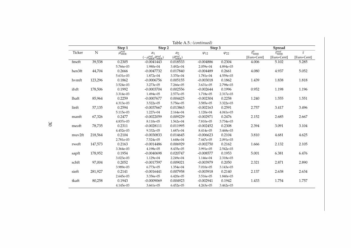
Table A.5.: (continued)Step 1 Step 2 Step 3 Spread

Ticker N ρmodMRR α1 α2 ϕ12 ϕ22 s0

MRR smodMRR s

(−ρmodMRRθ

modMRR) (θmod

MRR) [Euro-Cent] [Euro-Cent] [Euro-Cent]fmeft 39,538 0.2305 -0.0041443 0.018533 -0.004886 0.2304 4.006 5.102 5.285

5.766e-03 1.980e-04 3.492e-04 2.059e-04 4.894e-03hen3ft 44,704 0.2666 -0.0047732 0.017840 -0.004489 0.2661 4.080 4.937 5.052

5.631e-03 1.872e-04 3.370e-04 1.781e-04 4.559e-03hvmft 123,296 0.1862 -0.0006756 0.005155 -0.003018 0.1862 1.439 1.838 1.818

3.524e-03 3.273e-05 7.266e-05 3.631e-05 2.798e-03ifxft 178,506 0.1992 -0.0003704 0.002556 -0.002644 0.1996 0.952 1.198 1.196

3.314e-03 1.494e-05 2.577e-05 1.718e-05 2.317e-03lhaft 85,964 0.2259 -0.0007677 0.004425 -0.002304 0.2258 1.240 1.555 1.551

4.313e-03 3.522e-05 5.756e-05 3.585e-05 3.322e-03linft 57,135 0.2594 -0.0037667 0.013863 -0.002163 0.2591 2.757 3.417 3.496

5.115e-03 1.227e-04 2.164e-04 1.120e-04 4.041e-03manft 67,326 0.2477 -0.0022059 0.009229 -0.002971 0.2476 2.152 2.685 2.667

4.837e-03 8.110e-05 1.562e-04 7.810e-05 3.734e-03meoft 78,735 0.2311 -0.0028111 0.011995 -0.002452 0.2308 2.394 3.091 3.104

4.452e-03 9.332e-05 1.687e-04 8.414e-05 3.468e-03muv2ft 218,564 0.2104 -0.0030833 0.014645 -0.006623 0.2104 3.810 4.681 4.625

2.781e-03 7.524e-05 1.648e-04 7.447e-05 2.091e-03rweft 147,573 0.2163 -0.0014486 0.006929 -0.002750 0.2162 1.666 2.132 2.105

3.364e-03 4.198e-05 8.435e-05 3.991e-05 2.542e-03sapft 178,952 0.1954 -0.0040698 0.020747 -0.008577 0.1953 5.001 6.381 6.476

3.023e-03 1.129e-04 2.249e-04 1.146e-04 2.318e-03schft 97,004 0.2052 -0.0017597 0.009021 -0.003979 0.2050 2.321 2.871 2.890

3.989e-03 6.773e-05 1.354e-04 7.010e-05 3.143e-03sieft 281,927 0.2141 -0.0016441 0.007958 -0.003918 0.2140 2.137 2.638 2.634

2.645e-03 3.356e-05 6.420e-05 3.516e-05 1.840e-03tkaft 80,258 0.1943 -0.0009069 0.004923 -0.002941 0.1942 1.433 1.754 1.757

4.145e-03 3.661e-05 6.452e-05 4.263e-05 3.462e-03

30

Table A.5.: (continued)Step 1 Step 2 Step 3 Spread

Ticker N ρmodMRR α1 α2 ϕ12 ϕ22 s0

MRR smodMRR s

(−ρmodMRRθ

modMRR) (θmod

MRR) [Euro-Cent] [Euro-Cent] [Euro-Cent]tuift 67,646 0.2142 -0.0014879 0.007181 -0.003099 0.2139 1.863 2.273 2.320

4.723e-03 6.107e-05 1.071e-04 6.375e-05 3.756e-03vowft 162,360 0.2274 -0.0013031 0.007023 -0.002842 0.2274 1.751 2.227 2.175

3.340e-03 4.183e-05 7.897e-05 3.978e-05 2.417e-03Mean 133,835 0.2199 -0.0020728 0.009561 -0.003720 0.2198 2.356 2.933 2.955

31

Table A.6.: HS basic model. The table shows estimation results from the model of Huang andStoll (1997). φHS denotes the transitory component of the spread and θHS the ad-verse selection component. All estimations were conducted in R-3.0.2.

Ticker N φHS θHS sHS s Bias Rel BiasStd. err. [Euro-Cent] [Euro-Cent] [Euro-Cent] [%]

adsft 62,394 0.012280 0.0131824 5.092 6.51 -1.417 -21.83.777e-04 3.035e-04

altft 69,721 0.008196 0.0075555 3.150 3.87 -0.722 -18.72.310e-04 1.740e-04

alvft 288,276 0.011062 0.0081262 3.838 4.86 -1.027 -21.11.549e-04 1.162e-04

basft 164,692 0.004646 0.0042324 1.776 2.18 -0.404 -18.57.721e-05 5.753e-05

bayft 153,092 0.003873 0.0029494 1.364 1.71 -0.349 -20.45.225e-05 3.926e-05

bmwft 134,603 0.004519 0.0038961 1.683 2.07 -0.386 -18.77.828e-05 5.722e-05

cbkft 92,285 0.003557 0.0023784 1.187 1.52 -0.334 -22.05.022e-05 3.903e-05

contft 63,703 0.005342 0.0059456 2.258 2.89 -0.636 -22.01.822e-04 1.316e-04

db1ft 62,518 0.007759 0.0066456 2.881 3.51 -0.625 -17.81.948e-04 1.502e-04

dbkft 252,666 0.006811 0.0053298 2.428 2.96 -0.535 -18.09.462e-05 7.079e-05

dcxft 211,053 0.004782 0.0033294 1.622 1.98 -0.354 -17.95.521e-05 4.150e-05

dpwft 83,772 0.004544 0.0025697 1.423 1.76 -0.332 -18.97.577e-05 5.490e-05

dteft 283,502 0.003889 0.0008461 0.947 1.12 -0.175 -15.61.233e-05 1.216e-05

eoaft 183,284 0.005622 0.0045905 2.042 2.54 -0.497 -19.68.319e-05 6.241e-05

fmeft 39,538 0.009539 0.0105000 4.008 5.29 -1.277 -24.23.488e-04 2.758e-04

hen3ft 44,704 0.009937 0.0104722 4.082 5.05 -0.971 -19.23.337e-04 2.563e-04

hvmft 123,296 0.004363 0.0028343 1.439 1.82 -0.379 -20.87.936e-05 5.157e-05

ifxft 178,506 0.003597 0.0011641 0.952 1.20 -0.243 -20.42.234e-05 1.901e-05

lhaft 85,964 0.003708 0.0024947 1.240 1.55 -0.311 -20.05.083e-05 4.139e-05

linft 57,135 0.005771 0.0080257 2.759 3.50 -0.737 -21.12.095e-04 1.591e-04

manft 67,326 0.005656 0.0051081 2.153 2.67 -0.514 -19.31.504e-04 1.105e-04

meoft 78,735 0.005211 0.0067599 2.394 3.10 -0.710 -22.91.440e-04 1.137e-04

muv2ft 218,564 0.010630 0.0084203 3.810 4.62 -0.815 -17.61.631e-04 1.120e-04

rweft 147,573 0.004554 0.0037767 1.666 2.11 -0.439 -20.98.091e-05 5.902e-05

32

Table A.6.: (continued)Ticker N φHS θHS sHS s Bias Rel Bias

Std. err. [Euro-Cent] [Euro-Cent] [Euro-Cent] [%]sapft 178,952 0.013496 0.0115176 5.003 6.48 -1.474 -22.8

2.554e-04 1.893e-04schft 97,004 0.006365 0.0052438 2.322 2.89 -0.568 -19.7

1.365e-04 9.889e-05sieft 281,927 0.006206 0.0044811 2.137 2.63 -0.497 -18.9

6.474e-05 5.045e-05tkaft 80,258 0.004337 0.0028288 1.433 1.76 -0.324 -18.4

6.978e-05 5.370e-05tuift 67,646 0.005096 0.0042199 1.863 2.32 -0.457 -19.7

1.077e-04 8.581e-05vowft 162,360 0.004839 0.0039164 1.751 2.17 -0.424 -19.5

6.826e-05 5.336e-05Mean 133,835 0.006340 0.0054447 2.357 2.95 -0.598 -19.9

33

Table A.7.: HS covariances. The table shows for all stocks in the DAX-30 index the variancesof the new public information announcement, ut, the variance of the trade indicator,qt, as well as their common covariance and the correlation coefficient. All estimateswere performed in the statistical programming language R-3.0.2.

Ticker N σ2u σ2

q Cov[ut , qt] Corr[ut , qt]

adsft 62,394 0.00124621 0.9999 -0.006219 -0.17617altft 69,721 0.00039429 1.0000 -0.003425 -0.17249alvft 288,276 0.01027869 0.9983 -0.004182 -0.04128basft 164,692 0.00012235 0.9997 -0.002095 -0.18941bayft 153,092 0.00006326 0.9994 -0.001696 -0.21329bmwft 134,603 0.00011382 0.9995 -0.001998 -0.18736cbkft 92,285 0.00004837 1.0000 -0.001705 -0.24511contft 63,703 0.00024351 0.9992 -0.002594 -0.16631db1ft 62,518 0.00032504 0.9999 -0.002751 -0.15262dbkft 252,666 0.00020771 0.9994 -0.002639 -0.18316dcxft 211,053 0.00008536 0.9983 -0.001796 -0.19460dpwft 83,772 0.00005899 0.9999 -0.001521 -0.19809dteft 283,502 0.00001419 0.9998 -0.000836 -0.22192eoaft 183,284 0.00015605 1.0000 -0.002380 -0.19051fmeft 39,538 0.00081994 1.0000 -0.005201 -0.18164hen3ft 44,704 0.00067751 0.9997 -0.003981 -0.15297hvmft 123,296 0.00006960 0.9991 -0.001953 -0.23425ifxft 178,506 0.00002201 0.9975 -0.001195 -0.25491lhaft 85,964 0.00004965 0.9996 -0.001521 -0.21592linft 57,135 0.00034056 0.9992 -0.003053 -0.16549manft 67,326 0.00019291 0.9989 -0.002508 -0.18069meoft 78,735 0.00028310 0.9999 -0.003292 -0.19568muv2ft 218,564 0.00052437 0.9989 -0.004159 -0.18173rweft 147,573 0.00011254 0.9984 -0.002224 -0.20982sapft 178,952 0.00106215 0.9999 -0.006632 -0.20352schft 97,004 0.00021102 0.9999 -0.002642 -0.18191sieft 281,927 0.00014440 1.0000 -0.002396 -0.19937tkaft 80,258 0.00005840 0.9999 -0.001548 -0.20259tuift 67,646 0.00011880 0.9980 -0.001963 -0.18028vowft 162,360 0.00012537 1.0000 -0.002297 -0.20512Mean 133,835 0.00060567 0.9994 -0.002747 -0.18927

34

Table A.8.: HS VAR model. The table shows the results for the two-step estimation procedureof the Huang and Stoll (1997) model for each stock of the DAX-30. s0

HS is the spreadestimated under the assumption that Cov[ut, qt] = 0 and smod

HS is the spread estimatedwith an estimate of the empirical Cov[ut, qt]. All estimations have been performed inthe statistical programming language R-3.0.2 and for the VAR model the R-packagedse (version 2013.3.2) has been used.

Parameters SpreadsTicker N θmod

HS ϕ12 s0HS s2 s

Std. err. (−φmodHS ) [Euro-Cent] [Euro-Cent] [Euro-Cent]

adsft 62,394 0.01784 -0.01226 5.091 6.33 6.513.006e-04 1.841e-04

altft 69,721 0.01011 -0.00817 3.148 3.83 3.871.694e-04 1.021e-04

alvft 288,276 0.01133 -0.01104 3.837 4.67 4.862.001e-04 5.838e-05

basft 164,692 0.00577 -0.00464 1.775 2.19 2.186.206e-05 3.479e-05

bayft 153,092 0.00426 -0.00387 1.364 1.70 1.714.403e-05 2.586e-05

bmwft 134,603 0.00538 -0.00451 1.683 2.08 2.076.639e-05 3.599e-05

cbkft 92,285 0.00368 -0.00355 1.187 1.53 1.524.612e-05 2.808e-05

contft 63,703 0.00779 -0.00533 2.257 2.78 2.891.276e-04 8.001e-05

db1ft 62,518 0.00863 -0.00773 2.879 3.43 3.511.523e-04 9.382e-05

dbkft 252,666 0.00733 -0.00680 2.428 2.96 2.967.204e-05 3.760e-05

dcxft 211,053 0.00469 -0.00478 1.622 1.98 1.984.515e-05 2.541e-05

dpwft 83,772 0.00376 -0.00454 1.423 1.73 1.765.531e-05 3.460e-05

dteft 283,502 0.00152 -0.00389 0.947 1.11 1.121.441e-05 8.493e-06

eoaft 183,284 0.00639 -0.00562 2.042 2.52 2.546.743e-05 3.739e-05

fmeft 39,538 0.01447 -0.00950 4.006 5.05 5.292.615e-04 1.860e-04

hen3ft 44,704 0.01316 -0.00992 4.080 4.88 5.052.436e-04 1.575e-04

hvmft 123,296 0.00443 -0.00436 1.439 1.83 1.825.974e-05 3.063e-05

ifxft 178,506 0.00216 -0.00359 0.952 1.19 1.202.047e-05 1.310e-05

lhaft 85,964 0.00362 -0.00370 1.240 1.54 1.554.544e-05 2.990e-05

linft 57,135 0.01020 -0.00574 2.757 3.37 3.501.565e-04 1.005e-04

manft 67,326 0.00704 -0.00564 2.152 2.65 2.671.171e-04 6.903e-05

35

Table A.8.: (continued)Parameters Spreads

Ticker N θmodHS ϕ12 s0

HS s2 sStd. err. (−φmod

HS ) [Euro-Cent] [Euro-Cent] [Euro-Cent]meoft 78,735 0.00925 -0.00522 2.394 3.05 3.10

1.254e-04 7.515e-05muv2ft 218,564 0.01159 -0.01063 3.810 4.64 4.62

1.340e-04 6.433e-05rweft 147,573 0.00548 -0.00455 1.666 2.11 2.11

6.663e-05 3.457e-05sapft 178,952 0.01671 -0.01346 5.001 6.33 6.48

1.842e-04 1.008e-04schft 97,004 0.00727 -0.00636 2.321 2.85 2.89

1.134e-04 6.109e-05sieft 281,927 0.00631 -0.00620 2.137 2.62 2.63

4.898e-05 2.978e-05tkaft 80,258 0.00403 -0.00433 1.433 1.74 1.76

5.020e-05 3.514e-05tuift 67,646 0.00570 -0.00509 1.863 2.26 2.32

7.865e-05 5.443e-05vowft 162,360 0.00566 -0.00483 1.751 2.21 2.17

6.041e-05 3.451e-05Mean 133,835 0.00752 -0.00633 2.356 2.91 2.95

36

Bibliography

Ball, C., Chordia, T., 2001. True spreads and equilibrium prices. Journal of Finance 56 (5), 1801–1835.

Bessembinder, H., Maxwell, W., Venkataraman, K., 2006. Market transparency, liquidity exter-nalities, and institutional trading costs in corporate bonds. Journal of Financial Economics82 (2), 251–288.

Bjønnes, G. H., Rime, D., 2005. Dealer behavior and trading systems in foreign exchange mar-kets. Journal of Financial Economics 75 (3), 571–605.

Brockman, P., Chung, D., Yan, X., 44. Block ownership, trading activity, and market activity.Journal of Financial and Quantitative Analysis 6 (1403-1426).

Brockman, P., Chung, D. Y., 2001. Managerial timing and coprorate liquidity: evidence fromactual share repurchases. Journal of Financial Economics 61 (3), 417–448.

Brockwell, P. J., Davis, R. A., 2009. Time series: theory and methods. Springer.

Cao, C., Field, L., Hanka, H., 2004. Does Insider Trading Impair Market Liquidity? Evidencefrom IPO Lockup Expirations. Journal of Financial and Quantitative Analysis 39 (1), 25–46.

Chakravarty, S., Jaon, P., Upson, J., Robert, W., 2012. Clean sweep: Informed trading throughintermarket sweep orders. Journal of Financial and Quantitative Analysis 47 (2), 415–435.

Da, Z., Gao, P., Jagannathan, R., 2011. Impatient trading, liquidity provision, and stock selectionby mutual funds. Review of Financial Studies 24 (3), 675–720.

Glosten, L., Harris, L., 1988. Estimating the Components of the Bid-Ask Spread. Journal of Fi-nancial Economics 21 (1), 123–142.

Glosten, L. R., Milgrom, P. R., 1985. Bid, ask and transaction prices in a specialist market withheterogeneously informed traders. Journal of financial economics 14 (1), 71–100.

Grammig, J., Theissen, E., Wünsche, O., 2006. Zur Schätzung von Geld-Brief-Spannen ausTransaktionsdaten. In: Bessler, W. (Ed.), Börsen, Banken und Kapitalmärkte: Festschrift fürHartmut Schmidt zum 65. Geburtstag. Duncker & Humboldt, pp. 71–83.

Green, J., Smart, S., 1999. Liquidity provision and noise trading: Evidence from the "investmentdartboard" column. Journal of Finance 54 (5), 1885–1899.

37

Green, T. C., 2004. Economic news and the impact of trading on bond prices. Journal of Finance59 (3), 1201–1233.

Han, S., Zhou, X., 2014. Informed bond trading, corporate yield spreads, and corporate defaultprediction. Management Science 60 (3), 675–694.

Hasbrouck, J., 2007. Empirical market microstructure: The institutions, economics and econo-metrics of securities trading. Vol. 4. Oxford University Press New York.

Hatch, B. C., Johnson, S. A., 2002. The impact of specialist firm acquisitions on market quality.Journal of Financial Economics 66 (1), 139–167.

Heflin, F., Shaw, K. W., 2000. Blockholder ownership and market liquidity. Journal of Financialand Quantitative Analysis 35 (4), 621–633.

Huang, R., Stoll, H., 1997. The components of the bid-ask spread: A general approach. Reviewof Financial Studies 10 (4), 995–1034.

Lee, C. M. C., Ready, M. A., 1991. Inferring trade direction from intraday data. Journal of Finance46 (2), 733–746.

Lütkepohl, H., 2005. New introduction to multiple time series analysis. Cambridge Univ Press.

Madhavan, A., Richardson, M., Roomans, M., 1997. Why do security prices change? Atransaction-level analysis of NYSE stocks. Review of Financial Studies 10 (4), 1035–1064.

Odders-White, E., Ready, M., 2006. Credit ratings and stock liquidity. Review of Financial Stud-ies 19 (1), 119–157.

Petris, G., 2010. An r package for dynamic linear models. Journal of Statistical Software 36 (12),1–16.

Roll, R., 1984. A simple implicit measure of the effective bid-ask spread in an efficient market.The Journal of Finance 39 (4), 1127–1139.

Weston, J. P., 2000. Competition on the Nasdaq and the impact of recent market reforms. Journalof Finance 55 (6), 2565–2598.

38

Part II.

Bayesian estimation of the probability of informed trading

We propose a methodology to estimate the probability of informed trading (PIN) that only requires dataon the daily number of transactions (but not on the number of buyer-initiated and seller-initiated trades).Because maximum likelihood estimation of the model is problematic we propose a Bayesian estimationapproach. We perform extensive simulations to evaluate the performance of our estimator. Our method-ology increases the applicability of PIN estimation to situations in which the data necessary for tradeclassification is unavailable, or in which trade classification is inaccurate.

39

1. Introduction

The notion of informational asymmetries is central to our understanding of financial markets.Traders spend resources to acquire information, or to get access to information earlier than othertraders. Because the presence of informed traders imposes costs on other traders, the amount,or intensity, of informed trading has immediate implications for the distribution of profits fromtrading and for market liquidity. Against this background it is not surprising that researchersin market microstructure have sought to measure the amount of informed trading.

In a seminal paper, Easley et al. (1996) have proposed a direct measure of the probability ofinformed trading (PIN). Their approach builds on the theoretical work of Easley and O’Hara(1987) and Easley and O’Hara (1992). In their model it is assumed that there are three typesof trading days, good news days (with probability α(1 − δ)), bad news days (probability αδ)and no news days (probability (1−α)). The market is populated by liquidity traders, informedtraders and uninformed market makers. Liquidity traders buy and sell with intensity ε. In-formed traders buy with intensity µ on good news days, sell with intensity µ on bad newsdays, and abstain from trading on no-news days. Maximum likelihood estimation yields esti-mates of the structural parameters α, δ, ε and µ. From these estimates, an estimator of PIN isobtained as PIN = αµ/(αµ + 2ε). The data required for estimation are the daily numbers ofbuyer-initiated trades and seller-initiated trades. This data is typically generated by applyinga trade classification algorithm (such as the Lee and Ready (1991) algorithm) to time-stampedintraday data on bid, ask and transaction prices. This kind of data is usually available for de-veloped equity markets and recent sample periods. It is, however, often unavailable for lessdeveloped markets, for many derivatives markets, and for sample periods in the more distantpast. Therefore, a method to estimate PIN that does not require the availability of intraday datawould be of obvious interest.

Even in cases in which intraday data is available, there is an important impediment to ac-curate PIN estimation. It is well known that the Lee and Ready (1991) trade classification al-gorithm may yield inaccurate trade classification (e.g. Ellis et al. (2000), Lee and Radhakrishna(2000) and Odders-White (2000)). Boehmer et al. (2007) have shown that inaccurate trade classi-fication results in biased PIN estimates. If the bias is severe, a methodology to estimate PIN thatdoes not rely on trade classification may be superior to a method that uses misclassified data.

In this paper we build on previous research by Kokot (2004) and Jackson (2007) and proposea methodology to estimate PIN that only requires data on the daily number of transactions.This data is obviously much more easily available than the intraday data required to classifytrades into buyer-initiated and seller-initiated trades. Further, it is not necessary to apply atrade classification algorithm. Therefore, the estimation results are unaffected by inaccuratetrade classification. The intuition of our procedure is simple. From the formula for PIN shown

40

above it is obvious that the parameter δ is not needed. We consequently classify the tradingdays into two groups, information days and non-information days. On non-information daysonly liquidity traders trade (with intensity 2ε) while on information days both liquidity tradersand informed traders trade (with total intensity 2ε + µ). The resulting model is a mixture oftwo Poisson distributions with intensity parameters 2ε and (2ε+ µ) and mixing probability α.We refer to this model as the compressed model.

Unfortunately, even though the compressed model itself is very simple, estimation is not.It is well known that mixtures of Poisson distributions are difficult to estimate because of thepresence of local solutions.1 These difficulties arise particularly in small samples. We there-fore propose to estimate the model using a Markov chain Monte Carlo (MCMC) simulationapproach.

We evaluate our estimation procedure in extensive simulations. We know the data generatingprocess used in our simulations and therefore know the true parameters α, ε and µ, and weknow the true PIN. We then apply three versions of our MCMC estimation procedure (to bedescribed in detail in section 2.4) to the simulated data and compare the resulting PIN estimateto the true PIN. In order to assess the accuracy of our estimators we also compare them to thetraditional PIN estimator, to the traditional PIN estimator applied to misclassified data, and toa maximum likelihood estimator of the compressed model.

The simulation results indicate that our procedure yields accurate PIN estimates. We pick asan example the simulations in which we choose the true parameters to be equal to the param-eters that Easley et al. (1996) estimated for the first, fifth and eighth size decile of NYSE firms.The true PIN is 0.1581 for the first decile, 0.2143 for the fifth and 0.2253 for the eighth. Our bestestimation procedure (Bayesian maximum likelihood) yields an average PIN estimate (over 250simulation runs) of 0.1577 (standard error 0.0162) for the first decile, 0.2184 (0.0417) for the fifthdecile and 0.2369 (0.0698) for the eighth decile.

Our paper adds to the literature in two important ways. First, and most importantly, the sub-stantially lower data requirements of our procedure as compared to traditional PIN estimationbroaden the applicability of PIN estimation significantly. In particular, our procedure can beused to estimate PIN for markets and sample periods for which intraday data is unavailableand trade classification thus impossible. Further, because our procedure does not require tradeclassification it is unaffected by trade misclassification. It can thus be applied in cases in whichthe misclassification bias in traditional PIN estimates documented by Boehmer et al. (2007) is aconcern.

The remainder of the paper is organized as follows. In section 2.1 we briefly describe theEasley et al. (1996) model and our modified model. Sections 2.2 to 2.4 describes our estimation

1See e.g. Finch et al. (1989), Frühwirth-Schnatter (2006) and the documentation of the mix2Poisson com-mand in R at http://hosho.ees.hokudai.ac.jp/~kubo/Rdoc/library/VGAM/html/mix2poisson.html. We note that Jackson (2007) has proposed a model which is essentially identical to ours. He usesstandard ML to estimate his model and finds that the PIN estimates he obtains differ significantly fromthose of a traditional PIN model. Jackson (2007) argues that this is because his procedure is unaffectedby trade misclassification (but does not substantiate this claim). We argue instead that the differentresults are due to the fact that ML estimation of finite mixture models yields unreliable results.

41

strategy in detail. Chapter 3 describes the results, chapter 4 concludes.

2. Econometric methodology

2.1. Model

We start with a short description of the Easley et al. (1996) model. The model assumes amarket populated by competitive market makers, informed traders, and uninformed (liquidityor noise) traders. Uninformed traders are equally likely to buy or sell shares. The arrival ofuninformed buy and sell orders is modeled by two independent Poisson processes with equalarrival ratesε. Before the trading day begins an information event may occur with probabilityα.The information is either bad (with probability δ) or good (with probability (1− δ)). Informedtraders buy on good news days, sell on bad news days, and do not trade on no-news days. Thearrival of their orders is modeled as a Poisson process with intensity parameter µ (assumedto be identical for informed buy and sell orders). The four structural parameters of the model– the probability that an information event occurs on a given day, α, the probability that theinformation is bad news, δ, and the order arrival rates of uninformed and informed traders, εand µ – can be estimated by maximum likelihood (ML). The likelihood of observing B buyer-initiated trades and S seller-initiated trades on a given day, conditional on the true parametervector ϑEKOP = (α, δ, ε, µ), is

L(B, S | ϑEKOP) = αδ(εT)B exp (−εT)B!

((ε+µ)T)S exp (−(ε+µ)T)S!

(2.1)

+ (1−α)(εT)B exp (−εT)B!

(εT)S exp (−εT)S!

+α(1− δ)((ε+µ)T)B exp (−(ε+µ)T)B!

(εT)S exp (−εT)S!

,

where T denotes the length of the trading day in minutes. Easley et al. (1996) derive from theirmodel the unconditional probability of informed trading (PIN),

PIN =αµ

αµ + 2ε. (2.2)

In the following we refer to this model as the EKOP model.Estimation of PIN requires data on the number of buyer- and seller-initiated trades. This data

is typically obtained by applying a trade classification algorithm such as the Lee and Ready(1991) algorithm to intraday data. As noted in the introduction, there are two potential prob-lems with this procedure. First, the intraday data needed for trade classification may simply

42

be unavailable. Second, trade classification algorithms are known to be inaccurate, and inaccu-rate trade classification, in turn, is known to result in biased PIN estimates (see Boehmer et al.(2007)). It is thus desirable to develop a PIN estimator that does not require trade classification.Conceptually, such an estimator is easily developed (see also Kokot (2004) and later Jackson(2007)). Note from eq. (4.2), that the PIN does not depend on the direction of the information.Therefore, the distinction between good news days and bad news days is not necessary to esti-mate PIN. When we collapse the good news days and the bad news days into a new category‘information days’, we obtain a compressed likelihood function:

L(Q | ϑCOMP) = α((2ε+µ) T)Q exp (− (2ε+µ) T)Q!

+ (1−α)(2εT)Q exp (−2εT)Q!

, (2.3)

where Q = B + S is the number of transactions on a given trading day. From hereon thismodel is referred to as the ’compressed’ model or the ’compressed EKOP’ model.

Depending on the type of the day (news or no-news) an observation is generated from oneof the two component distributions (either a Poisson distribution with intensity parameter(2ε + µ) or a Poisson distribution with intensity parameter 2ε). Our modified model is thusa finite mixture model. It is well known that models of this type are difficult to estimate bymaximum likelihood methods because of the presence of local solutions.2 We therefore pro-pose the Bayesian estimation approach described in the next section.

2.2. Mixture likelihood and complete-data likelihood representation for thecompressed EKOP model

The starting point for our Bayesian PIN estimation procedure is the observation that theprobability to observe Q trades during a trading day of T minutes can be described as a mixtureof two Poisson distributions, viz

p(Q|ϑ) = γP(Q|λ1) + (1−γ)P(Q|λ2) , (2.4)

where ϑ = (γ, λ1, λ2)′, λ1 = (2ε + µ)T and λ2 = 2εT. P(Q|λ) = e−λ λ

Q

Q! denotes the Pois-son probability density function. Assuming that the information events are independent acrossdays, the joint probability of observing a sequence of the number of daily trades over N days,Q = (Q1, . . . , QN)

′, is given by p(Q|ϑ) = ∏Ni=1 p(Qi|ϑ), which implies the mixture log-likelihood

function

Lmix(ϑ) = ln p(Q|ϑ) =N

∑i=1

ln p(Qi|ϑ) . (2.5)

2See e.g. Finch et al. (1989), Frühwirth-Schnatter (2006) and the documentation of the mix2Poisson com-mand of the VGAM R-package in Yee (2013).

43

The parameters in (2.4) are defined up to a ‘label switch’, which means that

p(Q|ϑ∗) = γ∗P(Q|λ∗1) + (1−γ∗)P(Q|λ∗2) , (2.6)

where ϑ∗ = (γ∗, λ∗1 , λ∗2)′, γ∗ = 1 − γ, λ∗1 = λ2, and λ∗2 = λ1 represents an observationally

equivalent parametrization. As a consequence, the mixture-likelihood in (2.5) is symmetricallybimodal, a fact that must be accounted for when attempting to maximize it.

While the maximum likelihood method has been the standard approach towards estimatingmixture models (for a review see Redner and Walker (1984)), previous literature has identifiedsevere problems that will also affect PIN estimation through the maximization of the mixturelog-likelihood (2.5). Frühwirth-Schnatter (2006), among others, points out convergence prob-lems and starting value dependence of the maximization algorithm, poor performance in smallsamples and weakly separated components of the mixture distribution (here: information andno-information days). Moreover, there are severe caveats to apply asymptotic theory to com-pute reliable standard errors.3

Our Bayesian approach towards PIN estimation avoids these drawbacks. The starting point isthe so-called complete-data likelihood, which is based on the joint distribution of the number oftrades per day, Qi and the binary variables Zi, i = 1, . . . , N, henceforth referred to as allocations.The vector of allocations Z = (Z1, . . . , ZN)

′ consists of i.i.d. Bernoulli(γ) random variables thatare equal 1 when Qi is drawn from the Poisson distribution associated with the parameter λ1

and 0 when Qi is drawn from a Poisson distribution associated with the parameter λ2. The jointdistribution of Q and Z can then be written as:

p(Q, Z|ϑ) =p(Q|Z,ϑ)p(Z|ϑ) =N

∏i=1

p(Qi|Zi ,ϑ)p(Zi|ϑ) (2.7)

=N

∏i=1

(P(Qi|λ1)γ)Zi × (P(Qi|λ2)(1−γ))1−Zi

= ∏i:Zi=1

P(Qi|λ1)× ∏i:Zi=0

P(Qi|λ2)×(γN1(Z)(1−γ)N2(Z)

),

where N1(Z) = ∑Ni=1 Zi and N2(Z) = N − N1(Z). The maximization of the complete-data

log-likelihoodLcomp(ϑ) = ln p(Q, Z|ϑ) , (2.8)

requires knowing the allocations Z, which in the present application will not be available. How-

3Chung et al. (2004) report unreliable ML estimates for small sample sizes, Redner and Walker (1984)analyze the condition number of Hessian matrices and find that a sample size of 106 is needed to ensurereasonable standard errors for mixtures with weakly separated components. Chung et al. (2004) per-form simulations using small samples and report severe irregularities of likelihood surfaces, and thefailure to apply asymptotic reasoning to compute parameter standard errors. The problem of unreli-able standard errors is also addressed by Basford et al. (1997).

44

ever, we can use

p(Zi = 1|Qi ,ϑ) =p(Qi|Zi = 1,ϑ)p(Zi = 1|ϑ)

p(Qi|Zi = 1,ϑ)p(Zi = 1|ϑ) + p(Qi|Zi = 0,ϑ)p(Zi = 0|ϑ)

=P(Qi|λ1)γ

P(Qi|λ1)γ +P(Qi|λ2)(1−γ)(2.9)

for a classification of each trading day. As we will describe in detail in section 2.4, we use aMarkov chain Monte Carlo (MCMC) algorithm to alternate between N independent Bernoullidraws to generate the allocations vector Z using the probability in (2.9) (based on values for λ1,λ2, and γ), and draws from the posterior distributions of λ1, λ2, and γ based on Z. In the nexttwo sections we first describe how to obtain the posterior distributions conditional on Z and Qand then explain the MCMC procedure and how to obtain Bayesian point estimates of the PIN.

2.3. Posterior, prior, and hyperprior distributions

The key object of interest for our Bayesian approach towards PIN estimation is the posteriorjoint distribution of parameters and allocations, p(ϑ, Z|Q) ∝ p(Q, Z|ϑ)p(ϑ), where p(ϑ) is theprior joint density of the parameters. We can write:

p(ϑ, Z|Q) ∝ p(Q, Z|ϑ)p(ϑ)

= ∏i:Zi=1

P(Qi|λ1)× ∏i:Zi=0

P(Qi|λ2)×(γN1(Z)(1−γ)N2(Z)

)× p(ϑ). (2.10)

Assuming prior independence and conditioning on Z yields the following expressions forthe marginal posterior distributions of the model parameters:4

p(λ1|Q, Z) ∝(

∏i:Zi=1

P(Qi|λ1)

)p(λ1) , (2.11)

p(λ2|Q, Z) ∝(

∏i:Zi=0

P(Qi|λ2)

)p(λ2) , (2.12)

p(γ|Q, Z) ∝(γN1(Z)(1−γ)N2(Z)

)p(γ) . (2.13)

We choose conjugate prior distributions, which in the present case entails using a Gammadensity, G(a0, b0), for p(λ1), and p(λ2), and a Beta density, B(e0, e0), for p(γ).5 The posterior

4A detailed derivation can be found in section A.1 of chapter A in the appendix. We also used a de-pendent prior as suggested by Viallefont et al. (2002). Albeit the EKOP model structure may suggestotherwise, assuming prior independence yields superior results.

5Recall that the conjugate prior distribution for a Poisson likelihood is the Gamma distribution and the

45

densities in (2.11) -(2.13) are then given by:

λ1|Q, Z ∼ G(a1(Z), b1(Z)) , (2.14)

where a1(Z) = a0 + ∑Ni=1 Qi · Zi and b1(Z) = b0 + N1(Z), and

λ2|Q, Z ∼ G(a2(Z), b2(Z)) , (2.15)

where a2(Z) = a0 + ∑Ni=1 Qi · (1− Zi) and b2(Z) = b0 + N2(Z), and

γ|Z ∼ B(e1(Z), e2(Z)) , (2.16)

where e1(Z) = e0 + N1(Z) and e2(Z) = e0 + N2(Z).6

We follow the recommendations of previous literature and use a Gamma hyperprior for theparameter b0 in the prior distributions of λ1 and λ2, b0 ∼ G(g0, G0), (see Viallefont et al. (2002)).The posterior density of the hyperparameter b0 given by

p(b0|ϑ, Q, Z) = p(b0|ϑ) ∝ p(λ1|b0)p(λ2|b0)p(b0) (2.17)

∝ bg0+2a0−10 exp (− (G0 + (λ1 + λ2)) b0)

is then again a Gamma density,7

p(b0|ϑ, Q, Z) = p(b0|ϑ) ∼ G(g0 + 2a0, G0 + (λ1 + λ2). (2.18)

Regarding the other hyperparameters, we follow Viallefont et al. (2002) who suggest to usea0 = Q2

/(s2Q − Q), where Q and s2

Q denote the sample mean and variance of the data vectorQ, and Frühwirth-Schnatter (2006) who advocates using g0 = 0.5 and G0 = g0Q/a0. Accord-ingly, E(b0) = g0/G0 = a0/Q, which implies that E(λ1) = E(λ2) = Q (the sample mean) andVar(λ1) = Var(λ2) = s2

Q − Q (the sample overdispersion) when evaluated at b0 = E(b0). Theonly subjective choice is the hyperparameter for the Beta prior, e0. We want to ensure that γ isbounded away from zero, which is accomplished by setting e0 = 4 .8

conjugate prior distribution for a Bernoulli likelihood is the Beta distribution. We prefer conjugatepriors because as pointed out by Robert (2007), the information conveyed in Q about ϑ should not leadto a modification of the whole structure of p(ϑ), only of its parameters. In the present case conjugatepriors result in posteriors from standard distribution families, which facilitates sampling from thesedistributions.

6A detailed derivation of the posterior Gamma distribution is shown in section A.2 of chapter A in theappendix.

7This use of hierarchical priors should compensate for modeling errors at the lower levels and reinforcesthe non-informative perspective, while providing a well-defined posterior distribution of the parame-ters (Robert, 2007). We do not follow the approach taken in previous Bayesian market microstructureanalysis to use improper priors. We thereby pay heed to the warning of Frühwirth-Schnatter (2006),who points out that improper priors may lead to improper mixture posteriors.

8We also used smaller hyperparameter values and the results remain robust.

46

2.4. Gibbs sampling and Bayesian point estimates

In order to draw from the posterior distributions (2.14)-(2.16) and (2.18), we use a Gibbs sam-pling algorithm that works as follows. We start with an initial allocations vector Z(0) that re-sults from a two-means cluster analysis of the data Q, the vector of the number of daily trades,and an initial value for b0, for which we use the midrange of Q, the average of the smallestand largest number of daily trades in the sample. The next steps consist of M0 + M alternatedraws from the posterior distributions (2.14)-(2.16), based on the vector of allocations from theprevious step, and an update of the allocations vector along with a draw from the posteriordensity (2.18), for which the current draw from the posterior distributions for γ, λ1 and λ2 aretaken as given. This procedure yields the Gibbs-sampled sequences γ(m)M0+M

m=1 , λ(m)1

M0+Mm=1 ,

λ(m)2

M0+Mm=1 , Z(m)M0+M

m=1 , as well as b(m)0

M0+Mm=1 . The classification of the observations (trad-

ing days), which is required to obtain the allocations Z(m), is performed using Equation (2.9).M0 are the number of steps of the Gibbs sampler in the so-called burn-in phase, which is notused for post-processing.

The Gibbs sampling algorithm must account for the aforementioned label switching prob-lem, that is, the fact that (2.4) and (2.6) are observationally equivalent parametrizations. Forthat purpose, we use the random permutation Gibbs sampler proposed by Frühwirth-Schnatter(2001). Random permutation means allowing for the probability of a label switch after eachstep, such that one of the two observationally equivalent parameter combinations is randomlyselected. If a label switch is indicated, then the original draws λ(m)

1 λ(m)2 , γ(m) are replaced by

the permuted values λ(m)∗1 = λ

(m)2 , λ(m)∗

2 = λ(m)1 , and γ(m)∗ = 1 − γ(m). Moreover, all ones

in Z(m) are replaced by zeros, and all zeros are replaced by ones, so the allocations are alsopermuted.9 All steps of our Gibbs sampler are summarized by algorithm B.1.1 in section B.1of the appendix. An illustration of the resulting empirical marginal distributions of the Gibbs-sampled data λ(m)

1 Mm=M0+1, λ(m)

2 Mm=M0+1, and γ(m)M

m=M0+1 is depicted in Figure 2.1(a).The bimodal kernel densities reflect the purposeful label switching of the random permutationGibbs sampler.

We consider three Bayesian point estimates for the PIN, which are based on the Gibbs-sampled data. The first is the maximum a-posteriori (MAP) estimate, which is the parametercombination ϑMAP = (γMAP, λ1,MAP, λ2,MAP)

′ that provides the maximum value of the poste-rior joint density,

ϑMAP = maxϑ(m)p(ϑ(m)|Q, Z(m−1))|m = M0 + 1, . . . , M0 + M , (2.19)

where the posterior joint density is given by the product of the three marginal densities inEquations (2.14)-(2.16).

To provide point estimates of the structural parameters of the EKOP model (α, ε, µ, and the

9As noted by Jasra et al. (2005), label switching is a desirable property, as it indicates that the Gibbssampler is able to freely move around the parameter space.

47

120 140 160 180 200

0.00

0.01

0.02

0.03

0.04

Den

sity

λ1

Den

sity

120 140 160 180 200

0.00

0.01

0.02

0.03

0.04

Den

sity

λ2

0.3 0.4 0.5 0.6 0.7

02

46

8

Den

sity

γ

(a)

180 185 190 195

0.00

0.05

0.10

0.15

Den

sity

λ1

Den

sity

130 135 140 145

0.00

0.05

0.10

0.15

0.20

Den

sity

λ2

0.3 0.4 0.5 0.6 0.70

24

68

Den

sity

γ

(b)

Figure 2.1.: Marginal posterior densities. The figure depicts kernel density plots of themarginal posterior densities before (2.1(a)) and after relabeling (2.1(b)). Dashedlines indicate the true parameters. For the data generating process we used the firstEKOP decile with α = 0.5003, ε = 0.1757, δ = 0.3491, µ = 0.1320, and T = 390,i.e. λ1 = 137.046 trades per day and λ2 = 180.526 trades per day and γ = 0.5003.The data set contained N = 100 observations and the Gibbs sampler used a burn-inof M0 = 1000 iterations and a simulation size of M = 10000. We used the two-means clustering for classification of the resulting MCMC sample and applied akernel density with a Gaussian kernel to the data for the plots. All plots were gen-erated in R-3.0.1 using the package KernSmooth (version 2.23.10, see Wand andRipley (2006) for the KernSmooth-package). The bandwidth is chosen by the ‘over-sized bandwidth selector’, of Wand and Jones (1994, p.61). Original sample valuesin fig. 2.1(a) show a bimodal pattern for component parameters, λ1, and λ2, as la-bel switching mixed sampled values from both components. Values from the firstcomponent are displayed by black lines and respective values from the second com-ponent by gray lines. Relabeled parameters in fig. 2.1(b) then show, that relabelingis successful in separating values from the two components. Sample values for γscatter around the true value 0.5003 and therefore both component weights, γ and(1− γ), have very similar sample values and relabeling does not show significantchanges in the posterior densities.

48

implied PIN) we use

maxλ1,MAP, λ2,MAP = (2εMAP + µMAP)T (2.20)

minλ1,MAP, λ2,MAP = (2εMAP)T (2.21)

The point estimate of the probability of an information day αMAP is then either γMAP, if λ1,MAP >

λ2,MAP, or 1 − γMAP, if λ1,MAP < λ2,MAP. The MAP-based Bayesian PIN estimate is thenPINMAP = αMAP×µMAP

αMAP×µMAP+2εMAP.

The second vector of Bayesian point estimates ϑBML = (γBML, λ1,BML, λ2,BML)′ emerges from

ϑBML = maxϑ(m)p(Q|ϑ(m))|m = M0 + 1, . . . , M0 + M, (2.22)

and is, for obvious reasons, referred to as Bayesian maximum likelihood (BML) estimate. Thepoint estimates of the structural parameters of the EKOP model and the implied PIN are iden-tified analogously to the MAP case, yielding αBML, εBML, µBML, and the BML-implied BayesianPIN estimate PINBML = αBML×µBML

αBML×µBML+2εBML.

Because of this identification scheme, the bimodality of the posterior distributions used in(2.19) and the mixture likelihood function used in (2.22) do not pose a problem when computingthe MAP- and BML-based PIN estimates. However, the third Bayesian point estimate that weconsider requires a unique labeling. For that purpose we follow Celeux (1998) who proposesto apply a two-means cluster analysis on the Gibbs-sampled data, which assigns each of theM − M0 parameter vectors to one of two clusters. Once the grouping is accomplished, theparameters in one of the two clusters are re-labeled, such that λ(m)

1 λ(m)2 , γ(m) are replaced by

the permuted values λ∗(m)1 = λ

(m)2 , λ∗(m)

2 = λ(m)1 , and γ∗(m) = 1 − γ(m). Figure 2.1(b) shows

an example of the resulting empirical distributions after clustering and relabeling the data inFigure 2.1(a). The kernel densities have become unimodal.10 The third Bayesian point estimate,denoted ϑEIA = (γEIA, λ1,EIA, λ2,EIA)

′, is then computed as the sample average of these relabeleddraws produced by the Gibbs sampler. In line with previous literature, we refer to the estimateas the ergodic identified average (EIA) estimate. Using the relabeled Gibbs sample, we obtainthe EIA estimate as:

ϑEIA =1

M−M0

M0+M

∑m=M0+1

ϑ(m). (2.23)

Similar to the two other point estimates, the EIA-based PIN estimate results from equatingthe greater of the two estimates λ1,EIA or λ2,EIA with (2εEIA + µEIA)T and the smaller of the twopoint estimates with 2εEIAT. The point estimate of the probability of an information day αEIA isthen either γEIA, if λ1,EIA > λ2,EIA, or 1− γEIA, if λ1,EIA < λ2,EIA. The EIA-based Bayesian PINestimate is then PINEIA = αEIA×µEIA

αEIA×µEIA+2εEIA.

10We also applied the relabeling algorithms of Stephens (1997a,b). Results were quite similar and wedecided to use the simplest method.

49

3. Results

3.1. Simulation Results

In order to evaluate the three Bayesian estimators and compare them to the traditional max-imum likelihood estimators we perform extensive simulations. The simulations were imple-mented with the statistical software R-3.0.1 using a self-coded package.11 Our choice of theparametersα, ε and µ for the data generating process follows Boehmer et al. (2007). We choose11 different parameter constellations. For each constellation we run 250 simulations with 100data points each (corresponding to 100 days or slightly more than four months) and 250 sim-ulations with 250 data points each (corresponding to approximately one year). We sort theparameter constellations into three groups, A, B and C. Group A (parameter ids 1-3 and 12-14)contains ‘realistic’ parameter constellations. They correspond to the parameters estimated inEasley et al. (1996) for stocks in the first, fifth and eighth size decile of NYSE stocks. In groupB (ids 4-7 and 15-18) the intensity of informed trading, µ, is small relative to the intensity ofuninformed trading, ε. We therefore expect that our algorithm (as well as the traditional MLestimator) will have difficulties to separate information and non-information days, particularlyin cases in which the probability of an information event, α, is also small. In group C (ids 8-11and 19-22) the intensity of informed trading, µ, is high relative to the intensity of uninformedtrading, ε, and we therefore expect well separated components. All parameter combinationsare summarized in table C.1.

In our simulation study we implement six different estimation methods. MCMC with aburn-in of M0 = 1000 and a sample of M = 10000 using (1) the maximum likelihood es-timator (BML), (2) the maximum a-posteriori estimator (MAP), and (3) the ergodic identifiedaverage estimator (EIA). Further, we implement three maximum likelihood estimators, namely,(4) the original EKOP model (EKOP) using accurately classified data, (5) the original EKOPmodel with misclassified data (EKOPM), and (6) maximum likelihood estimation of the com-pressed EKOP model (COMPML). The three maximum likelihood estimators (EKOP, EKOPM,COMPML) serve as benchmarks against which to evaluate our Bayesian estimation approach.If the Bayesian approaches perform better than the compressed EKOP model, a Bayesian ap-proach should be used in all cases in which only data on the number of trades (but not on tradedirection) is available. If the Bayesian approaches perform better than the EKOP model on mis-classified data, then a Bayesian approach should be used whenever accurate trade classification

11R is a language and environment for statistical computing and graphics and it is open-source. Thislanguage shows the fastest growing user community in the area of statistical computing. For furtherinformation see R Core Team (2013). Our self-coded package relies heavily on C++ extensions using theAPI RcppArmadillo (Eddelbuettel and Sanderson (2013)) that wraps the C++ high-performance linearalgebra library Armadillo (Sanderson et al. (2010)).

50

is infeasible. We do not expect the Bayesian estimators to perform better than the EKOP modelapplied to accurately classified data because the EKOP model uses more information (namely,information on trade direction).

We also tested the performance of the EM-based REBMIX algorithm. Although the EM algo-rithm is the most commonly applied method to find the ML estimator nowadays, it has severaldrawbacks as reported by Reddy and Rajaratnam (2010). The REBMIX algorithm origins inNagode and Fajdiga (2011) and avoids these drawbacks. It is an iterative numerical procedurerelying on the following steps: First, an empirical density is assigned to the dataset and theglobal mode position is identified. Next, rough component parameters are estimated from theempirical density and its global mode. Based on the rough component parameters the datasetis then clustered successively into the classes linked to the predictive component density andthe residual. Enhanced component parameters and the component weights are then assessedfor all classes and the remaining observations are distributed between the existing componentsby the Bayes decision rule. Finally, the parameters of the finite mixture are fine-tuned.12 Theresults of the REBMIX algorithm applied to our simulated datasets are similar to the results ofthe ML estimation, though with greater bias and RMSE. In addition, the algorithm exhibitedsignificantly more convergence problems than the ML estimator and offered, for some datasetsin group B, solutions with one component only. For these reasons we omit the results. They areavailable from the authors upon request.

As noted above, each of the six estimation methods was applied to 250 samples of 100 datapoints (corresponding to 100 trading days or roughly four months) and another 250 samplesof 250 trading days (roughly a year). We produced the data samples by drawing values fromPoisson mixture distributions defined by the input parameters shown in table C.1 using theMersenne-Twister random number generator in R-3.0.1 with a seed of zero. We generate mis-classified data by randomly changing the trade direction.13 For each trade in the simulated datathe trade direction was reversed with a probability of 15%. This corresponds to a misclassifica-tion rate of 15%, consistent with Odders-White (2000).

For the ML procedures we adopted the optim function in R-3.0.1 with an L-BFGS-B algo-rithm using appropriate restrictions for the parameters and data-dependent starting values.14

More precisely, we used a logit transformation for the parameterα (and also for the parameter δwhich is estimated in the EKOP and EKOPM models) and starting valuesα = 0,ε = 0.75/2 ·Q,(δ = 0) and µ = 0.25/2 · Q. In cases in which the L-BFGS-B algorithm did not converge orproduced an error we applied as a second approach a derivate-free optimization, namely, abounded Nelder-Mead algorithm via the nmkb-function from the R-package dfoptim (version2011.8.1, Varadhan et al. (2011)).15

12For a more detailed description of the REBMIX algorithm we refer to the vignette of the R-packageREBMIX that we used, written by Nagode (2014).

13More precisely, we start at a random seed of zero and generate for each of the 11 parameter constellationsin table C.1 (ids 1-11) 100 data points and then for each of them another 250 observations (ids 12-22).All data sets contain misclassified data though the original trade direction is recorded.

14See Zhu et al. (1997) for the L-BFGS-B algorithm.15See Kelley (1999) for the bounded Nelder-Mead method.

51

All simulations were run on a node of the high-performance cluster of the RWTH AachenUniversity Computing Center.16 A run with 250 simulations, applied to all parameter con-stellations and the two sample sizes of 100 and 250 days required approximately 90 minutes.Running a single MCMC simulation with a burn-in of 1000 iterations and a sample of 10000 it-erations on a MacBook Pro with 2 Intel i7 cores (2.8 Ghz) takes about 0.85 seconds. Another 1.35seconds are consumed for relabelling the sample and computing the three estimators, namelyMAP, BML and EIA. These numbers demonstrate that the MCMC procedure is fast and is ap-plicable with standard hardware.

As noted in chapter 2 we used a random permutation Gibbs sampler (see algorithm B.1.1in the appendix) to improve mixing. Random permutation Gibbs samplers converged quicklyas can be seen in the example traceplots shown in fig. 3.1 and the corresponding plots of theposterior density of the PIN in fig. 3.2. Figure 3.1 shows traceplots for parameter constellationid 1 (which corresponds to the parameters estimated for the first NYSE size decile by Easleyet al. (1996)) before (panel a) and after (panel b) component classification. The traces fluctuatestationary around their mean values, thereby exploring the whole parameter space. For thecomponent parameters in λ random permutation is obviously necessary.17 From the identifiedtraceplot (fig. 3.1(b)) we can infer that the two-means clustering is successful in separating thetwo components of the mixture.

The posterior distributions of the PINs are shown in fig. 3.2 for the first four parameter con-stellations. Each plot shows the posterior estimated from the corresponding parameter draws ofthe Gibbs sampler (solid line) and the true PIN (dotted vertical line). The shaded areas mark thePIN values corresponding to the 95% highest posterior density (HPD).18 In all cases the HPDinterval includes the true PIN. This is evidence of the reliability and adequacy of the MCMCapproach for finite mixtures. Note that the posteriors are dependent on the generated data andtherefore simulated posteriors do inherently not disperse symmetrically around the true inputparameter values.

The simulation results for all six estimators (the three MCMC point estimators and the threeML estimators) are presented in table C.2 (simulations with 100 observations) and table C.3 (250observations). The tables show Monte Carlo averages of the PINs for each parameter combi-nation together with corresponding Monte Carlo standard errors, calculated over all simula-tions. The PIN estimates for most parameter constellations are reasonably close to the true PIN.There is one notable exception, though. The EKOPM estimator (the EKOP estimator applied tomisclassified data) tends to severly underestimate the true PIN. This confirms the findings ofBoehmer et al. (2007). PIN estimates are the least accurate for parameter constellations 4 and

16This node is based on a Bullx S6010 board with 32 Intel Xeon (Nehalem) X7550 processors (2 Ghz). Seefor further information http://www.itc.rwth-aachen.de/cms/IT-Center/Forschung-Projekte/~eubj/High-Perfomance-Computing/lidx/1/

17The parameter constellation shown in fig. 3.1 is characterized by α close to 0.5. For parameter constel-lations with small α (ids 4-7 and ids 15-18), random permutation is also necessary for the parameterγ.

18We used the LaplacesDemon package (version 14.6.23) in R to compute the highest posterior densityintervals.

52

130

140

150

160

170

180

190

λ1

130

140

150

160

170

180

190

λ2

0.4

0.5

0.6

0.7

γ

0.20

0.25

0.30

0.35

0.40

b

0 2000 4000 6000 8000 10000

Iterations

(a)

180

185

190

195

λ1

130

135

140

145

λ2

0.3

0.4

0.5

0.6

γ

0.20

0.25

0.30

0.35

0.40

b

0 2000 4000 6000 8000 10000

Iterations

(b)

Figure 3.1.: Trace plots. The figures depicts trace plots of the Gibbs-sampled sequencesγ(m)M0+M

m=1 , λ(m)1

M0+Mm=1 , λ(m)

2 M0+Mm=1 , and b(m)

0 M0+Mm=1 , of a simulation with

input parameters id 1 (first EKOP decile). All values are obtained by running aGibbs sampler on N = 100 data points for M = 10000 iterations with a burn-inof M0 = 1000. Results for fig. 3.1(a) come from the non-identified samples andfig. 3.1(b) plots the values identified through two-means clustering.

53

0.08 0.10 0.12 0.14 0.16 0.18 0.20 0.22

05

1020

PIN

Den

sity

PIN

Den

sity

0.10 0.15 0.20 0.25 0.30 0.35 0.40

02

46

810

PIN

Den

sity

PIN

(a)

0.1 0.2 0.3 0.4 0.5

02

46

PIN

Den

sity

PIN

Den

sity

0.00 0.05 0.10 0.15 0.20 0.25 0.30

02

46

810

PIN

Den

sity

PIN

(b)

Figure 3.2.: Posterior PINs. The figures depict posterior densities for the PIN of randomly cho-sen simulations with input parameters id 1 (corresponding to the first NYSE sizedecile), id 2 (left and right in fig. 3.2(a)), id 3, and id 4 (left and right in fig. 3.2(b))with N = 100 observations. The true PIN values are indicated by the dotted ver-tical lines. Shaded areas define the highest 95% posterior density intervals. Allvalues were obtained by random permutation Gibbs sampling with a burn-in ofM0 = 1000 iterations and a sample of M = 10000 iterations. HPD intervals werecomputed using the R-package LaplacesDemon (version 14.6.23).

54

5 in table C.2 and 15 and 16 in table C.3. This comes as no surprise, though, because theseparameter constellations are characterized by a low intensity of informed trading and a lowprobability of an information event.

For a more rigorous statistical evaluation of the six estimators we used the two common lossfunctions bias and root mean squared error (RMSE):

Bias(ϑE) =1

Sim

Sim

∑i=1

(ϑE,i −ϑ′), RMSE(ϑE) =

(1

Sim

Sim

∑i=1

(ϑE,i −ϑ′)2

)0.5

, (3.1)

where ϑE is the parameter estimate obtained with estimator E,ϑ′ is the true parameter and ‘Sim’the number of Monte Carlo iterations. The results for the bias are shown in table C.4, those forthe RMSE in table C.5.

Of all six estimators, the traditional EKOP estimator performs best. The average bias is (withthe notable exceptions of parameter constellations 3, 4, 14 and 15) low, and the RMSE is, withfew exceptions, the lowest of all six estimators. The good performance of the EKOP estimatorcomes as no surprise, though. It uses all available information (including trade direction), andit is based on the assumption that there are no trade classification errors. The effect of trade mis-classification is clearly visible when comparing the EKOP estimator (which is based on correctlyclassified data) to the EKOPM estimator (which is based on misclassified data). The EKOPMestimator exhibits a significant, and often large, downward bias. This bias has already beendocumented by Boehmer et al. (2007). There are some parameter constellations in which theEKOPM estimator has low bias (ids 3, 4, 5, 14, 15, 16). Interestingly, these are exactly those con-stellations in which the EKOP estimator has a large positive bias. In these cases, the downwardbias induced by trade misclassification counterbalances the positive bias of the EKOP estimator,resulting in low overall bias. This characteristic is likely to be of limited practical use, though,because the researcher does not typically know whether the EKOP estimator is biased in a par-ticular application and will therefore not be able to identify those circumstances under whichEKOPM performs well.

An important question in the presence of trade misclassification is whether it is better to usethe inaccurate data, or to resort to one of the concentrated likelihood estimators which doesnot use the trade classification data. In cases in which the data necessary to classify trades isunavailable, the application of one of the four concentrated likelihood estimators is withoutalternative anyway. Therefore, we now turn to the evaluation of the COMPML, BML, MAP andEIA estimators. We will first discuss the results for parameter constellation groups A and Cbefore turning to the more challenging conditions of group B.

The estimated PINs from the compressed model in tables C.2 and C.3 are reasonably close tothe true values in the parameter constellation groups A and C. The standard errors of the esti-mators do not differ much, however, the BML estimator has the largest range of standard de-viations, namely between 0.0100 for simulations with parameter combination id 12 and 0.0698for id 3.

The biases shown in table C.4 range from −5.2964× 10−2 for the EKOPM estimator on id 13

55

to 4.0392 × 10−2 for the EKOP estimator on id 3. Averaging the bias across different param-eter constellations is inappropriate because some parameter constellations result in a negativebias for all estimators while other constellations predominantly result in positive biases. Wetherefore consider the average across parameter constellations of the absolute bias. In parame-ter constellation groups A and C the Bayesian estimators perform very well. They have loweraverage absolute bias than the three ML estimators. The BML estimator performs best with anaverage absolute bias of 0.001852.

The EKOP estimator has the lowest RMSE (see table C.5. The average across the parameterconstellations in groups A and C is 0.020. The three Bayesian estimators are ranked secondto fourth and thus have a lower RMSE than the COMPML and the EKOPM estimators. Ofthe three Bayesian estimators the EIA estimator has the lowest average RMSE, followed by theMAP estimator.

We now turn to the results for the parameter constellations in group B. Here, the intensity ofinformed trading is low relative to the intensity of uninformed trading. Consequently, it is moredifficult for the estimators to differentiate between information days and non-information days.This is particularly true if the probability of an information event is also low. The plot of thelog-likelihood contours in fig. 3.3 illustrate this point. The first simulation (id 1, correspondingto the first NYSE decile) has well separated components and shows two well separated modesin the log-lieklihood surface (see fig. 3.3(a)). The second simulation (id 4, characterized by a lowvalue of µ and a low probabilityα) appears almost unimodal (see fig. 3.3(b)). Correspondingly,the PIN estimates in tables C.2 and C.3 reveal that the accuracy of the point estimates is ratherlow when, in addition to a low intensity of informed trading, the probability of an informationevent, α, is also low (as in parameter ids 4 and 15). We further note that increasing the numberof observations from 100 to 250 does not significantly increase the accuracy of the PIN point es-timates (tables C.2 and C.3) but does reduce bias and RMSE by a substantial amount (tables C.4and C.5).

In terms of bias the EKOP estimator dominates. The average absolute bias across the eightparameter constellations in group B is 0.0068× 10−2. Two of the Bayesian estimators, the MAPand EIA estimators, follow with average absolute biases of 0.0107× 10−2 and 0.0117× 10−2,respectively. The BML estimator (which has the lowest average absolute bias in groups A andC) performs worst with an average absolute bias of 0.0183× 10−2.

The EKOP estimator also has the lowest average RMSE (0.209× 10−2). The EKOPM estima-tor (i.e. the EKOP estimator estimated on misclassified data) has a low average RMSE as well(0.0222× 10−2). Of the Bayesian estimators the EIA and MAP estimators perform reasonablywell with average RMSEs of 0.0290× 10−2 and 0.0331× 10−2, respectively. In particular, thetwo estimators have a considerably lower RMSE than the COMPML estimator (0.0496× 10−2).The BML estimator again performs worst; its average RMSE amounts to 0.0576× 10−2.

The performance of the BML point estimator deserves a discussion. It performs very wellin parameter constellations of groups A and C but exhibits the largest RMSE and bias in pa-rameter constellations of group B. If the information provided by the data is inconclusive, i.e.insufficient for the two modes to clearly become apparent in the likelihood, the region around

56

0.2 0.4 0.6 0.8 1.0

0.2

0.3

0.4

0.5

0.6

0.7

0.8

λ1

λ 2

(0.48, 0.35)

(0.35, 0.48)

(a)

0.05 0.10 0.15 0.20 0.25 0.30 0.35

0.05

0.10

0.15

0.20

0.25

λ1

λ 2

(0.12, 0.1)

(0.1, 0.12)

(b)

Figure 3.3.: Log-likelihood contours. The figures depict log-likelihood contours for simulateddata sets with parameters from id 1 (fig. 3.3(a)) and id 4 (fig. 3.3(b)). The contourplots cover a sufficient range around the true component parameters λ1 = 2ε+ µand λ2 = 2ε and show the two possible optima due to label switching as labeledpoints.

57

the two modes forms rather a plateau and the optimization algorithm encounters difficultiesin finding the maximum. Consequently, estimated PINs suffer from higher bias.19 It is furtherpossible that the algorithm converges to the saddlepoint right in the middle of the line connect-ing the two modes in fig. 3.3(b). This will obviously result in a biased PIN estimate. It is furtherknown that saddlepoints may result in a positive definite or an indefinite hessian. The twoother Bayesian point estimators (MAP and EIA) are less affected by these difficulties becausethey include information about the prior distribution. Our simulation results indicate that thisfeature enables these estimators to reduce the bias significantly and to easily outperform theBML estimator (and also the EKOPM and COMPML estimators) in parametrical environmentscharacterized by components that are poorly separated.

Figure 3.4 provides further insights into the simulation results. It shows boxplots (con-structed from the results of all 250 simulations) for the same two parameter constellations (id1, corresponding to the first NYSE decile and id 4, a parameter set with poorly separated com-ponents) already shown in fig. 3.3 above. The figure further shows histograms of a representa-tive data sample. Parameter id 1 is characterized by well separated mixture components. Thedata sample shown in fig. 3.4(a) exhibits two clearly separated modes. All estimators (withthe exception of EKOPM) are hardly biased. The PIN estimates of the 250 simulations are dis-tributed symmetrically around the true PIN (see fig. 3.4(a)). The EKOPM estimator exhibits apronounced downward bias. The bias is a consequence of trade misclassification. Because ofthis bias we exclude the EKOPM estimator from the second plot. This plot shows a parame-ter constellation with poorly separated components and a low news probability (id 4, α = 0.2,fig. 3.4(b)). Correspondingly, the data sample in fig. 3.4(b) suggests a unimodal distribution.Consequently, the traditional maximum likelihood estimator (COMPML) and the BML estima-tor both produce a high number of outliers. The MAP and the EIA estimators, on the otherhand, show a reasonably good performance because they also use the information contained inthe prior distribution of the Bayesian framework. This advantage is of particular importance in‘difficult’ settings characterized by small and/or poorly separated components.

Figure 3.5 provides a different perspective on the simulation results. It shows the bias (Panela) and the RMSE (Panel b) of all four estimators of the compressed model (COMPML, BML,MAP and EIA) for all 22 parameter constellations. The parameter constellations are sorted bythe amount of bias (Panel a) and the RMSE (Panel b) of the maximum likelihood estimatorCOMPML. The shaded areas correspond to the parameter constellations belonging to group B.Figure 3.5 confirms the finding that in these difficult environments, the MAP and EIA estima-tors (which use information from the prior distribution) outperform the COMPML and BMLestimators. In less difficult environments, the differences between the four estimators are muchless pronounced. The RMSEs are hardly distinguishable. In terms of bias, the BML estimatorperforms best.

So far we have discussed the average performance of our estimators across all simulationruns. For practical applications it is also of interest how the estimators behave in individual

19In addition, if the likelihood forms a plateau around its modes, the hessian matrix could turn singular.

58

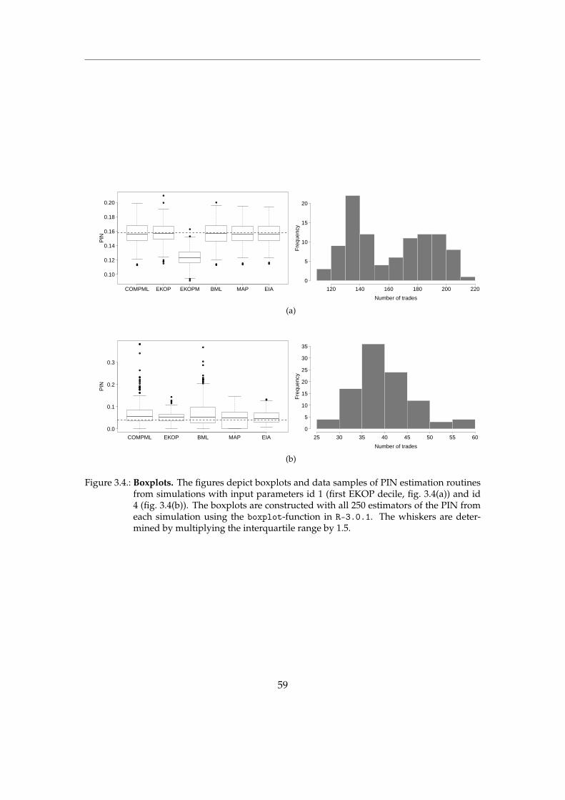
COMPML EKOP EKOPM BML MAP EIA

0.10

0.12

0.14

0.16

0.18

0.20

PIN

120 140 160 180 200 220

0

5

10

15

20

Number of tradesF

requ

ency

(a)

COMPML EKOP BML MAP EIA

0.0

0.1

0.2

0.3

PIN

25 30 35 40 45 50 55 60

0

5

10

15

20

25

30

35

Number of trades

Fre

quen

cy

(b)

Figure 3.4.: Boxplots. The figures depict boxplots and data samples of PIN estimation routinesfrom simulations with input parameters id 1 (first EKOP decile, fig. 3.4(a)) and id4 (fig. 3.4(b)). The boxplots are constructed with all 250 estimators of the PIN fromeach simulation using the boxplot-function in R-3.0.1. The whiskers are deter-mined by multiplying the interquartile range by 1.5.

59

0.00 0.01 0.02 0.03

21

12

19

1

22

20

10

11

18

8

9

13

7

2

17

16

6

5

15

4

3

14

Bias

id

BMLMAPEIAMLCOMP

(a)

0.00 0.02 0.04 0.06

12

19

21

22

20

1

8

9

10

11

13

16

17

18

2

15

14

7

5

3

4

6

RMSE

id

BMLMAPEIAMLCOMP

(b)

Figure 3.5.: Bias and RMSE. The figures depict plots of the bias (fig. 3.5(a)) and the RMSE(fig. 3.5(b)) for all estimators of the compressed EKOP model along all parametercombinations. Shaded areas identify parameter settings from group B with weaklyseparated components in the mixture.

60

data sets. Table C.6 provides some insights. The first three columns report the number of cases(out of a total of 250) in which the traditional maximum likelihood estimators (EKOP, EKOPMand COMPML) did not converge. On average slightly more than 7% of the estimations do notconverge. However, in some parameter settings (among them ids 3 and 14 which correspondto the parameter values for the eighth NYSE decile) the percentage increases to almost 20%. Inthese cases the ML estimators do not provide results while the Bayesian estimators do.20

The remaining columns of table C.6 show the percentage of cases in which the Bayesian es-timators produced results which were closer to the true PIN than the estimates produced bythe ML estimators. These figures suggest that the Bayesian estimators are less accurate thanthe EKOP estimator and more accurate than the COMPML estimator. Consequently, the EKOPestimator should be chosen when accurate trade classification data is available while one ofthe Bayesian estimators should be chosen when no trade classification data is available. Thecomparison of the Bayesian estimators to the EKOPM estimator (i.e. the EKOP estimator ap-plied to misclassified data) yields ambiguous results. The Bayesian estimators appear to bemore accurate for parameter constellations in groups A and C while the EKOPM estimator ismore accurate for parameter constellations in group B. The relatively good performance of theEKOPM estimator in group B was already documented earlier and is due to the fact that theinherent negative bias of the EKOPM estimator essentially corrects for a positive bias which theEKOP estimator exhibits in the parameter constellations of group B.

Of the three Bayesian estimators the BML estimator performs worst. Consider, for example,the comparison of the Bayesian estimators to the COMPML estimator in the last three columnsof table C.6. For 17 out of 22 parameter constellations the MAP and the EIA estimator yieldPIN estimates that are closer to the true value than the COMPML estimator in more than 50%of the cases. The BML estimator achieves a 50+% result only in 10 parameter constellations.The poor performance of the BML estimator documented here contrasts with the low averagebias reported previously. These findings are easily reconciled, though. The BML estimator hasa low bias but has high variance (as illustrated by the large RMSE documented in table C.5).Therefore, individual estimates are often inaccurate.

3.2. An algorithm to choose a best estimator

The discussion of the results in the previous section has revealed important differences be-tween the three Bayesian estimators. Which estimator is best depends on (a) whether the biasor the RMSE is used as a criterion and (b) whether the parameter constellation is character-ized by well separated components (constellations in groups A and C) or by poorly separated

20All results presented in this paper are based on all simulated datasets for which convergence wasachieved. Thus, when a ML estimator converges in 240 out of 250 cases, the ML results for these240 cases are compared to the Bayesian estimators obtained for the full set of 250 simulated datasets. Itis conceivable that ML estimation fails in ‘difficult’ datasets. If this is the case our procedure puts theBayesian estimators at a disadvantage. To control for this possibility we compared the ML estimatesto the Bayesian estimates obtained only for those cases in which ML estimation converged. The resultsare similar to those presented in the paper.

61

components (group B). When judged by the RMSE the EIA estimator performs best in all en-vironments. When judged by the bias, the BML estimator performs best in environments withwell separated components while the MAP and EIA estimators are less biased in environmentswith poorly separated components.

Thus, when the researcher is interested in an estimator with low RMSE she should choose theEIA estimator. However, when the focus is on reducing bias, the optimal choice of estimatordepends on the environment. In empirical applications the true parameter values are obviouslyunknown. What is thus needed is a method that uses the data to differentiate between envi-ronments with well separated components and those with poorly separated components. Inthe cases of MCMC simulations such a differentiation can be achieved by considering samplingrepresentations. Sampling representations were explored in Bayesian finite mixture estimationby Celeux et al. (2000); Frühwirth-Schnatter (2001) and Hurn et al. (2003) as a tool to visual-ize the posterior density in case of higher dimensionality. Sampled component parameters arestacked together and plotted against each other in a scatter plot, thereby revealing the modes ofthe posterior density. Figure 3.6 shows sampling representations of randomly chosen data setsfor four of our parameter combinations in table C.1, namely parameter ids 1, 4, 12 and 15. Whencomponents in the underlying model are well separated the clusters in the sampling represen-tation are also well separated (see fig. 3.6(a)). However, if the intensity of informed trading, µ,is small, the sampling representations of MCMC component parameter samples appear to bealmost unimodal (id 4 and id 15 in fig. 3.6(b)).

If the number of estimations is small (e.g. because the cross-section is small), choosing anestimator based on manual inspection of the sampling representations is feasible. This proce-dure will be cumbersome, however, when the number of estimations is large. In these cases itwill be preferable to conduct a formal test and decide upon the choice of estimator based onthe result of that test. A test-based procedure also has the advantage of being unaffected bypersonal judgement and thus more reliable.

As illustrated above (see fig. 3.6), well separated components result in a sampling repre-sentation which is clearly bimodal while sampling representations for data sets with poorlyseparated components appear to be almost unimodal. We therefore propose an algorithm (pre-sented as algorithm B.2.1 in section B.2 of the appendix) that uses the Hartigan and Hartigan(1985) test for unimodality. In the first step of the algorithm an MCMC simulation as describedpreviously is run. In the second step the Hartigan and Hartigan (1985) test is applied to thesample of component parameters, λ. If the test rejects the null hypothesis of unimodality atthe 5% level of significance the BML point estimator is chosen.21 If the null hypothesis is notrejected the MAP point estimator is chosen instead.

We tested this algorithm using all data samples of our simulation study. The performance ofthe algorithm is summarized in fig. 3.7. The figure shows the absolute average bias of all fourestimators of the compressed EKOP model (COMPML, BML, EIA and MAP) together with thepoint estimator proposed by our algorithm (denoted ALGBM, the solid line in the figure). The

21Tests with other significance levels gave similar results.

62

130 140 150 160 170 180 190

id 1

130

140

150

160

170

180

190

λ

λ

140 150 160 170 180 190

id 12

140

150

160

170

180

190

λ

λ

(a)

38 40 42 44

id 4

38

40

42

44

λ

λ

36 38 40 42 44 46

id 15

36

38

40

42

44

46

λ

λ

(b)

Figure 3.6.: Sampling representations. The figure shows sampling representations for the pa-rameter combinations 1 and 12 (fig. 3.6(a), 100 observations), as well as 4 and 15(fig. 3.6(b), 250 observations) from table C.1 on randomly chosen data sets. Eachplot displays the clusters of sampled component parameters resulting from the twoways of labelling these parameters.

63

algorithm consistently delivers a small bias. We therefore conclude that it can be successfullyapplied in cases in which the main objective is to obtain an estimator that delivers a small bias.

0.00 0.01 0.02 0.03

21

12

19

1

22

20

10

11

18

8

9

13

7

2

17

16

6

5

15

4

3

14

Bias

id

BMLMAPEIAMLCOMPALGBM

Figure 3.7.: Bias-reducing algorithm. The figure shows a plot of the bias for all estimators ofthe compressed EKOP model and our bias-reducing algorithm (ALGBM) along allparameter combinations. Shaded areas identify parameter settings from group Bwith weakly separated components in the mixture.

The results in fig. 3.7 are based on averages over the 250 simulations for each parameter con-stellation. Table C.7 considers the results from individual simulations instead. It reveals thatthe unimodality test always rejects the null hypothesis in the parameter constellations of groupsA and C. However, it also tends to reject the null hypothesis in the parameter constellations ofgroup B. In fact, there is only one parameter constellation (id 4) in which the rejection rate isbelow 50%. Thus, the ability of the Hartigan and Hartigan (1985) test to discriminate betweenenvironments with well separated and poorly separated components is limited. Consequently,our algorithm recommends the BML estimator most of the time. This is reflected by the resultsshown in the last three columns of table C.7. They show how frequently our algorithm deliv-

64

ers PIN estimates that are closer to the true value than the estimates obtained from the EKOP,EKOPM and COMPML estimators. These frequencies can be compared to the correspondingvalues for the BML, MAP and EIA estimators (shown in table C.6 above). In parameter constel-lations A and C the algorithm is equivalent to the BML algorithm. In parameter constellation Bit improves slightly upon the BML estimator but does not achieve the performance of the MAPand EIA estimators. This is a reflection of the fact that (as outlined above) the algorithm some-times selects the BML estimator when the MAP estimator would have been superior. In futureresearch we will try to improve further our algorithm by using a test of the null hypothesis ofbimodality.

4. Conclusion

In this paper we explore procedures to estimate the probability of informed trading (PIN)in settings in which data on trade classification is unavailable, or in which trade classificationis inaccurate. The starting point of our investigation is the compressed maximum likelihoodestimator first proposed by Kokot (2004). This estimator only requires data on the daily numberof trades (but not on the daily number of buyer- and seller-initiated trades as does the originalEasley et al. (1996) (EKOP) estimator).

The compressed maximum likelihood estimator estimates the parameters of a univariate mix-ture of two Poisson distributions. It is well known that maximum likelihood estimation of mix-ture distributions encounters difficulties. We therefore propose Bayesian estimation of the com-pressed model. Specifically, we apply a random permutation Gibbs sampler and evaluate in asimulation study the performance of three Bayesian point estimators, the Bayesian maximumlikelihood (BML), the maximum a-posteriori (MAP), and the ergodic identified average (EIA).To put the performance of these estimators into perspective we compare them to the traditionalEKOP estimator, the EKOP estimator applied to misclassified data, and an ML estimator of thecompressed likelihood model (COMPML).

In our simulation exercise we define different parameter constellations. If the probabilityof an information event is high and the intensity of informed trading is high relative to theintensity of uninformed trading the two components (information days and non-informationdays) are well separated and accurate estimation of the probability of informed trading is ‘easy’.If, on the other hand, the probability of an information event is low and/or the intensity ofinformed trading is low, the two components are poorly separated and accurate estimation is‘difficult’.

Our simulation results yield the following recommendations. If accurate trade classificationdata is available the traditional EKOP model should be used. It uses all information in the dataand yields the best PIN estimates in terms of bias and RMSE. If trade classification is inaccurateit may be advisable to discard the information on trade direction and estimate the compressed

65

model instead. Finally, if data on trade classification is unavailable, there is obviously no alter-native to the compressed model.

Of the four estimators of the compressed model the Bayesian estimators are generally su-perior to the COMPML estimator. The EIA estimator has the lowest RMSE. If the focus is onlow bias rather than low RMSE, the BML estimator should be used in environments with wellseparated components and the MAP or EIA estimator in environments with poorly separatedcomponents. We recommend to use sampling representations or a unimodality test to differen-tiate between these cases.

Our results have important implications for empirical research in market microstructure. Thecompressed model extends the applicability of PIN estimation considerably. All that is requiredis data on the daily number of trades. Intraday data (which, in the context of the traditionalEKOP model is required to classify trades) is not needed. Therefore, the compressed model canbe applied to historical data, or to data from markets that do not make available intraday data.The results of our simulation study provide valuable advice to researchers on how to implementthe compressed likelihood model.

66

A. Derivations

A.1. Derivation of posterior distributions

We assume the parameters to be independent a priori, i.e.

p(ϑ) = p(λ1)p(λ2)p(γ) . (A.1)

For the joint probability of ϑ and Z in the Markov chain holds

p(ϑ, Z|Q) =p(Q|Z,ϑ)p(Z,ϑ)

p(Q)=

p(Q|Z,ϑ)p(Z|ϑ)p(ϑ)p(Q)

=p(Q, Z|ϑ)p(ϑ)

p(Q), (A.2)

where p(Q, Z|ϑ) is the complete-data likelihood defined by

p(Q, Z|ϑ) =(

∏i:Zi=1

P(Qi|λ1)

)(∏

i:Zi=0P(Qi|λ2)

)

(γN1(Z)(1−γ)N2(Z)) (A.3)

= p(Q|Z,ϑ)p(Z|ϑ) . (A.4)

Furthermore, it holds via Bayes’ rule

p(ϑ|Q, Z) =p(Q, Z|ϑ)p(ϑ)

p(Q, Z). (A.5)

Let Λ j with j ∈ 1, 2 be the parameter space for λ j, and let E2 be the unit simplex. Then,

p(λ1|Q, Z) =∫Λ2×E2

p(ϑ|Q, Z)d(λ2,γ)

eq. (A.5)=∫Λ2×E2

p(Q, Z|ϑ)p(ϑ)p(Q, Z)

d(λ2,γ)

eq. (A.1)=∫Λ2×E2

p(Q, Z|ϑ)p(λ1)p(λ2)p(γ)p(Q, Z)

d(λ2,γ) (A.6)

67

It remains to identify the joint unconditional distribution p(Q, Z):

p(Q, Z) =∫Λ1×Λ2×E2

p(Q, Z,ϑ)d(ϑ)

=∫Λ1×Λ2×E2

p(Q, Z|ϑ)p(ϑ)d(ϑ)

eq.(A.1)=∫Λ1×Λ2×E2

p(Q, Z|ϑ)p(λ1)p(λ2)p(γ)d(λ1, λ2,γ)

eq.(A.3)=∫Λ1×Λ2×E2

(∏

i:Zi=1P(Qi|λ1)

)(∏

i:Zi=0P(Qi|λ2)

)(A.7)

(γN1(Z)(1−γ)N2(Z))p(λ1)p(λ2)p(γ)d(λ1, λ2,γ)

Using the derived equation (A.7) in equation (A.6) and considering the independence of thesingle terms in equation (A.3) gives us:

p(λ1|Q, Z) =∫Λ2×E2

(∏i:Zi=0 P(Qi|λ2)

)p(λ2)∫

Λ2×E2

(∏i:Zi=0 P(Qi|λ2)

)p(λ2)

(γN1(Z)(1−γ)N2(Z))p(γ)(γN1(Z)(1−γ)N2(Z))p(γ)d(λ2,γ)

d(λ2,γ)

(∏i:Zi=1 P(Qi|λ1)

)p(λ1)∫

Λ1(∏i:Zi=1 P(Qi|λ1)

)p(λ1)dλ1

(A.8)

and as the denominator defines a constant,

p(λ1|Q, Z) =

∫Λ2×E2

(∏i:Zi=0 P(Qi|λ2)

)p(λ2)∫

Λ2×E2

(∏i:Zi=0 P(Qi|λ2)

)p(λ2)

(γN1(Z)(1−γ)N2(Z))p(γ)d(λ2,γ)(γN1(Z)(1−γ)N2(Z))p(γ)d(λ2,γ)

(∏i:Zi=1 P(Qi|λ1)

)p(λ1)∫

Λ1(∏i:Zi=1 P(Qi|λ1)

)p(λ1)dλ1

=

(∏i:Zi=1 P(Qi|λ1)

)p(λ1)∫

Λ1(∏i:Zi=1 P(Qi|λ1)

)p(λ1)dλ1

(A.9)

The derivation of the marginal parameter distributions p(λ2) and p(γ) works analogously.

68

A.2. Derivation of the posterior Gamma distribution

We start with the notation of the posterior distribution of λ1 for given observations, Q, andallocations, Z:

p(λ1|Q, Z) =p(Q, Z|λ1)p(λ1)

p(Q, Z)∝ p(Q, Z|λ1)p(λ1) (A.10)

= ∏i:Zi=1

e−λ1λ

Qi1

Qi!︸ ︷︷ ︸p(Q,Z|λ1)

ba00

Γ(a0)λ

a0−11 e−b0λ1︸ ︷︷ ︸

p(λ1), λ1∼Γ(a0 ,b0)

∝ ∏i:Zi=1

e−λ1λQi1 λ

a0−11 e−b0λ1

∝ e−λ1 N1(Z)λ∑

Ni=1 QiZi

1 λa0−11 e−b0λ1

∝ e−λ1 N1(Z)−b0λ1λ∑

Ni=1 QiZi+a0−1

1

∝ e−λ1(N1(Z)+b0)λ∑

Ni=1 QiZi+a0−1

1

∝ e−λ1b1λa1−11

∝ba1

1Γ(a1)

e−λ1b1λa1−1

∝ Γ(a1, b1) ,

where a1 = a0 + ∑Ni=1 QiZi and b1 = b0 + N1(Z). The Gamma posterior for λ2 is derived

analogously.

69

B. Algorithms

B.1. MCMC algorithm

The algorithm of the Gibbs sampler consists of the following steps:

Algorithm B.1.1. Start with some classification Z(0) and a hyperparameter b(0)0 and repeat the followingsteps for m = 1, . . . , M0, . . . , M + M0.

1. Parameter simulation conditional on the classification Z(m−1):

a) Sample γ, (1−γ) from a B(e1(Z(m−1)), e2(Z(m−1)))-distribution, given by eq. (2.16).

b) Sample λ1 from a G(a1(Z(m−1)), b1(Z(m−1)))-distribution, given by eq. (2.14).

c) Sample λ2 from a G(a2(Z(m−1)), b2(Z(m−1)))-distribution, given by eq. (2.15).

2. Classification of each observation Qi conditional on knowing ϑ(m): sample Zi independently foreach i = 1, . . . , N from the conditional posterior distribution p(Zi|Qi ,ϑ(m)), which is given by

p(Zi = 1|Qi ,ϑ(m)) ∝ (λ(m)1 T)Qi exp (−λ(m)

1 T)γ(m) , (B.1)

p(Zi = 0|Qi ,ϑ(m)) ∝ (λ(m)2 T)Qi exp (−λ(m)

2 T)(1−γ)(m) . (B.2)

3. Sample b(m)0 from p(b0|λ) given by eq. (2.18):

b0|λ ∼ G(

g0 + 2a0, G0 + (λ(m)1 + λ

(m)2 )T

). (B.3)

4. Conclude each draw by selecting randomly one of the 2 possible permutations, denoted by ρs(1),ρs(2), s ∈ 1, 2 (namely 1, 2 and 2, 1), of the current labeling. This permutation isapplied to γ(m), the component parameters λ(m)

1 , λ(m)2 , and the classifications Z(m):

a) The group weightγ(m) is substituted byγ(m)∗ = (1−γ(m)), if the permutation ρ2(1),ρ2(2) =2, 1 is drawn and remains equal for ρ1(1),ρ1(2) = 1, 2.

b) The component parameters λ(m)1 and λ(m)

2 are substituted by λ(m)ρs(1)

and λ(m)ρs(2)

respectively.

c) The classifications Z(m)i , i = 1, . . . , N, are substituted by ρs(Z(m)

i + 1)− 1, i = 1, . . . , N.

M0 is called the burn-in of the sampler and denotes the number of iterations that are descardeddue to convergence criteria. M is the actual number of iterations after discarding the burn-in.

70

B.2. Bias-reducing algorithm

Algorithm B.2.1.

1. Run the MCMC simulation defined in algorithm B.1.1.

2. Apply the unimodality test of Hartigan and Hartigan (1985) with a certain confidence level, κ, tothe sampled component parameters, λ.

3. If the unimodality test in the second step accepts the null of unimodality, calculate the MAP fromsimulation results. Otherwise, calculate the BML.

71

C. Tables

Table C.1.: Input parameters. The table shows all parameter combinations used for theMonte Carlo simulation of the EKOP model. In addition the resulting Proba-bility of informed trading (PIN) is shown in the last column. ’id’ indicates thesimulation ID and ’N’ is the number of trades simulated per dataset.

EKOP Parametersid N α ε δ µ PIN

Newsprobability

Uninformedtrading

intensity

Probabilityof good

news

Informedtrading

intensity

Probabilityof Informed

trading

Group A1 100 0.5003 0.1757 0.3491 0.1320 0.15812 100 0.4340 0.0240 0.4444 0.0301 0.21443 100 0.3563 0.0096 0.5018 0.0157 0.2254

Group B4 100 0.2000 0.0500 0.5000 0.0200 0.03855 100 0.3000 0.0500 0.5000 0.0200 0.05666 100 0.4000 0.0500 0.5000 0.0200 0.07417 100 0.5000 0.0500 0.5000 0.0200 0.0909

Group C8 100 0.2000 0.1000 0.5000 0.1000 0.09099 100 0.3000 0.1000 0.5000 0.1000 0.1304

10 100 0.4000 0.1000 0.5000 0.1000 0.166711 100 0.5000 0.1000 0.5000 0.1000 0.2000

Group A12 250 0.5003 0.1757 0.3491 0.1320 0.158113 250 0.4340 0.0240 0.4444 0.0301 0.214414 250 0.3563 0.0096 0.5018 0.0157 0.2254

Group B15 250 0.2000 0.0500 0.5000 0.0200 0.038516 250 0.3000 0.0500 0.5000 0.0200 0.056617 250 0.4000 0.0500 0.5000 0.0200 0.074118 250 0.5000 0.0500 0.5000 0.0200 0.0909

Group C19 250 0.2000 0.1000 0.5000 0.1000 0.090920 250 0.3000 0.1000 0.5000 0.1000 0.130421 250 0.4000 0.1000 0.5000 0.1000 0.166722 250 0.5000 0.1000 0.5000 0.1000 0.2000

72

Table C.2.: Estimation results (100 observations). The table shows the estimation resultsfrom Monte Carlo simulations of the EKOP model and the compressed modelon N = 100 data points generated with the Mersenne-Twister RNG in R. Allparameter values are Monte Carlo means with corresponding Monte Carlostandard errors. For each parameter combination 250 simulations were con-ducted. Each parameter set has been estimated using R. For the MCMC ap-proach we used a burn-in of M0 = 1000 iterations and ran the Gibbs samplerfor M = 10000 iterations.

MCMC PIN Estimates ML PIN Estimatesid True PIN BML MAP EIA EKOP EKOPM COMPML

Std. err.

Group A1 0.1581 0.1577 0.1569 0.1569 0.1576 0.1239 0.1575

0.0162 0.0153 0.0151 0.0151 0.0115 0.01612 0.2144 0.2184 0.2192 0.2195 0.2173 0.1653 0.2168

0.0417 0.0362 0.0345 0.0279 0.0231 0.03973 0.2254 0.2369 0.2473 0.2480 0.2658 0.2133 0.2626

0.0698 0.0489 0.0467 0.0286 0.0287 0.0519

Group B4 0.0385 0.0728 0.0468 0.0518 0.0521 0.0410 0.0694

0.0637 0.0372 0.0267 0.0222 0.0191 0.05845 0.0566 0.0813 0.0606 0.0620 0.0649 0.0483 0.0778

0.0635 0.0379 0.0291 0.0228 0.0192 0.05316 0.0741 0.0943 0.0672 0.0670 0.0778 0.0558 0.0902

0.0629 0.0402 0.0331 0.0263 0.0201 0.07067 0.0909 0.1029 0.0737 0.0714 0.0904 0.0635 0.0933

0.0669 0.0370 0.0302 0.0219 0.0197 0.0605

Group C8 0.0909 0.0894 0.0962 0.0988 0.0895 0.0735 0.0892

0.0181 0.0170 0.0165 0.0176 0.0145 0.01819 0.1304 0.1285 0.1325 0.1341 0.1290 0.1051 0.1277

0.0188 0.0178 0.0173 0.0177 0.0143 0.018410 0.1667 0.1676 0.1690 0.1696 0.1671 0.1337 0.1675

0.0205 0.0193 0.0189 0.0182 0.0142 0.020111 0.2000 0.2012 0.2002 0.2000 0.2013 0.1581 0.2007

0.0217 0.0206 0.0203 0.0178 0.0140 0.0212

73

Table C.3.: Estimation results (250 observations). The table shows the estimation resultsfrom Monte Carlo simulations of the EKOP model and the compressed modelon N = 250 data points generated with the Mersenne-Twister RNG in R. Allparameter values are Monte Carlo means with corresponding Monte Carlostandard errors. For each parameter combination 250 simulations were con-ducted. Each parameter set has been estimated using R. For the MCMC ap-proach we used a burn-in of M0 = 1000 iterations and ran the Gibbs samplerfor M = 10000 iterations.

MCMC PIN Estimates ML PIN Estimatesid True PIN BML MAP EIA EKOP EKOPM COMPML

Std. err.

Group A12 0.1581 0.1584 0.1581 0.1580 0.1583 0.1250 0.1582

0.0100 0.0098 0.0097 0.0093 0.0072 0.009913 0.2144 0.2165 0.2169 0.2171 0.2148 0.1614 0.2177

0.0241 0.0226 0.0221 0.0174 0.0147 0.023914 0.2254 0.2260 0.2350 0.2377 0.2613 0.2194 0.2628

0.0400 0.0339 0.0317 0.0261 0.0164 0.0455

Group B15 0.0385 0.0579 0.0606 0.0604 0.0555 0.0486 0.0687

0.0400 0.0252 0.0218 0.0134 0.0114 0.029916 0.0566 0.0699 0.0710 0.0697 0.0625 0.0533 0.0716

0.0429 0.0200 0.0193 0.0151 0.0129 0.023717 0.0741 0.0857 0.0793 0.0773 0.0776 0.0594 0.0842

0.0465 0.0227 0.0228 0.0154 0.0119 0.029718 0.0909 0.1016 0.0836 0.0808 0.0928 0.0643 0.0924

0.0480 0.0247 0.0239 0.0153 0.0119 0.0393

Group C19 0.0909 0.0907 0.0935 0.0946 0.0908 0.0749 0.0907

0.0117 0.0113 0.0112 0.0111 0.0089 0.011720 0.1304 0.1311 0.1326 0.1333 0.1311 0.1067 0.1309

0.0127 0.0124 0.0123 0.0118 0.0094 0.012821 0.1667 0.1668 0.1673 0.1677 0.1662 0.1336 0.1667

0.0127 0.0124 0.0123 0.0111 0.0087 0.012822 0.2000 0.1995 0.1991 0.1991 0.1997 0.1573 0.1992

0.0127 0.0124 0.0124 0.0109 0.0084 0.0125

74

Table C.4.: Bias. The table shows the bias for the Markov chain Monte Carlo andthe maximum likelihood estimators. The bias is computed over all 250simulations corresponding to one combination of true parameters.

MCMC MLid BML MAP EIA EKOP EKOPM COMPML

[10−2] [10−2] [10−2] [10−2] [10−2] [10−2]

Group A1 −0.0477 −0.1198 −0.1265 −0.0556 −3.4190 −0.06002 0.4041 0.4796 0.5106 0.2951 −4.9056 0.24393 1.1525 2.1935 2.2594 4.0392 −1.2085 3.7194

Group B4 3.4300 0.8372 1.3357 1.3684 0.2580 3.09505 2.4670 0.4002 0.5375 0.8310 −0.8337 2.11896 2.0209 −0.6858 −0.7074 0.3774 −1.8267 1.61467 1.2025 −1.7202 −1.9537 −0.0549 −2.7418 0.2396

Group C8 −0.1494 0.5319 0.7872 −0.1369 −1.7376 −0.17579 −0.1933 0.2071 0.3625 −0.1392 −2.5312 −0.2723

10 0.0923 0.2299 0.2917 0.0443 −3.2953 0.085611 0.1186 0.0199 0.0032 0.1296 −4.1938 0.0690

Group A12 0.0236 −0.0045 −0.0092 0.0155 −3.3109 0.010113 0.2086 0.2530 0.2688 0.0416 −5.2964 0.334614 0.0641 0.9619 1.2311 3.5861 −0.5952 3.7377

Group B15 1.9396 2.2108 2.1895 1.7074 1.0185 3.022816 1.3310 1.4440 1.3071 0.5946 −0.3338 1.502717 1.1582 0.5259 0.3185 0.3537 −1.4699 1.007918 1.0718 −0.7266 −1.0095 0.1918 −2.6581 0.1442

Group C19 −0.0198 0.2549 0.3672 −0.0148 −1.6019 −0.019820 0.0628 0.2200 0.2882 0.0629 −2.3761 0.048421 0.0094 0.0643 0.0997 −0.0449 −3.3102 0.003122 −0.0467 −0.0903 −0.0884 −0.0339 −4.2671 −0.0796

75

Table C.5.: RMSE. The table shows the root mean squared error (RMSE) for theMarkov chain Monte Carlo and the maximum likelihood estima-tors. The RMSE is computed over all 250 simulations correspondingto one combination of true parameters.

MCMC MLid BML MAP EIA EKOP EKOPM COMPML

[10−2] [10−2] [10−2] [10−2] [10−2] [10−2]

Group A1 1.6181 1.5355 1.5075 1.5036 3.6059 1.61072 4.1824 3.6434 3.4774 2.8041 5.4224 3.96913 7.0619 5.3535 5.1755 4.9478 3.1126 6.3727

Group B4 7.2277 3.8106 2.9826 2.6003 1.9240 6.59895 6.8029 3.8037 2.9500 2.4228 2.0913 5.70566 6.5974 4.0660 3.3788 2.6491 2.7124 7.22907 6.7831 4.0744 3.5878 2.1828 3.3718 6.0374

Group C8 1.8092 1.7735 1.8234 1.7599 2.2582 1.81119 1.8835 1.7870 1.7684 1.7761 2.9047 1.8561

10 2.0449 1.9377 1.9106 1.8132 3.5879 2.010611 2.1683 2.0520 2.0231 1.7822 4.4216 2.1170

Group A12 0.9990 0.9759 0.9687 0.9277 3.3879 0.991713 2.4121 2.2740 2.2178 1.7415 5.4949 2.405414 3.9893 3.5171 3.3920 4.4299 1.7373 5.8770

Group B15 4.4370 3.3470 3.0876 2.1679 1.5298 4.244216 4.4796 2.4656 2.3284 1.6244 1.3347 2.802917 4.7844 2.3242 2.2975 1.5728 1.8893 3.127318 4.9136 2.5663 2.5870 1.5403 2.9095 3.9272

Group C19 1.1663 1.1571 1.1780 1.1040 1.8324 1.168620 1.2734 1.2545 1.2612 1.1765 2.5550 1.274721 1.2714 1.2405 1.2348 1.1128 3.4215 1.274222 1.2688 1.2447 1.2384 1.0926 4.3492 1.2537

76

Table C.6.: Convergence errors and frequencies. The table shows the frequencies of Bayesian estimations with lower ab-solute bias than the corresponding MLE from either EKOP, EKOPM, or COMPML. In addition the number ofconvergence errors in the gradient method for the maximum likelihood estimations are displayed. In case theL-BFGS-B algorithm did not converge a bounded Nelder-Mead routine was applied.

Conv. Errors MCMC vs. EKOP MCMC vs. EKOPM MCMC vs. COMPMLid EKOP EKOPM COMPML BML MAP EIA BML MAP EIA BML MAP EIA

[%] [%] [%] [%] [%] [%] [%] [%] [%]

Group A1 5 6 4 42 42 43 88 91 91 52 64 732 21 29 17 34 39 39 72 77 78 48 71 723 48 52 40 45 54 53 26 32 34 51 62 64

Group B4 11 26 17 34 28 50 28 26 45 54 56 665 18 24 16 29 36 44 30 29 40 46 58 626 16 18 19 21 33 36 27 40 40 41 60 587 20 15 20 18 34 27 38 54 49 41 53 52

Group C8 10 5 17 46 51 47 72 66 64 49 50 469 12 10 14 42 47 50 78 76 76 47 51 48

10 18 7 10 40 46 49 84 84 83 41 64 6011 8 11 8 34 42 43 88 90 90 50 72 72

Group A12 8 2 8 42 44 46 98 99 99 44 58 6713 33 28 19 39 39 40 92 92 92 54 66 7214 36 41 39 57 63 68 26 25 25 72 77 79

Group B15 25 31 28 50 34 38 34 14 22 62 68 7116 19 28 24 28 41 39 24 31 28 46 59 5917 14 16 18 21 36 32 29 46 44 38 56 5718 27 30 32 18 32 33 40 68 65 28 52 48

Group C19 13 4 8 44 44 41 81 78 75 44 46 4320 11 13 6 44 52 51 85 84 84 51 47 4521 8 7 11 39 41 43 94 95 95 46 62 5122 6 9 12 38 40 41 100 100 100 50 60 65

77

Table C.7.: Frequencies (bias-reducing algorithm). The tableshows the frequencies of Bayesian estimations withlower absolute bias than the corresponding MLE fromeither EKOP, EKOPM, or COMPML when using theALGBM. In addition the number of rejected unimodal-ity tests are presented.

ALGBM vs. MLEid Rejected EKOP EKOPM COMPML

unimodality tests [%] [%] [%]

Group A1 250 42 88 522 250 34 72 483 250 45 26 51

Group B4 98 37 33 575 148 34 33 466 154 20 28 397 177 17 34 36

Group C8 250 46 72 499 250 42 78 47

10 250 40 84 4111 250 34 88 50

Group A12 250 42 98 4413 250 39 92 5414 250 57 26 72

Group B15 207 50 37 6316 234 29 25 4517 233 21 29 3718 241 17 40 27

Group C19 250 44 81 4420 250 44 85 5121 250 39 94 4622 250 38 100 50

78

Bibliography

Basford, K., Greenway, D., McLachlan, G., Peel, D., 1997. Standard errors of fitted componentmeans of normal mixtures. Computational Statistics 12 (1), 1–18.

Boehmer, E., Grammig, J., Theissen, E., 2007. Estimating the probability of informed trading—does trade misclassification matter? Journal of Financial Markets 10 (1), 26–47.

Celeux, G., 1998. Bayesian inference for mixture: The label switching problem. In: Green, P.,Rayne, R. (Eds.), COMPSTAT 98. pp. 227–232.

Celeux, G., Hurn, M., Robert, C. P., 2000. Computational and inferential difficulties with mixtureposterior distributions. Journal of the American Statistical Association 95 (451), 957–970.

Chung, H., Loken, E., Schafer, J. L., 2004. Difficulties in drawing inferences with finite-mixturemodels. The American Statistician 58 (2).

Easley, D., Kiefer, N., O’Hara, M., Paperman, J., 1996. Liquidity, information, and infrequentlytraded stocks. Journal of Finance 51, 1405–1436.

Easley, D., O’Hara, M., 1987. Price, trade size, and information in securities markets. Journal ofFinancial economics 19 (1), 69–90.

Easley, D., O’Hara, M., 1992. Time and the process of security price adjustment. The Journal offinance 47 (2), 577–605.

Eddelbuettel, D., Sanderson, C., 2013. RcppArmadillo: Accelerating R with high-performanceC++ linear algebra. Computational Statistics and Data Analysis in press.URL http://dx.doi.org/10.1016/j.csda.2013.02.005

Ellis, K., Michaely, R., O’Hara, M., 2000. The accuracy of trade classification rules: Evidencefrom Nasdaq. The Journal of Financial and Quantitative Analysis 35 (4), 529–551.

Finch, S. J., Mendell, N. R., Henry Jr, C., 1989. Probabilistic measures of adequacy of a numericalsearch for a global maximum. Journal of the American Statistical Association 84 (408), 1020–1023.

Frühwirth-Schnatter, S., 2001. Markov chain Monte Carlo estimation of classical and dynamicswitching and mixture models. Journal of the American Statistical Association 96 (453), 194–209.

Frühwirth-Schnatter, S., 2006. Finite Mixture and Markov Switching Models. Springer Series inStatistics. Springer.

79

Hartigan, J. A., Hartigan, P., 1985. The dip test of unimodality. The Annals of Statistics, 70–84.

Hurn, M., Justel, A., Robert, C. P., 2003. Estimating mixtures of regressions. Journal of Compu-tational and Graphical Statistics 12 (1), 55–79.

Jackson, D., 2007. Inferring trader behavior from transaction data: A trade count model. Journalof Economics and Finance 31 (3), 283–301.

Jasra, A., Holmes, C. C., Stephens, D. A., 2005. Markov Chain Monte Carlo Methods and theLabel Switching Problem in Bayesian Mixture Modeling. Statistical Science 20 (1), 50–67.

Kelley, C. T., 1999. Iterative methods for optimization. Vol. 18. Siam.

Kokot, S., 2004. The Econometrics of Sequential Trade Models: Theory and Applications UsingHigh Frequency Data. Springer.

Lee, C., Ready, M. J., 1991. Inferring trade direction from intraday data. The Journal of Finance46 (2), 733–746.

Lee, C. M. C., Radhakrishna, B., 2000. Inferring investor behavior: Evidence from TORQ data.Journal of Financial Markets 3 (2), 83–111.

Nagode, M., 2014. rebmix: The Rebmix package.

Nagode, M., Fajdiga, M., 2011. The REBMIX algorithm and the univariate finite mixture estima-tion. Communications in Statistics—Theory and Methods 40 (5), 876–892.

Odders-White, E. R., 2000. On the occurrence and consequences of inaccurate trade classifica-tion. Journal of Financial Markets 3 (3), 259–286.

R Core Team, 2013. R: A Language and Environment for Statistical Computing. R Foundationfor Statistical Computing, Vienna, Austria.URL http://www.R-project.org

Reddy, C. K., Rajaratnam, B., 2010. Learning mixture models via component-wise parametersmoothing. Computational Statistics & Data Analysis 54 (3), 732–749.

Redner, R. A., Walker, H. F., 1984. Mixture densities, maximum likelihood and the EM algo-rithm. SIAM review 26 (2), 195–239.

Robert, C., 2007. The Bayesian choice: from decision-theoretic foundations to computationalimplementation. Springer.

Sanderson, C., et al., 2010. Armadillo: An open source C++ linear algebra library for fast proto-typing and computationally intensive experiments. Tech. rep., Technical report, NICTA.

Stephens, M., 1997a. Bayesian methods for mixtures of normal distributions. Ph.D. thesis, Uni-versity of Oxford.

80

Stephens, M., 1997b. Discussion of the paper by Richardson and Green. Journal of the RoyalStatistical Society: Series B (Statistical Methodology) 59, 768–769.

Varadhan, R., Johns Hopkins University, Borchers, H. W., ABB Corporate Research, 2011. dfop-tim: Derivative-free Optimization. R package version 2011.8-1.URL http://CRAN.R-project.org/package=dfoptim

Viallefont, V., Richardson, S., Green, P. J., 2002. Bayesian analysis of Poisson mixtures. Journalof Nonparametric Statistics 14 (1-2), 181–202.

Wand, M., Ripley, B., 2006. Kernsmooth: Functions for kernel smoothing for Wand & Jones(1995). R package version, 2–22.

Wand, M. P., Jones, M. C., 1994. Kernel smoothing. Vol. 60. Crc Press.

Yee, T. W., 2013. VGAM: Vector Generalized Linear and Additive Models. R package version0.9-2.URL http://CRAN.R-project.org/package=VGAM

Zhu, C., Byrd, R. H., Lu, P., Nocedal, J., 1997. Algorithm 778: L-BFGS-B: Fortran subroutines forlarge-scale bound-constrained optimization. ACM Transactions on Mathematical Software(TOMS) 23 (4), 550–560.

81

Part III.

The probability of informed trading on U.S. corporate bond markets:Conclusions from a fragmented market

This article investigates information asymmetries in U.S. corporate bond markets using transaction datafrom the Trade Reporting and Compliance Engine (TRACE) for constituents of the S&P 500 in the firsthalf-year of 2011. As a measurement of information asymmetry I employ the probability of informedtrading (PIN) proposed by Easley, Kiefer, O’Hara, and Paperman (1996). In a cross-sectional regressionof 4,155 fixed-income securities on bond characteristics, market variables, and stock statistics, I find thatnearly 50% of the variation in PINs is explained. All estimated coefficients conform to expectations.While a comparison of PINs in bond and corresponding equity markets confirms prior findings of lowerPINs on more active stock markets, it indicates the reverse for fixed-income securities: Less-frequentlytraded bonds exhibit lower PINs. These findings accord with there being lower transaction costs on lessactive bond markets as found by Goldstein, Hotchkiss, and Sirri (2007). However, as news probabilitiesfor bonds from the same issuer and bonds and corresponding stocks differ significantly I question the ap-propriateness of traditional models for measuring information asymmetries. The probability of informedtrading might not be a suitable measure for highly fragmented markets such as the U.S. corporate bondmarket.

82

1. Introduction

The secondary market for U.S. corporate bonds is organized as an ‘over-the-counter’ marketwith fragmented liquidity pools. The unavailability of transaction data left empirical research inthe field of market microstructure to fortunate authors in possession of proprietary data sets di-rectly provided by market participants. The field changed entirely after the introduction of theTrade Reporting and Compliance Engine (TRACE) in 2002 through efforts of the SEC. TRACEcollects trade reports from nearly all corporate bonds traded in the United States and makesthese data accessible to researchers. Since its introduction, empirical research on bond trad-ing has proliferated and offered important insights into trading costs and market efficiency ingeneral.

Although the TRACE data have been available since 2002, papers concerned with informa-tion asymmetry in corporate bond markets are rare. This paper begins to close this gap in theliterature by investigating the probability of informed trading (PIN), as proposed in a seminalpaper by Easley et al. (1996). To the best of my knowledge, I am the first to provide a thoroughstudy of information asymmetries in bond markets.

Cai et al. (2012) provide PIN estimates in their herding study. In contrast to their study, Iexclusively focus on information asymmetry. Two questions motivated this paper: (1) What arethe causes of information asymmetries and how do other market variables relate to informa-tion asymmetry? (2) Are information asymmetries in bond and corresponding stock marketscomparable? I begin my analysis with cross-sectional regressions to explain the causes of in-formation asymmetries in U.S. corporate bond markets. For this purpose I select from issuerslisted in the S&P 500 in the first half-year of 2011 all available bonds from the enhanced TRACEdatabase with complete information in the FISD Mergent and complete stock data in the Com-pustat Security Daily databases and estimate the PIN measure for each of the resulting 4,155bonds. To estimate the PIN I employ a slightly altered version of the Easley et al. (1996) (EKOP)model that is based on a compressed likelihood and only requires data on the number of trades.I apply a Bayesian approach first proposed in Grammig et al. (2014) and considered to be arobust procedure with reliable convergence. I then regress the PIN measure on several bond-,stock- and market-specific variables. The results indicate that nearly 50% of the variation in es-timated PINs can be explained by bond characteristics and market measures and certain issuercharacteristics.

In the second part of my analysis I compare PIN measures from U.S. corporate bond andcorresponding equity markets. Similar to Easley et al. (1996), I divide my sample by tradingvolume and investigate information asymmetries among different volume deciles. My bondsample comprises 108 companies from the S&P 500 composite index and market data from 1January 2011 to 30 June 2011. My results are the following: While PIN estimates for the stock

83

markets reveal a structure reported in previous studies of higher information asymmetry inless active markets, measures for bond markets indicate the reverse. Quite infrequently tradedbonds appear to suffer less from information asymmetries than bonds with high trading vol-umes. Furthermore, news probabilities for stocks and bonds of the same company differ signif-icantly and this could be considered conflicting evidence. Statistical tests reinforce my findingsand allow me to assess whether the EKOP and the compressed model can be appropriatelyapplied to fragmented markets.

My findings may be relevant for regulators and issuers. Referring to the recently publishedagenda for the roundtable of fixed income markets of the SEC many yet unanswered questionsrelate to information asymmetries and their drivers.1 For debt issuers information asymmetriesappear to be important, as reported in the recent paper of Han and Zhou (2013). The authorsdemonstrate that information asymmetries get priced and this in turn increases the issuer’s costof debt. My results indicate that there exist factors that there are factors under the issuer’s directcontrol and could therefore be used to design a debt obligation that accomodates the influencesissuer’s characteristics on information asymmetries.

The remainder of this paper is structured as follows. Section 2 describes the market structureof the U.S. corporate debt market and related literature. Section 3 contains details on the datasets used in my analyses and provides some summary statistics. In section 4 estimation methodsand results are discussed and section 5 concludes.

2. Market structure and literature

Corporate bonds represent in addition to equity an important capital resource for a company.They are contractual obligations to make a series of ‘coupon’ payments and repay the ‘facevalue’ at maturity. Coupons are either fixed or variable, where in the latter case the coupon istied to prevailing interest rates. There are also ‘zero-coupon’ bonds that only pay a face valueafter a pre-fixed time horizon. The typical coupon payment frequency is twice per year, how-ever, monthly or yearly payments are not unusual. Bonds are issued on the so called ‘primarymarket’ and afterwards trade on the ‘secondary market’ investigated in this paper. The marketvalues of bonds depend on general economic variables, most notably the interest rate and oncompany-related factors such as the default risk. In contrast to equity, bonds are issued in aseries of blocks where each block defines a distinct contract between the issuer and all buy-sideinvestors. This contract also occasionally involves special options that are also priced, such as arebuy option for the issuer.

If intended for public sale, the bond has to be registered with the SEC. An important aspectof bond issuance and subsequent trading on secondary markets is a publicly available rating

1For the agenda of the roundtable for fixed income markets see http://www.sec.gov/spotlight/fixed-income-markets/fixed-income-markets-agenda.htm (last visited on 11 November 2014).

84

issued by one of the main rating agencies, Fitch, Standard & Poor’s, Moody’s or Duff & Phelps.2

Issuers directly hire a rating agency to signal their credit worthiness and improve investors’trust in the payment obligation.

The annual value of newly issued bonds in the United States is enormous. In 2011, includedin my data set, companies issued a volume of $1,005.5 billions new debt in U.S. bond marketswith $8,324.7 billions in totals debt outstanding.3 As former SEC chairman Arthur Levitt notedin a speech at the Media Studies Center in New York 1998:4

There seems to be a common misconception that the bond market is somehow less impor-tant than the equity market. But history shows, if anything, that the opposite may be true.(Arthur Levitt, New York, 1998)

Levitt mentions in relation to this comment that the daily transaction volume in stocks on theNYSE is approximately $28 billion whereas the total corresponding volume on all secondarybond markets is over $380 billion per day.5

2.1. Trading on secondary markets

After bonds are issued they are traded on secondary markets. The secondary market forU.S. corporate bonds is organized as an ‘over-the-counter’ (OTC) market where broker-dealersexecute the majority of customer transactions in a principal capacity.6 Biais and Green (2007)provide a comprehensive overview of bond trading history and the development of contempo-rary markets.

Following the SEC’s definition, the OTC corporate bond market does not have a centralizedinterdealer quotation system and can therefore not be described as either a quote-driven dealermarket or an order-driven auction market.7 Instead, this market is most often referred to asa fragmented market. The way in which trade agreements are arranged does not appear tobe standardized: Saunders et al. (2002) find that the trading mechanism closely resembles afirst-price sealed-bid auction in which dealers collect bids and offers to match a client’s orderat the best price. Goldstein et al. (2007), Gu and Zhao (2006), Randall (2013), Harris (2002) andthe Securities Industry and Financial Markets Association (2006) mention a bargaining mecha-nism. As requests for quotations often have to be conducted over the telephone or in person,bargaining can be expected to determine an important share of a price agreement; this, then,particularly holds for large block trades.

2These four rating agencies were the only rating agencies assigning ratings to the fixed-income securitiesin my sample from Mergent FISD.

3This information was collected from the Securities Industry and Financial Markets’ (SIFMA) website(http://www.sifma.org/research/statistics.aspx, February 21, 2014).

4See Levitt (1998) for the entire speech.5However, one has to account for the large markets for government bonds, treasury bills and municipal

bonds.6‘Over-the-counter’ is the established term used by the SEC to describe markets not being legally orga-

nized like an ‘exchange’.7See Edwards (2006).

85

2.1.1. Electronic quotation systems

Early attempts to introduce centralized electronic quotation systems into the highly frag-mented U.S. bond markets were a costly failure.8 Edwards (2006) also comments on the failurein mid-1998 to embrace many of the technological innovations in trading that had swept othersecondary markets in the United States. Although the attempts to adopt centralized systemswere unsuccessful, several dealers and brokers had already implemented proprietary electronicinformation systems to serve their clients. Some of the large systems currently in use were intro-duced in these times: Tradeweb by Thomson Reuters and ten leading dealers began operatingin 1996 and reported a trading volume of $1 trillion per year in 2000.9 BondDesk Trading bythe BondDesk Group (acquired by Tradeweb in 2013), was founded in 1995 and then developedfrom thereon services to access liquidity pools, quotations, post-trade information and researchsupport.10 BGC Partners introduced the eSpeed system in 1996 (acquired by NASDAQ OMXGroup Inc. in 2013) and one of the largest players in the market, MarketAxess from ETP, beganoperating in 2002 with a system for requests of executable bids from multiple broker-dealers.11

Most of these systems are hybrid voice/electronic systems.In 2005 the Bond Market Association conducted a study of trading systems among 54 firms

that offered electronic trade execution systems in fixed-income securities.12 The study notes thattrading systems in fixed-income markets are characterized by broad variety and can be catego-rized by the participants trading on them (dealer-customer or dealer-dealer) and the method-ologies and technologies used for price discovery and trade execution. The largest tradingplatform in 2005 registered 7,650 buy-side participants and four other platforms reported over1,000 registered buy-side firms.

2.1.2. Market participants

Generally, market participants desiring to trade a certain bond contact dealers to obtainquotes and then select the best bid or offer for execution. However, this seemingly simpleprocess involves a series of costly operations in terms of human resources and especially time:

8The case of InterVest Financial Services made headlines when its chairman Larry E. Fondren offered anelectronic service that attempted to provide information on the bond market - at the time occasionallycalled a souk. His business was boycotted by bond dealers and closed in 1997 with a loss of more than$10 million. Fondres himself believes that the dealers’ rejection of his system was related to an informalinvestigation by the Justice Department and the SEC in 1996 into whether dealers were colluding tokeep InterVest from growing. His story was published in an article in BloombergBusinessweek byLaura Duffie (http://www.businessweek.com/stories/1998-03-08/never-cross-a-bond-dealer,last visited on 17 February 2014) and appeared in SEC publications (Edwards (2006)).

9For detailed information see http://www.tradeweb.com.10Additional information can be gathered from the company’s website at: http://www.bonddeskgroup.

com.11For eSpeed see http://www.espeed.com. MarketAxess offers services specifically designed for U.S.

and European high-grade corporate bonds, high-yield and emerging market bonds (http://www.marketaxess.com).

12Bond Market Association (2005) also found in a speech by an SEC commissioner in May 2006 (http://www.sec.gov/news/speech/2006/spch051906cag.htm, 17 February 2014).

86

To obtain the best price several dealers have to be contacted and prices have to be collectedand evaluated. As Bessembinder and Maxwell (2008) note, an executable quote by a dealer istypically only valid ‘as long as the breath is warm’, which limits the ability to obtain multiplequotations before committing to trade. This problem is exacerbated, if the bond is traded infre-quently or the dealer has no inventory. In the latter case, dealers have to either reject services tothe market participant or engage in a similar search process, although they profit from havingfar better market insight and substantially more contacts than a trader. If the dealer ultimatelyexecutes a client’s order, she faces an inventory adjustment and after a number of trades in acertain bond, inventory must be rebalanced to reduce risks. Inventory management may repre-sent ‘the’ most important aspect of a dealer’s business. A formal analysis of this dimension ofthe dealer’s problem is offered in the influential papers of Stoll (1978) and Ho and Stoll (1981)and has been the subject of intensive discussion since. Note however, that these models assumecompensation for inventory-based risks through higher spreads, whereas interdealer marketsreduce this inventory-based risk by simplifying the management of large positions.

To manage their inventory dealers trade with other dealers. This interdealer business can beconsidered delicate, especially, if the rebalancing of inventory involves substantial trade sizes.When a dealer approaches another dealer, she reveals her identity and likely sustains negativemarket impacts due to other dealers running in front of her order or earning significant markupsas counterparties. Revealing her identity and needs to trade reduces her bargaining power.

Regarding the interdealer market, Saunders et al. (2002) mention the perhaps least knownand least understood but likely most important market participants: The interdealer brokers(IDBs). Interdealer brokers are middlemen in fixed-income trades. It is difficult to find informa-tion describing the role of these special market entities in the fixed income markets, despite theirimportance. This void in the literature is due to their highly confidential services. The SecuritiesIndustry and Financial Markets Association (2006) provides an overview of the interdealer bro-kers’ business and cites the enhancement of price discovery and transparency, the provision ofanonymity and confidentiality, facilitating of information flow, liquidity enhancement, improv-ing market efficiency, and reducing costs as the general values added by these middlemen tothe fixed-income markets. Further, the Securities Industry and Financial Markets Association(2006) stresses that the corporate bond market in particular makes extensive use of IDBs. Asmentioned above, the information flow on this market is viscous and transparency is low dueto its highly fragmented structure. Search costs can be expected to be very high, in contrastto markets with a centralized structure such as the stock market, and the transaction of largeblocks becomes especially difficult in such an environment. As a result, interdealer brokers de-veloped naturally as there was a need for intermediaries to make markets efficient and it can besuspected that their special role might have significant effects on information asymmetries inthis market.

Before the SEC introduced TRACE, interdealers also constituted the main source for pricetransparency in the market. Through proprietary information systems IDBs provided pre-tradetransparency by aggregating multiple orders and dealer quotations either on an indicative oran executable basis. These systems were voice, electronic or hybrid brokerage models. Their

87

assurance of anonymity encouraged dealers to supply IDBs with their quotations, typically inthe form of calls received seeking bonds or seeking a buyer for their bonds. IDBs’ aggregationof trade interest and the subsequent dissemination of this information to participants enhancedprice formation, price discovery and trade frequency. Post-trade transparency was facilitatedby information on whether the bonds were reoffered or concerning the ‘cover bid’, the nextbest bid after the level at which a bond traded. The Securities Industry and Financial MarketsAssociation (2006) considers this information flow to be important for dealers to quote marketswith certainty, thereby reducing spreads.

In interdealer trades IDBs preserve the anonymity of their clients and reduce the marketimpact of inventory rebalancing orders. In addition, their broad range of contacts with otherdealers and brokers or large institutional traders enables them to divide a large block amongseveral potential buyers and sellers; this keeps markets more stable. Moreover, the businessmodel of IDBs allows dealers to better serve their clients’ needs: If a client requests a bondthat is not in the dealer’s inventory at a given point in time, the dealer can simply contact anIDB and request a quote for the security. The network between various market players oftenforms chains in which securities pass through more than three hands: From a client to a dealerthrough an IDB to another dealer who in turn transfers the bond to her client (if the client actsvia a broker the chain becomes even longer).13 Serving as the key party in a large number oftrades in U.S. bond markets, IDBs should be expected to learn permanently from orderflow andfrom the revealed identities of dealers and traders that are contacted directly.

As mentioned by the Securities Industry and Financial Markets Association (2006), the in-terdealer broker business is considered a pure agency function and therefore as predominantlyriskless. There are a few large IDBs in the corporate bond market, among them ICAP, BGC Part-ners, Tradition, GFI Group and Mint Partners which means that competition is questionable.14

Recently, IDBs emerged as key enablers of the Libor scandal in 2010. They are considered tohave played the role of central middleman in Libor-rigging.15 It is assumed that the specificmarket environment in which traders know one another made the assumed collusion possible.

However, interdealer brokers are not the only actors that possess delicate private information:Former SEC chairman Arthur Levitt reported in his speech at the Media Studies Center in NewYork, September 1998, that the SEC found anecdotal evidence of the possible misuse of insiderinformation in the high-yield bond market. Unidentified sources informed the SEC, that invest-ment banks and institutional investors that purchase high-yield corporate bonds occasionallyparticipate in loan syndicates for those same companies issuing high-yield bonds. At the timethe chairman was in contact with the FINRA (formerly NASD) concerning the introduction ofa standardized reporting system for the corporate bond market: TRACE.

13See Li and Schürhoff (2012) for an explicit overview over dealer networks.14See http://www.icap.com, http://www.bgcpartners.com, http://www.gfigroup.com and http://

www.mintpartners.com/default.aspx for further information.15Article published in BloombergBusinesweek in 2013 by Gavin Finch

and Liam Vaughan (http://www.bloomberg.com/news/2013-02-08/interdealer-brokers-emerge-as-key-enablers-in-libor-scandal.html, last visited on February17th, 2014).

88

2.1.3. Introduction of TRACE

After the introduction of the world-wide electronic reporting system GovX in 1991 for gov-ernment securities and the SEC’s encouragement of the Municipal Securities Rulemaking Board(MSRB) to collect the details of dealer-to-dealer transactions in the municipal bond market,Arthur Levitt believed that it was time for the corporate bond market to, in his words, ‘step upto the plate’ as he said. In the following years, the Trade Reporting And Compliance Engine(TRACE) was introduced in three large phases and replaced the prior system FIPS.16 TRACErequires brokers and dealers to report virtually all trades in the fixed-income securitized prod-uct market, stores these reports and makes them available. Asquith et al. (2013) describe theintroduction of TRACE in detail.

In its news release, FINRA (2005) cites the positive effects of the introduction of TRACE.While FINRA emphasizes its role to be the leading private-sector provider of financial regula-tory services, it notes increased interest among individual investors in the bond market follow-ing the sharp decline in the equity market at the time. Following the report, "[t]wo out of threecorporate bond transactions are carried out at the retail leve[l]".17 Edwards (2006) mentions thetestimony of Doug Shulman (FINRA) before the US Senate Committee, in which he declared,"[c]ontrary to popular belief [...] the bond market has a substantial retail participatio[n]". Table1 in Edwards (2006) demonstrates, that while the average trade size in corporate bonds is 788bonds in 2003 and 2004, median trade size is only 32. Institutional investors determine trans-action volumes, while the number of trades is dominated by the retail sector. Retail tradingis generally considered to be uninformative and hence this development in the U.S. corporatebond market should have an effect on information asymmetries.

While TRACE has improved post-trade transparency no effects are to be observed for pre-trade transparency. Indeed, as Edwards (2006) reports, the pre-trade transparency formerlyprovided by FIPS had been deliminated.18 The Securities Industry and Financial Markets Asso-ciation (2006) mentions that the benefits of market data distribution - long championed by IDBs- have now institutionalized by regulators. However, IDBs still provide pre-trade transparencyto their clients; therefore it is unlikely that retail investors are able to afford registration (theycould only access such services via their broker). While post-trade transparency was substan-tially improved through TRACE, the pre-trade transparency and fragmented market structureof the corporate bond market remain unchanged. The market microstructure and the initia-tion of trades are particularly important determinants of the distribution of information amongmarket participants. With middlemen masking the identities of their clients and maintainingpersonal contacts with them and dealers and large institutional investors enjoying long-timeprofitable relationships, information asymmetries could become crucial for market efficiency in

16The Fixed Income Reporting System (FIPS) had been used predominantly for high-yield bonds andoperated from 1994 to 2002. This reporting system resulted from a regulatory intervention to bettermonitor insider trading in this security segment; see Edwards (2006).

17It should be mentioned here that the literature classifies trades below a $100,000 par as ‘retail’ and theaverage par of a bond is $1,000.

18FIPS also reported one-sided quotations for 50 bonds.

89

an environment with a growing retail segment.This paper analyzes post-TRACE information asymmetry in the U.S. corporate bond market

and concludes, that information asymmetries are highly volitile in comparison to the equitysector though primarily driven by an insufficient amount of uninformed trading. Additionally,this paper challenges the traditional models for measuring information asymmetries when in-vestigating a highly fragmented market and poses the question of whether research should thencontinue to rely on these models’ results.

2.2. Related literature

Market microstructure models including information asymmetries in securities trading werefirst developed in the 1990s by Copeland and Galai (1983), Glosten and Milgrom (1985) andEasley and O’Hara (1987) but assume a centralized dealer-market underlying. Copeland andGalai (1983) analyze a one-period model of a dealer’s pricing problem under the assumptionthat certain traders possess superior information. As, on average, the market maker looses tothose traders, she compensates for her risk of losing by setting a spread. While the marketmaker’s loss in the model of Copeland and Galai (1983) depends on the demand elasticitiesof traders (and thus on the current bid and ask prices), Glosten and Milgrom (1985) relate thisloss to the speed of information inbound into prices and set thereby the foundation for the un-derstanding of how markets learn from information in order flow. Although this study doesnot focus on information asymmetry reflected in spreads, this important strand of the literaturemust be mentioned for the sake of completeness. Easley and O’Hara (1987) describe a modelsimilar in the spirit to Glosten and Milgrom (1985) and consider trade size as a second dimen-sion of order flow information. They conclude that informed traders have an incentive to tradein large order sizes. My analysis relates to their results in that many large orders submitted tothe market appear to have a positive effect on information asymmetry.

Empirical models to measure the impact of information asymmetry on transaction costs havebeen published for example by Glosten and Harris (1988), Hasbrouck (1988), Huang and Stoll(1997), and Madhavan et al. (1997), and are classified as the term ‘trade indicator models’. Theseempirical studies obtain results consistent with theory in that information asymmetries resultin higher spreads. Hasbrouck (1988) also finds evidence in his NYSE data set that large tradescontain more information.

In their seminal paper Easley et al. (1996) propose a new technique to measure informationasymmetry in financial markets. Rather than using prices to obtain indirect evidence of in-formed trading, the authors directly measure the effect of informed trading by estimating themarket maker’s beliefs (see Easley et al. (1996, p.1407)). The most important empirical result ofEasley et al. (1996) is that the probability of informed trading is lower for high volume stocks.My study follows their approach and concludes that this pattern may not hold when consider-ing debt markets.

The important segment of interdealer markets with their middlemen, the IDBs, is studiedin many papers, although for the government bond market, the commodities market and the

90

FX market rather than for the U.S. corporate bond market. Theoretical models that involve in-terdealer markets are developed in Lyons (1997) and Calcagno and Lovo (2006). Lyons (1997)develops a model for the foreign exchange market in which dealers trade with customers andthen among themselves. The basic premise of his model is that when a dealer engages in in-ventory balancing via the interdealer market, not only the customer’s trade but also any in-formation contained therein is passed from dealer to dealer. This information is subsequentlyrevealed in prices depending on the information content in interdealer markets. Lyons (1997)terms the passing of customer trades among dealers ‘hot-potato’ trading and demonstrates thatit reduces the information in interdealer trades, thus making prices less informative. Calcagnoand Lovo (2006) develop a theoretical model with a particular focus on information asymmetryin fragmented markets. In their model, a market maker with superior information competeswith market makers that are uninformed. To summarize the results of their study, the informedmarket maker has positive expected pay-offs due to price leadership. These findings illustratethat adverse selection does not exist solely in dealer-customer relationships but that there arealso profitable opportunities from using private information in interdealer markets.

Huang et al. (2002) analyze the U.S. Treasury note interdealer market. The authors examinethe trading behavior of primary dealers in the 5-year Treasury note interdealer broker market.They find that trading frequency is determined by public information and private information,represented by the dealers’ inventory and order flow information. Additionally, they mentionthat trade size appears to have no information content in this market. As mentioned above, myresults contrast those of Huang et al. (2002) in that trade size is important.

Evans and Lyons (1999) and Payne (2003) observe information content in FX order flowdata from direct interdealer trading platforms and broker platforms, respectively. Marsh andO’Rourke (2005) also observe private information in the FX customer order flow by analyzingthe order flow of a leading European commercial bank’s foreign exchange desk. In addition, theorder flows of different exchange rates contain information relevant for other exchange rates.As an interesting byproduct of their study, they mention that the dealer is also able to extractinformation from the trading accounts of its customers: Citibank clients appear to be better in-formed on average. Thus, even if the clients themself remain anonymous dealers distinguishbetween order flows from different brokers (accounts). Furthermore, Bjønnes and Rime (2005)analyze the proprietary order flow data of four interbank dealers in the foreign exchange spotmarket and find strong support for an information effect in incoming trades. They report thatthe direction of trade is the most important factor but that trade size is also relevant.

Menkhoff and Schmeling published a series of papers investigating the behavior and charac-teristics of informed orderflow. Menkhoff and Schmeling (2008) demonstrate that there is onlya permanent price impact for orders from certain geographical regions, typically the regionswhere political and financial decision making occurs. In Menkhoff and Schmeling (2010b) theauthors report that informed traders are characterized by simultaneously having large tradingvolumes, medium-sized orders, trading early during the trading session and at times with athin order book plus wide spreads, and finally by being located in a financial center. Menkhoffet al. (2010) analyze the limit-order submission strategies of informed traders and conclude that

91

informed traders are sensitive to spreads, volatility, momentum and depth. Furthermore, theyfind that the informed treat aggressive limit-orders as a substitute for market-orders. Finally,Menkhoff and Schmeling (2010a) focus on information about the counterparty in FX trades andobserve significant effects on the future trading decisions of individual traders. The effect issuch that traders tend to reverse their order flows to align them with those of better-informedcounterparties.

Studies specifically concerning with the U.S. corporate bond market have proliferated follow-ing the increased data availability offered by TRACE. Important studies concerning transactioncosts and price efficiency are Edwards et al. (2006), Bessembinder et al. (2006), Goldstein et al.(2007), and most recently, Asquith et al. (2013). All studies report a significant decrease in trans-action costs and price dispersion due to the increase in transparency. In addition, transactioncosts in more active markets are found to be significantly higher.19 Asquith et al. (2013) alsomention a negative effect of TRACE: The trading activity for certain categories of bonds de-creased.

Han and Zhou (2013) measure information asymmetry in bond markets using a trade indi-cator model and explain U.S. corporate bond yield spreads and default rates using bond char-acteristics, general economic variables and their information asymmetry measure. In contrastto their study my paper does not use a trade indicator model but a more general measure of in-formation asymmetry. I extend their study by describing the causes of information asymmetry,which might in turn be priced following their explanation of yield spreads.

Cai et al. (2012) also calculate the probability of informed trading in their study, althoughtheir focus is on institutional herding in U.S. corporate bond trading. The authors estimate themodel of Easley et al. (1996) using data on sell and buy trades and the range of their estimates issimilar to my results. In contrast to their study I exclusively focus on the probability of informedtrading, cover a broad range of stylized facts associated with this measure, and compare theprobabilities of informed trading in fixed-income and equity markets.

Studies concerned with explaining information asymmetries in debt markets are rare.Wittenberg-Moerman (2008) considers the secondary loan market and measures the effects ofloan characteristics on information asymmetry. As a measure of information asymmetry, theauthor adopts the bid-ask spread, a debatable measure with respect to the above mentionedempirical findings in Madhavan et al. (1997), Glosten and Harris (1988) and Huang and Stoll(1997). Information asymmetries determine only one of several components contained in thespread, and it remains questionable whether variation in spreads resemble variations in infor-mation asymmetries.

19Goldstein et al. (2007, Section 3.3) find their estimated spreads to increase in the level of trading activity.The authors offer the explanation that dealers might trade less active bonds differently than more activebonds.

92

3. Data

I used the enhanced TRACE data set for bond order flow data, the Mergent FISD data setfor information on ratings and issuance, the former online database of the Financial MarketsResearch Center of Vanderbilt University for stock orderflow data, and the Compustat Dailydatabase for information on stock trading volumes.20 For my analysis of the probability ofinformed trading, I considered a time range from 1 January 2011 to 30 June 2011. I selected allbonds available for the constituents of the S&P 500 during this period. Two different datasetswere constructed: For the cross-sectional analysis, from issuers listed in the S&P 500, I obtainedall available bonds from the enhanced TRACE database with more than 29 trades and completeinformation in the Mergent FISD database and the Compustat Security Daily database duringthe period between 1 January 2011 and 30 June 2011. This left 4,155 bonds for my analysis. Forthe comparison between bond and stock markets I used a different dataset. I followed Easleyet al. (1996) and divided bonds into ten deciles by their transaction volume observed during thefirst half of 2011. I then selected the three deciles, the 3rd, the 5th and 10th (the 10th being thedecile with highest transaction volume). For each company, the bond with highest transactionvolume and at least 30 trades in the period considered was chosen. This procedure yieldeda total of 9,728 observations for 108 bonds over the three deciles. Finally, I assigned to eachof these 108 bonds its corresponding equity, i.e., the deciles for equities are determined by thebonds.

As Dick-Nielsen (2013) notes, the enhanced TRACE data set is a tremendous improvement formost applications using TRACE and enjoys several advantages over the standard TRACE data.While the standard TRACE database caps large transaction volumes in reports to ‘1MM+’ and‘5MM+’, the enhanced TRACE set reports these transaction volumes uncapped. Furthermore,enhanced TRACE includes buy-sell side information and in addition to trade execution datesand times the corresponding report filing dates and times. The enhanced TRACE databasecontains transaction reports for all transactions dating back to the introduction of TRACE inJuly 2002, although this comes at the cost of an 18-month lag in availability.

Because TRACE includes raw reports the data must be cleaned to eliminate duplicate entriesdue to bilateral reporting of counterparties in trades involving two registered members of theFINRA. Furthermore, trades are often cancelled or corrected ex post on the same day or onlater days. Cancelled and corrected reports and duplicates from agency and interdealer tradeswould distort arrival rates in the EKOP or compressed model, respectively, and could havestrong effects on the measured PIN. In cleaning the data set I followed suggestions from Dick-

20All bond data were retrieved from Wharton Research Data Services (WRDS). For stock order flowdata see the website of the Financial Markets Research Center of Vanderbilt University, http://www.vanderbiltfmrc.org/databases/market-microstructure-database/.

93

Nielsen (2009, 2013) and Asquith et al. (2013).A detailed description of my cleaning algorithm is provided in appendix A, and a summary

of the cleaning procedure is presented in table B.1: Of the 507 companies included in the S&P500 during the first half-year of 2011, 387 issued publicly traded debt eligible for TRACE.21

For these 387 companies the enhanced TRACE sample included 10,818 bonds prior to clean-ing with a total of 4,483,549 reports filed. Of this amount, 31,842 reports indicated same-daycorrections resulting in a deletion of the related original report filings and 41,329 trades werecancelled, which resulted in a deletion of both, the original and cancelling reports. Cancella-tions or corrections on later days defined 43,900 more reports as deleted from the database andunmatched reversals from this step were matched with ‘as-of’ reports and resulted in 3,085 fur-ther deletions.22 Additionally, remaining 10,205 reversals that could not be matched to priortrade reports were excluded.

Agency trades are trades in which a so-called ‘introducing dealer’ acts as an agent for itsclient and transfers its client’s order to another dealer that in turn executes the order. This chainresults in three reports filed in TRACE, although only one trade was executed. I identifiedagency trades by three matching trade reports and deleted two of them. In total, 626,632 reportswere deleted due to agency trades. In interdealer trades both FINRA members involved in thetrade have a report obligation. I matched these reports based on a POSIX timestamp (date andtime) and in a second step by date alone and retained only the sell side of such trades. In total,656,026 filings could be identified as part of an interdealer trade by matching date-times, andfurther 901,328 reports were additionally found by matching only dates. Remaining unmatchedinterdealer buy-side reports were also deleted. Using this approach, I followed the conservativemethod of Asquith et al. (2013). I checked for special trade or settlement agreements and fordelayed reporting but no such reports were contained in my enhanced TRACE data sample. Insum, 2,594,567 reports were deleted and 1,888,982 reports remained in my database.

Bond order flow data from the enhanced TRACE database and information on issuance andratings from Mergent FISD were matched based on the securities’ complete CUSIPs. The stockand bond data were matched based on the company ticker.

Table B.2 reports summaries for daily contract volumes in the bond markets and for dailyshare volumes in stock markets during the considered time interval. The first block summarizesthe trading volume statistics of intraday bond data in enhanced TRACE. The volumes werecollected from individual trades and aggregated over each trading day for a bond. I reportmeans and medians from the deciles three, five and ten. Contract volumes differ substantiallyacross deciles ranging in mean from approximately 200,000 contracts in the lowest decile to 4.3million contracts in the highest. With a maximum of over 1.7 million contracts per day and aminimum of nearly 209 contracts, daily volumes in the 10th decile vary significantly. Similarvariations can be observed for deciles 3 and 5. Mean standard deviations resemble these high

21Constituents of the S&P 500 index are selected using guidelines and an index committee that meets oncea month. Over the period from January 2011 to June 2011 some companies in the index were replacedby others resulting in 507 companies over the full period.

22‘As-of’ reports are filed on subsequent days and replace the original reports.

94

variations. The median values on the right side of the table indicate that the daily contractvolumes in all deciles are driven by some large volumes.

For the stock markets I collected the daily share volumes from Compustat Security Daily tocalculate the statistics.23 The summary of the stock market volumes reveals similar distributionsfor all share volumes in the considered period. Beginning with a mean share volume of over 449million for the first half-year of 2011 in the lowest decile, the highest decile has an average of 2.9billion; these are between 500 to 2000 times the mean contract volumes in the bond markets forthis period. The daily share volume in stocks varies between 97 million and 10 million in decile10 and approximately 14 million and 1.5 million in decile 3. Note, that the minimum daily sharevolume in the highest stock decile is higher than the maximum contract volume in the highestbond decile. All median volumes are smaller than the mean volumes for the stock deciles andthis points to a right-skewed distribution. Interestingly, the bond market behaves accordingly.

Summaries of numbers of trades are contained in table B.3 and reveal a greater differencebetween fixed-income and equity markets. While on the equity markets trades occurred onapproximately 35% more days than on bond markets, the number of trades per day on thesemarkets is also substantially higher: The average in fixed-income markets in the highest decileis approximately 14 trades per day, whereas even in its lowest decile, the stock market recordsover 15,000 trades daily. Maximum numbers of trades per day were on average 163 in the high-est decile of the bond markets and over 54,000 in the lowest decile in the equity sector withvalues increasing along deciles. The minimum number of daily trades in fixed-income marketsis only between 1 and 3 trades on the average bond. Comparing these numbers to the stockmarkets I arrive at values that are more than 7,000 times higher in magnitude. Overall, theequity markets report between 1.9 and 7.2 million trades between 1 January 2011 and 30 June2011 whereas the bond markets range in total trades from between 320 in their lowest and 1,314in their highest decile. This clearly demonstrates that even if the structure of the bond marketenables very large transaction volumes, trades are rare compared to the equity markets. Thereare several hypotheses for these large differences in trade numbers between the markets forcorporate bonds and the associated markets for equity shares. One is the substantially lowertrading activity of the retail segment on bond markets. A further explanation would be highertransaction costs on fixed-income markets, as demonstrated by Edwards et al. (2006), Bessem-binder et al. (2006) and Goldstein et al. (2007). Yet another potential reason is the decentralizedmarket structure in which trading mechanisms continue to significantly rely on communicationvia phone, email and even face-to-face encounters and the preference for buy-and-hold strate-gies in fixed-income markets. Furthermore, in equity markets, the algorithmic trading segmentenjoyed substantial growth rates over the last seven years, whereas in fixed-income marketsthis segment is negligible.24

23The Compustat Security Daily data were collected via Wharton Research Data Services.24See Kishore (2013) for a brief overview of algorithmic trading in fixed-income securities.

95

4. Estimation and results

This section reports the methodology and results of the two analyses conducted in this paper,namely a cross-sectional regression to explain the causes of information asymmetries in bondmarkets, and a comparison of PINs between bonds and their corresponding equities. I beginwith the cross-sectional analysis.

4.1. Cross-sectional regressions

To explain the causes of information asymmetries in U.S. corporate bond markets I conducteda cross-sectional regression using 4,155 bonds traded in fixed-income markets in the periodbetween 1 January 2011 and 30 June 2011. The probability of informed trading for each bondwas estimated using a procedure described in the following paragraph.

Easley et al. (1996) propose a model (henceforth denoted as the EKOP model) to estimatethe information asymmetry in a security market using the probability of informed trades in theorder flow. Their model considers a market with competitive market makers, informed tradersand uninformed (liquidity or noise) traders. Buyer- and seller-initiated trades are counted oneach trading day and a mixed Poisson process is fitted to the data. Uninformed buyers anduninformed sellers each arrive at a rate ε. Information events occur with probability α andare either good (with probability (1 − δ)) or bad news (with probability δ). On good- andbad-news days informed traders are presumed to trade on the demand and supply side of themarket, respectively, thereby intensifying the arrival rates on these days byµ. Easley et al. (1996)assume a centralized market in their model, however, even if the market for corporate bonds isdecentralized with highly fragmented liquidity pools, TRACE represents a central collection ofthe market’s trading activity.

The enhanced TRACE database contains buy- and sell-flags and enables estimation of theEKOP model, although I used a slightly modified version of this model first described by Kokot(2004) and recently reanalyzed by Grammig et al. (2014) (denoted as the ‘compressed’ model).25

The compressed model forgoes the need for buy-sell flags and solely considers the number oftrades in a market. It does so by collapsing good- and bad-news days and therefore requiresone fewer parameter than the EKOP model, i.e., δ is no longer needed:

L(Q|ϑ) = α((2ε+µ)T)Q exp (−(2ε+µ)T)Q!

+ (1−α)(2εT)Q exp (−2εT)Q!

, (4.1)

where ϑ = (α,ε,µ)′, denotes the parameter vector, containing α, the probability of news, ε,

25Moreover, Wuensche (2007) uses a Poisson mixture and presents stylized facts concerning the empiricalcount data for trades.

96

the intensity parameter of uninformed (noise or liquidity) trading, and µ, the arrival rate ofinformed trading. Q denotes the number of trades per day and T is the length of the tradingday, set to 390 minutes (6.5 hours) in my analysis.

The measure for information asymmetry (the probability of informed trading) is then definedby the three parameters contained in ϑ:

PIN =αµ

αµ + 2ε. (4.2)

The reason for my choice of the compressed model was, first, the very low trading activitieson the sell and/or the buy side of the fixed-income markets (which are occasionally even zero)and, second, the prevailing instabilities of the maximum likelihood function in estimating theEKOP model. These instabilities are based on the nature of the EKOP likelihood function as afinite mixture of three bivariate Poisson distributions.26

The prevailing instabilities of the maximum likelihood procedure led me to employ the MarkovChain Monte Carlo (MCMC) approach proposed by Grammig et al. (2014). I ran the MCMCsampler with a burn-in of 1,000 iterations and collected parameter samples from the follow-ing 10,000 replications for all 4,155 bonds in my dataset.27 The resulting probabilities of in-formed trading in my bond sample vary between a minimum of 0.31× 10−5 and a maximumof 0.975 with an overall mean of 0.11 and a median of 6.25× 10−2. The 1st and 3rd quartilesare 4.17× 10−3 and 0.179, respectively. In summary, the distribution of PINs in my data set ishighly skewed to the right, with many bonds exhibiting small probabilities of informed tradingand a few bonds having very high probabilities.

The estimated PINs were then regressed on several variables describing either the bond andits market or the corresponding company’s stock. Table B.4 summarizes the variables used inthe multiple regression. Maturity and age are considered important variables for the evaluationof a bond and the bonds in my sample are on average 5 years old and have a mean of 10 yearsuntil maturity. The coupons are distributed around $5, with 404 bonds possessing a variablecoupon and 137 being zero-coupon bonds (all remaining bonds have a fixed coupon). Couponsare paid with an approximate frequency of twice annually. The offering amount is on average$400 million with a standard deviation of more than $600 million. The mean denomination

26The contour of this likelihood function contains six modes and in the case of overlapping componentsthese modes form a plateau that impedes the optimization algorithm to determine the maximum. Forinstance, in estimations of the EKOP model using a Nelder-Mead simplex on stock order flow, 103of 108 estimations did not depart from the initial values and all hessian matrices were singular. Iemployed two different likelihood functions: The original likelihood function reported in Easley et al.(1996) and a modified version accounting for large trade amounts proposed in Easley et al. (2008).A maximum likelihood approach with a compressed likelihood function and applied to bond tradesyielded better estimation results, although in 24 of 108 estimations, the hessian matrices were singularand had to be inverted via the Moore-Penrose approach and 10 covariance matrices were not positivedefinite. Results from these maximum likelihood estimations are available upon request.

27All estimations were performed by using a self-coded R-package based on C++-extensions that rely heav-ily on the high-performance library RcppArmadillo (0.3.920.1) (see Eddelbuettel and Sanderson(2013)).

97

(minimum trade size) of the bonds in my sample is approximately four bonds per trade butwith a standard deviation of more than 18 contracts. The high standard deviation results fromseveral bonds with denominations of between 100 and 250 bonds per trade.

Only a small number of bonds are convertible (65) and fewer bonds are exchangeable.28 Fivecompanies were in bankruptcy during my sample period and for 443 securities their issuer hadmade a debt tender offer since issuance. During the period from 1 January 2011 to 30 June 2011203 companies were (re)rated and over 900 companies were not (any longer) monitored by aratings agency (off-watch). Ratings are predominantly between A and BBB, and only 84 bondswere top-rated (AAA). Three rating agencies analyzed the creditworthiness of issuers, namelyStandard & Poor’s, Fitch, and Moody’s. Of 4,155 bonds, Fitch rated the most, 2,524, followedby Moody’s, with 1,087, and Standard & Poors, with 544.

Bond markets possess high volumes, as mentioned in prior sections: The average bond inthe cross-sectional sample had a volume of over $300 million traded in the first half-year of2011. The variables ‘MM1’ and ‘MM5’ determine the number of large trades with trading vol-umes between $1 and $5 million and above $5 million, respectively. The distributions of thesevariables are highly skewed, with a few bonds showing very large trades quite frequently, buta median at 13 and 4 for ‘MM1’ and ‘MM5’, respectively. Traditional market microstructuremeasures were added to my analysis, among them the Amihud (2002) (il)liquidity measure,the Roll (1984) measure of transaction costs, and dispersion as a second measure of transactioncosts. The Amihud liquidity measure was measured as in Dick-Nielsen (2009):

Amihudt =1N

N

∑|ri j,t|Vi,t

, (4.3)

where N is the number of trades of a bond on day t, ri j is the return between two consecutivetrades j and i and Vi is the dollar par volume for trade i (measured in $million). I then took themedian over all daily Amihud measures of a bond.

The Roll measure was computed using daily price differences:

Rollt = 2√−Cov(∆Pt,i , ∆Pt,i−1) , (4.4)

where t is the trading day and i denotes intraday transaction times. ∆Pt,i and ∆Pt,i−1 are theintraday price difference and its lag, respectively. The single Roll measure for a bond in mysample is the median over all trading days with negative autocovariance in price differences.

Price dispersion was proposed by Feldhütter (2012) and Dick-Nielsen et al. (2012) to capture

28A convertible bond includes the option to convert the bond into the equity of its issuer. An exchangeablebond also carries a convertibility option but in contrast to the convertible bond a bondholder has theright to exchange her bond to stock in a subsidiary or a company in which the issuer owns a stake.

98

roundtrip trading costs:29

Dispersiont =1N

N

∑Pt,max − Pt,min

Pt,last, (4.5)

where N is the number of days, Pt,max and Pt,min are the maximum and minimum price ontrading day t, and Pt,last denotes the closing price on day t.

The Amihud (2002) measures are very small indicating sufficient liquidity to avoid large pricejumps between consecutive trades. Further, the dispersion measure proposed by Feldhütter(2012) and Dick-Nielsen et al. (2012) is quite small.

Finally, I included the median of daily standard deviations of bond prices, the mean issuer’sstock return (measured in %) for the period between 1 January 2011 and 30 June 2011, theissuer’s stock return volatility for the same period (measured by the standard deviation of dailypercentage stock returns), and an indicator variable for affiliation with the highly regulatedfinancial or utility industries in the analysis. Prices on bond markets do not exhibit high dailyvolatility during the first half-year of 2011. The average bond issuer has daily average returnsof approximately 0.065%, with a median slightly lower at 0.052%. Stock return volatilities werein an acceptable range, approximately 1.8% for the average bond issuer. Interestingly, over halfof the bonds were issued by a company in the financial or utility industries. These industriesare highly regulated and one could expect, that the bonds of such firms behave differently.

For my examination of information asymmetries estimated from aggregated trading activityI specified my model as follows:30

PINi j =β0 +β1Maturityi +β2Agei +β3Couponi +β4VariableCouponi

+β5 log OfferingAmounti +β6Convertiblei +β7InBankruptcyi

+β8TenderOfferi +β9RatedInRangei +β10AAAdumi

+β11AAdumi +β12Adumi +β13S&Pi +β14Moody’si

+β15 log Volumei +β16MM1i +β17MM5i

+β18Dispersioni +β19PriceStdi +β20IssuerStockReturni j

+β21IssuerStockVolatiltyi j , (4.6)

29Feldhütter (2012) and Dick-Nielsen et al. (2012) demonstrate, that their measure is as robust as the Ami-hud (2002) liquidity measure.

30Beginning with an even larger set of variables, I used the Akaike information criterion (AIC, see Akaike(1974)) to exclude variables from the estimation. Specifically, the step-function in R-3.0.2 was usedto exclude and include variables in a stepwise manner. A list of excluded variables is available uponrequest.

99

where i indicates a certain bond i in the sample and j the corresponding stock j, Maturityi isthe number of days until bond i matures, Agei is defined as the number of days since bondi was issued, Coupon is the $-valued coupon of the bond, VariableCouponi is a dummy, in-dicating whether bond i has a variable coupon, OfferingAmti is the amount of debt issued,Convertiblei indicates whether a bond is convertible to common stock, InBankruptcyi is equalto one, if bankruptcy proceedings were initiated for an issuer, TenderOfferi indicates whethera debt tender offer had been made for bond i by its issuer since issuance, RatedInRangei is adummy reporting that bond i was (re)rated during the considered time period, AAAdumi toAdumi are dummies denoting the rating of bond i (always the most recent rating has been cho-sen), S&Pi and Moody’si are dummies indicating whether a bond has been rated by the tworating agencies. MM1i and MM5i count the number of large trades (between 1 and 5 mil-lion and more than 5 million contracts per trade) in bond i, Dispersioni is the price dispersionmeasure from eq. (4.5), PriceStdi is the median daily standard deviation of security’s i prices,IssuerStockReturni j is the mean of daily stock returns of bond i’s issuer j in the first half-yearof 2011, and IssuerStockVolatilityi j is the corresponding issuer’s volatility of daily stock returnsfrom January to June 2011.

Equation (4.6) was estimated by least squares using heteroskedasticity-consistent standarderrors and the results are reported in the first block of table B.5.31 The variables consideredexplain over 47% of the variation in the probability of informed trading with all variables beingsignificant at the 10% level. Other than Age all variables are also significant at the 5% leveland most of them as well at the 1% level. The Wald test supports the choice of the modeland rejects the null at a confidence level above 1%. A (re)rating (RatedInRange) substantiallyincreases information asymmetry. This is unsurprising, as a (re)rating typically indicates a caseof new information arrival. Conversely, a company in bankruptcy exhibits, on average, a lowerprobability of informed trading as reflected in the negative coefficient of InBankruptcy.

The large coefficient of the price dispersion is due to the very low values of this variable.However, large price movements increase information asymmetries in the corporate bond mar-ket. In the EKOP model large differences in maximum and minimum transaction prices in amarket can only be caused by informed trading, as otherwise the market maker does not al-ter her quotes. The regression results indicate that price dispersion increases the PIN and thusconform to the model.

Higher coupons positively affect the probability of informed trading. Whether this is becausehigher coupons could be considered a proxy for lower ratings remains ambiguous. However,a variable coupon also increases the PIN: Such a coupon is coupled with the interest rate andintroduces a further source of volatility, which increases information asymmetry in the market.

If an issuer has ever made a tender offer to repurchase its debt, investors regard a secondoffer as more likely, creating uncertainty concerning the value, thereby increasing informationasymmetry in the bond. A rating between AAA and A decreases the PIN: All coefficients forthe included rating dummies take a negative sign. This is unsurprising as a high rating makes

31In detail, I use the heteroscedasticity-consistent variance-covariance matrix proposed by Cribari-Netoand da Silva (2011). This matrix is implemented in the sandwich (2.3.0)-package for R (type HC4m).

100

unexpected losses less likely. Further, investment-grade bonds might enjoy higher trading ac-tivity in the retail sector, and as Easley et al. (1996) note, uninformed trading reduces the PIN.In the comparison analysis below, I demonstrate that probabilities of informed trading in differ-ent deciles of corporate bond markets are primarily driven by the relative rates of uninformedtraders.

Interestingly, a rating by S&P or Moody’s appears to increase information asymmetries, incontrast to the results for Fitch (which rated most of the bonds in the sample).

Whereas the trading volume of a bond increases information asymmetry, the offering amountat issuance has a negative impact. The former result conforms to the findings from the compar-ison analysis below, as bonds in higher volume deciles exhibit also higher PINs.

It is intriguing that having a number of trades with between $1 million and $5 million intrading volume increases the probability of informed trading, whereas having a high numberof trades with more than $5 million in trading volume decreases this measure to a substantiallygreater extend. The model of Easley and O’Hara (1987) predicts that informed traders will, onaverage, trade higher volumes to extract the largest rents possible, although the model does notdifferentiate between certain large trade volumes. It is possible that trades with a dollar volumein excess of $5 million are considered liquidity trades by institutional investors such as pensionfunds and do not rank among informed trades. Menkhoff and Schmeling (2010b) find thatinformed traders predominantly use medium-sized orders following a trading strategy calledstealth trading.

Edwards et al. (2006) regress estimated percentage transactions costs on various bond char-acteristics. Some of their bond characteristics are identical to the variables used in my cross-sectional regression. However, under the assumption of the commonly accepted adverse se-lection component in transaction costs, not all coefficient estimates coincide. Ratings of BBBto C increase transaction costs, and this agrees with the finding that ratings of A to AAA de-crease information asymmetries which in turn could be assumed to decrease transaction costs.The estimated coefficient of the coupon rate in the analysis of Edwards et al. (2006) is posi-tive as is the estimated coefficient in my cross-sectional analysis. The issue size (in my equationOfferingAmount) is positively and a variable coupon negatively related to transaction costs. Bothvariables affect the probability of informed trading similarly in that a variable coupon increasesinformation asymmetries in a market and the offering amount decreases it accordingly. How-ever, there are estimated coefficients that do not coincide with the findings in Edwards et al.(2006): InBankruptcy, Age, and Maturity. Indirect effects could account for these discrepancies inestimated coefficients.

There could be numerous covariance structures in the residuals that vary by the issuer, al-though the individual residuals are homoskedastic within each cluster. To allow for greaterflexibility in the variance-covariance matrix of the regression I applied cluster-robust standarderrors and the results are reported in the second block of table B.5.32 Accounting for cluster-ing changes the significance levels of the Age variable from below 10% to above 15%, of the

32For a discussion of robust inference under within-group correlated errors, see for example Cameronet al. (2011) and the references therein.

101

dummy AAAdum from 1.4% to 0.06%, of the dummy AAdum from 2.03% to 6.34%, and of thedummy InBankruptcy from above 1% to approximately zero, however, most other variables re-main highly significant and the Wald-statistic increases from 112.8 to 9,300.

4.2. Comparison of PINs between corporate bond and corresponding equitymarkets

As described in the data section above I divided bonds with more than 30 trades in the firsthalf-year of 2011 into deciles based on their transaction volume and selected the deciles 3, 5,and 10 for my comparison analysis. For each bond the corresponding stock was then assignedto the same decile. This procedure led to 39 bonds with an average of 87 observations and39 stocks with an average of 122 observations in the 3rd decile, 35 bonds with an average of92 observations and 35 corresponding stocks with an average of 121 observations in the 5thdecile, and 34 bonds with an average of 90 observations and 34 stocks with an average of 122observations in the 10th decile.

For all bonds and stocks, I estimated parameters using the random permutation Gibbs sam-pler with a burn-in of 1,000 iterations and collecting the following 10,000 replications. Parameterand PIN estimates from the comparison analysis (Bonds and Stocks) are reported in table B.6.Estimates in each decile are aggregated by the mean and median. The results reflect the findingsfrom the number of trades in table B.3: Arrival rates of Poisson processes on the stock marketsare much higher than corresponding rates on the fixed-income markets. The log-likelihoods ac-cord with these findings. While the stock market results reflect the expected pattern observed inearlier studies, e.g., by Easley et al. (1996), with greater information asymmetries on less activemarkets, the structure of PIN estimates for the bond markets is the reverse of prior findings. Es-timates for the stock market vary between 16.1% in the 3rd and 18.9% in the 5th decile. Easleyet al. (1996) obtained similar results with 22% in decile 3, 20.7% in decile 5 and 16.3% in decile10. Corresponding PIN estimates for bonds in my study vary between 9.9% in low-activitymarkets and 31.2% in markets with high trading activity. This structure is also observed withreduced values, for the median in the third block of the table, indicating that mean estimationsare dominated by a few large values. Standard errors for estimates in the fixed-income sectorare much higher than their stock counterparts. Relative standard errors in bond markets are be-tween 105% in the 3rd and 61% in the 10th decile, whereas average variation in stock markets’PINs is between 20% in decile 3 and approximately 28% in deciles 5 and 10.

The anomalous structure of information asymmetries in the bond markets cannot be easilyexplained by prevailing theories. Typically, more severe information asymmetries on less ac-tive markets are assumed to result from there being fewer uninformed traders in these markets(see e.g., Easley et al. (1996)). Comparing the differences in informed trading in bond and stockmarkets between deciles indicates that informed trading, measured by µ, is distributed simi-larly across deciles in the bond and stock markets. This also holds for the rates of uninformedtrading, measured by ε. However, fixed-income and equity markets, differ significantly in theratios between the intensity rates of informed and uninformed trading. Informed trading rates

102

are between 4.2 (decile 3) and 20.4 (decile 10) times larger than the arrival rates of uninformedtrading. The corresponding figures for the stock markets range between 1.8 (decile 3) and 1.9(decile 10). This indicates a much less uninformed trading activity relative to informed tradingintensities in fixed-income segments. The growing portion of retail trading in the fixed-incomesegment, presented in FINRA (2005) and Edwards (2006), does not appear to generate sufficientuninformed trading, especially for liquid bond markets in which retail traders can be assumedto be the most active.33 In contrast, this could create an incentive for informed traders to en-ter markets in which retail trading is more extensive, enabling them to extract greater profitsat the expense of the uninformed. Furthermore, it can be assumed that in less active bondmarkets more trade agreements are concluded on a personal basis. This environment couldmake informed trading costly relative to markets with more anonymous trading. In addition, asubstantial share of the information in corporate bond markets could be substitutional, e.g., in-formation on future interest rates, facilitating shifting informed trading between different bondmarkets. In turn, informed traders favor bond markets with frequent trading for their busi-ness, and as a result, the intensity of informed trading in markets with high trading volumeswill increase disproportionally. Marsh and O’Rourke (2005) report such substitution effects ininformation for FX markets.

Goldstein et al. (2007) and recently, Han and Zhou (2011) report that trading costs are higherin corporate bond markets with high transaction volumes than on markets with low transac-tion volumes. Differences in transaction costs between low-volume markets and high-volumemarkets are assumed to arise because of inventory holding costs, order processing costs, andadverse selection costs.34 Holding inventory in markets with infrequent trading is risky, asrebalancing could become difficult due to the limited number of counterparties. Particularlyin decentralized markets the order processing costs could determine a much larger share oftrading costs, as concluding trade agreements in this context requires more time and resources.However, the findings in this paper would suggest, that trading costs are primarily driven bythe adverse selection component as both transaction costs and information asymmetries appearto increase in transaction volume. My estimates agree with the regression results in the analysisof estimated spreads in Goldstein et al. (2007, Section 3.3).

I followed Easley et al. (1996) and conducted Kruskal-Wallis and Mann-Whitney tests forthe parameters of the compressed model and the PIN.35 The Kruskal-Wallis test allows me tocompare the three samples of PINs from deciles 3 to 10 and determine whether at least onesample does not stem from the same distribution as the two others. The Mann-Whitney test issimilar but allows for bilateral comparison.

The plots of the empirical distribution functions of PINs in fig. 4.1 depict similar results forthe equity markets (see fig. 4.1(b)) to those in Easley et al. (1996) with intersecting distributions

33Retail trading is generally assumed to be uninformative. See for instance Ferriani (2010) or Malinovaet al. (2013).

34See for example the empirical studies of Madhavan et al. (1997) and Huang and Stoll (1997).35All tests were performed in R-3.0.2 using the kruskal.test-function for the Kruskal-Wallis tests and

the wilcox.test-function with exact p-values for the Mann-Whitney tests.

103

for the lower deciles and clear dominance of the highest decile. In contrast, the probabilitiesof informed trading in bond markets (fig. 4.1(a)) indicate a reverse ordering with significantdistances between the functions.

0.0 0.1 0.2 0.3

0.0

0.2

0.4

0.6

0.8

1.0

PIN

P(X

> P

IN)

decile 3decile 5decile 10

(a)

0.10 0.15 0.20 0.250.

00.

20.

40.

60.

81.

0

PIN

P(X

> P

IN)

decile 3decile 5decile 10

(b)

Figure 4.1.: Empirical distributions of PINs. The figures depict empirical distribution functionsfor the PIN estimates in each decile in corporate bond markets (fig. 4.1(a)) and equitymarkets (fig. 4.1(b)).

The Kruskal-Wallis test statistics and their corresponding p-values in table B.7 all stronglyreject the null-hypothesis of identical distributions, except the tests for the news probability αon equity markets.

Mann-Whitney tests were applied by comparing the 3rd and 5th, 3rd and 10th, and 5th and10th deciles for all markets. The Mann-Whitney test results are presented in table B.8 and largelysupport the Kruskal-Wallis test results above. However, the difference between the parametersand PINs in the fixed-income markets is significant at the 1% level between the highest andlower deciles whereas both, stock and bond markets show no significant difference between thetwo lower deciles. The Mann-Whitney tests for equity markets reflect the results from Easleyet al. (1996): The null hypothesis is strongly rejected in a comparison of the 3rd and 5th decileswith the 10th decile, however, for the news probability, α, no significant difference betweendeciles was observed. Overall, the tests reinforce the anomalous structure of information asym-metries in fixed-income markets relative to equity markets.

As both stocks and bonds are issued by the same company it could be considered contradic-tory if the probabilities of news,α, for the two securities differ.36 For this reason I also conducted

36A more thorough discussion of this issue and a corresponding modeling approach can be found inGrammig et al. (2001), however, the authors investigate floor and screen trading of the same security.

104

Kruskal-Wallis and Mann-Whitney tests to test for the equality of the underlying population ofestimated α-parameters between stock and corporate bond markets in each decile. Table B.9presents the results. For decile 10, the null hypothesis of equal distributions is strongly rejected,but for decile 5, the hypothesis is rejected at the 5% level and for decile 3, this hypothesis cannotbe rejected. The empirical distribution plots in fig. 4.2 indicate that for each decile the distri-bution function of stocks intersects the corresponding distribution function of bonds. This alsoexplains the divergent results of the Kruskal-Wallis and the Mann-Whitney tests in deciles 3 and5: Both tests are based on ranks and as the intersection in deciles 3 and 5 is nearly symmetrical,no significant difference can be detected between corresponding ranks.

Regarding the discrepancies between the news probabilities, α, of a bond and stock from asingle company, I also investigated the news probabilities among different bonds issued by thesame company and found similar discrepancies in my cross-sectional dataset used in section 4.1.The results are summarized in fig. 4.3 and confirm the findings in the last paragraph. The newsprobabilities of bonds issued by the same company often vary within a range of 60%, and thisbehavior appears inconsistent.

There are various explanations for why news probabilities in stock and corresponding corpo-rate bond markets are not identical. First, it might be that the relevant news in the two marketsis not identical, i.e., at least part of exploitable news in one market is independent of exploitablenews in the other. However, the wide ranges of news probabilities from bonds issued by thesame company would contradict this hypothesis. Second, the EKOP model and its compressedversion could simply be inappropriate for applications involving highly fragmented markets.The last hypothesis is also supported by the large discrepancies between the arrival rates ofinformed and uninformed trading on the bond markets. The intensities of informed trading, µ,are between four and twenty times higher than the intensities of liquidity trading,ε. Intuitively,such a market should not function.

5. Conclusion

In this study I analyze the probability of informed trading on U.S. corporate bond marketsby first investigating the causes of information asymmetries through cross-sectional regressionsand second, by comparing information asymmetries in debt and corresponding equity markets.

In summary, the results from the cross-sectional analysis reveal that several variables appearto have a significant influence on information asymmetries in corporate bond markets. Severalsignificant factors are related to bond characteristics and could become relevant to debt issuersas Han and Zhou (2013) demonstrated that information asymmetry is priced and investorsdemand higher debt yields in compensation for the adverse-selection risks they carry.

The findings from the comparison study suggest that the relationship between liquidity andinformation asymmetry in the two markets is different. In equity markets information asym-

105

0.0 0.2 0.4 0.6

0.0

0.2

0.4

0.6

0.8

1.0

α Decile 3

P(X

> α

)

BondsStocks

(a)

0.0 0.2 0.4 0.6 0.80.

00.

20.

40.

60.

81.

0

α Decile 5

P(X

> α

)

BondsStocks

(b)

0.0 0.1 0.2 0.3 0.4 0.5 0.6

0.0

0.2

0.4

0.6

0.8

1.0

α Decile 10

P(X

> α

)

BondsStocks

(c)

Figure 4.2.: Empirical distribution functions of news probabilities. The figures compare em-pirical distribution functions for theα-estimates in corporate bond markets and eq-uity markets for decile 3 (fig. 4.2(a)), decile 5 (fig. 4.2(b)), and decile 10 (fig. 4.2(c)).

106

A

α

Fre

quen

cy

0.0 0.2 0.4 0.6

0.0

1.0

2.0

AA

α

0.0 0.3 0.6

02

4

ABC

α

0.0 0.2 0.4 0.6

0.0

1.0

2.0

ABT

α

0.0 0.2 0.4 0.6

02

4

ACE

α

Fre

quen

cy

0.0 0.2 0.4 0.6

0.0

1.0

2.0

ADBE

α

0.0 0.2 0.4 0.6

0.0

0.6

ADI

α

0.02 0.05 0.08

0.0

0.6

ADM

α

0.0 0.2 0.4 0.6

02

46

AEE

α

Fre

quen

cy

0.0 0.2 0.4 0.6

0.0

1.5

3.0

AEP

α

0.0 0.2 0.4 0.6

04

8

AES

α

0.0 0.4 0.8

02

4

AET

α

0.0 0.2 0.4 0.6

02

46

AFL

α

Fre

quen

cy

0.00 0.10 0.20

0.0

1.0

2.0

AGN

α

0.2 0.4 0.6

0.0

0.6

AIG

α

0.0 0.2 0.4

06

12

AIZ

α

0.0 0.2 0.4 0.6

0.0

0.6

Figure 4.3.: News probability distributions. The figure plots histograms of the news probabili-ties of bonds issued by a single company. The companies are the first 16 companiesin the cross sectional data set.

107

metry is greater for less active stocks than for stocks with high trading activity whereas infre-quently traded bonds seem to suffer less under information asymmetry than more active bonds.Possible explanations for this behavior may be related to the specific market structure of corpo-rate bond markets in the U.S., namely an OTC market complemented by interdealer brokerage.

My findings also suggest that the low relative rate of uninformed traders represents a crucialdriver of the information asymmetries in bond markets. The growing segment of retail tradingin the corporate bond market reported by the SEC and FINRA may adjust this imbalance overtime demonstrating its importance to an efficiently working market.

However, I also observe significant differences in the news probabilities between stocks andtheir bonds which could be regarded as contradictory. Thus, one must question the appropriate-ness of traditional models for measuring information asymmetry. The EKOP (and comparablythe compressed model) might not be suited for highly fragmented markets such as the U.S.corporate bond market investigated here.

There remain open questions that could not be covered in my study and are left for futureresearch. First, if the results in this study can be considered reliable, then they demand an expla-nation of the reversed structure of information asymmetries in relation to liquidity. Traditionaltheoretical models concerning information asymmetry cannot explain this relationship. Highertransaction costs for frequently traded debt, as observed by Goldstein et al. (2007) are consistentwith simultaneously higher information asymmetries, but there is currently no theory clarifyingthe causes. The literature holds that transaction costs are induced by information asymmetriesand a model is necessary to describe this relationship for fixed-income securities.

Second, investors’ pricing of information asymmetries was first investigated by Han andZhou (2013) and cross-sectional regressions reveal additional variables that appear to affect theinformation asymmetry. It remains unclear whether there are certain debt-issuer characteristicsthat could become crucial to reducing the cost of debt.

Finally, regulators would benefit from deeper insights into the causes of information asym-metries in debt markets. Recently, the SEC announced the agenda for the roundtable of fixed-income markets, which includes numerous questions to be answered by research and investi-gation.37 Some of these questions concretely address differences in information asymmetriescaused by bond characteristics making this study a promising initial contribution to a fruitfulliterature on the topic of information asymmetries in the U.S. corporate bond markets.

37See http://www.sec.gov/spotlight/fixed-income-markets/fixed-income-markets-agenda.htmfor the agenda of the roundtable for fixed income markets published by the SEC in April 2013.

108

A. Cleaning the enhanced TRACE data set

I cleaned my enhanced TRACE data set by eliminating same-day corrections and cancella-tions, trade reversals, duplicates from agency trades and interdealer trades. As Dick-Nielsen(2009) emphasizes, the TRACE system is essentially a one-day system, and reporting is onlypossible within the system’s operating hours. This enables easy trade corrections or cancella-tions within the same day as the report was filed, but necessitates a specific process to reversetrade reports from past days. In the event that a member wishes to correct same-day reportsshe must send a report identified as a correction and referring to the original report via theoriginal message sequence number. The same is true for trade cancellations. In the case ofsame-day corrections, the original report must be deleted, and in the case of a trade cancella-tion, the original report as well as the cancellation report must be removed from the data set.I use the algorithm developed by Dick-Nielsen (2013) to identify and delete redundant reportsfrom same-day corrections and cancellations.

Corrections and cancellations filed after the day the original report was created are not cap-tured by using the original message sequence number. Message sequence numbers are onlyunique for a given security on a single day; therefore members who wish to cancel trades on alater date must file a report identical to the original trade report indicated as a ‘reversal’. If themember wishes to correct a trade from a previous day, she must send a reversal report and inaddition a socalled ‘as-of’ report with identical information but corrected price and/or volume.Note that reversals could also cancel an as-of report. To identify reversals and as-of reports Icombined the approaches developed by Dick-Nielsen (2013) and Asquith et al. (2013): to matchreversals and as-of reports with their corresponding original filings, in addition to the bondsymbol I used a POSIX timestamp (combining trade execution date and time), the reportedprice, the entire volume quoted, and the buy-sell flag. In contrast to the approach adopted byDick-Nielsen (2013), I added the buy-sell flag, which was used in Asquith et al. (2013), to im-prove the matching. Furthermore, I followed the suggestion of Dick-Nielsen (2013) and onlycompared reports that have a trade execution date before the reversal or as-of filing’s reportdate. First, I deleted all reversed trades from my data set and the matching reversals. I thenrepeated this step by matching reversals and as-of reports. Finally, all remaining unmatchedreversals were also deleted.

Next I checked for reports filed with a delay; no such reports were contained in my data set.Agency trades are a further source of error. Generally a dealer can act in a trade in a principal

capacity or as an agent for another market participant. When she acts as an agent and anotherdealer is executing the trade for his customer, one trade results in three reports in TRACE: Tworeports describing the execution of the interdealer trade for each of the two counterparties andone report describing the following customer trade between the socalled ‘introducing dealer’

109

and her customer. Two of these three records must be deleted from the database. Similar toDick-Nielsen (2013), I matched the associated trade reports using the bond symbol, trade ex-ecution date, reported price and the full volume quoted. Further matching was restricted tomatches with at least one report indicated as an agency trade. When more than three reportscould be matched I only deleted two of them. This procedure was conducted for sell- and buy-side agency trades.

In a next step, I followed Asquith et al. (2013) and deleted all duplicates from interdealertrades. If dealers trade among one another, both sides of the trade have an obligation to reportand this results in two reports for one interdealer trade. I adopted a very conservative approachin cleaning my data set to eliminate interdealer trade duplicates: I first matched reports bybond symbol, POSIX timestamp (combining trade execution date and trade execution time),the reported price, the full volume quoted, and a contra-party flag, indicating that the trade wasbetween dealers. In a next step, I repeated this procedure using the trade execution date onlyinstead of a timestamp. As the dealers involved could report different trade execution times,this second step checks for missing matches in the first step. Finally, I reduced the number ofreports by all unmatched buy-side interdealer trades as in Asquith et al. (2013).

The final cleaning step is described fully in Dick-Nielsen (2013) and deletes reports fromtrades when the security was issued, trades from primary markets, trades executed underspecial circumstances and in equity-linked securities and trades with non-standard settlement,without cash payment and with commission. In my data set, no such reports were found.

Statistics for deleted records in my enhanced TRACE data set are summarized in table B.1.

110

B. Tables

Table B.1.: Clean-up statistics. The table shows report statistics from cleaning the enhancedTRACE data set collected from WRDS. While the number of securities was reducedby the deletion of reports, the number companies remained stable at 389.

Number of Securities Number of reports

Raw data 10,818 4,483,549

Corrections 31,842Cancellations 82,658

Reversed trades 43,900Reversed as-of trades 3,085Remaining reversals 10,205

Agency trades 626,631

Inter-dealer trades by date-time 656,026Inter-dealer trades by date 901,328Inter-dealer trades all buys 235,807

Deleted 2,594,567Remaining 10,735 1,888,982

111

Table B.2.: Daily trading volumes. The table shows daily contract volumes on bond and corresponding stock markets used in thecomparison analysis. Decile 3 contains 39 companies, decile 5 has 35 companies, and decile 10 is comprised of 34 companies.The average number of trades, ‘N’, is rounded up/down to the next integer value. For the bond data from TRACE singletrade volumes were aggregated and for the stock data daily share volumes were collected from the Compustat Daily database.Means and medians were used to summarize daily volumes in a decile.

Mean MedianDECILE N SUM MAX MIN STD SUM MAX MIN STD

Bonds3 87 203,257.9 34,897.92 8.974359 5,683.577 204,492 31,550 5 5,332.1025 92 379,644.1 64,754.34 9.057143 10,732.319 382,346 43,244 5 7,694.139

10 90 4,343,912.6 1,716,467.82 209.735294 205,891.987 3,018,882 1,656,765 37 198,204.050

Stocks3 122 449,788,749 13,878,202 1,501,749 1,727,601 357,128,048 11,287,470 1,168,290 1,305,3165 121 582,675,282 20,347,779 1,811,060 2,686,582 486,864,990 14,036,380 1,359,658 1,701,813

10 122 2,905,510,840 97,364,368 10,638,535 11,476,339 1,269,504,626 35,936,095 4,801,466 4,418,355

112

Table B.3.: Number of trades. The table shows trade summaries for 108 bonds and corresponding stocks used in the comparison anal-ysis. Decile 3 contains 39 companies, decile 5 has 35 companies and decile 10 is comprised of 34 companies. The averagenumber of days with trades, ‘N’ is rounded up/down to the next integer value. Data for the number of trades on bondmarkets were collected from reported trades in the enhanced TRACE data set and corresponding values for the stock marketswere taken from the former online database of the Financial Markets Research Center of the Vanderbilt University.

Mean MedianDECILE N SUM MEAN MAX MIN SUM MEAN MAX MIN

Bonds3 87 320.6667 3.179432 14.69231 1.102564 189 2 9 15 92 349.8857 3.641377 22.22857 1.028571 248 2 12 1

10 90 1,314.0000 14.849650 163.02941 2.676471 1,018 10 176 1

Stocks3 122 1,951,678 15,899.87 54,481.03 7,294.769 1,885,349 15,328 50,521 6,7915 121 2,466,261 20,253.49 66,569.63 8,758.600 2,353,870 19,137 53,360 7,421

10 122 7,150,904 58,240.39 187,085.74 29,831.176 4,631,340 37,653 107,888 19,929

113

Table B.4.: Variable summary. The table shows a summary of the regressors used in cross-sectional regression. Counting variables show their sum and numeric values showmedian, mean and standard deviation.

MEDIAN/SUM MEAN STD. DEVIATION

PIN 0.0128 0.15 0.188

IssuanceMaturity (days) 2,526 3,694 3,596Age (days) 1,359 1,724 1,459Coupon 5.62 5.32 2.03VariableCoupon 404ZeroCoupon 137InterestFrequency 2 2.9 3.7OfferingAmount ($) 400,000,000 554,224,517 673,415,325Denomination 1 4.268 18.36Convertible 65Exchangeable 13InBankruptcy 5TenderOffer 443RatedInRange 203OffWatch 981AAA 84AA 560A 1,686BBB 1,102S&P 544Moody’s 1,087Fitch 2,524

MarketVolume ($) 86,614,000 301,114,377 688,569,230MM1 13 31.26 54.62MM5 4 16.50 37.87Amihud ($ mio.) 0.05432 0.1148 0.5636Roll 1.486 1.607 0.8031Dispersion 6.536e-03 8.741e-03 7.627e-03PriceStd 0.5217 0.5994 0.4214

IssuerIssuerStockReturn (%) 0.05213 0.0642 0.3877IssuerStockVolatility (%) 1.461 1.803 4.147FinOrUtil 2,530

114

Table B.5.: Cross-sectional analysis. The table shows results from two cross-sectional regressions using the probability of informedtrading as dependent variable. Standard errors in the first regression were computed using a heteroskedasticity-consistentvariance-covariance matrix defined in the R-package sandwich (namely HC4m), and the second regression uses cluster-robuststandard errors where clusters are determined by the issuer. All estimations were conducted in R-3.0.2.

Dep. Var.: PIN Heteroskedastic ClusteredESTIMATE STD. ERROR t-VALUE P(> |t|) ESTIMATE STD. ERROR t-VALUE P(> |t|)

(Intercept) -1.62e-01 2.51e-02 -6.44 0e+00 -1.62e-01 2.32e-02 -6.96 0e+00Maturity -2.09e-06 5.87e-07 -3.56 0.0004 -2.09e-06 5.63e-07 -3.72 0.0002Age -2.02e-06 1.18e-06 -1.72 0.0855 -2.02e-06 1.55e-06 -1.30 0.1934Coupon 5.40e-03 1.10e-03 4.89 0e+00 5.40e-03 1.74e-03 3.10 0.0019VariableCoupon 5.98e-02 6.69e-03 8.95 <2e-16 5.98e-02 1.03e-02 5.83 0e+00log(OfferingAmount) -1.47e-02 2.23e-03 -6.57 0e+00 -1.47e-02 2.79e-03 -5.26 0e+00Convertible 4.66e-02 1.83e-02 2.54 0.0110 4.66e-02 1.95e-02 2.39 0.0171InBankruptcy -1.60e-01 6.65e-02 -2.40 0.0165 -1.60e-01 1.94e-02 -8.21 0e+00TenderOffer 1.53e-02 5.50e-03 2.78 0.0055 1.53e-02 5.74e-03 2.66 0.0078RatedInRange 2.78e-01 1.38e-02 20.18 <2e-16 2.78e-01 1.75e-02 15.89 <2e-16AAAdum -3.22e-02 1.32e-02 -2.45 0.0144 -3.22e-02 9.41e-03 -3.42 0.0006AAdum -1.33e-02 5.72e-03 -2.32 0.0203 -1.33e-02 7.15e-03 -1.86 0.0634Adum -1.62e-02 3.64e-03 -4.47 0e+00 -1.62e-02 5.03e-03 -3.23 0.0013S&P 1.18e-02 5.20e-03 2.27 0.0235 1.18e-02 5.94e-03 1.98 0.0472Moody’s 1.69e-02 4.23e-03 4.00 1e-04 1.69e-02 5.02e-03 3.37 0.0008log(Volume) 2.07e-02 2.16e-03 9.60 <2e-16 2.07e-02 2.20e-03 9.39 <2e-16MM1 4.98e-04 1.40e-04 3.56 0.0004 4.98e-04 1.53e-04 3.27 0.0011MM5 -9.45e-04 1.41e-04 -6.68 0e+00 -9.45e-04 1.38e-04 -6.86 0e+00Dispersion 6.97e+00 4.30e-01 16.22 <2e-16 6.97e+00 5.15e-01 13.53 <2e-16PriceStd -2.82e-02 7.55e-03 -3.74 0.0002 -2.82e-02 7.13e-03 -3.96 1e-04IssuerStockReturn -3.69e-02 1.07e-02 -3.45 0.0006 -3.69e-02 1.09e-02 -3.39 0.0007IssuerStockVolatility 3.34e-03 9.79e-04 3.41 0.0007 3.34e-03 1.00e-03 3.33 0.0009

Adj. R-squared 0.476 0.476F-statistic 112.7861 <2.22e-16 9,299.693 <2.22e-16Residual Std. Err. 0.09837898 0.09837898

115

Table B.6.: Comparison analysis. The table shows estimation results of the compressed model for fixed-income markets (Bonds)and equity markets (Stocks). The mean and the median are used to aggregate the results in each of the three deciles ofa market. Results were obtained by an MCMC procedure using a self-coded R-package and R-3.0.2.

Parameters Standard ErrorsDECILE COMP N α ε µ PIN α ε µ PIN LOGLIK

Bonds (avg.)3 39 87 0.281 0.00346 0.0145 0.0998 0.207 0.00285 0.0221 0.105 -1715 35 92 0.234 0.00378 0.0306 0.1608 0.208 0.00205 0.0589 0.127 -194

10 34 90 0.133 0.01409 0.2868 0.3123 0.169 0.01247 0.2347 0.193 -350

Stocks (avg.)3 39 122 0.291 16.8 30.3 0.183 0.1051 10.4 25.9 0.0364 -53,6195 35 121 0.289 20.9 41.3 0.189 0.1164 10.6 31.0 0.0533 -73,602

10 34 122 0.258 62.8 118.7 0.161 0.0957 47.5 141.2 0.0451 -176,127

Bonds (med.)3 39 87 0.2579 0.00264 0.00432 0.085 -1455 35 92 0.1489 0.00305 0.00846 0.125 -171

10 34 90 0.0512 0.01042 0.30043 0.288 -327

Stocks (med.)3 39 122 0.302 16.1 25.3 0.180 -43,5745 35 121 0.310 20.1 33.8 0.190 -51,283

10 34 122 0.284 40.5 73.4 0.158 -105,900

116

Table B.7.: Kruskal-Wallis tests. The table shows the results of Kruskal-Wallis tests appliedto the parameters of the compressed model and the PIN of all deciles for the bondmarket (Bonds) and the equity markets (Stocks). Tests were conducted in R-3.0.2using the function kruskal.test.

STATISTIC PROBABILITY

Bondsα 13.06 1.46e-03ε 48.78 2.55e-11µ 44.10 2.65e-10PIN 27.62 1.01e-06

Stocksα 2.06 3.57e-01ε 42.14 7.09e-10µ 30.64 2.22e-07PIN 9.31 9.50e-03

Table B.8.: Whitney-Mann tests. The table shows the Whitney-Mann statistics for the pa-rameters of the compressed model for all combinations of deciles of bond markets(Bonds) and stock markets (Stocks). All tests were conducted in R-3.0.2 using thewilcox.test with exact p-values.

3rd to 5th 3rd to 10th 5th to 10thSTAT. PROB. STAT. PROB. STAT. PROB.

Bondsα 766 0.3710 967 6.27e-04 824 5.58e-03ε 516 0.0722 102 5.13e-12 120 4.94e-10µ 544 0.1358 118 3.15e-11 153 1.28e-08PIN 493 0.0402 207 9.53e-08 310 4.89e-04

Stocksα 676 0.9485 781 1.95e-01 694 2.39e-01ε 495 0.0424 134 1.68e-10 173 7.31e-08µ 512 0.0655 191 2.77e-08 268 5.33e-05PIN 677 0.9571 927 3.18e-03 792 1.77e-02

Table B.9.: News probability tests. The table shows the results of Kruskal-Wallis and Whitney-Mann tests applied to the parameter α between bond and stock markets. Tests wereconducted in R-3.0.2 using the functions kruskal.test and wilcoxon.test.

DECILE STATISTIC PROBABILITY

Kruskal-Wallis3 0.09 7.68e-015 3.34 6.78e-0210 14.36 1.51e-04

Whitney-Mann3 790 7.73e-015 768 6.85e-0210 887 9.92e-05

117

Bibliography

Akaike, H., 1974. A new look at the statistical model identification. Automatic Control, IEEETransactions on 19 (6), 716–723.

Amihud, Y., 2002. Illiquidity and stock returns: cross-section and time-series effects. Journal offinancial markets 5 (1), 31–56.

Asquith, P., Covert, T., Pathak, P., 2013. The effects of mandatory transparency in financial mar-ket design: Evidence from the corporate bond market. Tech. rep., National Bureau of Eco-nomic Research.

Bessembinder, H., Maxwell, W., 2008. Markets: Transparency and the corporate bond market.The Journal of Economic Perspectives 22 (2), 217–234.

Bessembinder, H., Maxwell, W., Venkataraman, K., 2006. Market transparency, liquidity exter-nalities, and institutional trading costs in corporate bonds. Journal of Financial Economics82 (2), 251–288.

Biais, B., Green, R. C., 2007. The microstructure of the bond market in the 20th century. TepperSchool of Business, 134.

Bjønnes, G. H., Rime, D., 2005. Dealer behavior and trading systems in foreign exchange mar-kets. Journal of Financial Economics 75 (3), 571–605.

Bond Market Association, December 2005. eCommerce in the fixed-income markets. online.

Cai, F., Han, S., Li, D., 2012. Institutional herding in the corporate bond market. Federal ReserveBoard.

Calcagno, R., Lovo, S., 2006. Bid-ask price competition with asymmetric information betweenmarket-makers. The Review of Economic Studies 73 (2), 329–355.

Cameron, A. C., Gelbach, J. B., Miller, D. L., 2011. Robust inference with multiway clustering.Journal of Business & Economic Statistics 29 (2).

Copeland, T. E., Galai, D., 1983. Information effects on the bid-ask spread. the Journal of Finance38 (5), 1457–1469.

Cribari-Neto, F., da Silva, W. B., 2011. A new heteroskedasticity-consistent covariance matrixestimator for the linear regression model. AStA Advances in Statistical Analysis 95 (2), 129–146.

118

Dick-Nielsen, J., 2009. Liquidity biases in trace. Journal of Fixed Income 19 (2), 43.

Dick-Nielsen, J., 2013. How to clean enhanced trace data. Available at SSRN 2337908.

Dick-Nielsen, J., Feldhütter, P., Lando, D., 2012. Corporate bond liquidity before and after theonset of the subprime crisis. Journal of Financial Economics 103 (3), 471–492.

Easley, D., Engle, R. F., O’Hara, M., Wu, L., 2008. Time-varying arrival rates of informed anduninformed trades. Journal of Financial Econometrics 6 (2), 171–207.

Easley, D., Kiefer, N., O’Hara, M., Paperman, J., 1996. Liquidity, information, and infrequentlytraded stocks. Journal of Finance 51, 1405–1436.

Easley, D., O’Hara, M., 1987. Price, trade size, and information in securities markets. Journal ofFinancial economics 19 (1), 69–90.

Eddelbuettel, D., Sanderson, C., 2013. RcppArmadillo: accelerating R with high-performanceC++ linear algebra. ComputationalStatistics and Data Analysis in press.URL http://dx.doi.org/10.1016/j.csda.2013.02.005

Edwards, A. K., February 2006. Corporate bond market microstruture and transparency - theUS experience. BIS papers (26).

Edwards, A. K., Nimalendran, M., Piwowar, M. S., 2006. Corporate bond market transparency:Liquidity concentration, informational efficiency, and competition. document de travail, Se-curities Exchange Commission.

Evans, M. D., Lyons, R. K., inter-dealer, information 1999. Order flow and exchange rate dy-namics. Tech. rep., National Bureau of Economic Research.

Feldhütter, P., 2012. The same bond at different prices: identifying search frictions and sellingpressures. Review of Financial Studies 25 (4), 1155–1206.

Ferriani, F., 2010. Informed and uninformed traders at work: evidence from the french market.

FINRA, February 2005. NASD’s fully implemented “trace” brings unprecedented transparencyto corporate bond market. Tech. rep., FINRA.URL http://www.finra.org/Newsroom/NewsReleases/2005/p013274

Glosten, L., Harris, L., 1988. Estimating the Components of the Bid-Ask Spread. Journal of Fi-nancial Economics 21 (1), 123–142.

Glosten, L. R., Milgrom, P. R., 1985. Bid, ask and transaction prices in a specialist market withheterogeneously informed traders. Journal of financial economics 14 (1), 71–100.

Goldstein, M. A., Hotchkiss, E. S., Sirri, E. R., 2007. Transparency and liquidity: A controlledexperiment on corporate bonds. Review of Financial Studies 20 (2), 235–273.

119

Grammig, J., Schiereck, D., Theissen, E., 2001. Knowing me, knowing you:: Trader anonymityand informed trading in parallel markets. Journal of Financial Markets 4 (4), 385–412.

Grammig, J., Theissen, E., Zehnder, L. S., October 2014. Bayesian estimation of the probabilityof informed trading.

Gu, Z., Zhao, J. Y., 2006. Information precision and the cost of debt.

Han, S., Zhou, X., 2011. Informed bond trading, corporate yield spreads, and corporate defaultprediction. Corporate Yield Spreads, and Corporate Default Prediction (April 15, 2013).

Han, S., Zhou, X., 2013. Informed bond trading, corporate yield spreads, and corporate defaultprediction. Management Science 0 (0), 1–20.

Harris, L., 2002. Trading and exchanges: Market microstructure for practitioners. Oxford uni-versity press.

Hasbrouck, J., 1988. Trades, quotes, inventories, and information. Journal of Financial Eco-nomics 22 (2), 229–252.

Ho, T., Stoll, H. R., 1981. Optimal dealer pricing under transactions and return uncertainty.Journal of Financial economics 9 (1), 47–73.

Huang, R., Stoll, H., 1997. The components of the bid-ask spread: A general approach. Reviewof Financial Studies 10 (4), 995–1034.

Huang, R. D., Cai, J., Wang, X., 2002. Information-based trading in the treasury note interdealerbroker market. Journal of Financial Intermediation 11 (3), 269–296.

Kishore, A., 2013. Machine learning and algo trading in fixed income markets. Available atSSRN 2305886.

Kokot, S., 2004. The Econometrics of Sequential Trade Models: Theory and Applications UsingHigh Frequency Data. Springer.

Levitt, A., September 1998. The importance of transparency in America’s debt market. http://www.sec.gov/news/speech/speecharchive/1998/spch218.htm.

Li, D., Schürhoff, N., 2012. Dealer networks, available at ssrn.com.

Lyons, R. K., 1997. A simultaneous trade model of the foreign exchange hot potato. Journal ofInternational Economics 42 (3-4), 275–298.

Madhavan, A., Richardson, M., Roomans, M., 1997. Why do security prices change? Atransaction-level analysis of NYSE stocks. Review of Financial Studies 10 (4), 1035–1064.

Malinova, K., Park, A., Riordan, R., 2013. Do retail traders benefit from improvements in liquid-ity? Tech. rep., Working paper, Nov.

120

Marsh, I., O’Rourke, C., 2005. Customer order flow and exchange rate movements: is therereally information content? Cass Business School Research Paper.

Menkhoff, L., Osler, C. L., Schmeling, M., 2010. Limit-order submission strategies under asym-metric information. Journal of Banking &amp; Finance 34 (11), 2665–2677.

Menkhoff, L., Schmeling, M., 2008. Local information in foreign exchange markets. Journal ofInternational Money and Finance 27 (8), 1383–1406.

Menkhoff, L., Schmeling, M., 2010a. Trader see, trader do: How do (small) FX traders react tolarge counterparties’ trades? Journal of International Money and Finance 29 (7), 1283–1302.

Menkhoff, L., Schmeling, M., 2010b. Whose trades convey information? evidence from a cross-section of traders. Journal of Financial Markets 13 (1), 101–128.

Payne, R., 2003. Informed trade in spot foreign exchange markets: an empirical investigation.Journal of International Economics 61 (2), 307–329.

Randall, O., January 2013. Pricing and liquidity in the US corporate bond market.

Roll, R., 1984. A simple implicit measure of the effective bid-ask spread in an efficient market.The Journal of Finance 39 (4), 1127–1139.

Saunders, A., Srinivasan, A., Walter, I., 2002. Price formation in the otc corporate bond markets:a field study of the inter-dealer market. Journal of Economics and Business 54 (1), 95–113.

Securities Industry and Financial Markets Association, 2006. The role of interdealer brokers inthe fixed income markets.

Stoll, H. R., 1978. The supply of dealer services in securities markets. The Journal of Finance33 (4), 1133–1151.

Wittenberg-Moerman, R., 2008. The role of information asymmetry and financial reporting qual-ity in debt trading: Evidence from the secondary loan market. Journal of Accounting andEconomics 46 (2), 240–260.

Wuensche, O., 2007. Using mixed Poisson distributions in sequential trade models. Available atSSRN 1010989.

121