Information Dashboards and Selective College Admissions:

A Field Experiment

Michael N. Bastedo Center for the Study of Higher and Postsecondary Education

University of Michigan 610 E. University, 2117 SEB

Ann Arbor, MI 48109 bastedo@umich.edu

D’Wayne Bell

Jessica S. Howell Michael Hurwitz

Greg Perfetto Policy Research

The College Board 1919 M Street NW

Washington, DC 20036 mhurwitz@collegeboard.org

Note: Authors are provided in alphabetical order. Comments or suggestions are welcome, but please do

not circulate without permission of the authors.

Paper presented at the annual meeting of the Association for the Study of Higher Education, Houston, TX, November 2017

Date: October 9, 2017

1

Low-Income Students in Context:

A Field Experiment on Information Use in Selective College Admissions

Abstract

We describe the results of field experiments with admissions officers working in two selective

universities, which we call Elite U. and East Coast State. Elite U. uses a holistic review model

that considers a wide range of factors in the context of opportunities within the family and the

high school, while East Coast State has a more formula-driven admissions process. In the

treatment, admissions officers were provided with an “adversity dashboard” that provided a

wide range of data about the applicant’s neighborhood and high school, but admissions officers

were not instructed on how to use the data to make decisions. The addition of the adversity

dashboard had striking results. At East Coast State, with a more formula-driven admissions

process, the dashboard had virtually no impact. But at Elite U., with its holistic review process,

the impact on predicted probability of admission was dramatic: An applicant who previously had

a 50% chance of admission had an 87% chance of admission if that application were

accompanied by a dashboard revealing the student to be in the highest adversity category.

There was also a significant increase in the racial diversity of the class, with a 5-point reduction

in the percentage of white students admitted. There was no significant negative effect on the

academic credentials of the incoming class and the overall likelihood of admission was similar in

the treatment group. These results are another promising indicator that high-quality contextual

information has the potential to substantially increase the proportion of low-income students

who are admitted to selective colleges that use holistic review.

2

1. Introduction

Students from low-income backgrounds remain severely underrepresented at selective

institutions, remaining persistently less than 5 percent of enrollment over 30 years (Bastedo & Jaquette,

2011) and varying substantially across selective colleges (Chetty, Friedman, Saez, Turner, & Yagan,

2017). A student from a wealthy family, on the other hand, is approximately 25 times more likely to

attend a highly selective institution than a student from a lower income family. Persistently low

enrollment among low-income students at selective institutions is not due to a lack of qualified

candidates. There are a substantial number of low-income graduates each year who earn test scores

that are typical of highly selective colleges (Hoxby & Avery, 2009). Others have scores that are lower,

but are still impressive when compared to their school and neighborhood averages. And when low-

income students are admitted to a selective college, they have very similar earnings when compared to

their high-income family counterparts (Chetty, et al., 2017).

Unfortunately, the quality and consistency of high school information provided to admissions

offices is often quite poor (Bastedo, 2016), but information quality can be easily improved through the

use of state and national data. At the University of Colorado Boulder, for example, there has been

success with the use of disadvantage and overachievement indexes in the admissions process that, in an

experiment, increased the probability of admission for low-SES applicants by 9-20 percentage points

(Gaertner & Hart, 2013). In recent simulation experiments, admissions officers were 13-14 percentage

points more likely to admit a low-SES applicant when they had more robust information on the

applicant’s high school context (Bastedo & Bowman, 2017), and were 8 percentage points more likely to

admit a low-SES applicant when they had merely the average SAT scores for the high school and zip code

3

(Bastedo, Bowman, & Glasener, 2016). It is unknown, however, whether these results will hold in a field

experiment under more realistic conditions.

In this paper, we describe the results of field experiments with admissions officers working in

two selective universities, which we call Elite U. and East Coast State. Elite U. uses a holistic review

model that considers a wide range of factors in the context of opportunities within the family and the

high school. East Coast State has a more formula-driven admissions process that uses primarily

academic credentials to make admissions decisions. Elite U. provided 18 admissions officers for the

experiment who rescored 2700 applications from the previous admissions cycle that they had never

seen before, while East Coast State provided 16 admissions officers rescoring 4800 applications. In the

treatment, admissions officers were provided with an “adversity dashboard” that provided a wide range

of data about the applicant and their neighborhood and high school, but admissions officers were not

instructed on how to use the data to make admissions decisions.

The addition of the adversity dashboard had striking results. At East Coast State, with a more

formula-driven admissions process, the dashboard had virtually no impact. But at Elite U., with its

holistic review process, the impact on predicted probability of admission was dramatic: An applicant

who previously had a 50% chance of admission had an 87% chance of admission if that application were

accompanied by a dashboard revealing the student to be in the highest adversity category. There was

also a significant increase in the racial diversity of the class, with a 5-point reduction in the percentage

of white students admitted. There was no significant negative effect on the academic credentials of the

incoming class (a 3-point reduction in mean SAT score) and the likelihood of admission was similar in the

treatment group, meaning that admissions officers did not simply admit more students to the class.

Although we remain eager to test the effects of the adversity dashboard at additional institutions, these

results are a promising indicator that high-quality contextual information has the potential to

4

substantially increase the proportion of low-income students who are admitted to selective colleges

that use holistic review.

2. Adversity Dashboard

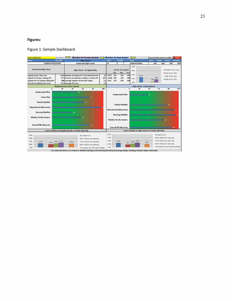
Figure 1 shows an example of an experimental dashboard. The dashboard shows characteristics

of the student’s high school, including the interquartile range of the SAT scores of the student’s high

school peers, obtained from College Board data. We merge student-level SAT data to college enrollment

data from the National Student Clearinghouse (NSC) to estimate the extent of student undermatch that

occurs both at the high school and neighborhood levels.1 These metrics are collapsed into percentiles

and expressed such that the lowest percentiles indicate high schools and neighborhoods where students

tend to make the best college choices.

The other dashboard adversity components are also shown on the panels where darker green

shades represent the least adversity and red represents the most adversity. We construct these

adversity components using a proprietary algorithm, which relies directly on data from the American

Community Survey (ACS). Finally, we add publicly available data from the Common Core of Data, such as

the fraction of students eligible for free/reduced price lunch and the high school enrollment to provide

important context for admissions readers unfamiliar with the student’s high school.

To provide readers with an overall view of the adversity faced by students, we collapse adversity

sub-components into three main categories: overall neighborhood adversity, overall high school

adversity, and overall adversity. The former adversity components are featured at the bottom of the

red/green panel and the overall adversity is expressed in the upper right-hand corner of the dashboard.

1 A student undermatches if her SAT score is 15 percentile points higher than that of the typical enrollee at her first college.

5

3. Data

In this study, we invited two postsecondary institutions to engage their admissions staff in re-

reading applications for students entering in the 2016-2017 academic year, and recommending

admissions decisions with information on the measures of neighborhood and high school adversity

discussed above. These two institutions differ markedly in terms of mission, admissions procedures, and

student body composition. The first institution, which we refer to as Elite University, is a private

Midwestern university with a rigorous admissions process and turns away many exceptional candidates

for admission. The second institution, which we call East Coast State University, is moderately selective,

and admissions decisions are made large on the basis of standardized test scores and high school GPA.

For both institutions, we relied on historical admissions data to identify potential experimental

candidates. Elite University provided the complete list of applicants for the classes entering between

2010 and 2016, and East Coast State shared the list of four cohorts of candidates applying to first enroll

in 2013 through 2016. Along with admissions decisions, both institutions shared data on SAT/ACT

scores, as well as student race and gender. To demonstrate the impact of the adversity tool, we

intentionally oversampled students on the cusp of admission, and we were able to identify such

students by fitting logit models where we regressed the admissions decisions on these student-level

academic and socio-demographic characteristics.2

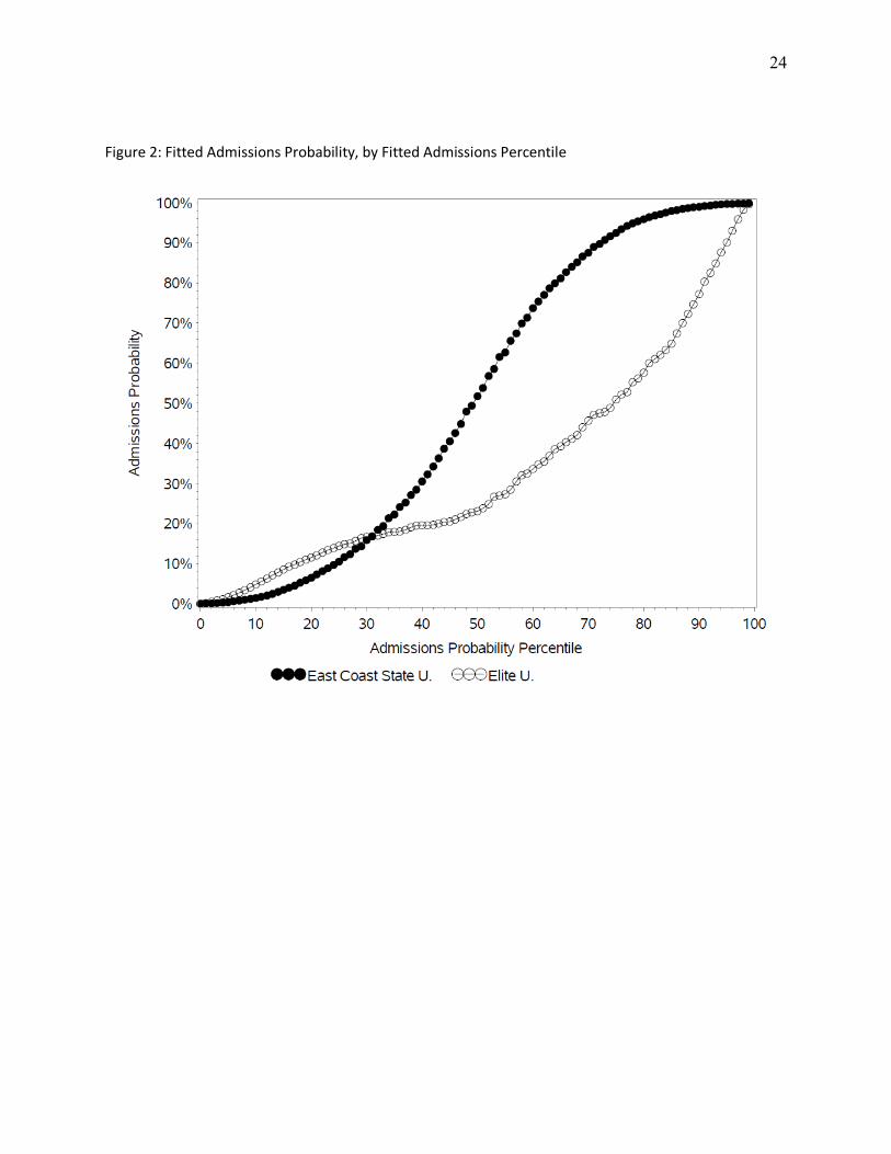
In Figure 2, we use predicted probabilities from these fitted models to show graphically that

admissions decisions are less easily predicted at Elite U. compared to East Coast State. Based on the

probabilities of admissions from the logit model parameter estimates, we rank order students. This rank,

expressed as percentiles, is depicted on the x-axis of Figure 2. On the y-axis, we show the admissions

2 Elite U. had three admissions outcomes (reject, waitlist, accept), so we fit a multinomial logistic model to the data from this institution.

6

probability corresponding to the x-axis percentiles. On average, students have a lower probability of

admission at Elite U than at East Coast State; however, the increases in admissions probability with

percentile rank are much more gradual for Elite U than for East Coast State. The “S-shaped” curve for

East Coast State means that East Coast State (ECS) applicants ranked as the least likely to gain admission

to ECS actually have a lower probability of admission than Elite U applicants ranked as least likely to earn

admission to Elite U. The gradual increases of the Elite U curve relative to the ECS curve demonstrate

that the more selective institution takes a more holistic approach to admission than does the state

institution.

4. Empirical Strategy

4.1 Sampling Strategy

For East Coast State, we selected 4,800 students who applied to join the class entering in the fall

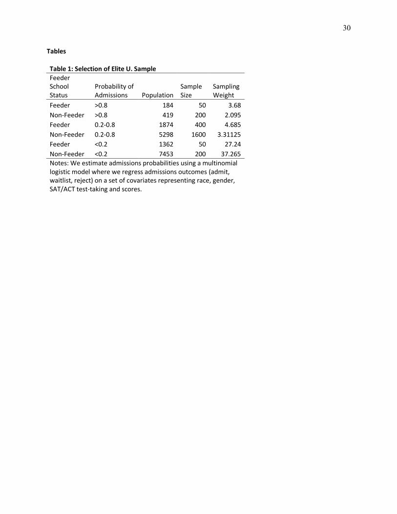
of 2016 with admissions probabilities between 2.6 percent and 98 percent. At Elite University, we

adopted a more complex sampling strategy to test whether the adversity dashboard was differentially

impactful for students attending high schools with a history of sending applicants to Elite U. We defined

these feeder high schools as sending an average of 10 or more applicants to Elite U. over the 2010

through 2016 period. Though we oversampled students in the mid-range of admissions probability

(between 20 and 80 percent), we also sampled some students with the highest and lowest probabilities

of acceptance to determine whether the adversity dashboard shifted decisions among applicants

expected to have the least uncertainty in admissions decisions. We show the population and sample size

counts for the stratified sample in Table 1.

Based on the availability of volunteers and the capacity of volunteers to read applications for

admission, we took two slightly different approaches to reader assignment between Elite U and East

Coast State. The Elite U. data included information on the identities of the admissions staff who

7

evaluated the applications for the cohort of students applying for entry in the fall of 2016. We randomly

assigned 150 students to 18 volunteers with the specification that volunteers had not served as

evaluators during the official, original application review. We also ensured that each of the readers had

equal numbers of applicants in the Table 1 categories, defined by admissions probability and whether

the student attended an Elite U feeder high school. The assignment of readers to applicants at East

Coast State was simpler: original reader identities were unavailable, so we simply randomly assigned

300 students to each of 16 volunteers.

To understand the impact of the adversity dashboard on changes in admissions decisions, we

randomly selected applications (24 per reader at Elite U. and 50 per reader at East Coast State) in which

volunteers were asked to read applications without access to the adversity dashboard information. In

other words, for this small set of applications, readers were asked to consider the original applications

with no additional information on neighborhood or high school contexts. These control students have

adversity data that are never disclosed to admissions readers. As we describe in the methods section,

these control groups allow us to account for the possibility that baseline preferences either in favor of or

against student adversity may have changed from the original read.

4.2 Methods

Since applications are randomized across readers and into control (no adversity dashboard) and

treatment groups (adversity dashboard), the empirical strategy for identifying the impact of the

adversity dashboard elements on admissions decisions is straightforward. We fit the data to the model

shown in EQ(1). The variable Adversity represents an adversity metric, such as the applicant’s

neighborhood or school-level adversity percentile, and the Treatment variable is an indicator for

whether the dashboard data were added to student i’s original application. Parameter β3 is the

parameter of interest in EQ(1), and indicates whether the relationship between Adversity and the

8

probability of admission differs between control and treatment students. The vector of covariates, Xi ,

includes student academic and demographic factors, the original admission recommendation and a set

of covariates representing the fixed effects of admissions readers. As would be expected from a properly

implemented RCT, the inclusion of these covariates does not alter any of the β3 parameter estimates. In

addition to the these logit models, we fit the data with standard OLS models in which the

Log(OddsAdmission) in EQ(1) is replaced with a binary variable representing whether the student was

admitted.

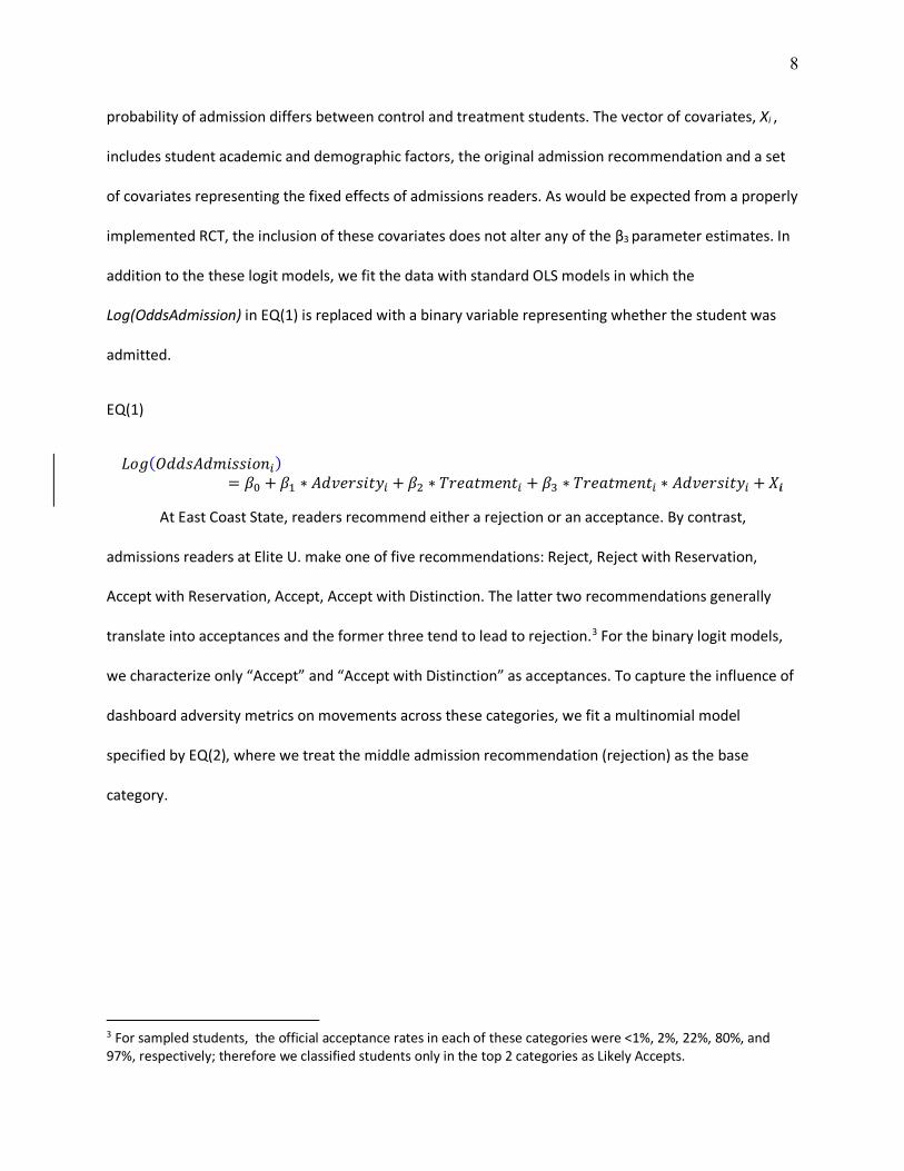
EQ(1)

!"#(%&&'(&)*''*"+,)= /0 + /2 ∗ (&456'*78, + /9 ∗ :65;7)5+7, + /< ∗ :65;7)5+7, ∗ (&456'*78, + =>

At East Coast State, readers recommend either a rejection or an acceptance. By contrast,

admissions readers at Elite U. make one of five recommendations: Reject, Reject with Reservation,

Accept with Reservation, Accept, Accept with Distinction. The latter two recommendations generally

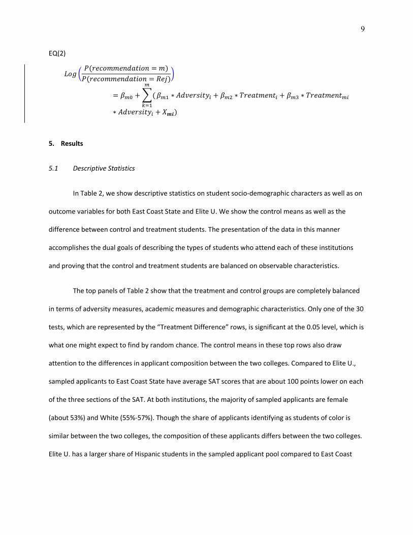
translate into acceptances and the former three tend to lead to rejection.3 For the binary logit models,

we characterize only “Accept” and “Accept with Distinction” as acceptances. To capture the influence of

dashboard adversity metrics on movements across these categories, we fit a multinomial model

specified by EQ(2), where we treat the middle admission recommendation (rejection) as the base

category.

3 For sampled students, the official acceptance rates in each of these categories were <1%, 2%, 22%, 80%, and 97%, respectively; therefore we classified students only in the top 2 categories as Likely Accepts.

9

EQ(2)

!"# ?@(65A"))5+&;7*"+ = ))

@(65A"))5+&;7*"+ = B5C)D

= /E0 +F(

E

GH2

/E2 ∗ (&456'*78, + /E9 ∗ :65;7)5+7, + /E< ∗ :65;7)5+7E,

∗ (&456'*78, + =I>)

5. Results

5.1 Descriptive Statistics

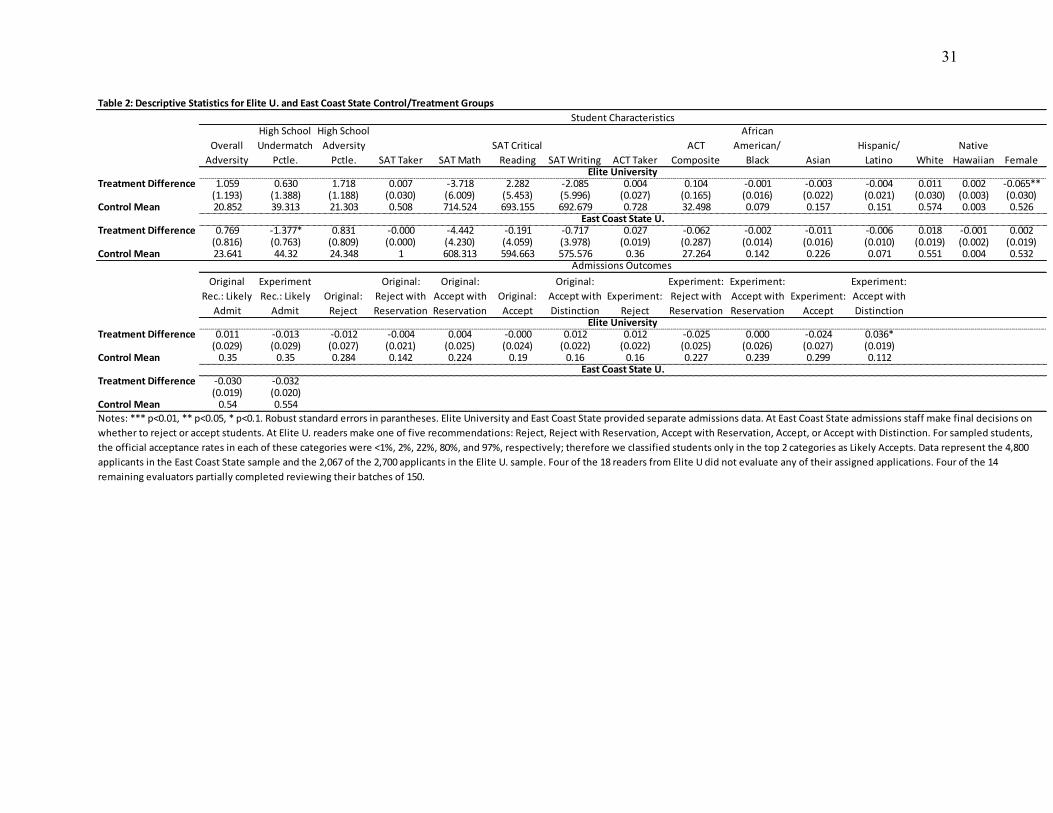
In Table 2, we show descriptive statistics on student socio-demographic characters as well as on

outcome variables for both East Coast State and Elite U. We show the control means as well as the

difference between control and treatment students. The presentation of the data in this manner

accomplishes the dual goals of describing the types of students who attend each of these institutions

and proving that the control and treatment students are balanced on observable characteristics.

The top panels of Table 2 show that the treatment and control groups are completely balanced

in terms of adversity measures, academic measures and demographic characteristics. Only one of the 30

tests, which are represented by the “Treatment Difference” rows, is significant at the 0.05 level, which is

what one might expect to find by random chance. The control means in these top rows also draw

attention to the differences in applicant composition between the two colleges. Compared to Elite U.,

sampled applicants to East Coast State have average SAT scores that are about 100 points lower on each

of the three sections of the SAT. At both institutions, the majority of sampled applicants are female

(about 53%) and White (55%-57%). Though the share of applicants identifying as students of color is

similar between the two colleges, the composition of these applicants differs between the two colleges.

Elite U. has a larger share of Hispanic students in the sampled applicant pool compared to East Coast

10

State (15% versus 7%). By contrast African-American (14% versus 8%) and Asian applicants (23% versus

16%) comprise larger shares of the sampled applicant pool at East Coast State compared to Elite U.

The bottom panels of Table 2 present descriptive data on both the original reader’s

recommendation and the experimental reader’s recommendation. The nature of these

recommendations differed between the two colleges, with East Coast U readers using a binary

evaluation method (reject or accept) and Elite U. readers placing students into one of 5 admissions

recommendation categories (Reject, Reject with Reservation, Accept with Reservation, Accept, Accept

with Distinction).4 At both institutions, the original and experimental admission recommendation

probabilities were identical, indicating that experimental readers were not offering more favorable

evaluations compared to the original readers. Moreover, the second column of Panel B shows that, on

average, treatment and control applications had the same likelihood of admission. This suggests that

simply providing adversity data does not impact the probability of admission for the typical applicant.

Even though we oversampled students in the mid-range of admissions probabilities, original and

final admissions decisions tended to be identical in both the control and treatment groups. For example,

in the treatment group at Elite U., only 14 percent of binary admissions recommendations differed

between the original reader and the experimental reader. In the control group, that number stood at 19

percent. At East Coast State, these percentages were considerably lower (3 and 4 percent for the

treatment and control groups), as the institution relied more heavily on SAT scores and HS GPA when

making admissions decisions.

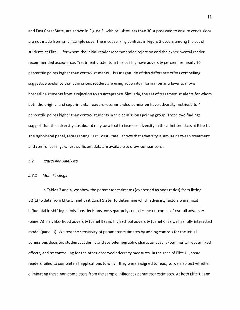
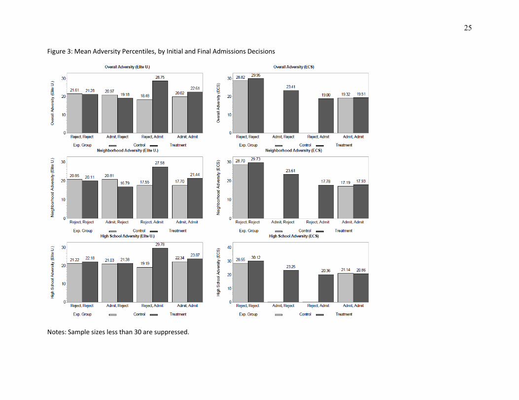
Descriptive data reveal that these shifts in admissions decisions are related to student adversity.

To offer a preview of our main results, we show the mean adversity percentiles, by control and

treatment groups and the original and experimental admissions decisions. These data, for both Elite U.

11

and East Coast State, are shown in Figure 3, with cell sizes less than 30 suppressed to ensure conclusions

are not made from small sample sizes. The most striking contrast in Figure 2 occurs among the set of

students at Elite U. for whom the initial reader recommended rejection and the experimental reader

recommended acceptance. Treatment students in this pairing have adversity percentiles nearly 10

percentile points higher than control students. This magnitude of this difference offers compelling

suggestive evidence that admissions readers are using adversity information as a lever to move

borderline students from a rejection to an acceptance. Similarly, the set of treatment students for whom

both the original and experimental readers recommended admission have adversity metrics 2 to 4

percentile points higher than control students in this admissions pairing group. These two findings

suggest that the adversity dashboard may be a tool to increase diversity in the admitted class at Elite U.

The right-hand panel, representing East Coast State., shows that adversity is similar between treatment

and control pairings where sufficient data are available to draw comparisons.

5.2 Regression Analyses

5.2.1 Main Findings

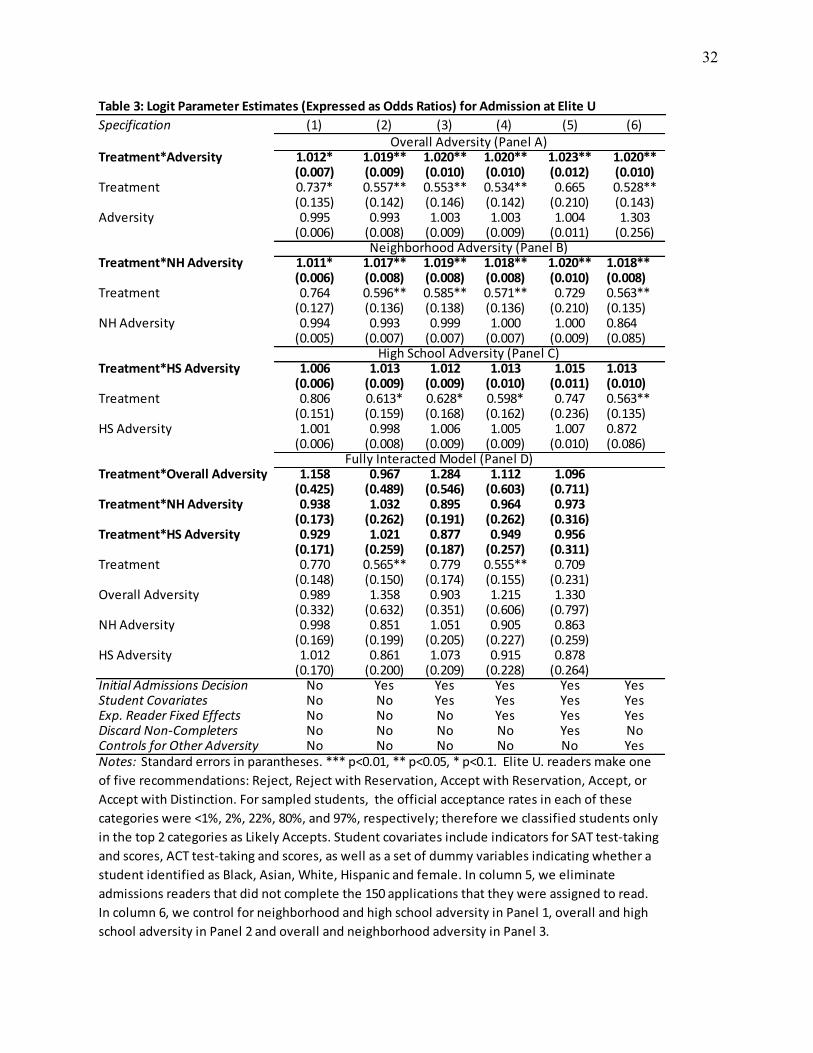
In Tables 3 and 4, we show the parameter estimates (expressed as odds ratios) from fitting

EQ(1) to data from Elite U. and East Coast State. To determine which adversity factors were most

influential in shifting admissions decisions, we separately consider the outcomes of overall adversity

(panel A), neighborhood adversity (panel B) and high school adversity (panel C) as well as fully interacted

model (panel D). We test the sensitivity of parameter estimates by adding controls for the initial

admissions decision, student academic and sociodemographic characteristics, experimental reader fixed

effects, and by controlling for the other observed adversity measures. In the case of Elite U., some

readers failed to complete all applications to which they were assigned to read, so we also test whether

eliminating these non-completers from the sample influences parameter estimates. At both Elite U. and

12

East Coast State, parameter estimates are generally insensitive to the inclusion of covariates, which is to

be expected given that treatment and control groups are balanced on observable characteristics.

Panel A of Table 3 reveals that a 1 percentile point in overall adversity, as represented on the

dashboard, increased the odds of admission by a factor of 1.02. Similarly, increases in dashboard-

presented neighborhood adversity by 1 percentile point also increased the odds of admission by a factor

of 1.02. These two odds ratios remain statistically significant even after controlling for neighborhood

and school adversity (Panel A, Column 6) and for overall and school adversity (Panel B, Column 6). This

finding suggests that admissions readers are likely separately considering each of these adversity

metrics when making admissions decisions. Interaction terms between treatment status and high

school-level adversity are positive, but fail to reach levels of statistical significance.

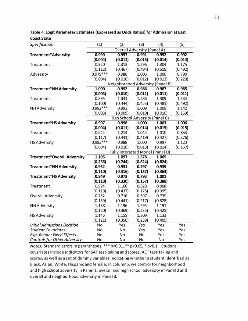
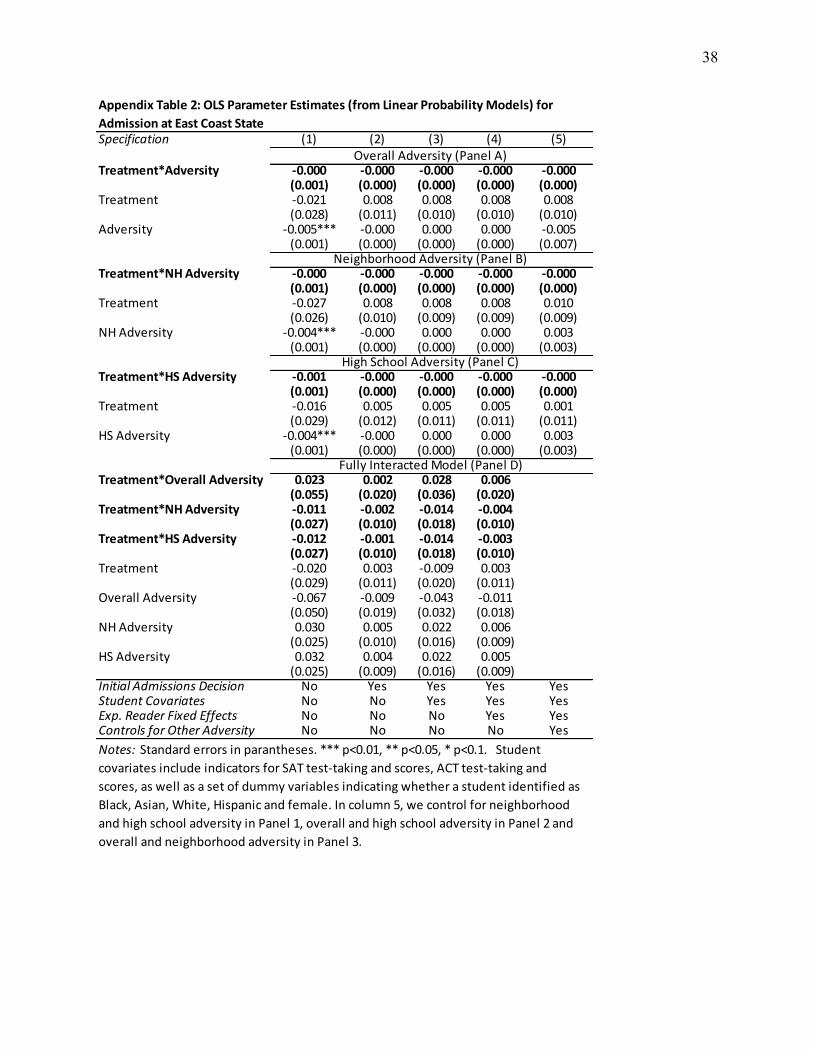
At East Coast State, none of the interaction terms between dashboard adversity and treatment

status reached traditional levels of statistical significance and the magnitudes of the odds ratio

parameter estimates are about 1.0. The absence of statistically significant interaction terms means that

we are unable to conclude that the adversity dashboard data influenced admissions decisions among

readers at East Coast State. As this college maintained a more formulaic approach to admissions that

relied heavily on SAT scores and HS GPA, it is unsurprising that the dashboard metrics exerted little

influence on admissions decisions.

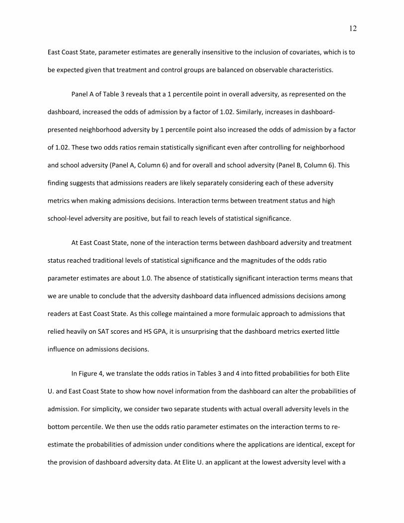
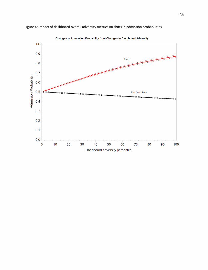
In Figure 4, we translate the odds ratios in Tables 3 and 4 into fitted probabilities for both Elite

U. and East Coast State to show how novel information from the dashboard can alter the probabilities of

admission. For simplicity, we consider two separate students with actual overall adversity levels in the

bottom percentile. We then use the odds ratio parameter estimates on the interaction terms to re-

estimate the probabilities of admission under conditions where the applications are identical, except for

the provision of dashboard adversity data. At Elite U. an applicant at the lowest adversity level with a

13

50% chance of admission would instead have an 87% chance of admission if that application were

accompanied by a dashboard revealing the student to be in the highest adversity category. At East Coast

State, the fitted probability of admission curve is fairly flat, reflecting our finding that the adversity

dashboard information tends not to shift admissions decisions.5

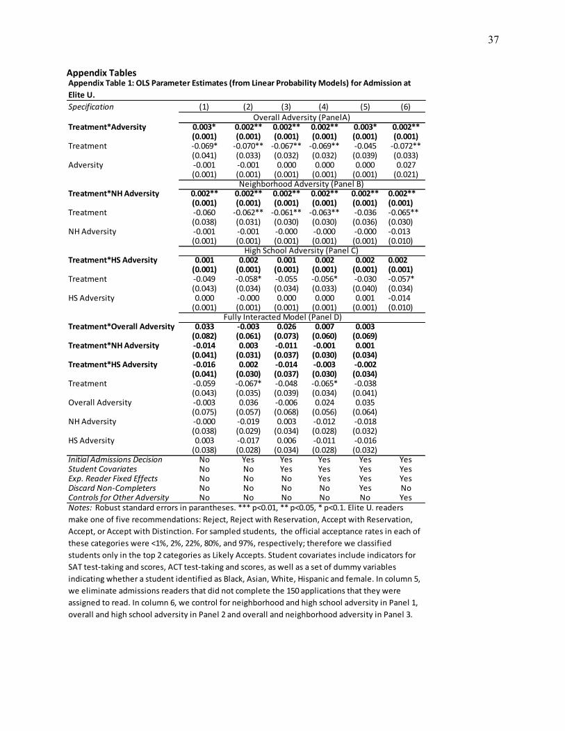
We test the sensitivity of our model specifications by fitting linear probability models mirroring

those shown in Tables 3 and 4. The parameter estimates from these fitted models are shown in

Appendix Tables 1 and 2. At Elite U, the interaction terms between Treatment and Dashboard Adversity

are significant and range between 0.002 and 0.003. These values suggest that, for a given student, the

probability of admission would increase by 0.2 to 0.3 percentage points for each 1 percentile point

increase in dashboard-identified adversity. This means that an applicant with the lowest adversity levels

would experience a 20 to 30 percentage point increase in the probability of admission if that student’s

application were accompanied by a dashboard revealing her to be in the highest adversity category. The

magnitude of these increases is similar to those shown from the logit models in Figure 4.

5.2.2 Alternative Adversity Metrics

Thus far, we have focused only on the main adversity percentiles. This focus suggests that, at

least in the case of Elite U., admissions readers are honing in on these metrics during the admissions

recommendation process. The adversity dashboard contains a host of data, and it may be the case that

admissions readers are actually focusing on other dashboard metrics that happen to be associated with

the overall, neighborhood and high school adversity metrics. Though we are unable to expose the exact

mechanisms through which readers are using the dashboard to shape admissions decisions, we can offer

insight into whether certain metrics are more influential than others.

5 Parameter estimates come from Column 2 of Panel A in Tables 3 and 4

14

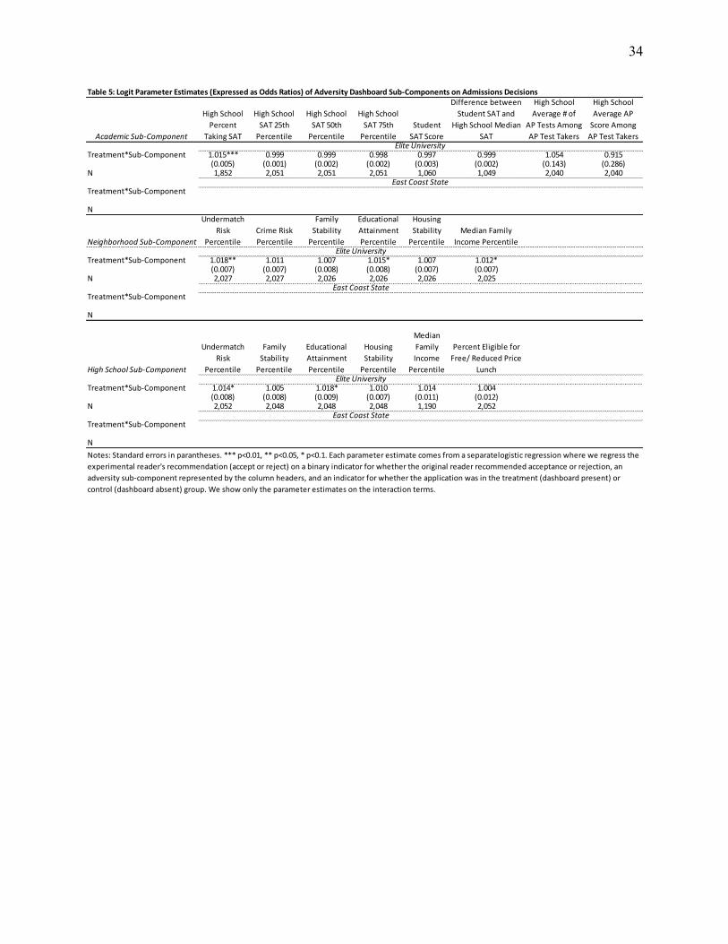
In Table 5, we re-fit EQ(1), substituting the three main adversity metrics with the high school

and neighborhood level adversity subcomponents (e.g. neighborhood context crime risk percentile) and

high school-level academic characteristics, such as the fraction of students at the high school who

historically undermatch by attending less selective colleges than they are qualified to attend. In

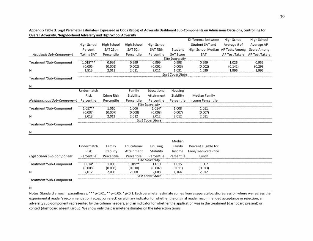
Appendix Table 3, we test the sensitivity of these parameter estimates to models where the three main

adversity metrics are added as covariates to confirm whether the adversity sub-components actually

supplement the three main adversity components.

Despite our findings that higher levels of overall and neighborhood adversity, as indicated on

the dashboard, were more likely to shift admissions decisions from rejections to acceptances, we find

that the majority of sub-components do not influence admissions decisions. Table 5 reveals that only

five of the 19 dashboard sub-components shift admissions decisions. All of the adversity percentile

metrics are scaled so that higher percentiles signify higher adversity, and the directions of the

statistically significant parameter estimates indicate that dashboard information conveying lower levels

of educational attainment among adults, lower family incomes in the student’s neighborhood and lower

college undermatch in students’ neighborhoods and high schools can induce readers to view student

applications more favorably. The lone metric that may advantage students in contexts with less

adversity is the percentage of students at the applicant’s high school who took the SAT. Table 5 shows

that a 1 percentage point increase in the dashboard-indicated fraction of high school seniors taking the

SAT increased the odds of admission by a factor of 1.015. All but one of the Table 5 findings persist after

the addition of the three main adversity metrics (Appendix Table 3), suggesting that there may be

additional value of including some of the adversity sub-components on the dashboard.

15

5.3 Elite U. Specific Analyses

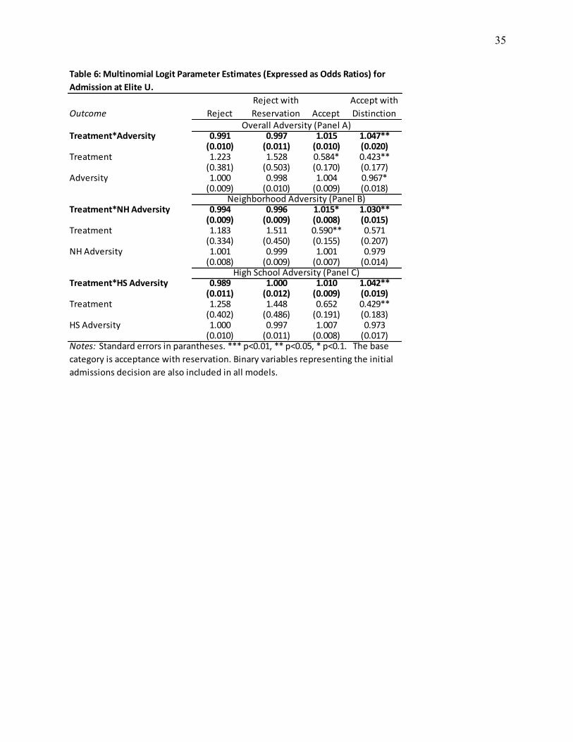
5.3.1 Multinomial Logit Models

Admissions readers at Elite U. make one of five admissions recommendations. We have mapped

these recommendations onto actual outcomes, and based on this mapping, we have grouped rejection,

rejection with reservation and accept with reservation as “rejections” and accept and accept with

distinction as “acceptances”. This binary outcome has been the focus of all analyses thus far.

In this section, consider the actual recommendations, and examine how the adversity

dashboard contributes to movement across the admissions recommendation categories. We accomplish

this by fitting the multinomial regression model specified in EQ(2), and we show the parameter

estimates (expressed as odds ratios) in Table 6. The odds ratios on the interaction terms in Table 6 show

changes, with each one percentile point change in adversity, in the odds of receiving one the four

admissions recommendations relative to the middle category (acceptance with reservation). For

example, the top row of Table 6 reveals that a one point increase in overall dashboard adversity

increases the odds that a student receives an accept with distinction rating over an accept with

reservation rating by a factor of 1.047.

From left to right, the steadily increasing odds ratios on the interaction term parameter

estimates show that increases in adversity shifts students across multiple margins, such as from reject to

reject with reservation or accept to accept with distinction. The largest shifts appear to be along the

accept with reservation/ accept and the accept/accept with distinction margins. This finding indicates

that reclassification is occurring largely among students who were realistic candidates for admission.

Not all of the odds ratios reach traditional levels of statistical significance, possibly due to the

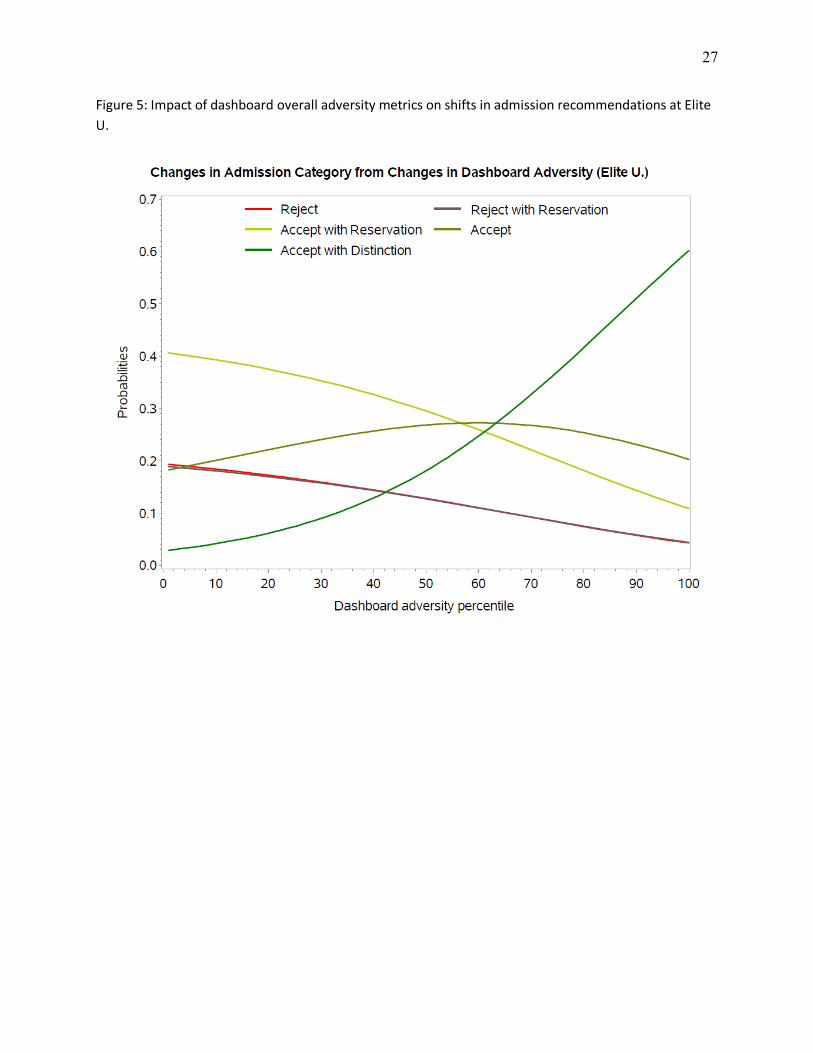
fairly small sample sizes. Nevertheless, we help contextualize these odds ratios in Figure 5 by showing

16

how the relative probabilities of admission shift as readers are presented with varying levels of overall

adversity through the dashboard for a given student’s application. We choose a profile of a typical

sampled applicant with roughly equal likelihoods (≈20 percent) of receiving a recommendation of

rejection, reject with reservation and acceptance, and a roughly 40 percent likelihood of receiving an

acceptance with reservation recommendation.

Tracing the curves in Figure 5 from the lowest dashboard adversity to the highest dashboard

adversity, we find that increases in dashboard-conveyed adversity increase the likelihood that students

receive favorable admissions decisions. These curves reveal that the typical sampled student perceived

by the admissions staff to be in the lowest adversity percentile would experience a whopping 60

percentage point increase in the probability of receiving an acceptance with distinction rating if the

admissions reader were provided with a dashboard indicating the student to be in the highest adversity

percentile. Obviously, such a scenario represents an extreme example, but the slopes of the curves

shown in Figure 5 demonstrate that even modest changes in how a reader views the adversity faced by

the student can shift probabilities of reclassification by 5 to 10 percentage points.

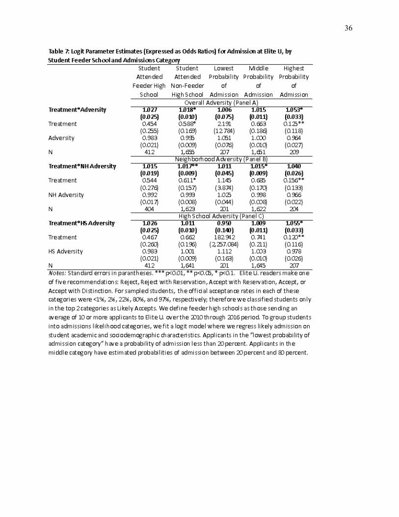
5.3.2 Effects of Adversity Dashboard by a Student’s Feeder School Status and Admissions Probability

In Table 7, we separately fit EQ(1) by whether the applicant attended a feeder high school to

Elite U, with an average of 10 or more applications per year over the period from 2010 through 2016.

We also separately fit EQ(1) by the student’s expected admissions probability, grouped into three

categories (less than 20 percent, between 20 and 80 percent, and 80 percent or higher). We initially

sampled from these categories to determine whether the admissions dashboard was more influential

among students attending high schools less familiar to admissions readers and whether the dashboard

was more influential among students whose application characteristics placed them on the cusp of

admission.

17

We find that the parameter estimates on Adversity*Treatment interaction terms are significant

among students from non-feeder high schools (Table 7, column 2). Odds ratios for these interaction

terms among students attending Elite U. feeder high schools do not reach conventional levels of

statistical significance, possibly because of the smaller sample sizes in this group. Differences in the

magnitudes of the parameter estimates between the column 1 and column 2 interaction terms means

that we are unable to make conclusions about whether the dashboard is more or less effective for

students attending familiar high schools.

Disaggregated by a priori probabilities of admission, the parameter estimates on the

Adversity*Treatment interaction terms are largest for the students with the highest probabilities of

admission and lowest for students least likely to gain admission to Elite U based on their academic and

socio-demographic characteristics. The final column in Table 7 shows that a one percentile point in

dashboard-indicated adversity increases the odds of admission to Elite U by a factor of 1.053.

Statistically significant parameter estimates are confined to students in the middle and high admissions

probability categories, suggesting that the dashboard only moves the needle among students with a

reasonable probability of admission.

6. Changes in Composition of Admitted Class

Admissions staff, particularly at selective postsecondary institutions, often seek to create classes

that are academically capable or accomplished and are also diverse (Clinedinst, 2016; Lucido, 2016).

Ideally, the adversity dashboard will help to achieve these goals. In this study, we find that the adversity

dashboard did not compromise the academic quality of the admitted students, and in the case of Elite U.

increased the share of non-White students in the admitted class.

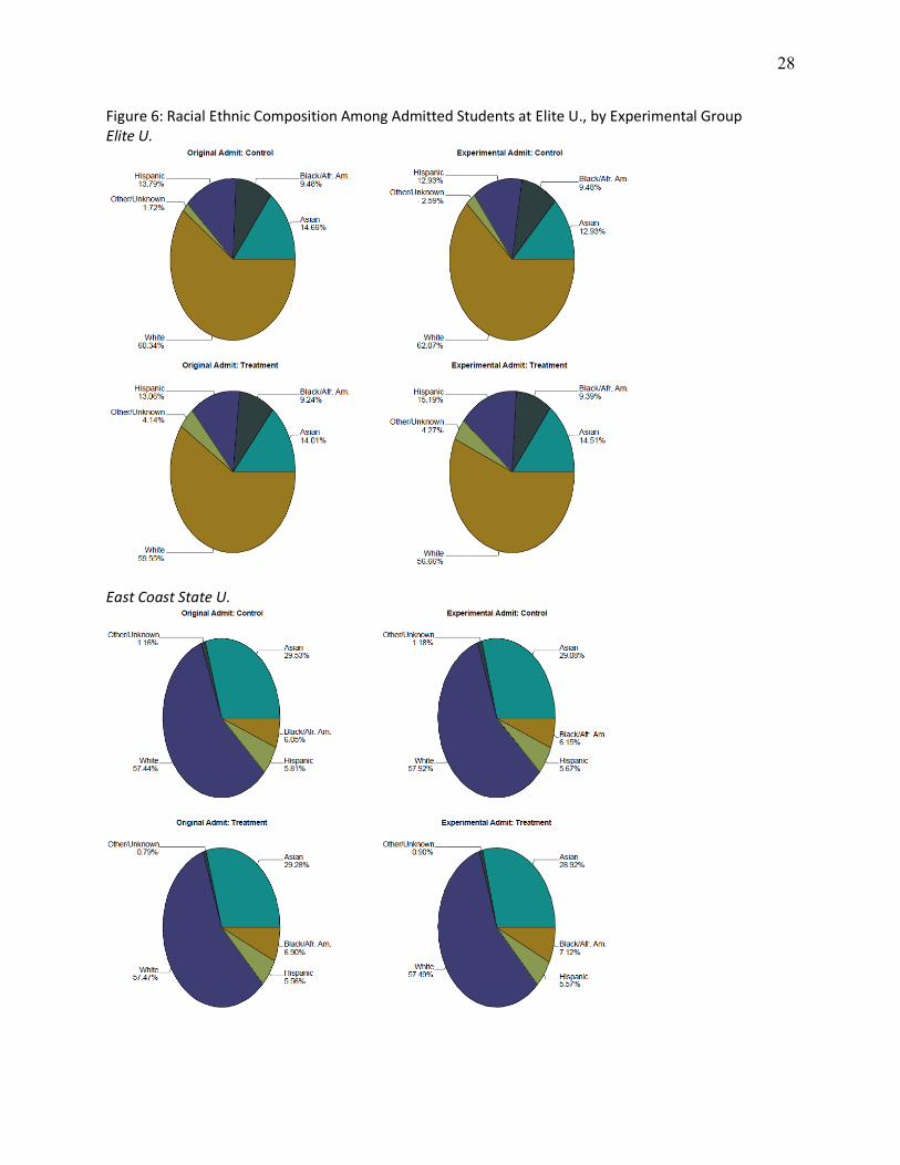
Figure 6 shows the racial/ethnic makeup of the admitted students in the experimental and

control groups, both among the originally admitted students and among the students from the

18

experimental group who were admitted. At Elite U., about 60 percent of sampled students who were in

the original admit group identified as White. This percentage was identical between the treatment and

control students. By contrast, in the experiment, less than 57 percent of admitted students in the

dashboard group (treatment) identified as White, compared to 62 percent in the admitted students

from the control group. Comparing the experimental treatment and control groups, we find all non-

White groups have greater representation in the treatment group than in the control group at Elite U.

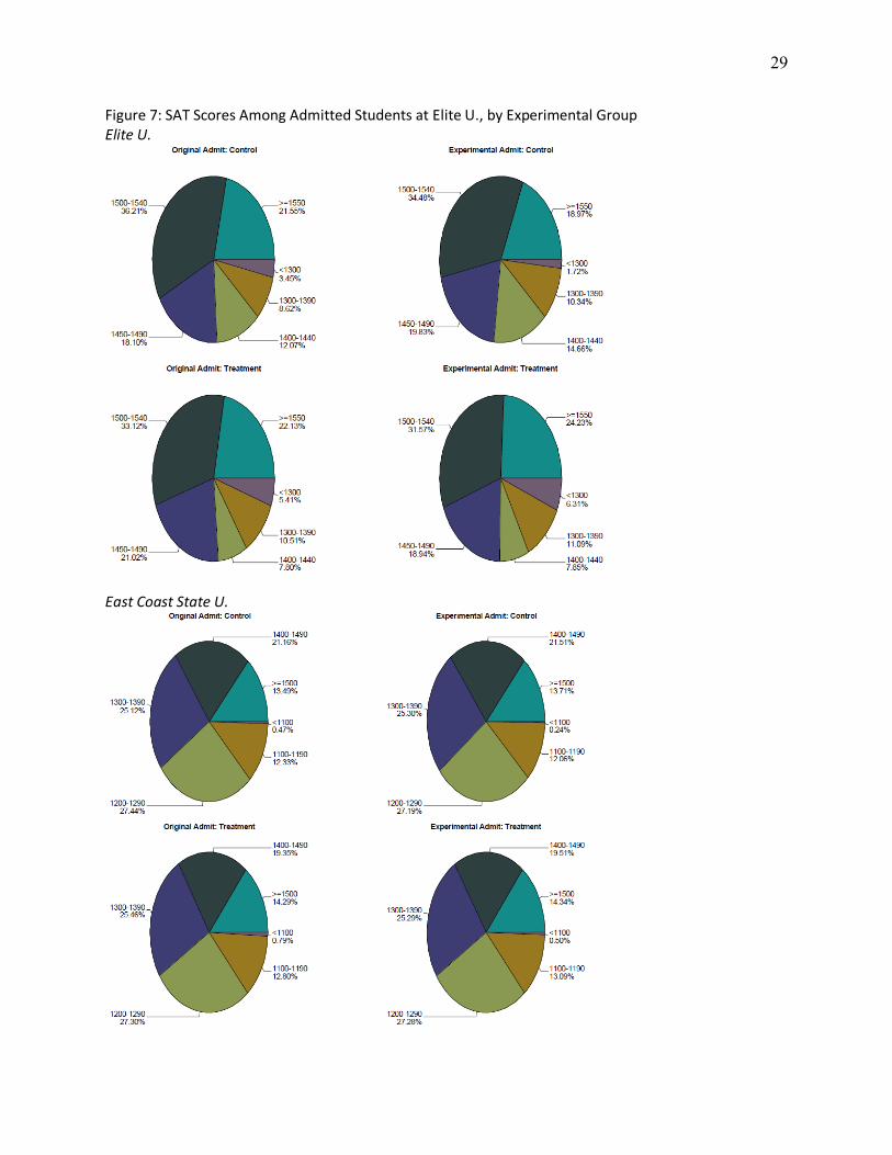
At Elite U., the average overall adversity among admitted students under experimental

conditions was 4 percentile points higher in the treatment versus the control group (23.6 versus 19.6)

and the average composite SAT scores between these two groups only differed by 3 points (1477 versus

1480).6 The distribution of SAT scores among admitted students in Figure 7 reveals that the Elite U.

dashboard increased the fraction of students in top SAT category as well as in the bottom SAT category.

For example, nearly one-quarter of the treatment admitted students in the experimental condition had

SAT or concorded ACT scores of 1550 or higher. The comparable fraction in the control group is 19

percent. At the other end of the distribution, students with SAT scores below 1300 comprise 6.3 percent

of the experimental treatment group, compared to 1.7 percent of the control group.

7. Discussion and Conclusion

Overall, our study supports emerging research that providing high-quality contextual

information can induce admissions officers to admit a larger proportion of low-SES applicants (Bastedo

& Bowman, 2017; Bastedo, Bowman, & Glasener, 2016; Gaertner & Hart, 2013). Given extensive

national discussions about the importance of increasing the representation of low-income students at

6 For students submitting the ACT in lieu of the SAT, we have concorded ACT scores to SAT scores using the concordance table located at https://research.collegeboard.org/sites/default/files/publications/2012/7/researchnote-2009-40-act-sat-concordance-tables.pdf

19

selective colleges, as well as the persistent stratification of American higher education by race and class,

these results can provide important insights into strategies to improve decision making in college

admissions.

The results here also mitigate concerns – largely discredited, at this point – that have been

raised about the potential for “mismatch” in college admissions. Low-SES applicants who were admitted

in our treatment group were similarly qualified on standardized test scores as students admitted during

regular holistic review. At the same time, we saw a modest increase in the racial diversity of the

admitted class as well, helping to mitigate any concerns that interventions that do not directly measure

race or ethnicity will fail to benefit students of color. Although the adversity dashboard does not focus

on questions of race or ethnicity, many of the mechanisms of racial discrimination in the U.S. – such as

neighborhood segregation, crime risk, educational opportunity, and family income – are well

represented in the dashboard data. In addition, the dashboard includes the race/ethnicity of each

applicant, allowing institutions to practice race-conscious admissions while simultaneously accounting

for the additional data provided by the adversity dashboard. This is vitally important, because a great

deal of research demonstrates that class-based “affirmative action” cannot replace the effects of race-

conscious admissions in producing a diverse class (e.g., Reardon, Baker, Kasman, Klasik, & Townsend,

2015).

Finally, the results of these field experiments help to mitigate concerns that laboratory or

simulation experiments may not be replicated in field conditions. In fact, the results found here at Elite

U. had larger effect sizes than were found in Bastedo and Bowman (2017). We look forward to

conducting additional field experiments at different types of selective colleges – public and private, large

and small, more and less selective – to see if we find similar effects across a range of schools.

20

Nonetheless, we must recognize that these results are only likely to replicate in admissions

offices that have high fidelity to holistic review practices. Although 95% of selective college admissions

offices report using holistic review, a recent review of holistic review practices suggests that perhaps as

few as 1/3 of offices use the kind of contextualized holistic review that is amenable to this intervention

(Bastedo, Glasener, Kelly, & Bowman, 2017). In addition, there is some evidence to suggest that there is

less fidelity to holistic review practices than has been commonly reported in the media (Bastedo,

Howard & Flaster, 2016). In future studies, it may be important to include training and or policy reforms

inside of admissions offices prior to introducing this dashboard.

21

References

Bastedo, M. N. (2014). Cognitive repairs in the admissions office: New strategies for improving equity and excellence at selective colleges. Presentation at the annual meeting of the American Educational Research Association, Philadelphia, PA, April 3-7, 2014.

Bastedo, M. N. (2016). Enrollment management and the low-income student: How holistic admissions and market competition can impede equity. In A. P. Kelly, J. S. Howell, & C. Sattin-Bajaj (Eds.), Matching Students to Opportunity: Expanding College Choice, Access, and Quality (pp. 121-134). Cambridge: Harvard Education Press.

Bastedo, M. N., & Bowman, N. A. (2017). Improving admission for low-SES student at selective colleges: Results from an experimental simulation. Educational Researcher.

Bastedo, M. N., Bowman, N. A., & Glasener, K. (2017). Standardized test scores in context: Grit, strivers, and selective college admissions. Paper in preparation.

Bastedo, M. N., Howard, J. E., & Flaster, A. (2016). Holistic admissions after affirmative action: Does “maximizing” the high school curriculum matter? Educational Evaluation and Policy Analysis, 38, 389-409.

Bastedo, M. N., & Jaquette, O. (2011). Running in place: Low-income students and the dynamics of higher education stratification. Educational Evaluation and Policy Analysis, 33(3), 318-339.

Bowen, W. G., Chingos, M. M., & McPherson, M. S. (2009). Crossing the finish line: Completing college at America’s public universities. Princeton, NJ: Princeton University Press.

Bowen, W. G., Kurzweil, M. A., & Tobin, E. M. (2006). Equity and excellence in American higher education. Charlottesville: University of Virginia Press.

Chetty, R., Friedman, J. N., Saez, E., Turner, N., & Yagan, D. (2017). Mobility report cards: The role of colleges in intergenerational mobility. Retrieved on March 1, 2017 from http://www.equality-of-opportunity.org/papers/coll_mrc_paper.pdf.

Clinedinst, M. (2016). State of college admission 2015. Washington, DC: National Association for College Admission Counseling.

Espenshade, T. J., & Hale, L. E., & Chung, C. Y. (2005). The frog pond revisited: High school academic context, class rank, and elite college admission. Sociology of Education, 78, 269-293.

Espenshade, T. J., & Radford, A. W. (2009). No longer separate, not yet equal: Race and class in elite college admission and campus life. Princeton, NJ: Princeton University Press.

Espinosa, L. L., Gaertner, M. N., & Orfield, G. (2015). Race, class, and college access: Achieving diversity in a shifting legal landscape. Washington, D.C.: American Council on Education.

Gaertner, M. N., & Hart, M. (2013). Considering class: College access and diversity. Harvard Law and Policy Review, 7, 367-87.

Grodsky, E. (2007). Compensatory sponsorship in higher education. American Journal of Sociology, 112, 1662–1712.

Henry, P. J. (2008). College sophomores in the laboratory redux: Influences of a narrow data base on social psychology’s view of the nature of prejudice. Psychological Inquiry, 19, 49-71.

Hill, C. B., & Winston, G. C. (2010). Low-income students and highly selective private colleges: Geography, searching, and recruiting. Economics of Education Review, 29(4), 495-503.

Holland, M. M. (2014). Navigating the road to college: Race and class variation in the college application process. Sociology Compass, 8(10), 1191-1205.

22

Hoxby, C. M., & Avery, C. (2012). The missing "one-offs": The hidden supply of high-achieving, low-income students. NBER Working Paper 18586. Cambridge, MA: National Bureau of Economic Research.

Hoxby, C., & Turner, S. (2013). Expanding college opportunities for high-achieving, low-income students. SIEPR Discussion Paper No. 12- 014.

Kahneman, D. (2011). Thinking, fast and slow. New York: Farrar, Straus, & Giroux. Karen, D. (1990). Toward a political-organizational model of gatekeeping: The case of elite

colleges. Sociology of Education, 63, 227-240. Klopfenstein, K. (2004). Advanced Placement: Do minorities have equal opportunity? Economics of

Education Review, 23, 115-131. Long, J. S. (1997). Regression models for categorical and limited dependent variables. Thousand Oaks,

CA: Sage. Lucido, J. A. (2015). How admission decisions get made. In Hossler, D., & Bontrager, B.

(Eds.), Handbook of strategic enrollment management (pp. 147-173). San Francisco: Jossey-Bass.

Mamlet, R., & VanDeVelde, C. (2011). College admission: From application to acceptance, step by step. New York: Three Rivers Press.

Moore, D. A., Swift, S. A., Sharek, Z. S., & Gino, F. (2010). Correspondence bias in performance evaluation: Why grade inflation works. Personality and Social Psychology Bulletin, 36(6), 843-852.

Perna, L. W. (2004). The key to college access: Rigorous academic preparation. In W. G. Tierney, Z. B. Corwin, & J. E. Colyar (Eds.), Preparing for college: Nine elements of effective outreach (pp. 113–134). Albany: SUNY Press.

Reardon, S. F., Baker, R., Kasman, M., Klasik, D., & Townsend, J. B. (2015). Can socioeconomic status substitute for race in affirmative action college admissions policies? Evidence from a simulation model. White paper, Educational Testing Service. Retrieved March 1, 2017 from https://www.ets.org/Media/Research/pdf/reardon_white_paper.pdf.

Swift, S. A., Moore, D. A., Sharek, Z. S., & Gino, F. (2013). Inflated applicants: Attribution errors in performance evaluation by professionals. PLoS One, 8(7), e69258.

Thaler, R., & Sunstein, C. (2009). Nudge: Improving decisions about health, wealth, and happiness (updated edition). New York: Penguin.

23

Figures:

Figure 1: Sample Dashboard

24

Figure 2: Fitted Admissions Probability, by Fitted Admissions Percentile

25

Figure 3: Mean Adversity Percentiles, by Initial and Final Admissions Decisions

Notes: Sample sizes less than 30 are suppressed.

26

Figure 4: Impact of dashboard overall adversity metrics on shifts in admission probabilities

27

Figure 5: Impact of dashboard overall adversity metrics on shifts in admission recommendations at Elite U.

28

Figure 6: Racial Ethnic Composition Among Admitted Students at Elite U., by Experimental Group Elite U.

East Coast State U.

29

Figure 7: SAT Scores Among Admitted Students at Elite U., by Experimental Group Elite U.

East Coast State U.

30

Tables

Table 1: Selection of Elite U. Sample Feeder School Status

Probability of Admissions Population

Sample Size

Sampling Weight

Feeder >0.8 184 50 3.68 Non-Feeder >0.8 419 200 2.095 Feeder 0.2-0.8 1874 400 4.685 Non-Feeder 0.2-0.8 5298 1600 3.31125 Feeder <0.2 1362 50 27.24 Non-Feeder <0.2 7453 200 37.265 Notes: We estimate admissions probabilities using a multinomial logistic model where we regress admissions outcomes (admit, waitlist, reject) on a set of covariates representing race, gender, SAT/ACT test-taking and scores.

31

Overall

Adversity

High School

Undermatch

Pctle.

High School

Adversity

Pctle. SAT Taker SAT Math

SAT Critical

Reading SAT Writing ACT Taker

ACT

Composite

African

American/

Black Asian

Hispanic/

Latino White

Native

Hawaiian Female

Treatment Difference 1.059 0.630 1.718 0.007 -3.718 2.282 -2.085 0.004 0.104 -0.001 -0.003 -0.004 0.011 0.002 -0.065**(1.193) (1.388) (1.188) (0.030) (6.009) (5.453) (5.996) (0.027) (0.165) (0.016) (0.022) (0.021) (0.030) (0.003) (0.030)

Control Mean 20.852 39.313 21.303 0.508 714.524 693.155 692.679 0.728 32.498 0.079 0.157 0.151 0.574 0.003 0.526

Treatment Difference 0.769 -1.377* 0.831 -0.000 -4.442 -0.191 -0.717 0.027 -0.062 -0.002 -0.011 -0.006 0.018 -0.001 0.002(0.816) (0.763) (0.809) (0.000) (4.230) (4.059) (3.978) (0.019) (0.287) (0.014) (0.016) (0.010) (0.019) (0.002) (0.019)

Control Mean 23.641 44.32 24.348 1 608.313 594.663 575.576 0.36 27.264 0.142 0.226 0.071 0.551 0.004 0.532

Original

Rec.: Likely

Admit

Experiment

Rec.: Likely

Admit

Original:

Reject

Original:

Reject with

Reservation

Original:

Accept with

Reservation

Original:

Accept

Original:

Accept with

Distinction

Experiment:

Reject

Experiment:

Reject with

Reservation

Experiment:

Accept with

Reservation

Experiment:

Accept

Experiment:

Accept with

Distinction

Treatment Difference 0.011 -0.013 -0.012 -0.004 0.004 -0.000 0.012 0.012 -0.025 0.000 -0.024 0.036*(0.029) (0.029) (0.027) (0.021) (0.025) (0.024) (0.022) (0.022) (0.025) (0.026) (0.027) (0.019)

Control Mean 0.35 0.35 0.284 0.142 0.224 0.19 0.16 0.16 0.227 0.239 0.299 0.112

Treatment Difference -0.030 -0.032(0.019) (0.020)

Control Mean 0.54 0.554

East Coast State U.

Notes: *** p<0.01, ** p<0.05, * p<0.1. Robust standard errors in parantheses. Elite University and East Coast State provided separate admissions data. At East Coast State admissions staff make final decisions on

whether to reject or accept students. At Elite U. readers make one of five recommendations: Reject, Reject with Reservation, Accept with Reservation, Accept, or Accept with Distinction. For sampled students,

the official acceptance rates in each of these categories were <1%, 2%, 22%, 80%, and 97%, respectively; therefore we classified students only in the top 2 categories as Likely Accepts. Data represent the 4,800

applicants in the East Coast State sample and the 2,067 of the 2,700 applicants in the Elite U. sample. Four of the 18 readers from Elite U did not evaluate any of their assigned applications. Four of the 14

remaining evaluators partially completed reviewing their batches of 150.

Table 2: Descriptive Statistics for Elite U. and East Coast State Control/Treatment GroupsStudent Characteristics

Elite University

East Coast State U.

Admissions Outcomes

Elite University

32

Specification (1) (2) (3) (4) (5) (6)

Treatment*Adversity 1.012* 1.019** 1.020** 1.020** 1.023** 1.020**(0.007) (0.009) (0.010) (0.010) (0.012) (0.010)

Treatment 0.737* 0.557** 0.553** 0.534** 0.665 0.528**(0.135) (0.142) (0.146) (0.142) (0.210) (0.143)

Adversity 0.995 0.993 1.003 1.003 1.004 1.303(0.006) (0.008) (0.009) (0.009) (0.011) (0.256)

Treatment*NH Adversity 1.011* 1.017** 1.019** 1.018** 1.020** 1.018**(0.006) (0.008) (0.008) (0.008) (0.010) (0.008)

Treatment 0.764 0.596** 0.585** 0.571** 0.729 0.563**(0.127) (0.136) (0.138) (0.136) (0.210) (0.135)

NH Adversity 0.994 0.993 0.999 1.000 1.000 0.864(0.005) (0.007) (0.007) (0.007) (0.009) (0.085)

Treatment*HS Adversity 1.006 1.013 1.012 1.013 1.015 1.013(0.006) (0.009) (0.009) (0.010) (0.011) (0.010)

Treatment 0.806 0.613* 0.628* 0.598* 0.747 0.563**(0.151) (0.159) (0.168) (0.162) (0.236) (0.135)

HS Adversity 1.001 0.998 1.006 1.005 1.007 0.872(0.006) (0.008) (0.009) (0.009) (0.010) (0.086)

Treatment*Overall Adversity 1.158 0.967 1.284 1.112 1.096(0.425) (0.489) (0.546) (0.603) (0.711)

Treatment*NH Adversity 0.938 1.032 0.895 0.964 0.973(0.173) (0.262) (0.191) (0.262) (0.316)

Treatment*HS Adversity 0.929 1.021 0.877 0.949 0.956(0.171) (0.259) (0.187) (0.257) (0.311)

Treatment 0.770 0.565** 0.779 0.555** 0.709(0.148) (0.150) (0.174) (0.155) (0.231)

Overall Adversity 0.989 1.358 0.903 1.215 1.330(0.332) (0.632) (0.351) (0.606) (0.797)

NH Adversity 0.998 0.851 1.051 0.905 0.863(0.169) (0.199) (0.205) (0.227) (0.259)

HS Adversity 1.012 0.861 1.073 0.915 0.878(0.170) (0.200) (0.209) (0.228) (0.264)

Initial Admissions Decision No Yes Yes Yes Yes YesStudent Covariates No No Yes Yes Yes YesExp. Reader Fixed Effects No No No Yes Yes YesDiscard Non-Completers No No No No Yes NoControls for Other Adversity No No No No No Yes

Fully Interacted Model (Panel D)

High School Adversity (Panel C)

Neighborhood Adversity (Panel B)

Overall Adversity (Panel A)

Notes: Standard errors in parantheses. *** p<0.01, ** p<0.05, * p<0.1. Elite U. readers make one of five recommendations: Reject, Reject with Reservation, Accept with Reservation, Accept, or Accept with Distinction. For sampled students, the official acceptance rates in each of these categories were <1%, 2%, 22%, 80%, and 97%, respectively; therefore we classified students only in the top 2 categories as Likely Accepts. Student covariates include indicators for SAT test-taking and scores, ACT test-taking and scores, as well as a set of dummy variables indicating whether a student identified as Black, Asian, White, Hispanic and female. In column 5, we eliminate admissions readers that did not complete the 150 applications that they were assigned to read. In column 6, we control for neighborhood and high school adversity in Panel 1, overall and high school adversity in Panel 2 and overall and neighborhood adversity in Panel 3.

Table 3: Logit Parameter Estimates (Expressed as Odds Ratios) for Admission at Elite U

33

Specification (1) (2) (3) (4) (5)

Treatment*Adversity 0.999 0.997 0.991 0.992 0.992(0.004) (0.011) (0.013) (0.014) (0.014)

Treatment 0.920 1.313 1.296 1.304 1.175(0.112) (0.467) (0.494) (0.519) (0.492)

Adversity 0.979*** 0.986 1.006 1.006 0.790(0.004) (0.010) (0.012) (0.013) (0.220)

Treatment*NH Adversity 1.000 0.992 0.986 0.987 0.985(0.003) (0.010) (0.011) (0.011) (0.011)

Treatment 0.895 1.341 1.286 1.309 1.334(0.100) (0.444) (0.453) (0.481) (0.492)

NH Adversity 0.982*** 0.993 1.009 1.009 1.142(0.003) (0.009) (0.010) (0.010) (0.159)

Treatment*HS Adversity 0.997 0.998 1.000 1.003 1.006(0.004) (0.011) (0.014) (0.015) (0.015)

Treatment 0.944 1.214 1.044 1.010 0.853(0.117) (0.441) (0.419) (0.427) (0.376)

HS Adversity 0.983*** 0.988 1.000 0.997 1.123(0.004) (0.010) (0.013) (0.014) (0.157)

Treatment*Overall Adversity 1.105 1.097 1.578 1.065(0.256) (0.744) (0.624) (0.824)

Treatment*NH Adversity 0.952 0.931 0.797 0.939(0.110) (0.316) (0.157) (0.363)

Treatment*HS Adversity 0.949 0.973 0.793 1.001(0.110) (0.330) (0.157) (0.388)

Treatment 0.924 1.160 0.828 0.908(0.119) (0.437) (0.175) (0.395)

Overall Adversity 0.752 0.716 0.597 0.739(0.159) (0.441) (0.217) (0.528)

NH Adversity 1.138 1.196 1.295 1.191(0.120) (0.369) (0.235) (0.425)

HS Adversity 1.145 1.155 1.309 1.133(0.121) (0.356) (0.239) (0.405)

Initial Admissions Decision No Yes Yes Yes YesStudent Covariates No No Yes Yes YesExp. Reader Fixed Effects No No No Yes YesControls for Other Adversity No No No No Yes

Table 4: Logit Parameter Estimates (Expressed as Odds Ratios) for Admission at East Coast State

Overall Adversity (Panel A)

Neighborhood Adversity (Panel B)

High School Adversity (Panel C)

Fully Interacted Model (Panel D)

Notes: Standard errors in parantheses. *** p<0.01, ** p<0.05, * p<0.1. Student covariates include indicators for SAT test-taking and scores, ACT test-taking and scores, as well as a set of dummy variables indicating whether a student identified as Black, Asian, White, Hispanic and female. In column5, we control for neighborhood and high school adversity in Panel 1, overall and high school adversity in Panel 2 and overall and neighborhood adversity in Panel 3.

34

Academic Sub-Component

High School Percent

Taking SAT

High School SAT 25th

Percentile

High School SAT 50th

Percentile

High School SAT 75th

PercentileStudent

SAT Score

Difference between Student SAT and

High School Median SAT

High School Average # of

AP Tests Among AP Test Takers

High School Average AP

Score Among AP Test Takers

Treatment*Sub-Component 1.015*** 0.999 0.999 0.998 0.997 0.999 1.054 0.915(0.005) (0.001) (0.002) (0.002) (0.003) (0.002) (0.143) (0.286)

N 1,852 2,051 2,051 2,051 1,060 1,049 2,040 2,040

Treatment*Sub-Component

N

Neighborhood Sub-Component

Undermatch Risk

PercentileCrime Risk Percentile

Family Stability

Percentile

Educational Attainment Percentile

Housing Stability

Percentile Median Family

Income Percentile

Treatment*Sub-Component 1.018** 1.011 1.007 1.015* 1.007 1.012*(0.007) (0.007) (0.008) (0.008) (0.007) (0.007)

N 2,027 2,027 2,026 2,026 2,026 2,025

Treatment*Sub-Component

N

High School Sub-Component

Undermatch Risk

Percentile

Family Stability

Percentile

Educational Attainment Percentile

Housing Stability

Percentile

Median Family Income

Percentile

Percent Eligible for Free/ Reduced Price

Lunch

Treatment*Sub-Component 1.014* 1.005 1.018* 1.010 1.014 1.004(0.008) (0.008) (0.009) (0.007) (0.011) (0.012)

N 2,052 2,048 2,048 2,048 1,190 2,052

Treatment*Sub-Component

N

East Coast State

Notes: Standard errors in parantheses. *** p<0.01, ** p<0.05, * p<0.1. Each parameter estimate comes from a separatelogistic regression where we regress the experimental reader's recommendation (accept or reject) on a binary indicator for whether the original reader recommended acceptance or rejection, an adversity sub-component represented by the column headers, and an indicator for whether the application was in the treatment (dashboard present) or control (dashboard absent) group. We show only the parameter estimates on the interaction terms.

Table 5: Logit Parameter Estimates (Expressed as Odds Ratios) of Adversity Dashboard Sub-Components on Admissions Decisions

Elite University

East Coast State

Elite University

East Coast State

Elite University

35

Outcome Reject Reject with Reservation Accept

Accept with Distinction

Treatment*Adversity 0.991 0.997 1.015 1.047**(0.010) (0.011) (0.010) (0.020)

Treatment 1.223 1.528 0.584* 0.423**(0.381) (0.503) (0.170) (0.177)

Adversity 1.000 0.998 1.004 0.967*(0.009) (0.010) (0.009) (0.018)

Treatment*NH Adversity 0.994 0.996 1.015* 1.030**(0.009) (0.009) (0.008) (0.015)

Treatment 1.183 1.511 0.590** 0.571(0.334) (0.450) (0.155) (0.207)

NH Adversity 1.001 0.999 1.001 0.979(0.008) (0.009) (0.007) (0.014)

Treatment*HS Adversity 0.989 1.000 1.010 1.042**(0.011) (0.012) (0.009) (0.019)

Treatment 1.258 1.448 0.652 0.429**(0.402) (0.486) (0.191) (0.183)

HS Adversity 1.000 0.997 1.007 0.973(0.010) (0.011) (0.008) (0.017)

Table 6: Multinomial Logit Parameter Estimates (Expressed as Odds Ratios) for Admission at Elite U.

Overall Adversity (Panel A)

Neighborhood Adversity (Panel B)

High School Adversity (Panel C)

Notes: Standard errors in parantheses. *** p<0.01, ** p<0.05, * p<0.1. The base category is acceptance with reservation. Binary variables representing the initial admissions decision are also included in all models.

36

37

Appendix Tables

Specification (1) (2) (3) (4) (5) (6)

Treatment*Adversity 0.003* 0.002** 0.002** 0.002** 0.003* 0.002**(0.001) (0.001) (0.001) (0.001) (0.001) (0.001)

Treatment -0.069* -0.070** -0.067** -0.069** -0.045 -0.072**(0.041) (0.033) (0.032) (0.032) (0.039) (0.033)

Adversity -0.001 -0.001 0.000 0.000 0.000 0.027(0.001) (0.001) (0.001) (0.001) (0.001) (0.021)

Treatment*NH Adversity 0.002** 0.002** 0.002** 0.002** 0.002** 0.002**(0.001) (0.001) (0.001) (0.001) (0.001) (0.001)

Treatment -0.060 -0.062** -0.061** -0.063** -0.036 -0.065**(0.038) (0.031) (0.030) (0.030) (0.036) (0.030)

NH Adversity -0.001 -0.001 -0.000 -0.000 -0.000 -0.013(0.001) (0.001) (0.001) (0.001) (0.001) (0.010)

Treatment*HS Adversity 0.001 0.002 0.001 0.002 0.002 0.002(0.001) (0.001) (0.001) (0.001) (0.001) (0.001)

Treatment -0.049 -0.058* -0.055 -0.056* -0.030 -0.057*(0.043) (0.034) (0.034) (0.033) (0.040) (0.034)

HS Adversity 0.000 -0.000 0.000 0.000 0.001 -0.014(0.001) (0.001) (0.001) (0.001) (0.001) (0.010)

Treatment*Overall Adversity 0.033 -0.003 0.026 0.007 0.003(0.082) (0.061) (0.073) (0.060) (0.069)

Treatment*NH Adversity -0.014 0.003 -0.011 -0.001 0.001(0.041) (0.031) (0.037) (0.030) (0.034)

Treatment*HS Adversity -0.016 0.002 -0.014 -0.003 -0.002(0.041) (0.030) (0.037) (0.030) (0.034)

Treatment -0.059 -0.067* -0.048 -0.065* -0.038(0.043) (0.035) (0.039) (0.034) (0.041)

Overall Adversity -0.003 0.036 -0.006 0.024 0.035(0.075) (0.057) (0.068) (0.056) (0.064)

NH Adversity -0.000 -0.019 0.003 -0.012 -0.018(0.038) (0.029) (0.034) (0.028) (0.032)

HS Adversity 0.003 -0.017 0.006 -0.011 -0.016(0.038) (0.028) (0.034) (0.028) (0.032)

Initial Admissions Decision No Yes Yes Yes Yes YesStudent Covariates No No Yes Yes Yes YesExp. Reader Fixed Effects No No No Yes Yes YesDiscard Non-Completers No No No No Yes NoControls for Other Adversity No No No No No Yes

Appendix Table 1: OLS Parameter Estimates (from Linear Probability Models) for Admission at Elite U.

Overall Adversity (PanelA)

Neighborhood Adversity (Panel B)

High School Adversity (Panel C)

Fully Interacted Model (Panel D)

Notes: Robust standard errors in parantheses. *** p<0.01, ** p<0.05, * p<0.1. Elite U. readers make one of five recommendations: Reject, Reject with Reservation, Accept with Reservation, Accept, or Accept with Distinction. For sampled students, the official acceptance rates in each of these categories were <1%, 2%, 22%, 80%, and 97%, respectively; therefore we classified students only in the top 2 categories as Likely Accepts. Student covariates include indicators for SAT test-taking and scores, ACT test-taking and scores, as well as a set of dummy variables indicating whether a student identified as Black, Asian, White, Hispanic and female. In column 5, we eliminate admissions readers that did not complete the 150 applications that they were assigned to read. In column 6, we control for neighborhood and high school adversity in Panel 1, overall and high school adversity in Panel 2 and overall and neighborhood adversity in Panel 3.

38

Specification (1) (2) (3) (4) (5)

Treatment*Adversity -0.000 -0.000 -0.000 -0.000 -0.000(0.001) (0.000) (0.000) (0.000) (0.000)

Treatment -0.021 0.008 0.008 0.008 0.008(0.028) (0.011) (0.010) (0.010) (0.010)

Adversity -0.005*** -0.000 0.000 0.000 -0.005(0.001) (0.000) (0.000) (0.000) (0.007)

Treatment*NH Adversity -0.000 -0.000 -0.000 -0.000 -0.000(0.001) (0.000) (0.000) (0.000) (0.000)

Treatment -0.027 0.008 0.008 0.008 0.010(0.026) (0.010) (0.009) (0.009) (0.009)

NH Adversity -0.004*** -0.000 0.000 0.000 0.003(0.001) (0.000) (0.000) (0.000) (0.003)

Treatment*HS Adversity -0.001 -0.000 -0.000 -0.000 -0.000(0.001) (0.000) (0.000) (0.000) (0.000)

Treatment -0.016 0.005 0.005 0.005 0.001(0.029) (0.012) (0.011) (0.011) (0.011)

HS Adversity -0.004*** -0.000 0.000 0.000 0.003(0.001) (0.000) (0.000) (0.000) (0.003)

Treatment*Overall Adversity 0.023 0.002 0.028 0.006(0.055) (0.020) (0.036) (0.020)

Treatment*NH Adversity -0.011 -0.002 -0.014 -0.004(0.027) (0.010) (0.018) (0.010)

Treatment*HS Adversity -0.012 -0.001 -0.014 -0.003(0.027) (0.010) (0.018) (0.010)

Treatment -0.020 0.003 -0.009 0.003(0.029) (0.011) (0.020) (0.011)

Overall Adversity -0.067 -0.009 -0.043 -0.011(0.050) (0.019) (0.032) (0.018)

NH Adversity 0.030 0.005 0.022 0.006(0.025) (0.010) (0.016) (0.009)

HS Adversity 0.032 0.004 0.022 0.005(0.025) (0.009) (0.016) (0.009)

Initial Admissions Decision No Yes Yes Yes YesStudent Covariates No No Yes Yes YesExp. Reader Fixed Effects No No No Yes YesControls for Other Adversity No No No No Yes

Appendix Table 2: OLS Parameter Estimates (from Linear Probability Models) for Admission at East Coast State

Overall Adversity (Panel A)

Neighborhood Adversity (Panel B)

High School Adversity (Panel C)

Fully Interacted Model (Panel D)

Notes: Standard errors in parantheses. *** p<0.01, ** p<0.05, * p<0.1. Student covariates include indicators for SAT test-taking and scores, ACT test-taking and scores, as well as a set of dummy variables indicating whether a student identified as Black, Asian, White, Hispanic and female. In column 5, we control for neighborhood and high school adversity in Panel 1, overall and high school adversity in Panel 2 and overall and neighborhood adversity in Panel 3.

39

Academic Sub-Component

High School Percent

Taking SAT

High School SAT 25th

Percentile

High School SAT 50th

Percentile

High School SAT 75th

PercentileStudent

SAT Score

Difference between Student SAT and

High School Median SAT

High School Average # of

AP Tests Among AP Test Takers

High School Average AP

Score Among AP Test Takers

Treatment*Sub-Component 1.015*** 0.999 0.999 0.999 0.998 0.999 1.026 0.952(0.005) (0.001) (0.002) (0.002) (0.003) (0.002) (0.142) (0.298)

N 1,815 2,011 2,011 2,011 1,031 1,029 1,996 1,996

Treatment*Sub-Component

N

Neighborhood Sub-Component

Undermatch Risk

PercentileCrime Risk Percentile

Family Stability

Percentile

Educational Attainment Percentile

Housing Stability

Percentile Median Family

Income Percentile

Treatment*Sub-Component 1.017** 1.010 1.006 1.014* 1.008 1.011(0.007) (0.007) (0.008) (0.008) (0.007) (0.007)

N 2,013 2,013 2,012 2,012 2,012 2,011

Treatment*Sub-Component

N

High School Sub-Component

Undermatch Risk

Percentile

Family Stability

Percentile

Educational Attainment Percentile

Housing Stability

Percentile

Median Family Income

Percentile

Percent Eligible for Free/ Reduced Price

Lunch

Treatment*Sub-Component 1.014* 1.006 1.019** 1.010 1.015 1.007(0.008) (0.008) (0.010) (0.007) (0.011) (0.013)

N 2,012 2,008 2,008 2,008 1,164 2,012

Treatment*Sub-Component

N

East Coast State

Notes: Standard errors in parantheses. *** p<0.01, ** p<0.05, * p<0.1. Each parameter estimate comes from a separatelogistic regression where we regress the experimental reader's recommendation (accept or reject) on a binary indicator for whether the original reader recommended acceptance or rejection, an adversity sub-component represented by the column headers, and an indicator for whether the application was in the treatment (dashboard present) or control (dashboard absent) group. We show only the parameter estimates on the interaction terms.

Appendix Table 3: Logit Parameter Estimates (Expressed as Odds Ratios) of Adversity Dashboard Sub-Components on Admissions Decisions, controlling for Overall Adversity, Neighborhood Adversity and High School Adversity

Elite University

East Coast State

Elite University

East Coast State

Elite University

40