Information Gaps for Risk and Ambiguity

Russell Golman, George Loewenstein, and Nikolos Gurney∗

May 6, 2015

AbstractWe apply a model of preferences for information to the domain of decision making

under risk and ambiguity. An uncertain prospect exposes an individual to an information

gap. Gambling makes the missing information more important, attracting more attention tothe information gap. To the extent that the uncertainty (or other circumstances) makes theinformation gap unpleasant to think about, an individual tends to be averse to risk and ambi-guity. Yet when an information gap happens to be pleasant, an individual may seek gamblesproviding exposure to it. The model provides explanations for source preference regardinguncertainty, the comparative ignorance effect under conditions of ambiguity, aversion tocompound risk, and other phenomena. We present an empirical test of one of the model’snovel predictions.

KEYWORDS: ambiguity, gambling, information gap, risk, uncertainty

JEL classification code: D81

∗Department of Social and Decision Sciences, Carnegie Mellon University, 5000 Forbes Ave, Pittsburgh,PA 15213, USA. E-mail: rgolman@andrew.cmu.edu; gl20@andrew.cmu.edu; nmgurney@andrew.cmu.edu

1

1 IntroductionIn this paper we derive both risk and ambiguity preferences from an underlying model ofpreferences for information. We argue that risk and ambiguity aversion arise from the dis-comfort of thinking about missing information regarding either outcomes or probabilities.Likewise, risk and ambiguity seeking occur in (rarer) cases in which thinking about themissing information is pleasurable. The main focus of our model is, therefore, on whenand how people think about missing information, and the hedonic consequences of doingso.

We define an information gap (Golman and Loewenstein, 2015a) as a question thatone is aware of but for which one is uncertain between possible answers, and propose thatthe attention paid to such an information gap depends on two key factors: salience, andimportance.1 The salience of a question indicates the degree to which contextual factors ina situation highlight it. Salience might depend, for example, on whether there is an obviouscounterfactual in which one does possess the missing information. The importance of aquestion is a measure of how much one’s utility would depend on the actual answer. Itis this factor – importance – which is influenced by actions like wagering on a gamble.We propose that wagering on a gamble raises the importance of the gamble’s associatedquestions (e.g., will I win, or what is my chance of winning?), which motivates one towager on gambles that are enjoyable to think about and to not wager on gambles thatare aversive to think about. Consistent with such an account, lottery players often preferto spread out drawings, perhaps in order to savor their thoughts about the possibility ofwinning (Kocher et al., 2014). Likewise, people are especially prone to insure against theloss of things they have an emotional attachment to (Hsee and Kunreuther, 2000), in ourview because they find it unpleasant to think about losing these items. Similarly, financialprofessionals primed to think about the bust of a financial bubble become more risk averse(even with known probabilities in a laboratory setting) than those primed to think about aboom (Cohn et al., 2015). In natural settings, it has been argued, the discomfort of thinkingabout risky situations is perhaps the primary motive behind risk avoidance (Loewenstein etal., 2001; see also Tymula et al., 2012).

Our theoretical model is substantially different from prior theoretical work that has pro-vided accounts of risk and ambiguity preferences that are inconsistent with expected utility

1Our application of this model to information acquisition and avoidance (Golman and Loewenstein,2015b) assumes that a third factor – surprise – contributes to attention when information is acquired, but thisassumption is unnecessary here.

2

over prizes (behavior such as low-stakes risk aversion (Rabin, 2000), the Allais (1953) com-mon consequence and common ratio paradoxes, and the Ellsberg (1961) paradox). Theseother approaches typically incorporate departures from expected utility maximization, suchas loss aversion (Kahneman and Tversky, 1979), non-additive probability weighting (Quig-gin, 1982), and imprecise (set-valued) probabilities (Gilboa and Schmeidler, 1989). In con-strast to these other approaches, our model adheres to expected utility, albeit over beliefsrather than outcomes.

Our model is not intended to be a mutually exclusive alternative to these other theoriesof risk and ambiguity preference, which capture many well-established behavioral patterns(see, e.g., Tversky and Kahneman, 1992; Koszegi and Rabin, 2006; Schmidt et al., 2008;Loomes and Sugden, 1982; Bordalo et al., 2012). Incorporating features from these theo-ries would no doubt improve the predictive power of our model. For simplicity, however,the only departure of our model from traditional expected utility is that people derive util-ity from beliefs in addition to outcomes. Within this framework, we are able to accountfor a wide range of anomalous phenomena under risk and ambiguity. No model, however,including ours, can account for the full range of anomalous patterns of risk and ambiguitypreference.

In the case of risk, in our model, the key question about which people are uncertain – theinformation gap – centers around the eventual outcome when the uncertainty is resolved.For example, when deciding whether to accept a fair odds bet on a coin toss, the informationgap is whether the coin flip will come out heads or tails. Thinking about the coin turning upheads (or about it turning up tails) does not seem intrinsically pleasurable or painful, but wesuggest that the feeling of uncertainty about this outcome is a source of discomfort. Thus, inour model, risk aversion (even with low stakes) arises from a desire to avoid thinking aboutsuch uncertainty. Moreover, the model predicts, there will be stronger risk aversion whenthe outcome depends on additional uncertainties, so there will be more pronounced aversionto compound lotteries. Our predictions of risk aversion (rather than risk seeking) requireinformation gaps to be unpleasant to think about. Despite the discomfort associated withfeelings of uncertainty, information gaps may be pleasurable to think about if the eventsunder consideration have intrinsically positive valence, in which case our model wouldpredict risk seeking. We would predict risk seeking behavior, for example, by a basketballfan for a lottery determined by his favorite basketball player making a free throw.

In the case of ambiguity, an additional key question comes into play: what the likeli-

3

hoods are of obtaining different outcomes.2 When thinking about this question is aversive,then we expect people to be ambiguity averse; when pleasurable, they should be ambigu-ity seeking. This account of ambiguity preference is related to an account proposed byFrisch and Baron (1988) according to which ambiguity aversion arises from the awarenessthat one is missing information that would help one to refine one’s judgment of a gamble’sprobabilities. Our account is similar to theirs in terms of focusing on missing informationas the source of ambiguity preference. However, our account is more specific about howand why thinking about the information gap leads to ambiguity preference. Our accountallows for the idea that thinking about information gaps can be pleasurable, and make theprediction that in these situations people will be ambiguity seeking.

While related to Frisch and Baron’s account of ambiguity preference, this account isquite different from other explanations that have been proposed. For example, Ellsberg(1961), in the paper that introduced his eponymous paradox, proposed that people are pes-simistic, fearing that the unknown probabilities will end up being unfavorable. Ellsberg’saccount seems reasonable enough in the scenario he described, but, like Frisch and Baron’saccount, it fails to explain many of the observed differences in ambiguity preference acrosssituations, or, most dramatically, to accommodate the not infrequent cases of ambiguityseeking.

Other models aim to capture ambiguity preference but shed no light on its under-lying cause. These models are intended to represent ambiguity-averse (and sometimesambiguity-seeking) preferences, but they are not meant to be explanations for these prefer-ences – the preferences are seen as fundamental. For example, ambiguity preferences havebeen captured by assuming non-additive subjective probability weighting (as in Schmei-dler’s (1989) Choquet expected utility model),3 or imprecise (set-valued) probabilities (asin Gilboa and Schmeidler’s (1989) Maxmin expected utility model or, more generally, Ghi-rardato et al.’s (2004) α-maxmin model or Maccheroni et al.’s (2005) variational prefer-

2Ambiguity is sometimes taken to mean that subjective odds cannot even be formulated, but such asituation would be extreme. People make subjective probability judgments all the time. In our view, thedistinction between ambiguity and risk is the decision maker’s awareness (and uncertainty) about sources ofuncertainty. With the so-called known urn in the Ellsberg paradox, the only uncertainty is about which ballwill be drawn, and there is unawareness of the mechanism that will determine it. With the ambiguous urn,the decision maker is aware of an additional uncertainty about the contents of the urn in the first place. Thismakes a subjective probability judgment about the color of the drawn ball uncertain, but not impossible.

3Non-additive subjective probability weighting captures ambiguity aversion when the weights are super-modular. These weights should not be interpreted as subjective probability judgments but merely as inputsinto the decision model.

4

ences model),4 or second-order risk aversion (toward distributions of outcomes) rather thanreduction of compound lotteries (as in Segal’s (1987; 1990) extension of rank dependentutility, Klibanoff et al.’s (2005) smooth model, or other recursive expected utility models(Nau, 2006; Ergin and Gul, 2009; Seo, 2009)). In contrast, we aim to derive ambiguityaversion – and, in appropriate situations, ambiguity seeking – by considering fundamentalpreferences for information as well as over outcomes.

In a study that provided neural support for our interpretation of ambiguity aversion,Hsu et al. (2005) scanned the brains of subjects as they made choices involving ambiguousand unambiguous gambles. The authors found that the level of ambiguity in choices cor-related positively with activation in the amygdala, a brain region that has been connectedby numerous studies to the experience of fear. The authors conclude that “under uncer-tainty, the brain is alerted to the fact that information is missing, that choices based onthe information available therefore carry more unknown (and potentially dangerous) con-sequences, and that cognitive and behavioral resources must be mobilized in order to seekout additional information from the environment.” Additional studies have found that de-cision making involving ambiguous gambles, and even the perception of ambiguity in theabsence of decision making, correlates with activity in the posterior inferior frontal sulcus/ posterior inferior frontal gyrus (Huettel et al., 2006; Bach et al., 2009), a region of thebrain that has been independently identified as responsible for attentiveness to relevant in-formation in a task switching paradigm (Brass and von Cramon, 2004). Consistent with ourinformation gap account, this region of the brain responds to ambiguity when information(that could potentially be known) is hidden from the observer, but not under conditions ofcomplete ignorance (Bach et al., 2009).

In building our model on the foundation of information preference, our model can helpto help to explain when and why ambiguity preference takes different forms in differentsituations, including those that produce ambiguity seeking rather than aversion. One lineof research (Fox and Tversky, 1995) shows that people value ambiguous and unambigu-ous gambles with similar subjective probabilities almost identically; it is only when thetwo types of gambles are compared to one-another that people become averse to ambigu-ity. The observation that people are more ambiguity averse when making choices between

4Imprecise probability captures ambiguity aversion when the decision maker is cautious or pessimisticand considers worst-case scenarios. Yet in many real world decision environments, there is so much uncer-tainty that worst-case scenarios would render a decision maker impossibly conservative. Moreover, evidencesuggests that people are often extremely optimistic in the face of uncertainty (Weinstein, 1980; Taylor andBrown, 1988).

5

ambiguous and unambiguous gambles can be explained by the information gap account, as-suming that such comparisons tend to raise the baseline attention weight on the informationgap(s) relating to the probabilities associated with the ambiguous option.

Another line of research (Heath and Tversky, 1991) shows that people actually like tobet on ambiguous outcomes – e.g., a horse race – when they feel they are expert in thedomain. People tend to be averse to ambiguity when they feel they are lacking informationor expertise in a domain. The information gap account of ambiguity preference can easilyaccount for these findings with a natural assumption that it is more pleasurable to thinkabout issues one is more expert on. Betting in domains of expertise increases the attentionweight on many questions about which one is confident, whereas betting on unfamiliarsituations increases the attention weight on questions one is more uncertain about. Wethus should expect people to have preferences over the source of uncertainty, generallypreferring a familiar source to an unfamiliar source. In fact, people do prefer to bet on theirvague beliefs in situations in which they feel especially competent or knowledgeable, butprefer to bet on chance when they do not (Heath and Tversky, 1991; Taylor, 1995; Keppeand Weber, 1995; Abdellaoui et al., 2011).

Such ‘source preference’ may also help explain the common observation of relativeover-investment in one’s domestic stock market and under-investment in foreign markets(Kilka and Weber, 2000). Note that a similar mechanism could easily account for thecommon phenomenon of risk-seeking observed, especially, in the domain of gambling.Gamblers often believe they have expertise on the particular events they wager on. Theynotoriously obey superstitions about hot or cold tables in a casino and rely on ‘systems’for choosing their stakes, even though many would acknowledge that the house retains amathematical edge.

A serious limitation for many models of decision making under risk and ambiguity istheir failure to make sense of the many situations in which people seem to enjoy takingrisks, including lotteries and other forms of gambling. von Neumann and Morgenstern(1944) explicitly disregarded the utility of gambling in capturing risk preferences withexpected utility (see also Luce and Raiffa, 1957). Others have tried to incorporate intrinsicpreferences for or against gambling into an expected utility framework (e.g., Fishburn,1980; Diecidue et al., 2004), but they associate a cost or benefit with a specific profileof material outcomes and probabilities (i.e., a “lottery”). A realistic behavioral model ofintrinsic preferences about gambling must acknowledge that such preferences depend onthe situation that gives rise to the gamble. In our model, the utility or disutility of gambling

6

is not attached to the risk inherent in a gamble, but instead to the source of that risk.Like other accounts of ambiguity aversion that draw a connection between risk and am-

biguity preference by assuming that ambiguity preference reflects second-order risk aver-sion (Segal, 1987; Klibanoff et al., 2005; Nau, 2006; Ergin and Gul, 2009; Seo, 2009), ouraccount also proposes that both phenomena stem from the same underlying mechanism,but, as we have already described, introduces a novel mechanism involving informationalpreferences. We do not doubt that other mechanisms, such as utility function curvature ora precautionary principle, also play a role in risk and ambiguity preferences. Nevertheless,we, like Caplin and Leahy (2001) and Epstein (2008), believe that affective feelings aboutuncertainty (i.e., information gaps) critically affect risk and ambiguity preferences. Wesuggest that these preferences are driven, or at least influenced, by the desire to not drawattention to questions one does not like thinking about.

The most straightforward, novel prediction of our model is that people should be ambi-guity seeking in situations in which they enjoy thinking about the uncertainties associatedwith a gamble. We test, and provide strong empirical support for, this novel prediction in anew experiment reported in the paper.

We proceed, in Section 2, to introduce our formal model. Section 3 presents resultsapplying this model to decisions under risk and Section 4 deals with ambiguity. We re-port experimental results supporting our theory in Section 5. Section 6 concludes. Allmathematical proofs are in the appendix.

2 Theoretical FrameworkFollowing Golman and Loewenstein (2015a), we represent a person’s state of awarenesswith a set of activated questions Q = {Q1, . . . , Qm}, where each question Qi has a set ofpossible (mutually exclusive) answersAi = {A1

i , A2i , . . .}. We let X denote a set of prizes.

Denote the space of answer sets together with prizes as α = A1 × A2 × · · · × Am × X .A cognitive state can then be defined by a probability measure π defined over α (i.e., overpossible answers to activated questions as well as eventual prizes) and a vector of attentionweights w = (w1, . . . , wm) ∈ Rm

+ . A utility function is defined over cognitive states,written as u(π,w).

The probability measure reflects a subjective probability judgment about the answers tothe activated questions and the prizes that may be received. The subjective probability overthese prizes is in general mutually dependent with the subjective probability over answers toactivated questions. That is, material outcomes may correlate with answers about activated

7

questions (and the answer to one question may correlate with the answer to another). Wecan consider a marginal distribution πi that specifies the subjective probability of possibleanswers to question Qi or πX that specifies the subjective probability over prizes.5

The attention weights specify how much a person is thinking about each question and,in turn, how much the beliefs about those questions directly impact utility. The attentionwi on question Qi is assumed to be strictly increasing in, and to have strictly increasingdifferences in, the question’s importance γi and salience σi. To characterize the importanceof question Qi, we consider the probabilities of discovering any possible answer Ai ∈ Ai(or, omitting answers thought to be impossible, in the support of the individual’s beliefabout the question, supp(πi)) and the utilities of the cognitive states (πAi ,wAi) that wouldresult from discovering each possible answer Ai. We assume that the importance γi ofquestion Qi is a function of the subjective distribution of utilities that would result fromdifferent answers to the question,

γi = φ(⟨πi(Ai), u

(πAi ,wAi

)⟩Ai∈ supp(πi)

), (1)

that increases with mean-preserving spreads of the distribution of utilities and that is in-variant with respect to constant shifts of utility.

We assume utility takes the form u(π,w) = uX(πX) +∑m

i=1wivi(πi).6 The first termdescribes the utility of a subjective distribution over prizes and the remaining terms describethe utilities of beliefs about each activated question, amplified by the attention weights oneach of these questions. We can identify as positive (neutral / negative) beliefs those forwhich increasing attention on the belief increases (does not affect / decreases) utility.

We further assume that the value of a belief (e.g., vi(πi)) depends only on the valencesof the answers that are considered possible (e.g., vi(Ai) for all Ai ∈ supp(πi)) and theamount of uncertainty in the belief.7 Golman and Loewenstein (2015a) posit a fundamen-tal preference for clarity, which asserts that more uncertainty in a belief decreases its value.While entropy serves as a natural measure of the uncertainty in a belief, we need not makeany assumptions quantifying uncertainty for our purposes here, and we instead simply as-sume their one-sided sure-thing principle, which holds that people always prefer a certainanswer to uncertainty amongst answers that all have valences no better than the certain an-

5For any A ⊆ Ai, we have πi(A) = π(A1 × · · · × Ai−1 × A ×Ai+1 × · · · × Am ×X).6Golman and Loewenstein’s (2015a) separability, monotonicity, and linearity properties would imply

this form for the utility function.7This is Golman and Loewenstein’s (2015a) label independence property.

8

swer (holding attention weight constant). If for all Ai ∈ supp(πi) we have vi(π′i) ≥ vi(Ai),then vi(π′i) ≥ vi(πi), with this inequality strict whenever πi is not degenerate.

Finally, we assume that uX(πX) =∑

x∈X πX(x)vX(x).8 That is, apart from the utilityderived from beliefs (and the attention paid to them), we would have expected utility overprizes. This assumption may well be unrealistically strong (it may preclude patterns ofrisk seeking for moderately likely losses or longshot gains, for example), but it simplifiesthe model so we can focus on the impact of beliefs on utility. Thus, to the extent thatour account can reconcile phenomena that a traditional expected utility model cannot, theexplanation will feature the utility of beliefs.

Wagering on an uncertain gamble is a kind of instrumental action that changes thechances of receiving various prizes, typically making them contingent on the answers toparticular activated questions. The obvious effect on the cognitive state is to transform theprobability measure by providing new beliefs about the distribution over prizes conditionalon beliefs about activated questions. A second effect is to impact attention weights becausethe change in prizes affects the importance of any question on which the prize is contingent.Such an action a, acting on a given cognitive state (π,w), determines a new cognitivestate (π[a],w[a]). It specifies a map from every answer set A ∈ A1 × · · · × Am to aconditional distribution over prizes in ∆(X). Along with the prior subjective judgmentabout the probability of each answer set, which is preserved by the action, this definesthe new subjective probability measure π[a] ∈ ∆(α). The new attention weights w[a] aredetermined by new values of importance as described by Equation (1). Preference betweenactions is determined by their impacts on the cognitive state, in accordance with the utilityfunction u(a |π,w) = u (π[a],w[a])− u(π,w).

3 Risk

3.1 Low-Stakes Risk Aversion

People tend to be risk averse, even over low-stakes lotteries (Holt and Laury, 2002). Theutility curvature needed to explain low-stakes risk aversion in a traditional expected utilitymodel implies an absurd amount of risk aversion in high-stakes lotteries, such that, forexample, an individual who at any wealth level rejects a 50-50 lottery to either gain $110or lose $100 would have to reject a 50-50 lottery with a potential loss of $1000, regardlessof the potential gain (Rabin, 2000). Utility function curvature almost certainly does play

8This would follow from Golman and Loewenstein’s (2015a) property of independence across prizes,which is von Neumann and Morgenstern’s (1944) independence axiom restricted just to material outcomes.

9

a role in risk aversion, but clearly something more is in play here, too. We suggest thatbetting on a lottery exacerbates the pain of thinking about an information gap by making itmore important.9

To illustrate the information gap account for low-stakes risk aversion, consider a sim-plifying assumption that the value function for prizes vX is linear over monetary prizes.(Of course, diminishing sensitivity to larger monetary prizes would be realistic, but anydifferentiable value function can be well approximated by a linear function over a smallneighborhood.) Consider a possible bet on a fair coin that could either pay x∗ (win) or−x∗

(lose). Assume the decision maker has no intrinsic preference for heads or for tails (apartfrom the preference to win the lottery, if the bet is accepted), assigning both outcomesneutral valence. Then the decision maker will strictly prefer rejecting the bet.

Proposition 1 Assume vX is linear over R. Suppose question Q1 is about the outcome of

the coin toss, so that it is independent of other questions, it is believed to be a fair coin

with π1(H) = π1(T) = 12, and both heads and tails have neutral valence, i.e., v1(H) =

v1(T) = 0. Suppose bet b attaches prize x∗ to heads and −x∗ to tails, so that πHX [b](x∗) =

πTX [b](−x∗) = 1. Suppose not betting (¬b) attaches prize 0 to both heads and tails, so that

πX [¬b](0) = 1. There is a strict preference not to bet, ¬b � b.

The intuition is that having to think about the outcome of the coin toss lowers utility, be-cause the uncertainty is aversive. Betting on the coin toss makes it more important, and theinformation gap would then attract more attention.

3.2 A Preference for Certainty

The observed patterns of non-standard risk preferences mostly seem to relate to a pref-erence to avoid exposure to uncertainty relative to having certainty. The preference forcertainty is well documented (e.g., Callen et al., 2013) and follows naturally from the in-formation gap account. The pain of thinking about an information gap leads to what mightbe called direct risk aversion, above and beyond the risk aversion that can result from util-ity function curvature. There is a direct cost in the utility function simply from awarenessof exposure to risk (i.e., from the existence of an information gap).10 Direct risk aver-

9In a rare case in which an uncertain lottery is pleasant to think about, we would suggest that risk seekingarises from the same mechanism.

10Ambiguity involves even more awareness of uncertainty than simple risk, so the information gap accountalso implies that there is an even larger direct utility cost from exposure to ambiguity, assuming this additionaluncertainty is unpleasant to think about. Analogous to the uncertainty effect for risk, Andreoni et al. (2014)find that many subjects evaluating compound lotteries with a component that may be ambiguous actuallyviolate (first-order stochastic) dominance as if there is a direct cost just to considering ambiguity.

10

sion could underlie Gneezy et al.’s (2006) uncertainty effect, in which individuals value arisky prospect (say, a lottery between gift certificates worth $50 or $100) less than its worstpossible realization (i.e., a $50 gift certificate for sure). (See also Simonsohn’s (2009) repli-cation of the uncertainty effect.) In our model, this extreme of direct risk aversion wouldrequire the uncertainty to relate to highly negative beliefs. Of course this state of affairsis rare. Given the empirical facts, we might speculate that people associate the particulartask of paying for a lottery over gift certificates with the danger of being suckered into abad deal (Yang et al., 2013), which might well be a highly negative belief (see Prelec andLoewenstein, 1998; Weaver and Frederick, 2012).

3.3 Compound Risk Aversion

Seeing that people generally try to avoid exposure to an information gap, we might expectthat compound lotteries – which expose an individual to multiple information gaps – areeven more aversive. Indeed, the empirical evidence is clear that people do not reducecompound lotteries, or at least do not value them equivalently to their reduced form versions(Bernasconi and Loomes, 1992; Halevy, 2007; Abdellaoui et al., 2013; Spears, 2013). Thisphenomena is particularly challenging to capture with theories that do not allow for framingeffects and that require the utility of a lottery to depend only on the possible outcomes andtheir probabilities. It is also a necessary consequence of the information gap account.

In this model, as long as the lotteries do not involve events with positive intrinsic va-lence, a compound lottery will be less preferred than an equivalent simple lottery.

Proposition 2 Suppose a subset of questions QE ⊂ Q is believed to be independent of

other questions and to have answers with neutral valence so that a belief in any such

answer with certainty is a neutral belief.11 Suppose questions Qi and Qj ∈ QE both

have the same salience (σi = σj) and are viewed to have the same subjective probabilities

(πi(Ahi ) = πj(Ahj )), but the belief about questionQi is pairwise dependent with belief about

some question Qı ∈ QE\{Qi, Qj} whereas the belief about question Qj is independent.

Given a sequence of prizes xh ∈ X with distinct valences, vX (xh1) 6= vX (xh2) for h1 6=h2, consider a pair of actions ai and aj that attach prize xh to answer Ahν of question Qν ,

ν ∈ {i, j}, so that πAhν

X [aν ] (xh) = 1 for all h. Any such bet attached to question Qj would

be preferred to the same bet attached to question Qi, i.e., aj � ai.

The intuition here is that the compound lottery (in contrast to the simple lottery) exposesthe decision maker to additional information gaps. By assumption, these information gaps

11That is, vi(Ai) = 0 for all Ai ∈ Ai, for Qi ∈ QE .

11

are unpleasant to think about. Putting a prize on the line to depend on the outcome of theuncertain events makes these information gaps more important. That makes the compoundlottery worse than the simple lottery.

4 AmbiguityInformation gaps underlie ambiguity as well as risk. Consider the preference for the knownurn in Ellsberg’s problem. Even if you bet on the urn with the known proportions of balls,the proportion of balls in the other urn you could have selected is still a piece of missinginformation. To explain the phenomenon in terms of our model, therefore, we need toassume that there is a relevant question for both urns: “What is the proportion of eachcolored ball?” and that the attention weight is relatively greater for the question relatingto the urn you choose. This follows from the assumption that attention weight increases ina question’s importance. One knows the answer to the question for the precisely specifiedurn, but not for the ambiguous one.

4.1 Ellsberg Two-Urn Paradox

In the Ellsberg two-urn paradox, subjects are presented with 2 urns. Urn I contains 100red and black balls, but in an unknown ratio. Urn II has exactly 50 red and 50 black balls.Subjects must choose an urn to draw from, and bet on the color that will be drawn – theywill receive a $100 payoff if that color is drawn, and $0 if the other color is drawn. Subjectsmust decide which they would rather bet on: 1) A red draw from Urn I, or a black drawfrom Urn I; 2) A red draw from Urn II, or a black draw from Urn II; 3) A red draw fromUrn I, or a red draw from Urn II; and 4) A black draw from Urn I, or a black draw fromUrn II. Intuition suggests that people will be indifferent between red and black in choices1 and 2, by the principle of insufficient reason, but will prefer Urn II to Urn I in choices 3and 4 because this urn is less ambiguous. The axioms of subjective expected utility theory(Savage, 1954 or Anscombe and Aumann, 1963), however, imply that a preference for anurn in choice 3 should imply a preference for the other urn in choice 4, because the changein colors simply reverses winning and losing. Indeed, experimental evidence confirmsthe suspected violation of subjective expected utility theory (Becker and Brownson, 1964;MacCrimmon and Larsson, 1979).12

According to our model, the desire for clarity along with the desire to pay less atten-tion to negative beliefs would cause an individual to bet on the known urn rather than the

12Non-neutral ambiguity attitudes have been observed in many other experiments as well (e.g., Borghanset al., 2009; Ahn et al., 2013).

12

ambiguous urn in the Ellsberg paradox. As in Ergin and Gul (2009), uncertainty aversionleads to second-order risk aversion. Proposition 2 from Section 3.3 applies directly to theEllsberg paradox. Consider Qi to be the question of which ball is drawn from the ambigu-ously specified urn. Belief about this question depends on the belief about the compositionof this urn. On the other hand, belief about Qj – which ball is drawn from the known urn –is independent of all other beliefs.13

We provide the intuition for this account of the Ellsberg paradox here. When a decisionmaker is presented with Ellsberg’s choices, the following questions, among others, areactivated:

• What is the composition of red and black balls in Urn I?

• What is the composition of red and black balls in Urn 2?

Only the second question is known with certainty. Despite having no information fromwhich to form an objective probability over answers to the first question, we assume thedecision maker can form a subjective probability (as in Segal (1987) or Seo (2009)), andspecifically that the decision maker is likely to believe there to be a uniform distributionover possible compositions of Urn 1. Moreover, savvy decision makers will recognize thatpayoffs result from a compound lottery with stage one determining the composition of theurn and stage two determining the ball drawn from an urn with that composition, and theywill reduce the compound lottery to form a belief that the prize will be won with probability.5. Nevertheless, a bet on a draw from Urn I makes the anticipated payoff contingent onthe uncertain answer to the first question, whereas a bet on a draw from Urn II makes theanticipated payoff contingent on the certain answer to the second question.

We rely on three assumptions from Section 2: 1) attention weight on a question in-creases with the importance of that question; 2) increasing attention weight on a questionwith an unfavorable belief decreases utility; and 3) uncertain beliefs over answers to whichone is indifferent are less favorable than certainty about one such answer. In this case,we assume no preference about the composition of an urn, independent of the eventualpayoff, but there is of course the aforementioned preference for certainty (formalized asthe one-sided sure-thing principle). We assume that knowing the composition (of Urn II),whatever it may be, is a neutral belief. The belief that Urn I has a uniform distribution overpossible compositions, because of this uncertainty, is a negative belief. Thus, the decision

13The belief that there is a one-half chance of drawing a red ball and a one-half chance of drawing ablack ball from the known urn is determined by the belief about its composition, but this belief is held withcertainty, and dependence on a probability zero / one event is impossible.

13

maker prefers not to increase the attention weight on (the composition of) Urn I and canavoid do so by choosing to bet on a draw from Urn II rather than a draw from Urn I. Rec-ognizing informational preference allows us to explain the preference for betting on theknown urn rather than on the unknown urn, even when the subjective probability judgmentabout the odds of winning a prize is the same for both urns. Crucially, our account relieson aversion to missing information rather than a distinction between objective and subjec-tive probabilities. Thus, consistent with Halevy’s (2007) experimental findings, we predictthat ambiguity preference goes hand in hand with preference over compound (objective)lotteries.14

4.2 Comparative Ignorance Effect

Note that our explanation of ambiguity preference is inherently context dependent. In theEllsberg paradox, ambiguity aversion arises from a desire not to pay attention to a salientinformation gap, combined with the opportunity to shift attention in the desired directionby placing the bet on the known urn. The description of the two urns in comparison makessalient the difference in their composition, so the questions about the composition of theurns get non-negligible attention weight. If, however, an individual is asked to price a beton a draw from just one of the urns in isolation, the question of the composition of that urnis less salient, and so receives less attention weight. As long as the question is activated,we would expect some degree of ambiguity aversion, because taking a sure payment in lieuof the bet still does shift attention away from an uncertain prospect, but (because attentionweight exhibits increasing differences in salience and importance) we would expect thedegree of ambiguity aversion to be less when pricing bets on isolated urns than when pricingbets on urns that can be compared. This is precisely the comparative ignorance effect thatFox and Tversky (1995) documented.15

Proposition 3 Retain the context of Proposition 2. Consider two possible baseline cogni-

tive states (π,w) and (π, w) that have the same probability judgments but with different

attention weights that result from question Qı being more salient in the latter state than

14Ambiguity preference may nevertheless be more extreme than compound lottery preference if the am-biguity makes the uncertainty more salient.

15Similarly, if an individual is presented with extraneous information that seems to relate to the ambiguousissue, but is not easily processed, this information activates additional questions about which the individualis uncertain. The individual can shift attention weight away from these uncertain beliefs by avoiding a bet onthe ambiguous issue. Indeed, Fox and Weber (2002) find that such unhelpful information makes ambiguousbets appear less attractive.

14

in the former, i.e., σı > σı and σν = σν for all other Qν ∈ QE .16 A bet attached to

question Qi would be more preferable in the former cognitive state than in the latter, i.e.,

u(ai | π,w) > u(ai | π, w).

Proposition 3 suggests that the comparative ignorance effect is an example of a moresalient information gap generating stronger ambiguity aversion. Consistent with this pat-tern, in a hypothetical scenario involving unknown risks of a vaccine (a scenario that sub-jects can intuitively grasp), salient missing information about whether the risk was highor had been eliminated made subjects more reluctant to vaccinate than when the subjectsfaced the same risk presented with no salient missing information (Ritov and Baron, 1990).

Other context effects have been noted as well,17 and they may be surprising. Studieshave found that ambiguity aversion is exacerbated when others can observe the choice(Curley et al., 1986) and reduced when no others (not even the experimenter) can observewhether the bet wins or loses (Trautmann et al., 2008). The authors interpret this findingto mean that that the preference to avoid subjecting oneself to unknown risks is relatedto a desire to avoid social disapproval. Our model does not treat social disapproval as afundamental, but our model could accommodate this phenomenon by positing, plausibly,we believe, that that the possibility of social disapproval makes the unknown compositionof the ambiguous urn that much more important if the bet on this urn is chosen.

4.3 Source Preference

Context dependence also helps us explain those situations in which ambiguous prospectsare, in fact, preferred to risky, but clearly-defined, gambles. In our analysis of the Ellsbergparadox, the prediction of ambiguity aversion depends on shifting attention between singlebeliefs that all involve neutral answers but that vary in their certainty. In general, shiftingattention to favorable issues or away from unfavorable issues should increase utility. Thatis, we predict a preference for betting on issues one likes thinking about and for not bettingon issues one does not like thinking about.

Proposition 4 Retain the context of Proposition 2, but relax the requirement that all an-

swers to question Qı have neutral valence. Instead, assume that these answers all have16Consider the latter cognitive state to result from joint evaluation of bets attached to questions Qi and Qj

and the former cognitive state to result from isolated valuation of a bet attached to question Qi.17For an example in the domain of risk, lotteries that are presented with narrow bracketing (and thus,

we believe, made more salient) generate stronger risk aversion (Gneezy and Potters, 1997; Bellemare et al.,2005; Haigh and List, 2005; Anagol and Gamble, 2011). Proposition 3 of course implies that the salienceof an information gap affects risk preferences as well as ambiguity preferences, in accord with this empiricalpattern.

15

the same valence, but allow this valence to be positive or negative, i.e., vı(Aı) = υ for

all Aı ∈ Aı. Preference for a bet attached to question Qi increases in this valence, i.e.,

u(ai | π,w) increases in υ. Moreover, for sufficiently high υ, it becomes preferred to a bet

attached to question Qj , i.e. ai � aj .

Proposition 4 implies that ambiguity-seeking behavior arises when information gapsare pleasurable to think about, i.e., in special cases in which outcomes have high valence.For example, ardent sports fans may enjoy betting on the outcome of a game they lookforward to watching. They would generally prefer to bet on their home team than onother teams, and especially in comparison to a team their home team is playing against(Babad and Katz, 1991; Morewedge, 2013). Cases of pleasurable information gaps mayoften coincide with issues about which one has significant expertise. To the extent thatpeople generally enjoy thinking about issues for which they have more expertise and dislikeunfamiliar situations, Proposition 4 would account for Heath and Tversky’s (1991) findingsdemonstrating a preference to bet on familiar rather than unfamiliar sources of uncertainty.

Also consistent with our hypothesis that gambling is correlated with the valence ofan issue is the fact that people become less willing to hold risky assets after realizing aloss (Imas, 2014), as the painful experience of a loss could make thinking about anotherrisky asset more unpleasant. This realization effect could lead to path dependent risk andambiguity attitudes. Barberis (2011) suggests that such dynamic changes in ambiguitypreference may amplify financial panics that begin with relatively modest declines in assetvalues.

4.4 Machina Paradoxes

Machina (2009) introduced two decision problems for which typical patterns of behaviorviolate the predictions of most models of choice under ambiguity, including Choquet ex-pected utility, maxmin expected utility, α-maxmin, variational preferences, and the smoothmodel of ambiguity aversion (Baillon et al., 2011). As these paradoxes have been so chal-lenging for models of ambiguity aversion to accommodate, we find it illuminating to showhow they are compatible with our model of informational preference.

Machina’s “50:51 Example” presents an urn holding 50 balls colored red or yellow (inunknown proportion) and 51 colored black or green (also in unknown proportion). Table 1displays four bets, showing the payoffs contingent upon the ball drawn. We may take 0,101, 202, and 303 to be prizes equally spaced on the utility scale, given one’s beliefs.18 An

18Actually eliciting prizes that are equally spaced on the utility scale requires, according to our model,

16

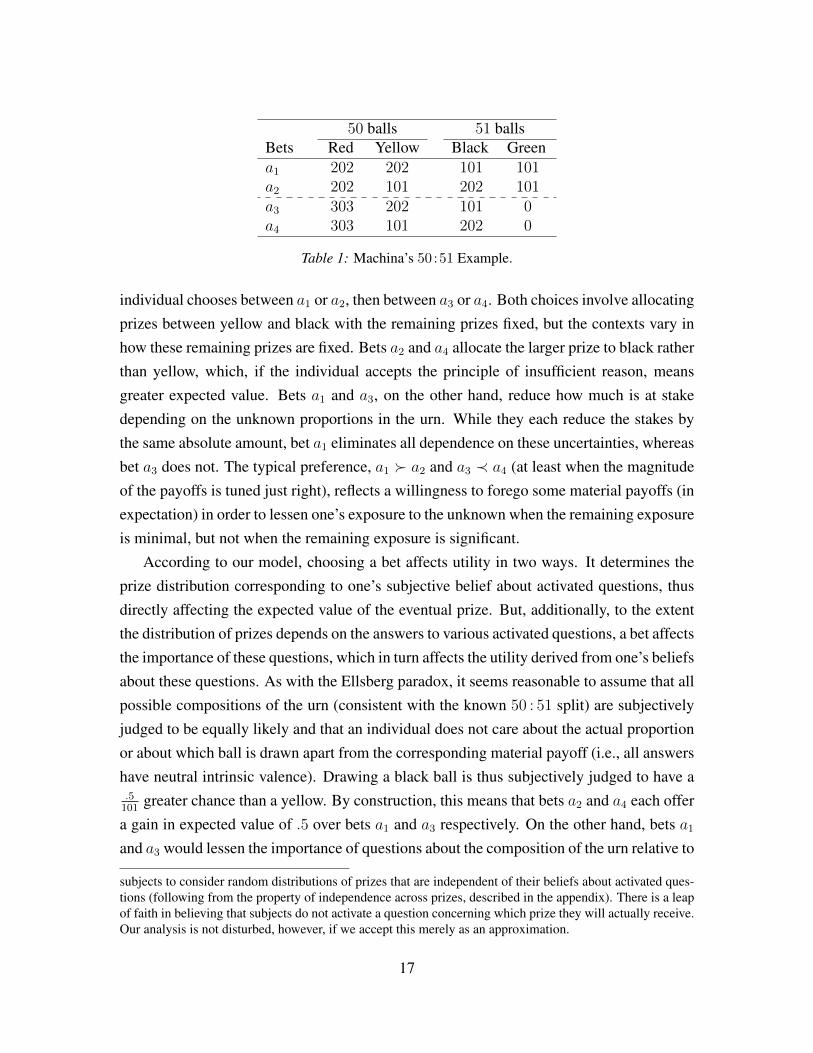
50 balls 51 ballsBets Red Yellow Black Greena1 202 202 101 101a2 202 101 202 101a3 303 202 101 0a4 303 101 202 0

Table 1: Machina’s 50:51 Example.

individual chooses between a1 or a2, then between a3 or a4. Both choices involve allocatingprizes between yellow and black with the remaining prizes fixed, but the contexts vary inhow these remaining prizes are fixed. Bets a2 and a4 allocate the larger prize to black ratherthan yellow, which, if the individual accepts the principle of insufficient reason, meansgreater expected value. Bets a1 and a3, on the other hand, reduce how much is at stakedepending on the unknown proportions in the urn. While they each reduce the stakes bythe same absolute amount, bet a1 eliminates all dependence on these uncertainties, whereasbet a3 does not. The typical preference, a1 � a2 and a3 ≺ a4 (at least when the magnitudeof the payoffs is tuned just right), reflects a willingness to forego some material payoffs (inexpectation) in order to lessen one’s exposure to the unknown when the remaining exposureis minimal, but not when the remaining exposure is significant.

According to our model, choosing a bet affects utility in two ways. It determines theprize distribution corresponding to one’s subjective belief about activated questions, thusdirectly affecting the expected value of the eventual prize. But, additionally, to the extentthe distribution of prizes depends on the answers to various activated questions, a bet affectsthe importance of these questions, which in turn affects the utility derived from one’s beliefsabout these questions. As with the Ellsberg paradox, it seems reasonable to assume that allpossible compositions of the urn (consistent with the known 50 : 51 split) are subjectivelyjudged to be equally likely and that an individual does not care about the actual proportionor about which ball is drawn apart from the corresponding material payoff (i.e., all answershave neutral intrinsic valence). Drawing a black ball is thus subjectively judged to have a.5101

greater chance than a yellow. By construction, this means that bets a2 and a4 each offera gain in expected value of .5 over bets a1 and a3 respectively. On the other hand, bets a1and a3 would lessen the importance of questions about the composition of the urn relative to

subjects to consider random distributions of prizes that are independent of their beliefs about activated ques-tions (following from the property of independence across prizes, described in the appendix). There is a leapof faith in believing that subjects do not activate a question concerning which prize they will actually receive.Our analysis is not disturbed, however, if we accept this merely as an approximation.

17

bets a2 and a4 respectively. This would decrease the attention weight on the uncertain beliefabout the composition of the urn – a negative belief because of the uncertainty. Decreasingthe attention weight on a negative belief, of course, increases utility. Our assumptions donot specify precisely how much the attention weight decreases as the stakes are reduced,but it is perfectly reasonable to think that there is diminishing sensitivity of attention weightto how much is at stake corresponding to an uncertain belief. Thus, our model can easilyaccommodate a greater gain in utility when rendering an uncertainty completely moot thanwhen partially drawing down a higher-stakes exposure (and merely limiting its importancesomewhat). This would allow the pattern a1 � a2 and a3 ≺ a4.

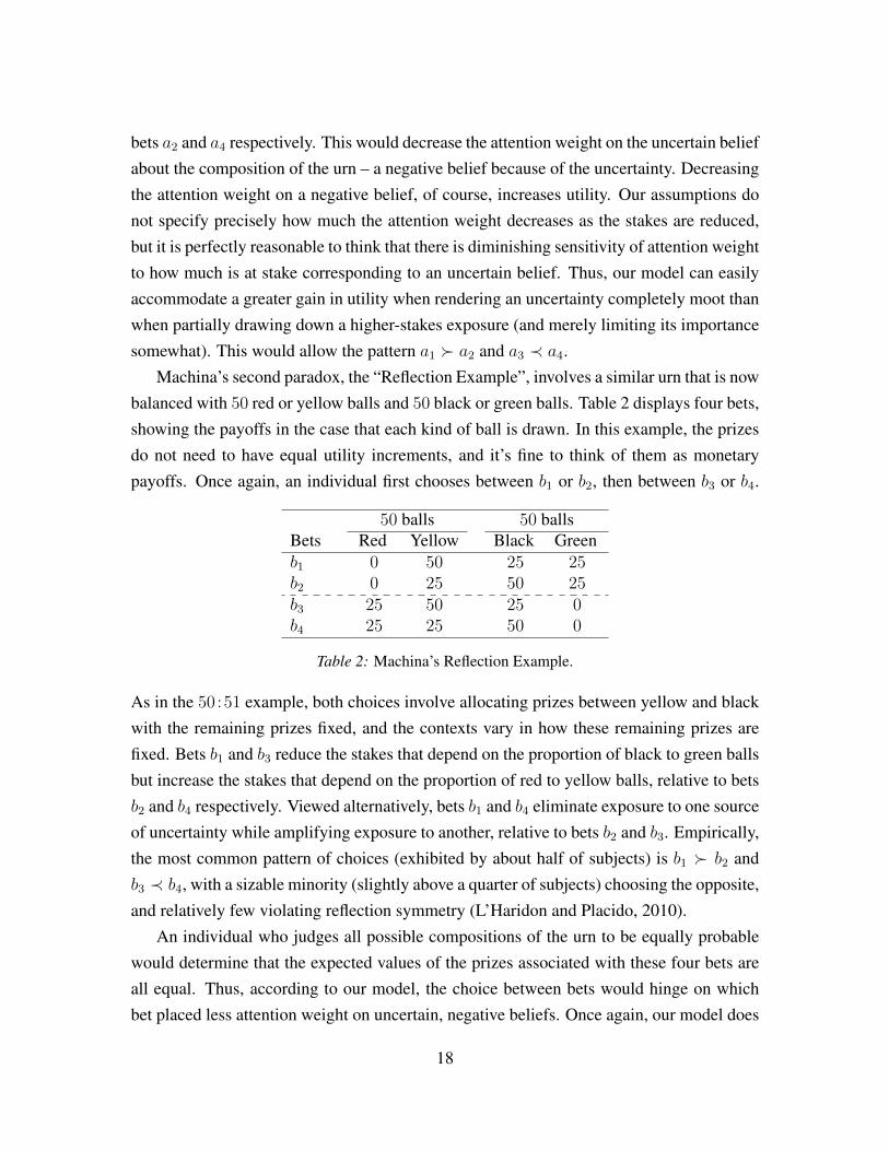
Machina’s second paradox, the “Reflection Example”, involves a similar urn that is nowbalanced with 50 red or yellow balls and 50 black or green balls. Table 2 displays four bets,showing the payoffs in the case that each kind of ball is drawn. In this example, the prizesdo not need to have equal utility increments, and it’s fine to think of them as monetarypayoffs. Once again, an individual first chooses between b1 or b2, then between b3 or b4.

50 balls 50 ballsBets Red Yellow Black Greenb1 0 50 25 25b2 0 25 50 25b3 25 50 25 0b4 25 25 50 0

Table 2: Machina’s Reflection Example.

As in the 50:51 example, both choices involve allocating prizes between yellow and blackwith the remaining prizes fixed, and the contexts vary in how these remaining prizes arefixed. Bets b1 and b3 reduce the stakes that depend on the proportion of black to green ballsbut increase the stakes that depend on the proportion of red to yellow balls, relative to betsb2 and b4 respectively. Viewed alternatively, bets b1 and b4 eliminate exposure to one sourceof uncertainty while amplifying exposure to another, relative to bets b2 and b3. Empirically,the most common pattern of choices (exhibited by about half of subjects) is b1 � b2 andb3 ≺ b4, with a sizable minority (slightly above a quarter of subjects) choosing the opposite,and relatively few violating reflection symmetry (L’Haridon and Placido, 2010).

An individual who judges all possible compositions of the urn to be equally probablewould determine that the expected values of the prizes associated with these four bets areall equal. Thus, according to our model, the choice between bets would hinge on whichbet placed less attention weight on uncertain, negative beliefs. Once again, our model does

18

not specify precisely how much importance, or, in turn, attention weight, decreases as thestakes associated with an uncertain belief are drawn down, and there could well be hetero-geneity across the population, so the model does not rule out any pattern of behavior inthis example. Still, from this perspective, the typical pattern of behavior is not surprising.If, as we hypothesized in order to explain the 50 : 51 example, attention weight exhibitsdiminishing sensitivity to exposure to an uncertain belief, then eliminating a modest ex-posure entirely would have a greater effect than partially reducing a large exposure by thesame amount. By the informational symmetry between the red/yellow composition and thegreen/black composition, the (negative) value of the (uncertain) belief about each shouldbe equal. Accordingly, a greater reduction in attention weight would lead to a greater in-crease in utility, regardless of which uncertainty is rendered moot. That is, we would thenpredict b1 � b2 and b3 ≺ b4. Thus, diminishing sensitivity of attention weight with respectto the stakes associated with an uncertain belief allows our model to accommodate both ofMachina’s paradoxes.

5 An Experimental Test of a Key PredictionThe ‘acid’ test of a new theory is to generate testable predictions that other theories do notpredict, and which have not already been tested. Here, we report such a test of our theory.The key prediction of the theory is that people will be more willing to bet on, and will betmore on, uncertainties that they like to think about. We created a situation likely to producestrong feelings by having pairs of people compete on a two-part intelligence test, with oneperson winning and one person losing. Both individuals then had the opportunity to bet onwhether they did better on the first part of the test than the second and to make the com-plementary bet that they did better on the second part of the test than the first. Our premiseis that people who won the competition would find it more pleasurable to think about thetest, so we predicted that winners would be willing to bet more, in total, on the two com-plementary bets than would losers. Of course, subjects could not be randomly assigned tothe conditions of winning or losing the competition, so there could be a selection effect. Torule out a selection effect, we controlled for idiosyncratic risk preferences by also offeringsubjects a third bet on a random event involving rolls of dice.

We recruited subjects for time slots, deliberately scheduling two subjects for each slot.The subjects were recruited separately (so most did not know one-another) and participatedfor a show-up fee of $10 and the opportunity to win additional money and/or prizes throughincentivized choices.

19

The two subjects first competed against one-another on a math quiz to win a non-monetary prize. The math quiz was derived from previous GRE tests. It consisted of18 questions, divided into two clusters of 9 problems. One cluster consisted of traditionalmath problems (e.g., if 5x + 32 = 42x, what is the value of x?), and the other consistedof quantitative comparison problems (e.g., which is greater: 54% of 360 or 150?). Theorder of the two clusters was randomly determined, and subjects were given 6 minutes towork on each cluster, with a warning one minute from the end of each 6 minute interval.The warning instructed them that they had a minute left, and encouraged them to guessas needed to give some answer to each question, since there was no penalty for incorrectanswers. Upon completion, quizzes were scored immediately. Subjects were informed oftheir total score on all 18 problems, but, crucially, were not told their score breakdown oneach cluster of the quiz. The subject in each pair who received the higher score was givena bonus prize – a succulent plant with a retail value of $3-$5.

Subjects were then told that they would be presented with three gambles and weretold that only one of them would count, to be determined randomly. Each gamble waspresented sequentially, with no preview of what subsequent gambles would consist of. Thefirst gamble was presented as follows:

Gamble 1 depends on your performance on the quiz. Gamble 1 will payequal to your wager if your score on the quantitative comparison questionsis greater than or equal to your score on the problem solving questions.

Please indicate how much you are willing to wager. You can wager up to halfyour money ($5). If you win the bet, then you will get back double the amountyou wager. If you lose the bet, then you will lose the amount you wager.

How much do you want to wager?

nothing $1 $2 $3 $4 $5

The second gamble was the complementary bet that paid only if their score on problemsolving questions was greater than or equal to that on the quantitative comparisons ques-tions. The third gamble involved two rolls of a ten-sided die. It paid out if the second rollwas greater than or equal to the first roll. The amount that subjects wanted to stake on eachof these gambles was elicited in the same way as it was for the first (with the knowledge thatonly one of their choices would count). An exit survey collected their attitudes regardingthe task and prize as well as demographic data.

20

Subjects were 102 individuals from Pittsburgh area universities (48 males, 54 females,Mage = 24.75) who were recruited using the Carnegie Mellon University Center for Be-havioral and Decision Research Participant Pool. One subject was excluded from the anal-ysis because he achieved a perfect score on the 20 item test, from which he could infer thathis score on the two parts would be equal.19

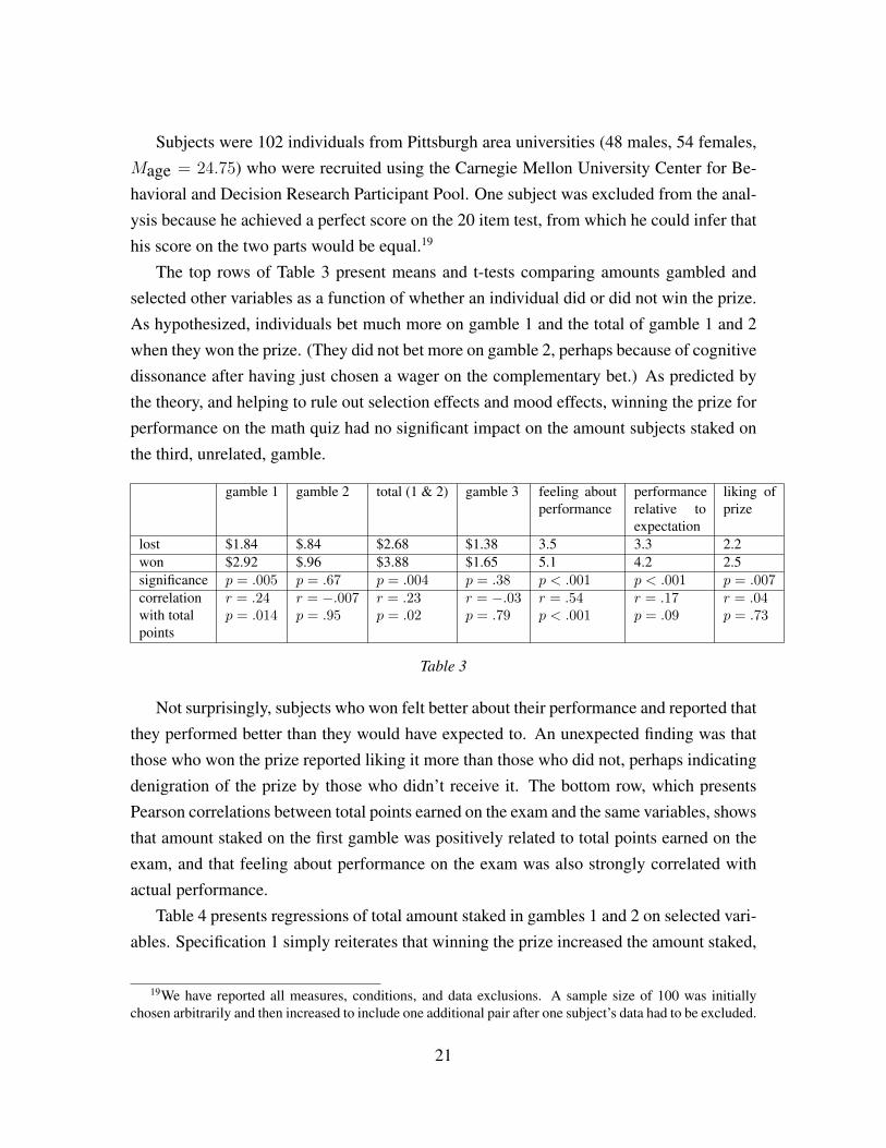
The top rows of Table 3 present means and t-tests comparing amounts gambled andselected other variables as a function of whether an individual did or did not win the prize.As hypothesized, individuals bet much more on gamble 1 and the total of gamble 1 and 2when they won the prize. (They did not bet more on gamble 2, perhaps because of cognitivedissonance after having just chosen a wager on the complementary bet.) As predicted bythe theory, and helping to rule out selection effects and mood effects, winning the prize forperformance on the math quiz had no significant impact on the amount subjects staked onthe third, unrelated, gamble.

gamble 1 gamble 2 total (1 & 2) gamble 3 feeling aboutperformance

performancerelative toexpectation

liking ofprize

lost $1.84 $.84 $2.68 $1.38 3.5 3.3 2.2won $2.92 $.96 $3.88 $1.65 5.1 4.2 2.5significance p = .005 p = .67 p = .004 p = .38 p < .001 p < .001 p = .007correlation r = .24 r = −.007 r = .23 r = −.03 r = .54 r = .17 r = .04with total p = .014 p = .95 p = .02 p = .79 p < .001 p = .09 p = .73points

Table 3

Not surprisingly, subjects who won felt better about their performance and reported thatthey performed better than they would have expected to. An unexpected finding was thatthose who won the prize reported liking it more than those who did not, perhaps indicatingdenigration of the prize by those who didn’t receive it. The bottom row, which presentsPearson correlations between total points earned on the exam and the same variables, showsthat amount staked on the first gamble was positively related to total points earned on theexam, and that feeling about performance on the exam was also strongly correlated withactual performance.

Table 4 presents regressions of total amount staked in gambles 1 and 2 on selected vari-ables. Specification 1 simply reiterates that winning the prize increased the amount staked,

19We have reported all measures, conditions, and data exclusions. A sample size of 100 was initiallychosen arbitrarily and then increased to include one additional pair after one subject’s data had to be excluded.

21

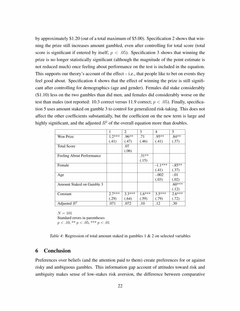
by approximately $1.20 (out of a total maximum of $5.00). Specification 2 shows that win-ning the prize still increases amount gambled, even after controlling for total score (totalscore is significant if entered by itself; p < .05). Specification 3 shows that winning theprize is no longer statistically significant (although the magnitude of the point estimate isnot reduced much) once feeling about performance on the test is included in the equation.This supports our theory’s account of the effect – i.e., that people like to bet on events theyfeel good about. Specification 4 shows that the effect of winning the prize is still signifi-cant after controlling for demographics (age and gender). Females did stake considerably($1.10) less on the two gambles than did men, and females did considerably worse on thetest than males (not reported: 10.3 correct versus 11.9 correct; p < .05). Finally, specifica-tion 5 uses amount staked on gamble 3 to control for generalized risk-taking. This does notaffect the other coefficients substantially, but the coefficient on the new term is large andhighly significant, and the adjusted R2 of the overall equation more than doubles.

1 2 3 4 5Won Prize 1.2*** .96** .71 .95** .84**

(.41) (.47) (.46) (.41) (.37)Total Score .07

(.06)Feeling About Performance .31**

(.15)Female -1.1*** -.85**

(.41) (.37)Age -.002 -.01

(.03) (.02)Amount Staked on Gamble 3 .60***

(.12)Constant 2.7*** 3.3*** 1.6*** 3.5*** 2.6***

(.29) (.64) (.59) (.79) (.72)Adjusted R2 .071 .072 .10 .12 .30

N = 101Standard errors in parenthesesp < .10, ** p < .05, *** p < .01

Table 4: Regression of total amount staked in gambles 1 & 2 on selected variables

6 ConclusionPreferences over beliefs (and the attention paid to them) create preferences for or againstrisky and ambiguous gambles. This information gap account of attitudes toward risk andambiguity makes sense of low-stakes risk aversion, the difference between comparative

22

and non-comparative responses to ambiguity vis a vis risk, and the sensitivity of ambiguitypreference to the source of the uncertainty. It is consistent with empirically documentedpatterns of behavior that have been difficult for other theories to reconcile. We have estab-lished the following testable predictions:

H1 Individuals prefer to avoid actuarially fair lotteries that do not involve events thatthey particularly enjoy thinking about.

H2 Individuals prefer an equivalent simple lottery to a compound lottery that does notinvolve events that they enjoy thinking about.

H3 Individuals prefer to wager on uncertainties they enjoy thinking about (i.e., that de-pend on positive beliefs) than on objectively random events, but prefer such randombets to wagers that depend on negative beliefs.

H4 Individuals forced to choose among wagers that depend on negative beliefs prefer towager on an uncertainty that is less salient.

Timing effects are not part of our formal model, and intuitions about the effects of timedelay runs in both directions. From one point of view, it seems intuitive that the costs (orbenefits) associated with thinking about negative (or positive) beliefs would scale with theamount of time that an individual spends thinking about them. To the extent the pleasuresor pains of focusing on an information gap account for risk and ambiguity preferences, weshould then expect that some time delay between exposure to uncertainty (risk or ambigu-ity) and resolution of that uncertainty would strengthen risk and ambiguity preferences. Onthe other hand, there is substantial evidence that the feelings associated with uncertaintyare strongest right before uncertainty is going to be resolved (van Winden et al., 2011).This suggests that short- and long-term time discounting will dictate whether time delaystrengthens or weakens risk and ambiguity preferences. Although we are reluctant to offerany general predictions about the effect of time delays, to the degree that time delay inten-sifies risk or ambiguity preferences, we would speculate that the effects would be strongerfor people who discount the future less.

The primary determinant of risk and ambiguity preference in our model is how peoplefeel when they think about the information they are missing about a gamble. These feelingsare likely to be a function of a wide range of factors, including the outcomes, associatedprobabilities, the vividness of outcomes, the individuals feeling of expertise, any contextualfactors (e.g., residual sadness or elation) which affect the individuals emotional reactions,and a variety of individual dispositional factors. Another tenet of our model is that feel-ings, and hence preferences, should depend on the salience of the missing information –

23

the information gap. Salience is, in turn, likely to depend on situational factors, decisionframing, and the existence of counterfactuals that highlight the information gap. We haveshown that these effects can make sense of a variety of already established empirical ef-fects, and also provided experimental evidence in support of a key, previously untested,prediction. Many other predictions will, we hope, be tested in future empirical research.

AppendixProof of Proposition 1

Linearity of vX implies that uX(πX [b]) = uX(πX [¬b]). However, because bet b spreadsout the utilities that would result from discovering either heads or tails, it increases γ1,which implies that w1[b] > w1[¬b]. By the one-sided sure-thing principle, we know thatv1(π1) < 0 (regardless of whether the bet is taken) because the belief about the coin flipis not degenerate (i.e., because it is uncertain). Accepting the bet would increase attentionweight on a negative belief and would thus lower utility, so ¬b � b.

Proof of Proposition 2

Actions ai and aj determine subjective probability measures π[ai] and π[aj] and attentionweight vectors w[ai] and w[aj] such that:

1. πA[ai](·) = πA[aj](·);

2. conditioning on any belief about questions outside of QE , we have πX [ai](·) =πX [aj](·);

3. wi[ai] = wj[aj] and wj[ai] = wi[aj];

4. for any ν such that Qν ∈ QE , ν 6= i, ν 6= j, we have wν [ai] ≥ wν [aj] with strictinequality for ν = ı;

5. for any ν such that Qν ∈ Q\QE , we have wν [ai] = wν [aj].

The first condition holds because instrumental actions determine prizes, but not beliefs. Thesecond condition must hold by the assumption that Qi and Qj have the same subjectiveprobabilities. Condition 3 follows from the assumption that Qi and Qj have the samesalience together with the observations that the same material importance is given to eachquestion when the corresponding action is taken (because the questions have the samesubjective probabilities and the actions attach the same prizes) and that neither question isimportant when the other action is taken. The crucially important fourth condition appliesbecause only question Qi has dependence on QE\{Qi, Qj}, so only action ai can increasethe importance of these other questions. Lastly, condition 5 holds because questions outsideof QE are independent of Qi and Qj .

24

The assumption of independence across prizes applies to the valence of prizes so thatfor the default belief about questions outside of QE , valence is equal for the two actionsbecause they create the same subjective distribution over prizes (condition 2).

Because questions Qi and Qj have the same subjective probabilities as well as thesame (neutral) valences for all possible answers, it can be shown (using the assumptionsof label independence and linearity with respect to attention weights) that the utility costof an increase in attention weight on one is equal to the utility cost of the same increase inattention weight on the other.

Any uncertain belief about a question inQE must be a negative belief because certaintywould be a neutral belief and the one-sided sure-thing principle applies. Thus, by theassumption of monotonicity with respect to attention weights, the increase in attentionweight on questionQı that occurs for action ai (according to condition 4) causes a decreasein utility.

Proof of Proposition 3

As in Proposition 2, bet ai attached to question Qi makes question Qı more important andthus increases the attention weight on a negative belief. By the assumption that attentionweight exhibits increasing differences in salience and importance, the decrease in utilitydue to this effect is worse in cognitive state (π, w) when question Qı is more salient thanin cognitive state (π,w).

Proof of Proposition 4

By our construction, utility exhibits increasing differences in the value of a belief and theattention weight on it. For sufficiently high υ, even an uncertain belief will be a positivebelief. In this case, increasing the attention weight on it increases utility, so the bet aibecomes favored relative to aj .ReferencesAbdellaoui, M., Baillon, A., Placido, L., Wakker, P. (2011). The Rich Domain of Uncer-

tainty: Source Functions and their Experimental Implementation. American EconomicReview 101, 695-723.

Abdellaoui, M., Klibanoff, P., Placido, L. (2013). Experiments on Compound Risk inRelation to Simple Risk and to Ambiguity.

Ahn, D., Choi, S., Gale, D., Kariv, S. (2013). Estimating Ambiguity Aversion in a PortfolioChoice Experiment.

Allais, M. (1953). Le Comportement de l’Homme Rationnel devant le Risque: Critiquedes Postulats et Axiomes de l’Ecole Americaine. Econometrica 21 (4), 503-546.

Anagol, S. Gamble, K. (2011). Does Presenting Investment Results Asset by Asset LowerRisk Taking? University of Pennsylvania Working Paper.

Andreoni, J., Schmidt, T., Sprenger, C. (2014). Measuring Ambiguity Aversion: Experi-mental Tests of Subjective Expected Utility. In prep.

Anscombe, F., Aumann, R. (1963). A Definition of Subjective Probability. Annals ofMathematical Statistics 34, 199-205.

25

Babad, E., Katz, Y. (1991). Wishful Thinking: Against all Odds. Journal of Applied SocialPsychology 21, 1921-1938.

Bach, D., Seymour, B., Dolan, R. (2009). Neural Activity Associated with the PassivePrediction of Ambiguity and Risk for Aversive Events. The Journal of Neuroscience29, 1648-1656.

Baillon, A., L’Haridon, O., Placido, L. (2011). Ambiguity Models and the Machina Para-doxes. American Economic Review 101, 1547-1560.

Barberis, N. (2011). Psychology and the Financial Crisis of 2007-2008.Becker, S., Brownson, F. (1964). What Price Ambiguity? Or the Role of Ambiguity in

Decision-Making. Journal of Political Economy 72, 62-73.Bellemare, C., Krause, M., Kroger, S., Zhang, C. (2005). Myopic Loss Aversion: Informa-

tion Feedback vs. Investment Flexibility. Economics Letters 87, 319-324.Bernasconi, M., Loomes, G. (1992). Failures of the Reduction Principle in an Ellbserg-

Type Problem. Theory and Decision 32(1), 77-100.Bordalo, P., Gennaioli, N., Shleifer, A. (2012). Salience Theory of Choice Under Risk.

Quarterly Journal of Economics 127 (3), 1243-1285.Borghans, L., Heckman, J., Golsteyn, B., Meijer, H. (2009). Gender Differences in Risk

Aversion and Ambiguity Aversion. Journal of the European Economic Association 7,649-658.

Brass, M., von Cramon, D. (2004). Selection for Cognitive Control: A Functional MagneticResonance Imaging Study on the Selection of Task-Relevant Information. The Journalof Neuroscience 24, 8847-8852.

Callen, M., Isaqzadeh, M., Long, J., Sprenger, C. (2013). Violence and Risk Preference:Experimental Evidence from Afghanistan? American Economic Review forthcoming.

Caplin, A., Leahy, J. (2001). Psychological Expected Utility Theory And AnticipatoryFeelings. Quarterly Journal of Economics 116 (1) 55-79.

Cohn, A., Engelmann, J., Fehr, E., Marechal, M. (2015). Evidence for Countercyclical RiskAversion: An Experiment with Financial Professionals. American Economic Review105 (2).

Curley, S., Yates., F., Abrams, R. (1986). Psychological Sources of Ambiguity Avoidance.Organizational Behavior and Human Decision Processes 38, 230-256.

Diecidue, E., Schmidt, U., Wakker, P. (2004). The Utility of Gambling Reconsidered.Journal of Risk and Uncertainty 29, 241-259.

Ellsberg, D. (1961). Risk, ambiguity, and the Savage axioms. Quarterly Journal of Eco-nomics 75, 643-699.

Epstein, L. (2008). Living with Risk. Review of Economic Studies 75 (4), 1121-1141.Ergin, H., Gul, F. (2009). A theory of subjective compound lotteries. Journal of Economic

Theory 144, 899-929.Fishburn, P. (1980). A Simple Model for the Utility of Gambling. Psychometrika 45,

435-448.Fox, C., Tverksy, A. 1995. Ambiguity Aversion and Comparative Ignorance. Quarterly

Journal of Economics 110 (3), 585-603.

26

Fox, C., Weber, M. (2002). Ambiguity Aversion, Comparative Ignorance, and DecisionContext. Organizational Behavior and Human Decision Processes 88, 476-498.

Frisch, D., Baron, J. (1988). Ambiguity and rationality. Journal of Behavioral DecisionMaking 1, 149-157.

Ghirardato, P., Maccheroni, F., Marinacci, M. (2004). Differentiating Ambiguity and Am-biguity Attitude. Journal of Economic Theory 118, 133-173.

Gilboa, I., Schmeidler, D. (1989). Maxmin Expected Utility with Non-Unique Prior. Jour-nal of Mathematical Economics 18 (2), 141-153.

Golman, R., Loewenstein, G. (2015a). An Information-Gap Framework for Capturing Pref-erences About Uncertainty. Proceedings of the Fifteenth Conference on TheoreticalAspects of Rationality and Knowledge.

Golman, R., Loewenstein, G. (2015b). Curiosity, Information Gaps, and the Utility ofKnowledge.

Gneezy, U., List, J., Wu, G. (2006). The Uncertainty Effect: When a Risky Prospect isValued Less than its Worst Possible Outcome. Quarterly Journal of Economics 121(4), 1283-1309.

Gneezy, U., Potters, J. (1997). An Experiment on Risk Taking and Evaluation Periods.Quarterly Journal of Economics 112 (2), 631-645.

Haigh, M., List, J. (2005). Do Professional Traders Exhibit Myopic Loss Aversion? AnExperimental Analysis. Journal of Finance 60 (1), 523-534.

Halevy, Y. (2007). Ellsberg Revisited: An Experimental Study. Econometrica 75 (2), 503-536.

Heath, C., Tversky, A. (1991). Preference and Belief: Ambiguity and Competence inChoice under Uncertainty. Journal of Risk and Uncertainty 4 (1), 5-28.

Holt, C., Laury, S. (2002). Risk Aversion and Incentive Effects. American EconomicReview 92 (5), 1644-1655.

Hsee, C., Kunreuther, H. (2000). The Affection Effect in Insurance Decisions. Journal ofRisk and Uncertainty 20, 141-159.

Hsu, M., Bhatt, M., Adolphs, R., Tranel, D., Camerer, C. (2005). Neural Systems Respond-ing to Degrees of Uncertainty in Human Decision-Making. Science 310, 1680-1683.

Huettel, S., Stowe, C., Gordon, E., Warner, B., Platt, M. (2006). Neural Signatures ofEconomic Preferences for Risk and Ambiguity. Neuron 49, 765-775.

Imas, A. (2014). The Realization Effect: Risk Taking after Realized versus Paper Losses.In prep.

Kahneman, D., Tversky, A. (1979). Prospect Theory: An Analysis of Decision Under Risk.Econometrica 47, 263-291.

Keppe, H.-J., Weber, M. (1995). Judged knowledge and ambiguity aversion. Theory andDecision 39, 51-77.

Kilka, M., Weber, M. (2000). Home bias in international stock return expectations. Journalof Psychology and Financial Markets 1, 176-192.

Klibanoff, P., Marinacci, M., Mukerji, S. (2005). A Smooth Model of Decision Makingunder Ambiguity. Econometrica 73, 1849-1892.

27

Kocher, M., Krawczyk, M., van Winden, F. (2014). Let Me Dream On! AnticipatoryEmotions and Preference for Timing in Lotteries. Journal of Economic Behavior andOrganization 2, 29-40.

Koszegi, B., Rabin, M. (2006). A Model of Reference-Dependent Preferences. QuarterlyJournal of Economics 121(4), 1133-1165.

L’Haridon, O., Placido, L. (2010). Betting on Machina’s Reflection Example: An Experi-ment on Ambiguity. Theory and Decision 69 (3), 375-393.

Loewenstein, G., Weber, E., Hsee, C., Welch, N. (2001). Risk as Feelings. PsychologicalBulletin 127, 267-286.

Loomes, G., Sugden, R. (1982). Regret Theory: An Alternative Theory of Rational Choiceunder Uncertainty. Economic Journal 92, 805-824.

Luce, R.D., Raiffa, H. (1957). Games and Decisions. New York: Wiley.Maccheroni, F., Marinacci, M., Rustichini, A. (2005). Ambiguity Aversion, Robustness,

and the Variational Representation of Preferences. Econometrica 74, 1447-1498.MacCrimmon, K., Larsson, S. (1979). Utility Theory: Axioms Versus “Paradoxes”. In

Expected Utility Hypotheses and the Allais Paradox, M. Allais and O. Hagen (Eds.),Holland: D. Reidel Publishing Company.

Machina, M. (2009). Risk, Ambiguity, and the Rank-Dependence Axioms. AmericanEconomic Review 99 (1), 385-392.

Morewedge, C. (2013). Reluctance to Hedge. In prep.Nau, R. (2006). Uncertainty Aversion with Second-Order Utilities and Probabilities. Man-

agement Science 52, 136-145.Prelec, D., Loewenstein, G. (1998). The Red and the Black: Mental Accounting of Savings

and Debt. Marketing Science 17, 4-28.Quiggin, J. (1982). A Theory of Anticipated Utility. Journal of Economic Behavior and

Organization 3 (4), 323-343.Rabin, M. (2000). Risk Aversion and Expected-utility Theory: A Calibration Theorem.

Econometrica 68 (5), 1281-1292.Ritov, I., Baron, J. (1990). Reluctance to vaccinate: Omission bias and ambiguity. Journal

of Behavioral Decision Making 3 (4), 263-277.Savage, L. (1954). The Foundations of Statistics. New York: Wiley.Schmeidler, D. (1989). Subjective Probability and Expected Utility without Additivity.

Econometrica 57 (3), 571-587.Schmidt, U., Starmer, C., Sugden, R. (2008). Third-Generation Prospect Theory. Journal

of Risk and Uncertainty 36, 203-223.Segal, U. (1987). The Ellsberg Paradox and Risk: An Anticipated Utility Approach. Inter-

national Economic Review 28, 175-202.Segal, U. (1990). Two-Stage Lotteries without the Reduction Axiom. Econometrica 58,

349-377.Seo, K. (2009). Ambiguity and Second-Order Belief. Econometrica 77, 1575-1605.Simonsohn, U. (2009). Direct Risk Aversion. Psychological Science 20 (6), 686-692.

28

Spears, D. (2013). Poverty and Probability: Aspiration and Aversion to Compound Lotter-ies in El Salvador and India. Experimental Economics 16 (3), 263-284.

Taylor, K. (1995). Testing credit and blame attributions as explanation for choices underambiguity. Organizational Behavior and Human Decision Processes 54, 128-137.

Taylor, S., Brown, J. (1988). Illusion and Well-Being: A Social Psychological Perspectiveon Mental Health. Psychological Bulletin 103 (2), 193-210.

Trautmann, S., Vieider, F., Wakker, P. (2008). Causes of ambiguity aversion: Known versusunknown preferences. Journal of Risk and Uncertainty 36, 225-243.

Tversky, A., Kahneman, D. (1992). Advances in Prospect Theory: Cumulative Represen-tation of Uncertainty. Journal of Risk and Uncertainty 5, 297-323.

Tymula, A., Belmaker, L., Roy, A., Ruderman, L., Manson, K., Glimcher, P., Levy, I.(2012). Adolescents’ Risk-Taking Behavior Is Driven by Tolerance to Ambiguity. Pro-ceedings of the National Academy of Sciences 109 (42), 17135-17140.

van Winden, F., Krawczyk, M., Hopfensitz, A. (2011). Investment, Resolution of Risk, andthe Role of Affect. Journal of Economic Psychology 32 (6), 918-939.

von Neumann, J., Morgenstern, O. (1944). Theory of Games and Economic Behavior.Princeton: Princeton University Press.

Weaver, R., Frederick, S. (2012). A Reference Price Theory of the Endowment Effect.Journal of Marketing Research, forthcoming.

Weinstein, N. (1980). Unrealistic Optimism About Future Life Events. Journal of Person-ality and Social Psychology 39 (5), 806-820.

Yang, Y., Vosgerau, J., Loewenstein, G. (2013). The Influence of Framing on Willingnessto Pay: An Explanation for the Uncertainty Effect.

29