Embed Size (px)
Citation preview
Information Retrieval Based on Spectral and
Semantic Analysis
By: Sara Saed Alnofaie
A thesis submitted for the requirement of the degree of Master of Science
Computer Science
Supervised By:
Dr. Mohamed Dahab
Dr. Mahmoud Kamel (Co-Advisor)
FACULTY OF COMPUTING AND INFORMATION TECHNOLOGY
KING ABDULAZIZ UNIVERSITY
JEDDAH – SAUDI ARABIA
1438H – 2016G


i
Information Retrieval Based on Spectral and
Semantic Analysis
By: Sara Saed Alnofaie
A thesis submitted for the requirement of the degree of Master of Science
Computer Science
Supervised By:
Dr. Mohamed Dahab
Dr. Mahmoud Kamel (Co-Advisor)
FACULTY OF COMPUTING AND INFORMATION TECHNOLOGY
KING ABDULAZIZ UNIVERSITY
JEDDAH – SAUDI ARABIA
1438H – 2016G
ii
Information Retrieval Based on Spectral and
Semantic Analysis
By: Sara Saed Alnofaie
This thesis has been approved and accepted in partial fulfilment of the
requirements for the degree of Master of Science (Computer Science)
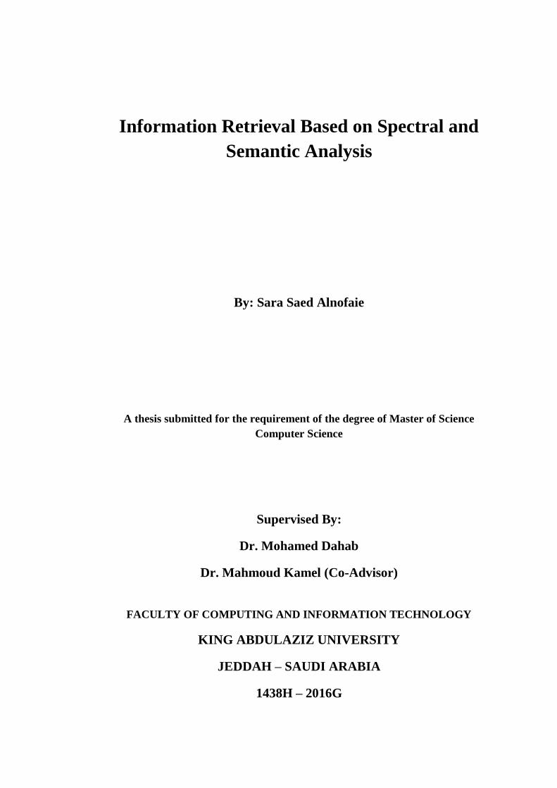
EXAMINATION COMMITTEE
KING ABDULAZIZ UNIVERSITY
1438 H- 2016 G
Signature Field Rank Name
Computer
Science
Associate
Professor
Dr.Abdullah
Basuhail Internal
Examiner
Electrical and
Computer
Engineering
Professor Prof. Yasser
Mostafa Kadah External
Examiner
Information
System
Assistant
Professor
Dr. Mahmoud Kamel
Co-Advisor
Computer
Science
Assistant
Professor
Dr. Mohammed Dahab Advisor

iii
Dedicated to:
This work dedicated to my beloved parents, my dear sisters, and brothers.

iv
ACKNOWLEDGEMENT
I would like to express my gratitude to Allah (God) for providing me the blessings to
complete this work. I also would like to ask Him to ensure that this thesis will be
beneficial to other researchers.
To my supervisors, Dr. Kamel and Dr. Dahab: I feel highly indebted to you. I am
deeply grateful for your suggestion of this topic, support, comments, and guidance.
To my wonderful Parents: Words fail me to express my appreciation to you, the best
mother and father. I wish to give you all thanks and love for your guidance, advice,
and endless support.
Thank you to my wonderful Brother and sisters, Meshal, Sana, and Basma, who was
supportive and helpful at every stage of this thesis and belief in me.

v
PUBLICATIONS
[1] S. Alnofaie, M. Dahab and M. Kamal , “A Novel Information Retrieval Approach
using Query Expansion and Spectral-based,” International Journal of Advanced
Computer Science and Applications (IJACSA), vol. 7, no. 9, 2016.
[2] M. Dahab, M. Kamal and S. Alnofaie," Further Investigations for Documents
Information Retrieval Based on DWT," in the 2nd International Conference on
Advanced Intelligent Systems and Informatics (AISI2016), 2016.

vi
Information Retrieval Based on Spectral and Semantic Analysis
Sara Saed ALnofaie
Abstract
Most of the information Retrieval (IR) models rank the documents by computing a
score using the lexicographical query terms or frequency of the query terms
information in the document. These models have limitations that do not consider the
terms proximity in the document or the term mismatch problem.
The terms proximity information is an important factor that determines the relatedness
of the document to the query. The ranking functions of the Spectral-Based Information
Retrieval Model (SBIRM) consider the query terms frequency and proximity in the
document by comparing the query terms signals in the spectral domain instead of the
spatial domain using Discrete Wavelet Transform (DWT).
The Query Expansion (QE) approaches are used to overcome the word mismatch
problem by expanding the query with terms having related meaning with the query.
The QE approaches are divided into the statistical approaches Kullback-Leibler
divergence (KLD), Local Context Analysis (LCA), newLCA, LCA with Jaccard,
Relevance Models (RM1) and semantic approach P-WNET that uses WordNet. All
these approaches improve the performance.
Based on the preceding considerations, the objective of this research is building the
efficient QESBIRM that combines QE and SBIRM by implementing the SBIRM using
the DWT and KLD, LCA, newLCA, LCA with Jaccard, RM1, P-WNET or
combination of them.
The experiments are conducted to test and evaluate the QESBIRM using Text
REtrieval Conference (TREC) dataset. The performance is evaluate in the term of
precision at top documents, precision at stander recall levels, R-precision, Geometric
Mean Average Precision (GMAP) and Mean Average Precision (MAP). The result
shows that the SBIRM with the KLD and P-WNET model outperformed the SBIRM
model; also that SBIRM with each co-occurrence approaches worse than the
performance of the SBIRM. In addition, the SBIRM with the P-WNETKLD that is a
combination of P-WNET and KLD is better than the SBIRM with each approach.

vii
الداللي والتحليل استرجاع المعلومات على أساس الطيف
سارة ساعد النفيعي
المستخلص
معلومات عدد مرات ظهور بناء على درجة تحسب باستخدام أغلب نماذج استرجاع المعلومات المستندات ترتب
الم من كلمات االستعنها ال تأخذ بعين االعتبار قرب هذه النماذج امن عيوب في المستند. االستعالم حرفياكلمات
مشكلة عدم تطابق الكلمات.بعضها لبعض أو
رتب الدالة التي تمن بعضها. كلمات االستعالمقرب من اهم العوامل التي تحدد مدى صلة المستند باالستعالم هو
ار عدد تأخذ باالعتباسترجاع المعلومات على االساس الطيفي لنموذج باالستعالم االمستندات بناء على صلته
دى قربها من بعض في المستند بواسطه مقارنة اشارات كلمات االستعالم في مرات ظهور كلمات االستعالم وم
.تحويل المويجات المتقطعةالمجال الطيفي بدال من المجال المكاني باستخدام
طرق توسيع االستعالم باستخدام كلمات لها معاني ذات صلة بكلمات االستعالم. تقوم لحل مشكلة عدم التطابق
Kullback-Leibler divergence Local Context, طرق توسيع االستعالم الى الطرق االحصائية تنقسم
Analysis, newLCA ,LCA with Jaccard Relevance Models, الداللية والطرقP-WNET التي
تحسين االداء.ب تقوم تستخدم الورد نت. كل هذه الطرق
الذي يجمع بين كفء QESBIRM نموذج هدف من هذا البحث هو بناءبناء على االعتبارات السالفة الذكر، ال
QE وSBIRM بتطبيقSBIRM و تحويل المويجات المتقطعةباستخدامKLD, LCA, newLCA, LCA
with Jaccard, RM1, P-WNET .او أي تجميع بين طريقتين
Text REtrieval Conferenceباستخدام مجموعة بيانات QESBIRMأجريت التجارب الختبار وتقييم
(TREC) باستخدام المقاييس .precision, R-precision, ,عند المستندات العلياprecision مستويات عند
recall ,القياسية Geometric Mean Average Precision (GMAP) وMean Average Precision
(MAP) . اظهرت التجارب أن نموذجSBIRM معKLD وP-WNET أفضل من اداء نموذج SBIRM
. باإلضافة لذلك SBIRMاداء نأسوء م co-occurrenceمع كل طريقة من طرق SBIRMو نموذج
SBIRM معP-WNETKLD استخدام طريقتيوهي عبارة عن P-WNET و KLD افضل كانت معا
مع كل طريقه بشكل منفصل. SBIRMمن
viii
TABLE OF CONTENTS
Dedication ................................................................................................................. iii
Acknowledgement .................................................................................................... iv
Abstract ..................................................................................................................... vi
Table of Contents ................................................................................................... viii
List of Figures .......................................................................................................... xii
List of Tables ........................................................................................................... xv
List of Symbols and Terminology ........................................................................ xvii
Chapter I: Introduction
1.1 Introduction ......................................................................................................... 1
1.2 Objectives ............................................................................................................ 3
1.3 Outline of the Thesis ............................................................................................. 3
Chapter II: Research Background
2.1 Information Retrieval ............................................................................................. 5
2.1.1 Boolean Retrieval ....................................................................................... 5
2.1.2 Ranked Retrieval ........................................................................................ 6
2.2 Spectral-Based Information Retrieval Model ..................................................... 13
2.2.1 Term Signal .............................................................................................. 14
2.2.2 Term Spectra ............................................................................................ 14
2.2.3 Discrete Wavelet Transform .................................................................... 15
2.2.4 Haar Wavelet Transform .......................................................................... 17
2.2.5 Document Score ....................................................................................... 21
ix
2.2.6 Spectral-Based Information Retrieval Model Example ........................... 22
2.3 WordNet ............................................................................................................. 24
2.3.1 WordNet Definition ................................................................................. 24
2.3.2 WordNet Structure ................................................................................... 25
2.3.3 Semantic Similarity Measures Based on WordNet .................................. 27
2.4 Automatic Query Expansion ............................................................................. 29
2.4.1 Automatic Query Expansion process ...................................................... 29
Chapter III: Literature Review
3.1 Proximity-Based Information Retrieval Model .................................................. 33
3.1.1 Shortest-Substring Model ........................................................................ 33
3.1.2 Fuzzy Proximity Model ........................................................................... 34
3.1.3 Combining Model .................................................................................... 35
3.1.4 Markov Random Field ............................................................................. 38
3.1.5 Spectral-Based Information Retrieval Model .......................................... 39
3.2 Automatic Query Expansion Approaches ........................................................... 40
3.2.1 Target Corpus Approaches ..................................................................... 40
3.2.2 External Resource Approaches ............................................................... 44
3.2.3 Target Corpus and External Resource Approaches ................................ 45
3.2.4 Combination Approach ......................................................................... 45
3.3 Automatic Query Expansion and Proximity-Based Information Retrieval
Model ................................................................................................................... 47
Chapter IV: Query Expansion approaches over the Spectral-Based Information
Retrieval Model
4.1 Design the Query Expansion approaches over the Spectral-Based Information
Retrieval Model .................................................................................................. 48
4.1.1 Preprocessing the Text ........................................................................... 51

x
4.1.2 Creating the Term Signals ...................................................................... 51
4.1.3 Applying the Weighting Scheme............................................................ 53
4.1.4 Applying the Transform ......................................................................... 54
4.1.5 Creating the Inverted Index .................................................................... 54
4.1.6 Applying the Query Expansion Approach ............................................. 55
4.1.6.1 Kullback-Leibler divergence Approach .............................. 55
4.1.6.2 LCA Approach .................................................................... 56
4.1.6.3 LCAnew Approach ............................................................. 56
4.1.6.4 LCA with Jaccard Approach ............................................... 57
4.1.6.5 Relevence Model Approach ................................................ 57
4.1.6.6 P-WNET Approach ............................................................. 58
4.1.6.7 Combination Approach ....................................................... 58
4.1.7 Applying the Re-weighting Scheme................................................... 58
4.2 Implement the Query Expansion approaches over the Spectral-Based Information
Retrieval Model .................................................................................................. 60
Chapter V: Experimental Results
5.1 Dataset ................................................................................................................. 61
5.2 Performance Measures ......................................................................................... 63
5.3 Experimental Results .......................................................................................... 64
5.3.1 Different Types of Document Segmentation ...................................... 66
5.3.2 Query Expansion Approaches over Spectral-Based Information
Retrieval Model .................................................................................. 67
5.3.3 Combine the Query Expansion Approaches over Spectral-Based
Information Retrieval Model .............................................................. 72
Chapter VI: Discussion and Comparison
6.1 Discussion ........................................................................................................... 74
6.2 Comparison ......................................................................................................... 82

xi
6.2.1 Frequency Based Information Retrieval Model ................................. 82
6.2.2 Proximity Based Information Retrieval Model .................................. 84
6.2.3 Query Expansion over the Frequency Based Information Retrieval
Model.................................................................................................. 86
6.2.4 Query Expansion over the Proximity Based Information Retrieval
Model................................................................................................ 100
Chapter VII: Conclusion and Future Work
7.1 Conclusion ........................................................................................................ 105
7.2 Future Work ............................................................................................................... 106
xii
LIST OF FIGURES
Figure Page
2.1 IR model Architecture ...................................................................................... 6
2.2 Vector Space Model ......................................................................................... 7
2.3 Cosine Similarity ............................................................................................. 9
2.4 Two sets with Jaccard similarity 3/8 ................................................................ 9
2.5 Document scoring by frequency IR models ................................................... 12
2.6 The example of create the term signals ……………………………………... 15
2.7 The relationship between 𝑉𝑛 as Ovals and 𝑊𝑛 as Annuli ................................ 16
2.8 The Dyadic Wavelet Transform (The High-Pass Filter (H) and the Low-Pass
Filter (L) ....................................................................................................... 16
2.9 The Recursive Filtering Process ..................................................................... 17
2.10 The Complete Haar Wavelet Transform Process .......................................... 20
2.11 Automatic QE process ................................................................................... 29
4.1 The text preprocessing and indexing phase steps ......................................... 49
4.2 The query processing phase steps ................................................................. 50
4.3 General Architecture of a proposed model ................................................... 51
4.4 Get Matrix Dimension procedure .................................................................. 53
4.5 Haar wavelet transform .................................................................................. 54
5.1 Document format in TREC dataset ............................................................... 62
5.2 Queries format in TREC dataset ................................................................... 63
6.1 The precision, Map, GMAP and RP of the document segmentations
methods......................................................................................................... 74
6.2 The Recall-Precision of the document segmentations methods .................... 75
6.3 The precision, Map, GMAP and RP of the SBIRM and KLD over the
SBIRM .......................................................................................................... 75

xiii
6.4 The Recall-Precision of the SBIRM and KLD over the SBIRM .................. 76
6.5 Comparison of the SBIRM and RM1 over the SBIRM ................................ 76
6.6 The Recall-Precision of the SBIRM and RM1 over the SBIRM .................. 77
6.7 Comparison of the SBIRM and LCA over the SBIRM ................................ 77
6.8 The Recall-Precision of the SBIRM and LCA over the SBIRM .................. 78
6.9 Comparison of the SBIRM and LCA with Jaccard over the SBIRM. .......... 78
6.10 The Recall-Precision of the SBIRM and LCA with Jaccard over the
SBIRM .......................................................................................................... 79
6.11 Comparison of the SBIRM and newLCA over the SBIRM ......................... 79
6.12 The Recall-Precision of the SBIRM and newLCA over the SBIRM ........... 80
6.13 Comparison of the SBIRM and P-WNET over the SBIRM ......................... 80
6.14 The Recall-Precision of the SBIRM and P-WNET over the SBIRM ........... 81
6.15 Comparison of the P-WNETKLD, P-WNET and KLD over the SBIRM .... 81
6.16 The Recall-Precision of the P-WNETKLD, P-WNET and KLD over the
SBIRM .......................................................................................................... 82
6.17 Comparison of the frequency based IR models and SBIRM with fixed
number segment............................................................................................ 83
6.18 The Recall-Precision the previous frequency based IR models and SBIRM
with fixed number segment .......................................................................... 84
6.19 Comparison of the proximity based IR models ............................................ 85
6.20 The Recall-Precision the proximity based IR models ................................... 86
6.21 Comparison of the KLD approach over the Okapi BM25, IFB2 model and
the SBIRM model ......................................................................................... 87
6.22 The Recall-Precision of the KLD approach over the Okapi BM25, IFB2 and
the SBIRM model ......................................................................................... 88
6.23 Comparison of the RM1 approach over the LM model and the SBIRM
model ............................................................................................................ 88
6.24 The Recall-Precision the RM1 approach over the LM and the SBIRM
model…... ..................................................................................................... 90
6.25 Comparison of the LCA approach over the IFB2 model and the LCA
approach over the SBIRM model ............................................................... 91
xiv
6.26 The Recall-Precision of the LCA approach over the IFB2 and the SBIRM
model ........................................................................................................... 92
6.27 Comparison of the LCA with Jaccard approach over the Jaccard model and
over the SBIRM model ............................................................................... 93
6.28 The Recall-Precision of the LCA with Jaccard approach over the Jaccard
and the SBIRM model ................................................................................ 94
6.29 Comparison of the newLCA over the IFB2 model and the newLCA
approach over the SBIRM model ............................................................... 95
6.30 The Recall-Precision of the newLCA approach over the IFB2 and the
SBIRM model ............................................................................................. 96
6.31 Comparison of the P-WNET approach over the IFB2 and over the SBIRM
model ........................................................................................................... 97
6.32 The Recall-Precision of the P-WNET approach over the IFB2 and the
SBIRM model ............................................................................................. 98
6.33 Comparison of the P-WNETKLD over the IFB2 and the SBIRM model.99
6.34 The Recall-Precision of the P-WNETKLD approach over the IFB2 and the
SBIRM model ........................................................................................... 100
6.35 Comparison of the KLD over the BM25P model and over the SBIRM
model ......................................................................................................... 101
6.36 The Recall-Precision of the KLD approach over the BM25P and over the
SBIRM model ........................................................................................... 102
6.37 Comparison of the RM1 over the MRF model and over the SBIRM
model ......................................................................................................... 103
6.38 The Recall-Precision of the RM1 approach over the MRF model and over
the SBIRM model ..................................................................................... 104

xv
LIST OF TABLES
Table Page
2.1 The Many Resolutions of the Transformed Signal f ̃_(d,t)=[3,0,0,1,1,0,0,0] . 21
2.2 A Sample of Terms Set and their Signals in the Documents .......................... 22
2.3 The transformed Signals using HWT.............................................................. 22
2.4 The synsets information of term "java" .......................................................... 25
2.5 The common sematic relation in WordNet ..................................................... 26
3.1 Term-ranking functions based on analysis of term distribution ..................... 42
3.2 Combination QE Approaches ......................................................................... 46
3.3 Query Expansion and Proximity-Based Information Retrieval Model ........... 47
5.1 Results of the fixed number of segment and the three proposed
segmentation .................................................................................................... 66
5.2 Recall-Precision of the fixed number of segment and the three proposed
segmentation. ................................................................................................... 67
5.3 Results of running the KLD approach over the SBIRM ................................. 67
5.4 Recall-Precision of running the KLD approach over the SBIRM. ................. 68
5.5 Results of running the RM1 approach over the SBIRM. ................................ 68
5.6 Recall-Precision of running the RM1 approach over the SBIRM. ................. 69
5.7 Results of running the LCA approach over the SBIRM ................................. 69
5.8 Recall-Precision of running the LCA approach over the SBIRM .................. 69
5.9 Results of running the LCA with Jaccard approach over the SBIRM ............ 70
5.10 Recall-Precision of running the LCA with Jaccard approach over the
SBIRM ............................................................................................................. 70
5.11 Results of running the newLCA approach over the SBIRM .......................... 71
5.12 Recall-Precision of running the newLCA approach over the SBIRM ........... 71
5.13 Results of running the P-WNET approach over the SBIRM .......................... 72
5.14 Recall-Precision of running the P-WNET approach over the SBIRM ........... 72
xvi
5.15 Results of running the P-WNETKLD approach over the SBIRM .................. 73
5.16 Recall-Precision of running the P-WNETKLD approach over the SBIRM ... 73
6.1 Results of the previous frequency based IR models ....................................... 82
6.2 Recall-Precision of the previous frequency based IR models ........................ 83
6.3 Results of the previous proximity based IR models ....................................... 84
6.4 Recall-Precision of the previous proximity based IR models ......................... 85
6.5 KLD approach over the Okapi BM25 and IFB2 ............................................. 86
6.6 Recall-Precision of the KLD approach over the Okapi BM25 and IFB2 ....... 87
6.7 RM1 approach over the LM ............................................................................ 88
6.8 Recall-Precision of the RM1 approach over the LM. ..................................... 90
6.9 LCA approach over the IFB2 .......................................................................... 90
6.10 Recall-Precision of the LCA approach over the IFB2 ................................... 91
6.11 LCA with Jaccard approach over the Jaccard model ..................................... 92
6.12 Recall-Precision of the LCA with Jaccard approach over the Jaccard .......... 93
6.13 newLCA over the IFB2 model ....................................................................... 94
6.14 Recall-Precision of the newLCA approach over the IFB2 ............................ 95
6.15 P-WNET approach over the IFB2 .................................................................. 96
6.16 Recall-Precision of the P-WNET approach over the IFB2 ............................ 97
6.17 P-WNETKLD approach over the IFB2 ......................................................... 98
6.18 Recall-Precision of the P-WNETKLD approach over the IFB2 .................... 99
6.19 KLD over the BM25P model ....................................................................... 100
6.20 Recall-Precision of the KLD approach over the BM25P. ............................ 101
6.21 RM1 over the MRF model ........................................................................... 102
6.22 Recall-Precision of the RM1 approach over the MRF ................................. 103

xvii
LIST OF SYMBOLS AND TERMINOLOGY
AP2WSJ2 Associated Press disk 2 and Wall Street Journal disk 2
avdl Average length of the document in the whole collection
avlp An average number of windows in documents.
𝑎𝑣𝑑є𝐷w′𝑑 Average of the documents vector norm in the collection
Bo1 Bose-Einstein Statistics
C, d, q Corpus, document and query
𝐶𝑡,𝑞𝑖 Number of common term between t and 𝑞𝑖 definitions
CET Candidate Expansion Terms
d⃗ , q⃗ Vector of document d and query q respectively
DCT Discrete Cosine Transform
DFR Divergence From Randomness
dqj Number of all relevant documents for query j
DWT Discrete Wavelet Transform
D(t) WordNet definitions concatenation for all the synsets containing
term t
𝒹−1(t) Set of positions where term t appear in the document
FD Full Dependence
FDS Fourier Domain Scoring
FI Full Independence
FT Fourier Transform
fC,t , fd,t, fq,t The frequency of term t in the corpus, document or query
fd,p Terms pair p frequency in the document that compute using
Window-based Counting method.
xviii
f̃d,t Term signal of term t in document d
fd,t,b Occurrence number of term t in bin b in document d
fm The large value of ft for all t.
ft, fp Number of documents that contains term t and p pair of the query
terms respectively
𝑓𝑡qi Number of documents that contain both terms t term qi
GCL Generalized Concordance List
GMAP Geometric Mean Average Precision
H The High-Pass Filter
Ηd,t,b Magnitude of the bth spectral component in term t of document d
HWT Haar Wavelet Transform
IR Information Retrieval
KLD Kullback-Leibler divergence
L Low-Pass Filter
LCA Local Context Analysis
LCS Least Common Super
LM Language Models
lp Number of windows in a document
MAP Mean Average Precision
MRA Multi-Resolution Analysis
MRF Markov Random Field
N Total documents number in the corpus
pj dit The j position number of term t in document i
P-WNETKLD Combination of P-WNET and KLD
P@y The precision after retrieves y documents
𝑃(𝑑𝑜𝑐𝑖) Precision at 𝑖𝑡ℎrelevant document

xix
QE Query Expansion
QESBIRM Query Expansion over the Spectral-Based Information Retrieval
Model
qi Term i in the query
R Sets of pseudo-relevant documents
relevant@y Set of relevant documents retrieved in the top y rank documents
RM1 Relevance Models
RP R-precision
RT&RL Number of relevant documents contained in the first thousand
retrieved documents
SBIRM Spectral-Based Information Retrieval Model
SD Sequential Dependence
𝑠𝑑,𝑏 Component b score in document d
SGML Standard Generalized Markup Language
sim(d, q) Similarity score of document d with q
TM Text Mining
TREC Text REtrieval Conference
V Scaling functions
VSM Vector Space Model
W Wavelet functions
wd,t,b Weight of term t in bin b in document d
𝑤𝑜𝑟𝑖𝑔(𝑡) Term t weight in the original query
wq,j, wd,j Weighted of term number j in the query q and d respectively
WSD Word Sense Disambiguate
w′𝑑 Document vector 𝑙2 norm
ζd,t,b The bth spectral component

xx
|C|, |d|, |q| Total number of tokens in the collection, document, and query
respectively
ζ̃d,t Term spectra of term t in document d
ϕd,t,b Phase of the bth spectral component in term t of document d
Φ̅d,b Zero phase precision of bin b in document d
#Q Number of queries
‖𝑥‖𝑝 The 𝑙𝑝 norm of x

1
Chapter I
Introduction
1.1 Introduction
The amount of information keeps growing at a rapid pace; therefore, a high demand
for accurate IR model becomes a necessity. The task of the IR model is to retrieve the
most relevant documents from large document collections related to the query
provided by a user. It computes the score of each document by comparing it with the
exact terms of the given query. The higher rank document indicates higher relevancy
to the query. The limitation of many IR models is that the ranking function does not
take into consideration the terms proximity in the document and the terms-mismatch
problem.
Many ranking functions or similar functions such as Cosine and Okapi do not take into
consideration the query terms proximity. The proximity based ranking functions based
on the supposition that when the query terms show closeness to each other, then the
document become more relevant to the query [1].The document that contains the query
terms in one sentence or paragraph is more related than the document which includes
the query terms that far from each other. In a document, the closeness of the query
terms is a significant factor as much as their frequency that must not be ignored in the
2
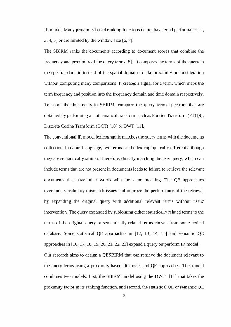
IR model. Many proximity based ranking functions do not have good performance [2,
3, 4, 5] or are limited by the window size [6, 7].
The SBIRM ranks the documents according to document scores that combine the
frequency and proximity of the query terms [8]. It compares the terms of the query in
the spectral domain instead of the spatial domain to take proximity in consideration
without computing many comparisons. It creates a signal for a term, which maps the
term frequency and position into the frequency domain and time domain respectively.
To score the documents in SBIRM, compare the query terms spectrum that are
obtained by performing a mathematical transform such as Fourier Transform (FT) [9],
Discrete Cosine Transform (DCT) [10] or DWT [11].
The conventional IR model lexicographic matches the query terms with the documents
collection. In natural language, two terms can be lexicographically different although
they are semantically similar. Therefore, directly matching the user query, which can
include terms that are not present in documents leads to failure to retrieve the relevant
documents that have other words with the same meaning. The QE approaches
overcome vocabulary mismatch issues and improve the performance of the retrieval
by expanding the original query with additional relevant terms without users'
intervention. The query expanded by subjoining either statistically related terms to the
terms of the original query or semantically related terms chosen from some lexical
database. Some statistical QE approaches in [12, 13, 14, 15] and semantic QE
approaches in [16, 17, 18, 19, 20, 21, 22, 23] expand a query outperform IR model.
Our research aims to design a QESBIRM that can retrieve the document relevant to
the query terms using a proximity based IR model and QE approaches. This model
combines two models: first, the SBIRM model using the DWT [11] that takes the
proximity factor in its ranking function, and second, the statistical QE or semantic QE
3
or both approaches which overcome vocabulary mismatch. With this merging, we can
benefit from proximity ranking function and extend the query with more informative
terms to improve the performance of the IR model.
1.2 Objectives
The general objective of our thesis is to study and evaluate the IR model that overcome
the word mismatch problem using QE approaches and consider terms proximity
information in the ranking function using proximity-based IR model. Many objectives
stem from the general goal as follows:
Evaluate various proximity based IR model.
Design an IR model that combines the query expansion approach and ranking
function that considers the proximity feature.
Study and evaluate different segmentation methods to divide a document into
a number of segments to consider the proximity feature.
Study and evaluate various QE approaches and the combination of them.
Evaluate the performance of the proposed combined IR model.
Compare the results of our model with results of previous works using the same
dataset.
1.3 Outline of the Thesis
Chapter 2 introduces the background of IR model and QE process.
Chapter 3 presents an overview of the proximity based IR models, QE approaches, and
study the combine the proximity based IR models and QE approaches.
Chapter 4 illustrates the reasoning behind the thesis and describes the architecture of
the proposed model.

4
Chapter 5 describes the datasets used in the experiments and present the experimental
results of the proposed model.
Chapter 6 discusses the results obtained by the proposed model and compare them
with the previous model.
Finally, Chapter 7 concludes the thesis, discusses the contributions of this research,
and highlights potential areas for future work.
5
Chapter II
Research Background
2.1 Information Retrieval
"IR model" is designed to analyze, process, store sources of information, and retrieve
those that match a particular user's requirements" [24]. The IR model has good
performance when retrieves more retrieving documents that are more relevant to the
query. The IR models classified to Boolean and ranked retrieval.
2.1.1 Boolean Retrieval
Boolean retrieval Model is one of the simplest and oldest models of IR. In this model,
the document is returned as relevant if it satisfied the query. It works term by term. To
do this task, initially select the first query term 𝑞1.Then, put the documents that contain
this term into the relevant set. After that, remove all the documents that do not satisfy
query term 𝑞2 from the relevant set. This step is applied for all the rest query terms.
Once all query terms are processed, the documents and relevant sets are returnned to
the user.
A set of relevant documents is returned by the Boolean retrieval model. Therefore, to
find the information that user needs, the user must check each document individually.
The retrieval model needs to arrange the documents from the more relevant to the less

6
to speed up the process. In addition, good queries must be formed to retrieve the
documents effectively because it does not retrieve the partially matched document. It
retrieves the exact match documents with the query only [8].
2.1.2 Ranked Retrieval
The ranked IR model calculates the query-relevant score for each document in the
collection, then retrieves documents in order based on that score from the most to least
relevant documents as seen in Figure 2.1.
Figure 2.1: Ranked IR model architecture.
The IR model is influenced by two factors; the accurate results and a fast rate. To
process the query, the similarity score is calculated for each document in the
documents collection. In order to do so a considerable time must be spent to achive a
fast query time. These two-factors depend on how to store data or document
representation method and the score function that computes the similarity score
between the document and the query [8]. The ranked retrieval models classify the two
frequency and proximity models based on the information use by the scoring function.
1) Frequency-Based Model
In the frequency-based model, the scoring function only needs the frequency
information of each term in the document. This model can be further classified into
three models: the Vector Space Model (VSM), the probabilistic model, and the
language model based on the scoring function approach. The VSM ranks documents
Retrieval Method
Ranked
documents
Query
Documents
collection
7
by measuring the similarity between query and document vectors. The probabilistic
retrieval model ranks documents in decreasing order based on the relevance
probability between the document and the query while the language model ranks the
documents based on the probability over sequences of query terms.
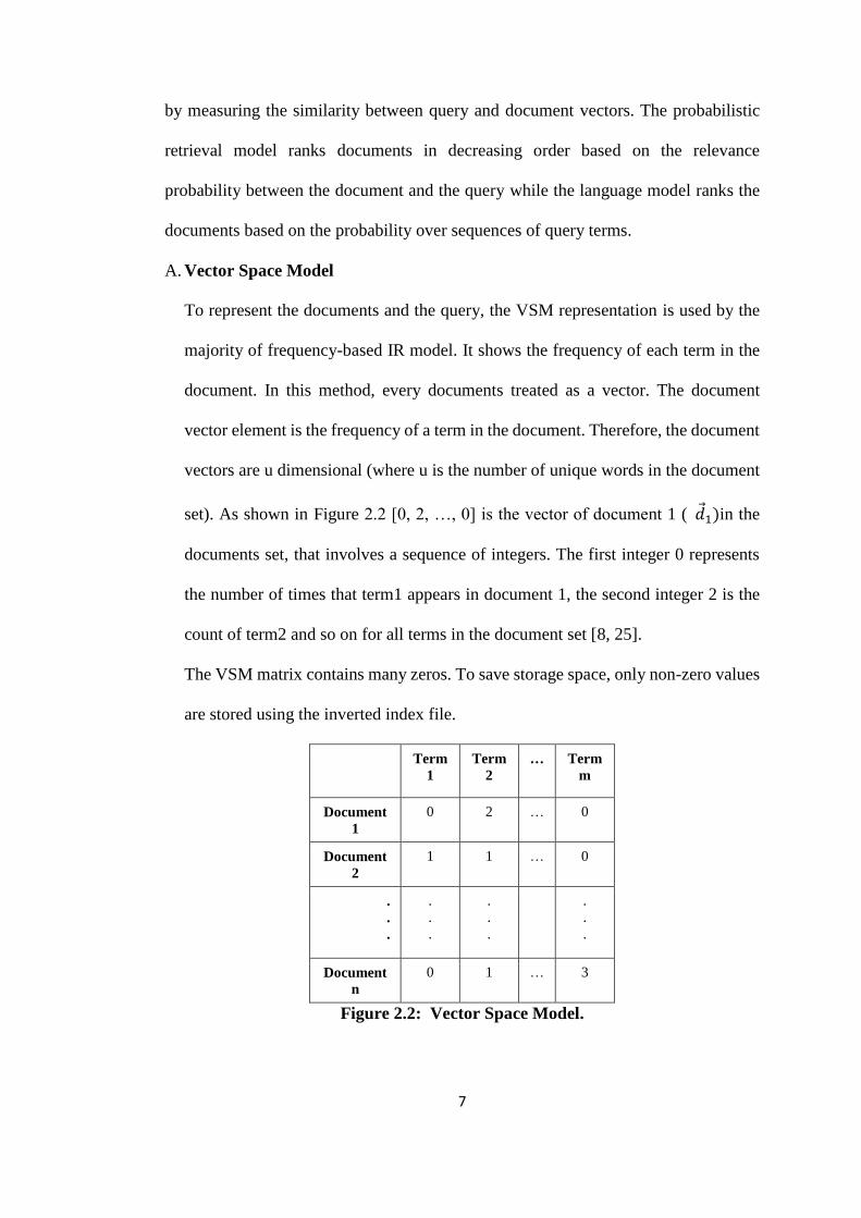
A. Vector Space Model
To represent the documents and the query, the VSM representation is used by the
majority of frequency-based IR model. It shows the frequency of each term in the
document. In this method, every documents treated as a vector. The document
vector element is the frequency of a term in the document. Therefore, the document
vectors are u dimensional (where u is the number of unique words in the document
set). As shown in Figure 2.2 [0, 2, …, 0] is the vector of document 1 ( 𝑑 1)in the
documents set, that involves a sequence of integers. The first integer 0 represents
the number of times that term1 appears in document 1, the second integer 2 is the
count of term2 and so on for all terms in the document set [8, 25].
The VSM matrix contains many zeros. To save storage space, only non-zero values
are stored using the inverted index file.
Term
m
… Term
2
Term
1
0 … 2 0 Document
1
0 … 1 1 Document
2
.
.
.
.
.
.
.
.
.
.
.
.
3 … 1 0 Document
n
Figure 2.2: Vector Space Model.

8
To store the documents, construct the inverted index that consists of two lists. The
term list contains all distinct term while posting list contains for every distinct term
a set of tuples. <doc_id, tf> is the form of the tuples. Therefore, the posting list of
distinct term is:
t → (d1 , fd1,t), (d2 , fd2,t) ,…., (di , fdi,t) (2.1)
where 𝑑𝑖 is the identifier of the document and 𝑓𝑑𝑖,𝑡 is occurs number of term t in
document i [26].
Consider document 1 contains one occurrence of the term "happy" and two
occurrences of "lucky" while document 2 contains one occurrence of "happy". The
posting list of this example is: happy → (1, 1) (2, 1)
lucky → (1, 2)
There are many VSM score or similarity functions such as cosine and Jaccard
coefficient.
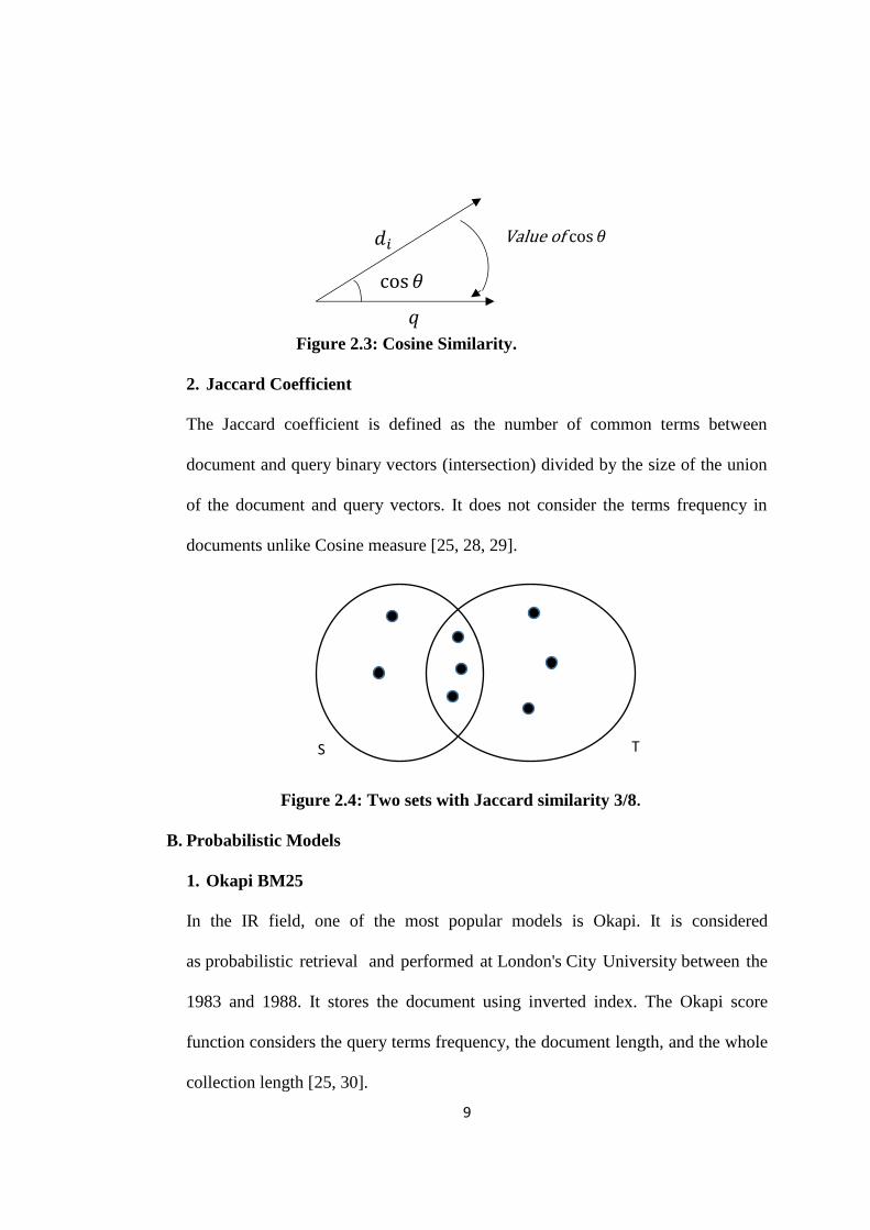
1. Cosine
The similarity between two vectors determines by measuring the cosine angle
between document and query vector. It is calculated as two vectors normalized dot
product.
𝑐𝑜𝑠𝑖𝑛𝑒 𝑠𝑖𝑚𝑖𝑙𝑎𝑟𝑖𝑡𝑦(𝑞 , 𝑑 ) =∑ 𝑤𝑞,𝑗 𝑤𝑑,𝑗𝑡𝑗=1
√∑ (𝑤𝑞,𝑗)2 ∑ (𝑤𝑑,𝑗)
2𝑡𝑗=1
𝑡𝑗=1
(2.2)
where t is the query terms number. 𝑤𝑞,𝑗 and 𝑤𝑑,𝑗is the weighted of term number j
in the query q and 𝑑 respectively. The dot product between 𝑞 and 𝑑 vector in the
numerator, while the product of their Euclidean lengths in the denominator.
When the angle between the vectors decreases, that means the similarity between
the document and query increases [25, 27, 28].
9
Figure 2.3: Cosine Similarity.
2. Jaccard Coefficient
The Jaccard coefficient is defined as the number of common terms between
document and query binary vectors (intersection) divided by the size of the union
of the document and query vectors. It does not consider the terms frequency in
documents unlike Cosine measure [25, 28, 29].
Figure 2.4: Two sets with Jaccard similarity 3/8.
B. Probabilistic Models
1. Okapi BM25
In the IR field, one of the most popular models is Okapi. It is considered
as probabilistic retrieval and performed at London's City University between the
1983 and 1988. It stores the document using inverted index. The Okapi score
function considers the query terms frequency, the document length, and the whole
collection length [25, 30].
T S
Value of cos 𝜃
cos 𝜃
𝑑𝑖
𝑞
10
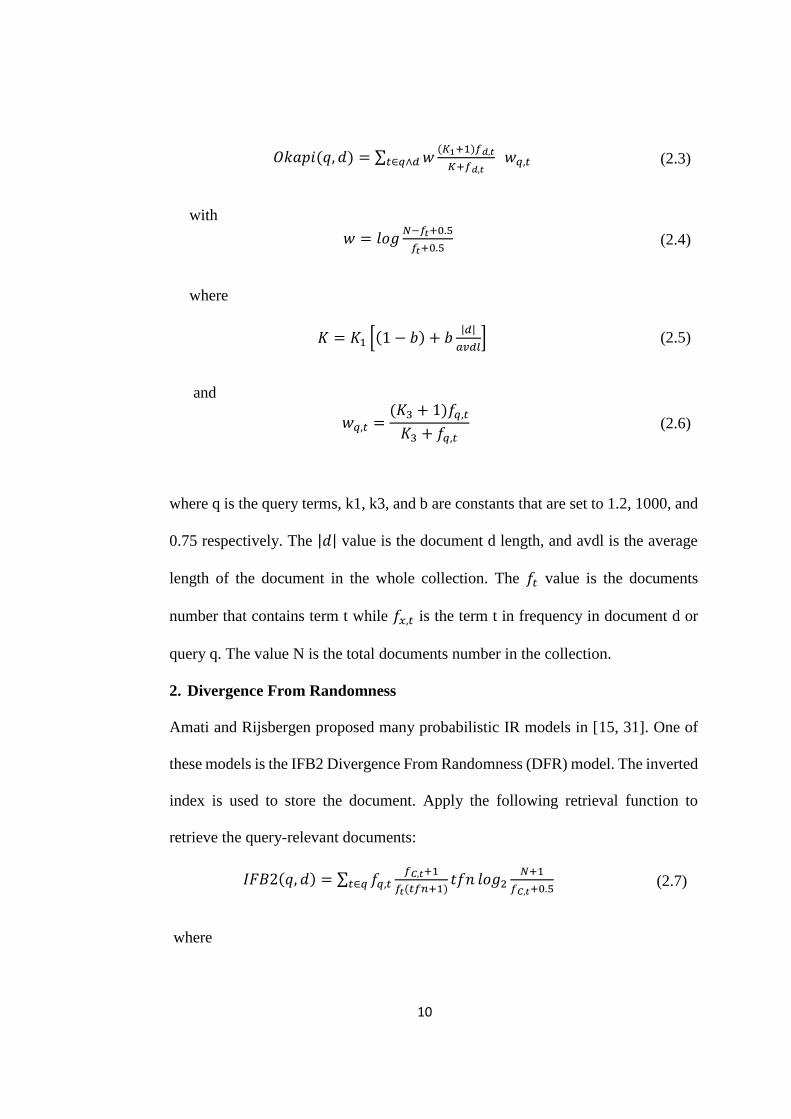
𝑂𝑘𝑎𝑝𝑖 (𝑞, 𝑑) = ∑ 𝑤(𝐾1+1)𝑓𝑑,𝑡
𝐾+𝑓𝑑,𝑡 𝑤𝑞,𝑡𝑡∈𝑞∧𝑑 (2.3)
with
𝑤 = 𝑙𝑜𝑔𝑁−𝑓𝑡+0.5
𝑓𝑡+0.5 (2.4)
where
𝐾 = 𝐾1 [(1 − 𝑏) + 𝑏|𝑑|
𝑎𝑣𝑑𝑙] (2.5)
and
𝑤𝑞,𝑡 =(𝐾3 + 1)𝑓𝑞,𝑡
𝐾3 + 𝑓𝑞,𝑡 (2.6)
where q is the query terms, k1, k3, and b are constants that are set to 1.2, 1000, and
0.75 respectively. The |𝑑| value is the document d length, and avdl is the average
length of the document in the whole collection. The 𝑓𝑡 value is the documents
number that contains term t while 𝑓𝑥,𝑡 is the term t in frequency in document d or
query q. The value N is the total documents number in the collection.
2. Divergence From Randomness
Amati and Rijsbergen proposed many probabilistic IR models in [15, 31]. One of
these models is the IFB2 Divergence From Randomness (DFR) model. The inverted
index is used to store the document. Apply the following retrieval function to
retrieve the query-relevant documents:
𝐼𝐹𝐵2(𝑞, 𝑑) = ∑ 𝑓𝑞,𝑡𝑡∈𝑞𝑓𝐶,𝑡+1
𝑓𝑡(𝑡𝑓𝑛+1)𝑡𝑓𝑛 𝑙𝑜𝑔2
𝑁+1
𝑓𝐶,𝑡+0.5 (2.7)
where

11
𝑡𝑓𝑛 = 𝑓𝑑,𝑡 𝑙𝑜𝑔2(1 + 𝑐𝑎𝑣𝑑𝑙
|𝑑|) (2.8)
The 𝑓𝐶,𝑡 is the t term frequency in the collection C. The c value is constants, which
set to 7.
C. Language Model
In the language models (LM), each document is viewed as a language model 𝑀𝑑,
which generates terms. These models rank the documents by the probability that a
specific document has generated the query [32]. Lavrenko generates the query terms
from the document as the following [33]:
𝑃(𝑞 ∣ 𝑀𝑑) = ∏ 𝑃(𝑡 ∣ 𝑀𝑑)𝑡𝑓𝑞,𝑡 (2.9)
where 𝜆 is a parameter set to 0.6 and |𝐶| is the total number of tokens in the collection
or corpus.
This frequency-based IR model is facing a problem that the term position information
of the document is lost. Once the document is converted to a vector, the vector
represented the number of times each term appeared but ignored the position of the
terms (the flow of the document) [8].
2) Proximity-Based Model
The proximity-based models capture dependencies among query terms by using the
proximity information while frequency-based IR models are based on term
independence assumption. It ignores the interdependence among them and
independently matches the query terms. The frequency-based IR models matching
process example is shown in Figure 2.5. For the query q, document 𝑑1 and 𝑑2 assigned
P( t ∣∣ Md ) = λfd,t
|d|+ (1 − λ)
fC,t
|C| (2.10)
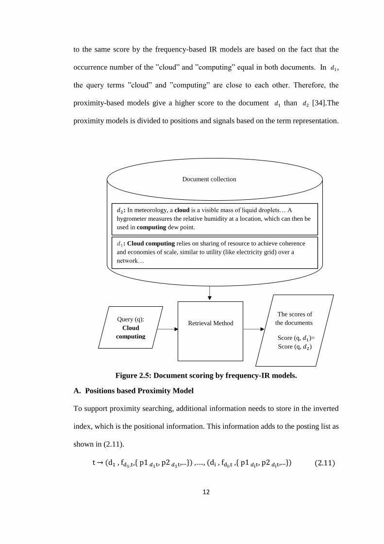
12
to the same score by the frequency-based IR models are based on the fact that the
occurrence number of the ”cloud” and ”computing” equal in both documents. In 𝑑1,
the query terms ”cloud” and ”computing” are close to each other. Therefore, the
proximity-based models give a higher score to the document 𝑑1 than 𝑑2 [34].The
proximity models is divided to positions and signals based on the term representation.
Figure 2.5: Document scoring by frequency-IR models.
A. Positions based Proximity Model
To support proximity searching, additional information needs to store in the inverted
index, which is the positional information. This information adds to the posting list as
shown in (2.11).
t → (d1 , fd1,t,{ p1 𝑑1t, p2 𝑑1t,...}) ,…., (di , fdi,t ,{ p1 𝑑it, p2 𝑑it,...}) (2.11)
𝑑1: Cloud computing relies on sharing of resource to achieve coherence
and economies of scale, similar to utility (like electricity grid) over a
network…
𝑑2: In meteorology, a cloud is a visible mass of liquid droplets… A
hygrometer measures the relative humidity at a location, which can then be
used in computing dew point.
Document collection
Retrieval Method Query (q):
Cloud
computing
The scores of
the documents
Score (q, 𝑑1)=
Score (q, 𝑑2)
13
Where p1 𝑑1t is the first position number of term t in document 1 [34, 35]. For example,
consider the term gold record in the inverted index is gold→ (5, 2, {3, 15}). That
means the term gold appear two times in document 5 at position 3 and 15.
Many scoring functions of the proximity based IR model introduce in [2, 3, 4, 5, 6, 7].
B. Signal based Proximity Model
In this model, in each document, each term is represented by signal. The term signal,
introduced by [9], is a vector representation that displays the spread of the term
throughout the document. It shows the occurrences number of term in specific
partitions or bins within the document.
In SBIRM, the scoring function compares the occurrence patterns of the query terms
in the document. It gives a high score to the document that contains a similar positional
pattern of the query terms while it gives the other document low score because it has
different query terms patterns [8, 9, 10, 11]. This model is discussed in the following
section.
2.2 Spectral-Based Information Retrieval Model
The SBIRM [8, 9, 10, 11] is proximity based model. It compares the query terms in
their spectral domain rather than their spatial domain. To perform this task, create a
term signal for each query term in each document. Then using the spectral transform
convert the term signals to the term spectra. Finally, obtain the document score by
combining the term spectra. The benefits of calculating the document score in the
spectral domain are:
The spectral domain magnitude and phase values are related to the frequency and
proximity of the spatial term, respectively.

14
The terms spectral components are orthogonal to each other. Therefore, there is
no need to cross compare components.
2.2.1 Term Signal
A term signal is a sequence of values that describes the term frequency in a specific
part of a document. To construct the term signal, first divide the document into specific
segments or bin number. Then, represent the term signal of term t in document d by:
where 𝑓𝑑,𝑡,0 is the frequency of term t in first bin of document d. The 𝑓d,t,b is the bth
component of the 𝑓𝑑,𝑡 term signal.
An example of how to create the term signals is shown in Figure 2.6. The top two lines
show the "computer" and "data" positions in a document. The bottom half shows the
term signal components generation from the term positions. As shown in the figure,
document d is divided into eight bins (B=8) and "computer" occurs two times in 𝑏𝑖𝑛3,
one time in 𝑏𝑖𝑛5 , and two times in 𝑏𝑖𝑛7 ; "data" occurs one time in 𝑏𝑖𝑛0 , one time in
𝑏𝑖𝑛2, three times in 𝑏𝑖𝑛5. The term signals for "computer" and "data "are as follows:
𝑓𝑑,computer= [0,0,0,2,0,1,0,2] 𝑓𝑑,data = [1,0,1,0,0,3,0,0]
2.2.2 Term Spectra
To compare the query terms patterns, the most convenient way is to convert the term
signal into the term spectra using the transform then examine their spectrum that is
given by
𝜁𝑑,𝑡 = [𝜁𝑑,𝑡,0 𝜁𝑑,𝑡,1 … 𝜁𝑑,𝑡,𝐵−1 ] (2.13)
where 𝜁𝑑,𝑡,𝑏 is the bth spectral component .The SBIRM uses many transforms such as
FT [9], DCT [10] or DWT [11].
𝑓𝑑,𝑡 = [𝑓𝑑,𝑡,0 𝑓𝑑,𝑡,1… 𝑓𝑑,𝑡,𝐵−1] (2.12)

15
Figure 2.6: The example of creating the term signals.
2.2.3 Discrete Wavelet Transform
The Multi-Resolution Analysis (MRA) must apply to examine the signal across
different time-frequency resolution scales when comparing the query terms signals.
To fulfill this task, a wavelet transform [11, 36] is applied. The wavelet refers to a
small wave, or the wave with a finite length.
The wavelet transform of the term signal provides the location information of the term
at any desired resolution. For example, the first component of the wavelet will identify
if the term appears in the document. The second will identify the occurrence
information of the term in the first and second half of the document and so on until it
finds the exact term location.
The wavelet transform decomposes a signal into wavelets using the scaling functions
(𝑉𝑛) and the wavelet functions(𝑊𝑛). The scaling function must satisfy the following
properties:
… ⊂ 𝑉𝑛+1 ⊂ 𝑉𝑛 ⊂ 𝑉𝑛−1… (2.14)
Computer"
Computer"
data"
data"

16
where 𝑊𝑛 = 𝑉𝑛⋂𝑉𝑛+1̅̅ ̅̅ ̅̅ or 𝑉𝑛 = 𝑊𝑛 ∪ 𝑉𝑛+1,𝑊𝑛 ∩ 𝑉𝑛+1 = ∅. In this recursive filtering
process, each scaling function resolution (𝑉𝑛) split into the next resolution of wavelet
functions (𝑊𝑛) and the next resolution of scaling functions(𝑉𝑛+1). Figure 2.7
illustrated the relationship between 𝑉𝑛 and 𝑊𝑛 .
In the wavelet discrete form, the dyadic wavelet transform can show as a sequence of
high-pass and low-pass filters. The wavelet function can be described by the high-pass
filter coefficients while the scaling function can be described by low-pass filter
coefficients to extract all the information (Figure 2.8).
Figure 2.7: The relationship between 𝑽𝒏 as Ovals and 𝑾𝒏 as Annuli.
Figure 2.8: The Dyadic Wavelet Transform (The High-Pass Filter (H) and the
Low-Pass Filter (L).
𝑉𝑛
𝑉𝑛+2 𝑉𝑛−1
𝑉𝑛+1 𝑊𝑛−2
𝑊𝑛
𝑉𝑛−2
𝑊𝑛−1
H 2
L 2 𝑉𝑛
𝑉𝑛+1
𝑊𝑛

17
The high-pass filter output (the wavelet components) is part of the transform final
result, and the low-pass filter output was fed back into another high and low-pass filter
as shown in Figure 2.9.
Figure 2.9: The Recursive Filtering Process.
2.2.4 Haar Wavelet Transform
The Haar functions were introduced in 1910 by Alfred Haar [37]. The Haar Wavelet
Transform (HWT) is performed at levels [11, 38]. The discrete signal decomposes into
two components with half of its length by the HWT at each level. One component
calculates using the scaling function with [ 1
√2 1
√2 ] coefficients (low-pass filter) while
the other component computes by wavelet function with [ 1
√2 −
1
√2 ] coefficients
(high-pass filter). The s-level HWT for a signal 𝑓 has ℎ values where ℎ power of two
can be defined by:
𝑓𝐻1→ 𝑎1| 𝑑1
𝑓𝐻2→ 𝑎2| 𝑑2| 𝑑1
(2.15)
2 H
L 2
X
H 2
L 2 H 2
L 2
18
𝑓𝐻3→ 𝑎3| 𝑑3| 𝑑2| 𝑑1
⋯⋯⋯
𝑓𝐻𝑠→ 𝑎𝑠| 𝑑𝑠| 𝑑𝑠−1| ⋯ | 𝑑1
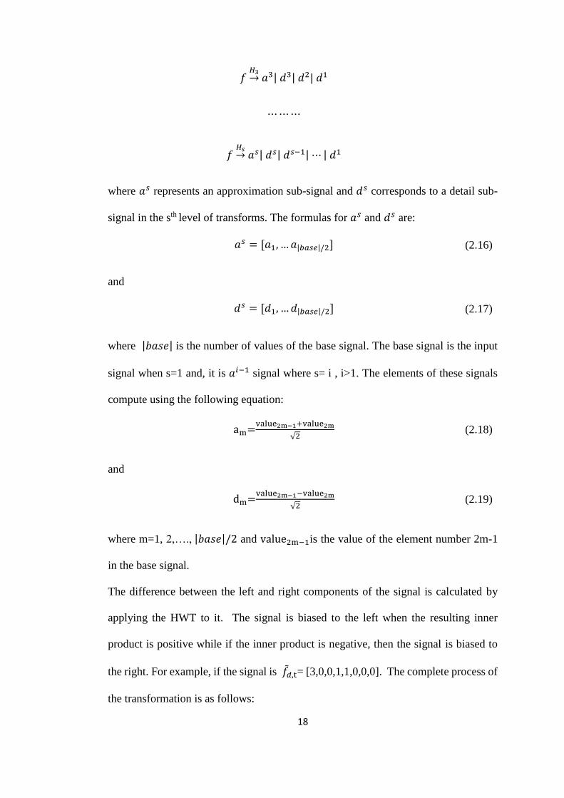
where 𝑎𝑠 represents an approximation sub-signal and 𝑑𝑠 corresponds to a detail sub-
signal in the sth level of transforms. The formulas for 𝑎𝑠 and 𝑑𝑠 are:
𝑎𝑠 = [𝑎1, … 𝑎|𝑏𝑎𝑠𝑒|/2] (2.16)
and
𝑑𝑠 = [𝑑1, … 𝑑|𝑏𝑎𝑠𝑒|/2] (2.17)
where |𝑏𝑎𝑠𝑒| is the number of values of the base signal. The base signal is the input
signal when s=1 and, it is 𝑎𝑖−1 signal where s= i , i>1. The elements of these signals
compute using the following equation:
am=value2m−1+value2m
√2 (2.18)
and
dm=value2m−1−value2m
√2 (2.19)
where m=1, 2,…., |𝑏𝑎𝑠𝑒|/2 and value2m−1is the value of the element number 2m-1
in the base signal.
The difference between the left and right components of the signal is calculated by
applying the HWT to it. The signal is biased to the left when the resulting inner
product is positive while if the inner product is negative, then the signal is biased to
the right. For example, if the signal is 𝑓𝑑,t= [3,0,0,1,1,0,0,0]. The complete process of
the transformation is as follows:
19
The first iteration of the transform consists of two steps. This produces the first version
of the scaling function with the signal𝑓 ̃ 𝑑,𝑡 using equations (2.18).
a1= (3 + 0 ) √2⁄ = 3 √2⁄ ,
a2= (0 + 1 ) √2⁄ = 1 √2⁄ ,
a3= (1 + 0 ) √2⁄ = 1 √2⁄ ,
a4= (0 + 0 ) √2⁄ = 0.
The scaling function of the first-level HWT for a signal 𝑓 produce 𝑎1 that equals to
[3 √2⁄ 1 √2⁄ 1 √2⁄ 0]. By performing the same operation with the wavelet function
using equation (2.19), the following results are produced:
𝑑1= (3 − 0 ) √2⁄ = 3 √2⁄ ,
𝑑2= (0 − 1) √2⁄ = −1 √2 ⁄ ,
𝑑3= (1 − 0 ) √2⁄ = 1 √2 ⁄ ,
𝑑4= (0 − 0 ) √2⁄ = 0.
The result of the Haar wavelet function with the signal 𝑓 produce 𝑑1 that equals to
[3 √2⁄ −1 √2⁄ 1 √2⁄ 0]. These results are concatenated to produce the first iteration
of the wavelet transform (Figure 2.9). The scaling function result passed to the second
iteration, and the wavelet result kept as part of the result.
In the second iteration, 𝑎2 that equal to ([4 √4⁄ 1 √4⁄ ]) is the result of the scaling
function of the second-level HWT for the signal 𝑎1:
a1= (3
√2+
1
√2) √2⁄ = 4 √4⁄ ,
a2= (1
√2+ 0) √2⁄ = 1 √4⁄ .
The second version of the wavelet function with the signal is produced by the scaling
function of the previous iteration:
20
d1= (3
√2−
1
√2 ) √2⁄ = 2 √4⁄ ,
d2= (1
√2− 0) √2⁄ = 1 √4⁄ .
In The third iteration, when performing the scaling function, the result is [5 √8⁄ ] .
𝑎1= (4
√4+
1
√4 ) √2⁄ = 5 √8⁄ .
The result of applying the wavelet function:
𝑑1= (4
√4−
1
√4 ) √2⁄ = 3 √8⁄ .
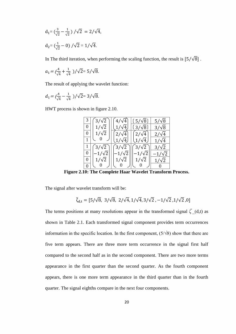
HWT process is shown in figure 2.10.
3 3 √2⁄
1 √2⁄
1 √2⁄ 0
4 √4⁄
1 √4⁄
5 √8⁄ 5 √8⁄
0 3 √8⁄ 3 √8⁄
0 2 √4⁄
1 √4⁄
2 √4⁄
1 √4⁄
2 √4⁄
1 1 √4⁄
1 3 √2⁄
−1 √2⁄
1 √2⁄ 0
3 √2⁄
−1 √2⁄
1 √2⁄ 0
3 √2⁄
−1 √2⁄
1 √2⁄ 0
3 √2⁄
0 −1 √2⁄
0 1 √2⁄
0 0
Figure 2.10: The Complete Haar Wavelet Transform Process.
The signal after wavelet transform will be:
ζ̃d,t = [5/√8, 3/√8, 2/√4, 1/√4, 3/√2 , −1/√2 ,1/√2 ,0].
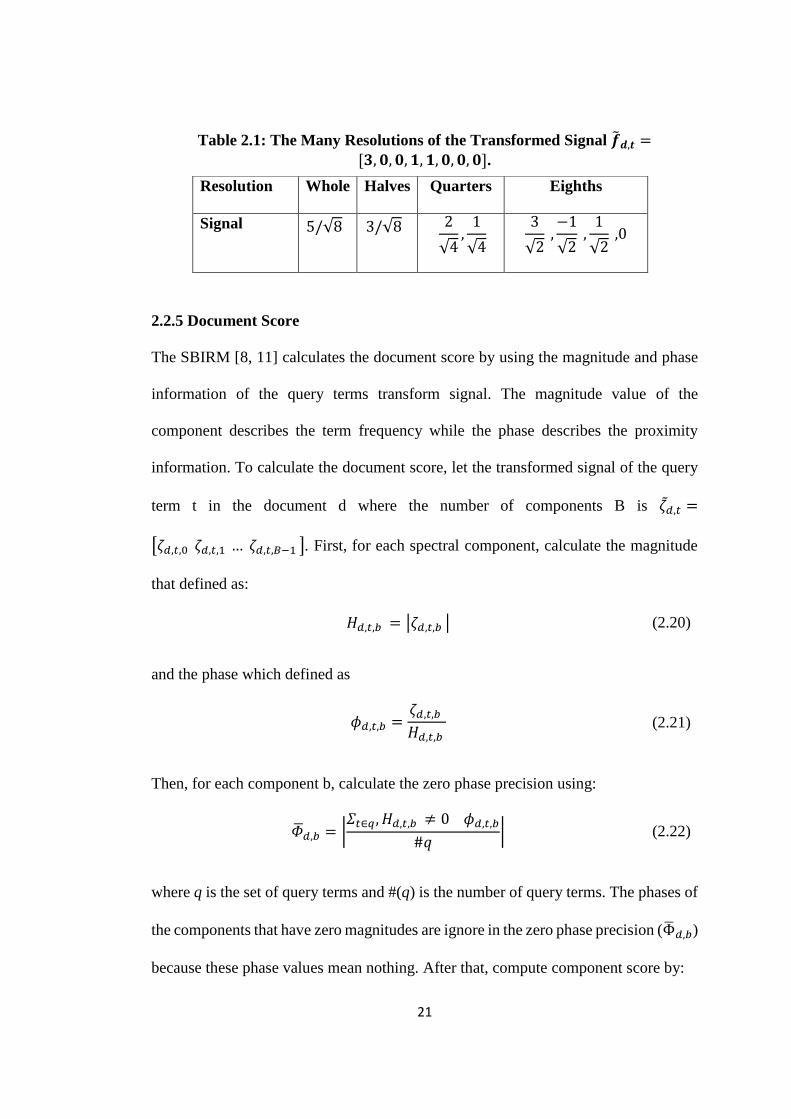
The terms positions at many resolutions appear in the transformed signal ζ ̃_(d,t) as
shown in Table 2.1. Each transformed signal component provides term occurrences
information in the specific location. In the first component, (5/√8) show that there are
five term appears. There are three more term occurrence in the signal first half
compared to the second half as in the second component. There are two more terms
appearance in the first quarter than the second quarter. As the fourth component
appears, there is one more term appearance in the third quarter than in the fourth
quarter. The signal eighths compare in the next four components.
21
Table 2.1: The Many Resolutions of the Transformed Signal �̃�𝒅,𝒕 =[𝟑, 𝟎, 𝟎, 𝟏, 𝟏, 𝟎, 𝟎, 𝟎].
2.2.5 Document Score
The SBIRM [8, 11] calculates the document score by using the magnitude and phase
information of the query terms transform signal. The magnitude value of the
component describes the term frequency while the phase describes the proximity
information. To calculate the document score, let the transformed signal of the query
term t in the document d where the number of components B is 𝜁𝑑,𝑡 =
[𝜁𝑑,𝑡,0 𝜁𝑑,𝑡,1 … 𝜁𝑑,𝑡,𝐵−1 ]. First, for each spectral component, calculate the magnitude
that defined as:
𝛨𝑑,𝑡,𝑏 = |𝜁𝑑,𝑡,𝑏 | (2.20)
and the phase which defined as
𝜙𝑑,𝑡,𝑏 =𝜁𝑑,𝑡,𝑏 𝛨𝑑,𝑡,𝑏
(2.21)
Then, for each component b, calculate the zero phase precision using:
�̅�𝑑,𝑏 = |𝛴𝑡∈𝑞 , 𝛨𝑑,𝑡,𝑏 ≠ 0 𝜙𝑑,𝑡,𝑏
#𝑞| (2.22)
where q is the set of query terms and #(q) is the number of query terms. The phases of
the components that have zero magnitudes are ignore in the zero phase precision (Φ̅𝑑,𝑏)
because these phase values mean nothing. After that, compute component score by:
Resolution Whole Halves Quarters Eighths
Signal 5/√8 3/√8 2
√4,1
√4
3
√2 ,−1
√2 ,1
√2 ,0
22
𝑠𝑑,𝑏 = �̅�𝑑,𝑏∑𝑡∈𝑄𝑤𝑞,𝑡𝛨𝑑,𝑡,𝑏 (2.23)
Finally, combine the components scores to obtain the document score:
𝑆𝑑 = ‖�̃�𝑑‖𝑝 (2.24)
where �̃�𝑑 = [𝑠𝑑,0 𝑠𝑑,1 … 𝑠𝑑,𝐵−1 ] and ‖�̃�𝑑‖𝑝 is the 𝑙𝑝 norm given by
‖�̃�𝑑‖𝑝 = ∑|𝑠𝑑,𝑏 |𝑝
𝐵−1
𝑏=0
(2.25)
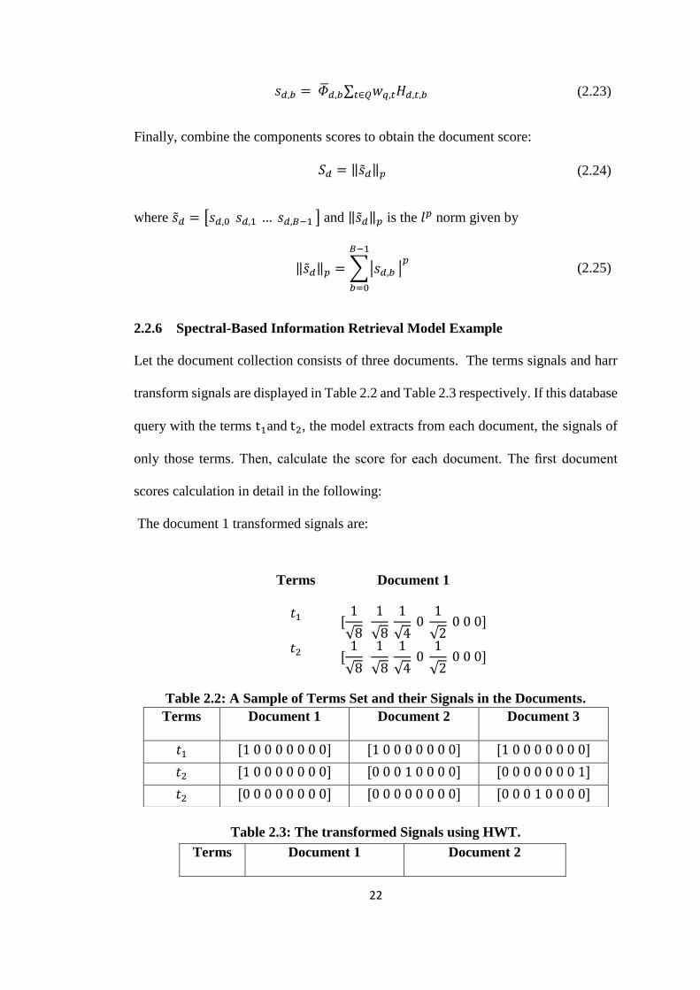
2.2.6 Spectral-Based Information Retrieval Model Example
Let the document collection consists of three documents. The terms signals and harr
transform signals are displayed in Table 2.2 and Table 2.3 respectively. If this database
query with the terms t1and t2, the model extracts from each document, the signals of
only those terms. Then, calculate the score for each document. The first document
scores calculation in detail in the following:
The document 1 transformed signals are:
Table 2.2: A Sample of Terms Set and their Signals in the Documents.
Table 2.3: The transformed Signals using HWT.
Terms Document 1
𝑡1 [1
√8 1
√8 1
√4 0 1
√2 0 0 0]
𝑡2 [1
√8 1
√8 1
√4 0 1
√2 0 0 0]
Terms Document 1 Document 2 Document 3
𝑡1 [1 0 0 0 0 0 0 0] [1 0 0 0 0 0 0 0] [1 0 0 0 0 0 0 0]
𝑡2 [1 0 0 0 0 0 0 0] [0 0 0 1 0 0 0 0] [0 0 0 0 0 0 0 1]
𝑡2 [0 0 0 0 0 0 0 0] [0 0 0 0 0 0 0 0] [0 0 0 1 0 0 0 0]
Terms Document 1 Document 2
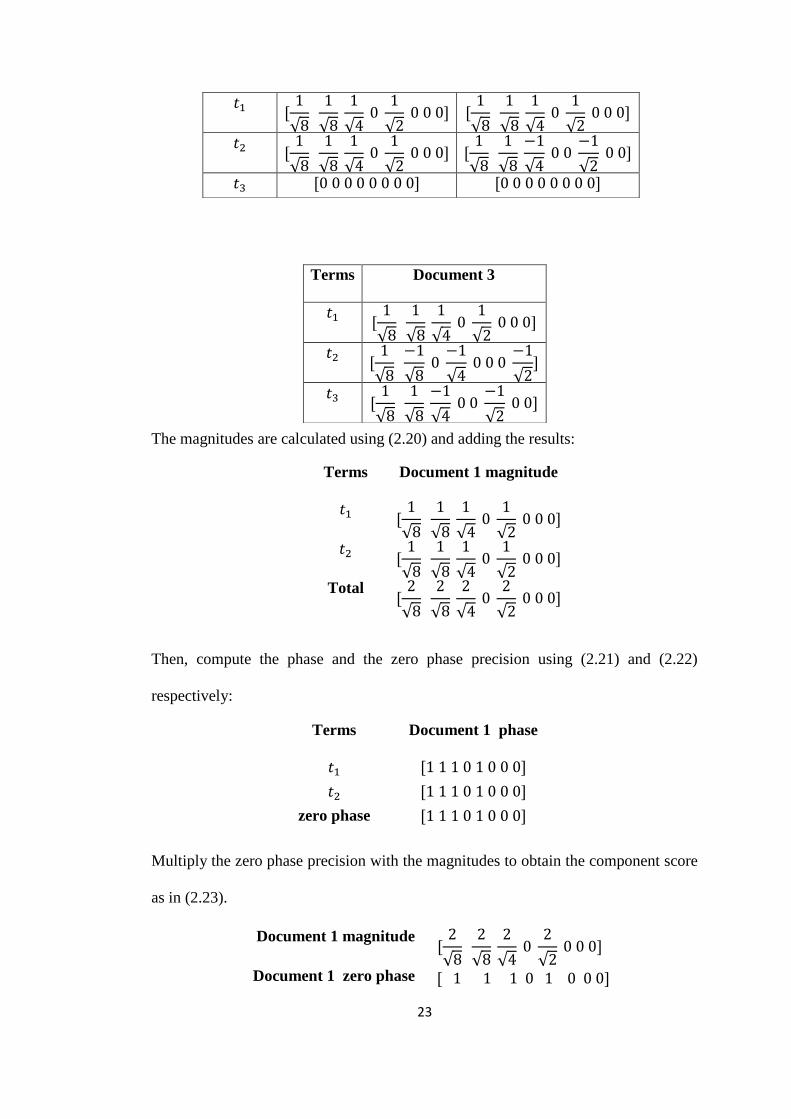
23
The magnitudes are calculated using (2.20) and adding the results:
Then, compute the phase and the zero phase precision using (2.21) and (2.22)
respectively:
Multiply the zero phase precision with the magnitudes to obtain the component score
as in (2.23).
𝑡1 [1
√8 1
√8 1
√4 0 1
√2 0 0 0] [
1
√8 1
√8 1
√4 0 1
√2 0 0 0]
𝑡2 [1
√8 1
√8 1
√4 0 1
√2 0 0 0] [
1
√8 1
√8 −1
√4 0 0
−1
√2 0 0]
𝑡3 [0 0 0 0 0 0 0 0] [0 0 0 0 0 0 0 0]
Terms Document 3
𝑡1 [1
√8 1
√8 1
√4 0 1
√2 0 0 0]
𝑡2 [1
√8 −1
√8 0 −1
√4 0 0 0
−1
√2]
𝑡3 [1
√8 1
√8 −1
√4 0 0
−1
√2 0 0]
Terms Document 1 magnitude
𝑡1 [1
√8 1
√8 1
√4 0 1
√2 0 0 0]
𝑡2 [1
√8 1
√8 1
√4 0 1
√2 0 0 0]
Total [2
√8 2
√8 2
√4 0 2
√2 0 0 0]
Terms Document 1 phase
𝑡1 [1 1 1 0 1 0 0 0]
𝑡2 [1 1 1 0 1 0 0 0]
zero phase [1 1 1 0 1 0 0 0]
Document 1 magnitude [2
√8 2
√8 2
√4 0 2
√2 0 0 0]
Document 1 zero phase [ 1 1 1 0 1 0 0 0]

24
The squared sum of the score vector obtains the document as in (2.25)
To obtain the document 2 and 3 scores follow the same above process the result is as
follows:
As seen, document 1 takes the highest score because the query terms
t1and t2 are closest to each other more than in document 2 and 3; in document 2 the
query terms are closer to each, therefore document 2 takes the second highest score.
While in document 3, they are least close to each other, therefore, document 3 takes
the less score.
2.3 WordNet
2.3.1 WordNet definition
WordNet [39, 40] is a lexical database that has remarkably broad coverage. It stores
words and meanings like a dictionary. However, there are many differences between
the traditional dictionary and WordNet. For instance, the terms arranged alphabetically
in the dictionary while arranged semantically in WordNet. As well, the synonymous
terms are collected together to form synonym sets or "synsets" in the WordNet.
Document 1 score vector [2
√8 2
√8 2
√4 0 2
√2 0 0 0]
Document 1 score 4
Document Score
1 4
2 1.25
3 0.875
25
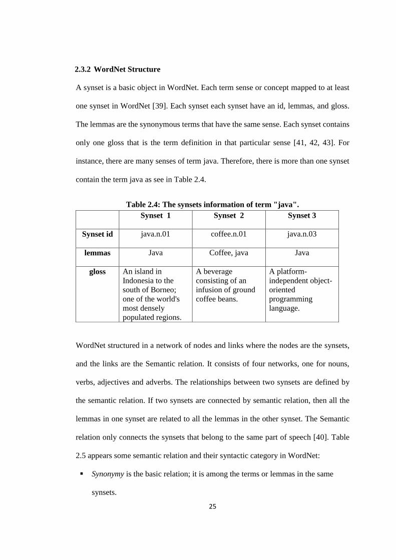
2.3.2 WordNet Structure
A synset is a basic object in WordNet. Each term sense or concept mapped to at least
one synset in WordNet [39]. Each synset each synset have an id, lemmas, and gloss.
The lemmas are the synonymous terms that have the same sense. Each synset contains
only one gloss that is the term definition in that particular sense [41, 42, 43]. For
instance, there are many senses of term java. Therefore, there is more than one synset
contain the term java as see in Table 2.4.
Table 2.4: The synsets information of term "java".
WordNet structured in a network of nodes and links where the nodes are the synsets,
and the links are the Semantic relation. It consists of four networks, one for nouns,
verbs, adjectives and adverbs. The relationships between two synsets are defined by
the semantic relation. If two synsets are connected by semantic relation, then all the
lemmas in one synset are related to all the lemmas in the other synset. The Semantic
relation only connects the synsets that belong to the same part of speech [40]. Table
2.5 appears some semantic relation and their syntactic category in WordNet:
Synonymy is the basic relation; it is among the terms or lemmas in the same
synsets.
Synset 1 Synset 2 Synset 3
Synset id java.n.01 coffee.n.01 java.n.03
lemmas Java Coffee, java Java
gloss An island in
Indonesia to the
south of Borneo;
one of the world's
most densely
populated regions.
A beverage
consisting of an
infusion of ground
coffee beans.
A platform-
independent object-
oriented
programming
language.

26
Antonymy (opposing-name) is a lexical relation between particular terms or
lemmas in different synsets.
Hyponymy (sub-name) and its opposite hypernymy (super-name), is is-a
semantic relation that connects a general synset or concept (the hypernym)
to a more specific one (its hyponym). Specifically, when synset A is a kind
of synset B that leads to A is the hyponym of B, and B is the hypernym of
A.
Meronymy (part-name) and its opposite, holonymy (whole-name), is part-
whole semantic relations that link synset A (holonym) to its part B
(meronym). Specifically, when synset A is part of synset B, then that lead to
A is the meronym of B, and B is the holonym of A. There is three type of
part-whole relation, which are Member–Of, Substance–Of and Part–Of. For
instance, a chapter is a part–of text, cellulose is a substance-of paper, and an
island is a member–of an archipelago.
Troponymy is for verbs while hyponymy is for nouns. The verb a is a
troponym of the verb b if the activity a is doing b in some manner.
Entailment is a semantic relation. A synset A is connected to synset B
through the entailment relation if A entails doing B. In another word, the
verb b is entailed by a if by doing a you must be doing b (The divorce
entails marry).
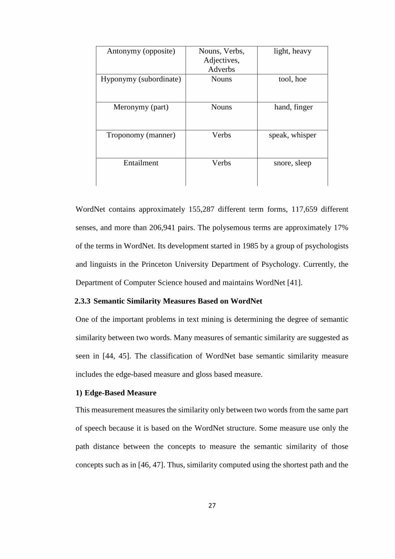
Table 2.5: The common semantic relation in WordNet.
Semantic relation Syntactic category Example
Synonymy (similar)
Nouns, Verbs,
Adjectives,
Adverbs
rapidly, speedily
27
WordNet contains approximately 155,287 different term forms, 117,659 different
senses, and more than 206,941 pairs. The polysemous terms are approximately 17%
of the terms in WordNet. Its development started in 1985 by a group of psychologists
and linguists in the Princeton University Department of Psychology. Currently, the
Department of Computer Science housed and maintains WordNet [41].
2.3.3 Semantic Similarity Measures Based on WordNet
One of the important problems in text mining is determining the degree of semantic
similarity between two words. Many measures of semantic similarity are suggested as
seen in [44, 45]. The classification of WordNet base semantic similarity measure
includes the edge-based measure and gloss based measure.
1) Edge-Based Measure
This measurement measures the similarity only between two words from the same part
of speech because it is based on the WordNet structure. Some measure use only the
path distance between the concepts to measure the semantic similarity of those
concepts such as in [46, 47]. Thus, similarity computed using the shortest path and the
Antonymy (opposite)
Nouns, Verbs,
Adjectives,
Adverbs
light, heavy
Hyponymy (subordinate)
Nouns tool, hoe
Meronymy (part)
Nouns hand, finger
Troponomy (manner)
Verbs speak, whisper
Entailment
Verbs snore, sleep
28
degree of similarity is determined using the path length. The close concepts that are
separate by short path are more semantically related than far concepts.
Other measures take the path and the depth into account like:
Wu and Palmer.
Li.
Leacock and Chodorow.
The Wu and Palmer measure [48] considers the depth of the Least Common Super
concept (LCS) and the path between each concept and LCS while the Li [49] measure
considers the LCS depth and the shortest path length between the two concepts. The
Leacock and Chodorow similarity measure took the shortest path length between the
two concepts and the maximum depth of taxonomy into account [50].
2) Gloss Based Measure
The Lesk metric [51] measure the semantic relatedness between two words by
counting the number of shared words or overlaps between their dictionary definitions
or glosses. The semantic relatedness degree between two words increases when the
overlapping between their glosses increase. In [21], the Lesk metric apply using the
WordNet information by retrieving the gloss of all the synsets in which the term 1 or
term 2 appears. After that, compute the semantic similarity using:
𝑠𝑖𝑚𝑖𝑙𝑎𝑟𝑡𝑦(𝑡1, 𝑡2) =|𝐷(𝑡1) ∩ 𝐷(𝑡2)|
|𝐷(𝑡1) ∪ 𝐷(𝑡2)| (2.25)
where D(t) is the definitions concatenation for all the synsets containing term t and |D|
is the words number of the set D.
29
2.4 Automatic Query Expansion
The average length of the query is around 2-3 words where may the users and the
document collection does not use the same words for the same concept that is known
as the vocabulary or mismatch problem. Therefore, there is difficulty in retrieving the
relevant documents set. To improve the performance of IR model, use the overcome
mismatch problem approaches. One of the successful approaches is to automatically
expand the original query with other terms that best capture the actual user intent that
makes the query more useful [52, 53].
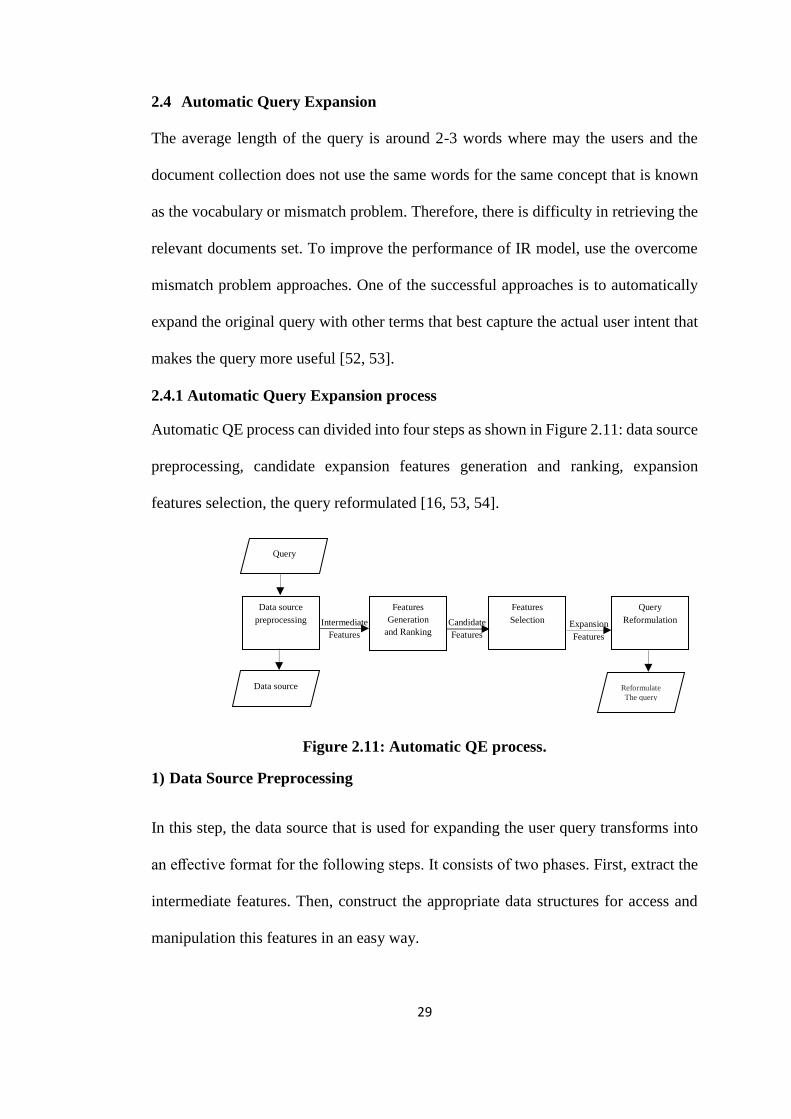
2.4.1 Automatic Query Expansion process
Automatic QE process can divided into four steps as shown in Figure 2.11: data source
preprocessing, candidate expansion features generation and ranking, expansion
features selection, the query reformulated [16, 53, 54].
Figure 2.11: Automatic QE process.
1) Data Source Preprocessing
In this step, the data source that is used for expanding the user query transforms into
an effective format for the following steps. It consists of two phases. First, extract the
intermediate features. Then, construct the appropriate data structures for access and
manipulation this features in an easy way.
Data source
preprocessing
Query
Features
Generation
and Ranking
Features
Selection
Data source
Query
Reformulation Candidate
Features
Intermediate
Features Expansion
Features
Reformulate
The query

30
Based on the source of the Candidate Expansion Terms (CET) the QE approach
classifies to the external resources such as the WordNet and the target corpus. The
WordNet approaches set some or all the synonyms terms of the synset the contain
query term as candidate terms. The target corpus approaches are also divided into local
and global. The global approaches set the whole corpus terms as candidate terms and
analyze it while the local approaches set only the top relevant documents terms of the
initial search results. The local approaches are known as pseudo relevance feedback.
In the IR model, the documents collection or corpus is indexing to run the query. As
seen in the above section, the documents store using inverted index file, which is useful
in some QE approach such as the global approach while the local approach needs to
the documents using direct index file.
2) Features Generation and Ranking
In this stage, the candidate expansion features generate and ranks by the model. The
original query and the data source is the input to this stage while the candidate
expansion features associated with the scores is the output. A small number of the
candidate features add to the query. Therefore, the feature ranking is important. The
relationship between the query terms and candidate features classify the generation
and ranking approaches to:
A. One-to-one associations
It is the simplest approach where for each query term generates one or more candidate
features, i.e., each candidate feature related to a single query term such as the linguistic
stemming approach. This approach produces the root or stem for each query term using
a stemming algorithm. Another linguistic approach in [55] that uses all the synonyms
of all or one query term synsets from a thesaurus like WordNet as candidate terms. In
some QE approach, the feature generation requires selecting one synset of the query
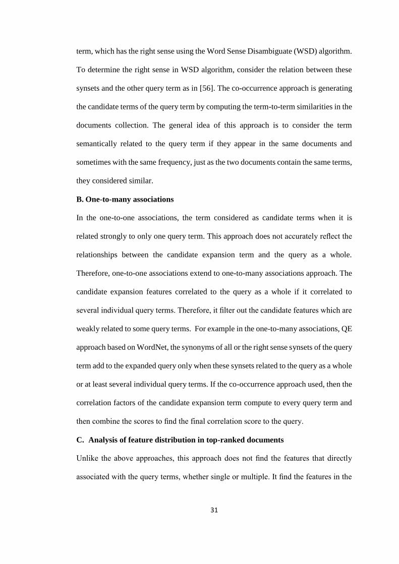
31
term, which has the right sense using the Word Sense Disambiguate (WSD) algorithm.
To determine the right sense in WSD algorithm, consider the relation between these
synsets and the other query term as in [56]. The co-occurrence approach is generating
the candidate terms of the query term by computing the term-to-term similarities in the
documents collection. The general idea of this approach is to consider the term
semantically related to the query term if they appear in the same documents and
sometimes with the same frequency, just as the two documents contain the same terms,
they considered similar.
B. One-to-many associations
In the one-to-one associations, the term considered as candidate terms when it is
related strongly to only one query term. This approach does not accurately reflect the
relationships between the candidate expansion term and the query as a whole.
Therefore, one-to-one associations extend to one-to-many associations approach. The
candidate expansion features correlated to the query as a whole if it correlated to
several individual query terms. Therefore, it filter out the candidate features which are
weakly related to some query terms. For example in the one-to-many associations, QE
approach based on WordNet, the synonyms of all or the right sense synsets of the query
term add to the expanded query only when these synsets related to the query as a whole
or at least several individual query terms. If the co-occurrence approach used, then the
correlation factors of the candidate expansion term compute to every query term and
then combine the scores to find the final correlation score to the query.
C. Analysis of feature distribution in top-ranked documents
Unlike the above approaches, this approach does not find the features that directly
associated with the query terms, whether single or multiple. It find the features in the

32
first documents retrieved in response to the original query. Consequently, the candidate
features related to the full query meaning.
3) Expansion Features Selection
After the candidate features ranking for some QE approach, the limited number of
features is added to the query to process the new query rapidly.
4) Query reformulation
This step usually involves assigning a weight to each expansion feature and re-weights
each query term before submitting the new query to the IR model. The most popular
query re-weighting scheme was proposed by Rocchio’s in [57] as in (2.24).
qnew⃗⃗ ⃗⃗ ⃗⃗ ⃗⃗ ⃗ = α qorig⃗⃗ ⃗⃗ ⃗⃗ ⃗⃗ ⃗ +β
|R|∑w
r∈R
(2.24)
where 𝑞𝑛𝑒𝑤⃗⃗ ⃗⃗ ⃗⃗ ⃗⃗ ⃗ is a weighted term vector for the expanded query while the 𝑞𝑜𝑟𝑖𝑔⃗⃗ ⃗⃗ ⃗⃗ ⃗⃗ ⃗ is a
weighted term vector for the original query. The R value represents the sets of relevant
documents; w is the term weighting vectors extracted from R. the 𝛼 and 𝛽 are the
parameters. Other reweight schemes will be discussed in the following. Some of them
consider the rank score.
33
Chapter III
Literature Review
3.1 Proximity-Based Information Retrieval Model
The basic assumption of the proximity-based model is that the document is extremely
relevant to the query when the query terms occur near to each other. It used spatial
location information as a new factor to compute the document score in information
retrieval. Rather than only touching the surface of the document by counting the query
terms. However, it is not easy to find the model that combines this extra information
into a scoring function.
3.1.1 Shortest-Substring Model
The shortest substring retrieval model is one of the proximity-based model proposed
by Clarke in [2]. In this model, the score function is based on the shortest substring of
text in the document that matches the query by creating a Generalized Concordance
List (GCL). These GCLs consist of the terms that span throughout the document where
the spans are minimum and unique. For instance, a GCL for the terms “red sea” is
shown as:
I (“red sea”) = {(3, 4), (22, 34), (50, 60), (80, 82)}
As presented, the extents ((3, 4) and (80, 82)) show that the terms “red sea” are nearby
to each other. It considers two assumptions when compute the document score:
34
Assumption A: The shorter the extent, the more likely that the part of the text
is relevant.
Assumption B: The more extents found within a document, the more likely
the document is relevant.
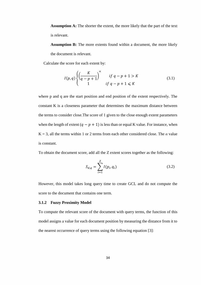
Calculate the score for each extent by:
𝐼(𝑝, 𝑞) {(
𝐾
𝑞 − 𝑝 + 1)∝
𝑖𝑓 𝑞 − 𝑝 + 1 > 𝐾
1 𝑖𝑓 𝑞 − 𝑝 + 1 ⩽ 𝐾
(3.1)
where p and q are the start position and end position of the extent respectively. The
constant K is a closeness parameter that determines the maximum distance between
the terms to consider close.The score of 1 given to the close enough extent parameters
when the length of extent (𝑞 − 𝑝 + 1) is less than or equal K value. For instance, when
K = 3, all the terms within 1 or 2 terms from each other considered close. The α value
is constant.
To obtain the document score, add all the Z extent scores together as the following:
𝑆𝑑,𝑞 =∑𝐼(𝑝𝑖, 𝑞𝑖)
𝑍
𝑖=1
(3.2)
However, this model takes long query time to create GCL and do not compute the
score to the document that contains one term.
3.1.2 Fuzzy Proximity Model
To compute the relevant score of the document with query terms, the function of this
model assigns a value for each document position by measuring the distance from it to
the nearest occurrence of query terms using the following equation [3]:
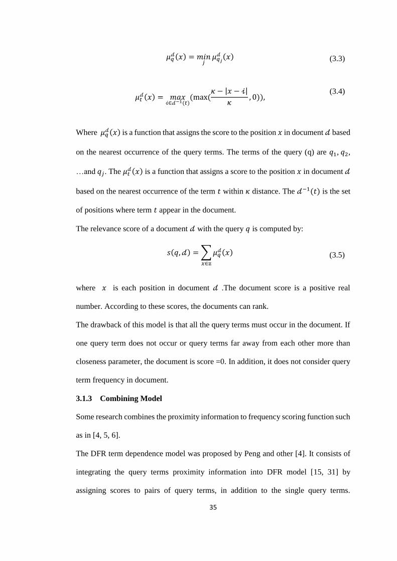
35
𝜇𝑞𝒹(𝑥) = 𝑚𝑖𝑛
𝑗𝜇𝑞𝑗𝒹 (𝑥) (3.3)
𝜇𝑡𝒹(𝑥) = 𝑚𝑎𝑥
𝒾∈𝒹−1(𝑡)(max (
𝜅 − |𝑥 − 𝒾|
𝜅, 0)),
(3.4)
Where 𝜇𝑞𝒹(𝑥) is a function that assigns the score to the position 𝑥 in document 𝒹 based
on the nearest occurrence of the query terms. The terms of the query (q) are 𝑞1, 𝑞2,
…and 𝑞𝑗. The 𝜇𝑡𝒹(𝑥) is a function that assigns a score to the position 𝑥 in document 𝒹
based on the nearest occurrence of the term 𝑡 within 𝜅 distance. The 𝒹−1(𝑡) is the set
of positions where term 𝑡 appear in the document.
The relevance score of a document 𝒹 with the query 𝑞 is computed by:
𝑠(𝑞, 𝒹) =∑𝜇𝑞𝒹(𝑥)
𝑥∈𝕫
(3.5)
where 𝑥 is each position in document 𝒹 .The document score is a positive real
number. According to these scores, the documents can rank.
The drawback of this model is that all the query terms must occur in the document. If
one query term does not occur or query terms far away from each other more than
closeness parameter, the document is score =0. In addition, it does not consider query
term frequency in document.
3.1.3 Combining Model
Some research combines the proximity information to frequency scoring function such
as in [4, 5, 6].
The DFR term dependence model was proposed by Peng and other [4]. It consists of
integrating the query terms proximity information into DFR model [15, 31] by
assigning scores to pairs of query terms, in addition to the single query terms.

36
Abdelkader and other in [34] evaluate this model for Arabic IR. The results display
proximity features yield significant improvements for Arabic IR. The proposed model
is as follows:
𝑠𝑐𝑜𝑟𝑒(𝒹, 𝑞) = 𝜆1∑𝑠𝑐𝑜𝑟𝑒(𝒹, 𝑡)
𝑡∈𝑞
+ 𝜆2 ∑ 𝑠𝑐𝑜𝑟𝑒(𝒹, 𝑝)
𝑝∈𝑞2
(3.6)
where score(𝒹, t) is the score assigned to a query term t in document 𝒹 by using any
DFR weighting model such as equation (2.7). The q2 is a set of all unordered pairs of
query terms, while the p is a pair of query terms. The score(𝒹, p) is the score assigned
to p in document 𝒹. This score considers the frequency of the pair of query terms p
that occur within window size tokens. This model ignores the proximity frequency
when the pair of query terms occur within more than the window size tokens. To ignore
the query terms proximity information, set the weighting parameters 𝜆1and 𝜆2 to 1 and
0 respectively, While when 𝜆1and 𝜆2 set to 1 and 1, the query terms proximity
information consider. The performance of this approach sometimes less than the DFR.
Buttcher and other integrate the proximity with the Okapi BM25 retrieval model by
adding the query terms proximity scores to the Okapi BM25 function. These scores
obtain from the accumulators that associate with each query term. First, fetch the query
terms posting lists and arranges them in a queue. Then, process each posting, one
posting at a time. When process a posting that belongs to the 𝑞2query term, it looks at
the previous posting, belonging to the 𝑞1query term, and calculates the distance
between the current posting and the previous one. Finally, update 𝑞1and
𝑞2 accumulators, but their experiments have not reached to effective retrieval function
through exploiting proximity [5].

37
As [6], He et al. propose BM25P that improves the classical Okapi BM25 model by
utilizing the term proximity evidence using equation (3.9) where score(𝒹, t) is the
score assigned to a query term t in document 𝒹 by using Okapi BM25 model such as
equation (2.3) and score(𝒹, p) compute using the following equation:
score(𝒹, p) = ∑ w(K1 + 1)fd,p
K + fd,p wq,p
𝑝∈𝑄2
(3.7)
Where
w = logN − fp + 0.5
fp + 0.5 (3.8)
and
𝑤𝑞,𝑝 =∑ 𝑤𝑞,𝑡𝑖𝑡𝑖 ∈𝑝
2 (3.9)
and
𝐾 = 𝐾1 [(1 − b) + 𝑏𝑙𝑝
𝑎𝑣𝑙𝑝] (3.10)
Where k1 = 1.2 , k3 = 1000 and b=0.5 as classical Okapi BM25. The fp is the number
of documents that contain the p pair of the query terms. 𝑤𝑞,𝑝 is the pair of the query
terms weight that given by the average of the query term weight of the terms 𝑡iand 𝑡j
using equation (2.6) where p=(𝑡i, 𝑡j). 𝑙𝑝 refers to the number of windows in a document
that computes by (l-window size+1) and 𝑎𝑣𝑙𝑝is the average number of windows in a
documents. fd,pis the terms pair p frequency in the document that computes using
Window-based Counting method.
The basic idea of the window-based counting method is to segment the document into
a list of sliding windows, with each window having a fixed window size. For instance,

38
let the document has four tokens A, B, C, and D, and the window size is 3. Then, there
are two windows in this document, namely A, B, C and B, C, D. The terms pair p
frequency defined as the number of windows that contain the terms pair. This paper
set the windows size to 10.
The main limitation of the BM25P IR model is its sensitivity to the window size.
3.1.4 Markov Random Field
The Markov Random Field (MRF) model considers three types of dependencies
between query terms; Full Independence (FI), Sequential Dependence (SD), and Full
Dependence (FD). In other words, the documents rank based on: query terms
occurrence in FI, order sub-phrase of the query in FD and unordered sub-phrase of the
query within a window or some short proximity of one another in SD [7].
𝑠𝑐𝑜𝑟𝑒(𝒹, 𝑞) = ∑ 𝜆𝑇𝑓𝑇(𝒹, 𝑟)𝑟∈𝑇 + ∑ 𝜆𝑂𝑓𝑂(𝒹, 𝑟)𝑟∈𝑂 +∑ 𝜆𝑈𝑓𝑈(𝒹, 𝑟)𝑟∈𝑈 (3.11)
𝑓𝑥(𝒹, 𝑟) = 𝑙𝑜𝑔 [(1 − 𝛼𝑑)𝑓𝑑,𝑟|𝑑|
+ 𝛼𝑑𝑓𝐶,𝑟|𝐶|] (3.12)
Where 𝜆𝑇, 𝜆𝑂and 𝜆𝑈 are a parameters set to 0.85, 0.1, 0.05 respectively. 𝛼𝑑=𝜇
𝜇+|𝑑| and
μ set to 3500. T is the set of all query terms (T={𝑞1,…, 𝑞𝑗} and j is the number of
query term), O is the set of all order sub phrases of the query and U is the set of all sub
sets of the query terms set that contain two or more query terms. In 𝑓𝑥(𝒹, 𝑟), x=T, O
or U. When 𝑟 ∈ 𝑇 then 𝑓𝑑,𝑟 and 𝑓𝐶,𝑟 is the frequency of r term in the document or
corpus while if 𝑟 ∈ 𝑂 then 𝑓𝑑,𝑟 and 𝑓𝐶,𝑟 is the frequency of r phrase in the document or
corpus. Finally, when 𝑟 ∈ 𝑈 then 𝑓𝑑,𝑟 and 𝑓𝐶,𝑟 is the frequency of subset terms appear
ordered or unordered within a window in the document or corpus. The window size
set to 8.
39
As well, the window size is the limitation of MRF.
The previous proximity models compare the position of each query term with the other
query terms to calculate the document score. Subsequently, the comparisons number
grows if the query terms number grows. SBIRM [8] overcomes this problem by
comparing the terms of the query in the spectral domain rather than their spatial
domain. In addition, the previous proximity models measure the proximity of the query
terms only in specific region or window while SBIRM measures the proximity of the
query terms in the whole document.
3.1.5 Spectral-Based Information Retrieval Model
The SBIRM steps: first, the term signal creates and stores every term in each
document. Next, retrieve the query terms signal for each document. Then, the term
signals transform into term spectra by using a spectral transform. Finally, the document
score obtained by combining the spectra of the query terms. In the spectral domain,
the query term frequency and position are represented by magnitude and phase values.
In [9] Park and others use FT in SBIRM. This model called Fourier Domain Scoring
(FDS). Unfortunately, the FDS has a large index storage space [58]. To overcome this
problem, the SBIRM uses the DCT [10]. The SBIRM high precision is still achieved
by this model. The frequency information can only extract from the signal as a whole
using the FT and DCT transforms.
Many data mining problems use the Wavelets transform as efficient and effective
solutions [59] because it has properties [60] such as multi-resolution decomposition
structure. Therefore, Park and others use DWT in SBIRM [11]. The DWT in document
ranking can concentrate at different resolutions on the signal portions [11].

40
The signal break into wavelets of different scales and positions, so that it can analyze
the patterns of the terms in the document at various resolutions (whole, halves,
quarters, or eighths).
Using the signal concept as representation model with DWT improves the performance
of text mining tasks such as document Clustering[61], document Classification [62,
63, 64] and recommender system on Twitter [65].
3.2 Automatic Query Expansion
In the information retrieval community, there is a long history for the QE. Usually, the
queries consist of two or three terms, which are sometimes not enough to understand
the expectations of the end user and fail to express topic of search. The QE is a process
of broadening the query terms using words that share statistical relationships with
query terms in the collection or share meaning with query terms. Various approaches
used to expand the query over IR model that ignore the proximity information. Some
of these approaches use target corpus or use an external resource or both.
3.2.1 Target Corpus Approaches
The target corpus approaches classified to local and global. The global approaches
consider all the terms in the corpus as CET then score these terms using co-occur
information with query terms in the whole corpus. The CET terms that frequently co-
occur with query term select as expansion terms. One of the global approaches
constructs automatically in the indexing phase and name as co-occurrence thesaurus.
On the other hand, the local approaches consider only all the terms in the top relevant
documents of the initial search results as CET. The global approaches less effective
than local because it relies on corpus frequent information instead of query-relevant

41
document frequent information. Therefore the global approach may expand the query
using terms that have high frequency in the collection but irrelevant to the query [16].
The latent semantic indexing (LSI) classify as global approach [66]. It captures the
dependencies between terms. It applies the singular value decomposition to the term-
document matrix.
The Rocchio’s is one of the simple local approaches [57]. It expands the query with
some terms in the top relevant documents that have high scores. The score of the term
calculates by sum the weights of that term in all top relevant documents. Rivas and
other in [67] enhance the performance of the Okapi BM25 IR model using Rocchio’s
with the biomedical dataset While Nawab et al. used the Rocchio in the plagiarism
detected system which led to bad performance [68]. This paper detects the plagiarism
of the document by splitting the document into sentences (queries). Then; use each
sentence as a query to retrieve a set of potential source documents. Finally, try to
improve the retrieval performance by expanded with one or more expansion terms
using the Rocchio’s approach. The limitation of this approach is the weight of the term
reflects the importance of that term to the entire collection instead of its usefulness to
the user query. The rest of the Local target corpus approaches divided to distribution
approaches and co-occurrence approaches.
1) Distribution Approaches
The following local approach based on distribution analysis, which distinguishes
between useful candidate expansion term and unuseful expansion term by comparing
the distribution of this term in the top relevant documents of the query with the
distribution of this term in all documents. In other words, the score of the appropriate
expansion term is high when the percentage of this term appearance in relevant
documents more than in the collection. There are many term-ranking functions based

42
on analysis of term distribution in pseudo-relevant documents such as shown in Table
3.1. The notations in Table 3.1 are 𝑃𝑅(𝑡) and 𝑃𝐶(𝑡) indicate the probability of
occurrence of term t in the set of pseudo-relevant documents R and in the whole corpus
C, respectively and 𝑓𝑎𝑣𝑔(𝑡, 𝐶) =𝑓𝐶,𝑡
𝑁 .
Table 3.1: Term-ranking functions based on analysis of term distribution.
Doszkocs in [14] earlier applied this concept using a chi-square variant to select the
relevant terms. On the other hand, The Robertson Selection Value (RSV) approach
Uses Swets IR theory [13]. Carpineto and other proposed an effective approach [12],
which relies on the relative entropy, or terms probability distributions in the relevant
documents and the corpus. On average, the KLD performance outperforms the
previous expansion approaches based on distribution analysis when used to selecting
and weighting the expansion terms over the Okapi BM25 IR [12]. In [15], Amati
calculates the divergence between the distributions of the term using Bose-Einstein
Statistics (Bo1). In general, The KLD gave a good performance compared with the
Bo1 based on IFB2 variant of the DFR IR model [69].
2) Co-occurrence Approaches
The co-occurrence approaches measure the semantic similarity between the query
terms and candidate expansion term using co-occurrence statistics information [70]. In
these approaches, the candidate expansion term occurring frequency with original
query terms are selected as expansion terms. The idea of these approaches based on
the Association Hypothesis:
Rank function Mathematical form
Chi-square [𝑃𝑅(𝑡)−𝑃𝐶(𝑡)]
2
𝑃𝐶(𝑡)
RSV ∑ 𝑤𝑑,𝑡𝑑∈𝑅 [𝑃𝑅(𝑡) − 𝑃𝑐(𝑡)]
Bo1 ∑ 𝑓𝑑,𝑡𝑑∈𝑅 𝑙𝑜𝑔2(1+𝑓𝑎𝑣𝑔(𝑡,𝐶)
𝑓𝑎𝑣𝑔(𝑡,𝐶))+𝑙𝑜𝑔2(1 + 𝑓𝑎𝑣𝑔(𝑡, 𝐶))

43
“If an index term is good at discriminating relevant from non-relevant documents then
any closely associated index term is likely to be good at this.”
The standard measures used to select co-occurring terms are the Jaccard coefficients
and the frequency of the term and query term in the top ranked documents.
The RM1 QE approach uses the frequency measure. This approach sometimes drops
the performance of the baseline LM [33].
However, there is a risk in adding these expansion terms directly the query. These
expansion terms could co-occur with the original query terms in the top relevant
documents by chance. The higher it occurs in the whole corpus, the more likely it co-
occurs with query terms by chance. In another word, sometimes the similar terms
identified by co-occurrence tend to occur also very frequently in the collection and
therefore, these terms are not good elements to be discriminate between relevant and
non-relevant documents. To scale down the effect of a chance factor, use the
normalization inverse document frequency along with above-discussed similarity
measures.
The co-occurrence similarity of a term measuring with the whole query by combining
its degrees of co-occurrence with all individual query terms. This approach when used
the frequency coefficients name as LCA [71] while name as LCA with Jaccard when
using Jaccard coefficients. The LCA sometimes improves the performance of the IFB2
variant of the DFR IR model in [69]. The experiment result showed that the LCA with
Jaccard QE approach can improve the performance of Jaccard IR model [72].
Pal and other modify the LCA in [69] based on two hypotheses. The first one is that
some unuseful CET has high LCA score because these terms and query terms occur
many times in only one top document. Thus, they set the number of term pair co-
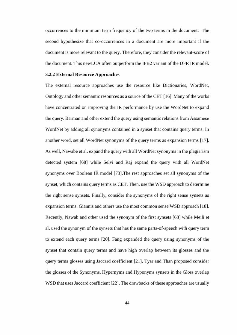
44
occurrences to the minimum term frequency of the two terms in the document. The
second hypothesize that co-occurrences in a document are more important if the
document is more relevant to the query. Therefore, they consider the relevant-score of
the document. This newLCA often outperform the IFB2 variant of the DFR IR model.
3.2.2 External Resource Approaches
The external resource approaches use the resource like Dictionaries, WordNet,
Ontology and other semantic resources as a source of the CET [16]. Many of the works
have concentrated on improving the IR performance by use the WordNet to expand
the query. Barman and other extend the query using semantic relations from Assamese
WordNet by adding all synonyms contained in a synset that contains query terms. In
another word, set all WordNet synonyms of the query terms as expansion terms [17].
As well, Nawabe et al. expand the query with all WordNet synonyms in the plagiarism
detected system [68] while Selvi and Raj expand the query with all WordNet
synonyms over Boolean IR model [73].The rest approaches set all synonyms of the
synset, which contains query terms as CET. Then, use the WSD approach to determine
the right sense synsets. Finally, consider the synonyms of the right sense synsets as
expansion terms. Giannis and others use the most common sense WSD approach [18].
Recently, Nawab and other used the synonym of the first synsets [68] while Meili et
al. used the synonym of the synsets that has the same parts-of-speech with query term
to extend each query terms [20]. Fang expanded the query using synonyms of the
synset that contain query terms and have high overlap between its glosses and the
query terms glosses using Jaccard coefficient [21]. Tyar and Than proposed consider
the glosses of the Synonyms, Hypernyms and Hyponyms synsets in the Gloss overlap
WSD that uses Jaccard coefficient [22]. The drawbacks of these approaches are usually
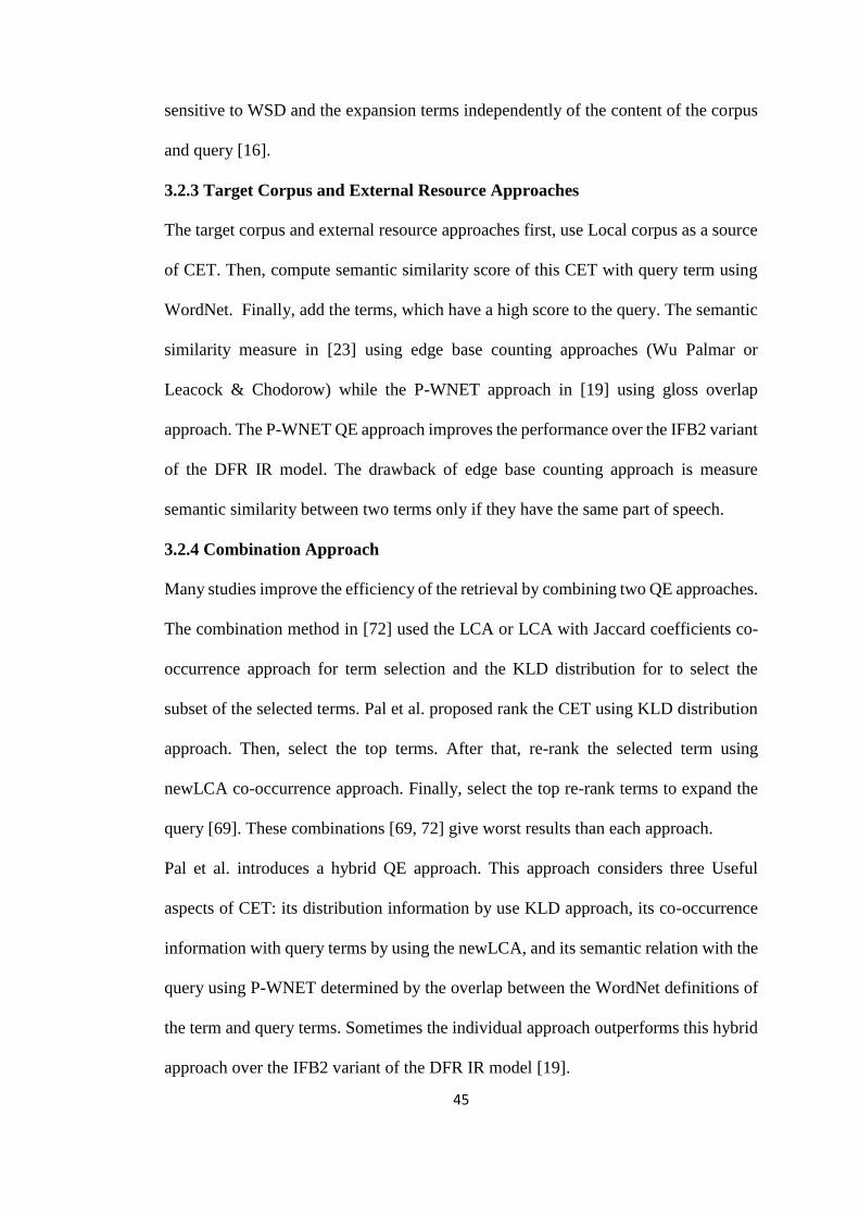
45
sensitive to WSD and the expansion terms independently of the content of the corpus
and query [16].
3.2.3 Target Corpus and External Resource Approaches
The target corpus and external resource approaches first, use Local corpus as a source
of CET. Then, compute semantic similarity score of this CET with query term using
WordNet. Finally, add the terms, which have a high score to the query. The semantic
similarity measure in [23] using edge base counting approaches (Wu Palmar or
Leacock & Chodorow) while the P-WNET approach in [19] using gloss overlap
approach. The P-WNET QE approach improves the performance over the IFB2 variant
of the DFR IR model. The drawback of edge base counting approach is measure
semantic similarity between two terms only if they have the same part of speech.
3.2.4 Combination Approach
Many studies improve the efficiency of the retrieval by combining two QE approaches.
The combination method in [72] used the LCA or LCA with Jaccard coefficients co-
occurrence approach for term selection and the KLD distribution for to select the
subset of the selected terms. Pal et al. proposed rank the CET using KLD distribution
approach. Then, select the top terms. After that, re-rank the selected term using
newLCA co-occurrence approach. Finally, select the top re-rank terms to expand the
query [69]. These combinations [69, 72] give worst results than each approach.
Pal et al. introduces a hybrid QE approach. This approach considers three Useful
aspects of CET: its distribution information by use KLD approach, its co-occurrence
information with query terms by using the newLCA, and its semantic relation with the
query using P-WNET determined by the overlap between the WordNet definitions of
the term and query terms. Sometimes the individual approach outperforms this hybrid
approach over the IFB2 variant of the DFR IR model [19].

46
Paskalis and Khodra failed to improve the performance of IR by merging 4 QE
approaches [74].The first approach set for each query term all the WordNet synonyms
of the right sense synset as CET where the right sense determine using gloss overlap
WSD. The second approach adds to the CET list the highest score co-occurrence terms
for every query terms using co-occurrence thesaurus. In the Third approach, the most
frequent terms occurring in pseudo-relevant documents selected and taken as CET.
Finally, the highest score CET set as the expansion terms and reweight using the KLD.
Table 3.2: Combination QE Approach.
Ref. Distribution
Approaches
Co-occurrence
Approach
WordNet
Approach
How combine Perfo-
rmance
[72] KLD LCA or LCA
with Jaccard
coefficients
They used the LCA
for term selection
and the KLD to
select the subset of
the selected terms.
poor
[69] KLD newLCA They used the KLD
for term selection
and the newLCA
for selected from the
selected term
[74] KLD occurring in
pseudo-
relevant
documents and
thesaurus
gloss
overlap
WSD
They used the
combining score of
Jaccard coefficients,
thesaurus and gloss
overlap WSD for
term selection and
the KLD for
weighting
[19] KLD newLCA P-WNET They use the
expansion terms of
[71] and the
expansion term of
the P-WNET
at times
poor

47
3.3 Automatic Query Expansion and Proximity-Based Information Retrieval
Model
Park expands the query using the Rocchio approach over the FDS model. The precision
of the expand query over the FDS model less than the FDS without expansion [8].
Audeh in [75] studied the effect of the QE on the proximity based IR. He uses LSI and
WordNet synonyms to extend the query over fuzzy proximity model. The experiment
shows a bad performance of the QE approaches over the fuzzy proximity model. The
low performance of the WordNet synonyms may explain by taking all query terms
synonyms instead of only the right sense ,while the LSI explain by need enough
number of pseudo documents. In addition, the fuzzy proximity model is high
selectivity model. For some queries; it got less than 5 documents.
Over the BM25P He et al. expands the query using KLD QE approach that sometimes
leads to a degraded the performance [6].
The performance of the MRF model improves by expanding the query using RM1
approach [76].
Table 3.3: Query Expansion and Proximity-Based Information Retrieval
Model.
Reference Proximity-Based IR QE Approach Performance
[8] FDS Rocchio poor
[75] fuzzy proximity LSI
all WordNet
synonyms of the
query terms
poor
[6] BM25P KLD Sometimes poor
[76] MRF RM1 improve

48
Chapter IV
Query Expansion Approaches over the Spectral-Based Information
Retrieval Model
4.1 Design the Query Expansion Approaches over the Spectral-Based
Information Retrieval Model
Our QESBIRM retrieves more relevant documents to the query by using the good
performance proximity model (SBIRM) and expands it with relevant semantic terms
that overcome the mismatch problem. The mismatch problem is overcome by finding
similar semantic term using the best distribution approach (KLD), all the often good
performance co-occurrence approaches (LCA, newLCA, LCA with Jaccard and
RM1) , and external resource approaches (P-WNET), and finally combine the good
performance approaches.
The proposed model is composed of two-phases: text preprocessing and indexing
phase, and query processing phase. The text preprocessing and indexing phase consists
of the following steps which are performed in offline mode. First the documents are
preprocessed. Then, for each document, term signals are created for all terms in that
document. Next, the weighting scheme is applied on the terms signals. After that,
wavelet transform is applied on the signals. Finally, an inverted index is created.
Figure 4.1 shows these steps.
The query processing phase steps consist of first preprocessing the query. Second,
applying weighting scheme on the query terms. Third, retrieving query terms signals.
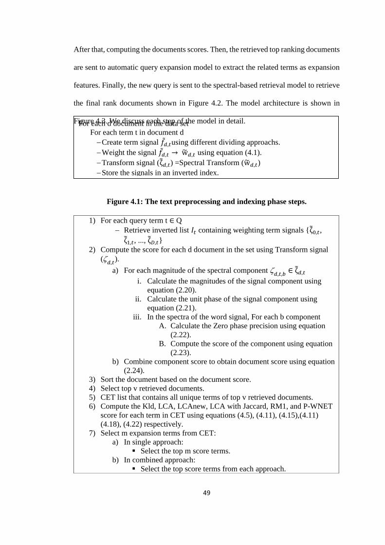
49
After that, computing the documents scores. Then, the retrieved top ranking documents
are sent to automatic query expansion model to extract the related terms as expansion
features. Finally, the new query is sent to the spectral-based retrieval model to retrieve
the final rank documents shown in Figure 4.2. The model architecture is shown in
Figure 4.3. We discuss each step of the model in detail.
Figure 4.1: The text preprocessing and indexing phase steps.
1) For each query term t ∈ Q
Retrieve inverted list 𝐼𝑡 containing weighting term signals {ζ̃0,𝑡,
ζ̃1,𝑡, ..., ζ̃𝐷,𝑡}
2) Compute the score for each d document in the set using Transform signal
(𝑑,𝑡
).
a) For each magnitude of the spectral component 𝑑,𝑡,𝑏
∈ ζ̃𝑑,𝑡
i. Calculate the magnitudes of the signal component using
equation (2.20).
ii. Calculate the unit phase of the signal component using
equation (2.21).
iii. In the spectra of the word signal, For each b component
A. Calculate the Zero phase precision using equation
(2.22).
B. Compute the score of the component using equation
(2.23).
b) Combine component score to obtain document score using equation
(2.24).
3) Sort the document based on the document score.
4) Select top v retrieved documents.
5) CET list that contains all unique terms of top v retrieved documents.
6) Compute the Kld, LCA, LCAnew, LCA with Jaccard, RM1, and P-WNET
score for each term in CET using equations (4.5), (4.11), (4.15),(4.11)
(4.18), (4.22) respectively.
7) Select m expansion terms from CET:
a) In single approach:
Select the top m score terms.
b) In combined approach:
Select the top score terms from each approach.
For each d document in the data set
For each term t in document d
Create term signal 𝑓𝑑,𝑡using different dividing approachs.
Weight the signal 𝑓𝑑,𝑡 → w̃𝑑,𝑡 using equation (4.1).
Transform signal (ζ̃𝑑,𝑡) =Spectral Transform (w̃𝑑,𝑡)
Store the signals in an inverted index.

50
Figure 4.2: The query processing phase steps.
8) Add expansion terms to the original query term to formulate the new
query.
9) Re-weight the new query using equations (4.23) for single approach and
equation (4.27) for combined approach.
10) Repeat step 1, 2 and 3 with the new query.
Documents Preprocessing the
Text
Applying the
Weighting Scheme
Creating the Term
Signals
Inverted Index Creating the
Inverted Index File
Applying the
Transform
1- Text Preprocessing and Indexing Phase
Query
Terms
Preprocessing the
Text
Applying the
Weighting Scheme
Query Preprocessing
2-Query Processing Phase
Retrieving the
Query Term Signal
Computing the
Documents Scores
SBIRM for the Original Query
Final
Retrieved
Ranks
Documents
Computing the
Documents Scores
SBIRM for the Expansion
Query
Retrieving the
Query Term
Signal
Top k
Retrieved
Documents
Creating the
CETL
Applying the
Reweighting
Scheme
Formulating the
New query
Selecting the
Expansion Terms
Computing the
KLD, P-WNET,
LCA, newLCA,
LCA with
Jaccard, RM1 or
any Combination
of them
Automatic Query Expansion model

51
Figure 4.3: General Architecture of a proposed model.
4.1.1 Preprocessing the Text
The text preprocessing is an essential part of any text mining application. At this step,
we typically use four common text-preprocessing methods: tokenization, case folding,
stop word removal and stemming [8, 62]. First, the tokenization step is the task of
converting a raw text file into a stream of individual tokens (words) by using spaces
and line breaks and removing all punctuation marks, brackets and symbols [62]. Next,
the case folding step involves converting the case of every letter in the tokens to a
common case. Usually, the lower case is the common case [8]. Then, stop word
removal step ignores many unuseful terms such as and, "a" and "the" in the English
language because they are so common. If they are used in a query, nearly all of the
documents in the set would return because every document would contain these words.
Therefore, these terms are ignored. By doing this, the number of terms contained in
the document set lexicon was reduced. Therefore, the amount of processing done by
the indexer also reduces [8]. Finally, the stemming step converts each term to its stem
by removing all of a term's prefixes and suffixes [8]. The information retrieval system
applies a stemming process in text preprocessing because it makes the tasks less
dependent on particular forms of words. It also reduces the size of the vocabulary,
which might otherwise have to contain all possible word forms [62]. In general, porter2
is the best overall stemming algorithm [77, 78].
4.1.2 Creating the Term Signals
Rather than mapping a document to a vector that contains the count of each word, the
SBIRM maps each document into a collection of term signals. To create the signal of
the term, first divid the document into segments. Then, represent the signal using
equation (2.12).

52
Park in [8] divided the document into fixed number of segment. There are many
drawbacks of using fixed number of bins in all dataset:
This segmentation approach divided the long documents and short documents
to the same segments number.
It does not take into consideration the semantic of documents such as a
paragraph or sentence that focused on a single topic.
It does not consider the query length.
This thesis tries to improve the performance of the SBIRM by use different methods
of segmentation: sentences-based segmentation, paragraphs-based segmentation, and
minimum distance terms segmentation.
In sentences, paragraphs and minimum distance terms segmentation, first, compute the
number of sentences or paragraphs or segments, respectively in the document (X). The
minimum distance terms segmentation considers the number of query terms and
minimum distance between any occurrences of these terms when determining the
segments size (X =|d|
(|q|−1)∗𝑀+|q|) ) where M is the minimum distance. Then, compute
the number of signal components (G=2𝑝𝑜𝑤𝑒𝑟) using the get matrix algorithm where
X⩽2𝑝𝑜𝑤𝑒𝑟 as shown in Figure 4.4. Finally, create the signal with length G for each
term using (2.12) equation. In sentences and paragraphs based segmentation, the
signal component is filled with zeros when the component number > a number of
sentences or paragraphs.
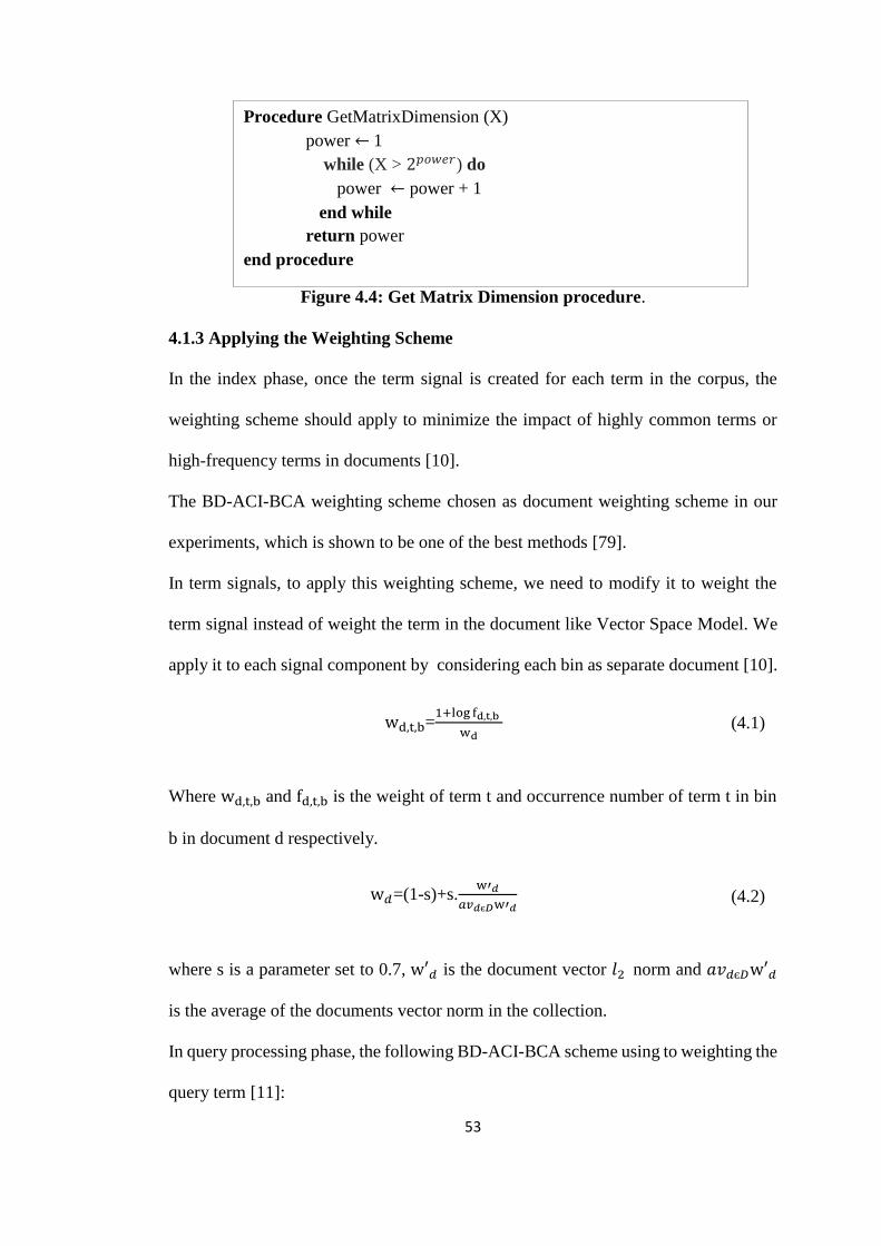
53
Figure 4.4: Get Matrix Dimension procedure.
4.1.3 Applying the Weighting Scheme
In the index phase, once the term signal is created for each term in the corpus, the
weighting scheme should apply to minimize the impact of highly common terms or
high-frequency terms in documents [10].
The BD-ACI-BCA weighting scheme chosen as document weighting scheme in our
experiments, which is shown to be one of the best methods [79].
In term signals, to apply this weighting scheme, we need to modify it to weight the
term signal instead of weight the term in the document like Vector Space Model. We
apply it to each signal component by considering each bin as separate document [10].
wd,t,b=1+log fd,t,b
wd (4.1)
Where wd,t,b and fd,t,b is the weight of term t and occurrence number of term t in bin
b in document d respectively.
w𝑑=(1-s)+s.w′𝑑
𝑎𝑣𝑑є𝐷w′𝑑 (4.2)
where s is a parameter set to 0.7, w′𝑑 is the document vector 𝑙2 norm and 𝑎𝑣𝑑є𝐷w′𝑑
is the average of the documents vector norm in the collection.
In query processing phase, the following BD-ACI-BCA scheme using to weighting the
query term [11]:
Procedure GetMatrixDimension (X)
power ← 1
while (X > 2𝑝𝑜𝑤𝑒𝑟) do
power ← power + 1
end while
return power
end procedure

54
wq,t = (1 + log (fq,t)) log (1 + fm / ft), (4.3)
Where wq,t is the term t weight in query q and fm is the large value of ftfor all t.
4.1.4 Applying the Transform
To analyze the term positions at many document resolutions, the Haar DWT is applied
on each weighted term signal in each document as in equation (2.15-2.19). The
calculation steps of Haar are illustrated in Figure 4.5 [11, 38].
Figure 4.5: Haar wavelet transform.
4.1.5 Creating the Inverted Index File
An inverted index can be created to store the word vectors. In this model, the words in
each documents represented as:
For each weighted term signal x in each document d
Repeat
no ← number of elements in x
Compute half of x as no/2
Initialize i to 0
Initialize j to 0
Set temp to empty list
Set result to empty list
While j < no–3
temp[i] = (x[j] + x[j+1]) / √2
temp[i+half] = (x[j] – x[j+1]) / √2
i ← i + 1
j ← j + 2
temp[i] = (x[no–2] + x[no–1]) / √2
temp[i+half] = (x[no–2] – x[no–1]) / √2
result ← second half of temp
x ← first half of temp
Until number of elements in x = 1

55
<𝑏1, 𝑓1 > < 𝑏2, 𝑓2 > . . . < 𝑏𝑦, 𝑓𝑦 > (4.4)
Where y is the non-zero bins component, 𝑏𝑎is the bin number and 𝑓𝑎is the spectral
value of bin 𝑏𝑎 [9].
4.1.6 Applying the Query Expansion Approach
4.1.6.1 Kullback-Leibler divergence Approach
Carpineto proposed interesting query expansion approaches based on term distribution
analysis [12]. They use the KLD concept [80]. The distributions variance between the
terms in the top relevant documents and entire document collection where those terms
obtain from the first pass retrieval using the query. The query expands with terms that
have a high probability in the top related document compare with low probability in
the whole set. The KLD score of term in the CET are compute using the following
equation:
𝐾𝐿𝐷(𝑡) = 𝑃𝑅(𝑡) 𝑙𝑜𝑔 𝑃𝑅(𝑡)
𝑃𝐶(𝑡) (4.5)
Where 𝑃𝑅(𝑡) is the probability of the term t in the top ranked documents R, and 𝑃𝐶(𝑡)
is the term t probability in the corpus C, given by the following equations:
𝑃𝑅(𝑡) =∑𝑑∈𝑅f𝑡,𝑑∑𝑑∈𝑅|𝑑|
(4.6)
PC(t) =∑d∈Cf𝑡,𝑑∑d∈C|𝐶|
(4.7)

56
4.2.1.1 LCA Approach
One of the well-known co-occurrences approaches is LCA [71]. To measure co-
occurrence between a candidate term t and a query q use the equations (4.8) through
(4.11).
idft = min(log10(N/ft)/5.0,1.0) (4.8)
Co(t,𝑞𝑖)=∑ 𝑓𝑡,𝑑 ∗ 𝑓𝑞𝑖,𝑑𝑑 ∈𝑅 (4.9)
Where query q consisting of terms q1,…, qk
Codegree(t,𝑞𝑖)= 𝑙𝑜𝑔10(𝐶𝑜(𝑡,𝑞𝑖)+1)∗ 𝑖𝑑𝑓𝑡
𝑙𝑜𝑔10 #𝑅 (4.10)
Where #R is the number of relevant documents.
S(t)=∏ (δ + Codegree(t, qi))qi∈q idfqi (4.11)
where δ set to 0.1.
4.2.1.2 LCAnew Approach
The LCA scoring function of the expansion terms modify in [69] to become more
efficient by considering two parameters. First, the score of the top-ranked document
that contains the term. Second, the appearance number of the term pair is the minimum
term appearance number of the two terms.
idft = log10N−ft+0.5
ft+0.5 (4.12)

57
Co(t,qi)=∑ (min(𝑓𝑡,𝑑 ∗ 𝑓qi,𝑑) ∗ max(idftνqi , 0) ∗sim(d,q)
maxd΄∈R
sim(d΄,q))d ∈R (4.13)
where idftνqi is the idf of the minimum frequency bettween term t or qi in document
d between and sim(d, q) similarity score of document d with q.
Codegree(t,qi)= log10(Co(t,qi)+1)
log10(n) (4.14)
S(t)=∑ idfqi ∗ log10(δ + Codegree(t, qi))qi∈q (4.15)
4.2.1.3 LCA with Jaccard Approach
The LCA with Jaccard approach use the same equations of the LCA except the Co
equation. It computes using the following equation:
Co(t,qi)=𝑓𝑡qi
𝑓𝑡+𝑓qi−𝑓𝑡qi (4.16)
Where 𝑓𝑡qi is the number of documents that contain both terms t term qi [72].
4.2.1.4 Relevence Model Approach
The RM1 is a co-occurrences approach [33]. It selects some terms with the highest
score that defined as:
S(t)=∑ 𝑃(𝑑)𝑃(𝑡 ∣ 𝑑)𝑑 ∈𝑅 ∏ P(qi ∣ 𝑑)qi∈q (4.17)
=∑1
#𝑅
𝑓𝑡,𝑑
|𝑑|𝑑 ∈𝑅 ∏𝑓qi,𝑑+𝜇PC(qi)
𝜇+|𝑑|qi∈q
(4.18)
where 𝜇 set to 2500 and PC(qi) compute using equation (4.7).

58
4.2.1.5 P-WNET Approach
The scoring function of the P-WNET approach considers three parameters [19]. First,
the semantic similarity between t and qiusing WordNet gloss overlap, Second, the t's
rareness in the corpus; Finally, the similarity score of the top relevant document that
contains t.
Relt,qi=Ct,qi
Ct+Cqi−Ct,qi (4.19)
Where 𝐶𝑡,𝑞𝑖Is the number of common term between t definitions and 𝑞𝑖 definitions
and 𝐶𝑡 is the number of terms in t definitions.
idft =max(0.0001, log10N−Nt+0.5
Nt+0.5) (4.20)
S(t,qi)= Relt,qi ∗ idft ∗ ∑ (sim(d,q)
maxd΄∈R
sim(d΄,q))d ∈R (4.21)
S(t)=∑S(t,qi)
1+S(t,qi)qi∈q
(4.22)
4.2.1.6 Combination Approach
Use two QE approaches that improves the performance to select two sets of the
expansion terms respectively. Then the union set of these two set uses to expansion
the query [19].
4.1.7 Applying the Re-weighting Scheme
After adding the expansion terms to the authentic query term. The new query must re-
weight. One of the best reweighting schemes is the scheme that derived from QE
59
scores. The weight of the new query is compute using the following equation [12, 19,
69]:
w𝑛𝑒𝑤(𝑡) = 𝛼 score𝑜𝑟𝑖𝑔(𝑡) + β 𝑠𝑐𝑜𝑟𝑒𝑒𝑥𝑝(𝑡) (4.23)
score𝑜𝑟𝑖𝑔(𝑡) = w𝑜𝑟𝑖𝑔(𝑡)
𝑚𝑎𝑥v∈𝑄w𝑜𝑟𝑖𝑔(𝑣) (4.24)
Where 𝑤𝑜𝑟𝑖𝑔(𝑡) is the term t weight in the original query that normalized using the
maximum weight of the original query terms.
The KLD, newLCA, LCA with Jaccard, RM1 and P-WNET compute the 𝑠𝑐𝑜𝑟𝑒𝑒𝑥𝑝(𝑡)
as the following:
𝑠𝑐𝑜𝑟𝑒𝑒𝑥𝑝(𝑡) = 𝑠 (𝑡)
𝑚𝑎𝑥v∈𝑅 𝑠(𝑣) (4.25)
The 𝑆𝑐𝑜𝑟𝑒(𝑡) is the KLD, newLCA, LCA with Jaccard, RM1 or P-WNET score of
the term t.
While LCA approach [71] compute the 𝑠𝑐𝑜𝑟𝑒𝑒𝑥𝑝(𝑡) by :
𝑠𝑐𝑜𝑟𝑒𝑒𝑥𝑝(𝑡)=1.0-0.9∗𝑗
𝑇 (4.26)
Where T is the number of selected expansion terms, and j is the order of t in T.
The combining re-weighting scheme calculates using equation (4.27).
Score (t)= 𝛼 ∗ 𝑠𝑐𝑜𝑟𝑒1(𝑡) + (1 − 𝛼) ∗ 𝑠𝑐𝑜𝑟𝑒2(𝑡) (4.27)
Where 𝑠𝑐𝑜𝑟𝑒1 and 𝑠𝑐𝑜𝑟𝑒2 are the normalized scores of a term calculates using
approach1 and approach 2, respectively.

60
4.2 Implement the Query Expansion approaches over the Spectral-Based
Information Retrieval Model
We implement QESBIRM using python 2.7 and Natural Language Toolkit (NLTK)
3.0 that is a leading platform for building Python programs to work with human
language data. It provides easy-to-use interfaces to over 50 corpora and lexical
resources such as WordNet, along with a suite of text processing libraries [81].
61
Chapter V
Experimental Results
5.1 Dataset
In IR, when performing experiment there is a need for a collection of documents, a
well-defined set of queries and determine which documents relevant to these queries.
We use the TREC dataset, which consists of [82]:
1) Documents collection
We used the Associated Press disk 2 and Wall Street Journal disk 2 (AP2WSJ2)
documents set which consist of 154,443 documents. The Standard Generalized
Markup Language (SGML) tags were used in each document, as shown in Figure 5.1.
2) Query
Queries, which also called ‘topics’ in TREC, have special SGML mark-up tags such
as narr, desc and title. We only used the queries title field, which is contained on
average 2.3-word length from Trec123 set (51-200).
3) Relevance judgments
In fact, the relevance judgment is marked in each document in the documents set as
either irrelevant or relevant to every query. The format of the judgment file is as
follows:
TOPIC# DOCUMENT# RELEVANCY

62
where TOPIC and DOCUMENT# is the query number and the document number that
corresponds to the "num" and "docno" field in the query and documents, respectively.
The RELEVANCY is a binary code of 0 for not relevant and 1 for relevant. For
example the relevance judgment:
53 AP880212-0161 0
Means that the query, which has number 53 is not relevant to the document that has
number AP880212-0161.
Figure 5.1: Document format in TREC dataset.
<DOC>
<DOCNO> AP880212-0004 </DOCNO>
<FILEID>AP-NR-02-12-88 1637EST</FILEID>
<FIRST>r w AM-Peanut Supports 02-12 0155</FIRST>
<SECOND>AM-Peanut Supports,150</SECOND>
<HEAD>Peanut Price Supports Will Go Higher This Year</HEAD>
<DATELINE>WASHINGTON (AP) </DATELINE>
<TEXT>
Price supports for peanuts grown under 1988 quotas will be $615.27
per ton, an increase of $7.80 from last year, the Agriculture Department
said Friday.
Deputy Secretary Peter C. Myers said the increase was required by a
formula in the law which takes rising production costs into consideration.
The annual quota is set at a level equal to the estimated quantity of
peanuts that will be needed for domestic edible uses, seed and related
purposes.
Production of non-quota peanuts, which can be grown for peanut oil
and meal, and for export, will be supported at $149.75 per ton,
unchanged from last year, Myers said.
In setting the support for non-quota peanuts, officials are required to
consider certain factors, including the demand for oil
and meal, the expected prices for other vegetable oils and meals, and the
foreign demand for peanuts.
</TEXT>
</DOC>

63
Figure 5.2: Queries format in TREC dataset.
5.1 Performance Measures
In IR model, there are many measures for evaluating the performance of the model
such as the following:
RT&RL: It is the number of relevant documents contained in the first ten
thousand retrieved documents [12].
Precision: It is the fraction of relevant retrieved documents and retrieved
documents [83].
P@y = |relevant@y|
y (5.1)
where relevant@y represents the set of relevant documents retrieved at y
position in the rank documents. In this thesis, the y=10, 15 and 20. In other
words, the precision is the ability to retrieve top-ranked documents that are
mostly relevant.
<top>
<num> Number: 151
<title> Topic: Coping with overcrowded prisons
<desc> Description:
The document will provide information on jail and prison overcrowding
and how inmates are forced to cope with those conditions; or it will
reveal plans to relieve the overcrowded condition.
<narr> Narrative:
A relevant document will describe scenes of overcrowding that have
become all too common in jails and prisons around the country. The
document will identify how inmates are forced to cope with those
overcrowded conditions, and/or what the Correctional System is doing ,
or planning to do, to alleviate the crowded condition.
</top>
64
R-precision (RP): It is the precision after R retrieved documents, where R is
the number of query-relevant documents [83].
MAP: For each query compute the sum of the precision at each relevant
document in the list divided by the total number of query-relevant documents.
Then, it is averaged over the set of queries as follow:
MAP =1
#Q∑AP(j)
#Q
j=1
(5.2)
AP =1
dqj∑P(doci)
dqj
i=1
(5.3)
where #Q is Number of queries, dqj Number of all relevant documents for
query j and 𝑃(𝑑𝑜𝑐𝑖) precision at 𝑖𝑡ℎrelevant document [83].
GMAP: It is designed to highlight the improvements of low-performing topics.
If a run doubles the average precision for topic A from 0.02 to 0.04, while
decreasing topic B from 0.4 to 0.38, the MAP is unchanged, but the geometric
mean will show an improvement.
It is averaging the log of each query average precision scores and then
exponentiation the final geometric MAP score [84].
GMAP = exp(1
#Q∑log(AP(i))
#Q
i=1
) (5.4)
Recall: It is the fraction of relevant retrieved documents and a total number of
relevant documents in the dataset [83].

65
Recall@y = |relevant@y|
|relevant documents in the dataset | (5.5)
In other words, the recall is the ability to find all the relevant documents in the
corpus.
To compute the recall-precision, first find the recall and precision value for
each position in the document rank until reach the last relevant document.
Then, create the recall-precision table by fill the recall and precision rows. The
recall row fills using the standard recall levels
𝑟𝑒𝑐𝑎𝑙𝑙𝑗∈{0.0,0.1,0.2,0.3,0.4,0.5,0.6,0.7,0.8,0.9,1.0}. To fill the precision row,
find the maximum precision value at each recall level, then, fill the precision
row where the precision at the 𝑗𝑡ℎ standard recall level is the maximum known
precision at any recall level between the 𝑗𝑡ℎ and (𝑗 + 1)𝑡ℎ level. Finally, draw
the recall-precision curve using the table.
5.3 Experimental Results
In the beginning, we used Python programming language to build the SBIRM, as we
explained in chapter 4. First, preprocessing the documents. Then, for each document,
create term signals for all terms in that document using four methods of segmentation:
The fixed number of segment and the three proposed segmentation: sentences-based
segmentation, paragraphs-based segmentation, and minimum distance terms
segmentation are evaluated. Next, apply the weighting scheme on the terms signal.
Then, apply wavelet transform on the signals and create an inverted index. After that,
preprocessing and applying the weighting scheme on the query. Later, retrieve the
query terms signals. Finally, compute the documents score for retrieve the rank
documents.
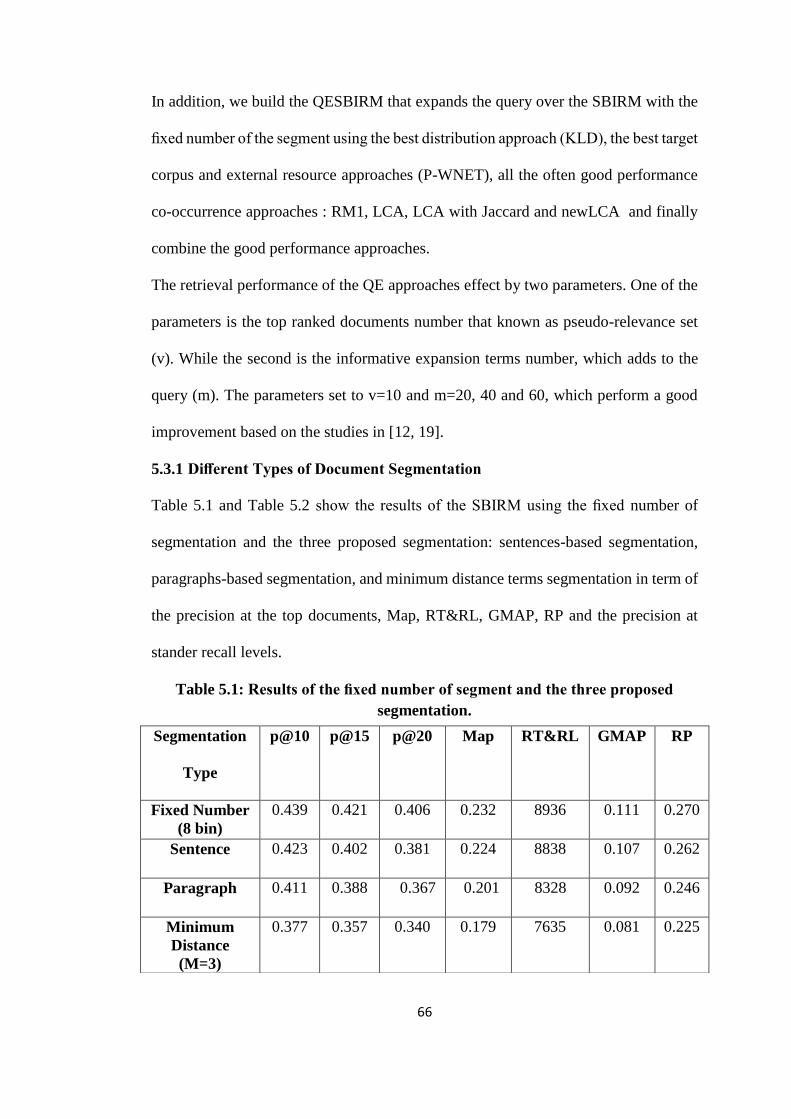
66
In addition, we build the QESBIRM that expands the query over the SBIRM with the
fixed number of the segment using the best distribution approach (KLD), the best target
corpus and external resource approaches (P-WNET), all the often good performance
co-occurrence approaches : RM1, LCA, LCA with Jaccard and newLCA and finally
combine the good performance approaches.
The retrieval performance of the QE approaches effect by two parameters. One of the
parameters is the top ranked documents number that known as pseudo-relevance set
(v). While the second is the informative expansion terms number, which adds to the
query (m). The parameters set to v=10 and m=20, 40 and 60, which perform a good
improvement based on the studies in [12, 19].
5.3.1 Different Types of Document Segmentation
Table 5.1 and Table 5.2 show the results of the SBIRM using the fixed number of
segmentation and the three proposed segmentation: sentences-based segmentation,
paragraphs-based segmentation, and minimum distance terms segmentation in term of
the precision at the top documents, Map, RT&RL, GMAP, RP and the precision at
stander recall levels.
Table 5.1: Results of the fixed number of segment and the three proposed
segmentation.
Segmentation
Type
p@10 p@15 p@20 Map RT&RL GMAP RP
Fixed Number
(8 bin)
0.439 0.421 0.406 0.232 8936 0.111 0.270
Sentence 0.423 0.402 0.381 0.224 8838 0.107 0.262
Paragraph 0.411 0.388 0.367 0.201
8328 0.092 0.246
Minimum
Distance
(M=3)
0.377 0.357 0.340 0.179 7635
0.081 0.225

67
Table 5.2: Recall-Precision of the fixed number of segment and the three
proposed segmentation.
5.3.2 Query Expansion Approaches over Spectral-Based Information Retrieval
Model
1) Distribution Approach
The results of expanding the query using KLD approach over the SBIRM is shown in
Table 5.3 and Table 5.4.
Table 5.3: Results of running the KLD approach over the SBIRM.
Minimum
Distance
(M=10)
0.392 0.369 0.348 0.183 7742 0.082 0.229
Recall Fixed
Number (8
bin)
Sentenc
e
Paragraph Minimum
Distance
(M=3)
Minimum
Distance
(M=10)
0.0 0.641 0.611 0.599 0.58 0.59
0.1 0.454 0.434 0.406 0.399 0.395
0.2 0.38 0.368 0.333 0.311 0.32
0.3 0.315 0.309 0.275 0.246 0.251
0.4 0.267 0.256 0.225 0.2 0.207
0.5 0.218 0.211 0.186 0.16 0.165
0.6 0.173 0.167 0.144 0.125 0.128
0.7 0.136 0.129 0.115 0.084 0.091
0.8 0.098 0.097 0.076 0.051 0.054
Approach p@10 p@15 p@20 Map RT&RL GMAP RP
KLD
(m=60)
0.465 0.447 0.421 0.244 9425 0.113 0.271

68
Table 5.4: Recall-Precision of running the KLD approach over the SBIRM.
2) Co-occurrence Approaches
The results of running the RM1, LCA, LCA with Jaccard and newLCA QE
approach over the SBIRM display in Table 5.5, 5.6, 5.7, 5.8, 5.9, 5.10, 5.11 and
5.12 respectively.
Table 5.5: Results of running the RM1 approach over the SBIRM.
KLD
(m=40)
0.469 0.448 0.430 0.249 9467 0.115 0.277
KLD
(m=20)
0.467 0.438 0.422 0.252 9484 0.114 0.281
Recall KLD
(m=60)
KLD
(m=40)
KLD
(m=20)
0.0 0.648 0.652 0.647
0.1 0.494 0.5 0.484
0.2 0.406 0.411 0.416
0.3 0.335 0.341 0.35
0.4 0.277 0.283 0.293
0.5 0.223 0.228 0.236
0.6 0.18 0.185 0.188
0.7 0.139 0.142 0.146
0.8 0.098 0.099 0.101
0.9 0.06 0.06 0.06
1.0 0.01 0.01 0.011
Approach p@10 p@15 p@20 Map RT&RL GMAP RP
RM1
(m=40)
0.421 0.397 0.373 0.196 7883 0.078 0.227
RM1
(m=20)
0.426 0.403 0.383 0.207 8134 0.082 0.237
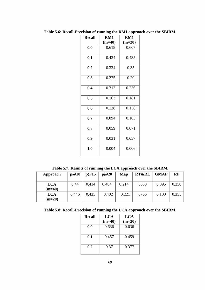
69
Table 5.6: Recall-Precision of running the RM1 approach over the SBIRM.
Recall RM1
(m=40)
RM1
(m=20)
0.0 0.618 0.607
0.1 0.424 0.435
0.2 0.334 0.35
0.3 0.275 0.29
0.4 0.213 0.236
0.5 0.163 0.181
0.6 0.128 0.138
0.7 0.094 0.103
0.8 0.059 0.071
0.9 0.031 0.037
1.0 0.004 0.006
Table 5.7: Results of running the LCA approach over the SBIRM.
Table 5.8: Recall-Precision of running the LCA approach over the SBIRM.
Approach p@10 p@15 p@20 Map RT&RL GMAP RP
LCA
(m=40)
0.44 0.414 0.404 0.214 8538 0.095 0.250
LCA
(m=20)
0.446 0.425 0.402 0.221 8756 0.100 0.255
Recall LCA
(m=40)
LCA
(m=20)
0.0 0.636 0.636
0.1 0.457 0.459
0.2 0.37 0.377
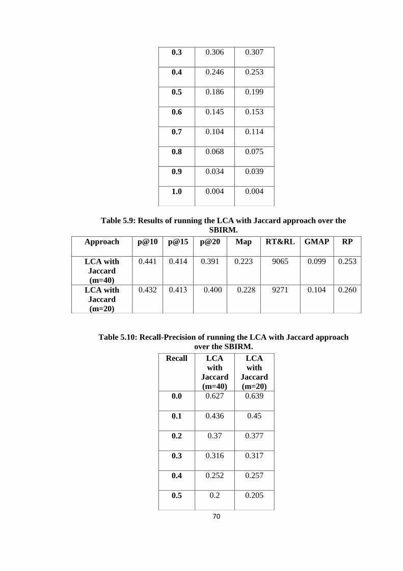
70
Table 5.9: Results of running the LCA with Jaccard approach over the
SBIRM.
Table 5.10: Recall-Precision of running the LCA with Jaccard approach
over the SBIRM.
0.3 0.306 0.307
0.4 0.246 0.253
0.5 0.186 0.199
0.6 0.145 0.153
0.7 0.104 0.114
0.8 0.068 0.075
0.9 0.034 0.039
1.0 0.004 0.004
Approach p@10 p@15 p@20 Map RT&RL GMAP RP
LCA with
Jaccard
(m=40)
0.441 0.414 0.391 0.223 9065 0.099 0.253
LCA with
Jaccard
(m=20)
0.432 0.413 0.400 0.228 9271 0.104 0.260
Recall LCA
with
Jaccard
(m=40)
LCA
with
Jaccard
(m=20)
0.0 0.627 0.639
0.1 0.436 0.45
0.2 0.37 0.377
0.3 0.316 0.317
0.4 0.252 0.257
0.5 0.2 0.205
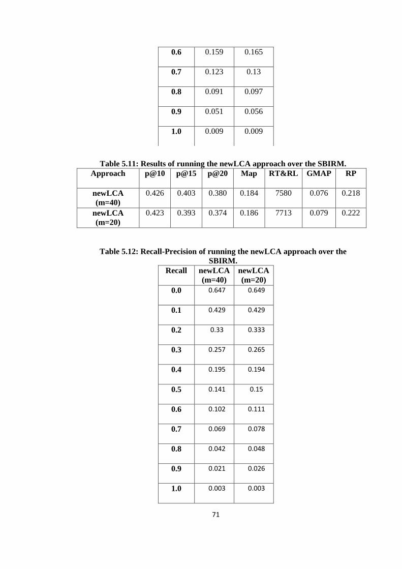
71
Table 5.11: Results of running the newLCA approach over the SBIRM.
Approach p@10 p@15 p@20 Map RT&RL GMAP RP
newLCA
(m=40)
0.426 0.403 0.380 0.184 7580 0.076 0.218
newLCA
(m=20)
0.423 0.393 0.374 0.186 7713 0.079
0.222
Table 5.12: Recall-Precision of running the newLCA approach over the
SBIRM.
Recall newLCA
(m=40)
newLCA
(m=20)
0.0 0.647 0.649
0.1 0.429 0.429
0.2 0.33 0.333
0.3 0.257 0.265
0.4 0.195 0.194
0.5 0.141 0.15
0.6 0.102 0.111
0.7 0.069 0.078
0.8 0.042 0.048
0.9 0.021 0.026
1.0 0.003 0.003
0.6 0.159 0.165
0.7 0.123 0.13
0.8 0.091 0.097
0.9 0.051 0.056
1.0 0.009 0.009

72
3) The Target Corpus and External Resource Approach
Table 5.13 and Table 5.14 show the result of expanding the query by the P-
WNET approach over the SBIRM.
Table 5.13: Results of running the P-WNET approach over the SBIRM.
Approach p@10 p@15 p@20 Map RT&RL GMAP RP
P-WNET
(m=60)
0.459 0.436 0.422 0.251 9425 0.119 0.284
P-WNET
(m=40)
0.472 0.444 0.422 0.245 9375 0.117 0.277
P-WNET
(m=20)
0.467 0.44 0.423 0.249 9490 0.119 0.281
Table 5.14: Recall-Precision of running the P-WNET approach over the
SBIRM.
Recall P-WNET
(m=60)
P-WNET
(m=40)
P-WNET
(m=20)
0.0 0.644 0.661 0.653
0.1 0.474 0.485 0.493
0.2 0.41 0.405 0.408
0.3 0.352 0.345 0.35
0.4 0.292 0.283 0.292
0.5 0.239 0.226 0.232
0.6 0.193 0.182 0.187
0.7 0.147 0.142 0.145
0.8 0.108 0.098 0.101
0.9 0.061 0.06 0.06
1.0 0.011 0.01 0.01
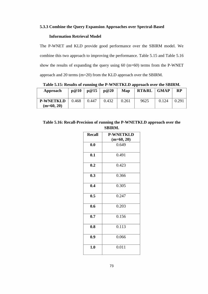
73
5.3.3 Combine the Query Expansion Approaches over Spectral-Based
Information Retrieval Model
The P-WNET and KLD provide good performance over the SBIRM model. We
combine this two approach to improving the performance. Table 5.15 and Table 5.16
show the results of expanding the query using 60 (m=60) terms from the P-WNET
approach and 20 terms (m=20) from the KLD approach over the SBIRM.
Table 5.15: Results of running the P-WNETKLD approach over the SBIRM.
Table 5.16: Recall-Precision of running the P-WNETKLD approach over the
SBIRM.
Approach p@10 p@15 p@20 Map RT&RL GMAP RP
P-WNETKLD
(m=60, 20)
0.468 0.447 0.432 0.261 9625 0.124 0.291
Recall P-WNETKLD
(m=60, 20)
0.0 0.649
0.1 0.491
0.2 0.423
0.3 0.366
0.4 0.305
0.5 0.247
0.6 0.203
0.7 0.156
0.8 0.113
0.9 0.066
1.0 0.011
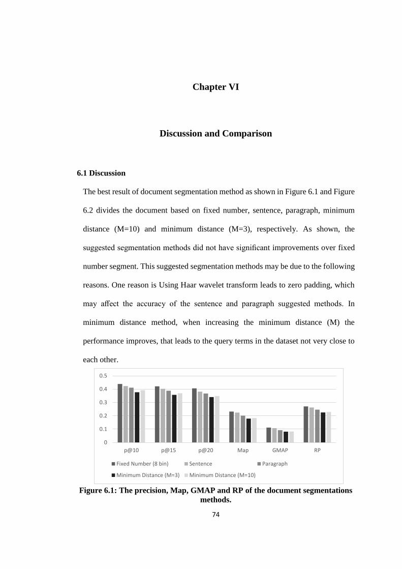
74
Chapter VI
Discussion and Comparison
6.1 Discussion
The best result of document segmentation method as shown in Figure 6.1 and Figure
6.2 divides the document based on fixed number, sentence, paragraph, minimum
distance (M=10) and minimum distance (M=3), respectively. As shown, the
suggested segmentation methods did not have significant improvements over fixed
number segment. This suggested segmentation methods may be due to the following
reasons. One reason is Using Haar wavelet transform leads to zero padding, which
may affect the accuracy of the sentence and paragraph suggested methods. In
minimum distance method, when increasing the minimum distance (M) the
performance improves, that leads to the query terms in the dataset not very close to
each other.
Figure 6.1: The precision, Map, GMAP and RP of the document segmentations
methods.
0
0.1
0.2
0.3
0.4
0.5
p@10 p@15 p@20 Map GMAP RP
Fixed Number (8 bin) Sentence Paragraph
Minimum Distance (M=3) Minimum Distance (M=10)

75
Figure 6.2: The Recall-Precision of the document segmentations methods.
Figure 6.3 and Figure 6.4 show that the KLD approach improves the performance of
the SBIRM where m=20, 40 and 60.The KLD improve the performance because it
selects the terms that statically related to the query. In other words, it occurs in top
relevant documents more than the rest corpus documents.
Figure 6.3: The precision, Map, GMAP and RP of the SBIRM and KLD over
the SBIRM.
0
0.05
0.1
0.15
0.2
0.25
0.3
0.35
0.4
0.45
0.5
p@10 p@15 p@20 Map GMAP RP
SBIRM KLD (m=60) KLD (m=40) KLD (m=20)
0
0.1
0.2
0.3
0.4
0.5
0.6
0.7
0 0.1 0.2 0.3 0.4 0.5 0.6 0.7 0.8 0.9 1
Pre
cisi
on
Recall
Fixed Number (8 bin) Sentence Paragraph
Minimum Distance (M=3) Minimum Distance (M=10)

76
Figure 6.4: The Recall-Precision of the SBIRM and KLD over the SBIRM.
All the co-occurrence approaches RM1, LCA, LCA with Jaccard and newLCA often
do not improve the performance of the SBIRM where m=20, 40 as appearing in
Figure 6.5, 6.6, 6.7, 6.8, 6.9, 6.10, 6.11 and 6.12 respectively. The bad performance
of the RM1 maybe because of the expansion terms common in the corpus. The LCA,
newLCA, and LCA with Jaccard used the normalization inverse document frequency
to lower the score of the common terms, but it does not work enough.
Figure 6.5: Comparison of the SBIRM and RM1 over the SBIRM.
0
0.05
0.1
0.15
0.2
0.25
0.3
0.35
0.4
0.45
0.5
p@10 p@15 p@20 Map GMAP RP
SBIRM RM1 (m=40) RM1 (m=20)
0
0.1
0.2
0.3
0.4
0.5
0.6
0.7
0 0.1 0.2 0.3 0.4 0.5 0.6 0.7 0.8 0.9 1
Pre
cisi
on
Recall
SBIRM KLD (m=60) KLD (m=40) KLD (m=20)
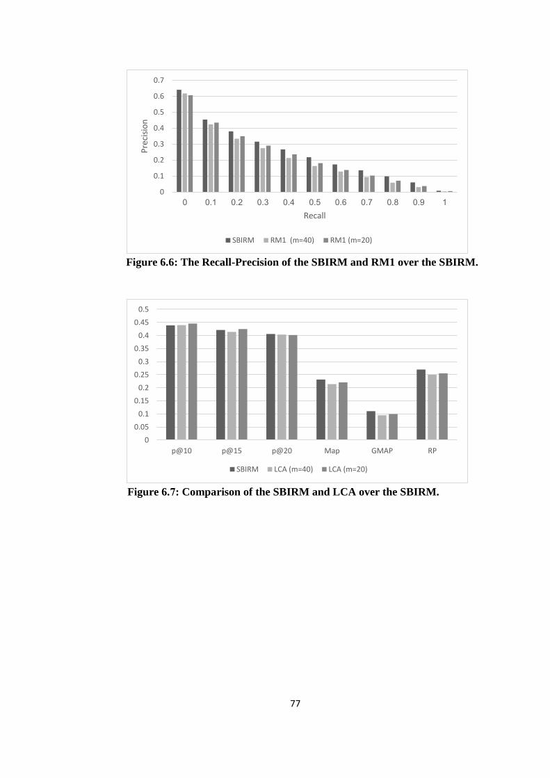
77
دد
دد
Figure 6.6: The Recall-Precision of the SBIRM and RM1 over the SBIRM.
Figure 6.7: Comparison of the SBIRM and LCA over the SBIRM.
0
0.05
0.1
0.15
0.2
0.25
0.3
0.35
0.4
0.45
0.5
p@10 p@15 p@20 Map GMAP RP
SBIRM LCA (m=40) LCA (m=20)
0
0.1
0.2
0.3
0.4
0.5
0.6
0.7
0 0.1 0.2 0.3 0.4 0.5 0.6 0.7 0.8 0.9 1
Pre
cisi
on
Recall
SBIRM RM1 (m=40) RM1 (m=20)
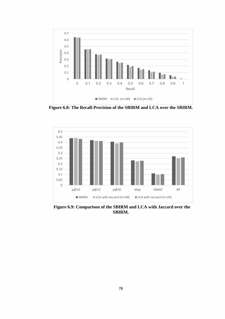
78
Figure 6.8: The Recall-Precision of the SBIRM and LCA over the SBIRM.
Figure 6.9: Comparison of the SBIRM and LCA with Jaccard over the
SBIRM.
0
0.05
0.1
0.15
0.2
0.25
0.3
0.35
0.4
0.45
0.5
p@10 p@15 p@20 Map GMAP RP
SBIRM LCA with Jaccard (m=40) LCA with Jaccard (m=20)
0
0.1
0.2
0.3
0.4
0.5
0.6
0.7
0 0.1 0.2 0.3 0.4 0.5 0.6 0.7 0.8 0.9 1
Pre
cisi
on
Recall
SBIRM LCA (m=40) LCA (m=20)

79
Figure 6.10: The Recall-Precision of the SBIRM and LCA with Jaccard over
the SBIRM.
Figure 6.11: Comparison of the SBIRM and newLCA over the SBIRM.
0
0.05
0.1
0.15
0.2
0.25
0.3
0.35
0.4
0.45
0.5
p@10 p@15 p@20 Map GMAP RP
SBIRM newLCA (m=40) newLCA (m=20)
0
0.1
0.2
0.3
0.4
0.5
0.6
0.7
0 0.1 0.2 0.3 0.4 0.5 0.6 0.7 0.8 0.9 1
Pre
cisi
on
Recall
SBIRM LCA with Jaccard (m=40) LCA with Jaccard (m=20)
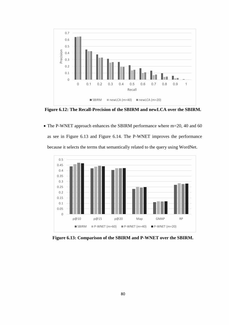
80
Figure 6.12: The Recall-Precision of the SBIRM and newLCA over the SBIRM.
The P-WNET approach enhances the SBIRM performance where m=20, 40 and 60
as see in Figure 6.13 and Figure 6.14. The P-WNET improves the performance
because it selects the terms that semantically related to the query using WordNet.
Figure 6.13: Comparison of the SBIRM and P-WNET over the SBIRM.
0
0.05
0.1
0.15
0.2
0.25
0.3
0.35
0.4
0.45
0.5
p@10 p@15 p@20 Map GMAP RP
SBIRM P-WNET (m=60) P-WNET (m=40) P-WNET (m=20)
0
0.1
0.2
0.3
0.4
0.5
0.6
0.7
0 0.1 0.2 0.3 0.4 0.5 0.6 0.7 0.8 0.9 1
Pre
cisi
on
Recall
SBIRM newLCA (m=40) newLCA (m=20)

81
Figure 6.14: The Recall-Precision of the SBIRM and P-WNET over the SBIRM.
The Figure 6.15 and Figure 6.16 shows that the P-WNETKLD approach improves
the performance of the SBIRM where m=60 and 20, respectively. The KLDP-WNET
better than the SBIRM with each approaches.
Figure 6.15: Comparison of the P-WNETKLD, P-WNET, and KLD over the
SBIRM.
0
0.05
0.1
0.15
0.2
0.25
0.3
0.35
0.4
0.45
0.5
p@10 p@15 p@20 Map GMAP RP
P-WNETKLD (m=60, 20) P-WNET (m=60) KLD (m=20)
0
0.1
0.2
0.3
0.4
0.5
0.6
0.7
0 0.1 0.2 0.3 0.4 0.5 0.6 0.7 0.8 0.9 1
Pre
cisi
on
Recall
SBIRM P-WNET (m=60) P-WNET (m=40) P-WNET (m=20)
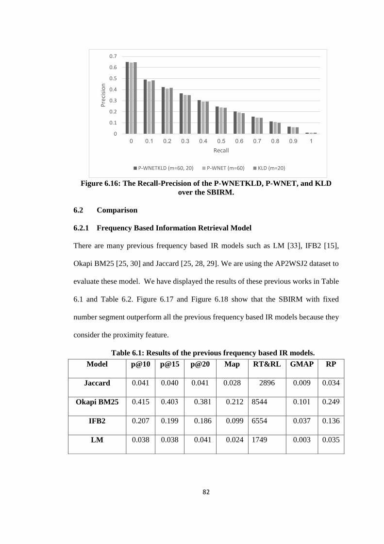
82
Figure 6.16: The Recall-Precision of the P-WNETKLD, P-WNET, and KLD
over the SBIRM.
6.2 Comparison
6.2.1 Frequency Based Information Retrieval Model
There are many previous frequency based IR models such as LM [33], IFB2 [15],
Okapi BM25 [25, 30] and Jaccard [25, 28, 29]. We are using the AP2WSJ2 dataset to
evaluate these model. We have displayed the results of these previous works in Table
6.1 and Table 6.2. Figure 6.17 and Figure 6.18 show that the SBIRM with fixed
number segment outperform all the previous frequency based IR models because they
consider the proximity feature.
Table 6.1: Results of the previous frequency based IR models.
Model p@10 p@15 p@20 Map RT&RL GMAP RP
Jaccard 0.041 0.040 0.041 0.028 2896 0.009 0.034
Okapi BM25 0.415 0.403 0.381 0.212 8544 0.101 0.249
IFB2 0.207 0.199 0.186 0.099 6554 0.037 0.136
LM 0.038 0.038 0.041 0.024 1749 0.003 0.035
0
0.1
0.2
0.3
0.4
0.5
0.6
0.7
0 0.1 0.2 0.3 0.4 0.5 0.6 0.7 0.8 0.9 1
Pre
cisi
on
Recall
P-WNETKLD (m=60, 20) P-WNET (m=60) KLD (m=20)

83
Figure 6.17: Comparison of the frequency based IR models and SBIRM
with fixed number segment.
Table 6.2: Recall-Precision of the previous frequency based IR models.
Recall Jaccard Okapi
BM25
IFB2 LM
0.0 0.108 0.618 0.398 0.081
0.1 0.053 0.434 0.224 0.052
0.2 0.044 0.356 0.177 0.044
0.3 0.035 0.293 0.133 0.032
0.4 0.032 0.246 0.106 0.027
0.5 0.027 0.194 0.081 0.022
0.6 0.023 0.147 0.062 0.019
0.7 0.02 0.115 0.046 0.016
0.8 0.015 0.08 0.031 0.013
0.9 0.006 0.042 0.015 0.005
1.0 0.002 0.007 0.003 0.002
0
0.05
0.1
0.15
0.2
0.25
0.3
0.35
0.4
0.45
0.5
p@10 p@15 p@20 Map GMAP RP
SBIRM Jaccard Okapi BM25 IFB2 LM

84
Figure 6.18: The Recall-Precision the previous frequency based IR models and
SBIRM with fixed number segment.
6.2.2 Proximity Based Information Retrieval Model
There are many previous proximity based IR models such as MRF [7] and BM25P [6].
We evaluate these models using AP2WSJ2 dataset. In Table 6.3 and Table 6.4, we
have displayed these previous works results. As shown in Figure 6.19 and Figure 6.20,
fixed number segment and all suggested segmentation methods outperform the MRF
model while only the fixed number segment method outperform the BM25P model.
Therefore, we select the good performance SBIRM with fixed number segment as our
proximity IR model.
Table 6.3: Results of the previous proximity based IR models.
Model p@10 p@15 p@20 Map RT&RL GMAP RP
MRF 0.067 0.061 0.056 0.023 1409 0.003 0.035
BM25P 0.431 0.418 0.391 0.218 8583 0.103 0.252
0
0.1
0.2
0.3
0.4
0.5
0.6
0.7
0 0.1 0.2 0.3 0.4 0.5 0.6 0.7 0.8 0.9 1
Pre
cisi
on
Recall
SBIRM Jaccard Okapi BM25 IFB2 LM

85
Figure 6.19: Comparison of the proximity based IR models.
Table 6.4: Recall-Precision of the previous proximity based IR models.
Recall MRF BM25P
0.0 0.134 0.634
0.1 0.061 0.439
0.2 0.044 0.363
0.3 0.027 0.295
0.4 0.02 0.248
0.5 0.017 0.197
0.6 0.015 0.153
0.7 0.013 0.121
0.8 0.01 0.091
0.9 0.004 0.055
1.0 0.002 0.008
0
0.05
0.1
0.15
0.2
0.25
0.3
0.35
0.4
0.45
0.5
p@10 p@15 p@20 Map GMAP RP
SBIRM MRF BM25P

86
Figure 6.20: The Recall-Precision the proximity based IR models.
6.2.3 Query Expansion over the Frequency Based Information Retrieval Model
We evaluate all the following previous work by implement these models using the
AP2WSJ2 dataset.
KLD approach over the Okapi BM25 and IFB2 model:
The study in [12] run the KLD approach over the Okapi BM25 model while [69] run
the KLD approach over IFB2 model. As see in Table 6.5 and Table 6.6, the KLD
approach improve the performance of the Okapi BM25 while the KLD does not
improve the performance of IFB2 model. The bad performance of KLD over IFB2
back to the bad performance of the IFB2 model itself. As see in Figure 6.21 and Figure
6.22 the result of KLD approach over the SBIRM model is better than over the Okapi
BM25 and IFB2 model.
Table 6.5: KLD approach over the Okapi BM25 and IFB2.
Model p@10 p@15 p@20 Map RT&RL GMAP RP
Okapi BM25 0.415 0.403 0.381 0.212 8544 0.101 0.249
0
0.1
0.2
0.3
0.4
0.5
0.6
0.7
0 0.1 0.2 0.3 0.4 0.5 0.6 0.7 0.8 0.9 1
Pre
cisi
on
Recall
SBIRM MRF BM25P
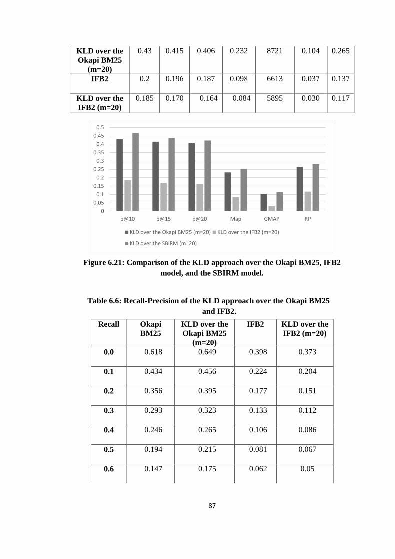
87
Figure 6.21: Comparison of the KLD approach over the Okapi BM25, IFB2
model, and the SBIRM model.
Table 6.6: Recall-Precision of the KLD approach over the Okapi BM25
and IFB2.
KLD over the
Okapi BM25
(m=20)
0.43 0.415 0.406 0.232 8721 0.104 0.265
IFB2 0.2 0.196 0.187 0.098 6613 0.037 0.137
KLD over the
IFB2 (m=20)
0.185 0.170 0.164 0.084 5895 0.030 0.117
Recall Okapi
BM25
KLD over the
Okapi BM25
(m=20)
IFB2 KLD over the
IFB2 (m=20)
0.0 0.618 0.649 0.398 0.373
0.1 0.434 0.456 0.224 0.204
0.2 0.356 0.395 0.177 0.151
0.3 0.293 0.323 0.133 0.112
0.4 0.246 0.265 0.106 0.086
0.5 0.194 0.215 0.081 0.067
0.6 0.147 0.175 0.062 0.05
0
0.05
0.1
0.15
0.2
0.25
0.3
0.35
0.4
0.45
0.5
p@10 p@15 p@20 Map GMAP RP
KLD over the Okapi BM25 (m=20) KLD over the IFB2 (m=20)
KLD over the SBIRM (m=20)
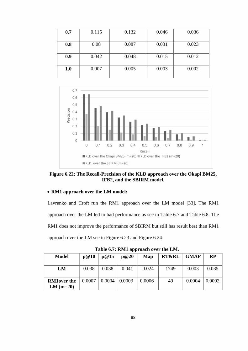
88
Figure 6.22: The Recall-Precision of the KLD approach over the Okapi BM25,
IFB2, and the SBIRM model.
RM1 approach over the LM model:
Lavrenko and Croft run the RM1 approach over the LM model [33]. The RM1
approach over the LM led to bad performance as see in Table 6.7 and Table 6.8. The
RM1 does not improve the performance of SBIRM but still has result best than RM1
approach over the LM see in Figure 6.23 and Figure 6.24.
Table 6.7: RM1 approach over the LM.
0.7 0.115 0.132 0.046 0.036
0.8 0.08 0.087 0.031 0.023
0.9 0.042 0.048 0.015 0.012
1.0 0.007 0.005 0.003 0.002
Model p@10 p@15 p@20 Map RT&RL GMAP RP
LM 0.038 0.038 0.041 0.024 1749 0.003 0.035
RM1over the
LM (m=20)
0.0007 0.0004 0.0003 0.0006 49 0.0004 0.0002
0
0.1
0.2
0.3
0.4
0.5
0.6
0.7
0 0.1 0.2 0.3 0.4 0.5 0.6 0.7 0.8 0.9 1
Pre
cisi
on
RecallKLD over the Okapi BM25 (m=20) KLD over the IFB2 (m=20)
KLD over the SBIRM (m=20)
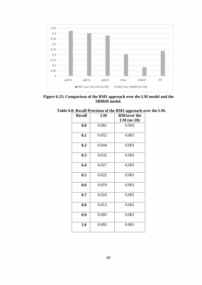
89
Figure 6.23: Comparison of the RM1 approach over the LM model and the
SBIRM model.
Table 6.8: Recall-Precision of the RM1 approach over the LM.
Recall LM RM1over the
LM (m=20)
0.0 0.081 0.003
0.1 0.052 0.001
0.2 0.044 0.001
0.3 0.032 0.001
0.4 0.027 0.001
0.5 0.022 0.001
0.6 0.019 0.001
0.7 0.016 0.001
0.8 0.013 0.001
0.9 0.005 0.001
1.0 0.002 0.001
0
0.05
0.1
0.15
0.2
0.25
0.3
0.35
0.4
0.45
p@10 p@15 p@20 Map GMAP RP
RM1 over the LM (m=20) RM1 over SBIRM (m=20)
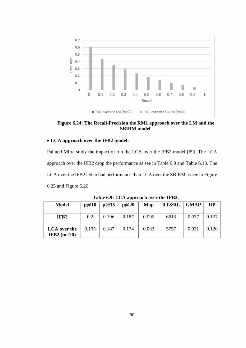
90
Figure 6.24: The Recall-Precision the RM1 approach over the LM and the
SBIRM model.
LCA approach over the IFB2 model:
Pal and Mitra study the impact of run the LCA over the IFB2 model [69]. The LCA
approach over the IFB2 drop the performance as see in Table 6.9 and Table 6.10. The
LCA over the IFB2 led to bad performance than LCA over the SBIRM as see in Figure
6.25 and Figure 6.26.
Table 6.9: LCA approach over the IFB2.
Model p@10 p@15 p@20 Map RT&RL GMAP RP
IFB2 0.2 0.196 0.187 0.098 6613 0.037 0.137
LCA over the
IFB2 (m=20)
0.195 0.187 0.174 0.083 5757 0.031 0.120
0
0.1
0.2
0.3
0.4
0.5
0.6
0.7
0 0.1 0.2 0.3 0.4 0.5 0.6 0.7 0.8 0.9 1
Pre
cisi
on
Recall
RM1 over the LM (m=20) RM1 over the SBIRM (m=20)
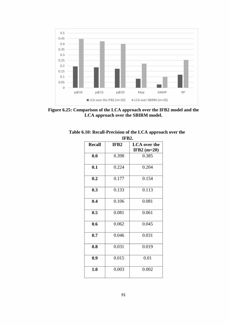
91
Figure 6.25: Comparison of the LCA approach over the IFB2 model and the
LCA approach over the SBIRM model.
Table 6.10: Recall-Precision of the LCA approach over the
IFB2.
Recall IFB2 LCA over the
IFB2 (m=20)
0.0 0.398 0.385
0.1 0.224 0.204
0.2 0.177 0.154
0.3 0.133 0.113
0.4 0.106 0.081
0.5 0.081 0.061
0.6 0.062 0.045
0.7 0.046 0.031
0.8 0.031 0.019
0.9 0.015 0.01
1.0 0.003 0.002
0
0.05
0.1
0.15
0.2
0.25
0.3
0.35
0.4
0.45
0.5
p@10 p@15 p@20 Map GMAP RP
LCA over the IFB2 (m=20) LCA over SBIRM (m=20)
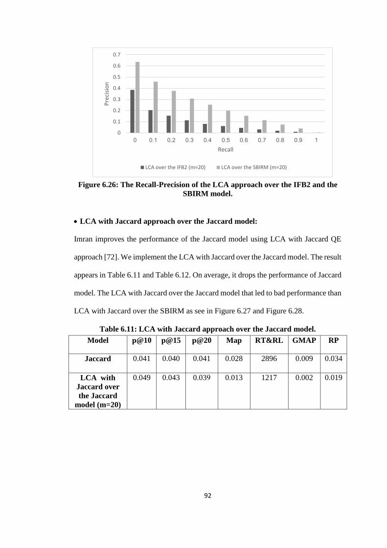
92
Figure 6.26: The Recall-Precision of the LCA approach over the IFB2 and the
SBIRM model.
LCA with Jaccard approach over the Jaccard model:
Imran improves the performance of the Jaccard model using LCA with Jaccard QE
approach [72]. We implement the LCA with Jaccard over the Jaccard model. The result
appears in Table 6.11 and Table 6.12. On average, it drops the performance of Jaccard
model. The LCA with Jaccard over the Jaccard model that led to bad performance than
LCA with Jaccard over the SBIRM as see in Figure 6.27 and Figure 6.28.
Table 6.11: LCA with Jaccard approach over the Jaccard model.
Model p@10 p@15 p@20 Map RT&RL GMAP RP
Jaccard 0.041 0.040 0.041 0.028 2896 0.009 0.034
LCA with
Jaccard over
the Jaccard
model (m=20)
0.049 0.043 0.039 0.013 1217 0.002 0.019
0
0.1
0.2
0.3
0.4
0.5
0.6
0.7
0 0.1 0.2 0.3 0.4 0.5 0.6 0.7 0.8 0.9 1
Pre
cisi
on
Recall
LCA over the IFB2 (m=20) LCA over the SBIRM (m=20)

93
Figure 6.27: Comparison of the LCA with Jaccard approach over the Jaccard
model and the SBIRM model
Table 6.12: Recall-Precision of the LCA with Jaccard approach over the
Jaccard.
Recall Jaccard LCA with
Jaccard over
the Jaccard
(m=20)
0.0 0.108 0.125
0.1 0.053 0.026
0.2 0.044 0.016
0.3 0.035 0.012
0.4 0.032 0.01
0.5 0.027 0.008
0.6 0.023 0.006
0.7 0.02 0.005
0.8 0.015 0.004
0.9 0.006 0.003
1.0 0.002 0.001
0
0.05
0.1
0.15
0.2
0.25
0.3
0.35
0.4
0.45
0.5
p@10 p@15 p@20 Map GMAP RP
LCA with Jaccard over the Jaccard model (m=20)
LCA with Jaccard over the SBIRM (m=20)

94
Figure 6.28: The Recall-Precision of the LCA with Jaccard approach over the
Jaccard and the SBIRM model.
newLCA approach over the IFB2 model:
Paper [69] improves the performance of the IFB2 by run the newLCA QE approach.
Table 6.13 and Table 6.14 present the result of our implementation of the newLCA
over the IFB2. It drops the performance of the IFB2. Although run the newLCA over
the SBIRM led to bad performance but still better than newLCA over the IFB2 SBIRM
as the result displays in Figure 6.29 and Figure 6.30.
Table 6.13: newLCA over the IFB2 model.
Model p@10 p@15 p@20 Map RT&RL GMAP RP
IFB2 0.2 0.196 0.187 0.098 6613 0.037 0.137
newLCA over
the IFB2
(m=20)
0.162 0.150 0.141 0.068 5243 0.024 0.100
0
0.1
0.2
0.3
0.4
0.5
0.6
0.7
0 0.1 0.2 0.3 0.4 0.5 0.6 0.7 0.8 0.9 1
Pre
cisi
on
Recall
LCA with Jaccard over the Jaccard (m=20) LCA with Jaccard over the SBIRM (m=20)
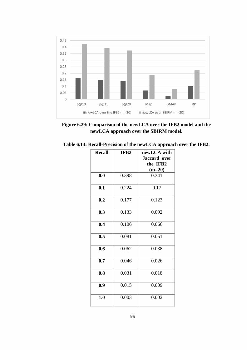
95
Figure 6.29: Comparison of the newLCA over the IFB2 model and the
newLCA approach over the SBIRM model.
Table 6.14: Recall-Precision of the newLCA approach over the IFB2.
Recall IFB2 newLCA with
Jaccard over
the IFB2
(m=20)
0.0 0.398 0.341
0.1 0.224 0.17
0.2 0.177 0.123
0.3 0.133 0.092
0.4 0.106 0.066
0.5 0.081 0.051
0.6 0.062 0.038
0.7 0.046 0.026
0.8 0.031 0.018
0.9 0.015 0.009
1.0 0.003 0.002
0
0.05
0.1
0.15
0.2
0.25
0.3
0.35
0.4
0.45
p@10 p@15 p@20 Map GMAP RP
newLCA over the IFB2 (m=20) newLCA over SBIRM (m=20)
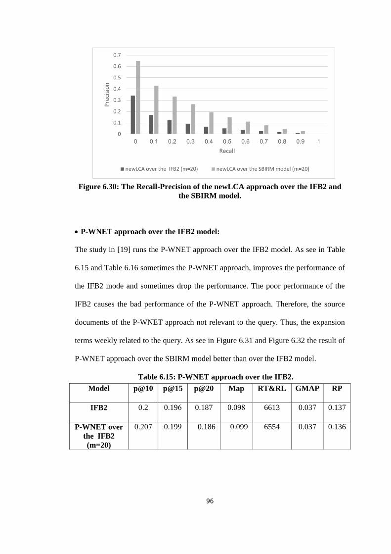
96
Figure 6.30: The Recall-Precision of the newLCA approach over the IFB2 and
the SBIRM model.
P-WNET approach over the IFB2 model:
The study in [19] runs the P-WNET approach over the IFB2 model. As see in Table
6.15 and Table 6.16 sometimes the P-WNET approach, improves the performance of
the IFB2 mode and sometimes drop the performance. The poor performance of the
IFB2 causes the bad performance of the P-WNET approach. Therefore, the source
documents of the P-WNET approach not relevant to the query. Thus, the expansion
terms weekly related to the query. As see in Figure 6.31 and Figure 6.32 the result of
P-WNET approach over the SBIRM model better than over the IFB2 model.
Table 6.15: P-WNET approach over the IFB2.
Model p@10 p@15 p@20 Map RT&RL GMAP RP
IFB2 0.2 0.196 0.187 0.098 6613 0.037 0.137
P-WNET over
the IFB2
(m=20)
0.207 0.199 0.186 0.099 6554 0.037 0.136
0
0.1
0.2
0.3
0.4
0.5
0.6
0.7
0 0.1 0.2 0.3 0.4 0.5 0.6 0.7 0.8 0.9 1
Pre
cisi
on
Recall
newLCA over the IFB2 (m=20) newLCA over the SBIRM model (m=20)

97
Figure 6.31: Comparison of the P-WNET approach over the IFB2 and the
SBIRM model.
Table 6.16: Recall-Precision of the P-WNET approach over the IFB2.
Recall IFB2 P-WNET
over the IFB2
(m=20)
0.0 0.398 0.393
0.1 0.224 0.173
0.2 0.177 0.094
0.3 0.133 0.03
0.4 0.106 0.018
0.5 0.081 0.007
0.6 0.062 0.004
0.7 0.046 0.003
0.8 0.031 0.002
0.9 0.015 0.001
1.0 0.003 0.0001
0
0.05
0.1
0.15
0.2
0.25
0.3
0.35
0.4
0.45
0.5
p@10 p@15 p@20 Map GMAP RP
P-WNET over the IFB2 (m=20) P-WNET over SBIRM (m=20)
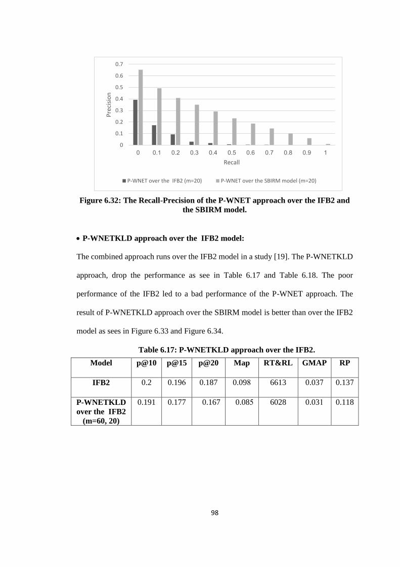
98
Figure 6.32: The Recall-Precision of the P-WNET approach over the IFB2 and
the SBIRM model.
P-WNETKLD approach over the IFB2 model:
The combined approach runs over the IFB2 model in a study [19]. The P-WNETKLD
approach, drop the performance as see in Table 6.17 and Table 6.18. The poor
performance of the IFB2 led to a bad performance of the P-WNET approach. The
result of P-WNETKLD approach over the SBIRM model is better than over the IFB2
model as sees in Figure 6.33 and Figure 6.34.
Table 6.17: P-WNETKLD approach over the IFB2.
Model p@10 p@15 p@20 Map RT&RL GMAP RP
IFB2 0.2 0.196 0.187 0.098 6613 0.037 0.137
P-WNETKLD
over the IFB2
(m=60, 20)
0.191 0.177 0.167 0.085 6028 0.031 0.118
0
0.1
0.2
0.3
0.4
0.5
0.6
0.7
0 0.1 0.2 0.3 0.4 0.5 0.6 0.7 0.8 0.9 1
Pre
cisi
on
Recall
P-WNET over the IFB2 (m=20) P-WNET over the SBIRM model (m=20)

99
Figure 6.33: Comparison of the P-WNETKLD over the IFB2 and the SBIRM
Model.
Table 6.18: Recall-Precision of the P-WNETKLD approach over the IFB2.
Recall IFB2 P-WNETKLD
over the IFB2
(m=60, 20)
0.0 0.398 0.369
0.1 0.224 0.207
0.2 0.177 0.154
0.3 0.133 0.111
0.4 0.106 0.084
0.5 0.081 0.066
0.6 0.062 0.05
0.7 0.046 0.036
0.8 0.031 0.023
0.9 0.015 0.012
1.0 0.003 0.002
0
0.05
0.1
0.15
0.2
0.25
0.3
0.35
0.4
0.45
0.5
p@10 p@15 p@20 Map GMAP RP
P-WNETKLD over the IFB2 (m=60, 20) P-WNETKLD over the SBIRM (m=60, 20)

100
Figure 6.34: The Recall-Precision of the P-WNETKLD approach over the IFB2
and the SBIRM model.
6.2.4 Query Expansion over the Proximity Based Information Retrieval Model
We implemented the following previous work model using the AP2WSJ2 dataset to
evaluate these models.
KLD approach over the BM25P model:
He et al. [6] study the effectiveness of expanding the query using the KLD over
BM25P proximity based IR and they concluded that the KLD on average improved
the performance. We implement the KLD over BM25P and the result display in Table
6.19 and Table 6.20. The result shows that the KLD improve the performance of
BM25P but less than the performance of KLD over SBIRM as present in Figure 6.35
and Figure 6.36.
Table 6.19: KLD over the BM25P model.
Model p@10 p@15 p@20 Map RT&RL GMAP RP
BM25P 0.431 0.418 0.391 0.218 8583 0.103 0.252
KLD over the
BM25P
(m=20)
0.463 0.43 0.417 0.245 9166 0.113 0.277
0
0.1
0.2
0.3
0.4
0.5
0.6
0.7
0 0.1 0.2 0.3 0.4 0.5 0.6 0.7 0.8 0.9 1
Pre
cisi
on
Recall
P-WNETKLD over the IFB2 (m=60, 20) P-WNETKLD over the SBIRM model (m=60, 20)

101
Figure 6.35: Comparison of the KLD over the BM25P model and the
SBIRM model.
Table 6.20: Recall-Precision of the KLD approach over the BM25P.
Recall BM25P KLD over the
BM25P
(m=20)
0.0 0.634 0.639
0.1 0.439 0.468
0.2 0.363 0.396
0.3 0.295 0.34
0.4 0.248 0.287
0.5 0.197 0.23
0.6 0.153 0.186
0.7 0.121 0.149
0.8 0.091 0.108
0.9 0.055 0.061
1.0 0.008 0.01
0
0.05
0.1
0.15
0.2
0.25
0.3
0.35
0.4
0.45
0.5
p@10 p@15 p@20 Map GMAP RP
KLD over the BM25P (m=20) KLD over SBIRM (m=20)
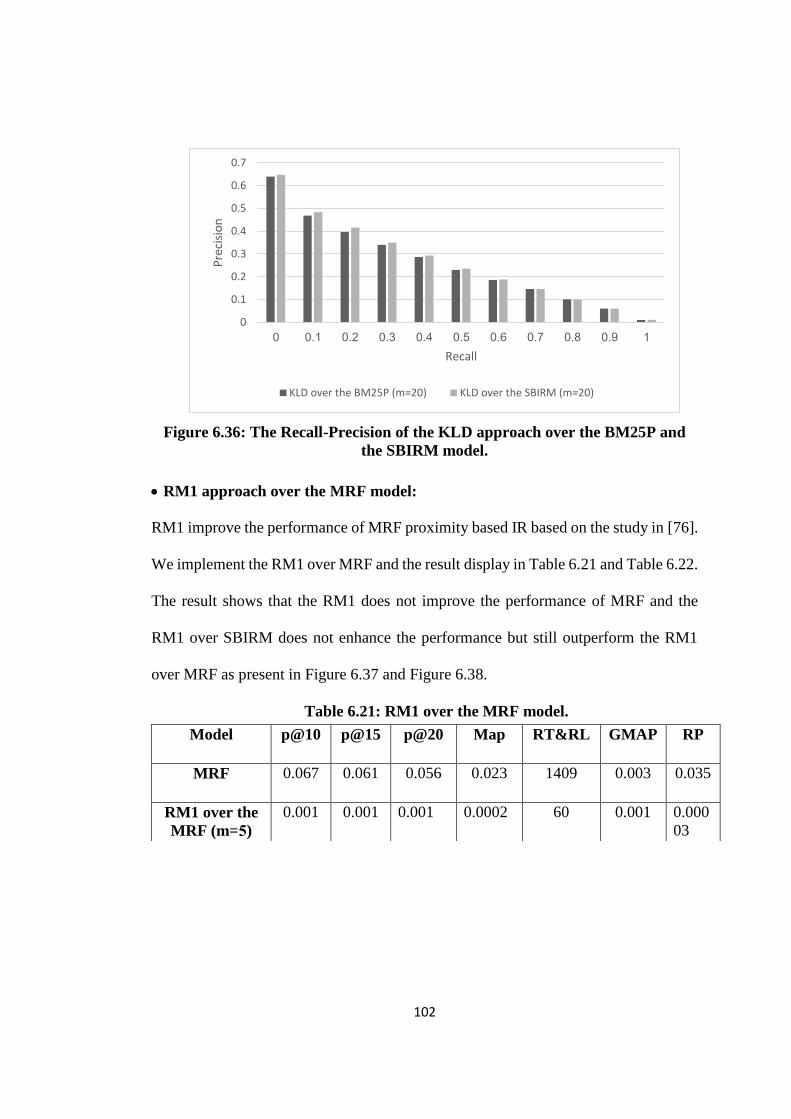
102
Figure 6.36: The Recall-Precision of the KLD approach over the BM25P and
the SBIRM model.
RM1 approach over the MRF model:
RM1 improve the performance of MRF proximity based IR based on the study in [76].
We implement the RM1 over MRF and the result display in Table 6.21 and Table 6.22.
The result shows that the RM1 does not improve the performance of MRF and the
RM1 over SBIRM does not enhance the performance but still outperform the RM1
over MRF as present in Figure 6.37 and Figure 6.38.
Table 6.21: RM1 over the MRF model.
Model p@10 p@15 p@20 Map RT&RL GMAP RP
MRF 0.067 0.061 0.056 0.023 1409 0.003 0.035
RM1 over the
MRF (m=5)
0.001 0.001 0.001 0.0002 60 0.001 0.000
03
0
0.1
0.2
0.3
0.4
0.5
0.6
0.7
0 0.1 0.2 0.3 0.4 0.5 0.6 0.7 0.8 0.9 1
Pre
cisi
on
Recall
KLD over the BM25P (m=20) KLD over the SBIRM (m=20)

103
Figure 6.37: Comparison of the RM1 over the MRF model and the SBIRM
model.
Table 6.22: Recall-Precision of the RM1 approach over the MRF.
Recall MRF RM1 over the
MRF (m=20)
0.0 0.134 0.007
0.1 0.061 0.003
0.2 0.044 0.003
0.3 0.027 0.003
0.4 0.02 0.003
0.5 0.017 0.003
0.6 0.015 0.002
0.7 0.013 0.002
0.8 0.01 0.002
0.9 0.004 0.002
1.0 0.002 0.001
0
0.05
0.1
0.15
0.2
0.25
0.3
0.35
0.4
0.45
p@10 p@15 p@20 Map GMAP RP
RM1 over the MRF (m=5) RM1 over SBIRM (m=5)
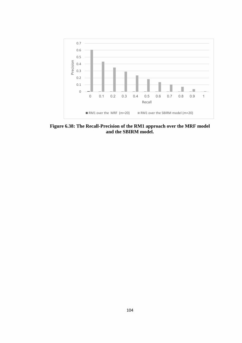
104
Figure 6.38: The Recall-Precision of the RM1 approach over the MRF model
and the SBIRM model.
0
0.1
0.2
0.3
0.4
0.5
0.6
0.7
0 0.1 0.2 0.3 0.4 0.5 0.6 0.7 0.8 0.9 1
Pre
cisi
on
Recall
RM1 over the MRF (m=20) RM1 over the SBIRM model (m=20)

105
Chapter VII
Conclusion and Future Work
7.1 Conclusion
This research studied the impact of extending the query by adding statistical and
semantic related terms to the original query terms over proximity based IR system.
This is done by combining the SBIRM model with the best QE approaches such as the
distribution approach (KLD), the best target corpus and external resource approaches
(P-WNET), all the often good performance co-occurrence approaches: RM1, LCA,
LCA with Jaccard and newLCA and finally combining the good performance QE
approaches. These models were tested and evaluated using TREC dataset.
The experiment results show that the QESBIRM using KLD, P-WNET and the
combination of these approach outperformed the SBIRM in precision at top
documents, precision at stander recall levels, R-precision, RET&REL, GMAP and
MAP metric while all co-occurrence approaches drop the performance.
In addition, we investigated three proposed document segmentation methods in
SBIRM using wavelet transform. These segmentation methods are sentences-based,
paragraphs-based and minimum distance terms segmentation. The experiments
demonstrate that dividing the documents into a specific number of segments (8 bin) is
better than the proposed segmentation methods but all the proposed segmentation

106
methods are still better than MRF proximity based model and Jaccard, LM and IFB2
frequency based mode. Only sentences-based segmentation method outperform the
Okapi BM25, which is one of the best-performing frequency based models.
7.2 Future Work
This thesis shows several conclusions about the presented QESBIRM model, but there
are some directions for future research:
We have used six QE approaches over the SBIRM proximity based IR. It
would be interesting to study the performance of other QE approaches such as
the approaches that use the Wikipedia as source of the expansion terms.
In this thesis, the experiments were conducted with documents written in
English. It would be interesting to evaluate our methods with a collection
written in other languages like Arabic.
In this work, we have used semantic and statistical feature over IR model. It
would be interesting to use the semantic, and statistical features in text mining
models such as text classification and clustering that consider the proximity.

107
LIST OF REFERENCES
[1] [1] D. Hawking and P. Thistlewaite, "Relevance weighting using distance
between term occurrences", ", Computer Science Technical Report TR-CS-96–
08 Australian National University, 1996.
[8] [2] C. L. A. Clarke and G. V. Cormack, "Shortest-substring retrieval and
ranking," ACM Transactions on Information Systems (TOIS), vol. 18, no. 1,
pp. 44-78, 2000.
[9] [3] M. Beigbeder and A. Mercier, "An information retrieval model using the fuzzy
proximity degree of term occurences," Proceedings of the 2005 ACM
symposium on Applied computing, pp. 1018-1022, 2005.
[10] [4] J. Peng, C. Macdonald, B. He, V. Plachouras, and I. Ounis, "Incorporating
term dependency in the DFR framework," Proceedings of the 30th annual
international ACM SIGIR conference on Research and development in
information retrieval, pp. 843-844, 2007.
[11] [5] S. Buttcher C. L. A. Clarke, and B. Lushman, "Term proximity scoring for ad-
hoc retrieval on very large text collections," Proceedings of the 29th annual
international ACM SIGIR conference on Research and development in
information retrieval, pp. 621-622, 2006.
[12] [6] B. He, J. X. Huang, and X. Zhou, "Modeling term proximity for probabilistic
information retrieval models," Information Sciences, vol. 181, no. 14, pp.
3017-3031, 2011.
[13] [7] D. Metzler and W. B. Croft, "A Markov random field model for term
dependencies," Proceedings of the 28th annual international ACM SIGIR
conference on Research and development in information retrieval, pp. 472-
479, 2005.
[14] [8] L. A. F. Park, "Spectral Based Information Retrieval," PhD thesis, Electrical
and Electronic Engineering Department, Melbourne University, Melbourne,
Australia, 2003.
[15] [9] L. A. F. Park, K. Ramamohanarao, and M. Palaniswami, "Fourier domain
scoring: A novel document ranking method," IEEE Transactions on
Knowledge and Data Engineering, vol. 16, no.5, pp. 529-539, 2004.
108
[35] [10] L. A. Park, M. Palaniswami, and K. Ramamohanarao, "A novel document
ranking method using the discrete cosine transform," IEEE transactions on
pattern analysis and machine intelligence, vol. 27, no.1, pp. 130-135, 2005.
[16] [11] L. A. F. Park, K. Ramamohanarao, and M. Palaniswami, "A novel document
retrieval method using the discrete wavelet transform," ACM Transactions on
Information Systems (TOIS), vol. 23, no. 3, pp. 267-298, 2005.
[17] [12] C. Carpineto, R. De Mori, G. Romano, and B. Bigi, "An information-theoretic
approach to automatic query expansion," ACM Transactions on Information
Systems (TOIS), vol. 19, no. 1, pp. 1-27, 2001.
[18] [13] S. E. Robertson, "On term selection for query expansion," Journal of
documentation, vol. 46, no. 4, pp. 359-364, 1990.
[19] [14] T. E. Doszkocs, "AID, an associative interactive dictionary for online
searching," Online Review, vol. 2, no. 2, pp. 163-173, 1978.
[20] [15] G. Amati, "Probabilistic models for information retrieval based on divergence
from randomness," PhD thesis, Computing Science Department, Glasgow
University, Glasgow , United Kingdom, 2003.
[21] [16] C. Carpineto and G. Romano, "A survey of automatic query expansion in
information retrieval," ACM Computing Surveys (CSUR), vol. 44, no. 1, pp. 1-
50, 2012.
[22] [17] A. K. Barman, J. Sarmah, and S. K. Sarma, "WordNet Based Information
Retrieval System for Assamese," Proceedings of the 2013 UKSim 15th
International Conference on Computer Modelling and Simulation, pp. 480-
484, 2013.
[23] [18] G. Varelas, E. Voutsakis, P. Raftopoulou, E. G. M. Petrakis, and E. E. Milios,
"Semantic similarity methods in wordNet and their application to information
retrieval on the web," Proceedings of the 7th annual ACM international
workshop on Web information and data management, pp. 10-16, 2005.
[2] [19] D. Pal, M. Mitra, and K. Datta, "Improving query expansion using
WordNet," Journal of the Association for Information Science and
Technology, vol. 65, no. 12, pp. 2469-2478, 2014.
[3] [20] M. Lu, X. Sun, S. Wang, D. Lo, and Y. Duan, "Query expansion via wordnet
for effective code search," Proceedings of the 2015 IEEE 22nd International
Conference on Software Analysis, Evolution, and Reengineering (SANER), pp.
545-549. 2015.
109
[60] [21] H. Fang, "A Re-examination of Query Expansion Using Lexical Resources,"
Proceedings of the Association for Computational Linguistics, pp. 139-147,
2008.
[62] [22] S. M. Tyar and M. M. Than, "Sense-based Information Retrieval System by
using Jaccard Coefficient Based WSD Algorithm,"Proceedings of the 2015
International Conference on Future Computational Technologies, pp. 197-
203, 2015.
[61] [23] J. Singh and A. Sharan, "Co-occurrence and Semantic Similarity Based Hybrid
Approach for Improving Automatic Query Expansion in Information
Retrieval," Proceedings of the International Conference on Distributed
Computing and Internet Technology, pp. 415-418, 2015.
[65] [24] G. Chowdhury, Introduction to modern information retrieval: Facet
Publishing, 2010.
[66] [25] Y. Gupta, A. Saini, and A. K. Saxena, "A review on important aspects of
information retrieval," International Journal of Computer, Information
Science and Engineering, vol. 7, no. 12, pp. 968-976, 2013.
[67] [26] D. A. Grossman and O. Frieder, Information retrieval: Algorithms and
heuristics. Springer Science & Business Media, 2012.
[46] [27] G. Salton, "Automatic text processing: The transformation, analysis, and
retrieval ," Addison-Wesley Longman, 1989.
[68] [28] P. Bhatnagar and N. K. Pareek, "A combined matching function based
evolutionary approach for development of adaptive information retrieval
system," International Journal of Emerging Technology and Advanced
Engineering, vol. 2, no. 6, pp. 249-256, 2012.
[69] [29] J. Leskovec, A. Rajaraman, and J. D. Ullman, Mining of Massive Datasets,
20th ed. Cambridge: Cambridge University Press, 2012.
[73] [30] S. E. Robertson and S. Walker, "Okapi/Keenbow at TREC-8," in Text
REtrieval Conference (TREC), pp. 151-162, 1999.
[71] [31] G. Amati and C. J. Van Rijsbergen, "Probabilistic models of information
retrieval based on measuring the divergence from randomness," ACM
Transactions on Information Systems (TOIS), vol. 20, no. 4, pp. 357-389,
2002.
[74] [32] M. Ristin, "Language Modelling in Information Retrieval," 2007.

110
[77] [33] V. Lavrenko and W. B. Croft, "Relevance based language models,"
Proceedings of the 24th annual international ACM SIGIR conference on
Research and development in information retrieval, pp. 120-127, 2001.
[79] [34] A. El Mahdaouy, E. r. Gaussier, and S. d. O. El Alaoui, "Exploring term
proximity statistic for Arabic information retrieval," 2014 Third IEEE
International Colloquium in Information Science and Technology (CIST), pp.
272-277, 2014.
[80] [35] C. Macdonald, I. Ounis, and V. Plachouras, Proceedings of the Advances in
Information Retrieval: 30th European Conference on IR Research, ECIR
2008, Glasgow, UK, Glasgow, UK. Germany: Springer-Verlag Berlin and
Heidelberg GmbH & Co. K, 2008
[81] [36] Chun-Lin and Liu, "A tutorial of the wavelet transform," NTUEE, Taiwan,
2010.
[40] [37] A. Haar, "Zur theorie der orthogonalen funktionensysteme," Mathematische
Annalen, vol. 69, no. 3, pp. 331-371, 1910.
[82] [38] R. W. Hamming and L. N. Trefethen, "Haar wavelets," CRC Press, LLC, 1999.
[32] [39] X. Li, S. Szpakowicz, and S. Matwin, "A WordNet-based algorithm for word
sense disambiguation," in International Joint Conference on Artificial
Intelligence, pp. 1368-1374, 1995.
[28] [40] S. Banerjee and T. Pedersen, "An adapted Lesk algorithm for word sense
disambiguation using WordNet," Proceedings of the International Conference
on Intelligent Text Processing and Computational Linguistics, pp. 136-145,
2002.
[33] [41] “What is WordNet?” [Online]. Available: https://wordnet.princeton.edu/.
[Accessed: 26-Jun-2016]
[36] [42] “WordNet Interface.” [Online]. Available:
http://www.nltk.org/howto/wordnet.html. [Accessed: 1-Jan-2016]
[37] [43] J. Nemrava, "Using WordNet glosses to refine Google queries," in Proc. of the
Dateso 2006 Workshop VSB–Technical University of Ostrava, Dept. of
Computer Science, pp. 85-94, 2006.
[4] [44] L. Meng, R. Huang, and J. Gu, "A review of semantic similarity measures in
wordnet," International Journal of Hybrid Information Technology, vol. 6, no.
1, pp. 1-12, 2013.

111
[34] [45] S. A. Elavarasi, J. Akilandeswari, and K. Menaga, "A survey on semantic
similarity measure," International Journal of Research in Advent
Technology, vol. 2, no. 4, pp. 389-398, 2014.
[78] [46] H. Bulskov, R. Knappe, and T. Andreasen, "On measuring similarity for
conceptual querying," Proceedings of the International Conference on
Flexible Query Answering Systems, pp. 100-111, 2002.
[38] [47] R. Rada, H. Mili, E. Bicknell, and M. Blettner, "Development and application
of a metric on semantic nets," IEEE transactions on systems, man, and
cybernetics, vol. 19, no. 1, pp. 17-30, 1989.
[39] [48] Z. Wu and M. Palmer, "Verbs semantics and lexical selection," Proceedings
of the 32nd annual meeting on Association for Computational Linguistics, pp.
133-138, 1994.
[27] [49] Y. Li, Z. A. Bandar, and D. McLean, "An approach for measuring semantic
similarity between words using multiple information sources," IEEE
Transactions on knowledge and data engineering, vol. 15, no. 4, pp. 871-882,
2003.
[41] [50] C. Leacock and M. Chodorow, "Combining local context and WordNet
similarity for word sense identification," WordNet: An electronic lexical
database, vol. 49, no. 2, pp. 265-283, 1998.
[42] [51] M. Lesk, "Automatic sense disambiguation using machine readable
dictionaries: how to tell a pine cone from an ice cream cone," Proceedings of
the 5th annual international conference on Systems documentation, pp. 24-26,
1986.
[52] Y. Kakde, "A survey of query expansion until june 2012," Indian Institute of
Technology, Bombay. 2012.
[53] J. Singh, A. Sharan, and S. Siddiqi, "A Literature Survey on Automatic Query
Expansion for Effective Retrieval Task," International Journal of Advanced
Computer Research, vol. 3, no. 3, pp. 170-178, 2013.
[54] J. Ooi, X. Ma, H. Qin, and S. C. Liew, "A survey of query expansion, query
suggestion and query refinement techniques," Proceedings of the International
Conference on Software Engineering and Computer Systems, IEEE, pp. 112-
117, 2015.
[55] E. M. Voorhees, "Query expansion using lexical-semantic relations,"
Proceedings of the 17 th annual international ACM SIGIR conference on
Research and development in information retrieval, pp. 61-69, 1994.
[56] S. Liu, F. Liu, C. Yu, and W. Meng, "An effective approach to document
retrieval via utilizing WordNet and recognizing phrases," Proceedings of the
112
27th annual international ACM SIGIR conference on Research and
development in information retrieval, pp. 266-272, 2004.
[57] J. J. Rocchio, "Relevance feedback in information retrieval," Proceedings of
the SMART Retrieval System- Experiments in Automatic Document, pp. 313-
323, 1971.
[43] [58] K. Ramamohanarao and L. A. F. Park, "Spectral-based document retrieval,"
Proceedings of the Advances in Computer Science-ASIAN 2004. Higher-Level
Decision Making: Springer, pp. 407-417, 2004.
[44] [59] T. Li, Q. Li, S. Zhu, and M. Ogihara, "A survey on wavelet applications in data
mining," ACM SIGKDD Explorations Newsletter, vol. 4, no. 2, pp. 49-68,
2002.
[45] [60] J. S. Walker, A primer on wavelets and their scientific applications,CRC press,
2008.
[47] [61] H. Almofareji, "Web Document Clustering Using Discrete Wavelet
Transforms," M.S. thesis, Computer Science Department, King Abdulaziz
University, Jeddah, Saudia Arabia, 2015.
[48] [62] A. Diwali, M. Kamel, and M. Dahab, "Arabic Text-Based Chat Topic
Classification Using Discrete Wavelet Transform," International Journal of
Computer Science Issues (IJCSI), vol. 12, no, 2, p. 86-94, 2015.
[49] [63] S. Thaicharoen, T. Altman, and K. J. Cios, "Structure-based document model
with discrete wavelet transforms and its application to document
classification," Proceedings of the 7th Australasian Data Mining Conference,
vol. 87, pp. 209-217, 2008.
[50] [64] G. Xexéo, J. d. Souza, P. F. Castro, and W. A. Pinheiro, "Using wavelets to
classify documents," Proceedings of the 2008 IEEE/WIC/ACM International
Conference on Web Intelligence and Intelligent Agent Technology, vol. 1, pp.
272-278, 2008.
[51] [65] G. Arru, D. Feltoni Gurini, F. Gasparetti, A. Micarelli, and G. Sansonetti,
"Signal-based user recommendation on twitter," Proceedings of the 22nd
International Conference on World Wide Web Steering Committee/ACM, pp.
941-944, 2013.
[52] [66] S. Deerwester, S. T. Dumais, G. W. Furnas, T. K. Landauer, and R. Harshman,
"Indexing by latent semantic analysis," Journal of the American Society for
Information Science, vol. 41, no. 6, pp. 391, 1990.

113
[53] [67] A. R. g. Rivas, E. L. Iglesias, and L. Borrajo, "Study of query expansion
techniques and their application in the biomedical information retrieval," The
Scientific World Journal, vol. 2014, pp. 1-10, 2014.
[54] [68] R. M. A. Nawab, M. Stevenson, and P. Clough, "Retrieving candidate
plagiarised documents using query expansion," in European Conference on
Information Retrieval, pp. 207-218, 2012.
[55] [69] D. Pal, M. Mitra, and K. Datta, "Query expansion using term distribution and
term association,", Computing Research Repository (CoRR), abs/1303.0667,
2013.
[56] [70] C. J. van Rijsbergen, "A theoretical basis for the use of co-occurrence data in
information retrieval," Journal of documentation, vol. 33, pp. 106-119, 1977.
[57] [71] J. Xu and W. B. Croft, "Improving the effectiveness of information retrieval
with local context analysis," ACM Transactions on Information Systems
(TOIS), vol. 18, no. 1, pp. 79-112, 2000.
[58] [72] H. Imran and A. Sharan, "Selecting effective expansion terms for better
information retrieval," International Journal of Computer Science and
Applications, vol. 7, no. 2, pp 52-64, 2010.
[59] [73] R. T. Selvi and E. G. D. P. Raj, "An Approach to Improve Precision and Recall
for Ad-hoc Information Retrieval Using SBIR Algorithm," in Computing and
Communication Technologies (WCCCT), 2014 World Congress on,IEEE pp.
137-141, 2014.
[74] F. B. D. Paskalis and M. L. Khodra, "Word sense disambiguation in
information retrieval using query expansion," in Electrical Engineering and
Informatics (ICEEI), 2011 International Conference on, IEEE, pp. 1-6, 2011.
[75] B. Audeh, "Experiments on two Query Expansion Approaches for a
Proximity-based Information Retrieval Model," in Rencontre des Jeunes
Chercheurs en Recherche d'Information 2012 (RJCRI), pp. 407-412, 2012.
[76] M. Lease, "An improved markov random field model for supporting verbose
queries." Proceedings of the 32nd international ACM SIGIR conference on
Research and development in information retrieval. ACM, pp. 476-483, 2009.
[77] M. F. Porter, "An algorithm for suffix stripping," Program, vol. 14, pp. 130-
137, 1980.
[78] M. Chaput, “stemming 1.0 : Python Package Index.” [Online]. Available:
https://pypi.python.org/pypi/stemming/1.0. [Accessed: 1-Jan-2016].

114
[79] J. Zobel and A. Moffat, "Exploring the similarity space," in ACM SIGIR
Forum, vol. 32. no. 1, pp. 18-34,1998.
[80] T. M. Cover and J. A. Thomas, "Elements of information," TheoryWiley, New
York, 1991.
[81] "NLTK 3.0 documentation" [Online]. Available: http://www.nltk.org/
[Accessed: 6-Oct-2016].
[82] “Text REtrieval Conference?” [Online]. Available: https://trec.nist.gov/
[Accessed: 26-Nov-2015].
[83] C. D. Manning, P. Raghavan and H. Schütze, An introduction to information
retrieval. New York: Cambridge University Press, 2008.
[84] E. M. Voorhees, "Overview of the TREC 2004 Robust Retrieval Track," in
TREC, pp. 69-77, 2004.

استرجاع المعلومات على أساس الطيف والتحليل الداللي
النفيعيسارة ساعد
(اتلنيل درجة الماجستير في )علوم الحاسب بحث مقدم
المعلومات ةكلية الحاسبات وتقني
جدة -جامعة الملك عبدالعزيز
2016نوفمبر -1438صفر