Embed Size (px)
Citation preview
Information Retrieval &
Web Information Access
ChengXiang (“Cheng”) Zhai
Department of Computer Science
Graduate School of Library & Information Science
Statistics, and Institute for Genomic Biology
University of Illinois, Urbana-Champaign
MIAS Tutorial Summer 2012 1
Introduction
• A subset of lectures given for CS410 “Text Information Systems” at UIUC:
– http://times.cs.uiuc.edu/course/410s12/
• Tutorial to be given on Tue, Wed, Thu, and Fri (special time for Friday: 2:30-4:00pm)
MIAS Tutorial Summer 2012 2
Tutorial Outline
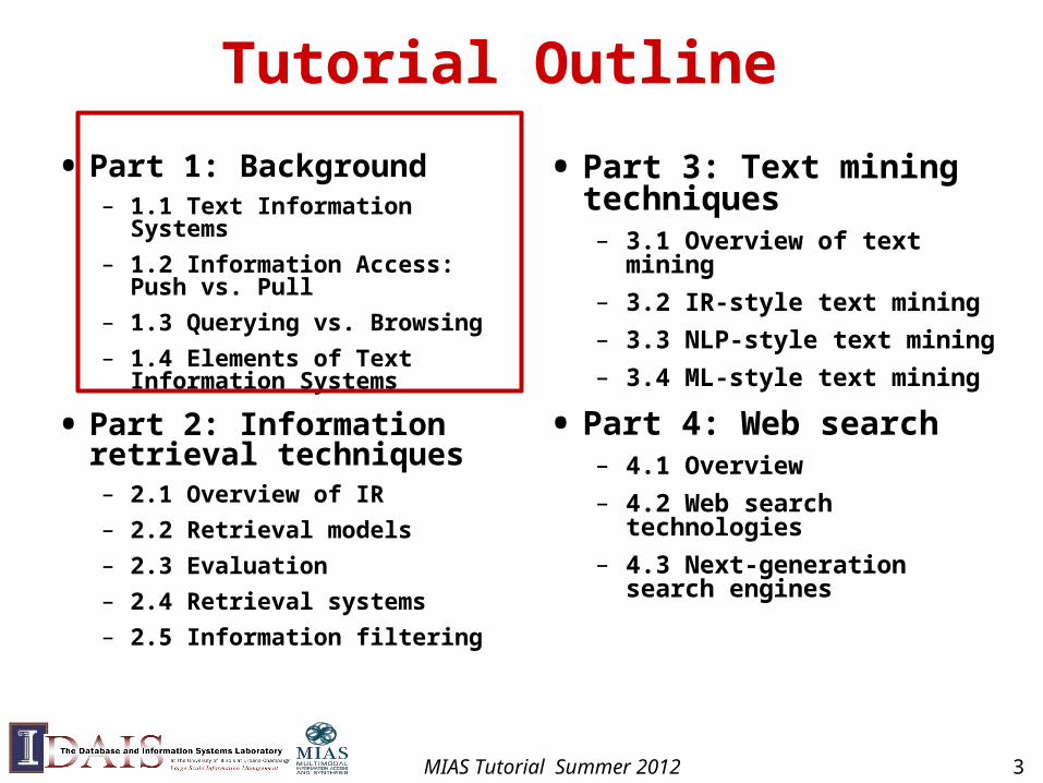
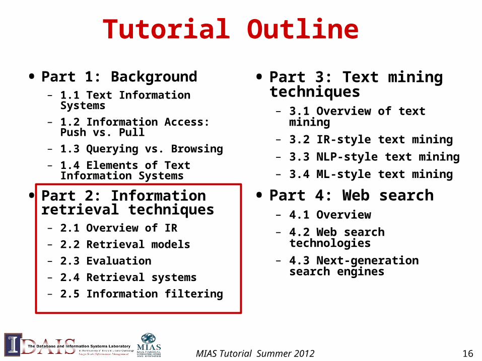
• Part 1: Background – 1.1 Text Information Systems
– 1.2 Information Access: Push vs. Pull
– 1.3 Querying vs. Browsing
– 1.4 Elements of Text Information Systems
• Part 2: Information retrieval techniques– 2.1 Overview of IR
– 2.2 Retrieval models
– 2.3 Evaluation
– 2.4 Retrieval systems
– 2.5 Information filtering
• Part 3: Text mining techniques– 3.1 Overview of text mining
– 3.2 IR-style text mining
– 3.3 NLP-style text mining
– 3.4 ML-style text mining
• Part 4: Web search – 4.1 Overview
– 4.2 Web search technologies
– 4.3 Next-generation search engines
MIAS Tutorial Summer 2012 3
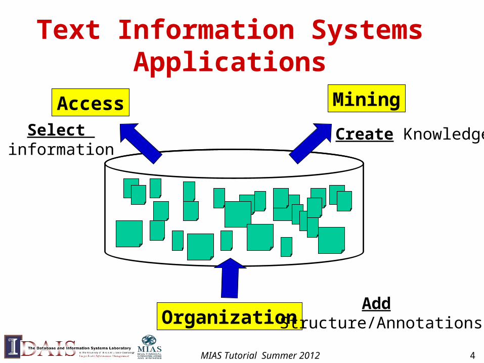
Text Information Systems Applications
Access Mining
Organization
Select information
Create Knowledge
Add Structure/Annotations
MIAS Tutorial Summer 2012 4
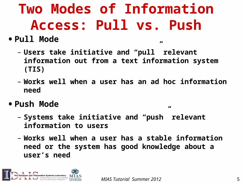
Two Modes of Information Access: Pull vs. Push
• Pull Mode
– Users take initiative and “pull” relevant information out from a text information system (TIS)
– Works well when a user has an ad hoc information need
• Push Mode
– Systems take initiative and “push” relevant information to users
– Works well when a user has a stable information need or the system has good knowledge about a user’s need
MIAS Tutorial Summer 2012 5
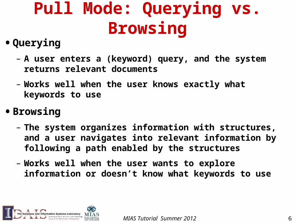
Pull Mode: Querying vs. Browsing
• Querying
– A user enters a (keyword) query, and the system returns relevant documents
– Works well when the user knows exactly what keywords to use
• Browsing
– The system organizes information with structures, and a user navigates into relevant information by following a path enabled by the structures
– Works well when the user wants to explore information or doesn’t know what keywords to use
MIAS Tutorial Summer 2012 6
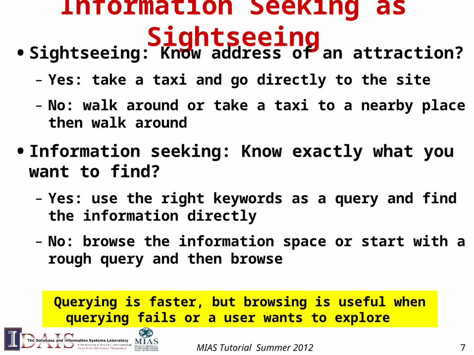
Information Seeking as Sightseeing• Sightseeing: Know address of an attraction?
– Yes: take a taxi and go directly to the site
– No: walk around or take a taxi to a nearby place then walk around
• Information seeking: Know exactly what you want to find?
– Yes: use the right keywords as a query and find the information directly
– No: browse the information space or start with a rough query and then browse
Querying is faster, but browsing is useful when querying fails or a user wants to explore
MIAS Tutorial Summer 2012 7
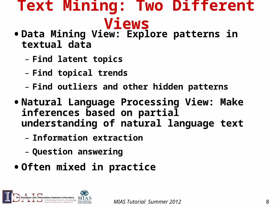
Text Mining: Two Different Views • Data Mining View: Explore patterns in textual data
– Find latent topics
– Find topical trends
– Find outliers and other hidden patterns
• Natural Language Processing View: Make inferences based on partial understanding of natural language text
– Information extraction
– Question answering
• Often mixed in practice
MIAS Tutorial Summer 2012 8
Applications of Text Mining
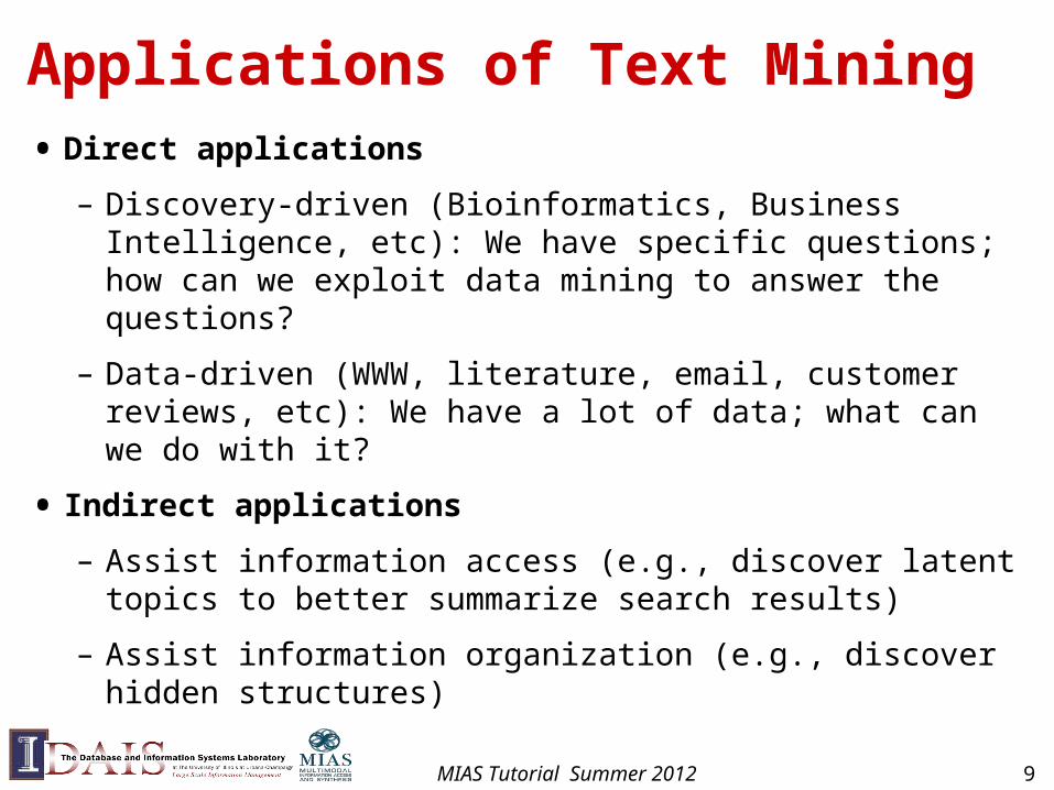
• Direct applications
– Discovery-driven (Bioinformatics, Business Intelligence, etc): We have specific questions; how can we exploit data mining to answer the questions?
– Data-driven (WWW, literature, email, customer reviews, etc): We have a lot of data; what can we do with it?
• Indirect applications
– Assist information access (e.g., discover latent topics to better summarize search results)
– Assist information organization (e.g., discover hidden structures)
MIAS Tutorial Summer 2012 9
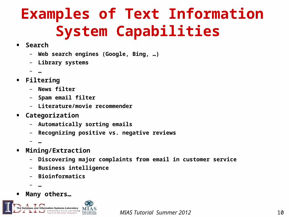
Examples of Text Information System Capabilities
• Search– Web search engines (Google, Bing, …)
– Library systems
– …
• Filtering– News filter
– Spam email filter
– Literature/movie recommender
• Categorization– Automatically sorting emails
– Recognizing positive vs. negative reviews
– …
• Mining/Extraction– Discovering major complaints from email in customer service
– Business intelligence
– Bioinformatics
– …
• Many others…
MIAS Tutorial Summer 2012 10
Conceptual Framework of Text Information Systems (TIS)
Search
Text
Filtering
Categorization
Summarization
Clustering
Natural Language Content Analysis
Extraction
Topic Analysis
VisualizationRetrievalApplications
MiningApplications
InformationAccess
KnowledgeAcquisition
InformationOrganization
MIAS Tutorial Summer 2012 11
Elements of TIS: Natural Language Content Analysis• Natural Language Processing (NLP) is the foundation of TIS
– Enable understanding of meaning of text
– Provide semantic representation of text for TIS
• Current NLP techniques mostly rely on statistical machine learning enhanced with limited linguistic knowledge
– Shallow techniques are robust, but deeper semantic analysis is only feasible for very limited domain
• Some TIS capabilities require deeper NLP than others
• Most text information systems use very shallow NLP (“bag of words” representation)
MIAS Tutorial Summer 2012 12
Elements of TIS: Text Access
• Search: take a user’s query and return relevant documents
• Filtering/Recommendation: monitor an incoming stream and recommend to users relevant items (or discard non-relevant ones)
• Categorization: classify a text object into one of the predefined categories
• Summarization: take one or multiple text documents, and generate a concise summary of the essential content
MIAS Tutorial Summer 2012 13
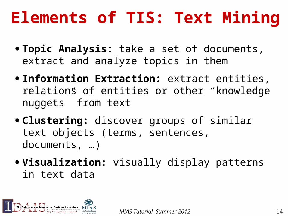
Elements of TIS: Text Mining
• Topic Analysis: take a set of documents, extract and analyze topics in them
• Information Extraction: extract entities, relations of entities or other “knowledge nuggets” from text
• Clustering: discover groups of similar text objects (terms, sentences, documents, …)
• Visualization: visually display patterns in text data
MIAS Tutorial Summer 2012 14
Big Picture
InformationRetrieval Databases
Library & InfoScience
Machine LearningPattern Recognition
Data Mining
NaturalLanguageProcessing
ApplicationsWeb, Bioinformatics…
StatisticsOptimization
Software engineeringComputer systems
Models
Algorithms
Applications
Systems
ComputerVision
MIAS Tutorial Summer 2012 15
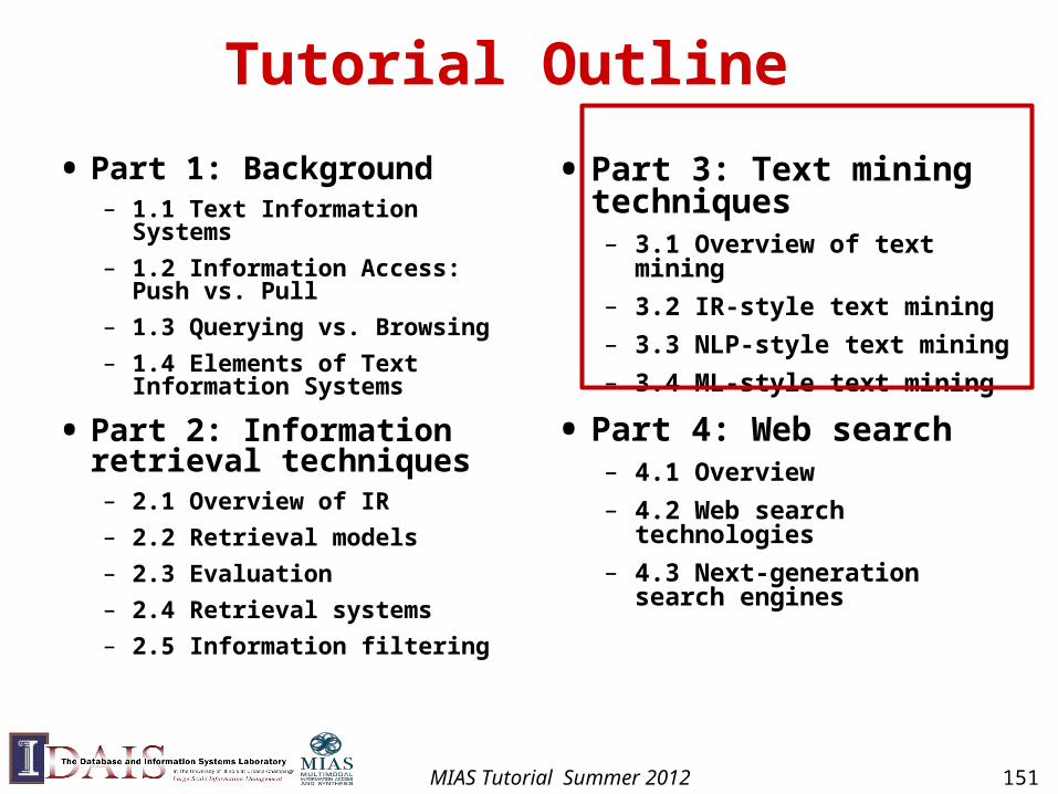
Tutorial Outline
• Part 1: Background – 1.1 Text Information Systems
– 1.2 Information Access: Push vs. Pull
– 1.3 Querying vs. Browsing
– 1.4 Elements of Text Information Systems
• Part 2: Information retrieval techniques– 2.1 Overview of IR
– 2.2 Retrieval models
– 2.3 Evaluation
– 2.4 Retrieval systems
– 2.5 Information filtering
• Part 3: Text mining techniques– 3.1 Overview of text mining
– 3.2 IR-style text mining
– 3.3 NLP-style text mining
– 3.4 ML-style text mining
• Part 4: Web search – 4.1 Overview
– 4.2 Web search technologies
– 4.3 Next-generation search engines
MIAS Tutorial Summer 2012 16
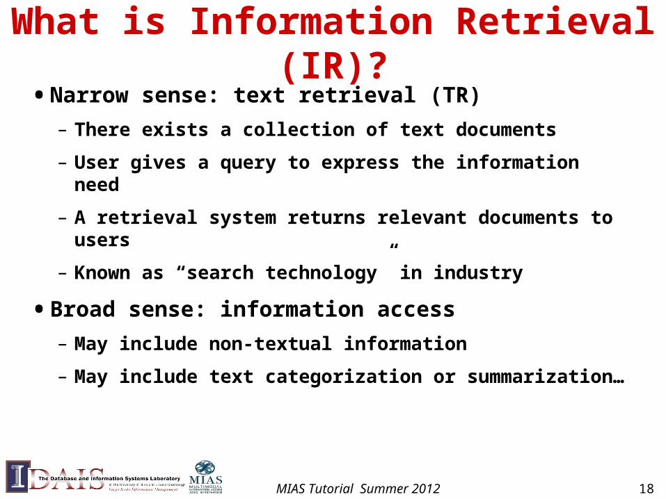
What is Information Retrieval (IR)?
• Narrow sense: text retrieval (TR)
– There exists a collection of text documents
– User gives a query to express the information need
– A retrieval system returns relevant documents to users
– Known as “search technology” in industry
• Broad sense: information access
– May include non-textual information
– May include text categorization or summarization…
MIAS Tutorial Summer 2012 18
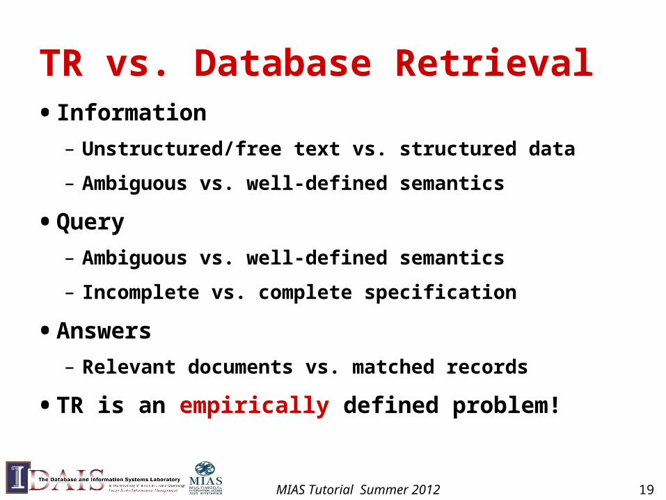
TR vs. Database Retrieval• Information
– Unstructured/free text vs. structured data
– Ambiguous vs. well-defined semantics
• Query
– Ambiguous vs. well-defined semantics
– Incomplete vs. complete specification
• Answers
– Relevant documents vs. matched records
• TR is an empirically defined problem!
MIAS Tutorial Summer 2012 19
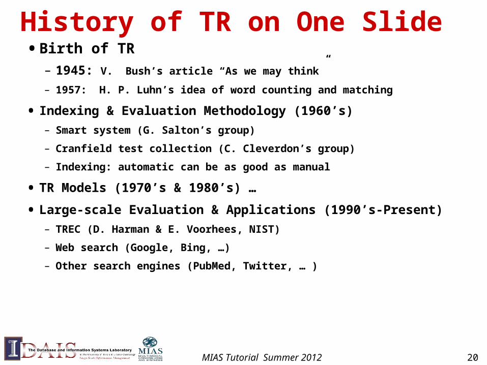
History of TR on One Slide• Birth of TR
– 1945: V. Bush’s article “As we may think”
– 1957: H. P. Luhn’s idea of word counting and matching
• Indexing & Evaluation Methodology (1960’s)
– Smart system (G. Salton’s group)
– Cranfield test collection (C. Cleverdon’s group)
– Indexing: automatic can be as good as manual
• TR Models (1970’s & 1980’s) …
• Large-scale Evaluation & Applications (1990’s-Present)
– TREC (D. Harman & E. Voorhees, NIST)
– Web search (Google, Bing, …)
– Other search engines (PubMed, Twitter, … )
MIAS Tutorial Summer 2012 20
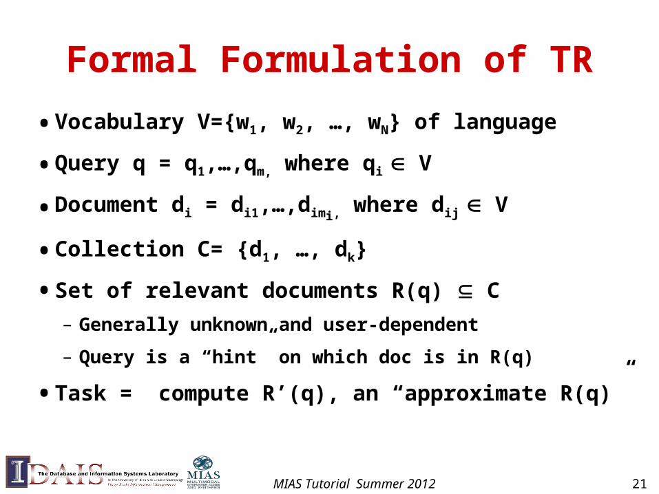
Formal Formulation of TR
• Vocabulary V={w1, w2, …, wN} of language
• Query q = q1,…,qm, where qi V
• Document di = di1,…,dimi, where dij V
• Collection C= {d1, …, dk}
• Set of relevant documents R(q) C
– Generally unknown and user-dependent
– Query is a “hint” on which doc is in R(q)
• Task = compute R’(q), an “approximate R(q)”
MIAS Tutorial Summer 2012 21
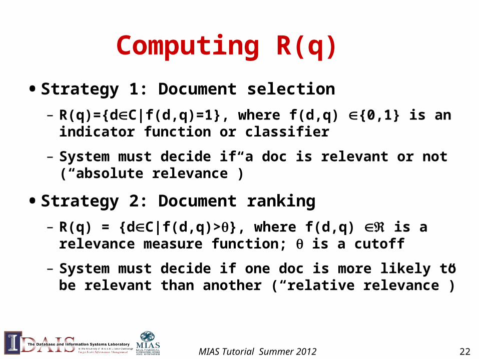
Computing R(q)
• Strategy 1: Document selection
– R(q)={dC|f(d,q)=1}, where f(d,q) {0,1} is an indicator function or classifier
– System must decide if a doc is relevant or not (“absolute relevance”)
• Strategy 2: Document ranking
– R(q) = {dC|f(d,q)>}, where f(d,q) is a relevance measure function; is a cutoff
– System must decide if one doc is more likely to be relevant than another (“relative relevance”)
MIAS Tutorial Summer 2012 22
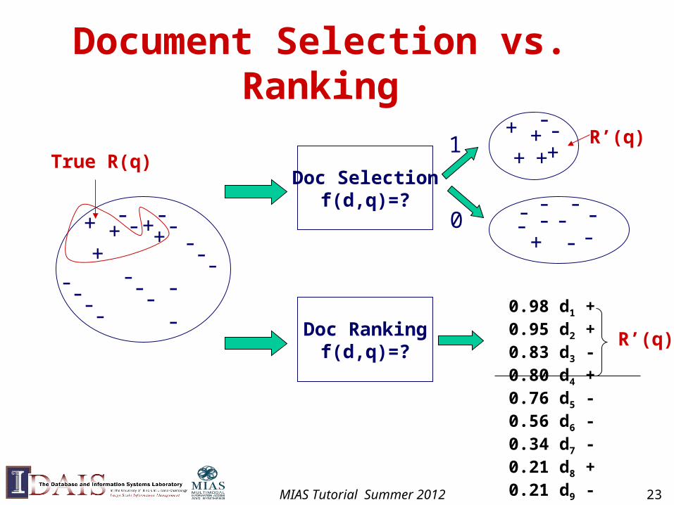
Document Selection vs. Ranking
++
+ +-- -
- - - -
- - - -
-
- - +- -
Doc Selectionf(d,q)=?
++
++
--+
-+
--
- --
---
Doc Rankingf(d,q)=?
1
0
0.98 d1 +0.95 d2 +0.83 d3 -0.80 d4 +0.76 d5 -0.56 d6 -0.34 d7 -0.21 d8 +0.21 d9 -
R’(q)
R’(q)
True R(q)
MIAS Tutorial Summer 2012 23
Problems of Doc Selection
• The classifier is unlikely accurate
– “Over-constrained” query (terms are too specific): no relevant documents found
– “Under-constrained” query (terms are too general): over delivery
– It is extremely hard to find the right position between these two extremes
• Even if it is accurate, all relevant documents are not equally relevant
• Relevance is a matter of degree!
MIAS Tutorial Summer 2012 24
Ranking is generally preferred• Ranking is needed to prioritize results for user browsing
• A user can stop browsing anywhere, so the boundary is controlled by the user
– High recall users would view more items
– High precision users would view only a few
• Theoretical justification (Probability Ranking Principle): returning a ranked list of documents in descending order of probability that a document is relevant to the query is the optimal strategy under the following two assumptions (do they hold?):
– The utility of a document (to a user) is independent of the utility of any other document
– A user would browse the results sequentially
MIAS Tutorial Summer 2012 25
How to Design a Ranking Function?
• Query q = q1,…,qm, where qi V
• Document d = d1,…,dn, where di V
• Ranking function: f(q, d)
• A good ranking function should rank relevant documents on top of non-relevant ones
• Key challenge: how to measure the likelihood that document d is relevant to query q?
• Retrieval Model = formalization of relevance (give a computational definition of relevance)
MIAS Tutorial Summer 2012 26

Many Different Retrieval Models• Similarity-based models:
– a document that is more similar to a query is assumed to be more likely relevant to the query
– relevance (d,q) = similarity (d,q)
– e.g., Vector Space Model
• Probabilistic models (language models):
– compute the probability that a given document is relevant to a query based on a probabilistic model
– relevance(d,q) = p(R=1|d,q), where R {0,1} is a binary random variable
– E.g., Query Likelihood
MIAS Tutorial Summer 2012 27
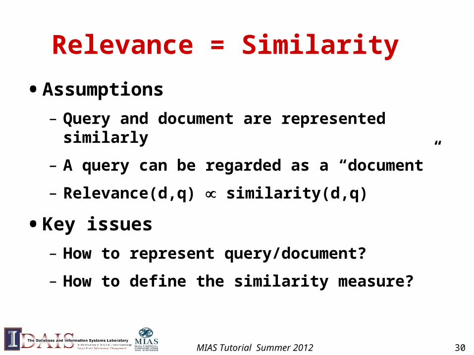
Relevance = Similarity
• Assumptions
– Query and document are represented similarly
– A query can be regarded as a “document”
– Relevance(d,q) similarity(d,q)
• Key issues
– How to represent query/document?
– How to define the similarity measure?
MIAS Tutorial Summer 2012 30
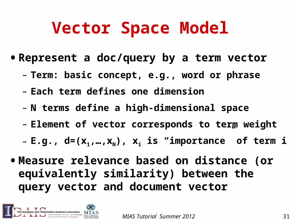
Vector Space Model
• Represent a doc/query by a term vector
– Term: basic concept, e.g., word or phrase
– Each term defines one dimension
– N terms define a high-dimensional space
– Element of vector corresponds to term weight
– E.g., d=(x1,…,xN), xi is “importance” of term i
• Measure relevance based on distance (or equivalently similarity) between the query vector and document vector
MIAS Tutorial Summer 2012 31
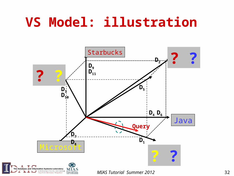
VS Model: illustration
Java
Microsoft
Starbucks
D6
D10
D9
D4
D7
D8
D5
D11
D2 ? ?
D1
? ?
D3
? ?
Query
MIAS Tutorial Summer 2012 32
What the VS model doesn’t say
• How to define/select the “basic concept”
– Concepts are assumed to be orthogonal
• How to assign weights
– Weight in query indicates importance of term
– Weight in doc indicates how well the term characterizes the doc
• How to define the similarity/distance measure
MIAS Tutorial Summer 2012 33
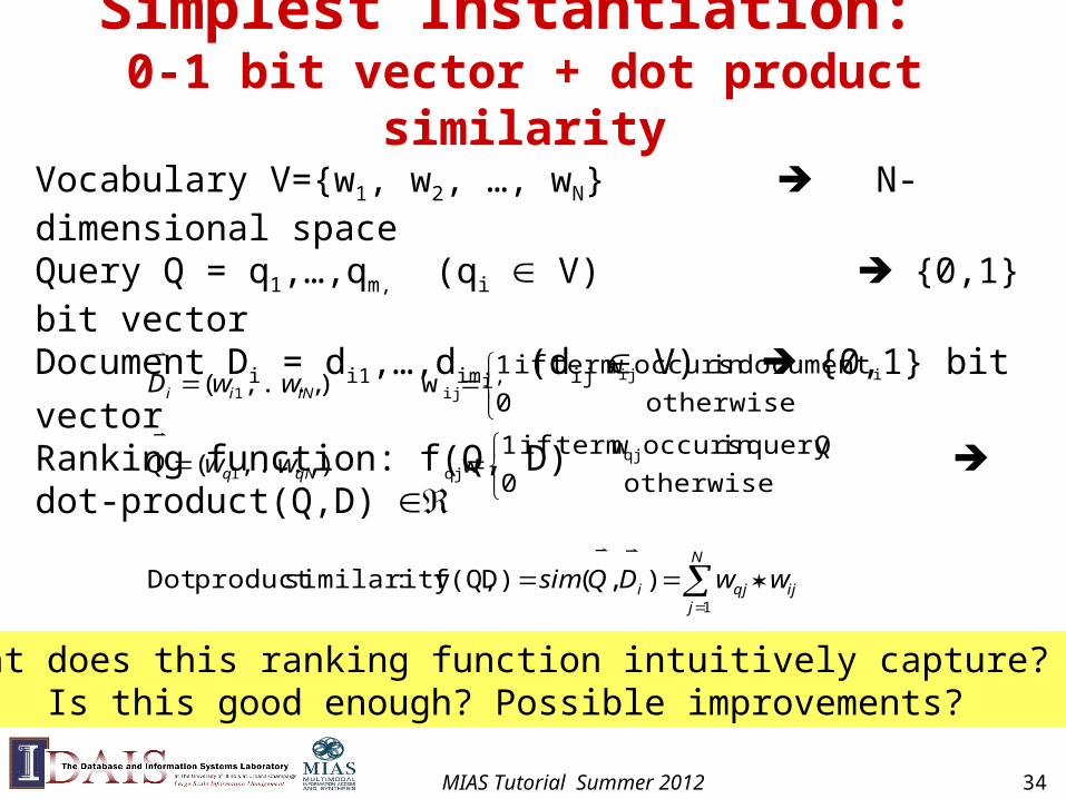
Simplest Instantiation: 0-1 bit vector + dot product similarity
),(D)f(Q, :similarityproduct Dot
otherwise
Qquery in occurs w termif
0
1 w ),...,(
otherwise
document D in occurs w termif
0
1w),...,(
1
qjqj1
iijij1
N
jijqji
qNq
iNii
wwDQsim
wwQ
wwD
Vocabulary V={w1, w2, …, wN} N-dimensional space Query Q = q1,…,qm, (qi V) {0,1} bit vectorDocument Di = di1,…,dimi,
(dij V) {0,1} bit vector
Ranking function: f(Q, D) dot-product(Q,D)
What does this ranking function intuitively capture? Is this good enough? Possible improvements?
MIAS Tutorial Summer 2012 34
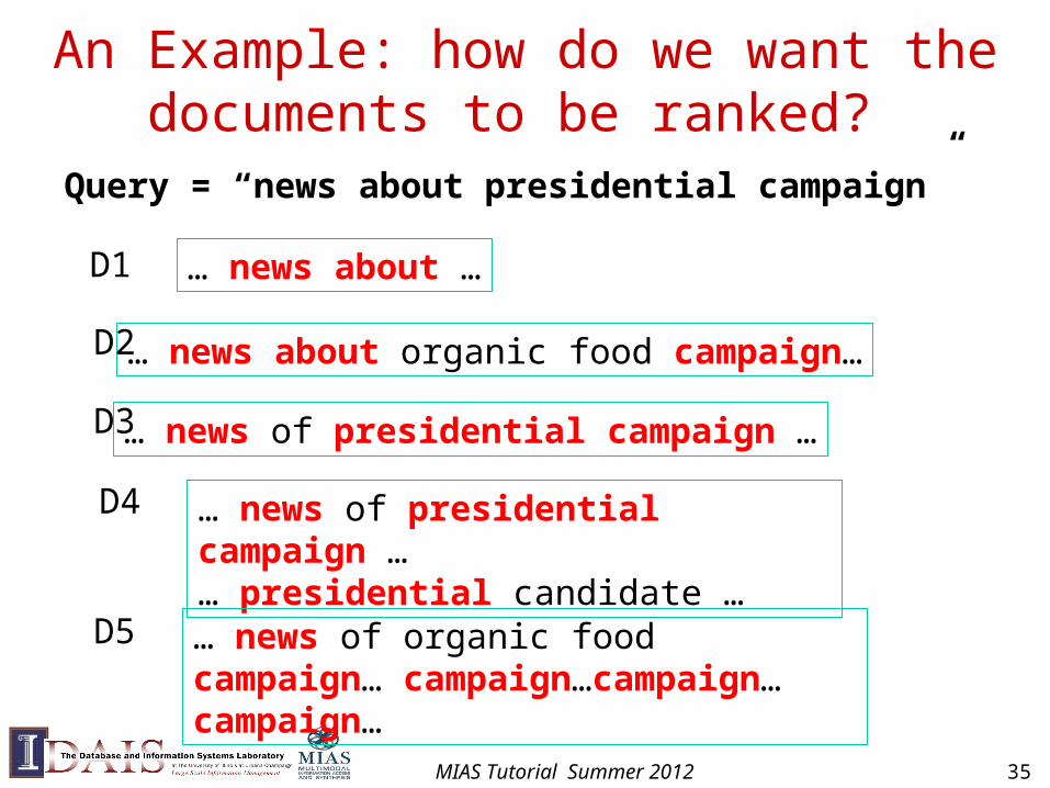
An Example: how do we want the documents to be ranked?
Query = “news about presidential campaign”
… news about …D1
… news about organic food campaign…D2
… news of presidential campaign …D3
… news of presidential campaign … … presidential candidate …
D4
… news of organic food campaign… campaign…campaign…campaign…
D5
MIAS Tutorial Summer 2012 35
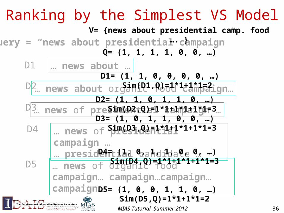
Ranking by the Simplest VS Model
Query = “news about presidential campaign”
… news about …D1
… news about organic food campaign…D2
… news of presidential campaign …D3
… news of presidential campaign … … presidential candidate …
D4
… news of organic food campaign… campaign…campaign…campaign…
D5
V= {news about presidential camp. food …. }
Q= (1, 1, 1, 1, 0, 0, …)
D1= (1, 1, 0, 0, 0, 0, …) Sim(D1,Q)=1*1+1*1=2
D2= (1, 1, 0, 1, 1, 0, …) Sim(D2,Q)=1*1+1*1+1*1=3
D3= (1, 0, 1, 1, 0, 0, …) Sim(D3,Q)=1*1+1*1+1*1=3
D4= (1, 0, 1, 1, 0, 0, …) Sim(D4,Q)=1*1+1*1+1*1=3
D5= (1, 0, 0, 1, 1, 0, …) Sim(D5,Q)=1*1+1*1=2
MIAS Tutorial Summer 2012 36
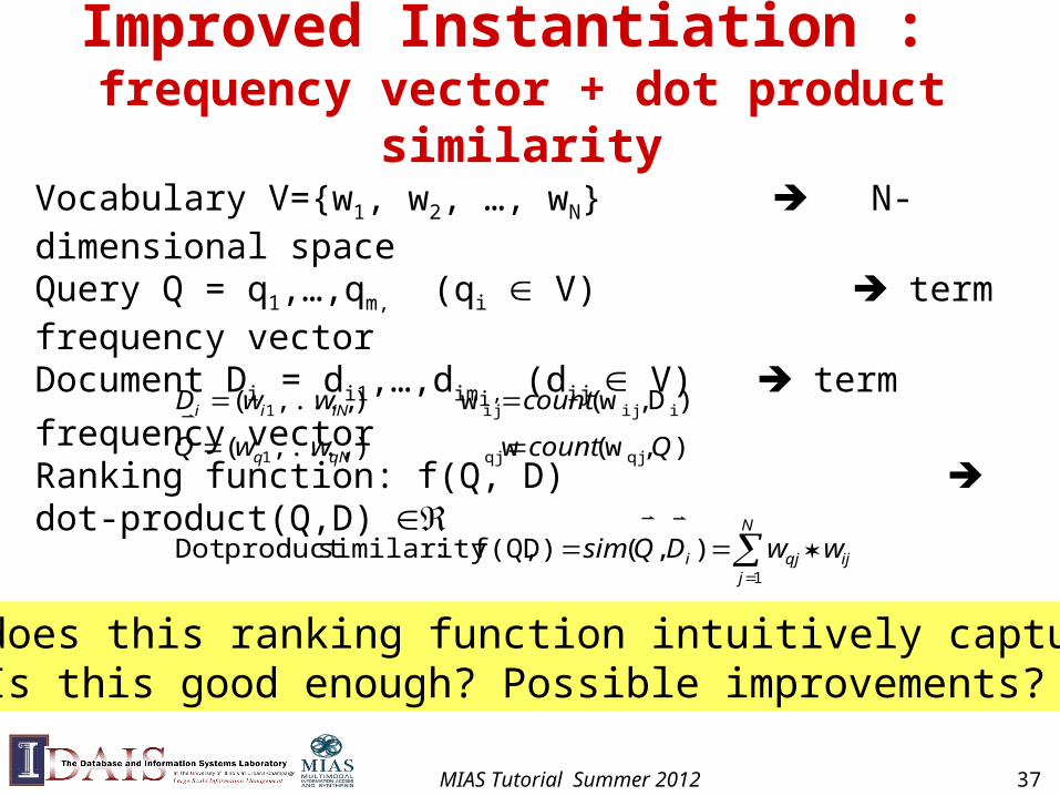
Improved Instantiation : frequency vector + dot product similarity
),(D)f(Q, :similarityproduct Dot
),w( w ),...,(
)D, w(w),...,(
1
qjqj1
iijij1
N
jijqji
qNq
iNii
wwDQsim
QcountwwQ
countwwD
Vocabulary V={w1, w2, …, wN} N-dimensional space Query Q = q1,…,qm, (qi V) term frequency vectorDocument Di = di1,…,dimi,
(dij V) term frequency
vectorRanking function: f(Q, D) dot-product(Q,D)
What does this ranking function intuitively capture? Is this good enough? Possible improvements?
MIAS Tutorial Summer 2012 37
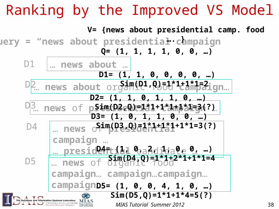
Ranking by the Improved VS Model
Query = “news about presidential campaign”
… news about …D1
… news about organic food campaign…D2
… news of presidential campaign …D3
… news of presidential campaign … … presidential candidate …
D4
… news of organic food campaign… campaign…campaign…campaign…
D5
V= {news about presidential camp. food …. }
Q= (1, 1, 1, 1, 0, 0, …)
D1= (1, 1, 0, 0, 0, 0, …) Sim(D1,Q)=1*1+1*1=2
D2= (1, 1, 0, 1, 1, 0, …) Sim(D2,Q)=1*1+1*1+1*1=3(?)
D3= (1, 0, 1, 1, 0, 0, …) Sim(D3,Q)=1*1+1*1+1*1=3(?)
D4= (1, 0, 2, 1, 0, 0, …) Sim(D4,Q)=1*1+2*1+1*1=4
D5= (1, 0, 0, 4, 1, 0, …) Sim(D5,Q)=1*1+1*4=5(?)
MIAS Tutorial Summer 2012 38
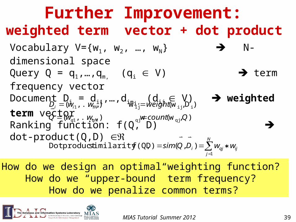
Further Improvement: weighted term vector + dot product
),(D)f(Q, :similarityproduct Dot
),w( w ),...,(
)D, w(w),...,(
1
qjqj1
iijij1
N
jijqji
qNq
iNii
wwDQsim
QcountwwQ
weightwwD
Vocabulary V={w1, w2, …, wN} N-dimensional space Query Q = q1,…,qm, (qi V) term frequency vectorDocument Di = di1,…,dimi,
(dij V) weighted term
vectorRanking function: f(Q, D) dot-product(Q,D)
How do we design an optimal weighting function? How do we “upper-bound” term frequency?
How do we penalize common terms?
MIAS Tutorial Summer 2012 39
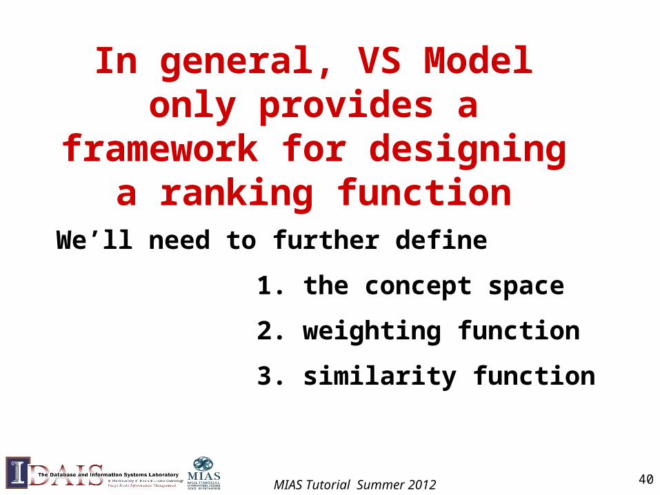
In general, VS Model only provides a framework for
designing a ranking function
We’ll need to further define
1. the concept space
2. weighting function
3. similarity function
MIAS Tutorial Summer 2012 40
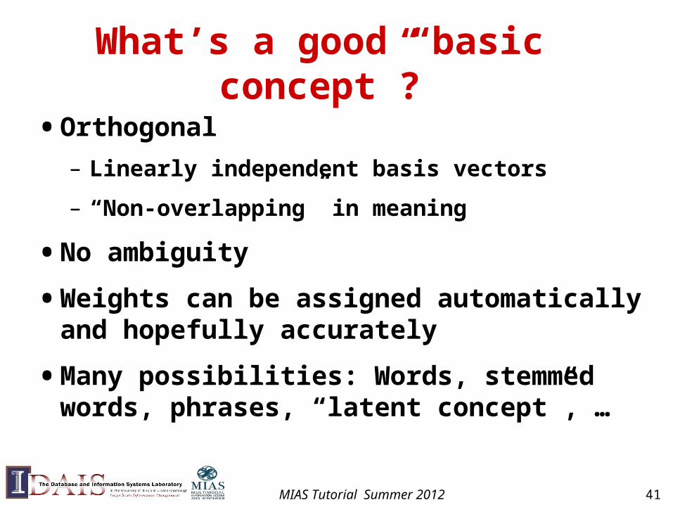
What’s a good “basic concept”?
• Orthogonal
– Linearly independent basis vectors
– “Non-overlapping” in meaning
• No ambiguity
• Weights can be assigned automatically and hopefully accurately
• Many possibilities: Words, stemmed words, phrases, “latent concept”, …
MIAS Tutorial Summer 2012 41

How to Assign Weights?
• Very very important!
• Why weighting– Query side: Not all terms are equally important
– Doc side: Some terms carry more information about contents
• How?
– Two basic heuristics
• TF (Term Frequency) = Within-doc-frequency
• IDF (Inverse Document Frequency)
– TF normalization
MIAS Tutorial Summer 2012 42
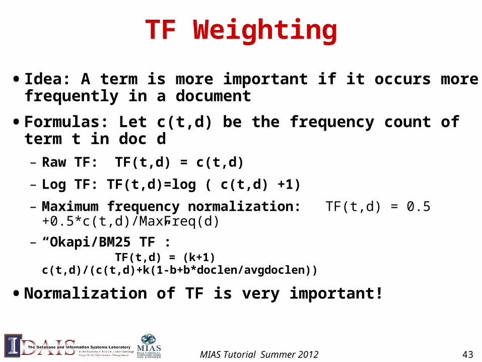
TF Weighting
• Idea: A term is more important if it occurs more frequently in a document
• Formulas: Let c(t,d) be the frequency count of term t in doc d
– Raw TF: TF(t,d) = c(t,d)
– Log TF: TF(t,d)=log ( c(t,d) +1)
– Maximum frequency normalization: TF(t,d) = 0.5 +0.5*c(t,d)/MaxFreq(d)
– “Okapi/BM25 TF”: TF(t,d) = (k+1) c(t,d)/(c(t,d)+k(1-b+b*doclen/avgdoclen))
• Normalization of TF is very important!
MIAS Tutorial Summer 2012 43
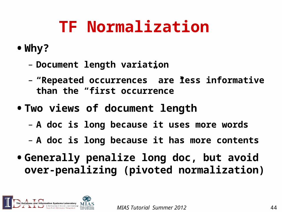
TF Normalization• Why?
– Document length variation
– “Repeated occurrences” are less informative than the “first occurrence”
• Two views of document length
– A doc is long because it uses more words
– A doc is long because it has more contents
• Generally penalize long doc, but avoid over-penalizing (pivoted normalization)
MIAS Tutorial Summer 2012 44
TF Normalization (cont.)
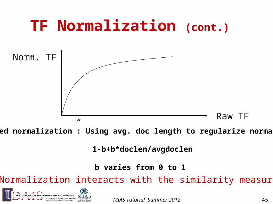
Norm. TF
Raw TF
“Pivoted normalization”: Using avg. doc length to regularize normalization
1-b+b*doclen/avgdoclen
b varies from 0 to 1
Normalization interacts with the similarity measure
MIAS Tutorial Summer 2012 45
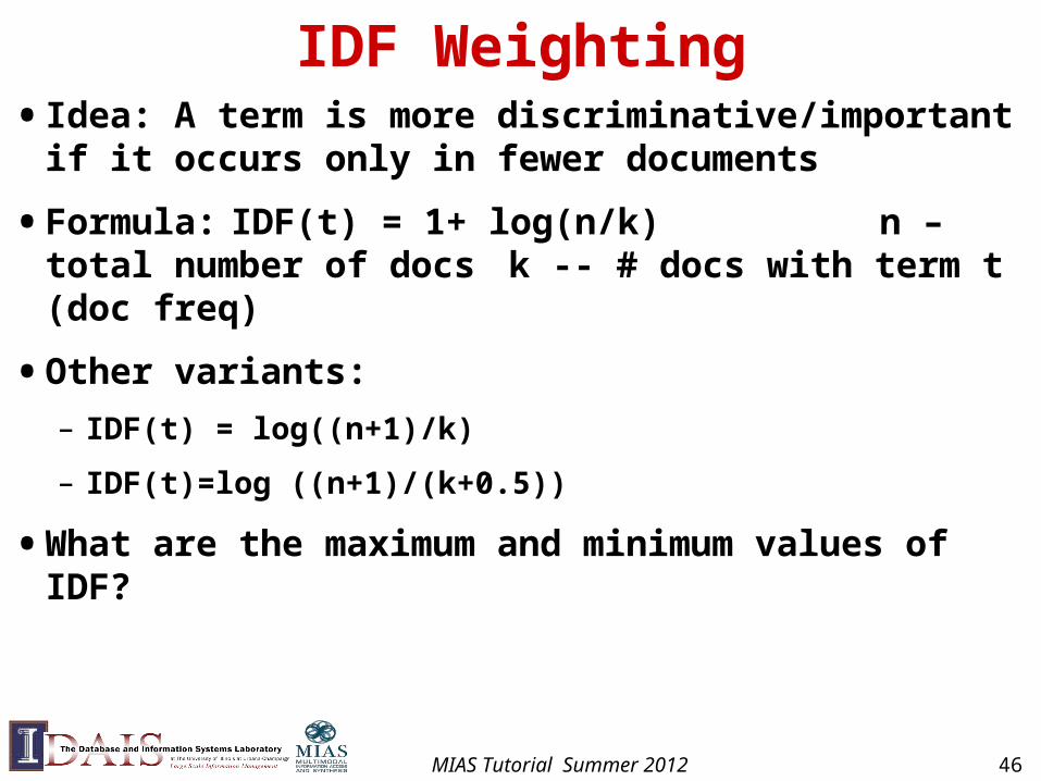
IDF Weighting• Idea: A term is more discriminative/important if it
occurs only in fewer documents
• Formula: IDF(t) = 1+ log(n/k) n – total number of docs
k -- # docs with term t (doc freq)
• Other variants:
– IDF(t) = log((n+1)/k)
– IDF(t)=log ((n+1)/(k+0.5))
• What are the maximum and minimum values of IDF?
MIAS Tutorial Summer 2012 46
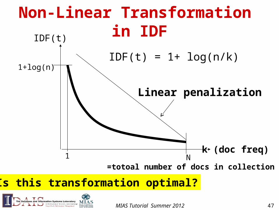
Non-Linear Transformation in IDFIDF(t)
k (doc freq)
IDF(t) = 1+ log(n/k)
N =totoal number of docs in collection
1
1+log(n)
Is this transformation optimal?
Linear penalization
MIAS Tutorial Summer 2012 47
TF-IDF Weighting
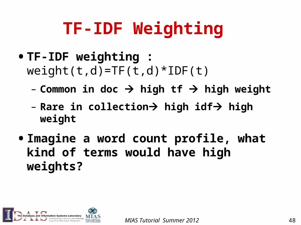
• TF-IDF weighting : weight(t,d)=TF(t,d)*IDF(t)
– Common in doc high tf high weight
– Rare in collection high idf high weight
• Imagine a word count profile, what kind of terms would have high weights?
MIAS Tutorial Summer 2012 48
Empirical distribution of words
• There are stable language-independent patterns in how people use natural languages
• A few words occur very frequently; most occur rarely. E.g., in news articles,
– Top 4 words: 10~15% word occurrences
– Top 50 words: 35~40% word occurrences
• The most frequent word in one corpus may be rare in another
MIAS Tutorial Summer 2012 49
Zipf’s Law
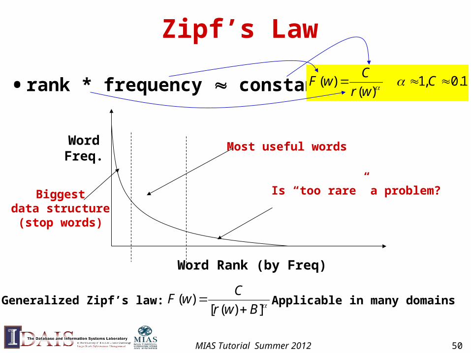
• rank * frequency constant
WordFreq.
Word Rank (by Freq)
Most useful words
Biggestdata structure(stop words)
Is “too rare” a problem?
( ) 1, 0.1( )
CF w C
r w
( )[ ( ) ]
CF w
r w B
Generalized Zipf’s law: Applicable in many domains
MIAS Tutorial Summer 2012 50
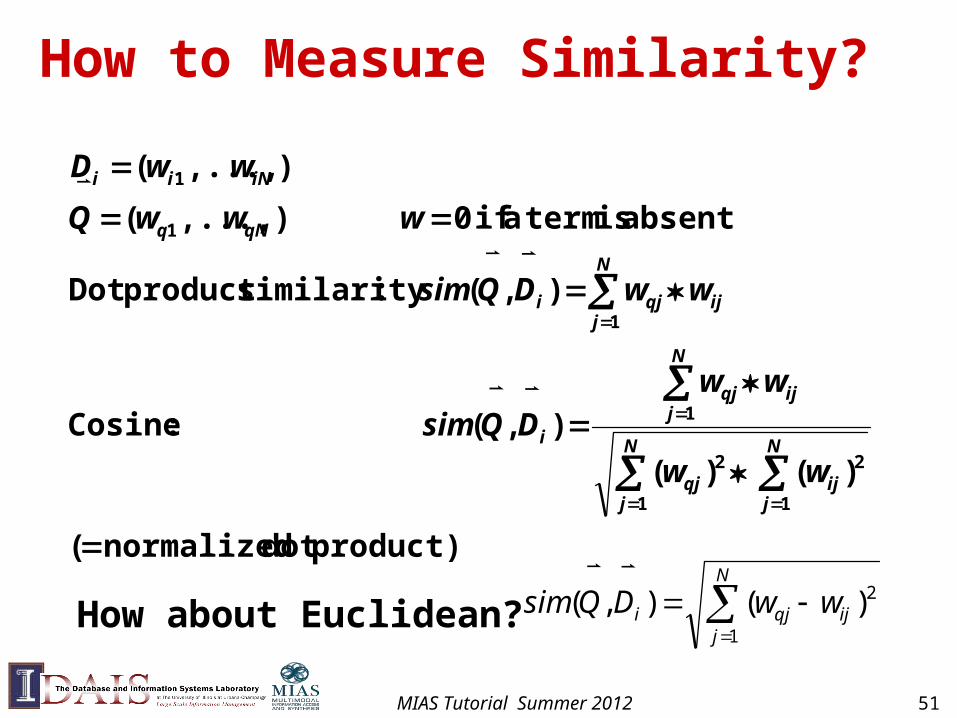
How to Measure Similarity?
product)dot normalized(
)()(
),( :Cosine
),( :similarityproduct Dot
absent is term a if 0 ),...,(
),...,(
1
2
1
2
1
1
1
1
N
jij
N
jqj
N
jijqj
i
N
jijqji
qNq
iNii
ww
ww
DQsim
wwDQsim
wwwQ
wwD
How about Euclidean?
N
jijqji wwDQsim
1
2)(),(
MIAS Tutorial Summer 2012 51
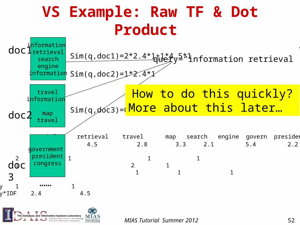
VS Example: Raw TF & Dot Product
info retrieval travel map search engine govern president congressIDF 2.4 4.5 2.8 3.3 2.1 5.4 2.2 3.2 4.3
doc1 2 1 1 1doc2 1 2 1 doc3 1 1 1
query 1 1query*IDF 2.4 4.5
doc3
information retrievalsearchengine
information
travelinformation
maptravel
government presidentcongress
doc1
doc2
……
query=“information retrieval”Sim(q,doc1)=2*2.4*1+1*4.5*1
Sim(q,doc2)=1*2.4*1
Sim(q,doc3)=0
How to do this quickly?More about this later…
MIAS Tutorial Summer 2012 52
What Works the Best?
(Singhal 2001)
•Use single words
•Use stat. phrases
•Remove stop words
•Stemming (?)
Error
[ ]
MIAS Tutorial Summer 2012 53
Advantages of VS Model
• Empirically effective
• Intuitive
• Easy to implement
• Warning: Many variants of TF-IDF!
MIAS Tutorial Summer 2012 54
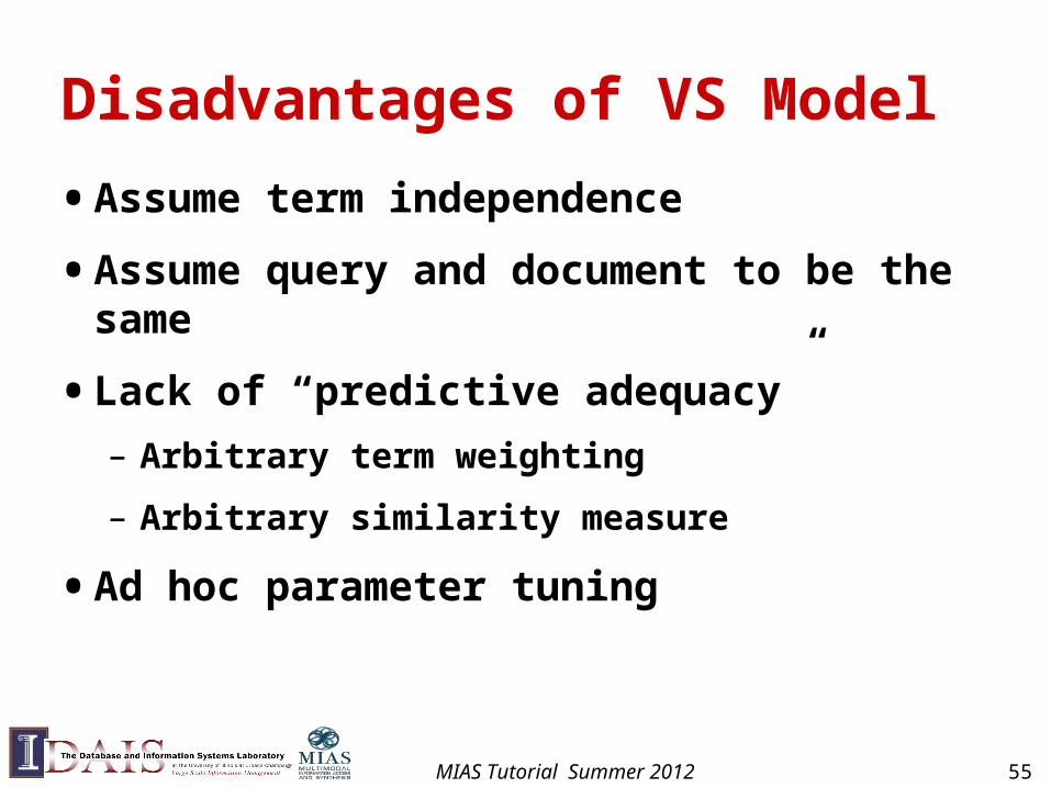
Disadvantages of VS Model
• Assume term independence
• Assume query and document to be the same
• Lack of “predictive adequacy”
– Arbitrary term weighting
– Arbitrary similarity measure
• Ad hoc parameter tuning
MIAS Tutorial Summer 2012 55
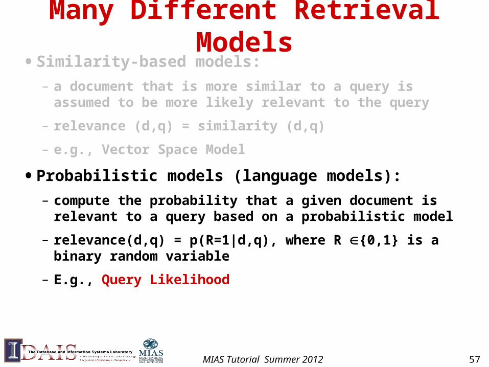
Many Different Retrieval Models• Similarity-based models:
– a document that is more similar to a query is assumed to be more likely relevant to the query
– relevance (d,q) = similarity (d,q)
– e.g., Vector Space Model
• Probabilistic models (language models):
– compute the probability that a given document is relevant to a query based on a probabilistic model
– relevance(d,q) = p(R=1|d,q), where R {0,1} is a binary random variable
– E.g., Query Likelihood
MIAS Tutorial Summer 2012 57
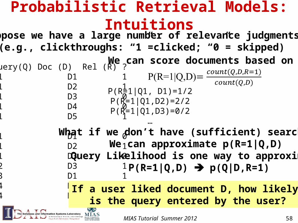
Probabilistic Retrieval Models: Intuitions
Query(Q) Doc (D) Rel (R) ?Q1 D1 1Q1 D2 1Q1 D3 0Q1 D4 0Q1 D5 1…Q1 D1 0Q1 D2 1Q1 D3 0 Q2 D3 1Q3 D1 1Q4 D2 1Q4 D3 0…
Suppose we have a large number of relevance judgments (e.g., clickthroughs: “1”=clicked; “0”= skipped)
We can score documents based on
P(R=1|Q1, D1)=1/2P(R=1|Q1,D2)=2/2P(R=1|Q1,D3)=0/2
…
What if we don’t have (sufficient) search log? We can approximate p(R=1|Q,D)
Query Likelihood is one way to approximate P(R=1|Q,D) p(Q|D,R=1)
If a user liked document D, how likely Q is the query entered by the user?
MIAS Tutorial Summer 2012 58
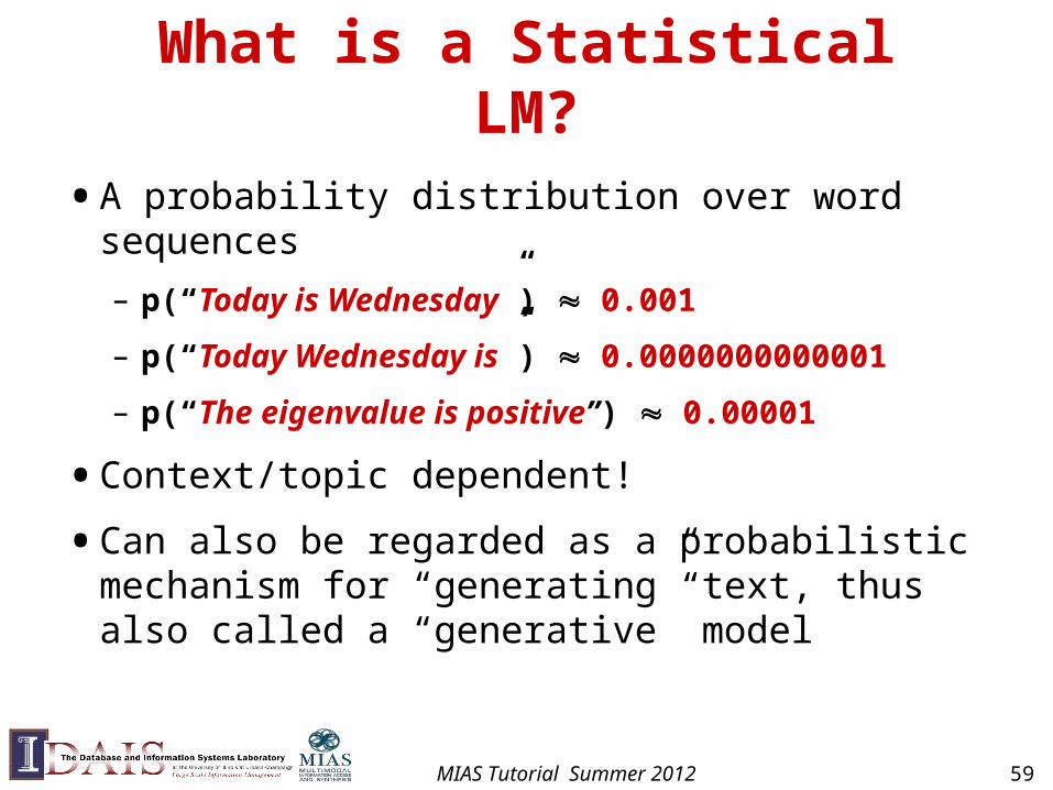
What is a Statistical LM?
• A probability distribution over word sequences
– p(“Today is Wednesday”) 0.001
– p(“Today Wednesday is”) 0.0000000000001
– p(“The eigenvalue is positive”) 0.00001
• Context/topic dependent!
• Can also be regarded as a probabilistic mechanism for “generating” text, thus also called a “generative” model
MIAS Tutorial Summer 2012 59
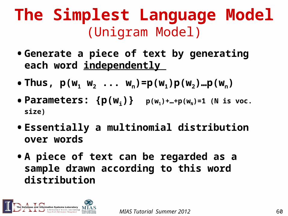
The Simplest Language Model(Unigram Model)
• Generate a piece of text by generating each word independently
• Thus, p(w1 w2 ... wn)=p(w1)p(w2)…p(wn)
• Parameters: {p(wi)} p(w1)+…+p(wN)=1 (N is voc. size)
• Essentially a multinomial distribution over words
• A piece of text can be regarded as a sample drawn according to this word distribution
MIAS Tutorial Summer 2012 60
Text Generation with Unigram LM
(Unigram) Language Model p(w| )
…text 0.2mining 0.1association 0.01clustering 0.02…food 0.00001
…
Topic 1:Text mining
…food 0.25nutrition 0.1healthy 0.05diet 0.02
…
Topic 2:Health
Document
Text miningpaper
Food nutritionpaper
Sampling
MIAS Tutorial Summer 2012 61
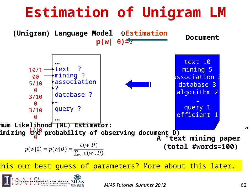
Estimation of Unigram LM(Unigram) Language Model p(w| )=?
Document
text 10mining 5
association 3database 3algorithm 2
…query 1
efficient 1
…text ?mining ?association ?database ?…query ?
…
Estimation
A “text mining paper”(total #words=100)
10/1005/1003/1003/100
1/100
Is this our best guess of parameters? More about this later…
Maximum Likelihood (ML) Estimator:(maximizing the probability of observing document D)
MIAS Tutorial Summer 2012 62

More Sophisticated LMs
• N-gram language models
– In general, p(w1 w2 ... wn)=p(w1)p(w2|w1)…p(wn|w1 …wn-1)
– n-gram: conditioned only on the past n-1 words
– E.g., bigram: p(w1 ... wn)=p(w1)p(w2|w1) p(w3|w2) …p(wn|wn-1)
• Remote-dependence language models (e.g., Maximum Entropy model)
• Structured language models (e.g., probabilistic context-free grammar)
• Will not be covered in detail in this tutorial. If interested, read [Manning & Schutze 99]
MIAS Tutorial Summer 2012 63
Why Just Unigram Models?
• Difficulty in moving toward more complex models
– They involve more parameters, so need more data to estimate (A doc is an extremely small sample)
– They increase the computational complexity significantly, both in time and space
• Capturing word order or structure may not add so much value for “topical inference”
• But, using more sophisticated models can still be expected to improve performance ...
MIAS Tutorial Summer 2012 64
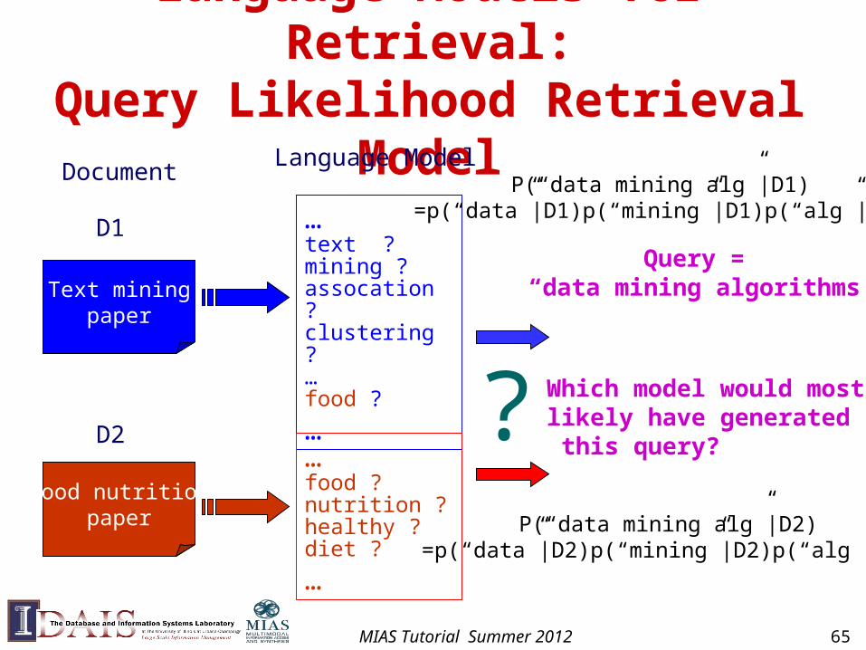
Language Models for Retrieval:Query Likelihood Retrieval Model
Document
Text miningpaper
Food nutritionpaper
Language Model
…text ?mining ?assocation ?clustering ?…food ?
…
…food ?nutrition ?healthy ?diet ?
…
Query = “data mining algorithms”
? Which model would most likely have generated this query?
D1
D2
P(“data mining alg”|D1)=p(“data”|D1)p(“mining”|D1)p(“alg”|D1)
P(“data mining alg”|D2)=p(“data”|D2)p(“mining”|D2)p(“alg”|D2)
MIAS Tutorial Summer 2012 65
n
Vw
n
ii
wwwqwhere
dwpqwcdwpdqp
...,
)|(log),()|(log)|(log
21
1
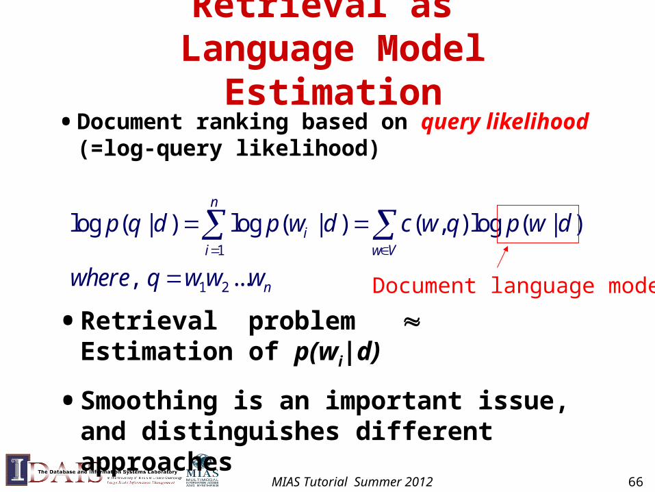
Retrieval as Language Model Estimation
• Document ranking based on query likelihood (=log-query likelihood)
• Retrieval problem Estimation of p(wi|d)
• Smoothing is an important issue, and distinguishes different approaches
Document language model
MIAS Tutorial Summer 2012 66
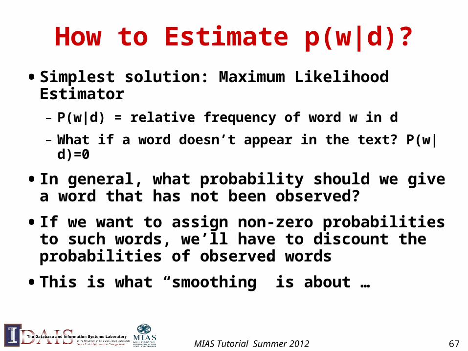
How to Estimate p(w|d)?
• Simplest solution: Maximum Likelihood Estimator
– P(w|d) = relative frequency of word w in d
– What if a word doesn’t appear in the text? P(w|d)=0
• In general, what probability should we give a word that has not been observed?
• If we want to assign non-zero probabilities to such words, we’ll have to discount the probabilities of observed words
• This is what “smoothing” is about …
MIAS Tutorial Summer 2012 67
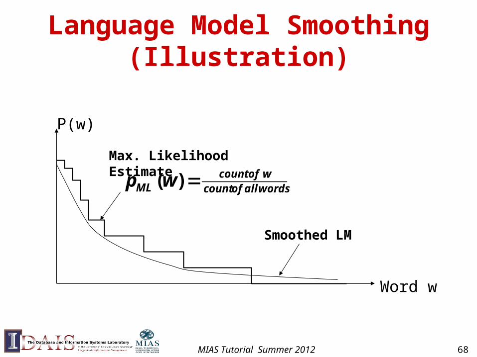
Language Model Smoothing (Illustration)
P(w)
Word w
Max. Likelihood Estimate
wordsallofcountwofcount
ML wp )(
Smoothed LM
MIAS Tutorial Summer 2012 68
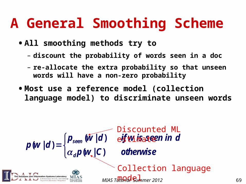
A General Smoothing Scheme
• All smoothing methods try to
– discount the probability of words seen in a doc
– re-allocate the extra probability so that unseen words will have a non-zero probability
• Most use a reference model (collection language model) to discriminate unseen words
otherwiseCwp
dinseeniswifdwpdwp
d
seen
)|(
)|()|(
Discounted ML estimate
Collection language modelMIAS Tutorial Summer 2012 69
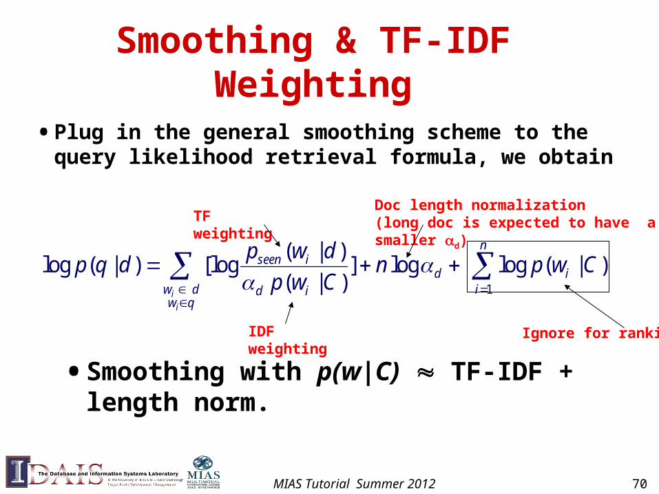
Smoothing & TF-IDF Weighting
• Plug in the general smoothing scheme to the query likelihood retrieval formula, we obtain
n
iid
qwdw id
iseen CwpnCwp
dwpdqp
i
i 1
)|(loglog])|(
)|([log)|(log
Ignore for rankingIDF weighting
TF weightingDoc length normalization(long doc is expected to have a smaller d)
• Smoothing with p(w|C) TF-IDF + length norm.
MIAS Tutorial Summer 2012 70
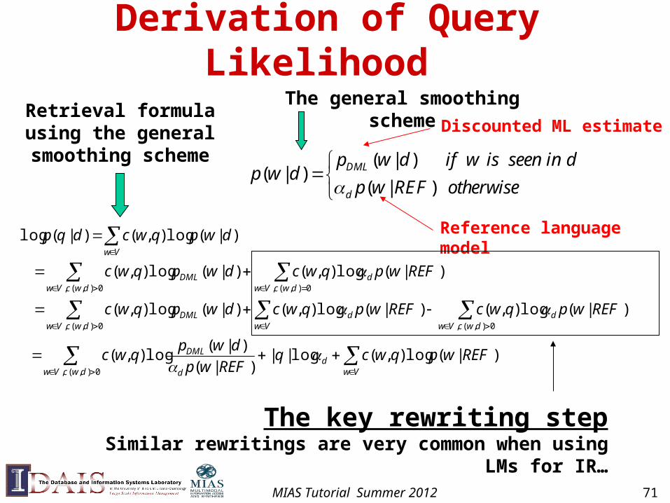
Derivation of Query Likelihood
( | )( | )
( | )DML
d
p w d if w is seen in dp w d
p w REF otherwise
Discounted ML estimate
Reference language model
Retrieval formula using the general smoothing
scheme
The key rewriting stepSimilar rewritings are very common when using LMs for IR…
The general smoothing scheme
0),(,
0),(,0),(,
0),(, 0),(,
)|(log),(log||)|(
)|(log),(
)|(log),()|(log),()|(log),(
)|(log),()|(log),(
)|(log),()|(log
dwcVw Vwd
d
DML
dwcVwd
dwcVw VwdDML
dwcVw dwcVwdDML
Vw
REFwpqwcqREFwp
dwpqwc
REFwpqwcREFwpqwcdwpqwc
REFwpqwcdwpqwc
dwpqwcdqp
MIAS Tutorial Summer 2012 71
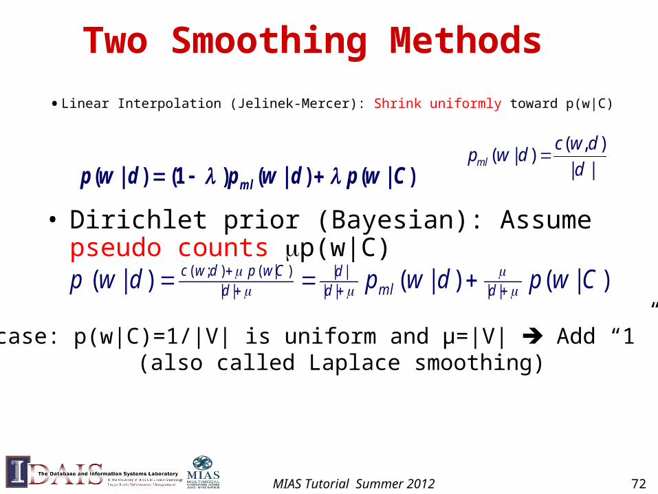
Two Smoothing Methods
• Linear Interpolation (Jelinek-Mercer): Shrink uniformly toward p(w|C)
)|()|()()|( Cwpdwpdwp m l 1
)|()|()|( ||||||
||)|();( Cwpdwpdwp dm ld
dd
Cwpdwc
• Dirichlet prior (Bayesian): Assume pseudo counts p(w|C)
Special case: p(w|C)=1/|V| is uniform and µ=|V| Add “1” smoothing (also called Laplace smoothing)
||
),()|(
d
dwcdwpml
MIAS Tutorial Summer 2012 72
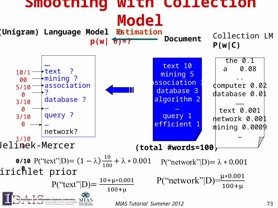
Smoothing with Collection Model(Unigram) Language Model p(w| )=? Document
text 10mining 5
association 3database 3algorithm 2
…query 1
efficient 1
…text ?mining ?association ?database ?…query ?…network?
Estimation
(total #words=100)
10/1005/1003/1003/100
1/100
0/100
the 0.1a 0.08
..computer 0.02database 0.01
……text 0.001
network 0.001mining 0.0009
…
Collection LMP(w|C)
Jelinek-Mercer
Dirichlet prior
MIAS Tutorial Summer 2012 73
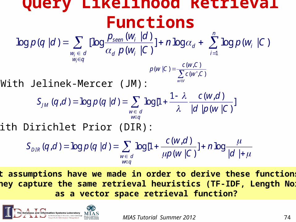
Query Likelihood Retrieval Functions
n
iid
qwdw id
iseen CwpnCwp
dwpdqp
i
i 1
)|(loglog])|(
)|([log)|(log
])|(||
),(11log[)|(log),(
qwdw
JM Cwpd
dwcdqpdqS
With Jelinek-Mercer (JM):
With Dirichlet Prior (DIR):
||
log])|(
),(1log[)|(log),(
dn
Cwp
dwcdqpdqS
qwdw
DIR
Vw
Cwc
CwcCwp
'
),'(
),()|(
What assumptions have we made in order to derive these functions? Do they capture the same retrieval heuristics (TF-IDF, Length Norm)
as a vector space retrieval function?
MIAS Tutorial Summer 2012 74
Pros & Cons of Language Models for IR
• Pros
– Grounded on statistical models; formulas dictated by the assumed model
– More meaningful parameters that can potentially be estimated based on data
– Assumptions are explicit and clear
• Cons
– May not work well empirically (non-optimal modeling of relevance)
– Not always easy to inject heuristics
MIAS Tutorial Summer 2012 75
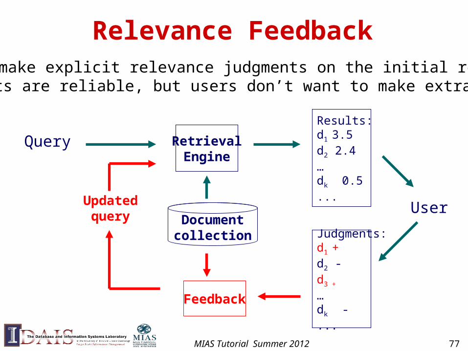
Relevance Feedback
Updatedquery
Feedback
Judgments:d1 +d2 -d3 +
…dk -...
Query RetrievalEngine
Results:d1 3.5d2 2.4…dk 0.5...
UserDocumentcollection
Users make explicit relevance judgments on the initial results(judgments are reliable, but users don’t want to make extra effort)
MIAS Tutorial Summer 2012 77
Pseudo/Blind/Automatic Feedback
Query RetrievalEngine
Results:d1 3.5d2 2.4…dk 0.5...
Judgments:d1 +d2 +d3 +
…dk -...
Documentcollection
Feedback
Updatedquery
top 10 assumed relevant
Top-k initial results are simply assumed to be relevant(judgments aren’t reliable, but no user activity is required)
MIAS Tutorial Summer 2012 78
Implicit Feedback
Updatedquery
Feedback
Clickthroughs:d1 +d2 -d3 +
…dk -...
Query RetrievalEngine
Results:d1 3.5d2 2.4…dk 0.5...
UserDocumentcollection
User-clicked docs are assumed to be relevant; skipped ones non-relevant (judgments aren’t completely reliable, but no extra effort from users)
MIAS Tutorial Summer 2012 79
Relevance Feedback in VS
• Basic setting: Learn from examples– Positive examples: docs known to be relevant
– Negative examples: docs known to be non-relevant
– How do you learn from this to improve performance?
• General method: Query modification– Adding new (weighted) terms
– Adjusting weights of old terms
– Doing both
• The most well-known and effective approach is Rocchio
MIAS Tutorial Summer 2012 80
+
Rocchio Feedback: Illustration
qqm
+ +
+++ +
+
+++
+
+
+
+
+- --
-
- - -
-
- - -
-
- - -- - - -
-
- - --
-
-
-+ + +
Centroid of non-relevant documents
Centroid of relevant documents
MIAS Tutorial Summer 2012 81
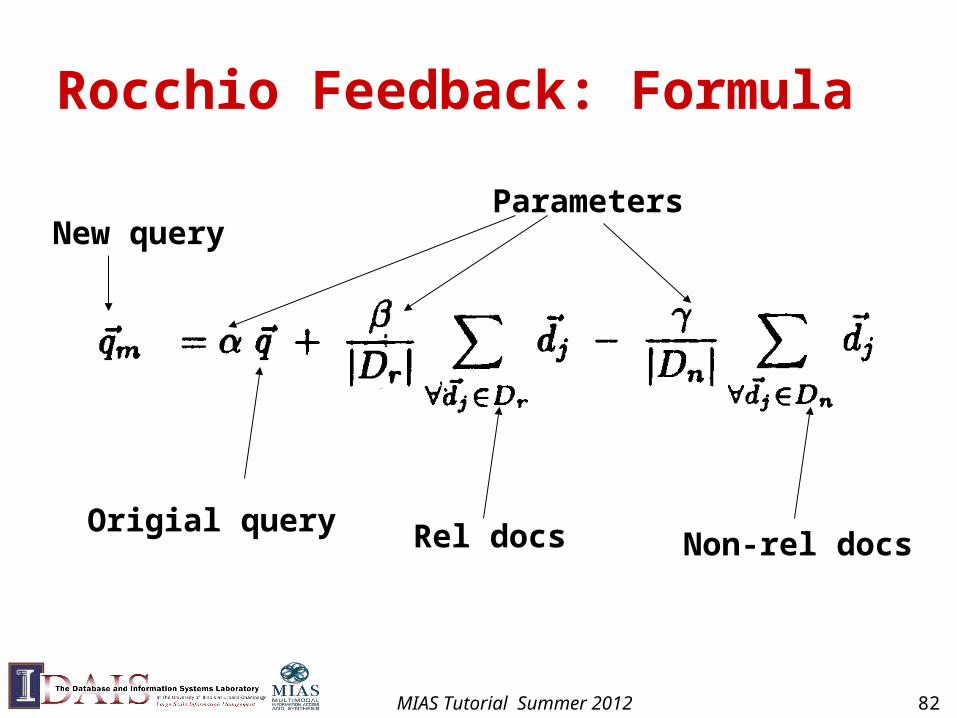
Rocchio Feedback: Formula
Origial query Rel docs Non-rel docs
ParametersNew query
MIAS Tutorial Summer 2012 82
Example of Rocchio Feedback
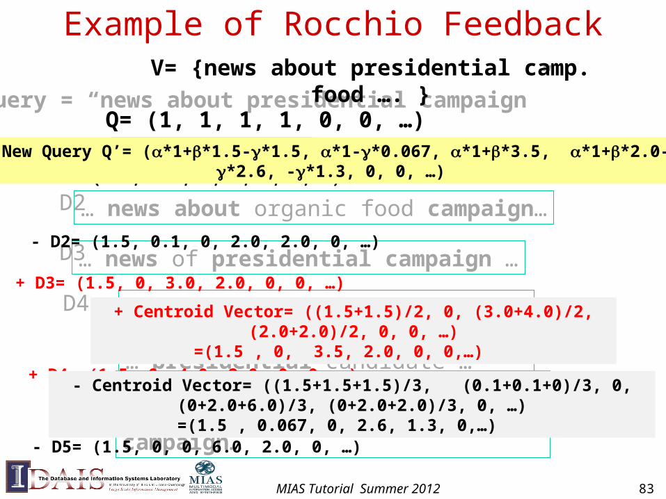
Query = “news about presidential campaign”
… news about …D1
… news about organic food campaign…D2
… news of presidential campaign …D3
… news of presidential campaign … … presidential candidate …
D4
… news of organic food campaign… campaign…campaign…campaign…
D5
V= {news about presidential camp. food …. }
Q= (1, 1, 1, 1, 0, 0, …)
- D1= (1.5, 0.1, 0, 0, 0, 0, …)
- D2= (1.5, 0.1, 0, 2.0, 2.0, 0, …)
+ D3= (1.5, 0, 3.0, 2.0, 0, 0, …)
+ D4= (1.5, 0, 4.0, 2.0, 0, 0, …)
- D5= (1.5, 0, 0, 6.0, 2.0, 0, …)
+ Centroid Vector= ((1.5+1.5)/2, 0, (3.0+4.0)/2, (2.0+2.0)/2, 0, 0, …)=(1.5 , 0, 3.5, 2.0, 0, 0,…)
- Centroid Vector= ((1.5+1.5+1.5)/3, (0.1+0.1+0)/3, 0, (0+2.0+6.0)/3, (0+2.0+2.0)/3, 0, …)
=(1.5 , 0.067, 0, 2.6, 1.3, 0,…)
New Query Q’= (*1+*1.5-*1.5, *1-*0.067, *1+*3.5, *1+*2.0-*2.6, -*1.3, 0, 0, …)
MIAS Tutorial Summer 2012 83
Rocchio in Practice
• Negative (non-relevant) examples are not very important (why?)
• Often truncate the vector (i.e., consider only a small number of words that have highest weights in the centroid vector) (efficiency concern)
• Avoid “over-fitting” (keep relatively high weight on the original query weights) (why?)
• Can be used for relevance feedback and pseudo feedback ( should be set to a larger value for relevance feedback than for pseudo feedback)
• Usually robust and effective
MIAS Tutorial Summer 2012 84
Feedback with Language Models
• Query likelihood method can’t naturally support feedback
• Solution:
– Kullback-Leibler (KL) divergence retrieval model as a generalization of query likelihood
– Feedback is achieved through query model estimation/updating
MIAS Tutorial Summer 2012 85
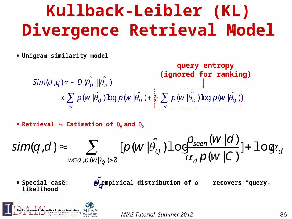
Kullback-Leibler (KL) Divergence Retrieval Model
• Unigram similarity model
• Retrieval Estimation of Q and D
• Special case: = empirical distribution of q recovers “query-likelihood”
ˆ ˆ( ; ) ( || )
ˆ ˆ ˆ ˆ( | ) log ( | ) ( ( | ) log ( | ))
Q D
Q D Q Qw w
Sim d q D
p w p w p w p w
query entropy(ignored for ranking)
Q̂
0)|(,
log])|(
)|(log)ˆ|([),(
Qwpdwd
d
seenQ Cwp
dwpwpdqsim
MIAS Tutorial Summer 2012 86
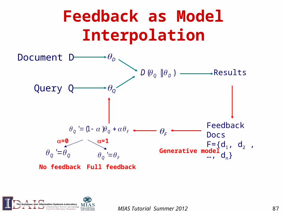
Feedback as Model Interpolation
Query Q
D
)||( DQD
Document D
Results
Feedback Docs F={d1, d2 , …, dn}
FQQ )1('
Generative model
Q
F=0
No feedback
FQ '
=1
Full feedback
QQ '
MIAS Tutorial Summer 2012 87
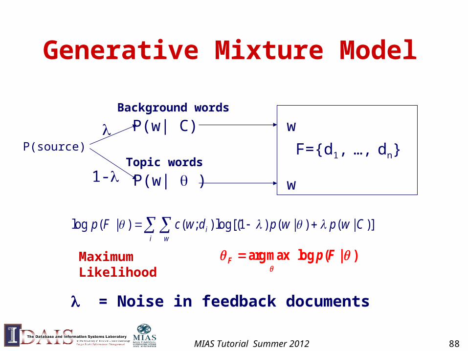
Generative Mixture Model
w
w
F={d1, …, dn}
log ( | ) ( ; ) log[(1 ) ( | ) ( | )]ii w
p F c w d p w p w C )|(logmaxarg
FpF Maximum
Likelihood
P(w| )
P(w| C)
1-
P(source)
Background words
Topic words
= Noise in feedback documents
MIAS Tutorial Summer 2012 88
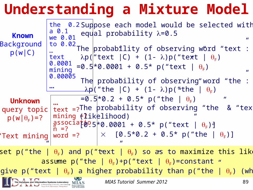
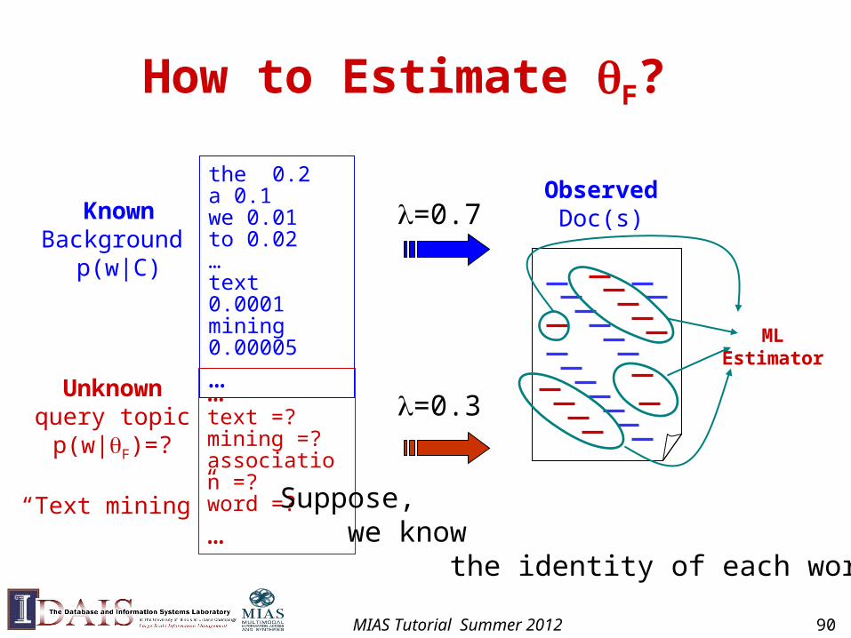
Understanding a Mixture Model the 0.2a 0.1we 0.01to 0.02…text 0.0001mining 0.00005
…
KnownBackground
p(w|C)
…text =? mining =? association =?word =?
…
Unknownquery topicp(w|F)=?
“Text mining”
Suppose each model would be selected with equal probability =0.5
The probability of observing word “text”: p(“text”|C) + (1- )p(“text”| F)=0.5*0.0001 + 0.5* p(“text”| F)
The probability of observing word “the”: p(“the”|C) + (1- )p(“the”| F)=0.5*0.2 + 0.5* p(“the”| F)The probability of observing “the” & “text”(likelihood) [0.5*0.0001 + 0.5* p(“text”| F)] [0.5*0.2 + 0.5* p(“the”| F)]
How to set p(“the”| F) and p(“text”| F) so as to maximize this likelihood?assume p(“the”| F)+p(“text”| F)=constant
give p(“text”| F) a higher probability than p(“the”| F) (why?)
MIAS Tutorial Summer 2012 89
How to Estimate F?
the 0.2a 0.1we 0.01to 0.02…text 0.0001mining 0.00005
…
KnownBackground
p(w|C)
…text =? mining =? association =?word =?
…
Unknownquery topicp(w|F)=?
“Text mining”
=0.7
=0.3
ObservedDoc(s)
Suppose, we know the identity of each word ...
MLEstimator
MIAS Tutorial Summer 2012 90
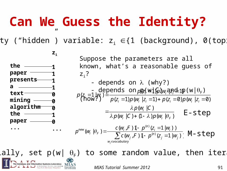
Can We Guess the Identity?Identity (“hidden”) variable: zi {1 (background), 0(topic)}
thepaperpresentsatextminingalgorithmthepaper...
zi
111100010...
Suppose the parameters are all known, what’s a reasonable guess of zi? - depends on (why?) - depends on p(w|C) and p(w|F) (how?)
( 1) ( | 1)( 1| )
( 1) ( | 1) ( 0) ( | 0)
( | )
( | ) (1 ) ( | )
i i ii i
i i i i i i
i
i i F
p z p w zp z w
p z p w z p z p w z
p w C
p w C p w
E-step
Initially, set p(w| F) to some random value, then iterate …
M-step
vocabularywjj
nj
iin
iFi
new
j
wzpFwc
wzpFwcwp
))|1(1)(,(
))|1(1)(,()|(
)(
)(
MIAS Tutorial Summer 2012 91
An Example of EM Computation
Iteration 1 Iteration 2 Iteration 3 Word # P(w|C) P(w|F) P(z=1) P(w|F) P(z=1) P(w|F) P(z=1)
The 4 0.5 0.25 0.67 0.20 0.71 0.18 0.74 Paper 2 0.3 0.25 0.55 0.14 0.68 0.10 0.75 Text 4 0.1 0.25 0.29 0.44 0.19 0.50 0.17 Mining 2 0.1 0.25 0.29 0.22 0.31 0.22 0.31
Log-Likelihood -16.96 -16.13 -16.02
Assume =0.5
Expectation-Step:Augmenting data by guessing hidden variables
Maximization-Step With the “augmented data”, estimate parameters
using maximum likelihood
vocabularywjj
nj
iin
iFi
n
Fin
i
iii
n
j
wzpFwc
wzpFwcwp
wpCwp
Cwpwzp
))|1(1)(,(
))|1(1)(,()|(
)|()1()|(
)|()|1(
)(
)()1(
)()(
MIAS Tutorial Summer 2012 92
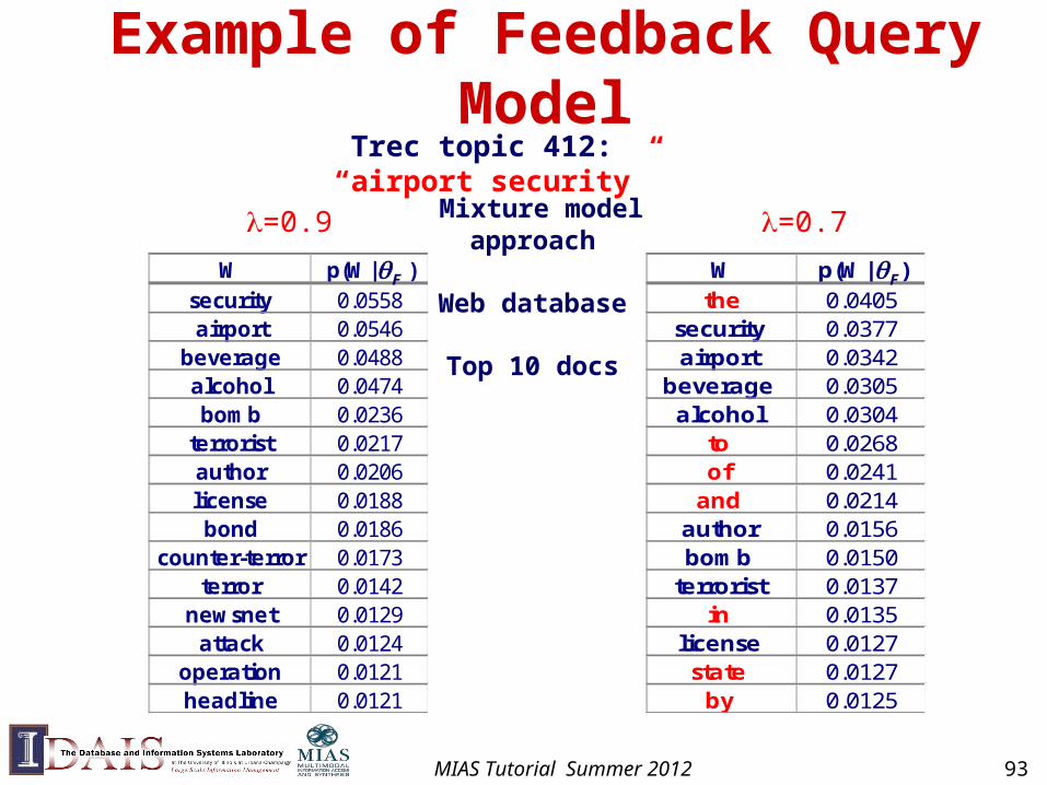
Example of Feedback Query Model
W p(W| )security 0.0558airport 0.0546
beverage 0.0488alcohol 0.0474bomb 0.0236
terrorist 0.0217author 0.0206license 0.0188bond 0.0186
counter-terror 0.0173terror 0.0142
newsnet 0.0129attack 0.0124
operation 0.0121headline 0.0121
Trec topic 412: “airport security”
W p(W| )the 0.0405
security 0.0377airport 0.0342
beverage 0.0305alcohol 0.0304
to 0.0268of 0.0241
and 0.0214author 0.0156bomb 0.0150
terrorist 0.0137in 0.0135
license 0.0127state 0.0127
by 0.0125
=0.9 =0.7
FF
Mixture model approach
Web database
Top 10 docs
MIAS Tutorial Summer 2012 93
Why Evaluation? • Reason 1: So that we can assess how useful an IR
system/technology would be (for an application)
– Measures should reflect the utility to users in a real application
– Usually done through user studies (interactive IR evaluation)
• Reason 2: So that we can compare different systems and methods (to advance the state of the art)
– Measures only need to be correlated with the utility to actual users, thus don’t have to accurately reflect the exact utility to users
– Usually done through test collections (test set IR evaluation)
MIAS Tutorial Summer 2012 95
What to Measure? • Effectiveness/Accuracy: how accurate are the search
results?
– Measuring a system’s ability of ranking relevant docucments on top of non-relevant ones
• Efficiency: how quickly can a user get the results? How much computing resources are needed to answer a query?
– Measuring space and time overhead
• Usability: How useful is the system for real user tasks?
– Doing user studies
MIAS Tutorial Summer 2012 96
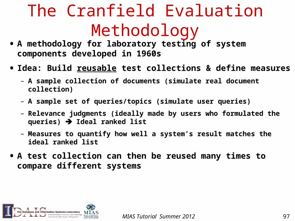
The Cranfield Evaluation Methodology• A methodology for laboratory testing of system components
developed in 1960s
• Idea: Build reusable test collections & define measures
– A sample collection of documents (simulate real document collection)
– A sample set of queries/topics (simulate user queries)
– Relevance judgments (ideally made by users who formulated the queries) Ideal ranked list
– Measures to quantify how well a system’s result matches the ideal ranked list
• A test collection can then be reused many times to compare different systems
MIAS Tutorial Summer 2012 97
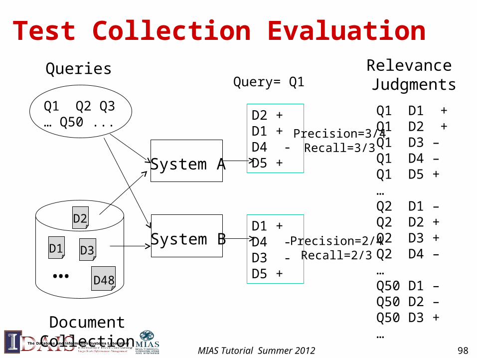
Test Collection Evaluation
Q1 D1 +Q1 D2 +Q1 D3 –Q1 D4 –Q1 D5 +…Q2 D1 –Q2 D2 +Q2 D3 +Q2 D4 –…Q50 D1 –Q50 D2 –Q50 D3 +…
Relevance Judgments
Document Collection
Q1 Q2 Q3… Q50 ...
D1
D2
D3
D48…
Queries
D2 +D1 + D4 - D5 +System A
System B
Query= Q1
D1 +D4 -D3 - D5 +
Precision=3/4Recall=3/3
Precision=2/4Recall=2/3
MIAS Tutorial Summer 2012 98
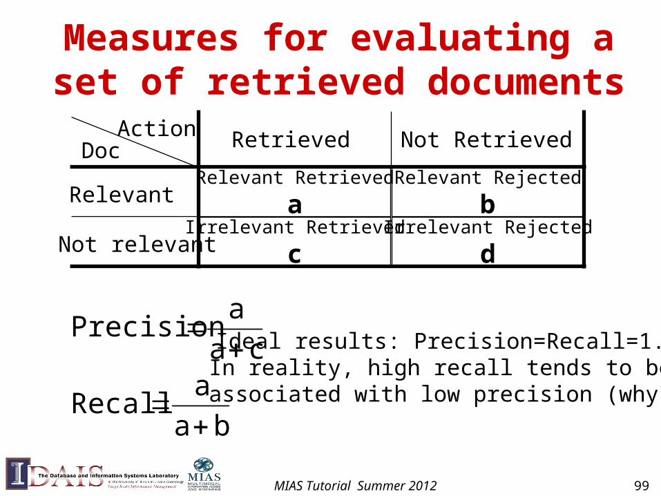
Measures for evaluating a set of retrieved documents
Relevant Retrieved
aIrrelevant Retrieved
cIrrelevant Rejected
d
Relevant Rejected
bRelevant
Not relevant
Retrieved Not RetrievedDocAction
ba
aRecall
ca
aPrecision
Ideal results: Precision=Recall=1.0
In reality, high recall tends to be associated with low precision (why?)
MIAS Tutorial Summer 2012 99
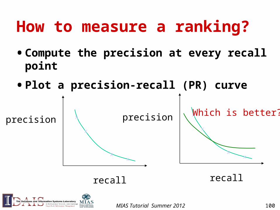
How to measure a ranking?
• Compute the precision at every recall point
• Plot a precision-recall (PR) curve
precision
recall
x
x
x
x
precision
recall
x
x
x
x
Which is better?
MIAS Tutorial Summer 2012 100
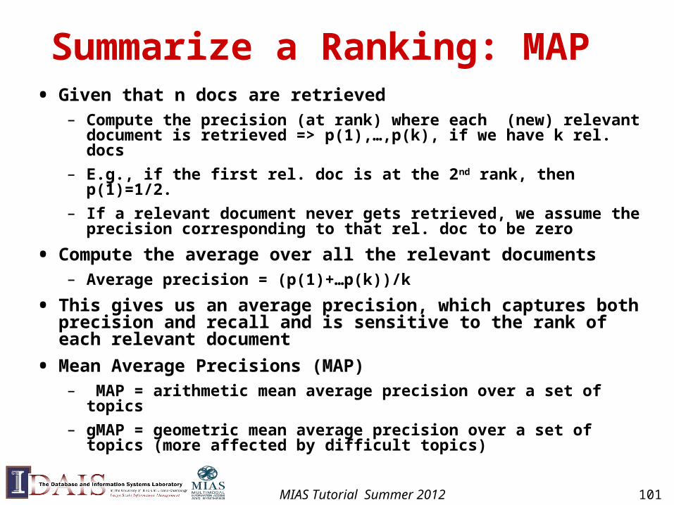
Summarize a Ranking: MAP• Given that n docs are retrieved
– Compute the precision (at rank) where each (new) relevant document is retrieved => p(1),…,p(k), if we have k rel. docs
– E.g., if the first rel. doc is at the 2nd rank, then p(1)=1/2.
– If a relevant document never gets retrieved, we assume the precision corresponding to that rel. doc to be zero
• Compute the average over all the relevant documents– Average precision = (p(1)+…p(k))/k
• This gives us an average precision, which captures both precision and recall and is sensitive to the rank of each relevant document
• Mean Average Precisions (MAP)– MAP = arithmetic mean average precision over a set of topics
– gMAP = geometric mean average precision over a set of topics (more affected by difficult topics)
MIAS Tutorial Summer 2012 101
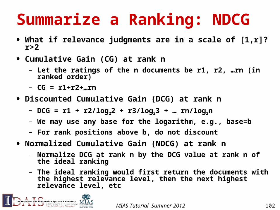
Summarize a Ranking: NDCG• What if relevance judgments are in a scale of [1,r]? r>2
• Cumulative Gain (CG) at rank n– Let the ratings of the n documents be r1, r2, …rn (in ranked order)
– CG = r1+r2+…rn
• Discounted Cumulative Gain (DCG) at rank n– DCG = r1 + r2/log22 + r3/log23 + … rn/log2n
– We may use any base for the logarithm, e.g., base=b
– For rank positions above b, do not discount
• Normalized Cumulative Gain (NDCG) at rank n– Normalize DCG at rank n by the DCG value at rank n of the ideal
ranking
– The ideal ranking would first return the documents with the highest relevance level, then the next highest relevance level, etc
MIAS Tutorial Summer 2012 102
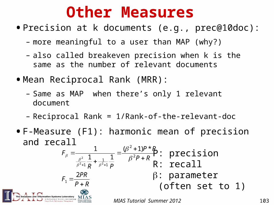
Other Measures• Precision at k documents (e.g., prec@10doc):
– more meaningful to a user than MAP (why?)
– also called breakeven precision when k is the same as the number of relevant documents
• Mean Reciprocal Rank (MRR):
– Same as MAP when there’s only 1 relevant document
– Reciprocal Rank = 1/Rank-of-the-relevant-doc
• F-Measure (F1): harmonic mean of precision and recall
RP
PRF
RP
RP
PR
F
2
*)1(11
1
1
2
2
11
1 22
2
P: precisionR: recall: parameter (often set to 1)
MIAS Tutorial Summer 2012 103
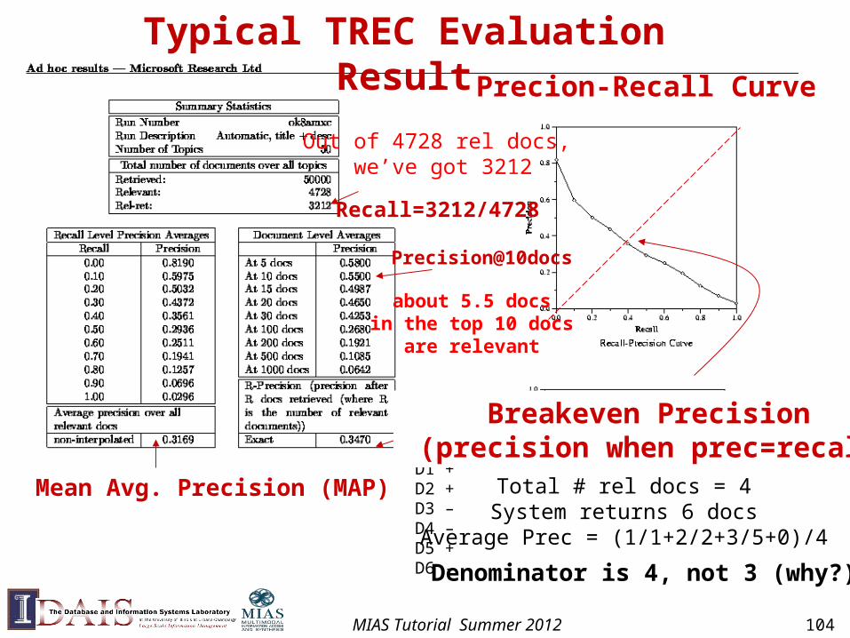
Precion-Recall Curve
Mean Avg. Precision (MAP)
Recall=3212/4728
Out of 4728 rel docs, we’ve got 3212
D1 +D2 +D3 –D4 –D5 +D6 -
Total # rel docs = 4System returns 6 docs
Average Prec = (1/1+2/2+3/5+0)/4
about 5.5 docsin the top 10 docs
are relevant
Precision@10docs
Typical TREC Evaluation Result
Denominator is 4, not 3 (why?)
104
Breakeven Precision (precision when prec=recall)
MIAS Tutorial Summer 2012
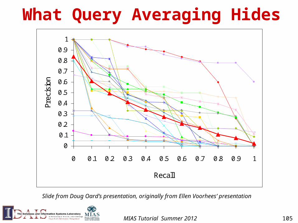
What Query Averaging Hides
0
0.1
0.2
0.3
0.4
0.5
0.6
0.7
0.8
0.9
1
0 0.1 0.2 0.3 0.4 0.5 0.6 0.7 0.8 0.9 1
Recall
Prec
isio
n
Slide from Doug Oard’s presentation, originally from Ellen Voorhees’ presentation
MIAS Tutorial Summer 2012 105
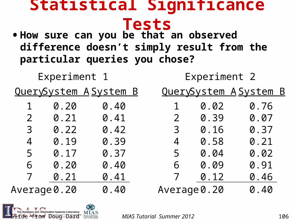
Statistical Significance Tests• How sure can you be that an observed difference
doesn’t simply result from the particular queries you chose?
System A
0.200.210.220.190.170.200.21
System B
0.400.410.420.390.370.400.41
Experiment 1
Query
1234567
Average 0.20 0.40
System A
0.020.390.160.580.040.090.12
System B
0.760.070.370.210.020.910.46
Experiment 2
Query
1234567
Average 0.20 0.40
Slide from Doug Oard MIAS Tutorial Summer 2012 106
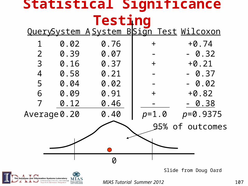
Statistical Significance TestingSystem A
0.020.390.160.580.040.090.12
System B
0.760.070.370.210.020.910.46
Query
1234567
Average 0.20 0.40
Sign Test
+-+--+-
p=1.0
Wilcoxon
+0.74- 0.32+0.21- 0.37- 0.02+0.82- 0.38
p=0.9375
0
95% of outcomes
Slide from Doug Oard
MIAS Tutorial Summer 2012 107
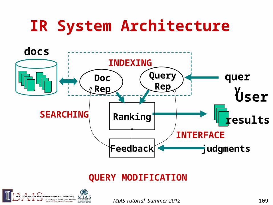
IR System Architecture
User
query
judgments
docs
results
QueryRep
DocRep
Ranking
Feedback
INDEXING
SEARCHING
QUERY MODIFICATION
INTERFACE
MIAS Tutorial Summer 2012 109
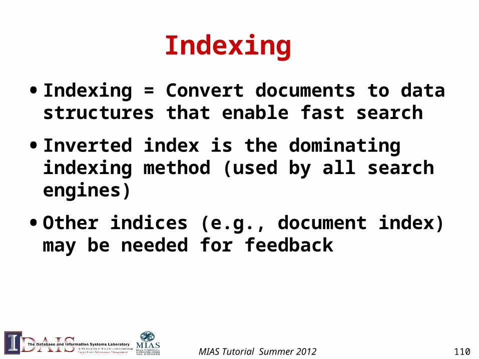
Indexing
• Indexing = Convert documents to data structures that enable fast search
• Inverted index is the dominating indexing method (used by all search engines)
• Other indices (e.g., document index) may be needed for feedback
MIAS Tutorial Summer 2012 110
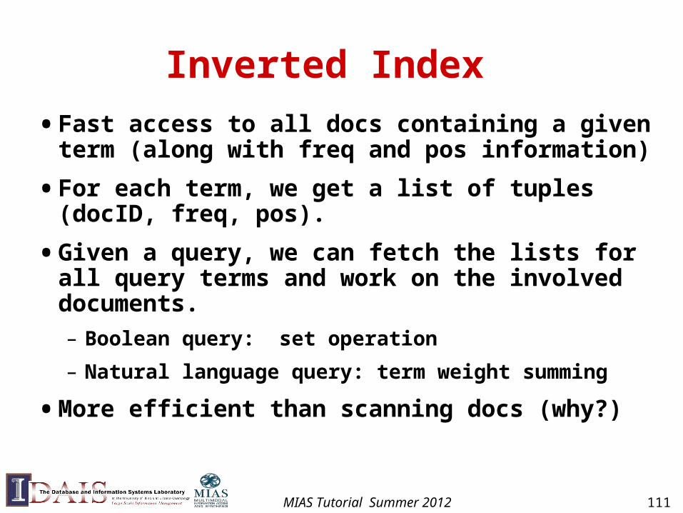
Inverted Index
• Fast access to all docs containing a given term (along with freq and pos information)
• For each term, we get a list of tuples (docID, freq, pos).
• Given a query, we can fetch the lists for all query terms and work on the involved documents.
– Boolean query: set operation
– Natural language query: term weight summing
• More efficient than scanning docs (why?)
MIAS Tutorial Summer 2012 111
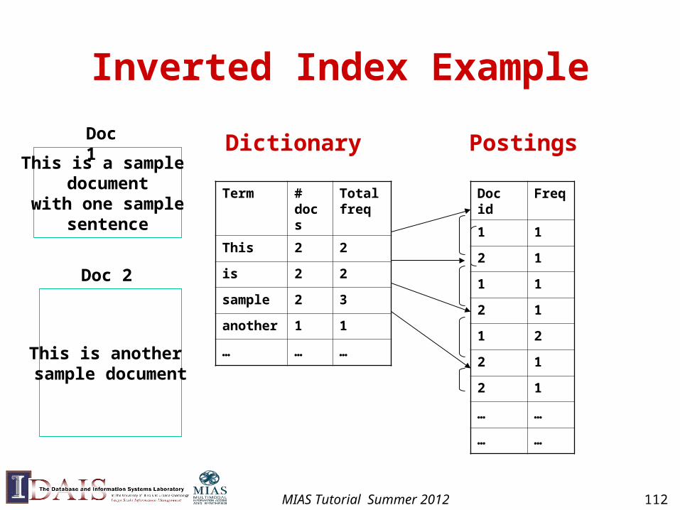
Inverted Index Example
This is a sample document
with one samplesentence
Doc 1
This is another sample document
Doc 2
Dictionary Postings
Term # docs
Total freq
This 2 2
is 2 2
sample 2 3
another 1 1
… … …
Doc id Freq
1 1
2 1
1 1
2 1
1 2
2 1
2 1
… …
… …
MIAS Tutorial Summer 2012 112
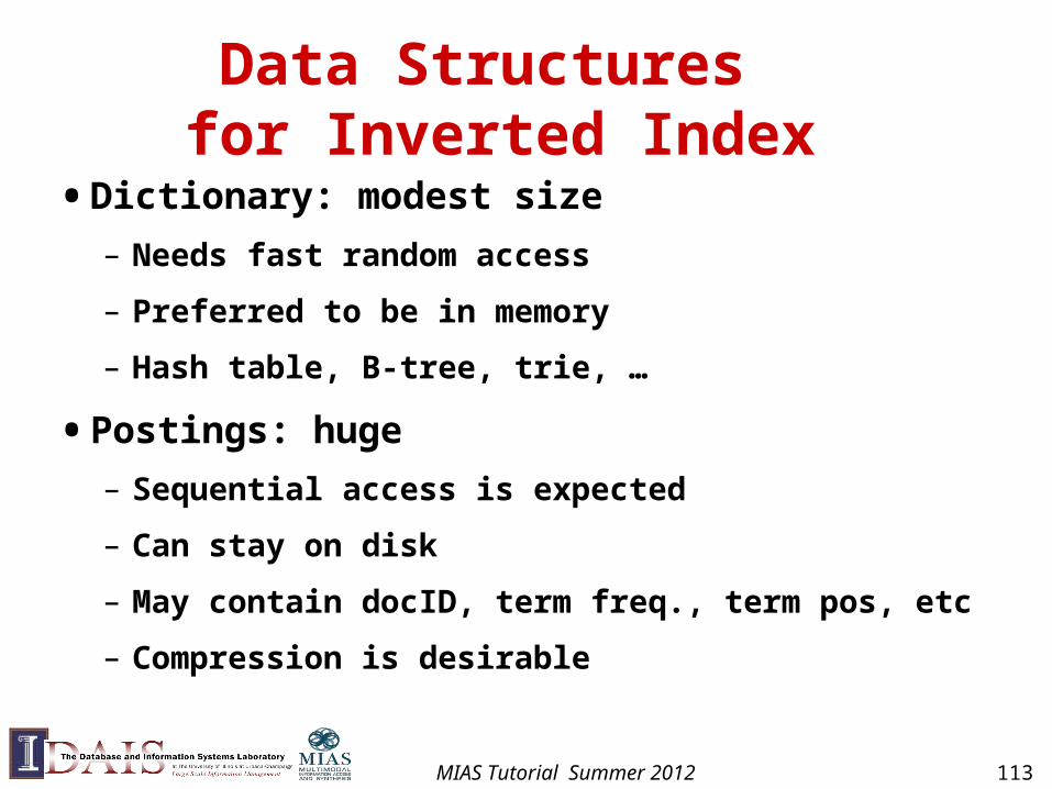
Data Structures for Inverted Index
• Dictionary: modest size
– Needs fast random access
– Preferred to be in memory
– Hash table, B-tree, trie, …
• Postings: huge
– Sequential access is expected
– Can stay on disk
– May contain docID, term freq., term pos, etc
– Compression is desirable
MIAS Tutorial Summer 2012 113
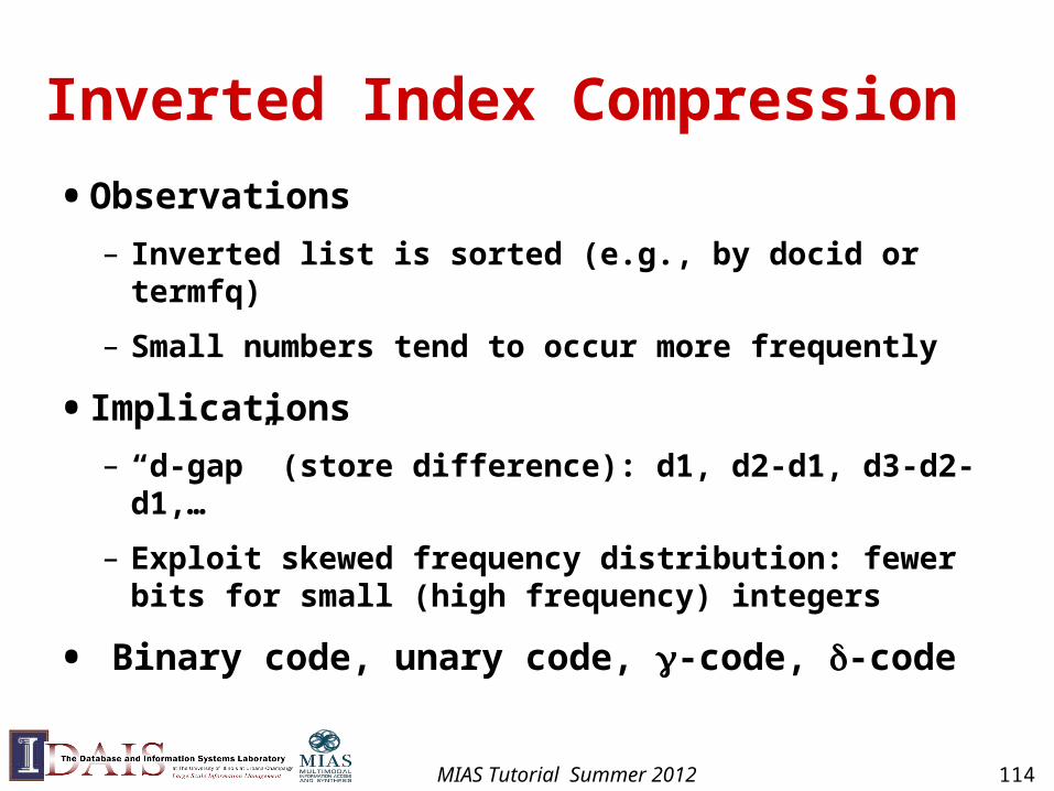
Inverted Index Compression
• Observations
– Inverted list is sorted (e.g., by docid or termfq)
– Small numbers tend to occur more frequently
• Implications
– “d-gap” (store difference): d1, d2-d1, d3-d2-d1,…
– Exploit skewed frequency distribution: fewer bits for small (high frequency) integers
• Binary code, unary code, -code, -code
MIAS Tutorial Summer 2012 114
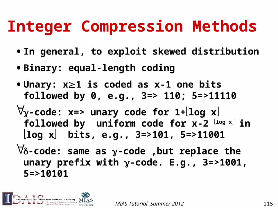
Integer Compression Methods
• In general, to exploit skewed distribution
• Binary: equal-length coding
• Unary: x1 is coded as x-1 one bits followed by 0, e.g., 3=> 110; 5=>11110
-code: x=> unary code for 1+log x followed by uniform code for x-2 log x in log x bits, e.g., 3=>101, 5=>11001
-code: same as -code ,but replace the unary prefix with -code. E.g., 3=>1001, 5=>10101
MIAS Tutorial Summer 2012 115
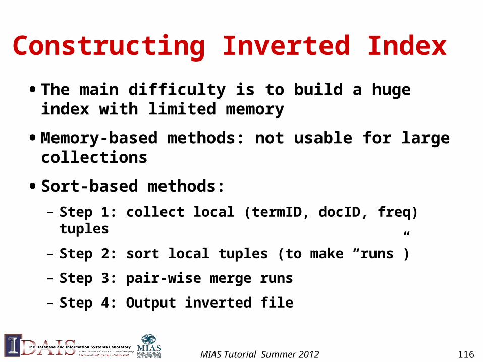
Constructing Inverted Index
• The main difficulty is to build a huge index with limited memory
• Memory-based methods: not usable for large collections
• Sort-based methods:
– Step 1: collect local (termID, docID, freq) tuples
– Step 2: sort local tuples (to make “runs”)
– Step 3: pair-wise merge runs
– Step 4: Output inverted file
MIAS Tutorial Summer 2012 116
Sort-based Inversion
...
Term Lexicon:
the 1cold 2days 3a 4
...
DocIDLexicon:
doc1 1doc2 2doc3 3
...
doc1
doc2
doc300
<1,1,3><2,1,2><3,1,1>... <1,2,2><3,2,3><4,2,2>…
<1,300,3><3,300,1>...
Sort by doc-id
Parse & Count
<1,1,3><1,2,2><2,1,2><2,4,3>...<1,5,3><1,6,2>…
<1,299,3><1,300,1>...
Sort by term-id
“Local” sort
<1,1,3><1,2,2><1,5,2><1,6,3>...<1,300,3><2,1,2>…
<5000,299,1><5000,300,1>...
Merge sort
All info about term 1
MIAS Tutorial Summer 2012 117
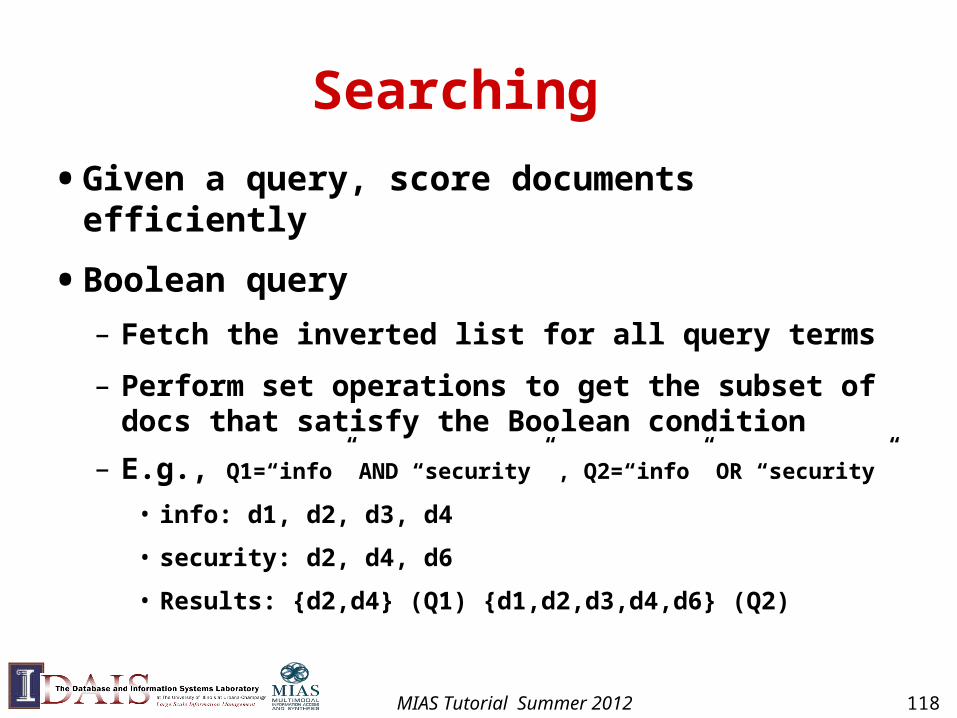
Searching
• Given a query, score documents efficiently
• Boolean query
– Fetch the inverted list for all query terms
– Perform set operations to get the subset of docs that satisfy the Boolean condition
– E.g., Q1=“info” AND “security” , Q2=“info” OR “security”
• info: d1, d2, d3, d4
• security: d2, d4, d6
• Results: {d2,d4} (Q1) {d1,d2,d3,d4,d6} (Q2)
MIAS Tutorial Summer 2012 118
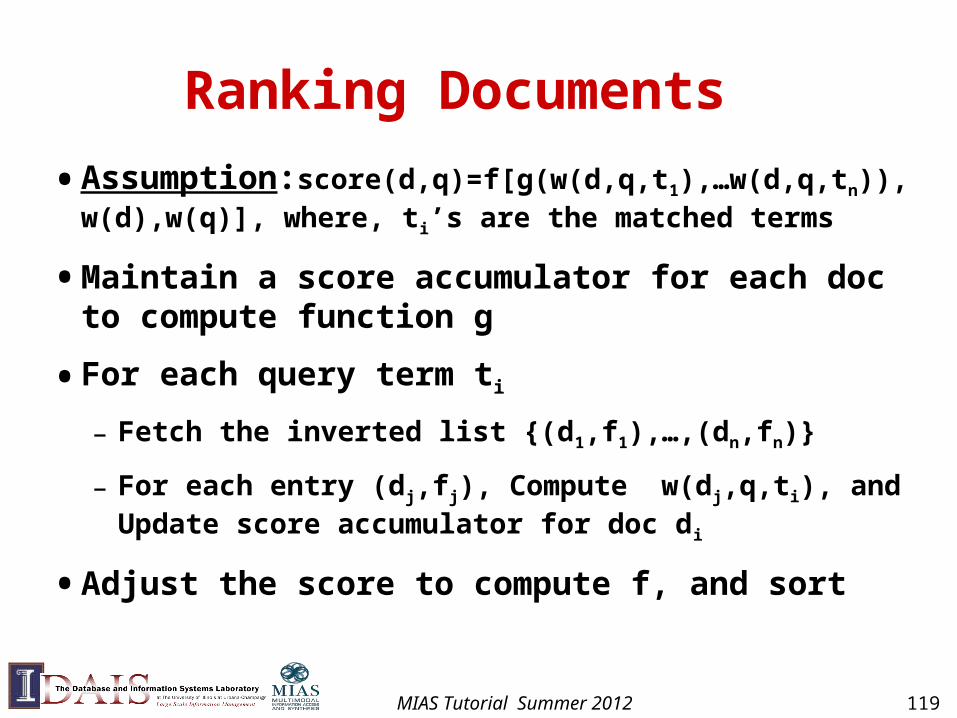
Ranking Documents
• Assumption:score(d,q)=f[g(w(d,q,t1),…w(d,q,tn)), w(d),w(q)], where, ti’s are the matched terms
• Maintain a score accumulator for each doc to compute function g
• For each query term ti
– Fetch the inverted list {(d1,f1),…,(dn,fn)}
– For each entry (dj,fj), Compute w(dj,q,ti), and Update score accumulator for doc di
• Adjust the score to compute f, and sort
MIAS Tutorial Summer 2012 119
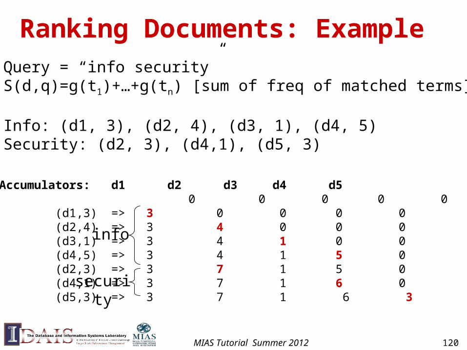
Ranking Documents: ExampleQuery = “info security”S(d,q)=g(t1)+…+g(tn) [sum of freq of matched terms]
Info: (d1, 3), (d2, 4), (d3, 1), (d4, 5)Security: (d2, 3), (d4,1), (d5, 3)
Accumulators: d1 d2 d3 d4 d5 0 0 0 0 0 (d1,3) => 3 0 0 0 0 (d2,4) => 3 4 0 0 0 (d3,1) => 3 4 1 0 0 (d4,5) => 3 4 1 5 0 (d2,3) => 3 7 1 5 0 (d4,1) => 3 7 1 6 0 (d5,3) => 3 7 1 6 3
info
security
MIAS Tutorial Summer 2012 120
121
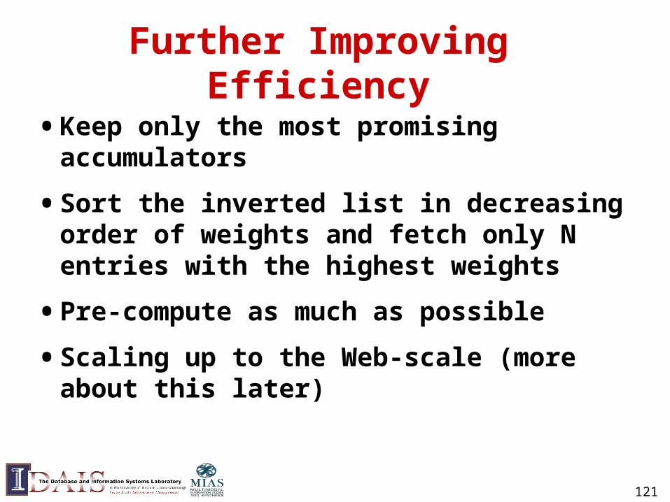
Further Improving Efficiency
• Keep only the most promising accumulators
• Sort the inverted list in decreasing order of weights and fetch only N entries with the highest weights
• Pre-compute as much as possible
• Scaling up to the Web-scale (more about this later)
Open Source IR Toolkits
• Smart (Cornell)
• MG (RMIT & Melbourne, Australia; Waikato, New Zealand),
• Lemur (CMU/Univ. of Massachusetts)
• Terrier (Glasgow)
• Lucene (Open Source)
MIAS Tutorial Summer 2012 122
Smart
• The most influential IR system/toolkit
• Developed at Cornell since 1960’s
• Vector space model with lots of weighting options
• Written in C
• The Cornell/AT&T groups have used the Smart system to achieve top TREC performance
MIAS Tutorial Summer 2012 123
MG
• A highly efficient toolkit for retrieval of text and images
• Developed by people at Univ. of Waikato, Univ. of Melbourne, and RMIT in 1990’s
• Written in C, running on Unix
• Vector space model with lots of compression and speed up tricks
• People have used it to achieve good TREC performance
MIAS Tutorial Summer 2012 124
Lemur/Indri
• An IR toolkit emphasizing language models
• Developed at CMU and Univ. of Massachusetts in 2000’s
• Written in C++, highly extensible
• Vector space and probabilistic models including language models
• Achieving good TREC performance with a simple language model
MIAS Tutorial Summer 2012 125
Terrier
• A large-scale retrieval toolkit with lots of applications (e.g., desktop search) and TREC support
• Developed at University of Glasgow, UK
• Written in Java, open source
• “Divergence from randomness” retrieval model and other modern retrieval formulas
MIAS Tutorial Summer 2012 126
Lucene
• Open Source IR toolkit
• Initially developed by Doug Cutting in Java
• Now has been ported to some other languages
• Good for building IR/Web applications
• Many applications have been built using Lucene (e.g., Nutch Search Engine)
• Currently the retrieval algorithms have poor accuracy
MIAS Tutorial Summer 2012 127
129
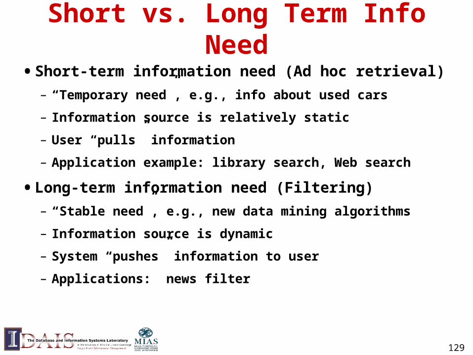
Short vs. Long Term Info Need
• Short-term information need (Ad hoc retrieval)
– “Temporary need”, e.g., info about used cars
– Information source is relatively static
– User “pulls” information
– Application example: library search, Web search
• Long-term information need (Filtering)
– “Stable need”, e.g., new data mining algorithms
– Information source is dynamic
– System “pushes” information to user
– Applications: news filter
130
Examples of Information Filtering
• News filtering
• Email filtering
• Movie/book recommenders
• Literature recommenders
• And many others …
131
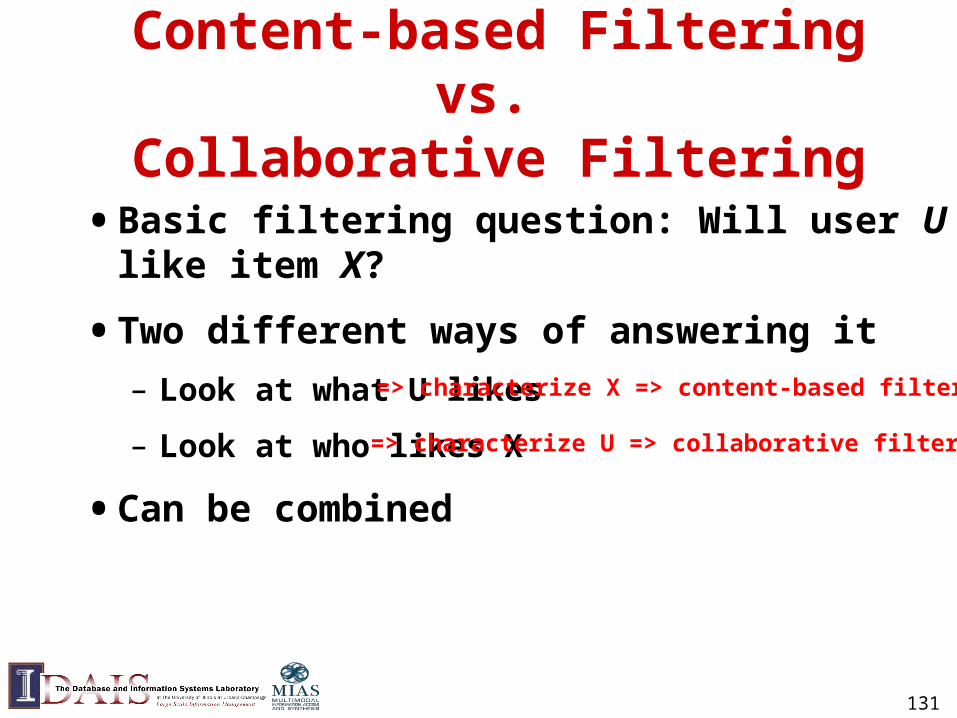
Content-based Filtering vs. Collaborative Filtering
• Basic filtering question: Will user U like item X?
• Two different ways of answering it
– Look at what U likes
– Look at who likes X
• Can be combined
=> characterize X => content-based filtering
=> characterize U => collaborative filtering
133
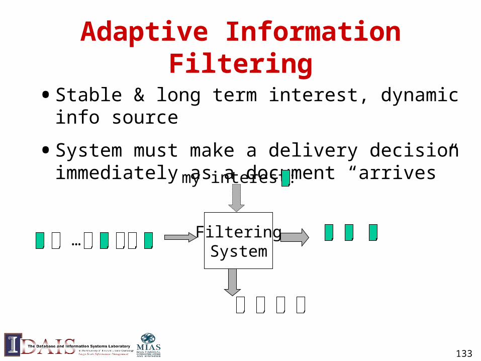
Adaptive Information Filtering
• Stable & long term interest, dynamic info source
• System must make a delivery decision immediately as a document “arrives”
FilteringSystem
…
my interest:
134
AIF vs. Retrieval, & Categorization
• Like retrieval over a dynamic stream of docs, but ranking is impossible and a binary decision must be made in real time
• Typically evaluated with a utility function
– Each delivered doc gets a utility value
– Good doc gets a positive value (e.g., +3)
– Bad doc gets a negative value (e.g., -2)
– E.g., Utility = 3* #good - 2 *#bad (linear utility)
135
A Typical AIF System
...Binary
Classifier
UserInterestProfile
User
Doc Source
Accepted Docs
Initialization
Learning FeedbackAccumulated
Docs
utility func
User profile text
136
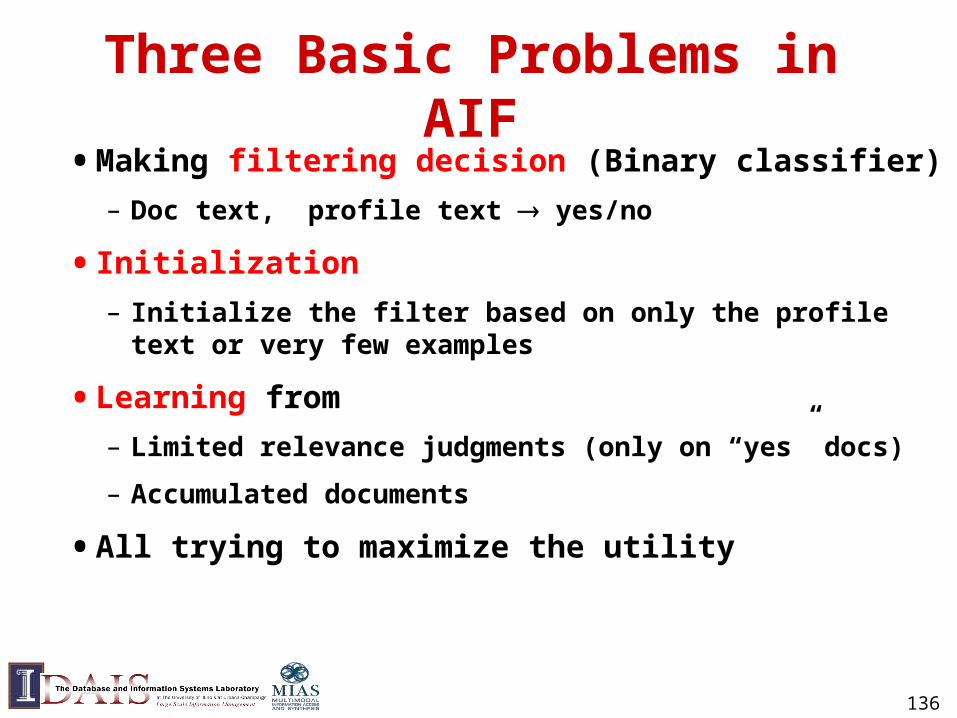
Three Basic Problems in AIF• Making filtering decision (Binary classifier)
– Doc text, profile text yes/no
• Initialization
– Initialize the filter based on only the profile text or very few examples
• Learning from
– Limited relevance judgments (only on “yes” docs)
– Accumulated documents
• All trying to maximize the utility
137
Extend a Retrieval System for Information Filtering
• “Reuse” retrieval techniques to score documents
• Use a score threshold for filtering decision
• Learn to improve scoring with traditional feedback
• New approaches to threshold setting and learning
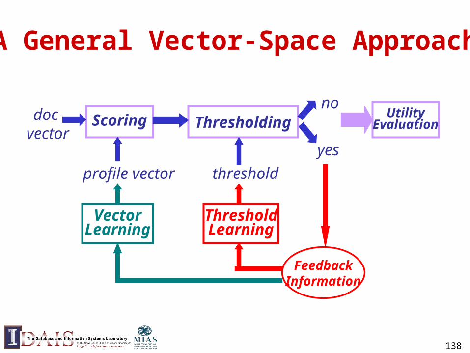
138
A General Vector-Space Approach
doc vector
profile vector
Scoring Thresholding
yes
no
FeedbackInformation
VectorLearning
ThresholdLearning
threshold
UtilityEvaluation
139
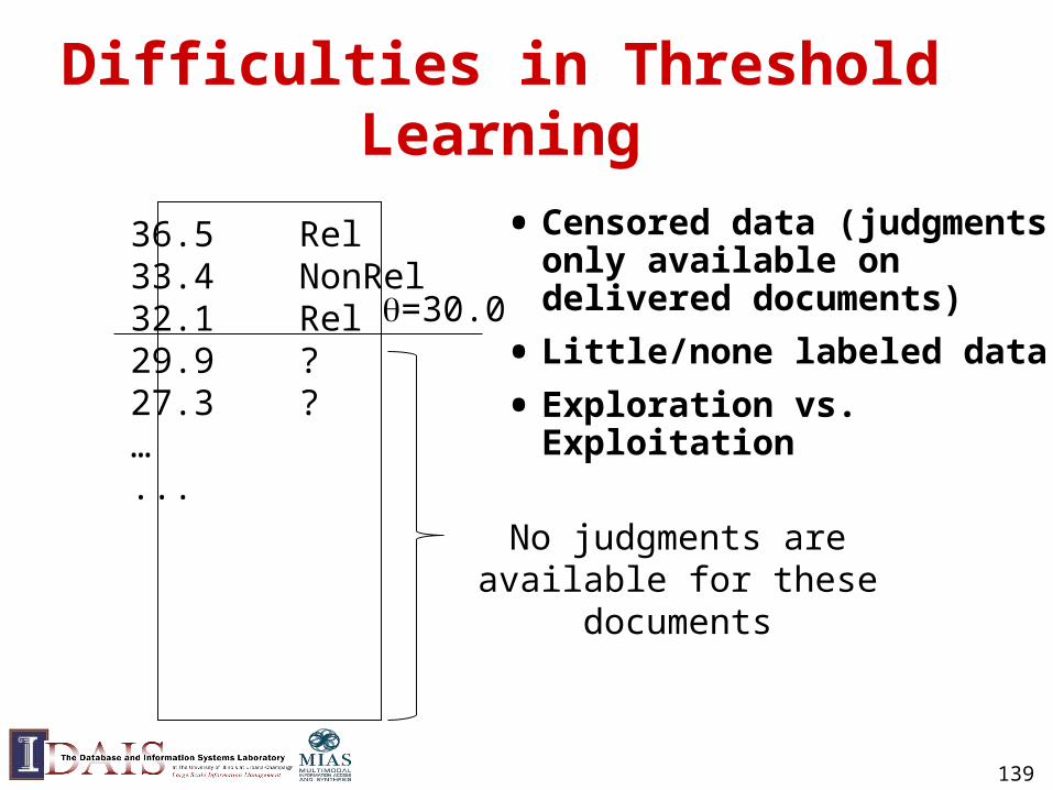
Difficulties in Threshold Learning
36.5 Rel33.4 NonRel32.1 Rel29.9 ?27.3 ?…...
=30.0
• Censored data (judgments only available on delivered documents)
• Little/none labeled data
• Exploration vs. Exploitation
No judgments are available for these documents
140
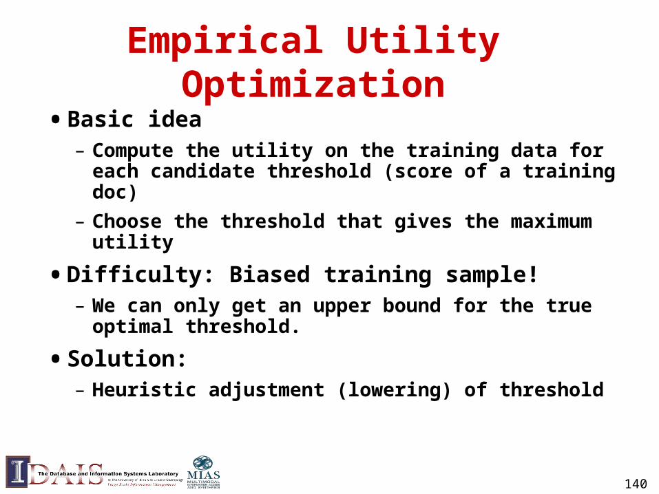
Empirical Utility Optimization
• Basic idea– Compute the utility on the training data for each
candidate threshold (score of a training doc)
– Choose the threshold that gives the maximum utility
• Difficulty: Biased training sample!– We can only get an upper bound for the true
optimal threshold.
• Solution:– Heuristic adjustment (lowering) of threshold
141
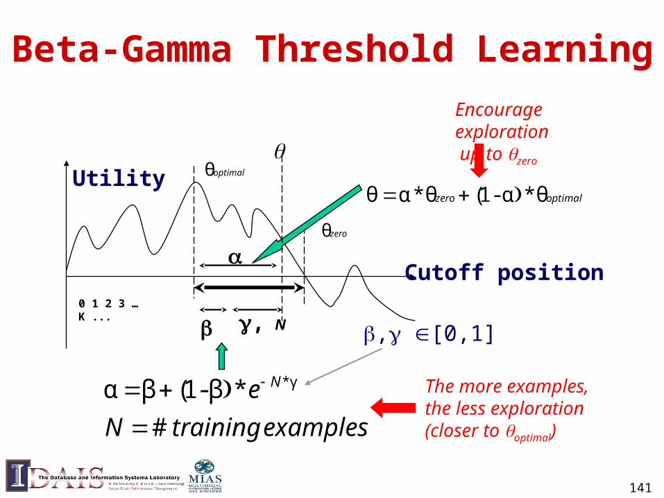
optimalθ
Beta-Gamma Threshold Learning
Cutoff position
Utility
0 1 2 3 … K ...
zeroθ
, N
examplestrainingN
e N
#
*β-1(βα γ*
, [0,1]
The more examples,the less exploration(closer to optimal)
optimalzero θ*α-1(θ*αθ
Encourage exploration up to zero
142
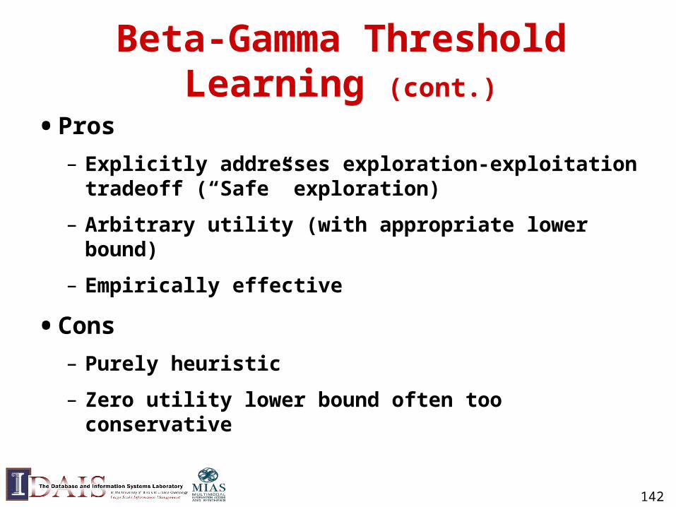
Beta-Gamma Threshold Learning (cont.)
• Pros
– Explicitly addresses exploration-exploitation tradeoff (“Safe” exploration)
– Arbitrary utility (with appropriate lower bound)
– Empirically effective
• Cons
– Purely heuristic
– Zero utility lower bound often too conservative
144
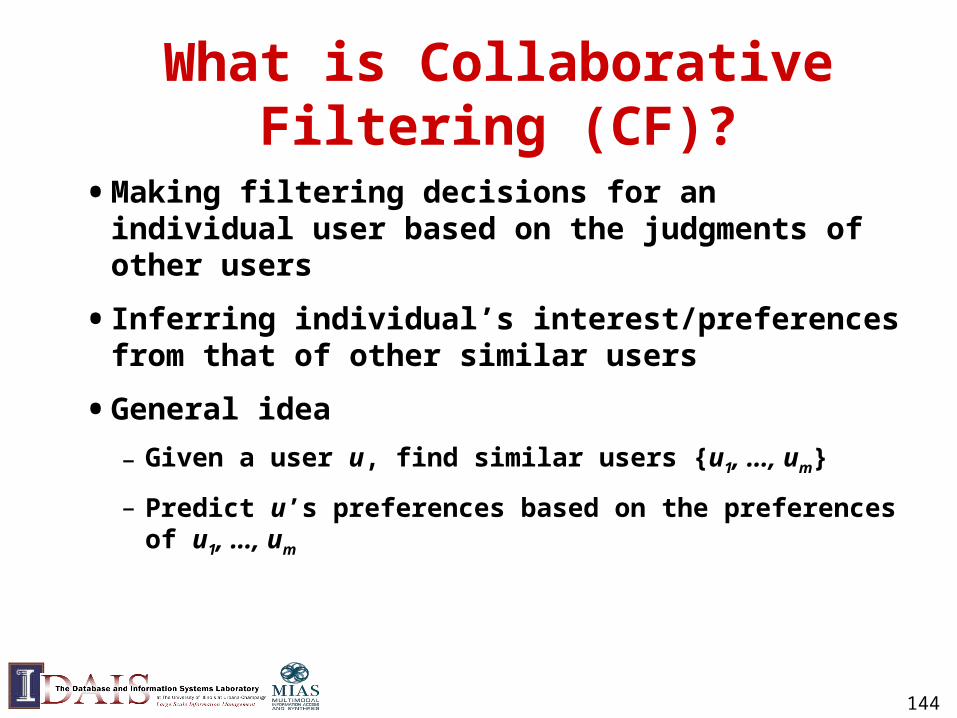
What is Collaborative Filtering (CF)?
• Making filtering decisions for an individual user based on the judgments of other users
• Inferring individual’s interest/preferences from that of other similar users
• General idea
– Given a user u, find similar users {u1, …, um}
– Predict u’s preferences based on the preferences of u1, …, um
145
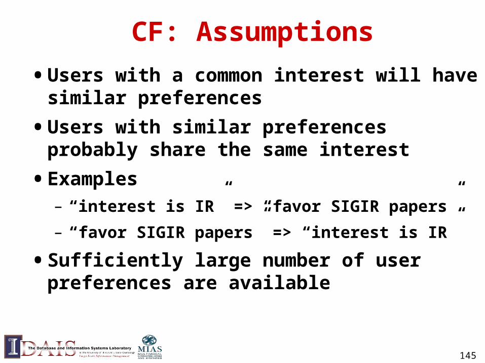
CF: Assumptions
• Users with a common interest will have similar preferences
• Users with similar preferences probably share the same interest
• Examples– “interest is IR” => “favor SIGIR papers”
– “favor SIGIR papers” => “interest is IR”
• Sufficiently large number of user preferences are available
146
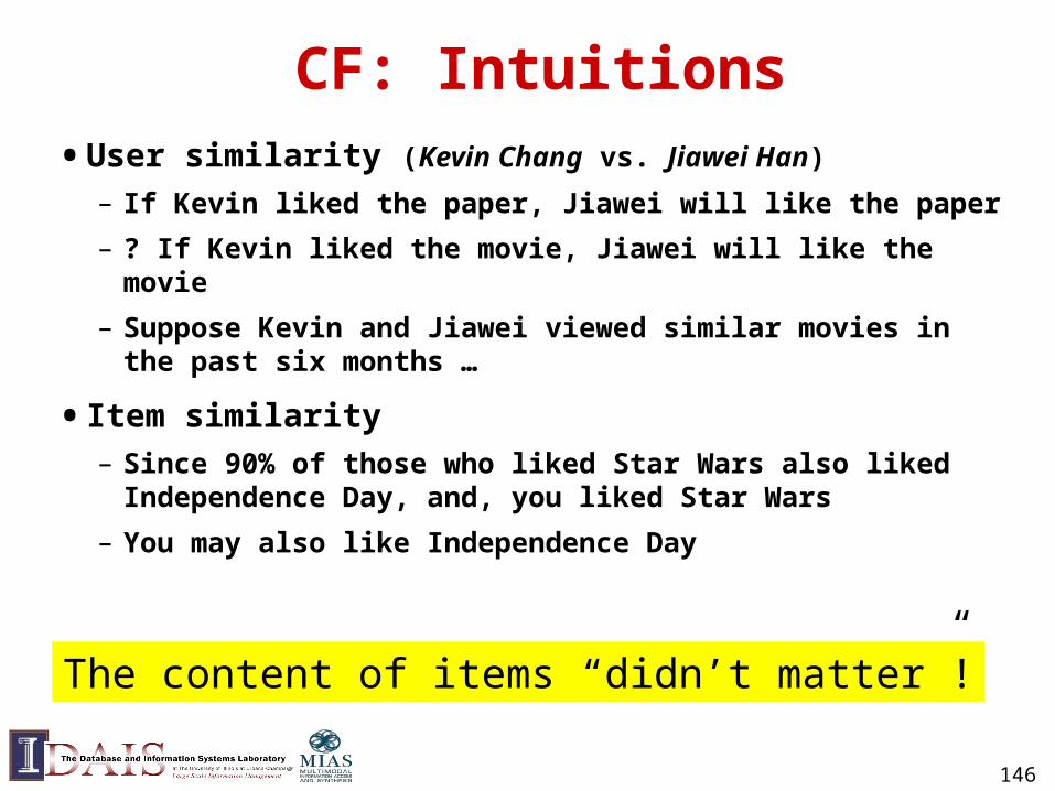
CF: Intuitions
• User similarity (Kevin Chang vs. Jiawei Han)
– If Kevin liked the paper, Jiawei will like the paper
– ? If Kevin liked the movie, Jiawei will like the movie
– Suppose Kevin and Jiawei viewed similar movies in the past six months …
• Item similarity– Since 90% of those who liked Star Wars also liked
Independence Day, and, you liked Star Wars
– You may also like Independence Day
The content of items “didn’t matter”!
147
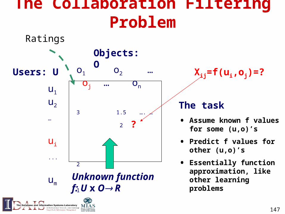
The Collaboration Filtering Problem
u1
u2
…
ui
...
um
Users: U
Objects: O
o1 o2 … oj … on
3 1.5 …. … 2
2
1
3
Xij=f(ui,oj)=?
?
The task
Unknown function f: U x O R
• Assume known f values for some (u,o)’s
• Predict f values for other (u,o)’s
• Essentially function approximation, like other learning problems
Ratings
148
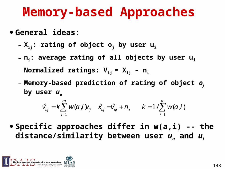
Memory-based Approaches
• General ideas:
– Xij: rating of object oj by user ui
– ni: average rating of all objects by user ui
– Normalized ratings: Vij = Xij – ni
– Memory-based prediction of rating of object oj by user ua
• Specific approaches differ in w(a,i) -- the distance/similarity between user ua and ui
1 1
ˆ ˆ ˆ( , ) 1/ ( , )m m
aj ij aj aj ai i
v k w a i v x v n k w a i
149
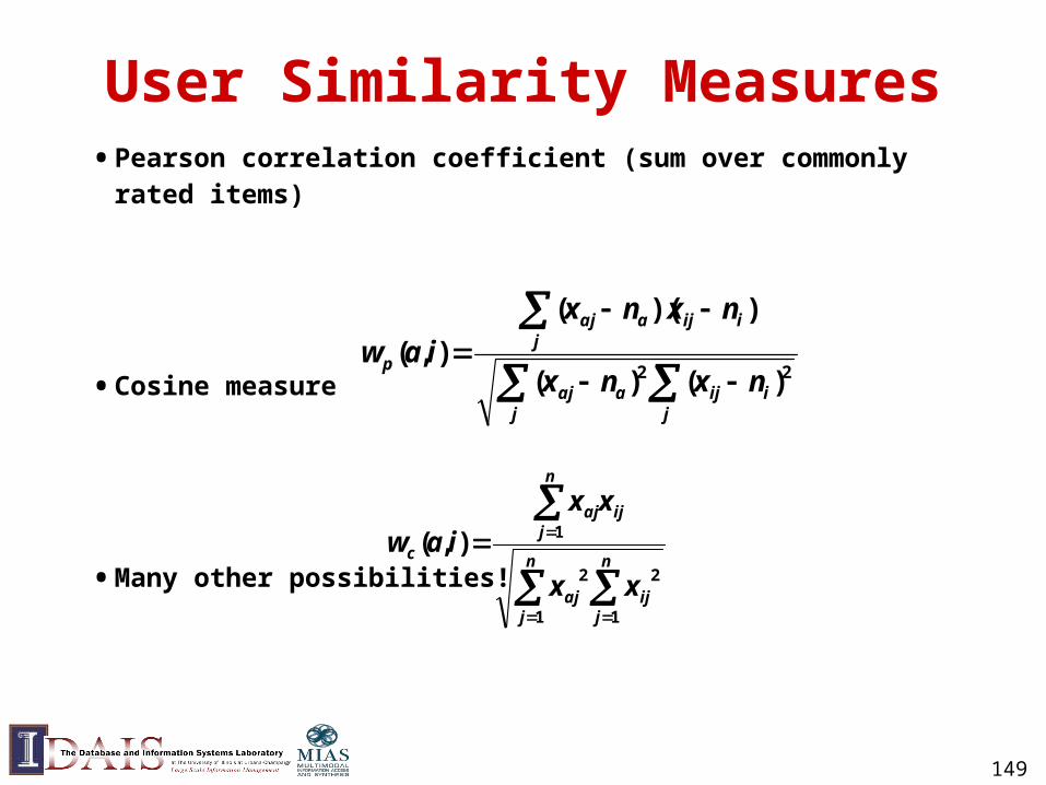
User Similarity Measures• Pearson correlation coefficient (sum over commonly
rated items)
• Cosine measure
• Many other possibilities!
jiij
jaaj
jiijaaj
pnxnx
nxnx
iaw22 )()(
))((
),(
n
jij
n
jaj
n
jijaj
c
xx
xx
iaw
1
2
1
2
1),(
150
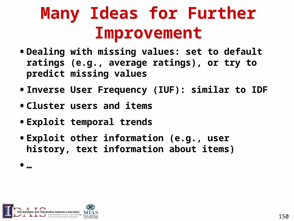
Many Ideas for Further Improvement
• Dealing with missing values: set to default ratings (e.g., average ratings), or try to predict missing values
• Inverse User Frequency (IUF): similar to IDF
• Cluster users and items
• Exploit temporal trends
• Exploit other information (e.g., user history, text information about items)
• …
Tutorial Outline
• Part 1: Background – 1.1 Text Information Systems
– 1.2 Information Access: Push vs. Pull
– 1.3 Querying vs. Browsing
– 1.4 Elements of Text Information Systems
• Part 2: Information retrieval techniques– 2.1 Overview of IR
– 2.2 Retrieval models
– 2.3 Evaluation
– 2.4 Retrieval systems
– 2.5 Information filtering
• Part 3: Text mining techniques– 3.1 Overview of text mining
– 3.2 IR-style text mining
– 3.3 NLP-style text mining
– 3.4 ML-style text mining
• Part 4: Web search – 4.1 Overview
– 4.2 Web search technologies
– 4.3 Next-generation search engines
MIAS Tutorial Summer 2012 151
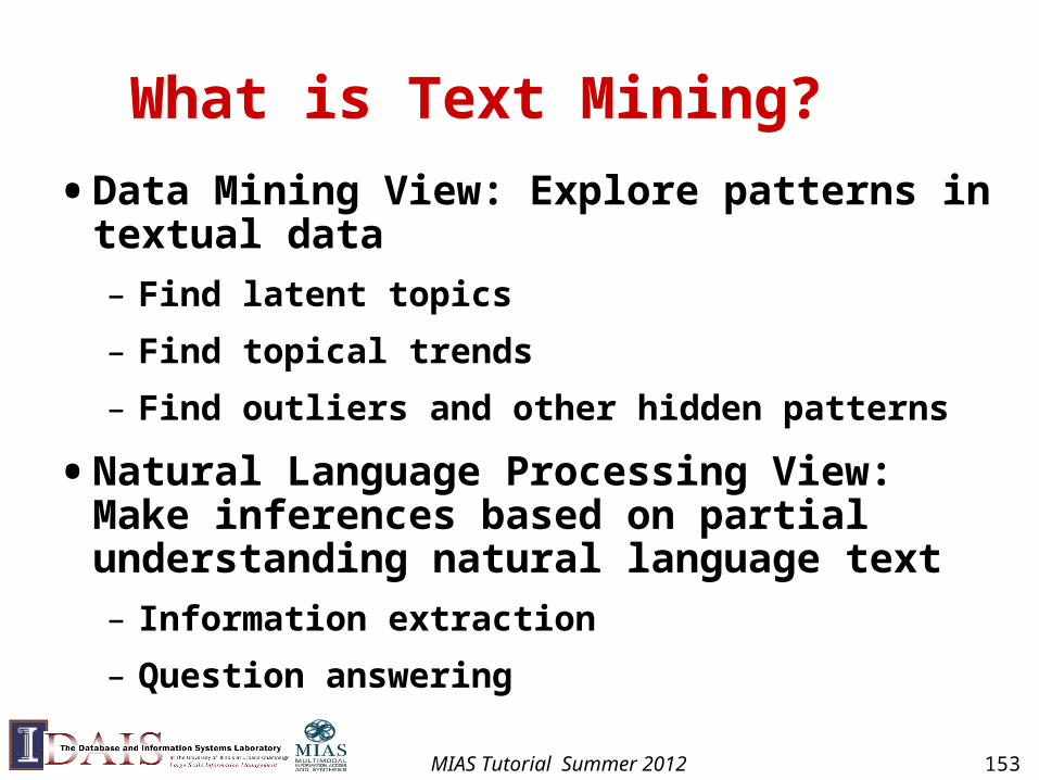
What is Text Mining?
• Data Mining View: Explore patterns in textual data
– Find latent topics
– Find topical trends
– Find outliers and other hidden patterns
• Natural Language Processing View: Make inferences based on partial understanding natural language text
– Information extraction
– Question answering
MIAS Tutorial Summer 2012 153
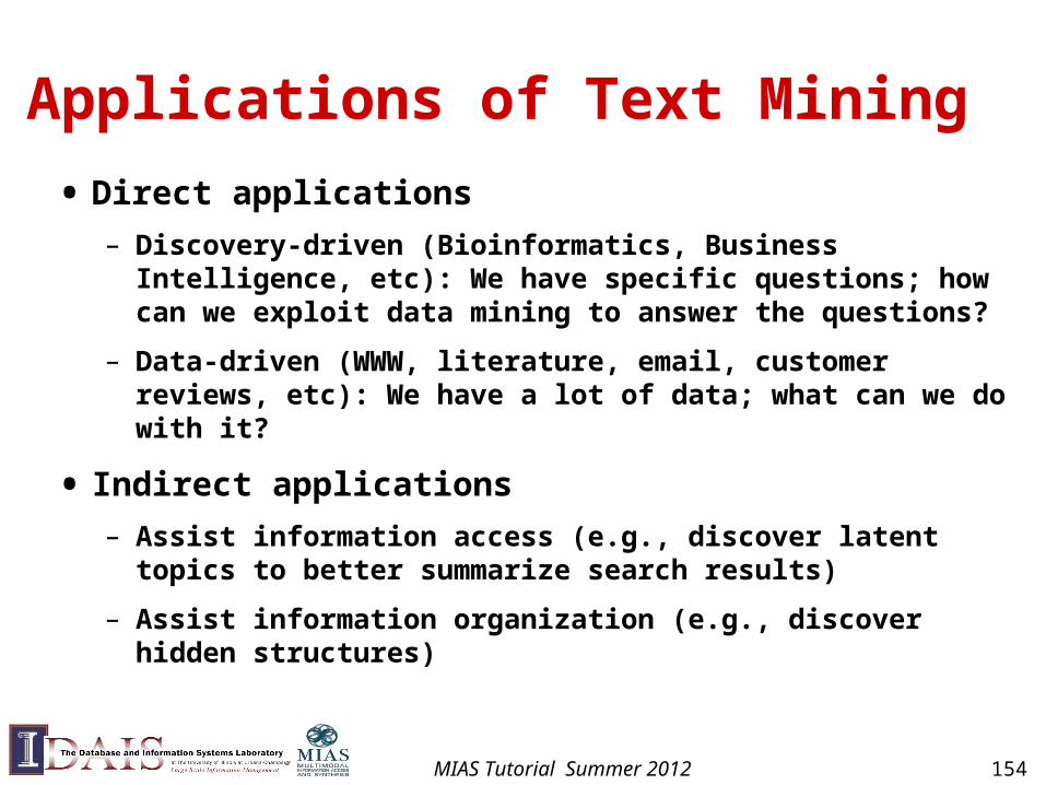
Applications of Text Mining
• Direct applications
– Discovery-driven (Bioinformatics, Business Intelligence, etc): We have specific questions; how can we exploit data mining to answer the questions?
– Data-driven (WWW, literature, email, customer reviews, etc): We have a lot of data; what can we do with it?
• Indirect applications
– Assist information access (e.g., discover latent topics to better summarize search results)
– Assist information organization (e.g., discover hidden structures)
MIAS Tutorial Summer 2012 154
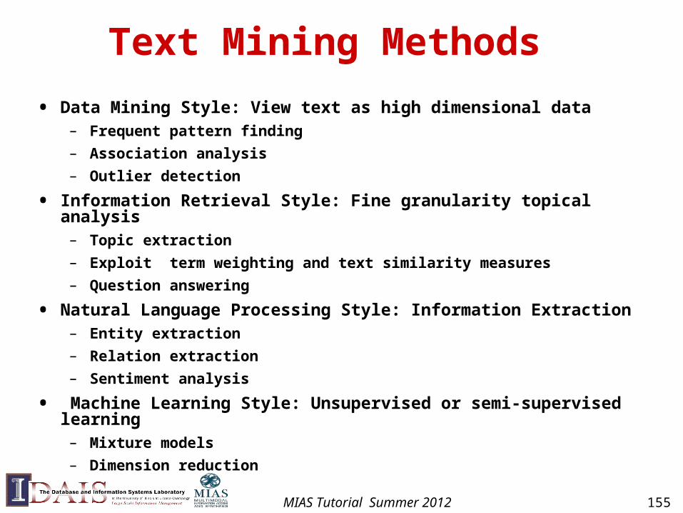
Text Mining Methods
• Data Mining Style: View text as high dimensional data– Frequent pattern finding
– Association analysis
– Outlier detection
• Information Retrieval Style: Fine granularity topical analysis– Topic extraction
– Exploit term weighting and text similarity measures
– Question answering
• Natural Language Processing Style: Information Extraction– Entity extraction
– Relation extraction
– Sentiment analysis
• Machine Learning Style: Unsupervised or semi-supervised learning– Mixture models
– Dimension reduction
MIAS Tutorial Summer 2012 155
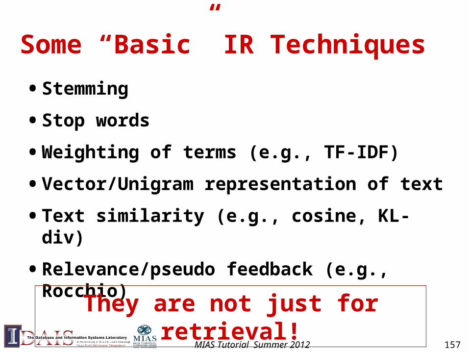
Some “Basic” IR Techniques
• Stemming
• Stop words
• Weighting of terms (e.g., TF-IDF)
• Vector/Unigram representation of text
• Text similarity (e.g., cosine, KL-div)
• Relevance/pseudo feedback (e.g., Rocchio)
They are not just for retrieval!
MIAS Tutorial Summer 2012 157
Generality of Basic Techniques
Raw text
Term similarity
Doc similarity
Vector centroid
CLUSTERING
d
CATEGORIZATION
META-DATA/ANNOTATION
d d d
d
d d
d
d d d
d d
d d
t t
t t
t t t
t t
t
t t
Stemming & Stop words
Tokenized text
Term Weighting
w11 w12… w1n
w21 w22… w2n
… …wm1 wm2… wmn
t1 t2 … tn
d1
d2 … dm
Sentenceselection
SUMMARIZATION
MIAS Tutorial Summer 2012 158
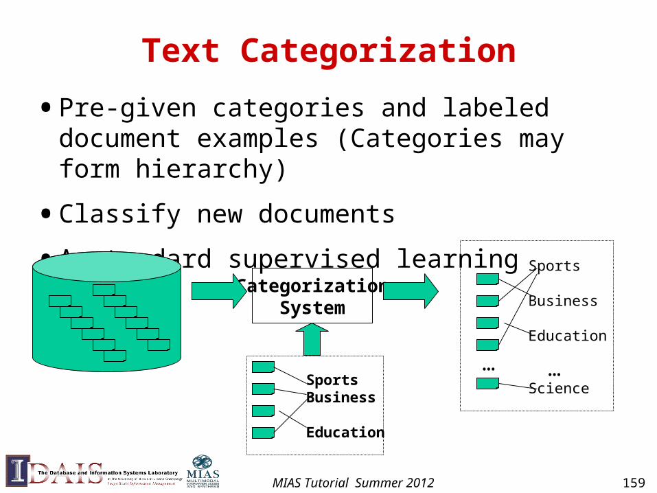
Text Categorization
• Pre-given categories and labeled document examples (Categories may form hierarchy)
• Classify new documents
• A standard supervised learning problem
CategorizationSystem
…
Sports
Business
Education
Science…
SportsBusiness
Education
MIAS Tutorial Summer 2012 159
“Retrieval-based” Categorization
• Treat each category as representing an “information need”
• Treat examples in each category as “relevant documents”
• Use feedback approaches to learn a good “query”
• Match all the learned queries to a new document
• A document gets the category(categories) represented by the best matching query(queries)
MIAS Tutorial Summer 2012 160
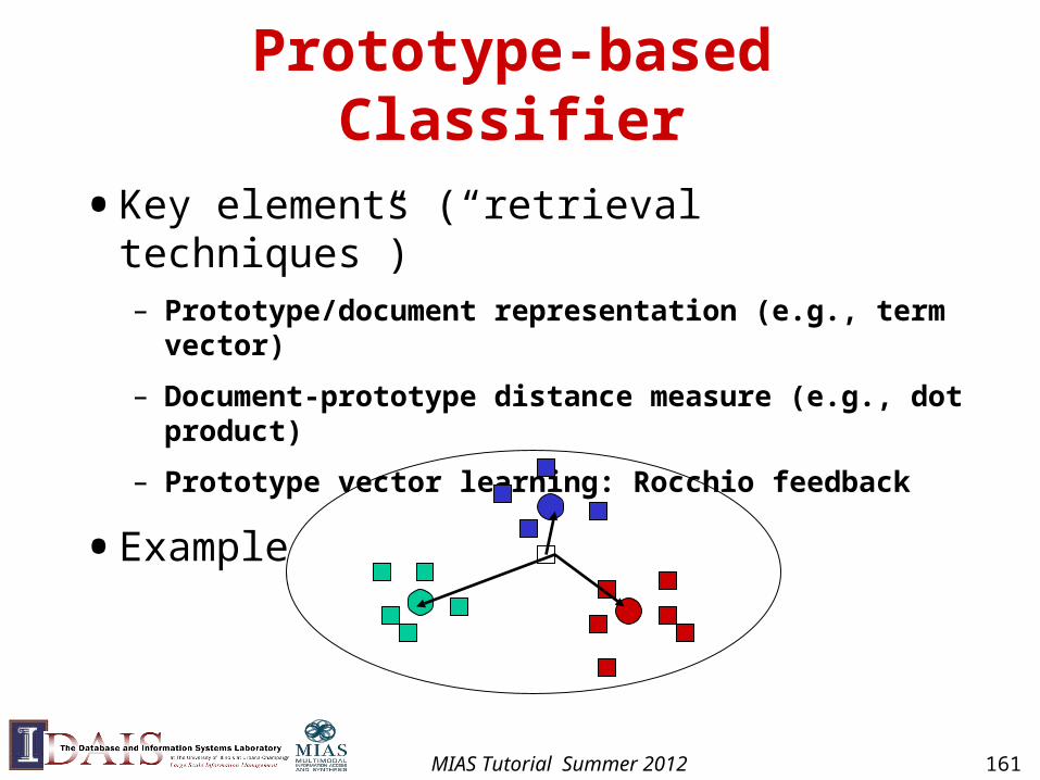
Prototype-based Classifier
• Key elements (“retrieval techniques”)– Prototype/document representation (e.g., term vector)
– Document-prototype distance measure (e.g., dot product)
– Prototype vector learning: Rocchio feedback
• Example
MIAS Tutorial Summer 2012 161
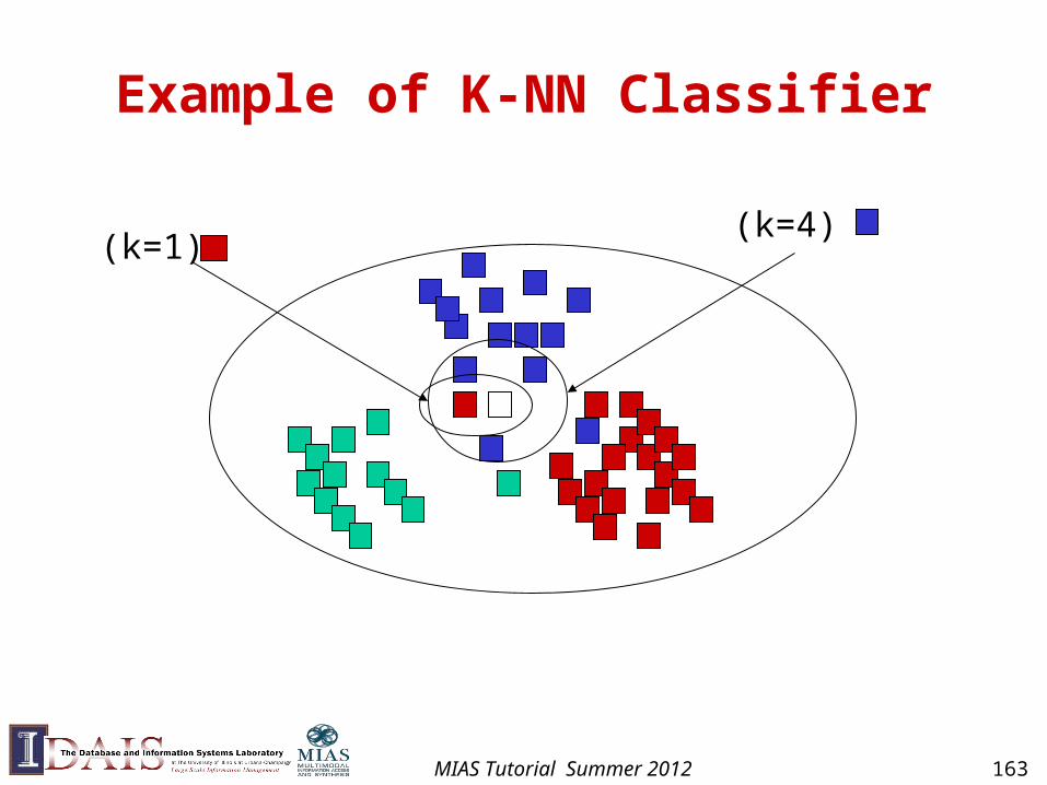
K-Nearest Neighbor Classifier
• Keep all training examples
• Find k examples that are most similar to the new document (“neighbor” documents)
• Assign the category that is most common in these neighbor documents (neighbors vote for the category)
• Can be improved by considering the distance of a neighbor ( A closer neighbor has more influence)
• Technical elements (“retrieval techniques”)– Document representation
– Document distance measure
MIAS Tutorial Summer 2012 162
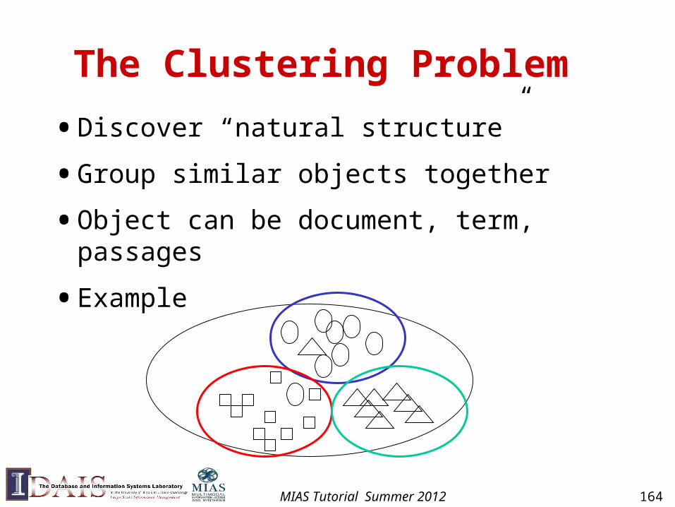
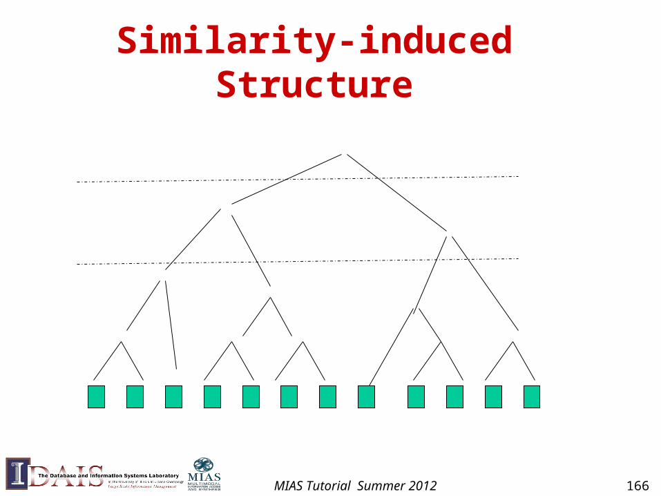
The Clustering Problem
• Discover “natural structure”
• Group similar objects together
• Object can be document, term, passages
• Example
MIAS Tutorial Summer 2012 164
Similarity-based Clustering(as opposed to “model-based”)
• Define a similarity function to measure similarity between two objects
• Gradually group similar objects together in a bottom-up fashion
• Stop when some stopping criterion is met
• Variations: different ways to compute group similarity based on individual object similarity
MIAS Tutorial Summer 2012 165
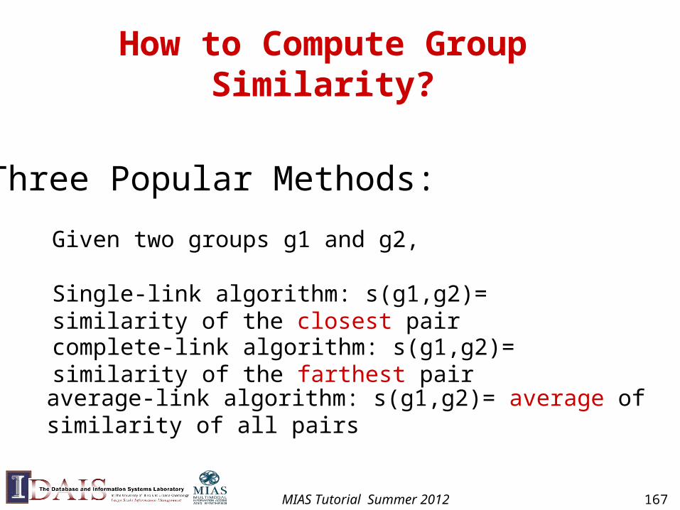
How to Compute Group Similarity?
Given two groups g1 and g2,
Single-link algorithm: s(g1,g2)= similarity of the closest pair
complete-link algorithm: s(g1,g2)= similarity of the farthest pair
average-link algorithm: s(g1,g2)= average of similarity of all pairs
Three Popular Methods:
MIAS Tutorial Summer 2012 167
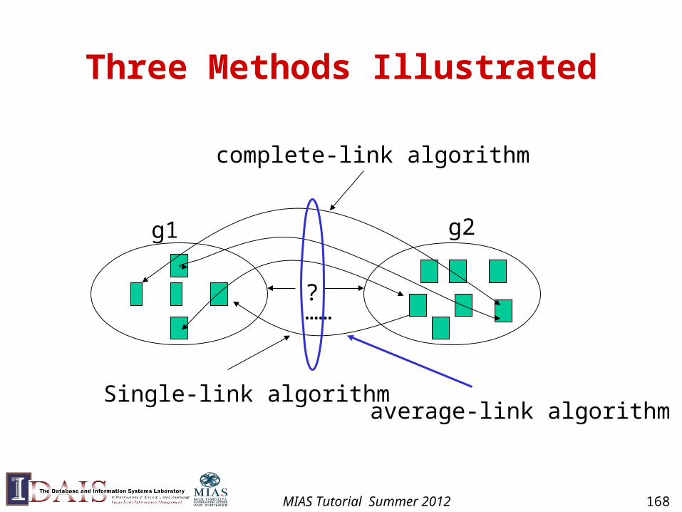
Three Methods Illustrated
Single-link algorithm
?
g1 g2
complete-link algorithm
……
average-link algorithm
MIAS Tutorial Summer 2012 168
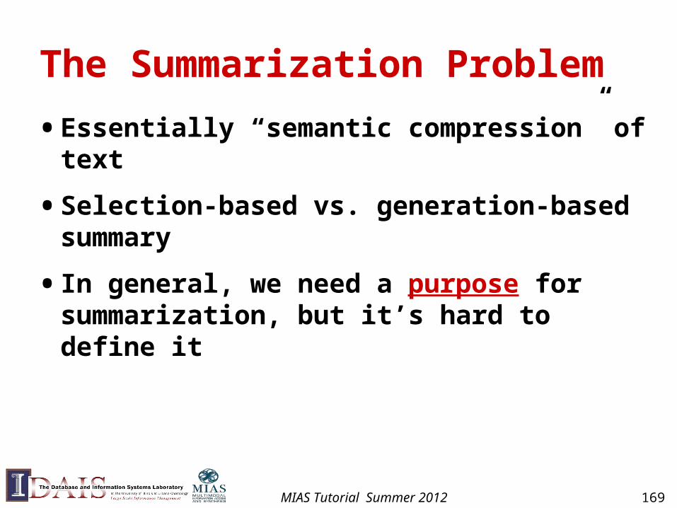
The Summarization Problem
• Essentially “semantic compression” of text
• Selection-based vs. generation-based summary
• In general, we need a purpose for summarization, but it’s hard to define it
MIAS Tutorial Summer 2012 169
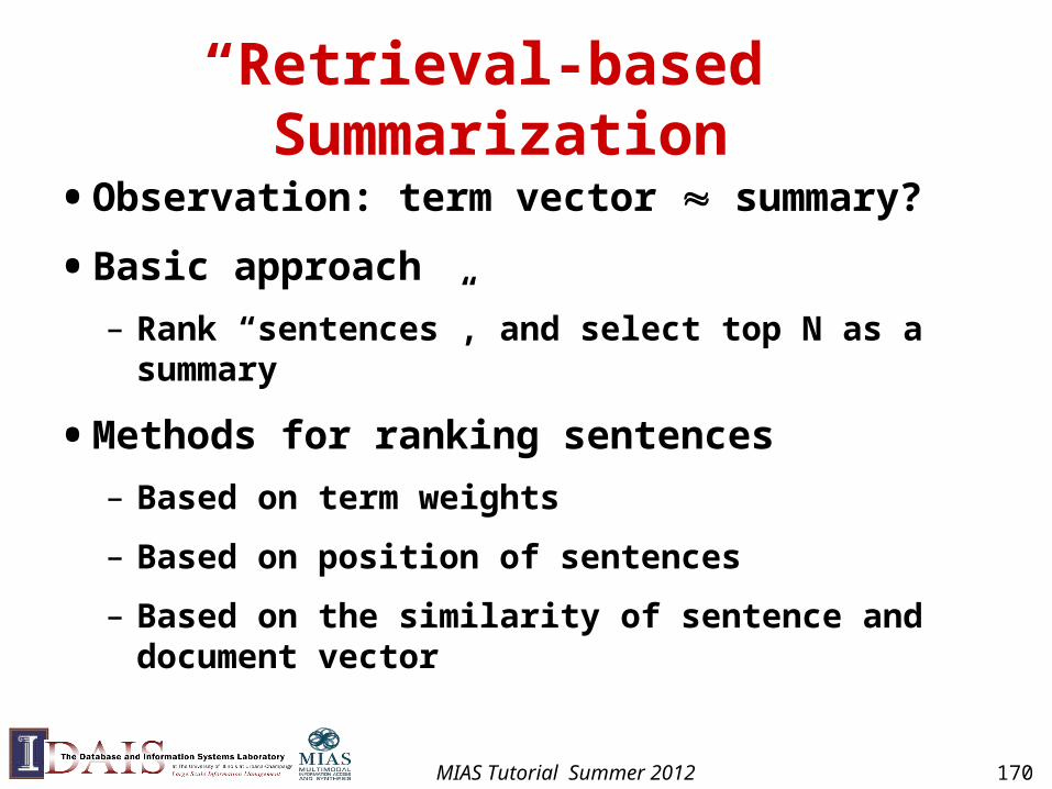
“Retrieval-based” Summarization
• Observation: term vector summary?
• Basic approach
– Rank “sentences”, and select top N as a summary
• Methods for ranking sentences
– Based on term weights
– Based on position of sentences
– Based on the similarity of sentence and document vector
MIAS Tutorial Summer 2012 170
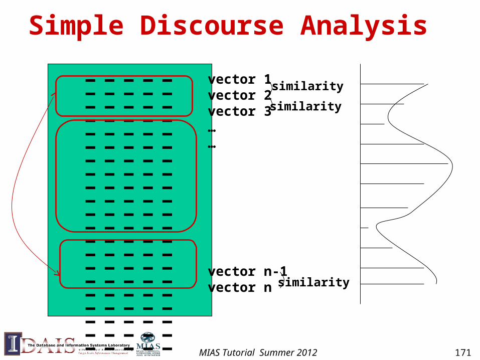
Simple Discourse Analysis
----------------------------------------------------------------------------------------------------------------------------------------------------------------
vector 1vector 2vector 3……
vector n-1vector n
similarity
similarity
similarity
MIAS Tutorial Summer 2012 171
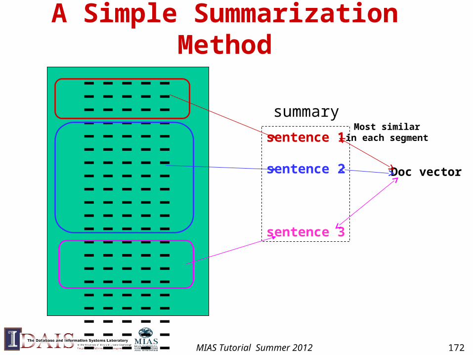
A Simple Summarization Method
----------------------------------------------------------------------------------------------------------------------------------------------------------------
sentence 1
sentence 2
sentence 3
summary
Doc vector
Most similarin each segment
MIAS Tutorial Summer 2012 172
Part 3.3: NLP-Style Text Mining Techniques
Most of the following slides are from William Cohen’s IE tutorial
MIAS Tutorial Summer 2012 173
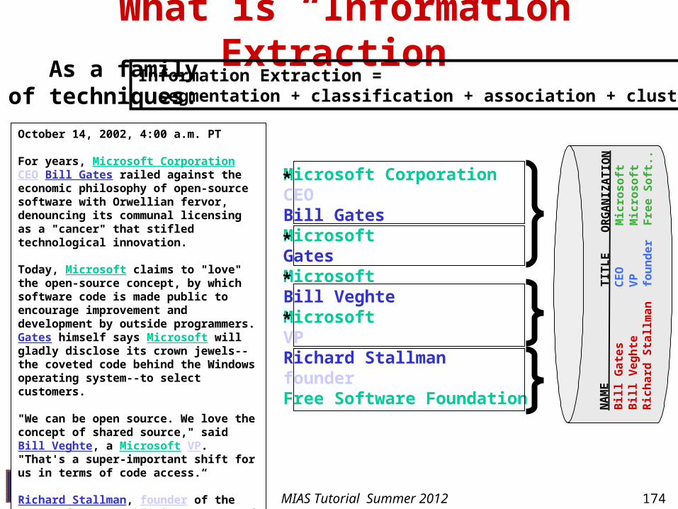
What is “Information Extraction”Information Extraction = segmentation + classification + association + clustering
As a familyof techniques:
October 14, 2002, 4:00 a.m. PT
For years, Microsoft Corporation CEO Bill Gates railed against the economic philosophy of open-source software with Orwellian fervor, denouncing its communal licensing as a "cancer" that stifled technological innovation.
Today, Microsoft claims to "love" the open-source concept, by which software code is made public to encourage improvement and development by outside programmers. Gates himself says Microsoft will gladly disclose its crown jewels--the coveted code behind the Windows operating system--to select customers.
"We can be open source. We love the concept of shared source," said Bill Veghte, a Microsoft VP. "That's a super-important shift for us in terms of code access.“
Richard Stallman, founder of the Free Software Foundation, countered saying…
Microsoft CorporationCEOBill GatesMicrosoftGatesMicrosoftBill VeghteMicrosoftVPRichard StallmanfounderFree Software Foundation N
AME
TITLE ORGANIZATION
Bill Gates
CEO
Microsoft
Bill Veghte
VP
Microsoft
Richard Stallman
founder
Free Soft..
*
*
*
*
MIAS Tutorial Summer 2012 174

Landscape of IE Tasks:Complexity
Closed set
He was born in Alabama…
Regular set
Phone: (413) 545-1323
Complex pattern
University of ArkansasP.O. Box 140Hope, AR 71802 …was among the six houses sold
by Hope Feldman that year.
Ambiguous patterns,needing context andmany sources of evidence
The CALD main office can be reached at 412-268-1299
The big Wyoming sky…
U.S. states U.S. phone numbers
U.S. postal addresses
Person names
Headquarters:1128 Main Street, 4th FloorCincinnati, Ohio 45210
Pawel Opalinski, SoftwareEngineer at WhizBang Labs.
E.g. word patterns:
MIAS Tutorial Summer 2012 175
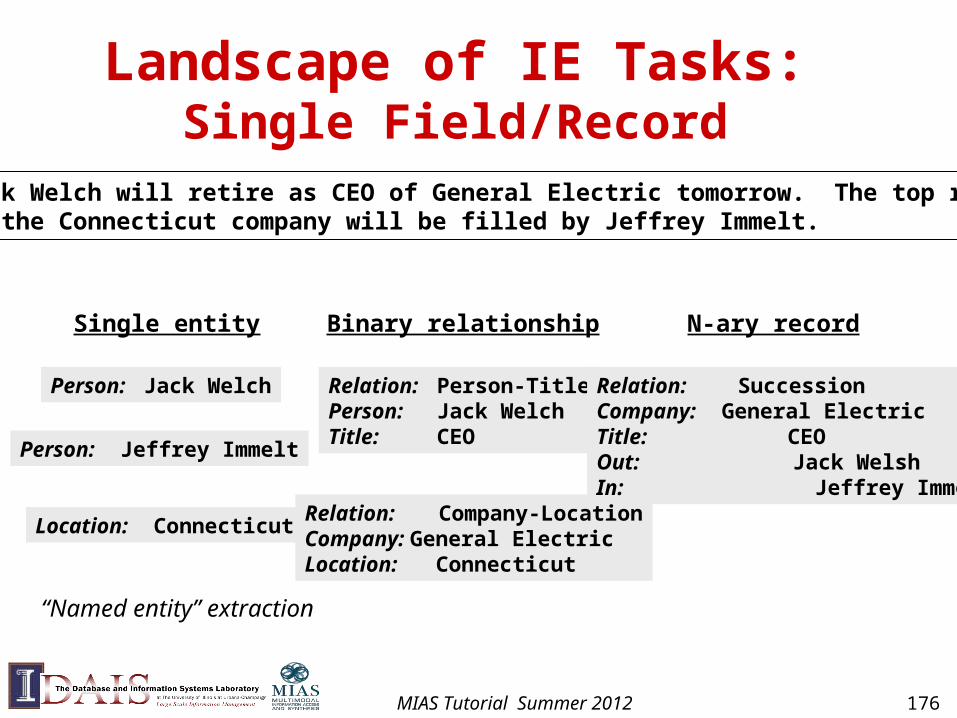
Landscape of IE Tasks:Single Field/Record
Single entity
Person: Jack Welch
Binary relationship
Relation: Person-TitlePerson: Jack WelchTitle: CEO
N-ary record
“Named entity” extraction
Jack Welch will retire as CEO of General Electric tomorrow. The top role at the Connecticut company will be filled by Jeffrey Immelt.
Relation: Company-LocationCompany: General ElectricLocation: Connecticut
Relation: SuccessionCompany: General ElectricTitle: CEOOut: Jack WelshIn: Jeffrey Immelt
Person: Jeffrey Immelt
Location: Connecticut
MIAS Tutorial Summer 2012 176
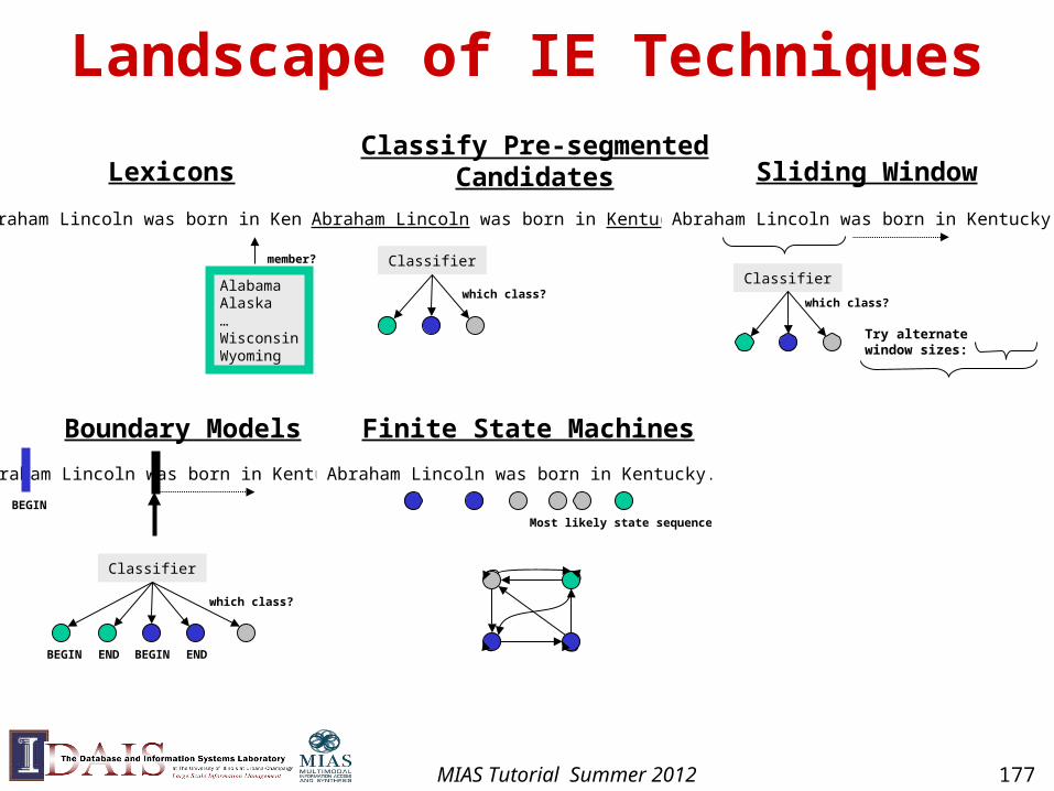
Landscape of IE Techniques
Lexicons
AlabamaAlaska…WisconsinWyoming
Abraham Lincoln was born in Kentucky.
member?
Classify Pre-segmentedCandidates
Abraham Lincoln was born in Kentucky.
Classifier
which class?
Sliding Window
Abraham Lincoln was born in Kentucky.
Classifier
which class?
Try alternatewindow sizes:
Boundary Models
Abraham Lincoln was born in Kentucky.
Classifier
which class?
BEGIN END BEGIN END
BEGIN
Context Free Grammars
Abraham Lincoln was born in Kentucky.
NNP V P NPVNNP
NP
PP
VP
VP
S
Mos
t lik
ely
pars
e?
Finite State Machines
Abraham Lincoln was born in Kentucky.
Most likely state sequence?
MIAS Tutorial Summer 2012 177
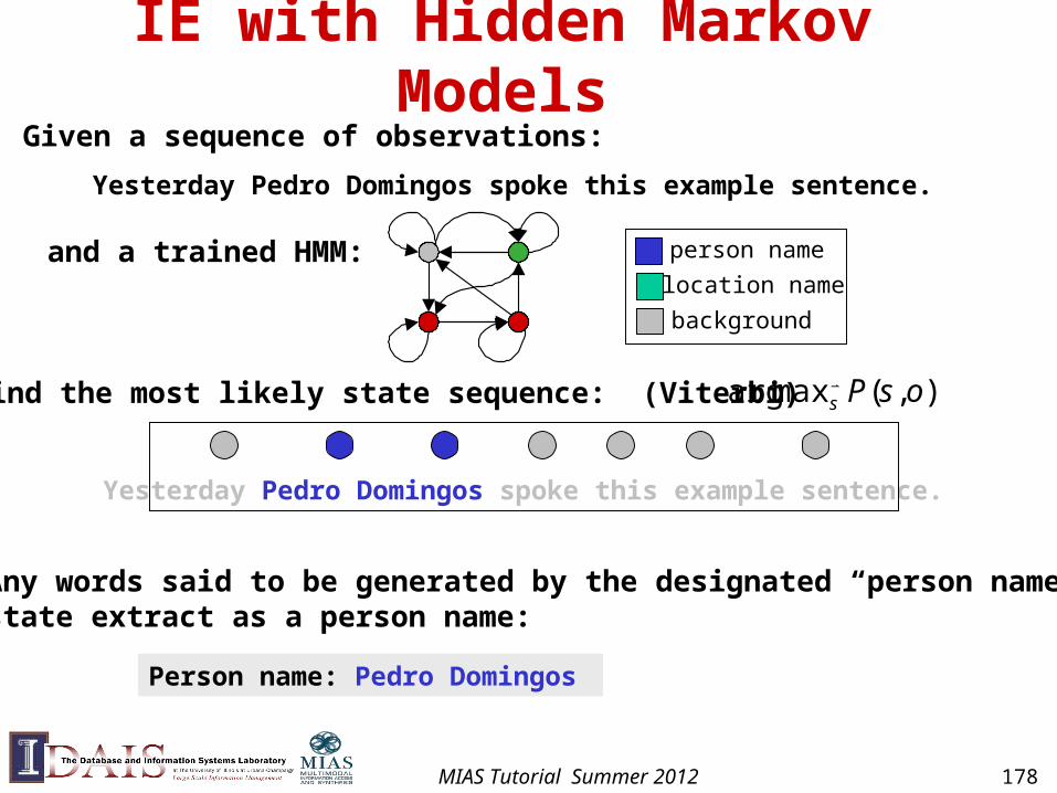
IE with Hidden Markov Models
Yesterday Pedro Domingos spoke this example sentence.
Yesterday Pedro Domingos spoke this example sentence.
Person name: Pedro Domingos
Given a sequence of observations:
and a trained HMM:
Find the most likely state sequence: (Viterbi)
Any words said to be generated by the designated “person name”state extract as a person name:
),(maxarg osPs
person name
location name
background
MIAS Tutorial Summer 2012 178
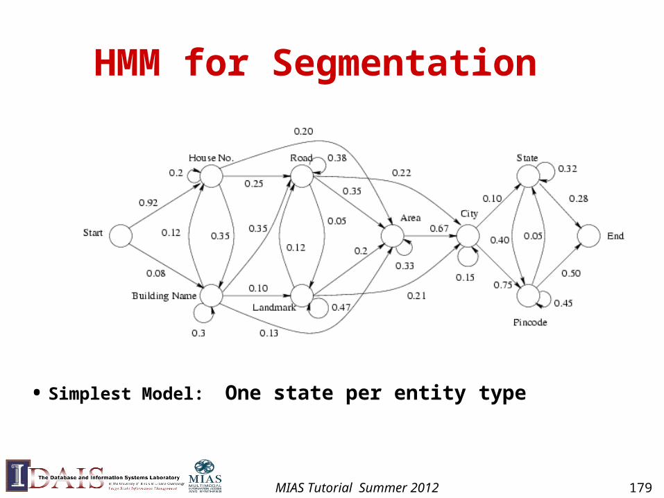
HMM for Segmentation
• Simplest Model: One state per entity type
MIAS Tutorial Summer 2012 179
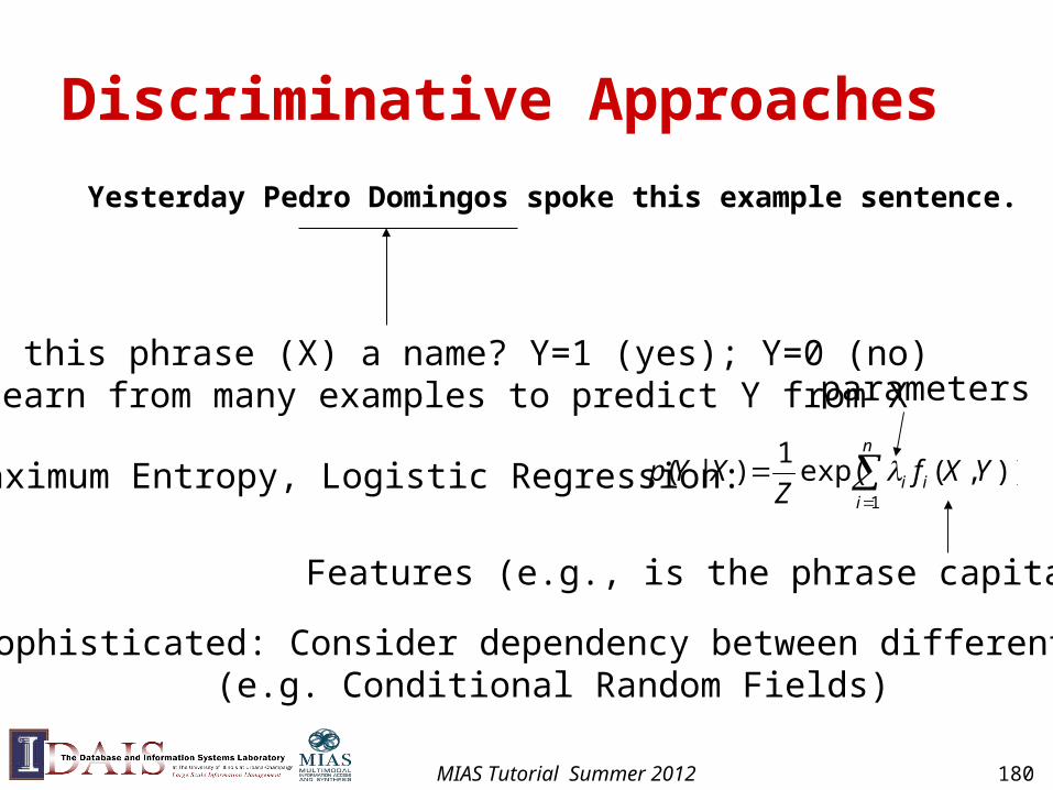
Discriminative Approaches
Yesterday Pedro Domingos spoke this example sentence.
Is this phrase (X) a name? Y=1 (yes); Y=0 (no)Learn from many examples to predict Y from X
n
iii YXf
ZXYp
1
)),(exp(1
)|( Maximum Entropy, Logistic Regression:
More sophisticated: Consider dependency between different labels (e.g. Conditional Random Fields)
Features (e.g., is the phrase capitalized?)
parameters
MIAS Tutorial Summer 2012 180
Part 3.4 Statistical Learning Style Techniques for Text Mining
MIAS Tutorial Summer 2012 181
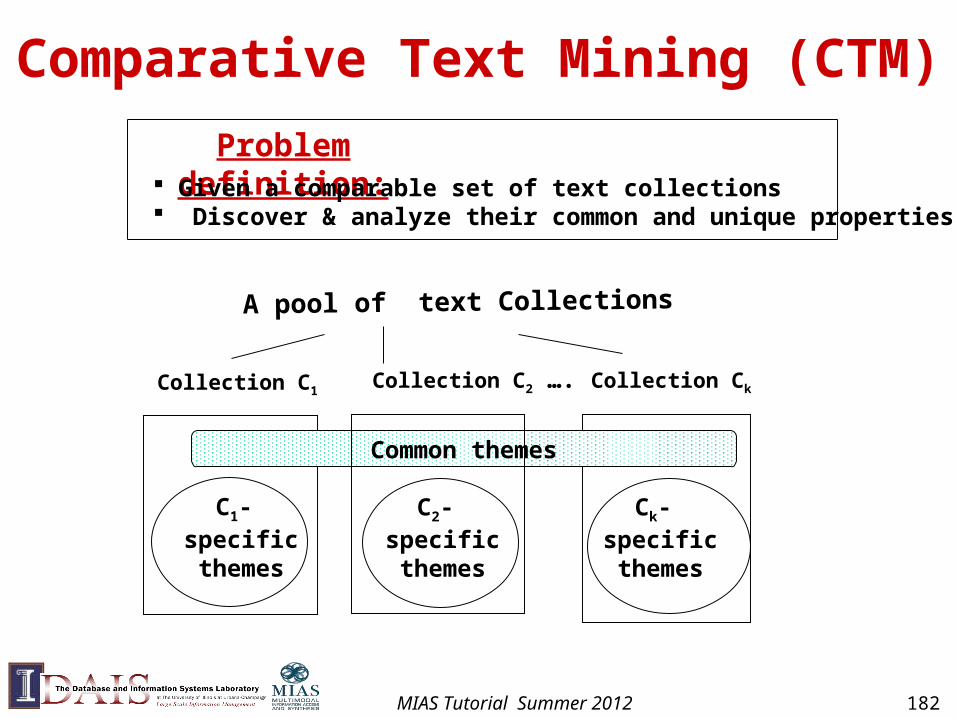
Problem definition: Given a comparable set of text collections Discover & analyze their common and unique properties
Collection C1 Collection C2 ….
C1- specificthemes
Common themes
C2- specificthemes
Ck- specificthemes
A pool of text Collections
Collection Ck
Comparative Text Mining (CTM)
MIAS Tutorial Summer 2012 182
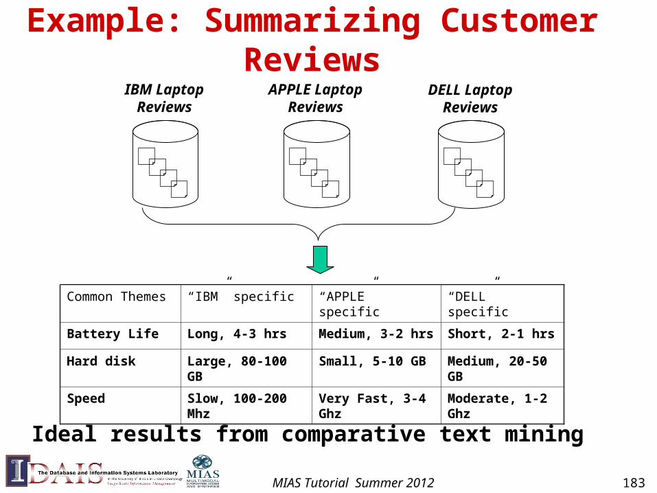
Example: Summarizing Customer Reviews
Common Themes “IBM” specific “APPLE” specific “DELL” specific
Battery Life Long, 4-3 hrs Medium, 3-2 hrs Short, 2-1 hrs
Hard disk Large, 80-100 GB Small, 5-10 GB Medium, 20-50 GB
Speed Slow, 100-200 Mhz Very Fast, 3-4 Ghz Moderate, 1-2 Ghz
IBM LaptopReviews
APPLE LaptopReviews
DELL LaptopReviews
Ideal results from comparative text mining
MIAS Tutorial Summer 2012 183
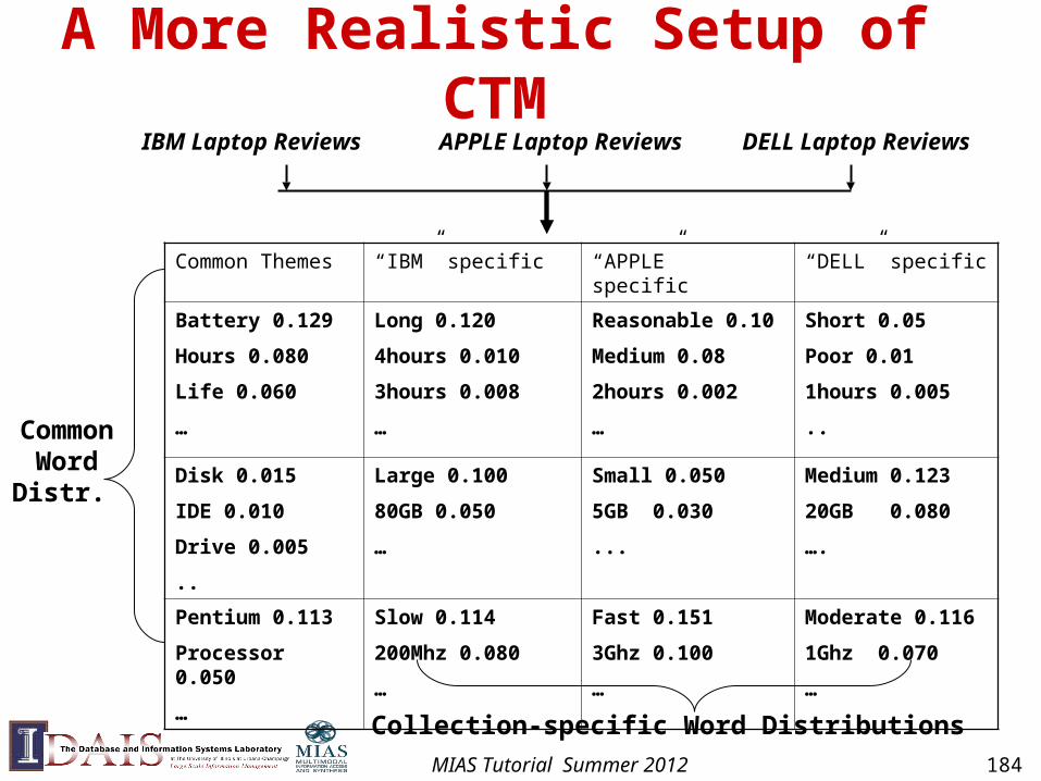
A More Realistic Setup of CTM
Common Themes “IBM” specific “APPLE” specific “DELL” specific
Battery 0.129
Hours 0.080
Life 0.060
…
Long 0.120
4hours 0.010
3hours 0.008
…
Reasonable 0.10
Medium 0.08
2hours 0.002
…
Short 0.05
Poor 0.01
1hours 0.005
..
Disk 0.015
IDE 0.010
Drive 0.005
..
Large 0.100
80GB 0.050
…
Small 0.050
5GB 0.030
...
Medium 0.123
20GB 0.080
….
Pentium 0.113
Processor 0.050
…
Slow 0.114
200Mhz 0.080
…
Fast 0.151
3Ghz 0.100
…
Moderate 0.116
1Ghz 0.070
…
IBM Laptop Reviews APPLE Laptop Reviews DELL Laptop Reviews
Collection-specific Word Distributions
Common Word Distr.
MIAS Tutorial Summer 2012 184
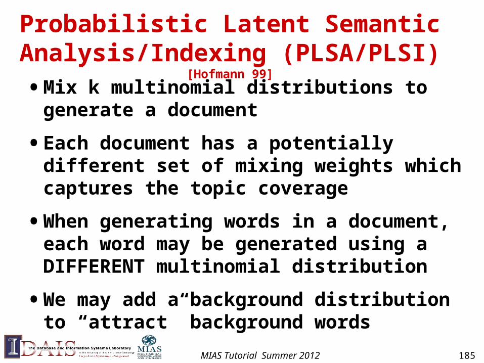
Probabilistic Latent Semantic Analysis/Indexing (PLSA/PLSI) [Hofmann 99]
• Mix k multinomial distributions to generate a document
• Each document has a potentially different set of mixing weights which captures the topic coverage
• When generating words in a document, each word may be generated using a DIFFERENT multinomial distribution
• We may add a background distribution to “attract” background words
MIAS Tutorial Summer 2012 185
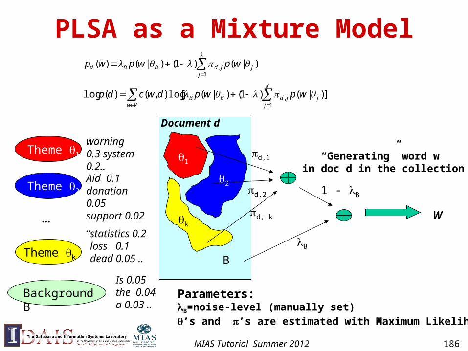
PLSA as a Mixture Model
Theme 1
Theme k
Theme 2
…
Document d
Background B
warning 0.3 system 0.2..
Aid 0.1donation 0.05support 0.02 ..
statistics 0.2loss 0.1dead 0.05 ..
Is 0.05the 0.04a 0.03 ..
k
1
2
B
B
W
d,1
d, k
1 - Bd,2
“Generating” word w in doc d in the collection
Parameters: B=noise-level (manually set)’s and ’s are estimated with Maximum Likelihood
])|()1()|([log),()(log
)|()1()|()(
1,
1,
k
jjjdBB
Vw
k
jjjdBBd
wpwpdwcdp
wpwpwp
MIAS Tutorial Summer 2012 186
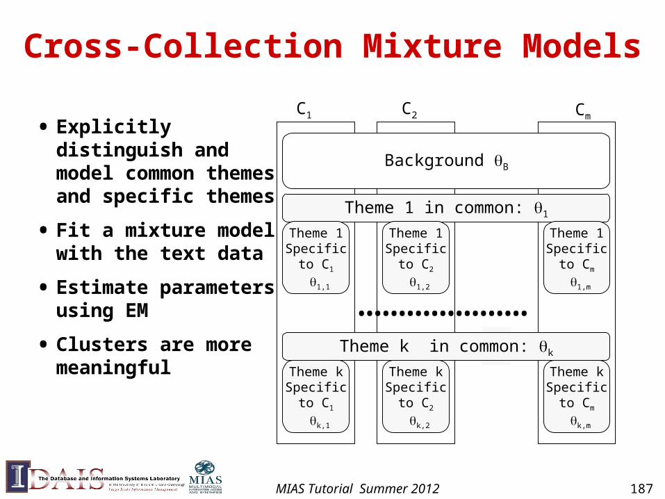
Cross-Collection Mixture Models
• Explicitly distinguish and model common themes and specific themes
• Fit a mixture model with the text data
• Estimate parameters using EM
• Clusters are more meaningful
…………………
Background B
Theme 1 in common: 1
Theme 1Specific
to C1
1,1
CmC2C1
…Theme k in common: k
Theme kSpecific
to C1
k,1
Theme 1Specific
to C2
1,2
Theme 1Specific
to Cm
1,m
Theme kSpecific
to C2
k,2
Theme kSpecific
to Cm
k,m
MIAS Tutorial Summer 2012 187
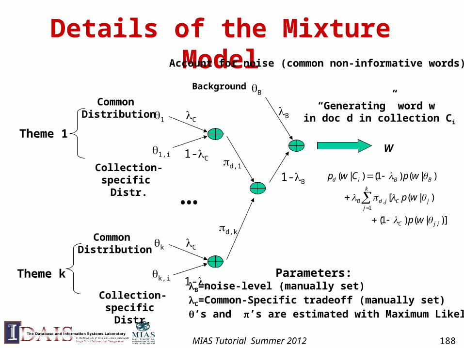
Details of the Mixture Model
C
B
1
1,i 1-C
Ck
k,i 1-C
…d,1
d,k
B
1-B
Theme 1
Background
,1
,
( | ) (1 ) ( | )
[ ( | )
(1 ) ( | )]
d i B B
k
B d j C jj
C j i
p w C p w
p w
p w
Account for noise (common non-informative words)
Common Distribution
Collection-specific Distr.
Collection-specific Distr.
Common Distribution
Theme k Parameters: B=noise-level (manually set)C=Common-Specific tradeoff (manually set)’s and ’s are estimated with Maximum Likelihood
W
“Generating” word w in doc d in collection Ci
MIAS Tutorial Summer 2012 188
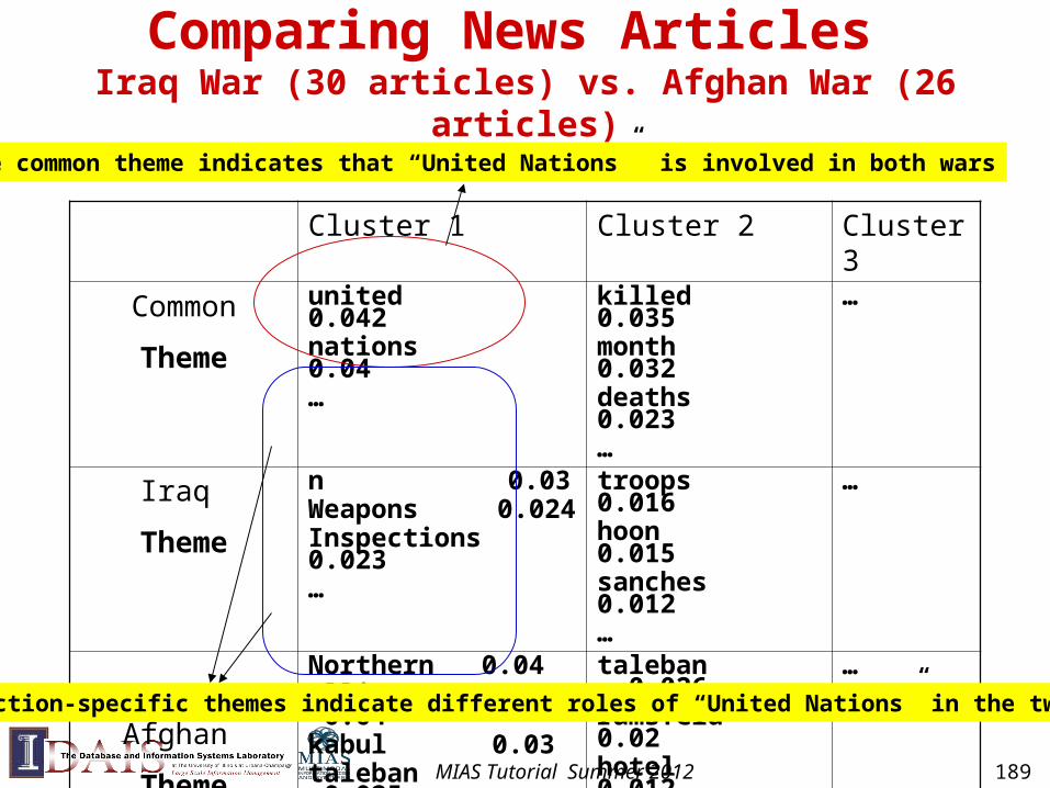
Comparing News Articles Iraq War (30 articles) vs. Afghan War (26 articles)
Cluster 1 Cluster 2 Cluster 3
Common
Theme
united 0.042nations 0.04…
killed 0.035month 0.032deaths 0.023…
…
Iraq
Theme
n 0.03Weapons 0.024Inspections 0.023…
troops 0.016hoon 0.015sanches 0.012…
…
Afghan
Theme
Northern 0.04alliance 0.04kabul 0.03taleban 0.025aid 0.02…
taleban 0.026rumsfeld 0.02hotel 0.012front 0.011…
…
The common theme indicates that “United Nations” is involved in both wars
Collection-specific themes indicate different roles of “United Nations” in the two wars
MIAS Tutorial Summer 2012 189
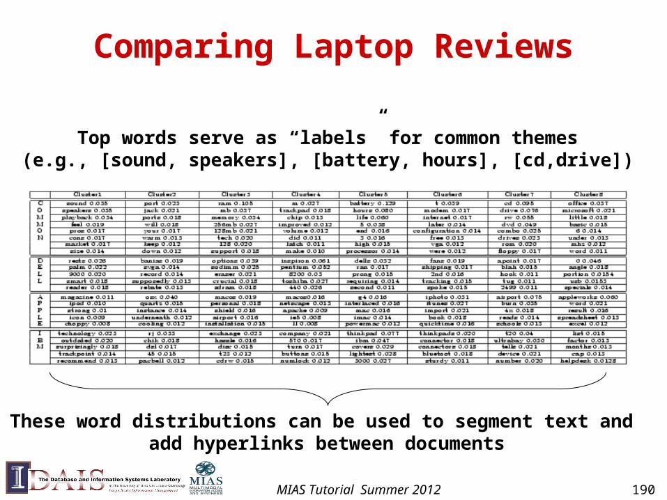
Comparing Laptop Reviews
Top words serve as “labels” for common themes(e.g., [sound, speakers], [battery, hours], [cd,drive])
These word distributions can be used to segment text and add hyperlinks between documents
MIAS Tutorial Summer 2012 190
Additional Results of Contextual Text Mining
• Spatiotemporal topic pattern analysis
• Theme evolution analysis
• Event impact analysis
• Sentiment summarization
• All results are from Qiaozhu Mei’s dissertation, available at:
http://www.ideals.illinois.edu/handle/2142/14707
MIAS Tutorial Summer 2012 191
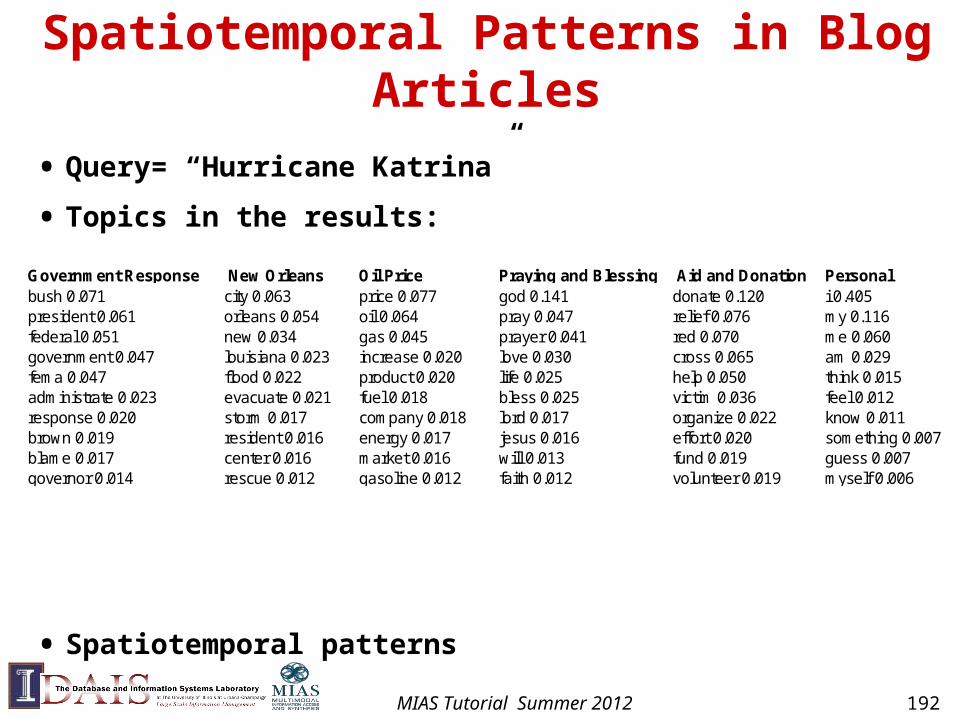
Spatiotemporal Patterns in Blog Articles
• Query= “Hurricane Katrina”
• Topics in the results:
• Spatiotemporal patterns
Government Response New Orleans Oil Price Praying and Blessing Aid and Donation Personal bush 0.071 city 0.063 price 0.077 god 0.141 donate 0.120 i 0.405president 0.061 orleans 0.054 oil 0.064 pray 0.047 relief 0.076 my 0.116federal 0.051 new 0.034 gas 0.045 prayer 0.041 red 0.070 me 0.060government 0.047 louisiana 0.023 increase 0.020 love 0.030 cross 0.065 am 0.029fema 0.047 flood 0.022 product 0.020 life 0.025 help 0.050 think 0.015administrate 0.023 evacuate 0.021 fuel 0.018 bless 0.025 victim 0.036 feel 0.012response 0.020 storm 0.017 company 0.018 lord 0.017 organize 0.022 know 0.011brown 0.019 resident 0.016 energy 0.017 jesus 0.016 effort 0.020 something 0.007blame 0.017 center 0.016 market 0.016 will 0.013 fund 0.019 guess 0.007governor 0.014 rescue 0.012 gasoline 0.012 faith 0.012 volunteer 0.019 myself 0.006
MIAS Tutorial Summer 2012 192
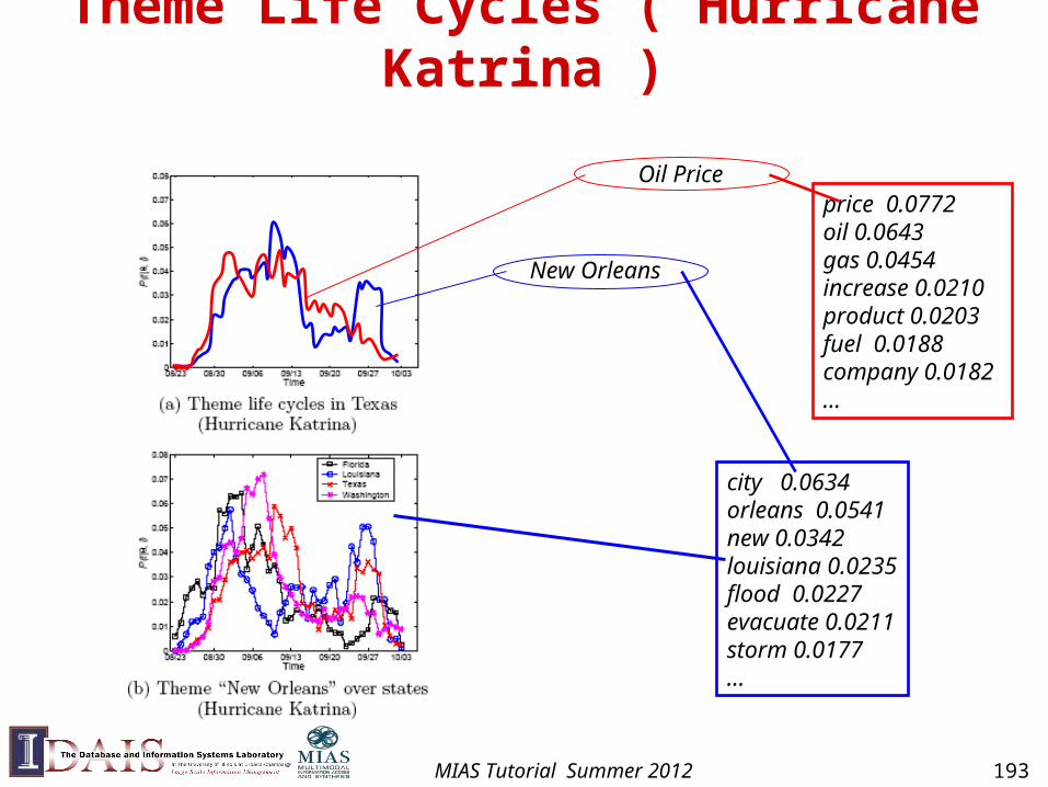
Theme Life Cycles (“Hurricane Katrina”)
city 0.0634orleans 0.0541new 0.0342louisiana 0.0235flood 0.0227evacuate 0.0211storm 0.0177…
price 0.0772oil 0.0643gas 0.0454 increase 0.0210product 0.0203fuel 0.0188company 0.0182…
Oil Price
New Orleans
MIAS Tutorial Summer 2012 193
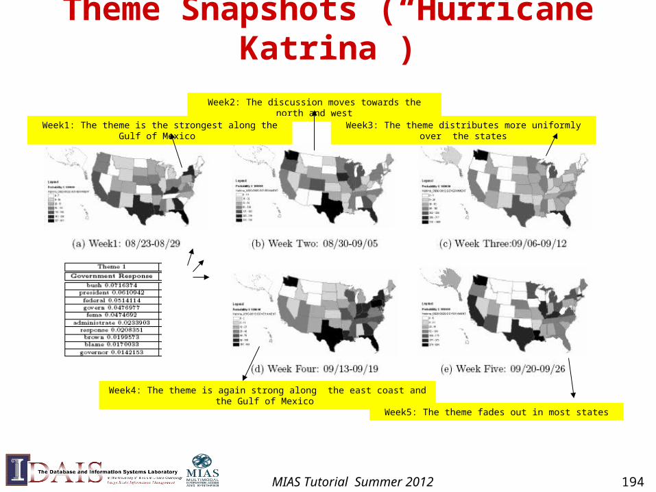
Theme Snapshots (“Hurricane Katrina”)
Week4: The theme is again strong along the east coast and the Gulf of Mexico
Week3: The theme distributes more uniformly over the states
Week2: The discussion moves towards the north and west
Week5: The theme fades out in most states
Week1: The theme is the strongest along the Gulf of Mexico
MIAS Tutorial Summer 2012 194
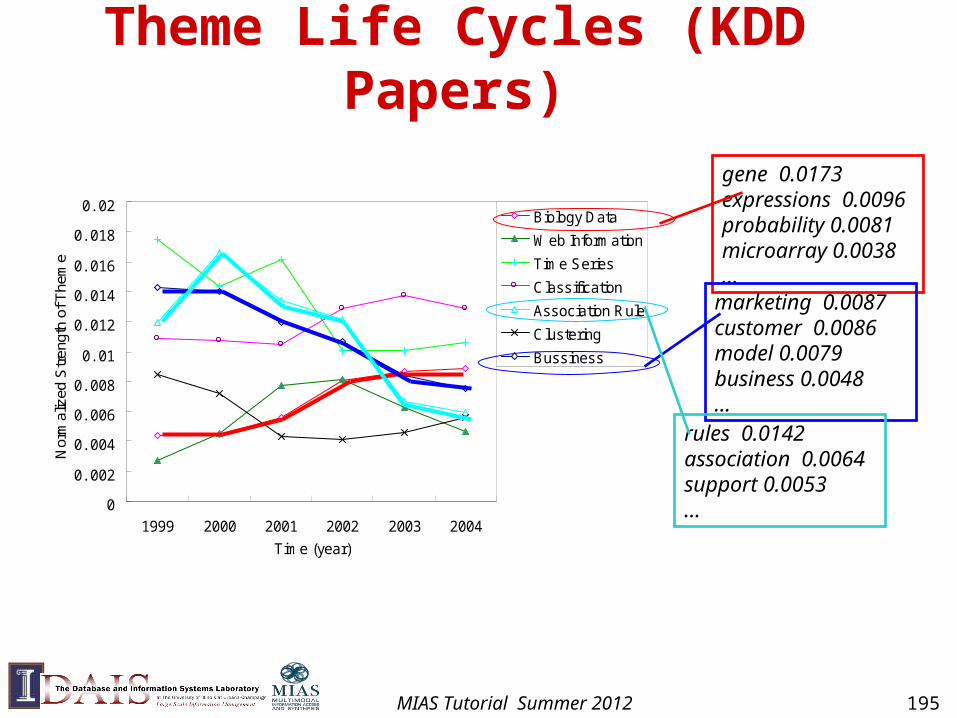
Theme Life Cycles (KDD Papers)
0
0. 002
0. 004
0. 006
0. 008
0. 01
0. 012
0. 014
0. 016
0. 018
0. 02
1999 2000 2001 2002 2003 2004Time (year)
Nor
mal
ized
Str
engt
h of
The
me
Biology Data
Web Information
Time Series
Classification
Association Rule
Clustering
Bussiness
gene 0.0173expressions 0.0096probability 0.0081microarray 0.0038…
marketing 0.0087customer 0.0086model 0.0079business 0.0048…
rules 0.0142association 0.0064support 0.0053…
MIAS Tutorial Summer 2012 195
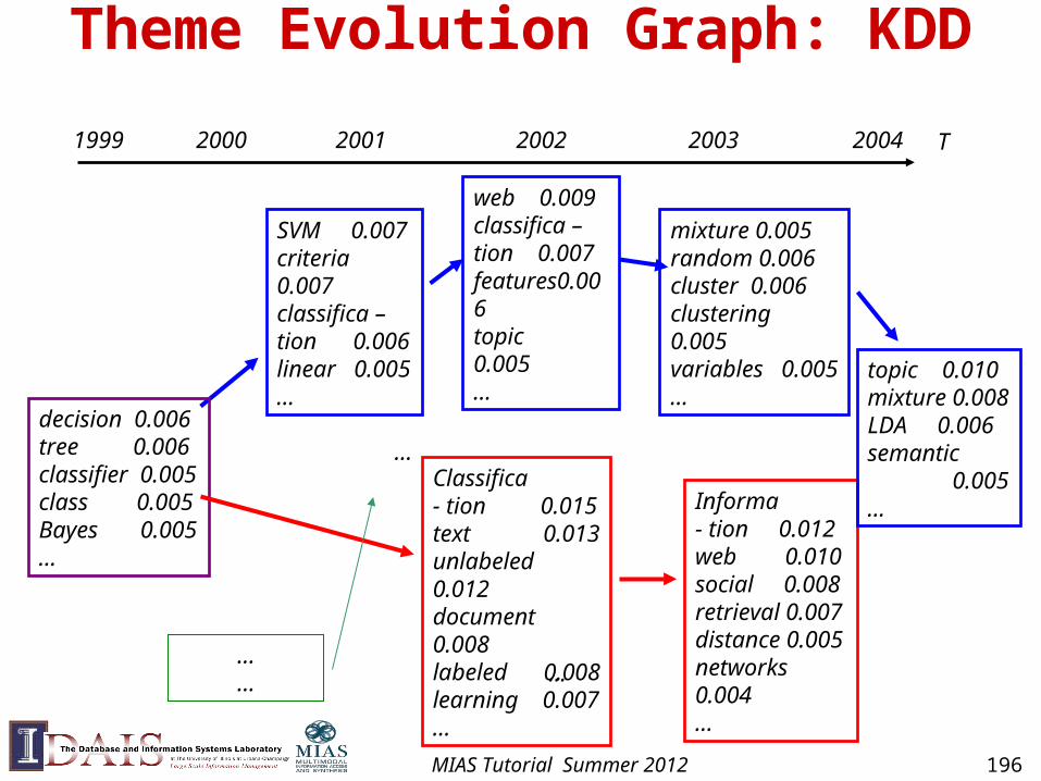
Theme Evolution Graph: KDD
T
SVM 0.007criteria 0.007classifica – tion 0.006linear 0.005…
decision 0.006tree 0.006classifier 0.005class 0.005Bayes 0.005…
Classifica - tion 0.015text 0.013unlabeled 0.012document 0.008labeled 0.008learning 0.007…
Informa - tion 0.012web 0.010social 0.008retrieval 0.007distance 0.005networks 0.004…
……
1999
…
web 0.009classifica –tion 0.007features0.006topic 0.005…
mixture 0.005random 0.006cluster 0.006clustering 0.005variables 0.005… topic 0.010
mixture 0.008LDA 0.006 semantic 0.005…
…
2000 2001 2002 2003 2004
MIAS Tutorial Summer 2012 196
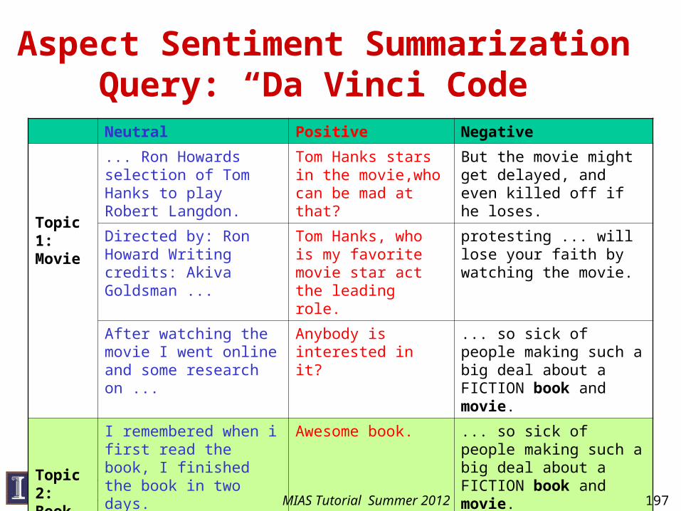
Aspect Sentiment SummarizationQuery: “Da Vinci Code”
Neutral Positive Negative
Topic 1:Movie
... Ron Howards selection of Tom Hanks to play Robert Langdon.
Tom Hanks stars in the movie,who can be mad at that?
But the movie might get delayed, and even killed off if he loses.
Directed by: Ron Howard Writing credits: Akiva Goldsman ...
Tom Hanks, who is my favorite movie star act the leading role.
protesting ... will lose your faith by watching the movie.
After watching the movie I went online and some research on ...
Anybody is interested in it?
... so sick of people making such a big deal about a FICTION book and movie.
Topic 2:Book
I remembered when i first read the book, I finished the book in two days.
Awesome book. ... so sick of people making such a big deal about a FICTION book and movie.
I’m reading “Da Vinci Code” now.
…
So still a good book to past time.
This controversy book cause lots conflict in west society.
MIAS Tutorial Summer 2012 197
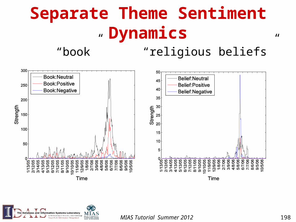
Separate Theme Sentiment Dynamics
“book” “religious beliefs”
MIAS Tutorial Summer 2012 198
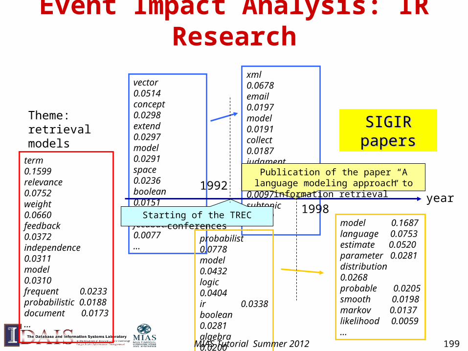
Event Impact Analysis: IR Research
vector 0.0514concept 0.0298extend 0.0297 model 0.0291space 0.0236boolean 0.0151function 0.0123feedback 0.0077…
xml 0.0678email 0.0197 model 0.0191collect 0.0187judgment 0.0102rank 0.0097subtopic 0.0079…
probabilist 0.0778model 0.0432logic 0.0404 ir 0.0338boolean 0.0281algebra 0.0200estimate 0.0119weight 0.0111…
model 0.1687language 0.0753estimate 0.0520 parameter 0.0281distribution 0.0268probable 0.0205smooth 0.0198markov 0.0137likelihood 0.0059…
1998
Publication of the paper “A language modeling approach to information
retrieval”
Starting of the TREC conferences
year1992
term 0.1599relevance 0.0752weight 0.0660 feedback 0.0372independence 0.0311model 0.0310frequent 0.0233probabilistic 0.0188document 0.0173…
Theme: retrieval models
SIGIR papersSIGIR papers
MIAS Tutorial Summer 2012 199
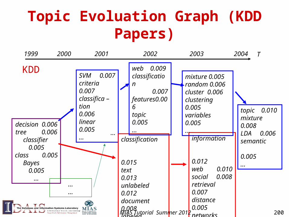
Topic Evoluation Graph (KDD Papers)
T
SVM 0.007criteria 0.007classifica – tion 0.006linear 0.005…
decision 0.006tree 0.006classifier 0.005class 0.005Bayes 0.005
…
classification 0.015text 0.013unlabeled 0.012document 0.008labeled 0.008learning 0.007
…
information 0.012web 0.010social 0.008retrieval 0.007distance 0.005networks 0.004…
……
1999
web 0.009classification 0.007features0.006topic 0.005…
mixture 0.005random 0.006cluster 0.006clustering 0.005variables 0.005…
topic 0.010mixture 0.008LDA 0.006 semantic 0.005…
…
2000 2001 2002 2003 2004
KDD
MIAS Tutorial Summer 2012 200
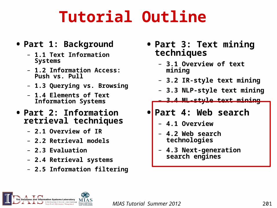
Tutorial Outline
• Part 1: Background – 1.1 Text Information Systems
– 1.2 Information Access: Push vs. Pull
– 1.3 Querying vs. Browsing
– 1.4 Elements of Text Information Systems
• Part 2: Information retrieval techniques– 2.1 Overview of IR
– 2.2 Retrieval models
– 2.3 Evaluation
– 2.4 Retrieval systems
– 2.5 Information filtering
• Part 3: Text mining techniques– 3.1 Overview of text mining
– 3.2 IR-style text mining
– 3.3 NLP-style text mining
– 3.4 ML-style text mining
• Part 4: Web search – 4.1 Overview
– 4.2 Web search technologies
– 4.3 Next-generation search engines
MIAS Tutorial Summer 2012 201
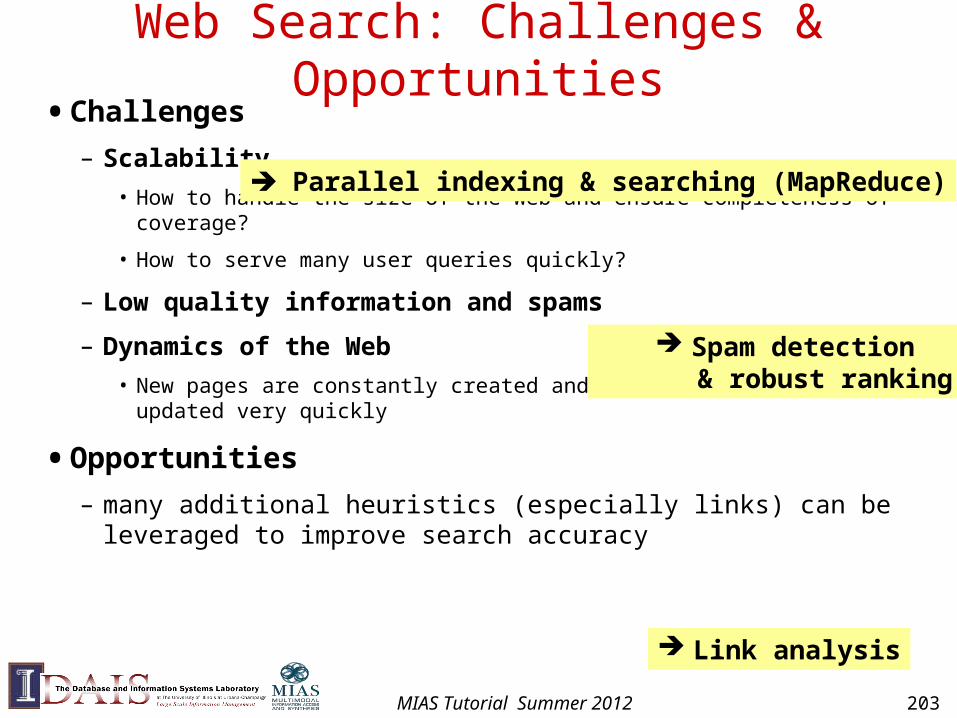
Web Search: Challenges & Opportunities• Challenges
– Scalability
• How to handle the size of the Web and ensure completeness of coverage?
• How to serve many user queries quickly?
– Low quality information and spams
– Dynamics of the Web
• New pages are constantly created and some pages may be updated very quickly
• Opportunities
– many additional heuristics (especially links) can be leveraged to improve search accuracy
Parallel indexing & searching (MapReduce)
Spam detection & robust ranking
Link analysis
MIAS Tutorial Summer 2012 203
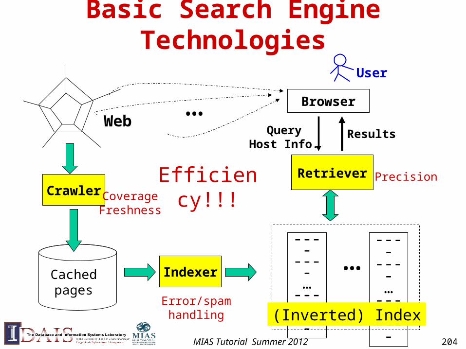
Basic Search Engine Technologies
Cachedpages
Crawler
Web
--------…--------
--------…--------
…Indexer
(Inverted) Index
…
Retriever
Browser
QueryHost Info.
Results
User
Efficiency!!!Coverage
Freshness
Precision
Error/spam handling
MIAS Tutorial Summer 2012 204
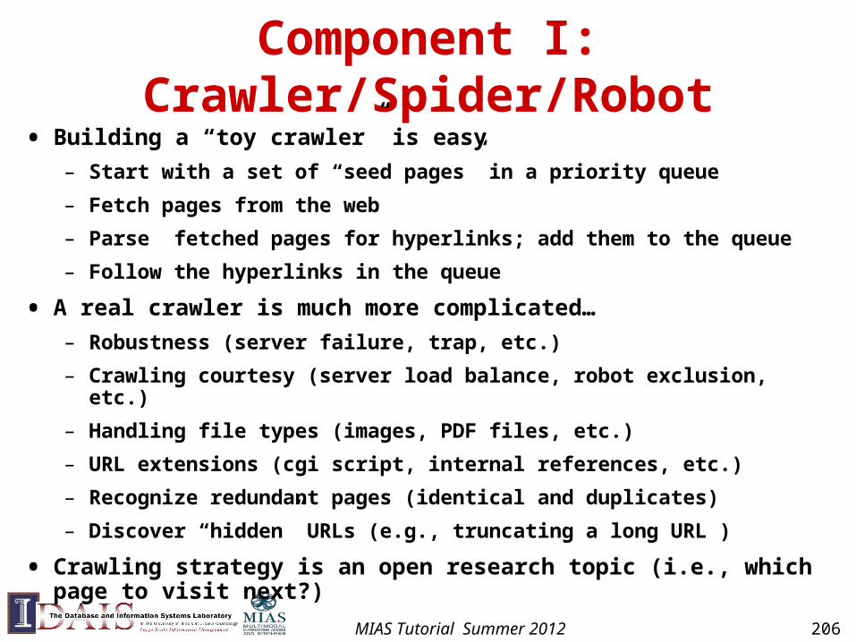
Component I: Crawler/Spider/Robot
• Building a “toy crawler” is easy
– Start with a set of “seed pages” in a priority queue
– Fetch pages from the web
– Parse fetched pages for hyperlinks; add them to the queue
– Follow the hyperlinks in the queue
• A real crawler is much more complicated…
– Robustness (server failure, trap, etc.)
– Crawling courtesy (server load balance, robot exclusion, etc.)
– Handling file types (images, PDF files, etc.)
– URL extensions (cgi script, internal references, etc.)
– Recognize redundant pages (identical and duplicates)
– Discover “hidden” URLs (e.g., truncating a long URL )
• Crawling strategy is an open research topic (i.e., which page to visit next?)
MIAS Tutorial Summer 2012 206
Major Crawling Strategies• Breadth-First is common (balance server load)
• Parallel crawling is natural
• Variation: focused crawling
– Targeting at a subset of pages (e.g., all pages about “automobiles” )
– Typically given a query
• How to find new pages (easier if they are linked to an old page, but what if they aren’t?)
• Incremental/repeated crawling (need to minimize resource overhead)
– Can learn from the past experience (updated daily vs. monthly)
– It’s more important to keep frequently accessed pages fresh
MIAS Tutorial Summer 2012 207
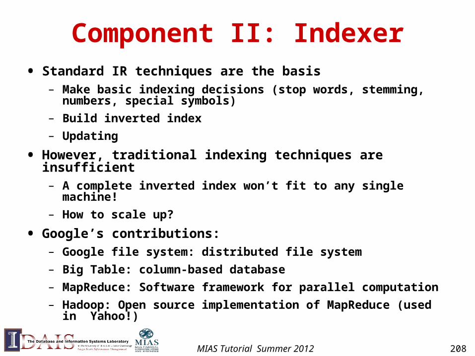
Component II: Indexer• Standard IR techniques are the basis
– Make basic indexing decisions (stop words, stemming, numbers, special symbols)
– Build inverted index
– Updating
• However, traditional indexing techniques are insufficient– A complete inverted index won’t fit to any single machine!
– How to scale up?
• Google’s contributions: – Google file system: distributed file system
– Big Table: column-based database
– MapReduce: Software framework for parallel computation
– Hadoop: Open source implementation of MapReduce (used in Yahoo!)
MIAS Tutorial Summer 2012 208
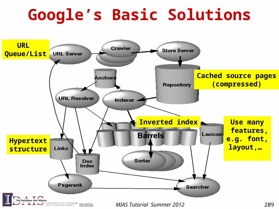
Google’s Basic Solutions
URL Queue/List
Cached source pages(compressed)
Inverted index
Hypertextstructure
Use many features,e.g. font,layout,…
MIAS Tutorial Summer 2012 209
Google’s Contributions
• Distributed File System (GFS)
• Column-based Database (Big Table)
• Parallel programming framework (MapReduce)
MIAS Tutorial Summer 2012 210
Google File System: Overview• Motivation: Input data is large (whole Web, billions of pages),
can’t be stored on one machine
• Why not use the existing file systems?– Network File System (NFS) has many deficiencies ( network
congestion, single-point failure)
– Google’s problems are different from anyone else
• GFS is designed for Google apps and workloads.– GFS demonstrates how to support large scale processing workloads
on commodity hardware
– Designed to tolerate frequent component failures.
– Optimized for huge files that are mostly appended and read.
– Go for simple solutions.
MIAS Tutorial Summer 2012 211
GFS Architecture
Fixed chunk size (64 MB)
Chunk is replicatedto ensure reliability
Simple centralized management
Data transfer is directly between application and
chunk servers
MIAS Tutorial Summer 2012 212
MapReduce
• Provide easy but general model for programmers to use
cluster resources
• Hide network communication (i.e. Remote Procedure Calls)
• Hide storage details, file chunks are automatically distributed
and replicated
• Provide transparent fault tolerance (Failed tasks are
automatically rescheduled on live nodes)
• High throughput and automatic load balancing (E.g.
scheduling tasks on nodes that already have data)
This slide and the following slides about MapReduce are from Behm & Shah’s presentation http://www.ics.uci.edu/~abehm/class_reports/uci/2008-Spring_CS224/Behm-Shah_PageRank.ppt
MIAS Tutorial Summer 2012 213
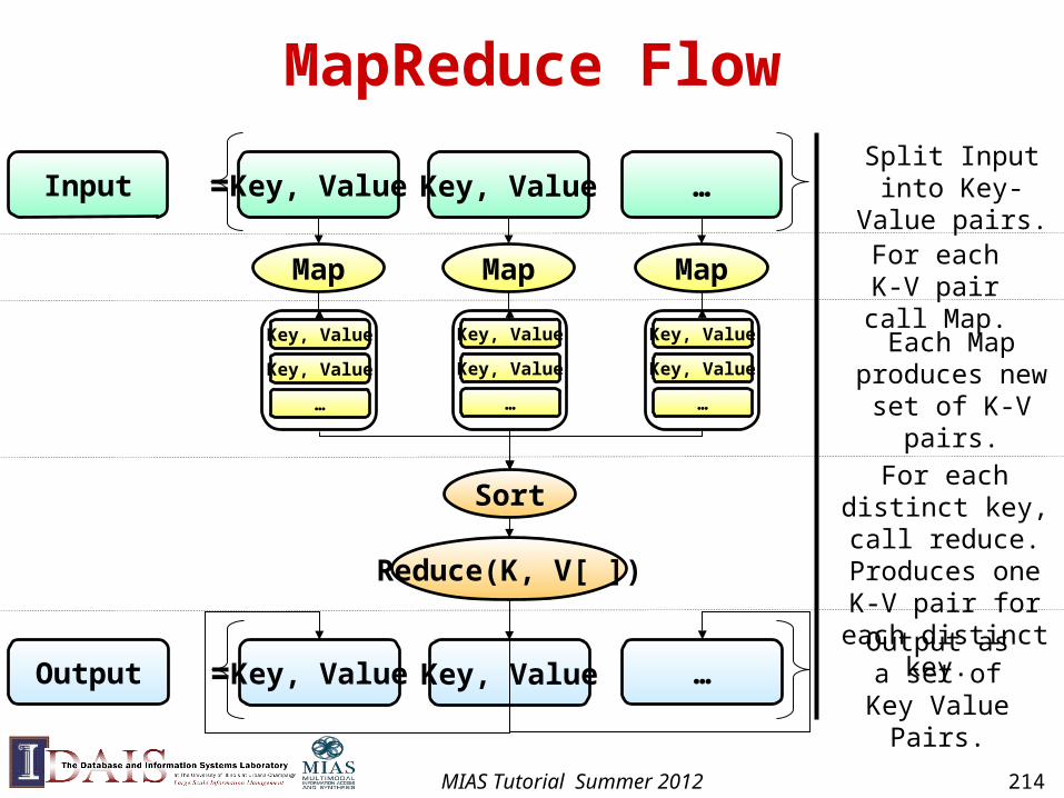
MapReduce Flow
Input
Map
Key, Value Key, Value …=
Map Map
Key, Value
Key, Value
…
Key, Value
Key, Value
…
Key, Value
Key, Value
…
Split Input into Key-Value pairs.
For each K-V pair call Map.
Each Map produces new set
of K-V pairs.
Reduce(K, V[ ])
Sort
Output Key, Value Key, Value …=
For each distinct key, call reduce.
Produces one K-V pair for each distinct key.
Output as a set of Key Value
Pairs.
MIAS Tutorial Summer 2012 214
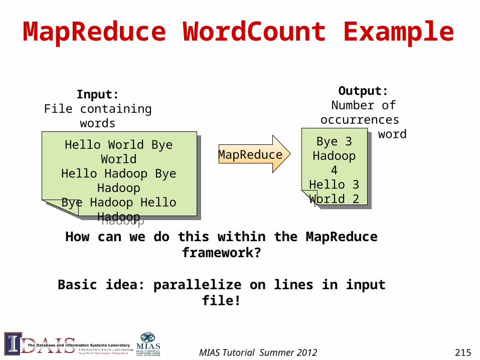
MapReduce WordCount Example
Output:Number of occurrences
of each word
Input:File containing words
Hello World Bye World
Hello Hadoop Bye Hadoop
Bye Hadoop Hello Hadoop
Hello World Bye World
Hello Hadoop Bye Hadoop
Bye Hadoop Hello Hadoop
Bye 3Hadoop
4Hello 3World 2
Bye 3Hadoop
4Hello 3World 2
MapReduce
How can we do this within the MapReduce framework?
Basic idea: parallelize on lines in input file!
MIAS Tutorial Summer 2012 215
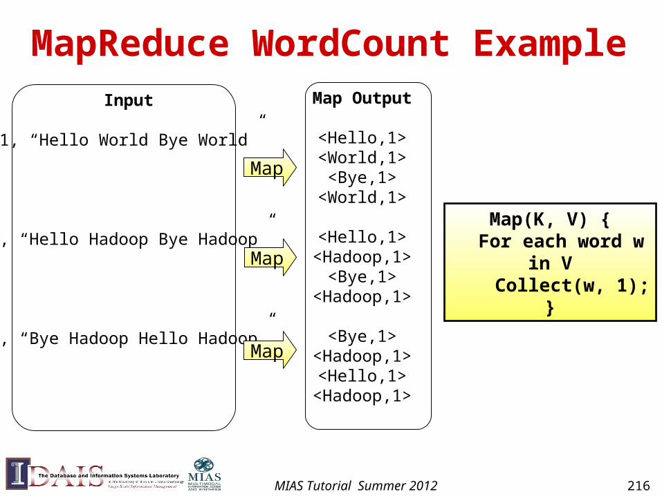
MapReduce WordCount ExampleInput
1, “Hello World Bye World”
2, “Hello Hadoop Bye Hadoop”
3, “Bye Hadoop Hello Hadoop”
Map Output
<Hello,1><World,1><Bye,1>
<World,1>
<Hello,1><Hadoop,1>
<Bye,1><Hadoop,1>
<Bye,1><Hadoop,1>
<Hello,1><Hadoop,1>
Map(K, V) { For each word w
in V Collect(w, 1);
}
Map
Map
Map
MIAS Tutorial Summer 2012 216
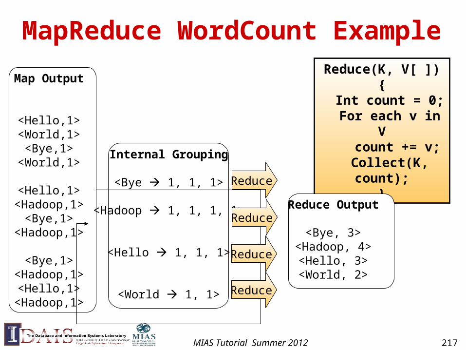
MapReduce WordCount ExampleReduce(K, V[ ]) { Int count = 0; For each v in V count += v;
Collect(K, count);
}
Map Output
<Hello,1><World,1><Bye,1>
<World,1>
<Hello,1><Hadoop,1>
<Bye,1><Hadoop,1>
<Bye,1><Hadoop,1>
<Hello,1><Hadoop,1>
Internal Grouping
<Bye 1, 1, 1>
<Hadoop 1, 1, 1, 1>
<Hello 1, 1, 1>
<World 1, 1>
Reduce Output
<Bye, 3><Hadoop, 4>
<Hello, 3><World, 2>
Reduce
Reduce
Reduce
Reduce
MIAS Tutorial Summer 2012 217
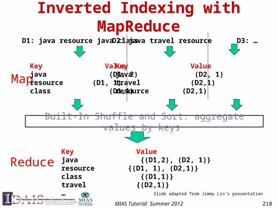
Inverted Indexing with MapReduce
Built-In Shuffle and Sort: aggregate values by keys
Map
Reduce
D1: java resource java class D2: java travel resource D3: …
Key Valuejava (D1, 2) resource (D1, 1)class (D1,1)
Key Valuejava (D2, 1) travel (D2,1)resource (D2,1)
Key Valuejava {(D1,2), (D2, 1)} resource {(D1, 1), (D2,1)}class {(D1,1)}travel {(D2,1)}… Slide adapted from Jimmy Lin’s presentation
MIAS Tutorial Summer 2012 218
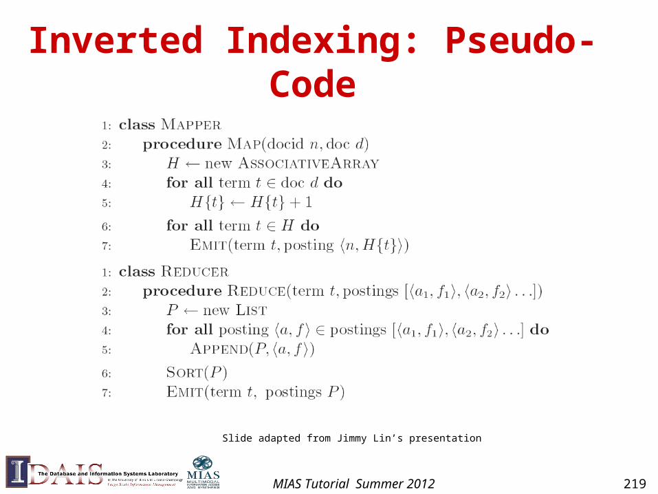
Inverted Indexing: Pseudo-Code
Slide adapted from Jimmy Lin’s presentation
MIAS Tutorial Summer 2012 219
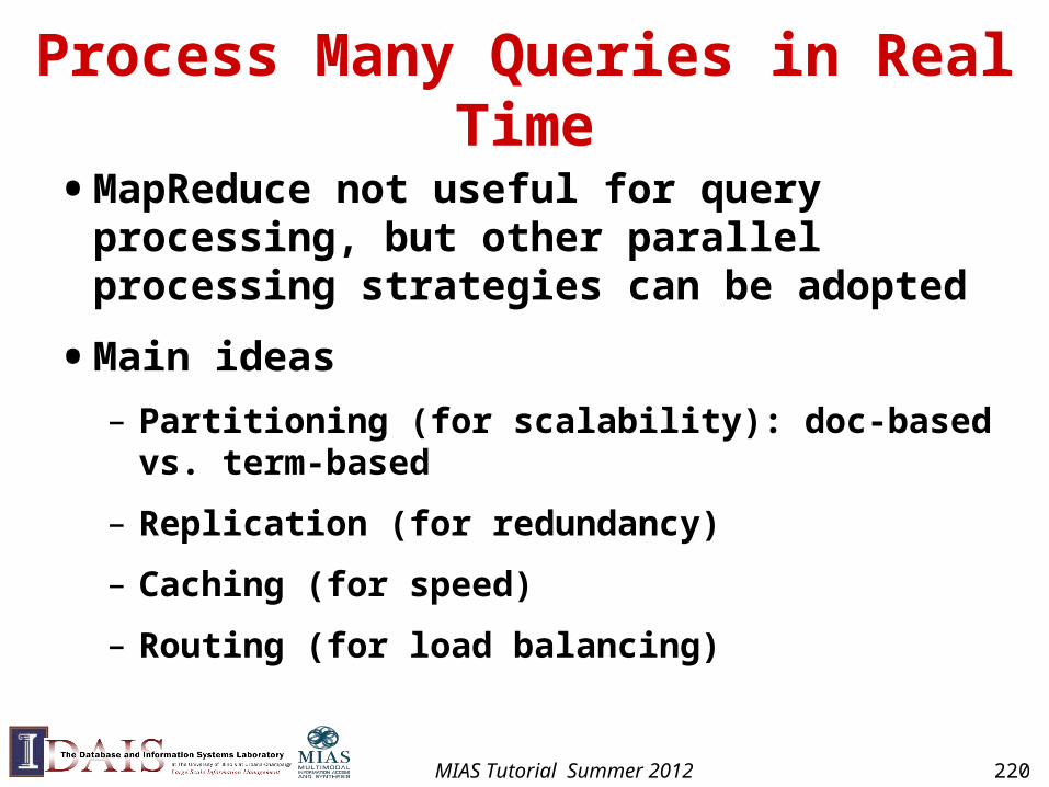
Process Many Queries in Real Time
• MapReduce not useful for query processing, but other parallel processing strategies can be adopted
• Main ideas
– Partitioning (for scalability): doc-based vs. term-based
– Replication (for redundancy)
– Caching (for speed)
– Routing (for load balancing)
MIAS Tutorial Summer 2012 220
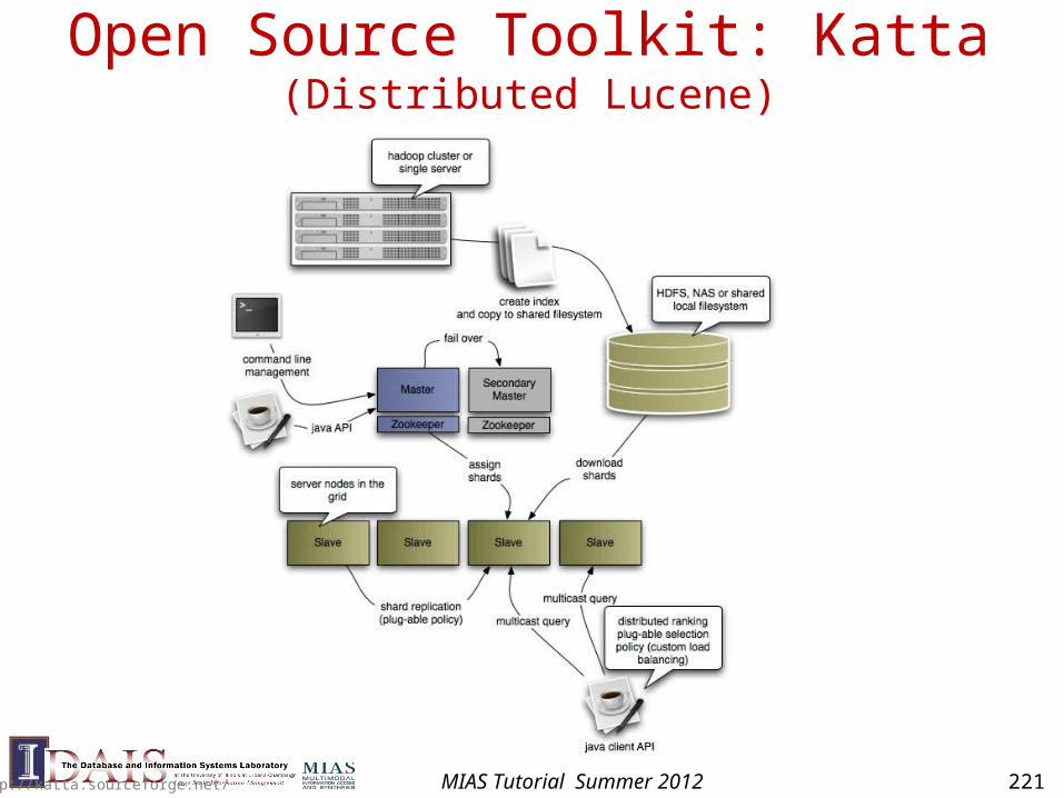
Open Source Toolkit: Katta(Distributed Lucene)
http://katta.sourceforge.net/ MIAS Tutorial Summer 2012 221
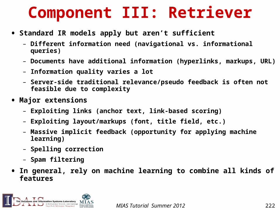
Component III: Retriever• Standard IR models apply but aren’t sufficient
– Different information need (navigational vs. informational queries)
– Documents have additional information (hyperlinks, markups, URL)
– Information quality varies a lot
– Server-side traditional relevance/pseudo feedback is often not feasible due to complexity
• Major extensions
– Exploiting links (anchor text, link-based scoring)
– Exploiting layout/markups (font, title field, etc.)
– Massive implicit feedback (opportunity for applying machine learning)
– Spelling correction
– Spam filtering
• In general, rely on machine learning to combine all kinds of features
MIAS Tutorial Summer 2012 222
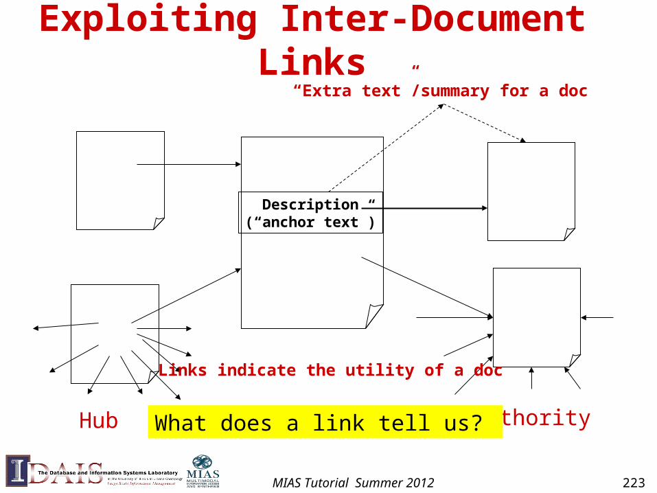
Exploiting Inter-Document Links
Description(“anchor text”)
Hub Authority
“Extra text”/summary for a doc
Links indicate the utility of a doc
What does a link tell us?
MIAS Tutorial Summer 2012 223
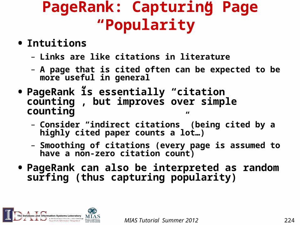
PageRank: Capturing Page “Popularity”
• Intuitions– Links are like citations in literature
– A page that is cited often can be expected to be more useful in general
• PageRank is essentially “citation counting”, but improves over simple counting– Consider “indirect citations” (being cited by a highly cited
paper counts a lot…)
– Smoothing of citations (every page is assumed to have a non-zero citation count)
• PageRank can also be interpreted as random surfing (thus capturing popularity)
MIAS Tutorial Summer 2012 224
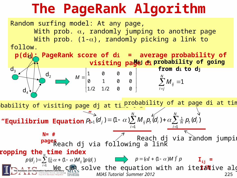
002/12/1
0010
0001
2/12/100
M
The PageRank Algorithm
Transition matrix
Random surfing model: At any page, With prob. , randomly jumping to another pageWith prob. (1-), randomly picking a link to follow.
p(di): PageRank score of di = average probability of visiting page di
d1
d2
d4
d3
Mij = probability of going from di to dj
1
N
jiijM
N= # pages
“Equilibrium Equation”:
N
iitN
N
iitijjt dpdpMdp
1
1
11 )()()1()(
probability of visiting page dj at time t+1 probability of at page di at time t
Reach dj via following a linkReach dj via random jumping
Iij = 1/NpMIp T ))1((
N
iiijNj dpMdp
1
1 )(])1([)( dropping the time index
We can solve the equation with an iterative algorithmMIAS Tutorial Summer 2012 225
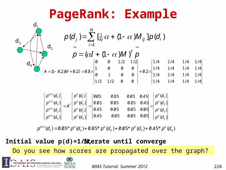
PageRank: Exampled1
d2
d4
d3
iterate until converge Initial value p(d)=1/N,
pMIp
dpMdp
T
N
iiijNj
))1((
)(])1([)(1
1
)(
)(
)(
)(
05.005.005.045.0
05.005.005.045.0
45.085.005.005.0
45.005.085.005.0
)(
)(
)(
)(
)(
)(
)(
)(
4/14/14/14/1
4/14/14/14/1
4/14/14/14/1
4/14/14/14/1
2.0
002/12/1
0010
0001
2/12/100
8.02.0)2.01(
4
3
2
1
4
3
2
1
41
31
21
11
dp
dp
dp
dp
dp
dp
dp
dp
A
dp
dp
dp
dp
IMA
n
n
n
n
n
n
n
n
T
n
n
n
n
)(*45.0)(*05.0)(*85.0)(*05.0)( 432111 dpdpdpdpdp nnnnn
Do you see how scores are propagated over the graph?
MIAS Tutorial Summer 2012 226
PageRank in Practice• Computation can be quite efficient since M is usually
sparse
• Interpretation of the damping factor (0.15):– Probability of a random jump
– Smoothing the transition matrix (avoid zero’s)
• Normalization doesn’t affect ranking, leading to some variants of the formula
• The zero-outlink problem: p(di)’s don’t sum to 1– One possible solution = page-specific damping factor
(=1.0 for a page with no outlink)
• Many extensions (e.g., topic-specific PageRank)
• Many other applications (e.g., social network analysis)
MIAS Tutorial Summer 2012 227
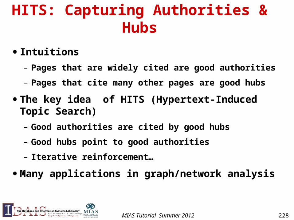
HITS: Capturing Authorities & Hubs
• Intuitions
– Pages that are widely cited are good authorities
– Pages that cite many other pages are good hubs
• The key idea of HITS (Hypertext-Induced Topic Search)
– Good authorities are cited by good hubs
– Good hubs point to good authorities
– Iterative reinforcement…
• Many applications in graph/network analysis
MIAS Tutorial Summer 2012 228
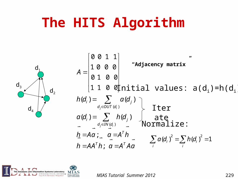
The HITS Algorithm
d1
d2
d4( )
( )
0 0 1 1
1 0 0 0
0 1 0 0
1 1 0 0
( ) ( )
( ) ( )
;
;
j i
j i
i jd OUT d
i jd IN d
T
T T
A
h d a d
a d h d
h Aa a A h
h AA h a A Aa
“Adjacency matrix”
d3 Initial values: a(di)=h(di)=1
Iterate
Normalize: 2 2
( ) ( ) 1i ii i
a d h d
MIAS Tutorial Summer 2012 229
Effective Web Retrieval Heuristics
• High accuracy in home page finding can be achieved by – Matching query with the title
– Matching query with the anchor text
– Plus URL-based or link-based scoring (e.g. PageRank)
• Imposing a conjunctive (“and”) interpretation of the query is often appropriate – Queries are generally very short (all words are necessary)
– The size of the Web makes it likely that at least a page would match all the query words
• Combine multiple features using machine learning
MIAS Tutorial Summer 2012 230
How can we combine many features? (Learning to Rank)
• General idea:
– Given a query-doc pair (Q,D), define various kinds of features Xi(Q,D)
– Examples of feature: the number of overlapping terms, BM25 score of Q and D, p(Q|D), PageRank of D, p(Q|Di), where Di may be anchor text or big font text, “does the URL contain ‘~’?”….
– Hypothesize p(R=1|Q,D)=s(X1(Q,D),…,Xn(Q,D), ) where is a set of parameters
– Learn by fitting function s with training data, i.e., 3-tuples like (D, Q, 1) (D is relevant to Q) or (D,Q,0) (D is non-relevant to Q)
MIAS Tutorial Summer 2012 231
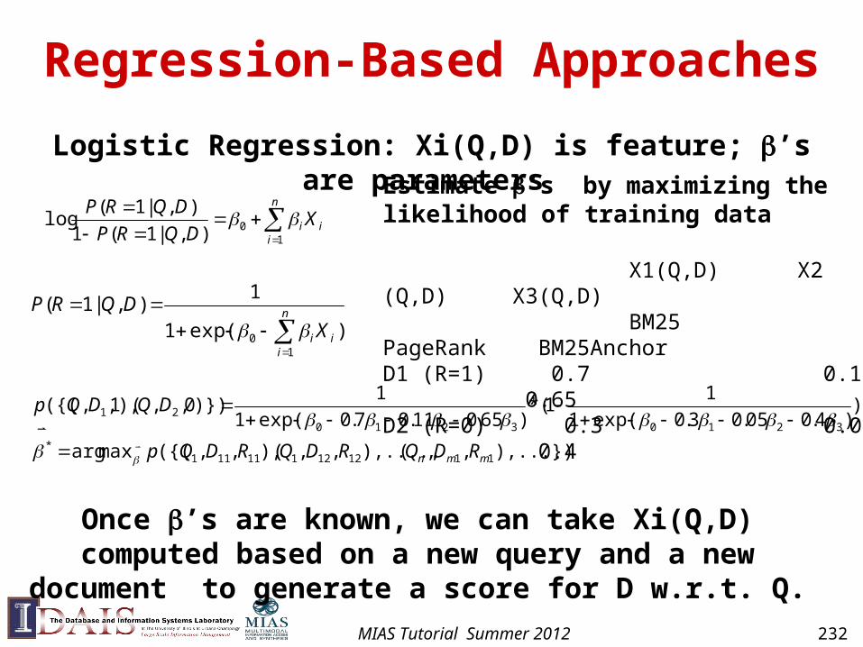
Regression-Based Approaches
)exp(1
1),|1(
10
n
iii X
DQRP
n
iii XDQRP
DQRP
10),|1(1
),|1(log
Logistic Regression: Xi(Q,D) is feature; ’s are parameters Estimate ’s by maximizing the likelihood of training data
X1(Q,D) X2 (Q,D) X3(Q,D) BM25 PageRank BM25AnchorD1 (R=1) 0.7 0.11 0.65D2 (R=0) 0.3 0.05 0.4
),...}),,(),....,,,(),,,({(maxarg
))4.005.03.0exp(1
11(*
)65.011.07.0exp(1
1)})0,,(),1,,({(
111212111111*
3210321021
mmn RDQRDQRDQp
DQDQp
Once ’s are known, we can take Xi(Q,D) computed based on a new query and a new document to generate a score for D w.r.t. Q.
MIAS Tutorial Summer 2012 232
Machine Learning Approaches: Pros & Cons
• Advantages
– A principled and general way to combine multiple features (helps improve accuracy and combat web spams)
– May re-use all the past relevance judgments (self-improving)
• Problems
– Performance mostly depends on the effectiveness of the features used
– No much guidance on feature generation (rely on traditional retrieval models)
• In practice, they are adopted in all current Web search engines (with many other ranking applications also)
MIAS Tutorial Summer 2012 233
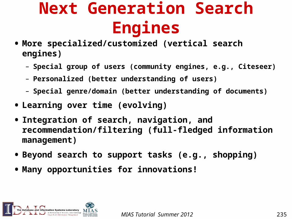
Next Generation Search Engines
• More specialized/customized (vertical search engines)
– Special group of users (community engines, e.g., Citeseer)
– Personalized (better understanding of users)
– Special genre/domain (better understanding of documents)
• Learning over time (evolving)
• Integration of search, navigation, and recommendation/filtering (full-fledged information management)
• Beyond search to support tasks (e.g., shopping)
• Many opportunities for innovations!
MIAS Tutorial Summer 2012 235
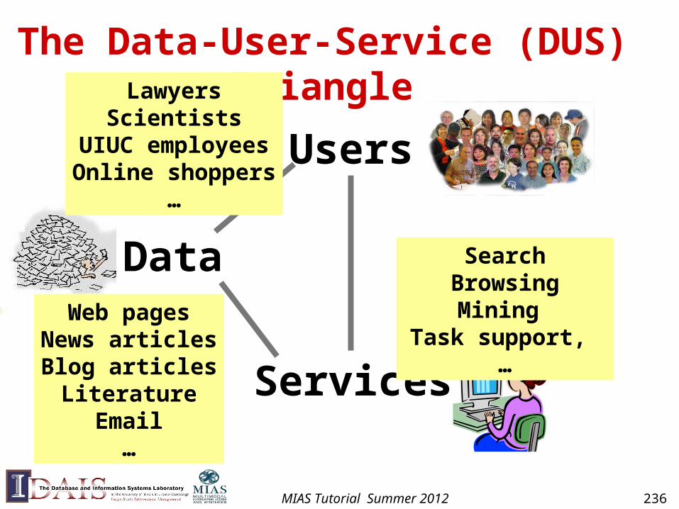
The Data-User-Service (DUS) Triangle
Users
Data
Services
Web pagesNews articlesBlog articlesLiterature
Email…
LawyersScientists
UIUC employeesOnline shoppers
…
SearchBrowsingMining
Task support, …
MIAS Tutorial Summer 2012 236
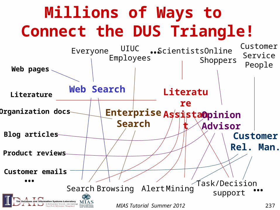
Millions of Ways to Connect the DUS Triangle!
Web pages
Literature
Organization docs
Blog articles
Product reviews
Customer emails…
Everyone ScientistsUIUCEmployees
OnlineShoppers
Search Browsing Alert MiningTask/Decision
support
CustomerServicePeople
Web Search
EnterpriseSearch
LiteratureAssistant
OpinionAdvisor
CustomerRel. Man.
…
…
MIAS Tutorial Summer 2012 237
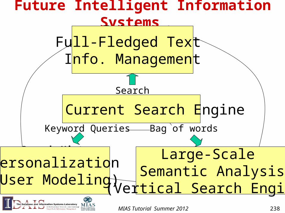
Future Intelligent Information Systems
Bag of words
Search
Keyword Queries
Access
Mining
Task Support
Entities-Relations
Knowledge Representation
Search History
Complete User Model
Current Search Engine
Personalization(User Modeling)
Large-Scale Semantic Analysis
(Vertical Search Engines)
Full-Fledged Text Info. Management
MIAS Tutorial Summer 2012 238
Check out cs410 websitehttp://times.cs.uiuc.edu/course/410s12/
for assignments and additional lectures
MIAS Tutorial Summer 2012 239


![CS276A Text Retrieval and Mining Lecture 12 [Borrows slides from Viktor Lavrenko and Chengxiang Zhai]](https://img.pdfslide.net/doc/110x75/551b01fa550346f70d8b5689/cs276a-text-retrieval-and-mining-lecture-12-borrows-slides-from-viktor-lavrenko-and-chengxiang-zhai.jpg)


![CS276A Text Retrieval and Mining Lecture 12 [Utilizando slides de Viktor Lavrenko e Chengxiang Zhai]](https://img.pdfslide.net/doc/110x75/552fc132497959413d8d6a63/cs276a-text-retrieval-and-mining-lecture-12-utilizando-slides-de-viktor-lavrenko-e-chengxiang-zhai.jpg)