INFORMATION THEORETIC MEASURES FOR PET IMAGE

RECONSTRUCTION AND NON-RIGID IMAGE REGISTRATION

by

Sangeetha Somayajula

A Dissertation Presented to theFACULTY OF THE USC GRADUATE SCHOOLUNIVERSITY OF SOUTHERN CALIFORNIA

In Partial Fulfillment of theRequirements for the DegreeDOCTOR OF PHILOSOPHY

(ELECTRICAL ENGINEERING)

December 2009

Copyright 2009 Sangeetha Somayajula

Dedication

To my parents Seshu and Venkata Lakshmana Rao Somayajula

ii

Acknowledgments

I thank Prof. Richard Leahy for being an excellent advisor and teacher. His guidance

at every step of my research work has been invaluable, and I am grateful for the encour-

agement he provided when I needed it. He has been an inspiring role model for me. I

thank him for providing financial support, for helping me form productive collaborations,

and for making my experience as a graduate student truly valuable. I also thank my

guidance committee Dr. Manbir Singh, Dr. Krishna Nayak, Dr. Antonio Ortega, and

Dr. Quanzheng Li for their time and feedback. I thank my collaborators Christos Pana-

giotou, Dr. Simon Arridge, and Dr. Anand Rangarajan for contributing to the PET

work through their valuable suggestions. Additionally, I thank Dr. Richard Laforest, Dr.

Quanzheng Li, and Dr. Giselle Petzinger for providing data to validate my PET work. I

am grateful to the Women in Science and Engineering program for awarding me a top-off

scholarship for the first two years of my PhD studies, and for providing travel grants that

helped me attend major conferences in my field.

It has been a pleasure to work with my colleagues in the USC Biomedical Imaging

group. It was an enriching experience to discuss my work with them, and I thank them for

being a helpful and collaborative research group. I thank Dr. Sangtae Ahn, Dr. Anand

Joshi, Dr. Quanzheng Li, and Dr. Sanghee Cho for always having the time to answer

iii

my questions, and Dr. Evren Asma for his help early in my research work. I thank

Dr. Abhijit Chaudhari, Joyita Dutta, and Dr. Belma Dogdas for being good friends

besides being great colleagues. I thank Dr. Zheng Li, Dr. Dimitrios Pantazis, Yu-teng

Chang, Yanguang Lin, Ran Ren, Syed Ashrafulla, Juan Poletti Soto, Hua Hui, and David

Wheland for being great colleagues, and for the fun times I had while being a part of the

research group.

I am grateful to my dear friends without whom I would be lost. I thank Kavitha

Buddharaju for the faith she has in me, and for not letting astronomical international

call rates stop her from always being there for me. I thank Lalit Varma for teaching

me to believe in myself. Though he left this world early in my PhD program, he was

and will continue to be a source of inspiration for me. I thank Suma Mallavarapu for

being my sounding board, though she had her own PhD and her baby to take care of.

I thank Gautam Thatte, Michelle Bardis, Laura Woo, Ashok and Amola Patel, Manoj

Gopalkrishnan, Krishna and Sandhya Gogineni, and Ratnakar Vejella for being strong

sources of support throughout my graduate student years. I thank Srikanth Pinninti,

Joaquin Rapela, Vijay Ponduru, Pradeep Natarajan, and Haritha Bodugam for making

my years at USC an enjoyable experience.

Finally, I thank my family for being pillars of support throughout my graduate studies.

I thank my grandmother Eswaramma Somayajula for taking immense pride in everything

I do, and my sister Sunitha Mukkavalli for being my friend for as long as I can remember.

My parents Seshu and Venkata Lakshmana Rao Somayajula cheered me on every step of

the way, and I thank them for their constant love and support.

iv

Table of Contents

Dedication ii

Acknowledgments iii

List Of Tables vii

List Of Figures viii

Abstract xii

Chapter 1: Introduction 1

1.1 Positron Emission Tomography Image Reconstruction . . . . . . . . . . . 1

1.2 Non-rigid image registration . . . . . . . . . . . . . . . . . . . . . . . . . . 7

1.3 Contributions . . . . . . . . . . . . . . . . . . . . . . . . . . . . . . . . . . 12

1.4 Organization of the dissertation . . . . . . . . . . . . . . . . . . . . . . . . 13

Chapter 2: PET Image Reconstruction Using Information Theoretic Anatom-

ical Priors 14

2.1 Methods . . . . . . . . . . . . . . . . . . . . . . . . . . . . . . . . . . . . . 16

2.1.1 MAP estimation using information theoretic priors . . . . . . . . . 16

2.1.2 Information theoretic priors . . . . . . . . . . . . . . . . . . . . . . 18

2.1.3 Extraction of feature vectors . . . . . . . . . . . . . . . . . . . . . 22

2.1.4 Computation of prior term . . . . . . . . . . . . . . . . . . . . . . 24

2.1.5 Computation of the MAP estimate . . . . . . . . . . . . . . . . . . 25

2.1.6 Efficient computation of entropy and its gradient . . . . . . . . . . 27

2.2 Results . . . . . . . . . . . . . . . . . . . . . . . . . . . . . . . . . . . . . . 32

2.2.1 Simulation Results . . . . . . . . . . . . . . . . . . . . . . . . . . . 33

2.2.1.1 Anatomical and PET images with identical structure . . 33

2.2.1.2 Anatomical and PET images with differences . . . . . . . 38

2.2.2 Clinical data . . . . . . . . . . . . . . . . . . . . . . . . . . . . . . 44

2.3 Application of Information Theoretic Priors to Positron Range Correction 49

2.3.1 Positron Range Simulations . . . . . . . . . . . . . . . . . . . . . . 51

2.3.2 Real data results . . . . . . . . . . . . . . . . . . . . . . . . . . . . 53

2.4 Conclusions . . . . . . . . . . . . . . . . . . . . . . . . . . . . . . . . . . . 54

2.5 Appendix: Alternative formulation to the JE prior . . . . . . . . . . . . . 59

v

Chapter 3: Mutual Information Based Non-Rigid Mouse Registration Us-

ing A Scale-Space Approach 62

3.1 Methods and Results . . . . . . . . . . . . . . . . . . . . . . . . . . . . . . 643.1.1 Mutual information based non-rigid registration . . . . . . . . . . 643.1.2 Scale-space feature vectors . . . . . . . . . . . . . . . . . . . . . . . 653.1.3 Displacement field and regularization . . . . . . . . . . . . . . . . . 673.1.4 Results . . . . . . . . . . . . . . . . . . . . . . . . . . . . . . . . . 68

3.2 Discussion . . . . . . . . . . . . . . . . . . . . . . . . . . . . . . . . . . . . 69

Chapter 4: Non-Rigid Registration Using Gaussian Mixture Models 73

4.1 Methods and Results . . . . . . . . . . . . . . . . . . . . . . . . . . . . . . 764.1.1 Estimation of parameters of Gaussian mixture model . . . . . . . . 774.1.2 Estimation of displacement field . . . . . . . . . . . . . . . . . . . 794.1.3 Relation to Mutual Information . . . . . . . . . . . . . . . . . . . . 834.1.4 Results . . . . . . . . . . . . . . . . . . . . . . . . . . . . . . . . . 874.1.5 Brain Image registration . . . . . . . . . . . . . . . . . . . . . . . . 874.1.6 Mouse image registration . . . . . . . . . . . . . . . . . . . . . . . 92

4.2 Discussion . . . . . . . . . . . . . . . . . . . . . . . . . . . . . . . . . . . . 97

Chapter 5: Summary and Future Work 100

5.1 Future Work . . . . . . . . . . . . . . . . . . . . . . . . . . . . . . . . . . 102

References 104

vi

List Of Tables

2.1 Run-times for combined computation of pdf and gradient for different im-age sizes, for the Parzen and FFT based methods . . . . . . . . . . . . . 31

4.1 Quantitative measures of overlap . . . . . . . . . . . . . . . . . . . . . . . 98

vii

List Of Figures

1.1 PET/CT imaging: Whole body PET image (left), its corresponding CTimage (middle), and their overlay (right). Image was obtained from thewebsite http:/medical.siemens.com . . . . . . . . . . . . . . . . . . . . . . 2

1.2 Positron range: The positron travels a distance before annihilation duringwhich it loses its kinetic energy. The LOR is a distance away from thesource, hence fundamentally limiting the resolution of PET. . . . . . . . . 6

1.3 Mouse imaging studies that require non-rigid registration . . . . . . . . . 8

2.1 Log of estimated joint probability distribution functions: Top: Anatomicalimage, Middle: Example reconstructed images (L to R): Blurred, Noisy,and true. Bottom: Estimated joint pdf of the images in the middle rowand anatomical image. . . . . . . . . . . . . . . . . . . . . . . . . . . . . . 21

2.2 Joint densities of reference image, and images with arbitrary intensities:Top (L to R) Image with same structure as reference image, but arbitraryintensities, image with two regions having same intensity, and referenceimage. Bottom: Log of estimated joint densities of the reference imageand the two functional images considered in the top row . . . . . . . . . . 22

2.3 Scale-space features of a coronal slice of an MR image of the brain . . . . 23

2.4 Comparison of Parzen and FFT-based methods: a) Image for which pdfand gradients were estimated, b) pdf estimates using M = 351, c) gradientof marginal entropy using the Parzen method (left) and the FFT-basedmethod (right). The normalized difference in the shown gradient imagesis 0.14% . . . . . . . . . . . . . . . . . . . . . . . . . . . . . . . . . . . . . 31

2.5 The phantoms used in the simulations to represent the MR image (left)and the PET image (right) . . . . . . . . . . . . . . . . . . . . . . . . . . . 34

viii

2.6 True and reconstructed images: Top: True PET image (left), QP recon-struction with β = 0.5 (right). Middle: MI reconstruction for µ = 10000(left), JE reconstruction for µ = 5000 (right). Bottom: MI-scale recon-struction for µ = 2500 (left), JE-scale reconstruction for µ = 2500. . . . . 35

2.7 Normalized error vs. iteration for best value of µ and β of the informationtheoretic and QP priors respectively. . . . . . . . . . . . . . . . . . . . . . 35

2.8 Results of Monte Carlo simulations for (L to R) QP (β = 0.5), MI (µ =2500), JE(µ = 5000), MI-scale(µ = 2500), JE-scale(µ = 2500) . . . . . . . 37

2.9 Joint pdfs of the anatomical image and a) true PET image, b) OSEMestimate used for initialization, c) image reconstructed using MI-Intensityprior, d) Image reconstructed using JE-Intensity prior . . . . . . . . . . . 37

2.10 Variation of marginal entropy for MI-Intensity prior and JE for MI-Intensityand JE-Intensity priors as a function of iteration . . . . . . . . . . . . . . 38

2.11 Coronal slice of an MR image of the brain, and true PET image generatedfrom manual segmentation of the MR image. . . . . . . . . . . . . . . . . 39

2.12 True and reconstructed images: Top: True PET image (left), QP recon-struction with β = 0.5 (right). Middle: MI reconstruction for µ = 1e5(left), JE reconstruction for µ = 150000,Bottom: MI-scale reconstructionfor µ = 1e5 (left), JE-scale reconstruction for µ = 1e5. . . . . . . . . . . . 40

2.13 Normalized error as a function of iteration. . . . . . . . . . . . . . . . . . 41

2.14 Coronal slice of bias and SD images: Top (L to R): QP (β = 0.5), MI-Intensity(µ = 1e5), JE-Intensity(µ = 150000), Bottom (L to R): MI-scale(µ = 1e5), JE-scale (µ = 1e5). . . . . . . . . . . . . . . . . . . . . . . 42

2.15 Absolute value of bias vs. standard deviation curves for selected regionsof interest for quadratic prior (QP), mutual information (MI) and jointentropy (JE) priors using only intensity as a feature, and MI scale-space(MIsc) and JE scale-space (JEsc) priors. . . . . . . . . . . . . . . . . . . . 43

2.16 Coronal slice of PET image (left) with co-registered MR image (right). . 46

2.17 Coronal slice of PET image reconstructions: Top (L to R): QP(µ = 1.5),MI-Intensity(µ = 75000), JE-Intensity(µ = 1e5). Bottom (L to R): MI-scale(µ = 1e5), JE-scale(µ = 1e5). . . . . . . . . . . . . . . . . . . . . . . 46

2.18 Overlay of PET reconstruction over co-registered MR image for QP (top)and JE-scale (bottom) priors. . . . . . . . . . . . . . . . . . . . . . . . . . 47

ix

2.19 Regions of interest for computing CRC vs noise curves: a)ROIs in caudate(red) and WM separating it from putamen (blue), (b) ROIs for computingnoise variance . . . . . . . . . . . . . . . . . . . . . . . . . . . . . . . . . 47

2.20 Contrast recovery coefficient versus noise variance plots as the hyperpa-rameter is varied. . . . . . . . . . . . . . . . . . . . . . . . . . . . . . . . . 48

2.21 Reconstruction for high value of µ for MI-scale(left) and JE-scale(right)priors. . . . . . . . . . . . . . . . . . . . . . . . . . . . . . . . . . . . . . . 48

2.22 The phantoms used in the simulations to represent the MR image (left),the PET image (middle), and the truncation mask (right). The line in thePET image shows the position of the profile shown in Fig. 2.25. . . . . . . 51

2.23 Positron range kernel for Cu-60 isotope vs distance (mm) . . . . . . . . . 52

2.24 Reconstructed images(L to R): No range correction with QP (NRC-QP), range correction with quadratic prior (RC-QP) with µ = 0.01, rangecorrection with JE prior (RC-JE), scale σ = 0.5 voxels and µ = 5e4. . . . 52

2.25 Profile drawn through true and reconstructed images . . . . . . . . . . . . 53

2.26 (a)CT image registered to reconstructed PET image and (b) truncationmask obtained from the CT image for truncated homogeneous model ofrange correction. . . . . . . . . . . . . . . . . . . . . . . . . . . . . . . . . 55

2.27 Positron range kernel for Br-76. . . . . . . . . . . . . . . . . . . . . . . . . 56

2.28 Reconstructed images: Top row: Coronal slice of PET images recon-structed using NRC-QP (left), RC-QP (middle), and RC-JE (right). Bot-tom row: Overlay on CT of the images shown in the top row. . . . . . . . 56

3.1 Coronal slice of scale-space images of a mouse for Ns = 2, with scale 1corresponding to no smoothing (left) and σ2 =3 (right). . . . . . . . . . . 66

3.2 Sagittal slice of target (left) and template (right) mouse images. . . . . . 68

3.3 Comparison of registered images: Coronal and sagittal views of overlayon target image of template (top row), hierarchical multi-scale registeredimage (middle row), and scale-space registered image (bottom row). . . . 70

3.4 Displacement field obtained from scale-space registration . . . . . . . . . . 71

x

4.1 Estimation of GMM parameters: (a) Target image, (b) Template image,(c) Joint histogram of intensities of target and template images,(d) Jointpdf of target and template images computed using GMM (the componentmeans shown with ’x’ marks). . . . . . . . . . . . . . . . . . . . . . . . . 80

4.2 (a) Gaussian window of width σ = 2, and (b) its derivative. . . . . . . . . 86

4.3 Registration results for one dataset:(a) Target, (b)Atlas, (c) SSD registeredimage, (d)Parzen-MI registered image, and (e) GMM-Cond registered image. 89

4.4 Displacement field obtained from GMM-Cond registration correspondingto the slice shown in Figure 4.3. . . . . . . . . . . . . . . . . . . . . . . . . 90

4.5 Comparison of Parzen-MI vs GMM-Cond based methods: Log of the es-timate of initial joint density between target and template images using(a) Parzen windon method, (b) GMM method (the ’x’ marks denote theGMM means) , and log of the estimate of joint density between target andregistered template using (c) Parzen window method and (d) GMM method. 90

4.6 Mean dice coefficients for different brain regions (Caud:Caudate, GM:Cerebral gray matter, WM: Cerebral white matter, Put: Putamen, Tha:Thalamus, HC: Hippocampus, CBGM: Cerebellar gray matter, CBWM:Cerebellar white matter) . . . . . . . . . . . . . . . . . . . . . . . . . . . 92

4.7 Mean squared error between intensities of target and deformed atlas imagesfor SSD, MI, and GMM methods . . . . . . . . . . . . . . . . . . . . . . . 93

4.8 Transaxial and sagittal views of average images: Top row:Template imageto which the atlases are registered. Middle row: Average of deformed at-lases using Parzen-MI approach, Bottom row: Average of deformed atlasesusing GMM based approach . . . . . . . . . . . . . . . . . . . . . . . . . 94

4.9 Multi-modality inter-subject registration: Coronal (top row) and sagittalviews (bottom row) of target , template, Parzen-MI registered image, andGMM-Cond registered image (left to right). . . . . . . . . . . . . . . . . 95

4.10 Overlay on target image of template (left), Parzen-MI registered image(middle), and GMM-Cond registered image (right). The target image isshown in red and the deformed template is shown in green. . . . . . . . . 96

xi

Abstract

We explore the use of information theoretic measures for positron emission tomography

(PET) image reconstruction and for multi-modality non-rigid registration.

PET is a functional imaging modality based on imaging the uptake of a radioactive

tracer. PET images are typically of low resolution and are accompanied by high res-

olution anatomical images such as CT or MR for localization of activity. PET tracer

uptake typically results in a spatial density that is highly correlated to the anatomical

morphology. The incorporation of this correlated anatomical information can potentially

improve the quality of low resolution PET images. We propose using priors based on

information theoretic similarity measures to incorporate anatomical information in PET

reconstruction. We compare and evaluate the use of mutual information (MI) and joint

entropy (JE) between feature vectors extracted from the anatomical and PET images as

priors in PET reconstruction. These feature vectors are defined using scale-space theory

such that they emphasize prominent boundaries in the anatomical and functional images,

and attach less importance to detail and noise that is less likely to be correlated in the

two images. We present an efficient method of computing these priors and their deriva-

tives based on fast Fourier transforms that reduce the complexity of their convolution-like

xii

expressions. Through simulations and clinical data reconstructions, we evaluate the per-

formance of MI and JE based priors in comparison to a quadratic prior, which does not

use any anatomical information. We also apply these priors to the problem of positron

range correction. Positron range is the distance traveled by a positron before annihilation,

thereby causing a blurring effect in the reconstructed image and limiting its resolution.

We use information theoretic priors in conjunction with a system model that incorporates

positron range by modeling it as a spatially invariant blurring that is truncated at the

boundary of the imaging volume. We present phantom simulation and real data results

comparing these priors to the range corrected system model with quadratic prior.

Small animal non-rigid registration is especially challenging because of the presence of

rigid structures like the skeleton within non-rigid soft tissue. We present two approaches

to multi-modality imaging that can be applied to clinical as well as pre-clinical images.

First, we describe a non-parametric scale-space approach to MI based non-rigid small

animal image registration. In this application, the goal is to simultaneously align global

structure as well as detail in the images. We present results based on CT images ob-

tained from two time points of a longitudinal mouse study that demonstrate that this

approach aligns both skeleton and soft tissue better than a commonly used hierarchical

approach. Second, we explore an alternative formulation that uses the log likelihood of

the reference image (target) given the image to be registered (template) as a similarity

metric wherein the likelihood is modeled using Gaussian mixture models (GMM). Using

the GMM formulation reduces the density estimation step to that of estimating the GMM

parameters. These parameters are small in number for images that have few regions of

distinct intensities, such as brain or microCT images. This approach is more robust than

xiii

the non-parametric MI based approach because of reduced overall dimensionality of the

problem and more robust and accurate density estimation. We present comparisons of

the non-parametric MI based approach to that of the GMM conditional likelihood based

approach through intra-modality brain and multi-modality mouse images.

Finally, we present future directions for the work described in this dissertation.

xiv

Chapter 1

Introduction

This dissertation explores the use of information theoretic measures for two biomedical

imaging applications - positron emission tomography (PET) image reconstruction, and

non-rigid image registration. In both applications, the goal is to maximize similarity in

the information theoretic sense between the image to be reconstructed or registered, and

a correlated image.

1.1 Positron Emission Tomography Image Reconstruction

Positron emission tomography is a non-invasive biomedical imaging tool that yields the

density distribution of a radioactive positron emitting tracer. It is a functional imaging

modality that can be used to track metabolic and hemodynamic processes in vivo. The

radioactive tracer is injected into or inhaled by the subject, after which it undergoes

decay, emitting positrons. Each emitted positron is annihilated by an electron, producing

two photons that travel in opposite directions by the law of conservation of momentum.

These photons are detected by a circular ring of detectors, and a pair of photons striking

detectors opposite to each other within a narrow timing window is called a coincidence.

1

Figure 1.1: PET/CT imaging: Whole body PET image (left), its corresponding CTimage (middle), and their overlay (right). Image was obtained from the websitehttp:/medical.siemens.com

The data obtained is the number of coincidences in each angular direction around the

subject. From this data, an image representing the spatial density of the tracer can be

reconstructed, which gives insight into the physiological process that is being studied.

PET images visualize physiological processes but do not provide anatomical context,

thus making it necessary to complement them with a CT or MR scan. Modern day PET

scanners have CT scanners built into them, and can output PET images that are overlaid

on the CT. Multi-modality systems including combined PET/MRI scanners is a growing

area of research, a review of which is given in [1], [2]. Thus, PET images which are of

low spatial resolution ( 2 mm at best for clinical PET) are usually accompanied by high

resolution CT or MR ( resolution < 1mm) images of the same subject. An example of

PET with corresponding CT image, and their overlay is shown in Figure 1.1.

PET tracer uptake has been observed to be highly correlated with the underlying

anatomical morphology of the subject. This can be seen in Figure 1.1, where the PET

2

activity is within regions that can be clearly delineated in the corresponding CT image.

Thus, the incorporation of anatomical information from correlated MR/CT images into

PET reconstruction algorithms can potentially improve the quality of low resolution PET

images. Quantitative inaccuracies due to partial volume effects in the PET image could

be corrected during the reconstruction process, or distinct structures that cannot be

resolved in the PET image from the data alone could be visible, because of the high

resolution anatomical information introduced into the reconstruction algorithm. In this

dissertation, we will explore a method of incorporating anatomical information into PET

reconstruction through a Bayesian framework wherein information theoretic measures of

similarity are used as priors on the PET image. The goal is to reconstruct a PET image

that fits the data and is most similar to the anatomical image in the information theoretic

sense.

Previous work on the use of anatomical priors can be broadly classified into: (i) Meth-

ods based on anatomical boundary information, which encourage boundaries in functional

images that correspond to anatomical boundaries [3] - [6], and (ii) methods that use

anatomical segmentation information, which encourage the distribution of tracers in re-

gions corresponding to anatomical regions [7]- [11]. In [12] a method that did not use

boundary or segmentation information was proposed, wherein the prior aimed to produce

homogeneous regions in the PET image where the anatomical image had an approximately

homogeneous distribution of intensities. These approaches rely on boundaries, segmen-

tation, or the intensities themselves to model the similarity in structure between the

anatomical and functional images. In this work, we use information theoretic measures

3

such as mutual information (MI) and joint entropy (JE) to model the similarity between

images in the information theoretic sense.

Mutual information (MI) between two random vectors is a measure of the amount

of information contained by one random vector about the other and can be used as

a similarity metric between two multi-modality images [13]. In [11], a Bayesian joint

mixture model was formulated such that the solution maximizes MI between class labels.

In [14, 15] we described a non-parametric method that uses MI between feature vectors

extracted from the anatomical and functional images to define a prior on the functional

image. This approach did not require explicit segmentation or boundary extraction, and

aimed to reconstruct images that had a distribution of intensities and/or spatial gradients

that matched that of the anatomical image. MI achieves this by minimizing the joint

entropy (JE), while maximizing a marginal entropy term that models the uncertainty in

the PET image itself. In [16] it was shown through anecdotal examples that due to the

marginal entropy term, MI tends to produce biased estimates in the case where there

are differences in the anatomical and functional images, and that joint entropy is a more

robust metric in these situations.

In this work, we extend the non-parametric framework of our MI based priors to

explore the use of both MI and JE as priors in PET image reconstruction. Since both these

information theoretic metrics are based on global distributions of the image intensities,

spatial information can be incorporated by adding features that capture the local variation

in image intensities. We define features based on scale space theory, which provides a

framework for the analysis of images at different levels of detail. It is based on generating a

one parameter family of images by blurring the image with Gaussian kernels of increasing

4

width (the scale parameter) and analyzing these blurred images to extract structural

features [17]. We evaluate the performance of both MI and JE priors in quantifying

uptake in specific regions as well as overall, through simulations and clinical data. We

also present an efficient method of computing the priors and their derivatives, which

makes these priors practical to use in 3D image reconstruction. The obtained results

indicate that using JE based priors in PET reconstruction can improve the resolution of

reconstructed PET images when there is reasonable agreement between the anatomical

and PET images.

One of the fundamental resolution limiting factors for PET is positron range [18].

In PET the positron emitting source is assumed to lie on the line of response (LOR)

that joins the detectors at which the the photon pair is detected after positron-electron

annihilation. However, a positron that is emitted from a radioactive source travels a

certain distance called the positron range, after which it annihilates with an electron and

emits a photon pair. A diagram showing this process is shown in Figure 1.2. The point

of annihilation is not the same as the source position, thus limiting the resolution of

the reconstructed PET image. For most popular PET isotopes such as F-18,C-11, etc.,

positron range is less than 1 mm, which is within the detector resolution of present day

scanners. However, for some high energy isotopes such as Cu-60, Br-13, etc., positron

range can be long (around 3mm), hence limiting their use as PET tracers, especially for

small animal imaging [19]. Correcting this positron range effect might open up the use

of new long range tracers that can possibly visualize physiological processes that cannot

be imaged using present day tracers, or give a different perspective on those that can

be monitored today. Additionally, with ongoing research in improving PET detector

5

Figure 1.2: Positron range: The positron travels a distance before annihilation duringwhich it loses its kinetic energy. The LOR is a distance away from the source, hencefundamentally limiting the resolution of PET.

technology [20] it is expected that detector resolution will improve in the future, making

it important to address this fundamental limitation in reconstruction.

Previous work in positron range correction involved obtaining a positron range blur

kernel from phantom experiments or Monte Carlo simulations, and using this kernel for

correction. The approaches that have been used for positron range correction can be

broadly classified into (i) methods that involve deconvolution of the range kernel from

the reconstructed image or projection data at each iteration of filtered back projection

[21] and (ii) methods that incorporate the range kernel into the system model and apply

the correction during statistical reconstruction [22], [23] - [25]. The second approach

was taken in [23] where the range kernel was assumed to be spatially invariant, and

was truncated at the object boundary to reflect the assumption that a positron that

escapes the object does not contribute to the sinogram counts. However, this method

did not correct for blurring of the internal boundaries within the object and produced

6

ring artifacts at boundaries, where the assumption of spatial invariance of blur kernel is

not valid. We apply the information theoretic anatomical priors to the positron range

problem with the goal of utilizing the available anatomical information to correct for

the positron range blurring effect. We employ the truncated homogeneous model in

conjunction with the anatomical priors to correct for range blurring at the object as well

as internal boundaries. We present results obtained through phantom simulations using

the Cu-60 isotope (range 3.09 mm), and real data obtained by imaging mice injected with

the Br-76 isotope (range 3.47 mm).

1.2 Non-rigid image registration

The second aspect of this work is related to image registration. Longitudinal and inter-

subject scans are often performed in imaging studies to study changes in the anatomy

and function of a subject over a period of time, or across populations. In longitudinal

studies, changes may occur in subject posture, tissue growth, organ movement, etc. In

inter-subject studies, anatomical variability across populations needs to be normalized

for accurate analysis.

Image registration finds a mapping between images such that homologous features in

the images have the same coordinates. The mapping that describes the relation between

the images can be a low dimensional rigid or affine registration that is described by

rotations, translations, and shear, or can be a high dimensional non-rigid registration. In

longitudinal and inter-subject studies, the changes in anatomy and function mentioned

above require non-rigid registration to align the images. Examples of imaging studies

7

Figure 1.3: Mouse imaging studies that require non-rigid registration

that require non-rigid registration are shown in Figure 1.2 for mouse imaging. Several

non-rigid registration algorithms have been developed, a review of which can be found

in [26], [27]. A large subset of these algorithms use voxel based similarity metrics that

measure similarity between the intensities of the images to be registered such as sum

of squared difference (SSD), or some statistical measure of the intensities, such as cross

correlation or MI.

MI based registration aims to find a deformation field that maximizes MI between

the intensities of the images to be registered. Since MI between two images is a function

of the distribution of intensities of the images rather than their actual values, it can

be used to register multi-modal images. MI based registration has been successfully

applied to rigid registration [13], and some approaches to non-rigid registration using MI

or similar information theoretic measures have also been proposed [28]- [30]. It has been

observed that though the existing non-rigid registration algorithms have been applied to

brain imaging with good results, these methods do not perform well for small animal

registration [31] -[33].

8

Small animal imaging is an important tool for pre-clinical studies. The registration

of small animal images is challenging because of the presence of rigid structures like the

skeleton within non-rigid soft tissue. In [31] and [32] mouse registration was performed

using piece-wise rigid registration of anatomical structures, which were defined in a seg-

mentation step prior to registration. In [33] a fully automated method was proposed

for whole body registration, where they first aligned the skeleton using a point based

method, after which they imposed stiffness constraints at the skeleton to align the whole

body images using intensity based non rigid registration with mutual information as the

similarity metric.

In this work, we describe two approaches to multi-modality non-rigid registration

that can potentially be used for pre-clinical as well as clinical applications. First, we

use MI as a similarity metric in a scale-space based framework similar to that proposed

for PET reconstruction. The goal is to find a common mapping that aligns the fine

structure that appears in the images at lower scales, as well as the global structure that

remains in the images at higher scales. For small animal imaging, the skeletal structure is

visible in the lower scales and is blurred out at the higher scales, while the global structure

remains in the images at the higher scales. Hence this scale-space approach can potentially

simultaneously align the skeleton as well as soft tissue. This multi-scale approach has

the additional advantage of having a cost function that is less prone to local minima

[27], and hence is able to perform large non-linear deformations more accurately than a

hierarchical approach that aligns each scale hierarchically. We evaluate our scale-space

method on a longitudinal mouse CT study by comparing it to a hierarchical approach.

The results indicate that the scale-space approach is able to align both the skeleton and

9

soft tissue more accurately than the hierarchical approach. In our MI based scale-space

registration, we used a non-parametric approach to estimate the unknown joint intensity

distribution of the reference image (target) and the image to be registered (template)

by Parzen windowing technique [34] to avoid making any assumptions about the joint

distribution. However, we note that this non-parametric approach is sensitive to small

changes in the images, and requires a large number of samples for accurate estimation.

Additionally, we note that using a non-parametric approach to estimate the entire joint

density based on the given images, in conjunction with estimation of the high dimensional

non-rigid deformation field from the non-convex MI cost function could increase the total

dimensionality of the problem, thus making the problem more ill-conditioned.

As an alternative approach, we use the log likelihood of the target given the template

as a similarity metric, wherein the joint distribution of the target and template intensities

is modeled by a Gaussian mixture model (GMM). The goal is to find a deformation

field that maximizes the conditional probability of the target image given the deformed

template image. Modeling the probability density using a GMM reduces the density

estimation step to that of estimating the parameters of the GMM. We choose the number

of components in the GMM from the joint histogram of the target and template images,

and keep this number constant throughout the registration. This can hence be considered

as a semi-parametric approach to density estimation. For images that have a few distinct

regions of intensity such as brain or mouse CT images, the number of parameters to be

estimated is small, and can be robustly estimated from the images.

Maximizing MI is closely related to maximizing the joint probability of the target and

template images, or the conditional probability of the target given the template images

10

[35]- [37]. An interpretation of MI as a special case of maximum likelihood estimation

is given in [36]. In [37] a MAP framework for non-rigid registration is used wherein a

conditional density estimate is computed using a Parzen-like density estimator, and used

as the likelihood term. It was shown that under certain conditions, the optimum of this

MAP objective function also maximizes the true MI. In [35] two different approaches to

modeling the joint intensity distributions were explored - the Parzen density estimation,

and the Gaussian mixture model (GMM). The distributions using these two approaches

were estimated using a registered training set for the same modality as that of the images

to be registered, and these estimated distributions were used to perform rigid registration

by maximizing the joint probability between the target and template image intensities.

Our approach of using the log-likelihood of the target given the template in con-

junction with a GMM can be viewed as a semi-parametric approximation to MI based

registration. However, we expect our GMM based approach to perform better than the

non-parametric MI based approach because of (1) reduced overall dimensionality of the

registration problem through the parametrization of the density estimation step, and (2)

more robust and accurate estimation of the joint density. We compare the performance of

the conditional likelihood metric with GMM parametrization, with that of MI with non-

parametric density estimation approach. We evaluate these methods using intra-modality

brain MR images, as well as inter-subject, inter-modality mouse images. Through these

datasets, we test the performance of our approach for clinical as well as pre-clinical imag-

ing applications.

11

1.3 Contributions

The contributions of this dissertation are as follows:

1. Developed priors based on information theoretic measures of similarity to incorpo-

rate anatomical information in PET reconstruction. These priors take advantage

of the available high resolution anatomical images to improve the reconstruction of

PET images.

2. Used scale-space based feature vectors to incorporate spatial information into the

global distribution based measures of MI and JE. We found that using these feature

vectors improved the stability of the anatomical priors based on these measures.

3. Applied the information theoretic anatomical priors to positron range correction, a

fundamental resolution limiting factor in PET.

4. Applied the scale-space feature vectors to MI based non-rigid mouse registration

to simultaneously align fine skeletal as well as global soft tissue structure in the

images.

5. Developed a non-rigid registration method that uses the log likelihood of the target

given the deformed template image as a similarity metric wherein the distribution

is modeled as a GMM. This approach reduces the dimensionality of the density

estimation step, and shows improved robustness and accuracy compared to the

non-parametric MI based approach.

12

1.4 Organization of the dissertation

Chapter 2 describes PET image reconstruction using information theoretic anatomical

priors. It presents the details of reconstruction using mutual information and joint en-

tropy based priors, and the simulation and clinical data results comparing the two metrics.

The application of these priors to positron range correction is also described with phan-

tom simulations and real data results. Chapter 3 describes MI based non-rigid mouse

registration using the scale-space approach. Results are presented for a longitudinal CT

study of a mouse. Chapter 4 describes the log-likelihood based non-rigid registration

using a Gaussian mixture model for the probability densities. Evaluations using clinical

and pre-clinical data are presented. Chapter 5 summarizes the work described in this

dissertation and proposes future directions for this work.

13

Chapter 2

PET Image Reconstruction Using Information Theoretic

Anatomical Priors

The uptake of positron emission tomographic (PET) tracers typically results in a spa-

tial density that reflects the underlying anatomical morphology. This results in a strong

correlation between the structure of the anatomical and functional images. The incor-

poration of anatomical information from co-registered MR/CT images into PET recon-

struction algorithms can potentially improve the quality of low resolution PET images.

This anatomical information is readily available from multimodality imaging equipment

that is often used for acquiring data and can be incorporated into the PET reconstruction

algorithm in a Bayesian framework through the use of priors.

We describe a non-parametric framework for incorporating anatomical information

in PET image reconstruction through priors based on mutual information and joint en-

tropy. Since both these information theoretic metrics are based on global distributions

of the image intensities, spatial information can be incorporated by adding features that

capture the local variation in image intensities. We define features based on scale space

theory, which provides a framework for the analysis of images at different levels of detail.

14

It is based on generating a one parameter family of images by blurring the image with

Gaussian kernels of increasing width (the scale parameter) and analyzing these blurred

images to extract structural features [17]. We define the scale-space features for informa-

tion theoretic priors as the original image, the image blurred at different scales, and the

Laplacians of the blurred images. These features reflect the assumption that boundaries

in the two images are similar, and that the image intensities follow similar distributions

within boundaries. By analyzing the images at different scales, we aim to automatically

emphasize stronger boundaries that delineate important anatomical structures, and at-

tach less importance to internal detail and noise which is blurred out in the higher scale

images.

We evaluate the performance of both MI and JE as priors through simulations as

well as clinical data. The simulations explore both the ideal case of perfect agreement

between the anatomical and functional images, as well as a more realistic case of the

images having some differences. The simulations are based on brain imaging with 18FDG,

which has uniform uptake in the three main anatomical regions of the brain, gray matter

(GM), white matter (WM), and cerebrospinal fluid (CSF). We perform Monte Carlo

simulations to evaluate quantitation accuracy in specific regions of interest, as well as

overall. Additionally, we compare reconstructions of clinical data obtained from a PET

scan using [F-18]Fallypride, which shows uptake mainly in the striatum region of the

brain. This clinical data serves not only as a validation of the simulation results, but also

explores the behavior of the information theoretic priors when the uptake is the same in

regions corresponding to different anatomical image intensities. We present an efficient

method of computing the priors and their derivatives, which reduces the complexity from

15

O(MNs) to O(M logM + Ns), where Ns is the number of voxels in the image and M

is the number of points at which the distribution is computed. This makes these priors

practical to use for 3D images where Ns is large.

We apply the information theoretic priors to a fundamental resolution limiting prob-

lem of PET, positron range. Positron range is the distance traveled by a positron before

annihilation. For some high energy isotopes such as Cu-60, Br-13, etc, this distance can

be long and causes a blurring in the reconstructed PET image, thus limiting its resolu-

tion [19]. In [23] a truncated homogeneous system model was used to correct the positron

range effect by modeling it as a spatially invariant blurring that is truncated at the ob-

ject boundary to reflect the assumption that a positron that escapes the object does not

contribute to the sinogram counts. We use the truncated homogeneous system model

in conjunction with information theoretic priors to correct for positron range by taking

advantage of anatomical information to improve the resolution of the reconstructed im-

age. We present simulation results based on the Cu-60 isotope (range 3.07 mm) and real

data results based on the Br-76 isotope (range 3.47 mm) and compare reconstructions

without range correction, and with range correction in conjunction with quadratic and

information theoretic priors.

2.1 Methods

2.1.1 MAP estimation using information theoretic priors

We represent the PET image by f = [f1, f2, · · · , fN ]T , where fi represents the activity

at voxel index i, and the co-registered anatomical image by a = [a1, a2, · · · , aN ]T . Let

16

g denote the sinogram data, which is modeled as a set of independent Poisson random

variables gi, i = 1, 2, · · · ,K. The maximum a posteriori estimate of f is given by

f = argmaxf≥0

p(g|f)p(f)

p(g), (2.1)

where p(f) is the prior on the image, and p(g|f) is the Poisson likelihood function given

by,

p(g|f) =

K∏

i=1

exp(−∑N

j=1 Pijfj)(∑N

j=1 Pijfj)gi

gi!. (2.2)

Pij represents the i, jth element of the K ×N forward projection matrix P. Here, P not

only models the geometric mapping between the source and detector but also incorporates

detector sensitivity, detector blurring, and attenuation effects [38].

The prior term p(f) can be used to incorporate a priori information about the PET

image. We utilize information that is available through co-registered anatomical images,

by defining the prior in terms of information theoretic measures of similarity between

the anatomical and functional images. Through this framework, we aim to reconstruct a

PET image that maximizes the likelihood of the data, while also being maximally similar

in the information theoretic sense to the anatomical image.

To define the prior, we extract feature vectors that can be expected to be correlated

in the PET and anatomical images. Let the Ns feature vectors extracted from the PET

and anatomical images be represented as xi and yi respectively for i = 1, 2, .., Ns. These

can be considered as independent realizations of the random vectors X and Y. Let m

be the number of features in each feature vector such that X = [X1,X2, · · · ,Xm]T . If

17

D(X,Y) is the information theoretic similarity metric that is defined between X and Y,

the prior is then defined as,

p(f) =1

Zexp(µD(X,Y)) (2.3)

where Z is a normalizing constant and µ is a positive hyperparameter.

Taking log of the posterior and dropping constants, the objective function L(f) is

given by,

L(f) =

K∑

i=1

−

N∑

j=1

Pijfj + gi log(

N∑

j=1

Pijfj) + µD(X,Y), (2.4)

and the MAP estimate of f is given by,

f = argmaxf≥0

L(f). (2.5)

2.1.2 Information theoretic priors

We use mutual information and joint entropy as measures of similarity between the

anatomical and functional images. Mutual information between two random variables

X and Y with marginal distributions p(x) and p(y), and joint distribution p(x, y) is

defined as [39],

I(X,Y ) = H(X) +H(Y )−H(X,Y ), (2.6)

18

where the entropy H(X) is defined as

H(X) = −

∫

p(x) log p(x)dx, (2.7)

and the joint entropy H(X,Y ) is given by

H(X,Y ) = −

∫

p(x, y) log p(x, y)dxdy. (2.8)

Mutual information can be interpreted as the reduction in uncertainty ( entropy) of

X by the knowledge of Y or vice versa. When X and Y are independent I(X,Y ) takes its

minimum value of zero, and is maximized when the two random variables are maximally

correlated. The distribution p(x, y) that maximizes MI is sparse with localized peaks.

This also corresponds to a reduction in the joint entropy H(X,Y ), from equations 2.6

and 2.8. We therefore define D(X,Y ) in terms of MI as,

D(X,Y ) = I(X,Y ), (2.9)

or in terms of JE as

D(X,Y ) = −H(X,Y ). (2.10)

For continuous random variables, the entropy H(X) (called differential entropy) can

go to −∞ unlike the Shannon entropy of a discrete random variable which has a min-

imum value of zero. Differential joint entropy approaches −∞ as the joint distribution

19

approaches a delta function. Mutual information, however, has a minimum value of zero

for continuous and discrete random variables.

In Figure 2.1, the pdfs (estimated from joint histograms) of a reference image with

some example reconstructed PET images are shown. The x axis of the pdfs shown denotes

PET image intensities, and y axis denotes the reference image intensities. The examples

shown are of a blurred reconstruction Xblur and a noisy reconstruction Xnoisy, of a true

image Xtrue that is identical in structure to a reference image Y . It can be seen that

the joint histogram of the true image is more clustered than that of the blurred or noisy

reconstructed image. The joint entropy of these pdfs is decreasing from left to right,

H(Xblur, Y ) > H(Xnoisy, Y ) > H(Xtrue, Y ). Similarly, their MI is increasing from left

to right, I(Xblur, Y ) < I(Xnoisy, Y ) < I(Xtrue, Y ). Thus, by using these priors, we can

potentially reconstruct PET images that are less noisy, and have higher resolution due

to the structural information that is available from the anatomical image.

Though both MI and JE have an optimum that is characterized by a clustered joint

pdf, the additional marginal entropy terms in MI cause a difference in the set of solu-

tions that can be obtained using these metrics. Examples of this are shown in Figure 2.2

through two test cases, the first where the functional image Xarbit has the same structure

as the reference image but with arbitrary intensities, and the second where the functional

image Xhom has two anatomically distinct regions combined into one homogeneous func-

tional region. The joint entropy H(Xarbit, Y ) = H(Xtrue, Y ) ≃ H(Xhom, Y ), whereas the

mutual information I(Xhom, Y ) < I(Xarbit, Y ) = I(Xtrue, Y ). Thus JE can possibly have

more than one anatomical region map to a homogeneous functional region without change

in its value, while MI remains the same for all images that have the same structure as

20

Figure 2.1: Log of estimated joint probability distribution functions: Top: Anatomi-cal image, Middle: Example reconstructed images (L to R): Blurred, Noisy, and true.Bottom: Estimated joint pdf of the images in the middle row and anatomical image.

the reference image. This causes JE to be more robust than MI to differences between

the PET and anatomical images, where the anatomical image has structures that are not

present in the PET image [16]. However, this property could also lead to distinct regions

in the PET image that correspond to clusters that are close to each other in the joint den-

sity to be combined into one region. It should also be noted that since the optimization

is with respect to image intensities, the marginal entropy term in MI may cause the PET

image intensities to have high variance, thereby increasing the uncertainty or entropy in

the image. Both these metrics measure similarity in distributions rather than actual val-

ues of intensities, and rely on the likelihood term to converge to the correct solution. We

explore the properties and performance of these metrics through simulations and clinical

data in the later sections.

21

Figure 2.2: Joint densities of reference image, and images with arbitrary intensities: Top(L to R) Image with same structure as reference image, but arbitrary intensities, imagewith two regions having same intensity, and reference image. Bottom: Log of estimatedjoint densities of the reference image and the two functional images considered in the toprow

2.1.3 Extraction of feature vectors

Mutual information and joint entropy between images are functions of the global distri-

bution of intensities in the images. In PET images reconstructed using MI or JE where

only intensity is taken as a feature, intensities in neighboring voxels of the PET image

can be different as long as its global distribution matches that of the anatomical image.

This can lead to voxels that have higher or lower intensities than their neighbors, which

is undesirable since PET images are usually homogeneous within regions. We introduce

spatial information into the information theoretic priors by defining feature vectors that

capture the local morphology of the images. The feature vectors should be chosen such

that they are correlated in the anatomical and functional images, and should reflect the

morphology of the images. Since the information theoretic priors defined in this work are

naturally insensitive to differences in intensity between the two images, the combination

22

(a) Original image (b) Blurred image (c) Laplacian of blurredimage

Figure 2.3: Scale-space features of a coronal slice of an MR image of the brain

of local measures of image morphology and information theoretic measures should facil-

itate reconstruction of PET images whose structure is similar to that of the registered

anatomical image.

Scale space theory provides a framework for the extraction of useful information from

an image through a multi-scale representation of the image. In this approach, a family

of images is generated from an image by blurring it with Gaussians of increasing width

(scale parameter), thus generating images at decreasing levels of detail. Relevant features

can then be extracted by analyzing this family of images rather than just the original

image. Scale-space theory has a well defined mathematical framework that is described

in [17].

We use this approach to define the feature vectors as:

1. The original image

2. The image blurred by a Gaussian kernel of width σ1

3. Laplacian of the blurred image

By analyzing the image at two different scales ( the original and image at scale σ1),

we are giving more emphasis to those boundaries that remain in the image at the higher

23

scale, and attach less importance to those that will be blurred out at the higher scale. A

coronal slice of an MR image of the brain and its scale-space features are shown in Figure

2.3. More features could be added by using different sizes of kernels, but we restrict our

analysis to two scales to limit complexity. We further make the simplifying assumption

of independence between features so that

D(X,Y) =

m∑

i=1

D(Xi, Yi). (2.11)

Though the scale-space images are correlated, we choose to make this independence as-

sumption to reduce the computational cost of the prior term.

2.1.4 Computation of prior term

The information theoretic priors defined in section 2.1.2 are expressed in terms of the

pdfs of the images, which are not known. We use a non-parametric approach to estimate

the joint density using the Parzen window method [34]. Given the samples f1, f2, · · · , fNs

of the random variable X, the Parzen estimate p(x) of p(x) is given by,

p(x) =1

Ns

Ns∑

j=1

φ(x− fj

σ), (2.12)

where φ(xσ) is a windowing function of width σ. The windowing function should integrate

to one, and is commonly chosen to be a Gaussian of mean zero and standard deviation

σ. For estimating the joint density between X and Y corresponding to the intensities of

PET and anatomical images f and a, we use a Gaussian window function with a diagonal

24

covariance matrix given by Σ =

σ2x 0

0 σ2y

. Thus, the joint density estimate is given

by

p(x, y) =1

Ns

Ns∑

k=1

φ(x− fkσx

)φ(y − akσy

). (2.13)

The variance of the Parzen window is taken as a design parameter. It has been shown

in [34] that as Ns → ∞, the Parzen estimate converges to the true pdf in the mean

squared sense. For PET image reconstruction (especially for the 3D case) Ns is large, so

it can be assumed that there are sufficient number of samples to give an accurate estimate

of the pdf. Hence, we replace p(x, y) with p(x, y) in equations 2.6 or 2.8 to compute the

prior term.

2.1.5 Computation of the MAP estimate

The objective function given in Equation 2.4 can be iteratively optimized by a precondi-

tioned conjugate gradient algorithm with an Armijo line search technique [40]. Let the es-

timate of the PET image at iteration k be f (k), the gradient vector be d(k) = ∇L(f)|f=f (k)

,

the preconditioner be C(k), the conjugate gradient direction vector be b(k), and the step

size computed from the line search be α(k). The PCG update equations are given by

f (k+1) = f (k) + α(k)b(k) (2.14)

b(k) = C(k)d(k) + β(k−1)b(k−1) (2.15)

β(k−1) =

(

d(k) − d(k−1))T

b(k)

d(k−1)Tb(k−1). (2.16)

25

The algorithm is initialized by b(0) = C(0)d0. We use the EM-ML preconditioner, which

is defined by C(k) = diag( f (k)∑i Pij

).

The kth element of the gradient vector d can be computed from Equation 2.4 as,

∂L(f)

∂fk=

N∑

i=1

(−Pik +gi

∑Nj=1 Pijfj

Pik) + µ∂D(X,Y)

∂fk. (2.17)

To compute the derivative of D(X,Y), we first define the derivative of marginal and joint

entropy terms corresponding to intensity of the original image. Replacing the integration

in Equation 2.7 with its numerical approximation, the derivative of marginal entropy

H(X) with respect to fk is given by

∂H(X)

∂fk= −

∆x

Ns

M∑

i=1

(1 + log p(xi))φ′(xi − fk

σx) (2.18)

where φ′(xi−fkσx

) = φ(xi−fkσx

)(xi−fkσ2x

), and M is the number of points at which the pdf is

computed. Similarly, the gradient of joint entropy is

∂H(X,Y )

∂fk= −

∆x∆y

Ns

M∑

i,j=1

(1 + log p(xi, yj))∂p(xi, yj)

∂fk

= −∆x∆y

Ns

M∑

i,j=1

(1 + log p(xi, yj))×

φ(yj − ak

σy)φ′(

xi − fkσx

). (2.19)

The gradient of the MI prior is then

∂I(X,Y )

∂fk=

∂H(X)

∂fk−

∂H(X,Y )

∂fk. (2.20)

26

The gradients corresponding to the other scale-space features can be computed easily

from these equations since the Laplacian and blurring are linear operations on f and a.

For an interpretation of these gradients through an alternative formulation, please refer

to the Appendix.

We perform an approximate line search using the Armijo rule since it does not require

the computation of the second derivative of L(f), which is computationally expensive for

the information theoretic priors. Whenever the non-negativity constraint is violated, we

use a bent line search technique by projecting the estimate from the first line search( with

negative values) onto the constraint set, and computing a second line search between the

current estimate and the projected estimate. The objective function is a non-convex

function of f , so optimization of the function using gradient based techniques require a

good initial estimate to converge to the correct solution.

2.1.6 Efficient computation of entropy and its gradient

The computation of the Parzen window estimate p(x) at M locations using Ns samples is

O(MNs). In addition, the gradient in Equation 2.18 is also of complexity O(MNs), since

for each fk, we compute a summation of M multiplications. This can be expensive for

large Ns, which is the case in PET reconstruction. We take an approach similar to [41]

27

to compute the entropy measures as well as their gradients efficiently through the use of

FFTs. The Parzen window estimate in Equation 2.12 can be rewritten as a convolution

p(x) =1

Ns

Ns∑

j=1

∫

φ(x− s

σ)δ(s − fj)ds

= φ(x

σ) ⋆

1

Ns

Ns∑

j=1

δ(s − fj). (2.21)

Here x is at continuous values, and the impulse train h(x) = 1Ns

∑Ns

j=1 δ(x − fj) has

impulses at non-equispaced locations.

Efficient fast Fourier transforms can be used to compute convolution on a uniform

grid. To take advantage of these efficient implementations, we interpolate the continuous

intensity values fj onto a uniform grid with equidistant discrete bin locations xj , where

j = 1, 2, · · · ,M , with spacing ∆x. Let the image with the quantized intensity values

be f . The impulses in h(x) are now replaced by triangular interpolation functions thus

giving

h(x) =1

Ns

Ns∑

j=1

∧(x− fj), (2.22)

where

∧(u) = 1− |u|, if |u| < ∆x

= 0, otherwise. (2.23)

28

Thus each continuous sample fj contributes to the bin it is closest to, as well as its

neighboring bins. The Parzen estimate at the equispaced locations is given by

p(x) = φ(x

σ) ⋆ h(x). (2.24)

This convolution can now be performed using fast Fourier transforms with complexity

O(M logM). We can then compute the approximate marginal entropy H(X) by replacing

p(x) with p(x) in Equation 2.7.

The gradient equation in Equation 2.18 also has a convolution structure, and can be

rewritten as

∂H(X)

∂fk= −

∆x

Ns(1 + log p(x)) ⋆ φ′(−

x

σ)

∣

∣

∣

∣

x=fk

. (2.25)

If we replace p(x) in the equation with p(x), we can compute the gradient corresponding

to the binned intensity values fk, k = 1, 2, · · · ,M using convolution with FFTs. We

represent this binned gradient as ∂H(X)

∂fj. To retrieve the gradient with respect to original

intensity values, we use similar interpolation as for binning giving,

∂H(X)

∂fk= −

M∑

j=1

∧(fk − fj)∂H(X)

∂fj. (2.26)

This means we take the gradients at neighboring bins and interpolate to get the true

gradient. Thus the complexity of computing the binned gradient is still O(M logM)

followed by interpolation which is of complexity O(Ns). Additionally, the bin locations

corresponding to each fk can be stored in the pdf estimation step, and retrieved in

the gradient estimation step, thus giving further computational savings. This method

29

can be extended to the 2D case by using bilinear interpolation instead of the triangular

windowing function to compute the binned joint density and to interpolate the gradient

at the binned locations to the continuous intensity values.

We compare the the Parzen window method with the FFT based method in terms of

run times and accuracy of the marginal pdf and gradient estimates. For both methods we

compute the pdf p(x) at the same locations xi, i = 1, 2, · · · ,M . To compute the Parzen

gradient, we expressed Equation 2.18 as the inner product of the vectors given by

Lp = −∆x

Ns[(1 + log(p(x1)), 1 + log(p(x2)), · · · , 1 + log(p(xM ))]T

Φk =

[

φ′(x1 − fk

σx), φ′(

x2 − fkσx

), · · · , φ′(xM − fk

σx)

]T

. (2.27)

This vectorized form enables us to use efficient linear algebra libraries for evaluating

the summation for each fk.

The run-times for the combined computation of pdf p(x) and the gradient ∇H(X)

using the Parzen and FFT based methods are shown in Table. 2.1 for different sizes of

image. The reported run-times were obtained on an AMD Opteron 870 cluster with 8

dual core CPUs, using a single processor. The estimated pdfs and gradients using the

two methods are shown in Figure 2.4. The norm of the difference between the gradients

of the two methods, normalized by the Parzen gradient was less than 1% for all the sizes

of image considered. Since the main computation cost for the FFT based method is the

FFT based convolutions that depend on M rather than image size, we see large speed-up

factors for 3D images compared to the Parzen method for which the complexity increases

linearly with image size.

30

(a) Image

−50 0 50 100 150 200 250 3000

0.005

0.01

0.015

0.02

0.025

0.03

0.035

ParzenFast

(b) Pdf estimate

−2

0

2

4

6

8

x 10−6

(c) Gradient estimates

Figure 2.4: Comparison of Parzen and FFT-based methods: a) Image for which pdf andgradients were estimated, b) pdf estimates usingM = 351, c) gradient of marginal entropyusing the Parzen method (left) and the FFT-based method (right). The normalizeddifference in the shown gradient images is 0.14%

Table 2.1: Run-times for combined computation of pdf and gradient for different imagesizes, for the Parzen and FFT based methods

Image Size (No. of Bins) Parzen (sec) FFT-based(sec)

Speed-upFactor

128× 128(M = 351) 1.01 0.11 9.1630

128× 128 × 111(M = 351) 117.44 0.88 133.63

256× 256 × 111(M = 351) 470.64 3.45 136.41

31

2.2 Results

We evaluate the performance of MI and JE priors through a) simulations that model the

best case scenario of the anatomical image having identical structure as the PET image,

b) simulations of a more realistic case where there are some differences between the MR

and PET regions, and c) clinical data obtained from brain imaging.

We consider four different information theoretic priors:

1. JE-Intensity : Joint entropy between the intensities of anatomical and PET images

2. MI-Intensity : Mutual information between the intensities of anatomical and PET

images

3. JE-scale : Joint entropy between scale-space feature vectors ( original image, image

blurred by Gaussian of width σ1, and Laplacian of blurred image) of the anatomical

and PET images

4. MI-scale : Mutual information between scale-space feature vectors of anatomical

and PET images

We compare the performance of these priors relative to each other, and to a quadratic

prior (QP), which does not use any anatomical information. QP penalizes large differences

in intensities within a neighborhood ηi defined by 8 nearest neighbors of each voxel i, and

is given by,

p(f) = −β

Ns∑

i=1

∑

j∈ηi

(fi − fj)2

κij(2.28)

where κij is a weight assigned to each voxel pair fi, and fj.

32

The weight on the prior is controlled by varying the hyperparameter µ for the infor-

mation theoretic priors, and β for the QP prior.

2.2.1 Simulation Results

The simulations are based on the 18FDG tracer that shows a uniform uptake in the gray

matter (GM), white matter (WM), and cerebrospinal fluid (CSF) regions of a normal

brain. For all the information theoretic priors considered, we computed the densities at

bin centers that we keep constant throughout the optimization, the range of which we set

to 2.5 times the range of intensities in the initial image. We chose the Parzen standard

deviation to be about 5% of the range of the initial image. To form the scale-space

features, we used a Gaussian kernel of standard deviation σ1 = 2.0 pixels to generate the

blurred image, and a 3× 3 Laplacian kernel given by

0 1 0

1 −4 1

0 1 0

.

2.2.1.1 Anatomical and PET images with identical structure

We used a 128×128 slice of the Hoffman brain phantom as our functional image and scaled

the three different regions (GM, WM, and CSF) differently to generate our anatomical

image. Both images are shown in Figure 2.5. The simulations are based on a single ring of

the microPET Focus 220 scanner, for which the sinogram dimensions are 288× 252. The

sinogram data had approximately 300,000 counts, corresponding to 30 counts per line

of response (LOR). We reconstructed all images using 30 iterations of PCG algorithm,

initialized by the image reconstructed after 2 iterations of ordered subset expectation

maximization (OSEM) algorithm using 6 subsets. The reconstructed images using QP

33

0

50

100

150

200

250

0

50

100

150

200

250

Figure 2.5: The phantoms used in the simulations to represent the MR image (left) andthe PET image (right) .

and the four information theoretic priors are shown in Figure 2.6 along with the true

image. The images shown for each prior are at values of hyperparameter that gave the

least error between true and reconstructed images for that prior. The normalized error

values as a function of iteration are shown in Figure 2.7. To evaluate the performance

of these priors in quantifying uptake, we perform Monte Carlo simulations. Bias and

variance of the estimated image were computed from 25 datasets, and are shown in

Figure 2.8.

It can be seen that the images reconstructed using information theoretic priors have

less overall error, sharper boundaries, and less noise than that of QP. MI-Intensity prior

produces images that follow the structure of the anatomical image, but have several high

intensity pixels distributed within the GM region. This is also reflected in the Monte

Carlo results, where the MI-Intensity prior has high variance in the GM region, and less

bias along the boundaries compared to QP. Adding spatial information through the MI-

scale prior reduces the occurrence of these high intensity pixels, and hence decreases the

variance in the estimate and also the overall reconstruction error. The JE-Intensity prior

reconstructs a near perfect image, with normalized error of about 2% with respect to the

true image. The bias and variance are both close to zero, except for a few pixels. This

34

0

100

200

300

400

500

Figure 2.6: True and reconstructed images: Top: True PET image (left), QP recon-struction with β = 0.5 (right). Middle: MI reconstruction for µ = 10000 (left), JEreconstruction for µ = 5000 (right). Bottom: MI-scale reconstruction for µ = 2500 (left),JE-scale reconstruction for µ = 2500.

0 5 10 15 20 25 300

0.05

0.1

0.15

0.2

0.25

0.3

0.35

0.4

0.45

Iteration number

Nor

mal

ized

err

or

QP

MI−Intensity

JE−Intensity

MI−scale

JE−scale

Figure 2.7: Normalized error vs. iteration for best value of µ and β of the informationtheoretic and QP priors respectively.

35

dataset illustrates the best case scenario for the JE prior, since the images are piecewise

constant and the JE prior prefers piecewise homogeneous solutions. The JE-scale prior

gives biased intensity values, and some smoothing along the boundaries. However, for a

more realistic case where the images are not piecewise constant, we expect the scale-space

features to help the JE reconstruction by providing local spatial information.

This simulation should also be the best case scenario for the MI prior, since the two

images are identical except in the values of intensity, to which it is robust. However, we

see that the MI priors do not reconstruct an image close to the true image. This can

be explained from the joint pdfs of the anatomical image and the intensity based MI

and JE reconstructions shown in Figure 2.6. These pdfs are shown in Figure 2.9, and

the variation of the terms in the MI and JE priors as a function of iteration number

are shown in Figure 2.10. For the same initial joint density, MI is optimized by initially

increasing the marginal entropy term by increasing the variance in the intensities of the

GM region, while decreasing the joint entropy by clustering the high intensity pixels

together as isolated peaks in the joint histogram. This caused MI to converge to a

local minimum in which the isolated peaks manifested as high intensity pixels that were

distributed throughout the GM. On the other hand, minimizing the JE term alone gave

a steeper decrease in JE and lower final value of JE than that of MI. However, even the

JE prior has an isolated peak in its joint pdf, associated with the background/CSF of the

anatomical image. Introduction of the scale-space features helps the priors avoid these

local minima by adding terms that penalize the formation of these isolated peaks.

36

50

100

150

200

(a) Absolute of bias

0

50

100

(b) SD

Figure 2.8: Results of Monte Carlo simulations for (L to R) QP (β = 0.5), MI (µ = 2500),JE(µ = 5000), MI-scale(µ = 2500), JE-scale(µ = 2500)

(a) True (b) Initial image

(c) MI (d) JE

Figure 2.9: Joint pdfs of the anatomical image and a) true PET image, b) OSEM esti-mate used for initialization, c) image reconstructed using MI-Intensity prior, d) Imagereconstructed using JE-Intensity prior

37

0 5 10 15 20 25 305.24

5.245

5.25

5.255

5.26

5.265

5.27

5.275

5.28

5.285

Iteration number

Hx

(a) Marginal entropy of MI-Intensityprior

0 5 10 15 20 25 309.1

9.2

9.3

9.4

9.5

9.6

9.7

Iteration number

Hxy

MIJE

(b) Joint entropy of MI-Intensity andJE-Intensity priors

Figure 2.10: Variation of marginal entropy for MI-Intensity prior and JE for MI-Intensityand JE-Intensity priors as a function of iteration

2.2.1.2 Anatomical and PET images with differences

To simulate a more realistic scenario, we used an MR image of the brain and its corre-

sponding manually segmented image from the IBSR dataset provided by the Center for

Morphometric Analysis at Massachusetts General Hospital and available at the website

http://www.cma.mgh.harvard.edu/ibsr/. We resized the MR image to size 256×256×111

and generated the PET image from the segmented MR image by setting the activity in

all voxels corresponding to GM as four times that corresponding to the WM, and CSF

activity as zero. A coronal slice of both images is shown in Figure 2.11. Though this PET

image was generated from the MR image, its structure is not identical to the MR image

since the labels assign some non-homogeneous anatomical regions to a homogeneous func-

tional region. The 3D simulations are based on a 55 ring Biograph scanner with sinogram

dimensions 336 × 336 × 559. The datasets simulated each had approximately 26 counts

per LOR. All images were reconstructed by initializing with 2 iterations of OSEM with

21 subsets, followed by 20 iterations of MAP.

38

50

100

150

200

(a) MR image

0

0.5

1

1.5

2

2.5

3

3.5

4

(b) True PET image

Figure 2.11: Coronal slice of an MR image of the brain, and true PET image generatedfrom manual segmentation of the MR image.

Reconstructed images using the QP and information theoretic priors are shown along

with the true image in Figure 2.12. Normalized error between true and reconstructed

images are shown in Figure 2.13 for the value of hyperparameter that gave the least error

for each prior. Bias and standard deviation images computed from 25 datasets are shown

in Figure 2.14 for the values of hyperparameter that gave the least overall error. We

compute the normalized bias and variance in mean uptake in regions of interest (ROIs)

by,

Bias =

1Nd

∑Nd

i=1¯f iROI − fROI

¯fROI

,

SD =

√

(∑Nd

i=1(¯f iROI −

1Nd

∑Nd

i=1

¯f iROI))

2

fROI

, (2.29)

where fROI is the mean true activity in the region of interest,¯f iROI is the mean activity

in ROI of the estimated image from the ith dataset, and Nd is the number of datasets.

We draw ROIs in the thalamus, caudate, putamen, and WM, and the plots of bias versus

39

0

1

2

3

4

5

6

Figure 2.12: True and reconstructed images: Top: True PET image (left), QP reconstruc-tion with β = 0.5 (right). Middle: MI reconstruction for µ = 1e5 (left), JE reconstructionfor µ = 150000,Bottom: MI-scale reconstruction for µ = 1e5 (left), JE-scale reconstruc-tion for µ = 1e5.

standard deviation as the hyperparameter is varied are shown in Figure 2.15 for these

regions.

The reconstructed images using the information theoretic priors show higher contrast

than that of QP, with the JE priors giving the best performance in terms of overall error

metric. MI-Intensity prior has isolated voxels with high intensity, and high variance in the

GM as expected. The MI-scale prior reduces the occurrence of these hot spots, and the

variance in the GM. However, the overall error for the MI priors is now higher than that

of QP, possibly both because of the differences in the anatomical and PET images, and

40

0 2 4 6 8 10 12 14 16 18 200.23

0.24

0.25

0.26

0.27

0.28

0.29

Iteration number

Nor

mal

ized

err

or

QP

MI

JE

MI−scale

JE−scale

Figure 2.13: Normalized error as a function of iteration.

the higher ratio of volume of GM to WM compared to the Hoffman phantom simulations

( 2.15 for this dataset compared to 0.7 for Hoffman phantom). In this realistic simulation,

the JE-Intensity prior has some isolated hot and cold spots within regions of homogeneous

activity, which is undesirable for any application of PET. The JE-scale prior reduces these

inhomogeneities and the variance in the estimate of the image relative to the JE-Intensity

prior.

The ROI curves shown in Figure 2.15 indicate that the information theoretic priors

do not offer a traditional trade-off between bias and variance. These priors are non-linear

functions of the image that is being estimated, and exhibit a non-monotonic variation

as the hyperparameter is changed. However, the ROI plots still offer an insight into the

relative performance of these priors with respect to QP and to each other. In the WM, all

the information theoretic priors have lesser bias and variance compared to QP. In all the

GM regions considered ( putamen, caudate, thalamus), the JE-Intensity prior gave the

least bias and variance compared to all the priors considered, but has an unpredictable

41

0.5

1

1.5

2

2.5

3

3.5

(a) Absolute of bias

0.2

0.4

0.6

0.8

1

1.2

1.4

(b) SD image

Figure 2.14: Coronal slice of bias and SD images: Top (L to R): QP (β = 0.5), MI-Intensity(µ = 1e5), JE-Intensity(µ = 150000), Bottom (L to R): MI-scale(µ = 1e5),JE-scale (µ = 1e5).

42

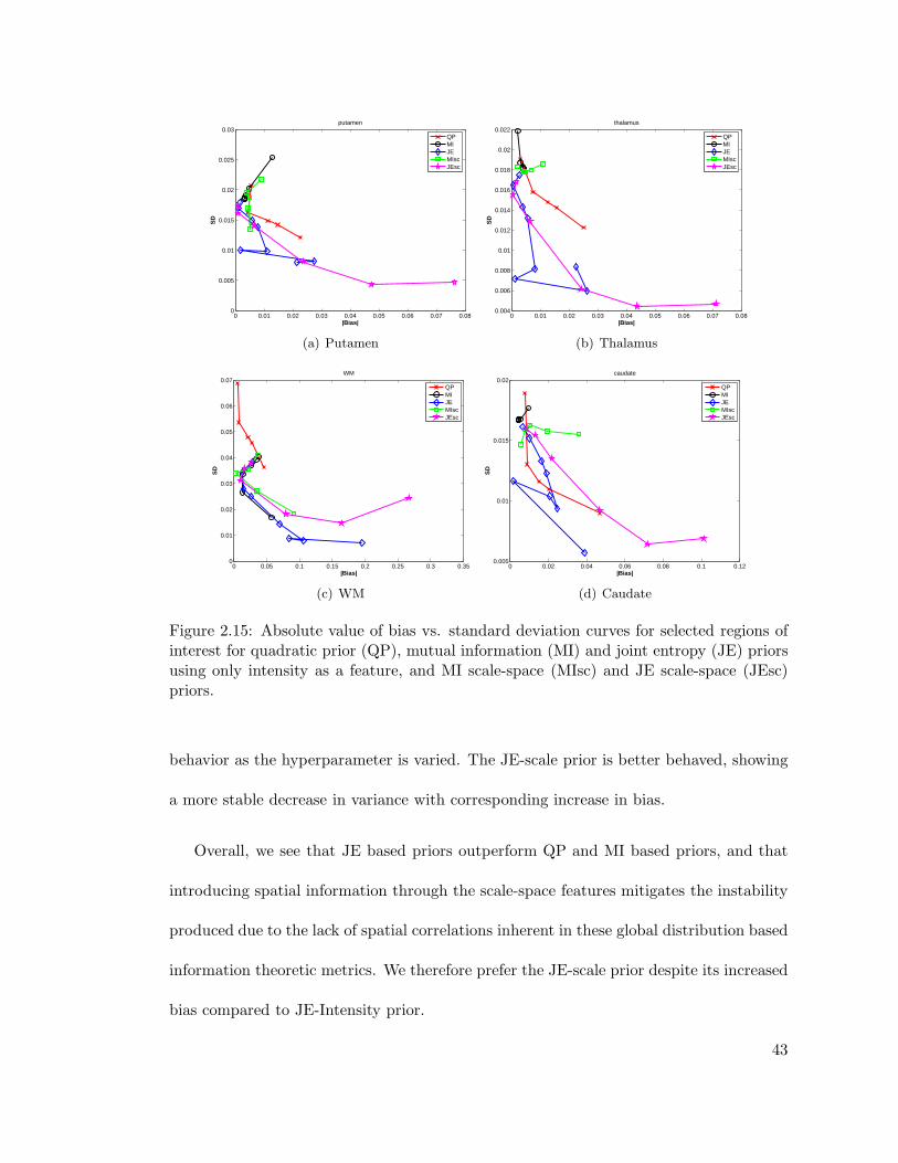
0 0.01 0.02 0.03 0.04 0.05 0.06 0.07 0.080

0.005

0.01

0.015

0.02

0.025

0.03putamen

|Bias|

SD

QPMIJEMIscJEsc

(a) Putamen

0 0.01 0.02 0.03 0.04 0.05 0.06 0.07 0.080.004

0.006

0.008

0.01

0.012

0.014

0.016

0.018

0.02

0.022thalamus

|Bias|

SD

QPMIJEMIscJEsc

(b) Thalamus

0 0.05 0.1 0.15 0.2 0.25 0.3 0.350

0.01

0.02

0.03

0.04

0.05

0.06

0.07WM

|Bias|

SD

QPMIJEMIscJEsc

(c) WM

0 0.02 0.04 0.06 0.08 0.1 0.120.005

0.01

0.015

0.02caudate

|Bias|

SD

QPMIJEMIscJEsc

(d) Caudate

Figure 2.15: Absolute value of bias vs. standard deviation curves for selected regions ofinterest for quadratic prior (QP), mutual information (MI) and joint entropy (JE) priorsusing only intensity as a feature, and MI scale-space (MIsc) and JE scale-space (JEsc)priors.

behavior as the hyperparameter is varied. The JE-scale prior is better behaved, showing

a more stable decrease in variance with corresponding increase in bias.

Overall, we see that JE based priors outperform QP and MI based priors, and that

introducing spatial information through the scale-space features mitigates the instability

produced due to the lack of spatial correlations inherent in these global distribution based

information theoretic metrics. We therefore prefer the JE-scale prior despite its increased

bias compared to JE-Intensity prior.

43

2.2.2 Clinical data

PET data was acquired on a Siemens Biograph True Point HD scanner from a Parkinsons

disease patient who was injected with [F-18]Fallypride. This tracer has a high affinity to

D2 receptors, which have a high density in the striatal regions of the brain. PET images

using this tracer show uptake mainly in the caudate and putamen subcortical nuclei

(jointly referred to as the striatum), and therefore this data would serve to both validate

the simulation results, and to investigate the behavior of the information theoretic priors

when the PET image intensities do not uniformly follow the variation in the anatomical

image intensities.

A T1 weighted MRI scan of the subject was performed on the same subject and is

used as the anatomical image for reconstruction. The MR image was registered to a

MAP with QP reconstructed image using MI based rigid registration in RView [42]. The

QP image along with the co-registered MR image is shown in Figure 2.16. Histogram

equalization was then performed on the MR image to improve contrast.

We initialized the MAP algorithm for all priors by the result of 2 iterations of OSEM

with 21 subsets, and ran 20 iterations of MAP. We used similar parameters for the bin

widths and Parzen variance as for the simulations. However, for the JE-scale prior,

we used a scale parameter of σ1 = 3.0 pixels, and dropped the Laplacian term. The

Laplacian of these PET images is non-zero in few voxels ( mainly in the striatal regions),

which produces a joint density of the Laplacian images consisting of a large peak around

zero, and a few peaks corresponding to the edges. Since the JE metric can produce

homogeneous solutions, it tends towards a Laplacian joint density which has one large

44

peak around zero, producing undesirable results. The marginal entropy term in the MI-

scale prior prevents this from occur

The images reconstructed using the different priors are shown in Figure 2.17 for the

slice corresponding to that of the anatomical image shown in Figure 2.16. The QP and

JE-scale reconstructions are overlaid on the anatomical image and the coronal, sagittal,

and transaxial views are shown in Figure 2.18. It can be seen that for QP, the activity

is often spread outside the anatomical region to which it belongs, while this spreading is

reduced for the priors using anatomical information.

We quantify the performance of these priors in terms of their contrast recovery coef-

ficient (CRC) as a function of noise. We define CRC between the uptake in a region of

the striatum and a region in the WM close to it as,

CRC =fStr

fWM

, (2.30)

where fStr is the mean activity in a region defined in the striatum, and fWM is the mean

activity in a WM region. We considered ROIs in the caudate region of the striatum,

and the WM that separates the caudate from the putamen on 11 contiguous slices of the

brain. One transaxial slice showing the ROIs for CRC computation are shown in Figure

2.19(a), with red and blue representing the caudate and WM ROIs. We computed the

noise variance from regions in the brain where we do not expect uptake of tracer, such as

the white matter in the posterior of the brain. The noise variance ROIs for one transaxial

slice is shown in Figure 2.19(b). The CRC vs noise plots are shown in Figure 2.20.

45

(a) (b)

Figure 2.16: Coronal slice of PET image (left) with co-registered MR image (right).

0

1

2

3

4

5

6

7

8

Figure 2.17: Coronal slice of PET image reconstructions: Top (L to R): QP(µ = 1.5),MI-Intensity(µ = 75000), JE-Intensity(µ = 1e5). Bottom (L to R): MI-scale(µ = 1e5),JE-scale(µ = 1e5).

These results demonstrate that the information theoretic priors can reconstruct high

contrast images that take advantage of anatomical image information, in a real world

scenario where the anatomical and functional images are independently acquired and

then registered to each other. Additionally, the results indicate that these priors can

be used even for tracers that bind non uniformly within regions of similar intensities

in the anatomical image (e.g., GM, WM, CSF for the brain), as long as the uptake is

homogeneous within some clearly delineated anatomical structure that is large enough to

form a prominent peak in the joint density.

46

Figure 2.18: Overlay of PET reconstruction over co-registered MR image for QP (top)and JE-scale (bottom) priors.

(a) (b)

Figure 2.19: Regions of interest for computing CRC vs noise curves: a)ROIs in caudate(red) and WM separating it from putamen (blue), (b) ROIs for computing noise variance

47

0.01 0.02 0.03 0.04 0.05 0.06 0.072.1

2.15

2.2

2.25

2.3

2.35

2.4

2.45

2.5

2.55

2.6

QPMIJEJEscMIsc

Figure 2.20: Contrast recovery coefficient versus noise variance plots as the hyperparam-eter is varied.

Figure 2.21: Reconstruction for high value of µ for MI-scale(left) and JE-scale(right)priors.

The CRC curves show that the information theoretic priors reconstructed images with

higher contrast than that of QP. While QP has a decreasing contrast and noise variance

as the hyperparameter is increased, the MI and JE based priors have increasing contrast

as µ is increased. An increasing µ would give larger weight on the prior, thus causing

the joint density to be more clustered, which would correspond to a higher contrast. We

see that consistent to our simulation results, the scale-space priors have reduced noise

variance compared to the intensity based priors, without appreciable loss in contrast.

48

The JE-scale prior gives the best contrast to noise performance among all the priors

considered.

However, we note that the behavior of the information theoretic priors is unpredictable

at high values of µ, where the prior dominates the likelihood term. MI tends to produce

images that spuriously follow the anatomical regions, whereas JE prefers a piecewise

homogeneous image, and may join regions that are close to each other in intensity. This

is illustrated in Figure 2.21, which shows the MI-scale and JE-scale reconstructions for

high values of µ.

This instability makes the choice of hyperparameter especially important for these

priors. We have observed that the knee of the L curve between the log likelihood and

log prior terms yields reasonable values of µ, but for clinical use, these results should

always be verified with the OSEM or MAP with QP results to ensure that no misleading

artifacts are produced.

2.3 Application of Information Theoretic Priors to Positron

Range Correction

In this section, we apply JE with scale-space features as a prior in conjunction with the

truncated homogeneous system model for positron range correction. The motivation for

using JE-scale priors for this application is to take advantage of anatomical information

to correct for the positron range effect where the truncated homogeneous system model is

insufficient. Using these priors can reduce blurring due to positron range outside regions

where uptake is expected, by using a co-registered anatomical image that delineates these

49

regions. Thus we aim to correct for positron range such that the PET image not only fits

the data, but also is most similar to the anatomical image in the information theoretic

sense.

The likelihood p(g|f) in Equation 2.1 is a Poisson likelihood function with mean Pf ,

where P is the system matrix that models the mapping from the source voxels to the

detectors. In [43] a factored system model is used, where this P matrix incorporates

detector blurring, detector sensitivity, and attenuation effects. Positron range effect can

also be included in this factored system model through a matrix Prange and the complete

system model can be written as

P = PsensPblurPattnPgeomPrange, (2.31)

where Pgeom represents the geometric projection from source to detector and Pattn, Pblur,

Psense, and Prange model the attenuation, detector blurring, sensitivity, and positron

range effects respectively. We use the truncated homogeneous model of [23] which can be

represented as

Prange = TPhomT, (2.32)

where Phom is a convolution matrix representing the spatially invariant blurring assumed

within the subject and T is a diagonal truncation matrix that truncates at the object

boundary.

We use the P matrix as defined in Equation 2.31 in the likelihood function to obtain

the objective function as defined in Equation 2.4, with the prior D(X,Y) being the

JE-scale prior defined as −H(X,Y), where X and Y are the scale-space features.

50

0

50

100

150

200

250

0

10

20

30

40

50

60

70

0

0.1

0.2

0.3

0.4

0.5

0.6

0.7

0.8

0.9

1

Figure 2.22: The phantoms used in the simulations to represent the MR image (left), thePET image (middle), and the truncation mask (right). The line in the PET image showsthe position of the profile shown in Fig. 2.25.

2.3.1 Positron Range Simulations

We used a 3D Hoffman brain phantom resampled to size 128 × 128 × 63 as our func-

tional image and scaled the three different regions (gray matter, white matter, and CSF)

differently to generate our anatomical image. A truncation mask for the homogeneous

truncated model was generated from the anatomical image, one transaxial slice of which

is shown along with the PET and anatomical images in Figure 2.22. For simulating

positron range blurring, we used the range kernel obtained from Monte Carlo simulations

of Cu-60 isotope in water, which has a range of 3.08mm [19] and is shown in Figure 2.23.

The same kernel is used for generating the data and for reconstruction. The simulations

are based on a Concorde R4 scanner, and the sinogram data obtained had 15 counts per

line of response. We used 30 PCG iterations to reconstruct all images at a voxel size of

0.4× 0.4 × 1.211 mm.

We compare three methods for reconstruction:

1. NRC-QP: No range correction and quadratic prior.

2. RC-QP: Range correction using the truncated homogeneous model, and quadratic

prior.

51

−4 −3 −2 −1 0 1 2 3 40

0.01

0.02

0.03

0.04

0.05

0.06

Distance(mm)

Ran

ge k

erne

l

Figure 2.23: Positron range kernel for Cu-60 isotope vs distance (mm)

0

50

100

Figure 2.24: Reconstructed images(L to R): No range correction with QP (NRC-QP) ,range correction with quadratic prior (RC-QP) with µ = 0.01, range correction with JEprior (RC-JE), scale σ = 0.5 voxels and µ = 5e4.

3. RC-JE: Range correction using truncated homogeneous model, and JE-scale prior.

The reconstructed images using NRC-QP, RC-QP, and RC-JE with scale σ = 0.5 voxels

are shown in Figure 2.24. A profile drawn through the reconstructed images is shown in

Figure 2.25.

It can be seen that without range correction, the reconstructed image is blurred and

the boundaries between GM/WM and WM/CSF are not clearly delineated. The RC-QP

images demonstrate improvement compared to the NRC-QP reconstruction, but we see

52

20 30 40 50 60 70 80 90 100 1100

10

20

30

40

50

60

70

80

90

100

TrueNRCRC−QPRC−JE

Figure 2.25: Profile drawn through true and reconstructed images

that the activity is overestimated close to the object boundary, and the internal structures

are still blurred. The RC-JE reconstruction is able to take advantage of the anatomical

information to provide sharper boundary definition even for the smaller internal structures

in the image. The overall normalized quantitation error between true and reconstructed

images is 0.6467 for NRC-QP, 0.5232 for RC-QP, and 0.1498 for RC-JE. Thus the JE

prior based reconstruction yields images with improved boundary definition and lower

quantitation error.

2.3.2 Real data results

PET data was acquired on a Focus 220 scanner from two mice that were injected with

Br-76 isotope. This isotope has a positron range of 3.47 mm. A CT image of these

mice was acquired on a microCT scanner at a resolution of 0.197 × 0.197 × 0.197 mm.

We reconstructed a PET image of size 256 × 256 × 95 at a resolution of 0.4 × 0.4 × 0.8

mm, without range correction and using a quadratic prior. The CT image was then

registered to the reconstructed PET image, and used as the anatomical image for the

53

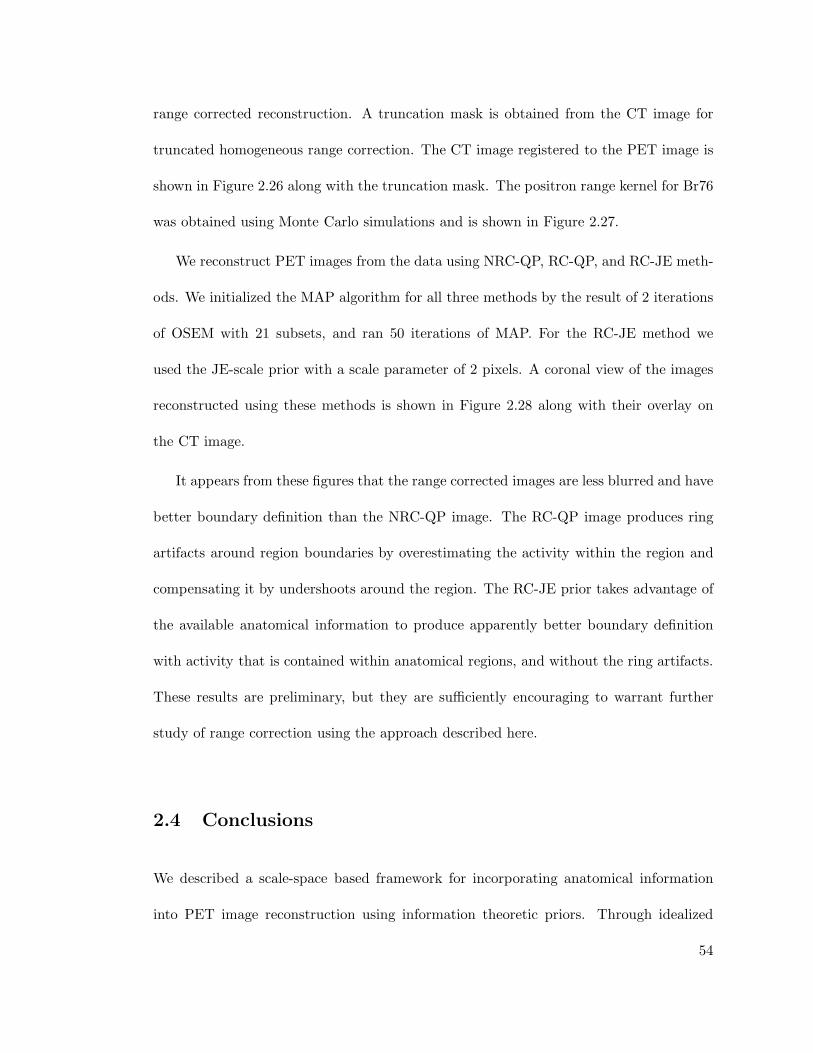
range corrected reconstruction. A truncation mask is obtained from the CT image for

truncated homogeneous range correction. The CT image registered to the PET image is

shown in Figure 2.26 along with the truncation mask. The positron range kernel for Br76

was obtained using Monte Carlo simulations and is shown in Figure 2.27.

We reconstruct PET images from the data using NRC-QP, RC-QP, and RC-JE meth-

ods. We initialized the MAP algorithm for all three methods by the result of 2 iterations

of OSEM with 21 subsets, and ran 50 iterations of MAP. For the RC-JE method we

used the JE-scale prior with a scale parameter of 2 pixels. A coronal view of the images

reconstructed using these methods is shown in Figure 2.28 along with their overlay on

the CT image.

It appears from these figures that the range corrected images are less blurred and have

better boundary definition than the NRC-QP image. The RC-QP image produces ring

artifacts around region boundaries by overestimating the activity within the region and

compensating it by undershoots around the region. The RC-JE prior takes advantage of

the available anatomical information to produce apparently better boundary definition

with activity that is contained within anatomical regions, and without the ring artifacts.

These results are preliminary, but they are sufficiently encouraging to warrant further

study of range correction using the approach described here.

2.4 Conclusions

We described a scale-space based framework for incorporating anatomical information

into PET image reconstruction using information theoretic priors. Through idealized

54

(a)

(b)

Figure 2.26: (a)CT image registered to reconstructed PET image and (b) truncationmask obtained from the CT image for truncated homogeneous model of range correction.

55

−5−4

−3−2

−10

12

34

5

−5

0

50

0.5

1

1.5

2

2.5

3

3.5

x 10−3

Distance(mm)

Distance(mm)

Ran

ge k

erne

l

Figure 2.27: Positron range kernel for Br-76.

Figure 2.28: Reconstructed images: Top row: Coronal slice of PET images reconstructedusing NRC-QP (left), RC-QP (middle), and RC-JE (right). Bottom row: Overlay on CTof the images shown in the top row.

56

simulations, realistic simulations, and clinical data, we evaluated the performance of

mutual information and joint entropy as priors in PET reconstruction . We presented an

efficient FFT based approach for the computation of these priors and their derivatives,

making it practical to use these priors for 3D image reconstruction.

The reconstructed images using the information theoretic priors have higher contrast

than those obtained using the quadratic prior, and look realistic without the mosaic-

like appearance that results from anatomical priors that impose piecewise smoothness.

Through simulation studies we showed that the marginal entropy term in MI tends to

increase the variance in the estimate of the image. We noted that testing the information

theoretic priors on piecewise constant images can give misleadingly accurate results while

using only intensity as a feature, especially for JE, since it prefers piecewise constant

images. The more realistic simulations that we performed show that using JE-Intensity is

prone to isolated hot and cold spots, and varies unpredictably with the hyperparameter. It

is therefore important to incorporate spatial correlations into these priors. The scale-space

based approach described in this dissertation improved the behavior of the information

theoretic priors, and the JE-scale prior gave better quantitation compared to QP while

using only two additional features, the coarser scale image and its Laplacian. The clinical

data results were consistent with the simulations, and show that these priors can be used

even for tracers that do not have homogeneous uptake in regions corresponding to similar

intensities in the anatomical image, provided the activity corresponds to a prominent

anatomical region.

It should however be noted that both mutual information and joint entropy priors in

PET reconstruction rely on the likelihood term to ensure convergence to an image with

57

the correct intensity. When the prior term dominated the objective function, MI tended

to produce an image that had a structure identical to the anatomical image, whereas

JE tended towards a piecewise homogeneous solution. This suggests that a weighting

between zero (JE) and one (MI) on the marginal entropy term of mutual information

could be used depending on the application.

We applied these information theoretic priors to a fundamental resolution limiting

problem in PET, positron range. These priors were used in conjunction with a truncated

homogeneous model for positron range that is incorporated into the system model. We

performed simulations that modeled the best case scenario where the PET and anatomical

images have identical structure, and the range kernel is the same for forward projection

and reconstruction. The results of these simulations indicate that using the JE-scale

prior with truncated homogeneous system model for range correction yielded images that

have better boundary definition and lower quantitation error than those obtained using no

range correction with QP or range correction with QP. We also performed reconstructions

from real data obtained by imaging mice that were injected with a long range isotope.

The results indicate that using the JE-scale prior along with a homogeneous system model

incorporating positron range is able to produce reconstructions with apparently better

boundary definition and without the ring artifacts that are produced by the RC-QP

method at regions where the system model is not accurate. The positron range modeling

used in these results is simple and does not consider the effects of spatially variant range

resulting from differences in electron density within the imaging volume. However, it is

promising that the JE based prior appears to perform well with experimental data, even

with this imperfect range model.

58

This framework of information theoretic priors can also be applied to other functional

imaging modalities where the data is severely ill-conditioned and the use of anatomical

information may improve the accuracy of reconstruction. Promising results were obtained

for diffuse optical tomography using this framework of information theoretic anatomical

priors [44]. For PET, we expect these priors to be most useful in applications involving

quantification of uptake in specific organs, where the uptake is within a region that is

clearly discernible in the anatomical image.

2.5 Appendix: Alternative formulation to the JE prior

Joint entropy between two random variables X and Y is defined as

H(X,Y ) = −

∫

p(x, y) log p(x, y)dxdy.

= −E(log p(X,Y )), (2.33)

This expectation can be approximated by the sample mean. If the intensities of image f

and a are realizations of X and Y respectively,

H(X,Y ) = −1

Ns

Ns∑

i=1

log p(fi, ai) (2.34)

If we use Parzen windows to estimate p as described in the chapter, then,

H(X,Y ) = −1

Ns

Ns∑

i=1

log(

Ns∑

j=1

φ(fi − fjσx

,ai − ajσy

)) (2.35)

59

The derivative of H(X,Y ) with respect to fm is then,

∂H(X,Y )

∂fm= −

1

Ns

Ns∑

i=1,i6=m

φ′(fi−fmσx

)φ(ai−amσy

)

p(fi, ai)

−1

Ns

Ns∑

i=1

φ′(fm−fiσx

)φ(am−aiσy

)

p(fm, am)(2.36)

Since we are using a symmetric Gaussian kernel with standard deviation σx for the

functional image, φ′(fi−fmσx

) = φ′(fm−fiσx

) = φ(fi−fmσx

)fi−fmσ2x

, we get

∂H(X,Y )

∂fm= −

1

Ns

Ns∑

i=1

(φ(fi−fm

σx)φ(ai−am

σy)

p(fi, ai)

+φ(fm−fi

σx)φ(am−ai

σx)

p(fm, am))(fi − fm

σ2x

). (2.37)

If we let

αim =φ(fi−fm

σx)φ(ai−am

σy)

p(fi, ai), and

βim =φ(fm−fi

σx)φ(am−ai

σy)

p(fm, am), (2.38)

then Equation 2.37 can be rewritten as,

∂H(X,Y )

∂fm= −

1

Ns

Ns∑

i=1

(αim + βim)(fi − fm

σ2x

),

= −1

Ns

Ns∑

i=1

Wim(fi − fm

σ2x

). (2.39)

60

The weights αim, and βim are both between 0 and 1, since the denominator in each of

these terms is obtained by a summation of the numerator over all m or i. The weight Wim

approaches 0 when fi and ai are distant from fm and am respectively , and approaches 2

when they are close . Hence, Wim selects the voxels with intensities that are within a few

standard deviations of fm in both the anatomical and functional images, and updates fm

such that the intensities in these voxels are clustered closer together.

The gradient in Equation 2.39 can be further approximated by considering only voxels

that are spatially close to the voxel m, i.e., in a neighborhood ηm, giving

∂H(X,Y )

∂fm= −

1

Ns

∑

i∈ηm

Wim(fi − fm

σ2x

). (2.40)

This expression is similar to that of the quadratic prior, except that the weight Wim

selects only those voxels within the neighborhood ηm that have intensities close to fm.

In this case, the voxels that are spatially close to each voxel influence the gradient rather

than the more global interaction described in Equation 2.39.

61

Chapter 3

Mutual Information Based Non-Rigid Mouse Registration

Using A Scale-Space Approach

Longitudinal and inter-subject studies are often performed in small animal imaging in or-

der to study changes in mouse anatomy and function over a period of time, or across popu-

lations. Changes in animal posture, tissue growth, organ movement and other anatomical

changes during longitudinal studies require non-rigid registration of the acquired images

for accurate analysis. Normalization of anatomical variability across populations in inter-

subject studies also requires non-rigid registration.

In this chapter, we describe a Gaussian scalespace theory based approach to simulta-

neously align global structure such as overall shape, as well as detail such as the skeleton,

in small animals. We extract scale-space feature vectors at each voxel of the target and

template images to be registered. Each feature vector is defined as a vector of the in-

tensities of its scale-space images at that voxel. Detail such as the skeletal structure is

visible in the lower scales and is blurred out at the higher scales, while the global struc-

ture such as overall shape remains in the images at the higher scales. The scale-space

feature vectors are aligned with the goal of finding a common mapping that aligns the

62

skeleton as well as overall shape in the mouse images. We do not explicitly impose any

rigidity constraints near the skeleton. We use mutual information (MI) as a similarity

metric between the target and template images since it measures the similarity between

distributions of intensities rather than actual values of intensities in the image, thus being

more robust to intensity differences in these images [13]. This multi-scale approach has

the additional advantage of having a cost function that is less prone to local minima [27],

and hence is able to perform large non-linear deformations accurately.

We parameterize the displacement field using the DCT basis, and use the Laplacian

of the field as a regularizing term. The DCT bases are eigen functions of the discrete

Laplacian, so using the DCT representation of the displacement field in conjunction with

Laplacian regularization simplifies the regularization term to a diagonal matrix. More-

over, the DCT basis gives an efficient representation of the displacement field, allowing

us to represent the field using only a few coefficients. Fast implementations of DCT are

readily available, and can be used to further reduce the computation time. In [45] a

similar parametrization is used for non-rigid registraton using SSD metric with Gauss

Newton optimization, which is fast but can be used only for the SSD metric. The Gauss-

Newton optimization also restricts the number of bases that can be used in practice. The

paper recommends the use of less than 8× 8 × 8 coefficients to avoid problems. We use

a conjugate gradient optimization with Armijo line search to optimize our cost function,

and there is no constraint on the number of bases that can be used.

We apply the scale-space registration algorithm to CT images from a longitudinal

mouse study. We compare the results of this scale-space approach with those obtained

by a hierarchical multi-scale approach that is commonly used in brain registration, where

63

images at each scale are aligned hierarchically, starting at the highest scale and ending

at the lowest scale.

3.1 Methods and Results

3.1.1 Mutual information based non-rigid registration

Let i1(x) and i2(x) represent the intensities of target and template images respectively

at position x. Let the transformation that maps the target to the template be T (x) =

x − u(x), where u(x) is the displacement field. Let the feature vectors extracted from

the target and template images at voxel x be i1(x) and i2(x) respectively. These can

be considered as realizations of the random vectors I1 and I2. Let Ns be the number of

features in each feature vector such that I1 = [I11 , I21 , · · · , I

Ns

1 ]T , where Ij1 is the random

variable corresponding to feature j of the target image. Then, the mutual information

between feature vectors of the target and deformed template, Du(I1, I2) is defined as [39],

Du(I1, I2) =

∫

pu(I1, I2) logpu(I1, I2)

p(I1)pu(I2)dI1dI2. (3.1)

A differentiable estimate of the density can be obtained using Parzen windows given by

[34],

pu(I1, I2) =∑

x

φ

(

I1 − i1(x)

ρ

)

φ

(

I2 − i2(x− u(x))

ρ

)

, (3.2)

where φ is a Gaussian window and ρ determines the width of the window.

64

We use the Laplacian of the displacement field as a regularizing term. The objective

function is given by

maxu

Du(I1, I2)− µ∣

∣

∣

∣∇2u(x)∣

∣

∣

∣

2, (3.3)

where µ is a hyperparameter that controls the weight on the regularizing term.

For simplicity, we assume independence between features so that MI between the feature

vectors simplifies to the sum of MI between the individual features.

Du(I1, I2) =

Ns∑

j=1

Du(Ij1 , I2

j). (3.4)

3.1.2 Scale-space feature vectors

We use a Gaussian scale-space theory based approach to define feature vectors that are

extracted from the images. We generate images at different scales by blurring the target

and template with Gaussian kernels of increasing widths. Let the width of the Gaussian

kernel at each scale be σj , j = 1, 2, · · · , Ns, such that σj > σk for j > k. Let the

smoothing kernel at scale j be represented by Sj(x). We define the scale-space based

feature vector as i1(x) = [i1(x)1, i1(x)

2, · · · , i1(x)Ns ], where i1(x)

j is the intensity of the

target image at scale j and position x, and is given by,

i1(x)j = Sj(x) ∗ i1(x). (3.5)

In this work, we use Ns=2, where the first scale corresponds to no smoothing and

σ2 = 3. A coronal slice of a mouse image at these scales is shown in Fig. 3.1.

65

Figure 3.1: Coronal slice of scale-space images of a mouse for Ns = 2, with scale 1corresponding to no smoothing (left) and σ2 =3 (right).

We generate the feature vector of the deformed template i2(x−u(x)) by first applying

the displacement field to the original template, and then generating the scale-space images

of that deformed image. So the feature i2(x− u)j is given by,

i2(x− u)j = Sj(x) ∗ (i2(x− u)). (3.6)

We observed that this performs better than deforming the original scale-space images

of the template. This could be because in our approach, we are retaining the original

relationship between intensities as a function of position in the template image while

computing i2(x− u(x)), and then computing the similarity metric between target and a

linear transformation (smoothing) of the deformed template. In contrast, applying the

displacement field to the original scale-space images will mean that we are computing

the similarity metric between the target and a new function (Sj ∗ i2)(x − u) of the

template. Though generating the scale-space feature vectors at every iteration increases

the computation, we take this approach for better accuracy.

66

3.1.3 Displacement field and regularization

The displacement field u(x) can be represented in terms of the DCT basis. Let bi(x)

and βi(x), i = 1, 2, · · · , Nb represent the DCT basis vectors, and the DCT coefficients

respectively. Then, the displacement field is given by,

u(x) =

Nb∑

i=1

βibi(x) = B(x)β, (3.7)

whereB(x) = [b1(x),b2(x), · · · ,bNb(x)], and the coefficient vector β = [β1, β2, · · · , βNb

]T .

The DCT basis vectors are eigen functions of the discrete Laplacian. Let L be the

discrete Laplacian matrix and γi, i = 1, 2, · · · , Nb be the eigen values of L corresponding

to the basis bi(x). Then,

Lu(x) = L

Nb∑

i=1

βibi(x) =

Nb∑

i=1

γiβibi(x) (3.8)

Hence, the discrete approximation of the norm of the Laplacian,∣

∣

∣

∣∇2u(x)∣

∣

∣

∣

2is given

by,

||Lu(x)||2 =

Nb∑

i=1

γi2βi

2. (3.9)

Thus we save the computation cost of the matrix vector multiplication required by the

left hand side of Equation 3.9, by reducing it to the vector norm on the right hand side.

Additionally, since the DCT gives a sparse representation, we can model the displacement

field with Nc < Nb coefficients to reduce computation time further.

67

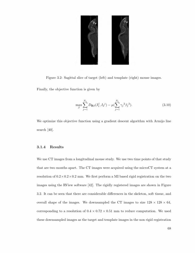
Figure 3.2: Sagittal slice of target (left) and template (right) mouse images.

Finally, the objective function is given by

maxβ

Ns∑

j=1

DBβ(Ij1 , I2

j)− µ(

Nc∑

j=1

γj2βj

2). (3.10)

We optimize this objective function using a gradient descent algorithm with Armijo line

search [40].

3.1.4 Results

We use CT images from a longitudinal mouse study. We use two time points of that study

that are two months apart. The CT images were acquired using the microCT system at a

resolution of 0.2×0.2×0.2 mm. We first perform a MI based rigid registration on the two

images using the RView software [42]. The rigidly registered images are shown in Figure

3.2. It can be seen that there are considerable differences in the skeleton, soft tissue, and

overall shape of the images. We downsampled the CT images to size 128 × 128 × 64,

corresponding to a resolution of 0.4 × 0.72 × 0.51 mm to reduce computation. We used

these downsampled images as the target and template images in the non rigid registration

68

algorithm. We use two scales to form our feature vectors- the unsmoothed image, and the

image smoothed by a Gaussian kernel of size [7x7x7] and width σ = 3. We use Nc = 30

DCT bases and µ = 5e − 6. We first perform the non-rigid registration at only the

higher scale (σ = 3), and we use this to initialize the scale-space non rigid registration.

Registration at only the lower scale (unsmoothed images) gave a local minimum that

would not be a good initialization.

We compare the scale-space registration results to those of hierarchical multi-scale

registration. We used the same number of DCT bases and the same scales as the scale-

space registration, with µ = 2e − 5. We first registered the smoothed images, and used

the resulting displacement field to initialize the registration for the unsmoothed images.

The overlay on the target image of the template image, and images registered using both

approaches are shown in Fig. 3.3. We applied the displacement field resulting from both

registration algorithms to the higher resolution (0.2 mm) images for display purposes.

The displacement field obtained from the scale-space registration is shown in Fig. 3.4,

for the coronal and sagittal slices shown in Fig. 3.3

It can be seen that the scale-space non-rigid registration algorithm gives better skele-

tal, limb, and soft tissue (such as liver and heart) alignment than the hierarchical multi-

scale algorithm.

3.2 Discussion

We used a scale-space theory based approach for non-rigid mouse registration using mu-

tual information. We used the DCT basis to efficiently represent the displacement field,

69

Figure 3.3: Comparison of registered images: Coronal and sagittal views of overlay ontarget image of template (top row), hierarchical multi-scale registered image (middle row),and scale-space registered image (bottom row).

70

Figure 3.4: Displacement field obtained from scale-space registration

as well as to simplify the Laplacian regularization term. We generated the scale-space

feature vectors at each iteration after applying the displacement field to the original im-

ages, since this approach gave better accuracy. We applied this algorithm to CT images

of a mouse in a longitudinal study.

By using images at different scales simultaneously, we obtained better alignment of

the global structure such as the overall shape of the mouse as well as improved align-

ment of detail such as the skeleton, compared to the hierarchical multi-scale approach.

Additionally, using multiple scales simultaneously gives a cost function that is less prone

to local minima. Though these results are encouraging, we note that this approach is

computationally intensive. We also note that using non-parametric density estimation in

conjunction with non-rigid MI based registration might pose problems because of the high

dimensionality of the problem coupled with the non-convexity of the cost function. In the

next chapter, we explore an alternative formulation for non-rigid registration that deals

71

with the high dimensionality of the combined density and displacement field estimation

problems.

72

Chapter 4

Non-Rigid Registration Using Gaussian Mixture Models

Registration techniques that use mutual information as a similarity metric typically use

a non-parametric approach for estimating the unknown distribution of intensities in the

images [13], [28] - [30], [Chapter 3]. This framework has some limitations when dealing

with the high dimensional non-rigid registration problem. Firstly, mutual information is

a non-convex function of the registration parameters and the registration could converge

to an inaccurate local optimum. This problem is exacerbated for the non-rigid registra-

tion case due to the increase in dimensionality of the deformation field to be estimated

compared to the rigid registration case, for which this framework has been successfully

applied [13]. Secondly, the non-parametric Parzen based approach that is typically used

in MI based registration estimates the entire joint density from the images, and this joint

density is then used to estimate the deformation field. Using these two high dimensional

estimation steps in conjunction with each other could result in a registration that is sen-

sitive to small changes in the images, thus making it more susceptible to local optima.

Additionally, the Parzen window method requires appropriate choice of the Parzen win-

dow width, which is usually taken as a design parameter, and is kept fixed over the entire

73

sample [34]. This has the drawback that for long-tailed distributions the density estimate

tends to be noisy at the tails, and increasing the window width to deal with this might

lead to oversmoothing the details in the distribution [46]. This would mean that the

former scenario results in a cost function that has more local optima, while the latter

could lead to inaccurate registration results. This approach also requires a large number

of samples to accurately estimate the distribution.

In this chapter, we describe an alternative approach for multi-modality non-rigid

registration that uses the log-likelihood of the target image given the deformed template as

a similarity metric for non-rigid registration, wherein the log-likelihood is modeled using

Gaussian mixture models (GMM). Gaussian distributions are commonly used in image

segmentation to represent the distribution of intensities corresponding to a particular

tissue type in MR or CT images [47]. The joint distribution of two MR or CT images

is characterized by localized blobs that can also be modeled as a mixture of Gaussians.

Using GMMs reduces the density estimation step to that of estimating the parameters of

the GMM, which consist of the mean, covariance, and weight of each Gaussian. Since the

estimated parameters can be different for each Gaussian, the density estimates obtained

using this approach are smoother than the non-parametric approach while retaining the

detail in the distribution. We choose the number of components in the GMM from

the joint histogram of the target and template images, and keep this number constant

throughout the registration. This can hence be considered as a semi-parametric approach

to density estimation. For images that have a few distinct regions of intensity such as

brain or mouse images, the number of parameters to be estimated is small, and can be

robustly estimated from fewer samples compared to the non-parametric approach.

74

Our approach of using the log-likelihood of the target given the template in con-

junction with a GMM can be viewed as a semi-parametric approximation to MI based

registration. However, we expect our GMM based approach to perform better than the

non-parametric MI based approach because of (1) reduced overall dimensionality of the

registration problem through the parametrization of the density estimation step, and (2)

more robust and accurate estimation of the joint density. Additionally, we parameter-

ize the displacement field using the DCT basis, and use the Laplacian of the field as a

regularizing term as described in Chapter 3.

We compare the performance of the conditional likelihood metric with GMM parametriza-

tion, with that of MI with non-parametric density estimation approach. We will hence-

forth refer to these methods as the GMM-Cond and the Parzen-MI approaches respec-

tively. We evaluate these methods using intra-modality brain MR images, as well as

inter-subject, inter-modality mouse images. Registration of mice and other small ani-

mals is challenging because of the presence of rigid skeleton within non-rigid soft tissue,

and it has been observed that though the existing non-rigid registration algorithms have

been applied to brain imaging with encouraging results, they do not perform well for

small animal images [31] -[33]. We test the performance of our approach for both brain

as well as mouse imaging to evaluate potential in clinical as well as pre-clinical imaging

applications.

75

4.1 Methods and Results

Let the target and template images be I1 and I2, and their intensity at position x be

i1(x) and i2(x) respectively. Let the transformation that maps the template to the target

be T (x) = x − u(x), where u is the displacement field. The deformed template is then

represented by Iu2 , whose intensities are given by i2(x − u(x)). We define the similarity

metric Du(I1, I2) between the target and deformed template as the log likelihood of the

target given the deformed template. Assuming that the voxel intensities in I1 and I2

are independent identically distributed random variables with joint density p(i1, i2), the

similarity metric is given by,

Du(I1, I2) = log p(I1|Iu

2 )

=∑

x

logp(i1(x), i2(x− u(x)))

p(i2(x− u(x))). (4.1)

We assume a Gaussian mixture model for the joint and marginal densities p(i1, i2) and

p(i2). Let the number of components of the Gaussian mixture model be K, the mixing

proportions be πk, and g(i1, i2|mk,Σk) be a Gaussian with mean mk and covariance

Σk, where k = 1, 2, · · · ,K. Let the unknown GMM parameters for each component k

be represented as θk = (πk,mk,Σk), and let Θ = [θ1, θ2, · · · , θK ] be the vector of all

unknown parameters. Then, the joint density is given by

p(i1, i2|Θ) =

K∑

k=1

πkg(i1, i2|mk,Σk), (4.2)

where πk > 0 and∑K

k=1 πk = 1.

76

We use the Laplacian of the displacement field as a regularizing term R(u) to penalize

deformations that are not smooth. Let L be the discrete Laplacian matrix. The objective

function is then given by,

maxu,Θ

∑

x

log p(i1(x)|i2(x− u(x)),Θ) − µ ||Lu||2 , (4.3)

where µ is a hyperparameter that controls the weight on the regularizing term.

To simplify the problem, we replace the combined optimization with respect to the

deformation field and GMM parameters with an iterative two step procedure. Here,

the GMM parameters are first estimated from the target and deformed template images

through maximum likelihood estimation, and the deformation field is then estimated

given the estimated GMM parameters. The two step optimization is given by

Θ(um) = argmaxΘ

∑

x

log p(i1(x), i2(x− um(x))|Θ) (4.4)

um+1 = argmaxu

∑

x

log p(i1(x)|i2(x− u(x)), Θ(um))

− µ ||Lu||2 , (4.5)

where um represents the estimated deformation field at overall optimization iteration m.

4.1.1 Estimation of parameters of Gaussian mixture model

The maximum likelihood estimate of the GMM parameters Θ in equation 4.4 can be

obtained by the EM algorithm [48]. Let the data sample at voxel j corresponding to

77

the position xj be Suj = [i1(xj), i2(xj − u(xj))]

T , where j = 1, 2, · · · , N , and N is the

number of voxels in each image. The component of the GMM from which Sj arises is

taken as the hidden variable in the EM algorithm. The EM update equations are given

by,

τ ijk =πikg(S

u

j ,mik(u),Σ

ik(u))

∑Kh=1 π

ih(u)g(S

uj ,m

ih(u),Σ

ih(u))

(4.6)

πi+1k (u) =

1

N

N∑

j=1

τ ijk (4.7)

mi+1k (u) =

∑Nj=1 τ

ijkS

u

j∑N

j=1 τijk

(4.8)

Σi+1k (u) =

∑Nj=1 τ

ijk(S

u

j −mi+1k (u))(Su

j −mi+1k (u))T

∑Nj=1 τ

ijk

, (4.9)

where πik(u),m

ik(u), and Σi

k(u) are the GMM parameter estimates at EM iteration i and

deformation field u.

The objective function to be optimized in equation 4.4 is a non-convex function of Θ,

so a good initial estimate is needed to converge to the correct local optimum. We use

the k-nearest neighbors algorithm [34] to identify cluster centers in the joint histogram

of the target and template images, and the number of samples that fall into a particular

cluster. The cluster centers and the proportion of samples in a cluster relative to the

total number of samples were used as the initializations m0k and p0k respectively, and Σ0

k

was assumed to be identity for all k. The number of clusters was chosen to match the

initial histogram of the two images, after which it was kept constant throughout the

registration process. Figure 4.1 shows an example of a pdf estimated using GMM. Two

brain images were considered, transaxial slices of which are shown in Figure 4.1(a) and

78

in Figure 4.1(b). The joint histogram of the intensities of these two images is shown

in Figure 4.1(c), and the pdf estimated using GMM is shown in Figure 4.1(d) with the

component means overlaid on it. The number of components was chosen to be K = 6 to

match the joint histogram.

In the GMM based approach for probability density estimation, the number of pa-

rameters to be estimated is K +KD +KD(D + 1)/2, where D is the dimensionality of

the sample, and K is the number of components in the GMM. For registration of two

images D = 2, so the number of parameters is 6K, which is small for small values of

K. On the other hand, the non-parametric Parzen based estimation computes the en-

tire Nbin × Nbin pdf from the samples, where Nbin is the number of bins at which the

pdf is computed. We expect to gain computationally as well as in robustness, from this

reduction in dimensionality of the problem. However, if the joint density does not fit a

GMM, the number of mixture components might be large, approaching a Parzen window

estimate.

4.1.2 Estimation of displacement field

Let the objective function in equation 4.5 be represented by Jm(u), which can be rewritten

as

Jm(u) = Du(I1, I2|Θ(um))− µR(u) (4.10)

We use conjugate gradient (CG) optimization to optimize this objective function with

an Armijo line search [40]. Let u(i) be the estimate of deformation field at CG iteration

i. Let the gradient vector be d(i) = ∇Jm(u)|u=u(i) , the conjugate gradient direction

79

(a) (b)

50 100 150 200 250

50

100

150

200

250

(c)

50 100 150 200 250

50

100

150

200

250

(d)

Figure 4.1: Estimation of GMM parameters: (a) Target image, (b) Template image, (c)Joint histogram of intensities of target and template images,(d) Joint pdf of target andtemplate images computed using GMM (the component means shown with ’x’ marks).

80

vector be b(i), and the step size computed from the line search be α(i). The CG update

equations are given by

u(i+1) = u(i) + α(i)b(i) (4.11)

b(i) = d(i) + β(i−1)b(i−1) (4.12)

β(i−1) =

(

d(i) − d(i−1))T

b(i)

d(i−1)Tb(i−1). (4.13)

The algorithm is initialized by b(0) = d0. If the CG algorithm converges in r iterations,

the estimated deformation field in equation 4.5 is um+1 = u(r).

The gradient vector d is given by

d =∂

∂uDu(I1, I2)− µ

∂

∂uR(u), (4.14)

where ∂∂u

Du(I1, I2) and ∂∂u

R(u) are the gradients of the similarity metric and the reg-

ularizing terms respectively. The gradient of the similarity metric with respect to the

displacement field at voxel position xl is given in equation 4.15, where i1(l) and iu2 (l) are

shorthand notations for i1(xl) and i2(xl−u(xl)) respectively, the intensities of the target

and deformed template at xl are represented by Su

l = [i1(l), iu2 (l)]

T , and ∇iu2 (l) is the

spatial gradient of the deformed template at xl. The gradient of the regularizing term is

given in equation 4.16.

81

∂Du(i1, i2)

∂u(xl)=

∇iu2 (l)

p(i1(l), iu2 (l))

K∑

k=1

πkg(Su

l |Θ(um))

[

0 1

]

Σ−1k

i1(l)−mk,1

iu2 (l)−mk,2

−∇iu2 (l)

p(iu2 (l))

K∑

k=1

πkg(iu

2 (l))|mk,2,Σk,2,2)(iu2 (l)−mk,2)

Σk,2,2, (4.15)

∂

∂uR(u) = 2LTLu. (4.16)

We use a DCT parametrization of the displacement field as described in Chapter 3.

The objective function is finally given by

maxβ

DBβ(I1, I2|Θ)− µ

Nc∑

i=1

γi2βi

2, (4.17)

where B, β represent the DCT bases and coefficients respectively, and γi, i = 1, 2, · · · , Nb

represents the eigen values of L corresponding to the ith basis vector.

Since the DCT is a linear transformation of u, the gradient with respect to β can be

obtained in terms of the gradient with respect to u as

∂

∂βDBβ(I1, I2) = BT ∂

∂uDu(I1, I2) (4.18)

Thus the gradient can be computed by using equation 4.15 and then taking its DCT .

The gradient of the regularizer is

∂

∂βR(Bβ) = 2Λβ, (4.19)

82

where Λ is a diagonal matrix with elements [γ21 , γ22 , · · · , γ

2Nc

].

4.1.3 Relation to Mutual Information

Let the random variables corresponding to the intensities of I1 and Iu2 be ζ1 and ζ2

respectively. Mutual information between ζ1 and ζ2 is defined as [39],

D(ζ1, ζ2) =

∫

p(z1, z2) logp(z1, z2)

p(z1)(z2)dz1dz2

= E(logp(z1, z2)

p(z1)p(z2)). (4.20)

MI between two random variables can be interpreted as the reduction in uncertainty of

one random variable given the other. Using MI as a similarity metric for registration aims

to find a deformation that makes the joint density of the target and deformed template

images maximally clustered, thus implying that the uncertainty of one image given the

other is minimized.

An alternative formulation can be obtained by approximating the expectation in equa-

tion 4.20 by a sample mean where the intensity at each voxel in the target and deformed

template images constitutes the random sample. Hence we get

D(ζ1, ζ2) =1

N

∑

x

logp(i1(x), i2(x− u(x)))

p(i1(x))p(i2(x− u(x)))

=1

N

∑

x

logp(i1(x), i2(x− u(x)))

p(i2(x− u(x)))

−1

N

∑

x

log p(i1(x)). (4.21)

83

Since the target is fixed and independent of u(x), dropping the terms containing the

marginal density p(i1), we get the approximate MI based similarity metric as

D(ζ1, ζ2) =1

N

∑

x

logp(i1(x), i2(x− u(x)))

p(i2(x− u(x))). (4.22)

Thus, computing the deformation field that maximizes mutual information is approx-

imately equivalent to maximizing the conditional density of the target given the template

image as defined in Equation 4.1. In [36] a similar relationship between maximum likeli-

hood and conditional entropy was derived. The pdf p(i1, i2) is unknown, and needs to be

estimated. The pdf can be estimated using a non-parametric approach such as Parzen

windowing, or a GMM based approach can be taken to parametrize the pdf and estimate

those parameters. The approach taken to estimate the pdf causes differences in the be-

havior of these metrics, and we will explore these differences by looking at the gradient

equations of these two methods.

The Parzen window estimate of a pdf at random variable values z1, z2 is defined by

[34]

p(z1, z2) =1

N

N∑

j=1

g(z1 − i1(j)

σ)g(

z2 − iu2 (j)

σ), (4.23)

where g(z2σ) is a Gaussian window of width σ, which is usually taken as a design parameter.

Note that this can be considered as a Gaussian mixture model with the fixed parameters

K = N , πk = 1N, mk = [i1(k), i

u2 (k)]

T , and Σk =

σ2 0

0 σ2

.

The gradient of Parzen based MI cost function with respect to the displacement field

at voxel l is then given by

84

D(ζ1, ζ2)

∂u(l)

= −1

N

∑

z1,z2

(1 + log p(z1, z2))g(z1 − i1(l)

σ)g′(

z2 − iu2 (l)

σ)∇iu2 (l)

+1

N

∑

z2

(1 + log p(z2))g′(z2 − iu2 (l))∇iu2 (l), (4.24)

where g′(z2 − iu2 (l)) = g(z2−iu2 (l)

σ)z2−iu2 (l)

σ2 .

We can rewrite the gradient equation for the GMM-Cond approach in Equation 4.15

as

∂Du(i1, i2)

∂u(xl)=

∇iu2 (l)

p(i1(l), iu2 (l))

K∑

k=1

πkg′(Su

l |Θ(um))−∇iu2 (l)

p(iu2 (l))

K∑

k=1

πkg′(iu2 (l)|mk,2,Σk,2,2)

where g′(Su

l |Θ(um)) =

[

0 1

]

Σ−1k

i1(l)−mk,1

iu2 (l)−mk,2

. Thus, in both Parzen-MI as

well as the GMM-Cond approaches, the gradient expressions have the derivative of a

Gaussian weighting the summand. In Parzen-MI case, the Gaussian that is being differ-

entiated has a mean given by the data sample at which it is centered, and a fixed variance

over the entire sample. In the GMM case, the Gaussian has a mean and covariance given

by the estimated GMM component mean and covariance. The Gaussian derivative has a

large magnitude for values that are close to but not equal to the mean, and low every-

where else. A plot of g′(z2) is shown for a Gaussian window of width σ = 2 in Figure

4.2. Thus, for MI, the gradient selects the voxels that are close (within a few standard

deviations (SDs) of Parzen window width) in intensity to a pdf bin value, and in order

85

−10 −8 −6 −4 −2 0 2 4 6 8 100

0.02

0.04

0.06

0.08

0.1

0.12

0.14

0.16

0.18

0.2

(a)

−10 −8 −6 −4 −2 0 2 4 6 8 10−0.08

−0.06

−0.04

−0.02

0

0.02

0.04

0.06

0.08

(b)

Figure 4.2: (a) Gaussian window of width σ = 2, and (b) its derivative.

to increase MI, deforms the image such that these voxel intensities get closer to that bin.

The GMM based approach on the other hand, selects voxels that are within a few SDs

of the estimated GMM mean, and tries to get the voxel intensities closer to the mean.

The GMM approach can thus be more robust to local minima, since the Parzen approach

might produce deformations that have regions of misalignment because of splitting a large

cluster in the joint density into multiple localized peaks around certain bin values.

We therefore expect the GMM-Cond approach to have the following two advantages

over the Parzen-MI approach.

1. The density estimation is reduced to that of estimating 6K GMM parameters that

can be robustly estimated from the given images for small K.

2. Estimation of displacement field may be more robust to local minima since the

gradient tries to form localized peaks around the estimated GMM means in the

joint pdf, rather than around the closest pdf bin.

86

4.1.4 Results

We perform validation studies of our method using (1) brain images, and (2) mouse

images. Through these studies, we evaluate the performance of our approach in brain

imaging as well as small animal imaging. Brain images usually consist of three distinct

regions of intensity, the gray matter, white matter, and cerbro-spinal fluid. Thus the

distribution of intensities of these images can be modeled using a GMM with a small

number of components, making the GMM-Cond approach feasible. Similarly mouse CT

images typically consist of mainly soft tissue versus bone contrast, and can be assumed

to follow a GMM. Though mouse MR images have a larger number of intensity levels

than the CT, the number of components required in the GMM is not prohibitively large.

4.1.5 Brain Image registration

We randomly chose 9 brains from the Internet Brain Segmentation Repository (IBSR)

provided by the Center for Morphometric Analysis at Massachusetts General Hospital

and is available at http://www.cma.mgh.harvard.edu/ibsr/. This dataset contains T1

weighted MR images along with their manual segmentations. We skull-stripped the brains

using the available manual segmentations, and performed histogram equalization on their

intensities to enhance contrast. Each brain from this dataset is used as an atlas that is

registered to the rest of the brains, thus giving 72 registrations in total. We first rigidly

registered each atlas to each target using AIR registration [49], [50], and then performed

non-rigid registration using the GMM-Cond, Parzen-MI, and SSD methods to register

these images. Though SSD is not a multi-modality metric like conditional likelihood

and MI, it is widely used for intra-modality registration and hence we include it in our

87

evaluation. For all three methods, we used 30 × 30 × 30 DCT bases, and conjugate

gradient optimization. Additionally, for all three methods, we check the determinant of

the Jacobian of the deformation field for negative values, and choose a value of µ to weight

the regularization term such that the Jacobian determinant has no negative values. This

ensures a smooth deformation field for all methods considered.

For the Parzen-MI registration we followed a hierarchical approach, first aligning the

images that were smoothed with a Gaussian of width 3 voxels, and using the displacement

field thus obtained to initialize the registration of the original images. We observed that

directly aligning the original images causes the algorithm to reach an inaccurate local

minimum. A Parzen window width of σ = 2 was used to compute the distribution at

every iteration. For the GMM-Cond approach, we used K = 6 components in the GMM,

and 5 overall iterations between the density estimation and deformation field estimation.

Each displacement field estimation in the GMM-Cond approach involved 50 iterations of

the conjugate gradient algorithm.

The registration results for one atlas to target registration are shown in Figure 4.3.

The corresponding displacement field obtained from GMM-Cond registration is shown in

Figure 4.4. The joint density estimated using the Parzen window and GMM methods

before and after registration of the brains is shown in Figure 4.5. It can be seen that the

GMM-Cond approach is able to cluster the intensities more tightly along the diagonal

than the MI-Parzen approach, implying a better alignment. The registration accuracy is

evaluated based on the following metrics:

88

(a) (b)

(c) (d)

(e)

Figure 4.3: Registration results for one dataset:(a) Target, (b)Atlas, (c) SSD registeredimage, (d)Parzen-MI registered image, and (e) GMM-Cond registered image.

89

50 100 150 200 2500

20

40

60

80

100

120

140

160

180

Figure 4.4: Displacement field obtained from GMM-Cond registration corresponding tothe slice shown in Figure 4.3.

(a) (b)

(c) (d)

Figure 4.5: Comparison of Parzen-MI vs GMM-Cond based methods: Log of the estimateof initial joint density between target and template images using (a) Parzen windonmethod, (b) GMM method (the ’x’ marks denote the GMM means) , and log of theestimate of joint density between target and registered template using (c) Parzen windowmethod and (d) GMM method.

90

1. Dice coefficients: Dice coefficient is a measure of the amount of overlap in sets A

and B, and is defined as,

d = 2|A ∩B|

|A|+ |B|, (4.25)

where |A| denotes the number of elements in the set A.

We use dice coefficients to evaluate registration accuracy in terms of its ability

to align various segmented regions of the brain. The deformation field obtained

from each atlas-target registration is applied to the labels of the atlas to obtain

the segmentation of the target image. The dice coefficients between the manual

segmentation of the target image, and that obtained by atlas based segmentation

is computed. The mean dice coefficients over all 72 atlas-target registrations are

shown for various brain regions in Figure 4.6.

2. Normalized mean squared difference between intensities: The images used are all

T1 weighted MR images, and computing the squared difference between the target

and deformed atlas image intensities gives a measure of registration accuracy. Since

SSD optimizes this metric, we expect this approach to have the best performance

for this metric. However, for the Parzen-MI and the GMM-Cond methods, this

would be an unbiased measure of registration accuracy. The MSE values are shown

in a box plot for the SSD, Parzen-MI, and GMM based methods in Figure 4.7.

3. Qualitative comparison : The deformed atlases registered to each image are av-

eraged to produce an image that would look more blurred if the registration was

inaccurate. The images obtained by averaging the atlases deformed to match one

target brain are shown in Figure 4.8 for the MI and GMM based methods.

91

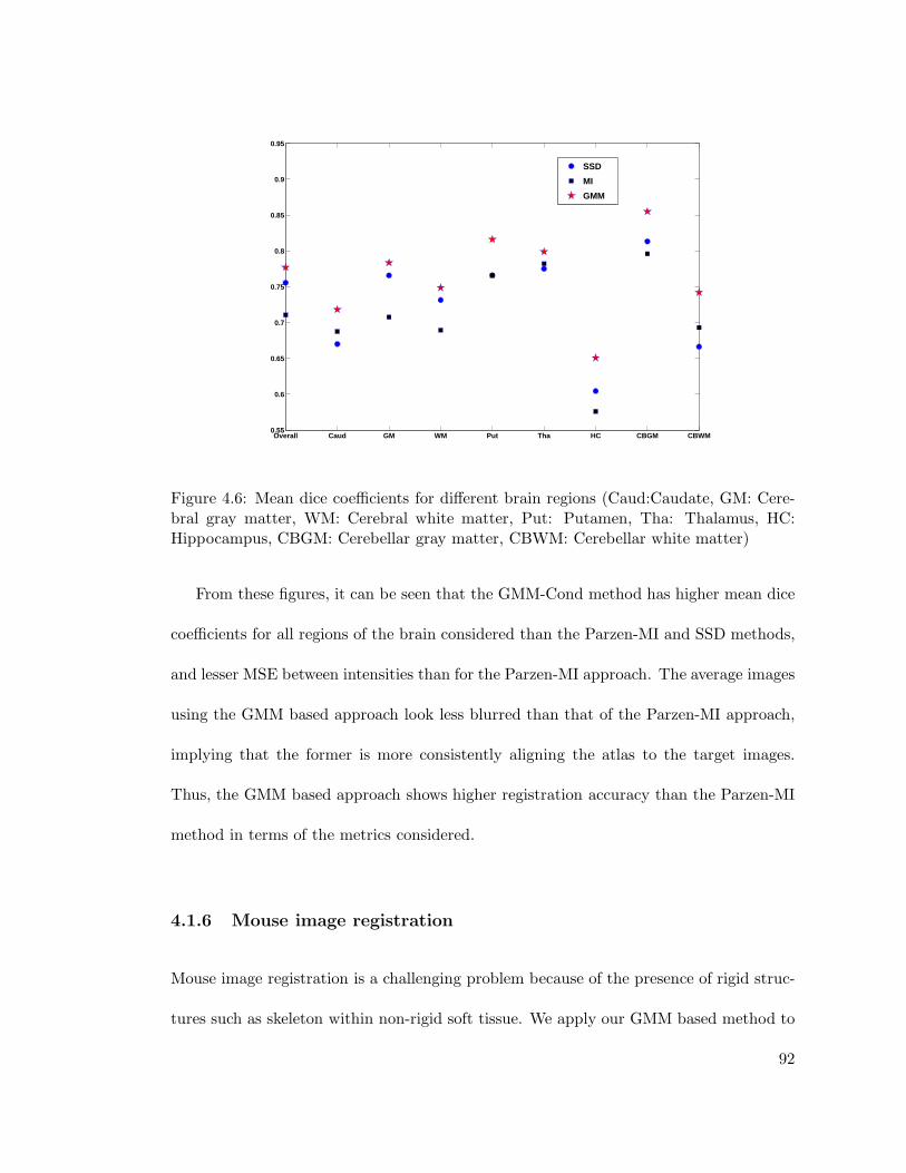
Overall Caud GM WM Put Tha HC CBGM CBWM0.55

0.6

0.65

0.7

0.75

0.8

0.85

0.9

0.95

SSD

MI

GMM

Figure 4.6: Mean dice coefficients for different brain regions (Caud:Caudate, GM: Cere-bral gray matter, WM: Cerebral white matter, Put: Putamen, Tha: Thalamus, HC:Hippocampus, CBGM: Cerebellar gray matter, CBWM: Cerebellar white matter)

From these figures, it can be seen that the GMM-Cond method has higher mean dice

coefficients for all regions of the brain considered than the Parzen-MI and SSD methods,

and lesser MSE between intensities than for the Parzen-MI approach. The average images

using the GMM based approach look less blurred than that of the Parzen-MI approach,

implying that the former is more consistently aligning the atlas to the target images.

Thus, the GMM based approach shows higher registration accuracy than the Parzen-MI

method in terms of the metrics considered.

4.1.6 Mouse image registration

Mouse image registration is a challenging problem because of the presence of rigid struc-

tures such as skeleton within non-rigid soft tissue. We apply our GMM based method to

92

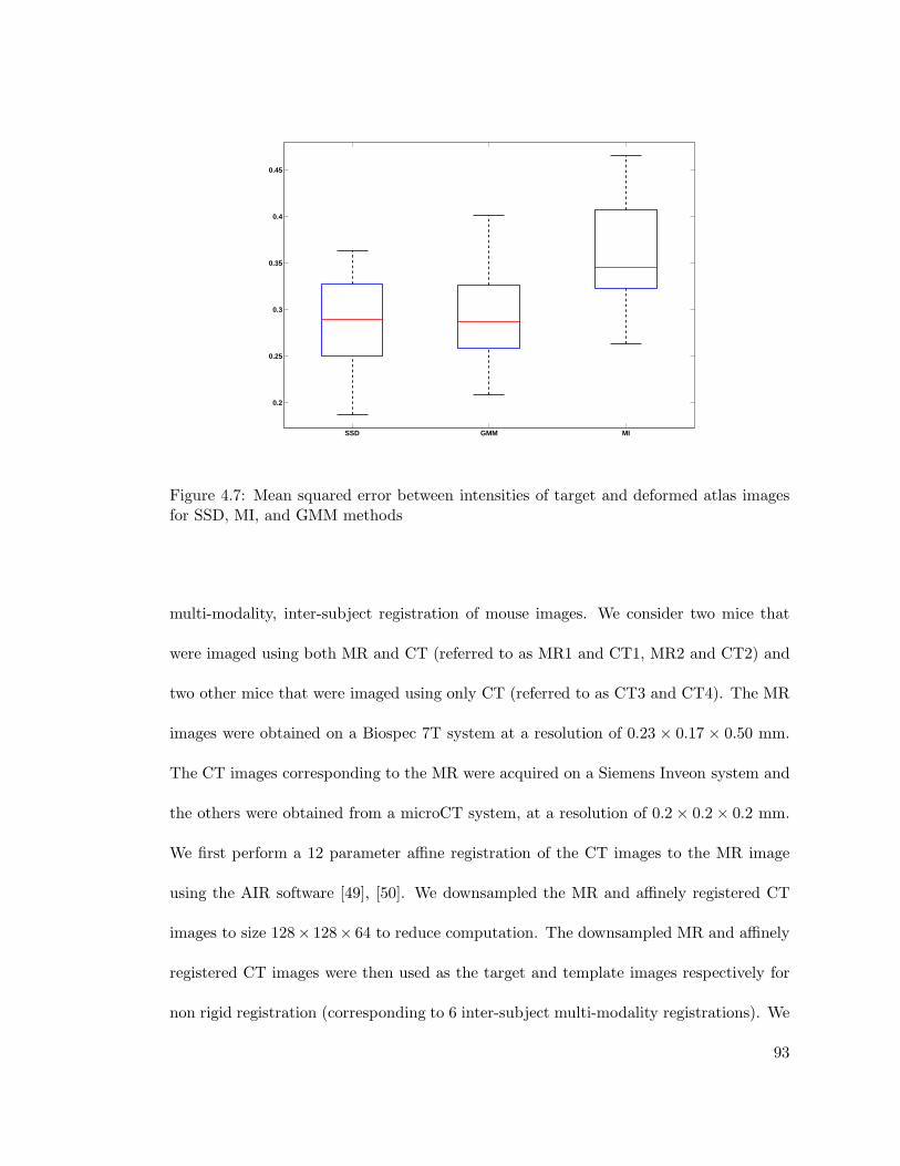
SSD GMM MI

0.2

0.25

0.3

0.35

0.4

0.45

Figure 4.7: Mean squared error between intensities of target and deformed atlas imagesfor SSD, MI, and GMM methods

multi-modality, inter-subject registration of mouse images. We consider two mice that

were imaged using both MR and CT (referred to as MR1 and CT1, MR2 and CT2) and

two other mice that were imaged using only CT (referred to as CT3 and CT4). The MR

images were obtained on a Biospec 7T system at a resolution of 0.23 × 0.17 × 0.50 mm.

The CT images corresponding to the MR were acquired on a Siemens Inveon system and

the others were obtained from a microCT system, at a resolution of 0.2× 0.2× 0.2 mm.

We first perform a 12 parameter affine registration of the CT images to the MR image

using the AIR software [49], [50]. We downsampled the MR and affinely registered CT

images to size 128× 128× 64 to reduce computation. The downsampled MR and affinely

registered CT images were then used as the target and template images respectively for

non rigid registration (corresponding to 6 inter-subject multi-modality registrations). We

93

Figure 4.8: Transaxial and sagittal views of average images: Top row:Template image towhich the atlases are registered. Middle row: Average of deformed atlases using Parzen-MI approach, Bottom row: Average of deformed atlases using GMM based approach

94

Figure 4.9: Multi-modality inter-subject registration: Coronal (top row) and sagittalviews (bottom row) of target , template, Parzen-MI registered image, and GMM-Condregistered image (left to right).

compare the GMM-Cond and Parzen-MI approaches. SSD is not a suitable metric for

multi-modality registration, and hence we do not use it for this comparison.

For both GMM-Cond and Parzen-MI methods, we used 15 × 15 × 15 DCT bases to

represent the displacement field. As before, we check the displacement field for foldings

(negative determinant of Jacobian) and use a value of µ that gives a smooth field without

foldings. We used a hierarchical approach for the Parzen-MI registration with images

smoothed by a Gaussian of 3 voxels as the first step, followed by registration of the

original images. A Parzen window width of σ = 5 was used to compute the distribution

at every iteration. For the GMM-Cond approach, we used K = 8 components in the

95

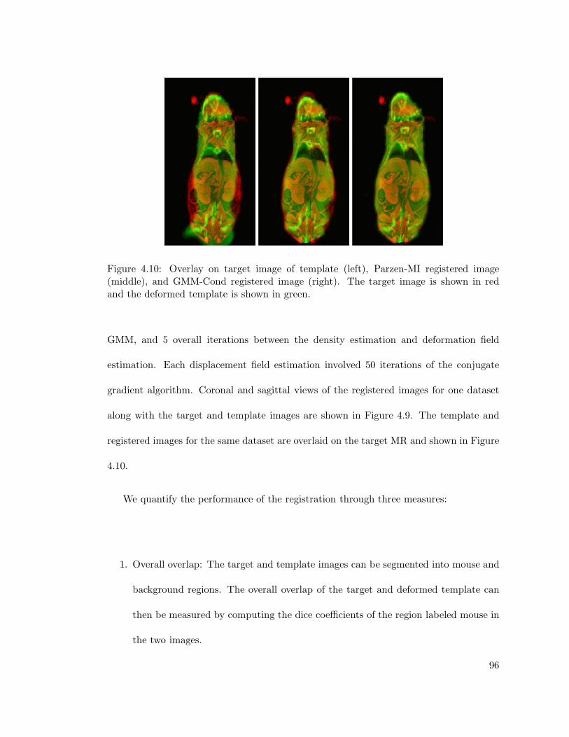
Figure 4.10: Overlay on target image of template (left), Parzen-MI registered image(middle), and GMM-Cond registered image (right). The target image is shown in redand the deformed template is shown in green.

GMM, and 5 overall iterations between the density estimation and deformation field

estimation. Each displacement field estimation involved 50 iterations of the conjugate

gradient algorithm. Coronal and sagittal views of the registered images for one dataset

along with the target and template images are shown in Figure 4.9. The template and

registered images for the same dataset are overlaid on the target MR and shown in Figure

4.10.

We quantify the performance of the registration through three measures:

1. Overall overlap: The target and template images can be segmented into mouse and

background regions. The overall overlap of the target and deformed template can

then be measured by computing the dice coefficients of the region labeled mouse in

the two images.

96

2. Overlap of skeleton: The skeleton can be segmented out in the target and template

images by thresholding. The dice coefficients of the skeleton in the target and

deformed template images give a measure of overlap in the skeleton.

3. Mean squared difference (MSD) between intensities: The target MR image has a

corresponding CT image acquired with it. The normalized mean squared differ-

ence between intensities of the CT corresponding to the target, and the deformed

template images gives a measure of registration accuracy.

The values of these measures for the four CT images registered to the MR images are

given in Table 4.1.

On an average, the GMM-Cond method has higher dice coefficients for the skeleton as

well as overall shape, and lower normalized MSD between intensities than the MI-Parzen

registration method, indicating better alignment. It is promising that the GMM-Cond

shows improved performance for the inter-subject, multi-modality registration considered,

since these images have considerable difference in intensities, overall shape, and skeletal

structure.

4.2 Discussion

We used the conditional density of the target given the deformed template as a similarity

metric for non-rigid registration, wherein the conditional density is modeled as a Gaussian

mixture model. A DCT representation of the deformation field was used in conjunction

with a Laplacian regularizing term to reduce computation. We compared the performance

of our approach with that of Parzen-MI based approach using clinical and pre-clinical

97

Table 4.1: Quantitative measures of overlapDice coefficients for overall overlap

Registration Affine Parzen-MI GMM-Cond

CT1-MR2 0.8953 0.9048 0.9584

CT3-MR2 0.8574 0.8917 0.9169

CT4-MR2 0.8253 0.8271 0.9386

CT2-MR1 0.8143 0.8980 0.8939

CT3-MR1 0.8137 0.8930 0.8833

CT4-MR1 0.8185 0.8271 0.8994

Average 0.8374 0.8892 0.9151

Dice coefficients for overlap of skeleton

CT1-MR2 0.3249 0.4051 0.3934

CT3-MR2 0.3045 0.3421 0.3520

CT4-MR2 0.2419 0.3498 0.3473

CT2-MR1 0.1955 0.2831 0.3164

CT3-MR1 0.1729 0.2372 0.2866

CT4-MR1 0.1576 0.2338 0.3470

Average 0.2383 0.3085 0.3404

Mean squared difference between intensities

CT1-MR2 0.5348 0.4212 0.3422

CT3-MR2 0.5618 0.5496 0.4213

CT4-MR2 0.4384 0.5735 0.4201

CT2-MR1 0.6101 0.5233 0.4400

CT3-MR1 0.6043 0.5383 0.6518

CT4-MR1 0.6087 0.4107 0.3515

Average 0.5596 0.5027 0.4378

98

images of both intra modality brain MR images as well as multi-modality MR/CT mouse

images.

The GMM-Cond approach showed higher registration accuracy than the Parzen-MI

approach in terms of dice coefficients and mean squared difference between intensities of

the target and registered images. The GMM parametrization is not only computationally

more efficient than the Parzen method, but also improves performance by reducing the

overall dimensionality of the estimation problem, and through more robust and accurate

density estimation. Additionally, the only design parameter that needs to be chosen is the

number of clusters in the GMM, which can be obtained from the initial joint histogram.

The consistent performance of the GMM-Cond method for brain as well as mouse

images, and for intra as well as multi-modality images indicates that this is a robust

approach that can potentially be applied to multimodality registration applications. This

approach can be used as an alternative to MI based registration when dealing with high

dimensional deformation fields. It can be viewed as a general framework that can be

used in conjunction with other models for the deformation field. It should be noted

however, that if the joint density of the images does not follow a GMM, a large number

of clusters would be required to fit the data, thus increasing the number of parameters

to be estimated and might not perform better than Parzen-MI in that case. We expect

this approach to be useful in applications where the images have a few distinct regions of

intensity, such as brain or mouse CT images.

99

Chapter 5

Summary and Future Work

We explored the application of information theoretic measures to PET image reconstruc-

tion and non-rigid registration. For PET imaging, we described an approach that uses

mutual information and joint entropy as anatomical priors on the PET image. We used

a scale-space framework to incorporate spatial information into these global distribution

based metrics. The novelty in this approach to using anatomical information in PET

reconstruction is in aiming to reconstruct a PET image that is similar to the anatomical

image in the information theoretic sense rather than defining explicit correlations be-

tween the the boundaries or regions in the images. We presented an efficient FFT based

method to compute these priors and their derivatives, making it practical to use these

priors for 3D image reconstruction. The simulations and clinical data results indicate

that joint entropy with scale-space information reconstructs images with more accurate

quantitation and sharper boundaries than that of the commonly used quadratic priors,

which do not use anatomical information. We applied these anatomical priors to positron

range correction, which is a fundamental resolution limiting problem in PET. A truncated

homogeneous model was used to incorporate range blurring into the system model, and

100

the joint entropy prior with scale-space features was used to correct for blurring outside

regions where uptake is expected. Promising results were obtained from simulations as

well as pre-clinical data, which indicate that joint entropy based priors can be used in con-

junction with a system model that incorporates positron range, to improve the resolution

of PET even when long range isotopes are used.

We described two approaches to non-rigid registration that can be applied to small

animal images. First, we apply the mutual information based scale-space framework to

non-rigid registration of mouse images. The results indicate that the scale-space based

registration gives better skeletal as well as soft tissue alignment than a hierarchical multi-

scale approach. We used a non-parametric approach to estimating the distribution of

intensities that defines the mutual information cost function, to avoid making assump-

tions about the form of the distribution. However, using this approach in conjunction

with estimation of the non-rigid deformation field increases the dimensionality of the

problem. We therefore describe an alternative approach that uses the log likelihood of

the target given the deformed template wherein the likelihood is described by a Gaussian

mixture model. This reduces the density estimation step to that of estimating the GMM

parameters, thus reducing the overall dimensionality of the problem for images that have

a few regions of distinct intensities. We evaluated the GMM approach using intramodal-

ity brain MR images, and multi-modality mouse MR/CT images. The results indicate

that this GMM based approach is robust and yields more accurate registration accuracy

compared to the non-parametric MI based approach. The GMM based approach can

therefore be potentially applied for clinical as well as preclinical imaging.

101

In summary, we find that the information theoretic measures considered in this dis-

sertation have potential for application in multi-modality imaging studies. Since there

is ongoing research in constructing multi-modality imaging systems, the approaches de-

scribed in this dissertation are relevant and could be used as a general framework for

reconstruction and registration utilizing the available multi-modality information.

5.1 Future Work

The work presented in this dissertation can be extended to various problems in recon-

struction and registration. A few of the possible extensions are:

1. Atlas based mouse segmentation: Mouse atlases such as the Digimouse described in

[51] have a mouse CT or MR image with the various organs labeled by an expert.

Automatic segmentation of a target image can be performed by registering the atlas

to it, and applying the obtained deformation field to the labels thus obtaining the

target image segmentation. This requires non-rigid registration, possibly of images

from different modalities. The GMM based non-rigid registration described in this

dissertation can be used to perform this registration of different subjects to the

atlas for segmentation.

2. Positron range: The positron range model used in this work assumes that the range

blurring is spatially invariant, which is not accurate especially at organ boundaries.

Though the JE based approach is able to improve the resolution of the reconstructed

image even with this assumption, using a more accurate range model in conjunction

with the JE prior might improve the results further.

102

3. Application of information theoretic anatomical priors to diffuse optical tomog-

raphy (DOT): We obtained some preliminary phantom results for application of

the information theoretic anatomical priors described in this dissertation to the

ill-conditioned problem of diffuse optical tomography [44]. This application can be

explored further to improve the resolution of DOT.

103

References

[1] Simon R. Cherry. Multimodality in vivo imaging systems: Twice the power or double

the trouble? Annual Review of Biomedical Engineering, 8(1):35–62, 2006. PMID:

16834551.

[2] D W Townsend. Multimodality imaging of structure and function. Physics in

Medicine and Biology, 53(4):R1–R39, 2008.

[3] R.Leahy and X.Yan. Incorporation of MR data for improved functional imaging with

PET. Inf. Proc. in Med. Imaging, pages 105–120, 1991.

[4] G.Gindi, M.Lee, A.Rangarajan, and I.G.Zubal. Bayesian reconstruction of functional

images using anatomical information as priors. IEEE Trans in Med. Imag., 12(4),

Dec 1993.

[5] Xiaolong Ouyang, W.H. Wong, V.E. Johnson, Xiaoping Hu, and Chin-Tu Chen.

Incorporation of correlated structural images in pet image reconstruction. Medical

Imaging, IEEE Transactions on, 13(4):627–640, Dec 1994.

[6] Babak A Ardekani, Michael Braun, Brian F Hutton, Iwao Kanno, and Hidehiro

Iida. Minimum cross-entropy reconstruction of pet images using prior anatomical

information. Physics in Medicine and Biology, 41(11):2497–2517, 1996.

104

[7] J.E.Bowsher, V.E.Johnson, T.G.Turkington, R.J.Jacszak, and C.E. Floyd Jr.

Bayesian reconstruction and use of anatomical a priori information for emission

tomography. IEEE Trans. Med. Imag., 15(5):673–686, 1996.

[8] S. Sastry and R.E. Carson. Multimodality bayesian algorithm for image reconstruc-

tion in positron emission tomography: a tissue composition model. Medical Imaging,

IEEE Transactions on, 16(6):750–761, Dec. 1997.

[9] B. Lipinski, H. Herzog, E. Rota Kops, W. Oberschelp, and H.W. Muller-Gartner.

Expectation maximization reconstruction of positron emission tomography images

using anatomical magnetic resonance information. Medical Imaging, IEEE Transac-

tions on, 16(2):129–136, April 1997.

[10] K. Baete, J. Nuyts, W. Van Paesschen, P. Suetens, and P. Dupont. Anatomical-

based fdg-pet reconstruction for the detection of hypo-metabolic regions in epilepsy.

Medical Imaging, IEEE Transactions on, 23(4):510–519, April 2004.

[11] A.Rangarajan, I.-T.Hsiao, and G.Gindi. A Bayesian joint mixture framework for the

integration of anatomical information in functional image reconstruction. Journ. of

Math. Imag. and Vision, 12:199–217, 2000.

[12] J.E.Bowsher, H. Yuan, L. W. Hedlund, T. G. Turkington, W. C. Kurylo, C. T.

Wheeler, G. P. Cofer, M. W. Dewhirst, and G. A. Johnson. Utilizing MRI informa-

tion to estimate F18-FDG distributions in rat flank tumors. Conf. Record: IEEE

Nucl. Sci. Symp. and Med. Imag. Conf., 4:2488–92, Oct 2004.

105

[13] W.Wells III, P.Viola, H.Atsumi, S.Nakajima, S.Nakajima, and R.Kikinis. Multi-

modal volume registration by maximization of mutual information. Med. Image

Analysis, 1(1):35–51, 1996.

[14] S.Somayajula, E.Asma, and R.M.Leahy. PET image reconstruction using anatomical

information through mutual information based priors. Conf. Rec: IEEE Nucl. Sci.

Symp. and Med. Imag. Conf., pages 2722–26, 2005.

[15] S. Somayajula, A. Rangarajan, and R.M. Leahy. PET image reconstruction using

anatomical information through mutual information based priors: A scale space

approach. Biomedical Imaging: From Nano to Macro, 2007. ISBI 2007. 4th IEEE

International Symposium on, pages 165–168, April 2007.

[16] J.Nuyts. The use of mutual information and joint entropy for anatomical priors in

emission tomography. Conf. Rec: IEEE Nucl. Sci. Symp. and Med. Imag. Conf.,

pages 4148–54, 2007.

[17] T.Lindeberg. Scale-Space Theory in Computer Vision. Kluwer Academic, Nether-

lands, 1994.

[18] C. S. Levin and E. J. Hoffman. Calculation of positron range and its effect on

the fundamental limit of positron emission tomography system spatial resolution.

Physics in medicine and biology, 44(3):781–799, March 1999.

[19] R. Laforest, D.J.Rowland, and M.J. Welch. Micropet imaging with nonconventional

isotopes. IEEE Trans. Nucl. Sci., pages 2119–2126, 2002.

106

[20] Tom K Lewellen. Recent developments in pet detector technology. Physics in

Medicine and Biology, 53(17):R287–R317, 2008.

[21] S.F. Haber, S.E. Derenzo, and D. Uber. Application of mathematical removal of

positron range blurring in positron emission tomography. Nuclear Science, IEEE

Transactions on, 37(3):1293–1299, Jun 1990.

[22] Adam Alessio and Lawrence MacDonald. Spatially variant positron range model-

ing derived from ct for pet image reconstruction. In Nuclear Science Symposium

Conference Record, 2008. NSS ’08. IEEE, pages 3637–3640, Oct. 2008.

[23] B. Bai, A. Ruangma, R. Laforest, Y.-C. Tai, and R.M. Leahy. Positron range mod-

eling for statistical pet image reconstruction. IEEE Nucl. Sci. Symposium and Med.

Imag. Conf, pages 2501–2505, 2003.

[24] Bing Bai, R. Laforest, A.M. Smith, and R.M. Leahy. Evaluation of MAP image re-

construction with positron range modeling for 3d PET. Nuclear Science Symposium

Conference Record, 2005 IEEE, 5:2686–2689, Oct. 2005.

[25] Ananya Ruangma, Bing Bai, Jason S. Lewis, Xiankai Sun, Michael J. Welch, Richard

Leahy, and Richard Laforest. Three-dimensional maximum a posteriori (map) imag-

ing with radiopharmaceuticals labeled with three cu radionuclides. Nuclear Medicine

and Biology, 33(2):217 – 226, 2006.

[26] D. L. G. Hill, P. G. Batchelor, M. Holden, and D. J. Hawkes. Medical image regis-

tration. Phys. Med. Biol., 46(4):R1–R45, March 2001.

107

[27] W.R. Krum, L.D.Griffin, and D.L.G.Hill. Non-rigid image registration: Theory and

practice. Br. Journ. Radiol., 1(77):S140–S153, 2004.

[28] Emiliano D’Agostino, Frederik Maes, Dirk Vandermeulen, and Paul Suetens. A

viscous fluid model for multimodal non-rigid image registration using mutual infor-

mation. Medical Image Analysis, 7(4):565 – 575, 2003. Medical Image Computing

and Computer Assisted Intervention.

[29] D. Rueckert, L. I. Sonoda, C. Hayes, D. L. Hill, M. O. Leach, and D. J. Hawkes.

Nonrigid registration using free-form deformations: application to breast mr images.

IEEE Trans Med Imaging, 18(8):712–721, August 1999.

[30] Ming-Chang Chiang, R.A. Dutton, K.M. Hayashi, A.W. Toga, O.L. Lopez, H.J.

Aizenstein, J.T. Becker, and P.M. Thompson. Fluid registration of medical images

using jensen-renyi divergence reveals 3d profile of brain atrophy in hiv/aids. In

Biomedical Imaging: Nano to Macro, 2006. 3rd IEEE International Symposium on,

pages 193–196, April 2006.

[31] N.Kovacevic, G.Hamameh, and M.Henkelman. Anatomically guided registration of

whole body mouse MR images. In MICCAI, pages 870–877, 2003.

[32] X. Papademetris, D. P. Dione, L. W. Dobrucki, L. H. Staib, and A. J. Sinusas.

Articulated rigid registration for serial lower-limb mouse imaging. In MICCAI (2),

pages 919–926, 2005.

[33] X.Li, T.E.Peterson, J.C.Gore, and B.M.Dawant. Automatic inter-subject registra-

tion of whole body images. Lecture Notes in Computer Science, 4057:18–25, 2006.

108

[34] R.O.Duda, P.E.Hart, and D.G.Stork. Pattern Classification. Wiley, second edition,

2001.

[35] M. E. Leventon, W. Eric, and L. Grimson. Multi-modal volume registration using

joint intensity distributions. In In Proc. MICCAI’98, pages 1057–1066. Springer,

1998.

[36] Alexis Roche, Grgoire Mal, Nicholas Ayache, and Sylvain Prima. Towards a better

comprehension of similarity measures used in medical image registration. In In

MICCAI, pages 555–566. Springer-Verlag, 1999.

[37] J.Zhang and A.Rangarajan. Bayesian multimodality non-rigid image registration

via conditional density estimation. In Information Proc. in Med. Imaging, pages

499–511, 2003.

[38] Richard M. Leahy and Jinyi Qi. Statistical approaches in quantitative positron

emissiontomography. Statistics and Computing, 10(2):147–165, 2000.

[39] T.Cover and J.Thomas. Elements of Information Theory. Wiley Series in Telecom-

munications, 1991.

[40] D.Bertsekas. Nonlinear Programming. Athena Scientific, 1999.

[41] Sarit Shwartz, Michael Zibulevsky, and Yoav Y. Schechner. Fast kernel entropy es-

timation and optimization. Signal Processing, 85(5):1045 – 1058, 2005. Information

Theoretic Signal Processing.

[42] C.Studholme, D.L.G.Hill, and D.J.Hawkes. An overlap invariant entropy measure of

3D medical image alignment. Pattern Recognition, 32(1):71–86, January 1999.

109

[43] Richard M. Leahy and Jinyi Qi. Statistical approaches in quantitative positron

emissiontomography. Statistics and Computing, 10(2):147–165, 2000.

[44] C.Panagiotou, S.Somayajula, A.P.Gibson, Schweiger M, R.M.Leahy, and

S.R.Arridge. Information theoretic regularization in diffuse optical tomography.

Journal of Optical Society of America, 26:1277–1290, May 2009.

[45] J. Ashburner and K.J. Friston. Nonlinear spatial normalization using basis functions.

Human Brain Mapping, 7(4):254–266, 1999.

[46] B.W.Silverman. Density estimation for Statistics and Data analysis. Chapman and

Hall, 1986.

[47] David W. Shattuck, Stephanie R. Sandor-Leahy, Kirt A. Schaper, David A. Rotten-

berg, and Richard M. Leahy. Magnetic resonance image tissue classification using a

partial volume model. NeuroImage, 13(5):856 – 876, 2001.

[48] G. MacLachlan and D.Peel. Finite Mixture Models. Wiley, 2000.

[49] Woods R.P., Grafton S.T., Watson J.D.G., Sicotte N.L., and Mazziotta J.C. Auto-

mated image registration: I. general methods and intrasubject, intramodality vali-

dation. Journal of Computed Assisted Tomography, 22:139–152, 1998.

[50] Woods R.P., Grafton S.T., Watson J.D.G., Sicotte N.L., and Mazziotta J.C. Auto-

mated image registration: Ii. intersubject validation of linear and nonlinear models.

Journal of Computed Assisted Tomography, 22:153–165, 1998.

110

[51] Belma Dogdas, David Stout, Arion F Chatziioannou, and Richard M Leahy. Digi-

mouse: a 3d whole body mouse atlas from ct and cryosection data. Physics in

Medicine and Biology, 52(3):577–587, 2007.

111