INFORMATION THEORY AND RADAR: MUTUAL INFORMATION …

INFORMATION THEORY AND RADAR:

MUTUAL INFORMATION AND THE DESIGN AND ANALYSIS

OF RADAR WAVEFORMS AND SYSTEMS

Thesis by

Mark Robert Bell

In Partial Fulfillment of the Requirements

for the Degree of

Doctor of Philosophy

California Institute of Technology

Pasadena, California

1988

(Submitted March 30, 1988)

- 11 -

© 1988

Mark Robert Bell

All Rights Reserved

-m-

ACKNOWLEDGE:rv.IBNTS

I wish to thank my thesis advisor, Dr. Edward C. Posner, for his insightful guidance,

discussions, and reviews of my work throughout the course of this research. His

comments and questions have made this work both clearer and more relevant. I

have been very fortunate to have an advisor with both the depth and breadth of

knowledge that he possesses.

I also wish to thank the professors who make up my thesis committee, Dr. Yaser

Abu-Mostafa, Dr. Charles Elachi, Dr. Joel N. Franklin, and Dr. Robert J. McEliece,

for both taking the time to be on my committee and offering the excellent courses

I have had the priviledge of taking with each of them.

I also thank Hughes Aircraft Company for sponsormg this work through a

Howard Hughes Doctoral Fellowship.

Finally, I thank my wife Catherine for her love, patience, and encouragement

while I pursued this research. This work is dedicated to my parents, who have given

me many years of support and encouragement.

- lV -

ABSTRACT

This thesis examines the use of information theory in the analysis and design

of radar, with a particular emphasis on the information-theoretic design of radar

waveforms. First, a brief review of information theory is presented and then the

applicability of mutual information to the measurement of radar performance is ex

amined. The idea of the radar target channel is introduced. The Radar /Information

Theory Problem is formulated and solved for a number of radar target channels,

providing insight into the problem of designing radar waveforms that maximize

the mutual information between the target and the received radar signal. Radar

scattering models are examined in order to obtain usable models for practical wave

form design problems. The target impulse response is introduced as a method of

characterizing the spatial range distribution of radar targets. The target impulse

response is used to formulate a new generalization of the matched filter in radar

that matches a transmitted-waveform/receiver-filter pair to a target of known im

pulse response, providing the maximum signal-to-noise ratio at the receiver under

a constraint on transmitted energy and the time duration of the waveform. Next,

the problem is formulated and solved of designing radar waveforms that maximize

the mutual information between the target and the received radar waveform for a

target characterized by an impulse response that is a finite-energy random process.

The characteristics of waveforms for optimum detection and for obtaining maximum

information about a target are compared. Finally, the information content of radar

images is examined. It is concluded that the information-theoretic viewpoint can

improve the performance of practical radar systems.

-v-

TABLE OF CONTENTS

ACKNOWLEDGEMENTS .................................................... iii

ABSTRACT .................................................................. iv

LIST OF ILLUSTRATIONS ................................................... ix

LIST OF TABLES ........................................................... xiii

CHAPTER 1. INTRODUCTION .............................................. 1

1.1 Background ................................................................ 1

1.2 Overview ................................................................... 7

1.3 Chapter 1 References ...................................................... 10

CHAPTER 2. THE INFORMATION-THEORETIC ANALYSIS OF RADAR .. 11

2.1 The Information-theoretic Analysis of Radar Systems ...................... 12

2.2 Information Theory and Discrete Random Variables ........................ 22

2.3 Information Theory and Continuous Random Variables .................... 37

2.4 Mutual Information and Radar Measurement Performance ................. 45

2.5 Chapter 2 References ...................................................... 52

- Vl -

CHAPTER 3. THE RADAR/INFORMATION THEORY PROBLEM ......... 54

3.1 General Formulation of the Radar/Information Theory Problem ............ 55

3.2 The Radar/Information Theory Problem for Discrete Target Channels ...... 58

3.2.1 Solution for Discrete Memoryless Target Channels ........................ 60

3.2.2 The Radar/Information Theory Problem for N Observations

of a Fixed Target ........................................................ 76

3.2.3 The Radar/Information Theory Problem for Finite-State Target Channels 79

3.3 The Radar/Information Theory Problem for Continuous Target Channels .. 95

3.3.1 The Continuous Memoryless Target Channel ............................. 97

3.4 Conclusions .............................................................. 103

3.5 Chapter 3 References ..................................................... 104

CHAPTER 4. RADAR SCATTERING MODELS ............................ 105

4.1 Radar Reflectivity and Radar Cross Section ............................... 106

4.2 The Analytic Signal Representation ....................................... 112

4.3 Polarization, Depolarization, and Scattering .............................. 114

4.4 Statistical Models of Radar Backscatter from Land ....................... 118

4.5 A Model for Cross Polarization Measurements from Rough Surfaces ....... 126

4.6 Spatial Resolution Characteristics of Radar vVaveforms ................... 128


- Vll -

CHAPTER 5. MATCHING A RADAR WAVEFORM/RECEIVER-FILTER PAIR

TO A TARGET OF KNOWN IMPULSE RESPONSE ....................... 148

5.1 Radar Target Detection by Energy Threshold Test ........................ 149

5.2 Matching a Waveform/Receiver-Filter Pair to a Target of Known

Impulse Response ........................................................ 156

5.3 Optimum Waveform/Receiver-Filter Pairs for Sphere Detection ........... 170


CHAPTER 6. INFORMATION THEORY AND RADAR WAVEFORM

DESIGN ..................................................................... 183

6.1 Radar Waveform Design for Maximum Information Transfer

Between the Target and the Received Radar Signal ........................ 184

6.2 A Numerical Example .................................................... 213

6.3 Radar Waveform Design and Implementation ............................. 228

6.4 Comparison of Waveforms for Optimum Detection and Ma."{imum

Information Extraction .......................................... ,. ........ 233


Vlll -

CHAPTER INFORMATION CONTENT OF RADAR IMAGES ..... 237

7.1 Radar Images ............................................................ 238

7.2 Information Theory and Speckle Noise in Radar Images ................... 259

7.3 Chapter 7 Appendix ...................................................... 276

7.3.1 Verification of Eq. (7.48) ................................................ 276

7.3.2 Verification of Eq. (7.49) ................................................ 277

7 .3.3 Verification of Eq. (7.54) ................................................ 279

7 .4 Chapter 7 References ..................................................... 283

CHAPTER 8. SUMMARY AND CONCLUSIONS ............................ 286

ILLUS

Figure Page

1.1. Block Diagram of a Generic Radar System .............................. 2

2.1. Block Diagram of a Generic Communication System ................... 13

2.2. Block Diagram of a Generic Radar System ............................. 16

2.3. Self Information I(x) versus p(x) ...................................... 23

2.4. Block Diagram of a Simple Communication System .................... 31

2.5. Binary Symmetric Channel ............................................ 32

2.6. The Binary Entropy Function 1-l((J) ................................... 34

2.7. Additive Gaussian Noise Channel ..................................... .41

2.8. Capacity of the Additive Gaussian Noise Channel ...................... 44

2.9. Block Diagram of a Measurement System .............................. 45

2.10. Rate Distortion Function of the Gaussian Measurement Example ...... .45

3.1. Block Diagram of Radar/Information Theory Problem ................. 56

3.2. Block Diagram of The Target Channel ................................. 57

3.3. Radar/Information Theory Problem for Discrete Target Channels ...... 59

3.4. Diagram of Target Channel for N = 1 andX = <Xj ••••••••••••••••••••• 61

3.5. Memoryless Binary Target Channel of Example 3.1 .................... 65

3.6. Memoryless Discrete Target Channel of Example 3.2 ................... 69

-x-

Page

3 Memoryless Discrete Target Channel of ....,,,.,_ .... ,.., ................... 70

3.8. Finite-State Target Channel of Example 3.5 ........................... 83

3.9. Finite-State Target Channel of Example 3.6 ........................... 84

10. Radar/Information Theory Problem for Continuous Target Channels ... 96

3.11. Continuous Target Channel Model ..................................... 99

4.1. Waveform Spectra X(f) and R(f) .................................... 130

4.2. Constructive Interference from Two Scatterers ........................ 132

4.2. Two-Frequency Constructive Interference from Two-Scatterers ........ 132

4.3. Single-Frequency Constructive Interference from Two-Scatterers ...... 134

4.4. Radar Measurement of a Rough Surface .............................. 134

4.5. Constructive Interference and Waveform Bandwidth .................. 139

4.6. Coordinate System of Scattering Problem ............................ 142

4.7. Linear Time-Invariant System Representation of Stationary Target-

Scattering Mechanism ................................................ 142

4.8. Continuous Spectra X(f) and R(/) of Radar Waveform .............. 142

5.1. Probability Density Functions /(elHo) and /(elH1 ) ..•................ 152

5.2. Block Diagram of Radar Waveform/Receiver-Filter Design Problem ... 157

5.3. Linear System Representation of the Relation Between Q(f)

and X(f) ............................................................ 163

5.4. The Backscatter Impulse Response h(n of a Sphere of Radius a ...... . 171

Page

5.5. Magnitude-Squared Spectrum JH(/) J2 versus f ....................... 173

5.6. Wave shape of i(i) for = 1 ......................................... 177

5 Wave shape of x(i) for T = 25 ........................................ 177

5.8. Wave shape of i(-t) for T = 50 ........................................ 178

5.9. Wave shape of £(1) for T = 100 ....................................... 178

6.1. Block Diagram of The Radar Target Channel ......................... 185

6.2. E( a) as a function of a= T /W ...................................... 190

6.3. Additive Gaussian Noise Channel. .................................... 193

6.4. Another Interpretation the of Radar Target Channel .................. 206

6.5. "Water-Filling Interpretation of IX(f)J2 •••••••••••••••••••••••••••••• 210

6.6. Example illustrating the resulting IX(/) 12 for a given crb (/)

and P1111 (/) •••••••••••••••••••••••••••••••••••••••••••••••••••••••••• 211

6.7. r(/) = P1111 (f)T /2<T;(f) as a function off ............................ 216

6.8. IX(f)J2 for T = 10 ms and Ps = 1000 W .............................. 217

6.9. JX(f)J 2 for T = 10 ms and Ps = 500 vV ............................... 218

6.10. JX(f)J 2 for T = 10 ms and Ps = 100 W ............................... 220

6.11. Imax(Y(i); g(i)Jx(-t)) as a function of T and Ps ........................ 221

6.12. Spectral Analysis of Bandwidth W Using M of Bandwidth ~/ .. 225

7.1. Spatial Sampling in an Imaging Radar System ........................ 241

7 .2. Discrete Radar Image as an m X n Array of Resolution Cells .......... 242

Xll

Page

7.3. Radar Image of San Francisco Area ................................... 247

7.4. Resolution Cell Neighborhoods on Which f ( q) Conditioned ......... 255

7.5. 10 X 10 Binary Markov Image ........................................ 257

7.6. ;ZIX = ak) and Iu(Y;ZIX = ak) versus k for D = 4 ............ 272

h(Y;ZIX = ak) and Iu(Y;ZIX =a,.) versus k for D = 8 ............ 272

7.8. h(Y;ZIX =a,.) and Iu(Y;ZJX = ak) versus k for D = 10 ........... 273

7.9. h(Y;ZJX = a,1;) and Iu(Y;ZIX =a,.) versus k for D = 20 ........... 273

7.10. h(Y;ZJX =a,.) and Iu(Y;ZIX = ak) versus k for D = 50 ........... 274

7.11. h (Y; ZIX = a,1;) and Iu (Y; ZIX = a,1;) versus k for D = 100 ......... 274

xm

LIST OF

Table Page

. Signal-To-Noise Ratio for Xn (-t) = v1£ Son ( o:T /2, 21 /T) ................. 168

5-2. Eigenvalues µmax. and Amax. for Various T .............................. 176

5-3. Signal-to-Noise ratios multiplied by N0 for Pulsed Sinusoid and

Optimal Detection vVaveforms for Various T .......................... 180

7-1. Radar Operating Characteristics ...................................... 248

7-2. Minimum Required Mutual Information for Classification into

One of J Equiprobable Classes ....................................... 275

-1-

1

ON

1 . Background.

In the last fifty years, radar has grown from its infancy as a technology with rela

tively few applications into a mature technology with a wide range of applications.

The acronym radar (radio detection and ranging) indicates the impetus for the

initial development of systems that use radiowave or microwave scattering to make

measurements of a remote object. Its primary use in the Second 'World vVar was de

tecting and locating enemy aircraft. This provided both advanced warning of attack

and information for the direction of anti-aircraft weapons. It was also effectively

used by the British to detect and locate German submarines [1.1-1.3].

The modern uses of radar, while still including these early applications, include

several additional applications. These include such remote sensing applications as

the measurement of water resources, agricultural resources, global ice-coverage, for

est conditions, and wind, as well as such radar techniques as ionospheric sounding,

geological mapping, radar meteorology, planetary remote sensing, and radar astron

omy. Radar has also expanded its application navigation. In aviation this can

be seen in its use in air traffic control and aircraft navigation radar. In navigation at

sea, radar is used aboard ships for collision avoidance and on land for harbor traffic

management. Applications in the areas of military surveillance have also expanded

to include terrain mapping and target identification. In radar target identification,

-2-

TRAN SM I TT I NG ANTENNA

TRANSMITTER

RECEIVER TARGET

RECEIVING ANTENNA

Figure 1.1. Block Diagram of a Generic Radar System.

DATA OUT

not only is the target detected and located, but the physical characteristics of the

target are determined, or the target is classified by type based on its radar signature

[1.4, 1.5].

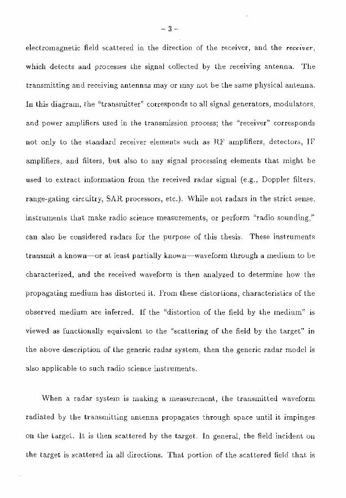
A radar, as considered in this thesis, is any system that uses the scattering of

microwave radiation from an object to obtain information about that object. Such

objects will be referred to as targets. Fig. 1.1 shows a block diagram of a generic

radar system. The radar consists of a transmitter, which generates the signal to

be transmitted, a transmitting antenna, which radiates the transmitter waveform

as an electromagnetic field, a receiving antenna, which intercepts a portion of the

3-

electromagnetic field scattered the direction of the receiver, and the recerner,

which detects and processes the signal collected by the receiving antenna. The

transmitting and receiving antennas may or may not be the same physical antenna.

In this diagram, the "transmitter" corresponds to all signal generators, modulators,

and power amplifiers used the transmission process; the "receiver" corresponds

not only to standard receiver elements such as RF amplifiers, detectors, IF

amplifiers, and filters, but also to any signal processing elements that might be

used to extract information from the received radar signal (e.g., Doppler filters,

range-gating circuitry, SAR processors, etc.). While not radars in the strict sense,

instruments that make radio science measurements, or perform "radio sounding,"

can also be considered radars for the purpose of this thesis. These instruments

transmit a known-or at least partially known-waveform through a medium to be

characterized, and the received waveform is then analyzed to determine how the

propagating medium has distorted it. From these distortions, characteristics of the

observed medium are inferred. If the "distortion of the field by the medium" is

viewed as functionally equivalent to the "scattering of the field by the target" in

the above description of the generic radar system, then the generic radar model is

also applicable to such radio science instruments.

When a radar system is making a measurement, the transmitted waveform

radiated by the transmitting antenna propagates through space until it impinges

on the target. It is then scattered by the target. general, the field incident on

the target is scattered in all directions. That portion of the scattered field that is

-4-

intercepted by the receiving antenna is then fed to the receiver. The receiver then

processes this received field

radar work dealt primarily

the desired information is extracted from it. Early

detecting presence or absence of the target, but

modern radar work concentrates on the extraction of additional information about

the target as well.

Note that in Fig 1.1, a link is depicted between the transmitter and the receiver.

This represents the fact that in most radar systems, the receiver has at least partial

knowledge of the transmitted waveform. A typical reason as to why this knowledge

may be only partial is that the phase of the transmitted waveform may not be

known. In the case of a bistatic radar system-one in which the transmitter and

receiver are not collocated-the time of transmission as well as the phase of the

carrier may not be known. The general shape and polarization of the transmitted

waveform will be known, however, and this knowledge will exhibit itself in the design

of the radar receiver. Some systems have very detailed knowledge of the transmitted

waveform at the receiver. Systems with quadrature detectors, for example, generally

have phase-lock between the transmitter and receiver, with a small portion of the

transmitter carrier fed directly to the receiver.

As many of the modern applications of radar deal not only with detecting

and locating objects but also measuring the scattering characteristics of these

objects, a method of characterizing measurement performance becomes desirable.

In making these measurements of the target-scattering characteristics, the primary

goal is to obtain information about the target. So an appropriate choice of per-

5-

formance metric might be one that measures the information obtained about the

target by radar observation. Such a metric would allow one not only to determine

how information can be determined about a target but also to design a radar

system that determines the maximum amount of information about a target for a

given set of design constraints-for example, a fixed bandwidth and a maximum

average power.

In addition, such a metric would allow one to determine whether or not a radar

is capable of performing its desired task. Standard approaches to the problem of

radar performance have been developed in the case of radar target detection, but in

the case of target identification or the precision measurement of a target parameter,

a metric based on information obtained about the target would be useful. We will

now investigate a simple example that illustrates the usefulness of such a metric.

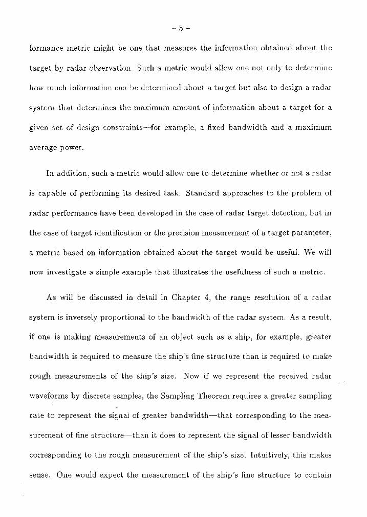
As will be discussed in detail in Chapter 4, the range resolution of a radar

system is inversely proportional to the bandwidth of the radar system. As a result,

if one is making measurements of an object such as a ship, for example, greater

bandwidth is required to measure the ship's fine structure than is required to make

rough measurements of the ship's size. Now if we represent the received radar

waveforms by discrete samples, the Sampling Theorem requires a greater sampling

rate to represent the signal of greater bandwidth-that corresponding to the mea

surement of fine structure-than it does to represent the signal of lesser bandwidth

corresponding to the rough measurement of the ship's size. Intuitively, this makes

sense. One would expect the measurement of the ship's fine structure to contain

6-

more information than the rough measurement of the ship's size, as the measure

ment of the ship's fine structure would include within it a measurement of the ship's

size as well as the additional information characterizing the ship's structure. vVhat

this example points out is the following: Different types of radar measurements

may require different information acquisition capabilities of a radar system. In this

thesis we will analyze this point quantitatively.

This simple example, while intuitively appealing, ignores many significant

points. There is not a direct relationship between the number of samples and the

amount of information conveyed. A single sample in the first case does not neces

sarily provide the same amount of information as a single sample in the second case.

Increasing the bandwidth may increase the number of samples required to represent

the target, taking full advantage of the information contained in this larger band

width, but if the same amount of total energy is available for obtaining the samples

in both cases, less energy is available per sample in the larger bandwidth case. As

a result, in the presence of noise, the individual samples will not be as reliable as

in the larger bandwidth case. This example does, however, bring up the question

of the trade-off between the number of samples and the energy per sample in the

design of a radar system that maximizes the information obtained about the target.

In terms of practical system design, the question could be stated as follows: How

does one distribute th.e transmitted power in frequency to maximize th.e information

obtained wh.en tl1ere is a constraint on th.e average transmitter power?

In this thesis, the radar measurement process will be analyzed m terms of

-7

information theory. The measure of information proposed by Shannon [1.6] will

be used to examine the ability of a radar system to collect information about a

target-that is, the information content of radar measurements will be examined.

We will then examine the information-theoretic design of radar systems so that

their measurements will yield the maximum amount of information about the tar

get being observed. A particularly interesting result of this analysis is that radar

systems designed for optimal target detectability-the most common approach to

radar system design today-differ significantly from those that would be designed

to collect the ma.ximum amount of information about a target known to be present.

This suggests that a different approach to radar waveform design should be used

in the case of radars designed for target identification and precision measurement

than for target detection.

1.2. Overview.

In Chapter 2 of this thesis, we will briefly review information theory by defining

the information-theoretic quantities that will be used in this thesis. This will be

done primarily to establish the notation to be used in the remainder of this thesis

and to highlight general concepts in information theory. More detailed and in-

depth discussions of information theory are found References [1. 7-1. 9]. After

our brief review, we will look at the relationship between information theory and

radar measurement. This will provide the motivation for a more detailed look

at the application of information theory to the problem of radar measurement by

pointing out the relationship between information acquired and target identification

-8

capabilities or measurement error.

Chapter 3, we introduce the Radar/Information Theory Problem, which

forms the basis for most of the rest of this thesis. The Radar/In.formation Theory

Problem addresses the problem of what a radar should transmit in order to obtain

the maximum amount of information about the target under observation. We then

look at the solution of this problem the general case.

Before the results of Chapter 3 can be applied to specific radar problems,

physical models of the radar measurement process must be established. This is done

in Chapter 4. Here we will look at statistical models of electromagnetic scattering

and the appropriateness of these models to the radar measurement process. We will

begin with a brief survey of scattering models and then will examine in detail those

that will be useful in our analysis.

In Chapter 5 we will apply the results of Chapter 4 to the problem of optimum

target detection. We will derive a new extension of the matched filter concept for

radar developed by North [l.10]. North's matched filter assumed that the target be

ing observed was a point target-one with no significant spatial extent. The results

in Chapter 5 take into account the interference patterns arising in the scattered

electric field because of the spatial extent of a target distributed in space. The

result of our analysis is a design procedure that gives both a realizable waveform

and a receiver filter, which together have optimum detection properties in additive

Gaussian noise with an arbitrary power spectral density.

Chapter 6, the information-theoretic design of radar waveforms is considered.

9-

Here we look at the problem of designing radar waveforms that maximize the rate

of information transfer about the target to the radar. These results are of particular

interest in the case of radar design for target identification and measurement. A

design procedure is then developed for radar systems that maximize the rate of

information extraction about the target. We then compare the optimum detection

waveforms of Chapters 5 to those derived in Chapter 6, which provide the maximum

amount of information about the target. This results in a very interesting physical

and information-theoretic interpretation of the waveforms for optimal detection and

information extraction.

Chapter 7, we apply mutual information to the analysis of imaging radar.

Here we examine the information content of radar images generated by both real

and synthetic aperture radars. We also give an information-theoretic interpretation

to some well-known results in the processing of radar images.

In Chapter 8, we summarize our results from the previous chapters and examine

their implications for the design of radar waveforms and systems.

10 -

1 er 1

1.1 Alvarez, L. W., of a Physicist, Basic Books, New York, NY, 1987.

1.2 Ridenour, L. N., Radar System Engineering, McGraw-Hill, New York, NY,

1948.

1.3 Brookner, E., Radar Tec.b.nolop;y, Artech House, Dedham, MA, 1977.

1.4 Skolnik, M. L., Introduction to Radar Systems, 2nd ed., McGraw-Hill, New

York, NY, 1980.

1.5 Stimson, G. W., Introduction to Ai.rborn.e Radar, Hughes Aircraft Company,

El Segundo, CA, 1983.

1.6 Shannon, C. E., "A Mathematical Theory of Communication," Bell Sys. Tech..

J. 27, 1948. pp. 379-423, 623-656. Reprinted in C. E. Shannon and W.

W. Weaver, Th.e Mathematical Theory of Communication, Univ. Ill. Press,

Urbana, IL, 1949.

1.7 McEliece, R. J ., The Theory of Information and Coding, Addison-Wesley,

Reading, MA, 1977.

1.8 Blahut, R. E., Principles and Practice of Information Theory, Addison-Wesley,

Reading, MA, 1987.

1.9 Gallager, R. G., Information. Theory and Reliable Communication, John Wiley

and Sons, New York, NY, 1968.

1.10 North, D. 0., "An Analysis of the Factors which Determine Signal-Noise Dis

crimination in Pulsed Carrier Systems", RCA Laboratory Report PTR-6C;

reprinted Proc. IEEE, 51 (July 1963), pp. 1016-27.

- 11 -

2

TFIE INF ON-TFIEORETIC ANALYSIS OF RADAR

In this chapter, we will examine the applicability of information theory to the anal

ysis of radar systems. In Section 2.1, we will consider the rationale for examining

radar systems from the viewpoint of information theory. This is done by examining

the similarities and differences between communication systems-which have been

analyzed for the last forty years using information theory with great success-and

radar systems-to which information theory was early considered applicable [2.13],

but to which information theory has not been traditionally applied. We will see

that a radar system can be seen as a "communication system" of an unusual type,

and that it is indeed reasonable to use information theory in the analysis of radar

systems. In Sections 2.2 and 2.3, we will briefly review the main points of informa

tion theory. The purpose here is twofold. First, it serves to establish the notation to

be used throughout this thesis with regard to information, but more importantly it

serves to introduce its basic principles to those radar engineers reading this thesis,

who may not be familiar with information theory. These sections are by no means

a complete introduction to information theory. An excellent introduction and ref

erence can be found in [2.1], on which much of these two sections is based. Having

introduced the basic concepts of information theory, we will look at their relevance

to the radar measurement problem in Section 2.4. There we will see the relevance

- 12 -

of information theory to radar measurement performance.

2.1. tic Analysis of Systems.

Information theory, introduced by Shannon in 1948 [2.2], provided a new and pow

erful framework for the analysis of communication systems. But information theory

was more a new tool for examining previously known results in communication

theory. It opened up a whole new realm of previouly unknown results about the

communication process, by offering new and fundamental insights into its nature.

This in turn spawned the field of error-correcting codes, providing the means by

which many of Shannon's results would be realized in practice. Information theory

has had a profound impact on the design of today's communication systems and the

methods of transferring information from one point to another, or from one time to

another in the case of computer memories.

In this thesis, we will examine radar systems using information theory in order

to derive some insights which information theory can provide into the design of radar

systems. It may not be immediately apparent that information theory provides an

appropriate or even desirable framework in which to analyze radar systems. In

this section, we will motivate such an approach by examining the similarities and

differences of radar systems and communication systems. References [2.3] and [2.4]

provide many of the details for the analysis of communications and radar systems,

both generally and specifically.

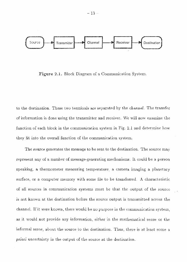
Consider the block diagram of a generic communication system shown in Fig. 2.1.

The purpose of the communication system is to transfer information from the source

- 13 -

2.1. Block Diagram of a Communication System.

to the destination. These two terminals are separated by the channel. The transfer

of information is done using the transmitter and receiver. 'We will now examine the

function of each block in the communication system in Fig. 2.1 and determine how

they fit into the overall function of the communication system.

The source generates the message to be sent to the destination. The source may

represent any of a number of message-generating mechanisms. It could be a person

speaking, a thermometer measuring temperature, a camera imaging a planetary

surface, or a computer memory with some file to be transferred. A characteristic

of all sources in communication systems must be that the output of the source

is not known at the destination before the source output is transmitted across the

channel. If it were known, there would be no purpose in the communication system,

as it would not provide any information, either in the mathematical sense or the

informal sense, about the source to the destination. Thus, there is at least some a

priori uncertainty in the output of the source at the destination.

- 14 -

transmitter maps output from the source into a suitable form for

the channel across which the message is to be transferred. Thus, the transmitter

matches the message from the source to the channel. The form of the transmitter

then will be a function of both the message source and the channel. For example,

if the source is human speech and the channel is free space, a microwave transmit

ter using wide deviation frequency modulation may be a good match of source to

channel, whereas if the source is a computer system with digital data files to be

transmitted and the channel is an optical fiber, a pulse modulated laser may be a

good choice as a transmitter matching the source to the channel.

The channel is determined by the medium across which the information is to be

transferred from the source to the destination. It may, for example, represent free

space, the earth's atmosphere, a coaxial cable, or an optical fiber when the source

and destination are spatially separated. It may also represent a magnetic, optical,

or solid-state storage medium when the source and destination are separated in

time, such as in a computer program, where data are stored away in memory and

then recalled at some later time. A characteristic of almost all physical channels

is that when a waveform is being transmitted across the channel, it is distorted by

physical processes present within the channel. As a result, the waveform received

at the channel output may not be interpreted as corresponding to the message pro

duced by the source. These distortions may be due to any of a number of physical

processes. For example, in the case of electromagnetic waveform transmission, ther

mally excited molecules emit electromagnetic radiation due to charge motion. This

- 15

exhibits itself radio communication systems as additive noise. Also present in

some radio channels is multipath fading that is due to the received signals from mul-

tiple propagation paths. change in the geometry of the transmitter, receiver,

or propagation paths can cause the amplitude of the received signal to change. This

exhibits itself as a multiplicative noise. In optical communication systems, noise in

the solid-state detectors can cause the detector to determine the presence of a pulse

from the transmitter when none is present.

The receiver observes the output of the channel and makes a decision as to what

the transmitted message was. Its function is complicated by noise and distortion

present in the channel. After making its estimate of the message from the source,

it passes this decision on to the destination. The destination represents or displays

the point to which the information is to be transmitted. It receives the decision on

the received message from the receiver and functions as the end user.

The role of information theory in the design of such a communication system is

to determine how the transmitter and receiver will be designed in order to efficiently

and reliably transmit the information from the source to the destination, given the

characteristics of the source and the channel. That is, given a model of what types

of messages the source is likely to produce and a characterization of the distorting

or noise properties of the channel, information theory determines whether or not a

receiver and transmitter can be designed so as to provide reliable communication.

It also provides some guidance as to how to design this transmitter and receiver.

The actual implementation of the transmitter and receiver often involves coding,

- 16

Transmit Antenna Receive Antenna

~ --.

- Transmit - Target ~ Receive . ...

Receiver Transmitter - Channel Channel I ' ~ Target Channel I

~ I Dest.

Figure 2 Block Diagram of a General Radar System.

and the field of error-correcting codes (2.1] provides the details of the specific coding

design. Information theory does, however, provide specific insights into the higher

level of system design. For example, in Reference [2.5], Shannon considers the spec-

tral distribution of transmitter power for optimal communications for an additive

Gaussian noise channel with a given noise power spectral density.

We now examine a general radar system. Consider the block diagram of the

radar system shown in Fig. 2.2. The purpose of this radar system is to determine

characteristics of the target. We will now consider the function and· effect of each

of these blocks in carrying out the purpose of radar.

The transmitter of the radar system provides the electromagnetic waves by

which the target will be probed. Typical radar systems have transmitters operating

at frequencies between 1 GHz and 50 GHz, although lower frequencies are some-

times used for over-the-horizon, long-range detection radars where the increased

reflectivity of the ionosphere can be used to good advantage [2.4]. Generally, larger

average transmitter powers, although not necessarily greater received powers, can

be obtained at lower frequencies, since the physical size of the components is greater,

and thus greater heat dissipation can take place. In some applications, however,

such as airborne and spaceborne systems, the limitation on average transmitter

power is determined by size and weight constraints on the transmitter power sup

plies [2.4]. The frequency and bandwidth of the transmitted waveform also play a

significant role in the measurement capabilities of the radar system. This will be

examined in detail in Chapter 4.

We next encounter the transmit antenna, whose function it is to radiate the

transmitter waveform into space at the target. In the case of the abstract commu

nication channel, we did not explicitly note the antenna or the method of coupling

the transmitter to the channel. The reason for this was that it was not necessary

in order to understand the function of the communication system. In the case of

radar, however, the antenna plays a more pronounced role. The characteristics of

the antenna-its beamwidth, polarization, and geometry-significantly affect the

outcome of the resulting radar measurements [2.6]. Antenna system design is a

significant part of the design of a radar system and in particular determines the

angular resolution with which radar measurements can be made.

We next encounter the block labelled as the target channel, made up of the

transmit channel, the target, and the receive channel. a real radar system, we

- 18 -

cannot directly separate the effects of these three elements by measurement. Any

processing that allows us to separate these effects is dependent on the estimation of

the the individual effects based on assumed physical models of the individual pro

cesses involved and measurements involving all of the effects acting simultaneously.

represents the path across which the transmitted wave

form travels as it propagates from the transmit antenna to the target. For free

space or the earth's atmosphere, this channel has little effect other than to attenu

ate the signal. This attenuation is the result of space loss (dispersion of the signal

in space) and atmospheric attenuation. Space loss is defined so as not to be a

frequency-selective process, so all frequencies in the transmitted waveform are at

tenuated equally when they reach the target. Atmospheric absorption, on the other

hand, is highly frequency-selective, as it is due to the absorption of electromagnetic

energy by specific molecules making up the atmosphere. The energy is absorbed at

frequencies corresponding to the molecular bonds of these molecules [2.3,pp.23,35].

In some cases, the transmit channel can distort the transmitted electromagnetic

field in still more severe ways. For example, plasmas made up of charged particles

interact with electromagnetic waves propagating through them. This results in a

decrease in velocity of propagation, dispersion (frequency-dependent propagation

time differences for different waveform spectral components) of the waveform, and

both amplitude and phase scintillation (rapid fluctuations about the mean value) of

the wave passing through the plasma [2.7). Such plasmas exist in the solar system

and could exhibit themselves as transmit channel distortions if the radar system

- 19 -

being modeled is used in radar astronomy measurements at high enough frequen

cies (although these frequencies would be higher than those currently used in radar

astronomy [2.14]).

The target is the object on which measurements are being made. It is the

element in the block diagram of which there is generally the greatest uncertainty,

yet about which the most information is desired. In fact, the sole purpose of the

radar system is to obtain information about the target to reduce this uncertainty. If

there were no uncertainty about the target-about its presence, geometry, physical

characteristics, and motion-there would be no need to make radar measurements

of it. In a sense, the target plays a parallel role in the radar system to that played

by the source in the communication system. The transmitted waveform, having

been radiated by the transmit antenna, propagates through space until it reaches

the target. Once the transmitted electromagnetic wave is intercepted by the target,

it is scattered by the target. This scattering can be viewed as a retransmission by

the target of the wave impinging on the target, but the resulting scattered wave is

modified as a function of the target's geometry and physical characteristics.

The receive channel, as shown in Fig. 2.2, includes the medium between the

target and the antenna. As in the case of the channel in the communication system,

there will generally be additive thermal noise present. In the case of the radar

system, the effect of the additive noise may be particularly severe. This is because

of the two-way transmission path from the transmitter to the target and the target to

the receiver. After suffering the one-way path loss squared, the received signal from

- 20

the target may be very faint. is especially true if the target is at a considerable

distance. the case of a monostatic (single antenna) radar, for instance, the

received signal power is inversely proportional to the fourth power of the range

from the antenna to the target.

The receiver detects the signal intercepted by the receive antenna and performs

any processing required to extract the desired information about the target. This

processing may involve filtering out unwanted noise, spectral analysis in order to

determine the spectrum of the Doppler shift resulting from target motion, and any

radar or target motion compensation that may be required to extract the desired

target characteristics from the received signal. So we should and do include any

postprocessing of the detected signal in the receiver block as well.

The output of the receiver goes to the destination, representing the end user

of the information obtained about the target. The output of the receiver that is

provided to the destination could take on any of a number of forms. For example,

it could be a radar map of the target in a geological mapping system, the position

and velocity of the target in an air-traffic control system, the Doppler spectrum of

the target a system used to study surface scattering behavior in remote sensing,

or the class of a target a target-identification system.

If we compare the block diagram of the communication system m Fig. 2 .1

to the block diagram of the radar system in Fig. 2.2, we see that several of the

elements in the two systems are similar. Both systems have a transmitter that

radiates electromagnetic energy, and both systems have a receiver that detects and

- 21

processes electromagnetic Both systems also have a channel through which

the signal passes as it propagates from transmitter to receiver, but the nature of

these channels is quite different.

the communication system, the information to be received by the destination

has its origin at the source. The channel acts primarily as the medium across

which the message is to be transferred, and as a result, acts primarily to corrupt

the message sent from the source to the destination. In the radar, however, it

is the channel, or the target channel to be precise, that contains the source of

information. In the communication system, then, the transmitter responds to the

message generated by the source and transmits a waveform to the receiver. In

the radar system, the target responds to the transmitted waveform and scatters a

modified waveform to the receiver. The source of uncertainty to be reduced in the

scattered waveform is only the result of the target channel itself, since the receiver

has knowledge of the transmitted waveform. Thus, the radar system functions by

probing the target and measuring its response. So the target itself acts as the source

of information or the "message source." The transmitter merely provides the energy

in an appropriate form for it to do so.

target will not, however, respond to differing waveforms of identical energy

in identical ways. While this is true of the idealized point targets encountered in

theoretical radar analysis, scattering from targets of spatial extent generates inter

ference patterns. These interference patterns can differ significantly for transmitted

waveforms made up of different frequency components. Thus, the question arises:

- 22 -

How does the shape or frequency content of the transmitted waveform affect the

amount of information obtained about the target by radar measurement? In this

thesis, we will examine this question, using information theory. The following two

sections provide a brief introduction and review of information theory.

2.2. and Dis e Random Variables.

Let be a discrete random variable (finite or countable) taking on values from a

set = {x 1,x2 , ... }. For eachx E Rx, Ietp(x) = P{X = x}, the probability

distribution of X. vVe wish to obtain a measure of the information obtained by

observing X. Equivalently, we wish to obtain a measure of the a priori uncertainty

in the outcome of X. In order to do this, we will define for each x E Rx a quantity

I(x) called the seH-informa.tion of x, by

I(x) = - log p(x). (2.1)

The base of the logarithm is left unspecified and determines the units of I(x). The

two most commonly used bases are base-2 and base-e, yielding units of bits and

nats, respectively. In this thesis, base-e or natural logarithms will be used almost

exclusively when a specific base needs to be specifed. This is done to simplify

calculations. N ats can be converted to bits by dividing by a scale factor of In 2.

Fig. 2.3 shows a graph of I(x) as a function of p(x ). For any given x E Rx,

p(x) E [O, 1]. Note that as the event = x becomes less probable, the self-

information I ( x) increases, and that as the event becomes more probable, the self

information decreases. This then says that the occurrence of an unlikely event-"It

23

I (x)

p ( x)

0

Figure 2.3. Self-Information I(x) versus p(x ).

is raining in Los Angeles"-contains more self-information than a likely event-"It

is raining somewhere." Intuitively, this is appealing, since if we are told the obvious,

we feel we have obtained very little "information," whereas when we are told the not

so obvious or the unlikely, we feel we have obtained significant "information." Note

as well the relationship between self-information and the certainty of an event's

occurrence. \Vhen we are quite certain an event will occur, the self-information

provided by its occurrence is As we become less certain of its occurrence, the

self-information provided by its occurrence becomes larger.

Defining I(x) as we have, we see that I( X) is a new random variable, defined

in terms of the random variable X. The expectation of the random variable I(X),

denoted by (X), is called the entropy of X, and is given by

H(X) = - p(x) log p(x ). (2.2) sERx

If p(x) is equal to zero for any x E Rx, p(x) log p(x) is defined as p(x) log p(x) 0,

the limit asp approaches zero from above:

lim plogp = 0. p-+O+

If X and Y are jointly distributed discrete random variables taking on val-

ues from Rx = {x1,x2, ... } and Ry = {y 1 ,y2, ... } respectively, and having joint

probability distributionp(x,y) = P{X=x,Y=y}, then the self-information in the

joint occurrence of X = x and Y = y is I(x,y) = -logp(x,y). The joint entropy

H(X, Y) of X and Y is

H(X,Y) p(x, y) log p(x, y ). (2.3)

- 25 -

now consider several properties of the entropy function. These properties

are easily proved, as References [2.1, 2.8]:

1. p = (p(.x1 ),p(x2 ), ... ) be the probability distribution of X. Then

H(X) is continuous in p.

2. H(X) ~ 0, with equality if and only if all but one of the p(xJ) are

equal to zero.

3. For a finite random variable X with Rx = {x1, ... ,xr}, H(X)::; log r,

with equality if and only if for all Xj E Rx, p(xJ) = l/r.

4. If X and Y are jointly distributed random variables,

H(X, Y) ::; H(X) + H(Y),

with equality if and only if X and Y are statistically independent.

5. H(X) is a convex n function of p.

We have previously noted that the entropy (X) is the mean value of the

self-information I(X), and that I(x) was small for events that occurred with great

certainty. follows then that H(X) must in some sense measure the average

uncertainty of the outcome of X. \Vhen H(X) is large, there is a greater a priori

uncertainty in the outcome of the random variable X. We will now consider the

five properties of entropy listed above in light of viewing entropy as a measure of a

priori uncertainty.

- 26 -

Property 1 states that entropy of is continuous in the probability distribution

of . This can be interpreted as saying that small changes in the probability

distribution of X produce small changes in the entropy of X. This is a reasonable

property of an uncertainty measure, as it states that very similar distributions have

very similar a priori uncertainty.

Property 2 states that entropy measures the uncertainty of X as a positive

quantity, and that if the outcome of X is certain, the entropy of X is zero. This is

an intuitively appealing property of an uncertainty measure.

Property 3 states that if there are a fixed, finite number of outcomes of X,

then there is an upper bound on the entropy of X, and this upper bound occurs

only when each of the outcomes is equally likely. This is a reasonable property of

an uncertainty measure, as intuitively, the case of equiprobable outcomes has the

greatest uncertainty-no single outcome is more favorable than another.

Property 4 states that for two random variables, the joint entropy of their

outcomes is less than or equal to the sum of the entropies of the individual outcomes.

Furthermore, the joint entropy of their outcome is exactly the sum of the entropies

of the individual outcomes when the two outcomes are statistically independent.

This, too, is a reasonable property of an uncertainty measure. It states that if the

two outcomes are statistically independent, then the uncertainty of the outcome

of the two jointly is the sum of the individual uncertainties. If, however, there is

statistical dependence between the two outcomes, observation of the outcome of

one must provide some information on the outcome of the other, and in such an

27

instance the joint uncertainty of the two random variables is strictly less than the

sum of the two individual uncertainties.

Property 5, convexity down, while not having the direct intuitive appeal of

the previous four properties, is significant in that it greatly simplifies finding dis-

tributions that maximize the entropy of X, as well as solving related optimization

problems in information theory. This is a fortunate benefit of adopting entropy as

an uncertainty measure.

As can be seen from these five properties of entropy, entropy is a very rea-

sonable measure of the a priori uncertainty in the outcome of a discrete random

variable. In fact, although several measures of uncertainty that have some of the

above properties have been proposed [2.9], only the entropy function (or actually

o:H(X), where a: is any positive real number) satisfies all of these properties [2.10].

Also, the entropy function measures the average code length needed to specify a

source [2.1,2.3], but we shall not pursue this point of view here.

Consider again the jointly distributed discrete random variables X and Y,

with joint distribution p(.x, y ). Let p(x) be the (marginal) distribution of X and

p(y) be the distribution of Y. Then the conditional probability distribution of Y

conditioned on X = x is

( I ) - p(x, y)

p y x - p(x) '

and the conditional probability distribution of X conditioned on Y = y is

( I ) - p(x, y)

pxy - p(y).

(2.4)

(2.5)

- 28 -

Given that X = x, the conditional entropy of , i.e., the entropy of Y conditioned

on X = x, is

IX= x) = - L p(ylx) log p(ylx). (2.6) vERy

Similarly, the entropy of X conditioned on Y - y is

H(XIY = y) = - L p(xly)logp(xly). (2.7) <>ERx

vVe define the conditional entropy H(YIX) by averaging over all x E Rx. This

yields

H(YIX) = - p(x) L p(ylx) logp(ylx) <>ERx vERy

(2.8) = - L L p(x, y) logp(y Ix).

<>ERx vERy

Similarly,

H(X IY) = - L p(y) L p(xly) logp(xly) vERy sERx

=-I:: p(x, y) logp(xly ). (2.9)

sERx vERy

vVe now define a quantity of central importance in information theory, known

as mutual information. Consider again the jointly distributed discrete random vari-

ables X and . The mutual information between X and Y, denoted I(X; Y), is

defined as

I(X; Y) - (X) - H(XIY). (2.10)

The mutual information represents the difference between the a priori uncertainty

in X and the uncertainty in X after observing Y. So I ( X; Y) is a measure of the

29

amount of information provides about X. is interesting to note that

; Y) = H(X) - (X!Y)

- L p(x) Iogp(x) L L p(x,y)logp(xly) a:ERx a:ERx yERy

" " p(xly) = L.t L.t p(x, y) log p(x) xERx vERy

x ERx yERy

p(x,y) p(x,y)Iog p(x)p(y)

" " p(ylx) L.t L.t p(x,y)log p(y)

x ERx vERy

= - L p(x) logp(y) + L L p(x,y)logp(ylx) xERx yERy

= H(Y) - H(YIX).

Thus, there is a symmetry in X and Y exhibited by I(X; Y), since I(X; Y) is not

only equal to H(X) - H(XIY), but also to H(Y) - H(YIX). Thus, we have

" " p(x,y) I(X;Y)=I(Y;X)= L.t L.t p(x,y)logp(x)p(y)' xERx vERy ·

(2.11)

and we see not only that I(X; Y) is the information that observation of Y provides

about X, but also that I(X; Y) is the information that observation of X provides

about Y; hence, the name mutual information given to I(X; Y).

The mutual information I(X; Y) has several interesting properties. \Ve note

some of them [2.1]:

1. I(X; Y) ;?::: 0,with equality if and only if and Y are statistically

independent.

2. I(X; Y) - I(Y; X), as was previously shown.

- 30

3. I(X; Y) is a convex n function of the input probabilities p(x).

4. I(X; Y) is a convex U function of the conditional probabilities p(y Jx ).

\Ve can generalize the definitions of entropy and mutual information to include

not only discrete random variables, but discrete random vectors as well. Let X =

( X 1, ... , X m) be an m-dimensional random vector of random variables X l, ... , X m,

with X taking on values from the set Rx. Let p(x) = P{X = x} = P{X1 =

Xj 1 , ••• , Xm = Xj.,,.,} be the probability distribution on X. Then the entropy of the

random variable X is

H(X) - L p(x) logp(x). (2.12) xERx

Let Y = (Y1, ... , Yn) be an n-dimensional random vector of random variables

Y1, ... , Yn, with Y taking on values from the set Ry. Let p(y) = P{Y = y} -

P{Y1 = Yj 1 , ••• , Yn = Yj,.,} be the probability distribution on Y. Let X and Y

be jointly distributed with joint distribution p(x, y) = P{X = x, Y = y }. Let

p(xJy) = P{X = xJY = y} and p(yJx) = P{Y - yJX = x}. Then the joint

entropy of X and Y is

H(X,Y) - L L p(x,y)logp(x,y). (2.13) xERx yERy

The entropy of conditioned on X is

H(YJX) = - L p(x) p(yJx) logp(yJx)

=- 2= p(x, y) logp(yJx). (2.14)

31 -

..... CHANNEL

.... RECEIVER TRANSMITTER F F

x y

Figure . Block Diagram of a Simple Communication System.

The entropy of X conditioned on Y is

H(XIY) = - L p(y) L p(xiy) logp(xiy) yERy sERx

= - L L p(x, y) logp(xiy). (2.15)

:rERx yERy

The mutual information between the random vectors X and Y is

I(X; Y) = H(X) - H(XIY)

= H(Y) - H(YIX) (2.16)

= L p(x, y) log p~x);(y). :rERx yERy

We will now introduce the concept of the communication channel in the discrete

case. Consider again the discrete random variables X and Y. \Ve have previously

looked at them abstractly as jointly distributed random variables, but now we will

examine how they might arise in a typical discrete communication system. Consider

the communication system depicted in Fig. 2.4. we have a transmitter that

transmits a message consisting of one of m symbols from an alphabet Rx =

32 -

1 - (

1 - £

Figure 2.5. Binary Symmetric Channel

{x1, ... ,xm}· The message is the random variable X with distribution p(x). The

transmitted message X proceeds through the channel, which stochastically maps to

a discrete random variable Y at the channel output. Y takes on one of n symbols

from the alphabet Ry = {y1, ... , Yn }. The stochastic mapping of the channel is

governed by the conditional probability distribution

p(ylx) = P{Y = vlX = x}. (2.17)

The resulting channel output Y thus has the marginal probability distribution

p(y) = ~ p(x)p(ylx) . .xERx

33 -

As a concrete example of a discrete communication channel, consider the binary

symmetric channel (BSC) shown in Fig. 2.5. Here the input and output alphabets

are identical; that is, - Ry = {0, 1}. \Ve will assume the input probability

distribution is

{P x - O·

p(x)= 1'-p, x=l'. (2.18)

The conditional probability distribution that governs the channel behavior is

{

1 - e, x = 0,y O;

( Ix) = e, x = 0,y = 1; P y e, x l,y = O;

1 - £, x - l,y = 1.

(2.19)

If we assume that the goal of the BSC is to reproduce faithfully the input symbol

at its output, then it can be seen that the probability of error for the BSC is £,

and the probability of correct transmission is 1 - £. Of course, we would intuitively

expect that the smaller £, the better the channel. Let us verify this by calculating

the mutual information between X and Y for the BSC. From Eq.s (2.2) and (2.9)

we have

H(X) = -p logp - (1 - p) log(l - p),

and H(XIY) - -p(l - e) log(l - e) - pdog £

- (1-p)(l - e)log(l - e)- (1-p)eloge

= -dog£ - (1 - e) log(l - e).

Thus, from Eq. (2.10) we have (noting that I(X; Y) ~ 0)

I(X;Y) =max( 0 ,-plogp (1-p)log(l p) +doge+ (1 e)log(l- e)].

- 31-

------- -----------~-----t---._

log 2

0.0 0.5 1.0

Figure 2.6. The Binary Entropy Function 'H.(/3).

If for all j3 E [O, 1], we define (recalling as above 0 log 0 = 0)

'H.(/3) = -/3 log/3 - (1 - /3) log(l - /3), (2.20)

then

I(X; Y) =max[ 0, 1-l.(p) -1-l.(i;)], (2.21)

where 1-l.(/3) is called the binary entropy function.

A plot of 'H.(/3) versus j3 is shown in Fig. 2.6. note that 'H.(/3) is symmetric

about j3 = 0.5, that it is a convex n function on j3 E [O, 1], and that it takes on its

maximum value of log 2 at the point j3 = 0.5. In order to examine the behavior of

35 -

I(X; ) as given Eq. (2.21), we note that for allp and€ such that 11.(p) > 1i.(E),

I(X;Y) is just the difference 1i.(p) -1i.(E), and for all other p and E, I(X;Y) is

zero. From Eq. (2.21) we see that I(X; Y) is maximized whenp = 0.5. · can be

seen by noting that Eq. (2.21) is maximized when 11.(p) is maximized, and 11.(p) is

ma.ximized when p = 0.5. So the BSC provides the maximum mutual information

between input and output when the input symbols 0 and 1 are equiprobable. \Ve

also see that I(X; Y) is maximized when 11.( E) = 0, which occurs when either€= 0

or € 1. That this is true for € - 0 makes intuitive sense, since this is the case in

which no errors whatsoever occur. That this is true for the case of € = 1 may at

first seem surprising, since this is the case of the channel's always making an error.

But if a binary symmetric channel always makes an error, X = 0 always produces

Y = 1 and X - 1 always produces Y = 0. Such a channel is really a very reliable

channel. The receiver simply assumes that when Y - 1 is received, X = 0 was sent,

and that when Y = 0 is received, X = 1 was sent.

Of particular interest is the fact that for all p and€ such that 11.(p) ~ 1i.(E),

I ( X; Y) = 0, and the channel is of no use whatsoever. In such cases, the channel

error rate € satifies the following inequality:

for all p and € such that 1i.(p) ~ 1i.(€).

Such channels are of no use m conveymg information m effect there is

greater uncertainty in the channel's performance than there is in what message was

sent. If one chooses the most likely symbol to be transmitted as the transmitted

symbol, the probability of error is no greater than that obtained by any decision

36

rule based on actual observation of the channel output.

the above example, we noted that for any given binary symmetric channel

and associated 7-l(E), p = 0.5, the mutual information I(X; Y) was max-

imized. general, any channel with mutual information I(X;Y) - H(X) -

H(XIY), there will be a maximum value of I(X; Y) over all probability distribu-

tions p(x ). This quantity is known as the capacity of the channel. We will denote

the channel capacity by C. Thus, the channel capacity is defined as

C = max {I ( X; Y)}. ;:{x)

(2.22)

The channel capacity is the largest rate at which information can be transferred

across the channel. Shannon [2.2] showed more importantly not only that the

capacity C of a channel was the maximum rate at which information could be sent

across the channel, but also that, with proper encoding, information can be sent

across the channel at any rate less than C with arbitrarily small error. The capacity

of a channel sets an upper bound on the rate at which highly reliable information

can be transferred across the channel.

- 37 -

2 • Theory c Variables.

In the previous section, we examined entropy and mutual information for discrete

random variables and vectors, but usually, and particularly in this thesis, we are in-

terested in the case of continuous random variables and vectors. vVe will now obtain

expressions for the mutual information between two continuous random variables.

Consider a continuous random variable X defined on the real line R with

probability density function (PDF) f(x). The differential entropy of X is defined

by 00

h(X) = - j J(x) log /(x) dx. (2.23)

-oo

The differential entropy is not the limit of the Riemann sum obtained. by discretizing

the real line into intervals of size .6.x [2.1]. For such a case we would have a Riemann

sum of the form

But

lim H(X) = lim {- Lf(xk)logf(x;;).6.x} ~s_,O ~s_,O

k

= lim {- Lf(xk)log/(xk)}+ lim {-log.6.x} ~s_,O ~s-0

k 00

= -! f(x)logf(x)dx- lim {log.6.x}. ~s_,O

- 00

- lim {log .6.x} = oo, ~s-0

(2.24)

so the limit as .6.x -+ 0 of the Riemann sum will in general diverge, and this limit

will be of little interest or use to us. Note, however, that the first term of the limit

in Eq. 2.24 is what we have defined as the differential entropy of X.

- 38 -

Assume we another continuous random variable defined on R and that

and Y are jointly distributed with joint PDF f(x,y). Assume also that f(x)

is the marginal pdf of X, f (y) is marginal pdf of y, f (xjy) is the PDF of X

conditioned on , and f (y Ix) is the PDF of Y conditioned on X. \Ve can then

define the joint differential entropy

00 00

h(X, Y) == - j j J(x,y)logf(x,y)dxdy, (2.25)

-00-00

and the conditional differential entropies

00 00

h(XjY) == - j j f(x,y)logf(xjy) dxdy, (2.26)

-oo -oo

and 00 00

h(YjX) == - j j f(x,y)logf(yjx)dxdy. (2.27)

-oo -oo

Consider again the limiting process of the Riemann sum approximation to

an entropy, but this time using the conditional entropy H(XjY). In the limit as

.6.x -+ 0, we obtain

lim lim H(XjY) == lim lim {- LLf(x1 ,y1;).6.x.6.yiogf(xJIYk).6.x} C.s-+O Ay-+0 ..:).s-+O As-+O

j k.

- lim lim {- LLf(xJ,Yk).6.x.6.ylogp(xJIY.~) As-+ 0 As-+ 0

j k

- lim lirn {'\:"""' J(x1 ,yk).6.x.6.yiog.6.x} As -+ 0 C.s -+ 0 L..;

J k 00 00

- j j f (x, y) log f (xjy) dx dy - lim log .6.x. As-+O

-00-00

(2.28)

Again, we note that the second term of the Riemann sum diverges as .6.x -+ 0, so

this approximation is of little use to us either. We do, however, note that the first

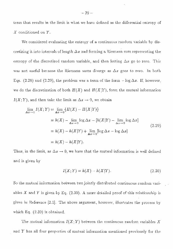
- 39 -

term that results the limit is what we have defined as the differential entropy of

conditioned on

considered evaluating the entropy of a continuous random variable by dis-

cretizing it into intervals of length l::,.x and forming a Riemann sum representing the

entropy of the discretized random variable, and then letting l::,.x go to zero. This

was not useful because the Riemann sums diverge as l::,.x goes to zero. In both

Eqs. (2.28) and (2.29), the problem was a term of the form - log l::,.x. If, however,

we do the discretization of both H(X) and H(XjY), form the mutual information

I(X;Y), and then take the limit as l::,.x--+ 0, we obtain

lim I(X; Y) = lim {H(X) - H(XJY)} Aa:---.O Aa:-+O

-h(X)- lim log/::,.x-[h(XJY)- lim log!::,.x] Aa:->O Aa:-+O

(2.29)

= h(X) - h(XJY) lim [log l::,.x - log !::,.x] Ll.a:-+ 0

= h(X) - h(XjY).

Thus, in the limit, as l::,.x --+ 0, we have that the mutual information is well defined

and is given by

I(X; Y) = h(X) - h(XJY). (2.30)

So the mutual information between two jointly distributed continuous random vari-

ables X and is given by Eq. (2.30). A more detailed proof of this relationship is

given in Reference [2.1). The above argument, however, illus~rates the process by

which (2.30) is obtained.

The mutual information I(X; Y) between the continuous random variables X

and Y has all four properties of mutual information mentioned previously for the

- 40

mutual information between discrete random variables. On the other hand, the dif-

ferential entropy of continuous random variables does not have many of the prop-

erties of the entropy of discrete random variables. \Ve will not consider these in

detail, as we will refer to differential entropy only when calculating calculating mu-

tual information

vVe can generalize the definitions of differential entropy and mutual informa-

tion for continuous random variables to include continuous random vectors as well.

Let X = ( X 1 , ... , X m) be an m-dimensional vector taking on values from the m-

dimensional vector space Rm defined over the field of real numbers R. Let f(x) be

the PDF of the random vector X. The differential entropy of the random variable

Xis given by 00 00

h(X) = - j · · · j f(x) log /(x) dx1 · · · dxm -oo -oo (2.31)

- - j /(x) log f (x) dx.

Let = (Y1, ... , Yn) be an n-dimensional random vector taking on values from

the n-dimensional vector space Rm defined over the field of real numbers R. Let

/(y) be the PDF of Y. Let X and Y be jointly distributed with joint PDF /(x, y).

Let f (xjy) be the PDF of X conditioned on Y = y and f (yjx) be the PDF of Y

conditioned on X = x. Then the joint differential entropy of and Y is

h(X,Y)- - j j /(x,y)log/(x,y)dxdy. (2.32)

The differential entropy of conditioned on Y is

h(XIY)= j j /(x,y)log/(xjy)dxdy. (2.33)

R"R"'

2.7. Additive Gaussian Noise Channel.

The differential entropy of Y conditioned on X is

h(YIX) = - j j f(x, y) log f(ylx) dx dy. (2.34)

R"Rm

The mutual information between X and Y is

I(X; Y) = h(X) - h(XIY)

= h(Y) - h(YIX) (2.35)

J J f(x,y)

= f(x,y)log /(x)f(x) dxdy. R"Rm

will now consider an example of a continuous communication channel that

will illustrate many of the principles of information theory for continuous random

variables. Consider the continuous communication channel shown in Fig. 2.7. Here

we have an additive noise channel in which the channel input is a Gaussian random

variable X, with zero mean and variance o-_i. As X proceeds through the channel,

42 -

another Gaussian random variable with zero mean and variance o-1 is added to

it. input X represents a message that we wish to transmit across the channel,

and Z represents some additive contaminating noise. resulting output of the

channel is a random variable , which is the sum of X and Z. vVe will assume

that and Z are statistically independent. It is well known that the sum of two

independent Gaussian random variables is a Gaussian random variable whose mean

is the sum of the means of the two component random variables and whose variance

is the sum of the variances of the component random variables [2.11]. Thus, Y is a

Gaussian random variable with zero mean and variance erf. - o-1- + er~.

Consider a Gaussian random variable S with zero mean and variance <r 2. The

PDF f ( s) of S is

1 - ,1

f(s) = e~. ~er

Then the differential entropy of S is

00

h(S) = - j f(s)logf(s)ds

-oo

00

= - j f(s)log [~er2 e~] ds -oo

00

j f(s) [1ogy'2;<r+ 2: 2 ] ds

-oo

1 1 2

log 2Jrer2 + "2

1 = 21og(27reer2).

Thus, since Y is a zero-mean Gaussian random variable with variance <r~ + <r.k, it

- 43 -

has differential entropy

h(Y) ~log (2Jre(o-~ + o-_i- )) . 2

is straightforward to show analytically that h(Y IX) = h(Z) [2.8], so

mutual information I(X; Y) between

I(X; Y) - h(Y) - h(YIX)

and Y is thus

=~log (2Jre(o-~ + o-_i- )) - ~log(2Jreo-~) 2 2

- ~l (O"~ + o-l-) - og 2 2 O"z

=~log ( 1 + :t). The capacity of the additive Gaussian noise channel with noise variance o-~ and

input X with variance o-_i is found by maximizing over all input density functions

with variance o-_i. Thus, if is the set of all PDF's with variance o-_i-, the capacity

of the additive Gaussian noise channel is

C = max I(X; Y). f(s)EF

It can be shown [2.1] that the maximum is attained by any Gaussian random vari-

able, regardless of its mean value, with variance O"_i. So the I( X; Y) calculated

above for the additive Gaussian noise channel achieves capacity. Thus, the capacity

C of the additive Gaussian noise channel with signal variance o-_i and noise variance

o- 2 lS z

1 ( 0"2 ) C = log 1 + ~ 2 O"z

1 = 21og(l + r),

C, (nats)

2.00

1.50

1.00

0.50

0.00 0 2 4

44 -

r 6 8 10

Figure 2.8. Capacity C of the Additive Gaussian Noise Channel versus r = o-_i. / o-~.

where r = o-1 / o-~, and can be interpreted as the signal-to-noise ratio. In a real

transmitter, we would be sending zero-mean signals since our real constraint 1s

power, and then the variance would be equal to the power (mean-square value). A

plot of C versus r is shown in Fig. 2.8.

45 -

x 1 ex ;Y) y

Figure 2.9. Block Diagram of a Measurement System.

2.4. Mutual Information and Radar Measurement Performance.

In Sections 2.2 and 2.3, we reviewed the basic definitions and principles of informa

tion theory, concentrating on the expressions for the mutual information between

two random variables or vectors. 'We will now examine the usefulness of mutual

information in describing radar performance.

As noted in Section 2.1, a radar system is a measurement system that makes

measurements of a target in order to obtain information about the target, decreasing

the a priori uncertainty about the target. This being the case, let us examine the

measurement process in general in light of information theory.

Consider the measurement system shown in Fig. 2.9. we have an object

to be measured, a measurement mechanism, and an observer. 'We assume that the

random vector consists of parameters characterizing the object we wish to mea-

sure, the measurement mechanism maps them into the random vector Y, and the

- 46 -

observer observes and from this observation determines the desired information

about X. The measurement mechanism, like all real measurement mechanisms, is

assumed to have · inaccuracies, and thus the measurements obtained with it

contain error. This can be modeled by assuming that the measurement mechanism

stochastically maps the random vector to the random vector Y. \Ve will assume

that the mutual information between X and is I(X; Y).

As an example of such a situation, consider a situation in which the object

being measured is a rectangular box whose dimensions X 1 , X2, and X 3 are un

known (we could assume, for example, that the box was randomly selected from

a large collection of boxes of various sizes). The parameter vector X would be

X = ( X 1 , X 2 , X 3 ). Assume that the measurement mechanism consists of some

method of measuring these dimensions-perhaps a person with a crudely marked

ruler. The measurements Y1 , Y2, and Y3 obtained as measurements of X 1 , X 2, and

X3 would form the measurement vector Y; that is, Y - (Y1 , Y2, Y3). Since X and

Y are jointly distributed random vectors, they have a mutual information I(X; Y)

between them.

The mutual information I(X; Y) between two random vectors X and Y tells us

how much information observation of provides about ; that is, J(X; Y) is the

amount of information that the measurement provides about the object param-

eter vector X. The significance of this is that the greater this mutual information,

the more information we are obtaining about the object by our measurement. \Ve

will examine this in two ways. We will first examine this by determining the maxi-

47

mum number of equiprobable classes into which we can assign X by observation of

, and then we will relate I(X; Y) to average measurement error through use of

the rate distortion function.

Consider

observation of

problem of putting X into one of N equiprobable classes based on

That is, assume that Rx has been partitioned into N equiprobable

subsets, and we wish to assign X to its proper partition based on observing the Y

generated by the measurement process. For any decision rule assigning X to a

partition based on observation of X, and for all possible equiprobable partitions

of Rx, the ma.ximum number of partitions N for which this can be done with an

arbitrarily small probability of error is

(2.36)

Here la J is the largest integer less than or equal to a.

To see that this is true, we note that, given J(X; Y) = ! 0 nats, we can calculate

the associated N, which we will designate N 0 , by

Let N = e10 ; then

No:::; N <No+ 1.

Since the logarithm is a monotonically increasing function of its argument for all

positive numbers,

No :::; lnN <In (No+ 1),

- 48 -

or equivalently,

In No:::; Io< ln(No + 1).

That sufficient information is being conveyed across the measurement channel to

classify X into one of No equiprobable classes, given observation of Y, follows from

the fact that only N 0 nats are required to do so, while I0 nats are currently being

transferred. That it is not possible to classify into one of No + 1 equiprobable

classes follows from the fact that by Shannon's Theorem for the noisy channel, this

cannot be done without the channel's transferring ln(No + 1) nats of information.

But the measurement mechanism cannot possibly do so, since Io < ln(No + 1).

When examining the accuracy of measurements, it is common to talk about the

accuracy in terms of some error criterion, for example, mean-square error or relative

mean square error. It would be useful if we could relate the mutual information

I(X; Y) to measure of measurement error. Fortunately, the framework for doing this

in our measurement problem has already been developed in information theory. It

is called Rate Distortion Theory, and was developed by Shannon in the last chapter

of [2.2] and in [2.12). References [2.1] and [2.3] discuss rate distortion theory and

its application in communications. We will now look at the application of rate

distortion theory to our measurement problem.

Referring again to Fig. 2.9, we have a measurement system by which a mea

surement mechanism conveys a quantity of information J(X; Y) about an object to

an observer. In the measurement process, we are trying to determine the character

istics of the object parameter vector from the measurement vector . Because of

- 49

. . mac curacies the measurement process, we cannot generally obtain X perfectly,

so there is an error associated with a given parameter vector x and a given mea-

surement vector y. Let us designate this error or distortion as d(x, y). \Ve assume

that this distortion is a non-negative function defined for all pairs of x E Rx and

y E Ry. being the case, the average distortion or error D, also known as the

.fidelity criterion., is expectation of d(x, y). Thus,

D= {d(x,y)}. (2.37)

The rate distortion function, R( 5), is defined as

R(5) = min{I(X, Y): D::; 5}. (3.38)

The minimization is over all measurement mechanisms that satisfy the condition

that the the fidelity criterion D is less than or equal to 5. The rate distortion func-

tion R( 5) gives the minimum possible rate at which information must be transferred

by a measurement mechanism in order to have an average error or distortion D less

than or equal to 5.

It is significant to note that for 51 < 52 , R(51 ) ~ R(52 ). Thus, R(5) is a

non-increasing function of 5. So the smaller the average error 5, the larger is the

minimum required information rate R( 5) required of the measurement mechanism.

This intuitively makes sense, as it says that if greater accuracy is required in the

measurements, measurement mechanism must provide more information about

the object being measured.

We will now look at a simple example of the use of the rate distortion function in

a measurement problem. Suppose we wish to measure a scalar parameter X, which

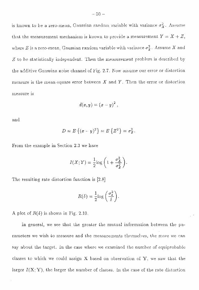
- 50 -

is known to be a zero-mean, random variable with variance crl. Assume

that the measurement mechanism is known to provide a measurement Y = + Z,

where is a zero-mean, Gaussian random variable with variance cr1. Assume X and

Z to be statistically independent. Then the measurement problem is described by

the additive Gaussian noise channel of Fig. 2.7. Now assume our error or distortion

measure is the mean-square error between and . Then the error or distortion

measure is

d(x,y)=(x y) 2,

and

From the example in Section 2.3 we have

The resulting rate distortion function is [2.8]

1 ( cr2) R(5) = 21og ; .

A plot of R( 5) is shown in Fig. 2.10.

general, we see that the greater the mutual information between the pa-

rameters we wish to measure and the measurements themselves, the more we can

say about the target. In the case where we examined the number of equiprobable

classes to which we could assign X based on observation of Y, we saw that the

larger I(X; Y), the larger the number of classes. the case of the rate distortion

51 -

R(S),( )

0 0.5 1.0

Figure 2.10. Rate Distortion Function of the Gaussian :Measurement Example.

function, we saw that the more precise we wanted our measurements to be, the

greater the minimum rate of information transfer by the measurement mechanism.

In applying these results to the measurement mechanism known as radar, we see

that if we design radar systems in such a way as to maximize the mutual information

between the target parameters of interest and their measurements, the better we

can expect our system performance to be. In the next chapter, we will look at the

problem of the design of radar systems. This will be done using the formalism of

Th.e Radar/Information Theory Problem.

52

2.5. er 2

2.1 McEliece, R. J., The of Information. and Coding, Addison-vVesley,

Reading, ' 1977.

2.2 Shannon, C. E., "A Mathematical Theory of Communication," Bell Sys. Tech.

J. 27, 1948. 379-423, 623-656. Reprinted in C. E. Shannon and \V. vV. vVeaver,

The Mathematical Theory of Communication, Univ. Ill. Press, Urbana, IL,

1949.

2.3 Pierce, J. R. and E. C. Posner, Introduction to Communication Science and

Systems, Plenum, New York, NY, 1980.

2.4 Stimson, G. W., Introduction to Airborne Radar, Hughes Aircraft Company,


2.5 Shannon, C. E., "Communication in the Presence of Noise," Proc. IRE, vol.

37, 11-21, 1949.

2.6 Ullaby, F. , R. K. Moore, and A. K. Fung, !vf.icrowave Remote Sensing, vol.

2, Addison-\Vesley, Reading, MA, 1982.

2.7 Posner, E. C. and R. Stevens, "Deep Space Communications," Encyclopedia of

Physical Science and Technology, Academic Press, New York, NY, 1987. pp.

165-185.

2.8 Blahut, R. E., Principles and Practice of Information Theory, Addison-\Vesley,

Reading, MA, 1987.

2.9 Simon, J. C., tterns and Operators: Th.e Foundations of Data Representa-

tion, McGraw-Hill, New York, NY, 1986.

- 53 -

2.10 Khinchin, A. I. 1'.1athematical Foundations of Information Theory, Dover, New

York, NY, 1957.

2.11 Hogg, V. and A. Craig, Introduction to Mathematical Statistics, MacMil-

lan, London, England, 1970.

2.12 Shannon, C. E., "Coding Theorems for a Discrete Source with a Fidelity Cri

terion," Information and Decision Processes, R. E. Machol, ed., McGraw-Hill,

New York, NY, 1960.

2.13 VVoodward, P. M., Probability and Information Theory with Applications to

Radar, Pergamon Press, London, England, 1953.

2.14 Ostro, S. J ., "Planetary Radar Astronomy," Encyclopedia of Physical Science

and Technology, Academic Press, New York, NY, 1987. pp. 612-634.

- 54 -

3

RADAR/INFORMATION PROBLEM

In the previous chapter, we examined the use of information theory to character-

ize the performance of radar systems. particular, we examined how the mutual

information between a vector of target parameters and the measurement obtained

by the radar characterized the radar measurement performance. As a result of

this analysis, we concluded that the greater this mutual information between target

and measurement, the better the radar's ability to reduce uncertainty about the

target-the purpose of making the radar measurement in the first place. This leads

us to the question: How do we design a radar system in order to max.im.ize the

mutual information between the target and the radar measurement of the target

under a given set of design constraints?

In this chapter, we will begin to address this question by studying a problem

we call The Radar/Information Theory Problem. The Radar/Information Theory

Problem allows us to formulate a mathematical framework that will provide in

sight into the problem of radar waveform design for maximum mutual information

between the target and the measurement obtained at the radar receiver.

3.1.

Consider the situation shown

measurements on a target.

- 55 -

Theory Problem.

Fig. 3.1. Here we have a radar system making

transmitter transmits an N-tuple X E A (N) of

waveforms, where A (N) is an ensemble of N-tuples of waveforms, with probability

distribution II(x), and = { a 1 , ... , am} is the set of possible transmitted wave-

forms. The transmitted N-tuple X proceeds through the target channel C, which

stochastically maps it into an N-tuple Y E B(N). The set B is the set of possible

waveforms that can be output by the target channel in response to a transmitted

waveform from A. The set of possible received waveforms B may be either a finite,

countable, or uncountable set.

The target channel C that stochastically maps X to Y can be viewed as being

made up of two mechanisms. The first of these represents the scattering character

istics of the physical target that we wish to measure. vVe will assume that these

target characteristics ,we are interested in measuring are characterized by a random

parameter vector Z E r<N). In general, r may be a finite, countable, or uncountable

set. In addition to the target-scattering mechanism characterized by Z, in general

there will also be random noise present in the target channel, which corrupts the

measurement of waveform scattered by the target. Such noise may be indepen-

dent of the target, such as thermal noise the radar receiver, or may be due to

the physical target itself, as in the case of speckle noise in synthetic aperture radar

(SAR) images of terrain. This noise mechanism in the target channel model includes

all measurement noise processes present in the radar system, whether they are due

XE A(N)

Transmitter

- 56 -

Target Channel

c z

Figure 3.1. Block Diagram of Radar/Information Theory Problem.

to thermal noise in the receiver, spurious reflections or "clutter" from the physical

environment in which the desired physical target is located, target "self-noise" such

as speckle noise in SAR that is due to target scattering effects which we are not

interested in, or to other system noise or error such as quantization noise in the

radar receiver itself when the receiver is not considered available for modification.

In Fig. 3.2 we have a block diagram showing these two mechanisms in our target

channel model. Here we assume we have a source that generates the random target

parameter vector Z E f'(N). The random vector Z then determines the behavior

of the scattering mechanism, which is itself deterministic for a fixed Z = z. The

resulting scattered signal then proceeds into the block labelled noise mechanism,

where any random errors corrupt it. The resulting signal then leaves the noise

channel and proceeds to the receiver.

- 57 -

( Source )

Z E r<N)

XE A(N) , II' Y E B(N)

Scattering Noise .... .... .... y

Mechanism ~ Mechanism -

Figure 3.2. Block Diagram of The Target Channel.

From the model of Fig. 3.2, we see that the target channel output N-tuple Y

is a function of the transmitted N-tuple X, the target-scattering mechanism char-

acterized by Z, and by random noise effects in the target channel. Thus, the radar

transmits X, receives Y, and from Y determines information about the target pa-

rameters Z. The Radar/Information Theory Problem, which we are interested in

investigating, can be stated as follows: Assume that the transmitter transmits an

N-tuple X through the target channel and that the receiver as a result receives

the N-tuple Y. Assume that the receiver has knowledge of the N-tuple of trans-

mitted waveforms X. Then which distribution or distributions Il(x) maximize the

mutual information I(Y; ZJX), and what is the resulting maximum value R(Y; Z)

of I(Y; ZJX)?

- 58

chapter, we will examine the Radar /Information Theory Problem for

several different types of target models, including discrete and continuous output

target models and target models that are memoryless as well as those with memory.

The results of chapter will then, in subsequent chapters, be extended to the

analysis of practical radar systems and the design of radar waveforms for maximum

information extraction.

3.2. The Radar /Information Theory Problem for Discrete Target

Channels.

Consider the situation shown in Fig. 3.3, in which a transmitter transmits an N

tuple X E A(N), where A(N) is an ensemble of N-tuples of waveforms with

probability distribution II( x), and A = { a1, ... , O:'m} is the set of possible trans

mitted waveforms. The transmitted N-tuple X, representing the transmission of N

successive waveforms by the radar, proceeds through the target channel C, which

perturbs X in such a way that an N-tuple Y E B(N) is received at the receiver.

Here B is the set of possible received waveforms B = {.81 , ... ,,.811 }. The received

waveform set B is a discrete set with n members. Such a situation might arise when

the radar receiver observes the received signal and discretizes or classifies it into one

of n levels or classes. The channel C perturbs the transmitted N-tuple X in such

a way that if x is a particular transmitted N-tuple, the N-tuple y E B(N) will be

received with probability p(ylx).

It is assumed that the transmitted N-tuple X is known at the receiver, which

observes the channel output Y. Let the random vector Z be the parameter vector

59

Y E B(N)

Transmitter .... Target .... Receiver

Channel ~

Figure . The Radar/Information Theory Problem for Discrete Target Channels.

specifying the random behavior of the scattering mechanism in the target channel C.

So for a particular occurrence Z = z, if the noise mechanism of the target channel

was not present, the channel output would be known with certainty if z was kno\vn.

In analyzing the Radar/Information Theory Problem for Discrete Target Channels,

we wish to find the input distribution II( x) that maximizes the mutual information

between the channel output Y and the target parameter vector Z, conditioned on

the transmitted waveform N-tuple X. This conditional information is designated

I(Y; ZIX). In addition to finding the maximizing distribution II(x), we wish to find

the maximum value of I(Y; ZIX) corresponding to this maximizing distribution.

This maximum value of I(Y; ZIX) will be designated R(Y; Z), and represents the

maximum amount of information about Z that can be determined by transmitting

an N-tuple and observing the resulting N-tuple

We will now look at the solution of this problem for two specific types of

- 60 -

discrete target channel models. First, we will look at the solution for memoryless

target channels, and we will examine the solution for discrete target channels

with a simple memory mechanism. In each case the maximizing distribution II(x)

will be determined, as well as the maximum information rate R(X; Z).

3.2.1 Solution for e Memoryless Target Channels.

Consider the Radar/Information theory problem as outlined in Fig. 3.3, but

with a memoryless target channel, by which we mean the propagation of each indi-

vidual waveform in the transmitted N-tuple propagates through the target channel

in a manner independent of the others. For any transmitted x E A (N) and y E B(N),

we have x = (.x1, ... ,.xN), .x; EA, for all l = 1, .. . ,N,

(3.1) y=(y1,···dJN), yzEB, foralll=l, ... ,N.

Since the channel is memoryless, the channel transition probabilities are given by

N

p(ylx) = ITP(Yzl.xz). (3.2) Z=l

In order to analyze the problem for the discrete memoryless target channel, we

will first examine the case where N =. 1 (a single use of the target channel). The

case for general N will then be examined as an extension of the case for N = 1.

In analyzing the memoryless channel for N = 1, it will be advantageous to use the

following notation: If x E A and y E B, then

(3.3)

the case where = 1, a single waveform from the ensemble A is transmit-

ted through the target channel and is perturbed by the target channel such that

- 61 -

71 f31

72 Discrete f32 Memoryless

(k' . 73 Channel {33 1 •

[uik] • •

7,,. f311

Figure 3.4. Diagram of Target Channel for N = 1 and X = <Xj.

an element of the set B is observed at the output of the channel. If the waveform

x = o:J· is transmitted, the probability of receiving y = f31r. at the channel output is

Pjlr.·

Referring to Fig. 3.3, which depicts the general form of the target channel, we

now construct a discrete target channel model for the case of N = 1. Assume that

a particular x = Otj is transmitted. Then we can view as being generated by a

source that produces letters from the ensemble - { r 1 , ... , 'Yr} with probability

distribution Qc. 1 - (qji, ... , qjr ). Here

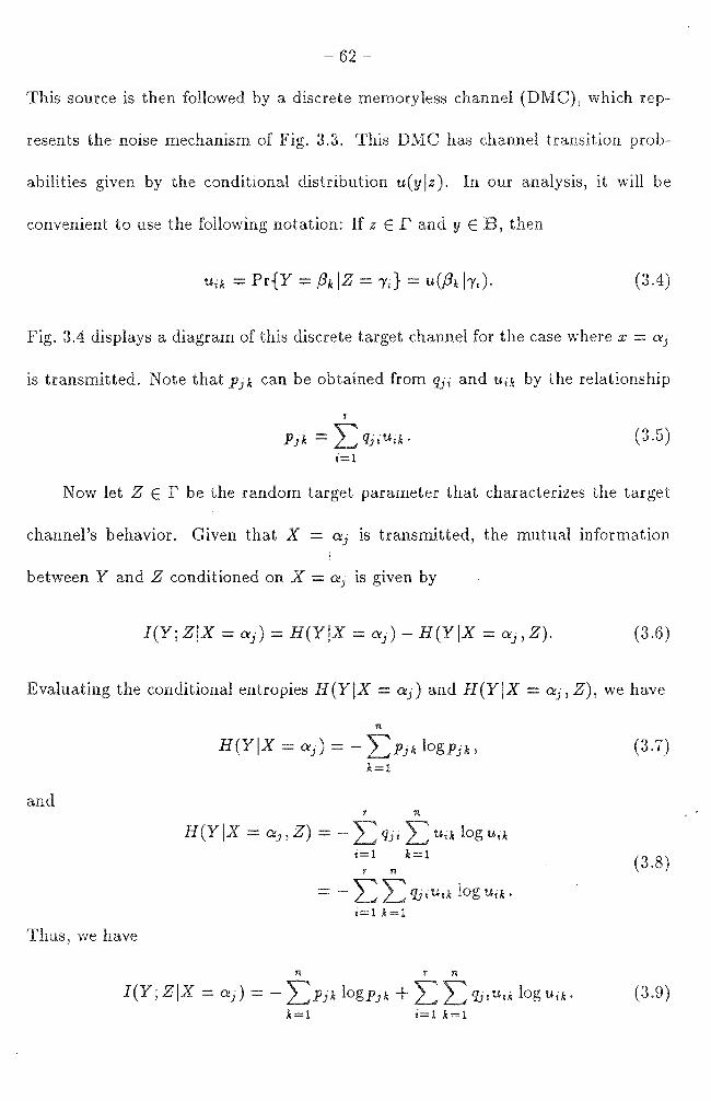
- 62 -

This source is then followed by a discrete memoryless channel (DMC), which rep-

resents the noise mechanism Fig. 3.3. This DMC has channel transition prob-

abilities given by conditional distribution u(y lz). our analysis, it will be

convenient to use the following notation: z E and y E B, then

ua = Pr{Y = /31r. IZ ='Yi}= u(/31'. lr1). (3.4)

Fig. 3.4 displays a diagram of this discrete target channel for the case where x = a:J

is transmitted. Note that Pik can be obtained from qji and Uik by the relationship

r

Pjk = I::qj1Uik·

i=l

(3.5)

Now let Z E r be the random target parameter that characterizes the target

channel's behavior. Given that X = Otj is transmitted, the mutual information

between Y and Z conditioned on X = Otj is given by

I(Y;Z!X = ai) = H(Y!X = ai) H(Y!X = aj,Z). (3.6)

Evaluating the conditional entropies H(YIX = aJ) and H(YIX = aj, Z), we have

11

H(Y!X = ai) = - I::Pik logpik, (3.7) k=l

and

H(YIX = Otj, Z) = - qji «ik log «ik

i=l k=l r 11

(3.8)

i=l k=l

we have

11 r 11

I(Y; Z!X = aJ) = - I::Pjk logpjk +I:: qj1Uik log Uik. (3.9) k=l i=l k=l

- 63 -

the expectation of Eq. (3.9) over the ensemble , we have

I(Y;ZIX) = L IT(x)I(Y;ZIX = x). (3.10) sEA

Defining Kj = IT( aJ), this can be rewritten as

m

I(Y;ZIX) = L I(Y;ZIX = 01J)· j=l

(3.11)

We wish to find the distribution rr = {;r1, ... 'Am} that maximizes I(Y; ZIX).

We must maximize Eq. (3.11) over the set {x-1 , ... , 1rm} C Rm under the constraints

{ 1C'j ?.'.: 0, for j = 1, ... , m;

m

L: 'X'j = 1. j=l

In order to do this, we define 1iAh as

(1) def . _ Imax - max{I(Y,ZIX - aJ)}·

J

Define A (l) ~ A as follows:

(3.12)

(3.13)

(3.14)

Then I(Y; ZIX) is maximized by any distribution II = { x- 1 ,. .. , 1r m} that satisfies

the following conditions:

'Kj = o, 1ij ?.'.: 0,

m

for all j such that <Xj ~ A.C 1);

for all j such that O:j E A.< 1);

L: = 1. j=O

(3.15)

- 64

The conditions on the maximizing distribution given by Eq. (3.15) have the

simple interpretation of assigning all of the probability to those °'j that provide

Z by observation of Y. None of the probability is

assigned to the set {A - A.< 1)}, as these waveforms do not provide the maximum

amount of information about the target. We note that the maximum is always

achieved by at least one of the aj, and thus A_(i) always has at least one element.

The maximum value R(Y; Z) of I(Y; ZIX), obtained with any distribution that

satisfies Eq. (3.15), is

R(Y;Z) = fx!2x = max{I(Y;ZIX = a:J)}. (3.16) J

This is, of course, as expected.

Note that the problem has a deterministic solution as well. If we transmit

any waveform x in A_(l) with certainty, we will achieve the maximum mutual in-

formation R(Y; Z). This is because the resulting probability distribution in this

case-probability one of transmitting the selected waveform in A (l) and prob a-

bility zero of transmitting all others-satisfies the requirements for a maximizing

distribution as given in Eq. (3.15).

This basic analysis will be applied to the analysis of more complicated channels

subsequently, but first we will examine a few examples of the discrete memoryless

target channel for the case of N = 1.

Example 3.1: Consider the discrete memoryless target channel in Fig. 3.5.

target channel is made up of two binary discrete channels in cascade. The

first represents the effects of uncertainty in the scattering mechanism and the

- 65 -

Figure 3.5. Memoryless Binary Target Channel of Example 3.1.

second represents observation noise. In this discrete target channel model, we

have A= {a1,a2}, r = {r1,r2}, and B = {,81,,82}. The discrete memoryless

channels making up the target channel have transition probabilities

q11 = Pr{Z = r1, X = ai} = 0.75,

q12 = Pr{Z = r2,X = ai} = 0.25,

q21 = Pr{Z = r1,X = a2} = 0.50,

qn = Pr{Z = r2,X = 0:2} = 0.50,

«11 = Pr{Y = ,81, Z - ri} = 0.90,

«12 = Pr{Y = ,82, Z = ri} = 0.10,

u21 = Pr{Y = ,81, Z = r2} = 0.10,

«22 = Pr{Y = ,82, Z - r2} = 0.90.

It is

66 -

straightforward to calculate the overall target ""~""v

Pu=

P12 = Pr{Y = /3z, X - 011} = 0.3,

P21 = Pr{Y = /31, X = az} = 0.5,

Pz2 = = /32, = a2} = 0.5.

transition proba-

Applying Eqs. (3.7) and (3.8) and using base-2 logarithms, we have

and

H(YIX = ai) = -0.7 log 2 0.7 - 0.3 log2 0.3 = 0.8813 bits,

H(YIX = 0:2) = -0.5 log2 0.5 - 0.5 log2 0.5 = 1 bit,

H(YIX = oq,Z) = 0.75[-0.9log0.9-0.llog0.1]

+ 0.25 [-0.9 log 0.9 - 0.1log0.1]

= 0.4690 bits,

H(YIX . a2, Z) = 0.5 [-0.9 log 0.9 - O.llog 0.1]

+ 0.5 [-0.9 log 0.9 - 0.1log0.1]

= 0.4690 bits.

From Eq. (3.6), we have

Thus, we have

I(Y; ZIX = cq) = 0.4123 bits,

I(Y; ZIX - a 2 ) = 0.5310 bits.

I~lx = max{I(Y;ZIX - ai),I(Y;ZIX = az)} = 0.5310bits.

- 67 -

follows then that

The maximizing distribution II of X is thus obtained by assigning all of the prob

ability to a:2 ; that is,

So I(Y; ZIX) is maximized by transmitting 0:2 with certainty, and R(Y; Z), the

resulting maximum value of I(X; YIX), is

R(Y;Z) = I~lx = 0.5310bits.

Example 3.2: Consider the discrete memoryless target channel shown in

Fig. 3.6. This target channel is again made up of two cascaded discrete mem

oryless channels. The first, with three inputs and two outputs, represents the

target-scattering process. The second, a noiseless binary symmetric channel,

represents the observation noise--in this case no observation noise is present.

68 -

channels making up the target channel have transition probabilities

q11= =r1, =a1}=0.50,

qi2 = Pr{Z = r2, X = ai} = 0.50,

u11 = Pr{Y = /31,Z = ri} = 1,

U21 = Pr{Y = /31, z = r2} = 0.10,

Un= Pr{Y = /32, z = r2} = 1.

The overall target channel transition probabilities are thus

P11 = Pr{Y = /31, X = ai} = 0.50,

Applying

P12 = Pr{Y = /32, X = ai} = 0.50,

P21 = Pr{Y = /31, X = a2} = 0.75,

p31 = Pr{Y = /31, = a3} = 0.50,

p32 = Pr{Y - /32, (3.7) and (3.8) usmg

a3} - 0.50.

logarithms, we have

IX = ai) = -0.5 log2 0.5 - 0.5 log2 0.5 = 1 bit,

IX = a2) -0.75 log2 0.75 - 0.25 log2 0.25 0.8113 bits,

H(YJ = a3) = -0.5 log2 0.5 - 0.5 log2 0.5 = 1 bit,

- 69 -

1.0 /31

y

Figure 3.6. Memoryless Discrete Target Channel of Example 3.2.

and H(YIX = a:- 1 , Z) = 0 bits,

H(YIX = a:- 2 ,Z) =Obits.

It follows from Eq. (3.6) that

I(Y; ZIX = ai) = 1 bit,

I(Y; ZJX = a 2 ) = 0.8113 bits~

I(Y; ZIX = a3) = 1 bit.

Thus,

I~12x = max{J(Y; ZJX = ai), I(Y; ZIX = az), I(Y; IX= a3)} = 1 bit.

So we have

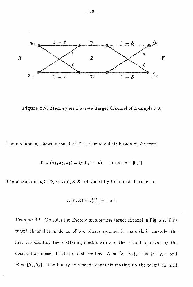
70

l - s /31

v

l E l - s

3 Memoryless Discrete Target Channel of Example 3.3.

The maximizing distribution II of X is thus any distribution of the form

II= (K1,11"2,K3) = (p,0,1-p), for allp E [0,1).

The maximum R(Y; Z) of I(Y; ZIX) obtained by these distributions is

R(Y; Z) = I~12x - 1 bit .

........ "V·"'' 3.3: Consider the discrete memoryless target channel in Fig. 3.7. This

target channel is made up of two binary symmetric channels in cascade, the

first representing the scattering mechanism and the second representing the

observation noise.

= {/11,/32}. The binary symmetric channels making up the target channel

- 71 -

have transition probabilities

q11 = Pr{Z = 'Y1,X = a:-1} = 1- €,

q12 = Pr{Z = "(2, X = ai} = €,

<l21 = Pr{Z = 'Y1, X = a:-2} = €,

q22 = Pr{Z = "(2, X = a:-2} = 1 - €,

u11 = Pr{Y = /31,Z ='Yd= 1- 5,

u12 = Pr{Y = /32, Z = 'Y1} = 5,

u21 = Pr{Y = /31,Z = 'Y2} = 5,

u22 = Pr{Y = /32,Z = r2} = 1- 5.

The overall target channel transition probabilities are thus

P11 = Pr{Y =/31,X = ai} = 1-(€+5-2€5),

P12 = Pr{Y = /32, X = ai} = € + 5 - 2€5,

P21 = Pr{Y = /31,X = et2} = € + 5 - 2€5,

Pn = Pr{Y = /32, X = a:-2} = 1 - ( € + 5 - 2€<5').

Applying Eqs. (3.7) and (3.8) , we have

and

H(YIX = a1) = 'H.(€ + 5 - 2€5),

H(YIX = a2) = 'H.( € + 5 - 2€5),

H(YIX = a:-1) = 'H.(5),

H(YIX = a2) = 'H.(5).

From Eq. (3.6), we have

I(Y;ZIX = ai) = I(Y;ZIX = a2) = 'H.(€+ 5-2€5)-'H.(5).

72 -

Thus, we have

I~lx = max{I(Y; ZIX = ai), I(Y; ZIX = az)} 1-i( € S - 2€S) -1-i( S),

where 1-i( €) is the binary entropy function defined in Chapter 2. It follows that

So any valid distribution II= (;f 1 , K 2 ) maximizes J(Y; ZIX), and the maximum

value R(Y; Z), which is obtained by all distributions of X, is

R(Y; Z) = 1-i( € + S - 2£5) -1-i( S).

As can be seen from these three single-observation examples, cases can arise in

which only one, several, or all of the possible transmitted waveforms in A achieve

the maximum information transfer between the target and the receiver.

We will now look at the solution for the general case of N observations of

the memoryless target channel. Assume that an N-tuple X E A(N) is transmitted

across the memoryless target channel, and the N-tuple YE B(N) is received at the

channel output. Given that a particular N-tuple x is transmitted, the probability

that a specific N-tuple y will be received is p(yix). Since the target channel is

memoryless, it perturbs each waveform in the N-tuple independently. Thus, if

p(y Ix) is the probability of receiving y E B, given that x E A was transmitted, then

as previously noted in Eq. (3.2),

N

p(yix) = rrp(y;Jx;). ?=l

- 73

Since the single-channel probabilities occur analysis of N uses of the memo-

ryless channel, we will again use the notation

transmitting an N-tuple across a memoryless channel, the independence of

each channel use means that we are using the channel N distinct times incorporating

the results of these N uses to form the N-tuple Y. Thus each of the N distinct uses

can be modeled as a single use as shown in Fig. 3.4. This means that the whole

process of the target channel's perturbing the transmitted N-tuple of waveforms,

such that the resulting received N-tuple is obtained, can be modeled as a source that

produces an N-tuple Z of letters from the ensemble r<N). If a particular N-tuple

x = ( Otj1 , ••• , Otj N) is transmitted, the probability of a particular z = ('y,1; 1 , ••• , 'Yk N)

by this source is N

q ( z Ix) = qj l kl qj 2 k 2 ••• qj N k N = II qJ ; k i )

!=1

(3.17)

where the single-use channel transition probabilities Pi ,k, corresponding to Xr - Otj

have distribution Q"; as in the case of the single channel use.

Once a particular N-tuple z E r<N) is generated, it is mapped to the N-tuple

y E B(N) at the channel output by N successive operations of the DMC representing

the observation noise process. If a particular N-tuple z = { 'Yi 1 , ••• , 11N} is generated

by the target source, the probability that a particular y = {th 1 , ... , ,6,1; N} is received

by the receiver is N

u(yJz) = Ui1k1 Ui2k2 • • • Ui2k2 =II ui,k,, J=l

(3.18)

- 74 -

where the channel transition probabilities u1 ilq are as defined in Eq. (3.4) for the

written terms of q(zjx) and u(yjz) as

p(yjx) = u(yjz)q(zjx). (3.19) zEI'< N)

Given that x = ( a 11 , ... , aj N) is transmitted, we have that the mutual information

between Y and Z conditioned on X = x is

I(Y; ZIX = x) = H(ZIX = x) - H(ZIX = x, Y). (3.20)

By the independence of the individual target channel uses, we have that

N

I(Y; ZIX = x) = '_LI(Yi;ZzlXz = aiJ· (3.21) Z=l

Taking the expectation of Eq. (3.21) with respect to X, we have

I(Y; ZIX) = L Il(x)J(Y; ZIX = x) zE r< N)

(3.22)

In order to find the distribution of X that maximizes I(Y; ZIX), define

(1) ~f • . - . Imax - max{I(Y, IX - aJ}. (3.23) J

Then we can once again define A= {aj EA: I(Y; ZIX = aj) = 1};1}, and the

set _A(N) ~ A(N) as the N-fold Cartesian product of .AC 1). We see from Eq. (3.22)

that I(Y; ZIX) is maximized by any distribution Il(x) that satisfies the following

conditions:

- 75 -

II(x) = 0, II(x) 2: 0,

for all x ~ }.._(N).

for x E }.._(N).

l:II(x)=l. xEA< N)

(3.24)

satisfies the conditions of Eq. (3.24) achieves the maxi-

mum value R(Y; Z) of I(Y; ZIX), and this maximum is given by (see Eq. (3.22))

R(Y;Z) = Nf.m12x = Nmax{I(Y;ZIX = a1 )}. (3.25) J

This is as expected.

Note that R(Y; Z), the maximum amount of information in the case when an

N-tuple of waveforms x is transmitted, is equal to N times R(Y; Z), the maxi-

mum amount of information obtained when a single waveform is transmitted (see

Eq. (3.16)). This is not surprising, as R(Y;Z) corresponds to the entropy of a

single letter from the ensemble r obtained from the channel model source, while

R(Y; Z) in the case of the memoryless target channel corresponds to joint entropy

of N independent uses of this source. Since the entropy of multiple independent

events taken jointly is equal to the sum of the entropies of the events individually,

we would expect that R(Y; Z) - NR(Y; Z).

Examples of the use of the memoryless channel for general N can be obtained

by making N-fold extensions of Example 3.1, Example 3.2, and Example 3.3. 'We

simply form the set }.._(N) from the set A in each of these examples, construct the

distributions such that all of the probability the ensemble A(N) is contained in

A_(N) as specified in

single use of the channel.

3

Fixed

vVe now consider

get. this case we

- 76 -

(3.24), calculate as N times the result for a

N a

case which multiple observations are made of a fixed tar

a target parameter Z, which is a discrete random variable

(vector) taking on values from the ensemble r. We can view Z as being generated

by a source that has probability distribution q(z) as shown in Fig. 3.2. Now, how

ever, we assume that once Z is generated, it remains fixed while N observations

are made by the radar system. These N observations are made by transmitting

an N-tuple of waveforms X and receiving a corresponding N-tuple Y of measure

ments. So we assume that X E A(N), with probability density II(x). Here again,

A = { a 1 , ... , am} is the set of possible transmitted waveforms.

When we transmit the N-tuple of waveforms X = {X1 , ... , XN }, we receive an

N-tuple Y = {Y1 , ... , YN} E B(N) at the output of the target channel (the output

Y,1; in response to the input Xk, for k = 1, ... , N). The output N-tuple Y is thus

dependent on the transmitted N-tuple X, the target parameter Z, and the noise

present in each observation. The probability distribution governing the out put y,

given that the channel parameter Z = z and the transmitted waveform X = x is

u(ylz,x) = Pr{Y = ylZ = z,X = x}. (3.26)

we define the conditional density p(y Ix) as

p(ylx) = Pr{Y = ylX = x}, (3.27)

- 77-

then we can write p(y!x) in of u(ylz, x) and q(z) as

p(y!x) = q(z)u(ylz,x). (3.28)

information J(Y; ZIX = x) in which we are interested is given by

I(Y; ZIX = x) = H(YIX = x) - H(YIZ, = x) (3.29)

= H(ZIX = x) - H(ZIY, = x).

Using the form given on the first line of Eq. (3.29), the conditional entropies of

interest are

H(YIX = x) = - L p(yJx) logp(yJx), (3.30) yE B( N)

and

H(YIZ,X = x) = Lq(z) L u(y!z,x)logu(yJz,x)

= - L L q(z)u(yJz,x)logu(ylz,x). (3.31) z:Er yEB(N)

Thus, from Eqs. (3.29) and (3.30),

I(Y; ZIX = x) = L {-p(y!x) logp(yJx) + L q(z )u(yJz, x) log u(y lz, x)} . yEB<N) zEr

(3.32)

We can now write

I(Y; ZJX) = L Il(x) {I(Y; ZJX = x)}. (3.33) xEA( N)

order to maximize I(Y; ZJX), we define

f:_N) def max {I(Y· ZIX = x)} max xEA( N) ' '

(3.34)

78

.A_(N) C A(N) as

A._(N) def {x E A(N): I(Y;ZIX = x) = I~J}. (3.35)

Then I(Y; ZIX) is maximized by any distribution II(x) that satisfies the following

conditions: II(x) = 0, II(x) ~ 0,

for all x ~ A (N);

for all x E A (N);

I:II(x)=l. xEA< N)

(3.36)

Any distribution II(x) that satisfies the conditions of Eq. (3.36) achieves the maxi-

mum value R(Y; Z) of I(Y; ZIX), which is

R(Y· Z) = f_N) = max {I(Y· ZIX = x)}. ' max xEA( N) '

(3.37)

From Eq. (3.29) and the fact that mutual information is a non-negative quantity,

we note that this R(Y; Z) is bounded by

0:::; R(Y;Z):::; min{H(YIX = x),H(ZIX = x)}.

But since H(ZIX = x) = H(Z)-that is, H(ZIX = x) is not independent of the

transmitted X-we have that no matter how large N grows for a fixed target,

R(Y; Z):::; H(Z). (3.38)

This makes sense, as it states that if there is an initial uncertainty H(Z) in the

fixed target, the most information we can obtain about it by making multiple mea-

surements of it is H(Z). After this much uncertainty has been obtained about the

fixed target, there is no more uncertainty to be resolved.

- 79

3 Finite-State Target

Section 3.2.1, we examined memoryless target channels where, although the

channel was used N times, the channel acted independently from use to use. While

this may be an accurate model of the target channel some instances, in many

others it may not be. order to illustrate this, we have the following example:

Example 3.4: Consider the radio sounding system that has a single waveform A =

{ ai} and which transmits an N-tuple x = (x1, ... , XN) = ( a1, ... , ai) across the

target channel, with each of the N waveforms a 1 transmitted T seconds apart.

Suppose that the target channel across which the N-tuple is being transmitted

is a slowly fading channel, with the typical fade having a period of T1. \Ve will

assume T1 ~ T. Such a channel could arise in radio sounding studies investigating

shortwave propagation. Now assume that the receiver receives the waveform at

the output of the target channel and decides between outputs from B = {/31,/32},

based on whether the energy in the received waveform is greater than or less than

some threshhold E0 • Assume that E0 is selected such that, on the average, Pr{Y =

/3i} = Pr{Y = /32} = 1/2 for each of the transmitted waveforms. Since T1 ~ T,

by looking at the output of the receiver for the last few waveforms received, we can

make a pretty good guess as to what the Q.ext output will be. By just guessing

the next receiver output to be equal to the last receiver output observed, we would

expect to be right significantly more often than half the time.

This simple example illustrates that the memoryless target channel does not

- 80 -

accurately model target channels encountered practice. As we will see in

the analysis of practical problems forthcoming this thesis, proper formulation of

target models where it might not at first be apparent that the memoryless model

is applicable. Still, it will be useful to have a target channel model that takes into

account target channels memory. We will now analyze the Radar /Information

Theory Problem for target channels with a simple memory mechanism. In order to

do this, we will formulate a target channel model which we will call the Finite-State

Target Ch.an.nel(FSTC). In this model, the target channel transition probabilities

will be controlled by a finite-state Markov process or Markov chain.

The Finite-State Target Channel (FSTC) maps the input sequence of wave

forms x1, ... , x N represented by the N-tuple x = ( x 1, ... , x N) into the out put se-

quence

y1, ... ,yN represented by the sequence y = (y1, ... ,yN), where x E A(N) and

y E B(N). This is done by the following mechanism.

The channel has a finite set of states S = { 0"1 , ... , crq}. At any given time, the

channel is in one of the states in S, and with each channel use the channel changes

to another state, with all elements of S (including the current state) being possible

candidates. Given that the channel is currently in a state q E S, if any input x E A

is input into the channel, the probability that y E

given by p("")(yix).

is received at the output is

The state transitions of the channel are assumed to be independent of both

- 81

channel inputs and states prior to current state at the time of transition. The se-

quence of states s = ( s1, ... , SN) that characterize the channel during the time that

x is being across channel is assumed a subsequence of a finite-state

ergodic Markov chain ( ... ,s-1,so,s1, ... ). For all G"a,ub ES, the state transition

probabilities of the Markov chain are given by

(3.39)

We also define the joint probability

(3.40)

We note that Eqs. (3.39) and (3.40) are valid for all integer values of the time

index 1, since the ergodicity of the Markov chain implies that the Markov chain is

stationary. Eqs. (3.39) and (3.40) are related by the expression

(3.41)

where

(3.42)

the FSTC, the overall target channel transition probabilities when the chan

nel is in state q isp((/")(yjx). Inside the FSTC, we assume that a source generates the

target parameter Z, and that the value of Z can statistically dependent on both

the transmitted waveform X and the current channel state <Tt. The probability that

a particular z is generated by the target source when a particular x is transmitted

and the channel is in state <T1 is q<(/" 1 )(zlx). The probability that a particular z will

- 82 -

be mapped to a particular at the channel output when the target channel is in

state (J't is t./" 1 )(yjz). p(")(ylx) is related to qC" 1 )(zjx) and t./" 1 \ylz) by the relation

(3.43)

order to illustrate FSTC, we will look at a pair of examples.

the FSTC that takes inputs from A = { a 1 , a 2 } and

maps them to outputs from B = {,81 ,,82}. Assume that the channel has states

S = { (}'1 , (}'2 } and that the state transition probabilities are

w( (}'1 l(J'i) = 0.99, w( (J'2 I0"1) = 0.01,

Assume also that the channel transition probabilities as a function of the cur-

rent state are

p<" 1 )(.B1 Ja1) =LO,

p(" 1 )(,B1 Ja2) = 0.0,

i"2 )(,B1 Ja1) = 0.8,

i" 1 )(/31 Ja2) = 0.2,

p<"d(/32 lai) = 0.0,

i" 1 )(/32 la2) = 1.0,

p<" 1 )(/32 lai) = 0.2,

p<" 1 )(/32 Ja2) = 0.8.

This channel is described graphically by the state diagram and channel transi-

tion diagrams Fig. 3.8. In a communications problem, such a channel would be

useful modeling a burst error channel [3.1, pp.97-99].

Recall Example 3.4, the fading channel. we noted that observation of the

current received waveform gave a pretty good indication of what the next received

waveform would be. Let us now construct a model of such a channel using the

FSTC.

- 83 -

0.01

9 o.a

fo)

Ql /31 Ql /31

H v v

Q2 • • /32 Q2 f32 1.0 0.6

S= s = (}"2

(b) ( c:)

Figure 3.8. Finite-State Target Channel of Example 3.5. (a) State Diagram of Channel; (b) Channel Transition Diagram for S = <11 ; ( c) Channel Transition Diagram for S = <12 •

Example 3.6: Consider the fading channel described in Example 3.4. Here the

period of a typical fade was T1 and a waveform x - a 1 was transmitted every

seconds. vVe also assumed that T1 ~ T. As a result of the fade, half the

time y = (31 was received at the output and half the time y = (32 was received

at the output. Thus, a reasonable model of this fading channel using an FSTC

84

T

(a)

1

H v

s = (J'2

(b) (c)

Figure 3.9. Finite-State Target Channel of Example 3.6. (a) State Diagram of Channel; (b) Channel Transition Diagram for S = cr1 ; ( c) Channel Transition Diagram for S = 0-2.

with S = { o-1 , cr2 } is as follows: The transmit and receive waveform sets are

The state transition probabilities are

- 85 -

channel transition probabilities are

/cr 1 )(,81 la1) = 1.0,

/cr 2 )(.81la1) = 0.0,

p(cr 1 )(.82 lai) = 0.0,

P(cr2)(.82lai) = 1.0.

The state diagram and channel transition diagrams of this channel are shown

in Fig. 3.9.

We will now look at the solution of the Radar/Information Theory Problem for

the FSTC. We are interested primarily in finding the distribution of X that maxi

mizes I(Y; ZIX) for the general case of N uses, as well as determine the maximum

value R(Y; Z). In the process we will look at several related problems.

The FSTC for N = 1:

Although the case of a single channel use of the FSTC does not illustrate the

statistical dependence between multiple uses of the channel, it is worth examining

because it illustrates several important features of the FSTC in as simple a context

as possible. Once the FSTC has been analyzed for the case of N = 1, the extension

to general N is straightforward, although not as trivial as it was in the case of the

memoryless channel. For the case of N = 1, we are primarily interested in finding

I(Y; ZIX) and the distribution II(x) of X that maximizes I(Y; ZIX). Before doing

this, however, we will first find I(Y;ZjX,S = a-t) and I(Y; IX,S). In practical

applications, these two quantities are of little interest, since S, the state of the

Markov chain characterizing the FSTC, is not known a priori. Still, determination of

I(Y; IX,S = a-.t) and I(Y;ZIX,S) gives insight into the FSTC and is intermediate

- 86 -

to obtaining the desired solution, so we will solve for these conditional mutual

informations.

Det I(Y; z1x, s = <Tt) N = 1:

Consider the situation where a j , o: j E , and S

I(Y; IX, S = o-1 ) is given by

I(Y;ZIX = aJ,S = <T-t) = H(YIX = aJ,S = <Tt) -H(YIX = aj,Z,S = <T-t).

Evaluating these conditional entropies, we have

n

H(YIX = Otj, S = 0-1) = - LPJ~1 ) logp)~ 1 ) k=l

and r n

H(YIX = a Z S = <T ) = - "'"'q(cr 1)"'"' ,}""

1) log t/"" 1

) J J ) l L..t JI L..t 1k 1k

i=l k=l

i=l k=l

Combining Eqs. (3.44), (3.45) and (3.46), we have

n

I(Y; ZIX = a1 , S = o-1 ) = - LP); 1) logp)~ 1 )

k=l

i=l k=l

Taking the expectation of Eq. (3.47) with respect to , we have

I(Y; ZIX, s = o-t) II(.x)I(Y; ZIX = x,S - 0-1) .rEA

m

= L 11"j {I(Y; ZIX = O:j' s o-t)}. j=l

(3.44)

(3.45)

(3.46)

(3.47)

(3.48)

- 87 -

We now solve Il(x) = maximize Eq. (3.48).

Define

( ) def 1;::x = max{I(Y; IX=aj,S=ut)}, (3.49)

J

and define .A_(o-;) C A as

(3.50)

a distribution Il(x) = {11"1, ... ,ll"m} maximizes I(Y;ZIX,S =qi) if and only

if it satisfies the following constraints:

'il"j = O, 'il"j > 0,

for all a tf .A_(o-;) J y::. '

for all a· EA(o-;) J )

2::: 'il"j = 1. j:o.;EA.<111)

(3.51)

Any distribution satisfying Eq.(3.51) achieves the maximum value R<" 1 )(Y; Z) of

I(Y;ZIX,S = q 1), given by

R<" 1 )(Y;Z) = J<;:j = max{I(Y;ZIX = aj,S =qi)}. (3.52) J

This is, as before, the expected result.

- 88

,S) N = 1:

(3.48), we have

m

;ZIX,S = o-.t) = L [I(Y;ZIX = ,S = 0-1)]. j=l

Let w1 = w( o-t) = = o-1}. Then taking the expectation with respect to the

state S, we have

I(Y; z1x, S) = t, w, {t ~j [l(Y; ZIX = "i, s = u,)]}

= tAj {tw1 [I(Y;ZIX = aj,S = o-1)]}. 1 i=l

In order to maximize this quantity, we proceed as follows: Define

and .A_(s) ~A such that

where Q

def'\:""' I(Y;ZJX = O:j,S) = ~ W1 [I(Y;ZIX = Otj,S = 0-1)].

i=l

(3.53)

(3.54)

(3.55)

(3.56)

Then a distribution II(x) = {11" 1 , ... ,-x-m} maximizes I(Y;ZIX,S) if and only if it

satisfies the following conditions:

ll"j = o, Aj ;?:: 0,

for all a A- .A_(s) J v: '

for all a· E .A_(s) J '

I: = i. j:a.iEA(s)

(3.57)

- 89 -

II(x) satisfies the conditions of Eq.(3.57) achieves the maxi-

mum J?< 5 )(Y; Z) of ; ZIX, S), given by

(3.58)

et I(Y; ZIX) for N = 1:

For the case of N = 1, we are most interested in finding I(Y; ZIX). This

is because the mutual information between Y and Z is conditioned only on X,

which is known to us a priori, whereas I(Y;ZjX,S = <r-i) and I(Y;ZIX,S) are

conditioned on the state of the channel, which is not generally known to us a priori.

We now look into the problem of determining I(Y; ZIX), finding the maximizing

distribution II(x) of X, and finding the resulting maximum R(Y;Z) of I(Y;ZIX).

If qji, Uik, and Pik are defined as

def q]i = Pr{Z=rilX=aJ},

def Ujk = Pr{Y = {3;;, IZ = ri}, (3.59)

def Pjk = Pr{Y = fJk IX = aj },

(3.60)

- 90 -

and the current state probabilities w1 as Q

q - ~ w q(o-1) JI - L i ji '

i=l

Q ~ (0-1)

u1,1; = L wi u 1;.; , (3.61) i=l

Q ~ (o-i)

Pjk = L W1P1k . i=l

Once again, assuming = Otj, we can model the FSTC as a new source with source

alphabet r = { ')'l' ... 'f11} followed by a discrete channel representing the observa-

tion noise. This new source produces the random variable Z E r - { r 1 , ... , r 11 }

with probability distribution Qa; = (<jj 1 , ... ,q1 11 ). Now

I(Y;ZIX = 0t1) = H(YIX = a1)- H(YIX = a1 ,Z). (3.62)

The conditional entropies H(YIX = Otj) and H(Y IX = a1 , Z) are given by 11

H(YIX = a1 ) = - LPJk Iogpjk k=l

= - t [t w,p)~·)] log [t w,p)~·)], (3.63)

and 11

H(YIX = Otj, Z) = - LL qjiUik log uik

i=l k=l

Thus, we have

I(Y;ZIX = "J) = t{ [tw,p)~·)] log [tw,p)~·)]

- 91 -

the expectation with respect to yields

m

I(Y; IX)= I>-j {I(Y; ZIX = o:J)}. (3.66) j=l

order to maximize ; ZIX) with respect to the input distribution of X, we

proceed as follows: Define

1< 1) <!::_f max{I(Y· ZIX =a)} max . ' J '

(3.67) )

and A_(l) ~A by

(3.68)

Thus, we see that a distribution II(x) = ( 1:" 1 , ... , 1:" m) maximizes I(Y; ZIX) if

and only if it satisfies the following conditions:

for all j: O:j ~ A_(i),

for all j: aj E A.< 1),

I: Kj = 1. j:Cll.; EAP)

(3.69)

The maximum value R(Y; Z) of I(Y; ZIX) achieved by the distribution II(x) sat-

isfying Eq. (3.69) is

R(Y · Z) = I(l) ' max '

(3.70)

where I~2x is as defined Eq. (3.67). This is , of course, as expected.

is now assumed the N-tuple E A(N) is transmitted across the FSTC

N-tuple E ) is received at the channel output. Given that a particular

N-tuple x is transmitted, probability that a N-tuple y is received

will be denoted by p(yJx).

Let s = { s1 , ... , SN} be the particular sequence of states that occurs during

the N uses of the channel in which x is mapped to y. Then we have s E S(N). The

probability of a given set of states s occurring is given by

w(s) = Pr{S =, s} = w(s1, ... , sN ). (3.71)

Because the state sequence of the channel is governed by an ergodic Markov chain,

we have

(3.72)

where w(sk ls;._i) and w(s 1 ) are defined in Eqs. (3.41) and (3.42), respectively.

Knowing this, we can now calculate q(zJx), u(yJz), and p(yJx).

Given that the channel has state sequence s = {s 1 , ... , SN}, the conditional

probabilities associated with the particular N-tuples z, and y are

q(s)(z Ix) - q<$ 1 )(z1 Jx1)pq(sa)(z2 lx2) · · · q(s N )(zN JxN ),

u(s)(ylz) = P(si)(Y1 Jzi)p(sa)(Y2 Jz2) · · ·p(sN)(YN JzN ), (3.73)

- 93

Ix), u(yiz), and p(ylx) are given by

q(zlx) = L w(s)q(s)(zjx), sE s< N)

iz) = L w(s)u(s)(yiz), sE s< N)

(3.74)

p(ylx) =

mutual information between Y and Z given that = x 1s

I(Y; ZIX = x) - H(YIX = x) - H(YIX = x, Z). (3.75)

The conditional entropies H(YIX = x) and H(YIX = x, Z) are given by

H(YIX = x) = - L p(ylx) logp(ylx) yE B( N)

= - L { [ L w(s)p(s)(ylx)] log [ L w(s)p(s)(ylx)] } , yEB(N) sES(N) sES(N)

(3.76)

and

H(YIX = x, Z) = - L L q(zly)u(ylz) log u(ylz)

Thus, we have

I(Y; ZIX - x) - L {- [ w(s)p(s)(ylx)] log [ L w(s)p(s)(ylx)] yEB(N) sES(N) sES(N)

{ (LsEs<N) w(s)q(s) Ix)] (LsES(N) w(s)1/s)(yjz)]}}

+ zEI'<") ·log (LsES(N) w(s)uCs)(ylz)] ·

(3.79)

- 94

Upon taking expectation of Eq. (3.79) with respect to X, we have

I(Y; ZJX) = Il(x) {I(Y; ZIX}. (3.80) xEA( N)

In order to maximize (3.80) with respect to the distribution Il(x), we proceed

as follows: Define

I(N) def max {I(Y· ZIX = x)} max xEA(N) ' '

(3.81)

and .A_(N) ~ A(N) by

.A_(N) def {XE A(N): I(Y; ZIX = x) = I~J}. (3.82)

Then a distribution Il(x) will maximize I(Y; ZIX) if and only if it satisfies the

following conditions:

II(x) = 0, for all x ~ .A_(N);

II(x) 2:: 0, for all x E .A_(N);

I: Il(x) = 1, xEA(N)

(3.83)

and the maximum value R(Y; Z) of I(Y; ZIX) obtained by any distribution satis-

fying Eq. (3.83) is

R(Y· Z) = JCN) ' ma::x:J (3.84)

where I~NJ is as defined Eq. (3.81).

3

- 95 -

Problem Continuous Target Channels.

Section 3.2, we examined the Radar/Information Theory Problem for discrete

target channels, in which, for each channel use, one of m waveforms was transmitted

by the transmitter and one of n waveforms was received at the receiver. In dealing

with real radar systems, it is reasonable to assume that one of a finite number

of waveforms is transmitted, but it is often not convenient to assume that one of

a finite number of waveforms is received. For example, if the radar receiver is

measuring the power scattered from the target, the received power can generally

take on a continuum of values. Although one could model the system-at least

approximately-by quantizing the received signal, this procedure can complicate

the analysis of the radar system. In addition, information is generally lost in the

quantization process. Thus, it is more appropriate to assume that the received

waveform can take on a continuum of values. In this section, we will examine

target channels that have a continuous target channel output. We will refer to such

channels as continuous target ch.annels, although the transmitted waveform is still

assumed to be a member of a finite set.

Consider the situation shown in Fig. 3.10, in which a transmitter transmits

an N-tuple E A(N), where A(N) is an ensemble of N-tuples of waveforms with

probability distribution Il(x), and A is the set of possible transmitted waveforms

A= { 0:1, ... , am}. The transmitted N-tuple X proceeds through the target channel

C, which perturbs X in such a way that an N-tuple E R(N) is received at the

receiver, where is the set of real numbers. The channel C perturbs the transmitted

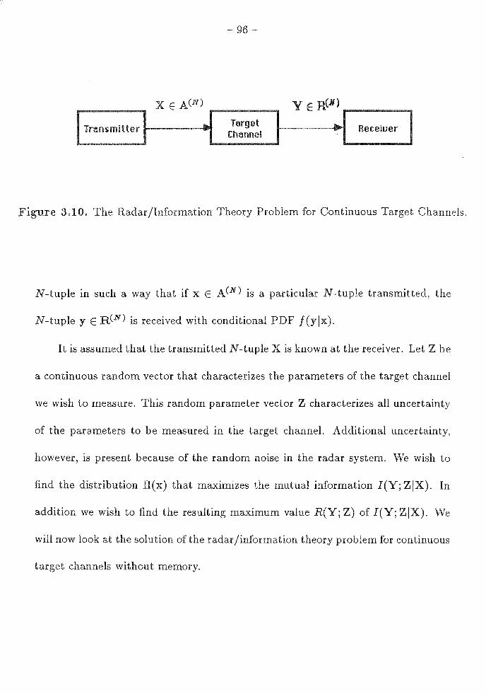
96

Transmitter .... Target .....

Receiuer Channel

~

Figure 3.10. The Radar/Information Theory Problem for Continuous Target Channels.

N-tuple in such a way that if x E A(N) is a particular N-tuple transmitted, the

N-tuple y E R(N) is received with conditional PDF f (yix).

It is assumed that the transmitted N-tuple Xis known at the receiver. Let Z be

a continuous random vector that characterizes the parameters of the target channel

we wish to measure. This random parameter vector Z characterizes all uncertainty

of the parameters to be measured in the target channel. Additional uncertainty,

however, is present because of the random noise in the radar system. We wish to

find the distribution II(x) that maximizes the mutual information l(Y; ZIX). In

addition we wish to find the resulting maximum value R(Y; Z) of l(Y; ZIX). We

will now look at the solution of the radar/information theory problem for continuous

target channels without memory.

- 97 -

c

Consider the Radar/Information theory problem as outlined in Fig. 3.10, but

with a memoryless continuous target channel, by which we mean that the propa-

gation of each individual waveform transmitted N-tuple propagates through

the target a manner independent of the others. For any transmitted

x E A(N) and y E ) we have

x = (x1, ... ,xN), Xk EA, for all k = 1, ... ,N, (3.85)

Y = (y1, ... ,yN), y;., ER, for all k -1, ... ,N.

Since the channel is memoryless, the channel transition PDF of y conditioned on x

is given by N

/(yjx) = II /(Yr Jxr ). (3.86) r=l

In order to analyze the problem for the continuous memoryless target channel,

we will first examine the case where N = 1 (a single use of the target channel). The

case for general N will then be an easy extension of the case for N = 1.

For the case where N = 1, a single waveform from the ensemble A is transmit-

ted through the target channel and is perturbed by the target channel such that an

element of the set a real number, is observed at the output of the channel.

the case of the discrete target channel, where calculations dealt with (ab-

solute, not differential) entropy, we modeled and target channel

together as a new source with a noiseless channel connecting Y and Z. In the case

of the continuous channel, however, a noiseless channel would have infinite capacity.

Thus, we cannot directly extend the model we used in the discrete case, as using a

98 -

channel model that has infinite capacity is neither intuitively appealing, physically

realistic, or mathematically tractable.

order to develop a model for continuous target channel, we look to

the physical measurement process that takes place the measurement of target

characteristics by a radar. transmitter transmits a waveform X that illuminates

the target in order to measure some characteristic of the target represented by

Z. The value of this random variable Z can be dependent on the transmitted

waveform X. For example, if Z represented the mean reflectivity of the target,

this could be a function of the frequency spectrum of the transmitted waveform.

The electromagnetic wave incident on the target is then scattered by the target. A

portion of the scattered wave is detected and processed by the receiver, resulting in

the measurement Y. Thus, Y is dependent on Z. Y is, of course, also dependent on

X, both through the dependence of Y on Z and the fact that receiver processing is

a function of the transmitted waveform. Taking these mechanisms into account in

the radar measurement process, we have the model shown in Fig. 3.11 for the case

of N = 1. As can be seen, this model is characterized by two PDFs, f(zlx) and

f(yjz,x). In our analysis, we will need the PDF's f(ylz,x) and f(ylx). This latter

PDF can be obtained from the two PDF's our model by 00

f(ylx) = j f(yJz,x)f(zjx)dz. -oo

From the definition of mutual information for continuous random variables as

given m (2.35), we have that I(Y; ZJX) is given by both

I(Y; ZIX) = h(YIX) - h(YIZ, ), (3.87)

99 -

H y

Figure 3.11. Continuous Target Channel Model.

and

I(Y; ZIX) = h(ZIX) - h(ZIY, X). (3.88)

Here, h(YIX), h(YIZ, X), h(ZIX), and h(ZIY, X) are conditional differential

entropies, given by

h(YIX) =•EA II(x) {-_l /(ylx) log f (yix) dy} , (3.89)

IZ, X) = ~ !I(x) {-_l _l f(y, z Ix) log f (y lz,x) dy dz} , (3.90)

h(ZIX) =•EA II(x) {-_l f(zix)logf(zix)dz}, (3.91)

h(YIZ, X) =•EA II(x) {-_l _l f(y, z ix) log /(yiz ,x) dy dz} . (3.92)

100

derivation that follows, we will use the form in Eq. (3.87), as it will be more

straightforward in the applications we will consider. However, our results could

also be us mg (3.88), and in some applications latter may be more

straigtforward.

From Eqs. (3.87), (3.89), and (3.90), we have

;ZIX) = IT(x)I(Y; ZIX - x), (3.93)

where

00 00 00

I(Y;ZIX=x)=- j f(ylx)logf(ylx)dy+ j j f(y,zlx)logf(ylz,x)dydz. -oo -00-00

(3.94)

In order to find the distribution Il(x) of X that maximizes I(Y; ZIX), we proceed

as follows: Define

I~lx def max{I(Y;ZIX = x)}. .'.l'EA

(3.95)

Define ,_c\(l) ~A as

,_c\(l) = {x EA: I(Y;ZIX = x) = I~lx}. (3.96)

Then I(Y; ZIX) is maximized by a distribution Il(x) if and only if it satisfies the

following conditions:

m

= O, for all j such that °'i ~ ,_c\(l);

~ O, for all j such that <Xj E ,_c\(l);

I: = 1. j=O

(3.97)

maximum value R(Y; Z) of I(Y; ZJX) obtained by any such distribution is

(3.98)

- 101

This is as expected.

We now examine general case of N uses of the memoryless target channel.

Assume an N-tuple X E A (N) is transmitted across the memoryless target

channel, and N-tuple E R(N) is received at the channel output. Given that

a particular N-tuple x is transmitted, the PDF of the N-tuple y being received is

f (yjx). Since the target channel is memoryless, it perturbs each waveform in the

N-tuple independently. Thus, if f(yjx) is the PDF of y E R, given x E A was

transmitted, then as previously noted in Eq. (3.86),

N

f (yjx) = IT f(Yr Jxr ). r=l

In transmitting an N-tuple across the continuous memoryless channel, the

independence of each channel use means that we are using the channel N distinct

times and are incorporating the results of these N uses to form the N-tuple Y. Thus,

each of the single uses can be modeled as shown in Fig. 3.11. If the transmitter

transmits an N-tuple x = (x 1 , ••• ,xN), the PDF of Z = (z 1, ... ,zN) conditioned

on xis N

/(zlx) =IT f(zr lxr ). (3.99) r=l

So the N-tuple Z characterizes the random behavior we wish to measure for the N

channel uses, with the r-th element Z 1 representing the r-th of N uses.

Given that a specific x is transmitted, the mutual information between Y and

Z conditioned on =XIS

I(Y; ZjX x) = h(YJX = x) - h(YI = x, Z). (3.100)

102

expectation of Eq. (3.100) respect to X, we have

I(Y; ZIX) = 2: II(x)I(Y; ZIX = x). (3.101) YEA(N)

order to distributions of that maximize I(Y; ZjX), we proceed as

follows: Define

I~12x <!.:_f max { I(Y; ZIX = x)}. a:EA

(3.102)

Define A_(l) ~A as

A ( 1) = { x E A : I ( y; z Ix = x) = I~ 2x} . (3.103)

Define A,.(N) as the N-fold Cartesian product of A,.(l). Then from Eq. (3.101), we see

that a distribution II(x) maximizes I(Y; ZjX) if and only if it satisfies the following

conditions: II(x) = 0, II(x) 2 0,

for all x ~ A (N);

for all x E A (N);

L: II(x) = 1. xEA< N)

(3.104)

The maximum value R(Y; Z) of I(Y; ZjX) achieved by distributions that satisfy

Eq. (3.104) is

R(Y; Z) = NI~2x = N ~~;3·f {I(Y; ZIX - x)}. (3.105)

This is what we would expect by analogy to the discrete memoryless target channel.

The extension of the memoryless continuous target channel to a finite-state

continuous target channel, with memory controlled by a Markov chain with a finite

number of states, is straightforward and is done in a manner analogous to that of the

discrete case. We assume that the conditional PDF's that characterize the statistical

- 103 -

behavior of the channel are a function of the Markov chain state s ES, just as was

done with the conditional probabilities in the discrete case. Thus, these distributions

would be would then use these

distributions to calculate the mutual information J(s)(Y; ZfX) and then calculate

I(Y; ZJX) by averaging over s as was done in the discrete case. Determination of

distributions that maximize I(Y; ZJX) and the resulting maximum values is then

done in an identical manner to that done in the discrete case. Since we will not be

using the finite-state continuous target channel in subsequent work, we will not go

through this straightforward derivation here.

3.4. Conclusions.

In this chapter we have formulated and investigated th.e Radar/Information Theory

Problem for both discrete and continuous target channels. This provides a basis for

the design of radar waveforms for obtaining the maximum amount of information

about a target, and also provides some of the tools for analyzing the information

content of radar images. Both of these problems will be examined in the remainder

of this thesis. Before the results in this chapter can be applied to these practical

radar problems, we must obtain models of the radar targets of interest. In the next

chapter we will review and develop statistical scattering models of radar targets,

with goal of applying the results of this chapter to these models. The results of

the Radar/Information Theory Problem in this chapter and the models of the next

chapter will form the basis of the information-theoretic design of radar waveforms

and analysis of practical radar systems.

104 -

3 er 3

3.1 Gallager, R. ., Theory and Reliable Communication, John Wiley

and Sons, New York, 1968.

- 105 -

4

SC MODELS

The Radar/Information Theory Problem, examined as the framework for the

information-theoretic analysis of radar systems in the previous chapter, is depen

dent on statistical models of radar scattering and noise behavior. This is reflected

in the PDFs that arise in the model. These PDF's are the sole representation of

target behavior in the target channel model. Thus, if the results of the previous

chapter are to be used in the analysis of practical radar systems, statistical models

of the radar targets and target channels for these systems must be developed.

When considering measurements of a radar target, we realize that the electro

magnetic wave scattered by the target, besides being a function of the transmitted

waveform, is also a function of both the target's spatial and material characteris

tics. We assume that the target is made up of either multiple scattering centers or a

continuum of scatterers distributed in space. Then, when the transmitted waveform

is reflected from the target, it is reflected by many points on the target that are

spatially separated. If these points have different material composition, the fraction

of the incident energy reflected will be a function of the material composition of the

points. addition, the scattered waves from the various points on the target will

add constructively and destructively at different points in space, generating an in-

terference pattern in space.

spatial distribution of the

shape or spectral content.

- 106 -

interference will a function of both the

scatterers and the transmitted waveform's wave

fact will be of considerable importance in our work

dealing with waveform design in Chapters 5 and 6, so we will also be interested in

models that characterize the scattering characteristics of spatially extended targets.

order to facilitate the development of our radar-scattering models, a brief

review of radar cross section, the analytic signal representation, and polarization

and depolarization in scattering will be presented.

4.1. Radar Reflectivity and Radar Cross Section.

In this section we will briefly review radar reflectivity and introduce the parameter

known as radar cross section. In the process, other parameters of interest in specify

ing radar systems will also be introduced. More detailed and specialized discussions

of radar reflectivity can be found in References [4.1-4.7].

If an electromagnetic wave is incident on a boundary at which two materials of

differing characteristic impedances ry 1 and ry 2 (rt - ;µ;;, whereµ is the permeabil

ity of the material and e is its dielectric constant), then the electromagnetic wave

will be at least partially reflected [4.8]. Thus, an electromagnetic wave transmitted

by a radar through free space or an atmosphere will generally be at least partially

reflected or scattered it impinges upon a target, such as the planetary sur-

face below or an aircraft flying in the atmosphere. So when a radar is making

measurements on an object, the magnitude of the reflected signal is a function of

the material making up the object. The magnitude of the reflected wave is also a

107 -

function of several other characteristics of the object, such as its size, orientation

with respect to the radar, frequency spectrum of the waveform illuminating the

target, and the transmitted electric field polarization.

radar cross section G' of a scatterer is a parameter that measures the

amount of power a target scatters toward a receiver. This will be a function of the

physical orientation of the transmitter, target, and receiver. In this chapter we will

concentrate primarily on monostatic radar systems, in which the transmitter and

receiver antennas are collocated (and often the same physical aptc.nna), but these

results can be extended in a straightforward manner to the case of bistatic radar

systems, in which the transmitter and receiver antennas are in different locations. In

dealing with monostatic radar systems, we are interested in the signal scattered back

at the radar, and we refer to the radar cross section in this case as the backscatter

cross section.

The radar cross section u is a parameter defined to be proportional to the

received echo power from the radar target. The received power for a monostatic

radar system is related to the radar cross section (J" by the relation

(4.1)

108 -

Here

def d . . . f <T = ra ar cross sect10n m umts o area,

receive<l power,

Py = transmitted power,

G = antenna gain (the same for both transmit and receive),

,\ = wavelength of transmitted signal in units of length,

R = radar-to-target range in units of length.

From Eq. ( 4.1), it can be seen that the radar cross section <T is the cross-

sectional area required of an isotropic scatterer in order to receive power PR given

Py, G, .A, and R. This can be derived from the Friis Transmission Equation [4.9,

Sections 1.7 and 3.10].

In considering the reflectivity of complex radar targets, we are often examining

the combined return from a large number of individual scatterers. When considering

such targets, the concepts of coherent and incoherent scattering can be useful. If

the phase of a wave is constant or varies in a deterministic manner, the wave is

said to be coherent. If the phase of the wave is randomly distributed over the

interval [O, 2;r], it is said to be incoherent. It is a well-known fact that the total

power resulting from the sum of multiple incoherent waves is equal to the sum of

the powers of each of the waves individually. The power resulting from the sum of

multiple coherent waves must be obtained by summing the electric field that is due

to each of the individual waves and then by determining the total power from the

resulting electric fiel<l. This is because the resulting power for the multiple coherent

109 -

waves can much greater than the sum of the power of the individual waves,

or it can be much less-the resulting power can even be zero. The resulting power

in the coherent case depends on whether the individual waves add constructively or

destructively.

Mathematically, if a target is composed of N individual scatterers with radar

cross sections q 1 , the total cross section that results from all of the individual

scatterers is N

fJ = L.,/(i;'e'..Pt j=l

(1.2)

where the tfj are the phase angles that are due to the phase delay corresponding to

the range of the j-th scatterer from the target. If the j-th scatterer is at distance

Rj from the target, assumed constant over the target, the phase if1 is given by

.I .. - 41' Rj ( 'f'J - ,\ mod 27f). (4.3)

If the tf J are independently and uniformly distributed on the interval [O, 2Jr],

corresponding to the case of incoherent scattering, then one has

N

<T1c = E L .,/(ij' ei'ift;

j=l

N N N

L .,/(ij' ./(ikE { ei( + 1- 'ift .,) } = <Tj'

j=lk=l j=l

since for j =f:. k

because

( 4.4)

- 110 -

But for j = k,

So from Eq. ( 4.4) we see that in non-coherent scattering, the power from the

individual scatterers add, or equivalently, the total radar cross section is the sum of

the individual radar cross sections. We are assuming here that there is no significant

shielding or multiple reflections between scatterers.

In general, the field scattered from a radar target has both a constant coherent

component as well as a random, incoherent component. For example, if the target

under consideration is land being illuminated by a scatterometer, there may be

a non-coherent component in the radar return because of the roughness of the

terrain. There may also be a coherent component that is due to a large specular

return from a large scatterer, for example, a large metal roof on a building which is

smooth compared to the scale of the wavelength of the radar signal. If the surface

being measured is very rough and there are no specular components, as in the

case of a perfectly diffuse surface, there may be only an incoherent scattered field.

This property is, of course, a (slowly varying) function of the wavelength of the

transmitted radar signal.

In talking about the roughness of a scattering surface or radar target, the

Rayleigh roughness criterion is often used to classify a surface as rough or smooth.

The Rayleigh roughness criterion can be described as follows. Assume that a radar

illuminates a target at a grazing angle () with respect to the normal of a rough

planar surface, as shown in Fig. 4.1. If the difference in height ( in the direction

111

normal to the surface) between two neighboring points on the surface is f:;.h, then

the phase difference between two waves reflected from these two points is

Here

f:;. <I> = 47r f:;.h sin() . ,\

f:;.h = difference in height between the two points,

.\ = wavelength of electromagnetic wave,

(4.5)

() - incidence or grazing angle of wave with respect to local surface tilt.

To give a qualitative description of whether a surface is rough or smooth, the

Rayleigh roughness criterion uses Eq. ( 4.5). A surface is considered rough if

and smooth if

f:;.h sin() > ~, 8

f:;.h sin() < ~.

(4.6)

(4.7)

It is clear that this is an imprecise criterion for surface roughness, but for f:;.h sin() <

>../8, it is safe to assume that the surface is smooth, and for f:;.h sin() > A./8, it is

safe to assume that the surface is rough.

- 112 -

4

Transmitted radar signals are general the result of the amplitude and phase

modulation of a sinusoidal carrier. As such, they can be represented as

s(t) = a(t) cos [2;r /oi + ¢{t)], (4.8)

where s(t) is the transmitted radar signal, a(i) is the envelope of the amplitude

modulation, ef>(t) is the phase modulation function, and / 0 is the transmitter carrier

frequency. It is straightforward to represent standard radar modulation formats

(pulse-amplitude modulation, linear and non-linear FM, bi-phase modulation) in

terms of Eq. ( 4.8). In most radar systems of interest, even such wideband systems as

direct-sequence spread-spectrum radars, the envelope a(t) and phase </;(i) are slowly

varying functions of time in contrast with cos 2;r / 0i. Thus, these waveforms are

"narrowband" waveforms in the sense that their Fourier transform S(f) is centered

and concentrated around the carrier frequency / 0 . Thus, although their bandwidth

can be very large, it is for all practical purposes much less than f 0 .

Since the waveform s(t) is real, it follows that the Fourier transform S(f) of

s(i) is conjugate-symmetric in f. That is,

S(f) = 5(-f). (4.9)

Here the bar over the right-hand side of the equation represents complex conjuga

tion.

In dealing with radar waveforms, it is often convenient to work with a complex

113 -

analytic function t.j; ( t) such that

s(-1) = Re { t./;(-t)}, ( 4.10)

and 00

1 J s( T) Im { t./;(t)} = s(t) = - - dr. K l - T

(4.11)

-oo

So s(i) is the Hilbert transform of s(t). Thus, we have that the analytic signal

representation t./;(t) of s(t) is given by

00

t./;(-1) = s(-1) + is(-1) = s(-1) + j_ j s(r) dr. K -I - T

( 4.12)

-oo

If s(t) is a narrowband waveform, that is, if

S(f) = 0, ( 4.13)

then it can be shown [4.10] that

t.j; ( t) = a( t) exp { i[2K f ot + 4{1)]} . ( 4.14)

Although the narrowband condition of Eq. ( 4.13) may not be exactly satisfied for

a given radar signal s(t), it is approximately satisfied for practical radar systems,

even for spread-spectrum radar systems.

· We also note that

00 00

'I!(!)= j t.J;(t)e-i 2 ~11 dt = j [sO) + ;-t * s(t)] e-i 2~11 dt - S(f) [1 + Q(f)]. - 00 -oo

Q(f) = { 01,, for f ;:=:: O;

for I < o.

1

So we have

iI!(f) = { 25(/), for f :;::: O; o, for I< o, ( 4.15)

and energy in the signal s(i) is given by

00

£ = J s ( t) s ( t) dt' ( 4.16)

-oo

or 00 1; -£ = 2 ~(t)~(t) dt. ( 4.17)

-oo

These relationships are useful both in representing radar-signals and in calculating

their energy or power.

4.3. Polarization, Depolarization, and Scattering.

Most monostatic radars both transmit and receive electromagnetic waves of the

same single polarization. When radar measurement of a target is made with such a

radar, the information obtained about the target by the radar is limited to the scat-

tering properties of the target for the particular polarization and target orientation

with which the measurement was made. Measurements made with additional polar-

izations and different polarizations on transmit and receive can provide additional

information about the scattering characteristics of the target. This information may

be useful in classification or identification of the radar target. In addition, some

polarizations will provide a larger backscattered field than others, making polariza-

tion diversity useful in target detection as well. Reference [4.11] provides a detailed

study of polarization in radar scattering problems. Reference [4.2, Ch.7] presents

115 -

data from several studies which the radar returns from land were measured by

airborne radars at several polarizations. These results show that polarization di-

versity is indeed valuable in obtaining information about terrain in radar remote

sensing, so we will now briefly examine polarization radar scattering.

The polarization of an electromagnetic plane wave can be described in terms of

two orthogonal linearly polarized components. Let z be the direction of propagation

of a plane wave and let x and y be two mutually orthogonal directions, both of

which are orthogonal to the direction of propagation z. Assume that the wave is

transmitted by a radar, scattered by a target, and that the scattered field is then

received by the radar. Let E!, E!, E;, and E; be the components of the transmitted

electric field strength in the x-direction, transmitted electric field strength in the y-

direction, received electric field strength in the x-direction, and received electric field

strength in the y-direction, respectively. Then the received electric field components

E; and E; can be expressed in terms of the transmitted electric field components

E! and E; by the relation

( 4.18)

The 2 X 2 matrix relating the transmitted and received fields in Eq. ( 4.18) is

known as the polarization scattering matrix and is a function of the scatterer. The

elements of this matrix are complex numbers relating the amplitude and phase of

the respective fields. If

and

116 -

then Eq.( 4.18) can be vectorially as

( 4.19)

The energy scattered by the target depends on the transmitter frequency, target

orientation, and position of the target with respect to the radar, and so the elements

of are also a function of these parameters. In the case of a monostatic

radar, the matrix is a symmetric matrix, with axy - ayx [4.12]. This can be most

easily seen by using reciprocity, that is, by interchanging the roles of the collocated

transmit and receive antennas of the monostatic radar system.

As was previously noted, polarization diversity can provide significant informa

tion about the surfaces being measured in radar remote sensing. This is due in part

to the depolarization. of the illuminating wave when it is scattered wave from the

surface being measured. When an electromagnetic wave is scattered by an object

or surface the backscattered wave may not have the same polarization as the wave

incident on the object or surface. This phenomenon is known as depolarization.. In

specular reflection, the sign of the polarization is reversed, but this does not count

as depolarization, since no energy is being transferred to an orthogonal polarization.

Generally, the rougher the surface or object scattering an electromagnetic wave,

the greater the depolarization. This is because multiple reflection is one of the ma-

jor mechanisms from surfaces. very large, smooth targets, there is usually very

little depolarization, but most natural surfaces have both a polarized backscatter

component and a depolarized backscatter component. Reference [4.2, Ch.3] dis

cusses several models of depolarization mechanisms in scattering processes.

117 -

depolarization of transmitted wave generally occurs in the scattering

process, we will now introduce a quantity known as the cross-polarization cross

section, is denoted (/ xy. is defined in the same manner as the radar cross

section in (4.1), except that it is assumed that the transmit antenna has linear

polarization x and the receive antenna has linear polarization y.

Typically, in dealing with backscattering from surfaces, the directions x and

y are taken to be either in the plane of incidence (vertically polarized) or perpen

dicular to the plane of incidence (horizontally polarized) [4.1, pp.168-9]. Radar

backscattering from the surface is then characterized by the four backscattering

cross sections uv y, <TH H, <TH y, and <:ry H. These four backscatter cross sections

are often used to characterize the backscatter characteristics of a surface in radar

remote sensing.

If direction x is taken to be vertical and direction y is taken to be horizontal in

Eq. ( 4.18), we have that the backscatter cross sections <rvv, <THH, <THY, and oy H

are related to the elements of the polarization-scattering matrix by the relations

O"y v = K lavv 1

2,

O"HH = J{ laHH 12

'

<iVH = K lavHl2

,

O"HV = K laHv 12

•

Here, K is a constant taking into account scaling that is due to space loss and taking

into account the spatial point of reference for the electric fields in Eq. ( 4.18).

- 118

4 St Models Backscatter

Radar backscatter from land can be caused by natural objects such as plants, trees,

grass, rocks, hills, and bare ground, as well as by man-made objects such as roads,

railroads, buildings, automobiles, fences, and power lines. 'When illuminating a

portion of the earth's surface with an airborne or spaceborne radar, a resolution

cell on the ground is generally large enough to have a large number of scatterers

in it. As the radar makes successive measurements, the radar moves and so does

the resolution cell along the earth's surface. As a result, from measurement to

measurement, a large number of scatterers leave the resolution cell, a large number

of new scatterers enter the resolution cell, and those scatterers that remain in the

resolution cell undergo a significant change of phase in their radar return because of

radar motion. Thus, from measurement to measurement, there can be considerable

fluctuation in the backscattered signal from the surface. In addition, there may be

large fixed objects that remain in the radar's field of view for several resolution cells,

contributing a strong constant component to the returned signal. Thus, it appears

that land scatterers viewed with airborne radars can be grouped (at least roughly)

into two broad categories:

1. Small scatterers of which there are a very large number and for which no

individual scatterer dominates in terms of total backscattered power, and

2. Large specular reflectors that contribute a significant portion of the total

backscattered power in a resolution cell.

Terrain made up of scatterers from the first group can be modeled as a large

- 119 -

number of random scatterers [4.2], and it is reasonable to assume that such a sur-

face is rough in the Rayleigh sense ( Lih sin 0 :> A./8). We will now look at the

development of a theoretical model for this case.

Consider a radar illuminating a surface made up of a large number of random

scatterers. the electric field at the receiving antenna reflected from the j-th of

a large number n of scatterers be given by

E . - A ·e 14'; J - J '

( 4.20)

where

A j the magnitude of the electric field scattered by the j-th scatterer,

<f>J = the phase of the electric field scattered by the j-th scatterer.

Assume that both transmit and receive are done with fixed, although not necessar-

ily the same, polarizations. Since the scatterers arf; randomly distributed over the

surface and, for surfaces of practical interest, will generally vary in size, we will as-

sume that both Aj and </>J are random variables. Assume that the positions of these

scatterers are independent of each other, that the size of an individual scatterer is

independent of other individual scatterers, and that scatterer sizes are independent

of scatterer positions. From these three assumptions, we can reasonably conclude

that:

1. is statistically independent of A.1;, for j f: k.

2. </>j is statistically independent of</>;., for j f: k.

3. Aj is statistically independent of</>;., for all j and k.

120 -

Since the surface is made up of scatterers randomly distributed and is rough

in the Rayleigh sense, we will assume that the <f>J are independent, identically dis-

tributed random variables uniformly distributed on [O, 2;r ]. vVe will also assume

that the Aj are independent, identically distributed random variables with mean

µA and finite variance o-~. We then have that the total electric field from a large

number n of scatterers is n

E = LA; ei.P i = V ei8 •

j=l

Expressing Eq. (4.21) in rectangular form, we have

E X + iY,

with n n

X = Vcos() = LAJ cos<f>J = LX;, j=l j=l

n n

Y = V sin()= LA; sin <f>J - L 1j. j=l j=l

Here,

1j = Aj sinef>J·

(4.21)

( 4.22)

(4.23)

( 4.24)

Now the X 1 constitute a set of independent identically distributed random variables,

as do the Yi. Their means and variances are given by

E(X1 ) = E(AJ cos <f>J) = E(AJ) E( cos <f>J) = ftA • 0 = 0,

0"2 + µ2 o-_i; = E(A} cos 2 <f>J) - E(A]) E(cos 2 <f>J) = A

2 A,

( 4.25)

( 4.26)

( 4.27)

( 4.28)

central limit theorem [4.13, p.193] states that if X 1 ,X2, ... ,Xn denotes a

random sample from a distribution that has mean µ and finite variance o- 2 , then

the random variable

has a limiting distribution that is Gaussian with mean 0 and variance 1, as n -too.

Applying the central limit theorem to

( 4.29)

and n

y =I:~, ( 4.30) j=l

and realizing that although n is finite, it is very large, we have that both X and Y

are approximately Gaussian, both having mean 0 and variance n(o-~ + µ~)/2.

We will assume the Gaussian approximation to be exact. This gives us density

functions of X and Y as

( 4.31)

and

( 4.32)

with

2 n(o-~ + µ~) O" = 2 . ( 4.33)

122 -

important thing to note is that for all practical purposes, X and Y are zero-

mean Gaussian random variables with finite variance o-2. In addition, we have

smce

E(XY) E (t X1 n Y") = E (t tA1A.1; cos</>) sin</>;.) J=l k=l 1=1 k 1

n n

= I: :LE (Al Ak) · E (cos </>1 sin <,bk) - 0, 1=1 k=l

{ J cos</>1 sin</>1d</>1=0 , for j = k;

E (cos </>j sin</>;.) = ~1(" 2 1("

J J cos </>1 sin <Px d</>1 d<,b;. = 0 , for j -:/: k. 0 0

But since E(X) = E(Y) - 0, we have

E(X)E(Y) = 0,

and thus,

E(XY) = E(X)E(Y),

which implies that X and Y are uncorrelated random variables. But since X and

Y are Gaussian random variables, they are statistically independent [4.13, p. 120].

From Eqs. ( 4.21) and ( 4.22), we have

Ve10 - X + iY, ( 4.35)

and so

v = Jx2 + y2 ( 4.36)

8 = tan- 1 (Y/X).

- 123 -

Thus, by a change of variables, we have that the joint density of V and 8 is

fv,11(v, B) = lo(x,y)I

y [x(v,B),y(v,B)] o(v,B)

1

8(x,y)I [ x ( v , e)] t y [11 ( v , e)]

8 (

11, 0

) ( 4.37)

=L , for 0 ::; v < oo, 0 ::; () < 21r;

, elsewhere.

Integrating the joint density fv,B(v,0) with respect to 8 on the interval (0,21r), we

obtain

fv(v) = 7 2;,,., exp(-v2 /2o-2 )d0 =;,exp(;;:).

0

Thus, we have that the magnitude V of the received electric field, that is V = jEj,

is a random variable which is Rayleigh distributed, and has the Rayleigh PDF

{ ( 2) 'ti ex -v fv(v) = r p 2;T

, v?::: O;

, elsewhere. ( 4.38)

The received power fron the surface of randomly distributed scatterers is given

by

( 4.39)

By a change of variable and the result of Eq. ( 4.38), we see that the PDF of P is

given by

= 2~2 exp ( i) · The mean of P, µp, is

00

µp = E (P) = j p · (1/2o-2) exp (-p /2o- 2

) dp = 2o-2•

0

( 4.40)

(4.41)

124 -

So we can write the PDF of the received power as

fp(p)- { ~l/µp)exp(-p/µp) , for p 2 O; , elsewhere.

( 4.42)

So the received power from a rough surface of randomly distributed scatterers is

exponentially distributed. This is a well-known and often quoted result, yet a

is given. A derivation is included here, as this result will be used

in our scattering model for the information-theoretic analysis of imaging radar in

Chapter 8.

As was previously noted, large specular returns can also be present in radar

returns from land. In such cases, there is a relatively constant component in the

return signal as well as the return from randomly distributed scatterers. We will

model the amplitude -YV of the return signal for such surfaces as

W = jVei0 + ae17 j. ( 4.43)

Here,

V=

X = a Gaussian random variable with mean 0 and variance 0"2 ,

Y = a Gaussian random variable with mean 0 and variance 0"2 ,

e = a random variable uniformly distributed on [O, 21r],

r = a random variable uniformly distributed on [O, 21r],

a= amplitude of return from the constant scatterer.

As before, X and Y are statistically independent. In addition, we will also assume e

and r to be statistically independent, which is reasonable, since we would not expect

- 125

the phase of the sum of the returns from the random scatterers to be dependent on

the phase of the return from the constant scatterer.

of Wis given [4.14, pp. 106,107]:

w ( w2+a

2) (wa) (w) - a: 2 exp - 20- 2 Io a: 2 , (4.44)

where I 0 (-) is the modified Bessel function of order zero [4.15, p. 147]. The mean

power (P - W 2 ) in this case is

- 2 2 2 µP - a- a . ( 4.45)

If we define the parameter m 2 as the ratio of the power of the constant component

to that of the random component, we have

a2 2 m =-.

2a-2

Then we can write the PDF of the received power P as

( 4.46)

( 4.47)

'When the terrain echo contains large, dominant scatters as well as a large num-

ber of randomly distributed scatterers, we would expect the PDF of the returned

power to satisfy Eq. (4.47). Note that as the parameter m 2 goes to zero, Eq. (4.47)

reduces to Eq. (4.42). Scattering mechanisms that have the PDF of the received

power given by Eq. ( 4.42) are often referred to as Rayleigh scatterers, whereas scat-

tering mechanisms that have the PDF of the received power given by Eq. ( 4.47) are

often referred to as Rician scatterers [4.2]. Note that Rayleigh scattering is actually

a special case of Rician scattering, the case where the constant scattering amplitude

a -+ 0.

- 126 -

4 A Model for Cross Me s From Rough Surfaces.

As was mentioned in Section 4.3 and as is well established References [4.2, 4.11,

and 4.16], polarization diversity can provide a substantial increase in a radar sys-

tern's ability to determine the characteristics of a target. Reference [4.16] discusses

the implementation of radar systems that both transmit and receive with multiple

polarizations. Reference [4.7, Ch.4] analyzes such systems in detail.

'We will now consider a relatively simple form of such a multiple polarization

problem for scattering from rough surfaces and will statistically model it. Consider

a system that transmits with a single linear polarization, which we will designate

as polarization A, and receives with both polarization A and an orthogonal linear

polarization, polarization B. Let PA be the received power from polarization A

and PB be the received power from polarization B. vVe already know from the

derivation leading to Eq. ( 4.32) that if the surface being illuminated is made up of

a large number of randomly distributed scatterers, then the PDFs of PA and PB

are given by

( 4.50)

and

( 4.51)

We will assume that PA and PB are statistically independent random variables. If

we make this assumption, the joint PDF of PA and PB is

( 4.52)

by

\Ve now define a parameter rJ, which we will call

def p.B 't]=-.

P.11.

cross polarization ratio,

( 4.53)

The parameter rt has the physical interpretation of being the ratio of the depolarized

power to the non-depolarized power in the backscattered radar return from the

surface. We note that this is a coarse measure of surface roughness, since smooth

surfaces have very little depolarization.

We are interested in finding the PDF of 'ff· To do this, we make the following

change of variable involving PA and P.B. Let

( 4.54)

Then the joint density function of 't] and r is given by

(4.55)

Letting a = µp 2 ryµp 1 and fJ - µp 1 µp 2 , and integrating with respect to /, Eq.

( 4.55) becomes

00 00

f11(Y1) = j f11,1(Y1, r) dr - j ~exp (- ';) dr 0 0

( 4.56)

fJ

128 -

we that the of rJ is

/,(?) ~ { 0

where p -

4.6. tics

, for 17 > 0,

, for !J < 0,

vVaveforms.

3.57

A radar waveform x(-t) is a function of time that represents the electric field trans

mitted by the radar at some fixed polarization. Thus, x(i) represents the magnitude

of the transmitted electric field as a function of time, and the direction (polariza

tion) of the electric field is assumed to be known. In the operation of a radar system,

the transmitted field is scattered by the target and a portion of it is received by the

receiver, which determines target characteristics from it. One of the target charac

teristics that can be determined by a radar system is the spatial extent of the target

in range. The ability of a radar system to do this is a function of the transmitted

radar waveform. We will now investigate how the pulse shape of a radar waveform

determines its spatial resolution properties.

In discussing the spatial resolution characteristics of radar signals, a commonly

quoted result is that the minimum resolvable distance between two objects is in

versely proportional to the bandwidth of the transmitted radar waveform. VVe will

now investigate this statement, using a very simple waveform of finite bandwidth,

one made up of two sinusoids. Such a waveform x(t) can be written as

x(i) = cos2x'/1i + cos27r/2i. ( 4.58)

129 -

Fourier transform X(f) of x(i) is

00

J . f 1 1 X(f) = x(i)e- 12

r t dt = 2 [5(! - Ji)+ 5(! +Ji)]+ 2 [5(/ - h) + 5(! + h)] · 00

( 4.59)

5( ·) is the Dirac delta function. The spectrum X (!) is shown in Fig. 4.1. As

can be seen from Fig. 4.1, x(t) can be viewed as a double-sideband, suppressed-

carrier waveform, and can be rewritten as

x(i) = 2 [cos 2K~ft] [cos 2Jr / 01]. (4.60)

Here,

f - fi+h 0 2 '

and

We now analyze this waveform's spatial resolution characteristics.

Consider a target consisting of two identical point scatterers as shown in Fig.

4.2. The scatterers are separated by a distance ~z along the direction of wave

propagation of a monostatic radar illuminating the object. If the waveform x('t) as

given m ( 4.58) is illuminating scatterers, there are interfering waves being

returned from the scatterers, and as a result, an interference pattern anses. As

the frequency difference ~f between the two sinusoids is varied from ~f = 0, the

situation arises in which the waves from the scatterers arrive back at the radar with

a phase difference of 180°, causing destructive interference at the radar antenna

- fo

- 130 -

X(f)

0

(a)

X(f)

0

(b)

R(f)

-M/2 0 M/2

(C)

fo

4.1. (a) Spectrum X(f) of the waveform x(i) of Eq. (4.58).

(b) Spectrum X(f) relabelled with the parameters of Eq. (4.60). (c) Spec

trum of the baseband waveform r(i), which modulates 2 cos 211' / 0 t to pro

duce x(t).

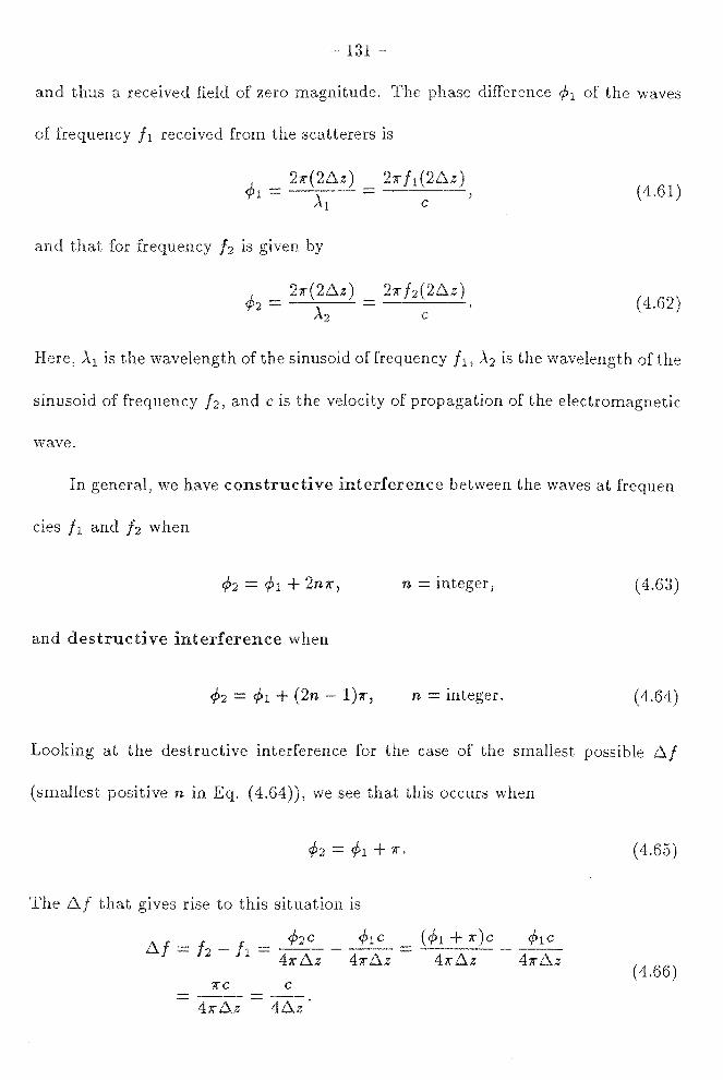
and thus a received field of zero magnitude. The phase difference </> 1 of the waves

of frequency Ji received from the scatterers is

21f Ji (2~z) c

(4.61)

and that for frequency h is given by

c ( 4.62)

Here, ,\ 1 is the wavelength of the sinusoid of frequency f 1 , ,\ 2 is the wavelength of the

sinusoid of frequency /2, and c is the velocity of propagation of the electromagnetic

wave.

In general, we have constructive interference between the waves at frequen-

cies Ji and h when

n =integer, ( 4.63)

and destructive interference when

4'2 = </>1 (2n - l);ir, n =integer. (4.64)

Looking at the destructive interference for the case of the smallest possible ~/

(smallest positive n Eq. ( 4.64)), we see that this occurs when

4>2 - 4'1 + Jf. (4.65)

The ~/ that gives rise to this situation is

JfC C ( 4.66)

41r~z - 4~z ·

132 -

Scatterer #1

Scatterer #2

Figure 4.2. Constructive interference from two scatterers separated by a

distance .6.z and illuminated by two sinusoids with a frequency difference

of .6./ = c/2.6.z.

Thus, we have that the frequency difference .6./ from constructive interference to

destructive interference is c/ 4.6.z.

The value of the smallest non-zero frequency difference for which constructive

interference occurs can be found from Eq. ( 4.63) taking n = 1. In this case, we

have

</>2 = </>1 + 211"' ( 4.67)

and thus,

.6.f - h - Ji=~ -~ = (</>1+2Jr)c -~ 411".6.z 411".6.z 4Jr.6.z 411".6.z

211"c c ( 4.68)

411" .6.z 2.6.z

From Eqs. ( 4.66) and ( 4.68), we see that for .6./ - 0 we have constructive

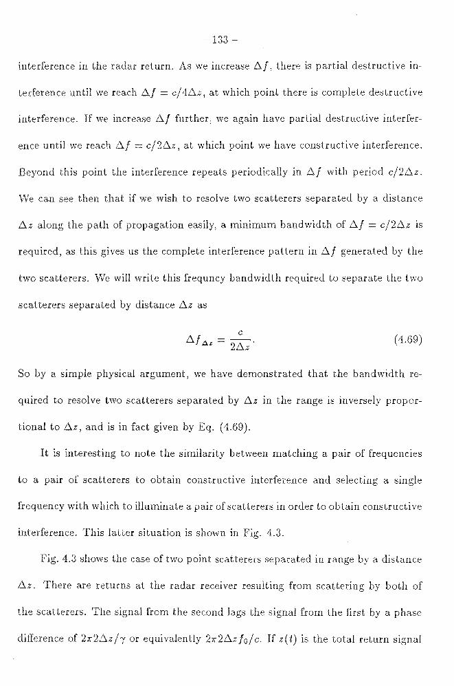
- 133 -

interference the radar return. As we increase , there is partial destructive in-

terference until we reach = c/ 4/:l.z, at which point there is complete destructive

interference. If we increase /:::;./ further, we again have partial destructive interfer-

ence until we reach f:l.f = c/2/:l.z, at which point we have constructive interference.

Beyond this point the interference repeats periodically in /:l./ with period c/2/:l.z.

We can see then that if we wish to resolve two scatterers separated by a distance

f:l.z along the path of propagation easily, a minimum bandwidth of l:l.f = c/26..z is

required, as this gives us the complete interference pattern in 6../ generated by the

two scatterers. \Ve will write this frequncy bandwidth required to separate the two

scatterers separated by distance 6..z as

c f:l.f A& = 26..z. ( 4.69)

So by a simple physical argument, we have demonstrated that the band width re-

quired to resolve two scatterers separated by 6..z in the range is inversely propor-

tional to , and is in fact given by Eq. ( 4.69).

It is interesting to note the similarity between matching a pair of frequencies

to a pair of scatterers to obtain constructive interference and selecting a single

frequency with which to illuminate a pair of scatterers in order to obtain constructive

interference. This latter situation is shown in Fig. 4.3.

Fig. 4.3 shows the case of two point scatterers separated in range by a distance

There are returns at the radar receiver resulting from scattering by both of

the scatterers. The signal from the second lags the signal from the first by a phase

difference of 27f21:l.z/r or equivalently 27f26..z/0 /c. If z(t) is the total return signal

- 134

Reder

Scatterer #' 1

Scatterer #2

Figure 4.3. Constructive interference from two scatterers separated by

a distance ilz and illuminated by a single sinusoid with a frequency of

f - c/2ilz.

at the radar receiver, then ignoring the round trip delay time to an<l from the first

scatterer, z(i) ex x(i) + x(i - 2ilz/c)

= cos27r/t + cos27r/(t - 2ilz/c) ( 4.70)

= cos 27r fl +cos (21r fl - 4x f ilzc).

vVe can see from Eq.( 4.70) that constructive interference occurs when 4x f 0ilz / c =

2ni. and destructive interference occurs when 41r foilz / c = (2n - l);r, where n is

any integer. Thus the frequencies at which constructive interference occurs are

given by

nc fc,n = 2ilz'

and the frequencies at which destructive interference occurs are given by

c ,n -

(4.71)

( 4.72)

and

- 135

n takes on integer values. particular, the smallest positive frequency at

c fc = 2~z'

smallest positive frequency at which

c fD=-.

4~z

( 4.73)

tive interference occurs is

(4.74)

Note the correspondence between the constructive interference cases of Eqs. ( 4.68)

and ( 4.73), as well as the correspondence between the destructive interference cases

of Eqs. (4.66) and (4.74).

That this phenomenon of constructive and destructive interference occurs on

frequency scales corresponding to both ~/ and / 0 can be seen by noting the sym-

metry of x(-t) as expressed in Eq. ( 4.60), which is repeated here:

x(-t) = 2 (cos 211"~/-t] [cos 211" /oi]. ( 4.60)

\Ve see that Eq. (4.60) is symmetric in cos2K~/i and cos2K/0-t, and that they

are both product terms of Eq. ( 4.60). The case of matching a single sinusoid of

frequency / 0 to the two scatterers is really just a special case of Eq. (4.60), in

which~/= 0 (ignoring the scale factor of 2). is interesting that many references

[4.2, 4.3, 4.4] that consider the interference from spatially distributed scatterers

emphasize the interaction that is due to the carrier frequency term, but not to that

of the modulation term. For most radar systems, fo ranges between 1 GHz and 20

GHz, and so the corresponding ~z for constructive interference would be on the

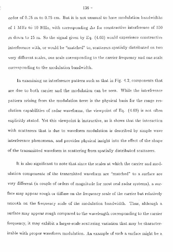
- 136 -

order of 0. m to 0.75 cm. But it is not unusual to have modulation bandwidths

of 1 MHz to 10 MHz, corresponding for constructive interference of 150

m down to 15 m. So the signal given by Eq. ( 4.60) would experience constructive

interference with, or would be "matched" to, scatterers spatially distributed on two

very different scales, one scale corresponding to the carrier frequency and one scale

corresponding to the modulation bandwidth.

In examining an interference pattern such as that in Fig. 4.2, components that

are due to both carrier and the modulation can be seen. 'While the interference

pattern arising from the modulation term is the physical basis for the range res

olution capabilities of radar waveforms, the viewpoint of Eq. ( 4.60) is not often

explicitly stated. Yet this viewpoint is instructive, as it shows that the interaction

with scatterers that is due to waveform modulation is described by simple wave

interference phenomena, and provides physical insight into the effect of the shape

of the transmitted waveform in scattering from spatially distributed scatterers.

It is also significant to note that since the scales at which the carrier and mod

ulation components of the transmitted waveform are "matched" to a surface are

very different (a couple of orders of magnitude for most real radar systems), a sur

face may appear rough or aiffuse on the frequency scale of the carrier but relatively

smooth on the frequency scale of the modulation bandwidth. Thus, although a

surface may appear rough compared to the wavelength corresponding to the carrier

frequency, it may exhibit a larger-scale scattering variation that may be character

izable with proper waveform modulation. An example of such a surface might be a

surface made up of several patches of homogeneous rough surface, each with differ

ent scattering characteristics, much like a checkerboard, with each square consisting

of a rough homogeneous scattering surface differing from neighboring squares. An

other example might be crops planted in rows, where the crops themselves would

appear to be rough compared to the wavelength of the carrier, but where the spac

ing between rows is on the order of the modulation wavelength corresponding to

D..f. Yet another example might be the surface of the ocean, where wind waves and

turbulence may cause the surface to be rough on the scale of the carrier frequency,

yet the larger gravity waves or swells may have a periodic structure on the order of

the wavelength corresponding to the waveform modulation bandwidth [4.17]. Fig.

4A illustrates what this surface might look like.

So one can view waveforms in terms of the interference patterns they generate

on the scales of both their carrier wavelength and their modulation wavelength when

considering the remote sensing of physical surfaces. The significance of this lies in

the fact that many natural surfaces are rough with respect to carrier wavelength, but

their material and geometric (or roughness) characteristics vary spatially. One of

the main purposes of remote sensing is, in fact, to determine the boundaries between

different regions and to produce an image or map that shows the distinctions be

tween these different regi:ms. Since the variation of importance distinguishing these

regions is often occurring on a scale larger than the carrier wavelength r = cf f 0 ,

the interference characteristics that are due to the waveform modulation may be

useful in characterizing the variation and texture of these regions.

138 -

Reder

Ocean Surf ece

Figure 4.4. Radar making measurements of a surface that is rough on the

scale corresponding to f 0 but that has variation on the scale corresponding

to .6.f.

Most real targets encountered are more complex than the two scatterers shown

m Fig. 4.2. They are generally made up of many distributed scattering centers.

In general, if a target is made up of n individual scatterers, there will be several

different effective .6.zi between scatters (in general n(n 1)/2 different .6.zi). \Vith

a different .6.fi for constructive interference corresponding to each distinct .6.z 1 ,

it seems feasible to characterize the structure of a group of distributed scatterers

by measuring the frequency response of the surface with respect to .6.f. Fig. 4.5

illustrates how this might be done for a real physical target. In this example,

the structure of the target on two different scales is determined with multiple .6.f

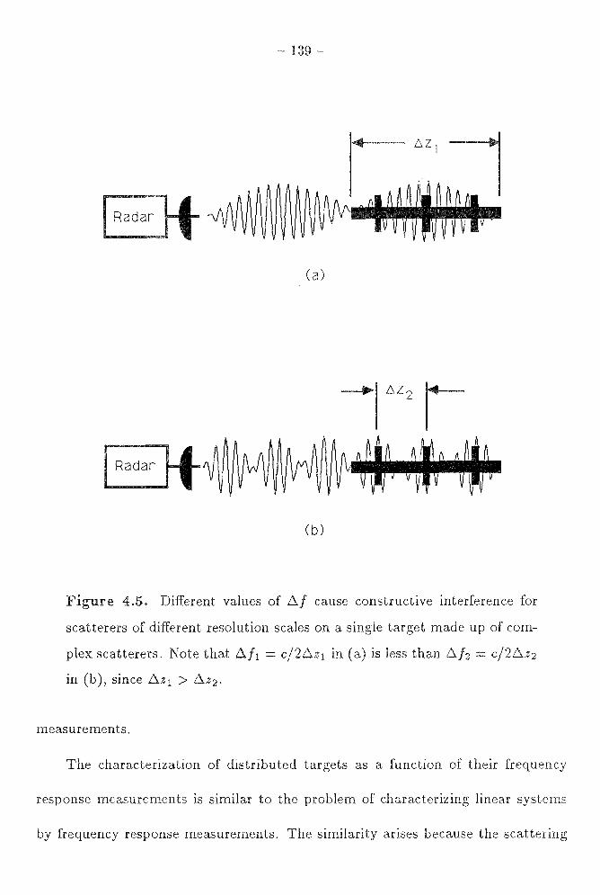
- 139 -

Radar

Ca)

(b)

Figure 4.5. Different values of l:lf cause constructive interference for

scatterers of different resolution scales on a single target made up of com

plex scatterers. Note that l:l/i = c/2/:lz1 in (a) is less than l:lh = c/21:lz2

in (b), since l:lz1 > tlzz.

measurements.

The characterization of distributed targets as a function of their frequency

response measurements is similar to the problem of characterizing linear systems

by frequency response measurements. The similarity arises because the scattering

- 140

of electromagnetic fields is a linear process. This can be seen by noting that if 1S

the incident electric field on a scatterer and E/ is the scattered electric field at some

point space, fields are related through the polarization scattering matrix

as specified Eqs. ( 4.18) and ( 4.19), by the relation

=AE 1• ( 4.75)

The elements of the polarization scattering matrix A are complex scalars. From Eq.

( 4.75), we can see that both homogeneity and superposition hold in electromagnetic

scattering, since if Ei = AEi and E2 AE2, then for any complex scalars a and

{3,

A ( o:E{ + f3E~) = aAEl + f3AE~

Thus, electromagnetic scattering can be modeled as a linear process.

In engineering, one common method of studying linear processes is to view them

as linear systems and to study the system input/output relationships. In addition

to being linear, the system can also be time-invariant, as would be true if the radar

and target were not moving rapidly with respect to each other. The system impulse

response is then a convenient tool for characterizing the input/output relationships

of the system. vVe will now examine the application of linear systems analysis to

electromagnetic scattering problems.

To apply linear systems analysis to scattering problems, we will first define

the input and output quantities to be the electric field magnitudes at a pair of

points in space. A block diagram of this linear time-invariant system is shown in

141

Fig. 4.7. We will assume a fixed, although not necessarily identical, polarization at

each point. input e(t) is x electric field intensity at point "P1 . VVe assume

that wave is moving along the line connecting "P1 and the origin. Now

if the plane wave is incident on the target located at the origin, as shown in Fig.

4.6, a scattered electric field will be present at an arbitrarily chosen observation

point P 2 • vVe select an arbitrary polarization x' at P 2 and view as the output of

our linear system the electric field v(t) at point P 2 with polarization x'. Thus,

restricting the direction and polarization of the incident plane wave and selecting

a point P 2 for measurement of the scattered wave for a fixed polarization, we have

that the relationship between e(t) and v(t) is that of a linear system. \Ve will also

assume that the scatterer is stationary during the period of observation, and that

the system relating e(t) and v(t) is a linear time-invariant system.

We will designate the impulse response of this system by h(t). In principle, the

impulse response of our linear time-invariant scattering system can be obtained at

the system output v(t) if the incident electric field is an impulsive plane wave, that

is, if e(t) = 5(t), where 5(-1) is the Dirac delta function. For general e(t), the output

v(t) of the linear system is given by

00

v(t) = j h(r)e(t r)dr. ( 4.76)

-oo

P1

142 -

"' x

..... Ei

Scatterer

__... c

Figure 4.6. Coordinate System of Scattering Problem.

Input Field Component

Target Impulse

Response

h(t)

~(t)

Output Field Component

A

z

Figure 4. 7. Linear Time-Invariant System Representation of the Station

ary Target-Scattering Mechanism.

- 143 -

Let the Fourier transforms of e(i), v(t), and h(t) be

00

E(f)= j e(i)e-i2Kftdi,

-oo

00

V(f) = j v(i)e-i2K fi dt' ( 4.77)

-oo

00

H (f) = j h ( i) e - 12 K f 1 di .

-oo

by the convolution theorem of Fourier transforms [4.18], we have

V(f) = E(f)H(f). (4.78)

The significance of Eq. ( 4. 78) to our analysis of scattering is that H (!) cor-

responds to a frequency response measurement of the target or scatterer, and the

impulse response can be obtained from H(f) by the inverse Fourier transform:

00

h(i) = j H(f)ei2K ft df. ( 4.78)

- 00

So the impulse response characterization of a target is equivalent to measuring its

frequency response for all frequencies. Practically, of course, this cannot be done.

It can, however, be done approximately, using large-bandwidth radar waveforms.

The impulse response characterization of targets also allows one to character-

ize not only discrete targets made up of a discrete collection of scatterers but also

distributed targets made up of a continuous scattering structure. The wideband

waveforms used in characterizing the impulse response of scatterers will in general

have continuous frequency spectra X (!), as opposed to the line spectra used when

- 144 -

illuminating targets with a pair of sinusoids as was previously done. Such a con

tinuous spectrum might be similar to the one shown in Fig. 4.Sa. These signals,

however, are still generated by modulating a baseband signal, such as that in Fig.

4.Sb, up to a higher frequency.

"'What is significant to note is that in the case of x(t) with continuous spectrum

X (!), there is still interference resulting from the carrier term cos 27r fot and also

from the modulating waveform r(t), which provides information about the target

on a frequency scale corresponding to the bandwidth of r(t) or more specifically to

the frequency differences present in the spectrum R(f) of r ( t).

In the next two chapters, we will examine the design of waveforms optimized for

two different tasks. We will use the notion of target impulse response in both cases.

First, we will examine the design of waveforms with optimum detection properties

for targets either with a given impulse response or with a given family of impulse

responses. After that, we will examine the design of radar waveforms that maximize

the mutual information between an ensemble of targets and the received signal at

the radar receiver.

- f 0

145 -

X(f)

0

(a)

R(f)

0

(b)

4 • (a) Continuous Spectrum X(f)

f o

f

·waveform. (b)

Spectrum R(f) of Baseband Modulating Signal Used to Generate vVave

form x(t) with Spectrum X(f).

146

4. er 4

4.1 Elachi, C., Physics and Techniques of Remote Sensing, John vViley and Sons,

New York, NY, 1987 .

4.2 Long, M. . , Radar Reflectivity of and Sea, Artech House, Dedham,

l 1983.

4.3 Ulaby, F. , 1'.iicrowave Remote Sensing, vol. 2, Addison-\!Vesley, Reading,

MA, 1982.

4.4 Ulaby, F. T., Microwave Remote Sensing, vol. 3, Artech House, Dedham, MA,

1986.

4.5 Tsang, L., J. A. Kong, and R. T. Shin, Theory of 1'.iicrowave Remote Sensing,

John Wiley and Sons, New York, NY, 1985.

4.6 Ruck, G. T., D. E. Barrick, W. D. Stuart, and C. K. Krichbaum, Radar Cross

Section Handbook, vols. 1 and 2, Plenum Press, New York, NY, 1970.

4.7 Ostrovityanov, R. V., and F. A. Basalov, Statistical Theory of Extended Radar

Targets, Artech House, Dedham, MA, 1985.

4.8 Ramo, S., J. R. Whinnery, and T. Van Duzer, Fields and Waves in Communi

cations Electronics, 2nd. ed., John vViley and Sons, New York, NY, 1984.


Systems, Plenum, New York, NY, 1980. 1984.

4.10 Cook, C. , and M. Bernfield, Radar Signals, Academic Press, New York, NY,

1967.

4.10 Rihaczek, A. \V., Principles of High. Resolution Radar, Mark Resources Inc.,

147

Marina del Rey, CA, 1977.

11 Zyl, J ., On the Importance of Polarization in Radar Scattering Problems,

Dissertation, California Institute of Technology, Pasadena, CA, 1986.

4.12 Berkowitz, R. S., Modern Radar, John 'Wiley and Sons, New York, NY, 1965.

4.13 Hogg, R. V. and Craig, Introduction to Mat.hematical Statistics, Macmil-

, New York, NY, 1970.

4.14 Rice, S. 0., "Mathematical Analysis of Random Noise," Bell System Tech. J.,

23, pp. 282-322; 24, 46-156. Reprinted in Noise and Stochastic Processes, N.

vVax, ed., Dover Publications, New York, NY, 1954.

4.16 Giuli, D., "Polarization Diversity in Radar Systems," Proceedings of the IEEE,

vol. 74, No. 2, Feb., 1986.

4.17 Gjessing, D. J ., Target Adaptive Matched illumination Radar: Principles and

Applications, Peter Peregrinus Ltd., London, U. K., 1986

4.18 Bracewell, R. N., The Fourier Transform and Its Applications, McGraw-Hill,

New York, NY, 1986.

- 148

5

A

A KNOWN ONSE

this chapter, we take a brief detour from our study of the information-

theoretic analysis of radar systems order to apply the target impulse response

discussed in the previous chapter to the problem of optimum waveform and receiver

filter design for radar target detection. While the matched filter is typically used in

radar detection problems, the matched filter derivation in radar assumes that the

target under observation is a point target. As a result, the solution achieving max

imum signal-to-noise ratio at the receiver output is independent of the transmitted

waveform's wave-shape and is a function only of its energy.

Real radar targets, however, are not point targets and may have considerable

spatial extent. As a result, the electric field scattered from such a target is scattered

from a multiple number or even a continuum of points in space. When this occurs,

the resultant scattered field is the superposition of the field scattered from the

various points on the target. The target impulse response discussed in Chapter

4 provides a convenient representation of this scattering from extended targets.

this chapter, we will assume that the target response of the target we

wish to detect is known, and we will design a waveform and a receiver-filter that

maximizes the signal-to-noise ratio at the receiver output. We will constrain the

transmitted waveform to a finite time interval and constrain the waveform energy

149 -

to a fixed value. be assumed that the scattered signal is received in the

presence of stationary additive noise with power spectral density 5 11 11 (!). We will

see that resulting waveforms are realizable.

Before we solve for optimum detection waveforms, we will briefly review

radar detection usmg a threshold test on the energy in the received waveform.

We will see for the two most common decision rules applied in radar detection

problems, the Neyman-Pearson and Bayes decision rules, the detection performance

improves as the signal-to-noise ratio increases. This is what we would intuitively

expect.

5.1. Radar Target Detection by Energy Threshold Test.

In the detection of radar targets, the presence or absence of a target is generally

determined by a threshold test on the energy in the received signal. When a target

is present, we expect that there will be greater energy in the received signal than

when no target is present. This is because when a target is present, the received

signal has a component that is due to reflection of the transmitted wave by the

radar target and a component that is due to noise. However, when no target is

present, all of the energy in the received signal is due to noise.

vVe would that in order to obtain the best target detection

performance, the ratio of the energy in the received signal that is due to reflection

from the target to the energy due to the noise-the sign.al-to-noise ratio--should be

as large as possible. Formally, it can be shown that this is also the case for radar

systems that use the Neyman-Pearson criterion and the Bayes criterion in order

150

to decide if a target is present [5.1, 5.2]. order to see why this is the case, we

consider notion of an energy threshold test radar detection problems. Let

Ebe energy the received radar signal. As we have already noted, there are

two possible components to the energy the received signal. There is a component

ET that is due to the reflection of the transmitted waveform from the target if a

target is present, a noise component , which is present whether or not a

target is present. Generally, ET and EN will both be random variables, EN being

random, since it is a functional of a random process, and ET being random because

of inexact knowledge of the target's nature and distance from the radar. We will

assume that ET and EN are statistically independent, and we note that since they

represent the energy components of the received signal, they are non-negative. vVe

will assume that the probability density function (PDF) of EN is f N ( eN) and, given

that a target is present, the PDF of ET is /T(ET ).

In the detection of radar targets, we either have the hypothesis Ho, that no

target is present, or we have the hypothesis H1 , that a target is present. We observe

the energy E in the received signal. Based on observation of E we make a decision

as to whether the hypothesis H 0 or the hypothesis H 1 is true. We note that in the

case that Ho is true, the conditional PDF of E is

/(elHo) = /N(e),

and the case that is true, the conditional PDF of is

/(e!Hi) = /N(e) * /T(e).

Here "*" denotes convolution. making an observation and decision as to the

presence or absence of a are four possible outcomes:

1. decided.

Ho true, decided.

3. true, H 0 decided.

4. H 1 true, decided.

Outcomes 1 and 4 correspond to correct decisions, whereas outcomes 2 and 3 cor-

respond to incorrect decisions or errors.

In order to make a decision as to whether H 0 or H 1 is true based on a threshold

test on the observation of E, we define a decision rule D( E) as

D(E) = {Ho Hi

, for E < e; , for E?::: e.

Here, the threshold e is a non-negative real number. Let p j 11 be the probability of

deciding Hj based on observation of E, given that H11 is true, for j, k = O, 1. Then

we have that the probabilities pj k for the four possible outcomes are as follows:

' Poo = j f( elHo) de, 0

00

Pio = j f( elHo) de,

e

' Po1 = J f(elH1)de, 0

00

P11 = j f ( elH1) de.

e

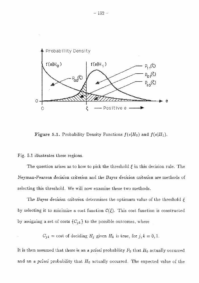
152

Probability Density

f(elH 0 ) f(elH 1 )

0 ~ - Positive e ---"11111"

P11(~)

Pol~)

~o(~)

e

Figure 5.1. Probability Density Functions /(e!Ho) and /(e!H1).

Fig. 5.1 illustrates these regions.

The question arises as to how to pick the threshold e in this decision rule. The

Neyman-Pearson decision criterion and the Bayes decision criterion are methods of

selecting this threshold. We will now examine these two methods.

The Bayes decision. criterion. determines the optimum value of the threshold e by selecting it to minimize a cost function C(fl. This cost function is constructed

by assigning a set of costs { Cjk} to the possible outcomes, where

Cjk =cost of deciding Hj given Hk is true, for j, k = 0, 1.

It is then assumed that there is an a priori probability P0 that H0 actually occurred

and an a priori probability that Ho actually occurred. The expected value of the

- 153 -

cost associated an observation and decision based on a threshold e IS then

by

P1Co1Po1(0 + P1C11p11(e).

criterion selects the decision threshold e such that C(O is min-

imum. is discussed Reference [5.2, p. 82), the e that minimizes C(O can be

found by setting

f(elH1) _ Po (C10 - Coo) f(elHo) - P1 (Co1 - C11).

The greater the signal energy, the farther to the right the PDF f ( eiH1 ), while

the density /( e!Ho) remains unchanged, since the noise energy is assumed to be

independent of the signal energy. As a result, increasing the signal energy decreases

bothp1o(e) andpo1(e), while increasingpoo(O andp11(0 for the optimum (As a

result, for C 10 > C00 and C01 > C11 , C(O decreases as the signal energy increases

for the optimally chosen ( So the Bayes decision rule gives better performance

as the signal-to-noise ratio increases if C10 > Coo and Co1 > Cu, that is, when

it is more costly to make an incorrect decision about the presence or absence of

a target than it is to make a correct decision. vVe would expect this to be true

of all reasonable cost functions. The Bayes decision criterion is not often used in

real radar detection problems because of the difficulty in determining the a priori

probabilities P0 and P 1 as well as a meaningful set of costs { C1 ,J.

The Neyman-Pearson decision criterion, when applied to radar detection prob-

gets around the problem of determining the a priori probabilities P0 and P 1

and the set of costs { Cj k}. Here instead we look at the problem of radar detection

- 154 -

as one we want to maximize the probability p 11 (e) of deciding that a target

is present when one is present, while holding the probability P1o(O of deciding that

a target is present when one is not present to a reasonably small level. In radar

target detection problems, p 1o(0 is often referred to as "false alarm" probabil-

ity. Ideally, we would, of course, like to select e to simultaneously make p11 (0 as

large as p 10 (e) as small as possible, but these are usually conflicting

objectives. As a result, we select as our maximum allowable value of p1o(O a prob-

ability PF' and we then maximize Pll (0 with respect toe under the constraint that

p 10 (e) <PF. For all energy threshold tests of the type we are considering, we note

thatp11(0 is a monotonically decreasing function of e andp1o(O is a monotonically

decreasing function of ( As a result, the Neyman-Pearson solution corresponds to

selecting the optimal threshold e such that

e

P1o(O = j f(elHo) de= PF.

0

Thenp11(0 is as large as possible under the constraint onp10(0, and this maximum

value is 00

P11(e) = j /(elH1) de.

' Again, we see that as the energy in the reflected signal from the target increases,

the /(el Hi) shifts to the right, while f ( elHo) remains unchanged. As a result,

the performance of the Neyman-Pearson decision improves (that is, p 11 (0 increases

for a fixed p1o(e)) as the signal-to-noise ratio increases.

We have seen that for radar detection systems that use energy thresholding of

the received signal as the method of determining the presence or absence of a target,

- 155 -

performance detection system improves signal-to-noise ratio of

signal, whether the threshold is chosen using a Bayes decision rule or

a decision by which the maximum signal-to-

n01se ratio of the received signal is obtained in radar sytems is that of matclied

the derivation of the matched filter radar [5.1], it is assumed that the

target reflecting the wave behaves as a point scatterer. The result is that

the backscattered waveform received by the receiver is a scaled and delayed version

of the transmitted waveform. Real radar targets, however, may be of significant

physical extent, and the assumption that the target behaves as a point scatterer

may, in fact, result in the design of a filter that is actually mismatched to the

received signal because of the interference pattern generated by the waveform and

target in combination. The matched filter in radar, derived under the assumption

that the target behaves as a point scatterer, leads to the conclusion that the wave

shape of the transmitted waveform has no effect on the signal-to-noise ratio at the

output of the receiver. As long as the receiver filter is a matched filter matched

to the transmitted waveform and the power spectral density (PSD) of the additive

noise, the signal-to-noise ratio is a function only of the transmitted waveform's

energy not its wave-shape. Thus, for a point target, all waveforms of equal

energy provide an equal signal-to-noise ratio at the receiver output if detected with

a matched filter.

But as we have noted, the point target assumption is not realistic for many real

- 156

radar targets. Because these extended targets interact with the transmitted wave

form to generate interference patterns that are a function both of the transmitted

waveform of the 's spatial characteristics, as we saw in Section 4.5, the

signal-to-noise ratio for a given target is a function of both the wave shape of the

transmitted waveform and the impulse response of the receiver filter. Thus, in order

to signal-to-noise ratio at receiver output for a given target, we

must optimize both the transmitted waveform and the receiver filter.

In this chapter, we will investigate radar waveform/receiver-filter pairs matched

to targets that exhibit behavior differing from that of a point target. This will be

done through the use of the target impulse response, developed in Section 4.6. As

a result of our investigation, a procedure for the design of optimum realizable radar

waveform/receiver-filter pairs for a given target in stationary additive Gaussian

noise of arbitrary power spectral density will be developed.

5.2. Matching a Waveform/Receiver-Filter Pair to a Target of Known

Impulse Response.

In this section, we will consider the problem of selecting a transmitted waveform

and receiver filter such that the signal-to-noise ratio at the output of a radar receiver

is maximized. In order to do this, we will assume that the target we are attempting

to detect has a known impulse response h(i). We will also assume that the signal

reflected from the target is contaminated by additive Gaussian noise with power

spectral density (PSD)

The problem of

nU).

is shown in Fig. 5.2. Here we have a radar transmitter

x(t)

Transmitter 11----PI Target h(t)

- 157 -

n<tJ

y(t)

Figure 5 Block Diagram of Radar Waveform/Receiver-Filter Design Problem.

transmitting a waveform x(i). The transmitted waveform is then scattered by the

target with a target impulse response h(i). The resulting scattered waveform v(i)

is then corrupted with additive Gaussian noise n(i) having PSD Snn (!), producing

the signal g(i) at the input to the receiver filter. Finally, the receiver filter, with

impulse response r(i), filters g(i) to produce the receiver output y(i).

The problem of interest can be stated as follows: Given a target impulse re-

sponse h(t) and stationary additive Gaussian noise n(t) with. PSD Snn (/), find a

transmitted waveform x(i) with. total energy£ and a receiver-filter impulse response

r(-') such. th.at the signal-to-noise ratio the receiver output y(i) is maximized at

time "to. In addition., since real radar waveforms are of finite duration., restrict the

waveform x(i) such th.at it is zero outside the interval [-T /2, T /2].

158

Fig. 5.2 we see receiver output is given by

y(i) = r(i) * g(i)

= r(t) * [x(i) * h(i) n(i)] (5.1)

= r(i) * x(i) * h(i) + r(t) * n(t)

= Ys (i) Yn (i).

Here, "*" denotes convolution, y, (i) is the signal component in the receiver output,

and Yn (i) is the noise component in the receiver output. These two components are

given by

00 00

Ys (i) = r(i) * x(i) * h(i) = j j x( T )h(y - T )r(i - p) dr dp, (5.2)

-00-00

and

00

Yn(i) = r(i) * n(i) = j n(y)r(i - p) dp. (5.3) -oo

Now as previously stated, we are interested in finding a waveform/receiver-

filter pair that will maximize the output signal-to-noise ratio (; t at time 10 . This

signal-to-noise ratio is defined as

(5.4)

problem of finding the waveform/filter pair that maximizes the output

signal-to-noise ratio is most easily solved in the frequency domain. Thus, we define

- 159

the following transforms: 00

(/) = j x(i)e-i2-irft dt,

-oo

00

H(f) = J h(i)e-i2 1rft di,

-oo

00

V(f) = j v(t)e- 12 -ir ft di, (5.5) -oo

00

G(f) = J g(t)e- 12-irf t dt, -oo

00

Y(f) = j y(t)e-i 21rft dt.

-oo

The corresponding inverse Fourier transforms are 00

x(t)= j X(f)ei 2,,;ftdt,

-oo

00

h(t) = J H(f)ei 2,,;ft dt,

-oo

00

v(t) = j V(f)ei 2 1rft dt, (5.6) 00

00

g(i) = J G(/)ei2-ir ft dt'

-oo

00

y(t) = J Y(!)ei2,,; ft dt.

-oo

The convolution theorem of Fourier transforms (5.4] states that if a(t) has

Fourier transform A(!) and b(t) has Fourier transform (/), then the Fourier trans-

form of the convolution a(t) * b(t) is A(f)B(!). That is, 00

j [a(t) * b(t)] e-i21rf-t dt = A(f)B(!). (5.7)

-oo

- 160 -

So from Eqs. (5.2), (5.6), (5.7), we have

l

oo 2

fy,{io)f 2 = £ X(/)H(/)R{f)e"<I'• df (5.8)

The mean-square value of y 11 (lo) is given by

00 00

= j 51 ,.y,.(/) d/ = j IR(/)12

Snn(/) df. (5.9)

-oo -oo

Here, 'R-y,.y,.(r) is the autocorrelation function of Yn(-t).

In what follows, we will need to make use of the Schwartz Inequality [5.4,

p.159], which says that if Ai(/) and A 2(f) are square integrable functions on the

real line, then

with equality if and only if Ai(/)= KA 2 (!), where K is a complex constant. \Ve

will use this inequality to maximize the signal-to-noise ratio.

From Eqs. (5.4), (5.8), and (5.9), we have

00

(~ ),, f X (/)H (/)R(/)ei2,,; f 1 df 00

(5.11) 00

J IR(f) 12

Snn (/) df -oo

This can be rewritten as

2

f [Hf X(j eihfio] [R(J)JSnnU)] df -oo S,..,.(f)

00 (5.12) J JR(f) 1

2 Snn (!) d/

-oo

-- 161

Applying Schwartz Inequality to the numerator, we have

2

-oo -oo

with equality if and only if

(5.14)

or equivalently,

K X (f )H(f )e- i27: fto

R(f) = Snn (/) ' (5.15)

where K is a complex constant. Thus, we have

oo 2 oo X(j)H(J)eihf1o l

S _£ IR(f)I Snn(/) df _£ s,.,. f df

(N t ~ f IR(f)l2 s •• (f) df -oo (5.16)

00

J IX(f)H(f)l2 df Snn (/) '

-oo

with equality if and only if Eq. (5.15) holds.

Thus, we have that Eq. (5.15) is a necessary condition to obtain the maximum

signal-to-noise ratio at the output of the receiver. However, it actually insures only

that

(§__) Joo IX(f)H(/)12 Jf. N to Snn(/)

(5.17)

-oo

order to obtain the maximum possible signal-to-noise ratio under the specified

energy and time constraints on the transmitted signal x(~), we must maximize Eq.

- 162 -

00

J IX(/)12

df = & ' -oo

(5.18)

x(i) = 0, for i ~ [-T/2,T/2].

Here, £ is the total energy available for the transmitted waveform x(-t).

We can rewrite Eq. (5.17) as

(!_) = J00

X(/) [ H(/) ] 2 df = J00

IX(f)B(/)12 df, (5.19) N to /Snn(/)

-oo -oo

where

B(f) = H(f) /Snn(/)

(5.20)

Examining Eq. (5.20), we see that we can view its maximization as that of

maximizing an integeral of the form

00 00 00

J lq(t)12

dt = J IQ(f)l2

df = J IX(f)B(f)l2

df, (5.21) -oo -oo -oo

where q(i) can be viewed as the output of a linear time-invariant system with input

x(i) and impulse response b(i). Here,

00

Q(f)= J q(i)e-i2-x-ftdi,

-oo

and 00

B(f) = J b(i)e-i2-x-ft

-oo

_f_) _-111t B(f) = H(f) /Su(/)

Q(f)

5 System Representation of Relation Between Q(/) and X(/).

Fig. 5.3 is a block diagram illustrating this situation. Since the system of Fig. 5.3

is a linear, time-invariant system, we have that

Q(f) = X(f)B(f). (5.22)

We must maximize Eq. (5.21) with respect to all X(f) that satisfy the constraints

of Eq. (5.18). We can rewrite Eq. (5.21) for the energy in q(i), noting that both

x(-t) and q(i) are real, as

[

T/'2 ] j x(p )ei'2'K" f P dp IB(f) 12 df.

-T/'2

(5.23)

Now define L(-t) as the inverse Fourier transform of IB(/)1 2; that is,

00

L(-t) def J IB(f) 1'2 el'2'K" f i df. (5.24)

-oo

Then from Eqs. (5.23) and (5.24), we have, changing the order of integration,

oo T/'2 T/'2

j q2 (t)dt= j j x(r)x(p)L(p-r) dp. (5.25)

-oo -T/'2 -T/'2

- 164 -

wish to function x(-t) on [-T /2, T /2], which maximizes Eq. (5.25).

can be [5.2, p.125] that the optimum function x(-1) satisfies the integral

equation T/2

.:\x(-t)= J x(r)L(-1-r)dr,

-T/2

(5.26)

where ,\ is the UUU"~HU.\.UU eigenvalue of Eq. (5.26). So x(-1) is an eigenfunction

corresponding to .:\, the maximum eigenvalue of Eq. (5.26), and having energy £.

From Eqs. (5.25) and (5.26), we then have

00 T/2 T/2 J q2(t)d-1= J x(r) J x(p)L(p-r)dpdr

-oo -T/2 -T/2

T /2 T /2

= J x(r)..\x(r) dr = ,\ J x(r)x(r) dr

(5.27)

-T/2 -T/2

= )...£.

Interpreting these results m terms of our problem, we substitute

B(f) = H(f)/ JSnnU) and then define L(-1) as in Eq. (5.24). This yields

OQ 2

L(t) = J IH(f)I ei21f f1 df. Snn (!)

(5.28)

-OQ

Then the waveform x(-1) time limited to the interval [-T /2, T /2], which maximizes

the signal-to-noise ratio at the receiver output, is given by the solution to

T/2

Amaxx(-1) = J x(t)L(-t - r) dr, (5.29)

-T/2

where ,\max is the maximum eigenvalue of Eq. (5.29) and x(-1) is a corresponding

eigenfunction scaled to have energy £.

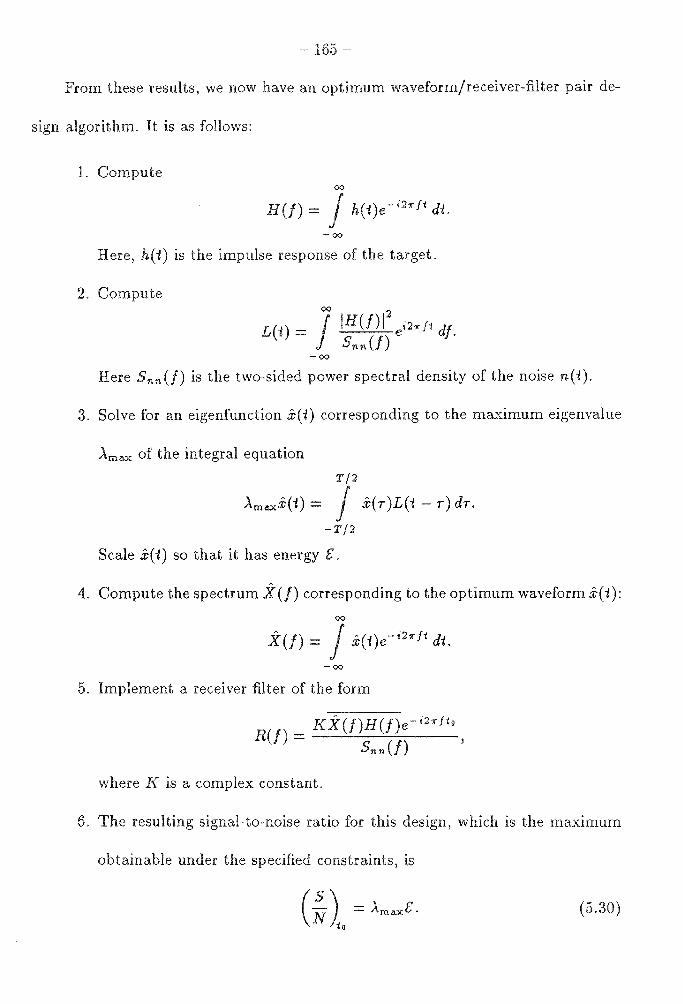
- 165 -

these results, we now an optimum waveform/receiver-filter pair de-

sign algorithm. is as follows:

1. Compute 00

(/)= j h(i)e-iz~fidi. -oo

Here, h(t) is the impulse response of the target.

2. Compute 00 2

L(i) = J IH(f) I ei2~ fi df. Snn (/)

-oo

Here Snn(/) is the two-sided power spectral density of the noise n(t).

3. Solve for an eigenfunction .i-(t) corresponding to the maximum eigenvalue

Amax of the integral equation

T/2

Ama.xi(t) = J x( T )L(t - T) dr.

T/2

Scale .X(t) so that it has energy & .

4. Compute the spectrum X(/) corresponding to the optimum waveform .X(t): 00

X(f) = j x(t)e-ihfi dt.

-oo

5. Implement a receiver filter of the form

where K is a complex constant.

6. The resulting signal-to-noise ratio for this design, which is the maximum

obtainable under the specified constraints, is

(5.30)

- 166

We note that since x(t) is designed to take on non-zero values

only on the [-T/2,T/2], it can take on non-zero values fort< 0, and so the

) is not necessarily causal (that is, it cannot in general be generated

by exciting a realizable filter). However, since x(t) = 0 for. all t < -T/2, we can

obtain a causal waveform .X(-t) = i(t - T /2), which will also yield the optimal

response at receiver output, except with delay T /2, that is, at time 10 + T /2.

To see that this waveform also maximizes the signal to noise ratio, we note that

X(/) = X(f)e-i'K"fT. But from Eq. (5.17) or intuition, we see that the phase term

e-i'K" fT, resulting from the delay of duration T /2, does not affect the resulting signal-

to-noise ratio. We do, however, note from Eq. (5.15) that the response occurs at

time t 0 + T/2 instead of time 10 .

The important thing to note here is that an optimal waveform x(t) that is

causal, and thus physically realizable, exists. In addition, the target impulse re-

sponse is causal for all real physical targets. This being the case, the resulting

receiver filter also has causal impulse response r(t), and thus is also a realizable

filter. So we note that from the optimum waveform/receiver-filter solution, we can

obtain a waveform/receiver-filter pair that is physically realizable.

We will now consider an example that both illustrates the use of the design

procedure and shows the effect that the transmission of various waveforms with

identical energy can have on t,he output signal-to-noise ratio. Assume that the

stationary additive Gaussian noise is white noise with PSD

No Snn(/) = 2'

assume that target

by

167 -

response h(i) has Fourier transform H(/) given

H(f) = { ~ ,forl/l<W, , for I/I> w.

Here k is a constant, which convenience we will take to be equal to ,/No/2, so

that

being the case, we have

w

, for I/ I :SW, ,forl/l>W.

( ) J dr; sin 21r Wt a sin 0::i

Li = 1 :J = 2W = ---. 21r w i 1f 0::i

-w

Here a = 21r W. So we have that .i(t) is a solution to the integral equation

T/2

J sin 2JrW(i - r) ,\11 xn(t) = Xn(i)2W 21rW(i _ r) dr,

-T/'2

which is known to have a countable number of solutions for n = O, 1, 2, ... [5.1]. The

solutions to this equation are known as the angular prolate spheroidal functions, and

are designated S 011 (0::T/2,2t/T). The associated eigenvalues ,\n can be written in

terms of the radial prolate spheroidal functions, which are designated R~~ ( 0::T /2, 1 ).

The eigenvalues and their associated eigenfunctions are given by

,\ 11 = 2WT R~~( 0::T /2, 1), for n = O, 1, 2, ....

x 11 (i) = So11 (aT/2,2i/T),

The sequence of eigenvectors Ao, .\1 , ,\z, ... , .\ 11 , ••• is a positive decreasing se-

quence n. So the largest eigenvector occurs n = 0. Thus, the solution .i(i)

energy & is

i(i) = VE Soo( o:T /2, 2t/T),

- 168

Table 5-1 Signal-To-Noise Ratio for x 11 ( t) = &So11 (aT/2,2t/T).

n 2WT = 2.55 0 0.966£ 1 0.912£ 2 0.519£ 3 0.110£ 4 0.009£ 5 0.004£ 6 7

and its associated eigenvalue is

(1) I Amax = 2WT R 00 ( aT 2, 1).

The signal-to noise ratio in this case is

( s) (1) N 10

= Amax& = 2WT£ R 00 ( aT /2, 1).

2WT = 5.10 1.000£ 0.999£ 0.997£ 0.961£ 0.748£ 0.321£ 0.061£ 0.006£

order to demonstrate the effect of the wave shape of the transmitted wave-

form on the output signal-to-noise ratio, consider the effect of transmitting the

waveforms x 11 (t) = -/£So11 (0.:T/2,2-t/T), for n = 0,1,2, .... All of these wave-

forms have transmitted energy & , but the resulting signal-to-noise ratios are A71 & .

As we noted previously, {A 11 } is a positive decreasing sequence of n, and thus

Ao£ > .\1 & > A.2& > · · ·. So we see that the output signal-to-noise ratio is def-

initely a function of the transmitted waveform. Table 5-1, we show the resulting

- 169 -

signal-to-noise ratio for the cases of 2WT = 2.55 and 2WT = 5.10. (The eigenval-

ues were obtained Reference [5.1, p.194].) As we can see, the signal-to-noise

ratios drop off very quickly for n > 2WT. So we see that the wave-shape or spec

content of the transmitted waveform plays a significant role in the resulting

signal-to-noise ratio.

we can these by noting that the maximum signal-

to-noise ratio occurs when the mode of target with the largest eigenvalue is excited

by the transmitted waveform. In order to obtain the largest response possible from

the target, we put as much of the transmitted energy as is possible into exciting

this mode. This gives us the largest possible signal-to-noise ratio and thus the best

possible target detection performance under the imposed constraints. vVe should,

however, note that other modes of the target may contain significant information

about the target, so putting as much energy as possible into the mode with the

largest eigenvalue will not in general be the best method of obtaining the maximum

amount of information about the target. When our task is target identification

or information extraction, we may thus wish to distribute the transmitted energy

among the different target modes in a different manner. vVe will examine this

problem in the next chapter.

- 170

5.3. er Sphere Detection.

In this section, we will apply the results of Section 5.2 to the problem of designing

a waveform/receiver-filter pair that is for detecting a perfectly conducting

metal sphere of radius a the presence of stationary noise. We will examine

the shape of the resulting waveform and compare its performance to that of a pulse-

modulated sinusoid and compare their target detection capabilities.

In order to apply the waveform/receiver-filter pair design procedure to a per-

fectly conducting sphere of radius a, we must find its impulse response h(-1). vVe

assume a monostatic radar system (transmit and receive antennas collocated) and

thus we are interested in the backscatter impulse response. vVe will also assume

that the transmit and receive antennas employ identical linear polarization. The

backscatter impulse response of a perfectly conducting sphere, when both trans-

mit and receive antennas have identical linear polarization, has been calculated by

Kennaugh and Moffatt, using the physical optics approximation (5.6]. This impulse

response can be written as

a 1 h(-1) = --8(i) + - [u(i) - u(t - 2a/c)].

c 2 (5.31)

Here, a is the radius of the sphere, c is the velocity of light, 5(i) is the Dirac delta

function, and u(i) is the unit step function, defined as

u(i) - { ~:

plot of h(i) appears in Fig. 5.4.

for i 2 O; for i < 0.

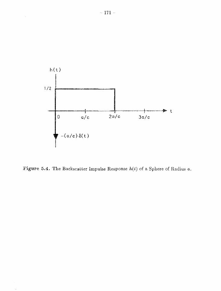
h(t)

1/2

~-1-~~~~~:1--~~~~+-~~~~+:~~--'~11111"' t

0 a/c 2a/c 3a/c

1, -(a/c) o(t)

Figure 5.4. The Backscatter Impulse Response h(-t) of a Sphere of Radius a.

Applying our waveform/receiver-filter design procedure (pp.155-6), we must

calculate the Fourier of h( t): 00

H(f) = J h(-t)e-i21f ft

If we define a as

-oo

00

=f ~5(t) + ~ [u(i) - u(t - 2a/c)J] e-i21ffi dt c 2

-oo

oo 2a/c

=-~ j 5(-t)e-i 21rf"1Jt+~ j e-i2 'K"f-tJt

-oo 0

_ a 1 [e-i41ffa/c _ 1] - --+-

c 2 -i27r I

= __ + -e-t21ffa./c a 1 . [ei21ffa/c _ e-i21ffa/c]

c 2 i2Jr I _ a a -i21ffa/c [sin2Jr/a/c] ---+-e .

c c 21ifa/c

A def a a=-, c

then we can rewrite Eq. (5.32) as

H(f) = -a+ae-i21ffa [si;:;[a].

The magnitude-squared spectrum IH(f) 12 is thus

jH(f)I' = a' [ 1 + ( si~:g• )' -2 ( si~:;{") cos 2ir fa l · A plot of IH(f) 12 appears in Fig. 5.5.

(5.32)

(5.33)

(5.34)

(5.35)

The next step our procedure is to find the inverse Fourier transform of the

function IH(/)12 /51111 (/). For white noise 5 1111 (/) = No/2. we have

IH(/)12

= 2a2 [i+ (sin27r/a)

2 sin2-x"/a) Al

N 0 I 2 N 0 2 Jr fa - 2 2 Jr I a cos 2 Jr I a

_ 2a2

2a2

(sin2x/a)2

_ 4a2

(sin211/a) f' - No + No 211 fa No 27r fa cos 211 a.

(5.36)

-5

(01

-4 -3 -2 -1 0

2

0

"'2 a

2 3 4

Figure 5.5. Magnitude-Squared Spectrum IH(/)12 versus f.

f o 5

Calculating the inverse Fourier transform of Eq. (5.36), we now obtain the L(t) as

specified in step 2 of our design procedure. To simplify notation, define the two

functions

and

V"(i) = { 1 - !ti/a, for ltl ~a; 0, elsewhere.

Bcc(t) = { 1, for l~I ~a; 0, elsewhere.

(5.37)

(5.38)

smce 00

j (-t)e-i2'A"ft d-t = 2asi;:;[a -oo

and 00 J V2a(t)e-i'.hf1 d-t = (

sin 2'1:" fa) 2

2'X'/a ' -oo

we can

00 2

L(i) = J IH(f)I ei2'A"/t d-t No/2

00

= 2

0.2

5(-t) + ~Via(-t)- ~Ba(-t) * [5(-t - a)+ 5(-t +a)] No No No 20. 2 a a = -5(1) + -Via(i) - -B2a.(t). No No No

We will now use this L(t) in our design procedure.

The next step in our design procedure is to solve the integral equation

T/2

,\ml!Xx(t) = J x( T )L(t - T) Jr

-T/2

(5.39)

(5.40)

(5.42)

for an eigenfunction x(t) corresponding to the maximum eigenvalue ,\ml!X· For our

particular L(t) as given in Eq. (5.41), this becomes

T/2

r2 j = ;o 5(t - r)x(r)

-T/'2

T/2

~o j [Via.(t-r)-B2a.(t-r)]x(r)dr.

-T/2

(5.43)

- 175 -

From Eq. (5.43), we see if x(t) is an eigenfunction corresponding to the maxi-

mum eigenvalue Amax, it must also be an eigenvector of the integral equation

- B2a(i - r)]x(r) dr (5.44)

corresponding to eigenvalue µmax. Note that

2a2

Amax = No + J.lmax· (5.4.5)

For convenience in our analysis, we will assume that the waveform x(t) that

we are designing has unit energy. This corresponds to the case where £ = 1 in

our design procedure. In addition, for computational convenience, we will assume

that a = 1. Although such a value of a does not correspond to values typically

encountered in practice (such a sphere would have a radius of 3 X 108 m), these

results can be applied to more typical values by normalizing both the amplitude of

the received signal and the time axis linearly in the length unit.

Solving the integral equation of Eq. (5.44) numerically for T = 1, 25, 50, and

100, we obtain the eigenvalues µmax of Eq.(5.44) and thus the eigenvalues Amax

of Eq. (5.43) as given in Table 5-2. The eigenfunctions corresponding to these

maximum eigenvalues have wave shapes as given in Figs. 5.6-5.9.

For the purpose of comparison with more typical radar waveforms, we will

consider the response of the target to a pulse modulated sinusoid of duration T

and having unit energy. The receiver filter will be a matched filter matched to the

transmitted waveform-the form of receiver filter normally used in radar detection

problems.

Table 5-2 Eigenvalues µmax and ,\max for Various T.

T µmax· No Amax· No 1 0.1737 2.1737

25 1.9108 3.9108 50 1.8682 3.8682

100 1.7477 3.7477

Such a waveform can be expressed as

x(i) =/3BT;2(i)cos2X"Joi. (5.46)

Here, for fixed T, /3 is a normalizing constant such that the waveform has unit

energy. For T = n/ Jo, /3 = /2}T, and for all T :-> 1/ Jo, /3 ~ /2}T. For

our analysis, however, the value of /3 need not be explicitly known, as it can be

conveniently calculated numerically in the process of evaluating the resulting signal-

to-noise ratio.

order to obtain the most favorable result when transmitting a waveform as

specified in (5.46), we must select the carrier frequency in order to take advan-

tage of the resonance of the spherical scatterer as expressed by IH (/) 12 . Looking at

the plot of IH(f)l 2 /a as shown Fig. 5.5, we see that IH(f)l2 has its peak value

at a frequency between 0.25/ a and 0.5/ a. Solving Eq. (5.35) numerically in order

to obtain the frequency at which this maximum occurs, we find that IH(f)l2 takes

on a maximum value of 1.5862 at a frequency of J - 0.3251/ a.

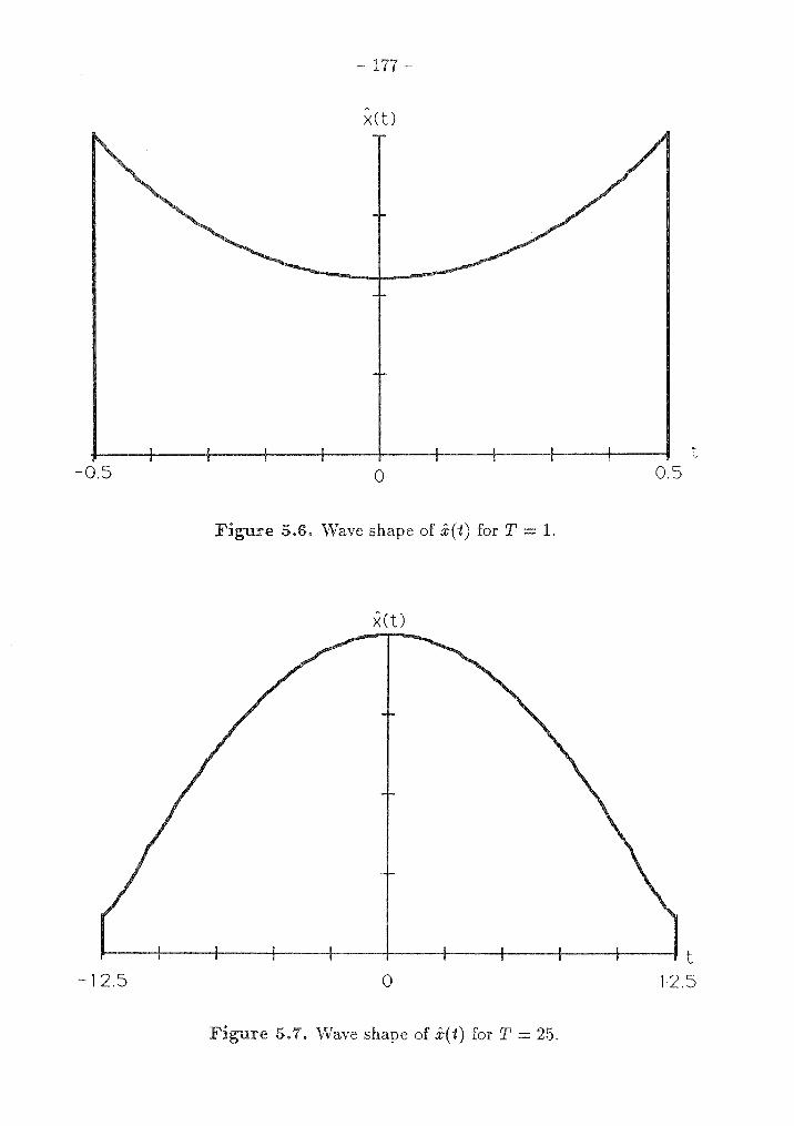
x(t)

-0.5 0

Figure 5.6. 'Wave shape of i(i) for T = 1.

x<u

-12.5 0

5. ·wave shape of i(t) for T = 25.

t 0.5

t 12.5

50

-so

- 178

x<t)

0

Figure 5.8. Wave shape of x(t) for T = 50.

x<u

0

Figure 5.9. Wave shape of x(t) for T = 100.

t 50

t 50

179

(!) be the Fourier transform of the transmitted waveform x(i) as given

(5.46). Then the matched filter matched to this waveform that gives the

maximum signal-to-noise ratio at time t 0 is specified by the transfer function

(5.4 7)

where k is any non-zero constant. From Fig. 5.2, we see that the signal-to-noise

ratio at time io is given by

1Ys(io)l2

EIYn(io)l 2

00

f X(f)H(f)R(f)ei27:f10 d/ 00

00

J IR(f) 12 Snn (/) d/ -oo

2

(5.48)

For white noise with power spectral density 5 1111 (/) = No/2 and R(/) as given in

Eq. (5.47), noting that H(/) is a conjugate-symmetric function off, this simplifies

to

(~) = (2-) IJ 1x(~l2 Re{H(f)} df

2

N 10 No J jX(/)12 df (5.49)

0

From Eq. (5.34), we have that when a = 1 as our example,

Re{H(/)} = ( si;:; I) cos - 1. (5.50)

For x(i) as given in Eq. (5.46), X(f) is given by

(/) = (JT [sin -x-(/ - fo)T + sin x(/ + fo)T] 2 7r(/ - /o)T 7r(/ + fo)T '

- 180

Table 5-3 Signal-to-Noise ratios multiplied by N0 for

Pulsed Sinusoid and Optimal Detection Waveforms for Various T. T Pulsed Sinusoid Optimal Improvement

1 1.1454 2.1737 2.78dB 25 2.7917 3.9108 1.46 dB 50 2.8183 3.8682 1.38 dB

100 2.8354 3.7477 1.21dB

and IX(!) 12 is given by

IX(f)i2 = (PT2

[(sin11:(/ - fo)T)2 + (sin7r(/ + /0 )T) 2

4 11:(/ - fo)T 11:(/ + fo)T

+ 2 (sin 11:(/ - fo)T) (sin 7r(/ + /0 )T)] · 11:(! - fo)T x(f + fo)T

(5.51)

Using Eqs. (5.49), (5.50), and (5.51), we can solve for the signal-to-noise ratio

that results when x(t) is the unit energy pulsed sinusoid given in Eq. (5.46). This

is done for T = 1, 25, 50, and 100. The values of f3 that provides a unit-energy

waveform for each of these T are calculated numerically. Table 5--3 shows the result-

ing signal-to-noise ratio for these unit-energy pulsed sinusoids with their associated

results when an optimum

waveform/receiver-filter pair is matched to the sphere being detected. In addition,

we note the improvement (in decibels) in the output signal-to-noise ratio for the

optimum waveform/receiver-filter pair over the pulsed sinusoid and its associated

matched filter.

- 181

can be seen from Table 5-3, is a significant improvement in the re-

suiting signal-to-noise ratio when the optimum waveform/receiver-filter pair is used

over that which occurs when a more typical c procedure is used. For the

range of T examined, the optimum waveform/receiver-filter pair provides approxi

mately 1.2-2.8 dB of gain over the pulsed sinusoid with its associated matched filter.

Considering that the received power is inversely proportional to the range to the

fourth power, such gains would correspond to an increased detection range of 7

to 17 percent. This is a significant increase in detection performance. In typical

aircraft detection radar systems where the target is assumed to be a point target,

the gain could be even greater, since the carrier frequency of the pulsed sinusoid

would not be specifically selected to match the resonance of the sphere. Thus, in

radar target detection problems where knowledge of the target impulse response is

known a priori, a significant gain in detection signal-to-noise ratio can be achieved

using the waveform/receiver-filter design procedure outlined in this chapter. Such

an improvement could be very helpful in marginal radar detection scenarios.

5

5.1

182 -

er 5

Trees, , Detection.,

Wiley and Sons, New , NY, 1968.

and Modulation Theory, Part 1, John

5.2 Helstrom, C. W., Statistical Theory of Signal Det

York, NY, 1968.

Pergamon Press, New

5.3 North, . 0., "An Analysis of the Factors which Determine Signal-Noise Dis-

crimination Pulsed Carrier Systems," RCA Laboratory Report PTR-6C;

reprinted in Proc. IEEE, 51 (July 1963), pp. 1016-27.

5.4 Bracewell, R. N., The Fourier Transform and Its Applications, McGraw-Hill,

New York, NY, 1986.

5.5 Papoulis, A., The Fourier Integral and its Applications, McGraw-Hill, New

York, NY, 1962.

5.6 Kennaugh, E. M., and D. L. Moffatt, "Transient and Impulse Response Ap

proximations," Proc. IEEE, 51, No. 8 (August 1965), pp. 893-901.

183 -

6

ON AND WAVEFORM DESIGN

, we examine the design of radar waveforms that maximize the

mutual information between the target and the received radar signal in the radar

measurement process. This is done using the target impulse response defined in

Section 4.6 to model the interaction of the transmitted radar waveform with the

target. However, now we will consider a target impulse response that is a random

process, in order to model our uncertainty of the target's scattering characteristics.

Using the model of a random target impulse response that is a finite energy

Gaussian random process, we will solve for a family of radar waveforms that max

imize the mutual information between the random, target impulse response and

the received radar signal. This will be done assuming that the signal is received

in additive Gaussian noise of arbitrary power spectral density Pnn (!). Next, we

will examine the characteristics of these waveforms through the use of several ex

amples. We will then address some of the considerations involved in implementing

these waveforms in real radar systems. Finally, we will compare these waveforms to

those derived Chapter 5 for the optimum detection of radar targets with kn()wn

impulse response.

- 184 -

6.1. Transfer Be-

Consider radar target model shown in Fig. 6.1. Here, x(-1), a finite-

energy deterministic waveform with energy £ and of duration T is transmitted by

the transmitter in order to make a measurement of the radar target. We will assume

x(i) is to the symmetric time interval [-T /2, T /2]. Thus,

T/2

£= j lx(i)J2d-I.

-T/2

(6.1)

Since the energy constraint in most real radar systems is not on the total energy

in the transmitted waveform, but rather on the average power of the waveform, we

have£= P.r:T, where is the average power of x(-1). Since£= Pa:T, we note that

for a given average power Pa:, the longer the duration T of x(t), the greater the total

energy in the transmitted waveform. We will also assume that the waveform x(-1)

is confined to a frequency interval W = [/0 , / 0 + W]. ·while strictly speaking, we

cannot have a waveform x(-1) confined to both a finite time interval and its Fourier

transform confined to a finite frequency interval, we will assume that W is selected

such that only a negligible fraction of the total energy resides outside the frequency

interval W. In real radar systems, the frequency band of operation corresponding

to W is ultimately determined by the bandwidth of the components making up the

radar system.

After transmission, the radar waveform x(-1) is scattered by the target, which

a scattering characteristic modeled by the random impulse response g( t). The

resulting scattered signal z(t) received at the receiver is a finite-energy random

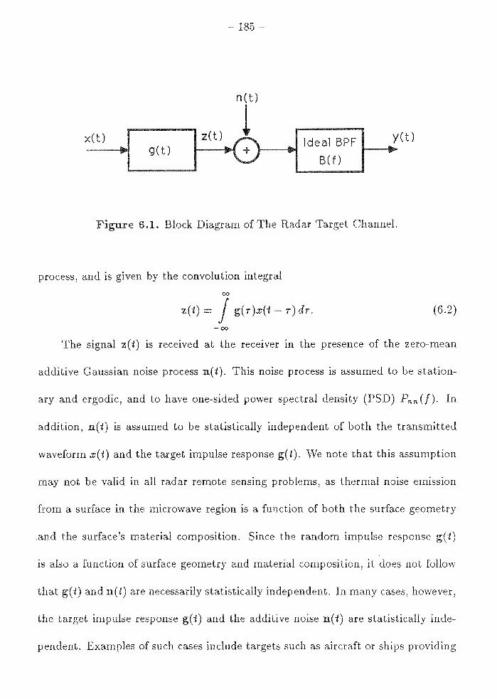
185 -

n ( t)

z(t) y( t) g( t)

Ideal BPF 1---.....

B(f)

x(t)

Figure 6 . Block Diagram of The Radar Target Channel.

process, and is given by the convolution integral

00

z(i)= j g(r)x(-t-r)dr. (6.2) -oo

The signal z(i) is received at the receiver in the presence of the zero-mean

additive Gaussian noise process n(i). This noise process is assumed to be station-

ary and ergodic, and to have one-sided power spectral density (PSD) Pnn (!). In

addition, n(i) is assumed to be statistically independent of both the transmitted

waveform x(i) and the target impulse response g(i). \Ve note that this assumption

may not be valid in all radar remote sensing problems, as thermal noise emission

from a surface in the microwave region is a function of both the surface geometry

.and the surface's material composition. Since the random impulse response g(i)

is also a function of surface geometry and material composition, it does not follow

that g(i) and n(i) are necessarily statistically independent. In many cases, however,

the target impulse response g(i) and the additive noise n(i) are statistically inde-

pendent. Examples of such cases include targets such as aircraft or ships providing

- 186 -

the scattering mechanism and additive noise coming from thermal noise radiated

by the environment and by the radar receiver itself. any case, when sensing sur-

faces with radar, independence of the additive noise from the backscattered signal

is commonly assumed [6.1, pp. 492-5]. our analysis, we will therefore assume

that g(i) and n(i) are statistically independent.

waveform received at the is shown in Fig. 6.1 to be z(i) n(i)

filtered by the ideal bandpass filter B(f), passing only frequencies in the band W.

This is just a statement of the fact that we assume that the transmitted signal has

no significant energy outside the frequency interval W. Thus, neither does z(i),

since it is the response of a linear time-invariant system to the transmitted signal.

Hence we will not consider frequencies outside this interval.

The random process g(-') can be thought of as an ensemble {g(-t)} of functions

with a probability measure assigned to each sample function g(-t). (Actually, the

sample functions g(-t) are more properly written as g(i, w), where w E n and n

is the underlying probability space.) We will now examine some properties of the

random impulse response g(i).

The first property which g(i) must possess is that all of the sample functions

g(i, w) must satisfy

00

j lg(t, w)l 2 dt :::; 1. (6.3) -oo

This follows from conservation of energy and the fact that electromagnetic scattering

is a passive process. The next property of g(t) we will assume is that all of its sample

- 187

functions are causal impulse responses; that is,

g(i,w) = 0, Vi< O, Vw En. (6.4)

This is a property of all linear time-invariant systems.

We define the Fourier transform G(/) of g(i) as

00

(/)= j g(i)e- 12 ~Jtdt. (6.5)

-oo

Thus, for any sample point w0 En, there is a sample function g(i,w0 ) of g(i) and

a sample function G(/, w0 ) of G(/), and these two sample functions are related by

00

G(f,wo) = j 9(t,wo)e-i2 ~Jt dt. (6.6)

-oo

vVe will also assume that g(i) is a Gaussian random process. As discussed in

Section 4.4, this is a reasonable assumption for targets made up of a large number

of scattering centers randomly distributed in space, since both the in-phase and

quadrature components of the received signal in such cases are Gaussian random

processes. This model is particularly good for natural surfaces as well as for many

complex, manmade targets. As will be seen the next chapter, such a scattering

process is also responsible for the "speckle" seen in synthetic aperture radar images.

Returning to Fig. 6.1, we see that for a given sample function g(i, w0 ) with

Fourier transform G(/, wo), the resulting spectrum of the scattered signal z(t) is

given by

Z(f, wo) - X(/)G(/, wo). (6.7)

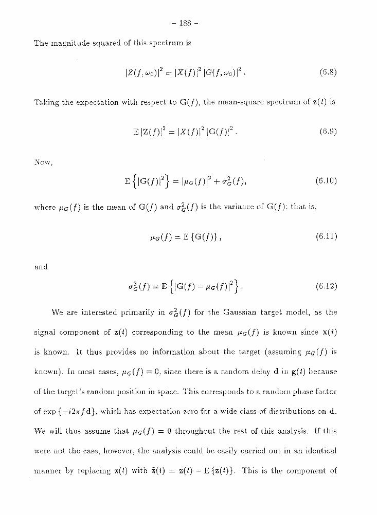
188

magnitude squared of this spectrum is

(6.8)

Taking the expectation with respect to G(f), the mean-square spectrum of z(i) is

(6.9)

Now,

(6.10)

where µG(f) is the mean of G(f) and <T~(f) is the variance of G(f); that is,

µG(f) = E {G(f)}, (6.11)

and

(6.12)

'We are interested primarily in <Tb(!) for the Gaussian target model, as the

signal component of z(i) corresponding to the mean µG(f) is known since x(t)

is known. It thus provides no information about the target (assuming µG (!) is

known). In most cases, µG(f) = 0, since there is a random delay din g(i) because

of the target's random position in space. This corresponds to a random phase factor

of exp {-i2K f d}, which has expectation zero for a wide class of distributions on d.

vVe will thus assume that µG(f) = 0 throughout the rest of this analysis. If this

were not the case, however, the analysis could be easily carried out in an identical

manner by replacing z(i) with z(i) = z(i) - E { z(t)}. This is the component of

189 -

z(i) that remains the mean component E { z( i)} corresponding to µa(!) is

removed.

Similarly, if we define

µz (/) = E {Z(/)} (6.13)

and

(6.14)

then

(6.15)

Referring again to Fig. 6.1, we will assume that the radar receiver observes

y(t) for a period T in order to obtain information about the target. The duration

of observation T must be long enough to allow the receiver to capture all but a

negligible portion of the energy in the scattered signal z(i). We know that the

duration of the transmitted waveform is T, and we know that z(i) must be at

least this long, since the convolution of two waveforms of finite duration T1 and T2

produces a waveform of duration T1 T2 • So if Tg is the duration of g(t), then the

duration of z(i) is T + Tg.

The received y(t) consists of the sum of the scattered signal z(t) and the addi-

tive Gaussian noise n(i) passed through the ideal bandpass filter B(f), passing the

frequency interval W. The impulse response hw ( t) of this filter is

hw(t) = sin 1f W-i

W cos (/o + W/2)1. 1f t

(6.16)

- 190 -

E( o:) 1.0

0.5

0.0+-~-1-~-1-~--1-~___.,1--~+-~-t-~-t-~-t-~-+~--:HllO

o 2 3 4 s 6 7 B 9 10

Figure 6.2. E(a) as a function of a T/W.

The duration of this pulse is infinite, but most of the energy is concentrated in an

interval of duration 1/W. Taking the duration to be Tw(a) = a/vV, the fraction

of the energy in the interval of duration Tw (a) centered about t = 0 is plotted as a

function of a in Fig. 6.2. These values were calculated numerically. As this figure

illustrates, it is reasonable to assume the impulse response duration Tw of the ideal

bandpass filter at the receiver to be Tw ~ 1/W.

It is reasonable to assume that the bandwidth over which most real radar

targets exhibit significant scattering of electromagnetic waves is much larger than

the bandwidth of a radar system we are able to build in order to make the scattering

191 -

measurements [6.3, Sec. 27.6]. it is reasonable to assume

(6.17)

Also, for most radar signals, the duration of the transmitted signal is much larger

than 1/W. This is often necessary in radar detection problems in order to get

enough energy into the signal for reliable target detection. An example of this is the

linear FM or "chirp" signal commonly encountered radar systems. This allows a

range resolution equivalent to a much narrower pulse than that actually transmitted.

Long transmission time, or "time-on-target" is also common in radar target recogni-

tion problems, where the longer observation time allows better frequency resolution

in the measured Doppler spectrum; spectral analysis of the Doppler spectrum is one

of the more common techniques in radar target recognition. For such signals, the

actual duration T of transmission is much larger than the l/W. For such systems,

1 T:>Tw ~ w·

So in summary, the observation interval T is

T= T+T9 +Tw

~T+Tw

1 ~T+

W'

and for systems that satisfy the condition T :> l/W,

~T.

(6.18)

(6.19)

(6.20)

We are interested in finding the mutual information I(g(i); y(t)lx(-1)), that

is, the mutual information between the random target impulse response and the

radar waveform. vVe note that x(-1) is a deterministic waveform. It is

explicitly denoted J(g(-1); y(t)jx(t)) because the mutual information is a func-

tion of x(-1), and we are interested in finding those functions x(-1) that maximize

I(g(t); y(-l)jx(-1)) under constraints on their energy and bandwidth. In order to find

the functions x(t) that maximize I(g(-1); y(i)lx(-1)), we will first find I(z(-1); y(-t)jx(-1))

and those functions x(t) that maximize it. vVe will then show that the functions

x(-1) that maximize J(z(-1); y(t)lx(-1)) also maximize I(g(-1); y(t)lx(-1)), and that for

these x(i), J(g(-1); y(t)lx(-1))=1(z(i); y(t)jx(-1)).

Consider the small frequency interval :Fk - [h, h + .6.f] of band width .6./

sufficiently small such that for all f E :Ft., X(f) ~ X(h. ), Z(f) ~ Z(h. ), and

Y(f) ~ Y(fk ). Let Xk (t) correspond to the component of x(-1) with frequency com-

ponents in :Fk, z,1; (-t) correspond to the component of z(-1) with frequency components

in :F,1;, and Yk (i) correspond to the component of x(-t) with frequency components in

:F,1;. Then, over the time interval T = [-1 0 , 10 + T], the mutual information between

h (-1) and z,. (-1), given that x(-t) is transmitted, is

I(:h (-t); zk (-t) lx(-t)) - T .6.f ln [1 + 2IX (h) 12 O"bJh )] Pnn (h. )T

(6.21)

To see why this is true, consider the continuous communication channel of

Fig. 6.3.

Here we have an additive Gaussian noise channel with input Z, a zero-mean Gaus-

sian random variable with variance O"~, and additive zero-mean Gaussian noise N

with variance <T'Jv. Y and N are statistically independent. The mutual information

193 -

z y

N

Figure 6 Additive Gaussian Noise Channel.

J(Y; Z) between Y and Z is

I(Y; Z) h(Y) - h(YIZ). (6.22)

Now Y, being the sum of two zero-mean Gaussian random variables, is itself a

zero-mean Gaussian random variable. Since Z and N are statistically independent,

the variance of Y, a}, is

O"~ = a-i + o-'Jr. (6.23)

This being the case, the differential entropy h(Y) of is

1 2 1 ( 2 h(Y) = 2

ln 21ro-y = 2 in 21r (J'z (J''Jr) (nats). (6.24)

The differential entropy h(Y IZ) is equal to the differential entropy h( N), since the

conditional density

- 194 -

is a Gaussian density for a random variable with mean z and variance cr'Jv. But the

differential entropy of a Gaussian random variable is a function only of its variance

not its mean;

h(YIZ) = h(N) - ~ 2Jrcr'Jv (nats). (6.25)

So the mutual information I(Y; Z) is given by the expression

; Z) = h(Y) - h(Y IZ)

1 ( 2 2) 1 2 = 2 in 21r ffz + crN - 2 In 2JrcrN

= ~ ln ( cr'Jv ~ ff~ )

2 crN

(6.26)

= ~ ln ( 1 + o-~ ) 2 o-'Jv

(nats ).

Referring again to the signals z.1; (t), h (t), and rl.1; (t) with frequency compo-

nents confined to the interval :F1; = [h, h + ~!], we have from the Sampling Theo-

rem [6.2, p.194] that each of the signals can be represented by a sequence of samples

taken at a uniform sampling rate of 2~/. Since we assume that the spectra X (!),

Z(f), and Y(f) are smooth and have a constant value (at least approximately) for

all f E :Ft., the samples of the Gaussian process sampled at a uniform rate 2~/ are

statistically independent.

The samples Zk (t) are independent, identically distributed random variables

with zero mean and variance o-i. In order to calculate this variance O"~, we note

that the total energy &;(:Fr.) in Zk (t) is

(6.27)

- 195 -

factor of 2 is due to fact that X(h) is the two-sided spectrum of x(i)

and that we are carrying out our calculations using only positive frequencies. This

energy is evenly spread among statistically independent samples. Hence, the

variance of each 2 . (]" z, IS

2t:,.f IX (h) 12 ub (h) 2t:,.fT

IX(f;.)12 ub(fk)

T (6.28)

Similarly, the noise process :fi.1; (i) has total energy £ii. (:Fk) on the interval T

given by

(6.29)

and this energy is evenly distributed among the 2t:,./T statistically independent,

zero-mean samples representing :fi.1; (i). Hence, the variance u'Jv of each sample is

(6.30)

Substituting the results of Eqs. (6.28) and (6.30) into Eq. (6.26), we have that

for each sample Zm of z.1; (i) and the corresponding sample Ym of Yk (t), the mutual

information between Zm and Ym is

( nats)

(6.31)

( nats).

Now there are 2t:,./T statistically independent sample values for both z.1; (t) and

Yk (-l) in the observation interval T. Thus,

I(h(i);zk(t)lx(t)) = 2t:,.fTI(Ym;Zm)

= Tt:,.f In [i + 2IX(h)l20-bjh)l (nats). Pnn(fk)T

(6.32)

196

This is the relation stated in Eq. (6.21) that we wished to show.

Now, if we consider two disjoint frequency intervals Fj and Fk, with y1 (i),

( t) components and :fk(i), zk(t), and nk(i) the components

in F,. of y(i), z(i), and n(i), respectively, then YJ(i) is statistically independent

of 'Jk (i), ZJ (i) is statistically independent of z,. (i), and Ilj (i) is statistically inde-

pendent of (t). We can see that this is true by noting that each of the pairs of

independent processes is made up of two Gaussian random processes with disjoint

PSD's, and such processes are known to be statistically independent [6.4, p.353].

Since the processes are statistically independent, the mutual information between

[YJ (-t), h (-t)] and [zJ (-t), Zk (-t)] given that x(-t) is transmitted is equal to the sum of

the mutual information between YJ (-t) and ZJ (t) given that x(i) was transmitted

and the mutual information between h (i) and z;. (t) given that x(t) is transmitted:

I ([YJ (t), h (-t)]; [z1 (-t), z;; (-t)]!x(t)) = I(-Y1(-t); i1 (-t)!x(-t)) + I(h (t); zk (-t)!x(-t)).

(6.33)

If we now consider the frequency interval W = [!0 , fo W], partition it into

a large number of disjoint intervals of bandwidth tlf, and then let the number

of intervals increase as -+ 0, in the limit we obtain an integral for the mutual

information I(y(-t); z(t)!x(t)), where we assume that x(t), y(-1), and z(-1) are confined

to the frequency interval W. This limit is

I(y(t);z(-t)lx(t)) = fjln [i+ 2 IX(f)l 2 0-~(f)l df. Pnn(/)T

w

(6.34)

We wish to maximize I(y(i); z(t)lx(t)) with respect to IX(f)l 2 under the aver-

- 197 -

power constraint,

j IX(f)l2 dJ - £. (6.35)

w Using the Lagrange multiplier technique [3.4, p.357-9], we form the objective func-

ti on

2IX(f)l2o-~(f)l dJ - ).. [! IX(f)l2 dJ £] . (6.36) Pnn (f)T

w

This is seen to be equivalent to maximizing</> (1X(f)l2) with respect to IX(f)l2,

for each J E W, where

and>.. is the Lagrange multiplier, to be determined from the constraint of Eq. (6.35).

This equivalence can be seen by noting that

Thus, when

it is also true that

<I> (IX(·)l2) = j </> (IX(f)l 2

) dJ. w

84> (IX(/) 12

)

----2- = 0, VJ E W, 8IX(J)I

8<1? (JX(f)l2)

----2,....._ - 0, V/ E W. 8IX(J)I

So we obtain an IX(f)l2 that maximizes Eq. (6.36) when we solve for an IX(f)l2

that maximizes Eq. (6.37). Thus, the IX(f)l2 that maximizes <I> (1X(f)l2) satisfies

the relation

8</> (1X(f)l2

) ----2- - 0, VJ E W.

BIX(f)I (6.38)

- 198

Taking the partial derivatives, we have

(6.39)

This must equal zero. Solving for IX(!) 12 then yields

(6.40)

Here, A - T / ,\ = constant.

Substituting the expression for IX(J)l 2 of Eq. (6.40) into the constraint of

Eq. (6.35), we obtain

J IX(/)1 2 df = j [A - Pnn(/)Tl df 2<Yb (!)

w w

=WA

- £.

Solving for the constant A, we have

A

So the IX(f)l 2 that maximizes J(y(i); z(t)lx(t)) is given by

If we define r (!) as

Pnn(f)T 2<Yb (!) .

(6.41)

(6.42)

(6.43)

(6.44)

199 -

we can write IX(!) 12 as

IX(f)l 2 =A - r(f).

maximum value of J(y(i); z(i)lx(i)), which this IX(f)l 2 achieves, is

Imax(y(J);z(J)jx(J)) = T j In [1

w

= fj1n [1 +A - r(f)] df r(f)

w

( 6 .45)

= T j ln [r~)] df (6.46) w

= T j [ln A - ln r (f)] df

w

= TWlnA-T j lnr(f)df (nats).

w

Note that since IX (f) 12 is the magnitude squared of the transmitted signal

spectrum, it must be real and non-negative for all f E W (we ass!lme it to be zero

for all f ~ W). Yet from Eq. (6.40),

It may be possible that for a given & , o-b (!), and W, one obtains a value of A

such that for some f E W, A< P1111 (f)T/2o-~(f). This would result in an invalid

I (!)12, as IX(f)l 2 would be negative for such f., In order to obtain the IX(f)l 2

that maximizes J(y(i); z(i) lxCn ), we must actually solve for the value of A that

satisfies

J [ nU)fl & - max 0, A - 2o-b(f) df. w

( 6 .4 7)

- 200

most cases, the solution of equation will have to be done numerically. How-

ever, any (positive) of£, A can be bounded as follows:

{ Pnn (f)T} < A < £ . { Pnn (f)T} max --mm JEW 2<!b(f) - - W JEW 2<!b(f) .

Once A has been solved for using Eq. (6.47), we have

-; [ (PnnU)T)] Imax(Y(i); z(i)lx(i)) = T max O, In A - ln 2

<J"b(f) df

w

=fr j max [O, ln A - ln r(/)] df.

w

The associated magnitude-squared spectrum IX (f) 12 that achieves it is

2 [ Pnn (/)Tl IX(f)I =max 0, A - 2<!b(f)

=max [O, A - r(/)].

(6.48)

(6.49)

(6.50)

We note as a check that the solution for IX(/)1 2 obtained by solving Eq. (6.47)

for A and substituting this A into Eq. (6.50) to obtain the IX(/) 12 that achieves

the maximum value of Imax(Y(i); z(i) lx(i)) as given in Eq. (6.49), is equivalent to

that of Eqs. (6.41) and (6.46), when A ;:=: P1111 (f)T /2<J"b(f) for all f E W.

\Ve have shown that the mutual information I(y(t); z(t)lx(t)) is ma..ximized by

an x(t) with IX(f)l 2 as given in Eq. (6.49). In reality, however, we are interested

in the mutual information J(y(i); g(t)lx(t)), the mutual information between the

target and the received signal y(t). We will now show that when IX(f)l 2 satis-

fies Eq. (6.49), I(y(t); g(t) lx(i)) is maximized, and the resulting maximum value

Imax(Y(i); z(t)lx(i)) is the same as Imax(Y(i); g(t)lx(t)). In order to show this, we

will make use of the following two theorems:

201

1: Let a(i) b(t) be finite-energy random processes and let D be a

transformation a(i) to a finite-energy process c(r) (where r is

a new en r could equal -t).

I(a(i);b(i)) = I(c(r);b(i)). (6.54)

2: ) b(i) be random processes with Fourier

transforms (!) and B(f), respectively. Then if I( a(i); b(i)) is the mutual infor

mation between a(i) and b(i) and I(A(f); B(f)) is the mutual information between

(f) and (!), we have

I(a(t);b(t)) = I(A(f);B(f)). (6.55)

To see that Theorem 1 is true, we note that if D is a reversible transformation

between a(t) and c(r), that is c(r) = D{a(t)}, then [6.5, p. 90-1]

h(c(r)) = h(a(i)) + K(D), (6.56)

and

h(c(r)lb(t)) - h(a(i)lb(i)) K(D). (6.57)

K( D) is a function only of the transformation D, not of the specific processes

a(i) and b(-t). Thus,

I(c(r);b(-1)) = h(c(r)) - h(c(r)lb(t))

= h(a(t)) + K(D) h(a(i)lb(i)) - K(D)

= h(a(-1)) - h(a(t)lb(i))

- I(c(r);b(i)).

- 202 -

To see that 2 is true, we choose as our reversible transform D the

transform, and apply it to both a(t) and b(t), yielding

00

D{a(t)} = j a(-t)e-i21rfi d-1 =A(!),

-oo

and 00

(-1)} = J b(-l)e-i2 ~f1 dt - B(f).

-oo

Applying Theorem 1 first to the transformation D{ a(i)} - A(!), we get

I(A(f); b(-t)) = I(a(i); b(i)).

Applying Theorem 1 again, this time to the transformation D{b(i)} = B(f), we

have

I(A(f);B(f)) = I(A(f);b(-t)).

So it follows that

I(a(t); b(i)) - I(A(f);B(f)).

In order to show that Imax(y(t); z(-t)ix(t)) = Imax(y(t); g(-t)lx(-t)), we define

the two-sided set of frequencies

W2 ~f {t: I/IE w, IX(f)l2 f. 0}. (6.58)

Note that W2 is a two-sided set of frequencies, including both positive and negative

frequencies, whereas W is a one-sided set of frequencies, containing only positive

frequencies. vVe also note that if x (!) has frequencies limited to W2' then so does

Z(f), since

Z(f) = X(f)G(f). (6.59)

203

So for f E W2 , we can determine G(/) from Z(/), since

Z(/) ~ G(/) = X(f), VJ E Wz. (6.60)

For f ¢:_ Wz, we cannot determine G(f) from Z(J), since X(f) f. 0 an<l thus 1/ X(f)

is indeterminate. However, physically we would not expect to determine anything

about G(f) for f ~ Wz. · is because the sample functions of (/) describe

linear, time-invariant systems. From such systems we would not expect an output

response at frequencies that have no input excitation [6.2, p. 185-7].

vVe now define

G(f) = { ~(!)

Z(f) - { ~(!) 00

, for f E Wz; , elsewhere;

, for f E Wz; , elsewhere;

g(t) = j G(f)eiZ'K"f-t dt;

-oo

00

z(t) = j Z(f)eiZ'K" f-t dt.

-oo

Then, from Theorem 2 we have

Imax(Y(i); z(t)J.x(i)) = Imax(Y(/); Z(J)J.x(t)).

(6.61)

(6.62)

(6.63)

(6.64)

(6.65)

Note that for f ¢:. Wz, Z(f) = 0, since Z(f) = (/) (!)and X(f) - 0 for f ~ Wz.

Thus, Z(/) = Z(J) from the definition of Z(f) in Eq. (6.55). So from Theorem 1,

Imax(y(t); z(i)Jx(i)) = Imax(Y(f); Z(f)J.x(t)). ( 6.66)

Now for all f E Wz, X(J) f. 0, so

(6.67)

204 -

means that for all f E W2, is a reversible transformation D that maps

Z(/) to G(/), given by

{

z(f)

D [ZUl] = :(!) (6.68)

, elsewhere.

But as we know from 1, mutual information is invariant under reversible

transformations, so

I(Y(f); Z(/)jx(i)) - I(Y(f); G(/)jx(-1)). (6.69)

Eqs. (6.66) and (6.69) yield

J(y(-1); z(-l)jx(i)) = I(Y(f); G(f)lx(t)). (6.70)

Note that G(/), defined by Eq. (6.61), is equal to G(/) for f E W2 and is zero

elsewhere. Thus, 'Io nats of information about G(f) is also 'Io nats of information

about G(/). So it follows that any information obtained about G(/) by observation

of Y(/) is an equivalent amount of information about G(/), and so immediately

we see that

I(Y(f); G(f)lx(t)) ~ I(Y(f); G(f)lx(t)). (6.71)

But for f ~ W2, Y(/) provides no additional information about G(f ). To see that

this is true, we note that for f ~ W2, = 0. Thus,

-io+T

Y(f) N:;(/) = j n(t)e- 2 ~ 11 dt, for f E W2. (6.72)

"t 0

Thus, for f ~ W2, Y(/) is a function only of the noise n(i). Since n(t) and

g(i) are statistically independent, the mutual information between the components

205 -

of these processes with frequency components f ~ W2 is zero, since the mutual

information between statistically independent random processes is zero. So the

inequality of (6.71) is actually an equality:

I(Y(f); G(f)jx(-t)) = I(Y(f); (/)jx(i)). (6.73)

From Theorem 2 we have

I(Y(f); G(/)jx(-t)) = J(y(i);g(-t)jx(i)). (6.74)

Thus, from Eqs. (6.70), (6.73), and (6.74), we have

I(y(-1); g(i)jx(-1)) = Imax(Y(-1); z(-1) Jx(-1)). (6.75)

We have now shown that for the class of functions x(-1) that maximize

J(y(-l);z(-l)lx(-1)) (that is, those x(t) with t E [-T/2,T/2] and with IX(f)l 2 given

by Eq. (6.40)), we have I(y(t); g(-l)Jx(t)) = I(y(t); z(i)Jx(i)). But we have not yet

shown that some other transmitted waveform x(t) confined to the time interval

[-T /2, T /2] satisfying the energy constraint of Eq. (6.1) with magnitude-squared

spectrum IX(f)l 2 does not result in a larger mutual information between g(i) and

y(t). In other words, we must show that there is not another waveform x(t) sat-

isfying constraints on the transmitted waveform for which I(y(t); g(i) Jx(i)) >

I(y(i); g(-t)lx(t)).

In order to show that no such x(i) exists, we redraw the target channel model

of Fig. 6.1 as shown Fig. 6.4. Here we view both g(t) and x(i) as inputs. The

target impulse response g( i) is observed by illuminating the target, resulting in the

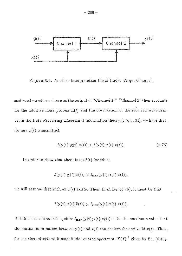
206 -

g (t) z(t) y(t) - Channel 1 ... Channel 2 ... - y

'~ .a.

x (t)

Figure 6.4. Another Interpretation the of Radar Target Channel.

scattered waveform shown as the output of "Channel 1." "Channel 2" then accounts

for the additive noise process n(i) and the observation of the received waveform.

From the Data Processing Theorem of information theory [6.6, p. 31], we have that,

for any x(i) transmitted,

I(y(i); g(i) lx(t)) :S I(y(-1); z(i) Jx(i)). (6.76)

In order to show that there is no .X(i) for which

I(y(-t); g(-t)lx(-t)) > Ima.x(y(-t); z(-t) lx(-t) ),

we will assume that such an .X(i) exists. Then, from Eq. (6.76), it must be that

I(y(i); z(i)J.X(i)) > Imax(Y(i); z(i)Jx(i)).

But this is a contradiction, since (y(-t); z(-t)Jx(i)) is the the maximum value that

the mutual information between y(i) and z(-t) can achieve for any valid x(-t). Thus,

for the class of x(-t) with magnitude-squared spectrum JX(f)J 2 given by Eq. (6.40),

207

l(y(t); g(t)jx(t)) is maximized, and the maximum value lmax(y(t); g(t)jx(t)) is

Imax(y(-t); g(t) lx(t)) Imax(y(t); z(t) lx(i) ). (6.77)

summary then, if x(t) is a finite-energy waveform with energy E confined to

the symmetric time interval [-T/2,T/2], and with all but a negligible fraction of its

energy confined to the frequency interval W = [/o, fo + W], the mutual information

I(y(t); g(t)lx(t)) between y(t) and g(t) is maximized by an x(-t) with a magnitude-

squared spectrum

I 12 [ Pnn (/)Tl

X(/) = ma.x O, A - 2ub(f)

=max [O, A - r(/)],

where r(/) = P1111 (f)T /2ub (!), and A is found by solving the equation

J [ PnnU)Tl E = max 0, A - 2ub (/) df. w

The resulting maximum value lmax(y(i); g(t)jx(t)) of l(y(-t); g(t)lx(t)) is

Im=(y(J);g(J)lx(J)) = T J max [o,lnA - In ( ~::mn l d/ w

- T j max [O, In A - In r(/)] df.

w

Note the behavior of the magnitude-square spectrum

I ( )1 2 [ PnnU)Tl X J - max O,A- 2ub(f) ,

(6.78)

(6.79)

(6.80)

which maximizes I(y( t); g(t) Jx(t)). the variance ub (!) of the frequency spectrum

(/) of the scattering function g(t) is held constant for f E W, JX (/) 12 gets larger

as Pnn(/) gets smaller, and IX(/)1 2 gets smaller as P1111 (/) gets larger, becoming

- 208 -

zero for n (!) 2 2Ao-b (f)/T. Similarly, if Pnn (!) is constant for all f E W, as

would be the case for additive white Gaussian noise, IX(f)l2 gets larger as o-b(f)

gets and IX(f)l2 gets smaller as <rb(f) gets smaller, with IX(f)l2 ~A for

- 2 -o-b(f) :> n(/)T/2A and IX(f)I = 0 for o-b(f) :::; n(/)T/2A. In order to

interpret this behavior physically, recall that o-b (!) is the variance of the frequency

spectrum (!). see that frequencies f E W with large <Tb(!) provide greater

information about the target than those with small <Tb(!). This is not surprising,

since for frequencies with small o-b (!), there is less uncertainty about the target

response at that frequency in the first place. In fact, for those frequencies at which

<Tb(!) = 0, there is no uncertainty at all in the outcome of <:rb (!), and thus, there

is no point in making any measurement at these frequencies.

Note that A= A(£,<:rb(f),Pnn(/)) is a function of the transmitted energy

£, of the size and shape of the spectral variance o-b (!) of the target, and of the

noise power spectral density Pnn (/). The fact that IX(f)l 2 = 0 for all f such that

<:rb (!) :::; P1111 (f)T /2A can then be interpreted as saying that a greater return in

mutual information can be obtained by using the energy at another frequency or

set of frequencies.

of relationship between IX(!) 12 , A, n(/),

in Fig. 6.4. Comparing Eq. (6.79) and Fig. 6.4, we see that the

total energy £ corresponds to the shaded area in Fig. 6.5a. The difference between

the line of value A forming the upper boundary of the shaded region and the curve

forming the lower boundary of the shaded region is IX(!) 12 . This difference is

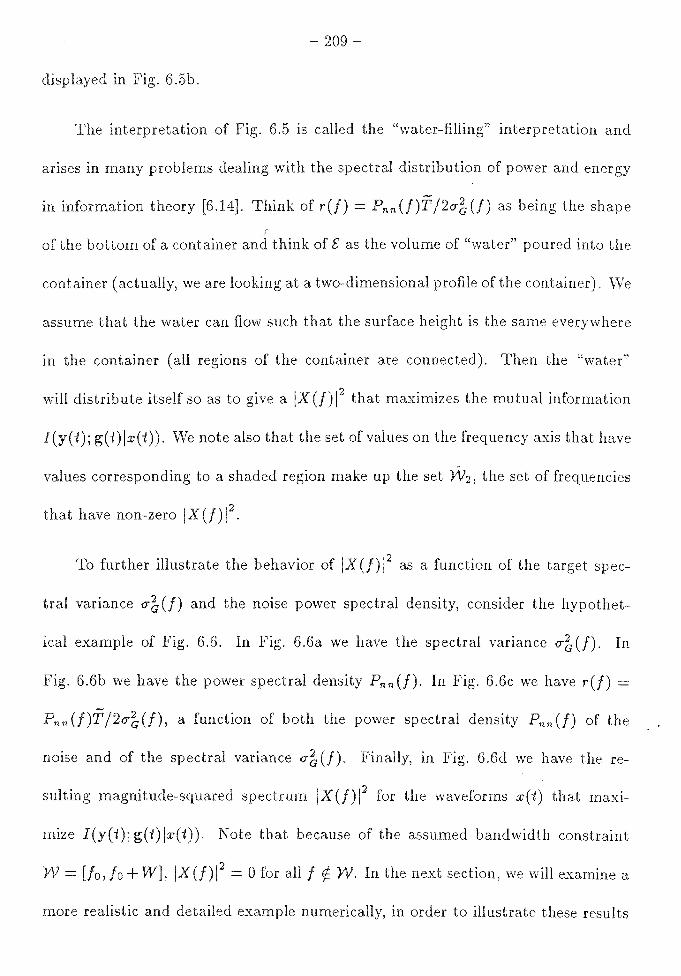
- 209

displayed in Fig. 6.5b.

The interpretation of Fig. 6.5 is called "water-filling" interpretation and

anses many problems dealing with the spectral distribution of power and energy

in information theory [6.14]. Think of r(f) = Pnn(f)T/2<Tb(f) as being the shape

of bottom of a container and think of£ as the volume of "water" poured into the

container (actually, we are looking at a two-dimensional profile of the container). \Ve

assume that the water can flow such that the surface height is the same everywhere

in the container (all regions of the container are connected). Then the "water"

will distribute itself so as to give a IX(!) j2 that maximizes the mutual information

I(y(t); g(t)lx(t)). We note also that the set of values on the frequency axis that have

values corresponding to a shaded region make up the set W2 , the set of frequencies

that have non-zero IX(!) 12 .

To further illustrate the behavior of IX(!) 12 as a function of the target spec

tral variance <Tb(!) and the noise power spectral density, consider the hypothet

ical example of Fig. 6.6. In Fig. 6.6a we have the spectral variance <Tb(!). In

Fig. 6.6b we have the power spectral density Pnn (!). In Fig. G.Gc we have r(f) =

Pnn (f)T /2a-b(f), a function of both power spectral density Pnn (!) of the

noise and of the spectral variance O"b(/). Finally, Fig. 6.6d we have the re

sulting magnitude-squared spectrum jX(/)1 2 for the waveforms x(t) that maxi

mize I(y(t); g(t)lx(-t)). Note that because of the assumed bandwidth constraint

W [/o, Jo+ vV], jX(/)12 = 0 for all f ~ W. In the next section, we will examine a

more realistic and detailed example numerically, in order to illustrate these results

- 210 -

r(/)

f

(a)

IX(/)12

f

(b)

Figure 6.5. (a) "Water-Filling" Interpretation of the Magnitude-Squared

Spectrum IX(f)l 2 that max1m1zes the Mutual Information

I(y(t); g(t)jx(i)). (b) Magnitude-Squared Spectrum IX(f)j 2 that maxi

mizes J(y(t); g(t)jx(t)). Note the Relationship to the Shaded Area in (a).

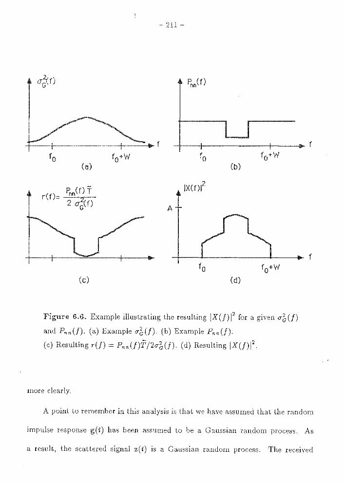
211

f

f o f0 +W f o f 0 +W

(a) (b)

pnn(f) T IX(012

r(O= 2 ()~f)

A

(c) (d)

Figure 6.6. Example illustrating the resulting JX(f) J2 for a given o-b (!)

and Pnn(/). (a) Example o-b(f). (b) Example Pnn(f).

(c) Resulting r(f) = Pn 11 (f)T/2o-'f;(f). (d) Resulting IX(/)12.

more clearly.

f

f

point to remember in this analysis is that we have assumed that the random

impulse response g(i) has been assumed to be a Gaussian random process. As

a result, the scattered signal z(i) is a Gaussian random process. The received

- 212

y(i) is also a Gaussian random process, smce the noise m the channel is

additive Gaussian noise. Thus, for a given ub(f), we are solving for the mutual

information the case of an additive Gaussian noise channel with a Gaussian input.

As we noted in Chapter 2 the case of the additive Gaussian noise channel, for a

input with a given variance u 2, the mutual information between the channel

input and the channel output is maximized when the input is Gaussian. Then in

assuming that g(-1) is a Gaussian random process, we have selected a Gaussian input

process for an additive Gaussian noise channel in our problem. Then in solving for

the maximum mutual information Ima.x(Y(-1); g(-l)!x(t)), we have derived an upper

bound in the maximum, achievable mutual information between y(t) and g(t) for

any g(-1) with spectral variance <Tb(!) under the imposed bandwidth and energy

constraints, whether g(t) is Gaussian or not. In the case when g(-1) is Gaussian, as

we have assumed, this upper bound is achieved.

- 213 -

6 A

now examine how

realistic problem.

results of the previous section can be applied to a

process, we will examine the characteristics of the

optimal transmitted signal's spectrum and the amount of information obtained.

For our example, we will assume that a radar system is observing a target

at a range of 10 \Ve will assume that the radar is a monostatic radar with

an antenna having an effective area Ae = 3 m2, an RF bandwidth of 10 MHz, a

transmitter frequency centered at 1 GHz, and we will assume that the antenna is

pointed directly at the target under observation. This gives us a frequency interval

Wof

W = [/o, /o + W] - [0.995GHz,1.005 GHz].

In the following analysis, we will analyze this radar system for a range of average

power constraints ranging from 1 W to 1000 vV and a range of observation times

from 10 µs to 100 ms. However, for the purpose of the narrative, we will look at

the case where the observation time T ~ T = 10 ms, a fairly typical value for

radar target recognition systems, and for a few specific values of average power

Numerically calculated results for the full ranges noted above will be presented after

going through sample calculations.

assume that the target under observation has a finite-energy, Gaussian

impulse response g(t) with spectral variance (]'b (!) given by

(6.81)

- 214 -

B and a are constants that respectively characterize the magnitude of the

spectral variance o-b (/) and rate at which it decreases as I/ - fp I increases.

will assume in our example that

a= 10- 13 s2 , (6.82)

a value illustrating well the effect of the transmitted waveform's spectral character-

is tics for the 10 MHz system band width being considered. In order to determine a

reasonable value of B for our example, we will assume that the spectral variance

o-b (/) at frequency fp corresponds to that of a 1 m 2 variance in the radar cross

section er of the target at this frequency. From the radar equation, Eq. (4.1), and

the fact that the gain G of an antenna of effective area Ae is [6.6, p. 11]

it follows that the ratio of the received power to the transmitted power is

PR A~cr PT - 41r ,\2 R4 •

(6.83)

Note that, in our example, we have

c 2.998 X 108 m/s ,\ = fp - 1.000 X 1Q9 Hz - 0.30 m.

This being the case, the ratio of the change in received power that is due to a 1 m 2

change in radar cross section, LlP.R, to the transmitted power, PT, is

(6.84)

- 215 -

will assume that the additive Gaussian noise present at the radar receiver is

thermal noise that is white over frequency interval W. will assume a system

noise tempertature of T, = 300 . Hence, the resulting one-sided noise PSD is [6.6,

p. 29]

P1111 (!) = No = kT, = (1.381 x 10- 23 J /K)(300 K) = 1430 x 10- 21 J.

Here, k is Boltzmann's constant, and k = 1.381 X 10- 23 J /K.

By definition, r(f) is given by

(!) _ Pnn (f)T

r - 2o-b(f) '

and so in our case, with T T - 10 ms,

( 4.1430 x 10- 21 J)(0.01 s) r(f) = 2(7.9577 X 10- 16 ) exp [-a(f - fp)2] (6.85)

= (2.7835 X 10- 8 J-s) exp [a(! - fp) 2],

where again, a= 10- 13 s2 and fp = 1 GHz. A plot of this r(f) is shown in Fig. 6.7.

From Eq. (6.42) we know that

where

£ - j max[O,

w

r(f)] df,

£ = P:i:T = (lOOOW)(lOms) = lOJ.

Solving for A numerically, we obtain

= 1.0870 X 10- 6 J-s.

(6.86)

(6.87)

216 -

r( f) -7

4.0 x 10 J-s

-7 3.0 x 1 0 J-s

-7 2.0 x 10 J-s

-7 1.0 x 1 0 J-s

0.996 0.998 1.000 1.002 1.004 0.995 0.997 0.999 1.001 1.003 1.005

Figure 6.7. r(f) = Pnn(f)T/2cr;(f) as a function off.

Thus, we have that IX(!) 12 =max [O, A - r(f)] is

I (!)12 = { 01.0870 X 10- 6 J-s - (2.7835 X 10- 8 J-s) exp [a(! - fp) 2

] , for f E W; , elsewhere.

(6.88)

Recall that this formula gives IX(f)l2 for positive frequencies only, but that IX(f)l2

is an even function, so IX(!) 12 = IX ( - !) 12 for f < 0. plot of IX(/) 12 for positive

f is shown in Fig. 6.8.

From (6.49), the mutual information J(y(t); g(-t)lx(t)) is given by the inte-

gr al

- 217 -

IX( 012

_7 12.0 x 10 J-s

6.0x 10-7 J-s

0.996 0.998 1.000 1.002 1.004

0.995 0.997 0.999 1.001 1.003 1.005

Figure 6.8. jX(/)1 2 for T - lOms and P:r = 1000\IV.

I(y(-t);g(t)jx(t)) = T j max[O,lnA-lnr(/)]d/.

w

Substituting A as given in Eq. 6.87 and r(f) as given in Eq. 6.88 into this equation

and integrating numerically over W, we obtain the result

I(y(t); g(t) lx(t)) = 2.3815 X 105 nats. (6.89)

If we repeat the calculation, reducing the available average power P:r to 500 vV,

- 218

IX( 012

6.0 x 1 o-7 J-s

3.0 x 1 o-7 J-s

0 4-~-1-~~~~--~-+~~+-~-+-~-+~~+-~-+-~--+-f, GHz

0.996 0.998 1.000 1.002 1.004

0.995 0.997 0.999 1.001 1.003 1.005

Figure 6.9. IX(/)12 for T = lOms and Px = 500vV.

maintaining T = T = 10 ms, we find

A = 5.8691 x 10- 7 J-s, (6.90)

and the resulting IX(f)l2 for positive frequencies is

IX(f)l2 = { ~.8691x10- 7 - (2.7835 X 10- 8 J-s) exp [a(f - fp) 2] , for f E W;

, elsewhere.

(6.91)

plot of this IX(f)l2 for positive frequencies is given in Fig. 6.9. The mutual

- 219 -

information I(y(-t); g(t)lx(t)) for case, obtained by numerical integration, is

I(y(1); g(t)lx(t)) = 2.2152 X 105 nats. (6.92)

We now investigate a case which for some f E W, r(/) > A. vVe assume that

the average available average power P.r is 100 W, still maintaining T - T = 10 ms.

Solving Eq. 6.47 numerically for A, where now

£ = P.rT = (100 W)(lO ms) = 1 J,

we have

A = 1.7709 x 10- 7 J-s,

and the resulting IX(/) 12 for positive frequencies is

IX(f)l2 = { ~.7709 X 10- 7 J-s - (2.7835 X 10- 8 J-s) exp [a(/ - fp) 2]

Here, W C W is given by

(6.93)

(6.94)

, for f E W; , elsewhere.

(6.95)

W = {/ E W: A ?'.". r(f)} = [0.995698 GHz, 1.004302 GHz]. (6.96)

So in this case, only 8.604 MHz of the available 10 MHz of RF bandwidth should

be used by the radar system. This is because more information is obtained by con-

centrating energy in W and providing a signal-to-noise ratio in W than

by distributing the energy across W. The latter would provide a greater number

of degrees of freedom to be measured, but they would be measured less reliably.

The IX(/)1 2 of Eq. 6.96 optimizes this tradeoff between the measured number of

- 220 -

IX( 012

2.0x 10-7 J-3

1.0x 10-7 J-3

Regions in which IX(fll equals zero

-i-..--+~~-i-~-i-~~;--~-r-0~---jr--~-t-~--i-~~-r---""""'t"f,GHz 0.996 0.998 1.000 1.002 1.004

0.995 0.997 0.999 1.001 1.003 1.005

Figure 6.10. IX(f)l 2 for T = lOms and P;;; = lOOvV.

degrees of freedom in the measurement and the reliability of the individual degrees

of freedom in the measurement-the optimization being done so as to maximize

the mutual information I(y(i); g(i)lx(t)). plot of IX(f)l 2 in this case is shown in

Fig. 6.10. The resulting value of I(y(i); g(i)Jx(t)) for this JX(/)1 2 is

I(y(i); g(-l)lx(i)) = 2.2152 X 105 nats. (6.97)

We will now display the results of the numerical solution of Eqs. (6.47) and

(6.49) for the mutual information I(y(i); g(i)lx(i)) as a function of both T and the

Ima.x(Y(i); g(-t) !x(t) ), nats

1 o7

1 06

1 o5

1 04

1 o3

1 o2

1 0

1 0

221

100

Average Power Px, Wat ts

T = 100 mS

T = 10 mS

T 1 ms

T = 100 µS

T = 10 µS

1000

Figure 6.11. Ima.x(y(-t); g(-t)!x(-t)) as a function of T and P;c.

average available power . This numerical solution was carried out for values of

T equal to 10 µs, 100 µs, 1 ms, 10 ms, and 100 ms. For each of these values, the

average power varies over the range of from 1 vV to 1000 W. All integrations

were numerically carried out using the Gaussian. Quadrature Met.hod [6.7, pp. 322-

6]. resulting maximum values of J(y(-t); g(t) lx(-t)) are plotted in Fig. 6.11. Note

that both scales in Fig. 6.11 are logarithmic.

Several points are worth noting in Fig. 6.11. The first is that the mutual

- 222 -

information Imax(y(-1); g(t)lx(t)) is proportional to T. Actually, this proportionality

is only approximate, but the approximation is very good for T :> 1/W, in which

case it is reasonable to assume that T - T. This is true for all T considered

Fig. 6.11, since 1/vV = 0.1 µs. This proportionality is reflected in Fig. 6.11 by noting

that each time T is increased by a factor of 10, the mutual information increases by

a constant increment on the logarithmic scale of Imax(y(t); g(t)lx(t)). Examining

the expression for Imax(y(t); g(t)lx(t)) of Eq. (6.80), we have

Im=(y(J); g(J)lx(J)) = T j max [ O, In A - In (~:HJ~)] df

w

- f j max [o, ln ( 2Ao-bU])] df. Pnn (f)T

w

But for T :> 1/W, which is true for all values of T considered in our example, it is

reasonable to assume that T - T. This gives

j [ (2Ao-b(f))] Imax(y(t); g(t) lx(t)) = T max 0, ln Pnn (f )T df · (6.98)

w

But as can be seen from Eq. (6.42), A is proportional to T, and so assuming T - T,

A is proportional to T. If we define

then we can write Eq. (6.98) as

vVe can thus see analytically that

def A a= -T' (6.99)

(6.100)

(y(t); g(t)lx(-t)) is proportional to T. In fact,

we can write the rate at which information is transferred to the receiver in the radar

- 223 -

measurement process as

(6.101)

which is not a function of vVe then have

Imax(Y(i); g(i)jx(i)) = TRmax(Y(i); g(t)jx(t)). (6.102)

The fact that (y(t); g(t)jx(t)) is proportional to T has an interesting in-

terpretation in terms of radar target-recognition problems. In Section 2.4, where

we examined the relationship between mutual information and radar-measurement

performance, we noted in Eq. (2.36) that, if I(X; Y) is the mutual information

between a set of parameters X to be measured and their measurement Y, the

maximum number of equiprobable classes N into which X can be assigned with

statistical reliability by observation of Y is

N = l el(X;Y) J

(la J denotes the largest integer less than or equal to a). Applying this result

to our problem, we have that given an x(t) that achieves Imax(Y(i); g(t)jx(t)) is

transmitted, the largest number of equiprobable classes into which g(t) can be

assigned with statistical reliability by observation of y(t) is

N = l ei.,..x(y(t);g(i)Js(t)) J

l eT Rm•x(y(t);g(t)js(i)) J (6.103)

Note that this number grows exponentially in T, the duration of the transmitted

signal. T is often referred to in radar target-recognition problems as the "time-

on-target." In radar target-recognition problems, it is well known that all other

224

things being equal, the longer the "time-on-target," the better the performance

of the target recognition system. As a result, within constraints imposed by other

system requirements such as searching for new targets and tracking targets that have

already been detected, the "time-on-target" in radar systems that perform target

recognition is generally made as large as possible. This is reflected quantitatively

Eq. (6.103), which shows that the maximum number of equiprobable classes into

which g(i) can be reliably classified by observation of y(i) increases exponentially

in T.

Let us examine this result in terms of a practical methodology often used in

radar target-recognition problems. One common method of classifying radar targets

in target-recognition problems is by examining the characteristics of the Doppler

spectrum of the target by performing spectral analysis on the signal reflected by

the target. Assume that the frequency interval over which this is done has band

width W~. Then, using classical methods of spectral analysis [6.8], the frequency

resolution 6./ of the measured spectrum is inversely proportional to T. Thus, the

number of frequency bins of bandwidth 6./ that span the interval of bandwidth

i-v is proportional to T. Call this number of frequency bins M, as is illustrated in

Fig. 6.12.

Assume that because of noise in the received signal, the energy in each fre

quency bin can be distinguished to only one of Q levels. Then the total number of

distinguishable spectra, N, is

(6.104)

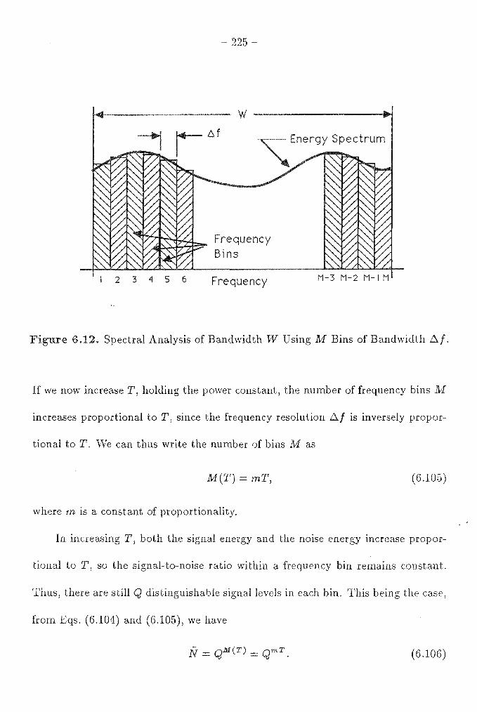
2 3 4 5 6

- 225

w

Frequency Bins

Frequency M-3 M-2 M-1 M

Figure 6.12. Spectral Analysis of Bandwidth W Using M Bins of Bandwidth!::../.

If we now increase T, holding the power constant, the number of frequency bins M

increases proportional to T, since the frequency resolution !::../ is inversely propor-

tional to T. We can thus write the number of bins M as

M(T) = mT, (6.105)

where m is a constant of proportionality.

increasing T, both the signal energy and the noise energy increase propor-

tional to T, so the signal-to-noise ratio within a frequency bin remains constant.

Thus, there are still Q distinguishable signal levels in each bin. This being the case,

from Eqs. (6.104) and (6.105), we have

(6.106)

226 -

Hence, the number of discernible frequency spectra also increases exponentially with

T. This is not to say that there is any equivalence between the discernible frequency

spectra and equiprobable classes of g(i) to which Eq. (6.103) refers, but this

heuristic example does show that the concept of the number of classes into which a

target recognition system can classify targets increasing exponentially with "time-

on-target" is not foreign to radar target-recognition problems. So the behavior of

Eq. (6.103) does make intuitive sense.

It is important to note that when a waveform x(t) that achieves

Imax(y(t); g(t)lx(t)) is transmitted, the N equiprobable classes referred to in

Eq. (6.103) are not under the control of the radar but are a function of the target. In

actuality, what Eq. (6.103) states is that the probability space Q can be partitioned

into N subsets 0 1 , 0 2 , ... , ON, where

1 Pr{w E Ok}= N' fork -1, ... ,N, (6.107)

where N is given by Eq. (6.103). These N subsets 0 1 , 02, ... , ON, which form a

partition of 0, correspond to a set of N classes into which g(t) can be reliably

classified by observation of g(t). These N classes may not, however, correspond

to classes that are of interest to the user of the radar system. Generally, the user

will have knowledge of x(t) and will wish to classify the radar target into one of V

classes A 1 ,A2 , .•• ,Av based on observation of y(t).

These classes may be linked to the physics of the problem, such as the case

where the classes Ak describe relative target size, or the classes may be less con-

nected with the physics of the problem, such as in the case where only two target

- 227 -

classes A 1 and A 2 are of interest: whether the aircraft being observed is friendly

or hostile. In general, the problem of assigning a target to one of the classes in

= {A 1 ,A2 , ... ,Av} based on observation of y(i) can be viewed indirectly as

finding a mapping from C: n -r A, such that fork= 1, ... , N, each Q.1; is mapped

to one of the Aj with a reasonable probability of error in determining the proper

target class. In general, as N becomes larger, we would expect the performance of

the best mapping C to improve for fixed V. Since N is an exponentially increasing

function of I(y(i); g(t)ix(t)), we would expect the probability of correct classifica

tion into one of the classes in A to improve as I(y(-t); g(-t)ix(t)) becomes larger. In

actually designing radar target classifiers, features that characterize y(t) are usually

determined empirically and decision rules based on these features are constructed,

allowing the classification of targets based on observation of y(-t). Iteference [6.9)

describes the approaches typically taken in designing such classifiers, and Iteference

[6.10) gives a detailed account of such classification techniques.

Returning again to the results in Fig. 6.11, we see that a very large amount of

information is obtained the radar measurements in our example. For example,

for T = 100 µs and Ps = 10 W, I(y(-t); g(-t)ix(-t)) is approximately 100 nats, which

equals approximately 144 bits. The corresponding N calculated from Eq. (6.103) is

2.69 x 1043 . we can conclude that a significant amount of information can

be obtained about the target in the radar measurement process. In order to put

this information to use, signal processing algorithms must be developed. The form

these take will generally be highly dependent on the specific application in which

- 228

the radar measurements will be used.

When processing the received signal into a form that is useful, a significant

amount of information can also be destroyed. We will see an example of this in the

next chapter, which synthetic aperture radar measurements are used to determine

the radar reflectivity of a natural surface.

6 Radar Waveform Design and Implementation.

We now turn to the problem of designing specific radar waveforms x(i) that have

a magnitude-squared spectrum IX(/) 12 , to be used in order to probe the target so

that the greatest amount of target information may be extracted from the received

signal scattered by the target. In the first section of this chapter, we determined

that any x(i) with jX(f)j 2 as given by Eq. (6.78) would maximize J(y(i); g(-l)lx(i)).

Now we must address the design of specific transmitter waveforms that will do this.

Some considerations in this waveform design will now be addressed.

The most theoretically obvious, although not the most practical, method of

designing a waveform x(t) with magnitude-squared spectrum IX(/) 12 is to excite

a filter with transfer function H(f) such that IH(f) 12 = IX(!) 12 with an impulse

or delta function. Given that IH(f)l 2 = IX(!) 12 , we see that such an H(f) must

satisfy

(6.108)

where </>(/) can be any arbitrary phase function off. A major shortcoming of this

approach is that it requires the design of high-frequency (microwave) filters with

very specific frequency characteristics. This can be very difficult to do and is also

229 -

an inefficient use of microwave energy, as it requires the broadband generation of

microwaves to be fed into filter. Here the frequencies to be attenuated are filtered

out to the degree required to obtain the desired spectral characteristic IX (f) 12, and

this energy is lost. addition, radar systems often employ signals of very high

power, and the direct generation of complex, high-power, broadband microwave

signals is not easily accomplished.

Typically in the design of radar systems, waveforms are generated at baseband

frequencies much lower that that of the microwave transmitter frequency and then

are used to modulate a microwave carrier in order to obtain the desired waveform at

the radar operating frequency. Typical modulation techniques used in radar signal

generation are amplitude, frequency, and phase modulation, with a large number of

systems using phase (phase-coded waveforms) and frequency (both linear and non

linear FM chirp) modulation. This is because some constant-amplitude microwave

amplifiers have greater efficiency than their variable-amplitude counterparts.

Generally, radar waveforms are bandpass waveforms because of practical band

width constraints on the components that generate and process them. As a result,

H(f) will typically have a bandpass filter response, and thus .x(-t) can be generated

by amplitude modulation of the carrier with a baseband signal. Such a bandpass

signal can also be obtained by phase or frequency modulation of the carrier with

a baseband waveform. However, synthesizing a desired spectrum using phase or

frequency modulation is mathematically a much more difficult problem, since both

phase modulation and frequency modulation are non-linear modulation processes.

230

As a result, it is more difficult to find a baseband modulating waveform to obtain

the desired RF spectral characteristics. Reference [6.6] gives descriptions of these

modulation processes, and Reference [6.11] gives an analysis of the spectral charac-

teristics of phase modulation and frequency modulation for deterministic signals.

A problem of a more fundamental nature that arises in the design of x(i) is

due to the form of IX(/)1 2 in Eq. (6.78). The problem lies with the realizability

of a waveform x(-1) with magnitude-squared spectrum IX (f )1 2. The realizability

problem is due to the fact that there may not be an x(i) with a magnitude-squared

spectrum IX(/) 12 that is causal. In practice, we get around this problem by gen

erating a waveform x(i) having a magnitude-squared spectrum /xU)/2

~ IX(f)l2.

This approximation is normally carried out by by delaying a non-causal x(t) cor

responding to IX(!) 12 and truncating the result prior to time zero in the delayed

version. Since x(-1) is considered to be confined to the interval T = [-T /2, T /2],

this should, in principle, be possible and a realizable waveform with magnitude

squared spectrum IX(/)1 2 (or at least approximately, ignoring some energy outside

the frequency interval W) will exist. For completeness however, we will investigate

those IX(/)1 2 that have no corresponding causal x(i).

order a system with transfer function H(f) and impulse response

h(i) to be physically realizable, it must be a causal system. A causal system is one in

which the output at time i does not depend on future input values. Mathematically,

if the system with impulse response h(-1) is causal, then, if the input is w(i) and the

- 231 -

output is x(t), we have

io

x(to) = j w(t)h(t - to) dt, Vto -oo

(6.109) io

= j w(r)h(to - r) dt, Vio. -oo

Thus, we have that an equivalent definition of a causal system is one in which the

the impulse response h(t) - 0, for all t < 0.

The magnitude-squared transfer function, IH(f) 12 , can also be tested directly

for causality using the Paley-Wiener Criterion [6.12]. The Paley- 'Wiener Criterion

states that for a magnitude-squared function IH(f) 12 to have an associated impulse

response h(-t) that is causal and thus realizable, a necessary and sufficient condition

on IH(/)1 2 is

;

00

~ln_IH_(_/)_12 1 + f2 df < 00. (6.110)

00

This says that for there to be any physically realizable h(t) with a magnitude

squared spectrum IH(/)1 2, the area under the curve lln IH(/)1 2 1/(1 + /2) must

be finite. This places two major constraints on the magnitude-squared function

IH(f) 12 . The first, which will not concern us, requires that IH(f) 12 < K exp (/2 )

as I/ I -t oo, for some positive constant K. This is obviously true in the case of

IX(!) 12 , since IX(/) 12 satisfies the finite-energy constraint of Eq. (6.2). The second

major restriction imposed by the Paley-\Viener Criterion is that the magnitude-

squared function IH(/)1 2 cannot be zero over any band or interval of frequencies.

IH(f) 12 may, however, have a countable number of zeroes in f without violating

the Paley-Wiener Criterion.

232 -

The significance of the Paley-\Viener Criterion to us is that it states that if

IX(/) 12 has any more than a countable number of zeroes in f, there is no realizable

x(i) that has a magnitude-squared spectrum IX(f)l2 (n.b., the Paley-vViener Cri

terion does not say that all x(i) with a magnitude-squared spectrum IX(/)12 are

realizable, only that there exist realizable x(i) with a magnitude-squared spectrum

IX(/)12). Since we specify that IX(/)12 = 0 for all f ~ W, it would appear that

none of the IX(/) 12 obtained for a finite frequency interval W would have realizable

x(i). Recall that, from our discussion in the first section of this chapter, we noted

that if x(i) is zero outside the time interval T = [-T/2,T/2], then X(f) cannot

be limited strictly to a finite frequency interval W. In reality, when we design our

waveforms to be limited to the time interval T, we attempt to concentrate as much

of the energy as possible into the frequency interval W, but some small portion of

the energy falls outside of W, and according to the Paley-Wiener Criterion, this is

unavoidable. In addition, within the interval W, for solutions yielding an IX(f)l 2

that is non-zero only on some W C W, IX(!) 12 will not have a corresponding real

izable x(-1) if the set {W- W} has more than a countable number of points. Again,

the solution to this apparent problem lies in the fact that since we cannot actually

build these filters, they must be approximated. These realizable approximations do

not violate the Paley-Wiener Criterion.

These approximations to the ideal, unrealizable filter can be done in several

different ways. Many of the methods are covered in References [6.12] and (6.13].

Perhaps the most commonly used technique to approximate a non-causal impulse

233 -

response in radar and communication systems is to delay the response until it is

causal or, in the case of impulse responses that are not of finite duration, delay them

as much as is feasible, and then truncate the part of the delayed impulse response

for time T less zero. For any finite-energy impulse response, this technique

can be used in principle to obtain arbitrarily small error in the magnitude-squared

spectrum IH(f)l2 . practice, however, this may not be practical because of the

cost of implementation. Note also that these delays in generating the signal at the

transmitter must be taken into account at the receiver.

6.4. Comparison of Waveforms for Optimum Detection and Maximum

Information Extraction.

In Chapter 5, we examined the design of radar waveforms and receiver filters for

optimum detection of targets with a known impulse response. In this chapter, we

have examined the design of radar waveforms that maximize the mutual information

between a target with random impulse response and the received signal at the radar

receiver. The question arises: How do these two types of waveform compare?

the case of the design of a waveform x(t) that optimizes the detection of

a target of known impulse response h(~), we noted in Chapter 5 that the solution

corresponded to the eigenfunction with energy £ corresponding to the largest eigen

value of the integral equation of Eq. (5.29). We noted that these results could be

interpreted, in the case of additive white Gaussian noise, as putting as much of the

transmitted energy as possible into the largest mode of the target under the time

and bandwidth constraints on the transmitted waveform. The result was that we

- 234 -

obtained the largest possible signal-to-noise ratio, and thus the optimal detection

performance, under the constraints on the transmitted waveform. We also noted

however, that the other eigenfunctions, corresponding to different modes of

the target, could contain significant information about the target. So if we wished

to extract information about the target, it might be advantageous to distribute the

available energy among the various modes. Of course, when the impulse response

of the target is known a priori, as was assumed in Chapter 5, there is nothing to be

gained by this approach.

In this chapter, we have assumed that the target has a random impulse response

g(t) and we distribute the energy in the transmitted signal as specified in Eq. (6.78).

If we interpret IH(f)l2 as "target response" in Chapter 5 and <r~(/) as "target

response" in this chapter, we see that IX(!) 12 tends to get larger at frequencies in

which the "target response" gets larger, and smaller at those frequencies at which

the power spectral density of the noise gets larger. Using the two-sided power

spectral density Snn (!) of the noise, we had

(Chapter 5)

where a was a constant, and here we have

(Chapter 6)

The power spectral density of the noise enters into the solution in two quite different

ways in the two solutions, and hence the form of the magnitude-squared spectrum

of the two waveforms is quite different. While the waveform design of Chapter 5

- 235 -

attempted to put as much of energy as possible into the mode of the target that

gave the largest response when weighted with respect to noise, the waveform

design of this chapter distributes the available energy order to maximize the

information obtained about the target.

6.5. ter 6 es.

6.1 Ulaby, F. T., R. K. Moore, A. K. Fung, !v.ficrowave Remote Sensing, vol. 2,

Addison-Wesley, Reading, MA, 1982.

6.2 Bracewell, R. N., The Fourier Transform and its Applications, McGraw-Hill,

New York, NY, 1986.

6.3 Papoulis, A., Probability, Random Variables, and Stochastic Processes,

McGraw-Hill, New York, NY, 1965.

6.4 Skolnik, M. I., Radar Handbook, McGraw-Hill, New York, NY, 1970.


J. 27, 1948. 379-423, 623-656. Reprinted in C. E. Shannon and vV. vV. Weaver,

The Mathematical Theory of Communication, Univ. Ill. Press, Urbana, IL,

1949.



6.7 Hamming, R. vV., Numerical Methods for Scientists and Engineers, 2d. ed.,

Dover Publications, New York, NY, 1973.

6.8 Blackman, R. B. and J. vV. Tukey, The Measurement of Power Spectra, Dover

Publications, New York, NY,1958.

236 -

6.9 Duda, R. 0. and P. E. Hart, Pattern Classifi.cation and Scene Analysis, John

VViley and Sons, New York, NY, 1973.

6.10 Simon, J. C., Patterns and Operators, McGraw-Hill, New York, NY, 1986.

6.11 Stark, . and F. B. Tuteur, Modern Electrical Communications, Prentice-Hall,

Englewood Cliffs, NJ, 1982.

6.12 Lindquist, C. S., Active Network Design with. Signal Filtering Applications,

Steward and Sons, Long Beach, CA, 1977.

6.13 Lam, H. Y-F ., Analog and Digital Filters, Prentice-Hall, Englewood Cliffs, NJ,

1979.

6.14 Gallager, R. G., Information Theory and Reliable Communication, John Wiley

and Sons, New York, NY, 1968.

- 237

1

CONTENT IMAGES

In this chapter, we will investigate the information content of radar images. We will

do this by defining the spatial information ch.annel and examining its characteristics.

We will then use these results and the results of Chapters 2, 3, and 4 to examine

quantitatively how much information is conveyed by a radar image. This analysis

will substantiate quantitatively certain qualitative results in the processing of radar

images, particularly in the area of machine analysis of radar images.

In Section 7.1, we will examine the general and information-theoretic charac

teristics of radar images. We will examine the general characteristics of images

and the way that discrete images arise as the result of the spatial sampling of two

dimensional, continuous images. We will then examine how such sampling arises

naturally an imaging system as a result of the spatial resolution of the imaging

system. Next, we will study the information-theoretic characteristics of discrete

images in order to determine their information content. This will provide us with

an understanding of the effects of spatial dependencies between pixels in a radar

image on the image's information content. In Section 7.1, we perform this analy

sis, assuming a general discrete distribution on the resolution cell or pixel intensity

values in the image.

Section 7 .2, we examine the information-theoretic characteristics of the in

tensity parameter of the individual pixels of a radar image when the displayed

- 238

quantity is received power from a diffuse surface. particular, we examine the mu-

information between the surface reflectivity and displayed power in the

note the effects of "speckle noise" limiting this mutual information.

We also note the effect averaging independent observations of a homogeneous

region of the surface to combat speckle noise and the effect of this procedure on

between the average reflectivity of the surface and the dis

played image intensity. From this mutual information, we are able to determine

the maximum number of equiprobable classes into which we can classify the sur

face reflectivity, based on our observation of received power. Coupling these results

with those of Section 7.1, we conclude that in order to obtain significant ability to

classify regions of a surface into categories that are a function of surface reflectivity,

a region made up of a large number of pixels or resolution cells is required. This is

an information-theoretic explanation of a well-known heuristic result.

7.1 Radar Images.

In this section, we will examine some general characteristics of radar images, that

is, images generated by either real aperture or synthetic aperture radars. vVe will

not present an in-depth analysis of imaging radar systems, as there are several good

books that give excellent in-depth coverage of the underlying physical principles

of radar imaging (7 .1-7 .6]. We will instead investigate the information-theoretic

characteristics of radar images.

, according to the definition [7.7, p. 361], is "a spatial dis-

tribution of a physical property such as radiation, electric charge, conductivity or

- 239

reflectivity, from another distribution of same or another physical

property." can be defined as an image obtained with the use

of a sensor employing active electromagnetic scattering. A radar image is a spatial

mapping of the scattering characteristics of the area being illuminated by the radar

transmitter. Actually, the radar image consists of some intensity parameter a( x, y)

displayed as a of two orthogonal coordinates x and y, and this parameter

is a function of the scattering characteristics of the target at the spatial point cor-

responding to these image coordinates. The displayed intensity parameter a(x, y)

could represent the reflected signal power, the ratio of received signal powers from

two orthogonal polarizations, or some other functions of the scattered radar signal.

Examples of these would include soil moisture, wind speed over water, crop charac-

teristics, or surface texture metrics [7.8]. If the intensity pattern a(x,y) is viewed as

a continuous random field with finite energy, the two-dimensional spectrum A(µ, v)

of a( x, y) is given by the two-dimensional Fourier Transform

00

A(µ,v) = j a(x,y)e-i"2"K"(µa:+vy)dxdy. (7.1) -oo

Here µ is the spatial frequency in the direction of the x-coordinate and v is the

spatial frequency the direction of the y-coordinate.

practice, the radar images obtained using imaging radars are discrete ran-

<lorn fields. The samples that make up these discrete images correspond to the

discrete sampling of a spatially bandlimited continuous image in ( x, y) with spatial

bandwidths µmax and :vmax corresponding to the x-coordinate and y-coordinate,

respectively. For sampling intervals of /::,.x in the x-coordinate and /::,,.y in the y-

coordinate, µmax and :vma.x are

- 240

1 µmax= 2~x'

1 :vmax = 2~y ·

This follows from the Sampling Theorem [7.8, pp. 127-8].

(7.2)

So we assume that

A(µ, :v) = 0 for JµI > µmax and !:v I > :vmax- Note that the spatial bandlimiting

is not a function of the surface alone, but is also a function of the imaging system

-in particular, the imaging system's spatial resolution. In an imaging system, ~x

and ~y correspond to the spatial resolution in the x and y directions, respectively.

Thus, although there may be spatial fluctuations in the physical scattering char-

acteristics of a surface with spatial frequencies greater than µmax and vmax, the

spatial resolution of the imaging system effectively low-pass-filters these fluctua-

tions out of the image produced by the imaging system. We can thus represent the

spatial sampling of the image as shown in Fig. 7.1. Here, H(µ, :v) represents the

two-dimensional, low-pass filtering effect that is due to the limited spatial resolu-

tion of the imaging system, and the two-dimensional sampler samples the resulting

spatially bandlimited signal at the Nyquist sampling rates

(7.3) , .

We can view the resulting image as an m X n array of resolution cells as shown

Fig. 7.2, with an intensity value a(i,j) for the discrete pair of coordinates (i,j),

where i E { 1, ... , m} and j E { 1, ... , n}. The intensity level corresponding to each

of these resolution cells is most easily modeled as a continuous parameter, and in our

Scatteri Terrain

H(µ, v)

Spatial Bandpass Filtering Imposed by Radar's Spatial Resolution

Ideal 2-Dim

Sampler

Ideal 2-Dim Sampling at the Nyquist Rate in both Dimensions

Figure 7.1. Spatial Sampling in an Imaging Radar System.

analysis we will often do so. However, in most real imaging systems and especially

those that use digital processing, these levels will be quantized into discrete levels.

For our present analysis, we will assume that there are K such levels. We will

designate the set of K possible values that the intensity parameter can take on in

each resolution cell as E = {E1 , ... ,Ex}. The image under consideration can be

considered to be an m x n array, with each element of the array taking on one of

the K elements of E. The elements of the array correspond to the resolution cells

or "pixels" of the image.

If we view the image under consideration as a noiseless communication channel,

we note that there are N unique messages that can be conveyed by such a channel,

with

(7.4)

242

y o.

-.......--, ..

n

~, ... _....__ ~

'-· J m 1~ - I

x

Figure 7.2. Discrete Radar Image as an m X n Array of Resolution Cells.

Equivalently, we see that there are N distinguishable images that can be con-

structed. By viewing the image as a spatial information channel, we are led to

consider the quantity of information that can be conveyed by the image. The

amount of information I that can be conveyed by this image viewed as a noiseless

channel is

I= logN

(7.5)

= mnlog

- 243

we take the logarithm to have base-e, we have

I= mnln (nats/image). (7.6)

Assume that we generate the image by assigning a value from E to each

of the m X n resolution cells independently, with each cell having probabilities

, ... , Px of taking on values E 1 , ... , Ex from E, respectively. Then when the

number of resolution cells mn grows large, the entropy H(F) of the image, and thus

the amount of information it conveys when generated by such a source, is

H(F) = mn H(E), (7.7)

where H ( E), the entropy of an individual resolution cell, is

X

H(E) = - Lpk log Pk. (7.8) k=l

To see that such an image does, in fact, convey this much information, assume that

there are a total of Q = mn resolution cells in the image under consideration. Let

ni, ... , nx be the number of resolution cells with intensities E 1 , ... , Ex, respec-

tively. Then we have Q = n 1 + · · · + nx, and the number N of distinguishable

images with a given set of numbers { n1, ... , nx} is

Ml N=--

n1! ·· · nx!'

Note that for large Q = mn, we have from the law of large numbers that

(7.9)

(7.10)

244 -

We saw previously that the information conveyed by an image is given by log N.

Taking the logarithm of (7.9), we obtain

Q! logN =log ni! ... nx!

···+log nx!].

Using Sterling's approximation [7.9, p. ], which states that

to approximate the factorials in Eq. (7.11), we have for large Q that

logN ~ -(K - l)log.;2";-Q + (n1 + ···+ nx)

+ (Q + 1/2) log Q - [(n1+1/2) log n1 + · · · + (nx + 1/2) log nx]

= (Q + 1/2) log Q - [(n1+1/2) log n1+ .. ·+(nx+1/2) log nx]

- (K - 1) log .;2";.

(7.11)

(7.12)

Since Q is very large, we will assume that ( Q + 1/2) log Q :> K log yf2;, and thus

we have

log N ~ (Q + 1/2) log Q - [(n 1 + 1/2) log n1 + · · · + (nx + 1/2) log nx]. (7.13)

From Eq. (7.10),

~ QPJ, for j = 1, ... ,K. (7.14)

This being the case, we can rewrite Eq. (7.13) as

log N ~ (Q + 1/2) log Q - [(QP1 1/2) log QP1 + · · · + (QPx + 1/2) log QPx].

(7.15)

245 -

assume that for probabilities Pj chosen, Q is sufficiently large such that

> 1/2. Then we can write

log N ~ Q log Q - [QP1 log QP1 + · · · + QPx log QPx]

K

= QlogQ- l::QP1r. [logQ+logP.d k=l

K

= Q log Q - Q log Q - Q P1r. log P1r. k=l (7.16)

K

= -QI: P.i. log P1r. k=l

= QH(E)

= mnH(E).

So as Q grows large, we have

log N ~ QH(E), (7.17)

and thus in the limit, as Q -t oo, we have

log N = mnH(E). (7.18)

So we see that the amount of information conveyed by an image in which all

mn resolution cells are statistically independent and in which each resolution cell

has entropy H(E) is given by Eq. (7.18). Thus, in order for this amount of infor-

mation to be maximum, it follows from Eq. 7.18 that the probability distribution

(P1 , ... , Px) must be selected to maximize H(E). It is easily seen that this oc-

curs when Pj = 1/ K, for all j = 1, ... , K. When the intensity levels are selected

according to this probability distribution, we have

K 1 1 H(E) = - L K log K

k=l (6.19)

= logK,

- 246

and thus the maximum amount of information that can be conveyed by an image is

logN = mnlogK, (7.20)

which is in agreement with the maximum amount of information that could be

conveyed by an image as given in Eq. (7.5).

mum amount of information a K-level m X n image can convey is mn log K. Our

primary interest here, however, is to consider the information content of radar im

ages. In finding the maximum amount of information that a K-level m X n image

can convey, we generated the image by selecting the intensity values of the resolution

cells independently of that of all other resolution cells and such that all of the K

intensity levels were equiprobable. As a result, we have that all of the Km 11 possible

images are equiprobable. Examination of real radar images indicates that that there

is significant correlation between adjacent pixels in the image. This is due to the

fact that there are usually significant similarities in the scattering characteristics of

the physical terrain being imaged for adjacent resolution cells.

As an illustration of this, consider the radar image in Fig. 7.3. This image

was obtained using a side-looking synthetic-aperture radar mounted on a NASA

CV990 aircraft and processed at the Jet Propulsion Laboratory. The operating

characteristics of the radar are given in Table 7.1. The image was generated using

linear cross-polarization between transmit and receive and a grazing angle (the

angle between the direction of wave propagation and the surface) of 45°. In this

image, four independent looks were averaged in order to reduce speckle. (Speckle

247 -

(Courtesy of Jet Propulsion Laboratory)

Figure 7 .3. Radar Image of San Francisco Area.

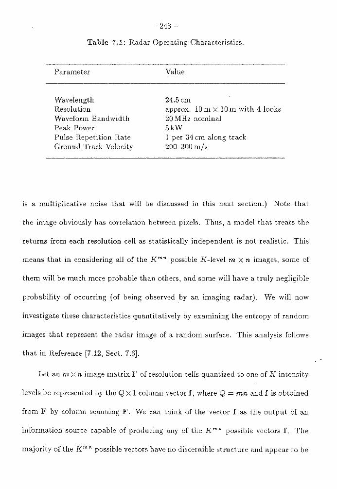
- 248 -

1: Radar Operating Characteristics.

Parameter

Wavelength Resolution Waveform Bandwidth Peak Power Pulse Repetition Rate Ground Track Velocity

Value

24.5cm approx. 10 m X 10 m with 4 looks 20 MHz nominal 5kW 1 per 34 cm along track 200-300 m/s

is a multiplicative noise that will be discussed in this next section.) Note that

the image obviously has correlation between pixels. Thus, a model that treats the

returns from each resolution cell as statistically independent is not realistic. This

means that in considering all of the Kmn possible K-level m X n images, some of

them will be much more probable than others, and some will have a truly negligible

probability of occurring (of being observed by an imaging radar). vVe will now

investigate these characteristics quantitatively by examining the entropy of random

images that represent the radar image of a random surface. This analysis follows

that in Reference [7.12, Sect. 7.6].

Let an m X n image matrix F of resolution cells quantized to one of K intensity

levels be represented by the Q X 1 column vector f, where Q = mn and f is obtained

from by column scanning . We can think of the vector f as the output of an

information source capable of producing any of the Kmn possible vectors f. The

majority of the Kmn possible vectors have no discernible structure and appear to be

- 249 -

similar to a random noise field (much like the output of a television receiver tuned to

a which no signal is present). For typical values of m,n, and K that one

would an imaging system, only a small fraction of the Kmn possible images

correspond to images that could be generated by a real radar system imaging terrain.

It is reasonable then, at least in principle, to consider the a priori probability of

occurrence for each of the T = Kmn possible images f.1• This probability will be

designated P(f.j ), where -t = 1, ... , T. The entropy H(f) of the image source is thus

T

H(f) = - L P(f1) log P(f1). (7.21) i=l

The significance of H(f) is derived from Shannon's noiseless channel coding th.e-

orem [7.10], which states that it is possible to encode a source of entropy H(f) bits

without error using H(f) + e code bits, where e is a small positive quantity. Con-

versely, it states that it is not possible to encode a source of entropy H(f) bits with

H(f) - e bits without error. In fact, if the source produces successive images inde-

pendently, then the information I (f.11 , ... , fu) required to specify L source images

(that is, a sequence of L source images) exhibits the following asymptotic behavior:

__ l ,_._._._, f_i_L_ L ~ H ( f). L

(7.22) .

We note that :::; mnlogK, with equality if and only if P(f.t) = K-mn = 1/T,

for 1 = 1, ... , the case of radar images as well as most other physically

generated images, H(f) < mn log K.

The probability of occurrence of f1 , P(f1 ), can be expressed as the joint prob-

- 250 -

ability distribution of the individual resolution cell intensities:

P ( fi) = { ! ( 1) = r j i ( 1) , ... , f ( Q) = Q ( Q)} . (7.23)

Here, rjp(p) represents the j-th intensity value at resolution cell p. An alternative

expression for P(f1 ) can be obtained by expanding Eq. (7.23) in terms of conditional

probabilities:

P(f1 ) =Pr{/ (1) = rj i (1)} Pr {f (2) = rj2(2) I/ (1) = rj 1 (1)}

···Pr {f(q) = rjq(q)lf(q - 1), f(q - 2), ... , /(1)}

{! ( Q) = rjq ( Q)I/ (Q - 1), !( Q - 2), ... ,J(l)}.

Using this expression and the definition of H(f) given in Eq. (7.21), we have

T

H(f) = L P(f1 ) log [Pr{/ (1) = rj1 (1)}] i=l

T

- LP(f1)log[Pr{/(2) = rj2(2)1/(1)}] i=l

T

- L P ( f1 ) log [Pr { f ( q) = r j q ( q) If ( q - 1), ... , f ( 1)}] i=l

T

- L P(f1) log [Pr {f(Q) = r1q(Q)lf(Q - 1), ... , /(1)}]. t=l

The general term in Eq. (7.25), which will be given the notation

[/(q)l/(q - 1), ... '/(1)]'

(7.24)

(7.25)

can be interpreted as the average information provided by the resolution cell at

image vector coordinate q when the values of the preceding q - 1 resolution cells

251 -

are can rewrite (7.25) as

q

H(f) =I: [f (q)l/(q - 1), ... ,f(l)]. (7.26) q=l

Eq. (7.26) gives the image source entropy of the radar image and thus gives a

measure of amount of information or "information content" of the image.

We will now make a simplification in our analysis. Recall that we are consider-

ing a column scanned image vector f. For such a random vector, it is easily shown

[7.11] that for j > k,

H [/ ( q) I I ( q - 1), ... , I ( q - j)] ::; H [f ( q) I I ( q - 1), ... , I ( q - k)] . (7.27)

We can interpret this inequality as saying that the more knowledge we have of pixels

preceding pixel q, the less uncertainty we have about the value of pixel q. To be more

precise, the inequality states that if we increase our knowledge of the pixel values

preceding q, our uncertainty of /(q) cannot increase, and it will either decrease

or remain constant. The uncertainty in /(q) remains constant as knowledge of the

history of preceding pixel values is increased if and only if the pixels in the increased

history are statistically independent off ( q).

For most physically generated images, an individual term of Eq. (7.26) of the

form [/(q)j/(q - 1), ... , /(1)] approaches a non-zero limiting value as J. becomes

large (i.e., as the history of previous pixel values becomes greater) [7.12, p. 187].

We will denote this limiting pixel value as H [/(q)loo]. If we now assume that end-

of-sequence effects are negligible, then from Eq. (7.26), the image entropy H(f) can

- 252 -

be approximated by Q

~I:: [f(q)looJ. (7.28) q=l

if behaves as an m X n element area of a stationary, two-dimensional

process, then [/(q)loo] is constant for all q, and Eq. (7.28) becomes

H(f) ~ QH (q)loo]. (7.29)

Eqs. (7.28) amd (7.29) provide a means for estimating the image entropy H(f), and

thus, of estimating the image's information content.

In order to use Eqs. (7.28) and (7.29) to estimate the entropy of a column-

scanned image, we must determine the limiting conditional entropy H [f (q) loo] of

f (q) from a finite sequence of pixels. So we will use an approximation of the form

H [f ( q) I 00] ~ H [/ ( q) If ( q 1)' ... ' I ( q - p)] K K

""" """ ] p [f ( q) ' ... ' f ( q - p)] = L...J ... L...JP[f(q), ... ,f(q-p) logP[/( -l) ... /( _ )]' Jo =l Jp=l q ' ' q P

(7.30)

where

P [/( q), ... ,f (q - p )] = Pr{/ (q) = rjo( q), ... ,/( q - P) = Y'jp(q)}. (7.31)

We note from Eq. (7.27) that the approximation given by Eq. (7.30) is an upper

bound.

order to make use of the (upper-bound) estimate of H [f(q)loo] given by

(7.30), we must estimate the distribution given in Eq. (7.31). This can be

done either by mathematically modeling the image source and deriving the source

- 253

statistics from this model or by histogram estimation of the distribution from real

radar image data. Mathematical modeling of the image source may be inaccurate if

detailed knowledge of the surface is not available, as there are many different surface

models widely varying scattering behavior [7.1, 7.3, 7.11, 7.13]. On the

other hand, the histogram estimation of the distribution has extreme computational

and image data requirements. The joint distribution P [f (q), ... , f (q - p )] for a k

level image has kP+l distinct sets of arguments at which it must be estimated.

Thus, for typical values of I{, such as k = 256 corresponding to 8-bit image level

quantization, the computational requirements become excessive for even relatively

small p. In addition, the number of sample values required for reliable estimation

of the distribution from the histograms can be quite large [7.14, Ch. 4].

An appreciation for the difficulties of the estimation of image distributions

using histograms can be gained from the work of Schrieber [7.15], who performed

such estimations on television images with I{ = 64 and p = 0, 1, and 2. The results

obtained in that study showed that the uncertainty in f ( q) was significantly reduced

in going from p = 0 top = 1 (from 4.39 bits to 1.91 bits), while there was only a

slight additional reduction in going fromp = 1top=2(from1.91 bits to l.49bits).

The joint entropy of f(q), f(q - 1), and f(q - 2) was 7.80 bits. These results seem

to indicate that most of the information that could be obtained from the preceding

pixels could be obtained from only one preceding pixel, although the rate at which

[f(q)lf(q - 1), ... , f(q - p)] converged to H [f(q)loo] could not be determined.

This was due to the computational difficulties of histogram estimation for larger p:

254 -

[/(q)l/(q - 1), ... , f(q - p)] could not be easily determined for p greater than 2.

So , we have been considering the conditional entropy of the pixel value f ( q)

conditioned on values of previous pixels in column-scanned image vector f of

situation is shown in Fig. 7.4a. is also possible, and perhaps physically

more meaningful, to condition the entropy of f ( q) on the values of other sets of

pixels, for example, those pixels directly neighboring the pixel q or some larger

neighborhood of the pixel q. Typical examples are shown in Fig. 7.4b, which shows

the neighborhood

{/(q); f(q - l),f(q + 1),/(q - m),f(q + m)},

and in Fig. 7.4c, which shows the neighborhood

{ /(q);/(q-1),/(q+l),/(q-m-1),/(q-m), }·

f(q n + 1,/(q + m - 1),/(q + m), f(q + m + 1)

Recall that m is the number of resolution cells per row in the image matrix F. Larger

neighborhoods, such as the one shown in Fig. 7.4d, could also be constructed in

principle, although the computational burden of computing the histogram estimates

of their associated conditional distributions would be prohibitive in practice for

typical numbers of quantization levels K.

general, in order to estimate the image entropy H(f), we will use one of

the previously mentioned estimates of H [/(q)loo] and then use either Eq. (7.28)

or Eq. (7.29) in order to determine H(f). practice, in order to simplify the

computation so that it is reasonable, we will most likely have to assume that the

m X n image F under consideration is a section of a stationary, two-dimensional,

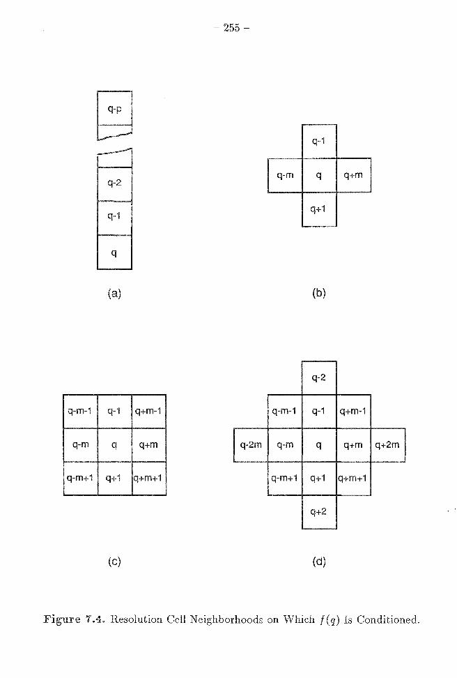
- 255 -

q-m q q+m

q-1 q+i

q

(a) (b)

q-2

q-m-1 q-1 q+m-1 q-m-1 q-1 q+m-1

q-m q q+m q-2m q-m q q+m q+2m

q-m+1 q+1 q+m+1 q-m+1 q+1 q+m+1

q+2

(c) (d)

Resolution Cell Neighborhoods on Which J(q) Is Conditioned.

- 256

random process and will use the approximation

H(f) ~ QH [f(q)Joo]

given m (7.29).

As a simple example to clarify these ideas, consider a 10 X 10 binary image F

with a Q = 100 element column-scanned image vector f = [/(1), ... , f (100)]. The

pixel intensities f(q) take on values of either "O" or "l." We will assume that the

image is generated by a binary Markov process, such that the probability distribu

tion of f(q) for 2::; q :=; 100 is dependent only on the previous pixel value f(q - 1).

We will assume that the conditional distribution governing these probabilities is

Pr{/(q) = OJ/(q - 1) = O} = 0.75,

Pr{/( q) = lJ/ (q - 1) = O} = 0.25,

Pr{/(q) = OJ/(q - 1) = 1} = 0.25,

Pr{/(q) = lJ/(q - 1) = 1} = 0.75.

We will assume that Pr{/(1) = O} = Pr{/(1) = 1} = 1/2. A typical image

constructed in this manner is shown in Fig. 7.5, where "l"" is represented by black

in the image and "O" is represented by white. Since the value of f ( q) is dependent

only on the previous pixel value. f ( q - 1), we have that

[/(q)Joo] = [/(q)J/(q - 1)]

= -0.25 ln 0.25 - 0.75 ln 0.75

= 0.5623 (nats).

Thus, since the probability distribution is stationary in q, we have that the entropy

257 -

Figure 7 .5. 10 x 10 Binary Markov Image.

of the image H(f), as given by Eq. (7.29), is

lS

H(f) ~ QH [/(q)ioo]

= 100 · 0.5623 (nats)

= 56.23 (nats).

To calculate the exact entropy of the image, we note that the entropy of /(1)

[/(1)] = -0.5ln0.5 - 0.5ln0.5,

= ln2

= 0.6931 (nats).

Each of the remaining 99 pixels has entropy H [f(q)lf(q - 1)] = 0.5623 nats condi-

tioned on previous

- 258

and thus we have

[/(1)] + 99 · [/( q) loo]

= 0.6931 + 99. 0.5623

= 56.36 (nats).

So we see that approximation of (7.29) is very good in this example.

note that the marginal probability that any pixel value f(q) equals "O" or

"1" is 1/2. If each of the pixels were statistically independent of all other pixels,

such a 100 pixel image would have an entropy of 69.31 nats. So we see that the

dependence between successive pixels in the binary Markov process that generates

this image accounts for a significant reduction in the entropy of the image. We can

see this visually in Fig. 7 .5 by noting the presence of a significant number of "runs"

of both "O" and "l" in the columns of the image.

Having considered the basic information-theoretic concepts of radar images,

we now look at some specific details determining the information content of radar

images.

- 259 -

eckle Noise Images.

In the previous section, we examined the general information-theoretic characteris

tics of radar images. However, we did not address the actual information content

of each individual resolution cell or pixel. We assumed that each resolution cell dis-

played an intensity that was quantized to one of levels, and we determined that

the maximum amount of information that could be obtained per resolution cell was

log K, but we did not actually investigate the information that could be expected

from a radar measurement of a resolution cell. this section, we will examine the

information per resolution cell when making measurements of the radar reflectivity

of a surface. vVe will do this not only for the case of an image generated by a single

look at the resolution cell, but also for an image in which each resolution cell is

made up of the arithmetic mean of multiple measurements of the reflected power

from a resolution cell, a technique used to reduce "speckle noise" in radar images.

Much of what is presented in this section is the result of an investigation by Frost

and Shanmugan [7.16].

Consider an imaging radar, with either real or synthetic aperture, making mea

surements of a homogeneous diffuse surface. By homogeneous, we mean that the

radar reflectivity Z of the surface is a wide-sense-stationary, 2-dimensional random

process. diffuse, we mean that the scattering characteristics of the surface at

the wavelength of the radar radiation satisfiy the characteristics of diffuse scatterers

as outlined in Section 4.4. That is, the surface area within a radar resolution cell

is assumed to be made up of a large number of independent scatterers, none of

- 260 -

which are dominant terms of the total scattered power. addition, they are

assumed to be spatially distributed such that the surface is rough in the Rayleigh

sense, as described Section 4.1. Such a surface would be a Category 1 surface in

the nomenclature of Section 4.4.

The radar reflectivity of the surface is a random variable Z, which we will

assume to be uniformly distributed over the interval [,81 , /32]. This assumption

is more than a mathematical convenience. In Reference [7.15], this assumption

is shown to be in good agreement with synthetic-aperture radar-measurements of

terrain.

We will now assume that a radar reflectivity measurement is made by measuring

the received power from the surface by using one of m "waveforms" from the set

A = { a 1 , ... , am}. Here, the term "waveform" has a special meaning. We will

assume that the actual waveform transmitted by the target is of any of a number of

typical forms used in imaging radar, such as a chirp or pulsed sinusoid waveforms.

However when we say that a "waveform" ak is used to make a measurement of

the radar reflectivity of the surface, we mean that k independent measurements of

the reflected power from a homogeneous region of the surface are made, and that

their as the output of the radar receiver. In terms of

the model presented Chapter 3 for the Radar/Information Theory Problem for

continuous target channels, we are using the target channel only one time (N = 1),

but the proper definition of the "waveform" ak allows us to average the results of

k independent observations of the received power reflected from the surface in the

- 261

use of a single "waveform." So the homogeneous region of the surface is assumed

to have a reflectivity and when a waveform = ak is used to measure this

reflectivity, the resulting output Y is the arithmetic mean of the received

power from each of the k independent measurements of received power scattered

from the surface.

We are interested in determining the mutual information J(Y; ZIX = ak) in

order to determine how much information is obtained about the surface reflectivity

Z by observation of Y. Y and Z are parameters of primary interest in radar

imaging. Y, as previously defined, represents the radar measurement of the surface

reflectivity, whereas Z represents the mean reflectivity of the region ( which is

unknown and modeled as a random variable). As was discussed in Chapter 4,

the radar reflectivity of an object is both a function of its material composition and

geometric or spatial structure. As we will see, Z corresponds to the surface material

characteristics, but Y includes the effects of a multiplicative noise called "speckle,"

resulting from the constructive and destructive interference occurring at the radar

receiver that is due to the roughness of the surface being imaged.

The mutual information I(Y; ZIX = ak) can be written as

IX= ak) = h(YIX = 0:1;) h(YjZ,X = a;r.). (7.32)

Here, the entropies h(Y IX °'k) and h(Y IZ, X a;,) (in nats) are

given by 00

h(YIX=cq)=- j /(ylX=a;.)ln/(yjX=ak)dy, (7.33) -oo

- 262

00 00

h(YIZ, =a;.)= - j j f(y,zJX = a;.)ln/(ylz, = a1;)dydz. (7.34)

-00-00

Thus, order to evaluate I(Y; ZIX = a,1;), we must determine the density functions

/(ylX = ak), f(y,zjX = ak), and /(yjz,X = ak). We will now determine these

density functions.

Assume that the radar is illuminating the homogeneous diffuse surface as previ-

ously described and that the transmitter and receiver have fixed (although possibly

different) antenna polarizations. We will assume that the received signal has suffi-

cient energy such that it is reasonable to ignore the effects of additive noise. This

assumption is reasonable, since multiplicative "speckle" noise, not additive noise, is

most often the limiting factor in imaging radars [7.3, §8-7, 9-8]. Then, as we deter-

mined in Section 4.4, the received power P from a single observation is exponentially

distributed, and its probability density function (PDF), given by Eq. ( 4.42), is

(p) = { ~ 1 / µ) exp ( -p / µ) , for p 2:: O; , elsewhere.

(7.35))

Here µis the mean value of The characteristic function '11 p ( w) corresponding to

this PDF is 00

(w) = J fp(p)eiwp dp

-oo (7.36) 1

- 1 - iwµ ·

When X = a,1;, Y is defined as the arithmetic means of k independent, iden-

tically distributed random variables Pj, each with a density function given by

263

(7.35). So we have for X = 01,1;,

order to the distribution of Y, we define the random variable W as

k

w~fkY=L j=l

(7.37)

(7.38)

Then, since the are independent and identically distributed, we have that \fl w ( w),

the characteristic function of W, is

But since

we have that

and thus we have

\f!w(w) = [\f!p(w)]k

1 - k.

(1 - i.wµ)

1 Y=-·W,

k

fy(y) = kfw(ky),

Hence, we have that the characteristic function of Y is

1 (w) = (1 - iwµ/k)k.

(7.39)

(7.40)

(7.41)

This is the characteristic function of the gamma distribution with mean µ/ k and k

degrees of freedom (7. p.104-6]. Thus, we have that the density function /(y!X =

/(I X= )=yk-1µ-kexp(-yk/µ) for">_O. Y ak r(k)k-k ' J

(7.42)

264

f(k) is the gamma function. For integer k, f(k) (k - 1)!.

imaging of terrain, we are primarily interested in finding the mean

value µ. We note that what is typically done radar images to determine µ at

a given point on the surface is to average several independent observations of the

received power from a resolution cell. This is done in order to reduce the effects

of "speckle" or "fading" in the radar image [7.3, pp. 586-90]. But we note that in

averaging k observations to obtain Y as described in Eq. (7.37), we obtain a random

variable with mean

E{Y} = µ (7.43)

and variance

E{(Y (7.44)

So as many independent looks are averaged to reduce speckle, Y converges toµ with

high probability. Thus, we are interested in determining µ. As we have previously

noted, however, this mean value µ is itself a random variable, the random variable

Z, which we have assumed to be uniformly distributed on the non-negative interval

[;31, .B2]. Thus, we have that the density of Y conditioned on Z is given by

/( I X - ) - yk-lz-k exp(-yk/z) for y 2 O, y z, - a.1; - f(k)k-k ' - (7.45)

and the joint density of and Z is

_ _ y"- 1z-k exp(-yk/z) /(y,zlX - a;i;) - f(k)k-"(.Bz -.Bi) , for y,z;?: 0. (7.46)

The density function f (y IX = a,1;) is found by integrating Eq. (7.46) with respect

- 265

to z over

fi l

J y k - 1 z - k exp ( -y k / z) f(ylX=ak)= f(k)k-k(!h-/31) dz. (7.47)

fi 1

For k = 1, this integral is given by (see Chapter 7, Appendix)

(7.48)

where Ei(x) is the exponential integral, given by

ii:

Ei(x) = j ±ea da.

-oo

Fork 2:: 2, this integral is given by (see Chapter 7, Appendix)

k { ( k Y ) k - 2 [ ( k Y //32) k - r - 2] 1)(/32 - {Ji) exp - /32 ~ (k - r - 2)!

_ (- ky) k-2 [(kyj{Ji)k-r-2]} exp /31 ~ ( k - r - 2) ! · (7.49)

The mean and variance of Y are given by [7.16]

(7.50)

and

2 (/32 - /31 )2 (f = ----

y 12 (7.51)

now the necessary density function to evaluate the mutual information

I(Y;ZIX = ak)· however, we will examine the relationship between the

density function /(ylz,X = o:k) and speckle noise. From Eq. ("f.45), we have that

the density function f (y lz, X = ak) of Y conditioned on Z = z and X = O:k is

Now, as pointed out

- 266 -

16], if we define the random variable V for a fixed z by

def 2kY v = --, z

(7.52)

then is a standard chi-square random variable with 2K degrees of freedom [7.18,

§4.32]. Hence, it follows that for a fixed Z = z, the random variable Y can be

written as

y = (~) ·Z. (7.53)

Thus, we have that the observed Y is the product of the mean reflectivity

Z = z of interest and the multiplicative noise term V /2k. This multiplicative

noise term is a function of the surface roughness on a length scale the order of the

wavelength of the transmitted radiation. It has mean value 1 and variance 1/2K.

Because it is a function of small-scale variations within a resolution cell, its value

varies from resolution cell to resolution cell and gives the radar image a speckled

appearance. Hence, this multiplicative noise is given the name "speckle." The

speckle phenomenon is known and has been studied extensively in the field

of coherent optical systems [7.19]. effects of speckle on the interpretability· of

radar images has been investigated (7.20, 7.21].

Having determined the necessary density functions, we now calculate the dif-

ferential entropies of Eqs. (7.33) and (7.34) needed to determine I(Y; ZIX = O:'k ).

Substituting the density functions of Eqs. (7.45) and (7.46) into Eq. (7.34), we

- 267

obtain (see Chapter 7 Appendix):

h(YIZ, [yk-lz-k exp(-yk/z)] d d

f(k)k-k y z

[

k 1 1 l = ln r ( k) - k k - ( k - 1) ~ ;- - r

/32 - /31 /31 - /32 + f3i] .

(7.54)

Here, r is Euler's constant ( r = 0.577 ... ).

Next, we evaluate the differential entropy h(Y IX = O:'k). Substitution of the

density of Eq. (7.45) into Eq. (7.33) we have

f3 2

h(YIX = ak) = j f(y!X = ak)log/(y!X = ak)dz

/31

dz.

(7.55)

closed-form solution for Eq. (7.55) has not been found. Thus, we will use two

approximations order to characterize its . The first approximation we

will consider is an upper bound on h(Y IX = a,1;). It makes use of the fact that of all

continuous random variables with finite variance u 2 , a Gaussian random variable

has the largest differential entropy, and this differential entropy, for any Gaussian

- 268 -

random variable with fixed variance o- 2 , is 1/2 log 2~eo-2 [7.11, p. 39). Using this

fact and the result of Eq. (7.51) giving the variance of Y when X = a,1;, we have

the follwing upper bound h~\Y) on h(YjX = a,1;):

(7.56)

Asymptotically, as k becomes large, we have

where

(7.57)

= ln (.82 - .Bi)+ 0.1765 (nats).

An approximation, derived by Frost and Shanmugan [7.16), will now be pre-

sented. The density function f (y IX = °"k) can be written in terms of the density

functions f (y jz, X = ak) and f z ( z) as

fi 2

/(yjX = ak) = j f(yjz,X = ak)fz(z)dz. (7.58)

fi l

We note that as k increases, the conditional distribution f (y lz, X = ak) becomes

narrower, centered around z. This can be seen by recalling that

µy = z

and

- 269

ask becomes , we have

f(ylz,

where 5(-) is the Dirac delta function.

For even moderate values of k, the density becomes sufficiently narrow such

that it is reasonable to assume that the integral of (7.58),

f(ylz,X = ak) ~ 5(y - z).

Using this approximation in Eq. (7.58), we obtain 00

f(yJX = ak) ~ j 5(y - z)fz(z) dz -oo

, for y E [81,/12]; , elsewhere.

This being the case, we have that as k becomes large, we have

/32

h(ylX=ak)~-1(/12 /1i)- 1 ln(/12 J1i)- 1 dz

jJ l

= In (/12 - J1i).

(7 .59)

(7.60)

(7.61)

Note that the approximation of Eq. (7.61) is actually a lower bound on h(y IX = ak ),

since it is equal to h( Z), but always has greater uncertainty than Z, since Y is

the product of a random variable V. This V is a standard chi-square random

variable of freedom, and is statistically independent of Z, as was

noted (7 .52). Thus, we have the lower bound hL (y) on h(Y IX = ak) given

by

(7.62)

270 -

and Shanmugan [7.16] note that Eq. (7.62) is a good approximation of

h(Y JX = a:;.), with an error of less than 5 percent for k greater than 4.

We can now develop an upper bound Iu(Y;ZIX = O:',!,) on I(Y;ZIX = a:k)

based on the results of Eqs. (7.54) and (7.56). vVe can also develop a lower bound

h(Y; IX a:k) on I(Y;ZI - a:k) based on Eqs.(7.54) and (7.62). The lower

bound h (Y; ZIX = 0:1;) is given by

h(Y;ZIX a:;J = h.i(Y)-h(YIZ,X =a:;;)

_ ln (P, - .81 ) - ln f ( k) + ln k k + ( k - 1) [~ ~ - 1'] 1

f3 f3 LB2 In.B2 - .81 ln.81 - .82 + .81]. 2 - l

(7.63)

The upper bound Iu (Y; ZIX = 0:,1;) is given by

Iu(Y;ZIX =a:;.)= h~)(Y) -h(YIZ,X = a:k)

= ~ ln [ 21re ( ~f 1

2

+ .Br+ .8~~2 + .85) J - In f(k) +Ink - k

[

k- l 1 l 1 + (k - 1) ~-;: - r - .8

2 _ .8

1 LB2 In.B2 - .81 In.81 - .82 +.Bi].

(7.64)

We now plot these upper and lower bounds on the mutual information as a

function of k for various intervals [81 ,{32]. In order to do this, we define the dynamic

range

For the cases we will consider, we will set ,81 = 1 and vary ,82 to obtain various

values of D. bounds (Y; IX = °"k) and Iu (Y; ZIX = ak) were evaluated

numerically for k ranging from 1 to 50 and for D equal to 4, 8, 10, 20, 50, and 100.

results are plotted in Figs.

- 271-

through 11.

the plots of (YIZ,X =a.It) and Iu(YIZ,X = ak), we see that

the mutual information per pixel of the radar image is very small. order to see

this, consider Table which shows the minimum required mutual information

I min (Y; Z) needed to classify Z into one of J equiprobable classes by observation of

Y with statistical reliability. Recalling that the lower bound h (Y IZ, X = ak) is a

good approximation for k > 4 (an error of less than 5 percent), we see that for all

of the dynamic ranges D analyzed, there is not sufficient information provided by a

single pixel in order to place it reliably in one of two classes until k is approximately

10. As a result, it would appear that any algorithm or procedure that would be used

to characterize a region of a radar image would require the use of multiple pixels.

In order to illustrate this, consider the radar image shown in Fig. 7.3. This image is

made up of approximately 267, 000 pixels, each of which is hard-limited such that

it is either black or white. Each pixel thus has the potential of conveying one bit or

0.6931 nats of information, although as our results indicate, each probably conveys

significantly less (recall that here k = 4). Yet several features of the San Francisco

Bay area can be distinguished from this image. In particular, note the Golden Gate

Bridge appearing as a vertical white line the upper right-hand corner.

When examining the image as a whole, or even when examining smaller multi

pixel regions of the image, it becomes possible to pick out features and characterize

regions in the image. Examining only a single pixel or a small number of pixels, it

is difficult to characterize the pixel or a small neighborhood of pixels under consid-

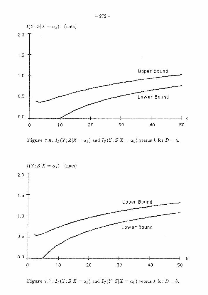
2

1.0

0

0.0

2.0

1.5

1.0

0.5

I(Y; ZIX = ak) (nats)

Upper Bound

Lower Bound

0 10 20 30 40

Figure 7.6. h(Y; ZIX = ak) and Iu(Y; ZIX = ak) versus k for D = 4.


Upper Bound

Lower Bound

k 50

0.0 -r--~---~~-t-~~~~+-~~~~1--~~~--1r--~~~--; k 0 10 20 30 40 50

1.1. (Y;ZIX =a,.) and Iu(Y;ZIX =a;.) versus k for D = 8.

; ZIX = ak) (nats)

2

Upper Bound

1.0

Lower Bound

0.5

0.0 +-~J--~~+-~~~~t---~~~--jt--~~~--1~~~~--j k 0 1 0 20 30 40 so

Figure 7.8. h(Y;ZIX = ak) and Iu(Y;ZIX = ak) versus k for D = 10.


2.0

Lower Bound 1.5 -------· 1.0

Upper Bound

0.0..,._..--~~~+-~~~~--~~~___,i--~~~~~~~~--< k 50 0 1 0 20 30 40

7.9. (Y; IX= ak) and Iu(Y;ZIX = ak) versus k for D - 20.

I(Y; ZIX = cq) (nats)

0

1.5

1.0

0.5

0 1 0 20 30

Upper ~B o:_u...:.n:.;.d_.-_..--

Lower Bound

40 k

50

Figure 1.10. h(Y;ZIX = a,1;) and Iu(Y;ZIX = a.1;) versus k for D = 50.

I(Y; ZIX = a.d ( nats)

2.0

Lower Bound

1.5

1.0 Upper Bound

0.5

O.O-f--"...__~~~+-~~~~-1--~~~~1--~~~--1~~~~--l k 0 1 0 20 30 40 so

1. (Y;ZIX = a.1;) and Iu(Y;ZIX = a.1;) versus k for D = 100.

- 275

Table 7-2: Minimum Required Mutual Information for Classification into One of J Equiprobable Classes.

J Required Imin(Y; Z) ( nats)

2 0.6931 3 1.0986 4 1.3863 5 1.6094

eration. This corresponds to the results of our analysis of the information content

of radar images, which shows that the information content of a single pixel is small.

In addition, as a result of the analysis in Section 7.1, we know that the information

contained in a group of pixels is less than or equal to (and most often much less

than) the sum of the individual, mutual informations conveyed individually by the

pixels. As a result, the classification and characterization of image regions by either

human or machine will generally have to be done on an extensive region of pixels,

with the extent of the region growing as the number of classes involved increases.

- 276 -

er 1

Eq. (7.48).

(7.48) states that for k = 1,

Ei(x) is 'p.93] $

J e" Ei(x)= -;;da.

-oo

order to see that this is true, we note from Eq. (7.47) that for k = 1,

/J2 - 1

/( Ix = ) = J z exp(-y/z) d y ai (/32-/31) z.

fJ 1

Making the change of variable z = l/w, Eq. (A-7.2) becomes

1/fJ2

!(IX= )=- J wexp(-yw) dw y ai (/32 - /31) w2

1 / fJ l

1/fJ1 = J exp (-yw) dw.

w(/32 - /31) 1/fJ2

Now by a change of variable in Eq. (A-7.1), we have

ls eb"

--;;- da - Ei(bx). -oo

Applying the relation given by Eq. (A-7.4) to Eq. (A-7.3), we get

1 / fJ l 1 J exp -y

/(ylX = a1) = (/32 _ /31) w dw

1/fJ2

1 11//Ji = (/3 _ /3 ) Ei( -yw)

2 l 1//Ja

= [Ei(-y//31)- Ei(-y//32)]. /32 - /31

(7.48)

(A-7.1)

(A-7.2)

(A-7.3)

(A-7.4)

(A-7.5)

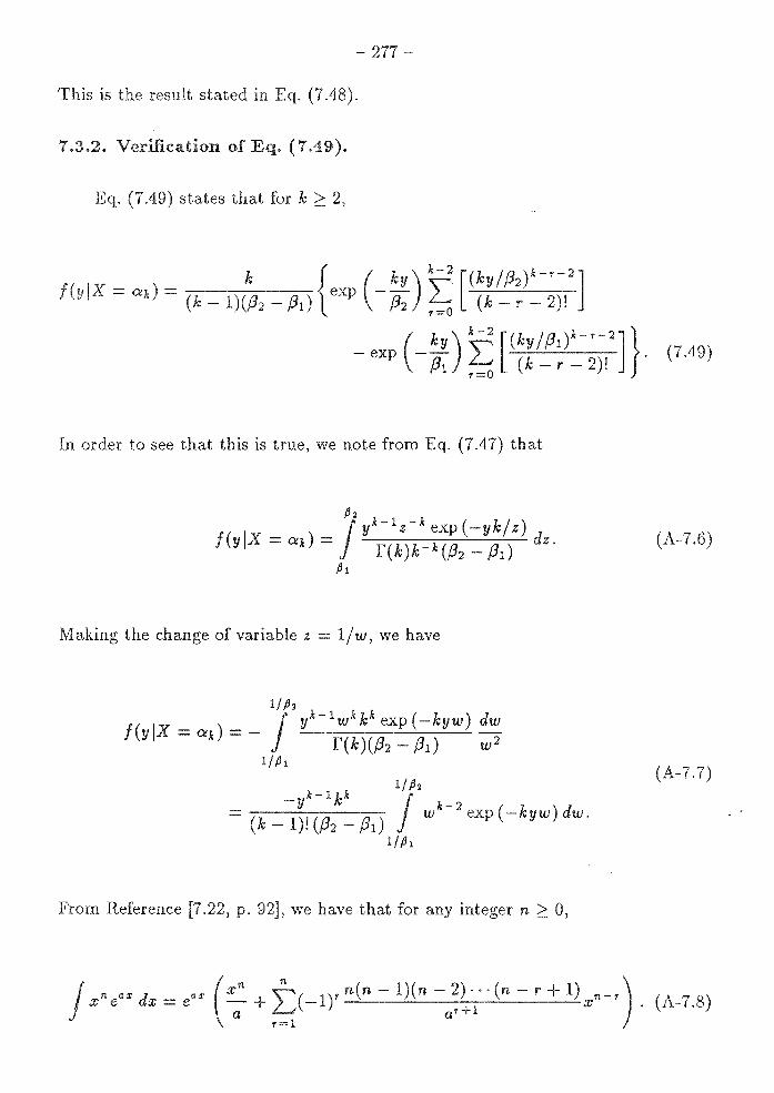
- 277

(7.49) states that k ~ 2,

k { ( ky) k-2

[(kyjfJ2)k-r-2] - a.1;) - exp --- - (k - l)(/32 - /Ji) /32 r=O (k - r - 2)!

_ (- ky) k.-2

[(ky//Ji)'"-r-2]} exp /31 ~ (k - r - 2)! ·

(7.49)

order to see that this is true, we note from Eq. (7.47) that

fi 2

J y k - 1 z - k exp ( -y k / z) f(y!X=a,1;)= f(k)k-"(/32-/Ji) dz. (A-7.6)

fi l

Making the change of variable z = l/w, we have

(A-7.7)

From Reference [7.22, p. 92], we have that for any integer n ~ 0,

J x"e" dx = e" ( x: + ,:, !)' n(n - l)(n -a:~·,·. (n - r + 1) ,,,•-•) . (A-7.8)

- 278

for k 2:: 2, (A-7.7) can be as

k-l(k

f(ylX = ak) = (k- l)!(/J2

-Pi) exp(-kyw)

x wk-2 k-2 l + -1 r -'---------'-Wk - r - 2

r=l

yk-lkk

(/J2 - P1 exp ( -kyw)

[

wk -2 ~ ( k - 2) · · · ( k - r - 1) k - 7 - 2]

X -k- + L.J (k )r+l W Y r=l Y

k-lkk [ k-2 k-2 k-r-2 l l/fi 2

= (k - ~)(!J2 - Pi) exp (-kyw) ky~k - 2)! + ~1 (ky)r+~(k - r - 2)! , i I fJ i

k - i kk [k -2 k - r - 2 l 1IfJ 2

= (k - ~)(fi2 - fii) exp (-kyw) Lr=O (ky)r+~(k - r - 2)! i I fJ i

k [,1; - 2 ( k y w) k - r - 2 l 1IfJ2

= (k - l)(fi2 - Pi) exp (-kyw) ~ (k - r - 2)! r-0 1/ /J1

k { ( ky) k- 2 [(ky/IJ2)k-r-2]

= (k - l)(P2 - Pi) exp - P2 ~ (k r 2)!

_ (- ky) ~ [(ky//Ji)k-r-2]} exp P1 ~ (k r 2)! ·

(A-7.9)

This is the result stated Eq. (7.49).

- 279

( ).

Eq. (7.54) states that

[

k-1 l = ln r ( k) - ln k + k - ( k - 1) ~ ~ - 'Y

1 f3 f3 [/32 ln /32 - /31 In /31 - /32 + f3i] ·

2 - 1

(7.54)

Here r is Euler's constant ( r = 0.577 ... ). In order to verify that Eq. (7.54) is true,

we note that

/J2 OQ

ff yk-lz-k exp(-yk/z) [yk-lz-k exp(-yk/z)] h(YIZ,X=ak)=- f(k)k-k(f3

2-f3i) ln f(k)k,. dydz

/31 0

/J2 OQ __ f f y k - l z - k exp ( y k / z) { ( k - 1) ln y - k In z } d dz - f(k)k-k(f32 -f3i) yk/z-lnf(k)+klnk y

fJ 1 0

/J2 OQ

f f y k - 1 z - k exp ( -y k / z) = lnf(k)-klnk- f(k)k-k(/3

2 -/3i) (k- l)lnydydz

fJ l 0

(A-7.10)

As we can see from Eq. (A-7.10), we must evaluate three integrals in order to

- 280

obtain Eq. (7.54) of these is evaluated as follows:

y dy

0

(A-7.11)

From [7.22, §4.352.2], we have that forµ> 0

00

J 11 -p.!;!;l d n! [ 1 1 1 1 ] x e nx x=-- 1+-+-+···+--r- nµ. µ 11 +1 2 3 n

(A-7.12)

0

Here 'Y is Euler's constant. Applying this result to Eq. (A-7.11), we have

fi2 k 00

(k 1) J z- J k-1 [ (k) ] = (/32

/Ji)f(k) k-k y exp - -; y lny dy dz fl l 0

= (/32 = f3

1J {~; -'Y - Ink+ lnz} dz

fi1 r-1

= ( k - 1) [~ ; - 'Y - In k] + (/32 = /3

1) Jin z dz

[~ ; - 'Y - Ink] + (/32 = /31) [ z In { -1 dz]

= (k - 1) [~ ;- 'Y - k] + (/32 = /3l) [/32 ln/32 {31 ln/31 - /32 + /31]

(A-7.13)

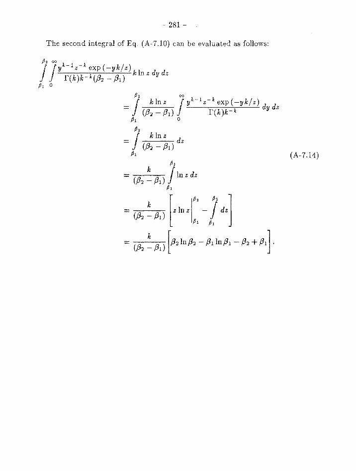
281 -

The second integral of Eq. (A-7.10) can be evaluated as follows:

fi2 00 = J klnz J yk-lz-k exp(-yk/z) d d

(/32 - /31) f(k )k-k y z fi1 0

fi 2

= J k lnz dz (/32 - /3i)

fi l (A-7.14)

= (/32

: /3i) [z lnz p, - J dz] fi1 fi1

= (f3, : /31) ~'In /32 - /31 ln /31 - /32 + /31] .

- 282

third integral of Eq. 10) can be evaluated as follows:

/32 00

J k J y k z - k exp -y k ------dydz

- z(/32 - j3i) f(k)k-/31 0

- J/32 k [Joo w" exp (-w) . z dw] dz - z(/32-/31) r(k) k

/31 0

/32 00 (A-7 .15)

= j (j32 -j3~)kf(k)J w"exp( w)dwdz /31 0

j3 2

= J (/32 - /31~f(k + 1) . r(k + 1) dz /31

Substituting the results of Eqs. (A-7.13), (A-7.14), and (A-7.15) into

Eq.(A-7.10), we have

This is the result stated Eq. (7.54).

283 -

er 1

1 C., of Remote Sensing, John Wiley and Sons,

New , NY, 1987.

7.2 Mensa, L., Resolution Radar Artech House, Dedham, MA,

1981.

7.3 Ullaby, F. , R. K. Moore, and A. K. Fung, !v.Ucrowave Remote Sensing, vol.

2, Addison-Wesley, Reading, MA, 1982.

7.4 Stimson, G. W., Introduction to Airborne Radar, Hughes Aircraft Company,


7.5 Harger, R. 0., Synthetic Aperture Radar Systems, Theory and Design, Aca

demic Press, New York, NY, 1970.

7.6 Hovanessian, S. A., Introduction to Synthetic Array and Imaging Radars,

Artech House, Dedham, MA, 1980.

7.7 Ullaby, F. , R. K. Moore, and K. Fung, !v.Ucrowave Remote Sensing, vol.

3, Artech House, Dedham, MA, 1986.

7 .8 Pierce, J. R. C. Posner, Introduction to Communication Science and


7.9 Feller, W., An Introduction to Probability Theory and Its Applications, 3d. ed.,

John Wiley and Sons, New York, NY, 1968.

- 284 -


27, 1948. 379-423, 623-656. Reprinted in C. E. Shannon and W.W. Weaver,

Univ. Ill. Press, Urbana, IL,

1949.

7.11 McEliece, R. J ., The Theory of Information. Coding, Addison-\'Vesley,

Reading, MA, 1977.

7.12 Pratt, W. K., Digital Image Processing, John Wiley and Sons, New York, NY,

1978.

7.13 Long, M. W., Radar Reflectivity of Land and Sea, Artech House, Dedham,

MA, 1983.

7.14 Duda, R. 0. and P. E. Hart, Pattern Classification. and Scene Analysis, John

Wiley and Sons, New York, NY, 1973.

7.15 Schreiber, W. F., "The Measurement of Third Order Probability Distributions

of Television Signals," IRE Trans. Inf. Theory, IT-2, 3, September 1956, 94-

105.

7.16 Frost, V. S. and S. Shanmugan, "The Information Content of Synthetic

Aperture Radar Images of Terrain," IEEE Trans. on. Aero. and Elec. Systems,

19, 5, 1983, 768-74.

7.17 Hogg, v. Craig, duction to Mathematical Statistics, Macmil-

Ian, New York, NY, 1970.

18 Manoukian, E. B., Modern Concepts and Theorems of Mathematical Statistics,

Springer-Verlag, New York, NY, 1986.

285 -

7. Speckle and Ph.e.nomenon, 2d. ed., ed. J. C. Dainty, Springer-

Verlag, New York, NY, 1984.

7.20 N. J. Pierce, "Detection of gratings and small features in

images corrupted by speckle," Applied Optics, Vol. 20, No. 2, January, 1981,

312-19.

7 .21 Korwar, N. and J. R. Pierce, "Discrimination of form in images corrupted

by speckle," Applied Optics, Vol. 20, No. 2, January, 1981, 320-25.

7.22 Gradshteyn, I. S., and I. M. Ryzhik, Table of Integrals, Series, and Products,

corrected and enlarged ed., Academic Press, New York, NY, 1980.

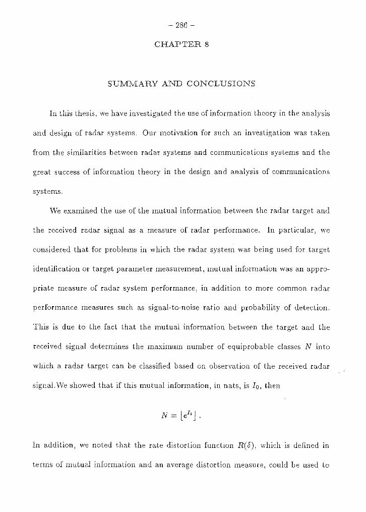
- 286 -

8

ONCLUSIONS

this thesis, we have investigated the use of information theory in the analysis

and design of radar systems. Our motivation for such an investigation was taken

from the similarities between radar systems and communications systems and the

great success of information theory in the design and analysis of communications

systems.

We examined the use of the mutual information between the radar target and

the received radar signal as a measure of radar performance. In particular, we

considered that for problems in which the radar system was being used for target

identification or target parameter measurement, mutual information was an appro

priate measure of radar system performance, in addition to more common radar

performance measures such as signal-to-noise ratio and probability of detection.

This is due to the fact that the mutual information between the target and the

received signal determines the maximum number of equiprobable classes N into

which a radar target can be classified based on observation of the received radar

signal.We showed that if this mutual information, in nats, is 10 , then

In addition, we noted that the rate distortion function R( 5), which is defined in

terms of mutual information and an average distortion measure, could be used to

287 -

determine the minimum required mutual information between the target and the

received radar waveform in order to obtain an average error or distortion less than

some specified value 8 in the radar measurement.

We then defined and solved the Radar/Information. Theory Problem, which

gave us a mathematical framework for the problem of waveform design for maxi

mizing the mutual information between the target and the received radar waveform.

Specifically, we looked at the problem of finding a distribution on an ensemble of

transmitted waveforms that maximized the mutual information between the target

and the received waveform. vVe solved the Radar/Information Theory Problem for a

number of general target types, both discrete and continuous. vVe also showed that

a deterministic solution also exists; that is, that from the family of distributions

of transmitted waveforms which maximize the mutual information between target

and received signal, there is a distribution that corresponds to sending a waveform

or sequence of waveforms with certainty.

Next, we examined statistical electromagnetic scattering models that would

allow us to apply the results of the Radar/Information Theory Problem to practical

radar problems. We also introduced the notion of target impulse response as a

description of linear time-invariant electromagnetic scattering.

Chap 5, we digressed from our information-theoretic analysis of radar

systems to apply the target impulse response to the problem of designing realizable

waveform/receiver .filter pairs that maximize the signal-to-noise ratio at the receiver

output when a target is present under contstraints on bandwidth and waveform

- 288 -

energy. new result is an extension of North's matched filter, which provides

the maximum signal-to-noise ratio for point targets but not for extended targets.

The resulting waveform/ receiver-filter pair allows for optimal detection of time-

invariant, extended targets additive noise of arbitrary power spectral density. vVe

developed the following procedure for designing a waveform/receiver-filter pair for

a target of known impulse response h(i) in the presence of additive noise with noise

power spectral density Snn (!), given the energy constraint that the total energy in

the transmitted signal is £ and the constraint that the waveform is confined to the

time interval [-T/2,T/2]:

1. Compute 00

H(f) = j h(i)e- i'2'K" ft di.

-oo

Here, h(i) is the impulse response of the target and H(f) its Fourier trans-

form.

2. Compute

-oo

Here, SnnU) is the two-sided power spectral density of the noise n(i), and

L(i) is inverse Fourier transform of jH(/)12 / Snn (/).

3. Solve for an eigenfunction x(t) corresponding to the maximum eigenvalue

Amax of the integral equation

T/'2

,\maxi(i)= j x(r)L(i-r)dr.

-T/'2

289

Scale x(t) so that it has energy £. This is the optimum radar detection

waveform.

4. Compute the spectrum X (f) corresponding to the optimum waveform x( t):

00

X(f) = j i(~)e-i2'K"ft d-t.

-oo

Implement a receiver filter of the form

KX(f)H(f )e-i"2'K" fto

R(f) = Snn (f) '

where K is any convenient complex constant and to is the time at which

the receiver output is observed.

6. The resulting signal-to-noise ratio for this design, which is the maximum

obtainable under the specified constraints, is

vVe noted that a waveform designed using this procedure in the presence of

additive white noise puts as much of the energy as is possible into the mode of the

target having the greatest response (largest eigenvalue). In the case of non-white

noise, this solution takes into account the relative strength of the noise components

in each mode and weights the distribution of energy among the target modes in

order to obtain the largest signal-to-noise ratio.

Next, we addressed the problem of designing radar waveforms that provide

maximum mutual information between a random target and the received radar

waveform in the presence of additive Gaussian noise of arbitrary power spectral

- 290

density. This was done by extending the concept of target impulse response to

include random scattering. Random scattering was incorporated by considering

finite-energy, random processes as random impulse responses and using them to

describe the response from random scatterers. \Ve then considered the case of

targets described by the finite-energy, Gaussian, random process g(i) with Fourier

transform G(f) having spectral variance <J"b (!). We showed that the waveforms x(i)

that have energy & and that maximize the mutual information l(y(i); g(i)Jx(t)) with

bandwidth concentrated in a frequency interval Wand a time interval [-T /2, T /2]

have a magnitude-squared spectrum

I 12 [ Pnn (/)Tl

X(f) =max O, A - 2<J"b(f) .

Here, T is the receiver observation time, which for most waveforms of interest

satisfies T ~ T; P1111 is the one-sided power spectral density of the additive Gaussian

noise; and A is a constant found by solving the following relation for A:

J [ Pnn(/)Tl £ = max 0, A - 2(jb (!) df.

w

resulting maximum mutual information lmax(y(i); g(i)lx(-t)) was found to be

Im=(y(i);g(i)lx(i)) = T j max [a, In A - In ( ~:mn l df. w

We the case of additive white Gaussian noise, these waveforms, in

contrast to the waveforms of Chapter 5 for optimal detection, which attempt to put

as much energy as possible into the largest target mode, distribute energy among

the target modes order to maximize the mutual information between the target

- 291

and the received signal. It is not surprising, then, that the form of the solution is

different from that for optimal detection, as modes besides the largest may carry

significant information about the target.

allotted to them for their measurement.

a result, we would expect energy to be

Finally, we examined some information-theoretic characteristics of radar im-

ages. vVe did by considering the general information-theoretic properties

of images in general and radar images in particular, and then examining the infor

mation per pixel of a radar image resulting from homogeneous diffuse terrain. vVe

saw that on a per-pixel basis, a very small amount of information is provided in

radar-imaging measurements for such a surface. As a result, we noted that multiple

pixel regions have to be examined in order to classify or characterize such a surface

based on its radar measurement. This was noted to be in agreement with heuristic

results on surface characterization based on radar images.

Documents

INFORMATION THEORY AND RADAR: MUTUAL INFORMATION …