Embed Size (px)
Citation preview

INFORMATION TO USERS
This manuscript has been reproduced tram the microfilm master. UMI films
the text directly trom the original or copy submitted. Thus, some thesis and
dissertation copies are in typewriter face, while others may be from any type of
computer printer.
The quality of this reproduction is dependent upon the quallty of the
cOPY submitted. Broken or indistinct print, corored or poor quality illustrations
and photographs, print bleedthrough, substandard margins, and improper
alignment can adversely affect reproduction.
ln the unlikely event that the author did not send UMI a complete manuscript
and there are missing pages, these will be noted. Also, if unauthorized
copyright material had ta be removed, a note will indicate the deletion.
Oversize materials (e.g., maps, drawings, charts) are reproduced by
sectioning the original, beginning al the upper left-hand corner and continuing
trom left to right in equal sections with smalt overtaps.
ProQuest Information and Leaming300 North Zeeb Road, Ann Arbor, MI 48106-1346 USA
800-521-0600


•
•
Desalination by membrane distillation
a comparative study oftubular and ho/lowfibremembrane units
byLudovic Plasse
Department of Chemical EngineeringMcGill University, Montreal
November, 2000
A thesis submitted to the Faculty of Graduate Studies and Research in partial fulfilmentof the requirements of the degree ofMaster ofEngineering
© Ludovic Plasse, 2000

1+1 National UbrarYof Canada
~uisitions andBibliographie Services
385 W"'tgIDn StrNtoea-ON K1A~
canIdI
BibüothèQue nationaledu Canada
Acquisitions etservices bibliographiques
385. fUI welingtanoaa.ON K1A0N4c..da
The author bas granted a nonexclusive licence allowing theNational Library ofCanada toreproduce, loan, distnbute or seUcopies of this thesis in microfonn,paper or electronic formats.
The author retains ownership ofthecopyright in tbis thesis. Neither thethesis Dor substantial extracts from itmay he printed or otherwisereproduced without the autbor'spermission.
0-612-70249-9
Canad~
L'auteur a accordé une licence nonexclusive pennettant à laBibliothèque nationale du Canada dereproduire, prêter, distribuer ouvendre des copies de cette thèse sousla forme de microfiche/film, dereproduction sur papier ou sur formatélectronique.
L'auteur consenre la propriété dudroit d'autem qui protège cette thèse.Ni la thèse ni des extraits substantielsde celle-ci ne doivent être imprimésou autrement reproduits sans sonautorisation.

•
•
,?i lIN!4~ - 'PflIU!AÛ" à HIe4 'PtVIbIÛ et à HU!4 *;tM

•
•
Abstract
Membrane distillation was considered as an alternative to traditional desalination
proeesses because this technique produces ultra-pure water without requiring high
temperatures nor high pressures.
The driving force of membrane distillation is a temperature difference aeross a
microporous membrane leading to a vapour pressure gradient. Hydrophobie membranes
are used for membrane distillation in order to permit the passage of vapours through the
pores while preventing the liquid phase trom passing.
The thickness of the membrane is a key variable which affects heat and mass
transfers between the warm feed side and cooling side. In this thesis, a module with thin
walled hollow fibres was compared to a module with thicker tubular membranes. The
permeate flux produced was compared at different operating conditions. Feed and
cooling water flow rates and temperatures were varied. The impact of salt concentration
in the feed was also examined.
Different models based on first principles were developed and compared to a
semi-empirical model based on the experimental determination of the mass transfer
coefficient. Their predictions were compared with experimentally obtained permeate
fluxes .

•
•
Résumé
La distillation membranaire est une possible alternative aux méthodes classiques de
dessalement car elle permet de produire une eau extrêmement pure sans avoir recours à
des températures ou à des pressions élevées.
Le principe de la distillation membranaire repose sur l'établissement d'une
différence de température entre les deux faces d'une membrane microporeuse créant
ainsi un gradient de pression de vapeur. Les membranes hydrophobes utilisées permettent
alors le passage de vapeurs au travers des pores mais empêchent tout liquide de traverser.
L'épaisseur de la membrane est un paramètre clef affectant les transferts de masse et
de châleur entre les côtés chaud et froid. Dans cette thèse, un module composé de fines
fibres creuses a été comparé à un module composé de tubes creux plus épais. Les flux de
perméat ont été comparé pour différentes conditions opératoires en variant les
températures et les débits des eaux d'alimentation et de refroidissement. L'impact de la
concentration en sels dans l'eau d'alimentation a de même été examiné.
Différents modèles basés sur les premiers principes ont été developpés et comparés à
un modèle semi-empirique basé sur la détermination expérimentale du coefficient de
transfert de masse. Leurs prédictions ont été comparées avec les résultats expérimentaux
obtenus pour les flux de perméat.
ii

•
•
Acknowledgements
1would like ta express my gratitude ta my supervisor Professor Jana Simandl for her
guidance and support. 1 greatly appreciated her suggestions throughout the research.
Thank you very much Professor Simandl.
The financial support of the Max Stern Scholarship was gratefully appreciated and
gave me the chance to do this research.
Thanks to my research group and to the staff of the Chemical Engineering
Department. Lou Cusmich for his computer and data acquisition assistance, Alain
Gagnon and Frank Caporuscio for their technical assistance. Frank, your advises and help
were greatly appreciated. In the future, 1might support the Italian soccer team ~
Hi

• Table of contents
AM~ad i------------------------------Résumé ;;
Acknowledgements i;;
Table ofcontents ivListoffigures, v
List oftables vi
Nomenclature vii---------------------------1
22.12.22.3
33.13.23.3
44.14.24.3
4.3.14.3.24.3.34.3.4
4.4
In~oduction 1-----------------------Literature review 2Membrane distillation 2Membrane distillation for desalination 5Membrane distillation for applications other than desalination 6
Model/ing 9Semi-empirical approach 10Computer Modelling 14Theoretica1 detennination of the membrane mass transfer coefficient 16
Experimental apparatus andprocedure 22Membrane modules 22Description of the apparatus 22Data acquisition system 28Transducers and signal conditioner 28Analog expansion chassis 30Analog to Digital Converter (ADC) 30Data acquisition software 30Experimental procedure 32
•
5 Results and discussion 335.1 Membrane wetting 335.2 Tubular unit 355.3 Comparative study of the tubular and hollow fibre units 39
5.3.1 Effect of the temperature 395.3.2 Etrect of the feed tlow rate ~3
5.3.3 Etrect of the cooling tlow rate ~6
5.3.4 Effect of the salt concentration 505.3.5 Economical considerations and comparison ofhighest penneate tluxes achieved by the
hollow fibre and tubular membrane units 525.4 Comparison of the semi-empirical and theoretical models 53
6 Conclusions and recommendations 56
7 References 58
~~6A ~
Appendix B 76
Appendix C 82
iv

•
•
List of figures
Figure 2. J : Different configurationsfor membrane distillation 4Figure 2.2 : Direct contact membrane distillation 5Figure 3. J : Temperature and concentration polarisation loyers 10Figure 3.2 : Screen capture ofthe interface 15Figure 3.3 : Division ofa membrane module in n segments 16Figure 4.1 : Tubular module 24Figure 4.2 : Hollow fibre module 25Figure 4.3 : Schematic ofapparatus 26Figure 4.4 : Schematic representation ofthe data acquisition system 29Figure 4.5 : Screen capture ofthe Daqview 7.0 interface 31Figure 5.1 : Wetting pressure determination experiment 34Figure 5.2 : Evaluation ofthe tubular membrane mass transfer coefficient 36Figure 5.3 : Experimental andpredictedpermeate fluxes 38Figure 5.4 : Vapour pressure ofpure water by Antoine 's equation 40Figure 5.5 : Semi-empirical modelpredictions ofthe permeate flux 41Figure 5.6 : Semi-empirical modelpredictionsfor the ho/lowfibre unit permeateflux _42Figure 5.7 : Semi-empirical mode/predictionsfor the luhular IIllit permeale flux__42Figure 5.8 : Experimental permeate fluxes at different Reynolds lnlmbers on Ihe feed
~~ 44Figure 5.9 : Feedflow rate influence onlhe membrane mass transfer coefficient__45Figure 5.10 : Tubular unit cross sections: a) three-tubes b) forty one-tubes 47Figure 5.11 : Hoi/ow fibre unit cross section 47Figure 5. /2 : Experimenta/ permeale fluxes at different Reynolds 11umbers on the
coo/ing side 48Figure 5. /3 : Influence ofthe cooling side flow raie 011 Ihe membrane mass Irallsfer
coefficienl in the ho/lowfibre unit 49Figure 5.14 : Permeate flux wilh disti//ed waler and a 3.4 wl. % NaCIfeed solulions _50Figure 5.15 : Permeale flow raIe, experimenla/ vailles and mode/ predictionsfor a
3.4 wt. ~1i NaC/ solution 51
v

•
•
List of tables
Table 4. J : Membrane unit characteristics 23---------------Table 4.2 : List ofthe apparatus 27Table 5. J : Experimental andpredictedfluxes 37Table 5.2 : Peiformances and experimental conditions comparison. 53Table 5.3 : Predictions ofthe semi-empirical and theoretical models 55
vi

• Nomenclature
Symbols
•
C Membrane mass transfercoefficient
c Molecular concentrationd diameterD Diffusion coefficientJ Mass flux ofpermeateK Mass transfer coefficientk Thermal conductivityM Molecular massN Molar flux ofpermeaten Number of segments in modelP PressureP' PressureQ Heat transferr RadiusT Temperaturev Atomic diffusion volumex Mole fractionz Direction of the flow
Greek Letters
Ô Thicknessg Porosity of the membraneÂ. Mean free pathJ.1 Viscosityp Densityt Tortuosity of the membrane\JI Latent heat ofvaporisationç Polarisation coefficient
Subscripts
A AirA1 Air at the entrance of
the poreA2 Air at the exit of
the porebl Feed bulkb2 Cooling water bulkbs Salt in the bulk feedc Conductiveg Gas phaseh Hydraulicm Membraneml Feed side membrane surfacem2 Cooling side membrane surfacems Salt at the membrane surfacep Polarisation layers Saltsolid Solid phasev Vapourvapo. VaporisationW Water vapourW1 Water vapour at the entrance of
the poreW2 Water vapour at the exit of
the pore
Dimensionless Numbers
Kn Knudsen NumberNu Nusselt NumberPr Prandl NumberRe Reynolds NumberSc Schmidt Number
vii

•
•
1 Introduction
Distillation/evaporation and reverse osmosis are the two major techniques currently
used for sea water desalination. These processes are expensive because of important heat
and pressure requirements. Membrane distillation may prove to be a viable alternative.
While establishing the feasibility of membrane distillation at McGill University's
Chemical Engineering Department, flat sheets and tubular membranes were used for the
production of fresh water from sea water and for the purification of water contaminated
by volatile organic compounds such as benzene, ethanol and acetone [1-3].
One of the key parameters in membrane distillation is the thickness of the
membrane. A thicker membrane slows down both heat transfer, which is an advantage,
and also mass transfer, which is obviously a disadvantage for the process. Globally, the
impact on mass transfer is expected to supersede that on the heat transfer. Thus, thin
flat-sheet membranes have an advantage over thicker tubular units. Unfortunately, it is
difficult to scale-up flat sheet membranes. A third alternative, and the purpose of this
thesis, is to use hollow fibre membranes which combine the advantages of both, a small
membrane thickness (three times thinner than the tubular membranes) and a scale-up
capability. It was expected that the flux per unit area would increase dramatically with
hollow fibre membranes compared to tubular ones.
A Iiterature review of membrane distillation and its application to desalination and to
other separation and concentration processes is presented in chapter 2. Semi-empirical
and theoretical models are developed in chapter 3. The description of the apparatus and
of the experimental procedure follows in chapter 4. The experimental results are
discussed in chapter 5. In chapter 6, conclusions are drawn and recommendations made.

•
•
Chapter 2 : Literature review
2 Literature review
2.1 Membrane distillation
Membrane distillation is a membrane process whose selectivity is based upon vapour
pressure ditferenees. The proeess was first studied in the sixties [4] and provides an
interesting alternative to other desalination proeesses sueh as reverse osmosis and
distillation/evaporation. Membrane fouling is less important in membrane distillation
than for eonventional membrane proeesses and an almast perfeet rejection of ions,
maeromoleeules, eolloids, eells and other non-volatile eomponents is aehieved.
Moreover, the operating temperatures (30 to 90°C) and pressures (atmospherie ta a few
hundreds kPa) result in 10wer costs with the possible exception of vacuum membrane
distillation [5].
Capillary distillation and trans-membrane distillation are different terms used to
designate membrane distillation. Since 1986 and the "Workshop on Membrane
Distillation" in Rome, the process has been detined as one which should exhibit the
following charaeteristics :
~ The membrane should be porous,
~ The membrane should not be wetted by the proeess liquids,
~ No capillary condensation should take place inside the pores of the membrane,
~ The membrane should not alter the liquid-vapour equilibrium of the different
eomponents in the process liquids,
» At least one side of the membrane should he in direct contact with the process
liquid.
The driving force of membrane distillation is the vapour pressure differenee across
the hydrophobie porous membrane whose surfaces are held at different temperatures. The
2

•
•
Chapter 2 : Literature review
liquid water phase cannot pass through the hydrophobie membrane whereas water
vapours cano The volatile components (water in desalination) diffuse from the warmer
side (feed side), to the cooler side (perrneate side), and condense. The limitation of the
process is the risk of membrane wetting. This places a limit on the upper concentration of
any surface active components permitted within the feed.
Four different configurations can be used for membrane distillation (Figure 2.1) :
direct contact membrane distillation, air gap membrane distillation, vacuum membrane
distillation and sweep gas membrane distillation [1-3,5,6]. In air gap, sweep gas and
vacuum membrane distillation, the cooling surface is separated from the membrane by,
respectively, an air gap, an inert gas which collects the vapours or a vacuum which draws
out the vapours from the permeate side [1-3,5,6]. In direct contact membrane distillation,
a cooling liquid is in contact with the membrane surface and the vapours which pass
through the pores condense within il. The operation is simple and it requires the least
equipment [5]. This configuration is the one used throughout ail the experiments
performed as part ofthis thesis.
3

•
•
Chapter 2 : Literature review
r Membrane
·t t ···n ··g. · en· ~Q. ·! · src = ·.s .s · '0= · ~:; C'. '; ··i 0 i=~
~ ~+
Direct contact Sweep gas membranemembrane distiUation distillation
t tAir 8
~~= gap = (")
.s .s =:; en ... c:"0 = a
~ ----. -0 ~u
~ ~ ··· +········Air gap membrane Vacuum membrane
distillation distillation
Figure 2.1 : Different configurations for membrane distillation [5]
4

•Chapter 2 : Literature review
2.2 Membrane distillation for desalination
Because of the very high quality of the water produced by membrane distillation, a
possible application of this process is the production of drinking water from sea water.
Direct contact membrane distillation is the most appropriate configuration for
desalination (5] and was used for the experiments (Figure 2.2).
- ---- ,
iWann feed tlow
(sea water)
Porousmembrane
,,-- Passage of vapour-JE2]==:E:::::!....:>~ through pore
OCooling liquid + condensed penneate
(fresh salt-tfee water)--- lr1
•
_ _ _ • Temperature profile
Figure 2.2 : Direct contact membrane distillation
Fawzi Banat [1] studied desalination by air gap membrane distillation with flat sheet
membranes while Stéphanie Lacoursière [2] and Praveen Ram Menta Prasanna [3]
investigated the effects of different factors on direct contact membrane distillation. First,
Banat [1] and Lacoursière [2] observed that the salt concentration has little effect on the
penneate flux up to five percent by weight salt. Secondly, aIl three observed that
increasing the feed flow rate in the laminar region increased the permeate flux because of
the reduction in temperature and concentration polarisation. Once turbulent flow was
established, changes in permeate flux were negligible. Thirdly, the temperature
difference between the feed side and the permeate side had an important effect on the
penneate flux : flux increased with an increase in temperature difference. And lastly,
they noted that the temperature of the feed side had a large effect on the penneate flux.
s

•
•
Chapter 2 : Literature review
The higher the feed side temperature is, the higher the flux. Two similar semi-empirical
models for heat and mass transfer were proposed by Lacoursière [2] and Prasanna [3] and
will be used in this work.
2.3 Membrane distillation for applications other than desalination
Membrane distillation could be useful in different industrial processes but most of
the applications are still at the laboratory scale and have not been evaluated on a larger
scale. One application in the food industry is the concentration of aqueous solutions such
as fruit juices or milk. F. Laganà, G. Barbieri and E. Drioli [7] used direct contact
membrane distillation with polypropylene hollow fibre modules MD-020-2N-CP from
ENKA Microdyn to produce a highly concentrated apple juice (64°Brix). Their results
were good but they did not compare the economics of this technique with traditional
evaporation.
M. Tomaszewska [8] found that direct contact membrane distillation could be
applied for the separation and concentration of fluosilicic acid during the production of
phosphoric acid by a wet process. The module used was a plate and frame module with a
PVDF membrane. A fluosilicic acid distillate, almost free of phosphoric acid, was
obtained at a higher concentration than that of the feed.
Membrane distillation has also a lot of possible environmental applications such as
the concentration of radioactive components in Iiquid low-Ievel radioactive waste. This
was studied by G. Zakrzewska-Trznadel, M. Harasimowicz and A.G. Chmielewski [9]. A
pilot plant with a spiral-wound PTFE membrane of 4m2 distillation area was used. A
distillate production of 0.05 m3/h with a radiochemical puritYofless than 10 Bq/dm3 for
P and y emitters was achieved. Moreover, this process avoided Many problems
encountered in normal evaporation (corrosion, scaling or foaming) or with other
membrane processes (fouling, sorption of radioactive ions, high pressure). A preliminary
economic analysis has shawn that membrane distillation is advantageous for low
capacity plants if waste heat is used.
6

•
•
Chapter 2 : Literature review
Another environmentaJ application is the processing of Iiquid photographie waste.
K.B. Grekovand V.E. Senatorov [la] used direct contact membrane distillation with a
fluoroplastic membrane and found that this process has a high efficiency and is
competitive with other membrane processes such as reverse osmosis. Moreover, a high
degree of concentration couId be achieved without affecting the retention capacity. The
energy requirement to heat the feed is low because of the high temperature of the effluent
(27-43OC).
Membrane distillation could also be applied to the separation of water and glycols.
C. Rincén, lM. Ortiz de Zârate, II. Mengual [11] investigated direct contact membrane
distillation, with three different PTFE flat sheet membranes, as a possible technology for
the concentration of used coolant liquids containing ethylene glycol. A high
concentration (70%) of ethylene glycol could be achieved by using moderate
temperatures and atmospheric pressure. This process could he competitive if waste heat
is used to pre-heat the feed.
M. Gryta and K. Karakulski [12] applied direct contact membrane distillation with a
polypropylene capillary membrane to the concentration of oil-water emulsions. The
authors achieved an almost perfect separation with a feed concentration up to 1000 ppm.
The oil concentration of the feed was maintained below 1000 ppm by removing the oil
phase formed by the emulsion breaking.
A potential application in drinking water treatment is the removal of volatile organic
compounds. N. Couffin, C. Cabassud and V. Lahoussine-Turcaud [13] studied the
removal of halogenated voes (chlorofonn, trichloroethylene, tetrachloroethylene) at a
very low concentration by vacuum membrane distillation with a flat PVDF membrane
from Millipore S.A.. They concluded that the process is an efficient and economical
technology to remove volatile halogenated organic compounds at low concentrations in
drinking water.
7
•
•
Chapter 2 : Literature review
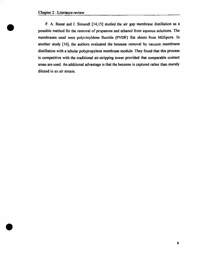
F. A. Banat and 1. Simandl [14,15] studied the air gap membrane distillation as a
possible method for the removal of propanone and ethanol from aqueous solutions. The
membranes used were polyvinyldene fluoride (PVDF) flat sheets from Millipore. In
another study [16], the authors evaluated the benzene removal by vacuum membrane
distillation with a tubular polypropylene membrane module. They found that this process
is competitive with the traditional air-stripping tower provided that comparable contact
areas are used. An additional advantage is that the benzene is captured rather than merely
diluted in an air stream.
8

•Chapter 3 : Modelling
3 Modelling
There have been two approaches taken for the modelling of membrane distillation. A
rigorous one which focuses on the transport mechanisms through the membrane, and a
semi-empirical approach for predicting the permeate flux at given operating
conditions [17]. For both, the general expression of the mass flux J is usually given by
equation (3.0) [2-3,5,6,18,19] :
(3.0)
•
Where PmI and Pm2 are the vapour pressures of the feed side and the cooling side
respectively. C is the mass transfer coefficient which is a strong function of the
membrane used (pore size, porosity, thickness) [18] and of the flow rates on both sides of
the membrane. C could be determined either experimentally (semi-empirical model)
[2,3,8,18,20] or theoretically (Knudsen diffusion, molecular diffusion, Hagen-Poiseuille
viscous flow) [5,6,17]. Both models are of interest; the semi-empirical for the
comparison ofexisting units scale..up and the theoretical for improving the understanding
ofwhat is happening. Both are described in this chapter and used in chapter 5.
In both cases, to predict the penneate flux in membrane distillation, heat and mass
transfer rates should be evaluated. These transfers are inter-related and are extensively
discussed in the literature [5,6,17-22]. The main modelling problem is the appearance of
temperature and concentration polarisation on both sides of the membrane as shown in
Figure 3. 1. The values of the membrane surface temperatures are unknown and depend
upon the estimation of the boundary layer thickness. The semi-empirical models
incorporate the polarisation effects into a membrane constant which is a function of the
flow conditions. The theoretical models strive to predict the polarisation from tirst
principles.
9

Tbl : buIk feed temperatmeTb2 : buIk cooling liquid temperntureTml : membrane surface tempernture.
feed sideTm2 : membrane surface tempernture,
cooling sideXt. : mole fraction salts in buIk fecdXm. : mole fraction salts at membrane
surface
Polarisation layers
Chapter 3 : Modelling
• Membrane
~
r Tbl;.
08·Ci:=a
?; 00 ~=~ Tb2 lXt.
Figure 3.1 : Temperature and concentration polarisation layers
3.1 Se~~en1piricalappnoach
The semi-empirical approach successfully predicted the permeate flux for the tubular
membranes used by Lacoursière [2] and Prasanna [3]. It was the starting point for the
modelling of the hollow fibre membrane in this thesis. Other similar semi-empirical
models were developed in the literature and showed a good correlation with their
respective experimental conditions [5,6,17-21].
•Equation (3.0), expressed previously, gives the mass flux, J, through the membrane
as a function of the membrane mass transfer coefficient, C, and of the vapour pressure
difference.
10

•Chapter 3 : Modelling
The vapour pressure cao be calculated using Antoine's equation:
(3.1.0)
Where Pv is the vapour pressure in Pascal, T is the temperature in Kelvin, and A,B
and 0 are experimental constants. For water, A=3841, B=23.238 and D=-45.
Any decrease in the vapour pressure due to the salt concentration is accounted for by
using Raoult' s law :
p'= (I - X,.). P (3.1.1)
Where P is the vapour pressure of pure water, P' is the vapour pressure of the water
with salt, and Xms is the mole fraction of the salt at the membrane surface.
Since concentration polarisation occurs, the mole fraction of the salt at the
membrane surface is not the same as in the bulk. The salt concentration at the surface of
the membrane could then be calculated using the film model :
Cms =cbs .exP(~JpK~
(J.1.2)
•
Where Cms and Cbs are respectively the salt concentration at the surface of the
membrane and in the bul~ p is the density of the bulk and Ks is the salt mass transfer
coefficient.
11

•Chapter 3 : Modelling
KI could be evaluated by employing the Dittus-Boelter correlation :
(3.1.3)
Where Re is the Reynolds number, Sc is the Schmidt number, DWA is the diffusion
coefficient of water vapour through stagnant air (-2.6*10·s m2/s at 30°C) and dh is the
hydraulic diameter (m).
The diffusion coefficient DWA (m2/s) ofwater vapour in stagnant air is given by the
Fuller and al. equation [23] :
( J1/2
0.01013. rUs. _1_ + _I_D = Mw MA~ ( ~p. V~3 +V~3J
(3.1.4)
•
Where T is the temperature in Kelvin, P the pressure in Pascal, Mw and MA the
molecular masses of water and air, Vw and VA the atomic diffusion volumes (20. 1 for air
and 12.7 for water) [23].
12

•Chapter 3 : Modelling
The temperatures at the surfaces of the membrane (Tml and Tm2) are necessary to
calculate the permeate flux taking into account the temperature polarisation. Evaluating
the heat transfer through the membrane will provide these temperatures. The heat
transfer (Q) is the sum of the conduetive (Qc) and vaporisation (Qvapo.) heat
transfers [2-3,5,6,17,18,20,21] :
Qc =; .. .(T.., - T..,)m
Qvapo. =N· fI/
kQ=Qc + Qvapo = 8m •(Tml - Tm2 )+ N 'If/
m
(1.1.5)
(3.1.6)
(1.1.7)
Where 'V is the latent heat of vaporisation, am is the thickness of the membrane, N
the molecular flux of water through the membrane and km is the thermal conductivity of
the membrane:
(1.1.8)
Where kg and ksolid are the thermal conductivity of the gas phase and of the solid
phase respectively. e is the porosity of the membrane [18].
Q is also equal ta the heat flux through the polarisation layer:
(1.1.9)
•Ôp is the thickness of the polarisation layer and kp is its thermal conductivity.
13
•Chapter 3 : Modelling
Manipulating (3.1.7) and (3.1.9) gives Tml and Tm2 so the vapour pressure at the
surfaces ofthe membrane could be calculated and then the permeate flux.
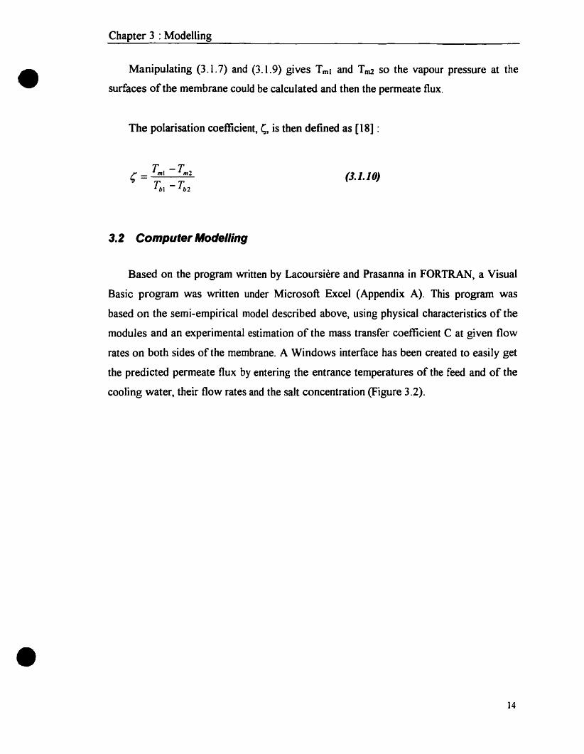
The polarisation coefficient, ç, is then defined as [18] :
(3.1.10)
•
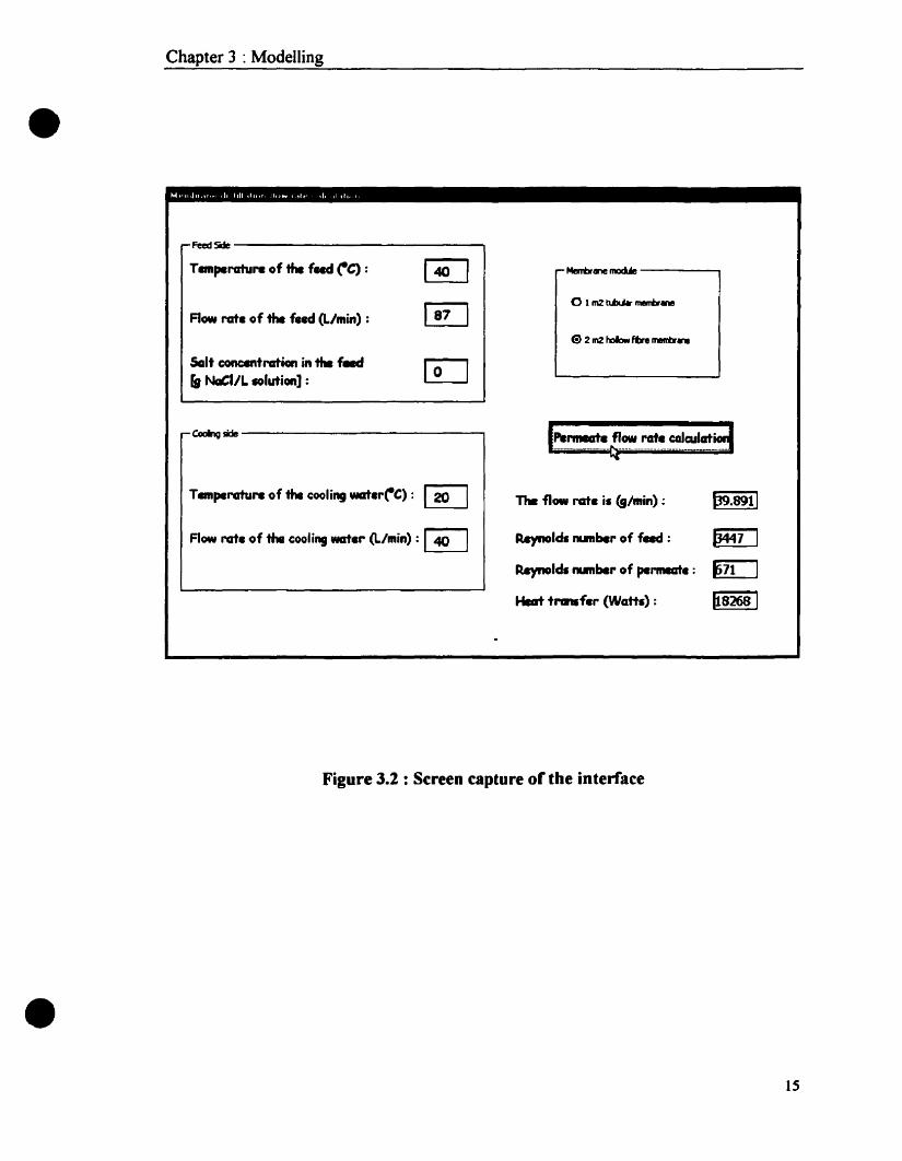
3.2 Computer Modelling
Based on the program WTitten by Lacoursière and Prasanna in FORTRAN, a Visual
Basic program was written under Microsoft Excel (Appendix A). This program was
based on the semi-empirical madel described above, using physical characteristics of the
modules and an experimental estimation of the mass transfer coefficient C al given flow
rates on both sides of the membrane. A Windows interface has been created to easily get
the predicted permeate flux by entering the entrance temperatures of the feed and of the
cooling water, their flow rates and the salt concentration (Figure 3.2).
14
•Chapter 3 : Modelling
FeedSide------------..-,
Flow rat. of ft. f••d (L/min) :
Salt concentration in 1h8 feedr. NaCI/L IOlution] :
o 1 rn2 tIbM-,........
eoœ.gside ------------.....,
T8ftlperature of the cooling watcr('C):~
Flow rat. of the cooling wat.r (L/min) :~
The flow rat. il Cg/min) : ~
Raynoldl numbcr of fad : ~
Raynolds runbcr of pcrrnlGt. : ~
Hart t.,..fcr (Wattl) : hS268 1
•
Figure 3.2 : Screen capture of the interface
IS

•Chapter 3 : Modelling
For the calculations, the module is divided into n segments and the water flux is
computed iteratively for each segment (Figure 3.3). The exit cooling temperature is first
set at twenty degrees celsius and an iteration is then performed to calculate the penneate
flux through the first segment.
The temperatures of the feed and of the cooling water are then calculated for the neX!
segment by assuming that the total heat is transferred from the previous segment. At the
last segment, the calculated cooling water temperature is compared with the actual one. If
the difference is greater than the maximum acceptable difference, the calculation is
repeated from the first segment with an updated entrance cooling water temperature. The
segment permeate fluxes are then added ta give the total permeate flux through the
membrane.
[Î ,: . ; .1 tJ
2 3 n
•
Figure 3.3 : Division of a membrane module in n segments
As will be seen in chapter 5, the predictions of the model compared very weil with
the experimental values for bath distilled water and a saline solution.
3.3 Theoretical determination of the membrane mass transfer coefficient
Based on the mean free path of water molecules, three theoretical approaches are
used in literature ta estimate the membrane mass transfer coefficient C : Knudsen
diffusion, molecular diffusion and Hagen-Poiseuille viscous flow. If the Mean free path
16

•Chapter 3 : Modelling
is very long compared to the pore size, Knudsen diffusion is deemed to happen and the
diffusion takes place by a series of collisions between the water molecules and the
membrane walls. At the opposite extreme, if the mean free path is very short compared to
the pore size, molecular diffusion is deemed to happen by a series of collisions between
the molecules. For very wide pores compared to the Mean free path, Hagen-Poiseuille
relation could be used.
For water, the Mean free path, À., couId be calculated as follow :
(1CRT)1/2
Â. =3.~. SM (3.2.0)
Where Il (pa.s) is the viscosity of the water vapour at a pressure P (pa) and a
temperature T (1<). M is the molecular mass of water (kg.mor l) and R the gas constant
(8.314 lK-1.mor1).
The predominant mechanism is determined by calculating the Knudsen number Kn :
ÀK =
n d (J.2.1)
•
Where d is the mean diameter of the membrane pores.
For Kn less than 0.01, the pore diameter is very large compared ta the Mean free
path and molecular diffusion takes place. If Kn is greater than 10, the Mean free path is
much larger than the pore diameter and Knudsen diffusion is the dominant mechanism.
Between 0.01 and lOis the transition region where both transport mechanisms occur.
The Hagen-Poiseuille relation is generally applied to newtonian fluids at fully
developed laminar tlow in a conduit.
17

•Chapter 3 : Modelling
The Knudsen ditlùsion equation is the following [6,24·26] :
(3.2.2)
Where r is the pore mean radius, t is the tortuosity of the pores and ôm the thickness
of the membrane.
The molecular diffusion is described by Fick's First Law:
(3.2.1)
Where Nw and NA are the molar fluxes of water vapour and air, Xw is the mole
fraction of water vapour, DWA is the diffusion coefficient of water vapour in air and c is
the malar density.
A derivation of Fick's First Law for the diffusion through a stagnant gas film is
given by Stefan's equation [1,27]:
N = -cDWA • dxww
I-xw dz
with,
pc=-
RT
(3.2.4)
(3.2.5)
•Where P is the total pressure, R the gas constant and T the temperature.
18
•Chapter 3 : Modelling
Replacing c in equation (3.2.4) by equation (3.2.5) gives :
At steady state, the molar flux is constant :
dNw :: 0dz
So, with equation (3.2.4) :
d(- cDWA • dxwJ}- Xw dz
~----~::O
dz
(J.2.6)
(3.2.7)
(3.2.8)
Considering that the gas mixture is ideal, 50 that c is constant, and that DWA is almost
independent of the concentration gives :
•
{1 dxwJ
l-xll' dz----'-----.:... = 0
dz
A tirst integration gives :
A second integration gives :
(3.2.9)
(3.2.10)
(3.2.11)
19

•Chapter 3 : Modelling
So,
And,
dxw ( )-::::C -exp -C ·z-Cdz 1 1 2
Replacing in equation (3.2.6) gives :
Using (3.2.12) for z = 0 (xw = xWI),and for z = ôm (xw = XW2):
C - ln xlU - In xA21-
ô",
So, with equation (3.2.14) :
(3.2.12)
(.3.2.1.3)
(.3.2.14)
(.3.2.15)
(3.2.16)
•
(.3.2.17)
20

•Chapter 3 : Modelling
At steady state, Nw is constant. Sa, calculating Nw for z = 0 or Z = ôm gives the
molar flux through the membrane :
Nw =PDWA 'In(XA2 JRTô", XA1
D Pln(P -Pv2 JWA p_p
N - vI
W - RTôm
(3.2.18)
(3.2.19)
Taking into account the porosity and the tortuosity, finally gives the molar flux Nw
through 1m2 of membrane :
en Pln(P - PV2 JWA p_p
N - vI
IV - RTôm
,(3.2.20)
In the case of a very large pore size compared to the mean free path, the mass flux
could also be calculated by using the Hagen-Poiseuille relation [1,6,25-27] :
•(3.2.21)
21

•
•
Chapter 4 : Experimental apparatus and procedure
4 Experimental apparatus and procedure
4.1 Membrane modules
Two membrane modules manufactured by Enka-Microdyn were used to conduct
experiments. One was a hollow fibre unit and the other a tubular membrane unit used
previously by Prasanna [3]. The characteristics of the two units are summarised in
Table 4.1. It is important to note that these membranes were not designed for membrane
distillation but for cross-flow microfiltration. It is the hydrophobicity of polypropylene
which allows them to be used for membrane distillation. The hydrodynamics of the units
were not optimised for membrane distillation. Indeed, the circulation of the cooling fluid
around the membranes is inadequate (Figures 4.1 and 4.2). This particular point will be
discussed in section 5.3.3.
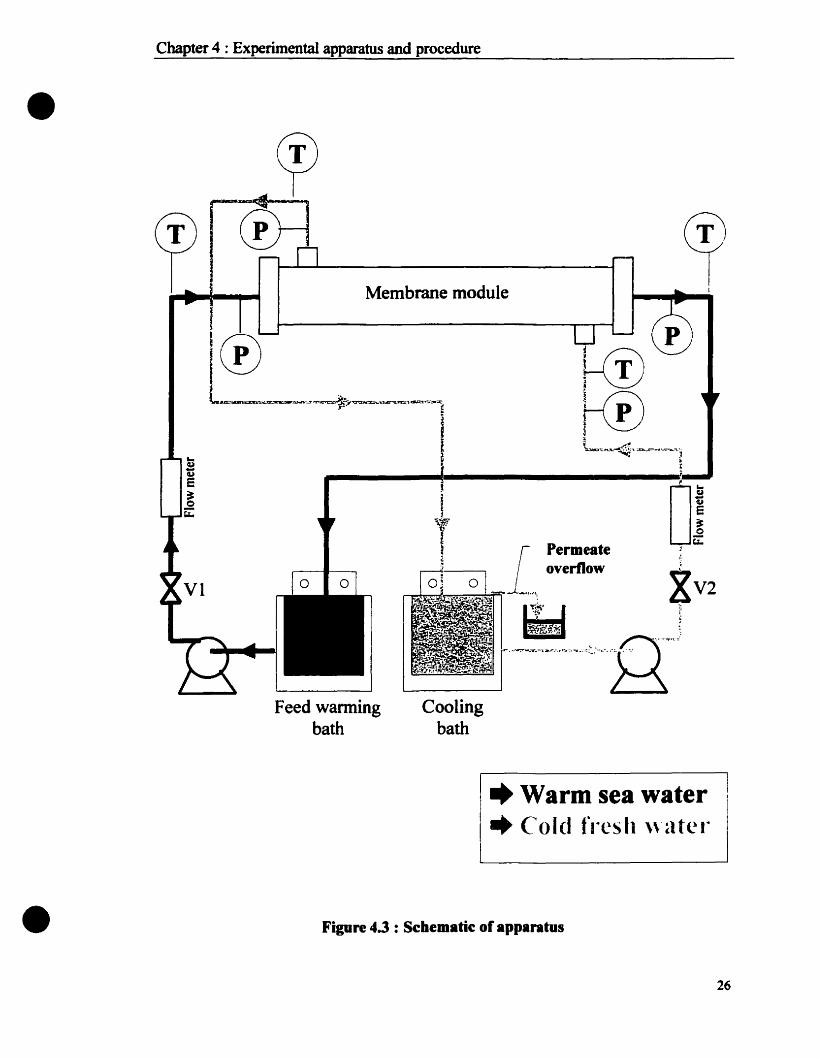
4.2 Description of the apparatus
The experimental apparatus was almost the same for both membrane modules
(Figure 4.3). The only difference was the addition of a more powerful pump and of a
bigger flow meter on the permeate side for the hollow fibre unit. The modules were
slightly inclined (-5%) to allow the air present on the permeate side ta be purged. The
cooling water was then in contact with the total membrane area.
The pressure gauges were Bourdon gauges ranging from 0 to 15 psig (0-103 kPa).
The temperatures were monitored with T-type thermocouples connected to a data
acquisition system (described in section 4.3). The conductivity was read on an Omega
CDW-75 conductivity meter ranging from 0 to 200 mS.
As the cooling capacity of the cooling bath was not enough~ two extra immersion
coolers were used when needed.
A complete list of the equipment is given in Table 4.2.
22

•
•
Chapter 4 : Experimental apparatus and procedure
Table 4.1 : Membrane unit cbaracteristics
Tubular module BoUow fibre module
Model type MD 090 TP 2N ANSI MD080CS2N
Membrane area 1 m2 2m2
Number of membranes 41 450
Nominal module diameter gem 8em
Module length 1.5m lm
Membrane ioDer diameter S.S mm 1.8 mm
Membrane outer diameter 8.5 mm 2.6 mm
Membrane tbiekness 1.5 mm 0.4 mm
Membrane porosity 75% 750/0
Average pore size
(determined by manufacturer) 0.2 J.lm 0.2 ~m
Maximum operatingtemperature 600 e 40°C
(specified by manufacturer)
Membrane material Polypropylene Polypropylene
Outer shell material Polypropylene Stainless Steel
Potting material Polyurethane Polyurethane
23

•
•
Coopter 4 : Experimental apparatus and procedure
Sideview
00000000000000000000000000000000000000000
Cross section
Figure 4.1 : Tubular module
....
....
24

•
•
Chapter 4 : Experimental apparatus and procedure
Side view
Cross section
Figure 4.2 : Hollow fibre module
25
•
•
Chapter 4 : Experimental apparatus and procedure
Feed warmingbath
Figure 4.3 : Schematic of apparatus
Cf1
26

•Chapter 4 : Experimental apparatus and procedure
Table 4.2 : List of the .pparatas
•
Apparatus
Membrane
Constant temperature heatingbath
Constant temperature coolingbath
Immersion cooler 1
Immersion cooler 2
Feed circuit pump
Cooling circuit pumps
Feed circuit flow meter
Cooling circuit flow meters
Thermocouples
Pressure gauges
Tubular 1hoBo. fibre UDit
MD090TP2N / MD080CS2N
Neslab GP-SOO
Neslab RTE-220
Neslab PBC-fi
Neslab V-COOL
Little Giant TE-7f\ID-HC
(centrifugai, magnetic drive)
March TE-SC-MD / TeellP702B
Blue White 3..30 GPM
Blue White
3-30 GPM 110-80 GPM
Omega, T-type
US Gauge 0-15 psig
27

•
•
Chapter 4 : Experimental apparatus and procedure
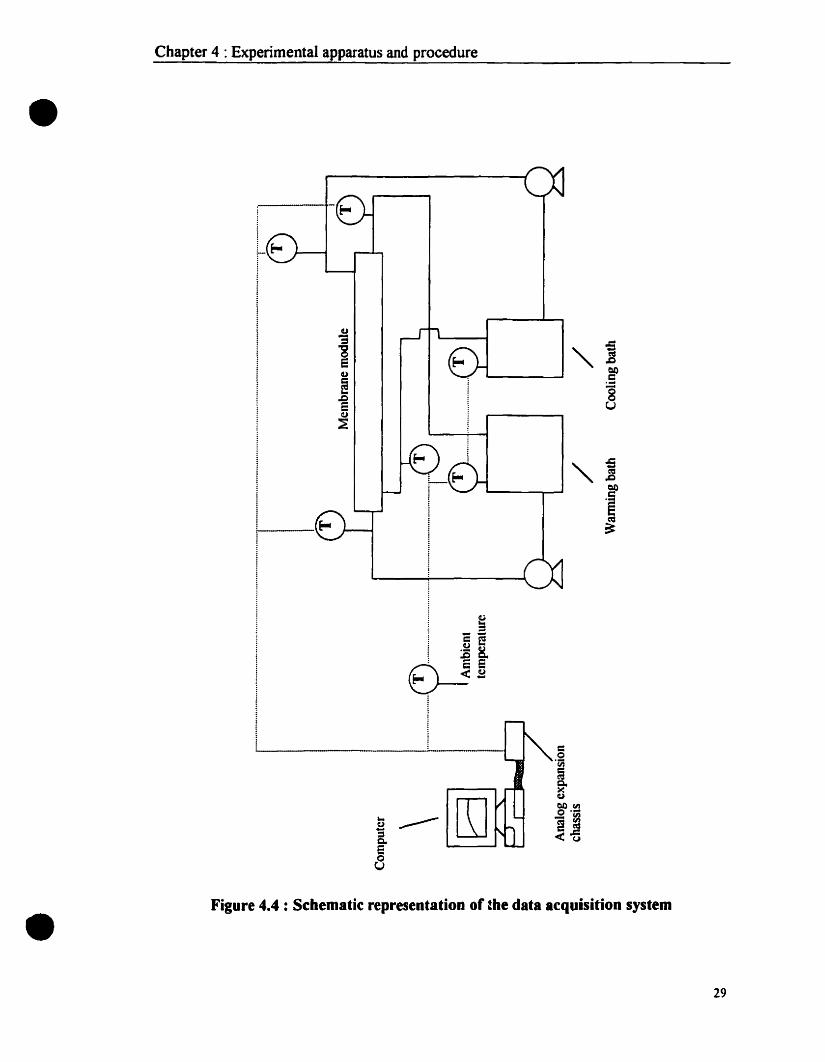
4.3 Data acquisition system
The permeate flux was determined manually by weighing the cooling circuit
overflow. The flow rates and pressures were recorded manually. The temperatures were
key variables used for establishing the existence of steady state conditions and for model
predictions. They were continuously monitored by a data acquisition system. Figure 4.4
gives the schematic representation of the acquisition system. The calibration was done at
the beginning following the procedure given in the owner's manual of the analog ta
digital converter board (DAQBOARD 200A) from Omega. The readings were
periodically verified with Mercury thermometers and always differed by less than D.SoC.
4.3.1 Transducen and signal conditioner
T-type thermocouples and a high accuracy thermocouple card (DBK19) trom
Omega ta which fourteen thermocouples could be connected were used. The
connections between the thermocouples and the signal conditioner (DBK19) were
done with unshielded cables.
28
•
•
Chapter 4 : Experimental apparatus and procedure
u:;oS'8
"cue .D
u 00
e .5.&J "8e uu~
"oSli
·f~
Figure 4.4 : Schematic representation of the data acquisition system
29

•
Chapter 4 : Experimental apparatus and procedure
4.3.2 Analog expansion chassis
The signal conditioner cards for thermocouples (OBK19), and potentially
pressure transducers (DBKIl) were installed inside the Analog Expansion Chassis
(DBK41 trom Omega). This extension box could contain ten cards and was
connected to the analog to digital board via a CA-37-x cable.
4.3.3 Analog to Digital Converter (ADe)
The ADC board (DAQBOARD 200A from OMEGA) was installed inside the
computer and is configured as follows :
- Base address : 300H
- DMA and interrupt selection : DRQ7, DACK7 and IRQ15
The DAQBOARD 200A was a 16-bit ADC board to which sixteen signal
conditioner cards can be connected through channels 0 to 15.
This board converted analog signais coming from the signal conditioners to
digital numbers that could be used by a computer and appropriate software to store
the results and ta draw graphs.
4.3.4 Data acquisition software
The software used was DaqView 7.0 provided with the DAQBOARD 200A
(Figure 4.5). It displays sixteen different channels corresponding to the possible
signal conditioners (OBKII, DBKI9 ... ). For each used channel, the signal
conditioner card must be specified and the software will then display as Many sub
channels as this card could atford. For example, fifteen thermocouples could be
connected to the DBKI9. If this card is attributed channel 2 on the DAQBOARD
200A, then the software will display fifteen different sub-channels for the
thermocouples connected to this card (2-1, 2-2,2-3, ... ,2-15).
30

•
•
Chapter 4 : Experimental apparatus and procedure
Figure 4.5: Screen capture orthe Daqview 7.0 interface
31

•
•
Chapter 4 : Experimental apparatus and procedure
4.4 Experimental procedure
Almast ail the experiments were perfonned with distilled water rather than saline
water. It was simpler to operate and previous studies [1-3] have shown that the presence
of salt (up to 5 wt.%) has little influence on the production of fresh water. A few
experiments with NaCI added to distilled water were done and confirmed the earlier
tindings.
The parameters of the experiments were the flow rates, the temperatures and
eventually the salt concentration. The flow rates on both sides of the membrane were
regulated by adjusting the opening ofvalves VI and V2 (Figure 4.3). The temperature of
the feed and of the cooling liquid were set by adjusting the wanning bath regulator and
the cooling assembly. The temperature of the feed side could be controlled over a wide
range (20-60°C) but the operator had little control on the temperature of the cooling
liquid. Indeed, tbis temperature was limited by the cooling capacities of the apparatus
and by coupling with the temperature of the warm side. The reference temperatures taken
for the calculation were the temperatures at the entrance of the feed and cooling sides.
The temperatures of the streams leaving the unit differed by less than O.3°C from the
entering values.
Levelling up and down the module at the beginning of each experiment permitted
the purging ofair in both circuits.
Due to the limited cooling and heating capacities, two hours were required to reach
steady state. When the temperatures reached steady state, measurements of the overflow
rate were taken over a period of 1 to 4 hours. The cooling circuit overflow was weighed
to determine permeate flux. The overflow was then retumed to the warming bath to keep
its volume constant.
The saline feed was obtained by adding a given weight of sodium chloride salt to get
the required concentration. To simulate sea water, a 3 to 3.5 wt.% saline water was used.
The experimental run times ranged from three to eight hours depending on the
module and the experimental conditions. The experimental data are given in Appendix B.
32

•
•
Chapter 5 : Results and discussion
5 Results and discussion
The membrane distillation mechanism depends upon the passage of vapour through
pores. It is vital that no liquid leaks through the membrane. As will be described in
section 5.1, the penetration pressure of the membrane was checked and the quality of the
permeate monitored for leaks.
Fifteen experiments were conducted with the tubular membrane to ascertain that the
results coincided with Prasanna [3] who used the same membrane module. This is
described in section 5.2. Subsequently, eighty experiments were condueted with the
hollow fibre membrane unit. A comparison of the two units for different operating
conditions is presented in section 5.3. The results and sen1i-empirical model predictions
are compared throughout that section. Section 5.4 is devoted to a comparison of the
semi-empirical and theoretical models to experimental results.
5.1 Membrane wetting
Surface tension is a critical parameter in membrane distillation. It has to be high
enough to balance the operating pressure. The penetration pressure, or wetting pressure,
was investigated by using a 0.036 m2 module containing three tubular membranes with
the same specifications as the ones of the 1 m2 unit. Distilled water was circulated, under
pressure, inside the tubes. No water or counter pressure was applied on the other side
(Figure 5.1). A pressure of32 psi gauge (221 kPa) was applied for thirty minutes without
any wetting of the membrane. The maximum pressure reached with the 1 m2 tubular unit
was of 1-2 psi gauge (7-14 kPa) far below the maximum pressure tested.
33

•Chapter 5 : Results and discussion
Free penneate ~outlet '\
Distilled t----------t~water
Centrifugaipump
Membranemodule
1
Figure 5.1 : Wetting pressure determination experiment
With the hollow fibre unit, the maximum operating pressure was of 9 psi gauge
(62 kPa) on the permeate side and 6 psi gauge (41 kPa) on the feed side. This is still far
below the maximum pressure tested for membrane wetting. To verify that no wetting
occurred during the experiments, tests were conducted with saline water on the feed side.
Had the membrane wetted, the conduetivity in the cooling bath would have increased
because liquid saline water would have passed through the membrane. Monitoring the
cooling circuit conductivity proved that no membrane wetting occurred under the
experimental conditions. Multiple experiments were done with a feed water conductivity
of 45 ± 5 mS. The conductivity of the cooling water slightly decreased during the
experiments as ultra-pure permeate vapour condensed in it. The cooling water
conductivity never exceeded 10 J.1S.
No membrane wetting occurred during the experiments but only distilled water and
distilled water with sodium chloride were used. Unfortunately, the presence of other
compounds such as organics in less pre-treated feed would lower the surface tension
which couId cause membrane wetting and the failure of the process. This happened at a
plant producing drinking water in the Caribs when a tanker released petroleum
compounds in the sea. The plant is no longer in operation. The composition of the feed
water is thus a critical parameter in desalination by membrane distillation.
34

•
•
Chapter 5 : Results and discussion
5.2 Tubular unit
The performance orthe 1 m2 tubular unit was already investigated by Prasanna [3].
The purpose of the present experiments was to determine if the membrane charaeteristics
were still the same in arder to use the results given by Prasanna for comparison purposes.
Only distilled water was used for the investigation of the tubular unit properties. AlI
the experiments were done at a feed flow rate of 20 Umin (Re=2000-3200,
T=26-47°C) and at a cooling flow rate ofalso 20 Umin (Re=800-1450, T=14-39°C). At
these flow rates, the permeate flux is independent of both sides' Reynolds numbers as
demonstrated by Prasanna.
The temperatures were varied to get different vapour pressure differences for ail the
experiments. The membrane mass transfer coefficient C was found by drawing the curve
J=f{Mlv) (Figure 5.2) and by calculating its slope.
35

•Evaluation of the membrane constant C for the tubular unit
Re feed =2150-3230, Re cooling =830-1440
•n
fu.
y = O.2917x
R2 = 0.9862
12.00
- 10.00Ëc:Ë 8.00a-g 6.00;:
s= 4.00~4J
IL 2.00
0.000.0 5.0 10.0 15.0 20.0 25.0 30.0 35.0 40.0
..
~cif8-Q.
~.
enenër::::J
w0\
Vapor pressure dlfference (mmHg)
Figure 5.2 : Evaluation of the tubular membrane ma•• transfer coefficient

•Coopter 5 : Results and discussion
Comparing the experimental flux J to the one calculated with the model gave
agreement within 5 % (Table 5.1 and Figure 5.3). The membrane constant obtained in
these eXPeriments is within 9xl0-9 kg.s-1.m-2.Pa-1 ofthat obtained by Prasanna [3]. It was
concluded that since the work of Prasanna, the membrane proPertïes have remained the
same. His results could then he used for comparison purposes.
Table S.l : Experimental and predieted fluxes
Experiment Experimental OUI Predieted OUI Difference(g.min-1.m-2) (g.miD.l.m-2) (%)
Tl 7.61 7.96 4.4
T2 9.42 8.96 S.l
T3 8.94 8.72 2.S
T4 8.66 8.68 0.2
T5-1 9.03 9.00 0.3
T5-2 5.12 5.01 2.2
T6-1 4.99 4.92 1.4
T6-2 8.16 7.96 2.S
T7 10.02 9.77 2.6
T8 9.12 9.46 3.6
T9 9.44 9.47 0.3
TI0 5.85 5.68 3.0
TIl 5.94 5.85 1.S
T12 3.75 3.60 4.2
• TI3 10.86 10.35 4.9
37

•Comparision of the experimental and predicted permeate fluxes
•n=-~...c..,v-
• experimental- ~odel pred~ction.s .
12.00
- 10.00ft
EC
8.00·sa.-JI(
6.00:J~
.1Il
4.00•~:.
2.00
0.0010.0 15.0 20.0 25.0 30.0 35.0
1
40.0
..
~=en
~D-o..~.
fAenër:s
~
oc
Vapor pressure difference (mmHg)
Figure 5.3 : Experimental and predicted permeate fluxes

•
•
Chapter 5 : Results and discussion
5.3 Comparative study of the tubular and hollow fibre units
5.3.1 Effeet of the temperature
As the perrneate flux is a function of the vapour pressure difference (J=CâPv)
which is itself a function of the temperature (Antoine's equation, Figure 5.4), the
permeate flux is strongly affected by the feed temperature and by the temperature
difference between the hot and the cold streams. In order to maximise the permeate
flux, the temperature difference and the Mean temperature should be as high as
possible, technically and economically speaking. Unfortunately, because of the
limited cooling and heating capacities of the experimental apparatus, the temperature
difference did not exceed 17°C (tubular unit) and 12.5°C (hollow fibre unit).
As expected, the cffects of the temperature were the same for both membrane
units. The permeate flux increased with increasing feed temperature and with
increasing temperature difference. The model predicts that the hollow fibre unit is
the more sensitive to temperatures (Figure 5.5).
Figures 5.6 and 5.7 show in 3D the model predictions of the permeate flux for
different feed temperature and temperature differences. The same trend is observed
once again. The permeate flux of the hollow fibre unit was expected ta exceed that
of the tubular membrane unit at the same conditions.
39

Vapour pressure of water vs temperature
,1
•
~~encn~
1 Q) C)~J:
~E:::J Eo '-'""a.~
800
700
600
500
400
300
200
100o
o 20 40 60 80 100
•n:r~
OS~V\..~~::;en
8-Q.~.
Cfi)fi)
o':3
.1;00o
Temperature (OC)
Figure 5.4 : Vapour pressure of pure water by Antoine's equation

~-
•
Model predictions of the permeate flux versus feed temperature(temperature difference : 10°C)
25
- • Hollow fibre unitft
•~ 20 •C~1 Tubular unit • •Os •..... 15 • •a» •- •M • •:::1 • • !il Il1;: 10 . • t!!
S • • II! l1liCI Il• fi:! B tri
• ~iIj
Ë 5 11 t"l SJ Il
CID.
O'25 27 29 31 33 35 37 39 41
Feed temperature (OC)
Figure &.5 : Semi-empirical model predictions of the permeate flux
•n::r~(D..,!JI
~Ë.U2
~Q.
Q.Vi'nt:CIJCIJ
0'::s

40
......................}:: ~~.. ~~j ......... ~
.i ~~... ~
25 \:--r-/b...~.....~.....~... ~T'=""'~""'-'-L.····1.····
_...~ .. ~
20...-C'JEc:
15E..........
(J')---x 10:::J
l.J...
5
Chapter 5 : Results and discussion
•
Figure 5.6 Semi-empirical model predictions for the hollowfi bre unit permeate flux
• Figure 5.7 Semi-empirical model predictions for thetubular unit permeate flux
42

•
•
Chapter 5 : Results and discussion
5.3.2 EtTect of the feed Dow rate
Banat [1], Lacoursière [2] and Prasanna [3] have demonstrated that for the same
operating conditions, increasing the fecd flow rate strongly increases the permeate
flux until it reaches a plateau. This phenomenon is explained by the transition
between laminar and turbulent flow. In the turbulent region, temperature polarisation
and concentration polarisation are minimised so the vapour pressure difference is
maximised.
With the tubular unit, the plateau is reached for a feed Reynolds number around
1200, corresponding ta a flow rate of 1DL/min, with a saline solution
(3 wt.% NaCI) [3]. During the experiments done with the hollow fibre unit
(Figure 5.8) the plateau was reached a Iittle bit sooner for a Reynolds number around
1000, corresponding to a flow rate of 30L/min (Figure 5.9). The ditTerence is not
really significant and may be explained by the use of distilled water instead of saline
water. However, to achieve the same Reynolds number in the narrow hollow fibre
unit as in the wide tubular unit, the feed flow rate has to be three times as high. This
lead to a much higher energy consumption.
43

• •
Evaluation of the membrane constant C (g/min.ml.mmHg)Re cooling = 750
.. ~-_." - -
!•• Re feed=3000, C=0.243
i. Re feed=1000, C=0.238
À Re feed=670, C=0.228
;.0 Re feed=410, C=0.211
18.0
n:r~
"0-('D..,VI..:=('Dfi)
c;:;-CI)
• ,g;Q.
Q.
fii'ncCArn0':s
16.014.012.010.08.0
4.50
4.00
3.50t:""'Ec: 3.00
12.50te:JCJI 2.00
:! 1.50
:.1.00
0.50
0.00
0.0 2.0 4.0 6.0
Vapor pressure dlfference (mmHg)
Figure 5.8 : Experimental permeate fluxes at different Reynolds numbers on the feed side
t

•Chapter 5 : Results and discussion
~
CllE 0.2E~
Ec
E~ 0.1'-'"
ü
Hollow fibre unit
.: Experimental data
•
o.0 ...--_--'--_---I-_~__~_---.&.-_ _...L._ ____J
o 500 1000 1500 2000 2500 3000 3500
Feed Reynolds number
Figure 5.9 : Feed flow rate influence on the
membrane mass transfer coefficient
45

•
•
Chapter 5 : Results and discussion
5.3.3 Effect of the cooling Dow rate
Prasanna [3] did not investigate the effect of the cooling water flow rate on the
permeate flux but Lacoursière [2] did on a smaller tubular unit with only three
tubes. It was demonstrated that the influence is far less significant than the one of the
feed f10w rate. The same trend was observed with an increase in permeate flux for an
increase in cooling water flow rate until a plateau was reached at Re=1500.
However, the unit hydrodynamics have to be taken into account. The cross
section temperature profile is not the same for a three or for a forty-one-tube units
(Figure 5.10). The temperature of the cooling water will be much warmer in the
centre of the forty-one-tube module. Increasing the tlow rate will then have a greater
influence by reducing the temperature of the cooling liquid in the centre of the
module. The plateau will be reached when the cooling water temperature gradient
will be as close as possible ta zero.
The cross section temperature gradient is a serious consideration in the case of
the hollow fibre unit. The fibres are extremely packed inside the module
(Figure 5. Il). The temperature gradient is then expected ta be very high over the
cross section of the unit.
This concept is supported by the experiments done with the hollow fibre unit
(Figure 5.12) and by Figure 5.13 which show that the permeate flux is strongly
dependent on the cooling water flow rate until it reaches a plateau al a Reynolds
number of approximately 1800. The hollow fibre unit requires 95 L/min to reach the
plateau versus 20 L/min for the tubular unit. Consequently, the hollow fibre unit,
once again, needs more energy for pumping ta reach higher permeate fluxes.
46

•
•
Chapter 5 : Results and discussion
a)
00000000000000000000000000000000000000000
b)
Figure 5..10 : Tubular unit cross sections: a) three-tubes b) forty one-tubes
Figure 5..11 : Hollow libre unit cross section
47

• •Evaluation of the membrane constant C (g/min.m2.mmHg)
Re feed =3000
n::r~
OS('1)~
VI
~Q.Q.C;;'
2(1)(1)
S'::s
~Ë.....(1)
25.0
• Rep=750, C=O.243
• Rep=540, C=O.192A Rep=380, C=0.127
• Rep=1200, C=O.399:( Rep=2200, C=0.523o Rep=1600, C=O.499
20.015.010.05.0
0.00 -=:-.--.----.-.---..--.-...---~
0.0
5.00
1.00
t:"" 4.00Eè
:@.!! 3.00Je::s;:
!~ 2.00
l.
Vapor pre••ure difference (mmHg)
~00
Figure 5.12 : Experimental penneate fluxes at different Reynolds numbera on the cooUng side

•Chapter 5 : Results and discussion
1000 1500 2000 2500500
0.0 .-__L--__~__~___'____ __'
o
0.6
0.5~
enl
0.4EE
NE 0.3c::E
.......... 0.20'1 .: Experimental data.........,
0Hollow fibre unit
0.1
Cooling side Reynolds number
Figure 5.13 : Influence of the cooling side flow rateon lhe membrane mass lransfer
coefficient in the hollow fibre unit
•49

•Chapter 5 : Results and discussion
5.3.4 Erreet of the salt concentration
The salt concentration reduces the permeate flux by reducing the vapour
pressure ofwater on the feed side.
Prasanna [3] did not notice a difference between a 3% NaCI solution and
distilled water for the tubular unit even if theoretical calculations predict a reduction
of 5% in vapour pressure.
With the hollow fibre unit, a 6% permeate flux reduction was experimentaIIy
demonstrated (for a 7.7% predicted reduction) by using a 3.4 wt.% NaCI
concentration (Figure 5.14). The model predictions are, once again,
good (Figure 5.15).
3.4N.%NaCI vs <1iIIIIed....Refeed =3000, Re cooIIlIJ=2200
10.08.04.0 6.0Vapar pressure ditrerenœ (rmttg)
2.0
DistiUed water
0.00 ~-"---.l....--l.--l.--+~---l.....-......Io.-..J....-+__.I.....-....l--l.~__+_---L...---'----......L-...o.-t____''-----''"~---'-___1
0.0
5.00 +- V~=-O'-5232-1-x---------i
~=O.œ:J)4
~ 4.00 -+-------------------~~~----------jËa;- 3.00 +-----------J~---___=~......v:---------____t~
-=~ 2.00 +-----------::o~""---------------_______jcuE NaCIl1.00 +--------:::r#f1iiG----------------------t
•Figure 5.14 : Permeate Oux with distilled water and a 3.4 wt.% NaCI feed solutions
50

• •
Experimental vs PredictedRe feed =3000, Re cooling =2200
3.4 wt.% NaCI
._-~---'--------~-----~---4
: • Experimental
~._~.~dE!l__pr~_~~~ti~~~
..
[fi)8-c.~.
cfi)fi)
o'=
n::rI»"S~Ul
8.07.57.06.56.05.55.0
- 8c·e 7.5-.!! 7s 65l! .~ 6-; 5.5i 5i 4.5a. 4
4.5
Vapor pressure difference (mmHg)
Figure 5.15 : Permeate flow rate, experimental values and model predictions for a3.4 wt.ok NaCI solution
Ut-

•
•
Chapter 5 : Results and discussion
S.3.S Economieal considerations and comparison of bigbest permeate Ouxes
acbieved by tbe hoUow fibre and tubular membrane uoits
As expected, the thin-walled hollow fibre unit had a higher membrane mass
transfer coefficient than the thicker tubular unit. This would indicate that the
permeate flux which could be achieved, for identical temperature conditions in the
two units, would be greater for the hollow fibre unit than for the tubular membrane
unit. Two factors prevented a conclusive experimental demonstration of this
prediction. The first was the difference in hydromechanics of the two unÎts. As
mentioned in eacHer sections of this chapter, the tightly packed hollow fibre unit
required much higher flow rates to achieve the same Reynolds numbers as the
tubular unit. Even when the same Reynolds numbers were reached, the trans
membrane temperature difference of the inner hollow fibres was less than that of the
inner tubular membranes. The second difficulty was in accommodating the high
heat-removal requirements of the hollow fibre unit. Although extra cooling capacity
was added, it still did not allow the unit to reach its full distillation potential.
Table 5.2 summarises the operating conditions under which the highest fluxes
were achieved in the two units. Although the membrane was wil1ing, the hollow
fibre unit heating, cooling and pumping peripherals were weak. It was not possible
to reach comparably high trans-membrane temperatures in the hollow fibre unit as in
the tubular unit. Even though the hollow fibre unit had twice as much surface area as
the tubular unit, at comparable Reynolds numbers, it produced only 0.414 kglh of
fresh water compared to 0.652 kglh produced by the tubular unit.
A preliminary economic analysis of this situation indicates that it is the
operating costs which will determine the competitiveness of these units. The capital
cost of the modules at this scale is comparable. The heatinglcooling and pumping
requirements of the hollo~ fibre unit exceed those of the tubular unit for comparable
permeate fluxes. Peripheral equipment more powerful than bench scale would have
to he involved ta optimise the hollow fibre unit.
52

•
•
Coopter 5 : Results and discussion
Table 5.2 : Performances and experimental conditions comparison
HoUow fibre unit Tubularanit(2D12) (1812)
Membrane constant 654.10.8 k ·1 ·2 P ·1 3 65.10-8 k -1 ·2 P .(. g.s .fi . a . g.s .m . a
Muimum permeate Oow 0.414 kglh 0.652 kglhobtained for that constant
Feed side flow rate 30 L/min 10 L/min(Re = 1000) (Re = 1200)
Cooling w.ter flow rate 95 L/min 20 L/min(Re = 1800) (Re = 1150)
Feed side temperature 33.6°C 41.2°C
Cooling water temperature 30.3°C 24.6°C
Membrane modale cost 2100$ (US) 1830$ (US)
5.4 Comparison of the semi-empirical and theoretical mode/s
The semi-empirical model fits the experimental values within 5% for the tubular
membrane and within 3% for the hollow fibre membrane when using distilled water feed
(Table 5.3).
Knudsen diffusion, molecular diffusion and Hagen-Poiseuille VISCOUS tlow
theoretical models were also examined. The calculations were done by taking the mean
temperature between the feed and the cooling water entrances. The vapour pressures
were taken at these temperatures and the pressure inside the pores was assumed to he
1 atm. Due to the unavailability of tortuosity data from the manufacturer of the
membranes, the tortuosity was assumed to he equal to 1.3. Details of the calculations are
presented in Appendix C.
S3

•
•
Chapter 5 : Results and discussion
At 30°C and 1 atm, the water molecules Mean free path is approximately 0.1 J.Ul1.
According to the theory developed in section 3.2 and with a pore diameter of0.2 J.un~ the
mass transport mechanism is in the transition region between the Knudsen diffusion and
the molecular diffusion. Surprisingly, the Hagen-Poiseuille viscous flow model
predictions of the permeate flow rate (Table 5.3) were better than the other two although
this theory is applicable to very large pore sizes compared to the Mean free path of the
water molecule. Its predictions are almost as good as the semi-empirical model and
within 9%.
These observations Mean that the Hagen-Poiseuille model is the best theoretical
model to describe the combination of the transport mechanism and of the hydraulics of
the modules. It does not mean that the transport mechanism follows a Hagen-Poiseuille
viscous flow transport mechanism. Indeed, the temperature of the cooling water in the
centre of the module was certainly not the same as at the periphery. So, the rate of the
permeate flux was lowered resulting in a lower experimental flow. Only experiments
with a unit containing one tube or one hollow fibre could determine which transport
mechanism is happening.
54

•
•
Chapter 5 : Results and discussion
Table 5.3 : Predictions of the semi-empirical and theoretical models
Knudsen DowMoleeular
Semi-empirieal (gfmin)diffusion Oow
Hagen-PoiseuilleRun Experimental model (gImin) (% ditTerence (gImiD)
8ow(glmin)(gImin) (e,4differenee) always greater
(% difference(%difference)
tban 30001'0)always greater
than 1()()OJ'o)
61 3.70 3.78 (2.1%) 30.7 20.6 4.08 (901'0)
68 5.25 5.36 (2.1%) 43.7 29.1 5.80(9%)
69 6.17 6.11 (1.0%) 49.1 33.3 6.50 (5%)
10 6.90 7.10 (2.8%) 56.4 38.8 7.43 (7%)
Tl 7.61 7.96 (4.4%) 23.5 17.7 7.93 (4%)
T2 9.42 8.96 (5.1%) 26.6 19.5 8.99(5%)
T3 8.94 8.72 (2.5%) 25.9 19.0 8.75 (2%)
T4 8.66 8.68 (0.2%) 25.8 18.9 8.71 (1%)
T5-1 9.03 9.00 (0.30/0) 26.7 19.6 9.03 (0%)
T5-2 5.12 5.01 (2.2%) 15.4 10.6 5.30 (3%)
T6-1 4.99 4.92 (1.4%) 15.2 10.4 5.21 (4%)
T6-2 8.16 7.96 (2.5%) 23.7 17.2 8.06 (1%)
T1 10.02 9.77 (2.6%) 29.6 20.4 \0.14 (1%)
T8 9.12 9.46 (3.6%) 28.6 19.7 9.82 (7%)
T9 9.44 9.47 (0.3%) 28.6 19.8 9.82 (4%)
TtO 5.85 5.68 (3.0%) 18.0 11.9 6.22 (6%)
Ttl 5.94 5.85 (1.5%) 18.5 12.2 6.41 (7%)
TI2 3.75 3.60 (4.2%) 11.7 7.5 4.10 (9%)
Tl3 10.86 10.35 (4.9%) 31.1 21.6 10.64 (20/0)
55

•
•
Chapter 6 : Conclusions and recommendation
6 Conclusions and recommendations
A hollow fibre membrane module was tested and its performance was compared to
that of a tubular unit. Experiments were conducted ta determine the behaviour of each
module for different experimental conditions (temperatures, flow rates). The following
conclusions were reached :
• The range of the possible operating conditions is greatly limited by the cooling and
heating capacities ofthe apparatus.
• The influence of the feed flow rate is almost the same for the hollow fibre and tubular
membrane units. The permeate fluxes reach a plateau at turbulent flow rates.
• The influence of the cooling water flow rate is more significant in the case of the
hollow fibre unit due to a strong cooling water temperature gradient perpendicular to
the direction of the flow. Increasing the flow rate decreases this gradient and leads to
a better permeate flux until a plateau is reached.
• The hollow fibre unit requires much higher feed and cooling water flow rates than the
tubular unit to achieve turbulent flow.
• A smaller membrane thickness increases the membrane constant.
• The hollow fibre unit could give a much better permeate flux but requires higher
energy input (pumping, warming and cooIing).
• The hydrodynamics within a membrane distillation unit are of fundamental
importance as they influence a critical variable, trans-membrane temperature.
56

•
•
Chapter 6 : Conclusions and recommendation
• With the hollow fibre module, a 3.4 wt.% NaCI solution decreases the penneate flux
by 6% compared to pure distilled water.
• The semi-empirical model was the best at predicting the permeate flux. Its
predictions were in very good agreement with the experimental values for bath the
hollow fibre and tubular units (3-6.4%).
• For the theoretical models, the Hagen-Poiseuille viscous flow fitted the best the
experimental results, even if the theory is not adapted ta that case, because of
hydrodynamics considerations.
The following recommendations may lead to improvement of the process itself and its
evaluatiùn :
• More powerfuI heating and cooling apparatus should be used to evaluate the
modules' capacities on a wider range oftemperatures and temperature differences.
• An economic study of heating, cooling and pumping requirements should be done to
detennine whether or not the greater permeate flux which could be achieved by the
hollow fibre unit compensates for the higher energy consumption.
• A spiral-wound configuration should be tested. Such membranes are thinner and may
advantageously combine the lower flow rates of the tubular membranes with the
higher membrane area and permeate fluxes of the hollow fibres to produce profitable
permeate ft uxes.
57

•
•
Chapter 7 : References
7 References
1. BANAT, F., Membrane Distillation for Desalination and Removal of Volatile
Organic Compoundsfrom Water, Ph.D. thesis, McGiIl University, Quebec, Canada,
1994.
2. LACOURSIÈRE, S., Water Purification by Membrane Distillation, M.Eng. thesis,
McGill University, Quebec, Canada, 1994.
3. PRASANNA, P.R.M., A Study and Scale-up of Desalination via Membrane
Distillation, M.Eng. thesis, McGilI University, Quebec, Canada, 1998.
4. FINDLEY, M.E., Vaporization Through Porous Membranes, Ind. Eng. Chem.
Process Des. Dev., 6, 226-230, 1967.
5. LAWSON, K. W., DOUGLAS, R.L., Membrane Distillation, Journal of Membrane
Science, 124, 1-25, 1997.
6. BRYK, M.T., NIGMATULLIN, R.R., Membrane Distillation, Russian Chemicals
Reviews, 63 (12), 1047-1062, 1994.
7. LAGANÂ, F., BARBIERI, G., DRIOLI, E., Direct Contact Membrane Distillation:
Modelling and Concentration Experiments, 166, 1-11, 2000.
8. TOMASZEWSKA, M., Concentration and Purification of Fluosilicic Acid by
Membrane Distillation, Ind. Eng. Chem. Res., 39, 3038-3041, 2000.
9. ZAKRZEWSKA-TRZNADEL, G., HARASIMOWICZ, M., CH1vfIELEWSKI, A.G.,
Concentration ofRadioactive Components in Liquid Low-Level Radioactive Waste by
Membrane Distillation, Journal of Membrane Science, 163, 257-264, 1999.
58

•
•
Chapter 7 : References
10. GREKOV, K.B., SENATOROV, V.E., Processing ofLiquid Photographie Waste by
Contact Membrane Distillation, Russian Journal of Applied Chemistry, 72, 1577
1580, 1999.
Il. RlNCON, C., ORTIZ DE ZÂRATE, J.M., MENGUAL, 1.1., Separation of Water and
Glycols by Direct Contacl Membrane Distillation, Journal of Membrane Science,
158, 155-165, 1999.
12. GRYTJ\ M., KARAKULSKI, K., The Application ofMembrane Distillation for the
Concentration ofOi/-Water Emulsions, 121,23-29, 1999.
13. COUFFIN, N., CABASSUD, C., LAHOUSSINE-TURCAUD, V., A New Process to
Remove Ha/ogenated VOCs for Drinking Water Production : Vacuum Membrane
Distillation, Desalination, 117, 233-245, 1998.
14. BANAT, F.A., SIMANDL, J., Membrane Distillationjor Propanone Remova/from
Aqueous Streams, Journal ofChemical Technology and Biotechnology, 75, 168-178,
2000.
15. BANAT, F.A., SIMANDL, 1., Membrane Distillationfor Di/ute Ethanol Separation
from Aqueous Streams, Journal ofMembrane Science, 163,333-348, 1999.
16. BANAT, F.A., SIMANDL, 1., Remova/ ofBenzene Traeesfrom COl1taminated Water
by Vacuum Membrane Distillation, Chemical Engineering Science, 51(8), 1257
1265, 1996.
17. BURGOYNE, A., VAlIDAII, M.M., Permeate Flux Modeling of Membrane
Distillation, Filtration and Separation, 49, January-February 1999.
18. MARTINEZ-DIEZ, L., VASQUEZ-GONSALEZ, M.I., Effects of Polarization on
Mass Transport Through Hydrophobie Porous Membranes, [nd. Eng. Chem. Res.,
37, 4128-4135, 1998.
S9

•
•
Chapter 7 : References
19. PEN~ L., GODINO, M.P., MENGUAL, li., A Method ta Eva/uate the Net
Membrane Distillation Coefficient, Journal of Membrane Science, 143, 219-233,
1998.
20. GRYTA, M., TOMASZEWS~ M., Heat Transport in Membrane Distillation
Process, Journal ofMembrane Science, 144, 211-222, 1998.
21. MARTINEZ-DIEZ, L., VASQUEZ-GONSALEZ, M.L, Temperature and
Concentratioll Po/arization in Membrane Distillation of Aqueous Salt Solutions,
Journal ofMembrane Science, 156,265-273, 1999.
22. BURGOYNE, A., VAHDATI, M.M., Direct Contact Membrane Distillation,
Separation Science and Technology, 35(8), 1257-1284, 2000.
23. PERRY, R.H., GREEN, D.W., MALONEY, J.O., Perry's Chemica/ Engineer's
Handbook, 7th edition, McGraw-Hill, New-York, NY, pp.2-320-2-321,2-370, 1997.
24. SCHOFIELD, R.W., FANE, A.G., FELL, C.J.D., Heat and Mass Transfer in
Membrane Distillation, Journal ofMembrane Science, 33, 299-313, 1987.
25. SCHOFIELD, R.W., FANE, A.G., FELL, C.I.D., Gas and Vapollr Transport
Through Microporous Membranes. /. KmuJsen-Poiseuille Transition, Journal of
Membrane Science, 53, 159-171, 1990.
26. SCHOFIELD, R. W., FANE, A.G., FELL, C.J.D., Gas and Vapollr Transport
Throllgh Microporolls Membranes. Il. Membrane Distillation, Journal of Membrane
Science, 53, 173-185, 1990.
27. BIRO, R. B., STEWART, W. E., LIGHTFOOT, E. N., Transport Phenomena, John
Wiley & Sons, 1960.
28. BENNETT, C.O., MEYERS, J.E., Momemtllm, Beat and Mass Transfer, McGraw·
Hill, New-York, NY, p.802, 1982.
60

•
•
Chapter 7 : References
29. BRETSZNAJDER, S., Predictions of Transport and Other Physical Properties of
Fluids, Pergamon Press, Oxford, UK, pp. 189-239, pp.289-328, 1971.
30. COULSON, lM., RICHARDSON, J.f., Chemical Engineering: Volume l-F/uid
Flow, Beai Transfer, andMoss Transjer, Pergamon Press, Oxford, UK, pp.312-441.
31. GEANKOPLIS, C., Transport Processes and Unit Operations, Prentice-Hall,
Englewood Cliffs" NI, pp.426-488, 1993.
61

•
•
Appendix A : Flux prediction program
Appendix A
Flux prediction program
62

•
•
Appendix A : Flux prediction program
'FLUX.xls
'TInS PROGRAM CALCULATES THE FLUX OF A MEMBRANE DISTILLATION
'UNIT
'THE CODE IS BASED ON THE ONE WRITTEN BY PRASANNA [3] IN FORTRAN.
'IT HAS BEEN ADAPTED AND WRITTEN IN VISUAL BASIC BY
'LUDOVIC PLASSE
NOVEMBER 2000
Option Explieit
Dim km, kg, porosity, delta, id, ad, pore, length As Double
Dim Clarge, C, Pfm, Ppm, Evap, Cfm As Double
Dim TtC, QFlm, TpC, QPlm, TfK, wtf, wtfrn, rho( cane, mufp, mufm, mut: kf20, kf
As Double
Dim TpK, mupp, mup, rhop, Tfilm, mufip, mufi, rhofilm, massf, massp As Double
Dim QFm3, QPm3, he, vf, Ref, Prf, Nuf, hf, vp, parea, dhyd, Rep, Prp, Nup As
Double
Dim hp, sirl, Cpf, kp, Cpp, TfilmK, mufipv, rhofilmv, diff, Sc, Ks, area As Double
Dim Jtot, Error, Toi, guess, Tp, Tpm, Tf, Tfm, Jseg, Qv, Qe, Q, Jfibre, J As Double
Dim Gain, hv, wfm, Tpl, Tfl, hp2 As Double
Dim Qheat As Double
Dim segment, num, l, dT As Integer
63

•
•
Appendix A : Flux prediction program
Sub calculO
'UNIVERSAL MEMBRANE PROPERTIES
'UNlTS: kg,km[W/mK];
km = 0.14 'Membrane Thermal Conductivity @ 50"C
kg = 0.0235 ' Thermal Conductivity Air/Water @ 50"C
porosity =0.75 ' Porosity of the Membranes
IfUserForml.OptionButton_1m2.Value =True Then
'1 ml\2 TUBULAR MEMBRANE PROPERTIES
'UNITS: Clarge[kgls m2 Pa]; delta,id,od,pore,length,mid [ml;
Clarge = 0.000000046585
delta =0.0015 1 Membrane Thickness- Vapour path length
id = 0.0055 1 Membrane Inoer Diameter
od = 0.0085 'Membrane Outer Diameter
pore =0.0000002 'Pore Size
length = 1.27 'Membrane Leogth
oum =41 ' Number ofTubes
segment =91 1 Number of Segments
sid = 0.09 ' Shell ioner diameter-estimate
C = Clarge
ElseIfUserForm1.0ptionButton_2m2.Value = True Then
'2 ml\2 HOLLOW FffiERS MEMBRANE PROPERTIES
'UNITS: Clarge[kgls m2 Pa); delta,id,od,pore,length,mid [ml;
Clarge = 0.000000065407
delta = 0.0004 'Membrane Thickness- Vapour path length
64
•
•
Appendix A : Flux prediction program
id = 0.0018 ' Membrane Inner Diameter
od =0.0026 1 Membrane Outer Diameter
pore = 0.0000002 t Pore Size
length = 0.875 ' Membrane Length
oum = 450 ' Number ofTubes
segment =91 ' Number of Segments
sid = 0.085 1 Shell ioner diameter-estimate
C = Clarge
End If
'FEED CONDITIONS INPUT
If IsNumeric(UserForm 1.TextBox_Tfeed.Value) = False Theo
UserForm1.TextBox_Tfeed.Value = 1'"
UserForm1.TextBox_Tfeed.SetFocus
Exit Sub
End If
IfIsNumeric(UserForm1.TextBox_Flowfeed.Value) = False Then
UserForm1.TextBox Flowfeed.Value = Illf
UserForm1.TextBox_Flowfeed.SetFocus
Exit Sub
End If
If IsNumeric(UserForm 1.TextBox_Saltconcentration.Value) = False Then
UserFoool.TextBox_Saltconcentration.Value = ""
UserF0001.TextBox_Saltconcentration.SetFocus
Exit Sub
End If
65
•
•
Appendix A : Flux prediction program
TtC =CDbl(UserFonnl.TextBox Tfeed.Value)
QFlm = CDbl(UserFormI.TextBox_Flowfeed.Value)
wtfm = CDbl(UserForml.TextBox_Saltconcentration.Value) '[gIL]
wtf = wtfm / 1000 '[kgIL] or [kg/kg]
'COOLING WATER CONDITIONS INPUT
IfIsNumeric(UserForml.TextBox_Tcooling.Value) =False Then
UserFonnl.TextBox_Tcooling.Value = 1111
UserFonnl.TextBox_Tcooling.SetFocus
Exit Sub
End If
IfIsNumeric(UserForm1.TextBox_Flowcooling.Value) = False Then
UserForml.TextBox_Flowcooling.Value = ""
UserForm 1.TextBox_Flowcooling. SetFocus
Exit Sub
End If
TpC = CDbl(UserForml.TextBox_Tcooling.Value)
QPlm = CDbl(UserForml.TextBox_Flowcooling.Value)
66

•
•
Appendix A : Flux prediction program
'FEED WATER PROPERTIES EVALUATION
'UNlTS: TfK[K],mufp[poise],mufm[pa*s],mufTPa*s],rhot{kglmI\3]
'eone[mol NaCl/L solution],knO,ktIW/mK],CptII/(kg K)]
'mufp ealculates the pure water viscosity. mufp is from [28], p 802. Then mufm converts
lthis viseosity. The final viseosity is computed using an equation from [29], p228.
TfK = TfC + 273.15
Ifwtfm = 0 Then
cone = 0
rhof = 0.0000000023076 * (TtC 1\ 5) - 0.00000068283 * (TtC 1\ 4) + 0.00008895 *
(TtC 1\ 3) - 0.0093 * (TtC 1\ 2) + 0.08 * TtC + 999.8011
mufp = 1 / (2.1482 * «TtC - 8.435) + «8078.4 + (Til: - 8.435) 1\ 2) 1\ 0.5» - 120)
muf= mufp * 0.1 '[28], p802
kf= -0.4732943 + 0.00579948887 * Tf1( - 0.00000725519 * (Tf1( 1\ 2)
Cpf = (45.359165 - 0.416094 * TfK + 0.00220052 * (Tf}( 1\ 2)
0.000004380770923 * (TtK 1\ 3) + 3.275994572E-09 * (TfI< 1\ 4» * 1000 'Reat
Capaeity of Liquid Water
Else
rhof= (0.7227 * (wtf) - 0.00033 * TtC + 1.003198) * 1000' NaCI Density
cone =wtf * (1 / 58.5) * rhof
mufp = 1 / (2.1482 • «TfC - 8.435) +«8078.4 + (TfC - 8.435) 1\ 2) 1\ 0.5» - 120)
mufm = mufp • O. l '[28], p802
muf=mufm * (1 + 0.0062 * (cone 1\ 0.5) + 0.0793 • cone + 0.008 * (cone 1\ 2» 1 [29]
kf20 = (0.515 - 0.0047 * cone) * 1000 • 4.1868/3600 ' [29], page 323
kf = kf'20 * «-1 / 103125) * (TpC 1\ 2) + (4877 / 1650000) * TpC + (155957 1
165000»
Cpf= (4.170528 - 5.55245 * wtf+ 9.19117 • (wtfl\ 2) + 0.0001737824 • TOC +
0.00001335187 • (TtC 1\ 2» * 1000
End If
67

•
•
Appendix A : Flux prediction program
'PERMEATE WATER PROPERTIES EVALUATION
UNITS: TpK[K],mupp[poise],mup(pa-s],rhop[kglmI\3], kp[W/(m-K)]
'Cpp[J/(kg*K)]
TpK =TpC + 273.15
rhop = 0.0000000023076 * (TpC 1\ 5) - 0.00000068283 - (TpC 1\ 4) + 0.00008895
(TpC 1\ 3) - 0.0093 * (TpC 1\ 2) + 0.08 - TpC + 999.80 Il ' Matlab Curve Fitting
mupp = 1 / (2.1482 • «TpC - 8.435) + «8078.4 + (TpC - 8.435) 1\ 2) 1\ 0.5» - 120)
mup = mupp - 0.1 1 [28], p.802
kp = -0.4732943 + 0.00579948887 * TpK - 0.00000725519 • (TpK 1\ 2)
Cpp = (45.359165 - 0.416094 • TpK + 0.00220052 - (TpK 1\ 2) - 0.000004380770923
* (TpK 1\ 3) + 3.275994572E-09 * (TpK 1\ 4» • 1000 'Heat Capacity ofLiquid Water
'FILM TEMPERATURE PROPERTIES
'UNITS: Tfilm[eC],TfilmK[K],mufip[poise],mufi[pa·s],rhofilm[kglmI\3]
mufipv[pa·s]
Tfilm = (TiC + TpC) / 2
TfilmK = Tfilm + 273.15
mufip = 1 / (2.1482 • «Tfilm - 8.435) + «8078.4 + (Tfilm - 8.435) 1\ 2) 1\ 0.5» - 120)
mufi = mufip • 0.1 1 [28], P 802
rhofilm = 0.0000000023076 • (Tfilm 1\ 5) - 0.00000068283 * (Tfilm 1\ 4) +
0.00008895 • (Ttilm 1\ 3) - 0.0093 • (Ttilm 1\ 2) + 0.08 • (Tfilm) + 999.8011
mufipv = -0.000002909707 + 0.00000004000022 - TfilmK 1 Viscosity ofWater(Vap.)
rhofilmv = 0.004971907 + 0.00024676 • Tfilm + 0.00001746339 - (Tfilm 1\ 2)
4.06779996E-08 • (Tfilm 1\ 3) + 0.000000004339217 • (Tfilm 1\ 4) 1 .-Vapour·-
68

•
•
Appendix A : Flux prediction program
'MASS AND VOLillvIETRIC FLOW RATES
massf = QFlm * rhof1 1000 160
massp = QPlm * rhop 1 1000 160
QFm3 = QFlm * (1/60) * (1 / 1000)
QPm3 = QPlm * (1 /60) * (1 / 1000)
'ESTIMATION OF hc, CONDUCTIVE HEAT TRANSFER COEFFICIENT
'UNITS: hc [W/(m"2*K)]
he = «porosity • kg) + «1 - porosity) • km» / delta
'ESTIMATION OF hf, CONVECTIVE HEAT TRANSFER COEFFICIENT
'UNITS: hf [W/(m"2*K)]
vf= QFm3 / (oum • 3.141592654 • (id" 2) 14) 'Velocity of Feed
Ref= Re(rhof, vt: id, mut) 'Reynolds Number ofFeed
prf= Pr(Cpf, muf, kt) 'Prandtl Number ofFeed
Nuf= Nusselt(Ref, Prt)
'Nuf=0.023 *(Ref"O.8)*(Prf'O.3) , Nusselt Number-Dittus-Boelter
hf= (Nuf * kt) / id 1 Reat Transfer Coeffeeient
'ESTIMATION OF hp, CONVECTION HEAT TRANSFER COEFFICIENT
'UNITS:
dhyd = (sid "2 - num * (od 1\ 2» / (sid + oum * od) 1 Hydraulic Diameter
parea = 3.141592654 * 0.25 * (sid 1\ 2 - oum • (od 1\ 2» 1 Area for permeate flow
vp = QPm3 / parea t Veloeity ofPermeate
69
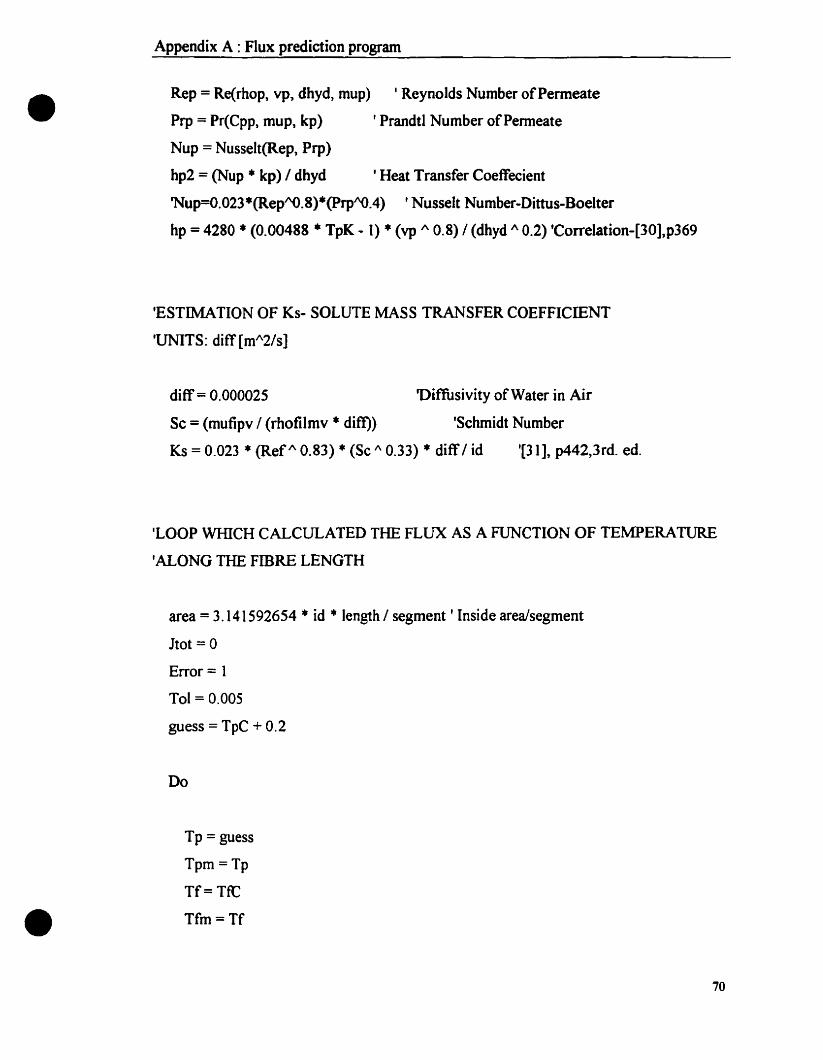
•
•
Appendix A : Flux prediction program
Rep = Re(rhop, vp, dhyd, mup) 'Reynolds Number ofPermeate
Prp = Pr(Cpp, mup, kp) 'Prandtl Number ofPenneate
Nup = Nusselt{Rep, Prp)
hp2 = (Nup * kp) / dhyd ' Beat Transfer Coeffecient
'Nup=O.023*(Rep"O.8)*(Prp"O.4) 'Nusselt Number-Dittus-Boelter
hp = 4280 * (0.00488 * TpK - 1) * (vp " 0.8) 1(dhyd 1\ 0.2) 'Correlation-[30],p369
'ESTIMATION Of Ks- SOLUTE MASS TRANSFER COEFFICIENT
'UNITS: diff [mI\2/s]
diff = 0.000025 'Diffùsivity ofWater in Air
Sc = (mufipv 1(rhofilmv * ditl) 'Schmidt Number
Ks = 0.023 * (Ref" 0.83) * (Sc 1\ 0.33) * diff1id '[31], p442,3rd. ed.
'LOOP WInCH CALCULATED THE FLUX AS A FUNCTION OF TEMPERATURE
'ALONG THE FmRE LENGTH
area = 3.141592654 * id * length 1segment 1 Inside area/segment
ltot = 0
Error = 1
Toi = 0.005
guess = TpC + 0.2
Do
Tp =guess
Tpm =Tp
Tf= TtC
Tfm =Tf
70
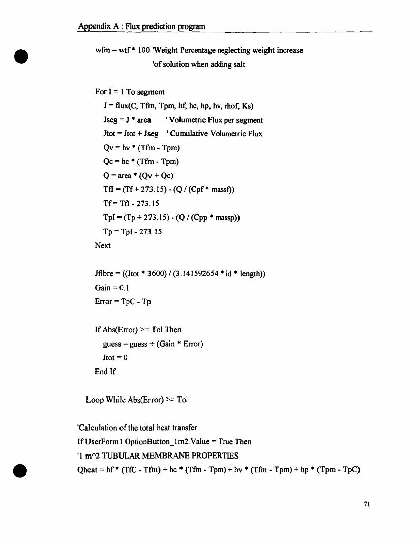
•
•
Appendix A : Flux prediction program
wfm = wtf· 100 'Weight Percentage neglecting weight inerease
'of solution when adding salt
For 1= 1To segment
J = flux(C, Tfm, Tpm, hf, he, hp, hv, rhof, Ks)
Jseg =J. area 'Volumetrie Flux per segment
Jtot =Itot + Jseg 'Cumulative Volumetrie Flux
Qv = hv • (Tfm - Tpm)
Qe = he * (Tfm - Tpm)
Q = area • (Qv + Qe)
Tf1 = (Tf+ 273.15) - (Q / (Cpf* masst)
Tf= Ttl - 273.15
TpI =(Tp + 273.15) - (Q / (Cpp • massp»
Tp = TpI - 273.15
Next
Ifibre = «Itot • 3600) / (3.141592654 * id • length»
Gain =0.1
Error = TpC - Tp
If Abs(Error) >= ToI Then
guess =guess + (Gain * Error)
Itot =0
End If
Loop While Abs(Error) >= Toi
'Caleulation of the total heat transfer
IfUserForm1.0ptionButton_lm2.Value =True Then
'1 mA 2 TUBULAR MEMBRANE PROPERTIES
Qheat =hf· (TtC· Tfm) + he • (Tfm - Tpm) + hv • (Tfm - Tpm) + hp • (Tpm - TpC)
71

•
•
Appendix A : Flux prediction program
ElseIf UserForm1.0ptionButton_2m2.Value = True Then
'2 mA 2 HOLLOW FffiERS MEMBRANE PROPERTIES
Qheat = 2 • (hf· (TtC - Tfm) + he • (Tfm - Tpm) + hv • (Tfm - Tpm) + hp • (Tpm
TpC»
End If
UserForml.Label_Flowrate = Itot • num • 60 • 1000
UserForml.Label_Reynolds_feed = Int(Ret)
UserForm I.Label_Reynolds-perm = Int(Rep)
UserForml.Label_Heattransfer = Int(Qheat)
End Sub
Funetion flux(C_membrane, Tfeedm, Tpermeatm, hconvective, heonduetive,
hconvection, hvapo, rhofeed, Ksolute)
Dim Jprev As Double
pfm = VPf(Tfeedm, wfm)
Ppm = VPp(Tpermeatm)
flux = C_membrane • (pfm - Ppm) • (101325/760)
Jprev = 20
Do While Abs(flux - Jprev) >= 0.0000000005 And flux> 0
Evap = Hvap(Tfeedm) • 1000
hvapo = (flux • Evap) / (Tfeedm - Tpermeatm)
72

•
•
Appendix A : Flux prediction program
Tfeedm = Tf - «Tf - Tp) • (1 / heonvective) / «1 1 (bvapo + hconductive» + (1 /
heonvective) + (11 hconvection»)
Tpermeatrn = Tp + «Tf - Tp) • (1 / hconvection) / «11 (hvapo + hconductive» + (1/
heonvective) + (1 1hconvection»)
Pfrn = VPf(Tfeedm, wfm)
Ppm = VPp(Tpenneatm)
Cfm = cone * Exp(flux 1(rhofeed • Ksolute» , We want the bulk density
wfm = Cfrn • 58.5/ rhofeed • 100
Jprev = flux
flux = C_membrane • (pfrn. Ppm) * (101325/760)
If flux <= 0 Then
flux = 0
End If
Loop
End Function
'FUNCTION WHICH CALCULATES THE REYNOLDS NUMBER
Function Re(rho, v, d, mu)
Re = (rho * v· d) / mu
End Function
'FUNCTION WInCH CALCULATES THE PRANDTL NUMBER
Funetion Pr(Cp, mu, k)
Pr = (Cp * mu) / k
End Function
73
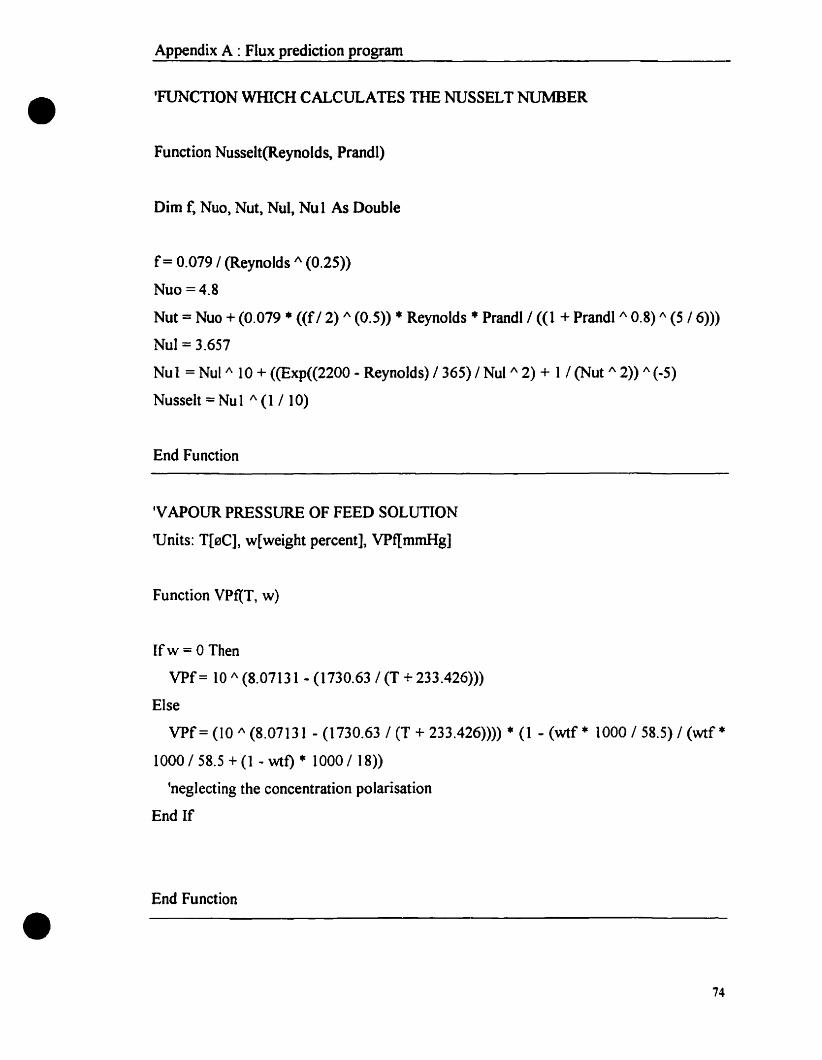
•
•
Appendix A : Flux prediction program
'FUNCTION WInCH CALCULATES THE NUSSELT NUMBER
Functian Nusselt(Reynolds, Prandl)
Dim t: Nua, Nut, Nul, Nu1 As Double
f= 0.0791 (Reynolds /\ (0.25»
Nuo =4.8
Nut =Nuo + (0.079 • «f/ 2) /\ (0.5» • Reynolds • Prandl / «1 + Prandl/\ 0.8) 1\ (5 /6»)
Nul =3.657
Nul = Nul/\ 10 + «Exp«2200 .. Reynolds) /365) / Nul/\ 2) + 1/ (Nut /\ 2» 1\ (-5)
Nusselt = Nul /\ (1/10)
End Function
'VAPOUR PRESSURE OF FEED SOLUTION
Vnits: T[eC], w[weight percent], VPf{mmHg]
Function VPttT, w)
Ifw = 0 Then
VPf= 101\ (8.07131 .. (1730.63 / (T + 233.426»)
Eise
VPf= (10 1\ (8.07131 - (1730.63 / (T + 233.426»» • (1 .. (wtf * 1000/ 58.5) / (wtf *1000/58.5 + (1 .. wti) * 1000 / 18»
'neglecting the concentration polarisation
End If
End Function
74

•
•
Appendix A : Flux prediction program
IVAPOUR PRESSURE OF PERMEATE SOLUTION
'UNlTS: T[0C], VPp[mmHg]
Function VPp(T)
VPp = 10/\ (8.07131 .. (1730.63 / (T + 233.426»)
End Function
'HEAT OF VAPORIZATION OF WATER
'UNlTS: Hvap[kJ/kg], T[0C]
Function Hvap(T)
Hvap =2503.035313 .. (2.430907 * T)
End Function
75

•
•
Appendix B : Experimental data
Appendix B
Experimental data
76

• •
-J.....
Hollow fibre module: DiatJlled water. Re feed=3000 (87Umln) and Re coolinga 800 (40Umln)
Exp. Nb Thot (OCl Tcool(°Cl dT Pv hot (mmHg) Pv cool (mmHg) dPv(mmHg) Flow (g/min) Flux (g/min.m2) Refeed Re coolina10 33.3 26.4 6.9 38.3 25.7 12.5 6.62 3.31 3032 77811 33.45 26 7.45 38.6 25.1 13.5 5.39 2.70 3041 77112 33 25.4 7.6 37.6 24.3 13.4 5.84 2.92 3014 76113 33.2 27.3 5.9 38.1 27.1 10.9 6.49 3.25 3026 79414 32.6 21.3 11.3 36.8 18.9 17.9 8.91 4.46 2989 69315 33.15 24.85 8.3 38.0 23.5 14.5 6.83 3.42 3023 75216 33.1 24.95 8.15 37.8 23.6 14.2 7.30 3.65 3020 75317 31.2 21.2 10 34.0 18.8 15.2 8.24 4.12 2905 69118 31.2 21.3 9.9 34.0 18.9 15.1 8.33 4.17 2905 69319 34 31 3 39.8 33.6 6.2 3.66 1.83 3074 85820 28.8 23.4 5.4 29.6 21.5 8.1 3.84 1.92 2763 72721 33 30.9 2.1 37.6 33.4 4.2 1.96 0.98 3014 85622 28.7 22.6 6.1 29.4 20.5 8.9 3.77 1.89 2757 71423 32.7 22.7 10 37.0 20.6 16.4 8.94 4.47 2995 71624 34 23.2 10.8 39.8 21.3 18.5 8.82 4.41 3074 72425 38.65 28.75 9.9 51.3 29.5 21.8 9.73 4.87 3362 81943 33.2 25.7 7.5 38.1 24.7 13.4 5.70 2.85 3026 76644 33.3 27.1 6.2 38.3 26.8 11.5 5.26 2.63 3032 79045 31.7 22.3 9.4 35.0 20.1 14.8 7.51 3.76 2935 70946 32.5 22.5 10 36.6 20.4 16.2 8.44 4.22 2983 71247 33 30.3 2.7 37.6 32.3 5.3 2.77 1.39 3014 84648 37.05 33.9 3.15 47.1 39.6 7.5 3.70 1.85 3262 910
Hollow fibre module: Distilled water, Re feed=1000 (30Umin) and Re coollng=540 (30Umln)
Exp. Nb Thot (OC) TcooIIOC) dT Pv hot (mmHa) Pv cool (mmHg) dPv(mmHa) Flow (almln) Flux la/min.m2) RefHd Re coollng26 28.7 20 8.7 29.4 17.5 12.0 4.63 2.32 950 50327 29.8 19.4 10.4 31.4 16.8 14.5 5.63 2.82 973 49628 30.7 27.1 3.6 33.0 26.8 6.2 2.68 1.34 991 59229 30.2 22.7 7.5 32.1 20.6 11.5 4.46 2.23 981 53730 31 26.8 4.2 33.6 26.4 7.3 2.48 1.24 997 58931 30.9 25.6 5.3 33.4 24.5 8.9 3.30 1.65 995 57332 31.6 19.1 12.5 34.8 16.5 18.3 7.00 3.50 1010 493
>:gn::s0.sr1:1:'
~"0n:2.3(Il
ae.Q.et~

• •
-...J00
Hollow fibre module : DiatJlled water, Re feed=1000 (30Umin) and Re eoollng=750 (40Umin)
Exp. Nb Thot (OC) leool(OC) dT Pv hot (mmHg) Pv cool (mmHg) dPv(mmHg) Flow (g/min) Flux (g/min.m2) Refeed Re eoollng33 30.3 20.9 9.4 32.3 18.5 13.8 6.51 3.26 983 68634 30.8 25 5.8 33.2 23.7 9.5 4.33 2.17 993 75435 31.4 29.4 2 34.4 30.7 3.7 2.29 1.15 1006 83036 30.4 23.3 7.1 32.5 21.4 11.1 5.39 2.70 985 726
HoUow fibre module: DistJlled water, Re feed=3000 (B7Umin) and Re cooling-400 (20Umin)
Exp. Nb Thot (OC) Tcool(OC) dT Pv hot (mmHg) Pv cool (mmHg) dPv(mmHg) Flow (g/min) Flux (glmln.m2) Refeed Recoollng38 35.2 23.4 11.8 42.5 21.5 21.0 5.60 2.80 3148 36339 35.6 27.4 8.2 43.5 27.3 16.2 4.24 2.12 3172 39740 35.8 29.8 6 44.0 31.4 12.6 2.77 1.39 3185 41841 36.9 28.1 8.8 46.7 28.4 18.3 4.40 2.20 3253 40342 31.5 26.7 4.8 34.6 26.2 8.4 2.34 1.17 2941 395
Hollow fibre module: Diatilled water, Re feed=670 (20Umin) and Re eooling=750 (40Umin)
Exp. Nb Thot (OC) Teool(OC) dT Pv hot (mmHg) Pv cool (mmHg) dPv(mmHg) Flow (g/min) Flux (g/mln.m2) Refeed Re eoollng50 31.3 24.3 7 34.2 22.7 11.5 5.05 2.53 669 74251 30.8 20.5 10.3 33.2 18.0 15.2 6.90 3.45 662 68052 31.8 29 2.8 35.2 30.0 5.2 2.80 1.40 676 82353 31.6 27.2 4.4 34.8 27.0 7.8 3.56 1.78 673 792
HoUow fibre module: Diatilled water, Re feed=1000 (30Umln) and Re cooling=400 (20Umin)
Exp. Nb Thot (OCl Teool(°Cl dT Pv hot (mmHg) Pv cool (mmHg) dPv(mmHa) Flow (almln) Flux (glmin.m2l Refeed Recooling54 31.4 20.6 10.8 34.4 18.1 16.2 4.16 2.08 1006 34055 31.3 19 12.3 34.2 16.4 17.8 4.75 2.38 1004 32756 32.3 29.3 3 36.2 30.5 5.7 1.06 0.53 1024 41457 32 27.5 4.5 35.6 27.5 8.1 2.09 1.05 1018 39858 34 29 5 39.8 30.0 9.8 1.75 0.88 1060 411
~"g&.)<'CO
m~tD::J.gste.c..a~

• •
......'0
Hollow fibre module: Distilled water, Re feed=400 (12Umlnt and Re cooling=750 (40Umlnt
Exp. Nb Thot (OC) Tcool(OCt dT Pv hot (mmHgt Pv cool (mmHg) dPv (mmHg) Flow (aImln) Flux (glmin.m2) Refeed Re cooling59 34 30.7 3.3 39.8 33.0 6.8 2.43 1.22 424 85360 32.2 25.8 6.4 36.0 24.8 11.1 4.51 2.26 409 76861 32 24.3 7.7 35.6 22.7 12.9 5.86 2.93 407 74262 31.9 21.5 10.4 35.4 19.2 16.2 6.82 3.41 406 696
Holtow fibre module: Dlstilled water, Re feed=3000 (87Umln) and Re coollng=1200 (&OUmln)
Exp. Nb Thot (OC) Tcool(OC) dT Pv hot (mmHg) Pv cool (mmHa) dPv(mmHg) Flow (g/mln) Flux (glmln.m2) Refeed Re coollng63 31.85 27 4.85 35.3 26.7 8.6 6.70 3.35 2944 118364 33.2 28.2 5 38.1 28.6 9.5 7.68 3.84 3026 121465 35.7 30.8 4.9 43.7 33.2 10.5 8.53 4.27 3179 128266 28.9 25.2 3.7 29.8 24.0 5.8 4.42 2.21 2769 1137
Hollow fibre module: Dlatilled water, Re feed=3000 (87Umln) and Re coollng-2200 (110Umln)
Exp. Nb Thot (OC) Tcool(OC) dT Pv hot (mmHg) Pv cool (mmHg) dPv(mmHg) Flow (Dlmln) Flux (glmln.m2) Refeed Re coollng67 28.9 26.7 2.2 29.8 26.2 3.6 3.70 1.85 2769 215568 28.9 25.7 3.2 29.8 24.7 5.1 5.25 2.63 2769 210869 31.3 28.1 3.2 34.2 28.4 5.8 6.17 3.09 2911 222170 33.6 30.3 3.3 38.9 32.3 6.6 6.90 3.45 3050 2327
Hollow fibre module: Distilled water, Re feed=3000 (87Umln) and Re cooling=1&OO (80Umln)
Exp. Nb Thot (DC) Tcool(OC) dT Pv hot (mmHg~1 Pv_cool (mmHg) dPv(mmHg) Flow tg/min) Flux (glmln.m2) Re feed Re coollng71 30 27 3 31.7 26.7 5.1 5.00 2.50 2834 157772 29.7 25.8 3.9 31.2 24.8 6.4 6.37 3.19 2816 153673 32.5 28.7 3.8 36.6 29.4 7.1 7.31 3.66 2983 163674 29.7 27.7 2 31.2 27.8 3.4 3.05 1.53 2816 1601
~"0~
6x'CD
~~
::J.ensae.Cl.ePo'

• •
!
HoUow fibre module: 3.4 wt..l. NaCl t Re feed=3000 (87Umin) and Re coollng=2300 (110Umin)
Exp. Nb Thot (OC) Tcool(OC) dT Pv hot (mmHg) Pv cool (mmHg) dPv (mmHg) Flow (g/mln) Flux (g/mln.m2) Refeed Re coollng77 33.2 30.05 3.15 38.1 31.8 6.2 6.05 3.03 2934 231578 35.2 32 3.2 42.5 35.6 7.0 7.17 3.59 3053 241079 36.9 33.75 3.15 46.7 39.2 7.4 7.35 3.68 3155 249680 30.2 27.1 3.1 32.1 26.8 5.3 4.84 2.42 2760 2174
~"'CtD
s..~.
0'
m~~:J.B~af!.Q.a~
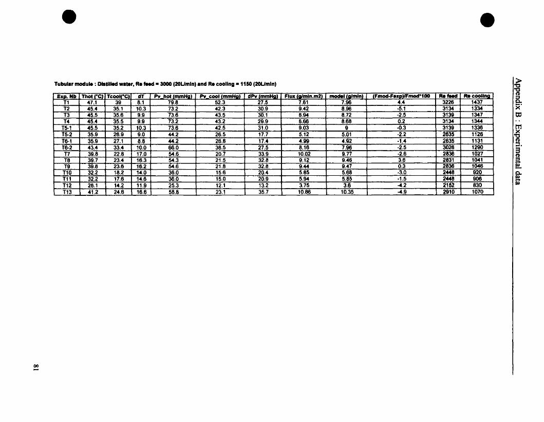
• •
oc-
Tubul.r module: Dlatilleci Wlter, R. fMd. 3000 (20Umln) and R. coollng -1150 (20Umln)
EXD.Nb Thot '-C) TcooU-Ct dT Pv hot frrunHa) po, cooflmmkilf dPv'mmHa) Flux 'glrnln.m2) modellalmlnt ,Fmod-F.xDUFmocr100 RefHd Re coollnciTl 47.1 39 8.1 79.8 52.3 27.5 7.61 7.96 4.4 3226 1437T2 45.4 35.1 10.3 73.2 42.3 30.9 9.42 8.96 ·5.1 3134 1334T3 45.5 35.6 9.9 73.6 43.5 30.1 8.94 8.72 -2.5 3139 1347T4 45.4 35.5 9.9 73.2 43.2 29.9 8.66 8.68 0.2 3134 1344
T5-1 45.5 35.2 10.3 73.6 42.5 31.0 9.03 9 .0.3 3139 1336T5-2 35.9 26.9 9.0 44.2 26.5 17.7 5.12 5.01 -2.2 2635 1126T6-1 35.9 27.1 8.8 44.2 26.8 17.4 4.99 4.92 -1.4 2635 1131T6-2 43.4 33.4 10.0 66.0 38.5 27.5 8.16 7.96 -2.5 3026 1290TI 39.8 22.8 17.0 54.6 20.7 33.9 10.02 9.77 -2.6 2836 1027T8 39.7 23.4 16.3 54.3 21.5 32.8 9.12 9.46 3.6 2831 1041T9 39.8 23.6 16.2 54.6 21.8 32.8 9.44 9.47 0.3 2836 1046
T10 32.2 18.2 14.0 36.0 15.6 20.4 5.85 5.68 -3.0 2448 920T11 32.2 17.6 14.6 36.0 15.0 20.9 5.94 5.85 -1.5 2448 906T12 26.1 14.2 11.9 25.3 12.1 13.2 3.75 3.6 ~.2 2152 830T13 41.2 24.6 16.6 58.8 23.1 35.7 10.86 10.35 ~.9 2910 1070
~'g::sQ..
~rte
tr1>C
"0QS'na~Q..a~

•
•
Appendix C : Calculation samples
Appendix C
Calculation samples
82

•
•
Appendix C : Calculation samples
Theoretical models calculatioDs
For the following experimental conditions (experiment Tubular-lO) and membrane
characteristics :
• Tfced=305.35 K, feed temperature
• Tcooling=291.35, cooling temperature
• APv=2720 Pa, vapour pressure difference
• P=I01325 Pa, pore pressure
• d=0.2 J.1rn, pore diameter
• e=0.75, membrane porosity
• 'F1.3, membrane tortuosity
• ôm=OA mm, membrane thickness (hollow fibre unit)
• J.1=1.85*IO·s Pa.s, viscosity ofwater vapour at 30°C [23]
Water mo.ecu.es mes" Cree path :
À = 3f.1/P [1tRT/(8M)fl2
À = 3* 1.85* 10·s/l01325*[7t*8.314*305.35/8/(18* 10.3)]112
À == 0.13 J.1m
Diffusion coefficient (231 :
Dwa = 0.010 13*305.351.7S*(1/18+1/28.86)112 / [101325*(20.1 1/3 + 12.i13 )2]
Dwa == 2.62*10·s m2/s
83

•
•
Appendix C : Calculation sampies
Knudsen diffusion:
1= 2/3 re / t [8M/(1tRT)]tl2 &P/ôm
1 = 2/3*0.1 *10-6*0.75/1.3*[S*18*10·3/8.314/305.35ht]1/2 * 2720/(0.4*10.3)
J == 1.11*10.3 kg/m2.s
Molecular diffusion:
NA = 0.75*2.62*] O·s* 101325*ln[(760-15.6)/(760.36)]/8.314/305.35/1.3/(0.4* 10.3)
NA == 0.042 mol/m2.s
Hagen-Poiseuille viscous now :
J = 1/8*(0.1· 10-6)2*0.75/1.3/1.85*} O·S. 18* 10.3*101325/8.314/305.35*2720/(0.4* 10.3)
J == 1.90*10-4 kg/m2.s·1
84