Embed Size (px)
Citation preview

Information Uncertainty and Expected Returns
GUOHUA JIANG
Guanghua School of Management, Peking University
CHARLES M. C. LEE* [email protected]
Johnson Graduate School of Management, Cornell University
YI ZHANG
Barclays Global Investors, 45 Fremont Street, San Francisco, CA, 94105
Abstract. This study examines the role of information uncertainty (IU) in predicting cross-sectional stock
returns. We define IU in terms of ‘‘value ambiguity,’’ or the precision with which firm value can be
estimated by knowledgeable investors at reasonable cost. Using several different proxies for IU, we show
that (1) on average, high-IU firms earn lower future returns (the ‘‘mean’’ effect), and (2) price and earnings
momentum effects are much stronger among high-IU firms (the ‘‘interaction’’ effect). These findings are
consistent with analytical models in which high IU exacerbates investor overconfidence and limits rational
arbitrage.
Keywords: behavioral finance, cross-sectional returns, information uncertainty, risk
JEL Classification: G12, G14, M41
This study examines the relation between information uncertainty (IU) and cross-sectional stock returns. By information uncertainty, we do not mean informationasymmetry, such that some agents know more about a firm’s value than others.Rather, we define IU in terms of ‘‘value ambiguity,’’ or the degree to which a firm’svalue can be reasonably estimated by even the most knowledgeable investors atreasonable costs. By this definition, high-IU firms are companies whose expectedcash flows are less ‘‘knowable,’’ perhaps due to the nature of their business oroperating environment. These firms are associated with higher information acqui-sition costs, and estimates of their fundamental value are inherently less reliable andmore volatile.Information uncertainty (IU), as we define it, is at the heart of a number of
curiously consistent findings in empirical finance that are difficult to reconcile withtraditional asset pricing models. Specifically, prior studies have found that firms withhigher volatility, higher volume (i.e., turnover), greater expected growth, higherprice-to-book (PB) ratios, wider dispersion in analyst earnings forecasts, and longerimplied duration in their future cash flows, all earn lower subsequent returns.1 Al-though various explanations have been proposed for these phenomena, it is also true
*Corresponding author.
Review of Accounting Studies, 10, 185–221, 2005
� 2005 Springer Science+Business Media, Inc., Manufactured in The Netherlands.

that in each instance, firms operating in higher IU environments are observed to earnlower future returns.These empirical results are puzzling because in standard CAPM or multi-factor
asset pricing models, non-systematic risk is not priced, and various IU proxiesshould have no ability to predict future returns. More recently, some analyticalpapers have argued in favor of a role for information risk in asset pricing (e.g.,Easley and O’Hara, 2003). But even in these models, the directional prediction is thathigher IU should be associated with higher information risk or greater informationacquisition costs, and therefore higher (not lower) expected returns.In this study, we present and empirically evaluate a theory of information
uncertainty that not only predicts a negative relation between IU and average ex-pected returns (the ‘‘mean’’ effect), but also predicts a relation between IU and themagnitude of the price and earnings momentum phenomena (an ‘‘interaction’’ ef-fect). Specifically, this theory predicts that high-IU firms will exhibit strongermomentum effects—that is, a strategy of buying recent winners and selling recentlosers will yield higher trading profits among high-IU firms.Our analysis is rooted in recent theoretical work in behavioral finance.
According to behavioral finance theory, market mispricings arise when two con-ditions are met: (1) an uninformed demand shock, and (2) a limit on arbitrage.2
Our two-part thesis is that the level of information uncertainty is positively cor-related with a particular form of decision bias (investor overconfidence), and that itis also positively correlated with arbitrage costs. Collectively, these two effectsconspire to produce lower mean returns and greater momentum profits amonghigh-IU firms.In the overconfidence literature (e.g., Odean, 1998; Daniel et al., 1998, 2001),
otherwise rational investors overestimate the precision of their information signals.DHS (1998), in particular, features a model in which investors overweight the valueof their private signals, and place inadequate weight on the information content ofimportant public events, such as earnings releases and past stock returns. Theirmodel, therefore, nominates investor overconfidence as a driving force behindmarket anomalies that feature post-event continuation of stock returns—e.g., thepost-earnings announcement drift (Bernard and Thomas, 1990).Building on this concept, we argue that the overconfidence bias is accentuated in
high-IU settings, where firm values are nebulous even to the most knowledgeableinvestors. With greater value ambiguity, investors will trade more aggressively ontheir private signals. More importantly, if pessimistic investors are kept out of themarket, even partially, by asymmetric costs associated with short-selling (Miller,1977), the prices of high-IU firms will reflect the excess optimism of the investorswith the highest private valuations. As the excess optimism incorporated in the priceof high-IU firms are corrected over time, these firms will earn lower returns in futureperiods.3
Our premise is that the degree to which the overconfidence bias affects returns willvary in a predictable manner across stocks with differing degrees of informationuncertainty. In higher IU firms, investors’ private valuations are more diffused andsolid feedback on the quality of their private signal is more difficult to obtain. Thus
JIANG ET AL.186

emboldened, investors in high-IU firms tend to overweight their private signals, andplace too little weight on public news and news about firm fundamentals. As a result,two empirical phenomena emerge: (1) high-IU firms tend to be over-priced, thusearning lower future returns; and (2) high-IU firms will exhibit greater price andearnings momentum effects.Another important feature of a high-IU environment is that informational arbi-
trage will be more difficult to implement among these firms. The literature on limitsto arbitrage identifies three types of costs facing would-be arbitrageurs: (1) infor-mation costs, (2) trading costs, and (3) holding costs.4 With greater IU, rationaltraders face elevated information acquisition and processing costs, as well as higherrisks associated with noisier value estimates.5 At the same time, trading costs(associated with entering and exiting a position) and holding costs (associated withrisk exposure while holding a position) are also generally higher for high-IU firms.We argue that increased arbitrage costs also contribute to greater price and earningsmomentum effects among higher IU-firms.Our empirical analyses examine the two main predictions of this theory: that is, the
‘‘mean’’ and ‘‘interaction’’ effects of IU on future returns. Specifically, we use fourbroadly available variables to proxy for information uncertainty: the age of the firm(Firm Age), return volatility (Volatility), average daily turnover (Volume), and theduration of its future cash flows (Duration).6 Based on the preceding discussion, weexpect younger firms, firms with higher returns volatility, greater trading volume, andlonger duration cashflows, tohavehigher IU.Wealso combine these variables to createcomposite portfolios that feature two, three, or all four of these IU characteristics.Consistent with prior studies, we find that younger firms, firms with higher vol-
atility, firms with higher turnover, and firms with higher cash flow duration, all earnlower returns. Interestingly, we show that the ‘‘mean’’ effect is not typically mono-tonic across the IU portfolios. Firms in the highest IU deciles (young firms, volatilefirms, firms with high turnover, and firms with long duration cash flows) earnsharply lower returns, while firms in the other nine IU portfolios tend to have fairlysimilar returns. In particular, low-IU firms do not generally earn significantly higherfuture returns.7 In fact, we show that the average underperformance of young,volatile, and high-volume firms reported in earlier studies is concentrated almostentirely in the most extreme high-IU decile. These results are strikingly consistentwith the Miller (1977) argument that short-sell related factors play an important rolein the lower returns earned by high-IU firms. In low-IU portfolios, where short-selling arguments do not apply, firms earn normal returns.We also document a strong ‘‘interaction’’ effect between IU and the profitability of
momentum strategies. In these tests, we define price momentum in terms of recentreturns, and earnings momentum in terms of average monthly revisions in analysts’earnings forecasts over the past quarter. For all four IU proxies, we find that returnson hedge (winner–loser) portfolios are much higher for high-IU firms. The results areeven sharper when we use composite measures of IU that combine two, three, or allfour IU proxies.We find similar results for both price momentum and earnings momentum
strategies. Among low-IU firms, price momentum strategies based on extreme
INFORMATION UNCERTAINTY AND EXPECTED RETURNS 187

quintiles earn average monthly returns that range from )0.10 to 0.27%. Among high-IU firms, the same momentum strategies produce average monthly returns of 1.26 to1.82%. Similarly, when firms are sorted on the basis of recent changes in analystforecast revisions, a strategy of buying positive revision stocks and shorting negativerevision stocks yields average monthly returns of 0.77–1.30% for low-IU firms, and1.94–2.66% for high-IU firms. Unlike the ‘‘mean’’ effect, this ‘‘interaction’’ effect isquite symmetrical—that is, momentum profits are sharply lower in low-IU firms,and are sharply higher in high-IU firms.Risk-based explanations do not appear to account for these findings. The standard
risk adjustments based on time-series (Fama and French, 1993) and cross-sectional(Fama and MacBeth, 1973) methodologies have little effect on these results.Moreover, a substantial portion of the returns earned by momentum strategies inhigh-IU firms is realized in short-windows around subsequent earnings announce-ments. This pattern is not observed among low-IU firms.Further analysis shows that the concentration of high (and low) IU firms varies by
industry. In general, the following industries have a large proportion of firms in thehigh-IU category (2-digit SIC code in parentheses): Business Services (73), HealthServices (80), Electronic Equipment (36), Engineering, Research and ConsultingServices (87), Home Furnishings Stores (57), Automotive Repairs (75), IndustrialMachinery and Computer Equipment (35), Eateries (58), Educational Services (82),and Recreational Services (79). In short, service providers and technology-orientedfirms are heavily represented in the high-IU category.In the other extreme, the following industries have relatively few firms in the high-
IU category: Tobacco Products (21), Utilities (49), Railroads (40), Furniture Makers(25), Banks (60), Food Stores (54), Nonmetal Minerals (14), Stone, Clay, Glass andConcrete Products (32), Paper Products (26), and Food Products (20). In short,utilities, transportation-related, basic materials and capital goods companies tend tobe under-represented in the high-IU category.Collectively, our findings support the view that market pricing dynamics, and
therefore the cross-section of expected returns, vary systematically according to thelevel of information uncertainty. On average, high-IU firms earn lower returns.Moreover, in high-IU environments, with greater value ambiguity, stocks exhibitstronger positive serial correlation in returns (i.e., price momentum), and the slug-gish price adjustment to the release of earnings news (i.e., earning momentum) ismuch more pronounced.
1. Hypotheses Development
Our two-part thesis is that the level of information uncertainty is positively corre-lated with a particular form of decision bias (investor overconfidence), and that it isalso positively correlated with arbitrage costs. In this section, we develop thesehypotheses and link our work to prior studies.
JIANG ET AL.188

1.1. Overconfidence and Information Uncertainty
Overconfidence is arguably the single most universal and well-documented behav-ioral bias in cognitive psychology. A large body of experimental evidence supportsthe view that individuals are overconfident about the precision of their own infor-mation (see Odean, 1998 and references therein). Psychologists also find that peoplesystematically overweight some types of information (e.g., more salient, less reliable)and underweight others (e.g., more abstract, statistical evidence).8 More recently,several theoretical models of investor behavior nominate overconfidence as thedriving force behind a host of empirical market anomalies, such as excessive vola-tility and trading volume, sluggish price adjustment to public news events, andpredictable patterns in cross-sectional returns (see Odean, 1998; DHS, 1998, 2001).None of these models, however, discusses explicitly the probable effect of informa-tion uncertainty on investor overconfidence.We argue that investor overconfidence is accentuated in high-IU settings. We base
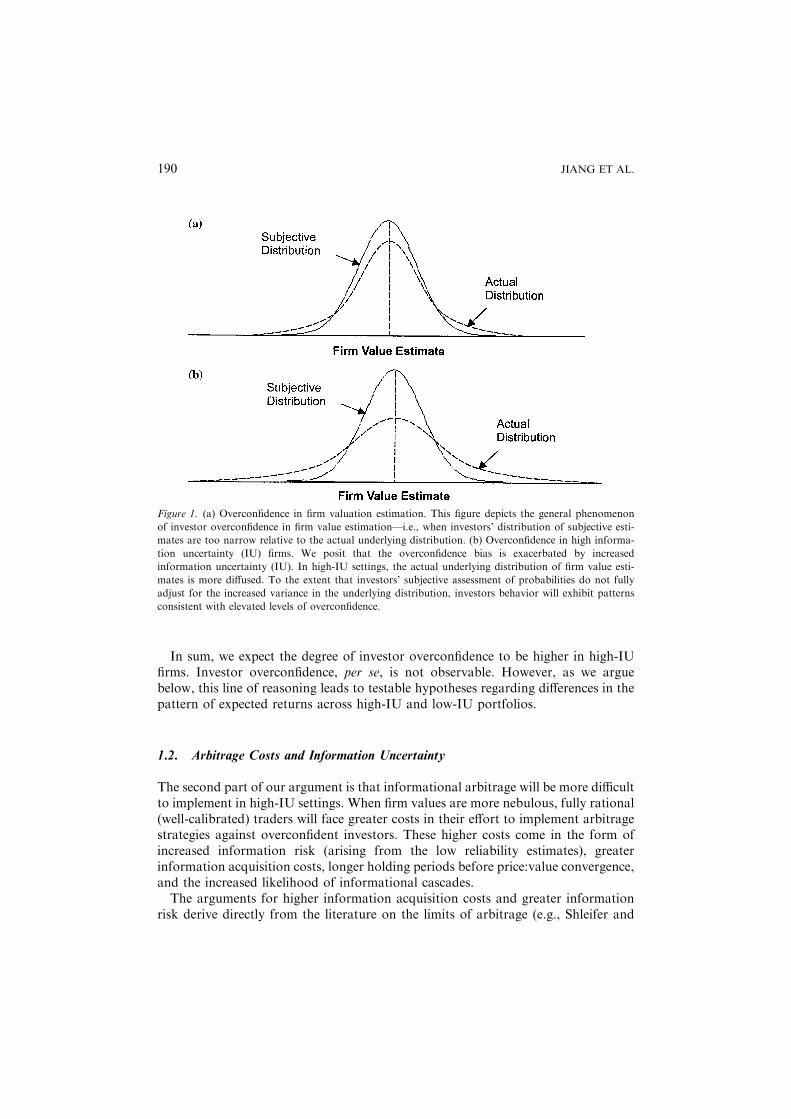
this argument on three observations. First, with greater value ambiguity, we expect agreater difference between subjective and actual distributions of firm value estimates.Figure 1 illustrates this phenomenon. Figure 1a presents the standard statisticalrepresentation of overconfidence, where the distribution of individuals’ subjectivevalue estimates is too narrow compared to the actual underlying distribution. Inhigh-IU settings, the true distribution of value estimates is more diffused, with widervariance (Figure 1b). Based on prior experimental evidence, we posit that investorsdo not adjust sufficiently for systematic changes in the IU environment across firms.Consequently, we expect investors to exhibit behavior consistent with greateroverconfidence in high-IU settings.Second, with higher IU, the quality of investor’s private signals is more difficult to
assess, and solid feedback is more difficult to obtain, thus minimizing the discipliningbenefits of trading experience. In other words, learning is a more difficult and pro-tracted exercise in high-IU settings.9 Finally, high-IU firms tend to be ‘‘story stocks,’’in which public signals about firm value are noisy, and by comparison private signalsappear more plausible. In these stocks, investors’ propensity to speculate is fueled byrumors and innuendos that have the cloak of legitimacy. Thus, extending thearguments in DHS (1998), we expect investors in higher-IU settings to overweighttheir own private (more salient) signals and underweight the (more abstract andstatistical) public information contained in past returns and earnings news.10
In an early study, Miller (1977) predicts that firms with a greater divergence ofopinions will earn lower returns. Miller based his argument on a combination ofoverconfidence bias and market frictions. Noting that private valuations are morediverse in high-IU firms, Miller reasons that if pessimistic investors are kept out ofthe market, even partially, by asymmetric costs associated with short-selling, theprices of high-IU firms will reflect the excess optimism of the investors with thehighest private valuations. As the excess optimism incorporated in the price of high-IU firms is corrected over time, these firms will earn lower returns in future periods.11
Our argument is an extension of the Miller (1977) proposition that predicts an‘‘interaction’’ effect with the momentum phenomenon.
INFORMATION UNCERTAINTY AND EXPECTED RETURNS 189
In sum, we expect the degree of investor overconfidence to be higher in high-IUfirms. Investor overconfidence, per se, is not observable. However, as we arguebelow, this line of reasoning leads to testable hypotheses regarding differences in thepattern of expected returns across high-IU and low-IU portfolios.
1.2. Arbitrage Costs and Information Uncertainty
The second part of our argument is that informational arbitrage will be more difficultto implement in high-IU settings. When firm values are more nebulous, fully rational(well-calibrated) traders will face greater costs in their effort to implement arbitragestrategies against overconfident investors. These higher costs come in the form ofincreased information risk (arising from the low reliability estimates), greaterinformation acquisition costs, longer holding periods before price:value convergence,and the increased likelihood of informational cascades.The arguments for higher information acquisition costs and greater information
risk derive directly from the literature on the limits of arbitrage (e.g., Shleifer and
Figure 1. (a) Overconfidence in firm valuation estimation. This figure depicts the general phenomenon
of investor overconfidence in firm value estimation—i.e., when investors’ distribution of subjective esti-
mates are too narrow relative to the actual underlying distribution. (b) Overconfidence in high informa-
tion uncertainty (IU) firms. We posit that the overconfidence bias is exacerbated by increased
information uncertainty (IU). In high-IU settings, the actual underlying distribution of firm value esti-
mates is more diffused. To the extent that investors’ subjective assessment of probabilities do not fully
adjust for the increased variance in the underlying distribution, investors behavior will exhibit patterns
consistent with elevated levels of overconfidence.
JIANG ET AL.190

Vishny, 1997; Mitchel et al., 2002; Barberis and Thaler, 2003). In high-IU settingsrational arbitrageurs face higher information acquisition and analysis costs and theireventual value estimates are less reliable, rendering their strategies more risky. Inaddition, when fundamental value is uncertain, the process of price convergence tovalue is more likely to be protracted, adding to the costs of maintaining the arbitrageposition.12
The arguments associated with informational cascades merit further elaboration.In their classic analysis of these cascades, Bikchandani et al. (1992) show that wheneach individual receives a noisy private signal, it is often optimal to follow thebehavior of the preceding traders without regard to his or her own information. Intheir model, the likelihood of an incorrect cascade is a function of the precision ofeach individual’s private signal—i.e., incorrect cascades are much more frequentwhen individuals receive noisy (low precision) signals. Therefore, their model sug-gests that in high-IU settings, incorrect pricing due to informational cascades ismuch more likely to occur.We assert that adaptive behavior by rational arbitrageurs can contribute to the
momentum effect in high-IU settings. When valuation is uncertain, rational arbit-rageurs will reduce the weight they place on their private fundamental signals, andupdate more quickly in the direction of other traders. In other words, in high-IUfirms, rational arbitrageurs will engage in a form of positive feedback trading (De-long et al., 1990) to compensate for the noisy nature of their own signals.13 As aresult, rather than helping to correct mispricings, the actions of rational investorscan in fact cause prices to diverge even further from fundamental values. The greaterfrequency of cascades is another source of increased arbitrage cost for high-IUfirms.14
In sum, we argue that when firm value is highly uncertain (i.e., when estimates offirm value are susceptible to wide swings over time), future returns will be charac-terized by two important empirical regularities: (1) lower average returns (the‘‘mean’’ effect); and (2) increased momentum profits (the ‘‘interaction’’ effect). Thesepredictions derive from elevated levels of investor confidence, as well as from in-creased costs associated with rational arbitrage. Our empirical analysis tests bothpredictions.After we completed our work, we became aware of a study by Zhang (2004), which
also examines the role of information uncertainty and its effects on stock return.Much of the motivation for his paper, and most of his results, are similar to ours.However, there are several interesting differences in research design and empiricalfindings.In terms of research design differences, Zhang uses a slightly different set of IU
proxies—specifically, he uses firm size, analyst coverage, the dispersion in analystforecasts, and cash flow volatility; but he does not use cash flow duration or tradingvolume. Some of Zhang’s IU measures are arguably more closely aligned with theunderlying economic construct. However, a potential disadvantage of these measuresis that they are only available for firms that have analyst coverage. As a result, hissample is smaller and more confined than ours (i.e. it reflects larger firms, and islimited to more recent time periods).
INFORMATION UNCERTAINTY AND EXPECTED RETURNS 191

In terms of empirical results, Zhang (2004) also finds greater IU produces rel-atively lower future returns following bad news, and relatively higher future returnsfollowing good news. In other words, his results show that momentum strategieswork better among high-IU stocks. His study also documents a ‘‘mean’’ effect, butthe difference in returns between high-IU firms and low-IU firms in that study isnot statistically significant. Comparing his study to ours, Zhang attributes thisdifference to the shorter sample period in his study, and his focus on near-termreturns.Overall, the results in Zhang (2004) complement the results in this paper; together,
the two studies present a consistent set of empirical facts that link informationuncertainty to cross-sectional returns.15
2. Sample and Methodology
Our sample consists of all firms listed on the NYSE, the AMEX and the NAS-DAQ during the period January 1965 through December 2001 with at least oneyear of data prior to the portfolio formation date. We exclude all closed-end funds,REIT, ADR, and foreign companies. To mitigate illiquidity concerns, we alsoeliminate any firm-month where the company’s market capitalization as of theportfolio formation date is less than 150 million in year 2001 dollars (adjusted forinflation).At the beginning of each event month t, we compute four information uncertainty
(IU) proxies as follows. Firm Age is defined as the number of months between eventmonth t and the first month that a stock appears in CRSP (Zhang, 2004 uses thesame proxy).16 Return volatility (Volatility) is defined as the standard deviation ofdaily returns of past 25 trading days.17 Trading volume (Volume) is defined as theaverage daily turnover in percentage over the past six months, where daily turnoveris the ratio of the number of shares traded each day to the number of shares out-standing at the end of the day.18 Duration is a measure of implied equity durationderived from financial statement data and the current stock price, using the meth-odology and estimation procedures developed in Dechow et al. (2004)—seeAppendix A for details.To compute the Duration measure, we also require firms to have several
financial variables available from COMPUSTAT. Specifically, we require bookvalue of equity (Compustat Data Item 60), Earnings (Item 18), Sales (Item 12)and Market Capitalization (Item 199 · Item 25). We use financial data from themost recent fiscal year end that ended at least four months before the portfolioformation date to ensure this information is publicly available at the beginning ofevent month t.We also compute two momentum variables using data publicly available at the
beginning of each event month. Our price momentum measure is simply the rawreturns for each firm over the past J months (J=3, 6, 9, 12). To avoid potentialmicrostructure biases, we impose a one-week lag between the end of the portfolioformation period (J) and the beginning of the performance measurement period (K
JIANG ET AL.192

months, K=3, 6, 9, 12). Because our results are robust to different time horizons, weonly report a subset of these findings (for J=6, and K=6, 12).Our measure of earnings momentum is the average revision in the analysts’
consensus forecast over the past three months, each scaled by end-of-month price.Specifically, we compute our earnings momentum measure for firm i in month tas
REVi;t ¼X3
j¼0
revi;t�jpi;t�j�1
where revi,t is the change in the consensus FY1 earnings forecasts in month t for firmi. Our results are quite similar if we use revisions computed over the past one or sixmonths, rather than the 3-month horizon.19
From January 1965 to December 2001, we rank stocks independently at thebeginning of the month using each of these four IU characteristics (Firm Age,Volatility, Volume, and Duration), as well as on the two momentum variables. Theintersections resulting from these two-way independent sorts give rise to our port-folios of interest. Most of our analysis focuses on the monthly returns of the extremewinner and loser portfolios over the next K months (K=6, 12).Similar to Jegadeesh and Titman (1993), the monthly return for a K-month
holding period is based on an equal-weighted average of portfolio returns fromstrategies implemented in the current month and the previous K)1 months. Forexample, the monthly return for a three-month holding period is based on an equal-weighted average of portfolio returns from this month’s strategy, last month’sstrategy, and the strategy from two months ago. This is equivalent to revising theweights of (approximately) one-third of the portfolio each month and carrying overthe rest from the previous month. The technique allows us to use simple t-statisticsfor monthly returns.Table 1 presents summary statistics for the four information uncertainty variables,
as well as the pairwise correlations between them. Panel A reports that the mean(median) age of the firms in our sample is 224 (159) months, the mean (median)volatility is 0.023 (0.020), the mean (median) average daily turnover is 0.382 (0.206),and the mean (median) duration is 15.54 (15.92) years. The number of firm-monthobservations for the first three IU variables ranges between 757,638 and 791,250. Asexpected, the number of firm-month observations drops (to 580,375) for the Dura-tion variable, reflecting its more stringent data requirements.Panel B shows that the four IU variables are correlated in the expected directions.
Younger firms tend to have higher volatility, greater turnover, and longer durationcash flows. However, the correlation between Age and the other three variables is notoverwhelming—i.e., range between )0.160 and )0.282. Volume and volatility aremore highly correlated (0.455 and 0.480), but generally these levels of pairwisecorrelation indicate that each IU measure is capable of providing independentinformation relative to the others.
INFORMATION UNCERTAINTY AND EXPECTED RETURNS 193

3. Empirical Results
3.1. The Mean Effect of Information Uncertainty
Table 2 reports the average monthly return to portfolios formed on each of the fourinformation uncertainty proxies. To construct this table, we calculate these variablesfor each sample firm at the beginning of every month. Starting in January 1965, eachmonth we sort all stocks using one of the four IU proxies into 10 equal-weightedportfolios. Table values represent the average monthly return for each portfolio overthe next K months, where K=6 or 12. The numbers in parentheses represent simpletime-series t-statistics for the average monthly returns.Table 2 shows that high-IU firms generally earn lower average returns over the
next six to twelve months. For example, panel A shows that firms in the youngestdecile earn average monthly returns of 0.89% over the next six months. This issignificantly ()0.23%) lower than the average monthly returns earned by the oldest
Table 1. Summary statistics.
Panel A: Summary statistics for Information Uncertainty (IU) variables
Number of
firm-months Mean 10%
Lower
quartile Median
Upper
quartile 90%
Standard
deviation
Firm Age 791,250 224 33 69 159 317 534 198
Volatility 791,250 0.023 0.010 0.014 0.020 0.028 0.040 0.016
Volume 757,638 0.382 0.050 0.097 0.206 0.421 0.854 0.633
Duration 580,375 15.541 11.969 14.189 15.917 17.204 18.234 3.076
Panel B: Pairwise correlations between Information Uncertainty (IU) cariables
Firm age Volatility Trading volume Duration
Firm Age – )0.229 )0.181 )0.160Volatility )0.282 – 0.455 0.272
Volume )0.196 0.480 – 0.271
Duration )0.221 0.315 0.339 –
This table presents summary statistics for the key variables used in this paper. Our sample consists of all
firms listed on NYSE/AMEX/NASDAQ between 1965 and 2001, excluding closed-end funds, REIT,
ADR, and foreign companies. In addition, we exclude any firm whose market capitalization as of the
portfolio formation date is less than $150 million in year 2001 dollars (adjusting for inflation), as well as
any firm with less than 12 months of past returns data on CRSP. At the beginning of each event month t,
we compute the following information uncertainty (IU) variables for each firm: Firm Age is defined as the
number of months between event month t and the first month that a stock appears in CRSP; Volatility is
defined as the standard deviation of daily returns for the past 25 trading days; and Volume is defined as the
average daily turnover in percentage over the past six months, where daily turnover is the ratio of the
number of shares traded each day to the number of shares outstanding at the end of the day. Duration is a
measure of how long in years it takes for the price of a stock to be repaid by its internal cash flows (see
Appendix A for details). In Panel B, Pearson correlation coefficients are shown above the diagonal, while
Spearman correlation coefficients are shown below the diagonal. All correlation coefficients are significant
at 1% level.
JIANG ET AL.194

Table
2.Returnsto
Inform
ationUncertainty
Portfolios.
Panel
A:Monthly
Returnsto
Firm
AgePortfolios
V1(O
ldest)
V2
V3
V4
V5
V6
V7
V8
V9
V10(Y
oungest)
V10–V1
K=
61.11(15.90)
1.25(16.66)1.11(14.72)1.18(14.97)1.22(14.63)1.19(13.77)1.14(11.42)1.20(11.82)0.99(9.94)
0.89(8.17)
)0.23()3.46)
K=
121.11(24.88)
1.25(25.21)1.10(23.23)1.17(23.59)1.22(23.41)1.21(21.88)1.12(17.10)1.12(17.87)0.98(15.26)0.80(15.02)
)0.31()6.38)
Panel
B:Monthly
Returnsto
Volatility
Portfolios
V1(Lowest)
V2
V3
V4
V5
V6
V7
V8
V9
V10(H
ighest)
V10–V1
K=
61.09(16.73)
1.16(16.87)1.20(16.69)1.23(16.55)1.24(15.67)1.25(14.92)1.23(13.30)1.16(11.36)1.02(8.76)
0.62(4.65)
)0.47()4.36)
K=
121.10(23.94)
1.15(25.12)1.17(24.61)1.20(24.88)1.21(23.88)1.21(22.59)1.18(20.31)1.12(17.22)1.01(13.60)0.67(7.96)
)0.43()5.62)
Panel
C:Monthly
Returnsto
TradingVolumePortfolios
V1(Lowest)
V2
V3
V4
V5
V6
V7
V8
V9
V10(H
ighest)
V10–V1
K=
61.20(17.80)
1.19(17.04)1.18(16.55)1.19(16.10)1.18(15.26)1.17(13.99)1.15(12.55)1.14(11.55)1.10(9.87)
0.83(6.58)
)0.37()3.87)
K=
121.21(26.60)
1.16(24.99)1.17(25.68)1.17(25.26)1.16(23.46)1.16(21.75)1.12(19.06)1.12(17.19)1.06(14.43)0.82(10.15)
)0.39()5.95)
Panel
D:Monthly
Returnsto
DurationPortfolios
V1(Lowest)
V2
V3
V4
V5
V6
V7
V8
V9
V10(H
ighest)
V10–V1
K=
61.57(17.66)
1.42(17.83)1.31(17.43)1.25(17.05)1.20(15.11)1.16(14.52)1.12(13.29)1.11(12.76)1.04(11.18)0.96(8.27)
)0.61()6.98)
K=
121.53(26.09)
1.40(27.00)1.31(26.93)1.23(25.92)1.18(23.50)1.13(21.80)1.11(20.25)1.05(18.92)0.97(16.22)0.90(12.16)
)0.63()10.28)
Thistablepresentsaveragemonthly
returnsto
portfoliosform
edonfourinform
ationuncertainty
(IU)proxies.See
Table
1foradescriptionofthesampleand
fordefinitionsofthefourIU
variables.Startingin
January
of1965,each
month
wesort
allstocksusingoneofthefourIU
proxiesinto
10equal-weighted
portfolios,anddocumenttheaveragemonthly
returnsover
thenextK
months,
whereK=
6or12.Toavoid
serial-correlationproblemsin
computingtest
statistics,monthly
holdingperiodreturnsare
defined
astheequal-weightedaverageofreturnsfrom
strategiesinitiatedatthebeginningofthismonth
andthe
past
K)1months.Thenumbersin
parentheses
representsimple
time-series
t-statisticsfortheaveragemonthly
returns.
INFORMATION UNCERTAINTY AND EXPECTED RETURNS 195

decile firms. However, the relation between Firm Age and returns is not monotonicacross the 10 portfolios. The most striking pattern is that the youngest firms (i.e.deciles 9 and 10) tend to underperform all other firms.A similar pattern is observed when firms are sorted on Volatility or Volume. High
volatility firms earn lower returns than low volatility firms (panel B). Similarly, highturnover firms earn lower returns than low turnover firms (panel C). Thesedifferences (V10–V1) range from )0.37% to )0.47% per month, and appear both
Table 3. Average monthly returns to portfolios based on Information Uncertainty (IU) and price
momentum.
Portfolio
Average monthly returns
Average number of
observations
V1 V2 V3 V3–V1 V1 V2 V3
Panel A: Portfolios based on firm age and past price momentum
R1 0.85 (8.10) 0.57 (5.18) 0.19 (1.63) )0.66 ()11.48) 44 58 76
R5 1.15 (16.12) 1.18 (14.88) 1.00 (11.26) )0.15 ()3.66) 70 58 50
R10 1.43 (15.75) 1.63 (14.80) 1.80 (14.40) 0.36 (6.32) 35 60 83
R10–R1 0.58 (7.50) 1.06 (13.42) 1.60 (18.94) 1.02 (16.57)
Panel B: Portfolios based on volatility and past price momentum
R1 0.95 (10.23) 0.80 (7.97) 0.21 (1.69) )0.74 ()10.63) 23 47 107
R5 1.17 (16.45) 1.22 (14.90) 0.86 (7.99) )0.31 ()4.36) 80 60 37
R10 1.46 (19.59) 1.79 (18.54) 1.64 (12.38) 0.17 (2.05) 25 46 106
R10–R1 0.51 (8.38) 0.99 (16.00) 1.43 (17.94) 0.92 (15.04)
Panel C: Portfolios based on trading volume and past price momentum
R1 0.74 (7.89) 0.51 (4.86) 0.27 (2.20) )0.48 ()9.11) 33 48 90
R5 1.19 (17.29) 1.15 (14.61) 0.98 (9.40) )0.21 ()2.24) 74 59 38
R10 1.58 (17.17) 1.72 (16.59) 1.66 (13.38) 0.08 (1.01) 25 44 100
R10–R1 0.84 (10.58) 1.20 (14.97) 1.40 (17.36) 0.56 (8.60)
Panel D: Portfolios based on duration and past price momentum
R1 1.04 (9.12) 1.13 (10.57) 0.53 (4.78) )0.50 ()8.60) 27 35 59
R5 1.40 (18.24) 1.10 (14.50) 0.92 (10.50) )0.49 ()8.35) 51 48 36
R10 1.81 (18.67) 1.74 (15.83) 1.88 (14.78) 0.08 (1.12) 35 34 54
R10–R1 0.77 (9.95) 0.61 (6.97) 1.35 (15.79) 0.58 (9.24)
This table presents average monthly returns to portfolios formed by independent two-way sorts on
information uncertainty proxies and past returns. See Table 1 for a description of the sample and for
definitions of the four IU variables. At the beginning of each month, stocks are sorted based on an IU
proxy into three equal-weighted portfolios, and independently sorted on past six-month returns into 10
portfolios. To avoid potential microstructure biases, we compute past returns after imposing a one-week
lag. V3 represents the highest IU portfolio (young, high volatility, high volume or high duration), while V1
represents the lowest IU portfolio (old, low volatility, low volume or low duration). R1 represents the loser
portfolio and R10 represents the winner portfolio. Table values are the average monthly return for each
portfolio over the next six months. The portfolio returns for each month is computed as an equal-weighted
average of returns from strategies initiated at the end of each of the past six months. The t-statistics in
parentheses are simple t-statistics for monthly returns. The three columns on the right report the average
number of firms per month in each sub-portfolio.
JIANG ET AL.196

statistically and economically significant. Interestingly, the effect is again asym-metric. In each case, the returns for the highest IU (high volatility or high volume)decile is distinctly lower than the returns for the other deciles; but we do not find asymmetrical increase in the returns of the low-IU portfolios. These findings arestrikingly consistent with the Miller (1977) argument that short-selling constraintsplay an important role in the lower returns earned by firms with divergent privatevaluations.Like the first three IU measures, the mean effect for Duration is in the expected
direction. Specifically, panel D shows high duration fines underperform low durationfirms by an average of 0.61–0.63% per month. This mean effect is stronger than theeffect observed for the other three variables. However, average returns across theDuration deciles are monotonic, and do not fit the pattern predicted by the IUhypothesis. One possible explanation is that duration is not a pure IU proxy—i.e.,high duration firms are also ‘‘glamour’’ stocks and low duration firms are also‘‘value’’ stocks. Thus, part of the higher returns to low duration stocks might be dueto general under-pricing of value firms.
3.2. Interaction with Price Momentum
Table 3 presents average monthly returns to portfolios formed by independent two-way sorts on information uncertainty proxies and past returns. To construct thistable, stocks are sorted at the beginning of each month on each IU variable, anddivided into three equal-weighted portfolios; we also independently sort stocks onpast six-month returns into 10 portfolios (after imposing a one-week lag). V3represents the highest IU portfolio (young, high volatility, high volume, or longduration), while V1 represents the lowest IU portfolio (old, low volatility, lowvolume, or short duration). R1 represents the loser portfolio and R10 represents thewinner portfolio. Table values are the average monthly return for each portfolioover the next six months (results are similar for 3, 9, and 12 month holding peri-ods). The portfolio return for each month is computed as an equal-weightedaverage of returns from strategies initiated at the end of each of the past sixmonths. The t-statistics in parentheses are simple t-statistics for monthly returns.The columns on the right report the average number of firms per month in eachsub-portfolio.This table reveals two striking patterns. First, the mean effect of IU is largely
driven by losers (R1–R5 stocks). This is evident by examining the V3–V1 column.The underperformance of young, volatile, high turnover, and long duration firms issignificant for R1 and R5, but is not evident in R10. Thus, consistent with Miller(1977), the mean effect associated with IU variables is only exploitable by eithershorting or underweighting high-IU stocks. Little can be gained by buying low-IUfirms. Indeed, among winners (R10 stocks), we find that high-IU firms actuallyoutperform low-IU firms in all four panels.
INFORMATION UNCERTAINTY AND EXPECTED RETURNS 197

Second, this table shows that the momentum effect (R10–R1) is much stronger forhigh-IU firms. Among younger firms (V3 by Age), losers earn 0.19% per month andwinners earn 1.80%, resulting in a momentum hedge return of 1.60% per month.Among older firms (V1 by Age), the return to the R10–R1 portfolio is only 0.58%per month. Thus, the momentum effect is almost three times as large among youngfirms. A similar pattern is observed for volatility, volume, and duration. In each case,returns to a momentum strategy are significantly larger for high-IU firms. The dif-ference appears economically significant, and ranges from 0.56% to 1.02% permonth.Because these sorts are conducted independently, a possible concern is that the
results are based on insufficient number of firms in the extreme cells. The right-hand-side columns address this issue. These table values represent the average number offirms per month in each sub-portfolio. For example, a strategy of buying youngwinners and shorting young losers would involve an average of 76 firms on the shortside and 83 firms on the long side. A similar high-IU momentum strategy wouldinvolve 106 firms long and 107 firms short for volatility; 100 longs and 90 shorts forvolume; and 54 long and 59 shorts for duration. These seem to be reasonableportfolio sizes, suggesting that our results are not due to a few unusual firms.Recognizing that each of the four IU proxies is unlikely to fully capture the
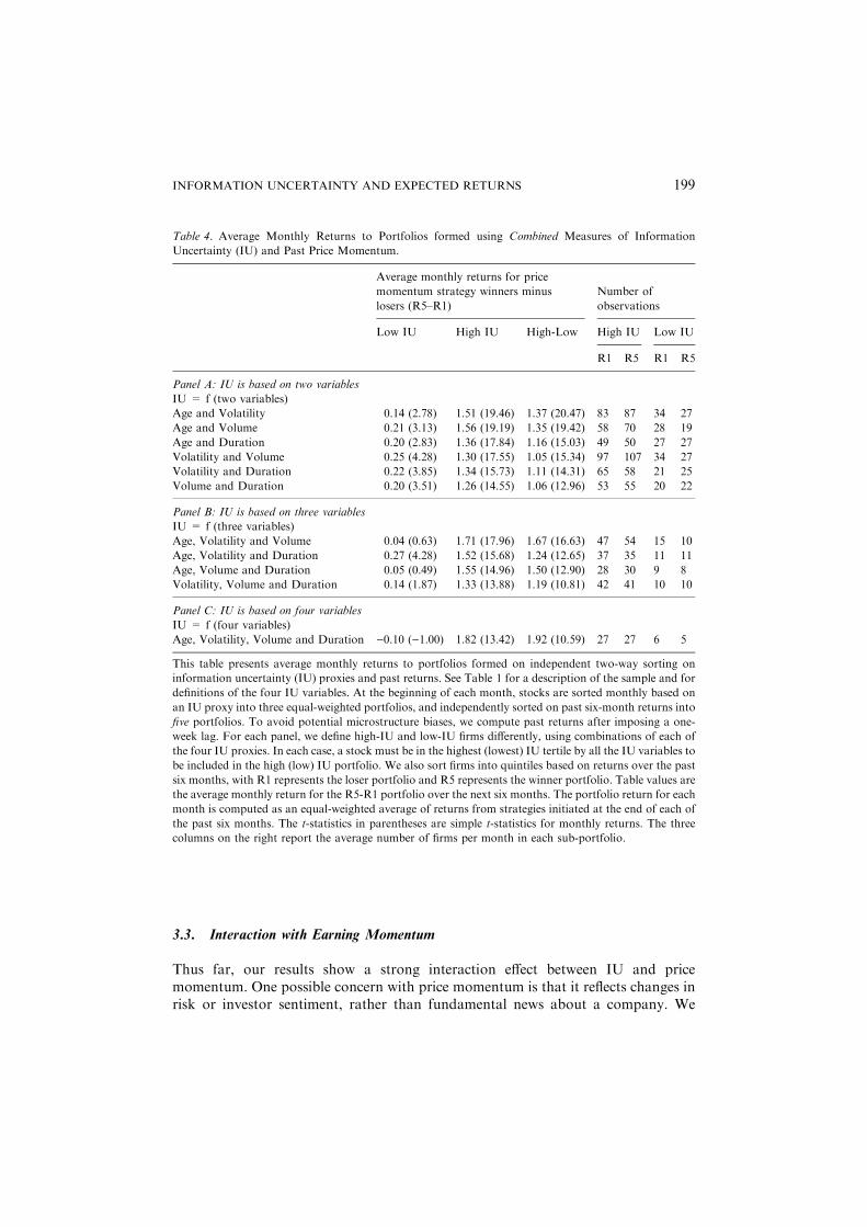
theoretical construct we have in mind, Table 4 reports results using combined mea-sures of IU—i.e., IU portfolios formed on the basis of two or more of the four IUproxies. In panel A, membership in the high-IU (low-IU) portfolio is defined usingtwo IU variables. For example, in the first row, we report results when IU = f(FirmAge and Volatility). In other words, a firm is deemed to be high-IU (low-IU) if it is inthe upper-(lower-) third by both Age and Volatility. The second row repeats theprocedure with IU defined by Age and Volume.In panel B, we report results when membership in High and Low IU portfolios is
based on three IU variables—i.e., a firm must be in the upper (or lower) tertile bythree IU measures. In panel C, we define IU in terms of all four variables. To ensurea sufficient number of firms for each sub-portfolio, we sort stocks into just fivemomentum portfolios, with R1 representing the loser portfolio and R5 representingthe winner. Table values represent average monthly returns for price momentumstrategies (R5–R1), with simple time-series t-statistics reported in parentheses. Theaverage number of firms in each extreme sub-portfolio (R1 or R5) is reported in theright side of each panel.Table 4 results show that the patterns observed using single IU measures simply
become stronger when we define IU using more than one proxy. In all three panels,the momentum effect (R5–R1) is much stronger for high-IU portfolios. In fact, ahigh-IU momentum strategy yields average monthly returns that range from 1.26%(panel A: IU = volume + duration) to 1.82% (panel C: IU = age + vol-ume + volatility + duration). The difference in momentum profits between high-IU and low-IU firms range between 1.05% and 1.92% per month—results that aretwo to three times larger than when IU was defined using only one empirical mea-sure. The average number of firms per high-IU portfolio range from 27 to 107,suggesting that these are reasonably sized portfolios.
JIANG ET AL.198
3.3. Interaction with Earning Momentum
Thus far, our results show a strong interaction effect between IU and pricemomentum. One possible concern with price momentum is that it reflects changes inrisk or investor sentiment, rather than fundamental news about a company. We
Table 4. Average Monthly Returns to Portfolios formed using Combined Measures of Information
Uncertainty (IU) and Past Price Momentum.
Average monthly returns for price
momentum strategy winners minus
losers (R5–R1)
Number of
observations
Low IU High IU High-Low High IU Low IU
R1 R5 R1 R5
Panel A: IU is based on two variables
IU = f (two variables)
Age and Volatility 0.14 (2.78) 1.51 (19.46) 1.37 (20.47) 83 87 34 27
Age and Volume 0.21 (3.13) 1.56 (19.19) 1.35 (19.42) 58 70 28 19
Age and Duration 0.20 (2.83) 1.36 (17.84) 1.16 (15.03) 49 50 27 27
Volatility and Volume 0.25 (4.28) 1.30 (17.55) 1.05 (15.34) 97 107 34 27
Volatility and Duration 0.22 (3.85) 1.34 (15.73) 1.11 (14.31) 65 58 21 25
Volume and Duration 0.20 (3.51) 1.26 (14.55) 1.06 (12.96) 53 55 20 22
Panel B: IU is based on three variables
IU = f (three variables)
Age, Volatility and Volume 0.04 (0.63) 1.71 (17.96) 1.67 (16.63) 47 54 15 10
Age, Volatility and Duration 0.27 (4.28) 1.52 (15.68) 1.24 (12.65) 37 35 11 11
Age, Volume and Duration 0.05 (0.49) 1.55 (14.96) 1.50 (12.90) 28 30 9 8
Volatility, Volume and Duration 0.14 (1.87) 1.33 (13.88) 1.19 (10.81) 42 41 10 10
Panel C: IU is based on four variables
IU = f (four variables)
Age, Volatility, Volume and Duration )0.10 ()1.00) 1.82 (13.42) 1.92 (10.59) 27 27 6 5
This table presents average monthly returns to portfolios formed on independent two-way sorting on
information uncertainty (IU) proxies and past returns. See Table 1 for a description of the sample and for
definitions of the four IU variables. At the beginning of each month, stocks are sorted monthly based on
an IU proxy into three equal-weighted portfolios, and independently sorted on past six-month returns into
five portfolios. To avoid potential microstructure biases, we compute past returns after imposing a one-
week lag. For each panel, we define high-IU and low-IU firms differently, using combinations of each of
the four IU proxies. In each case, a stock must be in the highest (lowest) IU tertile by all the IU variables to
be included in the high (low) IU portfolio. We also sort firms into quintiles based on returns over the past
six months, with R1 represents the loser portfolio and R5 represents the winner portfolio. Table values are
the average monthly return for the R5-R1 portfolio over the next six months. The portfolio return for each
month is computed as an equal-weighted average of returns from strategies initiated at the end of each of
the past six months. The t-statistics in parentheses are simple t-statistics for monthly returns. The three
columns on the right report the average number of firms per month in each sub-portfolio.
INFORMATION UNCERTAINTY AND EXPECTED RETURNS 199

address this issue by examining the interaction between IU and earnings momentum(defined by recent changes in the consensus FY1 forecast).Table 5 reports average monthly returns to combined measures of IU and port-
folios formed on earnings momentum. The construction of this table is analogous tothat of Table 4, except we form momentum quintile portfolios using the analyst
g p
Table 5. Average monthly returns to portfolios gormed using combined measures of information
uncertainty (IU) and past earnings momentum.
Average monthly returns for darnings
momentum strategy: winners minus
losers (R5–R1)
Number of
observations
Low IU High IU High-Low High IU Low IU
R1 R5 R1 R5
Panel A: IU is based on two variables
IU = f (two variables)
Age and Volatility 0.99 (22.21) 2.36 (35.52) 1.37 (17.91) 61 51 32 35
Age and Volume 1.02 (18.64) 2.55 (32.52) 1.53 (18.52) 42 40 25 26
Age and Duration 0.84 (15.38) 2.15 (28.53) 1.31 (15.10) 31 31 37 35
Volatility and Volume 1.30 (34.99) 2.19 (31.70) 0.89 (12.21) 77 63 28 38
Volatility and Duration 1.03 (25.71) 1.94 (29.65) 0.91 (12.80) 44 37 29 38
Volume and Duration 1.22 (23.90) 2.10 (26.66) 0.88 (10.40) 36 34 28 35
Panel B: IU is based on three variables
IU = f (three variables)
Age, Volatility and Volume 0.99 (18.89) 2.66 (26.96) 1.67 (16.16) 33 28 13 14
Age, Volatility and Duration 0.79 (14.97) 2.21 (24.59) 1.42 (13.01) 23 21 15 16
Age, Volume and Duration 0.81 (10.98) 2.55 (23.11) 1.74 (14.84) 17 16 11 12
Volatility Volume and Duration 1.14 (24.51) 2.23 (23.60) 1.08 (10.68) 27 23 13 18
Panel C: IU is based on four variables
IU = f (four variables)
Age, Volatility, Volume and Duration 0.77 (11.97) 2.51 (19.74) 1.74 (12.82) 15 13 6 8
This table presents average monthly returns to portfolios formed on independent two-way sorting on
information uncertainty (IU) proxies and earnings momentum. We define earnings momentum in terms of
the average monthly revision in the analysts’ consensus FY1 earnings forecast over the past three months,
each scaled by the end-of-month price. See Table 1 for a description of the sample and for definitions of
the four IU variables. In addition, the firm must have analysts’ consensus FY1 earnings forecasts in past
three months on I/B/E/S. At the beginning of each month, stocks are sorted monthly based on an IU
proxy into three equal-weighted portfolios, and independently sorted on cumulative price-deflated revi-
sions in the past three months into five portfolios. For each panel, we define high-IU and low-IU firms
differently, using combinations of each of the time IU proxies. In each case, a stock must be in the highest
(lowest) IU portfolio by all the IU variables to be included in the high (low) IU portfolio. We also sort
firms into quintiles based on earnings momentum, with R1 representing the loser portfolio and R5
represents the winner portfolio. Table values are the average monthly return for the R5–R1 portfolio over
the next six months, The portfolio returns for each month is computed as an equal-weighted average of
returns from strategies initiated at the end of each of the past sixmonths. The t-statistics in parentheses are
simple t-statistics for monthly returns.
JIANG ET AL.200

revision variable, revit, defined earlier. In this table, R5 (winners) are firms with themost positive revisions over the past three months, and R1 (losers) are firms withthe most negative revisions over the past three months. Table values represent theaverage monthly returns to earnings momentum strategies (R5–Rl) in different IUsub-portfolios.Table 5 results show that IU variables also have a strong interaction effect with
earnings momentum—i.e., hedge returns to analyst revision strategies are muchstronger for high-IU firms than for low-IU firms. Overall, earnings momentumstrategies seem to produce higher returns than price momentum strategies in oursample (this result holds for both high and low-IU firms). The returns to earningsmomentum strategies (R5–R1) in high-IU firms are particularly striking, rangingfrom 1.94% per month to 2.66% per month. Returns to earnings momentum strat-egies in low-IU firms, while also significant, are much more muted at 0.77–1.30% per
Figure 2. Average monthly returns to portfolios formed using combined measures of information
uncertainty (IU) and past price momentum. This figure depicts average monthly returns to portfolios
formed by independent two-way sorting on information uncertainty (IU) proxies and past returns. At
the beginning of each month, we compute the following information uncertainty (IU) variables for each
firm: Firm Age, Volatility, and Volume, as defined in Table 1, At the beginning of each month, stocks
are sorted based on an IU proxy into three equal-weighted portfolios, and independently sorted on
past six-month returns into five portfolios. A stock must be in the highest (lowest) IU portfolio by all
the IU variables to be included in the high (low) IU portfolio. R1 represents the loser portfolio and R5
represents the winner portfolio. We compute the average monthly return for each portfolio over the
next six months. The portfolio returns for each month is computed as an equal-weighted average of re-
turns from strategies initiated at the end of each of the past six months.
INFORMATION UNCERTAINTY AND EXPECTED RETURNS 201

month. The difference in profitability between high and low-IU firms is highly sig-nificant in every partition. The number of firms in each sub-portfolio is muchsmaller, due to the requirement that all firms have analyst coverage. Nevertheless,even in the most constrained sample (panel D: IU = f (four variables)), the longportfolio averaged 13 stocks per month and the short portfolio averaged 15 stocks.Figures 2 and 3 provide a graphical summary of these results. These figures
present the average monthly returns to portfolios formed by independent two-waysorts on IU and momentum. We use a combined measure of information uncertaintythat incorporates three of the four IU proxies (IU = V + V + A).20 Each IUvariable is used to sort firms into three tertiles, and high-IU firms are defined as thosein the top tertile of each IU proxy. We also independently sort firms into quintiles byeither price momentum (Figure 2) or earnings momentum (Figure 3). In both figuresR5 represents winner portfolios and R1 represents loser portfolios.
Figure 3. Average monthly returns to portfolios formed using combined measures of information
uncertainty (IU) and earnings momentum. This figure depicts average monthly returns to portfolios
formed by independent two-way sorting on information uncertainty (IU) proxies and past analysts’
earnings forecast revisions. At the beginning of each month, we compute the following information
uncertainty (IU) variables for each firm: Firm Age, Volatility, and Volume, as defined in Table 1. At the
beginning of each month, stocks are sorted based on an IU proxy into three equal-weighted portfolios,
and independently sorted on cumulative price-deflated revision in the past three months into five port-
folios. A stock must be in the highest (lowest) IU portfolio by all the IU variables to be included in the
high (low) IU portfolio. R1 represents the loser portfolio and R5 represents the winner portfolio. We
compute the average monthly return for each portfolio over the next six months. The portfolio returns
for each month is computed as an equal-weighted average of returns from strategies initiated at the end
of each of the past six months.
JIANG ET AL.202

Table 6. Industry Distribution of Sample.
SIC Industry name
Overall
sample
High IU
(V + V)
% of overall
sample
High IU
(V + V + A)
% of
overall
sample
73 Business Services 38,592 15,116 39.2% 10,557 27.4%
80 Health Services 9,720 3,534 36.4% 2,360 24.3%
36 Electronic/Electrical Equip
and Component (Except
Computer Equip)
44,537 17,188 38.6% 7,987 17.9%
87 Engineering, Accounting,
Research, Management
and Related Services
6,733 1,849 27.5% 1,142 17.0%
57 Home Furniture, Furnishing
and Equipment Stores
2,989 1,221 40.8% 476 15.9%
75 Automotive Repair,
Services and Parking
1,897 494 26.0% 292 15.4%
35 Industrial and Commercial
Machinery and Computer Equipment
47,375 14,789 31.2% 7,250 15.3%
58 Eating and Drinking Places 8,185 2,111 25.8% 1,224 15.0%
82 Educational Services 1,475 344 23.3% 217 14.7%
79 Amusement and Recreation Services 3,481 819 23.5% 506 14.5%
78 Motion Pictures 3,436 1,271 37.0% 418 12.2%
56 Apparel and Accessory Stores 6,730 1,836 27.3% 812 12.1%
70 Hotels, Rooming Houses,
Camps and Other Lodging Places
5,197 1,771 34.1% 621 11.9%
50 Wholesale Trade—Durable Goods 10,773 2,309 21.4% 1,277 11.9%
38 Measuring/Analyzing/Controlling
Instru/Photo/Medical/Optical Goods
24,970 7,357 29.5% 2,863 11.5%
59 Miscellaneous Retail 10,768 2,071 19.2% 1,233 11.5%
61 Non-depository Institutions 7,142 1,770 24.8% 807 11.3%
52 Building Materials, Hardware,
Garden Supply and Mobile
Home Dealers
2,235 468 20.9% 244 10.9%
89 Service, not Elsewhere Classified 1,176 161 13.7% 127 10.8%
45 Transportation by Air 8,546 3,839 44.9% 890 10.4%
13 Oil and Gas Extraction 25,203 6,357 25.2% 2,562 10.2%
48 Communications 21,044 3,492 16.6% 2,066 9.8%
15 Building Construction—General
Contractors and Operative Builders
3,098 736 23.8% 298 9.6%
62 Security and Commodity
Brokers, Dealers,
Exchanges and Services
6,657 1,069 16.1% 596 9.0%
39 Miscellaneous Manufacturing
Industries
6,437 1,391 21.6% 553 8.6%
17 Construction Special
Trades Contractors
1,166 285 24.4% 98 8.4%
01 Agriculture Production-Crops 1,006 158 15.7% 84 8.3%
28 Chemicals and Allied Products 50,913 8,928 17.5% 4,057 8.0%
72 Personal Services 1,998 274 13.7% 157 7.9%
31 Leather and Leather Products 2,366 579 24.5% 184 7.8%
23 Apparel/Other Finished Prod
Made From Fabrics and
Similar Materials
5,943 1,082 18.2% 450 7.6%
INFORMATION UNCERTAINTY AND EXPECTED RETURNS 203
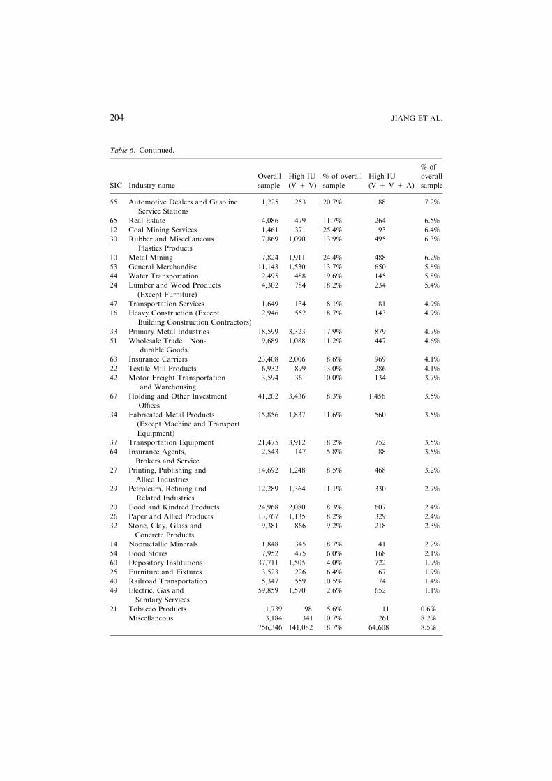
Table 6. Continued.
SIC Industry name
Overall
sample
High IU
(V + V)
% of overall
sample
High IU
(V + V + A)
% of
overall
sample
55 Automotive Dealers and Gasoline
Service Stations
1,225 253 20.7% 88 7.2%
65 Real Estate 4,086 479 11.7% 264 6.5%
12 Coal Mining Services 1,461 371 25.4% 93 6.4%
30 Rubber and Miscellaneous
Plastics Products
7,869 1,090 13.9% 495 6.3%
10 Metal Mining 7,824 1,911 24.4% 488 6.2%
53 General Merchandise 11,143 1,530 13.7% 650 5.8%
44 Water Transportation 2,495 488 19.6% 145 5.8%
24 Lumber and Wood Products
(Except Furniture)
4,302 784 18.2% 234 5.4%
47 Transportation Services 1,649 134 8.1% 81 4.9%
16 Heavy Construction (Except
Building Construction Contractors)
2,946 552 18.7% 143 4.9%
33 Primary Metal Industries 18,599 3,323 17.9% 879 4.7%
51 Wholesale Trade—Non-
durable Goods
9,689 1,088 11.2% 447 4.6%
63 Insurance Carriers 23,408 2,006 8.6% 969 4.1%
22 Textile Mill Products 6,932 899 13.0% 286 4.1%
42 Motor Freight Transportation
and Warehousing
3,594 361 10.0% 134 3.7%
67 Holding and Other Investment
Offices
41,202 3,436 8.3% 1,456 3.5%
34 Fabricated Metal Products
(Except Machine and Transport
Equipment)
15,856 1,837 11.6% 560 3.5%
37 Transportation Equipment 21,475 3,912 18.2% 752 3.5%
64 Insurance Agents,
Brokers and Service
2,543 147 5.8% 88 3.5%
27 Printing, Publishing and
Allied Industries
14,692 1,248 8.5% 468 3.2%
29 Petroleum, Refining and
Related Industries
12,289 1,364 11.1% 330 2.7%
20 Food and Kindred Products 24,968 2,080 8.3% 607 2.4%
26 Paper and Allied Products 13,767 1,135 8.2% 329 2.4%
32 Stone, Clay, Glass and
Concrete Products
9,381 866 9.2% 218 2.3%
14 Nonmetallic Minerals 1,848 345 18.7% 41 2.2%
54 Food Stores 7,952 475 6.0% 168 2.1%
60 Depository Institutions 37,711 1,505 4.0% 722 1.9%
25 Furniture and Fixtures 3,523 226 6.4% 67 1.9%
40 Railroad Transportation 5,347 559 10.5% 74 1.4%
49 Electric, Gas and
Sanitary Services
59,859 1,570 2.6% 652 1.1%
21 Tobacco Products 1,739 98 5.6% 11 0.6%
Miscellaneous 3,184 341 10.7% 261 8.2%
756,346 141,082 18.7% 64,608 8.5%
JIANG ET AL.204

These two figures illustrate: (1) the mean effect, that is, high-IU firms generallyearn lower returns than low-IU firms; and (2) the interaction effect, that is, the returndifference (spread) between R5 and R1 portfolios is much larger for high-IU firms.In the case of price momentum (Figure 2), hedge returns to the momentum strategyare non-existent for low-IU firms (i.e., returns for all five momentum quintiles areessentially the same). In contrast, for the high-IU firms, the effect results in a returnspread of more than 1.70% per month between R5 and R1 firms.In the case of earnings momentum (Figure 3), the post-revision price drift is also
much smaller for low-IU firms than for high-IU firms. In low-IU firms, the post-revision price drift yields an average return spread of 0.99% per month over the nextsix months. For high-IU firms, the same post-revision strategy produces an averagereturn spread of 2.66% per month.
3.4. Industry Distribution by Information Uncertainty
Table 6 provides additional information on the industries that have the highest andlowest concentration of high-IU firms. This table groups all the firm-months in oursample by two-digit SIC codes, and reports the proportion of firm-months in eachindustry that falls into the category of ‘‘high-IU’’. We define ‘‘high-IU’’ in two ways:first, using just volume and volatility (IU = V + V), so that high-IU firms are thosein the upper third by both volume and volatility each month; and second, by threeIU proxies (IU = V+ V + A), so that high-IU firms are those in the upper third byvolume and volatility, and the lower third by age.21 The results for each industry arepresented in descending order according to the concentration of high-IU firms,where high IU is defined using the latter definition (IU = V + V + A).The results show that the concentration of high (and low) IU firms varies quite
widely by industry. In general, the following industries have a large proportion offirms in the high-IU category (2-digit SIC code in parentheses): Business Services
This table presents the number and the percentage of firm-months represented by high-IU stocks for each
industry, defined by two-digit SIC code. Information uncertainty (IU) proxies (Firm Age, Volatility and
Volume) are defined as in Table 1. At the beginning of each month starting January of 1965, all stocks are
independently sorted into three equal-weighted portfolios using each IU variable. We identify two groups
of high-IU firms: (V + V) firms are firms that in the high-IU portfolio as measured by both volume and
volatility, and (V + V + A) firms are firms that are in the high-IU portfolio as measured by three IU
measures: firm age, volatility and volume. We report the proportion of high-IU firms-months by industry,
starting with the highest IU percentage industries as defined using (V + V + A). Our sample consists of
all firms listed on NYSE/AMEX/NASDAQ between 1965 and 2001. We exclude all closed-end funds,
REIT, ADR, and foreign companies. We also exclude firms with a market capitalization of less than
150 million in year 2001 dollars (after adjusted for inflation) as of the portfolio formation date, as well as
any firm with less than 12 months of past returns. Industry groups with less than 1,000 firm-months are
reported in the Miscellaneous category.
INFORMATION UNCERTAINTY AND EXPECTED RETURNS 205

(73), Health Services (80), Electronic Equipment (36), Engineering, Research andConsulting Services (87), Home Furnishings Stores (57), Automotive Repairs (75),Industrial Machinery and Computer Equipment (35), Eateries (58), EducationalServices (82), and Recreational Services (79). In short, service providers and tech-nology-oriented firms are more heavily represented in the high-IU category. Usingthe most stringent definition for high IU (IU = V + V + A), the proportion ofhigh-IU firm-months in these industries range from 14.5% to 27.4%. In terms ofimportance to the overall sample based on total number of observations, BusinessServices (73), Electronics (36) and Industrial and Computer Equipment (35) standout among the high-IU industries.In the other extreme, the following industries have relatively few firms in the high-
IU category: Tobacco Products (21), Utilities (49), Railroads (40), Furniture Makers(25), Banks (60), Food Stores (54), Nonmetal Minerals (14), Stone, Clay, Glass andConcrete Products (32), Paper Products (26), and Food Products (20). In short,utilities, transportation-related, basic materials and capital goods companies tend tobe under-represented in the high-IU category. In terms of importance to the overallsample, Utilities (49) and Banks (60) stand out among the low-IU industries.Collectively, these results suggest that some industries are more momentum-
oriented than others. In industries characterized by high-IU firms, rational arbitragemay call for a greater emphasis on momentum-related signals.
3.5. Risk-Adjustments and Robustness Checks
Thus far the results we have reported do not incorporate additional risk adjustments.In fact, prior studies have demonstrated the resilience of the price momentumphenomenon to the standard multi-factor risk adjustments (e.g., Fama, 1991; Jeg-adeesh and Titman, 1993; Grundy and Martin, 2001). However, we now turn to thisissue to ensure our results are not driven by difference in risk in the long and shortportfolios. We also seek to better understand the risk characteristics of the resultinghedge portfolios.Table 7 reports the result of three-factor (Fama-French, 1993) time-series
regressions of monthly excess returns for various price momentum and IU portfo-lios. For these regressions, we define firms in the high-IU portfolios as firms in thehighest tertile by three measures (young, high volatility, and high volume); low-IUportfolios are firms in the lowest tertile by these measures (old, low volatility, andlow volume). We use returns from the past six months (J=6) to form fivemomentum portfolios, where R1 represents the loser portfolio and R5 represents thewinner portfolio.For each portfolio, we estimate the following three-factor time-series regression:
ri � rf ¼ ai þ biðrm � rfÞ þ siSMBþ hiHMLþ ei ð1Þ
where ri is the return for portfolio i, rm is the return on the NYSE/AMEX/NAS-DAQ value-weighted market index, SMB is the small firm factor, and HML is the
JIANG ET AL.206

Table
7.Three-factorregressionsofmonthly
excess
returnsonprice
momentum-inform
ationuncertainty
portfolios.
Low
IUHighIU
High–
low
Low
IU
High
IU
High–
low
Low
IU
High
IU
High–
low
Low
IUHighIU
High–low
Low
IU
High
IUHigh–low
ab
sh
Adj.R2(%
)
Panel
A:FullSample
(1965–2001)
R1
0.432
(5.81)
)0.693
()5.48)
)1.125
()10.15)
0.141
(7.60)
0.235
(7.43)
0.094
(3.39)
0.065
(2.73)
0.245
(6.01)
0.180
(5.04)
0.132
(4.72)
)0.055
()1.17)
)0.187
()4.50)
15.62
27.54
21.17
R3
0.477
(7.60)
)0.049
()0.37)
)0.526
()4.54)
0.143
(9.13)
0.209
(6.26)
0.066
(2.26)
0.034
(1.67)
0.233
(5.43)
0.200
(5.35)
0.111
(4.74)
)0.127
()2.55)
)0.239
()5.51)
18.87
25.34
22.18
R5
0.510
(6.61)
1.102
(7.56)
0.593
(4.47)
0.127
(6.56)
0.184
(5.04)
0.057
(1.73)
0.055
(2.21)
0.249
(5.29)
0.194
(4.53)
0.042
(1.47)
)0.191
()3.49)
)0.233
()4.69)
12.43
23.64
16.54
R5–R1
0.077
(1.20)
1.796
(18.62)
1.718
(16.66)
)0.015
()0.92)
)0.051
()2.13)
)0.036
()1.41)
)0.011
()0.51)
0.003
(0.11)
0.014
(0.42)
)0.089
()3.68)
)0.136
()3.76)
)0.046
()1.20)
2.65
2.96
0.08
Panel
B:First
Sub-Period(1965–1983)
R1
0.230
(2.05)
)0.714
()3.52)
)0.933
()6.28)
0.148
(5.11)
0.266
(5.11)
0.119
(3.08)
0.064
(1.64)
0.365
(5.19)
0.301
(5.78)
0.031
(0.73)
)0.125
()1.64)
)0.155
()2.75)
17.26
33.76
29.81
R3
0.205
(2.10)
)0.270
()1.25)
)0.475
()2.83)
0.155
(6.17)
0.247
(4.46)
0.092
(2.13)
0.054
(1.61)
0.381
(5.09)
0.326
(5.61)
0.052
(1.40)
)0.190
()2.35)
)0.242
()3.85)
22.29
31.80
28.22
R5
0.361
(2.72)
0.771
(3.51)
0.409
(2.33)
0.147
(4.31)
0.200
(3.54)
0.053
(1.17)
0.084
(1.82)
0.402
(5.27)
0.318
(5.21)
)0.061
()1.23)
)0.176
()2.13)
)0.114
()1.73)
16.43
28.19
18.12
R5
)R1
0.131
(1.29)
1.485
(10.00)
1.353
(8.71)
)0.001
()0.02)
)0.066
()1.74)
)0.066
()1.65)
0.020
(0.56)
0.037
(0.71)
0.017
(0.31)
)0.092
()2.42)
)0.051
()0.91)
)0.041
(0.70)
1.94
0.12
0.70
Panel
C:SecondSub-Period(1984–2001)
R1
0.644
(6.90)
)0.681
()4.45)
)1.326
()8.59)
0.151
(6.32)
0.172
(4.37)
0.020
(0.51)
0.124
(4.01)
0.134
(2.63)
0.010
(0.19)
0.249
(6.54)
)0.099
()1.59)
)0.348
()5.53)
21.77
22.24
20.97
R3
0.741
(9.88)
0.142
(0.90)
)0.599
()3.84)
0.134
(6.96)
0.128
(3.19)
)0.006
()0.14)
0.057
(2.27)
0.107
(2.04)
0.050
(0.96)
0.172
(5.61)
)0.186
()2.91)
)0.358
()5.63)
20.43
21.54
21.88
R5
0.670
(8.45)
1.368
(7.16)
0.697
(3.61)
0.112
(5.49)
0.112
(2.29)
0.001
(0.01)
0.071
(2.69)
0.105
(1.66)
0.034
(0.54)
0.124
(3.84)
)0.309
()3.97)
)0.433
()5.49)
13.86
22.38
20.24
INFORMATION UNCERTAINTY AND EXPECTED RETURNS 207

Table
7.Continued.
Low
IUHighIU
High–
low
Low
IU
High
IU
High–low
Low
IU
High
IU
High–
low
Low
IUHighIU
High–low
Low
IU
High
IUHigh–low
ab
sh
Adj.R2(%
)
R5–R1
0.026
(0.31)
2.049
(16.57)
2.023
(15.09)
)0.040
()1.87)
)0.059
()1.87)
)0.020
()0.57)
)0.053
()1.95)
)0.029
()0.70)
0.025
(0.56)
)0.125
()3.71)
)0.210
()4.17)
)0.085
()1.56)
5.05
7.27
0.75
Thistable
summarizesthree-factorregressionresultsformonthly
returnsonprice
momentum
andinform
ationuncertainty
(IU)portfoliosfor(J=
6,K=
6)
portfoliostrategiesbetweenJanuary
1965andDecem
ber
2001.Wereportresultsforthewholesampleperiodandtw
osub-periods.ThethreeIU
variablesare
defined
asin
Table
1.LowIU
firm
sare
inthelowestIU
portfoliobythreemeasures(old,lowvolatility,andlowvolume)
whilehigh-IU
representthefirm
sin
thehighestIU
portfolio(young,highvolatility,andhighvolume).Weuse
returnsfrom
thepast
sixmonths(J=
6)to
form
five
momentum
portfolios,where
R1represents
theloserportfolioandR5represents
thewinner
portfolio.Thethree-factorregressionisasfollows:r i)r f=ai+
bi(r m
)r f)+
s iSMB+
hiH
ML+e i
wherer m
isthereturn
ontheNYSE/A
MEX/N
ASDAQ
value-weightedmarket
index,SMBisthesm
allfirm
factor,andHMListhevaluefactor.Thenumbers
within
parentheses
representWhiteheteroskedasticitycorrectedt-statistics.
JIANG ET AL.208

value factor. The numbers in parentheses represent White heteroskedasticity cor-rected t-statistics.Panel A reports results for the full sample period (1965–2001). These results show
that high-IU portfolios have slightly higher Betas (see results for b), and are some-what more sensitive to the SMB factor (see results for s). Also, high-IU stocks tendto behave like glamour stocks (i.e., they load negatively on the HML factor), whilelow-IU stocks tend to behave like value stocks (i.e., they have positive HML load-ings). However, the estimated coefficients on the intercept variable (a) show thatthese risk adjustments do little to change the earlier results.Like prior studies (e.g., Grundy and Martin, 2001), we find that price momentum
profits are generally sharper (strong in magnitude with larger t-statistics) aftercontrolling for other risk factors. We show that the mean negative performance ofhigh-IU firms is largely in the loser (R1–R3) portfolios, and that the effect actuallyreverses for winners. Also, the interaction effects we find earlier between IU andmomentum is clearly evident in this table. Momentum profits (R5–R1) for high-IUfirms average 1.796% per month, while they are an insignificant 0.077% per monthfor low-IU firms.Panels B and C report test results for the two sub-periods (1965–1983 and
1984–2001). These tables show that the same pattern holds in both halves of oursample. In fact, the mean effect and the interaction effect of IU are both stronger inthe second half of the sample period. For the period 1984–2001, momentum profitsin high-IU firms average 2.049% per month, compared to 0.026% per month forlow-IU firms. The difference in momentum profits between high and low-IU firms is,in fact, over 2% per month.Table 8 reports results of the same three-factor regressions using earnings
momentum to form winner and loser portfolios. Compared to Table 7, these resultsshow that the IU-hedge (high IU minus low IU) portfolios have no significantmarket (b) or size (s) exposure. However, these portfolios do tend to load negativelyon the book-to-market factor (h). More importantly, these risk adjustments actuallyincrease the abnormal returns (a) earned by earnings momentum strategies inhigh-IU firms to an average of 2.754% per month. Once again, the results arestronger in the second sub-period.As a further test, we also conduct cross-sectional (Fam-MacBeth, 1973 type)
regressions of stock returns on various firm characteristics. For this test, Size isdefined as market capitalization at the beginning of the month; book-to-market ratio(BM) is book value of equity of the previous fiscal year divided by beginning-of-month market capitalization; price momentum (J6) is the average monthly returns inthe six months before the beginning of the current month and earnings momentum(REV3) is the average forecast revision in the analyst consensus over the past threemonths.In these tests, IU is a dummy variable denoting information uncertainty, which is
defined differently for each set of regressions. In the first set of regressions for eachpanel, high-IU and low-IU firms are defined in terms of both volume and volatility(IU = volatility + volume). For the second set of regressions in each panel,
INFORMATION UNCERTAINTY AND EXPECTED RETURNS 209

Table
8.Three-FactorRegressionsofMonthly
Excess
ReturnsonEarningsMomentum–Inform
ationUncertainty
Portfolios.
Low
IU
High
IU
High
–low
Low
IUHighIU
High
–low
Low
IU
High
IU
High
–low
Low
IUHighIU
High
–low
Low
IU
High
IU
High
–low
ab
sh
Adj.R2(%
)
Panel
A:FullSample
(1977–2001)
R1
0.099
(1.20)
)0.855
()6.35)
)0.955
()7.82)
0.151
(7.27)
0.175
(5.19)
0.025
(0.80)
0.094
(3.51)
0.138
(3.17)
0.044
(1.12)
0.175
(5.57)
)0.087
()1.69)
)0.261
()5.64)
17.45
21.39
18.08
R3
0.637
(10.03)
0.574
(3.74)
)0.063
()0.42)
0.116
(7.26)
0.131
(3.41)
0.015
(0.41)
0.023
(1.140)
0.113
(2.28)
0.090
(1.83)
0.97
(4.01)
)0.225
()3.86)
)0.322
()5.61)
14.65
21.01
18.67
R5
1.138
(18.37)
1.898
(11.37)
0.760
(4.77)
0.116
(7.50)
0.157
(3.75)
0.041
(1.02)
0.053
(2.63)
0.053
(0.98)
)0.000
()0.00)
0.122
(5.17)
)0.276
()4.35)
)0.398
()6.58)
16.93
21.43
20.89
R5–R1
1.038
(19.40)
2.754
(28.11)
1.715
(16.43)
)0.034
()2.54)
)0.018
()0.73)
0.016
(0.61)
)0.041
()2.37)
)0.085
()2.69)
)0.044
()1.31)
)0.053
()2.62)
)0.190
()5.09)
)0.136
()3.44)
3.07
8.40
5.14
Panel
B:First
Sub-Period(1977–1989)
R1
0.140
(1.21)
)0.852
()4.93)
)0.992
()7.03)
0.136
(4.48)
0.139
(3.31)
0.003
(0.10)
0.051
(1.02)
0.167
(2.40)
0.116
(2.03)
0.033
(0.62)
)0.150
()2.01)
)0.183
()3.00)
14.61
21.73
10.43
R3
0.664
(6.85)
0.534
(2.57)
)0.130
()0.72)
0.112
(4.77)
0.107
(2.12)
)0.005
()0.12)
0.007
(0.19)
0.250
(3.00)
0.243
(3.340)
0.001
(0.01)
)0.326
()3.64)
)0.326
()4.19)
16.46
25.85
20.70
R5
1.228
(13.58)
1.870
(8.59)
0.642
(3.75)
0.099
(4.49)
0.138
(2.60)
0.039
(0.94)
0.044
(1.21)
0.177
(2.02)
0.133
(1.94)
)0.012
()0.36)
)0.335
()3.57)
)0.323
()4.37)
17.99
24.64
20.97
R5–R1
1.088
(14.07)
2.722
(19.30)
1.634
(9.70)
)0.037
()1.97)
)0.001
()0.04)
0.036
(0.87)
)0.007
()0.23)
0.011
(0.19)
0.018
()0.26)
)0.045
()1.35)
)0.185
()3.05)
)0.140
()1.93)
0.89
6.13
3.92
Panel
C:SecondSub-Period(1990–2001)
R1
0.111
(1.08)
)0.854
()4.05)
)0.965
()4.76)
0.163
(5.88)
0.213
(3.72)
0.049
(0.90)
0.149
(5.06)
0.143
(2.35)
)0.006
()0.11)
0.276
(7.50)
)0.041
()0.55)
)0.317
()4.35)
30.25
20.44
22.61
R3
0.648
(8.27)
0.634
(2.79)
)0.013
()0.05)
0.110
(5.21)
0.116
(1.88)
0.006
(0.08)
0.053
(2.33)
0.066
(1.00)
0.013
(0.18)
0.156
(5.56)
)0.205
()2.52)
)0.361
()4.09)
19.66
17.53
18.16
R5
1.089
(13.85)
1.932
(7.50)
0.843
(3.07)
0.126
(5.90)
0.145
(2.07)
0.019
(0.26)
0.087
(3.83)
0.002
(0.03)
)0.085
()1.07)
0.205
(7.28)
)0.278
()3.00)
)0.483
()4.90)
28.22
18.70
21.34
JIANG ET AL.210

Table
8.Continued.
Low
IU
High
IU
High
–low
Low
IUHighIU
High
–low
Low
IU
High
IU
High
–low
Low
IUHighIU
High
–low
Low
IU
High
IU
High
–low
ab
sh
Adj.R2(%
)
R5–R1
0.978
(13.15)
2.786
(20.67)
1.808
(14.97)
)0.038
()1.87)
)0.068
()1.86)
)0.030
()0.93)
)0.063
()2.93)
)0.141
()3.63)
)0.078
()2.25)
)0.071
()2.64)
)0.236
()4.89)
)0.166
()3.82)
5.43
13.99
8.66
Thistable
summarizesthree-factorregressionresultsformonthly
returnsonearningsmomentum
andinform
ationuncertainty
(IU)portfoliosforportfolio
strategiesbetweenJanuary
1977andDecem
ber
2001.Wereportresultsforthewholesampleperiodandtw
osub-periods.ThethreeIU
variablesare
defined
as
inTable
1.LowIU
firm
sare
inthelowestIU
portfoliobythreemeasures(old,lowvolatility,andlowvolume)
whilehighIU
representsthefirm
sin
thehighest
IUportfolio(young,highvolatility,andhighvolume).Weuse
cumulativeprice-deflatedrevisionsin
thepast
threemonthsto
form
five
earningsmomentum
portfolios,
where
R1
represents
the
loserportfolio
and
R5
represents
the
winner
portfolio.The
three-factorregression
isasfollows:
r i)r f=ai+
bi
(rm)r f)+
s iSMB+hiH
ML+e iwherer m
isthereturn
ontheNYSE/A
MEX/N
ASDAQ
value-weightedmarket
index,SMBisthesm
allfirm
factor,andHMLis
thevaluefactor.Thenumberswithin
parentheses
representWhiteheteroskedasticitycorrectedt-statistics.
INFORMATION UNCERTAINTY AND EXPECTED RETURNS 211
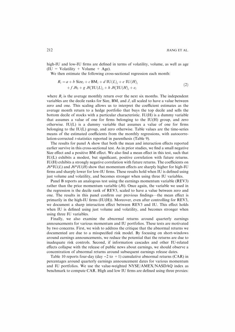
high-IU and low-IU firms are defined in terms of volatility, volume, as well as age(IU = Volatility + Volume + Age).We then estimate the following cross-sectional regression each month:
Ri ¼ aþ b Sizei þ cBMi þ d IUðLÞi þ e IUðHÞiþ f J6i þ g J6�i IUðLÞi þ h J6�i IUðHÞi þ ei
ð2Þ
where Ri is the average monthly return over the next six months. The independentvariables are the decile ranks for Size, BM, and J, all scaled to have a value betweenzero and one. This scaling allows us to interpret the coefficient estimates as theaverage month return to a hedge portfolio that buys the top decile and sells thebottom decile of stocks with a particular characteristic. IU(H) is a dummy variablethat assumes a value of one for firms belonging to the IU(H) group, and zerootherwise. IU(L) is a dummy variable that assumes a value of one for firmsbelonging to the IU(L) group, and zero otherwise. Table values are the time-seriesmeans of the estimated coefficients from the monthly regressions, with autocorre-lation-corrected t-statistics reported in parenthesis (Table 9).The results for panel A show that both the mean and interaction effects reported
earlier survive in this cross-sectional test. As in prior studies, we find a small negativeSize effect and a positive BM effect. We also find a mean effect in this test, such thatIU(L) exhibits a modest, but significant, positive correlation with future returns.IU(H) exhibits a strongly negative correlation with future returns. The coefficients onJ6*IU(L) and J6*IU(H) show that momentum effects are sharply higher for high-IUfirms and sharply lower for low-IU firms. These results hold when IU is defined usingjust volume and volatility, and becomes stronger when using three IU variables.Panel B reports an analogous test using the earnings momentum variable (REV3)
rather than the price momentum variable (J6). Once again, the variable we used inthe regression is the decile rank of REV3, scaled to have a value between zero andone. The results in this panel confirm our previous findings—the mean effect isprimarily in the high-IU firms (IU(H)). Moreover, even after controlling for REV3,we document a sharp interaction effect between REV3 and IU. This effect holdswhen IU is defined using just volume and volatility, and becomes stronger whenusing three IU variables.Finally, we also examine the abnormal returns around quarterly earnings
announcements for various momentum and IU portfolios. These tests are motivatedby two concerns. First, we wish to address the critique that the abnormal returns wedocumented are due to a misspecified risk model. By focusing on short-windowsaround earnings announcements, we reduce the potential that the returns are due toinadequate risk controls. Second, if information cascades and other IU-relatedeffects collapse with the release of public news about earnings, we should observe aconcentration of abnormal returns around subsequent earnings release dates.Table 10 reports four-day (day )2 to +1) cumulative abnormal returns (CAR) in
percentages around quarterly earnings announcement dates for various momentumand IU portfolios. We use the value-weighted NYSE/AMEX/NASDAQ index asbenchmark to compute CAR. High and low IU firms are defined using three proxies:
JIANG ET AL.212

Table
9.Monthly
Cross-SectionalRegressionofReturnsonSize,
Book-to-M
arket,Price
(Earnings)
Momentum
andInform
ationUncertainty
(IU)Prox-
ies.
Panel
A:ResultsforExtrem
eIU
Firms(Both
HighandLow
IU):Price
Momentum
K=
J=
IU=
Intercept
Size
BM
IU(L)
IU(H
)J6
J6*IU
(L)
J6*IU
(H)
66
Volatility
+Volume
0.007(2.29)
)0.003()2.01)0.005(2.73)0.002(2.92)
)0.006()4.50)0.008(5.91)
)0.005()5.12)0.005(4.52)
66
Volatility
+Volume+
Age
0.007(2.25)
)0.003()1.93)0.005(2.74)0.002(2.34)
)0.009()5.16)0.008(5.32)
)0.005()3.56)0.010(6.15)
Panel
B:ResultsforExtrem
eIU
Firms(Both
HighandLowIU
):EarningsMomentum
K=
J=
IU=
Intercept
Size
BM
IU(L)
IU(H
)REV3
REV3*IU
(L)
REV3*IU
(H)
66
Volatility
+Volume
0.005(1.75)
)0.004()2.51)0.005(1.80)0.001(0.54)
)0.004()3.29)0.017(15.19)
)0.003()3.40)0.007(3.87)
66
Volatility
+Volume+
Age
0.005(1.68)
)0.004()2.58)0.005(1.78)0.002(1.89)
)0.008()4.94)0.017(15.99)
)0.006()6.42)0.013(5.39)
Each
month
from
January
1965to
Decem
ber
2001,weregress
monthly
individualstock
returnsonsize,book-to-m
arket
ratio(BM),price
momentum
(J6),
andthreeinform
ationuncertainty
(IU)proxies:Firm
Age,Volatility,andVolumeasin
Table
1.Each
month
from
January
1977to
Decem
ber
2001,werunthe
sameregressionwithearningsmomentum
(REV3)replacingprice
momentum
(J6).Sizeismarket
capitalizationatthebeginningofthemonth.BM
isbook
valueofequityasofthepreviousfiscalyeardivided
bybeginning-of-month
market
capitalization.Price
momentum,J6,istheaveragemonthly
returnsin
the
sixmonthsbefore
thebeginningofthecurrentmonth,computedwitha1-w
eeklag.Earningsmomentum,REV3,isthecumulativeprice-deflatedrevisionsin
thepastthreemonths.Atthebeginningofeach
month
from
January
1965(orJanuary
1977),weindependentlyrankfirm
sonSize,BM,andJ6(orREV3)into
10portfolios.Theindependentvariablesusedin
theregressionare
thedecileranksofSize,BM
andJ6(orREV3),allscaledto
haveavaluebetweenzero
and
one.Atthebeginningofeach
month,wealsoindependentlysortstocksinto
threeportfoliosbyFirm
Age,Volatility
andVolume.IU
isadummyvariablethat
isdefined
differentlyforeach
setofregressions.Forthefirstsetofregressionsin
each
panel,high-IU
andlow-IU
firm
sare
defined
interm
sofboth
volumeand
volatility
(IU=
volatility
+volume).Forthesecondsetofregressionsin
each
panel,high-IU
andlow-IU
firm
sare
defined
interm
sofvolatility,volume,as
wellasage(IU=
Volatility
+Volume+
Age).In
Panel
A,wecompare
resultsforthehigh-IU
firm
s(IU
(H)),low-IU
firm
s(IU(L)),andthebenchmark
firm
swhereprice
momentum
(J6)isused.In
PanelB,wecompare
resultsforthehigh-IU
firm
s(IU(H
)),low-IU
firm
s(IU(L)),andthebenchmark
firm
swhere
earningsmomentum
(REV3)is
used.Table
values
are
thetime-series
meansoftheestimatedcoeffi
cients
from
themonthly
regressions.
Autocorrelation
correctedt-statisticsare
inparenthesis.
INFORMATION UNCERTAINTY AND EXPECTED RETURNS 213

Firm Age, Volatility, and Volume. We report results for both price momentum(panels A and B) and earnings momentum (panels C and D). R5 represent winnersand R1 represent losers. Quarter 0 is the most recent quarterly earnings announce-ment prior to the portfolio formation date. The sample is monthly observations from1/1985 to 12/2001, representing the period during which we have I/B/E/S earningsannouncement dates. The numbers in parentheses are Hansen-Hodrick t-statisticswith six moving average lags.Panel A results show that returns around subsequent earnings announcements of
high-IU firms exhibit the predicted pattern. The aggregate high-IU sample does notearn abnormal returns around future quarterly earnings announcements (see toprow; high-IU firms). However, high-IU winners (high IU R5) earn positive returnsover the next three quarterly announcement periods, while high-IU losers (high IUR1) earn negative or insignificant positive returns. The difference (high IU R5–highIU R1) is significant for the next two quarters, and shows some sign of a reversal bythe fourth quarter—a pattern reminiscent of the Bernard and Thomas (1990) resultfor post-earnings announcement drifts.Panel B shows that, for low-IU firms, we find no abnormal return patterns around
subsequent earnings announcements. For these firms, earnings announcement eventwindow returns are not significantly different from zero (see top row; low-IU firms).Moreover, among low-IU firms, price momentum has no predictive power for eventwindow returns—neither R1 nor R5 firms earn reliable returns around futureearnings dates. In conjunction with the evidence in panel A, these results suggest thata significant portion of the returns to price momentum strategies in high-IU firms isdue to investor misperceptions about future earnings.Panels C and D repeat these tests for earnings momentum portfolios. Once again,
we find that the IU proxy itself has no directional value in predicting futureabnormal returns around quarterly earnings announcements (see top row of panelsC and D). However, we find that the direction of past analyst forecast revisions haspowerful ability to predict these short-window returns, especially among high-IUfirms. Panel C shows that for high-IU firms, winner portfolios earn 2.95% more thanloser portfolios around the next quarterly earnings announcement. This effect issmaller for low-IU firms, but is still quite significant at 1.43%. In both panels, we findthat the predictive power of the earnings momentum variable decays quickly,suggesting that the information in past analyst revisions relates largely to the nextquarterly announcement. Comparing the two panels, we find that the difference inmomentum returns between high and low-IU firms (the last row in the table) ispositive over the next three quarters, and turns negative in the fourth.Overall, Table 10 findings indicate that the results we documented earlier are, at
least in part, due to investor misperceptions about earnings news. We find that asubstantial portion of the mispricing is corrected at the next quarterly announcementdate. Perhaps more importantly, we show that this effect is significantly morepronounced for high-IU firms. These findings are suggestive of the fact that futureearnings announcements play a more important role in resolving informationuncertainty among high-IU firms.
JIANG ET AL.214
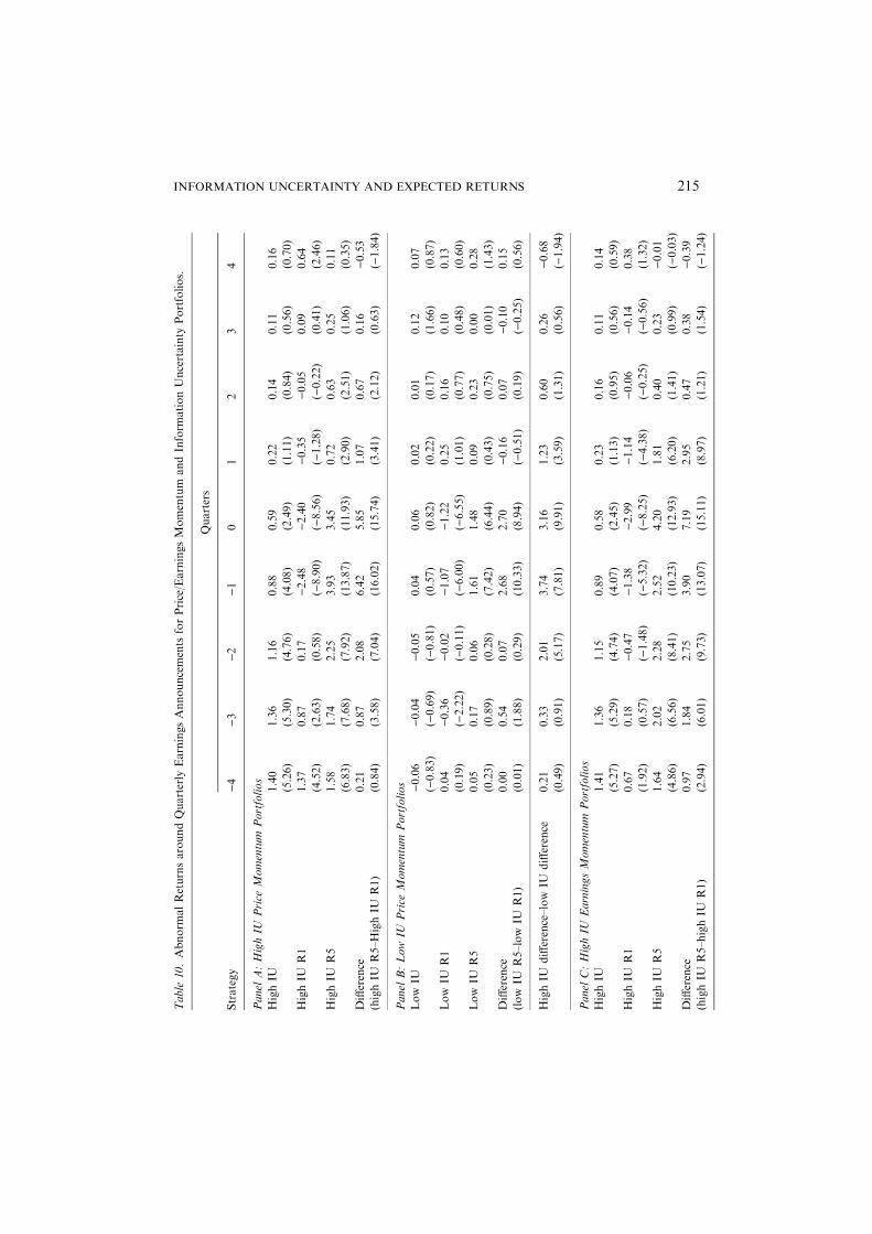
Table
10.Abnorm
alReturnsaroundQuarterly
EarningsAnnouncements
forPrice/EarningsMomentum
andInform
ationUncertainty
Portfolios.
Quarters
Strategy
)4
)3
)2
)1
01
23
4
Panel
A:HighIU
Price
Momentum
Portfolios
HighIU
1.40
(5.26)
1.36
(5.30)
1.16
(4.76)
0.88
(4.08)
0.59
(2.49)
0.22
(1.11)
0.14
(0.84)
0.11
(0.56)
0.16
(0.70)
HighIU
R1
1.37
(4.52)
0.87
(2.63)
0.17
(0.58)
)2.48
()8.90)
)2.40
()8.56)
)0.35
()1.28)
)0.05
()0.22)
0.09
(0.41)
0.64
(2.46)
HighIU
R5
1.58
(6.83)
1.74
(7.68)
2.25
(7.92)
3.93
(13.87)
3.45
(11.93)
0.72
(2.90)
0.63
(2.51)
0.25
(1.06)
0.11
(0.35)
Difference
(highIU
R5–HighIU
R1)
0.21
(0.84)
0.87
(3.58)
2.08
(7.04)
6.42
(16.02)
5.85
(15.74)
1.07
(3.41)
0.67
(2.12)
0.16
(0.63)
)0.53
()1.84)
Panel
B:LowIU
Price
Momentum
Portfolios
Low
IU)0.06
()0.83)
)0.04
()0.69)
)0.05
()0.81)
0.04
(0.57)
0.06
(0.82)
0.02
(0.22)
0.01
(0.17)
0.12
(1.66)
0.07
(0.87)
Low
IUR1
0.04
(0.19)
)0.36
()2.22)
)0.02
()0.11)
)1.07
()6.00)
)1.22
()6.55)
0.25
(1.01)
0.16
(0.77)
0.10
(0.48)
0.13
(0.60)
Low
IUR5
0.05
(0.23)
0.17
(0.89)
0.06
(0.28)
1.61
(7.42)
1.48
(6.44)
0.09
(0.43)
0.23
(0.75)
0.00
(0.01)
0.28
(1.43)
Difference
(low
IUR5–low
IUR1)
0.00
(0.01)
0.54
(1.88)
0.07
(0.29)
2.68
(10.33)
2.70
(8.94)
)0.16
()0.51)
0.07
(0.19)
)0.10
()0.25)
0.15
(0.56)
HighIU
difference–low
IUdifference
0.21
(0.49)
0.33
(0.91)
2.01
(5.17)
3.74
(7.81)
3.16
(9.91)
1.23
(3.59)
0.60
(1.31)
0.26
(0.56)
)0.68
()1.94)
Panel
C:HighIU
EarningsMomentum
Portfolios
HighIU
1.41
(5.27)
1.36
(5.29)
1.15
(4.74)
0.89
(4.07)
0.58
(2.45)
0.23
(1.13)
0.16
(0.95)
0.11
(0.56)
0.14
(0.59)
HighIU
R1
0.67
(1.92)
0.18
(0.57)
)0.47
()1.48)
)1.38
()5.32)
)2.99
()8.25)
)1.14
()4.38)
)0.06
()0.25)
)0.14
()0.56)
0.38
(1.32)
HighIU
R5
1.64
(4.86)
2.02
(6.56)
2.28
(8.41)
2.52
(10.23)
4.20
(12.93)
1.81
(6.20)
0.40
(1.41)
0.23
(0.99)
)0.01
()0.03)
Difference
(highIU
R5–highIU
R1)
0.97
(2.94)
1.84
(6.01)
2.75
(9.73)
3.90
(13.07)
7.19
(15.11)
2.95
(8.97)
0.47
(1.21)
0.38
(1.54)
)0.39
()1.24)
INFORMATION UNCERTAINTY AND EXPECTED RETURNS 215

Table
10.Continued.
Quarters
Strategy
)4
)3
)2
)1
01
23
4
Panel
D:Low
IUEarningsMomentum
Portfolios
Low
IU)0.06
()0.81)
)0.04
()0.60)
)0.04
()0.74)
0.04
(0.52)
0.06
(0.85)
0.01
(0.15)
0.01
(0.09)
0.12
(1.60)
0.07
(0.85)
Low
IUR1
)0.20
()1.68)
)0.57
()3.90)
)0.48
()3.36)
)0.46
()3.72)
)0.80
()6.36)
)0.73
()4.52)
0.04
(0.25)
0.09
(0.53)
0.22
(1.05)
Low
IUR5
0.10
(0.79)
0.28
(1.67)
0.15
(1.34)
0.56
(3.53)
1.14
(6.84)
0.70
(4.80)
0.19
(1.68)
)0.16
()1.28)
0.14
(0.87)
Difference
(low
IUR5–low
IUR1)
0.30
(1.73)
0.85
(3.59)
0.63
(3.51)
1.02
(4.42)
1.94
(8.16)
1.43
(6.66)
0.15
(0.77)
)0.25
()1.45)
)0.08
()0.32)
HighIU
difference–low
IUdifference
0.67
(1.87)
0.99
(3.06)
2.11
(6.93)
2.88
(8.19)
5.26
(11.17)
1.52
(5.08)
0.32
(0.76)
0.63
(2.16)
)0.31
()0.89)
Thistablereportsfour-day(from
day
)2to
day+
1)cumulativeabnorm
alreturns(C
AR)in
percentagearoundquarterly
earningsannouncementdatesfor
variousmomentum
andIU
portfolios.Thesampleismonthly
observationsfrom
1/1985to
12/2001.Atthebeginningofeach
month,werankfirm
sonprice
momentum
(panelsA
andB)orearningsmomentum
(panelsC
andD)into
five
portfolios.
R1represents
losers
andR5represents
winners.
Then
we
independentlysort
firm
sinto
threeportfoliosbyFirm
Age,
Volatility
andVolume.
High-IU
andlow-IU
firm
sare
defined
interm
softhesethreevariables.
Quarter
0isthemostrecentearningsannouncementpriorto
theportfolioform
ationdate.Priorquartersare
representedby
)k,andsubsequentquartersare
representedby+k,wherek=
1–4.Tobeincluded,werequirefirm
sto
haveannouncementperiodCAR
inallninequarters.TheNYSE/A
MEX/N
ASDAQ
value-weightedindex
isusedasthebenchmark
incomputingtheCAR.Thenumbersin
parentheses
are
Hansen-H
odrick
t-statisticswithsixmovingaverage
lags.
JIANG ET AL.216

4. Conclusion
In this study, we have explored the role of information uncertainty (IU) in theprediction of cross-sectional stock returns. We define IU in terms of ‘‘value ambi-guity,’’ or the precision with which a firm’s value can be estimated by knowledgeableinvestors at reasonable cost. Using several different proxies for IU, we show that: (1)on average, high-IU firms earn lower future returns than low-IU firms (the ‘‘mean’’effect), and (2) price and earnings momentum effects are much stronger among high-IU firms than among low-IU firms (the ‘‘interaction’’ effect).The fact that IU is negatively correlated with future returns is difficult to reconcile
with traditional asset pricing models, which either predict no role for IU in returnsprediction, or a positive relation between IU and subsequent returns. We argue thatthis finding can be understood in terms of generally elevated levels of investoroverconfidence in high-IU firms (DHS, 1998), in conjunction with market frictionassociated with short-selling constraints (Miller, 1977).In support of this argument, we show that the lower returns earned by high-IU
firms is generally concentrated in the highest-IU stocks, where short-sell constraintsare likely to be a significant factor. Our analysis certainly does not preclude otherexplanations for these pricing anomalies. However, our findings suggest that IUmight be an important dimension of the puzzle that deserves more attention fromresearchers.We also introduce a behavioral-based framework for understanding how IU might
affect price and earnings momentum. Behavioral finance theory asserts that marketmispricings arise when two conditions are met: (1) an uninformed demand shock,and (2) a limit on arbitrage. Our two-part thesis is that the level of informationuncertainty is positively correlated with a pervasive form of decision bias (investoroverconfidence), and that it is also positively correlated with arbitrage costs (inparticular, the prevalence of informational cascades). Collectively, these two effectsconspire to produce greater momentum effects among high-IU firms.Using a variety of IU proxies, and two measures of momentum, we find strong
evidence in support of this prediction. During our sample period, monthly hedgereturns to quintile-based price momentum strategies averaged 1.80% for high-IUfirms, and only 0.08% for low-IU firms—after adjusting for the three Fama-French(1993) factors. Earnings momentum (based on recent analyst FY1 forecast revisions)produced average monthly hedge returns of 2.75% for high-IU firms, and 1.04% forlow-IU firms. These results are robust to various risk adjustments, and are evenstronger in the most recent sub-sample period.Our findings have interesting implications for investment managers. Prior studies
show that value-related and momentum-related signals both have predictive powerfor returns. However, because these two types of signals are negatively correlated(Asness, 1997; Lee and Swaminathan, 2000), sorting out the appropriate weights foreach type of signal is a substantial challenge. Our findings suggest that IU is apotential arbiter in such decisions. Specifically, it is rational to place more weight onmomentum-related signals in high-IU settings, and more weight on value-relatedsignals in low-IU settings.
INFORMATION UNCERTAINTY AND EXPECTED RETURNS 217

Our results also nominate information uncertainty as a natural partitioningvariable when conducting contextual financial analysis. High-IU firms (andindustries populated by a greater proportion of such firms) call for a differentinvestment approach than low-IU firms. In fact, our results may help to explainwhy the investment industry is broadly grouped into style categories, with someportfolio managers focusing on ‘‘value’’ (low-IU) stocks while others specializing in‘‘growth’’ (high-IU) stocks. These groupings seem to arise quite naturally given ouranalyses.In sum, we believe IU is a central concept in understanding market pricing
dynamics. Our study does not explain the existence of momentum per se. However,our work helps to shed light on how IU can alter the price discovery process, andthus the magnitude of the momentum effect. We also introduce an alternativeexplanation for a series of puzzling empirical regularities in the asset pricing lit-erature. Our hope is that future work will extend this line of inquiry to provide amore complete picture of how the level of IU can affect capital markets.
Appendix A: Definition and Empirical Implementation of Implied Equity Duration
Duration is a measure of implied equity duration introduced by Dechow et al. (2004).Intuitively, it is analogous to the Macaulay measure of duration in bond pricing, andmeasures how long in years it takes for the price of a stock to be repaid by its internalcash flows. Dechow et al. (2004) nominate this variable as a measure of informationuncertainty, and show that it differentiates return co-movements better than themore traditional book-to-market ratio. We follow their methodology and estimationprocedure in computing this variable.An attractive feature of the Dechow et al. (2004) procedure is that it relies on only
a few financial variables, and no analyst-based data. Specifically, their procedurecalls for four financial variables and four forecasting parameters. We follow theirimplementation procedures, and use the following key inputs and forecastingparameters, as reported in Table 1 of their paper:
Financial Variables
Financial variables Compustat Data
Book value of equity (BV) Item 60
Earnings (E) Item 18 = Income before extraordinary items
Sales (S) Item 12
Market capitalization Item 199 · Item 25
Forecasting Parameters
Autocorrelation Coefficient for ROE 0.57
Cost of equity capital 0.12
Autocorrelation Coefficient for Growth in sales 0.24
Long-run growth rate in sales 0.06
JIANG ET AL.218

Acknowledgments
We thank two anonymous referees, Peter Easton (the editor), Ilia Dichev, David Hirshleif-
er, Paul Schultz (the discussant) as well as workshop participants at Cornell University,
Barclays Global Investors’ Advanced Strategies and Research Group, and 2004 RAST con-
ference at University of Notre Dame for helpful comments and discussions. We also grate-
fully acknowledge the contribution of Thomson Financial in providing earnings forecast
data, made available through I/B/E/S International, Inc.
Notes
1. A representative, non-exhaustive, list of references for these results includes: Volatility (Ang et al.,
2003); Volume (Datar et al., 1998; Lee and Swaminathan, 2000); Expected growth (LaPorta, 1996); PB
(Fama and French, 1992); Analyst dispersion (Diether et al., 2002); Duration of future cash flows
(DeChow et al., 2004). Our work is also closely related to Zhang (2004), discussed in more detail later.
2. See Shleifer (2000), Hirshleifer (2001), and Barberis and Thaler (2003) for surveys of this literature.
3. As we discuss in more detail later, Diether et al. (2002) makes the same point in motivating their study
on differences of opinion and future returns.
4. See Lee (2001), Shleifer and Vishny (1997), Mitchel et al. (2002), Barberis and Thaler (2003).
5. Bushman and Smith (2001) discuss the link between the quality of accounting data and information risk.
6. To exclude recent IPOs, we require past 12-month returns. To mitigate the effect of illiquid stocks, we
also limit our analysis to firms with a market capitalization as of the portfolio formation date of at
least 150 million in year 2001 dollars (inflation-adjusted).
7. The result holds for all the IU proxies except the Duration variable (which orders returns mono-
tonically).
8. For example, see Griffin and Tversky (1992).
9. Nelson et al. (2003) provide experimental evidence that timely feedback mitigates, but does not
eliminate, trader overconfidence.
10. A concrete example would be a value investor who is reluctant to forego the results of a careful
discounted cash flow analysis (DCF) even though the firm in question has highly uncertain cash flows.
More generally, the DCF process as taught in most financial analysis classes typically produces point
estimates of value, and does not provide systematic feedback on the confidence band of these estimates.
Thus value investors with a theoretically sound investment approach can also place too much reliance
on their own private signals.
11. Diether et al. (2002) makes the same point in motivating their study on differences of opinion and
future returns. As they observe, explicit constraints on short-selling is not the only reason firms with
greater divergence of opinion (or in our case high-IU firms) might become over-priced. More gen-
erally, any friction that prevents the revelation of negative opinions will produce an upward bias in the
prices of these stocks. For example, the documented reluctance of financial analysts to issue negative
(sell) recommendations could contribute an upward bias that is most pronounced among high-IU
firms. Rules that prohibit many large institutional investors from taking short positions can have a
similar effect.
12. Using a residual-income model estimate of firm value, Frankel and Lee (1998) provide evidence that
price convergence to value is a protracted process that takes place over extended periods of time,
averaging 3–5 years.
13. Brunnermeier and Nagel (2003) offer an interesting case study of this phenomenon. In their study, the
authors show that hedge fund managers initially resisted increasing their technology holdings as
valuation for these stocks soared in the late 1990s. However, toward the end of the bubble, most fund
managers capitulated and engaged in positive-feedback trading, increasing their exposure to tech-
nology stocks.
INFORMATION UNCERTAINTY AND EXPECTED RETURNS 219

14. In the original Bikchandani et al. (1992) paper, informational cascades collapse with the introduction
of endogenous price, because as people buy stocks, they drive up the price, making further purchases
less attractive. However, subsequent studies show that noise in the information aggregation process
can limit the inference individuals make from price, thus allowing cascades to persist even in the
presence of price (e.g., Avery and Zemsky, 1998). See Hirshleifer and Teoh (2003) for a good synthesis
of herding behavior and cascading studies in capital market settings.
15. In a less related study, Francis et al. (2003) also explore the empirical relation between accounting
anomalies and information uncertainty. However, their economic construct and empirical measure of
uncertainty bear little relation to ours, and their results do not address the issues we examine.
16. As a proxy for IU, firm age comes with some baggage. In particular, the addition of NASDAQ stocks
in 1972 could potentially taint our results. To partially address this problem, we exclude small firms
(firms with less than 150 million in market capitalization using 2001 dollars) and firms with less than
12-months of trading history. Further, we check our findings using composite IU measures that
exclude Firm Age (see Tables 4, 5, and 9). Finally, we find that using only NYSE firms also yields
similar results.
17. We use different time horizons in measuring past volume and past volatility in an attempt to derive
two signals that are less correlated. In fact, using the standard deviation of weekly returns over the
past six months produces very similar results.
18. In ranking firms into volume portfolios, we separately sort stocks listed on the NYSE/AMEX and
stocks on NASDAQ, because trading volume on NASDAQ is inflated relative to NYSE/AMEX
stocks due to double counting of dealer trades (Lee and Swaminathan, 2000).
19. In most months, revt is the mean FY1 estimate in month t minus the mean FY1 estimate in month t)1.However, in the month when a firm announces its fiscal earnings, analysts’ earnings forecasts switch to
the new fiscal years after the announcement. To ensure consistency in the month of the announcement,
if the announcement date is before the I/B/E/S compilation date, revt is defined as the mean FY1
estimate in month t minus the mean FY2 estimate in month t)1. If the announcement occurs after the
I/B/E/S compilation date, revt is defined as the difference between month t and t)1’s mean FY1
estimates, but revt+1 is defined as the mean FY1 estimate in month t+1 minus the mean FY2 estimate
in month t.
20. We exclude Duration because of its more stringent data requirements and because the results are
similar whether we include it or not.
21. Once again, we exclude Duration in the definition of IU for this and the ensuing tables, because of its
more stringent data requirements and because results are qualitatively the same using just three
variables to proxy for IU.
References
Ang, A., R. Hodrick, Y. Xing, and X. Zhang. (2003). ‘‘The Cross-section of Volatility and Expected
Returns.’’ Working paper, Columbia University.
Asness, C. (1997). ‘‘The Interaction of Value and Momentum Strategies.’’ Financial Analysts Journal 53,
29–36.
Avery, C. and P. Zemsky. (1998). ‘‘Multi-dimensional Uncertainty and Herd Behavior in Financial
Markets.’’ American Economic Review 88, 724–748.
Barberis, N. and R. Thaler. (2003). ‘‘A Survey of Behavioral Finance.’’ Handbook of the Economics of
Finance, Chapter 18, edited by G. M. Constantinides, M. Harris, and R. Stulz. Elsevier/North-Holland.
Bernard, V. L. and J. K. Thomas. (1990). ‘‘Evidence that Stock Prices do not Fully Reflect the Impli-
cations of Current Earnings for Future Earnings.’’ Journal of Accounting and Economics 13, 305–341.
Bikhchandani, S., D. Hirshleifer and I. Welch. (1992). ‘‘A Theory of Fads, Fashion, Custom and Cultural
Change as Information Cascades.’’ Journal of Political Economy 100, 992–1026.
Brunnermeier, M. K. and S. Nagel. (2003). ‘‘Hedge Funds and the Technology Bubble.’’ Journal of
Finance, forthcoming.
JIANG ET AL.220

Bushman, R. and A. Smith. (2001). ‘‘Financial Accounting Information and Corporate Governance.’’
Journal of Accounting and Economics 32, 237–333.
Daniel, K., D. Hirshleifer and A. Subrahmanyam. (1998). ‘‘Investor Psychology and Security Market
Under- and Over-reaction.’’ Journal of Finance 53, 1839–1886.
Daniel, K., D. Hirshleifer and A. Subrahmanyam. (2001). ‘‘Overconfidence, Arbitrage, and Equilibrium
Asset Pricing.’’ Journal of Finance 56, 921–965.
Datar, V., N. Naik and R. Radcliffe. (1998). ‘‘Liquidity and Asset Returns: an Alternative Test.’’ Journal
of Financial Markets 1, 203–220.
Dechow, P., R. Sloan and M. Soliman. (2004). ‘‘Implied Equity Duration: A New Measure of Equity
Security Risk.’’ Review of Accounting Studies 9, 197–228.
De Long, J. B., A. Shleifer, L. H. Summers and R. J. Waldmann. (1990). ‘‘Positive Feedback Investment
Strategies and Destabilizing Rational Speculation.’’ Journal of Finance 45, 379–395.
Diether, K., C. Malloy and A. Scherbina. (2002). ‘‘Differences of Opinion and the Cross-Section of Stock
Returns.’’ Journal of Finance 57, 2113–2141.
Easley, D. and M. O’Hara. (2003). ‘‘Information and the Cost of Capital.’’ Journal of Finance, forth-
coming.
Fama, E. F. (1991). ‘‘Efficient Capital Markets: II.’’ Journal of Finance 46, 1575–1617.
Fama, E. F. and K. R. French. (1992). ‘‘The Cross-section of Expected Stock Returns.’’ Journal of Finance
47, 427–465.
Fama, E. F. and K. R. French. (1993). ‘‘Common Risk Factors in the Returns on Stocks and Bonds.’’
Journal of Financial Economics 33, 3–56.
Fama, E. F. and J. MacBeth. (1973). ‘‘Risk, Return, and Equilibrium: Empirical Tests.’’ Journal of
Political Economy 81, 607–636.
Francis, J., R. LaFond, P. Olsson and K. Schipper. (2003). ‘‘Accounting Anomalies and Information
Uncertainty.’’ Working Paper, Duke University, Wisconsin University, and the Financial Accounting
Standards Board.
Frankel, R. and C. M. C. Lee. (1998). ‘‘Accounting Valuation, Market Expectation, and Cross-sectional
Stock Returns.’’ Journal of Accounting and Economics 25, 283–319.
Griffin, D. and A. Tversky. (1992). ‘‘The Weighing of Evidence and the Determinants of Confidence.’’
Cognitive Psychology 24, 411–443.
Grundy, B. and J. S. Martin. (2001). ‘‘Understanding the Nature of the Risks and the Source of the
Rewards to Momentum Investing.’’ Review of Financial Studies 14, 29–78.
Hirshleifer, D. (2001). ‘‘Investor Psychology and Asset Pricing.’’ Journal of Finance 56, 1533–1597.
Hirshleifer, D. and S. Hong Teoh. (2003). ‘‘Herding Behavior and Cascading in Capital Markets: A
Review and Synthesis.’’ European Financial Management 9, 25–66.
Jegadeesh, N. and S. Titman. (1993). ‘‘Returns to Buying Winners and Selling Losers: Implications for
Stock Market Efficiency.’’ Journal of Finance 48, 65–91.
La Porta, R. (1996). ‘‘Expectations and the Cross-section of StockReturns.’’ Journal of Finance 51, 1715–42.
Lee, C. M. C.. (2001). ‘‘Market Efficiency and Accounting Research: A Discussion of ‘Capital Market
Research’ by S.P. Kothari.’’ Journal of Accounting and Economics 31, 233–253.
Lee, C. M. C. and B. Swaminathan. (2000). ‘‘Price Momentum and Trading Volume.’’ Journal of Finance
55, 2017–2069.
Miller, E. M. (1977). ‘‘Risk, Uncertainty, and Divergence of Opinion.’’ Journal of Finance 32, 1151–1168.
Mitchell, M., T. Pulvino and E. Stafford. (2002). ‘‘Limited Arbitrage in Equity Markets.’’ Journal of
Finance 57, 551–584.
Nelson, M. W., S. D. Krische and R. J. Bloomfield. (2003). ‘‘Confidence and Investors’ Reliance on
Disciplined Trading Strategies.’’ Journal of Accounting Research 41, 503–523.
Odean, T. (1998). ‘‘Volume, Volatility, Price, and Profit when all Traders are Above Average.’’ Journal of
Finance 53, 1887–1934.
Shleifer, A. (2000). Inefficient Markets: An Introduction to Behavioral Finance. Oxford, UK: Oxford
University Press.
Shleifer, A. and R. W. Vishny. (1997). ‘‘The Limits of Arbitrage.’’ Journal of Finance 52, 35–55.
Zhang, F. (2004). ‘‘Information Uncertainty and Stock Returns.’’ Working paper, University of Chicago.
INFORMATION UNCERTAINTY AND EXPECTED RETURNS 221