Embed Size (px)
Citation preview
1
INFORMATIONAL EFFICIENCY OF
FUTURES MARKET IN INDIA
A thesis submitted to Pondicherry University in partial fulfillment of the
requirement for the award of the degree of
DOCTOR OF PHILOSOPHY
IN
COMMERCE
By
BABU JOSE
Under the Guidance of
Dr. D. LAZAR
Associate Professor
DEPARTMENT OF COMMERCE
SCHOOL OF MANAGEMENT
PONDICHERRY UNIVERSITY
PONDICHERRY-605 014
NOVEMBER-2011
2
MEMBERS OF DOCTORAL COMMITTEE
DR.K.CHANDRASEKHARA RAO
Professor & Head
Department of Banking Technology
Pondicherry University
DR. P.DHANAVANTHAN
Professor & Head
Department of Statistics
Pondicherry University
3
Dr. D. Lazar
Associate Professor
Department of Commerce
School of Management
Pondicherry University
Pondicherry-605 014
Certificate
This is to certify that the PhD thesis entitled “INFORMATIONAL EFFICIENCY
OF FUTURES MARKET IN INDIA” submitted to Pondicherry University for the
award of the degree of Doctor of Philosophy in Commerce by Babu Jose is the
bonafide research work carried out by him independently under my guidance and
supervision in the Department of Commerce. I also certify that this has not been
previously submitted for the award of any degree or associateship to any other
University or Institution.
Dr. D. Lazar
Associate Professor
Countersigned
Dean Head
School of Management Department of Commerce
Place:
Date:
4
BABU JOSE
Research Scholar- PhD (Full Time)
Department of Commerce
School of Management
Pondicherry University
Pondicherry-605 014
Declaration
I, Babu Jose hereby declare that the thesis entitled, “Informational Efficiency of
Futures Market in India” submitted to Pondicherry University, Pondicherry for the
award of the Degree of Doctor of Philosophy in Commerce is my original work and
it has not been previously submitted either in part or whole to this or any other
University for the award of any degree.
Babu Jose
Place:
Date:

5
to Him.................
who always
strengthen me

6
Acknowledgement
I bow before the God almighty for his special blessings on me from the beginning to
the completion of this study.
I am deeply indebted to Dr. Daniel Lazar, Associate Professor, Dept. of Commerce,
Pondicherry University, my Guide and Supervisor, for his timely supervision, strict
instruction and unconditional support for the successful Completion of this study. I
admire his motivation to keep me in the right track and his selfless assistance in
bringing out this work in the best way possible. I thank him meticulously for going
through all the pages and giving timely corrections, even the minute ones which
helped me a lot to do this research in the proper manner. I admire and cherish his
availability, encouragement, competence and scholarship.
I do thank Honorable Vice Chancellor Prof. J.A.K. Tareen, Prof. M. Ramadass,
Dean SOM , Dr. Malabika Deo, Professor & Head, Dept of Commerce, Pondicherry
University for giving me the opportunity to take up this study. I express my sincere
gratitude to My Doctoral Committee Members Dr. K.C. Chandrasekhara Rao,
Professor & Head, Dept. of Banking Technology, Dr. P. Dhanavanthan, Professor
& Head, Dept. of Statistics, Pondicherry University for their encouragement, keen
interest on the work, apt guidelines and strict monitoring which helped me a lot in the
course of this research.
With sentiment of joy and gratitude I express my sincere thanks to Mr. Sunil Paul,
Research Scholar, Dept. of Economics, Pondicherry University, Mr. Lagesh,
Research Scholar, Dept. of Economics, Hyderabad University, Dr. Sony Thomas,
Faculty, IIM Kozhikode, Dr. S. Shijin, Assistant Professor, Dept. of Commerce,
Pondicherry University and Mrs. Deepthi for their concern, kindness and selfless
help for the completion of my work. . I thank Bro. Benny Thadathil M.Ss.Cc, Mr.
Shinto Thomas and Mr. Vivek who helped me in the proof reading of the thesis.

7
I would like to thank Prof. P.Palanichamy, Prof. P. Natarajan, Dr. Velmurugan, Dr.
Shanmugasundaram, Sri. S. Aravanan and Mr. K.B. Nidheesh for their personal
encouragement and help during the research period. I take this opportunity to thank
Mrs. Savithri, office manager and Mr. Ammayiappan, Office Assistants, Dept. of
Commerce, for their personal help and cooperation during the research period.
It is great pleasure for me to thank, Meghanathan, Immanuel, Yazeer, Minija, Safir
Pasha , Mahindra Panday, Dharani and all other co-research scholars in the Dept.
of Commerce and of other Depts. for their co-operation, love, encouragement and
healthy personal relationship. I also thank my dear friends and teachers, Shaji. K.P,
Manoj. M, Joshy K.P, Hari Das, Sebastian.P.M, Dr. Madhusoodhana, Jose. M.V,
Rajesh and Raveesh for their motivating support and life long relationship they
rendered to me.
I avail this opportunity to express my sincere thanks to my wife Sindhu who is always
with me and her co-operating attitude, helping mentality and level of personal
understanding which helped me lot to balance my research and personal life in a
healthy manner. It is the time to sincerely thank my family members especially
Father, Mother, Sister, Brother-in-law, and all members of Thadathil and
Pinakkattu Family, without their consistent prayer, help and support, it would not
have been possible for me to get success in my personal and academic life.
Babu Jose
8
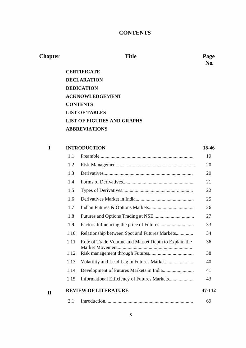
CONTENTS
Chapter Title Page
No.
CERTIFICATE
DECLARATION
DEDICATION
ACKNOWLEDGEMENT
CONTENTS
LIST OF TABLES
LIST OF FIGURES AND GRAPHS
ABBREVIATIONS
I INTRODUCTION 18-46
1.1 Preamble............................................................................ 19
1.2 Risk Management............................................................... 20
1.3 Derivatives........................................................................ 20
1.4 Forms of Derivatives......................................................... 21
1.5 Types of Derivatives......................................................... 22
1.6 Derivatives Market in India............................................... 25
1.7 Indian Futures & Options Markets..................................... 26
1.8 Futures and Options Trading at NSE................................. 27
1.9 Factors Influencing the price of Futures............................ 33
1.10 Relationship between Spot and Futures Markets.............. 34
1.11 Role of Trade Volume and Market Depth to Explain the
Market Movement............................................................
36
1.12 Risk management through Futures.................................... 38
1.13 Volatility and Lead Lag in Futures Market....................... 40
1.14 Development of Futures Markets in India......................... 41
1.15 Informational Efficiency of Futures Markets....................
43
II REVIEW OF LITERATURE 47-112
2.1 Introduction....................................................................... 69
9
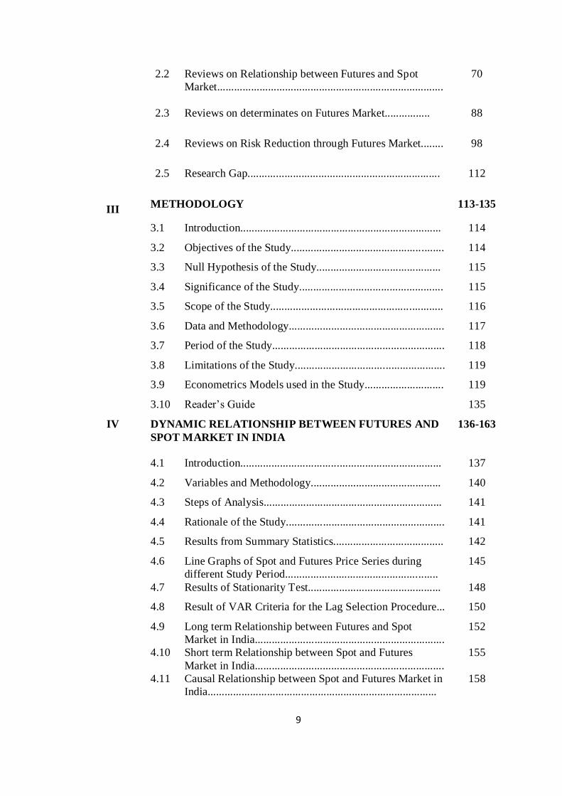
2.2 Reviews on Relationship between Futures and Spot
Market................................................................................
70
2.3 Reviews on determinates on Futures Market................ 88
2.4 Reviews on Risk Reduction through Futures Market........ 98
2.5 Research Gap.................................................................... 112
III METHODOLOGY 113-135
3.1 Introduction....................................................................... 114
3.2 Objectives of the Study...................................................... 114
3.3 Null Hypothesis of the Study............................................ 115
3.4 Significance of the Study................................................... 115
3.5 Scope of the Study............................................................. 116
3.6 Data and Methodology....................................................... 117
3.7 Period of the Study............................................................. 118
3.8 Limitations of the Study..................................................... 119
3.9 Econometrics Models used in the Study............................ 119
3.10 Reader’s Guide 135
IV DYNAMIC RELATIONSHIP BETWEEN FUTURES AND
SPOT MARKET IN INDIA
136-163
4.1 Introduction....................................................................... 137
4.2 Variables and Methodology.............................................. 140
4.3 Steps of Analysis............................................................... 141
4.4 Rationale of the Study........................................................ 141
4.5 Results from Summary Statistics....................................... 142
4.6 Line Graphs of Spot and Futures Price Series during
different Study Period......................................................
145
4.7 Results of Stationarity Test............................................... 148
4.8 Result of VAR Criteria for the Lag Selection Procedure... 150
4.9 Long term Relationship between Futures and Spot
Market in India...................................................................
152
4.10 Short term Relationship between Spot and Futures
Market in India...................................................................
155
4.11 Causal Relationship between Spot and Futures Market in
India.................................................................................
158
10
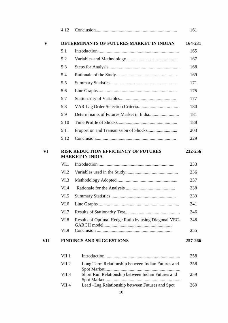
4.12 Conclusion.......................................................................
161
V DETERMINANTS OF FUTURES MARKET IN INDIAN 164-231
5.1 Introduction....................................................................... 165
5.2 Variables and Methodology............................................ 167
5.3 Steps for Analysis............................................................... 168
5.4 Rationale of the Study..................................................... 169
5.5 Summary Statistics......................................................... 171
5.6 Line Graphs..................................................................... 175
5.7 Stationarity of Variables................................................. 177
5.8 VAR Lag Order Selection Criteria................................... 180
5.9 Determinants of Futures Market in India.......................... 181
5.10 Time Profile of Shocks.................................................... 188
5.11 Proportion and Transmission of Shocks.......................... 203
5.12 Conclusion......................................................................
229
VI RISK REDUCTION EFFICIENCY OF FUTURES
MARKET IN INDIA
232-256
VI.1 Introduction................................................................... 233
VI.2 Variables used in the Study.............................................. 236
VI.3 Methodology Adopted..................................................... 237
VI.4 Rationale for the Analysis ........................................... 238
VI.5 Summary Statistics......................................................... 239
VI.6 Line Graphs....................................................................... 241
VI.7 Results of Stationarity Test................................................ 246
VI.8 Results of Optimal Hedge Ratio by using Diagonal VEC-
GARCH model............................................................
248
VI.9 Conclusion .................................................................. 255
VII FINDINGS AND SUGGESTIONS
257-266
VII.1 Introduction.................................................................. 258
VII.2 Long Term Relationship between Indian Futures and
Spot Market..................................................................
258
VII.3 Short Run Relationship between Indian Futures and
Spot Market..................................................................
259
VII.4 Lead –Lag Relationship between Futures and Spot 260
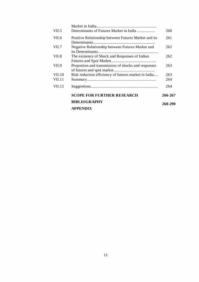
11
Market in India............................................................
VII.5 Determinants of Futures Market in India .................. 260
VII.6 Positive Relationship between Futures Market and its
Determinants..............................................................
261
VII.7 Negative Relationship between Futures Market and
its Determinants............................................................
262
VII.8 The existence of Shock and Responses of Indian
Futures and Spot Market.............................................
262
VII.9 Proportion and transmission of shocks and responses
of futures and spot market.........................................
263
VII.10 Risk reduction efficiency of futures market in India.... 263
VII.11 Summary..................................................................... 264
VII.12 Suggestions................................................................... 264
SCOPE FOR FURTHER RESEARCH
BIBLIOGRAPHY
APPENDIX
266-267
268-290
12
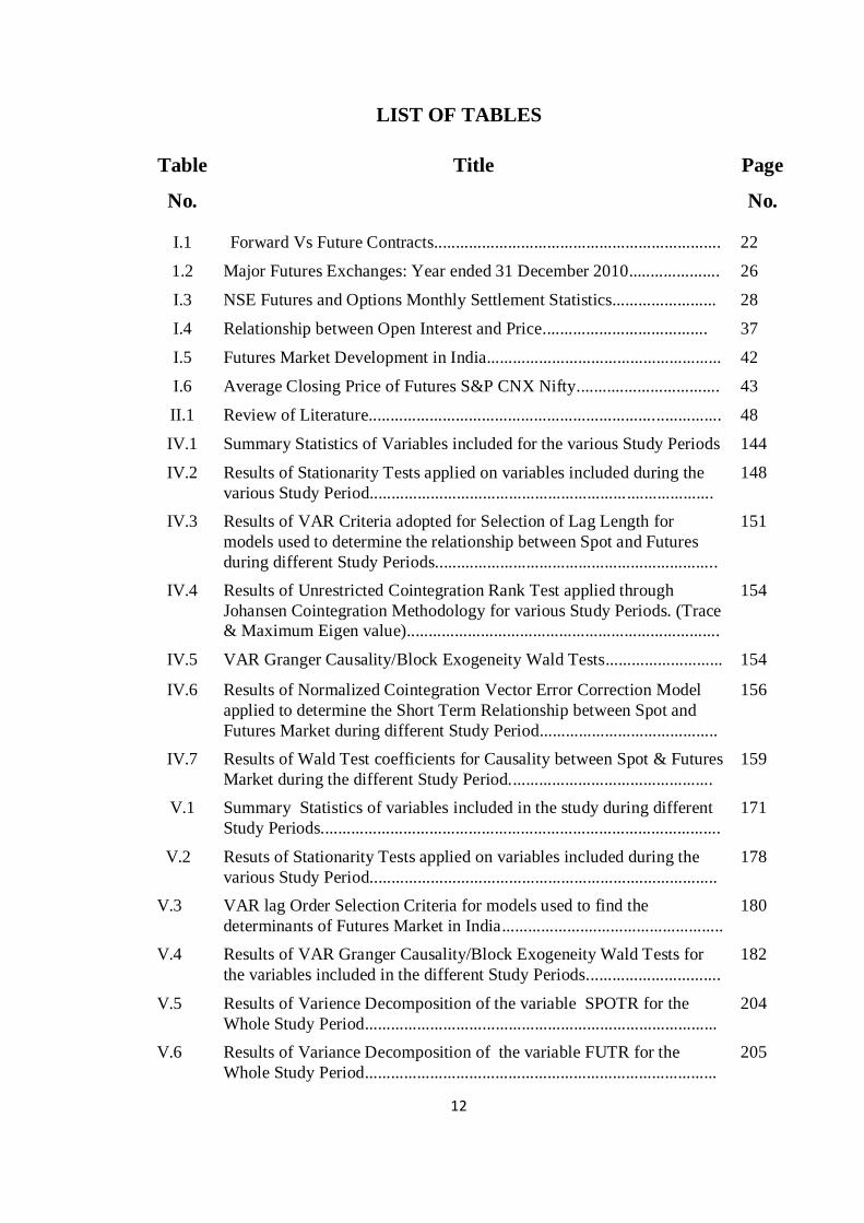
LIST OF TABLES
Table
No.
Title Page
No.
I.1 Forward Vs Future Contracts.................................................................. 22
1.2 Major Futures Exchanges: Year ended 31 December 2010..................... 26
I.3 NSE Futures and Options Monthly Settlement Statistics........................ 28
I.4 Relationship between Open Interest and Price...................................... 37
I.5 Futures Market Development in India...................................................... 42
I.6 Average Closing Price of Futures S&P CNX Nifty................................. 43
II.1 Review of Literature................................................................................. 48
IV.1 Summary Statistics of Variables included for the various Study Periods 144
IV.2 Results of Stationarity Tests applied on variables included during the
various Study Period............................................................................... 148
IV.3 Results of VAR Criteria adopted for Selection of Lag Length for
models used to determine the relationship between Spot and Futures
during different Study Periods.................................................................
151
IV.4 Results of Unrestricted Cointegration Rank Test applied through
Johansen Cointegration Methodology for various Study Periods. (Trace
& Maximum Eigen value)........................................................................
154
IV.5 VAR Granger Causality/Block Exogeneity Wald Tests........................... 154
IV.6 Results of Normalized Cointegration Vector Error Correction Model
applied to determine the Short Term Relationship between Spot and
Futures Market during different Study Period.........................................
156
IV.7 Results of Wald Test coefficients for Causality between Spot & Futures
Market during the different Study Period............................................... 159
V.1 Summary Statistics of variables included in the study during different
Study Periods............................................................................................
171
V.2 Resuts of Stationarity Tests applied on variables included during the
various Study Period................................................................................
178
V.3 VAR lag Order Selection Criteria for models used to find the
determinants of Futures Market in India...................................................
180
V.4 Results of VAR Granger Causality/Block Exogeneity Wald Tests for
the variables included in the different Study Periods...............................
182
V.5 Results of Varience Decomposition of the variable SPOTR for the
Whole Study Period.................................................................................
204
V.6 Results of Variance Decomposition of the variable FUTR for the
Whole Study Period.................................................................................
205
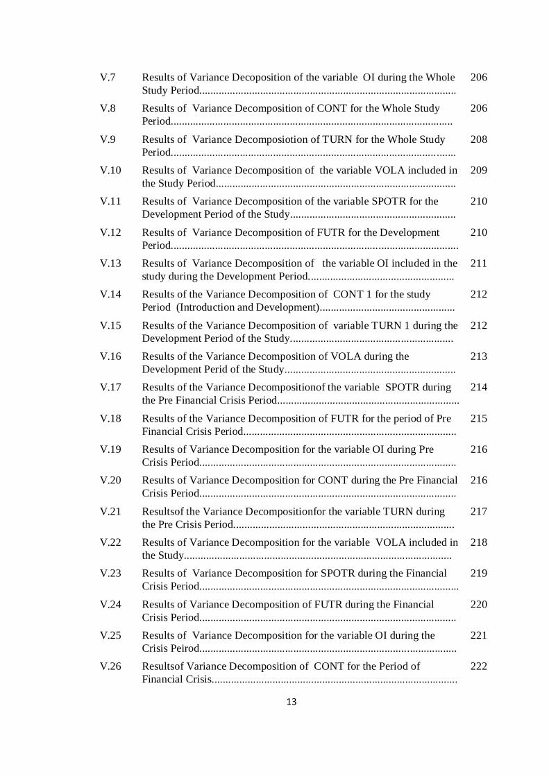
13
V.7 Results of Variance Decoposition of the variable OI during the Whole
Study Period.............................................................................................
206
V.8 Results of Variance Decomposition of CONT for the Whole Study
Period......................................................................................................
206
V.9 Results of Variance Decomposiotion of TURN for the Whole Study
Period.......................................................................................................
208
V.10 Results of Variance Decomposition of the variable VOLA included in
the Study Period.......................................................................................
209
V.11 Results of Variance Decomposition of the variable SPOTR for the
Development Period of the Study............................................................
210
V.12 Results of Variance Decomposition of FUTR for the Development
Period........................................................................................................
210
V.13 Results of Variance Decomposition of the variable OI included in the
study during the Development Period.....................................................
211
V.14 Results of the Variance Decomposition of CONT 1 for the study
Period (Introduction and Development).................................................
212
V.15 Results of the Variance Decomposition of variable TURN 1 during the
Development Period of the Study...........................................................
212
V.16 Results of the Variance Decomposition of VOLA during the
Development Perid of the Study..............................................................
213
V.17 Results of the Variance Decompositionof the variable SPOTR during
the Pre Financial Crisis Period..................................................................
214
V.18 Results of the Variance Decomposition of FUTR for the period of Pre
Financial Crisis Period.............................................................................
215
V.19 Results of Variance Decomposition for the variable OI during Pre
Crisis Period.............................................................................................
216
V.20 Results of Variance Decomposition for CONT during the Pre Financial
Crisis Period.............................................................................................
216
V.21 Resultsof the Variance Decompositionfor the variable TURN during
the Pre Crisis Period................................................................................
217
V.22 Results of Variance Decomposition for the variable VOLA included in
the Study.................................................................................................
218
V.23 Results of Variance Decomposition for SPOTR during the Financial
Crisis Period..............................................................................................
219
V.24 Results of Variance Decomposition of FUTR during the Financial
Crisis Period.............................................................................................
220
V.25 Results of Variance Decomposition for the variable OI during the
Crisis Peirod.............................................................................................
221
V.26 Resultsof Variance Decomposition of CONT for the Period of
Financial Crisis.........................................................................................
222
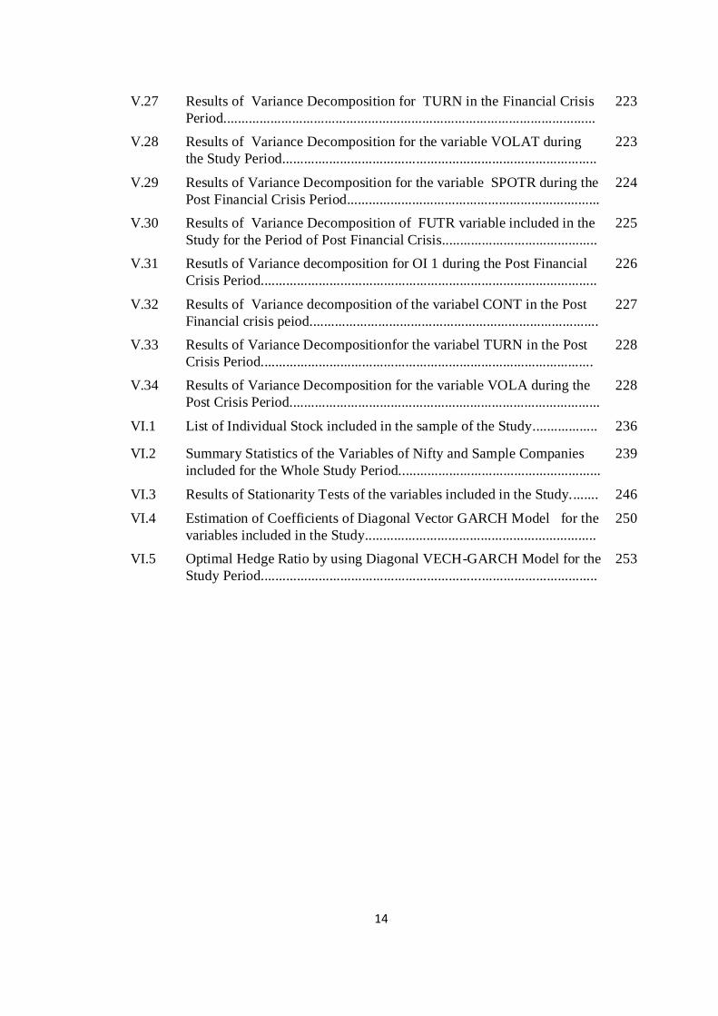
14
V.27 Results of Variance Decomposition for TURN in the Financial Crisis
Period.......................................................................................................
223
V.28 Results of Variance Decomposition for the variable VOLAT during
the Study Period.......................................................................................
223
V.29 Results of Variance Decomposition for the variable SPOTR during the
Post Financial Crisis Period......................................................................
224
V.30 Results of Variance Decomposition of FUTR variable included in the
Study for the Period of Post Financial Crisis...........................................
225
V.31 Resutls of Variance decomposition for OI 1 during the Post Financial
Crisis Period.............................................................................................
226
V.32 Results of Variance decomposition of the variabel CONT in the Post
Financial crisis peiod................................................................................
227
V.33 Results of Variance Decompositionfor the variabel TURN in the Post
Crisis Period............................................................................................
228
V.34 Results of Variance Decomposition for the variable VOLA during the
Post Crisis Period......................................................................................
228
VI.1 List of Individual Stock included in the sample of the Study.................. 236
VI.2 Summary Statistics of the Variables of Nifty and Sample Companies
included for the Whole Study Period........................................................
239
VI.3 Results of Stationarity Tests of the variables included in the Study........ 246
VI.4 Estimation of Coefficients of Diagonal Vector GARCH Model for the
variables included in the Study................................................................
250
VI.5 Optimal Hedge Ratio by using Diagonal VECH-GARCH Model for the
Study Period.............................................................................................
253
15
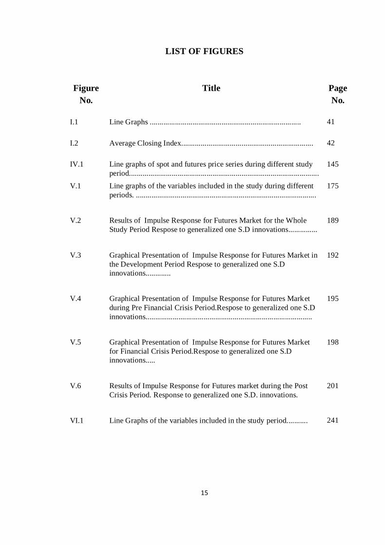
LIST OF FIGURES
Figure
No.
Title Page
No.
I.1 Line Graphs .............................................................................. 41
I.2 Average Closing Index.................................................................... 42
IV.1 Line graphs of spot and futures price series during different study
period..................................................................................................
145
V.1 Line graphs of the variables included in the study during different
periods. .............................................................................................
175
V.2 Results of Impulse Response for Futures Market for the Whole
Study Period Respose to generalized one S.D innovations...............
189
V.3 Graphical Presentation of Impulse Response for Futures Market in
the Development Period Respose to generalized one S.D
innovations.............
192
V.4 Graphical Presentation of Impulse Response for Futures Market
during Pre Financial Crisis Period.Respose to generalized one S.D
innovations......................................................................................
195
V.5 Graphical Presentation of Impulse Response for Futures Market
for Financial Crisis Period.Respose to generalized one S.D
innovations.....
198
V.6 Results of Impulse Response for Futures market during the Post
Crisis Period. Response to generalized one S.D. innovations.
201
VI.1 Line Graphs of the variables included in the study period........... 241
16
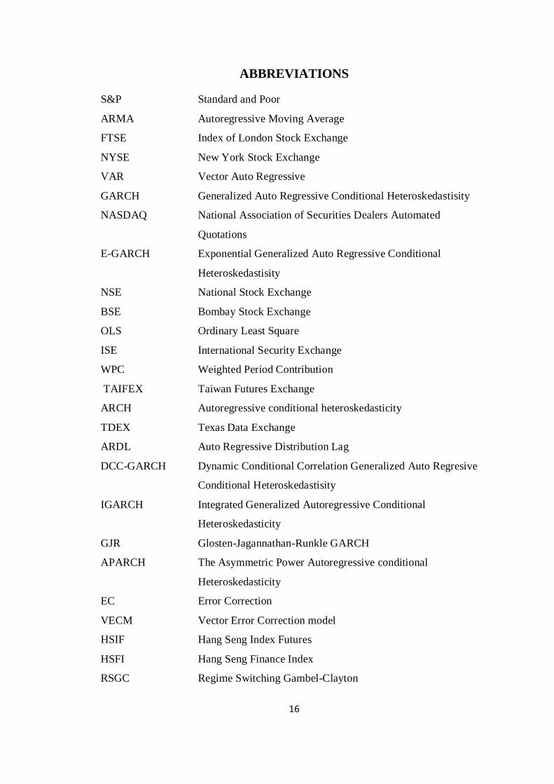
ABBREVIATIONS
S&P Standard and Poor
ARMA Autoregressive Moving Average
FTSE Index of London Stock Exchange
NYSE New York Stock Exchange
VAR Vector Auto Regressive
GARCH Generalized Auto Regressive Conditional Heteroskedastisity
NASDAQ National Association of Securities Dealers Automated
Quotations
E-GARCH Exponential Generalized Auto Regressive Conditional
Heteroskedastisity
NSE National Stock Exchange
BSE Bombay Stock Exchange
OLS Ordinary Least Square
ISE International Security Exchange
WPC Weighted Period Contribution
TAIFEX Taiwan Futures Exchange
ARCH Autoregressive conditional heteroskedasticity
TDEX Texas Data Exchange
ARDL Auto Regressive Distribution Lag
DCC-GARCH Dynamic Conditional Correlation Generalized Auto Regresive
Conditional Heteroskedastisity
IGARCH Integrated Generalized Autoregressive Conditional
Heteroskedasticity
GJR Glosten-Jagannathan-Runkle GARCH
APARCH The Asymmetric Power Autoregressive conditional
Heteroskedasticity
EC Error Correction
VECM Vector Error Correction model
HSIF Hang Seng Index Futures
HSFI Hang Seng Finance Index
RSGC Regime Switching Gambel-Clayton
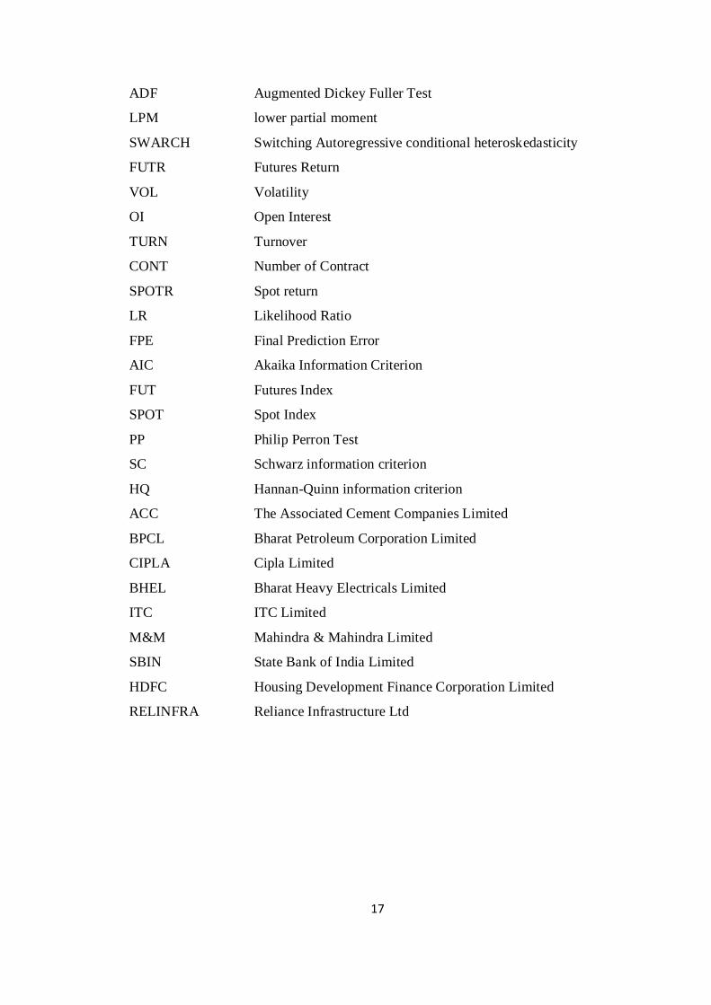
17
ADF Augmented Dickey Fuller Test
LPM lower partial moment
SWARCH Switching Autoregressive conditional heteroskedasticity
FUTR Futures Return
VOL Volatility
OI Open Interest
TURN Turnover
CONT Number of Contract
SPOTR Spot return
LR Likelihood Ratio
FPE Final Prediction Error
AIC Akaika Information Criterion
FUT Futures Index
SPOT Spot Index
PP Philip Perron Test
SC Schwarz information criterion
HQ Hannan-Quinn information criterion
ACC The Associated Cement Companies Limited
BPCL Bharat Petroleum Corporation Limited
CIPLA Cipla Limited
BHEL Bharat Heavy Electricals Limited
ITC ITC Limited
M&M Mahindra & Mahindra Limited
SBIN State Bank of India Limited
HDFC Housing Development Finance Corporation Limited
RELINFRA Reliance Infrastructure Ltd

18
Chapter -I
Introduction
19
CHAPTER –I
INTRODUCTION
1.1. PREAMBLE
Investment is a vital part of the basic behavior of civilized society. In the
financial environment, investment is essentially the process of depositing the money
with the dual objective of having regular income and capital appreciation. Stock
market satisfies both the objectives very systematically and effectively. Regular
income from the perspective of dividend or interest and capital appreciation is the
price changes in the basic value of the shares. Investors are of different types like risk
lovers and risk evaders. Risk evaders do not like to be active in the market and they
are willing to wait to get high return from their minimal investment money after a
long period. Risk lovers are the real players in the stock market. They expect more
return with low risk. Portfolio construction is one of the strategies to make more profit
and to reduce the risk. The beginning of derivatives would be traced from a distant
past when investors in foreign nation especially Europe, US and some developed
Asian nations started to think about alternative ways to make more profit from the
existing investments.
Derivatives are the contracts or assets whose values are changed on the basis
of the changes in the underlying assets. Primarily derivatives markets are identified
for price discovery, arbitrage and risk protection or risk reduction. There are many
products such as futures, options and swaps in the derivatives markets. Among these
products futures are more popular in India. Futures market is the market which
basically depends on the spot market. Theoretically, both the spot and futures market
must move together and adjust or respond to the information and events in a similar
manner. Ideally there is perfect relationship between spot and futures markets. It is
paradoxical that, in practice such close relationship is not evident in Indian spot and
futures markets as per researches done. It is interesting to note that most of the time
futures markets lead the spot market and very rarely spot market leads futures
markets. Literature indicates that futures market is leading the spot market because of
20
high trading volume, multiple trading patterns, less transaction cost, high leverage and
less restriction in short sales.
1.2. RISK MANAGEMENT
Risk is the inherited element of investment and the complementary aspects of
return. People like or dislike risk, it cannot be avoided from the investment process
due to the positive relationship with them. While risk increases return is also
increasing and risk reduction indicates the trend of decrease in return. Investors
always make strategies to get maximum return from minimum level of risk. It makes
the investment process interesting. There are many ways to reduce risk and make
maximum return. Investment portfolio and hedging strategies are so popular among
the risk reduction strategies.
Derivatives are the tool which has been introduced with an aim of enhancing
price discovery, arbitrage and hedging process. Risk of the spot market can be
managed through the hedging process in futures market. Hedgers are the one of the
participants in the derivatives market. Managing or controlling risk is the aim of these
traders in spot and futures market. In order to reduce the risk the traders offset their
investment in the opposite investment strategy. The traders who hedge their
investment by taking opposite position of spot in the futures market are known as
hedgers. In other words, making an investment to reduce the risk of adverse price
movements in an asset is the process of hedging. A hedge consists of taking an
offsetting position in a related security like futures contract. Investors use hedging
strategy when they are unsure of what the market will do. A perfect hedge reduces the
investment risk to nothing. It is important to note that if both markets are integrated
then there is a chance of hedging. According to the empirical result of the studies,
Indian spot market and future market are integrated, hence there is a possibility of
hedging between Indian spot and futures markets.
1.3. DERIVATIVES
The derivatives were in practice in post-1970 period due to growing instability
in the financial markets. These products are initially drawn as hedging devices against
fluctuations in commodity prices and linked product. Derivative is a product or
contract which does not have any value on its own that means, it derives its value
21
from some underlying products. Derivatives base may be an asset, or an index, or
even a phenomenon. They do not have an independent existence of their own. In
recent years, derivatives products become very popular and the emergence of the
market for derivative products like forwards, futures, options and swaps can be taken
as to the willingness of risk-averse economic agents to guard themselves against
uncertainties which are arising out of fluctuations in asset prices. The financial
markets are underlined by high degree of volatility.
A common fact to use derivatives is to manage or control the risk of the
financial operation but speculators and arbitrageurs can seek profits from general
price changes or simultaneous price variations in different markets. In the case of
equity derivatives, options and futures on stock indices have gained much popularity
than on individual stocks, especially among institutional investors who are major
users of index-linked derivatives. By using derivative products, it is possible to
transfer price risks fully or partially through blocking in assets prices. The financial
derivatives have been grown up due to the different factors such as high volatility of
assets prices in financial markets, increased integration of national and international
financial markets, development and use of more sophisticated risk management tools,
availability of many choices of risk management strategies and innovations in the
derivatives markets.
1.4. FORMS OF DERIVATIVES
Normally derivatives contracts are classified on the basis of its privilege and
right which are handled by the parties of contracts. Derivatives are the contracts on
the basis of underlying assets and their values are varied due to the change in the
value of underlying assets. These contracts are made with some privileges either to
the buyer or to the seller and these contracts are authorized or not, how these are
framed, are the basis to be considered to form the derivatives. There are mainly four
forms of derivatives such as forward, futures, options and swaps. Forward is the
basis of derivatives which contains a promise between two parties to buy or sell their
assets on a particular date with the agreed price. It is not authorized and there is no
guarantee for the execution. The same form of contract is done within the authorized
agency like stock exchanges is known as futures. In simple word, futures are the
standardized form of forward contract. Here only one side is protected that is risk and
22
can be managed but nothing is mentioned about the profit. Options, the buyer has the
right but he is not obliged to exercise it. Option contracts are giving more benefit to
the buyer, and the execution of the contracts is always upto the interest of option
buyer, not the option seller. An option is an agreement that gives the buyer the right,
but not the obligation, to buy or sell an underlying asset at a specific price on or
before a specified date. Swaps are private contracts between two parties to exchange
cash flows in the future according to a pre-arranged formula. It is a form of
derivatives in which counter parties exchange some benefits of one party’s financial
document for the benefit of another’s benefit. Normally, the two counterparties agree
to exchange one form of cash flow against another stream of flow. They can be
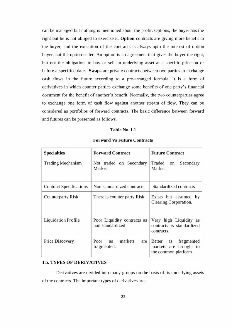
considered as portfolios of forward contracts. The basic difference between forward
and futures can be presented as follows.
Table No. I.1
Forward Vs Future Contracts
Specialties Forward Contract Future Contract
Trading Mechanism Not traded on Secondary
Market
Traded on Secondary
Market
Contract Specifications Non standardized contracts Standardized contracts
Counterparty Risk There is counter party Risk Exists but assumed by
Clearing Corporation.
Liquidation Profile Poor Liquidity contracts as
non standardized
Very high Liquidity as
contracts is standardized
contracts.
Price Discovery Poor as markets are
fragmented.
Better as fragmented
markets are brought to the common platform.
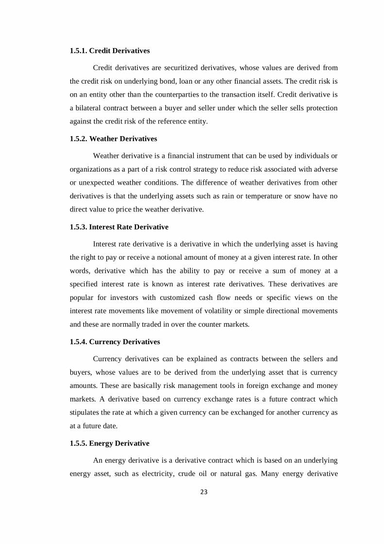
1.5. TYPES OF DERIVATIVES
Derivatives are divided into many groups on the basis of its underlying assets
of the contracts. The important types of derivatives are;
23
1.5.1. Credit Derivatives
Credit derivatives are securitized derivatives, whose values are derived from
the credit risk on underlying bond, loan or any other financial assets. The credit risk is
on an entity other than the counterparties to the transaction itself. Credit derivative is
a bilateral contract between a buyer and seller under which the seller sells protection
against the credit risk of the reference entity.
1.5.2. Weather Derivatives
Weather derivative is a financial instrument that can be used by individuals or
organizations as a part of a risk control strategy to reduce risk associated with adverse
or unexpected weather conditions. The difference of weather derivatives from other
derivatives is that the underlying assets such as rain or temperature or snow have no
direct value to price the weather derivative.
1.5.3. Interest Rate Derivative
Interest rate derivative is a derivative in which the underlying asset is having
the right to pay or receive a notional amount of money at a given interest rate. In other
words, derivative which has the ability to pay or receive a sum of money at a
specified interest rate is known as interest rate derivatives. These derivatives are
popular for investors with customized cash flow needs or specific views on the
interest rate movements like movement of volatility or simple directional movements
and these are normally traded in over the counter markets.
1.5.4. Currency Derivatives
Currency derivatives can be explained as contracts between the sellers and
buyers, whose values are to be derived from the underlying asset that is currency
amounts. These are basically risk management tools in foreign exchange and money
markets. A derivative based on currency exchange rates is a future contract which
stipulates the rate at which a given currency can be exchanged for another currency as
at a future date.
1.5.5. Energy Derivative
An energy derivative is a derivative contract which is based on an underlying
energy asset, such as electricity, crude oil or natural gas. Many energy derivative
24
options are based on petroleum or crude oil, but as fuel sources diversify, other kinds
of energy derivatives attract investors as well. The value of derivative may vary based
on the changes of the price of the underlying energy product which can be used for
both speculation and hedging purposes. Companies either they sell or just use energy,
can buy or sell energy derivatives to hedge against fluctuations in the movement of
underlying energy prices.
1.5.6. Insurance Derivative
A financial instrument which derives its value from an underlying insurance
index or the event that is related to insurance is known as insurance derivatives.
Insurance derivatives are useful for insurance companies who want to hedge their
exposure to crushing losses due to exceptional events such as earthquakes, hurricanes
or other natural calamities.
1.5.7. Health Insurance Derivatives
The introduction of trading on insurance derivatives at the CBOT offers
insurers, reinsurers, and in the case of health insurance, health care providers, hospital
managers and low-cost hedging alternatives. The main purpose of hedging with the
proposed health insurance futures is the management of the risk in changes in claims,
costs arising from unexpected volatility in the trend of these costs. It is important to
note that these new instruments do not provide insurance coverage and health
insurance futures are not alternative forms of insurance or reinsurance policies. The
health insurance futures contracts lead the way to health care futures contracts to
hedge rising health care costs.
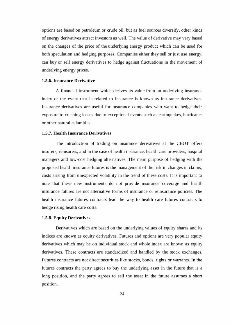
1.5.8. Equity Derivatives
Derivatives which are based on the underlying values of equity shares and its
indices are known as equity derivatives. Futures and options are very popular equity
derivatives which may be on individual stock and whole index are known as equity
derivatives. These contracts are standardized and handled by the stock exchanges.
Futures contracts are not direct securities like stocks, bonds, rights or warrants. In the
futures contracts the party agrees to buy the underlying asset in the future that is a
long position, and the party agrees to sell the asset in the future assumes a short
position.
25
1.5.9. Commodity Derivatives
Commodity derivatives are investment tools which allow investors to make
profit from certain items that are not possessing by them. The commodity derivatives
are the ways to protect the risk of farmers. The poor farmers can make promise to sell
crops in the future for a pre-arranged price and to protect the loss of the price during
the harvesting season. In short, commodity derivatives provide the confidence to the
farmers and encourage them to make trading strategies, which may help them to
sustain in their field.
1.6. DERIVATIVES MARKET IN INDIA
In India, commodity futures date back to 1875. In the sixties and seventies the
government banned futures trading in many of the commodities. Forward trading was
banned in the 1960s by the government despite the fact that India had a long tradition
of forward markets. In exercise of the power under section 16 of the Securities
Contracts (Regulation) Act, the government by its notification issued in 1969,
prohibited all forward trading in securities. However, the forward contracts in the
rupee dollar exchange rates that are foreign exchange rates are allowed by the Reserve
Bank and used on a fairly large scale. Futures trading are permitted in 41
commodities. There are 18 commodity exchanges in India. Now, the Forward Markets
Commission under the Ministry of Food and Consumer Affairs acts as a regulator of
commodity derivatives in India.
In the case of capital markets, the indigenous 125 year old badla system was
very popular among the broking and investor community. The advent of foreign
institutional investors in the nineties and a large number of scams led to a ban on
badla. The foreign institutional investors were not comfortable with this system and
they insisted on adequate risk-management tools. The Securities and Exchange Board
of India (SEBI) decided to introduce financial derivatives in India. However, there
were many legal hurdles which had to be overcome before introducing financial
derivatives. The position of Indian futures market, its market capitalization and trade
values are explained in the table.
26
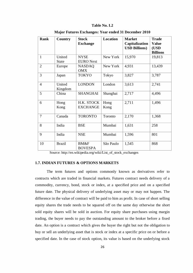
Table No. I.2
Major Futures Exchanges: Year ended 31 December 2010
Rank Country Stock
Exchange
Location Market
Capitalization
USD Billions)
Trade
Value
(USD
Billions
1 United
State
NYSE
EURO Next
New York 15,970 19,813
2 Europe NASDAQ
OMX
New York 4,931 13,439
3 Japan TOKYO
Tokyo 3,827 3,787
4 United
Kingdom
LONDON London 3,613 2,741
5 China SHANGHAI
Shanghai 2,717 4,496
6 Hong
Kong
H.K. STOCK
EXCHANGE
Hong
Kong
2,711 1,496
7 Canada TORONTO
Toronto 2,170 1,368
8 India BSE
Mumbai 1,631 258
9 India NSE
Mumbai 1,596 801
10 Brazil BM&F
BOVESPA
São Paulo 1,545 868
Source: http://en.wikipedia.org/wiki/List_of_stock_exchanges
1.7. INDIAN FUTURES & OPTIONS MARKETS
The term futures and options commonly known as derivatives refer to
contracts which are traded in financial markets. Futures contract needs delivery of a
commodity, currency, bond, stock or index, at a specified price and on a specified
future date. The physical delivery of underlying asset may or may not happen. The
difference in the value of contract will be paid to him as profit. In case of short selling
equity shares the trade needs to be squared off on the same day otherwise the short
sold equity shares will be sold in auction. For equity share purchases using margin
trading, the buyer needs to pay the outstanding amount to the broker before a fixed
date. An option is a contract which gives the buyer the right but not the obligation to
buy or sell an underlying asset that is stock or index at a specific price on or before a
specified date. In the case of stock option, its value is based on the underlying stock
27
and an index option the value of which is based on the underlying index. Options are
traded in the same way like stocks. They can be bought and sold just like any other
security. In case of options, the buyer pays only the premium amount and not the
value of the entire contract. The commission for the Options, however, will be based
on the value of the underlying assets. In Indian context, futures and options are very
popular among the derivatives products and it is mostly traded in Bombay Stock
Exchange and National Stock Exchange. Even though both markets are very popular,
on the basis of trade value of stock exchanges, the NSE (801USD Billion) is far better
than the BSE (258 USD Billion). On the basis of market capitalization, BSE performs
better way than the NSE as per the statistics of December 2010. On the basis of trade
value, NSE is the representative of Indian futures market.
1.8. FUTURES AND OPTIONS TRADING AT NSE
In India, at the National Stock Exchange, index futures trading were
introduced in the year 2000. Index Options trading was also made available in the
year 2001. Stock futures were introduced on 9th
Nov 2001. F&O index contracts are
available in Nifty, Junior Nifty, Bank Nifty, CNX IT and CNX 100. For individual
securities, F&O contracts are available in 223 scrips, starting from Aban Offshore to
Zee Entertainment Enterprises Limited. The contracts are traded as lots which mean a
contract will have certain fixed number of instruments. Stock futures are available for
most of the Nifty and Junior Nifty stocks. The stocks are chosen from amongst the top
500 stocks in terms of average daily market capitalization and average daily traded
value in the previous six months on a rolling basis. The market wide position limit in
the stock shall not be less than Rs.50 cores. The market wide position limit shall be
valued taking the closing prices of stocks in the underlying cash market on the date of
expiry of contract in the month.
28
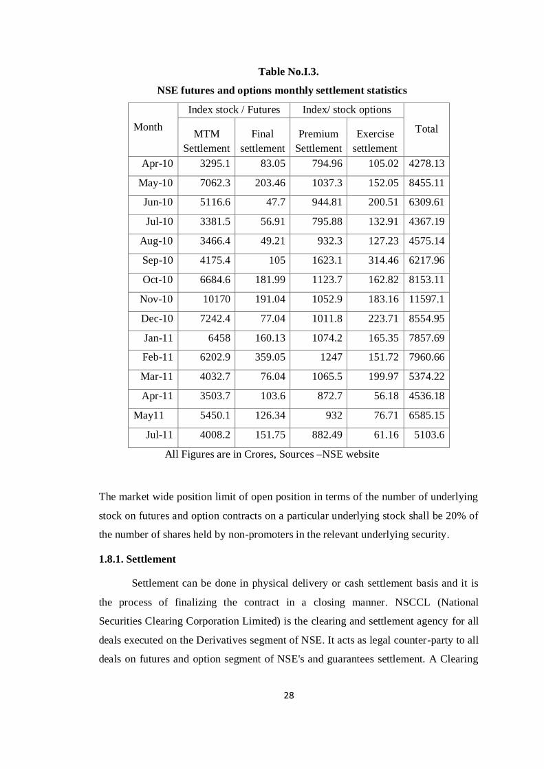
Table No.I.3.
NSE futures and options monthly settlement statistics
Month
Index stock / Futures Index/ stock options
Total MTM
Settlement
Final
settlement
Premium
Settlement
Exercise
settlement
Apr-10 3295.1 83.05 794.96 105.02 4278.13
May-10 7062.3 203.46 1037.3 152.05 8455.11
Jun-10 5116.6 47.7 944.81 200.51 6309.61
Jul-10 3381.5 56.91 795.88 132.91 4367.19
Aug-10 3466.4 49.21 932.3 127.23 4575.14
Sep-10 4175.4 105 1623.1 314.46 6217.96
Oct-10 6684.6 181.99 1123.7 162.82 8153.11
Nov-10 10170 191.04 1052.9 183.16 11597.1
Dec-10 7242.4 77.04 1011.8 223.71 8554.95
Jan-11 6458 160.13 1074.2 165.35 7857.69
Feb-11 6202.9 359.05 1247 151.72 7960.66
Mar-11 4032.7 76.04 1065.5 199.97 5374.22
Apr-11 3503.7 103.6 872.7 56.18 4536.18
May11 5450.1 126.34 932 76.71 6585.15
Jul-11 4008.2 151.75 882.49 61.16 5103.6
All Figures are in Crores, Sources –NSE website
The market wide position limit of open position in terms of the number of underlying
stock on futures and option contracts on a particular underlying stock shall be 20% of
the number of shares held by non-promoters in the relevant underlying security.
1.8.1. Settlement
Settlement can be done in physical delivery or cash settlement basis and it is
the process of finalizing the contract in a closing manner. NSCCL (National
Securities Clearing Corporation Limited) is the clearing and settlement agency for all
deals executed on the Derivatives segment of NSE. It acts as legal counter-party to all
deals on futures and option segment of NSE's and guarantees settlement. A Clearing
29
Member of NSCCL has the responsibility of clearing and settlement of all deals
executed by Trading Members on NSE.
1.8.2. Final Settlement
On the expiry date of the futures contracts, the NSCCL marks all positions of
trading members to the final settlement price and the profit loss is settled in the form
of cash. The final settlement profit or loss is computed as the difference between trade
price or the previous day's settlement price and the final settlement price of the
relevant futures contract. Final settlement loss or profit amount is debited or credited
to the relevant clearing member’s bank account on T+1day formula.
1.8.3. Settlement Period
The period between the trade date and the settlement date. In other words the
number of days between the trade date and the settlement date. The trade date is the
day on which investors agree on the security transaction, while the settlement date is
the day where securities transfer from one to another and settlement is made.
Different types of transactions have different settlement periods. The month in which
the underlying assets of futures contact are delivered to the contract holder is known
as settlement month and the date on which payment is made to settle a trade that is the
date on which either cash or a security must be in the hands of the broker to satisfy the
conditions of a security transaction is the settlement date, then the risk that a trade will
not settle that is the risk that one party will deliver and the counterparty will not be
able to pay is the settlement risk. The another important term which is so close to the
term settlement is the settlement price which is the official closing price for a future
set by the clearing house at the end of each trading day. Settlement prices are used to
determine both margin calls and invoice prices for deliveries.
1.8.4. Clearing Members
Clearing Members of NSCCL has the responsibility of clearing and
settlement of all deals executed by Trading Members on NSE. Primarily the functions
like settlement and risk management are performed by the clearing members. In the
settlement function the actual settlement that is only fund settlement is performed and
the margins are settled to reduce the risk.
30
1.8.5. Clearing Bank
NSCCL has made net work of 13 clearing banks which are required to operate
and maintain clearing accounts with any of the empanelled clearing banks at the
designated clearing bank branches. The clearing accounts are to be used exclusively
for clearing & settlement operations. In the NSE trading settlement schedule, the
settlement of trades is on T+1 working day basis. Trading members with a funds pay-
in obligation are required to have clear funds in their basic clearing account on or
before 10.30 a.m. on the settlement day and after that the payout of amount is credited
to the primary clearing account of the members. Daily mark to market settlement
system is followed. The positions of the trader in the futures contracts are marked-to-
market to the daily settlement price of the futures contracts at the end of each trading
day. The profit or loss as the difference between the current and previous day closing
price is transferred into clients account or to suffer the losses. Trading members are
responsible to collect and settle the profits or loss from the trading members through
the settlement system.
1.8.6. Traders of Futures Contract
Futures traders are traditionally considered in one of two groups such as
hedgers, who have an interest in the underlying asset and are seeking to hedge out the
risk of price changes, and speculators those who seek to make a profit by predicting
market moves and opening a derivative contract related to the asset. In other words,
the investor is seeking exposure to the asset in a long futures or the opposite effect
through a short futures contract. Hedgers typically include producers and consumers
of a commodity or the owner of an asset or assets subject to certain influences such as
an interest rate.
Both hedge and speculative notions involves a separately managed account
whose investment objective is to track the performance of a stock index. The Portfolio
manager normally manages cash inflows in an easy and cost effective manner by
investing in stock index futures. This gains the portfolio exposure to the index which
is consistent with the fund or account investment objective that without having to buy
an appropriate proportion of each of the individual in stocks. Futures market claims
social utility by providing the transfer of risk, increased liquidity and time preferences
to the traders. In real life, the actual delivery rate of the underlying goods specified in
31
futures contracts is very low, it indicates that the hedging or speculating benefits of
the contracts can be had largely without holding the contract until expiry and
delivering the goods.
1.8.7. Stock Index Futures
It is the futures which are framed on the basis of the individual stock which is
available for trading in the market. In simple term stock index future is a futures
contract on individual stock index. It is confirmed that markets in stock index futures
is the baskets of securities which provide an apt trading medium for uniformed
liquidity traders who wish to trade portfolios in the market. This future can be used to
speculate on the future direction of the stock market or to hedge a portfolio of
securities against normal market movements.
1.8.8. Stock Index Futures Contract
These are contracts which are traded in terms of number of contracts in the
futures markets. It is a standardized contract which is traded on a futures exchange in
the form of buying or selling a certain underlying instrument at a certain date in the
future, at a specified agreed price.
1.8.9. Volatility
The measure in the change of price on a financial instrument over time is
known as volatility. It explains the amount of uncertainty or risk about the size of
variations in an asset’s value. Normally volatility is expressed in yearly terms which
can either be measured by using the statistical measures like standard deviation or
variance between returns from that same security or market index. A higher volatility
indicates that an asset’s value can potentially be varied over a larger range of values,
in other words, the price of the assets can change dramatically over a short period in
either direction. Beta is one of the measures of relative volatility of a specific asset to
the market. Volatility can be estimated by the annualized standard deviation of daily
change in price and the price moves up and down rapidly over short time periods, it is
said that high volume of volatility.
1.8.10. Futures Margin
A margin is posted by the trader to minimize credit risk to the stock exchange.
Normally 5-15% of the value of contract is the margin of the futures contracts. To
32
minimize counterparty risk to traders, trades executed on regulated futures exchanges
which are guaranteed by clearing houses. The clearing house becomes the buyer to
each seller, and the seller to each buyer, so that in the event of a counterparty default
the clearer assumes the risk of loss.
There are different types of margins such as Clearing Margin which are
distinct from customer margins that individual buyers and sellers of futures and
options contracts are required to deposit with brokers, Customer Margin for which
Futures Commission Merchants are responsible for overseeing customer margin
accounts. This margin is determined on the basis of market risk and contract value,
Initial Margin which is calculated on the basis of maximum estimated change in
contract value within a trading day. Initial margin is set by the exchange. If a position
involves an exchange-traded product, the amount or percentage of initial margin is set
by the exchange concerned, Maintenance Margin which is set of minimum margin
per outstanding futures contract that a customer must maintain in his margin account,
Margin-Equity Ratio that is a term used by speculators those who are representing
the amount of their trading capital that is being held as margin at any particular time.
The low margin requirements of futures results in substantial leverage of the
investment. However, the exchanges require a minimum amount that varies
depending on the contract and the trader. The broker may set the requirement higher,
but may not set it lower, Performance Bond Margin in which the amount of money
deposited by both a buyer and seller of a futures contract or an options seller to ensure
performance of the term of the contract and finally Return on Margin which is often
used to judge performance, because it represents the gain or loss compared to the
exchange’s perceived risk as reflected in required margin.
1.8.11. Pricing of Futures Contracts
The price of a futures contract is determined through arbitrage process if the
underlying asset is in supply. This is normally for stock index futures, index futures,
treasury bond futures and futures on physical commodities. When the deliverable
commodity does not exist the futures price cannot be fixed by arbitrage and there is
only one force which is simple supply and demand for the asset in the future to set the
price during this time.
33
The forward price contains the expected future value of the underlying
discounted at the risk free rate. The value of the future F(t), will be found by
compounding the present value S(t) at time t to maturity T by the rate of risk-free
return. When the deliverable commodity is not in plentiful supply, rational pricing
cannot be applied. The price of the futures is determined by today's supply and
demand for the underlying asset in the futures. In a deep and liquid market, supply
and demand would be expected to balance out at a price which represents an unbiased
expectation of the future price of the actual asset and so be given by the simple
relationship.
1.9. FACTORS INFLUENCING THE PRICE OF FUTURES
The prices of index futures and on individual shares generally follow the price
development in the underlying asset. The difference in the price between the
underlying asset and the future, also called the basis, is fundamentally determined by
the current supply and demand in the future. Arbitrage between the equity market and
futures market will, however, ensure that price effects from the market expectations
are adjusted so that the basis essentially reflects the money market rate. The futures
price is determined by many factors such as the market price of the underlying asset ,
the money market rate and expected dividend on the underlying asset during the life
of the future supply or demand, movement of futures market and the other aspects of
futures market like number of contract and trade volume of futures contract. A
theoretical price of an index future may be decided based on the reasoning that the
index future serves as a substitute for a share portfolio that is based on the index
constituents. Regardless of the choice of investment the investor will achieve a capital
gain or a capital loss.
The holder of a futures contract will not receive any dividend payments from
the shares in the portfolio but equally he does not have to tie up funds in the shares as
the shareholder. The holder of a futures contract may thus achieve a payoff by using
the excess liquidity elsewhere in the money market. Since the size of this difference in
investment return is time sensitive, the difference between the futures price and the
index value will narrow towards futures expiry date and will be eliminated at expiry.
Returns in the form of dividend payments are relatively limited, and historically they
have underperformed the money market rate, which is why index futures are generally

34
priced higher than the index value. The pricing of futures on individual shares follows
the same principles as for index futures for buying the share. The buyer of a future
therefore does not tie up liquidity in the share, but does not receive dividends. The
price of a future on an individual share will generally be higher than the price of the
underlying share. The expected dividend on a single share may influence the price of
the future at the time when dividend is actually paid, by which the price of the share is
higher than the price of the future.
1.10. RELATIONSHIP BETWEEN SPOT AND FUTURES MARKETS
The relationship of the spot and futures markets is the basic element of price
discovery process. The price discovery process is the process of determining the price
of an asset in the marketplace through the interactions of buyers and sellers. In other
words it is a method of determining the price for a specific commodity or
security through basic supply and demand factors related to the market. The price
discovery takes place continuously in the modern and dynamic market. The price will
sometimes fall below the duration average and sometimes exceed the average as a
result of the noise due to uncertainties. Price discovery involves number of buyers and
sellers, market mechanism, information about the markets and risk management
mechanism. Actually, price discovery helps to find the exact price for a commodity or
a share of a company. The price discovery is used in speculative markets which help
the traders, manufacturers, exporters, farmers, refineries, governments, consumers,
and speculators.
Price discovery process begins to favor the more competitive markets, leaving
attractive trading exchanges with fewer participants and effectively redundant in price
determination. Price discovery predominantly originates in the local markets. It
originates primarily from the stock exchanges. Many research works suggested that a
lead-lag relationship of up to 30 minutes from futures price to the spot price.
Fleming, Ostdick and Whaley, (1996) observed that the market with the lowest
trading cost will react more quickly to new information.
Information transmission or price discovery is an indication of the relative
market efficiencies of related assets. There are three approaches to study the price
discovery of assets such as the lead lag relationship between the price of notional
market or between different securities, examination of the role of volatility in the
35
price discovery process and to study how information is transferred among different
markets. It is argued that price discovery occurs mainly in the spot market which is
dominated by foreign and domestic institutional investors (Bohl, Salm and Schuppli,
2010). The aim of security market design is optimal price discovery, so the choice of
market structure will heavily on the best market. Increased volatility in futures prices
will have consequences for hedging, arbitrage strategies and margin requirements.
Cost of trading, combined with the nature of new information, has relationship
between futures and cash markets. Futures price may temporarily contain more
information until such information flows from futures to cash price. Price discovery
refers to the process through markets converge towards the efficiency price of the
underlying assets. At any point in time there is a flow of new information into assets
markets and market prices for the assets concerned readjusted to such new flows.
Literally, when two markets for the same assets are faced with the same
information arriving simultaneously, the two markets should react at the same time in
a similar fashion. If the two markets do not react at the same time, then one market
will lead the other. When such a lead lag relation appears in case of price adjustment,
the leading market is considered as contributing a price discovery function for that
sector. In early times, it has been observed that the spot market has a greater speed of
assimilation of new information that comes to the market and has predictive power for
the futures price movements in the underlying assets. Normally futures market
incorporates new information more quickly than the spot markets, primarily because
of their inherent high leverage and low transaction cost. Price discovery function
implies the presence of an equilibrium relation binding the two prices together. In
other words, it is said that there is common factor or an unobservable efficient price
that drives both the spot and futures prices. Another arguments in price discovery is
that the existence of long run relationship. The share of price discovery originating in
futures markets has important implication for hedgers and arbitragers. Imperfect
trading specification of the futures contracts may be responsible for the violation of
the common notion that an asset which involves zero investment will always be an
efficient price discovery vehicle. In developed markets, new information is
incorporated in too quickly. Trading halt consistently help to reduce price dispersion
and enhance the efficiency of the price discovery process. When trading is halted due
36
to significant pending news release, the efficiency of the price discovery process is
enhanced by the halt.
1.11. ROLE OF TRADE VOLUME AND MARKET DEPTH TO EXPLAIN
THE MARKET MOVEMENT
Futures market movement is closely associated with spot market movement.
The price variations and the trade volume of the both market may have high level of
role to decide the efficiency of futures and spot market. Open interest is the variable
of market depth of futures market. The outstanding number of contracts which are not
settled is an open interest and it shows the depth of the market movement.
1.11.1. Open Interest
In simple terms open Interest is the total number of futures or option contracts
that are not closed or delivered on the particular day or the number of buy market
orders before the market opens. It applies primarily to the futures market and is often
used to confirm trends and trend reversals for futures and options contracts. Open
interest measures the flow of money into the futures market. For each seller of a
futures contract there must be a buyer of that contract. Thus a seller and a buyer
combine to create only one contract. Open interest provides useful information that
should be considered while entering a contract position. If both parties in the
transaction are closing positions then the open interest decreases accordingly. If they
are in opening positions then the open interest goes up accordingly. One way to use
open interest is to look at it relation to the volume of contracts traded. When the
volume exceeds the existing open interest on a given day, this suggests that trading in
that option was exceptionally high that day. Open interest provides information to
determine whether there is unusually high or low volume for any particular contract.
It is mostly used as an indication of the strength of the market, but is not the same as
volume which is also often used as a strength indicator.
The movement of open interest with other variables can be taken as the
indicator of the futures market. An increase in open interest along with an increase in
price is confirmed an upward trend. Similarly, an increase in open interest along with
a decrease in price confirms a downward trend. In the other context, an increase or
decrease in prices while open interest remains flat or declining may indicate a
37
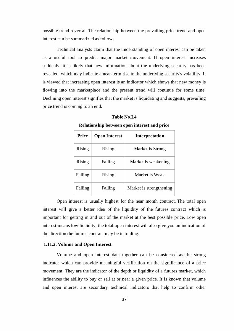
possible trend reversal. The relationship between the prevailing price trend and open
interest can be summarized as follows.
Technical analysts claim that the understanding of open interest can be taken
as a useful tool to predict major market movement. If open interest increases
suddenly, it is likely that new information about the underlying security has been
revealed, which may indicate a near-term rise in the underlying security's volatility. It
is viewed that increasing open interest is an indicator which shows that new money is
flowing into the marketplace and the present trend will continue for some time.
Declining open interest signifies that the market is liquidating and suggests, prevailing
price trend is coming to an end.
Table No.I.4
Relationship between open interest and price
Price Open Interest Interpretation
Rising Rising Market is Strong
Rising Falling Market is weakening
Falling Rising Market is Weak
Falling Falling Market is strengthening
Open interest is usually highest for the near month contract. The total open
interest will give a better idea of the liquidity of the futures contract which is
important for getting in and out of the market at the best possible price. Low open
interest means low liquidity, the total open interest will also give you an indication of
the direction the futures contract may be in trading.
1.11.2. Volume and Open Interest
Volume and open interest data together can be considered as the strong
indicator which can provide meaningful verification on the significance of a price
movement. They are the indicator of the depth or liquidity of a futures market, which
influences the ability to buy or sell at or near a given price. It is known that volume
and open interest are secondary technical indicators that help to confirm other
38
technical signals on the charts. If an upside price breakout is accompanied by heavy
volume that is a strong signal that the market may want to continue to move higher
because it indicates more traders jumped on the rising prices. A general trading rule is
that, if both volume and open interest are increasing, then the trend will probably
continue in its present direction. If volume and open interest are declining, this can be
interpreted as a signal that the current trend may be about to end.
It is utilized that three dimensional approach to market analysis which
includes a study on price, volume and open interest. Among these three elements,
price is the most important. However, volume and open interest provide important
secondary confirmation of the price action on a chart and often provide a lead
indication of an impending change of trend. Volume represents the total amount of
trading activity or contracts that have changed hands in a given commodity market for
a single trading day. The greater the amount of trading during a market session the
higher will be the trading volume. Another way to analyze these terms is that the
volume represents a measure of intensity or pressure behind a price trend. The greater
the volume, it can be expected the existing trend to continue rather than reverse. It is
believed that volume precedes price, meaning that the loss of upside price pressure in
an uptrend or downside pressure in a downtrend will show up in the volume figures.
Where volume measures the pressure or intensity behind a price trend, open interest
measures the flow of money into the futures market. For each seller of a futures
contract there must be a buyer of that contract. Thus, a seller and a buyer combine to
create only one contract.
1.12. RISK MANAGEMENT THROUGH FUTURES
The main aim of the introduction of futures is to control and reduce risk in the
price movement. Further this can be used to manage the systemic risk, vested in the
investment in assets or securities. Increasing or decreasing the equity exposure of a
portfolio is popular with the help of Index Futures. Index funds are the funds which
imitate replicate index with an objective to generate the return equivalent to the Index.
The hedge terminology of the futures is used to reduce risk. Long hedge, short hedge,
cross hedge and the hedge ratios are the terms commonly used in the hedging process.
Derivatives can be considered a form of insurance in hedging, which is a
technique that attempts to reduce risk. They allow the risk related to the price of the
39
underlying asset to be transferred from one party to another. Hedging occurs when an
individual or institution buys an asset, such as a commodity or a bond that has coupon
payments or a stock that pays dividends and sells it using a futures contract.
Risk management strategy is applied in controlling or reducing chances of loss
from the variation in the prices of commodities, currencies, or securities. In other
words, hedging is a transfer of risk without buying insurance policies. It employs
many techniques, by taking equal and opposite positions in two different markets,
such as cash and futures markets, further it is used to protect one's capital against
effects of inflation through investing in financial instruments like bonds, shares or real
estate. Hedging is very popular in forex futures market due to the importance of
neutralizing the effect of currency fluctuations on sales income.
1.12.1. Hedge Ratio
The value of the proportion of a position that is hedged to the value of the
entire position is known as hedge ratio. It is a ratio which is comparing the value of a
position protected through a hedge with the size of the entire position itself. Hedge is
comparing the value of futures contracts purchased or sold to the value of the cash
commodity being hedged.
1.12.2. Minimum Variance Hedge Ratio
Minimum Variance Hedge Ratio is the ratio of futures contracts to a specific
spot position that minimizes the variance of the profit from the overall hedged
position and is invariant to the cost of the hedge. One problem with using futures
contracts to hedge a portfolio of spot assets is that perfect futures contracts may not
exist, so a perfect hedge cannot be achieved. A variation on the theme might go as
follows. Although there exists a futures market for an underlying asset, that futures
market is so illiquid that it is functionally useless. Thus, we need to find ways to use
sub-optimal contracts, contracts that are highly correlated with the underlying asset
and who have a similar variance. This is achieved using the minimum variance hedge
ratio. The minimum variance hedge ratio is the ratio of futures position relative to the
spot position that minimizes the variance of the position. If the spot and future
positions are perfectly correlated, then a 1:1 hedge ratio results of a perfect hedge.
The minimum variance hedge ratio can be calculated by dividing the covariance of
40
futures and spot by variance of futures. In short the minimum variance hedge ratio is
the ratio that minimizes the basic risk and it involves making a second investment
which will pay off if the first investment loses money. Hedging aims to deal with
situations where an investor predicts a company's stock will do well in relation to
rivals in the same industry. To achieve this, the investor needs to find a way of
making profit when the company does better than its rivals, but minimizing losses
when the entire industry performs badly. The solution is to hedge by buying stock in
one company, but shorting stock in rival companies. Shorting means to borrow stock,
sell it now, then buy it back and return it to the lender at a later date. This means that
the investor will profit if the stock price falls. The theory behind this form of hedging
is that if the first company does well on its own merits, the investor will make a profit.
If the entire industry does badly, the investor will have made some money by shorting
the second company, which minimizes the losses on the first company's stock. In this
context investor can make profit by making short sale in his investment.
The investor will face very low level of risk if the hedge ratio is very high. It
can be applied to any pair of investments whose performance is in some way related,
including factors such as currency exchange rates or commodity prices. The apt
method of estimating the hedge ratio may vary from situation to situation, but the
principle is to compare the potential losses with hedging in place against the potential
losses which are the main investment made without hedging. A crucial aspect in
hedging of risk is the optimal hedge ratio which is defined as the relationship between
the price of the spot instrument and that of the hedging instrument.
1.13. VOLATILITY AND LEAD -LAG IN FUTURES MARKET
A lead-lag effect describes the situation where one variable that is leading
variable correlated with the values of another variable that is lagging at later time. It
indicates that the lagging Indicators without leading Indicators tell nothing about how
the outcomes will be achieved. Leading Indicators without Lagging Indicators may
enable to focus on short-term performance, but it will not be able to confirm that
broader organizational outcomes have been achieved. Leading Indicators should
enable to take pre-emptive actions to improve the chances of achieving strategic
goals.
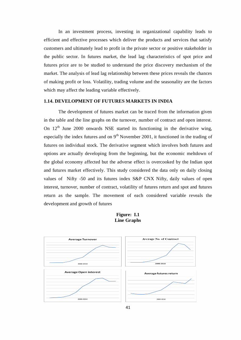
41
In an investment process, investing in organizational capability leads to
efficient and effective processes which deliver the products and services that satisfy
customers and ultimately lead to profit in the private sector or positive stakeholder in
the public sector. In futures market, the lead lag characteristics of spot price and
futures price are to be studied to understand the price discovery mechanism of the
market. The analysis of lead lag relationship between these prices reveals the chances
of making profit or loss. Volatility, trading volume and the seasonality are the factors
which may affect the leading variable effectively.
1.14. DEVELOPMENT OF FUTURES MARKETS IN INDIA
The development of futures market can be traced from the information given
in the table and the line graphs on the turnover, number of contract and open interest.
On 12th June 2000 onwards NSE started its functioning in the derivative wing,
especially the index futures and on 9th
November 2001, it functioned in the trading of
futures on individual stock. The derivative segment which involves both futures and
options are actually developing from the beginning, but the economic meltdown of
the global economy affected but the adverse effect is overcooked by the Indian spot
and futures market effectively. This study considered the data only on daily closing
values of Nifty -50 and its futures index S&P CNX Nifty, daily values of open
interest, turnover, number of contract, volatility of futures return and spot and futures
return as the sample. The movement of each considered variable reveals the
development and growth of futures
Figure: I.1
Line Graphs
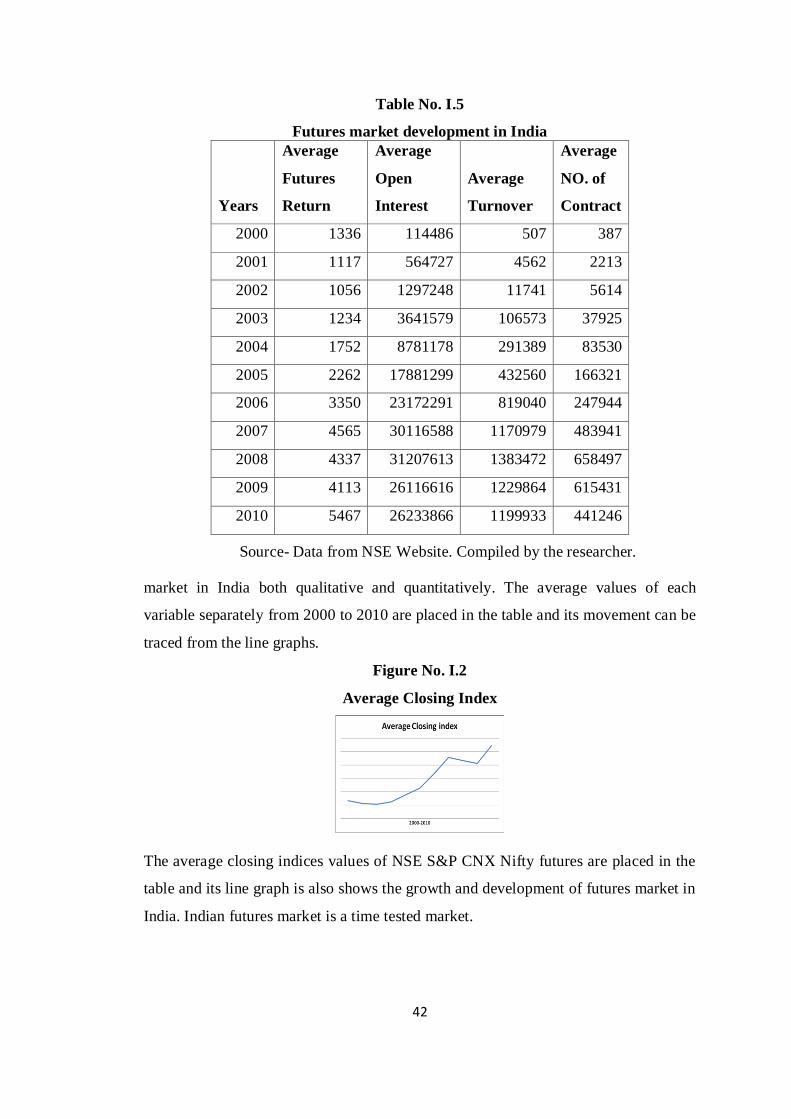
42
Table No. I.5
Futures market development in India
Years
Average
Futures
Return
Average
Open
Interest
Average
Turnover
Average
NO. of
Contract
2000 1336 114486 507 387
2001 1117 564727 4562 2213
2002 1056 1297248 11741 5614
2003 1234 3641579 106573 37925
2004 1752 8781178 291389 83530
2005 2262 17881299 432560 166321
2006 3350 23172291 819040 247944
2007 4565 30116588 1170979 483941
2008 4337 31207613 1383472 658497
2009 4113 26116616 1229864 615431
2010 5467 26233866 1199933 441246
Source- Data from NSE Website. Compiled by the researcher.
market in India both qualitative and quantitatively. The average values of each
variable separately from 2000 to 2010 are placed in the table and its movement can be
traced from the line graphs.
Figure No. I.2
Average Closing Index
The average closing indices values of NSE S&P CNX Nifty futures are placed in the
table and its line graph is also shows the growth and development of futures market in
India. Indian futures market is a time tested market.
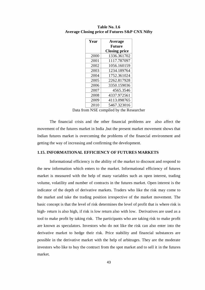
43
Table No. I.6
Average Closing price of Futures S&P CNX Nifty
Year Average
Future
Closing price
2000 1336.361702
2001 1117.787097
2002 1056.160159
2003 1234.189764
2004 1752.361024
2005 2262.817928
2006 3350.159036
2007 4565.3546
2008 4337.972561
2009 4113.098765
2010 5467.323016
Data from NSE compiled by the Researcher
The financial crisis and the other financial problems are also affect the
movement of the futures market in India ,but the present market movement shows that
Indian futures market is overcoming the problems of the financial environment and
getting the way of increasing and confirming the development.
1.15. INFORMATIONAL EFFICIENCY OF FUTURES MARKETS
Informational efficiency is the ability of the market to discount and respond to
the new information which enters to the market. Informational efficiency of futures
market is measured with the help of many variables such as open interest, trading
volume, volatility and number of contracts in the futures market. Open interest is the
indicator of the depth of derivative markets. Traders who like the risk may come to
the market and take the trading position irrespective of the market movement. The
basic concept is that the level of risk determines the level of profit that is where risk is
high- return is also high, if risk is low return also with low. Derivatives are used as a
tool to make profit by taking risk. The participants who are taking risk to make profit
are known as speculators. Investors who do not like the risk can also enter into the
derivative market to hedge their risk. Price stability and financial substances are
possible in the derivative market with the help of arbitrages. They are the moderate
investors who like to buy the contract from the spot market and to sell it in the futures
market.
44
Informational efficiency is the integral part of price discovery process. The
futures and spot market are formed on the basis of same assets. If both markets are
same in their ability and performance, the response and the movement of the markets
on any new information are to be in the same level, same volume, same direction and
at the same time but it are not seen in the practice. Even though the spot and futures
markets are co-integrated, they are not responding to the new information at the same
level. This makes the opportunity for the researcher to find the reason for the variation
in the movement and to find the efficiency of the market to discount to the new
information. Normally there is a chance for spot and futures market to respond to the
new information faster due to its special characteristics. Spot market may respond
faster than futures market because foreign institutional investors and domestic traders
are playing more in spot market in different context. But sometime futures market is
leading in responding to new information due to the high leverage, high trading
volume, different trading pattern, less transaction cost and less restriction for short
selling of the futures market. This relation is also known as lead lag relationship or
technically price discovery process. The market which is leading is passing the
information to the lagging market and simultaneously adjusting to the new
information and fixing the new price on the basis of market and other external
behavior. The market which is responding to the new information at first is known as
the leading market or more efficient market. Cointegrated markets and its relationship
helps the market players to identify the movement of the Cointegrated market and
make the investment and trading strategies according to the market movement. Daily
closing price movement of Indian futures market confirms the inefficiency. The data
distributions are not normal and they have random walk behavior and it is
nonstationary in its level form.
Efficient market movement is very clear to predict and its data structure is in
stationary or mean reverting at its level form. There is perfect arbitrauge opportunities
in the efficient market and very less chance for speculation and mal-practices in the
market. But random walk market provides uncertainty and high level of speculative
opportunities. Literature on futures market revealed different results on the
relationship between futures and spot market due to the special behavior of the
economy, market and time period. From the Indian market, studies on different period
support leading behavior of futures market, leading behavior of spot market and
45
bidirectional relationship between spot and futures market. It is because of the
difference in time period and the market movement. Again the different studies from
the literature shows the predicting ability of different variables like open interest,
trading volume, volatility and spot market movement. There is relationship between
these variables and the movement of futures market in India. But the level and
direction is different from to the foreign and developed market. When the quantitative
variables are integrated to the market return, it is very helpful to predict the futures
market effectively. The context where the variables are integrated or caused one to
another is the symbol of efficiency of variable to pass the information to another. This
study makes an attempt to cover the many aspects on futures and spot market to
understand the informational efficiency. In other words, it is a study to analyze the
efficiency of variables from futures and spot market with an objective of testing the
predictability of the movement and dependency of variables.
Relationship between futures and spot market reveals the efficiency in terms
of discovering the price at the earliest, lead- lag relationship and causality between
them. When relationship is established between the markets, efficiency can also be
established trough identifying the determinants of one to other variables. Efficiency is
also tested and proved through the ability of reducing the risk of investors in futures
than the spot market. Earlier studies have proved the relationship, this study makes an
attempt to find the efficiency in terms of relationship, determinants and risk reduction.
This study is organized in such a way that second chapter may give the reader
the thorough idea on the literature in the futures market, role of different variables as
the determinants of futures market, risk reduction efficiency through the hedging
process and the price discovery process of the futures and spot market. The third
chapter explains the methodology of the study, the tools and models used for the
analysis. The dynamic relationship between spot and futures market is thoroughly
analyzed and condensed in the fourth chapter. The role of spot market and the
determinants of futures market is analyzed and the influence of each variable on the
futures return is also depicted in the fifth chapter. Risk reduction efficiency of Indian
futures market is analyzed and the efficiency of individual stock also estimated in the
sixth chapter. Seventh chapter contains the findings and conclusions of the study. The

46
suggestions on the basis of the results and the scope for the further research due to the
limitations of the study are explained in the last part of this thesis.

47
Chapter-II
Review of Literature
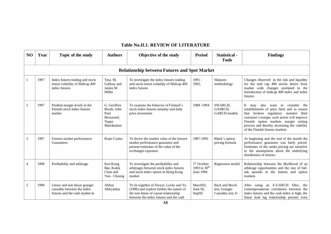
48
Table No.II.1. REVIEW OF LITERATURE
NO Year Topic of the study Authors Objective of the study Period Statistical -
Tools
Findings
Relationship between Futures and Spot Market
1 1997 Index futures trading and stock
return volatility of Midcap 400
index futures
Tina. M.
Galloay and
James M. Miller
To investigate the index futures trading
and stock return volatility of Midcap 400
index futures
1991 -
1992,
Skinners
methodology
Changes observed in the risk and liquidity
for the mid cap 400 stocks derive from
market wide changes unrelated to the introduction of midcap 400 index and index
futures
2 1997 Prudent margin levels in the Finnish stock index futures
market
G. Geoffrey Booth, John
Paul
Broussard,
Teppo Martikainen
To examine the behavior of Finland’s stock index futures intraday and daily
price movement
1988 -1994 SWARCH, GASRCH,
GARCH models
It may also want to consider the establishment of price limit and to ensure
that brokers regulatory monitor their
customer’s margin, such action will improve
Finnish option markets margin setting process and thereby increasing the viability
of the Finnish futures markets
3 1997 Futures market performance Guarantees
Rojer Craine To derive the market value of the futures market performance guarantee and
present estimates of the value of the
exchanges exposure.
1987-1995 Black’s option pricing formula
At beginning and the end of the month the performance guarantee was fairly priced.
Estimates of the under pricing are sensitive
to the assumptions about the underlying
distribution of returns.
4 1998 Profitability and arbitrage Kee-Kong
Bae, Kalok Chan and
Yan- Cheung
To investigate the profitability and
arbitrages between stock index futures and stock index option in Hong Kong
market.
1st October
1993 to 30th June 1994
Regression model Relationship between the likelihood of an
arbitrage opportunities and the size of bid-ask spreads in the futures and option
markets
5 1998 Linear and non linear granger causality between the index
futures and the cash market in
Abhay Abhyankar
To tie together of Dwyer, Locke and Yu (1996) and explore further the nature of
the non linear of causal relationship
between the index futures and the cash
March92, June 92,
Sept92
Back and Brock test, Granger
Causality test, E-
After using an E-GARCH filter, the contemporaneous correlation between the
index futures and the cash index is high, the
linear lead lag relationship persists even
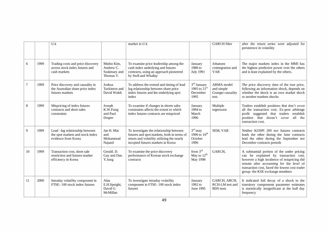
49
U.k market in U.k GARCH filter after the return series were adjusted for
persistence in volatility
6 1999 Trading costs and price discovery
across stock index futures and
cash markets
Minho Kim,
Andrew C.
Szakmary and Thomas V.
To examine price leadership among the
cash index underlying and futures
contracts, using an approach pioneered by Stoll and Whallay
January
1986 to
July 1991
Johansen
cointegration and
VAR
The major markets index in the MMI has
the highest predictive power over the others
and is least explained by the others.
7 1999 Price discovery and causality in
the Australian share price index futures markets
Joshua
Turkinton and David Walsh
To address the extend and timing of lead
lag relationship between share price index futures and the underlying spot
index
3rd January
1995 to 21st December
1995
ARMA model
and simple Granger causality
test.
The price discovery time of the true price,
following an information shock, depends on whether the shock is an own market shock
or another markets shocks
8 1999 Mispricing of index futures contracts and short sales
constraints
Joseph K.W.Fung
and Paul
Draper
To examine if changes in shorts sales constraints affects the extent to which
index futures contracts are mispriced
January 1994 to
March
1996
Multiple regression
Traders establish positions that don’t cover all the transaction cost. Ex-post arbitrage
profit suggested that traders establish
position that doesn’t cover all the transaction cost.
9 1999 Lead –lag relationship between
the spot markets and stock index evidence from Korea
Jae H. Min
and Mohammad
Najand
To investigate the relationship between
futures and spot markets, both in terms of return and volatility utilizing the nearly
incepted futures markets in Korea
3rd may
1996 to 16th October
1996
SEM, VAR Neither KOSPI 200 nor futures contracts
leads the other during the June contracts lead the other during the September nor
December contracts periods
10 1999 Transaction cost, short sale restriction and futures market
efficiency in Korea
Gerald. D. Gay and Dae.
Y.Jung
To examine the price discovery performance of Korean stock exchange
contracts
from 3rd May to 12th
May 1998
GARCH, A substantial portion of the under pricing can be explained by transaction cost,
however a high incidence of mispricing did
remain after accounting for the level of
transaction cost, faced the lowest cost trader group- the KSE exchange members
11 2000 Intraday volatility component in
FTSE- 100 stock index futures
Alan
E.H.Speight, David G.
McMillan
To investigate intraday volatility
component in FTSE- 100 stock index futures
January
1992 to June 1995
GARCH, ARCH,
RCH-LM test and BDS tests
It indicated full decay of a shock to the
transitory components parameter estimates is statistically insignificant at the half day
frequency
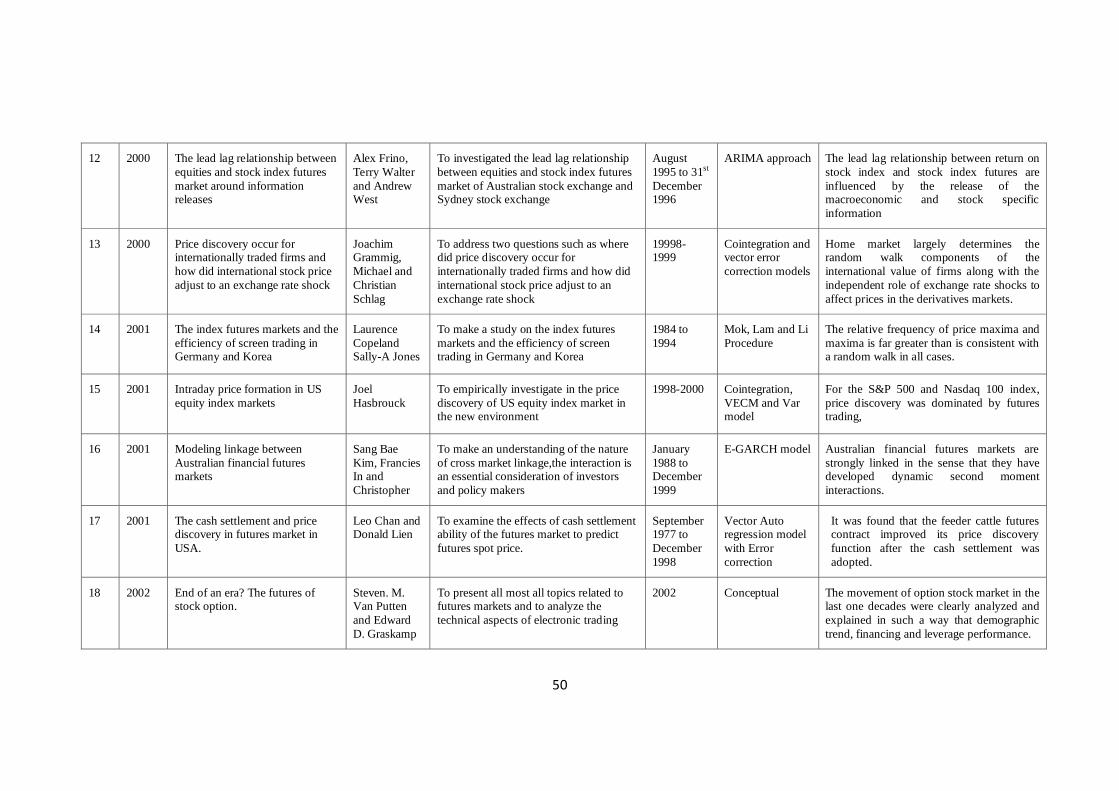
50
12 2000 The lead lag relationship between
equities and stock index futures
market around information releases
Alex Frino,
Terry Walter
and Andrew West
To investigated the lead lag relationship
between equities and stock index futures
market of Australian stock exchange and Sydney stock exchange
August
1995 to 31st
December 1996
ARIMA approach The lead lag relationship between return on
stock index and stock index futures are
influenced by the release of the macroeconomic and stock specific
information
13 2000 Price discovery occur for internationally traded firms and
how did international stock price
adjust to an exchange rate shock
Joachim Grammig,
Michael and
Christian
Schlag
To address two questions such as where did price discovery occur for
internationally traded firms and how did
international stock price adjust to an
exchange rate shock
19998-1999
Cointegration and vector error
correction models
Home market largely determines the random walk components of the
international value of firms along with the
independent role of exchange rate shocks to
affect prices in the derivatives markets.
14 2001 The index futures markets and the
efficiency of screen trading in Germany and Korea
Laurence
Copeland Sally-A Jones
To make a study on the index futures
markets and the efficiency of screen trading in Germany and Korea
1984 to
1994
Mok, Lam and Li
Procedure
The relative frequency of price maxima and
maxima is far greater than is consistent with a random walk in all cases.
15 2001 Intraday price formation in US
equity index markets
Joel
Hasbrouck
To empirically investigate in the price
discovery of US equity index market in the new environment
1998-2000 Cointegration,
VECM and Var model
For the S&P 500 and Nasdaq 100 index,
price discovery was dominated by futures trading,
16 2001 Modeling linkage between
Australian financial futures markets
Sang Bae
Kim, Francies In and
Christopher
To make an understanding of the nature
of cross market linkage,the interaction is an essential consideration of investors
and policy makers
January
1988 to December
1999
E-GARCH model Australian financial futures markets are
strongly linked in the sense that they have developed dynamic second moment
interactions.
17 2001 The cash settlement and price discovery in futures market in
USA.
Leo Chan and Donald Lien
To examine the effects of cash settlement ability of the futures market to predict
futures spot price.
September 1977 to
December
1998
Vector Auto regression model
with Error
correction
It was found that the feeder cattle futures contract improved its price discovery
function after the cash settlement was
adopted.
18 2002 End of an era? The futures of stock option.
Steven. M. Van Putten
and Edward
D. Graskamp
To present all most all topics related to futures markets and to analyze the
technical aspects of electronic trading
2002 Conceptual The movement of option stock market in the last one decades were clearly analyzed and
explained in such a way that demographic
trend, financing and leverage performance.
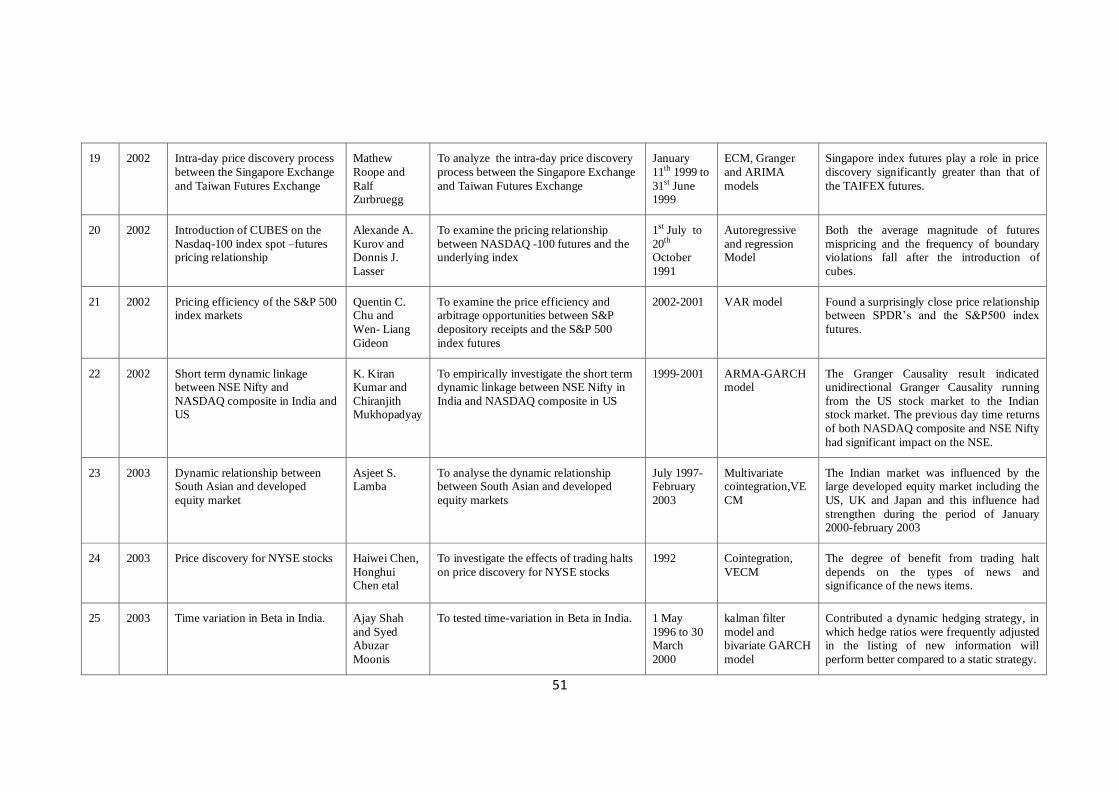
51
19 2002 Intra-day price discovery process
between the Singapore Exchange
and Taiwan Futures Exchange
Mathew
Roope and
Ralf Zurbruegg
To analyze the intra-day price discovery
process between the Singapore Exchange
and Taiwan Futures Exchange
January
11th 1999 to
31st June 1999
ECM, Granger
and ARIMA
models
Singapore index futures play a role in price
discovery significantly greater than that of
the TAIFEX futures.
20 2002 Introduction of CUBES on the
Nasdaq-100 index spot –futures pricing relationship
Alexande A.
Kurov and Donnis J.
Lasser
To examine the pricing relationship
between NASDAQ -100 futures and the underlying index
1st July to
20th October
1991
Autoregressive
and regression Model
Both the average magnitude of futures
mispricing and the frequency of boundary violations fall after the introduction of
cubes.
21 2002 Pricing efficiency of the S&P 500 index markets
Quentin C. Chu and
Wen- Liang
Gideon
To examine the price efficiency and arbitrage opportunities between S&P
depository receipts and the S&P 500
index futures
2002-2001 VAR model Found a surprisingly close price relationship between SPDR’s and the S&P500 index
futures.
22 2002 Short term dynamic linkage between NSE Nifty and
NASDAQ composite in India and US
K. Kiran Kumar and
Chiranjith Mukhopadyay
To empirically investigate the short term dynamic linkage between NSE Nifty in
India and NASDAQ composite in US
1999-2001 ARMA-GARCH model
The Granger Causality result indicated unidirectional Granger Causality running
from the US stock market to the Indian stock market. The previous day time returns
of both NASDAQ composite and NSE Nifty
had significant impact on the NSE.
23 2003 Dynamic relationship between South Asian and developed
equity market
Asjeet S. Lamba
To analyse the dynamic relationship between South Asian and developed
equity markets
July 1997-February
2003
Multivariate cointegration,VE
CM
The Indian market was influenced by the large developed equity market including the
US, UK and Japan and this influence had
strengthen during the period of January 2000-february 2003
24 2003 Price discovery for NYSE stocks Haiwei Chen,
Honghui Chen etal
To investigate the effects of trading halts
on price discovery for NYSE stocks
1992 Cointegration,
VECM
The degree of benefit from trading halt
depends on the types of news and significance of the news items.
25 2003 Time variation in Beta in India. Ajay Shah
and Syed Abuzar
Moonis
To tested time-variation in Beta in India. 1 May
1996 to 30 March
2000
kalman filter
model and bivariate GARCH
model
Contributed a dynamic hedging strategy, in
which hedge ratios were frequently adjusted in the listing of new information will
perform better compared to a static strategy.
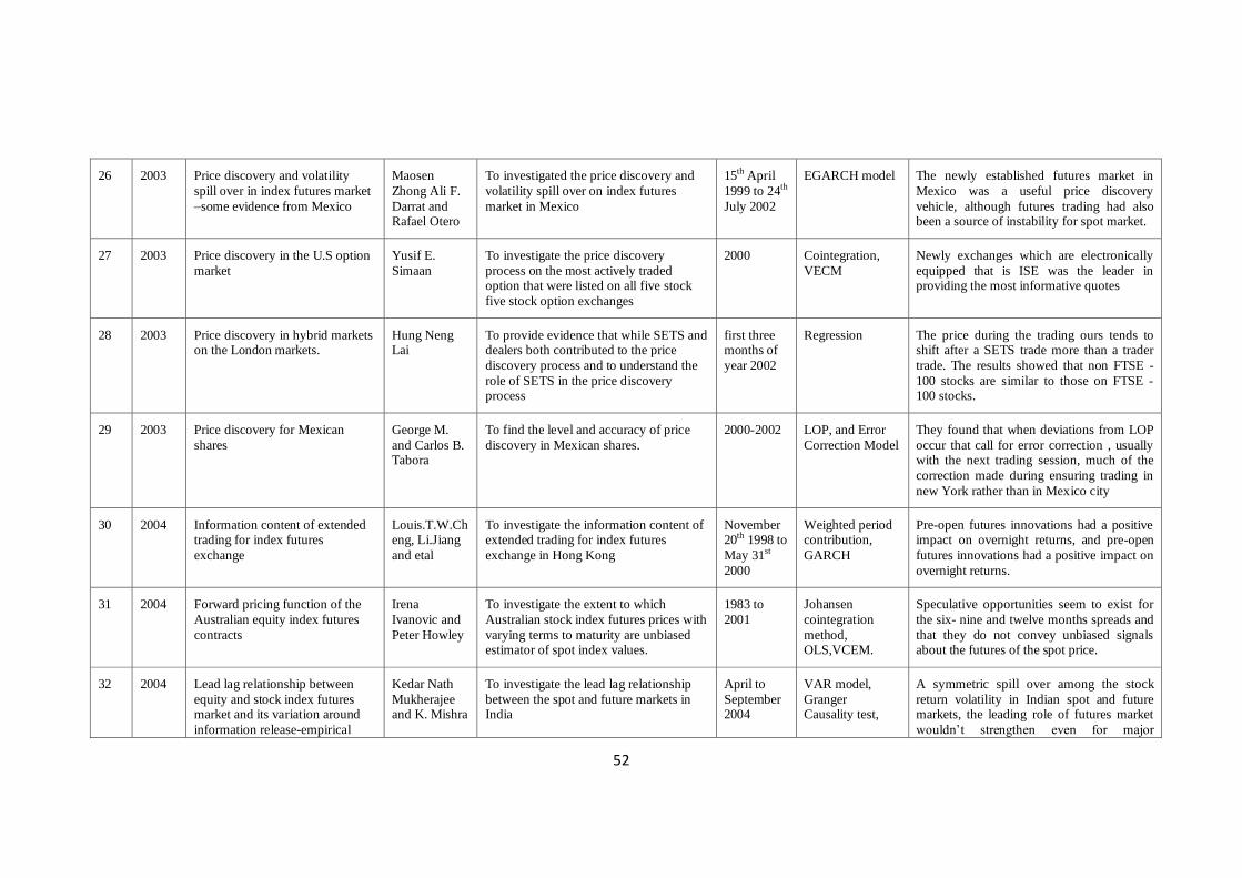
52
26 2003 Price discovery and volatility
spill over in index futures market
–some evidence from Mexico
Maosen
Zhong Ali F.
Darrat and Rafael Otero
To investigated the price discovery and
volatility spill over on index futures
market in Mexico
15th April
1999 to 24th
July 2002
EGARCH model The newly established futures market in
Mexico was a useful price discovery
vehicle, although futures trading had also been a source of instability for spot market.
27 2003 Price discovery in the U.S option
market
Yusif E.
Simaan
To investigate the price discovery
process on the most actively traded option that were listed on all five stock
five stock option exchanges
2000 Cointegration,
VECM
Newly exchanges which are electronically
equipped that is ISE was the leader in providing the most informative quotes
28 2003 Price discovery in hybrid markets on the London markets.
Hung Neng Lai
To provide evidence that while SETS and dealers both contributed to the price
discovery process and to understand the
role of SETS in the price discovery process
first three months of
year 2002
Regression The price during the trading ours tends to shift after a SETS trade more than a trader
trade. The results showed that non FTSE -
100 stocks are similar to those on FTSE -100 stocks.
29 2003 Price discovery for Mexican
shares
George M.
and Carlos B. Tabora
To find the level and accuracy of price
discovery in Mexican shares.
2000-2002 LOP, and Error
Correction Model
They found that when deviations from LOP
occur that call for error correction , usually with the next trading session, much of the
correction made during ensuring trading in
new York rather than in Mexico city
30 2004 Information content of extended trading for index futures
exchange
Louis.T.W.Cheng, Li.Jiang
and etal
To investigate the information content of extended trading for index futures
exchange in Hong Kong
November 20th 1998 to
May 31st
2000
Weighted period contribution,
GARCH
Pre-open futures innovations had a positive impact on overnight returns, and pre-open
futures innovations had a positive impact on
overnight returns.
31 2004 Forward pricing function of the
Australian equity index futures
contracts
Irena
Ivanovic and
Peter Howley
To investigate the extent to which
Australian stock index futures prices with
varying terms to maturity are unbiased estimator of spot index values.
1983 to
2001
Johansen
cointegration
method, OLS,VCEM.
Speculative opportunities seem to exist for
the six- nine and twelve months spreads and
that they do not convey unbiased signals about the futures of the spot price.
32 2004 Lead lag relationship between
equity and stock index futures market and its variation around
information release-empirical
Kedar Nath
Mukherajee and K. Mishra
To investigate the lead lag relationship
between the spot and future markets in India
April to
September 2004
VAR model,
Granger Causality test,
A symmetric spill over among the stock
return volatility in Indian spot and future markets, the leading role of futures market
wouldn’t strengthen even for major
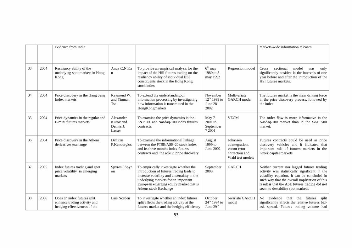
53
evidence from India markets-wide information releases
33 2004 Resiliency ability of the
underlying spot markets in Hong
Kong
Andy.C.N.Ka
n
To provide an empirical analysis for the
impact of the HSI futures trading on the
resiliency ability of individual HSI constituents stock in the Hong Kong
stock index
6th may
1980 to 5
may 1992
Regression model Cross sectional model was only
significantly positive in the intervals of one
year before and after the introduction of the HSI futures markets.
34 2004 Price discovery in the Hang Seng Index markets
Raymond W. and Yiuman
Tse
To extend the understanding of information processing by investigating
how information is transmitted in the
HongKongmarkets
November 12th 1999 to
June 28
2002
Multivariate GARCH model
The futures market is the main driving force in the price discovery process, followed by
the index.
35 2004 Price dynamics in the regular and E-mini futures markets
Alexander Kurov and
Dennis.J. Lasser
To examine the price dynamics in the S&P 500 and Nasdaq-100 index futures
contracts.
May 7 2001 to
September 7 2001
VECM The order flow is more informative in the Nasdaq-100 market than in the S&P 500
market.
36 2004 Price discovery in the Athens
derivatives exchange
Dimitris
F.Kenourgios
To examine the informational linkage
between the FTSE/ASE-20 stock index and its three months index futures
contracts and the role in price discovery
August
1999 to June 2002
Johansen
cointegration, vector error
correction and
Wald test models
Futures contracts could be used as price
discovery vehicles and it indicated that important role of futures markets in the
Greek capital markets
37 2005 Index futures trading and spot price volatility in emerging
markets
Spyros.I.Spyrou
To empirically investigate whether the introduction of futures trading leads to
increase volatility and uncertainty in the
underlying markets for an important European emerging equity market that is
Athens stock Exchange
September 2003
GARCH Neither current nor lagged futures trading activity was statistically significant in the
volatility equation. It can be concluded in
such way that the overall implication of this result is that the ASE futures trading did not
seem to destabilize spot markets.
38 2006 Does an index futures split enhance trading activity and
hedging effectiveness of the
Lars Norden To investigate whether an index futures split affects the trading activity at the
futures market and the hedging efficiency
October 24th 1994 to
June 29th
bivariate GARCH model
No evidence that the futures split significantly affects the relative futures bid-
ask spread. Futures trading volume had
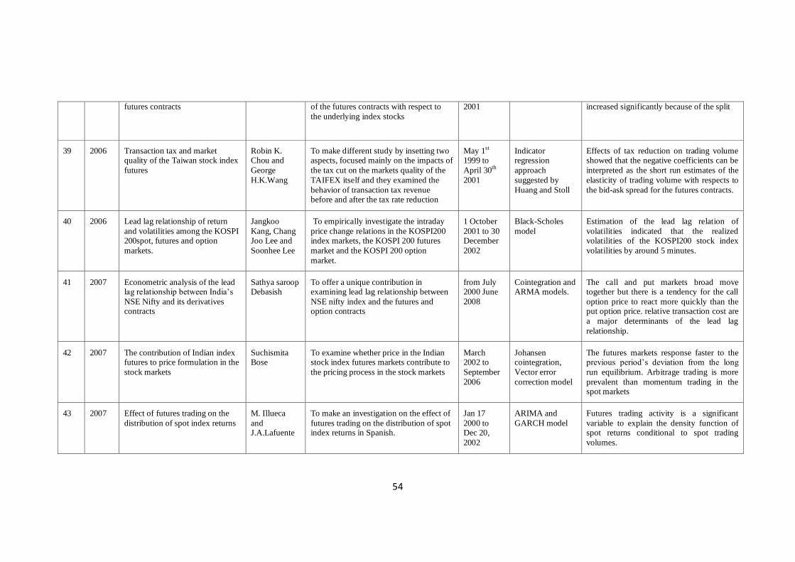
54
futures contracts of the futures contracts with respect to
the underlying index stocks
2001 increased significantly because of the split
39 2006 Transaction tax and market quality of the Taiwan stock index
futures
Robin K. Chou and
George
H.K.Wang
To make different study by insetting two aspects, focused mainly on the impacts of
the tax cut on the markets quality of the
TAIFEX itself and they examined the
behavior of transaction tax revenue before and after the tax rate reduction
May 1st 1999 to
April 30th
2001
Indicator regression
approach
suggested by
Huang and Stoll
Effects of tax reduction on trading volume showed that the negative coefficients can be
interpreted as the short run estimates of the
elasticity of trading volume with respects to
the bid-ask spread for the futures contracts.
40 2006 Lead lag relationship of return
and volatilities among the KOSPI 200spot, futures and option
markets.
Jangkoo
Kang, Chang Joo Lee and
Soonhee Lee
To empirically investigate the intraday
price change relations in the KOSPI200 index markets, the KOSPI 200 futures
market and the KOSPI 200 option
market.
1 October
2001 to 30 December
2002
Black-Scholes
model
Estimation of the lead lag relation of
volatilities indicated that the realized volatilities of the KOSPI200 stock index
volatilities by around 5 minutes.
41 2007 Econometric analysis of the lead lag relationship between India’s
NSE Nifty and its derivatives contracts
Sathya saroop Debasish
To offer a unique contribution in examining lead lag relationship between
NSE nifty index and the futures and option contracts
from July 2000 June
2008
Cointegration and ARMA models.
The call and put markets broad move together but there is a tendency for the call
option price to react more quickly than the put option price. relative transaction cost are
a major determinants of the lead lag
relationship.
42 2007 The contribution of Indian index futures to price formulation in the
stock markets
Suchismita Bose
To examine whether price in the Indian stock index futures markets contribute to
the pricing process in the stock markets
March 2002 to
September
2006
Johansen cointegration,
Vector error
correction model
The futures markets response faster to the previous period’s deviation from the long
run equilibrium. Arbitrage trading is more
prevalent than momentum trading in the spot markets
43 2007 Effect of futures trading on the
distribution of spot index returns
M. Illueca
and J.A.Lafuente
To make an investigation on the effect of
futures trading on the distribution of spot index returns in Spanish.
Jan 17
2000 to Dec 20,
2002
ARIMA and
GARCH model
Futures trading activity is a significant
variable to explain the density function of spot returns conditional to spot trading
volumes.
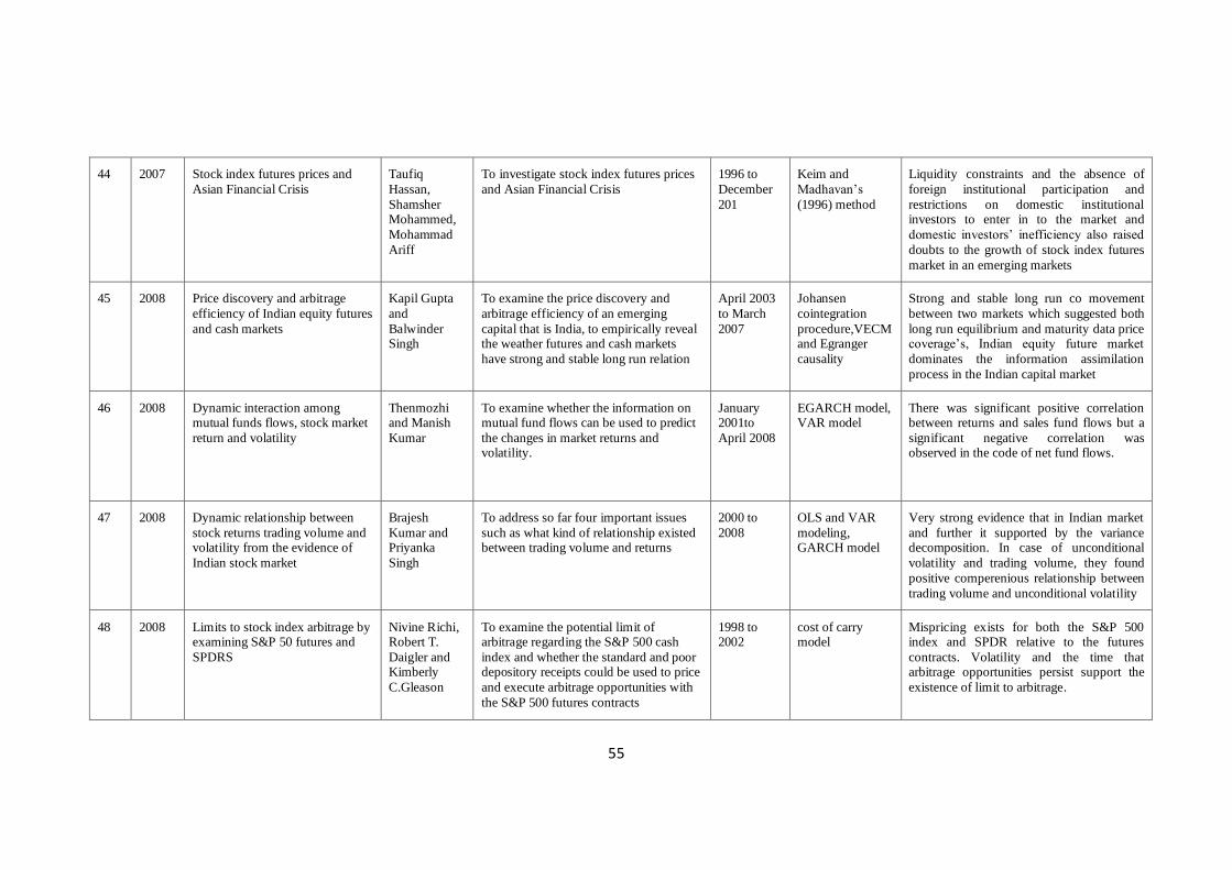
55
44 2007 Stock index futures prices and
Asian Financial Crisis
Taufiq
Hassan,
Shamsher Mohammed,
Mohammad
Ariff
To investigate stock index futures prices
and Asian Financial Crisis
1996 to
December
201
Keim and
Madhavan’s
(1996) method
Liquidity constraints and the absence of
foreign institutional participation and
restrictions on domestic institutional investors to enter in to the market and
domestic investors’ inefficiency also raised
doubts to the growth of stock index futures
market in an emerging markets
45 2008 Price discovery and arbitrage
efficiency of Indian equity futures
and cash markets
Kapil Gupta
and
Balwinder Singh
To examine the price discovery and
arbitrage efficiency of an emerging
capital that is India, to empirically reveal the weather futures and cash markets
have strong and stable long run relation
April 2003
to March
2007
Johansen
cointegration
procedure,VECM and Egranger
causality
Strong and stable long run co movement
between two markets which suggested both
long run equilibrium and maturity data price coverage’s, Indian equity future market
dominates the information assimilation
process in the Indian capital market
46 2008 Dynamic interaction among mutual funds flows, stock market
return and volatility
Thenmozhi and Manish
Kumar
To examine whether the information on mutual fund flows can be used to predict
the changes in market returns and volatility.
January 2001to
April 2008
EGARCH model, VAR model
There was significant positive correlation between returns and sales fund flows but a
significant negative correlation was observed in the code of net fund flows.
47 2008 Dynamic relationship between
stock returns trading volume and volatility from the evidence of
Indian stock market
Brajesh
Kumar and Priyanka
Singh
To address so far four important issues
such as what kind of relationship existed between trading volume and returns
2000 to
2008
OLS and VAR
modeling, GARCH model
Very strong evidence that in Indian market
and further it supported by the variance decomposition. In case of unconditional
volatility and trading volume, they found
positive comperenious relationship between
trading volume and unconditional volatility
48 2008 Limits to stock index arbitrage by examining S&P 50 futures and
SPDRS
Nivine Richi, Robert T.
Daigler and Kimberly
C.Gleason
To examine the potential limit of arbitrage regarding the S&P 500 cash
index and whether the standard and poor depository receipts could be used to price
and execute arbitrage opportunities with
the S&P 500 futures contracts
1998 to 2002
cost of carry model
Mispricing exists for both the S&P 500 index and SPDR relative to the futures
contracts. Volatility and the time that arbitrage opportunities persist support the
existence of limit to arbitrage.
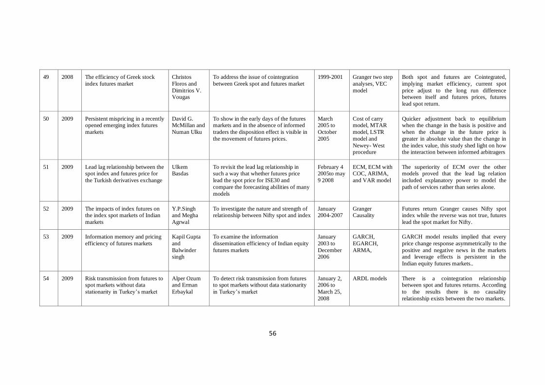
56
49 2008 The efficiency of Greek stock
index futures market
Christos
Floros and
Dimitrios V. Vougas
To address the issue of cointegration
between Greek spot and futures market
1999-2001 Granger two step
analyses, VEC
model
Both spot and futures are Cointegrated,
implying market efficiency, current spot
price adjust to the long run difference between itself and futures prices, futures
lead spot return.
50 2009 Persistent mispricing in a recently opened emerging index futures
markets
David G. McMillan and
Numan Ulku
To show in the early days of the futures markets and in the absence of informed
traders the disposition effect is visible in
the movement of futures prices.
March 2005 to
October
2005
Cost of carry model, MTAR
model, LSTR
model and
Newey- West procedure
Quicker adjustment back to equilibrium when the change in the basis is positive and
when the change in the future price is
greater in absolute value than the change in
the index value, this study shed light on how the interaction between informed arbitragers
51 2009 Lead lag relationship between the spot index and futures price for
the Turkish derivatives exchange
Ulkem Basdas
To revisit the lead lag relationship in such a way that whether futures price
lead the spot price for ISE30 and
compare the forecasting abilities of many
models
February 4 2005to may
9 2008
ECM, ECM with COC, ARIMA,
and VAR model
The superiority of ECM over the other models proved that the lead lag relation
included explanatory power to model the
path of services rather than series alone.
52 2009 The impacts of index futures on the index spot markets of Indian
markets
Y.P.Singh and Megha
Agrwal
To investigate the nature and strength of relationship between Nifty spot and index
January 2004-2007
Granger Causality
Futures return Granger causes Nifty spot index while the reverse was not true, futures
lead the spot market for Nifty.
53 2009 Information memory and pricing
efficiency of futures markets
Kapil Gupta
and
Balwinder singh
To examine the information
dissemination efficiency of Indian equity
futures markets
January
2003 to
December 2006
GARCH,
EGARCH,
ARMA,
GARCH model results implied that every
price change response asymmetrically to the
positive and negative news in the markets and leverage effects is persistent in the
Indian equity futures markets..
54 2009 Risk transmission from futures to spot markets without data
stationarity in Turkey’s market
Alper Ozum and Erman
Erbaykal
To detect risk transmission from futures to spot markets without data stationarity
in Turkey’s market
January 2, 2006 to
March 25,
2008
ARDL models There is a cointegration relationship between spot and futures returns. According
to the results there is no causality
relationship exists between the two markets.
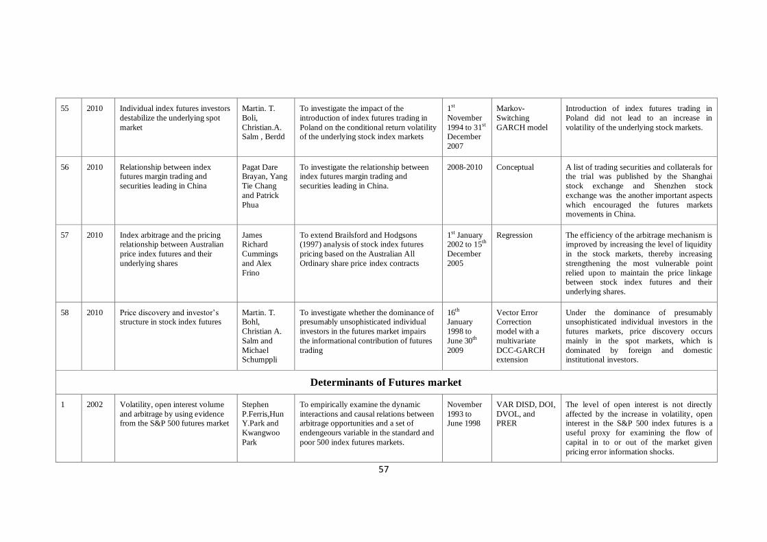
57
55 2010 Individual index futures investors
destabilize the underlying spot
market
Martin. T.
Boli,
Christian.A. Salm , Berdd
To investigate the impact of the
introduction of index futures trading in
Poland on the conditional return volatility of the underlying stock index markets
1st
November
1994 to 31st December
2007
Markov-
Switching
GARCH model
Introduction of index futures trading in
Poland did not lead to an increase in
volatility of the underlying stock markets.
56 2010 Relationship between index futures margin trading and
securities leading in China
Pagat Dare Brayan, Yang
Tie Chang
and Patrick
Phua
To investigate the relationship between index futures margin trading and
securities leading in China.
2008-2010 Conceptual A list of trading securities and collaterals for the trial was published by the Shanghai
stock exchange and Shenzhen stock
exchange was the another important aspects
which encouraged the futures markets movements in China.
57 2010 Index arbitrage and the pricing relationship between Australian
price index futures and their
underlying shares
James Richard
Cummings
and Alex
Frino
To extend Brailsford and Hodgsons (1997) analysis of stock index futures
pricing based on the Australian All
Ordinary share price index contracts
1st January 2002 to 15th
December
2005
Regression The efficiency of the arbitrage mechanism is improved by increasing the level of liquidity
in the stock markets, thereby increasing
strengthening the most vulnerable point
relied upon to maintain the price linkage between stock index futures and their
underlying shares.
58 2010 Price discovery and investor’s structure in stock index futures
Martin. T. Bohl,
Christian A.
Salm and
Michael Schumppli
To investigate whether the dominance of presumably unsophisticated individual
investors in the futures market impairs
the informational contribution of futures
trading
16th January
1998 to
June 30th
2009
Vector Error Correction
model with a
multivariate
DCC-GARCH extension
Under the dominance of presumably unsophisticated individual investors in the
futures markets, price discovery occurs
mainly in the spot markets, which is
dominated by foreign and domestic institutional investors.
Determinants of Futures market
1 2002 Volatility, open interest volume
and arbitrage by using evidence from the S&P 500 futures market
Stephen
P.Ferris,Hun Y.Park and
Kwangwoo
Park
To empirically examine the dynamic
interactions and causal relations between arbitrage opportunities and a set of
endengeours variable in the standard and
poor 500 index futures markets.
November
1993 to June 1998
VAR DISD, DOI,
DVOL, and PRER
The level of open interest is not directly
affected by the increase in volatility, open interest in the S&P 500 index futures is a
useful proxy for examining the flow of
capital in to or out of the market given
pricing error information shocks.
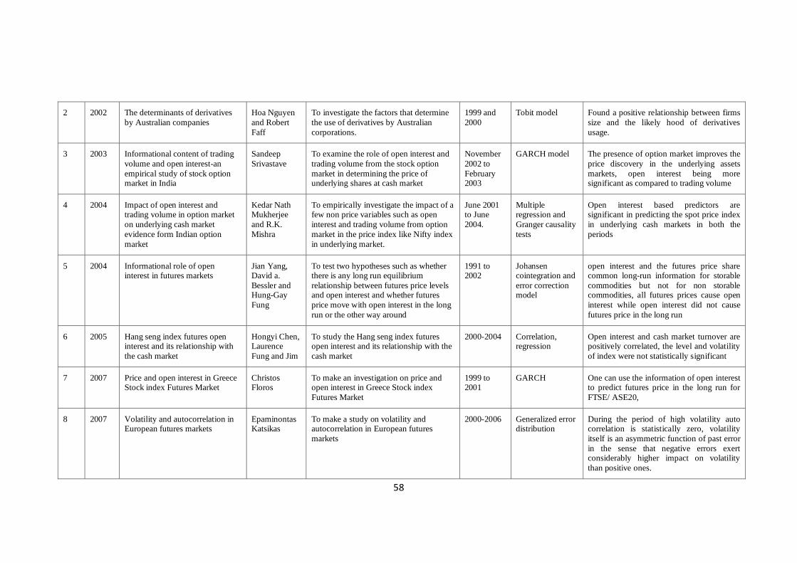
58
2 2002 The determinants of derivatives
by Australian companies
Hoa Nguyen
and Robert
Faff
To investigate the factors that determine
the use of derivatives by Australian
corporations.
1999 and
2000
Tobit model Found a positive relationship between firms
size and the likely hood of derivatives
usage.
3 2003 Informational content of trading
volume and open interest-an
empirical study of stock option market in India
Sandeep
Srivastave
To examine the role of open interest and
trading volume from the stock option
market in determining the price of underlying shares at cash market
November
2002 to
February 2003
GARCH model The presence of option market improves the
price discovery in the underlying assets
markets, open interest being more significant as compared to trading volume
4 2004 Impact of open interest and trading volume in option market
on underlying cash market
evidence form Indian option
market
Kedar Nath Mukherjee
and R.K.
Mishra
To empirically investigate the impact of a few non price variables such as open
interest and trading volume from option
market in the price index like Nifty index
in underlying market.
June 2001 to June
2004.
Multiple regression and
Granger causality
tests
Open interest based predictors are significant in predicting the spot price index
in underlying cash markets in both the
periods
5 2004 Informational role of open interest in futures markets
Jian Yang, David a.
Bessler and Hung-Gay
Fung
To test two hypotheses such as whether there is any long run equilibrium
relationship between futures price levels and open interest and whether futures
price move with open interest in the long
run or the other way around
1991 to 2002
Johansen cointegration and
error correction model
open interest and the futures price share common long-run information for storable
commodities but not for non storable commodities, all futures prices cause open
interest while open interest did not cause
futures price in the long run
6 2005 Hang seng index futures open interest and its relationship with
the cash market
Hongyi Chen, Laurence
Fung and Jim
To study the Hang seng index futures open interest and its relationship with the
cash market
2000-2004 Correlation, regression
Open interest and cash market turnover are positively correlated, the level and volatility
of index were not statistically significant
7 2007 Price and open interest in Greece Stock index Futures Market
Christos Floros
To make an investigation on price and open interest in Greece Stock index
Futures Market
1999 to 2001
GARCH One can use the information of open interest to predict futures price in the long run for
FTSE/ ASE20,
8 2007 Volatility and autocorrelation in European futures markets
Epaminontas Katsikas
To make a study on volatility and autocorrelation in European futures
markets
2000-2006 Generalized error distribution
During the period of high volatility auto correlation is statistically zero, volatility
itself is an asymmetric function of past error
in the sense that negative errors exert considerably higher impact on volatility
than positive ones.
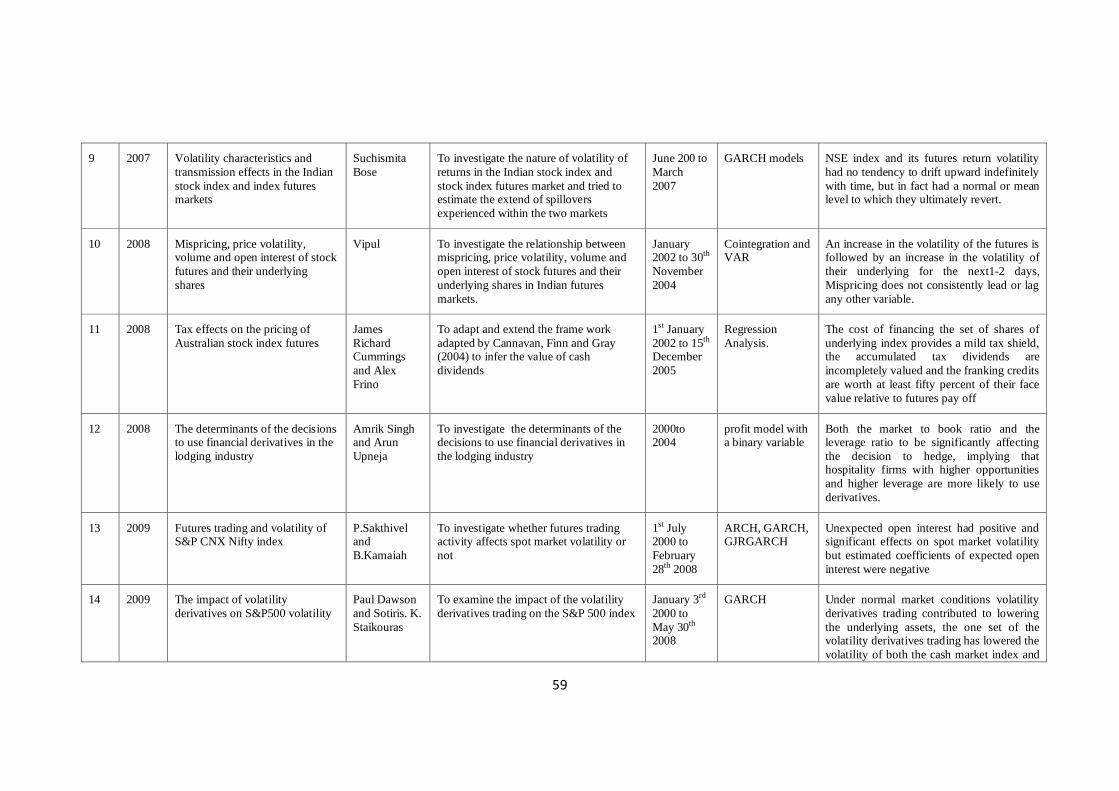
59
9 2007 Volatility characteristics and
transmission effects in the Indian
stock index and index futures markets
Suchismita
Bose
To investigate the nature of volatility of
returns in the Indian stock index and
stock index futures market and tried to estimate the extend of spillovers
experienced within the two markets
June 200 to
March
2007
GARCH models NSE index and its futures return volatility
had no tendency to drift upward indefinitely
with time, but in fact had a normal or mean level to which they ultimately revert.
10 2008 Mispricing, price volatility, volume and open interest of stock
futures and their underlying
shares
Vipul To investigate the relationship between mispricing, price volatility, volume and
open interest of stock futures and their
underlying shares in Indian futures
markets.
January 2002 to 30th
November
2004
Cointegration and VAR
An increase in the volatility of the futures is followed by an increase in the volatility of
their underlying for the next1-2 days,
Mispricing does not consistently lead or lag
any other variable.
11 2008 Tax effects on the pricing of
Australian stock index futures
James
Richard Cummings
and Alex
Frino
To adapt and extend the frame work
adapted by Cannavan, Finn and Gray (2004) to infer the value of cash
dividends
1st January
2002 to 15th December
2005
Regression
Analysis.
The cost of financing the set of shares of
underlying index provides a mild tax shield, the accumulated tax dividends are
incompletely valued and the franking credits
are worth at least fifty percent of their face
value relative to futures pay off
12 2008 The determinants of the decisions to use financial derivatives in the
lodging industry
Amrik Singh and Arun
Upneja
To investigate the determinants of the decisions to use financial derivatives in
the lodging industry
2000to 2004
profit model with a binary variable
Both the market to book ratio and the leverage ratio to be significantly affecting
the decision to hedge, implying that hospitality firms with higher opportunities
and higher leverage are more likely to use
derivatives.
13 2009 Futures trading and volatility of S&P CNX Nifty index
P.Sakthivel and
B.Kamaiah
To investigate whether futures trading activity affects spot market volatility or
not
1st July 2000 to
February
28th 2008
ARCH, GARCH, GJRGARCH
Unexpected open interest had positive and significant effects on spot market volatility
but estimated coefficients of expected open
interest were negative
14 2009 The impact of volatility
derivatives on S&P500 volatility
Paul Dawson
and Sotiris. K.
Staikouras
To examine the impact of the volatility
derivatives trading on the S&P 500 index
January 3rd
2000 to
May 30th 2008
GARCH Under normal market conditions volatility
derivatives trading contributed to lowering
the underlying assets, the one set of the volatility derivatives trading has lowered the
volatility of both the cash market index and
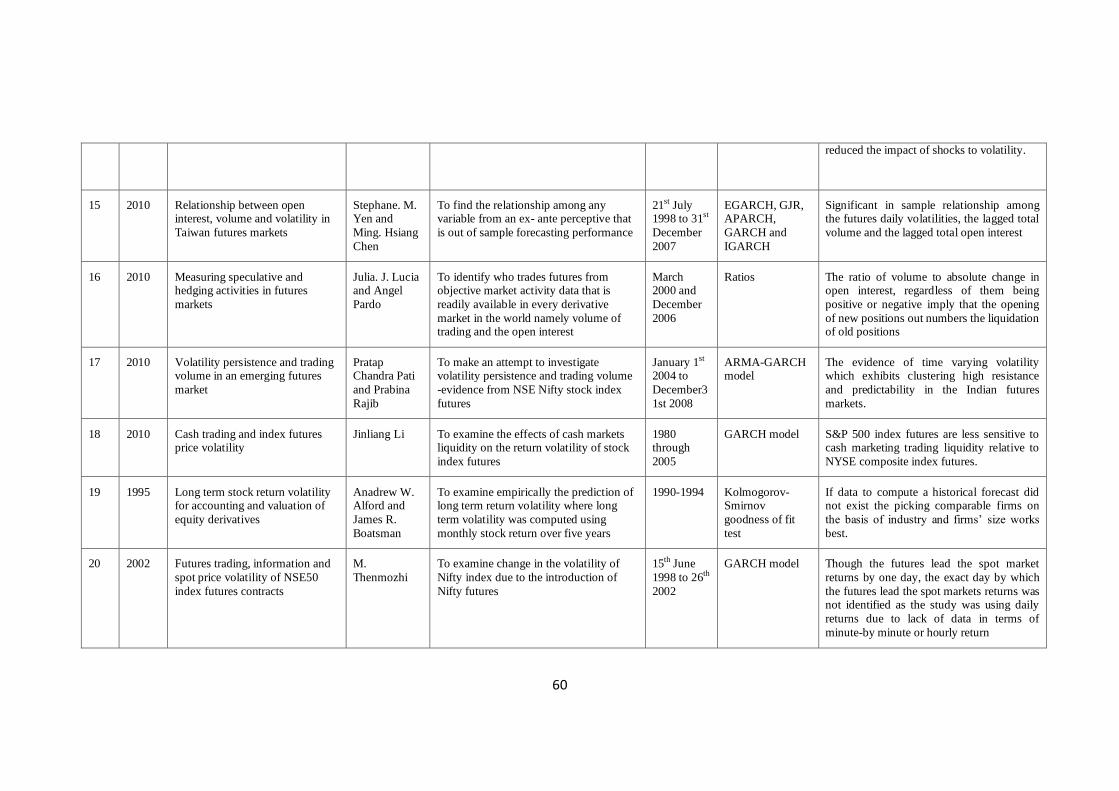
60
reduced the impact of shocks to volatility.
15 2010 Relationship between open interest, volume and volatility in
Taiwan futures markets
Stephane. M. Yen and
Ming. Hsiang
Chen
To find the relationship among any variable from an ex- ante perceptive that
is out of sample forecasting performance
21st July 1998 to 31st
December
2007
EGARCH, GJR, APARCH,
GARCH and
IGARCH
Significant in sample relationship among the futures daily volatilities, the lagged total
volume and the lagged total open interest
16 2010 Measuring speculative and hedging activities in futures
markets
Julia. J. Lucia and Angel
Pardo
To identify who trades futures from objective market activity data that is
readily available in every derivative
market in the world namely volume of trading and the open interest
March 2000 and
December
2006
Ratios The ratio of volume to absolute change in open interest, regardless of them being
positive or negative imply that the opening
of new positions out numbers the liquidation of old positions
17 2010 Volatility persistence and trading volume in an emerging futures
market
Pratap Chandra Pati
and Prabina
Rajib
To make an attempt to investigate volatility persistence and trading volume
-evidence from NSE Nifty stock index
futures
January 1st 2004 to
December3
1st 2008
ARMA-GARCH model
The evidence of time varying volatility which exhibits clustering high resistance
and predictability in the Indian futures
markets.
18 2010 Cash trading and index futures price volatility
Jinliang Li To examine the effects of cash markets liquidity on the return volatility of stock
index futures
1980 through
2005
GARCH model S&P 500 index futures are less sensitive to cash marketing trading liquidity relative to
NYSE composite index futures.
19 1995 Long term stock return volatility for accounting and valuation of
equity derivatives
Anadrew W. Alford and
James R.
Boatsman
To examine empirically the prediction of long term return volatility where long
term volatility was computed using
monthly stock return over five years
1990-1994 Kolmogorov-Smirnov
goodness of fit
test
If data to compute a historical forecast did not exist the picking comparable firms on
the basis of industry and firms’ size works
best.
20 2002 Futures trading, information and
spot price volatility of NSE50
index futures contracts
M.
Thenmozhi
To examine change in the volatility of
Nifty index due to the introduction of
Nifty futures
15th June
1998 to 26th
2002
GARCH model Though the futures lead the spot market
returns by one day, the exact day by which
the futures lead the spot markets returns was not identified as the study was using daily
returns due to lack of data in terms of
minute-by minute or hourly return
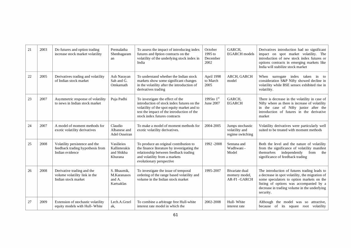
61
21 2003 Do futures and option trading
increase stock market volatility
Premalatha
Shenbagaram
an
To assess the impact of introducing index
futures and 0ption contracts on the
volatility of the underlying stock index in India
October
1995 to
December 2002
GARCH,
EGARCH models
Derivatives introduction had no significant
impact on spot market volatility. The
introduction of new stock index futures or options contracts in emerging markets like
India will stabilize stock market
22 2005 Derivatives trading and volatility of Indian stock market
Ash Narayan Sah and G.
Omkarnath
To understand whether the Indian stock markets show some significant changes
in the volatility after the introduction of
derivatives trading
April 1998 to March
2005
ARCH, GARCH model
When surrogate index taken in to consideration S&P Nifty showed decline in
volatility while BSE sensex exhibited rise in
volatility.
23 2007 Asymmetric response of volatility to news in Indian stock market
Puja Padhi To investigate the effect of the introduction of stock index futures on the
volatility of the spot equity market and to test the impact of the introduction of the
stock index futures contracts
1995to 1st June 2007
GARCH, EGARCH
There is decrease in the volatility in case of Nifty where as there is increase of volatility
in the case of Nifty junior after the introduction of futures in the derivative
market
24 2007
A model of moment methods for exotic volatility derivatives
Claudio Albanese and
Adel Osseiran
To make a model of moment methods for exotic volatility derivatives.
2004-2005 Jumps stochastic volatility and
regime switching
Volatility derivatives were particularly well suited to be treated with moment methods
25 2008 Volatility persistence and the feedback trading hypothesis from
Indian evidence
Vasilieios Kallinterakis
and Shikha
Khurana
To produce an original contribution to the finance literature by investigating the
relationship between feedback trading
and volatility from a markets
evolutionary perspective
1992 -2008 Sentana and Wadhwani -
Model
Both the level and the nature of volatility from the significance of volatility manifest
themselves independently from the
significance of feedback trading
26 2008 Derivative trading and the
volume volatility link in the
Indian stock market
S. Bhaumik,
M.Karanasos
and A. Kartsaklas
To investigate the issue of temporal
ordering of the range based volatility and
volume in the Indian stock market
1995-2007 Bivariate dual
momery model,
AR-FI –GARCH
The introduction of futures trading leads to
a decrease in spot volatility, the migration of
some speculators to option markets on the listing of options was accompanied by a
decrease in trading volume in the underlying
security.
27 2009 Extension of stochastic volatility equity models with Hull- White
Lech.A.Grzelak,
To combine a arbitrage free Hull-white interest rate model in which the
2002-2008 Hull- White interest rate
Although the model was so attractive, because of its square root volatility
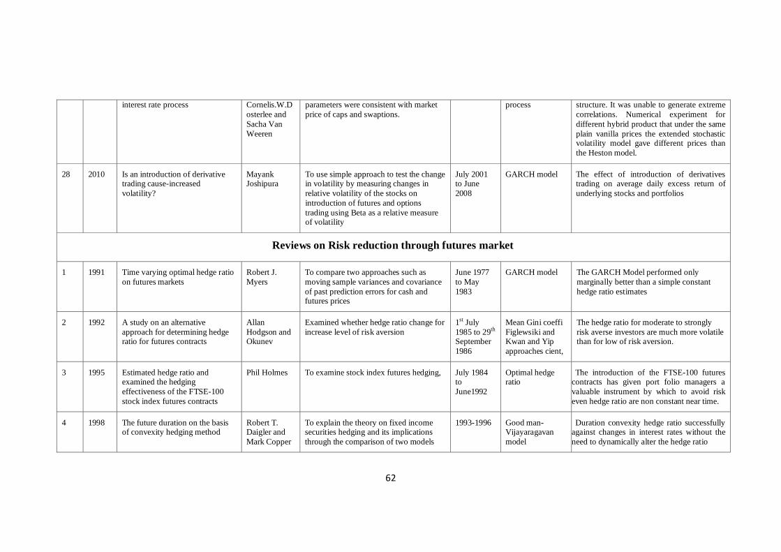
62
interest rate process Cornelis.W.D
osterlee and
Sacha Van
Weeren
parameters were consistent with market
price of caps and swaptions.
process structure. It was unable to generate extreme
correlations. Numerical experiment for
different hybrid product that under the same
plain vanilla prices the extended stochastic volatility model gave different prices than
the Heston model.
28 2010 Is an introduction of derivative trading cause-increased
volatility?
Mayank Joshipura
To use simple approach to test the change in volatility by measuring changes in
relative volatility of the stocks on
introduction of futures and options
trading using Beta as a relative measure of volatility
July 2001 to June
2008
GARCH model The effect of introduction of derivatives trading on average daily excess return of
underlying stocks and portfolios
Reviews on Risk reduction through futures market
1 1991 Time varying optimal hedge ratio
on futures markets
Robert J.
Myers
To compare two approaches such as
moving sample variances and covariance
of past prediction errors for cash and futures prices
June 1977
to May
1983
GARCH model The GARCH Model performed only
marginally better than a simple constant
hedge ratio estimates
2 1992 A study on an alternative
approach for determining hedge ratio for futures contracts
Allan
Hodgson and Okunev
Examined whether hedge ratio change for
increase level of risk aversion
1st July
1985 to 29th September
1986
Mean Gini coeffi
Figlewsiki and Kwan and Yip
approaches cient,
The hedge ratio for moderate to strongly
risk averse investors are much more volatile than for low of risk aversion.
3 1995 Estimated hedge ratio and examined the hedging
effectiveness of the FTSE-100
stock index futures contracts
Phil Holmes To examine stock index futures hedging, July 1984 to
June1992
Optimal hedge ratio
The introduction of the FTSE-100 futures contracts has given port folio managers a
valuable instrument by which to avoid risk
even hedge ratio are non constant near time.
4 1998 The future duration on the basis of convexity hedging method
Robert T. Daigler and
Mark Copper
To explain the theory on fixed income securities hedging and its implications
through the comparison of two models
1993-1996 Good man-Vijayaragavan
model
Duration convexity hedge ratio successfully against changes in interest rates without the
need to dynamically alter the hedge ratio
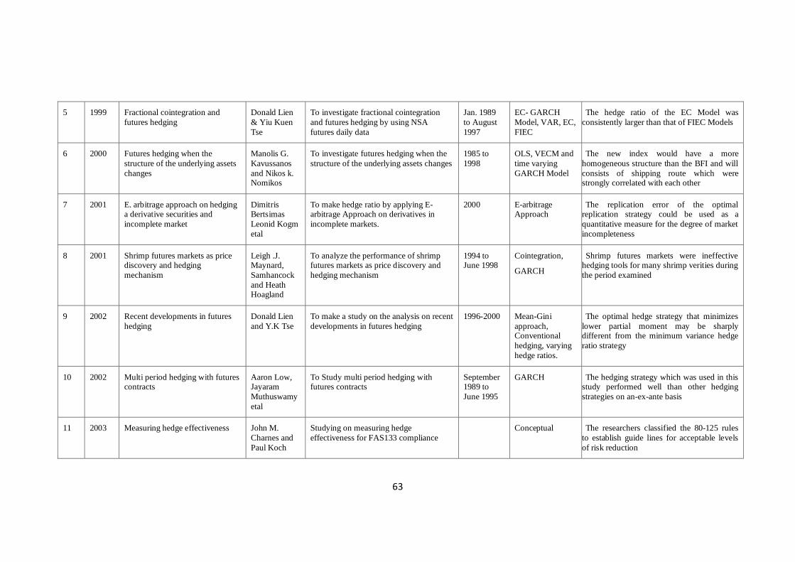
63
5 1999 Fractional cointegration and
futures hedging
Donald Lien
& Yiu Kuen
Tse
To investigate fractional cointegration
and futures hedging by using NSA
futures daily data
Jan. 1989
to August
1997
EC- GARCH
Model, VAR, EC,
FIEC
The hedge ratio of the EC Model was
consistently larger than that of FIEC Models
6 2000 Futures hedging when the
structure of the underlying assets
changes
Manolis G.
Kavussanos
and Nikos k. Nomikos
To investigate futures hedging when the
structure of the underlying assets changes
1985 to
1998
OLS, VECM and
time varying
GARCH Model
The new index would have a more
homogeneous structure than the BFI and will
consists of shipping route which were strongly correlated with each other
7 2001 E. arbitrage approach on hedging a derivative securities and
incomplete market
Dimitris Bertsimas
Leonid Kogm
etal
To make hedge ratio by applying E-arbitrage Approach on derivatives in
incomplete markets.
2000 E-arbitrage Approach
The replication error of the optimal replication strategy could be used as a
quantitative measure for the degree of market
incompleteness
8 2001 Shrimp futures markets as price discovery and hedging
mechanism
Leigh .J. Maynard,
Samhancock
and Heath Hoagland
To analyze the performance of shrimp futures markets as price discovery and
hedging mechanism
1994 to June 1998
Cointegration,
GARCH
Shrimp futures markets were ineffective hedging tools for many shrimp verities during
the period examined
9 2002 Recent developments in futures
hedging
Donald Lien
and Y.K Tse
To make a study on the analysis on recent
developments in futures hedging
1996-2000 Mean-Gini
approach, Conventional
hedging, varying
hedge ratios.
The optimal hedge strategy that minimizes
lower partial moment may be sharply different from the minimum variance hedge
ratio strategy
10 2002 Multi period hedging with futures contracts
Aaron Low, Jayaram
Muthuswamy
etal
To Study multi period hedging with futures contracts
September 1989 to
June 1995
GARCH The hedging strategy which was used in this study performed well than other hedging
strategies on an-ex-ante basis
11 2003 Measuring hedge effectiveness John M.
Charnes and
Paul Koch
Studying on measuring hedge
effectiveness for FAS133 compliance
Conceptual The researchers classified the 80-125 rules
to establish guide lines for acceptable levels
of risk reduction
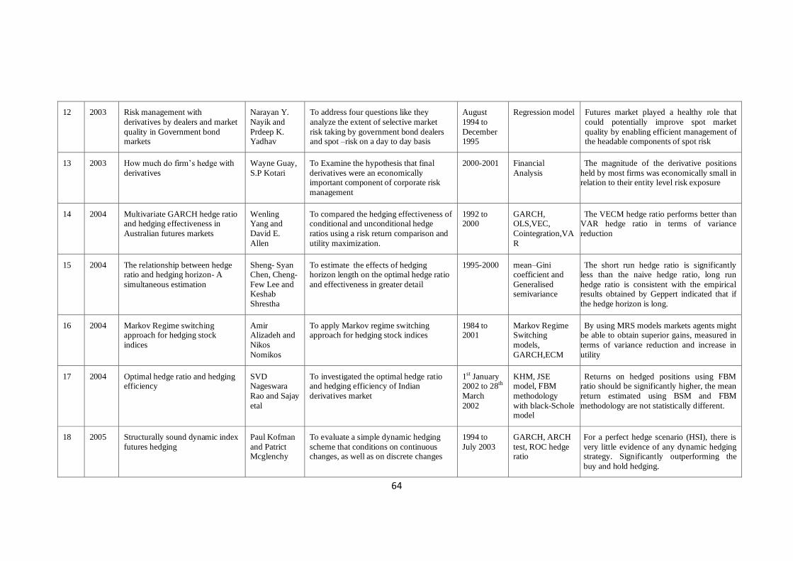
64
12 2003 Risk management with
derivatives by dealers and market
quality in Government bond markets
Narayan Y.
Nayik and
Prdeep K. Yadhav
To address four questions like they
analyze the extent of selective market
risk taking by government bond dealers and spot –risk on a day to day basis
August
1994 to
December 1995
Regression model Futures market played a healthy role that
could potentially improve spot market
quality by enabling efficient management of the headable components of spot risk
13 2003 How much do firm’s hedge with
derivatives
Wayne Guay,
S.P Kotari
To Examine the hypothesis that final
derivatives were an economically important component of corporate risk
management
2000-2001 Financial
Analysis
The magnitude of the derivative positions
held by most firms was economically small in relation to their entity level risk exposure
14 2004 Multivariate GARCH hedge ratio and hedging effectiveness in
Australian futures markets
Wenling Yang and
David E.
Allen
To compared the hedging effectiveness of conditional and unconditional hedge
ratios using a risk return comparison and
utility maximization.
1992 to 2000
GARCH, OLS,VEC,
Cointegration,VA
R
The VECM hedge ratio performs better than VAR hedge ratio in terms of variance
reduction
15 2004 The relationship between hedge ratio and hedging horizon- A
simultaneous estimation
Sheng- Syan Chen, Cheng-
Few Lee and Keshab
Shrestha
To estimate the effects of hedging horizon length on the optimal hedge ratio
and effectiveness in greater detail
1995-2000 mean–Gini coefficient and
Generalised semivariance
The short run hedge ratio is significantly less than the naive hedge ratio, long run
hedge ratio is consistent with the empirical results obtained by Geppert indicated that if
the hedge horizon is long.
16 2004 Markov Regime switching approach for hedging stock
indices
Amir Alizadeh and
Nikos
Nomikos
To apply Markov regime switching approach for hedging stock indices
1984 to 2001
Markov Regime Switching
models,
GARCH,ECM
By using MRS models markets agents might be able to obtain superior gains, measured in
terms of variance reduction and increase in
utility
17 2004 Optimal hedge ratio and hedging efficiency
SVD Nageswara
Rao and Sajay
etal
To investigated the optimal hedge ratio and hedging efficiency of Indian
derivatives market
1st January 2002 to 28th
March
2002
KHM, JSE model, FBM
methodology
with black-Schole model
Returns on hedged positions using FBM ratio should be significantly higher, the mean
return estimated using BSM and FBM
methodology are not statistically different.
18 2005 Structurally sound dynamic index
futures hedging
Paul Kofman
and Patrict Mcglenchy
To evaluate a simple dynamic hedging
scheme that conditions on continuous changes, as well as on discrete changes
1994 to
July 2003
GARCH, ARCH
test, ROC hedge ratio
For a perfect hedge scenario (HSI), there is
very little evidence of any dynamic hedging strategy. Significantly outperforming the
buy and hold hedging.
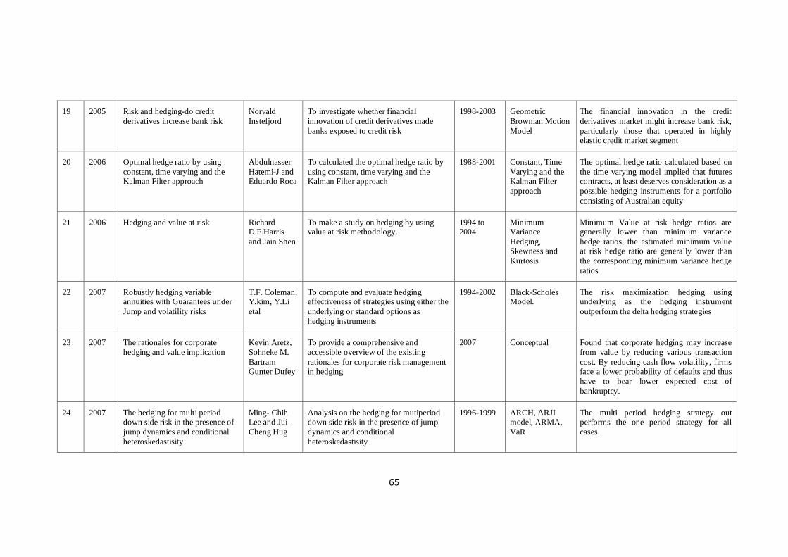
65
19 2005 Risk and hedging-do credit
derivatives increase bank risk
Norvald
Instefjord
To investigate whether financial
innovation of credit derivatives made
banks exposed to credit risk
1998-2003 Geometric
Brownian Motion
Model
The financial innovation in the credit
derivatives market might increase bank risk,
particularly those that operated in highly elastic credit market segment
20 2006 Optimal hedge ratio by using
constant, time varying and the Kalman Filter approach
Abdulnasser
Hatemi-J and Eduardo Roca
To calculated the optimal hedge ratio by
using constant, time varying and the Kalman Filter approach
1988-2001 Constant, Time
Varying and the Kalman Filter
approach
The optimal hedge ratio calculated based on
the time varying model implied that futures contracts, at least deserves consideration as a
possible hedging instruments for a portfolio
consisting of Australian equity
21 2006 Hedging and value at risk Richard D.F.Harris
and Jain Shen
To make a study on hedging by using value at risk methodology.
1994 to 2004
Minimum Variance
Hedging, Skewness and
Kurtosis
Minimum Value at risk hedge ratios are generally lower than minimum variance
hedge ratios, the estimated minimum value at risk hedge ratio are generally lower than
the corresponding minimum variance hedge
ratios
22 2007 Robustly hedging variable annuities with Guarantees under
Jump and volatility risks
T.F. Coleman, Y.kim, Y.Li
etal
To compute and evaluate hedging effectiveness of strategies using either the
underlying or standard options as
hedging instruments
1994-2002 Black-Scholes Model.
The risk maximization hedging using underlying as the hedging instrument
outperform the delta hedging strategies
23 2007 The rationales for corporate
hedging and value implication
Kevin Aretz,
Sohneke M.
Bartram Gunter Dufey
To provide a comprehensive and
accessible overview of the existing
rationales for corporate risk management in hedging
2007 Conceptual Found that corporate hedging may increase
from value by reducing various transaction
cost. By reducing cash flow volatility, firms face a lower probability of defaults and thus
have to bear lower expected cost of
bankruptcy.
24 2007 The hedging for multi period down side risk in the presence of
jump dynamics and conditional
heteroskedastisity
Ming- Chih Lee and Jui-
Cheng Hug
Analysis on the hedging for mutiperiod down side risk in the presence of jump
dynamics and conditional
heteroskedastisity
1996-1999 ARCH, ARJI model, ARMA,
VaR
The multi period hedging strategy out performs the one period strategy for all
cases.
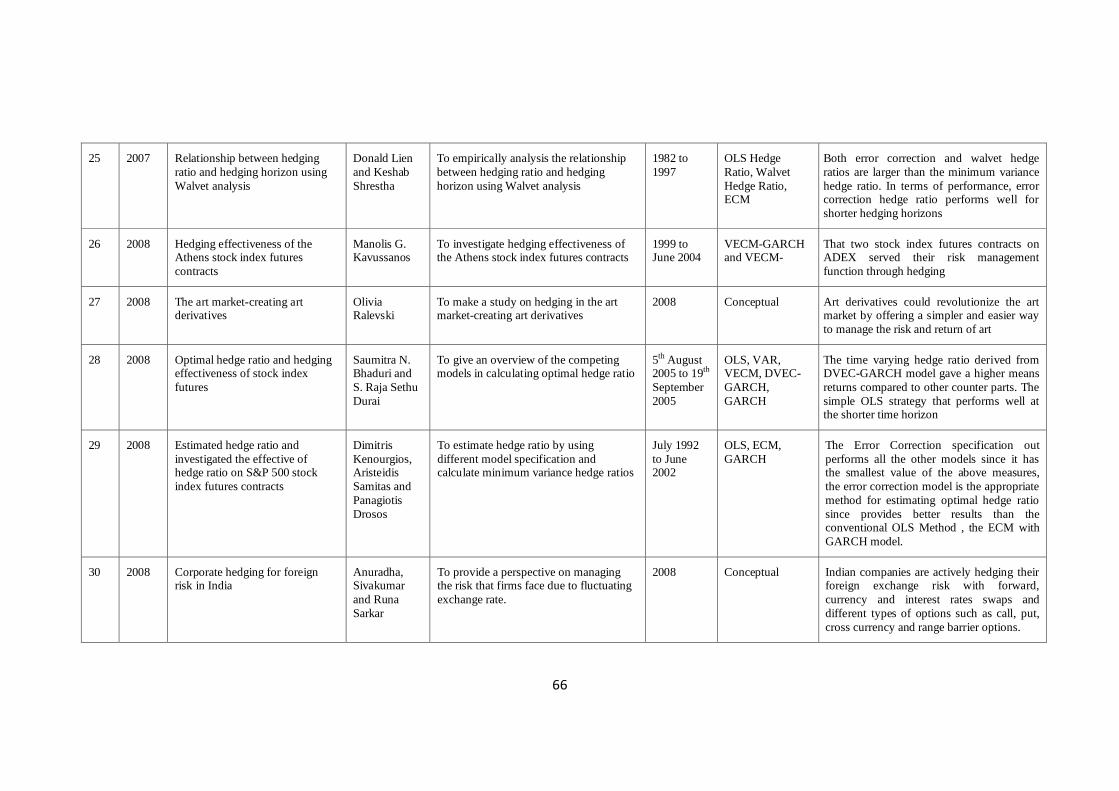
66
25 2007 Relationship between hedging
ratio and hedging horizon using
Walvet analysis
Donald Lien
and Keshab
Shrestha
To empirically analysis the relationship
between hedging ratio and hedging
horizon using Walvet analysis
1982 to
1997
OLS Hedge
Ratio, Walvet
Hedge Ratio, ECM
Both error correction and walvet hedge
ratios are larger than the minimum variance
hedge ratio. In terms of performance, error correction hedge ratio performs well for
shorter hedging horizons
26 2008 Hedging effectiveness of the Athens stock index futures
contracts
Manolis G. Kavussanos
To investigate hedging effectiveness of the Athens stock index futures contracts
1999 to June 2004
VECM-GARCH and VECM-
That two stock index futures contracts on ADEX served their risk management
function through hedging
27 2008 The art market-creating art derivatives
Olivia Ralevski
To make a study on hedging in the art market-creating art derivatives
2008 Conceptual Art derivatives could revolutionize the art market by offering a simpler and easier way
to manage the risk and return of art
28 2008 Optimal hedge ratio and hedging effectiveness of stock index
futures
Saumitra N. Bhaduri and
S. Raja Sethu
Durai
To give an overview of the competing models in calculating optimal hedge ratio
5th August 2005 to 19th
September
2005
OLS, VAR, VECM, DVEC-
GARCH,
GARCH
The time varying hedge ratio derived from DVEC-GARCH model gave a higher means
returns compared to other counter parts. The
simple OLS strategy that performs well at the shorter time horizon
29 2008 Estimated hedge ratio and
investigated the effective of hedge ratio on S&P 500 stock
index futures contracts
Dimitris
Kenourgios, Aristeidis
Samitas and
Panagiotis
Drosos
To estimate hedge ratio by using
different model specification and calculate minimum variance hedge ratios
July 1992
to June 2002
OLS, ECM,
GARCH
The Error Correction specification out
performs all the other models since it has the smallest value of the above measures,
the error correction model is the appropriate
method for estimating optimal hedge ratio
since provides better results than the conventional OLS Method , the ECM with
GARCH model.
30 2008 Corporate hedging for foreign risk in India
Anuradha, Sivakumar
and Runa
Sarkar
To provide a perspective on managing the risk that firms face due to fluctuating
exchange rate.
2008 Conceptual Indian companies are actively hedging their foreign exchange risk with forward,
currency and interest rates swaps and
different types of options such as call, put,
cross currency and range barrier options.
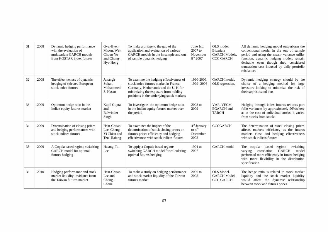
67
31 2008 Dynamic hedging performance
with the evaluation of
multivariate GARCH models from KOSTAR index futures
Gyu-Hyen
Mioon, Wei-
Choun Yu and Chung-
Hyo Hong
To make a bridge to the gap of the
application and evaluation of various
GARCH models in the in sample and out of sample dynamic hedging
June 1st,
2007 to
November 8th 2007
OLS model,
Bivariate
GARCH Models, CCC GARCH
All dynamic hedging model outperform the
conventional model in the out of sample
period and using the mean- variance utility function, dynamic hedging models remain
desirable even though they considered
transaction cost induced by daily portfolio
rebalances
32 2008 The effectiveness of dynamic
hedging of selected European
stock index futures
Jahangir
Sultan,
Mohammed S. Hasan
To examine the hedging effectiveness of
stock index futures market in France,
Germany, Netherlands and the U. K for minimizing the exposure from holding
positions in the underlying stock markets
1990-2006,
1999- 2006
GARCH model,
OLS regression,
Dynamic hedging strategy should be the
choice of a hedging method for large
investors looking to minimize the risk of their sophisticated bets
33 2009 Optimum hedge ratio in the Indian equity futures market
Kapil Gupta and
Balwinder
Singh
To investigate the optimum hedge ratio in the Indian equity futures market over
the period
2003 to 2009
VAR, VECM. EGARCH and
TARCH
Hedging through index futures reduces port folio variances by approximately 96%where
as in the case of individual stocks, it varied
from stocks from stocks
34 2009 Determination of closing prices and hedging performances with
stock indices futures
Hsiu-Chuan Lee, Cheng-
Yi Chien and Tzu- Haiang
To examines the impact of the determination of stock closing prices on
futures prices efficiency and hedging effectiveness with stock indices futures
4th January to 4th
December 2003
CCCGARCH The determination of stock closing prices affects markets efficiency as the futures
markets close and hedging effectiveness with stock indices futures
35 2009 A Copula based regime switching
GARCH model for optimal futures hedging
Haiang-Tai
Lee
To apply a Copula based regime
switching GARCH model for calculating optimal futures hedging
1991 to
2007
GARCH model The copula- based regime- switching
varying correlation GARCH model performed more efficiently in future hedging
with more flexibility in the distribution
specification.
36 2010 Hedging performance and stock market liquidity- evidence from
the Taiwan futures market
Hsiu-Chuan Lee and
Cheng –
Chene
To make a study on hedging performance and stock market liquidity of the Taiwan
futures market
2006 to 2008
OLS Model, GARCH Model,
CCC GARCH
The hedge ratio is related to stock market liquidity and the stock market liquidity
would affect the dynamic relationship
between stock and futures prices
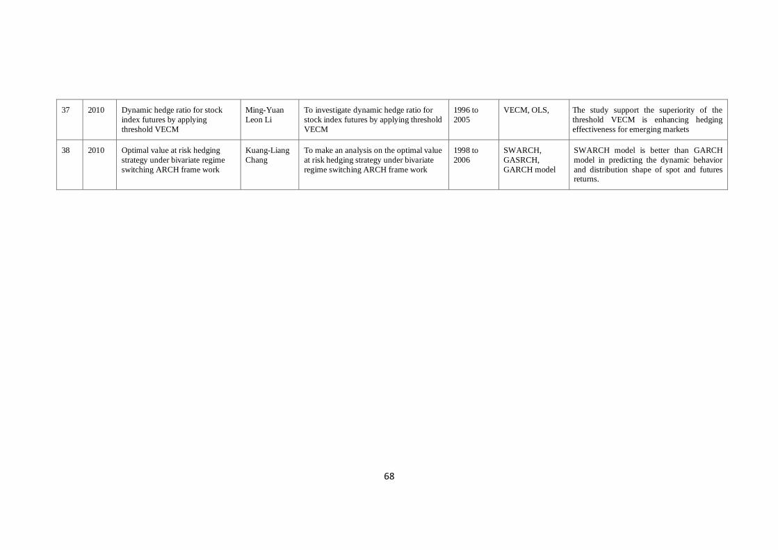
68
37 2010 Dynamic hedge ratio for stock
index futures by applying
threshold VECM
Ming-Yuan
Leon Li
To investigate dynamic hedge ratio for
stock index futures by applying threshold
VECM
1996 to
2005
VECM, OLS, The study support the superiority of the
threshold VECM is enhancing hedging
effectiveness for emerging markets
38 2010 Optimal value at risk hedging
strategy under bivariate regime
switching ARCH frame work
Kuang-Liang
Chang
To make an analysis on the optimal value
at risk hedging strategy under bivariate
regime switching ARCH frame work
1998 to
2006
SWARCH,
GASRCH,
GARCH model
SWARCH model is better than GARCH
model in predicting the dynamic behavior
and distribution shape of spot and futures returns.
69
DETAILED REVIEW OF LITERATURE
2.1. INTRODUCTION
Review of literature is a body of knowledge that aims to review the important
aspects of current knowledge in critical way. It has an ultimate goal of bringing the
reader up to date with present literature on a topic and makes a foundation for another
study that may be needed in the same area. Through the review of literature collects
information from the research field to support specific argument or writing about
particular study. It is the bridge between existing knowledge and the knowledge what
is to be explored. Literature review process may encourage the researcher to start
empirical work on a particular topic and it paves the way for right direction for the
research.
In this study, the researcher collected about 250 studies in the different area of
derivatives. Then studies which are so close to the objective are selected, reviewed
thoroughly and classified them in to three groups such as studies related to
relationship between spot and futures market, reviews on determinants of futures
market and literature about the risk reduction of futures market through hedging
process. To make a clear-cut path for the in depth research work on the area studies
on various period, different nations and multiple contexts were reviewed here. In the
first section of the chapter empirical researches on long term, short term and causality
relationship between spot and futures markets by using different methodologies have
been reviewed and included. The influence of different variables on futures market
has been critically reviewed. Finally, studies on hedge ratio and the efficiency of
futures market to reduce the risk is also included in the another section of the chapter.
The gap for the further study is placed in the last section.
70
2.2. REVIEWS ON RELATIONSHIP BETWEEN FUTURES AND SPOT
MARKET.
1. Tina. M. Galloay and James M. Miller (1997) investigated the index futures
trading and stock return volatility of Midcap 400 index futures. This study presented
new evidence on the relation between index futures trading and volatility in the equity
market using the S&P Midcap 400 stock index and Midcap 400 index futures. Daily
data and trading volume data were obtained from separate period such as pre index
period that is before June 1991, interim period which includes 175 trading after June
5th 1991 but before February 13
th 1992 and post futures which includes after February
13th 1992. To determine changes in return volatility, Skinners methodology was
employed. The analysis indicated that the documented decrease in return volatility for
the Midcap 400 stocks is simply a reflection of a decrease in return volatility that
affected all medium capitalization stocks.
2. G. Geoffrey Booth, John Paul Broussard, Teppo Martikainen and Vesa
Puttonen (1997) made a study on prudent margin levels in the Finnish stock index
futures market. The purpose of this study was to examine the behavior of Finland’s
stock index futures intraday and daily price movement and to incorporate the
observed external price behavior in an assessment of the Finnish futures markets
current initial and variation margin setting practices. Sample period of the study
began on 2nd
May 1988 and ended on December 5th
1994. Two different types of
intraday futures return such as minimal returns and the minimal and maximal returns
with in a day irrespective of the closing price were constructed. Empirical result of
estimating equations and minimal and maximal return indicated a close coherence
between actual and fitted observations.
3. Rojer Craine (1997) valued the futures market performance Guarantees. This
study derived the market value of the futures market performance guarantee and
presented estimates of the value of the exchanges exposure on the nearby S&P 500
contract during October 1987 market crash. This paper employed the econometrics
model to assess whether the probability is economically important or not. It was
illustrated the valuation technique by estimating the value of the exchanges
performance guarantee on the nearby contracts on December S&P 500 futures
contracts in October 1987. Black’s option pricing formula was applied for call option
71
valuation. The result showed that the implied variances from the November option,
although high by historical standards are an order of magnitude smaller than the G-K
estimates.
4. Kee-Kong Bae, Kalok Chan and Yan- Leung Cheung (1998) investigated the
profitability and arbitrage by dividing the analysis in to three parts in which first part
revealed arbitrage profitability, the second part was examined arbitrage profitability
based on quotations information and in third part transaction prices were used. This
study obtained data from Hong Kong Futures Exchange for Hang Sang futures index
and option contracts for the sample period from 1st October 1993 to 30
th June 1994.
The authors compared the results to examine the effectiveness of the approach that
evaluated arbitrage opportunity based on transaction price and it takes into account
the impact of bid- ask cost through estimated spread. Results showed that the
frequency of mispricing opportunities varies across different approaches in a pattern
similar to before the percentage violation are the highest for transaction prices, lower
for feasible transaction prices and the lowest for bid-ask quotations.
5. Abhay and Abhyankar (1998) made an investigation on linear and non linear
Granger Causality. The main purpose of this study was to tie together of Dwyer,
Locke and Yu (1996) and explore further the nature of the non linear of causal
relationship between the index futures and the cash market in U.K. Back and Brock
test, Granger Causality test and ARMA model were used in its empirical analysis as
tools to reveal the objectives. The data set consisted of intraday price histories for four
FTSE 100 index futures contracts maturing in March 92, June 92, Sept 92 and the
FTSE 100 index recorded minutes by minutes during 1992. The FTSE cash index
series exhibited high positive auto correlation at the first lag in each period with
statistically significant positive autocorrelation up to lag 6 during some futures
contracts periods. The results of the linear Granger Causality test based on the
multivariate regression index using both raw and AR filtered cash index return
indicated that a high degree of contemporaneous correlation between the cash and
futures contracts.
6. Minho Kim, Andrew C. Szakmary and Thomas V. Schwarz (1999) studied
trading costs and price discovery across stock index futures and cash markets. The
authors used the impulse response function to examine how an innovation in one
72
markets transmits across different markets. Transaction prices on the S&P 500, the
NYSE composite and the MMI futures contracts from January 1986 to July 1991 were
selected as sample. Johansen Cointegration and Vector Autoregressive techniques
were also applied as the tools for the analysis. The Trace and Maximal Eigen value
test indicated that there is no Cointegration relationship among the stock index futures
series of the S&P 500, NYSE index and major markets index. For VAR estimation,
results imply that in predicting unexpected movements among stock index futures
contracts, the S&P index futures has the highest predictive power.
7. Joshua Turkinton and David Walsh (1999) made an investigation on price
discovery and causality in the Australian share price index futures markets. This study
aimed to address the extend and timing of lead lag relationship between share price
index futures and the underlying spot index. The sample period of the study ran from
3rd
January 1995 to 21st December 1995 where the sample was drawn every 5
minutes. Simple Cost and Carry method, Cointegration test, ARMA model and simple
Granger Causality test were employed for the analysis of the study. The causality tests
results indicated that bi-directional causality among the variables and authors found
that an index shop appears to induce a very large response in the futures.
8. Joseph K.W.Fung and Paul Draper (1999) made an empirical analysis on
mispricing of index futures contracts and short sales constraints. The authors analyzed
the mispricing of the Hong Kong Hang Seng index futures contracts. Time stamped
transaction data of the Hang Seng index futures contracts for the period 1st April 1993
to 30th
September 1996 were obtained, minutes by minutes index prices and
annualized month end dividend yield for the same period from Hang Seng index
services were used in the empirical analysis. The empirical results revealed that
traders establish positions that don’t cover all the transaction cost. The result of
regression using mispricing as the dependent variable for both zero and number level
transaction cost was reported here.
9. Jae H. Min and Mohammad Najand (1999) investigated the lead –lag
relationship between the spot markets and stock index evidence from Korea. The
authors attempted to investigate the relationship between futures and spot markets,
both in terms of return and volatility utilizing the nearly incepted futures markets in
Korea. Dynamics Simultaneous Equation Models (SEM) and Vector Auto Regression
73
Models (VAR) were employed in the analysis part of this study. The authors used 10
minutes intraday data from 3rd
May 1996 to 16th October 1996 for the KOSPI 200
index. Simultaneous equation models results indicated that in the early inception of
Korean futures markets, the futures markets lead the spot markets by at least 30
minutes. The Wald statistics also indicated the model is well specified and there is a
strong relationship between the futures and spot markets. 10. Gerald. D. Gay and
Dae. Y.Jung (1999) had investigated a further look at transaction cost, short sale
restriction and futures market efficiency. The authors had taken Korean stock index
futures as the sample for the study. The aim of the study was to examine the price
discovery performance of Korean stock exchange contracts. The sample period of the
study started from 3rd
May to 12th May 1998. Daily credit depository rates to proxy
for the applicable financing rates also obtained for the analysis. Time varying market
volatility was estimated by using GARCH (1, 1) model. Results on nearby contracts
indicated that longer dated contracts are relatively more underpriced. It also suggested
that there may risk premia associated with longer dated contracts that is not captured
by the cost of carry model.
11. Alan E.H.Speight, David G. McMillan and Owain A.P Gwilyan (2000)
investigated intraday volatility component in FTSE- 100 stock index futures. This
study applied many models to intraday U.K stock index futures market return data at
various frequencies in an effort to determine whether permanent and transitory
component can be explicitly identified, in such data and whether the persistence of
short run volatility diminishes as the intraday frequencies decreases. The data sets
contain all trades on FTSE-100 stock index futures contracts from January 1992 to
June 1995. GARCH, RCH-LM test and BDS tests were employed in its empirical
analysis and the GARCH model specifically remaining diagnostic indicated the
presence of residual ARCH structure at all frequencies other than half day. Both
GARCH model and Wald tests results include complete dissipation of the transitory
component by the half day frequency. Only the GARCH model is adequately
capturing return dependency at the half day frequency following the dissipation of
transitory volatility.
12. Alex Frino, Terry Walter and Andrew West (2000) investigated the lead lag
relationship between equities and stock index futures market around information
74
releases by using data from the Australian stock exchange and Sydney stock
exchange. Share price index futures contracts on the Sydney futures exchange and
Australian stock index exchange were taken as the data for the period of 1st August
1995 to 31st December 1996. The empirical results implied that both adjustment for
infrequent trading work as expected, although there is some evidence that the
midpoint index adjustment may perform better. This study provided evidence that the
lead lag relationship between return on stock index and stock index futures are
influenced by the release of the macroeconomic and stock specific information.
13. Joachim Grammig, Michael and Christian Schlag (2000) addressed two
questions such as where did price discovery occur for internationally traded firms and
how did international stock price adjust to an exchange rate shock? Three large
German firms like Daimler Chrysler, Deutsche Telekom and SAP were analyzed to
find the answers for these questions. Cointegration and Vector Error Correction
Models were used for the analysis. A highly frequency sample of quotes from both
locations along with the dollar euro exchange rate were considered as the data. The
evidence suggested the structure of international equity market that had the home
market largely determine the random walk components of the international value of
firms along with the independent role of exchange rate shocks to affect prices in the
derivatives markets.
14. Laurence Copeland Sally-Ann Jones and KinLam (2001) made a study on the
index futures markets and the efficiency of screen trading in Germany and Korea. In
this study, the authors took more direct approach to measuring efficiency by
addressing many questions. Its empirical work, non-parametric tests were based on
the Arc sine Law which involves comparing the theoretical distribution implied by an
intraday random walk with the empirical frequency distribution of the intraday
high/low times were implemented. Real time transaction price and volume data for
three months futures on the FTSE-100 traded on LIFFE, the CAC-40 traded originally
on the MATIF, now on MONEP, the DAX in Germany and the KOSPI-100 in Korea
were taken as data sets for the study. The study period ran from 1984 to 1994.
Empirical study results indicated that the relative frequency of price maxima and
maxima is far greater than is consistent with a random walk in all cases.
75
15. Joel Hasbrouck (2001) studied on intraday price formation in US equity index
markets. This study empirically investigated in the price discovery of US equity index
market in the new environment where the mirror of index with exchange traded funds,
electronically traded markets, small denomination futures contracts and a family of
sector ETF that break the index into nine components. This paper assessed the
importance of the step by step development of US equity markets by considering the
NASDAQ 100 index, EFT futures contracts and S&P 500 index as the sample for the
analysis. Cointegration, Vector Error Correction Model and VAR Models result
suggested that for the S&P 500 and NASDAQ 100 index, price discovery was
dominated by futures trading. The S&P 500 sector funds were EFTs that were
constructed on industry lines and could be used to replicate the overall index.
16. Sang Bae Kim, Francies In and Christopher Viney (2001) investigated
modeling linkage between Australian financial and futures markets. This study made
an attempt to empirically analyze the dynamic interdependence and volatility linkage
between the Australian stock, bond and money market futures contracts traded on the
Sydney futures exchange using a Multivariate E-GARCH representation. The data set
of the study consists of daily settlement price for each contract obtained from the
Sydney Futures Exchange for the period from 4th January 1988 to 23
rd December
1999. In the initial stage, the authors examined the raw futures markets data and the
Univariate (GARCH (1,1), again the diagnostic test suggested by Eagle and Nag was
employed to check whether there is a potential asymmetry of volatility response to
past innovations. The empirical results concluded that there exists a strong multi-
directional influences among all three markets.
17. Leo Chan and Donald Lien (2001) examined the cash settlement and price
discovery in futures market in USA. The effects of cash settlement ability of the
futures market to predict futures spot price was thoroughly examined here. Vector
Auto Regression model with Error Correction was applied to analyze the data. They
collected cash and futures price data from September 1977 to December 1998 from
the commodity system Inc. Tuesday cash price and nearby futures price data were
taken for the analysis. It was found that the feeder cattle futures contract improved its
price discovery function after the cash settlement was adopted.
76
18. Steven. M. Van Putten and Edward D. Graskamp (2002) made an
investigation on the topic end of an era- the futures of stock option. They aimed to
present all most all topics related to futures markets and to analyze the technical
aspects of electronic trading. The movements of option stock market in the last one
decade were clearly analyzed and explained in such a way that demographic trend,
financing and leverages are performed well. The implication of futures and option
market also were explained. This study was ultimately theoretical and conceptual.
They concluded this study with aspiration and hope to a dawn of new era in futures
option.
19. Mathew Roope and Ralf Zurbruegg (2002) analyzed the intra-day price
discovery process between the Singapore Exchange and Taiwan Futures Exchange.
January 11th
1999 to 31st June 1999 were taken as the period of the study. Three
separate techniques such as Error Correction Model, Gonzalo and Granger (1995)
Methodology and ARMA Model were applied for the analysis. Test of erogeneity
results indicated that there is bidirectional relationship between Singapore futures
markets and Taiwan futures markets. Finally it was suggested that the majority of
information is impounded first in Singapore and therefore will tend to be the more
informational efficient market. In the case of regulatory regime in Singapore has
helped to establish it as the dominant market for trading in Taiwan index futures.
20. Alexande A. Kurov and Donnis J. Lasser (2002) investigated the effect of the
introduction of CUBES on the Nasdaq-100 index spot –futures pricing relationship.
This study used tick by tick transaction data for Nasdaq-100 futures and 15s interval
data for the Nasdaq-100 index from July 1st to October 20
th 1991. The entire sample
period was divided in to two sub periods about eight months each such as before the
introduction of cubes and after the introduction of cubes. To compute the mispricing
series futures prices are synchronized with the spot index value using a MIN SPAN
procedure suggested by Harris, Mclnish and Wood (1995) was applied. On the basis
of this result it was clear that simulated arbitrage trades becomes much riskier in the
post cube periods and introduction of cubes had reduced the effective transaction cost
needed to form the spot futures market arbitrage portfolios.
21. Quentin C. Chu and Wen- Liang Gideon Hsieh (2002) investigated price
efficiency of the S&P 500 index markets. The aim of the study was to examine the
77
price efficiency and arbitrage opportunities between S&P depository receipts and the
S&P 500 index futures. Through the empirical analysis, the authors defined the
occurrence of boundary violation as a series of same side violations so that any two
adjacent violations in the same occurrence occur within 20 minutes interval. Ex-ante
results between the index and futures revealed that only large price deviations and
transaction cost levels yields profitable ex-ante arbitrage profits. The study found a
surprisingly close price relationship between SPDR’s and the S&P500 index futures.
22. K. Kiran Kumar and Chiranjith Mukhopadyay (2002) made a comparative
study on short term dynamic linkage between NSE Nifty and NASDAQ composite in
India and US to empirically investigate the short term dynamic linkage between NSE
Nifty in India and NASDAQ composite in US during the period of 1999-2001 by
using intra daily data which determine the day time and overnight returns. The authors
employed two stages GARCH Model and ARMA-GARCH Model to capture the
mechanism by which NASDAQ composite daytime return and volatility had an
impact on not only the mean but also on the conditional volatility of Nifty overnight
returns. The Granger Causality result indicated unidirectional Granger Causality
running from the US stock market to the Indian stock market. Further it found that the
previous day time returns of both NASDAQ composite and NSE Nifty had significant
impact on the NSE Nifty over night returns.
23. Asjeet S. Lamba (2003) analyzed the dynamic relationship between South Asian
and developed equity market for analyzing the short and long run relationship
between each of equity market in the South Asian Region and the major developed
equity markets during July 1997-February 2003. For India, daily data on the CNX
Nifty50, for Pakistan and Srilanka, daily data on the Karachi 100 and the specific
developed equity market include in the analysis were France, Germany, Japan, UK,
and US. Using a Multivariate Cointegration frame work and Vector Error Correction
Model the authors found that the Indian market was influenced by the large developed
equity market including the US, UK and Japan.
24. Haiwei Chen, Honghui Chen and Nicholas Valerio (2003) investigated the
effects of trading halts on price discovery for NYSE stocks. In this study, intraday
data from the institute for the study of security market was used for the year 1992.
The stocks which are listed continuously on the NYSE during the entire year were
78
collected as the data for the empirical analysis. To address the potential bid ask spread
induced bias arising from using trading data, the midpoint of quoted bid and ask
prices was used to measure prices on each day. It was found that the degree of benefit
from trading halt depends on the types of news and significance of the news items.
Trading halts can be beneficial when some significant news items already hit the
market and investors need more time to digest the impact on price.
25. Ajay Shah and Syed Abuzar Moonis (2003) tested time-variation in Beta in
India. There are two approaches on time variation beta such as kalman filter model
and bivariate GARCH model in this study. The data sets of the study contained daily
return on the BSE for 50 highly liquid stocks and the NSE50 index for the period
from 1st May 1996 to 30
th March 2000. To measure the improvement on fit over the
conventional OLS beta market model, they used two measures, the coefficients of
determination and the variances of the errors. The empirical results showed a
tendency for beta to be mean reverting and showed little evidence of beta as a random
walk process.
26. Maosen Zhong Ali F. Darrat and Rafael Otero (2003) had investigated the
price discovery and volatility spill over in index futures market of Mexico. The
authors tested the hypothesis with daily data from Mexico in the context of EGARCH
model that also incorporated possible cointegration between the futures and spot
markets. The study covered the period from 15th
April 1999 to 24th
July 2002. IPC
index futures were the sample of the research. The analysis revealed that the newly
established futures market in Mexico was a useful price discovery vehicle, although
futures trading had also been a source of instability for spot market.
27. Yusif E. Simaan (2003) analyzed price discovery in the U.S option market. The
aim of the study was to investigate the price discovery process on the most actively
traded option that was listed on all five stock option exchanges. Based on real time
feeds from the option price reporting authority in January 2002 the researcher
analyzed both the quotes and trades on the 50 most actively traded stock option. They
measured the Hasbrouck (1995) information by using the second by second quotes
book and the link between price discovery and other market conditions also were
analyzed. This study found that newly exchanges which are electronically equipped
that is ISE, was the leader in providing the most informative quotes.
79
28. Hung Neng Lai (2003) made a study on price discovery in hybrid markets on the
London markets. This study attempted to provide evidence that while SETS and
dealers both contributed to the price discovery process and to understand the role of
SETS in the price discovery process. The sample included the trade records and the
transcripts of the limit order book during the first three months of year 2002. 171
stocks were taken and FTSE-100 was the main concentration of the study. Regression
was used to analyze the data. The study found that the price during the trading hours
tends to shift after SETS trade more than to a trader’s trade. The results showed that
non FTSE -100 stocks are similar to those on FTSE -100 stocks.
29. George M. and Carlos B. Tabora (2003) made a study on the topic price
discovery for Mexican shares. It was a comparative study on NYSE and Bolsa. The
study considered price discovery as a matter of degree of accuracy. Daily closing data
series from both the markets were taken into consideration for the analysis. In its
analysis part they analyzed the variance of daily stock price changes in the two
markets were compared, investigated market leadership through temporary departure
from LOP, and Error Correction Model also were applied. They found that when
deviations from LOP occur that call for Error Correction , usually with the next
trading session, much of the correction made during ensuring trading in new York
rather than in Mexico city.
30. Louis.T.W.Cheng, Li.Jiang and Renne W.Y.Ng (2004) made a study on
information content of extended trading for index futures exchange. In this study the
authors employed the S&P 500 and Hang Seng London reference index to control for
a possible spillover effects. Minutes by minute’s quotes of the HSI from Hang Seng
index services limited and HSIF transaction data from the Hong Kong Exchange were
obtained for the period of 20th
November 1998 to 31st May 2000. Weighted Period
Contribution (WPC) was used to measuring the price discovery in the extended
trading sessions. Futures return innovations from the post close trading sessions were
extracted by using a GARCH (1, 1) model. The explanatory power of the futures
returns innovations of the post- close and pre-open sessions on over night spot returns
were examined and information content of extended futures trading results showed
that pre-open futures innovations had a positive impact on overnight returns.
80
31. Irena Ivanovic and Peter Howley (2004) examined the forward pricing function
of the Australian equity index futures contracts. This study investigated the extent to
which Australian stock index futures prices with varying terms to maturity are
unbiased estimator of spot index values and examined Australian equity futures
contracts with six different terms of maturity and investigated the relationship
between futures and spot values. The settlement prices of futures contracts and spot
prices of Sydney futures Exchange and its corresponding spot price were taken for the
period of 1983 to 2001. The OLS, Johansen Cointegration and Vector Error
Correction Model were employed in the empirical analysis and found that Australian
equity index futures price are Cointegrated with the subsequent spot values for one,
two, three, six, nine and twelve months to maturity.
32. Kedar Nath Mukherajee and K. Mishra (2004) made an empirical study on the
topic lead lag relationship between equity and stock index futures market and its
variation around information release from India. The main objective of the study was
to investigate the lead lag relationship between the spot and future markets in India,
both in terms of return and volatility. Intraday price histories for the nearby contract
of Nifty index futures, Nifty cash index and also the price of some specific component
stocks during April to September 2004 were considered for the analysis. VAR model
and the Granger Causality test among the return series of the spot and the future
markets results indicated that on the volatility spill over among the spot and future
market in India and also revealed that a symmetric spill over among the stock return
volatility in Indian spot and future markets.
33. Andy.C.N.Kan (2004) studied Resiliency ability of the underlying spot markets
in Hong Kong after the introduction of index futures contracts. The aim of the study
was to provide an empirical analysis for the impact of the HSI futures trading on the
resiliency ability of individual HSI constituents stock in the Hong Kong stock index
which is the important financial markets in the Asian Pacific region. A cross sectional
regression model was employed in the study for investigation after controlling some
important factors. Daily stock price and return from 6th May 1980 to 5
th May 1992 of
HSI were taken for the analysis. Results of regression model in the four different
sampling intervals indicated that the increase in the liquidity ratios of the HSI
81
constituent stocks is significantly greater than that of the non-constituents stocks from
the pre-futures to the post futures periods after controlling other relevant factors.
34. Raymond W. and Yiuman Tse (2004) made a study on price discovery in the
Hang Seng Index markets by using index futures and the tracker fund. The objective
of the study was to extend of their understanding of information processing by
investigating how information is transmitted among the Hong Kong Hang Seng index
markets. They also examined the volatility spillover effects of the three markets via a
multivariate GARCH model. Minute by minute data of the Hang Seng index from
November 12th 1999 to June 28
th 2002 were taken in to consideration. The result of
Gonzalo and Granger model showed that the futures market is the main driving force
in the price discovery process, followed by the index. Multivariate GARCH model
indicated that the volatility of the index and futures market spill over to each other to
the strong effects from the futures to the index markets.
35. Alexander Kurov and Dennis.J. Lasser (2004) analyzed price dynamics in the
regular and E-mini futures markets. The purpose of the study was to examine the
price dynamics in the S&P 500 and Nasdaq-100 index futures contracts. This study
employed trade data for the regular and E-mini S&P 500 and Nasdaq-100 futures
from May 7th
2001 to September 7th
2001. The researcher included the total E-mini
trade series in the VECM and in the calculation of information shares. Information
shares statistics results supported the notion that general characteristics that are
inherent to the electronics trading mechanism and available to all traders. It was
calculated the cumulative impulse response functions to initiate traders by forecasting
the VECM after the unit shocks to one of the CTI price series and all trade series and
findings suggested that the order flow is more informative in the Nasdaq-100 market
than in the S&P 500 market.
36. Dimitris F.Kenourgios (2004) studied the price discovery in the Athens
derivatives exchange. The purpose of the study was to examine the informational
linkage between the FTSE/ASE-20 stock index and its three months index futures
contracts. Johansen cointegration, Vector Error Correction and Wald test models were
applied here for its estimation. Price data on the stock index and three months
FTSE/ASE-20 index futures contracts from Athens stock exchange and Athens
derivatives exchanges for the period from August 1999 to June 2002 were considered.
82
The findings suggested that both the markets are Cointegrated, there is bi-directional
relationship between both markets and there is informational linkage among them and
futures contracts could be used as price discovery vehicles in the Greek capital
markets.
37. Spyros.I.Spyrou (2005) investigated index futures trading and spot price
volatility on the basis of emerging markets. The aim of this article was to empirically
investigate whether the introduction of futures trading leads to increase volatility and
uncertainty in the underlying markets for an important European emerging equity
market that is Athens stock Exchange. For empirical analysis daily closing prices for
the main markets index, the FTSE/ASE 20 for the period September 2003 were
employed. The results from GARCH (1, 1) model indicated that all coefficients are
significantly for both periods, when both coefficients are slightly increased for the
post futures periods and Alpha is slightly increased and C1 is slightly reduced. Wald
test results revealed that there is no statistically significant effect on volatility
following the introduction of futures trading.
38. Lars Norden (2006) made an investigation on the topic does an index futures
split enhance trading activity and hedging effectiveness of the futures contracts. All
futures contracts with the omex- index as underlying securities at OM from October
24th 1994 to June 29
th 2001 were considered for the study. Bivariate GARCH model
was applied to obtain a measure of the optimal futures hedge ratio and the estimation
results for stock index return revealed that there is strong evidence of conditional
heteroskedastisity in both the stock index and the futures.
39. Robin K. Chou and George H.K.Wang (2006) investigated transaction tax and
market quality of the Taiwan stock index futures. The intraday futures price rates of
the TAIFEX from May 1st 1999 to April 30
th 2001 were selected for the analysis.
Generalized method of movement procedure and instrumental variable method were
applied to estimate the parameters. Exploratory data analysis results supported the
argument by the transaction tax opponents that the imposition of a transaction tax
would reduce markets liquidity. It was observed that tax reduction may bring in more
liquidity and this in turn would bring in even more liquidity.
40. Jangkoo Kang, Chang Joo Lee and Soonhee Lee (2006) made an empirical
investigation of the lead lag relationship of return and volatilities among the KOSPI
83
200 Spot, Futures and Option markets. This study empirically investigated the
intraday price change relations in the KOSPI 200 index markets, the KOSPI 200
futures market and the KOSPI 200 option market by taking the sample from 1st
October 2001 to 30th December 2002. The correlation between the stock index return
and the futures returns between the stock index return and the implied forward returns
are smaller. This revealed that option and futures markets lead the spot markets by
around 5 minutes, while the spot markets lead the futures markets to a much weaker
degree of around 5 minutes.
41. Sathya Saroop Debasish (2007) made a study on an econometric analysis of the
lead lag relationship between India’s NSE Nifty and its derivatives contracts. High
frequency data for the NSE Nifty stock index futures from July 2000 to June 2008
was taken as the sample for the study. Empirical results showed that the NSE Nifty
stock index hourly returns have significant first order positive auto correlation and the
series matched with calls and puts separately showed consistent serial correlation
structure. Cointegration and ARMA models were employed in the analysis part.
Findings evidenced on the lead lag relationship between the NSE Nifty index and the
NSE Nifty index futures. Overall, it was clear that the futures market generally lead
the index by up to one hour.
42. Suchismita Bose (2007) investigated the contribution of Indian index futures to
price formulation in the stock markets. The authors analyzed Indian stock index and
Indian futures price returns for the period of March 2002 to September 2006. In order
to examine that the index futures price provide any information that contribute to the
adjustment process of the stock index, daily closing prices of the futures contracts on
the S&P CNX Nifty index and the underlying index values were taken for the
analysis. The cross correlation matrices indicated that futures markets leading the spot
markets with a day lag, while the reverse was not true. This study showed that the
futures markets information showed the price discovery of the underlying Nifty is
marginally higher than what Nifty contributes to its futures price discovery.
43. M. Illueca and J.A.Lafuente (2007) made an investigation on the effect of
futures trading on the distribution of spot index returns. Data on the lbex 35 spot and
futures markets were provided by MEFFRV for the period January 17th
2000 to
December 20th
2002 was taken in to consideration. ARIMA and GARCH model were
84
employed to accomplish the objectives. The empirical findings for the Spanish market
revealed that futures trading activity is a significant variable to explain the density
function of spot returns conditional to spot trading volumes. The results confirmed
that futures markets significantly contribute to the price discovery process regardless
the day of the week.
44. Taufiq Hassan, Shamsher Mohammed, Mohammad Ariff and Annuar M.D
Nassir (2007) investigated stock index futures prices and Asian Financial Crisis. The
author’s referred to the Asian Financial crisis in July 1997 as the East Asian Region to
introduce stock index futures contracts. For the data of KLCI index and KLCI index
futures contracts were used. The sample period of the study was from January 1996 to
December 2001. They examined whether derivatives trading by either a domestic or a
foreign investors have any influence on these prices. Findings indicated that after
financial crisis, the stock market was extremely volatile and many legal restrictions
were imposed on the capital market which makes the arbitrage very risky. Keim and
Madhavan’s (1996) method was used to define permanent and temporary price
impacts associated with a domestic institution which suggests large temporary price
impacts.
45. Kapil Gupta and Balwinder Singh (2008) studied the price discovery and
arbitrage efficiency of Indian equity futures and cash markets with an objective to
empirically reveal that whether futures and cash markets have strong and stable long
run relation, which markets serves as a sources for information during short run and
how mispricing behave during the contact cycle by employing high frequency data
of Nifty index and fifty individual stocks from April 2003 to March 2007.The
research work applied Johansen Cointegration procedure, Vector Error Correction
Model, Granger Causality Methodology and Vector Auto Regression methodology.
This study found strong and stable long run co movement between two markets which
suggested both long run equilibrium and maturity data price coverage’s. During short
run, significant violation of equilibrium relationship had been observed.
46. Thenmozhi and Manish Kumar (2008) conducted a study on dynamic
interaction among mutual funds flows, stock market return and volatility with a
purpose of examining whether the information on mutual fund flows can be used to
predict the changes in market returns and volatility by using daily market index of
85
S&PCNX Nifty index from January 2001to April 2008. The conditional return
variances of the S&PCNX Nifty index were estimated using the EGARCH model and
the VAR model was also employed. The major findings indicated a strong positive
concurrent relationship between stock market return and mutual fund purchase, sales
and net. It was found that a positive relationship exists between stock market returns
and mutual fund flows, stock market volatility and mutual fund flows.
47. Brajesh Kumar and Priyanka Singh (2008) investigated the dynamic
relationship between stock returns trading volume and volatility from the evidence of
Indian stock market. This study addressed so far four important issues such as what
kind of relationship existed between trading volume and returns? Do trading volume
and returns exhibits dynamic relationship? What kind of relationship exists between
trading volume and price volatility and does there exists ARCH effect in the stock
return. Their data set consisted of all the stocks of S&PCNX Nifty index for the
period of 2000 to 2008. The study investigated the relationship between trading
volume and return and dynamic relationship using OLS and VAR modeling approach.
Mixed distribution hypothesis also was tested using GARCH model. Their findings
indicated evidence of positive contemporaneous correlation between absolute price
changes and trading volume in Indian stock markets.
48. Nivine Richi, Robert T. Daigler and Kimberly C.Gleason (2008) made a study
on the limits to stock index arbitrage by examining S&P 500 futures and SPDRS.
Authors attempted to examine the potential limit to arbitrage regarding the S&P 500
cash index and whether the S&P depository receipts could be used to price and
execute arbitrage opportunities with the S&P 500 futures contracts. Intraday futures
price and volume data of three months of high volatility from July 2002, September
1998, October 2002 and three months mid-level volatility and low months volatility
from 1998 to 2002 were employed. The application of cost of carry model was
employed to obtain fair futures value for both the S&P 500 cash index and the SPDR.
Empirical results offered insight into the limits to arbitrage regarding the S&P 500
futures, even given relatively high transaction cost.
49. Christos Floros and Dimitrios V. Vougas (2008) analyzed the efficiency of
Greek stock index futures market by addressing the issue of cointegration between
Greek spot and futures market over the period of 1999-2001. The short run efficiency
86
was examined by several Error Correction Models and long run efficiency was tested
through Johansen Cointegration approach. 525 daily observations on the FTSE/ASE
20 stock index and stock index futures contracts, 415 daily observations on the
FTSE/ASE mid 40 stock index and index futures contracts were considered. Granger
two step analyses indicated that both spot and futures are Cointegrated, implying
market efficiency. The results of VEC model for both FTSE/ASE 20 and FTSE-ASE
mid 40 indicated that futures lead spot return and it is confirmed that futures markets
are informally more efficient than underlying stock market in Greece.
50. David G. McMillan and Numan Ulku (2009) made a study on persistent
mispricing in a recently opened emerging index futures markets. The data set of this
study consists of five minutes values of the ISE30 spot index and index futures. The
sample covered the period from March 2005 to October 2005 and from November
2005 to February 2006 and provided with robustness also. Cost of Carry Model,
MTAR Model, LSTR Model and Newey- West procedure were employed to analyze
the data series and the results of MTAR Cointegration test revealed that quicker
adjustment back to equilibrium when the change in the basis is positive and when the
change in the future price is greater in absolute value than the change in the index
value.
51. Ulkem Basdas (2009) investigated the lead lag relationship between the spot
index and futures price for the Turkish derivatives exchange by using ISE30 and
compare the forecasting abilities of ECM, ECM with COC, ARIMA, and VAR model
considering the data from February 4th
2005 to May 9th
2008. The series of futures
prices on ISE 30 index was gathered from the Turk DEX Website and the spot value
also collected from the same source and for the same period. The Ganger causality
test results indicated that the log of spot price significantly Granger cause log of
futures but not vice versa.
52. Y.P.Singh and Megha Agrwal (2009) investigated the impacts of Indian index
futures on the index spot markets to understand the nature and strength of relationship
between Nifty spot and index and Nifty futures to determine the direction of flow of
information between Nifty spot index and Nifty futures and to establish a causal
relationship between return of Nifty spot and return of Nifty futures. Data sets of the
study consisted of closing price histories of Nifty futures and Nifty spot index for a
87
period of January 2004-2007. In order to analyze the lead lag relationship between
Nifty and its futures return series, cross correlation coefficients between Nifty spot
return and Nifty futures for 10 lead lags were calculated. This result indicated that
futures lead the spot market for Nifty.
53. Kapil Gupta and Balwinder Singh (2009) investigated information memory and
pricing efficiency of futures markets to examine the information dissemination
efficiency of Indians equity futures markets which is expected to provide important
policy implications of regulatory bodies and help to improve the knowledge base of
market participants. The weak form efficiency of three indices and 84 individual stock
futures permitted for trading futures and option segments of NSE was examined for
the period from January 2003 to December 2006 by considering daily closing prices
of futures contracts. GARCH and EGARCH econometrics models results implied that
previous information shock plays significant role in the return generation process.
54. Alper Ozum and Erman Erbaykal (2009) detected risk transmission from
futures to spot markets without data stationarity in Turkey’s market. The authors used
the Bond test to examine cointegration and Toda and Yamamoto test to analyze
causality between spot and futures markets. Daily time series of spot and futures
prices of the US dollar /Turkish lira Exchange rate from January 2nd
, 2006 to March
25th 2008 was employed for empirical analysis. The Unrestricted Error Correction
Model and Auto Regressive Distribution Lag (ARDL) models were applied to
distinguish long and short relationship. Bound test which was used to examine
cointegration results showed that there is a cointegration relationship between spot
and futures returns and there is informational efficiency in Turkish foreign exchange
markets.
55. Martin. T. Boli, Christian.A. Salm and Berdd Wilfling (2010) investigated the
individual index futures investors destabilize the underlying spot market by applying
Markov- Switching GARCH model. The sample periods ran from November 1st 1994
to December 31st, 2007 for the WIG 20 and the WIG from December 31
st 1994 to
December 31st 2007 and for the WIG 80 from 31
st December 1999 to 31
st December
2007. The empirical results denoted that the coefficient sums are less than one for all
stocks returns time series across both regimes.
88
56. Pagat Dare Brayan, Yang Tie Chang and Patrick Phua (2010) investigated the
relationship between index futures margin trading and securities leading in China. The
milestone of the China’s equity market was the announcement released on January 8th
2010 stated that council has given in principal approval to the trial implementation of
stock index futures trading, margin trading and securities lending in China. Stock
index futures trading were launched on April 16th
2010. This was a purely theoretical
study and here the authors mentioned that many questions about the proposed regime
for trading activities remain and are yet to be addressed by the Chinese regulators.
57. James Richard Cummings and Alex Frino (2010) examined index arbitrage and
the pricing relationship between Australian price index futures and their underlying
shares. This study analyzed the pricing efficiency of SFE SPI 200 index futures. The
independence of the absolute mispricing on the ex ante estimate of interest rate
volatility implied from interest rate option prices were investigated. The date series
describes the time, price and volume of each trade and the prices of the best available
bids and offers from 1st January 2002 to 15
th December 2005 were taken into
consideration for the analysis. Auto Regressive Regression Coefficients were
uniformly positive and significant which indicated a high degree of persistence in the
mispricing series.
58. Martin. T. Bohl, Christian A. Salm and Michael Schumppli (2010) had
investigated price discovery and investor structure in stock index futures with an aim
to understand whether the dominance of presumably unsophisticated individual
investors in the futures market impairs the informational contribution of futures
trading by taking daily closing prices for the WIG 20 index and daily settlement price
for the WIG 20 futures contracts from 16th January 1998 to June 30
th 2009. This study
used Vector Error Correction model with a Multivariate DCC-GARCH extension.
Estimation results suggested that the futures market does not fully perform the
expected price discovery function. Further, there was evidence of bidirectional
information flows and causality. Results revealed that futures price reacts more to
perturbations, implying a quicker correction of disequilibria.
2.3. REVIEWS ON DETERMINATES ON FUTURES MARKET
1. Stephen P.Ferris,Hun Y.Park and Kwangwoo Park (2002) made an
investigation on volatility, open interest ,volume and arbitrage by using evidence from
89
the S&P 500 futures market for empirically examining the dynamic interactions and
causal relations between arbitrage opportunities and a set of endogenous variable in
the S&P 500 index futures markets by using daily S&P 500 stock index spot data
from November 1993 to June 1998. Four variables in VAR system as VAR DISD,
DOI, DVOL, and PRER were estimated here. It was found that the level of open
interest is not directly affected by the increase in volatility. Pricing error plays a
critical role in linking volatility and the level of open interest and open interest in the
S&P 500 index futures is a useful proxy for examining the flow of capital in to or out
of the market.
2. Hoa Nguyen and Robert Faff (2002) made a study on the determinants of
derivatives by Australian companies. The primary aim of this study was to investigate
the factors that determine the use of derivatives by Australian corporations. The
authors formed their sample by examining the notes to the financial reports of the 500
largest Australian companies that are listed on the Australian stock exchange for the
financial year of 1999 and 2000. In this study they have conducted three levels of
analysis in which basic univariate tests, a logistic model and the Tobit model were
employed to investigate the partial impacts of the same set of independent variables
on the decisions of how much derivatives to be used. This study found a positive
relationship between firm’s size and the likely hood of derivatives usage. Tobit results
revealed that leverage is the most important factor in determining the extent of
derivatives use.
3. Sandeep Srivastave (2003) made a study on the topic informational content of
trading volume and open interest-an empirical study of stock option market in India to
examine the role of certain non price variables namely open interest and trading
volume from the stock option market in determining the price of underlying shares at
cash market. For the analysis call option and put option open interest and volume
based predictors were used. The sample of the study includes daily data on 15
individual stocks which were most liquid stock option in the NSE option market from
November 2002 to February 2003 and it was found that these predictors have
significant explanatory power with open interest being more significant as compared
to trading volume.
90
4. Kedar Nath Mukherjee and R.K. Mishra (2004) studied on impact of open
interest and trading volume in option market on underlying cash market evidence
form Indian option market. The objective of the study was to empirically investigate
the impact of a few non price variables such as open interest and trading volume from
option market in the price index like Nifty index in underlying cash market in India.
The study used daily data relating to price index in underlying cash market, open
interest and trading volume from June 2001 to December 2001 and January 2004 to
June 2004. The results of the Multiple Regression and Granger causality tests
confirmed that the open interest based predictors are significant in predicting the spot
price index in underlying cash markets in both the periods.
5. Jian Yang, David a. Bessler and Hung-Gay Fung (2004) investigated the
informational role of open interest in futures markets. The authors examined the long
run relationship between open interest and futures prices. Five futures contracts on
storable physical commodities and two stock indices, three non storable physical
commodities and one non storable financial future contract were selected from the
period 1991 to 2002. Johansen Cointegration and Error Correction Model were
employed and the empirical result showed that open interest and the futures price
share common long-run information for storable commodities but not for non storable
commodities. It was found that in the case of S&P 500 stock indexes, bidirectional
long term causality between futures prices and open interest rather than a
unidirectional causality.
6. Hongyi Chen, Laurence Fung and Jim Wong (2005) had studied the Hang seng
index futures open interest and its relationship with the cash market. In the analysis
two adjusted open interest indicators such as the de-trend open interest position and
the ratio of open interest to cash market turnover were calculated. Hang Seng futures
open interest and its underlying cash turn over were taken as the data for the study.
They analyzed the correlation between open interest and cash market turnover, open
interest and selling turn over and open interest and index volatility. It was found that
open interest and cash market turnover are positively correlated, the level and
volatility of index were not statistically significant and there was no clear-cut
relationship between open interest and short selling turn over. Analysis with ratio and
decomposed trend also showed positive relationship with open interest.
91
7. Christos Floros (2007) made an investigation on price and open interest in Greece
Stock index Futures Market with an aim to provide further case study of interesting
country Greece to go beyond GARCH, Johansen and Granger Causality econometrics
techniques. 525 daily nearby observations on the FTSE/ASE 20 stock index futures
contracts from August 1999 to August 2001 and 415 daily nearby observations on the
FTSE/ASE40 stock index futures contracts from January 2000 to August 2001 were
taken into consideration for the analysis. The results of cointegration relationship
between daily price and open interest for Greek futures markets showed that open
interest as a proxy in the conditional variance helps in explaining the GARCH effects
in futures markets return.
8. Epaminontas Katsikas (2007) made a study on volatility and autocorrelation in
European futures markets. The Generalized Error Distribution was applied in its
empirical analysis by considering daily figures for the stock index futures of France,
Germany and the U.K as the data for the study. Evidence suggested that index futures
return in Europe markets behave similarly in the sense that auto correlation and
volatility are linked in a non linear fashion. The model implied that during the period
of high volatility auto correlation is statistically zero.
9. Suchismita Bose (2007) attempted to understand the volatility characteristics and
transmission effects in the Indian stock index and index futures markets by using
daily data for the market index of NSE-S&P CNX Nifty for the period from June
2000 to March 2007. U.S Dow Jones Industrial average returns was also included in
the analysis. The empirical results indicated that NSE index and its futures return
volatility had no tendency to drift upward indefinitely with time, but in fact had a
normal or mean level to which they ultimately revert. In the case of volatility
transmission, it was found strong bidirectional volatility spillovers between the
markets implying that the price and returns dynamics in one market are capable of
explaining much of the movement in the other.
10. Vipul (2008) investigated the relationship between mispricing, price volatility,
volume and open interest of stock futures and their underlying shares in Indian futures
markets. The sample data was selected on the basis of average volume based rank of
the stock futures from 1st January 2002 to 30
th November 2004. The daily volatility
for the futures and underlying shares was computed using Parkinson’s formula and it
92
showed that the variance of daily returns can be estimated more efficiently using the
extreme value estimator. The results indicated that any increase or decrease in
mispricing did not lead to the significant change in volatility, volume or open interest
for any of the futures or the underlying shares.
11. James Richard Cummings and Alex Frino (2008) made an investigation on the
tax effects on the pricing of Australian stock index futures. To adapt and extend the
frame work adopted by Cannavan, Finn and Gray (2004) data for 1st January 2002 to
15th December 2005 have been taken. S&P/ASX 200 stock index values, time-
stamped approximately 30 seconds apart, were also considered. Daily series for the
overnight cash, 30, 90 and 180 days bank accepted bill rates had taken from the RB of
Australia. In the Australian markets, the timing option held by stock holders to
different capital gains and realize capital losses possibly accentuates the reduction in
the effective financing cost brought about by the tax deductibility of interest on loans.
12. Amrik Singh and Arun Upneja (2008) investigated the determinants of the
decisions to use financial derivatives in the lodging industry. Making distinction
between hedging and speculation is important because of the potential impact of
derivatives on firm cash flows and earnings volatility. All publically traded lodging
firms in the S&P composite data base were chosen for this study based on their 4 digit
standard industrial from 2000 to 2004. Annual and quarterly financial statement data,
as well as geographic statement data were obtained from S&P composite data base.
Results suggested that a comparison of derivatives users and non users on various
firms characterizes that proxy for incentives to hedge. The significant findings on
information asymmetry indicate that firms with large analyst have less incentive to
hedge.
13. P.Sakthivel and B.Kamaiah (2009) made a study on futures trading and
volatility of S&P CNX Nifty index to investigate whether futures trading activity
affects spot market volatility or not. The daily closing price of Nifty and trading
volume and open interest for Nifty index futures were collected from 1st July 2000 to
February 28th
2008. This study found that GARCH specification more appropriate
than the standard statistical models and the results of GARCH model revealed that
estimated coefficients of unexpected trading futures volume was positive and
significant which indicated that there is a positive relationship between spot market
93
volatility and unexpected trading volume in Nifty futures markets. The results of
GJRGARCH model indicated a positive and highly statistically significant.
14. Paul Dawson and Sotiris. K. Staikouras (2009) made an investigation on the
impact of volatility derivatives on S&P500 volatility. The aim of the study was to
examine the impact of the volatility derivatives trading on the S&P 500 volatility
index to offer a fresh perspective on the issue of spot market volatility. The sample of
the study consisted of daily data from January 3rd
2000 to May 30th 2008. GARCH (1,
1) estimation was applied in its analysis and found the most appropriate structure.
When the whole period was split into the pre and post event date intervals the results
provided a useful insight. Empirical result indicated that under normal market
conditions volatility derivatives trading contributed to lowering the underlying assets.
15. Stephane. M. Yen and Ming. Hsiang Chen (2010) investigated the relationship
between open interest, volume and volatility in Taiwan futures markets to find the
relationship among any variable from an ex- ante perceptive that is out of sample
forecasting performance. The volatility forecasting performance of all five models
such as EGARCH, GJR, APARCH, GARCH and IGARCH were compared with or
without lags in total markets volume or total open interest included as predictable
variables. Daily closing prices, total trading volume and open interest for the Taiwan
stock exchanges, electricity sector futures and insurance sector futures from 21st July
1998 to 31st December 2007 were collected as sample for the study. VAR model was
applied to find relationship between each pair of three variables and found that
significant relationship. These asymmetric GARCH models such as EGRCH, GJR,
and APGARCH as well as the standard GARCH and IGARCH models results
indicated that the significance of in sample relationship among the futures daily
volatilities, the lagged total volume and the lagged total open interest.
16. Julia. J. Lucia and Angel Pardo (2010) made a study on measuring speculative
and hedging activities in futures markets from volume and open interest data. This
study attempted to provide critical assessment of speculative and hedging positions.
Three of the most actively traded stock index futures contracts such as S&P 500
futures contracts, Nikkei 225 futures and Eurex DAX index futures were selected for
the study. Daily figures of trading volume and open interest for the futures contracts
with the three underlying indices with maturity dates in the month of March, June,
94
September and December between March 2003 and December 2006 has been taken
into consideration for the analysis. They tested the three ratios offer similar
information about the evaluation of speculation/hedging demand over time. The result
of positive cross correlation coefficient is particularly relevant to the aim of this study.
It was found that the ratio of volume to absolute change in open interest, regardless of
them being positive or negative imply that the opening of new positions out numbers
the liquidation of old positions.
17. Pratap Chandra Pati and Prabina Rajib (2010) made an attempt to investigate
volatility persistence and trading volume in an emerging futures market. This study
had taken evidence from NSE Nifty stock index futures and daily futures price and
trading volume from January 1st 2004 to December 31
st 2008 were taken as the data
for study. The results of F-statistics and LM test indicated the presence of ARCH
effect and time varying conditional heteroskedasticity in Nifty futures returns.
ARMA- GARCH and asymmetry ARMA-GARCH model were also applied and
found that the evidence of time varying volatility which exhibits clustering high
resistance and predictability in the Indian futures markets.
18. Jinliang Li (2010) made an analysis on cash trading and index futures price
volatility with an aim to examine the effects of cash markets liquidity on the return
volatility of stock index futures. The GARCH model was employed here to examine
the secular liquidity components in the daily stock index futures volatility. A quarterly
time series of the average commission rate for NYSE trading from 1980 to 2005 was
constructed and turnover of all NYSE stocks for the same period also was estimated.
Empirical findings indicated that the quarterly innovation to turn over does not
possess explanatory power to the daily volatility of the futures in the corresponding
quarter.
19. Anadrew W. Alford and James R. Boatsman (1995) predicted long term stock
return volatility for accounting and valuation of equity derivatives. The purpose of the
study was to examine empirically the prediction of long term return volatility where
long term volatility was computed using monthly stock return over five years. The
authors used monthly stock returns to compute futures because monthly returns were
approximately normally distributed while daily and weekly returns were not. They
95
presented the distributions of P-value from Kolmogorov-Smirnov Goodness of fit test
of normality over the forecast period of the sample.
20. M. Thenmozhi (2002) made a study on futures trading, information and spot
price volatility of NSE 50 index futures contracts to examine if there was any change
in the volatility of Nifty index due to the introduction of Nifty futures and whether
movement in the futures price provides productive information regarding subsequent
movement in index prices. For the analysis daily closing price returns of NSE 50
index was considered for the period 15th June 1998 to 26
th 2002. Volatility had been
measured using standard deviation and GARCH model. The lead lag relationship
between spot and index futures were estimated by using ordinary least square and two
stages least square regression. The lead lag analysis showed that futures had little or
no memory effect and infrequent trading was virtually absent in future market. It was
concluded that the futures lead the spot market returns by one day.
21. Premalatha Shenbagaraman (2003) made research on the topic do futures and
option trading increase stock market volatility with the objective to assess the impact
of introducing index futures and option contracts on the volatility of the underlying
stock index in India. Daily closing prices for the period October 1995 to December
2002 for the CNX Nifty, Nifty Junior, Nifty futures contract volume and open interest
were taken from NSE website. The authors used GARCH model, EGARCH model of
Nelson (1991), the GARCH mode with t. distribution and GJR-GARCH Model of
Glosten. The empirical results of the study revealed that derivatives introduction had
no significant impact on spot market volatility.
22. Ash Narayan Sah and G. Omkarnath (2005) made a study on derivatives
trading and volatility of Indian stock market. This study tried to understand whether
the Indian stock markets show some significant changes in the volatility after the
introduction of derivatives trading and also examined whether decline or rise in
volatility can be attributed to introduction of derivatives alone or due to some macro
economic reasons. The study used daily data like S&P Nifty, Junior Nifty, NSE 200
and S&PCNX 500, BSE Sensex-BSE 100, BSE 200 from the period April 1998 to
March 2005. Autoregressive conditional Heteroskedastic (ARCH) model was applied
to achieve the stated objective. The study concluded that the impact of the
introduction of the futures and options of the volatility of the underlying markets was
96
negligible as evident from the magnitude of the coefficient of the futures and options
dummies.
23. Puja Padhi (2007) investigated asymmetric response of volatility to news in
Indian stock market to examine the effect of the introduction of stock index futures
on the volatility of the spot equity market and to test the impact of the introduction of
the stock index futures contracts. The study used a GARCH model which is modified
along the lines of GJR- GARCH and EGARCH model, especially to take into
account the link between information and volatility. In the analysis, the dataset
comprises daily closing observations of the spot index rates for the aforementioned
markets from June 1995 to September 2006 for Nifty index and 7th June 2003 to 1
st
June 2007 for Nifty Junior. This study provided the evidence that there is not much
change in the volatility pattern after the introduction of futures in the Indian stock
market.
24. Claudio Albanese and Adel Osseiran (2007) made a model of moment methods
for exotic volatility derivatives. In this study the author gave an operator algebraic
treatment of the problem based on Dyson Expansions and Moment Methods and
discussed applications to exotic volatility derivatives. The methods were quite
flexible and allowed for a specification of the underlying process which was semi
parametric or even non parametric, including state- dependent local volatility, jumps
stochastic volatility and regime switching. The authors found that volatility
derivatives were particularly well suited to be treated with moment methods. The
authors considered a number of exotics such as variance knockouts, conditional
corridor variance swaps, gamma swaps and variance swaptions and gave valuation
formulas in detail.
25. Vasilieios Kallinterakis and Shikha Khurana (2008) investigated volatility
persistence and the feedback trading hypothesis from Indian evidence to produce an
original contribution to the finance literature by examining the relationship between
feedback trading and volatility from a markets evolutionary perspective, and to test
internationally established facts regarding feedback trading in an Indian markets
contexts. In order to test the feedback trading with the Senatana and Wadhwani
Model, the authors applied conditional variance. The daily closing prices from the
BSE 30, BSE 100 and BSE 200, and S&PCNX Nifty 50 from 1992 to 2008 were
97
taken in to consideration. The empirical result indicated that positive feedback
trading is evident throughout the period from 1999. Volatility was found to maintain
significant asymmetries in most of the period under examination.
26. S. Bhaumik, M.Karanasos and A. Kartsaklas (2008) had conducted a study on
derivative trading and the volume volatility link in the Indian stock market to
investigate the issue of temporal ordering of the range based volatility and volume in
the Indian stock market. It was estimated the two main parameters for driving the
degree of persistence in the two variables and their respective uncertainties using a
bivariate constant conditional correlation generalized ARCH model that is fractional
integration in both the Auto a regressive and Variance specification. They estimated
the bivariate AR-FI –GARCH Model with lagged value of one variable included in
the mean equation of the other variables by using data set comprised 2814 daily
trading volumes and price of the NSE index from 1995 November to 2007 January.
It was found that during the period the impact of number of traders on volatility was
negative, introduction of option trading may have weakened and the impact of
volume had on volatility through the information route.
27. Lech.A.Grzelak, Cornelis.W.Dosterlee and Sacha Van Weeren (2009) made
extension of Stochastic Volatility Equity Models with Hull- White Interest Rate
Process. In this study the author presented a flexible multifactor stochastic volatility
model which included the term structure of the stochastic interest rates. Their aim
was to combine arbitrage free Hull-white interest rate model in which the parameters
were consistent with market price of caps and swaptions. The study has shown the
Schobel-Zhu-Hull White Model belongs to the category of affine jump diffusion
process and they compared the model to the Heston-Hull-White hybrid model with
an indirectly implied correlation between the equity and interest rate. They had found
that even though the model was so attractive because of its square root volatility
structure it was unable to generate extreme correlations.
28. Mayank Joshipura (2010) made a study on the topic is an introduction of
derivative trading cause-increased volatility? The aim of the study was to use simple
approach to test the change in volatility by measuring changes in relative volatility of
the stocks on introduction of futures and options trading using Beta as a relative
measure of volatility by using the data from July 2001 to June 2008. The researchers
98
selected 12 different derivatives from the NSE and the changes in volatility of daily
stock return for one year period to derivative introduction and one year after the
derivative introduction was separately examined. The results showed that the effect
of introduction of derivatives trading on average daily excess return of underlying
stocks and portfolios.
2.4. REVIEWS ON RISK REDUCTION THROUGH FUTURES MARKET
1. Robert J. Myers (1991) estimated time varying optimal hedge ratio on futures
markets. This study attempted to compare two approaches such as moving sample
variances and covariance of past prediction errors for cash and futures prices and
GARCH model was used for estimating time varying optimal hedge ratios on futures
markets. All data were the Mid-Week closing price and the sample period ran from
June 1977 to May 1983. Separate bivariate GARCH model was estimated for cash
and May futures price, and for cash and December futures price. Preliminary results
suggested that a GARCH (1, 1) model, with one lag on the squared prediction errors
and one lag on past conditional covariance metrics, provided an adequate
representation of wheat price volatility.
2. Allan Hodgson and Okunev (1992) made a study on an alternative approach for
determining hedge ratio for futures contracts. The authors examined whether hedge
ratio change for increase in level of risk aversion or not. The authors created a port
folio by buying an underlying assets and selling futures contracts on the basis of
Figlewsiki and Kwan and Yip approaches. For the empirical analysis Associated
Australian Stock Exchange All Ordinary Index and the Share Price Index Futures
daily return was calculated for the period 1st July 1985 to 29
th September 1986.
Empirical results indicated that for low level of risk aversion, the hedge ratios are
significantly different to those of a mean variance hedge ratio. It was also confirmed
that as investors become more risk averse when they adopt different hedge ratios to
those of a mean variance investors.
3. Phil Holmes (1995) estimated hedge ratio and examined the hedging effectiveness
of the FTSE-100 stock index futures contracts. This study examined the performance
of ex ante hedge ratio is compared to that of the one to one hedge and the optimal
hedge. FTSE-100 stock index futures contracts from July 1984 to June 1992 of one
and two week’s duration were used for the analysis. Among many approach, two
99
approaches like annually estimated ex post hedge ratio and a more dynamic strategy
based on hedge ratio estimation using the rolling regression procedure were employed
here. The empirical results demonstrated that all three hedged port folios such as the
ex post minimum variance hedge ratio, the hedge portfolio based on previous years
minimum variance hedge ratio and the beta hedge ratio achieved substantial risk
reduction compared to being unhedged.
4. Robert T. Daigler and Mark Copper (1998) made a study on the future duration
on the basis of convexity hedging method. This study explained the theory on fixed
income securities hedging and its implications through the comparison of two models.
This study developed a duration convexity hedge ratio and compared the hedging
effectiveness of this hedge ratio to the Good Man-Vijayaragavan (1987, 1989), two
instruments hedge ratio and the typical one instrument duration hedge ratio. The three
based models were compared for a specific set of characteristics of the cash bond and
yield for the cash bond and futures contracts. It was revealed that the resultant hedge
ratio for the long term instrument is larger than necessary to hedge the duration and
convexity of the cash bond.
5. Donald Lien & Yiu Kuen Tse (1999) investigated fractional cointegration and
futures hedging by using NSA futures daily data. In this article, the authors compared
the effectiveness of the hedge ratio estimated from the regression, VAR, EC and FIEC
models. They examined the performance of the hedge ratios with respect to the
different hedge horizon. The period of the study was from January 1989 to August
1997. Daily closing values of the spot index and settlement price of the futures
contracts were used. The estimation results for the variance equations supported the
existence of conditional heteroscedasticity for both spot index and the futures price.
The futures price exhibited strong variance persistence than the spot index.
6. Manolis. G. Kavussanos and Nikos k. Nomikos (2000) investigated futures
hedging when the structure of the underlying assets changes. Constant and time
varying hedge ratios were estimated for different periods, corresponding to revisions
in the composition of the BFI and their performance was compared over sub periods
and across routes. This study covered the period from 1985 to 1998 and the total
period was broadly identified corresponding to different faring composition of the
underlying index. The data set consists of weekly spot and futures price which was
100
nearest to maturity. Minimum hedge risk was estimated and in its methodology OLS,
VECM and time varying GARCH model were employed to analyze the data sets.
They found that OLS hedge ratio was outperformed the other hedges in 24 cases out
of 33 for the remaining 9 cases, the VECM-GARCH hedges provided higher variance
reduction.
7. Dimitris Bertsimas Leonid Kogm and Andrew .W. Lo (2001) applied an E.
arbitrage approach on hedging a derivative securities and incomplete market. This
research projected a method for replicating derivative securities in dynamically
incomplete markets. Using stochastic dynamic programming, the authors constructed
a self financing dynamic portfolio strategy that is best to approximate an arbitrary
payoff function in a mean-squared sense. This study provided on explicit algorithm
for computing strategies which can be formidable challenge despite market
completeness.
8. Leigh .J. Maynard, Samhancock and Heath Hoagland (2001) analyzed the
performance of shrimp futures markets as price discovery and hedging mechanism.
The objective of the study was to test the hypothesis that persistent arbitrage
opportunities do not exists even in thinly traded futures markets and to determine if
the potential profits from arbitrage have economic significance. The analysis relied on
a panel of weekly whole sale cash price data for thirteen commercial Inc. and weekly
closing price data provided by the Minneapolis Grain Exchange. The study period ran
from November 1994 to June 1998. The empirical results showed that if a future price
series reflects all available information used in predicting forward price, one would
expect it is to be leading indicator of related cash prices.
9. Donald Lien and Y.K Tse (2002) made a study on the analysis on recent
developments in futures hedging. Various methods like Conventional hedging, time
varying hedge rations and minimum variance hedge ratios were applied in the study.
The empirical results formed that the optimal hedge ratio based on the extended
mean-Gini approach for low level of risk aversion are similar to the minimum
variance hedge ratio. For the higher level of risk aversion, the extended Mean –Gini
approach hedge ratio generally differ from the minimum variance hedge ratio, with no
regularity in their relative size. Non parametric time variant hedge ratio which was
proposed by Lien and Tse (2000) was empirically proved here. The results indicated
101
that a hedger who is willing to absorbed small losses but otherwise extremely cautious
about the large losses, the optimal hedge strategy that minimizes lower partial
moment may be sharply different from the minimum variance hedge ratio strategy.
10. Aaron Low, Jayaram Muthuswamy, Sudipto Sakar and Eric Terry (2002)
studied multi period hedging with futures contracts. In order to find hedge risk, main
financial instrument like futures contracts is used. In this study the authors examined
the hedging problem when futures prices obey the cost of carry model. The Nikkei
225 index futures contracts on SIMEX was used to hedge a portfolio of the
components stocks of this index and in the second part hedging is found on a spot
position in fuel oil using the high sulphur fuel oil contract on SIMEX. The sample
extended from September 1986 to April 1996 for Nikkei 225 index data and from
February 1989 to June 1995 for the high sulpher fuel oil data. The dynamic cost of
carry hedge model, the conventional hedge and the cointegrated price hedge were
used. It was found that the hedging strategy that is the cost of carry model performed
well than other hedging strategies on an-ex-ante basis, further the effectiveness of the
hedging was increased with its duration.
12. John M. Charnes and Paul Koch (2003) made a study on measuring hedge
effectiveness for FAST 133 compliance. In this study the authors outlined a basic
frame work for assessing anticipated hedging effectiveness. The frame work of the
study was based on a two part operational definitions that distinguishes between the
potential effectiveness of a hedging relationship and the attained effectiveness of a
selected hedge position. This study made an argument on hedging and speculation. A
hedging strategy involves choosing a hedging instrument and an appropriate hedge
ratio to accomplish the risk management. Various measures of effectiveness of hedge
ratio also were computed here. It is intended to measure the ability of the hedging
instrument in generating off setting changes in the fair value of the unhedged items. It
was argued that the ratio does not fully measure the degree to which the hedger has
effectively reduced risk.
13. Narayan Y. Nayik and Prdeep K. Yadhav (2003) conducted a research on the
topic risk management with derivatives by dealers and market quality in Government
bond markets. They investigated the relation between the selective market risk-taking
activity of dealers and market quality in the price effect of capital constraints for the
102
period from August 1994 to December 1995. They analyzed the close of business
reports of 15 dealer firms who were separately capitalized and subsidiaries of well
known banking houses by applying Regression Model and found that dealers engage
extensively in selective market risk taking throughout that dealers use future market to
a great extent when the cost of hedging was lower, large dealers carried a great
amount of risk on their books and hedged the changes in their spot risk less compared
to smaller dealers.
14. Wayne Guay, S.P Kotari (2003) investigated how much do firm’s hedge with
derivatives. The authors examined the hypothesis that final derivatives are an
economically important component of corporate risk management. For a random
sample of 234 large nonfinancial corporations, the authors presented detailed
evidence on the cash flows and market values sensitivities of financial derivatives
portfolios to extreme changes in the underlying assets price. This study estimated an
upper bond on the dollar amount of cash flows that a firm would derive from its
derivatives portfolio. This empirical result suggested that the magnitude of the
derivative positions held by most firms was economically small in relation to their
entity level risk exposure.
15. Wenling Yang and David E. Allen (2004) made an analysis on multivariate
GARCH hedge ratio and hedging effectiveness in Australian futures markets. This
study aimed to estimate hedging ratios derived from four specifications such as an
Ordinary Least Square based model, Bivariate Auto Regression, Vector Error
Correction Model and Diagonal-Vech Multivariate Generalized Auto Regressive
Conditional Heteroskedasticity Model with Time Varying Conditional Covariance.
Index values for all ordinary index of Australian market and the share price index
futures contracts on all ordinary index from the period of 1992 to 2000 were taken in
to consideration. As expected and the line with Gosh (1993), the hedge ratio estimated
from VECM is greater than that obtained from the VAR model.
16. Sheng- Syan Chen, Cheng- Few Lee and Keshab Shrestha (2004) made an
empirical analysis of the relationship between hedge ratio and hedging horizon- A
simultaneous estimation of the effects of hedging horizon length on the optimal hedge
ratio and effectiveness in greater detail by using 25 different futures contracts and
different hedging horizon. They considered the only minimum variance hedge ratio.
103
The authors found that most of the studies ignore the effects of hedging horizons
length of the optimal hedge ratios and hedging effectiveness. It is important to note
that all these studies considered the minimum variance hedge ratio instead of other
hedging ratios based on expected utility, extended Mean–Gini coefficient and
generalized semi variance. In sample analysis results indicated that the short run
hedge ratio is significantly less than the naive hedge ratio.
17. Amir Alizadeh and Nikos Nomikos (2004) applied a Markov regime switching
approach for hedging stock indices. This study described a new approach for
determining time varying minimum variance hedge ratio in stock index futures
markets by using the Markov Regime Switching Models. In this study the authors
developed a procedure that generated hedge ratios were regime dependent and change
as market conditions change. Hedging effectiveness of this model both in sample and
out of sample was tested and performance of regime switching hedge was compared
to GARCH and Error Correction Models. Using a multivariate extension of the
Markov Regime Model, they found that the relationship between spot and futures
return in the S&P 500 and FTSE 100 market was regime dependent. Weekly time
series of the FTSE-100 and S&P futures and spot indices for the period 1984 to 2001
were taken as the variable for the analysis. They calculated hedge ratios based on the
OLS model, Error Correction Model and GARCH Model and found that MRS
hedging strategies outperformed other models in terms of in sample port folio
variance reduction.
18. SVD Nageswara Rao and Sajay Kumar Thakur (2004) investigated the optimal
hedge ratio and hedging efficiency of Indian derivatives market. The authors had
made an attempt to estimate optimal hedge ratio based on KHM methodology using
JSE model as the bench mark for the futures. To estimate optimal hedge ratio for
options FBM methodology with Black-Schole Model has been used as the bench
mark. High frequency data for the period from 1st January 2002 to 28
th March 2002
for index futures and options had been taken in to consideration for the analysis of
hedging of Nifty price risk. In its analysis, the authors compared Herbest, Kare and
Marshall Methodology with Johanson and Stein methodology. Optimal hedge ratio
estimated by using HKM methodology was better and statistically significant at 95%
confidence level.
104
19. Paul Kofman and Patrict Mcglenchy (2005) made a study on structurally sound
dynamic index futures hedging. The objective of this study was to evaluate a simple
dynamic hedging scheme that conditions on continuous changes, as well as on
discrete changes in the relationship between unhedged portfolio and futures returns.
The study used the main stock index the Hang Seng Commerce and industry Index
(HSI) and its companion derivatives contracts Hang Seng Index Futures (HSIF) as
well as two sub indices such as the Hang Seng Commerce and Industry index and the
Hang Seng Finance Index (HSFI) for the periods from January 1994 to July 2003. To
estimate the volatility cluster a GARCH specifications was estimated for the full
sample of HSI returns and the conditional standard deviation. This study found that
for a perfect hedge scenario in (HSI) and there is very little evidence of any dynamic
hedging strategy significantly outperforming the buy and hold hedging strategy.
20. Norvald Instefjord (2005) made a study on risk and hedging-do credit
derivatives increase bank risk? The main objective of the study was to investigate
whether financial innovation of credit derivatives made banks exposed to credit risk.
The research work investigated the suggestion that credit derivatives are important for
hedging and securitizing credit risk, and thereby likely to enhance the sharing of such
risk. Geometric Brownian Motion Model was applied for the analysis. The analysis
identified two effects of credit derivatives innovations such as they enhance risk
sharing as suggested by the hedging argument and acquisition of risk more attractive.
The key findings of the research were the financial innovation in the credit derivatives
market might increase bank risk, particularly those that operated in highly elastic
credit market segment.
21. Abdulnasser Hatemi-J and Eduardo Roca (2006) calculated the optimal hedge
ratio by using constant, time varying and the Kalman Filter approach. This study
proposed and demonstrated a procedure based on the Kalman Filter approach. The
study used Australian price index for equity markets and the share price index for
Australian futures markets for the period of 1988-2001. Daily data were used for a
total of 3586 observations. Johansen Cointegration test and Eagle Granger test
showed that there is cointegration between variables and proceeded to estimate the
time varying parameters by using Kalman Filter procedure. Test result showed that
the null hypothesis of constant parameter model was strongly rejected in favor of the
105
alternative hypothesis of a time varying model. Further this study found that the
returns in the futures market had been greater than returns in the stock markets over
the time period.
22. Richard D.F.Harris and Jain Shen (2006) made a study on hedging and value at
risk. This study considered the consequences of minimum variance hedging in two
alternative frame works that implicitly incorporate portfolio skewness and kurtosis.
The effectiveness of the minimum variance hedging strategy was investigated by
considering both in sample and out sample performance. Daily returns provided by
Reuters for 10 developed markets currencies were measured against GBP for a period
1994 to 2004. Analysis of minimum variance hedging revealed that although it
reduced portfolio standard deviation, in many cases, it tends to increase left skewness
and increases kurtosis.
23. T.F. Coleman, Y.kim, Y.Li and M. Patron (2007) conducted a research on
robustly hedging variable annuities with Guarantees under Jump and volatility risks.
The authors focused on computing and evaluating hedging effectiveness of strategies
using either the underlying or standard options as hedging instruments. In this study,
the researchers compared discrete risk minimization hedging using the underlying
with that of using liquid standard options. The authors proposed to compute the risk
minimization hedging using standard options by jointly modeling the underlying price
dynamics and the Black-Scholes at the money implied volatility explicitly. The
performance of hedging strategies under jump and volatility risk could be analyzed
here. It was found that the risk maximization hedging using underlying as the hedging
instrument outperform the delta hedging strategies.
24. Kevin Aretz, Sohneke M. Bartram Gunter Dufey (2007) investigated the
rationales for corporate hedging and value implication. The research work aimed to
provide a comprehensive and accessible overview of the existing rationales for
corporate risk management in hedging which can lower the probability of future
financial distress and enable the firm to decrease its expected tax burden. It was found
that corporate hedging may increase from value by reducing various transaction cost.
By reducing cash flow volatility, firms face a lower probability of defaults and thus
have to bear lower expected cost of bankruptcy and financial distress. Further
106
corporate risk management can reduce fluctuations in pre- tax income and thus lower
the tax burden of firms if corporate income is subject to convex tax schedule.
25. Ming- Chih Lee and Jui-Cheng Hug (2007) made an analysis on the hedging for
multi period down side risk in the presence of jump dynamics and conditional
heteroskedastisity. In order to compare the hedging effectiveness of one period and
multi period zero VaR hedge ratios, the authors constructed the portfolio implied by
the computed hedge ratio for each hedging period and calculated the mean and
variance in order to obtain the value at risk of hedge port folio returns over the
sample. Futures hedging in the S&P 500 futures market daily price over the period
1996 to 1999 were considered for the study. The VaR of multi period hedge ratios
result indicated that the multi period hedging strategy outperforms the one period
strategy for all cases.
26. Donald Lien and Keshab Shrestha (2007) made an empirical analysis of the
relationship between hedging ratio and hedging horizon using Walvet analysis. 23
different futures contracts where the futures prices were associated with nearest to
maturity contracts had been analyzed here. Whole data set for the empirical analysis
were taken from Data Stream for the period started from 1982 to 1997. Analysis
results revealed that for the financial assets such as stock indices and currencies, both
spot and futures markets are to be highly liquid and therefore the variance of spot and
futures returns are likely to be closed to each other. It was found that in general both
Error Correction and Walvet Hedge Ratios are larger than the minimum variance
hedge ratio and in terms of performance; Error Correction Hedge Ratio performs well
for shorter hedging horizons.
27. Manolis G. Kavussanos and D. Visvikis (2008) investigated hedging
effectiveness of the Athens stock index futures contracts. The data set used for the
analysis consists of weekly and daily cash and futures prices of the FTSE/ATHEX 20
markets from September 1999 to June 2004 and weekly and daily cash and futures
prices of the FTSE/ATHEX mid 40 markets from February 2000 to June 2004.
VECM-GARCH and VECM-GARCH-X model were employed as the model for
estimation. The results for the FTSE/ATHEX-20 market in sample hedge ratio, based
on both daily and weekly data indicated that time varying hedge ratios estimated from
the VECM-GARCH model over performed the constant hedge ratio based on the VR
107
criterion. For daily data, the conventional model for the FTSE/ ATAEX-20 market
emanated from the VECM, where as for the FTSE/ ATHEX mid-40 market the
conventional OLS model was appropriate. In the case of out of sample hedge ratio, in
the FTSE/ATHEX mid -40 market the VECM-GARCH-X model had the worst
performance for weekly and daily data compared with the alternative constant
conventional and VECM hedging strategies.
28. Olivia Ralevski (2008) made a study on hedging the art market-creating art
derivatives. The objective of the study was to explore the opportunity for derivative
product in art. In order to create a true hedge for art, derivatives with art as the
underlying should be developed. The authors proposed a model for a total return art
swaps would allow investors to protect themselves against movement in the art
market. The need for tradable art indexes which were crucial for the successful
creation of art derivatives also had been discussed.
29. Saumitra N. Bhaduri and S. Raja Sethu Durai (2008) made a study on optimal
hedge ratio and hedging effectiveness of Indian stock index futures. This study
focused on estimating optimal hedge ratio for stock index futures in India and
compared its hedging effectiveness. Daily data on NSE stock index futures and S&P
CNX Nifty index for the period from 4 September 2000 to 4 August 2005 had been
considered for this study. The Regression Method, Bivariate VAR method, the Error
Correction Model and Multivariate GARCH method were adopted in its methodology
to calculate optimal hedge ratio. They checked the robustness of the result also.
Optimal hedge ratio results by using OLS Regression, VAR model, VEC model and
Multivariate GARCH model clearly showed the advantage and demerits of each
model and they claimed that bivariate GARCH model is the apt model which
eliminated and corrected the problems of the former models almost. Hedging
effectiveness of the stock index futures for the same period was estimated here and
they tested the effectiveness with 1,5,10 and 20 horizons. The results revealed that
within sample mean return the bench mark Naive strategy has significantly lesser
mean return than compared to all other strategies.
30. Dimitris Kenourgios, Aristeidis Samitas and Panagiotis Drosos (2008)
estimated hedge ratio and investigated the effective of hedge ratio on S&P 500 stock
index futures contracts. The hedging performance of the S&P 500 futures contracts
108
was examined using closing prices on weekly basis data relating to the period July
1992 to June 2002. GARCH, EGARCH and ECM with GARCH errors were
employed here. The empirical results of the analysis could be concluded that in terms
of risk reduction the error correction model is the appropriate method for estimating
optimal hedge ratio since it provides better results than the models such as
conventional OLS Method, the ECM with GARCH errors, the GARCH model and the
EGARCH model.
31. Anuradha, Sivakumar and Runa Sarkar (2008) made a study on the topic
corporate hedging for foreign risk in India. This study aimed to provide a perspective
on managing the risk that firms face due to fluctuating exchange rate. Authors
analyzed almost all regulations and policies regarding the foreign exchange risk in
India. It was found that a statistical significant association between the absolute value
of exposure and the absolute value of the percentage use of foreign currency
derivatives and prove that the use of derivatives in fact reduce exposure. It was
claimed that anecdotal evidence that the pricing policy is the most popular means of
hedging economic exposures.
32. Gyu-Hyen Mioon, Wei-Choun Yu and Chung-Hyo Hong (2008) investigated
dynamic hedging performance with the evaluation of multivariate GARCH models
from KOSTAR index futures. Authors’ provided the practical simple rolling OLS
model which is very rarely discussed in the literature as an alternative model.
Conventional hedging strategy assumes that the investors hold one unit in long
position in the spot stock market. Price of nearest futures contracts of KOSTAR index
spot and futures from November 8, 2005 through November 8, 2007 were taken into
consideration. To perform model estimation, forecasting and evaluation, the data
period was divided into two samples such as from 8th
November, 2005 to 31st May,
2007 that is in sample and out of sample from June 1st, 2007 to November 8
th 2007.
GARCH and its family members like DVED and CCC GARCH also were employed
here. It was surprised to see that the OLS conventional constant hedge model
performed well and is only inferior to the metrics-diagonal model. During the out of
sample period the principal component GARCH model is superior to other model.
33. Jahangir Sultan, Mohammed S. Hasan (2008) had made a study on the
effectiveness of dynamic hedging of selected European stock index futures. This
109
paper examined the hedging effectiveness of stock index futures market in France,
Germany, Netherlands and the U. K for minimizing the exposure from holding
positions in the underlying stock markets. They analyzed the effect of long run
relationship between the spot index and future index on hedging effectiveness. They
estimated optimal hedge ratio by using Bivariate Error Correction model with a
GARCH effects structure. They applied conventional and other advanced model to
find out the optimal hedge ratio and they argued that Bivariate GARCH model is
giving the highest optimal hedge ratio value. For the analysis the authors used weekly
data for the period of 1990-2006 for Netherland and U.K, and from 1999- 2006 for
Germany. The OLS regression results showed that the largest coefficient is found in
the case of France and lowest for U.K. The evidence of cointegration is consistent
with the literature for Australia, Germany, Japan and U.K. The result of variance
reduction in within sample period showed that in the case of France the dynamic
hedging model performs better when compared with a naive hedging strategy but fails
compared with the traditional OLS method.
34. Kapil Gupta and Balwinder Singh (2009) investigated the optimum hedge ratio
in the Indian equity futures market over the sample period January 2003 to December
2009. The scope of the study had been restricted to examine whether equity futures
contracts traded in India provide optimum hedging benefits. If, yes which statistical
methodology can help hedger to compute optimal hedge ratio so that they can
minimize port folio variance to minimum level at minimum trading as well as
transaction cost to execute such strategy which would result in increased portfolio
value? The sample size of the study had been restricted to three indices such Nifty,
Bank Nifty and CBXIT and 84 individual stocks. Six econometrics procedures were
employed to investigate an optimal hedge ratios which presumes a stable and strong
long run relationship between two markets and the hedging effectiveness would
depend up on the coefficient. The results confirmed that both markets observe stable
and strong co-movement over the contracts cycle. Hedge ratio estimated through
VAR methodology were the lowest for three indices are compared to those estimated
through other methodologies and the time varying hedge ratios estimated through
GARCH, EGARCH OR TARCH methodologies were the highest.
110
35. Hsiu-Chuan Lee, Cheng-Yi Chien and Tzu- Haiang Lian (2009) investigated
on determination of closing prices and hedging performances with stock indices
futures. This study empirically examined the impact of the determination of stock
closing prices on futures prices efficiency and hedging effectiveness with stock
indices futures. Daily closing prices for three futures indices like Taiwan stock
exchange index, Taiwan stock exchange finance sector index and Taiwan stock
exchange electric sector index and the corresponding underlying stock indices from
4th January to 4
th December 2003 were considered as the sample for the study. The
Bivariate Error Correction model with CCC GARCH (1, 1) structure suggested by
Kroner and Sultan (1993) was applied to examine the hedging effectiveness for the
futures indices. The empirical findings indicated that the determination of stock
closing prices affects markets efficiency as the futures markets close and hedging
effectiveness with stock indices futures.
36. Haiang-Tai Lee (2009) applied a Copula based regime switching GARCH model
for optimal futures hedging. This article developed a regime switching Gambel-
Clayton (RSGC) copula GARCH model for dealing the draw backs of the regime
switching GARCH model. In the empirical analysis, corn, oats and wheat nearby
futures contracts traded in the CBOT and COCOA nearby futures contracts traded in
the NYBOT were investigated for the period from January 1991 to December 2007
and the spot and futures data were on Wednesday closing price and empirical results
of out of sample hedging effectiveness showed that RGCS exhibits good hedging
performance in terms of variance reduction. The copula- based regime- switching
varying correlation GARCH model performed more efficiently in future hedging with
more flexibility in the distribution specification.
37. Hsiu-Chuan Lee and Cheng –Chene (2010) made a study on hedging
performance and stock market liquidity- evidence from the Taiwan futures market by
using the data from Taiwan stock exchange. The Taiwan weighted stock index prices,
the number of transactions and trading volumes in shares and dollar were taken into
consideration. This study aimed to examine the impact of stock market liquidity on
the hedging performance of stock index futures. It was found that the conditional OLS
model reduces the hedge ratio volatility better than the OLS and GARCH model. The
study period covered from 2nd
January 2006 to 20th
December 2008. Hedging strategy
111
can be evaluated and compared using three different performance metrics like
variance, semi variance and lower partial moment (LPM). The empirical results
indicated that stock markets liquidity contains information useful for predicting the
optimal hedge ratio and enhance the hedging performance during a bear markets.
38. Ming-Yuan Leon Li (2010) investigated dynamic hedge ratio for stock index
futures by applying threshold VECM. The authors employed rolling estimation to
include recent market information and continuously repeat the work of model
estimation and conducting a robust test of out of sample hedging performance for
various alternatives. The study conducted out sample hedging effectiveness test
through a rolling estimation process. This study covered the period from 3rd
January
1996 to 30th December 2005. OLS and VECM were applied here for estimating the
optimal hedge ratio through non-threshold system compared to OLS estimation. The
empirical result indicated that the setting without threshold setting over estimate or
under estimate the relative size of the standard error of the spot position to the futures
position for the outer region. Finally it revealed that the risk of spot position through
the VECM, the setting without threshold was smaller than for the setting with a
threshold.
39. Kuang-Liang Chang (2010) made analysis on the optimal value at risk hedging
strategy under bivariate regime switching ARCH frame work. This study used
bivariate switching Auto Regressive Conditional Heteroskedastisity Model which
extends from Hamilton and Susmel’s (1994) setting to calculate the optimal value at
risk hedge ratio. The aim of the work was to market hedgers precisely control the
down side risk that may happen to portfolio in the future holding period through
applying regime switching model. Daily closing prices of spot and futures indexes of
Taiwan Futures Exchange for the period July 1998 to December 2006 were
considered for the analysis. GARCH estimation results indicated that the persistence
volatility in spot and futures market is very strong. The in sample hedging results
under GARCH model showed the similarity to those of SWARCH model.
112
2.5. RESEARCH GAP
* It is found that almost all studies have considered only one or two variables to
assess the futures market for a particular period. Conclusions were drawn based on
that variable alone without including other important variables from futures market.
Conclusions drawn are not confirmed through robustness between periods.
* The variables considered in these studies provide different results in different
periods about the same market.
* Many studies were carried out to find the best econometric model for estimation,
but not for testing the informational efficiency.
* Studies are focused on determining the effectiveness of hedge ratio and not the
optimum hedge ratio for individual stocks from futures market.
* Causality between spot and futures returns was determined but not the causality
between price series.
* All studies have used data from pre financial crisis period; it is rare from post
financial crisis period.
* Studies have considered the data from later years and not from introduction of
derivatives in India.
* Studies have considered the near month data period together for the entire study
period without considering the structural breaks.
In order to fill the above said research gap, this study frames four objectives
which are mainly concentrating on the development of the futures market in India,
comparing the linkage between spot and futures market, to find the determinants of
futures market and analysis the risk reduction efficiency of futures market in India.

113
Chapter- III
Methodology
114
CHAPTER -III
METHODOLOGY
3.1. INTRODUCTION
This chapter aims to give a detailed explanation of the methodology adopted
for the study with an intention to clarify the basic research purpose. This study
primarily aimed at the informational efficiency of Indian futures market. In many
foreign countries, it is an established fact that derivatives helped the investors but no
such established facts have emerged in India. Therefore it was thought to make an
attempt to see where the Indian futures market has informational efficiency to
provide helps to investors. Once the informational efficiency is found then it will
serve as an indication that investors in Indian futures market would get greater
benefits.
Different sets of variables and methodologies have been employed by
researchers in the best of futures market studies. Various researches has sued indices
of share prices, volatility, open interest and other variables to establish a lead lag
relationship of causality between futures and spot and price discovery. It is believed
that derivatives would provide greater benefits to the investors through arbitrage and
hedge. In this chapter, Research Gap, Objectives of the study, Null Hypothesis of the
Study, Significance of the study, Data and Methodology, Limitations of the study
and Reader’s Guide are discussed. Econometrics models used for the analysis are
also provided in this chapter.
3.2. OBJECTIVES OF THE STUDY
The general objective of the study is to see the informational efficiency of futures
market in India. But it is specifically intended:
1. To examine the growth and development of futures market in India in respect of
values and quantities.
115
2. To analyze the pricing efficiency of futures market by comparing the linkage
between futures and spot market.
3. To find the significance of different determinants and their impact of futures return
in futures market in India.
4. To estimate the optimal hedge ratio and find the contribution of futures market in
mitigating investment risk in selected securities.
3.3. NULL HYPOTHESIS OF THE STUDY
Framing hypothesis gives the research a direction to make clear empirical
analysis and to specifically reveal the research results with rejection or acceptance of
the null hypothesis. In order to analyze the objectives, the following null hypotheses
are framed.
HO1: There is no significant relationship between spot and futures in long term and
short term period.
HO2: The futures price has no information to pass on to spot market.
HO3 : There is no significant lead- lag effect between spot and futures markets.
HO4 : Spot return plays very negligible role in determining the futures prices.
HO5: Open interest, Trading volume, volatility of futures return and number of
contracts are not the determinants of futures return.
HO6: No significant protection to investors risk through futures markets.
3.4. SIGNIFICANCE OF THE STUDY
The importance of this research and its contribution to the existing literature are
discussed under this section.
On the basis of review of literature, it is found that lot of studies have been
done on the futures market. Each study clearly analyzed and examined different
aspects of futures market in depth. While comparing the studies from abroad and
India lot of differences are seen in the movement of market, link between futures
market and its underlying market and in the basic structure of variables used. Many
116
studies analyzed the price discovery process of NSE futures market by considering
either with one variable or for different periods. Very few studies have been made on
the determinants of the futures return in Indian context. This research made an attempt
to fill the research gap by considering more number of variables such as futures price
series, spot price series, futures return, spot return, open interest, trading volume,
number of contracts and also volatility series of futures return. The whole study
period (12.06.2000-30.06.2011) has been divided in to four sub periods on the basis
of the structural break in the data set, the four periods are introduction and
development of derivatives (12.06.2000-28.02.2006), pre financial crisis period
(01.03.2006-14.01.2008), financial crisis period (15.01.2008-31.10.2008) and post
crisis period (01.11.2008-30.06.2011). Analyses were done for these sub periods
separately and collectively. This division is to check the robustness. This study
establishes the relationship between spot and futures market on the basis of its
depthness, inclusion of more variables and different analysis during structural break
periods. This research work provides basic knowledge on the movement of Indian
futures market and its underlying market. The basic movement of both markets gives
the investors and traders to take decision on their dealings in the market. Actual
relationship between spot and futures market shows the picture on the opportunities of
the hedging and arbitrage in the Indian market. Hence the overall result provides the
policy makers in depth knowledge on the regulations which helps the traders in the
futures market.
3.5. SCOPE OF THE STUDY
The scope means the boundary of the operations or the area for the study. This
study includes only the variables from futures market like futures return, open
interest, number of contract, turn over and volatility of futures market. Spot market
return is taken as the representative of underlying market. Instead of taking only
return series of spot and futures market, here index series are also taken in to
consideration. By using appropriate models and checking the output of different sub
periods makes the study more reliable. This study specifically excludes the effect of
mispricing, volatility of spot market, the role of base market and the presence of
sensitivity of spot market. By including these variables, the dimension of the study
117
can be expanded and it may give wide coverage on the area of the study. Even though
in the absence of these variables like mispricing, volatility of spot market and base
market concept this study may provide more relevance in the field of research.
3.6. DATA AND METHODOLOGY
National stock exchange of India (NSE) is the leading and very popular
exchange for derivatives in India. Therefore research is carried out by considering
NSE as representative of Indian derivatives market and particularly its Indian Nifty
spot and Nifty futures are taken. In order to access the relationship between spot and
futures market in India, daily closing indices of Nifty spot and Nifty futures from 12th
June 2000 to 30th June 2011 (11 years, 132 near month strikes) are included.
Determinants of futures return (FUTR) are identified with the help of variables like
open interest (OI), turnover (TURN), volatility (VOL), number of contract (CONT)
and spot return (SPOTR). Daily closing values of these variables were collected from
NSE for the period 12th June 2000 to 30
th June 2011. Risk reduction to investors of
derivatives market is measured through estimation of optimal hedge ratio. For this
purpose 19 companies which satisfy the conditions as it should be from the
introduction of derivatives being continuously trading till 30th
June 2011 and which is
part of Nifty are selected. The analysis of this study is done through the following
steps.
Structural break in time series was determined through Bai Perron Model and the
real market trend in the Indian futures market.
Individual stock prices are adjusted for Bonus issue and stock splits during the
study period.
Return is determined after converting the variable like Price series, index series,
open interest, turn over and number of contracts into log form.
Preliminary analysis is done through line graphs and descriptive statistics.
Long term relationship between spot and futures market is determined by using
Johansen Cointegration Model, after checking the stationarity properties through
118
Augmented Dickey Fuller and Philip Perron test and selection of lag length through
LR, FPE and AIC criteria.
Short term relationship and lead lag between spot and futures market is identified
through Vector Error Correction Model.
Causality of spot and futures price series is established by using Bivariate Error
Correction model and Wald Coefficient test.
In order to find the determinants of the futures market, Granger Causality Block/
Exogeneity test is employed on variables included in the study.
Influence of shocks, its sign and length in each variable and between other
variables is examined through Impulse Response and percentage changes between
variables are analyzed through Variance Decomposition Model.
Optimal hedge ratio was determined by dividing the covariance of spot and
futures return by variance of futures. Average is obtained for a particular period is the
optimal hedge ratio to indicate the level of protection to investors. Covariance
between spot and futures return and variance of futures return is determined through
Bivariate GARCH model.
The time series data are having some special features and these all
characteristics are to be analyzed to apply the apt model for analyzing the data to
satisfy the objective. Stationarity characteristics, Cointegration relationship, Error
Correction Model, Wald Coefficient for the causality relationships, GARCH (1,1)
model for making volatility series of futures return, VAR Granger Causality /Block
Exogeneity test for the causality between many variables, impulse Response
function, Variance Decomposition and Bivariate GARCH model for the estimating
optimum hedge ratio. These econometrics models are briefly explaining in the
chapter. It will definitely give the basic ideal on the each model and its application of
the different context.
3.7. PERIOD OF THE STUDY
Basically the study pertains to the period between 12th
June 2000 and 30th
June
2011. The period is divided in to four sub periods, 12th
June 2000 to 28.02.2006
representing initial development of derivatives market in India, 1st March 2006 to 14
th
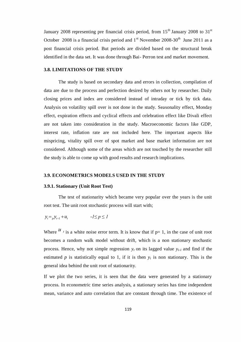
119
January 2008 representing pre financial crisis period, from 15th
January 2008 to 31st
October 2008 is a financial crisis period and 1st November 2008-30
th June 2011 as a
post financial crisis period. But periods are divided based on the structural break
identified in the data set. It was done through Bai- Perron test and market movement.
3.8. LIMITATIONS OF THE STUDY
The study is based on secondary data and errors in collection, compilation of
data are due to the process and perfection desired by others not by researcher. Daily
closing prices and index are considered instead of intraday or tick by tick data.
Analysis on volatility spill over is not done in the study. Seasonality effect, Monday
effect, expiration effects and cyclical effects and celebration effect like Divali effect
are not taken into consideration in the study. Macroeconomic factors like GDP,
interest rate, inflation rate are not included here. The important aspects like
mispricing, vitality spill over of spot market and base market information are not
considered. Although some of the areas which are not touched by the researcher still
the study is able to come up with good results and research implications.
3.9. ECONOMETRICS MODELS USED IN THE STUDY
3.9.1. Stationary (Unit Root Test)
The test of stationarity which became very popular over the years is the unit
root test. The unit root stochastic process will start with;
ttpt uyy 1 -1≤ p ≤ 1
Where is a white noise error term. It is know that if p= 1, in the case of unit root
becomes a random walk model without drift, which is a non stationary stochastic
process. Hence, why not simple regression yt on its lagged value yt-1 and find if the
estimated p is statistically equal to 1, if it is then yt is non stationary. This is the
general idea behind the unit root of stationarity.
If we plot the two series, it is seen that the data were generated by a stationary
process. In econometric time series analysis, a stationary series has time independent
mean, variance and auto correlation that are constant through time. The existence of
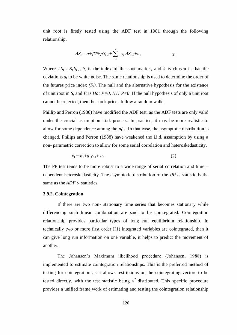
120
unit root is firstly tested using the ADF test in 1981 through the following
relationship.
ΔSt = α+βT+pSt-1+
k
i 1
γi ΔSt-1+ut (1)
Where ΔSt = St-St-1, St is the index of the spot market, and k is chosen is that the
deviations ut to be white noise. The same relationship is used to determine the order of
the futures price index (Ft). The null and the alternative hypothesis for the existence
of unit root in St and Ft is Ho: P=0, H1: P<0. If the null hypothesis of only a unit root
cannot be rejected, then the stock prices follow a random walk.
Phillip and Perron (1988) have modified the ADF test, as the ADF tests are only valid
under the crucial assumption i.i.d. process. In practice, it may be more realistic to
allow for some dependence among the ut’s. In that case, the asymptotic distribution is
changed. Philips and Perron (1988) have weakened the i.i.d. assumption by using a
non- parametric correction to allow for some serial correlation and heteroskedasticity.
yt = α0+a yt-1+ ut (2)
The PP test tends to be more robust to a wide range of serial correlation and time –
dependent heteroskedasticity. The asymptotic distribution of the PP t- statistic is the
same as the ADF t- statistics.
3.9.2. Cointegration
If there are two non- stationary time series that becomes stationary while
differencing such linear combination are said to be cointegrated. Cointegration
relationship provides particular types of long run equilibrium relationship. In
technically two or more first order I(1) integrated variables are cointegrated, then it
can give long run information on one variable, it helps to predict the movement of
another.
The Johansen’s Maximum likelihood procedure (Johansen, 1988) is
implemented to estimate cointegration relationships. This is the preferred method of
testing for cointegration as it allows restrictions on the cointegrating vectors to be
tested directly, with the test statistic being x2 distributed. This specific procedure
provides a unified frame work of estimating and testing the cointegration relationship
121
in VAR error correction mechanism, which incorporate different short term and long
run dynamic relationship in a variable system.
The Johansen’s procedure firstly specifies the following unrestricted N- variable
VAR’
Xt=μ+
k
i 1
i xt-i+εt (3)
Where xt= (ft, st), μ is a vector of intercepts terms and εt is a vector of error term.
Johansen (1988) and Johansen and Juselius (1990) reparameterizied the above
equation in the following way,
tktt
k
i
it xxx
1
1
1
(4)
This is now a VAR reparameterised in the error correction form, where П= - (П-П1-
.......- Пk) represent the long response matrix. Writing this matrix as П=αβ, then the
linear combinations β xt-k will be 1(0) in, with α being adjustment coefficients, and the
matrix П will be of reduced ranks. The Johansen approach can be used for
cointegration by assessing the rank (r) of the matrix П. If r=0 then all the variables
are no cointegrating vectors. If r=N then all the variables are I (0) and, given that any
linear combinations of stationary variables will also be staionary, there N
cointegrating vectors. Last if 0<r<N there will be r cointegrating vectors.
Evidence of price changes in one market generating price changes in the other market
so as to bring about a long- run equilibrium relationship from the equation
Ft-δ0-δ1St=εt (5)
Where Ft and St are contemporaneous futures and cash prices at time t, δ1 and δ0 are
parameter, and εt is the deviation from parity. If Ft and St are nonstionary then the OLS
method is inappropriate because the standard errors are not consistent. This
inconsistency does not allow hypothesis testing of the cointegrating parameters δ1. If
Ft and St are nonstationary but the deviation εt, are stationary, Ft and St are
cointegrated and an equilibrium relationship exists between them (Engle and Granger,
1987). For Ft and St to be cointegrated, they must be integrated of the same order.
Performing unit root tests on each price series determine the order of integration. If
each series is nonstationary in the levels, but the first difference and the deviation εt
122
are stationary, then the prices are cointegrated of order (1,1) denoted C1 (1,1) with the
cointegrating coefficient δ1.
3.9.3. Error Correction Model and Causality
Eagle Granger (1987) revealed the fact that the estimates of a VAR are
misspecified in the case of cointegrated variables, because the error correction terms
that are attached to error correction models are not accounted. The cointegration
between two series involves a continuous adjustment of innovations prices, so that
these would not become larger in the long run. Eagle and Granger (1987) have shown
that all the cointegrated series can include an error correction (the Granger
representation theorem) and, on the contrary, the existence of cointegration is
necessary condition in order to construct error correction models. The acceptance that
each pair of cash and futures prices composes a cointegrating system leads to the
implementation of an error correction model for each series, which is characterized by
the ability to overcome problems caused by spurious results. If ΔSt and ΔFt denotes the
first difference of the futures and cash prices, the following cointegrating regressions
are possible.
ΔSt=α1+aszt-1+ st
n
i
itit
n
i
Fii
1
12
1
11 )()( (6)
tF 2 Fa 1tz +
n
i 1
22 itSi )(
n
i 1
22 itFi )( Ft (7)
Where zt= St-[b+ a Ft] is the error correction term. Equation (5) and (6) represent a
vector auto regression in first difference. The Error Correction term enters in to two
equations with a one period lag and is estimated from the Cointegating Regression,
with constant terms being included to make the mean of the error series zero. The
coefficients αskαi αF attached to the error correction term measures the single period
response of the left hand side variable to departure from equilibrium. At least one
speed of adjustment coefficients must be nonzero for the model to be an error
correction model. Granger (1986), the link between cointegration and causality stems
from the fact that if spot and futures indices are cointegrated, then causality must exist
in at least one direction and possibly in both direction. Temporal causality can be
assessed by examining the statistical significance and the relative magnitudes of error
123
correction coefficients and coefficients on the lagged variables (Wahab and Lashgari,
(1993).
3.9.4. Wald Test (Coefficient Restrictions)
The Wald coefficient restriction test is used to find the causal relationship
between spot and futures market while restricting coefficient of spot and futures
separately. The Wald coefficient restrictions test (F-test) tests whether multiple
coefficients are simultaneously equal to 0 (or some other value). For the purpose
estimate both restricted and unrestricted equation and take the RSS of both models
denoted as UR RSSandRSS respectively. Then the following formula can be furnished
to estimate F-stat:
)/(
)/()(^
uU
ruUR
knSSR
kkRSSRSSF
This follows an F-type distribution with ( ),( URU knkk degrees of freedom.
3.9.5. VAR Model
Yt = C0+ tkt
p
k
kYA
1
, E (εt, εt1)=
Where Yt-k is a nx1 column vector of n stationary variables at time t-k, C0 is a nx1
column vector of constants, Ak is an nxn matrix of coefficients, p is the number of
lags, and εt is a nx1 column vector of white noise innovation terms with symmetric
and positive definite variance- covariance matrix Ὠ
VAR models were popularized in econometrics by Sims (1980) as a natural
generalization of univariate autoregressive models. VAR is a systems regression
model that can be considered a kind of hybrid between the univariate time series
models and the simultaneous equation models. VARs have often been advocated as an
alternative to large scale simultaneous equations structural models.
The simplest case that can be entertained is a bivariate VAR where there are
only two variables y1t and y2t, each of whose current values depend on different
combinations of the previous k values of both variables and error terms. An important
feature of the VAR model is its flexibility and the case of generalization. Instead of
having only two variables, y1t, y2t and y3t.....ygt, each of which has an equation.
124
Another useful facet of VAR models is the compactness with which the notation can
be expressed. This could be written as
ttyt uyyy 112111111101 (8)
tttt uyyy 211211221202 (9)
There are g=2 variables in the system. Extending the model to the case where
there are k lags of each variable in each equation is also easily accomplished.
3.9.6. Granger Causality
One test of causality is whether the lags of one variable enter in to the
equation for another variable. In a two equation model with p lags, {yt} does not
granger cause {zt} if and only if all of the coefficient of A21 (L) are equal to zero.
Thus if {yt} does not improve the forecasting performance of {zt} then {yt } granger
causes {Zt}. If all variables in the VAR are stationary, the direct way to test Granger
causality is to use a standard F-test of the restrictions:
a21(1)=a21(2)=a21(3) =....a21(p)=0 it is straight forward to generalize this notion
to the n- variable case of )log)(log( urcT . Since Aij(L) represent the
coefficients of lagged values of variable j on variables i, can be set equal to zero.
Granger causality actually measures whether current and past values of {yt} helps to
forecast futures values of {zt}. The following equation is considered for zt
izt
i
ytt iozz
)()(0
2221 If we forecast zt+1 conditional on the value of zt we
obtain the forecast error 122121 )0()0( ztyt given the value of information
concerning yt does not aid in reducing the forecast error for zt+1. The only additional
information contained in yt is the current past values of {ԑyt}. However such values do
not affect zt and so cannot improve of the zt sequences. A block exogenity test is
useful for detecting whether to incorporate an additional variable in to a VAR. This
multivariate generalization of the Granger causality test should actually be called a
block- causality test. Estimate the yt and zt equations using lagged values of {yt},{zt}
and {wt}and calculate ∑u. re estimate excluding the lagged values of {wt} and ∑r. find
the likelihood ratio statistic:
125
)log)(log( urcT
When a VAR includes many lags of variables, it will be difficult to see which
set of variables have significant effects on each dependent variable and which do not.
In order to address this issue tests are usually conducted that restrict all of the lags of
a particular variable to zero. The VAR (3) could be written out to express the
individual equation as
ttyttttt uyyyyyyy 1321231112212211112121111101
tttttttt uyyyyyyy 2322231212222212112221121202
Assuming that all of the variables in the VAR are stationary, the joint
hypothesis can easily be tested with in the F-test frame work, since each individual set
of restrictions parameters drawn from only one equation. The evaluation of the
significance of variables in the context of a VAR almost invariably occurs on the
basis of joint test on all of the lags of a particular variable in an equation. Granger
causality really means only a correlation between the current value of one variable
and the past values of others.
3.9.7. Impulse response function
An autoregression has a moving average representation, a vector
autoregression can be written as a vector moving average. In fact
1
0
1
t
i
ieAxt (10)
This equation is the VMA representation of ttt exAAx 110 in that the variables
(yt and Zt) are expressed in terms of the current and past values of the two types of
shocks. The VMA representation is an essential feature of Sims’s (1980) methodology
in that it allows us to trace out the time path of the various shocks on the variables
contained in the VAR system. Writing the two- variable VAR in matrix form,
t
t
t
t
t
t
e
e
z
y
aa
aa
a
a
z
y
1
1
1
1
2221
1211
20
10 (11)
Or
126
it
it
i
i
t
t
e
e
aa
aa
z
y
z
y
2
1
0 2221
1211 (12)
This equation expresses yt and zt in terms of the {e1t} and {e2t} sequences. However, it
is insightful to rewrite (12) in terms of the {ԑyt} and {ԑzt} sequences. The vector of
errors can be written as
zt
yt
t
t
b
b
bbe
e
1
1
1
1
21
12
21122
1 (13)
So that (12) and (13) can be combined to form
izt
iyt
i
i
t
t
t
b
b
aa
aa
bbz
y
z
y
1
1
1
1
21
12
0 2221
1211
2112
Hence, the moving average representation of (12) and (13) can be written in the error
tem of the {ԑyt} and {ԑzt} sequences:
izt
iyt
it
t
ii
ii
z
y
z
y
0 2221
1211
)()(
)()(
Or, more compactly,
0i
ititx (14)
The moving average representation is an especially useful tool to examine the
interaction between the {yt} and {zt} sequences. The coefficient of i can be used to
generate the effect of ԑyt and ԑzt shocks on the entire time paths of the {yt} and {zt}
sequences. The accumulated effects of unit impulses in ԑyt and ԑzt can be obtained by
the appropriate summation of the coefficients of the impulse response functions. The
four sets of coefficients )(),(),( 211211 iii and )(22 i are called the impulse response
function. Plotting the impulse response function is the practical way to visually
represent the behavior of the {yt} and {zt} series in response to the various shocks.
Block F- test and an examination of causality on a VAR will suggest which of
the variable in the model have statistically significant impacts on the futures values of
each of the variables in the system. But F-test results will not. By construction, be
able to explain the sign of the relationship or how long these effects required to take
127
place. F-test results will not reveal whether changes in the value of a given variable
have a positive or negative effect on other variables in the system, or how long it
would take for the effects of that variable to work through the system. Such
information will be given by an examination of the VAR’s impulse responses.
Impulse Responses trace out the responsiveness of the dependent variables in the
VAR to shocks to each of the variables. It is probably fairly easy to see what the
effects of shocks to the variables will be in such a simple VAR, the same principle
can be applied in the context of VAR containing more equations or more lags, where
it is much more difficult to see by eye are the interactions between the equations.
3.9.8. Variance Decomposition
Variance decompositions model a slightly different method for examining
VAR system dynamics. They give the proportion of the movements in the dependent
variables that are due to their own shocks, versus shocks to the other variables. A
shock to their ith variable will directly affect that variable of course, but it will also be
transmitted to all the other variables in the system through the dynamic structure of
the VAR. variance decomposition determine how much of the s- step head fore cast
error variance of a given variable is explained by innovations to each explanatory
variables for s=1, 2, 3,.... in practice, it is usually observed that own series shocks
explain most of the errors variances of the series in a VAR. To some extent, impulse
response and variance decompositions offer very similar information. Runkle (1987)
argues that confidence bands around the impulses response and variance
decomposition should always be constructed.
Since unrestricted VARs are overparameterized, they are not particularly
useful for short term forecast. However, understanding the properties of the forecast
errors is exceeding helpful uncovering interrelationships among the variables in the
system. The coefficients of A0 and A1 and wanted to forecast the various values of xt-i
conditional on the observed value of xt taking the conditional expectations of xt+1, we
can obtain
ttt xAAxE 101
128
It is noted that one step ahead forecast error is 11 ttt xEx 1te . If we take
conditional expectations, the two steps ahead forecast error is 112 tt eAe more
generally, it is easily verified that the n-step-ahead forecast is
t
nn
ntt xAAAAAIxE 10
1
1
2
11 )....(
and that the associated forecast error is
1
1
12
2
111 ...
t
n
ntntnt eAeAeAe (15)
The VMA and the VAR models contain exactly the same information but it is
convenient to describe the properties of the forecast errors in term of the {ԑt}
sequences. If the conditional forecast xt+1, the one- step- head the forecast error
is10 te . In general,
int
i
intx
0
So that the n- period forecast error nttnt xEx is
int
n
i
inttnt xEx
1
0
Denoting the n-step- ahead forecast error variance of yt+n as 2)(ny .
22)( yy n ])1(...)1()0([])1(...)1()0([ 2
12
2
12
2
12
22
11
2
11
2
11 nn z
Because all values of 2)(ijk are necessarily non negative, the variance of the
forecast error increase as the forecast horizon n increases. Note that it is possible to
decompose the n-step –ahead forecast error variance into the proportions due to each
shock. The proportions of 2)(ny due to shocks in the {ԑyt} and {ԑzt} sequences are
2
2
11
2
11
2
11
2
)(
])1(...)1()0([
n
n
y
y
and
2
2
12
2
12
2
12
2
)(
)1(...)1()0([
n
n
y
z
The forecast error variance decomposition gives the proportion of the
movements in a sequence due to its own shocks versus shocks to the other variables.
Variance decompositions can be useful tools to examine the relationship among
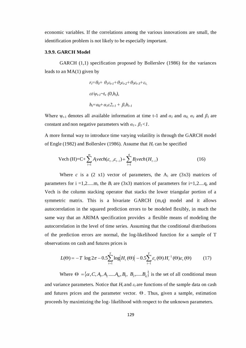
129
economic variables. If the correlations among the various innovations are small, the
identification problem is not likely to be especially important.
3.9.9. GARCH Model
GARCH (1,1) specification proposed by Bollerslev (1986) for the variances
leads to an MA(1) given by
rt=θ0+ θ1εt-1+θ2εt-2+θ3εt-3+εt,
εt/ψt-1~tv (0,ht),
ht=α0+α1ε2t-1 + β1ht-1
Where ψt-1 denotes all available information at time t-1 and α1 and α0, α1 and β1 are
constant and non negative parameters with α1+ β1<1.
A more formal way to introduce time varying volatility is through the GARCH model
of Engle (1982) and Bollerslev (1986). Assume that Ht can be specified
Vech (H)=C+ )()(11
it
q
i
iitit
m
i
i HvechBvechA
(16)
Where c is a (2 x1) vector of parameters, the Ai are (3x3) matrices of
parameters for i =1,2.....m, the Bi are (3x3) matrices of parameters for i=1,2....q, and
Vech is the column stacking operator that stacks the lower triangular portion of a
symmetric matrix. This is a bivariate GARCH (m,q) model and it allows
autocorrelation in the squared prediction errors to be modeled flexibly, in much the
same way that an ARIMA specification provides a flexible means of modeling the
autocorrelation in the level of time series. Assuming that the conditional distributions
of the prediction errors are normal, the log-likelihood function for a sample of T
observations on cash and futures prices is
)()()(5.0)(log5.02log)(1
1
1
t
T
t
tt
T
t
t HHTL (17)
Where ,,.....,,, 121 BAAAC m qBB ,.....2 is the set of all conditional mean
and variance parameters. Notice that Ht and εt are functions of the sample data on cash
and futures prices and the parameter vector. . Thus, given a sample, estimation
proceeds by maximizing the log- likelihood with respect to the unknown parameters.
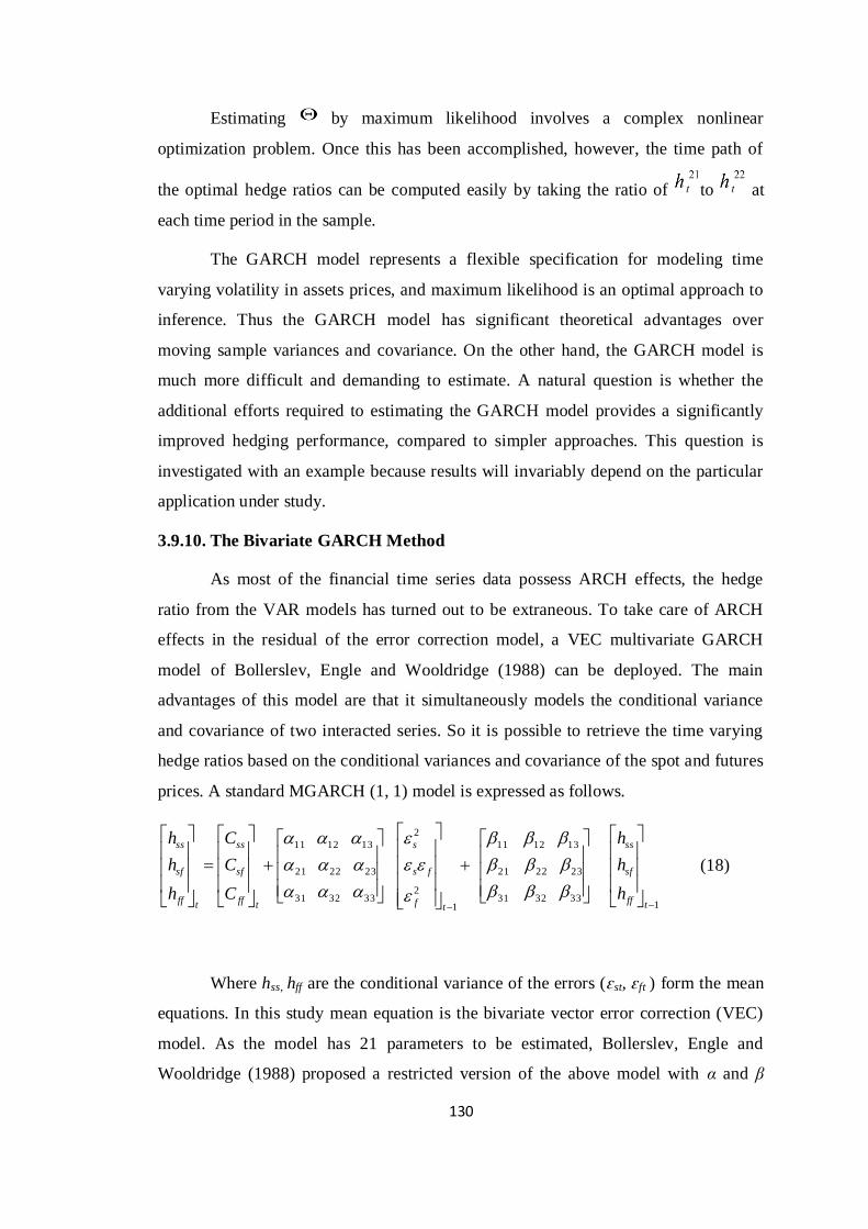
130
Estimating by maximum likelihood involves a complex nonlinear
optimization problem. Once this has been accomplished, however, the time path of
the optimal hedge ratios can be computed easily by taking the ratio of to at
each time period in the sample.
The GARCH model represents a flexible specification for modeling time
varying volatility in assets prices, and maximum likelihood is an optimal approach to
inference. Thus the GARCH model has significant theoretical advantages over
moving sample variances and covariance. On the other hand, the GARCH model is
much more difficult and demanding to estimate. A natural question is whether the
additional efforts required to estimating the GARCH model provides a significantly
improved hedging performance, compared to simpler approaches. This question is
investigated with an example because results will invariably depend on the particular
application under study.
3.9.10. The Bivariate GARCH Method
As most of the financial time series data possess ARCH effects, the hedge
ratio from the VAR models has turned out to be extraneous. To take care of ARCH
effects in the residual of the error correction model, a VEC multivariate GARCH
model of Bollerslev, Engle and Wooldridge (1988) can be deployed. The main
advantages of this model are that it simultaneously models the conditional variance
and covariance of two interacted series. So it is possible to retrieve the time varying
hedge ratios based on the conditional variances and covariance of the spot and futures
prices. A standard MGARCH (1, 1) model is expressed as follows.
1333231
232221
131211
1
2
2
333231
232221
131211
tff
sf
ss
tf
fs
s
tff
sf
ss
tff
sf
ss
h
h
h
C
C
C
h
h
h
(18)
Where hss, hff are the conditional variance of the errors (ԑst, ԑft ) form the mean
equations. In this study mean equation is the bivariate vector error correction (VEC)
model. As the model has 21 parameters to be estimated, Bollerslev, Engle and
Wooldridge (1988) proposed a restricted version of the above model with α and β
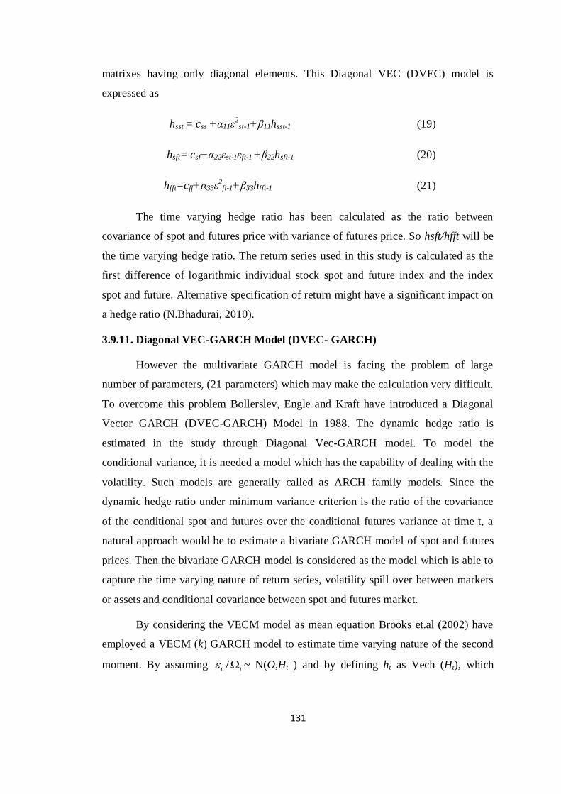
131
matrixes having only diagonal elements. This Diagonal VEC (DVEC) model is
expressed as
hsst = css +α11ε2
st-1+β11hsst-1 (19)
hsft= csf+α22εst-1εft-1 +β22hsft-1 (20)
hfft=cff+α33ε2
ft-1+β33hfft-1 (21)
The time varying hedge ratio has been calculated as the ratio between
covariance of spot and futures price with variance of futures price. So hsft/hfft will be
the time varying hedge ratio. The return series used in this study is calculated as the
first difference of logarithmic individual stock spot and future index and the index
spot and future. Alternative specification of return might have a significant impact on
a hedge ratio (N.Bhadurai, 2010).
3.9.11. Diagonal VEC-GARCH Model (DVEC- GARCH)
However the multivariate GARCH model is facing the problem of large
number of parameters, (21 parameters) which may make the calculation very difficult.
To overcome this problem Bollerslev, Engle and Kraft have introduced a Diagonal
Vector GARCH (DVEC-GARCH) Model in 1988. The dynamic hedge ratio is
estimated in the study through Diagonal Vec-GARCH model. To model the
conditional variance, it is needed a model which has the capability of dealing with the
volatility. Such models are generally called as ARCH family models. Since the
dynamic hedge ratio under minimum variance criterion is the ratio of the covariance
of the conditional spot and futures over the conditional futures variance at time t, a
natural approach would be to estimate a bivariate GARCH model of spot and futures
prices. Then the bivariate GARCH model is considered as the model which is able to
capture the time varying nature of return series, volatility spill over between markets
or assets and conditional covariance between spot and futures market.
By considering the VECM model as mean equation Brooks et.al (2002) have
employed a VECM (k) GARCH model to estimate time varying nature of the second
moment. By assuming tt / ~ N(O,Ht ) and by defining ht as Vech (Ht), which
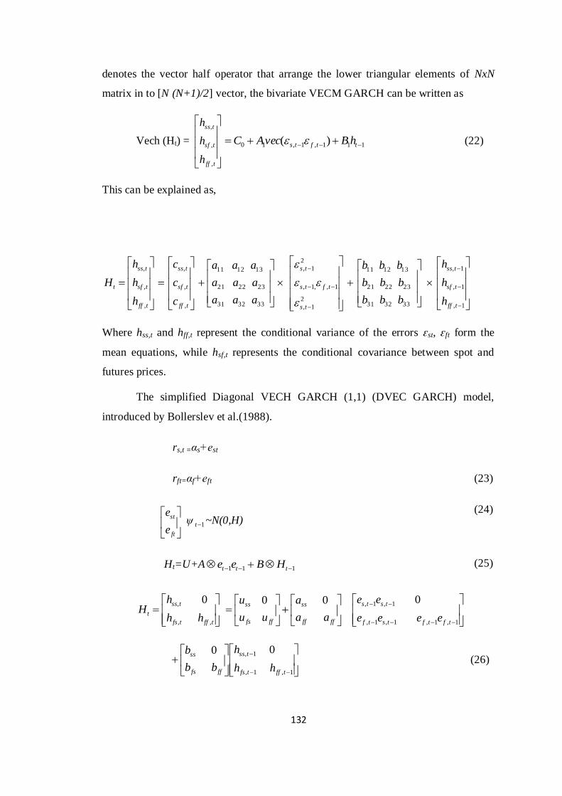
132
denotes the vector half operator that arrange the lower triangular elements of NxN
matrix in to [N (N+1)/2] vector, the bivariate VECM GARCH can be written as
Vech (Ht) =
tff
tsf
tss
h
h
h
,
,
,
111,1,10 )( ttfts hBvecAC (22)
This can be explained as,
1,
1,
1,
333231
232221
131211
2
1,
1,,1,
2
1,
333231
232221
131211
,
,
,
,
,
,
tff
tsf
tss
ts
tfts
ts
tff
tsf
tss
tff
tsf
tss
t
h
h
h
bbb
bbb
bbb
aaa
aaa
aaa
c
c
c
h
h
h
H
Where hss,t and hff,t represent the conditional variance of the errors ԑst, ԑft form the
mean equations, while hsf,t represents the conditional covariance between spot and
futures prices.
The simplified Diagonal VECH GARCH (1,1) (DVEC GARCH) model,
introduced by Bollerslev et al.(1988).
rs,t =αs+еst
rft=αf+еft (23)
ft
st
e
e ψ 1t ~N(0,H)
(24)
Ht=U+A 111 ttt HBee (25)
1,1,1,1,
1,1,
,,
, 0000
tftftstf
tsts
ffff
ss
fffs
ss
tfftfs
tss
teeee
ee
aa
a
uu
u
hh
hH
1,1,
1, 00
tfftfs
tss
fffs
ss
hh
h
bb
b (26)
133
Where equation (1) is the mean equation of the model, еt is the innovation
term, which follows a normal distribution with mean zero and conditional variance Ht,
ψt is the information set at time t-1 and is the Hadamard product. Equation (24)
and (25) show that conditional variance follow an ARMA (1,1) process, which
depends on its last period variance and last period squared residual. As shown in
equation (26) only consider the triangular part of the symmetric metrics of U, A and
B. The covariance matrix must be positive semi- definite (PSD) but Ht in the DVEC
model cannot be guaranteed to be PSD. Therefore, it is considered the fourth model-
matrix Diagonal GARCH (1, 1) model, modified form Bollerslev et al. (1994).
111 tttt HbeeAAUUH (27)
Where b is just a scalar. Equation (27) is a simple PSD version of the DVEC model.
3.9.12. Optimal Hedge Ratio
There are many techniques available for reducing and managing risk, the
simplest and the most widely used, is hedging with futures contracts. A hedge is
achieved by taking opposite positions in spot and futures market simultaneously, so
that any loss sustained from an adverse price movement in one market should to some
degree be offset by a favorable price movement in the other. The ratio of number of
units of the futures units that are purchased relative to the number of units of the spot
assets is known as hedge ratio. Since risk in this context is usually measured as the
volatility of portfolio returns, an intuitively plausible strategy might be to choose that
hedge ratio which minimizes the variance of the return of a portfolio containing the
spot and futures position. It is known as the optimal hedge ratio. The variance of the
change in the value of the hedged position is given by
FsFs hphv 2222
Minimizing this expression, h would be
F
sph
According to this formula, the optimal hedge ratio is time invariant, and would
be calculated using historical data. The standard deviation and the correlation between
134
movements in the spot and futures series could be forecast form a multivariate
GARCH model, so that the expression above is replaced by
tF
ts
tt ph,
,
Multivariate GARCH models are in spirit very similar to their univariate
counterparts, except that the former also specify equations for how the covariance
moves over time. Several different Multivariate GARCH model for estimation have
been proposed in the literature, including the VECH, the Diagonal VECH and the
BEKK models. In each case, it is assumed that there are two assets, whose return
variances and covariance are to be modeled. In the case of two assets, the conditional
variances equations for the unrestricted VECH model contain 21 parameters. As the
number of assets employed in the model increases, the estimation of the VECH model
can quickly become infeasible. Hence, the VECH model’s conditional variance
covariance matrix has been restricted to the form developed by Bollerslev, Engle and
Wooldridge (1988), in which A and B are assumed to 9 and the model, known as a
diagonal VECH, is then characterized by
1,1,1,, tijijtjtiijijtij huuh for i,j = 1,2,
Where and are parameters. The diagonal VECH multivariate
GARCH model could also be expressed as an infinite order multivariate ARCH
model, where the covariance is expressed as a geometrically declining weight
average of past cross products of unexpected returns, with recent observations
carrying higher weights. An alternative solution to the dimensionality problem would
be to use orthogonal GARCH or factor GARCH models. It is said that the VECH
model is having one disadvantage that there is no guarantee of a positive semi-
definite covariance matrix. A variance- covariance or correlation matrix must always
be positive semi-definite, and in the case where all the returns in a particular series
are all the same so that their variance is zero is disregarded, then the matrix will be
positive definite. Among other things, this means that the variance covariance have
matrix will have all positive numbers on the leading diagonal, and will be
symmetrical about this leading diagonal. These properties are intuitively appealing as
well as important from a mathematical – point of view, for variances can never be
135
negative, and the covariance between two series is the same irrespective of which of
the two series is taken first, and positive definiteness ensures that this is the case. The
modified correlation matrix may or may not positive definite, depending on the
values of the correlation that are put in, and the values of the remaining correlations.
If by chance, the matrix is not positive definite, the upshot is that for some weighting
of the individual assets in the portfolio, the estimated portfolio variance could be
negative.
3.10 .READER’S GUIDE
This study is divided in to 7 chapters in which First chapter deals with
introduction of study, back ground of the derivatives product, importance of
derivatives, futures market in India and the growth of derivatives market in India.
Second chapter covers the review of literature in the different area of the study.
Through the thorough review of existing literature on the inter relationship between
futures market and spot market, causal relationship, lead lag relationship between
spot and futures market, determinants of futures markets and its role to predict the
futures market return and the risk reduction efficiency of futures market. On the basis
of the review, it is being found the gap to make empirical analysis.
Third chapter is associated with the methodology of the study-objectives of the
study -significance of the study- null hypothesis of the study-detailed explanation on
the econometrics models which are applied in the study-limitations of the study.
Fourth chapter is examining the relationship of spot market and futures market in
India by using different methodology to find the long run relationship between spot
and futures market, short term relationship and causality relations among them.
Fifth chapter explains the determinants of futures market through causality of spot
and futures market- causality of open interest and turnover, trading volume and
volatility of futures return by using different models of VAR system.
Sixth Chapter deals with the analysis of risk protection level and estimation of
optimal hedge ratio for the different sub study period and.
Seventh chapter provides the findings, conclusion, suggestions and scope for further
research.

136
Chapter -IV
Dynamic Relationship
between
Futures and Spot Market
in India
137
CHAPTER-IV
DYNAMIC RELATIONSHIP BETWEEN
FUTURES AND SPOT MARKET IN INDIA
4.1. INTRODUCTION
Dynamic relationship between index futures and spot market shows the
informational efficiency of futures market. The link between cointegration and
causality stems from the fact that if spot and futures indices are cointegrated then
causality must exist in at least one direction and possibly in both directions (Granger
1986). Existence of cointegration amoung the spot and futures market indicate the
long term relationship between both markets. Cointegration suggest that although
both markets may be in disequilibrium during the short run such deviations are very
quickly corrected through the arbitrage process (Vipul 2005). Long term relationship
of same order integrated market proves the presence of cointegration. Cointegration of
futures and spot prices is a necessary condition for market efficiency (Fama, 1965
1970). Cointegrated spot and futures market indicates that market have informational
efficiency (Ozun and Erbay Kal 2009). The information on long term relationship of
both markets can be explained through the cointegration which implies that the
markets are not weak form effcient and it suggest that there is arbitrage opportunities
between the market (Christos Floros 2008).
In the long run integration of both spot market and futures markets, there is a
possibility of disequilibrium among the market for short run period. This imbalanced
situation provides the opportunities to the player in the market to earn profit through
brilliant trading offers. Gupta and Singh (2008) observes that during the short run
significant lead lag relationships exist between the two markets which may offer risk
free profit making opportunities to arbitrages. The speed with which the market
removes disequilibrium and maintains a balanced relationship between the spot and
138
futures market indicates the efficiency of the market. The speed of adjustment
parameters which explains the speed of adjustment in each markets in response to a
deviation from the equlibrium path (Suchismita Bose 2007).
Market traders are more interested to note where new information may be
reflected at first in prices. If any market is reducdant in the price dissemination
process, meaning it never reflects new information first, then traders would not expect
any favour from examining price changes in that market (Roop.M.and Zurbruegg .R,
2002). It can be assumed that if the same asset is traded in different markets, each
market responds to the new information in similar direction, level and at the same
time. But in reality this is not the case . The market with the lowest trading cost
normally denotes the price discovery process (Suchissmita Bose, 2007). In an
efficient market, information processing should be expedious and with the processing
of most volume of information, then efficient market should lead the others. In
formation trasmission is an indication of the relative market efficiencies of related
assets (Raymond and Tse, 2004).
Various empirical results such as Stoll and Whaley (1990), Whab and
Lashgari (1993), Hasbrouck (2003) and Chou and Chung(2006) have confirmed that
stock index futures lead the cash market which implies that a large part of price
discovery take place in futures market. Futures lead the spot market on the processing
of information (Raymond Yiuman Tse,2004). Supporting suggestions is also given by
Chu, Hisich and Tse (1999) that futures market is the dominant source of information.
As the futures market affects the price behavior in the spot markets, the futures
market is able to fullfil its function of directing the spot market (Alper Ozum and
Erman Erbaykal, 2009). Stoll and Whaley (1990) Chan (1992) support that the futures
market plays a leading role in reflecting new information faster than the cash market.
The index futures have the power of predicting unexpected movements among stock
index futures contract. Futures market may adjust to the new information because of a
number of factors including high leverage, low transaction cost, different trading
pattern, high liquidity and high trading volume. Futures prices may temporarily
contain more information units which flow from futures to cash prices. Markets with
low trading cost reacts more quickly to new information (Ostdick and Whatey, 1996).
139
Empirical results on the leading efficiency of spot maket also can be seen from
the literature. The stock market may occasionally lead the futures market (Grunbichler
et.al,1994). On the Indian market, Satya Swaroop (2008) finds that the cash market
may react more quickly to price movement over time. Though there is a
contemporaneous and bi- directional lead- lag relationship among the cash and futures
market in India, the cash market is found to show a stronger leading role than the
futures market for a short period (Kedar Nath mukerjee and Mishra, 2004).
Even though there is support for futures market leading and spot market
leading, many studies empirically proved the bi-directional relationship between
futures and spot markets. There is bi-directional flow of information in both market
(Mukerjee. K. and Mishra, 2004). Comovement and bi-directional information flows
between the price in the two markets (Bose 2006). A bidirectional informational flows
or feed back between the markets indicates that any regulatory initiatives on the
futures market will have an immidiate and desired impact on the spot makret
(Suchismita Bose, 2007). If both spot and futures markets Granger causes each other,
there is bidierectional Granger causality which implies that the price discovery
process is interdependent (Bohl et. al, 2010). A strong bidirectional causal
relationship between spot and futueres indiex market is supported by Turkington and
Walsh (1999) and Demitris F. Kenourgios (2004). Eventhough both markets are
sharing information and adjusting the information, on the basis of speed of adjustment
parameters of each market, it is possible to find the leading and lag market among
them. The market which is adjusting the new market information and making
equilibrium relationship faster is the leading market and it would transmit the
information to the other which is the following market.
This chapter deals with the empirical analysis on the long term, short run and
causal relationship between futures and spot market to identify the established
relationship between fuutres and spot markt in India during the study period. Inorder
to identify the established relationship between these markets and checking the
robustness of the result, the whole study period is divided in to four sub periods
according to the actual trends in the futures and spot market in India.

140
4.2. VARIABLES AND METHODOLOGY
A study with stock index futures market by applying the Johansen
Cointegration methodology which specifically account for the non- stationary nature
of the futures and spot price series (Ivanovic and Howley,2004). Applying Johansen
methodoly provides information on whether speculotors participating in the Indian
markets can earn excess return and the hedgers get a risk premium for their risk
bearing nature. S&P CNX Nifty (FUT) daily closing price series and its underlying
daily closing price series (SPOT) are taken as the variable for the study from 12th June
2000 to 30th June 2011. On the basis of market trend and structural break in the Indian
futures market, the whole study period is divided in to four sub study period like
introduction and development period which starts form 12th
June 2000 to 28th
February 2006, pre financial crisis for the period 1st March 2006-14
th january 2008,
financial crisis period form 15th
January 2008 to 31st October 2008 and post financial
period from 1st November 2008 to 30
th June 2011. The whole study period contains
2763 observations, introduction and development period has taken 1438 observation,
470 observations are included in pre financial crisis perid, only 197 observations are
there in financial crisis period and post crisis period includes 658 observations.
Priliminary analysis on the study is done through summary statistics and line
graphs, stationarity properties of time series data is tested by using Augmented
Dickey Fuller test and Philip Perron test, lag length of the model has been fixed
through the VAR lag selection criteria, long term integration among the futures and
spot market is analysed through Johansen cointegratrion methodology with trace
statistics and maxi- Eigen value statistics and Eagle –Granger methodology, the speed
of adjustment parameters of cointegrated market has been analysed by using Vector
Error Correction Model and the Causality between Indian futures and spot market is
identified through the Wald Coefficient test. The short run relationship between
futures market and spot market is assessed through VAR Granger Causality Block
Exogenity test.
141
4.3. STEPS FOR ANALYSIS
For analysing the dynamic relationship between Indian futures and spot
market the following proceedures are applied.
1. Daily closing price series of S&PCNX Nifty and Nifty -50 are taken.
2. Near month closing price series of index futures and its underlying values are
selected.
3. Closing price series are changed in to log form.
4. Preliminary analysis of futures market variable (FUT) and spot market
variable (SPOT) is done with summary statistics.
5. The movement and trend of the market is analysed through the line graph.
6. Stationarity properties of the variables are checked through ADF and PP test
statistics.
7. The optimal lag for the models is select by using VAR lag selection criterion.
8. Long term relationship between the markets are analysied by using Johansen
Cointegration methodology and Angle Granger methodology.
9. Speed of sdjutment parameters between two variable are indentified by using
Vector Error Correction Model.
10. Causal relationship between the markets is empirically analysed through Wald
Coefficient test statistics.
4.4. RATIONALE OF THE STUDY
Identifying the established relationship among the spot market and futures
market in India from the inception to the 2011 for a long period is important to
explain the efficiency of market to predict the movement of another market. Brenner
and Kroner (1995), Ivanovic (2004) found that futures price series have developed a
stable long run equilibrium relationship with the corresponding spot values across all
time spread. Long run relationship between futures market and its underlying market
has important effect on forecasting and hedging models to reduce risk involved in the
142
underlying asset. Many empirical studes proved the dominance of futures market in
India, but here, this chapter analysis the relationship between market through
differernt study period. It is very important to analyse the nature of relationship and it
helps the market traders to predict the market and make benefit from the relationship.
The thorough review process of existing literature reveals that no study which
covered and divided the study period on the basis of actual movement and trend of
the market, here, this chapter makes an attempt to fill this gap through the anlysis
which divided the whole study period in four that covered introduction and
development period, financial crisis period, pre crisis period, and post crisis period
separately. The efficiency of market also can be identified through the relationship.
This chapter provides the information on long run integration between futures and
spot , short run speed of adjustment parametes of both market and causal relationship
between futures and spot market in India.
4.5. RESULTS FROM SUMMARY STATISTICS
Table No.IV.1 shows the summary statistics of variables included in the study
period. In order to understand the behavior of raw data series included the study,
mean, median, standard deviation, skewness, kurtosis and Jarque- Bera are measured
and presented for various study periods. This table contains the descriptive statistics
of spot and futures variables for the five different study periods. During the whole
study period, the spot and futures variables mean are 7.8060 and 7.8069 respectively.
It shows that the average of this data set is about 7 and median value shows the mid
value of the series. Standard deviation shows the dispersion of the variables, 0.629092
and 0.629609 from the spot market and futures market respectively. Spot market and
futures markets are negatively skewed and the kurtosis values of spot and futures
markets are 1.49 and 1.50 respectively. Jarque-Bera test value and the probability
show that the both variables distributions from spot and futures market are not
normal.
Data series from Nifty spot and Nifty futures markets are divided in to various
sub period namely introduction and development of derivatives in India, pre- financial
crisis period, financial crisis period and post financial crisis periods. Behavior of these
data series are measured through summary statistics during these various study
143
periods individually. It is found that distribution is not normal, the entire sub periods
distribution is asymmetric tail extending out to the left or it is skewed to the left
during whole study period, crisis and post crisis period. It is also evident that
distribution peak top and thick tail during financial crisis period and flat top during
rest of study period. Post crisis period shows that both market variables are near to
normal distribution. Jarque Bera test and probability also shows that distributions are
not normal in its data behavior. In order to understand the movement of each variable
clearly, line graphs is to be used. These movements and basic characteristics are
presented in figure No.IV.
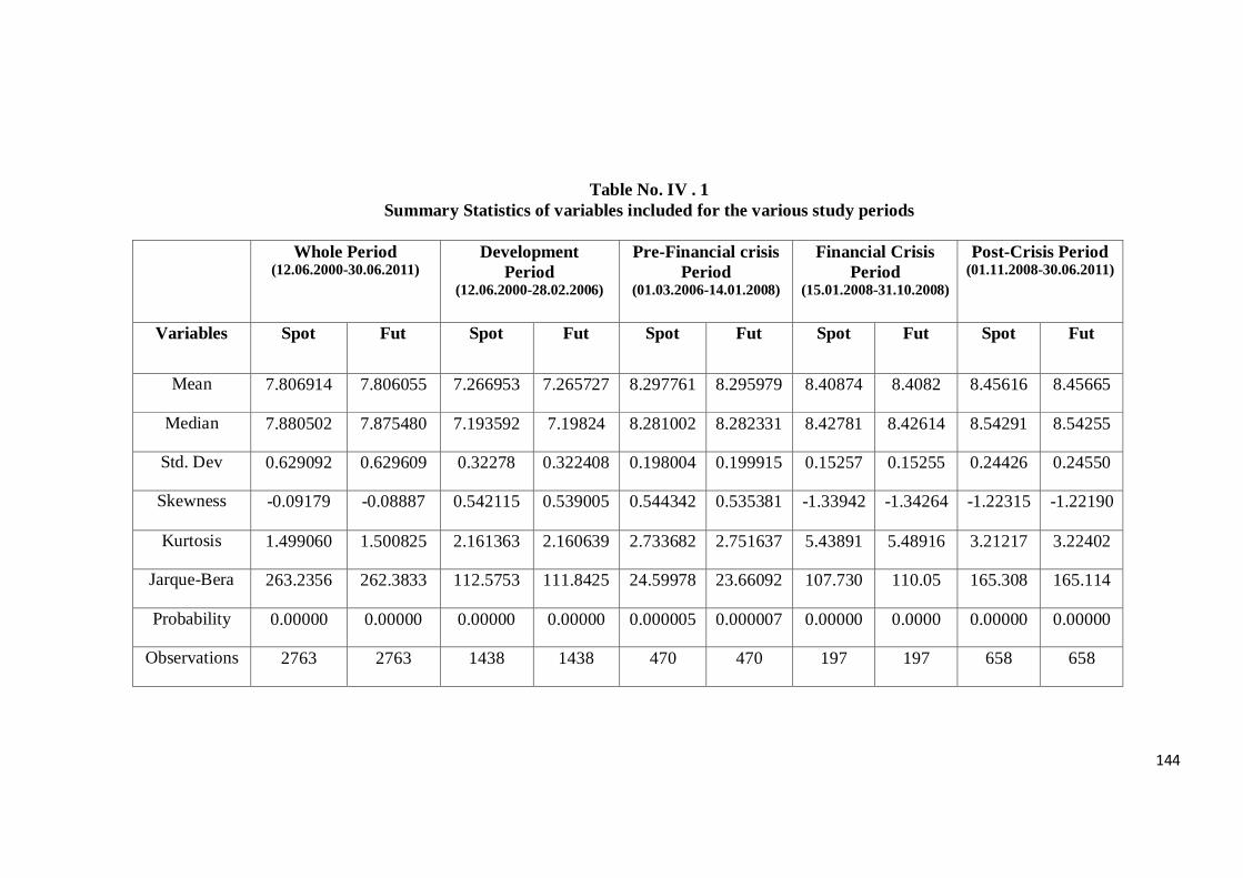
144
Table No. IV . 1
Summary Statistics of variables included for the various study periods
Whole Period (12.06.2000-30.06.2011)
Development
Period (12.06.2000-28.02.2006)
Pre-Financial crisis
Period (01.03.2006-14.01.2008)
Financial Crisis
Period (15.01.2008-31.10.2008)
Post-Crisis Period (01.11.2008-30.06.2011)
Variables Spot Fut Spot Fut Spot Fut Spot Fut Spot Fut
Mean 7.806914 7.806055 7.266953 7.265727 8.297761 8.295979 8.40874 8.4082 8.45616 8.45665
Median 7.880502 7.875480 7.193592 7.19824 8.281002 8.282331 8.42781 8.42614 8.54291 8.54255
Std. Dev 0.629092 0.629609 0.32278 0.322408 0.198004 0.199915 0.15257 0.15255 0.24426 0.24550
Skewness -0.09179 -0.08887 0.542115 0.539005 0.544342 0.535381 -1.33942 -1.34264 -1.22315 -1.22190
Kurtosis 1.499060 1.500825 2.161363 2.160639 2.733682 2.751637 5.43891 5.48916 3.21217 3.22402
Jarque-Bera 263.2356 262.3833 112.5753 111.8425 24.59978 23.66092 107.730 110.05 165.308 165.114
Probability 0.00000 0.00000 0.00000 0.00000 0.000005 0.000007 0.00000 0.0000 0.00000 0.00000
Observations 2763 2763 1438 1438 470 470 197 197 658 658
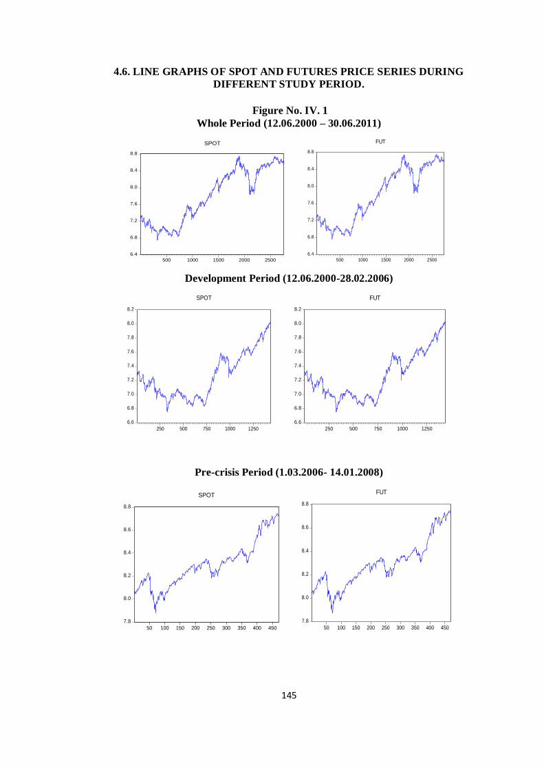
145
4.6. LINE GRAPHS OF SPOT AND FUTURES PRICE SERIES DURING
DIFFERENT STUDY PERIOD.
Figure No. IV. 1
Whole Period (12.06.2000 – 30.06.2011)
6.4
6.8
7.2
7.6
8.0
8.4
8.8
500 1000 1500 2000 2500
SPOT
6.4
6.8
7.2
7.6
8.0
8.4
8.8
500 1000 1500 2000 2500
FUT
Development Period (12.06.2000-28.02.2006)
6.6
6.8
7.0
7.2
7.4
7.6
7.8
8.0
8.2
250 500 750 1000 1250
SPOT
6.6
6.8
7.0
7.2
7.4
7.6
7.8
8.0
8.2
250 500 750 1000 1250
FUT
Pre-crisis Period (1.03.2006- 14.01.2008)
7.8
8.0
8.2
8.4
8.6
8.8
50 100 150 200 250 300 350 400 450
SPOT
7.8
8.0
8.2
8.4
8.6
8.8
50 100 150 200 250 300 350 400 450
FUT
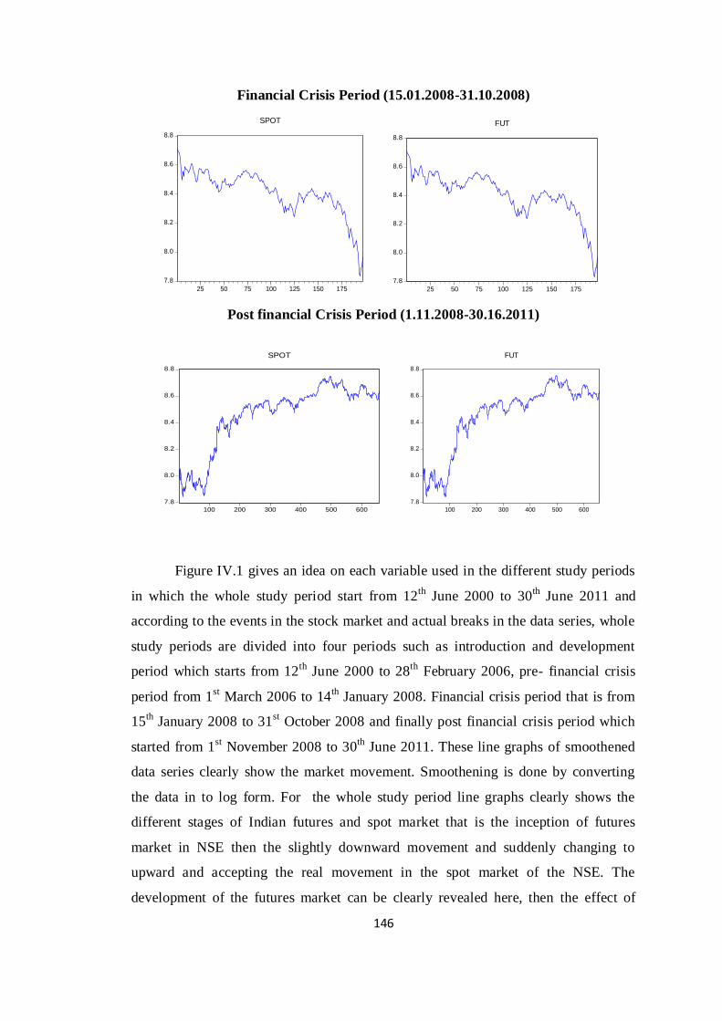
146
Financial Crisis Period (15.01.2008-31.10.2008)
7.8
8.0
8.2
8.4
8.6
8.8
25 50 75 100 125 150 175
SPOT
7.8
8.0
8.2
8.4
8.6
8.8
25 50 75 100 125 150 175
FUT
Post financial Crisis Period (1.11.2008-30.16.2011)
7.8
8.0
8.2
8.4
8.6
8.8
100 200 300 400 500 600
SPOT
7.8
8.0
8.2
8.4
8.6
8.8
100 200 300 400 500 600
FUT
Figure IV.1 gives an idea on each variable used in the different study periods
in which the whole study period start from 12th
June 2000 to 30th June 2011 and
according to the events in the stock market and actual breaks in the data series, whole
study periods are divided into four periods such as introduction and development
period which starts from 12th
June 2000 to 28th
February 2006, pre- financial crisis
period from 1st March 2006 to 14
th January 2008. Financial crisis period that is from
15th January 2008 to 31
st October 2008 and finally post financial crisis period which
started from 1st November 2008 to 30
th June 2011. These line graphs of smoothened
data series clearly show the market movement. Smoothening is done by converting
the data in to log form. For the whole study period line graphs clearly shows the
different stages of Indian futures and spot market that is the inception of futures
market in NSE then the slightly downward movement and suddenly changing to
upward and accepting the real movement in the spot market of the NSE. The
development of the futures market can be clearly revealed here, then the effect of
147
global financial crisis and the real response of Indian market also can be seen here.
The last part of the graphs tells us the tendency of recovering from the financial crisis
problem and shows the dynamic changes in the market. Futures and spot markets are
moving almost in the same manner and the relationship between them for a long run
is almost clear.
For the thorough analysis of the separate pattern in the market, each stage has
to be analyzed clearly. In the introduction and development period, the market shows
almost a stable movement and after 5 years that is from 2006 onwards market started
to move upward. There is a bullish trend in the Indian futures and spot market. This
trend is not in a steady manner during the period between 2006 and 2008, many ups
and downs can be seen from the line graphs. This period also shows a comovement
between spot market and futures market in India.
In 2006, a financial crisis was started in western nations and it might have no
effect in Indian market on the spot. According to the real market movement, this study
sub divided the whole period and considers March 2006 is the beginning of pre-
financial crisis period in India. No specific event had happened in Indian economy
during this period but the market variable like futures and spot price series data shows
different pattern and movement in Indian market. Line graphs of the pre-crisis period
also shows bullish market trend but it is not steady and fluctuations in the market is so
high. Futures market and spot markets are moving in the same direction and the
fluctuations also almost same during the period.
Financial crisis period of the study started from 15th
January 2008 and ended
on 31st October 2008. Sudden fall in the index and the black days have happened in
the US market on 21st January 2008, but this line graphs shows the real shocks in the
Indian market and the tendency of falling started in Indian market on the 15th January
2008 onwards. This period is the real bearish market period in the whole study period
in Indian context. Even though there is two up trends in the market movement, over
all movement of the market shows a diminishing trend. Both futures market and spot
market in India shows the same trend in the line graphs during the financial crisis
period.
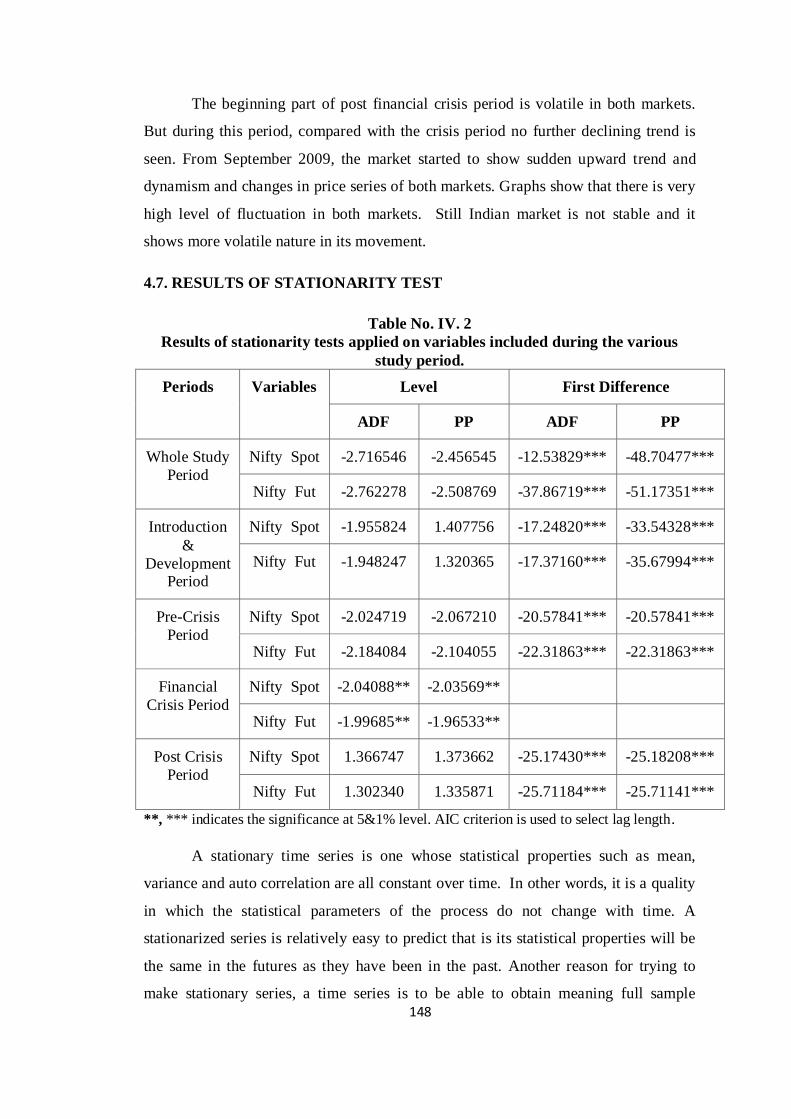
148
The beginning part of post financial crisis period is volatile in both markets.
But during this period, compared with the crisis period no further declining trend is
seen. From September 2009, the market started to show sudden upward trend and
dynamism and changes in price series of both markets. Graphs show that there is very
high level of fluctuation in both markets. Still Indian market is not stable and it
shows more volatile nature in its movement.
4.7. RESULTS OF STATIONARITY TEST
Table No. IV. 2
Results of stationarity tests applied on variables included during the various
study period.
Periods Variables Level First Difference
ADF PP ADF PP
Whole Study
Period
Nifty Spot -2.716546 -2.456545 -12.53829*** -48.70477***
Nifty Fut -2.762278 -2.508769 -37.86719*** -51.17351***
Introduction
&
Development Period
Nifty Spot -1.955824 1.407756 -17.24820*** -33.54328***
Nifty Fut -1.948247 1.320365 -17.37160*** -35.67994***
Pre-Crisis
Period
Nifty Spot -2.024719 -2.067210 -20.57841*** -20.57841***
Nifty Fut -2.184084 -2.104055 -22.31863*** -22.31863***
Financial
Crisis Period
Nifty Spot -2.04088** -2.03569**
Nifty Fut -1.99685** -1.96533**
Post Crisis
Period
Nifty Spot 1.366747 1.373662 -25.17430*** -25.18208***
Nifty Fut 1.302340 1.335871 -25.71184*** -25.71141***
**, *** indicates the significance at 5&1% level. AIC criterion is used to select lag length.
A stationary time series is one whose statistical properties such as mean,
variance and auto correlation are all constant over time. In other words, it is a quality
in which the statistical parameters of the process do not change with time. A
stationarized series is relatively easy to predict that is its statistical properties will be
the same in the futures as they have been in the past. Another reason for trying to
make stationary series, a time series is to be able to obtain meaning full sample
149
statistics such as mean, variance and correlation with other variables. Such statistics
are useful descriptor of futures behavior only if the series is stationary. Stationary is
the important properties of time series data which shows the ability of the data series
to explain the long and short term information. There is long term information in the
time series data if it is in non stationary at level form and stationary characteristics of
time series data tell us only short term relations. As a preliminary test, it is necessary
to test the stationarity of the time series variables such as Nifty spot and Nifty futures
by applying Augmented Dickey Fuller (ADF) and Philip Perron (PP) unit Root test.
The results of ADF and PP test for Nifty spot and Nifty futures are presented in Table
No. IV.2.
Nifty spot and Nifty futures variables are non stationary in its level form and
stationary at first difference. Technically, both variables are in I (1) process at 1%
level of significance. Nifty futures price series and its underlying values are having
long term informational ability during the whole study period and at all sub period
except the period of financial crisis. This means that Nifty futures price series and its
underlying values are having long term informational ability. In the case of financial
crisis period, Nifty spot and futures price series are stationary in its level form itself.
During this period the persistence of shocks will be infinite and the usual t-ratios will
not follow a t- distribution, so we cannot validly undertake hypothesis test. This
difference in the results between crisis period and all other sub- period indicates that
variables confirmed in the study that do not have any long term informational
efficiency due to the stationarity behavior of the variables. When data series are in I
(1) form, it is possible to establish cointegration relationship between the variables.
Absence of stationary predictable basis may be a result of either immaturity of the
markets and inappropriate regulatory frame work (Fortenbery and Zapata, 1997,
Kumar 2004). Here Nifty spot and futures are capable to test the role of one variable
on the other. The significance of these statistical results says that there is no
possibility of accepting the null hypothesis that there is unit root in the variable.
While rejecting the null hypothesis, it is absolutely confirmed that the data series are
losing their long term informational content. Cointegration of futures and spot prices
is a necessary condition for market efficiency (Fama, 1965, 1970). I(1) properties of
both data series are the basic assumption of the cointegration of spot and futures
150
which is useful for price discovery of spot prices in the futures (Christos Floros et.al,
2008).
4.8. RESULT OF VAR CRITERIA FOR THE LAG SELECTIONPROCEDURE
An important practical issue for the implementation of the test is the
specification of the lag length. If lag length is too small then the remaining the serial
correlation in the errors will bias the test. If it is too large then the power of the test
will suffer. The Lag length selection procedure result is indicated in stable size of the
test and minimal power loss. VAR models are widely used in forecasting and in
analyzing of the effects of the structural shocks. A critical element in the specification
of VAR models is the determination of the lag length of the VAR. according to Braun
and Mottnik (1993) the estimates of a VAR whose lag length differs from true the lag
length are in consistent as are the impulse response function and variance
Decompositions derived from the estimated VAR. Selecting a higher lag length than
the true lag length causes an increase in the mean- square forecast errors of the VAR
and that under fitting the lag length offer generates autocorrected errors.
Table No.IV.3 shows the result of VAR criteria adopted for the selection of
optimal lag length for statistical methodology used to determine the relationship
between futures and spot market during the various study periods. As per, Likelihood
Ratio (LR), Final Prediction Error (FPE) and Akaika Information Criterion (AIC) the
optimal lag length for the whole study period is 5. The error term of the each variable
is stationary at this point. During the introduction and development period of the
study the all lag selection criterion at 5% level of significant suggest that 2 is the
optimal lag length for the models. In the same way optimal lag order is selected by
FPE, AIC, LR, SC and HQ as 2 for the pre financial crisis period. Optimal lag length
of 2 is significant at 5% level in FPE, LR, AIC, SC and HQ criteria during the
financial crisis study period. During the post financial crisis, LR, FPE, AIC, SC and
HQ indicates that 2 is the optimal lag length. The optimal lag length helps the
researcher to avoid auto correlation problem from the time series data Set up to an
extent.
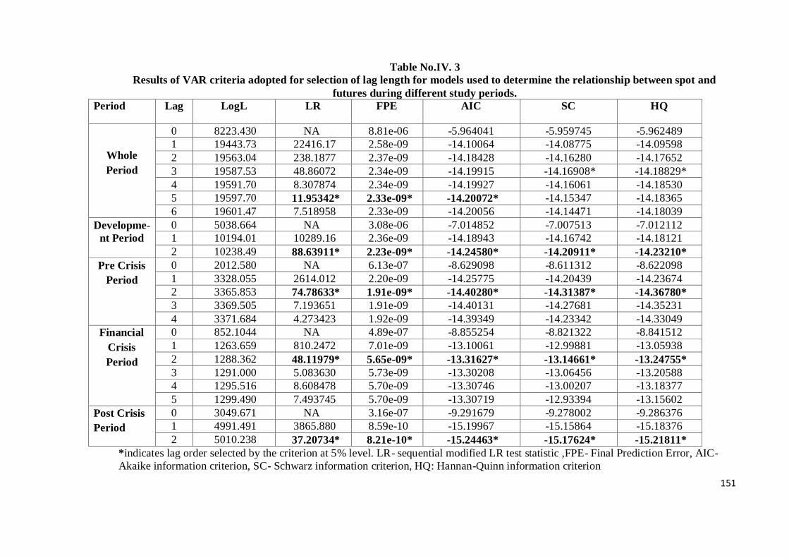
151
Table No.IV. 3
Results of VAR criteria adopted for selection of lag length for models used to determine the relationship between spot and
futures during different study periods.
Period Lag LogL LR FPE AIC SC HQ
Whole
Period
0 8223.430 NA 8.81e-06 -5.964041 -5.959745 -5.962489
1 19443.73 22416.17 2.58e-09 -14.10064 -14.08775 -14.09598
2 19563.04 238.1877 2.37e-09 -14.18428 -14.16280 -14.17652
3 19587.53 48.86072 2.34e-09 -14.19915 -14.16908* -14.18829*
4 19591.70 8.307874 2.34e-09 -14.19927 -14.16061 -14.18530
5 19597.70 11.95342* 2.33e-09* -14.20072* -14.15347 -14.18365
6 19601.47 7.518958 2.33e-09 -14.20056 -14.14471 -14.18039
Developme-
nt Period
0 5038.664 NA 3.08e-06 -7.014852 -7.007513 -7.012112
1 10194.01 10289.16 2.36e-09 -14.18943 -14.16742 -14.18121
2 10238.49 88.63911* 2.23e-09* -14.24580* -14.20911* -14.23210*
Pre Crisis
Period
0 2012.580 NA 6.13e-07 -8.629098 -8.611312 -8.622098
1 3328.055 2614.012 2.20e-09 -14.25775 -14.20439 -14.23674
2 3365.853 74.78633* 1.91e-09* -14.40280* -14.31387* -14.36780*
3 3369.505 7.193651 1.91e-09 -14.40131 -14.27681 -14.35231
4 3371.684 4.273423 1.92e-09 -14.39349 -14.23342 -14.33049
Financial
Crisis
Period
0 852.1044 NA 4.89e-07 -8.855254 -8.821322 -8.841512
1 1263.659 810.2472 7.01e-09 -13.10061 -12.99881 -13.05938
2 1288.362 48.11979* 5.65e-09* -13.31627* -13.14661* -13.24755*
3 1291.000 5.083630 5.73e-09 -13.30208 -13.06456 -13.20588
4 1295.516 8.608478 5.70e-09 -13.30746 -13.00207 -13.18377
5 1299.490 7.493745 5.70e-09 -13.30719 -12.93394 -13.15602
Post Crisis
Period
0 3049.671 NA 3.16e-07 -9.291679 -9.278002 -9.286376
1 4991.491 3865.880 8.59e-10 -15.19967 -15.15864 -15.18376
2 5010.238 37.20734* 8.21e-10* -15.24463* -15.17624* -15.21811*
*indicates lag order selected by the criterion at 5% level. LR- sequential modified LR test statistic ,FPE- Final Prediction Error, AIC- Akaike information criterion, SC- Schwarz information criterion, HQ: Hannan-Quinn information criterion
152
4.9. LONG TERM RELATIONSHIP BETWEEN FUTURES AND SPOT
MARKET IN INDIA
Both futures and cash prices series are non stationary at level and their
stationary nature denote that both markets may have strong cointegration relationship
over the long run (Gupta et.al 2006).Table No. IV.4 provides the results of
unrestricted cointegration rank test applied through Johanson cointegration
methodology for different study periods. The results of Johansen Cointegration are
explained through the Trace Statistics and the Maximum-Eigen test statistics. The
results of four sub study period are listed in the table. For the first period that is whole
study period, the null hypothesis that there is no cointegration equation among spot
and futures is rejected at 5% level of significance. Both test statistics like Trace
statistics and Max- Eigen statistics reject the null hypothesis at 5% significance level.
So the alternative hypothesis that there is at least one cointegration equation between
spot and futures market is accepted. The results are supported by the literature with
the evidence from India and abroad. This long run relationship between futures and
spot market helps the traders in hedging their portfolio risk and to exploit the arbitrage
opportunities (Anderson et.al. 1981, Karma and Seigel 1987, Myer and Herson 1996,
kapil Gupta 2008). There is no chance to accept the null hypothesis that there is no
cointegration between spot price series and futures price series during the introduction
and development period of the study. The established relationship of these variables
that is long term relationship between spot and futures market is proved here by
accepting the null hypothesis of the methodology. Trace statistics rejects the null
hypothesis at 5% level of significance and Max-Eigen value is giving support to it at
5% level of significance which indicates that during the development period of the
study there is one cointegration equation between Indian futures market and spot
market.
This result reveals that the movement of one market can be predicted by
another market during the long term period. During the pre- financial crisis period the
null hypothesis that no cointegration between the integrated variables such as futures
market and spot market are rejected by the Trace statistics and Max-Eigen value test
statistics at 5% level of significance. One cointegration equation between spot and
futures market is accepted as the alternative hypothesis during the pre financial crisis
153
period. The empirical result also supports the established relationship between these
two markets. Financial crisis period is totally different from other sub- periods of the
study. The unit root test result itself indicates that the price series of futures and spot
markets are not having any informational content on long term relationship as the
price series are stationary in their level form. During this period the market shows a
bearish trend due to the effect of global sub-prime financial crisis. Theory says that in
the bearish market there is no long term contract or investment is made instead only
speculation is possible to take advantage of short term fluctuation.
All established relationships are collapsed here and market is activated by
speculators. Since, the data series during the crisis period are stationary in its level
form, cointegration relationship cannot be established, and instead causality test is
applicable to find the short term relationship between spot and futures markets. Effect
of spot market on futures market is analyzed by restricting the spot and vice versa is
done in this test. Table No. IV.5 shows the result of VAR Granger Causality/ Block
Exogeneity Wald test. Result shows that both restrictions are not significant and it
reveals that during the financial crisis period no market depends on another market
and any causal effect or lead- lag relationship between both markets in India. This
result is again supported by the theory that during the financial crisis period market is
moved on the basis of speculative trading and no market is giving any information to
another market. The null hypothesis of causality test that is spot does not cause
futures and futures market does not causes spot market is accepted on the basis of test
statistics which does not provide any significance at critical level. In the post financial
crisis period results of Johansen cointegration reveals that the null hypothesis, there is
no long term relationship between spot and futures is rejected at 5% level of
significance. The trace test and max-Eigen value test statistics results indicate that the
alternative hypothesis, there is at least one cointegration equation between the spot
and futures market is accepted. Thus the established strong relationship between spot
and futures market is proved here.
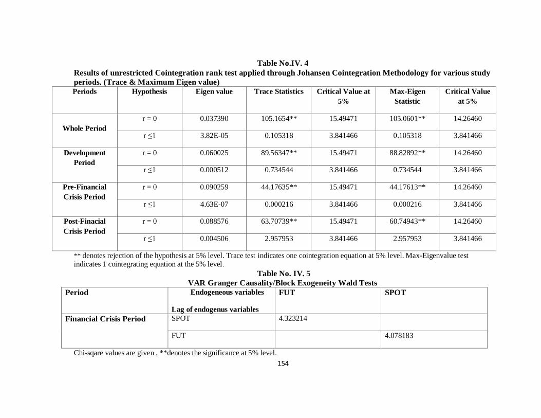
154
Table No.IV. 4
Results of unrestricted Cointegration rank test applied through Johansen Cointegration Methodology for various study
periods. (Trace & Maximum Eigen value)
Periods Hypothesis Eigen value Trace Statistics Critical Value at
5%
Max-Eigen
Statistic
Critical Value
at 5%
Whole Period
r = 0 0.037390 105.1654** 15.49471 105.0601** 14.26460
r ≤1 3.82E-05 0.105318 3.841466 0.105318 3.841466
Development
Period
r = 0 0.060025 89.56347** 15.49471 88.82892** 14.26460
r ≤1 0.000512 0.734544 3.841466 0.734544 3.841466
Pre-Financial
Crisis Period
r = 0 0.090259 44.17635** 15.49471 44.17613** 14.26460
r ≤1 4.63E-07 0.000216 3.841466 0.000216 3.841466
Post-Finacial
Crisis Period
r = 0 0.088576 63.70739** 15.49471 60.74943** 14.26460
r ≤1 0.004506 2.957953 3.841466 2.957953 3.841466
** denotes rejection of the hypothesis at 5% level. Trace test indicates one cointegration equation at 5% level. Max-Eigenvalue test indicates 1 cointegrating equation at the 5% level.
Table No. IV. 5
VAR Granger Causality/Block Exogeneity Wald Tests
Period Endogeneous variables
Lag of endogenus variables
FUT SPOT
Financial Crisis Period SPOT 4.323214
FUT 4.078183
Chi-sqare values are given , **denotes the significance at 5% level.
155
What is the real relationship between Indian spot and futures market is
analyzed and proved that during the different market trend the established relations
may be changed. According to the market movement, data pattern and theoretical
back ground, four sub periods are drawn and conducted separate analysis. The result
reveals that except during financial crisis period there is long term relationship
between both markets. The information on long term relationship is not found in the
data series of futures and spot market due to the bearish trend in the market during the
financial crisis period. Remaining periods, the study proved with the help of statistical
significance that the long term relationship exists between the markets.
There is possibility for disequilibrium in the long term relationship between
both variables for a short period. Existence of cointegration suggests that although
both markets may be in disequilibrium during the short run but such deviation are
very quickly corrected through arbitrage (Vipul 2005). This variation shows the
ability of the market to adjust to new information and shows the leading position in
Indian market. In order to get the clarification on this aspect, another econometric
model which is Vector Error Correction is applied. Even though these two markets are
cointegrated in the long run, there is a possibility for disequilibrium in the relationship
during short period. It may be due to the difference in the ability of the market to
adjust to new information.
4.10. SHORT TERM RELATIONSHIP BETWEEN SPOT AND FUTURES
MARKET IN INDIA
The standard way to derive the Error Correction Model is to show that two
variables are linear functions of a latent integrated process. The residuals of
dependent regressed or independent should be stationary. This derivation of the error
correction model starts with the assumption that two variables are integrated and
demonstrate that the Error Correction Model captures the equilibrium causal
movements between these two cointegrated processes. The Error Correction Model
reveals the speed of adjustment in to equilibrium relationship and also it eliminates
the danger of estimating spurious regression with near integrated data, as the
dependent variable in this model is differenced.
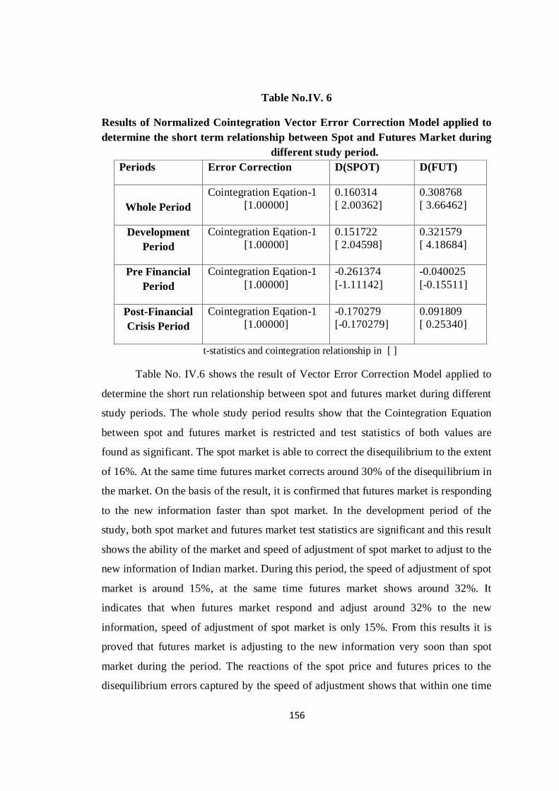
156
Table No.IV. 6
Results of Normalized Cointegration Vector Error Correction Model applied to
determine the short term relationship between Spot and Futures Market during
different study period.
Periods Error Correction D(SPOT) D(FUT)
Whole Period
Cointegration Eqation-1
[1.00000]
0.160314
[ 2.00362]
0.308768
[ 3.66462]
Development
Period
Cointegration Eqation-1
[1.00000]
0.151722
[ 2.04598]
0.321579
[ 4.18684]
Pre Financial
Period
Cointegration Eqation-1
[1.00000]
-0.261374
[-1.11142]
-0.040025
[-0.15511]
Post-Financial
Crisis Period
Cointegration Eqation-1
[1.00000]
-0.170279
[-0.170279]
0.091809
[ 0.25340]
t-statistics and cointegration relationship in [ ]
Table No. IV.6 shows the result of Vector Error Correction Model applied to
determine the short run relationship between spot and futures market during different
study periods. The whole study period results show that the Cointegration Equation
between spot and futures market is restricted and test statistics of both values are
found as significant. The spot market is able to correct the disequilibrium to the extent
of 16%. At the same time futures market corrects around 30% of the disequilibrium in
the market. On the basis of the result, it is confirmed that futures market is responding
to the new information faster than spot market. In the development period of the
study, both spot market and futures market test statistics are significant and this result
shows the ability of the market and speed of adjustment of spot market to adjust to the
new information of Indian market. During this period, the speed of adjustment of spot
market is around 15%, at the same time futures market shows around 32%. It
indicates that when futures market respond and adjust around 32% to the new
information, speed of adjustment of spot market is only 15%. From this results it is
proved that futures market is adjusting to the new information very soon than spot
market during the period. The reactions of the spot price and futures prices to the
disequilibrium errors captured by the speed of adjustment shows that within one time
157
period 32% of the disequilibrium errors is corrected in the futures market which
shows the leading behavior of the futures market. Thus as is to be expected, the result
shows that the futures market responds faster to the previous periods deviation from
the long run equilibrium (Suchismita Bose 2007). The pre-financial crisis period, the
Vector Error Correction statistics shows that in both market is not significant. At this
period spot market is adjusting to the new information faster than futures market. This
result is not supporting to the previous period results, but it is not statistically
significant. Post financial crisis results indicate that spot market statistics are not
significant but futures market test statistics are significant and it corrects the
disequilibrium around 9%.
During this period spot market plays a vital role to adjust the new information
but it is not statistically proved. In financial crisis period the relationship is not
confirmed and there is no chance for error correction model, it is possible to find the
short run relationship between futures and spot market and finds the short run
relationship between futures and spot markets in India. Properties of data series show
the stationarity at level form and it is confirmed that there is no possibility for the
short run disequilibrium in long run relationship. According to this study by using
VECM, we can confirm that futures market is leading the spot market during the
whole study period and development period. This result is supported by empirical
evidence of Stoll and Whaley (1990), Whab and Lashgari (1993) Chu, Hsich and Tse
(1999), Tse (2004), Raymond and Yiuman Tse (2004) and Chuu and Chung (2006).
In pre financial crisis period and post financial crisis period, the speed of adjustment
parameter of spot market is more than speed of adjustment parameter of futures
market, but spot market adjustment factor is not significant.
During financial crisis period short run relationship and causality relationship
of futures and spot market is also not significant (Table No.IV.5). Even though whole
study period and introduction and development period indicate the leading tendency
of the futures market, it cannot be seen in the other period. Therefore, we can
conclude that a bidirectional relationship between futures and spot market is
witnessed in India. It is confirmed that there is informational linkage between spot
and futures market in Indian equity futures market. This situation provides the
opportunities to the traders to make profit through arbitrage process. Informational
158
linkage between stock index spot and futures market implies that investors using these
markets to explore significant arbitrage profit and hedging opportunities (Demitris F.
Kenourgios 2004). But we cannot prove it from this analysis results. In order to prove
this conclusion another test like causality test is required. There are studies which
prove the bidirectional relationship between spot and futures market in India and
abroad and therefore an attempt is made here to examine empirically the causality
between futures and spot market in India by using Wald test coefficient.
4.11. CAUSAL RELATIONSHIP BETWEEN SPOT AND FUTURES MARKET
IN INDIA
Table No. IV.7 present the results of Wald test coefficient for causal
relationship between spot and futures market during the different study periods in
India. This table reports the results of F-statistics and chi-square for each variable in
different periods. The results of Wald test for the whole study period F-statistics and
chi-square values are significant which means that while restricting the lag values of
futures and residuals of spot, the null hypothesis of futures market does not cause spot
value is rejected at 5% level of significance and accepted the alternative hypothesis of
futures market causes spot market. In the same period, futures market as the
dependent variable, spot and its lag values and the residuals of futures variable are
restricted and find that both F- statistics and chi-square values are significant at 5%
level. It means that spot market causes futures market in short run period. Both
markets are causing each other during the whole study period which confirms that
there is bidirectional causality between futures market and spot market in India during
the whole study period (Kedar Nath Mukerjee and Mishra 2004, Suchismita Bose
2006, 2007, Bhol et al 2010).
In the introduction and development period of the study while restricting the
residuals and lag value of spot and futures in the spot and the futures variable as the
dependent variable, F-statistics and chi- square test result shows significance at 5%
level.
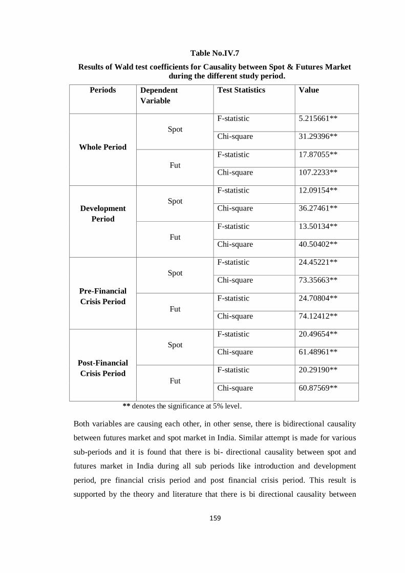
159
Table No.IV.7
Results of Wald test coefficients for Causality between Spot & Futures Market
during the different study period.
Periods Dependent
Variable
Test Statistics Value
Whole Period
Spot
F-statistic 5.215661**
Chi-square 31.29396**
Fut
F-statistic 17.87055**
Chi-square 107.2233**
Development
Period
Spot
F-statistic 12.09154**
Chi-square 36.27461**
Fut
F-statistic 13.50134**
Chi-square 40.50402**
Pre-Financial
Crisis Period
Spot
F-statistic 24.45221**
Chi-square 73.35663**
Fut
F-statistic 24.70804**
Chi-square 74.12412**
Post-Financial
Crisis Period
Spot
F-statistic 20.49654**
Chi-square 61.48961**
Fut
F-statistic 20.29190**
Chi-square 60.87569**
** denotes the significance at 5% level.
Both variables are causing each other, in other sense, there is bidirectional causality
between futures market and spot market in India. Similar attempt is made for various
sub-periods and it is found that there is bi- directional causality between spot and
futures market in India during all sub periods like introduction and development
period, pre financial crisis period and post financial crisis period. This result is
supported by the theory and literature that there is bi directional causality between
160
spot and futures market in India and abroad (Abhay Abhyankar 1998, Jae. H. Min
1999).
From this table, we can draw a picture on the causality relationship between
Indian spot and futures market. There is bidirectional relationship between futures and
spot market in India and the current study proves that the relationship is established in
all the study periods except the period of financial crisis. The Vector Error Correction
Model does not give the clear picture on the causality of the futures and spot market.
But with the help of Wald test, we can clearly observe and explain the existence of a
bidirectional relationship between the futures and spot market in India.
The literature also empirically proves that even though there is bidirectional
relationship between Indian futures and spot market, the futures market is found to
show a stronger leading role than the spot market. Many Indian studies like
Thenmozhi (2002), Raju and Karande (2003), Gupta and Sing (2006) Shah et al
(2006) Thomas (2006), Bose (2007) and Kapil Gupta et al (2008) have already proved
the importance of the futures market in India. The changing lead- lag relationship of
both spot and futures market is also proved. The stock market may occasionally lead
the futures market (Grunbichler et al 1994). This study also proves the bidirectional
relationship between both market and the dominance of futures market.
The Price discovery function of the futures market can be revealed from the
speed of adjustment of the market to the disequilibrium among the cointegration
relationship with the spot and futures market. The price discovery function of the
futures market is facilitated when the futures price are closely approximate the spot
price on the futures contract maturity date (Ivanovic and Howley 2004). The futures
market maintains a leading role in the price dynamics within the exchange rate market
(Baklaci 2007). Spot and futures prices respond to the arrival of new information at
different speed, causing the basis for the index futures contract to diverge temporarily
between sock and futures market following its arrival in one of the market (Hill et al
1998, Hong Kong, Draper and Fung 2003 and Cummings and Frino 2010). The
informational efficiency of the market can be assessed on the basis of the speed of
adjustment of the market to new information. In predicting unexpected movements
among stock index futures contracts, the index futures has the highest predictive
161
power (Minho Kim, Andrew C. Szakmary and Schwarz 1999). Futures market is
having the leading role by transmitting information to the spot market in India. Indian
equity futures market is an efficient price discovery vehicle (Bhatia 2007). When a
market is efficient no arbitrage opportunities via trade strategies can be profitable
(Christos Floros 2008). If futures prices respond first to the information, daily futures
lead daily spot, implying that arbitrage opportunities exists (Kolb 1994). It is
supported that Indian market provides the arbitrage opportunities to the traders.
In the case of financial crisis period this relationship cannot be seen due to the
unexpected variation in the market. When such unexpected variation is witnessed,
speculators drive the market with the intension of making abnormal profit with
changes in prices during the short span of time. Investors may not be interested to
play as they are not able to take a stand for long period with this short term
fluctuations.
With the help of these empirical results the null hypotheses of the studies such
as there is no significant relationship between spot and futures market in long and
short period, the futures price has no information to pass on to spot market and no
significant lead lag effect between spot and futures market are rejected. This study
clearly reveals that there is cointegration relationship between Indian spot and futures
market, even though there is bidirectional relationship between spot and futures
market, the futures market shows the dominant and leading role on the spot market in
India.
4.12. CONCLUSION
This chapter has dealt with analyzing dynamic relationship between futures
and spot market in India. The relationships such as long term, short term and causality
between futures and spot market are explained here. Due to data movement and
market trend the established relationships among markets may be changed. Literature
says when futures market and its underlying market are cointegrated then one market
will always lead another market for a long period or a particular period. The causal
relationship also reveals the lead- lag positions between the futures and spot markets.
To empirically prove the established relationship between these variables for a
particular period, the current study uses three econometrics models and divided the
162
whole study period into four sub periods on the basis of the actual structural break on
the data movement and the real market trend. The first period includes the
introduction and development stage of the futures market in India. Second sub-
division contains pre- financial crisis period which also shows upward trend in the
futures market. Third sub division is the critical period of the study which shows the
extreme falling trend in the futures market due to financial crisis, after a big fall there
is increasing trend which is the last subdivision of the study period is called post
financial crisis period.
The first part of the chapter shows summary statistics of the raw data and line
graphs of the smoothened data series. Unit root test results provide the stationarity
properties of each variable separately for different periods. In all study periods except
financial crisis period the price series of futures and spot market are in I (1) process.
This time series properties allow applying Cointegration methodology to analyze long
term relationship. Cointegration results of all periods except financial crisis period
indicate the possibility of rejection of null hypothesis that there is no cointegration
between futures and spot market in India which means that there is long term
relationship between both markets in India. This long term relationship between
futures and spot market does not exists during financial crisis period and the results
on VAR Granger Causality /Block Exogeneity test results shows that there is no
causality between the markets during the financial crisis period. On the basis of the
results of Johanson Cointegration Methodology, the current study also proves that
there is long term relationship and cointegration between futures market and its
underlying market. If the market shows deep fall and instability, the speculators play
well and the all established relationship may be collapsed. The speed of adjustment
parameters of futures and spot markets to the disequilibrium in the cointegration is
analyzed by using Vector Error Correction Model.
On the basis of this speed of adjustment parameters, it is possible to explain on
the leading behavior of the market or the ability of the market to adjust and respond to
the new information. During the whole study period and introduction and
development period of the study that futures market is leading the spot market in
India. In pre-financial crisis and post crisis period results prove that spot market is
leading the futures market but t-statistics values are not significant. From these

163
results, the study provides confusing results of lead- lag relationship between futures
and spot market in India. We cannot conclude that futures market leads the spot
market always and spot market attracts the futures market often. In short, the Indian
futures market is the leading market among the bidirectional relationship of spot and
futures market. The dominant role of futures market is witnessed through the
empirical result of this study.
Wald coefficient test for causality relationship between futures market and
spot market gives more clarity on such relations. This study used Angel Granger
(1987) cointegration methodology and Bivariate Error Correction Model. The result
of Wald coefficients clearly proves that there is bidirectional causality between
futures market and spot market except financial crisis period. Financial crisis period is
the evidence of collapsed market structure, which means no such established
relationship is found in this study period.
To conclude, this study can boldly say that the relationship of the futures and
spot markets are so dynamic and the real trend in the market affect the established
relationship of the futures and spot markets in India.
164
Chpater -V
The Determinants of
Futures Market in India
165
CHAPTER –V
THE DETERMINANTS OF FUTURES MARKET
IN INDIAN
5.1. INTRODUCTION
The movement of the futures market can be predicted with the help of other
factors from the futures market and spot market. Vipul (2008) made an attempt to
investigate the role of some variable from the futures market that can predict others.
Each variable from the futures market and variable from the spot market can also
predict the movement of other variables in the futures market. The relationship
between variables like open interest, trading volume, turnover, volatility and futures
return can be taken as the way in which the movement of one variable is related to
another variable, then this relationship can be used to predict the movement of another
variables. If some of the variables are able to predict the movement of another
variable, it can be said that it is the determinant of that variable. The positive and
contemporaneous relationship between price volatility and trading volume are found
by Clerk (1973), Lawrence and Harris (1986) and these relationship can be quite
effectively used for forecasting these variables with their past values (Vipul 2008).
Very strong relationship between futures index trading and the liquidity of its
underlying market shows that the trading of stock index futures enhances the liquidity
of the underlying stocks (Tina. M. Galloway and Miller 1997). The trading between
futures and its spot market also enhances the liquidity of its trading. The role of
arbitrage process in the index futures helps to increase the trading volume and its
liquidity. Danthin (2003) and Edward (2006) argued that index related trading
strategies like index arbitrage will increase liquidity. Trading between spot and
futures market enhances the trading volume and liquidity of the index trading.
Variables from the futures market can also be used as the element which may predict
the movement of futures return. Open interests, turn over and number of contract are
the representatives of trading volume of the futures market in quality and quantity
166
manner.
The relationship between different variables in the futures market reveals the
ability of each variable to reflect the information flow to the market and its role in
determining the futures markets movement. Information flow, measured by trading
volume has a positive relationship with volatility while market depth measured by
open interest has an inverse relationship with volatility (Bessembinder and Seguin
1992, P. Sakthivel and B.Kamaiah 2009).
The importance of trading volume in the form of number of contract or turn over can
be traced from many studies in the literature. The level of flow of information to the
market can be traced and it may be used as the proxy for the liquidity of the market.
Volatility and trading volumes are inter related which will provide lot of information
on the market movement. Trading volume is proxy for the flow of information in to
the market, trading volume and return volatility are driven by the same factors
(Lastrapes 1990, P. Sakthivel 2009).
Literature proves the point those variables both from spot and futures markets
play the role of passing information and their relationship helps to provide one with
another. Therefore in order to identify the role of each variable on the futures return
and find the level of influence of each one to the futures return, the VAR system is
used. This method takes each variable as endogenous and exogenous and finds the
influence of each variable to another separately and together. This study is an attempt
to find the determinants of futures market return through the influence and
relationship between variables from the futures market and spot market return. The
literature found that open interest, trading volume and volatility are playing their own
role in the futures market (Julio 2008, Pratap Chandra Pati (2010), Gwilym et al
(1999), Cambell et al (1993) Spyrou (2005) and Puja Padhi (2009).
The reaction and response of market shock on each variable help the traders to
predict the movement of another variable. The Impulse response function measures
the time profile of effect of a shock, on the expected futures values of a variable- a
conditional variance of equity volatility (Dawson and Stikouras 2009). The
unexpected shocks are easily absorbed and quickly disappeared as a result of risk
neutrality as participant have hedged their exposure to market fluctuation. The inter
relationship between variables in futures market and the ability of the variable to
167
respond to the shocks on the variables can also be traced with the help of impulse
response function.
The proportion of shocks reflected by the same variable and transmitted to
other variables is shown through the variance decomposition function. Impulse
responses and variance decomposition analysis explain economic significance in
addition to statistical significance (Brajesh Kumar and P.Singh 2009). The
interrelationship between futures return, spot return, open interest, turn over, number
of contract and futures market volatility are discussed in by this chapter with the help
of VAR Granger Causality/ Block Exogeneity test, Impulse Response Function and
Variance Decomposition. This chapter provides information on the causal relationship
between these variables separately and together to find the determinants of futures
market in India.
5.2. VARIABLES AND METHODOLOGY
In order to find the determinants of the futures market in India, this study
considered variables like volatility futures return, open interest, number of contracts
and turn over. Turnover and the number of contract of the futures contract are the
variable of trading volume of the futures market. Spot market return is another
variable which is taken in to consideration to analyze the determinants of futures
market. Chen etal (1995), Theo bald (1996), Stephen P Ferris etal (2002), Stephen
Yen and Ming (2009), Hsiang Chen (2009) found significant dynamic interactions
and causal relations among volatility, open interest and trading volume. Ross (1976)
suggested that volatility can be considered as a measure of information flow in a
leading indicator for predicting the next day volatility of the underlying. The
importance of trading volume, volatility and open interest is highlighted by Gulen and
Mayhew (2000) Vipul (2008) and Sakthivel (2009).
In this chapter, there are six variables out of which five variables from futures
market and one variable from spot market are included. Variables from futures
markets are futures market return (FUT) is the representative of futures market,
number of contract (CONT) , turnover (TURN), both are considered as a proxy for
trading volume, open interest (OI) which is the indicator of market depth and hedging
efficiency of the market, volatility of the futures return (VOL) and spot market return
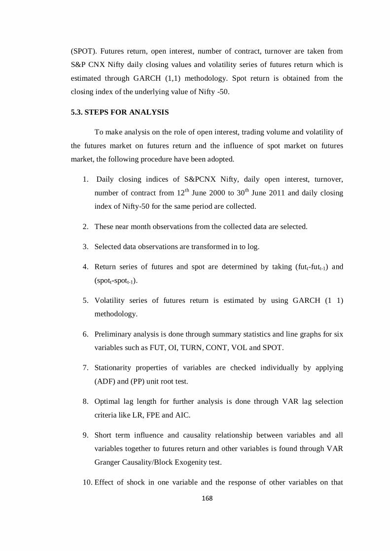
168
(SPOT). Futures return, open interest, number of contract, turnover are taken from
S&P CNX Nifty daily closing values and volatility series of futures return which is
estimated through GARCH (1,1) methodology. Spot return is obtained from the
closing index of the underlying value of Nifty -50.
5.3. STEPS FOR ANALYSIS
To make analysis on the role of open interest, trading volume and volatility of
the futures market on futures return and the influence of spot market on futures
market, the following procedure have been adopted.
1. Daily closing indices of S&PCNX Nifty, daily open interest, turnover,
number of contract from 12th
June 2000 to 30th June 2011 and daily closing
index of Nifty-50 for the same period are collected.
2. These near month observations from the collected data are selected.
3. Selected data observations are transformed in to log.
4. Return series of futures and spot are determined by taking (futt-futt-1) and
(spott-spott-1).
5. Volatility series of futures return is estimated by using GARCH (1 1)
methodology.
6. Preliminary analysis is done through summary statistics and line graphs for six
variables such as FUT, OI, TURN, CONT, VOL and SPOT.
7. Stationarity properties of variables are checked individually by applying
(ADF) and (PP) unit root test.
8. Optimal lag length for further analysis is done through VAR lag selection
criteria like LR, FPE and AIC.
9. Short term influence and causality relationship between variables and all
variables together to futures return and other variables is found through VAR
Granger Causality/Block Exogenity test.
10. Effect of shock in one variable and the response of other variables on that
169
shock and its direction are found by using impulse response function.
11. Proportion of shock transmitted from one variable to another due to the shock
in the same variable is determined by using Variance Decomposition.
12. The role of each variable on the futures return is determined for predicting the
movement of futures market through the above said steps.
5.4. RATIONALE OF THE STUDY
Review of literature focused on the role of trading volume, volatility of
underlying market, open interest and return of underlying markets in predicting the
movement of futures market. These studies considered variables separately and
together and made analysis of the determinants of futures market abroad and in India.
The importance of daily open interest on hedgers activity and market depth was
analyzed and reflected in many studies. Bessembinder (1993), Chen etal (1995),
Bhuyan and Yan (2002), Hongyi Chen, Laurence Fung and Jim Wong (2005) and
Julio (2008) found that the de- trended open interest position could be a useful
indicator of monitoring speculative activities in the futures market. The intensity of
speculative activities can be identified through the volume of daily open interest of
the futures market. Stephen- M. Yen etal (2010) found the bidirectional relationship
between open interest and volatility in the futures market.
Trading volume is the proxy for the flow of information in to the market
(Lastrapes 1990 and P. Sakthivel 2009). The efficiency of market to react the new
information shows the positive relationship between volatility and unexpected futures
trading activity. The relationship between trading volume and volatility of the market
can be found from Clerk (1973), Bessembinder and Seguin (1993) and Tan and
Gannon (2002). Studies with considered open interest, number of contract, turnover,
volatility, futures market return and spot market return are very rare and it is
important to take all of these variables together to analyze the predictive efficiency of
these variables on futures return. Julio (2008) found that it is impossible to
discriminate between day traders and subrogating traders from volume and open
interest data and the speculators don’t hold open position over night. Pratap
Chandrapathi (2010) commented that trading volume is an important statistics that
170
gives information about the status of financial market.
There is another argument which explains the relationship between price-
volume and volume- volatility of futures trading. The information content of volume
and sequential processing of information may lead to dynamic relationship between
returns and trading volume (Brajesh Kumar and Priyanka Singh 2009). The positive
volume- volatility relationship is driven by the general public where as the activity of
informed traders such as clearing members and floor traders is often inversely related
to volatility (Bhaumik, Karanasos and Kartsaklas 2008).
It is found that, a study which will cover many aspects like arbitrage
efficiency, informational content, responsive ability of the market, hedging efficiency
of the futures market and speculative nature of traders may help the policy makers and
traders to understand the real movement of futures market and the influence of each
aspects to another one and all aspects together to each one to predict the futures
movement of the market. This study is making an analysis on these aspects and
considering many dimensions of the market with the help of VAR system, impulse
response function and variance decomposition process to find the determinants of
futures market in India.
Table No. V.1 shows the summary statistics of variables included in the study
for different periods. Summary statistics provides the basic behavior of variables
individually for various sub- study periods. Nifty spot market return (SPOTR), Nifty
futures market return (FUTR), futures market open interest (OI), number of contract
(CONT), turn over (TURN) and volatility of futures market return series (VOL) are
the variables included in the study. The whole study period starts form 12.06.2000
and ends on 30.06.2011. Time series data expected to have variation due to many
factors which have an effect on the market. Analysis of these data without giving due
consideration for these factors, will lead for misleading conclusion and therefore data
series was divided in to various sub periods based on structural breaks and they are
named as initial period of introduction of derivatives, pre financial crisis, financial
crisis period and post financial crisis periods analysis is done for these periods
separately and their summary statistics are presented in the following table.
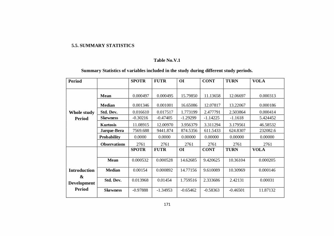
171
5.5. SUMMARY STATISTICS
Table No.V.1
Summary Statistics of variables included in the study during different study periods.
Period SPOTR FUTR OI CONT TURN VOLA
Whole study
Period
Mean 0.000497 0.000495 15.79850 11.13658 12.06697 0.000313
Median 0.001346 0.001001 16.65086 12.07817 13.22067 0.000186
Std. Dev. 0.016610 0.017517 1.773199 2.477791 2.503864 0.000414
Skewness -0.30216 -0.47405 -1.29299 -1.14225 -1.1618 5.424452
Kurtosis 11.08915 12.00970 3.956379 3.311294 3.179561 46.58532
Jarque-Bera 7569.688 9441.874 874.5356 611.5433 624.8307 232082.6
Probability 0.0000 0.0000 0.00000 0.00000 0.00000 0.00000
Observations 2761 2761 2761 2761 2761 2761
Introduction
&
Development
Period
SPOTR FUTR OI CONT TURN VOLA
Mean 0.000532 0.000528 14.62685 9.420625 10.36104 0.000205
Median 0.00154 0.000892 14.77156 9.610089 10.30969 0.000146
Std. Dev. 0.013968 0.01454 1.759516 2.333686 2.42131 0.00031
Skewness -0.97888 -1.34953 -0.65462 -0.58363 -0.46501 11.87132
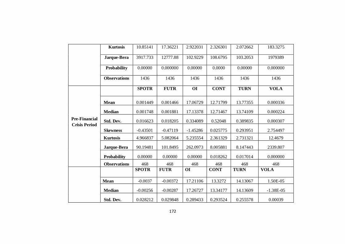
172
Kurtosis 10.85141 17.36221 2.922031 2.326301 2.072662 183.3275
Jarque-Bera 3917.733 12777.88 102.9229 108.6795 103.2053 1979389
Probability 0.00000 0.000000 0.00000 0.0000 0.00000 0.000000
Observations 1436 1436 1436 1436 1436 1436
Pre-Financial
Crisis Period
SPOTR FUTR OI CONT TURN VOLA
Mean 0.001449 0.001466 17.06729 12.71799 13.77355 0.000336
Median 0.001748 0.001881 17.13378 12.71467 13.74109 0.000224
Std. Dev. 0.016623 0.018205 0.334089 0.52048 0.389835 0.000307
Skewness -0.43501 -0.47119 -1.45286 0.025775 0.293951 2.754497
Kurtosis 4.966837 5.082064 5.235554 2.361329 2.731321 12.4679
Jarque-Bera 90.19481 101.8495 262.0973 8.005881 8.147443 2339.807
Probability 0.00000 0.00000 0.00000 0.018262 0.017014 0.000000
Observations 468 468 468 468 468 468
SPOTR FUTR OI CONT TURN VOLA
Mean -0.0037 -0.00372 17.21106 13.3272 14.13067 1.50E-05
Median -0.00256 -0.00287 17.26727 13.34177 14.13609 -1.38E-05
Std. Dev. 0.028212 0.029848 0.289433 0.293524 0.255578 0.00039
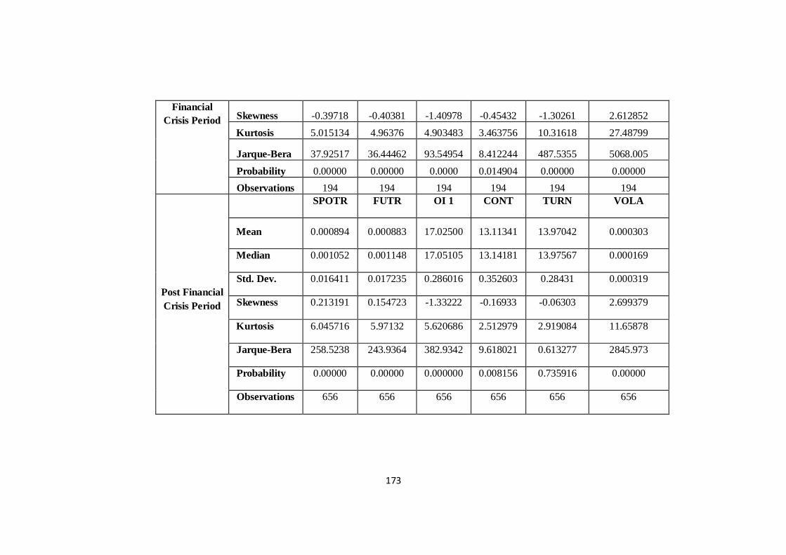
173
Financial
Crisis Period Skewness -0.39718 -0.40381 -1.40978 -0.45432 -1.30261 2.612852
Kurtosis 5.015134 4.96376 4.903483 3.463756 10.31618 27.48799
Jarque-Bera 37.92517 36.44462 93.54954 8.412244 487.5355 5068.005
Probability 0.00000 0.00000 0.0000 0.014904 0.00000 0.00000
Observations 194 194 194 194 194 194
Post Financial
Crisis Period
SPOTR FUTR OI 1 CONT TURN VOLA
Mean 0.000894 0.000883 17.02500 13.11341 13.97042 0.000303
Median 0.001052 0.001148 17.05105 13.14181 13.97567 0.000169
Std. Dev. 0.016411 0.017235 0.286016 0.352603 0.28431 0.000319
Skewness 0.213191 0.154723 -1.33222 -0.16933 -0.06303 2.699379
Kurtosis 6.045716 5.97132 5.620686 2.512979 2.919084 11.65878
Jarque-Bera 258.5238 243.9364 382.9342 9.618021 0.613277 2845.973
Probability 0.00000 0.00000 0.000000 0.008156 0.735916 0.00000
Observations 656 656 656 656 656 656
174
Summary statistics reveal that the mean, median and standard deviation of
futures returns are positive, indicating that the investors are getting returns and it is
negatively skewed (-0.474) and peakedness of the distribution is showed through
kurtosis (12.009), which is far from the basic value of 3. Jarque Bera test value
(9441.874) shows that the distribution is asymmetric and which is supported by the
probability value presented. Same trend is observed in spot return during whole study
period namely 12th June 2000 to 30
th June 2011. Similar result of non normality is
seen during the early stages of derivatives that is in the pre crisis and post crisis
period. Though the non normality is seen in all study periods, during the financial
crisis period mean return from both futures and spot markets are negative indicating
that there is a decline in the returns to investors. Other variables included in the study
are open interest, number of contracts, turn over and volatility. All these variables
have non normality distribution except turnover particularly during financial crisis
period.
The summary statistics of this study shows the asymmetric return in futures
and spot market which is supported by the findings of the previous studies like, Fama
(1965), Stevenson and Bear (1970), Kendull and Hill (1995) Chen (1996) Reddy
(1997) Kamath et al. (1998) and Kapil Gupta et al. (2009). Finding of Karpoff (1987)
also support the theoretical back ground of this distribution in such a way that in the
speculative derivative market, the volume of positive news is always higher than the
volume of negative news because in the increasing market trend the speculators take
every dip in the stock index as an opportunity to buy which may cause the speculative
assets return to behave asymmetrically. The risk averse nature of traders in a
speculative asset may be a prominent reason for the asymmetric returns (Moolman,
2004). The volatile nature of the derivative market also may cause the distribution of
spot and futures return in asymmetric. Diagler and Wiley (1999), finds that high
degree of volatility in speculative market, both optimistic and pessimistic views of
traders to information causes expected variation in prices. Negatively skewed indices
imply that futures market is in backwardation and offers significant arbitrage
opportunities to traders (Vipul 2005).
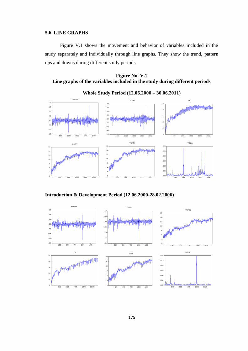
175
5.6. LINE GRAPHS
Figure V.1 shows the movement and behavior of variables included in the
study separately and individually through line graphs. They show the trend, pattern
ups and downs during different study periods.
Figure No. V.1
Line graphs of the variables included in the study during different periods
Whole Study Period (12.06.2000 – 30.06.2011)
-.15
-.10
-.05
.00
.05
.10
.15
.20
500 1000 1500 2000 2500
SPOTR
-.20
-.15
-.10
-.05
.00
.05
.10
.15
.20
500 1000 1500 2000 2500
FUTR
8
10
12
14
16
18
500 1000 1500 2000 2500
OI
2
4
6
8
10
12
14
16
500 1000 1500 2000 2500
CONT
2
4
6
8
10
12
14
16
500 1000 1500 2000 2500
TURN
.000
.001
.002
.003
.004
.005
.006
500 1000 1500 2000 2500
VOLA
Introduction & Development Period (12.06.2000-28.02.2006)
-.16
-.12
-.08
-.04
.00
.04
.08
.12
250 500 750 1000 1250
SPOTR
-.20
-.15
-.10
-.05
.00
.05
.10
250 500 750 1000 1250
FUTR
2
4
6
8
10
12
14
16
250 500 750 1000 1250
TURN
8
10
12
14
16
18
250 500 750 1000 1250
OI
2
4
6
8
10
12
14
250 500 750 1000 1250
CONT
.000
.001
.002
.003
.004
.005
.006
250 500 750 1000 1250
VOLA
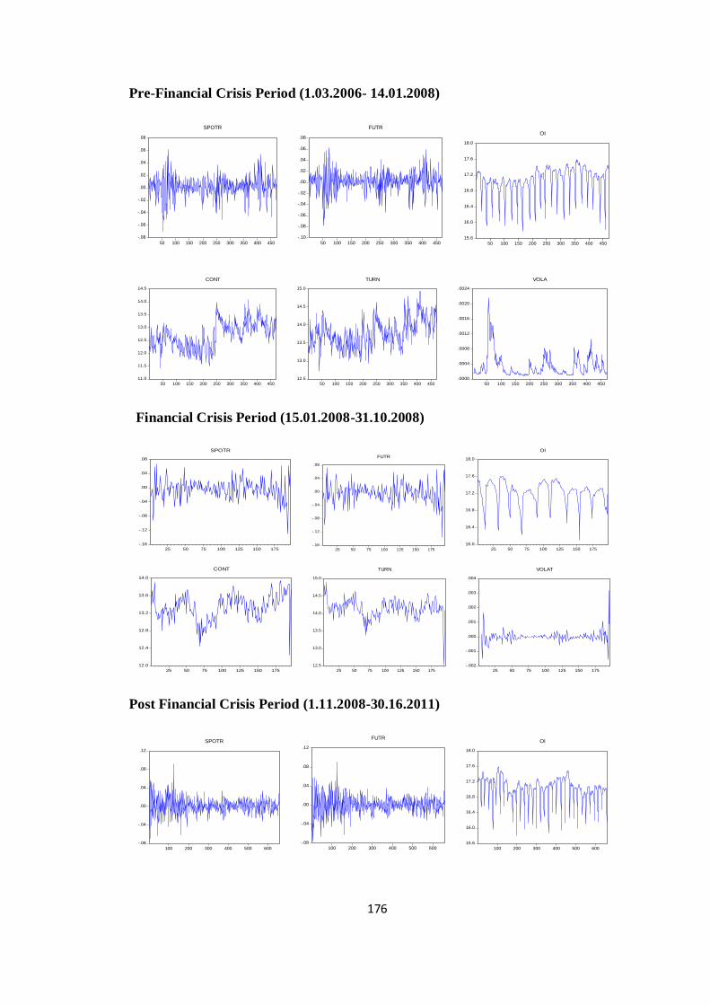
176
Pre-Financial Crisis Period (1.03.2006- 14.01.2008)
-.08
-.06
-.04
-.02
.00
.02
.04
.06
.08
50 100 150 200 250 300 350 400 450
SPOTR
-.10
-.08
-.06
-.04
-.02
.00
.02
.04
.06
.08
50 100 150 200 250 300 350 400 450
FUTR
15.6
16.0
16.4
16.8
17.2
17.6
18.0
50 100 150 200 250 300 350 400 450
OI
11.0
11.5
12.0
12.5
13.0
13.5
14.0
14.5
50 100 150 200 250 300 350 400 450
CONT
12.5
13.0
13.5
14.0
14.5
15.0
50 100 150 200 250 300 350 400 450
TURN
.0000
.0004
.0008
.0012
.0016
.0020
.0024
50 100 150 200 250 300 350 400 450
VOLA
Financial Crisis Period (15.01.2008-31.10.2008)
-.16
-.12
-.08
-.04
.00
.04
.08
25 50 75 100 125 150 175
SPOTR
-.16
-.12
-.08
-.04
.00
.04
.08
25 50 75 100 125 150 175
FUTR
16.0
16.4
16.8
17.2
17.6
18.0
25 50 75 100 125 150 175
OI
12.0
12.4
12.8
13.2
13.6
14.0
25 50 75 100 125 150 175
CONT
12.5
13.0
13.5
14.0
14.5
15.0
25 50 75 100 125 150 175
TURN
-.002
-.001
.000
.001
.002
.003
.004
25 50 75 100 125 150 175
VOLAT
Post Financial Crisis Period (1.11.2008-30.16.2011)
-.08
-.04
.00
.04
.08
.12
100 200 300 400 500 600
SPOTR
-.08
-.04
.00
.04
.08
.12
100 200 300 400 500 600
FUTR
15.6
16.0
16.4
16.8
17.2
17.6
18.0
100 200 300 400 500 600
OI
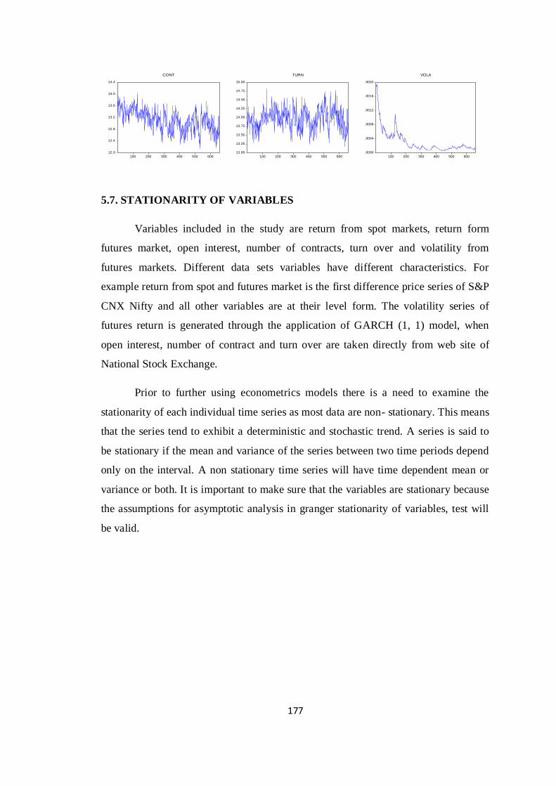
177
12.0
12.4
12.8
13.2
13.6
14.0
14.4
100 200 300 400 500 600
CONT
13.00
13.25
13.50
13.75
14.00
14.25
14.50
14.75
15.00
100 200 300 400 500 600
TURN
.0000
.0004
.0008
.0012
.0016
.0020
100 200 300 400 500 600
VOLA
5.7. STATIONARITY OF VARIABLES
Variables included in the study are return from spot markets, return form
futures market, open interest, number of contracts, turn over and volatility from
futures markets. Different data sets variables have different characteristics. For
example return from spot and futures market is the first difference price series of S&P
CNX Nifty and all other variables are at their level form. The volatility series of
futures return is generated through the application of GARCH (1, 1) model, when
open interest, number of contract and turn over are taken directly from web site of
National Stock Exchange.
Prior to further using econometrics models there is a need to examine the
stationarity of each individual time series as most data are non- stationary. This means
that the series tend to exhibit a deterministic and stochastic trend. A series is said to
be stationary if the mean and variance of the series between two time periods depend
only on the interval. A non stationary time series will have time dependent mean or
variance or both. It is important to make sure that the variables are stationary because
the assumptions for asymptotic analysis in granger stationarity of variables, test will
be valid.
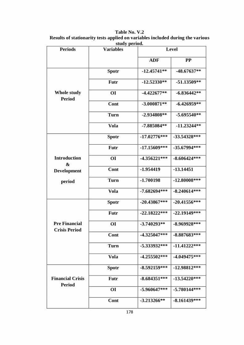
178
Table No. V.2
Results of stationarity tests applied on variables included during the various
study period.
Periods Variables Level
ADF PP
Whole study
Period
Spotr -12.45741** -48.67637**
Futr -12.52330** -51.13509**
OI -4.422677** -6.836442**
Cont -3.000871** -6.426959**
Turn -2.934808** -5.695540**
Vola -7.885084** -11.23244**
Introduction
&
Development
period
Spotr -17.02776*** -33.54328***
Futr -17.15609*** -35.67994***
OI -4.356221*** -8.606424***
Cont -1.954419 -13.14451
Turn -1.700198 -12.80008***
Vola -7.682694*** -8.240614***
Pre Financial
Crisis Period
Spotr -20.43867*** -20.41556***
Futr -22.18222*** -22.19149***
OI -3.740293** -8.969928***
Cont -4.325047*** -8.887683***
Turn -5.333932*** -11.41222***
Vola -4.255502*** -4.049475***
Financial Crisis
Period
Spotr -8.592159*** -12.98812***
Futr -8.684351*** -13.54220***
OI -5.960647*** -5.780144***
Cont -3.213266** -8.161439***
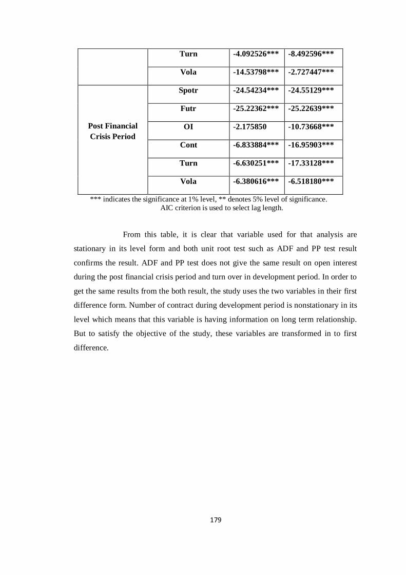
179
Turn -4.092526*** -8.492596***
Vola -14.53798*** -2.727447***
Post Financial
Crisis Period
Spotr -24.54234*** -24.55129***
Futr -25.22362*** -25.22639***
OI -2.175850 -10.73668***
Cont -6.833884*** -16.95903***
Turn -6.630251*** -17.33128***
Vola -6.380616*** -6.518180***
*** indicates the significance at 1% level, ** denotes 5% level of significance. AIC criterion is used to select lag length.
From this table, it is clear that variable used for that analysis are
stationary in its level form and both unit root test such as ADF and PP test result
confirms the result. ADF and PP test does not give the same result on open interest
during the post financial crisis period and turn over in development period. In order to
get the same results from the both result, the study uses the two variables in their first
difference form. Number of contract during development period is nonstationary in its
level which means that this variable is having information on long term relationship.
But to satisfy the objective of the study, these variables are transformed in to first
difference.
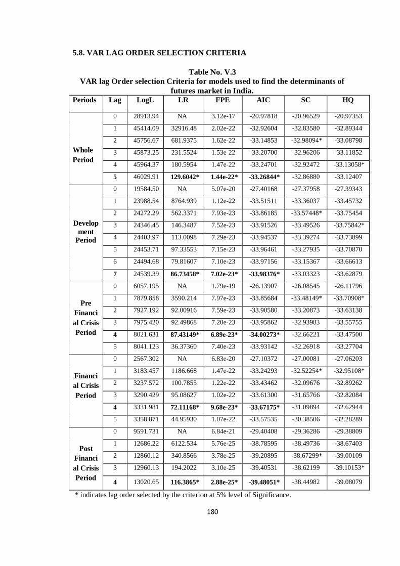
180
5.8. VAR LAG ORDER SELECTION CRITERIA
Table No. V.3
VAR lag Order selection Criteria for models used to find the determinants of
futures market in India.
Periods Lag LogL LR FPE AIC SC HQ
Whole
Period
0 28913.94 NA 3.12e-17 -20.97818 -20.96529 -20.97353
1 45414.09 32916.48 2.02e-22 -32.92604 -32.83580 -32.89344
2 45756.67 681.9375 1.62e-22 -33.14853 -32.98094* -33.08798
3 45873.25 231.5524 1.53e-22 -33.20700 -32.96206 -33.11852
4 45964.37 180.5954 1.47e-22 -33.24701 -32.92472 -33.13058*
5 46029.91 129.6042* 1.44e-22* -33.26844* -32.86880 -33.12407
Develop
ment
Period
0 19584.50 NA 5.07e-20 -27.40168 -27.37958 -27.39343
1 23988.54 8764.939 1.12e-22 -33.51511 -33.36037 -33.45732
2 24272.29 562.3371 7.93e-23 -33.86185 -33.57448* -33.75454
3 24346.45 146.3487 7.52e-23 -33.91526 -33.49526 -33.75842*
4 24403.97 113.0098 7.29e-23 -33.94537 -33.39274 -33.73899
5 24453.71 97.33553 7.15e-23 -33.96461 -33.27935 -33.70870
6 24494.68 79.81607 7.10e-23 -33.97156 -33.15367 -33.66613
7 24539.39 86.73458* 7.02e-23* -33.98376* -33.03323 -33.62879
Pre
Financi
al Crisis
Period
0 6057.195 NA 1.79e-19 -26.13907 -26.08545 -26.11796
1 7879.858 3590.214 7.97e-23 -33.85684 -33.48149* -33.70908*
2 7927.192 92.00916 7.59e-23 -33.90580 -33.20873 -33.63138
3 7975.420 92.49868 7.20e-23 -33.95862 -32.93983 -33.55755
4 8021.631 87.43149* 6.89e-23* -34.00273* -32.66221 -33.47500
5 8041.123 36.37360 7.40e-23 -33.93142 -32.26918 -33.27704
Financi
al Crisis
Period
0 2567.302 NA 6.83e-20 -27.10372 -27.00081 -27.06203
1 3183.457 1186.668 1.47e-22 -33.24293 -32.52254* -32.95108*
2 3237.572 100.7855 1.22e-22 -33.43462 -32.09676 -32.89262
3 3290.429 95.08627 1.02e-22 -33.61300 -31.65766 -32.82084
4 3331.981 72.11168* 9.68e-23* -33.67175* -31.09894 -32.62944
5 3358.871 44.95930 1.07e-22 -33.57535 -30.38506 -32.28289
Post
Financi
al Crisis
Period
0 9591.731 NA 6.84e-21 -29.40408 -29.36286 -29.38809
1 12686.22 6122.534 5.76e-25 -38.78595 -38.49736 -38.67403
2 12860.12 340.8566 3.78e-25 -39.20895 -38.67299* -39.00109
3 12960.13 194.2022 3.10e-25 -39.40531 -38.62199 -39.10153*
4 13020.65 116.3865* 2.88e-25* -39.48051* -38.44982 -39.08079
* indicates lag order selected by the criterion at 5% level of Significance.
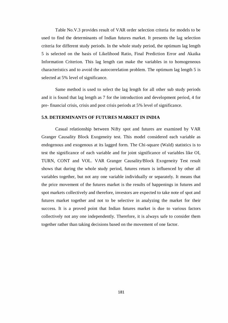
181
Table No.V.3 provides result of VAR order selection criteria for models to be
used to find the determinants of Indian futures market. It presents the lag selection
criteria for different study periods. In the whole study period, the optimum lag length
5 is selected on the basis of Likelihood Ratio, Final Prediction Error and Akaika
Information Criterion. This lag length can make the variables in to homogeneous
characteristics and to avoid the autocorrelation problem. The optimum lag length 5 is
selected at 5% level of significance.
Same method is used to select the lag length for all other sub study periods
and it is found that lag length as 7 for the introduction and development period, 4 for
pre- financial crisis, crisis and post crisis periods at 5% level of significance.
5.9. DETERMINANTS OF FUTURES MARKET IN INDIA
Casual relationship between Nifty spot and futures are examined by VAR
Granger Causality Block Exogeneity test. This model considered each variable as
endogenous and exogenous at its lagged form. The Chi-square (Wald) statistics is to
test the significance of each variable and for joint significance of variables like OI,
TURN, CONT and VOL. VAR Granger Causality/Block Exogeneity Test result
shows that during the whole study period, futures return is influenced by other all
variables together, but not any one variable individually or separately. It means that
the price movement of the futures market is the results of happenings in futures and
spot markets collectively and therefore, investors are expected to take note of spot and
futures market together and not to be selective in analyzing the market for their
success. It is a proved point that Indian futures market is due to various factors
collectively not any one independently. Therefore, it is always safe to consider them
together rather than taking decisions based on the movement of one factor.
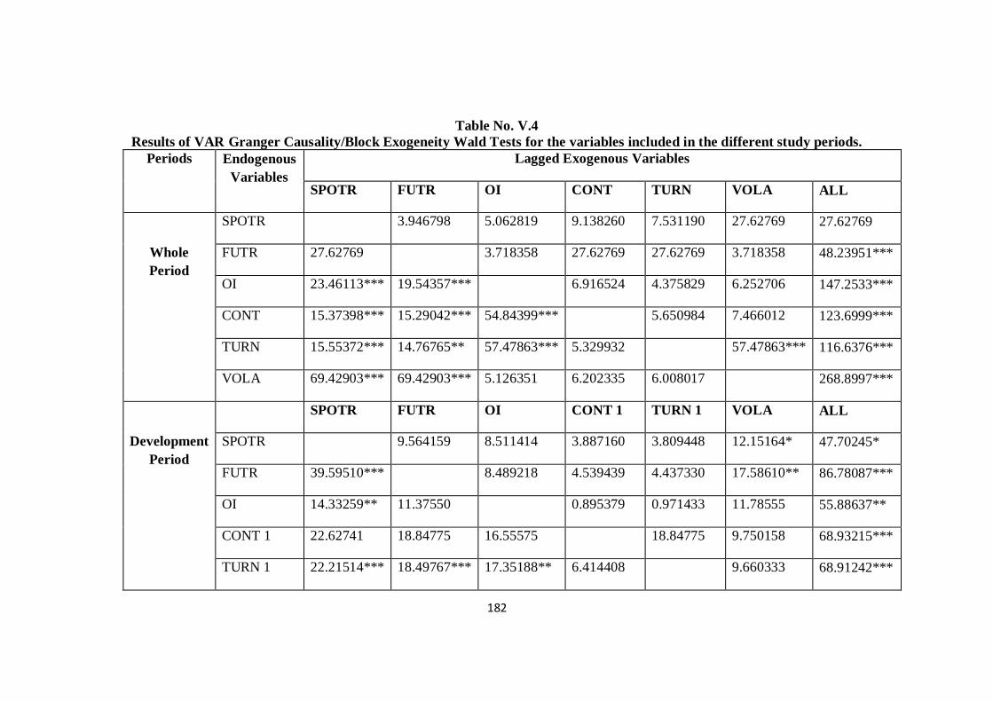
182
Table No. V.4
Results of VAR Granger Causality/Block Exogeneity Wald Tests for the variables included in the different study periods.
Periods Endogenous
Variables
Lagged Exogenous Variables
SPOTR FUTR OI CONT TURN VOLA ALL
Whole
Period
SPOTR 3.946798 5.062819 9.138260 7.531190 27.62769 27.62769
FUTR 27.62769 3.718358 27.62769 27.62769 3.718358 48.23951***
OI 23.46113*** 19.54357*** 6.916524 4.375829 6.252706 147.2533***
CONT 15.37398*** 15.29042*** 54.84399*** 5.650984 7.466012 123.6999***
TURN 15.55372*** 14.76765** 57.47863*** 5.329932 57.47863*** 116.6376***
VOLA 69.42903*** 69.42903*** 5.126351 6.202335 6.008017 268.8997***
Development
Period
SPOTR FUTR OI CONT 1 TURN 1 VOLA ALL
SPOTR 9.564159 8.511414 3.887160 3.809448 12.15164* 47.70245*
FUTR 39.59510*** 8.489218 4.539439 4.437330 17.58610** 86.78087***
OI 14.33259** 11.37550 0.895379 0.971433 11.78555 55.88637**
CONT 1 22.62741 18.84775 16.55575 18.84775 9.750158 68.93215***
TURN 1 22.21514*** 18.49767*** 17.35188** 6.414408 9.660333 68.91242***
183
VOLA 67.33719 148.5628 6.200235 2.483155 2.397656 504.7862
Pre
Financial
Crisis Period
SPOTR FUTR OI CONT TURN VOLA ALL
SPOTR 7.986068* 3.597548 9.786596** 8.265831* 4.410737 26.70021
FUTR 10.00406** 1.869880 9.340128* 8.588159* 3.106387 27.17512
OI 7.286120 7.505453 13.32188** 7.198444 3.270528 44.28424**
CONT 4.381615 3.415340 21.12063*** 12.72173** 5.603107 74.54318***
TURN 5.427352 4.239972 24.17342*** 4.258961 5.704711 62.58033***
VOLA 24.13182*** 29.32334*** 1.436859 3.028416 9.156310* 170.7805***
Financial
Crisis Period
SPOTR FUTR OI CONT TURN VOLA ALL
SPOTR 5.528309 5.727444 5.109009 3.661564 2.264592 22.85483
FUTR 4.000507 5.877795 4.704711 3.356324 1.664188 19.19652
OI 0.569786 0.890682 1.464480 1.525481 3.850676 15.94917
CONT 9.029903* 7.480348 3.845149 8.712995* 12.79380** 45.11890**
TURN 9.512457** 7.847992* 4.542223 8.195858* 12.73443** 40.51196**
VOLA 4.299809 3.949077 5.396989 16.20517** 16.79982** 70.69352***
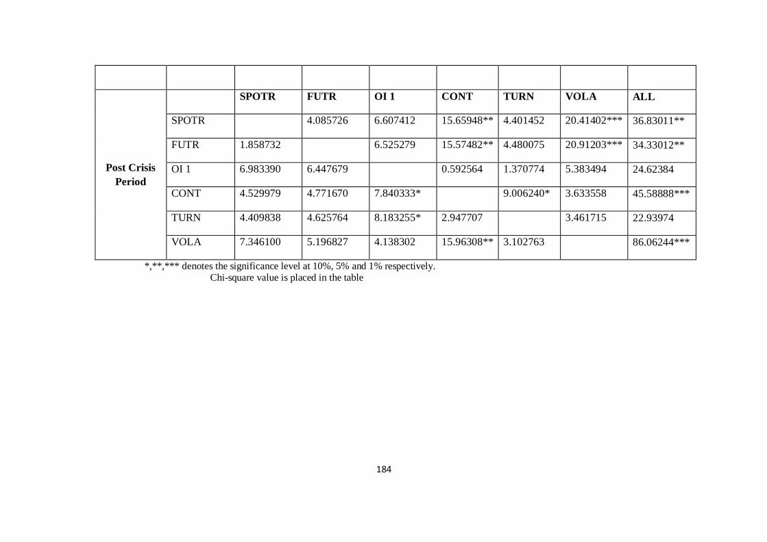
184
Post Crisis
Period
SPOTR FUTR OI 1 CONT TURN VOLA ALL
SPOTR 4.085726 6.607412 15.65948** 4.401452 20.41402*** 36.83011**
FUTR 1.858732 6.525279 15.57482** 4.480075 20.91203*** 34.33012**
OI 1 6.983390 6.447679 0.592564 1.370774 5.383494 24.62384
CONT 4.529979 4.771670 7.840333* 9.006240* 3.633558 45.58888***
TURN 4.409838 4.625764 8.183255* 2.947707 3.461715 22.93974
VOLA 7.346100 5.196827 4.138302 15.96308** 3.102763 86.06244***
*,**,*** denotes the significance level at 10%, 5% and 1% respectively. Chi-square value is placed in the table
185
During the same period, it is also observed that spot market is return is
independent of variables considered in the study. No factor either individually or
collectively inferences and spot return. The table also show that all other variables
like open interest, number of contracts, turn over and volatility in futures market are
made to move by returns from spot and futures markets individually and also by all
them together. Open interest plays a vital role, in addition to returns, on turnover and
number of contracts.
In addition to all happenings are influencing the futures returns, it is found that
spot market impacts the futures returns and volatility also play a role in determining
the return of futures market, individually. It shows that during the initial period of
introduction of derivatives in India, spot market had determined the futures return in
addition to volatility with all other determinants together, which means that there was
a need to observe the spot market movements to decide about the futures return.
Return from spot market is determined by volatility of futures return individually and
all variables together. It is supported by the empirical results of Chen etal (1995),
Stephen.P.Ferris etal (2002). They found significant dynamic interactions and causal
relationship among volatility, open interest and trading volume. Depth of futures
market is determined by the spot and also by all variables from futures market
together. Significantly it is found that the futures market is not having relationship
with any other variables included in the study. It suggests that investment in Nifty
futures market requires the analysis or emphasis on spot market and the price
changing pattern of futures market.
As far as, derivatives market in India is concerned this is the period of
development and maturity. During this period the spot market is influenced by the
futures market, number of contracts and turn over. Further futures market is having
short term and causal relationship with spot return, number of contracts and turn over.
Other variables are not influencing the futures return during the study period. From
this result, it is clear that both spot and futures markets are influencing each other and
it can be confirmed that there is bidirectional relationship between futures market and
spot market which can be exploited by the arbitrageurs. Modest and Sundraresan
(1983), Figlewski (1984) and Yadav and Pope (1994) found significant
186
inconsistencies between spot prices and the futures prices for stock indices that can be
exploited by arbitrageurs. During pre-financial crisis period spot return, number of
contracts of futures market and turnover are considered as the determinants of futures
market or futures return movement. All other variables together influence turnover. It
is summarized that, futures market as expected is determined by one movement of
spot market due to its maturity or growth, it is observed that instead of collective
influence, single factor started to determine the futures return. Financial crisis had
created ripples in whole financial system including stock market across the globe and
India too had the effect of it through it had insulated itself. There had been sharp
decline in the returns from stock market and therefore, an attempt is made to see what
had happened in Indian derivatives market. During this period, the result shows very
different relations between futures and its underlying market in India. The empirical
results show that the established relationship between futures and spot market is
collapsed.
During this period, all established relationships have disappeared and each
element is moving separately and independently which means that it is the period of
speculators and nobody can predict the decisions and movement of speculators in
Indian market. Speculators would involve in buying and selling shares in large scale
when volatility is high. In order to make more profit no one plays a determinants role
and only the proxies of trading volume like number of contracts and turn over are
interlinked and volatility of futures market causes the contract volume and turnover in
futures market. This indicates that trading volume is the strong indicator which can
provide some information in any trend of the market. Trading volume is a significant
explanatory variable (Gwilym etal 1999). Volatility is high during bearish market,
compared to bullish market trend (Paul Dawson 2009). The present empirical results
also project the role volatility and trading volume during the bearish market trend.
Crisis had distanced the spot and futures market, paving way for speculators to
have a field for short term benefits, without any factor determining the dynamism of
the markets. After this crisis, period, it is found that markets and linking towards
closure but not close. One or all factors together started to determine the markets.
Volatility individually along with all other variables determines the return of spot
187
market and number of contracts and volatility individually along with other variables
together determine the futures return.
During the post- financial crisis period the short term relationship between all
factors in futures market and spot return are established and the result is supported by
the previous studies also. Futures lead the cash index return by responding more
rapidly to economic events than stock prices. New market information may
disseminate faster in the futures market compared to stock market and futures
volatility spill some information over to cash market (Puja Padhi 2009). It is seen that
futures market is taking the lead position in the Indian market context. All other
variables like number of contract, volatility series and other all variables of futures
market can be taken as the determinants of the futures market in India. The level of
influence of each variable to futures return should be different and it is the duty of an
investor or the player of the futures market to analyze the role of each variable and
take the decision. But one thing is very clear that among these all variables trading
volume and volatility of futures markets are playing vital role to determine futures
market. Several price predictors have been developed from the open interest and trade
volume of individual stocks from the futures market and explained that they exhibit
significant explanatory and predictive power for the factors for the futures stock
prices (Bhuyan and Yan 2002).
Causal relationship and determinants of futures market is identified through
VAR Granger Causality/ Block Exogeneity test. Variables like return from futures
and spot market, OI, TURN, VOL are also included. It is found that all variables
together determine the futures return during the whole study period and bidirectional
causality is seen during the period’s financial crisis. Due to the negative effect of
crisis, return from futures and spot market does not show causal relationship.
In short, it is confirmed that spot market return, number of contract, turnover
and volatility of the futures market are having short run relationship with futures
market. On the basis of the empirical analysis it is clearly said that spot market is the
key factor which predicts the movement of futures market and the trader can depend
upon volatility and trading volume to take any decision on futures market trading. In
188
precise, spot market return, volatility of the futures market, turnover and number of
contract are the determinants of futures market in India. Information for decision
about investors can be taken through these factors. To conclude that spot market
return is the major determinants of futures market, indeed variables from futures
market itself like open interest and turnover of futures market can be taken in to
consideration for determining the futures market return.
5.10. TIME PROFILE OF SHOCKS
The effect and response of shock from and to each variable is important to
identify the effect of one to another. A shock in one variable may influence that
variable itself and it may pass on its shocks to other variables in due course time.
Analysis of such shock relationship and its period of existence provide idea for the
decisions to investors. The causality between variables reveal the leading effect but
how long such effect exists and in what duration it effects are presented through
impulse response or time profile of shocks. Impulse response measures the time
profile of the effects of shock on the expected future value of a variable- a conditional
variance of equity volatility (Dawson and Stai Kouras 2009). Results of time profile
shocks of variables included in the study are presented below for various study
periods.
5.10.1. Section-1 Whole Study Period:
Figure No.V.2 shows that changes in spot market return makes positive and
significant change in futures return for two days, but it makes negative and significant
changes in number of contracts and turnover. Insignificant impact is seen on
volatility, whereas, market depth represented by open interest is not responding to the
changes in spot market. Almost the same result is seen from the changes in futures
return, except making open interest to react insignificantly. Changes or shocks in
market depth do not make any change in spot and futures market return in the initial
days but in due course, it makes a very minimal positive response which lasts for 10
days. From the beginning of changes, open interest makes the trade volume to change
positively and negative response is seen in volatility due to change in open interest.
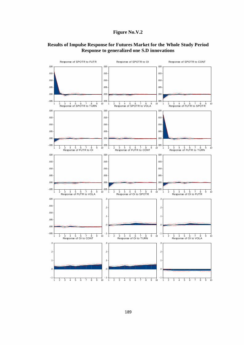
189
Figure No.V.2
Results of Impulse Response for Futures Market for the Whole Study Period
Response to generalized one S.D innovations
-.005
.000
.005
.010
.015
.020
1 2 3 4 5 6 7 8 9 10
Response of SPOTR to FUTR
-.005
.000
.005
.010
.015
.020
1 2 3 4 5 6 7 8 9 10
Response of SPOTR to OI
-.005
.000
.005
.010
.015
.020
1 2 3 4 5 6 7 8 9 10
Response of SPOTR to CONT
-.005
.000
.005
.010
.015
.020
1 2 3 4 5 6 7 8 9 10
Response of SPOTR to TURN
-.005
.000
.005
.010
.015
.020
1 2 3 4 5 6 7 8 9 10
Response of SPOTR to VOLA
-.005
.000
.005
.010
.015
.020
1 2 3 4 5 6 7 8 9 10
Response of FUTR to SPOTR
-.005
.000
.005
.010
.015
.020
1 2 3 4 5 6 7 8 9 10
Response of FUTR to OI
-.005
.000
.005
.010
.015
.020
1 2 3 4 5 6 7 8 9 10
Response of FUTR to CONT
-.005
.000
.005
.010
.015
.020
1 2 3 4 5 6 7 8 9 10
Response of FUTR to TURN
-.005
.000
.005
.010
.015
.020
1 2 3 4 5 6 7 8 9 10
Response of FUTR to VOLA
-.1
.0
.1
.2
.3
1 2 3 4 5 6 7 8 9 10
Response of OI to SPOTR
-.1
.0
.1
.2
.3
1 2 3 4 5 6 7 8 9 10
Response of OI to FUTR
-.1
.0
.1
.2
.3
1 2 3 4 5 6 7 8 9 10
Response of OI to CONT
-.1
.0
.1
.2
.3
1 2 3 4 5 6 7 8 9 10
Response of OI to TURN
-.1
.0
.1
.2
.3
1 2 3 4 5 6 7 8 9 10
Response of OI to VOLA
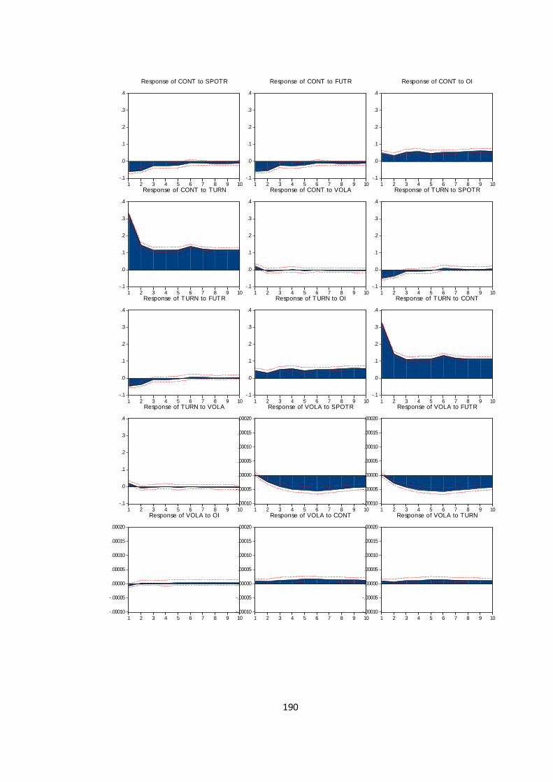
190
-.1
.0
.1
.2
.3
.4
1 2 3 4 5 6 7 8 9 10
Response of CONT to SPOTR
-.1
.0
.1
.2
.3
.4
1 2 3 4 5 6 7 8 9 10
Response of CONT to FUTR
-.1
.0
.1
.2
.3
.4
1 2 3 4 5 6 7 8 9 10
Response of CONT to OI
-.1
.0
.1
.2
.3
.4
1 2 3 4 5 6 7 8 9 10
Response of CONT to TURN
-.1
.0
.1
.2
.3
.4
1 2 3 4 5 6 7 8 9 10
Response of CONT to VOLA
-.1
.0
.1
.2
.3
.4
1 2 3 4 5 6 7 8 9 10
Response of TURN to SPOTR
-.1
.0
.1
.2
.3
.4
1 2 3 4 5 6 7 8 9 10
Response of TURN to FUTR
-.1
.0
.1
.2
.3
.4
1 2 3 4 5 6 7 8 9 10
Response of TURN to OI
-.1
.0
.1
.2
.3
.4
1 2 3 4 5 6 7 8 9 10
Response of TURN to CONT
-.1
.0
.1
.2
.3
.4
1 2 3 4 5 6 7 8 9 10
Response of TURN to VOLA
-.00010
-.00005
.00000
.00005
.00010
.00015
.00020
1 2 3 4 5 6 7 8 9 10
Response of VOLA to SPOTR
-.00010
-.00005
.00000
.00005
.00010
.00015
.00020
1 2 3 4 5 6 7 8 9 10
Response of VOLA to FUTR
-.00010
-.00005
.00000
.00005
.00010
.00015
.00020
1 2 3 4 5 6 7 8 9 10
Response of VOLA to OI
-.00010
-.00005
.00000
.00005
.00010
.00015
.00020
1 2 3 4 5 6 7 8 9 10
Response of VOLA to CONT
-.00010
-.00005
.00000
.00005
.00010
.00015
.00020
1 2 3 4 5 6 7 8 9 10
Response of VOLA to TURN

191
Any shock in number of contract makes spot and futures return to have
negative and significant changes for two days, when turnover and open interest have
positive and significant changes for 10 days time. Turnover and its changes show the
similar results as that of number of contract. While means that trade volume of futures
market makes spot and futures return have negative changes and with no response in
volatility. Futures market volatility and its shocks make spot and futures return
negatively and significantly and trade volume positively and significantly and almost
no result on open interest is seen from the results.
In short, it is found that spot and futures returns have bi directional positive
and significant relation for a two days period. Trade volume and volatility of futures
market influences spot and futures return negatively in the early stages of changes and
these variables have bidirectional position changes among themselves. Volatility
gives mined responses. Positive significant relationship between volatility and
unexpected volume is found (Watanabe 2001 and Pratap Chandrapati 2010).
5.10.2. Section -2: Introduction and Development of Derivatives
Figure. No. V.3 shows the graphical representation of time profile shocks of
variables during the sub periods. This period represents the introduction and
development of derivatives in India. It is found that changes in spot return make
changes in futures return for initial two days then it influences negatively. Shock on
spot return makes trade volume to change negatively but significantly but open
interest does not change with changes in spot return. Volatility is influenced
positively for three days. Exactly the same results are seen from futures return as that
of spot return, to indicate that spot and futures have bidirectional relationship and
other variables also react in the same manner for changes in both spot and futures
return.
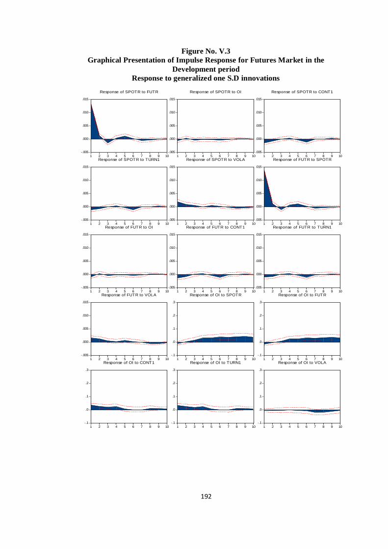
192
Figure No. V.3
Graphical Presentation of Impulse Response for Futures Market in the
Development period
Response to generalized one S.D innovations
-.005
.000
.005
.010
.015
1 2 3 4 5 6 7 8 9 10
Response of SPOTR to FUTR
-.005
.000
.005
.010
.015
1 2 3 4 5 6 7 8 9 10
Response of SPOTR to OI
-.005
.000
.005
.010
.015
1 2 3 4 5 6 7 8 9 10
Response of SPOTR to CONT1
-.005
.000
.005
.010
.015
1 2 3 4 5 6 7 8 9 10
Response of SPOTR to TURN1
-.005
.000
.005
.010
.015
1 2 3 4 5 6 7 8 9 10
Response of SPOTR to VOLA
-.005
.000
.005
.010
.015
1 2 3 4 5 6 7 8 9 10
Response of FUTR to SPOTR
-.005
.000
.005
.010
.015
1 2 3 4 5 6 7 8 9 10
Response of FUTR to OI
-.005
.000
.005
.010
.015
1 2 3 4 5 6 7 8 9 10
Response of FUTR to CONT1
-.005
.000
.005
.010
.015
1 2 3 4 5 6 7 8 9 10
Response of FUTR to TURN1
-.005
.000
.005
.010
.015
1 2 3 4 5 6 7 8 9 10
Response of FUTR to VOLA
-.1
.0
.1
.2
.3
1 2 3 4 5 6 7 8 9 10
Response of OI to SPOTR
-.1
.0
.1
.2
.3
1 2 3 4 5 6 7 8 9 10
Response of OI to FUTR
-.1
.0
.1
.2
.3
1 2 3 4 5 6 7 8 9 10
Response of OI to CONT1
-.1
.0
.1
.2
.3
1 2 3 4 5 6 7 8 9 10
Response of OI to TURN1
-.1
.0
.1
.2
.3
1 2 3 4 5 6 7 8 9 10
Response of OI to VOLA
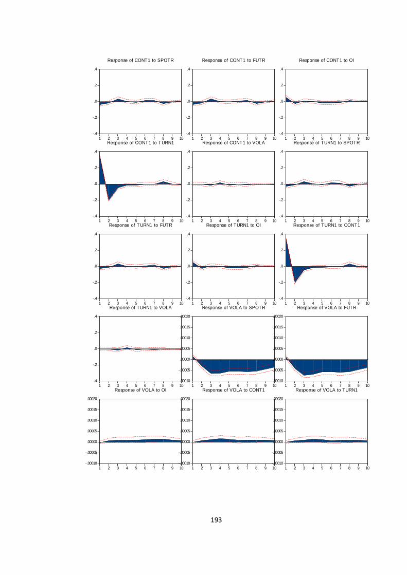
193
-.4
-.2
.0
.2
.4
1 2 3 4 5 6 7 8 9 10
Response of CONT1 to SPOTR
-.4
-.2
.0
.2
.4
1 2 3 4 5 6 7 8 9 10
Response of CONT1 to FUTR
-.4
-.2
.0
.2
.4
1 2 3 4 5 6 7 8 9 10
Response of CONT1 to OI
-.4
-.2
.0
.2
.4
1 2 3 4 5 6 7 8 9 10
Response of CONT1 to TURN1
-.4
-.2
.0
.2
.4
1 2 3 4 5 6 7 8 9 10
Response of CONT1 to VOLA
-.4
-.2
.0
.2
.4
1 2 3 4 5 6 7 8 9 10
Response of TURN1 to SPOTR
-.4
-.2
.0
.2
.4
1 2 3 4 5 6 7 8 9 10
Response of TURN1 to FUTR
-.4
-.2
.0
.2
.4
1 2 3 4 5 6 7 8 9 10
Response of TURN1 to OI
-.4
-.2
.0
.2
.4
1 2 3 4 5 6 7 8 9 10
Response of TURN1 to CONT1
-.4
-.2
.0
.2
.4
1 2 3 4 5 6 7 8 9 10
Response of TURN1 to VOLA
-.00010
-.00005
.00000
.00005
.00010
.00015
.00020
1 2 3 4 5 6 7 8 9 10
Response of VOLA to SPOTR
-.00010
-.00005
.00000
.00005
.00010
.00015
.00020
1 2 3 4 5 6 7 8 9 10
Response of VOLA to FUTR
-.00010
-.00005
.00000
.00005
.00010
.00015
.00020
1 2 3 4 5 6 7 8 9 10
Response of VOLA to OI
-.00010
-.00005
.00000
.00005
.00010
.00015
.00020
1 2 3 4 5 6 7 8 9 10
Response of VOLA to CONT1
-.00010
-.00005
.00000
.00005
.00010
.00015
.00020
1 2 3 4 5 6 7 8 9 10
Response of VOLA to TURN1
194
Changes in open interest makes spot and futures return to react positively and
significantly after three days toll such time it makes negative responses. Effect of
open interest on trade volume is positive and significant for four days and then slowly
it loses its impact. No response is seen from volatility to changes in open interest.
Trade volume represented by number of contracts and turnover have same
results on spot and futures return as well as on other variables like open interest and
volatility. Changes in number of contract and turnover makes spot and futures return
to change negatively in the first day and on the second day positively, after two days
they lose their significance. Trade volume deeds not influence volatility significantly.
Shocks in volatility makes spot and futures return react negatively after waiting for
two days, when it influences positively the trade volume and open interest from the
second day onwards.
5.10.3. Section -3: Pre- Financial Crisis Period
Figure No.V.4 reveals that spot return and its changes makes return to
react positively for 2 days when it makes all other variables except volatility to have
response negatively for 1 day and them slowly it loses its effect. Volatility is not
responding to the changes of spot return. Futures return and its shocks also reveal
similar reactions as that spot return. When open interest represents market depth of
futures market has shock, spot and futures market return responds negatively but
significantly for initial 3 days, while trade volume is responding positively for 4 days.
Responds of volatility is significant but negative in the in the initial days and days
passes by its significance is lost. Trading volume negatively for 3 days with higher
magnitude but slowly it goes away. The shocks of trade volume positively influence
market depth, when they have insignificant negative influences on volatility. Changes
in volatility have negative and significant reaction from spot and futures return, when
trade volume reacts positively after 2 days. In the case of open interest reaction comes
only after 4 days, when it does not react for 4 days. Open interest of futures market
apart from trading volume provides additional measure of trading activity (Chartrath
etal 2003). The Pre-financial crisis period is also the period of development for
futures market in India. During this period, spot and futures market have positive
bidirectional relationship and therefore, investors can make the trading strategies on
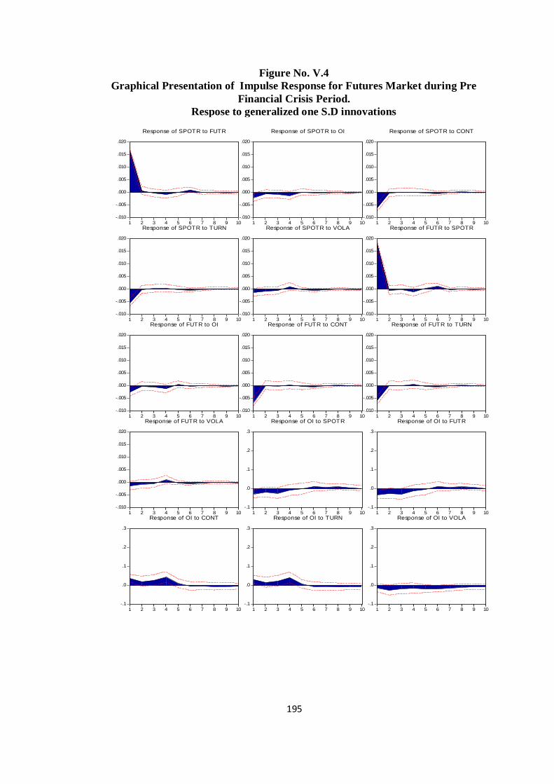
195
Figure No. V.4
Graphical Presentation of Impulse Response for Futures Market during Pre
Financial Crisis Period.
Respose to generalized one S.D innovations
-.010
-.005
.000
.005
.010
.015
.020
1 2 3 4 5 6 7 8 9 10
Response of SPOTR to FUTR
-.010
-.005
.000
.005
.010
.015
.020
1 2 3 4 5 6 7 8 9 10
Response of SPOTR to OI
-.010
-.005
.000
.005
.010
.015
.020
1 2 3 4 5 6 7 8 9 10
Response of SPOTR to CONT
-.010
-.005
.000
.005
.010
.015
.020
1 2 3 4 5 6 7 8 9 10
Response of SPOTR to TURN
-.010
-.005
.000
.005
.010
.015
.020
1 2 3 4 5 6 7 8 9 10
Response of SPOTR to VOLA
-.010
-.005
.000
.005
.010
.015
.020
1 2 3 4 5 6 7 8 9 10
Response of FUTR to SPOTR
-.010
-.005
.000
.005
.010
.015
.020
1 2 3 4 5 6 7 8 9 10
Response of FUTR to OI
-.010
-.005
.000
.005
.010
.015
.020
1 2 3 4 5 6 7 8 9 10
Response of FUTR to CONT
-.010
-.005
.000
.005
.010
.015
.020
1 2 3 4 5 6 7 8 9 10
Response of FUTR to TURN
-.010
-.005
.000
.005
.010
.015
.020
1 2 3 4 5 6 7 8 9 10
Response of FUTR to VOLA
-.1
.0
.1
.2
.3
1 2 3 4 5 6 7 8 9 10
Response of OI to SPOTR
-.1
.0
.1
.2
.3
1 2 3 4 5 6 7 8 9 10
Response of OI to FUTR
-.1
.0
.1
.2
.3
1 2 3 4 5 6 7 8 9 10
Response of OI to CONT
-.1
.0
.1
.2
.3
1 2 3 4 5 6 7 8 9 10
Response of OI to TURN
-.1
.0
.1
.2
.3
1 2 3 4 5 6 7 8 9 10
Response of OI to VOLA
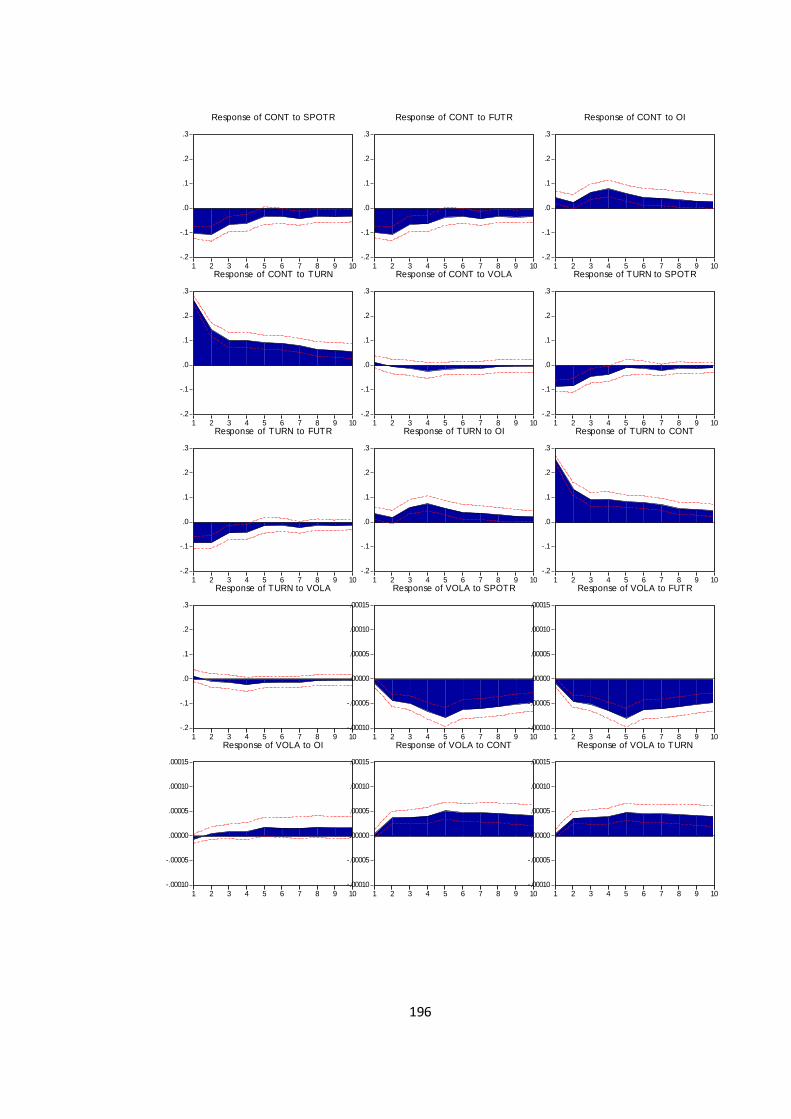
196
-.2
-.1
.0
.1
.2
.3
1 2 3 4 5 6 7 8 9 10
Response of CONT to SPOTR
-.2
-.1
.0
.1
.2
.3
1 2 3 4 5 6 7 8 9 10
Response of CONT to FUTR
-.2
-.1
.0
.1
.2
.3
1 2 3 4 5 6 7 8 9 10
Response of CONT to OI
-.2
-.1
.0
.1
.2
.3
1 2 3 4 5 6 7 8 9 10
Response of CONT to TURN
-.2
-.1
.0
.1
.2
.3
1 2 3 4 5 6 7 8 9 10
Response of CONT to VOLA
-.2
-.1
.0
.1
.2
.3
1 2 3 4 5 6 7 8 9 10
Response of TURN to SPOTR
-.2
-.1
.0
.1
.2
.3
1 2 3 4 5 6 7 8 9 10
Response of TURN to FUTR
-.2
-.1
.0
.1
.2
.3
1 2 3 4 5 6 7 8 9 10
Response of TURN to OI
-.2
-.1
.0
.1
.2
.3
1 2 3 4 5 6 7 8 9 10
Response of TURN to CONT
-.2
-.1
.0
.1
.2
.3
1 2 3 4 5 6 7 8 9 10
Response of TURN to VOLA
-.00010
-.00005
.00000
.00005
.00010
.00015
1 2 3 4 5 6 7 8 9 10
Response of VOLA to SPOTR
-.00010
-.00005
.00000
.00005
.00010
.00015
1 2 3 4 5 6 7 8 9 10
Response of VOLA to FUTR
-.00010
-.00005
.00000
.00005
.00010
.00015
1 2 3 4 5 6 7 8 9 10
Response of VOLA to OI
-.00010
-.00005
.00000
.00005
.00010
.00015
1 2 3 4 5 6 7 8 9 10
Response of VOLA to CONT
-.00010
-.00005
.00000
.00005
.00010
.00015
1 2 3 4 5 6 7 8 9 10
Response of VOLA to TURN
197
the basis of the movement of other market. The long term integration between
markets is maintained through the efficient arbitrage process. There is a possibility of
volume of arbitrage is moving together with market movement. Other variables and
their dependencies, either positively or negatively confirms that changes of futures
market is depending upon the changes in all other variables included in the study.
5.10.4. Section-4: Financial Crisis Period.
This period has witnessed sharp fall in every aspect of economic activity
across the globe and India too had its indirect effect, through not to the extend as
other countries had. Figure No. V.5 presents the results of impulse response for
futures market. It is found that during this period that the response of futures returns
to spot return shocks and spot returns to futures return is fluctuating and it is
consistent. On the first day there is a high and positive response between them and
from 2 to 4 days, there is no response but after that negative response is seen for one
day namely 5th day and the reaction was insignificant. Spot market return and its
changes make trade volume to react negatively when future return does not have
significant effect on trade volume. Same result of insignificant effect by trade volume
on spot. Spot market reacts only to changes in futures return positively. Only for two
days and after that spot market ignores the changes in futures market, all other
variables like market depth, trade volume ad volatility do not impact spot return.
Futures market also reacts to changes in spot and futures return and volatility.
Minimal level of reaction is exhibited by open interest just for few hours on the first
day of changes in trade volume positively. Trade volumes do not respond to the
changes in spot and futures return, but it reacts negatively to changes in trade volume.
Negative response was seen in volatility due to changes in spot and futures
return.Positive volume shocks have a greater impact on volatility than negative shocks
(Ragunathan and Pekar 1997). Even though all aspects of market are moving
independently, very minute positive response is seen from the shock of trade volume
in open interest. In short, all most all relations among variables are disappeared during
this period. But the basic connection of number of contract, turnover and open interest
is revealed in very minute level. Very minimal level of shocks and response are
transmitted to spot and futures and vice
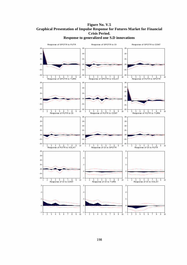
198
Figure No. V.5
Graphical Presentation of Impulse Response for Futures Market for Financial
Crisis Period.
Response to generalized one S.D innovations
-.02
-.01
.00
.01
.02
.03
1 2 3 4 5 6 7 8 9 10
Response of SPOTR to FUTR
-.02
-.01
.00
.01
.02
.03
1 2 3 4 5 6 7 8 9 10
Response of SPOTR to OI
-.02
-.01
.00
.01
.02
.03
1 2 3 4 5 6 7 8 9 10
Response of SPOTR to CONT
-.02
-.01
.00
.01
.02
.03
1 2 3 4 5 6 7 8 9 10
Response of SPOTR to TURN
-.02
-.01
.00
.01
.02
.03
1 2 3 4 5 6 7 8 9 10
Response of SPOTR to VOLAT
-.02
-.01
.00
.01
.02
.03
.04
1 2 3 4 5 6 7 8 9 10
Response of FUTR to SPOTR
-.02
-.01
.00
.01
.02
.03
.04
1 2 3 4 5 6 7 8 9 10
Response of FUTR to OI
-.02
-.01
.00
.01
.02
.03
.04
1 2 3 4 5 6 7 8 9 10
Response of FUTR to CONT
-.02
-.01
.00
.01
.02
.03
.04
1 2 3 4 5 6 7 8 9 10
Response of FUTR to TURN
-.02
-.01
.00
.01
.02
.03
.04
1 2 3 4 5 6 7 8 9 10
Response of FUTR to VOLAT
-.1
.0
.1
.2
.3
1 2 3 4 5 6 7 8 9 10
Response of OI to SPOTR
-.1
.0
.1
.2
.3
1 2 3 4 5 6 7 8 9 10
Response of OI to FUTR
-.1
.0
.1
.2
.3
1 2 3 4 5 6 7 8 9 10
Response of OI to CONT
-.1
.0
.1
.2
.3
1 2 3 4 5 6 7 8 9 10
Response of OI to TURN
-.1
.0
.1
.2
.3
1 2 3 4 5 6 7 8 9 10
Response of OI to VOLAT
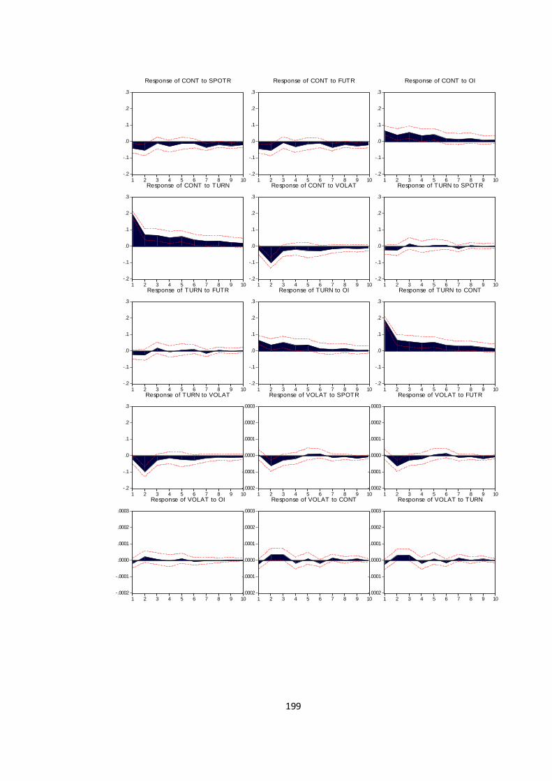
199
-.2
-.1
.0
.1
.2
.3
1 2 3 4 5 6 7 8 9 10
Response of CONT to SPOTR
-.2
-.1
.0
.1
.2
.3
1 2 3 4 5 6 7 8 9 10
Response of CONT to FUTR
-.2
-.1
.0
.1
.2
.3
1 2 3 4 5 6 7 8 9 10
Response of CONT to OI
-.2
-.1
.0
.1
.2
.3
1 2 3 4 5 6 7 8 9 10
Response of CONT to TURN
-.2
-.1
.0
.1
.2
.3
1 2 3 4 5 6 7 8 9 10
Response of CONT to VOLAT
-.2
-.1
.0
.1
.2
.3
1 2 3 4 5 6 7 8 9 10
Response of TURN to SPOTR
-.2
-.1
.0
.1
.2
.3
1 2 3 4 5 6 7 8 9 10
Response of TURN to FUTR
-.2
-.1
.0
.1
.2
.3
1 2 3 4 5 6 7 8 9 10
Response of TURN to OI
-.2
-.1
.0
.1
.2
.3
1 2 3 4 5 6 7 8 9 10
Response of TURN to CONT
-.2
-.1
.0
.1
.2
.3
1 2 3 4 5 6 7 8 9 10
Response of TURN to VOLAT
-.0002
-.0001
.0000
.0001
.0002
.0003
1 2 3 4 5 6 7 8 9 10
Response of VOLAT to SPOTR
-.0002
-.0001
.0000
.0001
.0002
.0003
1 2 3 4 5 6 7 8 9 10
Response of VOLAT to FUTR
-.0002
-.0001
.0000
.0001
.0002
.0003
1 2 3 4 5 6 7 8 9 10
Response of VOLAT to OI
-.0002
-.0001
.0000
.0001
.0002
.0003
1 2 3 4 5 6 7 8 9 10
Response of VOLAT to CONT
-.0002
-.0001
.0000
.0001
.0002
.0003
1 2 3 4 5 6 7 8 9 10
Response of VOLAT to TURN
200
versa. Actually this period results cannot give strong proof for any relationship among
the variables and their efficiency to predict others. The independency but reflective
relationship between each variable to other variables is seen from the figure. There is
reflective positive relationship between spot and futures market, open interest ad trade
volume. It is clear that number of contract and turnover is always show positive
bidirectional relationship between them. During this period, trade volume is
negatively influence volatility and not vice versa. This reflective nature of relationship
among variables can be utilized for speculative activity and it helps to make profit
from the price variations in the futures market for a reflective actions.
5.10.5. Section-5: Post Financial Crisis Period
This period is expected to provide opportunity to recover from the shocks
produced by financial crisis across the globe. During this recovery process, it is
attempted to see the type and nature of relationship between spot and futures market
in India and the results are presented in figure No. V.6, through impulse response
function. It is seen that shock in spot return is presented by futures return during the
first two days positively and significantly. After the second day of shock, spot return
is not responding to such shock from futures market. Trade volume influences the
spot significantly but negatively for just one day and spot market ignorers the changes
or shocks in trade volume after that. Market depth is not affecting the spot return,
changes in volatility makes spot market to have sudden positive changes for a day.
Exactly the same type of responses is seen from futures market return to various
shocks from spot market return, open interest, trade volume and volatility. Market
depth is not at all influenced by any variable considered in the study as it shows very
insignificant results. Number of contracts and turnover considered as proxy for trade
volume reacts to the changes in spot and futures return negatively and significantly.
Trade volume is reacting to volatility the initial first one day. Number of contracts
and turnover has mutual positive influences significantly. Volatility is responding to
changes in spot and futures return positively and significantly for five days and that
ignores the shocks. Changes in market depth do not impact the volatility, where as it
responds significantly and positively to trade volume consistently all days. The daily
open interest determine the number of outstanding contract at the end of a trading day,
that is the number of contact that have been entered in to but not yet
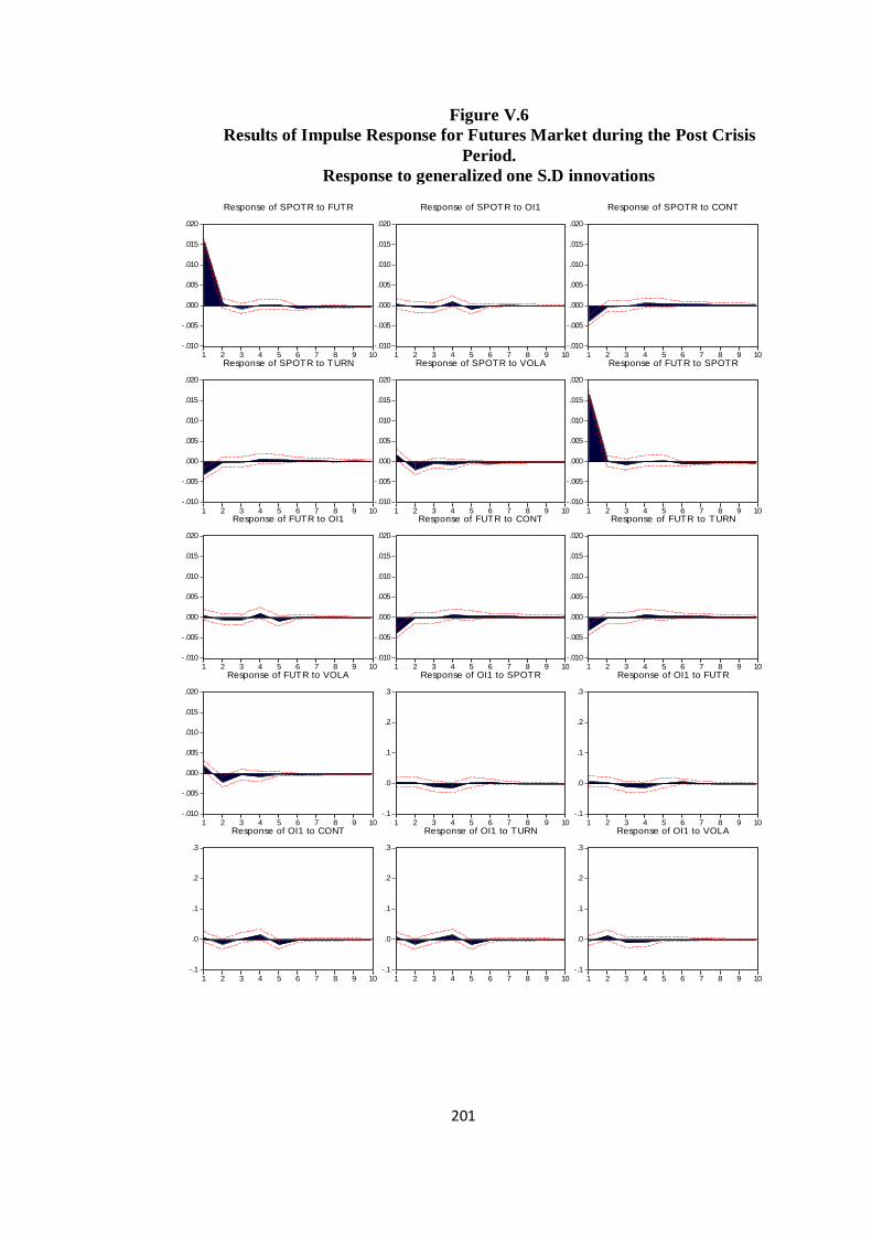
201
Figure V.6
Results of Impulse Response for Futures Market during the Post Crisis
Period.
Response to generalized one S.D innovations
-.010
-.005
.000
.005
.010
.015
.020
1 2 3 4 5 6 7 8 9 10
Response of SPOTR to FUTR
-.010
-.005
.000
.005
.010
.015
.020
1 2 3 4 5 6 7 8 9 10
Response of SPOTR to OI1
-.010
-.005
.000
.005
.010
.015
.020
1 2 3 4 5 6 7 8 9 10
Response of SPOTR to CONT
-.010
-.005
.000
.005
.010
.015
.020
1 2 3 4 5 6 7 8 9 10
Response of SPOTR to TURN
-.010
-.005
.000
.005
.010
.015
.020
1 2 3 4 5 6 7 8 9 10
Response of SPOTR to VOLA
-.010
-.005
.000
.005
.010
.015
.020
1 2 3 4 5 6 7 8 9 10
Response of FUTR to SPOTR
-.010
-.005
.000
.005
.010
.015
.020
1 2 3 4 5 6 7 8 9 10
Response of FUTR to OI1
-.010
-.005
.000
.005
.010
.015
.020
1 2 3 4 5 6 7 8 9 10
Response of FUTR to CONT
-.010
-.005
.000
.005
.010
.015
.020
1 2 3 4 5 6 7 8 9 10
Response of FUTR to TURN
-.010
-.005
.000
.005
.010
.015
.020
1 2 3 4 5 6 7 8 9 10
Response of FUTR to VOLA
-.1
.0
.1
.2
.3
1 2 3 4 5 6 7 8 9 10
Response of OI1 to SPOTR
-.1
.0
.1
.2
.3
1 2 3 4 5 6 7 8 9 10
Response of OI1 to FUTR
-.1
.0
.1
.2
.3
1 2 3 4 5 6 7 8 9 10
Response of OI1 to CONT
-.1
.0
.1
.2
.3
1 2 3 4 5 6 7 8 9 10
Response of OI1 to TURN
-.1
.0
.1
.2
.3
1 2 3 4 5 6 7 8 9 10
Response of OI1 to VOLA
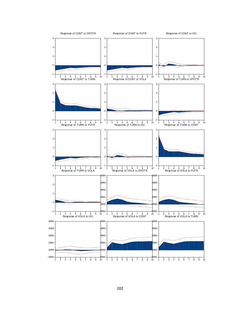
202
-.1
.0
.1
.2
.3
1 2 3 4 5 6 7 8 9 10
Response of CONT to SPOTR
-.1
.0
.1
.2
.3
1 2 3 4 5 6 7 8 9 10
Response of CONT to FUTR
-.1
.0
.1
.2
.3
1 2 3 4 5 6 7 8 9 10
Response of CONT to OI1
-.1
.0
.1
.2
.3
1 2 3 4 5 6 7 8 9 10
Response of CONT to TURN
-.1
.0
.1
.2
.3
1 2 3 4 5 6 7 8 9 10
Response of CONT to VOLA
-.1
.0
.1
.2
.3
1 2 3 4 5 6 7 8 9 10
Response of TURN to SPOTR
-.1
.0
.1
.2
.3
1 2 3 4 5 6 7 8 9 10
Response of TURN to FUTR
-.1
.0
.1
.2
.3
1 2 3 4 5 6 7 8 9 10
Response of TURN to OI1
-.1
.0
.1
.2
.3
1 2 3 4 5 6 7 8 9 10
Response of TURN to CONT
-.1
.0
.1
.2
.3
1 2 3 4 5 6 7 8 9 10
Response of TURN to VOLA
-.00001
.00000
.00001
.00002
.00003
.00004
1 2 3 4 5 6 7 8 9 10
Response of VOLA to SPOTR
-.00001
.00000
.00001
.00002
.00003
.00004
1 2 3 4 5 6 7 8 9 10
Response of VOLA to FUTR
-.00001
.00000
.00001
.00002
.00003
.00004
1 2 3 4 5 6 7 8 9 10
Response of VOLA to OI1
-.00001
.00000
.00001
.00002
.00003
.00004
1 2 3 4 5 6 7 8 9 10
Response of VOLA to CONT
-.00001
.00000
.00001
.00002
.00003
.00004
1 2 3 4 5 6 7 8 9 10
Response of VOLA to TURN
203
liquidated (Julio. J. Lucia etal 2008). It is confirmed during this period that
relationship between spot and futures market is strengthened. Spot and futures return
reacts to trade volume negatively. Market depth is not having any relation with any
other variable. There is a positive and significant relation between contracts and
turnover.
Market shocks and its responses to each variable, shocks in each variable and
its effect to all other variables separately, its duration of the response and its sign also
have been understood from this thorough analysis with impulse response function.
But the proportion of change and response of each variable that is transmitted to
another variable is not confirmed here. In order to understand the percentage change
in each variable due to the shocks in one variable, another econometrics model has to
be applied. Variance decomposition gives the response of each variable due to shocks
in another variable in percentage form and help to understand the relationship of each
variable to other variables. The intensity of relationship between variables shows the
efficiency of them to explain others very clearly. On the basis of the results explained
here, it can be made a conclusion in such a manner that spot market return, trading
volume, market depth and the variation in the futures market are considered as the
determinants of futures market in India (Julio 2008, Puja Pati 2009, Pratab Chandra
Pati etal 2010). In short, these variables can be considered as the factors which can
explain and predict the movement of futures market return because of their close
relationship with futures market return.
5.11. PROPORTION AND TRANSMISSION OF SHOCKS
The proportion of change in one variable due to the shock of that variable
itself and the transmission of proportionate change to other variable can be analyzed
from variance decomposition. It is the extension of impulse response model and this
model provides more clarity on the proportionate change in each variable due to
shocks in the same variable. Variance decomposition or forecast error variance
decomposition indicates the amount of information each variable contributes to the
other variables in Vector Auto Regression Models. It determines how much of the
forecast error variance of each of the variable can be explained by exogenous shocks
to the other variables.
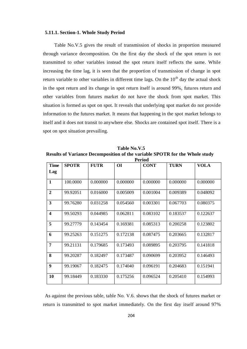
204
5.11.1. Section-1. Whole Study Period
Table No.V.5 gives the result of transmission of shocks in proportion measured
through variance decomposition. On the first day the shock of the spot return is not
transmitted to other variables instead the spot return itself reflects the same. While
increasing the time lag, it is seen that the proportion of transmission of change in spot
return variable to other variables in different time lags. On the 10th day the actual shock
in the spot return and its change in spot return itself is around 99%, futures return and
other variables from futures market do not have the shock from spot market. This
situation is formed as spot on spot. It reveals that underlying spot market do not provide
information to the futures market. It means that happening in the spot market belongs to
itself and it does not transit to anywhere else. Shocks are contained spot itself. There is a
spot on spot situation prevailing.
Table No.V.5
Results of Variance Decomposition of the variable SPOTR for the Whole study
Period
Time
Lag
SPOTR FUTR OI CONT TURN VOLA
1 100.0000 0.000000 0.000000 0.000000 0.000000 0.000000
2 99.92051 0.016000 0.005009 0.001004 0.009389 0.048092
3 99.76280 0.031258 0.054560 0.003301 0.067703 0.080375
4 99.50293 0.044985 0.062811 0.083102 0.183537 0.122637
5 99.27779 0.143454 0.169381 0.085313 0.200258 0.123802
6 99.25263 0.151275 0.172138 0.087475 0.203665 0.132817
7 99.21131 0.179685 0.173493 0.089895 0.203795 0.141818
8 99.20287 0.182497 0.173487 0.090699 0.203952 0.146493
9 99.19067 0.182475 0.174040 0.096191 0.204683 0.151941
10 99.18449 0.183330 0.175256 0.096524 0.205410 0.154993
As against the previous table, table No. V.6. shows that the shock of futures market or
return is transmitted to spot market immediately. On the first day itself around 97%
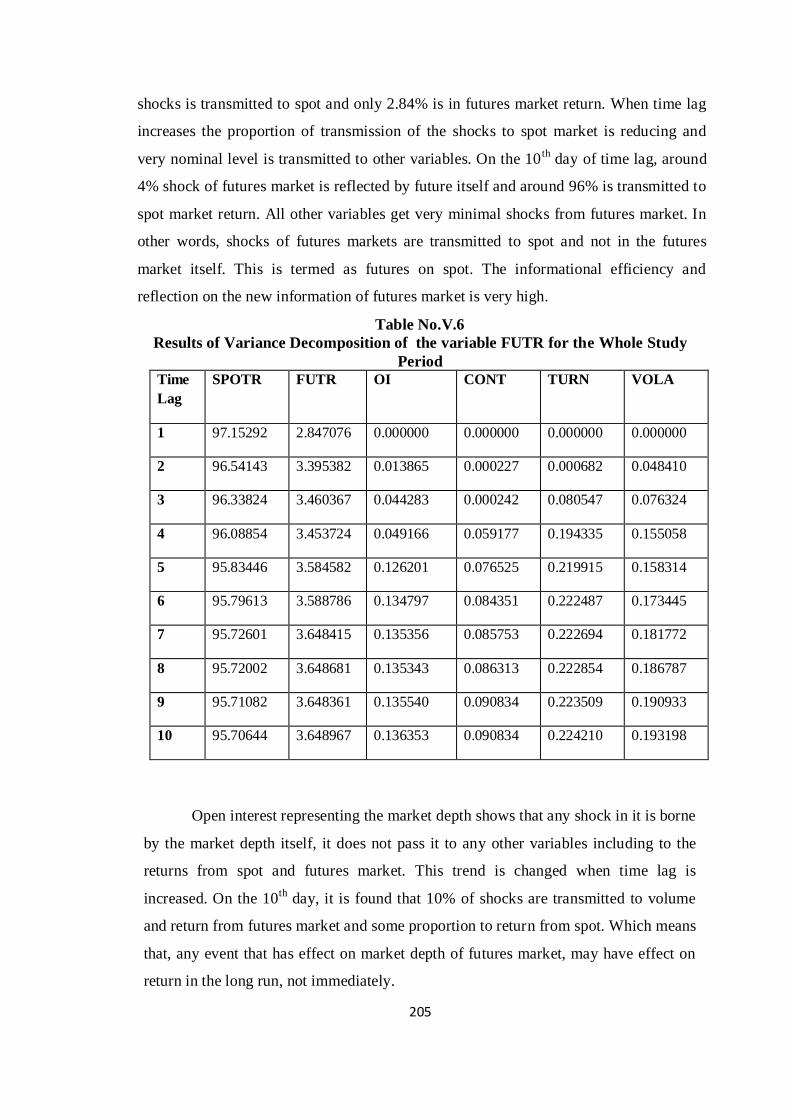
205
shocks is transmitted to spot and only 2.84% is in futures market return. When time lag
increases the proportion of transmission of the shocks to spot market is reducing and
very nominal level is transmitted to other variables. On the 10th
day of time lag, around
4% shock of futures market is reflected by future itself and around 96% is transmitted to
spot market return. All other variables get very minimal shocks from futures market. In
other words, shocks of futures markets are transmitted to spot and not in the futures
market itself. This is termed as futures on spot. The informational efficiency and
reflection on the new information of futures market is very high.
Table No.V.6
Results of Variance Decomposition of the variable FUTR for the Whole Study
Period
Time
Lag
SPOTR FUTR OI CONT TURN VOLA
1 97.15292 2.847076 0.000000 0.000000 0.000000 0.000000
2 96.54143 3.395382 0.013865 0.000227 0.000682 0.048410
3 96.33824 3.460367 0.044283 0.000242 0.080547 0.076324
4 96.08854 3.453724 0.049166 0.059177 0.194335 0.155058
5 95.83446 3.584582 0.126201 0.076525 0.219915 0.158314
6 95.79613 3.588786 0.134797 0.084351 0.222487 0.173445
7 95.72601 3.648415 0.135356 0.085753 0.222694 0.181772
8 95.72002 3.648681 0.135343 0.086313 0.222854 0.186787
9 95.71082 3.648361 0.135540 0.090834 0.223509 0.190933
10 95.70644 3.648967 0.136353 0.090834 0.224210 0.193198
Open interest representing the market depth shows that any shock in it is borne
by the market depth itself, it does not pass it to any other variables including to the
returns from spot and futures market. This trend is changed when time lag is
increased. On the 10th
day, it is found that 10% of shocks are transmitted to volume
and return from futures market and some proportion to return from spot. Which means
that, any event that has effect on market depth of futures market, may have effect on
return in the long run, not immediately.
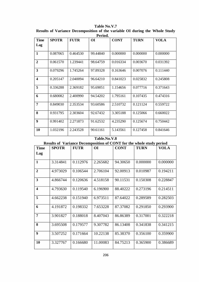
206
Table No.V.7
Results of Variance Decomposition of the variable OI during the Whole Study
Period.
Time
Lag
SPOTR FUTR OI CONT TURN VOLA
1 0.087065 0.464530 99.44840 0.000000 0.000000 0.000000
2 0.061570 1.239441 98.64759 0.016334 0.003670 0.031392
3 0.079296 1.745264 97.89328 0.163646 0.007076 0.111440
4 0.205147 2.040094 96.64210 0.841023 0.025832 0.245808
5 0.336288 2.369182 95.69051 1.154656 0.077716 0.371643
6 0.680082 2.400990 94.54202 1.795161 0.107435 0.474316
7 0.849030 2.353534 93.60586 2.510732 0.121124 0.559722
8 0.931795 2.303604 92.67432 3.305188 0.125066 0.660022
9 0.991402 2.271873 91.62532 4.235290 0.125674 0.750442
10 1.032196 2.243528 90.61161 5.143561 0.127458 0.841646
Table.No.V.8
Results of Variance Decomposition of CONT for the whole study period
Time
Lag
SPOTR FUTR OI CONT TURN VOLA
1 3.314841 0.112976 2.265682 94.30650 0.000000 0.000000
2 4.973029 0.106544 2.706104 92.00913 0.010987 0.194211
3 4.866744 0.120636 4.518158 90.11531 0.150308 0.228847
4 4.793630 0.119540 6.196900 88.40222 0.273196 0.214511
5 4.662238 0.151940 6.973511 87.64022 0.289589 0.282503
6 4.191872 0.198332 7.653228 87.37082 0.291850 0.293900
7 3.901827 0.188018 8.407043 86.86389 0.317001 0.322218
8 3.695508 0.179577 9.307782 86.13408 0.341838 0.341215
9 3.507252 0.171664 10.22138 85.38370 0.356100 0.359900
10 3.327767 0.166680 11.00083 84.75213 0.365900 0.386689
207
This may be termed as depth on depth situation during short period, but in the long
run it may be depth on others. This result shows that market depth and speculative
activities of the trading cannot be separated. Both are interrelated and change in one
affects the other
Table No.V.8 shows the results of variance decomposition of number of
contract as dependent variable for the whole study period. It indicates that 94%
change is happened in the number of contract variable itself due to the shock from the
same variable. On that moment around 3%, 1%and 2% shocks transmitted to spot
market, futures market and open interest respectively. If any events happens to have
effect on number of contracts, it is called on shocks, would have changes in the
number of contract itself and some proportion is transmitted to return from spot
market and futures market. But this slowly gets changed is time lag increases. Market
depth is the sole factor while have impact due to shocks from number of contract. It is
observed significantly that change in number of contract had increased effect on
return from spot market on the second day and after that the effect got reduced over
the time. The close relationship of number of contract and open interest during this
period can be understood from this study period. Number of contract is the
representative of trading volume which means that the response of market on new
information is very high and the open interest is the proxy of outstanding demand for
the market shocks. Both are interconnected and cannot be separated.
The table No.V.9. shows that any shock in turnover is reflected in number of
contract and as days pass by market depth is affected. Very negligible effect is seen in
the return from spot market. It means that the movement of turnover is predicted by
number of contract at that moment. Number of contract is the base for the trading
volume and it shows the tendency of the market to response to the new information
soon. The inter relationship between turnover and number of contract is seen from the
table. Both are normally considered as the proxy for market trade volume. Turnover is
also taken as the variable which can predict the movement of futures market during
the study period.
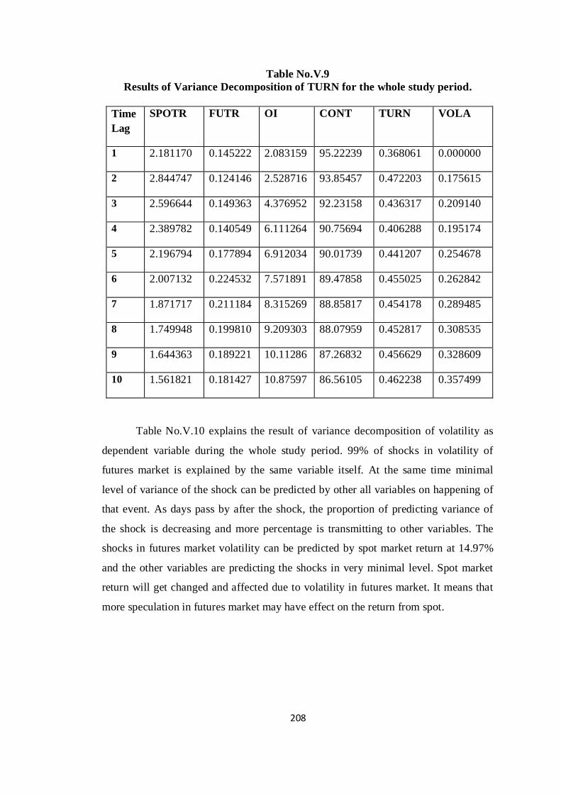
208
Table No.V.9
Results of Variance Decomposition of TURN for the whole study period.
Time
Lag
SPOTR FUTR OI CONT TURN VOLA
1 2.181170 0.145222 2.083159 95.22239 0.368061 0.000000
2 2.844747 0.124146 2.528716 93.85457 0.472203 0.175615
3 2.596644 0.149363 4.376952 92.23158 0.436317 0.209140
4 2.389782 0.140549 6.111264 90.75694 0.406288 0.195174
5 2.196794 0.177894 6.912034 90.01739 0.441207 0.254678
6 2.007132 0.224532 7.571891 89.47858 0.455025 0.262842
7 1.871717 0.211184 8.315269 88.85817 0.454178 0.289485
8 1.749948 0.199810 9.209303 88.07959 0.452817 0.308535
9 1.644363 0.189221 10.11286 87.26832 0.456629 0.328609
10 1.561821 0.181427 10.87597 86.56105 0.462238 0.357499
Table No.V.10 explains the result of variance decomposition of volatility as
dependent variable during the whole study period. 99% of shocks in volatility of
futures market is explained by the same variable itself. At the same time minimal
level of variance of the shock can be predicted by other all variables on happening of
that event. As days pass by after the shock, the proportion of predicting variance of
the shock is decreasing and more percentage is transmitting to other variables. The
shocks in futures market volatility can be predicted by spot market return at 14.97%
and the other variables are predicting the shocks in very minimal level. Spot market
return will get changed and affected due to volatility in futures market. It means that
more speculation in futures market may have effect on the return from spot.
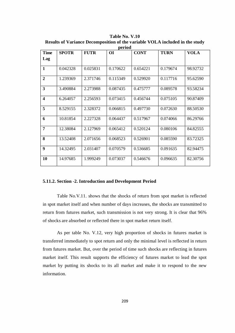
209
Table No. V.10
Results of Variance Decomposition of the variable VOLA included in the study
period
Time
Lag
SPOTR FUTR OI CONT TURN VOLA
1 0.042328 0.025831 0.170622 0.654221 0.179674 98.92732
2 1.239369 2.371746 0.115349 0.529920 0.117716 95.62590
3 3.490884 2.273988 0.087435 0.475777 0.089578 93.58234
4 6.264057 2.256593 0.073415 0.456744 0.075105 90.87409
5 8.529155 2.328372 0.066815 0.497730 0.072630 88.50530
6 10.81854 2.227328 0.064437 0.517967 0.074066 86.29766
7 12.38084 2.127969 0.065412 0.520124 0.080106 84.82555
8 13.52408 2.071656 0.068523 0.526901 0.085590 83.72325
9 14.32495 2.031407 0.070579 0.536685 0.091635 82.94475
10 14.97685 1.999249 0.073037 0.546676 0.096635 82.30756
5.11.2. Section -2. Introduction and Development Period
Table No.V.11. shows that the shocks of return from spot market is reflected
in spot market itself and when number of days increases, the shocks are transmitted to
return from futures market, such transmission is not very strong. It is clear that 96%
of shocks are absorbed or reflected there in spot market return itself.
As per table No. V.12, very high proportion of shocks in futures market is
transferred immediately to spot return and only the minimal level is reflected in return
from futures market. But, over the period of time such shocks are reflecting in futures
market itself. This result supports the efficiency of futures market to lead the spot
market by putting its shocks to its all market and make it to respond to the new
information.
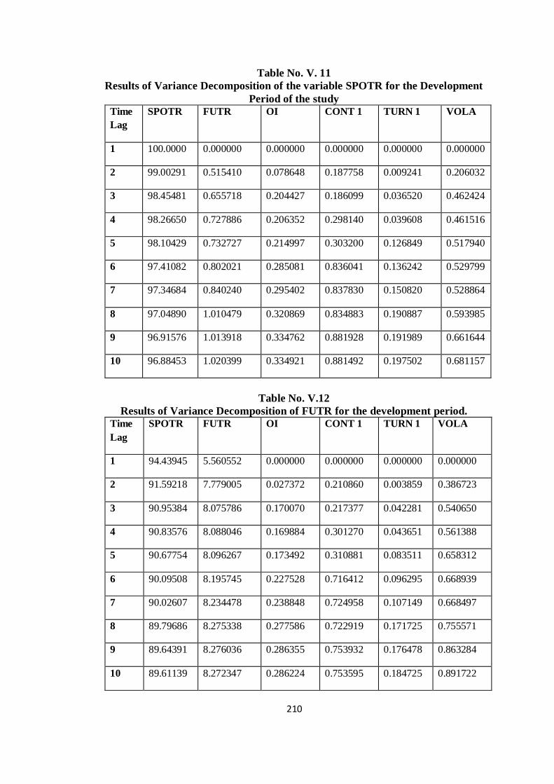
210
Table No. V. 11
Results of Variance Decomposition of the variable SPOTR for the Development
Period of the study
Time
Lag
SPOTR FUTR OI CONT 1 TURN 1 VOLA
1 100.0000 0.000000 0.000000 0.000000 0.000000 0.000000
2 99.00291 0.515410 0.078648 0.187758 0.009241 0.206032
3 98.45481 0.655718 0.204427 0.186099 0.036520 0.462424
4 98.26650 0.727886 0.206352 0.298140 0.039608 0.461516
5 98.10429 0.732727 0.214997 0.303200 0.126849 0.517940
6 97.41082 0.802021 0.285081 0.836041 0.136242 0.529799
7 97.34684 0.840240 0.295402 0.837830 0.150820 0.528864
8 97.04890 1.010479 0.320869 0.834883 0.190887 0.593985
9 96.91576 1.013918 0.334762 0.881928 0.191989 0.661644
10 96.88453 1.020399 0.334921 0.881492 0.197502 0.681157
Table No. V.12
Results of Variance Decomposition of FUTR for the development period.
Time
Lag
SPOTR FUTR OI CONT 1 TURN 1 VOLA
1 94.43945 5.560552 0.000000 0.000000 0.000000 0.000000
2 91.59218 7.779005 0.027372 0.210860 0.003859 0.386723
3 90.95384 8.075786 0.170070 0.217377 0.042281 0.540650
4 90.83576 8.088046 0.169884 0.301270 0.043651 0.561388
5 90.67754 8.096267 0.173492 0.310881 0.083511 0.658312
6 90.09508 8.195745 0.227528 0.716412 0.096295 0.668939
7 90.02607 8.234478 0.238848 0.724958 0.107149 0.668497
8 89.79686 8.275338 0.277586 0.722919 0.171725 0.755571
9 89.64391 8.276036 0.286355 0.753932 0.176478 0.863284
10 89.61139 8.272347 0.286224 0.753595 0.184725 0.891722
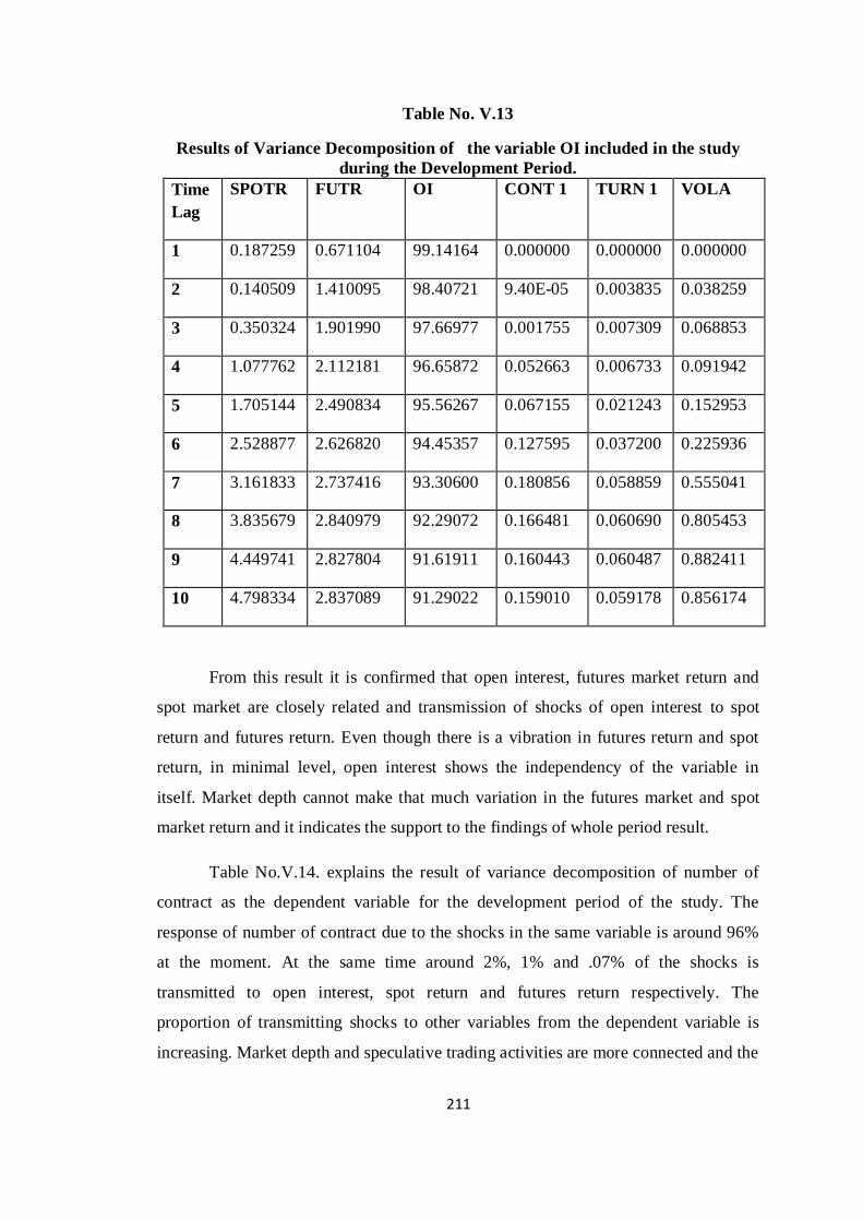
211
Table No. V.13
Results of Variance Decomposition of the variable OI included in the study
during the Development Period.
Time
Lag
SPOTR FUTR OI CONT 1 TURN 1 VOLA
1 0.187259 0.671104 99.14164 0.000000 0.000000 0.000000
2 0.140509 1.410095 98.40721 9.40E-05 0.003835 0.038259
3 0.350324 1.901990 97.66977 0.001755 0.007309 0.068853
4 1.077762 2.112181 96.65872 0.052663 0.006733 0.091942
5 1.705144 2.490834 95.56267 0.067155 0.021243 0.152953
6 2.528877 2.626820 94.45357 0.127595 0.037200 0.225936
7 3.161833 2.737416 93.30600 0.180856 0.058859 0.555041
8 3.835679 2.840979 92.29072 0.166481 0.060690 0.805453
9 4.449741 2.827804 91.61911 0.160443 0.060487 0.882411
10 4.798334 2.837089 91.29022 0.159010 0.059178 0.856174
From this result it is confirmed that open interest, futures market return and
spot market are closely related and transmission of shocks of open interest to spot
return and futures return. Even though there is a vibration in futures return and spot
return, in minimal level, open interest shows the independency of the variable in
itself. Market depth cannot make that much variation in the futures market and spot
market return and it indicates the support to the findings of whole period result.
Table No.V.14. explains the result of variance decomposition of number of
contract as the dependent variable for the development period of the study. The
response of number of contract due to the shocks in the same variable is around 96%
at the moment. At the same time around 2%, 1% and .07% of the shocks is
transmitted to open interest, spot return and futures return respectively. The
proportion of transmitting shocks to other variables from the dependent variable is
increasing. Market depth and speculative trading activities are more connected and the
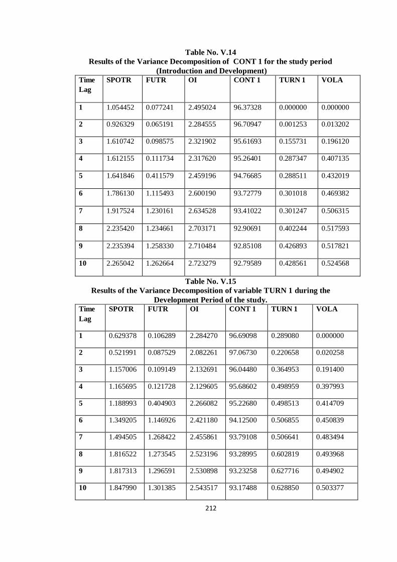
212
Table No. V.14
Results of the Variance Decomposition of CONT 1 for the study period
(Introduction and Development)
Time
Lag
SPOTR FUTR OI CONT 1 TURN 1 VOLA
1 1.054452 0.077241 2.495024 96.37328 0.000000 0.000000
2 0.926329 0.065191 2.284555 96.70947 0.001253 0.013202
3 1.610742 0.098575 2.321902 95.61693 0.155731 0.196120
4 1.612155 0.111734 2.317620 95.26401 0.287347 0.407135
5 1.641846 0.411579 2.459196 94.76685 0.288511 0.432019
6 1.786130 1.115493 2.600190 93.72779 0.301018 0.469382
7 1.917524 1.230161 2.634528 93.41022 0.301247 0.506315
8 2.235420 1.234661 2.703171 92.90691 0.402244 0.517593
9 2.235394 1.258330 2.710484 92.85108 0.426893 0.517821
10 2.265042 1.262664 2.723279 92.79589 0.428561 0.524568
Table No. V.15
Results of the Variance Decomposition of variable TURN 1 during the
Development Period of the study.
Time
Lag
SPOTR FUTR OI CONT 1 TURN 1 VOLA
1 0.629378 0.106289 2.284270 96.69098 0.289080 0.000000
2 0.521991 0.087529 2.082261 97.06730 0.220658 0.020258
3 1.157006 0.109149 2.132691 96.04480 0.364953 0.191400
4 1.165695 0.121728 2.129605 95.68602 0.498959 0.397993
5 1.188993 0.404903 2.266082 95.22680 0.498513 0.414709
6 1.349205 1.146926 2.421180 94.12500 0.506855 0.450839
7 1.494505 1.268422 2.455861 93.79108 0.506641 0.483494
8 1.816522 1.273545 2.523196 93.28995 0.602819 0.493968
9 1.817313 1.296591 2.530898 93.23258 0.627716 0.494902
10 1.847990 1.301385 2.543517 93.17488 0.628850 0.503377
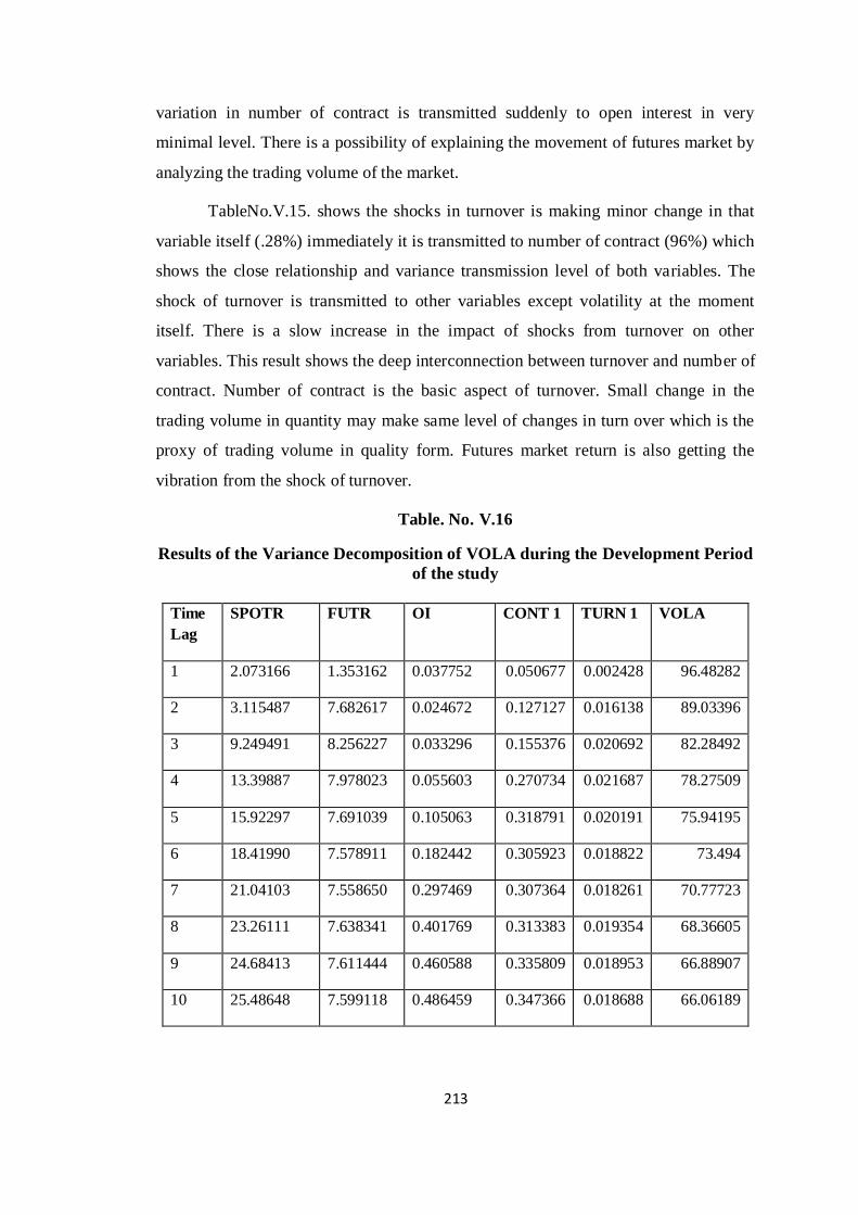
213
variation in number of contract is transmitted suddenly to open interest in very
minimal level. There is a possibility of explaining the movement of futures market by
analyzing the trading volume of the market.
TableNo.V.15. shows the shocks in turnover is making minor change in that
variable itself (.28%) immediately it is transmitted to number of contract (96%) which
shows the close relationship and variance transmission level of both variables. The
shock of turnover is transmitted to other variables except volatility at the moment
itself. There is a slow increase in the impact of shocks from turnover on other
variables. This result shows the deep interconnection between turnover and number of
contract. Number of contract is the basic aspect of turnover. Small change in the
trading volume in quantity may make same level of changes in turn over which is the
proxy of trading volume in quality form. Futures market return is also getting the
vibration from the shock of turnover.
Table. No. V.16
Results of the Variance Decomposition of VOLA during the Development Period
of the study
Time
Lag
SPOTR FUTR OI CONT 1 TURN 1 VOLA
1 2.073166 1.353162 0.037752 0.050677 0.002428 96.48282
2 3.115487 7.682617 0.024672 0.127127 0.016138 89.03396
3 9.249491 8.256227 0.033296 0.155376 0.020692 82.28492
4 13.39887 7.978023 0.055603 0.270734 0.021687 78.27509
5 15.92297 7.691039 0.105063 0.318791 0.020191 75.94195
6 18.41990 7.578911 0.182442 0.305923 0.018822 73.494
7 21.04103 7.558650 0.297469 0.307364 0.018261 70.77723
8 23.26111 7.638341 0.401769 0.313383 0.019354 68.36605
9 24.68413 7.611444 0.460588 0.335809 0.018953 66.88907
10 25.48648 7.599118 0.486459 0.347366 0.018688 66.06189
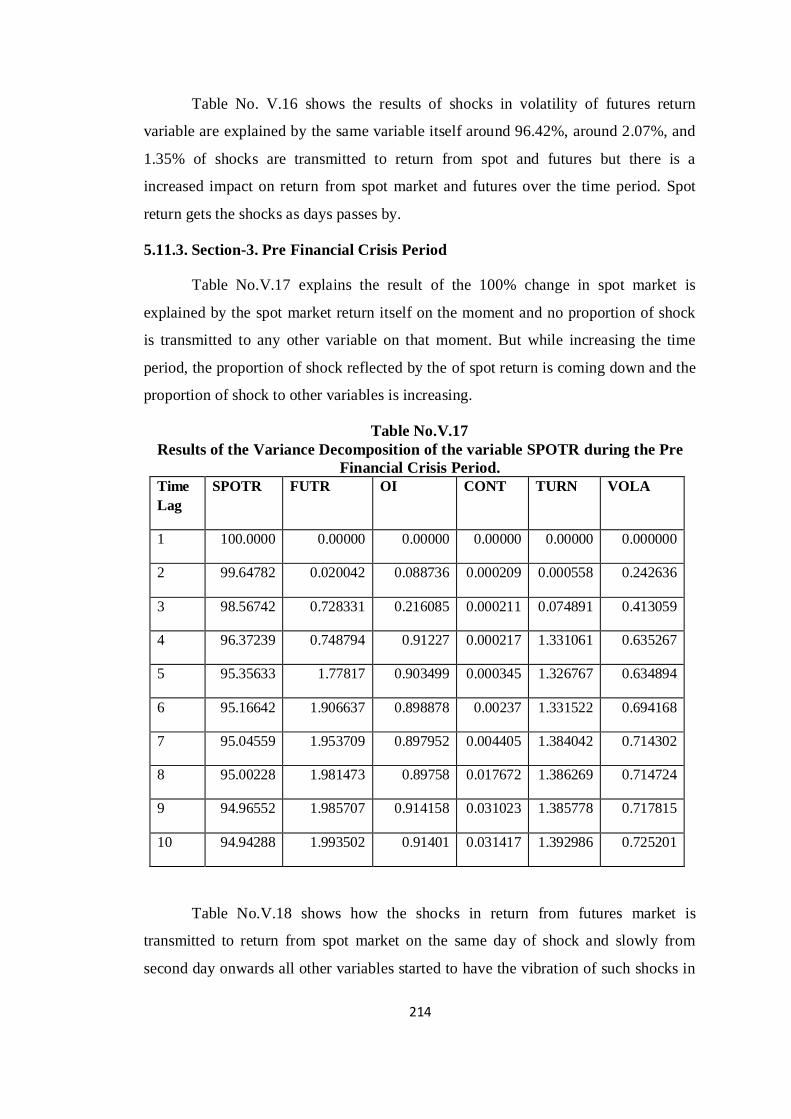
214
Table No. V.16 shows the results of shocks in volatility of futures return
variable are explained by the same variable itself around 96.42%, around 2.07%, and
1.35% of shocks are transmitted to return from spot and futures but there is a
increased impact on return from spot market and futures over the time period. Spot
return gets the shocks as days passes by.
5.11.3. Section-3. Pre Financial Crisis Period
Table No.V.17 explains the result of the 100% change in spot market is
explained by the spot market return itself on the moment and no proportion of shock
is transmitted to any other variable on that moment. But while increasing the time
period, the proportion of shock reflected by the of spot return is coming down and the
proportion of shock to other variables is increasing.
Table No.V.17
Results of the Variance Decomposition of the variable SPOTR during the Pre
Financial Crisis Period.
Time
Lag
SPOTR FUTR OI CONT TURN VOLA
1 100.0000 0.00000 0.00000 0.00000 0.00000 0.000000
2 99.64782 0.020042 0.088736 0.000209 0.000558 0.242636
3 98.56742 0.728331 0.216085 0.000211 0.074891 0.413059
4 96.37239 0.748794 0.91227 0.000217 1.331061 0.635267
5 95.35633 1.77817 0.903499 0.000345 1.326767 0.634894
6 95.16642 1.906637 0.898878 0.00237 1.331522 0.694168
7 95.04559 1.953709 0.897952 0.004405 1.384042 0.714302
8 95.00228 1.981473 0.89758 0.017672 1.386269 0.714724
9 94.96552 1.985707 0.914158 0.031023 1.385778 0.717815
10 94.94288 1.993502 0.91401 0.031417 1.392986 0.725201
Table No.V.18 shows how the shocks in return from futures market is
transmitted to return from spot market on the same day of shock and slowly from
second day onwards all other variables started to have the vibration of such shocks in
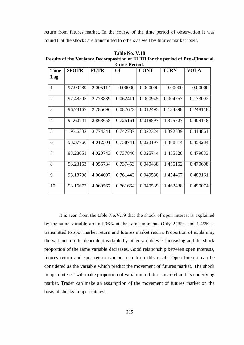
215
return from futures market. In the course of the time period of observation it was
found that the shocks are transmitted to others as well by futures market itself.
Table No. V.18
Results of the Variance Decomposition of FUTR for the period of Pre -Financial
Crisis Period.
Time
Lag
SPOTR FUTR OI CONT TURN VOLA
1 97.99489 2.005114 0.00000 0.000000 0.00000 0.00000
2 97.48505 2.273839 0.062411 0.000945 0.004757 0.173002
3 96.73167 2.785696 0.087622 0.012495 0.134398 0.248118
4 94.60741 2.863658 0.725161 0.018897 1.375727 0.409148
5 93.6532 3.774341 0.742737 0.022324 1.392539 0.414861
6 93.37766 4.012301 0.738741 0.023197 1.388814 0.459284
7 93.28051 4.020743 0.737846 0.025744 1.455328 0.479833
8 93.23153 4.055734 0.737453 0.040438 1.455152 0.479698
9 93.18738 4.064007 0.761443 0.049538 1.454467 0.483161
10 93.16672 4.069567 0.761664 0.049539 1.462438 0.490074
It is seen from the table No.V.19 that the shock of open interest is explained
by the same variable around 96% at the same moment. Only 2.25% and 1.49% is
transmitted to spot market return and futures market return. Proportion of explaining
the variance on the dependent variable by other variables is increasing and the shock
proportion of the same variable decreases. Good relationship between open interests,
futures return and spot return can be seen from this result. Open interest can be
considered as the variable which predict the movement of futures market. The shock
in open interest will make proportion of variation in futures market and its underlying
market. Trader can make an assumption of the movement of futures market on the
basis of shocks in open interest.
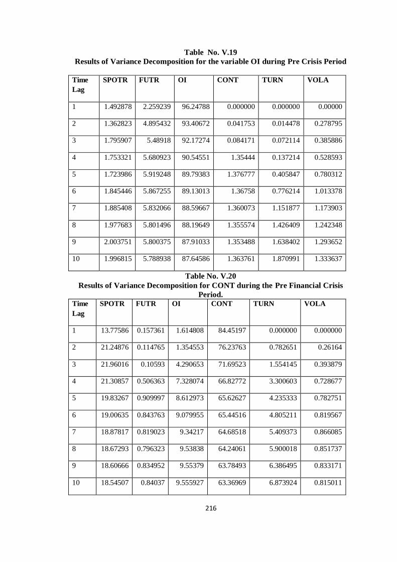
216
Table No. V.19
Results of Variance Decomposition for the variable OI during Pre Crisis Period
Time
Lag
SPOTR FUTR OI CONT TURN VOLA
1 1.492878 2.259239 96.24788 0.000000 0.000000 0.00000
2 1.362823 4.895432 93.40672 0.041753 0.014478 0.278795
3 1.795907 5.48918 92.17274 0.084171 0.072114 0.385886
4 1.753321 5.680923 90.54551 1.35444 0.137214 0.528593
5 1.723986 5.919248 89.79383 1.376777 0.405847 0.780312
6 1.845446 5.867255 89.13013 1.36758 0.776214 1.013378
7 1.885408 5.832066 88.59667 1.360073 1.151877 1.173903
8 1.977683 5.801496 88.19649 1.355574 1.426409 1.242348
9 2.003751 5.800375 87.91033 1.353488 1.638402 1.293652
10 1.996815 5.788938 87.64586 1.363761 1.870991 1.333637
Table No. V.20
Results of Variance Decomposition for CONT during the Pre Financial Crisis
Period.
Time
Lag
SPOTR FUTR OI CONT TURN VOLA
1 13.77586 0.157361 1.614808 84.45197 0.000000 0.000000
2 21.24876 0.114765 1.354553 76.23763 0.782651 0.26164
3 21.96016 0.10593 4.290653 71.69523 1.554145 0.393879
4 21.30857 0.506363 7.328074 66.82772 3.300603 0.728677
5 19.83267 0.909997 8.612973 65.62627 4.235333 0.782751
6 19.00635 0.843763 9.079955 65.44516 4.805211 0.819567
7 18.87817 0.819023 9.34217 64.68518 5.409373 0.866085
8 18.67293 0.796323 9.53838 64.24061 5.900018 0.851737
9 18.60666 0.834952 9.55379 63.78493 6.386495 0.833171
10 18.54507 0.84037 9.555927 63.36969 6.873924 0.815011
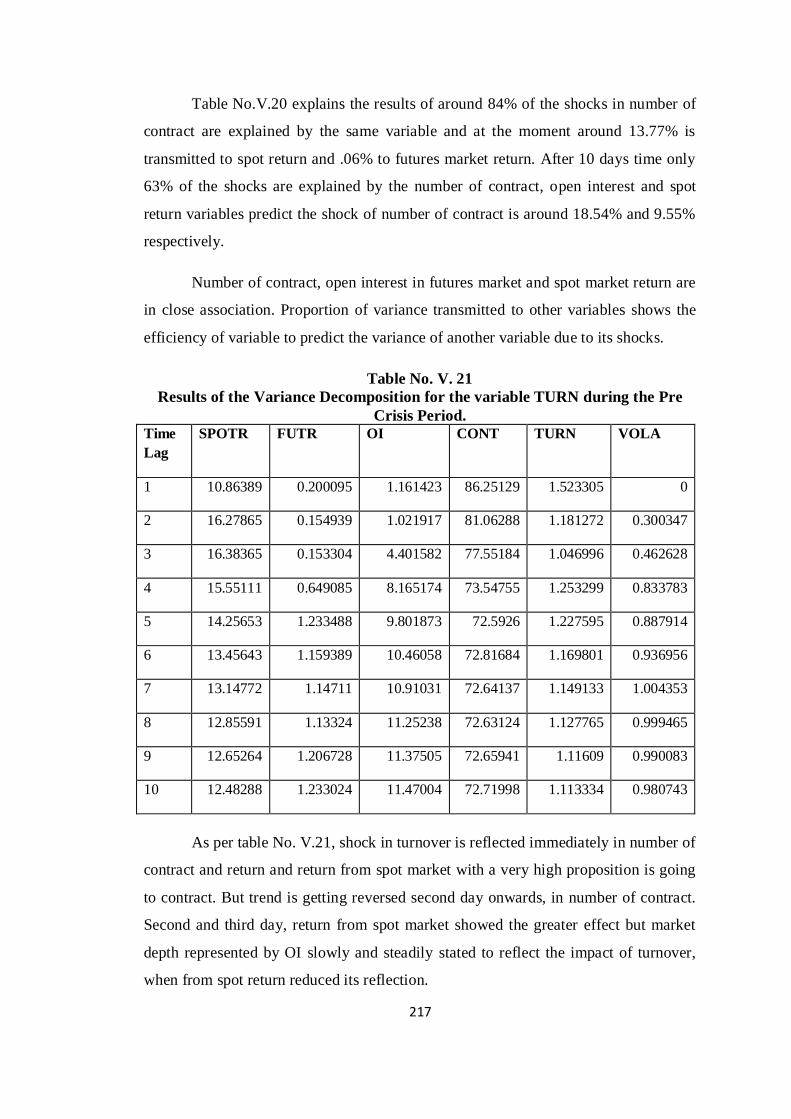
217
Table No.V.20 explains the results of around 84% of the shocks in number of
contract are explained by the same variable and at the moment around 13.77% is
transmitted to spot return and .06% to futures market return. After 10 days time only
63% of the shocks are explained by the number of contract, open interest and spot
return variables predict the shock of number of contract is around 18.54% and 9.55%
respectively.
Number of contract, open interest in futures market and spot market return are
in close association. Proportion of variance transmitted to other variables shows the
efficiency of variable to predict the variance of another variable due to its shocks.
Table No. V. 21
Results of the Variance Decomposition for the variable TURN during the Pre
Crisis Period.
Time
Lag
SPOTR FUTR OI CONT TURN VOLA
1 10.86389 0.200095 1.161423 86.25129 1.523305 0
2 16.27865 0.154939 1.021917 81.06288 1.181272 0.300347
3 16.38365 0.153304 4.401582 77.55184 1.046996 0.462628
4 15.55111 0.649085 8.165174 73.54755 1.253299 0.833783
5 14.25653 1.233488 9.801873 72.5926 1.227595 0.887914
6 13.45643 1.159389 10.46058 72.81684 1.169801 0.936956
7 13.14772 1.14711 10.91031 72.64137 1.149133 1.004353
8 12.85591 1.13324 11.25238 72.63124 1.127765 0.999465
9 12.65264 1.206728 11.37505 72.65941 1.11609 0.990083
10 12.48288 1.233024 11.47004 72.71998 1.113334 0.980743
As per table No. V.21, shock in turnover is reflected immediately in number of
contract and return and return from spot market with a very high proposition is going
to contract. But trend is getting reversed second day onwards, in number of contract.
Second and third day, return from spot market showed the greater effect but market
depth represented by OI slowly and steadily stated to reflect the impact of turnover,
when from spot return reduced its reflection.
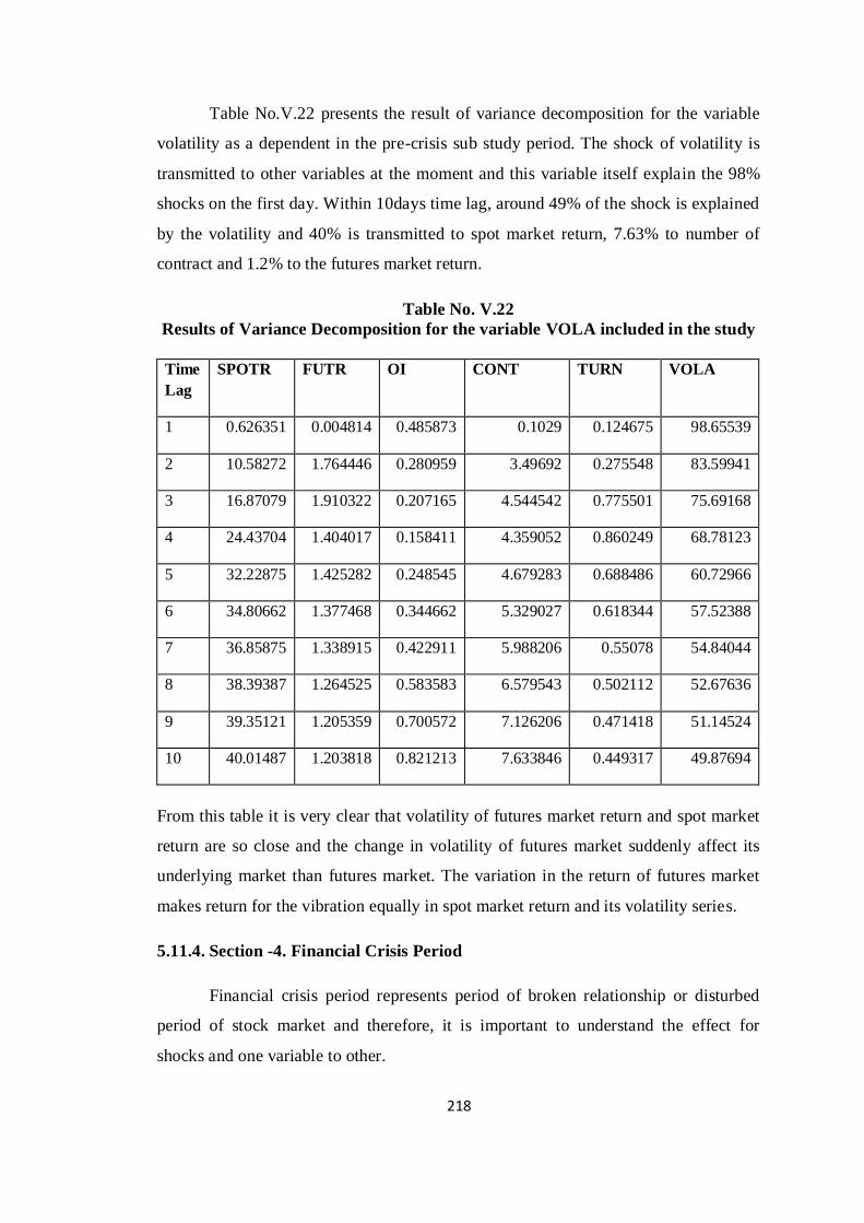
218
Table No.V.22 presents the result of variance decomposition for the variable
volatility as a dependent in the pre-crisis sub study period. The shock of volatility is
transmitted to other variables at the moment and this variable itself explain the 98%
shocks on the first day. Within 10days time lag, around 49% of the shock is explained
by the volatility and 40% is transmitted to spot market return, 7.63% to number of
contract and 1.2% to the futures market return.
Table No. V.22
Results of Variance Decomposition for the variable VOLA included in the study
Time
Lag
SPOTR FUTR OI CONT TURN VOLA
1 0.626351 0.004814 0.485873 0.1029 0.124675 98.65539
2 10.58272 1.764446 0.280959 3.49692 0.275548 83.59941
3 16.87079 1.910322 0.207165 4.544542 0.775501 75.69168
4 24.43704 1.404017 0.158411 4.359052 0.860249 68.78123
5 32.22875 1.425282 0.248545 4.679283 0.688486 60.72966
6 34.80662 1.377468 0.344662 5.329027 0.618344 57.52388
7 36.85875 1.338915 0.422911 5.988206 0.55078 54.84044
8 38.39387 1.264525 0.583583 6.579543 0.502112 52.67636
9 39.35121 1.205359 0.700572 7.126206 0.471418 51.14524
10 40.01487 1.203818 0.821213 7.633846 0.449317 49.87694
From this table it is very clear that volatility of futures market return and spot market
return are so close and the change in volatility of futures market suddenly affect its
underlying market than futures market. The variation in the return of futures market
makes return for the vibration equally in spot market return and its volatility series.
5.11.4. Section -4. Financial Crisis Period
Financial crisis period represents period of broken relationship or disturbed
period of stock market and therefore, it is important to understand the effect for
shocks and one variable to other.
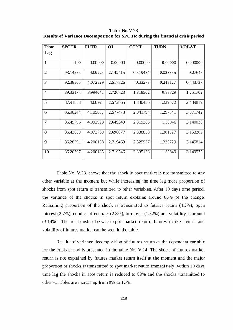
219
Table No.V.23
Results of Variance Decomposition for SPOTR during the financial crisis period
Time
Lag
SPOTR FUTR OI CONT TURN VOLAT
1 100 0.00000 0.00000 0.00000 0.00000 0.000000
2 93.14554 4.09224 2.142415 0.319484 0.023855 0.27647
3 92.38505 4.072529 2.517826 0.33273 0.248127 0.443737
4 89.33174 3.994041 2.720723 1.818502 0.88329 1.251702
5 87.91858 4.00921 2.572865 1.830456 1.229072 2.439819
6 86.90244 4.109007 2.577473 2.041794 1.297541 3.071742
7 86.49796 4.092928 2.649349 2.319263 1.30046 3.140038
8 86.43609 4.072769 2.698077 2.338838 1.301027 3.153202
9 86.28791 4.200158 2.719463 2.325927 1.320729 3.145814
10 86.26707 4.200185 2.719546 2.335128 1.32849 3.149575
Table No. V.23. shows that the shock in spot market is not transmitted to any
other variable at the moment but while increasing the time lag more proportion of
shocks from spot return is transmitted to other variables. After 10 days time period,
the variance of the shocks in spot return explains around 86% of the change.
Remaining proportion of the shock is transmitted to futures return (4.2%), open
interest (2.7%), number of contract (2.3%), turn over (1.32%) and volatility is around
(3.14%). The relationship between spot market return, futures market return and
volatility of futures market can be seen in the table.
Results of variance decomposition of futures return as the dependent variable
for the crisis period is presented in the table No. V.24. The shock of futures market
return is not explained by futures market return itself at the moment and the major
proportion of shocks is transmitted to spot market return immediately, within 10 days
time lag the shocks in spot return is reduced to 88% and the shocks transmitted to
other variables are increasing from 0% to 12%.
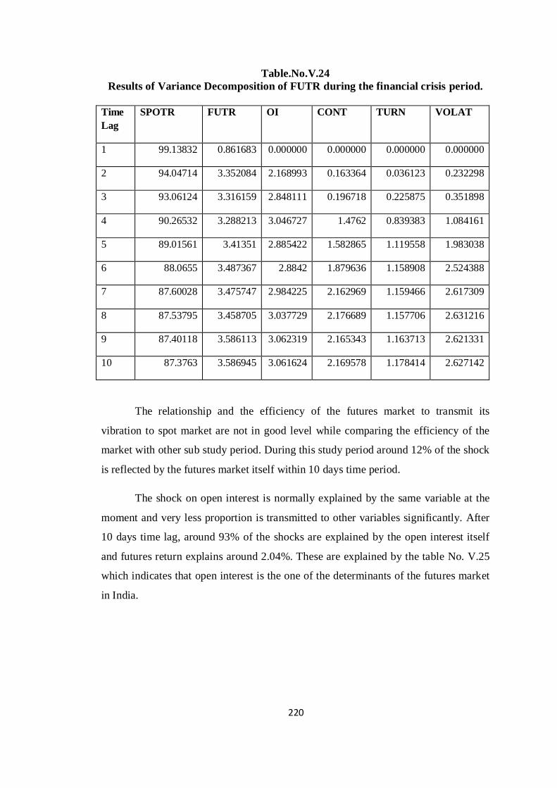
220
Table.No.V.24
Results of Variance Decomposition of FUTR during the financial crisis period.
Time
Lag
SPOTR FUTR OI CONT TURN VOLAT
1 99.13832 0.861683 0.000000 0.000000 0.000000 0.000000
2 94.04714 3.352084 2.168993 0.163364 0.036123 0.232298
3 93.06124 3.316159 2.848111 0.196718 0.225875 0.351898
4 90.26532 3.288213 3.046727 1.4762 0.839383 1.084161
5 89.01561 3.41351 2.885422 1.582865 1.119558 1.983038
6 88.0655 3.487367 2.8842 1.879636 1.158908 2.524388
7 87.60028 3.475747 2.984225 2.162969 1.159466 2.617309
8 87.53795 3.458705 3.037729 2.176689 1.157706 2.631216
9 87.40118 3.586113 3.062319 2.165343 1.163713 2.621331
10 87.3763 3.586945 3.061624 2.169578 1.178414 2.627142
The relationship and the efficiency of the futures market to transmit its
vibration to spot market are not in good level while comparing the efficiency of the
market with other sub study period. During this study period around 12% of the shock
is reflected by the futures market itself within 10 days time period.
The shock on open interest is normally explained by the same variable at the
moment and very less proportion is transmitted to other variables significantly. After
10 days time lag, around 93% of the shocks are explained by the open interest itself
and futures return explains around 2.04%. These are explained by the table No. V.25
which indicates that open interest is the one of the determinants of the futures market
in India.
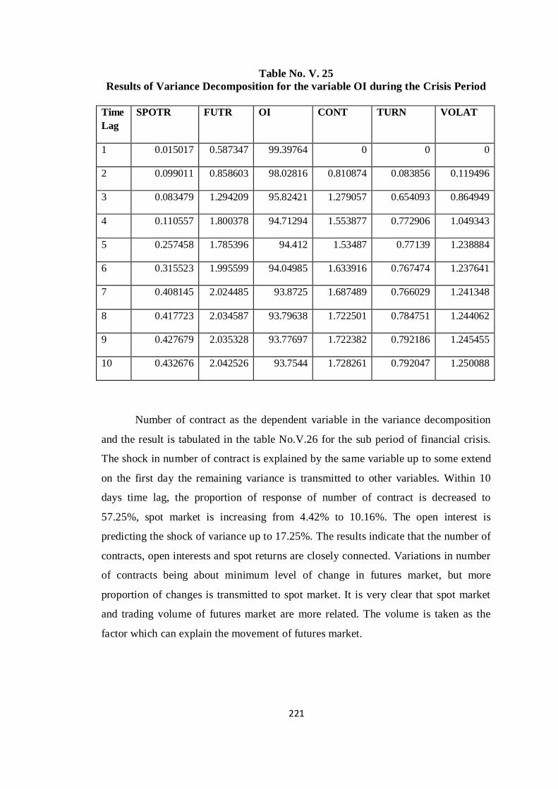
221
Table No. V. 25
Results of Variance Decomposition for the variable OI during the Crisis Period
Time
Lag
SPOTR FUTR OI CONT TURN VOLAT
1 0.015017 0.587347 99.39764 0 0 0
2 0.099011 0.858603 98.02816 0.810874 0.083856 0.119496
3 0.083479 1.294209 95.82421 1.279057 0.654093 0.864949
4 0.110557 1.800378 94.71294 1.553877 0.772906 1.049343
5 0.257458 1.785396 94.412 1.53487 0.77139 1.238884
6 0.315523 1.995599 94.04985 1.633916 0.767474 1.237641
7 0.408145 2.024485 93.8725 1.687489 0.766029 1.241348
8 0.417723 2.034587 93.79638 1.722501 0.784751 1.244062
9 0.427679 2.035328 93.77697 1.722382 0.792186 1.245455
10 0.432676 2.042526 93.7544 1.728261 0.792047 1.250088
Number of contract as the dependent variable in the variance decomposition
and the result is tabulated in the table No.V.26 for the sub period of financial crisis.
The shock in number of contract is explained by the same variable up to some extend
on the first day the remaining variance is transmitted to other variables. Within 10
days time lag, the proportion of response of number of contract is decreased to
57.25%, spot market is increasing from 4.42% to 10.16%. The open interest is
predicting the shock of variance up to 17.25%. The results indicate that the number of
contracts, open interests and spot returns are closely connected. Variations in number
of contracts being about minimum level of change in futures market, but more
proportion of changes is transmitted to spot market. It is very clear that spot market
and trading volume of futures market are more related. The volume is taken as the
factor which can explain the movement of futures market.
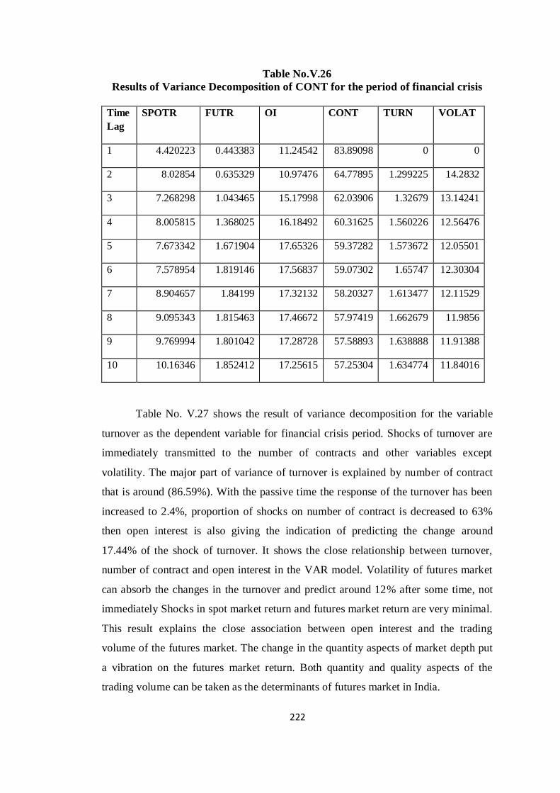
222
Table No.V.26
Results of Variance Decomposition of CONT for the period of financial crisis
Time
Lag
SPOTR FUTR OI CONT TURN VOLAT
1 4.420223 0.443383 11.24542 83.89098 0 0
2 8.02854 0.635329 10.97476 64.77895 1.299225 14.2832
3 7.268298 1.043465 15.17998 62.03906 1.32679 13.14241
4 8.005815 1.368025 16.18492 60.31625 1.560226 12.56476
5 7.673342 1.671904 17.65326 59.37282 1.573672 12.05501
6 7.578954 1.819146 17.56837 59.07302 1.65747 12.30304
7 8.904657 1.84199 17.32132 58.20327 1.613477 12.11529
8 9.095343 1.815463 17.46672 57.97419 1.662679 11.9856
9 9.769994 1.801042 17.28728 57.58893 1.638888 11.91388
10 10.16346 1.852412 17.25615 57.25304 1.634774 11.84016
Table No. V.27 shows the result of variance decomposition for the variable
turnover as the dependent variable for financial crisis period. Shocks of turnover are
immediately transmitted to the number of contracts and other variables except
volatility. The major part of variance of turnover is explained by number of contract
that is around (86.59%). With the passive time the response of the turnover has been
increased to 2.4%, proportion of shocks on number of contract is decreased to 63%
then open interest is also giving the indication of predicting the change around
17.44% of the shock of turnover. It shows the close relationship between turnover,
number of contract and open interest in the VAR model. Volatility of futures market
can absorb the changes in the turnover and predict around 12% after some time, not
immediately Shocks in spot market return and futures market return are very minimal.
This result explains the close association between open interest and the trading
volume of the futures market. The change in the quantity aspects of market depth put
a vibration on the futures market return. Both quantity and quality aspects of the
trading volume can be taken as the determinants of futures market in India.
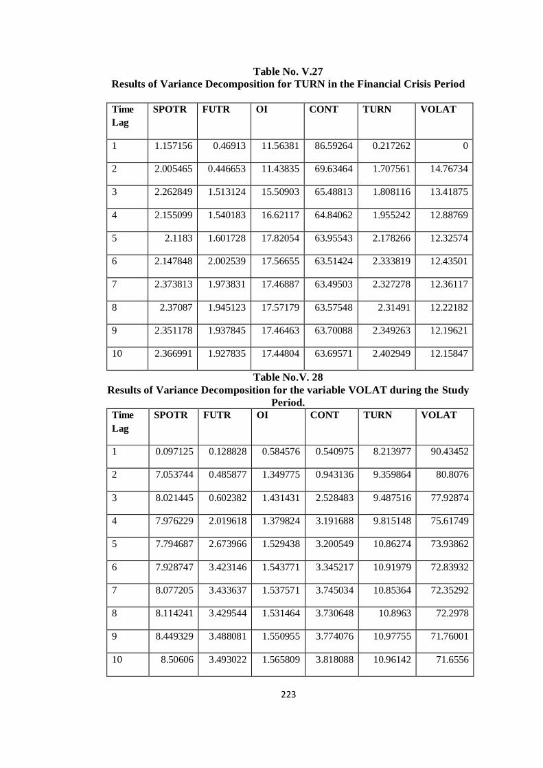
223
Table No. V.27
Results of Variance Decomposition for TURN in the Financial Crisis Period
Time
Lag
SPOTR FUTR OI CONT TURN VOLAT
1 1.157156 0.46913 11.56381 86.59264 0.217262 0
2 2.005465 0.446653 11.43835 69.63464 1.707561 14.76734
3 2.262849 1.513124 15.50903 65.48813 1.808116 13.41875
4 2.155099 1.540183 16.62117 64.84062 1.955242 12.88769
5 2.1183 1.601728 17.82054 63.95543 2.178266 12.32574
6 2.147848 2.002539 17.56655 63.51424 2.333819 12.43501
7 2.373813 1.973831 17.46887 63.49503 2.327278 12.36117
8 2.37087 1.945123 17.57179 63.57548 2.31491 12.22182
9 2.351178 1.937845 17.46463 63.70088 2.349263 12.19621
10 2.366991 1.927835 17.44804 63.69571 2.402949 12.15847
Table No.V. 28
Results of Variance Decomposition for the variable VOLAT during the Study
Period.
Time
Lag
SPOTR FUTR OI CONT TURN VOLAT
1 0.097125 0.128828 0.584576 0.540975 8.213977 90.43452
2 7.053744 0.485877 1.349775 0.943136 9.359864 80.8076
3 8.021445 0.602382 1.431431 2.528483 9.487516 77.92874
4 7.976229 2.019618 1.379824 3.191688 9.815148 75.61749
5 7.794687 2.673966 1.529438 3.200549 10.86274 73.93862
6 7.928747 3.423146 1.543771 3.345217 10.91979 72.83932
7 8.077205 3.433637 1.537571 3.745034 10.85364 72.35292
8 8.114241 3.429544 1.531464 3.730648 10.8963 72.2978
9 8.449329 3.488081 1.550955 3.774076 10.97755 71.76001
10 8.50606 3.493022 1.565809 3.818088 10.96142 71.6556
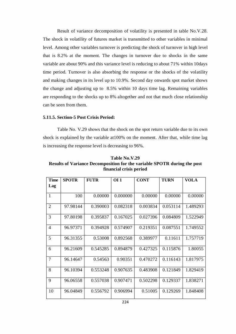
224
Result of variance decomposition of volatility is presented in table No.V.28.
The shock in volatility of futures market is transmitted to other variables in minimal
level. Among other variables turnover is predicting the shock of turnover in high level
that is 8.2% at the moment. The changes in turnover due to shocks in the same
variable are about 90% and this variance level is reducing to about 71% within 10days
time period. Turnover is also absorbing the response or the shocks of the volatility
and making changes in its level up to 10.9%. Second day onwards spot market shows
the change and adjusting up to 8.5% within 10 days time lag. Remaining variables
are responding to the shocks up to 8% altogether and not that much close relationship
can be seen from them.
5.11.5. Section-5 Post Crisis Period:
Table No. V.29 shows that the shock on the spot return variable due to its own
shock is explained by the variable at100% on the moment. After that, while time lag
is increasing the response level is decreasing to 96%.
Table No.V.29
Results of Variance Decomposition for the variable SPOTR during the post
financial crisis period
Time
Lag
SPOTR FUTR OI 1 CONT TURN VOLA
1 100 0.00000 0.000000 0.00000 0.00000 0.00000
2 97.98144 0.390003 0.082318 0.003834 0.053114 1.489293
3 97.80198 0.395837 0.167025 0.027396 0.084809 1.522949
4 96.97371 0.394928 0.574907 0.219351 0.087551 1.749552
5 96.31355 0.53008 0.892568 0.389977 0.11611 1.757719
6 96.21609 0.545285 0.894879 0.427325 0.115876 1.80055
7 96.14647 0.54563 0.90351 0.470272 0.116143 1.817975
8 96.10394 0.553248 0.907635 0.483908 0.121849 1.829419
9 96.06558 0.557038 0.907471 0.502298 0.129337 1.838271
10 96.04849 0.556792 0.906994 0.51005 0.129269 1.848408
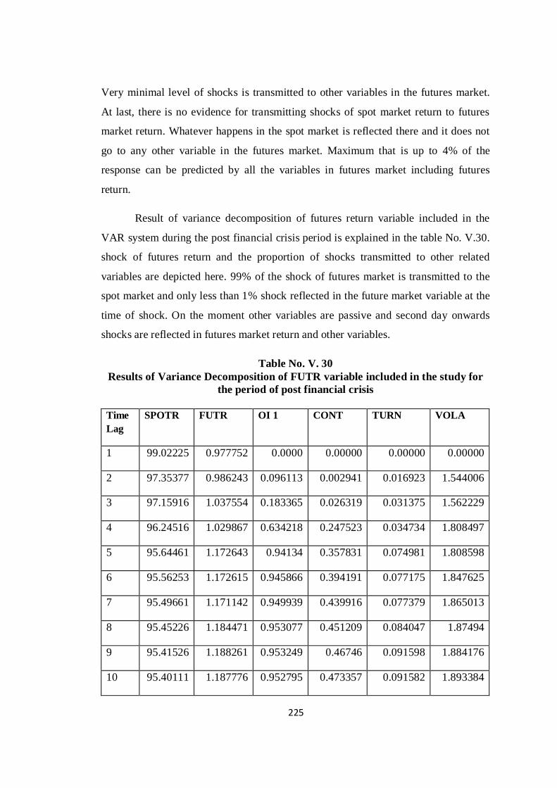
225
Very minimal level of shocks is transmitted to other variables in the futures market.
At last, there is no evidence for transmitting shocks of spot market return to futures
market return. Whatever happens in the spot market is reflected there and it does not
go to any other variable in the futures market. Maximum that is up to 4% of the
response can be predicted by all the variables in futures market including futures
return.
Result of variance decomposition of futures return variable included in the
VAR system during the post financial crisis period is explained in the table No. V.30.
shock of futures return and the proportion of shocks transmitted to other related
variables are depicted here. 99% of the shock of futures market is transmitted to the
spot market and only less than 1% shock reflected in the future market variable at the
time of shock. On the moment other variables are passive and second day onwards
shocks are reflected in futures market return and other variables.
Table No. V. 30
Results of Variance Decomposition of FUTR variable included in the study for
the period of post financial crisis
Time
Lag
SPOTR FUTR OI 1 CONT TURN VOLA
1 99.02225 0.977752 0.0000 0.00000 0.00000 0.00000
2 97.35377 0.986243 0.096113 0.002941 0.016923 1.544006
3 97.15916 1.037554 0.183365 0.026319 0.031375 1.562229
4 96.24516 1.029867 0.634218 0.247523 0.034734 1.808497
5 95.64461 1.172643 0.94134 0.357831 0.074981 1.808598
6 95.56253 1.172615 0.945866 0.394191 0.077175 1.847625
7 95.49661 1.171142 0.949939 0.439916 0.077379 1.865013
8 95.45226 1.184471 0.953077 0.451209 0.084047 1.87494
9 95.41526 1.188261 0.953249 0.46746 0.091598 1.884176
10 95.40111 1.187776 0.952795 0.473357 0.091582 1.893384
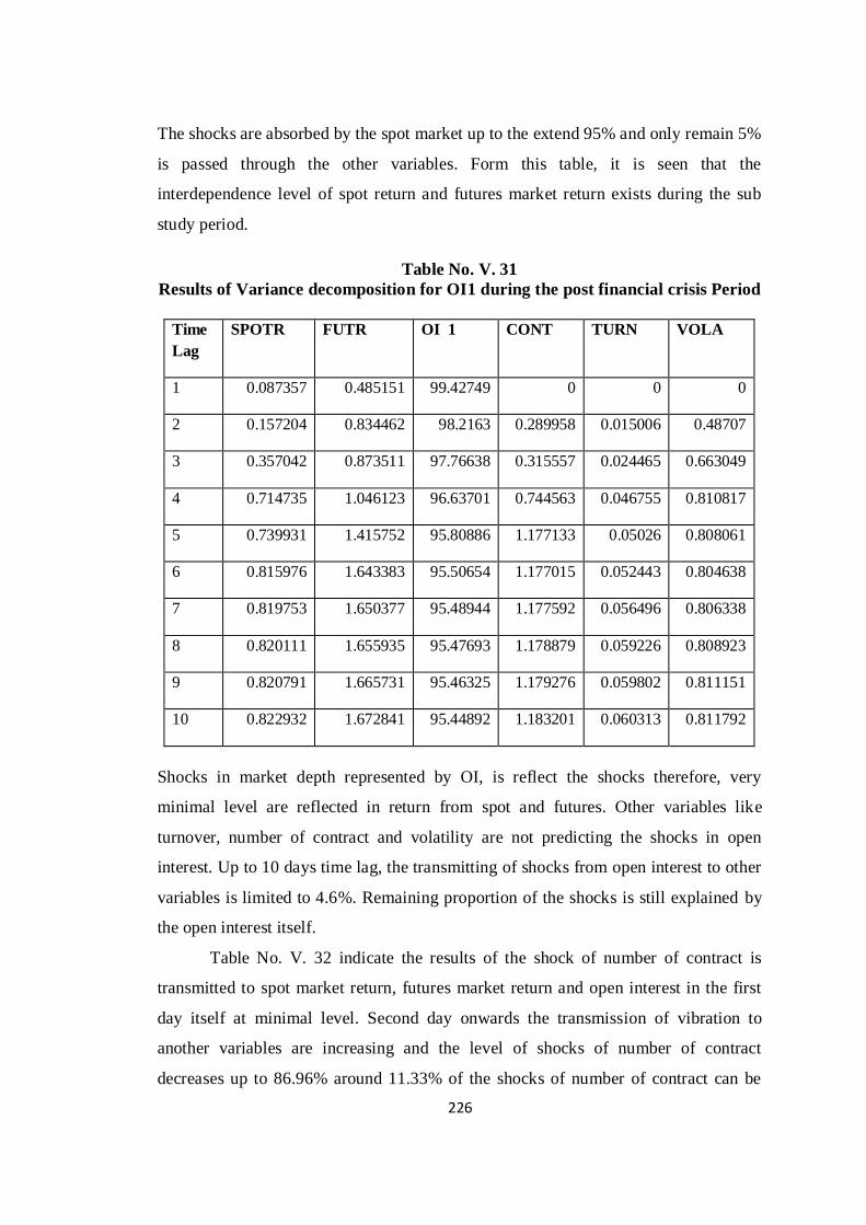
226
The shocks are absorbed by the spot market up to the extend 95% and only remain 5%
is passed through the other variables. Form this table, it is seen that the
interdependence level of spot return and futures market return exists during the sub
study period.
Table No. V. 31
Results of Variance decomposition for OI1 during the post financial crisis Period
Time
Lag
SPOTR FUTR OI 1 CONT TURN VOLA
1 0.087357 0.485151 99.42749 0 0 0
2 0.157204 0.834462 98.2163 0.289958 0.015006 0.48707
3 0.357042 0.873511 97.76638 0.315557 0.024465 0.663049
4 0.714735 1.046123 96.63701 0.744563 0.046755 0.810817
5 0.739931 1.415752 95.80886 1.177133 0.05026 0.808061
6 0.815976 1.643383 95.50654 1.177015 0.052443 0.804638
7 0.819753 1.650377 95.48944 1.177592 0.056496 0.806338
8 0.820111 1.655935 95.47693 1.178879 0.059226 0.808923
9 0.820791 1.665731 95.46325 1.179276 0.059802 0.811151
10 0.822932 1.672841 95.44892 1.183201 0.060313 0.811792
Shocks in market depth represented by OI, is reflect the shocks therefore, very
minimal level are reflected in return from spot and futures. Other variables like
turnover, number of contract and volatility are not predicting the shocks in open
interest. Up to 10 days time lag, the transmitting of shocks from open interest to other
variables is limited to 4.6%. Remaining proportion of the shocks is still explained by
the open interest itself.
Table No. V. 32 indicate the results of the shock of number of contract is
transmitted to spot market return, futures market return and open interest in the first
day itself at minimal level. Second day onwards the transmission of vibration to
another variables are increasing and the level of shocks of number of contract
decreases up to 86.96% around 11.33% of the shocks of number of contract can be
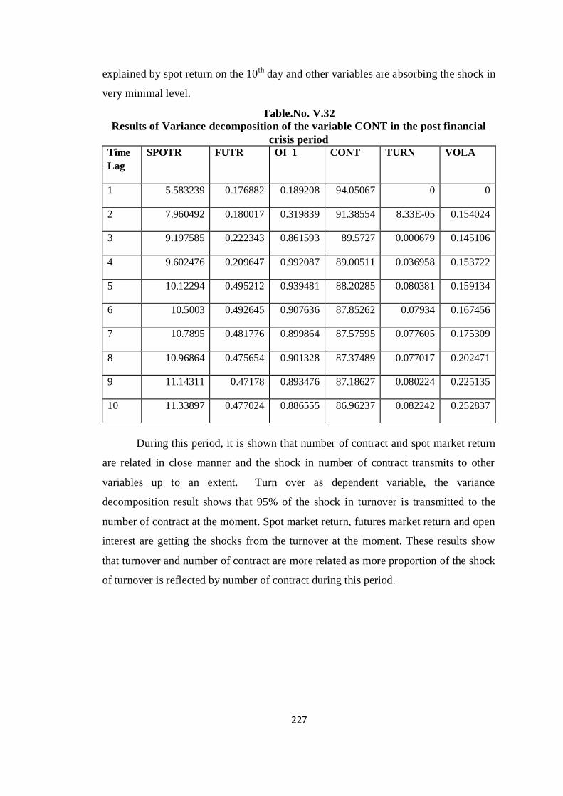
227
explained by spot return on the 10th
day and other variables are absorbing the shock in
very minimal level.
Table.No. V.32
Results of Variance decomposition of the variable CONT in the post financial
crisis period
Time
Lag
SPOTR FUTR OI 1 CONT TURN VOLA
1 5.583239 0.176882 0.189208 94.05067 0 0
2 7.960492 0.180017 0.319839 91.38554 8.33E-05 0.154024
3 9.197585 0.222343 0.861593 89.5727 0.000679 0.145106
4 9.602476 0.209647 0.992087 89.00511 0.036958 0.153722
5 10.12294 0.495212 0.939481 88.20285 0.080381 0.159134
6 10.5003 0.492645 0.907636 87.85262 0.07934 0.167456
7 10.7895 0.481776 0.899864 87.57595 0.077605 0.175309
8 10.96864 0.475654 0.901328 87.37489 0.077017 0.202471
9 11.14311 0.47178 0.893476 87.18627 0.080224 0.225135
10 11.33897 0.477024 0.886555 86.96237 0.082242 0.252837
During this period, it is shown that number of contract and spot market return
are related in close manner and the shock in number of contract transmits to other
variables up to an extent. Turn over as dependent variable, the variance
decomposition result shows that 95% of the shock in turnover is transmitted to the
number of contract at the moment. Spot market return, futures market return and open
interest are getting the shocks from the turnover at the moment. These results show
that turnover and number of contract are more related as more proportion of the shock
of turnover is reflected by number of contract during this period.
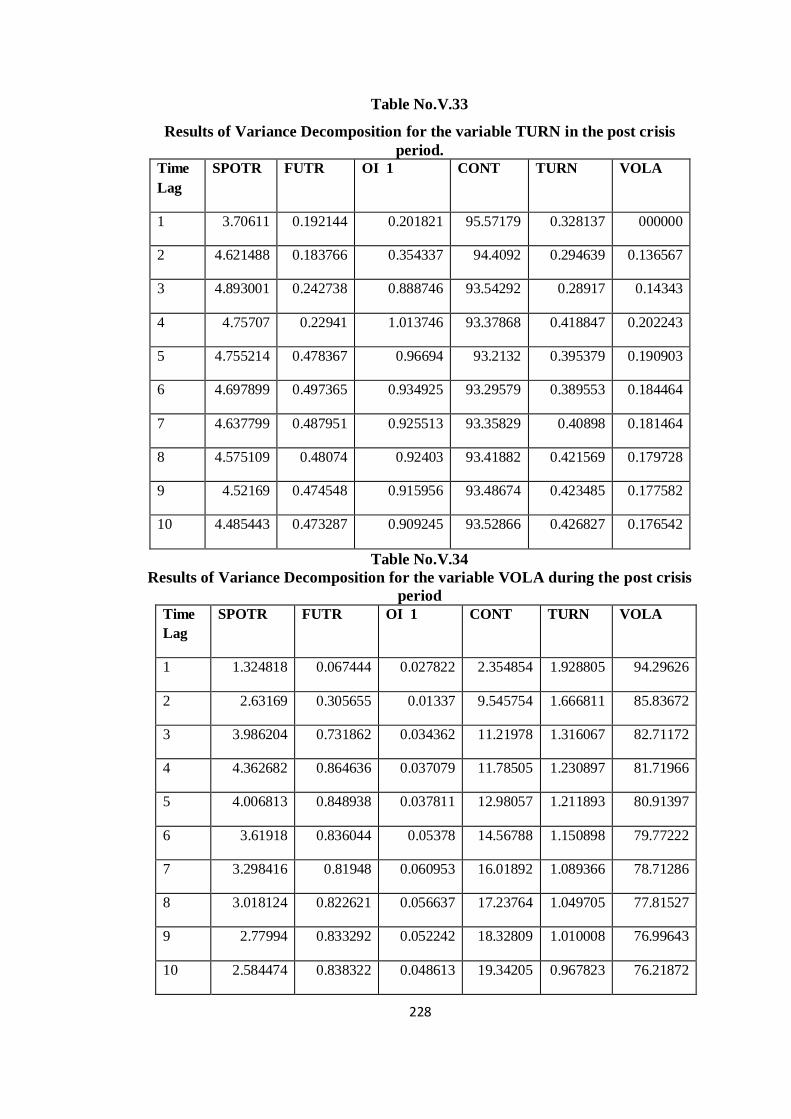
228
Table No.V.33
Results of Variance Decomposition for the variable TURN in the post crisis
period.
Time
Lag
SPOTR FUTR OI 1 CONT TURN VOLA
1 3.70611 0.192144 0.201821 95.57179 0.328137 000000
2 4.621488 0.183766 0.354337 94.4092 0.294639 0.136567
3 4.893001 0.242738 0.888746 93.54292 0.28917 0.14343
4 4.75707 0.22941 1.013746 93.37868 0.418847 0.202243
5 4.755214 0.478367 0.96694 93.2132 0.395379 0.190903
6 4.697899 0.497365 0.934925 93.29579 0.389553 0.184464
7 4.637799 0.487951 0.925513 93.35829 0.40898 0.181464
8 4.575109 0.48074 0.92403 93.41882 0.421569 0.179728
9 4.52169 0.474548 0.915956 93.48674 0.423485 0.177582
10 4.485443 0.473287 0.909245 93.52866 0.426827 0.176542
Table No.V.34
Results of Variance Decomposition for the variable VOLA during the post crisis
period
Time
Lag
SPOTR FUTR OI 1 CONT TURN VOLA
1 1.324818 0.067444 0.027822 2.354854 1.928805 94.29626
2 2.63169 0.305655 0.01337 9.545754 1.666811 85.83672
3 3.986204 0.731862 0.034362 11.21978 1.316067 82.71172
4 4.362682 0.864636 0.037079 11.78505 1.230897 81.71966
5 4.006813 0.848938 0.037811 12.98057 1.211893 80.91397
6 3.61918 0.836044 0.05378 14.56788 1.150898 79.77222
7 3.298416 0.81948 0.060953 16.01892 1.089366 78.71286
8 3.018124 0.822621 0.056637 17.23764 1.049705 77.81527
9 2.77994 0.833292 0.052242 18.32809 1.010008 76.99643
10 2.584474 0.838322 0.048613 19.34205 0.967823 76.21872
229
Table No. V.34 presents the result that on the first day itself the shocks in
volatility is transmitted to other variables in very low level. Second day onwards the
proportion of shocks reflected by volatility is reducing and the proportion of shocks to
other variables are increasing. Around 19% of shocks are transmitted to number of
contract and other variables observe very minimum level of shock from the volatility
variable. The thorough analysis in variance decomposition result help to understand
the proportion of shock explained by each variable and level of proportion of shocks
transmitted to another variable during different study period and for a very short run
period like 10 days time lag.
V.12. CONCLUSION
This chapter makes an attempt to satisfy the third objective of the study such
as to find determinants of futures market in India. Futures market return is the
variable of futures market and other all components like open interest, turnover of
futures market, number of contract, volatility series of futures return is estimated by
using GARCH (1,1) model are included in the study. In order to understand the real
movement of the futures market and a part of robustness checking, the whole study
period 12th
June 2000- 30th
June 2011 is divided in to four sub-periods such as
introduction and development period of derivatives market in India, pre- financial
crisis period, financial crisis period and post financial crisis period. The role of each
variable separately and all together is analyzed by using three econometrics model
such as Vector Autoregressive Granger Causality/ Block Exogeneity Test, Impulse
Response Function and Variance Decomposition of each variable as dependent.
Futures market return (FUTR), spot market return (FUTR), turnover (TURN), open
interest (OI), number of contract (CONT) and volatility of futures market (VOL) are
the variables used in this chapter. In the whole study period, all variables are in
stationary in its level. Futures market return and spot market return are the first
difference of their price series. Augmented Dickey Fuller (ADF) and Philip Perron
(PP) unit root test are applied and in ADF test AIC criterion is used to select
maximum lag length. Both test results indicate that the null hypothesis of the unit root
test is rejected at 5% &1% level of significance. During the development period, all
variables included for the analysis except number of contract and turnover are in I (0)
process. ADF test results accept the null hypothesis but PP test cannot find the
230
possibility to accept the null hypothesis that there is unit root, then number of contract
is non stationary in its level form and stationary at its first difference.
In order to make them suitable for the model, they are transformed in to first
difference. In pre- financial crisis period, all variables are found stationary in its level
form. Crisis period also shows the same result and support all variables are in
stationarity process. But in post financial crisis period, all included variables except
open interest are in I (0) process, then open interest variable is used in first difference.
VAR lag order selection criteria such as likelihood Ratio, Final Prediction Error and
Akaika Information Criteria are used to select optimal lag length for the different
model for various study periods.
V.12.1. Determinants
The short term causal relationship between each variable in the study is
analyzed and find the role of each variable individually and together to determine the
movement of futures market. For the whole study period, it is found that all variables
together is causing the futures market movement and the relationship of each variable
to futures market is to be taken in to consideration. In the introduction and
development stage, spot market is individually influencing the futures market and the
all variable together is also having the causal relationship with Nifty futures market.
The inter relationship between each variable and their influence can also be seen there
in the result. In pre- financial crisis period, Nifty spot market, number of contract of
Nifty futures market and turnover of the futures market are individually influencing
Nifty futures market. In financial crisis period, unfortunately the established
relationships are not seen. Inter relationships between all variables in the futures
market is disappeared. There is only one relationship that is relationship between
number of contract and turnover, but they do not have any causal relationship with
futures market during this crisis period. During post financial crisis period also all
included factors have relationship with futures market. During this period number of
contract is having individual linkage with futures market. From this analysis, it is
revealed that Nifty spot market return is the key indicator of Nifty futures market and
other variables like futures market open interest, number of contract, turnover and
volatility of futures market are to be considered as the determinants of futures market.
231
V.12.2. Time profile and Proportion of Shocks
The positive and negative response of each variable and causal relationship is
found through the impulse response function. This result shows that there is positive
significant response from the futures and spot market shocks. Variance decomposition
result explains the response and shocks of each variable and the proportion of the
shock transmitted to the other variables at the moment and one day or within 10 days.
On the basis of the empirical results the null hypothesis of the study such as
spot return pays very negligible role in determining futures return is rejected. It is
found that spot return is the key factor which can be considered as the determinants of
the futures market due to the informational efficiency of futures market. The another
null hypothesis that is open interest, trading volume, volatility of futures return and
number of contract are not the determinants of futures return is also rejected. This
analysis found that spot return, turnover, open interest, futures market volatility and
number of contracts are playing a vital role to predict the movement of futures market
because of their causal relationship among them.
To conclude, the variables which are used here are having effect on futures
market. Nifty spot market return, turnover, open interest, futures market volatility and
futures market number of contracts are taken as the determinants of futures in India.
Any one is taking the decision on futures contract should consider the above said all
factors as the determinants to predict the movement of futures market.
232
Chapter –VI
Risk Reduction Efficiency
of Futures Market
in India
233
CHAPTER- VI
RISK REDUCTION EFFICIENCY OF
FUTURES MARKET IN INDIA
6.1. INTRODUCTION
Principal functions of futures market are price discovery, speculation, risk
sharing and hedging (Johnson 1960, Silber 1985, Fortune 1989, Jahangir sultan et.al
2010). The spot market of equity futures market is playing a vital role to provide two
benefits such as long term capital appreciation and regular income to its players. Even
though futures market is the expectation of the underlying market, its consistency
cannot be predicted and the number of traders in futures market is really different
from spot market. Long term benefit of cash market is earned by the investors and
short run changes are exploited by the speculators. Changes in different market are
actually transmitted in to profit by the efforts of arbitrageurs. The entry of futures
market encourages arbitragers, promotes investors and helps the hedgers who are
interested to minimize the risk level of their investment by taking the opposite
position in cash as well as futures market. Another category is the speculators those
are violating the established relations of the market and making profit from the
variation in prices of stocks.
Hedgers use the futures market as means to avoid the risk associated with
price changes in the underlying cash market. They try to earn maximum return with
the minimal risk or to avoid maximum risk with reduction in minimal level of return.
Taking opposite position in futures market is the way to protect the risk involving the
spot asset due to change in the asset value. Technically, it is known as hedging,
practically, the number of units of opposite position to be taken to protect one unit
position in spot market is making confusion to the traders and the traditional that is
naive hedge ratio is 1:1. The hedge ratio is the number of futures contract which are
needed to maximize the exposure of a unit worth of position in the cash market.
234
According to Hull (2003) hedge ratio is the ratio of the size of the position taken in
futures contract to the size of exposure in cash market. It is very difficult to make a
perfect hedge ratio in the time varying and more volatile market, in short, a perfectly
correlated hedging instrument is not available in futures market.
Conventional view of hedging and hedge ratio which is estimated through
regression also is challenged by Holbrook (1953), then he supported the multipurpose
concept of hedging. He argues that the hedgers are basically risk lovers and the prime
aim is to maximize profit. They do not aim to minimize risk without maximizing of
profit. The theory of maximization of profit is the prime motive of the hedgers is
challenged and argued that the objective of hedging is to maximize the variance of the
assets port folio held by the investor, Johnson (1960) and Edirington (1979). Further
they argued that during 1980, researchers employed the traditional regression analysis
assuming that the optimal hedge ratio is time variant.
The conventional approach for optimal hedge ratio is to regress historical cash
prices, price changes or return on futures prices. The resulting slope coefficient is then
used as the estimated optimal hedge ratio (Ederington 1979, khal 1983, Myers 2000).
There are two problems with the conventional regression approach to optimal hedge
ratio estimation. The first problem is that it fails to take proper account of all of the
relevant conditioning information available to the hedgers when they make their
hedging decision (Myer and Thompson 1989) and the second is that it implicitly
assumes that the covariance matrix of cash and futures prices and hence optimal
hedge ratio are constant over time (Myers 2000).
The development of Generalized Autoregressive Conditional Heteroskedastic
(GARCH) modeling techniques to deal with time varying volatility has generated
interest on the empirical analysis on the effectiveness of dynamic hedging that allows
the hedge ratio to be time varying (Jahangir Sultan 2010). The hedge ratio equal to the
ratio of covariance between cash and futures prices to the variance of the futures price
(Anderson et.al and Benninga 1984). GARCH model of Bollerslev (1986) provides a
flexible and consistent framework for estimating time varying optimal hedge ratio, but
requires non linear maximum likely estimator. The GARCH model represents a
flexible specification for modeling time varying volatility in assets prices and
235
maximum likely hood is an optimal approach to inferences. This model is having
significant theoretical advantages over moving sample variances and covariance.
There are many studies which empirically revealed the disadvantages of
different econometrics model for estimating optimal hedge ratio. Hedge ratio obtained
from the regression methodology becomes biased one if there exists a cointegration
relationship between the spot and futures return (Saumitra etal.2010). In this context
vector error correction model to estimate the hedge ratio is suggested by Kroner and
Sultan (1993). These empirical methodologies are criticized due to the unconditional
moment and the constant hedge ratio does not consider the fact, the joint distribution
of spot and futures prices varies over time (Cecchetti, 1988). A multivariate GARCH
method developed by Bollerslev, Engle and Wooldridge (1988) is to be used to
estimate the time varying hedge ratio by considering the conditional variance and
covariance of spot and futures market return.
In order to satisfy the objective of the study of finding out the risk reduction
efficiency of futures market in India by estimating the optimal hedge ratio of
S&PCNX Nifty index and other 19 individual stocks in Nifty index, multivariate
Diagonal Vector –GARCH model is used. Risk sharing or risk reduction is one of the
important objectives of futures market. Hedging can be taken as the one of the means
to determine the function of futures market. The market players take simultaneous but
opposite trading position in to markets with the magnitude of prediction of one market
through other are known as the hedge ratio. Estimation of hedge ratio is a statistical
process which involves regressing cash market return on futures market (Kapil Gupta
et al, 2009).
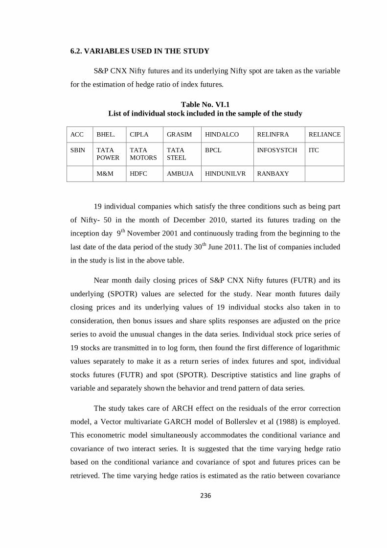
236
6.2. VARIABLES USED IN THE STUDY
S&P CNX Nifty futures and its underlying Nifty spot are taken as the variable
for the estimation of hedge ratio of index futures.
Table No. VI.1
List of individual stock included in the sample of the study
ACC BHEL. CIPLA GRASIM HINDALCO RELINFRA RELIANCE
SBIN TATA
POWER
TATA
MOTORS
TATA
STEEL
BPCL INFOSYSTCH ITC
M&M HDFC AMBUJA HINDUNILVR RANBAXY
19 individual companies which satisfy the three conditions such as being part
of Nifty- 50 in the month of December 2010, started its futures trading on the
inception day 9th
November 2001 and continuously trading from the beginning to the
last date of the data period of the study 30th June 2011. The list of companies included
in the study is list in the above table.
Near month daily closing prices of S&P CNX Nifty futures (FUTR) and its
underlying (SPOTR) values are selected for the study. Near month futures daily
closing prices and its underlying values of 19 individual stocks also taken in to
consideration, then bonus issues and share splits responses are adjusted on the price
series to avoid the unusual changes in the data series. Individual stock price series of
19 stocks are transmitted in to log form, then found the first difference of logarithmic
values separately to make it as a return series of index futures and spot, individual
stocks futures (FUTR) and spot (SPOTR). Descriptive statistics and line graphs of
variable and separately shown the behavior and trend pattern of data series.
The study takes care of ARCH effect on the residuals of the error correction
model, a Vector multivariate GARCH model of Bollerslev et al (1988) is employed.
This econometric model simultaneously accommodates the conditional variance and
covariance of two interact series. It is suggested that the time varying hedge ratio
based on the conditional variance and covariance of spot and futures prices can be
retrieved. The time varying hedge ratios is estimated as the ratio between covariance
237
of spot and futures price with variance of futures price. Time varying hedge ratio
isfft
sft
h
h.This study estimates the Diagonal VEC multivariate GARCH model of
Bollersev et al (1988). The estimated results of the DVECV model specified in
equation 111
2
111 sststsssst hch , 133
2
133 fftftfffft hch are presented in
the results of DVEC GARCH coefficient tables.
6.3. METHODOLOGY ADOPTED
Futures and spot daily closing price series of Nifty futures, ACC,AMBUJA,
BHEL, BPCL, CIPLA, GRASIM, HDFC, HINDALCO, HINDULVR,
INFOSYSTCH, ITC, M&M, RANBAXY and TATA STEEL are considered as the
variable to make an empirical analysis on the estimation of optimal hedge ratio of
S&P CNX Nifty and other 19 individual stocks which are being the part of Nifty -50,
those stated their business form the inception date and continuously trading in the
market up to 30th
June 2011. The important steps followed to estimate optimal hedge
are-
1. Near month daily closing prices of futures and its underlying spot price series
are selected.
2. The selected closing price series of spot and futures are changed in to log
form.
3. First difference of logarithmic values is determined to get the return series.
4. Summery statistics of each variable is calculated.
5. Line graphs of variables are presented.
6. Stationarity of the variables is checked through ADF and PP test statistics.
7. Corlogram is used to find the lag length of the model.
8. Diagonal Vector GARCH model is applied to calculate variance of futures,
variance of spot and covariance of spot and futures.
238
9. Time varying hedge ratio is determined by dividing the covariance of spot and
futures with variance of futures.
10. Optimal hedge ratio is estimated by taking the mean of daily hedge ratios of
individual company and index futures of a particular period,
11. Optimal hedge ratio for the index and individual stocks for various study
periods is estimated for checking the robustness.
6.4. RATIONALE FOR THE ANALYSIS
One of the important functions of futures market is hedging (Johnson 1960,
Fortune 1989, Jahangir Sulthan 2008). Hedging is the process of taking opposite
position in the futures market to protect the spot market asset which may lose its
value due to the volatile behavior of the market. Naive hedge ratio 1 is not proper
and the development of GARCH modeling technique has made an interest in the
empirical analysis on the effectiveness of the dynamic hedging. Conventional
approach to hedging has problem as it fails to take the proper account of related
conditioning information and assuming that hedge ratio are constant over time
(Myer& Thompson 1989). Further, it is confirmed that for estimating hedge ratio,
methodology based on ordinary least square may not be reliable (Kapil Gupta et. al
2009). Stocks returns are heteroskedastic in nature. So, ARCH model may be to
obtain robust statistical estimation and it may capturer the stylized behavior of
conditional volatility of market return. A bivariate GARCH methodology which is
developed by Bollerslev, Engle and Wooldrige (1988) can be used to estimate the
time varying hedge ratio (Bhaduri et. al.2008). This study makes an attempt to use
Diagonal VEC- GARCH model to estimate time varying hedge ratio and find the
optimal hedge ratio for the study. This chapter presents the results of an empirical
analysis of risk reduction efficiency in the Indian futures market.
The average value of the time varying hedge ratio series of index futures and
other 19 individuals stocks are used to estimate optimal hedge ratio for the various
sub study periods. The optimal hedge ratio estimated from the DVEC GARCH model
is presented in table no.VI.5.
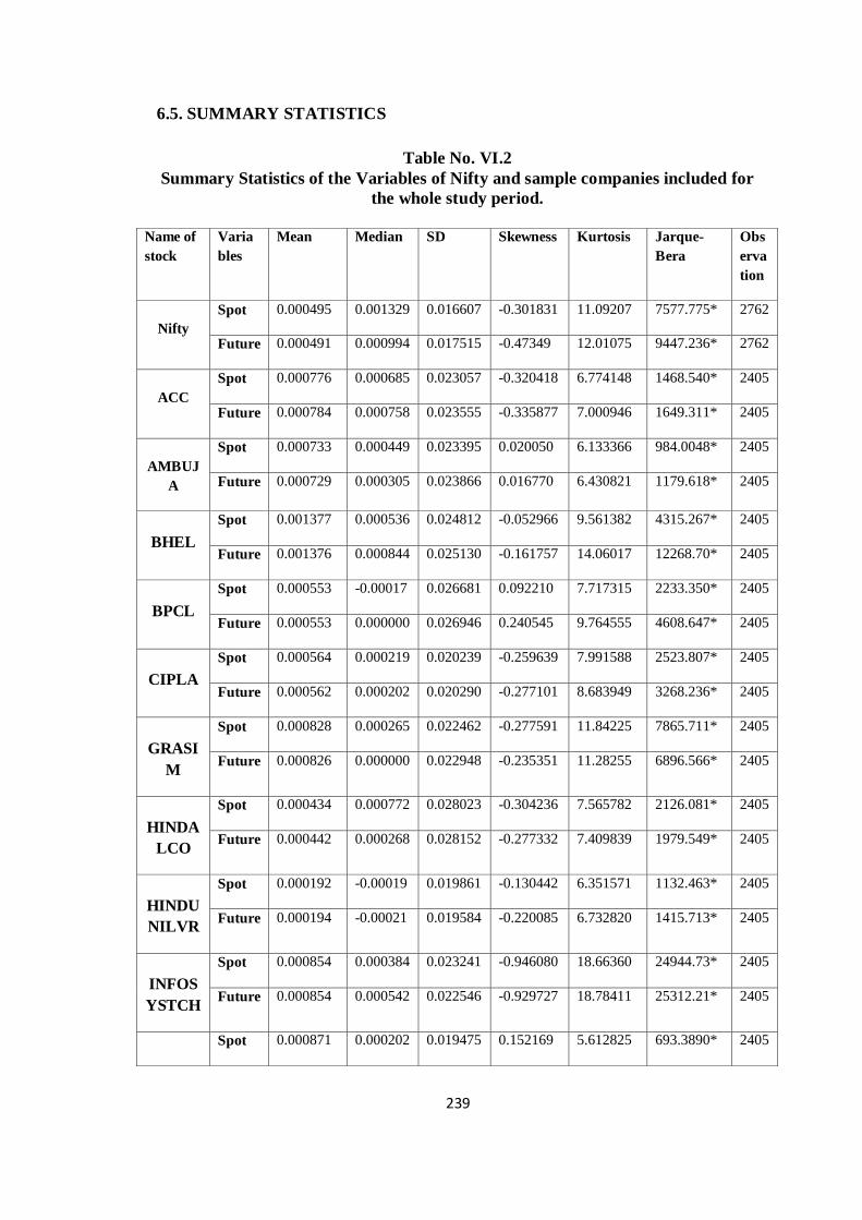
239
6.5. SUMMARY STATISTICS
Table No. VI.2
Summary Statistics of the Variables of Nifty and sample companies included for
the whole study period.
Name of
stock
Varia
bles
Mean Median SD Skewness Kurtosis Jarque-
Bera
Obs
erva
tion
Nifty
Spot 0.000495 0.001329 0.016607 -0.301831 11.09207 7577.775* 2762
Future 0.000491 0.000994 0.017515 -0.47349 12.01075 9447.236* 2762
ACC
Spot 0.000776 0.000685 0.023057 -0.320418 6.774148 1468.540* 2405
Future 0.000784 0.000758 0.023555 -0.335877 7.000946 1649.311* 2405
AMBUJ
A
Spot 0.000733 0.000449 0.023395 0.020050 6.133366 984.0048* 2405
Future 0.000729 0.000305 0.023866 0.016770 6.430821 1179.618* 2405
BHEL
Spot 0.001377 0.000536 0.024812 -0.052966 9.561382 4315.267* 2405
Future 0.001376 0.000844 0.025130 -0.161757 14.06017 12268.70* 2405
BPCL
Spot 0.000553 -0.00017 0.026681 0.092210 7.717315 2233.350* 2405
Future 0.000553 0.000000 0.026946 0.240545 9.764555 4608.647* 2405
CIPLA
Spot 0.000564 0.000219 0.020239 -0.259639 7.991588 2523.807* 2405
Future 0.000562 0.000202 0.020290 -0.277101 8.683949 3268.236* 2405
GRASI
M
Spot 0.000828 0.000265 0.022462 -0.277591 11.84225 7865.711* 2405
Future 0.000826 0.000000 0.022948 -0.235351 11.28255 6896.566* 2405
HINDA
LCO
Spot 0.000434 0.000772 0.028023 -0.304236 7.565782 2126.081* 2405
Future 0.000442 0.000268 0.028152 -0.277332 7.409839 1979.549* 2405
HINDU
NILVR
Spot 0.000192 -0.00019 0.019861 -0.130442 6.351571 1132.463* 2405
Future 0.000194 -0.00021 0.019584 -0.220085 6.732820 1415.713* 2405
INFOS
YSTCH
Spot 0.000854 0.000384 0.023241 -0.946080 18.66360 24944.73* 2405
Future 0.000854 0.000542 0.022546 -0.929727 18.78411 25312.21* 2405
Spot 0.000871 0.000202 0.019475 0.152169 5.612825 693.3890* 2405
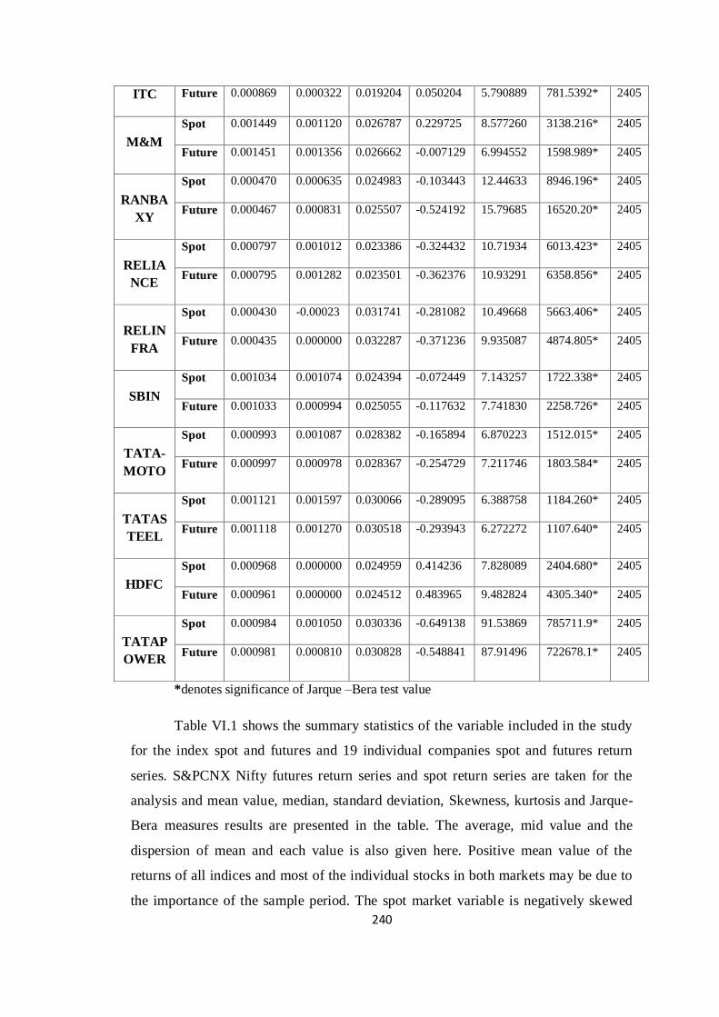
240
*denotes significance of Jarque –Bera test value
Table VI.1 shows the summary statistics of the variable included in the study
for the index spot and futures and 19 individual companies spot and futures return
series. S&PCNX Nifty futures return series and spot return series are taken for the
analysis and mean value, median, standard deviation, Skewness, kurtosis and Jarque-
Bera measures results are presented in the table. The average, mid value and the
dispersion of mean and each value is also given here. Positive mean value of the
returns of all indices and most of the individual stocks in both markets may be due to
the importance of the sample period. The spot market variable is negatively skewed
ITC Future 0.000869 0.000322 0.019204 0.050204 5.790889 781.5392* 2405
M&M
Spot 0.001449 0.001120 0.026787 0.229725 8.577260 3138.216* 2405
Future 0.001451 0.001356 0.026662 -0.007129 6.994552 1598.989* 2405
RANBA
XY
Spot 0.000470 0.000635 0.024983 -0.103443 12.44633 8946.196* 2405
Future 0.000467 0.000831 0.025507 -0.524192 15.79685 16520.20* 2405
RELIA
NCE
Spot 0.000797 0.001012 0.023386 -0.324432 10.71934 6013.423* 2405
Future 0.000795 0.001282 0.023501 -0.362376 10.93291 6358.856* 2405
RELIN
FRA
Spot 0.000430 -0.00023 0.031741 -0.281082 10.49668 5663.406* 2405
Future 0.000435 0.000000 0.032287 -0.371236 9.935087 4874.805* 2405
SBIN
Spot 0.001034 0.001074 0.024394 -0.072449 7.143257 1722.338* 2405
Future 0.001033 0.000994 0.025055 -0.117632 7.741830 2258.726* 2405
TATA-
MOTO
Spot 0.000993 0.001087 0.028382 -0.165894 6.870223 1512.015* 2405
Future 0.000997 0.000978 0.028367 -0.254729 7.211746 1803.584* 2405
TATAS
TEEL
Spot 0.001121 0.001597 0.030066 -0.289095 6.388758 1184.260* 2405
Future 0.001118 0.001270 0.030518 -0.293943 6.272272 1107.640* 2405
HDFC
Spot 0.000968 0.000000 0.024959 0.414236 7.828089 2404.680* 2405
Future 0.000961 0.000000 0.024512 0.483965 9.482824 4305.340* 2405
TATAP
OWER
Spot 0.000984 0.001050 0.030336 -0.649138 91.53869 785711.9* 2405
Future 0.000981 0.000810 0.030828 -0.548841 87.91496 722678.1* 2405
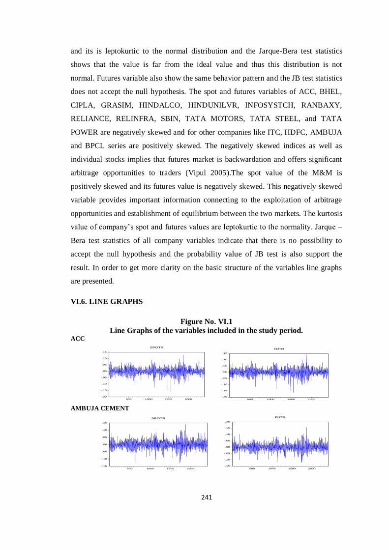
241
and its is leptokurtic to the normal distribution and the Jarque-Bera test statistics
shows that the value is far from the ideal value and thus this distribution is not
normal. Futures variable also show the same behavior pattern and the JB test statistics
does not accept the null hypothesis. The spot and futures variables of ACC, BHEL,
CIPLA, GRASIM, HINDALCO, HINDUNILVR, INFOSYSTCH, RANBAXY,
RELIANCE, RELINFRA, SBIN, TATA MOTORS, TATA STEEL, and TATA
POWER are negatively skewed and for other companies like ITC, HDFC, AMBUJA
and BPCL series are positively skewed. The negatively skewed indices as well as
individual stocks implies that futures market is backwardation and offers significant
arbitrage opportunities to traders (Vipul 2005).The spot value of the M&M is
positively skewed and its futures value is negatively skewed. This negatively skewed
variable provides important information connecting to the exploitation of arbitrage
opportunities and establishment of equilibrium between the two markets. The kurtosis
value of company’s spot and futures values are leptokurtic to the normality. Jarque –
Bera test statistics of all company variables indicate that there is no possibility to
accept the null hypothesis and the probability value of JB test is also support the
result. In order to get more clarity on the basic structure of the variables line graphs
are presented.
VI.6. LINE GRAPHS
Figure No. VI.1
Line Graphs of the variables included in the study period. ACC
-.20
-.15
-.10
-.05
.00
.05
.10
.15
500 1000 1500 2000
SPOTR
-.20
-.15
-.10
-.05
.00
.05
.10
.15
500 1000 1500 2000
FUTR
AMBUJA CEMENT
-.15
-.10
-.05
.00
.05
.10
.15
500 1000 1500 2000
SPOTR
-.15
-.10
-.05
.00
.05
.10
.15
.20
500 1000 1500 2000
FUTR
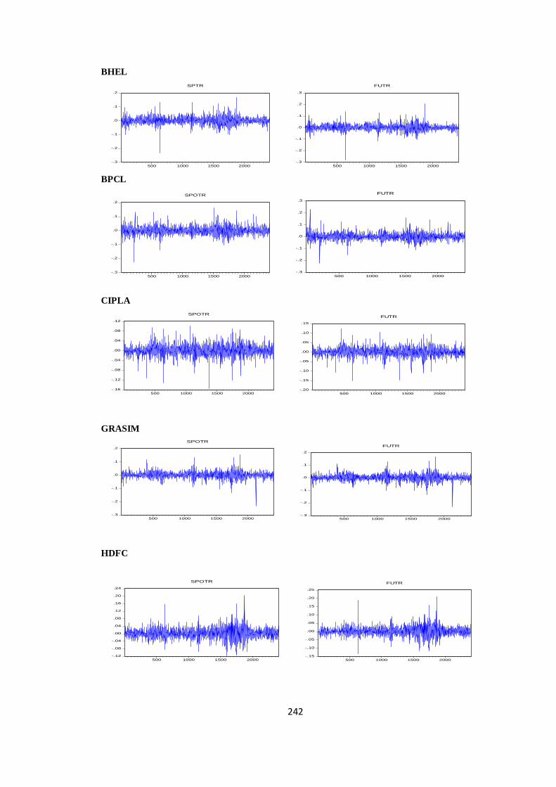
242
BHEL
-.3
-.2
-.1
.0
.1
.2
500 1000 1500 2000
SPTR
-.3
-.2
-.1
.0
.1
.2
.3
500 1000 1500 2000
FUTR
BPCL
-.3
-.2
-.1
.0
.1
.2
500 1000 1500 2000
SPOTR
-.3
-.2
-.1
.0
.1
.2
.3
500 1000 1500 2000
FUTR
CIPLA
-.16
-.12
-.08
-.04
.00
.04
.08
.12
500 1000 1500 2000
SPOTR
-.20
-.15
-.10
-.05
.00
.05
.10
.15
500 1000 1500 2000
FUTR
GRASIM
-.3
-.2
-.1
.0
.1
.2
500 1000 1500 2000
SPOTR
-.3
-.2
-.1
.0
.1
.2
500 1000 1500 2000
FUTR
HDFC
-.12
-.08
-.04
.00
.04
.08
.12
.16
.20
.24
500 1000 1500 2000
SPOTR
-.15
-.10
-.05
.00
.05
.10
.15
.20
.25
500 1000 1500 2000
FUTR
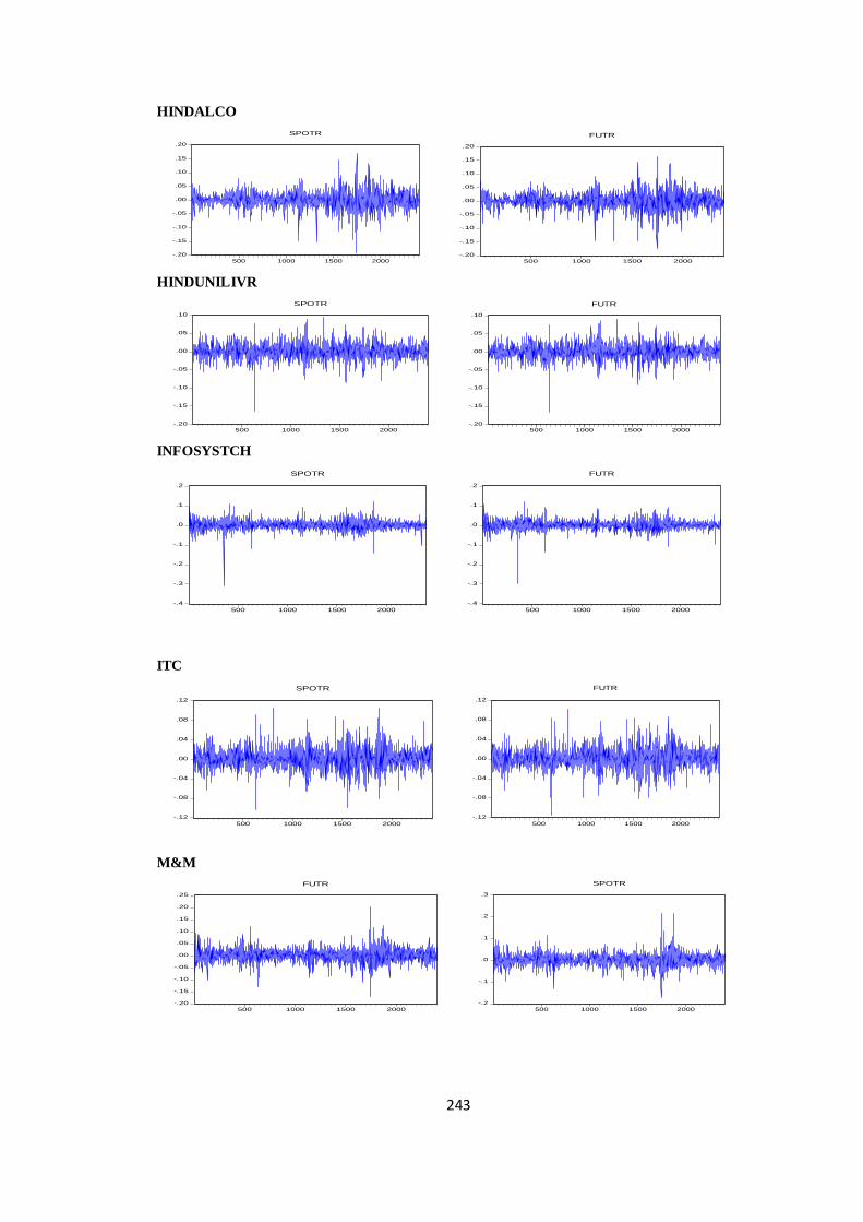
243
HINDALCO
-.20
-.15
-.10
-.05
.00
.05
.10
.15
.20
500 1000 1500 2000
SPOTR
-.20
-.15
-.10
-.05
.00
.05
.10
.15
.20
500 1000 1500 2000
FUTR
HINDUNILIVR
-.20
-.15
-.10
-.05
.00
.05
.10
500 1000 1500 2000
SPOTR
-.20
-.15
-.10
-.05
.00
.05
.10
500 1000 1500 2000
FUTR
INFOSYSTCH
-.4
-.3
-.2
-.1
.0
.1
.2
500 1000 1500 2000
SPOTR
-.4
-.3
-.2
-.1
.0
.1
.2
500 1000 1500 2000
FUTR
ITC
-.12
-.08
-.04
.00
.04
.08
.12
500 1000 1500 2000
SPOTR
-.12
-.08
-.04
.00
.04
.08
.12
500 1000 1500 2000
FUTR
M&M
-.20
-.15
-.10
-.05
.00
.05
.10
.15
.20
.25
500 1000 1500 2000
FUTR
-.2
-.1
.0
.1
.2
.3
500 1000 1500 2000
SPOTR
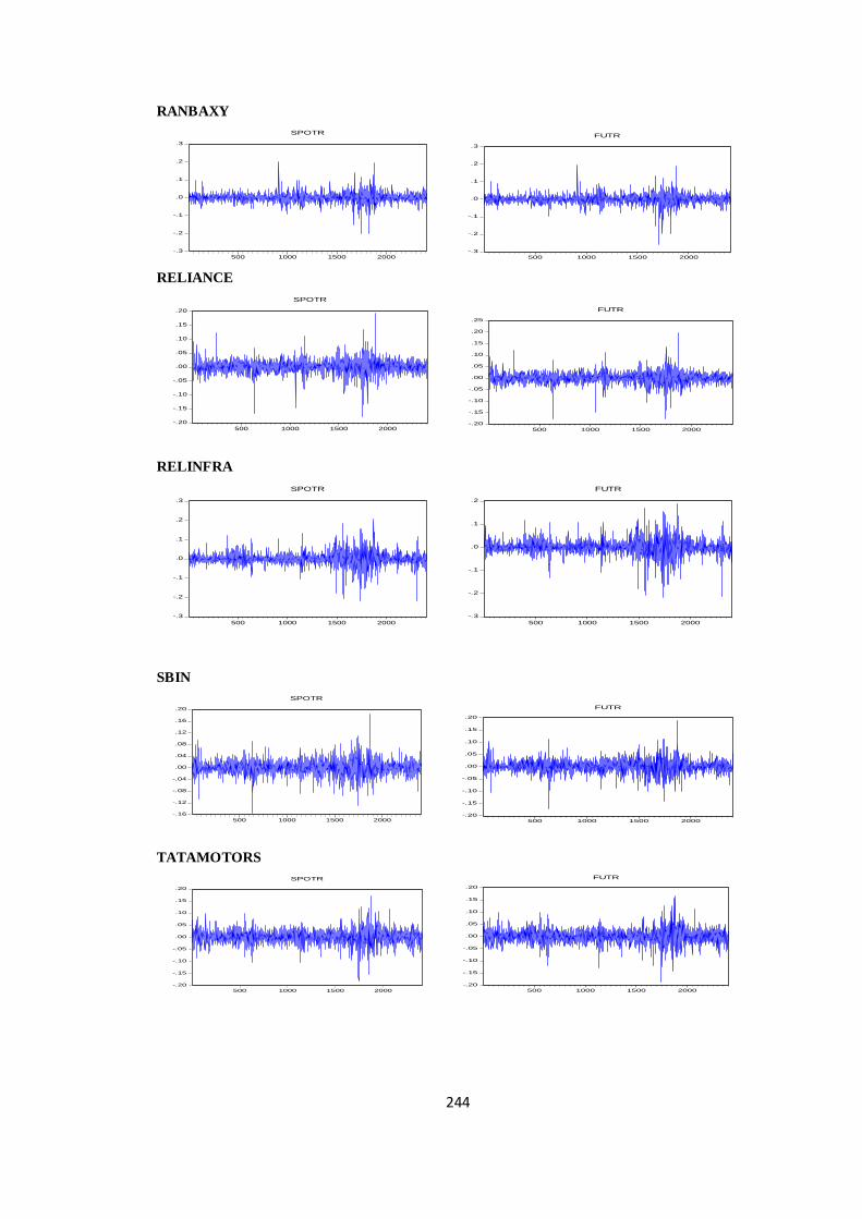
244
RANBAXY
-.3
-.2
-.1
.0
.1
.2
.3
500 1000 1500 2000
SPOTR
-.3
-.2
-.1
.0
.1
.2
.3
500 1000 1500 2000
FUTR
RELIANCE
-.20
-.15
-.10
-.05
.00
.05
.10
.15
.20
500 1000 1500 2000
SPOTR
-.20
-.15
-.10
-.05
.00
.05
.10
.15
.20
.25
500 1000 1500 2000
FUTR
RELINFRA
-.3
-.2
-.1
.0
.1
.2
.3
500 1000 1500 2000
SPOTR
-.3
-.2
-.1
.0
.1
.2
500 1000 1500 2000
FUTR
SBIN
-.16
-.12
-.08
-.04
.00
.04
.08
.12
.16
.20
500 1000 1500 2000
SPOTR
-.20
-.15
-.10
-.05
.00
.05
.10
.15
.20
500 1000 1500 2000
FUTR
TATAMOTORS
-.20
-.15
-.10
-.05
.00
.05
.10
.15
.20
500 1000 1500 2000
SPOTR
-.20
-.15
-.10
-.05
.00
.05
.10
.15
.20
500 1000 1500 2000
FUTR
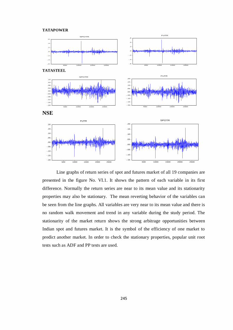
245
TATAPOWER
-.6
-.4
-.2
.0
.2
.4
.6
500 1000 1500 2000
SPOTR
-.6
-.4
-.2
.0
.2
.4
.6
500 1000 1500 2000
FUTR
TATASTEEL
-.20
-.16
-.12
-.08
-.04
.00
.04
.08
.12
.16
500 1000 1500 2000
SPOTR
-.20
-.15
-.10
-.05
.00
.05
.10
.15
.20
500 1000 1500 2000
FUTR
NSE
-.20
-.15
-.10
-.05
.00
.05
.10
.15
.20
500 1000 1500 2000 2500
FUTR
-.15
-.10
-.05
.00
.05
.10
.15
.20
500 1000 1500 2000 2500
SPOTR
Line graphs of return series of spot and futures market of all 19 companies are
presented in the figure No. VI.1. It shows the pattern of each variable in its first
difference. Normally the return series are near to its mean value and its stationarity
properties may also be stationary. The mean reverting behavior of the variables can
be seen from the line graphs. All variables are very near to its mean value and there is
no random walk movement and trend in any variable during the study period. The
stationarity of the market return shows the strong arbitrage opportunities between
Indian spot and futures market. It is the symbol of the efficiency of one market to
predict another market. In order to check the stationary properties, popular unit root
tests such as ADF and PP tests are used.
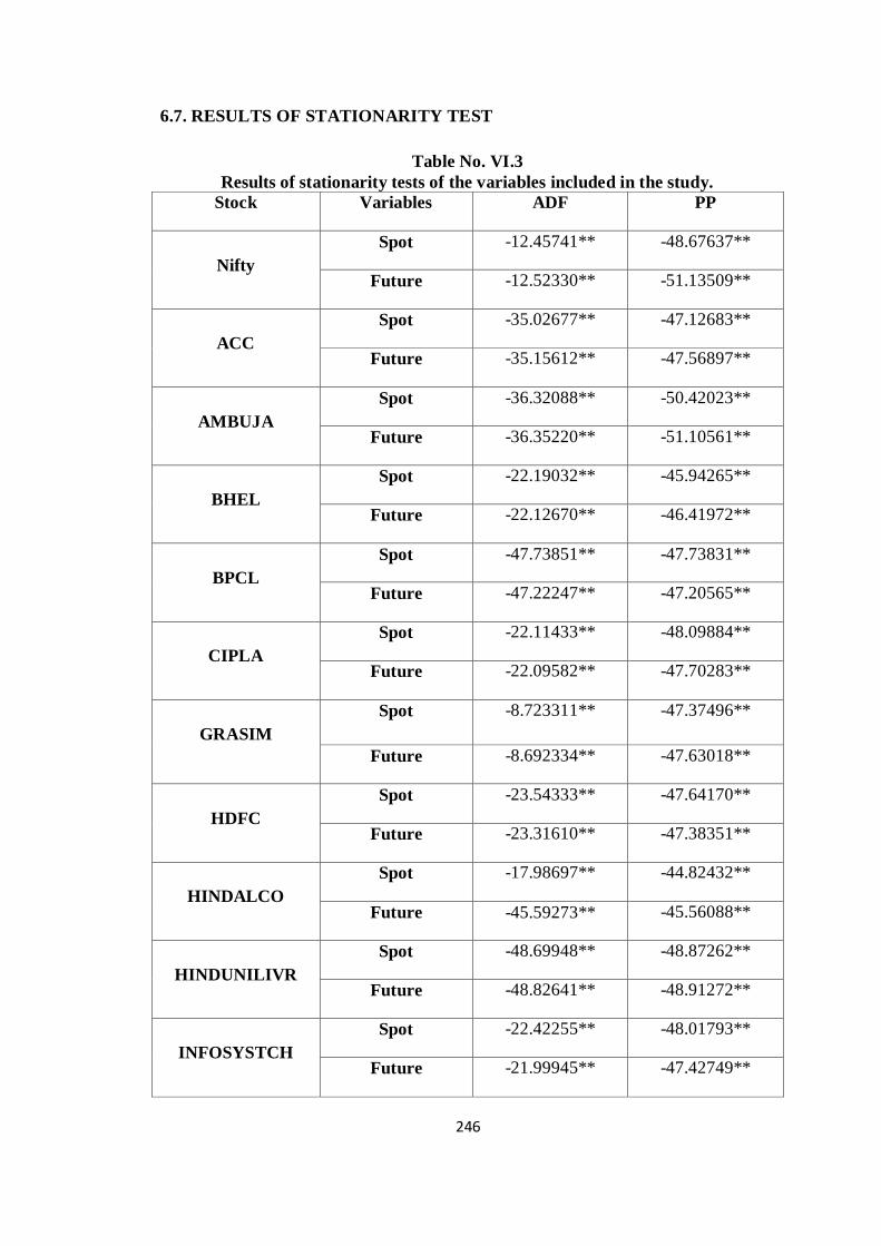
246
6.7. RESULTS OF STATIONARITY TEST
Table No. VI.3
Results of stationarity tests of the variables included in the study.
Stock Variables ADF PP
Nifty
Spot -12.45741** -48.67637**
Future -12.52330** -51.13509**
ACC
Spot -35.02677** -47.12683**
Future -35.15612** -47.56897**
AMBUJA
Spot -36.32088** -50.42023**
Future -36.35220** -51.10561**
BHEL
Spot -22.19032** -45.94265**
Future -22.12670** -46.41972**
BPCL
Spot -47.73851** -47.73831**
Future -47.22247** -47.20565**
CIPLA
Spot -22.11433** -48.09884**
Future -22.09582** -47.70283**
GRASIM
Spot -8.723311** -47.37496**
Future -8.692334** -47.63018**
HDFC
Spot -23.54333** -47.64170**
Future -23.31610** -47.38351**
HINDALCO
Spot -17.98697** -44.82432**
Future -45.59273** -45.56088**
HINDUNILIVR
Spot -48.69948** -48.87262**
Future -48.82641** -48.91272**
INFOSYSTCH
Spot -22.42255** -48.01793**
Future -21.99945** -47.42749**
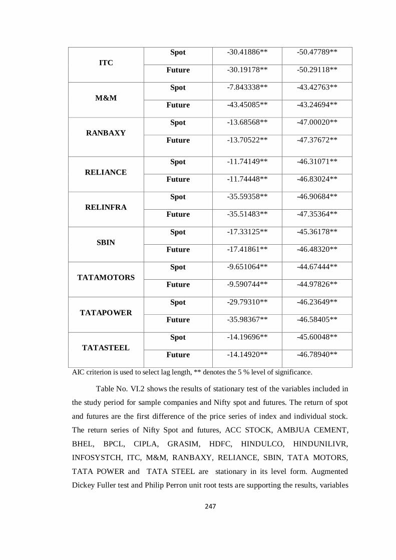
247
ITC
Spot -30.41886** -50.47789**
Future -30.19178** -50.29118**
M&M
Spot -7.843338** -43.42763**
Future -43.45085** -43.24694**
RANBAXY
Spot -13.68568** -47.00020**
Future -13.70522** -47.37672**
RELIANCE
Spot -11.74149** -46.31071**
Future -11.74448** -46.83024**
RELINFRA
Spot -35.59358** -46.90684**
Future -35.51483** -47.35364**
SBIN
Spot -17.33125** -45.36178**
Future -17.41861** -46.48320**
TATAMOTORS
Spot -9.651064** -44.67444**
Future -9.590744** -44.97826**
TATAPOWER
Spot -29.79310** -46.23649**
Future -35.98367** -46.58405**
TATASTEEL
Spot -14.19696** -45.60048**
Future -14.14920** -46.78940**
AIC criterion is used to select lag length, ** denotes the 5 % level of significance.
Table No. VI.2 shows the results of stationary test of the variables included in
the study period for sample companies and Nifty spot and futures. The return of spot
and futures are the first difference of the price series of index and individual stock.
The return series of Nifty Spot and futures, ACC STOCK, AMBJUA CEMENT,
BHEL, BPCL, CIPLA, GRASIM, HDFC, HINDULCO, HINDUNILIVR,
INFOSYSTCH, ITC, M&M, RANBAXY, RELIANCE, SBIN, TATA MOTORS,
TATA POWER and TATA STEEL are stationary in its level form. Augmented
Dickey Fuller test and Philip Perron unit root tests are supporting the results, variables
248
are stationary. Stationarity shows the strong lead- lag relationship between spot and
futures variables of the individual stocks and index. Existence of stationary suggests,
returns on both futures and spot market is significantly predictable. Stationary futures
and spot market return suggest that information dissemination efficiency in Indian
spot and futures market is weak and informed traders can frame market strategies to
exploit arbitrage and speculative opportunities as they become available (Kapil Gupta,
2009). The properties of the GARCH model suggest that the variables are in
stationary form to reveals the ARCH effect properly. This result reveal that the all
variables are having ARCH effect and it is possible to apply the bivriate D-VEC
GARCH model to estimate variance of spot and futures return and covariance of spot
return and futures return.
VI.8. RESULTS OF OPTIMAL HEDGE RATIO BY USING DIAGONAL VEC-
GARCH MODEL
Time varying hedge ratio is presented in the table No. VI.3. with coefficients
and its probabilities at 1% level of significance for each variable that is S&PCNX
Nifty and other 19 individual companies. Variance and covariance of spot and futures
return are estimated through Diagonal VEC- GARCH model. Time varying hedge
ratio is determined by dividing the covariance by variance of futures. Average of this
time varying hedge ratio is taken as optimal hedge ratio. The significant results of
coefficients support to capture the dynamic time varying behavior of the variable. The
optimal hedge ratios are presented in table No.VI.5.
Theoretically when optimal hedge ratio is 1, it is understood that there is a
perfect protection for investors when they take opposite position in the futures market
based on the underlying assets in the futures market. Table No. IV.5 presents the
optimal hedge ratio of variables included for the various study periods. It is found,
during the whole study period starting from the introduction of derivatives in India, it
is revealed that INFOSYSTECH provides opportunities to investors to protect their
risk by taking less than one unit of spot in futures market. This company shows the
exceptional protection behavior from other companies. TATA MOTORS too provide
almost 100% protections. The difference between these two companies is that in
INFOSYSTECH provides opportunities of holding lesser than one unit and where as
249
in the case of TATA MOTORS, investor is expected to have equalent number of units
in futures market to protect the loss from spot market. In other companies except
TATA POWER, needs to hold more number of units in futures market to reduce their
risk from spot. In other words, futures market does not provide risk reduction
opportunities to these investors due to its inherent nature of asset in spot market. The
TATA POWER, do not provide hedging opportunities to its investors. In order to
understand the robustness of this result, efforts are made to determine optimal hedge
ratio for various sub periods.
Soon after the introduction of derivatives in Indian market, it is found that
INFOSYSTCH, ITC, and TATAMOTORS were providing high level of risk
protection to investors through futures market. Investors of these companies were
expected to have less than one unit of their holding in spot, in futures market to
reduce their risk. RANBAXY and HINDUNILVR and its trading in futures markets
helped the investors by investing equivalent number of units in futures market to
reduce the risk. All other companies except TATA POWER provide adequate risk
protection through futures market during the initial time of derivatives.
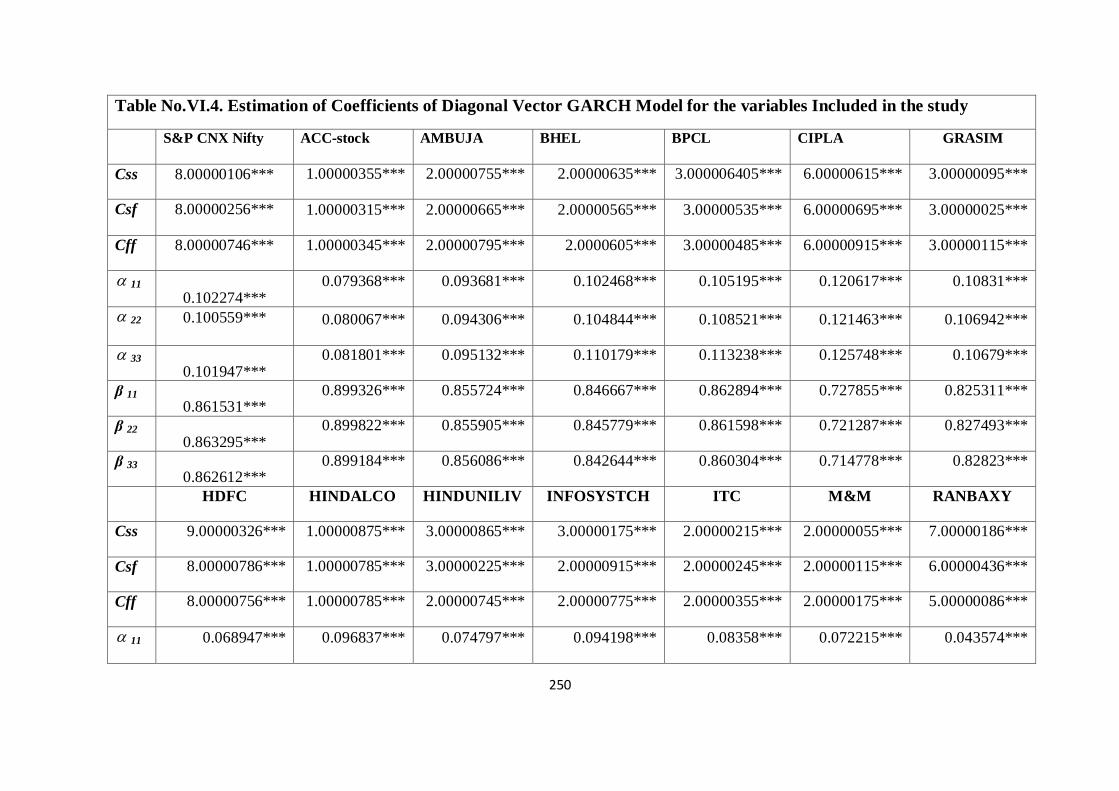
250
Table No.VI.4. Estimation of Coefficients of Diagonal Vector GARCH Model for the variables Included in the study
S&P CNX Nifty ACC-stock AMBUJA BHEL BPCL CIPLA GRASIM
Css 8.00000106*** 1.00000355*** 2.00000755*** 2.00000635*** 3.000006405*** 6.00000615*** 3.00000095***
Csf 8.00000256*** 1.00000315*** 2.00000665*** 2.00000565*** 3.00000535*** 6.00000695*** 3.00000025***
Cff 8.00000746*** 1.00000345*** 2.00000795*** 2.0000605*** 3.00000485*** 6.00000915*** 3.00000115***
11 0.102274***
0.079368*** 0.093681*** 0.102468*** 0.105195*** 0.120617*** 0.10831***
22 0.100559***
0.080067*** 0.094306*** 0.104844*** 0.108521*** 0.121463*** 0.106942***
33 0.101947***
0.081801*** 0.095132*** 0.110179*** 0.113238*** 0.125748*** 0.10679***
β 11 0.861531***
0.899326*** 0.855724*** 0.846667*** 0.862894*** 0.727855*** 0.825311***
β 22 0.863295***
0.899822*** 0.855905*** 0.845779*** 0.861598*** 0.721287*** 0.827493***
β 33 0.862612***
0.899184*** 0.856086*** 0.842644*** 0.860304*** 0.714778*** 0.82823***
HDFC HINDALCO HINDUNILIV INFOSYSTCH ITC M&M RANBAXY
Css 9.00000326*** 1.00000875*** 3.00000865*** 3.00000175*** 2.00000215*** 2.00000055*** 7.00000186***
Csf 8.00000786*** 1.00000785*** 3.00000225*** 2.00000915*** 2.00000245*** 2.00000115*** 6.00000436***
Cff 8.00000756*** 1.00000785*** 2.00000745*** 2.00000775*** 2.00000355*** 2.00000175*** 5.00000086***
11 0.068947*** 0.096837*** 0.074797*** 0.094198*** 0.08358*** 0.072215*** 0.043574***
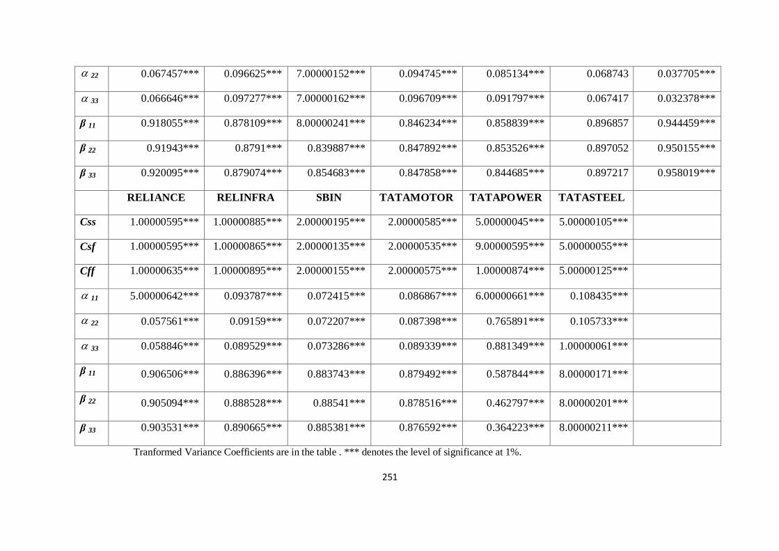
251
22 0.067457*** 0.096625*** 7.00000152*** 0.094745*** 0.085134*** 0.068743 0.037705***
33 0.066646*** 0.097277*** 7.00000162*** 0.096709*** 0.091797*** 0.067417 0.032378***
β 11 0.918055*** 0.878109*** 8.00000241*** 0.846234*** 0.858839*** 0.896857 0.944459***
β 22 0.91943*** 0.8791*** 0.839887*** 0.847892*** 0.853526*** 0.897052 0.950155***
β 33 0.920095*** 0.879074*** 0.854683*** 0.847858*** 0.844685*** 0.897217 0.958019***
RELIANCE RELINFRA SBIN TATAMOTOR TATAPOWER TATASTEEL
Css 1.00000595*** 1.00000885*** 2.00000195*** 2.00000585*** 5.00000045*** 5.00000105***
Csf 1.00000595*** 1.00000865*** 2.00000135*** 2.00000535*** 9.00000595*** 5.00000055***
Cff 1.00000635*** 1.00000895*** 2.00000155*** 2.00000575*** 1.00000874*** 5.00000125***
11 5.00000642*** 0.093787*** 0.072415*** 0.086867*** 6.00000661*** 0.108435***
22 0.057561*** 0.09159*** 0.072207*** 0.087398*** 0.765891*** 0.105733***
33 0.058846*** 0.089529*** 0.073286*** 0.089339*** 0.881349*** 1.00000061***
β 11 0.906506*** 0.886396*** 0.883743*** 0.879492*** 0.587844*** 8.00000171***
β 22 0.905094*** 0.888528*** 0.88541*** 0.878516*** 0.462797*** 8.00000201***
β 33 0.903531*** 0.890665*** 0.885381*** 0.876592*** 0.364223*** 8.00000211***
Tranformed Variance Coefficients are in the table . *** denotes the level of significance at 1%.
252
Estimation results on optimal hedge ratio during introduction and development
period shows almost same positions in all companies. In the case Nifty index, the
optimal hedge ratio is almost same. While taking 1438 observations for each company
and index separately. AIC, BHEL, CIPLA, HINDUNILVR, INFOSYSTCH,
RANBAXY, SBIN and TATA STEEL show the increasing trend in its hedge ratio.
While reducing the number of observation, the companies are showing more
confidence in its risk reduction level. But AMBUJS, BPCL, HDFC, HINDALCO,
M&M, RELIANCE, and TATA POWER are losing their power of risk reduction in
very minimal level. INFOSYSTCH Company keeps its position in the same level that
is above 1. During this period, ITC and TATAMOTORS are in the group of more
than one. This group shows that in order to protect the risk of one unit spot asset,
opposite sigh of less than one unit position in futures market is enough. The
integration between spot and futures assets of these companies very strong and the
speed of adjustment to remove the equilibrium in the integrated market is very higher
in the case of futures market of ITC and TATA MOTORS.
Pre- financial crisis period is another sub- study period which shows the
bullish trend in the spot and futures market in India. This sub- period starts from
March 2006 to January 2008. Even though there was bullish trend, it is more volatile.
Compared to other two period, hedge ratio of index futures is lesser than first two
periods. Hedge ratio of index futures is lesser than first two periods. Only 470
observations are taken for the estimation of optimal hedge ratio during this period. In
the period before financial crisis, research found different situation. INFOSYSTCH
provides greater opportunities of risk reduction through futures market, other
companies except TATAPOWER to help investors through futures market.
Significantly HDFC have gone up to protect the investor with equivalent units in
futures market. In the case of ACC stock, level of variance reduction is less than the
reduction in introduction and development period but it is higher than the whole study
period. The results BHEL, BPCL, CIPLA, GRASIM, HINDUNILVR, ITC M&M,
RANBAXY, SBIN, TATA MOTORS and TATASTEEL shows decreasing trend in
the hedge ratio. The risk reducing ability of futures market on these stocks are lesser
while comparing the other period. It is noted that reducing efficiency level very
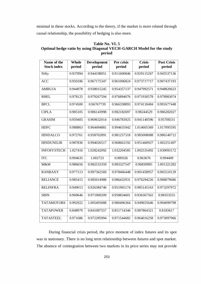
253
minimal in these stocks. According to the theory, if the market is more related through
causal relationship, the possibility of hedging is also more.
Table No. VI. 5
Optimal hedge ratio by using Diagonal VECH-GARCH Model for the study
period
Name of the
Stock index
Whole
period
Development
period
Pre crisis
period
Crisis
period
Post Crisis
period
Nifty 0.937894 0.944198051 0.911600846 0.929115267 0.945537136
ACC 0.950186 0.967175347 0.961006824 0.973717717 0.907437193
AMBUJA 0.944978 0.938015245 0.954357137 0.947992571 0.948820623
BHEL 0.978125 0.979267594 0.976894076 0.971930578 0.978983074
BPCL 0.974500 0.96767739 0.966338893 0.974118484 0.991677448
CIPLA 0.985105 0.986143998 0.982182697 0.98244529 0.986282027
GRASIM 0.959405 0.969632014 0.946783925 0.941140596 0.95708331
HDFC 0.988863 0.964494881 0.994655942 1.014605369 1.017095595
HINDALCO 0.972761 0.958702891 0.981257318 0.985008088 0.986140712
HINDUNILIR 0.987830 0.994026517 0.968663192 0.951460927 1.002251497
INFOSYSTECH 1.027416 1.028242092 1.032204585 1.002535492 1.030093172
ITC 0.994635 1.002723 0.989326 0.963676 0.994409
M&M 0.986656 0.982533359 0.983327547 0.96830985 1.001321282
RANBAXY 0.977113 0.997362569 0.978466448 0.901458957 0.965510129
RELIANCE 0.985415 0.985014988 0.986432931 0.976294226 0.988079686
RELINFRA 0.949013 0.926384746 0.951965174 0.985145163 0.973297972
SBIN 0.969646 0.971969209 0.958834601 0.936367562 0.98353555
TATAMOTORS 0.992922 1.005493088 0.980496364 0.949655646 0.994099798
TATAPOWER 0.848979 0.841087557 0.851714346 0.987864321 0.8183617
TATASTEEL 0.971686 0.972285994 0.971544682 0.964016258 0.973097966
During financial crisis period, the price moment of index futures and its spot
was in stationary. There is no long term relationship between futures and spot market.
The absence of cointegration between two markets in its price series may not provide
254
any possibility to the hedgers to take long run position in the market. Vipul (2005)
and Kapil Gupta (2009) find that existence of cointegration suggest even though both
market may be in disequilibrium during the short run but such deviation are very
quickly corrected through arbitrage process and the hedgers may take long run
positions to hedge market risk to the maximum extend.
Financial crisis period shows an interesting phenomenon of TATA POWER
showing higher level of risk protection unlike the past. HDFC has improved their
protection compared to previous period, with hedge rate crossing 1. INFOSYSTCH
maintain its portion of higher risk protection to investors. Interestingly all companies
show adequate risk protection but with minor reduction in the level of protection
barriers HDFC and INFOSYSTCH. During the period the index futures hedging
position is coming down than the whole period and introduction and development
period, but higher than the pre- crisis period. The hedge ratio of ACC, HDFC,
HINDALCO, RELINFRA and TATAPOWER is higher than the hedge ratio in other
study period. Not only market trend and the external environment, many internal
factors are also playing a role to maintain the standard position in the market. When
we make a study on individual stock and analyzing it, a thorough study on individual
stock and analyzing it, a thorough study on its operational behavior and market
positions are to be done. Here only market trend and duration of the study period is
considered. Hedge ratio of companies like AMBUJA, BHEL, GRASIM,
HINDUNILVR, INFOSYSTCH, ITC, M&M, RANBAXY, RELIANCE, SBIN,
TATAMOTORS and TATASTEEL are lesser than the pre- financial crisis period. But
in the case of BPCL, and CIPLA, the hedge ratio is higher in crisis period than other
periods. Making a conclusion on these results for those stocks may not be true due to
the inconsistency in their risk managing capacity.
Post financial crisis period shows the long term integration between spot and
futures market in India. Long term integrated markets gives the opportunities to the
hedgers to take long term hedging position to the maximum extent. During this
period, the optimal hedge ratio of index futures is in better position than the other
periods. Around 95% of the variance can be protected by hedging process of index
futures. ACC, RELINFRA and TATAPOWER are showing an instability in the
market movement and the optimal hedge ratio of those companies are minimal than
255
the hedge ratio during other periods. Remaining all companies except HDFC,
HINDUNILVR, INFOSYSTCH and M&M are performing well in this period. M&M,
HDFC, HINDUNILVR and INFOSYSTCH perform in extra ordinary manner that is ,
these companies optimal hedge ratio is above one which shows that to protect the risk
level of one unit asset in spot market needs lesser than one unit opposite position in
futures market. Very strong cointegration relationship and arbitrage process can be
seen from study period. From this analysis, it is clear that time horizon is the one
factor which influences the hedging efficiency of futures market. Not only time
period, the movement of the market and the integration relationship between both
market also having their own role in the risk managing process of futures market in
India.
Many studies, Saumitra et.al (2008), kapil Gupta et.al (209), Sheng-syan Chen
et. al (2004), Robert Myers (2000), Jahangir Sultan et. l (2008), Guy-Hyenmoon
(2007), Lagesh et.al (2009) made an attempt to estimate different econometrics model
and found Diagonal Vector GARCH model gives high optimal hedge ratio than the
other econometrics model. This study uses the D-VEC-GARCH model to estimate the
optimal hedge ratio for different study period and found that the level of risk
protection efficiency of futures market is varying due to the time horizon and market
movement. The market movement is having effect on the hedging efficiency of
futures market. The null hypothesis of no significant protection to investors risk is
rejected and it is very clear that in almost all sample stock, the reduction in protection
level is almost 90% which shows the real efficiency of futures market to protect the
risk of asset position in the spot market.
VI.9. CONCLUSION
The hedge ratio is the number of contracts needs to minimize the exposure of a
unit worth of position in the cash market (Jahangir, 2008). Hedgers use the market as
the way to reduce the risk associated with price changes in the connected cash market.
The integrated relationship between spot and futures market of a particular asset
shows the possibility of level of reducing the risk involved in the spot market assets.
This chapter has made an attempt to analysis the efficiency of futures market to
protect the risk level of spot market assts those values are always varying in the basis
of markets behavioral pattern.
256
S&P CNX Nifty futures and spot price series and 19 individual stocks spot
and futures price series are taken as the variable for the study then it is transformed in
to lag form and determined the first difference of price series as return series. The
summary statistics shows that all return variables are not having normal distribution,
the Jarque –Bera test statistics of each variable does not support its null that
distribution is normal. Probability value of the test is also support JB test result which
accepts the alternative hypothesis that the distribution is not in not normality position.
Spot futures return series of HDFC, ITC, BPCL and AMBUJA are positively skewed
and remaining sample companies are negatively skewed. Negatively skewed index
futures and individual stocks offer arbitrage opportunities to the traders and provide
important information relating to the exploitation of arbitrage opportunities. The unit
root test such as Philip Perron test and Augmented Dickey Fuller test results indicate
that all return series are stationary. The series is having unit root is rejected at 1%
level of significance for all variables in the sample. This results shows that return in
both futures and spot market are clearly predictable. DVEC-GARCH model
coefficients of index futures and all other individual stocks are significant at 1% level
of significance. Time varying hedge ratio for each individual stock and index futures
is estimated by dividing the covariance of spot return and futures return. The mean
value of the hedge ratio estimated for each company is presented for various periods
and the table shows that during different periods there is a small level of variation in
the optimal hedge ratio of sample companies.
It is confirmed that Indian futures market is able to satisfy the objectives like
risk sharing and hedging process effectively. The null hypothesis that is no protection
to the investors risk in Indian futures market is rejected on the basis of the empirical
analysis. It is confirmed that Indian futures and spot market are having strong causal
relationship and it allows the trader to make perfect arbitrage process and hedge their
risk to protect the assets in spot market.

257
Chapter-VII
Findings and Suggestions
258
CHAPTER -VII
FINDINGS AND SUGGESTIONS
7.1. INTRODUCTION
This chapter deals with the conclusion drawn out of the study on the basis of
empirical analysis done in the different chapters. This study has made an attempt to
find the overall performance of the futures market in India in the way of the long term
relationship between spot and futures market and short run relationship between
Indian futures and spot market. In order to understand the arbitrage efficiency of
Indian markets, causality of futures and spot market is also needed to be understood.
The influence and the ability of different variables in the futures and spot market are
determined from the analysis. The causal relationship between different variables, the
sign of relationship among variables and the time lag of the response in the market
has also been seen. The response and the shock of each variable in the proportion of
the shock to the other variables are explained here with the help of results of analysis.
As a part of determining the informational efficiency of futures market, this study has
analyzed the hedging efficiency of futures market. The findings and conclusion from
the analysis are summarized below under separate headings.
7.2. LONG TERM RELATIONSHIP BETWEEN INDIAN FUTURES AND
SPOT MARKET
The whole study period is divided in to four sub periods on the basis of
structural break in the data series which is identified by using Bai Perron model and
real market trend. It is very clear that the established relationship between both the
markets is confirmed through the robustness checking with the result of different
study period. Johansen cointegration methodology by using Trace statistics and Eigen
value were used as the tool to make the analysis. Existence of long term relationship
between Indian spot and futures market is seen during the whole study periods and
other sub- period except financial crisis period. During the financial crisis period both
259
the spot price and futures price series included are in stationary at its level to show the
absence of long term relationship between the markets. The VAR, Granger Causality
/Bock Exogenity test results showed that there is no causality relationship between
Indian spot and futures market during the study sub-periods. The test results indicate
that the null hypothesis of spot does not cause futures and futures does not cause spot
are accepted during the financial crisis period. All other study sub periods such as
introduction and development period, pre- financial crisis period and post financial
crisis period showed the similar results of the existence of long term relationship
between spot and futures market. The existence of long term relationship between
markets reveals the possibility of reducing the disequilibrium among the market
during the short term period also.
7.3. SHORT RUN RELATIONSHIP BETWEEN INDIAN FUTURES AND
SPOT MARKET.
The long term cointegrated relationship between Indian futures and spot
market shows that there is a possibility for disequilibrium among the market during
short run period. This disequilibrium among the relationship is corrected by the
markets very soon because those markets are integrated for a long period. In this
context, the speed of adjustment to correct the disequilibrium of the market is
different and the normalized cointegration equation through Vector Error Correction
Model tells the efficiency of market to correct the changes and make equilibrium
among the relationship. In the whole period of the study, futures market corrects the
variation in the Indian spot market. In India the efficiency of futures market to adjust
and to respond to the new information is very higher than to the spot market. The
robustness of the result is checked in different sub-periods and it shows different
result that is in the introduction and development period, the speed of adjustment of
futures market is faster than spot market due to the efficiency of responding to the
new information with less level of transaction cost and different type of futures
contract. During the pre- financial crisis period and the post financial crisis period
leading efficiency of futures market has not been seen. From these results, it can be
explained that if the market trend is almost predictable, the efficiency of futures
market is strong and the other periods which show more volatile trend is not
supporting the results. In this study no empirical results show the prominence of spot
260
market on the futures market. To conclude, the Indian futures market is adjusting the
changes in the market and making the equilibrium in the price changes than Indian
spot market. But during pre- financial crisis period and post financial crisis period, the
speed of adjustment of spot market is higher than futures market but it is not
statistically significant. From this point, it is clear that the role of spot market in the
process of information transmission is not explained. The actual causal relationship
between spot and futures market reveals the possibility of lead lag relationship
between Indian futures and spot market.
7.4. LEAD–LAG RELATIONSHIP BETWEEN FUTURES AND SPOT
MARKET IN INDIA
In Indian context, the futures and its underlying markets are integrated for a
long period. But in short run period, which market plays the role of leader and gives
any idea or information to the investors on the movement of another market is
analyzed clearly in the analysis. The causality relationship between futures and spot
market reveals the position of lead- lag among futures and spot market. Results of
Wald coefficients test indicate that there is bi directional causality relationship
between futures and spot market in India. The robustness checking results also
indicate that the null hypothesis of spot market does not cause futures market and
futures market does not cause spot market is rejected in all sub-study period and it
says that spot market and futures market are transmitting the information to each
other. It is clear that, there is no conclusive evidence on which market is leading
during which period. There is a tendency to lead and lag with two markets and to
transfer the information to another market. To conclude, there is bidirectional
relationship between Indian futures and spot market. Both markets are performing like
indicator and follower. The investors can observe the movement of both markets and
then decide what type of investment should be selected and which market should be
considered for the investment process.
7.5. DETERMINANTS OF FUTURES MARKET IN INDIA
Indian futures market movement depends on many factors which are laid
down in futures market and its underlying market. To predict the movement of futures
market is the inspiration of investors to decide their trading pattern in the spot and
futures market. Futures and spot markets are integrated and one market can predict the
261
movement of another market. This study empirically analysis the role of different
factors such as open interest, turn over, number of contract, volatility of futures
market and spot market return in the futures market. The properties of data allows to
apply Vector Autoregressive Granger Causality/ Block Exogenity test with all
variable to other variables and the influence of all factors together to each variable.
For the whole study period, all variables together are having influence on futures
market but not each variable separately. During the initial period of derivatives,
introduction and development period result reveals the role of all variables to
determine the futures market movement. During this period spot market and the
futures market volatility are playing a vital role to predict the movement of futures
market. In the pre- financial crisis period spot return, number of contract and turnover
are having influence on futures markets movement.
Financial crisis period is a critical period to the stock market and futures
market in India. No relationship can be found out during this period. The role of
speculators, decides the movement of the market and no established relationship is
there in the futures market during the crisis period. All other variables and futures
market return are moving independently, then there is no chance for predicting the
futures market on the basis of the movement of any other variable of the futures
market. Futures market is influenced by all variables together and number of contract
and volatility individually. This result confirms that the Indian futures market can be
predicted by the movement of spot market movement, volatility of futures market,
number of contract and turnover independently and all these variables together also
influences the futures market. On the basis of the results from the empirical analysis,
it is clear that spot market index return, futures market volatility, number of contract
and turnover of the futures market are the determinants of the futures market in India.
7.6. POSITIVE RELATIONSHIP BETWEEN FUTURES MARKET AND ITS
DETERMINANTS
The causal relationship between futures market and its determinants helps the
traders and investors to predict the market. The negative or positive sign of effect in
the futures market from the determinants provide more clarity on the movement and
help the traders to make decision on buying or selling option clearly. The response of
futures return to the change of determinants is revealed by the impulse response
262
function results. During the whole study period, result shows that the futures market is
positively responding to the shocks of spot market. The similar type of response can
be seen from introduction and development period. Sudden positive response is seen
in the futures market due to the change in spot market return. In the crisis period, only
very short moment positive shock in futures market due to the change in spot market.
Post financial crisis study period results indicate that futures market responses
positively in the same level. It is shorted that the results of impulse response function
of Indian futures market and spot market are positive.
7.7. NEGATIVE RELATIONSHIP BETWEEN FUTURES MARKET AND ITS
DETERMINANTS
The direction of relationship between variables is very important to understand
the role of each aspect in the prediction of other variable. Traders are looking keenly
on the positive or negative relationship among the determinants of futures market. In
the pre- financial crisis period, change in open interest, number of contract and
turnover on the first day may make very minimal level of negative response from
futures market. Post financial crisis period study results indicate that futures market
responses positively in the same level. So we can conclude the results of impulse
response function such a manner that the changes and responses of Indian futures
market and spot market are positive and responses of futures market to the variation in
other variables cannot be decided as negative or positive.
7.8. THE EXISTENCE OF SHOCK AND RESPONSES OF INDIAN FUTURES
AND SPOT MARKET
If the variables are related every shock and changes in one variable makes
responses and variation in another variable. Variance decomposition results for
various sub- period shows the effect of shock in one variable and the response of the
shock in that variable itself and the proportion of shock transmitted to another
variable. In the case of shocks in futures market, every day it around 90% of the
effects of shocks transmitted to spot market and within 10 days maximum 8% shocks
is reflected by futures market. What ever happened in the futures market is suddenly
converted to spot market but more proportion of shocks in spot market is reflected by
spot market itself. The similar type of relationship is seen from turnover and number
of contract. Other variables like volatility and open interest are reflecting more
263
portions of their shocks by themselves and very less proportion is transmitted to other
variables. While time is passing the level of proportion of shocks transmitted to
another variable is increasing. It is concluded that more portion of shocks in Indian
spot market is reflected by spot market itself and very minimal level is transmitted to
another market that is futures market. But any fluctuation in the futures market
suddenly affects the spot market with full sound. The shocks in other variables also is
transmitted to the other related variables and the level of proportion is reducing from
the source variable and it is increasing in the other variables.
7.9. PROPORTION AND TRANSMISSION OF SHOCKS AND RESPONSES
OF FUTURES AND SPOT MARKET
The shock of futures market transmits suddenly to spot market and the spot
market bears the shock in itself. The same relation is seen in the case of number of
contract and turnover. Around 90% of the reflection of the shock in the turnover
comes to the number of contract immediately and the shock of number of contracts is
stayed in the same variable itself. All related variables are transmitting their shocks to
each other and they are able to predict the movement of other variables up to an
extent.
7.10. RISK REDUCTION EFFICIENCY OF FUTURES MARKET IN INDIA
Risk reduction efficiency of Indian futures market is analyzed through the
hedging process. S&PCNX Nifty and its underlying index, 19 individual stocks
futures and spot return series are taken into consideration for the estimation of hedge
ratio. Optimal hedge ratio estimated through the DVEC-GARCH shows that all most
all sample companies and index futures market are reducing the risk of the assets in
the spot market. According to the sub- period analysis of hedging performance of
index futures and individual stock futures not that much variation in the risk
protection is seen from the results. On the basis of the empirical result it is confirmed
that Indian futures market is able to protect the risk of investors who are having asset
in spot market. The null hypothesis of the study futures do not provide risk protection
to the spot market asset is not accepted and prove the efficiency of futures market in
risk reduction.
264
7.11. SUMMARY
This study made an attempt to analyze the informational efficiency of Indian
futures market by three ways such as the dynamic linkage with Indian spot market,
the ability of spot and futures market factors to predict the movement of futures
market, that is the short run causal relationship between various determinants of the
futures market and the hedging process of futures market. In all these area, it is seen
that there is very smooth way of passing information from futures market to spot
market and both are linked. On the basis of empirical analysis and the theoretical
support from the literature, it is confirmed that the informational efficiency of futures
market in India. The market is so volatile in India due to the high level presence of
speculators and in this context decision on long term investment may not be crucial
and apt decision at the correct time helps the traders to make profit from the trading
process in Indian futures market.
7.12. SUGGESTIONS
From the research done and presented in previous pages, the researcher brings
forth the following suggestions to investors, regulators and policy makers.
7.12.1. INVESTORS
1. Go long – Investors are advised or suggested to make investment for a long period
in spot and futures market as it will help to stabilize the high return.
2. Rely on one market- Investors and traders need not struggle to observe the
movement of both markets for information, instead they can take the investment
decision based on the movement of one market as both are cointegrated. Whichever is
convenient for him can be considered.
3. Effectively utilize the arbitrage opportunities- The bidirectional relationship
between spot and futures market provides the perfect arbitrage opportunities between
them. The market players should utilize this opportunity effectively to make profit.
4. Future market is an indicator – Information from the futures market can be taken
as an indicator to take decision for investment in the spot market.
5. Consider trade volume and spot market movement- Market players should
consider trade volume like number of contract, turnover and the movement of spot
265
market to make investment in futures market as they have high degree of
dependencies.
6. Not fundas please – The movement of spot market cannot be predicted on the basis
of fundamentals of the companies alone. It depends on many aspects from futures
market. While considering spot market as the investment avenue the movement of
futures markets and its other aspects should also be considered, no fundas alone.
7. Indicators of futures market - Trade volume, volatility of futures market and spot
market are taken as the indicators of futures market return. The market players should
keenly observe the movement of trade volume of the futures market and its
fluctuations to predict the movement of futures market in addition to movement in
spot market.
8. Utilize the shock of futures market as an opportunity - The shock of futures
market will suddenly transmit to the spot market. It makes an opportunity to the
traders to make trading strategies to earn profit from the spot market due to the shock
of futures market. Something happens in future perspective may give trading
opportunity in spot market. Trader should utilize it for a short period.
9. Bearish market is not a tragedy – Speculators are playing more in bearish market
and making so negative trend to the investors. Actually nothing happens in the
fundamentals of the individual stock in the spot market and when the external
environment changes the real values of stocks may come out. Thus the investors can
use this time for long term investment by buying and through short term rational
trading strategies traders can make benefit from the bearish market.
10. Hedge it – Both spot and futures market are integrated and there is opportunities
for hedging. Investors can rely upon movement of one market and can take the
opposite position in the integrated market, thus the total risk of investment can be
reduced.
11. Investment in – Individual stock like HDFC, HINDUNILVR, INFOSYSTCH,
M&M and TATA MOTORS are the stocks which can provide nearly 100% risk
reduction in the investment through hedging process irrespective of market
movement.
266
7.11.2. GOVERNMENT & REGULATORS
1. Enrich investors – In the research it is found that there are many ways for reducing
risk but investors are not aware or rather they are not published and therefore, Govt.
or regulators like SEBI should introduce the scheme to equip more youth or potential
investors about the technicalities of futures market and its special benefits.
2. Fix Guide post – Agencies should introduce some effective indicators to warn the
traders and investors from the dangerous zone of the investment and to help the
traders and investors to diversify their avenues from one to another investment
channels.
3. Bring regulations – Regulation is a must to monitor the performance of speculators
during the bearish market condition so that traders can also make benefits.
SCOPE FOR FURTHER RESEARCH
This study has made effort to analyze the informational efficiency of futures
market in three ways such as the dynamic linkage between Indian futures and spot
market, the determinants of futures market through the informational relationship
between futures market and other variables, the risk reduction efficiency through the
hedging process between Indian futures and spot market. During the thorough
analysis it is found that there are some aspects which are to be analyzed thoroughly to
get more idea on the futures market movement and its investment possibilities in the
futures market. They are,
The long run relationship between futures market and one of its determinants,
turnover, can be analyzed.
The mispricing and its relationship between futures market is another area for the
future research.
The cointegration among futures price series and open interest may provide some
basic idea on the hedging efficiency of futures market.
Considering more number of individual stocks from the futures market and to
estimate hedge ratio provide investors deep idea on the optimal hedge ratio of futures
267
market and the efficiency of individual company to protect the interest of the
investors.
To find the basis of market by deducting the spot price from futures market and
making the analysis on the futures market offers basic knowledge on arbitrage
efficiency of futures and spot market.
There is another research gap in which new series of daily price can be estimated
by taking the average of daily low price and high price. It gives more idea on the day
trading movement of market and the analysis will be more fruitful small traders and
day traders.
The volatility of spot market is to be taken as the variable to predict the movement
of futures market may provides more clarity on the relationship between the spot and
futures market.
These are the future research opportunities which are identified by this empirical
study but could not have touched in the present analysis. Young researchers can make
lot of study on this area and provide fruitful contribution to the literature.

268
Bibliography
269
Bibliography
Published Articles:
1. Andreas A. Jobst (2008), The development of equity derivative markets,
International Journal of Emerging Markets, Vol.3, No.2, pp. 163-180
2. Alex Frino, Terry Walter and Andrew West (2000), The lead- lag
Relationship between equities and stock index futures markets around
information release, The Journal of Futures Markets, Vol.20, No.5, pp. 467-
487.
3. Alexander A. Kurov and Dennis J. Lasser (2002), The Effect of the
Introduction of Cubes on the NASARDQ-100 index spot- futures pricing
relationship, The Journal of Futures Markets, Vol.22, No.3, pp.197-218.
4. Andrew C. Szakmary and Dean B. Kiefer (2004), The Disappearing
January/ Turn of the Year effect- Evidence from stock index futures and
cash markets, The Journal of futures Markets, Vol.24, No.8, pp.755-
784.
5. Amirik Singh and Arun Upneja (2008), The deretminants of the decision to
usefinancial derivatives in lodging industry, Journal of Hospitality &
Tourrism Research, Vol.32,No.4, pp.423-447.
6. Andy C.N.Kan (2004) Resiliency ability of the underlying spot market after
the introduction of index of index futures contracts- Evidence from Hong
Kong, Journal of Emerging Market Finance, Vol.3,No.3 pp.269-283.
7. Alexander Kurov and Dennis .J .Lasser (2004), Price Dynamics in the
Regular and E- Mini Futures Markets, Journal of financilal and
Quantitative Analysis, Vol.39, No.2, pp.365- 384.
8. Abhay Abhyankar (1998), Linear and nonlinear Granger Causality- Evidence
from the U.K Stock Index Futures markets, The Journal of Futures Markets,
Vol.18,, No.5, pp.519-540.
9. Alan E.H.Speight, David G. Mc Millan and Owain A.P.Gwilym (2000),
Intraday Volatility Components on FTSE-100 stock index futures, The
Journal of Futures Markets, Vol.20, No.5, pp.425-444.
270
10. Allan Hodgson and John Okunev (1992), An alternative Approach for
determining hedge ratios for futures contracts, Journal of Business Finance
and Accounting, Vol. 19, No.2, pp. 211-224.
11. Aaron Low, Jayaram Muthuswamy, Sudipto Sarkar and Eric Terry (202)
Multiperiod hedging with futures contracts,The Journal of Futures Markets,
Vol.22, No.12, pp. 1179-1203.
12. Abdulnasser Hatemij. J and Eduardo Roca (2006), Calculating the optimal
hedge ratio- Constant, Time varying and the Kalman Filter approach,
Applied Economics Letters, Vol.13, No.3, pp. 293-299.
13. Amir Alizadesh and Nikos Nomikos (2004), A Markov Regime Switching
approach for hedging stock Indices, The Journal of Futures Markets, Vol.24,
No.7, pp. 649-674.
14. Aysegul Ates and Kate Phylaktis (2010) Related securities and price
discovery on floor versus screen based trading systems-A analysis of the
foreign exchange futures markets, Working papers series, Social Science
Research Net work .com,pp.1-32.
15. Asani Sarkar (2006), Indian derivatives Market, The Exford Companion to
Economics in India, pp.1-9.
16. Andreas.A.Jobst (2007),The development of Equity derivatives Market in
Emerging Asia, ssrn.com/Abstract-952033, pp.1-9.
17. Anurag.N.Banerjee (2007), A method of estimating the average derivatives,
Journal of Econometrics, Vol.136, pp. 65-88.
18. Alexander Van Haastrecht, Roger Lord, Antoon Pelsser and David
Schrager, Pricing long- maturity equity and FX derivatives with stochastic
interest rates and stochastic volatility, ssrn.com,pp.1-28.
19. Anjali Choksi (2010), Derivatives trading in Indian stock Market- Investors
perception, Indian Journal of Finance, pp. 50-58.
20. Asjeet.S. Lamba (2003), An analysis of the dynamic relationships between
South Asia and developed equity markets, ssrn.com, pp. 1-29.
21. Ash Narayan Sha (2009), Stock market seasonality- A study of the Indian
stock market, ssrn.com, pp.1-24.
22. Ash Narayan Sha and G.Omkarnath (2007) Derivatives trading and
volatility, ssrn.com, pp.1-15.
23. Andrew W. Alford and James R. Boatsman (1995), Predicting long term
stock return volatility, implications for accounting and valuation of Equity
Derivatives, The Accounting Review, Vol.70, No.4,pp. 599-618.
271
24. Ansew.S. Ahmed, Anne Beatty and Corolyn Takeda (1997), Evidence on
interest rate risk management and derivatives usage by commercial
Banks, ssrn.com, pp. 1-27.
25. Anju Thakur, Rahul Karkun and Sameer Kalra (2003),Financial
derivatives market and its development in India, ssrn.com, pp. 1-8.
26. Aline Muller and Willem F.C Verschoor (2008), The value- relevance of
currency derivatives disclosure, ssrn.com/ abstract- 1091263, pp 1-46.
27. Anuradha Sivakumar and Runa Sarkar (2009), Corporate hedging for
foreign Exchange risk in India, rbi.org, pp. 1-17.
28. Andy C. N. Kan (2004) Resiliency Ability of the underlying spot market after
the introduction of index futures contracts-Evidence from Hong Kong, Journal
of Emerging Market Finance, Vol.3,pp. 270-283.
29. Alper Ozum and Erman Erbaykal (2009), Detecting risk transmission form
futures to spot market without data stationarity-Evidence form Turkey’s
Markets, The Journal of risk Finance, Vol.10, pp.365-376.
30. Bhaumik.S, Karanasos.M, and A. Kartsaklas (2008), Derivatives trading
and the volume- volatility link in the Indian stock market, ssrn.com/abstract-
1344465,pp.1-34.
31. Brian.J. Henderson and Neil D. Pearson (2004), Patterns in the pay off of
structured equity derivatives, ssrn.com, pp. 1-50.
32. Bernadette Minton, Rene.M.Stulz and Rohan Williamson (2006), How
much do banks use credit derivatives to reduce risk, Fisher College of
Business –working paper series,ssrn.com,Vol.03, No.001, pp. 1-40.
33. Brajesh Kumar & Priyanka Singh (2009), The dynamic relationship
between stock returns- Trading volume and volatility- Evidence from Indian
stock market, ssrn.com pp. 1-28.
34. Brent Mc Clintock (1996),International Fianancial instability and the
financial derivatives Markets, Journal of Economic issue, Vol.30, No.2, pp.5-
13.
35. Bruce Mizrach (2009), Jump and c-Jump risk in subprime home equity
derivatives, ssrn.com/abstract-1089274,pp.1-50.
36. Chetan Swarup, Mudit Metha and Amalan- Chaudhuri (2008), Pricing of
option on Defty, ssrn.com, pp.1-19.
37. Coenrad Vrolijk (1997), Derivatives effect on monetary policy, IMF
Working Papers, Vol.97, No.121, pp. 1-56.
272
38. Christos Floros and Dimitrios .V Vougas (2008), The efficiency of Greek
stock index futures markets, Managerial Finance, Vol.34, No.7, pp.498-519.
39. Christos Floros (2007), Price and open interest in Greek stock index futures
market, Journal of Emerging Markets Finance, Vol.6, No.2, pp.191-202.
40. Claudio Albanese and Adel Osseriran (2007), Moments Methods for exotic
volatility derivatives, ssrn.com/ abstract- 1021401, pp. 1-16.
41. Christopher Geczy, Bernadette A. Minton and Catherine Schrand (1996),
Why firms use currency derivatives, The Journal of Finance, pp.1-50.
42. Catherine M.Daily and Dan R. Dalton (2003), Are Director equity policies
exclusionary, Business ethics quarterly, Vol.13,No.4, pp.415-432.
43. Charles J. Cunny (2002), Spread futures, why derivatives on derivatives,
ssrn.com, pp. 1-24.
44. Claudio Albanese and Alicia Vidler (2007), A structural model for credit-
equity derivatives and Bespoke CDOS, ssrn.com, pp 1-27.
45. Coleman T.F,Kim, Y.Li, M.Patron (2007), Robustly hedging variable
annuities with guarantee under jump and volatility risks, The Journal of Risk
and Insurance, Vol.74, No.2, pp.347-376.
46. David G. Mc Millan and Numan Ulku (2009) Persistend Mispricing in a
recently opened emerging index futures markets-Arbitrageurs invited,The
Journal of Futures Markets, Vol. 29, No.3, pp. 218-243.
47. Dimitris Bertsimas, Leonid Kogan and Andrew W. Lo (2001), Hwdging
derivatives securities and incomplete markets- An E-arbitrage approach,
Operation Research, Vol.49,No.3,pp.372-397.
48. Donald Lien and Y.K.Tse (2002), some recent development in futures
hedging, Journal of Economic Survey, Vol.16, No.3, pp.357-396.
49. Donald Lien & Yiu Kuen Tse (1999), Fractional cointegration and futures
hedging, The Journal of futures markets, Vol.19, No.4, pp. 457-474.
50. Donald Lien & keshab Shrestha (2007), An empirical analysis of the
relationship between hedge ratio and hedging horizon using Wavelet analysis,
The Journal of Futures Markets, Vol.27, No.2, pp. 127-150.
51. Demitris. F. Kenourgios (2004), Price discovery in the ATHENS derivatives
exchange- Evidence for the FTSE/ASE-20 futures markets, Economic and
Business Review, Vol.6, No.3, pp.229-243.
273
52. Damiano Brigo and Naoufel El- Bachir (2006) Credit derivatives pricing
with a smile – extended Jump Stochastic Intensity Model, ICMA Centre
discussion papers in France, Vol.13, pp. 1-21.
53. Debasis Bagchi (2009), Global stock futures –A diagnostic analysis of a
selected emerging and development markets with special reference to India,
ssrn.com, pp. 1-17.
54. Dimitris Kenourgios, Aristeids Samitas and Panagiotis Drosos (2008),
Hedge ratio estimation and hedging effectiveness – the case of the S&P 500
stock index futures contract, International Journal of Risk Assessment and
Management, Vol.9, No.1/2,pp.121-134.
55. Eli. M.Remolona and Ilhuiock Shin (2008) Credit derivatives and structured
credit, Nascent Markets of Asia and the Pacific, BIS Quarterly Review, pp. 57-
65.
56. Eugenio S.De Nardis (2004), Financial derivatives and the intrinsic
separation of ownership and control, ssrn.com / abstract-1347061,pp.1-28.
57. Emmanuel Derman (2001), The principles and practice of verifying
derivatives prices, ssrn.com,pp.1-8.
58. Ephraim Clark and Salma Mefteh (2006), Asymmetric foreign currency
exposure and derivative use- Evidence France, ssrn.com/abstract-
1421843,pp.1-23.
59. Epaminontas Katsikas (2007), Volatility and autocorrelation in European
futures market, Managerial Finance, Vol.33,No.3,pp.236-240.
60. Elijah Brewer, William E.Jackson and James. J.Moser (1996), Alligators
in the swap- the impact of derivatives on the financial performance of the
depository institutions ,Journal of Money, Credit and Banking ,Vol.28, No. 3,
Part.2, pp. 482-497.
61. Fulko Fecht and Hendrik Hakenes (2006), Money market derivatives and
the allocation of liquidity risk in the banking sector, ssrn.com, pp.1-29.
62. Florian Huehne (2006), Defaultable levy libor rates and credit derivatives,
ssrn.com, pp.1-16.
63. Fernando Dal- Ri Murciaand Ariovaldo Dos Santos (2010), Evidence of
internal financial reporting standards (IFRS) implementation in Brazil, the
case of derivatives, ssrn.com/ abstract-1536608, pp.1-8.
64. Frank H. Easter Brook (2002), Derivative Securities and Corporate
Governance, The University of Chicago Law Review, Vol.69, No.3, pp.733-
747.
274
65. Frank Shiller, Gerold Seidler and Maximilian Winner (2008), Temparature
model for pricing whether derivatives, ssrn.com/abstract-1289929, pp.1-25.
66. Frederick Abergel (2008), Credit risk in the pricing and hedging of
derivatives, ssrn.com/abstract-1360670, pp1-14.
67. Geoffrey.G.Booth, John Paul Broussard, Jeppo Martikainen, Vesa
Puttonen (1997) Prudent margine levels in the Finnish stock index futures
market, Management Science, Vol.43, No.8, pp.1177-1188.
68. George.M Von Furstenberg and Carlos (2004), Bolsa or NYSE:Price
Discovery of Mexican shares, Working papers series, ssrn.com,pp.1-24.
69. Gregory.J Ballentine (1980), Dividend policy and tax incidence in a growing
economy, The Quarterly Journal of Economics, Vol.95, No.4, pp.781-787.
70. Gunter Dufey and Florian Rehm (2000), An introduction of credit
derivatives, University of Michigan Business School,Working papers
series, Vol.00,No.013, pp.1-8.
71. George Tsetsekos and Panos Varangis (1997), The structure of derivative
exchange –lessons from developed and emerging markets, ssrn.com, pp.1- 44.
72. Gregory W. Brown (2000), Managing foreign exchange risk derivatives,
ssrn.com, pp. 1-46.
73. Gordon.M.Bodnar, Abe de Jong and Victor Macrae (2003), The impact of
Institutional Differences on Derivatives Usage-A comparative study of US
and Dutch firms, Report Series Research in Management, pp. 1-38.
74. Geoffrey B.Goldman (1995), Crafting a suitability requirement for the sale of
over- the counter derivatives-Should regulators punish the wall street
hounds of greed, Columbia Law Review, Vol.95, pp.1112-1159.
75. Gurdip Bakshi, Nikung Kapadia & Dilip Madan (2003), Stock return
characteristics, Skew Laws and the differential pricing individual equity
options, The Review of Financial Studies, Vol.16, No.1, pp.101-143.
76. Gyu –Hyen Moon, Wei-Choun Yu and Chung- Hyo Hong (2008), Dynamic
hedging performance with the evaluation of multivariate Garch models:
Evidence from KOSTAR index futures, ssrn.com/abstract-1324972, pp.1-19.
77. Gerald D. Gay and Dae Y.Jung (1999), A future look at transaction cost,
short sales restrictions, and futures markets efficiency-the case of Korean
stock index futures, The Journal of Futures Markets, Vol.19, No.2, pp.153-
174.
78. Haiwei, Chen, Honghui Chen and Nicholas Valerio (2003),The effects of
trading halts on price discovery for NYSE stocks, Applied
Economics,Vol.35, pp.91- 97.
275
79. Hsiu- Chuan Lee & Cheng-Yi Chien (2010), Hedging performance and
stock market liquidity- Evidence from the Taiwan futures markets, Asia
Pacific Journal of Financial Studies, Vol.39, pp.396-415.
80. Hsiang- Tai Lee (2009) A Copula-based regime-Switching Garch model for
optimal Futures hedging, The Journal of Futures Markets, Vol.29, No.10,
pp.946-972.
81. Hongyi Chen Laurence Faung and Jim Wong (2005), Hang Seng index
futures open interest and its relationship with the cash markets, Working
papers series , ssrn.com, pp.1-32.
82. Hung Neng- Lai (2003), Price discovery in hybrid markets:-Further
evidence from the London stock exchange, Working Papers series, ssrn,
com, pp.1-19.
83. Henk Berkman, Michel E. Bradbury and Stephen Magan (1997), An
international comparison of derivative use, Financial Management, Vol.26,
No.4, pp.69-73.
84. Heng Berkman and Michel E.Bradbery (1996), Empirical evidence on the
corporate use of derivatives, Financial Management, Vol.25, No.2, pp.5-13.
85. Henning. Fock, and Andreas W.Rathge Ber (2007), Debt and Equity as
Derivatives, ssrn.com/abstract-1067701,pp.1-32.
86. Hiroto Kuwahara and Jerry A. Marsh (1992), The pricing of Japanese
equity warrants, Management Science, Vol.38, No.1, pp.1610-1641.
87. Henry. T. C. Hu, Bernard Black (2008), Debt, Equity and Hybrid
Decoupling- Governance and systematic risk implications, European
Financial management, Vol.14, pp.1-41.
88. Hsiu-Chuan Lee, Cheng-Yi Chien and Tzu- Hsiang Liao (2009),
Determination of stock closing prices and hedging performance with
stock Indies futures, Accounting and Finance Vol.49.pp. 827-847.
89. Hoanguyen and Robert Faff (2002), On the determinants of derivative usage
by Australian companies, Australian Journal of Management, Vol.27, No.1,
pp.1-24.
90. Illueca M. and Lafuente.J.A (2007), The effect of futures trading on the
distribution of spot index returns implications for CVAR in the Spanish
market, The Journal of Futures Markets, Vol.27, No.9, pp.839-866.
91. IvanSlavchev and Sascha Wilkens (2008), The valuation of multivariate
equity options by means copulas- Theory and application to the European
derivatives markets, ssrn.com/abstract-1106724,pp.1-26.
276
92. Irena Ivanovic and Peter Howley (2004), Examining the forward pricing
function of the Australian equity index futures contracts, Accounting and
Finance, Vol.44,pp.57-73.
93. Jian,Yang, David A. Bessler, Hung- Gay Fung (2004), The informational
role of open interest in futures markets, Applied Economics Letters,
Vol.11, pp.569-573.
94. Jang Koo Kang, Chang Joo Lee and Soonhee Lee (2006), An empirical
investigation of the lead lag relations of rerturns and volatility among the
KOSPI-200 spot, futures and option markets and their explanations, Journal
of Emerging Market Finance, 5:3.
95. James Richard Cummings and Alex Frino (2008), Tax effects on the
pricing of Australian stock index futures, Australian Journal of
Management,Vol.33,No.2,pp.331-406.
96. Joshua Turkington and David Walsh (1999), Price discovery and Causality
in the Australian share price index futures markets, Australian Journal of
Management, Vol.24,No.2,pp.97-113.
97. Joseph.K.W.Fung and Paul Draper (1999), Mispricing of index futures
contracts and shorts sales constraints, The Journal of Futures Markets, Vol.19,
No.6, pp.695-715.
98. Jahangir Sultan, Mohammad S. Hasan (2008), The effectiveness of
dynamic hedging- Evidence from selected European stock index futures, The
European Journal of Finance, Vol.14, No.6, pp.469-488.
99. Julio J. Lucia & Angel Pardo (2010), On measuring speculative and hedging
activities in futures markets from volume and open interest, Applied
Economics, 42,pp.1549-1557.
100. John M. Charnes and Paul Koch (2003), Measuring hedge effectiveness for
FAS- 133 compliance, Journal of Applied corporate finance, Vol.15, No.4,
pp.95- 104.
101. Joel Hasbrouck (2001), Intraday price formation in US &equity index
markets, Working Papers Series, ssrn.com, pp.1-28.
102. Joachim Gramming, Michael Melvin and Christian Schlag (2000), Price
discovery in International equity trading, Working Papers Series,
ssrn.com,pp.1-32.
103. Jimmy E. Hilliard and Adam Schwatz (2005), Pricing European and
American derivatives under a jump diffusion process: A Bivariate Tree
Approach, The Journal of Financial and Quantitative analysis, Vol.40,
No.3, pp.671-691.
277
104. Jouanin.J.F, Rapuch.G, Riboulet. G and Ronncalli (2008), Modeling
dependence for credit derivatives with copulas, ssrn.com/abstract-
1032561,pp.1-23.
105. Janis Sarra (2008), Credit derivatives market design- Creating fairness and
sustainability, ssrn.com/abstract-1399630,pp.1-18.
106. Jose. M. Marin, Thomas A. Rangel (2006), The use of derivatives in the
Spanish Mutual Fund Industry, ssrn.com, pp.1-50.
107. Jorge A. Chan- Lau and Yoo Sook Kim (2004), Equity pricing, credit
default Swaps and bond spreads in Emerging Markets, International Monitory
Fund , Working Papers Vol.27, pp 1-40.
108. Jean- David Fermanian and Olivier Vigneron (2009), On break even
correlation- The way to price structured credit derivatives by replication,
ssrn.com/abstract-1423872,pp.1-17.
109. John Hull, Mirela Predescu and Alan White (2005), The valuation of
correlation- Dependent Credit Derivatives using a structural model, ssrn.com,
pp.1-13.
110. Jun Liu, Jun Pan (2003), Dynamic derivative strategies, Journal Financial
Economics, Vol.69, pp. 401-430.
111. Jianwei Zhu (2007), Generalised swap market modeland the vluation of
interest rate derivatives, ssrn.com, pp. 1-24.
112. Jue Gergens (2004), Average derivatives for Hazard function, Econometric
Theory, Vol.20, No.3, pp.437-463.
113. Jorge A. Chan- Lau (2006), Is systematic default risk priced in equity
return- A cross sectional analysis using credit derivatives prices, IMF Working
Papers Vol.148, pp.1-16.
114. James Richard Cumming and Alex Frino (2010), Index arbitrage and the
pricing relationship between Australian stock index futures and their
underlying shares, Accounting and Finance, 365, pp. 1429-1467.
115. Jae H. Min and Mohammad Najand (1999), A further investigation of the
lead lag relationship between the spot market and stock index futures:- Early
evidence from Korea, The Journal of Market, Vol.19,No..2, pp.217-232.
116. Jinliang Li (2010), Cash trading and index futures price volatility, The
Journal of Futures Markets, Vol.00,No.00,pp.1-22.
117. Kee-Kong Bee, Kalok Chan and Yan- Leung Cheung (1998), The
profitability of Index Futures Arbitrage- Evidence form Bid- Ask Quotes, The
Journal of Futures Markets, Vol.18,No.7,pp.743-763.
278
118. Kedar Nath Mukerjee and Misha R.K (2004), Impact of open interest and
trading volume in option market on underlying cash markets- Empirical
evidence from Indian equity option market, ssrn.com, pp. 1-26.
119. Kapil Gupta and Balwinder Singh (2008), Price discovery and Arbitrage
efficiency of Indian equity futures and cash markets, ssrn.com, pp.1-58.
120. Kapil Gupta and Balwinder Singh (2009), Estimating the optimal hedge
ratio in the Indian equity futures market, The IUP Journal of Financial Risk
Management, Vol.6, No.3&4,pp. 39-98.
121. Kevin Aretz, Sohnke. M. Bartram and Gunter Dufey (2007), Why hedge-
Rationales for corporate hedging and value implications, The Journal of Risk
Finance, Vol.8,No.5, pp.434-449.
122. Kuang- Liang Chan (2010), The optimal value at risk hedging strategy under
bivariate regime switching ARCH frame work, Applied Economics,
pp.1-14, i first.
123. Kapil Gupta & Balwinder Singh (2006), An examination of price discovery
and hedging efficiency of equity futures markets, ssrn.com/ abstract-962002,
pp.1-24.
124. Kedar Nath Mukerjee & Mishra. R.K (2006), Lead lag relationship between
equities and stock index futures market and its variation around information
release- Empirical evidence from India, ssrn.com, pp.1-23.
125. Kapil Lodha (2008), Derivatives in India financial market- structure and
financial concerns-An Indian Perspective,ssrn.com/abstract-1114102,pp.1-14.
126. Kingsley Fong, David R. Gallagher and Aaron Ng (2006), The use of
derivatives by Investment Managers and Implications for Portfolio
Performance and Risk, ssrn.com, pp.1-48.
127. Kirankumar.K. and Chiranjit Mukopadyay (1991), A case of US and
India, ssrn.com, pp.1-28.
128. Kabir Hassan and Ahamad Khasawneh (2009), The determinants of
activities in U.S commercial banks, net work financial institutes, Working
Papers, Vol.10, pp.1-24.
129. Kregel J.K (1998), Derivatives and Global capital flows application to Asia,
The Jerome Levy Economics Institute and University of Bologna, Working
Paper No. 246,pp.1-24.
130. Kapil Gupta adn Balwinder Singh (2009), Information memory and pricing
efficiency of futures contracts- evidence from the Indian equity futures
markets, Journal of Emerging Market Finance, Vol.8,No.2,pp.191-250.
279
131. Karen Benson and Barry Oliver (2004), Management motivation for using
financial derivatives in Australia, Australian Journal of Management, Vol.29,
No.2, pp. 225-242.
132. Lyndon Moore and Steve Jub (2006), Derivative pricing 60 years before
Blasck- Scholes- evidence from the Johannesburg stock exchange, The
Journal of Finance, Vol.61,No.6, pp. 3069-3098.
133. Lech A. Grzelak, Cornelis W. Dosterlee and Sachavan Weeren (2009),
Extension of stochastic volatility equity models with Hull- White interest rates
process, ssrn.com/abstract-1344959,pp.1-26.
134. Luciano Campi and Alessandro Sbuelz (2005), Closed form pricing of
bench mark equity default swaps under the CEV assumptions,
ssrn.com/abstract- 683110,pp.1-20.
135. Laurance Copeland and Kim Lam (2008), Kin Lam (2008), The index
futures markets- Is screen based trading more efficient, ssrn.com,pp.1-21.
136. Louis T.W. Cheng, Li Jiang and Renne.W.Y.NG (2004), Information
content of extended trading for index futures, The Journal of Futures
Market, Vol.24,No.9, pp.861-886.
137. Lars Norden (2006), Does an index futures split enhance trading activity and
hedging effectiveness of the futures contract, The journal of Futures Markets,
Vol.26,No.12,pp.1169-1194.
138. Leo Chan and Donald Lien (2001), Cash settlement and price discovery in
futures markets, Working papers series, ssrn.com, pp.1-24.
139. Leigh J. Maynard, Sam Hancock and Heath Hoagland (2001),
Performance of Shrimp Futures Markets as price discovery and hedging
mechanism, Aquaculture Economics and Management,Vol.5,(314) pp.115-
128.
140. Lucjan T. Orlowski (1995),Recent developments in international currency
derivatives market-Implications for Poland, ssrn.com/abstract-1476255,pp.1-
24.
141. Mino Lo Kim, Andrew C. Szakmary and Thomas V. Schward (1999),
Trading costs and price discovery across stock index futures cash
markets, The Journal of Futures Markets, Vol.19, No.4, pp.475-498.
142. Mathew Roope and Ralf Zurbruegg (2002), The intraday price discovery
process between the Singapore exchange and Taiwan futures exchange, The
Journal of Futures Markets, Vol.22, No.3, pp.219-240.
280
143. Martin T. Bohl, Christian A Salm and Michael Schumppli (2010), Price
discovery and investors structure in stock index futures, The journal of
Futures Markets, Vol.00,No.00, pp.1-25.
144. Ming-Chin Lee & Jui- Cheng hung (2007), Hedging for multiperiod
downside risk in the presence of jump dynamics and conditional
heteroskedasticity, Applied Economics, Vol.39, No.18,pp.2403-2412.
145. Manolis G. Kavussanos & Ilias D. Visvikis (2008), Hedging effectiveness of
the Athens stock index futures contracts, The European Journal of Finance,
Vol.14,No.3,pp.243- 270.
146. Manolis G. Kavussanos & Nikos K. Nomikos (2000), Futures hedging when
the structure of the underlying assets changes- the case of the BISFEX
contacts, The journal of Futures Markets, Vol.20,No.8,pp.775-801.
147. Ming-Yuan Leon Li (2010), Dynamic hedge ratio for stock index futures-
application of thresh hold VECM, Applied Economics, Vol.42, No.11,
pp.1403-1417.
148. Maosen Zhong, Alif. Darrat and Rafael Otero (2003), Price discovery and
volatility spill over in the index futures markets- some evidence from Mexico,
Working Papers Series, ssrn.com, pp.1-41.
149. Mayank Joshipura (2000), Does the stock market over react? Empirical
evidence of constrain return from Indian market, ssrn.com, pp.1-22.
150. Michael S. Gibson (2007), Credit derivatives and risk management, Finance
and Economics Discussion Series, Vol.47,pp.1-20.
151. Mia Hinnerich (2005), Pricing equity swaps in an economy with jumps,
ssrn.com, pp.1-23.
152. Mayank Joshpura (2010), Is an introduction of derivatives trading cause-
increased volatility? Indian Journal of Finance, Vol.3,pp.3-7.
153. Mark Rubinstein (2001), derivatives performance attribution, The Journal of
Financial and Quantitative Analysis, Vol.36,No.1,pp.75-92.
154. Mario.I.Blejer and Liliana Schumacher (2000), Central banks use of
derivatives and other contingent liabilities- Analytical issues and policy
implications, IMF Working Papers Series, pp.1-17.
155. Malik.N.S (2008), Risk return dynamics of derivative based investment
strategies, nseindia.com,pp.1-42.
156. Mustafa K.Yilmaz and Engin Kurun (2007), The impact of derivatives on
financial stability in Turkish economy evidence from the Isbul stock exchange
281
and TURKDEX, International Research Journal of Finance and Economics,
Issue 9,pp.180-200.
157. Matheiu Hamel, (2008), Get an implied correlation to price equity- interest
rates hybrids, ssrn.com/abstract-1071645,pp.1-18.
158. Myron S. Scholes (19998), Derivatives in a dynamic environment, The
American Economic Review, Vol.88,No.3,pp.350-370.
159. Martin J. Bohl, Christian.A.Salm and Bernd Wilfling (2010), Do
individual Index Futures Investors destabilize the underlying spot market, The
Journal of Futures Market, Vol.00,No.00,pp.1-21.
160. Nivine Richie, Rober T. Daigler and Kimberly.C.Gleason (2008), The
limits to stock index arbitrage-Examining S&P 500 futures and SPRDS, The
Journal of Futures Markets, Vol.28, No.12, pp.1182-1205.
161. Norvald Instefjord (2005), Risk and hedging, do credit derivatives increases
bank risk? Journal of Banking and Finance, Vol.29, pp.333-345.
162. Nageswara Rao.S.V.D. and Sanjay Kumar Thakur (2004), Optimal hedge
ratio and hedging efficiency-An empirical efficiency of hedging in Indian
derivatives markets, Working Papers Series, pp.1-23.
163. Nikola Tarashev and Haibin Zhu (2007), The pricing of correlated default
risk- Evidence from the credit derivatives markets, ssrn.com/abstract-967330,
pp.1-34.
164. Narayan Y. Naik and Pradeep K Yadav (2003), Risk management with
derivatives by dealers and market quality in Govt. bond markets, The Journal
of Finance, Vol.58, No.5,pp.1873-1904.
165. Nicolas Clear and Rajina Gibson (2000), Do newly listed derivatives affects
the market risk premium in Thin stock market? European Finance Review,4,
pp. 97-127.
166. Narender L. Ahuja (2006), Commodity derivatives market in India-
Development, regulation and futures prospects, International Research
Journal of Finance and Economics, Issue 2, pp. 153-162.
167. Obi-Wan Yoda (2004), BIC for derivatives pricing – the case of volatility
derivatives, Risk magazine,pp.1-7.
168. Olivia Ralevski (2008), Hwdging in the art market, creating art derivatives
ssrn.com,pp.1- 58.
169. Pradap Chandra Pati & Prabina Rajib (2010), Volatility persistence and
trading volume in an emerging futures makets-evidence from NSE Nifty stock
index futures, The Journal of Risk Finance,Vol.11,No.3,pp.269-309.
282
170. Paul Dawson and Sotiris K. Saikouras (2009), The impact of volatility
derivatives on S&P 500 volatility, The Journal of Futures Markets, Vol.29,
No.12,pp.1190-1213.
171. Phil Holmes (1995), Ex ante hedge ratios and the hedging effectiveness of the
FTSE-100 Stock Index Futures Contract, Applied Economics Letters,
Vol.2,pp.56-59.
172. Paul Kofman and Patrick Mc Glenchy (2005), structurally sound dynamic
Index Futures Hedging, The Journal of Futures Markets, Vol.25, No.12,
pp.1173-1202.
173. Piotr Korczak and Kate Phylaktis (2010), Related securities and price
discovery-Evidence form NYSE listed Non.U.S stocks, Working Papers
Series, ssrn.com, pp.1-23.
174. Pradap Chandra Pati (2008), Maturity and Volume effect on the volatility-
An evidence from NSE Nifty futures, ssrn.com/abstract-962319,pp.1-19.
175. Puja Padhi (2009), Derivatives and Asymmetric response of volatility to
news in Indian Stock Market, ssrn.com, pp.1-13.
176. Philippe Ehlers and Philipp.J.Schonbucher (2006), Pricing interest rate-
Sensitive credit portfolio derivatives, Swiss Finance Institute Research
Paper Service, Vol.39,pp.1-34.
177. Premalatha Shenbaragaraman (2004), Do futures and options trading
increasing stock market volatility, ssrm.com, pp. 1-22.
178. Paul Latimer (2009), Regulation of over the counter derivatives in Australia,
Australian Journal of Corporate Law, Vol.23,pp.1-18.
179. Philipp Koziol (2006), Enhancing FX risk management with inflation and
interest rate derivative, ssrn.com,pp.1-14.
180. Patrick.J. Raines and Charles G. Leathers (1994), Financial derivatives
instruments and social ethics, Journal of Business Ethics, Vol.13, No.3,
pp.197-204.
181. Pagat Dare Bryan, Yan Tie Chen and Patrick Phua (2010), index futures
trading, Margin trading and securities lending in China finally launched,
Journal of Investment Compliance, Vol.11, No.2, pp.23-26.
182. Quentin C. Chu and Wen-Liang Gideon Hsieh (2002) Pricing efficiency of
the S&P 500 index market- evidence from the S&P’s depository receipts, The
Journal of Futures Markets, Vol.22, No.9, pp 877-800.
183. Robin K.Chou and George H.K.Wang (2006), Transaction tax and market
quality of the Taiwan stock index futures, ssrn.com, pp.1-21.
283
184. Roger Craine (1997), Valuing the futures markets performance guarantee,
Macro Economics Dynamics, Vol.1, pp.701-719.
185. Raymond W.So & Yiuman Tse (2004), Price discovery in the Hang Seng
Index Markets, Index, Futures and the Tracker Fund, The Journal of Futures
Markets, Vol.24, No.9, pp.887-907.
186. Rafiqul Bhuyan &Mo Chaudhury (2001), Trading informational content of
open interest –evidence from the US equity options markets, ssrn.com, pp.1-
28.
187. Robert J. Myers (1991), Estimating time- varying optimal hedge ratios on
futures markets, The Journal of Futures Markets, Vol.20.No.1,pp.73-87.
188. Richard D.F. Harris (2006), Hedging and value at risk, The Journal of
Futures Markets, Vol.26,No.4, pp.369-390.
189. Robert T. Daigler (1998), A futures duration convexity hedging method, The
Financial Review, Vol.33,pp.61-80.
190. Robert J. Shiller (2008), Derivatives markets for home prices,
ssrn.com/abstract/ 1114102,pp.1-27.
191. Reuven.S.Avi-Yonah (2008), Enforcing dividend with holding on
derivatives,Tax Note, Vol.1,pp.746751.
192. Refet S. Gurkaynak, Justine Wolfers, Christopher, D.Carroll and Adam
Szeidl (2005),Macroeconomic derivatives- An initial analysis of markets,
based macro forecast, uncertainty and risk, Chicago Journals, pp. 11-64.
193. Ravi Agarwal, Sivakumar, Wasif Mukhtar and Hemanth Abar (2009),
Impact of Derivatives on Indian Stock Market, ssrn.com/abstract-1500327,
pp.1-17.
194. Rafael Mendoza and Vadin Linetsky (2009),Pricing equity default swaps
under the Jump to default extended CEV model, ssrn.com/abstract
1403545,pp.1-23.
195. Rama Cont and Yu Hang Kan (2009), Dynamic hedging of portfolio credit
derivatives, ssrn.com/abstract-1349847,pp.1-27.
196. Robert Almgren (2002), Financial derivatives and partial dfferenctial
equations, The American Mathematical Monthly, Vol.109,No.1,pp.1-12.
197. Robert A. Jones and Christopher Perignon (2009), Derivatives clearing and
systematic risk, ssrn.com /abstract-1095695,pp.1-40.
284
198. Robert G. Bowman, Kam Fong Chan and Mathew R. Comer (2000),
Contagion in world equity markets and the Asian economic crisis,
Ssrn.com/abstract-965316,pp.1-51.
199. Rene M. Stulz (2004), Should we fear derivatives, The Journal of Economic
Perspectives, Vol.18No.3,pp.173-192.
200. Ronald W.Masulis and Randall S. Thomas (2008), Does private equity
create wealth? Vanderbilt University Law school, Law and economics,
Working papers-20, Vol.76, pp.1-41.
201. Ronald J.Gilson and Charles K.Whitehead (2007), Deconstructing equity,
public ownership, agency cost and complete capital markets, Columbia Law
Review, pp.2-42.
202. Stephane M. Yen. Ming- Hsiang Chen (2010), Open interest, volume and
volatility: evidence from Taiwan futures markets, J.Econ Finan 34: 113-141.
203. Stphen P.Ferris, Hun Y. Park and Kwang Woo Park (2002),Volatility,
open interest, volume and arbitrage: evidence from the S&P 500 futures
market, Applied Economics Letters, Vol.9, pp.369-372.
204. Suchismita Bose (2007) Understanding the volatility characteristics and
transmission effects in the Indian stock index and index futures markets,
Money and Finance,Vol.9, pp.139- 162.
205. Syed Abuzar Moonis and Ajay Shah (2003), Testing for time variation in
Beta in India, Journal of Emerging Markets Finance 2:2.
206. Sangbae Kin, Francies In and Christopher Viney (2001), Modeling linkage
between Australian Financial futures markets, Australian Journal of
Management, Vol.26.No1pp.19-34.
207. Sandeep Srivastava,(2004), Informational content of trading volume and
open interest-An empirical study of stock option market in India, ssrn.com,
pp.1-21.
208. Soumitra N. Bhaduri, S.Raja Sethu Durai (2008), Optimal hedge ratio and
hedging effectiveness of stock index futures evidence from India,
Macroeconomics and Finance in Emerging Market Economics, Vol.1, No.1,
pp.121-134.
209. Sheng –Syan Chen, Cheng- Few Lee and Keshab Shrestha (2004) An
empirical analysis of the relationship between the hedge ratio and hedging
horizon, A simultaneous estimation of the short and long run hedge ratios,
The Journal of Futures markets, Vol.24,No.4,pp.359-386.
285
210. Sumon Bhaumik and Suchismita Bose (2007), Impact of derivatives trading
on emerging capital markets: A note on expiration day effects in India,
William Davidson Institute working paper No.863,pp.1-19.
211. Suchismita Bose and Dipankor Coondoo (23004),The impact of FII
regulations in India, Money and Finance Vol.4, pp.54-83.
212. Steven Shuye Wang, Wei Li, Louis T.W. Cheng (2008), The impact of H-
share Derivatives on the underlying equity markets, ssrn.com/abstract-
1145306,pp.1-46.
213. Safe Siddiqui (2009), Examining association S&P CNX Nifty and selected
Asian and US. Stock markets, nseindia.com, pp.1-40.
214. Susan Thomas and Ajay Shah (2004), Equity derivatives in India –the state
of the art, ssrn.com,pp.1-23.
215. Sondipon Adhikari (1999), Calculation of derivatives of complex modes
using classical normal modes, Computer and Structures, Vol.77,pp.625-633.
216. Singh Y.P and Megha Agarwal (2009), Impact of Index Futures on the Index
Spot Markets- the Indian evidence, ssrn.com /abstracts-1659565,pp.1-20.
217. Sakthivel P.and B.Kamaih (2009), Futures and trading and spot market
volatility-A case of S&P CNX Nifty index, GITAM Review of International
Business,pp.1-26.
218. Suchismita Bose (2007), Contribution of Indian index futures to price
formation in the stock market, Money and Finance, Vol.2pp.39-56.
219. Sathya Swaroop Debasish (2009), An econometric analysis of the lead lag
relationship between India’s NSE and its derivative contracts, The Journal
of Risk Finance, Vol.10, No.4 pp.350-364.
220. Sung C.Bae, Tack Ho Knon and Jong Wong Park (2004), Futures trading,
Spot Market volatility and market efficiency –the case of the Korean index
Futures Markets, The Journal of Futures Markets,Vol.24, No.12,pp.1195-
1228.
221. Spyros.I. Spyrou (2005) index futures trading and spot price volatility,
evidence from an emerging markets, Journal of Emerging Market
Finance,Vol.4,No.2.pp.151-167.
222. Steven M. Van Putten and Edward D, Graskamp (2002), End of an era?
The futures of stock option, Compensation and Benefits Review,
Vol.34.No.29, pp.29-36.
286
223. Taufiq Hassan, Shamsheer Mohamad, Mohamad Ariff and Annur
Md.Nassir (2007), Stock Index Futures prices and the Asian financial
crisi ,International Review of Finance, Vol.7, No.4, pp.119-141.
224. Thenmozhi M. (2004), Futures trading, information and spot price volatility
of NSE 50 index futures contract, ssrn.com,pp.1-19.
225. Tony Naughton, Malick O. Sy and Vikash Ramiah (2008), Momentum
strategies for equity versus equity derivatives application to Asia portfolio
management, ssrn.com/abstract-1087252,pp.1-26.
226. Thenmozhi M. and Manish kumar (2008), Dynamic interaction among
mutual fund flows, stock market return and volatility, ssrn.com,pp.1-30.
227. Thulasi Linga Reddy (2009), State of currency derivatives trading in India –
futures Vs forwards, ssrn.com/abstract-1469400,pp.1-7.
228. Tina M Galloway and James M. Miller (1997), index futures trading and
stock return volatility: evidence from the introduction of Mid Cap-400
Index Futures, The Financial Review, Vol.32, No.3, pp.845-866.
229. Udo Broll, Gerhard Schweimayer and Peter Welzel (2003),Managingcredit
risk with credit and macro derivatives, Institute for Volks Wirtschaftslehre,
Vol.252, pp.1-19.
230. Ulkem Basdas (2009), Lead lag relationship between the spot index and
futures price for the Turkish Derivative Exchange, ssrn.com, pp.1-18.
231. Vasileios Kallinterakis and Shikha Khurana (2009), Volatility persistence
and the feedback trading hypothesis- evidence from Indian market,
ssrn.com, pp.1-13.
232. Vipul (2008), Mispricing, volume, volatility and open interest: evidence from
Indian futures market, Journal of Emerging Market Finance, 7:3,263-292.
233. Viral V. Acharya, Sanjive Ranjan Das and Rangarajan, Sundaram K
(2001), Pricing credit derivatives with rating transition, Financial Analyst
Journal, pp.12-26.
234. Viral V. Acharya and Timothy C. Johnson (2005), Insider trading in credit
derivatives, ssrn.com, pp.1-26.
235. Viven Brunel (2001), Pricing credit derivatives with uncertain default
probabilities, ssrn.com, pp.1-29.
236. Waldemar Rotfub (2007), Options, futures, and other derivatives in Russia-
An over view, Discussion paper,Centre for European Economic Research,
059,pp.1-38.

287
237. Wayne Guay, Kothari S.P (2003), How much do firms hedge with
derivatives, Journal of Financial Economics, Vol.70, pp. 423-461.
238. Wenling Yang, David E. Allen (2004), Multivariate GARCH hedge ratios
and hedging effectiveness in Australian futures markets, Accounting and
Finance, Vol.45,pp.301-321.
239. Xiaowei Ding, Kay Giesecke and Pascal I. Tomecek (2008), Time changed
birth process and multi name credit derivatives, Operations Research, pp.1-32.
240. Ysif E. Simaan & Liuren Wu (2003), Price discovery in the U.S stock option
market, Working papers series, ssrn.com, pp.1-20.
Websites
1.www. wisegeek. Com
2.www.riskmanagementenerging derivative.com
3.www.investopedia.com
4.http://findarticles.com
5.http://finance.indiamart.com
6.http://www.citeman.com
7.http://www.nmce.com
8.http://www.associatedcontent.com
9.http://en.wikipedia.org
10.http://daytrading.about.com
11.http://www.piptrader.com
12.www.commodoties.about.com
13.http://www.futures-trading-mentor.com
14.http://www.investorglossary.com
15.http://futures.tradingchart.com
16.http://www.answers.com
17.http://www.unitedfutures.com
18.http://www.cmegroup.com
19.http://www.linkedin.com
20.http://www.financialstabilityboard.org
21.http://www.bis.org
22.http://rbi.org.in
288
23.http://financialexpress.com
24.http://www.wolframalpha.com
25.http://quantcorner.wordpress.com
26.http://www.talkstats.com
27.http://www.acted.co.uk
28.http://mansci.journal.informs.org
29.http://www.stata.com
30.http://financetrain.com
31.http://www.informaworld.com
32.http://www.acted.co.uk
33.http://www.thehindubusinessline.in
34.http://rfs.oxfordjournals.org
35.http://daytrading.about.com
36.http://www.tradingpicks.com
37.http://financial-dictionary.thefreedictionary.com
38.http://journals.cambridge.org
39.http://rfs.oxfordjournals.org
40.http://economictimes.indiatimes.com
41.http://www.sharemarketbasics.com
42.http://www.independent.co.uk
43.http://www.abcsofinvesting.net
44.http://financial-dictionary.thefreedictionary.com
45.http://www.mayin.org
46.http://www.economywatch.com
47.http://www.bseindia.com
48.http://moneyterms.co.uk/index-futures
49.http://www.hindu.com
289
50.http://www.traderji.com
51.http://in.answers.yahoo.com
52.http://invest.yourdictionary.com
53.http://www.financialcrisis2009.org
54.http://www.economywatch.com
55.http://www.karvy.com
56.http://www.riskglossary.com
57.http://www.bis.org
58.http://www.sas.com
59.http://www.margrabe.com
60.http://www.economywatch.com
61.http://www.finpipe.com
62.http://www.hdfcbank.com
63.http://www.finpipe.com
64.http://www.investorwords.com
65.http://www.russell.com
Books
1. Badi H. Baltagi, Econometrics, 3rd Edition, Springer.
2. Chris Brooks, Introductory Econometrics for Finance, Cambridge University
Press, Second Edition.
3. Damoder.N.Gujarathi and Sangeetha, Basic Econometrics, Tata McGraw
Hill Education Private ltd, Fourth edition.
4. John.C.Hull and Sankarshan Basu, Option, Futures and Other Derivatives,
Pearson seventh edition.
5. Richard A. Johnson Dean W. Wichern, Applied Multivariate Statistical
Analysis, PHI Learning, 5th Edition.

290
6. Ruey S. Tsey, Analysis of Financial Time Series, Wiley Series, Second Edition.
7. Tony Lancaster, An Introduction to Modern Bayesian Econometrics, Black
Well Publishing.
8. Walter Enders, Applied Econometric Time Series, Wiley, Second Edition.

291
Appendix

292