Embed Size (px)
Citation preview

Informe final* del Proyecto JM033 Improving species distribution models of endangered plants (Orchidaceae, Pinaceae,
Cupressaceae, Taxaceae, Podocarpaceae) in Mexico by utilizing remote sensing data and spatial measures of model uncertainty - in collaboration with IB - UNAM*
Responsable: Dr. Victor Werner Steinmann
Institución: Helmholtz Zemtrum für Umweltforschung GmbH - UFZ
Dirección: Permoserstraße 15, Leipzig, 04318 , ND
Correo electrónico: [email protected]
Teléfono/Fax: +49 (0)931-31-81865 fax: +49 (0)931-31-87358
Fecha de inicio: Noviembre 18, 2013.
Fecha de término: Diciembre 5, 2017.
Principales resultados: Base de datos, cartografía, informe final.
Forma de citar** el informe final y otros resultados:
Cord, A. y D. Gernandt. 2017. Improving species distribution models of endangered plants (Orchidaceae, Pinaceae, Cupressaceae, Taxaceae, Podocarpaceae) in Mexico by utilizing remote sensing data and spatial measures of model uncertainty - in collaboration with IB - UNAM. Helmholtz Zemtrum für Umweltforschung GmbH - UFZ. Informe final SNIB-CONABIO, Proyecto No. JM033. Ciudad de México.
Resumen:
The project aims to develop and refine species distribution models (SDM) of the 987 plant species included in the Norma Oficial Mexicana NOM-059-SEMARNAT-2010 with the perspective to support conservation management. The SDM refinement for these endangered species includes two major aspects, namely (1) the inclusion of remote sensing data besides climatic data and (2) spatial assessments of model uncertainty. For each species, different products of distribution ranges (continuous, categorical) are modeled at 1 km² resolution using different algorithms (e.g. Maxent, GLM, RandomForest). As remote sensing predictors, Terra-MODIS time series (Enhanced Vegetation Index, Land Surface Temperature, Surface reflectance) which have been shown to be useful for vegetation classification are analyzed. The project also involves importance assessments of climate and remote sensing variables to explain species distributions and the extraction of species-specific phenological profiles. Maps of areas where climatically suitable space is not occupied by a species according to remotely sensed distribution ranges are produced to identify probable hot spots of anthropogenic habitat deterioration in the country. The use of current remote sensing data for species distribution modeling thus paves the way towards a national biodiversity monitoring system.
_______________________________________________________________________________________________
* El presente documento no necesariamente contiene los principales resultados del proyecto correspondiente o la
descripción de los mismos. Los proyectos apoyados por la CONABIO así como información adicional sobre ellos,
pueden consultarse en www.conabio.gob.mx
** El usuario tiene la obligación, de conformidad con el artículo 57 de la LFDA, de citar a los autores de obras
individuales, así como a los compiladores. De manera que deberán citarse todos los responsables de los proyectos,
que proveyeron datos, así como a la CONABIO como depositaria, compiladora y proveedora de la información. En
su caso, el usuario deberá obtener del proveedor la información complementaria sobre la autoría específica de los
datos.

Comisión Nacional para el Conocimiento y Uso de la Biodiversidad
Final report for the project JM033
I. Project title
“Improving species distribution models of endangered plants (Orchidaceae,
Pinaceae, Taxaceae, Podocarpaceae) in Mexico by utilizing remote sensing
data and spatial measures of model uncertainty“
II. General information
Responsible for the project:
Anna F. Cord, PhD: Helmholtz-Centre for Environmental Research – UFZ, Computational
Landscape Ecology, Permoserstraße 15, 04318 Leipzig, Germany
Collaborators:
David S. Gernandt, PhD: Departamento de Botánica, Instituto de Biología, Universidad
Nacional Autónoma de México, México, D.F., 04510, México (responsible for project JM 078)
Gerardo A. Salazar Chávez, PhD: Departamento de Botánica, Instituto de Biología,
Universidad Nacional Autónoma de México, México, D.F., 04510, México
Michael Ewald, MSc Geoecology: freelance collaborator, Schwetzinger Straße 45, 76139
Karlsruhe, Germany
Eckardt Kasch, MSc Geoecology: freelance collaborator, Sophienthal 85,
95466 Weidenberg, Germany
Björn Reineking, PhD: UR EMGR Écosystèmes Montagnards, Irstea, 38402 St-Martin-
d’Hères, France
Leipzig, September 2017

2
III. Summary (Resumen ejecutivo)
The aim of this project – carried out as collaboration between the Helmholtz Centre for
Environmental Research-UFZ (Germany) and the Institute of Biology of the National
Autonomous University of Mexico (UNAM) – was to develop and refine species distribution
models (SDMs) of 227 plant species included in the Norma Oficial Mexicana NOM-059-
SEMARNAT-2010, belonging to the families Orchidaceae (188 species), Pinaceae (30
species), Cupressaceae (7 species), Taxaceae (1 species), and Podocarpaceae (1 species). The
SDM refinement for these endangered species included two major aspects, namely (1) the
inclusion of remote sensing variables (Terra-MODIS Enhanced Vegetation Index and Land
Surface Temperature) in addition to climatic predictors and (2) the spatially-explicit assessment
of model uncertainty. For each species, different products of distribution ranges (continuous
and categorical) were modeled at 1 km² resolution using different algorithms (Maxent, GLM,
and Random Forest). The project also involved importance assessments of climate and remote
sensing variables to explain species distributions and the extraction of species-specific
phenological profiles. Maps of areas where climatically suitable space is not occupied by a
species according to remotely sensed distribution ranges were produced to identify probable
hot spots of anthropogenic habitat deterioration for the modeled species.
Only for a subset of the 227 species initially considered in the project enough unique
species records could be compiled from existing databases and herbarium collections (done in
the context of project JM078) to allow reasonable SDMs. In total, predictions could therefore
be made based on climate data for 41 species and based on remote sensing data for 31 species,
respectively. Because of the limited number of species that could be modeled based on remote
sensing data, not enough results were available to further investigate the potential of remote
sensing data in SDMs based on species characteristics in a conceptual framework, which was
initially planned. However, once additional records will be available in the future, the way the
projected was implemented in the R programming language would allow re-running models for
the additional species. Remote sensing data showed great potential for reducing the typical
overprediction of climate-based SDMs. Even though also predictions based only on climate
data were produced in the project, we therefore highly recommend using the predictions for
habitat availability (which are based on remote sensing data but also consider limitations to
potential species distribution ranges based on climate) for further analyses.

3
IV. Table of contents (Indice)
I. Project title .............................................................................................................................. 1
II. General information ............................................................................................................... 1
III. Summary (Resumen ejecutivo) ............................................................................................ 2
IV. Table of contents (Indice) .................................................................................................... 3
V. Introduction (Introducción) ................................................................................................... 4
VI. Project development (Desarrollo del Proyecto) ................................................................... 5
1. Quality of information (Calidad de Información) .............................................................. 5
2. Criteria for the selection of the reference area per species (Criterio de Selección de la región
de referencia por especie) ....................................................................................................... 9
3. Variables used in the models (Variables utilizadas en la modelación) .............................. 9
4. Methods for modeling (Método de modelación) .............................................................. 12
5. Parameters used for modeling (Parámetros utilizados en la modelación) ........................ 14
6. Model evaluation (Evaluación del modelo) ...................................................................... 15
7. Conclusions and recommendations (Conclusiones y recomendaciones) ......................... 19
8. References ........................................................................................................................ 21
9. Appendix .......................................................................................................................... 23
1. Documentation of delivered materials (Documentación del material entregado) ........ 23
2. Quality of information (Calidad de información) ......................................................... 35
3. Other information .......................................................................................................... 36

4
V. Introduction (Introducción)
Particular attention has been paid to climatic parameters and the potential impacts of changing
climate on species distributions for a wide range of taxa, study areas and spatial scales (e.g.
Araújo et al., 2005). However, despite its importance, the impact of anthropogenic land use/land
cover (LULC) change is often not considered in species distribution modeling. We know that
climate governs species distributions at coarse (global, continental) scales whereas LULC is a
main aspect for presence of species at finer (regional to local) scales (Luoto et al., 2007).
Therefore, a hierarchical framework for the interaction of climate and LULC has been proposed
and successfully applied in species distribution modeling (Pearson et al., 2004; Thuiller et al.,
2004). Even though the incorporation of LULC data can allow identifying regions with suitable
climate but unsuitable land cover, LULC maps are often not (thematically) detailed enough to
improve predictions of species distributions (Bradley & Fleishman, 2008). In line with recent
studies (e.g. Buermann et al., 2008; Saatchi et al., 2008; Tuanmu et al., 2010), we therefore
used satellite imagery instead of LULC data as predictors in this project to model plant species
distributions in Mexico. Especially the analysis of remote sensing time series appears promising
to describe vegetation and habitat characteristics.
Uncertainty in the modeled probabilities of occurrence (arising from several sources such
as the quality of occurrence and environmental data and the choice of model algorithm) can be
substantial and spatially structured, and uncertainty maps are an important tool for
communicating the extent and spatial patterns of uncertainty (Elith et al. 2002). Building on
previous case studies (Dormann et al. 2008, Buisson et al. 2010), we therefore also provide
information about the reliability of the species distribution predictions. To account for
prediction uncertainty due to the choice of model algorithm, several algorithms (Maxent,
Generalized Linear Models and Random Forest) were employed and combined in so-called
‘ensemble models’.
The study species considered in this project (Orchidaceae: 188 species; Pinaceae: 30
species; Cupressaceae: 7 species: Taxaceae: 1 species; Podocarpaceae: 1 species, Appendix A1)
are endangered or at risk of extinction according to the official NOM-059-SEMARNAT-2010
standard. Especially for those species threatened by habitat loss, maps of potential distributions
based solely on climate data are insufficient to support sustainable conservation management
and decision making. Therefore, reliable and detailed estimates of their current distributions
(based for example on remote sensing data) and spatial indicators of model uncertainty are
required to target conservation efforts.
The main outcomes and novel technical aspects of this project were: (1) the use of a
hierarchical modeling scheme, i.e. the implementation of species distribution models separately
for climatic and remote sensing data and the subsequent combination of model predictions. (2)
The species-specific selection of predictors based on predictor collinearity and explanatory
power together with the analysis of variable importance of different products of remote sensing
data. (3) Spatially explicit uncertainty assessments for predicted probabilities of occurrence for
each modeled species.

5
VI. Project development (Desarrollo del Proyecto) 1. Quality of information (Calidad de Información)
Species records. Species records used in this project were collected within the project JM078
(lead by Dr. David S. Gernandt, UNAM). For this purpose, available presence records of the
227 conifer and orchid species considered in the NOM-059-SEMARNAT-2010 (Orchidaceae:
188 species; Pinaceae: 30 species; Cupressaceae: 7 species: Taxaceae: 1 species;
Podocarpaceae: 1 species) were compiled from existing databases and herbarium collections.
The existing databases considered here were collected by Dr. David Sebastian Gernandt and
Dr. Gerardo Adolfo Salazar Chávez, including the running project "Digitalización y
Sistematización de las Colecciones Biológicas Nacionales" (KE02; Head: Dr. Víctor Manuel
Sánchez-Cordero Dávila). The specimens in the resulting database of this project stem mainly
from the following herbaria: the Herbario Nacional of Mexico (MEXU), the Herbario AMO
(AMO), the California Academy of Sciences (CAS), the University of California, Berkeley
(UC) and the New York Botanical Garden (NY). To map the distribution of non-endemic
species of Mexico, also a limited number of records from GBIF (http://data.gbif.org) for species
with distributions in Canada, the United States, Belize, Guatemala, Honduras and El Salvador
were considered. The quality assessment of species records included cross referencing against
existing catalogs, the analysis of typographic and taxonomic problems and the verification of
their plausibility in geographical space. For those records for which no coordinates were
available, georeferencing was done using locality information from herbariums labels, Google
Earth and literature review. Information on species localities from SNIB (Sistema Nacional de
Información Sobre Biodiversidad) was not included in the project as initially planned because
of many taxonomic inconsistencies highlighted by the taxonomists involved. More detailed
information on the species database can be found in the report of project JM078.
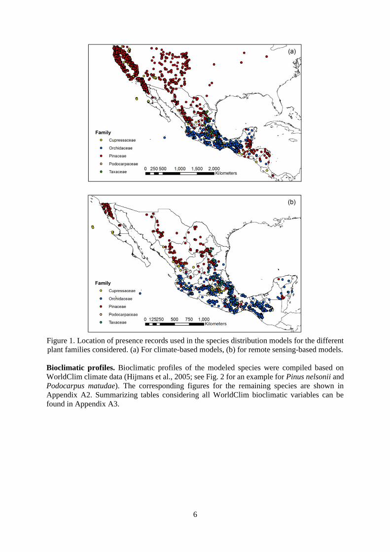
In order to avoid pseudo-replication in the species distribution models, duplicate
records, i.e. records within the same pixel of the environmental data (WorldClim climate data,
MODIS remote sensing data) were removed. Further, species records for which no
environmental data were available were not considered. Based on the recommendations of
Hijmans & Elith (2015), a minimum sample size of 20 presence localities for model building
was accepted. Species with less than 20 records were therefore not modeled (see Appendix A1).
This resulted in 3,162 records used for the climate-based models and 1,274 records used for the
remote sensing-based models, respectively (Table 1, Figure 1). A full overview of records used
in this project (in DarwinCore format) analogue to the results of project JM078 was submitted
together with this report.
Table 1. Overview of species records used for modeling.
Family
Number of records used in
climate-based models (number
of species)
Number of records used in
remote sensing-based models
(number of species)
Orchidaceae 653 (17) 640 (17)
Pinaceae 2,050 (17) 393 (10)
Cupressaceae 316 (5) 130 (2)
Taxaceae 51 (1) 51 (1)
Podocarpaceae 52 (1) 52 (1)
Total 3,122 (41) 1,266 (31)
6
Figure 1. Location of presence records used in the species distribution models for the different
plant families considered. (a) For climate-based models, (b) for remote sensing-based models.
Bioclimatic profiles. Bioclimatic profiles of the modeled species were compiled based on
WorldClim climate data (Hijmans et al., 2005; see Fig. 2 for an example for Pinus nelsonii and
Podocarpus matudae). The corresponding figures for the remaining species are shown in
Appendix A2. Summarizing tables considering all WorldClim bioclimatic variables can be
found in Appendix A3.

7
Figure 2. Bioclimatic profiles of (a) Pinus nelsonii and (b) Podocarpus matudae based on
WorldClim climate data (Hijmans et al., 2005; current conditions).
Profiles of land surface phenology. Phenological profiles of the modeled species were derived
from time series data of the Terra-MODIS Enhanced Vegetation Index (EVI) from the years
2001 to 2009 (for further details: see Section 3, Variables used in the models). For each species,
EVI values were extracted from the raster maps at the respective presence locations. Extracted
values were averaged for each date over all locations (Figure 3a) as well as stratified by
biogeographic region (Figure 3b; according to CONABIO, 1997) and vegetation type (Figure
(a)
(b)

8
3c; Rzedowski, 1978; Rzedowski, 1990). Both mean values and standard deviation were plotted
against time (see Appendix A4 for plots of the remaining species).
Figure 3. Phenological profiles of Pinus nelsonii. (a) Summarized over all locations, (b)
stratified by biogeographic region, and (c) stratified by vegetation type.
(a)
(b)
(c)

9
2. Criteria for the selection of the reference area per species (Criterio
de Selección de la región de referencia por especie)
Because of the large number of species considered in this project, we had - in consultation with
CONABIO - to refer to a fixed geographical extent. While the study area for modelling
available habitat based on remote sensing data was confined to Mexico, the area for modelling
potential species distributions based on climate data was set to a rectangular area of 10 degrees
(WGS84, in all four directions) beyond the extent of Mexico (according to the GADM database
of Global Administrative Areas, GADM 2012).
3. Variables used in the models (Variables utilizadas en la
modelación)
Climate data. Climatic variables were obtained at 30 arc seconds (~ 0.0083 degree) spatial
resolution from the WorldClim data base (Current conditions; Hijmans et al., 2005). WorldClim
parameters are derived from long-term time series (1950-2000) of a global network of climate
stations, express spatial variations in annual means, seasonality, and extreme or limiting
climatic factors, and represent biologically meaningful variables for characterizing species
distributions. For the species distribution models, bioclimatic layers were resampled from their
native resolution and gridded to pixel location, cell size and extent of the remote sensing data
to maintain spatial consistency. This was done with R 3.0.1 (R Core Team 2013) using the sp
package version 1.0 (Pebesma & Bivand, 2005).
Remote sensing data. The remote sensing parameters used in this project were selected to
effectively describe vegetation dynamics and land surface phenology (Colditz et al., 2009; Cord
& Rödder, 2011). Vegetation indices are an integrated measure of vegetation canopy greenness,
a composite property of leaf area, chlorophyll and canopy structure as important dimensions of
habitat characteristics. We used the Enhanced Vegetation Index (EVI) that is superior to the
Normalized Difference Vegetation Index (NDVI) due to its improved sensitivity in high biomass
regions and a reduction in atmospheric influences (Huete et al., 2002). In addition, Land Surface
Temperature (LST) as one of the key parameters in the physics of land surface processes, e.g.
surface-atmosphere interactions and energy fluxes, was analyzed. LST provides different
information compared to temperature measures derived from interpolated climate station data.
Remote sensing time series from 2001 to 2009 at 1 km² spatial resolution based on the
Terra-MODIS 16-day standard products MOD13A2 and MOD11A2 were compiled for
Mexico. For this purpose, the MODIS-specific pixel-level Quality Assurance Science Data Sets
(QA-SDS) were analyzed using the TiSeG software package (Colditz et al., 2008) to exclude
low-quality data, e.g. due to cloud cover or atmospheric contamination. With a critical
weighting between data quality and the necessary quantity for meaningful interpolation, high-
quality data were used as vertices for pixel-level linear temporal interpolation. In addition, an
adaptive Savitzky-Golay filter as implemented in the TIMESAT 3.0 software (Jönsson &
Eklundh, 2004; Eklundh & Jönsson, 2009) was applied to account for high-frequency
fluctuations and negatively-biased noise.
From the time series data, 18 annual phenological metrics including (1) Time-related
metrics: Start of season (date_SOS), mid of season (date_maximum), end of season (date_EOS),
dormancy (date_dormancy), length of season (length_season), (2) Net primary productivity
(NPP)-related metrics: Vegetation index value at SOS (value_SOS), value at EOS (value_EOS),
maximum value (maximum), minimum value (minimum), annual range (range), accumulated
integral during vegetation period (integral), annual mean (mean), annual median (median) and
(3) Seasonality-related metrics: rate of green-up (rate_greenup), rate of senescence

10
(rate_senescence), shape of phenology curve (skewness), standard deviation
(standard_deviation) and coefficient of variation (CoV). For temporal metrics referring to
certain stages within the phenological cycle, the number of the corresponding composite
(between 1 and 23 in accordance with the 16-day composite period of the MODIS products)
was assigned. In addition, annual statistical metrics (minimum, mean, median, maximum,
range, standard deviation, and coefficient of variation) were computed for the Land Surface
Temperature (LST) time series. All metrics were averaged over the nine year period to account
for inter-annual variation of vegetation seasonality or single-year anomalies before they were
used as predictors in the species distribution models.
Correlation analysis. To avoid model over-fitting and to exclude redundant data,
environmental predictors (both climate and remote sensing) were carefully selected. For both
data sets, species-specific pair-wise Spearman’s rank correlation coefficients were estimated.
Out of each pair of highly-correlated and hence redundant environmental predictors
(Spearman’s rank correlation coefficient |r| > 0.7) the variable with the higher explanatory
power for each study species according to a Generalized Linear Model (GLM) based on
presence and pseudo-absence locations was retained (select07 method in Dormann et al., 2013
which selects variables based on removing correlations > 0.7, retaining those variables more
important). However, because models still tended to be over-fitted in trial runs with these
reduced predictor set for species with more than 50 occurrence records, we decided to exclude
the time-related variables (EVI_date_SOS, EVI_date_EOS, EVI_date_maximum, EVI_date
dormancy and EVI_length_season) due to their low mean influence (relative variable
importance in most cases below 0.1) in the trial runs. Furthermore, because of its low ecological
interpretability the variable EVI_skewness was excluded. Collinearity among the remaining 19
remote sensing variables (Table 2) was analyzed using the select07 method in Dormann et al.
(2013) as described above. An overview of how often the variables were selected is given in
Appendix A5 (for climate) and A6 (for remote sensing).

11
Table 2. Final set of variables used in the species distribution models.
Short name (Abbreviation) Description C
lim
ate
BIO1 Annual Mean Temperature
BIO2 Mean Diurnal Range (Mean of monthly (max - min temp))
BIO3 Isothermality (BIO2/BIO7) (* 100)
BIO4 Temperature Seasonality (standard deviation *100)
BIO5 Max Temperature of Warmest Month
BIO6 Min Temperature of Coldest Month
BIO7 Temperature Annual Range (BIO5-BIO6)
BIO8 Mean Temperature of Wettest Quarter
BIO9 Mean Temperature of Driest Quarter
BIO10 Mean Temperature of Warmest Quarter
BIO11 Mean Temperature of Coldest Quarter
BIO12 Annual Precipitation
BIO13 Precipitation of Wettest Month
BIO14 Precipitation of Driest Month
BIO15 Precipitation Seasonality (Coefficient of Variation)
BIO16 Precipitation of Wettest Quarter
BIO17 Precipitation of Driest Quarter
BIO18 Precipitation of Warmest Quarter
BIO19 Precipitation of Coldest Quarter
Rem
ote
sen
sin
g
LST_standard_deviation (LSTSTD) Standard deviation of annual mean land surface
temperature
LST_range (LSTRANGE) Range of annual land surface temperature
LST_minimum (LSTMIN) Minimum annual land surface temperature
LST_median (LSTMEDIAN) Median annual land surface temperature
LST_mean (LSTMEAN) Annual mean land surface temperature
LST_maximum (LSTMAX) Minimum annual land surface temperature
LST_CoV (LSTCOV) Coefficient of Variation of land surface temperature
EVI_value_SOS (EVIVSOS) Mean Enhanced Vegetation Index at beginning of season
EVI_value_EOS (EVIVEOS) Mean Enhanced Vegetation Index at end of season
EVI_standard_deviation (EVISTD) Standard deviation of the mean annual value of the
Enhanced Vegetation Index
EVI_rate_senescence (EVISENES) Rate of senescence
EVI_rate_greenup
(EVIGREENUP) Rate of greenup
EVI_range (EVIRANGE) Annual range of the Enhanced Vegetation Index
EVI_minimum (EVIMIN) Minimum annual value of the Enhanced Vegetation Index
EVI_median (EVIMEDIAN) Median annual value of the Enhanced Vegetation Index
EVI_mean (EVIMEAN) Mean annual value of the Enhanced Vegetation Index
EVI_maximum (EVIMAX) Maximum annual value of the Enhanced Vegetation Index
EVI_integral (EVIINTEG) Sum of Enhanced Vegetation Index values between start
and end of season
EVI_CoV (EVICOV) Coefficient of Variation of the Enhanced Vegetation Index

12
4. Methods for modeling (Método de modelación)
Generation of pseudo-absence data. Pseudo-absence data were generated following the
target-group background approach (Phillips et al., 2009). According to this assumption, the
influence of spatially biased samples (e.g. towards roads and protected areas, which is typical
for biological collections) can be reduced by comparing the occurrences with background points
reflecting the same spatial bias. The underlying idea is that a model based on presence and
background data with the same bias will not focus on the sample selection bias, but on any
differentiation between the distribution of the occurrences and that of the background. Because
the species analyzed in this study are from different families, all species records belonging to
the kingdom Plantae within the study area extent were extracted from the GBIF database
(http://data.gbif.org) (in total 1,990,527 records). From this dataset, two randomized subsets of
10,000 unique locations were selected as pseudo-absence data sets for the potential species
distributions (based on climate data) and the extent of available habitat (based on remote
sensing data) (Figure 4 a and b).
Figure 4. Location of pseudo-absence records. a) For climate-based models, b) For remote
sensing-based models.
Model algorithms and ensemble modeling. Since the choice of model algorithm is a major
component of prediction uncertainty in species distribution modeling (Dormann et al., 2008;

13
Buisson et al., 2010), several algorithms were employed in order to estimate and account for
prediction uncertainty. The modelling procedure was conducted for both, potential distribution
and available habitat, using the same methodology. If not mentioned otherwise, model
adjustments were identical for both. All modelling procedures were performed using R version
3.1.2 (R Core Team 2014). The final models were run on a Linux-based cluster with 1,024
computing cores and 5TB RAM with a CentOS 6.5 as operating system.
We used three modeling methods that are representative for different classes of model
algorithms, namely regression-based methods, machine-learning methods and presence-only
methods. Generalized Linear Models (GLM), Random Forest (RF) and Maxent (Maximum
Entropy) version 3.3.3e were applied as implemented in the biomod2 package version 3.1
(Thuiller et al., 2014). Presences and pseudo-absences were weighted equally and were used as
response variables. Model runs were repeated 199 times for each species and model algorithm,
randomly selecting 70% of the presences and pseudo-absences for model calibration and 30%
for model testing in each model run. Models were scaled between 0 and 1,000 to ensure
comparability of model predictions derived from the different model algorithms. To generate
ensemble (“consensus”) models from the results of these three algorithms, the ROC (Relative
or Receiver Operating Characteristic) was used as evaluation metric (see the documentation of
the biomod2 package for further information). For species with more than 100 occurrences (see
below), additional model predictions were made using Generalized Additive Models (GAM)
and Boosted Regression Trees (BRT). These additional models were done with 10 repetitions.
The specific parameters used for each modeling algorithm are described in further detail in
section 5 ‘Parameters used for modeling’.
Conversion to binary maps and combination of climate and remote sensing-based model
predictions. From the resulting consensus maps (i.e., based on GLM, RF and Maxent; see
above), binary species-specific distribution maps were created by applying three different
threshold values that give different weight to omission and commission errors: The ‘minimum
training presence’, ‘10 percentile training presence’, and ‘maximum training sensitivity plus
specificity’ threshold. The ‘minimum training presence threshold’ (representing the lowest
value observed in the continuous prediction map at a presence location for a specific species)
aims at minimizing omission errors at the expense of a greater fractional predicted area per
species and may lead to model overprediction (Jarnevich & Reynolds, 2011). The ‘10 percentile
training presence threshold’ provides more conservative models by predicting the 10% most
extreme presence observations as absent. Finally, the ‘maximum sensitivity and specificity
threshold’ gives equal weight to both omission and commission errors (sensitivity = true
positive rate and specificity = true negative rate of the predictions) and aims at maximizing
both. It was identified as among the best approaches by Liu et al. (2005). Sensitivity and
specificity values were calculated using the PresenceAbsence package version 1.1.9 (Freeman
& Moisen, 2008).
Climatic and remote sensing-based species distribution models were finally integrated
in a hierarchical modeling framework where first the potential distribution range (based on the
‘10 percentile training presence’ threshold) was modeled based on climate data and then
remotely sensed habitat availability within this climatic range was integrated in a hierarchical
model design. These maps of current habitat availability were only produced for the Mexican
national territory. We finally used binary maps based on the ‘10 percentile training presence’
threshold to calculate maps of habitat loss by subtracting available habitat from the potential
distributions.

14
5. Parameters used for modeling (Parámetros utilizados en la
modelación)
Maxent. Maxent models were run using auto features, but excluding threshold and hinge
features, with the number of iterations limited to 500. To optimize model performance, the
regularization parameter β (to be applied to all linear, quadratic and product features; Phillips,
2006) was determined in trial runs for species with more than 80 occurrences for climate-based
models (Pseudotsuga menziesii glauca, Abies concolor, Cupressus lusitanica, Calocedrus
decurrens, Pinus attenuata, Pinus jeffreyi, Pinus coulteri, Rhynchostele cervantesii, Pinus
muricata, Prosthechea vitellina) and for species with more than 50 occurrences for remote
sensing-based models (Cupressus lusitanica, Pinus pinceana, Podocarpus matudae,
Prosthechea vitellina, Pseudotsuga menziesii glauca, Rhynchostele cervantesii, Taxus
globosa). For this purpose, we compared model performance using regularization multipliers
of 0.001, 0.002, 0.005, 0.01, 0.02, 0.05, 0.25, 0.5, 0.75, 1, 2, 5 and 10 separately for climate and
remote sensing variables. For the final models, the regularization parameter with the highest
mean AUC value in these trial runs was chosen (climate: β=0.02, remote sensing: β=0.002).
Generalized Linear Models. Generalized Linear Models (GLM) were fitted using a binomial
link function, including linear and quadratic terms as well as linear interaction terms of the
environmental predictors. Interactions considered in the models were chosen based on their
ecological meaningfulness which implied that interactions among temperature variables and
interactions among precipitation variables were not allowed. A stepwise backward selection
procedure starting with the full model was applied to select final models (MASS package,
Venables & Ripley 2002). In each step, the model was simplified and the Bayesian Information
Criterion (BIC) of the simplified model was compared to the BIC of the previous model. This
procedure was repeated until the BIC reached its minimum. Simplification was done by
dropping the variable which leads to a maximum decrease of BIC compared to the starting
model.
Random Forest. As for Maxent, algorithmic settings for RF models were determined in trial
runs for species more than 80 occurrences for climate-based models and for species with more
than 50 occurrences for remote sensing-based models. For this purpose, the number of trees
was tested between 500 and 3,000 in six steps and the number of tries was tested between 1 and
5 in five steps (again separately for climate and remote sensing variables). For each of these 30
different settings, the mean R² of the ‘out-of-bag error estimate’ (R²oob) over all test species
was calculated. The oob is the average misclassification over all trees tested by using the out-
of-bag examples (out-of-bag examples are the data that are left after bootstrapping the training
data; Livingston, 2005). The settings with the highest mean R²oob were chosen for the final
models (Leutner et al. 2012). Based on these results, the following settings were applied:
Climate data: 2,500 trees, 2 tries; Remote sensing data: 500 trees, 1 try.
Generalized additive models (GAM) and boosted regression trees (BRT). As for the other
algorithms, algorithmic settings for BRT models were determined in trial runs for species more
than 80 occurrences for climate-based models and for species with more than 50 occurrences
for remote sensing-based models. For this purpose, the number of trees was tested between
1,500 and 2,500 in three steps. The tree complexity parameter was tested between 3 and 5 in
three steps. The learning rate was tested between 0.005 and 0.008 in four steps. The bag fraction
was tested between 0.5 and 0.8 in four steps. For each of these 144 different settings, the mean
of deviance over all test species was calculated. This was done separately for climate and remote
sensing variable. Based on these results, the following settings were applied: climate: number

15
of trees = 2,500, tree complexity = 5, learning rate = 0.007 and bag fraction = 0.8; remote
sensing: number of trees = 1,500, tree complexity = 4, learning rate = 0.005 and bag fraction =
0.8. All other parameters of BRT models were set to default. The smoothing parameter k in the
GAM models was set to 30. To allow for a comparison among the different model algorithms,
predictions were made for the species Abies concolor, Calocedrus decurrens, Cupressus
lusitanica, Pinus attenuata and Pseudotsuga menziesii glauca using the GLM, RF, Maxent,
GAM and BRT algorithms with 10 repetitions and the model settings described above. Results
showed no significant differences to models run with only GLM, RF and Maxent.
6. Model evaluation (Evaluación del modelo)
Variable importance. Variable importance for GLM, RF, GAM and BRT models was
calculated using the implemented algorithm of the package biomod2 (function
‘variables_importance()’). This method is based on a comparison of the model prediction
derived from the original dataset and predictions derived from permuted datasets. These
permuted datasets were created by randomizing one environmental variable for each data set.
The predicted values of permuted datasets and the original dataset for presence/pseudo-absence
locations were compared by calculating the Pearson correlation coefficient. This procedure was
repeated three times for each variable. The smaller the correlation coefficient was the higher
was the independent influence of the permuted variable. Values of variable importance were
finally calculated by subtracting the correlation coefficient from 1. For the Maxent models,
variable importance was additionally expressed by the regularized model gain for each variable.
For all three algorithms (GLM, Maxent and RF), BIO4 (Temperature seasonality), BIO14
(Precipitation of Driest Month) and BIO15 (Precipitation Seasonality) showed the highest
variable importance among the climatic predictors considered. On average, 3.19 ± 0.65 (mean
± standard deviation) remote sensing variables were selected based on the collinearity and
variable importance analysis (select07 method) per species. These belonged in 11.6% to EVI-
based and in 25.8% to LST-based variables. While there was a high variability regarding
variable importance among the different study species, minimum LST turned out to have the
highest average variable importance for all three algorithms.
Model performance based on AUC, partial AUC and model deviance. We quantified model
performance by calculating AUC values, partial AUC values and model deviance. The AUC
value is the area under the Receiver Operating Characteristic curve (ROC) and describes the
ability of the model to discriminate between 0 and 1, or absence and presence respectively
(Peterson et al., 2008). The ROC is created by plotting the fraction of true presences out of
observed presences (sensitivity) against the fraction of false presences out of observed absences
(1-specificity), for different threshold levels. AUC values were calculated using the package
PresenceAbsence version 1.1.9 (Freeman, 2008). The partial AUC values gives the ratio of the
AUC of the model to the AUC of a random model in a defined range of sensitivity or specificity,
were the model is supposed to make predictions. We used the range of sensitivity between 0.2
and 1, following Peterson et al. (2008) who recommend restricting AUC calculations “to the
domain within which omission error is sufficiently low as to meet user-defined requirements of
predictive ability”. The partial AUC values were calculated by using the package pROC version
1.7.3 (Robin et al., 2011). The model deviance is a log-likelihood ratio statistics that compares
the saturated model with the proposed model. The model deviance was calculated as: D=-
2*(yi*log(ui))+((1-yi)*log(1-ui))n, where yi is the binary observed presence at a locations, ui is
the predicted probability at a location and n is the number of all presences and absences. In
addition, we used presence-absence records from the Mexican National Forest Inventory
(INFyS, Inventario Nacional Forestal y de Suelos) for model validation for those species that

16
were included in the INFyS database. For this purpose, AUC and model deviance were
calculated by using the INFyS presence-absence data as true presence-absence data. All
climate-based models showed very good performance measures based on AUC (i.e. > 0.9) and
partial AUC (i.e. > 0.7). For those species for which an additional model evaluation based on
INFyS data was possible, the obtained (partial)AUC scores were much lower, especially for
models using GLMs. Model performance of the remote sensing-based models was lower with
only 54% of the models having AUC scores of 0.9 or higher. 94% of the models, however,
showed AUC scores above 0.7 and partial AUC scores above 0.5. Again, model deviance was
highest for GLMs.
Exemplary model results. As two examples of a ‘good’ and a ‘bad’ model, the modeled habitat
availability of Pinus nelsonii and Podocarpus matudae are shown in Figure 5. The known
distribution of P. nelsonii (according to Farjon and Filer, 2013) is limited to Coahuila, Nuevo
León, San Luis Potosí and Tamaulipas, in foothills or lower slopes of the Sierra Madre Oriental
– which is well-captured by the model prediction. The species is restricted to sites on rocky
limestone with shallow soils (Farjon and Filer, 2013). Apparently, while climate-based SDMs
tended to overestimate distribution ranges for this species (data not shown), the inclusion of
remote sensing data allowed identifying those sites with suitable habitat conditions. In addition
to the distribution in Coahuila, Nuevo León, San Luis Potosí and Tamaulipas, the model for
habitat availability also predicted potential habitat in Hidalgo and Puebla, though with lower
suitability scores. The model of habitat suitability for P. matudae, however, overestimated
habitat availability, in particular on the Yucatán peninsula. The species occurs from Honduras
to Tamaulipas and Jalisco in Mexico and is mostly found in mixed pine forest, pine-oak forest,
montane rain forest and evergreen cloud forest at altitudes between 600 and 2,600m (Farjon
and Filer, 2013). Such habitat types do not exist on the Yucatán peninsula. However, even
though only one record from Jalisco was included in this project, the model correctly predicted
habitat availability in the Sierra Madre del Sur – Farjon and Filer (2013) list herbarium records
of P. matudae from this region.

17
Figure 5. Modeled habitat availability of (a) Pinus nelsonii and (b) Podocarpus matudae. The
inset map in (a) shows the main distribution range of P. nelsonii on karst limestone outcrops
in the Sierra Madre Oriental.
Spatial assessment of model uncertainty. Maps of spatially explicit model uncertainty were
derived by calculating the difference between the 97.5-percentile and the 2.5-percentile of cell
values derived from the continuous prediction maps, based on 199 model repetition runs. For
species with 40 or more independent presence locations, uncertainty maps were calculated
using the predictions of the Maxent, GLM and RF models. For species with less than 40
independent presence locations, only the Maxent predictions were considered. Results showed
that model uncertainty was generally higher in areas with high predicted suitability and lowest
in those region with the lowest suitability (i.e. that all model algorithms and repetitions
consistently predicted low suitability). In the case of Podocarpus matudae (Figure 6), the
uncertainty map revealed that the overestimated species distribution on the Yucatán peninsula
was modeled with comparatively high uncertainties. Uncertainty maps therefore can effectively
help refining species distribution predictions.

18
For three species with a wide spatial distribution all over Mexico (Cupressus lusitanica, Pinus
strobiformis, Pseudotsuga menziesii glauca), a spatially stratified resampling scheme was
implemented. For each of those species, we performed a k-means clustering (Hartigang &
Wong, 1979) using a maximum number of 10 iterations on the presence/pseudo-absence data
to derive 199 center points. Using each of the center points, the original dataset was divided
into 199 calibration datasets and one validation dataset. During each iteration, 30% of the
presence/pseudo-absence points with the smallest distance to the center points were chosen as
validation data and the remaining 70 % of the points as calibration data. Our aim here was to
test for the relative contributions of different components of model uncertainty (occurrence
data, environmental data, and model algorithm) using generalized linear models (according to
Buisson et al., 2010). For this purpose, the mean predicted probability of each replicate model
run was used as response and the used model type, data type (climatic or remote sensing) and
replicate number as explanatory variables (glm(formula = x ~ data + occurence + modeltype,
family = gaussian). For all species, we found significant effects (p < 0.001) of the environmental
data (i.e. climate or remote sensing) and the model algorithm (Maxent, GLM, RF) used, but not
for the occurrence data (i.e. random vs. spatially stratified resampling, p > 0.05).
Figure 6. Uncertainty map for modeled habitat availability of Podocarpus matudae.

19
7. Conclusions and recommendations (Conclusiones y
recomendaciones)
The project aims, i.e. the development and refinement of species distribution models by (1) the
inclusion of remote sensing variables (Terra-MODIS Enhanced Vegetation Index and Land
Surface Temperature) in addition to climatic predictors and (2) the spatially-explicit assessment
of model uncertainty could be achieved. The main limitation was the limited number of verified
herbarium records available as training data – a typical phenomenon for very rare species as in
the NOM – which did allow model building only for a fraction of the species considered. More
efforts therefore have to be undertaken to compile reliable information on species presence that
is readily accessible online.
Remote sensing data showed great potential for reducing the typical overprediction of
climate-based SDMs. Even though also predictions based only on climate data were produced
in the project, we therefore highly recommend using the predictions for habitat availability
(which are based on remote sensing data but also include potential distributions based on
climate) for further analyses. SDMs based on remote sensing data only, however, also in most
cases overestimated distribution ranges. The combination of climate and remote sensing data
therefore appears to be the most promising approach for modeling species distributions.
However, species records were mostly collected during a different time period than the
remote sensing data. More specifically, 314 records were collected between 2001 and 2009
(which is exactly the time period that the remote sensing data cover), 57 records were collected
after 2009, and 2,294 records were collected before 2001. Information concerning the collection
date was missing for 497 records. In summary, the majority of records were hence collected
before satellite data was available, with a mean collection year of 1968. How big the impact of
this temporal mismatch on the applicability of the model predictions is largely depends on the
characteristic of the collection sites. If specimen were collected in a site where almost no change
in vegetation cover has happened over the last few decades and where the species is still present
today, effects on the resultant prediction maps will be minimal. As many collectors of field data
tend to sample undisturbed and well-established populations, this will hold true at least for a
part of the records. On the other hand, in case land use/land cover change has happened in the
collection site (making the site no longer suitable for the species of concern) between the
collection date of the records and the acquisition date of the remote sensing data, this record
will be unsuitable for model training and should be left out. Generally, SDMs and the
algorithms used in this project can deal with some outliers or wrong records in the training data;
however, models will be significantly biased, if a large fraction of the records is affected by
this. Apparently, it is not possible to quantify the overall effects of the temporal mismatch of
species records and remote sensing data based on the data at hand. A rigorous approach would
require a lot of additional field work in order to collect recent data in those collection sites that
could be affected by land use/land cover change. We therefore recommend taking this into
account when interpreting remote sensing-based model results.
Further, the compiled maps of habitat loss are an indicator of anthropogenic impacts but
should not be overinterpreted and directly be used for decision-making. Other factors not
captured by climate but by remote sensing data (e.g. natural disturbances) may lead to areas
being identified as ‘lost habitat’ independent of any human impact. Obviously, the map
indicating total habitat loss (a summary of the species-specific habitat loss maps) is biased in
the way that it considers only a small number of species and therefore is not representative for
the entire country.
For some species, the different model algorithms used showed large differences
regarding model performance (AUC, partial AUC and model deviance). We therefore
recommend using ensemble models based on different algorithms for species distribution

20
modeling. The high variable importance of LST-derived parameters again supports the
importance of considering additional predictors beyond the ‘classical’ vegetation indices in
SDMs. Further research is needed to fully explore the relevance of the broad array of remotely
sensed parameters available for use in SDMs.
In the future, remotely sensed time series will be operationally available at much higher
spatial resolutions (e.g. from the ESA Sentinel satellites) and provide a unique opportunity for
assessing habitat availability and species diversity in space and time. Due to the automated
implementation of the modeling framework used in this project, the methods developed and
used here can (with slight modifications) transferred to remote sensing data with other spatial
resolutions available in the near future. In summary, future research therefore should focus on
(1) the applicability of other remotely sensed parameters not considered here for predicting
species distributions, (2) differences in the performance of remote sensing-based SDMs for
species associated with different habitat types and (3) the potential of remote sensing data to
verify (and falsify) species occurrence records.

21
8. References
Araújo, M.B., Pearson, R.G., Thuiller, W. & Erhard, M. (2005). Validation of species-climate impact
models under climate change. Global Change Biology, 11, 1504-1513.
Bradley, B.A. & Fleishman, E. (2008). Can remote sensing of land cover improve species distribution
modelling?, Journal of Biogeography, 35 (7), 1158-1159.
Buermann, W., Saatchi, S., Smith, T.B., Zutta, B.R., Chavesi, J.A., Mila, B. & Graham, C.H. (2008).
Predicting species distributions across the Amazonian and Andean regions using remote sensing
data. Journal of Biogeography, 35 (7), 1160-1176.
Buisson, L., Thuiller, W., Casajus, N., Lek, S. & Grenouillet, G. (2010). Uncertainty in ensemble
forecasting of species distribution. Global Change Biology, 16, 1145-1157.
Colditz, R.R., Conrad, C., Wehrmann, T., Schmidt, M., & Dech, S. (2008). TiSeG: A flexible Software
Tool for Time-Series Generation of MODIS Data Utilizing the Quality Assessment Science Data
Set. IEEE Transactions on Geoscience and Remote Sensing, 46(10), 3296-3308.
Colditz, R.R., Cord, A., Conrad, C., Mora, F., Maeda, P. & Ressl, R. (2009). Analyzing Phenological
Characteristics of Mexico with MODIS Time Series Products. Multi-Temp, Fifth international
Workshop on the Analysis of Multitemporal Remote Sensing Images, July 28-30, 2009. Mystic,
Connecticut, USA.
Comisión Nacional para el Conocimiento y Uso de la Biodiversidad – CONABIO (1997). Provincias
biogeográficas de México. Escala 1:4000000. México.
Cord, A. & Rödder, D. (2011). Inclusion of habitat availability in species distribution models through
multi-temporal remote sensing data? Ecological Applications, 21, 3285-3298.
Dormann, C.F., Purschke, O. García Márquez, J. R., Lautenbach, S. & Schröder, B. (2008). Components
of uncertainty in species distribution analysis: A case study of the Great Grey Shrike Lanius
excubitor L. Ecology, 89, 3371-3386.
Dormann, C.F., Elith, J., Bacher, S., Buchmann, C., Carl, G., Carré, G., García Marquéz, J.R., Gruber,
B., Lafourcade, B., Leitao, P.J., Münkemüller, T., McClean, C., Osborne, P.E., Reineking, B.,
Schröder, B., Skidmore, A.K., Zurell, D. & Lautenbach, S. (2013) Collinearity: a review of
methods to deal with it and a simulation study to evaluate their performance. Ecography, 36,
27-46.
Eklundh, L. & Jönsson, P. (2009). Timesat 3.0, Software Manual, Lund University, Sweden.
Elith, J., Burgman M. A. & Regan, H. M. (2002). Mapping uncertainties and vague concepts in
predictions of species distributions. Ecological Modelling, 157, 313-329.
Farjon, A. & Filer, D. (2013). An Atlas of the World's Conifers: An Analysis of Their Distribution,
Biogeography, Diversity and Conservation Status. Brill Academic Pub, 512 pp.
Freeman, E. A. & Moisen, G. (2008). PresenceAbsence: An R Package for Presence-Absence
Model Analysis. Journal of Statistical Software, 23(11),1-31.
GADM (2012). GADM database of Global Administrative Areas, Version 2.0, www.gadm.org
Hartigan, J.A. & Wong, M.A. (1979). Algorithm AS 136: A K-Means Clustering Algorithm. Journal of
the Royal Statistical Society, Series C (Applied Statistics), 28, 100–108.
Hijmans, R.J. and Elith, J. (2015). Species distribution modeling with R, http://cran.r-
project.org/web/packages/dismo/vignettes/sdm.pdf

22
Hijmans, R.J., Cameron, S.E., Parra, J.L., Jones, P.G., & Jarvis, A. (2005). Very high resolution
interpolated climate surfaces for global land areas. International Journal of Climatology, 25,
1965-1978.
Huete, A., Didan, K., Miura, T., Rodriguez, E.P., Gao, X. & Ferreira, L.G. (2002). Overview of the
radiometric and biophysical performance of the MODIS vegetation indices. Remote Sensing of
Environment, 83, 195-213
Jarnevich, C.S. & Reynolds, L.V. (2011). Challenges of predicting the potential distribution of a slow-
spreading invader: a habitat suitability map for an invasive riparian tree. Biological Invasions,
13, 153-163.
Jönsson, P. & Eklundh, L. (2004). TIMESAT – a program for analyzing time-series of satellite sensor
data, Computers & Geosciences, 30, 833-845.
Leutner, B.F., Reineking, B., Müller, J., Bachmann, M., Beierkuhnlein, C., Dech, S. & Wegmann, M.
(2012). Modelling Forest α -Diversity and Floristic Composition On the Added Value of LiDAR
plus Hyperspectral Remote Sensing. Remote Sensing, 4, 2818-2845.
Livingston, F. (2005). Implementation of Breiman’s Random Forest Machine Learning Algorithm,
ECE591Q Machine Learning Journal Paper, https://datajobs.com/data-science-repo/Random-
Forest-%5BFrederick-Livingston%5D.pdf
Liu, C., Pam, M., Dawson, T.P. & Pearson, R.G. (2005). Selecting thresholds of occurrence in the
prediction of species distributions. Ecography, 28, 385-393.
Luoto, M., Virkkala, R. & Heikkinen, R.K. (2007). The role of land cover in bioclimatic models depends
on spatial resolution. Global Ecology and Biogeography, 16, 34-42.
Pearson, R. G., Dawson, T. P. & Liu, C. (2004). Modelling species distributions in Britain: a hierarchical
integration of climate and landcover data. Ecography, 27, 285-298.
Pebesma, E.J. & Bivand, R.S. (2005). Classes and methods for spatial data in R. R News 5 (2),
http://cran.r-project.org/doc/Rnews/.
Peterson, A.T., Papes, M. & Soberón, J. (2008). Rethinking receiver operating characteristic analysis
applications in ecological niche modeling. Ecological Modelling, 213, 63-72.
Phillips, S.J., Anderson, R.P., & Schapire, R.E. (2006). Maximum entropy modeling of species
geographic distributions. Ecological Modelling, 190, 231-259.
Phillips, S.J., Dudík, M., Elith, J., Graham, C.H., Lehmann, A., Leathwick, J., & Ferrier, S. (2009).
Sample selection bias and presence-only distribution models: Implications for background and
pseudo-absence data. Ecological Applications, 19, 181-197.
R Core Team (2013). R: A language and environment for statistical computing. R Foundation for
Statistical Computing, Vienna, Austria. http://www.R-project.org/.
R Core Team (2014). R: A language and environment for statistical computing. R Foundation for
Statistical Computing, Vienna, Austria. http://www.R-project.org/.
Robin, X., Turck, N., Hainard, A., Tiberti, N., Lisacek, F., Sanchez, J.-C. & Müller, M. (2011). pROC:
an open-source package for R and S+ to analyze and compare ROC curves. BMC Bioinformatics,
77.
Rzedowski, J. (1978). Vegetación de México. Editorial Limusa, México. I.

23
Rzedowski (1990). Vegetación Potencial, Atlas Nacional de México. Vol II. Escala 1:4 000 000.
Instituto de Geografía, UNAM. México
Saatchi, S., Buermann, W., ter Steege, H., Mori, S. & Smith, T.B. (2008). Modeling distribution of
Amazonian tree species and diversity using remote sensing measurements. Remote Sensing of
Environment, 112, 2000-2017.
Thuiller, W. Miguel B. Araújo, M.B. & Lavorel, S. (2004). Do we need land-cover data to model species
distributions in Europe?. Journal of Biogeography, 31, 353-361.
Thuiller, W., Georges, D. & Engler, R. (2014). biomod2: Ensemble platform for species distribution
modeling. R package version 3.1-48. http://CRAN.R-project.org/package=biomod2.
Tuanmu, M.-N., Viña, A., Bearer, S., Xu, W., Ouyang, Z., Zhang, H. & Liu, J. (2010). Mapping
understory vegetation using phenological characteristics derived from remotely sensed data,
Remote Sensing of Environment, 114, 1833-1844.
Venables, W. N. & Ripley, B. D. (2002). Modern Applied Statistics with S. Fourth Edition. Springer,
New York. ISBN 0-387-95457-0.
9. Appendix
1. Documentation of delivered materials (Documentación del material
entregado)
See the following pages

24
A1. Species considered in this project. Overview of species considered and modeled in the project.
Family Names of included
species (NOM-059)
Accepted names of included species
(project JM078)
Species
with
models
Species
without
models
Short name
(maps and
metadata)
Unique
records
in
database
(covered
by
climate
data)
Model
algorithm
(s) used
for final
climate-
based
models
Unique
records in
database
(covered
by remote
sensing
data)
Model
algorith
m(s)
used for
final
remote
sensing-
based
models
Pinaceae Abies concolor Abies concolor x ABICON 577 Maxent,
GLM, RF 10
Pinaceae Abies flinckii Abies flinckii x 6 16
Pinaceae Abies guatemalensis Abies guatemalensis x 15 14
Pinaceae Abies hickelii Abies hickelii x 16 15
Pinaceae Abies vejari Abies vejarii x ABIVEJ 27 Maxent 24 Maxent
Pinaceae Abies vejari mexicana Abies vejarii subsp. mexicana x 0 0
Orchidaceae Acianthera eximia Acianthera eximia (L.O. Williams)
Solano x 8 9
Orchidaceae Acianthera unguicallosa Acianthera unguicallosa (Ames & C.
Schweinf.) Solano x 2 2
Orchidaceae Acianthera violacea Acianthera violacea (A. Rich. &
Galeotti) Pridgeon & M.W. Chase x 0 0
Orchidaceae Acineta barkeri Acineta barkeri (Bateman) Lindl. x 6 5
Orchidaceae Anathallis abbreviata Anathallis abbreviata (Schltr.)
Pridgeon & M.W. Chase x 0 0
Orchidaceae Anathallis oblanceolata Anathallis oblanceolata (L.O.
Williams) Solano & Soto Arenas x 1 1
Orchidaceae Aspidogyne stictophylla Aspidogyne stictophylla (Schltr.) Garay x 12 10
Orchidaceae Barbosella prorepens Barbosella prorepens (Rchb. f.) Schltr. x 2 2
Orchidaceae Barkeria dorotheae Barkeria dorotheae Halb. x 4 4
Orchidaceae Barkeria melanocaulon Barkeria melanocaulon A. Rich. &
Galeotti x 11 13
Orchidaceae Barkeria scandens Barkeria scandens (Lex.) Dressler &
Halb. x 19 19

25
Orchidaceae Barkeria shoemakeri Barkeria shoemakeri Halb. x 0 0
Orchidaceae Barkeria skinneri Barkeria skinneri (Bateman ex Lindl.)
Lindl. ex Paxton x 4 7
Orchidaceae Barkeria strophinx Barkeria strophinx (Rchb. f.) Halb. x 2 2
Orchidaceae Barkeria whartoniana Barkeria whartoniana (C. Schweinf.)
Soto Arenas x 3 7
Orchidaceae Bletia urbana Bletia urbana Dressler x 3 8
Cupressaceae Calocedrus decurrens Calocedrus decurrens x CALDEC 109
Maxent,
GLM,
RF
9
Orchidaceae Caularthron
bilamellatum
Caularthron bilamellatum (Rchb. f.)
R.E. Schultes x 0 0
Orchidaceae Chysis bractescens Chysis bractescens Lindl. x 12 18
Orchidaceae Chysis limminghei Chysis limminghei Linden & Rchb. f. x 3 2
Orchidaceae Clowesia glaucoglossa Clowesia glaucoglossa (Rchb. f.)
Dodson x 2 1
Orchidaceae Clowesia rosea Clowesia rosea Lindl. x 7 7
Orchidaceae Cochleanthes
flabelliformis
Cochleanthes flabeliformis (Sw.) R.E.
Schultes & Garay x 0 0
Orchidaceae Coelia densiflora Coelia densiflora Rolfe x 5 5
Orchidaceae Corallorhiza macrantha Corallorhiza macrantha Schltr., x 9 9
Orchidaceae Cryptarrhena lunata Cryptarrhena lunata R. Br. x 0 0
Orchidaceae Cuitlauzina candida Cuitlauzina candida (Lindl.) Dressler
& N.H. Williams, 2003 x 3 3
Orchidaceae Cuitlauzina
convallarioides
Cuitlauzina convallarioides (Schltr.)
Dressler & N.H. Williams x 0 0
Orchidaceae Cuitlauzina pendula Cuitlauzina pendula Lex. x 10 11
Cupressaceae Cupressus arizonica
montana Callitropsis montana x 0 0
Cupressaceae Cupressus forbesii Callitropsis forbesii x CUPFOR 36 Maxent 0
Cupressaceae Cupressus guadalupensis Callitropsis guadalupensis x 2 2
Cupressaceae Cupressus lusitanica Callitropsis lusitanica x CUPLUS 111
Maxent,
GLM,
RF
106
Maxent,
GLM,
RF
Orchidaceae Cycnoches ventricosum Cycnoches ventricosum Bateman x CYCVEN 23 Maxent 23 Maxent

26
Orchidaceae Cypripedium
dickinsonianum Cypripedium dickinsonianum Hágsater x 0 0
Orchidaceae Cypripedium irapeanum Cypripedium irapeanum Lex. x 0 0
Orchidaceae Cyrtochiloides
ochmatochila
Cyrtochiloides ochmatochila (Rchb.f.)
N.H. Williams & M.W. Chase x 3 3
Orchidaceae Dignathe pygmaeus Dignathe pygmaeus Lindl. x 0 0
Orchidaceae Dracula pusilla Dracula pusilla (Rolfe) Luer x 3 2
Orchidaceae Dryadella guatemalensis Dryadella guatemalensis (Schltr.) Luer x 5 6
Orchidaceae Elleanthus
hymenophorus
Elleanthus hymenophorus (Rchb. f.)
Rchb. f. x 0 0
Orchidaceae Encyclia adenocaula Encyclia adenocaula (Lex.) Schltr. x ENCADE 46
Maxent,
GLM,
RF
45
Maxent,
GLM,
RF
Orchidaceae Encyclia atrorubens Encyclia atrorubens (Rolfe) Schltr. x 0 0
Orchidaceae Encyclia distantiflora Oestlundia distantiflora (A. Rich. &
Galeotti) Dressler & Pollard x 0 0
Orchidaceae Encyclia kienastii Encyclia kienastii (Rchb. f.) Dressler &
G.E. Pollard x 5 7
Orchidaceae Encyclia lorata Encyclia lorata Dressler & G.E.
Pollard x 1 1
Orchidaceae Encyclia pollardiana Encyclia pollardiana (Withner)
Dressler & G.E. Pollard x 7 7
Orchidaceae Encyclia tuerckheimii Encyclia tuerckheimii Schltr. x 2 5
Orchidaceae Epidendrum
alabastrialatum
Epidendrum alabastrialatum
G.E.Pollard ex Hágsater x 7 5
Orchidaceae Epidendrum alticola Epidendrum alticola Ames & Correll x 4 5
Orchidaceae Epidendrum cerinum Epidendrum cerinum Schltr. x 7 8
Orchidaceae Epidendrum chloe Epidendrum chloe Rchb. f. x 5 6
Orchidaceae Epidendrum
cnemidophorum Epidendrum cnemidophorum Lindl. x 15 18
Orchidaceae Epidendrum coronatum Epidendrum coronatum Ruiz & Pav. x 1 1
Orchidaceae Epidendrum cystosum Epidendrum cystosum Ames x 3 3
Orchidaceae Epidendrum
dorsocarinatum Epidendrum dorsocarinatum Hágsater x 2 2
Orchidaceae Epidendrum dressleri Epidendrum dressleri Hágsater x 0 0
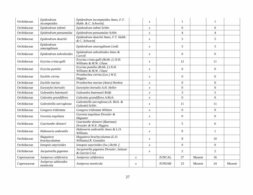
27
Orchidaceae Epidendrum
incomptoides
Epidendrum incomptoides Ames, F.T.
Hubb. & C. Schweinf. x 1 1
Orchidaceae Epidendrum isthmii Epidendrum isthmi Schltr. x 0 0
Orchidaceae Epidendrum pansamalae Epidendrum pansamalae Schltr. x 4 4
Orchidaceae Epidendrum skutchii Epidendrum skutchii Ames, F.T. Hubb.
& C. Schweinf. x 5 5
Orchidaceae Epidendrum
smaragdinum Epidendrum smaragdinum Lindl. x 5 5
Orchidaceae Epidendrum sobralioides Epidendrum sobralioides Ames &
Correll x 0 0
Orchidaceae Erycina crista-galli Erycina crista-galli (Rchb. f.) N.H.
Williams & M.W. Chase x 12 11
Orchidaceae Erycina pumilio Erycina pumilio (Rchb. f.) N.H.
Williams & M.W. Chase x 0 0
Orchidaceae Euchile citrina Prosthechea citrina (Lex.) W.E.
Higgins x 0 0
Orchidaceae Euchile mariae Prosthechea mariae (Ames) Hoehne x 0 0
Orchidaceae Eurystyles borealis Eurystyles borealis A.H. Heller x 0 0
Orchidaceae Galeandra batemanii Galeandra batemanii Rolfe x 3 5
Orchidaceae Galeottia grandiflora Galeottia grandiflora A.Rich. x 0 0
Orchidaceae Galeottiella sarcoglossa Galeottiella sarcoglossa (A. Rich. &
Galeotti) Schltr. x 11 11
Orchidaceae Gongora tridentata Gongora tridentata Whitten x 0 0
Orchidaceae Govenia tequilana Govenia tequilana Dressler &
Hágsater x 0 0
Orchidaceae Guarianthe skinneri Guarianthe skinneri (Bateman)
Dressler & W.E. Higgins x 5 6
Orchidaceae Habenaria umbratilis Habenaria umbratilis Ames & L.O.
Williams x 0 1
Orchidaceae Hagsatera
brachycolumna
Hagsatera brachycolumna (L.O.
Williams) R. González x 8 10
Orchidaceae Ionopsis satyrioides Ionopsis satyrioides (Sw.) Rchb. f. x 0 0
Orchidaceae Jacquiniella gigantea Jacquiniella gigantea Dressler, Salazar
& García-Cruz x 2 2
Cupressaceae Juniperus californica Juniperus californica x JUNCAL 37 Maxent 16
Cupressaceae Juniperus sabinoides
monticola Juniperus monticola x JUNSAB 23 Maxent 24 Maxent

28
Orchidaceae Kefersteinia lactea Kefersteinia tinschertiana Pupulin x 0 0
Orchidaceae Kraenzlinella hintonii Kraenzlinella hintonii (L.O. Williams)
Solano x 2 2
Orchidaceae Lacaena bicolor Lacaena bicolor Lindl. x 0 0
Orchidaceae Laelia anceps dawsonii Laelia anceps Lindl. subsp. dawsonii
(J. Anderson) Rolfe x 10 10
Orchidaceae Laelia gouldiana Laelia gouldiana Rchb. f. x 7 7
Orchidaceae Laelia speciosa Laelia speciosa (Kunth) Schltr. x LAESPE 43
Maxent,
GLM,
RF
43
Maxent,
GLM,
RF
Orchidaceae Laelia superbiens Laelia superbiens Lindl. x 13 12
Orchidaceae Lepanthes ancylopetala Lepanthes ancylopetala Dreesler x 1 1
Orchidaceae Lepanthes guatemalensis Lepanthes guatemalensis Schltr. x 2 2
Orchidaceae Lepanthes parvula Lepanthes parvula Dressler x 2 2
Orchidaceae Lepanthopsis floripecten Lepanthopsis floripecten (Rchb. f)
Ames x 2 3
Orchidaceae Ligeophila clavigera Ligeophila clavigera (Rchb. f.) Garay x 11 12
Orchidaceae Lycaste lasioglossa Lycaste lasioglossa Rchb. f. x 1 1
Orchidaceae Lycaste skinneri Lycaste skinneri (Bateman ex Lindl.)
Lindl. x 11 11
Orchidaceae Lyroglossa pubicaulis Lyroglossa pubicaulis (L.O.Williams)
Garay x 0 0
Orchidaceae Macradenia brassavolae Macradenia brassavolae Rchb. f. x 0 0
Orchidaceae Malaxis greenwoodiana Malaxis greenwoodiana Salazar &
Soto Arenas x 4 4
Orchidaceae Malaxis hagsateri Malaxis hagsateri Salazar x 5 4
Orchidaceae Malaxis pandurata Malaxis pandurata (Schltr.) Ames x 0 0
Orchidaceae Maxillaria alba Maxillaria alba (Hook.) Lindl. x 4 3
Orchidaceae Maxillaria nasuta Maxillaria nasuta Rchb. f. x 3 3
Orchidaceae Maxillaria oestlundiana Maxillaria oestlundiana L.O.Williams x 0 0
Orchidaceae Maxillaria tonsoniae Maxillaria tonsoniae Soto-Arenas x 11 11
Orchidaceae Mexipedium
xerophyticum
Mexipedium xerophyticum (Soto
Arenas, Salazar & Hágsater) V.A.
Albert & M.W. Chase
x 0 0
29
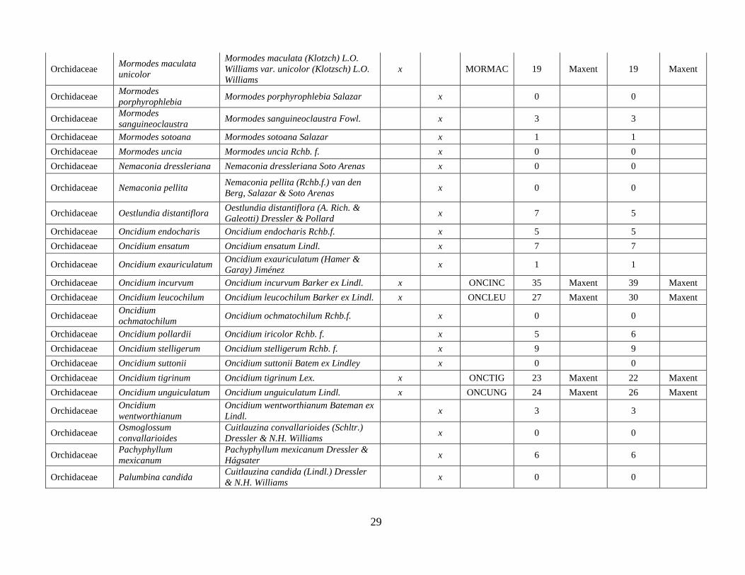
Orchidaceae Mormodes maculata
unicolor
Mormodes maculata (Klotzch) L.O.
Williams var. unicolor (Klotzsch) L.O.
Williams
x MORMAC 19 Maxent 19 Maxent
Orchidaceae Mormodes
porphyrophlebia Mormodes porphyrophlebia Salazar x 0 0
Orchidaceae Mormodes
sanguineoclaustra Mormodes sanguineoclaustra Fowl. x 3 3
Orchidaceae Mormodes sotoana Mormodes sotoana Salazar x 1 1
Orchidaceae Mormodes uncia Mormodes uncia Rchb. f. x 0 0
Orchidaceae Nemaconia dressleriana Nemaconia dressleriana Soto Arenas x 0 0
Orchidaceae Nemaconia pellita Nemaconia pellita (Rchb.f.) van den
Berg, Salazar & Soto Arenas x 0 0
Orchidaceae Oestlundia distantiflora Oestlundia distantiflora (A. Rich. &
Galeotti) Dressler & Pollard x 7 5
Orchidaceae Oncidium endocharis Oncidium endocharis Rchb.f. x 5 5
Orchidaceae Oncidium ensatum Oncidium ensatum Lindl. x 7 7
Orchidaceae Oncidium exauriculatum Oncidium exauriculatum (Hamer &
Garay) Jiménez x 1 1
Orchidaceae Oncidium incurvum Oncidium incurvum Barker ex Lindl. x ONCINC 35 Maxent 39 Maxent
Orchidaceae Oncidium leucochilum Oncidium leucochilum Barker ex Lindl. x ONCLEU 27 Maxent 30 Maxent
Orchidaceae Oncidium
ochmatochilum Oncidium ochmatochilum Rchb.f. x 0 0
Orchidaceae Oncidium pollardii Oncidium iricolor Rchb. f. x 5 6
Orchidaceae Oncidium stelligerum Oncidium stelligerum Rchb. f. x 9 9
Orchidaceae Oncidium suttonii Oncidium suttonii Batem ex Lindley x 0 0
Orchidaceae Oncidium tigrinum Oncidium tigrinum Lex. x ONCTIG 23 Maxent 22 Maxent
Orchidaceae Oncidium unguiculatum Oncidium unguiculatum Lindl. x ONCUNG 24 Maxent 26 Maxent
Orchidaceae Oncidium
wentworthianum
Oncidium wentworthianum Bateman ex
Lindl. x 3 3
Orchidaceae Osmoglossum
convallarioides
Cuitlauzina convallarioides (Schltr.)
Dressler & N.H. Williams x 0 0
Orchidaceae Pachyphyllum
mexicanum
Pachyphyllum mexicanum Dressler &
Hágsater x 6 6
Orchidaceae Palumbina candida Cuitlauzina candida (Lindl.) Dressler
& N.H. Williams x 0 0
30
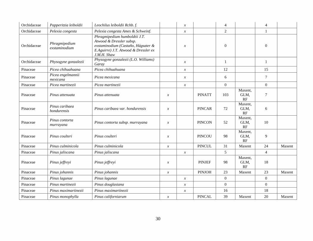
Orchidaceae Papperitzia leiboldii Leochilus leiboldii Rchb. f. x 4 4
Orchidaceae Pelexia congesta Pelexia congesta Ames & Schweinf. x 2 1
Orchidaceae Phragmipedium
exstaminodium
Phragmipedium humboldtii J.T.
Atwood & Dressler subsp.
exstaminodium (Castaño, Hágsater &
E.Aguirre) J.T. Atwood & Dressler ex
J.M.H. Shaw
x 0 0
Orchidaceae Physogyne gonzalezii Physogyne gonzalezii (L.O. Williams)
Garay x 1 1
Pinaceae Picea chihuahuana Picea chihuahuana x 12 15
Pinaceae Picea engelmannii
mexicana Picea mexicana x 6 7
Pinaceae Picea martinezii Picea martinezii x 0 0
Pinaceae Pinus attenuata Pinus attenuata x PINATT 103
Maxent,
GLM,
RF
7
Pinaceae Pinus caribaea
hondurensis Pinus caribaea var. hondurensis x PINCAR 72
Maxent,
GLM,
RF
6
Pinaceae Pinus contorta
murrayana Pinus contorta subsp. murrayana x PINCON 52
Maxent,
GLM,
RF
10
Pinaceae Pinus coulteri Pinus coulteri x PINCOU 98
Maxent,
GLM,
RF
9
Pinaceae Pinus culminicola Pinus culminicola x PINCUL 31 Maxent 24 Maxent
Pinaceae Pinus jaliscana Pinus jaliscana x 5 4
Pinaceae Pinus jeffreyi Pinus jeffreyi x PINJEF 98
Maxent,
GLM,
RF
18
Pinaceae Pinus johannis Pinus johannis x PINJOH 23 Maxent 23 Maxent
Pinaceae Pinus lagunae Pinus lagunae x 0 0
Pinaceae Pinus martinezii Pinus douglasiana x 0 0
Pinaceae Pinus maximartinezii Pinus maximartinezii x 16 18
Pinaceae Pinus monophylla Pinus californiarum x PINCAL 39 Maxent 20 Maxent

31
Pinaceae Pinus muricata Pinus muricata x PINMUR 86
Maxent,
GLM,
RF
9
Pinaceae Pinus nelsonii Pinus nelsonii x PINNEL 27 Maxent 27 Maxent
Pinaceae Pinus pinceana Pinus pinceana x PINPIN 59
Maxent,
GLM,
RF
59
Maxent,
GLM,
RF
Pinaceae Pinus quadrifolia Pinus quadrifolia x PINQUA 47
Maxent,
GLM,
RF
40
Maxent,
GLM,
RF
Pinaceae Pinus remota Pinus remota x 16 13
Pinaceae Pinus rzedowskii Pinus rzedowskii x 8 8
Pinaceae Pinus strobiformis Pinus strobiformis x PINSTR 59
Maxent,
GLM,
RF
49
Maxent,
GLM,
RF
Pinaceae Pinus strobus chiapensis Pinus chiapensis x PINSTRC
HI 41
Maxent,
GLM,
RF
40
Maxent,
GLM,
RF
Orchidaceae Platystele caudatisepala Platystele caudatisepala (C. Schwein
f.) Garay x 1 1
Orchidaceae Platystele
jungermannioides
Platystele jungermannioides (Schltr.)
Garay x 0 0
Orchidaceae Platystele repens Platystele repens (Ames) Garay x 0 0
Orchidaceae Platythelys venustula Platythelys venustula (Ames) Garay x 0 0
Orchidaceae Pleurothallis hintonii Kraenzlinella hintonii (L.O. Williams)
Solano x 0 0
Orchidaceae Pleurothallis nelsonii Pleurothallis nelsonii Ames x 3 3
Orchidaceae Pleurothallis
saccatilabia Pleurothallis saccatilabia C. Schweinf. x 0 0
Orchidaceae Pleurothallopsis
ujarensis
Pleurothallopsis ujarensis (Rchb.f.)
Pridgeon & M.W. Chase x 0 0
Podocarpaceae Podocarpus matudae Podocarpus matudae x PODMAT 52
Maxent,
GLM,
RF
52
Maxent,
GLM,
RF
Orchidaceae Ponthieva brittoniae Ponthieva brittoniae Ames & C.
Schwinf. x 3 4
Orchidaceae Prosthechea abbreviata Prosthechea abbreviata (Schltl.) W.E.
Higgins x 0 0

32
Orchidaceae Prosthechea citrina Prosthechea citrina (Lex.) W.E.
Higgins x PROCIT 41
Maxent,
GLM,
RF
36 Maxent
Orchidaceae Prosthechea mariae Prosthechea mariae (Ames) W.E.
Higgins x 13 11
Orchidaceae Prosthechea neurosa Prosthechea neurosa (Ames) W.E.
Higgins x 10 10
Orchidaceae Prosthechea vagans Prosthechea vagans (Ames) W.E.
Higgins x 0 0
Orchidaceae Prosthechea vitellina Prosthechea vitellina (Lindl.) W.E.
Higgins x PROVIT 86
Maxent,
GLM,
RF
83
Maxent,
GLM,
RF
Orchidaceae Pseudocranichis
thysanochila
Galeoglossum thysanochilum (B.L.
Rob. & Greenm.) Salazar x 0 4
Orchidaceae Pseudogoodyera
pseudogoodyeroides
Pseudogoodyera pseudogoodyeroides
(Rchb. f.) Schltr. x 4 0
Pinaceae Pseudotsuga menziesii
glauca Pseudotsuga menziesii var. glauca x PSEMEN 611
Maxent,
GLM,
RF
87
Maxent,
GLM,
RF
Orchidaceae Restrepia lankesteri Restrepia trichoglossa F.Lehm. ex
Sander x 0 0
Orchidaceae Rhynchostele beloglossa Rhynchostele beloglossa (Rchb. f.)
Dressler & N.H. Williams x 4 4
Orchidaceae Rhynchostele cervantesii Rhynchostele cervantesii (Lex.) Soto
Arenas & Salazar x RHYCER 95
Maxent,
GLM,
RF
94
Maxent,
GLM,
RF
Orchidaceae Rhynchostele cordata Rhynchostele cordata (Lindl.) Soto
Arenas & Salazar x RHYCOR 46
Maxent,
GLM,
RF
42
Maxent,
GLM,
RF
Orchidaceae Rhynchostele
ehrenbergii
Rhynchostele ehrenbergii (Link,
Klotzsch & Otto) Soto Arenas &
Salazar
x RHYEHR 24 Maxent 21 Maxent
Orchidaceae Rhynchostele galeottiana Rhynchostele galeottiana (A. Rich.)
Soto Arenas & Salazar x 0 0
Orchidaceae Rhynchostele
londesboroughiana
Rhynchostele londesboroughiana
(Rchb.f.) Halbinger x 5 5
Orchidaceae Rhynchostele madrensis Rhynchostele madrensis (Rchb.f.) Soto
Arenas & Salazar x 11 9

33
Orchidaceae Rhynchostele majalis
Rhynchostele majalis (Rchb.f.)
Halbinger y (Rchb.f.) Soto Arenas &
Salazar
x 4 4
Orchidaceae Rhynchostele pygmaea Rhynchostele pygmaea (Lindl.) Rchb. f. x 8 7
Orchidaceae Rhynchostele rossii Rhynchostele rossii (Lindl.) Soto
Arenas & Salazar x RHYROS 43
Maxent,
GLM,
RF
41
Maxent,
GLM,
RF
Orchidaceae Rhynchostele uroskinneri Rhynchostele uroskinneri (Lindl.) Soto
Arenas & Salazar x 0 0
Orchidaceae Rodriguezia dressleriana Rodriguezia dressleriana R. González x 2 2
Orchidaceae Rossioglossum grande Rossioglossum grande (Lindl.) Garay
& G.C.Kenn. x 5 6
Orchidaceae Rossioglossum insleayi Rossioglossum insleayi (Barker ex
Lindl.) Garay & G.C. Kenn. x 0 0
Orchidaceae Rossioglossum splendens Rossioglossum splendens (Rchb.f.)
Garay & G.C. Kenn. x 0 0
Orchidaceae Rossioglossum
williamsianum
Rossioglossum williamsianum (Rchb.
f.) Garay & G.C. Kenn. x 0 0
Orchidaceae Sarcoglottis cerina Sarcoglottis cerina (Lindl.) P.N. Don x 3 4
Orchidaceae Scelochilus tuerckheimii Comparettia tuerckheimii (Schltr.)
M.W. Chase & N.H. Williams x 0 0
Orchidaceae Schiedeella nagelii Schiedeella nagelii (L.O. Williams)
Garay x 6 6
Orchidaceae Sigmatostalix
guatemalensis
Oncidium poikilostalix (Kraenzl.)
M.W. Chase & N.H. Williams x 0 0
Orchidaceae Sigmatostalix mexicana Oncidium mexicanum (L.O. Williams)
M.W. Chase & N.H. Williams x 5 6
Orchidaceae Sobralia crispissima Sobralia crispissima Dressler x 1 1
Orchidaceae Sobralia mucronata Sobralia mucronata Ames x 4 4
Orchidaceae Specklinia digitale Specklinia digitale (Luer) Pridgeon &
M.W. Chase x 19 16
Orchidaceae Specklinia endotrachys Specklinia endotrachys (Rchb. f.)
Pridgeon & M.W. Chase x 15 15
Orchidaceae Specklinia fimbriata Specklinia fimbriata C. Schweinf. &
(Ames & C. Schweinf.) Solano x 4 4
Orchidaceae Specklinia glandulosa Specklinia glandulosa (Ames) Pridgeon
& M.W. Chase x 0 0

34
Orchidaceae Specklinia lateritia Specklinia lateritia (Rchb.f.) Pridgeon
& M.W. Chase x 0 0
Orchidaceae Spiranthes torta Spiranthes torta (Thunb.) Garay &
H.R. Sweet x 1 1
Orchidaceae Stanhopea ecornuta Stanhopea ecornuta Lem. x 2 1
Orchidaceae Stanhopea oculata Stanhopea oculata (G.Lodd.) Lindl. x STAOCU 22 Maxent 20 Maxent
Orchidaceae Stanhopea tigrina Stanhopea tigrina Bateman x STATIG 24 Maxent 24 Maxent
Orchidaceae Stelis chihobensis Stelis chihobensis Ames x 7 7
Orchidaceae Stelis cobanensis Stelis cobanensis (Schltr.) Pridgeon &
M.W. Chase x 18 18
Orchidaceae Stelis deregularis Stelis deregularis Barb. Rodr. x 3 2
Orchidaceae Stelis nigriflora Stelis nigriflora (L.O. Williams)
Pridgeon & M.W. Chase x 4 4
Orchidaceae Stellilabium standleyi Telipogon standleyi Ames x 1 1
Taxaceae Taxus globosa Taxus globosa x TAXGLO 51
Maxent,
GLM,
RF
51
Maxent,
GLM,
RF
Orchidaceae Teuscheria pickiana Teuscheria pickiana (Schltr.) Garay x 0 0
Orchidaceae Trichocentrum
flavovirens
Trichocentrum flavovirens L.O.
Williams x 6 6
Orchidaceae Trichocentrum hoegei Trichocentrum hoegei Rchb. f. x 9 8
Orchidaceae Trichocentrum
stramineum
Trichocentrum stramineum (Bateman
ex Lindl.) M.W. Chase & N.H. Williams x 14 16
Orchidaceae Trichopilia galeottiana Trichopilia galeottiana A.Rich. &
Galeotti x 3 2
Orchidaceae Trichopilia subulata Trichopilia subulata (Sw.) Rchb.f. x 0 0
Orchidaceae Trichosalpinx
cedralensis Trichosalpinx cedralensis (Ames) Luer x 0 0
Orchidaceae Vanilla planifolia Vanilla planifolia Jacks. x VANPLA 32 Maxent 32 Maxent
Orchidaceae Warrea costaricensis Warrea costaricensis Schltr. x 1 1

35
2. Quality of information (Calidad de información)
The following Appendices (A2, A3, A4 and A5) are submitted as separate files together with this
report.
A2. Climatic profiles (table). Summary of climatic conditions at the presence localities used in
the species distribution models (mean and standard deviation).
A3. Climatic profiles (boxplots). Summary of climatic conditions at the presence localities used
in the species distribution models (mean and standard deviation).
A4 and A5. Profiles of land surface phenology (tables). Species-specific phenological profiles
obtained from remotely sensed time series of the Enhanced Vegetation Index (a) for all occurrence
localities together, (b) stratified by biogeographic provinces and (c) stratified by vegetation types.
A5. Profiles of land surface phenology (figures). Species-specific phenological profiles obtained
from remotely sensed time series of the Enhanced Vegetation Index for all occurrence localities
together and stratified by biogeographic provinces and vegetation types.

36
3. Other information
A6. Overview of how often each climate variable was selected for the species distribution
models (as a result of the collinearity and variable importance analysis). 0.293 means that the
variable was selected in 29.3% of the models.
Variable Mean Standard deviation
BIO1 0.000 0.000
BIO2 0.293 0.461
BIO3 0.073 0.264
BIO4 0.439 0.502
BIO5 0.610 0.494
BIO6 0.024 0.156
BIO7 0.049 0.218
BIO8 0.317 0.471
BIO9 0.146 0.358
BIO10 0.098 0.300
BIO11 0.024 0.156
BIO12 0.000 0.000
BIO13 0.073 0.264
BIO14 0.780 0.419
BIO15 1.000 0.000
BIO16 0.122 0.331
BIO17 0.220 0.419
BIO18 0.415 0.499
BIO19 1.000 0.000

37
A7. Overview of how often each remote sensing variable was selected for the species
distribution models (as a result of the collinearity and variable importance analysis). 0.677 means
that the variable was selected in 67.7% of the models.
Variable Mean Standard deviation
EVI_CoV 0.677 0.475
EVI_integral 0.000 0.000
EVI_maximum 0.065 0.250
EVI_mean 0.000 0.000
EVI_median 0.129 0.341
EVI_minimum 0.129 0.341
EVI_range 0.000 0.000
EVI_rate_greenup 0.194 0.402
EVI_rate_senescence 0.000 0.000
EVI_standard_deviation 0.129 0.341
EVI_value_EOS 0.032 0.180
EVI_value_SOS 0.032 0.180
LST_CoV 0.129 0.341
LST_maximum 0.194 0.402
LST_mean 0.258 0.445
LST_median 0.226 0.425
LST_minimum 0.903 0.301
LST_range 0.065 0.250
LST_standard_deviation 0.032 0.180

38
Additional material delivered. The following additional material was delivered upon completion
of the project:
- Database of the georeferenced localities of the 227 species considered in the project
(DarwinCore format, compiled in the context of project JM078)
- Detailed description of the variables used for distribution modeling (tabular format)
- Species-specific overview of variables used in the species distribution models (tabular format)
- Variable importance: Contribution of environmental variables to explaining species
distribution patterns for both climate and remote sensing data (tabular format)
- Model evaluation (based on AUC, partial AUC and model deviance) (tabular format)
- R-Code for species distribution modeling including remote sensing data and model
uncertainty analysis
- Digital maps of distributions of the species modeled in the project:
(a) Climatic ranges (for distribution range from southern USA to Central America):
1. Continuous probability of occurrence
2. Binary distribution map at minimum training presence threshold
3. Binary distribution map at 10 percentile training presence threshold
4. Binary distribution map at maximum training sensitivity plus specificity threshold
(b) Habitat availability within bioclimatic range derived from remote sensing time series
(only for Mexico)
1. Continuous probability of occurrence
2. Binary distribution map at minimum training presence threshold
3. Binary distribution map at 10 percentile training presence threshold
4. Binary distribution map at maximum training sensitivity plus specificity threshold
(c) Species-specific maps of habitat loss computed from climatic distribution ranges and
remotely sensed land surface properties
(d) Cumulative habitat loss across all study species
(e) Species-specific uncertainty maps based on the difference between the 97.5-percentile
and the 2.5-percentile of values derived from the continuous prediction maps (based on
199 model repetition runs)