Informed search algorithms

This lecture topic Read Chapter 3.5-3.7

Next lecture topic Read Chapter 4.1-4.2

(Please read lecture topic material before

and after each lecture on that topic)

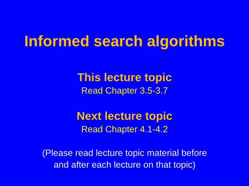
You will be expected to know

• evaluation function f(n) and heuristic function h(n) for each node n – g(n) = known path cost so far to node n. – h(n) = estimate of (optimal) cost to goal from node n. – f(n) = g(n)+h(n) = estimate of total cost to goal through node n.

• Heuristic searches: Greedy-best-first, A*

– A* is optimal with admissible (tree)/consistent (graph) heuristics – Prove that A* is optimal with admissible heuristic for tree search – Recognize when a heuristic is admissible or consistent

• h2 dominates h1 iff h2(n) ≥ h1(n) for all n • Effective branching factor: b* • Inventing heuristics: relaxed problems; max or convex combination

Outline

• Review limitations of uninformed search methods • Informed (or heuristic) search • Problem-specific heuristics to improve efficiency

• Best-first, A* (and if needed for memory limits, RBFS, SMA*) • Techniques for generating heuristics • A* is optimal with admissible (tree)/consistent (graph) heuristics • A* is quick and easy to code, and often works *very* well

• Heuristics • A structured way to add “smarts” to your solution • Provide *significant* speed-ups in practice • Still have worst-case exponential time complexity

• In AI, “NP-Complete” means “Formally interesting”

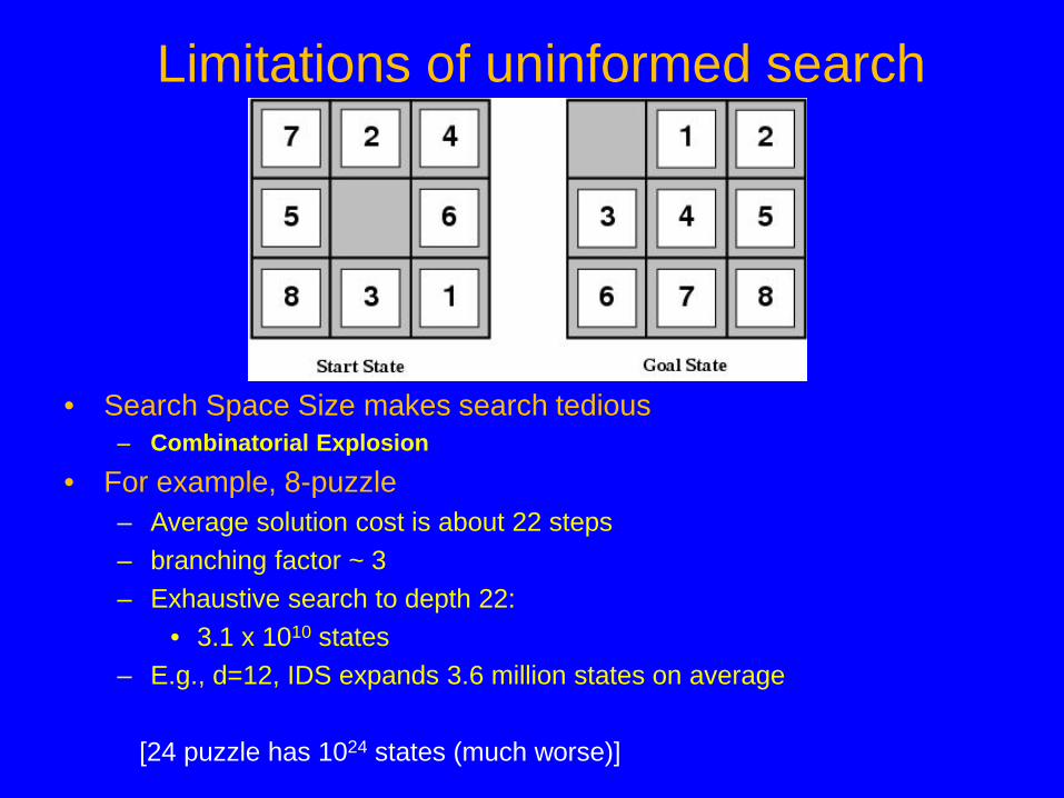
Limitations of uninformed search

• Search Space Size makes search tedious – Combinatorial Explosion

• For example, 8-puzzle – Average solution cost is about 22 steps – branching factor ~ 3 – Exhaustive search to depth 22:

• 3.1 x 1010 states – E.g., d=12, IDS expands 3.6 million states on average

[24 puzzle has 1024 states (much worse)]

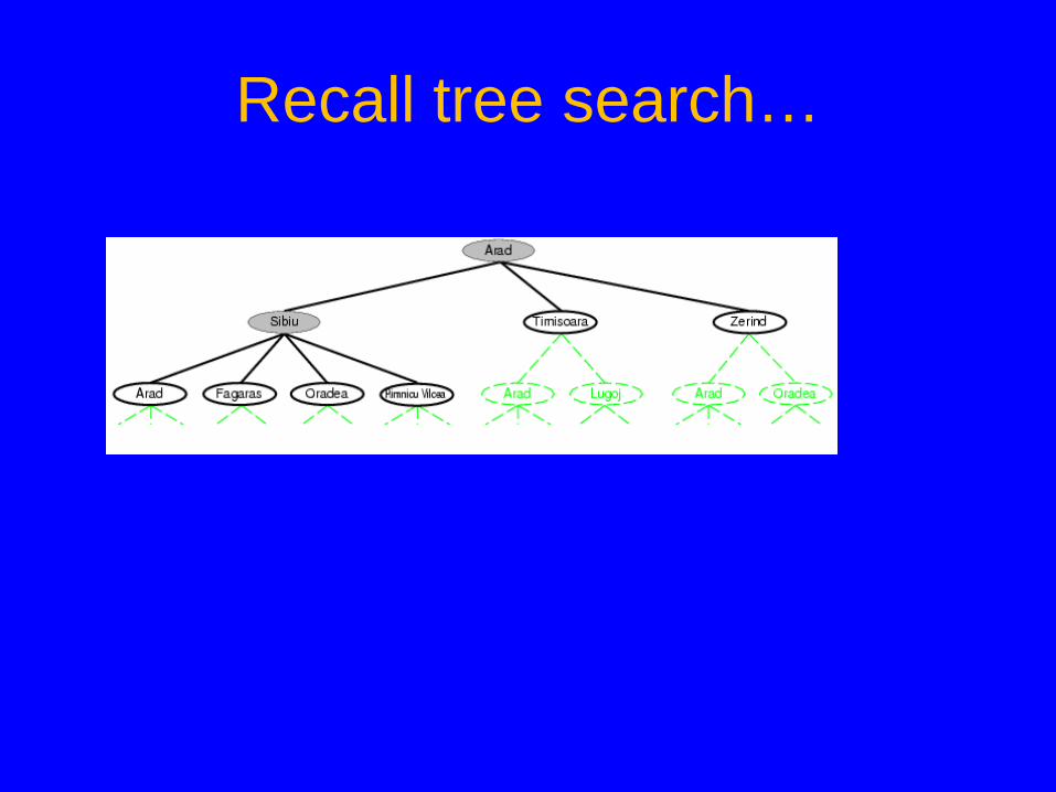
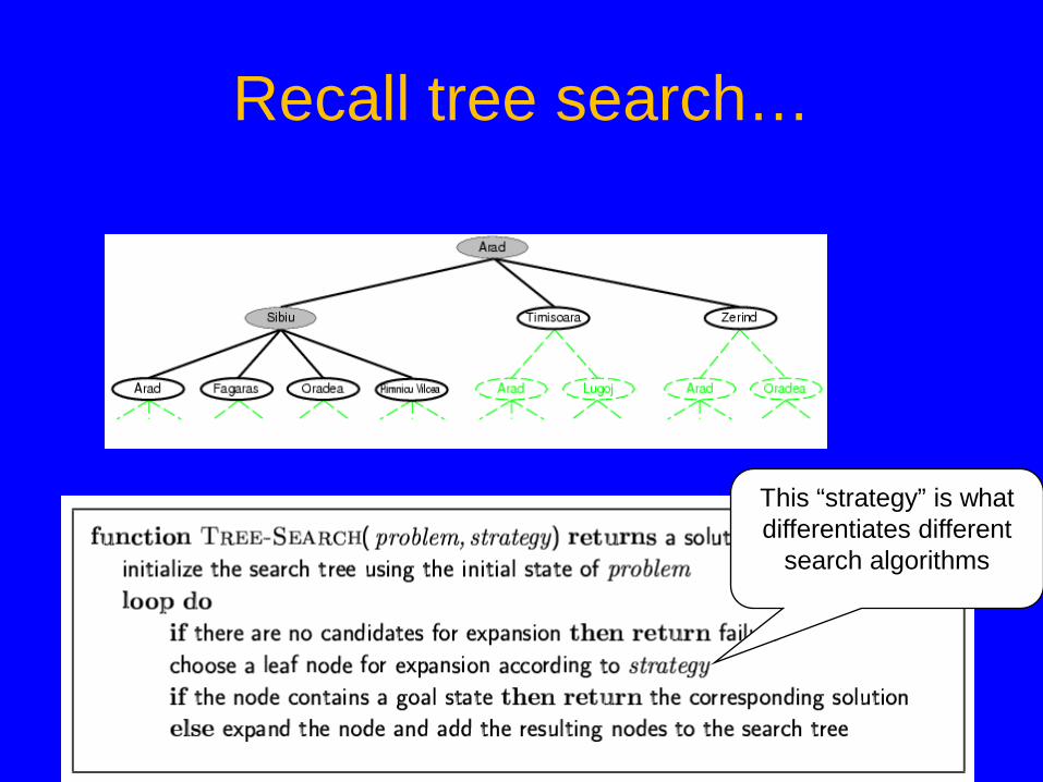
Recall tree search…

Recall tree search…

This “strategy” is what differentiates different

search algorithms

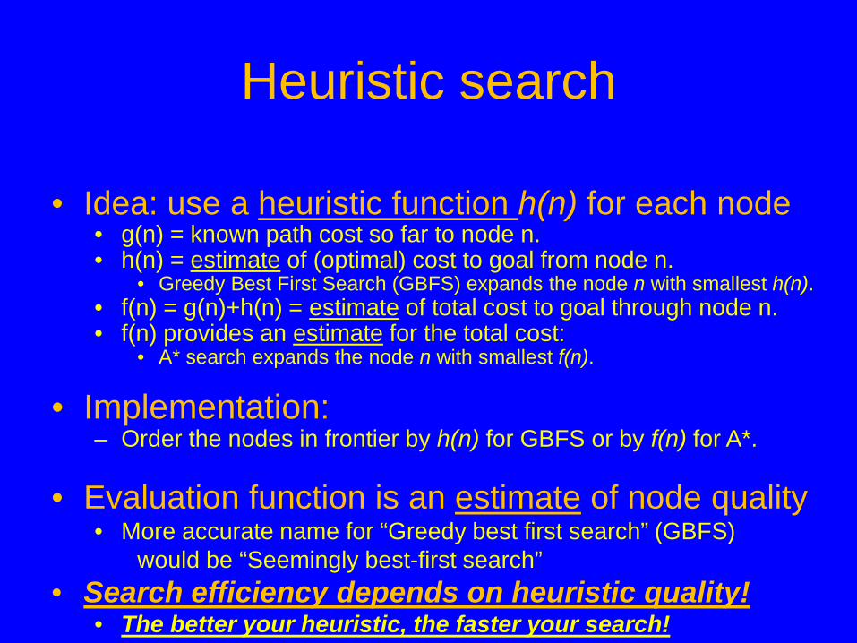
Heuristic search

• Idea: use a heuristic function h(n) for each node • g(n) = known path cost so far to node n. • h(n) = estimate of (optimal) cost to goal from node n.

• Greedy Best First Search (GBFS) expands the node n with smallest h(n). • f(n) = g(n)+h(n) = estimate of total cost to goal through node n. • f(n) provides an estimate for the total cost:

• A* search expands the node n with smallest f(n).

• Implementation: – Order the nodes in frontier by h(n) for GBFS or by f(n) for A*.

• Evaluation function is an estimate of node quality

• More accurate name for “Greedy best first search” (GBFS) would be “Seemingly best-first search”

• Search efficiency depends on heuristic quality! • The better your heuristic, the faster your search!

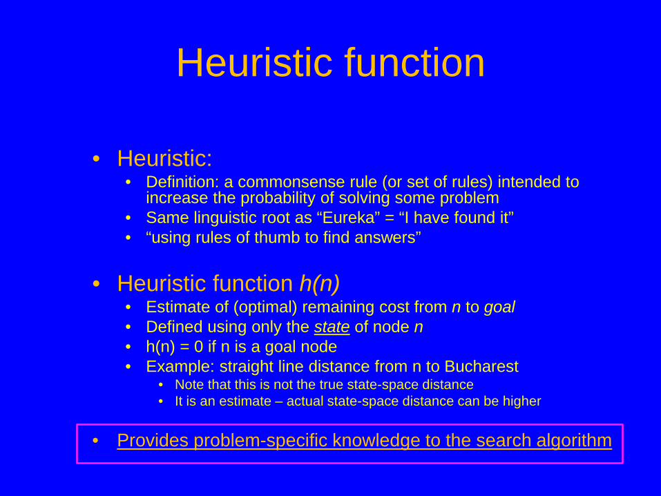
Heuristic function

• Heuristic: • Definition: a commonsense rule (or set of rules) intended to

increase the probability of solving some problem • Same linguistic root as “Eureka” = “I have found it” • “using rules of thumb to find answers”

• Heuristic function h(n)

• Estimate of (optimal) remaining cost from n to goal • Defined using only the state of node n • h(n) = 0 if n is a goal node • Example: straight line distance from n to Bucharest

• Note that this is not the true state-space distance • It is an estimate – actual state-space distance can be higher

• Provides problem-specific knowledge to the search algorithm

Heuristic functions for 8-puzzle

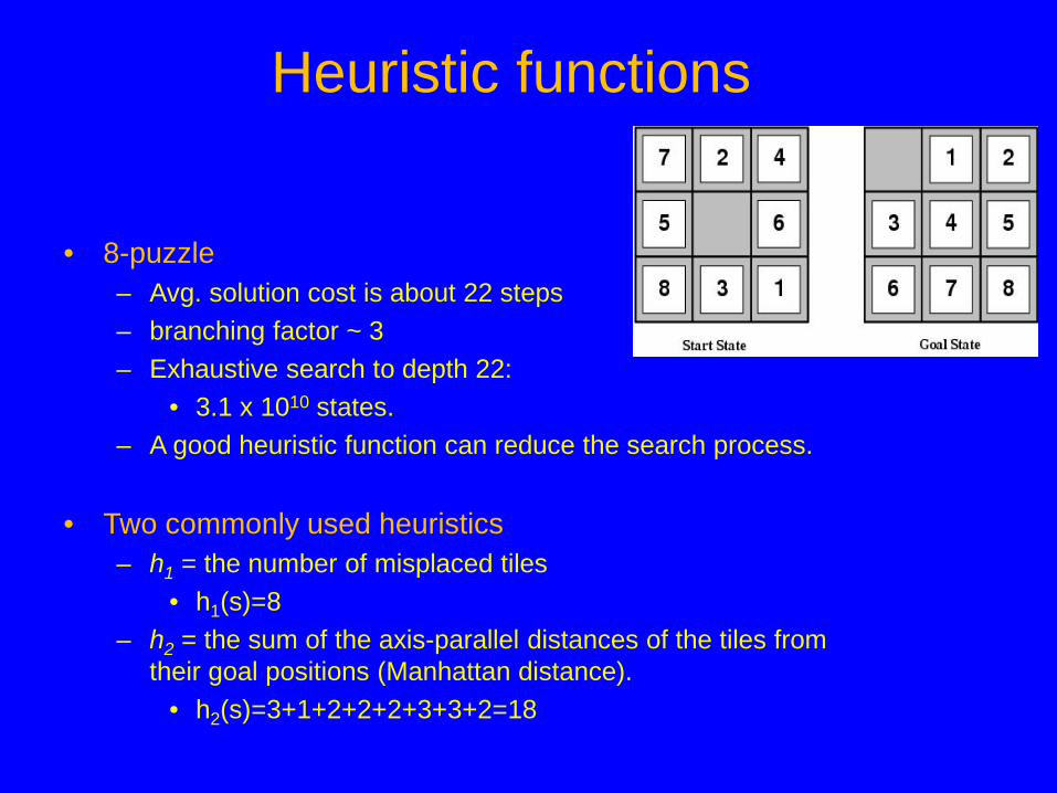
• 8-puzzle – Avg. solution cost is about 22 steps – branching factor ~ 3 – Exhaustive search to depth 22:

• 3.1 x 1010 states. – A good heuristic function can reduce the search process.

• Two commonly used heuristics

– h1 = the number of misplaced tiles • h1(s)=8

– h2 = the sum of the distances of the tiles from their goal positions (Manhattan distance).

• h2(s)=3+1+2+2+2+3+3+2=18

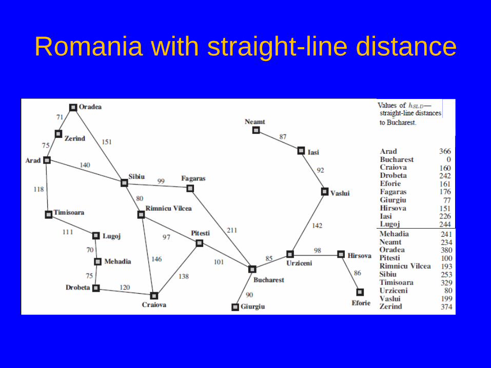
Romania with straight-line distance

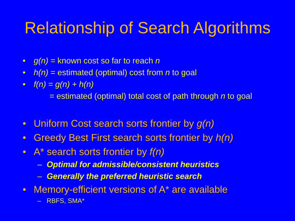
Relationship of Search Algorithms

• g(n) = known cost so far to reach n • h(n) = estimated (optimal) cost from n to goal • f(n) = g(n) + h(n) = estimated (optimal) total cost of path through n to goal

• Uniform Cost search sorts frontier by g(n) • Greedy Best First search sorts frontier by h(n) • A* search sorts frontier by f(n)

– Optimal for admissible/consistent heuristics – Generally the preferred heuristic search

• Memory-efficient versions of A* are available – RBFS, SMA*

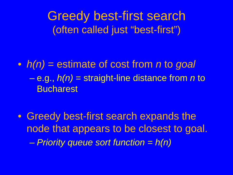
Greedy best-first search (often called just “best-first”)

• h(n) = estimate of cost from n to goal – e.g., h(n) = straight-line distance from n to

Bucharest

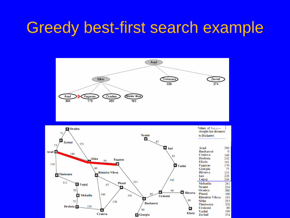
• Greedy best-first search expands the node that appears to be closest to goal. – Priority queue sort function = h(n)

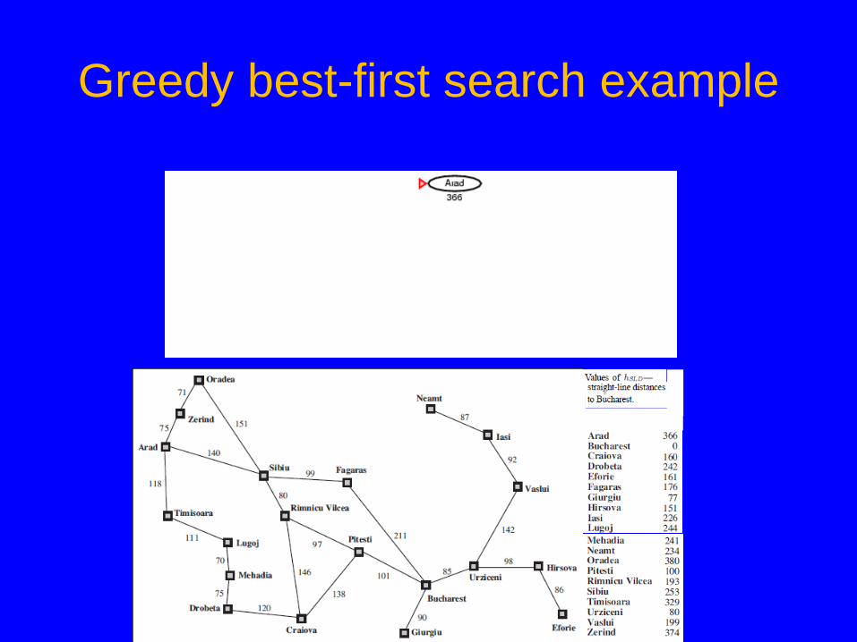
Greedy best-first search example

Greedy best-first search example

Greedy best-first search example

Greedy best-first search example

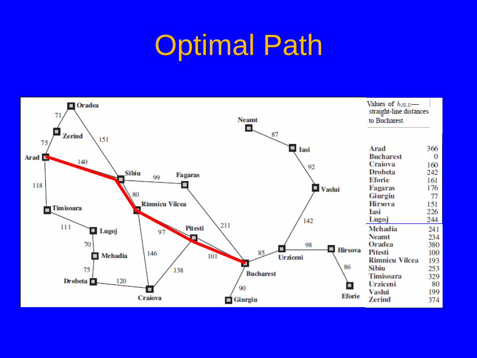
Optimal Path

Greedy Best-first Search With tree search, will become stuck in this loop

Order of node expansion: S A D S A D S A D. . . . Path found: none Cost of path found: none .

B

D

G

S

A C

h=5

h=7

h=6

h=8 h=9

h=0

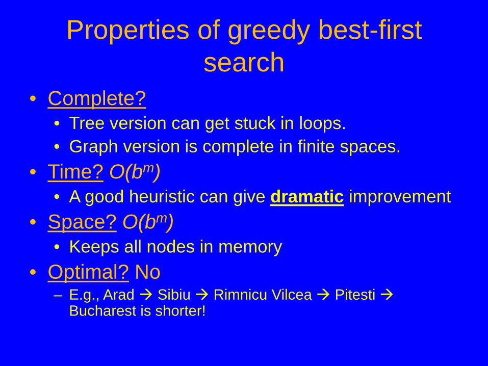
Properties of greedy best-first search

• Complete? • Tree version can get stuck in loops. • Graph version is complete in finite spaces.

• Time? O(bm) • A good heuristic can give dramatic improvement

• Space? O(bm) • Keeps all nodes in memory

• Optimal? No – E.g., Arad Sibiu Rimnicu Vilcea Pitesti

Bucharest is shorter!

A* search

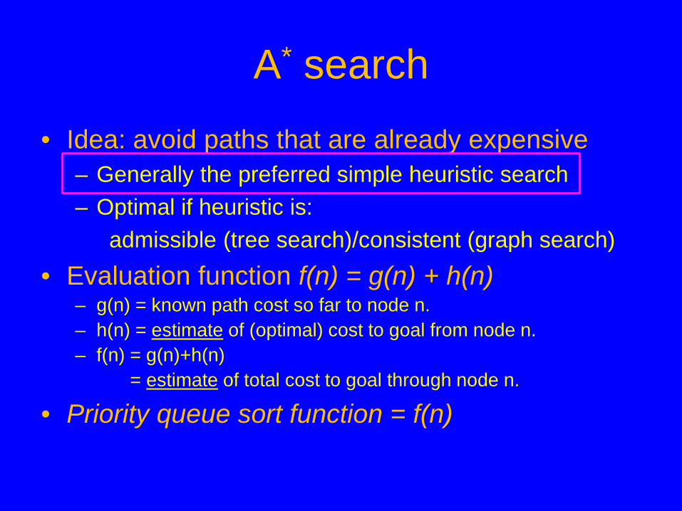
• Idea: avoid paths that are already expensive – Generally the preferred simple heuristic search – Optimal if heuristic is: admissible (tree search)/consistent (graph search)

• Evaluation function f(n) = g(n) + h(n) – g(n) = known path cost so far to node n. – h(n) = estimate of (optimal) cost to goal from node n. – f(n) = g(n)+h(n) = estimate of total cost to goal through node n.

• Priority queue sort function = f(n)

Admissible heuristics

• A heuristic h(n) is admissible if for every node n, h(n) ≤ h*(n), where h*(n) is the true cost to reach the goal state from n. • An admissible heuristic never overestimates the cost to reach

the goal, i.e., it is optimistic (or at least, never pessimistic) – Example: hSLD(n) (never overestimates actual road distance)

• Theorem: If h(n) is admissible, A* using TREE-SEARCH is optimal

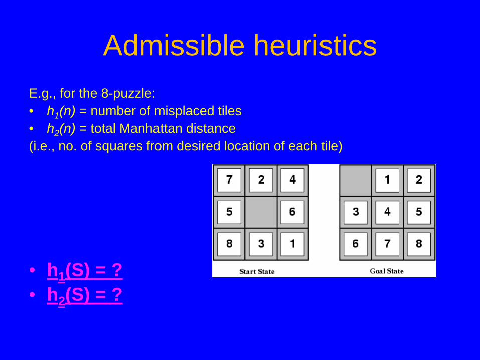
Admissible heuristics E.g., for the 8-puzzle: • h1(n) = number of misplaced tiles • h2(n) = total Manhattan distance (i.e., no. of squares from desired location of each tile)

• h1(S) = ? • h2(S) = ?

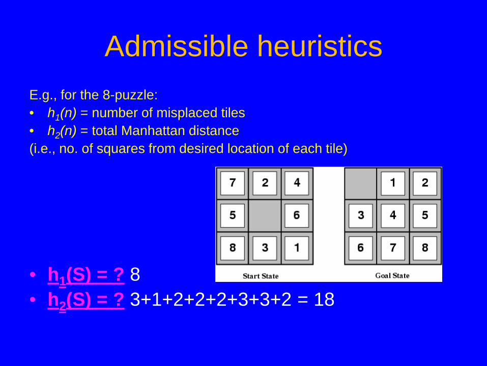
Admissible heuristics E.g., for the 8-puzzle: • h1(n) = number of misplaced tiles • h2(n) = total Manhattan distance (i.e., no. of squares from desired location of each tile)

• h1(S) = ? 8 • h2(S) = ? 3+1+2+2+2+3+3+2 = 18

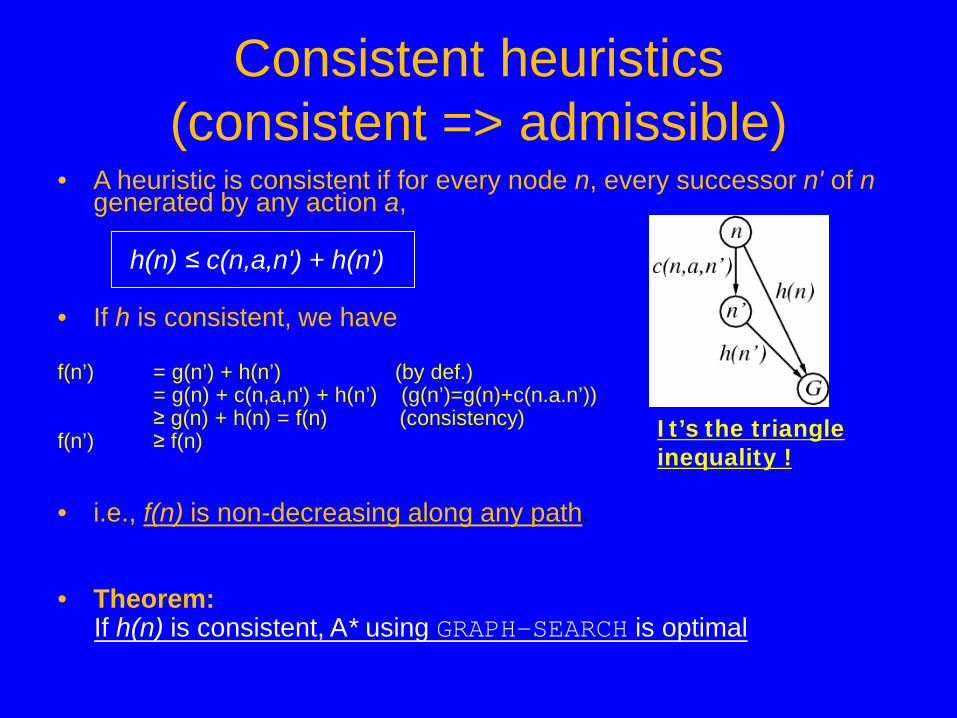
• A heuristic is consistent if for every node n, every successor n' of n generated by any action a,

h(n) ≤ c(n,a,n') + h(n')

• If h is consistent, we have

f(n’) = g(n’) + h(n’) (by def.) = g(n) + c(n,a,n') + h(n’) (g(n’)=g(n)+c(n.a.n’)) ≥ g(n) + h(n) = f(n) (consistency) f(n’) ≥ f(n) • i.e., f(n) is non-decreasing along any path.

• Theorem: If h(n) is consistent, A* using GRAPH-SEARCH is optimal

Consistent heuristics (consistent => admissible)

It’s the triangle inequality !

Admissible (Tree Search) vs.

Consistent (Graph Search)

• Why two different conditions? – In graph search you often find a long cheap path to a node

after a short expensive one, so you might have to update all of its descendants to use the new cheaper path cost so far

– A consistent heuristic avoids this problem (it can’t happen) – Consistent is slightly stronger than admissible – Almost all admissible heuristics are also consistent

• Could we do optimal graph search with an admissible heuristic? – Yes, but you would have to do additional work to update

descendants when a cheaper path to a node is found – A consistent heuristic avoids this problem

A* tree search example

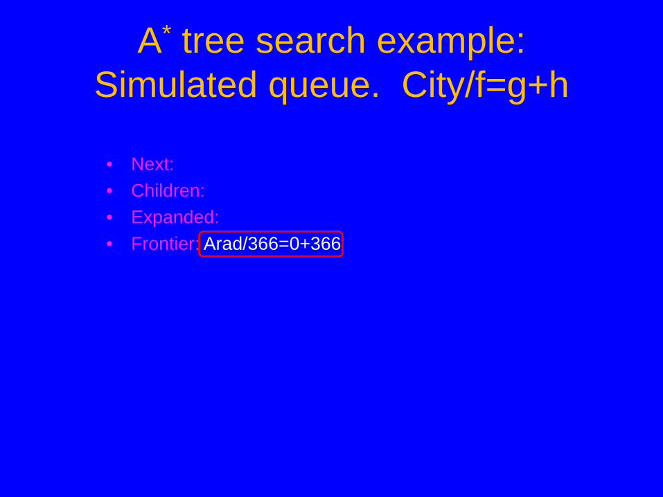
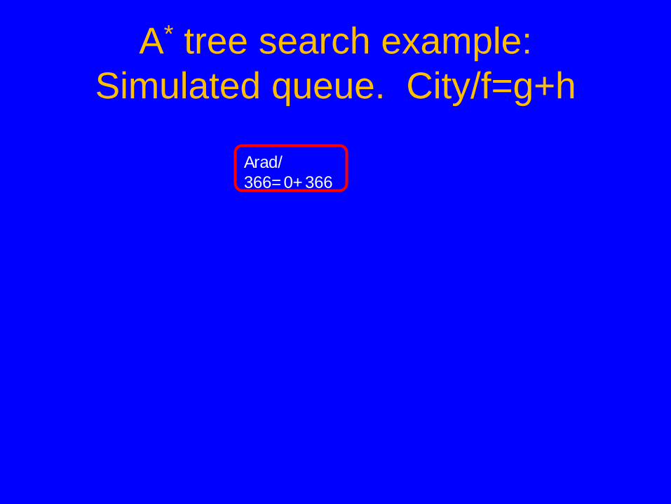
A* tree search example: Simulated queue. City/f=g+h

• Next: • Children: • Expanded: • Frontier: Arad/366=0+366

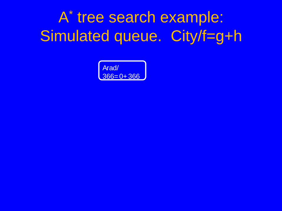
A* tree search example: Simulated queue. City/f=g+h

Arad/ 366=0+366

A* tree search example: Simulated queue. City/f=g+h

Arad/ 366=0+366

A* tree search example: Simulated queue. City/f=g+h

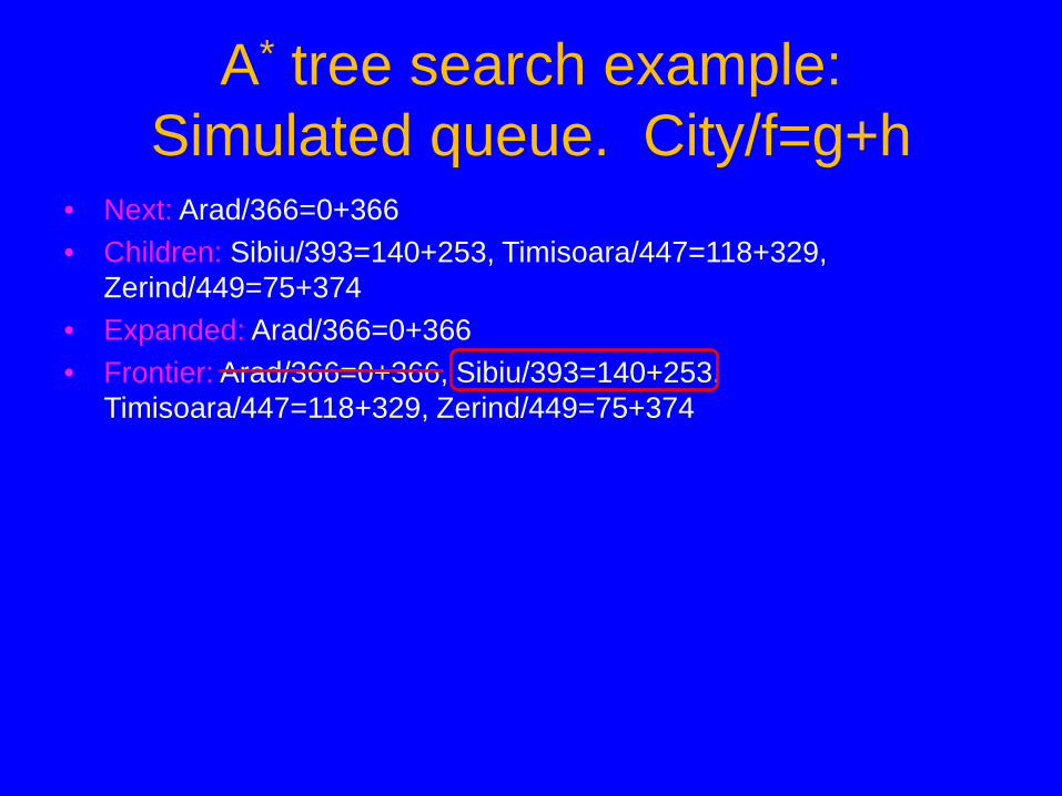
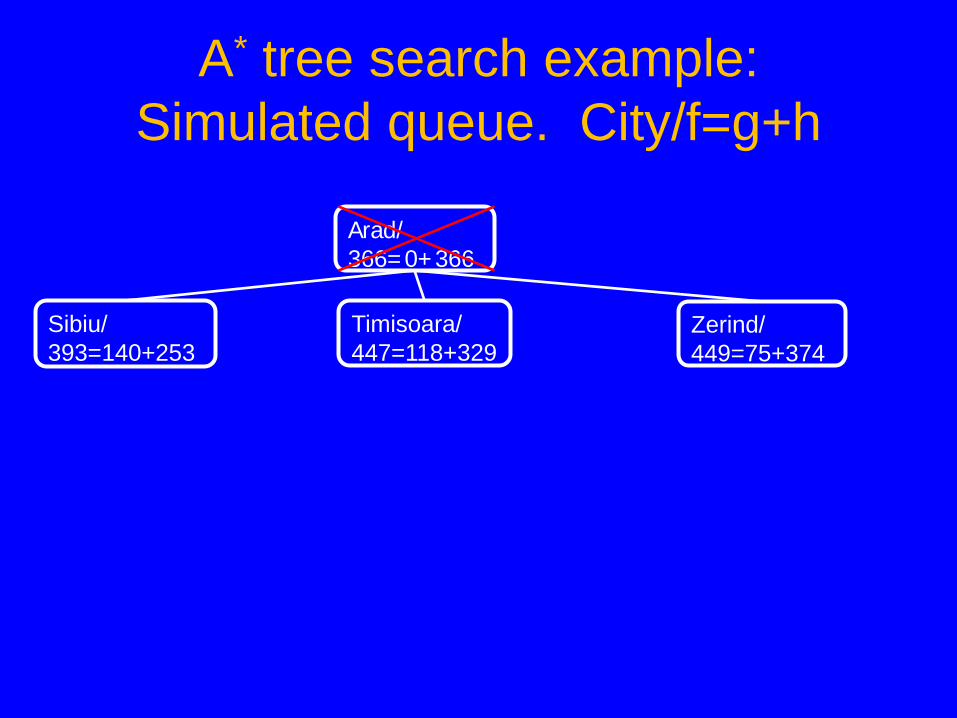
• Next: Arad/366=0+366 • Children: Sibiu/393=140+253, Timisoara/447=118+329,

Zerind/449=75+374 • Expanded: Arad/366=0+366 • Frontier: Arad/366=0+366, Sibiu/393=140+253,

Timisoara/447=118+329, Zerind/449=75+374

A* tree search example: Simulated queue. City/f=g+h

Sibiu/ 393=140+253

Timisoara/ 447=118+329

Zerind/ 449=75+374

Arad/ 366=0+366

A* tree search example: Simulated queue. City/f=g+h

Sibiu/ 393=140+253

Timisoara/ 447=118+329

Zerind/ 449=75+374

Arad/ 366=0+366

A* tree search example

A* tree search example: Simulated queue. City/f=g+h

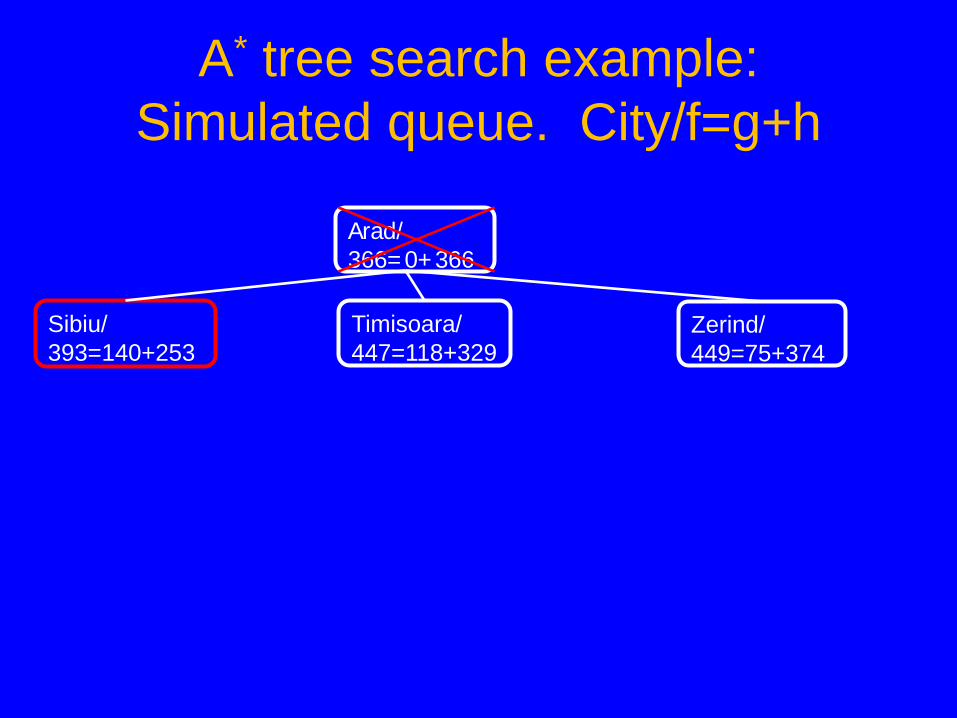
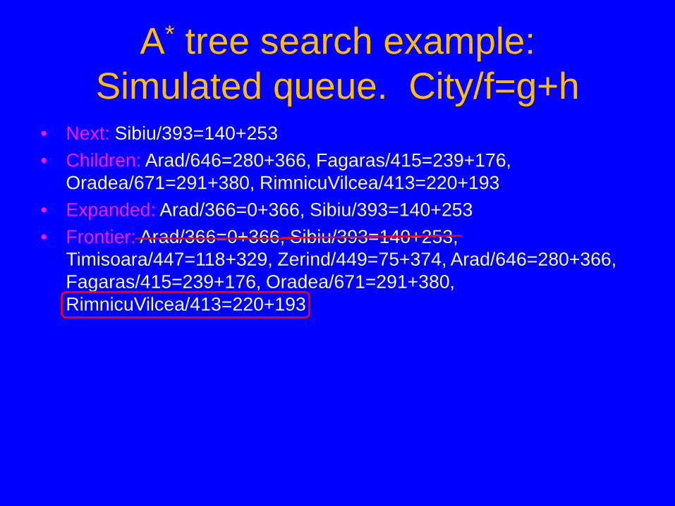
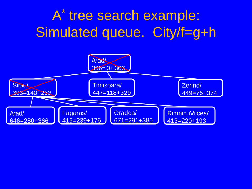
• Next: Sibiu/393=140+253 • Children: Arad/646=280+366, Fagaras/415=239+176,

Oradea/671=291+380, RimnicuVilcea/413=220+193 • Expanded: Arad/366=0+366, Sibiu/393=140+253 • Frontier: Arad/366=0+366, Sibiu/393=140+253,

Timisoara/447=118+329, Zerind/449=75+374, Arad/646=280+366, Fagaras/415=239+176, Oradea/671=291+380, RimnicuVilcea/413=220+193

A* tree search example: Simulated queue. City/f=g+h

Sibiu/ 393=140+253

Timisoara/ 447=118+329

Zerind/ 449=75+374

Arad/ 646=280+366

Fagaras/ 415=239+176

Oradea/ 671=291+380

RimnicuVilcea/ 413=220+193

Arad/ 366=0+366

A* tree search example: Simulated queue. City/f=g+h

Sibiu/ 393=140+253

Timisoara/ 447=118+329

Zerind/ 449=75+374

Arad/ 646=280+366

Fagaras/ 415=239+176

Oradea/ 671=291+380

RimnicuVilcea/ 413=220+193

Arad/ 366=0+366

A* tree search example

A* tree search example: Simulated queue. City/f=g+h

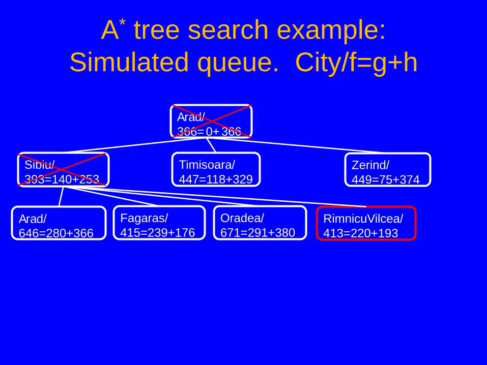
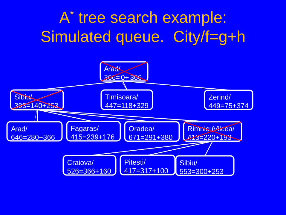
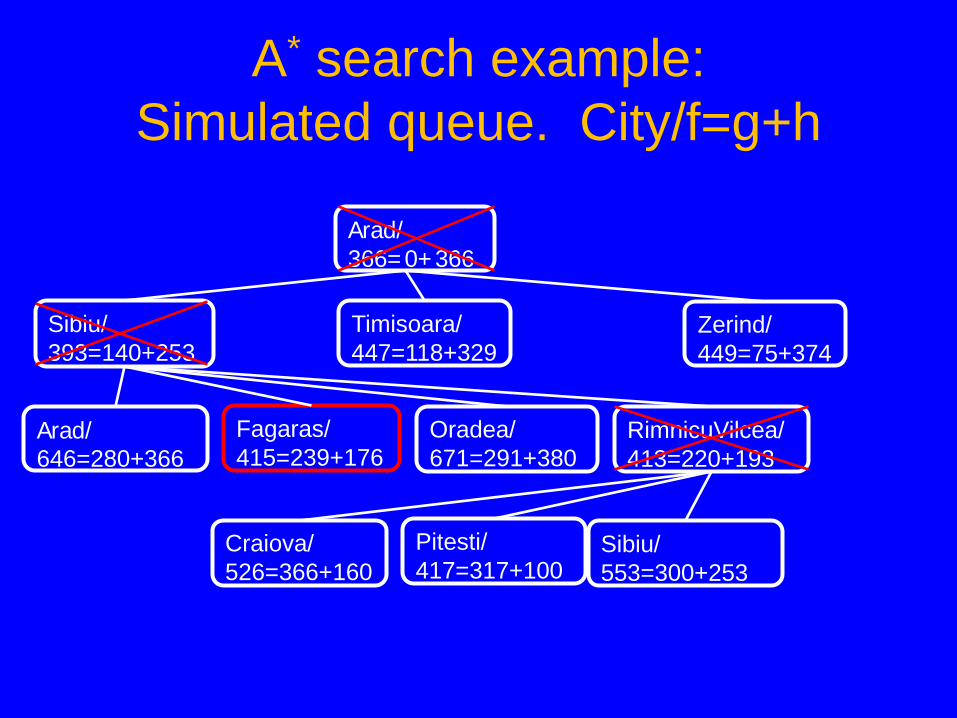
• Next: RimnicuVilcea/413=220+193 • Children: Craiova/526=366+160, Pitesti/417=317+100,

Sibiu/553=300+253 • Expanded: Arad/366=0+366, Sibiu/393=140+253,

RimnicuVilcea/413=220+193 • Frontier: Arad/366=0+366, Sibiu/393=140+253,

Timisoara/447=118+329, Zerind/449=75+374, Arad/646=280+366, Fagaras/415=239+176, Oradea/671=291+380, RimnicuVilcea/413=220+193, Craiova/526=366+160, Pitesti/417=317+100, Sibiu/553=300+253

A* tree search example: Simulated queue. City/f=g+h

Sibiu/ 393=140+253

Timisoara/ 447=118+329

Zerind/ 449=75+374

Arad/ 646=280+366

Fagaras/ 415=239+176

Oradea/ 671=291+380

Craiova/ 526=366+160

Pitesti/ 417=317+100

Sibiu/ 553=300+253

RimnicuVilcea/ 413=220+193

Arad/ 366=0+366

A* search example: Simulated queue. City/f=g+h

Sibiu/ 393=140+253

Timisoara/ 447=118+329

Zerind/ 449=75+374

Arad/ 646=280+366

Fagaras/ 415=239+176

Oradea/ 671=291+380

Craiova/ 526=366+160

Pitesti/ 417=317+100

Sibiu/ 553=300+253

RimnicuVilcea/ 413=220+193

Arad/ 366=0+366

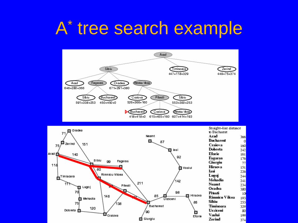
A* tree search example Note: The search below did not “back track.” Rather, both arms are being pursued in parallel on the queue.

A* tree search example: Simulated queue. City/f=g+h

• Next: Fagaras/415=239+176 • Children: Bucharest/450=450+0, Sibiu/591=338+253 • Expanded: Arad/366=0+366, Sibiu/393=140+253,

RimnicuVilcea/413=220+193, Fagaras/415=239+176 • Frontier: Arad/366=0+366, Sibiu/393=140+253,

Timisoara/447=118+329, Zerind/449=75+374, Arad/646=280+366, Fagaras/415=239+176, Oradea/671=291+380, RimnicuVilcea/413=220+193, Craiova/526=366+160, Pitesti/417=317+100, Sibiu/553=300+253, Bucharest/450=450+0, Sibiu/591=338+253

A* tree search example Note: The search below did not “back track.” Rather, both arms are being pursued in parallel on the queue.

A* tree search example: Simulated queue. City/f=g+h

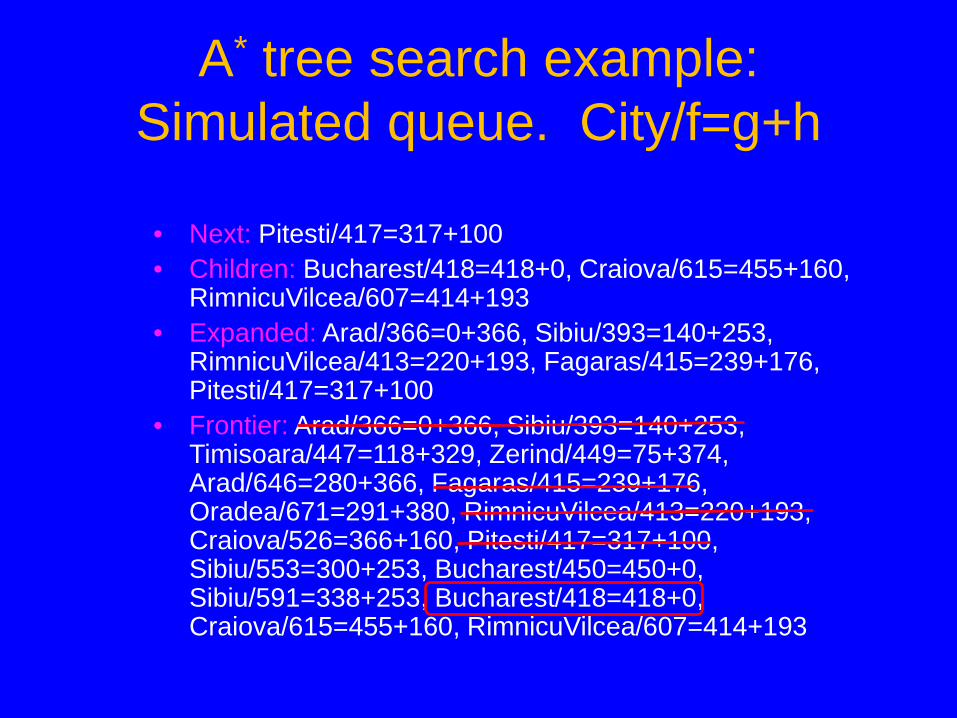
• Next: Pitesti/417=317+100 • Children: Bucharest/418=418+0, Craiova/615=455+160,

RimnicuVilcea/607=414+193 • Expanded: Arad/366=0+366, Sibiu/393=140+253,

RimnicuVilcea/413=220+193, Fagaras/415=239+176, Pitesti/417=317+100

• Frontier: Arad/366=0+366, Sibiu/393=140+253, Timisoara/447=118+329, Zerind/449=75+374, Arad/646=280+366, Fagaras/415=239+176, Oradea/671=291+380, RimnicuVilcea/413=220+193, Craiova/526=366+160, Pitesti/417=317+100, Sibiu/553=300+253, Bucharest/450=450+0, Sibiu/591=338+253, Bucharest/418=418+0, Craiova/615=455+160, RimnicuVilcea/607=414+193

A* tree search example

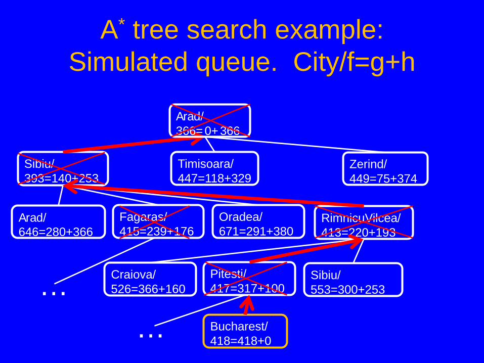
A* tree search example: Simulated queue. City/f=g+h

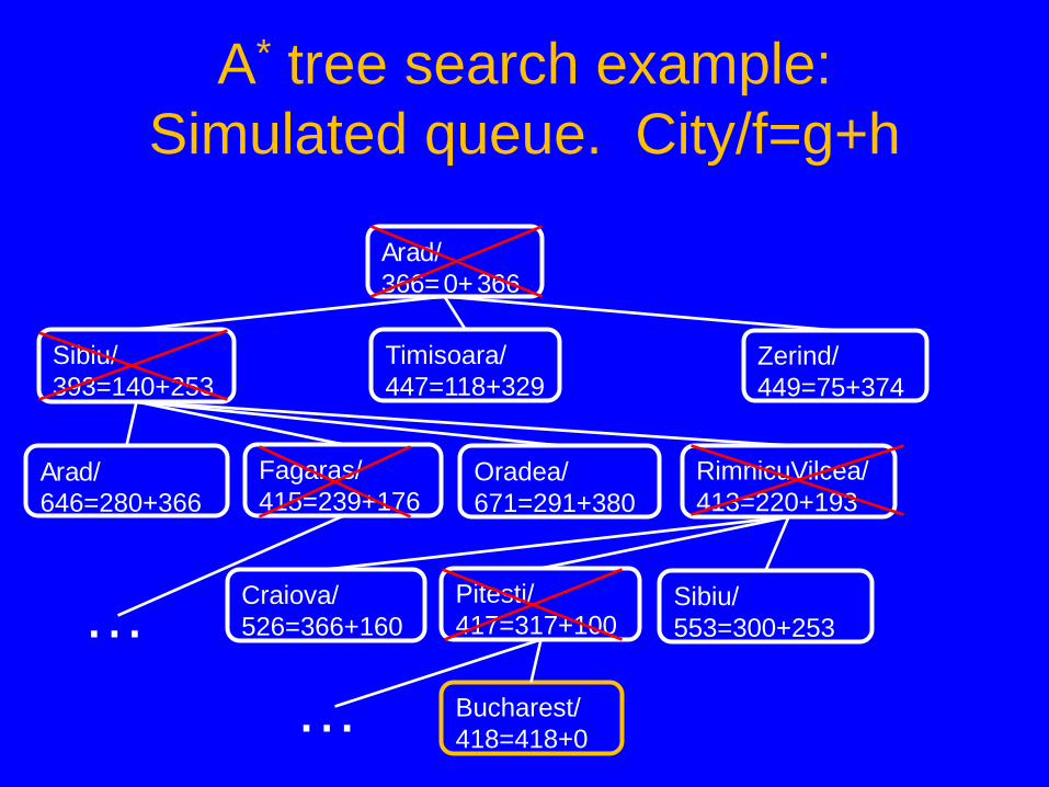
• Next: Bucharest/418=418+0 • Children: None; goal test succeeds. • Expanded: Arad/366=0+366, Sibiu/393=140+253,

RimnicuVilcea/413=220+193, Fagaras/415=239+176, Pitesti/417=317+100, Bucharest/418=418+0

• Frontier: Arad/366=0+366, Sibiu/393=140+253, Timisoara/447=118+329, Zerind/449=75+374, Arad/646=280+366, Fagaras/415=239+176, Oradea/671=291+380, RimnicuVilcea/413=220+193, Craiova/526=366+160, Pitesti/417=317+100, Sibiu/553=300+253, Bucharest/450=450+0, Sibiu/591=338+253, Bucharest/418=418+0, Craiova/615=455+160, RimnicuVilcea/607=414+193

Note that the short expensive path stays on the queue. The long cheap path is found and returned.

A* tree search example: Simulated queue. City/f=g+h

Sibiu/ 393=140+253

Timisoara/ 447=118+329

Zerind/ 449=75+374

Arad/ 646=280+366

Fagaras/ 415=239+176

Oradea/ 671=291+380

Craiova/ 526=366+160

Pitesti/ 417=317+100

Sibiu/ 553=300+253

RimnicuVilcea/ 413=220+193

Bucharest/ 418=418+0

… …

Arad/ 366=0+366

A* tree search example: Simulated queue. City/f=g+h

Sibiu/ 393=140+253

Timisoara/ 447=118+329

Zerind/ 449=75+374

Arad/ 646=280+366

Fagaras/ 415=239+176

Oradea/ 671=291+380

Craiova/ 526=366+160

Pitesti/ 417=317+100

Sibiu/ 553=300+253

RimnicuVilcea/ 413=220+193

Bucharest/ 418=418+0 …

…

Arad/ 366=0+366

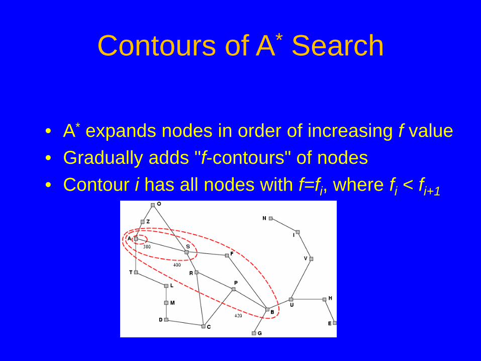
Contours of A* Search

• A* expands nodes in order of increasing f value • Gradually adds "f-contours" of nodes • Contour i has all nodes with f=fi, where fi < fi+1

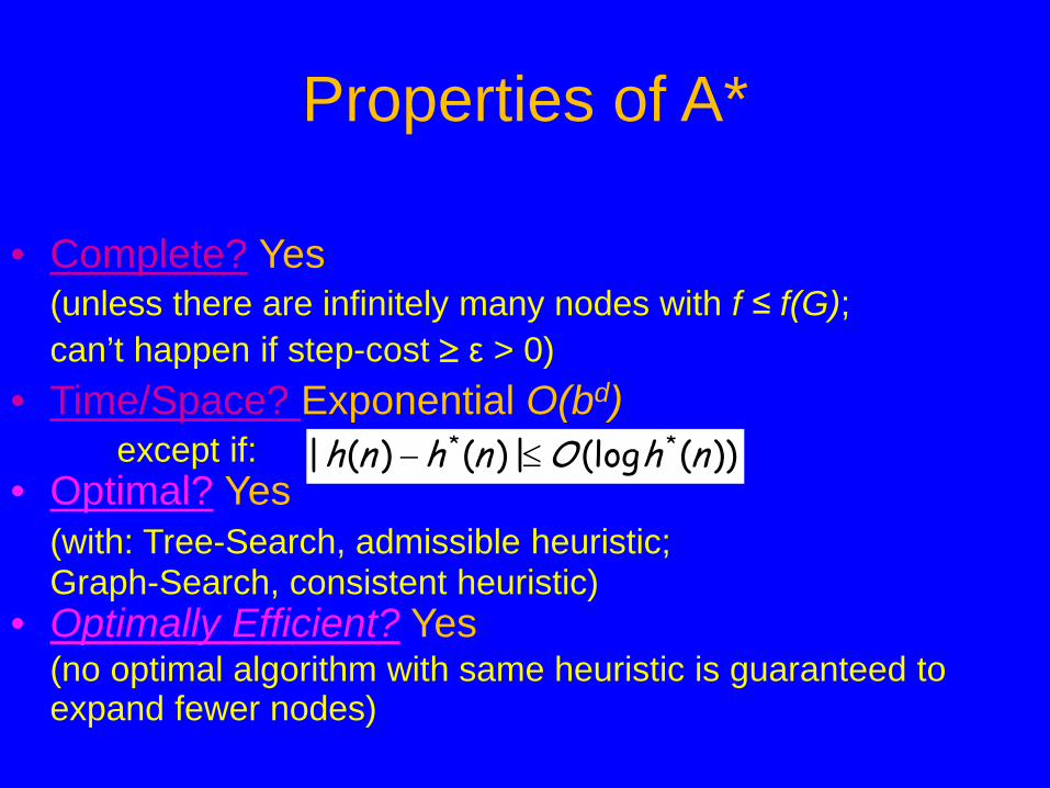
Properties of A*

• Complete? Yes (unless there are infinitely many nodes with f ≤ f(G); can’t happen if step-cost ≥ ε > 0) • Time/Space? Exponential O(bd) except if: • Optimal? Yes (with: Tree-Search, admissible heuristic; Graph-Search, consistent heuristic) • Optimally Efficient? Yes (no optimal algorithm with same heuristic is guaranteed to

expand fewer nodes)

* *| ( ) ( ) | (log ( ))h n h n O h n− ≤

Optimality of A* (proof) Tree Search, where h(n) is admissible

• Suppose some suboptimal goal G2 has been generated and is in the frontier. Let n be an unexpanded node in the frontier such that n is on a shortest path to an optimal goal G.

• f(G2) = g(G2) since h(G2) = 0 • f(G) = g(G) since h(G) = 0 • g(G2) > g(G) since G2 is suboptimal

• f(G2) > f(G) from above, with h=0 • h(n) ≤ h*(n) since h is admissible (under-estimate) • g(n) + h(n) ≤ g(n) + h*(n) from above • f(n) ≤ f(G) since g(n)+h(n)=f(n) & g(n)+h*(n)=f(G) • f(n) < f(G2) from above

We want to prove: f(n) < f(G2) (then A* will expand n before G2)

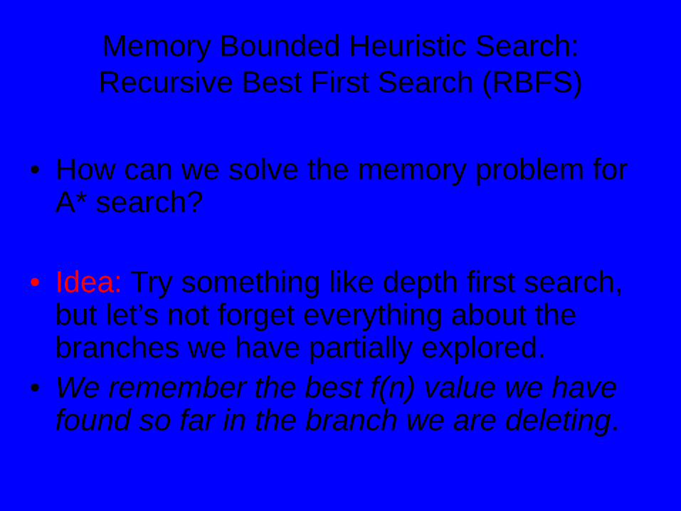
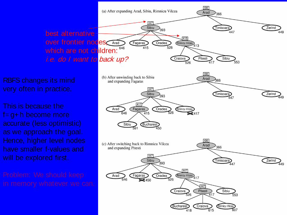
Memory Bounded Heuristic Search: Recursive Best First Search (RBFS)

• How can we solve the memory problem for A* search?

• Idea: Try something like depth first search,

but let’s not forget everything about the branches we have partially explored.

• We remember the best f(n) value we have found so far in the branch we are deleting.

RBFS:

RBFS changes its mind very often in practice. This is because the f=g+h become more accurate (less optimistic) as we approach the goal. Hence, higher level nodes have smaller f-values and will be explored first. Problem: We should keep in memory whatever we can.

best alternative over frontier nodes, which are not children: i.e. do I want to back up?

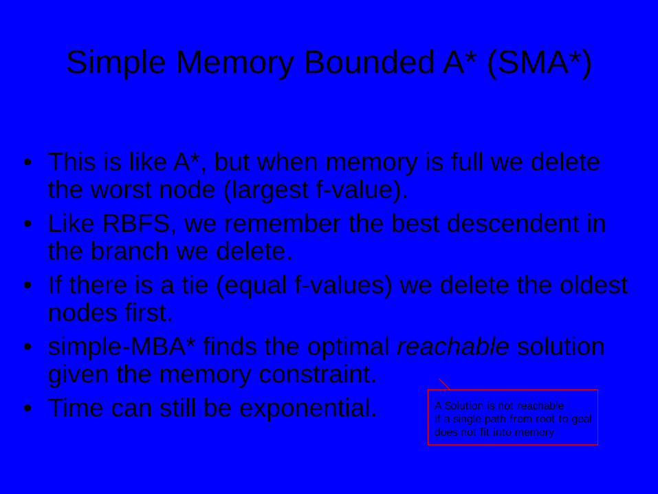
Simple Memory Bounded A* (SMA*)

• This is like A*, but when memory is full we delete the worst node (largest f-value).

• Like RBFS, we remember the best descendent in the branch we delete.

• If there is a tie (equal f-values) we delete the oldest nodes first.

• simple-MBA* finds the optimal reachable solution given the memory constraint.

• Time can still be exponential. A Solution is not reachable if a single path from root to goal does not fit into memory

SMA* pseudocode (not in 2nd edition of R&N) function SMA*(problem) returns a solution sequence inputs: problem, a problem static: Queue, a queue of nodes ordered by f-cost

Queue MAKE-QUEUE({MAKE-NODE(INITIAL-STATE[problem])}) loop do if Queue is empty then return failure n deepest least-f-cost node in Queue if GOAL-TEST(n) then return success s NEXT-SUCCESSOR(n) if s is not a goal and is at maximum depth then f(s) ∞ else f(s) MAX(f(n),g(s)+h(s)) if all of n’s successors have been generated then update n’s f-cost and those of its ancestors if necessary if SUCCESSORS(n) all in memory then remove n from Queue if memory is full then delete shallowest, highest-f-cost node in Queue remove it from its parent’s successor list insert its parent on Queue if necessary insert s in Queue end

Simple Memory-bounded A* (SMA*)

24+0=24

A

B G

C D

E F

H

J

I

K

0+12=12

10+5=15

20+5=25

30+5=35

20+0=20

30+0=30

8+5=13

16+2=18

24+0=24 24+5=29

10 8

10 10

10 10

8 16

8 8

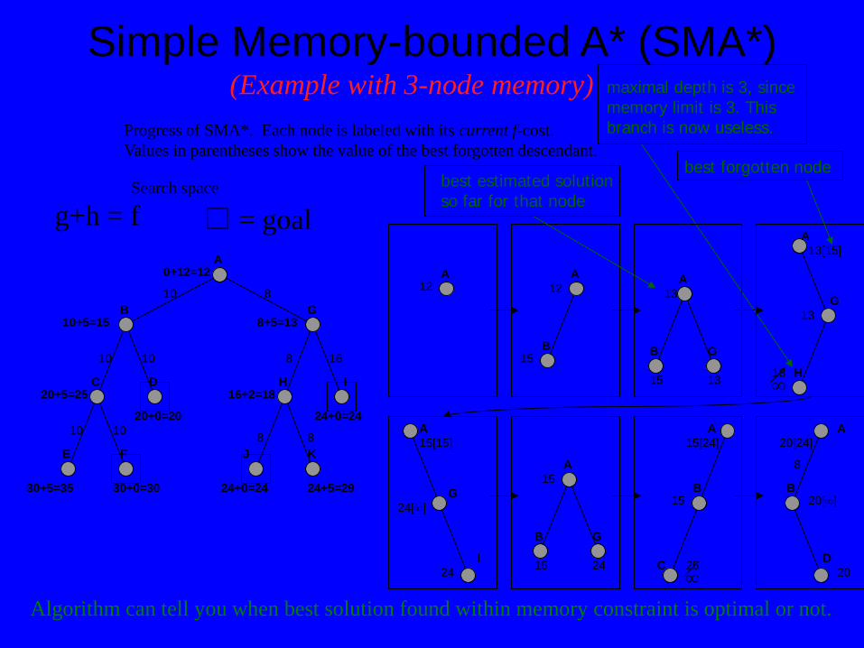
g+h = f

(Example with 3-node memory) Progress of SMA*. Each node is labeled with its current f-cost. Values in parentheses show the value of the best forgotten descendant.

Algorithm can tell you when best solution found within memory constraint is optimal or not.

☐ = goal Search space

maximal depth is 3, since memory limit is 3. This branch is now useless.

best forgotten node

A 12

A

B

12

15

A

B G

13

15 13 H

13

∞

A

G

18

13[15]

A

G 24[∞]

I

15[15]

24

A

B G

15

15 24 ∞

A

B

C

15[24]

15

25

A

B

D

8

20

20[24]

20[∞]

best estimated solution so far for that node

Memory Bounded A* Search

• The Memory Bounded A* Search is the best of the search algorithms we have seen so far. It uses all its memory to avoid double work and uses smart heuristics to first descend into promising branches of the search-tree.

• If memory not a problem, then plain A* search is easy to code and performs well.

Heuristic functions

• 8-puzzle – Avg. solution cost is about 22 steps – branching factor ~ 3 – Exhaustive search to depth 22:

• 3.1 x 1010 states. – A good heuristic function can reduce the search process.

• Two commonly used heuristics

– h1 = the number of misplaced tiles • h1(s)=8

– h2 = the sum of the axis-parallel distances of the tiles from their goal positions (Manhattan distance).

• h2(s)=3+1+2+2+2+3+3+2=18

Dominance

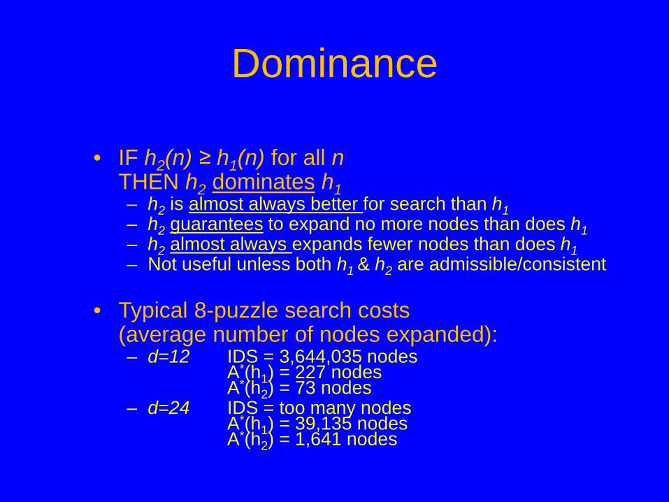
• IF h2(n) ≥ h1(n) for all n THEN h2 dominates h1

– h2 is almost always better for search than h1 – h2 guarantees to expand no more nodes than does h1 – h2 almost always expands fewer nodes than does h1 – Not useful unless both h1 & h2 are admissible/consistent

• Typical 8-puzzle search costs (average number of nodes expanded):

– d=12 IDS = 3,644,035 nodes A*(h1) = 227 nodes A*(h2) = 73 nodes

– d=24 IDS = too many nodes A*(h1) = 39,135 nodes A*(h2) = 1,641 nodes

Effective branching factor: b*

• Let A* generate N nodes to find a goal at depth d – b* is the branching factor that a uniform tree of depth d would have in

order to contain N+1 nodes.

– For sufficiently hard problems, the measure b* usually is fairly constant across different problem instances.

• A good guide to the heuristic’s overall usefulness. • A good way to compare different heuristics.

dd

d

d

NbbN

bbNbbbN

≈⇒≈

−−=+

++++=++

**)(

)1*/()1*)((1*)(...*)(*11

1

2

Effective Branching Factor Pseudo-code (Binary search)

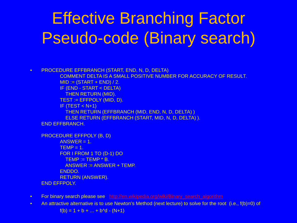
• PROCEDURE EFFBRANCH (START, END, N, D, DELTA) COMMENT DELTA IS A SMALL POSITIVE NUMBER FOR ACCURACY OF RESULT. MID := (START + END) / 2. IF (END - START < DELTA) THEN RETURN (MID). TEST := EFFPOLY (MID, D). IF (TEST < N+1) THEN RETURN (EFFBRANCH (MID, END, N, D, DELTA) ) ELSE RETURN (EFFBRANCH (START, MID, N, D, DELTA) ). END EFFBRANCH. PROCEDURE EFFPOLY (B, D) ANSWER = 1. TEMP = 1. FOR I FROM 1 TO (D-1) DO TEMP := TEMP * B. ANSWER := ANSWER + TEMP. ENDDO. RETURN (ANSWER). END EFFPOLY.

• For binary search please see: http://en.wikipedia.org/wiki/Binary_search_algorithm • An attractive alternative is to use Newton’s Method (next lecture) to solve for the root (i.e., f(b)=0) of

f(b) = 1 + b + ... + b^d - (N+1)

Effectiveness of different heuristics

• Results averaged over random instances of the 8-puzzle

Inventing heuristics via “relaxed problems”

A problem with fewer restrictions on the actions is called a relaxed problem

The cost of an optimal solution to a relaxed problem is an admissible heuristic for the original problem

If the rules of the 8-puzzle are relaxed so that a tile can move anywhere, then h1(n) gives the shortest solution

If the rules are relaxed so that a tile can move to any adjacent square, then h2(n) gives the shortest solution

Can be a useful way to generate heuristics E.g., ABSOLVER (Prieditis, 1993) discovered the first useful heuristic for

the Rubik’s cube puzzle

More on heuristics

• h(n) = max{ h1(n), h2(n), …, hk(n) } – Assume all h functions are admissible – E.g., h1(n) = # of misplaced tiles – E.g., h2(n) = manhattan distance, etc. – max chooses least optimistic heuristic (most accurate) at each

node

• h(n) = w1 h1 (n) + w2 h2(n) + … + wk hk(n) – A convex combination of features

• Weighted sum of h(n)’s, where weights sum to 1 – Weights learned via repeated puzzle-solving – Try to identify which features are predictive of path cost

Pattern databases

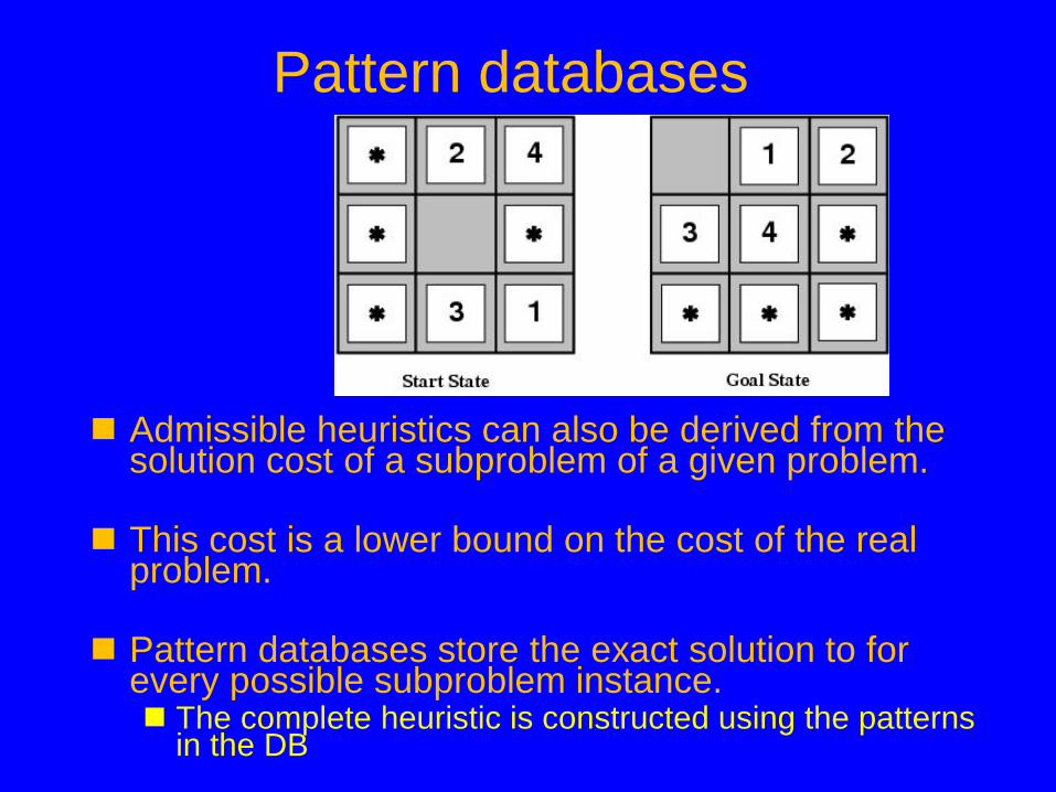
Admissible heuristics can also be derived from the solution cost of a subproblem of a given problem.

This cost is a lower bound on the cost of the real problem.

Pattern databases store the exact solution to for every possible subproblem instance. The complete heuristic is constructed using the patterns

in the DB

An Admissible but Inconsistent Heuristic For the 8-puzzle (interesting side note)

• h1 = Pattern Database for tiles 1,2,3,4 – Obviously, h1 is both admissible & consistent

• h2 = Pattern Database for tiles 5,6,7,8

– Obviously, h2 is both admissible & consistent

• h(n) = choose_randomly( h1(n), h2(n) ) – h is admissible but not (necessarily) consistent – h is (probably) not non-decreasing along all paths

• h1 and h2 are not necessarily related to each other • Random combination may not satisfy triangle inequality

Example adapted from “Inconsistent Heuristics in Theory and Practice” by Felner, Zahavi, Holte, Schaeffer, Sturtevant, & Zhang

Summary

• Uninformed search methods have uses, also severe limitations • Heuristics are a structured way to add “smarts” to your search

• Informed (or heuristic) search uses problem-specific heuristics

to improve efficiency • Best-first, A* (and if needed for memory limits, RBFS, SMA*) • Techniques for generating heuristics • A* is optimal with admissible (tree)/consistent (graph) heuristics

• Can provide significant speed-ups in practice

• E.g., on 8-puzzle, speed-up is dramatic • Still have worst-case exponential time complexity • In AI, “NP-Complete” means “Formally interesting”

• Next lecture topic: local search techniques

• Hill-climbing, genetic algorithms, simulated annealing, etc. • Read Chapter 4 in advance of lecture, and again after lecture