Embed Size (px)
Citation preview

Informing the practice of groundheat exchanger design through
numerical simulations
by
Simon R. Haslam
A thesispresented to the University of Waterloo
in fulfillment of thethesis requirement for the degree of
Master of Applied Sciencein
Civil Engineering
Waterloo, Ontario, Canada, 2013
© Simon R. Haslam 2013

I hereby declare that I am the sole author of this thesis. This is a true copy of the thesis,including any required final revisions, as accepted by my examiners.
I understand that my thesis may be made electronically available to the public.
ii

Abstract
Closed-loop ground source heat pumps (GSHPs) are used to transfer thermal energybetween the subsurface and conditioned spaces for heating and cooling applications. Abasic GSHP is composed of a ground heat exchanger (GHX), which is a closed loop ofpipe buried in the shallow subsurface circulating a heat exchange fluid, connected to aheat pump. These systems offer an energy efficient alternative to conventional heating andcooling systems; however, installation costs are higher due to the additional cost associatedwith the GHX. By further developing our understanding of how these ground loops interactwith the subsurface, it may possible to design them more intelligently, efficiently, andeconomically.
To gain insight into the physical processes occurring between the GHX and the subsur-face and to identify efficiencies and inefficiencies in GSHP design and operation, two mainresearch goals were defined: comprehensive monitoring of a fully functioning GSHP andintensive simulation of these systems using computer models.
A 6-ton GSHP was installed at a residence in Elora, ON. An array of 64 temperaturesensors was installed on and surrounding the GHX and power consumption and temper-ature sensors were installed on the system inside the residence. The data collected wereused to help characterize and understand the function of the system, provide motivationfor further investigations, and assess the impact of the time of use billing scheme on GSHPoperation costs.
To simulate GSHPs, two computer models were utilized. A 3D finite element modelwas employed to analyse the effects of pipe configuration and pipe spacing on system per-formance. A unique, transient 1D finite difference heat conduction model was developedto simulate a single pipe in a U-tube shape with inter-pipe interactions and was bench-marked against a tested analytical solution. The model was used to compare quasi-steadystate and transient simulation of GSHPs, identify system performance efficiencies throughpump schedule optimization, and investigate the effect of pipe length on system perfor-mance. A comprehensive comparison of steady state and pulsed simulation concludes thatit is possible to simulate transient operation using a steady state assumption for somecases. Optimal pipe configurations are identified for a range of soil thermal properties.Optimized pump schedules are identified and analysed for a specific heat pump and fluidcirculation pump. Finally, the effect of pipe spacing and length on system performanceis characterized. It was found that there are few design inefficiencies that could be easilyaddressed to improve general design practice.
iii

Acknowledgements
A huge thank you goes to Prof. James R. Craig, my supervisor and endless source ofknowledge at the University of Waterloo. Thank you for your constant help, motivation,and guidance. Your thorough edits and revisions helped to transform this document intowhat it is and your positive feedback helped to keep the project forever moving forward.
This project would not have been nearly as successful without the teamwork provided byRichard Simms, the other half of the ‘Geoexchange Research Department’ at the Universityof Waterloo. Richard was a constant source of brainstorming and insight in all areas of thisproject. Thanks for your hard work, patience, and understanding my lack of understandingwhen necessary.
The research presented herein was completed in partnership with NextEnergy Inc. basedout of Elmira, ON. NextEnergy offered industry experience and some of the facilities neededto perform the work presented. The knowledge and funding that has been made availableby NextEnergy assisted in all areas of this research.
David Brodrecht from NextEnergy Inc. provided significant insight into a variety ofaspects of this project, including brainstorming, much needed mechanical descriptions andlessons, and guidance in helping to understand GHX design. Thanks David.
Peter and Jane Robertson, with the support of NextEnergy and Rapid Cooling, gener-ously provided their fully function horizontal residential GSHP in Elora, ON, for analysis.Thank you to the Robertsons for your hospitality and cooperation throughout this research.
Thanks to Terry Ridgeway from the University of Waterloo for his technical assistanceand guidance in preparation for the installation of the monitoring equipment at the EloraField Site.
Sean McGregor from WILO Canada Inc. helped to assist with identification of fluidcirculation pump specifications necessary for GSHP system performance investigations.Thank you Sean.
A big thank you goes to NextEnergy Inc., NSERC, OCE, the University of Waterloo,and Rapid Cooling for their financial support throughout this project.
Finally, thank you to Angela for her continued support, much needed revisions, constantmotivation, and her ability to distract me just enough to keep me sane through this project.
iv

Dedication
This thesis is dedicated to my parents, Pam and Steve. Thank you for the physical,emotional, and financial support throughout my life that has lead me to this point. Nomatter how much of this document you may understand, understand that it could not havehappened if I wasn’t the man you shaped me into.
v

Table of Contents
List of Tables x
List of Figures xi
Nomenclature xiv
1 Introduction 1
1.1 Motivation . . . . . . . . . . . . . . . . . . . . . . . . . . . . . . . . . . . . 2
1.2 Problem Statement . . . . . . . . . . . . . . . . . . . . . . . . . . . . . . . 3
1.3 Thesis Scope . . . . . . . . . . . . . . . . . . . . . . . . . . . . . . . . . . . 4
2 Background 7
2.1 Ground Source Heat Pumps . . . . . . . . . . . . . . . . . . . . . . . . . . 7
2.1.1 Existing GHX Models . . . . . . . . . . . . . . . . . . . . . . . . . 10
2.2 Current Design Techniques . . . . . . . . . . . . . . . . . . . . . . . . . . . 15
2.3 GHX Design Guidelines and Standards . . . . . . . . . . . . . . . . . . . . 18
2.4 3D Finite Element Model . . . . . . . . . . . . . . . . . . . . . . . . . . . . 19
3 Elora Field Site 22
3.1 Ground Loop Design . . . . . . . . . . . . . . . . . . . . . . . . . . . . . . 23
3.2 Ground Loop Monitoring . . . . . . . . . . . . . . . . . . . . . . . . . . . . 26
3.3 Interior Monitoring . . . . . . . . . . . . . . . . . . . . . . . . . . . . . . . 33
3.3.1 GSHP Operation Costs . . . . . . . . . . . . . . . . . . . . . . . . . 34
vi

4 Model Development 41
4.1 Conceptual Model . . . . . . . . . . . . . . . . . . . . . . . . . . . . . . . . 41
4.2 Mathematical Model . . . . . . . . . . . . . . . . . . . . . . . . . . . . . . 47
4.2.1 Control Volume . . . . . . . . . . . . . . . . . . . . . . . . . . . . . 48
4.2.2 Governing Equations . . . . . . . . . . . . . . . . . . . . . . . . . . 49
4.2.3 Initial Conditions . . . . . . . . . . . . . . . . . . . . . . . . . . . . 53
4.2.4 Boundary Conditions . . . . . . . . . . . . . . . . . . . . . . . . . . 53
4.2.5 In-Pipe Dispersion . . . . . . . . . . . . . . . . . . . . . . . . . . . 55
4.2.6 Thermal Resistance . . . . . . . . . . . . . . . . . . . . . . . . . . . 56
4.2.7 Radius of Influence . . . . . . . . . . . . . . . . . . . . . . . . . . . 61
4.2.8 Intermediate Soil Radius . . . . . . . . . . . . . . . . . . . . . . . . 62
4.3 Finite Difference Approximation . . . . . . . . . . . . . . . . . . . . . . . . 62
4.4 Thermal Properties . . . . . . . . . . . . . . . . . . . . . . . . . . . . . . . 65
4.4.1 Heat Exchange Fluid Properties . . . . . . . . . . . . . . . . . . . . 65
4.4.2 Bulk Soil Properties . . . . . . . . . . . . . . . . . . . . . . . . . . 65
4.5 Model Benchmarking . . . . . . . . . . . . . . . . . . . . . . . . . . . . . . 66
4.5.1 Model Adjustments . . . . . . . . . . . . . . . . . . . . . . . . . . . 69
4.5.2 Benchmark Results . . . . . . . . . . . . . . . . . . . . . . . . . . . 70
4.6 System Performance . . . . . . . . . . . . . . . . . . . . . . . . . . . . . . 74
4.7 Sample Model Output . . . . . . . . . . . . . . . . . . . . . . . . . . . . . 77
5 Model Application 81
5.1 Base Case Definition . . . . . . . . . . . . . . . . . . . . . . . . . . . . . . 82
5.1.1 1D Base Case . . . . . . . . . . . . . . . . . . . . . . . . . . . . . . 82
5.1.2 3D Base Case . . . . . . . . . . . . . . . . . . . . . . . . . . . . . . 83
5.2 Pump Schedule Optimization . . . . . . . . . . . . . . . . . . . . . . . . . 84
5.2.1 Pumping Intensity . . . . . . . . . . . . . . . . . . . . . . . . . . . 85
5.2.2 Equivalent Resistance for Non-Turbulent Flow . . . . . . . . . . . . 90
vii

5.2.3 Cycle Frequency . . . . . . . . . . . . . . . . . . . . . . . . . . . . 95
5.2.4 Discussion . . . . . . . . . . . . . . . . . . . . . . . . . . . . . . . . 102
5.3 Transient and Steady State Pumping Behaviour . . . . . . . . . . . . . . . 103
5.3.1 Sensitivity of System COP . . . . . . . . . . . . . . . . . . . . . . . 104
5.3.2 Equivalence of Transient and Steady State Pumping . . . . . . . . . 107
5.4 Configuration Optimization . . . . . . . . . . . . . . . . . . . . . . . . . . 113
5.4.1 Pipe Spacing . . . . . . . . . . . . . . . . . . . . . . . . . . . . . . 113
5.4.2 Two Parallel Pipes . . . . . . . . . . . . . . . . . . . . . . . . . . . 119
5.4.3 GHX Layout . . . . . . . . . . . . . . . . . . . . . . . . . . . . . . 122
5.4.4 Loop Length . . . . . . . . . . . . . . . . . . . . . . . . . . . . . . . 126
6 Conclusions 130
6.1 Recommendations for Future Work . . . . . . . . . . . . . . . . . . . . . . 136
References 138
APPENDICES 143
A CSA 448 Multiple Measure Method 144
B GeoDesigner® Design Report 149
C Thermistor Calibration 161
D Finite Difference Model Derivation 164
D.1 Energy Equation . . . . . . . . . . . . . . . . . . . . . . . . . . . . . . . . 164
D.2 Coupled Equations . . . . . . . . . . . . . . . . . . . . . . . . . . . . . . . 169
D.3 Effective Thermal Resistance . . . . . . . . . . . . . . . . . . . . . . . . . . 170
D.4 Finite Difference Approximation . . . . . . . . . . . . . . . . . . . . . . . . 174
D.5 Boundary Conditions . . . . . . . . . . . . . . . . . . . . . . . . . . . . . . 177
viii

E Base Case Calculations 180
E.1 In-Pipe Dispersion . . . . . . . . . . . . . . . . . . . . . . . . . . . . . . . 180
E.2 Radius of Influence . . . . . . . . . . . . . . . . . . . . . . . . . . . . . . . 181
E.3 Intermediate Soil Radius . . . . . . . . . . . . . . . . . . . . . . . . . . . . 184
F Constant Versus Pulsed Pumping Comparison Results 186
ix

List of Tables
3.1 Ontario electricity time of use rates . . . . . . . . . . . . . . . . . . . . . . 36
3.2 Ontario electricity time of use delivery fees . . . . . . . . . . . . . . . . . . 37
3.3 Ontario electricity time of use regulatory fees . . . . . . . . . . . . . . . . . 37
3.4 Ontario electricity tiered billing system rates . . . . . . . . . . . . . . . . . 39
3.5 Comparison of GSHP operation costs for different billing schemes . . . . . 40
4.1 Analytical Solution Input Parameters - Test Case 1 . . . . . . . . . . . . . 71
5.1 Input parameters for 1D Finite Difference model . . . . . . . . . . . . . . . 83
x

List of Figures
2.1 Typical GSHP ground loop configurations . . . . . . . . . . . . . . . . . . 9
3.1 Elora Field Site ground loop design . . . . . . . . . . . . . . . . . . . . . . 24
3.2 Pipe configurations installed at Elora Test Site . . . . . . . . . . . . . . . . 26
3.3 Elora Field Site ground loop design with sensor array . . . . . . . . . . . . 27
3.4 Sensor locations at header trench cross section . . . . . . . . . . . . . . . . 28
3.5 Photograph of sensor locations across header trench . . . . . . . . . . . . . 29
3.6 Snapshot of temperature across heat trench at Elora Test Site . . . . . . . 30
3.7 Sensor locations at rabbit trench cross section . . . . . . . . . . . . . . . . 31
3.8 Sensor locations at the off-loop location . . . . . . . . . . . . . . . . . . . . 32
3.9 Total GSHP energy consumption by month . . . . . . . . . . . . . . . . . . 35
3.10 Time of use rates in Ontario, Canada . . . . . . . . . . . . . . . . . . . . . 36
3.11 Categorised monthly energy consumption of the GSHP . . . . . . . . . . . 38
3.12 GSHP monthly operating costs . . . . . . . . . . . . . . . . . . . . . . . . 39
3.13 Comparison of maximum and minimum tiered billing schemes to TOU . . 40
4.1 Vertical borehole and horizontal trench GHX configurations . . . . . . . . 42
4.2 Cross sections of conceptual model . . . . . . . . . . . . . . . . . . . . . . 44
4.3 Control volume used for thermal energy balance . . . . . . . . . . . . . . . 49
4.4 Bicylindrical system used for thermal resistance derivation . . . . . . . . . 58
4.5 Density of water as a function of temperature . . . . . . . . . . . . . . . . 66
xi

4.6 Fluid temperature comparison and percent difference - test case 1 . . . . . 72
4.7 Fluid temperature comparison - test case 2 . . . . . . . . . . . . . . . . . . 75
4.8 Three main phases of GSHP simulation - initial, depletion, and recovery . . 78
4.9 EWT and heat pump COP for initial, depletion, and recovery phases . . . 80
5.1 Simulated pump schedules with approximate flow regimes . . . . . . . . . . 87
5.2 System COP related to run time fraction . . . . . . . . . . . . . . . . . . . 88
5.3 Circulation pump power as a function of flow rate . . . . . . . . . . . . . . 89
5.4 System COP related to run time fraction - equivalent R . . . . . . . . . . . 94
5.5 Average COP vs. Cycle Frequency - 7 days . . . . . . . . . . . . . . . . . . 98
5.6 Average COP vs. Cycle Frequency - 14 day simulation . . . . . . . . . . . 99
5.7 EWT of the four most optimally performing cycle frequency simulations . . 100
5.8 COP comparison between pulsed and steady state . . . . . . . . . . . . . . 106
5.7 Pulsed vs. constant pumping . . . . . . . . . . . . . . . . . . . . . . . . . . 110
5.8 Fluid temperature along the pipe after continuous pumping . . . . . . . . . 115
5.9 Loop configuration for header trench investigation . . . . . . . . . . . . . . 116
5.10 COP as a function of header pipe spacing for a single rabbit loop . . . . . 118
5.11 Schematic of 2 parallel pipes test case . . . . . . . . . . . . . . . . . . . . . 120
5.12 COP as a function of parallel pipe spacing . . . . . . . . . . . . . . . . . . 120
5.13 GHX layouts investigated . . . . . . . . . . . . . . . . . . . . . . . . . . . 123
5.14 Performance based on GHX configuration - identical pipe spacing . . . . . 124
5.15 Performance based on GHX configuration - varying pipe spacing . . . . . . 125
5.16 Performance of U-bend configuration as a function of total pipe length . . 128
D.1 Control volume used for energy balance . . . . . . . . . . . . . . . . . . . . 166
D.2 Model node distribution . . . . . . . . . . . . . . . . . . . . . . . . . . . . 175
E.1 Soil temperature perturbation caused by ground loop . . . . . . . . . . . . 182
E.2 Sensitivity of model COP to radius of influence, r∞ . . . . . . . . . . . . . 183
xii

E.3 Sensitivity of model COP to intermediate soil radius, rs . . . . . . . . . . . 184
F.1 30 day pulsed vs. constant - fluid temperature . . . . . . . . . . . . . . . . 187
F.2 14 day pulsed vs. constant - fluid temperature . . . . . . . . . . . . . . . . 187
F.3 7 day pulsed vs. constant - fluid temperature . . . . . . . . . . . . . . . . . 188
F.4 1 day pulsed vs. constant - fluid temperature . . . . . . . . . . . . . . . . . 188
F.5 30 day pulsed vs. constant - cumulative energy . . . . . . . . . . . . . . . . 189
F.6 14 day pulsed vs. constant - cumulative energy . . . . . . . . . . . . . . . . 189
F.7 7 day pulsed vs. constant - cumulative energy . . . . . . . . . . . . . . . . 190
F.8 1 day pulsed vs. constant - cumulative energy . . . . . . . . . . . . . . . . 190
F.9 30 day pulsed vs. constant - total energy . . . . . . . . . . . . . . . . . . . 191
F.10 14 day pulsed vs. constant - total energy . . . . . . . . . . . . . . . . . . . 191
F.11 7 day pulsed vs. constant - total energy . . . . . . . . . . . . . . . . . . . . 192
F.12 1 day pulsed vs. constant - total energy . . . . . . . . . . . . . . . . . . . . 192
xiii

Nomenclature
α thermal diffusivity [m2/s]
β1 conductance term describing heat transfer between fluids in adjacent pipes [1/s]
β2 conductance term describing the heat transfer between the fluid in the pipe and thesoil at the intermediate radius [1/s]
β3 conductance term describing the heat transfer between the fluid in the pipe and thesoil at the intermediate radius [1/s]
β4 conductance term describing the heat transfer between the soil at the intermediateradius and the far field [1/s]
∆Efluid change in energy in the fluid due to external sources [J]
∆T prescribed change in temperature between the inlet and outlet temperatures [C]
∆t time step [s]
∆T sourcefluid change in temperature between the external source (fluid in adjacent pipe orsurrounding soil) and the fluid in the pipe [C]
∆x length of the control volume [m]
∀ volume [m3]
∀s volume of soil between the outer pipe radius and the intermediate soil radius [m3]
∀∞ volume of the hollow cylinder of soil created between the intermediate soil radiusand the radius of influence [m3]
µ dynamic viscosity [Pa·s]
xiv

ν kinematic viscosity [m2/s]
ρ density [kg/m3]
ρs density of the soil [kg/m3]
ρfluid fluid density [kg/m3]
ρfluidcpfluid volumetric heat capacity (V HC) of the fluid [J/(m3K]
A cross sectional area perpendicular to heat flow [m2]
a matrix coefficient [1/s]
Ap cross sectional area of the inner pipe perpendicular to flow [m2]
As cross sectional area perpendicular to fluid flow of the soil to the intermediate radiuswith the area of the pipes removed [m2]
A∞ cross sectional area perpendicular to fluid flow of the annulus between the interme-diate soil and the far field [m2]
b matrix coefficient [1/s]
c matrix coefficient [1/s]
cp specific heat capacity [J/(kgK)]
cps specific heat capacity of the soil [J/(kgK)]
cpfluid specific heat capacity of the fluid [J/(kgK)]
Cd heating correction factor
D dispersion coefficient [m2/s]
d matrix coefficient [1/s]
DH hydraulic length (pipe inner diameter) [m]
DL longitudinal dispersion coefficient [m2/s]
E thermal energy [J]
f friction factor of fluid flowing through a pipe [-]
xv

i degree of freedom [-]
k thermal conductivity [J/(smK)]
kpipe thermal conductivity of the pipe material [J/(smK)]
ksoil thermal conductivity of the soil between the pipes [J/(smK)]
L total pipe length [m]
N number of equations in each model segment: outgoing and incoming pipes and soil[-]
n node number [-]
Nu Nusselt number [-]
Nu00 approximation of the asymptote of the Nusselt number as Pr →0 and Re→0 [-]
Nui approximation of the asymptote of the Nusselt number in transition to laminar flow
Nut approximation of the Nusselt number for turbulent flows [-]
Nulc approximation of the Nusselt number [-] at Re = 2100
Nulc approximation of the Nusselt number [-] at Re = 2100
Numax Nusselt number [-] for the maximum flow rate considered in the model
Nunon−turbulent Nusselt number [-] for a non-turbulent flow rate
P total power (or energy per unit time) extracted from the subsurface by one circuitof the loop [J/s]
Pr Prandtl number [-], which is equivalent to the ratio of kinematic viscosity to thermaldiffusivity (Pr = ν/α)
Q volumetric flow rate of fluid through the heat pump [m3/s]
q heat flow [J/s]
Qsource thermal energy conduction through the pipe wall [J/sm]
Qpipessource heat flux from the adjacent pipe per metre [J/sm]
xvi

Qsoilsource heat flux from the subsurface per metre [J/sm]
R effective thermal resistance [smK/J]
R∗ absolute thermal resistance [sK/J]
r1 radius of cylinder 1 [m]
r2 radius of cylinder 2 [m]
ri inner radius of the pipe [m]
ro outer radius of the pipe [m]
Rp effective thermal resistance between the fluids in each of the pipes [smK/J]
Rs effective thermal resistance between the fluid in the pipe and the intermediate soil[smK/J]
rs intermediate soil radius [m]
r1o outer radius of one pipe [m]
r2o outer radius of adjacent pipe [m]
R∞ effective thermal resistance of the annulus of soil between the intermediate radiusand the far field [smK/J]
r∞ radius of influence [m]
Rabs absolute thermal resistance of the conducting material between the two parallelcylinders [sK/J]
Reff effective thermal resistance across the pipe wall [smK/J]
Rsourceeff effective thermal resistance between the external source (fluid in adjacent pipe or
surrounding soil) and the fluid in the pipe [smK/J]
Req equivalent effective thermal resistance across the pipe wall modified for non-turbulentflow [smK/J]
Rinter effective thermal resistance between either of the pipes and the soil at an interme-diate radius [smK/J]
xvii

Rpipe effective thermal resistance of the pipe wall [smK/J]
Rpipessoil effective thermal resistance of the medium between the two pipes [smK/J]
Re Reynolds number [-]
T ′(x, t) fluid temperature in the adjacent pipe [C]
T (x, t) fluid temperature in the pipe of interest [C]
T n temperature during current time step [C]
T n+1 temperature during next time step [C]
tR fluid residence time in the pipe [s]
Ts(x, t) temperature of the soil at the intermediate soil radius as a function of distancealong the pipe and time [C]
T∞ far field temperature at the radius of influence [C]
Tinner temperature on the inside of the pipe wall [C]
Tin fluid temperature at the pipe inlet [C]
Ti temperature at node i [C]
Touter temperature on the outside of the pipe wall [C]
Tout fluid temperature at the pipe outlet [C]
Tsi soil temperture at node i [C]
v mean fluid flow velocity [m/s]
V HC volumetric heat capacity [J/(m3K]
w half the distance between the pipe centres [m]
w1 distance from y-axis to centre of cylinder 1 [m]
w2 distance from y-axis to centre of cylinder 2 [m]
xviii

Chapter 1
Introduction
Ground source heat pumps (GSHPs) utilize stored energy in the subsurface to provide
efficient heating and cooling for buildings. A basic GSHP will return between two and half
to four units of energy per one unit consumed while in heating mode, and the equivalent
of between ten and twenty units while in cooling mode (NRCan, 2009). A typical GSHP
is a combination of a ground heat exchanger (GHX), which consists of a heat exchange
fluid circulating through a closed pipe circuit buried in the shallow subsurface and a heat
pump. Currently, GHXs are intentionally overdesigned to account for the uncertainty in
our understanding of subsurface energy processes.
1

1.1 Motivation
GSHPs offer a renewable method for heating and cooling applications. Thermal energy,
whose original source is predominantly solar energy, can either be extracted from the Earth,
heating a building, or injected into it, cooling a building. These systems have the ability to
provide efficient heating and cooling for a range of buildings in Ontario and when comparing
efficiency in operation costs to that of heating and cooling systems utilizing conventional
fuel sources, GSHPs offer the most economical option (Etcheverry et al., 2004). However,
since conventional systems have significantly lower initial costs, the use of GSHPs is not as
wide spread as it could be. The Oakridge National Laboratory (2008) states that the high
capital cost of GSHPs is the number one barrier to adoption to consumers. This barrier is
most significant for those properties where land area is limited, thus requiring that a more
expensive vertical system be used rather than a horizontal system. Horizontal systems can
be more economical but require larger land areas than the vertical equivalent. By reducing
horizontal GHX size through better loop design procedures, horizontal GSHPs could be-
come more logistically feasible for a larger range of properties, making them attainable for
more building owners. Therefore, an investigation into methods through which the initial
size and cost of GSHPs could be reduced would help to identify potential improvements in
the application of these systems.
2

1.2 Problem Statement
While GSHPs are not an entirely new technology, they have been understudied in research
circles (OSU, 1988). The main goal of this thesis was to investigate GHX design and
system operation and performance through field measurements and numerical simulation
to provide insight into their function and identify potential areas for improvement.
This goal was addressed by enhancing our understanding of the heat transfer mecha-
nisms in the subsurface and the interactions between soils and horizontal GHXs. Improving
our understanding in this area should lead to improved methods for GHX design, which
would allow installers to safely design their systems more efficiently. Upgrading the ef-
ficiency of GHX design may lead to decreased installation costs by reducing land area
and material requirements; therefore, increasing the feasibility of these systems for smaller
residential lots.
Currently, horizontal GHXs require large areas of land to meet existing design guide-
lines. Typically, it is assumed that approximately 230 m2 (2500 ft2) of land area is needed
per ton of heating (McQ, 2002), where 1 ton is equivalent to 3516 J/s (12000 BTU/h).
This assumption, along with other empirically-based design calculations, have likely led to
the improper design of many horizontal ground loop systems (Spitler and Cullin, 2008).
While this amount of land area may be necessary for some installations, updated horizon-
3

tal loop design methods may be able to determine land required on a unit-specific basis.
By identifying optimal ground loop configurations and developing novel design methods
based on insights into the physics of heat transfer processes, it should be possible to design
less conservatively and more intelligently. Ideally, such techniques will lead to reduced
materials, costs, and land area requirements, allowing for installation of horizontal GHXs
on smaller properties, increasing their utility.
1.3 Thesis Scope
The research presented helps to further the understanding of GSHP operation and the
physical processes between the pipe and the subsurface with the purpose of improving
GHX design techniques. This thesis provides a review of previous work, a summary of field
measurements, a presentation of a developed numerical model, and analyses of measured
and simulated data.
A field site in Elora, ON, consisting of a fully functioning horizontal GSHP, was thor-
oughly monitored throughout this research. The data collected was analysed and is pre-
sented in various forms, including total energy usage, operation costs, and temperature
measurements.
A transient one dimensional (1D) finite difference heat conduction model of a U-tube
4

shaped GHX in a cylindrical soil domain was developed to provide a tool through which
a range of test cases could be simulated and investigated. While a variety of informative
numerical models exist in the literature, a specialized model was developed to analyse
specific aspects of GHXs. For this research it was necessary for the model to adequately
represent the physical system on small time scales to analyse heat transfer on time scales
less than the pipe residence time. Also, the model was required to be fully transient,
have the ability to directly define the heat transfer between adjacent, parallel pipes, and
be computationally efficient for the time scales of interest (approximately the duration
of a heating season in Ontario). The developed 1D finite difference model is presented
herein, benchmarked against an existing analytical solution. It was used to analyse the
effects of modelling a transient system using a quasi-steady state approximation, investigate
the effect that pump scheduling has on overall GSHP performance using the coefficient of
performance (COP) metric, and further understand heat transfer between adjacent parallel
pipes in a GHX.
An investigation into the effects of horizontal GHX configuration on performance us-
ing model simulations is also presented. Simms (2013) developed a three dimensional
(3D) model using the finite element method (FEM) to simulate the interactions between
horizontal ground loops and the subsurface. The thermal energy flux within the system
was assessed based on the temperature gradient between the inside of the pipe and the
5

surrounding soil. The model is capable of simulating a system with multiple pipes and
multiple trenches in various orientations. The model output includes the fluid tempera-
ture within the ground loop and measures of system performance and efficiency over time.
This model was used in this thesis to investigate the variations in performance between a
range of different horizontal GHX configurations and the effects of pipe spacing on system
efficiency. These investigations were conducted with the purpose of determining the op-
timum horizontal GHX configuration to maximize GSHP performance and efficiency over
time. The conclusions made help to improve knowledge of specific details of GHX design.
This model is discussed in detail in Chapter 2.
6

Chapter 2
Background
This chapter describes the basic design and operation of GSHPs. Several existing numerical
models created to simulate the interaction between a GHX and the subsurface are presented
to summarize the current state of the science. Basic GSHP design techniques are discussed
and the Canadian standard design method is summarized.
2.1 Ground Source Heat Pumps
A closed-loop ground source heat pump (GSHP) is a combination of a ground heat ex-
changer (GHX) and a heat pump. These systems are utilized for the heating and cooling
of conditioned spaces. A GHX consists of a heat exchange fluid circulating through a
7

closed pipe circuit buried in the shallow subsurface (typically <200 m). This pipe circuit
is connected to a heat pump, whose function it is to transfer thermal energy between the
circulating fluid and a conditioned space, typically inside a building. In heating mode, the
heat pump extracts energy from the fluid and transfers it to the space and in cooling mode,
the heat pump rejects energy from the building into the fluid, changing the temperature of
the fluid as it flows across the heat pump. The GHX acts to moderate the temperature of
the circulating fluid to that of the ground temperature, providing a thermal energy source
or sink to the building depending on the operation mode of the heat pump.
A GHX can be of a variety of configurations. In typical GSHPs, the pipe is installed
vertically in a borehole, or series of boreholes, between 20 and 200 m deep or horizontally
in shallow trenches between the Earth’s surface and a depth of 3 m (OSU, 1988). Figure
2.1 is a schematic representation of the two main types of GHX configurations.
Vertical GHXs are most commonly installed in a U-tube shape. This configuration
involves two parallel pipes being installed in a single borehole, forming a U-bend connection
at the bottom of the borehole. Vertical systems with two U-tubes installed in the same
borehole are also common. Vertical borehole heat exchangers (BHEs) can exist as a single
borehole or an array of boreholes connected near the ground surface. A variety of vertical
GHX configurations are described by OSU (1988, 2009).
A range of horizontal GHX configurations are used in practice. Typical designs include
8

(a) (b)
Figure 2.1: Typical GSHP ground loop configurations: (a) vertical and (b) horizontal -not to scale
1 to 4 pipes buried in a single trench. These pipes can be buried within a single trench or
in multiple trenches connected by a common manifold trench. A slinky-loop configuration
is also common in horizontal GHX applications. This configuration involves a single coiled
pipe spread along the bottom of the trench or multiple coiled pipes spread adjacently along
a wider excavation. Some of the most widely used horizontal configurations are described
and investigated in Section 5.4. A variety of standard horizontal GHX configurations
are described in OSU (1988), OSU (2009), and IGSHPA (1994). Several horizontal GHX
configurations are further discussed in Chapter 5 (Figure 5.13).
Horizontally bored configurations can also be used as GHXs; however, these systems are
9

less common. Horizontally bored systems are constructed similarly to vertical BHE systems
with boreholes installed horizontally at shallower depths. Such systems are beneficial
for installing the GHX beneath existing infrastructure or landscape while minimizing the
disturbance at the Earth’s surface.
2.1.1 Existing GHX Models
A variety of numerical models examining specific aspects of the heat transfer mechanisms
between GHXs and the subsurface exist. However, the majority of these models focus on
vertical systems, or borehole heat exchangers (BHEs), while only a few exist which de-
scribe horizontal systems and even fewer which directly describe the heat transfer between
adjacent, parallel pipes. A number of previously proposed numerical, semi-numerical, and
basic design models are described below.
One of the original models using the finite element method to simulate BHEs was
developed by Muraya (1994). This model used an equivalent radius to simulate the two
pipes in a BHE and an effectiveness parameter to account for heat transfer between the
pipes.
Yavuzturk et al. (1999) presented a transient two dimensional (2D) finite volume model
to simulate U-tube shaped BHEs. This model was based on a thermal conduction equation
10

in polar coordinates and utilized a fully implicit finite volume approach using radial coordi-
nates to represent the U-tube shape of the pipe in a BHE. While this model does simulate
both pipes in the U-tube system it does not directly simulate the thermal interactions
between the pipes.
Al-Koury et al. (2005) developed a 3D steady state finite element model describing
BHEs and their interactions with the subsurface. This model used finite elements to
represent the U-tube shaped system. Each element was divided into two pipe segments and
two borehole grout segments to represent the physical processes between: the up pipe and
the borehole grout material, the down pipe and the borehole grout material, adjacent grout
material, and the borehole grout material and the subsurface. This model uses the grout
material to couple the heat transfer between pipes. Therefore, thermal energy transfer
occurs between each pipe and the grout surrounding that pipe and between adjacent grout
segments but the model does not consider direct interactions between pipes. Also, all
components of the BHE are combined into single elements. This model was extended by
Al-Koury and Bonnier (2006) to the transient system.
The model presented by Al-Koury and Bonnier (2006) was further improved upon by
Diersch et al. (2011a). They developed a transient 3D model of single and multiple vertical
U-tube BHEs by using the finite element method and implementing the numerical tech-
niques described by Al-Koury et al. (2005) and analytical techniques described by Eskilson
11

and Claesson (1988) in the FEFLOW simulator. Again, the numerical model presented by
Diersch et al. (2011a) uses a division of elements into segments of up pipe, down pipe, and
two borehole grout material segments. The inclusion of additional segments in the grout
helped to improve this model over that described by Al-Koury and Bonnier (2006). This
change improved the accuracy of the model and allowed for the simulation of additional
U-tube geometries in the BHE. The Diersch et al. (2011a) model has the ability to simulate
a double U-tube system, in which case there is an element segment for each of the four
pipes and the corresponding four borehole grout segments. This model is shown to pro-
duce results agreeable with analytical solutions for a variety of test cases as benchmarked
by Diersch et al. (2011b). However, similar to Al-Koury et al. (2005), there is no direct
heat transfer between the pipes in this model and the heat transfer is strictly between
the pipes and their corresponding grout segments, adjacent grout segments, and the grout
segments and the surrounding subsurface, and computational efficiency is dependent on
the optimization of the mesh configuration.
The analytical method employed by Diersch et al. (2011b) was originally described by
Eskilson and Claesson (1988), extended for additional BHE pipe geometries, and imple-
mented in the FEFLOW simulator. This method was originally proposed as a method for
the steady state simulation of an array of thermally interacting BHEs for only long term
analyses. Diersch et al. (2011a) found the analytical method accurate, highly efficient, and
12

robust for long term analyses but not applicable for short term simulations.
Nabi and Al-Khoury (2012a) proposed a 3D finite volume model for BHEs. This model
separates the soil domain and the BHE domain, solving each one as a heat source to the
other. It is an extension of the work presented by Al-Koury et al. (2005) and Al-Koury
and Bonnier (2006).
A variety of other finite element based numerical models describing vertical BHEs have
previously been proposed analysing a range of specific processes. For example, Raymond
et al. (2011), among others, used this numerical method to simulate BHEs with the purpose
of understanding the heat transfer during thermal response tests for the quantification of
thermal properties.
The finite element method has also been used to investigate ground water flow interac-
tions with BHEs. Muraya (1994), Rees et al. (2004), and He et al. (2011) have proposed
finite element models that include the effects of soil moisture and the presence of ground
water on the heat transfer between the subsurface and certain types BHEs.
For horizontal ground heat exchangers much less modelling work has been done; how-
ever, some analyses have been completed using numerical modelling techniques. Stevens
(2002) presented a numerical model to simulate the heat transfer between a single buried
cylindrical pipe and the surrounding semi-infinite subsurface. This model, developed us-
13

ing the finite difference method, examined the heat transfer differences between the fluid
and the subsurface for the steady pumping of a fluid through the pipe and the case of
intermittent pumping of a fluid through the pipe.
An earlier model proposed by Mei and Emerson (1985) described the behaviour of a
GHX as a single buried coil. This model included intermittent pumping and the freezing
effects of moisture in the soil surrounding the buried pipe.
Philippe et al. (2011) proposed a semi-analytical model to simulate the axial fluid
temperatures and pipe temperatures in a horizontal, serpentine (’S’-shaped) GHX. Several
techniques are combined by Philippe et al. (2011) to simulate this system. The finite
difference method is used to approximate the axial heat transfer between the fluid and the
pipe. An analytical cylindrical heat source solution first proposed by Baudoin (1988) was
employed to define a reference heat transfer problem that was used to describe the heat
transfer between the pipe and the soil. Finally, for longer simulations, the heat transfer
between adjacent pipes was described using spatial superposition of all the adjacent pipe
segments. An empirical temperature penalty was assigned to the subsurface at the location
of each pipe based on the effects of the other pipes in the system. These solution methods
were coupled iteratively through time to describe the fluid and pipe temperatures. To
include the ground surface boundary condition for longer simulations Philippe et al. (2011)
utilized mirror image pipe sections above the ground surface.
14

Fontaine et al. (2011) describe a transient analytical model based on the finite line
source that examines horizontally buried GHX pipes. The model was developed with the
goal of assessing the ability of GHXs to keep the subsurface below a building’s foundation
frozen in regions of permafrost while providing the energy required to heat the building.
However, the model does not directly describe the heat transfer between adjacent horizontal
pipes. The analytical model presented by Fontaine et al. (2011) was verified using the 3D
finite element simulation software COMSOL Multiphysics 3.5a (COM, 2008).
2.2 Current Design Techniques
In this section a brief introduction to a few of the available methods and software pack-
ages for GHX design is provided to summarize the current state of the science of GSHP
simulation and design.
A common practice in GHX design is the use of correlations describing thermal resis-
tances for transient conductive heat transfer between the buried pipe and the undisturbed
subsurface at a distance (Philippe et al., 2011). These correlations describe heat transfer
based on thermal conduction shape factors presented in ASHRAE (2009) for typical GHX
geometries. The thermal resistance correlations were originally presented by Kavanaugh
and Rafferty (1997) and are based on a modified version of an analytical solution describ-
15

ing thermal conduction shape factors for a line source in a conductive medium presented
by Carslaw and Jaeger (1947). The solution treats the GHX as a solid cylinder of spe-
cific radius and depends on the duration of system operation and thermal diffusivity of
the subsurface. It is used to approximate the thermal resistance between the pipe and the
subsurface for a range of GHX geometries, soil characteristics, and pumping durations that
are then used in ground loop design.
Philippe et al. (2011) presented a simple procedure to estimate BHE length using
spreadsheet calculations. The procedure utilizes the cylindrical heat solution developed by
Carslaw and Jaeger (1947) with temporal superposition proposed by Ingersoll and Plass
(1948). While the spreadsheet offers a simple method for preliminary calculation of BHE
lengths, more rigorous software exists for detailed designs.
One widely used design method for basic GSHP implementation was developed by
OSU (1988) and OSU (2009). This method involves a well defined design procedure that
utilizes various properties of the GHX configuration, pipe material and dimensions, and
geographic location to estimate the required GHX length for a specified heat pump. The
method considers the heat pump efficiency, pipe thermal resistance, estimated subsurface
thermal resistance, basic local meteorological data, and basic details of the system load
requirements. The method utilizes the thermal resistance correlations described above and
provides an estimate of the required pipe length per unit of heating or cooling capacity
16

based on the defined inputs.
Two similar design techniques for smaller systems are implemented within the software
packages GeoDesigner® developed by ClimateMaster® and WaterFurnace® Energy Anal-
ysis (WFEA) by WaterFurnace®. These software packages can be employed for the design
of residential or light commercial GHX system design. Loop length estimates are calcu-
lated using an iterative process attempting to create a GHX with the necessary capacity as
defined by user inputs. While extensive descriptions of the design processes are not avail-
able, the calculation procedures are based on an amalgamation of various meteorological,
geological, and mechanical inputs and empirical coefficients based on GHX configuration
and soil type (WaterFurnace, n.d.).
For more complex systems, more intensive design software packages are employed. One
such package is Ground Loop DesignTM developed by Gaia Geothermal (2010). This soft-
ware allows the user to estimate GHX design requirements for a variety of vertical and
horizontal configurations. When considering a vertical BHE, the software utilizes one of
two calculation methods. The first is fundamentally based on the cylindrical heat solu-
tion developed by Carslaw and Jaeger (1947), while the second method is based on the
analytical solution for heat conduction in a homogeneous medium solution proposed by
Eskilson (1987). The Ground Loop DesignTM utilizes the second method for constant heat
extraction cases.
17

When considering horizontal GHXs, Ground Loop DesignTM is again fundamentally
based on the cylindrical heat solution developed by Carslaw and Jaeger (1947). The
software has the ability to estimate GHX design requirements when using slinky type
horizontal configurations, using the approximation outlined by IGSHPA (1994).
2.3 GHX Design Guidelines and Standards
The design requirements for a GHX in a certain jurisdiction are dependent on the associ-
ation responsible for the governance of GSHP design. The most widely accepted method
is that described in the ASHRAE Handbook (ASHRAE, 2009) as mentioned above. These
guidelines are typically referenced in standards pertaining to GSHP design.
In Canada, the standard design method is outlined in CSA Standard C448: Design and
Installation of Earth Energy Systems (CSA, 2009). The design procedures for residential
GHX applications outlined by CSA (2009), referred to as the Multiple Measure Method,
are similar to other methods in the industry but applicable only for heating dominate GHX
designs. A summary of these guidelines is provided in Appedix A.
18

2.4 3D Finite Element Model
The 3D finite element model developed by Simms (2013) was used extensively in this thesis
because of its ability to simulate horizontal GHXs in a variety of configurations. This model
was composed of a 3D soil continuum model, representing the subsurface, coupled to a 1D
pipe model, representing the GHX. The continuum model characterizes a soil medium with
heterogeneous, isotropic thermal conductivity. The governing equation for the continuum
was defined by Simms (2013) as:
ρc∂T
∂t= ~∇ · (k · ~∇T ) + ~q (2.1)
where ~q is the volumetric heat flux from the GHX [J/(sm3)]; k is the thermal conductivity
tensor of the soil [J/(smK)]; ρc is the volumetric heat capacity of the soil [J/(m3K)];
and ∇T is the temperature gradient [K/m] in the soil (Simms, 2013). A Dirichlet fixed
temperature boundary condition was specified on the surface of the continuum domain,
while Neumann zero flux boundary conditions were specified on all sides and the bottom
of the continuum domain (Simms, 2013). The surface boundary condition was defined
using the shallow surface temperature data collected from the Elora Field Site discussed
in Chapter 3. Additional soil temperature data from the field site were used to define the
initial conditions of the continuum model, which were defined as a temperature varying
19

with depth (Simms, 2013).
The 1D pipe model describes the in-pipe advection-dispersion in a GHX and defines the
volumetric heat flux, ~q in Equation 2.1, to the continuum model. The governing equation
for the pipe model was defined by Simms (2013) as:
∂Tp∂t
= −v∂Tp∂x
+ (DL + αf )∂2Tp∂x2
− Kp
ρ · cp · L(Tp − T ) (2.2)
where Tp(x, t) is the temperature of the fluid in the pipe [K]; v(t) is the velocity of the fluid
within the pipe [m/s]; DL is the in-pipe longitudinal dispersivity caused by mechanical
mixing [m2/s]; αf is the thermal diffusivity of the fluid [m2/s]; ρ and cp are the density
[kg/m3] and specific heat capacity [J/(kgK)] of the fluid, respectively; L is the effective
thickness of the pipe wall [m]; Kp is a representative thermal conductivity of the pipe wall
[J/(smK)]; and T (x, t) is the temperature [K] of the soil continuum immediately adjacent
to the outside of the pipe wall at distance x down the pipe, determined using Equation
2.2 (Simms, 2013). The inlet boundary condition to the pipe model was defined as a
temperature difference between the pipe inlet and outlet fluid temperatures, which acts as
a forcing term. Along the length of the pipe, the difference in temperature between the soil
and the fluid acts as a Dirichlet boundary condition for the pipe model. The initial fluid
temperature in the pipe model was defined as the temperature of the soil immediately
20

surrounding the pipe, defined in the initial condition of the continuum model (Simms,
2013).
The coupling of the continuum and pipe models was iterative bidirectional. The soil
temperatures were used to define the Dirichlet boundary condition along the length of the
pipe, which allowed for the generation of a solution to fluid temperatures in the pipe model.
Using this fluid temperature profile, the thermal energy flux between the fluid and the soil
could be determined, defining the source term to the continuum model from the pipe. The
solution to the soil continuum model was then determined, updating the temperatures of
the soil continuum, ending a time step of the full model. This process was then repeated
for the duration of the simulation (Simms, 2013).
21

Chapter 3
Elora Field Site
A fully functioning residential ground source heat pump was installed in Elora, Ontario in
partnership with NextEnergy, Inc., Rapid Cooling, and the residents, the Robertsons. The
site was fitted with a range of temperature and power consumption monitoring equipment
to analyse the performance of the ground source heat pump (GSHP) and the temperature
changes on the ground heat exchanger (GHX), or ground loop, and in the subsurface
immediately surrounding the pipe.
The Robertsons agreed to the installation of the monitoring equipment and granted
access to their home for the necessary interior work. No special instructions were given
to the Robertsons and they used the system as it would typically be used for residential
heating and cooling.
22

The temperature and power consumption data acquired from the Elora Field Site,
while very much consistent with expectations, were analysed to gain insight into specific
objectives for this research, including investigations into the performance effects of pump
scheduling, GHX configurations, and pipe spacing.
3.1 Ground Loop Design
Figure 3.1 shows the GHX design of the Elora Test site. The drawing is an accurate
representation of the as-built GHX based on measurements taken during installation.
The ground loop design represented in Figure 3.1 was designed by the NextEnergy dealer
Rapid Cooling. It is a standard NextEnergy design procedure to use the GeoDesigner®
software package to estimate required GHX length (Brodrecht, 2010). This package was
used to simulate a design similar to that installed at the Robertson’s home. The details of
this design are shown in Appendix B. This design yielded a required trench length of 279
m (915 ft), which is similar to the approximately 260 m (850 ft) of loop trench installed
at the Robertson’s home. The presented design is meant only to provide insight into the
design process.
Appendix B shows an operating cost and performance comparison of the GSHP to two
conventional heating and cooling systems: an air-to-air heating and cooling system and
23

Fig
ure
3.1:
Appro
xim
ate
as-b
uilt
repre
senta
tion
ofE
lora
Fie
ldSit
egr
ound
loop
des
ign
wit
h:
(a)
slin
ky
loop
configu
rati
on,
(b)
rabbit
loop
configu
rati
on,
and
(c1)
&(c
2)“s
ide-
by-s
ide”
loop
configu
rati
ons
24

a mid-efficiency natural gas heating system with a standard air conditioning unit. This
comparison concludes that the GSHP is the most economical of these 3 systems to operate
on a annual basis.
The installed GHX utilized three different pipe configurations in four trenches. Figure
3.2 is a schematic representing how these three pipe configurations are positioned in a 1.5
m (5 foot) wide trench. Configuration (b) is referred to as the “rabbit” loop and consists of
one pipe 183 m (600 feet) in length; (a) is a “slinky” loop and consists of one pipe 183 m in
length; and configuration (c), referred to as a “side by side” loop, consists of two separate
183 m pipes. Two trenches with configuration (c) were installed at the Elora Test Site.
The system was designed for each 183 m length of pipe to have a heating capacity of 1 ton,
or 3516 J/s (12000 BTU/h). Therefore, configurations (a) and (b) each represent one ton
of heating capacity, while each configuration (c) represent two tons of heating capacity, for
a total of six tons of heating capacity.
The 4 loop trenches are connected by a perpendicular trench referred to as the manifold
trench. This manifold trench is connected to the house by an approximately 35 m trench
housing single supply and return pipes. This trench is referred to as the header trench.
25

(a) (b) (c)
Figure 3.2: Pipe configurations installed at Elora Test Site: (a) slinky loop, (b) rabbitloop, and (c) side-by-side loops - not to scale
3.2 Ground Loop Monitoring
A total of 64 thermistors were calibrated and installed at the Elora Field Site to monitor
temperature at various locations in the subsurface. The absolute values measured by the
thermistors were of electrical conductivity of the surrounding medium. These absolute
measurements were used to calculate the temperature at each sensor using the calcula-
tion method and thermistor calibration procedure summarized in Appendix C. Figure 3.3
shows the locations and depths of all thermistors along and surrounding the GHX and the
locations of the data loggers. The figure shows two heavily instrumented cross sections.
One cross section was installed with the purpose of monitoring the temperatures surround-
ing the header trench in close proximity to the house. The sensor locations of the header
trench cross section are shown in Figure 3.4.
26

Fig
ure
3.3:
Appro
xim
ate
as-b
uilt
repre
senta
tion
ofE
lora
Fie
ldSit
egr
ound
loop
des
ign
wit
hse
nso
rar
ray
show
ing
hea
vily
inst
rum
ente
dcr
oss
sect
ions
ofhea
der
tren
ch(F
igure
3.4)
and
rabbit
tren
ch(F
igure
3.7)
27

The header trench is where the temperature difference between two adjacent pipes is
largest throughout the GHX due to the significant temperature change across the ground
loop. The goal of this monitoring location was to analyse the effects of the proximity of the
supply and return pipes in the header trench on GSHP performance. Temperature sensors
were installed as shown in Figure 3.4 to monitor the subsurface temperature at locations
on a horizontal line through the two pipes, perpendicular to fluid flow.
Figure 3.4: Sensor locations at header trench cross section
A photograph of the temperature sensors across the header trench taken during instal-
lation of the GHX and the monitoring equipment is displayed in Figure 3.5.
Figure 3.6 shows a snapshot temperature measurement profile generated from each of
the thermistors across the header trench. This snapshot was taken on December 8, 2010
28

Figure 3.5: Photograph of sensor locations at header trench cross section during installation
while the GSHP was operating in heating mode. Figure 3.6 shows the cooler supply pipe on
the left in dark blue and the warmer return pipe on the right in light blue. The figure shows
how the GHX is extracting thermal energy from the surrounding subsurface, reducing the
temperature in the soil around the pipes. It is shown that the temperature in the soil
between the two pipes is significantly lower than that in the soil at a distance away from
the pipes. Therefore, a reduction in efficiency is experienced at this location. However, the
temperature between the pipes is still warmer than that of the return pipe, suggesting that
direct energy transfer between the adjacent pipes is unlikely, only that energy transfer into
the return pipe may be diminished due to the effects of the adjacent supply pipe. This
idea is investigated in Chapter 5.4 to quantify the effects of header pipe spacing.
29

Figure 3.6: Snapshot of temperature across heat trench at Elora Test Site taken duringGSHP heating mode on December 8, 2010. Red circles indicate sensor locations across thetrench - all sensors located at a depth of 48 inches below ground surface.
The other heavily instrument cross section shown in Figure 3.3 is located across the
rabbit loop trench approximately 9.5 m from the manifold. To analyse the temperature in
the rabbit trench several groups of thermistors were installed in various orientations relative
to the trench. Figure 3.7 shows the locations and depths of the temperature sensors along
this cross section. A group of thermistors were installed across the trench with a sensor on
30

each pipe and several between the pipes and outside the trench. A line of 4 thermistors
was installed along the trench on approximately 5 m intervals. Finally, 10 thermistors
were installed in a vertical line passing through the supply pipe between 10 cm and 275
cm below ground surface.
Figure 3.7: Sensor locations at rabbit trench cross section
Undisturbed soil temperature measurements were gathered at an off-loop monitoring
location. This location, shown in Figure 3.8, was over 5 m away from the GHX and
consisted of four thermistors at depths between 10 cm and 150 cm. This location was used
to determine background soil temperatures throughout the monitoring period.
31

Figure 3.8: Sensor locations at the off-loop location
32

The installed thermistors were connected to four data loggers for data collection pur-
poses. Measurements were gathered on 5 minute intervals between December 2010 and
December 2012.
The data collected were used by Simms (2013) to determine various effective soil param-
eter values at the Elora Field Site, including equivalent homogeneous values for soil thermal
conductivity, soil thermal diffusivity, soil volumetric heat capacity, and undisturbed soil
temperature. Values determined by Simms (2013) are used herein where described.
3.3 Interior Monitoring
Typically, the efficiency of ground source heat pumps is defined using the energy efficiency
ratio (EER) for cooling operation and the coefficient of performance (COP) for heating
operation (OSU, 1988). The EER is a ratio of the total cooling capacity of the system
to the power input during cooling operation (OSU, 1988). The COP is a ratio of the
heating capacity of the system to the power input during heating operation (OSU, 1988).
Therefore, to fully understand the efficiency of a GSHP it is necessary to monitor both
energy consumption and generation, thus the Elora Field Site was fitted with a range
of sensors on the heat pump system, or ‘furnace’, inside the house to quantify system
performance. These sensors included those used to monitor the power consumption of
33

the various components of the furnace and those for measuring temperatures at various
supply and return ports. To briefly summarize the power monitoring apparatus, four
energy sensors were used to directly monitor the power consumed by the main components
of the GSHP: the air circulation fan (blower), the fluid circulation pump, the heat pump
compressor, and the auxiliary electric heating system. The power consumption data were
used to analyse the operating costs of the GSHP at the Elora Filed Site.
3.3.1 GSHP Operation Costs
The power monitoring equipment at the Elora Field Site was continuously collecting data
on the power consumption of the main components of the installed GSHP. Figure 3.9
depicts the total energy consumption of the GSHP on a monthly basis for the period of
study. These monthly totals are based on the mean of measurements taken every 5 seconds
logged on 1 minute intervals. It is noted that power consumption data is not complete
for the month of October 2011 due to logger connectivity issues. Power consumption
information is missing between 12:00 AM and 7:59 PM October 1, 2011 and between 12:00
PM on October 24, 2011 and 11:59 PM on October 31, 2011. No actions were taken to
represent this missing data. Presented data is strictly composed of measured results with
the only known missing data as described.
Depicted in Figure 3.9 for reference, the monthly average shallow soil temperatures
34

Figure 3.9: Total GSHP energy consumption by month (*12:00 am Oct. 1 to 7:59 pm Oct.1 and 12:00 pm Oct. 24 to 11:59 pm Oct. 31)
are those that were measured by the off-site thermistor located 10 cm below the ground
surface as shown in Figure 3.8. The energy consumption information was used to quantify
the operation cost of the GSHP at the Elora Field Site.
The electric utility servicing the Robertson’s home imposes the time of use (TOU)
billing scheme defined by the Ontario Energy Board (OEB, 2012). The time of use rates
schedules for the Summer and Winter billing periods are shown in Figure 3.10 (OEB, 2012).
The values of these rates are summarized in Table 3.1 (OEB, 2012). These described time
of use system rates, combined with the additional regulatory and delivery fees summarized
in Table 3.2 and Table 3.3, were used to determine the exact cost to run the GSHP.
35

(a) (b)
Figure 3.10: Time of use rates in Ontario, Canada in a) Winter and b) Summer (OEB,2012)
Table 3.1: Ontario electricity time of use rates (OEB, 2012)
Period Rate ($/kWh)
Off-Peak 0.063Mid-Peak 0.099On-Peak 0.118
Using the amalgamated energy consumption data and the specified utility schedules,
the GSHP total energy consumption data were decomposed into the various rate categories.
This categorised energy consumption is shown in Figure 3.11. The average monthly shallow
soil temperature is provided as reference. This categorised hourly energy consumption data
and the described local utility rates were then used to calculate the actual operating costs
of the system.
36

Table 3.2: Ontario electricity time of use delivery fees (OEB, 2012)
Description Fee Unit
Monthly Service Charge 14.80 $/monthDistribution Volumetric Rate 0.0153 $/kWh
Transmission Connection 0.0052 $/kWhTransmission Network 0.0062 $/kWh
Table 3.3: Ontario electricity time of use regulatory fees (OEB, 2012)
Description Fee ($) Unit (¢/kWh)
Wholesale Market 0.0065 /kWhStandard Supply Service Administration 0.25 /month
Debt Retirement Charge 0.007 /kWh
Figure 3.12 shows the monthly electricity costs associated with operating the GSHP at
the Elora Field Site under the time of use billing system. The average monthly shallow
soil temperature is provided as reference.
The time of use billing system was introduced with the implementation of smart meters
in Ontario. However, for this billing system to be invoked the building must have had a
smart meter installed. For those buildings that do not have a smart meter the traditional
tiered billing system is imposed by the utility (OEB, 2012). The tiered billing system
invokes a lower billing rate for a fixed quantity of energy use for each month and a higher
billing rate for all additional energy use above this first tier. The tier structure and related
billing rates are summarized after OEB (2012) in Table 3.4.
Using the collected power consumption data it was possible to assess the differences
37

Figure 3.11: Categorised monthly energy consumption of the GSHP (*12:00 am Oct. 1 to7:59 pm Oct. 1 and 12:00 pm Oct. 24 to 11:59 pm Oct. 31)
between the costs associated with running the Robertson’s GSHP for the two billing types
to asses the impact of the time of use billing scheme on GSHP operation costs. However,
to adequately capture the potential costs associated with the tiered billing, two scenarios
were investigated: a minimum cost, where it was assumed that all energy consumed by
the GSHP was billed completely from the first tier until the quantity of the first tier was
exceeded; and a maximum cost, where it was assumed that all energy consumed by the
GSHP was billed completely from the second tier. These two scenarios were developed to
provide a range of possible direct operating costs of the GSHP. The costs associated with
38

Figure 3.12: GSHP monthly operating costs (*12:00 am Oct. 1 to 7:59 pm Oct. 1 and 12:00pm Oct. 24 to 11:59 pm Oct. 31)
Table 3.4: Ontario electricity tiered billing system rates (OEB, 2012)
TierWinter Fee($/kWh)
WinterRange (kWh)
Summer Fee($/kWh)
SummerRange (kWh)
1st Tier 0.074 0-1,000 0.075 0-600
2nd Tier 0.087 >1,000 0.088 >600
these minimum and maximum tiered billing schemes, including average monthly values for
each scheme, are presented with the time of use billing scheme in Figure 3.13.
Figure 3.13 shows that the two types of billing schemes typically result in similar
monthly operation costs. While the time of use scheme yielded a lower cost than the
maximum tiered scheme for every month of the investigation, the assumption made in the
calculation of this conservative maximum would not regularly be met.
39

Figure 3.13: Comparison of maximum and minimum tiered billing schemes to TOU (*12:00am Oct. 1 to 7:59 pm Oct. 1 and 12:00 pm Oct. 24 to 11:59 pm Oct. 31)
Table 3.5 summarizes the average annual cost of operating the GSHP for each billing
scheme, where average annual cost is defined as 12 times the average monthly cost. While
the time of use scheme tends to fall within the range of possible tiered billing scheme values,
the differences between the two systems (considering the tiered minimum) are minor (<5%)
and the type of billing scheme does not significantly affect the operation cost of the GSHP.
Table 3.5: Comparison of GSHP operation costs for different billing schemes
Billing Scheme Average Annual Cost
Tiered minimum $1,267Time of use $1,285
Tiered maximum $1,345
40

Chapter 4
Model Development
4.1 Conceptual Model
A conceptual and numerical model was developed to help better understand the physical
processes occurring between a GHX and the surrounding subsurface. Typically, in vertical
GHXs, a U-tube shaped pipe (Figure 4.1a) is installed in a vertical borehole in an array
of one or more boreholes. Horizontal GHXs are often installed in a similar configuration
where the pipe runs parallel to the ground surface buried in a shallow trench (Figure 4.1b).
This U-bend shape is the configuration around which the conceptual and mathematical
models were developed.
41

(a) (b)
Figure 4.1: Schematics of (a) vertical borehole with u-tube and (b) horizontal trenchconfigurations
These systems function in both heating and cooling modes depending on the needs of
the building being conditioned. While the developed model has the ability to simulate both
heating and cooling modes, heating operation will be favoured during discussion since it is
typically the dominant mode of operation for most buildings in Ontario.
As fluid circulates through a GHX, it extracts thermal energy from the subsurface, the
magnitude of which is controlled by the difference in temperature between the subsurface
and the fluid in the pipe. Since the dominant mode of heat transfer in these systems is
thermal conduction, thermal convection and radiation are not considered in this model.
In a GHX, as the radial distance from the pipes increases, the temperature perturbation
in the subsurface caused by the pipes decreases to zero at some distance. Beyond this radius
42

the far field temperature may be assumed constant (or independent of pipe effects).
The conceptual model used to represent the thermal energy transfer between the sub-
surface and the GHX and between pipes in the GHX was developed based on a single
U-tube shaped pipe in a cylindrical soil domain. The soil domain was characterized by
two zones: the intermediate soil zone and the far field. The intermediate soil represents
a cylinder with some radius measured from the centre of the U-tube and acts to connect
the pipe to the far field, which is at a radius measured from the centre of the U-tube to
some distance outside the intermediate soil. An effective thermal resistance was defined
for: the material between each pipe and the intermediate soil, the material between the
intermediate soil radius and the far field, and the material between the two adjacent pipes.
Figure 4.2a represents a cross section perpendicular to fluid flow, where: Ts [C] is
the temperature of the soil at the intermediate soil radius, rs [m]; T∞ [C] is the far field
temperature at the radius of influence, r∞ [m]; and T (x) and T (L− x) [C] represent the
temperatures of the fluid in adjacent pipes, where L is the total length (into the page in
Figure 4.2a) of the pipe [m]. Figure 4.2b is a cross section along the length of the pipes,
perpendicular to that in Figure 4.2a and shows the relationship between the 2 pipes, the
soil, and the far field, each connected by the effective thermal resistance between them.
The main advantage of this model configuration is that the interactions between the 2
pipes are well defined, allowing for the analysis of the effects of these interactions.
43

(a)
(b)
Figure 4.2: Cross sections of conceptual model: (a) perpendicular to flow and (b) parallelto flow, showing the intermediate soil radius and the far field radius - not to scale
44

As depicted in Figure 4.2b, the soil domain in this conceptual model is half the total
pipe length, L/2. The U-bend in the pipe, which would be located at L/2, is not directly
simulated in the model. The two adjacent pipes are represented by defining the thermal
interactions between them and it is assumed in the model that fluid leaving the outgoing
pipe immediately enters the incoming pipe. Therefore, since no discontinuity is present
in this conceptualization, there would be no negative effect of not directly simulating the
U-bend.
To represent the thermal energy change of the fluid caused by a heat pump, a change
in temperature between the fluid flowing out of the loop and the fluid flowing into the
loop was used as the forcing term. During periods when the system is idle, this boundary
condition has a value of zero since the heat pump would not be operating. When the
system is operating, this change in temperature has a non-zero value describing the amount
of energy being extracted from, or rejected into, the fluid. The forcing term is the inlet
boundary condition represented on the left in Figure 4.2b as ∆T and behaves as defined
in Equation 4.1.
Tin = Tout + ∆T (4.1)
Where Tin is the temperature of the fluid flowing into the loop [C]; Tout is the temperature
of the fluid flowing out of the loop [C]; and ∆T is the prescribed change in temperature
45

between the inlet and outlet temperatures, the primary forcing term in the developed
model [C].
Equation 4.1 is consistent with the physical operation of a heat pump. This boundary
condition provides an internal energy sink, which is directly related to the amount of energy
transferred from the fluid, defined in the model using Equation 4.2.
∆T =−P
Q · ρfluidcpfluid(4.2)
Where P is the total power (or energy per unit time) extracted by the loop [J/s]; Q is
the volumetric flow rate of fluid through the heat pump [m3/s]; and ρfluidcpfluid is the
volumetric heat capacity of the fluid circulating through the GHX [J/(m3K)], where ρfluid
is fluid density [kg/m3] and cpfluid is specific heat capacity of the fluid [J/(kgK)].
The expressions in Equation 4.1 and Equation 4.2 are defined such that the prescribed
energy transfer from the fluid by the heat pump is positive during heat extraction, or
heating mode. This convention ensures that a negative change in fluid temperature across
the heat pump is experienced when the GSHP is operating in heating mode.
As the fluid circulates through the GHX in heating mode, it absorbs energy and its
temperature rises. Given that the residence time of the fluid varies depending on the
location along the pipe, there is an inherent temperature difference between adjacent pipes
46

that is a function of the distance along the pipe. The temperature difference between
the pipes is greatest nearest the heat pump and decreases moving along the pipe toward
the U-bend. This difference in temperature between adjacent pipes may, if not properly
thermally insulted, results in the transfer of thermal energy from the warmer pipe to the
cooler pipe. This heat transfer between adjacent pipes is controlled by the temperature
difference between the fluid in the pipes and the effective thermal resistance between the
pipes. The effective thermal resistance between adjacent pipes is represented in Figure 4.2.
The volumetric heat capacity (VHC) of a medium refers to the ability of that medium
to store thermal energy in a unit volume. The VHC of the subsurface, which allows for the
storage of thermal energy in the soil surrounding the GHX, is incorporated into the model
as the intermediate soil zone (Figure 4.2). This intermediate radius acts as a thermal
energy storage buffer between the pipes and the far field.
The described conceptual model was used as the basis of a mathematical model to
simulate the operation of a GHX.
4.2 Mathematical Model
This section summarizes the developed mathematical model. Full derivations of all pre-
sented equations are provided in Appendix D.
47

To simulate the thermal processes in and around a ground heat exchanger, a one dimen-
sional (1D) finite difference heat conduction model was developed. This model is based on
two coupled differential equations defining the temperature in the fluid and the tempera-
ture in the surrounding soil at an intermediate radius away from the pipes, rs. A differential
equation representing the change in thermal energy flux in a fluid flowing through a pipe
was derived based on a thermal energy balance in a cylindrical finite volume of fluid in a
pipe (Figure 4.3). Both advective and dispersive fluxes in the pipe were considered, as well
as conductive transfer through the pipe wall.
4.2.1 Control Volume
A cylindrical control volume, depicted in Figure 4.3, was used as the basis for the devel-
opment of the mathematical model. In Figure 4.3, Ap is the cross sectional area of the
inner pipe perpendicular to flow [m2]; T is the fluid temperatures [C] in the pipe; ∆x is
the length of the control volume [m]; ρ and cp are the density [kg/m3] and specific heat
capacity [J/(kgK)] of the fluid, respectively; D is the dispersion coefficient of the flowing
fluid in [m2/s]; and Qsource is the thermal energy conduction through the pipe wall [J/sm].
The volume [m3] of fluid in the control volume, ∀, is equal to Ap ·∆x.
48

Figure 4.3: Control volume used for thermal energy balance
4.2.2 Governing Equations
From the energy balance flux, source, and sink terms depicted in Figure 4.3, assuming uni-
form flow and mixing across Ap and that Qsource may be represented using effective thermal
resistances to the soil and adjacent pipe, an equation defining the transient temperature
49

of the fluid along the pipe was derived (Equation 4.3).
∂T
∂t= D
∂2T
∂x2− v∂T
∂x− β1[T − T ′]− β2[T − Ts] (4.3)
Where T (x, t) is the temperature of the fluid in the pipe [C]; t is time [s]; D is a dispersion
coefficient describing the mechanical mixing and thermal diffusion of the fluid inside the
pipe [m2/s]; x is the coordinate describing distance along the pipe [m]; v is the mean fluid
flow velocity within the pipe [m/s]; β1 and β2 are conductance terms [1/s] describing the
heat transfer between the fluids in the two adjacent pipes and between the fluid in the pipe
and the soil at the intermediate radius, respectively; T ′(x, t) is the fluid temperature in
the pipe directly opposite the current location [C]; and Ts(x, t) is the soil temperature as
a function of distance along the soil domain and time [C]. Note that T ′(x, t) = T (L−x, t)
is the fluid temperature in the adjacent pipe as a function of distance away from the end
of the pipe and time [C], where L is the total length of the pipe [m]. Also note that
Ts(x, t) = Ts(L− x, t) defines the soil at x and L− x to be the same, due to U-tube shape
of the pipe.
To describe the temperature in the soil, Ts in Figure 4.2, at the intermediate radius, rs,
an equation was developed in a similar manner to Equation 4.3. Equation 4.4 incorporates
the radial, conductive heat transfer between both sections of the pipe and the soil and
50

between the soil and the far field to define the transient temperature of the soil at the
intermediate radius.
∂Ts∂t
= −β3[Ts − T )]− β3[Ts − T ′]− β4[Ts − T∞] (4.4)
Where β3 and β4 are conductance terms [1/s] describing the heat transfer between the fluid
in the pipe and the soil at the intermediate radius and between the soil at the intermediate
radius and the far field, respectively. Note that Equation 4.4 is effectively applied from
x = 0 to x = L/2 since this is the length of the soil domain as depicted in Figure 4.2, while
Equation 4.3 is applied from over the entire length of the pipe, x = 0 to x = L.
Equation 4.3 and Equation 4.4 are coupled through the heat transfer between both
sections of pipe and the soil at the intermediate radius. Together these equations represent
the mathematical model conceptualized in Figure 4.2 and describe the temperature inside
the GHX and in the soil at the intermediate radius.
The conductance terms control the energy transfer between the two pipes (β1), from
the fluid in each pipe to the soil at the intermediate radius (β2), from the soil at the
intermediate radius to the fluid in each pipe (β3), and between the intermediate soil and
the far field (β4). These parameters are inversely proportional to the properties of the
51

medium being investigated between the two bodies of interest, and are calculated as:
β1 =1
RpρcpAp
β2 =1
RsρcpAp
β3 =1
RsρscpsAs
β4 =1
R∞ρscpsA∞(4.5)
where Rp is the effective thermal resistance between the 2 pipes [smK/J]; Ap is the cross
sectional area inside the pipe perpendicular to fluid flow [m2]; Rs is the effective thermal
resistance between the fluid in the pipe and the soil at the intermediate radius [smK/J]; cps
is the specific heat capacity of the soil [J/(kgK)]; As is the cross sectional area perpendicular
to fluid flow of the soil to the intermediate radius with the area of the pipes removed [m2];
R∞ is the effective thermal resistance between the soil at the intermediate radius and
the far field [smK/J]; and A∞ is the cross sectional area perpendicular to fluid flow of
the annulus between the intermediate soil and the far field [m2]. The effective thermal
resistances are defined such that, for example, the thermal energy flux through the pipe
wall may be represented simply as a temperature gradient across the pipe wall:
Qsource =Touter − Tinner
Reff
(4.6)
52

where Qsource is the thermal energy flux across the pipe wall [J/(sm)]; Touter and Tinner
represent the temperatures [C] on the outside and inside of the pipe wall, respectively;
and Reff is the effective thermal resistance across the pipe wall [smK/J].
4.2.3 Initial Conditions
The initial conditions within the soil and the fluid inside the pipe were defined as every-
where equivalent to the far field soil temperature, T∞, representing an undisturbed system
at time zero. Equation 4.7 and Equation 4.8 define the initial conditions in the fluid and
the soil, respectively.
T (x, 0) = T∞ (4.7)
Ts(x, 0) = T∞ (4.8)
4.2.4 Boundary Conditions
The heat pump operates such that it maintains a fixed change in temperature, ∆T , between
the loop inlet and outlet temperatures. Therefore, while the heat pump is operating, the
53

inlet boundary condition is defined as:
T (0, t) = T (L, t)−∆T (4.9)
where ∆T is an input to the model and represents the change in temperature provided by
the heat pump [C].
When the pump is not operating there is no advection of fluid through the system and
it was assumed that there is no thermal energy transfer back into the heat pump from the
pipe inlet. Therefore, the fluid flow velocity becomes zero, v = 0, and a no thermal energy
flux condition is applied at the inlet, x = 0:
∂T
∂x
∣∣∣x=0
= 0 (4.10)
At the outlet of a GHX the fluid is fed directly into a heat pump. Therefore, to represent
the fluid entering the heat pump as that fluid exiting the GHX outlet, an advective-only
outflow condition (or “natural outflow” condition) is applied at the outlet, x = L (Equation
4.11).
∂T
∂x
∣∣∣x=L
= 0 (4.11)
The boundary condition at the outlet, Equation 4.11, was used for all times.
54
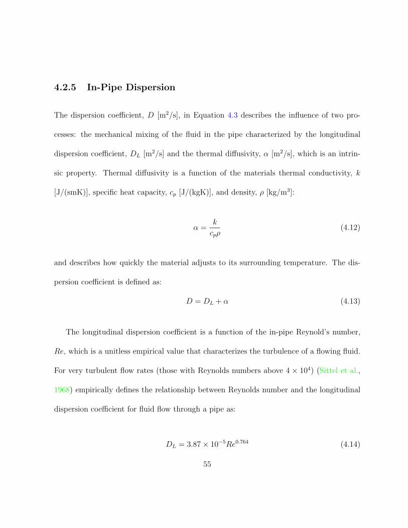
4.2.5 In-Pipe Dispersion
The dispersion coefficient, D [m2/s], in Equation 4.3 describes the influence of two pro-
cesses: the mechanical mixing of the fluid in the pipe characterized by the longitudinal
dispersion coefficient, DL [m2/s] and the thermal diffusivity, α [m2/s], which is an intrin-
sic property. Thermal diffusivity is a function of the materials thermal conductivity, k
[J/(smK)], specific heat capacity, cp [J/(kgK)], and density, ρ [kg/m3]:
α =k
cpρ(4.12)
and describes how quickly the material adjusts to its surrounding temperature. The dis-
persion coefficient is defined as:
D = DL + α (4.13)
The longitudinal dispersion coefficient is a function of the in-pipe Reynold’s number,
Re, which is a unitless empirical value that characterizes the turbulence of a flowing fluid.
For very turbulent flow rates (those with Reynolds numbers above 4 × 10⁴) (Sittel et al.,
1968) empirically defines the relationship between Reynolds number and the longitudinal
dispersion coefficient for fluid flow through a pipe as:
DL = 3.87× 10⁻⁵Re0.764 (4.14)
55

where DL is defined in ft2/s.
The Reynolds number of a fluid flowing through a pipe is dependent on the flow rate,
cross sectional geometry of the pipe, and the properties of the fluid (Menon, 2005):
Re =QDH
νAp(4.15)
where Q is the flow rate of the fluid in the pipe [m3/s]; DH is the inner pipe diameter [m];
and ν is the kinematic viscosity of the fluid [m2/s]. The kinematic viscosity is equivalent
to µ/ρ, where µ is the dynamic viscosity of the fluid [Pa·s] and ρ is the density of the fluid
[kg/m3] (Menon, 2005).
A base case calculation is described in Appendix E. This process was used in the
developed model to estimate the dispersion coefficient for each simulation, where varying
flow rates and temperatures were used.
4.2.6 Thermal Resistance
Specific thermal resistance [smK/J] is the reciprocal of thermal conductivity [J/(smK)] and
is a measure of a materials ability to resist the flow of thermal energy when subjected to
a thermal gradient. Specific thermal resistance is a material constant and is independent
of the general shape of the material. Comparatively, the absolute thermal resistance, R∗
56

[sK/J], of a body defines the ability of a finite body to resist the flow of thermal energy and
is dependent on the specific geometry of the body. With an absolute thermal resistance,
energy flux, q [J/s], through a body due to a temperature gradient may be calculated as:
q =∆T
R∗
but, for the absolute thermal resistance for a unit length used here, referred to as effective
thermal resistance, R [smK/J]:
R = R∗L
is equivalent to specific thermal resistance.
To estimate the effective thermal resistance between the fluids in each of the pipes,
Rp, and between the fluid in the pipe and the soil, Rs, as used in Equation 4.5, the
specific thermal resistances between each of these components were divided into sections
and combined in series (Equation 4.16).
Rp = Rpipessoil + 2Rpipe
Rs = Rinter +Rpipe (4.16)
Where Rpipessoil is the effective thermal resistance of the medium (typically soil in the model)
57

between the two pipes [smK/J]; Rpipe is the effective thermal resistance of the pipe wall
[smK/J]; and Rinter is the effective thermal resistance between either of the pipes and the
soil at an intermediate radius [smK/J].
To estimate expressions for Rpipessoil and Rinter, a solution presented by Yovanovich (1973)
was used to quantify the absolute thermal resistance of the medium between 2 parallel,
long cylinders as represented in Figure 4.4.
(a) (b)
Figure 4.4: Bicylindrical system used by Yovanovich (1973) for thermal resistance deriva-tion
Based on the dimensions in Figure 4.4 the absolute thermal resistance of the medium
58

between two cylinders of length L [m] was described by Yovanovich (1973) as:
Rabs =1
2πkL
ln√(
w1
r1
)2
− 1 +
(w1
r1
)±√(
w2
r2
)2
− 1 +
(w2
r2
) (4.17)
where k is the thermal conductivity of the medium between the cylinders [J/(smK)]; L is
the length of the cylinders [m]; r1 is the radius of cylinder 1 [m]; r2 is the radius of cylinder
2 [m]; w1 is the distance from the y-axis (Figure 4.4) to the centre of cylinder 1 [m]; w2
is the distance from the y-axis to the centre of cylinder 2 [m]; and Rabs is defined as the
absolute thermal resistance of the conducting material between the two parallel cylinders
[sK/J].
In Equation 4.17, a negative sign describes the absolute thermal resistance of the
medium between two cylinders on opposite sides of the y-axis (Figure 4.4a), as needed
to estimate the effective resistance of the material between the pipes, Rpipessoil . Normalizing
by L, the appropriate parameters were substituted into Equation 4.17 to yield:
Rpipessoil =
1
2πksoil
ln√(
w
r1o
)2
− 1 +
(w
r1o
)−√(
w
r2o
)2
− 1 +
(w
r2o
) (4.18)
where ksoil is the thermal conductivity of the soil between the pipes [J/(smK)]; w is equal
to half the distance between the pipe centres [m], where w = (w1 +w2)/2; r1o is the outer
radius of one pipe [m]; and r2o is the outer radius of the adjacent pipe [m].
59

A positive sign in Equation 4.17 describes the specific thermal resistance of the material
between two cylinders on the same side of the y-axis (Figure 4.4b), as needed to estimate
the effective thermal resistance of the material between each pipe and the soil at the
intermediate radius, Rinter. Therefore, Rinter was estimated as:
Rinter =1
2πksoil
ln√(
w
ro
)2
− 1 +
(w
ro
)+
√(
w
rs
)2
− 1 +
(w
rs
) (4.19)
where ro is the outer radius of the pipe of interest [m].
Equation 4.20 (Ingersoll et al., 1954) is a general form of Fourier’s Law of heat transfer,
defining the conductive heat flow through a thermally conductive medium.
q = −kAdTdη
(4.20)
Where q is heat flow [J/s] perpendicular to cross sectional area, A [m2]; k is the thermal
conductivity of the medium [J/(smK)]; and dT/dη is the temperature gradient in direction
η [K/m]. The effective thermal resistance across the pipe wall was derived from this
expression as:
Rpipe =ln( ro
ri)
2πkpipe(4.21)
where ri is the inner radius of the pipe [m] and kpipe is the thermal conductivity of the pipe
60

material [J/(smK)].
Similarly, the effective thermal resistance of the annulus of soil between the intermediate
radius and the far field was derived as:
R∞ =ln( r∞
rs)
2πksoil(4.22)
where R∞ is the effective thermal resistance of the annulus of soil between the intermediate
radius and the far field [smK/J]. Complete derivations of Equation 4.21 and Equation 4.22
are provided in Appendix D.
Equations 4.18, 4.19, and 4.21 were used to define the effective resistance terms, Rp
and Rs, in Equation 4.16. The definitions presented for Rp, Rs, and R∞ were used to
estimate the conductance terms β1, β2, β3, and β4 (Equation 4.5) utilized in Equation 4.3
and Equation 4.4.
4.2.7 Radius of Influence
In the system being simulated, the radius of influence, r∞, defines the radial distance from
the centre of the two pipes at which no effects from the GHX are observed. Beyond this
distance, the temperature in the subsurface remains constant. This parameter is important
as it is needed to define the specific thermal resistance to the far field (Equation 4.22) and it
61
describes the location of the Dirichlet type boundary condition, T∞, at the outer boundary
of the soil domain, r∞. It was found that a radius of influence of 5 m was most appropriate
(Appendix E). Therefore, the value of 5 m was maintained as the radius of influence for
all investigations herein unless otherwise specified.
4.2.8 Intermediate Soil Radius
The sensitivity of the model to changes in the intermediate soil radius over a range of
simulations was investigated (Appendix E). It was found that an intermediate soil radius
of 1 m was most appropriate. Therefore, this value of 1 m was used for all investigations
herein unless otherwise specified.
4.3 Finite Difference Approximation
To determine the solutions to Equation 4.3 and Equation 4.4, a finite difference approx-
imation was employed using a Crank-Nicholson time stepping scheme. The derivation of
the finite difference solution is detailed in Appendix D. To summarize, the solutions to
Equation 4.3 and Equation 4.4 were defined as Equation 4.23 for i = 1...2N and Equation
4.24 for i = 1...N , respectively. Here, i refers to the degree of freedom and 3N is the total
62

number of equations.
T n+1i−1
(−a
2
)+ T n+1
i
(1
∆t− b
2
)+ T n+1
i+1
(− c
2
)+ T n+1
2N−i+1
(−β1
2
)+ T n+1
si
(−β2
2
)= T ni−1
(a2
)+ T ni
(1
∆t+b
2
)+ T ni+1
( c2
)+ T n2N−i+1
(β12
)+ T nsi
(β22
)(4.23)
T n+1si
(1
∆t− d
2
)+ T n+1
i
(−β3
2
)+ T n+1
2N−i+1
(−β3
2
)= T nsi
(1
∆t+d
2
)+ T ni
(β32
)+ T n2N−i+1
(β32
)+ T∞ (β4) (4.24)
Where:
a =D
∆x2+
v
2∆x
b =−2D
∆x2− β1 − β2
c =D
∆x2− v
2∆x
d = −β3 −β42
The temperatures in the fluid, T1...T2N , and in the soil, Ts1 ...TsN , are solved simultaneously
in the model as a set of 3N equations, where N nodes are used to describe each of the
supply pipe, return pipe, and soil at the intermediate radius. The system node distribution
is represented in Figure D.2 on Page 175 in Appendix D.
63

Using this finite difference approximation the boundary conditions outlined in Equation
4.9, Equation 4.10, and Equation 4.11 were defined as Equation 4.25 for the change in
temperature boundary at the inlet when the pump is on, Equation 4.26 for the no flux
boundary at the inlet when the pump is off, and Equation 4.27 for the no flux boundary
at the outlet for all times. Full derivations of all boundary conditions are provided in
Appendix D.
T n+1i
(1
∆t− b
2
)+ T n+1
i+1
(− c
2
)+T n+1
2N−i+1
(−β1
2
)+ T n+1
2N
(−a
2
)+ T n+1
si
(−β2
2
)= T ni
(1
∆t+b
2
)+ T ni+1
( c2
)+ T n2N−i+1
(β12
)+T n2N
(a2
)+ T nsi
(β22
)+ ∆T (a) (4.25)
T n+1i
(−a
2+
1
∆t− b
2
)+ T n+1
i+1
(−c2
)+ T n+1
2N−i+1
(−β1
2
)+ T n+1
si
(−β2
2
)= T ni
(a
2+
1
∆t+b
2
)+ T ni+1
( c2
)+ T n2N−i+1
(β12
)+ T nsi
(β22
)(4.26)
T n+1i−1
(−a
2
)+ T n+1
i
(1
∆t− b
2− c
2
)+ T n+1
2N−i+1
(−β1
2
)+ T n+1
si
(−β2
2
)= T ni−1
(a2
)+ T ni
(1
∆t+b
2+c
2
)+ T n2N−i+1
(β12
)+ T nsi
(−β2
2
)(4.27)
64

4.4 Thermal Properties
4.4.1 Heat Exchange Fluid Properties
While the properties of water vary with temperature, the variation in thermal conductivity,
k, and specific heat capacity, cp, is not significant and for the purposes of the developed
model they were assumed constant at values representing water at approximately 10C.
At 10C, the thermal conductivity and specific heat capacity of water are approximately
0.6 J/(smK) and 4190 J/(kgK), respectively (Denny, 1993). However, the density of water
varies significantly with temperature. Figure 4.5 was adapted after Denny (1993) and
represents the density of water as a function of temperature. These properties of water
were used for calculations in the model.
4.4.2 Bulk Soil Properties
The bulk soil thermal diffusivity, α in Equation 4.12, and thermal conductivity, k, at the
Elora Field Site were approximated by Simms (2013) using the statistical parameter esti-
mation technique of inverse modelling. The thermal diffusivity and thermal conductivity of
the soil were approximately 6.01×10⁻⁷m2/s and 1.20 J/(smK), respectively (Simms, 2013).
These values were used as a basis upon which a range of soil thermal properties were simu-
65

Figure 4.5: Density of water as a function of temperature (Denny, 1993)
lated for analyses using the developed finite difference model and the finite element model
developed by Simms (2013).
4.5 Model Benchmarking
To verify the accuracy of the 1-D finite difference model, the model was compared to
an existing analytical solution. The analytical model used to benchmark the simulated
results was first described by van Genuchten and Alves (1982) as a method to solve the
1D convective-dispersive solute transport equation, which is similar in form to Equation
4.3 with β1 = 0 and fixed boundary conditions.
66

The differential equation governing 1D convective-dispersive solute transport in an ideal
column of porous medium is presented in Equation 4.28 (van Genuchten and Alves, 1982).
D∂2
∂x2− v∂C
∂x−R∂C
∂t= µC − γ (4.28)
Where C is the concentration of the solution [kg/m3]; D is the dispersion coefficient [m2/s];
R is the retardation factor [-]; µ [1/s] and γ [kg/(m3s] represent rate coefficients defining
the decay of the solute in the aqueous and solid phases [kg/(m3s]; x is distance [m]; and t
is time [s] (van Genuchten and Alves, 1982).
Equation 4.28 has the general initial condition (van Genuchten and Alves, 1982):
C(x, 0) = f(x) (4.29)
where f(x) is a function describing the distribution of the solute in the column at time zero
(van Genuchten and Alves, 1982). The boundary condition at the inlet to the column most
relevant to the 1D conductive heat transfer model is (van Genuchten and Alves, 1982):
C(0, t) = g(t) (4.30)
where g(t) is a function describing the concentration type boundary condition at the inlet
67

(van Genuchten and Alves, 1982).
The boundary condition at the outlet of the column most relevant to the 1D conductive
heat transfer model, assumes a semi-infinite soil column and is described in Equation 4.31
(van Genuchten and Alves, 1982).
∂C
∂x(∞, t) = 0 (4.31)
Based on these boundary conditions a solution to Equation 4.28 was presented by van
Genuchten and Alves (1982) as Equation 4.32 (translated here to temperatures for consis-
tency with the heat conduction model).
T (x, t) = Ts −Ts − Tin
2
[e
(u−v)x2α erfc
(z − vt2√αt
)+ e
(u+v)x2α erfc
(z + vt
2√αt
)](4.32)
Where T (x, t) is the temperature of the fluid in the pipe running along the x-axis [C]; Ts
is the constant temperature at the pipe outer wall [C]; Tin is the fluid inlet temperature
[C]; u is the fluid flow velocity [m/s], assumed to be constant across the cross section of
the pipe; and α is the thermal diffusivity of the fluid [m2/s]. The parameters η and v are
defined by van Genuchten and Alves (1982) as:
η =2bigriρc
& v = u
√1 +
4ηα
u2
68

Where big is a thermal conductance term [J/(sm2K)]; ri is the pipe inner radius [m]; and
ρc is the volumetric heat capacity of the fluid [J/(m3K)].
Equation 4.32 was utilized by Nabi and Al-Khoury (2012b) to solve the temperature
of a perfectly mixed fluid moving through a single, 1D pipe in contact with a medium at
a constant temperature at it’s outer surface.
4.5.1 Model Adjustments
In order to use Equation 4.32 as a benchmark for the developed model some modifications
had to be made to match the model to the analytical solution. First, the analytical
solution describes a single pipe model, while the finite difference model simulates two
parallel, adjacent pipes. To remove the second pipe from the finite difference model the
conductance term governing heat transfer between the pipes, β1 in Equation 4.23, was set
equal to zero. This modification acts to reset the finite difference model to a single pipe in
a cylindrical soil domain.
Second, to impose a constant temperature in the soil at the pipe outer wall, all soil
elements in the model were fixed at a temperature equal to that of the far field:
Tsi(x, t) = T∞ (4.33)
69

Therefore, Equation 4.24, which defines the change in temperature in the soil over time,
becomes homogeneous:
∂Tsi∂t
= 0 (4.34)
and the boundary condition at the outer radius of the pipe, ro, was set equal to the
background temperature, T∞.
Finally, it was necessary to change the pipe inlet to a simpler Dirichlet boundary
condition to impose a constant fluid inlet temperature, rather than a change in temperature
between the inlet and outlet.
4.5.2 Benchmark Results
The modified finite difference model was compared to the analytical solution using two test
cases. The first test case was the same used by Nabi and Al-Khoury (2012b). Table 4.1
summarizes the input parameters to the analytical solution defined in the first test case.
Figure 4.6 shows the temperatures and percent difference in temperatures of the fluid
flowing through the pipe for the referenced analytical solution and the developed finite
difference model for test case 1. The percent difference in temperature between the two
70

methods shown in Figure 4.6 was calculated at each node using:
%Difference =Tanalytical − Tnumerical
Tanalytical∗ 100% (4.35)
where Tanalytical and Tnumerical are the fluid temperatures [C] calculated using the analyt-
ical method outlined by van Genuchten and Alves (1982) and the finite difference model
developed herein, respectively.
Table 4.1: Analytical Solution Input Parameters - Test Case 1
Parameter Magnitude Units
Pipe Length 1 mSimulation Time 1800 s
Ts 10 CTin 50 Cri 0.0131 mρc 4.1298× 10⁶ J/(m3K)α 9.2× 10⁻⁸ m2/su 3.75× 10⁻⁴ m/sbig 12 J/(sm2K)
Model ∆t 1 sPipe Nodes in Model 2000 −
Figure 4.6 shows that the temperatures calculated using each model seem to coincide
for all nodes, giving evidence that the developed model is able to accurately simulate the
heat transfer between a fluid circulating through a pipe and the surrounding subsurface.
However, the test case presented in Table 4.1 is not completely relevant to the analyses
that were conducted using the finite difference model because of the extreme temperature
71

Figure 4.6: Comparison of fluid temperatures and percent difference in fluid temperaturesalong pipe for analytical and numerical models - test case 1
72

difference and the small pipe length. Therefore, a second test case was developed to
more closely represent a typical GHX. For this test case all physical parameters were
maintained as defined in Table 4.1 with changes to the pipe length, simulation time, fluid
inlet temperature, and fluid flow velocity.
The parameters for the second test case were defined to represent a typical GHX of
interest for the application of the finite difference model. The GHX at the Elora Test
Site was taken as a basis for this test case. The Elora Field Site consists of a set of six
183 m (600 ft) loops with an approximate inner pipe radius of 0.013 m and a total flow
rate of approximately 15 GPM. Therefore, a single loop consisting of a 183 m pipe was
chosen with a fluid velocity, u in the analytical model, of 0.29 m/s. A simulation time of
1800 s was chosen to represent approximately three total pipe volumes through the system
for these defined dimensions and flow velocity. An inlet temperature, Tin, of 6C was
chosen to represent a realistic temperature difference of 4C between the inlet fluid and
the surrounding soil. All other parameters for this test case were maintained as defined
for test case 1.
The temperatures and percent difference in temperatures of the fluid along the pipe as
simulated using the developed finite difference model and the analytical method proposed
by van Genuchten and Alves (1982) for test case 2 are represented in Figure 4.7, where the
percent difference in temperatures was calculated using Equation 4.35. The comparisons
73

in Figure 4.7 show that the solutions of both the numerical and analytical methods yield
similar results for test case 2.
Based on the results of the comparisons for each test case, it is concluded that the
developed finite difference model adequately solves (<1% error relative to the analytical
solution) the mathematical problem statement used to represent the GHX and has the
ability to simulate these systems.
4.6 System Performance
To accurately simulate the performance of the GSHP system as a whole, the function of a
specific heat pump and fluid circulation pump were included in the model. The heat pump
chosen was a variable speed equivalent of that installed at the Elora Field Site (Brodrecht,
2010), the ClimateMaster Tranquility ® 30 TE Series Model 072 (Cli, 2012). A variable
speed fluid circulation pump was chosen to correspond with this heat pump. Two Stratos
1.25x3-25 circulation pumps from WILO (2010) were modelled in series (Brodrecht, 2010).
The COP of a heat pump is a function of the flow rate and the temperature of the
fluid entering the heat pump. Using the specifications provided by the manufacturer (Cli,
2012), functions were developed to define the COP of the heat pump for all flow rates and
temperatures within these specifications.
74

Figure 4.7: Comparison of fluid temperatures along pipe for analytical and numericalmodels - test case 2
75

To predict the COP of the entire system it was necessary to investigate the circulation
pump input power. The power needed to operate the circulation pump is a function of flow
rate and head loss through the system. Therefore, a function was developed in the model
to utilize the circulation pump manufacturer’s specifications (WILO, 2010) to define the
pump power for the range of flow rates and system head losses within these specifications.
The total head loss through the system is a summation of the head loss through the
heat pump and the head loss through the GHX due to friction between the flowing fluid
and the pipe wall. To describe the head loss through the heat pump the manufacturer’s
specifications (Cli, 2012) were used to define a function in the model that estimates the
heat pump head loss as a function of temperature and flow rate through the system. To
quantify the head loss through the GHX, the method proposed by Moody (1944) was
utilized:
hf = fL
D
v2
2g(4.36)
where hf is head loss through the pipe due to friction [m]; f is an empirical parameter
refered to as the Moody friction factor [-]; L is the length of the pipe [m]; D is the inner
diameter of the pipe [m]; v is the average fluid flow velocity in the pipe [m/s]; and g is the
acceleration due to gravity [m2/s] (Moody, 1944).
The Moody friction factor is an empirical parameter based on the in-pipe Reynolds
76

number (Equation 4.15) and the relative roughness coefficient ε/D [-], which describes the
roughness of the inside of the pipe, where ε represents the absolute roughness of the pipe
material [m] (Moody, 1944).
The head loss through the GHX was combined with the head loss through the heat pump
to describe the total head loss through the system, which was translated into circulation
pump energy consumption during model simulation. Combining the circulation pump and
heat pump energy consumption, the actual COP of the system was estimated based on:
COP =EextractedEconsumed
(4.37)
where Eextracted is the total energy [J] extracted from the fluid for the length of the simu-
lation and Econsumed is the total energy [J] consumed by the system for the length of the
simulation. This COP metric was used as the basis for all performance comparisons using
the 1D finite difference model.
4.7 Sample Model Output
To illustrate the physical processes being modelled during simulation, an example model
output is shown in Figure 4.8 in the form of fluid temperature along the pipe for increasing
77

times during the simulation of a single cycle of the GSHP, where tR is the residence time
in the pipe [s] and v is the mean fluid flow velocity [m/s].
Figure 4.8: Three main phases of GSHP simulation - initial, depletion, and recovery
Figure 4.8 represents one pulse of fluid circulating through a ground loop with similar
parameters as the system at the Elora Field Site during heating mode. Once the system
78

turns on, the fluid temperature at the inlet immediately decreases and the pulse, driven by
the Dirichlet boundary condition at the inlet, circulates through the ground loop during
the start-up phase. This temperature pulse disperses along the loop as the system enters
the depletion phase. In the depletion phase the system is still operating and thermal
energy is constantly being withdrawn from the circulating fluid, steadily depleting the
temperature of the fluid. Once the system turns off, it enters the recovery phase where
energy is no longer being extracted from the fluid and the fluid temperature begins to rise,
approaching the temperature of the surrounding soil. The corresponding EWT, which is
the fluid temperature at the outlet (x = L), and heat pump COP for this sample simulation
are provided in Figure 4.9.
Figure 4.8 and Figure 4.9 show a single pulse travelling through the ground loop.
However, in actual operation the system cycles frequently, following the basic pattern
outlined in Figure 4.8 during each cycle with the average fluid temperature decreasing over
time.
79

Figure 4.9: EWT and heat pump COP for initial, depletion, and recovery phases
80

Chapter 5
Model Application
The 1D finite difference model and Simms (2013) 3D finite element model were developed to
investigate the function and performance of GSHPs, focusing upon the potential to improve
the design and operation of such systems. A variety of test cases were developed, simulated,
and analysed to attempt to: relate the behaviour of pulsed and steady state simulation
of GSHPs; identify potential efficiencies in system operation, including pumping intensity
and cycle frequency; and investigate the potential performance inefficiencies associated
with the specification of GHX pipe spacing, pipe configuration, and pipe length.
81

5.1 Base Case Definition
To develop a starting point for investigations using model simulations, base case model
realizations were developed for the 1D finite difference model and Simms (2013) 3D finite
element model. The base cases were developed using the Elora Field Site as a reference
and are detailed in Section 5.1.1 and Section 5.1.2.
5.1.1 1D Base Case
As installed, the GHX at the Elora Field Site consists of six 183 m loops. The model
represented six identical 183 m pipes in U-tube shapes by simulating a single pipe and
extending results to the full system by assuming that flow rates, fluid and soil temperatures,
energy consumption and extraction, and dimensions were consistent for all six pipes. This
assumption is valid since it represents a system composed of six identical U-tubes separated
by distances large enough to ensure no interactions between adjacent U-tubes.
The pipes in the simulated U-tube were separated by 0.5 m and were surrounded by
soil with homogeneous thermal properties: thermal conductivity, specific heat capacity,
and bulk density. A variable speed heat pump and fluid circulation pump were simulated
in all cases to analyse the performance of the system. Specific input parameters for the
base case are provided in Table 5.1.
82

Table 5.1: Input parameters for 1D Finite Difference model
Parameter Magnitude Unit
Soil thermal conductivity 1.22 J/smKSoil volumetric heat capacity 2.03 MJ/m3K
Fluid volumetric flow rate in single U-tube 0.00016 [2.5] m3/s [GPM]Fluid volumetric heat capacity 3.73 MJ/m3K
In-pipe dispersion 0.032 m2/sLoop pipe inner diameter 0.021 mLoop pipe outer diameter 0.027 mPipe thermal conductivity 0.4 J/(smK)
Average power extraction from fluid 3516 [1] J/s [ton]Heat pump and circulation pump cycles per day 24 [-]
Time step 2 sTotal number of nodes 900 [-]
Pipe length 183 mRadius of influence, r∞ 5 m
Intermediate soil radius, rs 1 mAmount of time pump is on 70 %
Farfield temperature, T∞ 11.1 C
5.1.2 3D Base Case
Parameters of the base case for the 3D FEM model are as defined in Table 5.1 with
changes to the model boundary conditions, energy load requirements of the GHX, and
element discretization. The sides and bottom of the soil domain were defined using no
flux boundary conditions (Simms, 2013), rather than constant temperature as in the 1D
model. The surface temperature was defined using the shallow soil temperature described
in Chapter 3 for a one year period from December 2010 to December 2011. The energy
requirements of the GHX were defined using the actual energy loads measured at the Elora
83

Field Site for the same period (Simms, 2013).
The base case realization for the 3D model used 6000 equal elements to represent
each 183 m pipe. In all cases the lengths of pipe were parallel to the y-dimension and
perpendicular to the x-dimension of the soil domain, while the z-dimension represented
depth from the ground surface. Pipe segments were always centred in the x-dimension of
the soil element in which they were passing through. A variable discretization was used in
the soil domain to enhance model accuracy surrounding the GHX. The element dimensions
increased from 0.05 m, 1.25 m, and 0.1 m near the pipes to 14.8 m, 10 m, and 24 m away
from the pipes in the x-, y-, and z-directions, respectively. The soil domain consisted of
240, 91, and 46 elements representing a 62 m by 127.5 m by 74.7 m soil domain in the
x-, y-, and z-directions, respectively. This pipe and soil discretization was used for all test
cases.
5.2 Pump Schedule Optimization
One of the main advantages of the 1D finite difference model is its ability to model a
dynamic system at fine temporal resolution. Therefore, it is possible to use the model
to examine various pumping scenarios. In this section, a number of pump scheduling
choices, including run time fraction and pump cycle frequency, are investigated to attempt
84

to identify potential efficiencies in GSHP operation. The run time fraction is the ratio of
the time the heat pump and fluid circulation pump are operating to the total simulation
time. The pump cycle frequency represents the number of pump cycles per unit of time,
typically expressed as cycles per day, where a pump cycle is considered to be a duration of
pump operation followed by a duration of no advection or heat pump operation.
5.2.1 Pumping Intensity
It was hypothesized that system COP was a function of pumping intensity since heat pump
and circulation pump power consumption are dependent on the intensity at which these
components are operating. By simulating variable speed heat pump and circulation pump
operation in the 1D finite difference model, it was possible to investigate a range of pumping
intensities to examine the effect on system performance. In this thesis, pumping intensity
refers to the magnitude of the flow rate at which fluid is circulated through the GHX. It
was expected that a system operating for a longer period at a lower pumping intensity
would be more efficient than an equivalent system operating for shorter periods at higher
intensities since, for example, the system (including the heat pump and circulation pump)
consumes more than twice the power to operate at twice the intensity.
A test case was developed in which the total energy extracted from the fluid was main-
tained across simulations but the pumping intensity and run time fraction were modified.
85

By altering the pumping intensity and run time fraction simultaneously, the total energy
extraction, which represents the heating load on the GHX, can be maintained while ex-
amining the effect of pump scheduling and intensity on system performance. All other
parameters in this test case are as defined in the base case in Section 5.1.1.
Figure 5.1 represents three of the pumping schedules that were simulated using run time
fractions of 100%, 70%, and 50%, in which each case was defined to represent an identical
average power extraction of 3516 J/s. In total, six pump schedules were examined using run
time fractions between 50% and 100%, which correspond to flow rates between 17.0 GPM
and 8.5 GPM, to represent the range of allowable flow rates for the heat pump specified
in Chapter 4. The turbulent, transitional, and laminar flow regimes are approximated in
Figure 5.1 based on the fluid properties and pipe specifications of the base case (Section
5.1.1).
The pumping schedules were compared in terms of COP using 100 day simulations for
a variety of pulsing cases, each extracting the same amount of total energy from the fluid.
Five sets of simulations were conducted, each examining a multiple of the total power
extraction used in the base case, 3516 J/s. This multiple ranged between 0.6 and 1.4. A
summary of the overall system performance based on changes in pumping schedules for
each energy extraction definition is depicted in Figure 5.2.
Since the total energy extraction from the fluid is fixed for each curve, the varying
86

Figure 5.1: Simulated pump schedules with approximate flow regimes
performance of the system is solely dependent on the intensity at which it operates. The
constant pumping case (run time fraction equal to 100%) yields the most efficient per-
formance in all cases (Figure 5.2), even though the heat pump and circulation pump are
operating continuously. The increase in performance as intensity decreases is attributed
to the power consumption of the circulation pump and the moderated energy load on the
subsurface. The relationship between circulation pump power and flow rate is not linear
and more than twice the power is required to double the flow rate (Figure 5.3). Also,
as the pumping intensity decreases, the instantaneous energy load on the subsurface is
reduced, helping to maintain soil temperature over time. Therefore, as initially expected,
87

Figure 5.2: System COP related to run time fraction (PO = 3516 J/s)
the constant pumping case at the minimum flow rate relevant to the selected heat pump
yields the most efficient pumping schedule.
The test case described above shows how a GSHP can operate more effectively at lower
flow rates and longer run times. However, in all cases it was assumed that the fluid was
well mixed and its temperature was constant across the entire cross sectional area of the
pipe, an assumption of fully turbulent flow. This assumption may not be valid for all
88

Figure 5.3: Circulation pump power as a function of flow rate for a range of head lossesthrough the system - the measured values represent the manufacturer’s performance spec-ifications (WILO, 2010) and the interpolated values represent an example of those used bythe model
cases since the minimum flow rates investigated yield Reynold’s numbers in the laminar
or transitional flow regimes for the simulated system. In cases where laminar flow exists,
there would be reduced heat transfer between the fluid and the soil caused by the increase
of the thermal resistance between them. Not accounting for this increased resistance to
heat transfer would lead to over estimation of the performance of a system flowing in the
89

laminar regime. Section 5.2.2 describes a test case in which this increase in resistance was
approximated.
5.2.2 Equivalent Resistance for Non-Turbulent Flow
The Nusselt number describes the ratio of radial heat transfer through a fully developed
flowing fluid to purely conductive radial heat transfer of stagnant fluid in a pipe. Therefore,
it was hypothesized that by relating the Nusselt number of the turbulent and non-turbulent
cases, an equivalent effective thermal resistance to radial heat transfer through the fluid
flowing in a pipe could be approximated to more accurately compare quasi-steady state
(laminar flow) and pulsed (turbulent flow) pump operation. It was expected that this
equivalent resistance would decrease the system COP for non-turbulent flows due to re-
duced heat transfer into the fluid in these cases. Equation 5.1 was developed to modify the
effective thermal resistance across the pipe wall (as defined in Equation 4.21) in the 1D fi-
nite difference model to approximate the equivalent resistance due to the lack of mechanical
mixing associated with non-turbulent flow.
Req =Numax
Nunon−turbulentRpipe (5.1)
90

Where Req represents the equivalent effective thermal resistance across the pipe wall mod-
ified for non-turbulent flow [smK/J]; Numax is the Nusselt number [-] for the maximum
flow rate considered in the model (17 GPM); and Nunon−turbulent is the Nusselt number [-]
for a flow rate less than or equal to the maximum flow rate. Numax and Nunon−turbulent
were approximated using the pipe characteristics defined in Section 5.1.1 and the method
proposed by Churchill (1977). Churchill (1977) presented an empirical relationship for ap-
proximating the Nusselt number based on the Reynolds number of a fluid flowing through
a smooth pipe. For Reynolds numbers below 2100, the expression simplifies to Equation
5.2 (Churchill, 1977).
Nu = 3.657
[1 +
(RePrD/L
7.60
)8/3]1/8
(5.2)
Where Pr is the Prandtl number [-], which is equivalent to the ratio of kinematic viscosity
to thermal diffusivity (Pr = ν/α); D is the inner diameter of the pipe [m]; and L is the
length of pipe [m] (Churchill, 1977).
For Reynolds numbers greater than 2100, the expression approximating the Nusselt
number simplifies to Equation 5.3 (Churchill, 1977).
Nu =
(1
Nu2t+
1
Nu2i
)−1/2(5.3)
91

Where Nut is an approximation of the Nusselt number for turbulent flows [-] and Nui is
an approximation of the asymptote of the Nusselt number in transition to laminar flow
(Churchill, 1977). Nut and Nui are approximated using Equation 5.4 and Equation 5.6,
respectively.
Nut = Nu00 +0.79Re
√fPr
[1 + Pr4/5]5/6
(5.4)
Where Nu00 is the approximation of the asymptote of the Nusselt number [-] as Pr →0
and Re →0 and f is a dimensionless friction factor for the fluid flowing through a pipe
approximated using Equation 5.5 (Churchill, 1977). The value of Nu00 appropriate for this
investigation was estimated to be 4.8 (Churchill, 1977).
f =
1[(8Re
)10+(
Re36500
)20]1/2 +
(2.21ln
[Re
7
])10
−1/5
(5.5)
Nui = NulceRe−2200)/730 (5.6)
Where Nulc is the approximation of the Nusselt number [-] at Re = 2100, which is estimated
using Equation 5.7 (Churchill, 1977).
Nulc = 3.657
[1 +
(276PrD
L
)8/3]1/8
(5.7)
92

Equation 5.2 and Equation 5.3 are used to approximate the Nusselt numbers used in
Equation 5.1 to calculate the modified effective thermal resistance across the pipe wall to
account for non-turbulent flow. Using this equivalent effective thermal resistance relation-
ship, simulations identical to those in Section 5.2.1 were conducted to more appropriately
compare the quasi-steady state and pulsed pumping cases. For the system specified in Sec-
tion 5.1.1, the minimum flow rate of 8.5 GPM yielded a Reynolds number of approximately
2050 and, using Equation 5.2, a Nusselt number of approximately 20. Comparatively, the
maximum flow rate of 17.0 GPM yielded a Reynolds number of approximately 4150 and,
using Equation 5.3, a Nusselt number of approximately 45. Therefore, the effective ther-
mal resistance across the pipe wall would nowhere exceed approximately 2.25 times the
unmodified case. The unmodified effective thermal resistance across the pipe wall for the
base case is approximately 0.1 smK/J, which yields a maximum equivalent effective ther-
mal resistance of 0.225 smK/J. Comparing this resistance to the base case effective thermal
resistance between the pipe and the intermediate soil radius, Rinter, of approximately 0.563
smK/J, this modification of the thermal resistance across the pipe wall does not signifi-
cantly impact the total effective thermal resistance between the fluid in the pipe and the
soil, Rs, as defined in Equation 4.16. Therefore, it was expected that this modification to
the thermal resistance across the pipe wall would not significantly effect the results for this
test case, which are summarized in Figure 5.4.
93

Figure 5.4: System COP related to run time fraction using equivalent effective thermalresistance for non-turbulent flow (PO = 3516 J/s)
Based on the results (Figure 5.4) of this equivalent resistance test case, the effect
of the reduced thermal transfer caused by non-turbulent flow reduces the system COP
compared to the test case presented in Section 5.2.1, in which turbulent flow was assumed
for all cases. However, the difference in COP for this equivalent resistance test case were
everywhere less than 1%, which, as expected, is negligible. Therefore, by assuming that
94

this equivalent resistance technique (Equation 5.1) is appropriate, the effect of the increase
in effective thermal resistance to radial heat transfer associated with non-turbulent flow is
not significant in a U-tube shaped GSHP, suggesting that the conclusions made in Section
5.2.1 are reasonable and system performance increases with decreasing pumping intensity.
Practically, these test cases show how a GSHP could operate marginally better (COP
increases of ∼5%) by increasing run time fraction from 50% to 100% and decreasing flow
rate from 17.0 GPM to 8.5 GPM for U-tube shaped GHXs, which is not a significant gain in
performance. However, a full investigation into the effect of the increased thermal resistance
and other potential mechanical issues associated with non-turbulent flow through the GHX
was not within the scope of this research and further analyses should be completed to fully
analyse the variations this may cause in simulated performance.
5.2.3 Cycle Frequency
While the differences in results observed between the test cases in Section 5.2.1, assuming
completely turbulent flow in all cases, and in Section 5.2.2, using an equivalent effective
thermal resistance for non-turbulent flow, were not significant (<1%), a full investigation
into the effect of non-turbulent flow regimes is not within the scope of this research. There-
fore, further analyses were conducted to attempt to identify system performance efficiencies
through pump schedule optimization independent of pumping intensity.
95

It was hypothesized that COP was a function of pump cycle frequency because subsur-
face soil temperatures and, thus heat extraction efficiency, are dependent on the duration
of pump operation. A test case in which pumping intensity is maintained while only
pump cycle frequency is varied is described and analysed below to test this hypothesis
with the expectation that an optimal frequency would provide a specific maximum COP.
By maintaining pumping intensity at a higher flow rate and modifying pump schedules
through pumping cycle duration and frequency, it was possible to eliminate the potential
performance bias associated with low flow regimes. To ensure appropriate fluid flow in
the pipe, a flow rate of 15 GPM (taken from the Elora Field Site) was simulated for all
scenarios, yielding a Reynold’s number of approximately 3655, which is in the transitional
to turbulent flow regime and applicable for GSHP operation (ASHRAE, 2009).
A pumping cycle was considered to consist of a period of pumping followed by a similar
or different duration of no pumping. To investigate the effects of pumping cycle frequency
on COP, a test case was developed using the parameters defined in Section 5.1.1 and
simulated using the 1D finite difference model. In this investigation the only variables
changed were the number of pumping cycles per day and the duration of the cycles. The
total operating time of the pump was consistent in all cases. Therefore, as cycle frequency
was increased the, cycle duration was decreased along with the run time per cycle. The
cycle frequency test case comprised a range of simulation durations (1 to 100 days) and run
96

time fractions (10% to 90%). These run time fractions could represent a range of realistic
pumping schedules from shoulder season operation (spring and fall, where minimal heating
capacity is required) at the lower run times to extreme operation (winter, where peak
heating capacity is required) at longer run times. Figure 5.5 illustrates the relationship
between system performance and cycle frequency for each of the 7 day simulations. Each
curve in this figure represents a 7 day simulation for a unique run time fraction, where all
other parameters are equal between curves. The run time fraction represents the percentage
of total simulation time that the pump is operating and, in this test case, ranges from 10%
to 90%. It is clear from the results summarized in Figure 5.5 that there are optimal cycle
frequencies for each run time fraction. These maximum would correspond to the point
at which the defined system is operating at maximum efficiency for the described power
extraction.
To further investigate the mechanisms dictating the shape of the curves in Figure 5.5,
a specific simulation was chosen for analysis. The 10% pump run time was isolated and
evaluated using the 14 day simulation. Figure 5.6 shows the system COP of the cases with
run time fraction equal to 10% and 50% (for comparison) for simulation durations between
1 day and 100 days.
Since the COP of these systems is a function of the temperature of the fluid entering
the heat pump and flow rate, the entering water temperature (EWT) was recorded for all
97

Figure 5.5: Cycle frequency test case: System performance as a function of cycle frequencyfor 7 day simulations and various run time fractions
time steps because flow rate was consistent across all simulations. In the model, the EWT
is defined as the fluid temperature at the outlet, T (L, t). This EWT was monitored for the
four most optimally performing simulations in Figure 5.6 to investigate the mechanisms
responsible for optimal performance. Figure 5.7 shows the EWT for the first day of these
four simulations.
98

Figure 5.6: Cycle frequecny test case: Simulated performance as a function of cycle fre-quency for 10% and 50% run time fractions and a range of simulation lengths
For low cycle frequencies (e.g., 2.8 cycles/day in Figure 5.7), when the system turns
on it reduces the fluid temperature considerably because of the relatively longer cycle run-
time, which has a negative effect on COP. When the system turns off, the fluid temperature
increases back to the soil background temperature. Since the fluid temperature has equili-
brated to the soil temperature, there is no thermal gradient between the two and, thus no
heat transfer occurring during this idle period. Therefore, it is concluded that when cycle
99

Figure 5.7: EWT of the four most optimally performing cycle frequency simulations
100
frequency is too low, cycle run times are too long, causing low fluid temperatures during
operation, hindering performance. Then, when the pump is off, the system remains idle
for too long, limiting heat transfer and reducing the potential energy extraction.
For higher cycle frequencies (e.g., 8.5 cycles/day in Figure 5.7), when the system turns
on it does not significantly reduce the fluid temperature because of the relatively shorter
pump runtime. However, when the system turns off, the fluid temperature does not com-
pletely return to the soil background temperature before the system turns back on, which
acts to reduce the average fluid temperature over the simulation time, depleting long term
system performance. Therefore, it is concluded that when cycle frequency is too high, fluid
temperature reduces over time, depleting GSHP performance.
Finally, in the two optimal simulation cases, where cycle frequency is approximately 4.2
cycles/day and 5.7 cycles/day in Figure 5.7, the cycle length appears to be such that when
the pump does turn off, the EWT rises to almost the background soil temperature before
the pump turns back on. Therefore, there is always active heat transfer within the system.
While the pump is on, energy is being extracted from the fluid and the soil surrounding
the GHX. When the system is off, there is always a temperature difference and, thus heat
transfer, between the fluid and the subsurface. It is concluded that the ideal scenario for
the given system is one in which the cycle length is long enough to allow for almost full
energy recovery of the fluid but still short enough to avoid periods of low energy transfer
101

between the GHX and the soil. It was expected that system performance would be a
function of cycle length and this result of a optimum pump frequency is consistent with
expectations.
5.2.4 Discussion
GSHP performance is a function of cycle frequency with an optimal performance existing
in all cases analysed. For those simulations conducted, system COP varied by up to ∼30%
when considering cycle frequency as the only variable, which could correspond to potential
operating cost reductions. The variation in COP summarized in Figure 5.5 was found to
be most significant during operation at lower pump run times, which represents shoulder
season operation when energy demands are relatively lower. The system being examined
(outlined in Section 5.1.1) represents a typical GSHP operating under a range of reasonable
system loads. Therefore, the relationship observed between COP and pumping frequency
could, with some confidence, be extended to most residential or light commercial GSHP
applications. The conclusion is important since pump cycle frequency can significantly ef-
fect overall system performance. This conclusion identifies a method through which GSHP
efficiency could be improved without substantial changes to design. Implementation of
monitoring equipment to quantify system loads and EWTs would provide the informa-
tion necessary to conduct a cycle frequency optimization exercise, either ensuring ideal
102

performance or providing insight into how the system could be more effectively operated.
Considering the potential 30% variation in COP associated with changes in pump cycle
frequency, this monitoring and optimization exercise could be beneficial in reducing GSHP
operation costs for residential and light commercial applications. This improvement would
act to further offset the high initial cost of the GHX installation, making these systems
more economically attractive to consumers.
5.3 Transient and Steady State Pumping Behaviour
GSHPs typically function in a transient manner, with the heat pump and circulation pump
turning off and on frequently during operation. This transient behaviour adds mathemat-
ical complexity when trying to simulate these systems using computational models. One
simplification that can be made when modelling such systems is the quasi-steady state as-
sumption, where the temperature distribution in the pipe is assumed to be in equilibrium
with the soil at all times, instantly responding to fluid inflow temperatures. In the case
of a GSHP, it could be assumed that instead of the system cycling off an on, it simply re-
mains on continuously during the timescale of interest, operating at a lower intensity. This
assumption would help to reduce the complexity of the mathematical equations governing
the processes in a GSHP model and potentially reduce the required number of simulated
103

time steps, improving the efficiency of the model. Several test cases were developed to
investigate the validity of such an assumption by comparing the outputs from a range of
constant pumping simulations against a simulation in which the system is cycling in a
transient manner for a variety of model realizations.
5.3.1 Sensitivity of System COP upon Pump Schedule and Soil
Conductivity
The 1D finite difference model was employed to simulate the operation of a GSHP with
constant and pulsed pumping schedules. The Elora Field Site operating in heating mode,
as defined in the base case for the 1D model (Section 5.1.1), was used as the basis for this
test case.
The constant pumping case was simulated by operating the circulation pump for 100%
of the simulation time at a flow rate of 8.5 GPM. The temperature change boundary
condition was defined using Equation 4.2 based on the fluid thermal properties and the
specified power extracted from the fluid (Sec 5.1.1).
To represent an equivalent pulsed case, the circulation pump operated for 50% of the
simulation time at a flow rate of 17.0 GPM with the same temperature change condition
as the constant case. Therefore, the total energy extracted for the pulsed case was exactly
104

equivalent to the constant case. This test case was developed to examine the difference in
performance associated with the quasi-steady state approximation across a range of soil
thermal conductivities. It was expected that the variation in pumping intensity would
result in differences between the two cases, with the quasi-steady state case yielding a
higher COP, due to efficiencies related to lower pumping intensity.
This simulation was conducted for the pulsed and steady pumping cases for a range of
50 realizations in which the only parameter varied was the average thermal conductivity
of the bulk soil medium in which the GHX was installed. The soil thermal conductivity
was varied between 0.5 and 2.06 J/(smK) to represent a range of realistic soil conditions.
Figure 5.8 presents the results of this investigation as a function of system performance
characterized by COP.
Figure 5.8 shows how the performance of the constant and pulsed pumping cases re-
late. The constant pumping case tends to yield a larger system COP (by between ∼6%
and ∼9%) for all soil thermal conductivities investigated, which can be attributed to the
increased fluid residence time in the pipe and the lower energy cost associated with the
lower flow rate. The increased residence time allows for extended thermal energy trans-
fer from the surrounding subsurface, while the lower pumping energy reduces the overall
power consumption, both processes increasing average COP. However, it is noted that the
shape and magnitude of the curves in Figure 5.8 are similar, suggesting that these pumping
105

Figure 5.8: Average COP for a range of soil thermal conductivities - comparison betweenpulsed and steady state
schemes are comparable and that the constant case can represent a system similar to the
transient case. Within a range of realistic soil thermal conductivities, for a typical U-tube
GHX, the quasi-steady state approximation over estimates COP by between ∼6% and
∼9% for an extreme transient case of the modelled system (pump operation at maximum
flow rate for 50% of simulation duration).
106

5.3.2 Equivalence of Transient and Steady State Pumping
The test case presented in Section 5.3.1 investigated the effect of the quasi-steady state
approximation on system COP for a range of soil thermal conductivities. To enhance this
investigation to further understand the differences in COP seen in Figure 5.8, the transient
base case from Section 5.3.1 was compared to a range of constant pumping cases to identify
and quantify potential sources of the difference between transient and quasi-steady state
simulation and attempt to relate the two cases. These constant pumping cases were defined
as described in Section 5.1.1 with the power extraction parameter varied between 2766 and
4266 J/s.
It was hypothesized that a relationship exists between the behaviour of the transient
and quasi-steady state cases. The author expected that, when comparing these cases,
variations in simulated fluid temperature and thermal energy flux into the fluid caused the
COP differences observed in 5.3.1 since these are the main factors in the calculation of COP.
Therefore, these factors were investigated to attempt to identify the relationship between
transient and quasi-steady state operation and investigate the validity of this quasi-steady
state approximation as it relates to analyses of system performance (COP).
The differences in fluid temperature between the pulsed and constant cases were exam-
ined by comparing the average fluid temperature over the entire 100 day simulation along
107

the total length of the pipe (Figure 5.7 (a)). The differences in energy flux into the fluid
along the pipe were analysed in two ways: the cumulative thermal energy change in the
fluid (Figure 5.7 (b)), to investigate energy flux as a function of distance along the pipe;
and the total change in energy at each node along the pipe (Figure 5.7 (c)), to investigate
the overall energy extracted from the subsurface. Finally, the average system COP was
compared to investigate the relationship between system performance of the pulsed and
steady cases (Figure 5.7 (d)).
Figure 5.7 summarizes the results of the comparison between a range of constant pump-
ing cases and a pulsed case for a simulation duration of 100 days. Here, P/PO represents
the average power extracted from the fluid for a specific trial normalized by the average
power extracted for the base case, where P0 = 3516 J/s for the base case. The average
temperature of the fluid in each node (Figure 5.7 (a)) represents the temperature in the
fluid at each time step averaged over the entire duration of the simulation.
The change in thermal energy in the fluid was quantified by calculating the energy
change in the fluid caused by external sources: the adjacent pipe and the surrounding soil.
These energy fluxes were calculated using:
∆Efluid =∆T sourcefluid
Rsourceeff
∆x∆t (5.8)
108

(a) Average temperature of the fluid in each element - 100 daysimulation
(b) Cumulative energy change of the fluid in each element - 100 daysimulation
109

(c) Total energy change of the fluid in each element - 100 day simu-lation
(d) COP for 1 day, 7 day, 14 day, 30 day, and 100 day simulationdurations
Figure 5.7: Comparison between pulsed and constant pumping cases
110

where ∆Efluid is the change in energy in the fluid due to external sources [J]; ∆T sourcefluid is
the change in temperature between the external source and the fluid in the pipe [C]; and
Rsourceeff is the effective thermal resistance between the external source and the fluid in the
pipe [smK/J], as defined in Chapter 4.
The cumulative energy change of the fluid in each element (Figure 5.7 (b)) represents
the summation along the length of the pipe of the total change in energy in the fluid for
the duration of the simulation, while the total energy change of the fluid in each element
(Figure 5.7 (c)) represents the total change in thermal energy at each point in the pipe for
the duration of the simulation.
The reduction in COP with increasing simulation duration summarized in Figure 5.7
(d) is caused by the reduced soil temperature associated with extended energy extrac-
tion. As the simulation progresses, the soil temperature decreases due to prolonged energy
extraction, reducing the energy available in the soil to be transferred to the fluid, thus re-
ducing the temperature of the fluid. As the fluid temperature decreases, the system must
perform more work to extract the defined energy, reducing system COP over time.
Based on the simulated average fluid temperature, thermal energy, and COP summa-
rized in Figure 5.7, the pulsed case shows similarities to the constant cases. The magnitude
and the trends of all curves are comparable and, except when considering COP, the single
pulsed case is seen to fall inside the range of realistic constant pumping cases for the sim-
111

ulation duration of 100 days. Identical simulations were conducted for 30 day, 14 day, 7
day, and 1 day durations. Results from these simulations are presented in Appendix F and
show comparable relationships to those in Figure 5.7. These similarities suggest that there
is a strong relationship between the fluid temperature and change in energy simulated for
the pulsed and constant pumping cases, as initially hypothesized. These differences are
everywhere within ∼10% for all cases simulated and account for the changes observed in
COP between the transient and quasi-steady state cases summarized in Section 5.3.1. The
observed differences in COP between the steady state case and the equivalent pulsed case
were approximately ≤5%, with the constant case estimating a larger COP than the pulsed
case. Therefore, the use of a constant pumping approximation, as in Simms (2013) 3D
FEM model, will lead to slight over prediction of system performance, which is attributed
to the decreased power consumption and instantaneous energy demand on the subsurface
associated with the lower pumping intensity (flow rate) in the constant case.
Since the differences in COP observed for the constant case are consistent across the
range of scenarios that were simulated, it is concluded that this quasi-steady state ap-
proximation is valid for cases that use the COP as a relative performance metric. This
conclusion helps to justify the use of this approximation by authors such as Simms (2013)
and validates the use of the 3D finite element model in this thesis.
112

5.4 Configuration Optimization
A major GHX design variable that was expected to have an effect on GSHP performance
was the configuration of the ground loop. Three specific aspects of GHX configuration
were investigated: pipe spacing, pipe layout, and pipe length.
5.4.1 Pipe Spacing
The conductive transfer of thermal energy between two points is proportional to the magni-
tude of the temperature difference between the points. In a GHX, the largest temperature
difference between two adjacent pipes will occur in the header trench near the heat pump,
where the supply and return pipes converge. The subsurface temperature data collected
from the Elora Field Site suggest that some efficiency may be lost in the system due to
the proximity of the adjacent supply and return pipes in the header trench. Figure 3.6,
a snapshot in time of temperature along the Elora Field Site header trench cross section
during heating mode, shows how the temperature anywhere between these two pipes does
not return to the background soil temperature. Since the temperature between the pipes
does rise above that in the supply pipe, it is concluded that no thermal energy is being
transferred between the pipes at this particular moment in time. However, the supply pipe
is affecting the temperature of the subsurface in the header trench in the vicinity of the
113

return pipe.
Since the developed finite difference model directly accounts for heat transfer between
two pipes, it was used to display the effect of the loss of efficiency between the supply and
return pipes in a header trench. Figure 5.8, which represents two simulations after 3600
seconds of continuous pumping, illustrates the effect that the effective thermal resistance
between the fluid in the pipes has on fluid temperature, since this thermal resistance is the
only parameter changed. While this test case uses the parameters defined in Section 5.1.1,
the thermal dispersion, pump run time, and thermal resistance between the pipes were
exaggerated to emphasize the interactions between the pipes. However, the mathematical
definitions and physical processes in the model are respected.
The differences in thermal resistance used to develop Figure 5.8 could represent changes
in any of the parameters that define the thermal resistance between the pipes, including
the distance between the pipes. As the distance between the pipes decreases, the resistance
to heat transfer decreases, increasing the thermal energy transfer between the pipes. This
increase in pipe interactions acts to decrease the fluid temperature at the end of the pipe
for the low thermal resistance simulation shown in Figure 5.8. These results illustrate how
a decrease in thermal resistance between the pipes (e.g., decreased pipe spacing) can lead
to lower system COP due to decreased operating temperatures attributed to the loss of
energy caused by the interactions between the pipes.
114

Figure 5.8: Fluid temperature along the pipe after continuous pumping
Simms (2013) FEM model was employed to further investigate the effect of header pipe
spacing on GSHP performance. A test case was developed in which a single, 183 m (600
ft) rabbit loop with a 30 m header trench (30 m supply and return pipes) was simulated
with varying header pipe spacing. All other parameters were as defined in Section 5.1.2.
Figure 5.9 is a schematic of this pipe configuration.
In this base case (Figure 5.9), each of the header pipes are connected to the loop by
a 0.5 m pipe. For this test case, the loop configuration will be referred to as “the loop”
and the combination of the header pipes and the pipes connecting the header pipes to
the loop will be referred to as “the header pipes”. The dimensions of the loop remained
115

Figure 5.9: Configuration including rabbit loop for header trench investigation in whichthe header pipe spacing varied from 0.01 to 10 m - not to scale
constant for all investigations, while only its position relative to the soil domain changed.
The combined total length of the header pipes was maintained at 61 m. Therefore, as
the header pipe spacing was changed the header pipe length was altered accordingly. In
all cases the header trench terminated at the edge of the modelled domain and all pipes
were located in the centre (in the x-dimension) of the soil elements they intersected. The
performance of this configuration was analysed for various header pipe spacings ranging
from 0.01 m to 10 m.
The performance of these systems was compared using the COP of the heat pump,
which was defined as a function of EWT using the manufacturer’s specification’s for the
116

the ClimateMaster Tranquility ® 27 (TT) Series Model 072 (Cli, 2010), the heat pump
installed at the Elora Test Site. Simms (2013) model outputs the average heat pump
COP for the entire simulation based on the EWT determined by the model. The COP
provided by Simms (2013) model was equivalent to heat pump COP rather than total
system COP. Therefore, this performance metric is higher than that associated with the
1D finite difference model since circulation pump energy was not incorporated. However,
since pumping intensity was always maintained at a constant flow rate, this heat pump
COP offers a valid performance metric for the relative comparisons conducted using the
3D model. In each model realization, the system was simulated for a period of 1 year with
the system loads and the surface boundary conditions defined as in Section 5.1.2. The
results of the header pipe spacing simulations are summarized in Figure 5.10 for the base
case with soil thermal conductivity, ksoil, equal to 1.22 J/(smK) and a range of realistic
soil thermal conductivities between 0.25 and 2.50 J/(smK).
Figure 5.10 illustrates that the performance of the simulated GSHP is dependent on the
spacing of the supply and return pipes in the header trench. However, the magnitude of the
variation in performance is small (≤2.5% in all cases) and much more strongly dependent
on the soil thermal conductivity, which is the homogeneous thermal conductivity of the
entire soil domain being simulated. It is noted that the effect of pipe spacing in the header
trench on performance is more significant for the low thermal conductivity case, which
117
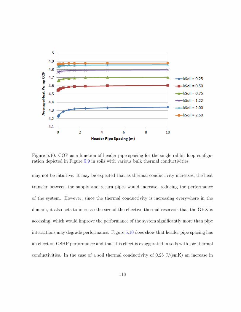
Figure 5.10: COP as a function of header pipe spacing for the single rabbit loop configu-ration depicted in Figure 5.9 in soils with various bulk thermal conductivities
may not be intuitive. It may be expected that as thermal conductivity increases, the heat
transfer between the supply and return pipes would increase, reducing the performance
of the system. However, since the thermal conductivity is increasing everywhere in the
domain, it also acts to increase the size of the effective thermal reservoir that the GHX is
accessing, which would improve the performance of the system significantly more than pipe
interactions may degrade performance. Figure 5.10 does show that header pipe spacing has
an effect on GSHP performance and that this effect is exaggerated in soils with low thermal
conductivities. In the case of a soil thermal conductivity of 0.25 J/(smK) an increase in
118

header pipe spacing from 5 cm to 1 m resulted in an increase in heat pump COP of
approximately 2.5%. This difference is negligible given the uncertainties and assumptions
used in the model.
5.4.2 Two Parallel Pipes
It was hypothesized that the differences in performance due to changes in header pipe spac-
ing illustrated in Section 5.4.1 were buffered by the large GHX being simulated. Therefore,
to isolate the effect of pipe interactions on system performance, a test case was developed
also using Simms (2013) 3D model to simulate two identical lengths of parallel pipes with
an imaginary disconnect replacing the U-bend (Figure 5.11). The imaginary disconnect
acts to eliminate any bias that may be associated with simulating this connection for a va-
riety of pipe spacings. Since the FEM model assumes that the fluid flows continuously from
the outlet of one pipe to the inlet of the other, the total length of the pipe is completely
independent of the space between them.
The simulated pipe configuration represented in Figure 5.11 consisted of two identical,
parallel 91.5 m lengths of pipe for a total of 183 m of pipe in a homogeneous soil domain.
This configuration was simulated for a range of pipe spacings between 0.05 m and 10 m
for a low, average, and high soil thermal conductivity (Figure 5.12).
119

Figure 5.11: Schematic of 2 parallel pipes test case
Figure 5.12: COP as a function of parallel pipe spacing
120

Figure 5.12 illustrates how pipe spacing in the two parallel pipe test case has a more
significant impact on performance than in the rabbit loop with header trench test case
(Section 5.4.1). Similar to that previous test case, the effect of pipe spacing is much more
significant for the low soil thermal conductivity.
The results of the header spacing and two parallel pipes test cases show that pipe
spacing has an effect on overall system performance. As pipe spacing increases the heat
pump COP of the simulated system increases. The magnitude of these effects is related
to the soil thermal conductivity and are most significant in systems within a soil of low
thermal conductivity. Therefore, when installing a GHX in a U-bend shape, it is necessary
to adequately characterize the soil thermal properties and, for low soil thermal conduc-
tivity cases, adequately separate the pipes to maintain system performance. For the low
thermal conductivity case investigated, a decrease in performance of approximately 25%
was observed when decreasing the pipe spacing from 100 cm to 5 cm. This change in
spacing represents the difference between a trenched GHX with pipe spacing of 1 m (a
standard excavator bucket width) and a horizontally bored U-tube shaped GHX (minimal
pipe spacing), suggesting that this change in system configuration could reduce operation
costs by up to 25% when installed in low thermal conductivity soils.
121

5.4.3 GHX Layout
In practice, GHXs are installed in a variety of configurations as described in Chapter 2.
It was expected that pipe configuration, independent of pipe length, would have only a
small impact on system performance but no substantial information exists on the topic.
Therefore, a test case was developed using Simms (2013) model to investigate the effects
of pipe layout on system performance by simulating systems in which the configuration
of the pipe is the only variable. Figure 5.13 is a schematic of the 6 configurations that
were investigated. In all simulations, two identical pipes of 183 m (600 ft) were considered
and all pipe spacings were 0.5 m. All other parameters were as defined in Section 5.1.2.
Each simulation had a duration of 1 year and used the system loads and shallow soil
temperatures summarized in Section 5.1.2. Since two loops were considered in each case
and all adjacent pipes were spaced 0.5 m apart, configurations (a), (b), and (c) were
simulated in a trench 3.5 m wide and approximately 50 m long, while configurations (d),
(e), and (f) were simulated in a trench 1.5 m wide and approximately 90 m long.
The GHX layout test case was simulated for homogeneous soil thermal conductivities of
1.22, 0.25, and 2.5 J/(smK). Figure 5.14 illustrates how system performance is a function
of GHX configuration. In all cases, the longer, more narrow trenches performed better than
the shorter, wider trenches by up to 3% for the low soil thermal conductivity case. The
122

(a) (b) (c)
(d) (e) (f)
Figure 5.13: Pipe configurations investigated using Simms (2013) FEM model: (a) “rabbitloop”, (b) spiral loop, (c) “floppy rabbit loop”, (d) side-by-side loops, (e) overlapping loops,and (f) cross over loops - not to scale
decreased performance of the wider trenches is likely a result of these trenches having eight
adjacent pipes, rather than four adjacent pipes as in the longer trench, because the heat
transfer from the soil domain to the inner pipes would be limited, depleting the efficiency of
the system. Based on this test case, it is concluded that longer trenches perform better than
wider, shorter trenches with identical pipe spacing when all other parameters are equal.
This difference in performance is most significant in soils of low thermal conductivity.
123

Figure 5.14: Performance based on GHX configuration - identical pipe spacing
The differences in performance based on the GHX configuration independent of trench
shape are negligible. The crossover loop performed <0.5% better than the side-by-side and
overlapping loops, and the spiral loop performed <0.5% better than the rabbit and floppy
loops in all cases.
To investigate when shorter, wider trenches may provide increased performance, the
simulations for configurations (a), (b), and (c) were duplicated using a spacing of 3 m
between the 2 loops while no changes were made to configurations (d), (e), and (f) (Figure
5.15).
124

Figure 5.15: Performance based on GHX configuration - varying pipe spacing
Figure 5.15 shows how increasing the spacing between the loops in the shorter, wider
trench increases the performance of these systems by approximately 1.5% relative to the
longer, more narrow trenches. This result suggests that system performance is mildly
improved through increased spacing of adjacent loops.
The relationships between pipe configurations and system performance could be used
practically to determine the most ideal configuration for a GHX depending on the land area
available for installation; however, no significant efficiencies in GHX layout were identified.
125

5.4.4 Loop Length
The most significant variable in GHX design is the length of pipe that is installed. A
typical design rule of thumb is to assume that 183 m (600 ft) of installed pipe would
provide 1 ton (3516 J/s) of heating capacity. However, this rule of thumb may not meet
the design requirements in all scenarios and could possibly result in the over or under design
of the GHX. Therefore, a test case was developed to investigate the effect of changing pipe
length on the performance of the GSHP and analyse the validity of this rule of thumb.
It was expected that increasing loop length would increase COP to a point at which
pumping losses become more significant than the increased heat transfer associated with
the additional pipe. It was expected that COP would decrease with increasing GHX length.
Since the developed 1D finite difference model takes into account the power consump-
tion of the fluid circulation pump, it was utilized for this test case. This power consumption
is dependent on the friction losses through the system which are a function of the length
of the pipe, the volumetric flow rate, and the physical properties of the fluid. The finite
difference model was employed to simulate a range of realizations in which the only variable
was the pipe length. All other model parameters were as described in Section 5.1.1. This
test case was simulated for 100 days using total pipe lengths from 90 m to over 400 m in a
U-tube configuration. Figure 5.16 summarizes the heat pump, circulation pump, and total
126

energy consumption of the system on the primary vertical axis and average system COP
on the secondary vertical axis, and shows how system performance is a function of loop
length.
Heat pump and total system energy consumption tend to decrease with increasing GHX
length for the range of loop lengths investigated. This trend is associated with the increase
in EWT to the heat pump with increasing loop length. Greater loop lengths provide more
thermal energy transfer from the subsurface to the fluid, increasing the fluid temperature
and reducing the energy required by the heat pump to extract the defined energy difference
from the fluid.
Comparatively, as GHX length increases, the circulation pump energy tends to decrease
initially then begins to increase with loop length. This trend is caused by the initial
reduction in head loss through the system as the average fluid temperature in the pipe
rises with increasing loop length. The fluid temperature rise reduces the fluid density and
viscosity, thus reducing its resistance to flow and the frictional head losses through the
GHX and the heat pump. However, as the loop length increases further, the head loss
associated with the additional pipe increases the energy required to maintain the specified
flow rate.
As initially expected, simulations showed that heat pump and total system COP in-
creased with loop length, while circulation energy consumption increased with longer
127

Figure 5.16: Performance of U-bend configuration as a function of total pipe length
128

GHXs. However, since the circulation pump energy consumption was significantly smaller
than that of the heat pump, which was not expected for extremely large GHX lengths, this
effect was negligible within the range of loop lengths investigated.
The vertical line representing the typical 1 ton design length in Figure 5.16 denotes the
common assumption that 183 m (600 ft) of pipe will provide 1 ton (3516 J/s) of heating
capacity. The results show how the total system energy consumption for GHXs beyond
this typical design length tends to plateau, suggesting that performance is not significantly
enhanced with increased loop length. This conclusion agrees with the typical design length
since increases in performance (COP) are marginal beyond this loop length (<10% for
length increase from 183 m to 413 m), suggesting that additional pipe is not required to
meet this energy demand for the system being investigated. Below this length, reduction
in system performance became significant. Therefore, GSHP design optimization becomes
a trade off between the additional installation cost of larger ground loops or increased
operating costs associated with shorter loops. The findings of this test case agree with
typical current design practice but only in the basic case examined. It would not be valid
to extend these findings to cases of extreme soil thermal conductivities or irregular GHX
configurations.
129

Chapter 6
Conclusions
The investigations conducted in this thesis help to improve the understanding of GSHP
operations. Some conclusions help to support existing practices in the industry, while
others help to advance it for a range of GHX designs. These systems offer an efficient
technology for heating and cooling applications and expanding the understanding of their
operation has an integral role in increasing their utility.
Two main research objectives were addressed to identify potential design efficiencies:
in-depth monitoring of a fully function residential GSHP and a comprehensive simulation
of these systems using computational models.
A fully functioning residential GSHP was monitored for insight into system operation
130

and performance at the Elora Field Site. An array of temperature sensors were installed
in the subsurface on and surrounding the GHX to investigate temperature changes due
to system operation. Power monitoring equipment and temperature sensors were installed
on the system inside the residence to quantify system energy loads and total operating
costs. Specific temperature measurements and power consumption data were presented
and provided motivation for further analyses using numerical computer models. The data
analysed, including system operating costs and basic subsurface temperature profiles, were
in line with initial expectations. The resolution of the subsurface temperature data was in-
sufficient to establish detailed energy flux estimates or conduct extensive loop configuration
performance comparisons.
The total power consumption of the GSHP at the Elora Field Site was directly measured
and operating costs were calculated using two different electric utility billing schemes: the
time of use billing scheme and the tiered billing scheme. A comparison of these two billing
schemes concluded that the time of use billing scheme yielded an average annual cost within
5% of that using the tiered billing scheme. Therefore, the implementation of the time of
use billing scheme does not significantly effect the operating costs of this GSHP. Since
costs associated with this billing scheme are a function of the time of energy consumption,
this conclusion could be extended to other systems with similar occupant schedules in
comparable climates.
131

In Section 5.4, a 3D finite element model developed by Simms (2013) was employed
to investigate the effects of GHX configuration on system performance. Test cases were
simulated using this model to investigate the effect of pipe spacing and GHX layout on
system performance. It was concluded that performance was only nominally a function of
pipe spacing and variations in performance were most significant in simulations with low
thermal conductivities. When considering a single 183 m ground loop with a 30 m header
trench, increases in header pipe spacing from 5 cm to 10 m increased heat pump COP by
approximately 2.5% for the extreme low soil thermal conductivity case investigated, which
is not a significant improvement related to the implications on system installation associ-
ated with this spacing increase. However, when considering a U-tube shaped configuration,
increases in pipe spacing from 5 cm to 1 m resulted in an increase in heat pump COP of
approximately 25% for the extreme low soil thermal conductivity case investigated. Since
operation costs are directly related to heat pump COP, this performance improvement is
significant when comparing horizontally bored GHXs (minimal pipe spacing) to potential
trenched GHXs in which spacing could be up to 1 m using existing excavating equipment.
To investigate the effect of pipe layout on system performance, the 3D finite element
model developed by Simms (2013) was employed to simulate a test case in which the pipe
configuration was the only variable. A group of six GHX configurations were investigated.
It was found that longer trenches performed better than shorter, wider trenches, which was
132

attributed to reduced pipe interactions in the longer trenches. However, the differences in
performance between all configurations were within ∼3.5% for all simulations, spanning
a range of reasonable soil thermal conductivities. In all of the longer trench cases, the
configuration referred to as the cross over loop (see Figure 5.13) had the highest system
performance by a negligible amount (<0.3%), which was attributed to the minor variations
in model output.
In Chapter 4, a 1D finite difference heat conduction model of a U-tube pipe configura-
tion was presented. The model was used to investigate the potential optimization of system
performance through pumping intensity, the differences between transient and steady state
simulation of GSHPs, and the effect of total loop length on overall system performance.
Comparisons between the transient and steady state simulations concluded that, in
the case of a U-tube shaped GHX operating under a range of reasonable energy loads,
it is appropriate to simulate the pulsed operation of a GSHP using an equivalent steady
state approximation. This result helps to justify the quasi-steady state assumption that
is sometimes made when simulating these systems using numerical modelling techniques,
as is done by Simms (2013) and in the configuration test cases described above. However,
the system COP for the steady state case would be overestimated by up to approximately
10% for the range of reasonable flow rates and soil thermal conductivities investigated.
To attempt to identify performance efficiencies through pump schedule optimization,
133

the effect of pump cycle frequency was investigated. System performance was shown to be a
function of cycle frequency. For the range of cycle frequencies, system loads, and simulation
times investigated, system COP varied by up to ∼30% when considering cycle frequency as
the only variable. The variation in COP was found to be most significant during operation
at lower pump run times, which would represent shoulder season operation when energy
demands are relatively lower. Since a typical GSHP operating under a range of reasonable
system loads was simulated, this relationship could, with some confidence, be extended
to most residential or light commercial GSHP applications. The conclusion is important
since pump cycle frequency can significantly effect overall system performance, identifying
a method through which system efficiency could be improved without substantial changes
to design. System monitoring could be implemented to optimize pump scheduling and
maximize system performance after installation.
Finally, the 1D finite difference model was used to investigate the effect of total pipe
length on overall system performance by analysing energy consumption and average COP
in heating mode with a constant energy demand of 3516 J/s. Pipe length is the primary
design variable and the one most likely controlling potential GHX over design. As initially
expected, simulations showed that heat pump and total system COP increased with loop
length. This increase in COP is caused by the improved heat pump efficiency resulting
from the increase in fluid temperature with loop length. The circulation pump energy
134

consumption initially decreased as loop length increased for the same reason but, for larger
loops, the circulation pump energy consumption increased due to the additional head loss
through the system. However, the circulation pump energy consumption was significantly
smaller than that of the heat pump and this effect was negligible within the range of loop
lengths investigated. Therefore, larger loop lengths may be beneficial for GSHP operation
since improved heat pump performance is observed with small increases in fluid pumping
costs.
The GHX length analysis compared the average COP of each simulation to a typical
design length of 183 m (600 ft) per ton (3516 J/s) of heating capacity. It was concluded
that this design rule of thumb is reasonable since improvements in COP were marginal
beyond this loop length (<10% for length increase from 183 m to 413 m). Below this
length, reduction in system performance became significant. Therefore, GSHP design
optimization becomes a trade off between the additional installation cost of larger ground
loops or increased operating costs associated with shorter loops.
Existing design standards for residential and light commercial GHX applications are
unlikely to be dramatically improved upon via changes in configuration or pipe spacing.
However, system monitoring could lead to, or at least ensure, optimal GSHP operation
through improved pump scheduling.
135

6.1 Recommendations for Future Work
The developed 1D finite difference model could be employed to conduct additional analy-
ses to further enhance our understanding of GHX design and GSHP operation beyond this
thesis. For example, the cycle frequency optimization exercise summarized in Chapter 5
was conducted using this model for a single heat pump and fluid circulation pump com-
bination. This investigation could be extended to any heat pump and circulation pump
combination by inputting the manufacturer’s specifications into the model and executing
similar simulations to provide insight into maximized operating efficiency of the specified
systems. The model could also be used to investigate the sensitivity of U-tube shaped
GSHP performance to various design parameters, including pipe wall thickness or thermal
conductivity, U-tube pipe spacing, heat exchange fluid thermal properties, or pipe diame-
ter. These parameters could be altered within the model to assess how the system reacts
to such changes, perhaps offering insight into potential design efficiencies.
In Chapter 3 the Elora Field Site and the associated monitoring data were introduced
and summarized. A large quantity of temperature and power consumption data were col-
lected at the field site but an extensive analysis of these data has not been completed.
These data could be used to investigate various aspects of this system. The power con-
sumption data could be combined with the temperature data from the supply and return
136

pipes inside the residence to calculate COP, quantifying the efficiency of the system dur-
ing heating and cooling operation. The subsurface temperature data could be analysed
to quantify temperature profiles around the GHX and estimate the magnitude of thermal
energy transfer, giving insight into the way in which heat transmits through the soil. The
temperature data could be further analysed to conduct a comparison between the different
loop configurations at the field site. It is hypothesized that the slinky loop may not per-
form as well as the other configurations since the same length of pipe would be extracting
energy from, or rejecting energy into, a relatively smaller volume of soil. Analysing the
temperatures on the supply and return pipes to each loop and the temperature profile
along the trenches would provide preliminary insight for such an investigation.
137

References
R. Al-Koury and P. G. Bonnier. Efficient finite element formulation for geothermal heatingsystems. part ii: Transient. International Journal for Numerical Methods in Engineering,67:725–745, 2006.
R. Al-Koury, P. G. Bonnier, and R. B. J. Brinkgreve. Efficient finite element formulation forgeothermal heating systems. part i: Steady state. International Journal for NumericalMethods in Engineering, 63:988–1013, 2005.
ASHRAE. 2007 ASHRAE Handbook - Heating, Ventilation, and Air-Conditioning Appli-cations. American Society of Heating, Refrigeration and Air-Conditioning Engineers,Inc., Atlanta, GA, USA, 2007.
ASHRAE. 2009 ASHRAE Handbook - Fundamentals. American Society of Heating, Re-frigeration and Air-Conditioning Engineers, Inc., Atlanta, GA, USA, 2009.
A. Baudoin. Stockage intersaisonnier de chaleur dans le sol par batterie d’echangeursbaıonnette verticaux: Modele de predimensionnement. PhD thesis, Reims University,France, 1988.
M. Bernier, A. Chala, and P. Pinel. Long-term ground-temperature changes in geo-exchange systems. ASHRAE Transactions, 114(2):342–350, 2008.
David J. Brodrecht. Personal communication, 2010. David Brodrecht is the Manager ofGeothermal Applications at NextEnergy Inc.
H. S. Carslaw and J. C. Jaeger. Conduction of Heat in Solids. Oxford University Press,Oxford, United Kingdom, 1947.
Stuart W. Churchill. Comprehensive correlating equations for heat, mass and momentumtransfer in fully developed flow in smooth tubes. Ind. Eng. Chem., Fundam., 16(1):109–116, 1977.
138
Tranquility® 27 (TT) Series IOM - Installation, operation & Maintenance Instructions.ClimateMaster® Geothermal Heat Pump Systems, USA, 2010.
Tranquility® 30 Digital (TE) Series IOM - Installation, operation & Maintenance Instruc-tions. ClimateMaster® Geothermal Heat Pump Systems, USA, 2012.
COMSOL Multiphyics User’s Guide. COMSOL AB: COMSOL, Stockholm, Sweden, 2008.
CSA. CAN/CSA-C448 Series-02: Design and Installation of Earth Energy Systems. Cana-dian Standards Association, Canada, 2009.
CSA. CAN/CSA-F280-12 Determining the required capacity of residential space heatingand cooling appliances. Canadian Standards Association, Canada, 2012.
Mark W. Denny. Modern Hydronic Heating: For Residential and Light Commercial Build-ings. Princeton University Press, Princeton, NJ, USA, 1993.
H.-J. G. Diersch, D. Bauer, W. Heidemann, W. Ruhaak, and P. Schatzl. Finite elementmodelling of borehole heat exchanger systems: Part 1. fundamentals. Computers andGeosciences, 37(8):1122–1135, 2011a.
H.-J. G. Diersch, D. Bauer, W. Heidemann, W. Ruhaak, and P. Schatzl. Finite elementmodelling of borehole heat exchanger systems: Part 2. numerical simulation. Computersand Geosciences, 37(8):1136–1147, 2011b.
P. Eskilson. Thermal analysis of heat extraction boreholes. PhD thesis, University of Lund,Lund, Sweden, 1987.
P. Eskilson and J. Claesson. Simulation model for thermally interacting heat extractionboreholes. Numerical Heat Transfer, 13(2):149–165, 1988.
Jose Etcheverry, Paul Gipe, William Kemp, roger Samson, Martijn Vis, Bill Eggerton, RobMcMonagle, Sarah Marchildon, and Dale Marshall. Smart Generation: Power Ontariowith Renewable Energy. The David Suzuki Foundation, Vancouver, B.C., Canada, 2004.
Pier-Olivier Fontaine, Denis Marcotte, Philippe Paquier, and Denis Thibodeau. Modelingof horizontal geoexchange systems for building heating and permafrost stabilization.Geothermics, 40(3):211–220, 2011.
Ground Loop DesignTM Premier 2010 User’s Manual. Gaia Geothermal, USA, 2010.
139

M. He, S. Rees, and L. Shao. Simulation of a domestic ground source heat pump sys-tem using a transient numerical borehole heat exchanger model. Journal of BuildingPerformance Simulation, 4(2):141–155, 2011.
G. Hellstrom. Ground Heat StorageThermal Analyses of Duct Storage Systems. PhD thesis,University of Lund, Lund, Sweden, 1991.
Patrick J. Hughes. Geothermal (ground-source) heat pumps: Market status, barriers toadoption, and actions to overcome barriers. Technical report, Oakrdige National Labo-ratory, 2008.
IGSHPA. Closed-Loop Geothermal Systems - Slinky Installation Guide. InternationalGround Source Heat Pump Association, Stillwater, OK, USA, 1994.
L. R. Ingersoll and H. J. Plass. Theory of the ground pipe heat source for the heat pump.Heating, Piping and Air Conditioning, 20(7):119–122, 1948.
L. R. Ingersoll, O. J. Zobel, and A. C. Ingersoll. Heat Conduction. The University ofWisconsin Press, Madison, WI, USA, 1954.
Stephen P. Kavanaugh and Kevin Rafferty. Ground-Source Heat Pumps - Design ofGeothermal Systems for Commercial and Institutional Buildings. American Society ofHeating, Refrigeration and Air-Conditioning Engineers, Inc., Atlanta, GA, USA, 1997.
Application Guide (AG 31-008): Geothermal Heat Pump Design Manual. McQuay® AirConditioning, 2002. RetrievedonMay20, 2011fromhttp : //www.mcquay.com/.
V. C. Mei and C. J. Emerson. New approach for analysis of ground-coil design for appliedheat pump systems. ASHRAE Transactions, 91(2B):1216–1226, 1985.
E. Shashi Menon. Gas Pipeline Hydraulics. CRC Press - Taylor and Francis Group, BocaRaton, FL, USA, 2005.
Lewis F. Moody. Friction factors for pipe flow. In The American Society of MechanicalEngineers Semi-Annual Meeting, Pittsburgh, PA, USA, June 1944.
Norman K. Muraya. Numerical Modelling of the Transient Thermal Interference of VerticalU-Tube Heat Exchangers. PhD thesis, Texas A&M University, 1994.
M. Nabi and R. Al-Khoury. An efficient finite volume model for shallow geothermal systems- part i: Model formulation. Computers and Geosciences, 49:290–296, 2012a.
140

M. Nabi and R. Al-Khoury. An efficient finite volume model for shallow geothermal systems- part ii: Verification, validation and grid convergence. Computers and Geosciences, 49:297–307, 2012b.
National Resources Canada: NRCan. Heating and cooling with a heatpump: Ground-source heat pumps (earth-energy systems). Website, 2009.RetrievedonMay26, 2011fromhttp : //oee.nrcan.gc.ca/.
OEB. Electricity prices. Webpage, Ontario Energy Board, 2012.http://www.ontarioenergyboard.ca/OEB/Consumers/Electricity/Electricity+Prices,Accessed 28 November, 2012.
Oklahoma State University: OSU. Closed-Loop/Ground-Source Heat Pump Systems: In-stallation Guide. International Ground Source Heat Pump Association, Stillwater, OK,USA, 1988.
Oklahoma State University: OSU. Ground Source Heat Pump Residential and Light Com-mercial: Design and Installation Guide. International Ground Source Heat Pump Asso-ciation, Stillwater, OK, USA, 2009.
Mikael Philippe, Michel Bernier, Dominique Marchio, and Simon Lopez. A semi-analyticalmodel for serpentine horizontal ground heat exchangers. HVAC&R Research, 17(6):1044–1058, 2011.
M. Phillipe, M. Bernier, and D. Marchio. Sizing calculation spreadsheet: Vertical geother-mal borefields. ASHRAE Journal, 52(7):20–28, 2010.
J. Raymond, R. Therrien, and L. Gosselin. Borehole temperature evolution during thermalresponse tests. Geothermics, 40(1):69–78, 2011.
S. J. Rees, J. D. Spitler, Z. Deng, C. D. Orio, and C. N. Johnson. A study of geothermalheat pump and standing column well performance. ASHRAE Transactions, 110(1):3–13,2004.
John Siegenthaler. Air and Water: The Biology and Physics of Life’s Media. DelmarLearning, Clifton Park, NY, USA, 2 edition, 2004.
Richard B. Simms. The effects of soil heterogeneity on the performance of horizontalground loop heat exchangers. Master’s thesis, The University of Waterloo, Waterloo,ON, Canada, 2013.
141

C. N. Jr. Sittel, W. D. Threadgill, and K. B. Schnelle Jr. Longitudinal dispersion forturbulent flow in pipes. I&EC Fundamentals, 7(1):39–43, 1968.
Jeffrey D. Spitler and James Cullin. Misconceptions regarding design of ground-sourceheat pump systems. In Proceedings of the World Renewable Energy Congress, Glasgow,Scotland, July 2008.
J. S. Steinhart and J. R. Hart. Calibration curves for thermistors. Deep-Sea Research, 15:497–503, 1968.
James W. Stevens. Coupled conduction and intermittent convective heat transfer from aburied pipe. Heat Transfer Engineering, 23(4):34–43, 2002.
M. Th. van Genuchten and W. J. Alves. Analytical solutions of the one-dimensionalconvective-dispersive solute transport equation. Technical Bulletin 1661, U.S. Depart-ment of Agriculture, 1982.
WaterFurnace. Waterfurnace® energy analysis. Spreadsheet, n.d.
VSX Vogel Software GMBH WILO. Software, 2010. Wilo-Select used to asses circulationpump power requirements.
S. D. Wood, B. W. Mangum, J. J. Filliben, and S. B. Tillett. Investigation of the stabilityof thermistors. J Res Natl Bur Stand (US), 83(3):247–263, 1978.
C. Yavuzturk, J. D. Spitler, and S. J. Rees. A transient two-dimensional finite volume modelfor the simulation of vertical u-tube ground heat exchangers. ASHRAE Transactions,105(2):465–474, 1999.
M. M. Yovanovich. A general expression for predicting conduction shape factors. In AIAA11th Aerospace Sciences Meeting, Washington, D.C., USA, January 1973.
142

APPENDICES
143

Appendix A
CSA 448 Multiple Measure Method
This appendix outlines the procedure, referred to as the Multiple Measure Method, defined
by the Canadian Standards Association (CSA, 2009) for the design of GHX systems in
Canada. To follow the CSA (2009) guidelines the designer must complete the seven step
process referred to as the Multiple Measure Method.
Step 1,2,3 - Residential Load Calculation and Gains Factor
The designer must first complete a heating and cooling load calculation in an acceptable
manner and is referred to the method defined by CSA (2012) as an example of an acceptable
load calculation procedure.
144

A gains factor is a coefficient describing the building thermal energy gains due to
internal and solar heat gains. This gains factor is defined based on basic quantifications
of building windows, occupancy, base electrical use, and construction quality. The gains
factor is used to determine the heating correction factor, Cd, as described in the ASHRAE
Handbook - Fundamentals (ASHRAE, 2009). Cd is determined using the gains factor and
the annual degree days for the specific GHX design. CSA (2009) includes a table of Cd
values as functions of degree days and the gains factor.
Step 4 - Determining the System Balance Point by Degree Days
CSA (2009) requires that a GHX provide 95% of the required heating load for a building.
This requirement is based on experience designing these systems in Canada. This step
involves estimating the minimum outdoor air temperature at which a back-up heating
system is required for a maximum of 5% of the heating load, the system balance point.
The system balance point is a function of the annual heating degree days and the heat
loss for the specific GHX design as described in the ASHRAE Handbook - Fundamentals
(ASHRAE, 2009). The heat loss is a function of the building envelop and is determined
during an energy audit for the building.
145

Step 5 - Heat Pump Heating Capacity and Entering Water Temperature Cor-
rection for Closed Loop Systems
The GSHP heat capacity is a quantification of the heating capacity of the subsurface in a
specific location. This parameter is estimated based on the heat loss, Cd factor, system
balance point, and the temperature difference, which is a measure of the design tempera-
ture heat loss in a specific location as defined in the ASHRAE Handbook - Fundamentals
(ASHRAE, 2009).
The minimum entering water temperature (EWT) of the fluid that will be entering the
heat pump is approximated by CSA (2009) as a difference from the average soil temperature
and is dependent on the relative soil moisture. In Canada, the difference between the
average soil temperature and the minimum EWT is approximated as 10C, 11C, and
14C for wet soils, damp soils, and dry soils, respectively (CSA, 2009).
Step 6 - Selecting an Appropriate Ground Heat Exchanger
To identify minimum GHX length, the heat pump manufacturer’s specifications must first
be examined to determine a unit that will provide the necessary heating capacity of the
system given the minimum EWT determined in Step 5. Once a heat pump with the
required heating capacity is identified, the minimum required GHX length is based on
146

the nominal cooling capacity of this heat pump. The nominal cooling capacity [W] is
the maximum total thermal energy that an air conditioner can remove from the air in
a unit of time and is defined by the heat pump manufacturer. CSA (2009) defines the
required loop length for specific GHX configurations based on pipe length per unit of
cooling capacity. Therefore, total GHX length is determined using the nominal cooling
capacity of the selected heat pump and the tables provided by CSA (2009), which are only
appropriate for Canadian applications where annual heating requirements are greater than
annual cooling requirements. The sources of these tables in CSA (2009) are not described
in detail.
Step 7 - Correcting for Soil Type
To this point in the design process, the type of soil has not been considered. CSA (2009)
defines a soil type correction factor to account for the variation in thermal properties of
different soils. This correction factor is based on specific soil type and GHX configuration.
It appears to the author that these factors are based on empirical data. The soil type cor-
rection factor is applied to the GHX minimum length calculation, increasing or decreasing
the required GHX length. For horizontal GHX applications, the soil type correction factor
ranges from 0.95 for wet sand to 3.9 for dray sand.
The Canadian standard for GHX design is an example of guidelines used in the in-
147

dustry. The summary was meant to provide insight into the techniques and some of the
requirements of GHX design. The investigations that follow attempt to further the under-
standing of GHX interactions with the intention of providing insight into the optimization
of their operation and design.
148

Appendix B
GeoDesigner® Design Report
149

ClimateMaster, Inc. Elora Test Site
GeoDesigner® 2/3/2011
Project Information
Prepared For: Prepared By:
Peter and Jane Robertson University of Waterloo
1 Some St. 200 University Avenue W.
Elora, ON Waterloo, CAN N2L 3G1
519-888-4567 x. 3117
Notes: Notes:
Design Data
Heating Load: 45,000 Btu/Hr Heating Setpoint: 72 Deg F
Htg Load Temp Diff: 65 Deg F Cooling Setpoint: 75 Deg F
Cooling Load: 30,000 Btu/Hr Begin Cooling At: 70 Deg F
Clg Load Temp Diff: 25 Deg F Hot Water Setpoint: 130 Deg F
Sensible Cooling: 26,400 Btu/Hr Hot Water Users: 2
Continuous Fan: Yes
Reference City: Waterloo-Wellington, CAN-ON
Winter Design: -2 Deg F Annual Heating: 109.0 Million Btu
Summer Design: 84 Deg F Annual Cooling: 12.8 Million Btu
Bldg Balance Temp: 62 Deg F Annual Water Heating: 12.1 Million Btu
Avg Internal Gains: 7,179 Btu/Hr Daily Hot Water Use: 40 Gallons
Estimated Operating Cost Summary
System Heating Cooling Hot Water Constant Total Per
Cost Cost Cost Fan Cost Month
TT 072 Vspd / Horz 4 pipe - 0.75" $1,146 $49 $239 $74 $1,508 $126
18 SEER - Twin Compressor - R22 System $1,470 $112 $209 $260 $2,052 $171
Gas-80%-Ignitor-Induced System $1,582 $147 $209 $336 $2,275 $190
Comments: Utility Cost Rate Summer Winter
UW Test Location Electric - Geothermal $/kwh .110 .110
Electric - Heat Pump $/kwh .110 .110
Electric - Furnace $/kwh .110 .110
Natural Gas $/therm 1.00 1.00
1 Propane $/gallon 3.50 3.50
elora_test_site.ged Fuel Oil $/gallon 3.50 3.50
Due to the variability of weather, system installation, and living habits this analysis is to be considered an estimate.
12/7/12
150

ClimateMaster, Inc. Elora Test Site
GeoDesigner® 2/3/2011 Page 2
System Comparison Graph
12/7/12
$0
$230
$460
$690
$920
$1,150
$1,380
$1,610
$1,840
$2,070
$2,300
Annual Operating Cost
Heating Cooling Hot Water Fan Total
TT 072 Vspd / Horz 4 pipe - 0.75"
18 SEER - Twin Compressor - R22 System
Gas-80%-Ignitor-Induced System
151

ClimateMaster, Inc. Elora Test SiteGeoDesigner® 2/3/2011
System Summary
TT 072 Vspd / Horz 4 pipe - 0.75"
ClimateMaster Unit Heating
Series: Tranquility 27 - EarthPure Tranquility 27 - EarthPure
Model: 72 Electrical Use: 10,420 Kwh
Style: Two Stage - Var. Speed Average Efficiency: 3.07 COP
Hot Water Generator: Yes Annual Contribution: 100 %
Heating Run Time: 2,474 Hours Annual Cost: $1,146
Cooling Run Time: 210 Hours
Heating Stage 1: 99 % of Htg Electric Resistance
Cooling Stage 1: 100 % of Clg
Electrical Use: 1 Kwh
Geothermal Source Average Efficiency: 100 %
Annual Contribution: 0 %
Source Type: Horizontal Closed Loop Annual Cost: $0
Soil Type: 0.75 - Damp Silt/Clay
Pipe Type: 3/4" IPS PE SDR 11 Annual Heating Cost: $1,146
Pipe Configuration: 4 Pipes in Trench
Avg Pipe Depth: 5 Feet Cooling
Trench Length: 915 Feet
Tranquility 27 - EarthPure
Min Freeze Protect: 10 Deg F Electrical Use: 447 Kwh
Average Efficiency: 28.7 EER
Max Source-Cooling: 66 Deg F
Avg Source-Cooling: 56 Deg F Annual Cooling Cost: $49
Avg Source-Heating: 40 Deg F
Min Source-Heating: 30 Deg F Water Heating
Geothermal Hot Water Generator
Deep Earth Temp: 50.1 Deg F Electrical Use: 665 Kwh
Surface Swing: 22.6 Deg F Average Efficiency: 3.36 COP
Swing Time Lag: 39 Days Annual Contribution: 63 %
Soil Conductivity: 0.75 Annual Cost: $73
Soil Diffusivity: 0.60
Loop Conductivity: 3.03 Electric Storage Water Heater
Electrical Use: 1,505 Kwh
Auxiliary Heat Average Efficiency: 88 %
Annual Contribution: 37 %
Type: Electric Resistance Annual Cost: $166
Style: Duct Heater
Auxiliary Required: 0 Kw Annual Water Heating Cost: $239
Optional Emergency: 14 Kw
Efficiency: 100 % Continuous Fan
Aux Balance Point: N/A Deg F Electrical Use: 668 Kwh
Water Heater
Annual Continuous Fan Cost: $74
Type: Electric Storage Water Heater
Style: Standard Efficiency
Efficiency: 88.0 % Total Annual Operating Cost: $1,508
Due to the variability of weather, system installation, and living habits this analysis is to be considered an estimate.
12/7/12
152

ClimateMaster, Inc. Elora Test Site
GeoDesigner® 2/3/2011
Temperature Bin Analysis
TT 072 Vspd / Horz 4 pipe - 0.75"
Outdoor Annual Space Hot Water Geo Htg - Clg H.W. Gen Geo Geo Aux Aux
Air Weather Load Load Source Capacity Capacity Run Operating Heating Hot Water
Temp Hours Btu/Hr Btu/Hr Temp Btu/Hr Btu/Hr Time Cost Cost Cost
112
107
102
97
92 5 22,697 1,387 61 59,798 3,653 38% $0.70
87 69 18,133 1,387 59 60,263 3,503 30% $7.56 $0.84
82 228 13,569 1,387 57 60,726 3,249 22% $18.25 $5.52
77 436 9,005 1,387 55 61,189 2,994 15% $22.62 $15.11
72 615 7,179 1,387 55 61,374 2,892 12% $23.61
67 705 1,387 $35.80
62 705 1,387 $35.80
57 672 -3,205 1,387 45 45,973 4,779 7% $24.45 $25.93
52 637 -6,667 1,387 44 45,304 4,742 15% $48.43 $16.07
47 586 -10,128 1,387 43 44,637 4,705 23% $68.01 $6.85
42 590 -13,590 1,387 42 44,145 4,504 31% $91.96
37 724 -17,052 1,387 42 44,406 3,611 38% $139.43
32 762 -20,513 1,387 41 44,387 3,000 46% $174.93 $0.01
27 618 -23,975 1,387 40 44,203 2,557 54% $164.90 $0.01
22 464 -27,436 1,387 39 43,916 2,219 62% $141.22 $0.01
17 367 -30,898 1,387 38 43,558 1,955 71% $125.58 $0.01
12 260 -34,359 1,387 37 43,151 1,741 80% $98.87 $0.01
7 160 -37,821 1,387 37 42,709 1,566 89% $66.98 $0.01
2 91 -41,282 1,387 36 42,240 1,419 98% $41.61
-3 43 -44,744 1,387 35 44,744 1,387 100% $21.20
-8 17 -48,205 1,387 34 48,205 1,387 100% $8.98
-13 5 -51,667 1,387 33 51,667 1,387 100% $2.82
-18 1 -55,128 1,387 33 54,541 1,387 100% $0.02
-23
-28
-33
8760 $1,269 $0 $166
12/7/12
153
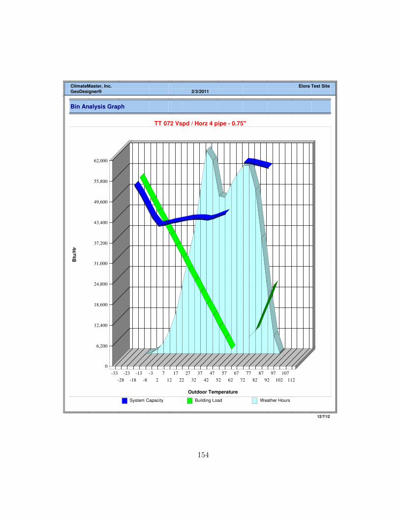
ClimateMaster, Inc. Elora Test Site
GeoDesigner® 2/3/2011
Bin Analysis Graph
TT 072 Vspd / Horz 4 pipe - 0.75"
12/7/12
0
6,200
12,400
18,600
24,800
31,000
37,200
43,400
49,600
55,800
62,000
Outdoor Temperature
Btu
/Hr
-33
-28
-23
-18
-13
-8
-3
2
7
12
17
22
27
32
37
42
47
52
57
62
67
72
77
82
87
92
97
102
107
112
System Capacity Building Load Weather Hours
154

ClimateMaster, Inc. Elora Test SiteGeoDesigner® 2/3/2011
System Summary
18 SEER - Twin Compressor - R22 System
Heat Pump Heating
Type: Heat Pump - Split Heat Pump - Split
Style: 18 SEER - 2stg - R22 Electrical Use: 3,576 Kwh
95 F Cool Capacity: 34,200 Btu/Hr Average Efficiency: 2.68 COP
95 F Cool Efficiency: 10.0 EER Annual Contribution: 30 %
47 F Heat Capacity: 33,840 Btu/Hr Annual Cost: $393
47 F Heat Efficiency: 3.28 COP
17 F Heat Capacity: 19,440 Btu/Hr Gas Furnace
17 F Heat Efficiency: 2.25 COP Fuel Use: 992 Therms
Heat Cut-off Temp: 35 Deg F Electrical Use: 774 Kwh
Indoor Coil Match: Standard Average Efficiency: 77 %
Outdoor Coil Rating: Average Annual Contribution: 70 %
Annual Cost: $1,077
95 F Low Cool Cap: 19,015 Btu/Hr
95 F Low Cool Eff: 12.9 EER Annual Heating Cost: $1,470
47 F Low Heat Cap: 18,875 Btu/Hr
47 F Low Heat Eff: 3.57 COP Cooling
17 F Low Heat Cap: 9,588 Btu/Hr
17 F Low Heat Eff: 2.09 COP Heat Pump - Split
Electrical Use: 1,017 Kwh
Heating Run Time: 2,104 Hours Average Efficiency: 12.6 EER
Cooling Run Time: 734 Hours
Annual Cooling Cost: $112Auxiliary Heat
Water Heating
Type: Gas Furnace
Style: Ignitor-Induced Draft Gas Storage Water Heater
Input Capacity: 100,000 Btu/Hr Fuel Use: 209 Therms
Output Capacity: 81,000 Btu/Hr Average Efficiency: 58 %
Efficiency: 80 AFUE
Annual Water Heating Cost: $209
Continuous Fan
Electrical Use: 2,367 Kwh
Water Heater
Annual Continuous Fan Cost: $260
Type: Gas Storage Water Heater
Style: Standard Efficiency
Efficiency: 58.0 % Total Annual Operating Cost: $2,052
Due to the variability of weather, system installation, and living habits this analysis is to be considered an estimate.
12/7/12
155

ClimateMaster, Inc. Elora Test Site
GeoDesigner® 2/3/2011
Temperature Bin Analysis
18 SEER - Twin Compressor - R22 System
Outdoor Annual Space Hot Water Heating Heating Cooling Cooling Heat Pump Aux Water
Air Weather Load Load Capacity Run Capacity Run Operating Heating Heating
Temp Hours Btu/Hr Btu/Hr Btu/Hr Time Btu/Hr Time Cost Cost Cost
112
107
102
97
92 5 22,697 1,387 22,697 100% $1.26 $0.12
87 69 18,133 1,387 18,814 97% $11.03 $1.65
82 228 13,569 1,387 19,318 76% $27.32 $5.45
77 436 9,005 1,387 19,821 53% $34.73 $10.42
72 615 7,179 1,387 20,325 42% $37.56 $14.70
67 705 1,387 $16.85
62 705 1,387 $16.85
57 672 -3,205 1,387 20,423 20% $23.26 $16.07
52 637 -6,667 1,387 18,875 42% $45.70 $15.23
47 586 -10,128 1,387 16,288 69% $67.02 $14.01
42 590 -13,590 1,387 14,050 98% $93.66 $14.11
37 724 -17,052 1,387 17,052 100% $163.76 $17.31
32 762 -20,513 1,387 $221.89 $18.22
27 618 -23,975 1,387 $209.78 $14.77
22 464 -27,436 1,387 $179.80 $11.09
17 367 -30,898 1,387 $159.77 $8.77
12 260 -34,359 1,387 $125.59 $6.22
7 160 -37,821 1,387 $84.89 $3.83
2 91 -41,282 1,387 $52.59 $2.18
-3 43 -44,744 1,387 $26.88 $1.03
-8 17 -48,205 1,387 $11.43 $0.41
-13 5 -51,667 1,387 $3.60 $0.12
-18 1 -55,128 1,387 $0.77 $0.02
-23
-28
-33
8760 $505 $1,077 $209
12/7/12
156

ClimateMaster, Inc. Elora Test Site
GeoDesigner® 2/3/2011
Bin Analysis Graph
18 SEER - Twin Compressor - R22 System
12/7/12
0
5,600
11,200
16,800
22,400
28,000
33,600
39,200
44,800
50,400
56,000
Outdoor Temperature
Btu
/Hr
-33
-28
-23
-18
-13
-8
-3
2
7
12
17
22
27
32
37
42
47
52
57
62
67
72
77
82
87
92
97
102
107
112
System Capacity Building Load Weather Hours
157

ClimateMaster, Inc. Elora Test SiteGeoDesigner® 2/3/2011
System Summary
Gas-80%-Ignitor-Induced System
Air Conditioner Heating
Type: Air Conditioner - Split Gas Furnace
Style: 12 SEER - R410a Fuel Use: 1,414 Therms
95 F Cool Capacity: 35,280 Btu/Hr Electrical Use: 1,534 Kwh
95 F Cool Efficiency: 10.3 EER Average Efficiency: 77 %
Indoor Coil Match: Standard
Outdoor Coil Rating: Average Annual Heating Cost: $1,582
Cooling
Air Conditioner - Split
Run Time: 424 Hours Electrical Use: 1,333 Kwh
Average Efficiency: 9.6 EERHeating System
Annual Cooling Cost: $147
Type: Gas Furnace
Style: Ignitor-Induced Draft Water Heating
Input Capacity: 71,886 Btu/Hr
Output Capacity: 58,228 Btu/Hr Gas Storage Water Heater
Efficiency: 80.0 AFUE Fuel Use: 209 Therms
Average Efficiency: 58 %
Annual Water Heating Cost: $209
Continuous Fan
Run Time: 1966 Hours
Electrical Use: 3,057 Kwh
Water Heater
Annual Continuous Fan Cost: $336
Type: Gas Storage Water Heater
Style: Standard Efficiency
Efficiency: 58.0 % Total Annual Operating Cost: $2,275
Due to the variability of weather, system installation, and living habits this analysis is to be considered an estimate.
12/7/12
158
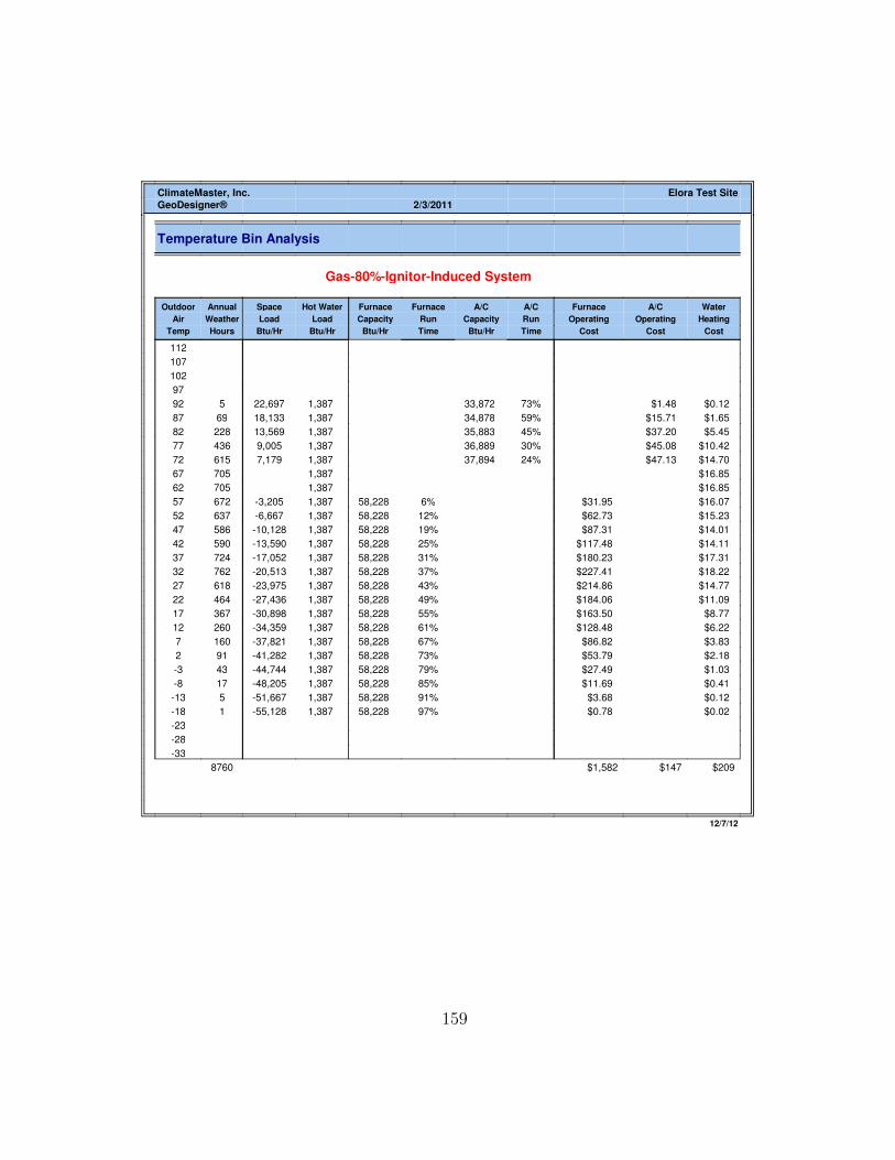
ClimateMaster, Inc. Elora Test Site
GeoDesigner® 2/3/2011
Temperature Bin Analysis
Gas-80%-Ignitor-Induced System
Outdoor Annual Space Hot Water Furnace Furnace A/C A/C Furnace A/C Water
Air Weather Load Load Capacity Run Capacity Run Operating Operating Heating
Temp Hours Btu/Hr Btu/Hr Btu/Hr Time Btu/Hr Time Cost Cost Cost
112
107
102
97
92 5 22,697 1,387 33,872 73% $1.48 $0.12
87 69 18,133 1,387 34,878 59% $15.71 $1.65
82 228 13,569 1,387 35,883 45% $37.20 $5.45
77 436 9,005 1,387 36,889 30% $45.08 $10.42
72 615 7,179 1,387 37,894 24% $47.13 $14.70
67 705 1,387 $16.85
62 705 1,387 $16.85
57 672 -3,205 1,387 58,228 6% $31.95 $16.07
52 637 -6,667 1,387 58,228 12% $62.73 $15.23
47 586 -10,128 1,387 58,228 19% $87.31 $14.01
42 590 -13,590 1,387 58,228 25% $117.48 $14.11
37 724 -17,052 1,387 58,228 31% $180.23 $17.31
32 762 -20,513 1,387 58,228 37% $227.41 $18.22
27 618 -23,975 1,387 58,228 43% $214.86 $14.77
22 464 -27,436 1,387 58,228 49% $184.06 $11.09
17 367 -30,898 1,387 58,228 55% $163.50 $8.77
12 260 -34,359 1,387 58,228 61% $128.48 $6.22
7 160 -37,821 1,387 58,228 67% $86.82 $3.83
2 91 -41,282 1,387 58,228 73% $53.79 $2.18
-3 43 -44,744 1,387 58,228 79% $27.49 $1.03
-8 17 -48,205 1,387 58,228 85% $11.69 $0.41
-13 5 -51,667 1,387 58,228 91% $3.68 $0.12
-18 1 -55,128 1,387 58,228 97% $0.78 $0.02
-23
-28
-33
8760 $1,582 $147 $209
12/7/12
159

ClimateMaster, Inc. Elora Test Site
GeoDesigner® 2/3/2011
Bin Analysis Graph
Gas-80%-Ignitor-Induced System
12/7/12
0
5,900
11,800
17,700
23,600
29,500
35,400
41,300
47,200
53,100
59,000
Outdoor Temperature
Btu
/Hr
-33
-28
-23
-18
-13
-8
-3
2
7
12
17
22
27
32
37
42
47
52
57
62
67
72
77
82
87
92
97
102
107
112
System Capacity Building Load Weather Hours
160

Appendix C
Thermistor Calibration
The Steinhart and Hart (1968) equation, Equation C.1, is the most commonly used em-
pirical approximation formula for thermistors. This expression relates resistance of the
thermistor to temperature.
1
T= A+B lnR + C(lnR)3 (C.1)
For higher accuracy or to accommodate a wider temperature range, a square term can be
included to create Equation C.2, taken after Wood et al. (1978).
1
T= A+B lnR + C(lnR)2 +D(lnR)3 (C.2)
161

For this investigation the expected range of temperatures surrounding the geothermal
loop was not expected to be significantly different than the control temperatures used to
calibrate the sensors. To this end, Equation C.1 was calibrated to. With an equation
of three variables, three equations are required to solve for them. The three reference
temperatures were created using: an icebath (∼ 0C), an environmental chamber (∼
18.2C), and a walk-in fridge (∼ 5.2C). This produced a system of linear equations:
1 lnR1 (lnR1)
3
1 lnR2 (lnR2)3
1 lnR3 (lnR3)3
A
B
C
=
1T1
1T2
1T3
To check the precision of this calibration 3 sensors were examined at a fourth controlled
temperature. Following the same system of equations, this produces a linear overdeter-
mined system of 4 equations and 3 unknowns. The relative residual of these three sensor
calibrations, as calculated by Equation C.3 were: 1.84E-04, 1.94E-04, and 1.97E-04. The
three thermistors were all rated 30kΩ. This thermistor type comprised 59 out of 64 ther-
mistors in the field.
R =||b− A× A\b||||A|| × ||A\b||
(C.3)
162

All thermistors in the field were initially suspected to be calibrated acceptably using this
method with the exception of one. The only 10kΩ thermistor was recording resistances of
over 1000kΩ during the initial 36 hour test period. According to its calibration curve, this
thermistor was recording temperatures of −80C, which is unrealistic when contrasted with
the coldest temperatures seen elsewhere on the system of −2C. The “broken” thermistor
was located on the farthest supply line off the manifold. It was recalibrated by assuming
that the temperature differential on average between the two long trench systems was
equivalent. This produced a system of 35 equations and 3 unknowns, which were used to
recalibrate the sensor.
163

Appendix D
1-Dimensional Finite Difference
Model Derivation
D.1 Energy Equation
Thermal energy in a fluid is defined as:
E = ρcpT∀
where E is the total thermal energy in a volume of fluid in J ; ρ is the density of the fluid in
kg/m3; T is the temperature of the fluid in C; and ∀ is the volume of the fluid in m3. By
164

assuming, for the purposes of this thesis, that the heat exchange fluid is incompressible and
changes in specific heat capacity and density of the fluid with temperature are negligible,
the following can be written:
∂cp∂t
=∂ρ
∂t=∂∀∂t
= 0
and the change in thermal energy in a fluid can be written as:
∆E = ρcp∀∆T (D.1)
In order to develop an expression for the change in temperature in the heat exchange fluid,
a thermal energy balance was applied to a cylindrical control volume representing a section
of the GHX. Figure D.1 represents a finite section of the pipe showing energy entering and
exiting the pipe through advection and dispersion, and entering the pipe as an energy flux
from the surrounding environment.
Considering a pipe of total length L [m], the change in thermal energy in this control
volume over time can be represented as:
∆E
∆t= ρcpAp
(−D∂T
∂x+ vT
) ∣∣∣x=xL
− ρcpAp(−D∂T
∂x+ vT
) ∣∣∣x=xR
+Qsource∆x
= ∆x∂
∂x
(ρcpAp
(D∂T
∂x− vT
))+Qsource∆x
∆E
∆t= ∆xρcpApD
∂2T
∂x2−∆xρcpApv
∂T
∂x+Qsource∆x
165

Figure D.1: Control volume used for energy balance
166

which, after substituting in Equation D.1, becomes:
∆xρcpAp∆T
∆t= ∆xρcpApD
∂2T
∂x2−∆xρcpApv
∂T
∂x+Qsource∆x
and reduces to:
∆T
∆t= D
∂2T
∂x2− v∂T
∂x+
1
ρcpApQsource
which, as the limit as ∆T → 0, is written as:
∂T
∂t= D
∂2T
∂x2− v∂T
∂x+
1
ρcpApQsource (D.2)
Equation D.2 is the advection-dispersion equation for the temperature flux a fluid flowing
through a pipe.
However, the thermal energy flux into the pipe is a combination of all energy sources and
sinks surrounding the pipe, which in this case are the adjacent pipe and the surrounding
subsurface:
Qsource = Qpipessource +Qsoil
source
where Qpipessource is the heat flux from the adjacent pipe per metre [J/sm] and Qsoil
source is the
heat flux from the subsurface per meter [J/sm].
To represent the energy transfer into the pipe an expression for the total energy flux
167

per unit length of pipe was adapted after Yovanovich (1973) as:
Qpipessource =
∆T
R= −T − T
′
Rp
(D.3)
Similarly, to represent the energy transfer from the the surrounding soil at some distance
into the fluid in the pipe, the total energy flux per unit length was adapted after Yovanovich
(1973) as:
Qsoilsource = −T − Ts
Rs
(D.4)
Therefore, using Equations D.3 and D.4, Equation D.2 becomes:
∂T
∂t= D
∂2T
∂x2− v∂T
∂x− 1
ρcpAp
T − T ′
Rp
− 1
ρcpAp
T − TsRs
(D.5)
and using the substitutions:
β1 =1
RpρcpAp& β2 =
1
RsρcpAp
Equation D.5 becomes:
∂T
∂t= D
∂2T
∂x2− v∂T
∂x− β1 [T − T ′]− β2 [T − Ts] (D.6)
168

D.2 Coupled Equations
Considering the temperature, Ts, at some intermediate point in the subsurface at a radial
distance, rs, between the pipe and the far field, Equation D.2 can be represented using two
coupled equations:
∂T
∂t= D
∂2T
∂x2− v∂T
∂x− β1[T − T ′]− β2[T − Ts] (D.7)
∂Ts∂t
= −β3[Ts − T ]− β3[Ts − T ′]− β4[Ts − T∞] (D.8)
Where:
β1 =1
RpρcpAp;
β2 =1
RsρcpAp;
β3 =1
Rsρsoilcps∀inter=
1
Rsρscpsπ(r2s − r2o);
β4 =1
R∞ρsoilcps∀∞=
1
R∞ρscpsπ(r2∞ − r2s);
and ∀s is the volume [m3] of soil between the outer pipe radius, ro, and the intermediate
soil radius, rs, and ∀∞ is the volume [m3] of the hollow cylinder of soil created between the
169

intermediate soil radius, rs, and the radius of influence, r∞:
∀s = π(r2s − r2o)∆x & ∀∞ = π(r2∞ − r2s)∆x
Since the model represents a pipe of length L in a U-tube shape, the length of the soil
domain is L/2. Therefore, the soil temperature, Ts, is equivalent at x and L− x.
D.3 Effective Thermal Resistance
Effective thermal resistances were divided into sections and combined in series:
Rp = Rpipessoil + 2Rpipe
Rs = Rinter +Rpipe (D.9)
where expressions for Rpipessoil and Rinter were estimated after Yovanovich (1973) in Chapter
4 as Equation D.10 and Equation D.11, respectively.
Rpipessoil =
1
2πksoil
ln√(
w
r1o
)2
− 1 +
(w
r1o
)−√(
w
r2o
)2
− 1 +
(w
r2o
) (D.10)
170

Rinter =1
2πksoil
ln√(
w
ro
)2
− 1 +
(w
ro
)+
√(
w
rs
)2
− 1 +
(w
rs
) (D.11)
The effective thermal resistances Rpipe and Rinter, were derived from Fourier’s Law:
q = −kA∂T∂η
(D.12)
For heat flux through the wall of a hollow cylindrical control volume:
A = 2πr∆x & η = r
where r is the radius of the control volume [m] and ∆x is the length of the control volume
[m]. Thus, Equation D.12 becomes:
q = −k2πr∆x∂T
∂r
Separating and integrating this equation from the inner radius, r1, at T1 to the outer radius,
r2, at T2: ∫ r2
r1
q
r∂r =
∫ T2
T1
−2πk∆x∂T
q [ln(r)]r2r1 = −2πk∆x [T ]T2T1
171

q[ln(r2)− ln(r2)] = −2πk∆x(T2 − T1) = 2πkLT (T1 − T2)
q =2πk∆x(T1 − T2)
ln( r2r1
)(D.13)
Equation D.13 defines the total heat flux across the wall of a hollow, cylindrical control
volume. Defining the heat flux per unit length of pipe, Q, in J/sm as:
Q =q
∆x=
2πk(T2 − T1)ln( r2
r1)
and using the definition for heat flux per unit length after Yovanovich (1973):
Q =(T2 − T1)
R
where R is effective thermal resistance of the cylindrical control volume in smK/J , this
effective thermal resistance can be expressed as:
R =ln( r2
r1)
2πk(D.14)
Equation D.15 defines the effective thermal resistance across the wall of a hollow cylin-
drical control volume, which can be used to estimate the effective thermal resistances, Rpipe
and Rinter. Substituting the appropriate parameters for the effective thermal resistance of
172

the pipe into Equation D.15, Rpipe is estimated as:
Rpipe =ln( ro
ri)
2πkpipe(D.15)
where Rpipe is the effective thermal resistance across the pipe wall [smK/J]; ro and ri are
the outer and inner radii of the pipe [m]; and kpipe is the thermal conductivity of the
pipe material [J/(smK)]. Substituting the appropriate parameters for the effective thermal
resistance of the soil between the intermediate radius and the far field into Equation D.15,
Rinter is estimated as:
R∞ =ln( r∞
rs)
2πksoil(D.16)
Where R∞ is the effective thermal resistance of the annulus of soil between the intermediate
radius and the far field [smK/J]; r∞ and rs are the far field and intermediate soil radii [m];
and ksoil is the average thermal conductivity of the soil [J/(smK)]. Equation D.16 describes
the effective thermal resistance, R∞ as used in Equation 4.5 to define β4.
Substituting Equation D.10, Equation D.11, and Equation D.15 into Equation D.9 to
complete the expressions describing the effective thermal resistances Rp and Rs as used in
Equation 4.5 to define β1, β2, and β3
173

D.4 Finite Difference Approximation
The finite difference approximation was employed to solve Equations D.7 and D.8 using
a grid of 3×N discrete nodes to represent the physical system. The system is composed
of a U-tube shaped pipe in a cylindrical soil domain. The fluid flowing away from the
heat pump and the fluid returning to the heat are contained in identical, parallel lengths
of pipe surrounded by a cylindrical subsurface. Therefore, using nodes to represent the
system, nodes 1...N represent the fluid in the pipe flowing away from the heat pump,
nodes N + 1...2N represent the fluid in the pipe returning to the heat pump, and nodes
2N + 1...3N represent the soil at an intermediate radius from the centre of the two pipes.
This node distribution is presented in Figure D.2, which represents N nodes in each of the
supply pipe (black), the return pipe (black), and the soil (blue).
Using Crank-Nicholson weighted average in time, Equation D.7, for 1 ≤ i ≤ 2N :
T n+1i − T ni
∆t=
1
2
[D
(T n+1i−1 − 2T n+1
i + T n+1i+1
∆x2
)− v
(T n+1i+1 − T n+1
i−1
2∆x
)
− β1(T n+1i − T n+1
2N−i+1
)− β2
(T n+1i − T n+1
si
) ]1
2
[D
(T ni−1 − 2T ni + T ni+1
∆x2
)− v
(T ni+1 − T ni−1
2∆x
)
− β1(T ni − T n2N−i+1
)− β2
(T ni − T nsi
) ]
174

Fig
ure
D.2
:N
ode
dis
trib
uti
onfo
rth
esu
pply
and
retu
rnpip
esan
dth
eso
il-
not
tosc
ale
175

which rearranges to:
T n+1i−1
(−a
2
)+ T n+1
i
(1
∆t− b
2
)+ T n+1
i+1
(− c
2
)+ T n+1
2N−i+1
(−β1
2
)+ T n+1
si
(−β2
2
)= T ni−1
(a2
)+ T ni
(1
∆t+b
2
)+ T ni+1
( c2
)+ T n2N−i+1
(β12
)+ T nsi
(β22
)(D.17)
where:
a =D
∆x2+
v
2∆x
b =−2D
∆x2− β1 − β2
c =D
∆x2− v
2∆x
With a finite difference approximation using Crank-Nicholson weighted average in time,
Equation D.8 becomes, for 1 ≤ i ≤ N :
T n+1si− T nsi
∆t= −β3
2
(T n+1si− Ti
)− β3
2
(T nsi − Ti
)− β3
2
(T n+1si− T n+1
2N−i+1
)− β3
2
(T nsi − T2N−i+1
)− β4
2
(T n+1si− T∞
)− β4
2
(T nsi − T∞
)
176

which rearranges to:
T n+1si
(1
∆t+β32
+β32
+β42
)+ T n+1
i
(−β3
2
)+ T n+1
2N−i+1
(−β3
2
)= T nsi
(1
∆t− β3
2− β3
2− β4
2
)+ T ni
(β32
)+ T n2N−i+1
(β32
)+ T∞ (β4)
and, after the substitution d = −β3 − β42
, becomes:
T n+1si
(1
∆t− d
2
)+ T n+1
i
(−β3
2
)+ T n+1
2N−i+1
(−β3
2
)= T nsi
(1
∆t+d
2
)+ T ni
(β32
)+ T n2N−i+1
(β32
)+ T∞ (β4)
D.5 Boundary Conditions
While the system is operating there is a fixed temperature delta boundary condition at
x = 0 representing the energy change in the fluid caused by the heat pump:
T (x = 0, t) = Tin = Tout + ∆T
where Tout = T2N . So the boundary condition at i = 1 can be defined using:
Ti−1 = Tin = Tout + ∆T = T2N + ∆T
177

It follows that the solution at i = 1 for the fixed temperature delta boundary condition at
x = 0 becomes:
T n+1i
(1
∆t− b
2
)+ T n+1
i+1
(− c
2
)+ T n+1
2N−i+1
(−β1
2
)+ T n+1
2N
(−a
2
)+ T n+1
si
(−β2
2
)= T ni
(1
∆t+b
2
)+ T ni+1
( c2
)+ T n2N−i+1
(β12
)+ T n2N
(a2
)+ T nsi
(β22
)+ ∆T (a)
(D.18)
When the system is not in operation the velocity and mechanical dispersion of the fluid
in the pipe are zero. While the system is not operating a no thermal energy flux boundary
condition is defined at x = 0:
∂T
∂x
∣∣∣x=0
= 0
where T (x = 0) = T1. So the boundary condition at i = 1 can be defined using:
∂T
∂x
∣∣∣x=0
=Ti−1 − Ti
∆x= 0 ⇒ Ti = Ti−1
It follows that when the system is not operating, using v = DL = 0, the solution at i = 1
178

for the no thermal energy flux boundary condition at x = 0 becomes:
T n+1i
(−a
2+
1
∆t− b
2
)+ T n+1
i+1
(−c2
)+ T n+1
2N−i+1
(−β1
2
)+ T n+1
si
(−β2
2
)= T ni
(a
2+
1
∆t+b
2
)+ T ni+1
( c2
)+ T n2N−i+1
(β12
)+ T nsi
(β22
)(D.19)
At all times an advective-only boundary condition is defined at x = L:
∂T
∂x
∣∣∣x=L
= 0
where T (x = L) = T2N . So the boundary condition at i = 2N can be defined using:
∂T
∂x
∣∣∣x=L
=Ti+1 − Ti
∆x= 0 ⇒ Ti+1 = Ti
It follows that the solution at i = 2N for the no thermal flux boundary condition at x = L
becomes:
T n+1i−1
(−a
2
)+ T n+1
i
(1
∆t− b
2− c
2
)+ T n+1
2N−i+1
(−β1
2
)+ T n+1
si
(−β2
2
)= T ni−1
(a2
)+ T ni
(1
∆t+b
2+c
2
)+ T n2N−i+1
(β12
)+ T nsi
(−β2
2
)(D.20)
179

Appendix E
Base Case Calculations
E.1 In-Pipe Dispersion
Using the Elora Test Site as a basis for calculations, a base-case dispersion coefficient
was calculated. The total volumetric flow rate through six identical pipes is 15 GPM, or
9.5 × 10⁻⁴ m3/s. The pipe used for the GHX at Elora is 3/4” IPS SDR11, which has an
average inner diameter of 0.827 inches, or 2.1× 10⁻² m (Cli, 2012).
The heat exchange fluid circulating through the GHX at the Elora Field Site is a
mixture of water and 20% by volume propylene glycol. However, above 0C the density of
propylene glycol is taken to be 1000 kg/m3 (Cli, 2012) and to simplify for the base-case,
180

the fluid properties were assumed to be that of water at 10C. Water at 10 C has a density
of 999.8 kg/m3 and a dynamic viscosity of 1.31× 10⁻³ Pa · s (Siegenthaler, 2004).
Based on these parameters, the base-case coefficient of longitudinal dispersion, DL, of
the fluid in the pipe was calculated using Equation 4.14 as 0.034 ft2/s or 0.0032 m2/s.
The thermal diffusivity, α, of the heat exchange fluid was defined as that of water of
water at 10C, 1.4x10⁻⁷m2/s (Siegenthaler, 2004), which is negligible compared to the
longitudinal dispersion coefficient. Therefore, the final dispersion coefficient was taken to
be the longitudinal dispersion coefficient defined by Equation 4.14, 0.013 m2/s.
E.2 Radius of Influence
Simms (2013) performed a study using a 3D finite element model describing a system rep-
resenting the Elora Test Site. The study investigated the change in soil temperature with
distance away from the ground loop for a range of heterogeneous soil thermal conductiv-
ities and the homogeneous case. Each simulation was a 400 day simulation utilizing the
measured heating and cooling loads, surface temperatures, and fluid properties from the
Elora Field Site. The bulk soil thermal properties from the Elora Field Site were used as a
basis upon which a range of soil thermal properties were generated for these simulations.
The results of this investigation are presented in Figure E.1 (Simms, 2013).
181

Figure E.1: Soil temperature perturbation caused by ground loop (Simms, 2013)
Figure E.1 illustrates that after the 400 day simulations there was negligible change
in soil temperature at a radius of approximately 5 m from the ground loop for the mean
heterogeneous and homogeneous cases. Therefore, the radius of influence, r∞, was initially
defined as 5 m in the developed finite difference model.
To investigate the sensitivity of the model to changes in the radius of influence, a
range of simulations were conducted in which only this parameter was changed. All other
182

parameters were as defined in Section 5.1.1. Figure E.2 shows the results of this sensitivity
analysis as it relates to the average coefficient of performance (COP) of the GSHP.
Figure E.2: Sensitivity of model COP to radius of influence, r∞
Figure E.2 shows the effect of changing the radius of influence relative to the initial value
of 5 m discussed above. The sensitivity to changes in this parameter are not significant
(<0.2%) when r∞ was increased above 5 m. However, the sensitivity to changes in the
radius of influence became more significant (≤2%) when r∞ was reduced from 5 m to 2 m.
Therefore, 5 m was used as the base value for the radius of influence.
183

E.3 Intermediate Soil Radius
This section summarizes the investigation into the sensitivity of the model to changes in
the intermediate soil radius over a range of simulations. While all other parameters were
representative of the Elora Field Site, only the intermediate soil radius, rs, was altered.
Figure E.3 shows the results of this sensitivity analysis as it relates to the average coefficient
of performance (COP) of the GSHP.
Figure E.3: Sensitivity of model COP to intermediate soil radius, rs
184

Figure E.3 illustrates the effect of changing the intermediate soil radius relative to a
base-case value of 1 m. The changes due to this parameter are slightly more significant
than the radius of influence for the range considered. However, the variation in COP due to
changes in the intermediate soil radius were only significant (>1%) below 1 m. Therefore,
1 m was used as the base value for the intermediate soil radius.
185

Appendix F
Constant Versus Pulsed Pumping
Comparison Results
186

Figure F.1: Average temperature of the fluid in each element after 30 day simulation -comparison between pulsed and constant pumping cases
Figure F.2: Average temperature of the fluid in each element after 14 day simulation -comparison between pulsed and constant pumping cases
187

Figure F.3: Average temperature of the fluid in each element after 7 day simulation -comparison between pulsed and constant pumping cases
Figure F.4: Average temperature of the fluid in each element after 1 day simulation -comparison between pulsed and constant pumping cases
188

Figure F.5: Cumulative energy change of the fluid in each element after 30 day simulation- comparison between pulsed and constant pumping cases
Figure F.6: Cumulative energy change of the fluid in each element after 14 day simulation- comparison between pulsed and constant pumping cases
189

Figure F.7: Cumulative energy change of the fluid in each element after 7 day simulation- comparison between pulsed and constant pumping cases
Figure F.8: Cumulative energy change of the fluid in each element after 1 day simulation- comparison between pulsed and constant pumping cases
190

Figure F.9: Total energy change of the fluid in each element after 30 day simulation -comparison between pulsed and constant pumping cases
Figure F.10: Total energy change of the fluid in each element after 14 day simulation -comparison between pulsed and constant pumping cases
191

Figure F.11: Total energy change of the fluid in each element after 7 day simulation -comparison between pulsed and constant pumping cases
Figure F.12: Total energy change of the fluid in each element after 1 day simulation -comparison between pulsed and constant pumping cases
192


![Implementation and validation of a Ground Source …...GHE Ground Heat Exchanger GSHP Ground Source Heat Pump H borehole active depth [m] HP Heat Pump HVAC Heating Ventilation and](https://img.pdfslide.net/doc/110x75/5f0b00d07e708231d42e605a/implementation-and-validation-of-a-ground-source-ghe-ground-heat-exchanger-gshp.jpg)