Infrared Spectroscopy of Molecules in the Gas Phase

Keqing Zhang

A t hesis

presented to the University of Waterloo

in fdflment of the

thesis requirement for the degree of

Doctor of Philosophy

in

C hemistry

Waterloo, Ontario, Canada. 1997

@Keqing Zhang 1997

Nationai Library Bibliothèque nationaie du Canada

Acqui..itions and Acquisitions et Bibliographie Senrices services bibliographiques

The author has granted a non- exclusive licence allowing the National LiIbrary of Canada to reproduce, loan, distn'biite or sell copies of Mer thesis by any means and in any form or format, making this thesis available to interested pemns.

The author retains omership of the copyright in M e r thesis. Neither the thesis nor substantiai extracts fkom it may be printed or otherwise reproduced with the author's permission.

L'auteur a accordé une licence non exclusive permettant à la Bibliothèque nationale du Canada de reproduire, prêter, distriiuer ou vendre des copies de sa thèse de quelque d è r e et sous queIque forme que ce soit pour mettre des exemplaires de cette thèse à la disposition des personnes intéressées.

L'auteur conserve la propriété du droit d'auieur qui protège sa thése. Ni ia thèse ni des extraits substantiels de celle-ci ne doivent être miprimés ou autrement reproduits sans son autorisation.

The University of Waterloo requires the signatures of all persons using or ph*

tocopying this thesis. Please sign below, and give address and date.

Abstract

Fourier transforxn idiared spectroscopy is appiied to the studies of several very

different moledar systems. The spectra of the diatomic moledes BF, ALF, and

MgF were recorded and analyzed. D d a m coefficients w a e obtained. The data of

two isotopomers, "BF and l0BF, were used to determine the mas-reduced Dunham

coefficients, dong with Born-Oppenheimer breakdom constants. Parameterized

potential energy functions of BF and ALF were determined by fitting the adab le

data using the soluti~ns of the radiai Schr6dinge.r equation.

Two vibrational modes of the short-lived and reactive BrCNO molecule were

recorded at high resolntion. Rotation-vibration transitions of the fundamental

bands of both isotopomers "BrCNO and "BrCNO were assigned and analyzed.

From the rotational constants, it was found that the Br-C bond length in BrCNO

anomalously short when a linear geometry was assnmed. This may indicate that

Br CNO is quasi-linear , simulating the parent HCNO molecule.

The emission spectra of the gaseous polycyclic aromatic hydrocarbon (PAH)

moledes napht halene, ant hracene, pyrene, and ehrysene were recorded in the far-

infiared and mid-infkared regions. The assignments of fundamental modes and

some combination modes were made. The vibrational bands that lie in the far-

infrared are unique for different PAHs and d o w diserimination among the four

PAH moledes. The far-i&ared PAH spectra, therefore, may prove useful in the

assignments of auidentified spectral features kom astronomical objects.

Acknowledgement s

1 would like to extend rny thanks to my supervisor Dr. Peter Bernath for his

suentific inspiration, patience, and constant encouragement throughout the course

of this research. It was a great pleasure to work with Dr. Bujin Guo on many

projects.

1 would also like to thank Dr. Nick Westwood and Dr. Tibor Pasinszki for

providing expertise and helping to set up the experiments on nitrile oxides.

Finally, 1 would like thank Pina Colanisso, Zulf Morbi and Chdeng Zhao for

th& collaboration and enlightenment.

For my d e Sue

and

my mother and father

Contents

A bst ract

Adcnowledgements

Table of Contents

List of Figures

List of Tables

vi i

1 Introduction 1

1.1 Absorption vs. Ernission Infiared Spectroscopy . . . . . . . . . . . . 5

1.2 Diatomic Molecules . . . . . . . . . . . . . . . . . . . . . . . . . . . 6

1.3 Polyatomic Molecales . . . . . . . . . . . . . . . . . . . . . . . . . . 9

2 Fourier Tkansform Idkared Spectroscopy 12

2.1 TheMichelsonInterferorneter . . . . . . . . . . . . . . . . . . . . . 13

2.2 Advantages of Fourier Transform Spectroscopy . . . . . . . . . . . . 16

2.3 The B d e r Spectrometer . . . . . . . . . . . . . . . . . . . . . . . 19

3 Infiared Spectroscopy of Diatomic Molecules 22

3.1 The Born-Oppenheimer Approximation . . . . . . . . . . . . . . . . 23

. . . . . . . . . . . . . . . . . . . . 3.2 Born-Oppenheimer Breakciown 27

3.3 The Dunham Potential Model . . . . . . . . . . . . . . . . . . . . . 28

3.4 The Parameterized Potential Mode1 . . . . . . . . . . . . . . . . . . 34

3.5 Mared Emission Spectroscopy of BF and AU? . . . . . . . . . . . . 38

. . . . . . . . . . . . . . . . . . . . . . . . . . . 3.5.1 Experiment 39

3.5.2 Results and Discussion . . . . . . . . . . . . . . . . . . . . . 43

. . . . . . . . . . . . . . . . . . . . . . . . . . . 3.5.3 Conclusion 52

. . . . . . . . . . . . . . . . 3.6 kifrared Emission Spectroscopy of MgF 54

. . . . . . . . . . . . . . . . . . . . . . . . . . . 3.6.1 Experiment 55

. . . . . . . . . . . . . . . . . . . . . . . . . . . . . . 3.6.2 Results 56

4 High Resolution Infhred Spectroscopy of Nitrile Oxides 60

. . . . . . . . . . . . . . . . . . . . . . . . . . . . . . . 4.1 Experiment 62

. . . . . . . . . . . . . . . . . . . . . . . . . . 4.2 Resdts and Analysis 65

. . . . . . . . . . . . . . . . . . . . . . . . . . . . . . . . 4.3 Conclusion 72

5 Vibrational Spectroscopy of Polycydic Aromatic Hydrocarbon Molecules 74

. . . . . . . 5.1 Classical Mechanical Tkeatment of MoIecular Vibration 75

5.2 Quantum Mechanical Tkeatment of Molecular Vibration . . . . . . . 78

. . . . . . . . . . . . . . . . . . . . . . . . . . . 5.3 Group Fiequenues 80

5.4 Selection Rdes for Normal Modes of Vibration . . . . . . . . . . . . 81

5.5 Polycydic Aromatic Hydrocarbon Moledes in Astronomy . . . . . 83

. . . . . . . . . . . . . . 5.6 Laboratory Infrared Experiments on PAHs 87

5.7 Results.. . . . . . . . . . . . . . . . . . . . . . . . . . - . . . . . . 89

5.7.1 Far-infrared Region . . . . . . . . . . . . . . . . . . . . . . - 90

5.7.2 Mid-infrared Region . . . . . . . . . . . . . . . . . . . . . . 95

References

A BF Line Positions

B MgF Line Positions

C BrCNO Line Positions

List of Figures

. . . . . . . . . . . . The schematic of the Michelson interferorneter 14

The optical layout of the B d e ~ IFS 120 HR Fouria transform spec-

trometer . . . . . . . . . . . . . . . . . . . . . . . . . . . . . . . . . 21

. . . . . . . . . . . . . . The schematic of CM Rapid Temp furnace 41

. . . . . . . . . . . . . . . Kigh resolution emission spectnun of BF 42

. . . . . . The Born-Oppenheimer potential energy hinction for BE' 49

. . . . . . . . . . . . . . High resolution emission s p e c t m of MgF 57

Setup for the BrCNO absorption experiment . . . . . . . . . . . . . 64

The overview of the high resolution spectrum of BrCNO ut band . . 67

The expanded view of BrCNO zq band R branch . . . . . . . . . . . 68

Far-infrared emission spectra of naphthalene . . . . . . . . . . . . . 91

Far-infrared emission spectra of anthracene . . . . . . . . . . . . . . 92

Far-infrared emission spectra of pyrene . . . . . . . . . . . . . . . . 93

Far-infrared emission spectra of chrysene . . . . . . . . . . . . . . . 94

Mid-infrared emission spectra of pyrene . . . . . . . . . . . . . . . . 96

List of Tables

3.1 Dunham coefficients for BF . . . . . . . . . . . . . . . . . . . . . . 45

3.2 Mas-reduced Dunham coefficients for BF . . . . . . . . . . . . . . 46

3.3 Internudearpotentialenergyparmetersfor BF . . . . . . . . . . . 48

3.4 Dunham coefficients for AlF . . . . . . . . . . . . . . . . . . . . . . 50

3.5 Internuclear potential energy parameters for AlF . . . . . . . . . . . 51

3.6 Relative transition dipole moments of "BF . . . . . . . . . . . . . . 53

3.7 Dunham coefficients for MgF . . . . . . . . . . . . . . . . . . . . . . 59

4.1 The spectroscopic constants of BrCNO . . . . . . . . . . . . . . . . 69

4.2 The bondlengthsin BrCNO . . . . . . . . . . . . . . . . . . . . . . 71

4.3 Theoretical structure of BrCNO . . . . . . . . . . . . . . . . . . . . 73

5.1 Vibrational fiequenaes and intensities of naphthalene . . . . . . . . 97

5.2 Vibrational frequencies and intensities of anthracene . . . . . . . . . 99

5.3 Vibrational fiequencies and intensities of pyrene . . . . . . . . . . . 101

5.4 Vibrational hequenues and intensities of chrysene . . . . . . . . . . 104

5.5 Requencies of combination bands of PAHs . . . . . . . . . . . . . . 108

5.6 Observed band positions of PAHs . . . . . . . . . . . . . . . . . . . 112

A . 1 O bserved line positions of BF . . . . . . . . . . . . . . . . . . . . . . 129

B . 1 O bserved line positions of MgF . . . . . . . . . . . . . . . . . . . . . 138

C.l Observed line positions of "BrCNO . . . . . . . . . . . . . . . . . . 147

. . . . . . . . . . . . . . . . . . C.2 Observed line positions of 'IBrCNO 153

Chapter 1

Introduction

Molecular spectroscopy is a branch of science in which the interactions of elec-

tromagnetic radiation and matter are studied. The aims of these stndies are to

elucidate information on moledar strnctnre and dynamics, the environment of

the sample molecules and their state of association, interactions witL solvents. and

many nther topics. The resuits fiom spectroscopy have, therefore, played an im-

portant role in many disciplines of science, induding biochemistry [l] , environ-

mental research [21, chernical dynamics [3], astrophysics [4,5], and atmospheric

diemis try [6,7].

The interaction of the radiation with the moledes is nsually expressed in terms

of a resonance condition, which implies that th energy clifference between two

stationary states in a molede must be matched exactly by the energy of the

where h is the Planck constant, c is the speed of light in vacuum, v is fiequency

and O is the wavenumber which has the unit mi". This view of the interaction

between light and m a t t a is, however, rather cursory, since radiation interacts with

matter even when its wavelength is different from the specific wavelength at which

a resonance occurs. These off-resonsnce interactions bet ween electromagnetic radi-

ation and matter give rise to well-hown phenornena such as the Raman d e c t [BI. The interactions between moledes and photons determine the intensit ies, widt hs,

and shifts of spectral lines and the intensity and spectral distribution of continuous

radiation [9].

Molecular spectroscopy is nsudy dassified by the wavelength range of the elec-

tromagnetic radiation, for example, idkared spectroscopy and microwave spec-

troscopy. This dissertation mainly covers some aspects of infrared spectroscopy.

Although vibration-rotation transitions in the infirarecl are relatively weak (101,

when compared with electronic transitions, aU molecules except hornonuclear di-

atonie molecules have at Ieast one electric-dipole allowed idiared transition [II].

The universal ap plicabilit y of infrared spectroscopy is the mos t attractive property

of this spect~oscopic technique.

lnfrared spectroscopy. partienlady emission spectroscopy. faces another seri-

ous challenge: btackbody radiation at room temperattue. This radiation has a

maximum arotmd 1000 cm-', resniting in a natnral elevation of the noise level in

bfiared spectra. Furthemore, high power, widely tunable lasers are not a d a b l e

to infirared spectroscopy. It was also true that infiared detectors and optics were

in general i n f ' o r to those accessible in o t h a spectral regions. The demand fiom

many practicd applications of infirared technology, in particdar, defense relateci

applications, has changed this situation. M a r e d detectors now have quantum ef-

ficiencies as high as 70% [12]. In the meantime, the qaality of hfkared materials

and optical coatings has made significant advances as wd. The room temperature

bladrbody radiation can be greatly reduced by the ose of cold band p a s flters.

The application of cold apertures can be used to limit the thermal background ra-

diation. As a result, new techniques of infiared spectroscopy have been developed,

and existing techniques have been improved dramatically.

Today, infrared spectroscopy is a discipline in its own right. Spectroscopy is

the bridge that connects advanced experimentd resalts to the sophisticated the-

oretical interpretations of molecdar structure. The combination of experiment

and theory is very helpfnl in the synthesis, identification and characterization of

new moleniles and cornplex moledes. For small molecules, high resolntion spec-

troscopy is the ideal tool for the determination of geometry. The spectra of small

stable molectdes at room temperature have been ad studied and understood. One

new area of research is the study of the spectra of these stable molecules at high

temperature, where the excited vibrational levels have very high energy [13]. As

the experimental techniques have improved, the high resolution infrared spectra of

fiee radicals 114-161, ions [17] and high tempaatare moledes [IO] have also been

recorded. These transient moledes usnally exist in low concentrations and in ex-

treme environments. The detection of their spectra often forces the instrumentation

to the limits of sensitivity.

Another area that requires significant improvement is fa-infrared spectroscopy.

Far-i&ared spectra are easily contaminated by the pure rotational transitions of

water vapor in the atmosphere. The blackbody radiation often overwhelms the

weak far-hfiared signals origkiating from the molecules. Furthetmore, far-kfkared

detectors are the least sensitive ones among the infiared detectors. Despite all of

these difEcdties, considerable amonnt of spectroscopic data have been coliected

in the far-infiared region. Chemists use the far-hfkared spectra to study weak

chemical bonds. They aiso use them for studies of molecules with heavy atoms

or long chains because many of the infiared bands of these molecules are in the

' far-idared region.

The infrared spectroscopic techniques are applied to many different areas. One

of the most practical applications is based on the correlation between infrared

spectra and chemical functional groups [NI. Group fiequencies can be usefiil aids

in ident*g an unknown compound by cornparison of the same group frequency in

a molecule of closely related stmctnre. Alternatively, because of the large number

of possible normal vibrational modes for a molecule of even modest sizeo the infrared

spectnun provides a nseful hgerprint which is nearly unique for a given molede.

Infiared spectra also contain quantitative information. The infrared spectro-

scopic technique is widely used in analyticd chemistry [19]. Since spectroscopic

techniques are not invasive, they are ided for remote sensing, snch as monitoring

the temperature profile of the atmosphere and "greenhouse' gases fiom space i201.

The combination of gas chromatogaphy [21] and Fourier transform irhared spec-

troscopy has proven to be a p o w d technique for adyzing cornplex mixtures

quickly and acearately. Obtaining the infrared spectra of biological samples is

a new but rapidly expandixtg field. Infrared spectral dinerences between healthy

and cancerous human colon and cervical c e b have been discovered [22]. The in-

frared spectra of these c& have also been used to help determine the biochemical

clifference between healthy and malignant tells? and to help mode1 the chemical

clifferences between the DNA in normal and malignant tissue.

The high resolution spectra reported in this stndy were recorded on a state-of-

the-art Fourier transform spectrometer. The development of the Fourier transform

spectrometer, is combined with the continuing improvements in in6rared detectors.

This has opened up the possibility of applying high resolution spectroscopy to many

diverse chemical systems. Fourier transform spectrometers are now commody used

for both low and high resolution work. Another advantage of Fourier transforrn

spectroscopy, as illustrated in this thesis. is wide spectral coverage.

1.1 Absorption vs. Emission Infkared Spectroscopy

Traditiondy, molecules are studied by means of absorption spectroscopy in the

infrared region. In absorption spectroscopy, the light source is directed through a

cell containing the sample of interest, and the resulting intensities of the dXerent

transitions are measured. The magnitude of an absorption is given by Beer's law'

where I refers to the intensity of the light f&g on the detector, Io is the intensity

of the reference beam, ~ ( u ) is the molar absorptivity coeficient at a given freqoency

v , c is the concentration of the absorbing materid, and I is the path length of light

in the cd containing the absorbing material.

For the study of spectra of transient molecules, absorption spectroscopy becomes

dif6cnlt, partly because transient speües often exist at temperatures which are

comparable to or higher than the temperatnre of the absorption source. kifrared

emission spectroscopy bas emerged as a w o n d d tool to study moledes at high

temperatures. When one examines the spontaneous emission process, the rate is

determined by the Einstein A factor (in s-' ), given by the equation [23]

where fi, is the transition dipole moment matrix dement in debyes and v is the

transition fiequency in cm-'. It is clear that emission rates favor high fkequency

transitions from the above expression (Equation (1.3)). This is one of the reasons

that in the visible and ultraviolet regions of the spectnim, emission spectroscopy is

the method of choice. Infrared transition dipole moments are typicaily 0.1 debyes.

while electronic transition dipole moments are on the order of 1 debye. Although

infrared transitions are relatively weak, infrared experiments are possible. and a

nnmber of high temperatnre moleenles have been recorded in emission.

1.2 Diatomic Molecules

Once a molecular system is observed, the challenge of spectroscopy becomes the ex-

traction of physically relevant information from the spectral line positions, widt hs,

and intensities. Rom the recorded line positions, it is possible to model the en-

ergy level pattern of the moledar system that is accessed by the experirnent. In

addition. more direct physical information, such as bond lengths, bond angles and

moments of inertia, may be calculated from the line positions.

Diatomic molecules are the simplest molecnlar systems. The analysis of th&

spectra has been aucial to the development of t heories of molecnlar structure and

chemical bonding [24]. Consequently, many of the prototypical models fist de-

veloped to describe the vibrational spectroscopy of diatomic molecules have been

extended to the s t udy of polyatomic moledes and transient species [25,26].

High resolution spectroscopy has dso been aitical in the development of theo-

retical foundation of molecular strnctme and in the determination of the Limitations

of these model t heories. A good example of the interaction between experimental

spectroscopy and theories of chemical stmcture and bondhg is the study of the

breakdown of the Born-Oppenheimer description of molecdar behavior.

The knowledge of the pattern of rotation-vibration energy levels bas several

practicd and theoretical uses. The most dominant practical use of high resolu-

tion spectroscopy is the identification of moledes in varions environments. For

example, transient moledes, by definition, exis t in extreme conditions such as

high temperatures and low pressures. Identification of transient molecules by non-

spectroscopie means is usudy uncertain or not possible. High resolution spec-

troscopy is ofken utilized in identification of radicals in flames. the upper atm*

sphere. and space.

In 1927, Born and Oppenheimer formdated the mathematical separation of

nudear and electronic motion of a molecular system [27]. The Born-Oppenheimer

approximation has electrons moving arolmd tixed nudei which act as point charges.

The neglect of the kinetic energy of the nucl& provides a means to solve the elec-

tronic Schmodinger equation, which is otherwise soluble for only a limited number of

model problems. The inability of the Boni-Oppenheimer solution to the vibration-

rotation SchrOdinger equation to adequately explain some physical behavior was

noted in 1936, shortly after the discovery of deuterium (281. The nature of its

limitations has been well studied [29,30] and mathematicdy described. Thus the

Born-Oppenheimer approximation still plays a crucial role in the development of

models of molenilar systems.

An important and u s d consequence of the Born-Oppenheimer approximation

is the internudear potentid energy fnnction [31]. The potential energy fnnction

may be thoaght, in a simplistic way, as desaibing the behavior of a chernical bond

as a function of internudear distances and angles. A high qua& potential en-

ergy function will provide a prediction of positions, and with a dipole moment

function. intensities of experimentaily anobserved transitions. In addition, ot her

experimental observables, like scattering data and transport properties, can be de-

termined fiom potentid energy bc t ions which are derived fiom spectroscopic data.

Potential energy fanctions can be determined fbm the inversion of spectroscopic

constants to a theoretical mudel, or fiom the direct fitting of spectral data to a

potential energy fnnction. Potential energy hinctions can &O be determined kom

ab initio calculations.

Two methods, the Dunham model (321 and the parameterized potentid model

[33-361, were used in the reduction of the diatomic data recorded in this study.

The Dunham model was developed in 1932, and has been used in the fitting of

rotation-vibration data. There are numerou methods ased to improve and modûy

Dunham's original work. In this work, the mass-independent Watson expression

with the high order tams constrained, was applied to determine vibrational coeffi-

cients. The parameterized potential energy model was also employed. This model

is based on the direct fitting of spectral data to a parameterized potential using the

radial Schrôdinger equation.

1.3 Polyatomic Molecules

The inFrared spectra of many, stable and unstable, smdl molecules have been exam-

ined and reexamined. Good infirared spectra are &O a d a b l e for larger molecules

with 10 to 20 atoms. In general, as the symmetry of molecules decreases, both

the quality and quantity of infiared spectra decrease. One of the trends in modern

infrared spectroscopy is toward studying larger moledes, such as polycydic are

matic hydrocarbon moiecules 137,381 and biochemical compounds [39] , for which

the interpretation of hfiared spectra is more diflicult.

The strncture and spectra of polyatomic moledes are mach more complicated

than those of diatomic nioledes. The nnmber of degrees of freedom in an n-

atom molecde is 3n. When translational and rotational degrees of freedom are

excluded, there are 3n - 6 vibrational modes for a nonlinear molede, and 3n - 5 vibrational modes for a Linear molede. It is possible to choose a set of 3n - 6 (or

3n - 5 in the Iinear case) coordinates in such a way that each equation of motion

involves one coordinate only. Then, the vibrational Schtodinger equation can thns

be approximately separated into 3n - 6 independent equations in the same way.

Each equation describes a normal mode of vibration, which is a simple harmonie

oscillator with a characteristic kequency. The actaal motion of each nucleus is a

complicated superposition of all the normal modes. Li a simple molecule, it is ofken

possible to regard each normal mode as representing either a change in length of

the bond between one pair of atoms. Le. stretching vibration, or a change in the

angle between two bonds, i.e. bending vibration. In a more complex molecuie? the

* normal modes may describe vibration either of the whole molecular skeleton, or of

particular gronps of atorns such as OH and Cb. Vibrations of the second type are

characteristic of the group and almost independent of the par t idar molecule to

which it is attached.

The vibrational frequencies of polyatomic moledes are in the same energy

range as those of diatomic moledes. The vibrationd bands have a rotational

structure as do diatomic molecules. Indeed the band stnicture of s m d polyatomic

moledes is rather simiIar to that of diatomic moledes. On the other hand, since

large molecules tend to have large moments of inertia and hence srnaIl rotational

constants, the separation of the rotational lines may become comparable with their

intrinsic width, resulting in a continnum-like s p e c t m . The spectra may be fnrther

complicated by the ovedapping of different vibrationai modes.

Because of theh complexity, the interpretation and assignment of vibrationd

spectra of polyatomic moledes is a difncult and time-consuming process. One ver^

simple approach to describe the molecular vibrations of large organic molecnles and

biologieal maaomolecules is to use group fÎeqnenues and qnalitative correlations.

This is certainly worthwhde but has to be viewed as strictly a qualitative tool for

stmcturai chemistry. Attempts to corroborate vibrational interpretations on such

large systems by normal mode caldations are usaally indeterminate since the

number of force field constants nsaally m e e d s the nnmber of known vibrational

fiequencies. A much more ~ ~ O ~ O U S approach is to atilize detailed isotopic data for a

vibrational assignment , foilowed by a t horough normal mode calculation. Enormous

effort is required since numerous isotopomers have to be synthesized and analyzed.

Chapter 2

Fourier Transform Infiared

Spectroscopy

There are two major types of instruments which are widely used in modem infiared

spectroscopy. Diode laser spectrometers [40-42] are mainly used for high resolution

spectroscopy, while Fourier transfonu spectrometers [43-45] are used for both high

and low resolation spectroscopy. For high resolution stadies. the diode laser pro-

vides the spectral brightness necessary for remarkably high sensitivity and narrow

spectral line width. Tunable semiconductor diodes supply hfiared radietion kom

360 to 3500 cm-' [46]. Diode laser spectroscopy is, however, limited by practical

diffiealtics. 4 single &diode can ody cover a spectral region of 50 to 100 an-'. and

wit hin that range the coverage is around 30%. Conseqaently the spectrometer bas

a very narrow tunable range. The high sensitivity of diode lasers is responsible for

their wide-spread use in spectroscopy [47], but the lads of complete spectrai coverage

is a serions and hstrat ing defect . Assignments of transitions between rotational

levels in the spectra of new moledes, partiCulady asymmetric top molecules, are

dinicult if only a partial spectram is available. In addition, diode spectrometers

have no inherent means of calibration.

Fourier transform spectrometers are less sensitive, bot have sever al inherent

advantages that make them ided for many applications. They can cover a wide

spectral range, from fat-idiared t O near ultraviolet region [45]. B y employing He-Ne

lasers to control sampling of light signal accurately, Fourier transfom spectrome-

ters have built-in high preusion fiequency calibration. Resolutions ranging fkom

a few wavenumbers to 0.002 an-' are routinely available, and Fourier trsnsform

spectrometers can record samples in gas, liquid or solid phase under a variety of

experimental conditions. Althongh the light source used with Fourier transform

spectrometers is iaferior to that of diode laser spectrometers, the wide and corn-

plete spectral coverage, and a precise intanal frequency calibration ensure their

important role in spectroscopy [48,49].

2.1 The Michelson Interferorneter

The development of Fourier transform spectroscopy is based on the two-beam

interferometer that was origindy designed by Michelson in 1891 [50,51]. A diagram

of the Michelson interferorneter is sbown in Figure 2.1. The Michelson interferom-

eter consists of four arms. The h s t am contains a source of light, the second arm

contains a stationary minor, the third arm contains a movable mlror, and the

fourth arm is open. At the intersection of the four arms is a beamsplitter. which

is designed to transmit half the radiation that is incident upon it, and CO reflect

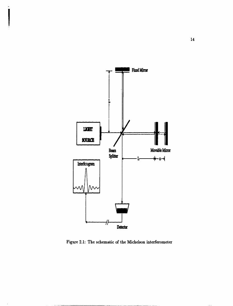
Figure 2.1: The schematic of the Michelson intedixorneter

half of it. As a result, the light transmitted by the beamsplitter strikes the station-

ary mirror, and the light reflected by the beamsplitter shikes the movable &or.

After reflecting off th& respective mirrors, the two light beams recombine at the

beamsplitter, and the recombined beam is directed to the detector.

If the movable minor and stationary mirror are the same optical dist m e hom

the beamsplitter, the distance traveled by the light beams that reflect off these

mirrors is the same. This condition is hown as zero path Merence (ZPD). In a

Michelson interferorneter, an opticai path difference is introduced between the two

light beams by translating the moving minor away fkom the beamsplitter. The light

beam tbat reflects off the moving mirror wiU travel further than the light beam that

reflects off the stationary minor. The distance that the mirror is moved from zero

path merence is cailed the &or displacement x . Since the light beams travel

back and forth from the mirrors, the extra distance is twice minor displacement,

and is called opticai path difference (OPD).

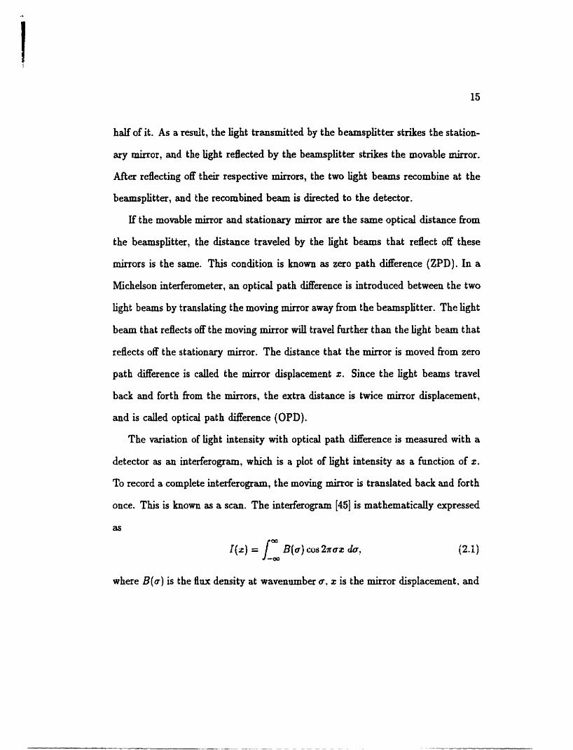
The variation of light intensity with optical path difference is measured with a

detector as an interferogram, which is a plot of light intensity as a function of x.

To record a complete interferogram, the moving mirror is translated back and forth

once. This is known as a scan. The interferogram [45] is rnathematicdy expressed

where B(u) is the flux density at wavenamber a. z is the minor displacement. and

I ( x ) is the interf'ogam. The inverse Fourier t r d o r m is

The value of x is determined by the product of the constant velocity of the moving

mirror and the time since the initial &or displacement of the scan. The mirror

veiocity and time are electronically controiled to high precision with the aid of

a singlemode He-Ne laser. This precision in the contrai of mirror displacement

provides a built-in frequency calibtation of the spectrnm. The spectrum, which is

a plot of light intensity as a fnnction of frequency, is obtained by calcdating the

Fourier transform of the interferogram (Equation (2.2)).

2.2 Advantages of Fourier Transform Spectroscopy

Michelson was aware of the potential use of his interferorneter to obtain spectra. and

manually measured many interfkrograms [52]. Unfortnnately, the time consuming

calculations required to convert an interferogram into a spectnim made using an

interfaorneta to obtain spectra impractical. It was the invention of cornputers

and the Fast Fourier Trandorm algorithm that established the basis for Fourier

transform spectroscopy [53].

The ultimate performance of any spectrometer is determined by measuring its

signal-to-noise ratio (SM). SNR is caldated by measuring the peak height of a

featare in an hfkared spectram, a d ratioing it to the level of noise at some baseline

point nearby in the spectrum. Noise is usnally observed as random hctuations

in the spectnun above and below the badine. For a given sample and set of

conditions, an instrument with a high SNR wilI be more sensitive, and d o w spectral

features to be measured more accurately than an instrument with a low SNR.

There are two reasons why Fourier transform spectrometers are capable of

achieving SNR significantly higher than dispersive instruments. The first advan-

tage is called the multiplex or Fellgett advantage. It is based on the fact that

light fkom the entire spectrum is detected at once, whereas in dispersive scanning

spectrometers, only a small wavenumber range at a time is measured. The noise

at a specsc ravenuniber is proportional to the square root of the time spent ob-

serving that wavenumber. If the dominant source of noise is hom the detectors or

the background. then the Fourier transform spectrometer d l have a rnultiplexing

advantage. The practical advantage of mdtiplexing is that a Fonrier transform

spectrometer can acquire a spectnun much faster than a dispersive instrument.

The second advantage is called the throughput or Jacquinot advantage. It is basd

on the fact that the circular apertures in Fourier transform spectrometers allow

a higher throughput of radiation than throngh the slits used in dispersive spec-

troriieters. There are no slits to restrict the wavenumber range and to reduce the

intensity of radiation. The detector, therefore, meastues the maximum amount of

light at dl points during a scan.

The advant aga of the Fourier traiisform spectrometer provide high resolu tion

and good sensitivity. The maximum spectral resolution [12] of an interferorneter is

invasely proportional to the maximum OPD dowed,

0.6 6a = -

OPD*

It follows that a Fourier transform spectrometer requires a large mirror displacement

and accurate control over the rnoving &or for recording high resolution spectra.

In an ideal interfkrometer, the light beam is a pdectly collimated cylinder,

and dl light rays are parallel to each other. In reality, the optics are not pedect,

and the light beam shape is not a cyhder, bat usnally a cone. The light rays in

a beam are not parallel, bot form an angle to each other. This phenornenon is

known as angnlar divergence. Because of angular divergence, light on the outside

of the beam travels a dinerent distance than light in the center of the beam. These

Lght rays can interfere destructively with each other. Angular divergence inmeases

with optical path merence because the light beam spreads out more the fnrther it

travels. Aperture size, t herefore, provides a practical limitation on resolution. The

achievable resolution [45] fiom an apertnre of diameter d is given by the expression

where F is the focal length of the interferorneter and o is the wavennmber being

analyzed.

The above equation exposes a serious challenge to the high resolution spec-

troscopist. The Iargest possible signal is obvionsly obtained throagh the use of

a large aperture, while conversely. hi& resolution requires that a s m d aperture

be used. The analysis of transient moleCuiest which are characterized by low con-

centrations and s m d signals, demands t hat the sensitivity factors be maximized.

These factors apart from aperture size, are quality of the light source. efnciency of

the beamsplit ter, transmit tance of the windows, and sensitivity of the detectors.

To obtain improvernents in signal, ofken some s a d c e in resolution needs to be

made in order to obtain a u s a spectruxu. The signai-to-noise r+.!i~ can &O b.i

improved by c*adding successively recorded interferograms.

2.3 The Bruker Spectrometer

The Bruker IFS 120 HR Fourier transform spectrometer, which ha9 been used

through this study, is one of the best and most versatile instruments of its kuid

available. Its design is optimized for spectroscopie measurements in the entire

infrared region at either high or low resolution. By choosing diffaent combinations

of Ïight sources, beamsplit ters. windows and detectors, the instrument can achieve

a resolution of better than 0.002 cm-' in spectral range extending fiom the far

in.ûared to the near ultraviolet (50 - 40 000 cm-').

The opticai layont of the Bruker spectrometer is shown in Figure 2.2. Radiation

from three water-cooled interna sources, or extemal sources for emission experi-

ments, entas the Michelson interferorneta throngh a eircuiar aperture of a chosen

diameter, ranging fiom 0.5 to 12.5 mm. The Braker Michelson interferorneter bas a

maximum optical path ciifference of approxîmately 4.8 meters, and thus a resoltttion

limit better than 0.002 cm-! The position and speed of the movable mirrot are

controlled by a single mode stabiliaed He-Ne laser. The recomhined beam leaves the

bearnsplitter and passes throngh an optical filter. The beam is then focused onto

one of the available detectors. There are four intemal detector positions. Among

them, one is used to hold a iiqttid nitrogen-cooled InSb detector (1800 - 9000 cm-'),

and one is nsed to hold a liquid nitrogen-cooled HgCdTe (MCT) detector (800 -

2000 cm-'). Two externa1 detector positions are available. A liqnid helium-cooled

boron doped dicon (Si:B) detector (350 - 3000 an-') and a liquid helium-cooled

bolometer (10 - 360 cm-') can be mounted at the extemal positions. The lower

iixnits of InSb, MCT and Si:B detectors are determined by the band gaps of the

materials. The upper limits are determined by the start of the next detector. The

response of the bolometer is flat over the entire spectral range, however, two cold

filters inside the bolometer set the upper limits to be 200 and 360 cm-', respec-

tively. The entire spectrometer can be evacnated to less than 0.02 Torr. The optical

hc t ions of the spectrometer and the collection, handling and output of data are

contrded by a personal cornputer ninning the OPUS software program which is

designed by Bruker.

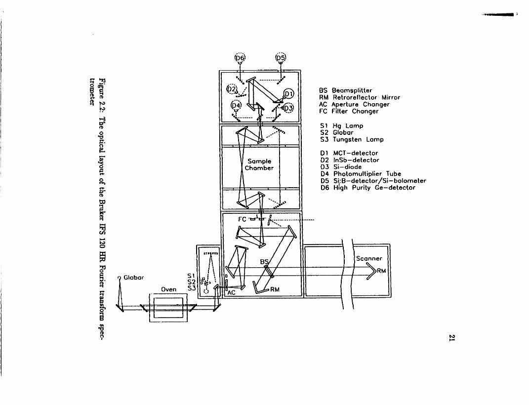
Filter Changer -

Hg tomp Globor Tungsten Lamp

MCT -detec t or InSb-detector Si-diode Photomultiplier Tube S!:B-detector/Si-bolorneter High Purity Ge-detector

Chapter 3

Infrared Spectroscopy of Diatomic

Molecules

A large amount of information on the physical propesties of molecdar speues can

be obtained fiom their spectra. One main objective of spectroscopy is the ex-

traction of concise representations of physicaily meaninghil data from the large

number of spectral iine positions. The reduction of line positions to spectroscopic

constants is accomplished t hrough the use of theoretical models. The set of spectre

scopic constants can serve as a compact representation of the experimental observa-

tions. A theoretical modd can help to derive the strncturdy relevant information

fiom e*pr?rirnental data, and predicb energy leveb for unobserveri transitions to

a certain degree of acmacy. The foundation of most theoretical models is the

Born-Oppenheimer description of the moledar system. The use of the Born-

Oppenheimer approximation greatly simplifies the Schriidinger equation.

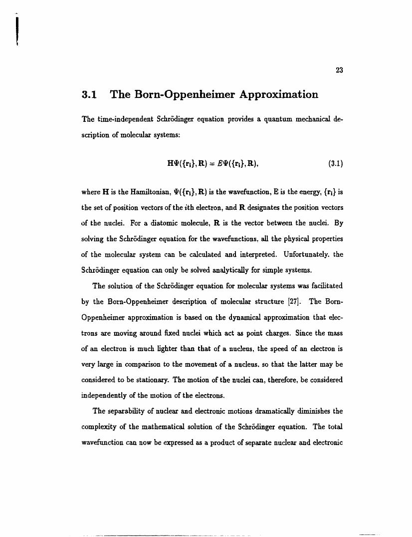
3.1 The Born-Oppenheimer Approximation

The tirne-independent Schr6dinger equation provides a quantum mechanical de-

scription of moledar systems:

where H is the Hamiltonian, @({ri), R) is the wavefanction, E is the energy, (ri) is

the set of position vectors of the ith electron, and R designates the position vectors

of the nuclei. For a diatomic molecule, R is the vector between the nu&. By

solving the Sehr6dinger equation for the wavefonctions, all the physical propetties

of the molecular system cm be calcnlated and interpreted. Unfortunately. the

S chrodinger equation can only be solved analyticdy for simple systems.

The solution of the Sùudinger equation for molecular systems was facilitated

by the Born-Oppenheimer description of molecnlar structure [27]. The Born-

Oppenheimer approximation is based on the dynamical approximation that elec-

trons are moving around fixed nudei which act as point charges. Since the mass

of an electron is mudi lighter than that of a nudeas, the speed of an electron is

very large in cornparison to the movement of a nucleus. so that the latter may be

considered to be stationary. The motion of the nadei cm, therefore, be considered

independently of the motion of the eiectrons.

The separability of nudear and electronic motions dramaticdy diminishes the

complexity of the mathematical solution of the Schriidinger equation. The total

wavefunction can now be expressed as a product of separate nudear and electronic

The total energy can be partitioned to

where En is the nuclear energy and U(R) is the electronic energy. The electronic

wavefanction. &(R) satides a unique Schrodinger equation which only represents

the motion of electrons

It is noticed that U and +e are fimctions of R, so a change in nudear position

results in a correspondhg change in the dectron charge distribution. The fùnctional

dependence of electronic enetgy on nuclear positions is called the potential energy

of nuclear motion.

The solution of the electronic Schr6dinger equation is used in the derivation

of the nnclear Schr0dinge.r equation. The mathematicd procedare is the physical

equivalent of stating that nudear motion takes place in an average field of electron

motion. The Sihdinger equakion of hhe molecular system now can he expressen

as

motion are separated, the Schrdinga eqnation of nadear motion is then

The nuclear motion can be further separated into rotation and vibration. This is

justified becanse vibration taLes place on mach shorter tirne scde than rotation

does.

For a diatomic molecule consisting of atoms A and B, the nuclear Hamiltonian

is

where MA and Mg are the nudear mass of atoms A and B respectively, and PA and

PB are the momenta of the nuclei of atoms A and B respectively. The electronic

Hamihonian is

where e. and m. are charge and mass of an electron, R is the internuclear separation

of A and B, ZA and ZB are nuclear charge of A and B, and RB are the distances

between ith electron and A or B, Q is the permittivity of vacuum, and t i j is the

distance between the ith and jth electrons.

In the case of a 'C+ electronic state, the wavehuiction of nudear motion is

where Yi,, are the spherical harmonic functions, which are the angular part of the

rotational wavefunction. The remaining task is to solve for the radial part of the

wavefunction $"J( R) from the effective one-dimensional SchrOdinger equation [3 11

where p is the reduced mas .

An important consequence of the Boni-Oppenheimer approximation is the con-

cept of the intemudear potential function U(R). This function is the average field

of electronst in which the nuclear motion takes place. There is no universd ana-

lyticd expression for U(R). Closed f o m mathematical expressions for II( R) may

be determined for systems individually. Bot such procedures are very complex and

have only b e n derived for very simple systems. Equation (3.10) may then be solved

u s u d y by numerical methods using a h c t i o n U(R). U(R) may be detamined

e m p l i c d y ~ or fiom the solution of the electronic Schrdinger equation by a variety

of met hods, or by combinations of both.

The choice of mode1 for the potential energy fimction used to solve the nuclear

SchrSdinger equation is critical in the analysis of the rotation-vibration spectra of

diatomic molecnles. Rotation-vibration spectra experimentally sample the separa-

tion between enagy levels of nuùei in different rotational and vibrational states. An

empkical U(R) may be constructed fkom the separation of enetgy levels elucidated

in spectra. High quality theoretical U(R) allow for the accurate extrapolation of

empkical potential fnnctions to energy levels beyond those observed experimentally.

3.2 Born-Oppenheimer Breakdown

The b i t s of the Born-Oppenheimer approximation and the concept of the inter-

nuclear po tential energy function have been revealed t hrough the interaction of

spectroscopy and theory. Evidence of Born-Oppenheimer breakdown was h s t sys-

tematicdy studied by van Vleck (281 $ta the discovery of d e u t a i m . As the

m,/M ratio has its greatest value for hydrogen, the efEects of Born-Oppenheimer

breakdown were most obvioas in hydrides.

Many studies on the nature and the magnitude of the Born-Oppenheimer break-

down in various moledes have been carried out [29,30]. Breakdown effects are

detected through the failure of theoretical relationships between spectroscopic con-

stants to describe experimentally derived constants. For example, let i and j be

two isotopomers of a molecde, the relationship between t heir rot ational constants

For hydride and deuteride isotopomers, the breakdown of this relationship was

reported in the 1930's [54]. As spectroscopic techniques become mGre accurate,

this breakdown is &O observed in heavier molecules [55]. Other experimental

examples of the Born-Oppenheimer breakdown include the fdure of relationships

between lower and higher orde spectroscopic constants of a single isotopomcr, the

coupling or perturbation between dinerent electronic states in the molede.

Breakdown effects may be characterized int O two different categories: adiabatic

and non-adiabatic [30]. Adiabatic corrections are necessary to account for the efFect

of the neglected kinetic energy of the nudei within each electronic state. In infrared

spectroscopy, adiabatic corrections are the resdt of the couphg between naclear

motion and electronic motion in the isolated electronic state. Non-adiabatic conec-

tions are necessary to account for interactions with other electronic states. Local

non-adiabatic breakdowns are regalarly detected experimentaily in the spectra of

rotationally and vibrationdy highly excited molecuies, made visible as perturba-

tions in the observed line positions. When the efFects of non-adiabatic coupling are

significant, the concept of U(R) , which is only responsible for nudear motion in an

isolated electronic state, does not provide an adequate explanation of physicd p r e

cesses. The remedy is to solve the Schrôdinger equation for complete wavefunctions

t hat explain nudear motion and electronic motion simdtaneously.

3.3 The Dunham Potential Mode1

The Dunham model was developed by J.L. Dnnham in 1932 (321. It has b e n

widely used ever since its introdnction. The Donham energy level formuiation has

been adopted for the analysis of rotation-vibration spectra in both high resolation

i ha r ed spectroscopy and microwave spectroscopy. knprovements in spectroseopic

techniques have r s d t e d in the determination of numeroos limitations of the model,

spurring the modification of the original D d a m expressions.

Dunharn chose to represent U( R) as a Taylor series expansion about the equi-

libriam inteniaclear separation &, where U(& ) = O,

where

and the set of {q) are the D d a m potential parameters. Using Equation (3.12)

for U ( R) , Dunham solved the firstsrder semi-classical Wentzel-Kramer-Brillouin

(WKB) quantkation condition [31]

to determine E(v , J ) , where R+ and R- are the classicai tnrning points for the po-

tential c w e at energy E(v, J ) . The result was the compact energy Ievel expression

where the K j Dunham coefficients are explicitly known functions of the potential

expansion parameters {ai).

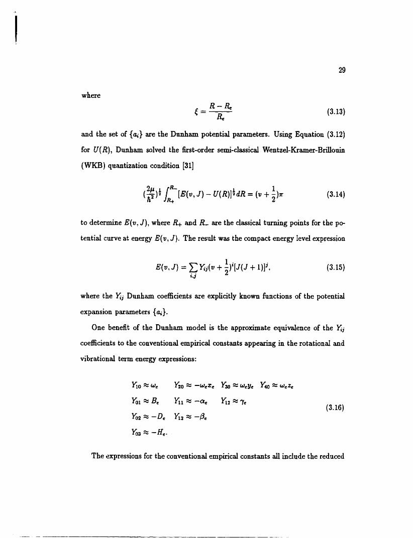
One benefit of the D d a m mode1 is the approximate equivalence of the xj coefficients to the conventionai empirical constants appearing in the rot ationd and

vibrat ional term energy tzcpressions:

The expressions for the conventional empmcal constants ail indude the redaced

mass of the molecale. The values of the sj coefficients are &O dependent on the

reduced mass of the molecale, and therefore, different isotopomers of a molecde

must have different sets of Dunham coefficients. Within the hst-order of WKB

approximation and the Born-Oppenheimer approximation, the rednced m a s de-

pendency of the xj coefficients can be factored out and the energy levels expressed

in terms of mass-independent Dunham coefficients II,,

When the fitting of spectroscopic data on multiple isotopomas of the same species

to Equation (3.17) fails. it reveals the failure of the Born-Oppenheimer approxima-

tion. This is so because the derivation of the Dunham energy level expression is

based on this approximation. The fact that the Born-Oppenheimer approximation

is not fully valid means that the approximate relation

is observed to breakdown. The above expression has routinely failed to explain the

relationships between the experimentally derived constants wit hin the experiment al

mors.

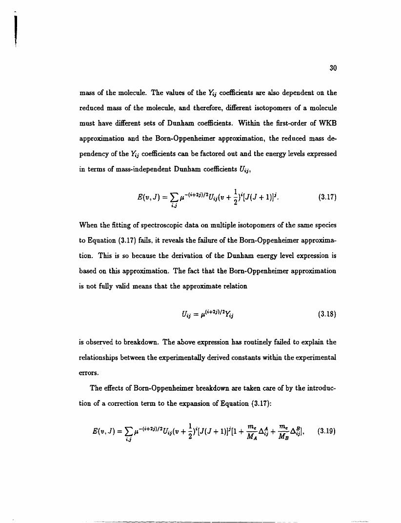
The effects of Born-Oppenheimer breakdown are taken care of by the introdnc-

tion of a correction term to the expansion of Equation (3.17):

where the Aij parameters are mass-independent breakdown constants. Equation (3.19)

was first introduced by Ross and CO-workers [56]. Later, it was theoreticaily justi-

fied by both Watson [57,58] and Bunker [59]. Equation (3.19) is usually reférred to

as the Watson modified mass-independent D d a m expression because of Watson's

major contribution.

The Aij parameters are empirical constants which take account of the Boni-

Oppenheimer breakdown. They are expected to be dose to unity for a well isolated

electronic state. The Aij parameters are the sum of the adiabatic correction term.

the non-adiabatic correction term, and the Dunham correction term 1321,

The Dunham correction term (A:)~** takes into account the failure of the

semi-classical WKB quantization condition to f d y explain ail quantum mechanical

effects 157.581.

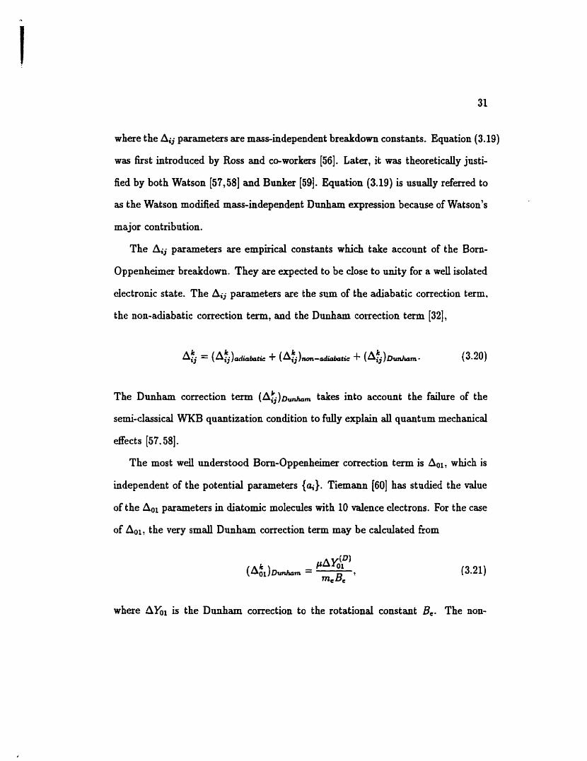
The most well understood Born-Oppenheimer correction term is Aoi, which is

independent of the potential parameters {ai). Tiemann [60] has studied the value

of the Aoi parameters in diatomic molecules with 10 valence electrons. For the case

of Aoi, the very small Dunham correction term may be ca lda ted fiom

where AKi is the D d a m correction to the rotationai constant B.. The non-

adiabatic contribution may be determined fiom

where m, is the mass of the proton and g~ is the rotational g factor meamred

in a Zeeman experiment. The term has no comparable independent

method of caldation. On average, the value of is l e s than 30% of

the total Atl d u e . It is predominantly eharacteristic of the atomic mas, and

therefore is independent of the bonding partner.

One trend was the determination of abnormally large Aol parameters for heavy

atomic centers [60]. Tiemann stodied this enlargement of Aol, and attnbuted it to

the effects of an isotopic field shih [61-641. For large nadei such as Pb and Tl [62],

the difference in the Coulomb potential of the tao isotopes results in a corresponding

energy shin of the obswed line positions. The field shift was characterized by

mat hematical expressions (641.

While the effects of field shin are not often applied to the examination of Aal

parameters directly. they do illustrate the limitation of Equation (3.19). The Aij

are empirical parameters, so that they cannot distinguish between different failures

of the Born-Oppenheimer approximation and the Dunham model. The values,

therefore. lack physical sign<ficance.

The Dunham potential parameters ai are functions of the enagy level coeffi-

cients:

As Dunham stated in his original papa, the Dunham potential can be expressed

entirely by the x0 and El coefficients. The immediate implication is that all xj coefficients with j 2 2 can be expressed in terms of the x0 and coefficients [58].

These constraints can act as tests to confirm that the empirically obtained param-

eters agree with the physical modd of the Dunham inteniuclear potential energy

The mass dependence of the D d a m coefficients can be derived directly from

expressions of (ai) given in Equation (3.23), by using the relationship in Eqna-

tion (3.18). Consequently, the theoretical relationships between IIij coefficients c m

be established, for example,

These relationships are only approximatc if thme CIij constants have absorbed the

AG corrections. The Aij terms in Equation (3.19) correct for the effects of Born-

Oppenheimer breakdom, so that equations like (3.24) become exact. Ln this case.

the values of the Uij coefficients with j 2 2 are ca ldated as Fanctions of empirically

determined Uio and UiI coefficients.

In spite of its wide spread application and constant improvement, there are

several limitations to the Dunham model. The major problem is that the Dunham

model is a poor choice of potential energy fnnction. In practice any Dunham

series is t m c a t e d to a finite nnmber of terms, and this polynomial diverges as

the intemudear separation increases, i.e., R + oo, while the realistic potential

function is bounded by the dissociation enagy. Thus, the Dunham model cannot

accurately describe the high vibrational states because the long range interactions

between atoms are poorly expressed. Because the Dnnham potential is hadequate,

the D d a m coefficients are not ideal for andyzing highly vibrationdy excited

states, and cannot reliably extrapolate to energy levels beyond the range covered

by experiment al observation.

-3.4 The Parameterized Potential Mode1

Another approach to reduce spectroseopic data to molecular constants is to use the

parameterized potential model. In this model, the observed line positions are fit di-

rectly to the eigendnes of the radiai Schr6dinger equation containhg an empirical.

or a semi-empirical parameterized patentid function. Synthetic spectra are pro-

duced by numerically solving the Schrodinger eqnation for all eigenstates involved

in the spectra. Then the agreement with experiment is optimized by varying the

parameters used to define a model potential for U!R). This method was used for

atom-molecule van der Waais complexes [65]. The method was first applied to

diatomic molecules by Kosman and Hhze (661, and was termed "invene perturba-

tion approachn, or "PAn. There was sigiuficant rehement of this technique by

Bunker and Moss [33], and more recently by Coxon and Hajigeorgiou [34-361. This

procedure has not been widely adopted, and the simpler semi-dassical Rydberg-

Klein-Rees (RKR) approach is still commonly used.

The direct deter mination of a parameterized potential fiom experiment has sev-

erai advantages over the Dunham model. The parameters defîning the potential

fnnction are determined by solving the Schriidinger equation of the moledar sys-

tem. The mors that are associated with the WKB approximation are avoided. It

has become possible to incorporate into the andysis sophisticated physical behav-

iors detennined fiom non-spectroscopic techniques. The resulting potential func-

tions are more reliable at long range. They can be used to predict observables

such as transition fiequencies between nnobserved levels [23], bulk properties of the

system, and collisional phenomena [67].

An inherent limitation of the parameterized potentid rnodel is the assumed

functional form of the interaction potential. Given a particdar fûnctional form.

there exists no general proof that the redting parameterized potentid is a unique

representation of the experiment. Since the model needs to be general, the hinc-

tional form for the potential mnst have flexibility. The fanctional form should be

flexible enough to describe the physical information contained in the data while

not introduhg large statistical inter-parameter correlations. A good fùnctional

form will be optimized in the region where data are observed, but will &O pro-

vide rneaningful information for the internudear separations not sampled by the

observed data.

The functiond form used in this stndy was provided by D d c k (68-701. It is

a modification d a huiction used by Cuxm and Hajigeorgiou to fit a wide range

of spectroscopie data [34-361. The function is contained within the effective radial

Schriidinger equation for a diatomic molecule in the ' C+ electronic states, given by

A centrihigal correction factor 1 + q(R) is introduced to take account of rota-

tiond Born-Oppenheimer breakdown dects. The dect ive internadear potential

for purely vibrational motion U e f f (R) is given by

wbere US' is the Born-Oppenheimer potential, and UA and Ug are the correction

functions for each atomic center respectively. UBo is chosen to be a modified Morse

where De is the dissociation energy of the rnolectde, and is used as a h e d constraint

in the fitting of data. T h P( R) t e m is the variable Morse nirvature function. which

accounts for radial dependence of the anharmonicity functions. P(R) is given as a

polynomial expansion n

P(R) = z C/3izi. i=O

P(m) is given by

is one-half of the Ogilvie-Tipping variable. The parameterized Morse hinction gives

excellent convergence and has been shown to behave welI for large intemuclear

separation R.

Throngh fitting data to Equation (3.25) using the potentid given by Equa-

tion (3.26), the correction terms are divided into vibrational and rotational Born-

Oppenheimer breakdown terms. As the energy of vibrational motion increases,

nuclear e x i t ation moves to the electron dond, thereby conpling the electrons f?om

distant C states to the ground C state. These homogeneoas, non-adiabatic e£Fects

along with any J-independent adiabatic effects are accounted for by the UA and

LIE fnnctions. These two functions are given by power senes expansions:

and

The coefficients are isotopicdy invariant. As the energy of rotational motion

increases. nuclear ôngular moment um moves t O the valence electrons , result h g in

a net non-zero electronic angnlar momentum as the electron distribution along the

internuclear axis becomes distorted. The electronic angdar momentum imparts a

partial II character into the C state. thereby resulting in couphg of the ground

electronic state with distant II states. These heterogeneous non-adiabatic effects

are accounted for by

3.5 Infrared Emission Spectroscopy of BF and

Since the BF spectrum was îust observed by Duil [71] in 1935, BF has been sub-

ject to numerous spectroscopic studies 172-811. The electronic emission spectra

of BF were recorded in many laboratones, but it was not until 1969 that Caton

and Douglas [79] fùst studied electronic absorption spectra of BF. In th& re-

port, Caton and Douglas gave an excellent overview of the eiectronic spectra.

They not only clarified the assignments of the electronic states, bat &O they o b

served a series of Rydberg states approaching the ionization limit. which enabled

them to determine the ionization potential (LP.) very accurately. Their value of

LP. (11.115 i 0.004 eV) agrees w d with the values obtained fkom electron im-

pact mass spectrometry (11.06 f 0.10 eV) [82] and photoelectron spectroscopy

(11.12 k 0.01 eV) 1831. Lovas and Johnson [84] recorded the îust microwave spec-

trum of BF. They measured the J = 1 + O transitions of "BF and I0BF and

andyzed the hyperfine structure. They reported a dipole moment for u = O of 0.5

f 0.2 D for BF. Recently. Cazzoli et al. extended the frequency coverage of the

microwave spectrnm and obtained more transitions [85]. Nahaga et al. measured

12 vibration-rotation transitions of "BF hindamentd band nsing a diode laser [86].

The vibrational band strength of "BF was measured, and the d u e of dpldr was

fotmd to be 4.9 f 0.8 DIA [87].

Since BF is a member of the int aes ting isoelectronic group of molecules NI, CO

and BF, several detailed theoretical caldations of the properties of the ground and

excited states have also been carried out [88-953. The spectroscopic constants are

in good agreement with the experimental values, including the value for dpldr. The

d u e of the calculated dipole moment is about twice the experimental value, so it

has been suggested that Lovas and Johnson underestimated po in their experiment.

During the course of this experiment, an improved spectrum of AiF was recorded

as impurity. This spectnun was aiso anaiyzed to prodace npdated spectroscopic

constants and potential huiction.

3.5.1 Experiment

BF was generated inadvertently during our spectroscopic study of the CaF [96]

free radical. A mixture of a trace amount of boron and 40 g of CaF2 powder was

contained in a carbon boat, which was placed in a reaction c d . The reaction cd

consisted of a 1.2 meter long alrimina (&O3) tube seded with two KRS-5 windows

at both ends. The dumina tube was further protected fiom the corrosive efFects of

the Ca& salt by a carbon liner tube. The central portion of the cell was situated

inside a CM Rapid Temp h a c e (Figure 3.1). The farnace was heated by eight

molybdennm disdicide elements. A Honeywell aniversal digital controller was nsed

to provide control over the temperature of the heating system. The maximum

heating rate which will prevent the dumina tube îkom cracking is 200°C per hom.

The cd was fkst heated unda vacuum up to 500°C, and was then pressurized

with 5 Torr of argon to prevent deposition of solid material onto the cd windows

which were at room temperature. Stainless steel threaded caps that held the c d

windows were placed on the end of the tubes. Copper cooling CO& that snrrounded

the end caps prevented them from overheating and melting the rubber O-rings.

There are two ports attached to the c d . One is for the gas inlet, which allows the

introduction of argon gas into the c d , the other is comected to a vacuum pump.

The alumina c d was aligned to the optical axis of the spectrometer through the

use of an external globar lamp. When the c d tempaature reached 1600°C. strong

emission of BF and AlF was detected.

When the temperature was below 1400°C. strong absorption of BF3 bands was

observed. The onginal experiment ras to record spectra of C S 2 and CaF. But

no band of CaF2 was found in the survey spectra. As the temperattue increased,

the intensity of BF3 absorption bands decreased, and BF started to form. The

high resolution spectnim of BF was recorded at a resolution of 0.01 cm-! A

Lquid nitrogen-cooled HgCdTe detector, a KBr beamsplitter, and a KRS-5 entrance

window were used. The Iowa limit of the spectral bandpass was set by the detector

response at 850 cm-' while the upper iimit was set by a red pass optical füter with

a cnt-off wavenumber of 1670 cm-'. The final spectnun of BF was a resdt of

ceadding 40 scans in about 40 minutes. A section of the spectram is shown in

Figure 3.2. AIF emission spectrum was obtaired in a similar way except a Si:B

photodeteetor was used.

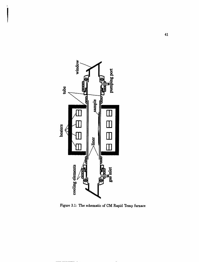
Figure 3.1: The schematic of CM Rapid Temp fùrnace

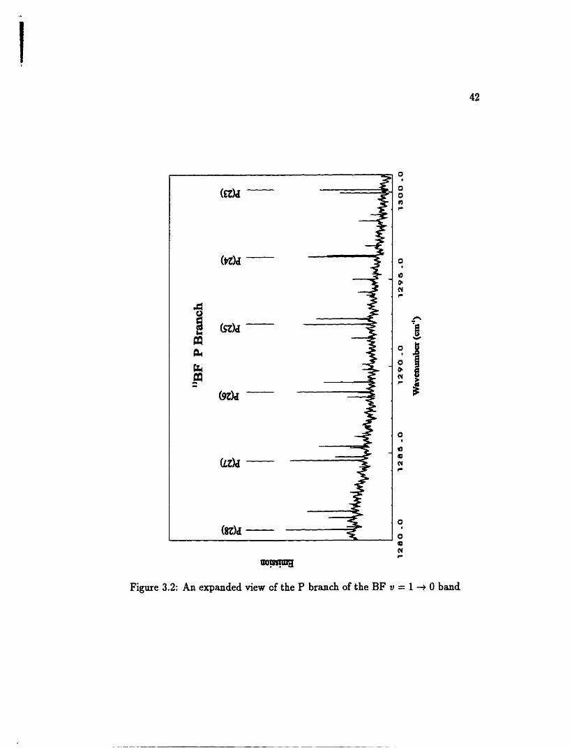
Figure 3.2: An expanded view cf the P branch of the BF v = 1 -t O band

3.5.2 Results and Discussion

Since BF3 was present in the cell when the spectnun was taken, part of the R

branches of "BF and all of the R branches of lCBF were buried in the absorption

of the us band of BF3.

The rotational lines are measured nsing the cornpater program PGDECOMP

developed by J.W. Brault. Rom the displayed experimental spectra, the user

chooses a baseline and selects spectral featmes of interest. The program then fits

each line profile to a Voigt line shape hinetion, which is a convolution of Gaussian

and Lorenziao h e shape hctions. The separation of different vibrational bands

and the assignment of the rotation-vibration transitions are facilitated by LOOMIS-

WOOD. an interactive color graphics program developed by C.N. Jarman.

The pure rotational h e s of RF which were present in the spectra as an impurity,

were used to calibrate the BF and AIF spectra [97]. The error in the calibrated line

positions is estimated to be 0.0002 cm-l for "BF and 0.0005 cm-' for 'OBF and

AU?. Five bands of "BF fiom u = 1 -t O to v = 5 -t 4 are andyzed, while three

bands of l0BF h m v = 1 + O to v = 3 -t 2 are studied. The line positions of BF

are given in Table A.1

"BF and 'OBF Dunham xj coefficients were determined fiom the observed line

positions fÎom a hear le&-squares fit. Mcrowave meastuements of the llBF and

'OBI? pure rotational transitions, with hyperfine structure corrected by Cazzoli et

al. [85], were &O added as input to the linear fit. The Dnnham coefficients for both

isotopomers are listed in Table 3.1, while the mas-rednced Dunham UG coefficients

are listed in Table 3.2. In Table 3.2, under the colamn heading "unconstrained",

the Uij coefficients were obtained fiom a combined fit of isotopomer data to Equa-

tion (3.17).

Since only one n a t u d y occurring isotope of fluorine exists, al1 isotopic infor-

mation on Born-Oppenheimer breakdown is confined to the boron atom. Therefore,

only Aij for the boron atom were determined fiom the least-squares fit of the data.

Finally, the set of Uij under the c o l m heading "constrained" in Table 3.2 were

obtained from a fit where the Ir, for j 2 2 were treated as independent parameters

while all remaining II, were k e d to values determined fiom the constraint rela-

tions impliut in the Dunham mode1 [98]. The rednced X 2 of the "unconstrained"

and "constrainedn fits are 0.9727 and 0.9667 respectively. It is believed that the

constrained fit is more meaningfd since it uses fewer parameters. Indeed the A:

parameters for the constrained fit have mach more reasonable values.

In order t O es timat e information on the high-lying rot ation-vibration levels of the

ground state, a diable inteniudear potential energy function is required. Such a

potentid hinction can be determined iiom a least-squares fit [98] of the combined

"BF and 'OBF data to the eigenvaiues of the radial Schriidinger equation.

Our fitting procedure is similar to the method reported by Coxon and Haji-

georgion and is described in greater detail elsewhere. None of the q parameters

that correct for J-dependent Born-Oppenheimer breakdown in the centrihigal term

could be determined using our data set. Results of the potentid fit are given in

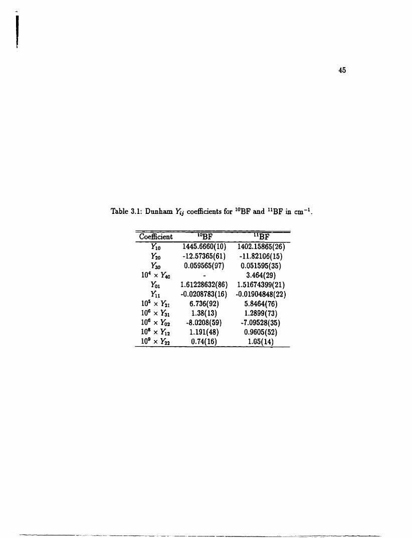
Table 3.1: Dunham K j coefficients for 'OBF and "BF in cm-'.

Coefficient l0BF "BE %O 1445.6660(10) 1402.15865(26) f i 0 -12.57365(61) -11.82106(15) y-& 0.059565(97) 0.051595(35)

lo4 y, - 3.464(29) Gr 1.61228632(86) 1.51674399(21) Yi r -0.0208783(16) -0.01904848(22)

lo5 6.736(92) 5.8464(76) IO6 x G1 1.38(13) 1.2899(73) IO6 x y02 -8.0208(59) -7.09528(35) 108 x Ki 1.191(48) 0.9605(52) log x 0.74(16) 1.05( 14)

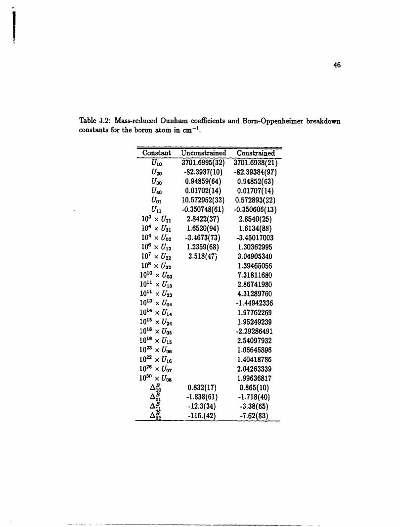
Table 3.2: Mas-rednced Dunham coefEuents and Born-Oppenheimer breakdown constants for the boron atom in cm".

Constant Unconstrained Constrained &O 3701.6995(32) 3701.6938(21)

Table 3.3. The potential energy c u v e of BF is shown in Figure 3.3. Potential pa-

rameters that were statisticdy detamined are listed dong with their uncatainties

quoted to one standard deviation. The value of De was fixed to t hat given in Buber

and Herzberg 1991. The standard deviation of the fit is 1.5864.

The analysis of AlF spectnun was similar to that of BF. Hot bands of AU?

up to v = 9 + 8 were meagured. The updated Dunham coefficients for AU? are

Listed in Table 3.4 together with those reported in Ref (1001. Although the highest

vibrational energy level accessed is v = 5 in the previotu work [IO01 while transitions

involving up to v = 9 were meastued in this study, the changes in the Dunham

coefficients are very small. This indicates that the Dunham mode1 is adequate

for a moderately heavy molecde such as AU?. A parameterized potential was also

determined, and the potential energy parameters for ALF are given in Table 3.5.

The value of De was also fixed to that given in Haber and Herzberg [99].

Relative Tkansition Dipole Moment

The experimental intensity parameters are very important in the evaluation of

abundances and temperatures of gaseous species by spectroscopic means. Mea-

suring line intensities are &O important for the understanding of the variation of

the molecdar dipole moment with respect to normal coordinates, i.e. the dipole

moment fanction [lOlj. Rmap. , rotation-vibration h e mtensities of Erec radicals

are difEcult to rneasure because of the srnail and uncertain column densities.

In our spectroscopic study of BF, we obtained a relatively high signal-to-noise

spectnim (Figure 3.2), thus enabling us to investigate the line intensities of BF.

Since there was no means of obtaining the concentration of BF present in the

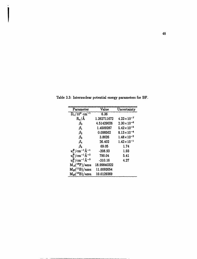
Table 3.3: Internudea. potential enagy parameters for BF.

Parameter Vahe Uncertainty ~ ~ 1 0 ~ cm-1 6.36

&/A 1.262711672 4.23 x IO-^ P o 4.51429026 2.30 x Pi 1.4509287 5.42 x /32 0.098562 8.13 x 10'~ Ba 3.8626 1.48 x a 4 26.402 1.42 x 10'' p 5 69.05 1.74

u ~ / ~ m - ~ A - ~ -208.93 1.93 ~ f / r n - ~ A - ~ 790.04 5.41 u 3 / c m - l k 3 -310.16 4.27 MA(l9F)/amu 18.99840322 MB(llB)/arnu 11.0093054 M ~ ( ' ~ B ) / a m a 10.0129369

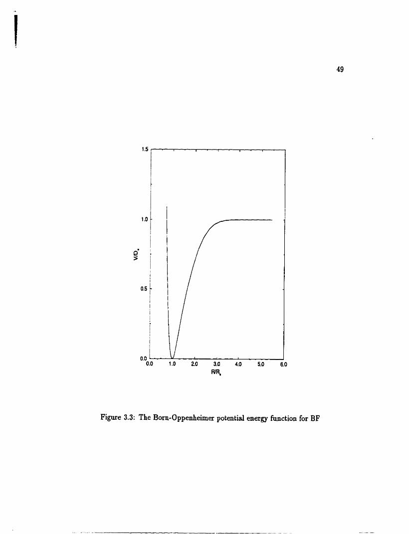
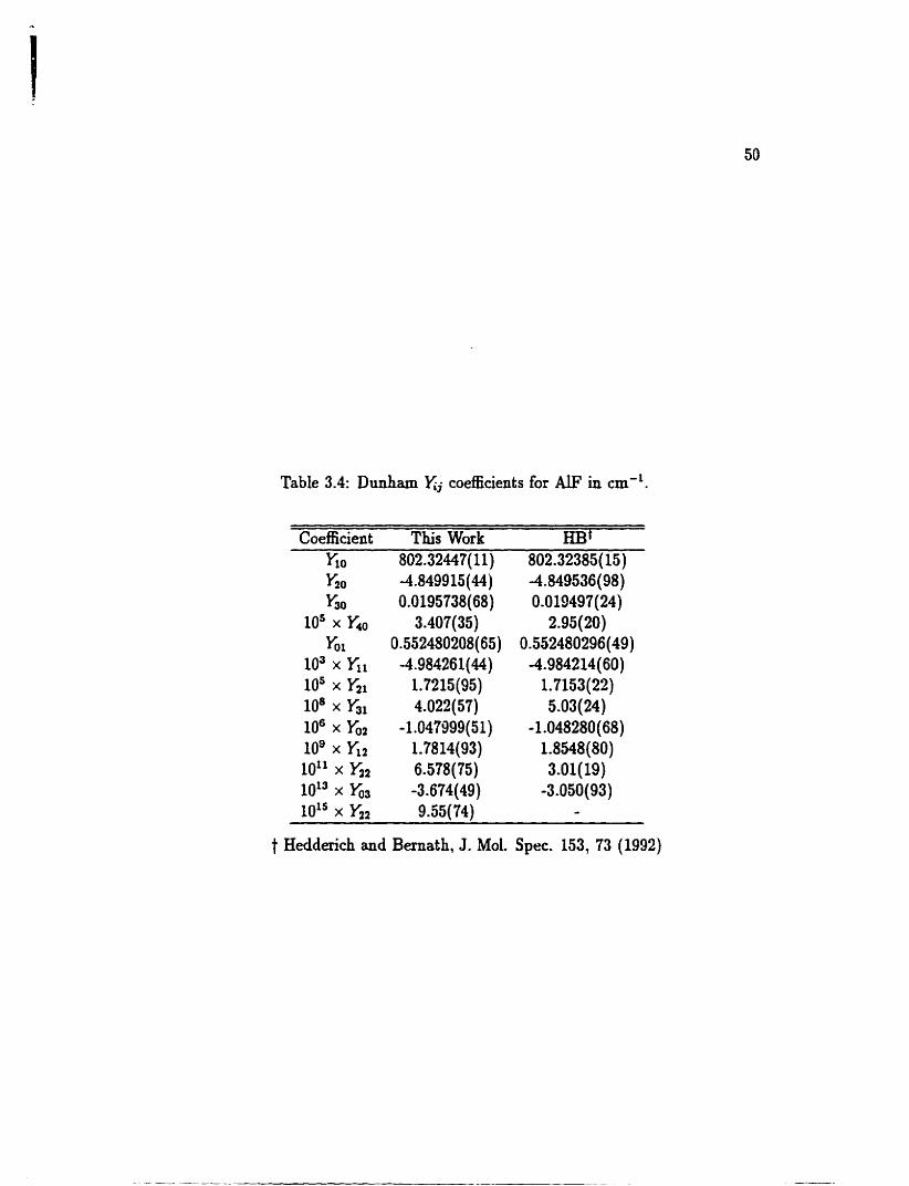
Table 3.4: Dunham xj coefficients for AlF in cm-'.

Coefficient ThisWork HBt &O 802.32447(11) 802.32385(15) &O -4.8499 15(44) -4.849536(98) y30 0.0195738(68) 0.019497(24)

los x &O 3.407(35) 2.95(20) &i 0.552480208(65) 0.552480296(49)

10% Yil -4.984261(44) -4.984214(60) los yti 1.7215(95) 1.7153(22) 108 x hl 4.022(57) 5.03(24) 10' x -1.047999(51) -1.048280(68) log x &2 1.7814(93) 1.8548(80) 10" x K2 6-578(75) 3.01(19) loi3 x ha -3.674(49) -3.050(93) 1015 x K~ 9.55(74) -

t Hedderich and Bernath, J. Mol. Spec. 153, 73 (1992)

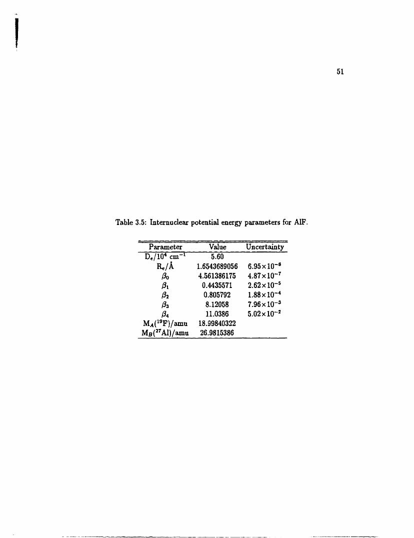
Table 3.5: Internudear potentid energy parameters for AU?.

Parameter Vdue Uncert ainty De/ 104 cm-' 5.60

&/A 1.6543689056 6.95 x 10'~ Po 4.561386175 4 . 8 7 ~ IO" PI 0,4435571 2.62 x 0 2 0.805792 1.88 x 10'~ 03 8.12058 7.96 x IO'= B 4 11 .O386 5.02 x IO-'

MA(lgF)/amu 18.99840322 MB (27Al)/amn 26.9815386

high temperature c d , only the reiative intensities of the llBF rotational lines were

measured. Due to the fact that the transmission of the optics, the efficiency of

the bearnsplitter and the response of the detector vary with frequency, a narrow

wavenumber range was chosen. The choice of wavenumber range was somewhat

arbitrary, but it was chosen in such a way that there were intense lines within

the range, and the line intensities can be rneasnred readily, i.e. there were no

blended lines and the continuum level codd be determined to a high degree of

accuracy. Consequently, the range between 1280 and 1300 cm-' was selected. Since

' v = 5 + 4 band is weak, ody four bands from v = 1 -t O to v = 4 -t 3

were compared. Equation (3) in Ref [102] was appüed to convert rotational line

int ensities to transition dipole moments. The measarecl average transition dipole

moments were normalized to that of v = 1 + O band. th& values are listed in

Table 3.6 together with the ab initio predictions obtained fiom Refs [95] and [93]

There is a good agreement between our experimental values and the ab initio resdts.

The ab initio calculations of the dipole moment hinction are cleariy of high quality.

3.5.3 Conclusion

Fourier transform infiarecl emission spectroscopy is a very nsefnl technique for

recording high resolution vibration-rotation spectra of hi& temperature molecnles.

Our iafrared data on "BF and l0BF together with Msting microwave data, were

converted to spectroscopie constants in two ways. The first approach ntilized the

tradi tional Dnnham mode1 extended t O indude data from different iso t opomas.

It is evident that imposing constraints on the Dnnham coefficients improves con-

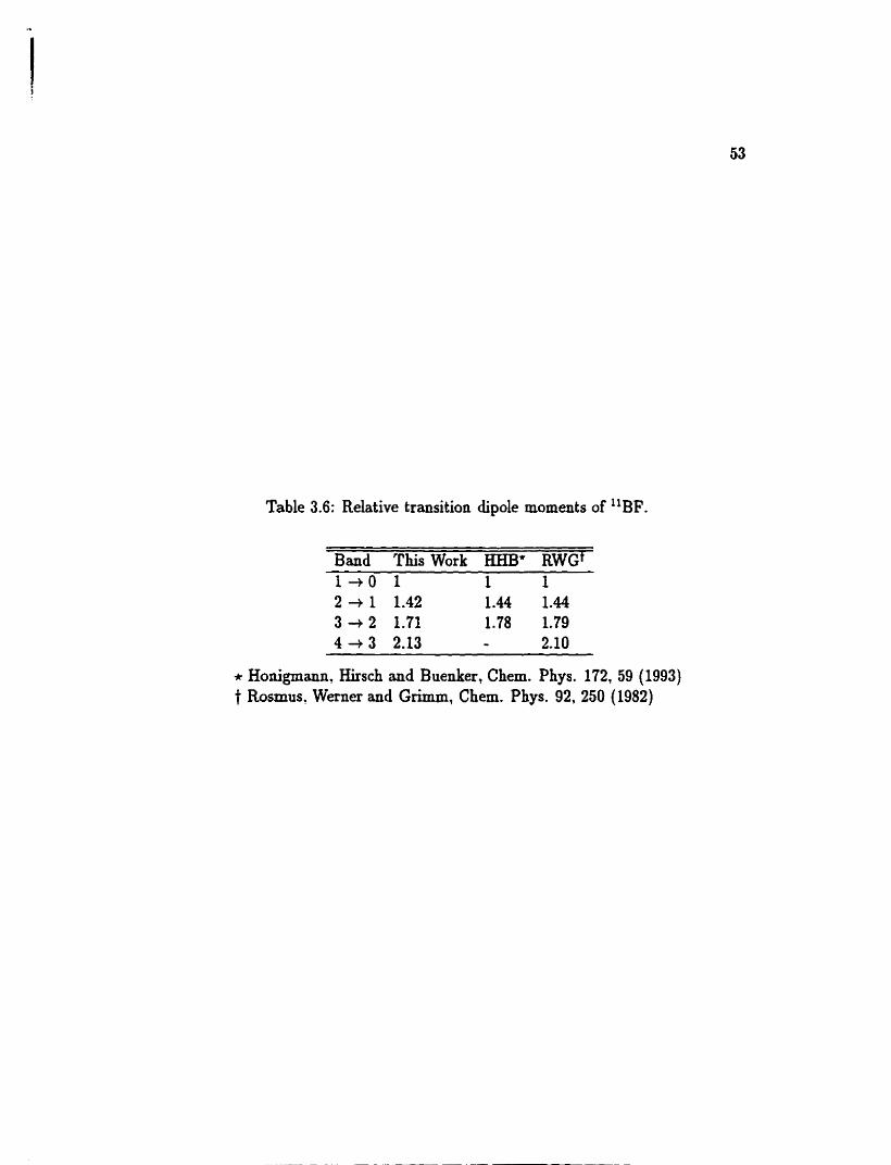
Table 3.6: Relative transition dipole moments of "BF.

Band This Work HHB' RWGt

* Honigmann, Rirsch and Buenka, Chem. Phys. 172, 59 (1993) t Rosmus, Werner and Grimm, Chem. Phys. 92, 250 (1982)

sistency among the parametas. The second approach employed a parameterized

potential model which uses a direct cornparison between the experimental data and

solutions to the Schriidinga equation. The second model can predict higher ly-

ing rotation-vibration energy levels of the electronic gronnd state t hat are at l e s t

qualitatively correct. The traditional Dnnham model is inadequate when extrap

olating f a beyond the range of experimental measurements. Finally, the relative

transition moments were &O measnred, and the values agree with the ab initio

calculation satisfactorily. Provïded that spectra wit h good signal-tu-noise ratio are

available, the relative transition dipole moments of other transient molecules can

be determined, and possibly the dipole moment htnctions.

The BF experiment proves once again that the superior spectral coverage of

the Fourier transform spectrometer is important for recording new spectra. The

original experiment to obtain spectra of CaF (961 was carried out near 600 cm-',

but the BF band was recorded near 1300 cm-'. The ability to sarvey a wide range

of fiequencies in a short perïod of t h e makes the Fourier transform spectroscopy

the ideal technique to investigate new spectra.

3.6 Infrared Emission Spectroscopy of MgF

The electronic and miuowave spectra of alkaline earth monohalides have b e n stud-

ied extensively [103-1061. b e v e r , little is hown about the ir6rared spectra of

these molecules. Dnring our systematic investigation of the infrared spectra of

the aUcaiine earth monofluorides, the high resolution vibration-rotation emission

spectram of MgF was recorded for the first time.

The rotational analysis of the electronic spectmm of MgF was performed by

Barrow and Beale [107]. The structure and bonding of MgF was detamined from

its millimeter-wave spectrum [lO8,lO9]. MgF, like all the okher alkaüne earth mono-

halides, is found to be highly ionic [110]. When compared with the other heavier

alkaiine earth monofluondes, MgF has a greater degree of covalent bonding as de-

termined by the hyperfine structure.

Ionic molecules are suitable candidates for testing simple semi-classical bond

models [Ill-1151. Because MgF and the other alkaline earth monohalides are

maidy ionic molecules, a Rittner-type model for the potential energy was devel-

oped by Torring et al. [112,113]. But as Bauschlicheï et al. [Il41 pointed out. when

more accurate polarizabilities are nsed, the model by Tonhg et al. fails completely.

R e h e d ab uiitio calculations [Ill, 1151 were also carried out.

3.6.1 Experiment

The experimental arrangement was sirnilar to that desaibed in a published pa-

per [116]. A sample of 30 g of MgF2 was contained in a carbon boat placed in the

center of a carbon liner that was housed inside of a muliite (3A1203*2Si02) tube.

The central 50 cm portion of the m d i t e tube was heated by a CM Rapid Temp

fiirnace. The ends of the mullite tube were water-cooled and sealed with KRS-5

windows. The tube was heated ap to 1550°C at a rate of 200°C per hour. The

sample cd was pressnrized with 10 Torr of argon gas to prevent condensation of

s d t vapors on the c d windows.

The infrared radiation emitted fiom the farnace was introdaced through the

emission port into a Bruker IFS 120 HR Fourier trandorm spectrometer. The

infrared emission spectnim was recorded with a fiquid heliom-cooled Si:B detector

and a KBr beamsplit ter.

The bands of MgFl were found but codd not be analyzed because of their

compleuity. The best spectrum of MgF was recorded at 1550°C, wit h 50 scans co-

added in about 50 minutes at a resolution of 0.01 cm-' in the spectral range fiom

350 to 1000 cm-'. A portion of the infrared emission spectrum of MgF is shown in

Figure 3.4. Rotational h e s are well resolved, but the spin-rotation splitting in the

X2C+ state was oot resolved.

3.6.2 Results

Rotationai spectral lines were measured by using the program PC-DECOMP writ-

ten by J.W. Brault. Centers of Lines were determined by fitting line profles to Voigt

line shape functions. Rotational lines of HF, which were present in our spectrum as

an impurity, were nsed to calibrate MgF iine positions [97]. The assignment of the

MgF s p e c t m was facilitated by an interactive color Loomis-Wood program. The

accuracy of most calibrated iine positions is 0.001 cm-'. More than 800 spectral

lines of bands from v = 1 -t O to v = 7 -t 6 were assigned. The line positions are

listed in Table B.1.

Since the spin-rotation splitting was not resolved in the spectnun, the ground

state of MgF was treated as if it were a 'C+ state. Dttnham xj constants for MgF'

were obtained by fitting the observed frequencies and avaiiable microwave data to

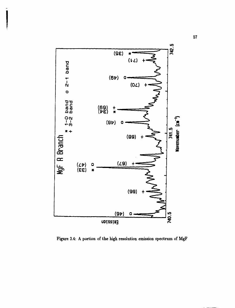
Figure 3.4: A portion of the high resolution emission spectrom of MgF

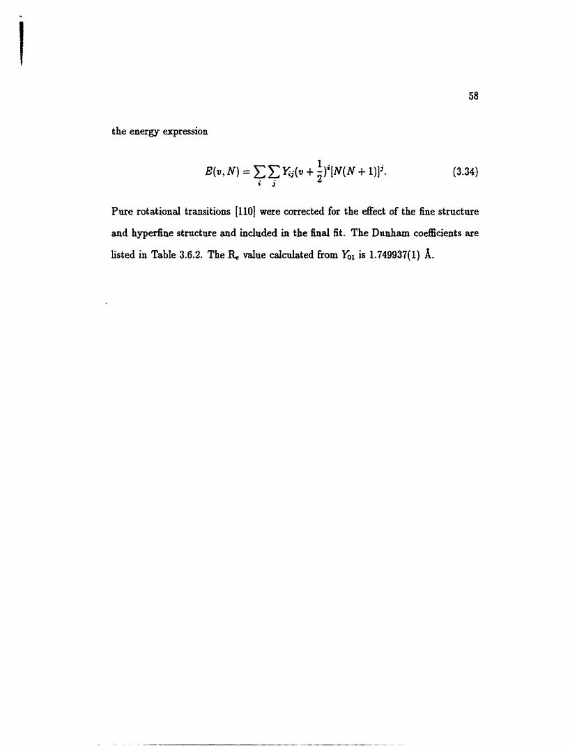
the energy expression

Pure rotational transitions [Il01 were corrected for the a e c t of the fine structure

and hyperfine strncture and induded in the final fit. The Dunham coefficients are

listed in Table 3.6.2. The R. value calcuiated fiom Gr is 1.749937(1) A.

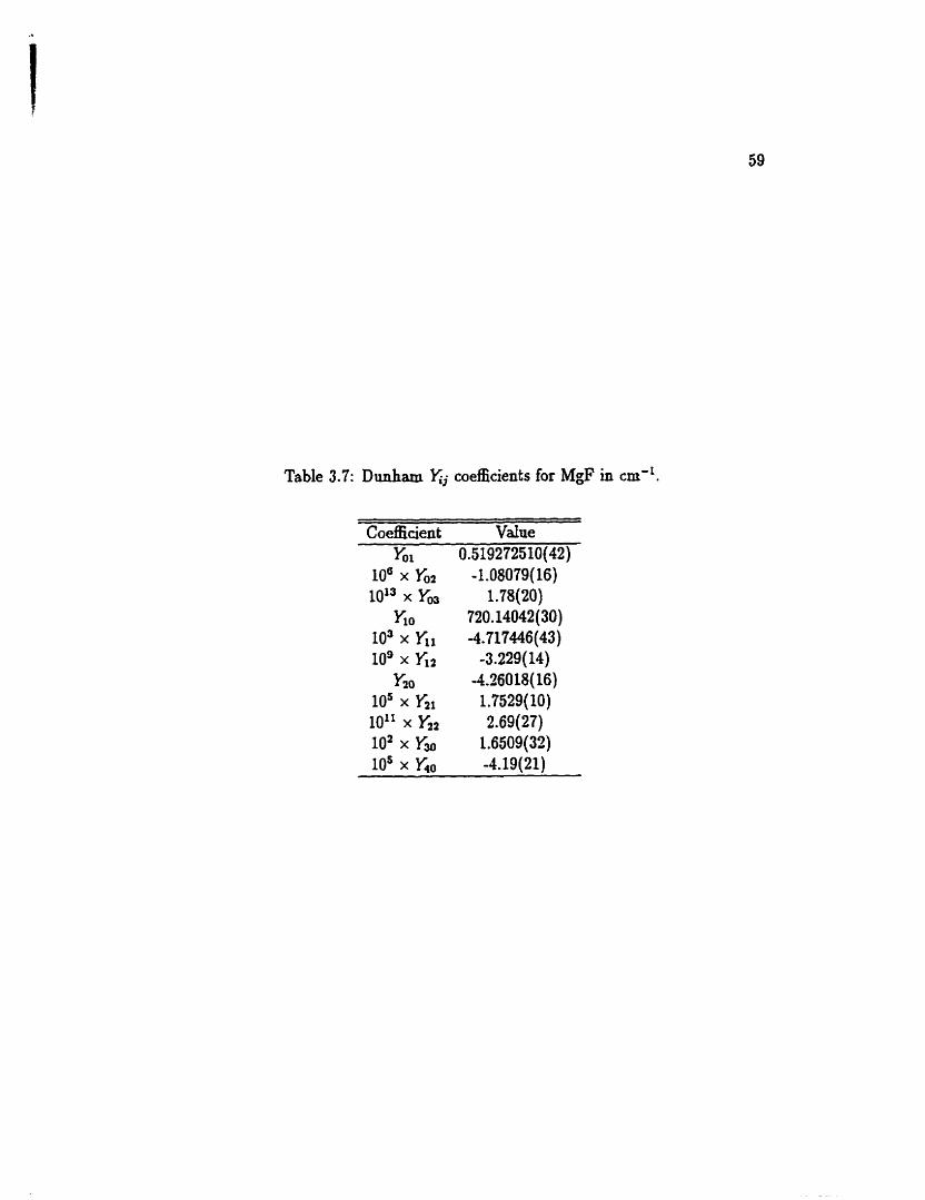
Table 3.7: Dunham xj coefficients for MgF in cm-!

Coefficient Vdue hl 0.519272510(42)

IO6 x x2 -1.08079(16) loS3 x & 1.78(20)

K o 720. 14042(30) IO3 x fii -4.717446(43) l o s x yi2 -3.229(14) ho -4.26018(16)

los x ~ I I 1.7529(10) 10" x fi2 2.69(27) IO2 x Yw 1.6509(32) los x -4.19(21)

Chapter 4

High Resolution Infrared

Spectroscopy of Nitrile Oxides

Most nitrile oxides (RCNO) are short-lived. and reactive species. They are stmc-

turally isomeric with isocyanates (RNCO), and cyanates (ROCN). The parent mem-

bers of the series? f-c acid (HCNO), and cyanogen di-Koxide (ONCCNO) are

explosive and have to be handled wit'h great caution. Since nitrile oxides dimerize

via a cydoaddition to furoxans, they are widely ased in synthetic chemistry for

1.3-dipolar cydoadditions by in situ generation and snbsequent reaction in solu-

tion [117-1191. Little is known, however, about their structure and spectroscopy.

Becanse the reactivity of nitrile oxides is very &ho their isolation was considered

to be di fndt . There has been some success in isolating nitrile oxides in low tem-

perature inert gas matrices. Maia and Teks [120] have reported the first htiared

spectra of CICNO, BrCNO and NCCNO in argon matrices at 10 K.

AIthongh experimental difEdties prevented Maier and Tdes [120] fiom coIlect-

h g detailed spectroscopie data on nitrile oxides, quantum mechanical calculations

can provide information on the proptrties of these molecules. The parent species,

fulminic acid HCNO is one of the few nitrile oxides to have been subjected to intense

experimental scrutiny by means of infrared and microwave spectroscopy [101,120].

The investigation was focused on its quari-hem behavior, and alternative isomeric

forms. It is diilicdt to determine hom ab initio calculations whether HCNO has a

bent or h e a r equilibrium s tructtue. Inaeasingly extensive ab initio studies have

shown that both geometries are possible, depending on the level of theory. For the

BrCNO molecule, ab initio caldations have beeo carried out at the levels of HF?

MP2. MP3, MPISQD, and MPQSDTQ [121]. The calctdated structure of BrCNO.

depending on the Ievel of theory chosen, can be eitha linear or bent.

As wit h all large-amplitude molecular motions, quasi-linearity is assouated wit h

an anharmonic potential energy function, and cannot be explained by iafinitesimal

rectilinear coordinat es. The quasi-hear bending motion is the only large-am p h ude

molecular motion that characterizes a rnoledar system assuming two entirely dif-

ferent geometries. A linear molecule has 2 rotationd and 372 - 5 vibrationai degrees

of keedom, and a bent planar molede has 3 rotationd and 372 - 6 vibrational

degrees of freedom. It is clear that there is a smooth transition between these two

cases through the behavior of quasi-linear bending. However, the ty-picd treatments

which are constantly applied to ngid moleenles, are not very osefid here. These

methods indude separation of rotational and vibrational motion as an essential

assnmption. The bending motion and rotation about the axis of l e s t moment of

inertia, are so strongly coupled in quasi-linear moledes that they must be treated

togetha.

The spectra of quasi-linear bending fùndament al modes are anomalous, as are

the spectra of combination modes that involve quasi-linear bending. High rese

lution stadies are necessary to i den t e details in the vibration-rotation spectra.

However the high resolution infrared spectroscopy alone cannot f d y explain the

qilasi-hear bending motion. Microwave spectroscopy and other techniques, such

as photoelectron spectroscopy, also play an important role.

4.1 Experiment

Pasinszki and Westwood (1211 have devised good methods for the generation of NG

CNO and ONCCNO molecules in the gas phase. Thek work led to recording high

resolution infrared spectra of ONCCNO [122] and NCCNO (1231, and rniaowave

spectra of NCCNO [124]. Encouraged by their success, Pasinszki and Westwood

have recorded the first gas phase spectra of BrCNO 11211. An obvious challenge to

high resolution spectroscopy of reactive moledes is rnaintaining sdcient concen-

tration of sample in the cell for an extended period of tirne. Because of its reactive

nature? the sample constantly disappears, and therefore, must be generated con-

tinuously. This requites that a large amonnt of precursor must be prepared before

the experiment.

There are two convenient ways of generating BrCNO. One method is pyrolysis of

dibromoformaldoxime (Br2C=NOH), and the other is pyrolysis of the huoxan-like

dimer of BrCNO. In this stndy, the BrCNO molede was generated in situ nsing

gas phase pyrolysk of dibromoformaldoxime, Br2C=NOH.

The experimentai setup was typical for absorption work nsing a single-pas

sample cell and a glower (Figure 4.1). The infrared glower was collimated with

a parabolic mirror and passed through a 120 cm long absorption c d sealed with

two KRS-5 windows. The hfiared radiation was then collected with a 45' off-

axis parabolic mirror, and entaed the Fourier t r d o r m spectrometer through the

emission port. There are two ports attached to the absorption cd. One is for

the gas inlet, and the other is the pomping port. The pyrolysis apparatus was

comected to the gas inlet, and the pyrolysis products were pumped slowly out of

the sample c d with the cell pressure maintained at about 250 mTorr.

The pyrolysis was carried out in a 15 cm long quartz tube with 8 mm inner

diameter. For more efficient thermal contact, the tube was loosely padced with

quartz chips. The quartz tube was placed inside a small h a c e whose tempera-

ture was controlled by manually adjusting the voltage. Dibromoformaldoxime had

adeqaate vapor pressure at room temperature: and its vapor was introduced into

the furnace. Dibromoformaldoxime started to decompose at 300°C. The pyrolysis

prodaced a large nnmba of species, with relative amounts that varied as the tem-

perature of pyrolysis increased. At 500°C, the yield of BrCNO was abundant with

s m d amounts of CO, CO2, HCNO, HNCO present in the spectra either as the side

prodacts of the thermolysis or fiom the subsequent destruction of BrCNO.

The high resolution absorption spectra were recorded with a Bruker IFS 120 HR

spectrorneter. The resolntion of the spectra was 0.004 cm-l. Although a higha

resolution wodd be desirable. the period of tirne t hat the sample wodd last forced

some sacrifice in resolntion. A KBr beamsplit t a was used for all experiments. The

Fignre 4.1: Setap for the BrCNO absorption expaiment

VI mode, near 2200 cm-=, was recorded with a liquid nitrogen-cooled InSb detector.

A total of 60 scans were cwadded in the 1800-2900 un-L region, which was limited

by a red-pass Hter with a cutoff at 2900 and the response of the InSb detector.

The v2 mode, near 1300 cm-', was recorded with a liqaid nitrogen-cooled MCT

detector. The lower limit of the spectrum was determined by the response of the

MCT detector, while the upper k t was set by a red-pass Elter with a cutoff at

1672 cm-'. In total, 50 scans wae CO-added.

4.2 Results and Analysis

The spectral line measnrements were made with the spectral analysis program PC-

DECOMP. developed by J.W. Bradt. The peak positions were determined by

fitting a Voigt line shape fiuiction to each spectral feature. The signal-tenoise

ratio for the strong lines in both spectra was about 5:l and the preusion of the

line position measurement was about 0.0005 cm-' for these lines. Since bromine

has two nearly equally abundant isotopes with similar atomic mas, the rotationai

constants for both isotopomers of BrCNO are very dose. This situation caused

the spectra to be severely blended in many regions. The precision is, therefore.

0.001 cm-' for the many blended and weak features.

In order to sort out the brandies and to help in the assignment of the spectra.

an interactive color Loomis-Wood cornputer program was utilized. The calibration

of the y mode was c&ed out using the CO lines in the spectnim [125]. The u?

mode was calibrated with the water Iines in the s p e c t m [126].

Figure 4.2 shows an overview of the high tesolution spectnun of the VI mode of

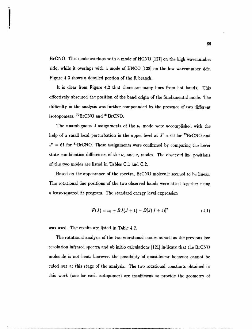
BrCNO. This mode overlaps with a mode of HCNO [127] on the Ligh wavenumber

sidc. while it overlaps with a mode of ANCO [128] on the low wavcnumber side.

Figure 4.3 shows a detailed portion of the R branch.

It is dear from Figure 4.2 that there are many lines from hot bands. This

effectively obscured the position of the band origin of the fundamental mode. The

clificulty in the analysis wns futlier compoundecl by the presence of two Merent

isotoponiers. '9rCCN mcl 81BrCN0.

The iinambiguous J assignments of the ul mode were accompLislierl witli the

Lelp of a small local perturbation in the upper lcvel at .Jt = 60 for "BrCNO ; i n c l

.If = 61 for "BrCNO. These assignments were confirmed by cornpnring tiic lower

statc combination ciifferences of the and u? modes. The obscrvrd Luc positioiis

of tlie two modes are listecl in Tables C.1 c?aci C.2.

Bnsed on the appearmce of the spectra. BrCNO niolecitir seeuied to hi: Liiiear.

The rotational line positions of the two observecl bauds were fitted togcther iisirig

a lest-squared fit program. The standard energy level expression

was used. The results arc listed in Table 4.2.

The rotational cmalysis of the two vibrationai modes as weU as tlie prcvioiis low

resolution infrared spectra cuid ab initio calcnlations [El] inclicate t h the BrCNO

molecule is not bent: kowever. the possibility of quasi-linear beliavior c'unot be

d e d out at this stage of the analysis. The two rotational constants obtained in

this work (one for each isotopomer) are insufficient to providc the geoonictry of

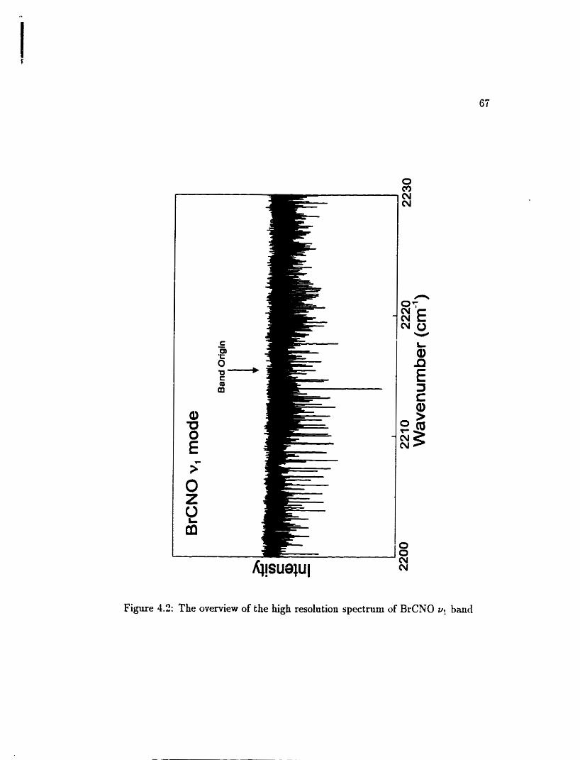
Figure 4.2: The o v e ~ e w of the high resolution spcctrum of BrCWO v! band

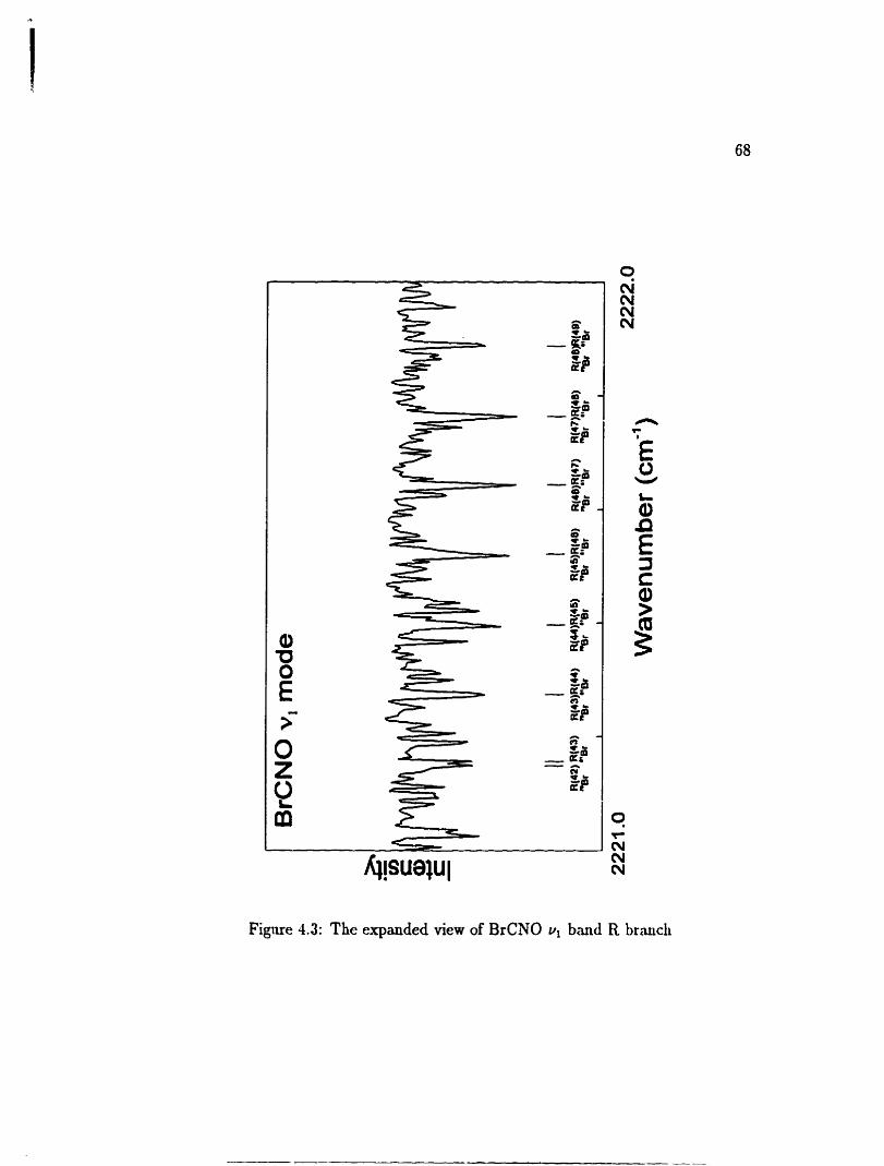
Figure 4.3: The expanded view of BrCNO y band R branch

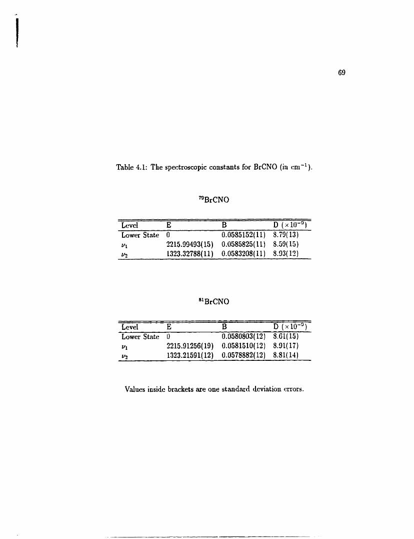
Table 4.1: The spectroscopie constants for BrCNO (in cm-').

Level E B D ( x IO-') Lower State O 0.0585152( i l ) 5.49( 13) h ?215.99493(15) 0.0585825(11) 5.59( 15) ~2 1323.32788(11) 0.0583208( 11) 5.93( 13)

Level E B D ( x ~ o - ) ) Lower State O 0.0580803( 12 3 S.G1( 15)

Values inside brackets are one standard deviatiou mors.

BrCNO without some assumptions. One approack to this problcni is to assume a

linear structure and to use the known NO bond length of the HCNO or CHjCNO

moleculcs. This. of course. assumes that the NO bond lengt h is tramferable kom

HCNO or CH3CN0. The ab initio caldations of substituted nitrile oxides [EI)]

have indicated that the NO bond length is less sensitive to substittient effects tlian

tliat of CN. The cdculations also Uidicate that the NO bond lengtli in BrCNO is

cxpected to be between that of HCNO and CH3CN0. In Table 1.2. strtietur<is I and

II show tlie structure of BrCNO predicted by this methocl. and also n rouiparison

of tlie derived bond lengths with those of related molecules BrCCH. BrCN. HCNO.

aiid CH3CN0.

From Table 4.2 it cm be seen tkat the BrC bond lengtli deriveci froiu tliti Bu

rotational constants is anomdously short compwed to t h of BrCN .and BrCCH.

aiid the CN bond lengtli is anomdously long comparecl to tiwt of HCNO a i d

CHICNO. This is similar to the case of HCNO. nnother floppy moleciilc wlierc xi

snomdously short CH bond length has been derived assiiming a lineu strtiettuc

;and a rigid bender mode1 [132] ( s e Table 4.2). A reliable geometry and a good fit

for the bending energy levels could ody be achieved using the serui-rigid bender

model. which makes possible the introduction of the bending 'angle clepoti<lencies of

the bond lengtlis and bending reduced mas: these effects are important becatise of

the large amplitude of the bending motion ii33j.

Clearly. experimental and theoretical studies on BrCNO have a long way to go

before a fuil characterization will be aehieved. To tLis end it is important to record

the microwave and infrared spec tra of isotopically stibsti tuted derivat ives and to

Table 4.2: Cornparison of the bond lengths iii BrCNO (in A ) .

Molecule Met hod Br-C C-N N-O C~ninients BrCCH MW Ref. [130] 1.7916 - - r s

BrCN MW Ref. il311 1.789 1.158 - re

BrCNO B3-LYP 1.8007 1.1616 1.2041 r, b

struct. 1 1.6843 1.2131 1.1994' struct. II 1.6922 1.1915 1.3189'

HCNO bIlV Ref. [132] (1.0266)~ 1.1679 1.1994' r s '

MW Ref. [133] (1.060)~ 1.16919 1.199 r s ' CHaCNO MW Ref. il341 - 1.1671 1.2189 r(i

a) G311G(2d) bnsis set used. molecule is quasi-linear at tliis level of tlicory. b) 6-31 lG(2d) basis set used. molecule is linear at tlus levcl of tlieory. c ) k e d parameter. c l ) C-H bond length. e ) structure dcrived fiom a Linear model. f ) structure denved boni a serni-rigid model.

include large amplitude effects in the structural analysis. To aid future workers.

the equilibrium BrCN bending potential. and the dependence of bond lengths on

the BrCN angle (Table 4.2) were calcdated by Pasinszki.

4.3 Conclusion

The reactive BrCNO molecule can be produced in the gas phase by viicuiuu thesmol-

ysis of dibromoformaldoxime. The high resolution spectra of the two most intense

vibrational modes have been recorded. The assumptioii tLat the strtictiire of the

molecide is linex. wns made rlnring the rotationd aidysis of tlicsc two niodcs. Diu:

to the complexity of the spectra. only two bands have becri ,malyze<l. niid sevcrd

hot b;uids and the fundamental bands associated with these modes Lave yet to be

analyzed.

The lower stôte Bo const.mt is in good agreement with the ab i~utio pretliction.

The rotationd constants wme usefd in the searcli for the niiçrownv(: spectsiiiri

of BrCNO. Based on this work. microwave spectra of BrCNO werc recor~kd by

otlicr workers. Preliminary results indicated that the b'uids aiiaiyzed licrc wtiro

not the fundamental bands. More analysis will be ciuried out to (letcrminc the

fundamental inFrad bands. Until the pure rotational spectrum is obtaincd aucl

analyson for several wlditionai isnkopomers. a mliable stnict~irr of BrCNO remains

to be determined.

Table 4.3: Theoretical stmctnre of BrCNO using the B3-LYP/6-311G(2d) method (bond lengths in A, bond angles in degrees? total energy in atomic units).

Total Energy -2742.1498299 -2742.1498611 -2742.1498661 -2742.1498231 -2742.1493821 -2742.1479620 -2742.1449741

Br-C-N 180 170 165.35 160 150 140 130

Br-C C-N N-O C-N-O 1.7963 1.1587 1.2051 180 1.7993 1.1599 1.2048 177.31 1.8007 1.1616 1.2041 176.04 1.8050 1.1641 1.2029 174.78 1.8165 1.1705 1.2001 172.29 1.8322 1.1788 1.1964 170.39 1-8555 1.1882 1.1923 169.16

Chapter 5

Vibrational Spectroscopy of

Polycyclic Aromat ic Hydrocarbon

Molecules

The vibrational motion of polyatomic molecules is, in general. very complicated.

For a non-linear polyatomic molecular system consisting of n atoms, there are 3

degrees of fkeedom for translation, and another 3 degrees of freedom for rotation.

Subtracting these fiom the total degrees of fieedom, 3n. the number of vibrational

degrees of keedom is 3n - 6. To gain insight into the cornplex problem of rnolecdar

vibrations, a dassical mode1 is ma& usea. The molede is opproximated by a

system of point partides with masses, which are held in their eqnilibriom positions

by springs obeying Hooke's law. This model system ha normal modes of vibration

similar to the vibrating molecale.

5.1 Classical Mechanical Treatment of Molecular

Vibration

The dassicai treatment (1351 starts with the classical HamiItonian given by

where V is the potential energy and T is the kinetic energy, and

where (z;, yi, &) are a set of Cartesian coordinates of the ith partide, and the dot

notation indicates derivative with respect to t h e , e.g. zi = &;/dt.

Next. the problem is expressed in terms of mas-weighted Cartesian coordinates

qi- The reason for this is tbat the amplitude of a partide's oscillation depends on

its mus. When mas-weighted coordinates are used, all amplitudes are properly

adjusted for the different masses of particles. Let

Then the kinetic enagy can be written as

In generd, the potential energy V is a complicated fnnction of the Cartesian

coordinat es of the atoms. For the purpose of vibrational spectroscopy, the molecule

often osdates with a small amplitude of vibration about the equilibrinm position.

The potential V can be expanded in a Taylor series in the neighborhood of the

equilibrinm position. The expansion is

If the zero-point potentiai energy is chosen to be at the equilïbrium, then \

By the definition of the equilibriam position, aV/aqi = O at equilibrium. Ignoring

the cubic and higher order expansion t m s gives the harmonic approximation of

where

In generalized coordinates, Lagrange's equations are the equivalent to Newton's

law of motion. In classicd mechanies, Lagrange's equation of motion is

where L is the Lagrangian

For the vibration of a molede, sabstitnting

into Equatior. (5.8), the equation of motion becomes

where 6 denotes the second derivative of q with respect to tirne.

There are 372 coupled diEerentia1 equations (5.11) wit h constant coefficients.

Such a set of equations can be solved by assuming a solution of the form

Substituthg this solution into Equation (5.11) yields a set of 372 homogeneous linear

equations

The non-trivial solution of A exists only when the secdar equation

is satisfied. The solution of this equation gives the eigenvalues A, which are related

to the vibrational fiequenues of the system. It t m s out that six of the eigenvalues

are zero for a non-linear molede. Thae are three degrees of fieedom which are

associated with the translation of the center of mars, and three with rotational

motion of the molenile as a whole. Since there is no restoring force acting on these

degrees of freedom, their frequencies are zero.

There is a a o m d mode coordinate Qi that is related to each eigendne &. The

set of a coordinates representing normal modes are reiated to the set of q; by a

linear transformation. The h e t i c and potential energies can be hitten as

Since both T and V have no cross-tenns that connect diffkrent coordinates, the

system behsvcs like a set a 3n -6 independent harmonie oscillators, each oscillating

at a frequency

When the higher order anharmonie terms of Equation (5.5) are considered, the

normal mode approach is not entirely valid because che normal modes become

coupled.

5.2 Quantum Mechanical Treatment of Molecu-

lar Vibration

The Born-Oppenheimer approximation is applied to separate the motion of the

electrons and naclei, and the validity of htrther separation of rotational motion horn

vibrational motion is also assnmed. Based on the previons dassical description, the

transition to quantum mechanical treatment is rather straight forarard [Il]. In

normal mode coordinates, the elagsical Hamiltonian is translated to a quantum

mechanical operator by making the osual snbstitutions

where

is the classical generalized momentum associated with the normal coordinate Qi-

The quantum mechanical Haniltonian for vibration is

In t m s of normal coordinates, the Hamiltonian operator (5.19) is just a sum of

3n - 6 independent harmonic oscillator Hamiltonians. It follows that the vibrational

wavefunction is just a prodact of 372 - 6 harmonic oscillator wavefnnctions. The

total vibrational energy is simply given by the surn of 3n - 6 harmonic oscillator

where vi is the vibrational quantum number.

There are some limitations to this simple harmonic oscillator approach. The

vibrational and rotational motions are not always separable. The Coriolis &ect

[136] is a result of the coopling between rotation and vibration. The separation

of the total vibrational wavefnnction into the prodnct of wavefanctions associated

with only one normal coordinate can break down nnda certain circumstances. This

leads to phenomena such as Fermi resonance [9] and other types of minng.

5.3 Group Fkequencies

One of the most usefd aspects of vibrational spectroscopy is the fact that a given

group or bond in a molecule will produce spectral features that are characteristic of

this group or bond. These spectral features are, therdore, often refmed to as group

fiequencies [W]. Similar groupspecific signatures are common in nudear magnetic

resonance, ultraviolet and visible spectroscopy, however, these techniques are quali-

tative analyticai tools. Mared spectroscopy also permits qualitative identification . -

of compounds by exhmuung their group vibrations. Furthetmore, the group fie-

quenues allow for an initial vibrational assignment . For example. a single C-Br goup. or bond prodaces a strong infirared absorption

around 560 cm-l [ll), whîch is more or less independent of the r a t of the molecule.

This vibration is a group frequency typical of a CBr gronp. However, if a molede

possesses two C-Br goops in dose prolrimity, e.g., in a CBrl group, a symmetric

and an antisymmetric Br-C-Br stretching mode are observed, in addition to a Br-

CBr bending vibration. AU of the three are again characteristic group kequencies

of a CBr2 group.

Although the discussion of molecuiar vibrations in terms of group vibrations

may appear somewhat crnde, particalarly after the discussions of normai modes

of vibration, it is amazing how w d the grmp fieqnency approach holds, and how

frequently it can be used for identification of componnds. For the detailed under-

standing of vibrational spectroscopy, it is worth noticing that a normal mode of

vibration involves the entire molecnle. but that the major contribution to a mode

may involve just one group, which gives rise to the group fiequency.

5.4 Selection Rules for Normal Modes of Vibra-

tion

The intensity of an LiGared transition is given by the absolute square of the tran-

sition moment integral (311

(5.21)

where +Jr and $i are final and initial vibrational wavefnnctions within the same

electronic stste, p is the dipole moment function, and the integral is over dl vibra-

tional coordinates. The transition moment mnst be nonzero for the transition to

be dowed. The hc t iona l form of p is often difficnlt to obtain. so it is erpressed

as a Taylor series expansion

Now Equation (5.21) becomes

The first term on the right-hand side of the above expression is zero because the vi-

brational wavefunctions are orthogonal. The vibrational wavehinction is a product

of 3n - 6 harmonic osda tor wavehctions, therefore, the ground state wavehuic-

tion consisting of the product of symmetric Ganssian fnnctions is to tdy spmetnc .

For a fundamental vibrational transition, qb, d 8 é r s from only in the jth nor-

mal mode. Under the harmonie osdator assumption, the symmetry of the excited

state has the symmetry of Qk itself. This becomes similar to a single h m o n i c

osciuator, the selection d e is Avi = f 1. This is only a fkst order approximation

since all the higher order terms are neglected.

Rom Equation (5.21) the integand 4j p +i must be totally symmetric for al-

lowed vibrational transitions. The symmetry of this integrand is r($j) @ ï ( p ) @ I'($i)

[138]. For a findamentai transition, +i is to tdy symmetric while $ j has the sym-

metry of the j th normal mode, which is at exuted level uj = 1. This indicates that

the symmetry of the integrand is

Because electric dipole moment operator is a vector with an expression

$t must contain the representation of the symmetries of 2, y, or z in order to have

a~ i&ared transition. Considerable amount of information of the normal modes of

a molecule can be predicted on the basis of symmetries and gronp frequencies.

5.5 Polycyclic Aromatic Hydrocarbon Molecules

in Astronomy

An important question in astronomy is the role of the polycydic aromatic hydrocar-

bon (PAIX) compounds in the chemistry of the interstellar mediun. PAE molecules

have been identified in meteorites [139,140] and interplanetary dnst partides 11411

by mass spectrometry. Several features in the spectra of astronomical objects have

also been attribated to neutral or ionized PAHs. These featnres match the group

frequencies of PAH molecules. One example is the unidentified ixûrared emission

bands (UIRs) that are observed in the spectra of objects including planetary nebu-

lae, reflection nebulae and H II regions [142-1451. It has been hypothesized that the

UIRs Mse because the PAH moledes absorb ultraviolet radiation, undergo inter-

na1 conversion, and then emit radiation in the infrared region [142-1451. Indeed, the

UIR bands (at 3.3 am. 6.2 Pm, 7.7 Fm, 8.7 prn and 11.3 pm) [145] resemble some

of the characteristic features in the P A . spectra. Other models propose that these

features arise fkom molecdar groups attached to carbonaceous dust grains [146],

&om quenched carbonaceaus composites [147,148], or fkom a mixtures of PAHs and

hydrogenated amorphous carbon [149,150].

The argument in favor of the PAH mode1 is that the UIR bands c a ~ o t arise

Lom thermal emission as grains are too cold in most of the regions where these

bands are observed. This is partiealarly true for the 3.3 pm emission band which

implies a temperat are of about 1000 K for the carriers. For an isolated molede,

snch temperatures are easily achieved after the absorption of a single dtraviolet

photon. After absorption of the photon, there is a fast intenial conversion that

converts electronic energy into gromd state vibrational energy. Then the cooling

process taka place through relatively slow idiared emission [143]. Although the

observed UIR bands have characteristic freqnencies of the vibrational modes of

PAHs, a detailed stndy of these featnres is necessary to test the PAH hypothesis.

In particdar, no laboratory mixtures of PAH moledes have been able to simulate

in detail, the obswed infrared emission bands. This discrepancy has motivated

both Iaboratory experiments and quantum mechanical caldations.

Sehutte et al. [151] have modeled the UIR bands assnming that they are due

to fluorescence fiom a distribution of PAHs embedded in the radiation field of a

hot star. The distinct featnres in the spectra were predicted to occur fiom rela-

tively small species of size l e s than 1000 carbon atoms, which upon excitation by

absorbing an ultraviolet photon could emit radiation in the infrared. To determine

whether the PAH mode1 is valid, it is important to have diable spectra of a large

distribution of PAEs.

Several groops have recorded laboratory spectra of the PA% in an attempt

to assign the nnidentified featares in astronomical spectra. The easiest way to

obtain infrared spectra of PAH moledes is to observe PAH molecules in the solid

state or in solvents. Moledar crystals were dispased in an ionic crystd p d e t

(e.g. KBr, CsI) [152-1541 or in a solvent (e.g. CCL, CS2). Most of the presently

a d a b l e data on PAHs have been recorded under these conditions, eitha at room

temperature [155] or at elevated temperatures [156,157]. The major deficiency of

t hese experirnents is that the PAH moledes interact with each ot her in the crys t al,

and with pellet materiais or solvents. The interactions may change the vibrational

band positions and intensities. The rotational motion of PAH is quenched in the

solid state, and is hdered in solvents.

Another experimental approach is to isolate PAH moledes in rare gas matrices.

The vapor of PAH molecdes is de~osited on a window, which is usually made of

KBr or CsI, together with rare gas atoms at temperatares below 20 K (1581. The

rare gas atoms interact weakly with the PAH molecules. When the dilution ratio

between rare gas atorns and PAHs is high, PAHs are w d separated so that the

interactions between PAHs are negligible. The vibrational band positions of PAR

spectra recorded in matrices are dose to those recorded in the gas phase, bat the

mat& effect is present, and is ofien diflicult to predict. The rotational motion of

the PAH molecdes is &O quenched in matrices at low temperature. The vibrational

bands shapes are, thmefore, different from those in gas phase spectra.

The interstellar environments that are thought to contain PAHs range fiom

the sudaces of dust grains to the exploding shells of supernovae; this diversity

must be approximated for by collecting spectra under a variety of experimental

conditions. Thus, in recent years, research efforts were dkected into studying PAH

moledes in the gas phase. There are in generd two ways to excite the vibrational

modes of a PAH molede. One method is direct heating of PAHs, while the other

involves laser ablation and dtraviolet laser excitation. In both cases, the infrared

spectra can be recorded. The second technique is probably the best approach

toward as tronornical conditions, i.e. exatation by high energy ultraviolet photons

[159,160]. Unfortunately, this approach was o d y applied to a s m d group of PAHs,

and the mearurements were limited to the spectral region near 3 p. SaykalIy and

c-workers [161,162] have improved this technique, and they have measared the

infiared emission spectra of naphthaiene, perylene, pyrene, and coronene from 3 to

14 p n (3300 - 700 c d ) using a new hfiared photon counting technique.

One most notable shortcornhg in ultraviolet photon excitation experiments is

that the level of infrared signal is low. There were situations where the infiared sin-

gle photon counting technique was used. On the other hand. direct heating of PAH

moledes can inaease the population of vibrationdy excited moledes dramati-

cally, and consequently, the amount of infrared radiation emitted fiom the PAHs.

Kmtz recorded the first gasphase coronene spectra in the region between 400 and

3500 cm-' using this method [163]. M a r e d absorption spectra of several other

gas-phase PAH molecules wexe obtained by Joblin et al. in the same wavelength

region 1164,1651.

To ducidate the chemistry of the PAHs in the intenitdar medium, it is nec-

essary to identify the individual PAH moledes. In prlliciple, it is possible to

distinguish among the diE& types of PAHs on the basis of their spectra. Yet

the task is not a trivial one, because the PAHs exhibit very similar spectra in the

mid-infrared, the region that contains most of the normal vibrational modes. The

vibrational assignment, howeva, may be faeilitated throagh theoretical rnethods.

Recently, Langhoff [38] calcdated the infrared spectra of thirteen neutral and ion-

ized PAR molecules using density fnnctional theory. The calculations confirmed

the previous assignments of the PAH spectra. Furthemore, Langhoff pointed out

that the far-infrared region, which contains the vibrational fiequenues associated

with the bending of the aromatic rings, may provide a way to diseriminate among

the different moledes 1381. Because there were no available far-infrared spectra of

isoiated PAR moledes, t his stndy was und& &en.

5.6 Laboratory Infkared Experiments on PAHs

In order to obtain the spectra of gas-phase PAH molecules, the mid-infiared and

far-infrared emission and absorption were detected with a Fourier transform spec-

trometer. The use of thennal emission spectroscopy in addition to the traditional

absorption technique is unusual [166], but we h d emission spectroscopy to be more

sensitive. even at long wavelengths. A cd consisting of a stainless steel tube 120 cm

long, sealed with a window at each end, was ased to contain the samples. The PAH

solids were placed near the center of a quartz liner tube 100 cm long, which was

inserted into the sample cell. After evacuation, a commercial h a c e was used to

heat the central 50 cm portion of the sample cd to prodnce PAIX vapor. The two

ends of the sample cd were water-cooled to protect the O-ring se& and to prevent

deposition on the end windows. Appropriate optics and detectors were used to

cover the spectral range h m 50 to 4000 cm-*.

Nap ht halene, ant hracene, pyrene, and hysene solids (97% pure) were obt ained

from Aldrich and ased without further pdca t i on . In every experiment. about 30

g of sample was placed in the central portion of a stainless steel tube lined with

pyrex. The stadess tube was sealed with KRS-5 or polyethylene windows at both

ends. The transmission range of KRS-5 window is from 250 to over 15 000 cm-',

and that of polyethylene window is fiom 30 to 625 cm-'. The sample c d was

then evacuated. About 15 Tom of argon gas were introduced to the cd to prevent

deposition of the sample onto the windows.

The sample was heated slowly up to a maximum of 450°C by a CM Rapid

Temp furnace. Spectra were recorded about every 50°C separately in emission and

absorption. For both the emission and absorption mea~urements~ the idiared Iight

was directed wit h a parabolic mirror t hrough an external port of a Fourier transform

spectrometer. The regions between the tube and the port were purged with dry

nitrogen gas in order to minimize the effect fiom atmospheric contaminants such

as CO2 and H20. Mer each experirnent, the remaining solid sample was analyzed

by a mass spectrometer, and no decomposition product was detected.

A KBr beamsplitter (400 - 4800 cm-') was used for mid-infrared measurements.

and a 3.5 pm thidc Mylar beamsplitter (100 - 720 cm-') was used for far-infrared

measurements. Liquid nitrogen-cooled MCT and InSb detectors as well as a iiqaid

helium-cooled Si:B detector and a Si bolorneter were used to record the spectra. The

spectral resolution in all cases was 1 cm-'. The integation t h e for each spectnun

varied 6om 4 to 10 minutes. and the number of scans c ~ a d d e d ranged fiom 100

to 200. Background spectra were &O recorded in a similar fashion but without a

sample in the ceU. The ha1 spectra reported here were obtained by dividing the

raw spectnun by the background spectrum taken at the same temperature.

5.7 Results

Emission and absorption spectra of gas-phase naphthdene, anthracene, chrysene.

and pyrene were obtained over the intervai fiom 50 to 4000 cm-'. Although the

spectra were recorded in both emission and absorption, the emission results are

presented here because the emission technique provided a higher SNR for most

modes, wit h less atmospheric contamination. Similar results were obtained in the

infrared spectra of nucleic aud bases [39]. In PAB nomendsture, naphthalene and

anthracene are classified as simple "hear" PAH molecules, chrysene is classified as

a typical 'non-linear7 PAH molecule, and pyrene is classified as a simple compact

PAH molede [38]. The emission spectrnm of pyrene in the region above 400 cm-'

is similar to the absorption spectrum reported by Joblin et al. [164.165]. It was

observed that there were several strong bands in the interval between 1700 and

2800 cm", that must be combination bands because there are no infrared active

fundamental transitions in this region. The unambiguous assignment of these vibra-

tiond modes is difficult, however, because the namber of infrared active modes is

large for even a srnaIl PAH molecde such as naphthalene. In addition. in the region

from 400 to 1700 cm-' where hdamenta l bands dominate, numerous combination

and overtone bands are present. The general similarity between the mid-infiared

spectra of diffetent PAHs and the spectral complexity makes it difficult to ciifferen-

tiate between individual types of PARS.

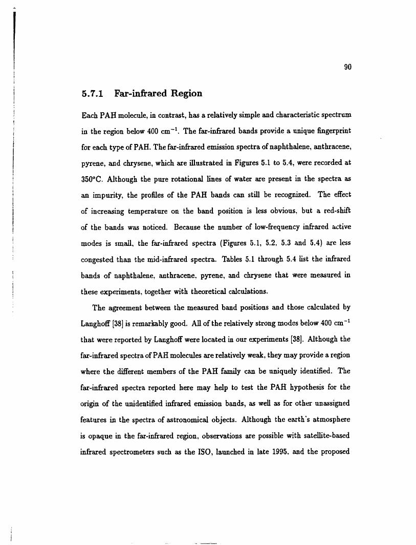
Each PAR molea.de, in contrast, has a relatively simple and characteristic spectrum

in the region below 400 cm-'. The fat-kifrared bands provide a Mique fingerprint

for each type of PAH. The far-infrared emission spectra of naphthdene, anthracene,

pyrene, and ehrysene, which are Uustrated in Figures 5.1 to 5.4, were recorded at

350°C. Although the pure rotational lines of water are present in the spectra as

an impurity, the profiles of the PAH bands c m still be recognized. The effect

of increasing temperature on the band position is less obvions7 but a red-shift

of the bands was noticed. Because the number of low-frequency infrared active

modes is s m d , the far-infrared spectra (Figures 5.1, 5.2, 5.3 and 5.4) are less

congested than the mid-infrared spectra. Tables 5.1 through 5.4 Est the infrared

bands of naphthalene, anthracene. pyrene, and chrysene that were measured in

t hese experiments. together with theoretical calculations.

The agreement between the measured band positions and those calculated by

Langhoff [38] is remarkably good. AJl of the relatively strong modes below 400 cm-'

that were reported by Langhoff were located in our experiments [38]. Although the

far-infiared spectra of PAB molecules are relatively weak. they may provide a region

where the different members of the PAR family can be uniquely identified. The

fa-infrared spectra reported here may help to test the PAH hypothesis for the

origin of the Midentifted infrared emission bands, as weli as for othm unassigned

features in the spectra of astronornicd objects. Although the earth's atmosphere

is opaque in the far-infrared region, observations are possible with satellitebased

i.&ared spectrometers such as the ISO, laanched in late 1995. and the proposed

Please Note

UMI

95

Space Inûared Telescope Faeility (SIRTF) platform, which have orbits above the

earth's atmosphere [167]. Observations wilI also be possible from high-flying aircraft

platforms such as the Stratospheric Observatory for Miared Astronomy (SOFIA),

which will commence operations in the early part of the next century.

The mid-inhared region is rich in spectral features, and the interpretation of these

bands caa be difficdt. This is illustrated in Figure 5.5. The PAH molecules t hat

were studied have a large number of normal modes ranging kom 48 for naphthalene

to 84 for chrysene. The situation is made worse by the fact that the majority of

the fundamental modes are in the range fiom 400 to 1800 cm-'. Great care must

be taken in the assignment of the mid-idiared spectra.

Moledar symmetry and selection rules play an important role in arsigning the

PAH spectra. Among the PAHs studied, naphthalene. anthracene and pyrene be-

long to the D2h point group, and chrysene belongs to the Czh point group. Accord-

ing to the character table, the DZh group has six ineducible reyresentations, which

are A,. Au, BI,, Blul BzuT BZuT Bag, and B3u; the C2h GOUP has four irreducible

representations, which are A,, Au, B,, and Bu [9]. Rom symmetry arguments. the

product in Equation (5.24) must be t o tdy symmetric to have a transition in the

idiared. Since the electnc dipole moment contains symmetries of x, y, and 2. the

modes t hat have infiated transitions must have the same symmetries. In the DZh

gronp, t, y, and z correspond to irreducible representations BI,, B2,? and Bau; in

the C2h group, they correspond to A, and Bu.

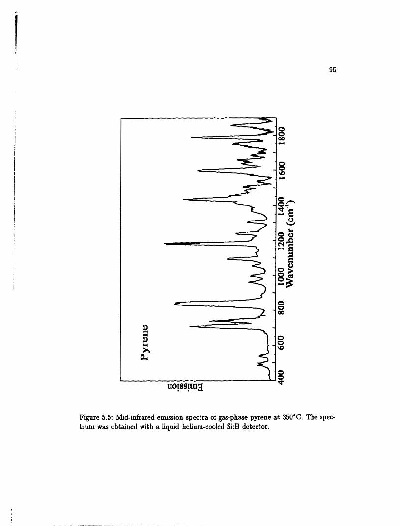
Figure 5.5: Mid-idkared emission spectra of gas-phase pyrene at 350°C. The spec- trum ras obtained with a liquid helinm-cooled Si:B detector.

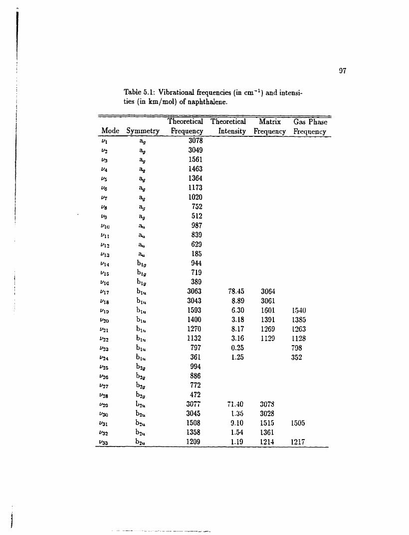
Table 5.1: Vibrational frequencies (in cm-' ) and intensi- ties (in km/rnol) of naphthalene.

Theoretical Theoretical Matrix Gas Phase Mode Symmetry Frequency Intensity Frequency Frcqiieney

% 3078

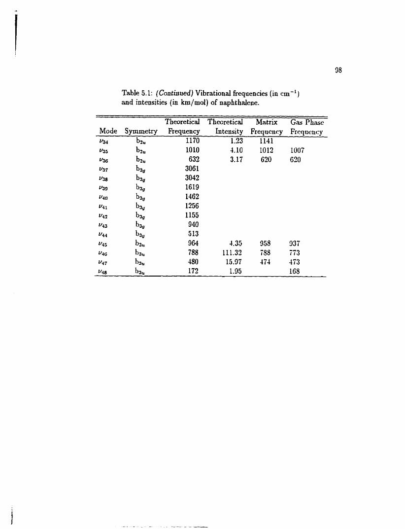
Table 5.1: (Conthued) Vibrational fkequencies (in cmF1) and intensities (in km/mol) of naphthalene.

Theoretical Theoretical Matrix Gu Phase Mode Symmetry Frequency Intensity Frequency Fitiqueiicy 4.4 bu 1170 1.23 1141

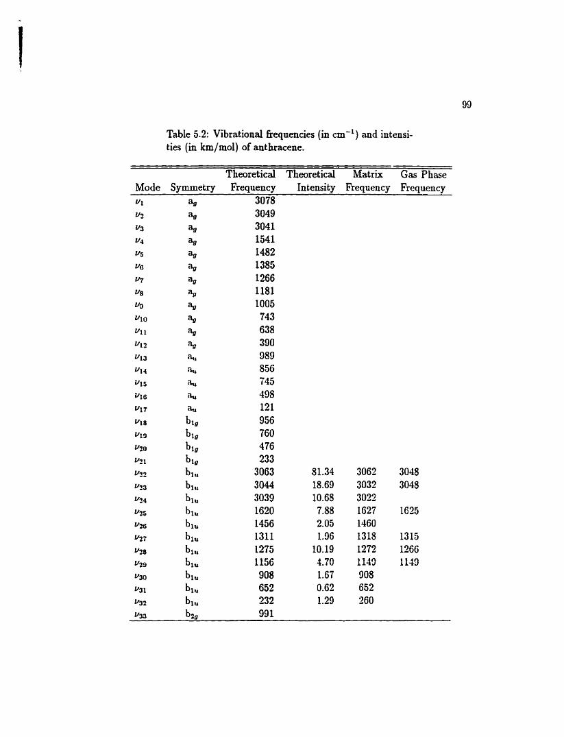
Table 5.2: Vibrational fiequenues (in cm-') and intensi- ties (in kmfmol) of anthracene.

Theoretical Theoretical Matrix Ga Phase Mode S ymmetry Frequency Intensity Frequency Frequency

3078

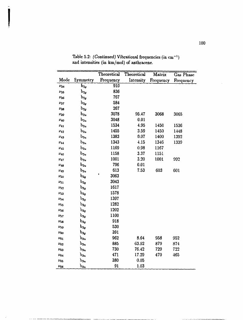
Table 5.2: (Contianed) Vibrational frequencies (in cm- l ) and intensities (in km/mol) of anthracene.

Theoretical Theoretical Matrix Gas Phase Mode Symmetry Frequency Intensity Frequency Frequency v34 b2* 910

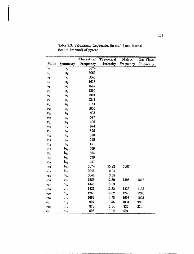
Table 5.3: Vibrational Beqnencies (in cm-') and intensi- ties (in km/mol) of pyrene.

Theoreticd Theoretical Matrix Gas Phase Mode Symmetry Frequency htensity Frequency Frequency

% 3074

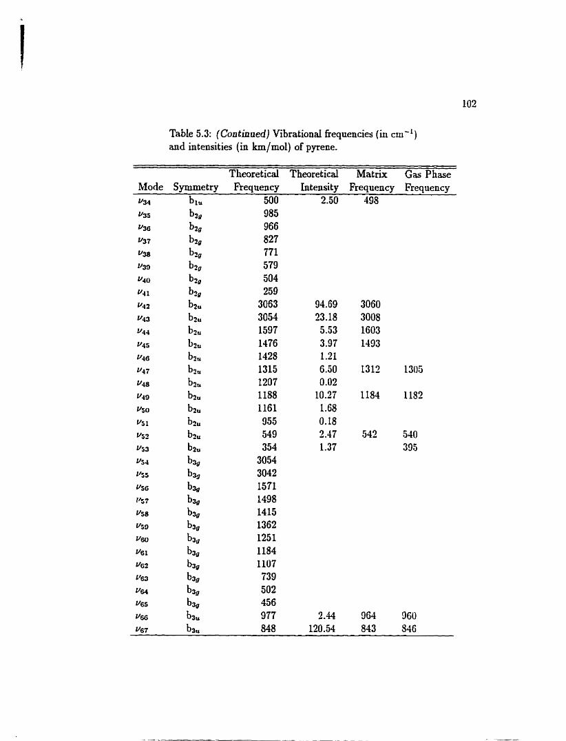
Table 5.3: (Continued) Vibrationai fiequencies (in cm-') and intensities (in km/mol) of pyrene.

Theoretical Theoretical Matrix Gas Phase hfode Symmetry Frequency Intensity Frequency Frequency

b lu 500 2.50

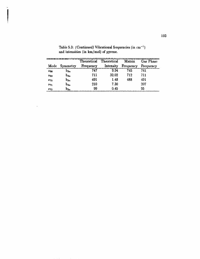
Table 5.3: (Con tinued) Vibrational fiequencies (in cm- l )

and intensities (in km/mol) of pyrene.

Theoretical Theoretical Matrix Gas Phase Mode Symrnetry Frequency Intensity Frequency Frequency 4 8 b3u 747 9.94 745 74 1

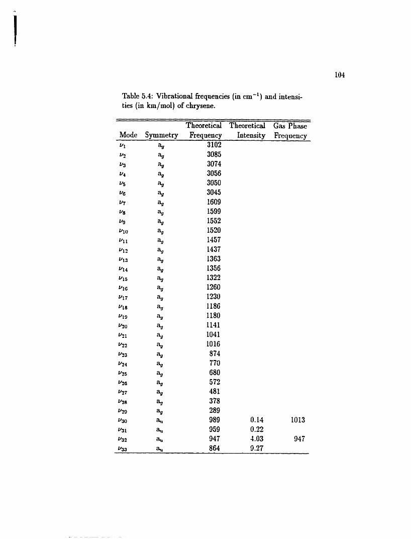
Table 5.4: Vibrational fiegoencies (in cm-') and intensi- ties (in km/rnol) of chrysene.

Theoretical Theoretical Gas Phase Mode S ymmetry Frequency Intensity Frequericy

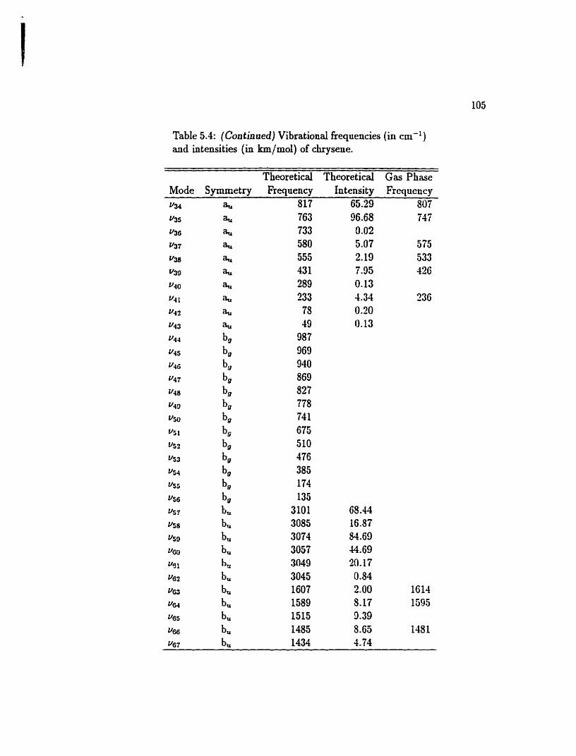
Table 5.4: (Con tinued) Vibrational frequencies (in cm- ) and intensities (in km/mol) of chrysene.

Theoretical Theoretical Gas Phase Mode Symmetry Frequency Intensity Frequency

817 65 -29 807

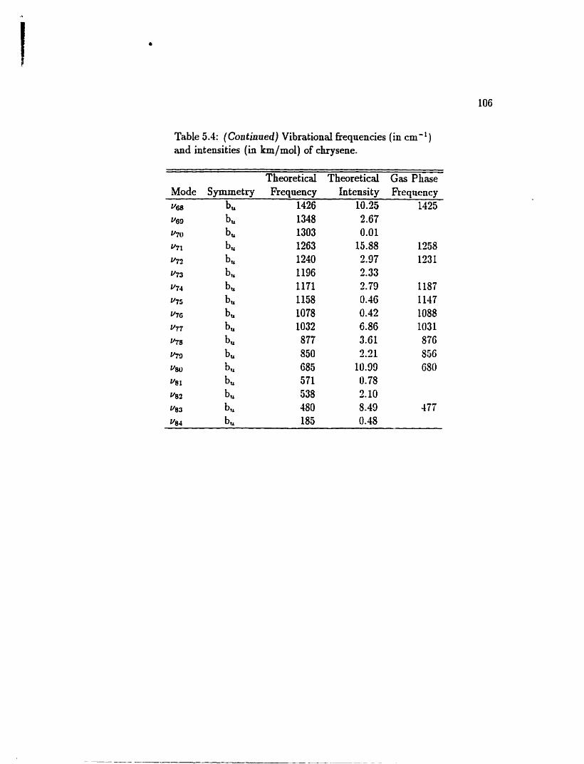
Table 5.4: (Continued) Vibrational fiequencies (in cm-') and intensities (in km/mol) of chrysene.

Theoretical Theoretical Gas Phase Mode Symmetry Frequency Intensity Frequency "68 bu 1426 10.25 1425

The selection rules for combination and overtone modes can be denved in a

similar manner. The symmetry of a combination or overtone mode is obtained by

taking the direct product of the symmetries of the fundamental modes involved.

For example. the synunetry of n combination mode involving fundamental modes i

and j is

The direct products for different symmetry groups are tisualiy listed in text books

[Il]. It is iuteresting to notice that g-u selection rules are

Sirice the infrarcd active modes of the DZh and CZh groups cd hiive il symnictry. .d

t tie first overtone vibrations are not allowed.

It is conventiond to use lower case letters to indicate the symmetries of nor-

mal modes. i.c. bt, instead of BI,. The normal vibrationai modes arc listcil in

Tables 5.1 - 5.4. together with matrix fiequencies and gns phase freqtiencics fioui

tlJs study. The C-H stretching region near 3300 cm-' is too congestetl to ni.&

assignments. In gcneral. the data obtained fiom this study are in good agrccnicnt

with theoretical calculations and matrix data. Because of brondeuing of bauds at

high temperatures. gas phase bands are not as well deftied as matrix bands.

It is noticed that the calculations for naphthalene. anthracene. ,and pyrene are

closer to experimentai values. while those for chrysene are in gnera l iderior. Never-

t heless. the agreement between experiments and ab initio calctilations is renixkable.

This is especidy so in the fa-infrared region where the theoretical prcdictions are

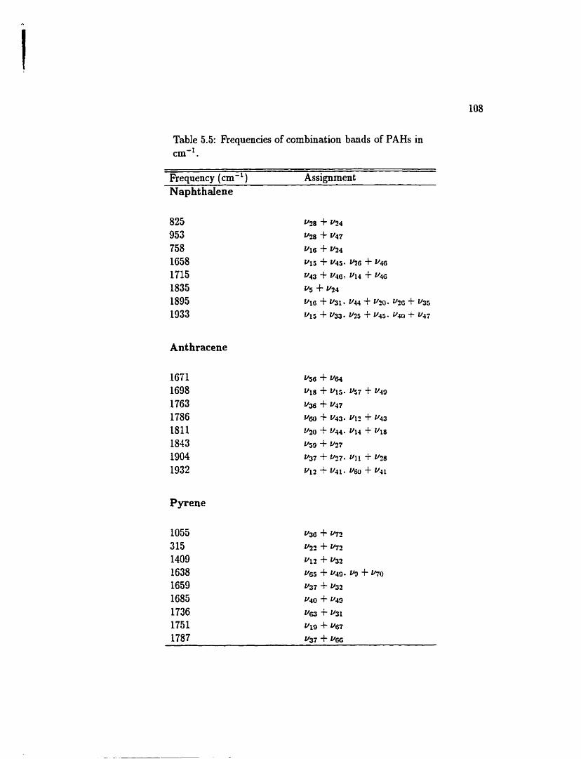
Table 5.5: Frequencies of combination bands of PAHs in

Frequency (cm-') Assignment Napht haiene

Anthracene

P yrene

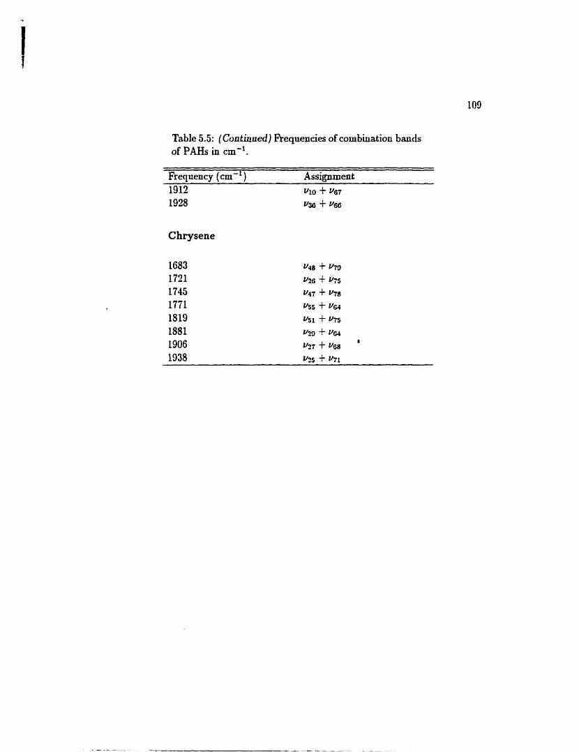
Table 5.5: (Continueci) Frequenües of combkiation bands of PAHs in cm".

Frequency (cmdL ) Assignment

Chrysene

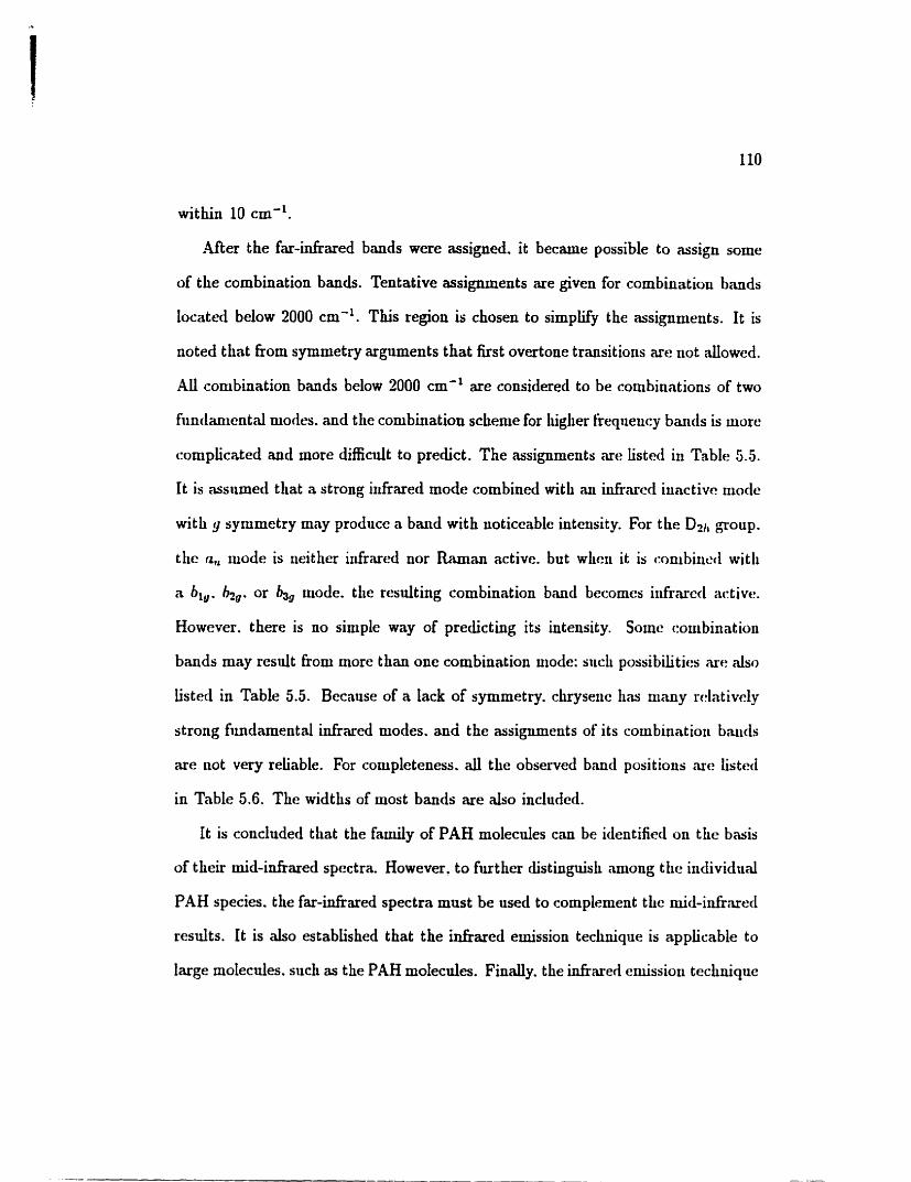
within 10 cm-'.

After the far-idiared bands were assigned. it became possible to assign some

of the combination bands. Tentative assignments are given for combinat ion bands

located below 2000 cm% This region is chosen to simplify the assignments. It is

noted tkat from symmetry arguments that f b t overtone transitions are uot dowed.

Ail combination bands below 2000 cm" are considered to be combinations of two

hindmental niocles. and the combination scheme for lùglier fkequeticy bands is more

complicated and more diacult to predict. The assignments are listcd in Table 5.5.

It is assumed that a strong iiifrared mode combined witli an infiarecl iunctive niocle

wit k g synunetry may produce a band with noticcable intensity. For the D?,, group.

the a, mode is neither infrxed nor Rcunc?n active. but wliea it is combineci witli

a biU. h2*. or b3* mode. the resulting combination band becomes iiifrnred active.

However. there is no simple way of predicting its intensity. Somc combination

bands may rnult fiom more than one combination mode: sticli possibilities are dso

listed in Table 5.5. Becnuse of a lack of symmetry. chrysetie hw nmny rolntivcly

strong fundamental infrared modes. and the assignments of its combinatioti bauds

are not very reliable. For conipleteness. all the observed band positions are listeci

in Table 5.6, The widths of most bands are also included.

It is concluded that the family of PAH molecules can be identified un the basis

of t heir mid-infiared spectra. However. to furt hm distinyisk m o n g t lie individual

PAH species. the far-infrared spectra must be ased to cornplexnent the mibinfrwed

results. It is also estabiished that the idrarecl emission technique is applicable to

large molecules. such as the PAH molecules. Finally. the infrard emissiou technique

is superior ta infrard absorption. as most dearly observed.

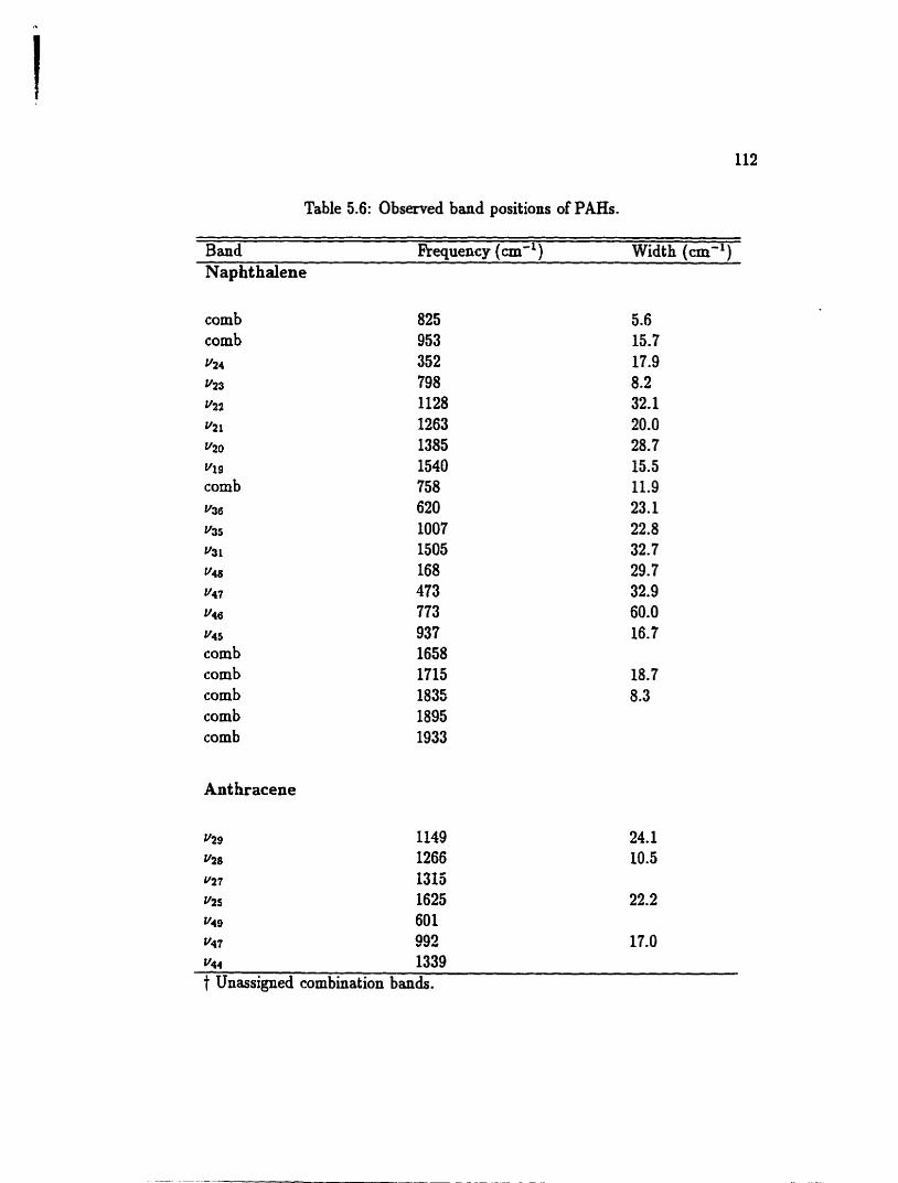
Table 5.6: Observed band positions of P B .

Band Fkequency (cm-l) Width (cm-l) Napht halene

comb comb v24

Y23

v22

v21

v20

v19

comb v36

v35

v3 1

V48

v47

v46

v45

comb comb comb comb comb

Ant hracene

v29 1149 24.1 vzs 1266 10.5 v27 131s v25 1625 22.2 v49 601 v47 993 17.0 v44 1339 t Unassigned combination bands.

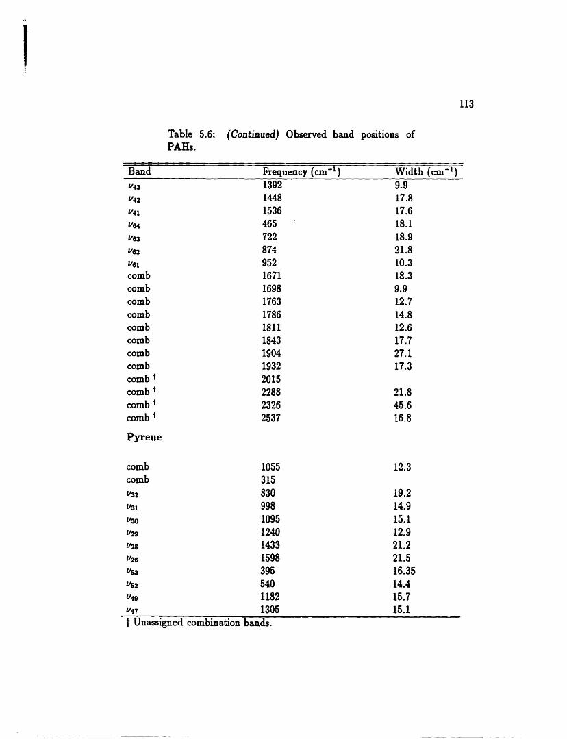
Table 5.6: (Continued) Observed band positions of PAHS.

Band Fkequency (cm-l ) Width (cm-') v43 1392 9.9 v4z 1448 17.8 v4 1 1536 17.6 v a 465 18.1

722 18.9 "62 874 21.8 vsi 952 10.3 comb 1671 18.3 comb 1698 9.9 comb 1763 12.7 comb 1786 14.8 comb 1811 12.6 comb 1843 17.7 comb 1904 27.1 comb 1932 17.3 comb 2015 comb 2288 21.8 comb 2326 45.6 comb 2537 16.8

Pyrene

comb 1055 12.3 comb 315 '42 830 19.2 hl 998 14.9 v30 1095 15.1 v2g 1240 12.9 @8 1433 21.3 v26 1598 21.5 t'53 395 16.35 us2 540 14.4 "49 1182 15.7 ~ 4 7 1305 15.1 t Unassigned combination bands.

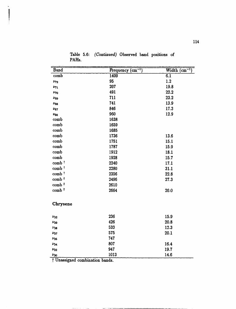
Table 5.6: (Continued) Observed band positions of PARS.

Band Requency (cm-' ) Width (cm-') comb 1409 6.1 m? Y71

y70

u69

4 0

v67

v66

comb comb comb comb comb comb comb comb comb f

comb f

comb comb t

comb comb t

Chrysene

b 2 236 15.9 4 9 426 20.8 Vas 533 13.3 u37 575 20.1 u35 747 v34 807 16.4 v32 947 19.7 %I 1013 14.6 t Unassigned combination bands.

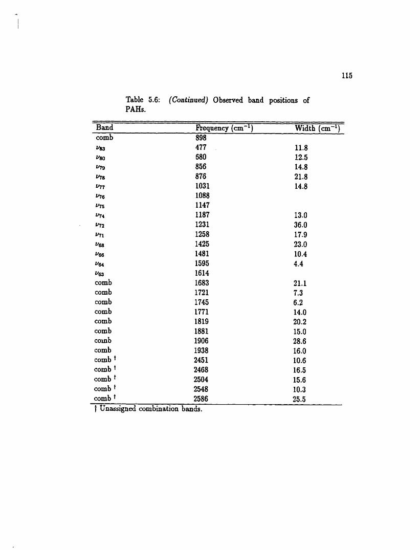
Table 5.6: (Continued) O bserved band positions of PAHs.

Band Fkequency (cm-') Width (cxül ) comb 898 y83 477 . 11.8 ha 680 12.5 ~ 7 9 856 14.8 V?8 870 21.8 Yn 1031 14.8 -6 1088 v75 1147 y74 1187 13.0 v72 123 1 36.0 p71 1258 17.9 uss 1425 23.0

1481 10.4 h.4 1595 4.4 y63 1614 cornb 1683 21.1 comb 1721 7.3 comb 1745 6.2 comb 1771 14.0 comb 1819 20.2 comb 1881 15.0 comb 1906 28.6 comb 1938 16.0 comb 245 1 10.6 comb 2468 16.5 comb 2504 15.6 comb t 2548 10.3 comb 2586 25.5 t ünassigned combination bands.

References

1. InfrBnd Spectroscopy of Biomolecules, edited by J. Liquier and E. Taillandier

(Wiley-Liss, New York, 1996).

2. High Resolution Infrnred Renrote Sensing for Earth 5 Weather and CIimate

Studies. edited by A. Chedin, M.T. Chahine and N. A. Scott (Springer-Verlag,

Berlin, 1993).

3. E. Hirota and K. Kawaguchi, Annu. Rev. Phys. Chem. 36. 53 (1985).

4 . The Infnrred Spectral Region of S t a q edited by C . Jaschek and Y. Andrillat

(Cambridge University Press, Cambridge, 1991).

5. The Impact of Ve y High S ' N Spectroscopy on Stellar Physàcs, edited by G.C.

de Strobel and M. Spite (Klnwer Acadamic Publishers, Paris, 1987).

6. D.K. m g e r and A. Mooradian. Optical and Laser Remote Sewing

( S pringer-Verlag , Berlin, 1983).

7. G. Stephens, Remote Sensing of the Lourer Atmosphere (Odord University

Press, Oxford, 1994).

8. J. HoIlas, High Resolutzon Spectroscopy (Butterworths, London, 1982).

9 . G . Herzberg, Moleçular Spectra and Mole&+ Structure (Krieger Publishing

Company, Florida, 199 1).

10. P. Bernath. Annu. Rev. Phys. Chem. 41, 91 (1990).

11. P. Bernatb, Spectra of Atoms and Molecules (Oxford University Press, Odord,

1995).

12. M. Birk and J.W. Brault, Mikroehim. Acta 2, 243 (1988).

13. L. Wdace, P. Bernath, W. Livingston, K. Hinkle, J. Busler, B. Guo and K.

Zhang, Science 268, 1158 (1995).

14. E. Hirota, J . Phys. Chem. 87, 3375 (1983).

15. E. Hirota, Vib. Spectra Stmct. 14, 1 (1985).

16. E. Hirota and S. Saito, Rev. Chem. Intenned. 7, 353 (1987).

17. Ion CIwter and Ion Spectroscopy and Structure, edited by J. Maier (Elsevier,

Amsterdam. 1989).

18. N.B. Colthup, L.H. Daly and S.E. Wiberley, Introduction to Infiand and

Raman Spectroscop y ( Academic Press, San Diego, 1990).

19. A. H&er, K. Norton, P. Griûiths, S. Boanie and R. Curbelo, Anal. Chem.

60, 2441 (1988).

20. R. Beer, Remote Sensing by Fourier ~ u n s f o n n Spectrometry (Wiley, New

York, 1992).

21. M. Low and S. Reeman, Anal. Chem. 39, 194 (1967).

22. P. Wang, S. Lacele and H. Yazdi, Appl. Spec. 47, 1830 (1993).

23. H. Lefebvre-Brion and R.W. Field, Perturbations in the Spectra of Diatomie

Molecules ( Academic Press, London, 1984).

24. W. Kolos and L. Wolniewicz, J. Chem. Phys. 41, 3663 (1964).

25. M.S. Child and D.J. Nesbitt, Chem. Phys. Lett. 149, 404 (1988).

26. D.J. Nesbitt, M.S. Child and D.C. Clary, J. Chem. Phys. 90, 4855 (1989).

27. M. Born and R. Oppenheimer, Annal. Phys. 26, 30 (1927).

28. J. van Vleck, J. Chem. Phys. 4, 327 (1936).

29. R. Berman and A. Asgharian, J. Mol. Spec. 19, 305 (1966).

30. P. Bunker, J. Mol. Spec. 42, 478 (1972).

31. 1. Levine, Quantum Chernid y, 4th edition ( Allyn and Bacon, Boston, 1991).

32. J. Dunham. Phys. Rev. 41, 721 (1932).

33. P. B d e r and R. Moss, Mol. Phys. 33, 417 (1977).

34. J.A. Coxon and P.G. Hajigeorgion, Cm. J. Phys. 70, 40 (1992).

35. J.A. Coxon and P.G. Hajigeorgion, Chem. Phys. 167, 327 (1992).

36. J.A. Coxon and P.G. Rajigeorgiou, J. Mol. Spec. 150, 1 (1991).

37. K. Zhang, B. Guo, P. Colarnsso and P. Bernath, Science 274,582 (1996).

38. S. Langhoff, J. Phys. Chem. 100, 2819 (1996).

39. P. Colmsso, K. Zhang, B. Guo, and P. Beniath, Chem. Phys. Lett. (in press)

(1996).

40. E. Hirota, High Resolution Spectroscop y of Tkufzst'ent Molecules (Springer-

Verlag, Berlin, 1985).

41. A. Maki, J. Mol. Spec. 102.361 (1983).

42. H. Jones and J. Lindenmayer, Chem. Phys. Lett. 135, 189 (1987).

43. J. Bell, Introducto y Founer lfansfonn Spectroscopy (Academic Press, Lon-

don, 1971).

44. Vibrational Spectra and Structure vol. 19. edited b y J. Durig (Ekevier. Ams-

terdam, 1988).

45. P.R. Griffiths and J.A. de Haseth, Fourier ïkamfonn InfrBred Sprctroscopy

(Wiley, New York. 1986).

46. J-C. Hill and G.P. Montgomery, App. Opt. 15. 748 (1976).

47. C.B. Carlisle. D.E. Cooper and A. Preier, App. Opt. 13? 2567 (1989).

48. A.G. Robiette and J.L. Duncan, h a . Rev. Phys. Chem. 34, 245 (1983).

49. J. Brault, Philos. Trans. R. Soc. London Sa. A 307, 503 (1982).

50. A. Michelson, Phil. Mag. 31, 256 (1891).

51. A. Michelson, Light Waues and Their Uses (University of Chicago Press,

Chicago, 1902).

52. A. Michelson, Studies in Optics (Universityof Chicago Press, Chicago, 1927).

53. J. Cooley and J. Tukey, Math. Comput. 19, 297 (1965).

54. J. van Vleck, Phys. Rev. 33, 467 (1929).

55. R.M. Dale, R. Berman, J.W.C. Johns, A.R.W. McKellar, S. Nagler an,

Strathy. Can. J. Phys. 57, 677 (1979).

56. A. Ross, R. Eng and H. Kildal, Opt. Comm. 12,433 (1974).

57. J. Watson. J. Mol. Spec. 80, 411 (1980).

58. J. Watson, J. Mol. Spec. 45, 99 (1973).

59. P. Bunker, J. Mol. Spec. 68, 367 (1977).

60. E. Tiemann, A. Arnet, W.U. Stieda, T. Torring and J. Ho&, Chem. Phys.

67' 133 (1982).

61. E. Tiemann, J. Mol. Stmct. 97, 331 (1983).

62. J. Schlembach and E. Tiemann, Chem. Phys. 68, 21 (1982).

63. H. Knockel and E. Tiernann, Chem. Phys. 68, 13 (1982).

64. E. Tiemann, H. Knockd and J. Schlembach, Ber. Bunsenges. Phys. Chem.

86,821 (1982).

65. R. LeRoy and J. van Kranendonk, J. Chem. Phys. 61,4750 (1974).

66. W. Kosman and J. Hinze, J . Mol. Spec. 56 ,92 (1975).

67. G.C. Maitland, M. Rigby, E.B. Smith and W.A. Wakeham, Intermoleetclar

Forces: Thezr Ongin and Determination (Clarendon Press, Odord, 1981).

. 68. KG. Hedderich, M. Dulick and P.F. Bemath, J. Chem. Phys. 99,8363 (1993).

69. J.M. Campbell, M. Dulick, D. Klapstein, J.B. White and P.F. Bernath, J.

Chem. Phys. 99. 8379 (1993).

70. J.B. White, M. Duiick and P.F. Beniath, J. Chem. Phys. 99,8371 (1993).

71. R. Dull? Phys. Rev. 47, 458 (1935).

72. M. Chretien and E. Miescher, Nature 163, 996 (1949).

73. M. Chretien. Phys. Acta 23, 259 (1950).

74. R. Onalsa, J. Chem. Phys. 27, 374 (1957).

75. R.F. Barrow, D. Premaswarnp, J. Winternitz and P.B. Zeeman, Proc. Phys.

Soc. A 71, 61 (1958).

76. D. Robinson, J. Mol. Spec. 11, 275 (1963).

77. S. Krishnamachari and M. Singh, Curxent S u . 34,655 (1965).

78. J. Czarny and P. Felenbok, Chem. Phys. Lett. 2,533 (1968).

79. R. Caton and A. Douglas, Cm. J. Phys. 48, 432 (1970).

80. A.C. Le Floch, J. Lebreton, F. Launay, J. Fenan and J. Rostas, J. Phys. B

13, 3989 (1980).

81. H. Bredohl, 1. Dubois, F. Melen and M. Vervloet, J. Mol. Spec. 129, 145

(1988).

82. D. Hildenbrand, Int. J. Mass Spectrom. Ion Phys. 7, 255 (1971).

83. J.M. Dyke, C. Kirby and A. Moms, J. Chem. Soc.. Faraday Tkans. 2 79.483

(1983).

84. F. Lovas and D. Johnson, J. Chem. Phys. 55,41 (1971).

85. G. Cazzoli, L. Cludi, C.D. Esposti and L. Dore. J. Mol. Spec. 134, 159 (1989).

86. T. Nakanaga, H. Takeo, S. Kondo and C. Matsumura, Chem. Phys. Lett.

114, 88 (1985).

87. M. Zahniser and M. Gersh, J. Chem. Phys. 75, 52 (1981).

88. R. Nesbet, J. Chem. Phys. 40, 3619 (1964).

89. R. Nesbet, J. Chem. Phys. 43, 4403 (1965).

90. W. Huo, J. Chem. Phys. 43,624 (1965).

91. H. Lefebvre-Brion and C. Moser, J. Mol. Spec. 15,211 (1965).

92. A. Kurtz and K. Jordon, Chem. Phys. Lett. 81, 104 (1981).

93. H. W. P. Rosmns and M. Grimm, Chem. Phys. Lett. 92,250 (1982).

94. P. Botschwina, J. Mol. Spec. 118, 76 (1986).

95. M. Honigmann, G. IIirsch and R.J. Buenker, Chem. Phys. 172,59 (1993).

96. F. Charron, B. Guo, K. Zhang, 2. Morbi and P.F. Bernath, J. Mol. Spec.

171, 160 (1995).

97. R. LeBlanc, J. White and P. Bernath, J. Mol. Spec. 164, 571 (1994).

98. B.G. Hedderich, M. Dulick and P.F. Bernath: J. Chem. Phys. 99,8363 (1993).

99. K. Huber and G . Herzberg, Constants of Diatomic Moleeules (Van Nostrand-

Reinhold, New York, 1979).

100. H. Hedderich and P. Bernath, J. Mol. Spec. 153, 73 (1992).

10 1 . Mofecular Spedroscop y: Modern Research, vol. 9 edited by R. Rao ( Academic

Prcss, New York, 1355).

102. E. Whiting, A. Schadee, J. Tatum. J. Hougen and R. Nicholls, J. Mol. Spec.

80, 249 (1980).

103. Ch. Rydewin, H.U. Schutze-Pahlmann, J. Ho&, and T. Torring, Chem.

Phys. 71, 389 (1982).

104. K. Moller. H.U. SchutzePahlmann, J. Hoeft. and T. Toming, Chem. Phys.

82, 399 (1982).

105. Y. Azurna, W.J. Childs, G.L. Goodman and T.C. Steimle, J. Chem. Phys.

93, 5533 (1990).

106. W.J. Childs and L.S. Goodman, Phys. Rev. Lett. 44, 316 (1980).

107. R. Barrow and J. Beale, Proc. Phys. Soc. 91,483 (1967).

108. M.A. Anderson, M.D. Allen and L.M. Zinrys, J. Chem. Phys. 100,824 (1994).

109. M.A. Anderson, M.D. M e n and L.M. Ziuys, Astrophys. J. Lett. 425, 53

(1994).

110. L. Knight Jr.. W. Easley, W. Weitner Jr. and M. Wilson, J. Chem. Phys. 54,

322 (1971).

111. A.D. Buckingham and R.M. Olegario, Chem. Phys. Lett. 212,253 (1993).

112. T. T o h g , W.E. Ernst and S. Kindt. J. Chem. Phys. 81.4614 (1984).

113. T. T o h g , W.E. Ernst and J. Kandler, J. Chem. Phys. 90.4927 (1989).

114. C. Bauschlicher Jr., S. Langhoff, T. Steimle and J. Shirley, J . Chem. Phys.

93.4179 (1990).

115. S. Meth, R.J. Bsrtlett and M. Nooijen? private commanication .

116. K. Zhang, B. Guo, V. Braun, M. Dtilick and P.F. Bernath, J. Mol. Spec. 170,

82 (1995).

117. C. Grundmann and P. Grnnanger, The N i t d e Ozides: Versatile Tools of

?'heoretzcai and Preparative Chemistiy ( S pringer-Verlag, Berlin. N'il 1.

118. A. Padwa, 1,2-Cycloadditzon Chembtry (Wiley, New York, 1984).

119. H. Feuer, N i t d e ûxides, Nitmnes, and Nitronates in Organic SpW esis (VCH

Publishers, hc . , New York, 1988).

120. G. Maier and J. Teles, Angew Chem. Int. Ed. Engl. 26, 155 (1987).

121. T. Pasinszki and N.P.C. Westwood, J. Phys. Chem. 99, 6401 (1995).

122. B. Guo, T. Pasinszki, N.P.C. Westwood and P. Bernath, J. Phys. Chem. 103,

123. B. Guo, T. Pasinszki, N.P.C. Westwood, K. Zhang and P. Bernath, J. Chem.

Phys. 105. 4457 (1996).

124. Th. Brupbacher. R. Bohn, W. Jager, M.C.L. Gerry, T. Pasinszki and N.P.C.

Westwood. J. Mol. Spec. 181, 316 (1997).

125. A. Maki and J. Wells, Wavenumber Calibration Tables £iom Hetaodyne Fre-

qnency Measurements, NIST Specid Publication 821 (1991).

126. Toth, J. Opt. Soc. Am. B 8,2236 (1991).

127. E. Ferretti and R. Rao, J. Mol. Spec. 51, 97 (1974).

128. D. Steiner, S. Polo, T. McCnbbin and K. Wishah? J. Mol. Spec. 98. 453

(1983).

129. T. Pasinszki and N.P.C. Westwood, unpnblished ranlts .

130. H. Jones. J. Sheridan and O.L. Stiehmta, 2. Natdimch. 32. 866 (1977).

131. J. Tyler and J. Sheridan, %S. Faraday Soc. 59, 2661 (1963).

132. B.P. Winnewisser, M. Winewisser and F. Winther, J. Mol. Spec. 51, 65

(1974).

133. P.R. Bunker, B.M. Landsberg and B.P. Winnewisser, J. Mol. Spec. 74, 9

(1979).

134. P. Blackburn. R.D. Brown, F. Bnrden, J. Crofts and L. Gillard, Chem. Phys.

Lett. 7, 102 (1970).

135. H. Goldstein, CZassical Mechanies (Addison- Wesley, Reading, 1980).

136. D. Papousek and M. Aliev. M o l e d u r Vibrutàonul- Rotational Spectra (Else-

vier, Amsterdam, 1982).

137. M. Diem, Introduction to Modem Vibrational Spectroscopy ( Wiley, New York.

1993).

138. D. Bishop, Croup Theory and Chemistry (Dover, New York, 1993).

139. J.H. Hahn, R. Zenobi. J.F. Bada and R.N. Zare, Science 239, 1523 (1988).

140. F. Mnllie and J. Reisse, Top. C m . Chem. 139, 83 (1987).

141. S. Clemett, C. bIaechling, R.N. Zare, P. Swan and R. WaIker, Science 262,

721 (1993).

142. L.P. Anamandola, A. Tielens and J.R. Barka, Astrophys. J. Lett. 390. 25

(1985).

143. A. Lega and J. Puget, Astr. Astrophys. 137,s (1984).

144. J. Puget and A. Leger, Annu. Rev. Astron. Astrophys. 27, 161 (1989).

145. L.J. Allamandola, A. Tielens and J.R. Barker, Astrophys. J. Snppl. 71, 733

(1989).

146. W. Ddey and D. Williams, Mon. Notices R. Astro. Soc. 196, 269 (1981).

147. A. Sakata. S. Wada, T. Tanabe and T. Onaka, Astrophys. J. Lett. 287, 51

(1984).

148. A. Sakata, S. Wada, T. Onaka and A.T. Tokmaga, Astrophys. J. Lett. 320,

63 (1987).

149. A. Borghesi, E. Bwsoietti and L. Colangeli, Astrophys. J. 314, 422 (1987).

150. A. Blanco, E. Bussoletti and L. Colangeli, Astrophys. J. 334, 875 (1988).

151. W.A. Schutte, A. Tielens and L.J. Allamandola, Astrophys. J. 415, 397

(N93).

152. C. Moutoa, A. Leger and L. d'Hendecourtt Astron. Astrophys. 310, 297

(1996).

153. J.P. Bernard, L. dXendecourt and A. Leger, Astron. Astrophys. 220, 245

(1989).

154. A. Blanco, S. Fonti and V. Orofho, Astrophys. J. 364, 152 (1990).

155. A. Leger, L. d9Hendecourt and D. Defourneau, Astron. Astrophys. 216, 148

(1989).

156. G. Flinckinger and T. Wdowiak, Astrophys. J. Lett. 362, 71 (1990).

157. L. Colangeli, V. Menneila and E. Bussoletti, Astrophys. J. 385, 577 (1992).

158. R. Clark and R. Hester, Spedroscopy of Matriz Isolated Spenes (Wiley, New

York, 1989).

159. J . Shan, M. Suto and L.C. Lee, Astrophys. J. 383, 459 (1991).

160. J. Brenner and J. Barker. Astrophys. J. Lett. 388, 39 (1992).

161. S. Schlemmer. D. Cook, J. Harrison, B. W d d , W. Chapman and R. Saykally,

Science 265, 1686 (1994).

162. D. Cook, S. Schlemmer, N. Balucani and R. Saykally, Nature 380,227 (1996).

163. J. Knrtz, Astron. Astrophys. Lett. 255, 1 (1992).

164. C. Joblin. L. d'Hendecourt, A. Leger and D. Defounieau, Astron. Astrophys.

281, 923 (1995).

165. C. Joblin, P. Boissel, A. Leger, L. dTHendecoart and D. Defouneau, Astron.

Astrophys. 299,835 (1995).

166. P. Bernath, Chem. Soc. Rev. 25. 111 (1996).

167. P. Bernath, in Lecture Notes in Physies, vol. 407, edited by P. Smith and W.

Wiese ( S pringer-Verlag , Berlin, 1992).

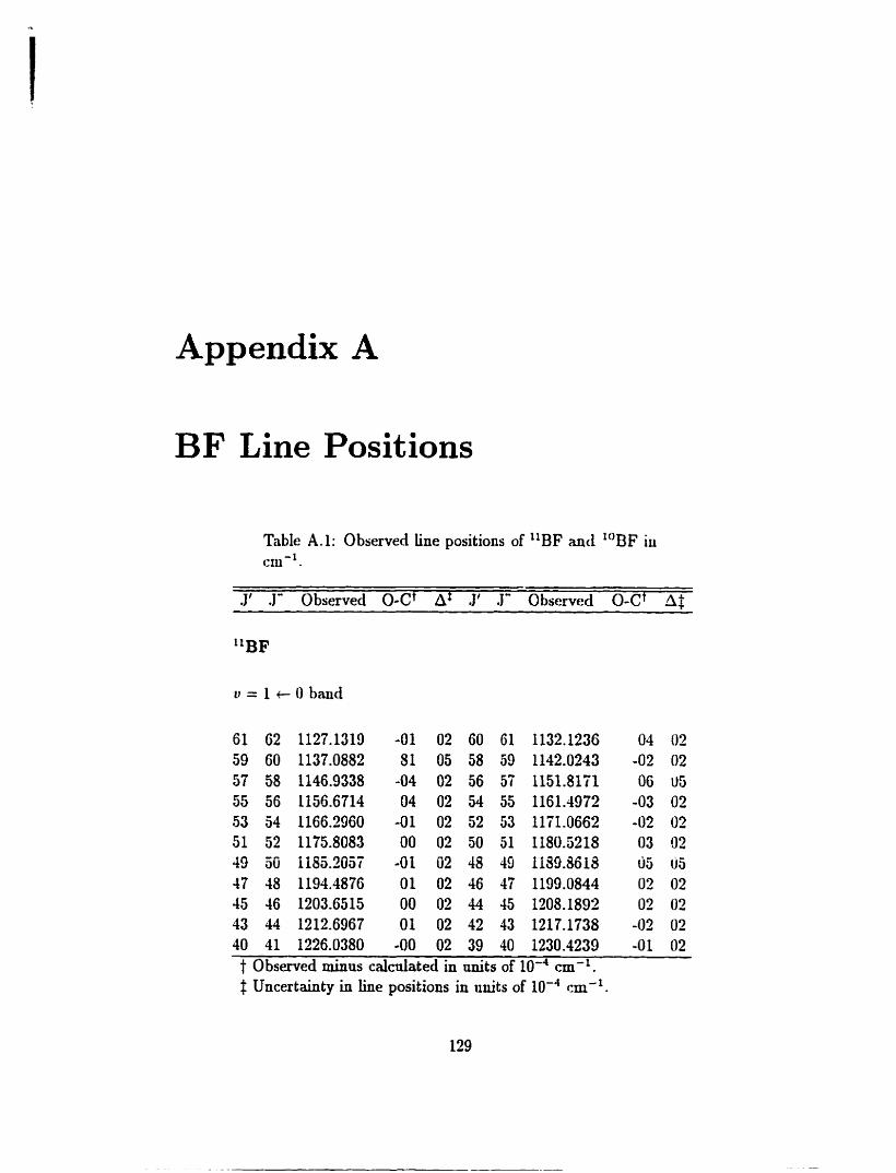
Appendix A

BF Line Positions

Table A.1: Observed Iine positions of "BI? and "BF iti cm-!

J' J Observed O-Cf Af J ' J a Observed O-Ct A$

61 62 1127.1319 -01 02 60 61 1132.1236 04 02 59 60 1137.0882 SI 05 58 59 1142.0243 -02 02 57 58 1146.9338 -04 02 56 57 1151.8171 06 U5 55 56 1156.6714 04 02 54 55 1161.4972 -03 02 53 54 1166.2960 -01 02 52 53 1111-0663 -02 02 51 52 1175.8083 O0 02 50 51 1180.5218 03 03 49 50 Z185.3057 -01 02 48 49 ii39.8618 05 05 47 48 1194.4876 01 02 46 47 1199.0844 02 02 15 46 1203.6515 O0 02 4l 45 1208.1892 02 02 43 44 1212.6967 01 02 42 43 1217.1738 -02 02 40 41 1226.0380 -00 02 39 40 1230.4239 -01 02 t Obsenred minus calcniated in nnits of IO-" cm-'. f Uncertainty in line positions in units of IO-' cm-'.

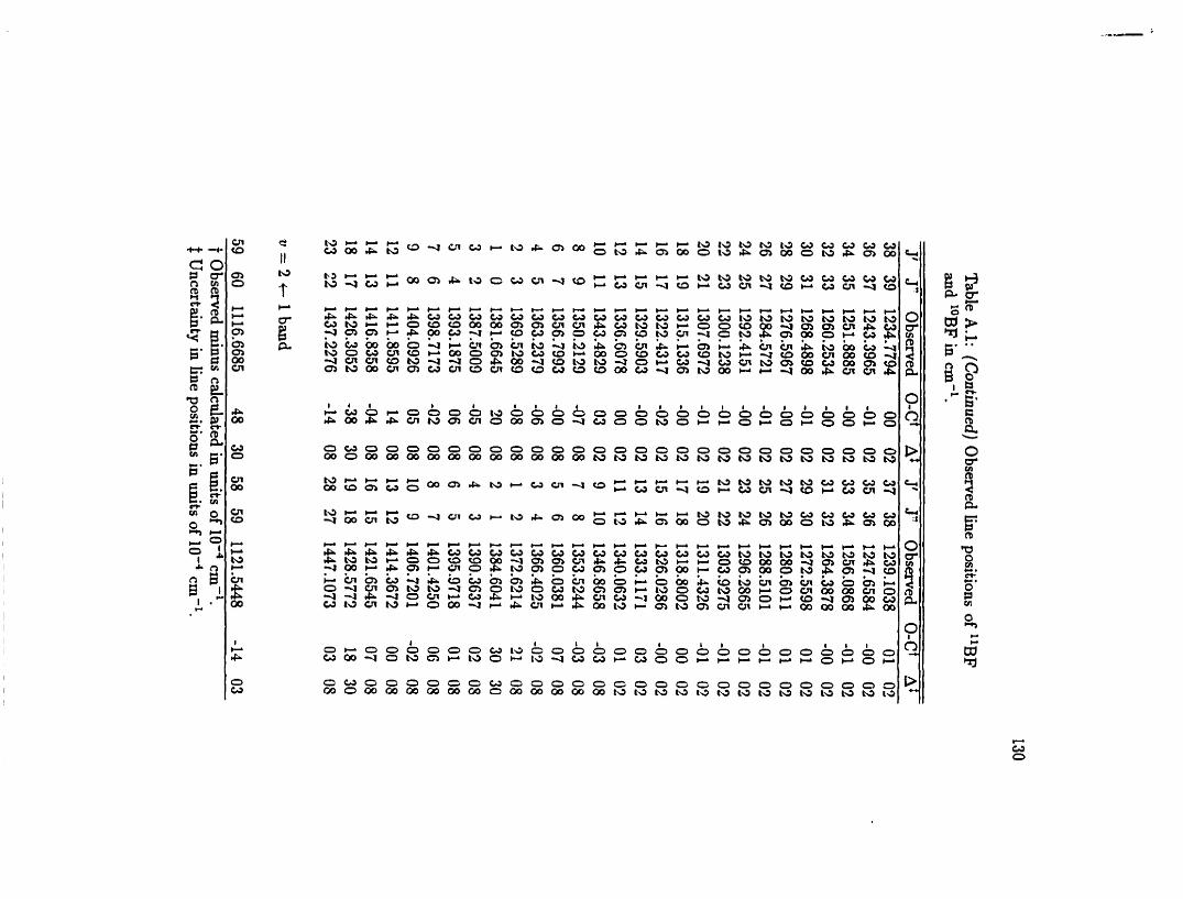
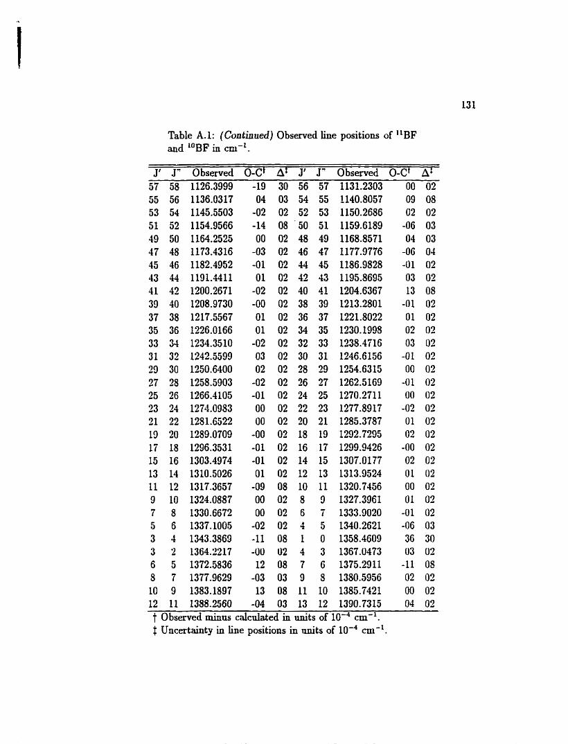
Table A. 1: (Continueci) Observed Line positions of "BF and 'OBF in cm-'.

J' J" Observed O-Cf Af J' Jw Observed O-Ct Af 57 58 1126.3999 -19 30 56 57 1131.2303 O0 02

- - - - -

t Observed minus calculated in M i t s of lW4 cm". $ Uncertainty in line positions in M i t s of cm-'.

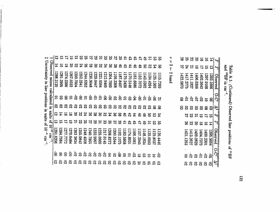
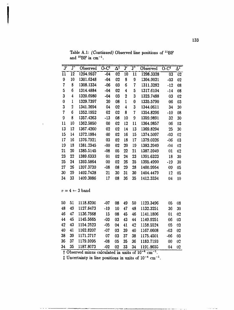
Table A.l: (Continued) Observed h e positions of "BF and l0BF in cm?

J' J' Observed O-Ct Af J' J" Observed O-Ct A:

Observed minus calcnlated in units of IO-'' cm-'. $ Uncettainty in h e positions in units of IO-' cm-'.

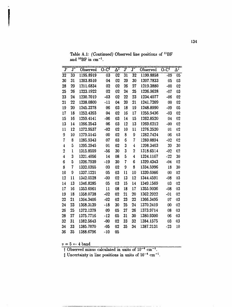
Table A.l : (Continued) Observed Line positions of llBF and l0BF in cm".

J' J" Observed O-Ct At J' J" Observed O-Cf A: 32 33 1195.8919 03 02 31 32 1199.8858 -09 05

t Observed minus calculated in units of IO-' cm-'. $ Uncertainty in line positions in units of 1W4 cm-!

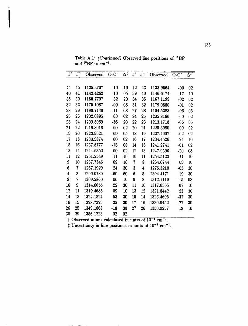
Table A.1: (Continued) Observeci line positions of 'lBF and 'OBF in cm-l.

J' J' Observed O-Ct Af J' Jn Observed O-Cf A:

44 45 1125.3707 -10 10 42 43 1133.9564 40 41 1142.4262 10 05 39 40 1146.6174 38 39 1150.7797 32 20 34 35 1167.1199 32 33 1175.1087 -09 OS 31 32 1179.0580 28 29 1190.7149 -11 08 27 28 1194.5383 25 26 1202.0895 03 02 24 25 1205.8160 23 24 1209.5069 -36 20 22 23 1213.1715 21 22 1316.8016 00 02 20 21 1220.3980 19 20 1223.9621 09 05 18 19 1227.4907 17 18 1230.9874 O0 02 16 17 1234.4526 15 16 1237.8777 -15 O8 14 15 1241.3741 13 14 1244.6352 OU 02 12 13 1247.9596 11 12 1251.2549 11 10 10 11 1254.5132 9 10 1257.7346 09 10 7 8 1264.0744 6 7 1267.1929 24 30 3 3 1276.3210 4 3 1299.0780 -60 60 6 5 1304.4171 8 7 1309.5860 06 10 9 8 1313.1119 10 9 1314.6055 22 30 11 10 1317.0555 12 11 1319.4685 09 10 13 12 1321.8442 14 13 1324.1823 53 30 15 14 1326.4695 16 15 1328.7329 25 30 17 16 1330.9452 26 25 1349.1068 -18 30 27 26 1350.9257 30 29 1356.1323 02 02 t Observed minus caidated in units of IO-'' cm-'. # Uncertainty in line positions in units of cm-'.

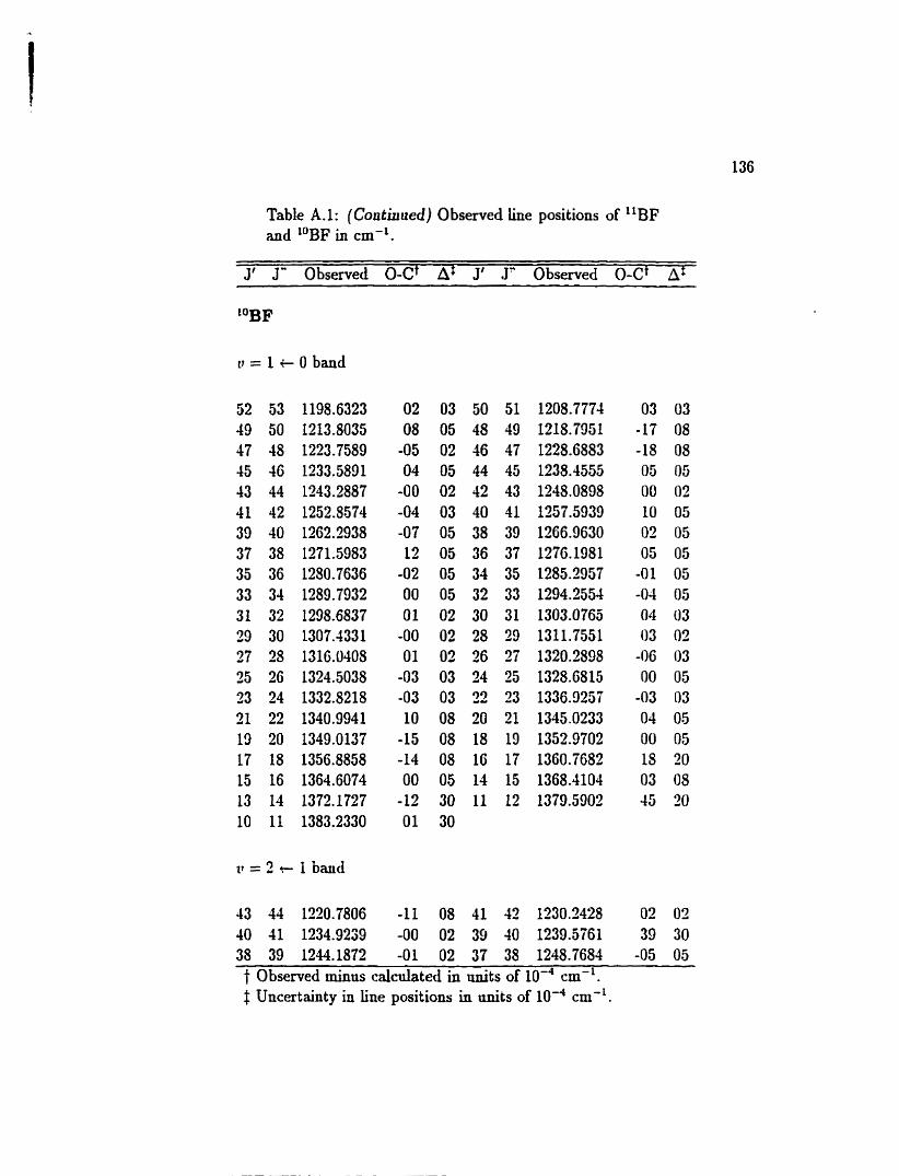
Table A.l: (Continued) Observed line positions of ''BF and 'OBF in cm-'.

J' Jn Observed O-Ct Af J' J* Obsenred O-Ct A:

o = 1 t O band

- - -

t Observed minus calculated in nni ts of IO-" cm-'. f Uncertainty in line positions in units of cm-'.

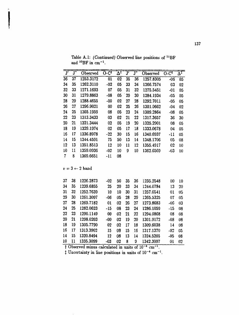
Table A.1: (Continued) Observed iine positions of "BF aud l0BF in cm".

J' J' Observed O-Ct At J' J" Observed O-Cf A: 36 37 1253.3172 O1 O2 35 36 1257.8305 -06 05

t Observed minus calculated in units of IO-" cm-'. t Uncertainty in line positions in units of cm-'.

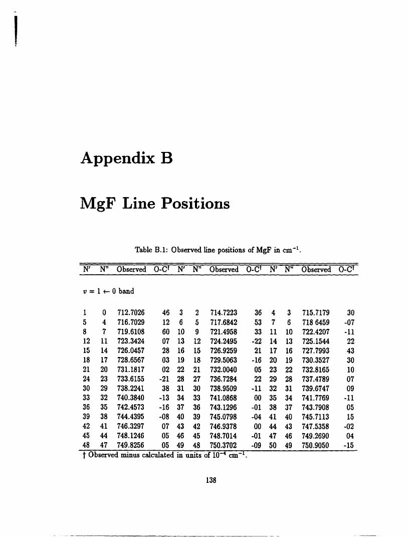
Appendix B

MgF Line Positions

Table B. 1: O bserved line positions of MgF in cm-l.

N' Nn Observed O-Ct N' W Observed O-Ct N' N" Observed O-Ct

v = 1 t- O band

t Obsemed minus calculated in units of cm-'.

138

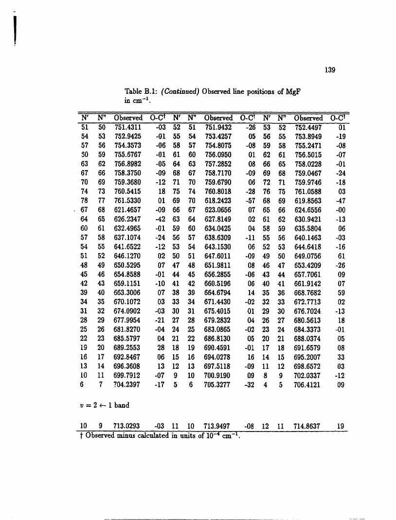
Table B.l: (Conthed) Observed line positions of MgF in cmd1.

N' N" Observed O-Ct N' N" Observed O-Ct N' N" Observed O-Ct 51 50 751.4311 -03 52 5 1 751.9432

t Observed niinus caldated in nnits of IOw4 cm-'.

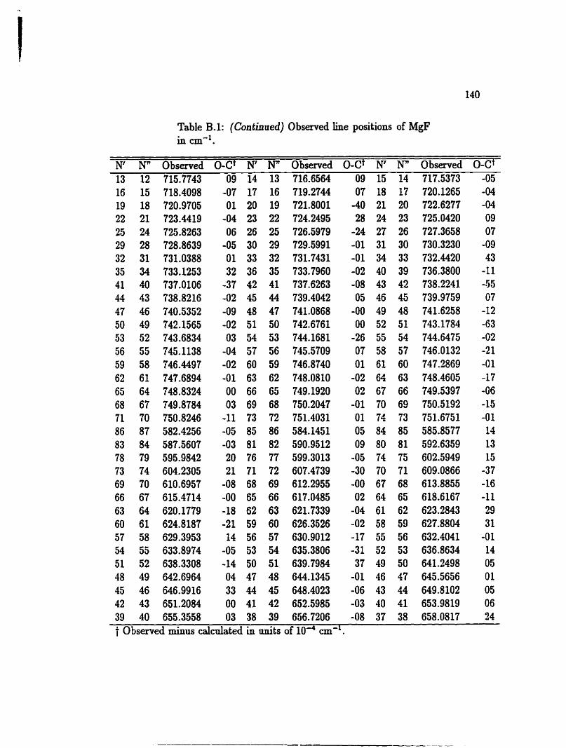
Table B.1: (Continued) Observed line positions of MgF in cm-'.

N' N" Observed O-Ct N' N" Observed O-Ct N' N" Observed O-Ct 13 12 715.7743 09 14 13 716.6564 09 15 14 717.5373 -05

t Observed minus calcnlated in un i ts of 1om4 cm-'.

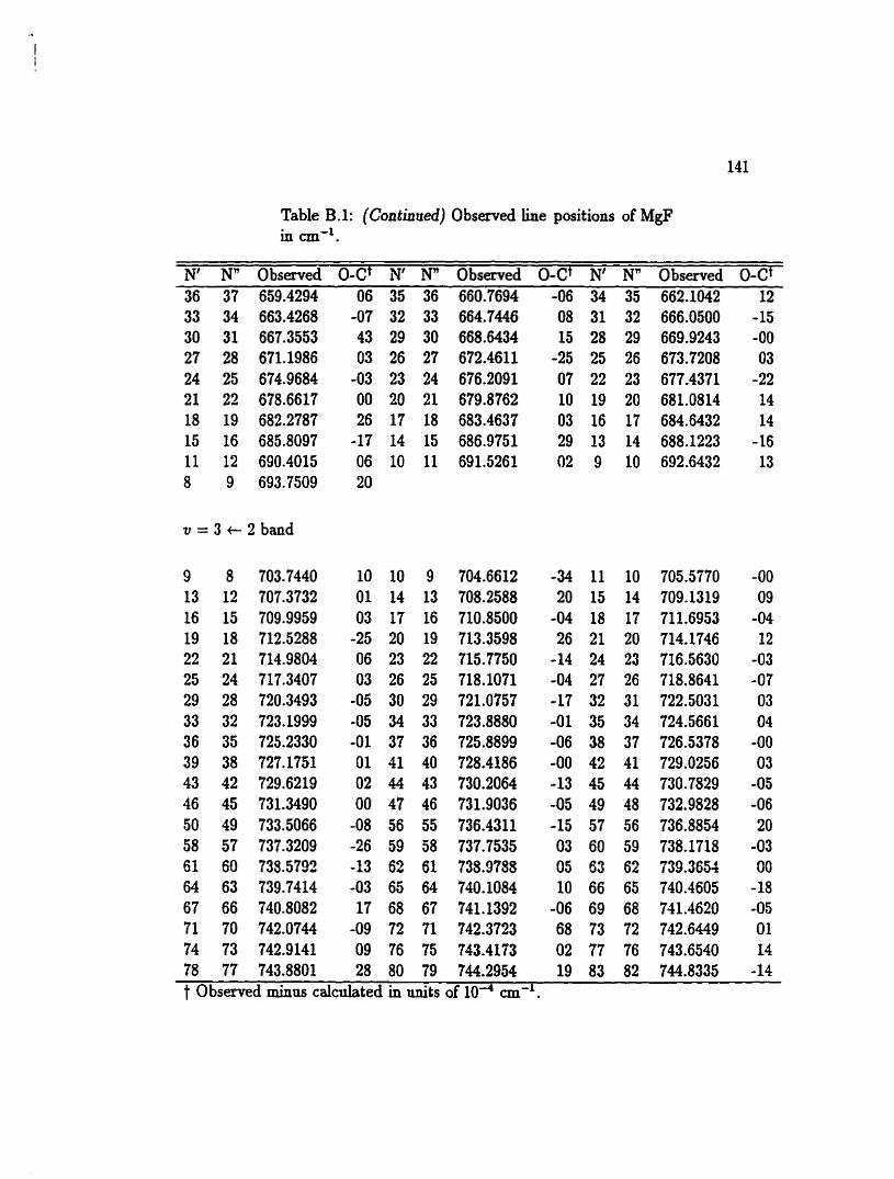
Table B.l: (Continued) Observed line positions of MgF in cm-'.

W Nn Observed O-Cf Nt N" Observed 0-0 Nt N" Observed O-Ct

t Observed minus calculated in units of IOd4 cm-'.

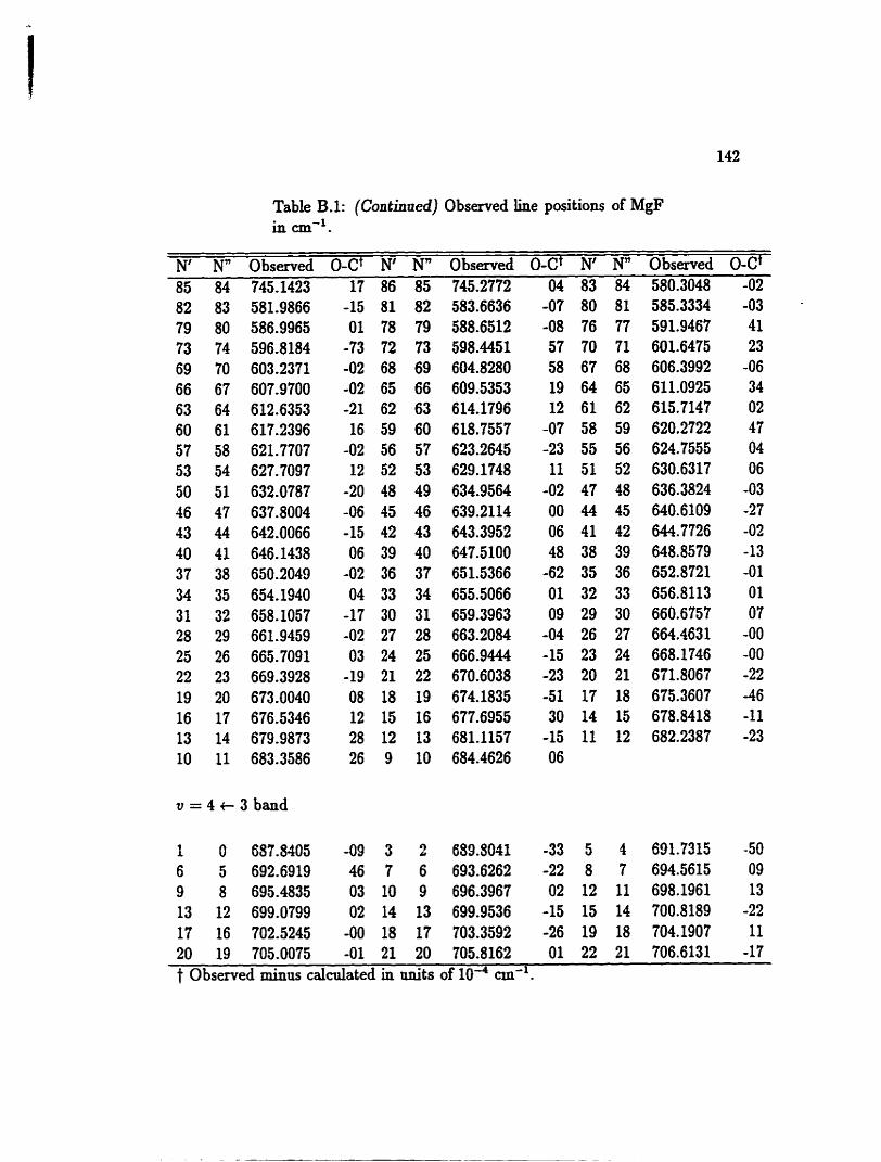
Table B.l: (Continned) Observed line positions of MgF in mi".

N' Nn Observed O-Ct Nt N" Observed O-Ct Nt Nn Observed O-Cf 85 84 745.1423 04 83 84 580.3048 -02

v = 4 + 3 band

t Observed minus calculated in M i t s of IO4 cm-'.

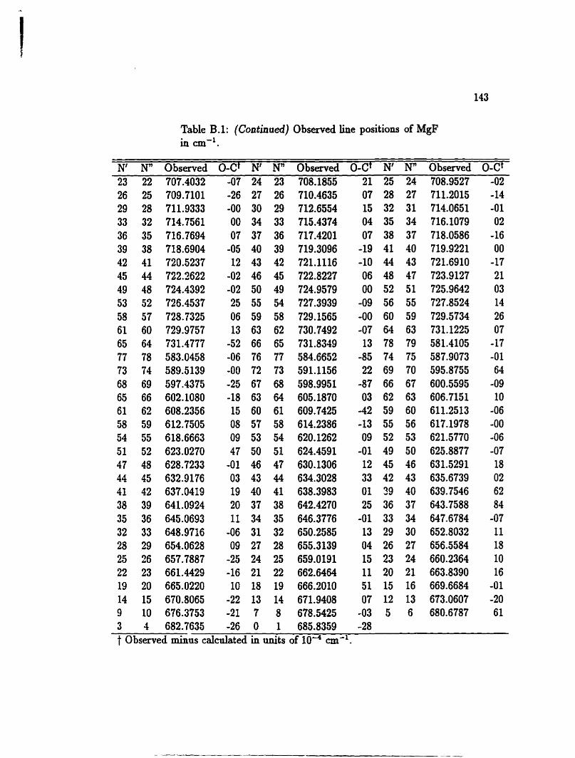
Table B.l: (Continued) Observed line positions of MgF in cm-'.

Nt N" Observed O-Ct N' N" Obsaved O-Ct N' N" Observed O-Ct 23 22 707.4032 -07 24 23 708.1855 21 25 24 708.9527 -02

t Observed minus calcnlated in uni ts of W4 cm-'.

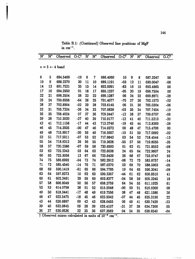
Table B.1: (Continued) Observed line positions of MgF in cm".

N' N" Observed O-Ct NI N" Obsaved O-Cf N' N" Observed O-Ct

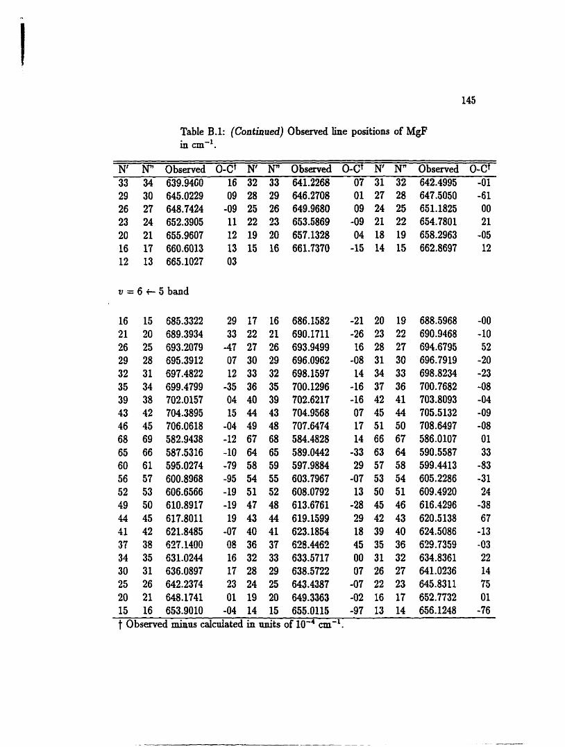
Table B.l: (Continued) Observed line positions of MgF in cm-'.

N' N" Observed O-Ct N' N" Observed O-Cf N' Nn Observed O-Ct

u = 6 +- 5 band

t Observed minus calculated in units of cm-!

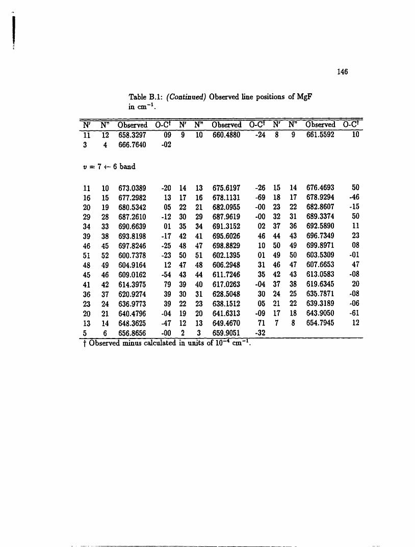
Table B.l: (Continaed) Observed line positions of MgF in cm-'.

Nt Nn Observed O-Ct Nt N" Observed O-Ct N' Nn Observed O-Ct

v = 7 +- 6 band

11 10 673.0389 -20 14 13 675.6197 -26 16 15 677.2982 13 17 16 678.1131 -69 20 19 680.5342 05 22 21 682.0955 -00 29 28 687.2610 -12 30 29 687.9619 -00 34 33 690.6639 O1 35 34 691.3152 02 39 38 693.8198 -17 42 41 695.6026 46 46 45 697.8246 -25 48 47 698.8829 10 51 52 600.7378 -23 50 51 602.1395 01 48 49 604.9164 12 47 48 606.2948 31 45 46 609.0162 -54 43 44 611.7246 35 41 42 614.3975 79 39 40 617.0263 -04 36 37 620.9274 39 30 31 628.5048 30 23 24 636.9773 39 22 23 638.1512 05 20 21 640.4796 -04 19 20 641.6313 -09 13 14 648.3625 -47 12 13 649.4670 71 5 6 656.8656 -00 2 3 659.9051 -32 t Observed minus calculated in u n i t s of IO4 cm-'.

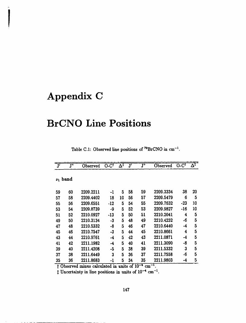
Appendix C

BrCNO Line Positions

Table C.1: Observed line positions of "BrCNO in cm-'.

J' J" Observed O-Cf Al J' J" Observed O-Ct At

VI band

59 60 57 58 55 56 53 54 51 52 49 50 47 48 45 46 43 44 41 42 39 40 37 38 35 36 t Observed minas calculated in d t s of IO4 cm-'. # Uncertainty in Line positions in n n i t s of 104 an-'.

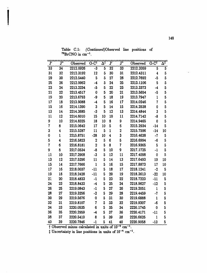
Table C. 1: (Continued)Observed line positions of mBrCNO in cm".

J' J" Observed O-Ct Al J' J" Observed 0-0 A$ 34 2212.0926 -3 5 32 33 2212.2059 5 5

t Observed m h s calculated in M i t s of 10-4 cm-'. Uocertainty in h e positions in M i t s of an-'.

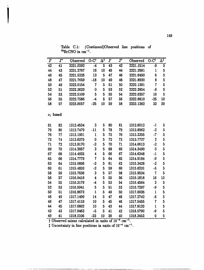
Table C.1: (Continued)Observed line positions of "BrCNO in cm-'.

J' J" Observed O-Ct Af 3' J" Observed O-Ct At 4 2 41 44 43 46 45 48 47 50 49 52 51 54 53 56 55 58 57

ul band

t Observed minus caldated in Mits of 10-~ cm-'. t Uncertainty in line positions in a a i t s of IO-' cm-'.

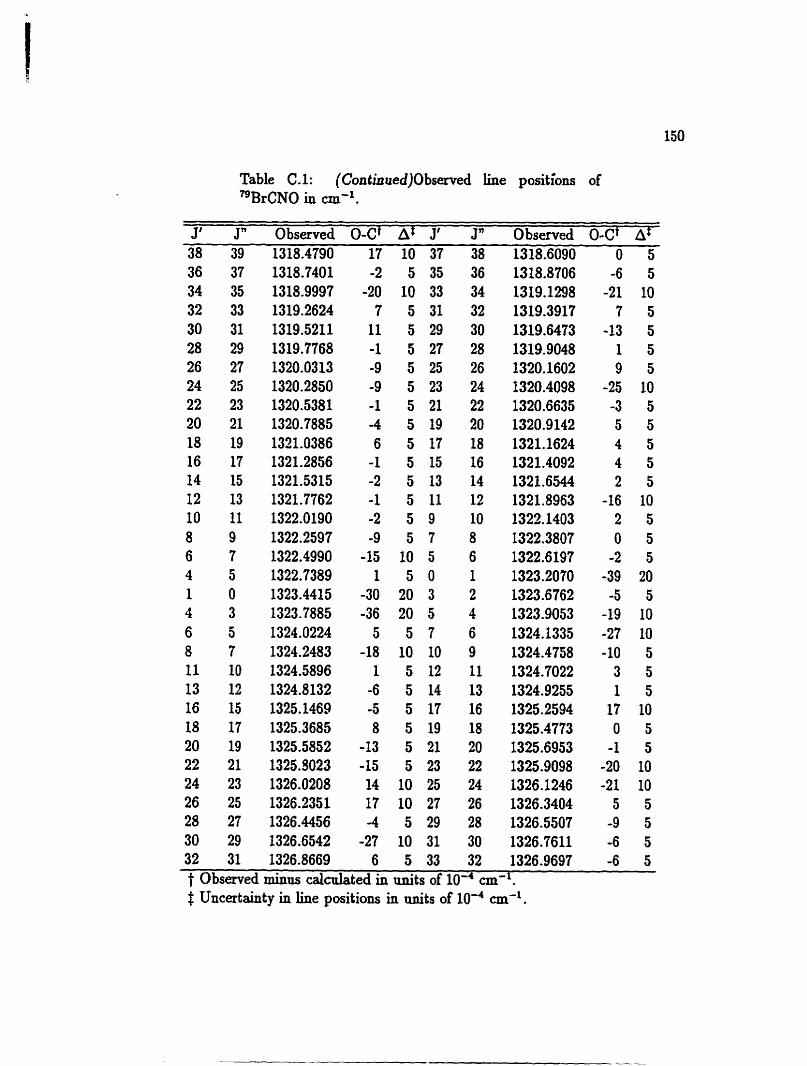
Table C.1: (Continued)Observed line positions of 79BrCN0 in cm".

J' Jn Observed O-Ct Af J' Jn Observed O-Ct Af

t Observed minus caldated in ttnits of cm-'. $ Uncatainty in line positions in uni ts of cm-'.

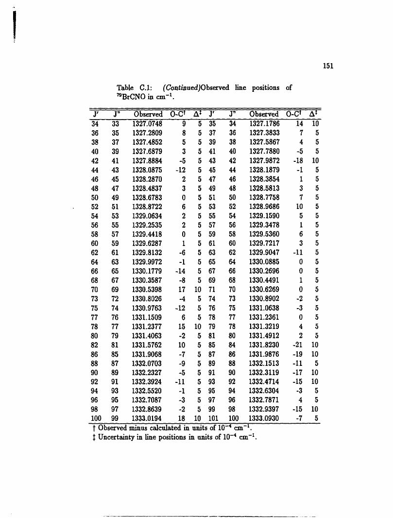
Table C.1: (Continued)Observed line positions of 79BrCN0 in cm-'.

J' J" Observed O-Cf Af J' Jn Observed O-Cf Af 1327.0748 9 5 35 34 1327.1786 10

t Observed minus calcnlated in un i ts of IO4 cm-'. f Uncertainty in line positions in nni ts of cm-'.

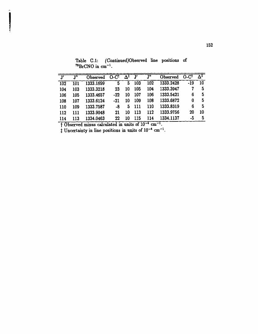
Table C .l: (Continued)Obsaved line positions of 79BrCN0 in cm".

J' Jn Observed O-Ct Af J' J" Observed O-Ct Af 102 IO1 1333.1699 5 5 103 102 1333.2428 -19 10 104 103 1333.3218 23 10 105 104 1333.3947 7 5 106 105 1333.4657 -22 10 107 106 1333.5421 6 5 108 107 1333.6124 -21 10 109 108 1333.6872 O 5 110 109 1333.7587 -8 5 111 110 1333.8319 6 5 112 111 1333.9048 21 10 113 112 1333.9756 20 10 114 113 1334.0463 22 10 115 114 1334.1137 -5 5 t Observed minus caldated in units of cm-'. f Uncertainty in h e positions in ani ts of cm-'.

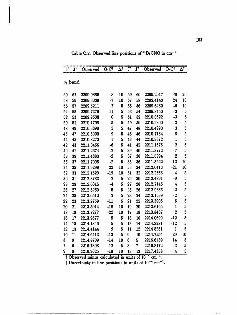
Table C.2: Observed line positions of 81BrCN0 in cm-'.

J' J" Observed O-Ct Af J' J" Obsewed O-Ct Af

t Observed min- caldated in units of 104 cm-'. $ UncertainS. in line positions in uni ts of 10m4 an-'.

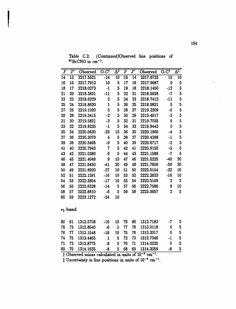
Table C .2: (Continned)O bserved line positions of 81BrCN0 in cmd1.

J' 3" Observed O-Ct A J' J" Obsesved O-Ct At

v, band

t Observed minus c a l d t e d in M i t s of cm-'. $ Uncertainty in &ne positions in M i r s of cm-'.

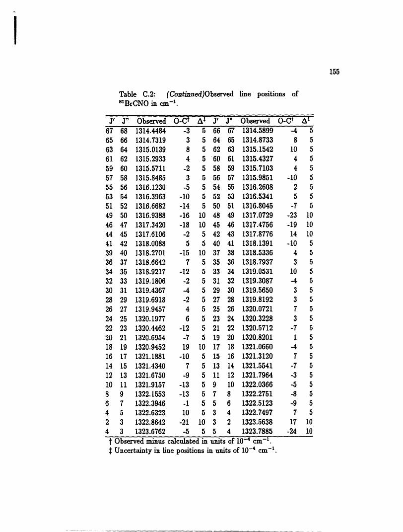
Table C.2: (Continaed)Observed iine positions of 8'BrCN0 in cm-'.

J' J" Observed O-Ct At J' Jn Observed O-Ct Af 67 68 1314.4484 -3 5 66 67 1314.5899 -4 5 65 66 1314.7319 3 5 64 65 1314.8733 8 5 63 64 1315.0139 8 5 62 63 1315.1542 10 5 61 62 13152933 4 5 '60 61 1315.4327 4 5 59 60 1315.5711 -2 5 58 59 1315.7103 4 5 57 58 1315.8485 3 5 56 57 1315.9851 -10 5 55 56 1316.1230 -5 5 54 55 1316.2608 2 5 53 54 1316.3963 -10 5 52 53 1316.5341 5 5 51 52 1316.6682 -14 5 50 51 1316.8045 -7 5 49 50 1316.9388 -16 10 48 49 1317.0729 -23 10 46 47 1317.3420 -18 10 45 46 1317.4756 -19 10 44 45 1317.6106 -2 5 42 43 1317.8776 14 10 41 42 1318.0088 5 5 40 41 1318.1391 -10 5 39 40 1318.2'701 -15 10 37 38 1318.5336 4 5 36 37 1318.6642 7 5 35 36 1318.7937 3 5 34 35 1318.9217 -12 5 33 34 1319.0531 10 5 32 33 1319.1806 -2 5 31 32 1319.3087 -4 5 30 31 1319.4367 -4 5 29 30 1319.5650 3 5 28 29 1319.6918 -2 5 27 28 1319.8192 3 5 26 27 1319.9457 4 5 25 26 1320.0721 7 5 24 25 1320.1977 6 5 23 24 1320.3228 3 5 22 23 1320.4462 -12 5 21 22 1320.5712 -7 5 20 21 1320.6954 -7 5 19 20 1320.8201 1 5 18 19 1320.9452 19 IO 17 18 1321.0660 -4 5 16 17 1321.1881 -10 5 15 16 1321.3120 7 5 14 15 1321.4340 7 5 13 14 1321.5541 -7 5 12 13 1321.6750 -9 5 11 12 1321.7964 -3 5 10 11 1321.9157 -13 5 9 10 1322.0366 -5 5 8 9 1322.1553 -13 5 7 8 1322.2751 -8 5 6 7 1322.3946 -1 5 5 6 1322.5123 -9 5 4 5 1322.6323 10 5 3 4 1322.7497 7 5 2 3 1322.8642 -21 10 3 2 1323.5638 17 10 4 3 1323.6762 -5 5 5 4 1323.7885 -24 10 t Observed minus calctdated in uni ts of IO4 cm-'. t Uncertainty in line positions in uni ts of IO-' cm-'.

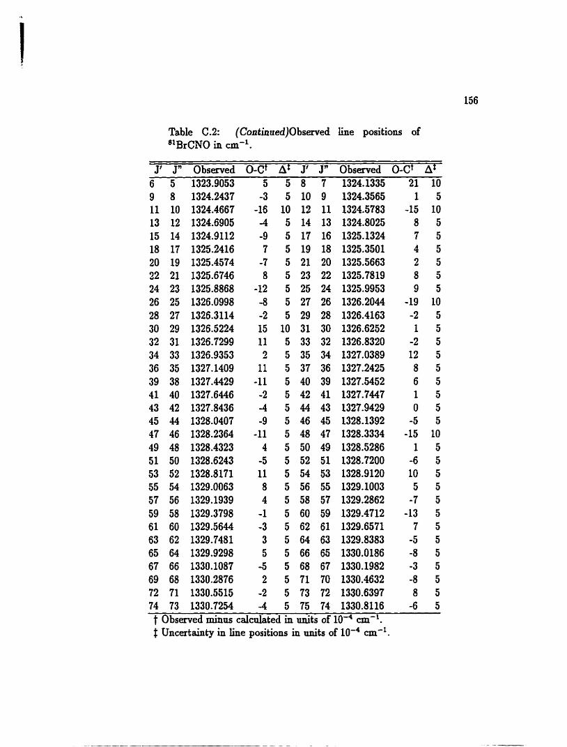
Table C.2: (Continued)Observed line positions of $lBrCNO in mi-'.

J' J" Observed O-Ct At J' Jn Observed O-Ct Af 6 5 1323.9053 5 5 8 7 1324,1335

t Obsenred minus cdculated in units of IO4 an-'. Uncertainty in line positions in nnits of IO-* cm-'.

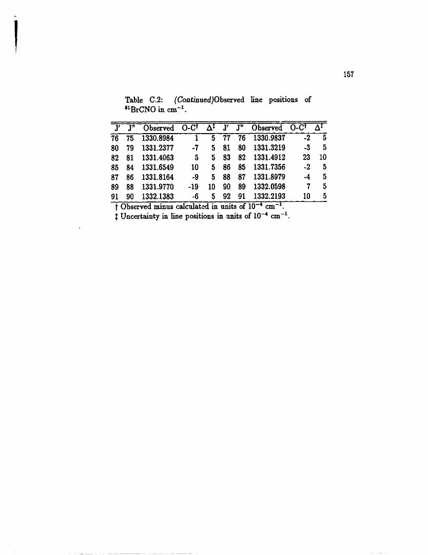
Table C.2: (Contkiued)Observed line positions of 81BrCN0 in cm".

J' J" Observed O-Ct AT J' Jn Observed O-Ct Af 76 75 1330.8984 1 5 77 76 1330.9837 -2 5 80 79 1331.2377 -7 5 81 80 1331.3219 -3 5 82 81 1331.4063 5 5 83 82 1331.4912 23 10 85 84 1331.6549 10 5 86 85 1331.7356 -2 5 87 86 1331.8164 -9 5 88 87 1331.8979 -4 5 89 88 1331.9770 -19 10 90 89 1332.0598 7 5 91 90 1332.1383 -6 5 92 91 1332.2193 10 5 t Observed minus caldated in uxtits of cm-'. $ Uncertainty in b e positions in nnits of IO-' cm-'.