Embed Size (px)
Citation preview

Answers to Exercises from
Linear Algebra
∣∣∣∣1 23 1
∣∣∣∣
∣∣∣∣x · 1 2x · 3 1
∣∣∣∣
∣∣∣∣6 28 1
∣∣∣∣
Jim Hefferon

Notation
R real numbersN natural numbers: {0, 1, 2, . . . }C complex numbers
{. . .∣∣ . . . } set of . . . such that . . .〈. . . 〉 sequence; like a set but order matters
V,W,U vector spaces~v, ~w vectors~0, ~0V zero vector, zero vector of VB,D bases
En = 〈~e1, . . . , ~en〉 standard basis for Rn~β,~δ basis vectors
RepB(~v) matrix representing the vectorPn set of n-th degree polynomials
Mn×m set of n×m matrices[S] span of the set S
M ⊕N direct sum of subspacesV ∼= W isomorphic spaces
h, g homomorphismsH,G matricest, s transformations; maps from a space to itselfT, S square matrices
RepB,D(h) matrix representing the map hhi,j matrix entry from row i, column j|T | determinant of the matrix T
R(h),N (h) rangespace and nullspace of the map hR∞(h),N∞(h) generalized rangespace and nullspace
Lower case Greek alphabet
name symbol name symbol name symbolalpha α iota ι rho ρbeta β kappa κ sigma σgamma γ lambda λ tau τdelta δ mu µ upsilon υepsilon ε nu ν phi φzeta ζ xi ξ chi χeta η omicron o psi ψtheta θ pi π omega ω
Cover. This is Cramer’s Rule applied to the system x + 2y = 6, 3x + y = 8. The area of the first box is the
determinant shown. The area of the second box is x times that, and equals the area of the final box. Hence, x is the
final determinant divided by the first determinant.

These are answers to the exercises in Linear Algebra by J. Hefferon. Corrections or comments are verywelcome, email to jimjoshua.smcvt.edu
An answer labeled here as, for instance, 1.II.3.4, matches the question numbered 4 from the first chapter,second section, and third subsection. The Topics are numbered separately.


Chapter 1. Linear Systems
. . . . . . . . . . . . . . . . . . . . . . . . . . . . . . . . . . . . . . . . . . . . .
Answers for subsection 1.I.1
1.I.1.22 This system with more unknowns than equations
x+ y + z = 0x+ y + z = 1
has no solution.
1.I.1.23 Yes. For example, the fact that the same reaction can be performed in two different flasks showsthat twice any solution is another, different, solution (if a physical reaction occurs then there must be atleast one nonzero solution).
1.I.1.25(a) Yes, by inspection the given equation results from −ρ1 + ρ2.(b) No. The given equation is satisfied by the pair (1, 1). However, that pair does not satisfy the firstequation in the system.
(c) Yes. To see if the given row is c1ρ1 + c2ρ2, solve the system of equations relating the coefficients of x,y, z, and the constants:
2c1 + 6c2 = 6c1 − 3c2 =−9−c1 + c2 = 54c1 + 5c2 =−2
and get c1 = −3 and c2 = 2, so the given row is −3ρ1 + 2ρ2.
1.I.1.26 If a 6= 0 then the solution set of the first equation is {(x, y)∣∣ x = (c− by)/a}. Taking y = 0 gives
the solution (c/a, 0), and since the second equation is supposed to have the same solution set, substituting intoit gives that a(c/a)+d ·0 = e, so c = e. Then taking y = 1 in x = (c−by)/a gives that a((c−b)/a)+d ·1 = e,which gives that b = d. Hence they are the same equation.
When a = 0 the equations can be different and still have the same solution set: e.g., 0x + 3y = 6 and0x+ 6y = 12.
1.I.1.29 For the reduction operation of multiplying ρi by a nonzero real number k, we have that (s1, . . . , sn)satisfies this system
a1,1x1 + a1,2x2 + · · ·+ a1,nxn = d1
...kai,1x1 + kai,2x2 + · · ·+ kai,nxn = kdi
...am,1x1 + am,2x2 + · · ·+ am,nxn = dm
if and only if
a1,1s1 + a1,2s2 + · · ·+ a1,nsn = d1...
and kai,1s1 + kai,2s2 + · · ·+ kai,nsn = kdi...
and am,1s1 + am,2s2 + · · ·+ am,nsn = dm

2 Linear Algebra, by Hefferon
by the definition of ‘satisfies’. But, because k 6= 0, that’s true if and only if
a1,1s1 + a1,2s2 + · · ·+ a1,nsn = d1...
and ai,1s1 + ai,2s2 + · · ·+ ai,nsn = di...
and am,1s1 + am,2s2 + · · ·+ am,nsn = dm
(this is straightforward cancelling on both sides of the i-th equation), which says that (s1, . . . , sn) solves
a1,1x1 + a1,2x2 + · · ·+ a1,nxn = d1
...ai,1x1 + ai,2x2 + · · ·+ ai,nxn = di
...am,1x1 + am,2x2 + · · ·+ am,nxn = dm
as required.For the pivot operation kρi + ρj , we have that (s1, . . . , sn) satisfies
a1,1x1 + · · ·+ a1,nxn = d1
...ai,1x1 + · · ·+ ai,nxn = di
...(kai,1 + aj,1)x1 + · · ·+ (kai,n + aj,n)xn = kdi + dj
...am,1x1 + · · ·+ am,nxn = dm
if and only if
a1,1s1 + · · ·+ a1,nsn = d1...
and ai,1s1 + · · ·+ ai,nsn = di...
and (kai,1 + aj,1)s1 + · · ·+ (kai,n + aj,n)sn = kdi + dj...
and am,1s1 + am,2s2 + · · ·+ am,nsn = dm
again by the definition of ‘satisfies’. Subtract k times the i-th equation from the j-th equation (remark: hereis where i 6= j is needed; if i = j then the two di’s above are not equal) to get that the previous compoundstatement holds if and only if
a1,1s1 + · · ·+ a1,nsn = d1...
and ai,1s1 + · · ·+ ai,nsn = di...
and (kai,1 + aj,1)s1 + · · ·+ (kai,n + aj,n)sn− (kai,1s1 + · · ·+ kai,nsn) = kdi + dj − kdi
...and am,1s1 + · · ·+ am,nsn = dm

Answers to Exercises 3
which, after cancellation, says that (s1, . . . , sn) solvesa1,1x1 + · · ·+ a1,nxn = d1
...ai,1x1 + · · ·+ ai,nxn = di
...aj,1x1 + · · ·+ aj,nxn = dj
...am,1x1 + · · ·+ am,nxn = dm
as required.1.I.1.30 Yes, this one-equation system:
0x+ 0y = 0is satisfied by every (x, y) ∈ R2.1.I.1.32 Swapping rows is reversed by swapping back.
a1,1x1 + · · ·+ a1,nxn = d1
...am,1x1 + · · ·+ am,nxn = dm
ρi↔ρj−→ ρj↔ρi−→a1,1x1 + · · ·+ a1,nxn = d1
...am,1x1 + · · ·+ am,nxn = dm
Multiplying both sides of a row by k 6= 0 is reversed by dividing by k.a1,1x1 + · · ·+ a1,nxn = d1
...am,1x1 + · · ·+ am,nxn = dm
kρi−→ (1/k)ρi−→a1,1x1 + · · ·+ a1,nxn = d1
...am,1x1 + · · ·+ am,nxn = dm
Adding k times a row to another is reversed by adding −k times that row.a1,1x1 + · · ·+ a1,nxn = d1
...am,1x1 + · · ·+ am,nxn = dm
kρi+ρj−→ −kρi+ρj−→a1,1x1 + · · ·+ a1,nxn = d1
...am,1x1 + · · ·+ am,nxn = dm
Remark: observe for the third case that if i = j then the result doesn’t hold:
3x+ 2y = 72ρ1+ρ1−→ 9x+ 6y = 21
−2ρ1+ρ1−→ −9x− 6y =−21
1.I.1.33 Let p, n, and d be the number of pennies, nickels, and dimes. For real variables, this systemp+ n+ d= 13p+ 5n+ 10d= 83
−ρ1+ρ2−→ p+ n+ d= 134n+ 9d= 70
has infinitely many solutions. However, it has a limited number of solutions in which p, n, and d are non-negative integers. Running through d = 0, . . . , d = 8 shows that (p, n, d) = (3, 4, 6) is the only sensiblesolution.1.I.1.34 Solving the system
(1/3)(a+ b+ c) + d= 29(1/3)(b+ c+ d) + a= 23(1/3)(c+ d+ a) + b= 21(1/3)(d+ a+ b) + c= 17
we obtain a = 12, b = 9, c = 3, d = 21. Thus the second item, 21, is the correct answer.1.I.1.36 Eight commissioners voted for B. To see this, we will use the given information to study howmany voters chose each order of A, B, C.
The six orders of preference are ABC, ACB, BAC, BCA, CAB, CBA; assume they receive a, b, c, d,e, f votes respectively. We know that
a+ b+ e= 11d+ e+ f = 12a+ c+ d= 14

4 Linear Algebra, by Hefferon
from the number preferring A over B, the number preferring C over A, and the number preferring B overC. Because 20 votes were cast, we also know that
c+ d+ f = 9a+ b+ c= 8b+ e+ f = 6
from the preferences for B over A, for A over C, and for C over B.The solution is a = 6, b = 1, c = 1, d = 7, e = 4, and f = 1. The number of commissioners voting for B
as their first choice is therefore c+ d = 1 + 7 = 8.Comments. The answer to this question would have been the same had we known only that at least 14commissioners preferred B over C.
The seemingly paradoxical nature of the commissioners’s preferences (A is preferred to B, and B ispreferred to C, and C is preferred to A), an example of “non-transitive dominance”, is not uncommon whenindividual choices are pooled.
1.I.1.37 (This is how the solution appeared in the Monthly. We have not used the word “dependent” yet; itmeans here that Gauss’ method shows that there is not a unique solution.) If n ≥ 3 the system is dependentand the solution is not unique. Hence n < 3. But the term “system” implies n > 1. Hence n = 2. If theequations are
ax+ (a+ d)y = a+ 2d(a+ 3d)x+ (a+ 4d)y = a+ 5d
then x = −1, y = 2.
. . . . . . . . . . . . . . . . . . . . . . . . . . . . . . . . . . . . . . . . . . . . .
Answers for subsection 1.I.2
1.I.2.21 For each problem we get a system of linear equations by looking at the equations of compo-nents.(a) Yes; take k = −1/2.(b) No; the system with equations 5 = 5 · j and 4 = −4 · j has no solution.(c) Yes; take r = 2.(d) No. The second components give k = 0. Then the third components give j = 1. But the firstcomponents don’t check.
1.I.2.22 This system has 1 equation. The leading variable is x1, the other variables are free.
{
−11...0
x2 + · · ·+
−10...1
xn∣∣ x1, . . . , xn ∈ R}
1.I.2.26
(a)
1 42 53 6
(b)(
2 1−3 1
)(c)
(5 1010 5
)(d)
(1 1 0
)1.I.2.28 On plugging in the five pairs (x, y) we get a system with the five equations and six unknowns a,. . . , f . Because there are more unknowns than equations, if no inconsistency exists among the equationsthen there are infinitely many solutions (at least one variable will end up free).
But no inconsistency can exist because a = 0, . . . , f = 0 is a solution (we are only using this zero solutionto show that the system is consistent — the prior paragraph shows that there are nonzero solutions).
1.I.2.29

Answers to Exercises 5
(a) Here is one — the fourth equation is redundant but still OK.x+ y − z + w = 0
y − z = 02z + 2w = 0z + w = 0
(b) Here is one.x+ y − z + w = 0
w = 0w = 0w = 0
(c) This is one.x+ y − z + w = 0x+ y − z + w = 0x+ y − z + w = 0x+ y − z + w = 0
1.I.2.30(a) Formal solution of the system yields
x =a3 − 1a2 − 1
y =−a2 + a
a2 − 1.
If a+ 1 6= 0 and a− 1 6= 0, then the system has the single solution
x =a2 + a+ 1a+ 1
y =−aa+ 1
.
If a = −1, or if a = +1, then the formulas are meaningless; in the first instance we arrive at the system{−x+ y = 1,x− y = 1,
which is a contradictory system. In the second instance we have{x+ y = 1,x+ y = 1,
which has an infinite number of solutions (for example, for x arbitrary, y = 1− x).(b) Solution of the system yields
x =a4 − 1a2 − 1
y =−a3 + a
a2 − 1.
Here, is a2 − 1 6= 0, the system has the single solution x = a2 + 1, y = −a. For a = −1 and a = 1, weobtain the systems {
−x+ y =−1,x− y = 1
{x+ y = 1,x+ y = 1,
both of which have an infinite number of solutions.1.I.2.31 (This is how the answer appeared in Math Magazine.) Let u, v, x, y, z be the volumes in cm3 ofAl, Cu, Pb, Ag, and Au, respectively, contained in the sphere, which we assume to be not hollow. Since theloss of weight in water (specific gravity 1.00) is 1000 grams, the volume of the sphere is 1000 cm3. Then thedata, some of which is superfluous, though consistent, leads to only 2 independent equations, one relatingvolumes and the other, weights.
u+ v + x+ y + z = 10002.7u+ 8.9v + 11.3x+ 10.5y + 19.3z = 7558
Clearly the sphere must contain some aluminum to bring its mean specific gravity below the specific gravitiesof all the other metals. There is no unique result to this part of the problem, for the amounts of three metalsmay be chosen arbitrarily, provided that the choices will not result in negative amounts of any metal.
If the ball contains only aluminum and gold, there are 294.5 cm3 of gold and 705.5 cm3 of aluminum.Another possibility is 124.7 cm3 each of Cu, Au, Pb, and Ag and 501.2 cm3 of Al.

6 Linear Algebra, by Hefferon
. . . . . . . . . . . . . . . . . . . . . . . . . . . . . . . . . . . . . . . . . . . . .
Answers for subsection 1.I.31.I.3.16 The answers from the prior subsection show the row operations.(a) The solution set is
{
2/3−1/3
0
+
1/62/31
z∣∣ z ∈ R}.
A particular solution and the solution set for the associated homogeneous system are 2/3−1/3
0
and {
1/62/31
z∣∣ z ∈ R}.
(b) The solution set is
{
1300
+
1−210
z∣∣ z ∈ R}.
A particular solution and the solution set for the associated homogeneous system are1300
and {
1−210
z∣∣ z ∈ R}.
(c) The solution set is
{
0000
+
−1010
z +
−1−101
w∣∣ z, w ∈ R}.
A particular solution and the solution set for the associated homogeneous system are0000
and {
−1010
z +
−1−101
w∣∣ z, w ∈ R}.
(d) The solution set is
{
10000
+
−5/7−8/7
100
c+
−3/7−2/7
010
d+
−1/74/7001
e∣∣ c, d, e ∈ R}.
A particular solution and the solution set for the associated homogeneous system are10000
and {
−5/7−8/7
100
c+
−3/7−2/7
010
d+
−1/74/7001
e∣∣ c, d, e ∈ R}.
1.I.3.19 The first is nonsingular while the second is singular. Just do Gauss’ method and see if the echelonform result has non-0 numbers in each entry on the diagonal.1.I.3.22 Because the matrix of coefficients is nonsingular, Gauss’ method ends with an echelon form whereeach variable leads an equation. Back substitution gives a unique solution.

Answers to Exercises 7
(Another way to see the solution is unique is to note that with a nonsingular matrix of coefficients theassociated homogeneous system has a unique solution, by definition. Since the general solution is the sumof a particular solution with each homogeneous solution, the general solution has (at most) one element.)1.I.3.23 In this case the solution set is all of Rn, and can be expressed in the required form
{c1
10...0
+ c2
01...0
+ · · ·+ cn
00...1
∣∣ c1, . . . , cn ∈ R}.1.I.3.25 First the proof.
Gauss’ method will use only rationals (e.g., −(m/n)ρi+ρj). Thus the solution set can be expressed usingonly rational numbers as the components of each vector. Now the particular solution is all rational.
There are infinitely many (rational vector) solutions if and only if the associated homogeneous system hasinfinitely many (real vector) solutions. That’s because setting any parameters to be rationals will producean all-rational solution.
. . . . . . . . . . . . . . . . . . . . . . . . . . . . . . . . . . . . . . . . . . . . .
Answers for subsection 1.II.11.II.1.5 The vector 2
03
is not in the line. Because 2
03
−−1
0−4
=
307
that plane can be described in this way.
{
−104
+m
112
+ n
307
∣∣ m,n ∈ R}1.II.1.8 The “if” half is straightforward. If b1 − a1 = d1 − c1 and b2 − a2 = d2 − c2 then√
(b1 − a1)2 + (b2 − a2)2 =√
(d1 − c1)2 + (d2 − c2)2
so they have the same lengths, and the slopes are just as easy:b2 − a2
b1 − a1=d2 − c2d1 − a1
(if the denominators are 0 they both have undefined slopes).For “only if”, assume that the two segments have the same length and slope (the case of undefined slopes
is easy; we will do the case where both segments have a slope m). Also assume, without loss of generality,that a1 < b1 and that c1 < d1. The first segment is (a1, a2)(b1, b2) = {(x, y)
∣∣ y = mx+ n1, x ∈ [a1..b1]}(for some intercept n1) and the second segment is (c1, c2)(d1, d2) = {(x, y)
∣∣ y = mx+ n2, x ∈ [c1..d1]} (forsome n2). Then the lengths of those segments are√
(b1 − a1)2 + ((mb1 + n1)− (ma1 + n1))2 =√
(1 +m2)(b1 − a1)2
and, similarly,√
(1 +m2)(d1 − c1)2. Therefore, |b1 − a1| = |d1 − c1|. Thus, as we assumed that a1 < b1 andc1 < d1, we have that b1 − a1 = d1 − c1.
The other equality is similar.1.II.1.9 We shall later define it to be a set with one element — an “origin”.1.II.1.11 Euclid no doubt is picturing a plane inside of R3. Observe, however, that both R1 and R3 alsosatisfy that definition.
8 Linear Algebra, by Hefferon
. . . . . . . . . . . . . . . . . . . . . . . . . . . . . . . . . . . . . . . . . . . . .
Answers for subsection 1.II.21.II.2.13 Solve (k)(4) + (1)(3) = 0 to get k = −3/4.1.II.2.14 The set
{
xyz
∣∣ 1x+ 3y − 1z = 0}
can also be described with parameters in this way.
{
−310
y +
101
z∣∣ y, z ∈ R}
1.II.2.16 Clearly u1u1 + · · ·+ unun is zero if and only if each ui is zero. So only ~0 ∈ Rn is perpendicularto itself.1.II.2.18(a) Verifying that (k~x) ~y = k(~x ~y) = ~x (k~y) for k ∈ R and ~x, ~y ∈ Rn is easy. Now, for k ∈ R and~v, ~w ∈ Rn, if ~u = k~v then ~u ~v = (k~u) ~v = k(~v ~v), which is k times a nonnegative real.
The ~v = k~u half is similar (actually, taking the k in this paragraph to be the reciprocal of the k abovegives that we need only worry about the k = 0 case).
(b) We first consider the ~u ~v ≥ 0 case. From the Triangle Inequality we know that ~u ~v = ‖~u ‖ ‖~v ‖ if andonly if one vector is a nonnegative scalar multiple of the other. But that’s all we need because the firstpart of this exercise shows that, in a context where the dot product of the two vectors is positive, the twostatements ‘one vector is a scalar multiple of the other’ and ‘one vector is a nonnegative scalar multipleof the other’, are equivalent.
We finish by considering the ~u ~v < 0 case. Because 0 < |~u ~v| = −(~u ~v) = (−~u) ~v and ‖~u ‖ ‖~v ‖ =‖ − ~u ‖ ‖~v ‖, we have that 0 < (−~u) ~v = ‖ − ~u ‖ ‖~v ‖. Now the prior paragraph applies to give that one ofthe two vectors −~u and ~v is a scalar multiple of the other. But that’s equivalent to the assertion that oneof the two vectors ~u and ~v is a scalar multiple of the other, as desired.
1.II.2.19 No. These give an example.
~u =(
10
)~v =
(10
)~w =
(11
)1.II.2.22 Assume that ~v ∈ Rn has components v1, . . . , vn. If ~v 6= ~0 then we have this.√(
v1√v1
2 + · · ·+ vn2
)2
+ · · ·+(
vn√v1
2 + · · ·+ vn2
)2
=
√(v1
2
v12 + · · ·+ vn2
)+ · · ·+
(vn2
v12 + · · ·+ vn2
)= 1
If ~v = ~0 then ~v/‖~v ‖ is not defined.1.II.2.23 For the first question, assume that ~v ∈ Rn and r ≥ 0, take the root, and factor.
‖r~v ‖ =√
(rv1)2 + · · ·+ (rvn)2 =√r2(v1
2 + · · ·+ vn2 = r‖~v ‖For the second question, the result is r times as long, but it points in the opposite direction in that r~v +(−r)~v = ~0.1.II.2.25 Write
~u =
u1
...un
~v =
v1
...vn

Answers to Exercises 9
and then this computation works.
‖~u+ ~v ‖2 + ‖~u− ~v ‖2 = (u1 + v1)2 + · · ·+ (un + vn)2
+ (u1 − v1)2 + · · ·+ (un − vn)2
= u12 + 2u1v1 + v1
2 + · · ·+ un2 + 2unvn + vn
2
+ u12 − 2u1v1 + v1
2 + · · ·+ un2 − 2unvn + vn
2
= 2(u12 + · · ·+ un
2) + 2(v12 + · · ·+ vn
2)
= 2‖~u ‖2 + 2‖~v ‖2
1.II.2.26 We will prove this demonstrating that the contrapositive statement holds: if ~x 6= ~0 then there isa ~y with ~x ~y 6= 0.
Assume that ~x ∈ Rn. If ~x 6= ~0 then it has a nonzero component, say the i-th one xi. But the vector~y ∈ Rn that is all zeroes except for a one in component i gives ~x ~y = xi. (A slicker proof just considers~x ~x.)
1.II.2.27 Yes. We prove this by induction.Assume that the vectors are in some Rk. Clearly the statement applies to one vector. The Triangle
Inequality is this statement applied to two vectors. For an inductive step assume the statement is true forn or fewer vectors. Then this
‖~u1 + · · ·+ ~un + ~un+1‖ ≤ ‖~u1 + · · ·+ ~un‖+ ‖~un+1‖follows by the Triangle Inequality for two vectors. Now the inductive hypothesis, applied to the first summandon the right, gives that as less than or equal to ‖~u1‖+ · · ·+ ‖~un‖+ ‖~un+1‖.1.II.2.28 By definition
~u ~v
‖~u ‖ ‖~v ‖ = cos θ
where θ is the angle between the vectors. Thus the ratio is | cos θ|.1.II.2.29 So that the statement ‘vectors are orthogonal iff their dot product is zero’ has no exceptions.
1.II.2.30 The angle between (a) and (b) is found (for a, b 6= 0) with
arccos(ab√a2√b2
).
If a or b is zero then the angle is π/2 radians. Otherwise, if a and b are of opposite signs then the angle is πradians, else the angle is zero radians.
1.II.2.31 The angle between ~u and ~v is acute if ~u ~v > 0, is right if ~u ~v = 0, and is obtuse if ~u ~v < 0.That’s because, in the formula for the angle, the denominator is never negative.
1.II.2.33 Where ~u,~v ∈ Rn, the vectors ~u+~v and ~u−~v are perpendicular if and only if 0 = (~u+~v) (~u−~v) =~u ~u− ~v ~v, which shows that those two are perpendicular if and only if ~u ~u = ~v ~v. That holds if and onlyif ‖~u ‖ = ‖~v ‖.1.II.2.34 Suppose ~u ∈ Rn is perpendicular to both ~v ∈ Rn and ~w ∈ Rn. Then, for any k,m ∈ R we havethis.
~u (k~v +m~w) = k(~u ~v) +m(~u ~w) = k(0) +m(0) = 0
1.II.2.35 We will show something more general: if ‖~z1‖ = ‖~z2‖ for ~z1, ~z2 ∈ Rn, then ~z1 + ~z2 bisects theangle between ~z1 and ~z2
©©©©*
¢¢¢¢
¡¡¡¡¡µ
¢¢¢¢©©©©
gives
©©©©
¢¢¢¢
¡¡¡¡¡
¢¢¢¢©©©©
′′′′ ′′′′′′

10 Linear Algebra, by Hefferon
(we ignore the case where ~z1 and ~z2 are the zero vector).The ~z1 + ~z2 = ~0 case is easy. For the rest, by the definition of angle, we will be done if we show this.
~z1 (~z1 + ~z2)‖~z1‖ ‖~z1 + ~z2‖
=~z2 (~z1 + ~z2)‖~z2‖ ‖~z1 + ~z2‖
But distributing inside each expression gives~z1 ~z1 + ~z1 ~z2
‖~z1‖ ‖~z1 + ~z2‖~z2 ~z1 + ~z2 ~z2
‖~z2‖ ‖~z1 + ~z2‖and ~z1 ~z1 = ‖~z1‖ = ‖~z2‖ = ~z2 ~z2, so the two are equal.1.II.2.36 We can show the two statements together. Let ~u,~v ∈ Rn, write
~u =
u1
...un
~v =
v1
...vn
and calculate.
cos θ =ku1v1 + · · ·+ kunvn√
(ku1)2 + · · ·+ (kun)2√b1
2 + · · ·+ bn2
=k
|k|~u · ~v‖~u ‖ ‖~v ‖ = ± ~u ~v
‖~u ‖ ‖~v ‖
1.II.2.39 This is how the answer was given in the cited source. The actual velocity ~v of the wind is thesum of the ship’s velocity and the apparent velocity of the wind. Without loss of generality we may assume~a and ~b to be unit vectors, and may write
~v = ~v1 + s~a = ~v2 + t~b
where s and t are undetermined scalars. Take the dot product first by ~a and then by ~b to obtains− t~a ~b = ~a (~v2 − ~v1)
s~a ~b− t = ~b (~v2 − ~v1)
Multiply the second by ~a ~b, subtract the result from the first, and find
s =[~a− (~a ~b)~b] (~v2 − ~v1)
1− (~a ~b)2.
Substituting in the original displayed equation, we get
~v = ~v1 +[~a− (~a ~b)~b] (~v2 − ~v1)~a
1− (~a ~b)2.
1.II.2.40 We use induction on n.In the n = 1 base case the identity reduces to
(a1b1)2 = (a12)(b12)− 0
and clearly holds.For the inductive step assume that the formula holds for the 0, . . . , n cases. We will show that it then
holds in the n+ 1 case. Start with the right-hand side( ∑1≤j≤n+1
aj2)( ∑
1≤j≤n+1
bj2)−
∑1≤k<j≤n+1
(akbj − ajbk
)2=[(∑
1≤j≤naj
2) + an+12][
(∑
1≤j≤nbj
2) + bn+12]−[ ∑1≤k<j≤n
(akbj − ajbk
)2 +∑
1≤k≤n
(akbn+1 − an+1bk
)2]=( ∑
1≤j≤naj
2)( ∑
1≤j≤nbj
2)
+∑
1≤j≤nbj
2an+12 +
∑1≤j≤n
aj2bn+1
2 + an+12bn+1
2
−[ ∑1≤k<j≤n
(akbj − ajbk
)2 +∑
1≤k≤n
(akbn+1 − an+1bk
)2]=( ∑
1≤j≤naj
2)( ∑
1≤j≤nbj
2)−
∑1≤k<j≤n
(akbj − ajbk
)2 +∑
1≤j≤nbj
2an+12 +
∑1≤j≤n
aj2bn+1
2 + an+12bn+1
2
−∑
1≤k≤n
(akbn+1 − an+1bk
)2

Answers to Exercises 11
and apply the inductive hypothesis
=( ∑
1≤j≤najbj
)2 +∑
1≤j≤nbj
2an+12 +
∑1≤j≤n
aj2bn+1
2 + an+12bn+1
2
−[ ∑1≤k≤n
ak2bn+1
2 − 2∑
1≤k≤nakbn+1an+1bk +
∑1≤k≤n
an+12bk
2]
=( ∑
1≤j≤najbj
)2 − 2( ∑
1≤k≤nakbn+1an+1bk
)+ an+1
2bn+12
=[( ∑
1≤j≤najbj
)+ an+1bn+1
]2to derive the left-hand side.
. . . . . . . . . . . . . . . . . . . . . . . . . . . . . . . . . . . . . . . . . . . . .
Answers for subsection 1.III.1
1.III.1.10 Routine Gauss’ method gives one:
−3ρ1+ρ2−→−(1/2)ρ1+ρ3
2 1 1 30 1 −2 −70 9/2 1/2 7/2
−(9/2)ρ2+ρ3−→
2 1 1 30 1 −2 −70 0 19/2 35
and any cosmetic change, like multiplying the bottom row by 2,2 1 1 3
0 1 −2 −70 0 19 70
gives another.
1.III.1.13(a) The ρi ↔ ρi operation does not change A.(b) For instance, (
1 23 4
)−ρ1+ρ1−→
(0 03 4
)ρ1+ρ1−→
(0 03 4
)leaves the matrix changed.
(c) If i 6= j then
...ai,1 · · · ai,n
...aj,1 · · · aj,n
...
kρi+ρj−→
...ai,1 · · · ai,n
...kai,1 + aj,1 · · · kai,n + aj,n
...
−kρi+ρj−→
...ai,1 · · · ai,n
...−kai,1 + kai,1 + aj,1 · · · −kai,n + kai,n + aj,n
...
does indeed give A back. (Of course, if i = j then the third matrix would have entries of the form−k(kai,j + ai,j) + kai,j + ai,j .)

12 Linear Algebra, by Hefferon
. . . . . . . . . . . . . . . . . . . . . . . . . . . . . . . . . . . . . . . . . . . . .
Answers for subsection 1.III.2
1.III.2.12 First, the only matrix row equivalent to the matrix of all 0’s is itself (since row operations haveno effect).
Second, the matrices that reduce to (1 a0 0
)have the form (
b bac ca
)(where a, b, c ∈ R).
Next, the matrices that reduce to (0 10 0
)have the form (
0 a0 b
)(where a, b ∈ R).
Finally, the matrices that reduce to (1 00 1
)are the nonsingular matrices. That’s because a linear system for which this is the matrix of coefficients willhave a unique solution, and that is the definition of nonsingular. (Another way to say the same thing is tosay that they fall into none of the above classes.)
1.III.2.13(a) They have the form (
a 0b 0
)where a, b ∈ R.
(b) They have this form (for a, b ∈ R). (1a 2a1b 2b
)(c) They have the form (
a bc d
)(for a, b, c, d ∈ R) where ad − bc 6= 0. (This is the formula that determines when a 2× 2 matrix isnonsingular.)
1.III.2.14 Infinitely many.
1.III.2.15 No. Row operations do not change the size of a matrix.
1.III.2.16(a) A row operation on a zero matrix has no effect. Thus each zero matrix is alone in its row equivalenceclass.
(b) No. Any nonzero entry can be rescaled.
1.III.2.20

Answers to Exercises 13
(a) If there is a linear relationship where c0 is not zero then we can subtract c0~β0 and divide both sides byc0 to get ~β0 as a linear combination of the others. (Remark. If there are no others — if the relationshipis, say, ~0 = 3 · ~0 — then the statement is still true because zero is by definition the sum of the empty setof vectors.)
If ~β0 is a combination of the others ~β0 = c1~β1 + · · ·+ cn~βn then subtracting ~β0 from both sides givesa relationship where one of the coefficients is nonzero, specifically, the coefficient is −1.
(b) The first row is not a linear combination of the others for the reason given in the proof: in the equationof components from the column containing the leading entry of the first row, the only nonzero entry isthe leading entry from the first row, so its coefficient must be zero. Thus, from the prior part of thisquestion, the first row is in no linear relationship with the other rows. Hence, to see if the second row canbe in a linear relationship with the other rows, we can leave the first row out of the equation. But nowthe argument just applied to the first row will apply to the second row. (Technically, we are arguing byinduction here.)
1.III.2.22(a) The inductive step is to show that if the statement holds on rows 1 through r then it also holds onrow r + 1. That is, we assume that `1 = k1, and `2 = k2, . . . , and `r = kr, and we will show that`r+1 = kr+1 also holds (for r in 1 ..m− 1).
(b) Lemma 2.3 gives the relationship βr+1 = sr+1,1δ1 + sr+2,2δ2 + · · · + sr+1,mδm between rows. Insideof those rows, consider the relationship between entries in column `1 = k1. Because r + 1 > 1, the rowβr+1 has a zero in that entry (the matrix B is in echelon form), while the row δ1 has a nonzero entry incolumn k1 (it is, by definition of k1, the leading entry in the first row of D). Thus, in that column, theabove relationship among rows resolves to this equation among numbers: 0 = sr+1,1 ·d1,k1 , with d1,k1 6= 0.Therefore sr+1,1 = 0.
With sr+1,1 = 0, a similar argument shows that sr+1,2 = 0. With those two, another turn gives thatsr+1,3 = 0. That is, inside of the larger induction argument used to prove the entire lemma is here ansubargument by induction that shows sr+1,j = 0 for all j in 1 .. r. (We won’t write out the details since itis just like the induction done in Exercise 21.)
(c) First, `r+1 < kr+1 is impossible. In the columns of D to the left of column kr+1 the entries are are allzeroes as dr+1,kr+1 leads the row k+1) and so if `k+1 < kk+1 then the equation of entries from column `k+1
would be br+1,`r+1 = sr+1,1 · 0 + · · ·+ sr+1,m · 0, but br+1,`r+1 isn’t zero since it leads its row. A symmetricargument shows that kr+1 < `r+1 also is impossible.
1.III.2.23 The zero rows could have nonzero coefficients, and so the statement would not be true.1.III.2.25 If multiplication of a row by zero were allowed then Lemma 2.6 would not hold. That is, where(
1 32 1
)0ρ2−→
(1 30 0
)all the rows of the second matrix can be expressed as linear combinations of the rows of the first, but theconverse does not hold. The second row of the first matrix is not a linear combination of the rows of thesecond matrix.1.III.2.27 Define linear systems to be equivalent if their augmented matrices are row equivalent. The proofthat equivalent systems have the same solution set is easy.
. . . . . . . . . . . . . . . . . . . . . . . . . . . . . . . . . . . . . . . . . . . . .
Answers for Topic: Computer Algebra Systems1(a) The commands
> A:=array( [[40,15],
[-50,25]] );
> u:=array([100,50]);
> linsolve(A,u);

14 Linear Algebra, by Hefferon
yield the answer [1, 4].(b) Here there is a free variable:
> A:=array( [[7,0,-7,0],
[8,1,-5,2],
[0,1,-3,0],
[0,3,-6,-1]] );
> u:=array([0,0,0,0]);
> linsolve(A,u);
prompts the reply [ t1, 3 t1, t1, 3 t1].2 These are easy to type in. For instance, the first
> A:=array( [[2,2],
[1,-4]] );
> u:=array([5,0]);
> linsolve(A,u);
gives the expected answer of [2, 1/2]. The others are entered similarly.(a) The answer is x = 2 and y = 1/2.(b) The answer is x = 1/2 and y = 3/2.(c) This system has infinitely many solutions. In the first subsection, with z as a parameter, we gotx = (43 − 7z)/4 and y = (13 − z)/4. Maple responds with [−12 + 7 t1, t1, 13 − 4 t1], for some reasonpreferring y as a parameter.
(d) There is no solution to this system. When the array A and vector u are given to Maple and it is askedto linsolve(A,u), it returns no result at all, that is, it responds with no solutions.
(e) The solutions is (x, y, z) = (5, 5, 0).(f) There are many solutions. Maple gives [1,−1 + t1, 3− t1, t1].
3 As with the prior question, entering these is easy.(a) This system has infinitely many solutions. In the second subsection we gave the solution set as
{(
60
)+(−21
)y∣∣ y ∈ R}
and Maple responds with [6− 2 t1, t1].(b) The solution set has only one member
{(
01
)}
and Maple has no trouble finding it [0, 1].(c) This system’s solution set is infinite
{
4−10
+
−111
x3
∣∣ x3 ∈ R}
and Maple gives [ t1,− t1 + 3,− t1 + 4].(d) There is a unique solution
{
111
}and Maple gives [1, 1, 1].
(e) This system has infinitely many solutions; in the second subsection we described the solution set withtwo parameters
{
5/32/300
+
−1/32/310
z +
−2/31/301
w∣∣ z, w ∈ R}
as does Maple [3− 2 t1 + t2, t1, t2,−2 + 3 t1 − 2 t2].

Answers to Exercises 15
(f) The solution set is empty and Maple replies to the linsolve(A,u) command with no returned solutions.
4 In response to this prompting> A:=array( [[a,c],
[b,d]] );
> u:=array([p,q]);
> linsolve(A,u);
Maple thought for perhaps twenty seconds and gave this reply.[−−d p+ q c
−b c+ a d,−b p+ a q
−b c+ a d
]
. . . . . . . . . . . . . . . . . . . . . . . . . . . . . . . . . . . . . . . . . . . . .
Answers for Topic: Input-Output Analysis
1 These answers were given by Octave.(a) s = 33 379, a = 43 304(b) s = 37 284, a = 43 589(c) s = 37 411, a = 43 589
2 Octave gives these answers.(a) s = 24 244, a = 30 309(b) s = 24 267, a = 30 675
. . . . . . . . . . . . . . . . . . . . . . . . . . . . . . . . . . . . . . . . . . . . .
Answers for Topic: Accuracy of Computations
1 Sceintific notation is convienent to express the two-place restriction. We have .25 × 102 + .67 × 100 =.25× 102. The 2/3 has no apparent effect.
2 The reduction−3ρ1+ρ2−→ x+ 2y = 3
−8 =−7.992
gives a solution of (x, y) = (1.002, 0.999).
3(a) The fully accurate solution is that x = 10 and y = 0.(b) The four-digit conclusion is quite different.
−(.3454/.0003)ρ1+ρ2−→(.0003 1.556 1.569
0 1789 −1805
)=⇒ x = 10460, y = −1.009
4(a) For the first one, first, (2/3) − (1/3) is .666 666 67 − .333 333 33 = .333 333 34 and so (2/3) + ((2/3) −(1/3)) = .666 666 67 + .333 333 34 = 1.000 000 0. For the other one, first ((2/3) + (2/3)) = .666 666 67 +.666 666 67 = 1.333 333 3 and so ((2/3) + (2/3))− (1/3) = 1.333 333 3− .333 333 33 = .999 999 97.
(b) The first equation is .333 333 33·x+1.000 000 0·y = 0 while the second is .666 666 67·x+2.000 000 0·y = 0.
5

16 Linear Algebra, by Hefferon
(a) This calculation
−(2/3)ρ1+ρ2−→−(1/3)ρ1+ρ3
3 2 1 60 −(4/3) + 2ε −(2/3) + 2ε −2 + 4ε0 −(2/3) + 2ε −(1/3)− ε −1 + ε
−(1/2)ρ2+ρ3−→
3 2 1 60 −(4/3) + 2ε −(2/3) + 2ε −2 + 4ε0 ε −2ε −ε
gives a third equation of y − 2z = −1. Substituting into the second equation gives ((−10/3) + 6ε) · z =(−10/3) + 6ε so z = 1 and thus y = 1. With those, the first equation says that x = 1.
(b) The solution with two digits kept.30× 101 .20× 101 .10× 101 .60× 101
.10× 101 .20× 10−3 .20× 10−3 .20× 101
.30× 101 .20× 10−3 −.10× 10−3 .10× 101
−(2/3)ρ1+ρ2−→−(1/3)ρ1+ρ3
.30× 101 .20× 101 .10× 101 .60× 101
0 −.13× 101 −.67× 100 −.20× 101
0 −.67× 100 −.33× 100 −.10× 101
−(.67/1.3)ρ2+ρ3−→
.30× 101 .20× 101 .10× 101 .60× 101
0 −.13× 101 −.67× 100 −.20× 101
0 0 .15× 10−2 .31× 10−2
comes out to be z = 2.1, y = 2.6, and x = −.43.
. . . . . . . . . . . . . . . . . . . . . . . . . . . . . . . . . . . . . . . . . . . . .
Answers for Topic: Analyzing Networks5(a) 40/13(b) 8 ohms(c) R = 1/((1/R1) + (1/R2))

Answers to Exercises 17
Chapter 2. Vector Spaces
. . . . . . . . . . . . . . . . . . . . . . . . . . . . . . . . . . . . . . . . . . . . .
Answers for subsection 2.I.1
2.I.1.17(a) 0 + 0x+ 0x2 + 0x3
(b)(
0 0 0 00 0 0 0
)(c) The constant function f(x) = 0(d) The constant function f(n) = 0
2.I.1.21 The usual operations (v0 +v1i)+(w0 +w1i) = (v0 +w0)+(v1 +w1)i and r(v0 +v1i) = (rv0)+(rv1)isuffice. The check is easy.2.I.1.23 The natural operations are (v1x+v2y+v3z)+(w1x+w2y+w3z) = (v1+w1)x+(v2+w2)y+(v3+w3)zand r·(v1x+v2y+v3z) = (rv1)x+(rv2)y+(rv3)z. The check that this is a vector space is easy; use Example 1.3as a guide.2.I.1.24 The ‘+’ operation is not commutative; producing two members of the set witnessing this assertionis easy.2.I.1.25(a) It is not a vector space.
(1 + 1) ·
100
6=1
00
+
100
(b) It is not a vector space.
1 ·
100
6=1
00
2.I.1.29(a) No: 1 · (0, 1) + 1 · (0, 1) 6= (1 + 1) · (0, 1).(b) Same as the prior answer.
2.I.1.30 It is not a vector space since it is not closed under addition since (x2) + (1 + x− x2) is not in theset.2.I.1.31(a) 6(b) nm(c) 3(d) To see that the answer is 2, rewrite it as
{(a 0b −a− b
) ∣∣ a, b ∈ R}so that there are two parameters.
2.I.1.34 Addition is commutative, so in any vector space, for any vector ~v we have that ~v = ~v+~0 = ~0 +~v.2.I.1.36 Each element of a vector space has one and only one additive inverse.
For, let V be a vector space and suppose that ~v ∈ V . If ~w1, ~w2 ∈ V are both additive inverses of ~v thenconsider ~w1 + ~v + ~w2. On the one hand, we have that it equals ~w1 + (~v + ~w2) = ~w1 +~0 = ~w1. On the otherhand we have that it equals (~w1 + ~v) + ~w2 = ~0 + ~w2 = ~w2. Therefore, ~w1 = ~w2.2.I.1.37

18 Linear Algebra, by Hefferon
(a) Every such set has the form {r · ~v + s · ~w∣∣ r, s ∈ R} where either or both of ~v, ~w may be ~0. With the
inherited operations, closure of addition (r1~v + s1 ~w) + (r2~v + s2 ~w) = (r1 + r2)~v + (s1 + s2)~w and scalarmultiplication c(r~v + s~w) = (cr)~v + (cs)~w are easy. The other conditions are also routine.
(b) No such set can be a vector space under the inherited operations because it does not have a zeroelement.
2.I.1.39 Yes. A theorem of first semester calculus says that a sum of differentiable functions is differentiableand that (f + g)′ = f ′ + g′, and that a multiple of a differentiable function is differentiable and that(r · f)′ = r f ′.2.I.1.40 The check is routine. Note that ‘1’ is 1 + 0i and the zero elements are these.(a) (0 + 0i) + (0 + 0i)x+ (0 + 0i)x2
(b)(
0 + 0i 0 + 0i0 + 0i 0 + 0i
)2.I.1.41 Notably absent from the definition of a vector space is a distance measure.2.I.1.43(a) We outline the check of the conditions from Definition 1.1.
Item (1) has five conditions. First, additive closure holds because if a0 +a1 +a2 = 0 and b0 +b1 +b2 = 0then
(a0 + a1x+ a2x2) + (b0 + b1x+ b2x
2) = (a0 + b0) + (a1 + b1)x+ (a2 + b2)x2
is in the set since (a0 + b0) + (a1 + b1) + (a2 + b2) = (a0 + a1 + a2) + (b0 + b1 + b2) is zero. The secondthrough fifth conditions are easy.
Item (2) also has five conditions. First, closure under scalar multiplication holds because if a0+a1+a2 =0 then
r · (a0 + a1x+ a2x2) = (ra0) + (ra1)x+ (ra2)x2
is in the set as ra0 + ra1 + ra2 = r(a0 + a1 + a2) is zero. The second through fifth conditions here are alsoeasy.
(b) This is similar to the prior answer.(c) Call the vector space V . We have two implications: left to right, if S is a subspace then it is closedunder linear combinations of pairs of vectors and, right to left, if a nonempty subset is closed under linearcombinations of pairs of vectors then it is a subspace. The left to right implication is easy; we here sketchthe other one by assuming S is nonempty and closed, and checking the conditions of Definition 1.1.
Item (1) has five conditions. First, to show closure under addition, if ~s1, ~s2 ∈ S then ~s1 + ~s2 ∈ S as~s1 + ~s2 = 1 · ~s1 + 1 · ~s2. Second, for any ~s1, ~s2 ∈ S, because addition is inherited from V , the sum ~s1 + ~s2
in S equals the sum ~s1 + ~s2 in V and that equals the sum ~s2 + ~s1 in V and that in turn equals the sum~s2 + ~s1 in S. The argument for the third condition is similar to that for the second. For the fourth,suppose that ~s is in the nonempty set S and note that 0 · ~s = ~0 ∈ S; showing that the ~0 of V acts underthe inherited operations as the additive identity of S is easy. The fifth condition is satisfied because forany ~s ∈ S closure under linear combinations shows that the vector 0 ·~0 + (−1) · ~s is in S; showing that itis the additive inverse of ~s under the inherited operations is routine.
The proofs for item (2) are similar.
. . . . . . . . . . . . . . . . . . . . . . . . . . . . . . . . . . . . . . . . . . . . .
Answers for subsection 2.I.2
2.I.2.23(a) Yes; it is in that span since 1 · cos2 x+ 1 · sin2 x = f(x).(b) No, since r1 cos2 x+ r2 sin2 x = 3 + x2 has no scalar solutions that work for all x. For instance, settingx to be 0 and π gives the two equations r1 ·1+r2 ·0 = 3 and r1 ·1+r2 ·0 = 3+π2, which are not consistentwith each other.
(c) No; consider what happens on setting x to be π/2 and 3π/2.

Answers to Exercises 19
(d) Yes, cos(2x) = 1 · cos2(x)− 1 · sin2(x).2.I.2.27 Technically, no. Subspaces of R3 are sets of three-tall vectors, while R2 is a set of two-tall vectors.Clearly though, R2 is “just like” this subspace of R3.
{
xy0
∣∣ x, y ∈ R}2.I.2.29 It can be improper. If ~v = ~0 then this is a trivial subspace. At the opposite extreme, if the vectorspace is R1 and ~v 6= ~0 then the subspace is all of R1.2.I.2.30 No, such a set is not closed. For one thing, it does not contain the zero vector.2.I.2.31 No. The only subspaces of R1 are the space itself and its trivial subspace. Any subspace S of Rthat contains a nonzero member ~v must contain the set of all of its scalar multiples {r · ~v
∣∣ r ∈ R}. But thisset is all of R.2.I.2.32 Item (1) is checked in the text.
Item (2) has five conditions. First, for closure, if c ∈ R and ~s ∈ S then c · ~s ∈ S as c · ~s = c · ~s + 0 · ~0.Second, because the operations in S are inherited from V , for c, d ∈ R and ~s ∈ S, the scalar product (c+d) ·~sin S equals the product (c+ d) · ~s in V , and that equals c · ~s+ d · ~s in V , which equals c · ~s+ d · ~s in S.
The check for the third, fourth, and fifth conditions are similar to the second conditions’s check justgiven.2.I.2.33 An exercise in the prior subsection shows that every vector space has only one zero vector (thatis, there is only one vector that is the additive identity element of the space). But a trivial space has onlyone element and that element must be this (unique) zero vector.2.I.2.35(a) It is not a subspace because these are not the inherited operations. For one thing, in this space,
0 ·
xyz
=
100
while this does not, of course, hold in R3.
(b) We can combine the arguments showing closure under addition and scalar multiplication into one singleargument showing closure under linear combinations of two vectors. If r1, r2, x1, x2, y1, y2, z1, z2 are in Rthen
r1
x1
y1
z1
+ r2
x2
y2
z2
=
r1x1 − r1 + 1r1y1
r1z1
+
r2x2 − r2 + 1r2y2
r2z2
=
r1x1 − r1 + r2x2 − r2 + 1r1y1 + r2y2
r1z1 + r2z2
(note that the first component of the last vector does not say ‘ + 2’ because addition of vectors in thisspace has the first components combine in this way: (r1x1−r1 +1)+(r2x2−r2 +1)−1). Adding the threecomponents of the last vector gives r1(x1 − 1 + y1 + z1) + r2(x2 − 1 + y2 + z2) + 1 = r1 · 0 + r2 · 0 + 1 = 1.
Most of the other checks of the conditions are easy (although the oddness of the operations keeps themfrom being routine). Commutativity of addition goes like this.x1
y1
z1
+
x2
y2
z2
=
x1 + x2 − 1y1 + y2
z1 + z2
=
x2 + x1 − 1y2 + y1
z2 + z1
=
x2
y2
z2
+
x1
y1
z1
Associativity of addition has
(
x1
y1
z1
+
x2
y2
z2
) +
x3
y3
z3
=
(x1 + x2 − 1) + x3 − 1(y1 + y2) + y3
(z1 + z2) + z3
while x1
y1
z1
+ (
x2
y2
z2
+
x3
y3
z3
) =
x1 + (x2 + x3 − 1)− 1y1 + (y2 + y3)z1 + (z2 + z3)

20 Linear Algebra, by Hefferon
and they are equal. The identity element with respect to this addition operation works this wayxyz
+
100
=
x+ 1− 1y + 0z + 0
=
xyz
and the additive inverse is similar.xy
z
+
−x+ 2−y−z
=
x+ (−x+ 2)− 1y − yz − z
=
100
The conditions on scalar multiplication are also easy. For the first condition,
(r + s)
xyz
=
(r + s)x− (r + s) + 1(r + s)y(r + s)z
while
r
xyz
+ s
xyz
=
rx− r + 1ryrz
+
sx− s+ 1sysz
=
(rx− r + 1) + (sx− s+ 1)− 1ry + syrz + sz
and the two are equal. The second condition compares
r · (
x1
y1
z1
+
x2
y2
z2
) = r ·
x1 + x2 − 1y1 + y2
z1 + z2
=
r(x1 + x2 − 1)− r + 1r(y1 + y2)r(z1 + z2)
with
r
x1
y1
z1
+ r
x2
y2
z2
=
rx1 − r + 1ry1
rz1
+
rx2 − r + 1ry2
rz2
=
(rx1 − r + 1) + (rx2 − r + 1)− 1ry1 + ry2
rz1 + rz2
and they are equal. For the third condition,
(rs)
xyz
=
rsx− rs+ 1rsyrsz
while
r(s
xyz
) = r(
sx− s+ 1sysz
) =
r(sx− s+ 1)− r + 1rsyrsz
and the two are equal. For scalar multiplication by 1 we have this.
1 ·
xyz
=
1x− 1 + 11y1z
=
xyz
Thus all the conditions on a vector space are met by these two operations.
Remark. A way to understand this vector space is to think of it as the plane in R3
P = {
xyz
∣∣ x+ y + z = 0}
displaced away from the origin by 1 along the x-axis. Then addition becomes: to add two members of thisspace, x1
y1
z1
,
x2
y2
z2
(such that x1 + y1 + z1 = 1 and x2 + y2 + z2 = 1) move them back by 1 to place them in P and add asusual, x1 − 1
y1
z1
+
x2 − 1y2
z2
=
x1 + x2 − 2y1 + y2
z1 + z2
(in P )

Answers to Exercises 21
and then move the result back out by 1 along the x-axis.x1 + x2 − 1y1 + y2
z1 + z2
.
Scalar multiplication is similar.(c) For the subspace to be closed under the inherited scalar multiplication, where ~v is a member of thatsubspace,
0 · ~v =
000
must also be a member.
The converse does not hold. Here is a subset of R3 that contains the origin
{
000
,
100
}(this subset has only two elements) but is not a subspace.
2.I.2.36(a) (~v1 + ~v2 + ~v3)− (~v1 + ~v2) = ~v3
(b) (~v1 + ~v2)− (~v1) = ~v2
(c) Surely, ~v1.(d) Taking the one-long sum and subtracting gives (~v1)− ~v1 = ~0.
2.I.2.37 Yes; any space is a subspace of itself, so each space contains the other.2.I.2.38(a) The union of the x-axis and the y-axis in R2 is one.(b) The set of integers, as a subset of R1, is one.(c) The subset {~v} of R2 is one, where ~v is any nonzero vector.
2.I.2.39 Because vector space addition is commutative, a reordering of summands leaves a linear combina-tion unchanged.2.I.2.40 We always consider that span in the context of an enclosing space.2.I.2.41 It is both ‘if’ and ‘only if’.
For ‘if’, let S be a subset of a vector space V and assume ~v ∈ S satisfies ~v = c1~s1 + · · · + cn~sn wherec1, . . . , cn are scalars and ~s1, . . . , ~sn ∈ S. We must show that [S ∪ {~v}] = [S].
Containment one way, [S] ⊆ [S ∪ {~v}] is obvious. For the other direction, [S ∪ {~v}] ⊆ [S], note that if avector is in the set on the left then it has the form d0~v+ d1~t1 + · · ·+ dm~tm where the d’s are scalars and the~t ’s are in S. Rewrite that as d0(c1~s1 + · · ·+ cn~sn) + d1~t1 + · · ·+ dm~tm and note that the result is a memberof the span of S.
The ‘only if’ is clearly true — adding ~v enlarges the span to include at least ~v.2.I.2.44 It is; apply Lemma 2.9. (You must consider the following. Suppose B is a subspace of a vectorspace V and suppose A ⊆ B ⊆ V is a subspace. From which space does A inherit its operations? The answeris that it doesn’t matter — A will inherit the same operations in either case.)2.I.2.46 Call the subset S. By Lemma 2.9, we need to check that [S] is closed under linear combinations.If c1~s1 + · · ·+ cn~sn, cn+1~sn+1 + · · ·+ cm~sm ∈ [S] then for any p, r ∈ R we havep · (c1~s1 + · · ·+ cn~sn) + r · (cn+1~sn+1 + · · ·+ cm~sm) = pc1~s1 + · · ·+ pcn~sn + rcn+1~sn+1 + · · ·+ rcm~sm
which is an element of [S]. (Remark. If the set S is empty, then that ‘if . . . then . . . ’ statement is vacuouslytrue.)2.I.2.47 For this to happen, one of the conditions giving the sensibleness of the addition and scalar multi-plication operations must be violated. Consider R2 with these operations.(
x1
y1
)+(x2
y2
)=(
00
)r
(xy
)=(
00
)

22 Linear Algebra, by Hefferon
The set R2 is closed under these operations. But it is not a vector space.
1 ·(
11
)6=(
11
)
. . . . . . . . . . . . . . . . . . . . . . . . . . . . . . . . . . . . . . . . . . . . .
Answers for subsection 2.II.12.II.1.22 No, that equation is not a linear relationship. In fact this set is independent, as the systemarising from taking x to be 0, π/6 and π/4 shows.2.II.1.23 To emphasize that the equation 1 · ~s+ (−1) · ~s = ~0 does not make the set dependent.2.II.1.26(a) A singleton set {~v} is linearly independent if and only if ~v 6= ~0. For the ‘if’ direction, with ~v 6= ~0,we can apply Lemma 1.4 by considering the relationship c · ~v = ~0 and noting that the only solution isthe trivial one: c = 0. For the ‘only if’ direction, just recall that Example 1.11 shows that {~0} is linearlydependent, and so if the set {~v} is linearly independent then ~v 6= ~0.
(Remark. Another answer is to say that this is the special case of Lemma 1.15 where S = ∅.)(b) A set with two elements is linearly independent if and only if neither member is a multiple of the other(note that if one is the zero vector then it is a multiple of the other, so this case is covered). This is anequivalent statement: a set is linearly dependent if and only if one element is a multiple of the other.
The proof is easy. A set {~v1, ~v2} is linearly dependent if and only if there is a relationship c1~v1+c2~v2 = ~0with either c1 6= 0 or c2 6= 0 (or both). That holds if and only if ~v1 = (−c2/c1)~v2 or ~v2 = (−c1/c2)~v1 (orboth).
2.II.1.27 This set is linearly dependent set because it contains the zero vector.2.II.1.28 The ‘if’ half is given by Lemma 1.13. The converse (the ‘only if’ statement) does not hold. Anexample is to consider the vector space R2 and these vectors.
~x =(
10
), ~y =
(01
), ~z =
(11
)2.II.1.29(a) The linear system arising from
c1
110
+ c2
−120
=
000
has the unique solution c1 = 0 and c2 = 0.
(b) The linear system arising from
c1
110
+ c2
−120
=
320
has the unique solution c1 = 8/3 and c2 = −1/3.
(c) Suppose that S is linearly independent. Suppose that we have both ~v = c1~s1 + · · · + cn~sn and ~v =d1~t1 + · · ·+ dm~tm (where the vectors are members of S). Now,
c1~s1 + · · ·+ cn~sn = ~v = d1~t1 + · · ·+ dm~tm
can be rewritten in this way.c1~s1 + · · ·+ cn~sn − d1~t1 − · · · − dm~tm = ~0
Possibly some of the ~s ’s equal some of the ~t ’s; we can combine the associated coefficients (i.e., if ~si = ~tjthen · · · + ci~si + · · · − dj~tj − · · · can be rewritten as · · · + (ci − dj)~si + · · · ). That equation is a linearrelationship among distinct (after the combining is done) members of the set S. We’ve assumed that S islinearly independent, so all of the coefficients are zero. If i is such that ~si does not equal any ~tj then ci is

Answers to Exercises 23
zero. If j is such that ~tj does not equal any ~si then dj is zero. In the final case, we have that ci − dj = 0and so ci = dj .
Therefore, the original two sums are the same, except perhaps for some 0 · ~si or 0 · ~tj terms that wecan neglect.
(d) This set is not linearly independent:
S = {(
10
),
(20
)} ⊂ R2
and these two linear combinations give the same result(00
)= 2 ·
(10
)− 1 ·
(20
)= 4 ·
(10
)− 2 ·
(20
)Thus, a linearly dependent set might have indistinct sums.
In fact, this stronger statement holds: if a set is linearly dependent then it must have the property thatthere are two distinct linear combinations that sum to the same vector. Briefly, where c1~s1 + · · ·+cn~sn = ~0then multiplying both sides of the relationship by two gives another relationship. If the first relationshipis nontrivial then the second is also.
2.II.1.30 In this ‘if and only if’ statement, the ‘if’ half is clear — if the polynomial is the zero polynomialthen the function that arises from the action of the polynomial must be the zero function x 7→ 0. For ‘onlyif’ we write p(x) = cnx
n + · · · + c0. Plugging in zero p(0) = 0 gives that c0 = 0. Taking the derivativeand plugging in zero p′(0) = 0 gives that c1 = 0. Similarly we get that each ci is zero, and p is the zeropolynomial.2.II.1.31 The work in this section suggests that an n-dimensional non-degenerate linear surface should bedefined as the span of a linearly independent set of n vectors.2.II.1.32(a) For any a1,1, . . . , a2,4,
c1
(a1,1
a2,1
)+ c2
(a1,2
a2,2
)+ c3
(a1,3
a2,3
)+ c4
(a1,4
a2,4
)=(
00
)yields a linear system
a1,1c1 + a1,2c2 + a1,3c3 + a1,4c4 = 0a2,1c1 + a2,2c2 + a2,3c3 + a2,4c4 = 0
that has infinitely many solutions (Gauss’ method leaves at least two variables free). Hence there arenontrivial linear relationships among the given members of R2.
(b) Any set five vectors is a superset of a set of four vectors, and so is linearly dependent.With three vectors from R2, the argument from the prior item still applies, with the slight change that
Gauss’ method now only leaves at least one variable free (but that still gives infintely many solutions).(c) The prior item shows that no three-element subset of R2 is independent. We know that there aretwo-element subsets of R2 that are independent — one is
{(
10
),
(01
)}
and so the answer is two.2.II.1.34 Yes. The two improper subsets, the entire set and the empty subset, serve as examples.2.II.1.35 In R4 the biggest linearly independent set has four vectors. There are many examples of suchsets, this is one.
{
1000
,
0100
,
0010
,
0001
}To see that no set with five or more vectors can be independent, set up
c1
a1,1
a2,1
a3,1
a4,1
+ c2
a1,2
a2,2
a3,2
a4,2
+ c3
a1,3
a2,3
a3,3
a4,3
+ c4
a1,4
a2,4
a3,4
a4,4
+ c5
a1,5
a2,5
a3,5
a4,5
=
0000
24 Linear Algebra, by Hefferon
and note that the resulting linear system
a1,1c1 + a1,2c2 + a1,3c3 + a1,4c4 + a1,5c5 = 0a2,1c1 + a2,2c2 + a2,3c3 + a2,4c4 + a2,5c5 = 0a3,1c1 + a3,2c2 + a3,3c3 + a3,4c4 + a3,5c5 = 0a4,1c1 + a4,2c2 + a4,3c3 + a4,4c4 + a4,5c5 = 0
has four equations and five unknowns, so Gauss’ method must end with at least one c variable free, sothere are infinitely many solutions, and so the above linear relationship among the four-tall vectors has moresolutions than just the trivial solution.
The smallest linearly independent set is the empty set.The biggest linearly dependent set is R4. The smallest is {~0}.
2.II.1.38(a) Assuming first that a 6= 0,
x
(ac
)+ y
(bd
)=(
00
)gives
ax+ by = 0cx+ dy = 0
−(c/a)ρ1+ρ2−→ ax+ by = 0(−(c/a)b+ d)y = 0
which has a solution if and only if 0 6= −(c/a)b+d = (−cb+ad)/d (we’ve assumed in this case that a 6= 0,and so back substitution yields a unique solution).
The a = 0 case is also not hard — break it into the c 6= 0 and c = 0 subcases and note that in thesecases ad− bc = 0 · d− bc.
Comment. An earlier exercise showed that a two-vector set is linearly dependent if and only if eithervector is a scalar multiple of the other. That can also be used to make the calculation.
(b) The equation
c1
adg
+ c2
beh
+ c3
cfi
=
000
gives rise to a homogeneous linear system. We proceed by writing it in matrix form and applying Gauss’method.
We first reduce the matrix to upper-triangular. Assume that a 6= 0.
(1/a)ρ1−→
1 b/a c/a 0d e f 0g h i 0
−dρ1+ρ2−→−gρ1+ρ3
1 b/a c/a 00 (ae− bd)/a (af − cd)/a 00 (ah− bg)/a (ai− cg)/a 0
(a/(ae−bd))ρ2−→
1 b/a c/a 00 1 (af − cd)/(ae− bd) 00 (ah− bg)/a (ai− cg)/a 0
(where we’ve assumed for the moment that ae − bd 6= 0 in order to do the row reduction step). Then,under the assumptions, we get this.
((ah−bg)/a)ρ2+ρ3−→
1 ba
ca 0
0 1 af−cdae−bd 0
0 0 aei+bgf+cdh−hfa−idb−gecae−bd 0
shows that the original system is nonsingular if and only if the 3, 3 entry is nonzero. This fraction isdefined because of the ae − bd 6= 0 assumption, and it will equal zero if and only if its numerator equalszero.
We next worry about the assumptions. First, if a 6= 0 but ae− bd = 0 then we swap1 b/a c/a 00 0 (af − cd)/a 00 (ah− bg)/a (ai− cg)/a 0
ρ2↔ρ3−→
1 b/a c/a 00 (ah− bg)/a (ai− cg)/a 00 0 (af − cd)/a 0

Answers to Exercises 25
and conclude that the system is nonsingular if and only if either ah− bg = 0 or af − cd = 0. That’s thesame as asking that their product be zero:
ahaf − ahcd− bgaf + bgcd = 0ahaf − ahcd− bgaf + aegc = 0a(haf − hcd− bgf + egc) = 0
(in going from the first line to the second we’ve applied the case assumption that ae−bd = 0 by substitutingae for bd). Since we are assuming that a 6= 0, we have that haf−hcd−bgf+egc = 0. With ae−bd = 0 wecan rewrite this to fit the form we need: in this a 6= 0 and ae−bd = 0 case, the given system is nonsingularwhen haf − hcd− bgf + egc− i(ae− bd) = 0, as required.
The remaining cases have the same character. Do the a = 0 but d 6= 0 case and the a = 0 and d = 0but g 6= 0 case by first swapping rows and then going on as above. The a = 0, d = 0, and g = 0 case iseasy — a set with a zero vector is linearly dependent, and the formula comes out to equal zero.
(c) It is linearly dependent if and only if either vector is a multiple of the other. That is, it is notindependent iff ad
g
= r ·
beh
or
beh
= s ·
adg
(or both) for some scalars r and s. Eliminating r and s in order to restate this condition only in termsof the given letters a, b, d, e, g, h, we have that it is not independent — it is dependent — iff ae− bd =ah− gb = dh− ge.
(d) Dependence or independence is a function of the indices, so there is indeed a formula (although at firstglance a person might think the formula involves cases: “if the first component of the first vector is zerothen . . . ”, this guess turns out not to be correct).
2.II.1.40(a) This check is routine.(b) The summation is infinite (has infinitely many summands). The definition of linear combinationinvolves only finite sums.
(c) No nontrivial finite sum of members of {g, f0, f1, . . . } adds to the zero object: assume that
c0 · (1/(1− x)) + c1 · 1 + · · ·+ cn · xn = 0
(any finite sum uses a highest power, here n). Multiply both sides by 1−x to conclude that each coefficientis zero, because a polynomial describes the zero function only when it is the zero polynomial.
2.II.1.41 It is both ‘if’ and ‘only if’.Let T be a subset of the subspace S of the vector space V . The assertion that any linear relationship
c1~t1 + · · · + cn~tn = ~0 among members of T must be the trivial relationship c1 = 0, . . . , cn = 0 is astatement that holds in S if and only if it holds in V , because the subspace S inherits its addition and scalarmultiplication operations from V .
. . . . . . . . . . . . . . . . . . . . . . . . . . . . . . . . . . . . . . . . . . . . .
Answers for subsection 2.III.1
2.III.1.18 A natural basis is 〈1, x, x2〉. There are bases for P2 that do not contain any polynomials ofdegree one or degree zero. One is 〈1 +x+x2, x+x2, x2〉. (Every basis has at least one polynomial of degreetwo, though.)
2.III.1.19 The reduction (1 −4 3 −1 02 −8 6 −2 0
)−2ρ1+ρ2−→
(1 −4 3 −1 00 0 0 0 0
)

26 Linear Algebra, by Hefferon
gives that the only condition is that x1 = 4x2 − 3x3 + x4. The solution set is
{
4x2 − 3x3 + x4
x2
x3
x4
∣∣ x2, x3, x4 ∈ R} = {x2
4100
+ x3
−3010
+ x4
1001
∣∣ x2, x3, x4 ∈ R}
and so the obvious candidate for the basis is this.
〈
4100
,
−3010
,
1001
〉We’ve shown that this spans the space, and showing it is also linearly independent is routine.
2.III.1.22 We will show that the second is a basis; the first is similar. We will show this straight from thedefinition of a basis, because this example appears before Theorem 2.III.1.12.
To see that it is linearly independent, we set up c1 · (cos θ− sin θ)+ c2 · (2 cos θ+ 3 sin θ) = 0 cos θ+ 0 sin θ.Taking θ = 0 and θ = π/2 gives this system
c1 · 1 + c2 · 2 = 0c1 · (−1) + c2 · 3 = 0
ρ1+ρ2−→ c1 + 2c2 = 0+ 5c2 = 0
which shows that c1 = 0 and c2 = 0.The calculation for span is also easy; for any x, y ∈ R4, we have that c1·(cos θ−sin θ)+c2·(2 cos θ+3 sin θ) =
x cos θ + y sin θ gives that c2 = x/5 + y/5 and that c1 = 3x/5− 2y/5, and so the span is the entire space.
2.III.1.25 Yes. Linear independence and span are unchanged by reordering.
2.III.1.26 No linearly independent set contains a zero vector.
2.III.1.28 Each forms a linearly independent set if ~v is ommitted. To preserve linear independence, wemust expand the span of each. That is, we must determine the span of each (leaving ~v out), and then picka ~v lying outside of that span. Then to finish, we must check that the result spans the entire given space.Those checks are routine.(a) Any vector that is not a multiple of the given one, that is, any vector that is not on the line y = x willdo here. One is ~v = ~e1.
(b) By inspection, we notice that the vector ~e3 is not in the span of the set of the two given vectors. Thecheck that the resulting set is a basis for R3 is routine.
(c) For any member of the span {c1 · (x) + c2 · (1 + x2)∣∣ c1, c2 ∈ R}, the coefficient of x2 equals the con-
stant term. So we expand the span if we add a quadratic without this property, say, ~v = 1 − x2. Thecheck that the result is a basis for P2 is easy.
2.III.1.30 No; no linearly independent set contains the zero vector.
2.III.1.31 Here is a subset of R2 that is not a basis, and two different linear combinations of its elementsthat sum to the same vector.
{(
12
),
(24
)} 2 ·
(12
)+ 0 ·
(24
)= 0 ·
(12
)+ 1 ·
(24
)Subsets that are not bases can possibly have unique linear combinations. Linear combinations are unique
if and only if the subset is linearly independent. That is established in the proof of the theorem.
2.III.1.34 We have (using these peculiar operations with care)
{
1− y − zyz
∣∣ y, z ∈ R} = {
−y + 1y0
+
−z + 10z
∣∣ y, z ∈ R} = {y ·
010
+ z ·
001
∣∣ y, z ∈ R}and so a natural candidate for a basis is this.
〈
010
,
001
〉

Answers to Exercises 27
To check linear independence we set up
c1
010
+ c2
001
=
100
(the vector on the right is the zero object in this space). That yields the linear system
(−c1 + 1) + (−c2 + 1)− 1 = 1c1 = 0
c2 = 0
with only the solution c1 = 0 and c2 = 0. Checking the span is similar.
. . . . . . . . . . . . . . . . . . . . . . . . . . . . . . . . . . . . . . . . . . . . .
Answers for subsection 2.III.2
2.III.2.15 The solution set is
{
4x2 − 3x3 + x4
x2
x3
x4
∣∣ x2, x3, x4 ∈ R}
so a natural basis is this
〈
4100
,
−3010
,
1001
〉(checking linear independence is easy). Thus the dimension is three.
2.III.2.17(a) As in the prior exercise, the space M2×2 of matrices without restriction has this basis
〈(
1 00 0
),
(0 10 0
),
(0 01 0
),
(0 00 1
)〉
and so the dimension is four.(b) For this space
{(a bc d
) ∣∣ a = b− 2c and d ∈ R} = {b ·(
1 10 0
)+ c ·
(−2 01 0
)+ d ·
(0 00 1
) ∣∣ b, c, d ∈ R}this is a natural basis.
〈(
1 10 0
),
(−2 01 0
),
(0 00 1
)〉
The dimension is three.(c) Gauss’ method applied to the two-equation linear system gives that c = 0 and that a = −b. Thus, wehave this description
{(−b b0 d
) ∣∣ b, d ∈ R} = {b ·(−1 10 0
)+ d ·
(0 00 1
) ∣∣ b, d ∈ R}and so this is a natural basis.
〈(−1 10 0
),
(0 00 1
)〉
The dimension is two.

28 Linear Algebra, by Hefferon
2.III.2.19 First recall that cos 2θ = cos2 θ − sin2 θ, and so deletion of cos 2θ from this set leaves the spanunchanged. What’s left, the set {cos2 θ, sin2 θ, sin 2θ}, is linearly independent (consider the relationshipc1 cos2 θ + c2 sin2 θ + c3 sin 2θ = Z(θ) where Z is the zero function, and then take θ = 0, θ = π/4, andθ = π/2 to conclude that each c is zero). It is therefore a basis for its span. That shows that the span is adimension three vector space.2.III.2.20 Here is a basis
〈(1 + 0i, 0 + 0i, . . . , 0 + 0i), (0 + 1i, 0 + 0i, . . . , 0 + 0i), (0 + 0i, 1 + 0i, . . . , 0 + 0i), . . . 〉and so the dimension is 2 · 47 = 94.2.III.2.21 A basis is
〈
1 0 0 0 00 0 0 0 00 0 0 0 0
,
0 1 0 0 00 0 0 0 00 0 0 0 0
, . . . ,
0 0 0 0 00 0 0 0 00 0 0 0 1
〉and thus the dimension is 3 · 5 = 15.2.III.2.23(a) The diagram for P2 has four levels. The top level has the only three-dimensional subspace, P2 itself. Thenext level contains the two-dimensional subspaces (not just the linear polynomials; any two-dimensionalsubspace, like those polynomials of the form ax2 + b). Below that are the one-dimensional subspaces.Finally, of course, is the only zero-dimensional subspace, the trivial subspace.
(b) For M2×2, the diagram has five levels, including subspaces of dimension four through zero.2.III.2.25 We need only produce an infinite linearly independent set. One is 〈f1, f2, . . . 〉 where fi : R→ Ris
fi(x) =
{1 if x = i
0 otherwise
the function that has value 1 only at x = i.2.III.2.26 Considering a function to be a set, specifically, a set of ordered pairs (x, f(x)), then the onlyfunction with an empty domain is the empty set. Thus this is a trivial vector space, and has dimension zero.2.III.2.27 Apply Corollary 2.8.2.III.2.28 The first chapter defines a plane — a ‘2-flat’ — to be a set of the form {~p+ t1~v1 + t2~v2
∣∣ t1, t2 ∈ R}(also there is a discussion of why this is equivalent to the description often taken in Calculus as the set ofpoints (x, y, z) subject to some linear condition ax + by + cz = d). When the plane passes throught theorigin we can take the particular vector ~p to be ~0. Thus, in the language we have developed in this chapter,a plane through the origin is the span of a set of two vectors.
Now for the statement. Asserting that the three are not coplanar is the same as asserting that no vectorlies in the span of the other two — no vector is a linear combination of the other two. That’s simplyan assertion that the three-element set is linearly independent. By Corollary 2.12, that’s equivalent to anassertion that the set is a basis for R3.2.III.2.29 Let the space V be finite dimensional. Let S be a subspace of V .(a) The empty set is a linearly independent subset of S. By Corollary 2.10, it can be expanded to a basisfor the vector space S.
(b) Any basis for the subspace S is a linearly independent set in the superspace V . Hence it can beexpanded to a basis for the superspace, which is finite dimensional. Therefore it has only finitely manymembers.
2.III.2.30 It ensures that we exhaust the ~β’s. That is, it justifies the first sentence of the last paragraph.2.III.2.32 First, note that a set is a basis for some space if and only if it is linearly independent, becausein that case it is a basis for its own span.(a) The answer to the question in the second paragraph is “yes” (implying “yes” answers for both questionsin the first paragraph). If BU is a basis for U then BU is a linearly independent subset of W . ApplyCorollary 2.10 to expand it to a basis for W . That is the desired BW .
The answer to the question in the third paragraph is “no”, which implies a “no” answer to the questionof the fourth paragraph. Here is an example of a basis for a superspace with no sub-basis forming a basis

Answers to Exercises 29
for a subspace: in W = R2, consider the standard basis E2. No sub-basis of E2 forms a basis for thesubspace U of R2 that is the line y = x.
(b) It is a basis (for its span) because the intersection of linearly independent sets is linearly independent(the intersection is a subset of each of the linearly independent sets).
It is not, however, a basis for the intersection of the spaces. For instance, these are bases for R2:
B1 = 〈(
10
),
(01
)〉 and B2 = 〈
(20
),
(02
)〉
and R2 ∩R2 = R2, but B1 ∩B2 is empty. All we can say is that the intersection of the bases is a basis fora subset of the intersection of the spaces.
(c) The union of bases need not be a basis: in R2
B1 = 〈(
10
),
(11
)〉 and B2 = 〈
(10
),
(02
)〉
have a union B1 ∪B2 that is not linearly independent. A necessary and sufficient condition for a union oftwo bases to be a basis
B1 ∪B2 is linearly independent ⇐⇒ [B1 ∩B2] = [B1] ∩ [B2]it is easy enough to prove (but perhaps hard to apply).
(d) The complement of a basis cannot be a basis because it contains the zero vector.2.III.2.34 The possibilities for the dimension of V are 0, 1, n− 1, and n.
To see this, first consider the case when all the coordinates of ~v are equal.
~v =
zz...z
Then σ(~v) = ~v for every permutation σ, so V is just the span of ~v, which has dimension 0 or 1 according towhether ~v is ~0 or not.
Now suppose not all the coordinates of ~v are equal; let x and y with x 6= y be among the coordinates of~v. Then we can find permutations σ1 and σ2 such that
σ1(~v) =
xya3
...an
and σ2(~v) =
yxa3
vdotsan
for some a3, . . . , an ∈ R. Therefore,
1y − x
(σ1(~v)− σ2(~v)
)=
−110...0
is in V . That is, ~e2 − ~e1 ∈ V , where ~e1, ~e2, . . . , ~en is the standard basis for Rn. Similarly, ~e3 − ~e2, . . . ,~en − ~e1 are all in V . It is easy to see that the vectors ~e2 − ~e1, ~e3 − ~e2, . . . , ~en − ~e1 are linearly independent(that is, form a linearly independent set), so dimV ≥ n− 1.
Finally, we can write~v = x1~e1 + x2~e2 + · · ·+ xn~en
= (x1 + x2 + · · ·+ xn)~e1 + x2(~e2 − ~e1) + · · ·+ xn(~en − ~e1)This shows that if x1 + x2 + · · · + xn = 0 then ~v is in the span of ~e2 − ~e1, . . . , ~en − ~e1 (that is, is in thespan of the set of those vectors); similarly, each σ(~v) will be in this span, so V will equal this span anddimV = n− 1. On the other hand, if x1 +x2 + · · ·+xn 6= 0 then the above equation shows that ~e1 ∈ V andthus ~e1, . . . , ~en ∈ V , so V = Rn and dimV = n.

30 Linear Algebra, by Hefferon
. . . . . . . . . . . . . . . . . . . . . . . . . . . . . . . . . . . . . . . . . . . . .
Answers for subsection 2.III.3
2.III.3.16
(a)(
2 31 1
)(b)
(2 11 3
)(c)
1 64 73 8
(d)(0 0 0
)(e)
(−1−2
)2.III.3.22 Only the zero matrices have rank of zero. The only matrices of rank one have the formk1 · ρ
...km · ρ
where ρ is some nonzero row vector, and not all of the ki’s are zero. (Remark. We can’t simply say thatall of the rows are multiples of the first because the first row might be the zero row. Another Remark. Theabove also applies with ‘column’ replacing ‘row’.)2.III.3.24 The column rank is two. One way to see this is by inspection — the column space consistsof two-tall columns and so can have a dimension of at least two, and we can easily find two columns thattogether form a linearly independent set (the fourth and fifth columns, for instance). Another way to seethis is to recall that the column rank equals the row rank, and to perform Gauss’ method, which leaves twononzero rows.2.III.3.25 We apply Theorem 2.III.3.13. The number of columns of a matrix of coefficients A of a linearsystem equals the number n of unknowns. A linear system with at least one solution has at most one solutionif and only if the space of solutions of the associated homogeneous system has dimension zero (recall: in the‘General = Particular + Homogeneous’ equation ~v = ~p + ~h, provided that such a ~p exists, the solution ~v isunique if and only if the vector ~h is unique, namely ~h = ~0). But that means, by the theorem, that n = r.2.III.3.27 There is little danger of their being equal since the row space is a set of row vectors while thecolumn space is a set of columns (unless the matrix is 1×1, in which case the two spaces must be equal).
Remark. Consider
A =(
1 32 6
)and note that the row space is the set of all multiples of
(1 3
)while the column space consists of multiples
of (12
)so we also cannot argue that the two spaces must be simply transposes of each other.2.III.3.28 First, the vector space is the set of four-tuples of real numbers, under the natural operations.Although this is not the set of four-wide row vectors, the difference is slight — it is “the same” as that set.So we will treat the four-tuples like four-wide vectors.
With that, one way to see that (1, 0, 1, 0) is not in the span of the first set is to note that this reduction1 −1 2 −31 1 2 03 −1 6 −6
−ρ1+ρ2−→−3ρ1+ρ3
−ρ2+ρ3−→
1 −1 2 −30 2 0 30 0 0 0
and this one
1 −1 2 −31 1 2 03 −1 6 −61 0 1 0
−ρ1+ρ2−→−3ρ1+ρ3−ρ1+ρ4
−ρ2+ρ3−→−(1/2)ρ2+ρ4
ρ3↔ρ4−→
1 −1 2 −30 2 0 30 0 −1 3/20 0 0 0
yield matrices differing in rank. This means that addition of (1, 0, 1, 0) to the set of the first three four-tuplesincreases the rank, and hence the span, of that set. Therefore (1, 0, 1, 0) is not already in the span.
Answers to Exercises 31
2.III.3.30 This can be done as a straightforward calculation.
(rA+ sB)trans =
ra1,1 + sb1,1 . . . ra1,n + sb1,n...
...ram,1 + sbm,1 . . . ram,n + sbm,n
trans
=
ra1,1 + sb1,1 . . . ram,1 + sbm,1...
ra1,n + sb1,n . . . ram,n + sbm,n
=
ra1,1 . . . ram,1...
ra1,n . . . ram,n
+
sb1,1 . . . sbm,1...
sb1,n . . . sbm,n
= rAtrans + sBtrans
2.III.3.32 It cannot be bigger.2.III.3.33 The number of rows in a maximal linearly independent set cannot exceed the number of rows.A better bound (the bound that is, in general, the best possible) is the minimum of m and n, because therow rank equals the column rank.2.III.3.35 False. The first is a set of columns while the second is a set of rows.
This example, however,
A =(
1 2 34 5 6
), Atrans =
1 42 53 6
indicates that as soon as we have a formal meaning for “the same”, we can apply it here:
Columnspace(A) = [{(
14
),
(25
),
(36
)}]
whileRowspace(Atrans) = [{
(1 4
),(2 5
),(3 6
)}]
are “the same” as each other.2.III.3.37 A linear system
c1~a1 + · · ·+ cn~an = ~d
has a solution if and only if ~d is in the span of the set {~a1, . . . ,~an}. That’s true if and only if the columnrank of the augmented matrix equals the column rank of the matrix of coefficients. Since rank equals thecolumn rank, the system has a solution if and only if the rank of its augmented matrix equals the rank ofits matrix of coefficients.2.III.3.38(a) Row rank equals column rank so each is at most the minimum of the number of rows and columns.Hence both can be full only if the number of rows equals the number of columns. (Of course, the conversedoes not hold: a square matrix need not have full row rank or full column rank.)
(b) If A has full row rank then, no matter what the right-hand side, Gauss’ method on the augmentedmatrix ends with a leading one in each row and none of those leading ones in the furthest right column(the “augmenting” column). Back substitution then gives a solution.
On the other hand, if the linear system lacks a solution for some right-hand side it can only be becauseGauss’ method leaves some row so that it is all zeroes to the left of the “augmenting” bar and has anonzero entry on the right. Thus, if A does not have a solution for some right-hand sides, then A doesnot have full row rank because some of its rows have been eliminated.
(c) The matrix A has full column rank if and only if its columns form a linearly independent set. That’sequivalent to the existence of only the trivial linear relationship.
(d) The matrix A has full column rank if and only if the set of its columns is linearly independent set, andso forms a basis for its span. That’s equivalent to the existence of a unique linear representation of allvectors in that span.

32 Linear Algebra, by Hefferon
2.III.3.39 Instead of the row spaces being the same, the row space of B would be a subspace (possiblyequal to) the row space of A.
. . . . . . . . . . . . . . . . . . . . . . . . . . . . . . . . . . . . . . . . . . . . .
Answers for subsection 2.III.4
2.III.4.22 It is. Showing that these two are subspaces is routine. To see that the space is the direct sum ofthese two, just note that each member of P2 has the unique decomposition m+nx+px2 = (m+px2)+(nx).
2.III.4.24 Each of these is R3.(a) These are broken into lines for legibility.
W1 +W2 +W3, W1 +W2 +W3 +W4, W1 +W2 +W3 +W5, W1 +W2 +W3 +W4 +W5,W1 +W2 +W4, W1 +W2 +W4 +W5, W1 +W2 +W5,
W1 +W3 +W4, W1 +W3 +W5, W1 +W3 +W4 +W5,W1 +W4, W1 +W4 +W5,W1 +W5,W2 +W3 +W4, W2 +W3 +W4 +W5,W2 +W4, W2 +W4 +W5,W3 +W4, W3 +W4 +W5,W4 +W5
(b) W1 ⊕W2 ⊕W3, W1 ⊕W4, W1 ⊕W5, W2 ⊕W4, W3 ⊕W4
2.III.4.26 It is W2.
2.III.4.27 True by Lemma 4.8.
2.III.4.28 Two distinct direct sum decompositions of R4 are easy to find. Two such are W1 = [{~e1, ~e2}]and W2 = [{~e3, ~e4}], and also U1 = [{~e1}] and U2 = [{~e2, ~e3, ~e4}]. (Many more are possible, for example R4
and its trivial subspace.)In contrast, any partition of R1’s single-vector basis will give one basis with no elements and another
with a single element. Thus any decomposition involves R1 and its trivial subspace.
2.III.4.29 Set inclusion one way is easy: {~w1 + · · ·+ ~wk∣∣ ~wi ∈Wi} is a subset of [W1 ∪ . . . ∪Wk] because
each ~w1 + · · ·+ ~wk is a sum of vectors from the union.For the other inclusion, to any linear combination of vectors from the union apply commutativity of
vector addition to put vectors from W1 first, followed by vectors from W2, etc. Add the vectors from W1 toget a ~w1 ∈W1, add the vectors from W2 to get a ~w2 ∈W2, etc. The result has the desired form.
2.III.4.30 One example is to take the space to be R3, and to take the subspaces to be the xy-plane, thexz-plane, and the yz-plane.
2.III.4.32 It can contain a trivial subspace; this set of subspaces of R3 is independent: {{~0}, x-axis}. Nononzero vector from the trivial space {~0} is a multiple of a vector from the x-axis, simply because the trivialspace has no nonzero vectors to be candidates for such a multiple (and also no nonzero vector from the x-axisis a multiple of the zero vector from the trivial subspace).
2.III.4.35(a) The intersection and sum are
{(
0 0c 0
) ∣∣ c ∈ R} {(
0 bc d
) ∣∣ b, c, d ∈ R}which have dimensions one and three.

Answers to Exercises 33
(b) We write BU∩W for the basis for U ∩W , we write BU for the basis for U , we write BW for the basisfor W , and we write BU+W for the basis under consideration.
To see that that BU+W spans U +W , observe that any vector c~u+ d~w from U +W can be written asa linear combination of the vectors in BU+W , simply by expressing ~u in terms of BU and expressing ~w interms of BW .
We finish by showing that BU+W is linearly independent. Consider
c1~µ1 + · · ·+ cj+1~β1 + · · ·+ cj+k+p~ωp = ~0
which can be rewritten in this way.c1~µ1 + · · ·+ cj~µj = −cj+1
~β1 − · · · − cj+k+p~ωp
Note that the left side sums to a vector in U while right side sums to a vector in W , and thus both sidessum to a member of U ∩W . Since the left side is a member of U ∩W , it is expressible in terms of themembers of BU∩W , which gives the combination of ~µ’s from the left side above as equal to a combinationof ~β’s. But, the fact that the basis BU is linearly independent shows that any such combination is trivial,and in particular, the coefficients c1, . . . , cj from the left side above are all zero. Similarly, the coefficientsof the ~ω’s are all zero. This leaves the above equation as a linear relationship among the ~β’s, but BU∩Wis linearly independent, and therefore all of the coefficients of the ~β’s are also zero.
(c) Just count the basis vectors in the prior item: dim(U + W ) = j + k + p, and dim(U) = j + k, anddim(W ) = k + p, and dim(U ∩W ) = k.
(d) We know that dim(W1 + W2) = dim(W1) + dim(W2) − dim(W1 ∩W2). Because W1 ⊆ W1 + W2, weknow that W1 + W2 must have dimension greater than that of W1, that is, must have dimension eight,nine, or ten. Substituting gives us three possibilities 8 = 8+8−dim(W1∩W2) or 9 = 8+8−dim(W1∩W2)or 10 = 8 + 8− dim(W1 ∩W2). Thus dim(W1 ∩W2) must be either eight, seven, or six. (Giving examplesto show that each of these three cases is possible is easy, for instance in R10.)
2.III.4.36 Expand each Si to a basis Bi for Wi. The concatenation of those bases B1_ · · ·_Bk is a basis
for V and thus its members form a linearly independent set. But the union S1 ∪ · · · ∪ Sk is a subset of thatlinearly independent set, and thus is itself linearly independent.2.III.4.37(a) Two such are these. (
1 22 3
) (0 1−1 0
)For the antisymmetric one, entries on the diagonal must be zero.
(b) A square symmetric matrix equals its transpose. A square antisymmetric matrix equals the negativeof its transpose.
(c) Showing that the two sets are subspaces is easy. Suppose that A ∈Mn×n. To express A as a sum of asymmetric and an antisymmetric matrix, we observe that
A = (1/2)(A+Atrans) + (1/2)(A−Atrans)and note the first summand is symmetric while the second is antisymmetric. Thus Mn×n is the sum ofthe two subspaces. To show that the sum is direct, assume a matrix A is both symmetric A = Atrans andantisymmetric A = −Atrans. Then A = −A and so all of A’s entries are zeroes.
2.III.4.38 Assume that ~v ∈ (W1 ∩ W2) + (W1 ∩ W3). Then ~v = ~w2 + ~w3 where ~w2 ∈ W1 ∩ W2 and~w3 ∈ W1 ∩W3. Note that ~w2, ~w3 ∈ W1 and, as a subspace is closed under addition, ~w2 + ~w3 ∈ W1. Thus~v = ~w2 + ~w3 ∈W1 ∩ (W2 +W3).
This example proves that the inclusion may be strict: in R2 take W1 to be the x-axis, take W2 to be they-axis, and take W3 to be the line y = x. Then W1 ∩W2 and W1 ∩W3 are trivial and so their sum is trivial.But W2 +W3 is all of R2 so W1 ∩ (W2 +W3) is the x-axis.2.III.4.39 It happens when at least one of W1,W2 is trivial. But that is the only way it can happen.
To prove this, assume that both are non-trivial, select nonzero vectors ~w1, ~w2 from each, and consider~w1 + ~w2. This sum is not in W1 because ~w1 + ~w2 = ~v ∈ W1 would imply that ~w2 = ~v − ~w1 is in W1, whichviolates the assumption of the independence of the subspaces. Similarly, ~w1 + ~w2 is not in W2. Thus thereis an element of V that is not in W1 ∪W2.

34 Linear Algebra, by Hefferon
2.III.4.42 No. The standard basis for R2 does not split into bases for the complementary subspaces theline x = y and the line x = −y.2.III.4.43(a) Yes, W1 +W2 = W2 +W1 for all subspaces W1,W2 because each side is the span of W1∪W2 = W2∪W1.(b) This one is similar to the prior one — each side of that equation is the span of (W1 ∪W2) ∪W3 =W1 ∪ (W2 ∪W3).
(c) Because this is an equality between sets, we can show that it holds by mutual inclusion. ClearlyW ⊆ W + W . For W + W ⊆ W just recall that every subset is closed under addition so any sum of theform ~w1 + ~w2 is in W .
(d) In each vector space, the identity element with respect to subspace addition is the trivial subspace.(e) Neither of left or right cancelation needs to hold. For an example, in R3 take W1 to be the xy-plane,take W2 to be the x-axis, and take W3 to be the y-axis.
2.III.4.44(a) They are equal because for each, V is the direct sum if and only if each ~v ∈ V can be written in aunique way as a sum ~v = ~w1 + ~w2 and ~v = ~w2 + ~w1.
(b) They are equal because for each, V is the direct sum if and only if each ~v ∈ V can be written in aunique way as a sum of a vector from each ~v = (~w1 + ~w2) + ~w3 and ~v = ~w1 + (~w2 + ~w3).
(c) Any vector in R3 can be decomposed uniquely into the sum of a vector from each axis.(d) No. For an example, in R2 take W1 to be the x-axis, take W2 to be the y-axis, and take W3 to be theline y = x.
(e) In any vector space the trivial subspace acts as the identity element with respect to direct sum.(f) In any vector space, only the trivial subspace has a direct-sum inverse (namely, itself). One way to seethis is that dimensions add, and so increase.
. . . . . . . . . . . . . . . . . . . . . . . . . . . . . . . . . . . . . . . . . . . . .
Answers for Topic: Fields1 These checks are all routine; most consist only of remarking that property is so familiar that it does notneed to be proved.2 For both of these structures, these checks are all routine. As with the prior question, most of the checksconsist only of remarking that property is so familiar that it does not need to be proved.3 There is no multiplicative inverse for 2, so the integers do not satisfy condition (5).4 These checks can be done by listing all of the possibilities. For instance, to verify the commutativity ofaddition, that a + b = b + a, we can easily check it for all possible pairs a, b, because there are only foursuch pairs. Similarly, for associativity, there are only eight triples a, b, c, and so the check is not too long.(There are other ways to do the checks, in particular, a reader may recognize these operations as arithmetic‘mod 2’.)5 These will do.
+ 0 1 20 0 1 21 1 2 02 2 0 1
· 0 1 20 0 0 01 0 1 22 0 2 1
As in the prior item, the check that they satisfy the conditions can be done by listing all of the cases,although this way of checking is somewhat long (making use of commutativity is helpful in shortening thework).
. . . . . . . . . . . . . . . . . . . . . . . . . . . . . . . . . . . . . . . . . . . . .
Answers for Topic: Crystals
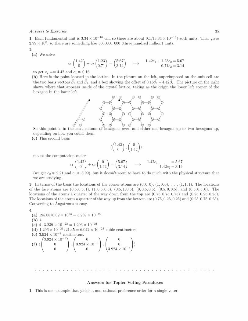
Answers to Exercises 35
1 Each fundamental unit is 3.34× 10⁻¹⁰ cm, so there are about 0.1/(3.34× 10−10) such units. That gives2.99× 108, so there are something like 300, 000, 000 (three hundred million) units.
2(a) We solve
c1
(1.42
0
)+ c2
(1.230.71
)=(
5.673.14
)=⇒ 1.42c1 + 1.23c2 = 5.67
0.71c2 = 3.14
to get c2 =≈ 4.42 and c1 ≈ 0.16.(b) Here is the point located in the lattice. In the picture on the left, superimposed on the unit cell arethe two basis vectors ~β1 and ~β2, and a box showing the offset of 0.16~β1 + 4.42~β2. The picture on the rightshows where that appears inside of the crystal lattice, taking as the origin the lower left corner of thehexagon in the lower left.
So this point is in the next column of hexagons over, and either one hexagon up or two hexagons up,depending on how you count them.
(c) This second basis
〈(
1.420
),
(0
1.42
)〉
makes the computation easier
c1
(1.42
0
)+ c2
(0
1.42
)=(
5.673.14
)=⇒ 1.42c1 = 5.67
1.42c2 = 3.14
(we get c2 ≈ 2.21 and c1 ≈ 3.99), but it doesn’t seem to have to do much with the physical structure thatwe are studying.
3 In terms of the basis the locations of the corner atoms are (0, 0, 0), (1, 0, 0), . . . , (1, 1, 1). The locationsof the face atoms are (0.5, 0.5, 1), (1, 0.5, 0.5), (0.5, 1, 0.5), (0, 0.5, 0.5), (0.5, 0, 0.5), and (0.5, 0.5, 0). Thelocations of the atoms a quarter of the way down from the top are (0.75, 0.75, 0.75) and (0.25, 0.25, 0.25).The locations of the atoms a quarter of the way up from the bottom are (0.75, 0.25, 0.25) and (0.25, 0.75, 0.25).Converting to Angstroms is easy.
4(a) 195.08/6.02× 1023 = 3.239× 10⁻²²
(b) 4(c) 4 · 3.239× 10−22 = 1.296× 10⁻²¹
(d) 1.296× 10⁻²¹/21.45 = 6.042× 10⁻²³ cubic centimeters(e) 3.924× 10⁻⁸ centimeters.
(f) 〈
3.924× 10⁻⁸
00
,
03.924× 10⁻⁸
0
,
00
3.924× 10⁻⁸
〉
. . . . . . . . . . . . . . . . . . . . . . . . . . . . . . . . . . . . . . . . . . . . .
Answers for Topic: Voting Paradoxes
1 This is one example that yields a non-rational preference order for a single voter.

36 Linear Algebra, by Hefferon
character experience policiesDemocrat most middle leastRepublican middle least mostThird least most middle
The Democrat is preferred to the Republican for character and experience. The Republican is preferred tothe Third for character and policies. And, the Third is preferred to the Democrat for experience and policies.
2 First, compare the D > R > T decomposition that was done out in the Topic with the decomposition ofthe opposite T > R > D voter.−1
11
=13·
111
+23·
−110
+23·
−101
and
1−1−1
= d1 ·
111
+ d2 ·
−110
+ d3 ·
−101
Obviously, the second is the negative of the first, and so d1 = −1/3, d2 = −2/3, and d3 = −2/3. Thisprinciple holds for any pair of opposite voters, and so we need only do the computation for a voter from thesecond row, and a voter from the third row. For a positive spin voter in the second row,
c1 − c2 − c3 = 1c1 + c2 = 1c1 + c3 =−1
−ρ1+ρ2−→−ρ1+ρ3
(−1/2)ρ2+ρ3−→c1 − c2 − c3 = 1
2c2 + c3 = 0(3/2)c3 =−2
gives c3 = −4/3, c2 = 2/3, and c1 = 1/3. For a positive spin voter in the third row,
c1 − c2 − c3 = 1c1 + c2 =−1c1 + c3 = 1
−ρ1+ρ2−→−ρ1+ρ3
(−1/2)ρ2+ρ3−→c1 − c2 − c3 = 1
2c2 + c3 =−2(3/2)c3 = 1
gives c3 = 2/3, c2 = −4/3, and c1 = 1/3.
3 The mock election corresponds to the table on page 150 in the way shown in the first table, and aftercancellation the result is the second table.
positive spin negative spin
D > R > T
5 voters
T > R > D
2 voters
R > T > D
8 voters
D > T > R
4 voters
T > D > R
8 voters
R > D > T
2 voters
positive spin negative spin
D > R > T
3 voters
T > R > D
–
R > T > D
4 voters
D > T > R
–
T > D > R
6 voters
R > D > T
–
All three come from the same side of the table (the left), as the result from this Topic says must happen.Tallying the election can now proceed, using the cancelled numbers
3 ·D
1 voter
T1 voter
R
−1 voter
+ 4 ·D −1 voter
T1 voter
R1 voter
+ 6 ·D
1 voter
T−1 voter
R1 voter
=D
5 voters
T1 voter
R7 voters
to get the same outcome.
4(a) The two can be rewritten as −c ≤ a − b and −c ≤ b − a. Either a − b or b − a is nonpositive and so−c ≤ −|a− b|, as required.
(b) This is immediate from the supposition that 0 ≤ a+ b− c.(c) A trivial example starts with the zero-voter election and adds any one voter. A more interestingexample is to take the Political Science mock election and add two T > D > R voters (they can beadded one at a time, to satisfy the “addition of one more voter” criteria in the question). Observe thatthe additional voters have positive spin, which is the spin of the votes remaining after cancellation in theoriginal mock election. This is the resulting table of voters, and next to it is the result of cancellation.

Answers to Exercises 37
positive spin negative spin
D > R > T
5 voters
T > R > D
2 voters
R > T > D
8 voters
D > T > R
4 voters
T > D > R
10 voters
R > D > T
2 voters
positive spin negative spin
D > R > T
3 voters
T > R > D
–
R > T > D
4 voters
D > T > R
–
T > D > R
8 voters
R > D > T
–The election, using the cancelled numbers, is this.
3 ·D
1 voter
T1 voter
R
−1 voter
+ 4 ·D −1 voter
T1 voter
R1 voter
+ 8 ·D
1 voter
T−1 voter
R1 voter
=D
7 voters
T−1 voter
R9 voters
The majority cycle has indeed disappeared.(d) One such condition is that, after cancellation, all three be nonnegative or all three be nonpositive,and: |c| < |a+ b| and |b| < |a+ c| and |a| < |b+ c|. This follows from this diagram.
Da
T
a
R
−a+
D −bT
b
R
b
+
Dc
T
−cR
c
=
Da− b+ c
T
a+ b− cR
−a+ b+ c
5(a) A two-voter election can have a majority cycle in two ways. First, the two voters could be opposites,resulting after cancellation in the trivial election (with the majority cycle of all zeroes). Second, the twovoters could have the same spin but come from different rows, as here.
1 ·D
1 voter
T1 voter
R
−1 voter
+ 1 ·D −1 voter
T1 voter
R1 voter
+ 0 ·D
1 voter
T−1 voter
R1 voter
=D
0 voters
T2 voters
R0 voters
(b) There are two cases. An even number of voters can split half and half into opposites, e.g., half thevoters are D > R > T and half are T > R > D. Then cancellation gives the trivial election. If the numberof voters is greater than one and odd (of the form 2k + 1 with k > 0) then using the cycle diagram fromthe proof,
Da
T
a
R
−a+
D −bT
b
R
b
+
Dc
T
−cR
c
=
Da− b+ c
T
a+ b− cR
−a+ b+ c
we can take a = k and b = k and c = 1. Because k > 0, this is a majority cycle.6 It is nonempty because it contains the zero vector. To see that it is closed under linear combinations oftwo of its members, suppose that ~v1 and ~v2 are in U⊥ and consider c1~v1 + c2~v2. For any ~u ∈ U ,
(c1~v1 + c2~v2) ~u = c1(~v1 ~u) + c2(~v2 ~u) = c1 · 0 + c2 · 0 = 0and so c1~v1 + c2~v2 ∈ U⊥.
. . . . . . . . . . . . . . . . . . . . . . . . . . . . . . . . . . . . . . . . . . . . .
Answers for Topic: Dimensional Analysis1(a) This relationship
(L1M0T 0)p1(L1M0T 0)p2(L1M0T−1)p3(L0M0T 0)p4(L1M0T−2)p5(L0M0T 1)p6 = L0M0T 0
gives rise to this linear systemp1 + p2 + p3 + p5 = 0
0 = 0−p3 − 2p5 + p6 = 0

38 Linear Algebra, by Hefferon
(note that there is no restriction on p4). The natural paramatrization uses the free variables to givep3 = −2p5 + p6 and p1 = −p2 + p5 − p6. The resulting description of the solution set
{
p1
p2
p3
p4
p5
p6
= p2
−110000
+ p4
000100
+ p5
10−2010
+ p6
−101001
∣∣ p2, p4, p5, p6 ∈ R}
gives {y/x, θ, xt/v02, v0t/x} as a complete set of dimensionless products (recall that “complete” in this
context does not mean that there are no other dimensionless products; it simply means that the set is abasis). This is, however, not the set of dimensionless products that the question asks for.
There are two ways to proceed. The first is to fiddle with the choice of parameters, hoping to hit onthe right set. For that, we can do the prior paragraph in reverse. Converting the given dimensionlessproducts gt/v0, gx/v2
0 , gy/v20 , and θ into vectors gives this description (note the ? ’s where the parameters
will go).
{
p1
p2
p3
p4
p5
p6
= ?
00−1011
+ ?
10−2010
+ ?
01−2010
+ p4
000100
∣∣ p2, p4, p5, p6 ∈ R}
The p4 is already in place. Examining the rows shows that we can also put in place p6, p1, and p2.The second way to proceed, following the hint, is to note that the given set is of size four in a four-
dimensional vector space and so we need only show that it is linearly independent. That is easily done byinspection, by considering the sixth, first, second, and fourth components of the vectors.
(b) The first equation can be rewrittengx
v02
=gt
v0cos θ
so that Buckingham’s function is f1(Π1,Π2,Π3,Π4) = Π2 − Π1 cos(Π4). The second equation can berewritten
gy
v02
=gt
v0sin θ − 1
2
(gt
v0
)2
and Buckingham’s function here is f2(Π1,Π2,Π3,Π4) = Π3 −Π1 sin(Π4) + (1/2)Π12.
2 We consider
(L0M0T−1)p1(L1M−1T 2)p2(L−3M0T 0)p3(L0M1T 0)p4 = (L0M0T 0)
which gives these relations among the powers.p2 − 3p3 = 0−p2 + p4 = 0
−p1 + 2p2 = 0
ρ1↔ρ3−→ ρ2+ρ3−→−p1 + 2p2 = 0
−p2 + p4 = 0−3p3 + p4 = 0
This is the solution space (because we wish to express k as a function of the other quantities, p2 is taken asthe parameter).
{
21
1/31
p2
∣∣ p2 ∈ R}
Thus, Π1 = ν2kN1/3m is the dimensionless combination, and we have that k equals ν−2N−1/3m−1 times aconstant (the function f is constant since it has no arguments).
3

Answers to Exercises 39
(a) Setting(L2M1T−2)p1(L0M0T−1)p2(L3M0T 0)p3 = (L0M0T 0)
gives this2p1 + 3p3 = 0p1 = 0
−2p1 − p2 = 0which implies that p1 = p2 = p3 = 0. That is, among quantities with these dimensional formulas, the onlydimensionless product is the trivial one.
(b) Setting(L2M1T−2)p1(L0M0T−1)p2(L3M0T 0)p3(L−3M1T 0)p4 = (L0M0T 0)
gives this.2p1 + 3p3 − 3p4 = 0p1 + p4 = 0
−2p1 − p2 = 0
(−1/2)ρ1+ρ2−→ρ1+ρ3
ρ2↔ρ3−→2p1 + 3p3 − 3p4 = 0−p2 + 3p3 − 3p4 = 0
(−3/2)p3 + (5/2)p4 = 0Taking p1 as parameter to express the torque gives this description of the solution set.
{
1−2−5/3−1
p1
∣∣ p1 ∈ R}
Denoting the torque by τ , the rotation rate by r, the volume of air by V , and the density of air by d wehave that Π1 = τr−2V −5/3d−1, and so the torque is r2V 5/3d times a constant.
4(a) These are the dimensional formulas.
quantitydimensionalformula
speed of the wave v L1M0T−1
separation of the dominoes d L1M0T 0
height of the dominoes h L1M0T 0
acceleration due to gravity g L1M0T−2
(b) The relationship(L1M0T−1)p1(L1M0T 0)p2(L1M0T 0)p3(L1M0T−2)p4 = (L0M0T 0)
gives this linear system.p1 + p2 + p3 + p4 = 0
0 = 0−p1 − 2p4 = 0
ρ1+ρ4−→ p1 + p2 + p3 + p4 = 0p2 + p3 − p4 = 0
Taking p3 and p4 as parameters, the solution set is described in this way.
{
0−110
p3 +
−2101
p4
∣∣ p3, p4 ∈ R}
That gives {Π1 = h/d,Π2 = dg/v2} as a complete set.(c) Buckingham’s Theorem says that v2 = dg · f(h/d), and so, since g is a constant, if h/d is fixed then vis proportional to
√d .
5 Checking the conditions in the definition of a vector space is routine.6(a) The dimensional formula of the circumference is L, that is, L1M0T 0. The dimensional formula of thearea is L2.
(b) One is C +A = 2πr + πr2.(c) One example is this formula relating the the length of arc subtended by an angle to the radius andthe angle measure in radians: `− rθ = 0. Both terms in that formula have dimensional formula L1. Therelationship holds for some unit systems (inches and radians, for instance) but not for all unit systems(inches and degrees, for instance).

40 Linear Algebra, by Hefferon
Chapter 3. Maps Between Spaces
. . . . . . . . . . . . . . . . . . . . . . . . . . . . . . . . . . . . . . . . . . . . .
Answers for subsection 3.I.13.I.1.12 To verify it is one-to-one, assume that f1(c1x + c2y + c3z) = f1(d1x + d2y + d3z). Then c1 +c2x + c3x
2 = d1 + d2x + d3x2 by the definition of f1. Members of P2 are equal only when they have the
same coefficients, so this implies that c1 = d1 and c2 = d2 and c3 = d3. Therefore f1(c1x + c2y + c3z) =f1(d1x+ d2y + d3z) implies that c1x+ c2y + c3z = d1x+ d2y + d3z, and so f1 is one-to-one.
To verify that it is onto, consider an arbitrary member of the codomain a1 + a2x + a3x2 and observe
that it is indeed the image of a member of the domain, namely, it is f1(a1x + a2y + a3z). (For instance,0 + 3x+ 6x2 = f1(0x+ 3y + 6z).)
The computation checking that f1 preserves addition is this.f1 ( (c1x+ c2y + c3z) + (d1x+ d2y + d3z) ) = f1 ( (c1 + d1)x+ (c2 + d2)y + (c3 + d3)z )
= (c1 + d1) + (c2 + d2)x+ (c3 + d3)x2
= (c1 + c2x+ c3x2) + (d1 + d2x+ d3x
2)= f1(c1x+ c2y + c3z) + f1(d1x+ d2y + d3z)
The check that f1 preserves scalar multiplication is this.f1( r · (c1x+ c2y + c3z) ) = f1( (rc1)x+ (rc2)y + (rc3)z )
= (rc1) + (rc2)x+ (rc3)x2
= r · (c1 + c2x+ c3x2)
= r · f1(c1x+ c2y + c3z)
3.I.1.14 It is one-to-one and onto, a correspondence, because it has an inverse (namely, f−1(x) = 3√x).
However, it is not an isomorphism. For instance, f(1) + f(1) 6= f(1 + 1).3.I.1.16 Here are two.
a0 + a1x+ a2x2 7→
a1
a0
a2
and a0 + a1x+ a2x2 7→
a0 + a1
a1
a2
Verification is straightforward (for the second, to show that it is onto, note thatst
u
is the image of (s− t) + tx+ ux2).3.I.1.18 Here are two:
r1
r2
...r16
7→r1 r2 . . .
. . . r16
and
r1
r2
...r16
7→r1
r2
......r16
Verification that each is an isomorphism is easy.3.I.1.20 If n ≥ 1 then Pn−1
∼= Rn. (If we take P−1 and R0 to be trivial vector spaces, then the relationshipextends one dimension lower.) The natural isomorphism between them is this.
a0 + a1x+ · · ·+ an−1xn−1 7→
a0
a1
...an−1
Answers to Exercises 41
Checking that it is an isomorphism is straightforward.
3.I.1.21 This is the map, expanded.
f(a0 + a1x+ a2x2 + a3x
3 + a4x4 + a5x
5) = a0 + a1(x− 1) + a2(x− 1)2 + a3(x− 1)3
+ a4(x− 1)4 + a5(x− 1)5
= a0 + a1(x− 1) + a2(x2 − 2x+ 1)
+ a3(x3 − 3x2 + 3x− 1) + a4(x4 − 4x3 + 6x2 − 4x+ 1)
+ a5(x5 − 5x4 + 10x3 − 10x2 + 5x− 1)
= (a0 − a1 + a2 − a3 + a4 − a5) + (a1 − 2a2 + 3a3 − 4a4 + 5a5)x
+ (a2 − 3a3 + 6a4 − 10a5)x2 + (a3 − 4a4 + 10a5)x3
+ (a4 − 5a5)x4 + a5x5
This map is a correspondence because it has an inverse, the map p(x) 7→ p(x+ 1).To finish checking that it is an isomorphism, we apply item (2) of Lemma 1.9 and show that it preserves
linear combinations of two polynomials. Briefly, the check goes like this.
f(c · (a0 + a1x+ · · ·+ a5x5) + d · (b0 + b1x+ · · ·+ b5x
5))
= · · · = (ca0 − ca1 + ca2 − ca3 + ca4 − ca5 + db0 − db1 + db2 − db3 + db4 − db5) + · · ·+ (ca5 + db5)x5
= · · · = c · f(a0 + a1x+ · · ·+ a5x5) + d · f(b0 + b1x+ · · ·+ b5x
5)
3.I.1.22 No vector space has the empty set underlying it. We can take ~v to be the zero vector.
3.I.1.23 Yes; where the two spaces are {~a} and {~b}, the map sending ~a to ~b is clearly one-to-one and onto,and also preserves what little structure there is.
3.I.1.24 A linear combination of n = 0 vectors adds to the zero vector and so Lemma 1.8 shows that thethree statements are equivalent in this case.
3.I.1.25 Consider the basis 〈1〉 for P0 and let f(1) ∈ R be k. For any a ∈ P0 we have that f(a) = f(a ·1) =af(1) = ak and so f ’s action is multiplication by k. Note that k 6= 0 or else the map is not one-to-one.(Incidentally, any such map a 7→ ka is an isomorphism, as is easy to check.)
3.I.1.27 One direction is easy: by definition, if f is one-to-one then for any ~w ∈W at most one ~v ∈ V hasf(~v ) = ~w, and so in particular, at most one member of V is mapped to ~0W . The proof of Lemma 1.8 doesnot use the fact that the map is a correspondence and therefore shows that any structure-preserving map fsends ~0V to ~0W .
For the other direction, assume that the only member of V that is mapped to ~0W is ~0V . To show that fis one-to-one assume that f(~v1) = f(~v2). Then f(~v1)− f(~v2) = ~0W and so f(~v1 − ~v2) = ~0W . Consequently~v1 − ~v2 = ~0V , so ~v1 = ~v2, and so f is one-to-one.
3.I.1.28 We will prove something stronger—not only is the existence of a dependence preserved by isomor-phism, but each instance of a dependence is preserved, that is,
~vi = c1~v1 + · · ·+ ci−1~vi−1 + ci+1~vi+1 + · · ·+ ck~vk
⇐⇒ f(~vi) = c1f(~v1) + · · ·+ ci−1f(~vi−1) + ci+1f(~vi+1) + · · ·+ ckf(~vk).
The =⇒ direction of this statement holds by item (3) of Lemma 1.9. The⇐= direction holds by regrouping
f(~vi) = c1f(~v1) + · · ·+ ci−1f(~vi−1) + ci+1f(~vi+1) + · · ·+ ckf(~vk)= f(c1~v1 + · · ·+ ci−1~vi−1 + ci+1~vi+1 + · · ·+ ck~vk)
and applying the fact that f is one-to-one, and so for the two vectors ~vi and c1~v1+· · ·+ci−1~vi−1+ci+1f~vi+1+· · ·+ ckf(~vk to be mapped to the same image by f , they must be equal.
3.I.1.30 First, the map p(x) 7→ p(x+ k) doesn’t count because it is a version of p(x) 7→ p(x− k). Here isa correct answer (many others are also correct): a0 + a1x+ a2x
2 7→ a2 + a0x+ a1x2. Verification that this
is an isomorphism is straightforward.
3.I.1.31

42 Linear Algebra, by Hefferon
(a) For the ‘only if’ half, let f : R1 → R1 to be an isomorphism. Consider the basis 〈1〉 ⊆ R1. Designatef(1) by k. Then for any x we have that f(x) = f(x · 1) = x · f(1) = xk, and so f ’s action is multiplicationby k. To finish this half, just note that k 6= 0 or else f would not be one-to-one.
For the ‘if’ half we only have to check that such a map is an isomorphism when k 6= 0. To checkthat it is one-to-one, assume that f(x1) = f(x2) so that kx1 = kx2 and divide by the nonzero factor k toconclude that x1 = x2. To check that it is onto, note that any y ∈ R1 is the image of x = y/k (again,k 6= 0). Finally, to check that such a map preserves combinations of two members of the domain, we havethis.
f(c1x1 + c2x2) = k(c1x1 + c2x2) = c1kx1 + c2kx2 = c1f(x1) + c2f(x2)(b) By the prior item, f ’s action is x 7→ (7/3)x. Thus f(−2) = −14/3.(c) For the ‘only if’ half, assume that f : R2 → R2 is an automorphism. Consider the standard basis E2 forR2. Let
f(~e1) =(ac
)and f(~e2) =
(bd
).
Then the action of f on any vector is determined by by its action on the two basis vectors.
f((xy
)) = f(x · ~e1 + y · ~e2) = x · f(~e1) + y · f(~e2) = x ·
(ac
)+ y ·
(bd
)=(ax+ bycx+ dy
)To finish this half, note that if ad− bc = 0, that is, if f(~e2) is a multiple of f(~e1), then f is not one-to-one.
For ‘if’ we must check that the map is an isomorphism, under the condition that ad − bc 6= 0. Thestructure-preservation check is easy; we will here show that f is a correspondence. For the argument thatthe map is one-to-one, assume this.
f((x1
y1
)) = f(
(x2
y2
)) and so
(ax1 + by1
cx1 + dy1
)=(ax2 + by2
cx2 + dy2
)Then, because ad− bc 6= 0, the resulting system
a(x1 − x2) + b(y1 − y2) = 0c(x1 − x2) + d(y1 − y2) = 0
has a unique solution, namely the trivial one x1 − x2 = 0 and y1 − y2 = 0 (this follows from the hint).The argument that this map is onto is closely related—this system
ax1 + by1 = xcx1 + dy1 = y
has a solution for any x and y if and only if this set
{(ac
),
(bd
)}
spans R2, i.e., if and only if this set is a basis (because it is a two-element subset of R2), i.e., if and onlyif ad− bc 6= 0.
(d)
f((
0−1
)) = f(
(13
)−(
14
)) = f(
(13
))− f(
(14
)) =
(2−1
)−(
01
)=(
2−2
)3.I.1.32 There are many answers; two are linear independence and subspaces.
To show that if a set {~v1, . . . , ~vn} is linearly independent then its image {f(~v1), . . . , f(~vn)} is also linearlyindependent, consider a linear relationship among members of the image set.
0 = c1f(~v1) + · · ·+ cnf( ~vn) = f(c1~v1) + · · ·+ f(cn ~vn) = f(c1~v1 + · · ·+ cn ~vn)Because this map is an isomorphism, it is one-to-one. So f maps only one vector from the domain tothe zero vector in the range, that is, c1~v1 + · · · + cn~vn equals the zero vector (in the domain, of course).But, if {~v1, . . . , ~vn} is linearly independent then all of the c’s are zero, and so {f(~v1), . . . , f(~vn)} is linearlyindependent also. (Remark. There is a small point about this argument that is worth mention. In a set,repeats collapse, that is, strictly speaking, this is a one-element set: {~v,~v}, because the things listed as init are the same thing. Observe, however, the use of the subscript n in the above argument. In moving fromthe domain set {~v1, . . . , ~vn} to the image set {f(~v1), . . . , f(~vn)}, there is no collapsing, because the imageset does not have repeats, because the isomorphism f is one-to-one.)

Answers to Exercises 43
To show that if f : V →W is an isomorphism and if U is a subspace of the domain V then the set ofimage vectors f(U) = {~w ∈W
∣∣ ~w = f(~u) for some ~u ∈ U} is a subspace of W , we need only show that it isclosed under linear combinations of two of its members (it is nonempty because it contains the image of thezero vector). We have
c1 · f(~u1) + c2 · f(~u2) = f(c1~u1) + f(c2~u2) = f(c1~u1 + c2~u2)and c1~u1 + c2~u2 is a member of U because of the closure of a subspace under combinations. Hence thecombination of f(~u1) and f(~u2) is a member of f(U).3.I.1.33(a) The association
~p = c1~β1 + c2~β2 + c3~β3RepB(·)7−→
c1c2c3
is a function if every member ~p of the domain is associated with at least one member of the codomain, and ifevery member ~p of the domain is associated with at most one member of the codomain. The first conditionholds because the basis B spans the domain—every ~p can be written as at least one linear combination of~β’s. The second condition holds because the basis B is linearly independent—every member of the domain~p can be written as at most one linear combination of the ~β’s.
(b) For the one-to-one argument, if RepB(~p) = RepB(~q), that is, if RepB(p1~β1+p2
~β2+p3~β3) = RepB(q1
~β1+q2~β2 + q3
~β3) then p1
p2
p3
=
q1
q2
q3
and so p1 = q1 and p2 = q2 and p3 = q3, which gives the conclusion that ~p = ~q. Therefore this map isone-to-one.
For onto, we can just note that abc
equals RepB(a~β1 + b~β2 + c~β3), and so any member of the codomain R3 is the image of some member ofthe domain P2.
(c) This map respects addition and scalar multiplication because it respects combinations of two membersof the domain (that is, we are using item (2) of Lemma 1.9): where ~p = p1
~β1 + p2~β2 + p3
~β3 and ~q =q1~β1 + q2
~β2 + q3~β3, we have this.
RepB(c · ~p+ d · ~q) = RepB( (cp1 + dq1)~β1 + (cp2 + dq2)~β2 + (cp3 + dq3)~β3 )
=
cp1 + dq1
cp2 + dq2
cp3 + dq3
= c ·
p1
p2
p3
+ d ·
q1
q2
q3
= RepB(~p) + RepB(~q)
(d) Use any basis B for P2 whose first two members are x+ x2 and 1− x, say B = 〈x+ x2, 1− x, 1〉.3.I.1.34 See the next subsection.3.I.1.35(a) Most of the conditions in the definition of a vector space are routine. We here sketch the verificationof part (1) of that definition.
For closure of U×W , note that because U and W are closed, we have that ~u1+~u2 ∈ U and ~w1+ ~w2 ∈Wand so (~u1 + ~u2, ~w1 + ~w2) ∈ U ×W . Commutativity of addition in U ×W follows from commutativity ofaddition in U and W .
(~u1, ~w1) + (~u2, ~w2) = (~u1 + ~u2, ~w1 + ~w2) = (~u2 + ~u1, ~w2 + ~w1) = (~u2, ~w2) + (~u1, ~w1)

44 Linear Algebra, by Hefferon
The check for associativity of addition is similar. The zero element is (~0U ,~0W ) ∈ U ×W and the additiveinverse of (~u, ~w) is (−~u,−~w).
The checks for the second part of the definition of a vector space are also straightforward.(b) This is a basis
〈 (1,(
00
)), (x,
(00
)), (x2,
(00
)), (1,
(10
)), (1,
(01
)) 〉
because there is one and only one way to represent any member of P2 × R2 with respect to this set; hereis an example.
(3 + 2x+ x2,
(54
)) = 3 · (1,
(00
)) + 2 · (x,
(00
)) + (x2,
(00
)) + 5 · (1,
(10
)) + 4 · (1,
(01
))
The dimension of this space is five.(c) We have dim(U ×W ) = dim(U) + dim(W ) as this is a basis.
〈(~µ1,~0W ), . . . , (~µdim(U),~0W ), (~0U , ~ω1), . . . , (~0U , ~ωdim(W ))〉(d) We know that if V = U ⊕W then each ~v ∈ V can be written as ~v = ~u + ~w in one and only one way.This is just what we need to prove that the given function an isomorphism.
First, to show that f is one-to-one we can show that if f ((~u1, ~w1)) = ((~u2, ~w2)), that is, if ~u1 + ~w1 =~u2 + ~w2 then ~u1 = ~u2 and ~w1 = ~w2. But the statement ‘each ~v is such a sum in only one way’ is exactlywhat is needed to make this conclusion. Similarly, the argument that f is onto is completed by thestatement that ‘each ~v is such a sum in at least one way’.
This map also preserves linear combinationsf( c1 · (~u1, ~w1) + c2 · (~u2, ~w2) ) = f( (c1~u1 + c2~u2, c1 ~w1 + c2 ~w2) )
= c1~u1 + c2~u2 + c1 ~w1 + c2 ~w2
= c1~u1 + c1 ~w1 + c2~u2 + c2 ~w2
= c1 · f( (~u1, ~w1) ) + c2 · f( (~u2, ~w2) )and so it is an isomorphism.
. . . . . . . . . . . . . . . . . . . . . . . . . . . . . . . . . . . . . . . . . . . . .
Answers for subsection 3.I.23.I.2.14 There are many answers, one is the set of Pk (taking P−1 to be the trivial vector space).3.I.2.15 False (except when n = 0). For instance, if f : V → Rn is an isomorphism then multiplying by anynonzero scalar, gives another, different, isomorphism. (Between trivial spaces the isomorphisms are unique;the only map possible is ~0V 7→ 0W .)3.I.2.16 No. A proper subspace has a strictly lower dimension than it’s superspace; if U is a propersubspace of V then any linearly independent subset of U must have fewer than dim(V ) members or else thatset would be a basis for V , and U wouldn’t be proper.3.I.2.19 We must show that if ~a = ~b then f(~a) = f(~b). So suppose that a1
~β1+· · ·+an~βn = b1~β1+· · ·+bn~βn.Each vector in a vector space (here, the domain space) has a unique representation as a linear combinationof basis vectors, so we can conclude that a1 = b1, . . . , an = bn. Thus,
f(~a) =
a1
...an
=
b1...bn
= f(~b)
and so the function is well-defined.3.I.2.20 Yes, because a zero-dimensional space is a trivial space.3.I.2.21(a) No, this collection has no spaces of odd dimension.(b) Yes, because Pk ∼= Rk+1.

Answers to Exercises 45
(c) No, for instance, M2×3∼=M3×2.
3.I.2.22 One direction is easy: if the two are isomorphic via f then for any basis B ⊆ V , the set D = f(B) isalso a basis (this is shown in Lemma 2.3). The check that corresponding vectors have the same coordinates:f(c1~β1 + · · ·+ cn~βn) = c1f(~β1) + · · ·+ cnf(~βn) = c1~δ1 + · · ·+ cn~δn is routine.
For the other half, assume that there are bases such that corresponding vectors have the same coordinateswith respect to those bases. Because f is a correspondence, to show that it is an isomorphism, we need onlyshow that it preserves structure. Because RepB(~v ) = RepD(f(~v )), the map f preserves structure if andonly if representations preserve addition: RepB(~v1 + ~v2) = RepB(~v1) + RepB(~v2) and scalar multiplication:RepB(r · ~v ) = r · RepB(~v ) The addition calculation is this: (c1 + d1)~β1 + · · · + (cn + dn)~βn = c1~β1 + · · · +cn~βn + d1
~β1 + · · ·+ dn~βn, and the scalar multiplication calculation is similar.3.I.2.23(a) Pulling the definition back from R4 to P3 gives that a0 + a1x+ a2x
2 + a3x3 is orthogonal to b0 + b1x+
b2x2 + b3x
3 if and only if a0b0 + a1b1 + a2b2 + a3b3 = 0.(b) A natural definition is this.
D(
a0
a1
a2
a3
) =
a1
2a2
3a3
0
3.I.2.25 Because V1 ∩ V2 = {~0V } and f is one-to-one we have that f(V1) ∩ f(V2) = {~0U}. To finish, countthe dimensions: dim(U) = dim(V ) = dim(V1) + dim(V2) = dim(f(V1)) + dim(f(V2)), as required.3.I.2.26 Rational numbers have many representations, e.g., 1/2 = 3/6, and the numerators can vary amongrepresentations.
. . . . . . . . . . . . . . . . . . . . . . . . . . . . . . . . . . . . . . . . . . . . .
Answers for subsection 3.II.13.II.1.19 Each of these projections is a homomorphism. Projection to the xz-plane and to the yz-planeare these maps. xy
z
7→x0z
xyz
7→0yz
Projection to the x-axis, to the y-axis, and to the z-axis are these maps.xy
z
7→x0
0
xyz
7→0y0
xyz
7→0
0z
And projection to the origin is this map. xy
z
7→0
00
Verification that each is a homomorphism is straightforward. (The last one, of course, is the zero transfor-mation on R3.)3.II.1.20 The first is not onto; for instance, there is no polynomial that is sent the constant polynomialp(x) = 1. The second is not one-to-one; both of these members of the domain(
1 00 0
)and
(0 00 1
)are mapped to the same member of the codomain, 1 ∈ R.3.II.1.21 Yes; in any space id(c · ~v + d · ~w) = c · ~v + d · ~w = c · id(~v) + d · id(~w).3.II.1.24

46 Linear Algebra, by Hefferon
(a) Let ~v ∈ V be represented with respect to the basis as ~v = c1~β1 + · · · + cn~βn. Then h(~v) = h(c1~β1 +· · ·+ cn~βn) = c1h(~β1) + · · ·+ cnh(~βn) = c1 ·~0 + · · ·+ cn ·~0 = ~0.
(b) This argument is similar to the prior one. Let ~v ∈ V be represented with respect to the basis as~v = c1~β1 + · · ·+ cn~βn. Then h(c1~β1 + · · ·+ cn~βn) = c1h(~β1) + · · ·+ cnh(~βn) = c1~β1 + · · ·+ cn~βn = ~v.
(c) As above, only c1h(~β1) + · · ·+ cnh(~βn) = c1r~β1 + · · ·+ cnr~βn = r(c1~β1 + · · ·+ cn~βn) = r~v.
3.II.1.29 Let h : R1 → R1 be linear. A linear map is determined by its action on a basis, so fix the basis〈1〉 for R1. For any r ∈ R1 we have that h(r) = h(r · 1) = r · h(1) and so h acts on any argument r bymultiplying it by the constant h(1). If h(1) is not zero then the map is a correspondence—its inverse isdivision by h(1)—so any nontrivial transformation of R1 is an isomorphism.
This projection map is an example that shows that not every transformation of Rn acts via multiplicationby a constant when n > 1, including when n = 2.
x1
x2
...xn
7→x1
0...0
3.II.1.30(a) Where c and d are scalars, we have this.
h(c ·
x1
...xn
+ d ·
y1
...yn
) = h(
cx1 + dy1
...cxn + dyn
)
=
a1,1(cx1 + dy1) + · · ·+ a1,n(cxn + dyn)...
am,1(cx1 + dy1) + · · ·+ am,n(cxn + dyn)
= c ·
a1,1x1 + · · ·+ a1,nxn...
am,1x1 + · · ·+ am,nxn
+ d ·
a1,1y1 + · · ·+ a1,nyn...
am,1y1 + · · ·+ am,nyn
= c · h(
x1
...xn
) + d · h(
y1
...yn
)
(b) Each power i of the derivative operator is linear because of these rules familiar from calculus.
di
dxi( f(x) + g(x) ) =
di
dxif(x) +
di
dxig(x) and
di
dxir · f(x) = r · d
i
dxif(x)
Thus the given map is a linear transformation of Pn because any linear combination of linear maps is alsoa linear map.
3.II.1.31 (This argument has already appeared, as part of the proof that isomorphism is an equivalence.)Let f : U → V and g : V →W be linear. For any ~u1, ~u2 ∈ U and scalars c1, c2 combinations are preserved.
g ◦ f(c1~u1 + c2~u2) = g( f(c1~u1 + c2~u2) ) = g( c1f(~u1) + c2f(~u2) )= c1 · g(f(~u1)) + c2 · g(f(~u2)) = c1 · g ◦ f(~u1) + c2 · g ◦ f(~u2)
3.II.1.33 Recall that the entry in row i and column j of the transpose of M is the entry mj,i from row j

Answers to Exercises 47
and column i of M . Now, the check is routine.
[r ·
...
· · · ai,j · · ·...
+ s ·
...
· · · bi,j · · ·...
]
trans
=
...
· · · rai,j + sbi,j · · ·...
trans
=
...
· · · raj,i + sbj,i · · ·...
= r ·
...
· · · aj,i · · ·...
+ s ·
...
· · · bj,i · · ·...
= r ·
...
· · · aj,i · · ·...
trans
+ s ·
...
· · · bj,i · · ·...
trans
The domain is Mm×n while the codomain is Mn×m.3.II.1.34(a) For any homomorphism h : Rn → Rm we have
h(`) = {h(t · ~u+ (1− t) · ~v)∣∣ t ∈ [0..1]} = {t · h(~u) + (1− t) · h(~v)
∣∣ t ∈ [0..1]}which is the line segment from h(~u) to h(~v).
(b) We must show that if a subset of the domain is convex then its image, as a subset of the range, is alsoconvex. Suppose that C ⊆ Rn is convex and consider its image h(C). To show h(C) is convex we mustshow that for any two of its members, ~d1 and ~d2, the line segment connecting them
` = {t · ~d1 + (1− t) · ~d2
∣∣ t ∈ [0..1]}is a subset of h(C).
Fix any member t · ~d1 +(1− t) · ~d2 of that line segment. Because the endpoints of ` are in the image of C,there are members of C that map to them, say h(~c1) = ~d1 and h(~c2) = ~d2. Now, where t is the scalar thatis fixed in the first sentence of this paragraph, observe that h(t ·~c1 +(1− t) ·~c2) = t ·h(~c1)+(1− t) ·h(~c2) =t · ~d1 + (1− t) · ~d2 Thus, any member of ` is a member of h(C), and so h(C) is convex.
3.II.1.36 Suppose that h : V →W is a homomorphism and suppose that S is a subspace of V . Consider themap h : S →W defined by h(~s) = h(~s). (The only difference between h and h is the difference in domain.)Then this new map is linear: h(c1 · ~s1 + c2 · ~s2) = h(c1~s1 + c2~s2) = c1h(~s1) + c2h(~s2) = c1 · h(~s1) + c2 · h(~s2).3.II.1.37 This will appear as a lemma in the next subsection.(a) The range is nonempty because V is nonempty. To finish we need to show that it is closed undercombinations. A combination of range vectors has the form, where ~v1, . . . , ~vn ∈ V ,
c1 · h(~v1) + · · ·+ cn · h(~vn) = h(c1~v1) + · · ·+ h(cn~vn) = h(c1 · ~v1 + · · ·+ cn · ~vn),which is itself in the range as c1 · ~v1 + · · · + cn · ~vn is a member of domain V . Therefore the range is asubspace.
(b) The nullspace is nonempty since it contains ~0V , as ~0V maps to ~0W . It is closed under linear com-binations because, where ~v1, . . . , ~vn ∈ V are elements of the inverse image set {~v ∈ V
∣∣ h(~v) = ~0W }, forc1, . . . , cn ∈ R
~0W = c1 · h(~v1) + · · ·+ cn · h(~vn) = h(c1 · ~v1 + · · ·+ cn · ~vn)and so c1 · ~v1 + · · ·+ cn · ~vn is also in the inverse image of ~0W .
(c) This image of U nonempty because U is nonempty. For closure under combinations, where ~u1, . . . , ~un ∈U ,
c1 · h(~u1) + · · ·+ cn · h(~un) = h(c1 · ~u1) + · · ·+ h(cn · ~un) = h(c1 · ~u1 + · · ·+ cn · ~un)which is itself in h(U) as c1 · ~u1 + · · ·+ cn · ~un is in U . Thus this set is a subspace.

48 Linear Algebra, by Hefferon
(d) The natural generalization is that the inverse image of a subspace of is a subspace.Suppose that X is a subspace of W . Note that ~0W ∈ X so the set {~v ∈ V
∣∣ h(~v) ∈ X} is not empty.To show that this set is closed under combinations, let ~v1, . . . , ~vn be elements of V such that h(~v1) = ~x1,. . . , h(~vn) = ~xn and note that
h(c1 · ~v1 + · · ·+ cn · ~vn) = c1 · h(~v1) + · · ·+ cn · h(~vn) = c1 · ~x1 + · · ·+ cn · ~xnso a linear combination of elements of h−1(X) is also in h−1(X).
3.II.1.38 No; the set of isomorphisms does not contain the zero map (unless the space is trivial).
3.II.1.39 If 〈~β1, . . . , ~βn〉 doesn’t span the space then the map needn’t be unique. For instance, if we tryto define a map from R2 to itself by specifying only that ~e1 is sent to itself, then there is more than onehomomorphism possible; both the identity map and the projection map onto the first component fit thiscondition.
If we drop the condition that 〈~β1, . . . , ~βn〉 is linearly independent then we risk an inconsistent specification(i.e, there could be no such map). An example is if we consider 〈~e2, ~e1, 2~e1〉, and try to define a map fromR2 to itself that sends ~e2 to itself, and sends both ~e1 and 2~e1 to ~e1. No homomorphism can satisfy thesethree conditions.
3.II.1.40(a) Briefly, the check of linearity is this.
F (r1 · ~v1 + r2 · ~v2) =(f1(r1~v1 + r2~v2)f2(r1~v1 + r2~v2)
)= r1
(f1(~v1)f2(~v1)
)+ r2
(f1(~v2)f2(~v2)
)= r1 · F (~v1) + r2 · F (~v2)
(b) Yes. Let π1 : R2 → R1 and π2 : R2 → R1 be the projections(xy
)π17−→ x and
(xy
)π27−→ y
onto the two axes. Now, where f1(~v) = π1(F (~v)) and f2(~v) = π2(F (~v)) we have the desired componentfunctions.
F (~v) =(f1(~v)f2(~v)
)They are linear because they are the composition of linear functions, and the fact that the compoistionof linear functions is linear was shown as part of the proof that isomorphism is an equivalence relation(alternatively, the check that they are linear is straightforward).
(c) In general, a map from a vector space V to an Rn is linear if and only if each of the component functionsis linear. The verification is as in the prior item.
. . . . . . . . . . . . . . . . . . . . . . . . . . . . . . . . . . . . . . . . . . . . .
Answers for subsection 3.II.2
3.II.2.25 The shadow of a scalar multiple is the scalar multiple of the shadow.
3.II.2.26(a) Setting a0 +(a0 +a1)x+(a2 +a3)x3 = 0+0x+0x2 +0x3 gives a0 = 0 and a0 +a1 = 0 and a2 +a3 = 0,so the nullspace is {−a3x
2 + a3x3∣∣ a3 ∈ R}.
(b) Setting a0 + (a0 + a1)x + (a2 + a3)x3 = 2 + 0x + 0x2 − x3 gives that a0 = 2, and a1 = −2,and a2 + a3 = −1. Taking a3 as a parameter, and renaming it a3 = a gives this set description{2− 2x+ (−1− a)x2 + ax3
∣∣ a ∈ R} = {(2− 2x− x2) + a · (−x2 + x3)∣∣ a ∈ R}.
(c) This set is empty because the range of h includes only those polynomials with a 0x2 term.
Answers to Exercises 49
3.II.2.29 For any vector space V , the nullspace
{~v ∈ V∣∣ 2~v = ~0}
is trivial, while the rangespace
{~w ∈ V∣∣ ~w = 2~v for some ~v ∈ V }
is all of V , because every vector ~w is twice some other vector, specifically, it is twice (1/2)~w. (Thus, thistransformation is actually an automorphism.)
3.II.2.30 Because the rank plus the nullity equals the dimension of the domain (here, five), and the rank isat most three, the possible pairs are: (3, 2), (2, 3), (1, 4), and (0, 5). Coming up with linear maps that showthat each pair is indeed possible is easy.
3.II.2.31 No (unless Pn is trivial), because the two polynomials f0(x) = 0 and f1(x) = 1 have the samederivative; a map must be one-to-one to have an inverse.
3.II.2.33(a) One direction is obvious: if the homomorphism is onto then its range is the codomain and so its rankequals the dimension of its codomain. For the other direction assume that the map’s rank equals thedimension of the codomain. Then the map’s range is a subspace of the codomain, and has dimensionequal to the dimension of the codomain. Therefore, the map’s range must equal the codomain, and themap is onto. (The ‘therefore’ is because there is a linearly independent subset of the range that is of sizeequal to the dimension of the codomain, but any such linearly independent subset of the codomain mustbe a basis for the codomain, and so the range equals the codomain.)
(b) By Theorem 3.II.2.20, a homomorphism is one-to-one if and only if its nullity is zero. Because rankplus nullity equals the dimension of the domain, it follows that a homomorphism is one-to-one if and onlyif its rank equals the dimension of its domain. But this domain and codomain have the same dimension,so the map is one-to-one if and only if it is onto.
3.II.2.34 We are proving that h : V →W is nonsingular if and only if for every linearly independent subsetS of V the subset h(S) = {h(~s)
∣∣ ~s ∈ S} of W is linearly independent.One half is easy—by Theorem 3.II.2.20, if h is singular then its nullspace is nontrivial (contains more
than just the zero vector). So, where ~v 6= ~0V is in that nullspace, the singleton set {~v } is independent whileits image {h(~v)} = {~0W } is not.
For the other half, assume that h is nonsingular and so by Theorem 3.II.2.20 has a trivial nullspace.Then for any ~v1, . . . , ~vn ∈ V , the relation
~0W = c1 · h(~v1) + · · ·+ cn · h(~vn) = h(c1 · ~v1 + · · ·+ cn · ~vn)
implies the relation c1 ·~v1 + · · ·+ cn ·~vn = ~0V . Hence, if a subset of V is independent then so is its image inW .
Remark. The statement is that a linear map is nonsingular if and only if it preserves independence for allsets (that is, if a set is independent then its image is also independent). A singular map may well preservesome independent sets. An example is this singular map from R3 to R2.xy
z
7→ (x+ y + z
0
)Linear independence is preserved for this set
{
100
} 7→ {(10
)}
and (in a somewhat more tricky example) also for this set
{
100
,
010
} 7→ {(10
)}

50 Linear Algebra, by Hefferon
(recall that in a set, repeated elements do not appear twice). However, there are sets whose independence isnot preserved under this map;
{
100
,
020
} 7→ {(10
),
(20
)}
and so not all sets have independence preserved.3.II.2.35 (We use the notation from Theorem 3.II.1.9.) Fix a basis 〈~β1, . . . , ~βn〉 for V and a basis〈~w1, . . . , ~wk〉 for W . If the dimension k of W is less than or equal to the dimension n of V then thetheorem gives a linear map from V to W determined in this way.
~β1 7→ ~w1, . . . , ~βk 7→ ~wk and ~βk+1 7→ ~wk, . . . , ~βn 7→ ~wkWe need only to verify that this map is onto.
Any member of W can be written as a linear combination of basis elements c1 · ~w1 + · · ·+ ck · ~wk. Thisvector is the image, under the map described above, of c1 · ~β1 + · · ·+ ck · ~βk + 0 · ~βk+1 · · ·+ 0 · ~βn. Thus themap is onto.3.II.2.36 By assumption, h is not the zero map and so a vector ~v ∈ V exists that is not in the nullspace.Note that 〈h(~v)〉 is a basis for R, because it is a size one linearly independent subset of R. Consequently his onto, as for any r ∈ R we have r = c · h(~v) for some scalar c, and so r = h(c~v).
Thus the rank of h is one. Because the nullity is given as n, the dimension of the domain of h (the vectorspace V ) is n+1. We can finish by showing {~v, ~β1, . . . , ~βn} is linearly independent, as it is a size n+1 subsetof a dimension n+ 1 space. Because {~β1, . . . , ~βn} is linearly independent we need only show that ~v is not alinear combination of the other vectors. But c1~β1 + · · · + cn~βn = ~v would give −~v + c1~β1 + · · · + cn~βn = ~0and applying h to both sides would give a contradiction.3.II.2.38 This is a simple calculation.
h([S]) = {h(c1~s1 + · · ·+ cn~sn)∣∣ c1, . . . , cn ∈ R and ~s1, . . . , ~sn ∈ S}
= {c1h(~s1) + · · ·+ cnh(~sn)∣∣ c1, . . . , cn ∈ R and ~s1, . . . , ~sn ∈ S}
= [h(S)]
3.II.2.40 Because the rank of t is one, the rangespace of t is a one-dimensional set. Taking 〈h(~v)〉 as abasis (for some appropriate ~v), we have that for every ~w ∈ V , the image h(~w) ∈ V is a multiple of this basisvector—associated with each ~w there is a scalar c~w such that t(~w) = c~wt(~v). Apply t to both sides of thatequation and take r to be ct(~v)
t ◦ t(~w) = t(c~w · t(~v)) = c~w · t ◦ t(~v) = c~w · ct(~v) · t(~v) = c~w · r · t(~v) = r · c~w · t(~v) = r · t(~w)to get the desired conclusion.3.II.2.41 Fix a basis 〈~β1, . . . , ~βn〉 for V . We shall prove that this map
hΦ7−→
h(~β1)...
h(~βn)
is an isomorphism from V ∗ to Rn.
To see that Φ is one-to-one, assume that h1 and h2 are members of V ∗ such that Φ(h1) = Φ(h2). Thenh1(~β1)...
h1(~βn)
=
h2(~β1)...
h2(~βn)
and consequently, h1(~β1) = h2(~β1), etc. But a homomorphism is determined by its action on a basis, soh1 = h2, and therefore Φ is one-to-one.
To see that Φ is onto, consider x1
...xn

Answers to Exercises 51
for x1, . . . , xn ∈ R. This function h from V to R
c1~β1 + · · ·+ cn~βnh7−→ c1x1 + · · ·+ cnxn
is easily seen to be linear, and to be mapped by Φ to the given vector in Rn, so Φ is onto.The map Φ also preserves structure: where
c1~β1 + · · ·+ cn~βnh17−→ c1h1(~β1) + · · ·+ cnh1(~βn)
c1~β1 + · · ·+ cn~βnh27−→ c1h2(~β1) + · · ·+ cnh2(~βn)
we have
(r1h1 + r2h2)(c1~β1 + · · ·+ cn~βn) = c1(r1h1(~β1) + r2h2(~β1)) + · · ·+ cn(r1h1(~βn) + r2h2(~βn))
= r1(c1h1(~β1) + · · ·+ cnh1(~βn)) + r2(c1h2(~β1) + · · ·+ cnh2(~βn))
so Φ(r1h1 + r2h2) = r1Φ(h1) + r2Φ(h2).
3.II.2.42 Let h : V →W be linear and fix a basis 〈~β1, . . . , ~βn〉 for V . Consider these n maps from V to W
h1(~v) = c1 · h(~β1), h2(~v) = c2 · h(~β2), . . . , hn(~v) = cn · h(~βn)
for any ~v = c1~β1+· · ·+cn~βn. Clearly h is the sum of the hi’s. We need only check that each hi is linear: where~u = d1
~β1 + · · ·+ dn~βn we have hi(r~v + s~u) = rci + sdi = rhi(~v) + shi(~u).3.II.2.43 Either yes (trivially) or no (nearly trivially).
If V ‘is homomorphic to’ W is taken to mean there is a homomorphism from V into (but not necessarilyonto) W , then every space is homomorphic to every other space as a zero map always exists.
If V ‘is homomorphic to’ W is taken to mean there is an onto homomorphism from V to W then therelation is not an equivalence. For instance, there is an onto homomorphism from R3 to R2 (projection isone) but no homomorphism from R2 onto R3 by Corollary 2.16, so the relation is not reflexive.∗
3.II.2.44 That they form the chains is obvious. For the rest, we show here that R(tj+1) = R(tj) impliesthat R(tj+2) = R(tj+1). Induction then applies.
Assume that R(tj+1) = R(tj). Then t : R(tj+1)→ R(tj+2) is the same map, with the same domain, ast : R(tj)→ R(tj+1). Thus it has the same range: R(tj+2) = R(tj+1).
. . . . . . . . . . . . . . . . . . . . . . . . . . . . . . . . . . . . . . . . . . . . .
Answers for subsection 3.III.1
3.III.1.12
(a)(
2 · 4 + 1 · 23 · 4− (1/2) · 2
)=(
1011
)(b)
(41
)(c) Not defined.
3.III.1.18 Where the space is n-dimensional,
RepB,B(id) =
1 0 . . . 00 1 . . . 0
...0 0 . . . 1
B,B
is the n×n identity matrix.3.III.1.19 Taking this as the natural basis
B = 〈~β1, ~β2, ~β3, ~β4〉 = 〈(
1 00 0
),
(0 10 0
),
(0 01 0
),
(0 00 1
)〉
the transpose map acts in this way~β1 7→ ~β1
~β2 7→ ~β3~β3 7→ ~β2
~β4 7→ ~β4
∗More information on equivalence relations is in the appendix.

52 Linear Algebra, by Hefferon
so that representing the images with respect to the codomain’s basis and adjoining those column vectorstogether gives this.
RepB,B(trans) =
1 0 0 00 0 1 00 1 0 00 0 0 1
B,B
3.III.1.20(a) With respect to the basis of the codomain, the images of the members of the basis of the domain arerepresented as
RepB(~β2) =
0100
RepB(~β3) =
0010
RepB(~β4) =
0001
RepB(~0) =
0000
and consequently, the matrix representing the transformation is this.
0 0 0 01 0 0 00 1 0 00 0 1 0
(b)
0 0 0 01 0 0 00 0 0 00 0 1 0
(c)
0 0 0 01 0 0 00 1 0 00 0 0 0
3.III.1.21(a) The picture of ds : R2 → R2 is this.
~u
~v
ds7−→ds(~u)
ds(~v)
This map’s effect on the vectors in the standard basis for the domain is(10
)ds7−→(s0
) (01
)ds7−→(
0s
)and those images are represented with respect to the codomain’s basis (again, the standard basis) bythemselves.
RepE2((s0
)) =
(s0
)RepE2(
(0s
)) =
(0s
)Thus the representation of the dilation map is this.
RepE2,E2(ds) =(s 00 s
)(b) The picture of f` : R2 → R2 is this.
~vf`7−→
f`(~v)

Answers to Exercises 53
Some calculation (see Exercise I.29) shows that when the line has slope k(10
)f`7−→(
(1− k2)/(1 + k2)2k/(1 + k2)
) (01
)f`7−→(
2k/(1 + k2)−(1− k2)/(1 + k2)
)(the case of a line with undefined slope is separate but easy) and so the matrix representing reflection isthis.
RepE2,E2(f`) =1
1 + k2·(
1− k2 2k2k −(1− k2)
)3.III.1.23(a) The images of the members of the domain’s basis are
~β1 7→ h(~β1) ~β2 7→ h(~β2) . . . ~βn 7→ h(~βn)and those images are represented with respect to the codomain’s basis in this way.
Reph(B)(h(~β1) ) =
10...0
Reph(B)(h(~β2) ) =
01...0
. . . Reph(B)(h(~βn) ) =
00...1
Hence, the matrix is the identity.
RepB,h(B)(h) =
1 0 . . . 00 1 0
. . .0 0 1
(b) Using the matrix in the prior item, the representation is this.
Reph(B)(h(~v) ) =
c1...cn
h(B)
3.III.1.24 The product h1,1 . . . h1,i . . . h1,n
h2,1 . . . h2,i . . . h2,n
...hm,1 . . . hm,i . . . h1,n
0...1...0
=
h1,i
h2,i
...hm,i
gives the i-th column of the matrix.3.III.1.26(a) It is the set of vectors of the codomain represented with respect to the codomain’s basis in this way.
{(
1 00 0
)(xy
) ∣∣ x, y ∈ R} = {(x0
) ∣∣ x, y ∈ R}As the codomain’s basis is E2, and so each vector is represented by itself, the range of this transformationis the x-axis.
(b) It is the set of vectors of the codomain represented in this way.
{(
0 03 2
)(xy
) ∣∣ x, y ∈ R} = {(
03x+ 2y
) ∣∣ x, y ∈ R}With respect to E2 vectors represent themselves so this range is the y axis.
(c) The set of vectors represented with respect to E2 as
{(a b2a 2b
)(xy
) ∣∣ x, y ∈ R} = {(ax+ by
2ax+ 2by
) ∣∣ x, y ∈ R} = {(ax+ by) ·(
12
) ∣∣ x, y ∈ R}is the line y = 2x, provided either a or b is not zero, and is the set consisting of just the origin if both arezero.

54 Linear Algebra, by Hefferon
3.III.1.28 We mimic Example 1.1, just replacing the numbers with letters.Write B as 〈~β1, . . . , ~βn〉 and D as 〈~δ1, . . . , ~δm〉. By definition of representation of a map with respect to
bases, the assumption that
RepB,D(h) =
h1,1 . . . h1,n
......
hm,1 . . . hm,n
means that h(~βi) = hi,1~δ1 + · · ·+hi,n~δn. And, by the definition of the representation of a vector with respectto a basis, the assumption that
RepB(~v) =
c1...cn
means that ~v = c1~β1 + · · ·+ cn~βn. Substituting gives
h(~v) = h(c1 · ~β1 + · · ·+ cn · ~βn)
= c1 · h(~β1) + · · ·+ cn · ~βn= c1 · (h1,1
~δ1 + · · ·+ hm,1~δm) + · · ·+ cn · (h1,n~δ1 + · · ·+ hm,n~δm)
= (h1,1c1 + · · ·+ h1,ncn) · ~δ1 + · · ·+ (hm,1c1 + · · ·+ hm,ncn) · ~δmand so h(~v) is represented as required.3.III.1.30(a) Write BU as 〈~β1, . . . , ~βk〉 and then BV as 〈~β1, . . . , ~βk, ~βk+1, . . . , ~βn〉. If
RepBU (~v) =
c1...ck
so that ~v = c1 · ~β1 + · · ·+ ck · ~βk
then,
RepBV (~v) =
c1...ck0...0
because ~v = c1 · ~β1 + · · ·+ ck · ~βk + 0 · ~βk+1 + · · ·+ 0 · ~βn.
(b) We must first decide what the question means. Compare h : V →W with its restriction to the subspaceh¹ U : U →W . The rangespace of the restriction is a subspace of W , so fix a basis Dh(U) for this rangespaceand extend it to a basis DV for W . We want the relationship between these two.
RepBV ,DV (h) and RepBU ,Dh(U)(h¹ U )
The answer falls right out of the prior item: if
RepBU ,Dh(U)(h¹ U ) =
h1,1 . . . h1,k
......
hp,1 . . . hp,k
then the extension is represented in this way.
RepBV ,DV (h) =
h1,1 . . . h1,k h1,k+1 . . . h1,n
......
hp,1 . . . hp,k hp,k+1 . . . hp,n0 . . . 0 hp+1,k+1 . . . hp+1,n
......
0 . . . 0 hm,k+1 . . . hm,n

Answers to Exercises 55
(c) Take Wi to be the span of {h(~β1), . . . , h(~βi)}.(d) Apply the answer from the second item to the third item.(e) No. For instance πx : R2 → R2, projection onto the x axis, is represented by these two upper-triangularmatrices
RepE2,E2(πx) =(
1 00 0
)and RepC,E2(πx) =
(0 10 0
)where C = 〈~e2, ~e1〉.
. . . . . . . . . . . . . . . . . . . . . . . . . . . . . . . . . . . . . . . . . . . . .
Answers for subsection 3.III.2
3.III.2.12 A general member of the domain, represented with respect to the domain’s basis as
a cos θ + b sin θ =(
aa+ b
)B
is mapped to (0a
)D
representing 0 · (cos θ + sin θ) + a · (cos θ)
and so the linear map represented by the matrix with respect to these bases
a cos θ + b sin θ 7→ a cos θ
is projection onto the first component.
3.III.2.14 Let the matrix be G, and suppose that it rperesents g : V →W with respect to bases B and D.Because G has two columns, V is two-dimensional. Because G has two rows, W is two-dimensional. Theaction of g on a general member of the domain is this.(
xy
)B
7→(x+ 2y3x+ 6y
)D
(a) The only representation of the zero vector in the codomain is
RepD(~0) =(
00
)D
and so the set of representations of members of the nullspace is this.
{(xy
)B
∣∣ x+ 2y = 0 and 3x+ 6y = 0} = {y ·(−1/2
1
)D
∣∣ y ∈ R}(b) The representation map RepD : W → R2 and its inverse are isomorphisms, and so preserve the dimen-sion of subspaces. The subspace of R2 that is in the prior item is one-dimensional. Therefore, the imageof that subspace under the inverse of the representation map—the nullspace of G, is also one-dimensional.
(c) The set of representations of members of the rangespace is this.
{(x+ 2y3x+ 6y
)D
∣∣ x, y ∈ R} = {k ·(
13
)D
∣∣ k ∈ R}(d) Of course, Theorem 3.III.2.3 gives that the rank of the map equals the rank of the matrix, which isone. Alternatively, the same argument that was used above for the nullspace gives here that the dimensionof the rangespace is one.
(e) One plus one equals two.

56 Linear Algebra, by Hefferon
3.III.2.17 Yes. Consider
H =(
1 00 1
)representing a map from R2 to R2. With respect to the standard bases B1 = E2,D1 = E2 this matrixrepresents the identity map. With respect to
B2 = D2 = 〈(
11
),
(1−1
)〉
this matrix again represents the identity. In fact, as long as the starting and ending bases are equal—as longas Bi = Di—then the map represented by H is the identity.3.III.2.19 The first map (
xy
)=(xy
)E27→(
3x2y
)E2
=(
3x2y
)stretches vectors by a factor of three in the x direction and by a factor of two in the y direction. The secondmap (
xy
)=(xy
)E27→(x0
)E2
=(x0
)projects vectors onto the x axis. The third(
xy
)=(xy
)E27→(yx
)E2
=(yx
)interchanges first and second components (that is, it is a reflection about the line y = x). The last(
xy
)=(xy
)E27→(x+ 3yy
)E2
=(x+ 3yy
)stretches vectors parallel to the y axis, by an amount equal to three times their distance from that axis (thisis a skew.)3.III.2.20(a) This is immediate from Theorem 3.III.2.3.(b) Yes. This is immediate from the prior item.
To give a specific example, we can start with E3 as the basis for the domain, and then we require abasis D for the codomain R3. The matrix H gives the action of the map as this1
00
=
100
E3
7→
120
D
010
=
010
E3
7→
001
D
001
=
001
E3
7→
000
D
and there is no harm in finding a basis D so that
RepD(
100
) =
120
D
and RepD(
010
) =
001
D
that is, so that the map represented by H with respect to E3,D is projection down onto the xy plane. Thesecond condition gives that the third member of D is ~e2. The first condition gives that the first memberof D plus twice the second equals ~e1, and so this basis will do.
D = 〈
0−10
,
1/21/20
,
010
〉3.III.2.21(a) Recall that the representation map RepB : V → Rn is linear (it is actually an isomorphism, but wedo not need that it is one-to-one or onto here). Considering the column vector x to be a n×1 matrixgives that the map from Rn to R that takes a column vector to its dot product with ~x is linear (this is amatrix-vector product and so Theorem 3.III.2.1 applies). Thus the map under consideration h~x is linearbecause it is the composistion of two linear maps.
~v 7→ RepB(~v) 7→ ~x · RepB(~v)
Answers to Exercises 57
(b) Any linear map g : V → R is represented by some matrix(g1 g2 · · · gn
)(the matrix has n columns because V is n-dimensional and it has only one row because R is one-dimensional). Then taking ~x to be the column vector that is the transpose of this matrix
~x =
g1
...gn
has the desired action.
~v =
v1
...vn
7→g1
...gn
v1
...vn
= g1v1 + · · ·+ gnvn
(c) No. If ~x has any nonzero entries then h~x cannot be the zero map (and if ~x is the zero vector then h~xcan only be the zero map).
3.III.2.22 See the following section.
. . . . . . . . . . . . . . . . . . . . . . . . . . . . . . . . . . . . . . . . . . . . .
Answers for subsection 3.IV.13.IV.1.8 Represent the domain vector ~v ∈ V and the maps g, h : V →W with respect to bases B,D in theusual way.(a) The representation of (g + h) (~v) = g(~v) + h(~v)(
(g1,1v1 + · · ·+ g1,nvn)~δ1 + · · ·+ (gm,1v1 + · · ·+ gm,nvn)~δm)
+((h1,1v1 + · · ·+ h1,nvn)~δ1 + · · ·+ (hm,1v1 + · · ·+ hm,nvn)~δm
)regroups
= ((g1,1 + h1,1)v1 + · · ·+ (g1,1 + h1,n)vn) · ~δ1 + · · ·+ ((gm,1 + hm,1)v1 + · · ·+ (gm,n + hm,n)vn) · ~δmto the entry-by-entry sum of the representation of g(~v) and the representation of h(~v).
(b) The representation of (r · h) (~v) = r ·(h(~v)
)r ·((h1,1v1 + h1,2v2 + · · ·+ h1,nvn)~δ1 + · · ·+ (hm,1v1 + hm,2v2 + · · ·+ hm,nvn)~δm
)= (rh1,1v1 + · · ·+ rh1,nvn) · ~δ1 + · · ·+ (rhm,1v1 + · · ·+ rhm,nvn) · ~δm
is the entry-by-entry multiple of r and the representation of h.3.IV.1.10 For any V,W with bases B,D, the (appropriately-sized) zero matrix represents this map.
~β1 7→ 0 · ~δ1 + · · ·+ 0 · ~δm · · · ~βn 7→ 0 · ~δ1 + · · ·+ 0 · ~δmThis is the zero map.
There are no other matrices that represent only one map. For, suppose that H is not the zero matrix.Then it has a nonzero entry; assume that hi,j 6= 0. With respect to bases B,D, it represents h1 : V →Wsending
~βj 7→ h1,j~δ1 + · · ·+ hi,j~δi + · · ·+ hm,j~δm
and with respcet to B, 2 ·D it also represents h2 : V →W sending~βj 7→ h1,j · (2~δ1) + · · ·+ hi,j · (2~δi) + · · ·+ hm,j · (2~δm)
(the notation 2 ·D means to double all of the members of D). These maps are easily seen to be unequal.3.IV.1.13 That the trace of a sum is the sum of the traces holds because both trace(H+G) and trace(H)+trace(G) are the sum of h1,1 + g1,1 with h2,2 + g2,2, etc. For scalar multiplication we have trace(r · H) =r · trace(H); the proof is easy. Thus the trace map is a homomorphism from Mn×n to R.3.IV.1.14

58 Linear Algebra, by Hefferon
(a) The i, j entry of (G+H)trans is gj,i + hj,i. That is also the i, j entry of Gtrans +Htrans.(b) The i, j entry of (r ·H)trans is rhj,i, which is also the i, j entry of r ·Htrans.
. . . . . . . . . . . . . . . . . . . . . . . . . . . . . . . . . . . . . . . . . . . . .
Answers for subsection 3.IV.2
3.IV.2.16(a) Yes. (b) Yes. (c) No. (d) No.
3.IV.2.19 Technically, no. The dot product operation yields a scalar while the matrix product yields a1×1 matrix. However, we usually will ignore the distinction.
3.IV.2.21 It is true for all one-dimensional spaces. Let f, g be transformations of a one-dimensional space.We must show that g◦f (~v) = f ◦g (~v) for all vectors. Fix a basis B for the space and then the transformationsare represented by 1×1 matrices.
F = RepB,B(f) =(f1,1
)G = RepB,B(g) =
(g1,1
)Therefore, the compositions can be represented as GF and FG.
GF = RepB,B(g ◦ f) =(g1,1f1,1
)FG = RepB,B(f ◦ g) =
(f1,1g1,1
)These two matrices are equal and so the compositions have the same effect on each vector in the space.
3.IV.2.22 It would not represent linear map composition; Theorem 3.IV.2.6 would fail.
3.IV.2.25 We have not seen a map interpretation of the transpose operation, so we will verify these byconsidering the entries.(a) The i, j entry of GHtrans is the j, i entry of GH, which is the dot product of the j-th row of G andthe i-th column of H. The i, j entry of HtransGtrans is the dot product of the i-th row of Htrans and thej-th column of Gtrans, which is the the dot product of the i-th column of H and the j-th row of G. Dotproduct is commutative and so these two are equal.
(b) By the prior item each equals its transpose, e.g., (HHtrans)trans = HtranstransHtrans = HHtrans.
3.IV.2.27 It doesn’t matter (as long as the spaces have the appropriate dimensions).For associativity, suppose that F is m×r, that G is r×n, and that H is n×k. We can take any r dimensional
space, any m dimensional space, any n dimensional space, and any k dimensional space—for instance, Rr,Rm, Rn, and Rk will do. We can take any bases A, B, C, and D, for those spaces. Then, with respect toC,D the matrix H represents a linear map h, with respect to B,C the matrix G represents a g, and withrespect to A,B the matrix F represents an f . We can use those maps in the proof.
The second half is done similarly, except that G and H are added and so we must take them to representmaps with the same domain and codomain.
3.IV.2.28(a) The product of rank n matrices can have rank less than or equal to n but not greater than n.
To see that the rank can fall, consider the maps πx, πy : R2 → R2 projecting onto the axes. Each isrank one but their composition πx ◦ πy, which is the zero map, is rank zero. That can be translated overto matrices representing those maps in this way.
RepE2,E2(πx) · RepE2,E2(πy) =(
1 00 0
)(0 00 1
)=(
0 00 0
)To prove that the product of rank n matrices cannot have rank greater than n, we can apply the
map result that the image of a linearly dependent set is linearly dependent. That is, if h : V →W andg : W → X both have rank n then a set in the range R(g ◦ h) of size larger than n is the image under gof a set in W of size larger than n and so is linearly dependent (since the rank of h is n). Now, the imageof a linearly dependent set is dependent, so any set of size larger than n in the range is dependent. (Bythe way, observe that the rank of g was not mentioned. See the next part.)
Answers to Exercises 59
(b) Fix spaces and bases and consider the associated linear maps f and g. Recall that the dimension ofthe image of a map (the map’s rank) is less than or equal to the dimension of the domain, and considerthe arrow diagram.
Vf7−→ R(f)
g7−→ R(g ◦ f)First, the image of R(f) must have dimension less than or equal to the dimension of R(f), by the priorsentence. On the other hand, R(f) is a subset of the domain of g, and thus its image has dimension lessthan or equal the dimension of the domain of g. Combining those two, the rank of a composition is lessthan or equal to the minimum of the two ranks.
The matrix fact follows immediately.3.IV.2.29 The ‘commutes with’ relation is reflexive and symmetric. However, it is not transitive: forinstance, with
G =(
1 23 4
)H =
(1 00 1
)J =
(5 67 8
)G commutes with H and H commutes with J , but G does not commute with J .3.IV.2.31 Note that (S + T )(S − T ) = S2 − ST + TS − T 2, so a reasonable try is to look at matrices thatdo not commute so that −ST and TS don’t cancel: with
S =(
1 23 4
)T =
(5 67 8
)we have the desired inequality.
(S + T )(S − T ) =(−56 −56−88 −88
)S2 − T 2 =
(−60 −68−76 −84
)3.IV.2.33 Here are four solutions.
T =(±1 00 ±1
)3.IV.2.34(a) The vector spaceM2×2 has dimension four. The set {T 4, . . . , T, I} has five elements and thus is linearlydependent.
(b) Where T is n×n, generalizing the argument from the prior item shows that there is such a polynomialof degree n2 or less, since {Tn2
, . . . , T, I} is a n2 + 1-member subset of the n2-dimensional space Mn×n.(c) First compute the powers
T 2 =(
1/2 −√
3/2√3/2 1/2
)T 3 =
(0 −11 0
)T 4 =
(−1/2 −
√3/2√
3/2 −1/2
)(observe that rotating by π/6 three times results in a rotation by π/2, which is indeed what T 3 represents).Then set c4T 4 + c3T
3 + c2T2 + c1T + c0I equal to the zero matrix(
−1/2 −√
3/2√3/2 −1/2
)c4 +
(0 −11 0
)c3 +
(1/2 −
√3/2√
3/2 1/2
)c2 +
(√3/2 −1/2
1/2√
3/2
)c1 +
(1 00 1
)c0 =
(0 00 0
)to get this linear system.
−(1/2)c4 + (1/2)c2 + (√
3/2)c1 + c0 = 0−(√
3/2)c4 − c3 − (√
3/2)c2 − (1/2)c1 = 0(√
3/2)c4 + c3 + (√
3/2)c2 + (1/2)c1 = 0−(1/2)c4 + (1/2)c2 + (
√3/2)c1 + c0 = 0
Apply Gaussian reduction.
−ρ1+ρ4−→ ρ2+ρ3−→−(1/2)c4 + (1/2)c2 + (
√3/2)c1 + c0 = 0
−(√
3/2)c4 − c3 − (√
3/2)c2 − (1/2)c1 = 00 = 00 = 0
−√
3ρ1+ρ2−→−(1/2)c4 + (1/2)c2 + (
√3/2)c1 + c0 = 0
− c3 −√
3c2 − 2c1 −√
3c0 = 00 = 00 = 0

60 Linear Algebra, by Hefferon
Setting c4, c3, and c2 to zero makes c1 and c0 also come out to be zero so no degree one or degree zeropolynomial will do. Setting c4 and c3 to zero (and c2 to one) gives a linear system
(1/2) + (√
3/2)c1 + c0 = 0−√
3− 2c1 −√
3c0 = 0
that can be solved with c1 = −√
3 and c0 = 1. Conclusion: the polynomial m(x) = x2 −√
3x + 1 isminimal for the matrix T .
3.IV.2.35 The check is routine:
a0 + a1x+ · · ·+ anxn s7−→ a0x+ a1x
2 + · · ·+ anxn+1 d/dx7−→ a0 + 2a1x+ · · ·+ (n+ 1)anxn
while
a0 + a1x+ · · ·+ anxn d/dx7−→ a1 + · · ·+ nanx
n−1 s7−→ a1x+ · · ·+ anxn
so that under the map (d/dx ◦ s)− (s ◦ d/dx) we have a0 + a1x+ · · ·+ anxn 7→ a0 + a1x+ · · ·+ anx
n.
3.IV.2.36(a) Tracing through the remark at the end of the subsection gives that the i, j entry of (FG)H is this
s∑t=1
( r∑k=1
fi,kgk,t)ht,j =
s∑t=1
r∑k=1
(fi,kgk,t)ht,j =s∑t=1
r∑k=1
fi,k(gk,tht,j)
=r∑
k=1
s∑t=1
fi,k(gk,tht,j) =r∑
k=1
fi,k( s∑t=1
gk,tht,j)
(the first equality comes from using the distributive law to multiply through the h’s, the second equalityis the associative law for real numbers, the third is the commutative law for reals, and the fourth equalityfollows on using the distributive law to factor the f ’s out), which is the i, j entry of F (GH).
(b) The k-th component of h(~v) isn∑j=1
hk,jvj
and so the i-th component of g ◦ h (~v) is thisr∑
k=1
gi,k( n∑j=1
hk,jvj)
=r∑
k=1
n∑j=1
gi,khk,jvj =r∑
k=1
n∑j=1
(gi,khk,j)vj =n∑j=1
r∑k=1
(gi,khk,j)vj =n∑j=1
(r∑
k=1
gi,khk,j) vj
(the first equality holds by using the distributive law to multiply the g’s through, the second equalityrepresents the use of associativity of reals, the third follows by commutativity of reals, and the fourthcomes from using the distributive law to factor the v’s out).
. . . . . . . . . . . . . . . . . . . . . . . . . . . . . . . . . . . . . . . . . . . . .
Answers for subsection 3.IV.3
3.IV.3.26 The product is the identity matrix (recall that cos2 θ + sin2 θ = 1). An explanation is that thegiven matrix represents, with respect to the standard bases, a rotation in R2 of θ radians while the transposerepresents a rotation of −θ radians. The two cancel.
3.IV.3.28 No. In P1, with respect to the unequal bases B = 〈1, x〉 and D = 〈1 + x, 1 − x〉, the identitytransformation is represented by by this matrix.
RepB,D(id) =(
1/2 1/21/2 −1/2
)B,D
3.IV.3.29 For any scalar r and square matrix H we have (rI)H = r(IH) = rH = r(HI) = (Hr)I = H(rI).

Answers to Exercises 61
There are no other such matrices; here is an argument for 2×2 matrices that is easily extended to n×n.If a matrix commutes with all others then it commutes with this unit matrix.(
0 a0 c
)=(a bc d
)(0 10 0
)=(
0 10 0
)(a bc d
)=(c d0 0
)From this we first conclude that the upper left entry a must equal its lower right entry d. We also concludethat the lower left entry c is zero. The argument for the upper right entry b is similar.
3.IV.3.30 It is false; these two don’t commute.(1 00 0
) (0 01 0
)3.IV.3.32 The generalization is to go from the first and second rows to the i1-th and i2-th rows. Row i ofGH is made up of the dot products of row i of G and the columns of H. Thus if rows i1 and i2 of G areequal then so are rows i1 and i2 of GH.
3.IV.3.33 If the product of two diagonal matrices is defined—if both are n×n—then the product of thediagonals is the diagonal of the products: where G,H are equal-sized diagonal matrices, GH is all zerosexcept each that i, i entry is gi,ihi,i.
3.IV.3.34 One way to produce this matrix from the identity is to use the column operations of firstmultiplying the second column by three, and then adding the negative of the resulting second column to thefirst. (
1 00 1
)−→
(1 00 3
)−→
(1 0−3 3
)Column operations, in contrast with row operations) are written from left to right, so doing the above twooperations is expressed with this matrix product.(
1 00 3
)(1 0−1 1
)Remark. Alternatively, we could get the required matrix with row operations. Starting with the identity,first adding the negative of the first row to the second, and then multiplying the second row by three willwork. Because successive row operations are written as matrix products from right to left, doing these tworow operations is expressed with: the same matrix product.
3.IV.3.36 Perhaps the easiest way is to show that each n×m matrix is a linear combination of unit matricesin one and only one way:
c1
1 0 . . .0 0...
+ · · ·+ cn,m
0 0 . . ....0 . . . 1
=
a1,1 a1,2 . . ....
an,1 . . . an,m
has the unique solution c1 = a1,1, c2 = a1,2, etc.
3.IV.3.37 Call that matrix F . We have
F 2 =(
2 11 1
)F 3 =
(3 22 1
)F 4 =
(5 33 2
)In general,
Fn =(fn+1 fnfn fn−1
)where fi is the i-th Fibonacci number fi = fi−1 + fi−2 and f0 = 0, f1 = 1, which is verified by induction,based on this equation. (
fi−1 fi−2
fi−2 fi−3
)(1 11 0
)=(fi fi−1
fi−1 fi−2
)

62 Linear Algebra, by Hefferon
3.IV.3.40 The sum along the i-th row of the product is this.pi,1 + · · ·+ pi,n = (hi,1g1,1 + hi,2g2,1 + · · ·+ hi,ngn,1)
+ (hi,1g1,2 + hi,2g2,2 + · · ·+ hi,ngn,2)+ · · ·+ (hi,1g1,n + hi,2g2,n + · · ·+ hi,ngn,n)
= hi,1(g1,1 + g1,2 + · · ·+ g1,n)+ hi,2(g2,1 + g2,2 + · · ·+ g2,n)+ · · ·+ hi,n(gn,1 + gn,2 + · · ·+ gn,n)
= hi,1 · 1 + · · ·+ hi,n · 1= 1
3.IV.3.42 The combination is to have all entries of the matrix be zero except for one (possibly) nonzeroentry in each row and column. Such a matrix can be written as the product of a permutation matrix and adiagonal matrix, e.g., 0 4 0
2 0 00 0 −5
=
0 1 01 0 00 0 1
4 0 00 2 00 0 −5
and its action is thus to rescale the rows and permute them.3.IV.3.43(a) Each entry pi,j = gi,1h1,j + · · ·+ g1,rhr,1 takes r multiplications and there are m ·n entries. Thus thereare m · n · r multiplications.
(b) Let H1 be 5×10, let H2 be 10×20, let H3 be 20×5, let H4 be 5×1. Then, using the formula from theprior part,
this association uses this many multiplications((H1H2)H3)H4 1000 + 500 + 25 = 1525(H1(H2H3))H4 1000 + 250 + 25 = 1275(H1H2)(H3H4) 1000 + 100 + 100 = 1200H1(H2(H3H4)) 100 + 200 + 50 = 350H1((H2H3)H4) 1000 + 50 + 50 = 1100
shows which is cheapest.(c) This is reported by Knuth as an improvement by S. Winograd of a formula due to V. Strassen: wherew = aA− (a− c− d)(A− C +D),(a bc d
)(A BC D
)=(
aA+ bB w + (c+ d)(C −A) + (a+ b− c− d)Dw + (a− c)(D − C)− d(A−B − C +D) w + (a− c)(D − C) + (c+ d)(C −A)
)takes seven multiplications and fifteen additions (save the intermediate results).
3.IV.3.44 This is how the answer was given in the cited source. No, it does not. Let A and B represent,with respect to the standard bases, these transformations of R3.xy
z
a7−→
xy0
xyz
a7−→
0xy
Observe that xy
z
abab7−→
000
but
xyz
baba7−→
00x
.
3.IV.3.45 This is how the answer was given in the cited source.(a) Obvious.(b) If AtransA~x = ~0 then ~y · ~y = 0 where ~y = A~x. Hence ~y = ~0 by (a).
The converse is obvious.(c) By (b), A~x1, . . . ,A~xn are linearly independent iff AtransA~x1, . . . , AtransA~vn are linearly independent.(d) col rank(A) = col rank(AtransA) = dim {Atrans(A~x)
∣∣ all ~x} ≤ dim {Atrans~y∣∣ all ~y} = col rank(Atrans).
Thus also col rank(Atrans) ≤ col rank(Atranstrans) and so col rank(A) = col rank(Atrans) = row rank(A).

Answers to Exercises 63
3.IV.3.46 This is how the answer was given in the cited source. Let 〈~z1, . . . , ~zk〉 be a basis for R(A)∩N (A)(k might be 0). Let ~x1, . . . , ~xk ∈ V be such that A~xi = ~zi. Note {A~x1, . . . , A~xk} is linearly independent,and extend to a basis for R(A): A~x1, . . . , A~xk, A~xk+1, . . . , A~xr1 where r1 = dim(R(A)).
Now take ~x ∈ V . WriteA~x = a1(A~x1) + · · ·+ ar1(A~xr1)
and soA2~x = a1(A2~x1) + · · ·+ ar1(A2~xr1).
But A~x1, . . . , A~xk ∈ N (A), so A2~x1 = ~0, . . . , A2~xk = ~0 and we now knowA2~xk+1, . . . , A
2~xr1spans R(A2).
To see {A2~xk+1, . . . , A2~xr1} is linearly independent, write
bk+1A2~xk+1 + · · ·+ br1A
2~xr1 = ~0
A[bk+1A~xk+1 + · · ·+ br1A~xr1 ] = ~0and, since bk+1A~xk+1 + · · · + br1A~xr1 ∈ N (A) we get a contradiction unless it is ~0 (clearly it is in R(A),but A~x1, . . . , A~xk is a basis for R(A) ∩N (A)).
Hence dim(R(A2)) = r1 − k = dim(R(A))− dim(R(A) ∩N (A)).
. . . . . . . . . . . . . . . . . . . . . . . . . . . . . . . . . . . . . . . . . . . . .
Answers for subsection 3.IV.43.IV.4.13 Here is one way to proceed.
ρ1↔ρ2−→
1 0 1 0 1 00 3 −1 1 0 01 −1 0 0 0 1
−ρ1+ρ3−→
1 0 1 0 1 00 3 −1 1 0 00 −1 −1 0 −1 1
(1/3)ρ2+ρ3−→
1 0 1 0 1 00 3 −1 1 0 00 0 −4/3 1/3 −1 1
(1/3)ρ2−→−(3/4)ρ3
1 0 1 0 1 00 1 −1/3 1/3 0 00 0 1 −1/4 3/4 −3/4
(1/3)ρ3+ρ2−→−ρ3+ρ1
1 0 0 1/4 1/4 3/40 1 0 1/4 1/4 −1/40 0 1 −1/4 3/4 −3/4
3.IV.4.18(a) The proof that the inverse is r−1H−1 = (1/r) ·H−1 (provided, of course, that the matrix is invertible)is easy.
(b) No. For one thing, the fact that H +G has an inverse doesn’t imply that H has an inverse or that Ghas an inverse. Neither of these matrices is invertible but their sum is.(
1 00 0
) (0 00 1
)Another point is that just because H and G each has an inverse doesn’t mean H +G has an inverse; hereis an example. (
1 00 1
) (−1 00 −1
)Still a third point is that, even if the two matrices have inverses, and the sum has an inverse, doesn’timply that the equation holds:(
2 00 2
)−1
=(
1/2 00 1/2
)−1 (3 00 3
)−1
=(
1/3 00 1/3
)−1
but (5 00 5
)−1
=(
1/5 00 1/5
)−1
and (1/2)+(1/3) does not equal 1/5.
64 Linear Algebra, by Hefferon
3.IV.4.20 Yes, the inverse of H−1 is H.
3.IV.4.21 One way to check that the first is true is with the angle sum formulas from trigonometry.(cos(θ1 + θ2) − sin(θ1 + θ2)sin(θ1 + θ2) cos(θ1 + θ2)
)=(
cos θ1 cos θ2 − sin θ1 sin θ2 − sin θ1 cos θ2 − cos θ1 sin θ2
sin θ1 cos θ2 + cos θ1 sin θ2 cos θ1 cos θ2 − sin θ1 sin θ2
)=(
cos θ1 − sin θ1
sin θ1 cos θ1
)(cos θ2 − sin θ2
sin θ2 cos θ2
)Checking the second equation in this way is similar.
Of course, the equations can be not just checked but also understood by recalling that tθ is the map thatrotates vectors about the origin through an angle of θ radians.
3.IV.4.22 There are two cases. For the first case we assume that a is nonzero. Then−(c/a)ρ1+ρ2−→
(a b 1 00 −(bc/a) + d −c/a 1
)=(a b 1 00 (ad− bc)/a −c/a 1
)shows that the matrix is invertible (in this a 6= 0 case) if and only if ad − bc 6= 0. To find the inverse, wefinish with the Jordan half of the reduction.
(1/a)ρ1−→(a/ad−bc)ρ2
(1 b/a 1/a 00 1 −c/(ad− bc) a/(ad− bc)
)−(b/a)ρ2+ρ1−→
(1 0 d/(ad− bc) −b/(ad− bc)0 1 −c/(ad− bc) a/(ad− bc)
)
The other case is the a = 0 case. We swap to get c into the 1, 1 position.ρ1↔ρ2−→
(c d 0 10 b 1 0
)This matrix is nonsingular if and only if both b and c are nonzero (which, under the case assumption thata = 0, holds if and only if ad− bc 6= 0). To find the inverse we do the Jordan half.
(1/c)ρ1−→(1/b)ρ2
(1 d/c 0 1/c0 1 1/b 0
)−(d/c)ρ2+ρ1−→
(1 0 −d/bc 1/c0 1 1/b 0
)(Note that this is what is required, since a = 0 gives that ad− bc = −bc).3.IV.4.23 With H a 2×3 matrix, in looking for a matrix G such that the combination HG acts as the 2×2identity we need G to be 3×2. Setting up the equation(
1 0 10 1 0
)m np qr s
=(
1 00 1
)and solving the resulting linear system
m +r = 1n +s= 0p = 0q = 1
gives infinitely many solutions.
{
mnpqrs
=
100100
+ r ·
−100010
+ s ·
0−10001
∣∣ r, s ∈ R}
Thus H has infinitely many right inverses.As for left inverses, the equation(
a bc d
)(1 0 10 1 0
)=
1 0 00 1 00 0 1

Answers to Exercises 65
gives rise to a linear system with nine equations and four unknowns.a = 1b = 0
a = 0c = 0d = 1
c = 0e = 0f = 0
e = 1This system is inconsistent (the first equation conflicts with the third, as do the seventh and ninth) and sothere is no left inverse.3.IV.4.24 With respect to the standard bases we have
RepE2,E3(η) =
1 00 10 0
and setting up the equation to find the matrix inverse(
a b cd e f
)1 00 10 0
=(
1 00 1
)= RepE2,E2(id)
gives rise to a linear system.a = 1b = 0
d = 0e = 1
There are infinitely many solutions in a, . . . , f to this system because two of these variables are entirelyunrestricted
{
abcdef
=
100010
+ c ·
001000
+ f ·
000001
∣∣ c, f ∈ R}
and so there are infinitely many solutions to the matrix equation.
{(
1 0 c0 1 f
) ∣∣ c, f ∈ R}With the bases still fixed at E2, E2, for instance taking c = 2 and f = 3 gives a matrix representing this map.xy
z
f2,37−→(x+ 2zy + 3z
)The check that f2,3 ◦ η is the identity map on R2 is easy.3.IV.4.25 By Lemma 4.3 it cannot have infinitely many left inverses, because a matrix with both left andright inverses has only one of each (and that one of each is one of both—the left and right inverse matricesare equal).3.IV.4.27 Multiply both sides of the first equation by H.3.IV.4.30 Assume that B is row equivalent to A and that A is invertible. Because they are row-equivalent,there is a sequence of row steps to reduce one to the other. That reduction can be done with matrices, forinstance, A can be changed by row operations to B as B = Rn · · ·R1A. This equation gives B as a productof invertible matrices and by Lemma 4.5 then, B is also invertible.3.IV.4.31

66 Linear Algebra, by Hefferon
(a) See the answer to Exercise 28.(b) We will show that both conditions are equivalent to the condition that the two matrices be nonsingular.
As T and S are square and their product is defined, they are equal-sized, say n×n. Consider theTS = I half. By the prior item the rank of I is less than or equal to the minimum of the rank of T andthe rank of S. But the rank of I is n, so the rank of T and the rank of S must each be n. Hence each isnonsingular.
The same argument shows that ST = I implies that each is nonsingular.
3.IV.4.32 Inverses are unique, so we need only show that it works. The check appears above as Exercise 31.
3.IV.4.33(a) See the answer for Exercise 25.(b) See the answer for Exercise 25.(c) Apply the first part to I = AA−1 to get I = Itrans = (AA−1)trans = (A−1)trans
Atrans.(d) Apply the prior item with Atrans = A, as A is symmetric.
3.IV.4.35 No, there are at least four. (±1 00 ±1
)3.IV.4.36 It is not reflexive since, for instance,
H =(
1 00 2
)is not a two-sided inverse of itself. The same example shows that it is not transitive. That matrix has thistwo-sided inverse
G =(
1 00 1/2
)and while H is a two-sided inverse of G and G is a two-sided inverse of H, we know that H is not a two-sidedinverse of H. However, the relation is symmetric: if G is a two-sided inverse of H then GH = I = HG andtherefore H is also a two-sided inverse of G.
3.IV.4.37 This is how the answer was given in the cited source. Let A be m×m, non-singular, with thestated property. Let B be its inverse. Then for n ≤ m,
1 =m∑r=1
δnr =m∑r=1
m∑s=1
bnsasr =m∑s=1
m∑r=1
bnsasr = k
m∑s=1
bns
(A is singular if k = 0).
. . . . . . . . . . . . . . . . . . . . . . . . . . . . . . . . . . . . . . . . . . . . .
Answers for subsection 3.V.1
3.V.1.8 One way to go is to find RepB(~δ1) and RepB(~δ2), and then concatenate them into the columnsof the desired change of basis matrix. Another way is to find the inverse of the matrices that answerExercise 7.

Answers to Exercises 67
(a)(
0 11 0
)(b)
(1 12 4
)(c)
(2 −1/2−1 1/2
)(d)
(2 11 1
)3.V.1.11 This question has many different solutions. One way to proceed is to make up any basis Bfor any space, and then compute the appropriate D (necessarily for the same space, of course). Another,easier, way to proceed is to fix the codomain as R3 and the codomain basis as E3. This way (recall that therepresentation of any vector with respect to the standard basis is just the vector itself), we have this.
B = 〈
320
,
1−10
,
414
〉 D = E3
3.V.1.12 Checking that B = 〈2 sin(x) + cos(x), 3 cos(x)〉 is a basis is routine. Call the natural basis D. Tocompute the change of basis matrix RepB,D(id) we must find RepD(2 sin(x) + cos(x)) and RepD(3 cos(x)),that is, we need x1, y1, x2, y2 such that these equations hold.
x1 · sin(x) + y1 · cos(x) = 2 sin(x) + cos(x)x2 · sin(x) + y2 · cos(x) = 3 cos(x)
Obviously this is the answer.
RepB,D(id) =(
2 01 3
)For the change of basis matrix in the other direction we could look for RepB(sin(x)) and RepB(cos(x)) bysolving these.
w1 · (2 sin(x) + cos(x)) + z1 · (3 cos(x)) = sin(x)w2 · (2 sin(x) + cos(x)) + z2 · (3 cos(x)) = cos(x)
An easier method is to find the inverse of the matrix found above.
RepD,B(id) =(
2 01 3
)−1
=16·(
3 0−1 2
)=(
1/2 0−1/6 1/3
)3.V.1.13 We start by taking the inverse of the matrix, that is, by deciding what is the inverse to the mapof interest.
RepD,E2(id)RepD,E2(id)−1 =1
− cos2(2θ)− sin2(2θ)·(− cos(2θ) − sin(2θ)− sin(2θ) cos(2θ)
)=(
cos(2θ) sin(2θ)sin(2θ) − cos(2θ)
)This is more tractable than the representation the other way because this matrix is the concatenation ofthese two column vectors
RepE2(~δ1) =(
cos(2θ)sin(2θ)
)RepE2(~δ2) =
(sin(2θ)− cos(2θ)
)and representations with respect to E2 are transparent.
~δ1 =(
cos(2θ)sin(2θ)
)~δ2 =
(sin(2θ)− cos(2θ)
)For illustration, taking θ as here,
2θ
this pictures the action of the map that transforms D to E2 (it is, again, the inverse of the map that is theanswer to this question). (
cos(2θ)sin(2θ)
)= ~δ1
(sin(2θ)− cos(2θ)
)= ~δ2
7−→~e1
~e2

68 Linear Algebra, by Hefferon
This action is easier to understand if we superimpost the domain and codomain planes.
Geometrically, the action of this map is to reflect vectors over the line through the origin at angle θ. Sincereflections are self-inverse, the answer to the question is: it reflects about the line through the origin withangle of elevation θ. (Of course, it does this to any basis.)3.V.1.15 Each is true if and only if the matrix is nonsingular.3.V.1.16 What remains to be shown is that left multiplication by a reduction matrix represents a changefrom another basis to B = 〈~β1, . . . , ~βn〉.
Application of a row-multiplication matrix Mi(k) translates a representation with respect to the basis〈~β1, . . . , k~βi, . . . , ~βn〉 to one with respect to B, as here.
~v = c1 · ~β1 + · · ·+ ci · (k~βi) + · · ·+ cn · ~βn 7→ c1 · ~β1 + · · ·+ (kci) · ~βi + · · ·+ cn · ~βn = ~v
Applying a row-swap matrix Pi,j translates a representation with respect to 〈~β1, . . . , ~βj , . . . , ~βi, . . . , ~βn〉 toone with respect to 〈~β1, . . . , ~βi, . . . , ~βj , . . . , ~βn〉. Finally, applying a row-combination matrix Ci,j(k) changesa representation with respect to 〈~β1, . . . , ~βi + k~βj , . . . , ~βj , . . . , ~βn〉 to one with respect to B.
~v = c1 · ~β1 + · · ·+ ci · (~βi + k~βj) + · · ·+ cj ~βj + · · ·+ cn · ~βn7→ c1 · ~β1 + · · ·+ ci · ~βi + · · ·+ (kci + cj) · ~βj + · · ·+ cn · ~βn = ~v
(As in the part of the proof in the body of this subsection, the various conditions on the row operations,e.g., that the scalar k is nonzero, assure that these are all bases.)3.V.1.19 This is the topic of the next subsection.
. . . . . . . . . . . . . . . . . . . . . . . . . . . . . . . . . . . . . . . . . . . . .
Answers for subsection 3.V.23.V.2.12 Recall the diagram and the formula.
R2w.r.t. B
t−−−−→T
R2w.r.t. D
idy id
yR2
w.r.t. B
t−−−−→T
R2w.r.t. D
T = RepD,D(id) · T · RepB,B(id)
(a) These two (11
)= 1 ·
(−10
)+ 1 ·
(21
) (1−1
)= (−3) ·
(−10
)+ (−1) ·
(21
)show that
RepD,D(id) =(
1 −31 −1
)and similarly these two (
01
)= 0 ·
(10
)+ 1 ·
(01
) (11
)= 1 ·
(10
)+ 1 ·
(01
)give the other nonsinguar matrix.
RepB,B(id) =(
0 11 1
)

Answers to Exercises 69
Then the answer is this.
T =(
1 −31 −1
)(1 23 4
)(0 11 1
)=(−10 −18−2 −4
)Although not strictly necessary, a check is reassuring. Arbitrarily fixing
~v =(
32
)we have that
RepB(~v) =(
32
)B
(1 23 4
)B,D
(32
)B
=(
717
)D
and so t(~v) is this.
7 ·(
11
)+ 17 ·
(1−1
)=(
24−10
)Doing the calculation with respect to B, D starts with
RepB(~v) =(−13
)B
(−10 −18−2 −4
)B,D
(−13
)B
=(−44−10
)D
and then checks that this is the same result.
−44 ·(−10
)− 10 ·
(21
)=(
24−10
)(b) These two (
11
)=
13·(
12
)+
13·(
21
) (1−1
)= −1 ·
(12
)+ 1 ·
(21
)show that
RepD,D(id) =(
1/3 −11/3 1
)and these two (
12
)= 1 ·
(10
)+ 2 ·
(01
) (10
)= −1 ·
(10
)+ 0 ·
(01
)show this.
RepB,B(id) =(
1 12 0
)With those, the conversion goes in this way.
T =(
1/3 −11/3 1
)(1 23 4
)(1 12 0
)=(−28/3 −8/338/3 10/3
)As in the prior item, a check provides some confidence that this calculation was performed withoutmistakes. We can for instance, fix the vector
~v =(−12
)(this is selected for no reason, out of thin air). Now we have
RepB(~v) =(−12
) (1 23 4
)B,D
(−12
)B
=(
35
)D
and so t(~v) is this vector.
3 ·(
11
)+ 5 ·
(1−1
)=(
8−2
)With respect to B, D we first calculate
RepB(~v) =(
1−2
) (−28/3 −8/338/3 10/3
)B,D
(1−2
)B
=(−46
)D
and, sure enough, that is the same result for t(~v).
−4 ·(
12
)+ 6 ·
(21
)=(
8−2
)

70 Linear Algebra, by Hefferon
3.V.2.17 Yes. Row rank equals column rank, so the rank of the transpose equals the rank of the matrix.Same-sized matrices with equal ranks are matrix equivalent.3.V.2.18 Only a zero matrix has rank zero.3.V.2.21 There are two matrix-equivalence classes of 1×1 matrices—those of rank zero and those of rankone. The 3×3 matrices fall into four matrix equivalence classes.3.V.2.22 For m×n matrices there are classes for each possible rank: where k is the minimum of m and nthere are classes for the matrices of rank 0, 1, . . . , k. That’s k+ 1 classes. (Of course, totaling over all sizesof matrices we get infinitely many classes.)3.V.2.23 They are closed under nonzero scalar multiplication, since a nonzero scalar multiple of a matrixhas the same rank as does the matrix. They are not closed under addition, for instance, H + (−H) has rankzero.3.V.2.24(a) We have
RepB,E2(id) =(
1 −12 −1
)RepE2,B(id) = RepB,E2(id)−1 =
(1 −12 −1
)−1
=(−1 1−2 1
)and thus the answer is this.
RepB,B(t) =(
1 −12 −1
)(1 13 −1
)(−1 1−2 1
)=(−2 0−5 2
)As a quick check, we can take a vector at random
~v =(
45
)giving
RepE2(~v) =(
45
) (1 13 −1
)(45
)=(
97
)= t(~v)
while the calculation with respect to B,B
RepB(~v) =(
1−3
) (−2 0−5 2
)B,B
(1−3
)B
=(−2−11
)B
yields the same result.
−2 ·(
12
)− 11 ·
(−1−1
)=(
97
)(b) We have
R2w.r.t. E2
t−−−−→T
R2w.r.t. E2
idy id
yR2
w.r.t. Bt−−−−→T
R2w.r.t. B
RepB,B(t) = RepE2,B(id) · T · RepB,E2(id)
and, as in the first item of this question
RepB,E2(id) =(~β1 · · · ~βn
)RepE2,B(id) = RepB,E2(id)−1
so, writing Q for the matrix whose columns are the basis vectors, we have that RepB,B(t) = Q−1TQ.3.V.2.25(a) The adapted form of the arrow diagram is this.
Vw.r.t. B1
h−−−−→H
Ww.r.t. D
idyQ id
yPVw.r.t. B2
h−−−−→H
Ww.r.t. D
Since there is no need to change bases in W (or we can say that the change of basis matrix P is theidentity), we have RepB2,D(h) = RepB1,D(h) ·Q where Q = RepB2,B1
(id).

Answers to Exercises 71
(b) Here, this is the arrow diagram.
Vw.r.t. Bh−−−−→H
Ww.r.t. D1
idyQ id
yPVw.r.t. B
h−−−−→H
Ww.r.t. D2
We have that RepB,D2(h) = P · RepB,D1
(h) where P = RepD1,D2(id).
3.V.2.26(a) Here is the arrow diagram, and a version of that diagram for inverse functions.
Vw.r.t. Bh−−−−→H
Ww.r.t. D
idyQ id
yPVw.r.t. B
h−−−−→H
Ww.r.t. D
Vw.r.t. Bh−1
←−−−−H−1
Ww.r.t. D
idyQ id
yPVw.r.t. B
h−1
←−−−−H−1
Ww.r.t. D
Yes, the inverses of the matrices represent the inverses of the maps. That is, we can move from the lowerright to the lower left by moving up, then left, then down. In other words, where H = PHQ (and P,Qinvertible) and H, H are invertible then H−1 = Q−1H−1P−1.
(b) Yes; this is the prior part repeated in different terms.(c) No, we need another assumption: if H represents h with respect to the same starting as ending basesB,B, for some B then H2 represents h ◦ h. As a specific example, these two matrices are both rank oneand so they are matrix equivalent (
1 00 0
) (0 01 0
)but the squares are not matrix equivalent—the square of the first has rank one while the square of thesecond has rank zero.
(d) No. These two are not matrix equivalent but have matrix equivalent squares.(0 00 0
) (0 01 0
)
. . . . . . . . . . . . . . . . . . . . . . . . . . . . . . . . . . . . . . . . . . . . .
Answers for subsection 3.VI.1
3.VI.1.9
1213
−11−11
−11−11
−11−11
·
−11−11
=34·
−11−11
=
−3/43/4−3/43/4
3.VI.1.11 Suppose that ~v1 and ~v2 are nonzero and orthogonal. Consider the linear relationship c1~v1+c2~v2 =~0. Take the dot product of both sides of the equation with ~v1 to get that
~v1 (c1~v1 + c2~v2) = c1 · (~v1 ~v1) + c2 · (~v1 ~v2) = c1 · (~v1 ~v1) + c2 · 0 = c1 · (~v1 ~v1)
is equal to ~v1~0 = ~0. With the assumption that ~v1 is nonzero, this gives that c1 is zero. Showing that c2 is
zero is similar.3.VI.1.12

72 Linear Algebra, by Hefferon
(a) If the vector ~v is in the line then the orthogonal projection is ~v. To verify this by calculation, notethat since ~v is in the line we have that ~v = c~v · ~s for some scalar c~v.
~v ~s
~s ~s· ~s =
c~v · ~s ~s
~s ~s· ~s = c~v ·
~s ~s
~s ~s· ~s = c~v · 1 · ~s = ~v
(Remark. If we assume that ~v is nonzero then the above is simplified on taking ~s to be ~v.)(b) Write c~p~s for the projection proj[~s ](~v). Note that, by the assumption that ~v is not in the line, both ~vand ~v− c~p~s are nonzero. Note also that if c~p is zero then we are actually considering the one-element set{~v }, and with ~v nonzero, this set is necessarily linearly independent. Therefore, we are left consideringthe case that c~p is nonzero.
Setting up a linear relationshipa1(~v) + a2(~v − c~p~s) = ~0
leads to the equation (a1 + a2) ·~v = a2c~p ·~s. Because ~v isn’t in the line, the scalars a1 + a2 and a2c~p mustboth be zero. The c~p = 0 case is handled above, so the remaining case is that a2 = 0, and this gives thata1 = 0 also. Hence the set is linearly independent.
3.VI.1.13 If ~s is the zero vector then the expression
proj[~s ](~v) =~v ~s
~s ~s· ~s
contains a division by zero, and so is undefined. As for the right definition, for the projection to lie in thespan of the zero vector, it must be defined to be ~0.3.VI.1.14 Any vector in Rn is the projection of some other into a line, provided that the dimension n isgreater than one. (Clearly, any vector is the projection of itself into a line containing itself; the question isto produce some vector other than ~v that projects to ~v.)
Suppose that ~v ∈ Rn with n > 1. If ~v 6= ~0 then we consider the line ` = {c~v∣∣ c ∈ R} and if ~v = ~0 we take
` to be any (nondegenerate) line at all (actually, we needn’t distinguish between these two cases—see theprior exercise). Let v1, . . . , vn be the components of ~v; since n > 1, there are at least two. If some vi is zerothen the vector ~w = ~ei is perpendicular to ~v. If none of the components is zero then the vector ~w whosecomponents are v2,−v1, 0, . . . , 0 is perpendicular to ~v. In either case, observe that ~v + ~w does not equal ~v,and that ~v is the projection of ~v + ~w into `.
(~v + ~w) ~v
~v ~v· ~v =
(~v ~v
~v ~v+
~w ~v
~v ~v
)· ~v =
~v ~v
~v ~v· ~v = ~v
We can dispose of the remaining n = 0 and n = 1 cases. The dimension n = 0 case is the trivial vectorspace, here there is only one vector and so it cannot be expressed as the projection of a different vector. Inthe dimension n = 1 case there is only one (nondegenerate) line, and every vector is in it, hence every vectoris the projection only of itself.3.VI.1.16 Because the projection of ~v into the line spanned by ~s is
~v ~s
~s ~s· ~s
the distance squared from the point to the line is this (a vector dotted with itself ~w ~w is written ~w2).
‖~v − ~v ~s
~s ~s· ~s ‖2 = ~v ~v − ~v (
~v ~s
~s ~s· ~s)− (
~v ~s
~s ~s· ~s ) ~v + (
~v ~s
~s ~s· ~s )2
= ~v ~v − 2 · (~v ~s
~s ~s) · ~v ~s+ (
~v ~s
~s ~s) · ~s ~s
=(~v ~v ) · (~s ~s )− 2 · (~v ~s )2 + (~v ~s )2
~s ~s
=(~v ~v )(~s ~s )− (~v ~s )2
~s ~s
3.VI.1.17 Because square root is a strictly increasing function, we can minimize d(c) = (cs1−v1)2 +(cs2−v2)2 instead of the square root of d. The derivative is dd/dc = 2(cs1 − v1) · s1 + 2(cs2 − v2) · s2. Setting itequal to zero 2(cs1−v1) · s1 + 2(cs2−v2) · s2 = c · (2s2
1 + 2s22)− (v1s1 +v2s2) = 0 gives the only critical point.
c =v1s1 + v2s2
s12 + s2
2=~v ~s
~s ~s

Answers to Exercises 73
Now the second derivative with respect to cd2 d
dc2= 2s1
2 + 2s22
is strictly positive (as long as neither s1 nor s2 is zero, in which case the question is trivial) and so the criticalpoint is a minimum.
The generalization to Rn is straightforward. Consider dn(c) = (cs1 − v1)2 + · · · + (csn − vn)2, take thederivative, etc.
3.VI.1.21 The sequence need not settle down. With
~a =(
10
)~b =
(11
)the projections are these.
~v1 =(
1/21/2
), ~v2 =
(1/20
), ~v3 =
(1/41/4
), . . .
This sequence doesn’t repeat.
. . . . . . . . . . . . . . . . . . . . . . . . . . . . . . . . . . . . . . . . . . . . .
Answers for subsection 3.VI.2
3.VI.2.9(a)
~κ1 =(
11
)
~κ2 =(
21
)− proj[~κ1](
(21
)) =
(21
)−
(21
) (11
)(
11
) (11
) · (11
)=(
21
)− 3
2·(
11
)=(
1/2−1/2
)
(b)
~κ1 =(
01
)
~κ2 =(−13
)− proj[~κ1](
(−13
)) =
(−13
)−
(−13
) (01
)(
01
) (01
) ·(
01
)=(−13
)− 3
1·(
01
)=(−10
)
(c)
~κ1 =(
01
)
~κ2 =(−10
)− proj[~κ1](
(−10
)) =
(−10
)−
(−10
) (01
)(
01
) (01
) ·(
01
)=(−10
)− 0
1·(
01
)=(−10
)

74 Linear Algebra, by Hefferon
The corresponding orthonormal bases for the three parts of this question are these.
〈(
1/√
21/√
2
),
( √2/2
−√
2/2
)〉 〈
(01
),
(−10
)〉 〈
(01
),
(−10
)〉
3.VI.2.12 Reducing the linear systemx− y − z + w = 0x + z = 0
−ρ1+ρ2−→ x− y − z + w = 0y + 2z − w = 0
and paramatrizing gives this description of the subspace.
{
−1−210
· z +
0101
· w ∣∣ z, w ∈ R}So we take the basis,
〈
−1−210
,
0101
〉go through the Gram-Schmidt process
~κ1 =
−1−210
~κ2 =
0101
− proj[~κ1](
0101
) =
0101
−
0101
−1−210
−1−210
−1−210
·
−1−210
=
0101
− −26·
−1−210
=
−1/31/31/31
and finish by normalizing.
〈
−1/√
6−2/√
61/√
60
,
−√
3/6√3/6√3/6√3/2
〉3.VI.2.13 A linearly independent subset of Rn is a basis for its own span. Apply Theorem 3.VI.2.7.
Remark. Here’s why the phrase ‘linearly independent’ is in the question. Dropping the phrase wouldrequire us to worry about two things. The first thing to worry about is that when we do the Gram-Schmidtprocess on a linearly dependent set then we get some zero vectors. For instance, with
S = {(
12
),
(36
)}
we would get this.
~κ1 =(
12
)~κ2 =
(36
)− proj[~κ1](
(36
)) =
(00
)This first thing is not so bad because the zero vector is by definition orthogonal to every other vector, so wecould accept this situation as yielding an orthogonal set (although it of course can’t be normalized), or wejust could modify the Gram-Schmidt procedure to throw out any zero vectors. The second thing to worryabout if we drop the phrase ‘linearly independent’ from the question is that the set might be infinite. Ofcourse, any subspace of the finite-dimensional Rn must also be finite-dimensional so only finitely many of itsmembers are linearly independent, but nonetheless, a “process” that examines the vectors in an infinite set

Answers to Exercises 75
one at a time would at least require some more elaboration in this question. A linearly independent subsetof Rn is automatically finite—in fact, of size n or less—so the ‘linearly independent’ phrase obviates theseconcerns.
3.VI.2.15(a) The argument is as in the i = 3 case of the proof of Theorem 3.VI.2.7. The dot product
~κi
(~v − proj[~κ1](~v )− · · · − proj[~vk](~v )
)can be written as the sum of terms of the form −~κi proj[~κj ](~v ) with j 6= i, and the term ~κi (~v−proj[~κi](~v )).The first kind of term equals zero because the ~κ’s are mutually orthogonal. The other term is zero becausethis projection is orthogonal (that is, the projection definition makes it zero: ~κi (~v − proj[~κi](~v )) =~κi ~v − ~κi ((~v ~κi)/(~κi ~κi)) · ~κi equals, after all of the cancellation is done, zero).
(b) The vector ~v is shown in black and the vector proj[~κ1](~v ) + proj[~v2](~v ) = 1 · ~e1 + 2 · ~e2 is in gray.
The vector ~v − (proj[~κ1](~v ) + proj[~v2](~v )) lies on the dotted line connecting the black vector to the grayone, that is, it is orthogonal to the xy-plane.
(c) This diagram is gotten by following the hint.
The dashed triangle has a right angle where the gray vector 1 · ~e1 + 2 · ~e2 meets the vertical dashed line~v−(1 ·~e1 +2 ·~e2); this is what was proved in the first item of this question. The Pythagorean theorem thengives that the hypoteneuse—the segment from ~v to any other vector—is longer than the vertical dashedline.
More formally, writing proj[~κ1](~v ) + · · ·+ proj[~vk](~v ) as c1 ·~κ1 + · · ·+ ck ·~κk, consider any other vectorin the span d1 · ~κ1 + · · ·+ dk · ~κk. Note that
~v − (d1 · ~κ1 + · · ·+ dk · ~κk)=(~v − (c1 · ~κ1 + · · ·+ ck · ~κk)
)+((c1 · ~κ1 + · · ·+ ck · ~κk)− (d1 · ~κ1 + · · ·+ dk · ~κk)
)and that (
~v − (c1 · ~κ1 + · · ·+ ck · ~κk)) (
(c1 · ~κ1 + · · ·+ ck · ~κk)− (d1 · ~κ1 + · · ·+ dk · ~κk))
= 0
(because the first item shows the ~v− (c1 ·~κ1 + · · ·+ ck ·~κk) is orthogonal to each ~κ and so it is orthogonalto this linear combination of the ~κ’s). Now apply the Pythagorean Theorem (i.e., the Triangle Inequality).
3.VI.2.16 One way to proceed is to find a third vector so that the three together make a basis for R3, e.g.,
~β3 =
100
(the second vector is not dependent on the third because it has a nonzero second component, and the firstis not dependent on the second and third because of its nonzero third component), and then apply the

76 Linear Algebra, by Hefferon
Gram-Schmidt process.
~κ1 =
15−1
~κ2 =
220
− proj[~κ1](
220
) =
220
−2
20
15−1
1
5−1
15−1
· 1
5−1
=
220
− 1227·
15−1
=
14/9−2/94/9
~κ3 =
100
− proj[~κ1](
100
)− proj[~κ2](
100
)
=
100
−1
00
15−1
1
5−1
15−1
· 1
5−1
−1
00
14/9−2/94/9
14/9−2/94/9
14/9−2/94/9
·14/9−2/94/9
=
100
− 127·
15−1
− 712·
14/9−2/94/9
=
1/18−1/18−4/18
The result ~κ3 is orthogonal to both ~κ1 and ~κ2. It is therefore orthogonal to every vector in the span of theset {~κ1, ~κ2}, including the two vectors given in the question.
3.VI.2.18 First, ‖~v ‖2 = 42 + 32 + 22 + 12 = 50.(a) c1 = 4 (b) c1 = 4, c2 = 3 (c) c1 = 4, c2 = 3, c3 = 2, c4 = 1
For the proof, we will do only the k = 2 case because the completely general case is messier but no moreenlightening. We follow the hint (recall that for any vector ~w we have ‖~w ‖2 = ~w ~w).
0 ≤(~v −
( ~v ~κ1
~κ1 ~κ1· ~κ1 +
~v ~κ2
~κ2 ~κ2· ~κ2
)) (~v −
( ~v ~κ1
~κ1 ~κ1· ~κ1 +
~v ~κ2
~κ2 ~κ2· ~κ2
))= ~v ~v − 2 · ~v
(~v ~κ1
~κ1 ~κ1· ~κ1 +
~v ~κ2
~κ2 ~κ2· ~κ2
)+(~v ~κ1
~κ1 ~κ1· ~κ1 +
~v ~κ2
~κ2 ~κ2· ~κ2
) (~v ~κ1
~κ1 ~κ1· ~κ1 +
~v ~κ2
~κ2 ~κ2· ~κ2
)= ~v ~v − 2 ·
(~v ~κ1
~κ1 ~κ1· (~v ~κ1) +
~v ~κ2
~κ2 ~κ2· (~v ~κ2)
)+(
(~v ~κ1
~κ1 ~κ1)2 · (~κ1 ~κ1) + (
~v ~κ2
~κ2 ~κ2)2 · (~κ2 ~κ2)
)(The two mixed terms in the third part of the third line are zero because ~κ1 and ~κ2 are orthogonal.) Theresult now follows on gathering like terms and on recognizing that ~κ1 ~κ1 = 1 and ~κ2 ~κ2 = 1 because thesevectors are given as members of an orthonormal set.
3.VI.2.19 It is true, except for the zero vector. Every vector in Rn except the zero vector is in a basis,and that basis can be orthogonalized.
3.VI.2.20 The 3×3 case gives the idea. The set
{
adg
,
beh
,
cfi
}

Answers to Exercises 77
is orthonormal if and only if these nine conditions all hold(a d g
) adg
= 1(a d g
) beh
= 0(a d g
) cfi
= 0
(b e h
) adg
= 0(b e h
) beh
= 1(b e h
) cfi
= 0
(c f i
) adg
= 0(c f i
) beh
= 0(c f i
) cfi
= 1
(the three conditions in the lower left are redundant but nonetheless correct). Those, in turn, hold if andonly if a d g
b e hc f i
a b cd e fg h i
=
1 0 00 1 00 0 1
as required.
This is an example, the inverse of this matrix is its transpose. 1/√
2 1/√
2 0−1/√
2 1/√
2 00 0 1
3.VI.2.21 If the set is empty then the summation on the left side is the linear combination of the emptyset of vectors, which by definition adds to the zero vector. In the second sentence, there is not such i, so the‘if . . . then . . . ’ implication is vacuously true.3.VI.2.22(a) Part of the induction argument proving Theorem 3.VI.2.7 checks that ~κi is in the span of 〈~β1, . . . , ~βi〉.(The i = 3 case in the proof illustrates.) Thus, in the change of basis matrix RepK,B(id), the i-th columnRepB(~κi) has components i+ 1 through k that are zero.
(b) One way to see this is to recall the computational procedure that we use to find the inverse. We writethe matrix, write the identity matrix next to it, and then we do Gauss-Jordan reduction. If the matrixstarts out upper triangular then the Gauss-Jordan reduction involves only the Jordan half and these steps,when performed on the identity, will result in an upper triangular inverse matrix.
3.VI.2.23 For the inductive step, we assume that for all j in [1..i], these three conditions are true of each~κj : (i) each ~κj is nonzero, (ii) each ~κj is a linear combination of the vectors ~β1, . . . , ~βj , and (iii) each ~κj isorthogonal to all of the ~κm’s prior to it (that is, with m < j). With those inductive hypotheses, consider~κi+1.
~κi+1 = ~βi+1 − proj[~κ1](βi+1)− proj[~κ2](βi+1)− · · · − proj[~κi](βi+1)
= ~βi+1 −βi+1 ~κ1
~κ1 ~κ1· ~κ1 −
βi+1 ~κ2
~κ2 ~κ2· ~κ2 − · · · −
βi+1 ~κi~κi ~κi
· ~κi
By the inductive assumption (ii) we can expand each ~κj into a linear combination of ~β1, . . . , ~βj
= ~βi+1 −~βi+1 ~κ1
~κ1 ~κ1· ~β1
−~βi+1 ~κ2
~κ2 ~κ2·(
linear combination of ~β1, ~β2
)− · · · −
~βi+1 ~κi~κi ~κi
·(
linear combination of ~β1, . . . , ~βi
)The fractions are scalars so this is a linear combination of linear combinations of ~β1, . . . , ~βi+1. It is thereforejust a linear combination of ~β1, . . . , ~βi+1. Now, (i) it cannot sum to the zero vector because the equationwould then describe a nontrivial linear relationship among the ~β’s that are given as members of a basis(the relationship is nontrivial because the coefficient of ~βi+1 is 1). Also, (ii) the equation gives ~κi+1 asa combination of ~β1, . . . , ~βi+1. Finally, for (iii), consider ~κj ~κi+1; as in the i = 3 case, the dot product
78 Linear Algebra, by Hefferon
of ~κj with ~κi+1 = ~βi+1 − proj[~κ1](~βi+1) − · · · − proj[~κi](~βi+1) can be rewritten to give two kinds of terms,
~κj
(~βi+1 − proj[~κj ](~βi+1)
)(which is zero because the projection is orthogonal) and ~κj proj[~κm](~βi+1) with
m 6= j and m < i+ 1 (which is zero because by the hypothesis (iii) the vectors ~κj and ~κm are orthogonal).
. . . . . . . . . . . . . . . . . . . . . . . . . . . . . . . . . . . . . . . . . . . . .
Answers for subsection 3.VI.33.VI.3.12(a) Paramatrizing the equation leads to this basis for P .
BP = 〈
103
,
012
〉(b) Because R3 is three-dimensional and P is two-dimensional, the complement P⊥ must be a line. Anyway,the calculation as in Example 3.5
P⊥ = {
xyz
∣∣ (1 0 30 1 2
)xyz
=(
00
)}
gives this basis for P⊥.
BP⊥ = 〈
32−1
〉(c)
112
= (5/14) ·
103
+ (8/14) ·
012
+ (3/14) ·
32−1
(d) projP (
112
) =
5/148/1431/14
(e) The matrix of the projection1 0
0 13 2
((1 0 30 1 2
)1 00 13 2
)−1(
1 0 30 1 2
)=
1 00 13 2
(10 66 5
)−1(1 0 30 1 2
)=
114
5 −6 3−6 10 23 2 13
when applied to the vector, yields the expected result.
114
5 −6 3−6 10 23 2 13
112
=
5/148/1431/14
3.VI.3.14 No, a decomposition of vectors ~v = ~m+~n into ~m ∈M and ~n ∈ N does not depend on the baseschosen for the subspaces—this was shown in the Direct Sum subsection.3.VI.3.15 The orthogonal projection of a vector into a subspace is a member of that subspace. Since atrivial subspace has only one member, ~0, the projection of any vector must equal ~0.3.VI.3.16 The projection into M along N of a ~v ∈ M is ~v. Decomposing ~v = ~m + ~n gives ~m = ~v and~n = ~0, and dropping the N part but retaining the M part results in a projection of ~m = ~v.3.VI.3.17 The proof of Lemma 3.7 shows that each vector ~v ∈ Rn is the sum of its orthogonal projectionsonto the lines spanned by the basis vectors.
~v = proj[~κ1](~v ) + · · ·+ proj[~κn](~v ) =~v ~κ1
~κ1 ~κ1· ~κ1 + · · ·+ ~v ~κn
~κn ~κn· ~κn
Since the basis is orthonormal, the bottom of each fraction has ~κi ~κi = 1.3.VI.3.20 True; the only vector orthogonal to itself is the zero vector.3.VI.3.21 This is immediate from the statement in Lemma 3.7 that the space is the direct sum of the two.3.VI.3.25

Answers to Exercises 79
(a) First note that if a vector ~v is already in the line then the orthogonal projection gives ~v itself. One wayto verify this is to apply the formula for projection into the line spanned by a vector ~s, namely (~v ~s/~s ~s) ·~s.Taking the line as {k · ~v
∣∣ k ∈ R} (the ~v = ~0 case is separate but easy) gives (~v ~v/~v ~v) ·~v, which simplifiesto ~v, as required.
Now, that answers the question because after once projecting into the line, the result proj`(~v) is inthat line. The prior paragraph says that projecting into the same line again will have no effect.
(b) The argument here is similar to the one in the prior item. With V = M ⊕ N , the projection of~v = ~m + ~n is projM,N (~v ) = ~m. Now repeating the projection will give projM,N (~m) = ~m, as required,because the decomposition of a member of M into the sum of a member of M and a member of N is~m = ~m+~0. Thus, projecting twice into M along N has the same effect as projecting once.
(c) As suggested by the prior items, the condition gives that t leaves vectors in the rangespace unchanged,and hints that we should take ~β1, . . . , ~βr to be basis vectors for the range, that is, that we should takethe range space of t for M (so that dim(M) = r). As for the complement, we write N for the nullspace oft and we will show that V = M ⊕N .
To show this, we can show that their intersection is trivial M ∩ N = {~0} and that they sum to theentire space M + N = V . For the first, if a vector ~m is in the rangespace then there is a ~v ∈ V witht(~v) = ~m, and the condition on t gives that t(~m) = (t ◦ t) (~v) = t(~v) = ~m, while if that same vector isalso in the nullspace then t(~m) = ~0 and so the intersection of the rangespace and nullspace is trivial. Forthe second, to write an arbitrary ~v as the sum of a vector from the rangespace and a vector from thenullspace, the fact that the condition t(~v) = t(t(~v)) can be rewritten as t(~v − t(~v)) = ~0 suggests taking~v = t(~v) + (~v − t(~v)).
So we are finished on taking a basis B = 〈~β1, . . . , ~βn〉 for V where 〈~β1, . . . , ~βr〉 is a basis for therangespace M and 〈~βr+1, . . . , ~βn〉 is a basis for the nullspace N .
(d) Every projection (as defined in this exercise) is a projection into its rangespace and along its nullspace.(e) This also follows immediately from the third item.
3.VI.3.26 For any matrix M we have that (M−1)trans = (M trans)−1, and for any two matrices M , N wehave that MN trans = N transM trans (provided, of course, that the inverse and product are defined). Applyingthese two gives that the matrix equals its transpose.(
A(AtransA)−1Atrans)trans
= (Atranstrans)(((AtransA)−1
)trans)(Atrans)
= (Atranstrans)(((AtransA)trans)−1)(Atrans) = A(AtransAtranstrans)−1Atrans = A(AtransA)−1Atrans
. . . . . . . . . . . . . . . . . . . . . . . . . . . . . . . . . . . . . . . . . . . . .
Answers for Topic: Line of Best Fit
1 As with the first example discussed above, we are trying to find a best m to “solve” this system.
8m= 416m= 924m= 1332m= 1740m= 20
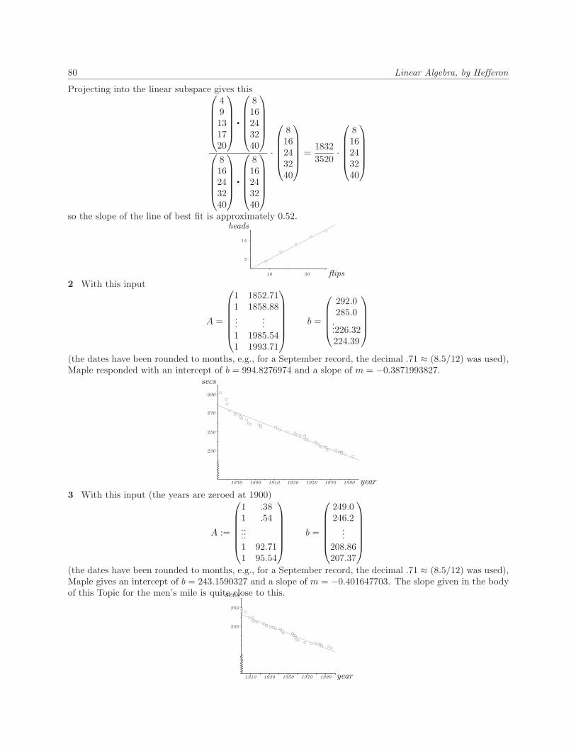
80 Linear Algebra, by Hefferon
Projecting into the linear subspace gives this49131720
816243240
816243240
816243240
·
816243240
=18323520
·
816243240
so the slope of the line of best fit is approximately 0.52.
flips
heads
10 30
5
15
bc
bc
bc
bc
bc
2 With this input
A =
1 1852.711 1858.88...
...1 1985.541 1993.71
b =
292.0285.0
...226.32224.39
(the dates have been rounded to months, e.g., for a September record, the decimal .71 ≈ (8.5/12) was used),Maple responded with an intercept of b = 994.8276974 and a slope of m = −0.3871993827.
year
secs
1870 1890 1910 1930 1950 1970 1990
230
250
270
290bc
bc
bc
bc
bcbc bcbcbc bc
bcbc bcbcbc bcbc
bcbc bc
bcbcbc bcbcbcbcbc
bcbcbcbc bcbcbc
bcbc bcbc bcbcbcbcbc bc
bc
3 With this input (the years are zeroed at 1900)
A :=
1 .381 .54......1 92.711 95.54
b =
249.0246.2
...208.86207.37
(the dates have been rounded to months, e.g., for a September record, the decimal .71 ≈ (8.5/12) was used),Maple gives an intercept of b = 243.1590327 and a slope of m = −0.401647703. The slope given in the bodyof this Topic for the men’s mile is quite close to this.
year
secs
1910 1930 1950 1970 1990
230
250 bcbc bc
bc bcbcbcbcbc
bcbcbcbcbcbcbc bc
bcbcbc bcbcbcbcbc
bcbcbc
bc bc bcbcbcbcbcbc bcbc

Answers to Exercises 81
4 With this input (the years are zeroed at 1900)
A =
1 21.461 32.63...
...1 89.541 96.63
b =
373.2327.5
...255.61252.56
(the dates have been rounded to months, e.g., for a September record, the decimal .71 ≈ (8.5/12) was used),MAPLE gave an intercept of b = 378.7114894 and a slope of m = −1.445753225.
year
secs
1930 1950 1970 1990
270
290
310
330
350
370bc
bc
bcbcbc
bcbc
bcbcbc
bcbcbcbc
bc
bc
bcbcbcbcbcbc
bc
bcbcbcbcbcbcbcbc bc
bc
5 These are the equations of the lines for men’s and women’s mile (the vertical intercept term of theequation for the women’s mile has been adjusted from the answer above, to zero it at the year 0, becausethat’s how the men’s mile equation was done).
y = 994.8276974− 0.3871993827xy = 3125.6426− 1.445753225x
Obviously the lines cross. A computer program is the easiest way to do the arithmetic: MuPAD givesx = 2012.949004 and y = 215.4150856 (215 seconds is 3 minutes and 35 seconds). Remark. Of course allof this projection is highly dubious — for one thing, the equation for the women is influenced by the quiteslow early times — but it is nonetheless fun.
year
secs
1870 1890 1910 1930 1950 1970 1990
230
250
270
290
310
330
350
370
bc
bc
bc
bcbcbc bc
bcbc bc
bcbc bcbcbc bcbc
bcbc bc
bcbcbc bcbcbcbcbc
bcbcbcbc bcbcbc
bcbc bcbc bcbcbcbcbc bc
bc
+
++++++
+++++++
++
+ ++++++
+++++++++ +
6

82 Linear Algebra, by Hefferon
(a) A computer algebra system like MAPLE or MuPAD will give an intercept of b = 4259/1398 ≈ 3.239628and a slope of m = −71/2796 ≈ −0.025393419 Plugging x = 31 into the equation yields a predicted numberof O-ring failures of y = 2.45 (rounded to two places). Plugging in y = 4 and solving gives a temperatureof x = −29.94◦F.
(b) On the basis of this information
A =
1 531 75...1 801 81
b =
32...00
MAPLE gives the intercept as b = 187/40 = 4.675 and the slope as m = −73/1200 ≈ −0.060833. Here,plugging x = 31 into the equation predicts y = 2.79 O-ring failures (rounded to two places). Plugging iny = 4 failures gives a temperature of x = 11◦F.
◦F
number fails
35 45 55 65 75 85
0
1
2
3
4
bc
bc
bcbc bc bcbc
bcbcbcbcbcbcbcbc bcbc bcbcbc bcbcbcbc
7(a) The plot is nonlinear.
planet
log of dist
1 2 3 4 5 6 7 8
5
15
bcbc
bcbc
bc
bc
bc
(b) Here is the plot.
planet
log of dist
1 2 3 4 5 6 7 8
0.0
1.0
bcbc
bcbc
bcbc
bc
There is perhaps a jog up between planet 4 and planet 5.(c) This plot seems even more linear.
planet
log of dist
1 2 3 4 5 6 7 8 9
0.0
1.0
bcbc
bcbc
bcbc
bc
(d) With this input
A =
1 11 21 31 41 61 71 8
b =
−0.40893539−0.1426675
00.181843590.716003340.979548371.2833012
MuPAD gives that the intercept is b = −0.6780677466 and the slope is m = 0.2372763818.

Answers to Exercises 83
planet
log of dist
1 2 3 4 5 6 7 8 9
0.0
1.0
bcbc
bcbc
bcbc
bc
(e) Plugging x = 9 into the equation y = −0.6780677466 + 0.2372763818x from the prior item gives thatthe log of the distance is 1.4574197, so the expected distance is 28.669472. The actual distance is about30.003.
(f) Plugging x = 10 into the same equation gives that the log of the distance is 1.6946961, so the expecteddistance is 49.510362. The actual distance is about 39.503.
8(a) With this input
A =
1 3061 3291 3561 3671 3961 4271 4151 424
b =
975969948910890906900899
MAPLE gives that the intercept is b = 34009779/28796 ≈ 1181.0591 and the slope is m = −19561/28796 ≈−0.6793.
avg. hours squandered
SAT
325 375 425
900
950
bc
bc
bc
bc
bc
bc
bc bc
. . . . . . . . . . . . . . . . . . . . . . . . . . . . . . . . . . . . . . . . . . . . .
Answers for Topic: Geometry of Linear Maps1(a) To represent H, recall that rotation counterclockwise by θ radians is represented with respect to thestandard basis in this way.
RepE2,E2(h) =(
cos θ − sin θsin θ cos θ
)A clockwise angle is the negative of a counterclockwise one.
RepE2,E2(h) =(
cos(−π/4) − sin(−π/4)sin(−π/4) cos(−π/4)
)=( √
2/2√
2/2−√
2/2√
2/2
)This Gauss-Jordan reduction
ρ1+ρ2−→(√
2/2√
2/20
√2
)(2/√
2)ρ1−→(1/√
2)ρ2
(1 10 1
)−ρ2+ρ1−→
(1 00 1
)produces the identity matrix so there is no need for column-swapping operations to end with a partial-identity.

84 Linear Algebra, by Hefferon
(b) The reduction is expressed in matrix multiplication as(1 −10 1
)(2/√
2 00 1/
√2
)(1 01 1
)H = I
(note that composition of the Gaussian operations is performed from right to left).(c) Taking inverses
H =(
1 0−1 1
)(√2/2 00
√2
)(1 10 1
)︸ ︷︷ ︸
P
I
gives the desired factorization of H (here, the partial identity is I, and Q is trivial, that is, it is also anidentity matrix).
(d) Reading the composition from right to left (and ignoring the identity matrices as trivial) gives that Hhas the same effect as first performing this skew
~u
~v
(xy
)7→
−→
(x+ yy
)h(~u)
h(~v)
followed by a dilation that multiplies all first components by√
2/2 (this is a “shrink” in that√
2/2 ≈ 0.707)and all second components by
√2, followed by another skew.~u
~v
(xy
)7→
−→
(x
−x+ y
)h(~u)
h(~v)
For instance, the effect of H on the unit vector whose angle with the x-axis is π/3 is this.(√3/2
1/2
) (xy
)7→
−→
(x+ yy
) ((√
3 + 1)/21/2
) (xy
)7→
−→
((√
2/2)x√2y
) (√2(√
3 + 1)/4√2/2
)(xy
)7→
−→
(x
−x+ y
) (√2(√
3 + 1)/4√2(1−
√3)/4
)Verifying that the resulting vector has unit length and forms an angle of −π/6 with the x-axis is routine.
2 We will first represent the map with a matrix H, perform the row operations and, if needed, columnoperations to reduce it to a partial-identity matrix. We will then translate that into a factorization H =PBQ. Subsitituting into the general matrix
RepE2,E2(rθ)(
cos θ − sin θsin θ cos θ
)gives this representation.
RepE2,E2(r2π/3)(−1/2 −
√3/2√
3/2 −1/2
)Gauss’ method is routine.√
3ρ1+ρ2−→(−1/2 −
√3/2
0 −2
)−2ρ1−→
(−1/2)ρ2
(1√
30 1
)−√
3ρ2+ρ1−→(
1 00 1
)That translates to a matrix equation in this way.(
1 −√
30 1
)(−2 00 −1/2
)(1 0√3 1
)(−1/2 −
√3/2√
3/2 −1/2
)= I
Taking inverses to solve for H yields this factorization.(−1/2 −
√3/2√
3/2 −1/2
)=(
1 0−√
3 1
)(−1/2 0
0 −2
)(1√
30 1
)I
3 This Gaussian reduction
−3ρ1+ρ2−→−ρ1+ρ3
1 2 10 0 −30 0 1
(1/3)ρ2+ρ3−→
1 2 10 0 −30 0 0
(−1/3)ρ2−→
1 2 10 0 10 0 0
−ρ2+ρ1−→
1 2 00 0 10 0 0

Answers to Exercises 85
gives the reduced echelon form of the matrix. Now the two column operations of taking −2 times the firstcolumn and adding it to the second, and then of swapping columns two and three produce this partialidentity.
B =
1 0 00 1 00 0 0
All of that translates into matrix terms as: where
P =
1 −1 00 1 00 0 1
1 0 00 −1/3 00 0 1
1 0 00 1 00 1/3 1
1 0 00 1 0−1 0 1
1 0 0−3 1 00 0 1
and
Q =
1 −2 00 1 00 0 1
0 1 01 0 00 0 1
the given matrix factors as PBQ.4 Represent it with respect to the standard bases E1, E1, then the only entry in the resulting 1×1 matrixis the scalar k.5 We can show this by induction on the number of components in the vector. In the n = 1 base case theonly permutation is the trivial one, and the map(
x1
)7→(x1
)is indeed expressible as a composition of swaps—as zero swaps. For the inductive step we assume that themap induced by any permutation of fewer than n numbers can be expressed with swaps only, and we considerthe map induced by a permutation p of n numbers.
x1
x2
...xn
7→xp(1)
xp(2)
...xp(n)
Consider the number i such that p(i) = n. The map
x1
x2
...xi...xn
p7−→
xp(1)
xp(2)
...xp(n)
...xn
will, when followed by the swap of the i-th and n-th components, give the map p. Now, the inductivehypothesis gives that p is achievable as a composition of swaps.6(a) A line is a subset of Rn of the form {~v = ~u+ t · ~w
∣∣ t ∈ R}. The image of a point on that line ish(~v) = h(~u+ t · ~w) = h(~u) + t ·h(~w), and the set of such vectors, as t ranges over the reals, is a line (albeit,degenerate if h(~w) = ~0).
(b) This is an obvious extension of the prior argument.(c) If the point B is between the points A and C then the line from A to C has B in it. That is, there isa t ∈ (0 .. 1) such that ~b = ~a+ t · (~c− ~a) (where B is the endpoint of ~b, etc.). Now, as in the argument ofthe first item, linearity shows that h(~b) = h(~a) + t · h(~c− ~a).
7 The two are inverse. For instance, for a fixed x ∈ R, if f ′(x) = k (with k 6= 0) then (f−1)′(x) = 1/k.
x
f(x)
f−1(f(x))

86 Linear Algebra, by Hefferon
. . . . . . . . . . . . . . . . . . . . . . . . . . . . . . . . . . . . . . . . . . . . .
Answers for Topic: Markov Chains1(a) With this file coin.m
# Octave function for Markov coin game. p is chance of going down.
function w = coin(p,v)
q = 1-p;
A=[1,p,0,0,0,0;
0,0,p,0,0,0;
0,q,0,p,0,0;
0,0,q,0,p,0;
0,0,0,q,0,0;
0,0,0,0,q,1];
w = A * v;
endfunction
this Octave session produced the output given here.octave:1> v0=[0;0;0;1;0;0]
v0 =
0
0
0
1
0
0
octave:2> p=.5
p = 0.50000
octave:3> v1=coin(p,v0)
v1 =
0.00000
0.00000
0.50000
0.00000
0.50000
0.00000
octave:4> v2=coin(p,v1)
v2 =
0.00000
0.25000
0.00000
0.50000
0.00000
0.25000...
octave:26> v24=coin(p,v23)
v24 =
0.39600
0.00276
0.00000
0.00447
0.00000
0.59676
(b) Using these formulasp1,n+1 = 0.5 · p2,n p2,n+1 = 0.5 · p1,n + 0.5 · p3,n p3,n+1 = 0.5 · p2,n + 0.5 · p4,n p5,n+1 = 0.5 · p4,n

Answers to Exercises 87
and these initial conditions p0,0
p1,0
p2,0
p3,0
p4,0
p5,0
=
000100
we will prove by induction that when n is odd then p1,n = p3,n = 0 and when n is even then p2,n = p4,n = 0.Note first that this is true in the n = 0 base case by the initial conditions. For the inductive step, supposethat it is true in the n = 0, n = 1, . . . , n = k cases and consider the n = k + 1 case. If k + 1 is odd then
p1,k+1 = 0.5 · p2,k = 0.5 · 0 = 0 p3,k+1 = 0.5 · p2,k + 0.5 · p4,k = 0.5 · 0 + 0.5 · 0 = 0
follows from the inductive hypothesis that p2,k = p4,k = 0 since k is even. The case where k + 1 is even issimilar.
(c) We can use, say, n = 100. This Octave sessionoctave:1> B=[1,.5,0,0,0,0;
> 0,0,.5,0,0,0;
> 0,.5,0,.5,0,0;
> 0,0,.5,0,.5,0;
> 0,0,0,.5,0,0;
> 0,0,0,0,.5,1];
octave:2> B100=B**100
B100 =
1.00000 0.80000 0.60000 0.40000 0.20000 0.00000
0.00000 0.00000 0.00000 0.00000 0.00000 0.00000
0.00000 0.00000 0.00000 0.00000 0.00000 0.00000
0.00000 0.00000 0.00000 0.00000 0.00000 0.00000
0.00000 0.00000 0.00000 0.00000 0.00000 0.00000
0.00000 0.20000 0.40000 0.60000 0.80000 1.00000
octave:3> B100*[0;1;0;0;0;0]
octave:4> B100*[0;1;0;0;0;0]
octave:5> B100*[0;0;0;1;0;0]
octave:6> B100*[0;1;0;0;0;0]
yields these outputs.
starting with: $1 $2 $3 $4s0,100
s1,100
s2,100
s3,100
s4,100
s5,100
0.800000.000000.000000.000000.000000.20000
0.600000.000000.000000.000000.000000.40000
0.400000.000000.000000.000000.000000.60000
0.200000.000000.000000.000000.000000.80000
2(a) From these equations
(1/6)s1,n + 0s2,n + 0s3,n + 0s4,n + 0s5,n + 0s6,n = s1,n+1
(1/6)s1,n + (2/6)s2,n + 0s3,n + 0s4,n + 0s5,n + 0s6,n = s2,n+1
(1/6)s1,n + (1/6)s2,n + (3/6)s3,n + 0s4,n + 0s5,n + 0s6,n = s3,n+1
(1/6)s1,n + (1/6)s2,n + (1/6)s3,n + (4/6)s4,n + 0s5,n + 0s6,n = s4,n+1
(1/6)s1,n + (1/6)s2,n + (1/6)s3,n + (1/6)s4,n + (5/6)s5,n + 0s6,n = s5,n+1
(1/6)s1,n + (1/6)s2,n + (1/6)s3,n + (1/6)s4,n + (1/6)s5,n + (6/6)s6,n = s6,n+1

88 Linear Algebra, by Hefferon
We get this transition matrix. 1/6 0 0 0 0 01/6 2/6 0 0 0 01/6 1/6 3/6 0 0 01/6 1/6 1/6 4/6 0 01/6 1/6 1/6 1/6 5/6 01/6 1/6 1/6 1/6 1/6 6/6
(b) This is the Octave session, with outputs edited out and condensed into the table at the end.
octave:1> F=[1/6, 0, 0, 0, 0, 0;
> 1/6, 2/6, 0, 0, 0, 0;
> 1/6, 1/6, 3/6, 0, 0, 0;
> 1/6, 1/6, 1/6, 4/6, 0, 0;
> 1/6, 1/6, 1/6, 1/6, 5/6, 0;
> 1/6, 1/6, 1/6, 1/6, 1/6, 6/6];
octave:2> v0=[1;0;0;0;0;0]
octave:3> v1=F*v0
octave:4> v2=F*v1
octave:5> v3=F*v2
octave:6> v4=F*v3
octave:7> v5=F*v4
These are the results.
1 2 3 4 5100000
0.166670.166670.166670.166670.166670.16667
0.0277780.0833330.1388890.1944440.2500000.305556
0.00462960.03240740.08796300.17129630.28240740.4212963
0.000771600.011574070.050154320.135030860.284722220.51774691
0.000128600.003986630.027134770.100437240.270190330.59812243
3(a) It does seem reasonable that, while the firm’s present location should strongly influence where it isnext time (for instance, whether it stays), any locations in the prior stages should have little influence.That is, while a company may move or stay because of where it is, it is unlikely to move or stay becauseof where it was.
(b) This Octave session has been edited, with the outputs put together in a table at the end.octave:1> M=[.787,0,0,.111,.102;
> 0,.966,.034,0,0;
> 0,.063,.937,0,0;
> 0,0,.074,.612,.314;
> .021,.009,.005,.010,.954]
M =
0.78700 0.00000 0.00000 0.11100 0.10200
0.00000 0.96600 0.03400 0.00000 0.00000
0.00000 0.06300 0.93700 0.00000 0.00000
0.00000 0.00000 0.07400 0.61200 0.31400
0.02100 0.00900 0.00500 0.01000 0.95400
octave:2> v0=[.025;.025;.025;.025;.900]
octave:3> v1=M*v0
octave:4> v2=M*v1
octave:5> v3=M*v2
octave:6> v4=M*v3
is summarized in this table.

Answers to Exercises 89
~p0 ~p1 ~p2 ~p3 ~p40.0250000.0250000.0250000.0250000.900000
0.1142500.0250000.0250000.2997500.859725
0.2108790.0250000.0250000.4552510.825924
0.3007390.0250000.0250000.5398040.797263
0.3779200.0250000.0250000.5825500.772652
(c) This is a continuation of the Octave session from the prior item.
octave:7> p0=[.0000;.6522;.3478;.0000;.0000]
octave:8> p1=M*p0
octave:9> p2=M*p1
octave:10> p3=M*p2
octave:11> p4=M*p3
This summarizes the output.~p0 ~p1 ~p2 ~p3 ~p4
0.000000.652200.347800.000000.00000
0.000000.641850.366980.025740.00761
0.00363290.63250470.38429420.04529660.0151277
0.00943010.62406560.39993150.06090940.0225751
0.0164850.6164450.4140520.0739600.029960
(d) This is more of the same Octave session.
octave:12> M50=M**50
M50 =
0.03992 0.33666 0.20318 0.02198 0.37332
0.00000 0.65162 0.34838 0.00000 0.00000
0.00000 0.64553 0.35447 0.00000 0.00000
0.03384 0.38235 0.22511 0.01864 0.31652
0.04003 0.33316 0.20029 0.02204 0.37437
octave:13> p50=M50*p0
p50 =
0.29024
0.54615
0.54430
0.32766
0.28695
octave:14> p51=M*p50
p51 =
0.29406
0.54609
0.54442
0.33091
0.29076
This is close to a steady state.
4(a) This is the relevant system of equations.
(1− 2p) · sU,n + p · tA,n + p · tB,n = sU,n+1
p · sU,n + (1− 2p) · tA,n = tA,n+1
p · sU,n + (1− 2p) · tB,n = tB,n+1
p · tA,n + sA,n = sA,n+1
p · tB,n + sB,n = sB,n+1

90 Linear Algebra, by Hefferon
Thus we have this. 1− 2p p p 0 0p 1− 2p 0 0 0p 0 1− 2p 0 00 p 0 1 00 0 p 0 1
sU,ntA,ntB,nsA,nsB,n
=
sU,n+1
tA,n+1
tB,n+1
sA,n+1
sB,n+1
(b) This is the Octave code, with the output removed.
octave:1> T=[.5,.25,.25,0,0;
> .25,.5,0,0,0;
> .25,0,.5,0,0;
> 0,.25,0,1,0;
> 0,0,.25,0,1]
T =
0.50000 0.25000 0.25000 0.00000 0.00000
0.25000 0.50000 0.00000 0.00000 0.00000
0.25000 0.00000 0.50000 0.00000 0.00000
0.00000 0.25000 0.00000 1.00000 0.00000
0.00000 0.00000 0.25000 0.00000 1.00000
octave:2> p0=[1;0;0;0;0]
octave:3> p1=T*p0
octave:4> p2=T*p1
octave:5> p3=T*p2
octave:6> p4=T*p3
octave:7> p5=T*p4
Here is the output. The probability of ending at sA is about 0.23.
~p0 ~p1 ~p2 ~p3 ~p4 ~p5
sUtAtBsAsB
10000
0.500000.250000.250000.000000.00000
0.3750000.2500000.2500000.0625000.062500
0.312500.218750.218750.125000.12500
0.265620.187500.187500.179690.17969
0.226560.160160.160160.226560.22656
(c) With this file as learn.m
# Octave script file for learning model.
function w = learn(p)
T = [1-2*p,p, p, 0, 0;
p, 1-2*p,0, 0, 0;
p, 0, 1-2*p,0, 0;
0, p, 0, 1, 0;
0, 0, p, 0, 1];
T5 = T**5;
p5 = T5*[1;0;0;0;0];
w = p5(4);
endfunction
issuing the command octave:1> learn(.20) yields ans = 0.17664.(d) This Octave session
octave:1> x=(.01:.01:.50)’;
octave:2> y=(.01:.01:.50)’;
octave:3> for i=.01:.01:.50
> y(100*i)=learn(i);
> endfor
octave:4> z=[x, y];
octave:5> gplot z
yields this plot. There is no threshold value — no probability above which the curve rises sharply.

Answers to Exercises 91
0
0.05
0.1
0.15
0.2
0.25
0.3
0.35
0.4
0 0.05 0.1 0.15 0.2 0.25 0.3 0.35 0.4 0.45 0.5
line 1
5(a) From these equations
0.90 · pT,n + 0.01 · pC,n = pT,n+1
0.10 · pT,n + 0.99 · pC,n = pC,n+1
we get this matrix.
(0.90 0.010.10 0.99
)(pT,npC,n
)=(pT,n+1
pC,n+1
)
(b) This is the result from Octave.n = 0 1 2 3 4 5
0.300000.70000
0.277000.72300
0.256530.74347
0.238310.76169
0.222100.77790
0.207670.79233
6 7 8 9 100.194820.80518
0.183390.81661
0.173220.82678
0.164170.83583
0.156110.84389
(c) This is the sT = 0.2 result.n = 0 1 2 3 4 5
0.200000.80000
0.188000.81200
0.177320.82268
0.167810.83219
0.159360.84064
0.151830.84817
6 7 8 9 100.145130.85487
0.139160.86084
0.133850.86615
0.129130.87087
0.124930.87507
(d) Although the probability vectors start 0.1 apart, they end only 0.032 apart. So they are alike.
6 These are the p = .55 vectors,

92 Linear Algebra, by Hefferon
n = 0 n = 1 n = 2 n = 3 n = 4 n = 5 n = 6 n = 7
0-01-00-12-01-10-23-02-11-20-34-03-12-21-30-44-13-22-31-44-23-32-44-33-4
100000000000000000000000
00.550000.45000000000000000000000000
0000.302500.495000.20250000000000000000000
0000000.166380.408370.334120.0911200000000000000
00000000000.091510.299480.367540.200470.04101000000000
00000000000.091510000.041010.164710.336910.275650.0902100000
00000000000.091510000.041010.16471000.090210.185300.303220.1240400
00000000000.091510000.041010.16471000.090210.1853000.124040.166770.13645
and these are the p = .60 vectors.n = 0 n = 1 n = 2 n = 3 n = 4 n = 5 n = 6 n = 7
0-01-00-12-01-10-23-02-11-20-34-03-12-21-30-44-13-22-31-44-23-32-44-33-4
100000000000000000000000
00.600000.40000000000000000000000000
0000.360000.480000.16000000000000000000000
0000000.216000.432000.288000.0640000000000000000
00000000000.129600.345600.345600.153600.02560000000000
00000000000.129600000.025600.207360.345600.230400.0614400000
00000000000.129600000.025600.20736000.061440.207360.276480.0921600
00000000000.129600000.025600.20736000.061440.2073600.092160.165890.11059
(a) The script from the computer code section can be easily adapted.# Octave script file to compute chance of World Series outcomes.
function w = markov(p,v)
q = 1-p;
A=[0,0,0,0,0,0, 0,0,0,0,0,0, 0,0,0,0,0,0, 0,0,0,0,0,0; # 0-0
p,0,0,0,0,0, 0,0,0,0,0,0, 0,0,0,0,0,0, 0,0,0,0,0,0; # 1-0

Answers to Exercises 93
q,0,0,0,0,0, 0,0,0,0,0,0, 0,0,0,0,0,0, 0,0,0,0,0,0; # 0-1_
0,p,0,0,0,0, 0,0,0,0,0,0, 0,0,0,0,0,0, 0,0,0,0,0,0; # 2-0
0,q,p,0,0,0, 0,0,0,0,0,0, 0,0,0,0,0,0, 0,0,0,0,0,0; # 1-1
0,0,q,0,0,0, 0,0,0,0,0,0, 0,0,0,0,0,0, 0,0,0,0,0,0; # 0-2__
0,0,0,p,0,0, 0,0,0,0,0,0, 0,0,0,0,0,0, 0,0,0,0,0,0; # 3-0
0,0,0,q,p,0, 0,0,0,0,0,0, 0,0,0,0,0,0, 0,0,0,0,0,0; # 2-1
0,0,0,0,q,p, 0,0,0,0,0,0, 0,0,0,0,0,0, 0,0,0,0,0,0; # 1-2_
0,0,0,0,0,q, 0,0,0,0,0,0, 0,0,0,0,0,0, 0,0,0,0,0,0; # 0-3
0,0,0,0,0,0, p,0,0,0,1,0, 0,0,0,0,0,0, 0,0,0,0,0,0; # 4-0
0,0,0,0,0,0, q,p,0,0,0,0, 0,0,0,0,0,0, 0,0,0,0,0,0; # 3-1__
0,0,0,0,0,0, 0,q,p,0,0,0, 0,0,0,0,0,0, 0,0,0,0,0,0; # 2-2
0,0,0,0,0,0, 0,0,q,p,0,0, 0,0,0,0,0,0, 0,0,0,0,0,0; # 1-3
0,0,0,0,0,0, 0,0,0,q,0,0, 0,0,1,0,0,0, 0,0,0,0,0,0; # 0-4_
0,0,0,0,0,0, 0,0,0,0,0,p, 0,0,0,1,0,0, 0,0,0,0,0,0; # 4-1
0,0,0,0,0,0, 0,0,0,0,0,q, p,0,0,0,0,0, 0,0,0,0,0,0; # 3-2
0,0,0,0,0,0, 0,0,0,0,0,0, q,p,0,0,0,0, 0,0,0,0,0,0; # 2-3__
0,0,0,0,0,0, 0,0,0,0,0,0, 0,q,0,0,0,0, 1,0,0,0,0,0; # 1-4
0,0,0,0,0,0, 0,0,0,0,0,0, 0,0,0,0,p,0, 0,1,0,0,0,0; # 4-2
0,0,0,0,0,0, 0,0,0,0,0,0, 0,0,0,0,q,p, 0,0,0,0,0,0; # 3-3_
0,0,0,0,0,0, 0,0,0,0,0,0, 0,0,0,0,0,q, 0,0,0,1,0,0; # 2-4
0,0,0,0,0,0, 0,0,0,0,0,0, 0,0,0,0,0,0, 0,0,p,0,1,0; # 4-3
0,0,0,0,0,0, 0,0,0,0,0,0, 0,0,0,0,0,0, 0,0,q,0,0,1]; # 3-4
v7 = (A**7) * v;
w = v7(11)+v7(16)+v7(20)+v7(23)
endfunction
Using this script, we get that when the American League has a p = 0.55 probability of winning each gamethen their probability of winning the first-to-win-four series is 0.60829. When their probability of winningany one game is p = 0.6 then their probability of winning the series is 0.71021.
(b) This Octave sessionoctave:1> v0=[1;0;0;0;0;0;0;0;0;0;0;0;0;0;0;0;0;0;0;0;0;0;0;0];
octave:2> x=(.01:.01:.99)’;
octave:3> y=(.01:.01:.99)’;
octave:4> for i=.01:.01:.99
> y(100*i)=markov(i,v0);
> endfor
octave:5> z=[x, y];
octave:6> gplot z
yields this graph. By eye we judge that if p > 0.7 then the team is close to assurred of the series.
0
0.1
0.2
0.3
0.4
0.5
0.6
0.7
0.8
0.9
1
0 0.1 0.2 0.3 0.4 0.5 0.6 0.7 0.8 0.9 1
line 1
7(a) They must satisfy this condition because the total probability of a state transition (including back tothe same state) is 100%.
(b) See the answer to the third item.

94 Linear Algebra, by Hefferon
(c) We will do the 2×2 case; bigger-sized cases are just notational problems. This product(a1,1 a1,2
a2,1 a2,2
)(b1,1 b1,2b2,1 b2,2
)=(a1,1b1,1 + a1,2b2,1 a1,1b1,2 + a1,2b2,2a2,1b1,1 + a2,2b2,1 a2,1b1,2 + a2,2b2,2
)has these two column sums(a1,1b1,1 + a1,2b2,1) + (a2,1b1,1 + a2,2b2,1) = (a1,1 + a2,1) · b1,1 + (a1,2 + a2,2) · b2,1 = 1 · b1,1 + 1 · b2,1 = 1
and(a1,1b1,2 + a1,2b2,2) + (a2,1b1,2 + a2,2b2,2) = (a1,1 + a2,1) · b1,2 + (a1,2 + a2,2) · b2,2 = 1 · b1,2 + 1 · b2,2 = 1
as required.
. . . . . . . . . . . . . . . . . . . . . . . . . . . . . . . . . . . . . . . . . . . . .
Answers for Topic: Orthonormal Matrices1(a) Yes.(b) No, the columns do not have length one.(c) Yes.
2 Some of these are nonlinear, because they involve a nontrivial translation.
(a)(xy
)7→(x · cos(π/6)− y · sin(π/6)x · sin(π/6) + y · cos(π/6)
)+(
01
)=(
x · (√
3/2)− y · (1/2) + 0x · (1/2) + y · cos(
√3/2) + 1
)(b) The line y = 2x makes an angle of arctan(2/1) with the x-axis. Thus sin θ = 2/
√5 and cos θ = 1/
√5.(
xy
)7→(x · (1/
√5)− y · (2/
√5)
x · (2/√
5) + y · (1/√
5)
)(c)
(xy
)7→(x · (1/
√5)− y · (−2/
√5)
x · (−2/√
5) + y · (1/√
5)
)+(
11
)=(x/√
5 + 2y/√
5 + 1−2x/
√5 + y/
√5 + 1
)3(a) Let f be distance-preserving and consider f−1. Any two points in the codomain can be written asf(P1) and f(P2). Because f is distance-preserving, the distance from f(P1) to f(P2) equals the distancefrom P1 to P2. But this is exactly what is required for f−1 to be distance-preserving.
(b) Any plane figure F is congruent to itself via the identity map id: R2 → R2, which is obviously distance-preserving. If F1 is congruent to F2 (via some f) then F2 is congruent to F1 via f−1, which is distance-preserving by the prior item. Finally, if F1 is congruent to F2 (via some f) and F2 is congruent to F3 (viasome g) then F1 is congruent to F3 via g ◦ f , which is easily checked to be distance-preserving.
4 The first two components of each are ax+ cy + e and bx+ dy + f .5(a) The Pythagorean Theorem gives that three points are colinear if and only if (for some ordering ofthem into P1, P2, and P3), dist(P1, P2) + dist(P2, P3) = dist(P1, P3). Of course, where f is distance-preserving, this holds if and only if dist(f(P1), f(P2)) + dist(f(P2), f(P3)) = dist(f(P1), f(P3)), which,again by Pythagoras, is true if and only if f(P1), f(P2), and f(P3) are colinear.
The argument for betweeness is similar (above, P2 is between P1 and P3).If the figure F is a triangle then it is the union of three line segments P1P2, P2P3, and P1P3. The
prior two paragraphs together show that the property of being a line segment is invariant. So f(F ) is theunion of three line segments, and so is a triangle.
A circle C centered at P and of radius r is the set of all points Q such that dist(P,Q) = r. Applyingthe distance-preserving map f gives that the image f(C) is the set of all f(Q) subject to the conditionthat dist(P,Q) = r. Since dist(P,Q) = dist(f(P ), f(Q)), the set f(C) is also a circle, with center f(P )and radius r.
(b) Here are two that are easy to verify: (i) the property of being a right triangle, and (ii) the property oftwo lines being parallel.
(c) One that was mentioned in the section is the ‘sense’ of a figure. A triangle whose vertices read clockwiseas P1, P2, P3 may, under a distance-preserving map, be sent to a triangle read P1, P2, P3 counterclockwise.
Answers to Exercises 95
Chapter 4. Determinants
. . . . . . . . . . . . . . . . . . . . . . . . . . . . . . . . . . . . . . . . . . . . .
Answers for subsection 4.I.1
4.I.1.2(a) 6 (b) 21 (c) 27
4.I.1.5(a) Nonsingular, the determinant is 3.(b) Singular, the determinant is 0.(c) Singular, the determinant is 0.
4.I.1.7 Using the formula for the determinant of a 3×3 matrix we expand the left side
1 · b · c2 + 1 · c · a2 + 1 · a · b2 − b2 · c · 1− c2 · a · 1− a2 · b · 1and by distributing we expand the right side.
(bc− ba− ac+ a2) · (c− b) = c2b− b2c− bac+ b2a− ac2 + acb+ a2c− a2b
Now we can just check that the two are equal. (Remark. This is the 3×3 case of Vandermonde’s determinantwhich arises in applications).
4.I.1.9 We first reduce the matrix to echelon form. To begin, assume that a 6= 0 and that ae− bd 6= 0.
(1/a)ρ1−→
1 b/a c/ad e fg h i
−dρ1+ρ2−→−gρ1+ρ3
1 b/a c/a0 (ae− bd)/a (af − cd)/a0 (ah− bg)/a (ai− cg)/a
(a/(ae−bd))ρ2−→
1 b/a c/a0 1 (af − cd)/(ae− bd)0 (ah− bg)/a (ai− cg)/a
This step finishes the calculation.
((ah−bg)/a)ρ2+ρ3−→
1 b/a c/a0 1 (af − cd)/(ae− bd)0 0 (aei+ bgf + cdh− hfa− idb− gec)/(ae− bd)
Now assuming that a 6= 0 and ae − bd 6= 0, the original matrix is nonsingular if and only if the 3, 3entry above is nonzero. That is, under the assumptions, the original matrix is nonsingular if and only ifaei+ bgf + cdh− hfa− idb− gec 6= 0, as required.
We finish by running down what happens if the assumptions that were taken for convienence in the priorparagraph do not hold. First, if a 6= 0 but ae− bd = 0 then we can swap1 b/a c/a
0 0 (af − cd)/a0 (ah− bg)/a (ai− cg)/a
ρ2↔ρ3−→
1 b/a c/a0 (ah− bg)/a (ai− cg)/a0 0 (af − cd)/a
and conclude that the matrix is nonsingular if and only if either ah− bg = 0 or af − cd = 0. The condition‘ah − bg = 0 or af − cd = 0’ is equivalent to the condition ‘(ah − bg)(af − cd) = 0’. Multiplying out andusing the case assumption that ae− bd = 0 to substitute ae for bd gives this.
0 = ahaf − ahcd− bgaf + bgcd = ahaf − ahcd− bgaf + aegc = a(haf − hcd− bgf + egc)
Since a 6= 0, we have that the matrix is nonsingular if and only if haf − hcd− bgf + egc = 0. Therefore, inthis a 6= 0 and ae− bd = 0 case, the matrix is nonsingular when haf − hcd− bgf + egc− i(ae− bd) = 0.
The remaining cases are routine. Do the a = 0 but d 6= 0 case and the a = 0 and d = 0 but g 6= 0 caseby first swapping rows and then going on as above. The a = 0, d = 0, and g = 0 case is easy—that matrixis singular since the columns form a linearly dependent set, and the determinant comes out to be zero.

96 Linear Algebra, by Hefferon
4.I.1.10 Figuring the determinant and doing some algebra gives this.
0 = y1x+ x2y + x1y2 − y2x− x1y − x2y1
(x2 − x1) · y = (y2 − y1) · x+ x2y1 − x1y2
y =y2 − y1
x2 − x1· x+
x2y1 − x1y2
x2 − x1
Note that this is the equation of a line (in particular, in contains the familiar expression for the slope), andnote that (x1, y1) and (x2, y2) satisfy it.
4.I.1.12 The determinant is (x2y3−x3y2)~e1 +(x3y1−x1y3)~e2 +(x1y2−x2y1)~e3. To check perpendicularity,we check that the dot product with the first vector is zerox1
x2
x3
x2y3 − x3y2
x3y1 − x1y3
x1y2 − x2y1
= x1x2y3 − x1x3y2 + x2x3y1 − x1x2y3 + x1x3y2 − x2x3y1 = 0
and the dot product with the second vector is also zero.y1
y2
y3
x2y3 − x3y2
x3y1 − x1y3
x1y2 − x2y1
= x2y1y3 − x3y1y2 + x3y1y2 − x1y2y3 + x1y2y3 − x2y1y3 = 0
4.I.1.13(a) Plug and chug: the determinant of the product is this
det((a bc d
)(w xy z
)) = det(
(aw + by ax+ bzcw + dy cx+ dz
))
= acwx+ adwz + bcxy + bdyz−acwx− bcwz − adxy − bdyz
while the product of the determinants is this.
det((a bc d
)) · det(
(w xy z
)) = (ad− bc) · (wz − xy)
Verification that they are equal is easy.(b) Use the prior item.
That similar matrices have the same determinant is immediate from the above two: det(PTP−1) = det(P ) ·det(T ) · det(P−1).
4.I.1.15 The computation for 2×2 matrices, using the formula quoted in the preamble, is easy. It does alsohold for 3×3 matrices; the computation is routine.
4.I.1.17 Bring out the c’s one row at a time.
4.I.1.18 There are no real numbers θ that make the matrix singular because the determinant of the matrixcos2 θ+ sin2 θ is never 0, it equals 1 for all θ. Geometrically, with respect to the standard basis, this matrixrepresents a rotation of the plane through an angle of θ. Each such map is one-to-one — for one thing, it isinvertible.
4.I.1.19 This is how the answer was given in the cited source. Let P be the sum of the three positive termsof the determinant and −N the sum of the three negative terms. The maximum value of P is
9 · 8 · 7 + 6 · 5 · 4 + 3 · 2 · 1 = 630.
The minimum value of N consistent with P is
9 · 6 · 1 + 8 · 5 · 2 + 7 · 4 · 3 = 218.
Any change in P would result in lowering that sum by more than 4. Therefore 412 the maximum value forthe determinant and one form for the determinant is∣∣∣∣∣∣
9 4 23 8 65 1 7
∣∣∣∣∣∣ .
Answers to Exercises 97
. . . . . . . . . . . . . . . . . . . . . . . . . . . . . . . . . . . . . . . . . . . . .
Answers for subsection 4.I.2
4.I.2.8
(a)∣∣∣∣ 2 −1−1 −1
∣∣∣∣ =∣∣∣∣2 −10 −3/2
∣∣∣∣ = −3; (b)
∣∣∣∣∣∣1 1 03 0 25 2 2
∣∣∣∣∣∣ =
∣∣∣∣∣∣1 1 00 −3 20 −3 2
∣∣∣∣∣∣ =
∣∣∣∣∣∣1 1 00 −3 20 0 0
∣∣∣∣∣∣ = 0
4.I.2.9 When is the determinant not zero?∣∣∣∣∣∣∣∣1 0 1 −10 1 −2 01 0 k 00 0 1 −1
∣∣∣∣∣∣∣∣ =
∣∣∣∣∣∣∣∣1 0 1 −10 1 −2 00 0 k − 1 10 0 1 −1
∣∣∣∣∣∣∣∣Obviously, k = 1 gives nonsingularity and hence a nonzero determinant. If k 6= 1 then we get echelon formwith a (−1/k − 1)ρ3 + ρ4 pivot.
=
∣∣∣∣∣∣∣∣1 0 1 −10 1 −2 00 0 k − 1 10 0 0 −1− (1/k − 1)
∣∣∣∣∣∣∣∣Multiplying down the diagonal gives (k − 1)(−1− (1/k − 1)) = −(k − 1)− 1 = −k. Thus the matrix has anonzero determinant, and so the system has a unique solution, if and only if k 6= 0.4.I.2.12 It is the trivial subspace.4.I.2.14
(a)(1),(
1 −1−1 1
),
1 −1 1−1 1 −11 −1 1
(b) The determinant in the 1×1 case is 1. In every other case the second row is the negative of the first,and so matrix is singular and the determinant is zero.
4.I.2.15
(a)(2),(
2 33 4
),
2 3 43 4 54 5 6
(b) The 1×1 and 2×2 cases yield these. ∣∣2∣∣ = 2
∣∣∣∣2 33 4
∣∣∣∣ = −1
And n×n matrices with n ≥ 3 are singular, e.g.,∣∣∣∣∣∣2 3 43 4 54 5 6
∣∣∣∣∣∣ = 0
because twice the second row minus the first row equals the third row. Checking this is routine.4.I.2.17 No, we cannot replace it. Remark 2.2 shows that the four conditions after the replacement wouldconflict — no function satisfies all four.4.I.2.18 A upper-triangular matrix is in echelon form.
A lower-triangular matrix is either singular or nonsingular. If it is singular then it has a zero on itsdiagonal and so its determinant (namely, zero) is indeed the product down its diagonal. If it is nonsingularthen it has no zeroes on its diagonal, and can be reduced by Gauss’ method to echelon form without changingthe diagonal.4.I.2.19(a) The properties in the definition of determinant show that |Mi(k)| = k, |Pi,j | = −1, and |Ci,j(k)| = 1.(b) The three cases are easy to check by recalling the action of left multiplication by each type of matrix.

98 Linear Algebra, by Hefferon
(c) If TS is invertible (TS)M = I then the associative property of matrix multiplication T (SM) = I showsthat T is invertible. So if T is not invertible then neither is TS.
(d) If T is singular then apply the prior answer: |TS| = 0 and |T | · |S| = 0 · |S| = 0. If T is not singularthen it can be written as a product of elementary matrices |TS| = |Er · · ·E1S| = |Er| · · · |E1| · |S| =|Er · · ·E1||S| = |T ||S|.
(e) 1 = |I| = |T · T−1| = |T ||T−1|4.I.2.20(a) We must show that if
Tkρi+ρj−→ T
then d(T ) = |TS|/|S| = |T S|/|S| = d(T ). We will be done if we show that pivoting first and thenmultiplying to get T S gives the same result as multiplying first to get TS and then pivoting (because thedeterminant |TS| is unaffected by the pivot so we’ll then have |T S| = |TS|, and hence d(T ) = d(T )). Thatargument runs: after adding k times row i of TS to row j of TS, the j, p entry is (kti,1 + tj,1)s1,p + · · ·+(kti,r + tj,r)sr,p, which is the j, p entry of T S.
(b) We need only show that swapping Tρi↔ρj−→ T and then multiplying to get T S gives the same result as
multiplying T by S and then swapping (because, as the determinant |TS| changes sign on the row swap,we’ll then have |T S| = −|TS|, and so d(T ) = −d(T )). That argument runs just like the prior one.
(c) Not surprisingly by now, we need only show that multiplying a row by a nonzero scalar Tkρi−→T and
then computing T S gives the same result as first computing TS and then multiplying the row by k (asthe determinant |TS| is rescaled by k the multiplication, we’ll have |T S| = k|TS|, so d(T ) = k d(T )). Theargument runs just as above.
(d) Clear.(e) Because we’ve shown that d(T ) is a determinant and that determinant functions (if they exist) areunique, we have that so |T | = d(T ) = |TS|/|S|.
4.I.2.21 We will first argue that a rank r matrix has a r×r submatrix with nonzero determinant. A rankr matrix has a linearly independent set of r rows. A matrix made from those rows will have row rank r andthus has column rank r. Conclusion: from those r rows can be extracted a linearly independent set of rcolumns, and so the original matrix has a r×r submatrix of rank r.
We finish by showing that if r is the largest such integer then the rank of the matrix is r. We need onlyshow, by the maximality of r, that if a matrix has a k×k submatrix of nonzero determinant then the rankof the matrix is at least k. Consider such a k×k submatrix. Its rows are parts of the rows of the originalmatrix, clearly the set of whole rows is linearly independent. Thus the row rank of the original matrix is atleast k, and the row rank of a matrix equals its rank.4.I.2.23 This is how the answer was given in the cited source. The value (1 − a4)3 of the determinant isindependent of the values B, C, D. Hence operation (e) does not change the value of the determinant butmerely changes its appearance. Thus the element of likeness in (a), (b), (c), (d), and (e) is only that theappearance of the principle entity is changed. The same element appears in (f) changing the name-label ofa rose, (g) writing a decimal integer in the scale of 12, (h) gilding the lily, (i) whitewashing a politician, and(j) granting an honorary degree.
. . . . . . . . . . . . . . . . . . . . . . . . . . . . . . . . . . . . . . . . . . . . .
Answers for subsection 4.I.3
4.I.3.17 This is all of the permutations where φ(1) = 1φ1 = 〈1, 2, 3, 4〉 φ2 = 〈1, 2, 4, 3〉 φ3 = 〈1, 3, 2, 4〉 φ4 = 〈1, 3, 4, 2〉 φ5 = 〈1, 4, 2, 3〉 φ6 = 〈1, 4, 3, 2〉
the ones where φ(1) = 1φ7 = 〈2, 1, 3, 4〉 φ8 = 〈2, 1, 4, 3〉 φ9 = 〈2, 3, 1, 4〉 φ10 = 〈2, 3, 4, 1〉 φ11 = 〈2, 4, 1, 3〉 φ12 = 〈2, 4, 3, 1〉

Answers to Exercises 99
the ones where φ(1) = 3φ13 = 〈3, 1, 2, 4〉 φ14 = 〈3, 1, 4, 2〉 φ15 = 〈3, 2, 1, 4〉 φ16 = 〈3, 2, 4, 1〉 φ17 = 〈3, 4, 1, 2〉 φ18 = 〈3, 4, 2, 1〉
and the ones where φ(1) = 4.φ19 = 〈4, 1, 2, 3〉 φ20 = 〈4, 1, 3, 2〉 φ21 = 〈4, 2, 1, 3〉 φ22 = 〈4, 2, 3, 1〉 φ23 = 〈4, 3, 1, 2〉 φ24 = 〈4, 3, 2, 1〉
4.I.3.18 Each of these is easy to check.(a) permutation φ1 φ2
inverse φ1 φ2
(b) permutation φ1 φ2 φ3 φ4 φ5 φ6
inverse φ1 φ2 φ3 φ5 φ4 φ6
4.I.3.19 For the ‘if’ half, the first condition of Definition 3.2 follows from taking k1 = k2 = 1 and thesecond condition follows from taking k2 = 0.
The ‘only if’ half also routine. From f(~ρ1, . . . , k1~v1 + k2~v2, . . . , ~ρn) the first condition of Definition 3.2gives = f(~ρ1, . . . , k1~v1, . . . , ~ρn) + f(~ρ1, . . . , k2~v2, . . . , ~ρn) and the second condition, applied twice, gives theresult.4.I.3.20 To get a nonzero term in the permutation expansion we must use the 1, 2 entry and the 4, 3 entry.Having fixed on those two we must also use the 2, 1 entry and the the 3, 4 entry. The signum of 〈2, 1, 4, 3〉 is+1 because from
0 1 0 01 0 0 00 0 0 10 0 1 0
the two rwo swaps ρ1 ↔ ρ2 and ρ3 ↔ ρ4 will produce the identity matrix.4.I.3.21 They would all double.4.I.3.22 For the second statement, given a matrix, transpose it, swap rows, and transpose back. The resultis swapped columns, and the determinant changes by a factor of −1. The third statement is similar: givena matrix, transpose it, apply multilinearity to what are now rows, and then transpose back the resultingmatrices.4.I.3.24 False. ∣∣∣∣1 −1
1 1
∣∣∣∣ = 2
4.I.3.25(a) For the column index of the entry in the first row there are five choices. Then, for the column index ofthe entry in the second row there are four choices (the column index used in the first row cannot be usedhere). Continuing, we get 5 · 4 · 3 · 2 · 1 = 120. (See also the next question.)
(b) Once we choose the second column in the first row, we can choose the other entries in 4 · 3 · 2 · 1 = 24ways.
4.I.3.26 n · (n− 1) · · · 2 · 1 = n!4.I.3.27 In |A| = |Atrans| = | −A| = (−1)n|A| the exponent n must be even.4.I.3.30 Let T be n×n, let J be p×p, and let K be q×q. Apply the permutation expansion formula
|T | =∑
permutations φ
t1,φ(1)t2,φ(2) . . . tn,φ(n) |Pφ|
Because the upper right of T is all zeroes, if a φ has at least one of p + 1, . . . , n among its first p columnnumbers φ(1), . . . , φ(p) then the term arising from φ is 0 (e.g., if φ(1) = n then t1,φ(1)t2,φ(2) . . . tn,φ(n) is 0).So the above formula reduces to a sum over all permutations with two halves: first 1, . . . , p are rearranged,and after that comes a permutation of p+ 1, . . . , p+ q. To see this gives |J | · |K|, distribute.[ ∑
perms φ1of 1,...,p
t1,φ1(1) · · · tp,φ1(p) |Pφ1 |]·[ ∑
perms φ2of p+1,...,p+q
tp+1,φ2(p+1) · · · tp+q,φ2(p+q) |Pφ2 |]
4.I.3.32 This is how the answer was given in the cited source. When two rows of a determinant areinterchanged, the sign of the determinant is changed. When the rows of a three-by-three determinant

100 Linear Algebra, by Hefferon
are permuted, 3 positive and 3 negative determinants equal in absolute value are obtained. Hence the 9!determinants fall into 9!/6 groups, each of which sums to zero.4.I.3.33 This is how the answer was given in the cited source. When the elements of any column aresubtracted from the elements of each of the other two, the elements in two of the columns of the deriveddeterminant are proportional, so the determinant vanishes. That is,∣∣∣∣∣∣
2 1 x− 44 2 x− 36 3 x− 10
∣∣∣∣∣∣ =
∣∣∣∣∣∣1 x− 3 −12 x− 1 −23 x− 7 −3
∣∣∣∣∣∣ =
∣∣∣∣∣∣x− 2 −1 −2x+ 1 −2 −4x− 4 −3 −6
∣∣∣∣∣∣ = 0.
4.I.3.34 This is how the answer was given in the cited source. Leta b cd e fg h i
have magic sum N = S/3. Then
N = (a+ e+ i) + (d+ e+ f) + (g + e+ c)− (a+ d+ g)− (c+ f + i) = 3e
and S = 9e. Hence, adding rows and columns,
D =
∣∣∣∣∣∣a b cd e fg h i
∣∣∣∣∣∣ =
∣∣∣∣∣∣a b cd e f3e 3e 3e
∣∣∣∣∣∣ =
∣∣∣∣∣∣a b 3ed e 3e3e 3e 9e
∣∣∣∣∣∣ =
∣∣∣∣∣∣a b ed e e1 1 1
∣∣∣∣∣∣S.4.I.3.35 This is how the answer was given in the cited source. Denote by Dn the determinant in questionand by ai,j the element in the i-th row and j-th column. Then from the law of formation of the elementswe have
ai,j = ai,j−1 + ai−1,j , a1,j = ai,1 = 1.
Subtract each row of Dn from the row following it, beginning the process with the last pair of rows. Afterthe n− 1 subtractions the above equality shows that the element ai,j is replaced by the element ai,j−1, andall the elements in the first column, except a1,1 = 1, become zeroes. Now subtract each column from theone following it, beginning with the last pair. After this process the element ai,j−1 is replaced by ai−1,j−1,as shown in the above relation. The result of the two operations is to replace ai,j by ai−1,j−1, and to reduceeach element in the first row and in the first column to zero. Hence Dn = Dn+i and consequently
Dn = Dn−1 = Dn−2 = · · · = D2 = 1.
. . . . . . . . . . . . . . . . . . . . . . . . . . . . . . . . . . . . . . . . . . . . .
Answers for subsection 4.I.4
4.I.4.10 This is the permutation expansion of the determinant of a 2×2 matrix∣∣∣∣a bc d
∣∣∣∣ = ad ·∣∣∣∣1 00 1
∣∣∣∣+ bc ·∣∣∣∣0 11 0
∣∣∣∣and the permutation expansion of the determinant of its transpose.∣∣∣∣a c
b d
∣∣∣∣ = ad ·∣∣∣∣1 00 1
∣∣∣∣+ cb ·∣∣∣∣0 11 0
∣∣∣∣As with the 3×3 expansions described in the subsection, the permutation matrices from corresponding termsare transposes (although this is disguised by the fact that each is self-transpose).4.I.4.13 The pattern is this.
i 1 2 3 4 5 6 . . .sgn(φi) +1 −1 −1 +1 +1 −1 . . .

Answers to Exercises 101
So to find the signum of φn!, we subtract one n! − 1 and look at the remainder on division by four. If theremainder is 1 or 2 then the signum is −1, otherwise it is +1. For n > 4, the number n! is divisible by four,so n! − 1 leaves a remainder of −1 on division by four (more properly said, a remainder or 3), and so thesignum is +1. The n = 1 case has a signum of +1, the n = 2 case has a signum of −1 and the n = 3 casehas a signum of −1.4.I.4.14(a) Permutations can be viewed as one-one and onto maps φ : {1, . . . , n} → {1, . . . , n}. Any one-one andonto map has an inverse.
(b) If it always takes an odd number of swaps to get from Pφ to the identity, then it always takes an oddnumber of swaps to get from the identity to Pφ (any swap is reversible).
(c) This is the first question again.4.I.4.15 If φ(i) = j then φ−1(j) = i. The result now follows on the observation that Pφ has a 1 in entryi, j if and only if φ(i) = j, and Pφ−1 has a 1 in entry j, i if and only if φ−1(j) = i,
. . . . . . . . . . . . . . . . . . . . . . . . . . . . . . . . . . . . . . . . . . . . .
Answers for subsection 4.II.1
4.II.1.8 For each, find the determinant and take the absolute value.(a) 7 (b) 0 (c) 58
4.II.1.13 The starting area is 6 and the matrix changes sizes by −14. Thus the area of the image is 84.4.II.1.14 By a factor of 21/2.4.II.1.15 For a box we take a sequence of vectors (as described in the remark, the order in which thevectors are taken matters), while for a span we take a set of vectors. Also, for a box subset of Rn there mustbe n vectors; of course for a span there can be any number of vectors. Finally, for a box the coefficientst1, . . . , tn are restricted to the interval [0..1], while for a span the coefficients are free to range over all of R.4.II.1.18(a) If it is defined then it is (32) · (2) · (2−2) · (3).(b) |6A3 + 5A2 + 2A| = |A| · |6A2 + 5A+ 2I|.
4.II.1.24 Any permutation matrix has the property that the transpose of the matrix is its inverse.For the implication, we know that |Atrans| = |A|. Then 1 = |A ·A−1| = |A ·Atrans| = |A| · |Atrans| = |A|2.The converse does not hold; here is an example.(
3 12 1
)4.II.1.25 Where the sides of the box are c times longer, the box has c3 times as many cubic units of volume.4.II.1.27(a) The new basis is the old basis rotated by π/4.
(b) 〈(−10
),
(0−1
)〉, 〈(
0−1
),
(10
)〉
(c) In each case the determinant is +1 (these bases are said to have positive orientation).(d) Because only one sign can change at a time, the only other cycle possible is
· · · −→(
++
)−→
(+−
)−→
(−−
)−→
(−+
)−→ · · · .
Here each associated determinant is −1 (such bases are said to have a negative orientation).(e) There is one positively oriented basis 〈(1)〉 and one negatively oriented basis 〈(−1)〉.(f) There are 48 bases (6 half-axis choices are possible for the first unit vector, 4 for the second, and 2 forthe last). Half are positively oriented like the standard basis on the left below, and half are negativelyoriented like the one on the right

102 Linear Algebra, by Hefferon
~e1~e2
~e3
~β1~β2
~β3
In R3 positive orientation is sometimes called ‘right hand orientation’ because if a person’s right hand isplaced with the fingers curling from ~e1 to ~e2 then the thumb will point with ~e3.
4.II.1.28 We will compare det(~s1, . . . , ~sn) with det(t(~s1), . . . , t(~sn)) to show that the second differs fromthe first by a factor of |T |. We represent the ~s ’s with respect to the standard bases
RepEn(~si) =
s1,i
s2,i
...sn,i
and then we represent the map application with matrix-vector multiplication
RepEn( t(~si) ) =
t1,1 t1,2 . . . t1,nt2,1 t2,2 . . . t2,n
...tn,1 tn,2 . . . tn,n
s1,j
s2,j
...sn,j
= s1,j
t1,1t2,1
...tn,1
+ s2,j
t1,2t2,2
...tn,2
+ · · ·+ sn,j
t1,nt2,n
...tn,n
= s1,j~t1 + s2,j~t2 + · · ·+ sn,j~tn
where ~ti is column i of T . Then det(t(~s1), . . . , t(~sn)) equals det(s1,1~t1+s2,1~t2+. . .+sn,1~tn, . . . , s1,n~t1+s2,n~t2+. . .+sn,n~tn).
As in the derivation of the permutation expansion formula, we apply multilinearity, first splitting alongthe sum in the first argument det(s1,1~t1, . . . , s1,n~t1 + s2,n~t2 + · · ·+ sn,n~tn) + · · · + det(sn,1~tn, . . . , s1,n~t1 +s2,n~t2 + · · ·+ sn,n~tn) and then splitting each of those n summands along the sums in the second arguments,etc. We end with, as in the derivation of the permutation expansion, nn summand determinants, each of theform det(si1,1~ti1 , si2,2~ti2 , . . . , sin,n~tin). Factor out each of the si,j ’s = si1,1si2,2 . . . sin,n ·det(~ti1 ,~ti2 , . . . , ~tin).
As in the permutation expansion derivation, whenever two of the indices in i1, . . . , in are equal then thedeterminant has two equal arguments, and evaluates to 0. So we need only consider the cases where i1, . . . ,in form a permutation of the numbers 1, . . . , n. We thus have
det(t(~s1), . . . , t(~sn)) =∑
permutations φ
sφ(1),1 . . . sφ(n),n det(~tφ(1), . . . ,~tφ(n)).
Swap the columns in det(~tφ(1), . . . ,~tφ(n)) to get the matrix T back, which changes the sign by a factor ofsgnφ, and then factor out the determinant of T .
=∑φ
sφ(1),1 . . . sφ(n),n det(~t1, . . . ,~tn) · sgnφ = det(T )∑φ
sφ(1),1 . . . sφ(n),n · sgnφ.
As in the proof that the determinant of a matrix equals the determinant of its transpose, we commute thes’s so they are listed by ascending row number instead of by ascending column number (and we substitutesgn(φ−1) for sgn(φ)).
= det(T )∑φ
s1,φ−1(1) . . . sn,φ−1(n) · sgnφ−1 = det(T ) det(~s1, ~s2, . . . , ~sn)
. . . . . . . . . . . . . . . . . . . . . . . . . . . . . . . . . . . . . . . . . . . . .

Answers to Exercises 103
Answers for subsection 4.III.1
4.III.1.15 adj(T ) =
T1,1 T2,1 T3,1
T1,2 T2,2 T3,2
T1,3 T2,3 T3,3
=
+∣∣∣∣5 68 9
∣∣∣∣− ∣∣∣∣2 38 9
∣∣∣∣+∣∣∣∣2 35 6
∣∣∣∣−∣∣∣∣4 67 9
∣∣∣∣+∣∣∣∣1 37 9
∣∣∣∣− ∣∣∣∣1 34 6
∣∣∣∣+∣∣∣∣4 57 8
∣∣∣∣− ∣∣∣∣1 27 8
∣∣∣∣+∣∣∣∣1 24 5
∣∣∣∣
=
−3 6 −36 −12 6−3 6 −3
4.III.1.18
T1,1 T2,1 T3,1 T4,1
T1,2 T2,2 T3,2 T4,2
T1,3 T2,3 T3,3 T4,3
T1,4 T2,4 T3,4 T4,4
=
4 −3 2 −1−3 6 −4 22 −4 6 −3−1 2 −3 4
4.III.1.23 Consider this diagonal matrix.
D =
d1 0 0 . . .0 d2 00 0 d3
. . .dn
If i 6= j then the i, j minor is an (n−1)×(n−1) matrix with only n−2 nonzero entries, because both di anddj are deleted. Thus, at least one row or column of the minor is all zeroes, and so the cofactor Di,j is zero.If i = j then the minor is the diagonal matrix with entries d1, . . . , di−1, di+1, . . . , dn. Its determinant isobviously (−1)i+j = (−1)2i = 1 times the product of those.
adj(D) =
d2 · · · dn 0 0
0 d1d3 · · · dn 0. . .
d1 · · · dn−1
By the way, Theorem 4.III.1.9 provides a slicker way to derive this conclusion.
4.III.1.25 It is false; here is an example.
T =
1 2 34 5 67 8 9
adj(T ) =
−3 6 −36 −12 6−3 6 −3
adj(adj(T )) =
0 0 00 0 00 0 0
4.III.1.26(a) An example
M =
1 2 30 4 50 0 6
suggests the right answer.
adj(M) =
M1,1 M2,1 M3,1
M1,2 M2,2 M3,2
M1,3 M2,3 M3,3
=
∣∣∣∣4 50 6
∣∣∣∣ −∣∣∣∣2 30 6
∣∣∣∣ ∣∣∣∣2 34 5
∣∣∣∣−∣∣∣∣0 50 6
∣∣∣∣ ∣∣∣∣1 30 6
∣∣∣∣ −∣∣∣∣1 30 5
∣∣∣∣∣∣∣∣0 40 0
∣∣∣∣ −∣∣∣∣1 20 0
∣∣∣∣ ∣∣∣∣1 20 4
∣∣∣∣
=
24 −12 −20 6 −50 0 4
The result is indeed upper triangular.

104 Linear Algebra, by Hefferon
A check of this is detailed but not hard. The entries in the upper triangle of the adjoint are Ma,b wherea > b. We need to verify that the cofactor Ma,b is zero if a > b. With a > b, row a and column b of M ,
m1,1 . . . m1,b
m2,1 . . . m2,b
......
ma,1 . . . ma,b . . . ma,n
...mn,b
when deleted, leave an upper triangular minor, because entry i, j of the minor is either entry i, j of M(this happens if a > i and b > j; in this case i < j implies that the entry is zero) or it is entry i, j + 1 ofM (this happens if i < a and j > b; in this case, i < j implies that i < j + 1, which implies that the entryis zero), or it is entry i+ 1, j + 1 of M (this last case happens when i > a and j > b; obviously here i < jimplies that i + 1 < j + 1 and so the entry is zero). Thus the determinant of the minor is the productdown the diagonal. Observe that the a− 1, a entry of M is the a− 1, a− 1 entry of the minor (it doesn’tget deleted because the relation a > b is strict). But this entry is zero because M is upper triangular anda− 1 < a. Therefore the cofactor is zero, and the adjoint is upper triangular. (The lower triangular caseis similar.)
(b) This is immediate from the prior part, by Corollary 1.11.4.III.1.27 We will show that each determinant can be expanded along row i. The argument for column jis similar.
Each term in the permutation expansion contains one and only one entry from each row. As in Exam-ple 1.1, factor out each row i entry to get |T | = ti,1 · Ti,1 + · · ·+ ti,n · Ti,n, where each Ti,j is a sum of termsnot containing any elements of row i. We will show that Ti,j is the i, j cofactor.
Consider the i, j = n, n case first:
tn,n · Tn,n = tn,n ·∑φ
t1,φ(1)t2,φ(2) . . . tn−1,φ(n−1) sgn(φ)
where the sum is over all n-permutations φ such that φ(n) = n. To show that Ti,j is the minor Ti,j , we needonly show that if φ is an n-permutation such that φ(n) = n and σ is an n− 1-permutation with σ(1) = φ(1),. . . , σ(n− 1) = φ(n− 1) then sgn(σ) = sgn(φ). But that’s true because φ and σ have the same number ofinversions.
Back to the general i, j case. Swap adjacent rows until the i-th is last and swap adjacent columns untilthe j-th is last. Observe that the determinant of the i, j-th minor is not affected by these adjacent swapsbecause inversions are preserved (since the minor has the i-th row and j-th column omitted). On the otherhand, the sign of |T | and Ti,j is changed n−i plus n−j times. Thus Ti,j = (−1)n−i+n−j |Ti,j | = (−1)i+j |Ti,j |.4.III.1.28 This is obvious for the 1×1 base case.
For the inductive case, assume that the determinant of a matrix equals the determinant of its transposefor all 1×1, . . . , (n − 1)×(n − 1) matrices. Expanding on row i gives |T | = ti,1Ti,1 + . . . + ti,nTi,n andexpanding on column i gives |T trans| = t1,i(T trans)1,i + · · ·+ tn,i(T trans)n,i Since (−1)i+j = (−1)j+i the signsare the same in the two summations. Since the j, i minor of T trans is the transpose of the i, j minor of T ,the inductive hypothesis gives |(T trans)i,j | = |Ti,j |.4.III.1.29 This is how the answer was given in the cited source. Denoting the above determinant by Dn,it is seen that D2 = 1, D3 = 2. It remains to show that Dn = Dn−1 + Dn−2, n ≥ 4. In Dn subtract the(n − 3)-th column from the (n − 1)-th, the (n − 4)-th from the (n − 2)-th, . . . , the first from the third,obtaining
Fn =
∣∣∣∣∣∣∣∣∣∣1 −1 0 0 0 0 . . .1 1 −1 0 0 0 . . .0 1 1 −1 0 0 . . .0 0 1 1 −1 0 . . .. . . . . . . . .
∣∣∣∣∣∣∣∣∣∣.
By expanding this determinant with reference to the first row, there results the desired relation.

Answers to Exercises 105
. . . . . . . . . . . . . . . . . . . . . . . . . . . . . . . . . . . . . . . . . . . . .
Answers for Topic: Cramer’s Rule1
(a) x = 1, y = −3 (b) x = −2, y = −22 z = 13 Determinants are unchanged by pivots, including column pivots, so det(Bi) = det(~a1, . . . , x1~a1 + · · · +xi~ai+ · · ·+xn~an, . . . ,~an) is equal to det(~a1, . . . , xi~ai, . . . ,~an) (use the operation of taking −x1 times the firstcolumn and adding it to the i-th column, etc.). That is equal to xi · det(~a1, . . . ,~ai, . . . ,~an) = xi · det(A), asrequired.4 Because the determinant of A is 1, Cramer’s Rule applies, and shows that xi = |Bi|. With Bi a matrixof integers, its determinant is an integer.5 The solution of
ax +by = ecx+dy = f
is
x =ed− fbad− bc y =
af − ecad− bc
provided of course that the denominators are not zero.6 Of course, singular systems have |A| equal to zero, but the infinitely many solutions case is characterizedby the fact that all of the |Bi| are zero as well.
. . . . . . . . . . . . . . . . . . . . . . . . . . . . . . . . . . . . . . . . . . . . .
Answers for Topic: Speed of Calculating Determinants1(a) Under Octave, rank(rand(5)) finds the rank of a 5×5 matrix whose entries are (uniformily distributed)in the interval [0..1). This loop which runs the test 5000 times
octave:1> for i=1:5000
> if rank(rand(5))<5 printf("That’s one."); endif
> endfor
produces (after a few seconds) returns the prompt, with no output.The Octave scriptfunction elapsed_time = detspeed (size)
a=rand(size);
tic();
for i=1:10
det(a);
endfor
elapsed_time=toc();
endfunction
lead to this session.octave:1> detspeed(5)
ans = 0.019505
octave:2> detspeed(15)
ans = 0.0054691
octave:3> detspeed(25)
ans = 0.0097431
octave:4> detspeed(35)
ans = 0.017398
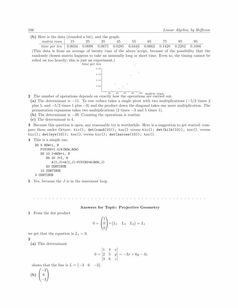
106 Linear Algebra, by Hefferon
(b) Here is the data (rounded a bit), and the graph.matrix rows 15 25 35 45 55 65 75 85 95time per ten 0.0034 0.0098 0.0675 0.0285 0.0443 0.0663 0.1428 0.2282 0.1686
(This data is from an average of twenty runs of the above script, because of the possibility that therandomly chosen matrix happens to take an unusually long or short time. Even so, the timing cannot berelied on too heavily; this is just an experiment.)
matrix rows20 40 60 80 100
time per ten
0.05
0.10
0.15
0.20
bcbc
bc
bc
bc
bc
bc
bc
bc
2 The number of operations depends on exactly how the operations are carried out.(a) The determinant is −11. To row reduce takes a single pivot with two multiplications (−5/2 times 2plus 5, and −5/2 times 1 plus −3) and the product down the diagonal takes one more multiplication. Thepermutation expansion takes two multiplications (2 times −3 and 5 times 1).
(b) The determinant is −39. Counting the operations is routine.(c) The determinant is 4.
3 Because this question is open, any reasonable try is worthwhile. Here is a suggestion to get started: com-pare these under Octave: tic(); det(rand(10)); toc() versus tic(); det(hilb(10)); toc(), versustic(); det(eye(10)); toc(), versus tic(); det(zeroes(10)); toc().4 This is a simple one.
DO 5 ROW=1, N
PIVINV=1.0/A(ROW,ROW)
DO 10 I=ROW+1, N
DO 20 J=I, N
A(I,J)=A(I,J)-PIVINV*A(ROW,J)
20 CONTINUE
10 CONTINUE
5 CONTINUE
5 Yes, because the J is in the innermost loop.
. . . . . . . . . . . . . . . . . . . . . . . . . . . . . . . . . . . . . . . . . . . . .
Answers for Topic: Projective Geometry1 From the dot product
0 =
100
(L1 L2 L3
)= L1
we get that the equation is L1 = 0.2(a) This determinant
0 =
∣∣∣∣∣∣1 4 x2 5 y3 6 z
∣∣∣∣∣∣ = −3x+ 6y − 3z
shows that the line is L =(−3 6 −3
).
(b)
−36−3

Answers to Exercises 107
3 The line incident on
u =
u1
u2
u3
v =
v1
v2
v3
can be found from this determinant equation.
0 =
∣∣∣∣∣∣u1 v1 xu2 v2 yu3 v3 z
∣∣∣∣∣∣ = (u2v3 − u3v2) · x+ (u3v1 − u1v3) · y + (u1v2 − u2v1) · z
The equation for the point incident on two lines is the same.4 If p1, p2, p3, and q1, q2, q3 are two triples of homogeneous coordinates for p then the two column vectorsare in proportion, that is, lie on the same line through the origin. Similarly, the two row vectors are inproportion.
k ·
p1
p2
p3
=
q1
q2
q3
m ·(L1 L2 L3
)=(M1 M2 M3
)Then multiplying gives the answer (km) · (p1L1 + p2L2 + p3L3) = q1M1 + q2M2 + q3M3 = 0.5 The picture of the solar eclipse — unless the image plane is exactly perpendicular to the line from thesun through the pinhole — shows the circle of the sun projecting to an image that is an ellipse. (Anotherexample is that in many pictures in this Topic, the circle that is the sphere’s equator is drawn as an ellipse,that is, is seen by a viewer of the drawing as an ellipse.)
The solar eclipse picture also shows the converse. If we picture the projection as going from left to rightthrough the pinhole then the ellipse I projects through P to a circle S.6 A spot on the unit sphere p1
p2
p3
is non-equatorial if and only if p3 6= 0. In that case it corresponds to this point on the z = 1 planep1/p3
p2/p3
1
since that is intersection of the line containing the vector and the plane.7(a) Other pictures are possible, but this is one.
T0U0
V0
T1U1
V1
V2U2
T2
The intersections T0U1 ∩ T1U0 = V2, T0V1 ∩ T1V0 = U2, and U0V1 ∩ U1V0 = T2 are labeled so that oneach line is a T , a U , and a V .
(b) The lemma used in Desargue’s Theorem gives a basis B with respect to which the points have thesehomogeneous coordinate vectors.
RepB(~t0) =
100
RepB(~t1) =
010
RepB(~t2) =
001
RepB(~v0) =
111
(c) First, any U0 on T0V0
RepB(~u0) = a
100
+ b
111
=
a+ bbb

108 Linear Algebra, by Hefferon
has homogeneous coordinate vectors of this formu0
11
(u0 is a parameter; it depends on where on the T0V0 line the point U0 is, but any point on that line has ahomogeneous coordinate vector of this form for some u0 ∈ R). Similarly, U2 is on T1V0
RepB(~u2) = c
010
+ d
111
=
dc+ dd
and so has this homogeneous coordinate vector. 1
u2
1
Also similarly, U1 is incident on T2V0
RepB(~u1) = e
001
+ f
111
=
ff
e+ f
and has this homogeneous coordinate vector. 1
1u1
(d) Because V1 is T0U2 ∩ U0T2 we have this.
g
100
+ h
1u2
1
= i
u0
11
+ j
001
=⇒g + h = iu0
hu2 = i
h = i+ j
Substituting hu2 for i in the first equation hu0u2
hu2
h
shows that V1 has this two-parameter homogeneous coordinate vector.u0u2
u2
1
(e) Since V2 is the intersection T0U1 ∩ T1U0
k
100
+ l
11u1
= m
010
+ n
u0
11
=⇒k + l = nu0
l = m+ n
lu1 = n
and substituting lu1 for n in the first equation lu0u1
llu1
gives that V2 has this two-parameter homogeneous coordinate vector.u0u1
1u1

Answers to Exercises 109
(f) Because V1 is on the T1U1 line its homogeneous coordinate vector has the form
p
010
+ q
11u1
=
qp+ qqu1
(∗)
but a previous part of this question established that V1’s homogeneous coordinate vectors have the formu0u2
u2
1
and so this a homogeneous coordinate vector for V1.u0u1u2
u1u2
u1
(∗∗)
By (∗) and (∗∗), there is a relationship among the three parameters: u0u1u2 = 1.(g) The homogeneous coordinate vector of V2 can be written in this way.u0u1u2
u2
u1u2
=
1u2
u1u2
Now, the T2U2 line consists of the points whose homogeneous coordinates have this form.
r
001
+ s
1u2
1
=
ssu2
r + s
Taking s = 1 and r = u1u2 − 1 shows that the homogeneous coordinate vectors of V2 have this form.

110 Linear Algebra, by Hefferon
Chapter 5. Similarity
. . . . . . . . . . . . . . . . . . . . . . . . . . . . . . . . . . . . . . . . . . . . .
Answers for subsection 5.II.1
5.II.1.4 One way to proceed is left to right.
PSP−1 =(
4 2−3 2
)(1 3−2 −6
)(2/14 −2/143/14 4/14
)=(
0 0−7 −21
)(2/14 −2/143/14 4/14
)=(
0 0−11/2 −5
)5.II.1.6 Gauss’ method shows that the first matrix represents maps of rank two while the second matrixrepresents maps of rank three.5.II.1.7(a) Because t is described with the members of B, finding the matrix representation is easy:
RepB(t(x2)) =
011
B
RepB(t(x)) =
10−1
B
RepB(t(1)) =
003
B
gives this.
RepB,B(t)
0 1 01 0 01 −1 3
(b) We will find t(1), t(1 +x), and t(1 +x+x2, to find how each is represented with respect to D. We aregiven that t(1) = 3, and the other two are easy to see: t(1 + x) = x2 + 2 and t(1 + x+ x2) = x2 + x+ 3.By eye, we get the representation of each vector
RepD(t(1)) =
300
D
RepD(t(1 + x)) =
2−11
D
RepD(t(1 + x+ x2)) =
201
D
and thus the representation of the map.
RepD,D(t) =
3 2 20 −1 00 1 1
(c) The diagram, adapted for this T and S,
Vw.r.t. Dt−−−−→S
Vw.r.t. D
idyP id
yPVw.r.t. B
t−−−−→T
Vw.r.t. B
shows that P = RepD,B(id).
P =
0 0 10 1 11 1 1
5.II.1.9 The only representation of a zero map is a zero matrix, no matter what the pair of basesRepB,D(z) = Z, and so in particular for any single basis B we have RepB,B(z) = Z. The case of theidentity is related, but slightly different: the only representation of the identity map, with respect to anyB,B, is the identity RepB,B(id) = I. (Remark: of course, we have seen examples where B 6= D andRepB,D(id) 6= I — in fact, we have seen that any nonsingular matrix is a representation of the identity mapwith respect to some B,D.)

Answers to Exercises 111
5.II.1.13 Let fx and fy be the reflection maps (sometimes called ‘flip’s). For any bases B and D, thematrices RepB,B(fx) and RepD,D(fy) are similar. First note that
S = RepE2,E2(fx) =(
1 00 −1
)T = RepE2,E2(fy) =
(−1 00 1
)are similar because the second matrix is the representation of fx with respect to the basis A = 〈~e2, ~e1〉:(
1 00 −1
)= P
(−1 00 1
)P−1
where P = RepA,E2(id).
R2w.r.t. A
fx−−−−→T
V R2w.r.t. A
idyP id
yPR2
w.r.t. E2fx−−−−→S
R2w.r.t. E2
Now the conclusion follows from the transitivity part of Exercise 12.To finish without relying on that exercise, write RepB,B(fx) = QTQ−1 = QRepE2,E2(fx)Q−1 and
RepD,D(fy) = RSR−1 = RRepE2,E2(fy)R−1. Using the equation in the first paragraph, the first of these twobecomes RepB,B(fx) = QPRepE2,E2(fy)P−1Q−1 and rewriting the second of these two as R−1 ·RepD,D(fy) ·R = RepE2,E2(fy) and substituting gives the desired relationship
RepB,B(fx) = QPRepE2,E2(fy)P−1Q−1
= QPR−1 · RepD,D(fy) ·RP−1Q−1 = (QPR−1) · RepD,D(fy) · (QPR−1)−1
Thus the matrices RepB,B(fx) and RepD,D(fy) are similar.5.II.1.14 We must show that if two matrices are similar then they have the same determinant and the samerank. Both determinant and rank are properties of matrices that we have already shown to be preserved bymatrix equivalence. They are therefore preserved by similarity (which is a special case of matrix equivalence: iftwo matrices are similar then they are matrix equivalent).
To prove the statement without quoting the results about matrix equivalence, note first that rank isa property of the map (it is the dimension of the rangespace) and since we’ve shown that the rank of amap is the rank of a representation, it must be the same for all representations. As for determinants,|PSP−1| = |P | · |S| · |P−1| = |P | · |S| · |P |−1 = |S|.
The converse of the statement does not hold; for instance, there are matrices with the same determinantthat are not similar. To check this, consider a nonzero matrix with a determinant of zero. It is not similarto the zero matrix, the zero matrix is similar only to itself, but they have they same determinant. Theargument for rank is much the same.5.II.1.15 The matrix equivalence class containing all n×n rank zero matrices contains only a single matrix,the zero matrix. Therefore it has as a subset only one similarity class.
In contrast, the matrix equivalence class of 1×1 matrices of rank one consists of those 1×1 matrices (k)where k 6= 0. For any basis B, the representation of multiplication by the scalar k is RepB,B(tk) = (k), soeach such matrix is alone in its similarity class. So this is a case where a matrix equivalence class splits intoinfinitely many similarity classes.5.II.1.16 Yes, these are similar (
1 00 3
) (3 00 1
)since, where the first matrix is RepB,B(t) for B = 〈~β1, ~β2〉, the second matrix is RepD,D(t) for D = 〈~β2, ~β1〉.5.II.1.19 There are two equivalence classes, (i) the class of rank zero matrices, of which there is one:C1 = {(0)}, and (2) the class of rank one matrices, of which there are infinitely many: C2 = {(k)
∣∣ k 6= 0}.Each 1×1 matrix is alone in its similarity class. That’s because any transformation of a one-dimensional
space is multiplication by a scalar tk : V → V given by ~v 7→ k · ~v. Thus, for any basis B = 〈~β〉, the matrixrepresenting a transformation tk with respect to B,B is (RepB(tk(~β))) = (k).

112 Linear Algebra, by Hefferon
So, contained in the matrix equivalence class C1 is (obviously) the single similarity class consisting of thematrix (0). And, contained in the matrix equivalence class C2 are the infinitely many, one-member-each,similarity classes consisting of (k) for k 6= 0.
5.II.1.20 No. Here is an example that has two pairs, each of two similar matrices:(1 −11 2
)(1 00 3
)(2/3 1/3−1/3 1/3
)=(
5/3 −2/3−4/3 7/3
)and (
1 −2−1 1
)(−1 00 −3
)(−1 −2−1 −1
)=(−5 −42 1
)(this example is mostly arbitrary, but not entirely, because the the center matrices on the two left sides addto the zero matrix). Note that the sums of these similar matrices are not similar(
1 00 3
)+(−1 00 −3
)=(
0 00 0
) (5/3 −2/3−4/3 7/3
)+(−5 −42 1
)6=(
0 00 0
)since the zero matrix is similar only to itself.
5.II.1.21 If N = P (T − λI)P−1 then N = PTP−1 − P (λI)P−1. The diagonal matrix λI commutes withanything, so P (λI)P−1 = PP−1(λI) = λI. Thus N = PTP−1 − λI and consequently N + λI = PTP−1.(So not only are they similar, in fact they are similar via the same P .)
. . . . . . . . . . . . . . . . . . . . . . . . . . . . . . . . . . . . . . . . . . . . .
Answers for subsection 5.II.2
5.II.2.7(a) Setting up (
−2 10 2
)(b1b2
)= x ·
(b1b2
)=⇒ (−2− x) · b1 + b2 = 0
(2− x) · b2 = 0gives the two possibilities that b2 = 0 and x = 2. Following the b2 = 0 possibility leads to the first equation(−2− x)b1 = 0 with the two cases that b1 = 0 and that x = −2. Thus, under this first possibility, we findx = −2 and the associated vectors whose second component is zero, and whose first component is free.(
−2 10 2
)(b10
)= −2 ·
(b10
)~β1 =
(10
)Following the other possibility leads to a first equation of −4b1 + b2 = 0 and so the vectors associated withthis solution have a second component that is four times their first component.(
−2 10 2
)(b14b1
)= 2 ·
(b14b1
)~β2 =
(14
)The diagonalization is this. (
1 10 4
)−1(−2 10 2
)(1 10 4
)−1(−2 00 2
)(b) The calculations are like those in the prior part.(
5 40 1
)(b1b2
)= x ·
(b1b2
)=⇒ (5− x) · b1 + 4 · b2 = 0
(1− x) · b2 = 0The bottom equation gives the two possibilities that b2 = 0 and x = 1. Following the b2 = 0 possibility,and discarding the case where both b2 and b1 are zero, gives that x = 5, associated with vectors whosesecond component is zero and whose first component is free.
~β1 =(
10
)

Answers to Exercises 113
The x = 1 possibility gives a first equation of 4b1 + 4b2 = 0 and so the associated vectors have a secondcomponent that is the negative of their first component.
~β1 =(
1−1
)We thus have this diagonalization.(
1 10 −1
)−1(5 40 1
)(1 10 −1
)=(
5 00 1
)5.II.2.9 These two are not similar (
0 00 0
) (1 00 1
)because each is alone in its similarity class.
For the second half, these (2 00 3
) (3 00 2
)are similar via the matrix that changes bases from 〈~β1, ~β2〉 to 〈~β2, ~β1〉. (Question. Are two diagonal matricessimilar if and only if their diagonal entries are permutations of each other’s?)5.II.2.10 Contrast these two. (
2 00 1
) (2 00 0
)The first is nonsingular, the second is singular.5.II.2.12(a) The check is easy.(
1 10 −1
)(3 20 1
)=(
3 30 −1
) (3 30 −1
)(1 10 −1
)−1
=(
3 00 1
)(b) It is a coincidence, in the sense that if T = PSP−1 then T need not equal P−1SP . Even in the case ofa diagonal matrix D, the condition that D = PTP−1 does not imply that D equals P−1TP . The matricesfrom Example 2.2 show this.(
1 21 1
)(4 −21 1
)=(
6 05 −1
) (6 05 −1
)(1 21 1
)−1
=(−6 12−6 11
)5.II.2.13 The columns of the matrix are chosen as the vectors associated with the x’s. The exact choice,and the order of the choice was arbitrary. We could, for instance, get a different matrix by swapping thetwo columns.5.II.2.14 Diagonalizing and then taking powers of the diagonal matrix shows that(
−3 1−4 2
)k=
13
(−1 1−4 4
)+ (−23
)k(
4 −14 −1
).
5.II.2.16 Yes, ct is diagonalizable by the final theorem of this subsection.No, t+ s need not be diagonalizable. Intuitively, the problem arises when the two maps diagonalize with
respect to different bases (that is, when they are not simultaneously diagonalizable). Specifically, these twoare diagonalizable but their sum is not: (
1 10 0
) (−1 00 0
)(the second is already diagonal; for the first, see Exercise 15). The sum is not diagonalizable because itssquare is the zero matrix.
The same intuition suggests that t ◦ s is not be diagonalizable. These two are diagonalizable but theirproduct is not: (
1 00 0
) (0 11 0
)(for the second, see Exercise 15).5.II.2.18

114 Linear Algebra, by Hefferon
(a) Using the formula for the inverse of a 2×2 matrix gives this.(a bc d
)(1 22 1
)· 1ad− bc ·
(d −b−c a
)=
1ad− bc
(ad+ 2bd− 2ac− bc −ab− 2b2 + 2a2 + abcd+ 2d2 − 2c2 − cd −bc− 2bd+ 2ac+ ad
)Now pick scalars a, . . . , d so that ad − bc 6= 0 and 2d2 − 2c2 = 0 and 2a2 − 2b2 = 0. For example, thesewill do. (
1 11 −1
)(1 22 1
)· 1−2·(−1 −1−1 1
)=
1−2
(−6 00 2
)(b) As above,(
a bc d
)(x yy z
)· 1ad− bc ·
(d −b−c a
)=
1ad− bc
(adx+ bdy − acy − bcz −abx− b2y + a2y + abzcdx+ d2y − c2y − cdz −bcx− bdy + acy + adz
)we are looking for scalars a, . . . , d so that ad − bc 6= 0 and −abx− b2y + a2y + abz = 0 and cdx + d2y −c2y − cdz = 0, no matter what values x, y, and z have.
For starters, we assume that y 6= 0, else the given matrix is already diagonal. We shall use thatassumption because if we (arbitrarily) let a = 1 then we get
−bx− b2y + y + bz = 0(−y)b2 + (z − x)b+ y = 0
and the quadratic formula gives
b =−(z − x)±
√(z − x)2 − 4(−y)(y)−2y
y 6= 0
(note that if x, y, and z are real then these two b’s are real as the discriminant is positive). By the sametoken, if we (arbitrarily) let c = 1 then
dx+ d2y − y − dz = 0(y)d2 + (x− z)d− y = 0
and we get here
d =−(x− z)±
√(x− z)2 − 4(y)(−y)
2yy 6= 0
(as above, if x, y, z ∈ R then this discriminant is positive so a symmetric, real, 2×2 matrix is similar to areal diagonal matrix).
For a check we try x = 1, y = 2, z = 1.
b =0±√
0 + 16−4
= ∓1 d =0±√
0 + 164
= ±1
Note that not all four choices (b, d) = (+1,+1), . . . , (−1,−1) satisfy ad− bc 6= 0.
. . . . . . . . . . . . . . . . . . . . . . . . . . . . . . . . . . . . . . . . . . . . .
Answers for subsection 5.II.35.II.3.20(a) This
0 =∣∣∣∣10− x −9
4 −2− x
∣∣∣∣ = (10− x)(−2− x)− (−36)
simplifies to the characteristic equation x2− 8x+ 16 = 0. Because the equation factors into (x− 4)2 thereis only one eigenvalue λ1 = 4.
(b) 0 = (1− x)(3− x)− 8 = x2 − 4x− 5; λ1 = 5, λ2 = −1(c) x2 − 21 = 0; λ1 =
√21, λ2 = −
√21
(d) x2 = 0; λ1 = 0(e) x2 − 2x+ 1 = 0; λ1 = 1

Answers to Exercises 115
5.II.3.22 The characteristic equation
0 =∣∣∣∣−2− x −1
5 2− x
∣∣∣∣ = x2 + 1
has the complex roots λ1 = i and λ2 = −i. This system(−2− x) · b1 − 1 · b2 = 0
5 · b1 (2− x) · b2 = 0For λ1 = i Gauss’ method gives this reduction.
(−2− i) · b1 − 1 · b2 = 05 · b1 − (2− i) · b2 = 0
(−5/(−2−i))ρ1+ρ2−→ (−2− i) · b1 − 1 · b2 = 00 = 0
(For the calculation in the lower right get a common denominator5
−2− i − (2− i) =5
−2− i −−2− i−2− i · (2− i) =
5− (−5)−2− i
to see that it gives a 0 = 0 equation.) These are the resulting eigenspace and eigenvector.
{(
(1/(−2− i))b2b2
) ∣∣ b2 ∈ C} (1/(−2− i)
1
)For λ2 = −i the system
(−2 + i) · b1 − 1 · b2 = 05 · b1 − (2 + i) · b2 = 0
(−5/(−2+i))ρ1+ρ2−→ (−2 + i) · b1 − 1 · b2 = 00 = 0
leads to this.
{(
(1/(−2 + i))b2b2
) ∣∣ b2 ∈ C} (1/(−2 + i)
1
)5.II.3.23 The characteristic equation is
0 =
∣∣∣∣∣∣1− x 1 1
0 −x 10 0 1− x
∣∣∣∣∣∣ = (1− x)2(−x)
and so the eigenvalues are λ1 = 1 (this is a repeated root of the equation) and λ2 = 0. For the rest, considerthis system.
(1− x) · b1 + b2 + b3 = 0−x · b2 + b3 = 0
(1− x) · b3 = 0When x = λ1 = 1 then the solution set is this eigenspace.
{
b100
∣∣ b1 ∈ C}When x = λ2 = 0 then the solution set is this eigenspace.
{
−b2b20
∣∣ b2 ∈ C}So these are eigenvectors associated with λ1 = 1 and λ2 = 0.1
00
−110
5.II.3.26 λ = 1,
(0 00 1
)and
(2 31 0
), λ = −2,
(−1 01 0
), λ = −1,
(−2 11 0
)5.II.3.28 The determinant of the triangular matrix T − xI is the product down the diagonal, and so itfactors into the product of the terms ti,i − x.5.II.3.30 Any two representations of that transformation are similar, and similar matrices have the samecharacteristic polynomial.

116 Linear Algebra, by Hefferon
5.II.3.33 The characteristic equation
0 =∣∣∣∣a− x bc d− x
∣∣∣∣ = (a− x)(d− x)− bc
simplifies to x2 + (−a − d) · x + (ad − bc). Checking that the values x = a + b and x = a − c satisfy theequation (under the a+ b = c+ d condition) is routine.
5.II.3.37(a) Where the eigenvalue λ is associated with the eigenvector ~x then Ak~x = A · · ·A~x = Ak−1λ~x =λAk−1~x = · · · = λk~x. (The full details can be put in by doing induction on k.)
(b) The eigenvector associated wih λ might not be an eigenvector associated with µ.
5.II.3.38 No. These are two same-sized, equal rank, matrices with different eigenvalues.(1 00 1
) (1 00 2
)5.II.3.39 The characteristic polynomial has an odd power and so has at least one real root.
5.II.3.40 The characteristic polynomial x3 − 5x2 + 6x has distinct roots λ1 = 0, λ2 = −2, and λ3 = −3.Thus the matrix can be diagonalized into this form.0 0 0
0 −2 00 0 −3
5.II.3.41 We must show that it is one-to-one and onto, and that it respects the operations of matrixaddition and scalar multiplication.
To show that it is one-to-one, suppose that tP (T ) = tP (S), that is, suppose that PTP−1 = PSP−1, andnote that multiplying both sides on the left by P−1 and on the right by P gives that T = S. To show thatit is onto, consider S ∈Mn×n and observe that S = tP (P−1SP ).
The map tP preserves matrix addition since tP (T + S) = P (T + S)P−1 = (PT + PS)P−1 = PTP−1 +PSP−1 = tP (T +S) follows from properties of matrix multiplication and addition that we have seen. Scalarmultiplication is similar: tP (cT ) = P (c · T )P−1 = c · (PTP−1) = c · tP (T ).
5.II.3.42 This is how the answer was given in the cited source. If the argument of the characteristicfunction of A is set equal to c, adding the first (n − 1) rows (columns) to the nth row (column) yields adeterminant whose nth row (column) is zero. Thus c is a characteristic root of A.
. . . . . . . . . . . . . . . . . . . . . . . . . . . . . . . . . . . . . . . . . . . . .
Answers for subsection 5.III.1
5.III.1.8 For the zero transformation, no matter what the space, the chain of rangespaces is V ⊃ {~0} ={~0} = · · · and the chain of nullspaces is {~0} ⊂ V = V = · · · . For the identity transformation the chains areV = V = V = · · · and {~0} = {~0} = · · · .5.III.1.9(a) Iterating t0 twice a+ bx+ cx2 7→ b+ cx2 7→ cx2 gives
a+ bx+ cx2 t207−→ cx2
and any higher power is the same map. Thus, while R(t0) is the space of quadratic polynomials withno linear term {p+ rx2
∣∣ p, r ∈ C}, and R(t20) is the space of purely-quadratic polynomials {rx2∣∣ r ∈ C},
this is where the chain stabilizes R∞(t0) = {rx2∣∣ n ∈ C}. As for nullspaces, N (t0) is the space of purely-
linear quadratic polynomials {qx∣∣ q ∈ C}, and N (t20) is the space of quadratic polynomials with no x2
term {p+ qx∣∣ p, q ∈ C}, and this is the end N∞(t0) = N (t20).

Answers to Exercises 117
(b) The second power (ab
)t17−→(
0a
)t17−→(
00
)is the zero map. Consequently, the chain of rangespaces
R2 ⊃ {(
0p
) ∣∣ p ∈ C} ⊃ {~0 } = · · ·
and the chain of nullspaces
{~0 } ⊂ {(q0
) ∣∣ q ∈ C} ⊂ R2 = · · ·
each has length two. The generalized rangespace is the trivial subspace and the generalized nullspace isthe entire space.
(c) Iterates of this map cycle around
a+ bx+ cx2 t27−→ b+ cx+ ax2 t27−→ c+ ax+ bx2 t27−→ a+ bx+ cx2 · · ·and the chains of rangespaces and nullspaces are trivial.
P2 = P2 = · · · {~0 } = {~0 } = · · ·Thus, obviously, generalized spaces are R∞(t2) = P2 and N∞(t2) = {~0 }.
(d) We have abc
7→aab
7→aaa
7→aaa
7→ · · ·and so the chain of rangespaces
R3 ⊃ {
ppr
∣∣ p, r ∈ C} ⊃ {ppp
∣∣ p ∈ C} = · · ·
and the chain of nullspaces
{~0 } ⊂ {
00r
∣∣ r ∈ C} ⊂ {0qr
∣∣ q, r ∈ C} = · · ·
each has length two. The generalized spaces are the final ones shown above in each chain.5.III.1.10 Each maps x 7→ t(t(t(x))).5.III.1.11 Recall that if W is a subspace of V then any basis BW for W can be enlarged to make a basisBV for V . From this the first sentence is immediate. The second sentence is also not hard: W is the span ofBW and if W is a proper subspace then V is not the span of BW , and so BV must have at least one vectormore than does BW .5.III.1.12 It is both ‘if’ and ‘only if’. We have seen earlier that a linear map is nonsingular if and onlyif it preserves dimension, that is, if the dimension of its range equals the dimension of its domain. With atransformation t : V → V that means that the map is nonsingular if and only if it is onto: R(t) = V (andthus R(t2) = V , etc).5.III.1.13 The nullspaces form chains because because if ~v ∈ N (tj) then tj(~v) = ~0 and tj+1(~v) =t( tj(~v) ) = t(~0) = ~0 and so ~v ∈ N (tj+1).
Now, the “further” property for nullspaces follows from that fact that it holds for rangespaces, alongwith the prior exercise. Because the dimension of R(tj) plus the dimension of N (tj) equals the dimension nof the starting space V , when the dimensions of the rangespaces stop decreasing, so do the dimensions ofthe nullspaces. The prior exercise shows that from this point k on, the containments in the chain are notproper — the nullspaces are equal.5.III.1.14 (Of course, many examples are correct, but here is one.) An example is the shift operator ontriples of reals (x, y, z) 7→ (0, x, y). The nullspace is all triples that start with two zeros. The map stabilizesafter three iterations.5.III.1.15 The differentiation operator d/dx : P1 → P1 has the same rangespace as nullspace. For anexample of where they are disjoint — except for the zero vector — consider an identity map (or anynonsingular map).

118 Linear Algebra, by Hefferon
. . . . . . . . . . . . . . . . . . . . . . . . . . . . . . . . . . . . . . . . . . . . .
Answers for subsection 5.III.2
5.III.2.19 By Lemma 1.3 the nullity has grown as large as possible by the n-th iteration where n is thedimension of the domain. Thus, for the 2×2 matrices, we need only check whether the square is the zeromatrix. For the 3×3 matrices, we need only check the cube.(a) Yes, this matrix is nilpotent because its square is the zero matrix.(b) No, the square is not the zero matrix.(
3 11 3
)2
=(
10 66 10
)(c) Yes, the cube is the zero matrix. In fact, the square is zero.(d) No, the third power is not the zero matrix.1 1 4
3 0 −15 2 7
3
=
206 86 30426 8 26438 180 634
(e) Yes, the cube of this matrix is the zero matrix.
Another way to see that the second and fourth matrices are not nilpotent is to note that they are nonsingular.5.III.2.23 A couple of examples(
0 01 0
)(a bc d
)=(
0 0a b
) 0 0 01 0 00 1 0
a b cd e fg h i
=
0 0 0a b cd e f
suggest that left multiplication by a block of subdiagonal ones shifts the rows of a matrix downward. Distinctblocks
0 0 0 01 0 0 00 0 0 00 0 1 0
a b c de f g hi j k lm n o p
=
0 0 0 0a b c d0 0 0 0i j k l
act to shift down distinct parts of the matrix.
Right multiplication does an analgous thing to columns. See Exercise 17.5.III.2.24 Yes. Generalize the last sentence in Example 2.9. As to the index, that same last sentenceshows that the index of the new matrix is less than or equal to the index of N , and reversing the roles ofthe two matrices gives inequality in the other direction.
Another answer to this question is to show that a matrix is nilpotent if and only if any associated map isnilpotent, and with the same index. Then, because similar matrices represent the same map, the conclusionfollows. This is Exercise 30 below.5.III.2.26 No, by Lemma 1.3 for a map on a two-dimensional space, the nullity has grown as large aspossible by the second iteration.5.III.2.27 The index of nilpotency of a transformation can be zero only when the vector starting the stringmust be ~0, that is, only when V is a trivial space.5.III.2.29 We must check that B ∪ C ∪ {~v1, . . . , ~vj} is linearly independent where B is a t-string basis forR(t), where C is a basis for N (t), and where t(~v1) = ~β1, . . . , t(~vi = ~βi. Write
~0 = c1,−1~v1 + c1,0~β1 + c1,1t(~β1) + · · ·+ c1,h1th1(~~β1) + c2,−1~v2 + · · ·+ cj,hit
hi(~βi)
and apply t.
~0 = c1,−1~β1 + c1,0t(~β1) + · · ·+ c1,h1−1t
h1(~~β1) + c1,h1~0 + c2,−1
~β2 + · · ·+ ci,hi−1thi(~βi) + ci,hi~0
Conclude that the coefficients c1,−1, . . . , c1,hi−1, c2,−1, . . . , ci,hi−1 are all zero as B ∪ C is a basis. Substituteback into the first displayed equation to conclude that the remaining coefficients are zero also.

Answers to Exercises 119
5.III.2.30 For any basis B, a transformation n is nilpotent if and only if N = RepB,B(n) is a nilpotentmatrix. This is because only the zero matrix represents the zero map and so nj is the zero map if and onlyif N j is the zero matrix.5.III.2.31 It can be of any size greater than or equal to one. To have a transformation that is nilpotentof index four, whose cube has rangespace of dimension k, take a vector space, a basis for that space, and atransformation that acts on that basis in this way.
~β1 7→ ~β2 7→ ~β3 7→ ~β4 7→ ~0~β5 7→ ~β6 7→ ~β7 7→ ~β8 7→ ~0
...~β4k−3 7→ ~β4k−2 7→ ~β4k−1 7→ ~β4k 7→ ~0
...–possibly other, shorter, strings–
So the dimension of the rangespace of T 3 can be as large as desired. The smallest that it can be is one —there must be at least one string or else the map’s index of nilpotency would not be four.5.III.2.32 These two have only zero for eigenvalues(
0 00 0
) (0 01 0
)but are not similar (they have different canonical representatives, namely, themselves).5.III.2.33 A simple reordering of the string basis will do. For instance, a map that is assoicated with thisstring basis
~β1 7→ ~β2 7→ ~0
is represented with respect to B = 〈~β1, ~β2〉 by this matrix(0 01 0
)but is represented with respect to B = 〈~β2, ~β1〉 in this way.(
0 10 0
)5.III.2.35 For the matrices to be nilpotent they must be square. For them to commute they must be thesame size. Thus their product and sum are defined.
Call the matrices A and B. To see that AB is nilpotent, multiply (AB)2 = ABAB = AABB = A2B2,and (AB)3 = A3B3, etc., and, as A is nilpotent, that product is eventually zero.
The sum is similar; use the Binomial Theorem.5.III.2.36 Some experimentation gives the idea for the proof. Expansion of the second power
t2S(T ) = S(ST − TS)− (ST − TS)S = S2 − 2STS + TS2
the third powert3S(T ) = S(S2 − 2STS + TS2)− (S2 − 2STS + TS2)S
= S3T − 3S2TS + 3STS2 − TS3
and the fourth powert4S(T ) = S(S3T − 3S2TS + 3STS2 − TS3)− (S3T − 3S2TS + 3STS2 − TS3)S
= S4T − 4S3TS + 6S2TS2 − 4STS3 + TS4
suggest that the expansions follow the Binomial Theorem. Verifying this by induction on the power of tS isroutine. This answers the question because, where the index of nilpotency of S is k, in the expansion of t2kS
t2kS (T ) =∑
0≤i≤2k
(−1)i(
2ki
)SiTS2k−i
for any i at least one of the Si and S2k−i has a power higher than k, and so the term gives the zero matrix.

120 Linear Algebra, by Hefferon
5.III.2.37 Use the geometric series: I −Nk+1 = (I −N)(Nk +Nk−1 + · · ·+ I). If Nk+1 is the zero matrixthen we have a right inverse for I −N . It is also a left inverse.
This statement is not ‘only if’ since (1 00 1
)−(−1 00 −1
)is invertible.
. . . . . . . . . . . . . . . . . . . . . . . . . . . . . . . . . . . . . . . . . . . . .
Answers for subsection 5.IV.1
5.IV.1.15 Its characteristic polynomial has complex roots.∣∣∣∣∣∣−x 1 00 −x 11 0 −x
∣∣∣∣∣∣ = (1− x) · (x− (−12
+√
32i)) · (x− (−1
2−√
32i))
As the roots are distinct, the characteristic polynomial equals the minimal polynomial.5.IV.1.18 The n = 3 case provides a hint. A natural basis for P3 is B = 〈1, x, x2, x3〉. The action of thetransformation is
1 7→ 1 x 7→ x+ 1 x2 7→ x2 + 2x+ 1 x3 7→ x3 + 3x2 + 3x+ 1and so the representation RepB,B(t) is this upper triangular matrix.
1 1 1 10 1 2 30 0 1 30 0 0 1
Because it is triangular, the fact that the characteristic polynomial is c(x) = (x − 1)4 is clear. For theminimal polynomial, the candidates are m1(x) = (x− 1),
T − 1I =
0 1 1 10 0 2 30 0 0 30 0 0 0
m2(x) = (x− 1)2,
(T − 1I)2 =
0 0 2 60 0 0 60 0 0 00 0 0 0
m3(x) = (x− 1)3,
(T − 1I)3 =
0 0 0 60 0 0 00 0 0 00 0 0 0
and m4(x) = (x− 1)4. Because m1, m2, and m3 are not right, m4 must be right, as is easily verified.
In the case of a general n, the representation is an upper triangular matrix with ones on the diagonal.Thus the characteristic polynomial is c(x) = (x − 1)n+1. One way to verify that the minimal polynomialequals the characteristic polynomial is argue something like this: say that an upper triangular matrix is0-upper triangular if there are nonzero entries on the diagonal, that it is 1-upper triangular if the diagonalcontains only zeroes and there are nonzero entries just above the diagonal, etc. As the above exampleillustrates, an induction argument will show that, where T has only nonnegative entries, T j is j-uppertriangular. That argument is left to the reader.

Answers to Exercises 121
5.IV.1.19 The map twice is the same as the map once: π ◦ π = π, that is, π2 = π and so the minimalpolynomial is of degree at most two since m(x) = x2 − x will do. The fact that no linear polynomial will dofollows from applying the maps on the left and right side of c1 · π + c0 · id = z (where z is the zero map) tothese two vectors. 0
01
100
Thus the minimal polynomial is m.5.IV.1.20 This is one answer. 0 0 0
1 0 00 0 0
5.IV.1.21 The x must be a scalar, not a matrix.5.IV.1.22 The characteristic polynomial of
T =(a bc d
)is (a− x)(d− x)− bc = x2 − (a+ d)x+ (ad− bc). Substitute(
a bc d
)2
− (a+ d)(a bc d
)+ (ad− bc)
(1 00 1
)=(a2 + bc ab+ bdac+ cd bc+ d2
)−(a2 + ad ab+ bdac+ cd ad+ d2
)+(ad− bc 0
0 ad− bc
)and just check each entry sum to see that the result is the zero matrix.5.IV.1.25 A minimal polynomial must have leading coefficient 1, and so if the minimal polynomial of amap or matrix were to be a degree zero polynomial then it would be m(x) = 1. But the identity map ormatrix equals the zero map or matrix only on a trivial vector space.
So in the nontrivial case the minimal polynomial must be of degree at least one. A zero map or matrixhas minimal polynomial m(x) = x, and an identity map or matrix has minimal polynomial m(x) = x− 1.5.IV.1.27 For a diagonal matrix
T =
t1,1 00 t2,2
. . .tn,n
the characteristic polynomial is (t1,1 − x)(t2,2 − x) · · · (tn,n − x). Of course, some of those factors may berepeated, e.g., the matrix might have t1,1 = t2,2. For instance, the characteristic polynomial of
D =
3 0 00 3 00 0 1
is (3− x)2(1− x) = −1 · (x− 3)2(x− 1).
To form the minimal polynomial, take the terms x− ti,i, throw out repeats, and multiply them together.For instance, the minimal polynomial of D is (x− 3)(x− 1). To check this, note first that Theorem 5.IV.1.8,the Cayley-Hamilton theorem, requires that each linear factor in the characteristic polynomial appears atleast once in the minimal polynomial. One way to check the other direction — that in the case of a diagonalmatrix, each linear factor need appear at most once — is to use a matrix argument. A diagonal matrix,multiplying from the left, rescales rows by the entry on the diagonal. But in a product (T − t1,1I) · · · , evenwithout any repeat factors, every row is zero in at least one of the factors.
For instance, in the product
(D − 3I)(D − 1I) = (D − 3I)(D − 1I)I =
0 0 00 0 00 0 −2
2 0 00 2 00 0 0
1 0 00 1 00 0 1

122 Linear Algebra, by Hefferon
because the first and second rows of the first matrix D− 3I are zero, the entire product will have a first rowand second row that are zero. And because the third row of the middle matrix D − 1I is zero, the entireproduct has a third row of zero.
5.IV.1.29(a) This is a property of functions in general, not just of linear functions. Suppose that f and g areone-to-one functions such that f ◦ g is defined. Let f ◦ g(x1) = f ◦ g(x2), so that f(g(x1)) = f(g(x2)).Because f is one-to-one this implies that g(x1) = g(x2). Because g is also one-to-one, this in turn impliesthat x1 = x2. Thus, in summary, f ◦ g(x1) = f ◦ g(x2) implies that x1 = x2 and so f ◦ g is one-to-one.
(b) If the linear map h is not one-to-one then there are unequal vectors ~v1, ~v2 that map to the same valueh(~v1) = h(~v2). Because h is linear, we have ~0 = h(~v1) − h(~v2) = h(~v1 − ~v2) and so ~v1 − ~v2 is a nonzerovector from the domain that is mapped by h to the zero vector of the codomain (~v1 − ~v2 does not equalthe zero vector of the domain because ~v1 does not equal ~v2).
(c) The minimal polynomial m(t) sends every vector in the domain to zero and so it is not one-to-one(except in a trivial space, which we ignore). By the first item of this question, since the composition m(t)is not one-to-one, at least one of the components t− λi is not one-to-one. By the second item, t− λi hasa nontrivial nullspace. Because (t − λi)(~v) = ~0 holds if and only if t(~v) = λi · ~v, the prior sentence givesthat λi is an eigenvalue (recall that the definition of eigenvalue requires that the relationship hold for atleast one nonzero ~v).
5.IV.1.30 This is false. The natural example of a non-diagonalizable transformation works here. Considerthe transformation of C2 represented with respect to the standard basis by this matrix.
N =(
0 10 0
)The characteristic polynomial is c(x) = x2. Thus the minimal polynomial is either m1(x) = x or m2(x) = x2.The first is not right since N − 0 · I is not the zero matrix, thus in this example the minimal polynomialhas degree equal to the dimension of the underlying space, and, as mentioned, we know this matrix is notdiagonalizable because it is nilpotent.
5.IV.1.31 Let A and B be similar A = PBP−1. From the facts that
An = (PBP−1)n = (PBP−1)(PBP−1) · · · (PBP−1) = PB(P−1P )B(P−1P ) · · · (P−1P )BP−1 = PBnP−1
and c ·A = c · (PBP−1) = P (c ·B)P−1 follows the required fact that for any polynomial function f we havef(A) = P f(B)P−1. For instance, if f(x) = x2 + 2x+ 3 then
A2 + 2A+ 3I = (PBP−1)2 + 2 · PBP−1 + 3 · I= (PBP−1)(PBP−1) + P (2B)P−1 + 3 · PP−1 = P (B2 + 2B + 3I)P−1
shows that f(A) is similar to f(B).(a) Taking f to be a linear polynomial we have that A − xI is similar to B − xI. Similar matrices haveequal determinants (since |A| = |PBP−1| = |P | · |B| · |P−1| = 1 · |B| · 1 = |B|). Thus the characteristicpolynomials are equal.
(b) As P and P−1 are invertible, f(A) is the zero matrix when, and only when, f(B) is the zero matrix.(c) They cannot be similar since they don’t have the same characteristic polynomial. The characteristicpolynomial of the first one is x2 − 4x− 3 while the characteristic polynomial of the second is x2 − 5x+ 5.
5.IV.1.32 Suppose that m(x) = xn +mn−1xn−1 + · · ·+m1x+m0 is minimal for T .
(a) For the ‘if’ argument, because Tn + · · · + m1T + m0I is the zero matrix we have that I = (Tn +· · · + m1T )/(−m0) = T · (Tn−1 + · · · + m1I)/(−m0) and so the matrix (−1/m0) · (Tn−1 + · · · + m1I)is the inverse of T . For ‘only if’, suppose that m0 = 0 (we put the n = 1 case aside but it is easy) sothat Tn + · · · + m1T = (Tn−1 + · · · + m1I)T is the zero matrix. Note that Tn−1 + · · · + m1I is notthe zero matrix because the degree of the minimal polynomial is n. If T−1 exists then multiplying both(Tn−1 + · · ·+m1I)T and the zero matrix from the right by T−1 gives a contradiction.
(b) If T is not invertible then the constant term in its minimal polynomial is zero. Thus,
Tn + · · ·+m1T = (Tn−1 + · · ·+m1I)T = T (Tn−1 + · · ·+m1I)
is the zero matrix.

Answers to Exercises 123
. . . . . . . . . . . . . . . . . . . . . . . . . . . . . . . . . . . . . . . . . . . . .
Answers for subsection 5.IV.2
5.IV.2.17 We are required to check that(3 01 3
)= N + 3I = PTP−1 =
(1/2 1/2−1/4 1/4
)(2 −11 4
)(1 −21 2
)That calculation is easy.5.IV.2.18(a) The characteristic polynomial is c(x) = (x− 3)2 and the minimal polynomial is the same.(b) The characteristic polynomial is c(x) = (x+ 1)2. The minimal polynomial is m(x) = x+ 1.(c) The characteristic polynomial is c(x) = (x+ (1/2))(x− 2)2 and the minimal polynomial is the same.(d) The characteristic polynomial is c(x) = (x− 3)3 The minimal polynomial is the same.(e) The characteristic polynomial is c(x) = (x− 3)4. The minimal polynomial is m(x) = (x− 3)2.(f) The characteristic polynomial is c(x) = (x+ 4)2(x− 4)2 and the minimal polynomial is the same.(g) The characteristic polynomial is c(x) = (x− 2)2(x− 3)(x− 5) and the minimal polynomial is m(x) =(x− 2)(x− 3)(x− 5).
(h) The characteristic polynomial is c(x) = (x−2)2(x−3)(x−5) and the minimal polynomial is the same.5.IV.2.20 For each, because many choices of basis are possible, many other answers are possible. Ofcourse, the calculation to check if an answer gives that PTP−1 is in Jordan form is the arbiter of what’scorrect.(a) Here is the arrow diagram.
C3w.r.t. E3
t−−−−→T
C3w.r.t. E3
idyP id
yPC3
w.r.t. Bt−−−−→J
C3w.r.t. B
The matrix to move from the lower left to the upper left is this.
P−1 =(RepE3,B(id)
)−1 = RepB,E3(id) =
1 −2 01 0 1−2 0 0
The matrix P to move from the upper right to the lower right is the inverse of P−1.
(b) We want this matrix and its inverse.
P−1 =
1 0 30 1 40 −2 0
(c) The concatenation of these bases for the generalized null spaces will do for the basis for the entirespace.
B−1 = 〈
−10010
,
−10−101
〉 B3 = 〈
11−100
,
000−22
,
−1−1120
〉The change of basis matrices are this one and its inverse.
P−1 =
−1 −1 1 0 −10 0 1 0 −10 −1 −1 0 11 0 0 −2 20 1 0 2 0

124 Linear Algebra, by Hefferon
5.IV.2.23 The restriction of t+ 2 to N∞(t+ 2) can have only the action ~β1 7→ ~0. The restriction of t− 1to N∞(t− 1) could have any of these three actions on an associated string basis.
~β2 7→ ~β3 7→ ~β4 7→ ~0 ~β2 7→ ~β3 7→ ~0~β4 7→ ~0
~β2 7→ ~0~β3 7→ ~0~β4 7→ ~0
Taken together there are three possible Jordan forms, the one arising from the first action by t − 1 (alongwith the only action from t+ 2), the one arising from the second action, and the one arising from the thirdaction.
−2 0 0 00 1 0 00 1 1 00 0 1 1
−2 0 0 00 1 0 00 1 1 00 0 0 1
−2 0 0 00 1 0 00 0 1 00 0 0 1
5.IV.2.25 There are two possible Jordan forms. The action of t+ 1 on a string basis for N∞(t+ 1) mustbe ~β1 7→ ~0. There are two actions for t − 2 on a string basis for N∞(t − 2) that are possible with thischaracteristic polynomial and minimal polynomial.
~β2 7→ ~β3 7→ ~0~β4 7→ ~β5 7→ ~0
~β2 7→ ~β3 7→ ~0~β4 7→ ~0~β5 7→ ~0
The resulting Jordan form matrics are these.−1 0 0 0 00 2 0 0 00 1 2 0 00 0 0 2 00 0 0 1 2
−1 0 0 0 00 2 0 0 00 1 2 0 00 0 0 2 00 0 0 0 2
5.IV.2.29 Its characteristic polynomial is c(x) = x2 + 1 which has complex roots x2 + 1 = (x+ i)(x− i).Because the roots are distinct, the matrix is diagonalizable and its Jordan form is that diagonal matrix.(
−i 00 i
)To find an associated basis we compute the null spaces.
N (t+ i) = {(−iyy
) ∣∣ y ∈ C} N (t− i) = {(iyy
) ∣∣ y ∈ C}For instance,
T + i · I =(i −11 i
)and so we get a description of the null space of t+ i by solving this linear system.
ix− y = 0x+ iy = 0
iρ1+ρ2−→ ix− y = 00 = 0
(To change the relation ix = y so that the leading variable x is expressed in terms of the free variable y, wecan multiply both sides by −i.)
As a result, one such basis is this.
B = 〈(−i1
),
(i1
)〉
5.IV.2.30 We can count the possible classes by counting the possible canonical representatives, that is,the possible Jordan form matrices. The characteristic polynomial must be either c1(x) = (x+ 3)2(x− 4) orc2(x) = (x+ 3)(x− 4)2. In the c1 case there are two possible actions of t+ 3 on a string basis for N∞(t+ 3).
~β1 7→ ~β2 7→ ~0 ~β1 7→ ~0~β2 7→ ~0

Answers to Exercises 125
There are two associated Jordan form matrices.−3 0 01 −3 00 0 4
−3 0 00 −3 00 0 4
Similarly there are two Jordan form matrices that could arise out of c2.−3 0 0
0 4 00 1 4
−3 0 00 4 00 0 4
So in total there are four possible Jordan forms.5.IV.2.32 One example is the transformation of C that sends x to −x.5.IV.2.33 Apply Lemma 2.7 twice; the subspace is t− λ1 invariant if and only if it is t invariant, which inturn holds if and only if it is t− λ2 invariant.5.IV.2.34 False; these two 4×4 matrices each have c(x) = (x− 3)4 and m(x) = (x− 3)2.
3 0 0 01 3 0 00 0 3 00 0 1 3
3 0 0 01 3 0 00 0 3 00 0 0 3
5.IV.2.35(a) The characteristic polynomial is this.∣∣∣∣a− x b
c d− x
∣∣∣∣ = (a− x)(d− x)− bc = ad− (a+ d)x+ x2 − bc = x2 − (a+ d)x+ (ad− bc)
Note that the determinant appears as the constant term.(b) Recall that the characteristic polynomial |T − xI| is invariant under similarity. Use the permutationexpansion formula to show that the trace is the negative of the coefficient of xn−1.
(c) No, there are matrices T and S that are equivalent S = PTQ (for some nonsingular P and Q) butthat have different traces. An easy example is this.
PTQ =(
2 00 1
)(1 00 1
)(1 00 1
)=(
2 00 1
)Even easier examples using 1×1 matrices are possible.
(d) Put the matrix in Jordan form. By the first item, the trace is unchanged.(e) The first part is easy; use the third item. The converse does not hold: this matrix(
1 00 −1
)has a trace of zero but is not nilpotent.
5.IV.2.36 Suppose that BM is a basis for a subspace M of some vector space. Implication one way isclear; if M is t invariant then in particular, if ~m ∈ BM then t(~m) ∈ M . For the other implication, letBM = 〈~β1, . . . , ~βq〉 and note that t(~m) = t(m1
~β1 + · · · + mq~βq) = m1t(~β1) + · · · + mqt(~βq) is in M as any
subspace is closed under linear combinations.5.IV.2.38 One such ordering is the dictionary ordering. Order by the real component first, then by thecoefficient of i. For instance, 3 + 2i < 4 + 1i but 4 + 1i < 4 + 2i.5.IV.2.39 The first half is easy—the derivative of any real polynomial is a real polynomial of lower degree.The answer to the second half is ‘no’; any complement of Pj(R) must include a polynomial of degree j + 1,and the derivative of that polynomial is in Pj(R).5.IV.2.40 For the first half, show that each is a subspace and then observe that any polynomial can beuniquely written as the sum of even-powered and odd-powered terms (the zero polynomial is both). Theanswer to the second half is ‘no’: x2 is even while 2x is odd.5.IV.2.41 Yes. If RepB,B(t) has the given block form, take BM to be the first j vectors of B, where J isthe j×j upper left submatrix. Take BN to be the remaining k vectors in B. Let M and N be the spansof BM and BN . Clearly M and N are complementary. To see M is invariant (N works the same way),

126 Linear Algebra, by Hefferon
represent any ~m ∈ M with respect to B, note the last k components are zeroes, and multiply by the givenblock matrix. The final k components of the result are zeroes, so that result is again in M .5.IV.2.42 Put the matrix in Jordan form. By non-singularity, there are no zero eigenvalues on the diagonal.Ape this example: 9 0 0
1 9 00 0 4
=
3 0 01/6 3 00 0 2
2
to construct a square root. Show that it holds up under similarity: if S2 = T then (PSP−1)(PSP−1) =PTP−1.
. . . . . . . . . . . . . . . . . . . . . . . . . . . . . . . . . . . . . . . . . . . . .
Answers for Topic: Computing Eigenvalues—the Method of Powers1(a) The largest eigenvalue is 4.(b) The largest eigenvalue is 2.
3(a) The largest eigenvalue is 3.(b) The largest eigenvalue is −3.
5 In theory, this method would produce λ2. In practice, however, rounding errors in the computationintroduce components in the direction of ~v1, and so the method will still produce λ1, although it may takesomewhat longer than it would have taken with a more fortunate choice of initial vector.6 Instead of using ~vk = T~vk−1, use T−1~vk = ~vk−1.
. . . . . . . . . . . . . . . . . . . . . . . . . . . . . . . . . . . . . . . . . . . . .
Answers for Topic: Stable Populations
. . . . . . . . . . . . . . . . . . . . . . . . . . . . . . . . . . . . . . . . . . . . .
Answers for Topic: Linear Recurrences
![J]‚~=[ƒ⁄l]¯fl¤fl{Iƒ~ - wpiran.org · ˚cccıy=]¯cccfl¤ ¥ccc¢{]¯cccfl¤fl{iƒccc~˙hccccu‚qcccc w¥¡cccch°flcccc q˙£cccc¤ ~j‚hccccj] ... °xcc‚|cci=‚yccƒcc£⁄~](https://img.pdfslide.net/doc/110x75/5b16c8117f8b9a686d8dbb8d/jflif-ccciyccc-ccccccifccchccccuqcccc.jpg)


![5 PowerPoint 2010 · 5 245 ˛˚ ˜ˇˆPowerPoint 2010 5-4 PowerPoint 20100]VWX 5-5 åæ/ÉCfiæ Ú fl Ya[ åæ/ fl Yb[P ª fl 5-6 åæ//Pª fl åæ/ÉCƒ](https://img.pdfslide.net/doc/110x75/5f37cdc70738bb36b27a8168/5-powerpoint-5-245-oepowerpoint-2010-5-4-powerpoint-20100vwx-5-5-ci.jpg)
![· 2013-09-26 · ,!3!45 ’!!"’!?@56AB78!"’"!!(BCD!!˛]^‘\ˆ‹lZOm!S)fldcłbc#%fldc̨˝WKÙ!#*!fl˛Šdˇ- fi Ó—#fl˛ŠdßU=-fi´% Ñ4!—ÒÓ>ÔOm!fl¨‘m‘Š](https://img.pdfslide.net/doc/110x75/5e4918cd99df657d022d0477/2013-09-26-345-aa56ab78abcdaalzomsidcbcidcoewkid-.jpg)


![ı –−•ł†ı Ÿ fl⁄ ı • ł‡ • €–Ÿ– _ ı • •fl € ‘€• flfi⁄[ÛŸ ¡] ¡ kı fl ‚ı • Œ ‘ Ÿ ‚Ÿ ¡ ‘€fi Œ ‘ł ł kı žı](https://img.pdfslide.net/doc/110x75/612327f02eb15700be7eb6a9/-aaa-a-ia-a-a-a-aaa-a-ai-a.jpg)