Boundary-Layer Meteorol (2011) 138:299–319DOI 10.1007/s10546-010-9555-3

ARTICLE

Influences of Tidal Fronts on Coastal Winds Overan Inland Sea

Rui Shi · Xinyu Guo · Hidetaka Takeoka

Received: 16 January 2010 / Accepted: 19 October 2010 / Published online: 6 November 2010© Springer Science+Business Media B.V. 2010

Abstract A regional numerical model of the atmosphere was applied to an inland sea, theSeto Inland Sea in Japan, to study the influence of sea-surface temperature (SST) variations,accompanied by a tidal front, on the coastal winds in summer when tidal fronts fully develop.After confirmation of the model performance, two sensitivity simulations, which used spa-tially uniform SST with the highest and lowest values over the study area, were performed.The control and sensitivity simulations show that the mean wind speeds were apparentlyreduced by the low SST and the SST gradient accompanying the tidal front. The comparisonof the terms in the momentum equations in control and sensitivity simulations indicates thatthe change of the perturbation pressure gradient force with the SST gradient is the mostimportant factor in the modification of near-surface winds with SST variations. When the airflows across a tidal front, the air cools over the low SST area and warms over the high SSTarea. Consequently, the surface perturbation pressure increases over the low SST area anddecreases over the high SST area. This adjustment in surface perturbation pressure producesan additional pressure gradient force with direction from the low SST area to the high SSTarea that decelerates the surface wind in the area upwind of the tidal front and acceleratesthe surface wind downwind of the tidal front.

Keywords Coastal winds · Numerical simulation · Sea-surface temperature ·Seto Inland Sea · Tidal fronts

R. ShiGraduate School of Science and Engineering, Ehime University, Bunkyo-cho 2-5,Matsuyama 790-8577, Japan

X. Guo (B) · H. TakeokaCenter for Marine Environmental Studies, Ehime University,Bunkyo-cho 2-5, Matsuyama 790-8577, Japane-mail: guoxinyu@sci.ehime-u.ac.jp

123

300 R. Shi et al.

1 Introduction

The influences of sea-surface temperature (SST) fronts on atmospheric processes have beenreported in many regions such as the eastern Pacific equatorial area (e.g. Lindzen and Nigam1987; Wallace et al. 1989), the Gulf Stream (Mahrt et al. 2004; Song et al. 2006; Minobe et al.2008), and the Kuroshio and the Kuroshio extension (Nonaka and Xie 2003). These observa-tion- or simulation-based studies indicate a positive correlation between surface winds andthe SST (Xie 2004; Chelton et al. 2001, 2004; Chelton 2005). In addition, wind convergence,humidity, wind stress curl and the structure of the marine atmospheric boundary layer arealso affected by SST fronts (Small et al. 2008).

According to Yanagi and Koike (1987), oceanic fronts can be classified into three types:coastal water fronts, shelf fronts and open ocean fronts. Compared to continental shelf andopen ocean fronts, the modification of the surface wind by the coastal water front has beenless studied. There are four major types of coastal water fronts (Yanagi and Koike 1987): anestuarine front located near a river mouth and essentially a salinity front; a thermal effluentfront close to a power plant for which scale and location are limited; a thermohaline frontformed in winter in a transition zone between cold coastal water and warm oceanic wateroutside a bay or an inland sea; and a tidal front formed in summer in a transition zone betweenvertical well-mixed water and stratified water inside a bay or an inland sea. Amongst thesetypes, the tidal front has the highest potential to affect the winds inside a bay or an inlandsea, due both to its location of formation and its formation season.

Two hypotheses have been proposed to explain the mechanism of the surface wind responseto oceanic SST fronts. With an application of a one-dimensional planetary boundary-layermodel to the response of the surface winds to tropical instability waves in the eastern equa-torial Pacific, Lindzen and Nigam (1987) found that the horizontal structure in the marineatmospheric boundary-layer wind field is mainly driven by horizontal pressure gradientsdeveloping in response to the boundary-layer baroclinicity induced by the underlying SSTgradient. Song et al. (2006) suggested that the perturbation pressure gradient resulting fromthermal forcing with SST fronts accounts for the decrease in wind speed when air movesfrom warm water to cold water in the Gulf Stream region and for the increase in wind speedwhen air moves from cold water to warm water. They also found that the adjustment of thesurface wind in response to the front occurred as a result of vertical motions induced bythe horizontal convergence/divergence, while advection and Coriolis forces are additionalfactors.

Wallace et al. (1989) and Hayes et al. (1989) presented an alternative hypothesis. Fromthe fact that surface winds are strongest over warm water to the north of the strongest SSTgradients in the eastern equatorial Pacific, they argued that the vertical momentum transportby convective mixing, which brings fast moving upper layer air down to the surface layer,is the dominant process in the intensification in surface winds over warm water. Recently,Skyllingstad et al. (2007) applied a two-dimensional large-eddy simulation model to studythe mean wind response to an SST front, and found that the turbulent momentum flux diver-gence dominates the velocity field tendency while the pressure forcing accounts for relativesmall changes to the momentum flux. Therefore, the debate over the mechanism has not beenresolved yet (Small et al. 2008).

The Seto Inland Sea is a semi-enclosed coastal sea surrounded by the Honshu, Shikokuand Kyushu Islands of Japan (Fig. 1b). Its coastline is complex due to the presence of manypeninsulas and islands, which divides the sea into wide basins and narrow channels (Takeoka2002). The difference in vertical mixing ability caused by the strong tidal currents in thechannels and the weak tidal currents in the wide basins induces the formation of tidal fronts

123

Tidal Fronts on Coastal Winds Over an Inland Sea 301

Longitude

Lat

itu

de

128oE 132

oE 136

oE

30oN

32oN

34oN

36oN

K

S

H

Pacific

Korea

D1

D2

D3

Longitude131

oE 132

oE 133

oE

33oN

34oN

Kyushu

Honshu

Shikoku

Bungo C

hannel

H.Str.

Iyo-nada

Suo-nada

H.B

ay

Aki-nada

(a) (b)

Japan

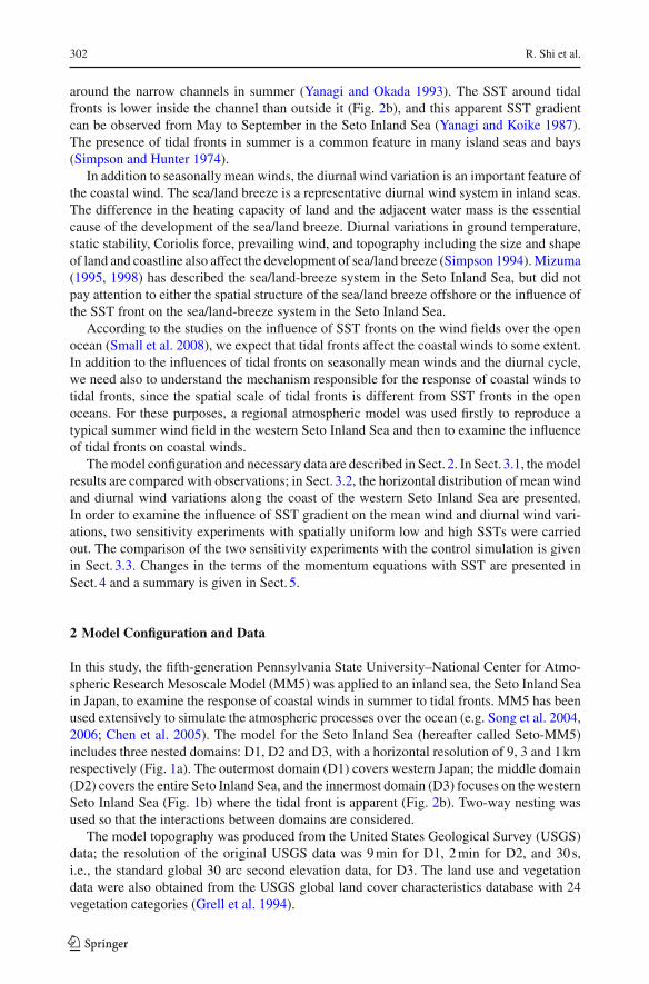
Fig. 1 Map of model domains (a). D1, D2 and D3 denote three model domains in Seto-MM5. The SetoInland Sea is surrounded by Honshu (H), Shikoku (S) and Kyushu (K) Islands. Detailed map of D3 domain(b), in which H. Str. denotes the Hayasui Strait, H. Bay denotes the Hiroshima Bay, and black dots denote theAMeDAS observatories

131oE 132

oE 133

oE

Longitude

Lat

itu

de

Initial surface wind (m s-1)

0.0

0.5

1.0

1.5

2.0

2.5

3.0

3.5

4.0

MSST (K)

294

295

296

297

298

299

300

301

302

303

33oN

34oN

Lat

itu

de

Terrain elevation (m)

0

200

400

600

800

1000

1200

1400

1600

Initial surface pressure (Pa)

101300

101320

101340

101360

101380

101400

101420

101440

101460(c) (d)

(b)

August

(a)

33oN

34oN

131oE 132

oE 133

oE

Longitude

Fig. 2 Topography of D3 domain (a). The mean SST in August from 1964 to 1993 in the D3 domain (b) usedin the control simulation of Seto-MM5. Initial conditions for surface winds and surface pressures are shownin (c) and (d)

123

302 R. Shi et al.

around the narrow channels in summer (Yanagi and Okada 1993). The SST around tidalfronts is lower inside the channel than outside it (Fig. 2b), and this apparent SST gradientcan be observed from May to September in the Seto Inland Sea (Yanagi and Koike 1987).The presence of tidal fronts in summer is a common feature in many island seas and bays(Simpson and Hunter 1974).

In addition to seasonally mean winds, the diurnal wind variation is an important feature ofthe coastal wind. The sea/land breeze is a representative diurnal wind system in inland seas.The difference in the heating capacity of land and the adjacent water mass is the essentialcause of the development of the sea/land breeze. Diurnal variations in ground temperature,static stability, Coriolis force, prevailing wind, and topography including the size and shapeof land and coastline also affect the development of sea/land breeze (Simpson 1994). Mizuma(1995, 1998) has described the sea/land-breeze system in the Seto Inland Sea, but did notpay attention to either the spatial structure of the sea/land breeze offshore or the influence ofthe SST front on the sea/land-breeze system in the Seto Inland Sea.

According to the studies on the influence of SST fronts on the wind fields over the openocean (Small et al. 2008), we expect that tidal fronts affect the coastal winds to some extent.In addition to the influences of tidal fronts on seasonally mean winds and the diurnal cycle,we need also to understand the mechanism responsible for the response of coastal winds totidal fronts, since the spatial scale of tidal fronts is different from SST fronts in the openoceans. For these purposes, a regional atmospheric model was used firstly to reproduce atypical summer wind field in the western Seto Inland Sea and then to examine the influenceof tidal fronts on coastal winds.

The model configuration and necessary data are described in Sect. 2. In Sect. 3.1, the modelresults are compared with observations; in Sect. 3.2, the horizontal distribution of mean windand diurnal wind variations along the coast of the western Seto Inland Sea are presented.In order to examine the influence of SST gradient on the mean wind and diurnal wind vari-ations, two sensitivity experiments with spatially uniform low and high SSTs were carriedout. The comparison of the two sensitivity experiments with the control simulation is givenin Sect. 3.3. Changes in the terms of the momentum equations with SST are presented inSect. 4 and a summary is given in Sect. 5.

2 Model Configuration and Data

In this study, the fifth-generation Pennsylvania State University–National Center for Atmo-spheric Research Mesoscale Model (MM5) was applied to an inland sea, the Seto Inland Seain Japan, to examine the response of coastal winds in summer to tidal fronts. MM5 has beenused extensively to simulate the atmospheric processes over the ocean (e.g. Song et al. 2004,2006; Chen et al. 2005). The model for the Seto Inland Sea (hereafter called Seto-MM5)includes three nested domains: D1, D2 and D3, with a horizontal resolution of 9, 3 and 1 kmrespectively (Fig. 1a). The outermost domain (D1) covers western Japan; the middle domain(D2) covers the entire Seto Inland Sea, and the innermost domain (D3) focuses on the westernSeto Inland Sea (Fig. 1b) where the tidal front is apparent (Fig. 2b). Two-way nesting wasused so that the interactions between domains are considered.

The model topography was produced from the United States Geological Survey (USGS)data; the resolution of the original USGS data was 9 min for D1, 2 min for D2, and 30 s,i.e., the standard global 30 arc second elevation data, for D3. The land use and vegetationdata were also obtained from the USGS global land cover characteristics database with 24vegetation categories (Grell et al. 1994).

123

Tidal Fronts on Coastal Winds Over an Inland Sea 303

The medium range forecast planetary boundary-layer scheme in MM5 was chosen inour simulations since it is an efficient scheme based on the Troen–Mahrt non-local verticaldiffusion theory (Troen and Mahrt 1986), and has been demonstrated to successfully simu-late realistic daytime boundary-layer structure (Hong and Pan 1996). The surface roughnesslength over the water is calculated using Charnock’s equation z0 = Cu2∗/g + o, where C isthe Charnock coefficient (= 0.032), u∗ is the friction velocity (m s−1), g is the accelerationdue to gravity (= 9.806 m s−2), and o is a small constant (= 10−4).

Following Lo et al. (2007), who presented the benefit of using the Noah land-surfacemodel (Chen and Dudhia 2001) in simulating the sea/land breeze, we also adopted the sameland-surface model. In addition, the simple explicit microphysical parameterisation for cloudwater, rainwater, and ice (Dudhia 1993) and the Grell convective parameterisation scheme(Grell 1993) were used in our simulations. A cloud radiation scheme was used for shortwaveradiation processes while a rapid radiative transfer model (Mlawer et al. 1997) was used forlongwave radiation processes.

The three domains (D1, D2, and D3) in Seto-MM5 were initialised with the grid-pointmesoscale model (MSM) re-analysis data, which were produced by the Japanese Meteo-rological Agency non-hydrostatic model (Saito et al. 2006). The MSM re-analysis data areavailable from 22.4◦N to 47.6◦N and 120◦E to 150◦E with a resolution of 0.1◦ ×0.125◦ at 16pressure levels and a time interval of 3 h (Saito et al. 2006). The lateral boundary conditionsfor D1 were also supplied by the MSM re-analysis data.

An accurate SST field is an important boundary condition for this study. We used theSST from the Marine Information Research Center (MIRC) in Japan for the domain insidethe Seto Inland Sea. The initial MIRC SST is from monthly hydrographic survey data, andis available from 1964 to 1993. Figure 2 shows the SST distribution in the D3 domain inAugust, averaged over the period of 1964–1993. Two low SST areas are apparent near theHayasui Strait and south of Aki-nada, respectively (see Fig. 1b for the names used in text:‘nada’ is a Japanese word denoting a wide-water like bay). For the domain outside the SetoInland Sea, we used the operational SST and sea-ice analysis data, which combine satellitedata from the group for high resolution SST and in situ observations (Stark et al. 2007).

The simulation period was selected as 0000 UTC (0900 LST) 5th August to 0000 UTC(0900 LST) 7th August 2006 when the seasonal winds were weak and the weather conditionsstable. The initial conditions for surface winds and surface pressure fields are given in Fig. 2cand d. The observation data used to validate model results were from the Automated Mete-orological Data Acquisition System (AMeDAS), operated by the Japanese MeteorologicalAgency.

3 Results and Analysis

3.1 Comparison with Observations

Both the Seto-MM5 results and MSM re-analysis data were interpolated to all theAMeDAS observatories in the D3 domain (see Fig. 1b for their positions) and comparedwith observations to confirm the precision of the two models. Two statistical parameters, theroot-mean-square-error (RMSE) and mean error (MEAN), were calculated from,

RMSE =√∑i=N

i=1

(Xi

m − Xia

)2

N, (1)

123

304 R. Shi et al.

Table 1 Comparison of MSM and Seto-MM5 results with observations from 86 AMeDAS observatories inthe D3 domain

MSM Seto-MM5

RMSE of wind speed (m s−1) 1.23 1.32

MEAN of wind speed (m s−1) 0.94 1.06

RMSE of temperature (K) 2.08 1.88

MEAN of temperature (K) 1.81 1.61

The wind speed is at the height of 10 m while the air temperature is at a height of 2 m. See text for definitionsof RMSE and MEAN

(a) (b)Seto-MM5 surface temperature (K) MSM surface temperature (K)

Lat

itu

de

(o)

Longitude (o) Longitude (o)

Fig. 3 Horizontal distributions of surface temperature at 2-m height simulated by the Seto-MM5 using MIRCSST (a) and that from MSM (b). Time of (a) and (b) was 1500 LST on 6 August 2006, 30 h after the Seto-MM5simulation commenced

MEAN = 1

N

i=N∑i=1

∣∣∣Xim − Xi

a

∣∣∣, (2)

where Xm denotes the model variable, Xa is the corresponding variable for the AMeDASobservations, N is the data number, and i is the station number. We choose surface wind speedand surface air temperature as comparison variables. According to Table 1, the Seto-MM5had the same precision as the MSM at the AMeDAS observatories.

Although the MSM and Seto-MM5 show little difference in the statistical parameterscompared to observations over the land, they presented an apparent difference in the hor-izontal distribution of surface air temperature and winds over the sea. As an example, wepresent the surface air temperature over the sea from two models in Fig. 3. The surface airtemperature in the Seto-MM5 responded well to the two lowest SST areas in the prescribedMIRC SST distribution (Fig. 2b) and showed a clear gradient of the surface air temperatureover the sea (Fig. 3a), while for the MSM results the surface air temperature was generallyuniform (Fig. 3b).

123

Tidal Fronts on Coastal Winds Over an Inland Sea 305

3.2 Harmonic Analysis on the Near-Surface Winds

According to the wind-fields at every hour (figures not shown here), the surface wind simu-lated by the Seto-MM5 was stronger over the sea than over the land. The MSM gave a moreuniform and weaker wind field than Seto-MM5. An alteration of wind direction can be foundin the results of Seto-MM5. The south-westerly landward flow in the daytime turned to a north-erly or easterly seaward wind at night over Iyo-nada. This alteration could also be confirmedat the AMeDAS observatories along the coast but was not well represented by the MSM.

To separate the mean and diurnal variation components in the wind fields during thesimulation period, we carried out a harmonic analysis, in which eastward and northwardcomponents of the wind are represented by following equations,

u (t) = u + au sin ωt + bu cos ωt + resu (3a)

v (t) = v + av sin ωt + bv cos ωt + resv (3b)

where, u and v denote the eastward and northward wind component, t is time, u, v are themean values, ω is the diurnal frequency, au, av, bu and bv are four harmonic constants forthe diurnal variation with the unit of velocity; and res is the residual. Using the least squaresmethod to minimize the residual res, the mean value (u, v) and four harmonic constantscan be obtained from hourly model results or observations during the simulation period. Thediurnal variation of the wind vector forms an ellipse whose major axis and orientation can becalculated from the four harmonic constants. The major axis denotes the magnitude of thediurnal wind variation while the orientation of the axis gives the direction of the strongestdiurnal wind component: 48 h of AMeDAS data, Seto-MM5 and MSM results from 0100UTC on 5 August to 0000 UTC on 7 August were used to calculate the mean values andharmonic constants in Eqs. 3a and 3b.

The daily mean winds at the observatories along the western Seto Inland Sea coast weregenerally weak except for the northern coastal location of Suo-nada (Fig. 4a, c). In general, theSeto-MM5 model overestimated the mean wind at several AMeDAS observatories (Fig. 4a)while the MSM underestimated the mean wind at most observatories (Fig. 4c). The strongwestward mean wind along the northern coast of Suo-nada is reproduced by the Seto-MM5but not found in the MSM results.

The major axes of the diurnal wind ellipses are perpendicular to the coastline at mostobservatories (Fig. 4b, d), a feature of the sea/land breeze. The lengths of the ellipse’s majoraxes at the observatories indicate a large spatial variation in the magnitude of the diurnalwind variations. For example, the diurnal wind variations were apparent along the southcoast of Suo-nada, but weak along the northern coast. The Seto-MM5 reproduced well thefeatures of the diurnal wind variations (Fig. 4b) while the MSM apparently underestimatedthe magnitude of the diurnal wind variations (Fig. 4d).

Generally, the sea/land breeze over land weakens with distance from the coast; this fea-ture is demonstrated by the magnitudes of the diurnal wind variations, which were calculatedusing both observations and model results (Seto-MM5 and MSM) at all the AMeDAS obser-vatories in the D3 domain, versus the distance from the coast (Fig. 5). The observationsfor AMeDAS suggest that the penetration distance of the sea/land breeze to the land duringthe simulation period was approximately 20 km, within which the magnitude of the sea/landbreeze fell sharply in the area over a distance less than 5 km from the coast. The Seto-MM5model reproduced a strong diurnal variation of wind speed over the area close to the coast butoverestimated the diurnal variation for the area greater than 5 km from the coast. The MSMfailed to reproduce the strong diurnal variations of wind over the area close to the coast.

123

306 R. Shi et al.

4 m s-1

AME

Seto-MM5

4 m s-1

AME

MSM

Longitude

Lat

itu

de

131oE 132

oE 133

oE

33oN

34oN

4 m s-1

AME

MSM

Lat

itu

de

33oN

34oN

4 m s-1

AME

Seto-MM5

(a) (b)

(c) (d)

Mean wind vectors Diurnal variation ellipses

Longitude131

oE 132

oE 133

oE

Fig. 4 Mean surface winds from a harmonic analysis from results of Seto-MM5 (red arrows in a), those ofMSM (red arrows in c), and those of observations (blue arrows in a and c). Diurnal variations in surface windsfrom results of Seto-MM5 (red ellipses in b), those of MSM (red ellipses in d), and those of observations (blueellipses in b and d). AMeDAS observatories in a–d are limited to those with a distance of less than 10 kmfrom the coast

3.3 Sensitivity Experiments

In order to examine the influence of the SST and the SST gradient on the wind fields calculatedby the Seto-MM5, two additional experiments were carried out. One used a uniform SSTof 296 K (CSST case) and the other 300 K (WSST case). The two values of SST representthe lowest and highest SSTs in our study area. In two additional experiments, only the SSTin the D3 domain was changed while the other model parameters, as well as the initial andboundary conditions, were the same as in the control simulation using realistic SST (MSSTcase). Since the change of the SST affects both the mean and diurnal components of the windfields, we again used the harmonic analysis to separate them.

There was little change in the direction of the mean winds among the three cases, whilethe change was relatively apparent in the magnitude of the mean winds (Fig. 6a, c, e).A strong southerly or south-easterly wind can be found over the area from the Bungo Channel

123

Tidal Fronts on Coastal Winds Over an Inland Sea 307

0 10 20 30 40 50 60 700

1

2

3

4

5

Distance (km)

Mag

nit

ud

es (

m s

-1)

AMeDAS

Seto-MM5

MSM

Fig. 5 Reduction in the diurnal variation magnitude in surface winds (ordinate) with distance from the coast(abscissa) as given at all AMeDAS observatories in the D3 domain for the results of Seto-MM5 (red crosses),those of MSM (black stars) and the observations (blue dots)

to Suo-nada. Its magnitude over the northern part of Bungo Channel and south-western partof Iyo-nada is larger in the WSST case (Fig. 6c) than in the other two cases. The low SSTassociated with the tidal front in the MSST case and the low SST itself in the CSST caseweakened the winds over those areas. The south-easterly wind in Suo-nada is stronger inthe MSST case than in the WSST and CSST cases, suggesting a possibility of accelerationin the MSST case as the air flows from cold to warm water. In the next section, we discussthis possibility by examining the change in the terms in the momentum equations with SSTvariations.

The magnitudes of diurnal components in the wind field from the MSST case (Fig. 6b)suggest that there are apparent diurnal variations with a magnitude larger than 2 m s−1 fromthe Bungo Channel towards Hiroshima Bay along the eastern part of Iyo-nada, whereas themean wind is relatively weak. It is therefore expected that the wind changes direction fromdaytime to nighttime in these areas where the magnitude of the diurnal components are largerthan the mean wind speed. The diurnal variation is generally weak over Suo-nada and cantherefore affect only the wind speed there. It is worth noting that the apparent diurnal vari-ation (>2 m s−1) of wind speed occurs in a larger range (>10 km offshore) over the sea thanover the land (<10 km from the coast, Fig. 5).

Compared with the CSST case (Fig. 6f), the WSST case expanded the area where the mag-nitudes of the diurnal component are larger than 2.5 m s−1. Such intensification is apparentover the Bungo Channel, the western part of Iyo-nada and Aki-nada (Fig. 6d). Differences inthe diurnal variations between the MSST and CSST cases are not as apparent as the differencebetween the CSST and the WSST case. Therefore, the influence of SST itself on the diurnalwind variations is more important than that of the SST gradient due to the tidal front.

In summary, the Seto-MM5 reproduced well the spatial variation of mean winds and thediurnal wind variations in the Seto Inland Sea for a typical summer weather condition. Basedon the Seto-MM5, the influence of SST variations due to a tidal front on the surface winds wasexamined with additional two sensitivity simulations, in which high and low uniform SSTwas specified, respectively. Comparison of two sensitivity simulations with the simulation

123

308 R. Shi et al.

33oN

34oN

131oE 132

oE 133

oE

Longitude

Lat

itu

de

33oN

34oN

Lat

itu

de

MSST

CSST

(e)

(a)

33oN

34oN

Lat

itu

de

WSST

(c)

WSST

(d)

CSST

(f)

0.0

1.0

2.0

3.0

4.0

5.0

MSST

(b)

131oE 132

oE 133

oE

Longitude

0.0

1.0

2.0

3.0

4.0

5.0

6.0 (m s

0.0

1.0

2.0

3.0

4.0

5.0

6.0 (m s-1)

-1)

6.0 (m s-1)

Fig. 6 Mean near-surface winds from the MSST case (a), from the WSST case (c) and from the CSST case(e); the magnitude of diurnal variation in near-surface winds from the MSST case (b), from the WSST case(d), and from the CSST case (f). Shaded colours in the left panels denote the mean wind speeds. The contourinterval for all panels is 0.5 m s−1

using realistic SST indicated that the tidal front had significant influences on the mean windsover the sea. The presence of SST gradient around the tidal front had apparent influences onthe mean surface wind speed. The mechanism responsible for the change in mean surfacewinds is further discussed below.

123

Tidal Fronts on Coastal Winds Over an Inland Sea 309

4 Dynamical Analysis and Discussions

The sensitivity analysis suggests an influence by both SST and SST gradients on the meannear-surface wind (Fig. 6a, c, e). To understand the physical processes that affect the responseof the mean winds to the change in SST, we examined the terms in the momentum equations.Since the northward wind component is the major surface wind component across the tidalfront, we focused on the northward wind component in the following discussion. The sameprocedures can be applied to the eastward wind component.

In terms of terrain-following σ coordinates (x, y, σ ), the horizontal momentum equationof MM5 for the northward component (v) is:

∂v(t)

∂t= P + A + C + R + VD + HD, (4)

where t is time, and P,A,C,R, VD and HD denote the terms of perturbation pressure gradi-ent, advection, Coriolis force, curvature effect, vertical diffusivity and horizontal diffusivity,respectively. Detailed expressions for these terms are:

P = −m

ρ

(∂p′

∂y− σ

p∗∂p∗

∂y

∂p′

∂σ

), (5a)

A = −u∂v

∂x− v

∂v

∂y− σ

∂v

∂σ, (5b)

C = −f u + ew sin α, (5c)

R = −u

(u

∂m

∂y− v

∂m

∂x

)− vw

rearth

, (5d)

where m is a map-scale factor, ρ is density, p∗ is the reference pressure defined as the pressuredifference between the surface and top of atmosphere, p′ is perturbation pressure; u, v andσ respectively denote eastward, northward and vertical velocity under the σ coordinates,f = 2� sin λ and e = 2� cos λ, in which λ is latitude, � is the rate of the earth’s rotation,α = φ −φc, φ is longitude, and φc is the central longitude of the model domain; rearth is theEarth’s radius. Detailed expressions of VD and HD are not explained here but can be foundin detail in Hong and Pan (1996).

4.1 Responses of Mean Wind and Forcing Terms to Variations in SST

The mean northward wind speed V during the simulation period (48 h) can be expressed as,

V = 1

n

m=n∑m=1

vm = 1

n

m=n∑m=1

(v0 + t

i=m∑i=1

Fi

)= v0 + t

n

i=n∑i=1

(n − i + 1) Fim, (6)

where m is the index of the integration step, n is the number of total integration steps duringthe simulation period, vm is the northward component of winds at an integration step m,t

is the timestep, v0 is the initial value, F is the sum of the right-hand side terms in Eq. 4 ateach timestep. The difference in the mean wind speed from its initial value is expressed as,

V − v0 = t

n

i=n∑i=1

(n − i + 1) Fi = SF. (7)

123

310 R. Shi et al.

-50-40-30-20-10010203040

50 (m s-1)

-3.0

-2.0

-1.0

0.0

1.0

2.0

3.0 (m s-1) MSST WSST WSST CSST WSST

131oN 132

oN 133

oN

33oN

34oN

V v0

(d)

(f) (g)

(e)

(c)(b)(a)

Longitude

Lat

itu

de

ΔVΔV

PSΔPSΔ

ΔSVD ΔSVD

33oN

34oN

Lat

itu

de

33oN

34oN

Lat

itu

de

131oN 132

oN 133

oN

Longitude131

oN 132

oN 133

oN

Longitude

-50-40-30-20-10010203040

50 (m s-1)

Fig. 7 Differences of the mean northward wind speed from the initial values in the WSST case (a). Differencein the mean northward wind speed V , of the perturbation pressure gradient term SP , and of the verticaldiffusivity term SV D between the MSST case and the WSST case (b, d, f), and between the CSST case andthe WSST case (c, e, g). The wind curls near the coast (within two grids, 6 km from coast), where the variationwas significantly influenced by the land, are not shown in d, f. The forcing terms in each case were calculatedby the right-hand side of Eq. 7. Units are in m s−1 in all panels. Black line in a denotes a cross-section alongwhich the vertical structure of potential temperature, perturbation pressure and northward wind speed aregiven in Figs. 10, 11, 12 and 14

According to Eq. 7, the difference of the mean northward wind speed from its initial valuearises from SF , in which S is the arithmetic calculation in Eq. 7 whereas F is replaced by theright-hand side terms in Eq. 4. Consequently, SF includes the contribution from the termsof the perturbation pressure gradient (SP ), advection (SA), Coriolis force (SC), curvatureeffect (SR), vertical diffusivity term (SVD) and horizontal diffusivity (SHD). During thesimulations, each of the right-hand side terms in Eq. 4 was saved at every timestep and thearithmetic calculations in Eq. 7 were then carried out. From the examination of each termin SF , we determined which term was important in the wind development from the initialvalue. Furthermore, since the initial values v0 were the same in the three cases of WSST,CSST and MSST, the difference in the mean northward wind component could be directlyrelated to the response of the forcing terms in SF .

123

Tidal Fronts on Coastal Winds Over an Inland Sea 311

0 25

0

1

2

R2 =0.17

ΔSP (m s-1)

ΔV (

m s

-1)

MSST case WSST case

R2=0.10

R2=0.14

CSST case WSST case

R2=0.17

50-25-50-3

-2

-1

0

1

2

ΔV (

m s

-1)

-3

-2

-1

0 25

ΔSP (m s-1) 50-25-50 0 25

ΔSP (m s-1) 50-25-50

0 25

ΔSP (m s-1) 50-25-50

0

1

2

ΔV (

m s

-1)

-3

-2

-1

0

1

2

ΔV (

m s

-1)

-3

-2

-1

Fig. 8 The scatter plot of the difference in the mean northward wind speed V versus the difference in theperturbation pressure gradient term SP ; and versus the difference in the vertical diffusivity term SV D

between the MSST case and the WSST case (a, c); and between the CSST case and the WSST case (b, d) atall sea grids in the D3 domain. The values less than 10−2 m s−1 and the values at the closest three grids fromcoast were removed. The red line in each panel is the linear regression line given by the least-square method.R2 is the determination coefficient

The differences of the mean northward wind components from the initial values in theWSST case (the difference between Figs. 6c and 2c) are the development of the northwardwind speed over the entire domain (Fig. 7a). The mean northward wind speed is weaker in theMSST case than in the WSST case (Fig. 7b). Such a reduction in the mean northward windspeed is attributed mostly to the negative difference in the perturbation pressure gradient termbetween the two cases (Fig. 7d). The CSST case also simulated a weaker mean northwardwind speed than did the WSST case (Fig. 7c). Such a change in wind speed is partly causedby the negative difference in the perturbation pressure gradient term (Fig. 7e) and partly fromthe negative difference in the vertical diffusivity term at the Bungo Channel (Fig. 7g). Sincethe advection and Colioris forces are directly affected by the wind speed variation rather thanby variation of the underlying SST, and the curvature effect and horizontal diffusion weremuch smaller than the other terms, these forcing terms will not be discussed in detail.

Although both the perturbation pressure gradient term and vertical diffusivity term likelycontribute to the variation in surface wind speed (Fig. 7), their effects were different (Fig. 8).The difference in the mean northward wind speed (V ) between the MSST case and theWSST case has an apparent positive linear relationship with the difference in the perturba-tion pressure gradient term (SP ) (Fig. 8a), and has a negative linear relationship with the

123

312 R. Shi et al.

20

40

60F

req

uen

cy (

%)

0-5 -4 -3 -2 -1 0 1 2 3 4

0

20

40

60

Fre

qu

ency

(%

)

(b)

(a)

ΔSVD /ΔSP (MSST WSST)

5

-5 -4 -3 -2 -1 0 1 2 3 4

ΔSVD /ΔSP (CSST WSST)

5

Fig. 9 Histogram of the occurrence frequency for the ratio of the difference in vertical diffusivity term SV D

to the difference in the perturbation pressure gradient term SP between the MSST case and the WSST case(a); between the CSST case and the WSST case (b). The ratio was calculated from the values given in Fig. 8.The abscissa denotes the range of ratio and the ordinate denotes the occurrence frequency. There are ten rangesfor the ratio from −5 to 5 with an interval of one as shown in the abscissa

difference in the vertical diffusivity term (SV D) (Fig. 8c). The same positive and nega-tive linear relationships can also be confirmed between the CSST case and the WSST case(Fig. 8b, d). The Fisher–Snedecor F -test was used to further examine the significance ofthe linear regressions in Fig. 8. For the significance level α = 0.01, the critical value of thedetermination coefficient is 4.6 × 10−4 for the sample number (n = 14277) in Fig. 8. There-fore, the linear regressions in Fig. 8 were significant because the determination coefficientsin Fig. 8 were much larger than the critical value.

Two new variables were defined to further examine the relative importance of perturba-tion pressure gradient and vertical diffusivity terms. The ratio of the perturbation pressuregradient term to the vertical diffusivity term was defined as η = SV D/SP . The occur-rence frequency of the ratio was defined as f (η) = γ /ζ , where ζ is the total number ofsea-grid points at which η was calculated; γ is the number of grid points where η is withina given range. The occurrence frequencies of the ratio from −5 to 5, with an interval of 1,are presented in Fig. 9. Beyond the range from −5 to 5, the occurrence frequency is smallenough to be neglected.

The occurrence frequency in the range −1 < η < 0 was over 40% (Fig. 9), suggestingthat for over 40% of the total sea surface, the difference in vertical diffusivity has an oppositesign to, but smaller magnitudes than, the difference in the perturbation pressure gradient.The occurrence frequency in the range |η| < 1 was larger than 60% (Fig. 9a, b), indicating

123

Tidal Fronts on Coastal Winds Over an Inland Sea 313

296

296

296.5296.5297297

297.5297.5298298

298.5298.5 299

299 299.5299.5 300

300

304304308308

316316

Lo

gar

ith

mic

hei

gh

t (m

)

5

10

20

50

100

200

500

1000

2000

4000

(c)

Lo

gar

ith

mic

hei

gh

t (m

)

5

10

20

50

100

200

500

1000

2000

4000

(d)

-40

-20

0

20

40

60

80

Tota

l hea

t fl

ux

(W m

-2)

WSSTMSSTCSST

(e)

294296298300302304306

SS

T (

K)

32.8 33.0 33.2 33.4 33.6 33.8Latitude (°)

WSSTMSSTCSST

WSSTMSSTCSST

296.5

297

297.5297.

5

298

298

298.5

298.

5

299299 299.5

299.5 300300

304304308308

316316

Lo

gar

ith

mic

hei

gh

t (m

)

5

10

20

50

100

200

500

1000

2000

4000(b) Mean θ (MSST)

Mean θ (CSST)

298.

5

299

299299.5

299.5 300300

304304308308

316316

(a) Mean θ (WSST)

Fig. 10 Vertical distribution of the mean potential temperature (K) simulated by the WSST case (a), by theCSST case (b), and by the MSST case (c) at the cross-section shown in Fig. 7a. The abscissa denotes latitudeand the ordinate denotes the logarithm of height. The sum of the sensible and latent total fluxes (d) and theSST distribution (e) along the cross-section are shown in three cases

the area, for which the difference in vertical diffusivity is generally smaller than that in theperturbation pressure gradient, is over 60% of the total sea surface.

Therefore, the perturbation pressure gradient is more effective than diffusivity in modify-ing the sea-surface wind.

4.2 Response of Vertical Structure to Variations in SST

To understand the extent to which the SST affects the vertical structure of the marine atmo-spheric boundary layer, we examined the vertical distributions of several variables along asection across the tidal front (Fig. 7a).

According to the vertical distribution of the potential air temperature along a cross-section,the air is well mixed in the WSST case (Fig. 10a) and the mixed layer reaches a height of over200 m. In the MSST case, the mixed layer is over 200 m in depth in the southern high SSTarea, nearly disappears over the central low SST area, and then redevelops in the northern

123

314 R. Shi et al.

11701180

1180119011901200

12001220 1220

1260 12601300 1300

1400 1400

1600 16001800 18002000 2000

3000 3000

4000 4000

Lo

gar

ith

mic

hei

gh

t (m

)Mean p

5

10

20

50

100

200

500

1000

2000

4000

11801190

11901200 1200

1220 1220

1260 12601300 1300

1400 1400

1600 16001800 1800

000 2000

3000 3000

4000 4000

Lo

gar

ith

mic

hei

gh

t (m

)

Mean p

5

10

20

50

100

200

500

1000

2000

4000

(a)

(c)

(e)

32.8 33.0 33.2 33.4 33.6 33.8294296298300302304306

Latitude (°)

SS

T (

K) WSST

MSSTCSST

11801180

119011901200 1200

1220 12201260 1260

1300 13001400 1400

1600 16001800 1800

2000 2000

3000 3000

Lo

gar

ith

mic

hei

gh

t (m

) 4000 4000

Mean p

5

10

20

50

100

200

500

1000

2000

4000(b)

(d)

-0.8

-0.6

-0.4

-0.2

0.0

0.2

0.4

0.6WSSTMSSTCSST

−∂p

/∂y

(×10

-3 P

a m

-1)

Fig. 11 Same as Fig. 10 but for the mean perturbation pressure (Pa) in three cases (a–c) and the meridionalgradient of perturbation pressure in three cases along the cross-section (d)

high SST area (Fig. 10b). The mixed layer nearly disappears in the CSST case, giving anapparent stable stratification along the cross section (Fig. 10c).

The air inside the mixed layer was heated by warm sea water with high SST in the WSSTcase. The surface potential temperature in the WSST case (≈298.5 K) was lower than theunderlying SST (≈300 K), but that in the CSST case (≈295.5 K) was close to the underlyingSST (≈296 K). The positive air-sea temperature difference in the WSST case produced thelargest total flux (the sum of the latent and sensible heat fluxes) from the sea to the air (redline in Fig. 10d) in three cases, which increased the mixed-layer height. The small air-seatemperature difference in the CSST case reduced the total flux from the sea to the air almost tozero (blue line in Fig. 10d), and maintained stratification in the air. The MSST case releasednearly the same total flux over the two sides of the cross-section as did the WSST case, but asmall or even negative total flux in the central area of the cross-section occurred (black linein Fig. 10d), therefore limiting the development of a mixed layer in that area.

In all three cases, the surface mean perturbation pressure was low in the central area andhigh on the two sides of the cross-section (Fig. 11a–c). As a result, the northward pressuregradient forcing (Fig. 11d) accelerates the northward wind component from the southern

123

Tidal Fronts on Coastal Winds Over an Inland Sea 315

-1-1

1-0.8

-0.8

-0.8

-0.6

-0.6

-0.6

-0.4

-0.4

-0.4 -0.4

-0.2-0.2

-0.2-0.2-0.2 -0.2

00

0 0 00

0 00

0

0

0

0 0

00

00

0.2

0.2

0.40.4

Lo

gar

ith

mic

hei

gh

t (m

)

5

10

20

50

100

200

500

1000

2000

4000

1

1

1

2

2 2

2

22

3

3

3

3

Lo

gar

ith

mic

hei

gh

t (m

)

5

10

20

50

100

200

500

1000

2000

4000

(a)

(c)

V (WSST)

294296298300302304306

SS

T (

K)

(d)

32.8 33.0 33.2 33.4 33.6 33.8Latitude (°)

WSSTMSSTCSST

ΔV (CSST WSST)

-0.8 - 08-0.6

-0.4-0.4

-0.2

-0.2

-0.2-0.2 --0.2

0.2

0

0

0 0

0

0

0

00

0

0

00 00

0

0 0

00

00

0.20.2

0.2

0.4

Lo

gar

ith

mic

hei

gh

t (m

)

5

10

20

50

100

200

500

1000

2000

4000

(b) ΔV (MSST WSST)

Fig. 12 Same as Fig. 10 but for the mean northward wind speed (m s−1) of WSST case (a), the difference inthe mean northward wind speed between the MSST case and the WSST case (b), and that between the CSSTcase and the WSST case (c). The dashed contour lines in b and c show the reduction of the northward windspeed

side to the central area of the cross-section, while the southward pressure gradient forcingdecelerates the northward wind component from the central area to the northern side of thecross-section (Fig. 12a). The change in air density with potential temperature affected thesurface perturbation pressure distribution and therefore modified the surface winds.

The potential air temperature over the central area of the cross-section was lower in theMSST case than in the WSST case. As a result, the denser air due to a lower potentialtemperature increased the surface perturbation pressure at the central area and consequentlychanged the horizontal perturbation pressure gradient. In the southern section, where the airflows from the high SST area to the low SST area, the surface perturbation pressure in theMSST case was nearly the same as that in the WSST case over the high SST area, but itincreased over the low SST area (Fig. 11b). Such variations in the MSST case weakened thenorthward pressure gradient forcing (Fig. 11d, 32.8◦N–33.3◦N), as well as an increase of thenorthward surface wind speed, which resulted in a lower northward surface wind speed overthe southern tidal front than in the WSST case (Fig. 12b). In the northern area where the airflows from low to high SST area, the increase in SST from the central to the northern areaweakens the southward pressure gradient forcing (Fig. 11d, 33.5◦N–33.8◦N) as well as adecrease of the surface northward wind speed. Therefore, the surface northward wind speedis a little larger in the MSST case than in the WSST case (Fig. 12b).

A similar explanation can also be applied to the CSST case. Denser air in the CSST caseincreased the surface perturbation pressure through the cross-section, and changed the hori-zontal gradient of the surface perturbation pressure. In the southern area of the cross-section,

123

316 R. Shi et al.

131oE 132oE 133oE

33oN

34oN

Longitude

Lat

itu

de

294

295

296

297

298

299

300

301

302

303 (K)(b)

MSST_IF

(a)

MSST_NF

131oE 132oE 133oE

Longitude

Fig. 13 Horizontal distribution of SST in the case without the tidal front (a, MSST_NF), and in the casewith an intensified tidal front (b, MSST_IF) at the Haysui Strait. In the case of MSST_NF, SST less than298 K around the Hayashui Strait was set to 298 K. In the case of MSST_IF, the original in situ SST inside theHayashui Strait was reduced by 1 K and re-interpolated

the northward pressure gradient forcing was weaker in the CSST case than in the WSST case(Fig. 11d, 32.8◦N–33.3◦N). Consequently, the acceleration of the northward wind from thesouthern to the central area was weaker in the CSST case than in the WSST case. At thenorthern side of the cross-section, the southward pressure gradient forcing was stronger inthe CSST case than in the WSST case (Fig. 11d, 33.5◦N–33.8◦N) and therefore decelerationwas stronger in the CSST case than in the WSST case. As a whole, the surface northwardwind component was weaker in the CSST case than in the WSST case (Fig. 12c).

In addition to the change in pressure gradients with SST, the vertical profile of the windspeed also corresponded to the development of the mixed layer, which was strongly affectedby the underlying SST. The maximum northward wind speed occurred at a height of approx-imately 200 m. Below this, the WSST case produced a well-mixed wind-speed profile atthe cross-section (Fig. 12a) while the CSST case produced strong shear as implied by thedifferential reduction in wind speed in the vertical direction (Fig. 12c). In the MSST case(Fig. 12b), the wind speed profile was well-mixed over the high SST area but sheared overthe low SST area.

The variations in SST (Fig. 2b) include two parts: the first is for a slow change from theoffshore to the inland sea, and the second is the abrupt change near the Hayasui Strait dueto the presence of the tidal front. Since the SST used in the MSST case is an average of datafrom 1964 to 1993, it may weaken the intensity of the tidal front. In order to examine theinfluence of tidal front intensity on the near-surface winds, we carried out two additionalsimulations in which only the abrupt SST change near the tidal front was artificially modi-fied. One simulation used the MSST without the tidal front at the Hayasui Strait (Fig. 13a,MSST_NF in short), the other used the MSST with an enhanced tidal front at the strait(Fig. 13b, MSST_IF in short). The two additional simulations confirmed that the presenceof the tidal front weakens the winds in the area upwind of the front and intensifies the windsdownwind of the front (Fig. 14b). Moreover, this effect is likely in proportion to the intensityof the tidal front (Fig. 14b, c).

123

Tidal Fronts on Coastal Winds Over an Inland Sea 317

(d)

32.8 33.0 33.2 33.4 33.6 33.8294296298300302304306

Latitude (°)

SS

T (

K) MSST_NF

MSSTMSST_IF

1

1

1

2

2 2

2

222

3

3

3

3

Lo

gar

ith

mic

hei

gh

t (m

)

5

10

20

50

100

200

500

1000

2000

4000(a) ΔV (MSST_NF)

-0.3

-0.2

-0.1-0.1

0 00

0

0 0

0

0

0

0

0

0

00

0 00

00

0

0

0.1

0.1

0.1

0.2

0.2

0.3Lo

gar

ith

mic

hei

gh

t (m

)

5

10

20

50

100

200

500

1000

2000

4000(c) ΔV (MSST_IF MSST_NF)

-0.2-0.2

-0.1 -0.1

-0.1-0.1

-0.1

00

0

0

0

0 0

0

00

00

0

00

00

0

0.1

0.1

0.1

0.1

0.1

0.1

0.2

0.2

0.2

Lo

gar

ith

mic

hei

gh

t (m

)

5

10

20

50

100

200

500

1000

2000

4000

(b) ΔV (MSST MSST_NF)

Fig. 14 Vertical distribution of mean northward wind speed (m s−1) simulated by the MSST_NF case (a) andthe differences in mean northward wind speed between the MSST case and the MSST_NF case (b) and thatbetween the MSST_IF case and the MSST_NF case (c) at the cross-section shown in Fig. 7a. The abscissa inpanels (a–c) denotes latitude and the ordinate denotes the logarithm of height. The dashed contour lines in band c show the reduction of the northward wind speed. The distribution of SST along the cross-section in theMSST_NF case (red line), the MSST case (black line) and the MSST_IF case (blue line) is shown in d

5 Summary

A regional numerical model of the atmosphere, referred to as Seto-MM5, was configured foran inland sea in Japan to examine the influence of variations in SST associated with a tidalfront on the surface winds. The Seto-MM5 reproduced well the spatial variation in meanwinds, and captured the essential features of diurnal variation in winds, i.e., sea/land breeze,which were also confirmed in observations.

Comparison of two sensitivity simulations, which used spatially uniform high and lowSSTs, along with the control simulation using realistic SST, indicated that the mean windsover the sea were affected by both the SST magnitude and its horizontal gradient, whilevariations in diurnal winds over the sea were affected more by the SST magnitude than byits gradient. Among the results from the three simulations, the direction of the mean windsshowed little difference but the magnitude of the mean winds showed apparent differences.The simulation with high (low) SST gives strongest (weakest) mean winds over most areas.The simulation with realistic SST gave a weak mean wind over the area upwind of the tidalfront and a strong mean wind downwind of the front, suggesting that the presence of the tidalfront likely decelerates the mean winds in the upwind area and accelerates the mean windsin the downwind area.

The changes in the terms of the momentum equations with variations in SST show that thevariation in the perturbation pressure gradient is the dominant factor determining the response

123

318 R. Shi et al.

of surface winds to variations in SST. The vertical diffusivity operates as the secondary factorin changing the surface wind. Variations of other terms in the momentum equations dependedclosely on the modification of the surface winds but not on the SST and therefore were notdiscussed in detail.

The perturbation pressure was thermally related to the underlying SST. When the airflows from a high SST area to a low SST area, i.e., entering a tidal front, the air progressivelybecomes cooler and its density increases. The denser air increases the surface perturbationpressure, which induces an additional pressure gradient force with a direction from the lowSST area to the high SST area, and therefore weakens the surface wind speed upwind of thefront. On the other hand, when the air flows from a low SST area to a high SST area, i.e.,departing a tidal front, the situation is reversed and the surface wind downwind of the frontis intensified.

Although the spatial scale of SST fronts in this study are much smaller than that usedby Song et al. (2006), our results are consistent with their conclusion that the perturbationpressure gradient is the dominant force modifying surface winds over a SST front. In thissense, our study expands on their results to the relationship between summer coastal windsand tidal fronts. However, because of the small scale of the tidal front, the deceleration andacceleration of the surface winds in the areas upwind and downwind of the front are weakerthan those occurring over fronts in the open ocean.

Acknowledgments The mesoscale model re-analysis data used in this study were obtained from the dataserver of the Research Institute for Sustainable Humanosphere, Kyoto University. We thank Drs. Gao HW,Zhao L, Gao SH and Wang Q for their useful suggestions and comments. This study was supported by theGlobal COE (Centers of Excellence) Program and the Grants-in-Aid for Scientific Research (22106002) fromthe Ministry of Education, Culture, Sports, Science and Technology, Japan. We thank reviewers for theirinsightful and constructive comments.

References

Chelton DB, Esbensen SK, Schlax MG, Thum N, Freilich MH, Wentz FJ, Gentemann CL, McPhaden MJ,Schopf PS (2001) Observations of coupling between surface wind stress and sea surface temperature inthe Eastern Tropical Pacific. J Clim 14(7):1479–1498

Chelton DB, Schlax MG, Freilich MH, Milliff RF (2004) Satellite measurements reveal persistent small-scalefeatures in ocean winds. Science 303:978–983

Chelton DB (2005) The impact of SST specification on ECMWF surface wind stress fields in the EasternTropical Pacific. J Clim 18(4):530–550

Chen CS, Beardsley RC, Hu S, Xu Q, Lin HC (2005) Using MM5 to hindcast the ocean surface forcing fieldsover the Gulf of Marine and Georges Bank region. J Atmos Ocean Technol 22(2):131–145

Chen F, Dudhia J (2001) Coupling and advanced land surface-hydrology model with the Penn State–NCARMM5 modelling system, Part I: model implementation and sensitivity. Mon Weather Rev 129(4):569–585

Dudhia J (1993) A nonhydrostatic version of the Penn State–NCAR mesoscale model: validation tests andsimulation of an Atlantic cyclone and cold front. Mon Weather Rev 121(5):1493–1513

Grell GA (1993) Prognostic evaluation of assumptions used by cumulus parametreisations. Mon Weather Rev121(3):764–787

Grell GA, Dudhia J, Stauffer DR (1994) A description of the fifth-generation Penn State/NCAR mesoscalemodel (MM5). NCAR Tech Note, NCAR/TN-398+STR, 122 pp. http://nldr.library.ucar.edu/collections/technotes/asset-000-000-000-214.pdf

Hayes SP, McPhaden MJ, Wallace JM (1989) The influence of sea surface temperature on surface wind in theeastern equatorial Pacific: weekly to monthly variability. J Clim 2(12):1500–1506

Hong SY, Pan HL (1996) Non-local boundary layer vertical diffusion in a medium range forecast model. MonWeather Rev 124(10):2322–2339

Lindzen R, Nigam S (1987) On the role of sea surface temperature gradients in forcing low-level winds andconvergence in the tropics. J Atmos Sci 44(17):2418–2436

123

Tidal Fronts on Coastal Winds Over an Inland Sea 319

Lo JCF, Lau AKH, Chen FJ, Fung CH, Leung KKM (2007) Urban modification in a mesoscale model and theeffects on the local circulation in the Pearl River Delta region. J Appl Meteorol Climatol 46(4):457–476

Mahrt L, Vickers D, Moore E (2004) Flow adjustments across sea-surface temperature changes. Boundary-Layer Meteorol 111(3):553–564

Minobe S, Kuwano-Yoshida A, Komori N, Xie SP, Small RJ (2008) Influence of the Gulf Stream on thetroposphere. Nature 452:206–209

Mizuma M (1995) General aspects of land and sea breezes in Osaka Bay and surrounding area. J MeteorolSoc Jpn 73(6):1029–1040

Mizuma M (1998) General aspects of land and sea breezes in western Seto Inland Sea and surrounding areas.J Meteorol Soc Jpn 76(3):403–418

Mlawer EJ, Taubman SJ, Brown PD, Iacono MJ, Clough SA (1997) Radiative transfer for inhomogeneousatmosphere: RRTM, a validated correlated-k model for the longwave. J Geophys Res 102(D14):16663–16682

Nonaka M, Xie SP (2003) Covariations of sea surface temperature and wind over the Kuroshio and its exten-sion: evidence for ocean-to-atmosphere feedback. J Clim 16(9):1404–1413

Saito K, Fujita T, Yamada Y, Ishida JI, Kumagai Y, Aranami K, Ohmori S, Nagasawa R, Kumagai S, MuroiC, Kato T, Eito H, Yamazaki Y (2006) The operational JMA nonhydrostatic mesoscale model. MonWeather Rev 134(4):1266–1298

Simpson JE (1994) Sea breeze and local wind. Cambridge University Press, New York, 234 ppSimpson JH, Hunter JR (1974) Fronts in the Irish Sea. Nature 250:404–406Skyllingstad E, Vickers D, Mahrt L (2007) Effects of mesoscale sea-surface temperature fronts on the marine

atmospheric boundary layer. Boundary-Layer Meteorol 123(2):219–317Small RJ, DeSzoeke SP, Xie SP, O’Neill L, Seo H, Song Q, Cornillon P, Spall M, Minobe S (2008) Air-sea

interaction over ocean fronts and eddies. Dyn Atmos Ocean 45(3–4):274–319Song Q, Hara T, Cornillon P, Friehe CA (2004) A comparison between observations and MM5 simulations of

the marine atmospheric boundary layer across a temperature front. J Atmos Ocean Technol 21(2):170–178

Song Q, Cornillon P, Hara T (2006) Surface wind response to oceanic fronts. J Geophys Res 111(C12):C12006Stark JD, Donlon CJ, Martin MJ, McCulloch ME (2007) OSTIA: an operational, high resolution, real time,

global sea surface temperature analysis system. In Proceedings of the Oceans 2007. Marine challenges:coastline to deep sea, Aberdeen, Scotland, IEEE/OES, 4 pp. http://ghrsst-pp.metoffice.com/pages/latest_analysis/docs/Stark_et_al_OSTIA_description_Oceans07.pdf

Takeoka H (2002) Progress in Seto Inland Sea research. J Oceanogr 58(1):93–107Troen I, Mahrt L (1986) A simple model of the atmospheric boundary layer: sensitivity to surface evaporation.

Boundary-Layer Meteorol 37(1–2):129–148Wallace JM, Mitchell TP, Deser C (1989) The influence of sea surface temperature on surface wind in the

eastern equatorial Pacific: seasonal and interannual variability. J Clim 2(12):1492–1499Xie SP (2004) Satellite observations of cool ocean-atmosphere interaction. Bull Am Meteorol Soc 85(2):

195–208Yanagi T, Koike T (1987) Seasonal variation in thermohaline and tidal fronts, Seto Inland Sea, Japan. Cont

Shelf Res 7(2):149–160Yanagi T, Okada S (1993) Tidal fronts in the Seto Inland Sea. Mem Fac Eng Ehime Univ 12:61–67 (in Japanese)

123