Embed Size (px)
Citation preview

INL/EXT-16-38310
Light Water Reactor Sustainability Program
Grizzly Usage and Theory Manual
B. W. Spencer M. Backman
P. Chakraborty D. Schwen Y. Zhang H. Huang
X. Bai W. Jiang
March 2016
DOE Office of Nuclear Energy

DISCLAIMER
This information was prepared as an account of work sponsored by an agency of the U.S. Government. Neither the U.S. Government nor any agency thereof, nor any of their employees, makes any warranty, expressed or implied, or assumes any legal liability or responsibility for the accuracy, completeness, or usefulness, of any information, apparatus, product, or process disclosed, or represents that its use would not infringe privately owned rights. References herein to any specific commercial product, process, or service by trade name, trade mark, manufacturer, or otherwise, does not necessarily constitute or imply its endorsement, recommendation, or favoring by the U.S. Government or any agency thereof. The views and opinions of authors expressed herein do not necessarily state or reflect those of the U.S. Government or any agency thereof.

INL/EXT-16-38310
Light Water Reactor Sustainability Program
Grizzly Usage and Theory Manual
B. W. Spencer – INL M. Backman – University of Tennesse, Knoxville
P. Chakraborty – INL D. Schwen – INL Y. Zhang – INL H. Huang – INL
X. Bai – INL W. Jiang – INL
March 2016
Idaho National Laboratory Idaho Falls, Idaho 83415
http://www.inl.gov/lwrs
Prepared for the U.S. Department of Energy Office of Nuclear Energy
Under DOE Idaho Operations Office Contract DE-AC07-05ID14517


Acknowledgments
Development of Grizzly is funded by the Risk-Informed Safety Margins Characterization (RISMC) pathway
of the Department of Energy’s Light Water Reactor Sustainability (LWRS) program.
Grizzly includes contributions made by the University of Tennessee, Knoxville (UTK). The support of
Professors Brian Wirth and Robert Dodds at UTK in this effort is gratefully acknowledged.
Much of the general capability for thermomechanical analysis that Grizzly is based on was originally
developed for the BISON nuclear fuel performance modeling code. Likewise, much of the documentation
of these general capabilities provided in this manual was derived from the BISON User’s Manual.
ii

Contents
1 Introduction 11.1 The role of Grizzly in multiscale modeling of RPVs . . . . . . . . . . . . . . . . . . . . . . 1
1.2 Software Environment . . . . . . . . . . . . . . . . . . . . . . . . . . . . . . . . . . . . . 2
1.3 Document Organization . . . . . . . . . . . . . . . . . . . . . . . . . . . . . . . . . . . . . 3
2 Running Grizzly 42.1 Checking Out the Code . . . . . . . . . . . . . . . . . . . . . . . . . . . . . . . . . . . . . 4
2.1.1 Internal Users . . . . . . . . . . . . . . . . . . . . . . . . . . . . . . . . . . . . . . 4
2.1.2 External Users . . . . . . . . . . . . . . . . . . . . . . . . . . . . . . . . . . . . . 5
2.2 Updating Grizzly . . . . . . . . . . . . . . . . . . . . . . . . . . . . . . . . . . . . . . . . 5
2.3 Executing Grizzly . . . . . . . . . . . . . . . . . . . . . . . . . . . . . . . . . . . . . . . . 6
2.4 Getting Started . . . . . . . . . . . . . . . . . . . . . . . . . . . . . . . . . . . . . . . . . 6
2.4.1 Input to Grizzly . . . . . . . . . . . . . . . . . . . . . . . . . . . . . . . . . . . . . 6
2.4.2 Post Processing . . . . . . . . . . . . . . . . . . . . . . . . . . . . . . . . . . . . . 7
2.4.3 Graphical User Interface . . . . . . . . . . . . . . . . . . . . . . . . . . . . . . . . 7
3 Input File Structure 83.1 Basic Syntax . . . . . . . . . . . . . . . . . . . . . . . . . . . . . . . . . . . . . . . . . . 8
3.2 Summary of MOOSE Object Types . . . . . . . . . . . . . . . . . . . . . . . . . . . . . . 9
3.3 Grizzly Syntax Page . . . . . . . . . . . . . . . . . . . . . . . . . . . . . . . . . . . . . . 9
3.4 Units . . . . . . . . . . . . . . . . . . . . . . . . . . . . . . . . . . . . . . . . . . . . . . . 9
4 Common Commands For All Physics 104.1 GlobalParams . . . . . . . . . . . . . . . . . . . . . . . . . . . . . . . . . . . . . . . . . . 10
4.2 Problem . . . . . . . . . . . . . . . . . . . . . . . . . . . . . . . . . . . . . . . . . . . . . 10
4.3 Mesh . . . . . . . . . . . . . . . . . . . . . . . . . . . . . . . . . . . . . . . . . . . . . . 10
4.4 Executioner . . . . . . . . . . . . . . . . . . . . . . . . . . . . . . . . . . . . . . . . . . . 11
4.5 Timestepping . . . . . . . . . . . . . . . . . . . . . . . . . . . . . . . . . . . . . . . . . . 12
4.5.1 ConstantDT . . . . . . . . . . . . . . . . . . . . . . . . . . . . . . . . . . . . . . . 12
4.5.2 FunctionDT . . . . . . . . . . . . . . . . . . . . . . . . . . . . . . . . . . . . . . . 12
4.5.3 IterationAdaptiveDT . . . . . . . . . . . . . . . . . . . . . . . . . . . . . . . . . . 13
4.6 PETSc Options . . . . . . . . . . . . . . . . . . . . . . . . . . . . . . . . . . . . . . . . . 15
4.7 Quadrature . . . . . . . . . . . . . . . . . . . . . . . . . . . . . . . . . . . . . . . . . . . 15
4.8 Variables . . . . . . . . . . . . . . . . . . . . . . . . . . . . . . . . . . . . . . . . . . . . 15
4.9 Kernels . . . . . . . . . . . . . . . . . . . . . . . . . . . . . . . . . . . . . . . . . . . . . 16
4.9.1 TimeDerivative . . . . . . . . . . . . . . . . . . . . . . . . . . . . . . . . . . . . . 16
4.9.2 BodyForce . . . . . . . . . . . . . . . . . . . . . . . . . . . . . . . . . . . . . . . 17
4.10 AuxVariables . . . . . . . . . . . . . . . . . . . . . . . . . . . . . . . . . . . . . . . . . . 17
4.11 Materials . . . . . . . . . . . . . . . . . . . . . . . . . . . . . . . . . . . . . . . . . . . . 18
4.12 Postprocessors . . . . . . . . . . . . . . . . . . . . . . . . . . . . . . . . . . . . . . . . . . 18
4.12.1 ElementalVariableValue . . . . . . . . . . . . . . . . . . . . . . . . . . . . . . . . 19
4.12.2 NodalVariableValue . . . . . . . . . . . . . . . . . . . . . . . . . . . . . . . . . . 19
4.12.3 NumNonlinearIterations . . . . . . . . . . . . . . . . . . . . . . . . . . . . . . . . 19
4.12.4 PlotFunction . . . . . . . . . . . . . . . . . . . . . . . . . . . . . . . . . . . . . . 20
4.12.5 SideAverageValue . . . . . . . . . . . . . . . . . . . . . . . . . . . . . . . . . . . 20
iii

4.12.6 SideFluxIntegral . . . . . . . . . . . . . . . . . . . . . . . . . . . . . . . . . . . . 20
4.12.7 TimestepSize . . . . . . . . . . . . . . . . . . . . . . . . . . . . . . . . . . . . . . 21
4.13 VectorPostprocessors . . . . . . . . . . . . . . . . . . . . . . . . . . . . . . . . . . . . . . 21
4.13.1 LineValueSampler . . . . . . . . . . . . . . . . . . . . . . . . . . . . . . . . . . . 21
4.14 Functions . . . . . . . . . . . . . . . . . . . . . . . . . . . . . . . . . . . . . . . . . . . . 22
4.14.1 Composite . . . . . . . . . . . . . . . . . . . . . . . . . . . . . . . . . . . . . . . 22
4.14.2 ParsedFunction . . . . . . . . . . . . . . . . . . . . . . . . . . . . . . . . . . . . . 22
4.14.3 PiecewiseBilinear . . . . . . . . . . . . . . . . . . . . . . . . . . . . . . . . . . . . 22
4.14.4 PiecewiseConstant . . . . . . . . . . . . . . . . . . . . . . . . . . . . . . . . . . . 23
4.14.5 PiecewiseLinear . . . . . . . . . . . . . . . . . . . . . . . . . . . . . . . . . . . . 24
4.15 BCs . . . . . . . . . . . . . . . . . . . . . . . . . . . . . . . . . . . . . . . . . . . . . . . 24
4.15.1 DirichletBC . . . . . . . . . . . . . . . . . . . . . . . . . . . . . . . . . . . . . . . 25
4.15.2 PresetBC . . . . . . . . . . . . . . . . . . . . . . . . . . . . . . . . . . . . . . . . 25
4.15.3 FunctionDirichletBC . . . . . . . . . . . . . . . . . . . . . . . . . . . . . . . . . . 25
4.15.4 FunctionPresetBC . . . . . . . . . . . . . . . . . . . . . . . . . . . . . . . . . . . 26
4.16 AuxKernels . . . . . . . . . . . . . . . . . . . . . . . . . . . . . . . . . . . . . . . . . . . 26
4.16.1 MaterialRealAux . . . . . . . . . . . . . . . . . . . . . . . . . . . . . . . . . . . . 26
4.17 Constraints . . . . . . . . . . . . . . . . . . . . . . . . . . . . . . . . . . . . . . . . . . . 27
4.17.1 EqualValueBoundaryConstraint . . . . . . . . . . . . . . . . . . . . . . . . . . . . 27
4.18 UserObjects . . . . . . . . . . . . . . . . . . . . . . . . . . . . . . . . . . . . . . . . . . . 28
4.19 Outputs . . . . . . . . . . . . . . . . . . . . . . . . . . . . . . . . . . . . . . . . . . . . . 28
4.19.1 Basic Input File Syntax . . . . . . . . . . . . . . . . . . . . . . . . . . . . . . . . . 28
4.19.2 Advanced Syntax . . . . . . . . . . . . . . . . . . . . . . . . . . . . . . . . . . . . 28
4.19.3 Common Output Parameters . . . . . . . . . . . . . . . . . . . . . . . . . . . . . . 29
4.19.4 File Output Names . . . . . . . . . . . . . . . . . . . . . . . . . . . . . . . . . . . 30
4.20 Dampers . . . . . . . . . . . . . . . . . . . . . . . . . . . . . . . . . . . . . . . . . . . . . 30
4.20.1 MaxIncrement . . . . . . . . . . . . . . . . . . . . . . . . . . . . . . . . . . . . . 30
5 Thermal Governing Equations and Associated Commands 315.1 Kernels . . . . . . . . . . . . . . . . . . . . . . . . . . . . . . . . . . . . . . . . . . . . . 31
5.1.1 Heat Conduction . . . . . . . . . . . . . . . . . . . . . . . . . . . . . . . . . . . . 31
5.1.2 Heat Conduction Time Derivative . . . . . . . . . . . . . . . . . . . . . . . . . . . 31
5.1.3 Heat Source . . . . . . . . . . . . . . . . . . . . . . . . . . . . . . . . . . . . . . . 31
5.2 Materials . . . . . . . . . . . . . . . . . . . . . . . . . . . . . . . . . . . . . . . . . . . . 32
5.2.1 HeatConductionMaterial . . . . . . . . . . . . . . . . . . . . . . . . . . . . . . . . 32
5.3 BCs . . . . . . . . . . . . . . . . . . . . . . . . . . . . . . . . . . . . . . . . . . . . . . . 32
5.3.1 ConvectiveFluxFunction . . . . . . . . . . . . . . . . . . . . . . . . . . . . . . . . 32
6 Mechanical Governing Equation, Kinematics, and Associated Commands 346.1 Temperature-dependent thermal expansion . . . . . . . . . . . . . . . . . . . . . . . . . . . 34
6.2 Kernels . . . . . . . . . . . . . . . . . . . . . . . . . . . . . . . . . . . . . . . . . . . . . 35
6.2.1 SolidMechanics . . . . . . . . . . . . . . . . . . . . . . . . . . . . . . . . . . . . . 35
6.2.2 Gravity . . . . . . . . . . . . . . . . . . . . . . . . . . . . . . . . . . . . . . . . . 36
6.3 AuxKernels . . . . . . . . . . . . . . . . . . . . . . . . . . . . . . . . . . . . . . . . . . . 36
6.3.1 MaterialTensorAux . . . . . . . . . . . . . . . . . . . . . . . . . . . . . . . . . . . 36
6.4 Materials . . . . . . . . . . . . . . . . . . . . . . . . . . . . . . . . . . . . . . . . . . . . 37
6.4.1 Elastic . . . . . . . . . . . . . . . . . . . . . . . . . . . . . . . . . . . . . . . . . . 37
6.5 Density . . . . . . . . . . . . . . . . . . . . . . . . . . . . . . . . . . . . . . . . . . . . . 38
iv

6.6 VectorPostprocessors . . . . . . . . . . . . . . . . . . . . . . . . . . . . . . . . . . . . . . 39
6.6.1 LineMaterialSymmTensorSampler . . . . . . . . . . . . . . . . . . . . . . . . . . . 39
6.7 BCs . . . . . . . . . . . . . . . . . . . . . . . . . . . . . . . . . . . . . . . . . . . . . . . 40
6.7.1 Pressure . . . . . . . . . . . . . . . . . . . . . . . . . . . . . . . . . . . . . . . . . 40
7 Submodeling 417.1 UserObjects . . . . . . . . . . . . . . . . . . . . . . . . . . . . . . . . . . . . . . . . . . . 41
7.1.1 SolutionUserObject . . . . . . . . . . . . . . . . . . . . . . . . . . . . . . . . . . . 41
7.2 Functions . . . . . . . . . . . . . . . . . . . . . . . . . . . . . . . . . . . . . . . . . . . . 42
7.2.1 SolutionFunction . . . . . . . . . . . . . . . . . . . . . . . . . . . . . . . . . . . . 42
7.3 Axisymmetric2D3DSolutionFunction . . . . . . . . . . . . . . . . . . . . . . . . . . . . . 43
8 Theory and Commands for Reactor Pressure Vessel Analysis 448.1 Fluence Map . . . . . . . . . . . . . . . . . . . . . . . . . . . . . . . . . . . . . . . . . . 44
8.2 EONY Embrittlement Model . . . . . . . . . . . . . . . . . . . . . . . . . . . . . . . . . . 45
8.3 Fracture Toughness From Master Curve . . . . . . . . . . . . . . . . . . . . . . . . . . . . 47
8.4 Fracture Domain Integrals . . . . . . . . . . . . . . . . . . . . . . . . . . . . . . . . . . . 48
8.4.1 𝐽 -integral . . . . . . . . . . . . . . . . . . . . . . . . . . . . . . . . . . . . . . . . 48
8.4.2 Interaction integral . . . . . . . . . . . . . . . . . . . . . . . . . . . . . . . . . . . 50
8.4.3 Usage . . . . . . . . . . . . . . . . . . . . . . . . . . . . . . . . . . . . . . . . . . 51
9 Demonstration RPV Analysis 549.1 Global RPV Model (2D Axisymmetric) . . . . . . . . . . . . . . . . . . . . . . . . . . . . 54
9.2 Global RPV Model (3D) . . . . . . . . . . . . . . . . . . . . . . . . . . . . . . . . . . . . 54
9.3 Local Fracture Submodels . . . . . . . . . . . . . . . . . . . . . . . . . . . . . . . . . . . 54
10 References 57
v

List of Figures
1 Map for models being developed for RPV embrittlement modeling with Grizzly . . . . . . . 2
2 Criteria used to determine adaptive timestep size . . . . . . . . . . . . . . . . . . . . . . . 14
3 Instantaneous and mean coefficients of thermal expansion . . . . . . . . . . . . . . . . . . . 35
4 Attenuation through the thickness of the wall computed using FluenceFunction and a map
of the fluence on the inner surface of the RPV. . . . . . . . . . . . . . . . . . . . . . . . . . 44
5 Mesh used for 2D axisymmetric strip RPV model. . . . . . . . . . . . . . . . . . . . . . . . 54
6 Mesh used for 3D RPV model. . . . . . . . . . . . . . . . . . . . . . . . . . . . . . . . . . 55
7 Mesh used for local fracture model of axial surface-breaking flaw. . . . . . . . . . . . . . . 56
vi

1 Introduction
Grizzly is a multiphysics simulation code for characterizing the behavior of nuclear power plant (NPP) struc-
tures, systems and components (SSCs) subjected to a variety of age-related degradation mechanisms. Grizzly
simulates both the progression of aging processes, as well as the capacity of aged components to safely per-
form.
This initial beta release of Grizzly includes capabilities for engineering-scale thermo-mechanical anal-
ysis of reactor pressure vessels (RPVs). Grizzly will ultimately include capabilities for a wide range of
components and materials. Grizzly is in a state of constant development, and future releases will broaden
the capabilities of this code for RPV analysis, as well as expand it to address degradation in other critical
NPP components.
1.1 The role of Grizzly in multiscale modeling of RPVs
RPVs are put into service with large populations of flaws introduced in the manufacturing process. During
normal or abnormal conditions, transients in the temperature and pressure of the coolant can induce elevated
stresses, which results in stress concentrations at the tips of these pre-existing flaws. To determine whether
these stress concentrations are below the threshold to initiate fractures at those flaws requires a detailed
engineering analysis. As the RPV steel is exposed to irradiation and elevated temperature, the microstructure
evolves and the steel becomes more brittle, making it more susceptible to fracture initiation and growth from
flaws. This increased susceptibility to fracture is an important consideration when contemplating long term
operation beyond 60 years.
A number of embrittlement trend curves have been developed to represent the effect of long-term en-
vironmental exposure and are currently employed in practice in engineering fracture assessments of RPVs.
These are based on data extending to the lifetime of the current reactor fleet, and hence can not be confidently
extrapolated to applications beyond 60 years of service. For more confidence in predictions of material be-
havior under long term operation, a science-based, bottom-up capability to simulate phenomena leading to
embrittlement at lower length scales is necessary. This will permit evaluation of behavior outside the range
of applicability of the physically motivated, empirically calibrated models currently used for that purpose.
The goal of the development effort for RPVs in Grizzly is to provide capabilities for both engineering-
scale fracture mechanics and for modeling microstructure evolution, to provide a predictive simulation tool
that can improve the confidence in predictions of the fracture response of very general flaw configurations,
including the effects of microstructure evolution on the material’s resistance to fracture after long-term ex-
posure to irradiation and high temperatures.
Because of the multiple scales and physical phenomena involved, multiple modeling techniques are being
developed for RPVs in Grizzly. A map of the methods employed is shown in Figure 1, demonstrating how the
microstructure evolution and engineering scale models will be used together in a probabilistic risk assessment
framework to compute a probability of failure of the RPV under off-normal conditions, accounting for the
effects of age-related material degradation.
At the engineering scale, Grizzly first computes the thermo-mechanical response (stress, temperature) of
RPVs under pressurized thermal shock scenarios. Local fracture submodels then use these results to compute
the stress intensity at pre-existing flaws and determine whether fracture propagation will occur. These flaw
region fracture models are used in a probabilistic simulation, which is difficult to do directly using the models
because of the high computational costs involved. Reduced order models will be developed using these
detailed fracture models to efficiently evaluate their response within a probabilistic model using the RAVEN
code. Within the probabilistic evaluation, an embrittlement trend curve is employed to represent the effect
of exposure to high neutron flux and temperature on the toughness of the material.
The RPV modeling roadmap shows two parallel paths to model the two dominant mechanisms leading
1

Figure 1: Map for models being developed for RPV embrittlement modeling with Grizzly
to RPV steel embrittlement: irradiation damage and solute precipitation. These mechanisms both lead to
material hardening and embrittlement, which will be quantified using other models. The methods involved
span multiple length and time scales, including molecular dynamics, lattice kinetic Monte Carlo (LKMC),
rate theory (of which cluster dynamics is a subset), crystal plasticity and fracture mechanics. Some of these
models (e.g. atomistic models) by necessity are developed using other codes, but they are being developed
in Grizzly wherever applicable. These are still under development, but will be included in future releases as
they are completed.
1.2 Software Environment
Grizzly is based on the MOOSE multiphysics simulation platform developed at Idaho National Laboratory
(INL). MOOSE provides a general platform for solving a variety of physics problems, including LWR com-
ponent aging problems. MOOSE provides capabilities for solving a general set of coupled partial differential
equations using the finite element method. This includes support for equation solvers, file input/output, in-
frastructure for communication between processors in a parallel high performance computing environment,
finite element data structures and functions, and a modular architecture that permits incorporation of physics
models within an application derived on MOOSE, such as Grizzly.
Because of the highly modular nature of the MOOSE framework, it is easy to compose together physics
modules from a variety of sources. MOOSE is distributed with both the core framework, as well as a basic
set of physics modules, which provide capabilities for physics shared by multiple end applications.
Many of the capabilities of Grizzly are provided by the solid_mechanics and heat_conduction mod-
2

ules in the MOOSE code base. From the user’s perspective, the method for incorporating a set of physics
modules in an analysis is independent of where the source code for those modules exists. This document
covers the usage of the set of capabilities needed to apply Grizzly to LWR aging problems of interest. Those
capabilities that are general-purpose are implemented in MOOSE modules, while Grizzly is a repository for
capabilities specific to LWR aging problems.
1.3 Document Organization
This document includes the following sections:
• Section 2 documents the procedures for obtaining and compiling the Grizzly source code, and for
running Grizzly.
• Section 3 provides a summary of the structure of the Grizzly input file.
• Section 4 summarizes the input file syntax for features common to all types of physics models in
MOOSE-based codes.
• Section 5 summarizes the governing equations and associated commands for thermal analysis.
• Section 6 summarizes the governing equation, kinematics, and associated commands for mechanical
analysis.
• Section 7 summarizes the procedure and commands used for submodeling.
• Section 8 summarizes the input file syntax for reactor pressure vessel fracture analysis beyond what
is covered in previous sections, with accompanying discussion of the theory behind the code features
used.
• Section 9 shows full input files for global thermo-mechanical RPV analyses and fracture analyses of
local flaws, with commentary on the features and options used.
3

2 Running Grizzly
2.1 Checking Out the Code
Grizzly is hosted on an internal GitLab server in INL’s High Performance Computing enclave. The instruc-
tions for checking out the code are different depending upon whether you are an internal (INL onsite user)
or external user. These instructions are only for checking out and running the code. If you plan to contribute
to Grizzly, detailed instructions for contributing can be found on the idaholab/grizzly wiki page on GitLab.
2.1.1 Internal Users
The first step is to obtain an INL High Performance Computing (HPC) account. Once HPC access has been
granted go to the GitLab website (https://hpcgitlab.inl.gov/) and login with your HPC username and password
on the LDAP tab.
Once logged in and access has been granted to the idaholab/grizzly repository the following steps are
required for the initial checkout of the code:
First add an SSH key to your GitLab profile. To do so execute the code below in a terminal.
ssh-keygen -t rsa -C "your_email"
cat ~/.ssh/id_rsa.pub
Then copy-paste the key to the ’My SSH Keys’ section under the ’SSH’ tab in your user profile on GitLab.
Next clone the Grizzly GitLab repository.
cd ~/projects/
git clone [email protected]:idaholab/grizzly.git
Next initialize the MOOSE submodule:
cd ~/projects/grizzly/
git submodule update --init
It is necessary to build libMesh before building any application:
cd ~/projects/grizzly/moose/scripts
./update_and_rebuild_libmesh.sh
Once libMesh has compiled successfully, you may now compile Grizzly:
cd ~/projects/grizzly/
make (add -jn to run on multiple "n" processors)
Once Grizzly has compiled successfully, it is recommended to run the tests to make sure the version of
the code you have is running correctly.
cd ~/projects/grizzly/
./run_test (add -jn to run "n" jobs at one time)
4

2.1.2 External Users
For external users there are a few additional steps to checking out the code. First request an HPC account.
This can be requested at the HPC registration page (https://secure.inl.gov/caims/). Once an HPC account
has been generated an ssh tunnel will need to be set up to access GitLab. Add the following lines to your
~/.ssh/config file. Replace <USERNAME> with the username for your HPC account.
#Multiplex connections for less RSA typing
Host *
ControlMaster auto
ControlPath ~/.ssh/master-%r@%h:%p
# General Purpose HPC Machines
Host eos hpcsc flogin1 flogin2 quark
User <USERNAME>
ProxyCommand ssh <USERNAME>@hpclogin.inl.gov netcat %h %p
#GitLab
Host hpcgitlab.inl.gov
User <USERNAME>
ProxyCommand nc -x localhost:5555 %h %p
#Forward license servers, webpages, and source control
Host hpclogin hpclogin.inl.gov
User <USERNAME>
HostName hpclogin.inl.gov
LocalForward 8080 hpcweb:80
LocalForward 4443 hpcsc:443
Next create a tunnel into the HPC environment and leave it running while you require access to GitLab.
If you close this window, you close the connection:
ssh -D 5555 [email protected]
Then you have to adjust your socks proxy settings for your web browser to reflect the following settings
hostname: localhost
port: 5555
If you do not know how to do that, look up Change socks proxy settings for <insert the name of yourweb browser here> on google.com or some other search engine. Once that is complete you can login to the
GitLab website. The rest of the steps for checking out the code are the same as for internal users.
2.2 Updating Grizzly
If it has been some time since you have checked out the code an update will be required to gain access to the
new features within Grizzly. The following instructions apply to both internal and external users to update
the code. Note that external users must have their ssh tunnel set up prior to proceeding. First update Grizzly:
cd ~/projects/grizzly/
git pull
5

Then update the MOOSE submodule:
cd ~/projects/grizzly/
git submodule update
Next rebuild libMesh:
cd ~/projects/grizzly/moose/scripts/
./update_and_rebuild_libmesh.sh
And finally recompile Grizzly:
cd ~/projects/grizzly/
make (add -jn to run on multiple "n" processors)
2.3 Executing Grizzly
When first starting out with Grizzly, it is recommended to start from an example problem similar to the prob-
lem that you are trying to solve. Multiple examples can be found at grizzly/examples/ and grizzly/assessment/.
It may be worth running the example problems to see how the code works and modifying input parameters
to see how the run time, results and convergence behavior change.
To demonstrate running Grizzly, consider the 2d strip model of the global response of an RPV included
in the Grizzly distribution:
cd ~/projects/grizzly/demonstration/rpv_global/2d_strip
# To run with one processor
~/projects/grizzly/grizzly-opt -i 2d_strip.i
# To run in parallel (2 processors)
mpiexec -n 2 ../../grizzly-opt -i 2d_strip.i
Note that the procedure for running this model in parallel is shown only for illustrative purposes. This
particular model is quite small, and would not benefit from being run in parallel, although it can be run that
way.
2.4 Getting Started
2.4.1 Input to Grizzly
Grizzly simulation models are defined by the user through a text file that defines the parameters of the run.
This text file specifies the set of code objects that are composed together to simulate a physical problem, and
provides parameters that control how those objects behave and interact with each other. This text file can be
prepared using any text editor.
In addition to the text file describing the model parameters, Grizzly also requires a definition of the finite
element mesh on which the physics equations are solved. The mesh can be generated internally by Grizzly
using parameters defined in Grizzly’s input file for very simple geometries, or can be read from a file as
defined in the Grizzly input file. Grizzly supports the full set of mesh file formats supported by MOOSE,
although the most common mesh format is the ExodusII format.
6

2.4.2 Post Processing
Grizzly typically writes solution data to an ExodusII file. Data may also be written in other formats, a simple
comma separated file giving global data being the most common.
Several options exist for viewing ExodusII results files. These include commercial as well as open-source
tools. One good choice is Paraview, which is open-source.
Paraview is available on a variety of platforms. It is capable of displaying node and element data in
several ways. It will also produce line plots of global data or data from a particular node or element. A
complete description of Paraview is not possible here, but a quick overview of using Paraview with Grizzly
results is available in the Grizzly workshop material.
2.4.3 Graphical User Interface
It is worth noting that a graphical user interface (GUI) exists for all MOOSE-based applications. This GUI
is named Peacock. Information about Peacock and how to set it up for use may be found on the MOOSE
wiki page.
Peacock may be used to generate a text input file. It is also capable of submitting the analysis. It also
provides basic post processing capabilities.
7
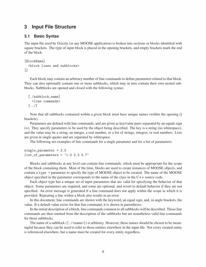
3 Input File Structure
3.1 Basic Syntax
The input file used by Grizzly (or any MOOSE application) is broken into sections or blocks identified with
square brackets. The type of input block is placed in the opening brackets, and empty brackets mark the end
of the block.
[BlockName]
<block lines and subblocks>
[]
Each block may contain an arbitrary number of line commands to define parameters related to that block.
They can also optionally contain one or more subblocks, which may in turn contain their own nested sub-
blocks. Subblocks are opened and closed with the following syntax:
[./subblock_name]
<line commands>
[../]
Note that all subblocks contained within a given block must have unique names (within the opening []
brackets).
Parameters are defined with line commands, and are given as key/value pairs separated by an equals sign
(=). They specify parameters to be used by the object being described. The key is a string (no whitespace),
and the value may be a string, an integer, a real number, or a list of strings, integers, or real numbers. Lists
are given in single quotes and are separated by whitespace.
The following are examples of line commands for a single parameter and for a list of parameters:
single_parameter = 2.3
list_of_parameters = ’1.0 2.3 3.7’
Blocks and subblocks at any level can contain line commands, which must be appropriate for the scope
of the block containing them. Most of the time, blocks are used to create instances of MOOSE objects, and
contain a type = parameter to specify the type of MOOSE object to be created. The name of the MOOSE
object specified in the parameter corresponds to the name of the class in the C++ source code.
Each object type has a unique set of input parameters that are valid for specifying the behavior of that
object. Some parameters are required, and some are optional, and revert to default behavior if they are not
specified. An error message is generated if a line command does not apply within the scope in which it is
provided. Repeating a line within a block also results in an error.
In this document, line commands are shown with the keyword, an equal sign, and, in angle brackets, the
value. If a default value exists for that line command, it is shown in parentheses.
In the initial description of a block, line commands common to all subblocks will be described. Those line
commands are then omitted from the description of the subblocks but are nonetheless valid line commands
for those subblocks.
The name of a subblock ([./<name>]) is arbitrary. However, these names should be chosen to be mean-
ingful because they can be used to refer to those entities elsewhere in the input file. Not every created entity
is referenced elsewhere, but a name must be created for every entity regardless.
8

3.2 Summary of MOOSE Object Types
MOOSE is an objected-oriented system with well-defined interfaces for applications to define their own
physics-specific code modules. The following is a listing of the major types of MOOSE objects used by
Grizzly:
• Variable
• Kernel
• AuxVariable
• AuxKernel
• Material
• BoundaryCondition
• Function
• Postprocessor
• VectorPostprocessor
• Constraint
• Damper
Specialized versions of these object types are implemented to provide the functionality needed to model
physics of interest for Grizzly.
3.3 Grizzly Syntax Page
A complete listing of all input syntax options in MOOSE is available on the MOOSE Documentation page.
See the section on Input File Documentation. Note also that you can run
grizzly-opt --dump
to get a list of valid input options for Grizzly.
3.4 Units
Grizzly can be run using any unit system preferred by the user. Empirical models within Grizzly that depend
on a specific unit system are noted in this documentation.
9

4 Common Commands For All Physics
4.1 GlobalParams
The GlobalParams block specifies parameters that are available, as appropriate, in any other block or sub-
block in the input file. For example, consider a subblock that accepts a line command with the keyword
value. If the subblock has a line command for value, that line command will be used regardless of what is
in GlobalParams. However, if the line command is missing in the subblock but defined in GlobalParams,
the subblock will use the parameter defined in GlobalParams. In the example below, the line commands
order = FIRST and family = LAGRANGE will be available in all other blocks and subblocks defined in the
input file.
[GlobalParams]
order = FIRST
family = LAGRANGE
[]
4.2 Problem
The Problem block is optionally used to define parameters for the Problem object. It only needs to be
included to specify non-default behavior. Typically, the only parameter set here is coord_type, which
specifies that the model should be treated as axisymmetric (RZ) or spherically symmetric (RSPHERICAL).
For 3D or 2D plane strain models, this block may be omitted.
[Problem]
coord_type = <string>
[]
4.3 Mesh
The Mesh block’s purpose is to give details about the finite element mesh to be used. Externally created
meshes can be imported from separate files in a variety of formats supported by the libMesh library that is
used by MOOSE for finite element functionality. The most commonly used mesh is ExodusII.
Typically meshes are created using the mesh generation tool Cubit (for U.S. government users) or Trelis
(the commercialized version of Cubit).
[Mesh]
file = <string>
displacements = <string list>
patch_size = <integer> (40)
[]
file Required. The name of the file containing the mesh.
displacements List of the displacement variables used to create the
displaced mesh. This line must be given if the model is to
use contact or large displacement theory. Typically disp_x
disp_y disp_z for a 3D model.
10

4.4 Executioner
The Executioner block describes how the simulation will be executed. It includes commands to control
the solver behavior and timestepping. Time stepping is controlled by a combination of commands in the
Executioner block, and the TimeStepper block nested within the Executioner block.
[Executioner]
type = <string>
solve_type = <string>
petsc_options = <string list>
petsc_options_iname = <string list>
petsc_options_value = <string list>
line_search = <string>
l_max_its = <integer>
l_tol = <real>
nl_max_its = <integer>
nl_rel_tol = <real>
nl_abs_tol = <real>
start_time = <real>
dt = <real>
end_time = <real>
num_steps = <integer>
dtmax = <real>
dtmin = <real>
[TimeStepper]
#TimeStepper commands
[../]
type Required. Several available. Typically Transient.
solve_type One of PJFNK (preconditioned JFNK), JFNK (JFNK),
NEWTON (Newton), or FD (Jacobian computed by finite
difference–serial only, slow).
petsc_options PETSc flags.
petsc_options_iname Names of PETSc name/value pairs.
petsc_options_value Values of PETSc name/value pairs.
line_search Line search type. Typically none.
l_max_its Maximum number of linear iterations per solve.
l_tol Linear solve tolerance.
nl_max_its Maximum number of nonlinear iterations per solve.
nl_rel_tol Nonlinear relative tolerance.
nl_rel_abs Nonlinear absolute tolerance.
start_time The start time of the analysis.
end_time The end time of the analysis.
num_steps The maximum number of timesteps.
dtmax The maximum allowed timestep size.
dtmin The minimum allowed timestep size.
11

Several Executioner types exist, although the Transient type is typically the appropriate one to use
for transient analyses.
Similarly, many PETSc options exist. Please see the online PETSc documentation for details.
4.5 Timestepping
The method used to calculate the size of the timesteps taken by MOOSE is controlled by the TimeStepper
block. There are a number of types of TimeStepper available. Three of the types most commonly used
are described here. These permit the timestep to be controlled directly by providing either a single fixed
timestep to take throughout the analysis, by providing the timestep as a function of time, or by using adaptive
timestepping algorithm can be used to modify the time step based on the difficulty of the iterative solution, as
quantified by the numbers of linear and nonlinear iterations required to drive the residual below the tolerance
required for convergence.
4.5.1 ConstantDT
The ConstantDT type of TimeStepper simply takes a constant timestep size throughout the analysis.
[TimeStepper]
type = ConstantDT
dt = <real>
[../]
type ConstantDT
dt Required. The initial timestep size.
ConstantDT begins the analysis taking the step specified by the user with the dt parameter. If the solver
fails to obtain a converged solution for a given step, the executioner cuts back the step size and attempts to
advance the time from the previous step using a smaller time step. The timestep is cut back by multiplying
the timestep by 0.5.
If the solution with the cut-back timestep is still un-successful, it is repeatedly cut back until a success-
ful solution is obtained. The user can specify a minimum timestep through the dtmin parameter in the
Executioner block. If the timestep must be cut back below the minimum size without obtaining a solution,
the code will exit with an error. If the timestep is cut back using ConstantDT, that cut-back step size will be
used for the remainder of the the analysis.
4.5.2 FunctionDT
If the FunctionDT type of TimeStepper is used, time steps vary over time according to a user-defined
function.
[TimeStepper]
type = FunctionDT
time_t = <real list>
time_dt = <real list>
[../]
12

type FunctionDT
time_t The abscissas of a piecewise linear function for timestep size.
time_dt The ordinates of a piecewise linear function for timestep size.
The timestep is controlled by a piecewise linear function defined using the time_t and time_dt pa-
rameters. A vector of timesteps is provided using the time_dt parameter. An accompanying vector of
corresponding times is specified using the time_t parameter. These two vectors are used to form a timestep
vs. time function. The timestep for a given step is computed by linearly interpolating between the pairs of
values provided in the vectors.
The same procedure that is used with ConstantDT is used to cut back the timestep from the user-specified
value if a failed solution occurs.
4.5.3 IterationAdaptiveDT
The IterationAdaptiveDT type of TimeStepper provides a means to adapt the timestep size based on the
difficulty of the solution.
[TimeStepper]
type = IterationAdaptiveDT
dt = <real>
optimal_iterations = <integer>
iteration_window = <integer> (0.2*optimal_iterations)
linear_iteration_ratio = <integer> (25)
growth_factor = <real>
cutback_factor = <real>
timestep_limiting_function = <string>
max_function_change = <real>
force_step_every_function_point = <bool> (false)
[../]
dt Required. The initial timestep size.
optimal_iterations The target number of nonlinear iterations for adaptive
timestepping.
iteration_window The size of the nonlinear iteration window for adaptive
timestepping.
linear_iteration_ratio The ratio of linear to nonlinear iterations to determine target
linear iterations and window for adaptive timestepping.
growth_factor Factor by which timestep is grown if needed.
cutback_factor Factor by which timestep is cut back if needed.
timestep_limiting_function Function used to control the timestep.
max_function_change Maximum change in the function over a timestep.
force_step_every_function_pointControls whether a step is forced at every point in the
function.
IterationAdaptiveDT grows or shrinks the timestep based on the number of iterations taken to obtain
a converged solution in the last converged step. The required optimal_iterations parameter controls the
number of nonlinear iterations per timestep that provides optimal solution efficiency. If more iterations than
13

that are required to obtain a converged solution, the timestep may be too large, resulting in undue solution
difficulty, while if fewer iterations are required, it may be possible to take larger timesteps to obtain a solution
more quickly.
A second parameter, iteration_window, is used to control the size of the region in which the timestep
is held constant. As shown in Figure [fig:adaptive_dt_criteria], if the number of nonlinear iterations for
convergence is lower than (optimal_iterations−iteration_window), the timestep is increased, while if
more than (optimal_iterations+iteration_window), iterations are required, the timestep is decreased.
The iteration_window parameter is optional. If it is not specified, it defaults to 1∕5 the value specified for
optimal_iterations.
The decision on whether to grow or shrink the timestep is based both on the number of nonlinear iterations
and the number of linear iterations. The parameters mentioned above are used to control the optimal iterations
and window for nonlinear iterations. The same criterion is applied to the linear iterations. Another parameter,
linear_iteration_ratio, which defaults to 25, is used to control the optimal iterations and window for the
linear iterations. These are calculated by multiplying linear_iteration_ratio by optimal_iterations
and iteration_window, respectively.
To grow the timestep, the growth criterion must be met for both the linear iterations and nonlinear
iterations. If the timestep shrinkage criterion is reached for either the linear or nonlinear iterations, the
timestep is decreased. To control the timestep size only based on the number of nonlinear iterations, set
linear_iteration_ratio to a large number.
If the timestep is to be increased or decreased, the amount of the increase or decrease in the timestep
is controlled by the growth_factor and cutback_factor parameters, respectively. If a solution fails to
converge when adaptive time stepping is active, a new attempt is made using a smaller timestep in the same
manner as with the fixed timestep methods. The maximum and minimum timesteps can be optionally spec-
ified in the Executioner block using the dtmax and dtmin parameters, respectively.
In addition to controlling the timestep based on the iteration count, IterationAdaptiveDT also has
an option to limit the timestep based on the behavior of a time-dependent function, optionally specified by
providing the function name in timestep_limiting_function. This is typically a function that is used to
drive boundary conditions of the model. The step is cut back if the change in the function from the previous
step exceeds the value specified in max_function_change. This allows the step size to be changed to limit
the change in the boundary conditions applied to the model over a step. In addition to that limit, the Boolean
parameter force_step_every_function_point can be set to true to force a timestep at every point in a
PiecewiseLinear function.
0 iterations
increase time step decrease time stepmaintain time step
optimal
window
window
Figure 2: Criteria used to determine adaptive timestep size
14

4.6 PETSc Options
The PETSc solver used by MOOSE is very flexible and permits the use of multiple solution strategies. The
full set of options provided by PETSc cannot be covered in detail here. The solver options used by any
code that uses PETSc can be controlled with command line parameters. MOOSE-based codes addition-
ally permit the specification of these PETSc options through two parameters: petsc_options_iname and
petsc_options_value in the Executioner block. Using these options permits specifying the solver op-
tions in the input file so that they do not need to be specified at the command line, which can greatly simplify
the process of running the code.
The following PETSc options invoke the use of an algebraic multigrid preconditioner, which scales well
in parallel and uses minimal memory.
[Executioner]
...
petsc_options_iname = ’-ksp_gmres_restart -pc_type -pc_hypre_type
-pc_hypre_boomeramg_max_iter’
petsc_options_value = ’201 hypre boomeramg 4’
...
[../]
These options are recommended for most problems.
4.7 Quadrature
The order of the quadrature rule used for finite element integration can optionally be specified using a
[./Quadrature] subblock within the [Executioner] block as follows:
[./Quadrature]
type = <string>
element_order = <string>
order = <string>
side_order = <string>
[../]
type The type of quadrature used. Default is Gauss.
element_order Order of quadrature on the elements.
order Order of quadrature used.
side_order Order of quadrature used on the sides.
4.8 Variables
The Variables block is where all of the primary solution variables are identified. The name of each variable
is assigned according to the name of its subblock. Primary solution variables often include temperature
(usually named temp) and displacement (usually named disp_x, disp_y, and disp_z).
[Variables]
[./var1]
order = <string>
15
family = <string>
[../]
[./var2]
order = <string>
family = <string>
initial_condition = <real>
scaling = <real> (1)
[../]
[]
order The order of the variable. Typical values are FIRST and
SECOND.
family The finite element shape function family. A typical value is
LAGRANGE.
initial_condition Optional initial value to be assigned to the variable. Zero is
assigned if this line is not present.
scaling Amount to scale the variable during the solution process.
This scaling affects only the residual and preconditioning
steps and not the final solution values. This is sometimes
helpful when solving coupled systems where one variable’s
residual is orders of magnitude different that the other
variables’ residuals.
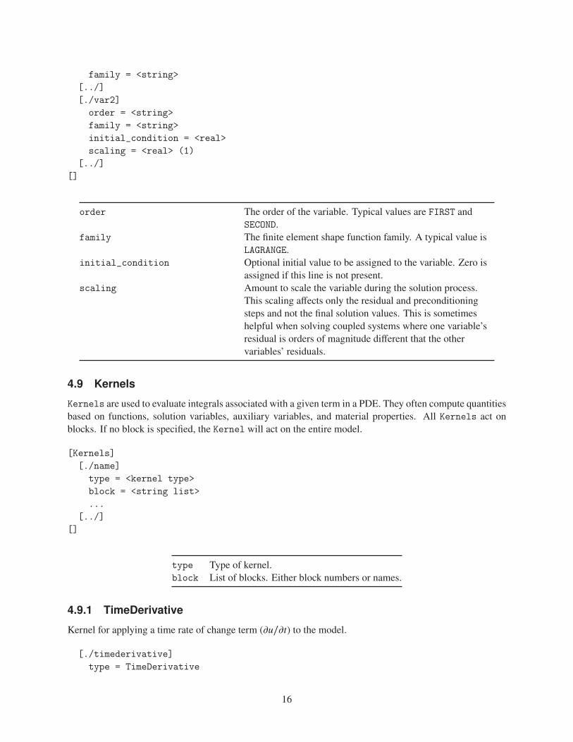
4.9 Kernels
Kernels are used to evaluate integrals associated with a given term in a PDE. They often compute quantities
based on functions, solution variables, auxiliary variables, and material properties. All Kernels act on
blocks. If no block is specified, the Kernel will act on the entire model.
[Kernels]
[./name]
type = <kernel type>
block = <string list>
...
[../]
[]
type Type of kernel.
block List of blocks. Either block numbers or names.
4.9.1 TimeDerivative
Kernel for applying a time rate of change term (𝜕𝑢∕𝜕𝑡) to the model.
[./timederivative]
type = TimeDerivative
16

variable = <variable>
[../]
type TimeDerivative
variable Required. Variable associated with this volume integral.
4.9.2 BodyForce
Kernel for applying an arbitrary body force to the model.
[./bodyforce]
type = BodyForce
variable = <variable>
value = <real> (0)
function = <string> (1)
[../]
type BodyForce
variable Required. Variable associated with this volume
integral.
value Constant included in volume integral. Multiplied
by the value of function if present.
function Function to be multiplied by value and used in the
volume integral.
4.10 AuxVariables
The AuxVariables block is where the auxiliary variables are identified. Auxiliary variables are field vari-
ables that are not solved for in the equation system, but are used for storing the values of auxiliary quantities
that are used in the simulation or for output. The name of each auxiliary variable is assigned according to
the name of its subblock.
[AuxVariables]
[./var1]
order = <string>
family = <string>
[../]
[./var2]
order = <string>
family = <string>
initial_condition = <real>
[../]
[]
order The order of the variable. Typical values are CONSTANT,
FIRST, and SECOND.
17

family The finite element shape function family. Typical values are
MONOMIAL and LAGRANGE.
initial_condition Optional initial value to be assigned to the variable. Zero is
assigned if this line is not present.
4.11 Materials
The Materials block is for specifying material properties and models.
[Materials]
[./name]
type = <material type>
block = <string list>
...
[../]
[]
type Type of material model
block List of blocks. Either block numbers or names.
4.12 Postprocessors
MOOSE Postprocessors compute a single scalar value at each timestep. These can be minimums, maxi-
mums, averages, volumes, or any other scalar quantity.
[Postprocessors]
[./name]
type = <postprocessor type>
block = <string list>
boundary = <string list>
execute_on = <string list>
outputs = <string>
...
[../]
[]
type Type of postprocessor
block List of blocks. Either block numbers or names.
boundary List of boundaries (side sets). Either boundary numbers or
names.
execute_on Set to (nonlinear | linear | timestep_end |
timestep_begin) to execute at that moment.
outputs Vector of output names where you would like to restrict the
output of variable(s) associated with the postprocessor.
18
Most Postprocessors act on either boundaries or blocks. If no block or boundary is specified, the
Postprocessor will act on the entire model. There are a few Postprocessors that act on specific nodes
or elements within the finite element mesh.
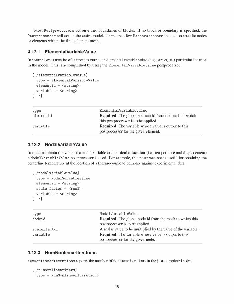
4.12.1 ElementalVariableValue
In some cases it may be of interest to output an elemental variable value (e.g., stress) at a particular location
in the model. This is accomplished by using the ElementalVariableValue postprocessor.
[./elementalvariablevalue]
type = ElementalVariableValue
elementid = <string>
variable = <string>
[../]
type ElementalVariableValue
elementid Required. The global element id from the mesh to which
this postprocessor is to be applied.
variable Required. The variable whose value is output to this
postprocessor for the given element.
4.12.2 NodalVariableValue
In order to obtain the value of a nodal variable at a particular location (i.e., temperature and displacement)
a NodalVariableValue postprocessor is used. For example, this postprocessor is useful for obtaining the
centerline temperature at the location of a thermocouple to compare against experimental data.
[./nodalvariablevalue]
type = NodalVariableValue
elementid = <string>
scale_factor = <real>
variable = <string>
[../]
type NodalVariableValue
nodeid Required. The global node id from the mesh to which this
postprocessor is to be applied.
scale_factor A scalar value to be multiplied by the value of the variable.
variable Required. The variable whose value is output to this
postprocessor for the given node.
4.12.3 NumNonlinearIterations
NumNonlinearIterations reports the number of nonlinear iterations in the just-completed solve.
[./numnonlineariters]
type = NumNonlinearIterations
19

[../]
type NumNonlinearIterations
4.12.4 PlotFunction
PlotFunction gives the value of the supplied function at the current time, optionally scaled with scale_factor.
[./plotfunction]
type = PlotFunction
function = <string>
scale_factor = <real> (1)
[../]
type PlotFunction
function Required. The function to evaluate.
scale_factor Scale factor to be applied to the function value.
4.12.5 SideAverageValue
SideAverageValue computes the area- or volume-weighted average of the named variable. It may be used,
for example, to calculate the average temperature over a side set.
[./sideaveragevalue}
type = SideAverageValue
variable = <string>
[../]
type SideAverageValue
variable Required. The variable this Postprocessor acts on.
4.12.6 SideFluxIntegral
SideFluxIntegral computes the integral of the flux over the given boundary.
[./sidefluxintegral]
type = SideFluxIntegral
variable = <string>
diffusivity = <string>
[../]
type SideFluxIntegral
variable Required. Variable to be used in the flux calculation.
diffusivity Required. The diffusivity material property to be used in the
calculation.
20

4.12.7 TimestepSize
TimestepSize reports the timestep size.
[./dt]
type = TimestepSize
[../]
type TimestepSize
4.13 VectorPostprocessors
VectorPostprocessors computes vectors of values and outputs them in comma separated files, one file
for each VectorPostprocessor at each timestep. The parameter csv must be set to true in the Outputs block
to allow the files to be output.
[VectorPostprocessors]
[./name]
type = <vectorpostprocessor type>
execute_on = <string list>
...
[../]
[]
type Type of postprocessor
execute_on Set to (nonlinear | linear | timestep_end |
timestep_begin) to execute at that moment.
4.13.1 LineValueSampler
The LineValueSampler VectorPostprocessor samples the values of a variable along a user-specified line.
[./linevaluesampler]
type = LineValueSampler
variable = <string>
start_point = <vector>
end_point = <vector>
num_points = <integer>
sort_by = <x or y or z or id>
[../]
type LineValueSampler
variable Required The names of the variables that this
VectorPostprocessor operates on.
start_point Required The beginning of the line.
end_point Required The ending of the line.
21

num_points Required The number of points to sample along the line.
sort_by Required What to sort the samples by.
4.14 Functions
4.14.1 Composite
The Composite function takes an arbitrary set of functions, provided in the functions parameter, evaluates
each of them at the appropriate time and position, and multiplies them together. The function can optionally
be multiplied by a scale factor, which specified using the scale_factor parameter.
[./composite]
type = CompositeFunction
functions = <string list>
scale_factor = <real> (1.0)
[../]
type CompositeFunction
functions List of functions to be multiplied together.
scale_factor Scale factor to be applied to resulting function. Default is 1.
4.14.2 ParsedFunction
The ParsedFunction function takes a mathematical expression in value. The expression can be a function
of time (t) or coordinate (x, y, or z). The expression can include common mathematical functions. Examples
include ’4e4+1e2*t’, ’sqrt(x*x+y*y+z*z)’, and ’if(t<=1.0, 0.1*t, (1.0+0.1)*cos(pi/2*(t-1.0))
- 1.0)’. Constant variables may be used in the expression if they have been declared with vars and defined
with vals. Further information can be found at http://warp.povusers.org/FunctionParser/.
[./parsedfunction]
type = ParsedFunction
value = <string>
vals = <real list>
vars = <string list>
[../]
type ParsedFunction
value Required. String describing the function.
vals Values to be associated with variables in vars.
vars Variable names to be associated with values in vals.
4.14.3 PiecewiseBilinear
The PiecewiseBilinear function reads a csv file and interpolates values based on the data in the file. The
interpolation is based on x-y pairs. If axis is given, time is used as the y index. Either xaxis or yaxis or
both may be given. Time is used as the other index if one of them is not given. If radius is given, xaxis
22

and yaxis are used to orient a cylindrical coordinate system, and the x-y pair used in the query will be the
radial coordinate and time.
[./piecewiselinear]
type = PiecewiseBilinear
data_file = <string>
axis = <0, 1, or 2 for x, y, or z>
xaxis = <0, 1, or 2 for x, y, or z>
yaxis = <0, 1, or 2 for x, y, or z>
scale_factor = <real> (1.0)
radial = <bool> (false)
[../]
type PiecewiseBilinear
data_file File holding the csv data.
axis Coordinate direction to use in the function evaluation.
xaxis Coordinate direction used for x-axis data.
yaxis Coordinate direction used for y-axis data.
scale_factor Scale factor to be applied to resulting function. Default is 1.
radial Set to true if interpolation should be done along a radius
rather than along a specific axis. Requires xaxis and yaxis.
4.14.4 PiecewiseConstant
The PiecewiseConstant function defines the data using a set of x-y data pairs. Instead of linearly inter-
polating between the values, however, the PiecewiseConstant function is constant when the abscissa is
between the values provided by the user. The direction parameter controls whether the function takes
the value of the abscissa of the user-provided point to the right or left of the value at which the function is
evaluated.
[./piecewiseconstant]
type = PiecewiseConstant
x = <real list>
y = <real list>
xy_data = <real list>
data_file = <string>
format = <string> (rows)
scale_factor = <real> (1.0)
axis = <0, 1, or 2 for x, y, or z>
direction = <string> (left)
[../]
type PiecewiseConstant
x List of x values for x-y data.
y List of y values for x-y data.
xy_data List of pairs of x-y data points.
23

data_file Name of an file containing x-y data.
format Format of x-y data in external file.
scale_factor Scale factor to be applied to resulting function. Default is 1.
axis Coordinate direction to use in the function evaluation. If not
present, time is used as the function input.
4.14.5 PiecewiseLinear
The PiecewiseLinear function performs linear interpolations between user-provided pairs of x-y data. The
x-y data can be provided in three ways. The first way is through a combination of the x and y parameters,
which are lists of the x and y coordinates of the data points that make up the function. The second way is
in the xy_data parameter, which is a list of pairs of x-y data that make up the points of the function. This
allows for the function data to be specified in columns by inserting line breaks after each x-y data point.
Finally, the x-y data can be provided in an external file containing comma-separated values. The file name
is provided in data_file, and the data can be provided in either rows (default) or columns, as specified in
the format parameter.
By default, the x-data corresponds to time, but this can be changed to correspond to x, y, or z coordinate
with the axis line. If the function is queried outside of its range of x data, it returns the y value associated
with the closest x data point.
[./piecewiselinear]
type = PiecewiseLinear
x = <real list>
y = <real list>
xy_data = <real list>
data_file = <string> (rows)
format = <string>
scale_factor = <real> (1.0)
axis = <0, 1, or 2 for x, y, or z>
[../]
type PiecewiseLinear
x List of x values for x-y data.
y List of y values for x-y data.
xy_data List of pairs of x-y data points.
data_file Name of an file containing x-y data.
format Format of x-y data in external file.
scale_factor Scale factor to be applied to resulting function. Default is 1.
axis Coordinate direction to use in the function evaluation. If not
present, time is used as the function input.
4.15 BCs
The BCs block is for specifying various types of boundary conditions. Boundary conditions that are appli-
cable to any physics are listed here.
[BCs]
24

[./name]
type = <BC type>
boundary = <string list>
...
[../]
[]
type Type of boundary condition.
boundary List of boundaries (side sets). Either boundary numbers or
names.
4.15.1 DirichletBC
The DirichletBC boundary condition is used to directly specify the value of a solution variable. It can be
applied to any solution variable.
[./dirichletbc]
type = DirichletBC
variable = <variable>
boundary = <string list>
value = <real>
[../]
type DirichletBC
variable Required. Primary variable associated with this boundary
condition.
boundary Required. List of boundary names or ids where this
boundary condition will apply.
value Required. Value to be assigned.
4.15.2 PresetBC
The PresetBC takes the same inputs as DirichletBC and also acts as a Dirichlet boundary condition. How-
ever, the implementation is slightly different. PresetBC causes the value of the boundary condition to be
applied before the solve begins where DirichletBC enforces the boundary condition as the solve progresses.
In certain situations, one is better than another.
4.15.3 FunctionDirichletBC
[./functiondirichletbc]
type = FunctionDirichletBC
variable = <variable>
boundary = <string list>
function = <string>
[../]
25

type FunctionDirichletBC
variable Required. Primary variable associated with this boundary
condition.
boundary Required. List of boundary names or ids where this
boundary condition will apply.
function Required. Function that will give the value to be applied by
this boundary condition.
4.15.4 FunctionPresetBC
The FunctionPresetBC takes the same inputs as FunctionDirichletBC and also acts as a Dirichlet bound-
ary condition. However, the implementation is slightly different. FunctionPresetBC causes the value of
the boundary condition to be applied before the solve begins where FunctionDirichletBC enforces the
boundary condition as the solve progresses. In certain situations, one is better than another.
4.16 AuxKernels
AuxKernels are used to compute values for AuxVariables. They often compute quantities based on func-
tions, solution variables, and material properties. AuxKernels can apply to blocks or boundaries. If no block
or boundary is specified, the AuxKernel applies to the entire model.
[AuxKernels]
[./name]
type = <AuxKernel type>
block = <string list>
boundary = <string list>
...
[../]
[]
type Type of auxiliary kernel.
block List of blocks. Either block numbers or names.
boundary List of boundaries (side sets). Either boundary numbers or
names.
4.16.1 MaterialRealAux
The MaterialRealAux AuxKernel is used to output material properties. Typically, the AuxVariable com-
puted by MaterialRealAux will be an element-level, constant variable. The computed value will be the
volume-averaged quantity over the element.
[./materialrealaux]
type = MaterialRealAux
property = <material property>
variable = <variable>
[../]
26

type MaterialRealAux
property Required. Name of material property.
variable Required. Name of AuxVariable that will hold result.
4.17 Constraints
The Constraints block is for specifying various types of constraints. Constraints that are applicable to any
physics are listed here.
[Constraints]
[./name]
type = <Constraint type>
...
[../]
[]
type Type of constraint.
4.17.1 EqualValueBoundaryConstraint
The EqualValueBoundaryConstraint Constraint is used to constrain a variable to have the same value on
a boundary or set of nodes.
[./equalvalueboundaryconstraint]
type = EqualValueBoundaryConstraint
variable = <variable>
master = <integer>
slave = <string>
slave_node_ids = <integer list>
formulation = <Penalty or Kinematic> (Penalty)
penalty = <real>
[../]
type EqualValueBoundaryConstraint
variable Required. Primary variable associated with this boundary
condition.
master The id of the master node. If no id is provided, first node of
slave set is chosen.
slave The boundary id associated with the slave side. Must use
either this or slave_node_ids.
slave_node_ids The ids of the slave nodes. Must use either this or slave.
formulation Formulation used to calculate constraint. One of Penalty or
Kinematic.
penalty Required The penalty stiffness value to be used in the
constraint.
27

4.18 UserObjects
UserObjects in MOOSE provide a capability to implement a wide variety of capabilities that do not readily
fit into the interfaces provided by other types of MOOSE objects. These are defined within the UserObjects
block in the input file.
[UserObjects]
[./name]
type = <UserObject type>
...
[../]
[]
type Type of user object.
4.19 Outputs
The Outputs block lists parameters that control the frequency and type of results files produced. It is possible
to create multiple output objects each outputting at different intervals, or different variables, or varying file
types. The Outputs system is very complex and enables a large amount of customization. This section will
highlight the capabilities of the system.
4.19.1 Basic Input File Syntax
To enable output an input file must contain an Outputs block. The simplest method for enabling output is to
utilize the shortcut syntax as shown below, which enables the Console output (prints to screen) and Exodus
output for writing data to a file.
[Outputs]
console = true #output to the screen with default settings
exodus = true #output to ExodusII file with default settings
[]
4.19.2 Advanced Syntax
To take full advantage of the output system the use of subblocks is required. For example, the input file
snippet below is exactly equivalent, including the subblock names, to the snippet shown above that utilizes
the shortcut syntax.
[Outputs]
[./console]
type = Console #output to the screen with default settings
[../]
[./exodus]
type = Exodus #output to ExodusII file with default settings
[../]
[]
28

However, the subblock syntax allows for increased control over the output and allows for multiple outputs
of the same type to be specified. For example, the following creates two Exodus outputs, one outputting the
a mesh at every timestep including the initial condition the other outputs every 3 timesteps without the initial
condition. Additionally, performance logging was enabled for Console output.
[Outputs]
execute_on = ’timestep_end’ # Limit the output to timestep end (no initial state)
[./console]
type = Console
perf_log = true # enable performance logging
[../]
[./exodus]
type = Exodus
execute_on = ’initial timestep_end’ # output the initial state
[../]
[./exodus_3] # create a second [Exodus II][1] output
# that utilizes a different output interval
type = Exodus
file_base = exodus_3 # set the file base
# (the extension is automatically applied)
interval = 3 # only output every third step
[../]
[]
4.19.3 Common Output Parameters
In addition to allowing for shortcut syntax, the Outputs block also supports common parameters. For ex-
ample, the parameter execute_on may be specified outside of individual subblocks, indicating that all sub-
blocks should output at the specified time. If within a subblock the parameter is given a different value,
the subblock parameter takes precedence. The input file snippet below demonstrate the usage of a common
values as well as the use of multiple output blocks.
[Outputs]
execute_on = ’timestep_end’ # disable the output of initial state
vtk = true # output VTK file with default setting
[./exodus]
type = Exodus
execute_on = ’initial’ # this file will contain ONLY the initial state
[../]
[./exodus_displaced]
type = Exodus
file_base = displaced
use_displaced = true
interval = 3 # this file will only output every third time step
[../]
[]
29

4.19.4 File Output Names
The default naming scheme for output files utilizes the input file name (e.g., input.i) with a suffix that differs
depending on how the output is defined:
• output files created using the shortcut syntax have an _out suffix
• subblocks use the actual subblock name as the suffix.
For example, if the input file (input.i) contained the following [Outputs] block, two files would be
created: input_out.e and input_other.e.
[Outputs]
console = true
exodus = true # creates input_out.e
[./other] # creates input_other.e
type = Exodus
interval = 2
[../]
[]
4.20 Dampers
Dampers are used to decrease the attempted change to the solution with each nonlinear step. This can be
useful in preventing the solver from changing the solution dramatically from one step to the next. This may
prevent, for example, the solver from attempting to evaluate negative temperatures.
The MaxIncrement damper is commonly used.
4.20.1 MaxIncrement
The MaxIncrement damper limits the change of a variable from one nonlinear step to the next.
[Dampers]
[./maxincrement]
type = MaxIncrement
max_increment = <real>
variable = <string>
[../]
[]
type MaxIncrement
max_increment Required. The maximum change in solution variable
allowed from one nonlinear step to the next.
variable Required. Variable that will not be allowed to change
beyond max_increment from nonlinear step to nonlinear
step.
30
5 Thermal Governing Equations and Associated Commands
The energy balance is given in terms of the heat conduction equation
𝜌𝐶𝑝
𝜕𝑇
𝜕𝑡+ ∇ ⋅ 𝒒 = 0,
where 𝑇 , 𝜌 and 𝐶𝑝 are the temperature, density and specific heat, respectively. The heat flux is given as
𝒒 = −𝑘∇𝑇 ,
where 𝑘 denotes the thermal conductivity of the material.
5.1 Kernels
5.1.1 Heat Conduction
Kernel for diffusion of heat or divergence of heat flux.
[./heatconduction]
type = HeatConduction
variable = <variable>
[../]
type HeatConduction
variable Required. Variable name corresponding to the heat
conduction equation. Typically temp.
5.1.2 Heat Conduction Time Derivative
Kernel for 𝜌𝐶𝑝𝜕𝑇 ∕𝜕𝑡 term of the heat equation.
[./heatconductiontimederivative]
type = HeatConductionTimeDerivative
variable = <variable>
[../]
type HeatConductionTimeDerivative
variable Required. Variable name corresponding to the heat
conduction equation. Typically temp.
5.1.3 Heat Source
The HeatSource kernel applies a volumetric heat source to specified blocks within the model. Built on
the BodyForce kernel’s code, the HeatSource kernel provides a more relevant name for easier input-file
specification.
[./heatsource]
type = HeatSource
31

variable = <variable>
value = <real> (1)
function = <string> (1)
block = <string list>
[../]
type HeatSource
variable Required. The variable associated with the heat source.
value Value of the heat source; will be multiplied by the optional
function.
function The function describing the volumetric heat source.
block The list of block id’s (SubdomainID) to which the heat
source will be applied.
5.2 Materials
5.2.1 HeatConductionMaterial
HeatConductionMaterial is a general-purpose material model for heat conduction. It sets the thermal
conductivity and specific heat at integration points.
[heatconductionmaterial]
type = HeatConductionMaterial
temp = <string>
thermal_conductivity = <real>
thermal_conductivity_temperature_function = <string>
specific_heat = <real>
specific_heat_temperature_function = <string>
block = <string list>
[../]
type HeatConductionMaterial
temp Name of temperature variable. Typically temp.
thermal_conductivity Coefficient of thermal conductivity.
thermal_conductivity_temperature_functionFunction describing thermal conductivity as a function of
temperature.
specific_heat Specific heat capacity.
specific_heat_temperature_functionFunction describing specific heat capacity as a function of
temperature.
block List of blocks this material applies to.
5.3 BCs
5.3.1 ConvectiveFluxFunction
The ConvectiveFluxFunction boundary condition determines the value on a boundary based upon the
heat transfer coefficient of the fluid on the outside of boundary and far-field temperature.
32

[./convectivefluxFunction]
type = ConvectiveFluxFunction
variable = <variable>
boundary = <string list>
T_infinity= <string>
coefficient = <real>
coefficient_function = <string>
[../]
type ConvectiveFluxFunction
variable Required. Primary variable associated with this boundary
condition.
boundary Required. List of boundary names or ids where this
boundary condition will apply.
T_infinity Required. The name of the function describing the far-field
temperature.
coefficient Required. The heat transfer coefficient of the fluid in contact
with the boundary. If coefficient_function is provided
this coefficient multiplies the function.
coefficient_function Function defining the heat transfer coefficient as a function
of time.
33

6 Mechanical Governing Equation, Kinematics, and Associated Com-mands
Momentum conservation is prescribed assuming static equilibrium at each time increment using Cauchy’s
equation,
∇ ⋅ 𝝈 + 𝜌𝒇 = 0,where𝝈 is the Cauchy stress tensor and𝒇 is the body force per unit mass (e.g. gravity). The displacement field
𝑢, which is the primary solution variable, is connected to the stress field via the strain, through a constitutive
relation.
For geometrically linear analysis, the strain 𝜖 is defined as 1∕2[∇𝒖 + ∇𝒖𝑇 ]. Furthermore, with a linear
elastic constitutive model, the stress is simply 𝐶 𝜖. We now outline our approach for nonlinear analysis. We
follow the approach in [1] and the software package FMA3D [2].
We begin with a complete set of data for step 𝑛 and seek the displacements and stresses at step 𝑛+1. We
first compute an incremental deformation gradient,
𝑭 = 𝜕𝑥𝑛+1
𝜕𝑥𝑛.
With 𝑭 , we next compute a strain increment that represents the rotation-free deformation from the con-
figuration at 𝑛 to the configuration at 𝑛 + 1. Following [1], we seek the stretching rate 𝑫:
𝑫 = 1Δ𝑡
log(�̂� )
= 1Δ𝑡
log(sqrt
(𝑭
𝑇𝑭))
= 1Δ𝑡
log(sqrt
(�̂�))
.
Here, �̂� is the incremental stretch tensor, and �̂� is the incremental Green deformation tensor. Through a
Taylor series expansion, this can be determined in a straightforward, efficient manner. 𝑫 is passed to the
constitutive model as an input for computing 𝝈 at 𝑛 + 1.
The next step is computing the incremental rotation, �̂� where 𝑭 = �̂��̂� . Like for 𝑫, an efficient algo-
rithm exists for computing �̂�. It is also possible to compute these quantities using an eigenvalue/eigenvector
routine.
With 𝝈 and �̂�, we rotate the stress to the current configuration.
6.1 Temperature-dependent thermal expansion
Both the base metal and the liner in RPVs have temperature-dependent elastic properties and thermal expan-
sion coefficients. The thermal expansion coefficient can be specified as an instantaneous thermal expansion
coefficient, which defines the thermal strain increment under an infinitesimal change in the temperature. Us-
ing the notation of [3], for an isotropic material, this instantaneous thermal expansion coefficient at a given
temperature, 𝑇 is referred to as 𝛼(𝑇 ), and the instantaneous thermal strain, 𝜖𝑡ℎ is defined as:
d𝜖𝑡ℎ = 𝛼(𝑇 )d𝑇 .
Alternatively, the thermal expansion can be expressed as a mean coefficient of thermal expansion, �̄�(𝑇 )at a given temperature relative to the strain at a reference temperature, 𝑇𝑟𝑒𝑓 :
�̄�(𝑇 ) =𝐿(𝑇 ) − 𝐿(𝑇𝑟𝑒𝑓 )
𝐿(𝑇𝑟𝑒𝑓 )(𝑇 − 𝑇𝑟𝑒𝑓 )
34

Because mean thermal expansion can be readily measured experimentally, it is common to express thermal
expansion for materials in this manner, as is the case for RPV materials.
Figure 3: Instantaneous and mean coefficients of thermal expansion
To permit the use of data in its most available form and facilitate comparisons with other codes, Grizzly
allows temperature-dependent thermal expansion data to be provided in either format. If the data is provided
in the mean form, a reference temperature must be specified, and it does not need to coincide with the stress-
free temperature. Indeed, it is often assumed that the thermal strain in the nuclear reactor components is zero
at the operating temperature, and this can be achieved in Grizzly by assigning the operating temperature as the
stress-free temperature. The method outlined in [3] is employed to calculate the incremental thermal strain
when the reference and stress-free temperatures differ. Regression tests have been developed to demonstrate
that these two methods produce the same results for equivalent mean and instantaneous thermal expansion
functions, including usage with fracture integrals.
6.2 Kernels
6.2.1 SolidMechanics
The SolidMechanics block specifies inputs for the divergence of stress as part of the equations of solid
mechanics. The divergence of stress is a Kernel in MOOSE nomenclature. The SolidMechanics block
informs MOOSE of the divergence kernels but is not placed inside the Kernels block in the input file.
[SolidMechanics]
[./solidmechanics]
disp_x = <variable>
disp_y = <variable>
disp_z = <variable>
disp_r = <variable>
temp = <variable>
[../]
[]
35

disp_x Variable name for displacement variable in x
direction. Typically disp_x.
disp_y Variable name for displacement variable in y
direction. Typically disp_y.
disp_z Variable name for displacement variable in z
direction. Typically disp_z for 3D and disp_y for
axisymmetric models.
disp_r Variable name for displacement variable in radial
direction for axisymmetric or spherically
symmetric cases. Typically disp_x.
temp Variable name for temperature variable. Necessary
for thermal expansion. Typically temp.
6.2.2 Gravity
Gravity may be applied to the model with this kernel. The required density is computed and provided inter-
nally given inputs in the Materials block.
[./gravity]
type = Gravity
variable = <variable>
value = <real> (0)
[../]
type Gravity
variable Required. Variable name corresponding to the
displacement direction in which the gravity load
should be applied.
value Acceleration of gravity. Typically -9.81 (m/s2).
6.3 AuxKernels
6.3.1 MaterialTensorAux
The MaterialTensorAux AuxKernel is used to output quantities related to second-order tensors used as
material properties. Stress and strain are common examples of these tensors. The AuxKernel allows output
of specific tensor entries or quantities computed from the entire tensor. Typically, the AuxVariable computed
by MaterialTensorAux will be an element-level, constant variable. By default, the computed value is a
volume-averaged quantity over the element.
[./materialtensoraux]
type = MaterialTensorAux
tensor = <material property tensor>
variable = <variable>
index = <integer>
quantity = <string>
point1 = <vector> (0, 0, 0)
36
point2 = <vector> (0, 1, 0)
direction = <vector>
qp_select = <integer> (0, 1, ..., n)
[../]
type MaterialTensorAux
tensor Required. Name of second-order tensor material property.
A typical second-order tensor material property is stress.
variable Required. Name of AuxVariable that will hold result.
index Index into tensor, from 0 to 5 (xx, yy, zz, xy, yz, zx). Either
index or quantity must be specified.
quantity One of VonMises, PlasticStrainMag, Hydrostatic,
Direction, Hoop, Radial, Axial, MaxPrincipal,
MedPrincipal, MinPrincipal, FirstInvariant,
SecondInvariant, ThirdInvariant, TriAxiality, or
VolumetricStrain. Either index or quantity must be
specified.
point1 Start point for axis used to calculate some material tensor
quantities.
point2 End point for axis used to calculate some material tensor
quantities.
direction Direction vector used to calculate some material tensor
quantities.
qp_select Output the value at the specified integration point number
rather than volume averaging.
6.4 Materials
6.4.1 Elastic
The Elastic model is a simple hypo-elastic model.
[./elastic]
type = Elastic
disp_x = <string>
disp_y = <string>
disp_z = <string>
disp_r = <string>
temp = <string>
youngs_modulus = <real>
youngs_modulus_function = <string>
poissons_ratio = <real>
poissons_ratio_function = <string>
thermal_expansion = <real> (0)
thermal_expansion_function = <string>
stress_free_temperature = <real>
thermal_expansion_function_type = <string> (Mean)
37

thermal_expansion_function = <string>
thermal_expansion_reference_temperature = <real>
block = <string list>
[../]
type Elastic
disp_x Variable name for displacement variable in x
direction. Typically disp_x.
disp_y Variable name for displacement variable in y
direction. Typically disp_y.
disp_z Variable name for displacement variable in z
direction. Typically disp_z for 3D and disp_y for
axisymmetric models.
disp_r Variable name for displacement variable in radial
direction for axisymmetric or spherically
symmetric cases. Typically disp_x.
temp Name of temperature variable. Typically temp.
youngs_modulus Young’s modulus.
youngs_modulus_function Function describing Young’s modulus as a function
of temperature.
poissons_ratio Poisson’s ratio.
poissons_ratio_function Function describing Poisson’s ratio as a function of
temperature.
thermal_expansion Coefficient of thermal expansion.
stress_free_temperature The stress-free temperature. If not specified, the
initial temperature is used.
thermal_expansion_function_type Type of thermal expansion data. Options are Mean
or Instantaneous.
thermal_expansion_function Function describing thermal expansion as a
function of temperature.
thermal_expansion_reference_temperature Reference temperature for mean thermal expansion
function.
block List of blocks this material applies to.
6.5 Density
The Density model creates a material property named ‘density’. If coupled to displacement variables, the
model adjusts density based on deformation.
[./density]
type = Density
disp_x = <string>
disp_y = <string>
disp_z = <string>
disp_r = <string>
density = <real>
[../]
38

type Density
disp_x Variable name for displacement variable in x direction.
Typically disp_x.
disp_y Variable name for displacement variable in y direction.
Typically disp_y.
disp_z Variable name for displacement variable in z direction.
Typically disp_z for 3D and disp_y for axisymmetric
models.
disp_r Variable name for displacement variable in radial direction
for axisymmetric or spherically symmetric cases. Typically
disp_x.
density Required. Density.
6.6 VectorPostprocessors
6.6.1 LineMaterialSymmTensorSampler
LineMaterialSymmTensorSampler samples stress tensor quantities along a user-specified line.
[./linematerialsymmtensorsampler]
type = LineMaterialSymmTensorSampler
start = <vector>
end = <vector>
property = <string>
quantity = <string>
index = <integer>
point1 = <vector> (0, 0, 0)
point2 = <vector> (0, 1, 0)
direction = <vector>
sort_by = <x or y or z or id>
block = <string list>
[../]
type LineMaterialSymmTensorSampler
start Required The beginning of the line.
end Required The ending of the line.
property Required Name of second-order tensor material property. A
typical second-order tensor material property is stress.
index Index into tensor, from 0 to 5 (xx, yy, zz, xy, yz, zx). Either
index or quantity must be specified.
quantity One of VonMises, PlasticStrainMag, Hydrostatic,
Direction, Hoop, Radial, Axial, MaxPrincipal,
MedPrincipal, MinPrincipal, FirstInvariant,
SecondInvariant, ThirdInvariant, TriAxiality, or
VolumetricStrain. Either index or quantity must be
specified.
39

direction Direction vector used to calculate some material tensor
quantities.
point1 Start point for axis used to calculate some material tensor
quantities.
point2 End point for axis used to calculate some material tensor
quantities.
sort_by Required What to sort the samples by.
block List of blocks this vectorpostprocessor applies to.
6.7 BCs
6.7.1 Pressure
The Pressure boundary condition uses two levels of nesting within the BCs block. This allows the pressure
to be applied properly in all coordinate directions although it is specified one time only.
[./Pressure]
[./pressure]
boundary = <string list>
factor = <real> (1)
function = <string>
[../]
[../]
boundary Required. List of boundary names or ids where this
boundary condition will apply.
factor Magnitude of pressure to be applied. If function is also
given, factor is multiplied by the output of the function and
then applied as the pressure.
function Function that will give the value to be applied by this
boundary condition.
40

7 Submodeling
Grizzly includes capabilities for solution transfer that facilitate submodeling. Typically the global model is
the whole or part of a vessel and the submodel is a smaller region containing a flaw. Solutions stored in an Ex-
odusII or XDA file can be used as input to a submodel using a SolutionUserObject. The mesh of the sub-
model must fit inside the physical domain of the global model. Advanced options of SolutionUserObject
allow users to scale, translate and rotate the submodel. A solution function is required to interpolate in time
and space the data from SolutionUserObject. The solution function to use depends on the type of solution
mapping needed.
7.1 UserObjects
7.1.1 SolutionUserObject
A solution user object reads a variable from a mesh in one simulation to another. To use a SolutionUserObject
three additional parameters are required, an AuxVariable , a Function and an AuxKernel. The AuxVariable
represents the variable to be read by the solution user object. The SolutionUserObject is set up to read
the old output file. A SolutionFunction is required to interpolate in time and space the data from the
SolutionUserObject. Finally, the FunctionAux is required that will query the function and write the
value into the AuxVariable. An example of what additions are required to the input file is shown below:
[AuxVariables]
[./temp]
[../]
[]
[Functions]
[./interpolated_temp]
type = SolutionFunction
from_variable = ’temp’
solution = read_thermo_solution
[../]
[]
[UserObjects]
[./read_thermo_solution]
type = SolutionUserObject
mesh = ’temp_from_another_simulation.e’
execute_on = ’residual’
nodal_variables = ’temp’
[../]
[]
[AuxKernels]
[./interp_temp]
type = FunctionAux
variable = ’temp’
function = ’interpolated_temp’
[../]
41

[]
Note that in the SolutionUserObject subblock that the mesh parameter is required.
7.2 Functions
7.2.1 SolutionFunction
If the global model and submodel have the same dimensionality, the SolutionFunction can be used as a
forcing function for a boundary condition. The SolutionFunction uses a SolutionUserObject to read
the data from a results file from a previous run. An example of how this is achieved in the input file is shown
below:
[UserObjects]
[./soln]
type = SolutionUserObject
mesh = ’global_model_out.e’
system_variables = ’disp_x disp_y’
timestep = 1
[../]
[]
[Functions]
[./bc_func_x]
type = SolutionFunction
solution = soln
from_variable = disp_x
[../]
[]
[BCs]
[./x_soln_bc]
type = FunctionDirichletBC
variable = disp_x
boundary = ’1 2 3 4 5 6’
function = bc_func_x
[../]
[]
mesh Required. The name of the mesh file containing the global
model solution. Must be ExodusII or XDA file.
system_variables The name of the nodal and elemental variables from the file
you want to use for values.
timestep Index of the single timestep used or “LATEST” for the last
timestep (ExodusII only). If not supplied, time interpolation
will occur.
solution Required. The SolutionUserObject to extract data from.
from_variable The name of the variable in the file that is to be extracted.
42

7.3 Axisymmetric2D3DSolutionFunction
If a two-dimensional axisymmetric model is used as the global model, the solution can be mapped onto a two-
or three-dimensional submodel using Axisymmetric2D3DSolutionFunction. This function then replaces
SolutionFunction in the example above.
[Functions]
[./bc_func_x]
type = Axisymmetric2D3DSolutionFunction
solution = soln
3d_axis_point1 = ’0.0 0.0 0.0’
3d_axis_point2 = ’0.0 0.0 1.0’
from_variables = ’disp_x disp_y’
component = 0
axial_dimension_ratio = 200.0
[../]
[]
solution Required. The SolutionUserObject to extract data from.
2d_axis_point1 Start point for axis of symmetry for the 2d model.
2d_axis_point2 End point for axis of symmetry for the 2d model.
3d_axis_point1 Start point for axis of symmetry for the 3d model.
3d_axis_point2 End point for axis of symmetry for the 3d model.
from_variables The name of the variables in the file that are to be extracted,
in x, y order if they are vector components.
component Component of the variable to be computed if it is a vector.
axial_dimension_ratio Ratio of the axial dimension in the 3d model to that in the 2d
model. Optionally permits the 3d model to be larger than the
2d model in that dimension, and scales vector solutions in
that direction by this factor.
43

8 Theory and Commands for Reactor Pressure Vessel Analysis
8.1 Fluence Map
Grizzly includes a capability to apply a neutron fluence map to the interior surface of the vessel. Inside the
vessel wall, the fluence is calculated using the equation accepted by the NRC for fast neutron attenuation
in RPV steel [4]. The fluence 𝑓 at a given distance 𝑥 (in inches) from the inner surface is expressed as a
function of that distance and the fluence at the inner surface, 𝑓𝑖:
𝑓 (𝑥) = 𝑓𝑖 exp(−0.24 ∗ 𝑥).
The calculated fluence can be used in the EONY model presented below to calculate the transition-
temperature shift for every location in the vessel, which in turn can provide the level of embrittlement in the
fracture toughness given by the master curve model.
Figure 4: Attenuation through the thickness of the wall computed using FluenceFunction and a map of
the fluence on the inner surface of the RPV.
The fluence is computed in the function FluenceFunction and can be output as an AuxVariable.
FluenceFunction requires two data files describing the axial and azimuthal variation, respectively, of the
fluence at the interior surface of the vessel. The second column in the data files gives the variation in fluence.
In the file describing the axial variation of fluence, the first column is the height (in inches). The parameter
axis1 determines where the axial fluence profile will start and the vector from axis1 to axis2 defines the
axial direction. In the file describing the azimuthal variation, the first column is the angle within a 90 degree
sector of the RPV. The angle is defined relative to the position determined by the parameter azimuth0, which
gives the position of the azimuthal origin in relation to the axial axis defined by the points axis1 and axis2.
The parameter inner_radius gives the radial distance from the center of the RPV at which the fluence
map should be applied. At radial distances larger than inner_radius, the attenuated fluence is computed
44

using the formula presented above. In the end, the fluence is a product of the axial and azimuthal variation,
respectively, the attenuation, and the scale_factor provided in the input block:
𝜙 = (axial value) × (azimuthal value) × (scale factor) × (attenuation).
[AuxVariables]
[./fluence]
order = FIRST
family = LAGRANGE
[../]
[]
[Functions]
[./flu_fun]
type = FluenceFunction
axial_file = <string>
azimuthal_file = <string>
axis1 = <vector>
axis2 = <vector>
azimuth0 = <vector>
inner_radius = <real>
scale_factor = <real>
[../]
[]
[AuxKernels]
[./fluence]
type = FunctionAux
function = flu_fun
variable = fluence
execute_on = initial
[../]
[]
axial_file Required. File with the fluence vs axial position
azimuthal_file Required. File with the fluence vs azimuthal position
axis1 Required. First point on axis of rotation
axis2 Required. Second point on axis of rotation
azimuth0 Required. Point at azimuthal origin
inner_radius Required. Inner radius of vessel (in meters)
scale_factor Scale factor to be applied to the fluence
8.2 EONY Embrittlement Model
The EONY model by Eason, Odette, Nanstad and Yamamoto [5] is an empirically calibrated model based
on U.S. nuclear reactor surveillance data for the embrittlement of RPV steel. It has been accepted for regu-
lation and is incorporated in the U.S. NRC Regulations on Pressurized Thermal Shock, 10CFR50.61a. The
45

model predicts the transition-temperature shift in a RPV steel Charpy V-notch test as a function of fast neu-
tron fluence, while considering the effects of flux, irradiation temperature, and chemical composition of the
material. In this model, TTS is calculated as a function of two terms due to the matrix features (MF) and
copper-rich precipitates (CRP):
TTS = MF term + CRP term
The MF term is calculated as
MF term = 𝐴(1 − 0.001718𝑇𝑖)(1 + 6.13𝑃𝑀𝑛2.47)√𝜙𝑡𝑒
where
𝐴 =⎧⎪⎨⎪⎩1.140 × 10⁻⁷ for forgings
1.561 × 10⁻⁷ for plates
1.417 × 10⁻⁷ for welds,
𝑇𝑖 is the irradiation temperature (F), 𝑃 is the weight % phosphorous content, 𝑀𝑛 is the weight % man-
ganese content, and 𝜙𝑡𝑒 is the fast neutron fluence (n∕cm2). The CRP term is calculated as:
CRP term = 𝐵(1 + 3.77𝑁𝑖1.191)𝑓 (𝐶𝑢𝑒, 𝑃 )𝑔(𝐶𝑢𝑒,𝑁𝑖, 𝜙𝑡𝑒)
where
𝐵 =
⎧⎪⎪⎪⎨⎪⎪⎪⎩
102.3 for forgings
102.5 for plates in non-CE mfg. vessels
135.2 for plates in CE mfg. vessels
155.0 for welds
128.2 for SRM plates,
𝐶𝑢𝑒 =
{0 for 𝐶𝑢 ≤ 0.072 wt%min(𝐶𝑢,max(𝐶𝑢𝑒)) for 𝐶𝑢 > 0.072 wt%,
𝐶𝑢𝑒 is the weight % copper content, 𝑁𝑖 is the weight % nickel content,
max(𝐶𝑢𝑒) =
{0.243 for typical (𝑁𝑖 ≤ 0.5) Linde 80 welds
0.301 for all other materials,
𝑓 (𝐶𝑢𝑒, 𝑃 ) =⎧⎪⎨⎪⎩0 for 𝐶𝑢 ≤ 0.072(𝐶𝑢𝑒 − 0.072)0.668 for 𝐶𝑢 > 0.072 and 𝑃 ≤ 0.008(𝐶𝑢𝑒 − 0.072 + 1.359(𝑃 − 0.008))0.668 for 𝐶𝑢 > 0.072 and 𝑃 > 0.008
and
𝑔(𝐶𝑢𝑒,𝑁𝑖, 𝜙𝑡𝑒) =12+ 1
2tanh
( log10(𝜙𝑡𝑒) + 1.139𝐶𝑢𝑒 − 0.448𝑁𝑖 − 18.1200.629
).
Because it is calibrated to experimental data, this model provides reasonable predictions of the effect
of embrittlement within the range of the data used to calibrate it. As acknowledged by its authors, it is
46

only applicable for limited fluence levels. The authors are working to provide an authoritative limit for its
applicability, but provide a preliminary suggestion that it be limited to fluences of 5×10¹⁹ n∕cm2. Ranges and
mean values of all the independent variables in the calibration database are provided in table 2 of reference
[5].
The TTS predicted by the EONY model is calculated using the AuxKernel EONYAux, which outputs it
as a material property field in the model. Typically the fluence variable is calculated in FluenceFunction
and is a function of location in the vessel.
[./EONYAux]
type = EONYAux
variable = <string>
fluence = <string>
block = <string list>
A = <real>
B = <real>
Cu = <real>
Mn = <real>
Ni = <real>
P = <real>
irradiation_time = <real>
irradiation_temp = <real>
[../]
variable Required. Name of AuxVariable that will hold transition
temperature shift result.
fluence Required. Variable name for fluence variable.
block Required. List of blocks.
A Required. A parameter.
B Required. B parameter.
Cu Required. Weight percentage of Cu.
Mn Required. Weight percentage of Mn.
Ni Required. Weight percentage of Ni.
P Required. Weight percentage of P.
irradiation_time Required. Irradiation time.
irradiation_temp Required. Irradiation temperature (in degrees Fahrenheit).
8.3 Fracture Toughness From Master Curve
The master curve approach is typically used to obtain the DBTT in steels [6], [7]. It is based on fitting the
experimentally obtained scattered fracture toughness data with the modified Weibull distribution function
𝑃𝑓 = 1 − exp
[−(𝐾𝐽 − 20𝐾0 − 20
)4]
𝐾𝐽𝐶 (𝑇 ) = 𝐴 + 𝐵 exp[𝐶(𝑇 − 𝑇0
)]MPa
√𝑚
where, 𝑃𝑓 , 𝐾0, and 𝑇0 are the cumulative failure probability, 63𝑟𝑑 percentile fracture toughness value
47

and the DBTT, respectively. The temperature that provides a median fracture toughness of 100 MPa√𝑚 is
considered as the DBTT. However, the master curve equation is based on small scale yielding and neglects
the influence of ductile damage. Hence, the applicability of the master curve approach is limited near the
transition region and lower failure probabilities.
The temperature dependent fracture toughness 𝐾𝐽𝐶 is computed using the AuxKernel K1cAux and is
output as an AuxVariable in the model.
[./K1cAux_1]
type = K1cAux
variable = <string>
temperature = <string>
transition_temperature_shift = <string>
A = <real>
B = <real>
C = <real>
T0 = <real>
Kmin = <real> (20)
confidence_level = <real> (0.632)
[../]
type K1cAux
variable Required. Name of AuxVariable that will hold result.
temperature Required. Variable name for temperature variable. Typically
temp.
transition_temperature_shift Required. Variable name for transition temperature shift variable
(given in degrees F).
A Required. Parameter in the master curve function
B Required. Parameter in the master curve function
C Required. Parameter in the master curve function
T0 Required. Ductile-to-brittle transition temperature, defined as the
temperature for K1C=100 MPa m0.5 (in K).
confidence_level The cumulative probability of fracture 𝑃𝑓 (0 < 𝑃𝑓 ≤ 1).
Kmin Lower bound fracture toughness (in MPa m0.5).
In models with a crack, 𝐾𝐽𝐶 can be output along the crack front using the parameter output_variables
= 'k1c_1 k1c_50' within the [DomainIntegral] block.
8.4 Fracture Domain Integrals
8.4.1 𝐽 -integral
Linear elastic fracture mechanics (LEFM) is widely accepted as an appropriate methodology to assess the
susceptibility of a reactor pressure vessel (RPV) to fracture during a loading event [8]. LEFM is based on
the assumption that the material ahead of a crack front behaves in a linearly elastic manner, resulting in a
singularity in the stress field ahead of the crack tip. The mode-I stress intensity factor, 𝐾𝐼 is a measure of
the degree of the singularity of that field on a crack under mode-𝐼 (normal to crack plane) loading.
A finite element calculation in which a crack is represented in the mesh geometry can be used to calculate
the displacement and stress fields in the vicinity of the crack. One straightforward way to evaluate the stress
48

intensity from a finite element solution is through the 𝐽 -integral [9], which provides the mechanical energy
release rate. If the crack is subjected to pure mode-𝐼 loading, 𝐾𝐼 can be calculated from 𝐽 using the following
relationship:
𝐽 =
{1−𝜈2𝐸
𝐾2𝐼
plane strain1𝐸𝐾2
𝐼plane stress
where 𝐸 is the Young’s modulus and 𝜈 is the Poisson’s ratio. For assessing flaws in a RPV, plane strain
conditions are assumed.
The 𝐽 -integral was originally formulated as an integral over a closed curve around the crack tip in 2D.
It can alternatively be expressed as an integral over a surface in 2D or a volume in 3D using the method of
[10], which is more convenient for implementation within a finite element code.
Following the terminology of [11], the integrated value of the 𝐽 -integral over a segment of a crack front,
represented as 𝐽 , can be expressed as a summation of four terms:
𝐽 = 𝐽1 + 𝐽2 + 𝐽3 + 𝐽4
where the individual terms are defined as:
𝐽1 = ∫𝑉0
(𝑃𝑗𝑖
𝜕𝑢𝑖
𝜕𝑋𝑘
𝜕𝑞𝑘
𝜕𝑋𝑗
−𝑊𝜕𝑞𝑘
𝜕𝑋𝑘
)𝑑𝑉0
𝐽2 = −∫𝑉0
(𝜕𝑊
𝜕𝑋𝑘
− 𝑃𝑗𝑖
𝜕2𝑢𝑖𝜕𝑋𝑗𝜕𝑋𝑘
)𝑞𝑘𝑑𝑉0
𝐽3 = −∫𝑉0
(𝑇
𝜕𝑞𝑘
𝜕𝑋𝑘
− 𝜌𝜕2𝑢𝑖
𝜕𝑡2𝜕𝑢𝑖
𝜕𝑋𝑘
𝑞𝑘 + 𝜌𝜕𝑢𝑖
𝜕𝑡
𝜕2𝑢𝑖𝜕𝑡𝜕𝑋𝑘
𝑞𝑘
)𝑑𝑉0
𝐽4 = −∫𝐴0
𝑡𝑖𝜕𝑢𝑖
𝜕𝑋𝑘
𝑞𝑘𝑑𝐴0
In these equations, 𝑉0 is the undeformed volume, 𝐴0 is the combined area of the two crack faces, 𝑃𝑗𝑖 is
the 1st Piola-Kirchoff stress tensor, 𝑢𝑖 is the displacement vector, 𝑋𝑘 is the undeformed coordinate vector,
𝑊 is the stress-work density, 𝑇 is the kinetic energy density, 𝑡 is time, 𝜌 is the material density, and 𝑡𝑖 is the
vector of tractions applied to the crack face.
The vector field 𝑞𝑘 is a vector field that is oriented in the crack normal direction. This field has a mag-
nitude of 1 between the crack tip and the inner radius of the ring over which the integral is to be performed,
and drops from 1 to 0 between the inner and outer radius of that ring, and has a value of 0 elsewhere. In 3D,
𝐽 is evaluated by calculating the integral 𝐽 over a segment of the crack front. A separate 𝑞 field is formed
for each segment along the crack front, and for each ring over which the integral is to be evaluated. Each of
those 𝑞 fields is multiplied by a weighting function that varies from a value of 0 at the ends to a finite value
in the middle of the segment. The value of 𝐽 at each point on the curve is evaluated by dividing 𝐽 by the
integrated value of the weighting function over the segment containing that point.
The first term in 𝐽 , 𝐽1, represents the effects of strain energy in homogeneous material in the absence of
thermal strains or inertial effects. The second term, 𝐽2, accounts for the effects of material inhomogenieties
and gradients of thermal strain. For small strains, this term can be represented as:
𝐽2 = ∫𝑉0
𝜎𝑖𝑗
[𝛼𝑖𝑗
𝜕�̄�
𝜕𝑋𝑘
+𝜕𝛼𝑖𝑗
𝜕𝑋𝑘
�̄�
]𝑞𝑘𝑑𝑉0
49

where 𝜎𝑖𝑗 , 𝛼𝑖𝑗 and �̄� are the Cauchy stress, thermal conductivity, and difference between the current
temperature and a reference temperature, respectively.
The third term in 𝐽 , 𝐽3, accounts for inertial effects in a dynamic analysis, and the fourth term, 𝐽4accounts for the effects of surface tractions on the crack face.
The implementation of the 𝐽 -integral calculator in Grizzly can be used for arbitrary curved 3D crack
fronts, and includes the 𝐽1 and 𝐽2 terms to account for the effects of quasistatic mechanically and thermally
induced strains. The last two terms have not been implemented. Because the RPV analyses are all quasistatic,
there are no inertial effects, so 𝐽3 = 0. 𝐽4 would be nonzero for surface-breaking cracks because of the effects
of the fluid pressure, but its contribution is expected to be negligible relative to that of the first two terms.
Pointwise values 𝐽 (𝑠) are calculated from the 𝐽 -integral over a crack front segment 𝐽 using the expression
𝐽 (𝑠) = 𝐽 (𝑠)∫ 𝑞(𝑠)𝑑𝑠
.
To use the 𝐽 -integral capability in Grizzly, a user specifies a set of nodes along the crack front, infor-
mation used to calculate the crack normal directions along the crack front, and the inner and outer radii of
the set of rings over which the integral is to be performed. Grizzly automatically defines the full set of 𝑞
functions for each point along the crack front, and outputs either the value of 𝐽 or 𝐾𝐼 at each of those points.
In addition, the user can ask for any other variable in the model to be output at points corresponding to those
where 𝐽 is evaluated along the crack front.
8.4.2 Interaction integral
The interaction integral method is based on the 𝐽 -integral and makes it possible to evaluate mixed-mode
stress intensity factors 𝐾𝐼 , 𝐾𝐼𝐼 and 𝐾𝐼𝐼𝐼 , as well as the T-stress, in the vicinity of three-dimensional cracks.
The formulation relies on superimposing Williams’ solution for stress and displacement around a crack (in
this context called ‘auxiliary fields’) and the computed finite element stress and displacement fields (called
‘actual fields’). The total superimposed 𝐽 can be separated into three parts: the 𝐽 of the actual fields, the
𝐽 of the auxiliary fields, and an interaction part containing the terms with both actual and auxiliary field
quantities. The last part is called the interaction integral and for a fairly straight crack without body forces,
thermal loading or crack face tractions, the interaction integral over a crack front segment can be written
[12]:
𝐼(𝑠) = ∫𝑉
[𝜎𝑖𝑗𝑢
aux𝑗,1 + 𝜎aux
𝑖𝑗𝑢𝑗,1 − 𝜎𝑗𝑘𝜖
aux𝑗𝑘
𝛿1𝑖
]𝑞,𝑖 d𝑉
where 𝜎 is the stress, 𝑢 is the displacement, and 𝑞 is identical to the 𝑞-functions used for 𝐽 -integrals.
This is the formulation of the interaction integral used currently in Grizzly. It is therefore not recommended
to use the interaction integral method in analyses where thermal loading, body forces or crack face tractions
are important, as Grizzly does not include the necessary correction terms in the integral.
In the same way as for the 𝐽 -integral, the pointwise value 𝐼(𝑠) at location 𝑠 is obtained from 𝐼(𝑠) using:
𝐼(𝑠) = 𝐼(𝑠)∫ 𝑞(𝑠)d𝑠
.
Next, we relate the interaction integral 𝐼(𝑠) to stress intensity factors. By writing 𝐽𝑆 , with actual and
auxiliary fields superimposed, in terms of the mixed-mode stress intensity factors
𝐽𝑆(𝑠) = 1 − 𝜈2
𝐸
[(𝐾𝐼 +𝐾aux
𝐼
)2 + (𝐾𝐼𝐼 +𝐾aux
𝐼𝐼
)2] + 1 + 𝜈
𝐸
(𝐾𝐼𝐼𝐼 +𝐾aux
𝐼𝐼𝐼
)2 = 𝐽 (𝑠) + 𝐽aux(𝑠) + 𝐼(𝑠)
50

the interaction integral part evaluates to
𝐼(𝑠) = 1 − 𝜈2
𝐸
(2𝐾𝐼𝐾
aux𝐼
+ 2𝐾𝐼𝐼𝐾aux𝐼𝐼
)+ 1 + 𝜈
𝐸
(𝐾𝐼𝐼𝐼𝐾
aux𝐼𝐼𝐼
)To obtain individual stress intensity factors, the interaction integral is evaluated with different auxiliary
fields. For instance, by choosing 𝐾aux𝐼
= 1.0 and 𝐾aux𝐼𝐼
= 𝐾aux𝐼𝐼𝐼
= 0 and computing the volume integral
𝐼(𝑠) over the actual and auxiliary fields, 𝐾𝐼 can be solved for.
If all three interaction integral stress intensity factors are computed, Grizzly includes an option to output
an equivalent stress intensity factor computed by:
𝐾𝑒𝑞 =
√𝐾2
𝐼+𝐾2
𝐼𝐼+
𝐾2𝐼𝐼𝐼
1 − 𝜈.
The 𝑇 -stress is the first second-order parameter in Williams’ expansion of stress at a crack tip and is a
constant stress parallel to the crack [13], [14]. Contrary to 𝐽 , 𝑇 -stress depends on geometry and size and
can give a more accurate description of the stresses and strains around a crack tip than 𝐽 alone. The 𝑇 -stress
characterizes the crack-tip constraint and a negative 𝑇 -stress is associated with loss of constraint and a higher
fracture toughness than would be predicted from a one-parameter 𝐽 description of the load on the crack. 𝑇 -
stresses can be calculated with the interaction integral methodology using appropriate auxiliary fields [15].
The current implementation of the 𝑇 -stress computation is valid for two-dimensional and three-dimensional
cracks under Mode I loading.
8.4.3 Usage
To use the 𝐽 -integral or interaction integral capability, a DomainIntegral block is needed in the input file.
The domain integrals operate on a set of crack front nodes (in standard FEM) or points (in XFEM). In the
former, the crack front should be defined as a nodeset in the mesh file and is supplied in the parameter
boundary.
[DomainIntegral]
integrals = <string list>
boundary = <string list>
crack_direction_method = <string>
crack_direction_vector = <vector>
crack_mouth_boundary = <string list>
2d = <bool> (false)
axis_2d = <0, 1, or 2 for x, y, or z>
radius_inner = <real list>
radius_outer = <real list>
symmetry_plane = <0, 1, or 2 for x, y, or z>
output_variable = <string list>
convert_J_to_K = <bool> (false)
position_type = <Distance or Angle> (Distance)
q_function_type = <Geometry or Topology> (Geometry)
[]
integrals Required. List of quantities to compute. Options are JIntegral,
InteractionIntegralKI, InteractionIntegralKII,
InteractionIntegralKIII, and InteractionIntegralT.
51

boundary The boundary id(s) for the crack front node nodeset. Must use
either this or crack_front_points.
crack_front_points Set of points to define a crack front. Must use either this or
boundary.
crack_direction_method Required. Method to determine direction of crack propagation.
One of CrackDirectionVector, CrackMouth, or CurvedCrackFront.
crack_direction_vector Direction of crack propagation. Required if
crack_direction_method is CrackDirectionVector.
crack_mouth_boundary Boundaries whose average coordinate defines the crack mouth.
Required if crack_direction_method is CrackMouth.
crack_end_direction_method Method to determine direction of crack propagation at ends of
crack. One of NoSpecialTreatment and CrackDirectionVector.
crack_direction_vector_end_1 Direction of crack propagation for the node at end 1 of the crack.
Required if crack_end_direction_method is
CrackDirectionVector.
crack_direction_vector_end_2 Direction of crack propagation for the node at end 2 of the crack.
Required if crack_end_direction_method is
CrackDirectionVector.
intersecting_boundary Boundaries intersected by ends of crack.
q_function_type The method used to define the integration domain. One of
Geometry or Topology.
radius_inner Inner radii for volume integral domains. Used if
q_function_type is Geometry.
radius_outer Outer radii for volume integral domains. Used if
q_function_type is Geometry.
ring_first The first ring of elements for volume integral domain. Used if
q_function_type is Topology.
ring_last The last ring of elements for volume integral domain. Used if
q_function_type is Topology.
2d Treat body as two-dimensional.
axis_2d Out of plane axis for models treated as two-dimensional (0=x,
1=y, 2=z).
symmetry_plane Account for a symmetry plane passing through the plane of the
crack, normal to the specified axis (0=x, 1=y, 2=z)
output_variable Variable values to be reported along the crack front.
convert_J_to_K Convert 𝐽 -integral to stress intensity factor K.
position_type The method used to calculate position along crack front. One of
Angle or Distance. If Angle, must have a
crack_mouth_boundary.
The following parameters apply only to the computation of interaction integrals:
poissons_ratio Required. Poisson’s ratio.
youngs_modulus Required. Young’s modulus.
block Required. Block ids where InteractionIntegralAuxFields is
defined.
52

equivalent_k Calculate an equivalent stress intensity factor 𝐾𝑒𝑞 from 𝐾𝐼 , 𝐾𝐼𝐼
and 𝐾𝐼𝐼𝐼 , assuming self-similar crack growth.
disp_x Required. Variable name for displacement variable in x direction.
Typically disp_x.
disp_y Required. Variable name for displacement variable in y direction.
Typically disp_y.
disp_z Required. Variable name for displacement variable in z direction.
Typically disp_z.
The parameter 2d determines if the crack front will be treated as two- or three-dimensional. If the crack
is treated as three-dimensional, domain integral results will be output for each node or point along the crack
front. If the crack is treated as two-dimensional, whether the mesh is two- or three-dimensional, it is assumed
to be a straight crack and only one value for the entire crack front is output. In this case, the crack front
nodes or points should form a line parallel to the coordinate axis given in axis_2d. Note that if the crack
is treated as three-dimensional the domain integral results will be output as comma separated files using
VectorPostprocessors. To turn on this output, csv must be set to true in the Outputs block.
The integration domain around the crack tip is determined by the q_function_type and a combination
of either radius_inner and radius_outer or ring_first and ring_last. The default method to create
the 𝑞 function is by defining inner and outer radii relative to the crack tip of the integration domains. This is
the geometry-based method, which works for sharp and blunt crack tips. The mesh topology-based 𝑞 function
type creates rings of elements around the crack tip and currently only works for sharp crack tips.
At free surfaces or symmetry planes, the automatic computation of the direction of crack extension
can be prone to errors. If crack_end_direction_method is set to CrackDirectionVector, the crack di-
rections at the two crack ends are provided using the parameters crack_direction_vector_end_1 and
crack_direction_vector_end_2. If there are spurious results at the node next to an end node, this can
be helped by supplying the indices of the boundaries intersected by the end nodes as a list to the parameter
intersecting_boundary.
53

9 Demonstration RPV Analysis
Demonstration models of a PWR RPV subjected to a transient loading scenario are included in the Grizzly
code repository under the demonstration directory. These include a full 3D model of the RPV and a small
2D axisymmetric model of a slice of the RPV. Examples of transfers of results from both of these models to
a local fracture analysis of an axis-aligned flaw are also included.
9.1 Global RPV Model (2D Axisymmetric)
Because the region of the RPV that experiences the highest irradiation dose is in the beltline of the vessel, the
response of the vessel in that region is typically of the most interest. The thermo-mechanical response of that
region of the vessel can be characterized as that of an infinite cylinder. A simple 2D model of a single strip
of elements, with appropriate boundary conditions, can be used to represent this response. This provides an
accurate simulation of the response of this region of the vessel with minimal computational cost.
The 2D strip model of the RPV is in the directory demonstration/rpv_global/2d_strip. This di-
rectory includes the journal file to generate the mesh with Cubit, the mesh, and a Grizzly input file.
The Grizzly input file for this model is named 2d_strip.i.
This model reads in time histories of the heat transfer coefficient, coolant pressure, and coolant temper-
ature from files in the demonstration/rpv_global/loadhist directory.
This model has fixed displacement boundary conditions on the bottom surface of the strip in the y direc-
tion, and uses an EqualValueBoundaryConstraint block to constrain the displacement in the y direction
to be equal across the top surface of the model. This represents conditions for an infinite cylinder that is free
to expand in its axial direction, with planar sections remaining planar.
Figure 5: Mesh used for 2D axisymmetric strip RPV model.
9.2 Global RPV Model (3D)
The 3D global model of the RPV is in the directory demonstration/rpv_global/3d. This directory
includes the journal file to generate the mesh with Cubit, the mesh, and a Grizzly input file.
The Grizzly input file for this model is named 3d_rpv.i. This model is representative of geometry typical
of a PWR RPV, and is based entirely on openly-available data. It is important to note that this model does
not represent an actual RPV.
This model reads in time histories of the heat transfer coefficient, coolant pressure, and coolant temper-
ature from files in the demonstration/rpv_global/loadhist directory.
This model is quite large, and should be run in parallel.
9.3 Local Fracture Submodels
The directory demonstration/rpv_fracture_submodel contains multiple variants of submodels for local
fracture analysis of flaws. There are two versions of the geometry modeled in this directory: an axial flaw
and a circumferential flaw. The mesh directory contains the Cubit journal files and Exodus meshes for both
of these flaw orientations.
54

Figure 6: Mesh used for 3D RPV model.
The transfer_from_2d_strip directory contains input files for both of these models using the results
from the 2D strip model to drive the boundary conditions. These use Axisymmetric2D3DSolutionFunction
to map the displacement and temperature histories from the 2D strip global model.
The transfer_from_3d directory contains input files for both of these models using the results from the
2D strip model to drive the boundary conditions. These use SolutionFunction to map the displacement
and temperature histories from the 3D strip global model.
Aside from the differences in the sources of the displacement and temperature fields, these two sets of
models are identical. Both of these use DomainIntegral to compute fracture domain integrals for points
along the crack front.
As all of these submodels read data from the output of global models, the corresponding global models
must be run first before these models are run.
55

Figure 7: Mesh used for local fracture model of axial surface-breaking flaw.
56

10 References
1. M. M. Rashid, “Incremental kinematics for finite element applications”, vol. 36, pp. 3937–3956, 1993.
2. S. Key, FMA-3D Theoretical Manual, Ver 32, FMA Development, LLC, Great Falls, Montanta, 2011.
3. M. Niffenegger and K. Reichlin, “The proper use of thermal expansion coefficients in finite element
calculations”, Nuclear Engineering and Design, vol. 243, pp. 356–359, Feb. 2012.
4. U.S. Nuclear Regulatory Commission Regulatory Guide 1.99, Revision 2, Radiation Embrittlement ofReactor Vessel Materials, U.S. NRC, 1988.
5. E. Eason, G. Odette, R. Nanstad, and T. Yamamoto, “A physically-based correlation of irradiation-
induced transition temperature shifts for RPV steels”, Journal of Nuclear Materials, vol. 433, no. 1-3,
pp. 240–254, Feb. 2013.
6. K. Wallin, “The Scatter in K𝐼𝐶 Results”, Engineering Fracture Mechanics, vol. 19, no. 6, pp. 1085–
1093, 1984.
7. Standard Test Method for Determination of Reference Temperature, To, for Ferritic Steels in TransitionRange, 13th ed., ASTM, 2013.
8. T. L. Dickson, P. T. Williams, and S. Yin, Fracture Analysis of Vessels - Oak Ridge FAVOR, v09.1,Computer Code: User’s Guide, Oak Ridge National Laboratory, Dec. 2009.
9. J. R. Rice, “A Path Independent Integral and the Approximate Analysis of Strain Concentration by
Notches and Cracks”, Journal of Applied Mechanics, vol. 35, no. 2, p. 379, 1968.
10. F. Z. Li, C. F. Shih, and A. Needleman, “A comparison of methods for calculating energy release rates”,
Engineering Fracture Mechanics, vol. 21, no. 2, pp. 405–421, 1985.
11. B. Healy, A. Gullerud, K. Koppenhoefer, A. Roy, S. RoyChowdhury, M. Walters, B. Bichon, K. Cochran,
A. Carlyle, J. Sobotka, M. Messner, and R. Dodds, WARP3D-Release 17.3.1, UILU-ENG-95-2012,
University of Illinois at Urbana-Champaign, 2012.
12. M. C. Walters, G. H. Paulino, and R. H. Dodds, “Interaction integral procedures for 3-D curved cracks
including surface tractions”, Engineering Fracture Mechanics, vol. 72, no. 11, pp. 1635–1663, July
2005.
13. S. Larsson and A. Carlsson, “Influence of non-singular stress terms and specimen geometry on small-
scale yielding at crack tips in elastic-plastic materials”, Journal of the Mechanics and Physics of Solids,
vol. 21, no. 4, pp. 263–277, July 1973.
14. J. Rice, “Limitations to the small scale yielding approximation for crack tip plasticity”, Journal of theMechanics and Physics of Solids, vol. 22, no. 1, pp. 17–26, Jan. 1974.
15. T. Nakamura and D. M. Parks, “Determination of elastic T-stress along three-dimensional crack fronts
using an interaction integral”, International Journal of Solids and Structures, vol. 29, no. 13, pp. 1597–
1611, Jan. 1992.
57