Embed Size (px)
Citation preview
Utah State UniversityDigitalCommons@USU
All Graduate Theses and Dissertations Graduate Studies, School of
5-1-2014
Innovative Payloads for Small Unmanned AerialSystem-Based Personal Remote Sensing andApplicationsAustin M. JensenUtah State University
This Dissertation is brought to you for free and open access by theGraduate Studies, School of at DigitalCommons@USU. It has beenaccepted for inclusion in All Graduate Theses and Dissertations by anauthorized administrator of DigitalCommons@USU. For moreinformation, please contact [email protected].
Recommended CitationJensen, Austin M., "Innovative Payloads for Small Unmanned Aerial System-Based Personal Remote Sensing and Applications"(2014). All Graduate Theses and Dissertations. Paper 2192.http://digitalcommons.usu.edu/etd/2192
INNOVATIVE PAYLOADS FOR SMALL UNMANNED AERIAL
SYSTEM-BASED PERSONAL REMOTE SENSING AND APPLICATIONS
by
Austin M. Jensen
A dissertation submitted in partial fulfillmentof the requirements for the degree
of
DOCTOR OF PHILOSOPHY
in
Electrical Engineering
Approved:
Dr. YangQuan Chen Dr. Mac McKeeMajor Professor Committee Member
Dr. David Geller Dr. Don CrippsCommittee Member Committee Member
Dr. Jacob Gunther Dr. Mark R. McLellanCommittee Member Vice President for Research and
Dean of the School of Graduate Studies
UTAH STATE UNIVERSITYLogan, Utah
2014

ii
Copyright © Austin M. Jensen 2014
All Rights Reserved
iii
Abstract
Innovative Payloads for Small Unmanned Aerial System-Based Personal Remote Sensing
and Applications
by
Austin M. Jensen, Doctor of Philosophy
Utah State University, 2014
Major Professor: Dr. YangQuan ChenDepartment: Electrical and Computer Engineering
Remote sensing enables the acquisition of large amounts of data, over a small period
of time, in support of many ecological applications (i.e. precision agriculture, vegetation
mapping, etc.) commonly from satellite or manned aircraft platforms. This dissertation
focuses on using small unmanned aerial systems (UAS) as a remote sensing platform to
collect aerial imagery from commercial-grade cameras and as a radio localization platform
to track radio-tagged fish. The small, low-cost nature of small UAS enables remotely
sensed data to be captured at a lower cost, higher spatial and temporal resolution, and in a
more timely manner than conventional platforms. However, these same attributes limit the
types of cameras and sensors that can be used on small UAS and introduce challenges in
calibrating the imagery and converting it into actionable information for end users. A major
contribution of this dissertation addresses this issue and includes a complete description on
how to calibrate imagery from commercial-grade visual, near-infrared, and thermal cameras.
This includes the presentation of novel surface temperature sampling methods, which can
be used during the flight, to help calibrate thermal imagery. Landsat imagery is used to
help evaluate these methods for accuracy; one of the methods performs very well and is
logistically feasible for regular use. Another major contribution of this dissertation includes

iv
novel, simple methods to estimate the location of radio-tagged fish using multiple unmanned
aircraft (UA). A simulation is created to test these methods, and Monte Carlo analysis is
used to predict their performance in real-world scenarios. This analysis shows that the
methods are able to locate the radio-tagged fish with good accuracy. When multiple UAs
are used, the accuracy does not improve; however the fish is located much quicker than
when one UA is used.
(154 pages)
v
Public Abstract
Innovative Payloads for Small Unmanned Aerial System-Based Personal Remote Sensing
and Applications
by
Austin M. Jensen, Doctor of Philosophy
Utah State University, 2014
Major Professor: Dr. YangQuan ChenDepartment: Electrical and Computer Engineering
Remote sensing enables the acquisition of large amounts of data, over a small period
of time, in support of many ecological applications (i.e. precision agriculture, vegetation
mapping, etc.) commonly from satellite or manned aircraft platforms. This dissertation
focuses on using small unmanned aerial systems (UAS) as a remote sensing platform to col-
lect aerial imagery from commercial-grade cameras and as a platform to track radio-tagged
fish. The small, low-cost nature of small UAS enable remotely sensed data to be captured
at a lower cost, higher spatial and temporal resolution, and in a more timely manner than
conventional platforms. However, these same attributes limit the types of cameras and
sensors that can be used on small UAS and introduce challenges in calibrating the imagery
and converting it into actionable information for end users. A major contribution of this
dissertation addresses this issue and includes a complete description on how to calibrate
imagery from commercial-grade visual, near-infrared, and thermal cameras. Another major
contribution includes novel, simple methods to estimate the location of radio-tagged fish.
Simulations are used to evaluate these methods and predict their performance in real-world
scenarios.
vi
Acknowledgments
I am very grateful to my adviser, Dr. YangQuan Chen, for giving me this opportunity,
providing me with such a great project, and teaching me how to properly conduct mean-
ingful research. My committee members have also been vital in support of this project,
especially Dr. Mac McKee whose vision started the AggieAir project and who has been a
great mentor and friend to me. I appreciate all those who helped me collect and process
the data needed for the surface temperature sampling (Rick Cressall, Ian Gowing, Shan-
non Syrstad, Mark Winkelaar, Chris Thomas, Dan Robinson, Ben Kendall, Jon Thorne,
Tyler Jacox, Alfonso Torres, Manal Alarab, Miguel Leonardo, etc.). Thank you Miguel
Leonardo and Ivan Jimenez for your hardware developments on the fish-tracking payload
which was used to collect the data used in the propagation model. I also acknowledge the
countless others over the past few years who have contributed indirectly to this work in
many ways (Cal Coopmans, Chris Coffin, Aaron Quitberg, Jarret Bone, Jinlu Han, Nathan
Hoffer, Jeremy Frint, Haiyang Chao, Di Long, etc.). Most of all, I owe this work to my en-
during, loving wife and my patient children for their endless sacrifices and relentless support.
Austin M. Jensen
vii
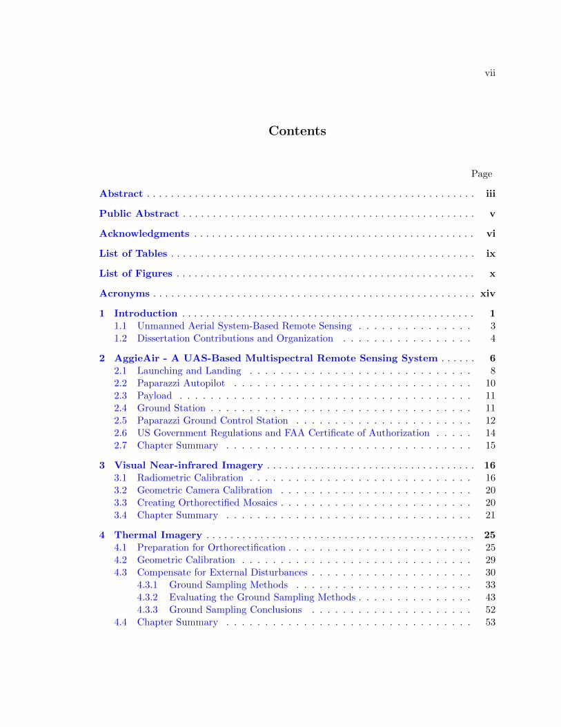
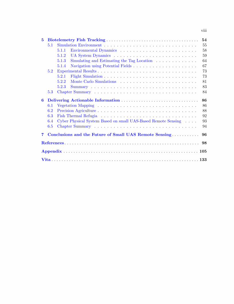
Contents
Page
Abstract . . . . . . . . . . . . . . . . . . . . . . . . . . . . . . . . . . . . . . . . . . . . . . . . . . . . . . . iii
Public Abstract . . . . . . . . . . . . . . . . . . . . . . . . . . . . . . . . . . . . . . . . . . . . . . . . . v
Acknowledgments . . . . . . . . . . . . . . . . . . . . . . . . . . . . . . . . . . . . . . . . . . . . . . . vi
List of Tables . . . . . . . . . . . . . . . . . . . . . . . . . . . . . . . . . . . . . . . . . . . . . . . . . . . ix
List of Figures . . . . . . . . . . . . . . . . . . . . . . . . . . . . . . . . . . . . . . . . . . . . . . . . . . x
Acronyms . . . . . . . . . . . . . . . . . . . . . . . . . . . . . . . . . . . . . . . . . . . . . . . . . . . . . . xiv
1 Introduction . . . . . . . . . . . . . . . . . . . . . . . . . . . . . . . . . . . . . . . . . . . . . . . . . 11.1 Unmanned Aerial System-Based Remote Sensing . . . . . . . . . . . . . . . 31.2 Dissertation Contributions and Organization . . . . . . . . . . . . . . . . . 4
2 AggieAir - A UAS-Based Multispectral Remote Sensing System . . . . . . 62.1 Launching and Landing . . . . . . . . . . . . . . . . . . . . . . . . . . . . . 82.2 Paparazzi Autopilot . . . . . . . . . . . . . . . . . . . . . . . . . . . . . . . 102.3 Payload . . . . . . . . . . . . . . . . . . . . . . . . . . . . . . . . . . . . . . 112.4 Ground Station . . . . . . . . . . . . . . . . . . . . . . . . . . . . . . . . . . 112.5 Paparazzi Ground Control Station . . . . . . . . . . . . . . . . . . . . . . . 122.6 US Government Regulations and FAA Certificate of Authorization . . . . . 142.7 Chapter Summary . . . . . . . . . . . . . . . . . . . . . . . . . . . . . . . . 15
3 Visual Near-infrared Imagery . . . . . . . . . . . . . . . . . . . . . . . . . . . . . . . . . . . 163.1 Radiometric Calibration . . . . . . . . . . . . . . . . . . . . . . . . . . . . . 163.2 Geometric Camera Calibration . . . . . . . . . . . . . . . . . . . . . . . . . 203.3 Creating Orthorectified Mosaics . . . . . . . . . . . . . . . . . . . . . . . . . 203.4 Chapter Summary . . . . . . . . . . . . . . . . . . . . . . . . . . . . . . . . 21
4 Thermal Imagery . . . . . . . . . . . . . . . . . . . . . . . . . . . . . . . . . . . . . . . . . . . . . 254.1 Preparation for Orthorectification . . . . . . . . . . . . . . . . . . . . . . . . 254.2 Geometric Calibration . . . . . . . . . . . . . . . . . . . . . . . . . . . . . . 294.3 Compensate for External Disturbances . . . . . . . . . . . . . . . . . . . . . 30
4.3.1 Ground Sampling Methods . . . . . . . . . . . . . . . . . . . . . . . 334.3.2 Evaluating the Ground Sampling Methods . . . . . . . . . . . . . . . 434.3.3 Ground Sampling Conclusions . . . . . . . . . . . . . . . . . . . . . 52
4.4 Chapter Summary . . . . . . . . . . . . . . . . . . . . . . . . . . . . . . . . 53
viii
5 Biotelemetry Fish Tracking . . . . . . . . . . . . . . . . . . . . . . . . . . . . . . . . . . . . . 545.1 Simulation Environment . . . . . . . . . . . . . . . . . . . . . . . . . . . . . 55
5.1.1 Environmental Dynamics . . . . . . . . . . . . . . . . . . . . . . . . 585.1.2 UA System Dynamics . . . . . . . . . . . . . . . . . . . . . . . . . . 595.1.3 Simulating and Estimating the Tag Location . . . . . . . . . . . . . 645.1.4 Navigation using Potential Fields . . . . . . . . . . . . . . . . . . . . 67
5.2 Experimental Results . . . . . . . . . . . . . . . . . . . . . . . . . . . . . . . 735.2.1 Flight Simulation . . . . . . . . . . . . . . . . . . . . . . . . . . . . . 735.2.2 Monte Carlo Simulations . . . . . . . . . . . . . . . . . . . . . . . . 815.2.3 Summary . . . . . . . . . . . . . . . . . . . . . . . . . . . . . . . . . 83
5.3 Chapter Summary . . . . . . . . . . . . . . . . . . . . . . . . . . . . . . . . 84
6 Delivering Actionable Information . . . . . . . . . . . . . . . . . . . . . . . . . . . . . . . 866.1 Vegetation Mapping . . . . . . . . . . . . . . . . . . . . . . . . . . . . . . . 866.2 Precision Agriculture . . . . . . . . . . . . . . . . . . . . . . . . . . . . . . . 886.3 Fish Thermal Refugia . . . . . . . . . . . . . . . . . . . . . . . . . . . . . . 926.4 Cyber Physical System Based on small UAS-Based Remote Sensing . . . . 936.5 Chapter Summary . . . . . . . . . . . . . . . . . . . . . . . . . . . . . . . . 94
7 Conclusions and the Future of Small UAS Remote Sensing . . . . . . . . . . . 96
References . . . . . . . . . . . . . . . . . . . . . . . . . . . . . . . . . . . . . . . . . . . . . . . . . . . . . . 98
Appendix . . . . . . . . . . . . . . . . . . . . . . . . . . . . . . . . . . . . . . . . . . . . . . . . . . . . . . 105
Vita . . . . . . . . . . . . . . . . . . . . . . . . . . . . . . . . . . . . . . . . . . . . . . . . . . . . . . . . . . . 133
ix
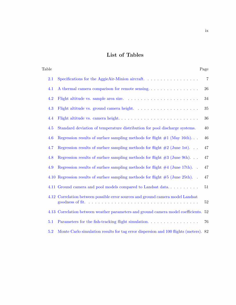
List of Tables
Table Page
2.1 Specifications for the AggieAir-Minion aircraft. . . . . . . . . . . . . . . . . 7
4.1 A thermal camera comparison for remote sensing. . . . . . . . . . . . . . . . 26
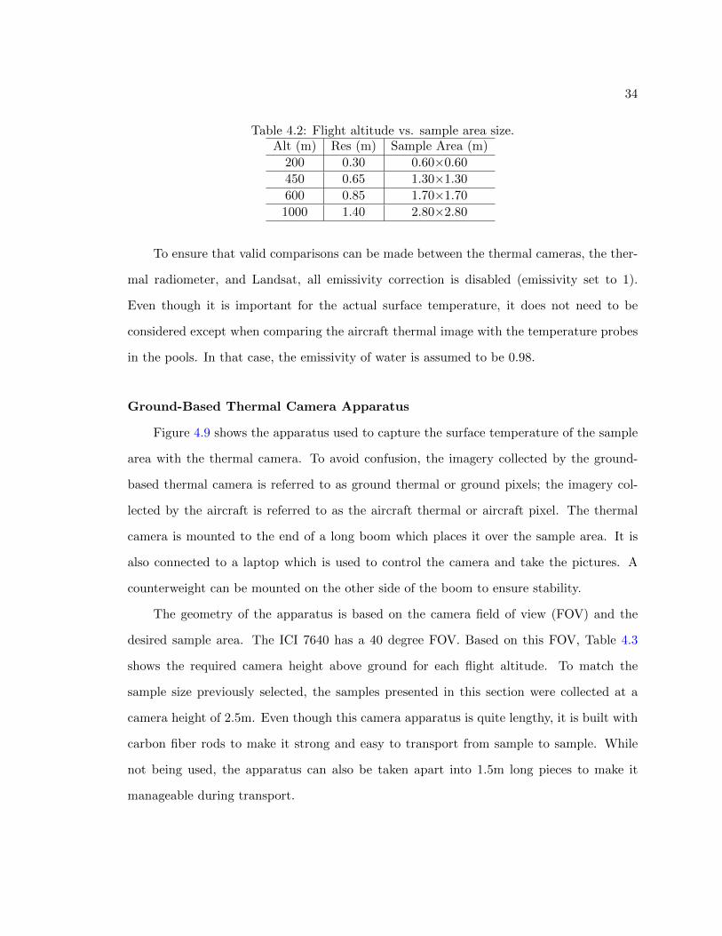
4.2 Flight altitude vs. sample area size. . . . . . . . . . . . . . . . . . . . . . . 34
4.3 Flight altitude vs. ground camera height. . . . . . . . . . . . . . . . . . . . 35
4.4 Flight altitude vs. camera height. . . . . . . . . . . . . . . . . . . . . . . . . 36
4.5 Standard deviation of temperature distribution for pool discharge systems. 40
4.6 Regression results of surface sampling methods for flight #1 (May 16th). . . 46
4.7 Regression results of surface sampling methods for flight #2 (June 1st). . . 47
4.8 Regression results of surface sampling methods for flight #3 (June 9th). . . 47
4.9 Regression results of surface sampling methods for flight #4 (June 17th). . 47
4.10 Regression results of surface sampling methods for flight #5 (June 25th). . 47
4.11 Ground camera and pool models compared to Landsat data. . . . . . . . . . 51
4.12 Correlation between possible error sources and ground camera model Landsatgoodness of fit. . . . . . . . . . . . . . . . . . . . . . . . . . . . . . . . . . . 52
4.13 Correlation between weather parameters and ground camera model coefficients. 52
5.1 Parameters for the fish-tracking flight simulation. . . . . . . . . . . . . . . . 76
5.2 Monte Carlo simulation results for tag error dispersion and 100 flights (meters). 82
x
List of Figures
Figure Page
1.1 The Processing Cycle for Meaningful Remote Sensing. . . . . . . . . . . . . 2
1.2 The AggieAir-Minion aircraft with a VIS-NIR payload. . . . . . . . . . . . . 5
2.1 AggieAir-Minion airframe layout. . . . . . . . . . . . . . . . . . . . . . . . . 7
2.2 AggieAir-Minion fuselage layout. . . . . . . . . . . . . . . . . . . . . . . . . 7
2.3 AggieAir-Minion avionics layout. . . . . . . . . . . . . . . . . . . . . . . . . 8
2.4 Diagram of AggieAir auto-takeoff procedure. . . . . . . . . . . . . . . . . . 9
2.5 Diagram of AggieAir auto-landing procedure. . . . . . . . . . . . . . . . . . 9
2.6 Diagram of the AggieAir payload system. . . . . . . . . . . . . . . . . . . . 11
2.7 AggieAir ground station diagram. . . . . . . . . . . . . . . . . . . . . . . . . 12
2.8 Paparazzi ground control station software interface. . . . . . . . . . . . . . . 13
3.1 Processing diagram for VIS-NIR imagery. . . . . . . . . . . . . . . . . . . . 17
3.2 Reflectance factor explanation. . . . . . . . . . . . . . . . . . . . . . . . . . 18
3.3 Taking a picture of the white panel before and after flight. . . . . . . . . . . 19
3.4 The picture of the white panel after stretching the contrast. . . . . . . . . . 20
3.5 Target for camera calibration toolbox for Matlab. . . . . . . . . . . . . . . . 21
3.6 The reference target for geometric camera calibration. . . . . . . . . . . . . 22
3.7 Individual raw visual images captured from a flight. . . . . . . . . . . . . . 23
3.8 Individual images after direct georeferencing. . . . . . . . . . . . . . . . . . 23
3.9 Orthorectified mosaic using 200 images from AggieAir and EnsoMOSAIC. . 24
4.1 Processing flow chart for thermal imagery from uncooled TIR cameras. . . . 26
4.2 Tool used to choose map from brightness temperature to digital numbers. . 27
xi
4.3 Comparison between original sensor brightness temperature images and im-ages after applying uniform map to digital numbers. . . . . . . . . . . . . . 28
4.4 Sensor brightness temperature images after applying uniform map to digitalnumbers. . . . . . . . . . . . . . . . . . . . . . . . . . . . . . . . . . . . . . 29
4.5 Tool used to find thermal camera temperature drift. . . . . . . . . . . . . . 30
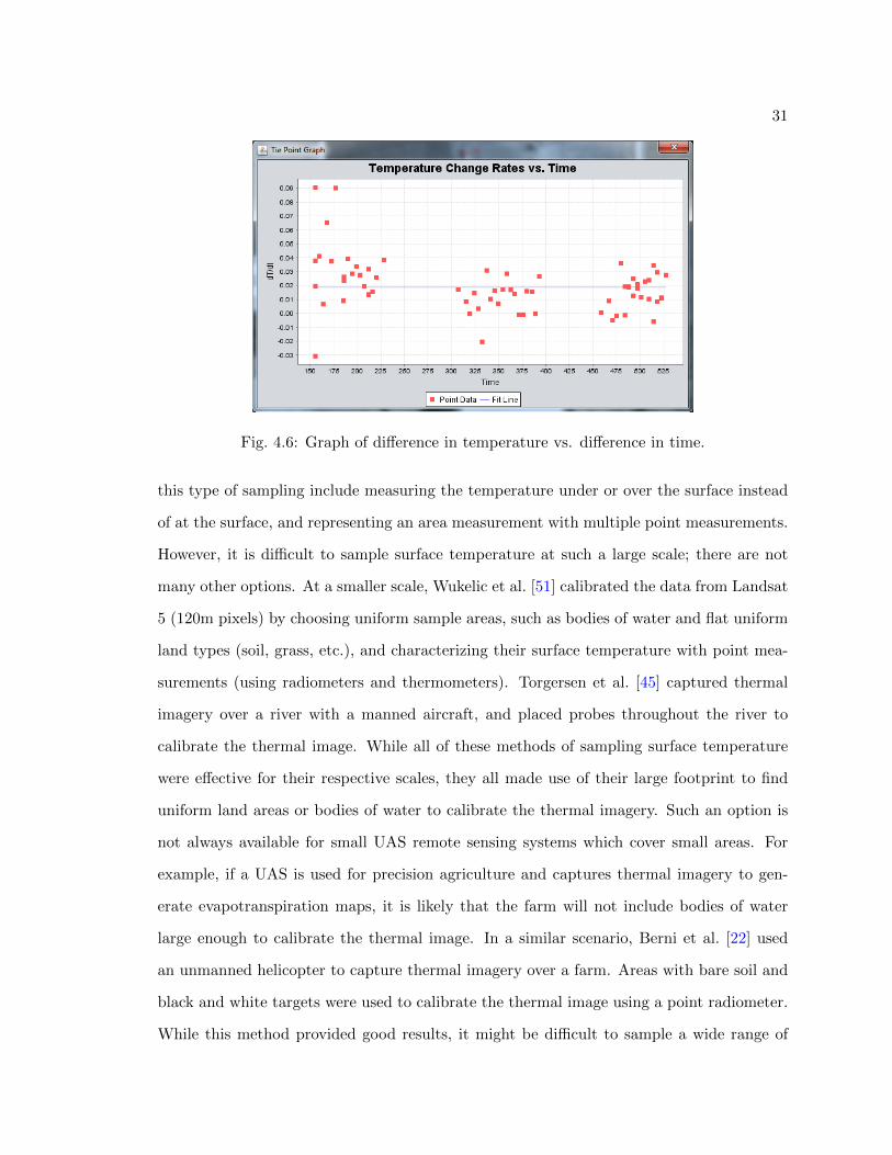
4.6 Graph of difference in temperature vs. difference in time. . . . . . . . . . . 31
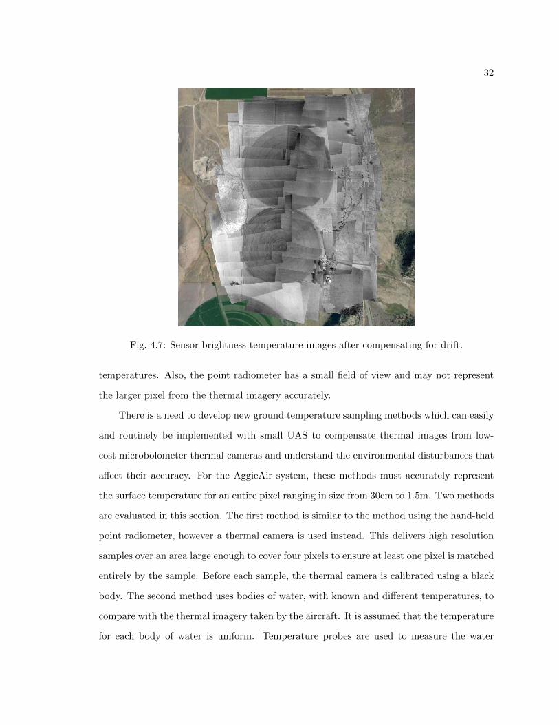
4.7 Sensor brightness temperature images after compensating for drift. . . . . . 32
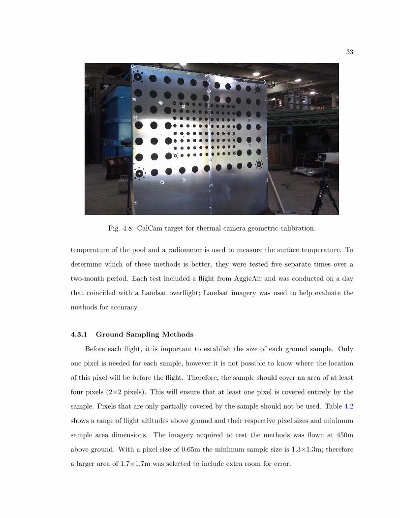
4.8 CalCam target for thermal camera geometric calibration. . . . . . . . . . . 33
4.9 Diagram of ground-based thermal camera apparatus. . . . . . . . . . . . . . 35
4.10 Diagram of thermal pool system. . . . . . . . . . . . . . . . . . . . . . . . . 37
4.11 Basic Discharge System for temperature pools. . . . . . . . . . . . . . . . . 38
4.12 L Discharge System for temperature pools. . . . . . . . . . . . . . . . . . . 39
4.13 Pressure Nozzle Discharge System for temperature pools. . . . . . . . . . . 39
4.14 Weir Discharge System for temperature pools. . . . . . . . . . . . . . . . . . 40
4.15 Circulation patterns in the Basic System. . . . . . . . . . . . . . . . . . . . 41
4.16 Thermal image for the Pressure Nozzle System. . . . . . . . . . . . . . . . . 41
4.17 Thermal image for L System. . . . . . . . . . . . . . . . . . . . . . . . . . . 42
4.18 Analysis area where pool temperatures were taken from. . . . . . . . . . . . 43
4.19 The thermal mosaic acquired on June 9th 2013 from 450m AGL. . . . . . . 44
4.20 A ground thermal image of bare-ground taken from ground-based thermalcamera. . . . . . . . . . . . . . . . . . . . . . . . . . . . . . . . . . . . . . . 45
4.21 Aircraft thermal pixels vs. ground thermal images (June 17th). . . . . . . . 45
4.22 Thermal aircraft image of cool temperature pool. . . . . . . . . . . . . . . . 48
4.23 Aircraft thermal pixels vs. pool temperature samples (June 17th). . . . . . 48
4.24 Aircraft thermal pixels vs. Landsat thermal pixels (June 17th). . . . . . . . 49
4.25 Aircraft thermal pixels vs. Landsat thermal pixels (June 17th). . . . . . . . 49
xii
4.26 Aircraft thermal pixels vs. sample methods (June 17th). . . . . . . . . . . . 50
5.1 The processing cycle for fish tracking. . . . . . . . . . . . . . . . . . . . . . 56
5.2 Flight simulation system diagram. . . . . . . . . . . . . . . . . . . . . . . . 57
5.3 UA system diagram. . . . . . . . . . . . . . . . . . . . . . . . . . . . . . . . 60
5.4 Closed-loop heading controller. . . . . . . . . . . . . . . . . . . . . . . . . . 65
5.5 The flower flight path used to collect flight data. . . . . . . . . . . . . . . . 65
5.6 The two-dimensional, fourth-order polynomial model plotted with the testflight data. . . . . . . . . . . . . . . . . . . . . . . . . . . . . . . . . . . . . 67
5.7 Residuals of the flight data vs. the signal model. . . . . . . . . . . . . . . . 68
5.8 Repulsive fractional order potential field (1 ≤ n ≤ 5). . . . . . . . . . . . . . 70
5.9 Attractive fractional order potential field (1 ≤ n ≤ 5). . . . . . . . . . . . . 71
5.10 Potential field map for the Attractive Method. . . . . . . . . . . . . . . . . 72
5.11 Potential field map for the Repulsive Method. . . . . . . . . . . . . . . . . . 73
5.12 Potential field map for the Offset Repulsive Method. . . . . . . . . . . . . . 74
5.13 Potential field map for the Dual-offset Repulsive Method. . . . . . . . . . . 74
5.14 Map for the fish-tracking flight simulation. . . . . . . . . . . . . . . . . . . . 75
5.15 Plot of UA position error in x and y. . . . . . . . . . . . . . . . . . . . . . . 77
5.16 Plot of wind magnitude and direction. . . . . . . . . . . . . . . . . . . . . . 77
5.17 Plot of actual and measured ground speed. . . . . . . . . . . . . . . . . . . 78
5.18 Plot of yaw, heading, and wind direction. . . . . . . . . . . . . . . . . . . . 78
5.19 Plot of measured and modeled signal strength. . . . . . . . . . . . . . . . . 79
5.20 Simulation results for the Repulsive Method. . . . . . . . . . . . . . . . . . 79
5.21 Simulation results for the Offset Repulsive Method. . . . . . . . . . . . . . . 80
5.22 Tag position variance plot for the Offset Repulsive Method. . . . . . . . . . 80
5.23 Simulation results for the Dual-offset Repulsive Method (2 UAs). . . . . . . 81
xiii
5.24 MC simulation with 1 UA using Repulsive Method. . . . . . . . . . . . . . . 83
5.25 MC simulation with 1 UA using Offset Repulsive Method. . . . . . . . . . . 84
5.26 MC simulation with 3 UA using Repulsive Method. . . . . . . . . . . . . . . 85
6.1 VIS-NIR mosaics and a classified image of Phragmites Australius. . . . . . . 87
6.2 A series of vegetation maps can be used for change detection. . . . . . . . . 88
6.3 VIS-NIR and thermal mosaics of two center pivots. . . . . . . . . . . . . . . 89
6.4 NDVI and LAI maps of two center pivots. . . . . . . . . . . . . . . . . . . . 90
6.5 Chlorophyll maps of oats five weeks after germination and early flowering. . 90
6.6 Nitrogen maps of oats five weeks after germination and early flowering. . . . 91
6.7 Evapotranspiration maps of two center pivots. . . . . . . . . . . . . . . . . . 91
6.8 VIS-NIR and thermal mosaics of river. . . . . . . . . . . . . . . . . . . . . . 93
6.9 Thermal mosaic of river displayed over visual mosaic. . . . . . . . . . . . . 94

xiv
Acronyms
AGL Above Ground Level
AOI Area of Interest
BRMBR Bear River Migratory Bird Refuge
BFT Biotelemetry Fish Tracking
BT Brightness Temperature
COA Certificate of Authorization
CPS Cyber Physical System
DEM Digital Elevation Model
DN Digital Number
FAA Federal Aviation Administration
FOV Field of View
FOPF Fractional Order Potential Field
GPS Global Positioning System
GCS Ground Control Station
IMU Inertial Measurement Units
ICI Infrared Cameras Inc.
MP Megapixels
NUC Non-Uniformity Correction
NOTAM Notice to Airmen
PF Potential Field
RVM Relevance Vector Machine
RC Remote Control
TIR Thermal Infrared
UAS Unmanned Aerial System
UA Unmanned Aircraft
USU Utah State University

xv
VIS-NIR Visual (red, green, blue) and Near-Infrared
VLOS Visual Line-of-sight
1
Chapter 1
Introduction
Remote sensing is a method of capturing information without physical contact. The
freedom from this physical connection enables large amounts of data to be gathered quickly
from a single point over a large area of interest (AOI). For this reason, remote sensing is
commonly used to measure the surface of the earth which can include complex, dynamic,
distributed systems. From the air (e.g. manned aircraft or satellite), large portions of
the earth can be measured in a short period of time and used for many ecological applica-
tions including agriculture [1–7], wildlife management [8,9], vegetation management [10–12],
stream and river management [13–15], and forestry [16–18]. To properly use this data it
must be converted into the actionable information needed by end users; otherwise, the data
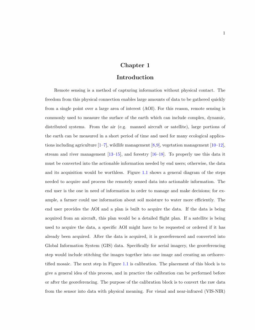
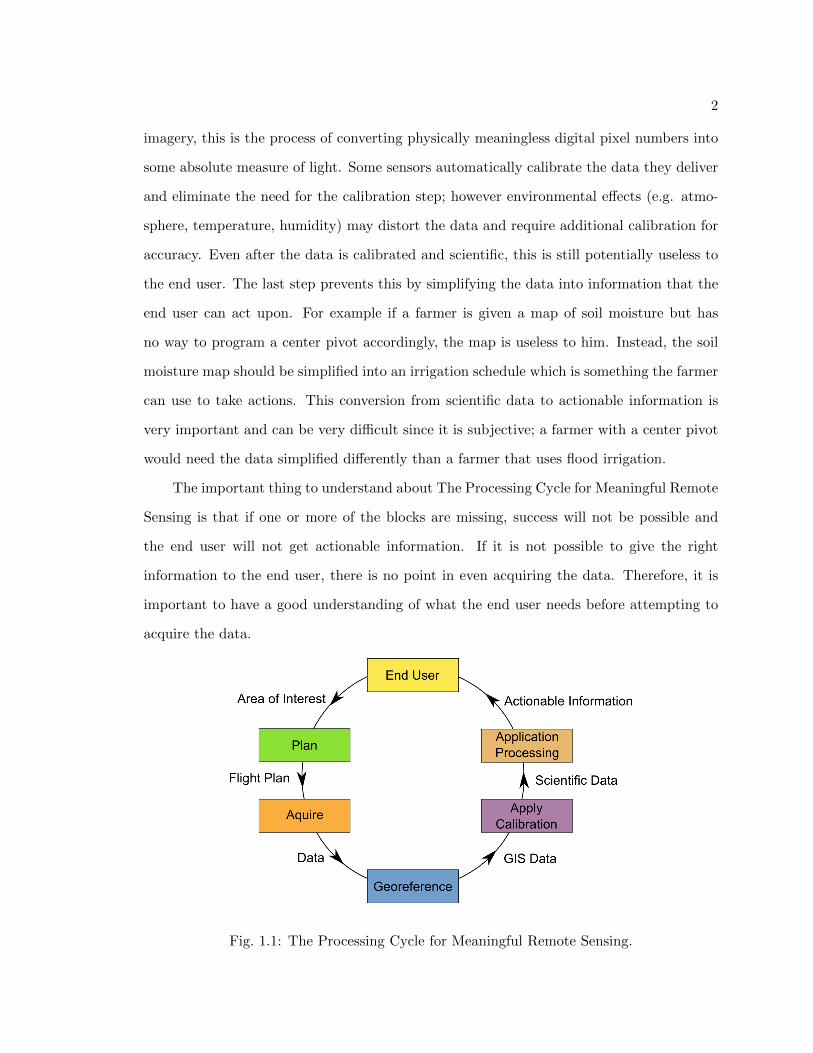
and its acquisition would be worthless. Figure 1.1 shows a general diagram of the steps
needed to acquire and process the remotely sensed data into actionable information. The
end user is the one in need of information in order to manage and make decisions; for ex-
ample, a farmer could use information about soil moisture to water more efficiently. The
end user provides the AOI and a plan is built to acquire the data. If the data is being
acquired from an aircraft, this plan would be a detailed flight plan. If a satellite is being
used to acquire the data, a specific AOI might have to be requested or ordered if it has
already been acquired. After the data is acquired, it is georeferenced and converted into
Global Information System (GIS) data. Specifically for aerial imagery, the georeferencing
step would include stitching the images together into one image and creating an orthorec-
tified mosaic. The next step in Figure 1.1 is calibration. The placement of this block is to
give a general idea of this process, and in practice the calibration can be performed before
or after the georeferencing. The purpose of the calibration block is to convert the raw data
from the sensor into data with physical meaning. For visual and near-infrared (VIS-NIR)
2
imagery, this is the process of converting physically meaningless digital pixel numbers into
some absolute measure of light. Some sensors automatically calibrate the data they deliver
and eliminate the need for the calibration step; however environmental effects (e.g. atmo-
sphere, temperature, humidity) may distort the data and require additional calibration for
accuracy. Even after the data is calibrated and scientific, this is still potentially useless to
the end user. The last step prevents this by simplifying the data into information that the
end user can act upon. For example if a farmer is given a map of soil moisture but has
no way to program a center pivot accordingly, the map is useless to him. Instead, the soil
moisture map should be simplified into an irrigation schedule which is something the farmer
can use to take actions. This conversion from scientific data to actionable information is
very important and can be very difficult since it is subjective; a farmer with a center pivot
would need the data simplified differently than a farmer that uses flood irrigation.
The important thing to understand about The Processing Cycle for Meaningful Remote
Sensing is that if one or more of the blocks are missing, success will not be possible and
the end user will not get actionable information. If it is not possible to give the right
information to the end user, there is no point in even acquiring the data. Therefore, it is
important to have a good understanding of what the end user needs before attempting to
acquire the data.
Fig. 1.1: The Processing Cycle for Meaningful Remote Sensing.
3
Many have been successful at closing this loop. For agricultural applications, VIS-NIR
multispectral imagery has been used to estimate many variables including, yield estimation
[1, 2], nitrogen deficiencies [3, 4], crop types [5], disease [6], and general health to help
with applying herbicides and pesticides [7]. By adding thermal-infrared (TIR) imagery, soil
moisture and evapotranspiration have also been estimated [4,19]. In vegetation management
applications, VIS-NIR imagery has been used to classify vegetation and help manage and
remove invasive plant species which displace native vegetation and affect wildlife habitat [10–
12]. For river and stream applications, monitoring and managing fish habitat is important
for maintaining and sustaining native fish populations. VIS-NIR imagery has been used to
map the river channel [13] and identify types of fish habitat while TIR imagery has been
used to map river surface temperatures [14,15] for fish thermal refugia. In addition to using
multispectral imagery for fish habitat, acoustic biotelemetry is another important form of
remote sensing to track fish movement [20].
1.1 Unmanned Aerial System-Based Remote Sensing
The successful applications mentioned above were all acquired using either manned
aircraft or satellite. The data acquired by these sources can include high costs, poor image
resolution, inflexible acquisition times, and slow turn-around times. In order to deal with
these shortcomings, many are turning to unmanned aerial systems (UAS) as an alternative
platform for remote sensing [21–24]. Since many of these UAS are small, remotely sensed
data can be obtained at a low-cost, quickly, and at high spatial and temporal resolution.
However, the small (less than 20lbs), low-cost nature of these systems introduces problems
that make it difficult to successfully deliver actionable information. This is most apparent in
the small, low-cost navigation sensors (GPS and inertial measurement units (IMU)) which
provide position and orientation information to the autopilot. Because they are small and
low-cost, they tend to be less accurate than other systems used by manned aircraft and
satellite. Even though their accuracy is enough to navigate the aircraft, they have enough
errors to make georeferencing remotely-sensed data very difficult. In addition to these
challenges with georeferencing, data quality is also a problem for low-cost, small, consumer-
4
grade cameras compatible with small UAS. In many cases, these sensors do not come with
calibration information which is important for generating scientific data. Some have used
larger UAS to carry expensive, scientific-grade sensors to provide actionable information
to end users. Laliberte et al. [25] used a large UAS, and VIS-NIR imagery for mapping
vegetation over rangeland. Berni et al. [22] looked at using thermal imagery for soil moisture
and compared that to methods for soil moisture using VIS-NIR imagery. While quality
scientific data was produced in both of these cases, large UAS (20lb takeoff weight) were
used along with expensive scientific grade sensors.
1.2 Dissertation Contributions and Organization
One of the main contributions of this dissertation includes a complete description on
how to calibrate imagery from consumer grade VIS-NIR and TIR cameras for small UAS
and scientific applications. While other documents may contain some of these steps, this
is the first document to include every step in detail for both VIS-NIR and TIR. Another
important contribution in this dissertation is a presentation of novel surface temperature
sampling methods to help calibrate the TIR imagery [26]. Comparisons are made between
the different sampling techniques and a trusted source of remote sensing data: Landsat. The
final major contribution details the conversion of raw data from a novel biotelemetry fish
tracking (BFT) payload into scientific data (estimated location of a radio-tagged fish) [27].
In addition to presenting new, simple methods for multi-UAV navigation and radio source
estimation, Monte Carlo analysis was used to take a detailed look into how much accuracy
can be expected in real-world scenarios. Such an analysis has never been done before with
biotelemetry and small UAS.
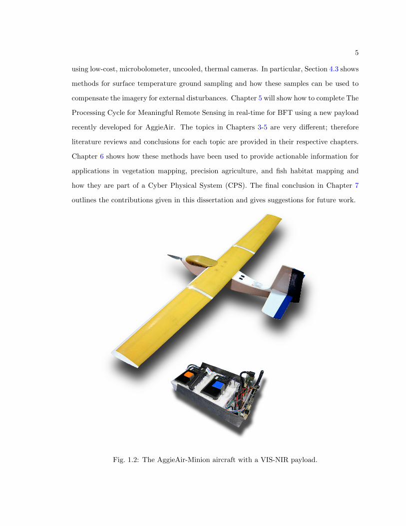
The small UAS used to gather the data is called AggieAir (Figure 1.2) and is described
in Chapter 2. Each chapter thenceforth will outline the conversion process to scientific data
for the three different payloads (VIS-NIR, TIR, BFT). Chapter 3 will show how VIS-NIR
imagery is converted into scientific data for commercial-grade, point-and-shoot cameras.
This process is already well established; therefore Chapter 3 will be a review of current
practices. Chapter 4 will show how TIR imagery can be converted into surface temperature
5
using low-cost, microbolometer, uncooled, thermal cameras. In particular, Section 4.3 shows
methods for surface temperature ground sampling and how these samples can be used to
compensate the imagery for external disturbances. Chapter 5 will show how to complete The
Processing Cycle for Meaningful Remote Sensing in real-time for BFT using a new payload
recently developed for AggieAir. The topics in Chapters 3-5 are very different; therefore
literature reviews and conclusions for each topic are provided in their respective chapters.
Chapter 6 shows how these methods have been used to provide actionable information for
applications in vegetation mapping, precision agriculture, and fish habitat mapping and
how they are part of a Cyber Physical System (CPS). The final conclusion in Chapter 7
outlines the contributions given in this dissertation and gives suggestions for future work.
Fig. 1.2: The AggieAir-Minion aircraft with a VIS-NIR payload.
6
Chapter 2
AggieAir - A UAS-Based Multispectral Remote Sensing
System
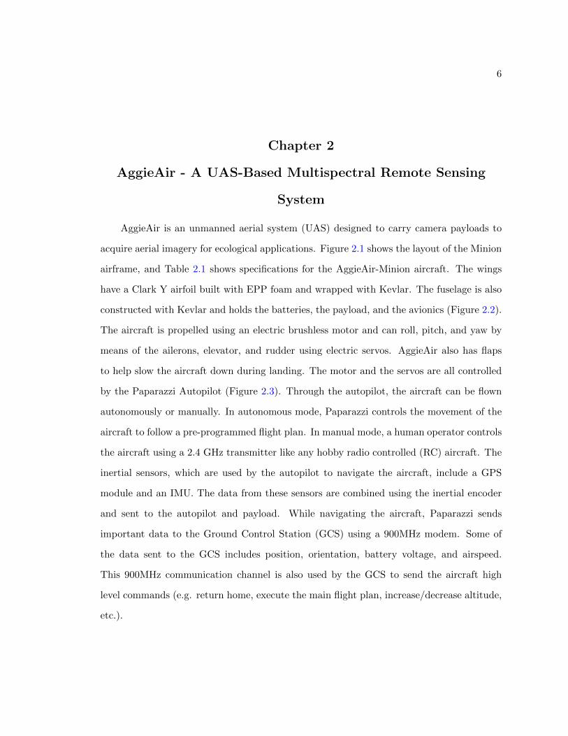
AggieAir is an unmanned aerial system (UAS) designed to carry camera payloads to
acquire aerial imagery for ecological applications. Figure 2.1 shows the layout of the Minion
airframe, and Table 2.1 shows specifications for the AggieAir-Minion aircraft. The wings
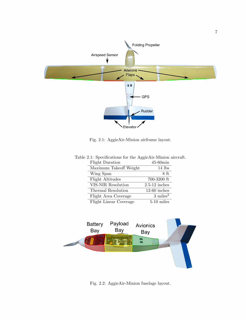
have a Clark Y airfoil built with EPP foam and wrapped with Kevlar. The fuselage is also
constructed with Kevlar and holds the batteries, the payload, and the avionics (Figure 2.2).
The aircraft is propelled using an electric brushless motor and can roll, pitch, and yaw by
means of the ailerons, elevator, and rudder using electric servos. AggieAir also has flaps
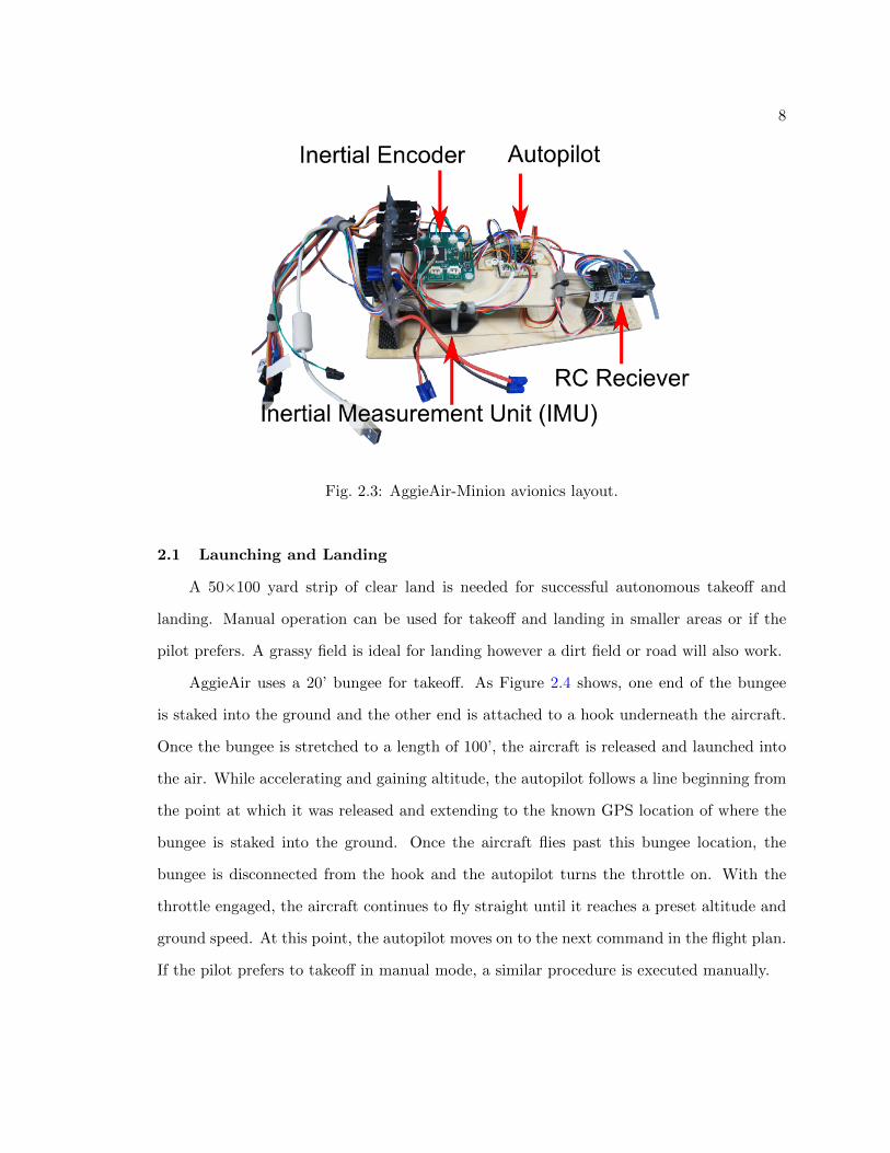
to help slow the aircraft down during landing. The motor and the servos are all controlled
by the Paparazzi Autopilot (Figure 2.3). Through the autopilot, the aircraft can be flown
autonomously or manually. In autonomous mode, Paparazzi controls the movement of the
aircraft to follow a pre-programmed flight plan. In manual mode, a human operator controls
the aircraft using a 2.4 GHz transmitter like any hobby radio controlled (RC) aircraft. The
inertial sensors, which are used by the autopilot to navigate the aircraft, include a GPS
module and an IMU. The data from these sensors are combined using the inertial encoder
and sent to the autopilot and payload. While navigating the aircraft, Paparazzi sends
important data to the Ground Control Station (GCS) using a 900MHz modem. Some of
the data sent to the GCS includes position, orientation, battery voltage, and airspeed.
This 900MHz communication channel is also used by the GCS to send the aircraft high
level commands (e.g. return home, execute the main flight plan, increase/decrease altitude,
etc.).
7
Fig. 2.1: AggieAir-Minion airframe layout.
Table 2.1: Specifications for the AggieAir-Minion aircraft.Flight Duration 45-60min
Maximum Takeoff Weight 14 lbs
Wing Span 8 ft
Flight Altitudes 700-3200 ft
VIS-NIR Resolution 2.5-12 inches
Thermal Resolution 12-60 inches
Flight Area Coverage 3 miles2
Flight Linear Coverage 5-10 miles
Fig. 2.2: AggieAir-Minion fuselage layout.
8
Fig. 2.3: AggieAir-Minion avionics layout.
2.1 Launching and Landing
A 50×100 yard strip of clear land is needed for successful autonomous takeoff and
landing. Manual operation can be used for takeoff and landing in smaller areas or if the
pilot prefers. A grassy field is ideal for landing however a dirt field or road will also work.
AggieAir uses a 20’ bungee for takeoff. As Figure 2.4 shows, one end of the bungee
is staked into the ground and the other end is attached to a hook underneath the aircraft.
Once the bungee is stretched to a length of 100’, the aircraft is released and launched into
the air. While accelerating and gaining altitude, the autopilot follows a line beginning from
the point at which it was released and extending to the known GPS location of where the
bungee is staked into the ground. Once the aircraft flies past this bungee location, the
bungee is disconnected from the hook and the autopilot turns the throttle on. With the
throttle engaged, the aircraft continues to fly straight until it reaches a preset altitude and
ground speed. At this point, the autopilot moves on to the next command in the flight plan.
If the pilot prefers to takeoff in manual mode, a similar procedure is executed manually.
9
Fig. 2.4: Diagram of AggieAir auto-takeoff procedure.
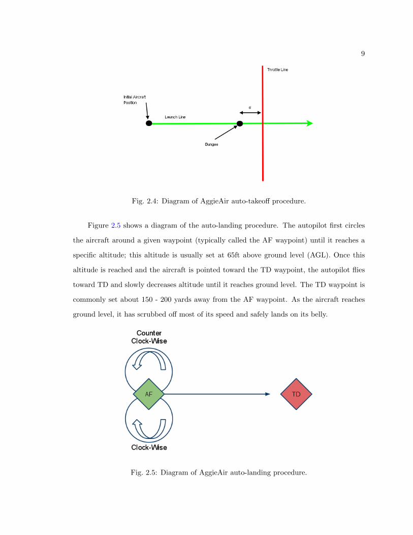
Figure 2.5 shows a diagram of the auto-landing procedure. The autopilot first circles
the aircraft around a given waypoint (typically called the AF waypoint) until it reaches a
specific altitude; this altitude is usually set at 65ft above ground level (AGL). Once this
altitude is reached and the aircraft is pointed toward the TD waypoint, the autopilot flies
toward TD and slowly decreases altitude until it reaches ground level. The TD waypoint is
commonly set about 150 - 200 yards away from the AF waypoint. As the aircraft reaches
ground level, it has scrubbed off most of its speed and safely lands on its belly.
Fig. 2.5: Diagram of AggieAir auto-landing procedure.
10
2.2 Paparazzi Autopilot
The Paparazzi Autopilot has three modes of operation: manual, semi-autonomous,
and fully-autonomous. The pilot can switch between these modes using a switch on the RC
transmitter. If Paparazzi does not detect the transmitter, the default mode of operation is
fully-autonomous.
When in manual mode, the RC receiver on the aircraft receives the command signals
from the transmitter and passes them on to the Paparazzi board. The Paparazzi board
then actuates the motor and servos according to these control signals. Even though the
actuators are controlled through the Paparazzi board, the pilot is in complete control of the
aircraft.
Like manual mode, control of the aircraft in semi-autonomous mode is also through
the pilot and an RC transmitter at the GCS. However, the roll and pitch of the aircraft are
stabilized using the autopilot and the IMU; the throttle is still manually controlled. For
example, if the pilot pulls the stick to the right, the autopilot will interpret this as a specific
positive roll value and will try to hold the aircraft in that orientation. If the pilot lets go of
the stick, Paparazzi will hold the aircraft at zero roll and zero pitch. The semi-autonomous
mode is used to help trim and tune the aircraft.
When in fully autonomous mode, Paparazzi flies the aircraft according to a prepro-
grammed flight plan. The flight plan contains waypoints and blocks which are used to tell
the aircraft where to go and what to do there. A waypoint is a point of interest on the map
defined by its location (GPS and altitude). The blocks use the waypoints to give specific
commands to the autopilot. An example of a block is the Goto Block; the Goto Block
simply tells the autopilot to go to a given waypoint. Another example is the Circle Block,
which tells the autopilot to circle around a given waypoint at a given radius. Blocks can be
set up to simply move to the next block when finished, to move to a different block some-
where else in the flight plan, or to repeat until the operator directs it to a different block.
Exceptions can also be used in the flight plan to detect specific conditions and to redirect
the aircraft accordingly. For example, an exception could be used to tell the autopilot to
11
come home if it gets too far away.
2.3 Payload
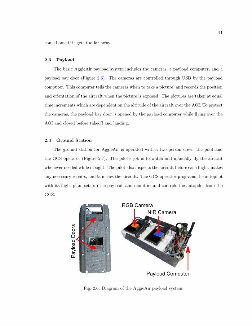
The basic AggieAir payload system includes the cameras, a payload computer, and a
payload bay door (Figure 2.6). The cameras are controlled through USB by the payload
computer. This computer tells the cameras when to take a picture, and records the position
and orientation of the aircraft when the picture is exposed. The pictures are taken at equal
time increments which are dependent on the altitude of the aircraft over the AOI. To protect
the cameras, the payload bay door is opened by the payload computer while flying over the
AOI and closed before takeoff and landing.
2.4 Ground Station
The ground station for AggieAir is operated with a two person crew: the pilot and
the GCS operator (Figure 2.7). The pilot’s job is to watch and manually fly the aircraft
whenever needed while in sight. The pilot also inspects the aircraft before each flight, makes
any necessary repairs, and launches the aircraft. The GCS operator programs the autopilot
with its flight plan, sets up the payload, and monitors and controls the autopilot from the
GCS.
Fig. 2.6: Diagram of the AggieAir payload system.

12
Fig. 2.7: AggieAir ground station diagram.
2.5 Paparazzi Ground Control Station
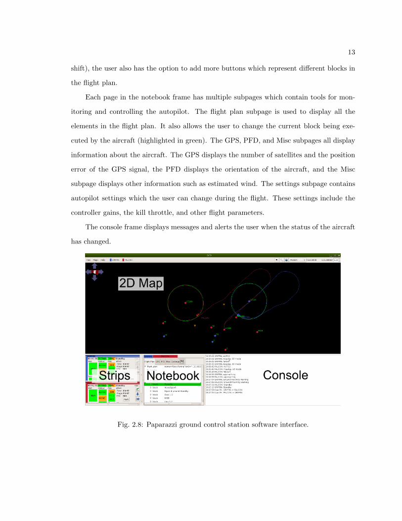
The Paparazzi GCS is used to monitor and control the autopilot while in flight or
simulation. Figure 2.8 shows the layout of the GCS.
The 2D map gives the user an aerial perspective to help control and monitor the
aircraft. The current aircraft position, the flight plan waypoints, the path of the aircraft,
and the desired path of the aircraft are all displayed on the 2D map. To help visualize
where the aircraft is, background images can be downloaded from Google maps under the
Maps menu. The 2D map can be navigated using the mouse, the arrow keys, or by using
the menus and buttons above the map.
Each strip on the GCS displays important telemetry data and has buttons for common
commands for the autopilot. Examples of the telemetry data displayed on each strip include
battery voltage, speed, throttle, current altitude, target altitude, and the autonomous mode.
In addition to common command buttons (e.g. launch, kill throttle, altitude, and lateral
13
shift), the user also has the option to add more buttons which represent different blocks in
the flight plan.
Each page in the notebook frame has multiple subpages which contain tools for mon-
itoring and controlling the autopilot. The flight plan subpage is used to display all the
elements in the flight plan. It also allows the user to change the current block being exe-
cuted by the aircraft (highlighted in green). The GPS, PFD, and Misc subpages all display
information about the aircraft. The GPS displays the number of satellites and the position
error of the GPS signal, the PFD displays the orientation of the aircraft, and the Misc
subpage displays other information such as estimated wind. The settings subpage contains
autopilot settings which the user can change during the flight. These settings include the
controller gains, the kill throttle, and other flight parameters.
The console frame displays messages and alerts the user when the status of the aircraft
has changed.
Fig. 2.8: Paparazzi ground control station software interface.
14
2.6 US Government Regulations and FAA Certificate of Authorization
In the United States (US), all flights of an unmanned aircraft (UA) are regulated by
the Federal Aviation Administration (FAA). A UA is defined as any aircraft where a pilot is
not on-board. This includes autonomous UAS aircraft, like AggieAir, as well as hobby RC
aircraft. Since most RC hobbyists usually fly their aircraft for recreation, the FAA allows
flight according to The Academy of Model Aeronautics National Model Aircraft Safety
Code [28]. If a UA is flown for anything beyond recreation (e.g. to support a research
project, profit, emergency response, etc.), at any altitude, the operator should apply for
a Certificate of Authorization (COA) from the FAA [29]. Before using them to authorize
UA flights, the FAA used COAs to give permission for aviation events such as airshows
which required temporary alteration of current regulations for the period of the airshow.
Applicants would state which regulations would need to be waived, and how they would
mitigate the additional risks. The COA is used for UA in a similar way: since the pilot is not
on-board the aircraft and cannot comply with the standard see-and-avoid responsibilities
to avoid mid-air collision, these risks must be mitigated before the flight is allowed. To
mitigate the risks of UA flights, the FAA has additional regulations and restrictions that
must be satisfied in the COA application. Some of these restrictions include no UA flights
at night, no UA flights over a populated area, no UA flights in class B airspace, one UA in
the airspace at a time, and keeping the UA within visual line-of-sight (VLOS) at all times.
There are also certain qualifications the crew must have; some flight operations require a
pilot with a private pilot’s license, others require a minimum of ground school [29]. In
addition to the pilot, at least one observer must be included in the flight operations to keep
the UA within VLOS at all times. Specific fail-safe procedures also need to be included in
the COA application to explain what the UA will do if it looses link with the ground station
or looses GPS link. The types of organizations who can receive a COA is also restricted.
Only public entities like municipalities, police forces, state universities, military, etc. can
receive a COA; all private companies (profit or non-profit) are excluded. FAA officials will
also look at airworthiness of the aircraft in the COA application. For a public entity, this
15
is done using a signed airworthiness statement which contains a maintenance schedule and
a preflight checklist to ensure airworthiness before each flight.
After a COA is approved, it is only valid for the specific aircraft, during specific times,
at a specific location, and for the flight operation included in the application. Before flying
the UA, the COA may also require the operators to file a Notice to Airmen (NOTAM) and
to contact local airports and airspace managers in advance. Depending on the applicant’s
experience and the number of COAs in the queue, a COA may take between 2 to 9 months
before it is approved. An example COA for AggieAir on the North Slope of Alaska is
included in the Appendix along with the flight operations which were submitted with the
application. This example is one of many COAs approved for the AggieAir UAS through
state universities such as Utah State University (USU), Texas State University, and UC
Merced.
2.7 Chapter Summary
This chapter presented the AggieAir UAS and how it is programmed, launched, recov-
ered, and controlled. Government regulations were also briefly reviewed and insight was
given into what is required to apply for an FAA COA. However, this only covers the first
two steps in the Processing Cycle for Meaningful Remote Sensing. There is no value in a
UAS with a camera unless the rest of the cycle can be completed. The following chapters
will detail how to make sense of the remotely sensed data, specifically, to georeference and
calibrate the data from the UAS.
16
Chapter 3
Visual Near-infrared Imagery
Many scientific VIS-NIR cameras are developed either for aerial imaging from a manned
aircraft or for industrial use. The cameras developed for aerial imaging from a manned
aircraft commonly have high quality optics and high resolution; however, they also tend to
be very large, heavy, and expensive which does not work with small UAS. There are also
small, less-expensive aerial imaging cameras which are more compatible with small UAS.
Laliberte et al. [30] used the Mini MCA-6 multispectral camera on the BAT3 UAS to map
vegetation over a rangeland. The MCA-6 is small and designed to output scientific data;
however it is still costly and has a coarse resolution (1.3 megapixels (MP)). Others have
also used the MCA-6 for UAV remote sensing for its data quality [31, 32]. Small industrial
cameras could work for UAS aerial imaging; however they are generally designed to produce
video and can be very expensive at high resolution. Another type of camera available for
small UAS are consumer-grade cameras (personal point-and-click cameras); these cameras
are ideal because they are small, low-cost, and have high resolution (8-12 MP) [25, 33].
However they can be difficult to control and synchronize with the inertial data from the
aircraft [34]. In addition, using consumer-grade cameras for scientific applications can be
difficult since they do not come with the calibrations performed on typical remote sensing
VIS-NIR cameras [35]. This chapter will show how the data from consumer-grade cameras
can be processed and converted into quality scientific data, and used to collect multispectral
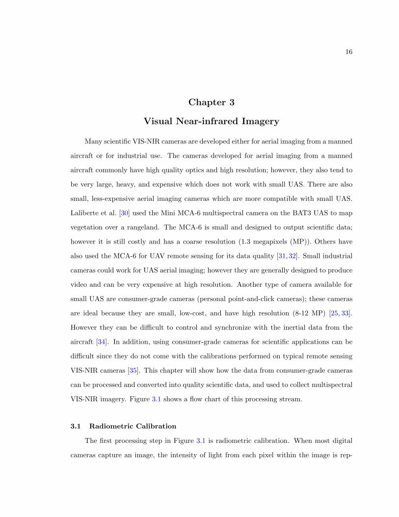
VIS-NIR imagery. Figure 3.1 shows a flow chart of this processing stream.
3.1 Radiometric Calibration
The first processing step in Figure 3.1 is radiometric calibration. When most digital
cameras capture an image, the intensity of light from each pixel within the image is rep-
17
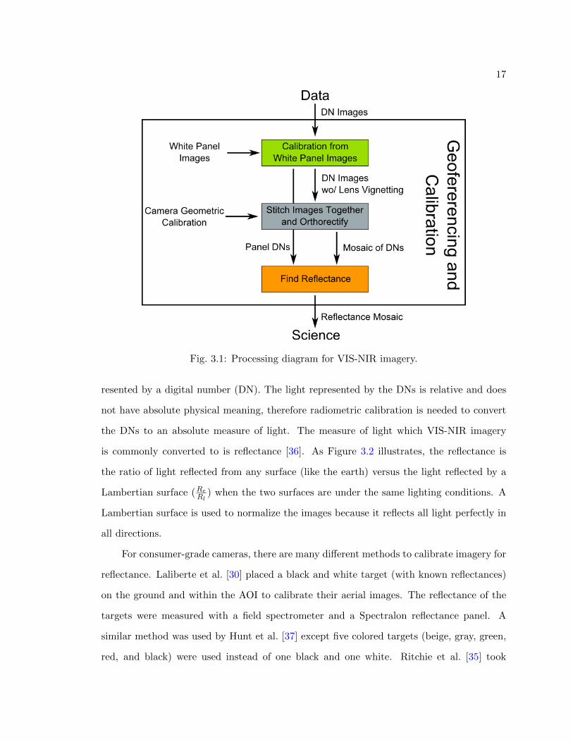
Fig. 3.1: Processing diagram for VIS-NIR imagery.
resented by a digital number (DN). The light represented by the DNs is relative and does
not have absolute physical meaning, therefore radiometric calibration is needed to convert
the DNs to an absolute measure of light. The measure of light which VIS-NIR imagery
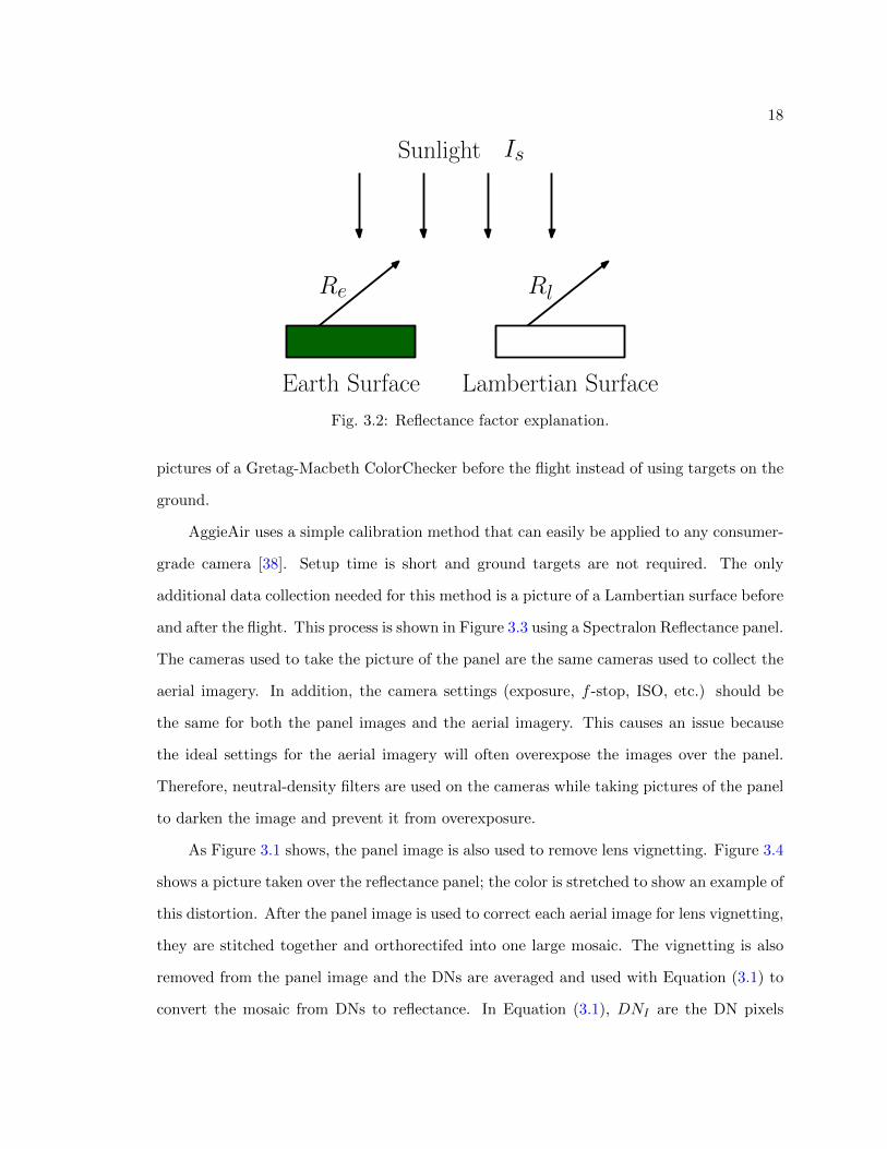
is commonly converted to is reflectance [36]. As Figure 3.2 illustrates, the reflectance is
the ratio of light reflected from any surface (like the earth) versus the light reflected by a
Lambertian surface (ReRl
) when the two surfaces are under the same lighting conditions. A
Lambertian surface is used to normalize the images because it reflects all light perfectly in
all directions.
For consumer-grade cameras, there are many different methods to calibrate imagery for
reflectance. Laliberte et al. [30] placed a black and white target (with known reflectances)
on the ground and within the AOI to calibrate their aerial images. The reflectance of the
targets were measured with a field spectrometer and a Spectralon reflectance panel. A
similar method was used by Hunt et al. [37] except five colored targets (beige, gray, green,
red, and black) were used instead of one black and one white. Ritchie et al. [35] took
18
Lambertian SurfaceEarth Surface
Sunlight Is
Re Rl
Fig. 3.2: Reflectance factor explanation.
pictures of a Gretag-Macbeth ColorChecker before the flight instead of using targets on the
ground.
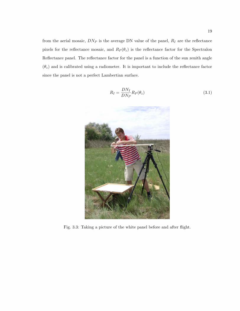
AggieAir uses a simple calibration method that can easily be applied to any consumer-
grade camera [38]. Setup time is short and ground targets are not required. The only
additional data collection needed for this method is a picture of a Lambertian surface before
and after the flight. This process is shown in Figure 3.3 using a Spectralon Reflectance panel.
The cameras used to take the picture of the panel are the same cameras used to collect the
aerial imagery. In addition, the camera settings (exposure, f -stop, ISO, etc.) should be
the same for both the panel images and the aerial imagery. This causes an issue because
the ideal settings for the aerial imagery will often overexpose the images over the panel.
Therefore, neutral-density filters are used on the cameras while taking pictures of the panel
to darken the image and prevent it from overexposure.
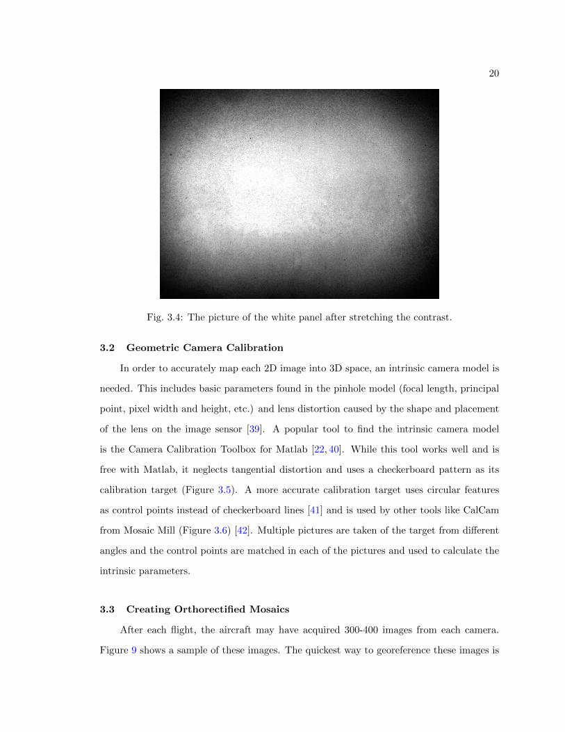
As Figure 3.1 shows, the panel image is also used to remove lens vignetting. Figure 3.4
shows a picture taken over the reflectance panel; the color is stretched to show an example of
this distortion. After the panel image is used to correct each aerial image for lens vignetting,
they are stitched together and orthorectifed into one large mosaic. The vignetting is also
removed from the panel image and the DNs are averaged and used with Equation (3.1) to
convert the mosaic from DNs to reflectance. In Equation (3.1), DNI are the DN pixels
19
from the aerial mosaic, DNP is the average DN value of the panel, RI are the reflectance
pixels for the reflectance mosaic, and RP (θz) is the reflectance factor for the Spectralon
Reflectance panel. The reflectance factor for the panel is a function of the sun zenith angle
(θz) and is calibrated using a radiometer. It is important to include the reflectance factor
since the panel is not a perfect Lambertian surface.
RI =DNI
DNPRP (θz) (3.1)
Fig. 3.3: Taking a picture of the white panel before and after flight.
20
Fig. 3.4: The picture of the white panel after stretching the contrast.
3.2 Geometric Camera Calibration
In order to accurately map each 2D image into 3D space, an intrinsic camera model is
needed. This includes basic parameters found in the pinhole model (focal length, principal
point, pixel width and height, etc.) and lens distortion caused by the shape and placement
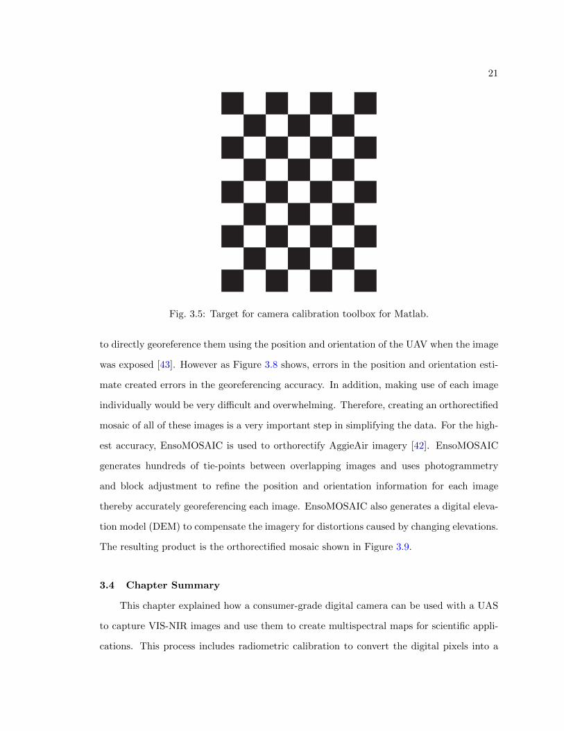
of the lens on the image sensor [39]. A popular tool to find the intrinsic camera model
is the Camera Calibration Toolbox for Matlab [22, 40]. While this tool works well and is
free with Matlab, it neglects tangential distortion and uses a checkerboard pattern as its
calibration target (Figure 3.5). A more accurate calibration target uses circular features
as control points instead of checkerboard lines [41] and is used by other tools like CalCam
from Mosaic Mill (Figure 3.6) [42]. Multiple pictures are taken of the target from different
angles and the control points are matched in each of the pictures and used to calculate the
intrinsic parameters.
3.3 Creating Orthorectified Mosaics
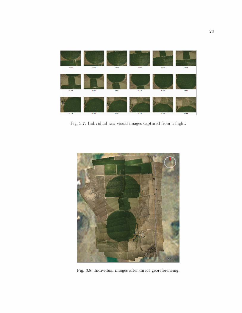
After each flight, the aircraft may have acquired 300-400 images from each camera.
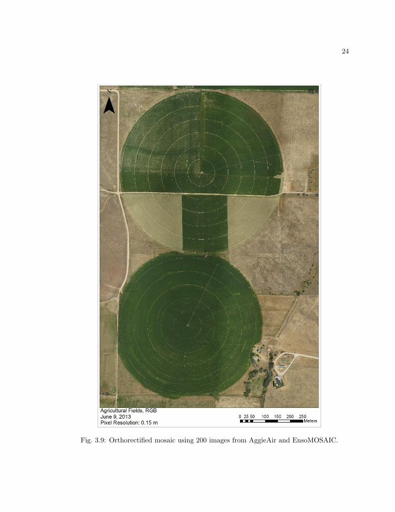
Figure 9 shows a sample of these images. The quickest way to georeference these images is
21
Fig. 3.5: Target for camera calibration toolbox for Matlab.
to directly georeference them using the position and orientation of the UAV when the image
was exposed [43]. However as Figure 3.8 shows, errors in the position and orientation esti-
mate created errors in the georeferencing accuracy. In addition, making use of each image
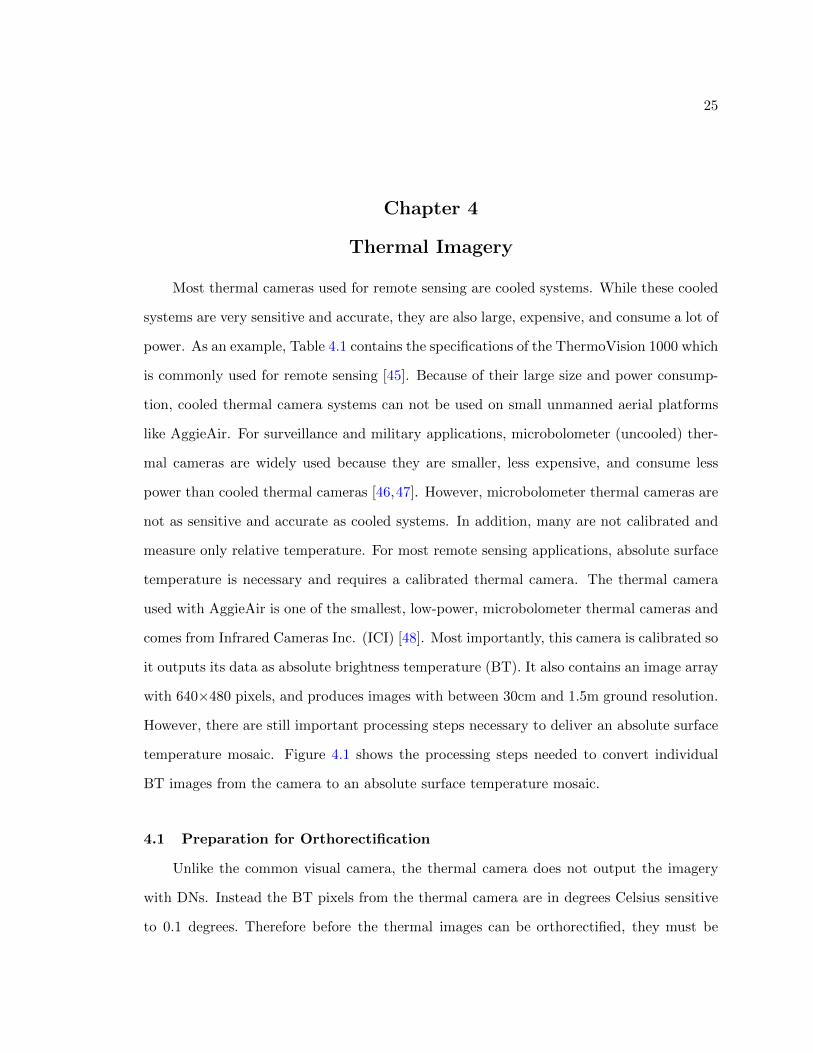
individually would be very difficult and overwhelming. Therefore, creating an orthorectified
mosaic of all of these images is a very important step in simplifying the data. For the high-
est accuracy, EnsoMOSAIC is used to orthorectify AggieAir imagery [42]. EnsoMOSAIC
generates hundreds of tie-points between overlapping images and uses photogrammetry
and block adjustment to refine the position and orientation information for each image
thereby accurately georeferencing each image. EnsoMOSAIC also generates a digital eleva-
tion model (DEM) to compensate the imagery for distortions caused by changing elevations.
The resulting product is the orthorectified mosaic shown in Figure 3.9.
3.4 Chapter Summary
This chapter explained how a consumer-grade digital camera can be used with a UAS
to capture VIS-NIR images and use them to create multispectral maps for scientific appli-
cations. This process includes radiometric calibration to convert the digital pixels into a

22
Fig. 3.6: The reference target for geometric camera calibration.
measure of reflectance, geometric calibration to help project the 2D images into a 3D space,
and the stitching and orthorectification process to combine all of the images into one large
mosaic. Different options for these processes were reviewed with current literature, but the
process used with AggieAir was featured. Beneficial future research in this area would be
to improve the speed of the orthorectification without sacrificing spatial accuracy. In many
cases, the actionable information needed by the end user is very time sensitive and the
orthorectification step, for accurate mosaics, is still very time consuming (one week to one
month per flight). Another area of research would be to improve the radiometric calibration
by finding the spectral response of the cameras using a monochromator [44].
23
Fig. 3.7: Individual raw visual images captured from a flight.
Fig. 3.8: Individual images after direct georeferencing.
24
Fig. 3.9: Orthorectified mosaic using 200 images from AggieAir and EnsoMOSAIC.
25
Chapter 4
Thermal Imagery
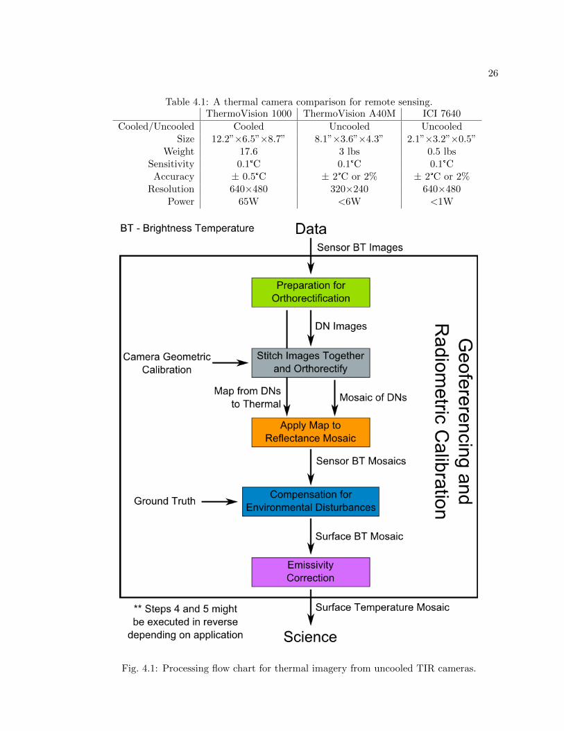
Most thermal cameras used for remote sensing are cooled systems. While these cooled
systems are very sensitive and accurate, they are also large, expensive, and consume a lot of
power. As an example, Table 4.1 contains the specifications of the ThermoVision 1000 which
is commonly used for remote sensing [45]. Because of their large size and power consump-
tion, cooled thermal camera systems can not be used on small unmanned aerial platforms
like AggieAir. For surveillance and military applications, microbolometer (uncooled) ther-
mal cameras are widely used because they are smaller, less expensive, and consume less
power than cooled thermal cameras [46,47]. However, microbolometer thermal cameras are
not as sensitive and accurate as cooled systems. In addition, many are not calibrated and
measure only relative temperature. For most remote sensing applications, absolute surface
temperature is necessary and requires a calibrated thermal camera. The thermal camera
used with AggieAir is one of the smallest, low-power, microbolometer thermal cameras and
comes from Infrared Cameras Inc. (ICI) [48]. Most importantly, this camera is calibrated so
it outputs its data as absolute brightness temperature (BT). It also contains an image array
with 640×480 pixels, and produces images with between 30cm and 1.5m ground resolution.
However, there are still important processing steps necessary to deliver an absolute surface
temperature mosaic. Figure 4.1 shows the processing steps needed to convert individual
BT images from the camera to an absolute surface temperature mosaic.
4.1 Preparation for Orthorectification
Unlike the common visual camera, the thermal camera does not output the imagery
with DNs. Instead the BT pixels from the thermal camera are in degrees Celsius sensitive
to 0.1 degrees. Therefore before the thermal images can be orthorectified, they must be
26
Table 4.1: A thermal camera comparison for remote sensing.ThermoVision 1000 ThermoVision A40M ICI 7640
Cooled/Uncooled Cooled Uncooled UncooledSize 12.2”×6.5”×8.7” 8.1”×3.6”×4.3” 2.1”×3.2”×0.5”
Weight 17.6 3 lbs 0.5 lbsSensitivity 0.1°C 0.1°C 0.1°CAccuracy ± 0.5°C ± 2°C or 2% ± 2°C or 2%
Resolution 640×480 320×240 640×480Power 65W <6W <1W
Fig. 4.1: Processing flow chart for thermal imagery from uncooled TIR cameras.
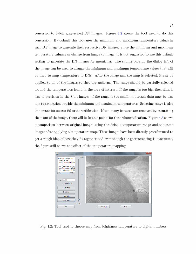
27
converted to 8-bit, gray-scaled DN images. Figure 4.2 shows the tool used to do this
conversion. By default this tool uses the minimum and maximum temperature values in
each BT image to generate their respective DN images. Since the minimum and maximum
temperature values can change from image to image, it is not suggested to use this default
setting to generate the DN images for mosaicing. The sliding bars on the dialog left of
the image can be used to change the minimum and maximum temperature values that will
be used to map temperature to DNs. After the range and the map is selected, it can be
applied to all of the images so they are uniform. The range should be carefully selected
around the temperatures found in the area of interest. If the range is too big, then data is
lost to precision in the 8-bit images; if the range is too small, important data may be lost
due to saturation outside the minimum and maximum temperatures. Selecting range is also
important for successful orthorectification. If too many features are removed by saturating
them out of the image, there will be less tie points for the orthorectification. Figure 4.3 shows
a comparison between original images using the default temperature range and the same
images after applying a temperature map. These images have been directly georeferenced to
get a rough idea of how they fit together and even though the georeferencing is inaccurate,
the figure still shows the effect of the temperature mapping.
Fig. 4.2: Tool used to choose map from brightness temperature to digital numbers.
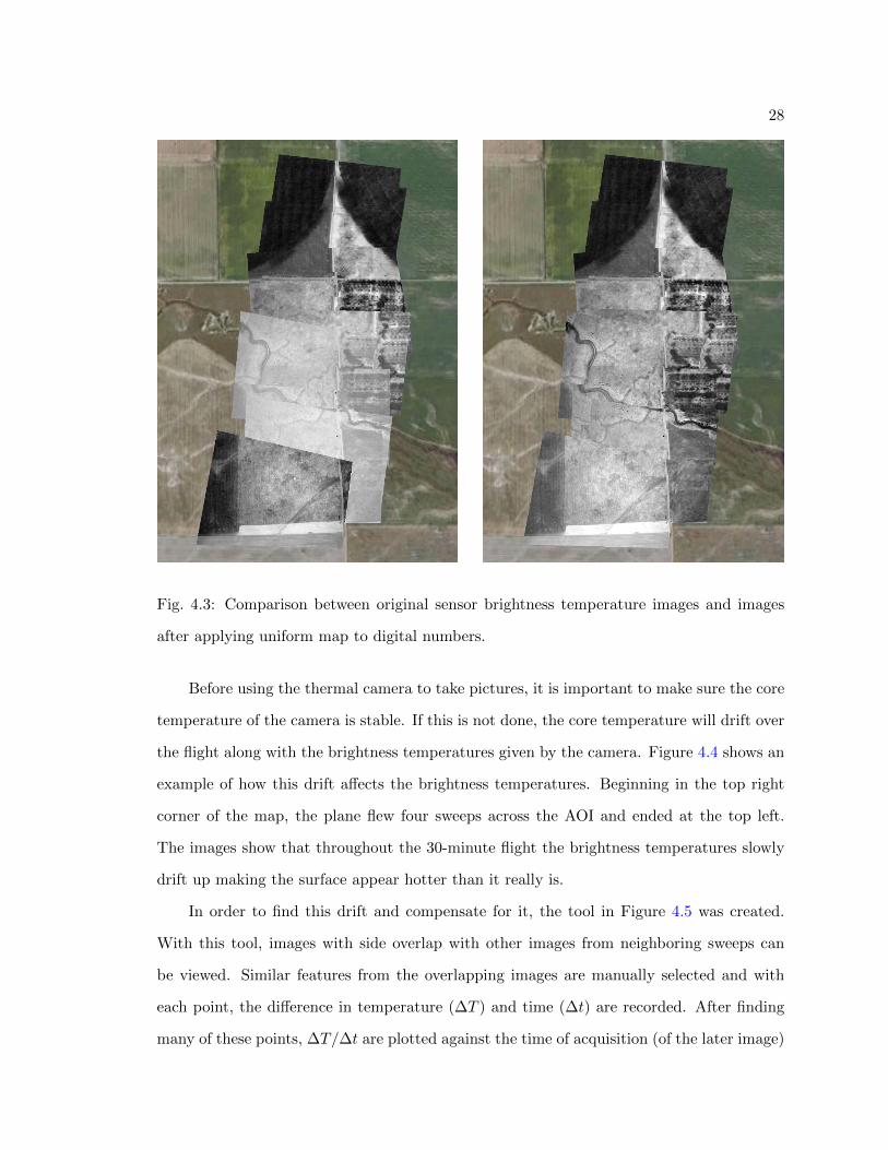
28
Fig. 4.3: Comparison between original sensor brightness temperature images and images
after applying uniform map to digital numbers.
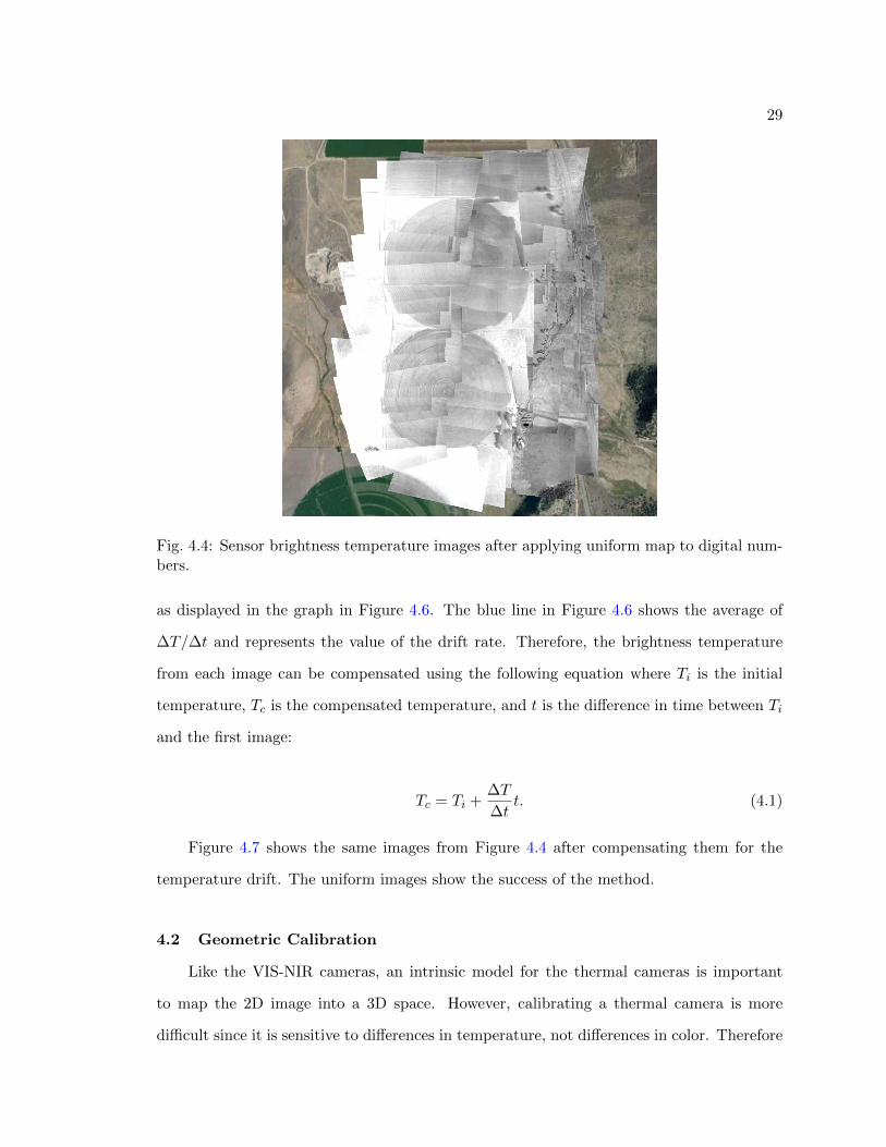
Before using the thermal camera to take pictures, it is important to make sure the core
temperature of the camera is stable. If this is not done, the core temperature will drift over
the flight along with the brightness temperatures given by the camera. Figure 4.4 shows an
example of how this drift affects the brightness temperatures. Beginning in the top right
corner of the map, the plane flew four sweeps across the AOI and ended at the top left.
The images show that throughout the 30-minute flight the brightness temperatures slowly
drift up making the surface appear hotter than it really is.
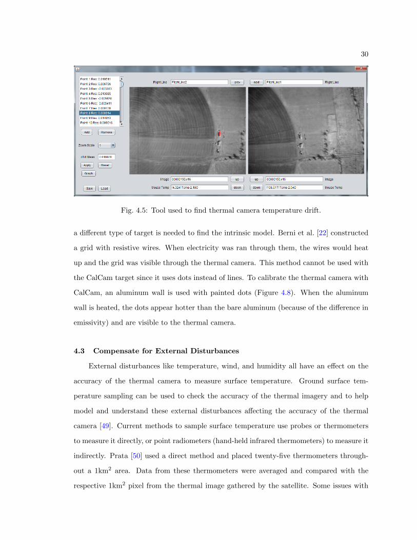
In order to find this drift and compensate for it, the tool in Figure 4.5 was created.
With this tool, images with side overlap with other images from neighboring sweeps can
be viewed. Similar features from the overlapping images are manually selected and with
each point, the difference in temperature (∆T ) and time (∆t) are recorded. After finding
many of these points, ∆T/∆t are plotted against the time of acquisition (of the later image)
29
Fig. 4.4: Sensor brightness temperature images after applying uniform map to digital num-bers.
as displayed in the graph in Figure 4.6. The blue line in Figure 4.6 shows the average of
∆T/∆t and represents the value of the drift rate. Therefore, the brightness temperature
from each image can be compensated using the following equation where Ti is the initial
temperature, Tc is the compensated temperature, and t is the difference in time between Ti
and the first image:
Tc = Ti +∆T
∆tt. (4.1)
Figure 4.7 shows the same images from Figure 4.4 after compensating them for the
temperature drift. The uniform images show the success of the method.
4.2 Geometric Calibration
Like the VIS-NIR cameras, an intrinsic model for the thermal cameras is important
to map the 2D image into a 3D space. However, calibrating a thermal camera is more
difficult since it is sensitive to differences in temperature, not differences in color. Therefore
30
Fig. 4.5: Tool used to find thermal camera temperature drift.
a different type of target is needed to find the intrinsic model. Berni et al. [22] constructed
a grid with resistive wires. When electricity was ran through them, the wires would heat
up and the grid was visible through the thermal camera. This method cannot be used with
the CalCam target since it uses dots instead of lines. To calibrate the thermal camera with
CalCam, an aluminum wall is used with painted dots (Figure 4.8). When the aluminum
wall is heated, the dots appear hotter than the bare aluminum (because of the difference in
emissivity) and are visible to the thermal camera.
4.3 Compensate for External Disturbances
External disturbances like temperature, wind, and humidity all have an effect on the
accuracy of the thermal camera to measure surface temperature. Ground surface tem-
perature sampling can be used to check the accuracy of the thermal imagery and to help
model and understand these external disturbances affecting the accuracy of the thermal
camera [49]. Current methods to sample surface temperature use probes or thermometers
to measure it directly, or point radiometers (hand-held infrared thermometers) to measure it
indirectly. Prata [50] used a direct method and placed twenty-five thermometers through-
out a 1km2 area. Data from these thermometers were averaged and compared with the
respective 1km2 pixel from the thermal image gathered by the satellite. Some issues with
31
Fig. 4.6: Graph of difference in temperature vs. difference in time.
this type of sampling include measuring the temperature under or over the surface instead
of at the surface, and representing an area measurement with multiple point measurements.
However, it is difficult to sample surface temperature at such a large scale; there are not
many other options. At a smaller scale, Wukelic et al. [51] calibrated the data from Landsat
5 (120m pixels) by choosing uniform sample areas, such as bodies of water and flat uniform
land types (soil, grass, etc.), and characterizing their surface temperature with point mea-
surements (using radiometers and thermometers). Torgersen et al. [45] captured thermal
imagery over a river with a manned aircraft, and placed probes throughout the river to
calibrate the thermal image. While all of these methods of sampling surface temperature
were effective for their respective scales, they all made use of their large footprint to find
uniform land areas or bodies of water to calibrate the thermal imagery. Such an option is
not always available for small UAS remote sensing systems which cover small areas. For
example, if a UAS is used for precision agriculture and captures thermal imagery to gen-
erate evapotranspiration maps, it is likely that the farm will not include bodies of water
large enough to calibrate the thermal image. In a similar scenario, Berni et al. [22] used
an unmanned helicopter to capture thermal imagery over a farm. Areas with bare soil and
black and white targets were used to calibrate the thermal image using a point radiometer.
While this method provided good results, it might be difficult to sample a wide range of
32
Fig. 4.7: Sensor brightness temperature images after compensating for drift.
temperatures. Also, the point radiometer has a small field of view and may not represent
the larger pixel from the thermal imagery accurately.
There is a need to develop new ground temperature sampling methods which can easily
and routinely be implemented with small UAS to compensate thermal images from low-
cost microbolometer thermal cameras and understand the environmental disturbances that
affect their accuracy. For the AggieAir system, these methods must accurately represent
the surface temperature for an entire pixel ranging in size from 30cm to 1.5m. Two methods
are evaluated in this section. The first method is similar to the method using the hand-held
point radiometer, however a thermal camera is used instead. This delivers high resolution
samples over an area large enough to cover four pixels to ensure at least one pixel is matched
entirely by the sample. Before each sample, the thermal camera is calibrated using a black
body. The second method uses bodies of water, with known and different temperatures, to
compare with the thermal imagery taken by the aircraft. It is assumed that the temperature
for each body of water is uniform. Temperature probes are used to measure the water
33
Fig. 4.8: CalCam target for thermal camera geometric calibration.
temperature of the pool and a radiometer is used to measure the surface temperature. To
determine which of these methods is better, they were tested five separate times over a
two-month period. Each test included a flight from AggieAir and was conducted on a day
that coincided with a Landsat overflight; Landsat imagery was used to help evaluate the
methods for accuracy.
4.3.1 Ground Sampling Methods
Before each flight, it is important to establish the size of each ground sample. Only
one pixel is needed for each sample, however it is not possible to know where the location
of this pixel will be before the flight. Therefore, the sample should cover an area of at least
four pixels (2×2 pixels). This will ensure that at least one pixel is covered entirely by the
sample. Pixels that are only partially covered by the sample should not be used. Table 4.2
shows a range of flight altitudes above ground and their respective pixel sizes and minimum
sample area dimensions. The imagery acquired to test the methods was flown at 450m
above ground. With a pixel size of 0.65m the minimum sample size is 1.3×1.3m; therefore
a larger area of 1.7×1.7m was selected to include extra room for error.
34
Table 4.2: Flight altitude vs. sample area size.Alt (m) Res (m) Sample Area (m)
200 0.30 0.60×0.60
450 0.65 1.30×1.30
600 0.85 1.70×1.70
1000 1.40 2.80×2.80
To ensure that valid comparisons can be made between the thermal cameras, the ther-
mal radiometer, and Landsat, all emissivity correction is disabled (emissivity set to 1).
Even though it is important for the actual surface temperature, it does not need to be
considered except when comparing the aircraft thermal image with the temperature probes
in the pools. In that case, the emissivity of water is assumed to be 0.98.
Ground-Based Thermal Camera Apparatus
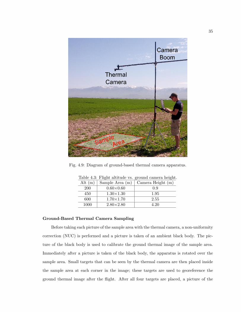
Figure 4.9 shows the apparatus used to capture the surface temperature of the sample
area with the thermal camera. To avoid confusion, the imagery collected by the ground-
based thermal camera is referred to as ground thermal or ground pixels; the imagery col-
lected by the aircraft is referred to as the aircraft thermal or aircraft pixel. The thermal
camera is mounted to the end of a long boom which places it over the sample area. It is
also connected to a laptop which is used to control the camera and take the pictures. A
counterweight can be mounted on the other side of the boom to ensure stability.
The geometry of the apparatus is based on the camera field of view (FOV) and the
desired sample area. The ICI 7640 has a 40 degree FOV. Based on this FOV, Table 4.3
shows the required camera height above ground for each flight altitude. To match the
sample size previously selected, the samples presented in this section were collected at a
camera height of 2.5m. Even though this camera apparatus is quite lengthy, it is built with
carbon fiber rods to make it strong and easy to transport from sample to sample. While
not being used, the apparatus can also be taken apart into 1.5m long pieces to make it
manageable during transport.
35
Fig. 4.9: Diagram of ground-based thermal camera apparatus.
Table 4.3: Flight altitude vs. ground camera height.Alt (m) Sample Area (m) Camera Height (m)
200 0.60×0.60 0.9
450 1.30×1.30 1.95
600 1.70×1.70 2.55
1000 2.80×2.80 4.20
Ground-Based Thermal Camera Sampling
Before taking each picture of the sample area with the thermal camera, a non-uniformity
correction (NUC) is performed and a picture is taken of an ambient black body. The pic-
ture of the black body is used to calibrate the ground thermal image of the sample area.
Immediately after a picture is taken of the black body, the apparatus is rotated over the
sample area. Small targets that can be seen by the thermal camera are then placed inside
the sample area at each corner in the image; these targets are used to georeference the
ground thermal image after the flight. After all four targets are placed, a picture of the
36
sample area is captured. Before moving to the next sample area, flags are placed in the
center of the targets and their locations are measured with a survey grade GPS receiver.
Multiple locations for the ground-based thermal camera samples should be determined
before the flight to spread the temperature range between samples as far apart as possi-
ble. The collection process should also be carefully timed close to the flight to reduce the
difference between the fly-over time and the collection time.
Temperature Pools
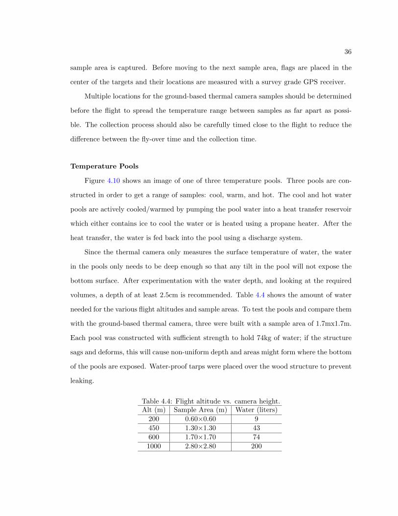
Figure 4.10 shows an image of one of three temperature pools. Three pools are con-
structed in order to get a range of samples: cool, warm, and hot. The cool and hot water
pools are actively cooled/warmed by pumping the pool water into a heat transfer reservoir
which either contains ice to cool the water or is heated using a propane heater. After the
heat transfer, the water is fed back into the pool using a discharge system.
Since the thermal camera only measures the surface temperature of water, the water
in the pools only needs to be deep enough so that any tilt in the pool will not expose the
bottom surface. After experimentation with the water depth, and looking at the required
volumes, a depth of at least 2.5cm is recommended. Table 4.4 shows the amount of water
needed for the various flight altitudes and sample areas. To test the pools and compare them
with the ground-based thermal camera, three were built with a sample area of 1.7mx1.7m.
Each pool was constructed with sufficient strength to hold 74kg of water; if the structure
sags and deforms, this will cause non-uniform depth and areas might form where the bottom
of the pools are exposed. Water-proof tarps were placed over the wood structure to prevent
leaking.
Table 4.4: Flight altitude vs. camera height.Alt (m) Sample Area (m) Water (liters)
200 0.60×0.60 9
450 1.30×1.30 43
600 1.70×1.70 74
1000 2.80×2.80 200
37
Fig. 4.10: Diagram of thermal pool system.
Two devices are used to measure the water temperature: a temperature probe and a
thermal radiometer. The temperature probe is placed in the pool at setup and measures
the temperature of the water body every minute for the duration of the flight. The thermal
radiometer is used to measure the water surface temperature at ten different points over
the pools right before the fly-over time. Along with this temperature data, the locations of
the pool corners are measured with a GPS receiver to help determine their location in the
aircraft thermal image.
Pool Discharge Systems
A vital part of the temperature pools is the system that cycles the water from the pool,
through a heat transfer reservoir, and then back into the pool. While the body temperature
of water is slow to change, the surface temperature changes easily and is very sensitive to
wind. Therefore, the ideal discharge system keeps the surface temperature of the pool
uniform by making sure the water is always moving and stirring. This section presents four
discharge systems and evaluates them by how uniform they are able to keep the surface
temperature of the pools.
38
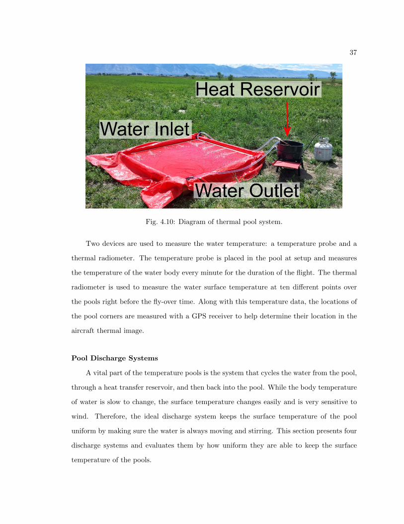
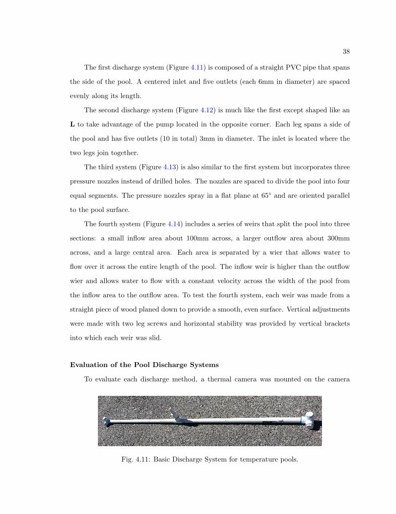
The first discharge system (Figure 4.11) is composed of a straight PVC pipe that spans
the side of the pool. A centered inlet and five outlets (each 6mm in diameter) are spaced
evenly along its length.
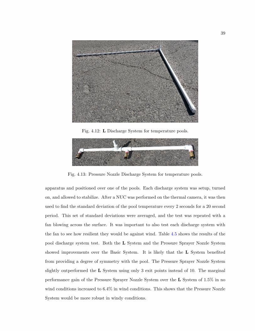
The second discharge system (Figure 4.12) is much like the first except shaped like an
L to take advantage of the pump located in the opposite corner. Each leg spans a side of
the pool and has five outlets (10 in total) 3mm in diameter. The inlet is located where the
two legs join together.
The third system (Figure 4.13) is also similar to the first system but incorporates three
pressure nozzles instead of drilled holes. The nozzles are spaced to divide the pool into four
equal segments. The pressure nozzles spray in a flat plane at 65 and are oriented parallel
to the pool surface.
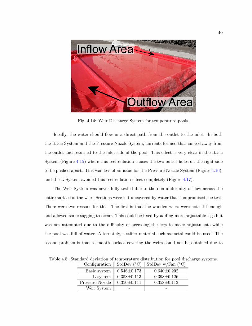
The fourth system (Figure 4.14) includes a series of weirs that split the pool into three
sections: a small inflow area about 100mm across, a larger outflow area about 300mm
across, and a large central area. Each area is separated by a wier that allows water to
flow over it across the entire length of the pool. The inflow weir is higher than the outflow
wier and allows water to flow with a constant velocity across the width of the pool from
the inflow area to the outflow area. To test the fourth system, each weir was made from a
straight piece of wood planed down to provide a smooth, even surface. Vertical adjustments
were made with two leg screws and horizontal stability was provided by vertical brackets
into which each weir was slid.
Evaluation of the Pool Discharge Systems
To evaluate each discharge method, a thermal camera was mounted on the camera
Fig. 4.11: Basic Discharge System for temperature pools.
39
Fig. 4.12: L Discharge System for temperature pools.
Fig. 4.13: Pressure Nozzle Discharge System for temperature pools.
apparatus and positioned over one of the pools. Each discharge system was setup, turned
on, and allowed to stabilize. After a NUC was performed on the thermal camera, it was then
used to find the standard deviation of the pool temperature every 2 seconds for a 20 second
period. This set of standard deviations were averaged, and the test was repeated with a
fan blowing across the surface. It was important to also test each discharge system with
the fan to see how resilient they would be against wind. Table 4.5 shows the results of the
pool discharge system test. Both the L System and the Pressure Sprayer Nozzle System
showed improvements over the Basic System. It is likely that the L System benefited
from providing a degree of symmetry with the pool. The Pressure Sprayer Nozzle System
slightly outperformed the L System using only 3 exit points instead of 10. The marginal
performance gain of the Pressure Sprayer Nozzle System over the L System of 1.5% in no
wind conditions increased to 6.4% in wind conditions. This shows that the Pressure Nozzle
System would be more robust in windy conditions.
40
Fig. 4.14: Weir Discharge System for temperature pools.
Ideally, the water should flow in a direct path from the outlet to the inlet. In both
the Basic System and the Pressure Nozzle System, currents formed that curved away from
the outlet and returned to the inlet side of the pool. This effect is very clear in the Basic
System (Figure 4.15) where this recirculation causes the two outlet holes on the right side
to be pushed apart. This was less of an issue for the Pressure Nozzle System (Figure 4.16),
and the L System avoided this recirculation effect completely (Figure 4.17).
The Weir System was never fully tested due to the non-uniformity of flow across the
entire surface of the weir. Sections were left uncovered by water that compromised the test.
There were two reasons for this. The first is that the wooden wiers were not stiff enough
and allowed some sagging to occur. This could be fixed by adding more adjustable legs but
was not attempted due to the difficulty of accessing the legs to make adjustments while
the pool was full of water. Alternately, a stiffer material such as metal could be used. The
second problem is that a smooth surface covering the weirs could not be obtained due to
Table 4.5: Standard deviation of temperature distribution for pool discharge systems.Configuration StdDev (C) StdDev w/Fan (C)
Basic system 0.546±0.173 0.640±0.202
L system 0.358±0.113 0.398±0.126
Pressure Nozzle 0.350±0.111 0.358±0.113
Weir System - -
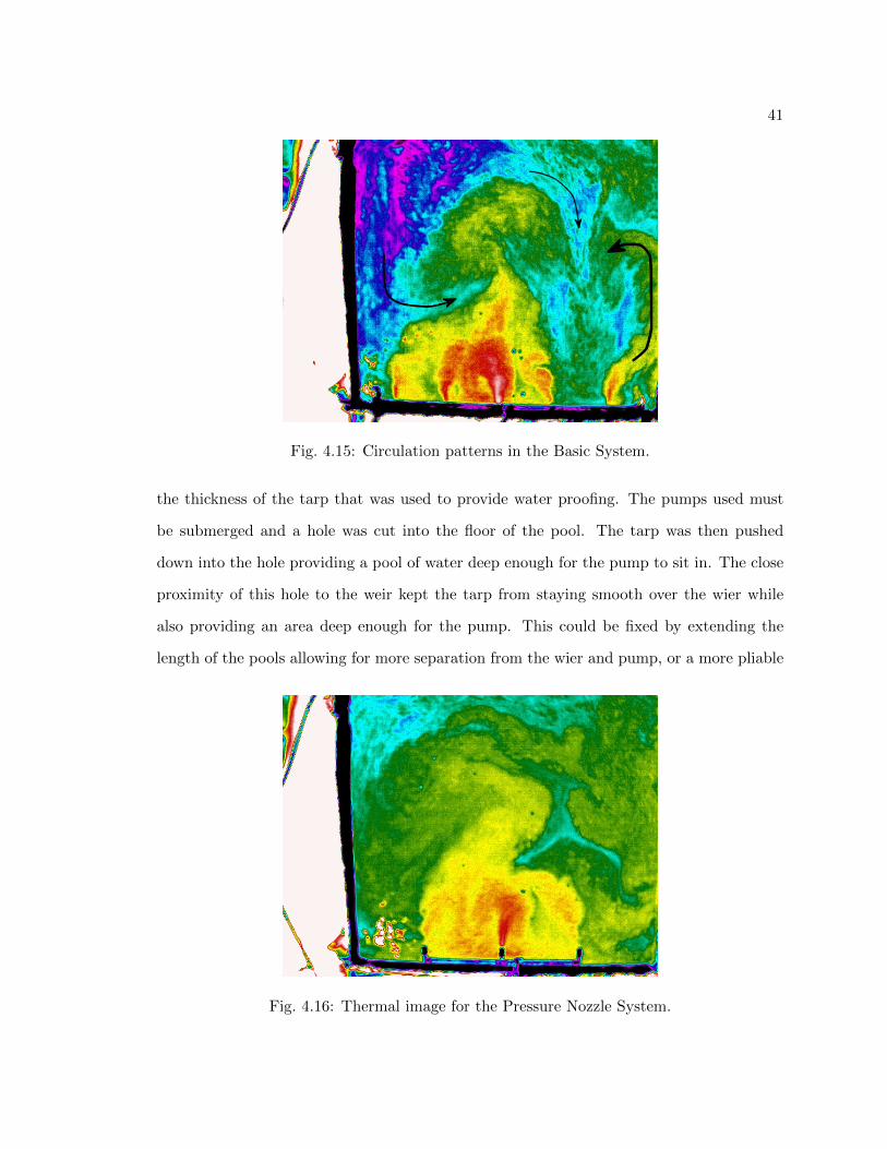
41
Fig. 4.15: Circulation patterns in the Basic System.
the thickness of the tarp that was used to provide water proofing. The pumps used must
be submerged and a hole was cut into the floor of the pool. The tarp was then pushed
down into the hole providing a pool of water deep enough for the pump to sit in. The close
proximity of this hole to the weir kept the tarp from staying smooth over the wier while
also providing an area deep enough for the pump. This could be fixed by extending the
length of the pools allowing for more separation from the wier and pump, or a more pliable
Fig. 4.16: Thermal image for the Pressure Nozzle System.
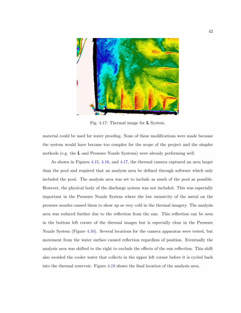
42
Fig. 4.17: Thermal image for L System.
material could be used for water proofing. None of these modifications were made because
the system would have become too complex for the scope of the project and the simpler
methods (e.g. the L and Pressure Nozzle Systems) were already performing well.
As shown in Figures 4.15, 4.16, and 4.17, the thermal camera captured an area larger
than the pool and required that an analysis area be defined through software which only
included the pool. The analysis area was set to include as much of the pool as possible.
However, the physical body of the discharge system was not included. This was especially
important in the Pressure Nozzle System where the low emissivity of the metal on the
pressure nozzles caused them to show up as very cold in the thermal imagery. The analysis
area was reduced further due to the reflection from the sun. This reflection can be seen
in the bottom left corner of the thermal images but is especially clear in the Pressure
Nozzle System (Figure 4.16). Several locations for the camera apparatus were tested, but
movement from the water surface caused reflection regardless of position. Eventually the
analysis area was shifted to the right to exclude the effects of the sun reflection. This shift
also avoided the cooler water that collects in the upper left corner before it is cycled back
into the thermal reservoir. Figure 4.18 shows the final location of the analysis area.
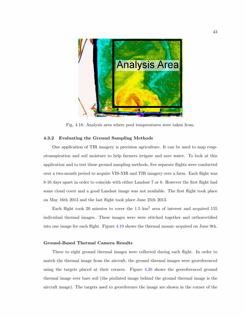
43
Fig. 4.18: Analysis area where pool temperatures were taken from.
4.3.2 Evaluating the Ground Sampling Methods
One application of TIR imagery is precision agriculture. It can be used to map evap-
otranspiration and soil moisture to help farmers irrigate and save water. To look at this
application and to test these ground sampling methods, five separate flights were conducted
over a two-month period to acquire VIS-NIR and TIR imagery over a farm. Each flight was
8-16 days apart in order to coincide with either Landsat 7 or 8. However the first flight had
some cloud cover and a good Landsat image was not available. The first flight took place
on May 16th 2013 and the last flight took place June 25th 2013.
Each flight took 20 minutes to cover the 1.5 km2 area of interest and acquired 155
individual thermal images. These images were were stitched together and orthorectified
into one image for each flight. Figure 4.19 shows the thermal mosaic acquired on June 9th.
Ground-Based Thermal Camera Results
Three to eight ground thermal images were collected during each flight. In order to
match the thermal image from the aircraft, the ground thermal images were georeferenced
using the targets placed at their corners. Figure 4.20 shows the georeferenced ground
thermal image over bare soil (the pixilated image behind the ground thermal image is the
aircraft image). The targets used to georeference the image are shown in the corner of the
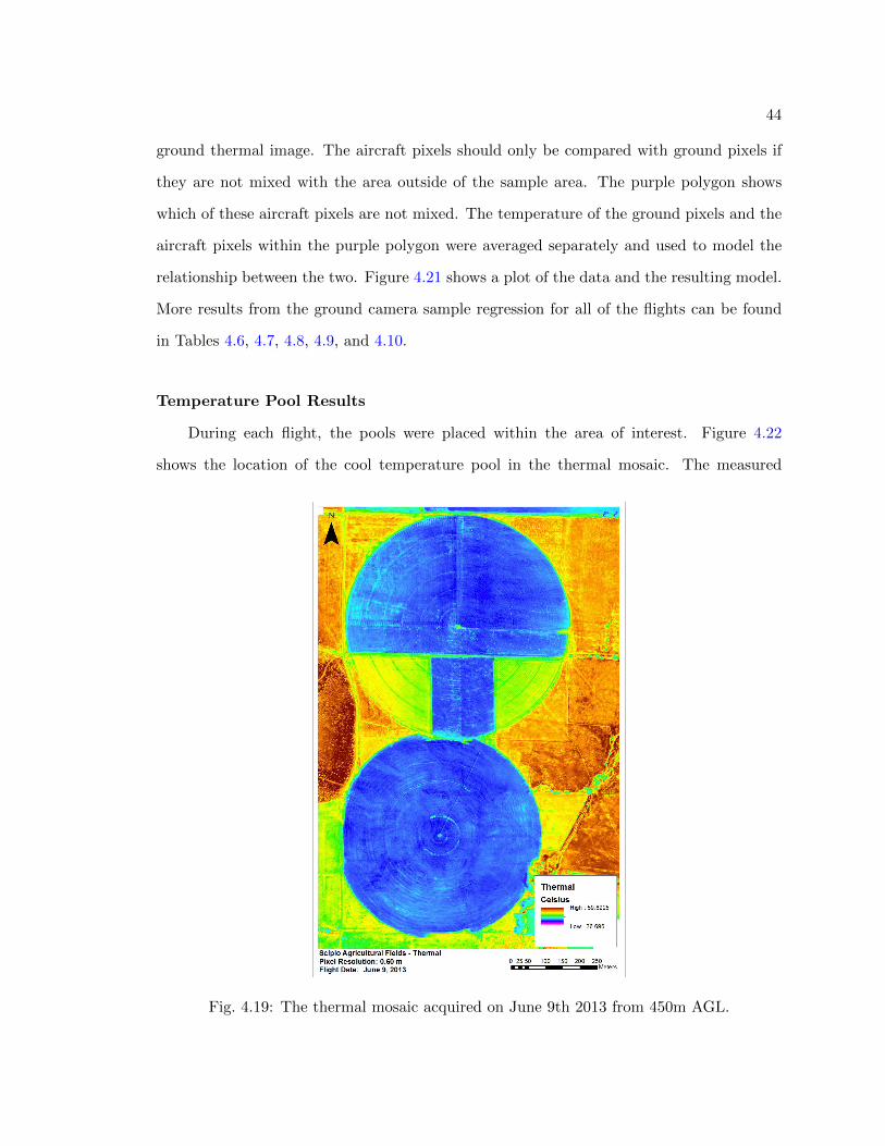
44
ground thermal image. The aircraft pixels should only be compared with ground pixels if
they are not mixed with the area outside of the sample area. The purple polygon shows
which of these aircraft pixels are not mixed. The temperature of the ground pixels and the
aircraft pixels within the purple polygon were averaged separately and used to model the
relationship between the two. Figure 4.21 shows a plot of the data and the resulting model.
More results from the ground camera sample regression for all of the flights can be found
in Tables 4.6, 4.7, 4.8, 4.9, and 4.10.
Temperature Pool Results
During each flight, the pools were placed within the area of interest. Figure 4.22
shows the location of the cool temperature pool in the thermal mosaic. The measured
Fig. 4.19: The thermal mosaic acquired on June 9th 2013 from 450m AGL.
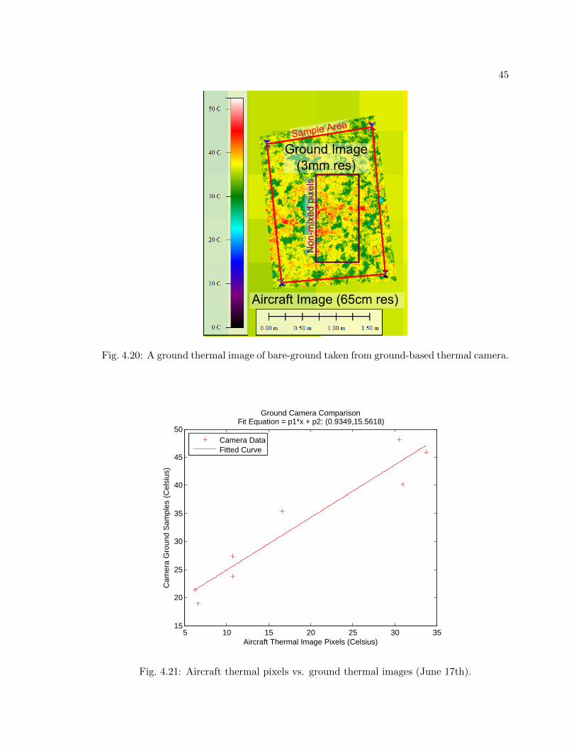
45
Fig. 4.20: A ground thermal image of bare-ground taken from ground-based thermal camera.
5 10 15 20 25 30 3515
20
25
30
35
40
45
50
Aircraft Thermal Image Pixels (Celsius)
Cam
era
Gro
und
Sam
ples
(C
elsi
us)
Ground Camera ComparisonFit Equation = p1*x + p2: (0.9349,15.5618)
Camera DataFitted Curve
Fig. 4.21: Aircraft thermal pixels vs. ground thermal images (June 17th).
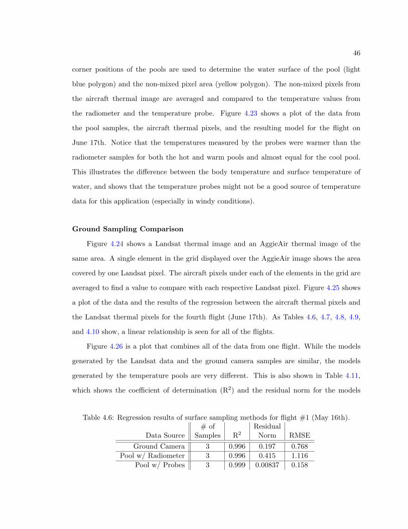
46
corner positions of the pools are used to determine the water surface of the pool (light
blue polygon) and the non-mixed pixel area (yellow polygon). The non-mixed pixels from
the aircraft thermal image are averaged and compared to the temperature values from
the radiometer and the temperature probe. Figure 4.23 shows a plot of the data from
the pool samples, the aircraft thermal pixels, and the resulting model for the flight on
June 17th. Notice that the temperatures measured by the probes were warmer than the
radiometer samples for both the hot and warm pools and almost equal for the cool pool.
This illustrates the difference between the body temperature and surface temperature of
water, and shows that the temperature probes might not be a good source of temperature
data for this application (especially in windy conditions).
Ground Sampling Comparison
Figure 4.24 shows a Landsat thermal image and an AggieAir thermal image of the
same area. A single element in the grid displayed over the AggieAir image shows the area
covered by one Landsat pixel. The aircraft pixels under each of the elements in the grid are
averaged to find a value to compare with each respective Landsat pixel. Figure 4.25 shows
a plot of the data and the results of the regression between the aircraft thermal pixels and
the Landsat thermal pixels for the fourth flight (June 17th). As Tables 4.6, 4.7, 4.8, 4.9,
and 4.10 show, a linear relationship is seen for all of the flights.
Figure 4.26 is a plot that combines all of the data from one flight. While the models
generated by the Landsat data and the ground camera samples are similar, the models
generated by the temperature pools are very different. This is also shown in Table 4.11,
which shows the coefficient of determination (R2) and the residual norm for the models
Table 4.6: Regression results of surface sampling methods for flight #1 (May 16th).# of Residual
Data Source Samples R2 Norm RMSE
Ground Camera 3 0.996 0.197 0.768
Pool w/ Radiometer 3 0.996 0.415 1.116
Pool w/ Probes 3 0.999 0.00837 0.158

47
Table 4.7: Regression results of surface sampling methods for flight #2 (June 1st).# of Residual
Data Source Samples R2 Norm RMSE
Ground Camera 3 0.988 1.472 2.101
Pool w/ Radiometer 3 0.944 13.590 6.385
Pool w/ Probes 3 0.928 18.453 7.440
Landsat 1097 0.910 3.587 1.896
Table 4.8: Regression results of surface sampling methods for flight #3 (June 9th).# of Residual
Data Source Samples R2 Norm RMSE
Ground Camera 8 0.924 12.734 4.120
Pool w/ Radiometer 3 0.987 1.788 2.316
Pool w/ Probes 3 0.980 2.499 2.738
Landsat 1188 0.878 5.006 2.239
Table 4.9: Regression results of surface sampling methods for flight #4 (June 17th).# of Residual
Data Source Samples R2 Norm RMSE
Ground Camera 8 0.922 8.771 3.420
Pool w/ Radiometer 3 0.973 4.051 3.486
Pool w/ Probes 3 0.986 2.788 2.892
Landsat 1071 0.931 4.415 2.103
Table 4.10: Regression results of surface sampling methods for flight #5 (June 25th).# of Residual
Data Source Samples R2 Norm RMSE
Ground Camera 8 0.959 2.286 1.749
Pool w/ Radiometer 3 0.999 0.010 0.177
Pool w/ Probes 3 0.999 0.043 0.362
Landsat 1744 0.696 1.909 1.382
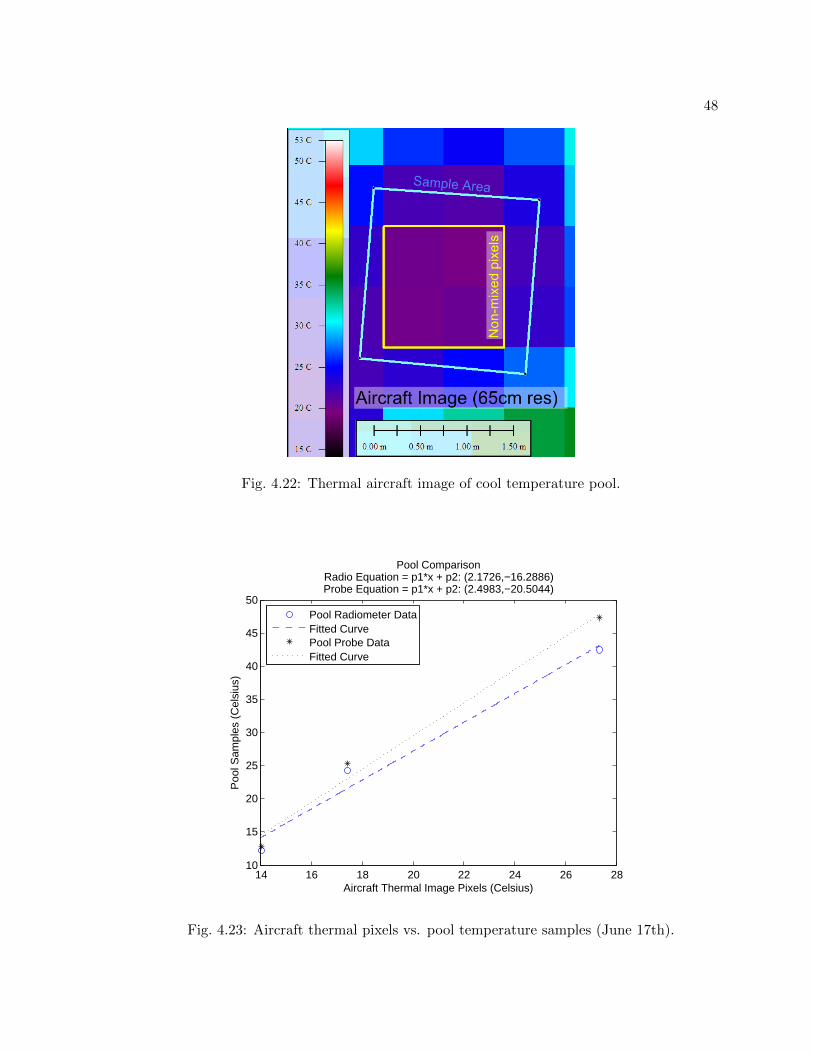
48
Fig. 4.22: Thermal aircraft image of cool temperature pool.
14 16 18 20 22 24 26 2810
15
20
25
30
35
40
45
50
Aircraft Thermal Image Pixels (Celsius)
Poo
l Sam
ples
(C
elsi
us)
Pool ComparisonRadio Equation = p1*x + p2: (2.1726,−16.2886)Probe Equation = p1*x + p2: (2.4983,−20.5044)
Pool Radiometer DataFitted CurvePool Probe DataFitted Curve
Fig. 4.23: Aircraft thermal pixels vs. pool temperature samples (June 17th).
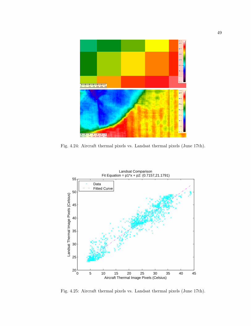
49
Fig. 4.24: Aircraft thermal pixels vs. Landsat thermal pixels (June 17th).
0 5 10 15 20 25 30 35 40 4520
25
30
35
40
45
50
55
Aircraft Thermal Image Pixels (Celsius)
Land
sat T
herm
al Im
age
Pix
els
(Cel
sius
)
Landsat ComparisonFit Equation = p1*x + p2: (0.7157,21.1791)
DataFitted Curve
Fig. 4.25: Aircraft thermal pixels vs. Landsat thermal pixels (June 17th).
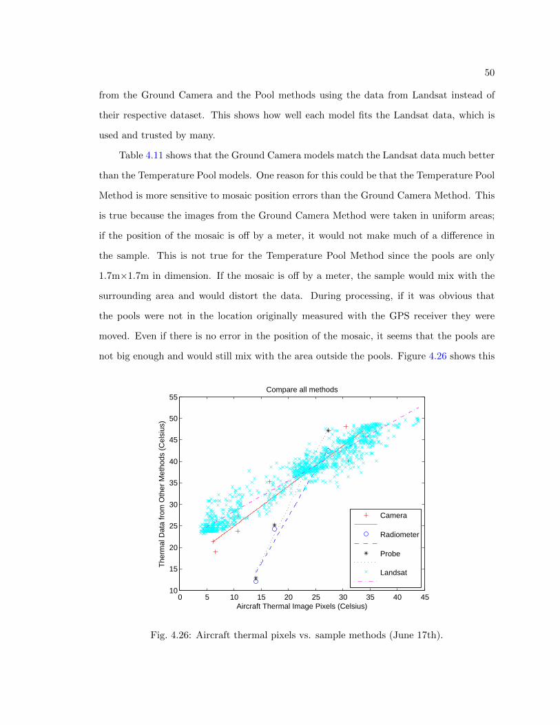
50
from the Ground Camera and the Pool methods using the data from Landsat instead of
their respective dataset. This shows how well each model fits the Landsat data, which is
used and trusted by many.
Table 4.11 shows that the Ground Camera models match the Landsat data much better
than the Temperature Pool models. One reason for this could be that the Temperature Pool
Method is more sensitive to mosaic position errors than the Ground Camera Method. This
is true because the images from the Ground Camera Method were taken in uniform areas;
if the position of the mosaic is off by a meter, it would not make much of a difference in
the sample. This is not true for the Temperature Pool Method since the pools are only
1.7m×1.7m in dimension. If the mosaic is off by a meter, the sample would mix with the
surrounding area and would distort the data. During processing, if it was obvious that
the pools were not in the location originally measured with the GPS receiver they were
moved. Even if there is no error in the position of the mosaic, it seems that the pools are
not big enough and would still mix with the area outside the pools. Figure 4.26 shows this
0 5 10 15 20 25 30 35 40 4510
15
20
25
30
35
40
45
50
55
Aircraft Thermal Image Pixels (Celsius)
The
rmal
Dat
a fr
om O
ther
Met
hods
(C
elsi
us)
Compare all methods
Camera
Radiometer
Probe
Landsat
Fig. 4.26: Aircraft thermal pixels vs. sample methods (June 17th).
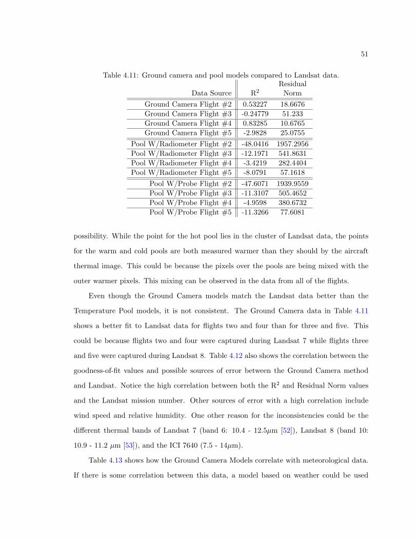
51
Table 4.11: Ground camera and pool models compared to Landsat data.Residual
Data Source R2 Norm
Ground Camera Flight #2 0.53227 18.6676
Ground Camera Flight #3 -0.24779 51.233
Ground Camera Flight #4 0.83285 10.6765
Ground Camera Flight #5 -2.9828 25.0755
Pool W/Radiometer Flight #2 -48.0416 1957.2956
Pool W/Radiometer Flight #3 -12.1971 541.8631
Pool W/Radiometer Flight #4 -3.4219 282.4404
Pool W/Radiometer Flight #5 -8.0791 57.1618
Pool W/Probe Flight #2 -47.6071 1939.9559
Pool W/Probe Flight #3 -11.3107 505.4652
Pool W/Probe Flight #4 -4.9598 380.6732
Pool W/Probe Flight #5 -11.3266 77.6081
possibility. While the point for the hot pool lies in the cluster of Landsat data, the points
for the warm and cold pools are both measured warmer than they should by the aircraft
thermal image. This could be because the pixels over the pools are being mixed with the
outer warmer pixels. This mixing can be observed in the data from all of the flights.
Even though the Ground Camera models match the Landsat data better than the
Temperature Pool models, it is not consistent. The Ground Camera data in Table 4.11
shows a better fit to Landsat data for flights two and four than for three and five. This
could be because flights two and four were captured during Landsat 7 while flights three
and five were captured during Landsat 8. Table 4.12 also shows the correlation between the
goodness-of-fit values and possible sources of error between the Ground Camera method
and Landsat. Notice the high correlation between both the R2 and Residual Norm values
and the Landsat mission number. Other sources of error with a high correlation include
wind speed and relative humidity. One other reason for the inconsistencies could be the
different thermal bands of Landsat 7 (band 6: 10.4 - 12.5µm [52]), Landsat 8 (band 10:
10.9 - 11.2 µm [53]), and the ICI 7640 (7.5 - 14µm).
Table 4.13 shows how the Ground Camera Models correlate with meteorological data.
If there is some correlation between this data, a model based on weather could be used
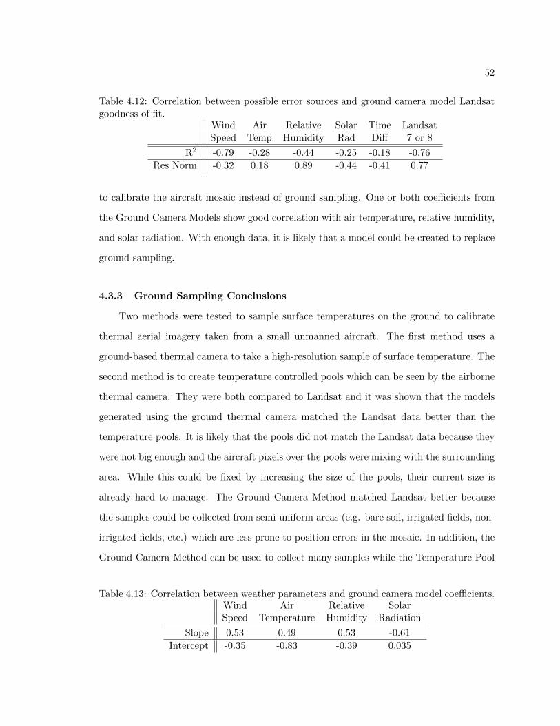
52
Table 4.12: Correlation between possible error sources and ground camera model Landsatgoodness of fit.
Wind Air Relative Solar Time LandsatSpeed Temp Humidity Rad Diff 7 or 8
R2 -0.79 -0.28 -0.44 -0.25 -0.18 -0.76
Res Norm -0.32 0.18 0.89 -0.44 -0.41 0.77
to calibrate the aircraft mosaic instead of ground sampling. One or both coefficients from
the Ground Camera Models show good correlation with air temperature, relative humidity,
and solar radiation. With enough data, it is likely that a model could be created to replace
ground sampling.
4.3.3 Ground Sampling Conclusions
Two methods were tested to sample surface temperatures on the ground to calibrate
thermal aerial imagery taken from a small unmanned aircraft. The first method uses a
ground-based thermal camera to take a high-resolution sample of surface temperature. The
second method is to create temperature controlled pools which can be seen by the airborne
thermal camera. They were both compared to Landsat and it was shown that the models
generated using the ground thermal camera matched the Landsat data better than the
temperature pools. It is likely that the pools did not match the Landsat data because they
were not big enough and the aircraft pixels over the pools were mixing with the surrounding
area. While this could be fixed by increasing the size of the pools, their current size is
already hard to manage. The Ground Camera Method matched Landsat better because
the samples could be collected from semi-uniform areas (e.g. bare soil, irrigated fields, non-
irrigated fields, etc.) which are less prone to position errors in the mosaic. In addition, the
Ground Camera Method can be used to collect many samples while the Temperature Pool
Table 4.13: Correlation between weather parameters and ground camera model coefficients.Wind Air Relative SolarSpeed Temperature Humidity Radiation
Slope 0.53 0.49 0.53 -0.61
Intercept -0.35 -0.83 -0.39 0.035
53
Method is restricted to three.
Even though the Ground Camera Method performs better than the pool method, it
was inconsistent with matching the Landsat data. Results showed that this is likely to be
caused by the different Landsat satellites used to collect the data (Landsat 7 and Landsat
8). Overall, the Ground Camera Method seems like a good method to calibrate the thermal
mosaics from AggieAir. More data should be obtained to confirm this.
Future work includes gathering more data to further investigate the relationship be-
tween the Ground Camera Method and Landsat. Since strong correlations were shown
between the ground camera models and meteorological data, more data is also needed to
establish a model to calibrate the thermal mosaic based on weather to replace the ground
sampling.
4.4 Chapter Summary
Even though they share many of the same procedures, processing TIR imagery can
be a lot more complex than VIS-NIR imagery. For example preparing the images for
orthorectification is required in order to compensate for potential problems (like drift)
and to map the temperature values into DNs so the orthorectification software can stitch
them together. Geometric calibration is also more challenging with a thermal camera since
it cannot distinguish differences in color and the standard target cannot be used. The
largest challenge with using TIR imagery for aerial imagery is compensating for external
disturbances (e.g. atmosphere and moving air cooling the lens) which affect the output
of the camera. In order to compensate for these effects, new ground sampling techniques
were presented in this chapter and compared against a trusted source or remotely sensed
data (Landsat). Future work in this area includes gathering more ground sampling data to
generate models to compensate for external disturbances.
54
Chapter 5
Biotelemetry Fish Tracking
In order to preserve our native fish species in the watersheds of the United States,
managing, monitoring, and studying fish habitat is very important. Extensive fish habi-
tat studies are conducted to minimize environmental impact before building a dam, while
restoring natural habitat in a river, or in ensuring the economic strength of a fisheries mar-
ket. An important part of these studies is tracking where fish are migrating, moving and
living. This is commonly accomplished by tagging the fish of interest with a radio trans-
mitter to locate the fish in the future to see where it has moved [20, 54]. The transmitter
does not include position information, so localization is performed using a receiver and a
directional antenna. As the antenna is pointed in the direction of the fish, the signal sent
from the transmitter becomes louder. The operator can hear the beacon through the re-
ceiver and navigates toward the fish. While this method has proved to be effective, it can
be time consuming and costly.
An alternative method for tracking fish utilizes AggieAir and a recently developed fish
tracking payload [55]. Using the fish tracking payload, AggieAir is able to fly over a body
of water and receive the signal transmitted by tagged fish. As AggieAir flies over the area
of interest, the fish tracker measures the signal strength from its receiver and logs other
data, including position, orientation, and speed of the aircraft. With this information, the
aircraft is directed toward areas of the map to improve the estimate of the tag location.
Others have looked into similar scenarios. In a general radio tracking problem, Frew et
al. [56] proposed a radio localization technique cast as a distributed estimation problem.
Consensus within a group of UAs was reached with a decentralized method; however, the
algorithms used are computationally complex and only considered communication with one
neighboring aircraft. Korner et al. [57] introduced a method that uses particle filters to
55
track multiple targets with radio tags. Implementation employed only one UA. While these
methods work, a simple, decentralized method is needed for multi-UA navigation and radio
tag localization. A method employing these features could be more practical for use in
small UAS with embedded systems.
The fish-tracking methods introduced in this chapter are focused on simplicity for
navigation, multi-UA coordination, and radio transmitter location estimation. Simplic-
ity is important for real-world, real-time fish-tracking applications. Therefore, swarm-like
rules (using potential fields [58]) are established for navigation and multi-UA coordina-
tion/avoidance. While navigating according to these rules, an Extended Kalman Filter is
used to estimate the position of the transmitter. Four simple navigation methods are in-
troduced which use this estimate and its covariance to direct the aircraft toward areas to
improve the estimate of the tag position. Figure 5.1 shows the steps to estimate the posi-
tion of the tag and how it relates to The Processing Cycle for Meaningful Remote Sensing.
Notice the similarities between Figure 5.1 and Figure 1.1; they are identical except that the
blocks and signals are labeled more specifically for fish tracking in Figure 5.1. An interesting
difference between this fish tracking application and the VIS-NIR and TIR applications is
that the fish tracking payload closes the loop in real-time and the actionable information is
used by the UA to gather better data.
A real-world simulation is created and used with Monte Carlo analysis to test and
evaluate these methods using one to three UAs. Part of this simulation includes a complex
propagation model for the tag which is based on real flight data. The results from the Monte
Carlo analysis give clear answers to which methods are effective, and what the expected
performance would be in real-world scenarios.
5.1 Simulation Environment
In order to properly test different methods to locate tagged fish, a real-world simulation
is needed. Figure 5.2 shows a diagram that describes the different pieces of the simulation.
Multiple UAs can be included in the simulation. Each UA (i) uses wind (|W |,∠W ) and
noise (ω, η) to generate truth states (Xi), and estimation states (Xi). The potential field
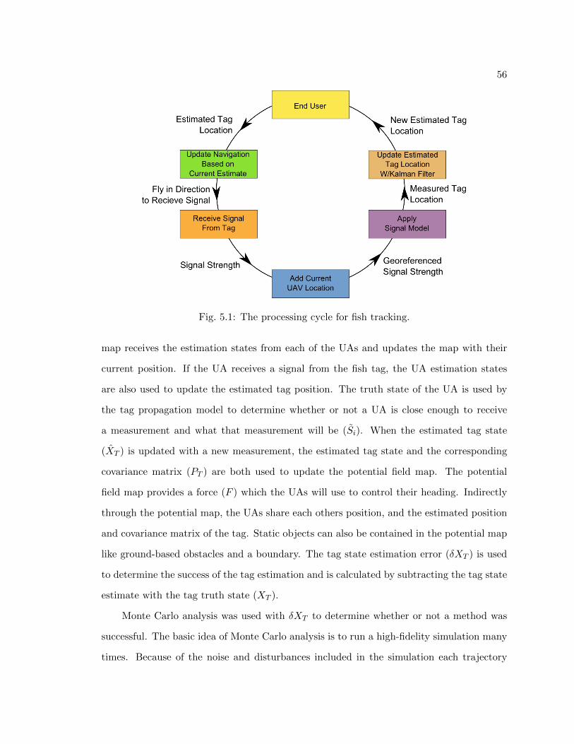
56
Fig. 5.1: The processing cycle for fish tracking.
map receives the estimation states from each of the UAs and updates the map with their
current position. If the UA receives a signal from the fish tag, the UA estimation states
are also used to update the estimated tag position. The truth state of the UA is used by
the tag propagation model to determine whether or not a UA is close enough to receive
a measurement and what that measurement will be (Si). When the estimated tag state
(XT ) is updated with a new measurement, the estimated tag state and the corresponding
covariance matrix (PT ) are both used to update the potential field map. The potential
field map provides a force (F ) which the UAs will use to control their heading. Indirectly
through the potential map, the UAs share each others position, and the estimated position
and covariance matrix of the tag. Static objects can also be contained in the potential map
like ground-based obstacles and a boundary. The tag state estimation error (δXT ) is used
to determine the success of the tag estimation and is calculated by subtracting the tag state
estimate with the tag truth state (XT ).
Monte Carlo analysis was used with δXT to determine whether or not a method was
successful. The basic idea of Monte Carlo analysis is to run a high-fidelity simulation many
times. Because of the noise and disturbances included in the simulation each trajectory
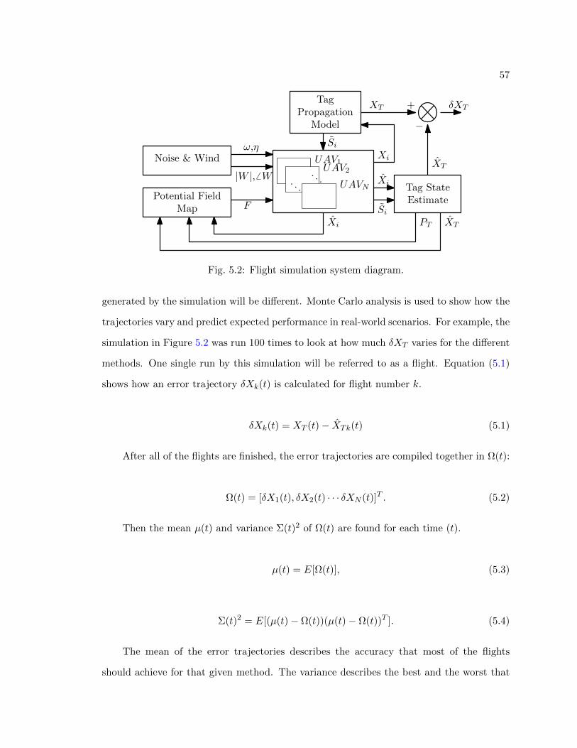
57
Potential FieldMap
. . .. . .
UAV1UAV2
UAVN
F
Tag StateEstimate
Xi
Xi XT
Noise & Windω,η
|W |,6 W
TagPropagation
Model
Si
Si
XT
XT
−
+ δXT
Xi
PT
Fig. 5.2: Flight simulation system diagram.
generated by the simulation will be different. Monte Carlo analysis is used to show how the
trajectories vary and predict expected performance in real-world scenarios. For example, the
simulation in Figure 5.2 was run 100 times to look at how much δXT varies for the different
methods. One single run by this simulation will be referred to as a flight. Equation (5.1)
shows how an error trajectory δXk(t) is calculated for flight number k.
δXk(t) = XT (t)− XTk(t) (5.1)
After all of the flights are finished, the error trajectories are compiled together in Ω(t):
Ω(t) = [δX1(t), δX2(t) · · · δXN (t)]T . (5.2)
Then the mean µ(t) and variance Σ(t)2 of Ω(t) are found for each time (t).
µ(t) = E[Ω(t)], (5.3)
Σ(t)2 = E[(µ(t)− Ω(t))(µ(t)− Ω(t))T ]. (5.4)
The mean of the error trajectories describes the accuracy that most of the flights
should achieve for that given method. The variance describes the best and the worst that
58
can be expected around the mean. Many applications require thousands of runs to reduce
the uncertainty of the estimated variance. For this application, 100 flights are enough to
compare navigation methods. In addition, the uncertainty of the variance is documented
and confidence intervals around the variance curves are calculated using the chi-squared
distribution.
The subsections below describe the important pieces of the flight simulation. These
include the environmental dynamics, the UA system dynamics, simulating and estimating
the tag Location, and navigation using potential fields.
5.1.1 Environmental Dynamics
Equation (5.5) is used to calculate the magnitude and direction of wind. |W |0 and
∠W0 are nominal values of the wind and b|W | and b∠W are random biases modeled as first
order Markov stochastic processes (Equation (5.6)).
|W | = |W |0 + b|W |,
∠W = ∠W0 + b∠W . (5.5)
|W |0 = 0,
∠W0 = 0,
b|W | = −b|W |
τ|W |+ ω|W |,
b∠W = −b∠Wτ∠W
+ ω∠W . (5.6)
The driving noise (ω|W |, ω∠W ) is Gaussian with the following properties:
E[ω|W |] = 0, E[ω|W |ω′|W |] =
2σ2|W |
τ|W |δ(t− t′).
E[ω∠W ] = 0, E[ω∠Wω′∠W ] =
2σ2∠Wτ∠W
δ(t− t′). (5.7)
59
5.1.2 UA System Dynamics
Figure 5.3 shows a detailed diagram of the simulated UA system for UAVi. The force
from the potential field map (F ) is used by the controller to generate ui (desired rate
of change for the heading). This control input along with the noise and wind are used to
generate the UA truth states (Xi) and the GPS measurements (zi). The GPS measurements
are used as measurements in the Kalman Filter to generate the estimated states of the UA.
Truth Dynamics
Equation (5.8) shows the UA truth state dynamics. xi and yi describe the position of
the UA and its time derivative is a function of the airspeed vi, the yaw ψi, and the x and y
components of the wind (Wx, Wy). The airspeed is assumed to be constant and the change
in yaw is equal to the controller output (ui).
xi = vi cos(ψi) +Wx,
yi = vi sin(ψi) +Wy,
vi = 0,
ψi = ui,
bxi = −bxiτx
+ ωxi,
byi = −byiτy
+ ωyi. (5.8)
bxi and byi are biases in the GPS measurement. These biases are also modeled as first
order Markov stochastic processes.
E[ωxi] = 0, E[ωxiω′xi] =
2σ2xτx
δ(t− t′).
E[ωyi] = 0, E[ωyiω′yi] =
2σ2yτy
δ(t− t′). (5.9)
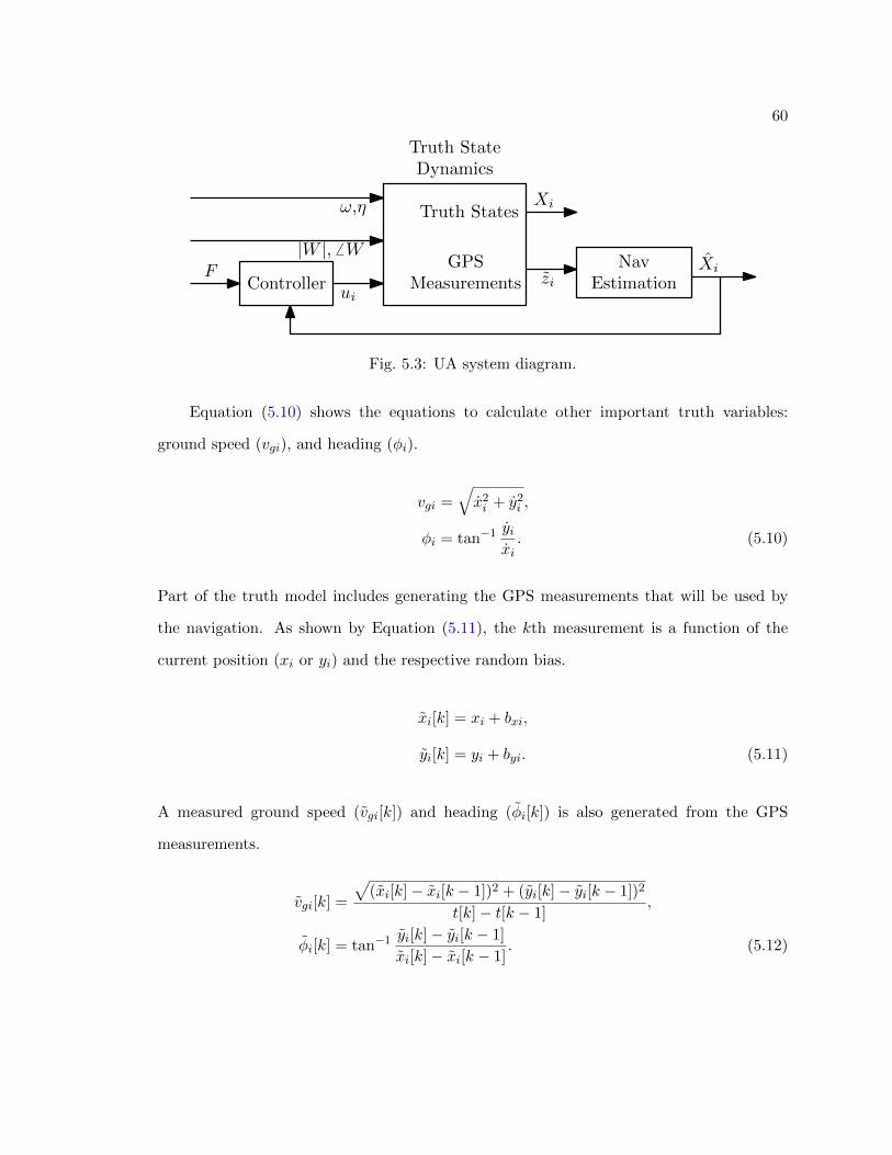
60
F Xi
ω,η
|W |, 6 W
Truth States
Controllerui
ziGPS
Measurements
Xi
NavEstimation
Truth StateDynamics
Fig. 5.3: UA system diagram.
Equation (5.10) shows the equations to calculate other important truth variables:
ground speed (vgi), and heading (φi).
vgi =√x2i + y2i ,
φi = tan−1yixi. (5.10)
Part of the truth model includes generating the GPS measurements that will be used by
the navigation. As shown by Equation (5.11), the kth measurement is a function of the
current position (xi or yi) and the respective random bias.
xi[k] = xi + bxi,
yi[k] = yi + byi. (5.11)
A measured ground speed (vgi[k]) and heading (φi[k]) is also generated from the GPS
measurements.
vgi[k] =
√(xi[k]− xi[k − 1])2 + (yi[k]− yi[k − 1])2
t[k]− t[k − 1],
φi[k] = tan−1yi[k]− yi[k − 1]
xi[k]− xi[k − 1]. (5.12)
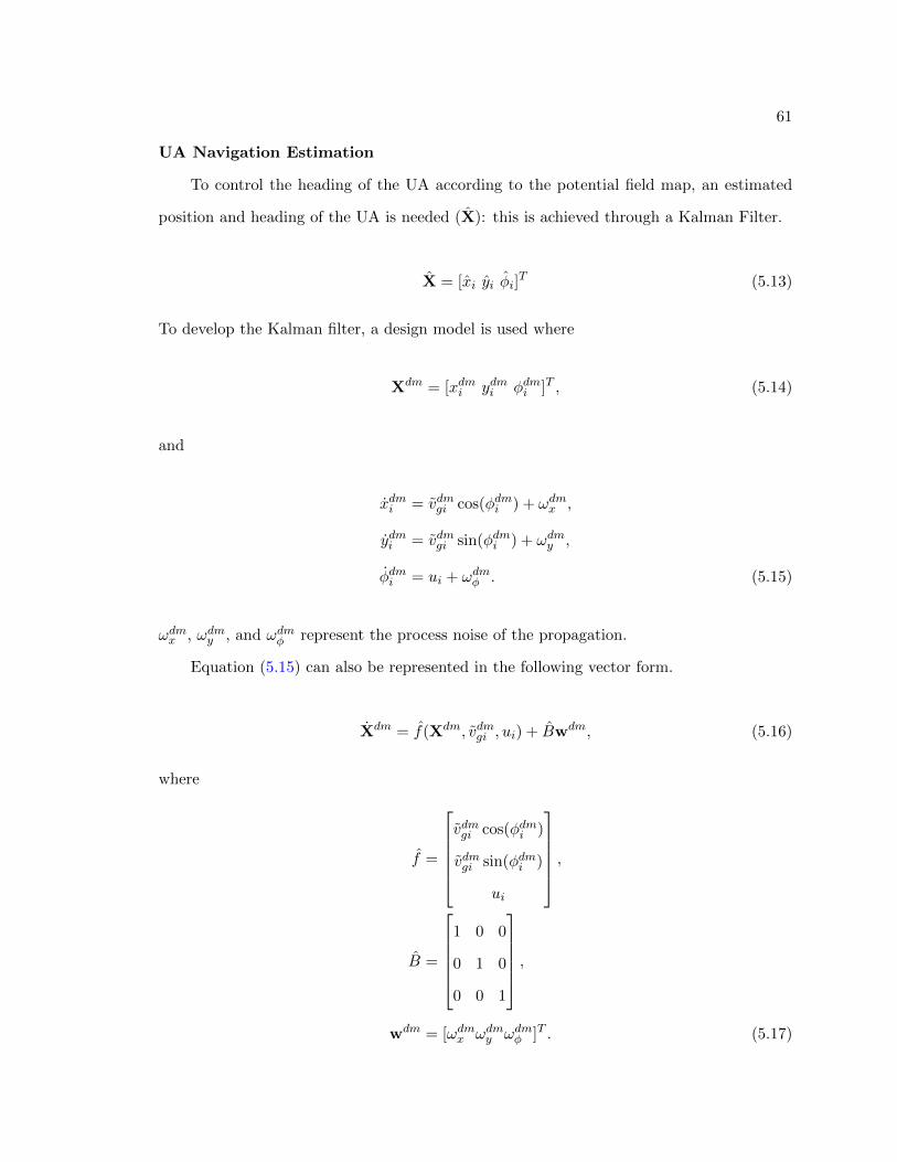
61
UA Navigation Estimation
To control the heading of the UA according to the potential field map, an estimated
position and heading of the UA is needed (X): this is achieved through a Kalman Filter.
X = [xi yi φi]T (5.13)
To develop the Kalman filter, a design model is used where
Xdm = [xdmi ydmi φdmi ]T , (5.14)
and
xdmi = vdmgi cos(φdmi ) + ωdmx ,
ydmi = vdmgi sin(φdmi ) + ωdmy ,
φdmi = ui + ωdmφ . (5.15)
ωdmx , ωdmy , and ωdmφ represent the process noise of the propagation.
Equation (5.15) can also be represented in the following vector form.
Xdm = f(Xdm, vdmgi , ui) + Bwdm, (5.16)
where
f =
vdmgi cos(φdmi )
vdmgi sin(φdmi )
ui
,
B =
1 0 0
0 1 0
0 0 1
,wdm = [ωdmx ωdmy ωdmφ ]T . (5.17)
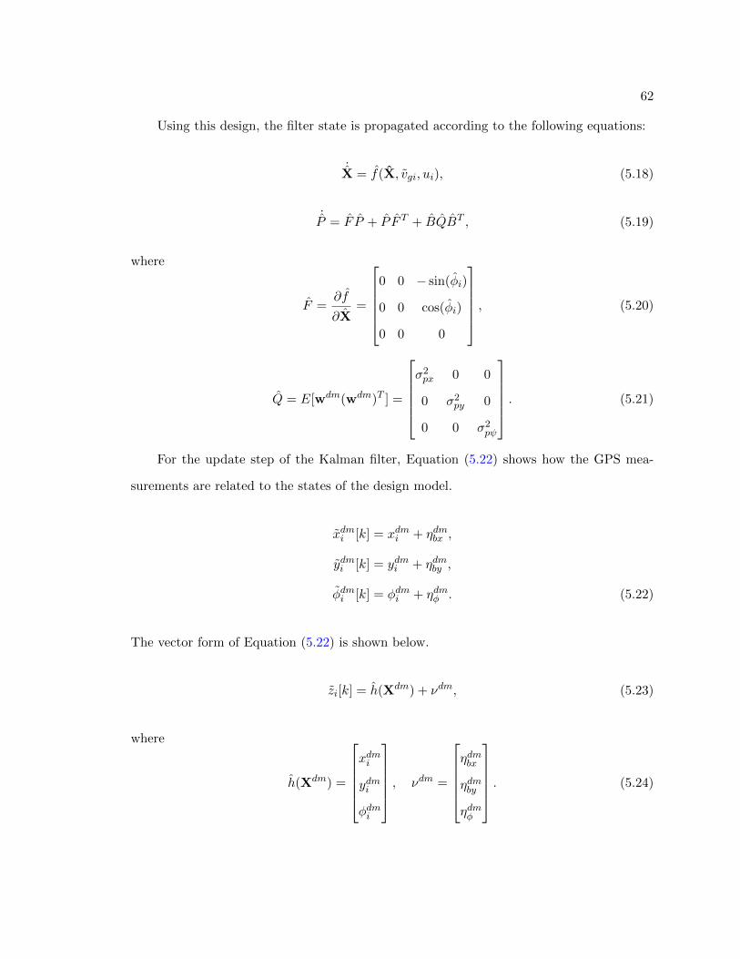
62
Using this design, the filter state is propagated according to the following equations:
˙X = f(X, vgi, ui), (5.18)
˙P = F P + P F T + BQBT , (5.19)
where
F =∂f
∂X=
0 0 − sin(φi)
0 0 cos(φi)
0 0 0
, (5.20)
Q = E[wdm(wdm)T ] =
σ2px 0 0
0 σ2py 0
0 0 σ2pψ
. (5.21)
For the update step of the Kalman filter, Equation (5.22) shows how the GPS mea-
surements are related to the states of the design model.
xdmi [k] = xdmi + ηdmbx ,
ydmi [k] = ydmi + ηdmby ,
φdmi [k] = φdmi + ηdmφ . (5.22)
The vector form of Equation (5.22) is shown below.
zi[k] = h(Xdm) + νdm, (5.23)
where
h(Xdm) =
xdmi
ydmi
φdmi
, νdm =
ηdmbx
ηdmby
ηdmφ
. (5.24)
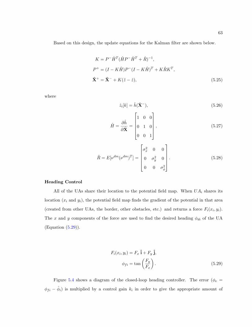
63
Based on this design, the update equations for the Kalman filter are shown below.
K = P−HT (HP−HT + R)−1,
P+ = (I −KH)P−(I −KH)T +KRKT ,
X+ = X− +K(z − z), (5.25)
where
zi[k] = h(X−), (5.26)
H =∂h
∂X=
1 0 0
0 1 0
0 0 1
, (5.27)
R = E[νdm(νdm)T ] =
σ2x 0 0
0 σ2y 0
0 0 σ2φ
. (5.28)
Heading Control
All of the UAs share their location to the potential field map. When UAi shares its
location (xi and yi), the potential field map finds the gradient of the potential in that area
(created from other UAs, the border, other obstacles, etc.) and returns a force Fi(xi, yi).
The x and y components of the force are used to find the desired heading φdi of the UA
(Equation (5.29)).
Fi(xi, yi) = Fx i + Fy j,
φfi = tan
(FyFx
). (5.29)
Figure 5.4 shows a diagram of the closed-loop heading controller. The error (φe =
φfi − φi) is multiplied by a control gain ki in order to give the appropriate amount of
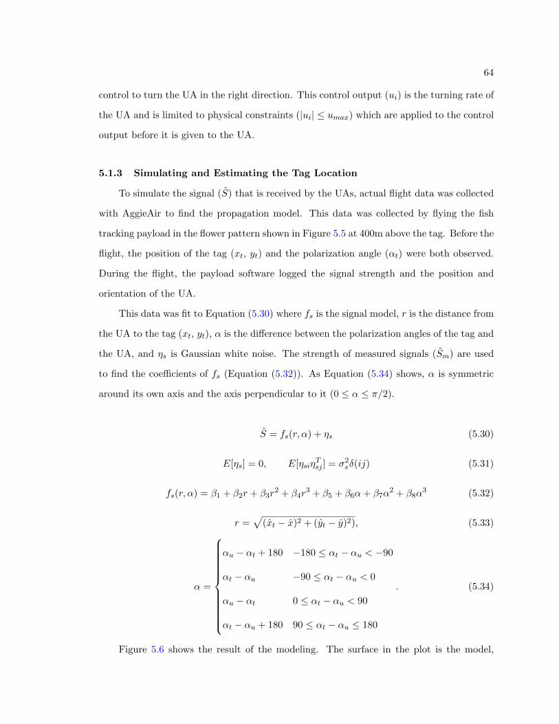
64
control to turn the UA in the right direction. This control output (ui) is the turning rate of
the UA and is limited to physical constraints (|ui| ≤ umax) which are applied to the control
output before it is given to the UA.
5.1.3 Simulating and Estimating the Tag Location
To simulate the signal (S) that is received by the UAs, actual flight data was collected
with AggieAir to find the propagation model. This data was collected by flying the fish
tracking payload in the flower pattern shown in Figure 5.5 at 400m above the tag. Before the
flight, the position of the tag (xt, yt) and the polarization angle (αt) were both observed.
During the flight, the payload software logged the signal strength and the position and
orientation of the UA.
This data was fit to Equation (5.30) where fs is the signal model, r is the distance from
the UA to the tag (xt, yt), α is the difference between the polarization angles of the tag and
the UA, and ηs is Gaussian white noise. The strength of measured signals (Sm) are used
to find the coefficients of fs (Equation (5.32)). As Equation (5.34) shows, α is symmetric
around its own axis and the axis perpendicular to it (0 ≤ α ≤ π/2).
S = fs(r, α) + ηs (5.30)
E[ηs] = 0, E[ηsiηTsj ] = σ2sδ(ij) (5.31)
fs(r, α) = β1 + β2r + β3r2 + β4r
3 + β5 + β6α+ β7α2 + β8α
3 (5.32)
r =√
(xt − x)2 + (yt − y)2), (5.33)
α =
αu − αt + 180 −180 ≤ αt − αu < −90
αt − αu −90 ≤ αt − αu < 0
αu − αt 0 ≤ αt − αu < 90
αt − αu + 180 90 ≤ αt − αu ≤ 180
. (5.34)
Figure 5.6 shows the result of the modeling. The surface in the plot is the model,
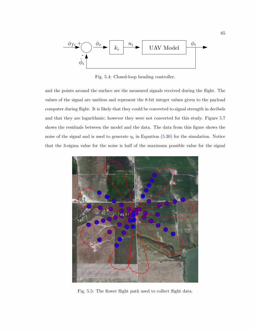
65
UAV Modelkiφeφfi φiui
-
+
φi
Fig. 5.4: Closed-loop heading controller.
and the points around the surface are the measured signals received during the flight. The
values of the signal are unitless and represent the 8-bit integer values given to the payload
computer during flight. It is likely that they could be converted to signal strength in decibels
and that they are logarithmic; however they were not converted for this study. Figure 5.7
shows the residuals between the model and the data. The data from this figure shows the
noise of the signal and is used to generate ηs in Equation (5.30) for the simulation. Notice
that the 3-sigma value for the noise is half of the maximum possible value for the signal
Fig. 5.5: The flower flight path used to collect flight data.
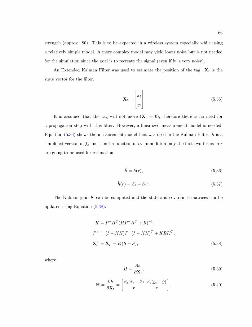
66
strength (approx. 80). This is to be expected in a wireless system especially while using
a relatively simple model. A more complex model may yield lower noise but is not needed
for the simulation since the goal is to recreate the signal (even if it is very noisy).
An Extended Kalman Filter was used to estimate the position of the tag. Xt is the
state vector for the filter.
Xt =
xtyt
(5.35)
It is assumed that the tag will not move (Xt = 0), therefore there is no need for
a propagation step with this filter. However, a linearized measurement model is needed.
Equation (5.36) shows the measurement model that was used in the Kalman Filter. h is a
simplified version of fs and is not a function of α. In addition only the first two terms in r
are going to be used for estimation.
S = h(r), (5.36)
h(r) = β1 + β2r. (5.37)
The Kalman gain K can be computed and the state and covariance matrices can be
updated using Equation (5.38).
K = P−HT (HP−HT +R)−1,
P+ = (I −KH)P−(I −KH)T +KRKT ,
X+t = X−t +K(S − S), (5.38)
where
H =∂h
∂Xt, (5.39)
H =∂h
∂Xt=
[β2(xt − x)
r,β2(yt − y)
r
], (5.40)
67
0
200
400
600
800
1000
020406080100
0
20
40
60
80
100
120
α
Actual Signal Data and Model
r
Sig
nal
Model
Actual Data
Fig. 5.6: The two-dimensional, fourth-order polynomial model plotted with the test flightdata.
R = E[ηs(ηs)T ] = σ2s . (5.41)
5.1.4 Navigation using Potential Fields
Conventional Potential Fields
Potential fields (PFs) are commonly used to dynamically plan the motion of ground [58]
and air-based [59] mobile robots (agents). They are used to attract or repel agents to or
from objects and other agents. For example, repulsive PFs around all agents could ensure
that they do not collide with one another. Equation (5.42) shows a conventional definition
of an attractive PF [60].
U(x) =1
2k(xa − xg)2 (5.42)
This PF is applied to the agents through a force defined as the negative gradient of the PF:
F (x) = −∇U(x). (5.43)
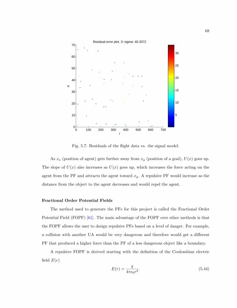
68
0 100 200 300 400 500 600 7000
10
20
30
40
50
60
70
r
α
Residual error plot. 3−sigma: 40.3372
5
10
15
20
25
30
Fig. 5.7: Residuals of the flight data vs. the signal model.
As xa (position of agent) gets further away from xg (position of a goal), U(x) goes up.
The slope of U(x) also increases as U(x) goes up, which increases the force acting on the
agent from the PF and attracts the agent toward xg. A repulsive PF would increase as the
distance from the object to the agent decreases and would repel the agent.
Fractional Order Potential Fields
The method used to generate the PFs for this project is called the Fractional Order
Potential Field (FOPF) [61]. The main advantage of the FOPF over other methods is that
the FOPF allows the user to design repulsive PFs based on a level of danger. For example,
a collision with another UA would be very dangerous and therefore would get a different
PF that produced a higher force than the PF of a less dangerous object like a boundary.
A repulsive FOPF is derived starting with the definition of the Coulombian electric
field E(r)
E(r) =q
4πε0r2. (5.44)
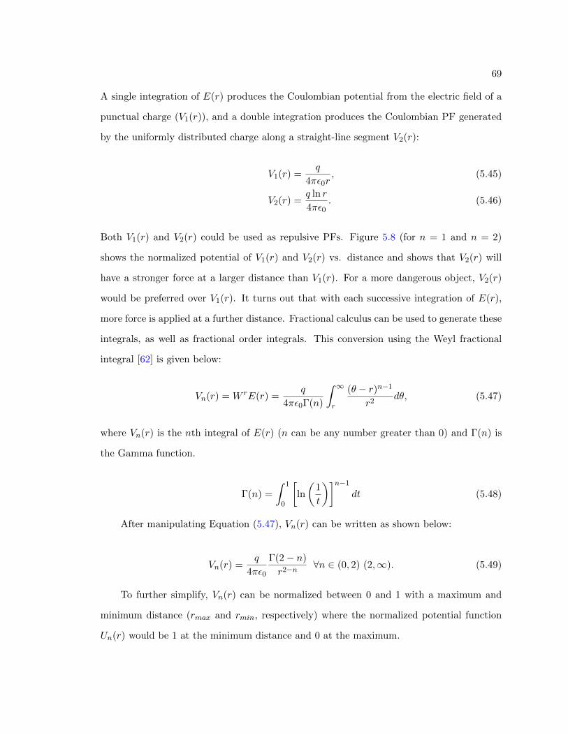
69
A single integration of E(r) produces the Coulombian potential from the electric field of a
punctual charge (V1(r)), and a double integration produces the Coulombian PF generated
by the uniformly distributed charge along a straight-line segment V2(r):
V1(r) =q
4πε0r, (5.45)
V2(r) =q ln r
4πε0. (5.46)
Both V1(r) and V2(r) could be used as repulsive PFs. Figure 5.8 (for n = 1 and n = 2)
shows the normalized potential of V1(r) and V2(r) vs. distance and shows that V2(r) will
have a stronger force at a larger distance than V1(r). For a more dangerous object, V2(r)
would be preferred over V1(r). It turns out that with each successive integration of E(r),
more force is applied at a further distance. Fractional calculus can be used to generate these
integrals, as well as fractional order integrals. This conversion using the Weyl fractional
integral [62] is given below:
Vn(r) = W rE(r) =q
4πε0Γ(n)
∫ ∞r
(θ − r)n−1r2
dθ, (5.47)
where Vn(r) is the nth integral of E(r) (n can be any number greater than 0) and Γ(n) is
the Gamma function.
Γ(n) =
∫ 1
0
[ln
(1
t
)]n−1dt (5.48)
After manipulating Equation (5.47), Vn(r) can be written as shown below:
Vn(r) =q
4πε0
Γ(2− n)
r2−n∀n ∈ (0, 2) (2,∞). (5.49)
To further simplify, Vn(r) can be normalized between 0 and 1 with a maximum and
minimum distance (rmax and rmin, respectively) where the normalized potential function
Un(r) would be 1 at the minimum distance and 0 at the maximum.
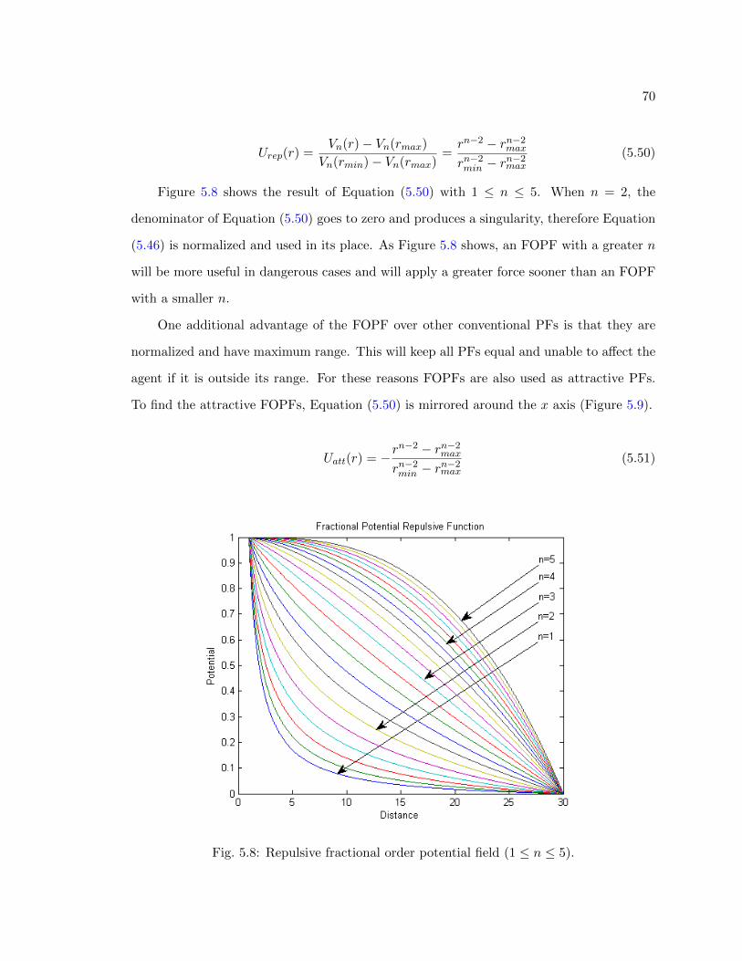
70
Urep(r) =Vn(r)− Vn(rmax)
Vn(rmin)− Vn(rmax)=rn−2 − rn−2max
rn−2min − rn−2max(5.50)
Figure 5.8 shows the result of Equation (5.50) with 1 ≤ n ≤ 5. When n = 2, the
denominator of Equation (5.50) goes to zero and produces a singularity, therefore Equation
(5.46) is normalized and used in its place. As Figure 5.8 shows, an FOPF with a greater n
will be more useful in dangerous cases and will apply a greater force sooner than an FOPF
with a smaller n.
One additional advantage of the FOPF over other conventional PFs is that they are
normalized and have maximum range. This will keep all PFs equal and unable to affect the
agent if it is outside its range. For these reasons FOPFs are also used as attractive PFs.
To find the attractive FOPFs, Equation (5.50) is mirrored around the x axis (Figure 5.9).
Uatt(r) = −rn−2 − rn−2max
rn−2min − rn−2max(5.51)
Fig. 5.8: Repulsive fractional order potential field (1 ≤ n ≤ 5).
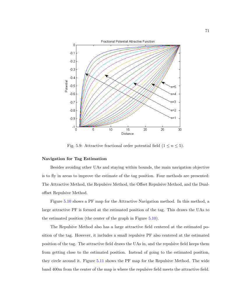
71
Fig. 5.9: Attractive fractional order potential field (1 ≤ n ≤ 5).
Navigation for Tag Estimation
Besides avoiding other UAs and staying within bounds, the main navigation objective
is to fly in areas to improve the estimate of the tag position. Four methods are presented:
The Attractive Method, the Repulsive Method, the Offset Repulsive Method, and the Dual-
offset Repulsive Method.
Figure 5.10 shows a PF map for the Attractive Navigation method. In this method, a
large attractive PF is formed at the estimated position of the tag. This draws the UAs to
the estimated position (the center of the graph in Figure 5.10).
The Repulsive Method also has a large attractive field centered at the estimated po-
sition of the tag. However, it includes a small repulsive PF also centered at the estimated
position of the tag. The attractive field draws the UAs in, and the repulsive field keeps them
from getting close to the estimated position. Instead of going to the estimated position,
they circle around it. Figure 5.11 shows the PF map for the Repulsive Method. The wide
band 400m from the center of the map is where the repulsive field meets the attractive field.
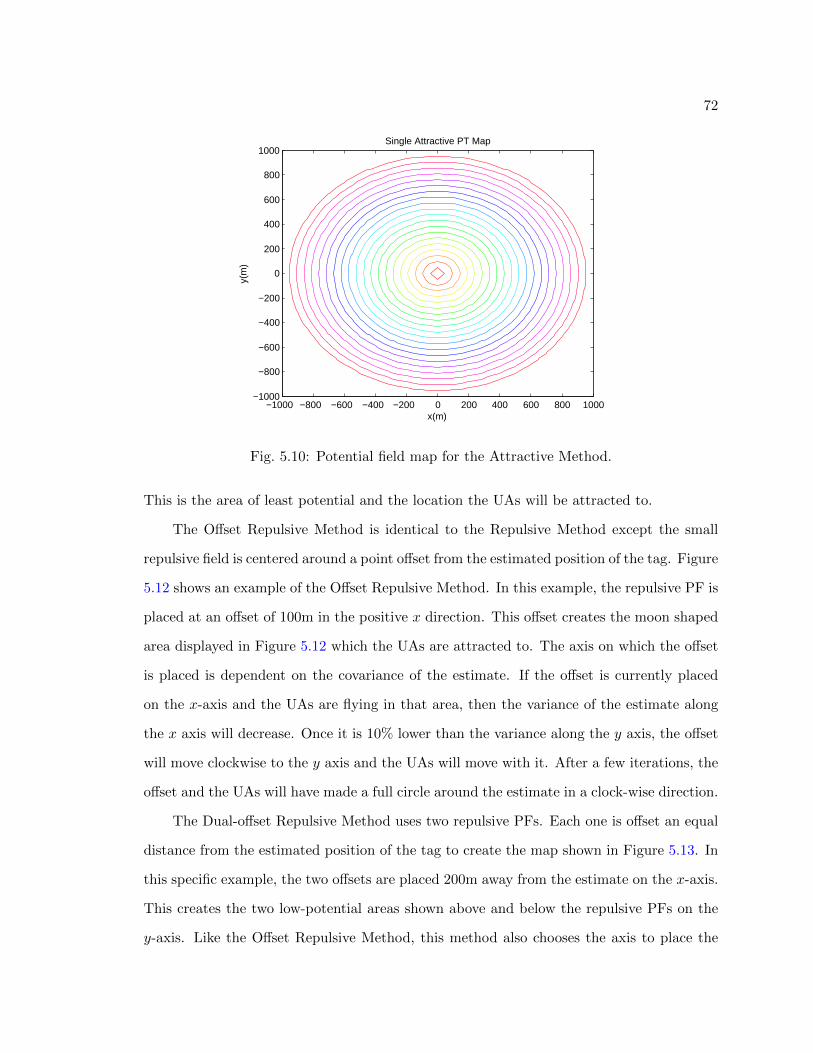
72
Single Attractive PT Map
x(m)
y(m
)
−1000 −800 −600 −400 −200 0 200 400 600 800 1000−1000
−800
−600
−400
−200
0
200
400
600
800
1000
Fig. 5.10: Potential field map for the Attractive Method.
This is the area of least potential and the location the UAs will be attracted to.
The Offset Repulsive Method is identical to the Repulsive Method except the small
repulsive field is centered around a point offset from the estimated position of the tag. Figure
5.12 shows an example of the Offset Repulsive Method. In this example, the repulsive PF is
placed at an offset of 100m in the positive x direction. This offset creates the moon shaped
area displayed in Figure 5.12 which the UAs are attracted to. The axis on which the offset
is placed is dependent on the covariance of the estimate. If the offset is currently placed
on the x-axis and the UAs are flying in that area, then the variance of the estimate along
the x axis will decrease. Once it is 10% lower than the variance along the y axis, the offset
will move clockwise to the y axis and the UAs will move with it. After a few iterations, the
offset and the UAs will have made a full circle around the estimate in a clock-wise direction.
The Dual-offset Repulsive Method uses two repulsive PFs. Each one is offset an equal
distance from the estimated position of the tag to create the map shown in Figure 5.13. In
this specific example, the two offsets are placed 200m away from the estimate on the x-axis.
This creates the two low-potential areas shown above and below the repulsive PFs on the
y-axis. Like the Offset Repulsive Method, this method also chooses the axis to place the
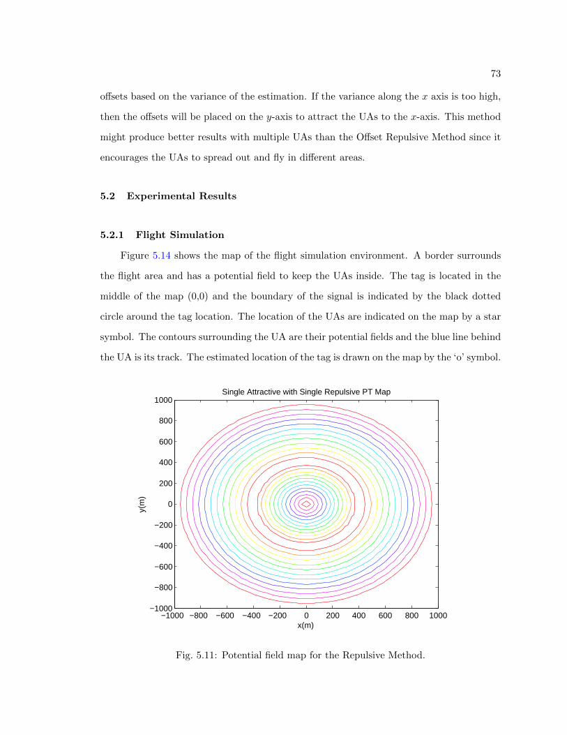
73
offsets based on the variance of the estimation. If the variance along the x axis is too high,
then the offsets will be placed on the y-axis to attract the UAs to the x-axis. This method
might produce better results with multiple UAs than the Offset Repulsive Method since it
encourages the UAs to spread out and fly in different areas.
5.2 Experimental Results
5.2.1 Flight Simulation
Figure 5.14 shows the map of the flight simulation environment. A border surrounds
the flight area and has a potential field to keep the UAs inside. The tag is located in the
middle of the map (0,0) and the boundary of the signal is indicated by the black dotted
circle around the tag location. The location of the UAs are indicated on the map by a star
symbol. The contours surrounding the UA are their potential fields and the blue line behind
the UA is its track. The estimated location of the tag is drawn on the map by the ‘o’ symbol.
Single Attractive with Single Repulsive PT Map
x(m)
y(m
)
−1000 −800 −600 −400 −200 0 200 400 600 800 1000−1000
−800
−600
−400
−200
0
200
400
600
800
1000
Fig. 5.11: Potential field map for the Repulsive Method.
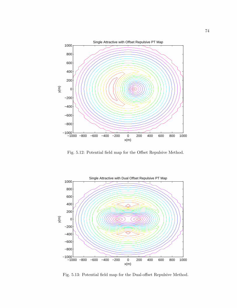
74
Single Attractive with Offset Repulsive PT Map
x(m)
y(m
)
−1000 −800 −600 −400 −200 0 200 400 600 800 1000−1000
−800
−600
−400
−200
0
200
400
600
800
1000
Fig. 5.12: Potential field map for the Offset Repulsive Method.
Single Attractive with Dual Offset Repulsive PT Map
x(m)
y(m
)
−1000 −800 −600 −400 −200 0 200 400 600 800 1000−1000
−800
−600
−400
−200
0
200
400
600
800
1000
Fig. 5.13: Potential field map for the Dual-offset Repulsive Method.
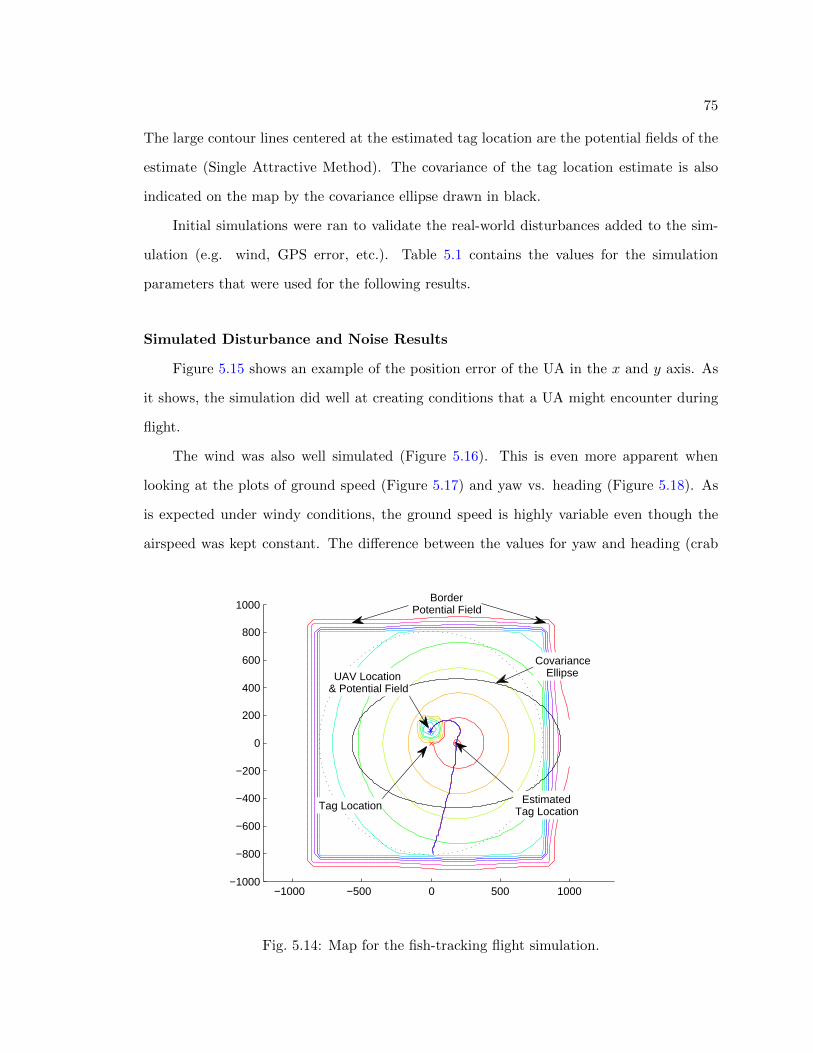
75
The large contour lines centered at the estimated tag location are the potential fields of the
estimate (Single Attractive Method). The covariance of the tag location estimate is also
indicated on the map by the covariance ellipse drawn in black.
Initial simulations were ran to validate the real-world disturbances added to the sim-
ulation (e.g. wind, GPS error, etc.). Table 5.1 contains the values for the simulation
parameters that were used for the following results.
Simulated Disturbance and Noise Results
Figure 5.15 shows an example of the position error of the UA in the x and y axis. As
it shows, the simulation did well at creating conditions that a UA might encounter during
flight.
The wind was also well simulated (Figure 5.16). This is even more apparent when
looking at the plots of ground speed (Figure 5.17) and yaw vs. heading (Figure 5.18). As
is expected under windy conditions, the ground speed is highly variable even though the
airspeed was kept constant. The difference between the values for yaw and heading (crab
−1000 −500 0 500 1000−1000
−800
−600
−400
−200
0
200
400
600
800
1000
CovarianceEllipse
EstimatedTag LocationTag Location
UAV Location & Potential Field
BorderPotential Field
Fig. 5.14: Map for the fish-tracking flight simulation.
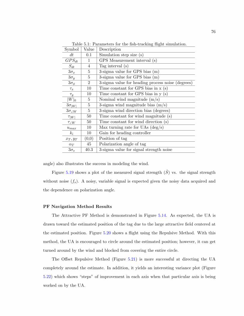
76
Table 5.1: Parameters for the fish-tracking flight simulation.Symbol Value Description
dt 0.1 Simulation step size (s)
GPSdt 1 GPS Measurement interval (s)
Sdt 4 Tag interval (s)
3σx 5 3-sigma value for GPS bias (m)
3σy 5 3-sigma value for GPS bias (m)
3σφ 2 3-sigma value for heading process noise (degrees)
τx 10 Time constant for GPS bias in x (s)
τy 10 Time constant for GPS bias in y (s)
|W |0 5 Nominal wind magnitude (m/s)
3σ|W | 5 3-sigma wind magnitude bias (m/s)
3σ∠W 5 3-sigma wind direction bias (degrees)
τ|W | 50 Time constant for wind magnitude (s)
τ∠W 50 Time constant for wind direction (s)
umax 10 Max turning rate for UAs (deg/s)
ki 10 Gain for heading controller
xT , yT (0,0) Position of tag
αT 45 Polarization angle of tag
3σs 40.3 3-sigma value for signal strength noise
angle) also illustrates the success in modeling the wind.
Figure 5.19 shows a plot of the measured signal strength (S) vs. the signal strength
without noise (fs). A noisy, variable signal is expected given the noisy data acquired and
the dependence on polarization angle.
PF Navigation Method Results
The Attractive PF Method is demonstrated in Figure 5.14. As expected, the UA is
drawn toward the estimated position of the tag due to the large attractive field centered at
the estimated position. Figure 5.20 shows a flight using the Repulsive Method. With this
method, the UA is encouraged to circle around the estimated position; however, it can get
turned around by the wind and blocked from covering the entire circle.
The Offset Repulsive Method (Figure 5.21) is more successful at directing the UA
completely around the estimate. In addition, it yields an interesting variance plot (Figure
5.22) which shows “steps” of improvement in each axis when that particular axis is being
worked on by the UA.
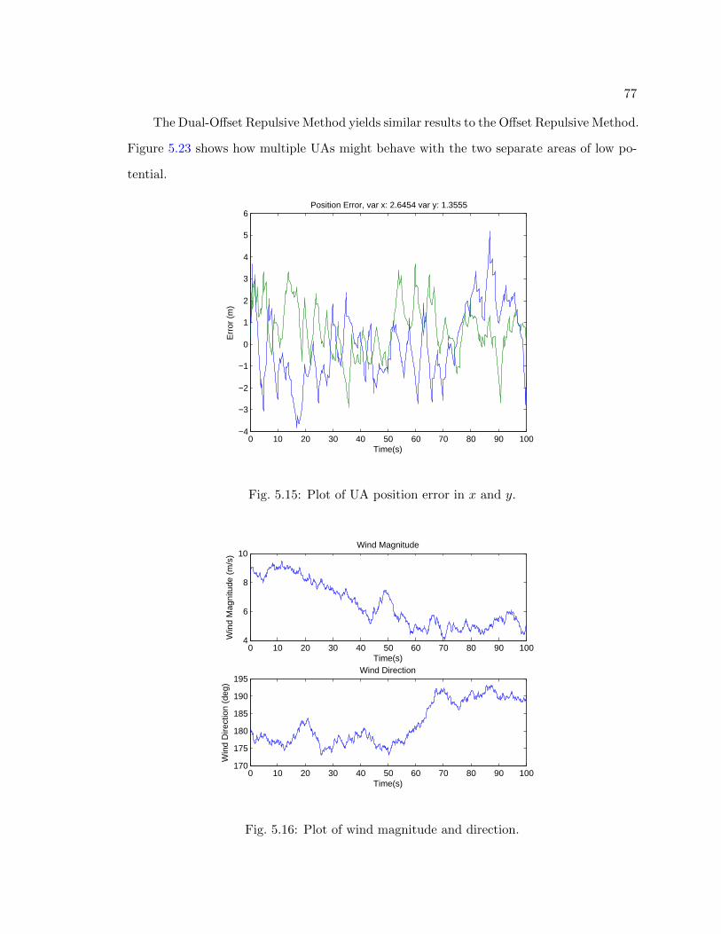
77
The Dual-Offset Repulsive Method yields similar results to the Offset Repulsive Method.
Figure 5.23 shows how multiple UAs might behave with the two separate areas of low po-
tential.
0 10 20 30 40 50 60 70 80 90 100−4
−3
−2
−1
0
1
2
3
4
5
6Position Error, var x: 2.6454 var y: 1.3555
Time(s)
Err
or (
m)
Fig. 5.15: Plot of UA position error in x and y.
0 10 20 30 40 50 60 70 80 90 1004
6
8
10Wind Magnitude
Time(s)
Win
d M
agni
tude
(m
/s)
0 10 20 30 40 50 60 70 80 90 100170
175
180
185
190
195Wind Direction
Time(s)
Win
d D
irect
ion
(deg
)
Fig. 5.16: Plot of wind magnitude and direction.
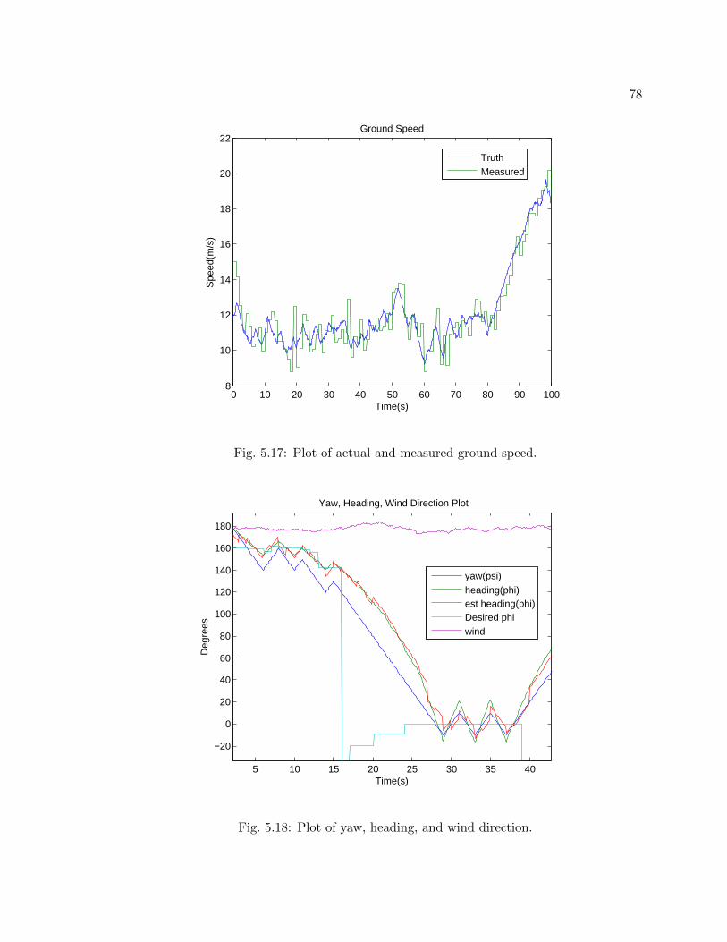
78
0 10 20 30 40 50 60 70 80 90 1008
10
12
14
16
18
20
22Ground Speed
Time(s)
Spe
ed(m
/s)
TruthMeasured
Fig. 5.17: Plot of actual and measured ground speed.
5 10 15 20 25 30 35 40
−20
0
20
40
60
80
100
120
140
160
180
Yaw, Heading, Wind Direction Plot
Time(s)
Deg
rees
yaw(psi)heading(phi)est heading(phi)Desired phiwind
Fig. 5.18: Plot of yaw, heading, and wind direction.
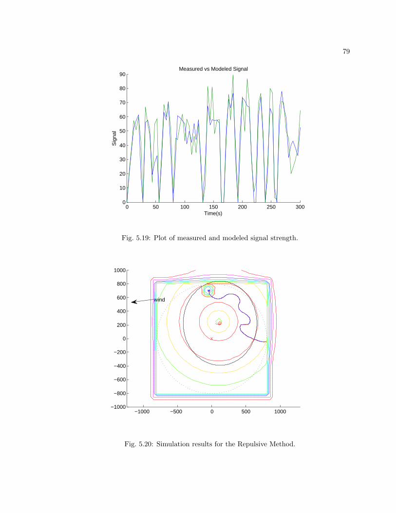
79
0 50 100 150 200 250 3000
10
20
30
40
50
60
70
80
90Measured vs Modeled Signal
Time(s)
Sig
nal
Fig. 5.19: Plot of measured and modeled signal strength.
−1000 −500 0 500 1000−1000
−800
−600
−400
−200
0
200
400
600
800
1000
wind
Fig. 5.20: Simulation results for the Repulsive Method.
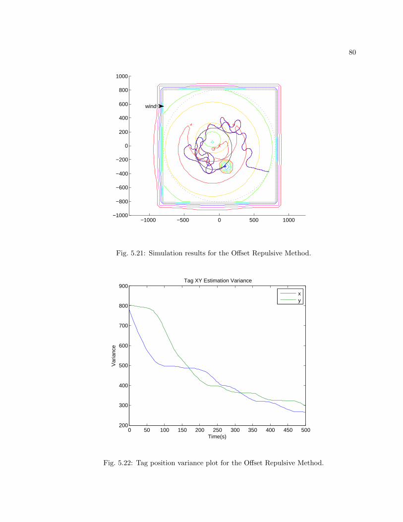
80
−1000 −500 0 500 1000−1000
−800
−600
−400
−200
0
200
400
600
800
1000
wind
Fig. 5.21: Simulation results for the Offset Repulsive Method.
0 50 100 150 200 250 300 350 400 450 500200
300
400
500
600
700
800
900Tag XY Estimation Variance
Time(s)
Var
ianc
e
xy
Fig. 5.22: Tag position variance plot for the Offset Repulsive Method.
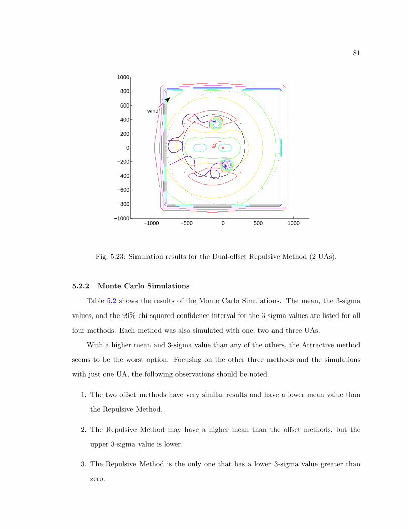
81
−1000 −500 0 500 1000−1000
−800
−600
−400
−200
0
200
400
600
800
1000
wind
Fig. 5.23: Simulation results for the Dual-offset Repulsive Method (2 UAs).
5.2.2 Monte Carlo Simulations
Table 5.2 shows the results of the Monte Carlo Simulations. The mean, the 3-sigma
values, and the 99% chi-squared confidence interval for the 3-sigma values are listed for all
four methods. Each method was also simulated with one, two and three UAs.
With a higher mean and 3-sigma value than any of the others, the Attractive method
seems to be the worst option. Focusing on the other three methods and the simulations
with just one UA, the following observations should be noted.
1. The two offset methods have very similar results and have a lower mean value than
the Repulsive Method.
2. The Repulsive Method may have a higher mean than the offset methods, but the
upper 3-sigma value is lower.
3. The Repulsive Method is the only one that has a lower 3-sigma value greater than
zero.
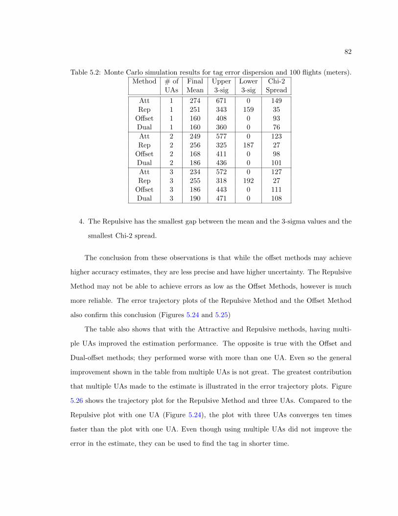
82
Table 5.2: Monte Carlo simulation results for tag error dispersion and 100 flights (meters).Method # of Final Upper Lower Chi-2
UAs Mean 3-sig 3-sig Spread
Att 1 274 671 0 149Rep 1 251 343 159 35
Offset 1 160 408 0 93Dual 1 160 360 0 76
Att 2 249 577 0 123Rep 2 256 325 187 27
Offset 2 168 411 0 98Dual 2 186 436 0 101
Att 3 234 572 0 127Rep 3 255 318 192 27
Offset 3 186 443 0 111Dual 3 190 471 0 108
4. The Repulsive has the smallest gap between the mean and the 3-sigma values and the
smallest Chi-2 spread.
The conclusion from these observations is that while the offset methods may achieve
higher accuracy estimates, they are less precise and have higher uncertainty. The Repulsive
Method may not be able to achieve errors as low as the Offset Methods, however is much
more reliable. The error trajectory plots of the Repulsive Method and the Offset Method
also confirm this conclusion (Figures 5.24 and 5.25)
The table also shows that with the Attractive and Repulsive methods, having multi-
ple UAs improved the estimation performance. The opposite is true with the Offset and
Dual-offset methods; they performed worse with more than one UA. Even so the general
improvement shown in the table from multiple UAs is not great. The greatest contribution
that multiple UAs made to the estimate is illustrated in the error trajectory plots. Figure
5.26 shows the trajectory plot for the Repulsive Method and three UAs. Compared to the
Repulsive plot with one UA (Figure 5.24), the plot with three UAs converges ten times
faster than the plot with one UA. Even though using multiple UAs did not improve the
error in the estimate, they can be used to find the tag in shorter time.
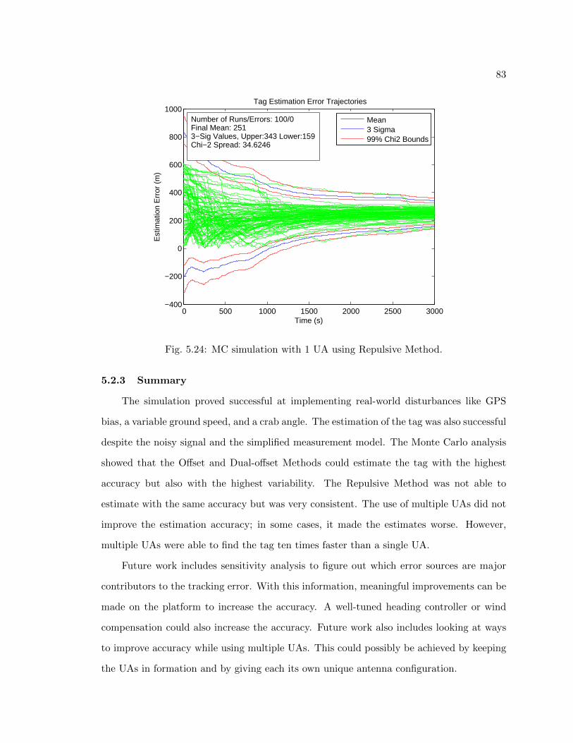
83
0 500 1000 1500 2000 2500 3000−400
−200
0
200
400
600
800
1000Tag Estimation Error Trajectories
Time (s)
Est
imat
ion
Err
or (
m)
Mean3 Sigma99% Chi2 Bounds
Number of Runs/Errors: 100/0Final Mean: 2513−Sig Values, Upper:343 Lower:159Chi−2 Spread: 34.6246
Fig. 5.24: MC simulation with 1 UA using Repulsive Method.
5.2.3 Summary
The simulation proved successful at implementing real-world disturbances like GPS
bias, a variable ground speed, and a crab angle. The estimation of the tag was also successful
despite the noisy signal and the simplified measurement model. The Monte Carlo analysis
showed that the Offset and Dual-offset Methods could estimate the tag with the highest
accuracy but also with the highest variability. The Repulsive Method was not able to
estimate with the same accuracy but was very consistent. The use of multiple UAs did not
improve the estimation accuracy; in some cases, it made the estimates worse. However,
multiple UAs were able to find the tag ten times faster than a single UA.
Future work includes sensitivity analysis to figure out which error sources are major
contributors to the tracking error. With this information, meaningful improvements can be
made on the platform to increase the accuracy. A well-tuned heading controller or wind
compensation could also increase the accuracy. Future work also includes looking at ways
to improve accuracy while using multiple UAs. This could possibly be achieved by keeping
the UAs in formation and by giving each its own unique antenna configuration.
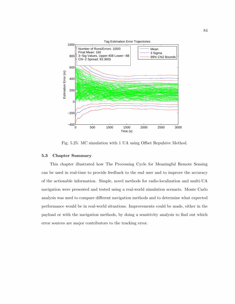
84
0 500 1000 1500 2000 2500 3000−400
−200
0
200
400
600
800
1000Tag Estimation Error Trajectories
Time (s)
Est
imat
ion
Err
or (
m)
Mean3 Sigma99% Chi2 Bounds
Number of Runs/Errors: 100/0Final Mean: 1603−Sig Values, Upper:408 Lower:−88Chi−2 Spread: 93.3655
Fig. 5.25: MC simulation with 1 UA using Offset Repulsive Method.
5.3 Chapter Summary
This chapter illustrated how The Processing Cycle for Meaningful Remote Sensing
can be used in real-time to provide feedback to the end user and to improve the accuracy
of the actionable information. Simple, novel methods for radio-localization and multi-UA
navigation were presented and tested using a real-world simulation scenario. Monte Carlo
analysis was used to compare different navigation methods and to determine what expected
performance would be in real-world situations. Improvements could be made, either in the
payload or with the navigation methods, by doing a sensitivity analysis to find out which
error sources are major contributors to the tracking error.
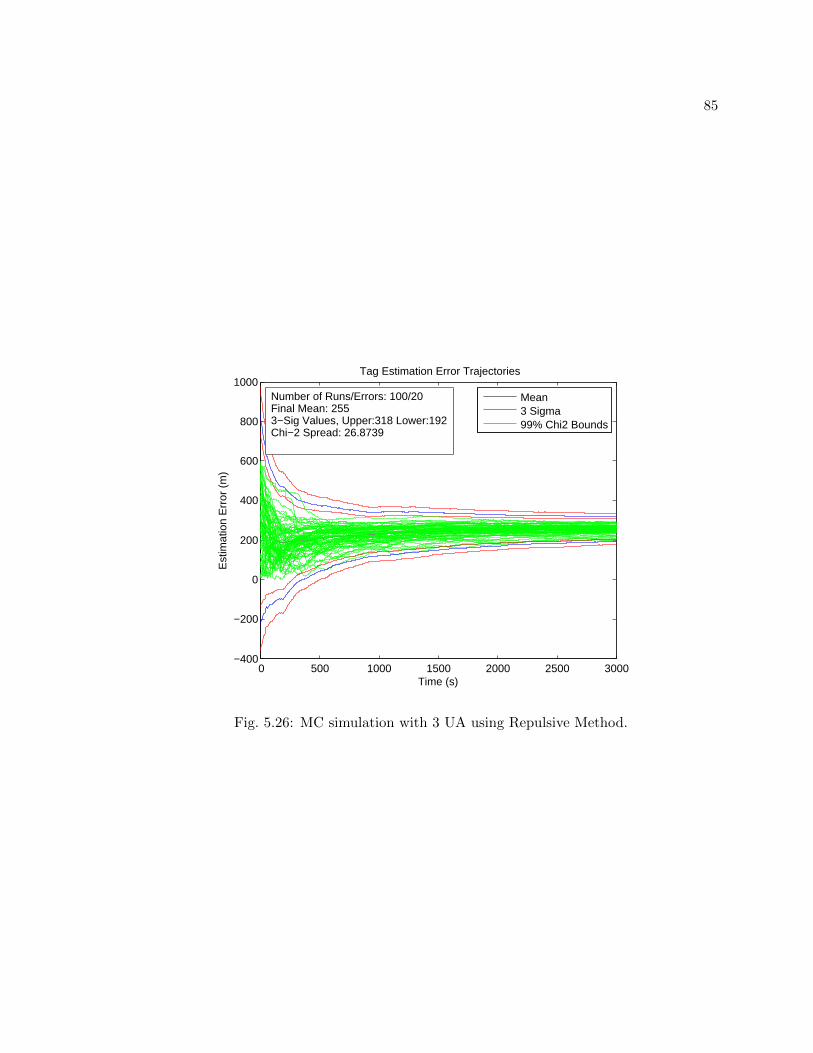
85
0 500 1000 1500 2000 2500 3000−400
−200
0
200
400
600
800
1000Tag Estimation Error Trajectories
Time (s)
Est
imat
ion
Err
or (
m)
Mean3 Sigma99% Chi2 Bounds
Number of Runs/Errors: 100/20Final Mean: 2553−Sig Values, Upper:318 Lower:192Chi−2 Spread: 26.8739
Fig. 5.26: MC simulation with 3 UA using Repulsive Method.
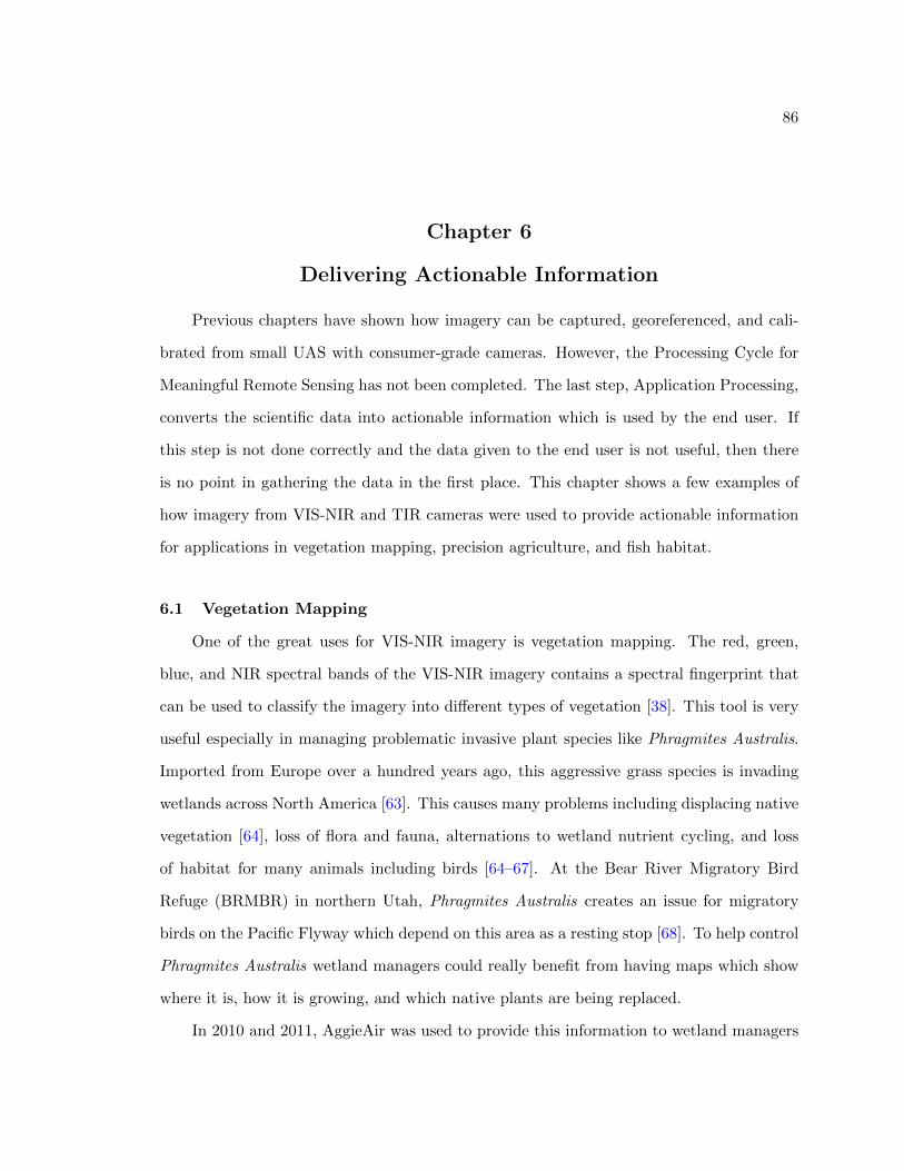
86
Chapter 6
Delivering Actionable Information
Previous chapters have shown how imagery can be captured, georeferenced, and cali-
brated from small UAS with consumer-grade cameras. However, the Processing Cycle for
Meaningful Remote Sensing has not been completed. The last step, Application Processing,
converts the scientific data into actionable information which is used by the end user. If
this step is not done correctly and the data given to the end user is not useful, then there
is no point in gathering the data in the first place. This chapter shows a few examples of
how imagery from VIS-NIR and TIR cameras were used to provide actionable information
for applications in vegetation mapping, precision agriculture, and fish habitat.
6.1 Vegetation Mapping
One of the great uses for VIS-NIR imagery is vegetation mapping. The red, green,
blue, and NIR spectral bands of the VIS-NIR imagery contains a spectral fingerprint that
can be used to classify the imagery into different types of vegetation [38]. This tool is very
useful especially in managing problematic invasive plant species like Phragmites Australis.
Imported from Europe over a hundred years ago, this aggressive grass species is invading
wetlands across North America [63]. This causes many problems including displacing native
vegetation [64], loss of flora and fauna, alternations to wetland nutrient cycling, and loss
of habitat for many animals including birds [64–67]. At the Bear River Migratory Bird
Refuge (BRMBR) in northern Utah, Phragmites Australis creates an issue for migratory
birds on the Pacific Flyway which depend on this area as a resting stop [68]. To help control
Phragmites Australis wetland managers could really benefit from having maps which show
where it is, how it is growing, and which native plants are being replaced.
In 2010 and 2011, AggieAir was used to provide this information to wetland managers
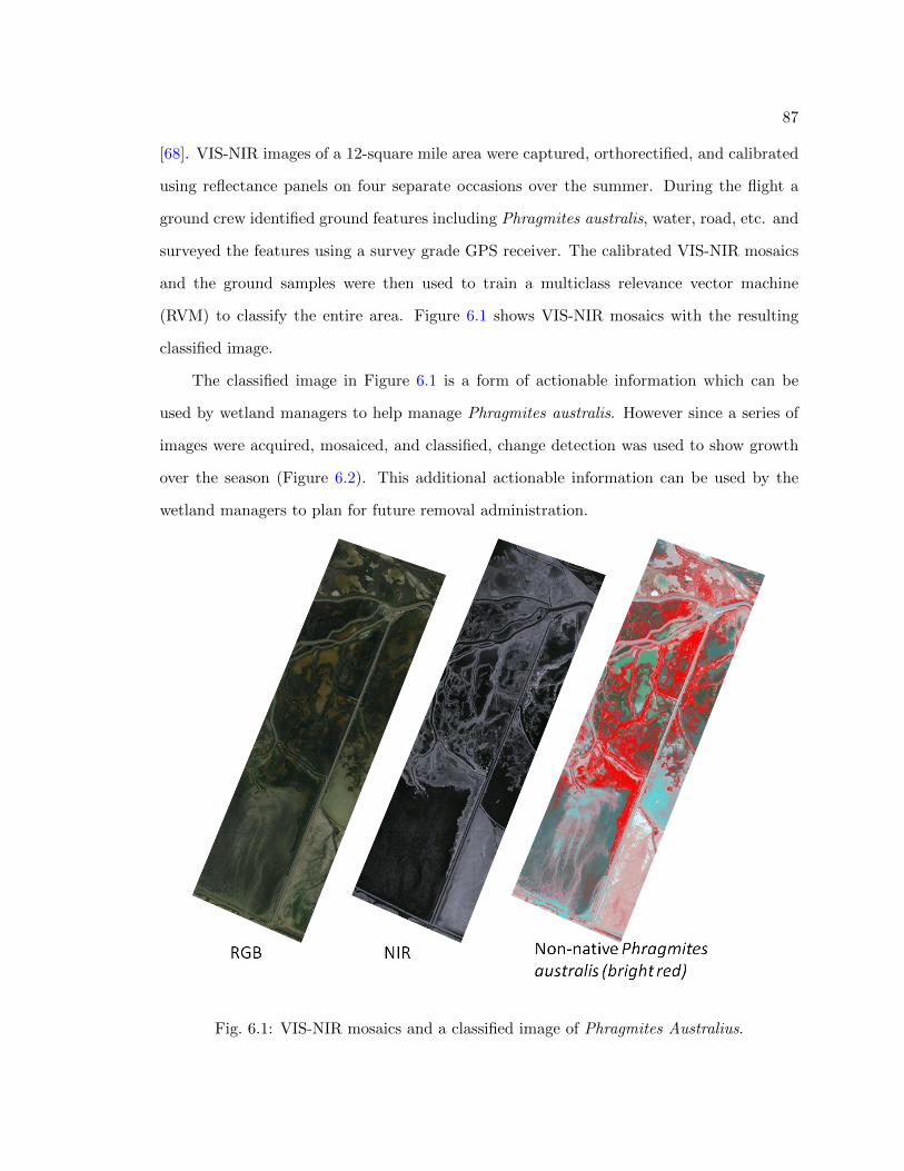
87
[68]. VIS-NIR images of a 12-square mile area were captured, orthorectified, and calibrated
using reflectance panels on four separate occasions over the summer. During the flight a
ground crew identified ground features including Phragmites australis, water, road, etc. and
surveyed the features using a survey grade GPS receiver. The calibrated VIS-NIR mosaics
and the ground samples were then used to train a multiclass relevance vector machine
(RVM) to classify the entire area. Figure 6.1 shows VIS-NIR mosaics with the resulting
classified image.
The classified image in Figure 6.1 is a form of actionable information which can be
used by wetland managers to help manage Phragmites australis. However since a series of
images were acquired, mosaiced, and classified, change detection was used to show growth
over the season (Figure 6.2). This additional actionable information can be used by the
wetland managers to plan for future removal administration.
Fig. 6.1: VIS-NIR mosaics and a classified image of Phragmites Australius.
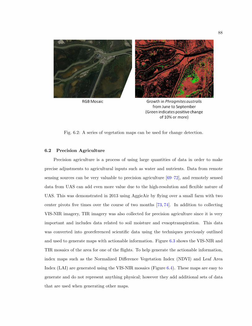
88
Fig. 6.2: A series of vegetation maps can be used for change detection.
6.2 Precision Agriculture
Precision agriculture is a process of using large quantities of data in order to make
precise adjustments to agricultural inputs such as water and nutrients. Data from remote
sensing sources can be very valuable to precision agriculture [69–72], and remotely sensed
data from UAS can add even more value due to the high-resolution and flexible nature of
UAS. This was demonstrated in 2013 using AggieAir by flying over a small farm with two
center pivots five times over the course of two months [73, 74]. In addition to collecting
VIS-NIR imagery, TIR imagery was also collected for precision agriculture since it is very
important and includes data related to soil moisture and evaoptranspiration. This data
was converted into georeferenced scientific data using the techniques previously outlined
and used to generate maps with actionable information. Figure 6.3 shows the VIS-NIR and
TIR mosaics of the area for one of the flights. To help generate the actionable information,
index maps such as the Normalized Difference Vegetation Index (NDVI) and Leaf Area
Index (LAI) are generated using the VIS-NIR mosaics (Figure 6.4). These maps are easy to
generate and do not represent anything physical; however they add additional sets of data
that are used when generating other maps.
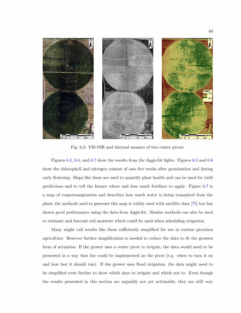
89
Fig. 6.3: VIS-NIR and thermal mosaics of two center pivots.
Figures 6.5, 6.6, and 6.7 show the results from the AggieAir fights. Figures 6.5 and 6.6
show the chlorophyll and nitrogen content of oats five weeks after germination and during
early flowering. Maps like these are used to quantify plant health and can be used for yield
predictions and to tell the farmer where and how much fertilizer to apply. Figure 6.7 is
a map of evapotranspiration and describes how much water is being transpired from the
plant; the methods used to generate this map is widely used with satellite data [75] but has
shown good performance using the data from AggieAir. Similar methods can also be used
to estimate and forecast soil moisture which could be used when scheduling irrigation.
Many might call results like these sufficiently simplified for use in routine precision
agriculture. However further simplification is needed to reduce the data to fit the growers
form of actuation. If the grower uses a center pivot to irrigate, the data would need to be
presented in a way that the could be implemented on the pivot (e.g. when to turn it on
and how fast it should run). If the grower uses flood irrigation, the data might need to
be simplified even further to show which days to irrigate and which not to. Even though
the results presented in this section are arguably not yet actionable, they are still very
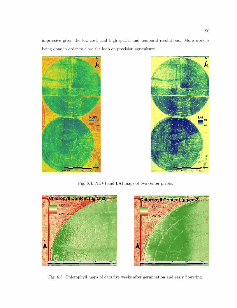
90
impressive given the low-cost, and high-spatial and temporal resolutions. More work is
being done in order to close the loop on precision agriculture.
Fig. 6.4: NDVI and LAI maps of two center pivots.
Fig. 6.5: Chlorophyll maps of oats five weeks after germination and early flowering.
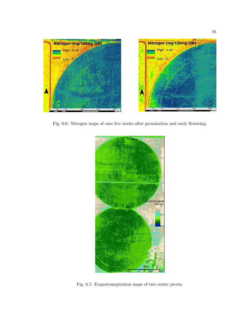
91
Fig. 6.6: Nitrogen maps of oats five weeks after germination and early flowering.
Fig. 6.7: Evapotranspiration maps of two center pivots.
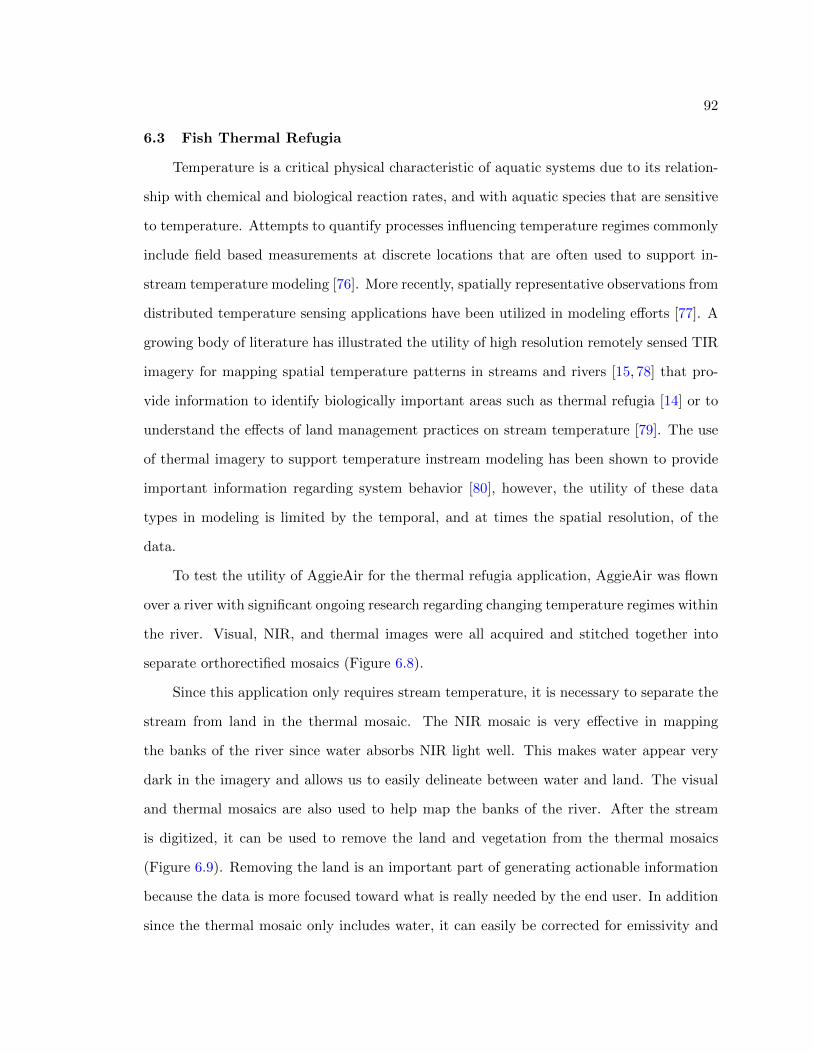
92
6.3 Fish Thermal Refugia
Temperature is a critical physical characteristic of aquatic systems due to its relation-
ship with chemical and biological reaction rates, and with aquatic species that are sensitive
to temperature. Attempts to quantify processes influencing temperature regimes commonly
include field based measurements at discrete locations that are often used to support in-
stream temperature modeling [76]. More recently, spatially representative observations from
distributed temperature sensing applications have been utilized in modeling efforts [77]. A
growing body of literature has illustrated the utility of high resolution remotely sensed TIR
imagery for mapping spatial temperature patterns in streams and rivers [15, 78] that pro-
vide information to identify biologically important areas such as thermal refugia [14] or to
understand the effects of land management practices on stream temperature [79]. The use
of thermal imagery to support temperature instream modeling has been shown to provide
important information regarding system behavior [80], however, the utility of these data
types in modeling is limited by the temporal, and at times the spatial resolution, of the
data.
To test the utility of AggieAir for the thermal refugia application, AggieAir was flown
over a river with significant ongoing research regarding changing temperature regimes within
the river. Visual, NIR, and thermal images were all acquired and stitched together into
separate orthorectified mosaics (Figure 6.8).
Since this application only requires stream temperature, it is necessary to separate the
stream from land in the thermal mosaic. The NIR mosaic is very effective in mapping
the banks of the river since water absorbs NIR light well. This makes water appear very
dark in the imagery and allows us to easily delineate between water and land. The visual
and thermal mosaics are also used to help map the banks of the river. After the stream
is digitized, it can be used to remove the land and vegetation from the thermal mosaics
(Figure 6.9). Removing the land is an important part of generating actionable information
because the data is more focused toward what is really needed by the end user. In addition
since the thermal mosaic only includes water, it can easily be corrected for emissivity and
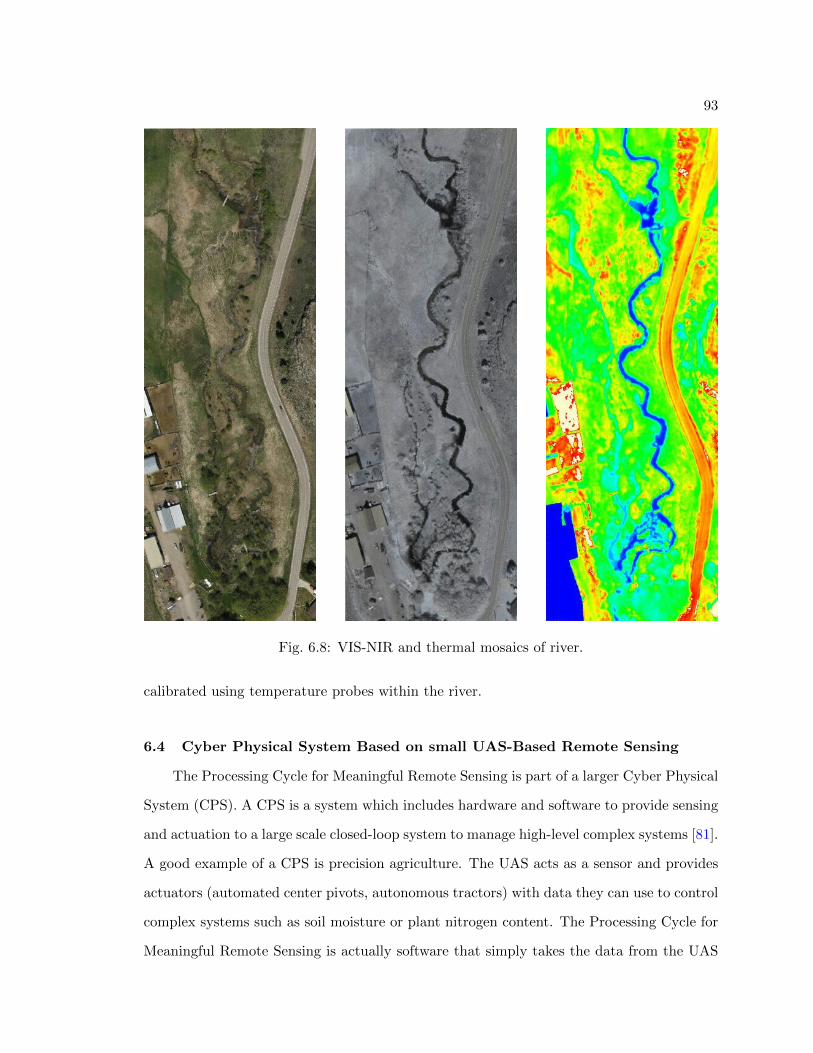
93
Fig. 6.8: VIS-NIR and thermal mosaics of river.
calibrated using temperature probes within the river.
6.4 Cyber Physical System Based on small UAS-Based Remote Sensing
The Processing Cycle for Meaningful Remote Sensing is part of a larger Cyber Physical
System (CPS). A CPS is a system which includes hardware and software to provide sensing
and actuation to a large scale closed-loop system to manage high-level complex systems [81].
A good example of a CPS is precision agriculture. The UAS acts as a sensor and provides
actuators (automated center pivots, autonomous tractors) with data they can use to control
complex systems such as soil moisture or plant nitrogen content. The Processing Cycle for
Meaningful Remote Sensing is actually software that simply takes the data from the UAS
94
Fig. 6.9: Thermal mosaic of river displayed over visual mosaic.
and converts it in a form which can be understood by the actuators. Another example of
a CPS is using multiple UAs for diffusion control in diffusion processes such as chemical
and radiation leaks [82]. In this case, a group of sensor UAs could be used to measure the
diffusion process while another group of actuation or sprayer UAs could be used to release
chemicals to control the diffusion process.
6.5 Chapter Summary
This chapter showed some examples of how the Processing Cycle for Meaningful Remote
Sensing can be completed by proving actionable information to the users and how this
process is related to a CPS. For vegetation mapping, AggieAir VIS-NIR imagery was used
to map an invasive plant species to help wetland managers manage the species. In addition,
a series of images were captured over the growing season and change detection was used to
map how the invasive plant species was growing. In precision agriculture, AggieAir VIS-
NIR and TIR imagery was captured over two center pivots and used to generate maps of

95
plant chlorophyll, plant nitrogen, and evapotranspiration. While this data could be used
as actionable information to know where to apply nitrogen or where to water, more work
is still needed to simplify the data in a form that can be used by growers. Finally, an
application in mapping fish habitat was included. This showed how VIS-NIR imagery can
be used to map a river channel to simplify TIR imagery by removing the land so just the
surface temperature of the river is left: thereby giving biologists actionable information
about thermal refugia for fish.
96
Chapter 7
Conclusions and the Future of Small UAS Remote Sensing
This dissertation has shown how raw data from consumer-grade sensors can be ac-
quired using a small unmanned aerial system (UAS), AggieAir, and converted to georefer-
enced scientific-grade data. Chapter 3 reviewed literature for the different processes used
to convert digital numbers (DN) from visual and near-infrared (VIS-NIR) cameras into ra-
diometric values of reflectance, where the process used by AggieAir was emphasized. The
methods used to geometrically calibrate the camera and to create an orthorectified mosaic
were also covered in Chapter 3, but also apply to processing images from a thermal-infrared
(TIR) camera in Chapter 4. However, since the thermal camera is radiometric and outputs
calibrated temperature, additional steps are presented to prepare the images for orthorec-
tification. In addition, since a TIR camera is not sensitive to changes in color, a different
calibration target is presented for geometrically calibrating the TIR camera. Special focus
in Chapter 4 was made in Section 4.3 where the issues with external disturbances on the TIR
camera is addressed. In order to calibrate for and model these external disturbances, two
new ground sampling techniques are introduced, tested, and evaluated. Finally, Chapter 5
presents novel methods for tracking fish using biotelemetry and shows how the conversion
from raw data into georeferenced scientific data can happen in real-time to give feedback
to the UAS for navigation.
More work can be done in order to improve the data quality even further. One piece
missing from the VIS-NIR processing chain includes a spectral calibration of the consumer-
grade cameras. Knowing the spectral sensitivity of these cameras will help improve the
radiometric calibration. While the ground sampling techniques worked well to calibrate
the TIR imagery from the aircraft, more data should be gathered in order to model the
external disturbances and remove the need for ground sampling. Since the biotelemetry fish
97
tracking application is still in its infancy, lots of work is needed to be done before this is
made for routine use. Additional simulations are needed to perform sensitivity analysis and
find out ways to improve the accuracy of the tag location estimation. At that point, the
navigation routines need to be implemented in the autopilot and real-world experiments
should be conducted under different scenarios to prove the system.
There is a lot of potential for using small UAS as a remote sensing platform. They
have proved very useful in delivering quality data for many applications including vegetation
mapping, fish habitat mapping, and precision agriculture. Perhaps if The Processing Cycle
for Remote Sensing becomes more automated and actionable information can be delivered
at the click of a button, small UAS will enable remote sensing to become “personal.” And
like personal computers or phones, many will be able to use small UAS to improve their
everyday lives.
98
References
[1] R. Benedetti and P. Rossini, “On the use of NDVI Profiles as a Tool for AgriculturalStatistics: The Case Study of Wheat Yield Estimate and Forecast in Emilia Romagna,”Remote Sensing of Environment, vol. 45, no. 3, pp. 311–326, Sept. 1993.
[2] B. Rudorff and G. Batista, “Yield Estimation of Sugarcane Based onAgrometeorological-Spectral Models,” Remote Sensing of Environment, vol. 33, no. 3,pp. 183–192, Sept. 1990.
[3] M. L. Stone, J. B. Solie, W. R. Raun, R. W. Whitney, S. L. Taylor, and J. D. Ringer,“Use of Spectral Radiance for Correcting in-season Fertilizer Nitrogen Deficiencies inWinter Wheat,” Transactions of the American Society of Agricultural and BiologicalEngineers, vol. 39, no. 5, pp. 1623–1631, 1996.
[4] R. D. Jackson, S. B. Idso, R. J. Reginato, and P. J. Pinter, “Canopy Temperature as aCrop Water Stress Indicator,” Water Resources Research, vol. 17, no. 4, p. 1133, 1981.
[5] A. Mathur and G. M. Foody, “Crop Classification by Support Vector Machine withIntelligently Selected Training Data for an Operational Application,” InternationalJournal of Remote Sensing, vol. 29, no. 8, pp. 2227–2240, Apr. 2008.
[6] J. Franke and G. Menz, “Multi-temporal Wheat Disease Detection by Multi-spectralRemote Sensing,” Precision Agriculture, vol. 8, no. 3, pp. 161–172, June 2007.
[7] S. Thomson, L. Smith, J. Ray, and P. Zimba, “Remote Sensing and Implications forVariable-rate Application Using Agricultural Aircraft,” in Proceedings of Society ofPhotographic Instrumentation Engineers, vol. 5153, 2004, p. 13.
[8] N. Coops and P. Catling, “Predicting the Complexity of Habitat in Forests from Air-borne Videography for Wildlife Management,” International Journal of Remote Sens-ing, vol. 18, no. 12, 1997.
[9] R. D. Wulf and R. Goossens, “Remote Sensing for Wildlife Management: Giant PandaHabitat Mapping from LANDSAT MSS Images,” Geocarto International, vol. 3, no. 1,1988.
[10] J. H. Everitt, C. Yang, R. S. Fletcher, C. J. Deloach, and M. R. Davis, “Using RemoteSensing to Assess Biological Control of Saltcedar,” Southwestern Entomologist, vol. 32,no. 2, pp. 93–103, June 2007.
[11] P. H. Evangelista, T. J. Stohlgren, J. T. Morisette, and S. Kumar, “Mapping Inva-sive Tamarisk (Tamarix): A Comparison of Single-scene and Time-series Analyses ofRemotely Sensed Data,” Remote Sensing, vol. 1, no. 3, pp. 519–533, Aug. 2009.
[12] S. Sriharan, J. Everitt, C. Yang, and R. Fletcher, “Mapping Riparian and WetlandWeeds with High Resolution Satellite Imagery,” in Proceedings IEEE InternationalGeoscience and Remote Sensing Symposium (IGARSS), 2008.
99
[13] C. Walter and D. D. Tullos, “Downstream Channel Changes after a Small Dam Re-moval: Using Aerial Photos and Measurement Error for Context; Calapooia River,Oregon,” River Research and Applications, vol. 26, no. 10, pp. 1220–1245, Dec. 2010.
[14] C. E. Torgersen, D. M. Price, H. W. Li, and B. A. McIntosh, “Multiscale ThermalRefugia and Stream Habitat Associations of Chinook Salmon in Northeastern Oregon,”Ecological Applications, vol. 9, no. 1, pp. 301–319, Feb. 1999.
[15] J. Kay, R. Handcock, A. Gillespie, C. Konrad, S. Burges, N. Naveh, and D. Booth,“Stream-temperature Estimation from Thermal Infrared Images,” in IEEE 2001 Inter-national Geoscience and Remote Sensing Symposium, vol. 1. IEEE, 2001, pp. 112–114.
[16] P. Coppin and M. Bauer, “Digital Change Detection in Forest Ecosystems with RemoteSensing Imagery,” Remote Sensing Reviews, vol. 13, no. 3-4, 1996.
[17] M. Lefsky, D. Harding, and W. Cohen, “Surface Lidar Remote Sensing of Basal Areaand Biomass in Deciduous Forests of Eastern Maryland, USA,” Remote Sensing ofEnvironment, vol. 67, no. 1, pp. 83–98, 1999.
[18] C. Wessman, J. Aber, D. Peterson, and J. Melillo, “Remote Sensing of Canopy Chem-istry and Nitrogen Cycling in Temperate Forest Ecosystems,” Nature, vol. 335, no.6186, 1988.
[19] S. G. Bajwa and E. D. Vories, “Spectral Response of Cotton Canopy to Water Stress,”in Proceedings of the American Society of Agricultural and Biological Engineers AnnualMeeting, July 2006.
[20] R. H. Gray and J. M. Haynes, “Spawning Migration of Adult Chinook Salmon ( On-corhynchus tshawytscha ) Carrying External and Internal Radio Transmitters,” Journalof the Fisheries Research Board of Canada, vol. 36, no. 9, pp. 1060–1064, Sept. 1979.
[21] A. Rango, A. Laliberte, J. E. Herrick, C. Winters, K. Havstad, C. Steele, and D. Brown-ing, “Unmanned Aerial Vehicle-based Remote Sensing for Rangeland Assessment, Mon-itoring, and Management,” Journal of Applied Remote Sensing, vol. 3, no. 1, p. 033542,Jan. 2009.
[22] J. Berni, P. J. Zarco-Tejada, L. Suarez, and E. Fereres, “Thermal and NarrowbandMultispectral Remote Sensing for Vegetation Monitoring from an Unmanned AerialVehicle,” IEEE Transactions on Geoscience and Remote Sensing, vol. 47, no. 3, pp.722–738, Mar. 2009.
[23] L. Wallace, A. Lucieer, C. Watson, and D. Turner, “Development of a UAV-LiDARSystem with Application to Forest Inventory,” Remote Sensing, vol. 4, no. 6, pp. 1519–1543, May 2012.
[24] A. M. Jensen, T. Hardy, M. McKee, and Y. Q. Chen, “Using a Multispectral Au-tonomous Unmanned Aerial Remote Sensing Platform (AggieAir) for Riparian andWetland Applications,” in Proceedings IEEE International Geoscience and RemoteSensing Symposium (IGARSS), Aug. 2011.

100
[25] A. Laliberte, C. Winters, and A. Rango, “UAS Remote Sensing Missions for RangelandApplications,” Geocarto International, vol. 26, no. 2, pp. 141–156, Dec. 2011.
[26] A. M. Jensen, M. McKee, and Y. Chen, “Calibrating Thermal Imagery from an Un-manned Aerial System - AggieAir,” in Proceedings IEEE International Geoscience andRemote Sensing Symposium (IGARSS), 2013.
[27] A. M. Jensen, D. K. Geller, and Y. Chen, “Monte Carlo Simulation Analysis of TaggedFish Radio Tracking Performance by Swarming Unmanned Aerial Vehicles in FractionalOrder Potential Fields,” Journal of Intelligent & Robotic Systems, vol. 74, no. 1-2, pp.287–307, Oct. 2014.
[28] “Academy of Model Aeronautics Membership Manual,” Academy of Model Aeronau-tics, 2014. [Online]. Available: https://www.modelaircraft.org/files/memanual.pdf
[29] “Unmanned Aircraft Systems (UAS) Operational Approval (8900.227),” FederalAviation Administration, 2013. [Online]. Available: https://www.faa.gov/regulationspolicies/orders notices/index.cfm/go/document.information/documentID/1021650
[30] A. S. Laliberte, M. A. Goforth, C. M. Steele, and A. Rango, “Multispectral RemoteSensing from Unmanned Aircraft: Image Processing Workflows and Applications forRangeland Environments,” Remote Sensing, vol. 3, no. 11, pp. 2529–2551, Nov. 2011.
[31] J. Kelcey and A. Lucieer, “Sensor Correction of a 6-Band Multispectral Imaging Sensorfor UAV Remote Sensing,” Remote Sensing, vol. 4, no. 5, pp. 1462–1493, May 2012.
[32] J. Berni, P. J. Zarco-Tejada, L. Surez, V. Gonzalez-Dugo, and E. Fereres, “RemoteSensing of Vegetation from UAV Platforms using Lightweight Multispectral and Ther-mal Imaging Sensors,” in The International Archives of the Photogrammetry, RemoteSensing and Spatial Information Sciences, 2008.
[33] A. Simpson, T. Stombaugh, L. Wells, and J. Jacob, “Imaging Techniques and Applica-tions for UAV’s in Agriculture,” in Proceedings of the American Society of Agriculturaland Biological Engineers Annual Meeting, July 2003.
[34] C. Coopmans, B. Stark, and C. M. Coffin, “A Payload Verification and ManagementFramework for Small UAV-based Personal Remote Sensing Systems,” in Proceedingsof the 5th International Symposium on Resilient Control Systems. IEEE, Aug. 2012,pp. 184–189.
[35] G. L. Ritchie, D. G. Sullivan, C. D. Perry, J. E. Hook, and C. W. Bednarz, “Preparationof a Low-Cost Digital Camera System for Remote Sensing,” Applied Engineering inAgriculture, vol. 24, no. 6, pp. 885–894, 2008.
[36] T. Miura and A. Huete, “Performance of Three Reflectance Calibration Methods forAirborne Hyperspectral Spectrometer Data,” Sensors, vol. 9, no. 2, pp. 794–813, 2009.
[37] E. R. Hunt, M. Cavigelli, C. S. T. Daughtry, J. E. Mcmurtrey, and C. L. Walthall,“Evaluation of Digital Photography from Model Aircraft for Remote Sensing of CropBiomass and Nitrogen Status,” Precision Agriculture, vol. 6, no. 4, pp. 359–378, Aug.2005.
101
[38] S. Clemens, “Procedures for Correcting Digital Camera Imagery Acquired by the Ag-gieAir Remote Sensing Platform,” Master’s thesis, Utah State University, 2012.
[39] J. Kannala, J. Heikkila, and S. S. Brandt, “Geometric Camera Calibration,” in WileyEncyclopedia of Computer Science and Engineering. Hoboken, NJ: John Wiley &Sons, Inc., Mar. 2007, pp. 1–11.
[40] J. Bouguet, “Camera Calibration Toolbox for Matlab,” 2012. [Online]. Available:http://www.vision.caltech.edu/bouguetj/calib doc/
[41] J. Heikkila and O. Silven, “A Four-Step Camera Calibration Procedure with ImplicitImage Correction,” in Proceedings of IEEE Computer Society Conference on ComputerVision and Pattern Recognition. IEEE Computer Society, 1997, pp. 1106–1112.
[42] “MosaicMill EnsoMOSAIC,” 2012. [Online]. Available: http://www.ensomosaic.com
[43] A. Jensen, “gRAID: A Geospatial Real-Time Aerial Image Display for a Low-Cost Au-tonomous Multispectral Remote Sensing Platform (AggieAir),” Master’s thesis, UtahState University, 2009.
[44] W. Ji and P. Rhodes, “Spectral Color Characterization of Digital Cameras: A Review,”in Proceedings of Society of Photographic Instrumentation Engineers Vol, 2012.
[45] C. E. Torgersen, R. N. Faux, B. A. McIntosh, N. J. Poage, and D. J. Norton, “AirborneThermal Remote Sensing for Water Temperature Assessment in Rivers and Streams,”Remote Sensing of Environment, vol. 76, no. 3, pp. 386–398, 2001.
[46] M. A. Gallo, D. S. Willits, R. A. Lubke, and E. C. Thiede, “Low-cost Uncooled IRSensor for Battlefield Surveillance,” in Proceedings Society of Photographic Instrumen-tation Engineers 2020, Infrared Technology XIX, vol. 2020, 1993, pp. 351–362.
[47] T. W. Parker, C. A. Marshall, M. Kohin, and R. Murphy, “Uncooled Infrared Sensorsfor Surveillance and Law Enforcement Applications,” in Proceedings Society of Pho-tographic Instrumentation Engineers 2935, Surveillance and Assessment Technologiesfor Law Enforcement, vol. 2935, 1997, pp. 182–187.
[48] “Infrared Cameras Incorporated,” 2012. [Online]. Available: http://www.infraredcamerasinc.com
[49] A. Jensen, B. Neilson, M. McKee, and Y. Chen, “Thermal Remote Sensing With anAutonomous Unmanned Aerial Remote Sensing Platform for Surface Stream Tempera-tures,” in Proceedings IEEE International Geoscience and Remote Sensing Symposium(IGARSS), 2012, pp. 5049–5052.
[50] A. J. Prata, “Land Surface Temperatures Derived from the Advanced Very High Res-olution Radiometer and the Along-Track Scanning Radiometer: 2. Experimental Re-sults and Validation of AVHRR Algorithms,” Journal of Geophysical Research, vol. 99,no. D6, 1994.
102
[51] G. Wukelic, D. Gibbons, L. Martucci, and H. Foote, “Radiometric Calibration of Land-sat Thematic Mapper Thermal Band,” Remote Sensing of Environment, vol. 28, pp.339–347, 1989.
[52] R. R. Irish, “Landsat 7 Science Data Users Handbook,” National Aeronautics andSpace Administration, 2000.
[53] “Landsat Data Continuity Mission,” 2013. [Online]. Available: http://ldcm.gsfc.nasa.gov/index.html
[54] R. W. Hillyard and E. R. Keeley, “Distribution and Spawning Migrations of FluvialBonneville Cutthroat Trout in the Bear River, Idaho,” Idaho State University, Feb.,2009.
[55] M. Leonardo, A. Jensen, C. Coopmans, M. McKee, and Y. Chen, “A Miniature WildlifeTracking UAV Payload System using Acoustic Biotelemetry,” in Proceedings of theASME International Design Engineering Technical Conferences & Computers and In-formation in Engineering Conference, Portland, Aug. 2013.
[56] E. W. Frew, C. Dixon, B. Argrow, and T. Brown, “Radio Source Localization by aCooperating UAV Team,” in Infotech@ Aerospace, 2005.
[57] F. Korner, R. Speck, A. H. Goktogan, and S. Sukkarieh, “Autonomous AirborneWildlife Tracking Using Radio Signal Strength,” in Proceedings of the IEEE/RSJ In-ternational Conference on Intelligent Robots and Systems. IEEE, Oct. 2010, pp.107–112.
[58] S. Ge and Y. Cui, “Dynamic Motion Planning for Mobile Robots Using Potential FieldMethod,” Autonomous Robots, vol. 13, no. 3, pp. 207–222, Nov. 2002.
[59] T. Paul, T. R. Krogstad, and J. T. Gravdahl, “Modelling of UAV Formation FlightUsing 3D Potential Field,” Simulation Modelling Practice and Theory, vol. 16, no. 9,pp. 1453–1462, Oct. 2008.
[60] O. Khatib, “Real-time Obstacle Avoidance for Manipulators and Mobile Robots,” inProceedings of the IEEE International Conference on Robotics and Automation, vol. 2.Institute of Electrical and Electronics Engineers, 1985, pp. 500–505.
[61] Y. Chen, Z. Wang, and K. Moore, “Optimal Spraying Control of a Diffusion ProcessUsing Mobile Actuator Networks with Fractional Potential Field Based Dynamic Ob-stacle Avoidance,” in Proceedings of the IEEE International Conference on Networking,Sensing and Control. IEEE, 2006, pp. 107–112.
[62] K. Miller, “The Weyl Fractional Calculus,” in Fractional Calculus and Its Applications,ser. Lecture Notes in Mathematics, B. Ross, Ed. Berlin, Heidelberg: Springer, 1975,vol. 457, pp. 80–89.
[63] S. Galatowitsch, N. Anderson, and P. Ascher, “Invasiveness in Wetland Plants in Tem-perate North America,” Wetlands, vol. 19, no. 4, pp. 733–755, 1999.
103
[64] M. Marks, B. Lapin, and J. Randall, “Phragmites Australis (P. communis): Threats,Management and Monitoring.” Natural Areas Journal, 1994.
[65] L. Meyerson, R. Chambers, and K. Vogt, “The Effects of Phragmites Removal onNutrient Pools in a Freshwater Tidal Marsh Ecosystem,” Biological Invasions, vol. 1,no. 2-3, pp. 129–136, 1999.
[66] L. Meyerson, K. Saltonstall, and L. Windham, “A Comparison of Phragmites Australisin Freshwater and Brackish Marsh Environments in North America,” Wetlands Ecologyand Management, vol. 8, no. 2-3, pp. 89–103, 2000.
[67] L. Windham and J. Ehrenfeld, “Net Impact of a Plant Invasion on Nitrogen-cyclingProcesses within a Brackish Tidal Marsh,” Ecological Applications, vol. 13, pp. 883–896, 2003.
[68] B. Zaman, M. McKee, and A. Jensen, “Use of High-Resolution Multispectral ImageryAcquired with an Autonomous Unmanned Aerial Vehicle to Quantify the Spread of anInvasive Wetland Species,” in Proceedings IEEE International Geoscience and RemoteSensing Symposium (IGARSS), Aug. 2011.
[69] M. Moran, Y. Inoue, and E. Barnes, “Opportunities and Limitations for Image-basedRemote Sensing in Precision Crop Management,” Remote Sensing of Environment,vol. 61, no. 3, pp. 319–346, 1997.
[70] B. Brisco, R. Brown, and T. Hirose, “Precision Agriculture and the Role of RemoteSensing: A Review,” Can J Remote Sensing, vol. 24, no. 3, pp. 315–327, 1998.
[71] R. Pearson, J. Grace, and G. May, “Real-time Airborne Agricultural Monitoring,”Remote Sensing of Environment, vol. 49, no. 3, pp. 304–310, 1994.
[72] D. Lamb and R. Brown, “Precision Agriculture: Remote-Sensing and Mapping ofWeeds in Crops,” Journal of Agricultural Engineering Research, vol. 78, no. 2, pp.117–125, 2001.
[73] M. Al-Arab, A. M. Ticlavilca, A. F. Torres-Rua, I. Maslova, and M. McKee, “Use ofHigh-Resolution Multispectral Imagery to Estimate Chrorophyll and Plant Nitrogen inOats (Avena sativa),” Abstract B43C-0493 presented at 2013 Fall Meeting, AmericanGeophysical Union (AGU), San Francisco, CA, 2013.
[74] M. Al-Arab, A. Torres-Rua, A. Ticlavilca, A. Jensen, and M. McKee, “Use of High-Resolution Multispectral Imagery from an Unmanned Aerial Vehicle in Precision Agri-culture,” in Proceedings IEEE International Geoscience and Remote Sensing Sympo-sium (IGARSS), 2013.
[75] A. F. Torres-Rua, W. R. Walker, and M. McKee, “The Lower Sevier River BasinCrop Monitor and Forecast Decision Support System: Exploiting Landsat Imagery toProvide Continuous Information to Farmers and Water Managers,” Abstract IN14A-07presented at 2013 Fall Meeting, American Geophysical Union (AGU), San Francisco,CA, 2013.
104
[76] G. W. Brown, “Predicting Temperatures of Small Streams,” Water Resources Research,vol. 5, no. 1, p. 68, 1969.
[77] M. C. Westhoff, H. H. G. Savenije, W. M. J. . Luxemburg, G. S. Stelling, N. C. Van DeGiesen, J. S. Selker, L. Pfister, and S. Uhlenbrook, “A Distributed Stream TemperatureModel using High Resolution Temperature Observations,” Hydrology and Earth SystemSciences, vol. 11, no. 4, pp. 1469–1480, July 2007.
[78] B. H. Atwell, R. B. MacDonald, and L. A. Bartolucci, “Thermal Mapping of Streamsfrom Airborne Radiometric Scanning,” Journal of the American Water Resources As-sociation, vol. 7, no. 2, pp. 228–243, Apr. 1971.
[79] D. J. Norton, M. A. Flood, B. McIntosh, N. J. Poage, P. J. LaPlaca, J. P. Craig, S. R.Karalus, J. R. Sedell, C. Torgersen, Y. D. Chen, S. C. McCutheeon, S. C. Duong,H. Puffenberger, J. Moeller, V. Kelley, E. Porter, and L. Shoemaker, “Modeling, Mon-itoring, and Restoring Water Quality and Habitat in the Pacific Northwestern Water-sheds,” U.S. Environmental Protection Agency, Washington, DC, 1996.
[80] N. C. Cristea and S. J. Burges, “Use of Thermal Infrared Imagery to ComplementMonitoring and Modeling of Spatial Stream Temperatures,” Journal of HydrologicEngineering, vol. 14, no. 10, p. 1080, Feb. 2009.
[81] C. Coopmans, B. Stark, A. Jensen, Y. Chen, and M. McKee, “Cyber-Physical Sys-tems Enabled By Small Unmanned Aerial Vehicles,” in Handbook of Unmanned AerialVehicles, K. P. Valavanis and G. J. Vachtsevanos, Eds. New York, NY: Springer, 2014.
[82] H. Chao and Y. Chen, Remote Sensing and Actuation Using Unmanned Vehicles.Hoboken, NJ: Wiley-IEEE Press, 2012.

105
Appendix

106
Certificate of Authorization
This appendix contains an FAA COA given to Utah State University using AggieAir
to fly on the North slope of Alaska near a remote field station called Toolik. The flight op-
erations for this COA and part of the pre-flight checklist for airworthiness are also included.
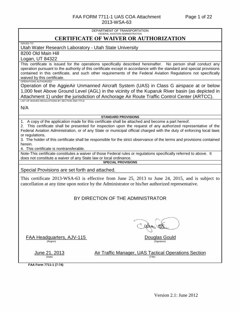
FAA FORM 7711-1 UAS COA Attachment 2013-WSA-63
Version 2.1: June 2012
Page 1 of 22
DEPARTMENT OF TRANSPORTATION FEDERAL AVIATION ADMINISTRATION
CERTIFICATE OF WAIVER OR AUTHORIZATION
ISSUED TO
Utah Water Research Laboratory - Utah State University 8200 Old Main Hill Logan, UT 84322 This certificate is issued for the operations specifically described hereinafter. No person shall conduct any operation pursuant to the authority of this certificate except in accordance with the standard and special provisions contained in this certificate, and such other requirements of the Federal Aviation Regulations not specifically waived by this certificate. OPERATIONS AUTHORIZED Operation of the AggieAir Unmanned Aircraft System (UAS) in Class G airspace at or below 1,000 feet Above Ground Level (AGL) in the vicinity of the Kuparuk River basin (as depicted in Attachment 1) under the jurisdiction of Anchorage Air Route Traffic Control Center (ARTCC). LIST OF WAIVED REGULATIONS BY SECTION AND TITLE
N/A
STANDARD PROVISIONS 1. A copy of the application made for this certificate shall be attached and become a part hereof. 2. This certificate shall be presented for inspection upon the request of any authorized representative of the Federal Aviation Administration, or of any State or municipal official charged with the duty of enforcing local laws or regulations. 3. The holder of this certificate shall be responsible for the strict observance of the terms and provisions contained herein. 4. This certificate is nontransferable. Note-This certificate constitutes a waiver of those Federal rules or regulations specifically referred to above. It does not constitute a waiver of any State law or local ordinance.
SPECIAL PROVISIONS
Special Provisions are set forth and attached.
This certificate 2013-WSA-63 is effective from June 25, 2013 to June 24, 2015, and is subject to cancellation at any time upon notice by the Administrator or his/her authorized representative.
BY DIRECTION OF THE ADMINISTRATOR
FAA Headquarters, AJV-115 Douglas Gould (Region) (Signature)
June 21, 2013 Air Traffic Manager, UAS Tactical Operations Section (Date) (Title)
FAA Form 7711-1 (7-74)

FAA FORM 7711-1 UAS COA Attachment 2013-WSA-63
Version 2.1: June 2012
Page 2 of 22
COA Number: 2013-WSA-63 Issued To: Utah Water Research Laboratory - Utah State University, referred herein as the “proponent” Address: 8200 Old Main Hill Logan, UT 84322 Activity: Operation of the AggieAir Unmanned Aircraft System (UAS) in Class G airspace at or below 1,000 feet Above Ground Level (AGL) in the vicinity of the Kuparuk River basin (as depicted in Attachment 1) under the jurisdiction of Anchorage Air Route Traffic Control Center (ARTCC). Purpose: To prescribe UAS operating requirements in the National Airspace System (NAS) for the purpose of quantifying the influences of lateral inflows on river water temperatures in the Kuparuk River basin. Dates of Use: This COA is valid from June 25, 2013 to June 24, 2015. Should a renewal become necessary, the proponent shall advise the Federal Aviation Administration (FAA), in writing, no later than 45 business days prior to the requested effective date. Public Aircraft
1. A public aircraft operation is determined by statute, 49 USC §40102(a)(41) and §40125.
2. All public aircraft flights conducted under a COA must comply with the terms of the statute.
3. All flights must be conducted per the declarations submitted on COA on-line.
FAA FORM 7711-1 UAS COA Attachment 2013-WSA-63
Version 2.1: June 2012
Page 3 of 22
STANDARD PROVISIONS A. General.
The review of this activity is based upon current understanding of UAS operations and their impact in the NAS. This COA will not be considered a precedent for future operations. (As changes in or understanding of the UAS industry occur, limitations and conditions for operations will be adjusted.)
All personnel connected with the UAS operation must read and comply with the contents of this authorization and its provisions.
A copy of the COA including the special limitations must be immediately available to all operational personnel at each operating location whenever UAS operations are being conducted.
This authorization may be canceled at any time by the Administrator, the person authorized to grant the authorization, or the representative designated to monitor a specific operation. As a general rule, this authorization may be canceled when it is no longer required, there is an abuse of its provisions, or when unforeseen safety factors develop. Failure to comply with the authorization is cause for cancellation. The proponent will receive written notice of cancellation.
During the time this COA is approved and active, a site safety evaluation/visit may be accomplished to ensure COA compliance, assess any adverse impact on ATC or airspace, and ensure this COA is not burdensome or ineffective. Deviations, accidents/incidents/mishaps, complaints, etc will prompt a COA review or site visit to address the issue. Refusal to allow a site safety evaluation/visit may result in cancellation of the COA. Note: This section does not pertain to agencies that have other existing agreements in place with the FAA.
B. Airworthiness Certification.
The unmanned aircraft must be shown to be airworthy to conduct flight operations in the NAS. Utah Water Research Laboratory - Utah State University has made its own determination that the AggieAir unmanned aircraft is airworthy. The AggieAir must be operated in strict compliance with all provisions and conditions contained in the Airworthiness Safety Release, including all documents and provisions referenced in the COA application.
1. A configuration control program must be in place for hardware and/or software changes
made to the UAS to ensure continued airworthiness. If a new or revised Airworthiness Release is generated as a result of changes in the hardware or software affecting the operating characteristics of the UAS, notify the UAS Integration Office of the changes as soon as practical.
FAA FORM 7711-1 UAS COA Attachment 2013-WSA-63
Version 2.1: June 2012
Page 4 of 22
a. Software and hardware changes should be documented as part of the normal maintenance procedures. Software changes to the aircraft and control station as well as hardware system changes are classified as major changes unless the agency has a formal process, accepted by the FAA. These changes should be provided to the UAS Integration office in summary form at the time of incorporation.
b. Major modifications or changes, performed under the COA, or other
authorizations that could potentially affect the safe operation of the system must be documented and provided to the FAA in the form of a new AWR, unless the agency has a formal process, accepted by the FAA.
c. All previously flight proven systems to include payloads, may be installed or
removed as required, and that activity recorded in the unmanned aircraft and ground control stations logbooks by persons authorized to conduct UAS maintenance Describe any payload equipment configurations in the UAS logbook that will result in a weight and balance change, electrical loads, and or flight dynamics, unless the agency has a formal process, accepted by the FAA.
d. For unmanned aircraft system discrepancies, a record entry should be made by an
appropriately rated person to document the finding in the logbook. No flights may be conducted following major changes, modifications or new installations unless the party responsible for certifying airworthiness has determined the system is safe to operate in the NAS and a new AWR is generated, unless the agency has a formal process, accepted by the FAA. The successful completion of these tests must be recorded in the appropriate logbook, unless the agency has a formal process, accepted by the FAA.
2. The AggieAir must be operated in strict compliance with all provisions and conditions contained within the spectrum analysis assigned and authorized for use within the defined operations area.
3. All items contained in the application for equipment frequency allocation must be
adhered to, including the assigned frequencies and antenna equipment characteristics. A ground operational check to verify the control station can communicate with the aircraft (frequency integration check) must be conducted prior to the launch of the unmanned aircraft to ensure any electromagnetic interference does not adversely affect control of the aircraft.
4. The use of a Traffic Collision Avoidance System (TCAS) in any mode while operating an
unmanned aircraft is prohibited. C. Operations.
1. Unless otherwise authorized as a special provision, a maximum of one unmanned aircraft will be controlled:

FAA FORM 7711-1 UAS COA Attachment 2013-WSA-63
Version 2.1: June 2012
Page 5 of 22
a. In any defined operating area,
b. From a single control station, and
c. By one pilot at a time.
2. A Pilot-in-Command (PIC) is the person who has final authority and responsibility for the operation and safety of flight, has been designated as PIC before or during the flight, and holds the appropriate category, class, and type rating, if appropriate, for the conduct of the flight. The responsibility and authority of the PIC as described by 14 CFR 91.3, Responsibility and Authority of the Pilot-in-Command, apply to the unmanned aircraft PIC. The PIC position may rotate duties as necessary with equally qualified pilots. The individual designated as PIC may change during flight. Note: The PIC can only be the PIC for one aircraft at a time. For Optionally Piloted Aircraft (OPA), PIC must meet UAS guidance requirements for training, pilot licensing, and medical requirements when operating OPA as a UAS.
3. The PIC must conduct a pre-takeoff briefing as applicable prior to each launch. The
briefing should include but is not limited to the:
a. Contents of the COA,
b. Altitudes to be flown,
c. Mission overview including handoff procedures,
d. Frequencies to be used,
e. Flight time, including reserve fuel requirements,
f. Contingency procedures to include lost link, divert, and flight termination, and
g. Hazards unique to the flight being flown.
Note: Flight Crew Member (UAS). In addition to the flight crew members identified in 14 CFR Part 1, Definitions and Abbreviations, an Unmanned Aircraft System flight crew members include pilots, sensor/payload operators, and visual observers and may include other persons as appropriate or required to ensure safe operation of the aircraft.
4. All operations will be conducted in compliance with Title 14 CFR Part 91. Special attention should be given to:
a. § 91.3 Responsibility and authority of the pilot in command
b. § 91.13 Careless or reckless operation
c. § 91.17 Alcohol or drugs
d. § 91.103 Preflight Actions
e. § 91.111 Operating near other aircraft.
f. § 91.113 Right-of-way rules: Except water operations
g. § 91.115 Right-of-way rules: Water operations
FAA FORM 7711-1 UAS COA Attachment 2013-WSA-63
Version 2.1: June 2012
Page 6 of 22
h. § 91.119 Minimum safe altitudes: General
i. § 91.123 Compliance with ATC clearances and instructions.
j. § 91.133 Restricted and prohibited areas
k. § 91.137 Temporary flight restrictions in the vicinity of disaster/hazard areas
l. § 91.145 Management of aircraft operations in the vicinity of aerial demonstrations and major sporting events
m. § 91.151 Fuel requirements for flight in VFR conditions
n. § 91.155 Basic VFR weather minimums
o. § 91.159 VFR cruising altitude or flight level
p. § 91.209 Aircraft Lights
q. § 91.213 Inoperative instruments and equipment
r. § 91.215 ATC transponder and altitude reporting equipment and use
s. Appendix D to Part 91—Airports/Locations: Special Operating Restrictions
5. Unless otherwise authorized as a special provision, all operations must be conducted in
visual meteorological conditions (VMC) during daylight hours in compliance with Title 14 of the Code of Federal Regulations (CFR) Part 91 §91.155 and the following:
6. Special Visual Flight Rules (VFR) operations are not authorized.
a. VFR cloud clearances specified in 14 CFR Part 91 §91.155, must be maintained,
except in Class G airspace where Class E airspace visibility requirements must be applied, but not less than 3 statute miles (SM) flight visibility and 1000’ ceiling.
b. Flights conducted under Instrument Flight Rules (IFR) in Class A airspace shall
remain clear of clouds. NOTE: Deviations from IFR clearance necessary to comply with this provision must have prior ATC approval.
c. Chase aircraft must maintain 5 NM flight visibility.
7. Night operations are prohibited unless otherwise authorized as a special provision.
8. Operations (including lost link procedures) must not be conducted over populated areas,
heavily trafficked roads, or an open-air assembly of people. D. Air Traffic Control (ATC) Communications.
1. The pilot and/or PIC will maintain direct, two-way communication with ATC and have the ability to maneuver the unmanned aircraft in response to ATC instructions, unless addressed in the Special Provision Section.
FAA FORM 7711-1 UAS COA Attachment 2013-WSA-63
Version 2.1: June 2012
Page 7 of 22
a. When required, ATC will assign a radio frequency for air traffic control during flight. The use of land-line and/or cellular telephones is prohibited as the primary means for in-flight communication with ATC.
2. The PIC must not accept an ATC clearance requiring the use of visual separation,
sequencing, or visual approach.
3. When necessary, transit of airways and routes must be conducted as expeditiously as possible. The unmanned aircraft must not loiter on Victor airways, jet routes, Q and T routes, IR routes, or VR routes.
4. For flights operating on an IFR clearance at or above 18,000 feet mean sea level (MSL),
the PIC must ensure positional information in reference to established National Airspace System (NAS) fixes, NAVAIDs, and/or waypoints is provided to ATC. The use of latitude/longitude positions is not authorized, except oceanic flight operations.
5. If equipped, the unmanned aircraft must operate with:
a. An operational mode 3/A transponder with altitude encoding, or mode S transponder (preferred) set to an ATC assigned squawk.
b. Position/navigation and anti-collision lights on at all times during flight unless stipulated in the special provisions or the proponent has a specific exemption from 14 CFR Part 91.209.
6. Operations that use a Global Positioning System (GPS) for navigation must check
Receiver Autonomous Integrity Monitoring (RAIM) notices prior to flight operations. Flight into a GPS test area or degraded RAIM is prohibited for those aircraft that use GPS as their sole means for navigation.
E. Safety of Flight.
1. The proponent or delegated representative is responsible for halting or canceling activity in the COA area if, at any time, the safety of persons or property on the ground or in the air is in jeopardy, or if there is a failure to comply with the terms or conditions of this authorization.
2. ATC must be immediately notified in the event of any emergency, loss and subsequent
restoration of command link, loss of PIC or observer visual contact, or any other malfunction or occurrence that would impact safety or operations.
3. Sterile Cockpit Procedures:
a. Critical phases of flight include all ground operations involving:
(1) Taxi (movement of an aircraft under its own power on the surface of an airport).
(2) Take-off and landing (launch or recovery).
FAA FORM 7711-1 UAS COA Attachment 2013-WSA-63
Version 2.1: June 2012
Page 8 of 22
(3) All other flight operations in which safety or mission accomplishment might be compromised by distractions.
b. No crewmember may perform any duties during a critical phase of flight not required for the safe operation of the aircraft.
c. No crewmember may engage in, nor may any PIC permit, any activity during a critical phase of flight which could:
(1) Distract any crewmember from the performance of his/her duties, or
(2) Interfere in any way with the proper conduct of those duties.
d. The pilot and/or the PIC must not engage in any activity not directly related to the operation of the aircraft. Activities include, but are not limited to, operating UAS sensors or other payload systems.
e. The use of cell phones or other electronic devices is restricted to communications pertinent to the operational control of the unmanned aircraft and any required communications with Air Traffic Control.
4. See-and-Avoid.
Unmanned aircraft have no on-board pilot to perform see-and-avoid responsibilities; therefore, when operating outside of active restricted and warning areas approved for aviation activities, provisions must be made to ensure an equivalent level of safety exists for unmanned operations. Adherence to 14 CFR Part 91 §91.111, §91.113 and §91.115, is required.
a. The proponent and/or delegated representatives are responsible at all times for
collision avoidance with all aviation activities and the safety of persons or property on the surface with respect to the UAS.
b. UAS pilots will ensure there is a safe operating distance between aviation activities
and unmanned aircraft at all times.
c. Any crew member responsible for performing see-and-avoid requirements for the UA must have and maintain instantaneous communication with the PIC.
d. UA operations will only be conducted within Reduced Vertical Separation Minimum
(RVSM) altitudes, when appropriately equipped or having received a clearance under an FAA deviation. NOTE: UA operations should not plan on an en-route clearance in RVSM altitudes, without being RVSM equipped.
e. Visual observers must be used at all times except in Class A, airspace, active
Restricted Areas, and Warning areas designated for aviation activities.
(1) Observers may either be ground-based or in a chase plane.
FAA FORM 7711-1 UAS COA Attachment 2013-WSA-63
Version 2.1: June 2012
Page 9 of 22
(2) If the chase aircraft is operating more than 100 feet above/below and/or more than ½ NM laterally of the unmanned aircraft, the chase aircraft PIC will advise the controlling ATC facility.
f. The PIC is responsible to ensure visual observers are:
(1) Able to see the aircraft and the surrounding airspace throughout the entire flight, and
(2) Able to provide the PIC with the UA’s flight path, and proximity to all aviation activities and other hazards (e.g., terrain, weather, structures) sufficiently to exercise effective control of the UA to:
(a) Comply with CFR Parts 91.111, 91.113 and 91.115, and
(b) Prevent the UA from creating a collision hazard.
5. Observers must be able to communicate clearly to the pilot any instructions required to remain clear of conflicting traffic, using standard phraseology as listed in the Aeronautical Information Manual when practical.
6. A PIC may rotate duties as necessary to fulfill operational requirements; a PIC must be
designated at all times.
7. Pilots flying chase aircraft must not concurrently perform observer or UA pilot duties.
8. Pilot and observers must not assume concurrent duties as both pilot and observer.
9. The required number of ground observers will be in place during flight operations.
10. The use of multiple successive observers (daisy chaining) is prohibited unless otherwise authorized as a special provision.
11. The dropping or spraying of aircraft stores, or carrying of hazardous materials (including
ordnance) outside of active Restricted, Prohibited, or Warning Areas approved for aviation activities is prohibited unless specifically authorized as a special provision.
F. Crewmember Requirements.
1. All crewmembers associated with the operation of the unmanned aircraft, including chase operations, must be qualified or must be receiving formal training under the direct supervision of a qualified instructor, who has at all times, responsibility for the operation of the unmanned aircraft.
2. Pilots and observers must have an understanding of, and comply with, Title 14 Code of
Federal Regulations, and/or agency directives and regulations, applicable to the airspace where the unmanned aircraft will operate.
FAA FORM 7711-1 UAS COA Attachment 2013-WSA-63
Version 2.1: June 2012
Page 10 of 22
3. Pilots, supplemental pilots, and observers must maintain a current second class (or higher) airman medical certificate that has been issued under 14 CFR Part 67, or an FAA accepted agency equivalent based on the application.
4. At a minimum, the use of alcohol and/or drugs in violation of 14 CFR Part 91 §91.17
applies to UA pilots and observers.
5. At a minimum, observers must receive training on rules and responsibilities described in 14 CFR Part 91 §91.111. §91.113 and §91.115, regarding cloud clearance, flight visibility, and the pilot controller glossary, including standard ATC phraseology and communication.
6. Recent Pilot Experience (Currency). The proponent must provide documentation, upon
request, showing the pilot/supplemental pilot/PIC maintains an appropriate level of recent pilot experience in either the UAS being operated or in a certified simulator. At a minimum, he/she must conduct three takeoffs (launch) and three landings (recovery) in the specific UAS within the previous 90 days (excluding pilots who do not conduct launch/recovery during normal/emergency operations). If a supplemental pilot assumes the role of PIC, he/she must comply with PIC rating requirements.
7. A PIC and/or supplemental pilot have the ability to assume the duties of an internal or an external UAS pilot at any point during the flight.
8. A PIC may be augmented by supplemental pilots.
9. PIC Ratings.
Rating requirements for the UAS PIC depend on the type of operation conducted. The requirement for the PIC to hold, at a minimum, a current FAA private pilot certificate or the FAA accepted agency equivalent, based on the application of 14 CFR Part 61, is predicated on various factors including the location of the planned operations, mission profile, size of the unmanned aircraft, and whether or not the operation is conducted within or beyond visual line-of-sight.
a. The PIC must hold, at a minimum, a current FAA private pilot certificate or the FAA accepted agency equivalent, based on the application or 14 CFR Part 61.under all operations:
(1) Approved for flight in Class A, B, C, D, E, and G (more than 400 feet above ground level (AGL)) airspace.
(2) Conducted under IFR (FAA instrument rating required, or the FAA accepted agency equivalent, based on the application or 14 CFR Part 61.
(3) Approved for night operations.
(4) Conducted at or within 5 NM of a joint use or public airfields.
(5) Requiring a chase aircraft.
FAA FORM 7711-1 UAS COA Attachment 2013-WSA-63
Version 2.1: June 2012
Page 11 of 22
(6) At any time the FAA has determined the need based on the UAS characteristics, mission profile, or other operational parameters.
b. Operations without a pilot certificate may be allowed when all of the following conditions are met:
(1) The PIC has successfully completed, at a minimum, FAA private pilot ground instruction and passed the written examination, or the FAA accepted agency equivalent, based on the application. Airman Test reports are valid for the 24-calendar month period preceding the month the exam was completed, at which time the instruction and written examination must be repeated.
(2) Operations are during daylight hours.
(3) The operation is conducted in a sparsely populated location.
(4) The operation is conducted from a privately owned airfield, military installation, or off-airport location.
(5) Operations are approved and conducted solely within visual line-of-sight in Class G airspace.
(6) Visual line-of-sight operations are conducted at an altitude of no more than 400 feet Above Ground Level (AGL) in class G airspace at all times.
c. The FAA may require specific aircraft category and class ratings in manned aircraft depending on the UAS seeking approval and the characteristics of its flight controls interface.
10. PIC Recent Flight Experience (Currency).
a. For those operations that require a certificated pilot or FAA accepted agency equivalent, based on the application, the PIC must have flight reviews 14 CFR Part 61.56, and if the pilot conducts takeoff, launch, landing or recovery the PIC must maintain recent pilot experience in manned aircraft per 14 CFR Part 61.57,; Recent Flight Experience: Pilot in Command.
b. For operations approved for night or IFR through special provisions, the PIC must maintain minimum recent pilot experience per 14 CFR Part 61.57, Recent Flight Experience: Pilot in Command, as applicable.
11. Supplemental pilots must have, at a minimum, successfully completed private pilot
ground school and passed the written test or the FAA accepted agency equivalent, based on the application. The ground school written test results are valid for two years from the date of completion, at which time the instruction and written examination must be repeated. If a supplemental pilot assumes the role of PIC, he/she must comply with PIC rating, currency, medical, and training requirements listed in this document.
12. Ancillary personnel such as systems operators or mission specialists must be thoroughly
familiar with and possess operational experience of the equipment being used. If the systems being used are for observation and detection of other aircraft for collision
FAA FORM 7711-1 UAS COA Attachment 2013-WSA-63
Version 2.1: June 2012
Page 12 of 22
avoidance purposes, personnel must be thoroughly trained on collision avoidance procedures and techniques and have direct communication with the UAS pilot, observer, and other crewmembers.
13. The Agency will ensure that Crew Resource Management (CRM) training is current for
all crew members before flying operational or training missions. The CRM program must consist of initial training, as well as CRM recurrent training during every recurrent training cycle, not to exceed a 12 month interval between initial training and recurrent training or between subsequent recurrent training sessions.
G. Notice to Airmen (NOTAM).
1. A distant (D) NOTAM must be issued when unmanned aircraft operations are being conducted. This requirement may be accomplished:
a. Through the proponent’s local base operations or NOTAM issuing authority, or
b. By contacting the NOTAM Flight Service Station at 1-877-4-US-NTMS (1-877-487-6867) not more than 72 hours in advance, but not less than 48 hours prior to the operation, unless otherwise authorized as a special provision. The issuing agency will require the:
(1) Name and address of the pilot filing the NOTAM request
(2) Location, altitude, or operating area
(3) Time and nature of the activity.
2. For proponents filing their NOTAM with the Department of Defense: The requirement to
file with an Automated Flight Service Station (AFSS) is in addition to any local procedures/requirements for filing through the Defense Internet NOTAM Service (DINS).
H. Data Reporting.
1. Documentation of all operations associated with UAS activities is required regardless of the airspace in which the UAS operates. This requirement includes COA operations within Special Use airspace. NOTE: Negative (zero flights) reports are required.
2. The proponent must submit the following information through UAS COA On-Line on a monthly basis:
a. The number of flights conducted under this COA. (A flight during which any portion is conducted in the NAS must be counted only once, regardless of how many times it may enter and leave Special Use airspace between takeoff and landing)
b. Aircraft operational hours per flight
c. Ground control station operational hours in support of each flight, to include Launch and Recovery Element (LRE) operations
FAA FORM 7711-1 UAS COA Attachment 2013-WSA-63
Version 2.1: June 2012
Page 13 of 22
d. Pilot duty time per flight
e. Equipment malfunctions (hardware/software) affecting either the aircraft or ground control station
f. Deviations from ATC instructions and/or Letters of Agreement/Procedures
g. Operational/coordination issues
h. The number and duration of lost link events (control, vehicle performance and health monitoring, or communications) per aircraft per flight.
I. Incident/Accident/Mishap Reporting. Immediately after an incident or accident, and before additional flight under this COA, the proponent must provide initial notification of the following to the FAA via the UAS COA On-Line forms (Incident/Accident).
1. All accidents/mishaps involving UAS operations where any of the following occurs:
a. Fatal injury, where the operation of a UAS results in a death occurring within 30 days of the accident/mishap
b. Serious injury, where the operation of a UAS results in a hospitalization of more than 48 hours, the fracture of any bone (except for simple fractures of fingers, toes, or nose), severe hemorrhage or tissue damage, internal injuries, or second or third-degree burns
c. Total unmanned aircraft loss
d. Substantial damage to the unmanned aircraft system where there is damage to the airframe, power plant, or onboard systems that must be repaired prior to further flight
e. Damage to property, other than the unmanned aircraft.
2. Any incident/mishap that results in an unsafe/abnormal operation including but not
limited to:
a. A malfunction or failure of the unmanned aircraft’s on-board flight control system (including navigation)
b. A malfunction or failure of ground control station flight control hardware or software (other than loss of control link)
c. A power plant failure or malfunction
d. An in-flight fire
e. An aircraft collision
f. Any in-flight failure of the unmanned aircraft’s electrical system requiring use of alternate or emergency power to complete the flight
g. A deviation from any provision contained in the COA
FAA FORM 7711-1 UAS COA Attachment 2013-WSA-63
Version 2.1: June 2012
Page 14 of 22
h. A deviation from an ATC clearance and/or Letter(s) of Agreement/Procedures
i. A lost control link event resulting in
(1) Fly-away, or
(2) Execution of a pre-planned/unplanned lost link procedure.
3. Initial reports must contain the information identified in the COA On-Line
Accident/Incident Report.
4. Follow-on reports describing the accident/incident/mishap(s) must be submitted by providing copies of proponent aviation accident/incident reports upon completion of safety investigations. Such reports must be limited to factual information only where privileged safety or law enforcement information is included in the final report.
5. Public-use agencies other than those which are part of the Department of Defense are advised that the above procedures are not a substitute for separate accident/incident reporting required by the National Transportation Safety Board under 49 CFR Part 830 §830.5.
6. This COA is issued with the provision that the FAA be permitted involvement in the proponent’s incident/accident/mishap investigation as prescribed by FAA Order 8020.11, Aircraft Accident and Incident Notification, Investigation, and Reporting.
FAA FORM 7711-1 UAS COA Attachment 2013-WSA-63
Version 2.1: June 2012
Page 15 of 22
FLIGHT STANDARDS SPECIAL PROVISIONS A. Contingency Planning
1. Point Identification. The proponent must submit contingency plans that address emergency recovery or flight termination of the unmanned aircraft (UA) in the event of unrecoverable system failure. These procedures will normally include Lost Link Points (LLP), Divert/Contingency Points (DCP) and Flight Termination Points (FTP) for each operation. LLPs and DCPs must be submitted in latitude/longitude (Lat/Long) format along with a graphic representation plotted on an aviation sectional chart (or similar format). FTPs or other accepted contingency planning measures must also be submitted in latitude/longitude (Lat/Long) format along with a graphic representation plotted on an aviation sectional chart, or other graphic representation acceptable to the FAA. The FAA accepts the LLPs, DCPs, FTPs, and other contingency planning measures, submitted by the proponent but does not approve them. When conditions preclude the use of FTPs, the proponent must submit other contingency planning options for consideration and approval. At least one LLP, DCP, and FTP (or an acceptable alternative contingency planning measure) is required for each operation. The proponent must furnish this data with the initial COA application. Any subsequent changes or modifications to this data must be provided to AJV-13 for review and consideration no later than 30 days prior to proposed flight operations.
2. Risk Mitigation Plans. For all operations, the proponent must develop detailed plans to
mitigate the risk of collision with other aircraft and the risk posed to persons and property on the ground in the event the UAS encounters a lost link, needs to divert, or the flight needs to be terminated. The proponent must take into consideration all airspace constructs and minimize risk to other aircraft by avoiding published airways, military training routes, NAVAIDs, and congested areas. In the event of a contingency divert or flight termination, the use of a chase aircraft is preferred when the UAS is operated outside of Restricted or Warning Areas. If time permits, the proponent should make every attempt to utilize a chase aircraft to monitor the aircraft to a DCP or to the FTP. In the event of a contingency divert or flight termination, the proponent will operate in Class A airspace and Special Use airspace to the maximum extent possible to reduce the risk of collision with non-participating air traffic.
a. LLP Procedures.
(1) LLPs are defined as a point, or sequence of points where the aircraft will proceed and hold at a specified altitude, for a specified period of time, in the event the command and control link to the aircraft is lost. The aircraft will autonomously hold, or loiter, at the LLP until the communication link with the aircraft is restored or the specified time elapses. If the time period elapses, the aircraft may autoland, proceed to another LLP in an attempt to regain the communication link, or proceed to an FTP for flight termination. LLPs may be used as FTPs. In this case, the aircraft may loiter at the LLP/FTP until link is re-established or fuel exhaustion occurs.
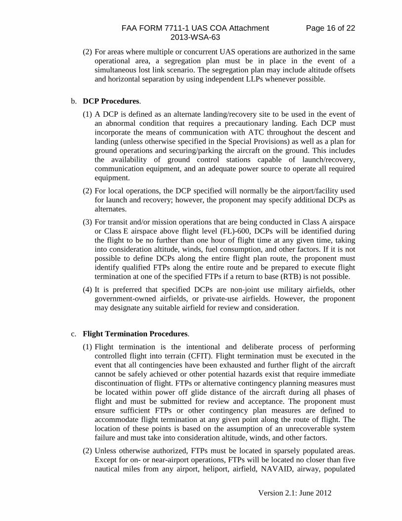
FAA FORM 7711-1 UAS COA Attachment 2013-WSA-63
Version 2.1: June 2012
Page 16 of 22
(2) For areas where multiple or concurrent UAS operations are authorized in the same operational area, a segregation plan must be in place in the event of a simultaneous lost link scenario. The segregation plan may include altitude offsets and horizontal separation by using independent LLPs whenever possible.
b. DCP Procedures.
(1) A DCP is defined as an alternate landing/recovery site to be used in the event of an abnormal condition that requires a precautionary landing. Each DCP must incorporate the means of communication with ATC throughout the descent and landing (unless otherwise specified in the Special Provisions) as well as a plan for ground operations and securing/parking the aircraft on the ground. This includes the availability of ground control stations capable of launch/recovery, communication equipment, and an adequate power source to operate all required equipment.
(2) For local operations, the DCP specified will normally be the airport/facility used for launch and recovery; however, the proponent may specify additional DCPs as alternates.
(3) For transit and/or mission operations that are being conducted in Class A airspace or Class E airspace above flight level (FL)-600, DCPs will be identified during the flight to be no further than one hour of flight time at any given time, taking into consideration altitude, winds, fuel consumption, and other factors. If it is not possible to define DCPs along the entire flight plan route, the proponent must identify qualified FTPs along the entire route and be prepared to execute flight termination at one of the specified FTPs if a return to base (RTB) is not possible.
(4) It is preferred that specified DCPs are non-joint use military airfields, other government-owned airfields, or private-use airfields. However, the proponent may designate any suitable airfield for review and consideration.
c. Flight Termination Procedures.
(1) Flight termination is the intentional and deliberate process of performing controlled flight into terrain (CFIT). Flight termination must be executed in the event that all contingencies have been exhausted and further flight of the aircraft cannot be safely achieved or other potential hazards exist that require immediate discontinuation of flight. FTPs or alternative contingency planning measures must be located within power off glide distance of the aircraft during all phases of flight and must be submitted for review and acceptance. The proponent must ensure sufficient FTPs or other contingency plan measures are defined to accommodate flight termination at any given point along the route of flight. The location of these points is based on the assumption of an unrecoverable system failure and must take into consideration altitude, winds, and other factors.
(2) Unless otherwise authorized, FTPs must be located in sparsely populated areas. Except for on- or near-airport operations, FTPs will be located no closer than five nautical miles from any airport, heliport, airfield, NAVAID, airway, populated
FAA FORM 7711-1 UAS COA Attachment 2013-WSA-63
Version 2.1: June 2012
Page 17 of 22
area, major roadway, oil rig, power plant, or any other infrastructure. For offshore locations, the proponent must refer to appropriate United States Coast Guard (USCG) charts and other publications to avoid maritime obstructions, shipping lanes, and other hazards. Populated areas are defined as those areas depicted in yellow on a VFR sectional chart or as determined from other sources.
(a) It is preferred that flight termination occurs in Restricted or Warning Areas, government-owned land, or offshore locations that are restricted from routine civil use. However, the proponent may designate any suitable location for review and consideration.
(b) The proponent is required to survey all designated areas prior to their use as an FTP. All FTPs will be reviewed for suitability on a routine and periodic basis, not to exceed six months. The proponent assumes full risk and all liability associated with the selection and use of any designated FTP.
(c) It is desirable that the proponent receive prior permission from the land owner or using agency prior to the use of this area as an FTP. The proponent should clearly communicate the purpose and intent of the FTP.
(d) For each FTP, plans must incorporate the means of communication with ATC throughout the descent as well as a plan for retrieval/recovery of the aircraft.
(e) Contingency planning must take into consideration all airspace constructs and minimize risk to other aircraft by avoiding published airways, military training routes, NAVAIDs, and congested areas to the maximum extent possible.
(f) In the event of a contingency divert or flight termination, if time permits, the use of a chase aircraft is preferred when the UA is operated outside of Restricted or Warning Areas.
(g) In the event of a contingency divert or flight termination or other approved contingency measures, the proponent will operate in Class A airspace and Special Use airspace to the maximum extent possible to reduce the risk of collision with non-participating air traffic.
B. Night Operation Limitations.
UAS night operations are those operations that occur between the end of evening civil twilight and the beginning of morning civil twilight, as published in the American Air Almanac, converted to local time. (Note: this is equal to approximately 30 minutes after sunset until 30 minutes before sunrise).
1. Night operations are not authorized.
FAA FORM 7711-1 UAS COA Attachment 2013-WSA-63
Version 2.1: June 2012
Page 18 of 22
AIR TRAFFIC CONTROL SPECIAL PROVISIONS A. Coordination Requirements. 1. At least 24 hours prior to operations the proponent shall notify Anchorage ARTCC and
advise of time for commencement and termination of operations and provide NOTAM number and information.
2. Additionally, the proponent shall coordinate all UAS operations with the Toolik Field Station at (907) 455-2533 to deconflict helicopter operations in the vicinity.
B. Communication Requirements. 1. Proponent will make a blind broadcast on CTAF (122.9 MHz) indicating the launch and
termination of UAS operations and monitor CTAF during flight operations.
2. ATC special provisions A & C will be used in lieu of maintaining direct two-way communications with ATC.
C. Emergency/Contingency Procedures.
Lost Link Procedures:
In the event of a lost link, the UAS pilot will immediately notify Toolik Field Station at (907) 455-2533, state pilot intentions, and comply with the following provisions:
a) Comply with those procedures outlined in Attachment 2.
b) If lost link occurs within a restricted or warning area, or the lost link procedure above takes the UA into the restricted or warning area – the aircraft will not exit the restricted or warning areas until the link is re-established.
c) The unmanned aircraft lost link mission will not transit or orbit over populated areas.
d) Lost link programmed procedures will avoid unexpected turn-around and/or altitude changes.
e) Lost link orbit points shall not coincide with the centerline of Victor airways.
Lost Communications: Comply with those procedures outlined in Attachment 3.

FAA FORM 7711-1 UAS COA Attachment 2013-WSA-63
Version 2.1: June 2012
Page 19 of 22
AUTHORIZATION This Certificate of Waiver or Authorization does not, in itself, waive any Title 14 Code of Federal Regulations, nor any state law or local ordinance. Should the proposed operation conflict with any state law or local ordinance, or require permission of local authorities or property owners, it is the responsibility of Utah Water Research Laboratory - Utah State University to resolve the matter. This COA does not authorize flight within Special Use airspace without approval from the using agency. Utah Water Research Laboratory - Utah State University is hereby authorized to operate the AggieAir Unmanned Aircraft System in the operations area depicted in the Activity section of this attachment.
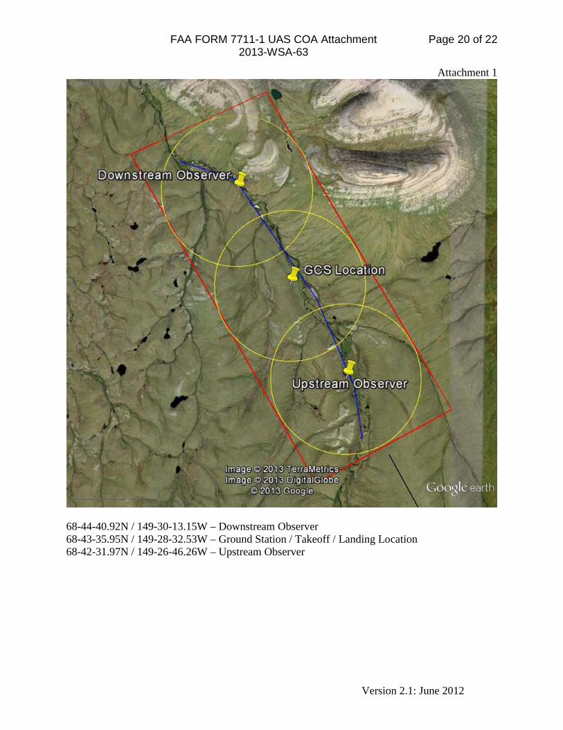
FAA FORM 7711-1 UAS COA Attachment 2013-WSA-63
Version 2.1: June 2012
Page 20 of 22
Attachment 1
68-44-40.92N / 149-30-13.15W – Downstream Observer 68-43-35.95N / 149-28-32.53W – Ground Station / Takeoff / Landing Location 68-42-31.97N / 149-26-46.26W – Upstream Observer
FAA FORM 7711-1 UAS COA Attachment 2013-WSA-63
Version 2.1: June 2012
Page 21 of 22
Attachment 2 LOST LINK PROCEDURE(S) Before takeoff, the UA is preprogrammed with a flight plan. This flight plan can be modified during flight if the UA is within communication range of the ground control station (GCS). However, the flight plan is built and simulated such that the UA can successfully fly the flight plan without any interaction from the GCS operator. Therefore the communication link between the UA and the GCS operator is not necessary for a successful flight. Nonetheless, for more safety, the UA is programmed to fly back to the GCS Location and circle above at 650’ AGL if communication is lost for more than 30 seconds. The GCS Location is located near the pilot (68°43'35.95"N 149°28'32.53"W). If communication is reestablished while flying towards the GCS Location, the pilot can change the flight plan to stay within communication range and resume the flight. The pilot could also land the UA using the landing area indicated by the flight operations. If communication is not reestablished, the pilot will take manual control and land the UA in the landing area when it comes into visual line-of-sight. If the pilot is not able to take manual control of the UA and communication has not been reestablished with the GCS, the UA will continue circling around GCS Location for 2 minutes or until the battery voltage falls below 10v. At this point, the motor will shut off, the autopilot will stop holding altitude, and the UA will safely descend to the ground in the same pattern around the GCS Location.
FAA FORM 7711-1 UAS COA Attachment 2013-WSA-63
Version 2.1: June 2012
Page 22 of 22
Attachment 3 LOST COMMUNICATIONS PROCEDURE(S) To keep the UA within line-of-sight (LOS), one observer is placed at the GCS Location (68°43'35.95"N 149°28'32.53"W) and one observer is placed at each end of the flight area (a total of three observers during the flight). The downstream observer will be located at 68°44'40.92"N 149°30'13.15"W and the upstream observer will be located at 68°42'31.97"N 149°26'46.26"W. This always keeps the UA within a distance of 1 mile from an observer at all times. When an observer has the UA within LOS, this observer will be referred to as the active observer. The active observer will report to the pilot every 30 seconds using a commercial handheld two-way radio. This report will include whether the UA is within sight and the current status of the airspace around the UA. If another aircraft enters the airspace around the UA the observer will use the two-way radio to alert the pilot and suggest appropriate avoidance maneuvers. During the planned flight over the river, the three observers will exchange the responsibility of the active observer as the UA flies out of LOS of one observer and into LOS of another observer. With the two-way radios, the active observer will make sure that the next observer is ready and has the UA within LOS before exchanging the responsibilities of the active observer. If LOS is not established with the next observer before the UA flies outside LOS of the active observer, then the pilot will abort the planned flight over the river and send a command to the aircraft to return to the GCS Location and circle above it at 650’ AGL. If the pilot does not get a report every 30 seconds from the active observer, then communication loss is assumed and the pilot will abort the planned flight over the river and send a command to the aircraft to return to the GCS Location and circle above it at 650’ AGL. At the GCS location, the observer and the pilot are collocated and will always have communication. With an active observer at the GCS, the pilot can either reestablish communication with the other observers and continue the flight or land the aircraft.
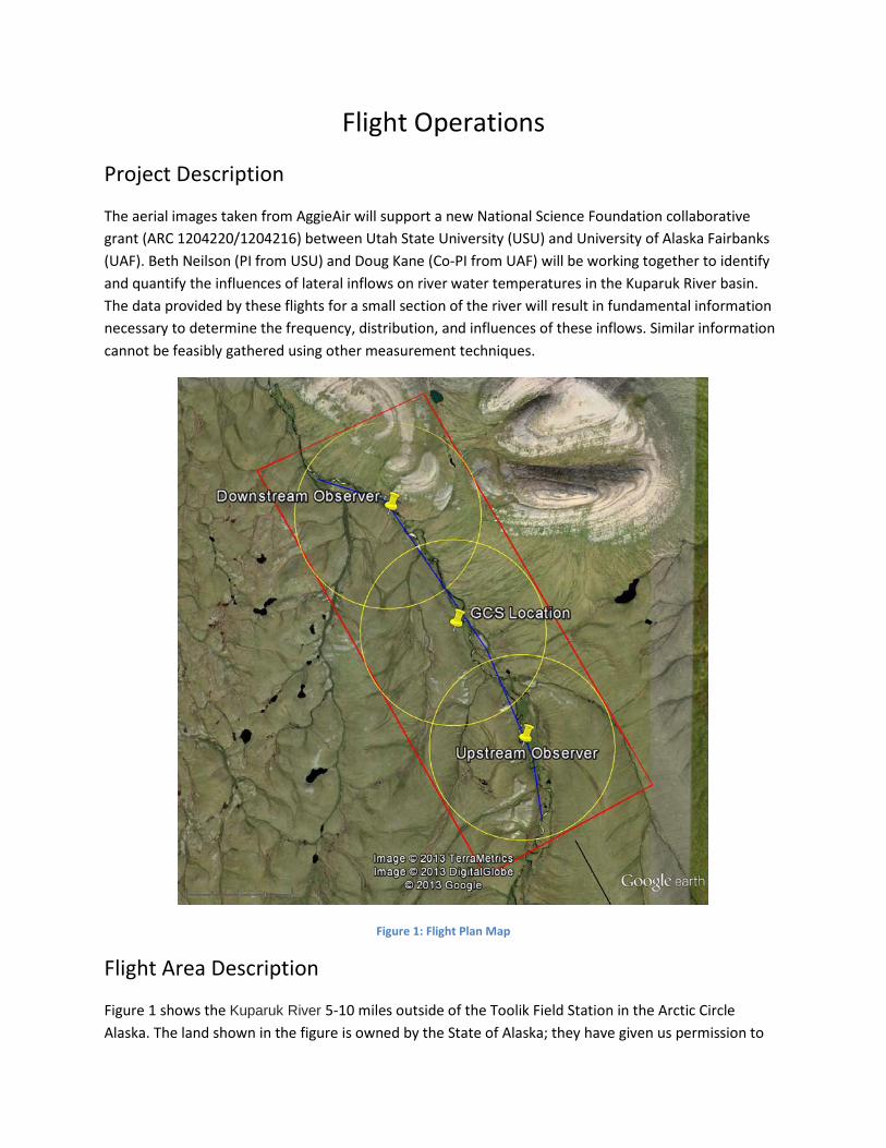
Flight Operations
Project Description
The aerial images taken from AggieAir will support a new National Science Foundation collaborative grant (ARC 1204220/1204216) between Utah State University (USU) and University of Alaska Fairbanks (UAF). Beth Neilson (PI from USU) and Doug Kane (Co-PI from UAF) will be working together to identify and quantify the influences of lateral inflows on river water temperatures in the Kuparuk River basin. The data provided by these flights for a small section of the river will result in fundamental information necessary to determine the frequency, distribution, and influences of these inflows. Similar information cannot be feasibly gathered using other measurement techniques.
Figure 1: Flight Plan Map
Flight Area Description
Figure 1 shows the Kuparuk River 5-10 miles outside of the Toolik Field Station in the Arctic Circle Alaska. The land shown in the figure is owned by the State of Alaska; they have given us permission to
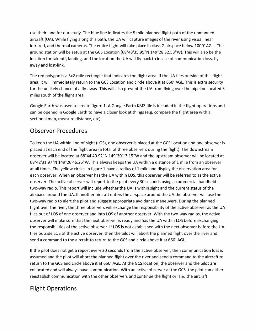
use their land for our study. The blue line indicates the 5 mile planned flight path of the unmanned aircraft (UA). While flying along this path, the UA will capture images of the river using visual, near infrared, and thermal cameras. The entire flight will take place in class G airspace below 1000’ AGL. The ground station will be setup at the GCS Location (68°43'35.95"N 149°28'32.53"W). This will also be the location for takeoff, landing, and the location the UA will fly back to incase of communication loss, fly away and lost-link.
The red polygon is a 5x2 mile rectangle that indicates the flight area. If the UA flies outside of this flight area, it will immediately return to the GCS Location and circle above it at 650’ AGL. This is extra security for the unlikely chance of a fly-away. This will also prevent the UA from flying over the pipeline located 3 miles south of the flight area.
Google Earth was used to create figure 1. A Google Earth KMZ file is included in the flight operations and can be opened in Google Earth to have a closer look at things (e.g. compare the flight area with a sectional map, measure distance, etc).
Observer Procedures
To keep the UA within line-of-sight (LOS), one observer is placed at the GCS Location and one observer is placed at each end of the flight area (a total of three observers during the flight). The downstream observer will be located at 68°44'40.92"N 149°30'13.15"W and the upstream observer will be located at 68°42'31.97"N 149°26'46.26"W. This always keeps the UA within a distance of 1 mile from an observer at all times. The yellow circles in figure 1 have a radius of 1 mile and display the observation area for each observer. When an observer has the UA within LOS, this observer will be referred to as the active observer. The active observer will report to the pilot every 30 seconds using a commercial handheld two-way radio. This report will include whether the UA is within sight and the current status of the airspace around the UA. If another aircraft enters the airspace around the UA the observer will use the two-way radio to alert the pilot and suggest appropriate avoidance maneuvers. During the planned flight over the river, the three observers will exchange the responsibility of the active observer as the UA flies out of LOS of one observer and into LOS of another observer. With the two-way radios, the active observer will make sure that the next observer is ready and has the UA within LOS before exchanging the responsibilities of the active observer. If LOS is not established with the next observer before the UA flies outside LOS of the active observer, then the pilot will abort the planned flight over the river and send a command to the aircraft to return to the GCS and circle above it at 650’ AGL.
If the pilot does not get a report every 30 seconds from the active observer, then communication loss is assumed and the pilot will abort the planned flight over the river and send a command to the aircraft to return to the GCS and circle above it at 650’ AGL. At the GCS location, the observer and the pilot are collocated and will always have communication. With an active observer at the GCS, the pilot can either reestablish communication with the other observers and continue the flight or land the aircraft.
Flight Operations
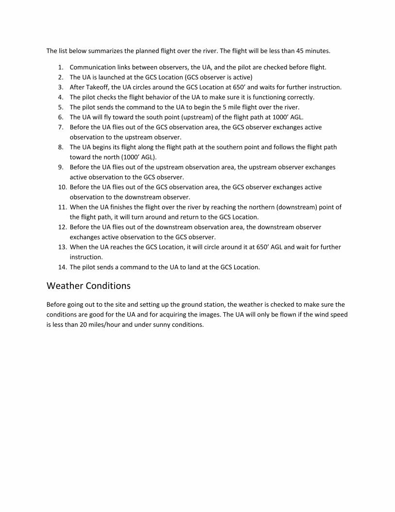
The list below summarizes the planned flight over the river. The flight will be less than 45 minutes.
1. Communication links between observers, the UA, and the pilot are checked before flight. 2. The UA is launched at the GCS Location (GCS observer is active) 3. After Takeoff, the UA circles around the GCS Location at 650’ and waits for further instruction. 4. The pilot checks the flight behavior of the UA to make sure it is functioning correctly. 5. The pilot sends the command to the UA to begin the 5 mile flight over the river. 6. The UA will fly toward the south point (upstream) of the flight path at 1000’ AGL. 7. Before the UA flies out of the GCS observation area, the GCS observer exchanges active
observation to the upstream observer. 8. The UA begins its flight along the flight path at the southern point and follows the flight path
toward the north (1000’ AGL). 9. Before the UA flies out of the upstream observation area, the upstream observer exchanges
active observation to the GCS observer. 10. Before the UA flies out of the GCS observation area, the GCS observer exchanges active
observation to the downstream observer. 11. When the UA finishes the flight over the river by reaching the northern (downstream) point of
the flight path, it will turn around and return to the GCS Location. 12. Before the UA flies out of the downstream observation area, the downstream observer
exchanges active observation to the GCS observer. 13. When the UA reaches the GCS Location, it will circle around it at 650’ AGL and wait for further
instruction. 14. The pilot sends a command to the UA to land at the GCS Location.
Weather Conditions
Before going out to the site and setting up the ground station, the weather is checked to make sure the conditions are good for the UA and for acquiring the images. The UA will only be flown if the wind speed is less than 20 miles/hour and under sunny conditions.
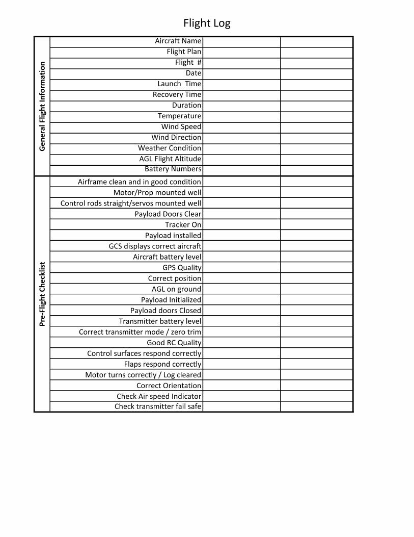
Flight Log
Aircraft Name
Flight Plan
Flight #
Date
Launch Time
Recovery Time
Duration
Temperature
Wind Speed
Wind Direction
Weather Condition
AGL Flight AltitudeBattery Numbers
Airframe clean and in good condition
Motor/Prop mounted well
Control rods straight/servos mounted well
Payload Doors Clear
Tracker On
Payload installed
GCS displays correct aircraft
Aircraft battery level
GPS Quality
Correct position
AGL on ground
Payload Initialized
Payload doors Closed
Transmitter battery level
Correct transmitter mode / zero trim
Good RC Quality
Control surfaces respond correctly
Flaps respond correctly
Motor turns correctly / Log cleared
Correct Orientation
Check Air speed IndicatorCheck transmitter fail safe
Pre
-Flig
ht
Ch
eckl
ist
Gen
era
l Flig
ht
Info
rmat
ion

133
Vita
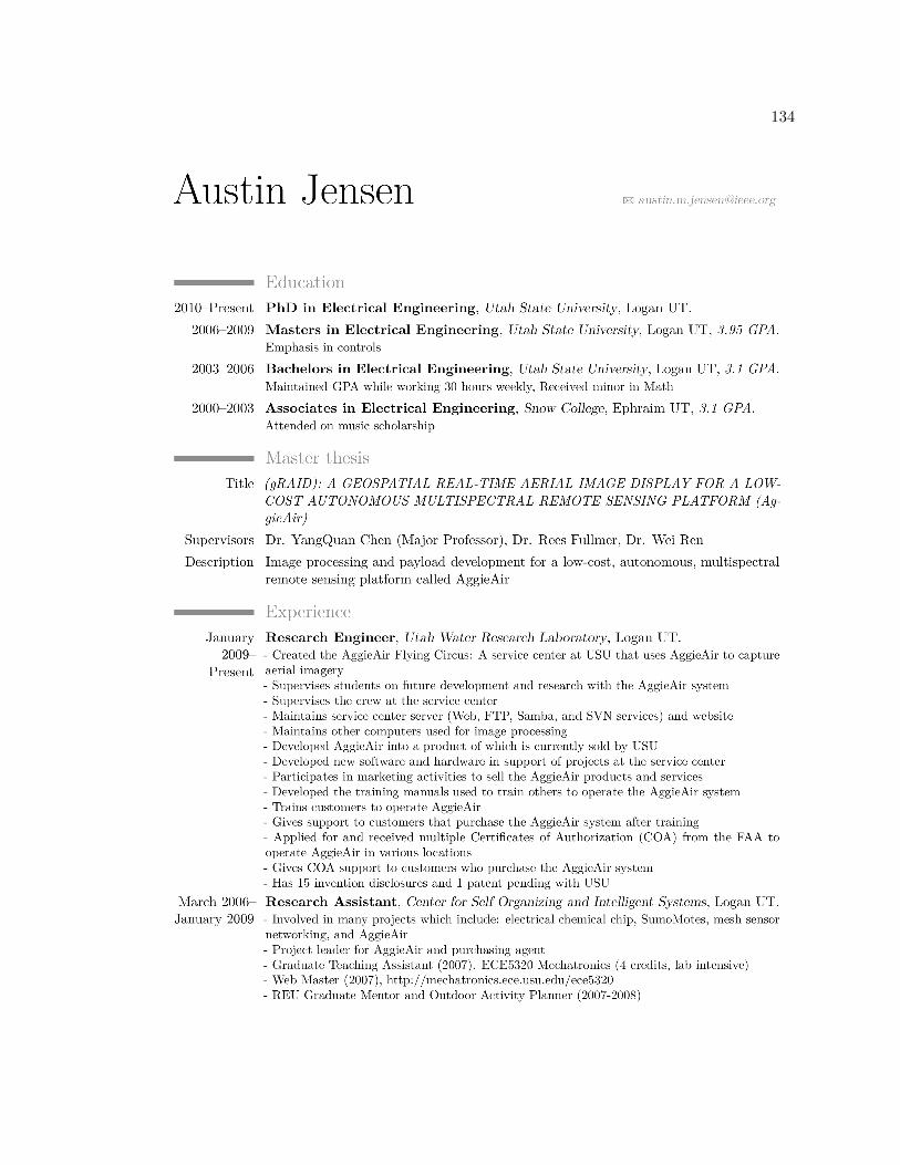
134
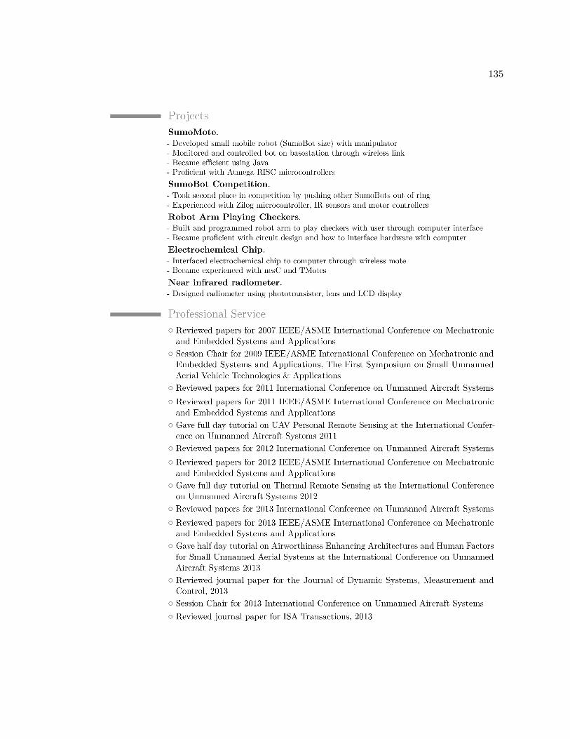
135

136

137

138

139


![FY18 RWDC State Unmanned Aerial System Challenge ... · Unmanned Aerial System Challenge: Practical Solutions to ... , Real World Design Challenge ... , unmanned aerial vehicle [UAV])](https://img.pdfslide.net/doc/110x75/5ae85cfb7f8b9a8b2b8fe5e5/fy18-rwdc-state-unmanned-aerial-system-challenge-aerial-system-challenge-practical.jpg)