1  

Input-output analysis for water consumption in Macedonia

Jordan Hristov1, Aleksandra Martinovska-Stojceska2, Yves Surry3 1. Corresponding author, PhD candidate in Economics at the Department of Economics

within the Swedish University of Agricultural Sciences, Uppsala Sweden. E-mail: Jordan.Hristov@slu.se 2. Assistant professor at the Institute of Agricultural Economics, Faculty of Agriculture

Sciences and Food, within the St. Cyril and Methodius University, Skopje, Macedonia. 3. Professor at the Department of Economics within the Swedish University of Agricultural

Sciences, Uppsala Sweden.

Working paper submitted to the European Summer School in Resource and Environmental Economics: Management of International Water, 1-7 July, 2012 – Venice, Italy.

May, 2012

”This document has been produced with the financial assistance of the Swedish International Development Cooperation Agency, SIDA. The views herein shall not necessarily be taken to reflect the official opinion of SIDA.”

  

2  

Abstract

This paper examines the water consumption and associated water relationship of the Macedonian economic agents in 2005 by using an input-output methodology. Additionally by linkage analysis (backward and forward linkage), the main findings for both open and closed economy support the initial assumption that agriculture is the major water consuming sector. It also exhibit high rate of direct water use but also most of the industrial sectors indirect consumption was mainly driven by the agriculture. Additional to the agriculture, some of the manufacturing sectors such as the coke and refined petroleum, the other mining and quarrying products followed by the basic metals as well as the energy sector are identified as key water use sectors. The competition between agriculture and household consumption is another important aspect. Therefore, necessity to introduce changes in the production technology or specialization in this region or reconsidering the existing water pricing policy based on comprehensive research which will capture economic, social and environmental aspects ought to be an option. The trade balance in terms of “virtual water” is not an imperative aspect here. Although the main water consuming sectors shown to be characterized by positive net exports, the quantity relative to the total output was insignificantly small with an exception of the basic metals sector.

Key words: input-Output model, Macedonia, water consumption, backward and forward linkages, open and closed economy, virtual water

  

3  

Introduction

Fresh water is irreplaceable, limited natural resource and an essential factor for existence and development of the entire society. Without water it is impossible to imagine how the world would be like! Fresh water is only 2.5% of the total water resources (Duarte et. al. 2002). Water scarcity has now become a severe problem mainly due irregular spatial, time and quality distribution. The problem has become even more severe given the increased water demand in response to economic and population growth. However, the shortfall in water supply may stems from mismanagement of the water resources. According to Wang et. al. (2009, p.894) “promoting sustainable development of water resources must involve a consideration of the interactions between water use and the economic sectors”. Decision support for sustainable development requires information on the economy-wide implications on resources. Moreover, the importance of climate change must be considered in careful coordination with appropriate water management, the environment and economic development.

In Republic of Macedonia1 there is growing awareness of the limits of water resource endowments consistent with the above mentioned concerns (MOEPP, 2006,a). Given the climate change issue, the availability and demand for clean, safe and quality water in the long run is questioned. However, there has been no research done yet the on economic analysis of water use and management in this country. Proper quantification and rationalization in terms of water consumption is essential for understanding and creating equitable and effective use of water. Thus, identification of key water consuming sectors in the Macedonian economy is necessary for sustainable water management.

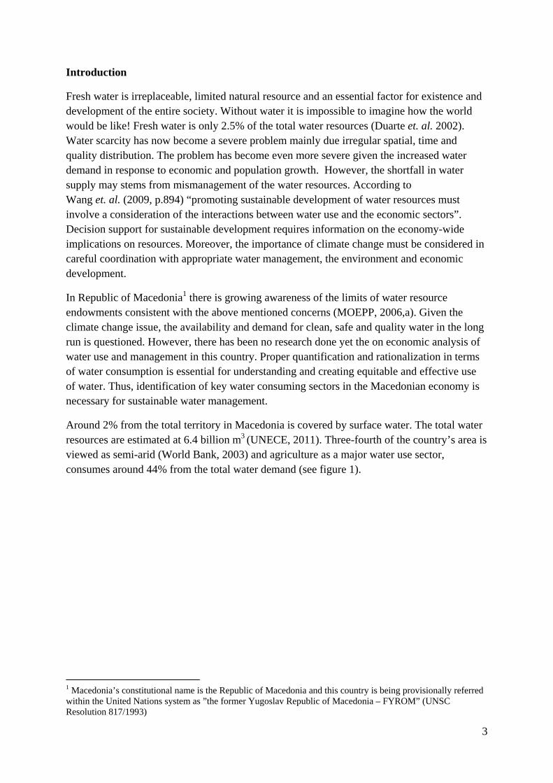
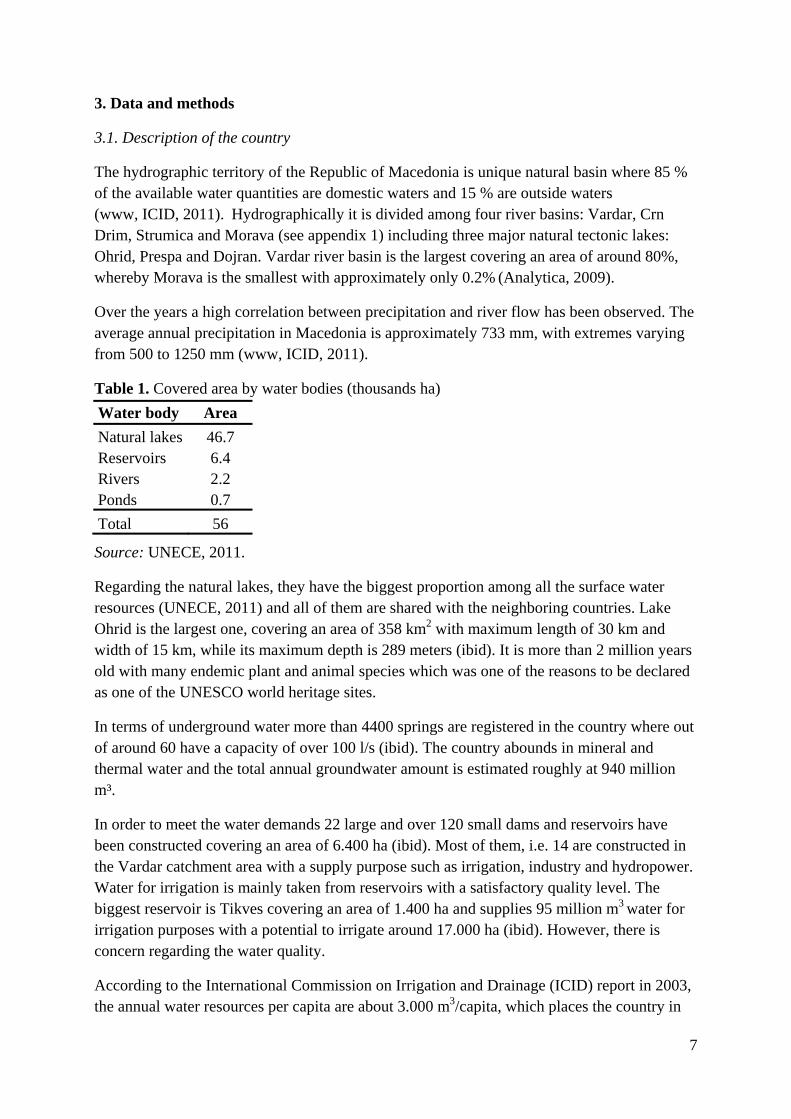
Around 2% from the total territory in Macedonia is covered by surface water. The total water resources are estimated at 6.4 billion m3 (UNECE, 2011). Three-fourth of the country’s area is viewed as semi-arid (World Bank, 2003) and agriculture as a major water use sector, consumes around 44% from the total water demand (see figure 1).

                                                            1 Macedonia’s constitutional name is the Republic of Macedonia and this country is being provisionally referred within the United Nations system as ”the former Yugoslav Republic of Macedonia – FYROM” (UNSC Resolution 817/1993)

  

4  

Figure 1. Total water demands in 2010 Source: UNECE, 2011.

Hence, assessing the future water needs of the agricultural sector as the major water consumer, taking into account the increasing demand for water by other sectors and/or segments of the Macedonian economy is the focus of this research. Moreover, the direct and indirect water requirements linked with the production of each economic sector and their impacts on the availability of the resources will be investigated.

Agriculture with a share in GDP around 11%, it is the third largest important sector after industry and services (SSO, 2011). According to the 2009 Annual Agricultural Report (MAFWE, 2010), irrigation potential is estimated to be 78% of the total arable land. However, in 2009 only 2-3% of the agricultural land was irrigated (ibid). The main reason for the low effective use of irrigate water may stem from the long term exploitation of the irrigation schemes followed by negligence and poor maintenance by the institutions dealing with irrigation schemesm, causing deteriorating functioning. In addition, some of the farmers who are at the beginning of the irrigation schemes use the water services, but don’t compensate for the used water. However, the water still needs to be delivered to the farmers who are at the end of the irrigation scheme and compensate for the provided service and distributed water. Thus, there is a presence of a free rider problem. Therefore, reduced income for proper irrigation schemes maintenance results in high water losses in water supply systems (up to 40%), smaller irrigated area and smaller yields followed by soil and erosion as well as water quality issues (MAFWE, 2010). Thus, there is significant inefficient utilization of irrigation water.

Besides the technical, financial and institutional nature of the problem the uncertainty caused by climate change is crucial. Over the period from 1961 to 2003 there has been a noticeable decline in the river flows in all the water basins (MOOEP, 2006,b). Future climate projections for Macedonia, forecast that by 2050 there will be a decline in the average annual precipitation by 5% and 17% in the summer period (World Bank, 2010). In addition, according to the World Bank report on Agriculture and Climate Change (www, World Bank,

0

5

10

15

20

25

30

35

40

45

Population and tourism

Industry Agriculture Minimum accepted

flow

11%14%

44%

31%

2010

  

5  

2012) “the combined effect of climate change on crop yields in those areas where irrigation water shortages are forecast will be substantial leading to up to 50% decrease in yields in the Crna river basin” situated in the Pelagonia region of the Vardar river basin. Moreover, the fact that there is uneven spatial and time distribution of water resources throughout the country, with more favourable supply conditions in the western part, the problem concerning availability and demand of water becomes even more important. The competition with the urban water supply in the summer months is another important aspect. Hence, the main research question i.e. assessing the agricultural direct and indirect water requirement is an essential aspect given the above mentioned concerns.

Most widely and appropriate methodology that studies the direct and indirect water consumption i.e. the intersectoral water relationship in the economy is the environmentally extended input-output (I-O) table. This relationship illustrates how the output of the economic sector is captured by another sector, where is serves as an input (Miller and Blair, 2009). Extension of the traditional Leontief input-output model consists of introducing water inputs as a production factor (measured in physical units). According to Velazquez (2006) this enables the analysis of the structural relationship between a production activity and its physical relationship with the environment. Consequently, with better understanding of the relationship among the economy and the environment, awareness can be raised of sustainable water consumption. Identification of key water consumption patterns and trends may help to design sustainable water consumption policies at the national level thus mitigating the climate change effects.

2. Literature review

The interest in consumption based resource accounting emerged back in the 1960s (Velazquez, 2006), but its significance has grown significantly in the last two decades (Wiedmann, 2009). The number of studies based on environmentally extended I-O table which Leontief developed in 1970, emphasize the interest in the subject. Most of them adopt a consumption perspective to energy consumption and environmental pollution. Wiedmann et. al. (2007) and Wiedmann (2009) reviewed some of the recent conducted studies in terms of natural resource consumption. In 1988, Proops utilized energy use input-output model and identified the direct and indirect effect based on a number of indicators. Later, Hewdon and Pearson displayed the complicated relationship between energy, environment and economic welfare by using 10 sector I-O model of UK. Furthermore, by using I-O environmental model Hubacek and Sun (2001) estimated the Chinese changes in land use. More recently, Peters and Hertwich (2006) did an analysis of pollution in international trade whereas Liang et. al. (2007) conducted an energy requirement and CO2 emissions analysis by using the Chinese I-O table.

However, little attention from a economic point of view has been given to water consumption I-O analysis although the first studies in this area date back to the 1950s (Wang et. al, 2009). The main reason was due to methodological difficulties that arose when the water consumption variables were introduced in the input-output model (ibid). The assumption of

  

6  

proportionality among monetary and physical transactions is violated because of the considerable variation in water prices of the economic sectors. Yet, these difficulties were overcomed by Lofting and McGauhey in 1968 who introduced the water requirements in physical units as inputs in the I-O framework. Chen (2000) used this framework to study the water supply and demand balance in Shanxi Province in China. On the basis on the table by using translog production function and linear programming model, they were able to asses an economic value of the water. Along with the I-O analysis results, they were able to propose a water resource saving economy of the Shanxai Province. Lenzen and Foran (2001) analyzed the water use in Australia where they displayed that the predominantly urban population is responsible for the entire water consumption. One year after Duarte et. al. (2002) studied the effect of Spanish water consumption in Hypothetical Extraction framework by using I-O methodology. Okadera et. al. (2006) did an analysis of the water demand and pollution discharge in the Three Gorges Dam in China. Velazquez in 2006 studied the intersectoral water relationship in Andalusia. In addition, Velazquez’s methodology was adapted by Wang et. al. (2009) to analyze regional water consumption in Zhangye City. However, the matrix of interindustryl water relationship was derived in slightly different manner. The next chapter explores this in detail. Another recent study was that of Yu et. al.(2010) who tried to identify the key water consuming sectors in North and South UK by using regional extended I-O methodology.

Nevertheless, although the methodology used in all the above studies is similar, one of the most important aspects that need to be considered is the availability of water accounting data. In the study conducted by Velazquez (2006) the Andalusian Environmental I-O table enables her to quantify the intersectoral relationship in terms of cubic meters water consumption. Furthermore, Wang et. al. (2009) at their disposal had water intensive agricultural use at the most detailed level which is published annually by the Gansu Provincial Bureau of Water Resources. Moreover, Lanzen and Foran (2001) use the first published water accounts 1993-1997 by Australian Bureau of Statistics (ABS) in their I-O analysis. These water accounts contain the use and supply on state and territory level of self-extracted and mains water, as well as effluent reuse and regulated discharge of households and industries.

In the case of Macedonia there are no such detailed water accounts. Most of the existing data, especially for the agriculture, is at an aggregated level which causes complication in distinction between the key water consuming sectors. The next section describes which data were used, as well as how the water accounts were constructed and which sectors were aggregated. Needless to say that the references such as EUROSTAT (2002) “Water Accounts-Results of pilot studies” publication as well as the ABS report published in 2010 on Water Account Australia 2008-2009, were highly appreciated in constructing of the water accounts.

  

7  

3. Data and methods

3.1. Description of the country

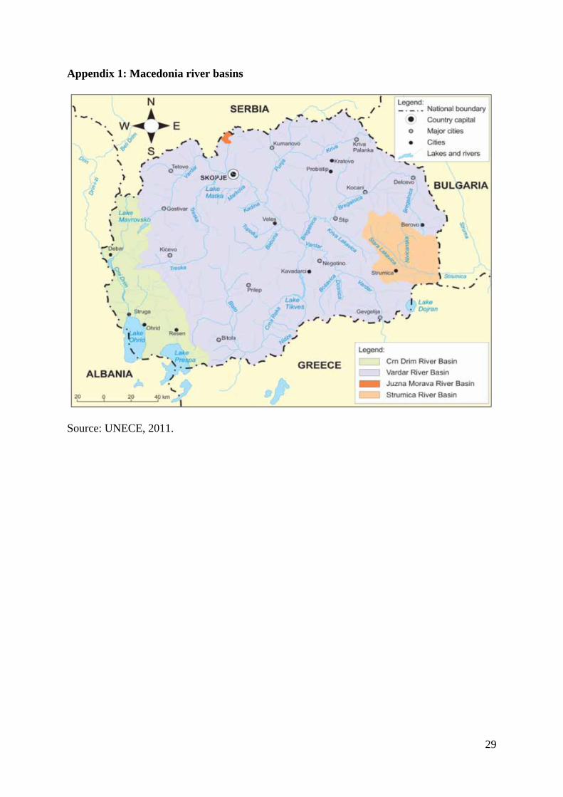
The hydrographic territory of the Republic of Macedonia is unique natural basin where 85 % of the available water quantities are domestic waters and 15 % are outside waters (www, ICID, 2011).  Hydrographically it is divided among four river basins: Vardar, Crn Drim, Strumica and Morava (see appendix 1) including three major natural tectonic lakes: Ohrid, Prespa and Dojran. Vardar river basin is the largest covering an area of around 80%, whereby Morava is the smallest with approximately only 0.2% (Analytica, 2009).

Over the years a high correlation between precipitation and river flow has been observed. The average annual precipitation in Macedonia is approximately 733 mm, with extremes varying from 500 to 1250 mm (www, ICID, 2011).

Table 1. Covered area by water bodies (thousands ha)

Water body Area

Natural lakes 46.7 Reservoirs 6.4 Rivers 2.2 Ponds 0.7

Total 56

Source: UNECE, 2011.

Regarding the natural lakes, they have the biggest proportion among all the surface water resources (UNECE, 2011) and all of them are shared with the neighboring countries. Lake Ohrid is the largest one, covering an area of 358 km2 with maximum length of 30 km and width of 15 km, while its maximum depth is 289 meters (ibid). It is more than 2 million years old with many endemic plant and animal species which was one of the reasons to be declared as one of the UNESCO world heritage sites.

In terms of underground water more than 4400 springs are registered in the country where out of around 60 have a capacity of over 100 l/s (ibid). The country abounds in mineral and thermal water and the total annual groundwater amount is estimated roughly at 940 million m³.

In order to meet the water demands 22 large and over 120 small dams and reservoirs have been constructed covering an area of 6.400 ha (ibid). Most of them, i.e. 14 are constructed in the Vardar catchment area with a supply purpose such as irrigation, industry and hydropower. Water for irrigation is mainly taken from reservoirs with a satisfactory quality level. The biggest reservoir is Tikves covering an area of 1.400 ha and supplies 95 million m3 water for irrigation purposes with a potential to irrigate around 17.000 ha (ibid). However, there is concern regarding the water quality.

According to the International Commission on Irrigation and Drainage (ICID) report in 2003, the annual water resources per capita are about 3.000 m3/capita, which places the country in

  

8  

the middle category of the European countries in terms of available per capita water resources. For comparison, the European average is around 1900 m3/capita (www, ICID, 2011). However, according to the water stress indicator in the Wastewater report (Analytica, 2009), in Macedonia there is heavy exploitation of the water resources. This brings back the question, i.e. what are the key water consuming sectors? In other words what are their intersectoral direct and indirect water consumption relationships with different economic sectors including household consumption as one of the final demand economic agents?

3.2 . Methodology

3.2.1. Traditional Leontief input-output model

This section describes the conventional I-O table used as basis for extending it in terms of water consumption. The basic framework of the Leontief I-O analysis concerns the “flow of products from each sector, considered as producer, to each of the sectors, itself and others, considered as producers” (Miller and Blair, 2009, p.2). It is generated from observed data for a particular time period and a given geographic region. The mathematical structure consists of set of linear equations which in a matrix representation, rows represent the distribution of the producers output and the columns is the required inputs by particular sector to produce its output (ibid).

Table 2. Input output transactions table

Producer sector

Consumer sector Final demand Total

output Agriculture Mining etc Consumption Investment Exports

Agriculture Zij Fi Xi Mining

… Value added Vj VF

j Vi Imports Ij IF

j Ii

Total inputs Xj Fj

note: capital letters indicate matrix notation Source: Miller and Blair, 2009.

The additional columns in table 2 labelled final demand are consumers of the economy who are exogenous to the industrial sectors which domestic and foreign demanded units are not used as an input but rather as such (ibid). Household and government consumption, as well as capital investment and exports belong to this column. Moreover, the additional row categorized as value added accounts to other non-industiral inputs to production such as labour, capital, taxes, etc. Value added combined with imports are usually considered as payment sectors (ibid).

The input-output transaction balance among the industrial sectors is presented by set of equations:

  

9  

n

jiiji fzx

1                                                                                                                                              (1) 

where zij represent the values of the transactions from each sector i to sector j, where as fi is

the final demand for goods by each sector (Miller and Blair, 2009).

Equation (1) can be rewritten as to include the technical coefficients of production (aij),which

are defined as the purchases that sector j makes from sector i per total effective production unit of sector j and which represent the direct input required by that sector (ibid), i.e.

j

ijij x

za (2)

n

jijiji fxax

1 (3)

These coefficients are assumed to be constant, i.e. when the output of sector j doubled, the

input from i to j doubled as well (ibid). Therefore, it is assumed there are constant returns to

scale.

In matrix notation it becomes:

fAxx (4)

and solving for x, the total production delivered to final demand is obtained.

fAIx 1)( (5)

where 1)( AI is known as the Leontief inverse matrix or the total requirement matrix

representing the total production that every sector must generate to satisfy the final demand of

the economy (ibid). In more detailed manner, the production of sector i in equation (5) may

be formulated as:

n

jiiji flx

1 (6)

where lij are the elements in the Leontief inverse matrix describing the increase in production

generated by sector i if the demand of sector j increases by one unit. The column sums of this matrix express the total (direct and indirect) requirements of a sector to meet its final demand (ibid). The diagonal elements in the matrix are the direct effect and the column sum of the off-diagonal elements is the indirect effect.

  

10  

3.2.2. Water input-output model

Up until this point, only the basic Leontief I-O model is summarized. As explained before the extension of the traditional approach is done in terms of water consumption. It is done in a manner by adding an extra row (W) where physical data on water use by each sector is considered as a production factor i.e. input.

In order to formulate a matrix of intersectoral water relationship and additionally analyze the importance of direct and indirect consumption, the indicator of total direct consumption per unit produced may be formulated. According to Velazquez (2006), it is defined by dividing

the total amount directly consumed by each sector (wj) with the total input to that sector (xj):

j

jj x

ww *

(7)

In matrix notation as before it may be represented as:

1* ˆ xww

(8)

where denotes a diagonal matrix with the elements of x on the leading diagonal. To be able to distinguish among direct and indirect effects, equation (8) may be rewritten in terms of total water consumption multiplier simply by multiplying the direct water

consumption coefficient (w*j) by the quantity produced by each sector.

wxw *

(9)

According to eq. (5) the production vector x may be reformulated as open Leontief model and obtain the total water consumption of the economy in terms of own demand.

fAIww 1* )(ˆ

(10)

1** )( AIwwt

(11)

Velazquez (2006) continues with her analysis in the model adaptation of Proops energy use

(1988) by defining the expression 1* )( AIw as an indicator of total water consumption

(wt*). It is a row vector and determines the total amount of water that the economy will both directly and indirectly consume, if there is an increase by one unit of any given sector. As indicated before the total water consumption may be separated in direct and indirect effect. However, in order to be able to capture the indirect effect first there is a need to consider the “drag effect”. The Leontief model accounts for this effect which indicates how the evolution

  

11  

of a given sector can “drag” the total economic production. In terms of water consumption, the “drag effect” is captured by the quotient between the earlier defined indicator of total

consumption (wt*) and indicator of total direct consumption (w*), i.e. by the water

consumption multiplier (wcm).

j

tj

j w

wAIwcm

*

*

1)(

(12)

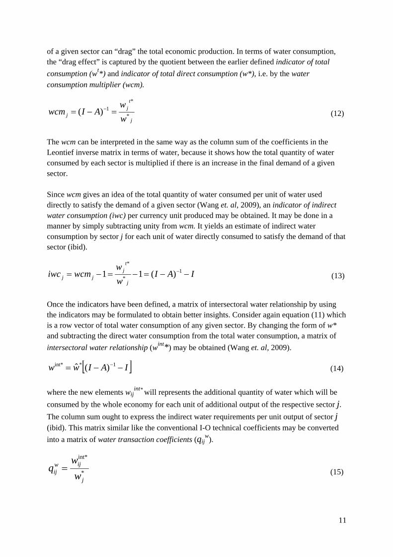
The wcm can be interpreted in the same way as the column sum of the coefficients in the Leontief inverse matrix in terms of water, because it shows how the total quantity of water consumed by each sector is multiplied if there is an increase in the final demand of a given sector. Since wcm gives an idea of the total quantity of water consumed per unit of water used directly to satisfy the demand of a given sector (Wang et. al, 2009), an indicator of indirect water consumption (iwc) per currency unit produced may be obtained. It may be done in a manner by simply subtracting unity from wcm. It yields an estimate of indirect water consumption by sector j for each unit of water directly consumed to satisfy the demand of that sector (ibid).

IAIw

wwcmiwc

j

tj

jj 1*

*

)(11

(13)

Once the indicators have been defined, a matrix of intersectoral water relationship by using the indicators may be formulated to obtain better insights. Consider again equation (11) which is a row vector of total water consumption of any given sector. By changing the form of w* and subtracting the direct water consumption from the total water consumption, a matrix of

intersectoral water relationship (wint*) may be obtained (Wang et. al, 2009).

IAIww 1*int* )(ˆ

(14)

where the new elements wijint* will represents the additional quantity of water which will be

consumed by the whole economy for each unit of additional output of the respective sector j. The column sum ought to express the indirect water requirements per unit output of sector j (ibid). This matrix similar like the conventional I-O technical coefficients may be converted

into a matrix of water transaction coefficients (qijw).

*

int*

j

ijwij w

wq

(15)

  

12  

i.e. in coefficients that indicates the additional quantity of water that the sector j will be consumed if the final demand for water by sector j increases by one unit. The column sum of

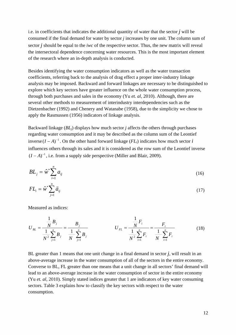
sector j should be equal to the iwc of the respective sector. Thus, the new matrix will reveal the intersectoral dependence concerning water resources. This is the most important element of the research where an in-depth analysis is conducted. Besides identifying the water consumption indicators as well as the water transaction coefficients, referring back to the analysis of drag effect a proper inter-industry linkage analysis may be imposed. Backward and forward linkages are necessary to be distinguished to explore which key sectors have greater influence on the whole water consumption process, through both purchases and sales in the economy (Yu et. al, 2010). Although, there are several other methods to measurement of interindustry interdependencies such as the Dietzenbacher (1992) and Chenery and Watanabe (1958), due to the simplicity we chose to apply the Rasmussen (1956) indicators of linkage analysis. Backward linkage (BLj) displays how much sector j affects the others through purchases regarding water consumption and it may be described as the column sum of the Leontief

inverse 1)( AI . On the other hand forward linkage (FLi) indicates how much sector i influences others through its sales and it is considered as the row sum of the Leontief inverse

1)( AI , i.e. from a supply side perspective (Miller and Blair, 2009).

n

iijj awBL

1

*ˆ

(16)

n

jiji awFL

1

*ˆ

(17)

Measured as indices:

n

jj

j

n

jj

j

BL

BN

B

BN

BNU

112

11

1

n

ii

in

ii

i

FL

FN

F

FN

FNU

112

11

1

(18)

BL greater than 1 means that one unit change in a final demand in sector j, will result in an

above-average increase in the water consumption of all of the sectors in the entire economy. Converse to BL, FL greater than one means that a unit change in all sectors’ final demand will lead to an above-average increase in the water consumption of sector in the entire economy (Yu et. al, 2010). Simply stated indices greater that 1 are indicators of key water consuming sectors. Table 3 explains how to classify the key sectors with respect to the water consumption.

  

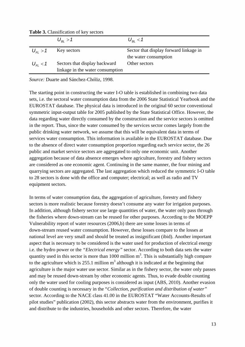
13  

Table 3. Classification of key sectors

1UBL 1UBL

1UFL Key sectors Sector that display forward linkage in the water consumption

1UFL Sectors that display backward Other sectors linkage in the water consumption

Source: Duarte and Sánchez-Chóliz, 1998. The starting point in constructing the water I-O table is established in combining two data sets, i.e. the sectoral water consumption data from the 2006 State Statistical Yearbook and the EUROSTAT database. The physical data is introduced in the original 60 sector conventional symmetric input-output table for 2005 published by the State Statistical Office. However, the data regarding water directly consumed by the construction and the service sectors is omitted in the report. Thus, since the water consumed by the services sector comes largely from the public drinking water network, we assume that this will be equivalent data in terms of services water consumption. This information is available in the EUROSTAT database. Due to the absence of direct water consumption proportion regarding each service sector, the 26 public and market service sectors are aggregated to only one economic unit. Another aggregation because of data absence emerges where agriculture, forestry and fishery sectors are considered as one economic agent. Continuing in the same manner, the four mining and quarrying sectors are aggregated. The last aggregation which reduced the symmetric I-O table to 28 sectors is done with the office and computer; electrical; as well as radio and TV equipment sectors. In terms of water consumption data, the aggregation of agriculture, forestry and fishery sectors is more realistic because forestry doesn’t consume any water for irrigation purposes. In addition, although fishery sector use large quantities of water, the water only pass through the fisheries where down-stream can be reused for other purposes. According to the MOEPP Vulnerability report of water resources (2006,b) there are some losses in terms of down-stream reused water consumption. However, these losses compare to the losses at national level are very small and should be treated as insignificant (ibid). Another important aspect that is necessary to be considered is the water used for production of electrical energy i.e. the hydro power or the “Electrical energy” sector. According to both data sets the water quantity used in this sector is more than 1000 million m3. This is substantially high compare to the agriculture which is 255.1 million m3 although it is indicated at the beginning that agriculture is the major water use sector. Similar as in the fishery sector, the water only passes and may be reused down-stream by other economic agents. Thus, to evade double counting only the water used for cooling purposes is considered as input (ABS, 2010). Another evasion of double counting is necessary in the “Collection, purification and distribution of water” sector. According to the NACE class 41.00 in the EUROSTAT “Water Accounts-Results of pilot studies” publication (2002), this sector abstracts water from the environment, purifies it and distribute to the industries, households and other sectors. Therefore, the water

  

14  

requirement as input in this sector is considered to be “zero”. Finally, the direct water requirement for the construction sector is generated in a slightly different manner. Due absence of information in both data sets, it is done by approximation relative to the neighbouring countries sectoral water consumption and total output for the respective year 2005. Another attempt by using a normative of used water per cubic meter of produced concrete was done, given the information on total annual beton production. However, due to the unrealistic obtained number of total water consumed by the construction sector, this approach was dropped. Maybe both of them are not the most appropriate approaches, but as soon as there is available information from the Macedonian Statistical Office the first assumption will hold. While comparing and combining the two data sets to find an appropriate water demand quantities for services and construction sectors, we notice some irregularities which may cause misleading interpretation. In the State Statistical Yearbook, some of the information that refers to water abstraction by sector is the same as the water supply data in the EUROSTAT data base. Whereas the information on water supply in the State Statistical Yearbook is much higher. For example in the EUROSTAT data base, the total Manufacturing sector water supply is 230.5 million m3 which is the exact water abstraction for technical purposes in the State Statistical Yearbook 2006. On the other hand in the State Statistical Yearbook 2006, the total supply to water for the Manufacturing sector is 477.95 million m3. Meaning that agriculture with abstraction of 255.1 million m3 is not a major water consuming sector or that there are huge losses by more than 50%. Thus, identification and quantification of the direct and indirect sectoral relationship may be jeopardized. Given this uncertainty necessity of ranking the sectors in a fuzzy environment is welcomed in this study. However, at this stage of the research there won’t be any changes in the methodology and the obtained results will be analysed and discussed as they are. Completed analysis with improvements will be an imperative in the future.

4. Results and discussion

This section presents and discuss the obtained results from the previously formulated indicators and linkage indices as well as the matrix of water transaction coefficients, which will be basis for the analysis and discussion part.

4.1. Water consumption indicators

Table 4 displays the total direct water consumption (w), the indicator of total direct consumption per unit produced (w*) and the indicator of total water consumption (wt*). In addition, table 4 lists the ratios of the direct and total water consumption indicators which enable us to distinguish between direct and indirect water consumption.

  

15  

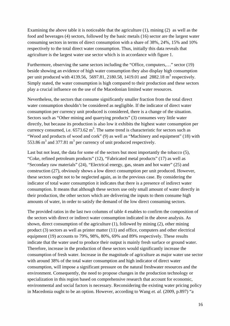
Table 4. Summary of the water consumption indicators

Nr. Sectors

Direct total water cons.

per sector (in million m3)

% of total

direct water cons.

Indicator of direct water

cons. per currency unit

produced (in m3)

Indicator of total water

cons. (in m3 per millions of MKD2)

directwd/wt

(%)

indirect (wt-wd)/wt

(%)

1 Agriculture, forestry and fisheries 255.10 37.77 4139.56 5833.75 70.96 29.04

2 Mining and quarrying 161.33 23.89 5697.81 5821.49 97.88 2.12

3 Other mining and quarrying products 26.43 3.91 6573.62 8168.80 80.47 19.53

4 Food products and beverages 103.37 15.31 2180.58 4109.67 53.06 46.94

5 Tobacco products 0.40 0.06 42.68 2786.31 1.53 98.47

6 Textiles 0.45 0.07 24.14 82.87 29.13 70.87

7 Wearing apparel; furs 0.97 0.14 31.83 195.78 16.26 83.74

8 Leather and leather products 0.04 0.01 8.50 160.25 5.31 94.69

9 Wood and products of wood and cork (except furniture); articles of straw and plaiting materials

2.20 0.33 553.86 1282.24 43.19 56.81

10 Pulp, paper and paper products 0.08 0.01 9.17 229.08 4.00 96.00

11 Printed matter and recorded media 0.29 0.04 163.27 237.64 68.71 31.29 12 Coke, refined petroleum products and

nuclear fuels 0.28 0.04 10.21 3937.40 0.26 99.74

13 Chemicals, chemical products and man-made fibres

4.71 0.70 222.78 397.57 56.03 43.97

14 Rubber and plastic products 0.07 0.01 8.09 159.90 5.06 94.94

15 Other non-metallic mineral products 1.46 0.22 145.14 1330.13 10.91 89.09

16 Basic metals 68.13 10.09 1419.01 2838.04 50.00 50.00 17 Fabricated metal products, except

machinery and equipment 0.09 0.01 12.37 992.07 1.25 98.75

18 Machinery and equipment 4.52 0.67 377.81 628.53 60.11 39.89 19 Office, computers; Electrical

machinery and apparatus; Radio, TV, communication

42.81 6.34 2882.18 3328.16 86.60 13.40

20 Medical, precision and optical instruments, watches and clocks

0.18 0.03 3.98 28.42 14.01 85.99

21 Motor vehicles, trailers and semi-trailers

0.00 0.00 18.57 316.32 5.87 94.13

22 Other transport equipment 0.13 0.02 80.90 594.64 13.60 86.40

23 Furniture; other manufactured goods 0.31 0.05 69.86 170.78 40.91 59.09

24 Secondary raw materials 0.00 0.00 2.92 859.30 0.34 99.66 25 Electrical energy, gas, steam and hot

water 1.00 0.15 55.58 1497.27 3.71 96.29

26 Collected and purified water, distribution services of water

0.00 0.00 0.00 505.95 0.00 100.00

27 Construction work 1.00 0.15 23.34 1076.58 2.17 97.83

28 Services 8.40 1.24 29.55 459.90 6.42 93.58

Total direct water consumption 675.38 100

                                                            2 61,5 MKD = 1 €

  

16  

Examining the above table it is noticeable that the agriculture (1), mining (2) as well as the food and beverages (4) sectors, followed by the basic metals (16) sector are the largest water consuming sectors in terms of direct consumption with a share of 38%, 24%, 15% and 10% respectively to the total direct water consumption. Thus, initially this data reveals that agriculture is the largest water use sector which is in accordance with figure 1.

Furthermore, observing the same sectors including the “Office, computers,…” sector (19) beside showing an evidence of high water consumption they also display high consumption per unit produced with 4139.56, 5697.81, 2180.58, 1419.01 and 2882.18 m3 respectively. Simply stated, the water consumption is high compared to their production and these sectors play a crucial influence on the use of the Macedonian limited water resources.

Nevertheless, the sectors that consume significantly smaller fraction from the total direct water consumption shouldn’t be considered as negligible. If the indicator of direct water consumption per currency unit produced is considered, there is a change of the situation. Sectors such as “Other mining and quarrying products” (3) consumes very little water directly, but because its production is also low it exhibits the highest water consumption per currency consumed, i.e. 6573.62 m3. The same trend is characteristic for sectors such as “Wood and products of wood and cork” (9) as well as “Machinery and equipment” (18) with 553.86 m3 and 377.81 m3 per currency of unit produced respectively.

Last but not least, the data for some of the sectors but most importantly the tobacco (5), “Coke, refined petroleum products” (12), “Fabricated metal products” (17) as well as “Secondary raw materials” (24), “Electrical energy, gas, steam and hot water” (25) and construction (27), obviously shows a low direct consumption per unit produced. However, these sectors ought not to be neglected again, as in the previous case. By considering the indicator of total water consumption it indicates that there is a presence of indirect water consumption. It means that although these sectors use only small amount of water directly in their production, the other sectors which are delivering the inputs to them consume high amounts of water, in order to satisfy the demand of the low direct consuming sectors.

The provided ratios in the last two columns of table 4 enables to confirm the composition of the sectors with direct or indirect water consumption indicated in the above analysis. As shown, direct consumption of the agriculture (1), followed by mining (2), other mining product (3) sectors as well as printer matter (11) and office, computers and other electrical equipment (19) accounts to 79%, 98%, 80%, 69% and 89% respectively. These results indicate that the water used to produce their output is mainly fresh surface or ground water. Therefore, increase in the production of these sectors would significantly increase the consumption of fresh water. Increase in the magnitude of agriculture as major water use sector with around 38% of the total water consumption and high indicator of direct water consumption, will impose a significant pressure on the natural freshwater resources and the environment. Consequently, the need to propose changes in the production technology or specialization in this region based on comprehensive research that account for economic, environmental and social factors is necessary. Reconsidering the existing water pricing policy in Macedonia ought to be an option. However, according to Wang et. al. (2009, p.897) “a

  

17  

broadened economic policy should account for not only productive criteria but also on social and environmental factors”.

Converse to this, most of the industrial sectors are characterized by relatively high indirect consumption shares compare to the total water use indicator. Sectors such as tobacco (5), leather (8), pulp products (10), coke and refined petroleum (12), followed by rubber and plastic (14) and fabricated metals products (17) as well as motor vehicle (21), secondary raw materials (24) and electrical energy (25) are characterized with a share around 95% or exceeding this degree by reaching almost 99% of indirect water consumption. Construction (27) and services (28) sectors follow the same pattern of high indirect consumption as the industrial sectors with 98% and 94% respectively. This means that these sectors have a huge potential to “drag” the economy in terms of water use.

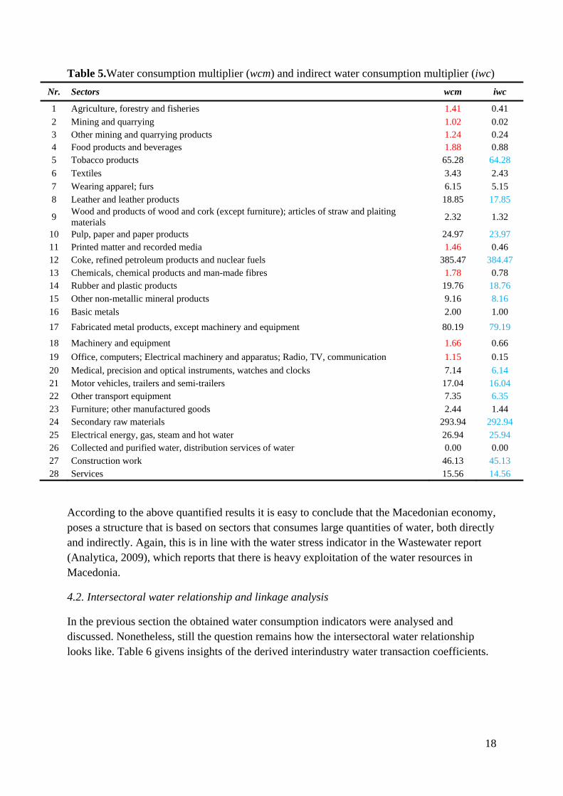
However, what is of great interest is how much this “drag effect” is in quantity. Table 5 gives an overview of the water consumption multipliers (wcm) and the indirect water consumption multipliers (iwc) for each sector. The above distinction of direct and indirect water consuming sectors is confirmed by the provided values. Hence, the low values of wcm verify the statement we made earlier on sectors such as agriculture (1), mining (2), food and beverages (4), electrical equipment (19) etc. that are attributed by direct water consumption. In other words, if there is an increase of one unit in the final demand of a given sector, the total water consumption will be increased by 1.41 for agriculture, 1.02 for mining sector, 1.88 for the food and beverages, etc. Therefore, the “drag effect” is very small. On the other hand, the sectors considered as indirect consumers display very high iwc values compare to the sectors that shown low wcm values. As mentioned earlier, if only the indicator of direct water consumption was considered in table 4 these sectors would be disregarded. However, examining table 5 it is noticeable that for each cubic meter of water consumed directly, to satisfy its production tobacco sector (5) requires additional 64.28 m3 of water to be consumed by the other sectors. Similarly, for the fabricated metals (17) and construction work (27) sectors, each cubic meter of directly consumed water requires additional indirect consumption by the other sectors of 79.19 m3 and 45.13 m3 of water respectively. What is important to be noticed here is the significantly high levels of indirect water consumption by the coke and refined petroleum sector (12) and the secondary raw materials sector (24) with 384.47 m3 and 292.94 m3 of water consumed indirectly per 1 m3 of directly consumed water. However, given the results in table 4, i.e. the share of indirect consumption relative to the total consumption is 99.74% and 99.66%. Therefore, such a high level of indirect consumption it should be expected to some extent. These results reveal that such sectors with relatively high indirect water consumption ought to be considered as the driving forces of the Macedonian economy due to the strong influence of their product demand will affect the production of the remaining economic agents. Nevertheless, as indicated above more complete research and relevant economic policy that will take into account the environmental factors besides the productive decisive factor is essential due to the pressure may emerge on the limited water resources.

  

18  

Table 5.Water consumption multiplier (wcm) and indirect water consumption multiplier (iwc)

Nr. Sectors wcm iwc

1 Agriculture, forestry and fisheries 1.41 0.41

2 Mining and quarrying 1.02 0.02 3 Other mining and quarrying products 1.24 0.24 4 Food products and beverages 1.88 0.88 5 Tobacco products 65.28 64.28

6 Textiles 3.43 2.43

7 Wearing apparel; furs 6.15 5.15 8 Leather and leather products 18.85 17.85

9 Wood and products of wood and cork (except furniture); articles of straw and plaiting materials

2.32 1.32

10 Pulp, paper and paper products 24.97 23.97 11 Printed matter and recorded media 1.46 0.46 12 Coke, refined petroleum products and nuclear fuels 385.47 384.47 13 Chemicals, chemical products and man-made fibres 1.78 0.78 14 Rubber and plastic products 19.76 18.76 15 Other non-metallic mineral products 9.16 8.16

16 Basic metals 2.00 1.00

17 Fabricated metal products, except machinery and equipment 80.19 79.19

18 Machinery and equipment 1.66 0.66

19 Office, computers; Electrical machinery and apparatus; Radio, TV, communication 1.15 0.15

20 Medical, precision and optical instruments, watches and clocks 7.14 6.14 21 Motor vehicles, trailers and semi-trailers 17.04 16.04 22 Other transport equipment 7.35 6.35 23 Furniture; other manufactured goods 2.44 1.44 24 Secondary raw materials 293.94 292.94 25 Electrical energy, gas, steam and hot water 26.94 25.94 26 Collected and purified water, distribution services of water 0.00 0.00 27 Construction work 46.13 45.13 28 Services 15.56 14.56

According to the above quantified results it is easy to conclude that the Macedonian economy, poses a structure that is based on sectors that consumes large quantities of water, both directly and indirectly. Again, this is in line with the water stress indicator in the Wastewater report (Analytica, 2009), which reports that there is heavy exploitation of the water resources in Macedonia.

4.2. Intersectoral water relationship and linkage analysis

In the previous section the obtained water consumption indicators were analysed and discussed. Nonetheless, still the question remains how the intersectoral water relationship looks like. Table 6 givens insights of the derived interindustry water transaction coefficients.

  

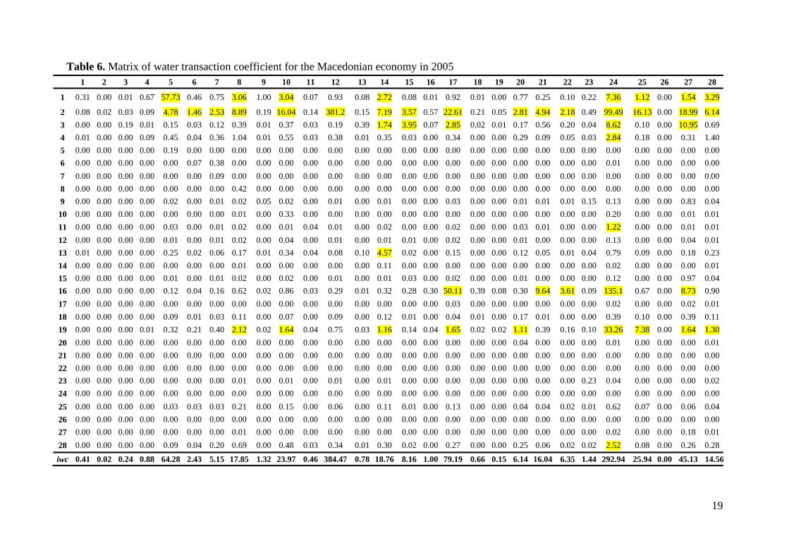
19  

Table 6. Matrix of water transaction coefficient for the Macedonian economy in 2005 1 2 3 4 5 6 7 8 9 10 11 12 13 14 15 16 17 18 19 20 21 22 23 24 25 26 27 28

1 0.31 0.00 0.01 0.67 57.73 0.46 0.75 3.06 1.00 3.04 0.07 0.93 0.08 2.72 0.08 0.01 0.92 0.01 0.00 0.77 0.25 0.10 0.22 7.36 1.12 0.00 1.54 3.29

2 0.08 0.02 0.03 0.09 4.78 1.46 2.53 8.89 0.19 16.04 0.14 381.2 0.15 7.19 3.57 0.57 22.61 0.21 0.05 2.81 4.94 2.18 0.49 99.49 16.13 0.00 18.99 6.14

3 0.00 0.00 0.19 0.01 0.15 0.03 0.12 0.39 0.01 0.37 0.03 0.19 0.39 1.74 3.95 0.07 2.85 0.02 0.01 0.17 0.56 0.20 0.04 8.62 0.10 0.00 10.95 0.69

4 0.01 0.00 0.00 0.09 0.45 0.04 0.36 1.04 0.01 0.55 0.03 0.38 0.01 0.35 0.03 0.00 0.34 0.00 0.00 0.29 0.09 0.05 0.03 2.84 0.18 0.00 0.31 1.40

5 0.00 0.00 0.00 0.00 0.19 0.00 0.00 0.00 0.00 0.00 0.00 0.00 0.00 0.00 0.00 0.00 0.00 0.00 0.00 0.00 0.00 0.00 0.00 0.00 0.00 0.00 0.00 0.00

6 0.00 0.00 0.00 0.00 0.00 0.07 0.38 0.00 0.00 0.00 0.00 0.00 0.00 0.00 0.00 0.00 0.00 0.00 0.00 0.00 0.00 0.00 0.00 0.01 0.00 0.00 0.00 0.00

7 0.00 0.00 0.00 0.00 0.00 0.00 0.09 0.00 0.00 0.00 0.00 0.00 0.00 0.00 0.00 0.00 0.00 0.00 0.00 0.00 0.00 0.00 0.00 0.00 0.00 0.00 0.00 0.00

8 0.00 0.00 0.00 0.00 0.00 0.00 0.00 0.42 0.00 0.00 0.00 0.00 0.00 0.00 0.00 0.00 0.00 0.00 0.00 0.00 0.00 0.00 0.00 0.00 0.00 0.00 0.00 0.00

9 0.00 0.00 0.00 0.00 0.02 0.00 0.01 0.02 0.05 0.02 0.00 0.01 0.00 0.01 0.00 0.00 0.03 0.00 0.00 0.01 0.01 0.01 0.15 0.13 0.00 0.00 0.83 0.04

10 0.00 0.00 0.00 0.00 0.00 0.00 0.00 0.01 0.00 0.33 0.00 0.00 0.00 0.00 0.00 0.00 0.00 0.00 0.00 0.00 0.00 0.00 0.00 0.20 0.00 0.00 0.01 0.01

11 0.00 0.00 0.00 0.00 0.03 0.00 0.01 0.02 0.00 0.01 0.04 0.01 0.00 0.02 0.00 0.00 0.02 0.00 0.00 0.03 0.01 0.00 0.00 1.22 0.00 0.00 0.01 0.01

12 0.00 0.00 0.00 0.00 0.01 0.00 0.01 0.02 0.00 0.04 0.00 0.01 0.00 0.01 0.01 0.00 0.02 0.00 0.00 0.01 0.00 0.00 0.00 0.13 0.00 0.00 0.04 0.01

13 0.01 0.00 0.00 0.00 0.25 0.02 0.06 0.17 0.01 0.34 0.04 0.08 0.10 4.57 0.02 0.00 0.15 0.00 0.00 0.12 0.05 0.01 0.04 0.79 0.09 0.00 0.18 0.23

14 0.00 0.00 0.00 0.00 0.00 0.00 0.00 0.01 0.00 0.00 0.00 0.00 0.00 0.11 0.00 0.00 0.00 0.00 0.00 0.00 0.00 0.00 0.00 0.02 0.00 0.00 0.00 0.01

15 0.00 0.00 0.00 0.00 0.01 0.00 0.01 0.02 0.00 0.02 0.00 0.01 0.00 0.01 0.03 0.00 0.02 0.00 0.00 0.01 0.00 0.00 0.00 0.12 0.00 0.00 0.97 0.04

16 0.00 0.00 0.00 0.00 0.12 0.04 0.16 0.62 0.02 0.86 0.03 0.29 0.01 0.32 0.28 0.30 50.11 0.39 0.08 0.30 9.64 3.61 0.09 135.1 0.67 0.00 8.73 0.90

17 0.00 0.00 0.00 0.00 0.00 0.00 0.00 0.00 0.00 0.00 0.00 0.00 0.00 0.00 0.00 0.00 0.03 0.00 0.00 0.00 0.00 0.00 0.00 0.02 0.00 0.00 0.02 0.01

18 0.00 0.00 0.00 0.00 0.09 0.01 0.03 0.11 0.00 0.07 0.00 0.09 0.00 0.12 0.01 0.00 0.04 0.01 0.00 0.17 0.01 0.00 0.00 0.39 0.10 0.00 0.39 0.11

19 0.00 0.00 0.00 0.01 0.32 0.21 0.40 2.12 0.02 1.64 0.04 0.75 0.03 1.16 0.14 0.04 1.65 0.02 0.02 1.11 0.39 0.16 0.10 33.26 7.38 0.00 1.64 1.30

20 0.00 0.00 0.00 0.00 0.00 0.00 0.00 0.00 0.00 0.00 0.00 0.00 0.00 0.00 0.00 0.00 0.00 0.00 0.00 0.04 0.00 0.00 0.00 0.01 0.00 0.00 0.00 0.01

21 0.00 0.00 0.00 0.00 0.00 0.00 0.00 0.00 0.00 0.00 0.00 0.00 0.00 0.00 0.00 0.00 0.00 0.00 0.00 0.00 0.00 0.00 0.00 0.00 0.00 0.00 0.00 0.00

22 0.00 0.00 0.00 0.00 0.00 0.00 0.00 0.00 0.00 0.00 0.00 0.00 0.00 0.00 0.00 0.00 0.00 0.00 0.00 0.00 0.00 0.00 0.00 0.00 0.00 0.00 0.00 0.00

23 0.00 0.00 0.00 0.00 0.00 0.00 0.00 0.01 0.00 0.01 0.00 0.01 0.00 0.01 0.00 0.00 0.00 0.00 0.00 0.00 0.00 0.00 0.23 0.04 0.00 0.00 0.00 0.02

24 0.00 0.00 0.00 0.00 0.00 0.00 0.00 0.00 0.00 0.00 0.00 0.00 0.00 0.00 0.00 0.00 0.00 0.00 0.00 0.00 0.00 0.00 0.00 0.00 0.00 0.00 0.00 0.00

25 0.00 0.00 0.00 0.00 0.03 0.03 0.03 0.21 0.00 0.15 0.00 0.06 0.00 0.11 0.01 0.00 0.13 0.00 0.00 0.04 0.04 0.02 0.01 0.62 0.07 0.00 0.06 0.04

26 0.00 0.00 0.00 0.00 0.00 0.00 0.00 0.00 0.00 0.00 0.00 0.00 0.00 0.00 0.00 0.00 0.00 0.00 0.00 0.00 0.00 0.00 0.00 0.00 0.00 0.00 0.00 0.00

27 0.00 0.00 0.00 0.00 0.00 0.00 0.00 0.01 0.00 0.00 0.00 0.00 0.00 0.00 0.00 0.00 0.00 0.00 0.00 0.00 0.00 0.00 0.00 0.02 0.00 0.00 0.18 0.01

28 0.00 0.00 0.00 0.00 0.09 0.04 0.20 0.69 0.00 0.48 0.03 0.34 0.01 0.30 0.02 0.00 0.27 0.00 0.00 0.25 0.06 0.02 0.02 2.52 0.08 0.00 0.26 0.28

iwc  0.41 0.02 0.24 0.88 64.28 2.43 5.15 17.85 1.32 23.97 0.46 384.47 0.78 18.76 8.16 1.00 79.19 0.66 0.15 6.14 16.04 6.35 1.44 292.94 25.94 0.00 45.13 14.56

  

20  

Examining the table it is evident that most coefficients are relatively low, showing that the water transactions are limited and dominated by only few sectors. Given this, the associated transactions with low coefficient should be ignored. As indicated in table 5 most of the manufacturing sectors were attributed with high indirect water use. Thus, for the tobacco (5), leather (8), wood (10) and secondary raw material (24) sectors, table 6 reveal the obvious result that the indirect water consumption is mainly driven by the agricultural (1) sector. Meaning that for each cubic meter of water consumed directly by the tobacco, leather, wood as well as secondary raw material sectors, to satisfy this demand there will be additional quantity of 57.53, 3.06, 3.04 and 7.36 m3 of water, to be consumed by agriculture. Furthermore, another obvious result is noticeable in table 6. The coke and refined petroleum (12) sector which displayed the highest iwc, its indirect water consumption is mainly focused on the mining and quarrying (2) sector. The same relationship holds for the secondary raw material (24) sector followed by the fabricated metal products (17) as well as the energy (25) and the constriction (27) sector. Thus, for each 1m3 direct consumption by the above listed sectors, satisfying this demand requires additional 381.2, 99.49, 22.61, 16.13 and 18.99 m3 of water respectively, to be consumed by the mining (2) sector. Inference of the other water relationships may be conducted in the same manner. Basic metals (16) sector needs an additional 50.11 and 135.1 m3 of water to satisfy the direct demand of the fabricated metal products (17) and secondary raw material (24) sector.

Although the above interpretation of table 6 may looks straight forward, to some level the reader may find it complex and hard to follow the transactions among the sectors. Thus, the linkage analysis will give us a clearer picture in identifying the key water consuming sectors. From table 7, the different values of the indices of backward and forward linkages may be observed i.e. sectors that have greater impact on the whole water consumption process through both purchases and sales. Observing the values it may be noticed that agriculture (1), other mining and quarry (3), food (4), tobacco (5) such as the fuel (12), basic metal (16) and energy (25) sectors display greater backward water linkages with respect to the water consumption. Meaning that with their purchases of products from the rest of the economy the water consumption is increased more than the other sectors do. Coke and refined petroleum (12) sector exhibits the highest backward linkage index with 7.56. With respect to the forward linkage, agriculture (1) is also found to show high forward linkage index of 5.59. Among the manufacturing sectors, again the other mining and quarrying (3), as well as the coke and refined petroleum (12), basic metals (16) and the energy (25) sectors appears to have relative greater forward linkages indices. Chemical products (13) have the smallest forward linkage index of 1.30 whereas the service (28) sectors display the highest forward linkage index in the economy, 7.97. This may be explained by the fact that the service sector in Macedonia provides around 40% to the GDP. However, In terms of interpretation of the indices in water consumption, it means that these sectors with their sells to the other economic agents, they push up the water consumption more than the other sectors do. In relation to table 3 and the provided values of the backward and forward linkages in table 7, it may be argued and confirmed that agriculture (1), other mining and quarrying (3), coke and refined petroleum (12) as well as the basic metals (16) and the energy sectors (25) are the key water use sectors

  

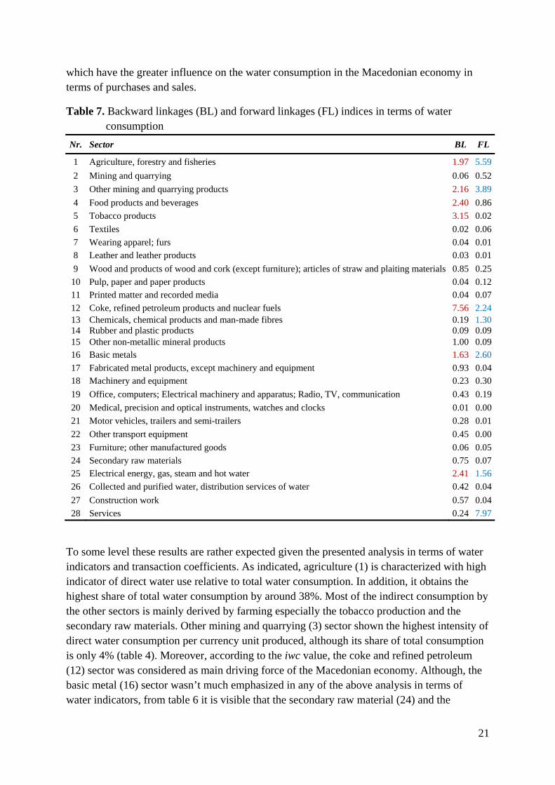
21  

which have the greater influence on the water consumption in the Macedonian economy in terms of purchases and sales.

Table 7. Backward linkages (BL) and forward linkages (FL) indices in terms of water consumption

Nr. Sector BL FL

1 Agriculture, forestry and fisheries 1.97 5.59

2 Mining and quarrying 0.06 0.52

3 Other mining and quarrying products 2.16 3.89

4 Food products and beverages 2.40 0.86

5 Tobacco products 3.15 0.02

6 Textiles 0.02 0.06

7 Wearing apparel; furs 0.04 0.01

8 Leather and leather products 0.03 0.01

9 Wood and products of wood and cork (except furniture); articles of straw and plaiting materials 0.85 0.25

10 Pulp, paper and paper products 0.04 0.1211 Printed matter and recorded media 0.04 0.07

12 Coke, refined petroleum products and nuclear fuels 7.56 2.2413 Chemicals, chemical products and man-made fibres 0.19 1.3014 Rubber and plastic products 0.09 0.0915 Other non-metallic mineral products 1.00 0.0916 Basic metals 1.63 2.60

17 Fabricated metal products, except machinery and equipment 0.93 0.0418 Machinery and equipment 0.23 0.30

19 Office, computers; Electrical machinery and apparatus; Radio, TV, communication 0.43 0.19

20 Medical, precision and optical instruments, watches and clocks 0.01 0.00

21 Motor vehicles, trailers and semi-trailers 0.28 0.01

22 Other transport equipment 0.45 0.00

23 Furniture; other manufactured goods 0.06 0.05

24 Secondary raw materials 0.75 0.0725 Electrical energy, gas, steam and hot water 2.41 1.56

26 Collected and purified water, distribution services of water 0.42 0.04

27 Construction work 0.57 0.04

28 Services 0.24 7.97

To some level these results are rather expected given the presented analysis in terms of water indicators and transaction coefficients. As indicated, agriculture (1) is characterized with high indicator of direct water use relative to total water consumption. In addition, it obtains the highest share of total water consumption by around 38%. Most of the indirect consumption by the other sectors is mainly derived by farming especially the tobacco production and the secondary raw materials. Other mining and quarrying (3) sector shown the highest intensity of direct water consumption per currency unit produced, although its share of total consumption is only 4% (table 4). Moreover, according to the iwc value, the coke and refined petroleum (12) sector was considered as main driving force of the Macedonian economy. Although, the basic metal (16) sector wasn’t much emphasized in any of the above analysis in terms of water indicators, from table 6 it is visible that the secondary raw material (24) and the

  

22  

electrical equipment sector (17) their indirect consumption is mainly derived by the basic metals products. Last but not least that needs to be considered is the deviation which the electrical energy (25) sector displays. Although it was characterized as sector with high indirect water consumption share (around 96%) in most of the result interpretation it didn’t display any high importance. On the other hand, the secondary raw material products (24) which obtained the second largest iwc value (292.94) didn’t display any high linkage indices although from the transaction coefficient matrix much indirect interaction is noticeable. The mining (2) sector which was main provider of water to the other industrial sector didn’t also display any high linkage analysis that may categorize it as key water use sector. Therefore, this relationship should be investigated furthermore and ranking the sectors on fuzzy environment is again an imperative in that manner. Other aspect that might be of interest is measurement of sectoral interdependencies based on Dietzenbacher method or the eigenvector method. It is well know that this method is superior and provides better indicator of the interindustry linkages that the above implemented Rasmussen linkage analysis (Dietzenbacher, 1992).

4.3. Trade balance and closing the economy

Before concluding the paper some important aspects will be investigated briefly in this section, which the other studies raised in their concluding remarks. Velazquez (2006), Yu et. al. (2010), Wang et. al. (2010) are among the others that raise the concern of completing their studies by incorporating other variables such as the value added or study the international trade by means of so called “virtual water”.

The term “virtual water” was firstly introduced by Allan in 1998 (Velazquez, 2007; Wang et. al, 2010). It indicates the water consumption that may not be directly detected i.e. “embodied” during the process of production. However, Hoekstra (2002) extended the definition in two broad categories: real and theoretical virtual water. The first one refers to the water that is actually used in the domestic production whereas the other category refers to potential water that would have been used in the production in the country of destination. Whatever category is used, both are appropriate to study the importance of water in trade balance.

The idea that the agricultural sector was identified as key water consuming sector with high indicator of direct water consumption, it conveys the idea that high quantities of water that is embodied in the agriculture products are then as intermediate products incorporated in other sectors. Thus, it is the main supplier of indirect virtual water to the other economic agents. According to Wang et. al. (2010) animal husbandry and fisheries are additional suppliers of virtual water because of it high water content in their products.

Although reservoirs and dams are build to control the supply, or measures such as pricing policies and awareness campaign are imposed to reduce the water demand, Velazquez (2007) argues that trading virtual water may be an instrument to control and promote sustainable natural resource management as well as reduce the pressure on the existing water resources. Geographical regions with water scarcity issues should export products that have competitive advantage, i.e. require less water and import water intensive products.

  

23  

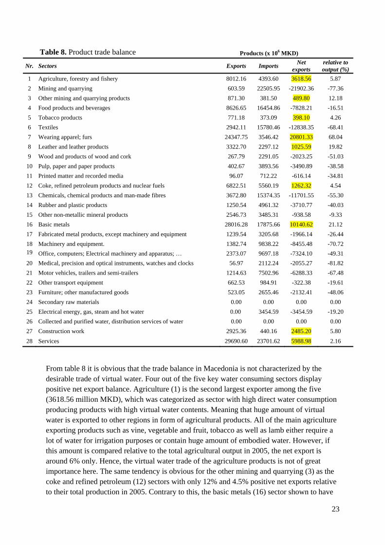
Table 8. Product trade balance Products (x 106 MKD)

Nr. Sectors Exports Imports Net

exports relative to output (%)

1 Agriculture, forestry and fishery 8012.16 4393.60 3618.56 5.87

2 Mining and quarrying 603.59 22505.95 -21902.36 -77.36

3 Other mining and quarrying products 871.30 381.50 489.80 12.18

4 Food products and beverages 8626.65 16454.86 -7828.21 -16.51

5 Tobacco products 771.18 373.09 398.10 4.26

6 Textiles 2942.11 15780.46 -12838.35 -68.41

7 Wearing apparel; furs 24347.75 3546.42 20801.33 68.04

8 Leather and leather products 3322.70 2297.12 1025.59 19.82

9 Wood and products of wood and cork 267.79 2291.05 -2023.25 -51.03

10 Pulp, paper and paper products 402.67 3893.56 -3490.89 -38.58

11 Printed matter and recorded media 96.07 712.22 -616.14 -34.81

12 Coke, refined petroleum products and nuclear fuels 6822.51 5560.19 1262.32 4.54

13 Chemicals, chemical products and man-made fibres 3672.80 15374.35 -11701.55 -55.30

14 Rubber and plastic products 1250.54 4961.32 -3710.77 -40.03

15 Other non-metallic mineral products 2546.73 3485.31 -938.58 -9.33

16 Basic metals 28016.28 17875.66 10140.62 21.12

17 Fabricated metal products, except machinery and equipment 1239.54 3205.68 -1966.14 -26.44

18 Machinery and equipment. 1382.74 9838.22 -8455.48 -70.72 19 Office, computers; Electrical machinery and apparatus; … 2373.07 9697.18 -7324.10 -49.31

20 Medical, precision and optical instruments, watches and clocks 56.97 2112.24 -2055.27 -81.82

21 Motor vehicles, trailers and semi-trailers 1214.63 7502.96 -6288.33 -67.48

22 Other transport equipment 662.53 984.91 -322.38 -19.61

23 Furniture; other manufactured goods 523.05 2655.46 -2132.41 -48.06

24 Secondary raw materials 0.00 0.00 0.00 0.00

25 Electrical energy, gas, steam and hot water 0.00 3454.59 -3454.59 -19.20

26 Collected and purified water, distribution services of water 0.00 0.00 0.00 0.00

27 Construction work 2925.36 440.16 2485.20 5.80

28 Services 29690.60 23701.62 5988.98 2.16

From table 8 it is obvious that the trade balance in Macedonia is not characterized by the desirable trade of virtual water. Four out of the five key water consuming sectors display positive net export balance. Agriculture (1) is the second largest exporter among the five (3618.56 million MKD), which was categorized as sector with high direct water consumption producing products with high virtual water contents. Meaning that huge amount of virtual water is exported to other regions in form of agricultural products. All of the main agriculture exporting products such as vine, vegetable and fruit, tobacco as well as lamb either require a lot of water for irrigation purposes or contain huge amount of embodied water. However, if this amount is compared relative to the total agricultural output in 2005, the net export is around 6% only. Hence, the virtual water trade of the agriculture products is not of great importance here. The same tendency is obvious for the other mining and quarrying (3) as the coke and refined petroleum (12) sectors with only 12% and 4.5% positive net exports relative to their total production in 2005. Contrary to this, the basic metals (16) sector shown to have

  

24  

around 20% positive net exports compare to its total production. Although none of the water indicators display extreme values for this sector, still the direct water consumption per unit produced is larger compare to the other sectors (1419.01 m3) and it was shown that most of the indirect water consumption for the fabricated metal products (17) and secondary raw material (24) sector is derived by it. Thus, future water strategies should be designed for this sector.

Closing the economy similar results were obtained in terms of water consumption indicators and linkage analysis. Almost all manufacturing sectors display high rate of indirect consumption. The results won’t be discussed in detailed as in the case of open economy, but all results and associated tables are provided in appendix 2. The only exception in the analysis is that now the household demand appears to be categorized as main water consuming sectors along with the other five previously mentioned. The agricultural demand share compare to the total direct water consumption dropped to 28% and similar percentage obtains the household demand, i.e. 24%. Hence, there is significant competition between the urban and agriculture water supply as indicated in the introduction. Converse to the agriculture, the household demand (29) sector is characterized with indirect water consumption but according to the iwc it was significantly small (see appendix 2). Yet, the transaction coefficient matrix reveals that significant number of the economic agents in the Macedonian economy derive their indirect water consumption largely from the household demand. If there is an increase by 1 m3 of water directly consumed by the leather (8), paper (10), fabricated metals (17) products as well as the medical instrument (20), secondary raw material (24) and construction (27) sector, to satisfy this use the household sector as main supplier of work force should additionally consume 27.44, 34.31, 21.90 as well as 23.39, 98.20 and 17.08 m3 of water. In terms of linkage analysis, the forward linkage index is even greater than the one obtained for the services (28) when the economy was closed, meaning that individually on average it boosts up the water consumption more than the other sectors do together.

Therefore, given these results, the competition with agriculture and the climate change issue especially the future climate projections for the agriculture yield and precipitation reduction, necessity in reconsidering agriculture water pricing policies or the utilized production technology where water is used as production factor, is fundamental.

5. Conclusion

This paper gives an overview of the water consumption in Macedonia in 2005 in an input-output framework. Although, the paper doesn’t provide any significant contribution to the existing developed model, the most relevant contribution is the first attempt to quantify and investigate the water relationships in Macedonia which may serve as basis for promoting and developing sustainable management of water resources. The main conclusion is that the Macedonian economy is characterized by water intensive structure mainly focused around agriculture and several industrial sectors. The derived indicator unable us to observe and trace a distinction between direct and indirect water consumption where agriculture present a high rate of direct water use. In addition, agriculture is the main sector where the indirect

  

25  

consumption is derived especially for the tobacco and the secondary raw material sectors. On the other hand, the manufacturing sectors such as coke and refined petroleum as well as the secondary raw material shown the highest rate of indirect consumption which was mainly derived by the mining and basic metals sector.

Closing the economy in terms of household demand didn’t change much the situation. Except that now the agriculture has to compete with the urban household water demand which both were identified as key water consuming sectors.

Although, virtual water is considered to be an alternative source of ensuring water security the option to import water in the form of economic goods is not an imperative here apart from the basic metal product with the highest positive net exports.

Necessity to introduce changes in the production technology or specialization in this region or reconsidering the existing water pricing policy based on comprehensive research ought to be an option.

Important limitations of I-O methodology need to be recognized although I-O analysis is the most widely used method for assessing the environmental impacts of economic production (Wang et. al, 2009). The main critic on input-output analysis brings to the forefront the fact that the analysis is static, i.e. it is just a “snapshot” of the Macedonian economy in 2005. Over the years the economic structure might be different, so the results here presented are intended to be only indicative for that certain year. Considering changes in the composition or proportion of the input use over time may be analysed by using new recently published I-O table. In addition, linearity assumption of the model structure as well as fixed proportion production technology with constant prices ensures additional limitation of this methodology (Miller and Blair, 2009). Absence of substitution in consumption or input use may not be in line with the reality. However at this point the conclusion that Wang et. al. (2009) draw, i.e. that the model may overstate the water consumption multipliers due to the absence of substitution, we find it inappropriate. Referring back to the first sentence of the paper we, declare that water is “essential, irreplaceable and limited” natural resource. Thus, from our point of view there is no such input that may substitute water in any stage of the production process of all the economic agents. Their claim is only true in terms of conventional input-output analysis.

Improvements of our research in terms of water consumption may be disaggregation of agriculture (which by now is viewed as a single agricultural unit) by developing a make-and-use matrix. The approach for disaggregation of agriculture as major water consuming sectors, could be similar to the one used by Lindberg and Hansson (2009) for Sweden where the end result will be a detailed and disaggregated input-output table of the Macedonian economy with a special emphasis on agriculture. More in depth analysis by including the waste water generation by each economic agent may be included in order to gain a wider picture of the economic production structures and its environmental impact. Most important future development of our work should be focused on incorporating fuzzy input-output analysis due to the absence and uncertainty of the used data.

  

26  

References

1. ABS - Australian Bureau of Statistics. 2010. Water Account Australia 2008-09. Catalogue no. 4610.0. Canberra.

2. Analytica. Wastewater Issue: High time for better management - The case of Macedonia. 2009.

3. Chen, X.K. (2000). Shanxi water resource input–occupancy–output table and its application in Shanxi Province of China. In: Thirteenth International Conference on Input–Output Techniques, Macerata, Italy.

4. Chenery, H.B., Watanabe, T., 1958. International Comparisons of the Structure of Production. Econometrica 26:487-521.

5. Dietzenbacher, E. (1992). The measurement of inter-industry linkages: Key sectors in the Netherlands. Economic Modelling 9:449-437.

6. Donveska, K., Dodeva, S. & Taseva, J. Urban and agricultural competition for water in the Republic of Macedonia. Paper presented at the 54th Executive Council of ICID, 20th European Regional Conference, Montpellier, 14-19 September, 2003.

7. Duarte, R., Sanchez-Choliz, J. & Bielsa, J. (2002). Water use in the Spanish economy: an input-output approach. Ecological Economics 43, 71-85.

8. Duarte, R. and Chóliz, S.J. (1998). Regional Productive Structure and Water Pollution: An Analysis using the Input-Output Model. In: 38th Congress of The European Regional Science Association, August -1st September, Vienna, European Regional Science Association.

9. Duarte, R., Chóliz, J.S. and Bielsa, J. (2002). Water use in the Spanish economy: an input-output approach. Ecological Economics 43 (1), 71–85.

10. EUROSTAT (2002). Water Accounts – Results of pilot studies. Theme 2: Economy and finance. Belgium.

11. Hawdon, D. & Pearson, P. (1995). Input–output simulations of energy, environment, economy interactions in the UK. Energy Economics 17 (1), 73– 86.

12. Hoekstra, A.Y.( 2002). Virtual water. An introduction. Virtual water trade. Proceedings of the International Expert Meeting on Virtual Water Trade. Values of Water Research Report Series, vol. 12. IHE, Delft, Holanda.

13. Hubacek, K. and Sun, L. (2001). A Scenario Analysis of China’s Land Use and Land Cover Change: Incorporating Biophysical Information Into Input–Output Modeling, Structural Change and Economic Dynamics, 12(4), pp. 367–397.

14. ICID, International Commission on Irrigation and Drainage, http://www.icid.org/

1. Macedonia country report, 2011-11-13, www.icid.org/v_macedonia.pdf 

  

27  

15. Lenzen, M. and Foran, B. (2001). An Input-Output Analysis of Australian Water Usage, Water Policy, 3(4), pp.321-340.

16. Leontief, W. (1970). Environmental repercussions and the economic structure: an input–output approach. Review of Economics and Statistics, 52: 262–271. In: Kurz, H.D, Dietzenbacher, E. & Lager, C. (Eds.), 1998: 24–33.

17. Liang, Q.M., Fan, Y. and Wei, E.M. (2007). Multi-regional input–output model for regional energy requirements and CO2 emissions in China, Energy Policy, 35(3), pp.1685-1700.

18. Lindberg G. and H. Hansson (2009). Economic impacts of agriculture in Sweden: A disaggregated input-output approach.. Food Economics- Acta Agriculturae Scandinavica, Section C. Vol 6:119-133.

19. Lofting, E.M. & Mcgauhey, P.H. (1968). Economic Valuation ofWater. An Input–Output Analysis of California Water Requirements, Contribution, vol. 116. Water Resources Center.

20. MAFWE (Ministry of Agriculture, Forestry and Water Economy). Agricultural Annual Report, Skopje, 2010.

21. Miller, R. E. and Blair, P. D. (2009). Input-output analysis. Foundations and extensions. Cambridge: Cambridge University Press. Second edition.

22. MOEPP (Ministry of Environment and Physical Planning). Annual Report on the State and Quality of Environment. Skopje, 2006, a.

23. MOEPP (Ministry of Environment and Physical Planning). Second National Report under the United Nations Climate Change Kyoto Protocol: Assessment of vulnerability and adaptation of the water resource sector. Skopje, December, 2006, b.

24. Okadera, T., Watanabe, M. and Xu, K. (2006). Analysis of Water Demand and Water Pollutant Discharge Using a Regional Input–Output Table: An application to the City of Chongqing, Upstream of the Three Gorges Dam in China, Ecological Economics, 58(2), pp.221-237.

25. Peters, G.P., and Hertwich, E.G. (2006). Pollution Embodied in Trade: The Norwegian Case, Global Environmental Change, 16(4), pp. 379-387.

26. Proops, J.L.R (1988) in Ciaschini, M. (ed). Energy Intensities, Input-Output Ananlysis and Economic Development, p. 201-215.

27. Rasmussen, P.N., 1956. Studies in Intersectoral Relations. Amsterdam:North-Holland.

28. SSO (State Statistical Office). State Statistical Yearbooks 2006-2011, Skopje.

29. UNECE (United Nations Economic Commission for Europe). 2nd Environmental Performance Review: The Former Yugoslav Republic of Macedonia. New York and Geneva, 2011.

  

28  

30. Velazquez, E. (2006) . “An input–output model of water consumption: Analysing intersectoral water relationships in Andalusia” Ecological Economics (56) 226– 240.

31. Velazquez, E. (2007), “Water trade in Andalusia. Virtual water: An alternative way to manage water use”, Ecological Economics, vol.63, pp.201-208.

32. Wang, Y., Xiao, H.L. & Lu, M.F. (2009). Analysis of water consumption using a regional input-output model: Model development and application to Zhangye City, Northwestern China. Journal of Arid Environments 73: 894-900.

33. Wiedmann, T. (2009). A review of recent multi-region input-output models used for consumption-based emission and resource accounting. Ecological Economics 69(2): 211-222.

34. Wiedmann, T., Lenzen,M., Turner, K. and Barrett, J., (2007). Examining the global environmental impact of regional consumption activities—part 2: reviewof input–outputmodels for the assessment of environmental impacts embodied in trade. Ecological Economics 61 (1), 15–26.

35. World Bank (2003). Water resources management in South Eastern Europe. Country water notes and water fact sheets, Volume II. Environmentally and Socially Sustainable Development Department. Europe and Central Asia Region. Washington.

36. World Bank. Climate change and agricultural country note. September 2010.

37. World Bank, http://www.worldbank.org.mk

1. Agriculture and Climate Change, 2012-05-11, http://go.worldbank.org/CRFSITRKF0

38. Yu, Y., Hubacek, K., Guan, D. & Feng, K. (2010). Assessing Regional and Global Footprints for the UK, Ecological Economics, 69, 1140 – 1147

  

29  

Appendix 1: Macedonia river basins

Source: UNECE, 2011.

 

 

 

 

 

 

 

 

 

 

 

 

  

30  

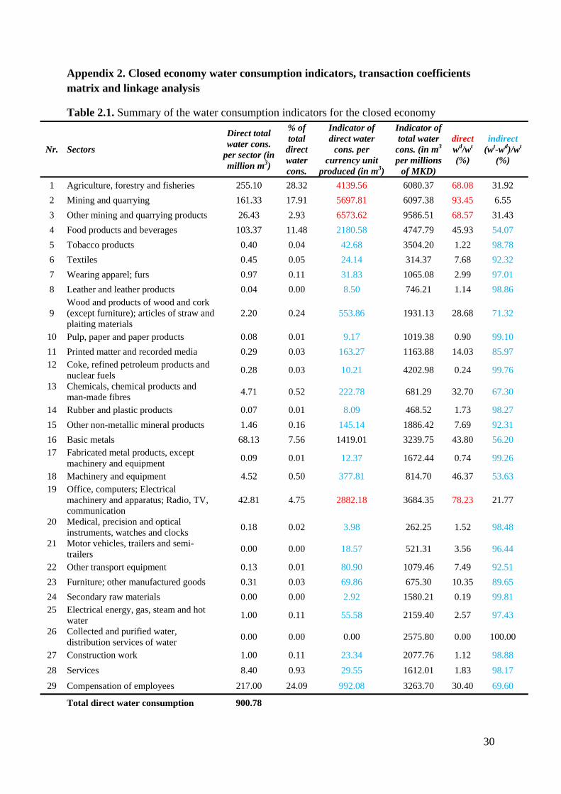
Appendix 2. Closed economy water consumption indicators, transaction coefficients matrix and linkage analysis

Table 2.1. Summary of the water consumption indicators for the closed economy

Nr. Sectors

Direct total water cons.

per sector (in million m3)

% of total

direct water cons.

Indicator of direct water

cons. per currency unit

produced (in m3)

Indicator of total water

cons. (in m3 per millions

of MKD)

directwd/wt

(%)

indirect (wt-wd)/wt

(%)

1 Agriculture, forestry and fisheries 255.10 28.32 4139.56 6080.37 68.08 31.92

2 Mining and quarrying 161.33 17.91 5697.81 6097.38 93.45 6.55

3 Other mining and quarrying products 26.43 2.93 6573.62 9586.51 68.57 31.43

4 Food products and beverages 103.37 11.48 2180.58 4747.79 45.93 54.07

5 Tobacco products 0.40 0.04 42.68 3504.20 1.22 98.78

6 Textiles 0.45 0.05 24.14 314.37 7.68 92.32

7 Wearing apparel; furs 0.97 0.11 31.83 1065.08 2.99 97.01

8 Leather and leather products 0.04 0.00 8.50 746.21 1.14 98.86

9 Wood and products of wood and cork (except furniture); articles of straw and plaiting materials

2.20 0.24 553.86 1931.13 28.68 71.32

10 Pulp, paper and paper products 0.08 0.01 9.17 1019.38 0.90 99.10

11 Printed matter and recorded media 0.29 0.03 163.27 1163.88 14.03 85.97 12 Coke, refined petroleum products and

nuclear fuels 0.28 0.03 10.21 4202.98 0.24 99.76

13 Chemicals, chemical products and man-made fibres

4.71 0.52 222.78 681.29 32.70 67.30

14 Rubber and plastic products 0.07 0.01 8.09 468.52 1.73 98.27

15 Other non-metallic mineral products 1.46 0.16 145.14 1886.42 7.69 92.31

16 Basic metals 68.13 7.56 1419.01 3239.75 43.80 56.20 17 Fabricated metal products, except

machinery and equipment 0.09 0.01 12.37 1672.44 0.74 99.26

18 Machinery and equipment 4.52 0.50 377.81 814.70 46.37 53.63 19 Office, computers; Electrical

machinery and apparatus; Radio, TV, communication

42.81 4.75 2882.18 3684.35 78.23 21.77

20 Medical, precision and optical instruments, watches and clocks

0.18 0.02 3.98 262.25 1.52 98.48

21 Motor vehicles, trailers and semi-trailers

0.00 0.00 18.57 521.31 3.56 96.44

22 Other transport equipment 0.13 0.01 80.90 1079.46 7.49 92.51

23 Furniture; other manufactured goods 0.31 0.03 69.86 675.30 10.35 89.65

24 Secondary raw materials 0.00 0.00 2.92 1580.21 0.19 99.81 25 Electrical energy, gas, steam and hot

water 1.00 0.11 55.58 2159.40 2.57 97.43

26 Collected and purified water, distribution services of water

0.00 0.00 0.00 2575.80 0.00 100.00

27 Construction work 1.00 0.11 23.34 2077.76 1.12 98.88

28 Services 8.40 0.93 29.55 1612.01 1.83 98.17

29 Compensation of employees 217.00 24.09 992.08 3263.70 30.40 69.60

Total direct water consumption 900.78

  

31  

Table 2.2. Water consumption multiplier (wcm) and indirect water consumption multiplier (iwc) for the closed economy

Nr. Sectors wcm iwc

1 Agriculture, forestry and fisheries 1.47 0.47

2 Mining and quarrying 1.07 0.07 3 Other mining and quarrying products 1.46 0.46 4 Food products and beverages 2.18 1.18 5 Tobacco products 82.10 81.10

6 Textiles 13.02 12.02

7 Wearing apparel; furs 33.46 32.46 8 Leather and leather products 87.75 86.75 9 Wood and products of wood and cork (except furniture); articles of straw and plaiting

materials 3.49 2.49

10 Pulp, paper and paper products 111.14 110.14 11 Printed matter and recorded media 7.13 6.13 12 Coke, refined petroleum products and nuclear fuels 411.47 410.47 13 Chemicals, chemical products and man-made fibres 3.06 2.06 14 Rubber and plastic products 57.90 56.90 15 Other non-metallic mineral products 13.00 12.00

16 Basic metals 2.28 1.28

17 Fabricated metal products, except machinery and equipment 135.18 134.18

18 Machinery and equipment 2.16 1.16

19 Office, computers; Electrical machinery and apparatus; Radio, TV, communication 1.28 0.28

20 Medical, precision and optical instruments, watches and clocks 65.88 64.88 21 Motor vehicles, trailers and semi-trailers 28.08 27.08 22 Other transport equipment 13.34 12.34 23 Furniture; other manufactured goods 9.67 8.67 24 Secondary raw materials 540.53 539.53 25 Electrical energy, gas, steam and hot water 38.85 37.85 26 Collected and purified water, distribution services of water 0.00 0.00 27 Construction work 89.02 88.02 28 Services 54.56 53.56 29 Compensation of employees 3.29 2.29

  

32  

Table 2.3. Matrix of water transaction coefficient for the closed economy 1 2 3 4 5 6 7 8 9 10 11 12 13 14 15 16 17 18 19 20 21 22 23 24 25 26 27 28 29

1 0.32 0.02 0.07 0.76 62.71 3.31 8.84 23.48 1.34 28.56 1.75 8.63 0.46 14.02 1.22 0.09 17.21 0.16 0.04 18.1 3.52 1.87 2.36 80.42 4.65 0.00 14.25 14.84 0.97

2 0.08 0.02 0.05 0.12 6.30 2.33 5.00 15.14 0.29 23.86 0.65 383.6 0.26 10.65 3.92 0.59 27.60 0.25 0.06 8.14 5.95 2.72 1.14 121.8 17.21 0.00 22.88 9.68 0.30

3 0.00 0.00 0.20 0.01 0.28 0.10 0.33 0.93 0.02 1.04 0.07 0.39 0.40 2.04 3.98 0.07 3.28 0.03 0.01 0.62 0.64 0.25 0.09 10.53 0.19 0.00 11.28 0.99 0.03

4 0.02 0.01 0.04 0.14 3.05 1.53 4.59 11.72 0.19 13.90 0.91 4.40 0.21 6.26 0.62 0.05 8.86 0.08 0.02 9.39 1.80 0.97 1.15 41.04 2.03 0.00 6.96 7.44 0.51

5 0.00 0.00 0.00 0.00 0.20 0.00 0.01 0.02 0.00 0.02 0.00 0.01 0.00 0.01 0.00 0.00 0.02 0.00 0.00 0.02 0.00 0.00 0.00 0.07 0.00 0.00 0.01 0.01 0.00

6 0.00 0.00 0.00 0.00 0.00 0.07 0.39 0.01 0.00 0.01 0.00 0.00 0.00 0.01 0.00 0.00 0.01 0.00 0.00 0.01 0.00 0.00 0.00 0.04 0.00 0.00 0.01 0.01 0.00

7 0.00 0.00 0.00 0.00 0.00 0.00 0.10 0.02 0.00 0.02 0.00 0.01 0.00 0.01 0.00 0.00 0.01 0.00 0.00 0.01 0.00 0.00 0.00 0.06 0.00 0.00 0.01 0.01 0.00

8 0.00 0.00 0.00 0.00 0.00 0.00 0.00 0.42 0.00 0.00 0.00 0.00 0.00 0.00 0.00 0.00 0.00 0.00 0.00 0.00 0.00 0.00 0.00 0.00 0.00 0.00 0.00 0.00 0.00

9 0.00 0.00 0.00 0.00 0.04 0.01 0.03 0.09 0.05 0.10 0.01 0.03 0.00 0.05 0.00 0.00 0.08 0.00 0.00 0.06 0.02 0.01 0.16 0.36 0.01 0.00 0.87 0.08 0.00

10 0.00 0.00 0.00 0.00 0.00 0.00 0.00 0.01 0.00 0.34 0.00 0.01 0.00 0.01 0.00 0.00 0.01 0.00 0.00 0.01 0.00 0.00 0.00 0.22 0.00 0.00 0.01 0.02 0.00

11 0.00 0.00 0.00 0.00 0.04 0.01 0.01 0.04 0.00 0.04 0.04 0.02 0.00 0.03 0.00 0.00 0.03 0.00 0.00 0.04 0.01 0.00 0.00 1.30 0.01 0.00 0.03 0.03 0.00

12 0.00 0.00 0.00 0.00 0.01 0.00 0.01 0.03 0.00 0.05 0.00 0.02 0.00 0.02 0.01 0.00 0.03 0.00 0.00 0.02 0.01 0.00 0.00 0.18 0.00 0.00 0.05 0.02 0.00

13 0.01 0.00 0.00 0.00 0.32 0.07 0.18 0.46 0.01 0.71 0.07 0.19 0.11 4.73 0.04 0.00 0.38 0.00 0.00 0.37 0.10 0.03 0.07 1.85 0.14 0.00 0.36 0.40 0.01

14 0.00 0.00 0.00 0.00 0.00 0.00 0.00 0.01 0.00 0.01 0.00 0.00 0.00 0.11 0.00 0.00 0.01 0.00 0.00 0.01 0.00 0.00 0.00 0.04 0.00 0.00 0.01 0.01 0.00

15 0.00 0.00 0.00 0.00 0.01 0.01 0.02 0.06 0.00 0.06 0.00 0.02 0.00 0.03 0.03 0.00 0.05 0.00 0.00 0.04 0.01 0.00 0.00 0.24 0.01 0.00 0.99 0.06 0.00

16 0.00 0.00 0.00 0.01 0.28 0.14 0.42 1.28 0.03 1.69 0.09 0.54 0.02 0.68 0.32 0.30 50.64 0.39 0.08 0.87 9.74 3.67 0.16 137.4 0.78 0.00 9.14 1.28 0.03

17 0.00 0.00 0.00 0.00 0.00 0.00 0.00 0.01 0.00 0.01 0.00 0.00 0.00 0.00 0.00 0.00 0.03 0.00 0.00 0.00 0.00 0.00 0.00 0.03 0.00 0.00 0.02 0.01 0.00

18 0.00 0.00 0.00 0.00 0.13 0.03 0.08 0.25 0.01 0.24 0.01 0.14 0.00 0.20 0.02 0.00 0.15 0.01 0.00 0.28 0.03 0.02 0.02 0.87 0.13 0.00 0.48 0.19 0.01

19 0.01 0.00 0.01 0.01 0.72 0.44 1.05 3.76 0.05 3.69 0.17 1.36 0.06 2.07 0.23 0.04 2.96 0.03 0.02 2.50 0.65 0.30 0.27 39.13 7.67 0.00 2.66 2.23 0.08

20 0.00 0.00 0.00 0.00 0.00 0.00 0.01 0.01 0.00 0.02 0.00 0.01 0.00 0.01 0.00 0.00 0.01 0.00 0.00 0.05 0.00 0.00 0.00 0.05 0.00 0.00 0.01 0.01 0.00

21 0.00 0.00 0.00 0.00 0.00 0.00 0.00 0.00 0.00 0.00 0.00 0.00 0.00 0.00 0.00 0.00 0.00 0.00 0.00 0.00 0.00 0.00 0.00 0.00 0.00 0.00 0.00 0.00 0.00

22 0.00 0.00 0.00 0.00 0.00 0.00 0.00 0.00 0.00 0.00 0.00 0.00 0.00 0.00 0.00 0.00 0.00 0.00 0.00 0.00 0.00 0.00 0.00 0.01 0.00 0.00 0.00 0.00 0.00

23 0.00 0.00 0.00 0.00 0.01 0.00 0.01 0.03 0.00 0.03 0.00 0.01 0.00 0.02 0.00 0.00 0.02 0.00 0.00 0.02 0.00 0.00 0.24 0.12 0.00 0.00 0.02 0.03 0.00

24 0.00 0.00 0.00 0.00 0.00 0.00 0.00 0.00 0.00 0.00 0.00 0.00 0.00 0.00 0.00 0.00 0.00 0.00 0.00 0.00 0.00 0.00 0.00 0.00 0.00 0.00 0.00 0.00 0.00

25 0.00 0.00 0.00 0.00 0.05 0.04 0.06 0.29 0.00 0.25 0.01 0.09 0.00 0.16 0.02 0.00 0.19 0.00 0.00 0.11 0.05 0.02 0.02 0.91 0.08 0.00 0.11 0.08 0.00

26 0.00 0.00 0.00 0.00 0.00 0.00 0.00 0.00 0.00 0.00 0.00 0.00 0.00 0.00 0.00 0.00 0.00 0.00 0.00 0.00 0.00 0.00 0.00 0.00 0.00 0.00 0.00 0.00 0.00

27 0.00 0.00 0.00 0.00 0.00 0.00 0.01 0.02 0.00 0.02 0.00 0.01 0.00 0.01 0.00 0.00 0.01 0.00 0.00 0.01 0.00 0.00 0.00 0.07 0.00 0.00 0.19 0.02 0.00

28 0.00 0.00 0.00 0.00 0.23 0.11 0.42 1.23 0.01 1.16 0.07 0.54 0.02 0.60 0.05 0.00 0.70 0.01 0.00 0.72 0.14 0.06 0.08 4.47 0.17 0.00 0.60 0.59 0.03

29 0.02 0.02 0.09 0.12 6.70 3.82 10.88 27.44 0.47 34.31 2.26 10.35 0.51 15.19 1.53 0.11 21.90 0.20 0.05 23.3 4.40 2.39 2.88 98.20 4.74 0.00 17.08 15.53 0.31

iwc  0.47 0.07 0.46 1.18 81.10 12.0 32.46 86.75 2.49 110.1 6.13 410.4 2.06 56.90 12.0 1.28 134.1 1.16 0.28 64.8 27.08 12.3 8.67 539.5 37.85 0.00 88.02 53.56 2.29

  

33  

Table 2.4. Closed economy backward linkages (BL) and forward linkages (FL) indices in terms of water consumption

Nr. Sector BL FL

1 Agriculture, forestry and fisheries 1.61 4.05

2 Mining and quarrying 0.12 0.36

3 Other mining and quarrying products 2.18 2.68

4 Food products and beverages 2.12 0.96

5 Tobacco products 2.71 0.05

6 Textiles 0.10 0.05

7 Wearing apparel; furs 0.29 0.05

8 Leather and leather products 0.15 0.01

9 Wood and products of wood and cork (except furniture); articles of straw and plaiting materials 0.92 0.17

10 Pulp, paper and paper products 0.26 0.0811 Printed matter and recorded media 0.39 0.06

12 Coke, refined petroleum products and nuclear fuels 6.05 1.5713 Chemicals, chemical products and man-made fibres 0.24 0.9414 Rubber and plastic products 0.15 0.0715 Other non-metallic mineral products 0.94 0.0716 Basic metals 1.37 1.79

17 Fabricated metal products, except machinery and equipment 0.96 0.03

18 Machinery and equipment 0.24 0.22

19 Office, computers; Electrical machinery and apparatus; Radio, TV, communication 0.45 0.15

20 Medical, precision and optical instruments, watches and clocks 0.10 0.00

21 Motor vehicles, trailers and semi-trailers 0.29 0.04

22 Other transport equipment 0.55 0.00

23 Furniture; other manufactured goods 0.21 0.04

24 Secondary raw materials 0.78 0.05

25 Electrical energy, gas, steam and hot water 2.13 1.15

26 Collected and purified water, distribution services of water 1.26 0.05

27 Construction work 0.72 0.05

28 Services 0.58 6.6829 Compensation of employees 1.12 7.59