INPUT -OUTPUT MODEL FOR MACCS NUCLEAR ACCIDENT IMP ACTS

ESTIMATION 1

Alexander V. Outkin, Nathan E. Bixler, Vanessa N. Vargas

Sandia National Laboratories

January 27, 2015

1 We would like to thank Verne Loose, Joe Jones, Michael Mitchell, Shirley Starks, Douglas Osborn, Lee Eubank, Katherine MacFadden, Prabuddha Sanyal, and Bern Caudill for valuable suggestions and comments. We also would like to thank the NRC staff members for their support and advice during this project. All remaining errors are ours. Parts of this document are based directly on our previous MACCS materials, reports, and publications, including Outkin and Vargas (2012) and Vargas et al. (2011).

Sandia National Laboratories is a multi-program laboratory managed and operated by Sandia Corporation, a wholly owned subsidiary of Lockheed Martin Corporation, for the U.S. Department of Energy's National Nuclear Security Administration under contract DE-AC04-94AL85000.

SAND2015-7541R

2

Table of Contents (added for clarity, will be deleted in the released version)

Abstract ......................................................................................................................................3

1 Introduction...........................................................................................................................3

2 Input-Output Modeling Overview and Our Approach ............................................................6

2.1 Input-Output Based Approach and its Limitations...........................................................7

3 Connecting REAcct with MACCS ― Overview....................................................................9

4 Macroeconomic Impacts of a Nuclear Accident...................................................................11

4.1 Model of GDP Loss Estimation ....................................................................................12

4.2 GDP Loss Model Parameter Estimation........................................................................14

4.2.1 Loss Calculation Timeframe ..................................................................................14

4.2.2 Social Discount Rate..............................................................................................15

5 Direct and Indirect Economic Impact Estimation.................................................................16

5.1 Estimating Direct Economic Impacts ............................................................................17

5.2 Estimating Indirect Economic Impacts..........................................................................18

5.3 List of Industries in REAcct..........................................................................................18

5.3.1 Economic Impacts and Loss Estimation Based on Area Or Population...................19

5.4 Advantages and Limitations of GDP-based Model and REAcct ....................................21

6 Conclusions.........................................................................................................................21

7 References...........................................................................................................................22

3

ABSTRACTSince the original economic model for MACCS was developed, better qualityeconomic data (as well as the tools to gather and process it) and better computational capabilities have become available. The update of the economic impacts component of the MACCS legacy model will provide improvedestimates of business disruptions through the use of Input-Output-based economic impact estimation. This paper presents an updated MACCS model, based on Input-Output methodology, in which economic impacts are calculated using the Regional Economic Accounting analysis tool (REAcct) created at Sandia National Laboratories. This new GDP-based model allows quick and consistent estimation of gross domestic product (GDP) losses due to nuclear power plant accidents. This paper outlines the steps taken to combine the REAcct Input-Output-based model with the MACCS code, describes the GDP loss calculation, and discusses the parameters and modeling assumptions necessary for the estimation of long-term effects of nuclear power plant accidents.

1 INTRODUCTION

The original MACCS economic model was published in Jow et al. (1990). Since the original economic model for MACCS was developed, better quality economic data, improved tools to gather and process that data, and better computational capabilities have become available. It hasbecome desirable to add an alternative MACCS economic model to utilize these new capabilities. This new model (referred to as the GDP-based model throughout this paper) is based on the Regional Economic Accounting analysis tool (REAcct) created at Sandia National Laboratories. The implementation of REAcct in MACCS will upgrade the economic impacts model to the current state of practice in Input-Output-based economic impact estimation,providing an approach more suitable for estimates of the business disruption. This paper outlines the steps taken to combine the REAcct model with the MACCS code, describes the gross domestic product (GDP) loss calculation, and discusses the parameters and modeling assumptions necessary for the estimation of long-term economic effects of nuclear power plant accidents.

In use for over 5 years, the REAcct analysis tool rapidly estimates approximate economic impacts for disruptions due to natural and manmade events. More information on REAcct can be found in Vargas et al. (2011) and Ehlen et al. (2009). Applied to real-world disruptions such as hurricanes and earthquakes, the results of REAcct analyses have contributed to real-world decision making by the Department of Homeland Security (see Vargas and Ehlen (2013)).

The methodology employed by REAcct is based on and derived from the well-known and extensively documented input-output modeling technique initially developed by Leontief (see Leontief (1936) for the original treatment and Miller & Blair (2009) for the current state of the art) and more recently further elaborated by numerous contributors. The REAcct economic method is based on a framework of inter-industry commodity flows and uses multipliers to

4

estimate the total, direct, and indirect economic impacts of business disruptions.2 REAcct provides county-level economic impact estimates of GDP and employment for any region in the United States. The REAcct implementation process incorporates geospatial computational tools and site-specific economic data, enabling the identification of geographic impact zones, which, in turn, allow differential magnitude and duration estimates to be specified for regions affected by a simulated or actual event. Using these data as input to REAcct, the number of employees for the directly affected economic sectors3 are calculated and aggregated to provide direct impact estimates. Estimates of indirect economic impacts are then calculated using Regional Input-Output Modeling System (RIMS II) multipliers. The interdependent relationships among critical infrastructures, industries, and markets are captured through the relationships embedded in the input-output modeling structure. The data used by REAcct is based on I-O, value added, and final demand output-driven multipliers (RIMS II model) provided by the U.S. Bureau of Economic Analysis (BEA).

The total economic impact of a disruption is typically grouped into two categories:

Direct GDP impacts, which occur to firms located in the affected area

Indirect GDP impacts, which occur to firms that are not in the affected area, but that are affected, for example, by the loss of sales to directly affected firms4

Total national impacts are calculated as a sum of the direct and indirect impacts.

Elements of our process for updating MACCS economic impact estimates include the following:

Estimate reduction of GDP/value added, including both direct and indirect impacts on the economy

Enable creation of geographically specific scenarios with minimal user inputs

Enable consistent model application across different geographic regions and time periods while minimizing the need for manual inputs from the user

Enable near-automated updating of the model as new data becomes available

Conduct case studies and compare REAcct loss estimates with the MACCS original costs to understand the implications of using the GDP-based model.

MACCS models deal with the offsite consequences of a severe nuclear accident that releases a plume of radioactive materials into the atmosphere. Such an event could cause environmentalcontamination and population exposure to the radioactive materials. Estimation of the economic

2 While I-O multipliers require that the analyst make many strong assumptions about how disaster impacts propagate

through the economy, the I-O framework does not; what the framework provides is a useful, structured approach for understanding and modeling highly detailed economic processes.

3 REAcct contains the employment and GDP data for 400+ industries representing the entire US economy. For the purposes of this model the 400+ industries were aggregated into 19 industries and two government sectors, thus making 21 aggregated industries in total, to simplify the analysis and for consistency with the current REAcct model. The data from all 400+ industries data are available in REAcct and can be used if necessary.

4 Impact analysis often also separate out the induced impacts, which are the impacts to households and their expenditures resulting from lost income. These are not calculated in REAcct.

5

losses resulting from such a release is the primary objective of the original MACCS economic model.

The MACCS cost estimation methodology and model are described in the MACCS Model Description document by Jow et al. (1990). The costs are delineated by the emergency response and remedial actions, the productive use of the affected area (farmland vs. non-farmland), and the long-term protective actions. Emergency response and remedial actions include evacuation, sheltering, and relocation. Long-term protective actions include decontamination, temporary land interdiction, and associated relocation of population, crop disposal, control/prohibition of foodproduction, and condemnation of property. The underlying economic methodology is described in Burke et al. (1984). Specifically, the costs calculated in MACCS include:

Temporary evacuation and relocation costs, including food, lodging, and optionally lost income for the displaced population

Permanent relocation costs

Cost of decontaminating land and property

Lost return on investments from properties that are temporarily interdicted

Depreciation of temporarily interdicted property

The value of crops destroyed or not grown in the first year of the accident

The value of farmland and of individual, public, and non-farm commercial property that is condemned

As adapted to interface with MACCS, the REAcct tool estimates the direct, indirect, and total GDP impact of a nuclear power plant accident. The estimates of lost income and lost returns on capital of the original MACCS model are replaced in the GDP-based model by county- andindustry-level GDP loss estimates. We combine the GDP-based loss estimates with the information from the original MACCS model when necessary, for the example when estimating decontamination costs.

As with the original MACCS economic estimator, the goal of the GDP-based model is to provide consistent and conservative estimates of the economic impacts of the nuclear power plant accidents to support licensing and re-licensing decisions.

The rest of this paper presents an outline of the GDP-based model, our motivation for using this specific approach and its limitations, and describes the GDP-loss calculation.

6

2 INPUT-OUTPUT MODELING OVERVIEW AND OUR APPROACH

Input-Output modeling (I-O) is a method for representing transactions in the economy in a compact, aggregated form. It was developed by Leontief in the 1930s (cf., Leontief (1936, 1986), Miller and Blair (2009)).

Leontief’s starting premise is that economic change on the level of aggregate macroeconomic variables, such as the effect of wage changes on price levels, propagates via a “…complex series of transactions in which actual goods and services are exchanged among real people” (Leontief1986). Leontief’s original motivation was to represent the relationships between the economic variables by capturing the transactions in a real economy in aggregated form: “…the individual transactions, like individual atoms and molecules, are far too numerous for observation and description in detail. But it is possible, as with physical particles, to reduce them to some kind of order by classifying and aggregating them into groups. This is the procedure employed by input-output analysis in improving the grasp of economic theory upon the facts with which it is concerned in every real situation” (ibid).

On the mathematical level, I-O modeling represents the transactions in a matrix form as inputs to an industry or outputs of an industry (thus input-output). Modifications and enhancements made to the framework since its original development include, for example, the ability to represent US input-output data on the level of individual counties, representation on the level of individual commodities (commodity by industry), dynamic input-output analysis, as well as many others. Miller and Blair (2009) provide an extensive and comprehensive overview of the current state of I-O modeling and its history.

I-O modeling is consistent with double-entry bookkeeping (as an example, inputs to one industry are outputs of another) and is an integral part of the System of National Accounts (SNA) data collections across the world. SNA aims to measure the key descriptors of macroeconomic activity and includes production, consumption, investment, savings, and other measures. The SNA framework is formalized in the 1968 United Nations publication “The System of Accounts” (United Nations, 1968).

I-O has many practical uses. Some of its first uses were for war and reconstruction efforts planning during and after the World War II. Since its introduction I-O has been expanded for implementation in a variety of areas including disruptions modeling where it is used forestimating the impacts of hurricanes, earthquakes, radiological releases, analysis of effects of various policies, and others (see Rose, 1995 and 2004 for example).

As reported in Leontief (1986), by 1985 I-O tables had been constructed for more than 80 countries. This number is likely significantly higher at present. I-O data are compiled in the course of collecting SNA data, as, for example, explained in the "Eurostat Manual of Supply, Use and Input-Output Tables.”5 Some countries, such as those in the Organization for Economic Co-operation and Development (OECD), have common rules for collecting the national accounts 5http://epp.eurostat.ec.europa.eu/portal/page/portal/product_details/publication?p_product_code=KS-RA-07-013.

Accessed 6/5/2014.

7

data. OECD has input-output data for 48 economies.6 Additionally, there is an effort by the World Input-Output Database (WIOD)7 to create input-output data for the entire world.

2.1 INPUT-OUTPUT BASED APPROACH AND ITS LIMITATIONS

While I-O is a versatile and powerful tool, it has its limitations. One of them is the difficulty of representing the long-term structural change in the economy following an accident. We are fully aware of these limitations in applying I-O to nuclear power plant disruptions.

Our additional motivation for using I-O for this effort is based on the fact that this modeling effort and the resulting tool are constrained by the following requirements:

Consistently and defensibly estimate impacts simply and quickly across different accidents and geographic locations.

Eliminate the need for user intervention when creating a scenario. Instead, calculatescenario parameters automatically from the underlying data and, therefore, minimize the subjectivity of implementing remedial actions that affect economic losses.

Therefore tools such as computational general equilibrium models (CGEs, see Rose 2005 for example), which allow evaluation of long-term economic change but require significant user input regarding accident specifics and scenario parameter estimation, do not appear to be suitable for this task. Tools such as agent-based modeling (ABM, see Epstein and Axtell (1996) or Tesfatsion (2002)), which allow detailed representation on the causal level of scenario-response and proactive planning, are too fine-grained at the short time scale required of the MACCS application.

In using the I-O approach, we do not attempt to represent economic adaptation but instead estimate the impacts associated with the affected area until the time when it becomes usable for economic activity again or until the displaced population is effectively absorbed into the unaffected area. We do not attempt to model this process of absorption, but instead represent it by an estimate of the time it takes for such absorption economic to occur. We call this parameter “Loss Calculation Timeframe”. It affects the magnitude of estimated impacts for the areas that has been abandoned.

We also point out that the developers of the original cost-based MACCS economic model had considered I-O. Their two principal reasons for using the cost-based analysis instead of GDP-based methodologies (Burke et al. (1984) are:

1. Costs involved in generating the GDP-based estimates2. Non-equilibrium nature of the disruption

The first constraint no longer applies and the second item is not a differentiating factor between the cost-based and I-O approaches, as described below.

6 http://www.oecd.org/trade/input-outputtables.htm. Accessed 6/5/2014.7 http://www.voxeu.org/article/new-world-input-output-database. Accessed 6/5/2014.

8

1. Costs involved in generating the GDP-based estimates.

With regard to the costs, Burke et al. (1984) specifically state: “The input-output technique is far too costly and data intensive for consideration in LWR risk analysis applications which require sampling of hundreds of meteorological conditions for each accident category.”

We believe that the far-too costly part is no longer applicable. The level of computational power available now makes GDP-based calculations trivial and data gathering has been automated as well. In particular the underlying REAcct model includes a comprehensive database that is frequently updated with new data. Additionally, by integrating the GDP-based economic model with the underlying MACCS engine, any number of simulations can be conducted for different meteorological conditions without significant manual effort.

Since the original MACCS economic model was created, the situation regarding availability of economic data has also been reversed. For the U.S., the GDP-related data are presently available at the county level. It is therefore a trivial matter not only to update the data, but also to generate estimates specific to the affected area. By contrast, the cost-based version of MACCS requires manual input of a few cost-based parameters and provides no method for automatically calibrating them to the specific affected area. While this does not entail a large effort, the GDP-based model has fewer inputs, some of which are typically chosen to be the defaults, saving the user the requirement of entering them manually. Thus, the GDP-based model is less prone to the effects of user inputs.

2. Non-equilibrium nature of the disruption.

We believe that the non-equilibrium character of disruption is not a differentiating factor at the level of the analysis in either the original or the GDP-based MACCS economic models. In particular, neither the original model nor the GDP-based method treats non-equilibrium adaptation processes associated with severe nuclear accidents. Such processes include adaptation to the disruption in areas that are not directly affected as well as structural changes to the economy at large.8

Such modeling may not even be beneficial because corresponding path-dependence, effects of response and remediation actions, public perception, and other factors outside of the economic model would likely make results from either modeling approach unreliable.

Furthermore, our GDP-based approach is consistent with the principles for federal cost-benefit analysis, in particular as outlined in the OMB Circular A-94. We specifically use the OMB methodology for evaluating the present value of future GDP losses and for factoring in social discount rates as described later in this document.

8 While those changes can be significant (for example shut down of nuclear power plants in Japan as well as in

Germany following the Fukushima nuclear incident), modeling of such consequences is outside of the scope of this project.

9

3 CONNECTING REACCT WITH MACCS ― OVERVIEW

This section outlines the main steps necessary to combine REAcct with MACCS for the creation of a GDP-based economic model. In the combined MACCS – REAcct framework, MACCSassesses specific scenarios using REAcct data and specification of certain scenario parameters. The combined GDP-based economic model software addresses the economic consequences andprovides a systematic view of the economic impacts of nuclear accidents.

An economic model using MACCS and REAcct requires the following steps to estimate total economic impacts:

Identify for each industry the number of employees directly affected by the accident by establishing impact zones based on the geographic extent of the event. In the case of a reactor accident, we assume that all economic activities within the affected area are interrupted.

Estimate the direct impacts to industries indirectly affected by the accident. Estimate the indirect impacts using I-O multipliers. Considering the duration of the interruption for an area, estimate the present worth of the

economic losses in future years.

Connecting MACCS to REAcct software works as follows:

A file created by SecPop defines the set of counties, including area and population fractions that are in each grid element.

WinMACCS passes the SecPop file to REAcct by communicating the set of counties that are affected by an accident.

REAcct computes the GDP losses (direct, indirect, and total GDP losses) for each area (grid cell) and passes these values to MACCS.

For a specific weather trial, MACCS determines the affected areas and the durations of the disruptions.

MACCS estimates the present value of future year GDP losses by accounting for an annual GDP growth rate and a social discount rate.

MACCS sums the overall results over the affected areas and disruption period to get a present value of GDP losses for each weather trial and calculates statistical results based on the set of weather trials that are evaluated.

In the case that an area is condemned, the affected area’s GDP is lost for the foreseeable future.A user-specified number of years of GDP loss are evaluated for a condemned area. In other cases, an area may only be interdicted for a shorter period of time. Then the affected area’s GDP is lost for the period of interdiction. In both cases, the GDP losses are calculated relative to a scenario in which there was no loss in GDP, i.e., there was no disruption in the economic activity.

The main difference between the cases of complete area abandonment and temporary interdictionlies in the duration for which losses are calculated. When the area is condemned, the losses are calculated for the duration of time determined by the model variable “Loss Calculation

10

Timeframe” discussed below. When the area is interdicted temporarily, the losses are calculated according to the duration of the interdiction.9

Decontamination costs and evacuation/relocation costs are carried over from the original MACCS model to the GDP-based model. These costs are not a part of the GDP-based calculation, but are considered when making decisions on whether to decontaminate a particular area and are available as part of the output.

9 For agriculture the minimum interdiction duration is assumed to be one year, because of the seasonal nature of this

industry. Here, a disruption to the planting or growing process is likely lead to the loss of the output for the entire year.

4 MACROECONOMIC IMPACTS OF A NUCLEAR ACCIDENT

At the top level, GDP-based impacts are estimated by creating a baseline scenario or forecast, a disruption scenario, and by estimating the GDP difference between the two scenarios as represented in the Figure 1.

Figure 1: GDP impacts as the difference between baseline and disruption scenarios

The entire scenario definition in MACCS specifically includes the following:

Affected geographic area

Duration of disruption for each grid element, accounting for countermeasures and the time required to restore the geographic area to usability

Other parameters, such as the social discount rate, to aggregate the effects of the disruption over time

A fundamental goal of the GDP-based model, as of the old model, is to provide consistent and conservative estimates of the economic impacts of nuclear power plant accidents to enable licensing and re-licensing decisions. We do not attempt to predict the economic evolution after an accident, but rather to provide defensible estimates of potential losses that are consistent across different geographic locations and possible accidents. We also do not attempt to forecast future recovery scenarios. Creating realistic and defensible recovery scenarios is still a largely unresolved issue in economics, as acknowledged for example by Chang and Miles (2004), who also propose a prototype framework for addressing the recovery. One of the principal differences between nuclear power accidents and events such as hurricanes is the possibility that the contaminated area will be interdicted for a very long period of time or even permanently abandoned. In this case, recovery may never occur in a particular area. Instead, parts of the

10

economy unaffected by the accident will experience the effects of recovery: the affected population will move to unaffected areas, find new jobs, start new businesses, and otherwise transfer their lives. There is little relevant historic precedent specific to the nuclear power plant accidents that would support estimation of how long this process would take and when the affected population can be become productive in unaffected areas. However, because of this possibility of a long interdiction period or complete abandonment of affected areas, a method of calculating the losses associated with the areas abandoned in perpetuity is needed. Our assumption is that at some point, the overall economy will recover from such losses. We represent the duration of this recovery as the “Loss Calculation Timeframe” parameter (further discussed in the section 3.1).

4.1 MODEL OF GDP LOSS ESTIMATION

REAcct uses lost gross domestic product (GDP) to represent the macroeconomic impacts of a nuclear accident. GDP refers to the value of all final goods and services produced within a country’s borders in a given time period. Mathematically, this can be expressed as following:

� =∑ �������� (1)

where Y is GDP, q is quantity of each final good or service produced in a given period of time, and p is the corresponding price, as measured by transaction prices.

For the purposes of MACCS, GDP losses generally need to be calculated for arbitrary time periods. The data used by MACCS and REAcct to calculate the GDP losses are available only for a given year, defined as the “base year” (the most recently available data is for 2011). Some lost GDP calculations may need to be performed for a different starting date, also known as an “accident year.” In this case it is necessary to adapt the GDP available for a year �� (base year) to GDP consistent with a particular accident year ��. We do this by using the historical real GDP growth rate and calculating the accident year GDP as a function of the base year GDP assuming a constant GDP growth rate. We also apply the concept of the social discount rate to discount the real GDP in the future years.

Notation:

� - historical real GDP growth rate. We estimate g using the historic data on the US GDP growth rates. Usually, economists consider less than 2% annualized growth of GDP to be sluggish, between 3 and 3.5 percent as healthy, and greater than 5 percent as very rapid. The long-term growth rate of GDP for the U.S is 3.3 percent for the period 1947-2010, as estimated by BEA.10

� – social discount rate. This parameter estimates the discounting of future costs expressed in real terms. Estimation of the social discount rate is discussed below.

10 See for example, http://www.econedlink.org/lessons/projector.php?lid=995&type=educator

10

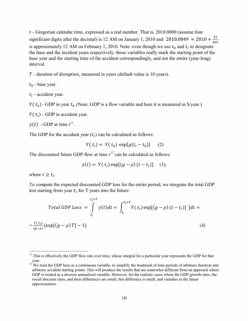
� - Gregorian calendar time, expressed as a real number. That is, 2010.0000 (assume four

significant digits after the decimal) is 12 AM on January 1, 2010 and 2010.0849 ≈ 2010 +��

���

is approximately 12 AM on February 1, 2010. Note: even though we use �� and �� to designate the base and the incident years respectively, those variables really mark the starting point of the base year and the starting time of the accident correspondingly, and not the entire (year-long) interval.

� - duration of disruption, measured in years (default value is 10 years).

��- base year.

�� - accident year.

�(��) - GDP in year �� . (Note: GDP is a flow variable and here it is measured in $/year.)

�(��) - GDP in accident year.

�(�) - GDP at time t11.

The GDP for the accident year (��) can be calculated as follows:

�(��) = �(��)exp[�(�� − ��)] (2)

The discounted future GDP flow at time t12 can be calculated as follows:

�(�) = �(��) exp[(� − �) (� − ��)] (3),

where � ≥ ��.

To compute the expected discounted GDP loss for the entire period, we integrate the total GDP lost starting from year �� for T years into the future:

������������ = � �(�)�� = � �(��) exp[(� − �) (� − ��)]]������

��

����

��

=

= �(��)

(���){exp[(� − �) �] − 1} (4)

11 This is effectively the GDP flow rate over time, whose integral for a particular year represents the GDP for that

year.12 We treat the GDP here as a continuous variable, to simplify the treatment of time periods of arbitrary duration and

arbitrary accident starting points. This will produce the results that are somewhat different from an approach where GDP is treated as a discrete annualized variable. However, for the realistic cases where the GDP growth rates, the social discount rates, and their differences are small, this difference is small, and vanishes in the linear approximation.

10

By changing the integration limits in (4), the GDP loss for a specific year t, can be expressed as follows:

��������������� = ∫ �(�)�����

�=∫ �(��)exp[(g − ρ) (� − ��)]dt

���

�(5)

Which can be expressed as follows:

��������������� =

= �(��)

(���){exp[(� − �) (� − �� + 1)] − exp[(� − �) (� − ��)]} (6)

Note: this section represents the GDP loss calculation for single industry in a single interdicted parcel of land (such as a county); the actual loss calculation in the combined MACCS-REAcct framework is performed for each affected industry and the affected region and aggregated over time as described above. Additionally, the parameter T above can represent both the interdiction period and the maximum duration of the economic impact.

The calculation described above represents the core component of the GDP loss estimation in the combined model. To implement this framework in practice, certain parameters from MACCS that affect the scenario definition and the GDP loss calculation need to be defined. One such parameter is the Loss Calculation Timeframe variable that affects the time frame for which losses are calculated. The next section outlines the definitions and estimation of the variables necessary for calculating the macroeconomic impacts of a nuclear accident in the GDP-based MACCS economic model.

4.2 GDP LOSS MODEL PARAMETER ESTIMATION

4.2.1 LOSS CALCULATION TIMEFRAME

Losses arising from a nuclear accident refer to the effects on households and businesses directly affected by the countermeasures applied to mitigate the effects of released radiation on the population. If the area is decontaminated relatively quickly, then the period for which business or industry remains closed can be considered as the time period over which economic losses should be computed. However, if the area remains interdicted over a longer time period or abandoned completely, the choice of a time frame for calculating the GDP losses depends on how quickly the rest of the economy can absorb the business and people from the affected area and to recover in general. . There remains considerable uncertainty regarding the maximum time period (represented as T in the text) over which losses should be calculated. For the GDP-based model, we have selected 10 years as the default value for calculating the economic impacts. This 10-year period (or other period as selected by the user) represents only an upper bound in the simulation on the duration of impacts. For example, if the affected area is decontaminated quickly, say in a year, then this parameter would not be binding and would not affect the calculation.

One way to look at the loss period is to consider the duration of time in which the overall economy would recover if an affected area were condemned. The recovery to a normal condition

10

requires that the population and business from the affected area move to other parts of the country and resume pre-accident activities. Therefore, the question becomes how long would it take for the overall economy to absorb the resulting migration and for the affected people to find new jobs or restart businesses. Relevant data that can be used to evaluate time for the economy to recover includes: 1) the length of the U.S. recessions, 2) past disruption events, like Hurricane Katrina, and 3) existing literature. We examine the available data below.

1). The length of recessions. According to the National Bureau of Economic Research, the average length of the US recessions calculated using all available data from 1854 to 2009 is 17.5 months, and 11.1 months if only using the period from 1945 to 200913.

2) Past disruption events. Recovery after the hurricanes has been analyzed for example in Deryugina (2011), who concludes that the employment rate declines following a hurricane persists even 5 – 10 years after the event. Deryugina et al. (2014) analyze the effects of hurricane Katrina specifically and conclude that the nominal wages have recovered relatively quickly for those who returned to New Orleans after the hurricane, and even exceeded their pre-hurricane levels in two years after the hurricane, but those who choose not to return or were unable to it took approximately five years for their wages to reach the pre-hurricane levels. Basker and Miranda (2014) analyze the after-Katrina recovery at the Mississippi coast and conclude that the areas with most damage “had not recovered within five years despite significant help from both federal and state sources”.

3) Existing literature. COCO-2 (an I-O model to assess the economic impact of a nuclear accident in the United Kingdom, see Higgins et al., 2008) uses a period of 2 years to restore production to pre-accident levels.

We believe the length of the U.S. recessions and the COCO-2 period of 2 years to restore production represent the lower bound on the duration of impacts of such a catastrophic event as a nuclear power accident that requires long interdiction periods or complete abandonment of the affected area. We believe the long and still ongoing struggles to recover after hurricanes such as Katrina where the impacts persist even 5-10 years after the event, justifies a longer time frame for calculating the duration of economics losses after significant nuclear power plan accidents.Based on theses considerations, and the fact that long interdiction or complete area abandonmentis likely to preclude a significant fraction of the population from returning due either to actual contamination levels or psychological factors, we selected 10 years as the default time frame for the losses calculation.

4.2.2 SOCIAL DISCOUNT RATE

There are three primary methods in the U.S. for measuring social discount rates:

Benchmark financial rate approach, which suggests that discount rate be based on the social opportunity cost of capital, a weighted average of the pre-tax and after tax rates of

13 More information can be found at www.nber.org/cycles.html. Accessed January 15, 2015.

10

return, where the weights reflect the proportions of funds that are obtained from displaced investment, postponed consumption, and incremental funding from abroad when the government borrows to finance a project (OMB circular A-94, Burgess (2011))

Building upon the rate of time preference using an appropriate rate of growth in per-capita consumption

The Marginal Cost of Funds criterion (MCF), which discounts within generation benefits at the after tax rate, between generation benefits at the pre-tax rates, and costs at the pre-tax rates (Liu et al., 2004).

For the purposes of this project, we use the OMB approach. In this method, the benchmark real Treasury interest rates are used to approximate the social discount rate, implicitly assuming that the safe opportunity cost of capital should be the yield on a long-term U.S. Treasury security. The average rate prescribed by OMB for 30 year projects based on real interest rates on T-securities based on the data available at present (2013) is 1.1 percent. Florio (2006), based on a similar methodology, recommends a social discount rate between 3 and 4 percent. We use a discount rate of 3% following Florio (2006) as the default value for MACCS. In our judgmentthe discount rate of 1.1% is not representative of the past historic conditions and is unlikely to persist. Significantly higher discount rates of 6% to 8% are prescribed in Burgess, 2011. We use the latter as the upper bound for the range of discount rates in MACCS.

The Table 1 below summarizes the default, upper, and lower values for the variables discussed above.

Table 1: Default and boundary values for Real GDP growth rate and loss calculation duration

Real GDP Growth rates (%)

Duration of Economic Impact (years)

Social Discount Rate (%)

Default value 3.3 10 3

Lower bound 1 2 1

Upper bound 8 30 8

5 DIRECT AND INDIRECT ECONOMIC IMPACT ESTIMATION

The two sections below describe the initial annual GDP loss calculation for a particular area to which the mathematical framework described in the section “Model of GDP Loss Estimation” issubsequently applied to estimate the direct and indirect GDP losses for a specific scenario and for the entire affected area as it is defined in WinMACCS/MACCS.

10

5.1 ESTIMATING DIRECT ECONOMIC IMPACTS14

Given a particular disruption or change, a subset of the overall economy is directly affected. The two primary subsets are the productive sectors (e.g. firms) and consumptive sector (e.g. households). For each day of business interruption, impacted industry sectors lose economic output or production, resulting in lost income for their employees. REAcct estimates the lost output and income directly at the industry level as categorized by the North American Industry Classification System (NAICS)15. For the purposes of the MACCS-REAcct integration, REAcct provides annual GDP estimates for the affected industries and regions for the base year. Specifically, REAcct estimates the annual GDP as the average value added per worker nationally (or regionally16) times the number of employees in that industry in the disrupted region as follows:

�������������������������������������������� =����

���� × ��

� (7)

where, ���� �����

�� are national annual output and employment for industry �, and ��� is

employment in region r for industry �. Given those estimates and additional scenario parameters, MACCS estimates the GDP losses for a particular scenario using the framework outlined in the section “3.

14 This and the following section (4.2) are based on materials from Vargas (2011) and Ehlen (2009) with minor

modifications. It is provided for user convenience and logical completeness.15 This can be at the 2, 3, or 4 digit NAICS level, depending on the availability of data. Typically the most

comprehensive data are available at the 2 or 3 digit NAICS level.16 This is dependent on availability of data. Some states do calculate this information and can be obtained from

public sources. Some states do not calculate this and it must be estimated at the national level. In the most unique cases, this data may also be available at the county level.

24

Macroeconomic Impacts of a Nuclear Accident” for the set of affected industry sectors and regions.

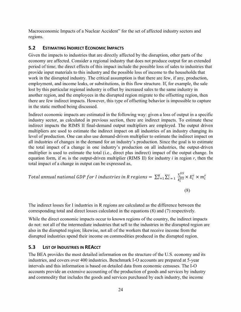
5.2 ESTIMATING INDIRECT ECONOMIC IMPACTS

Given the impacts to industries that are directly affected by the disruption, other parts of the economy are affected. Consider a regional industry that does not produce output for an extended period of time; the direct effects of this impact include the possible loss of sales to industries that provide input materials to this industry and the possible loss of income to the households that work in the disrupted industry. The critical assumption is that there are few, if any, production, employment, and income leaks, or substitutions, in this flow structure. If, for example, the sale lost by this particular regional industry is offset by increased sales to the same industry in another region, and the employees in the disrupted region migrate to the offsetting region, then there are few indirect impacts. However, this type of offsetting behavior is impossible to capture in the static method being discussed.

Indirect economic impacts are estimated in the following way: given a loss of output in a specific industry sector, as calculated in previous section, there are indirect impacts. To estimate these indirect impacts the RIMS II final-demand output multipliers are employed. The output drivenmultipliers are used to estimate the indirect impact on all industries of an industry changing its level of production. One can also use demand-driven multiplier to estimate the indirect impact on all industries of changes in the demand for an industry’s production. Since the goal is to estimate the total impact of a change in one industry’s production on all industries, the output-driven multiplier is used to estimate the total (i.e., direct plus indirect) impact of the output change. Inequation form, if mi is the output-driven multiplier (RIMS II) for industry i in region r, then the total impact of a change in output can be expressed as,

���������������������������������������������� = ∑ ∑����

����

����

���� × ��

� × ���

(8)

The indirect losses for I industries in R regions are calculated as the difference between the corresponding total and direct losses calculated in the equations (8) and (7) respectively.

While the direct economic impacts occur to known regions of the country, the indirect impacts do not: not all of the intermediate industries that sell to the industries in the disrupted region are also in the disrupted region; likewise, not all of the workers that receive income from the disrupted industries spend their income on commodities produced in the disrupted region.

5.3 LIST OF INDUSTRIES IN REACCT

The BEA provides the most detailed information on the structure of the U.S. economy and its industries, and covers over 400 industries. Benchmark I-O accounts are prepared at 5-year intervals and this information is based on detailed data from economic censuses. The I-O accounts provide an extensive accounting of the production of goods and services by industry and commodity that includes the goods and services purchased by each industry, the income

24

earned in each industry, and the distribution of sales of goods and services to consumers, businesses, governments, and foreign entities.17

These accounts are used to examine the effects of changes in final demand on the economy as well as to show the interdependencies among producers and consumers in the economy.

For the purposes of MACCS analysis and integration, the 400+ industries are aggregated into 2-digit NAICS codes covering 21 industries (19 industries and 2 government sectors). Below we illustrate the choice of loss estimation methods for industries by area, population, or both based on the existing literature and BEA tool for industry analysis.

5.3.1 ECONOMIC IMPACTS AND LOSS ESTIMATION BASED ON AREA OR POPULATION

For certain disruption scenarios, only a fraction of a county would be affected. For the version of REAcct used for this effort, county is the smallest geographic entity for which the data are available. It is therefore necessary to develop a procedure for estimating the GDP losses for a fraction of a county.

The fraction of the county land area and the fraction of the county population in the affected zone are two principal quantities we have considered for calculating the GDP losses for the counties only partially affected. We have considered for the industries in REAcct whether they are geographically distributed or geographically concentrated and whether the output is labor intensive. For the industries that are geographically distributed and which do not depend on concentrated labor, such as agriculture, we have calculated the fractional impacts based on the area affected; for the industries that are geographically concentrated and depend on concentrated labor, such as manufacturing, we calculated the fractional impacts based on the population affected. For less clear-cut examples, we have used our judgment to decide. The Table 2 below summarizes our current assumptions and the current implementation in REAcct, as integrated with WinMACCS.

17 http://www.bea.gov/papers/pdf/IOmanual_092906.pdf

24

Table 2: GDP impacts calculation by area vs. population for areas smaller than a county

Industry By Area By Population Comments

Agriculture, forestry, fishing, and hunting

X As crop area is a relevant measure of agricultural sector losses

Mining X Concentrated only in certain geographicallocations

Utilities X Likely to affect a region or local area

Construction X Damages to construction are likely to be more local

Wholesale trade X If GDP loss for sector is local, loss estimates should be based on area

Retail trade X Same argument as above

Transportation & Warehousing

X Depending on the extent of transportation & warehousing reconstruction, loss estimates can be normalized based on population

Information X Reconstruction of information systems should be based on population as it covers larger networks than simply local neighborhoods

Finance & Insurance X As Insurance premiums are recorded on a “where sold” basis which locates economic activity of home state; difference between sum of net interest by state and NIPA value is distributed to the states based on computed series of net interest by states

Manufacturing X Heavy manufacturing tends to be geographically concentrated and crucially dependent on the labor force availability to run the operations.

Real estate & rental leasing

X Damages to real estate is usually locally concentrated

Professional, scientific, and technical services

X Structural retrofitting of educational facilities are usually local in scope

Management of companies & Enterprises

X Usually based on area, however loss estimate can also depend on the nature of the company, whether it is global or local in its operations

Administrative & Waste management services

X BLS wages and salaries per FTE are computed for local employees

Educational services X Often these services are beyond the immediate local area of the accident

Health care & Social assistance

X Loss estimates can also be based on population if medium and long-term medical care to injured individuals are beyond the local area / population affected

Arts, entertainment & recreation

X These industries are usually geographically concentrated

Accommodations & food services

X Same as above

Other services, except government

X Religious, labor and political organizations may go beyond the local area impacted

Federal civilian X Scope of government sector budget is beyond the area affected

State & local government

X Same as above

24

5.4 ADVANTAGES AND LIMITATIONS OF GDP-BASED MODEL AND REACCT

While this modeling method is simple to understand and implement, it employs a number of strong assumptions and related limitations.

This method can be applied to address nuclear power plant accidents as described above. Because of its simplicity, it can provide approximate estimates of economic impacts that can be generated quickly by the analyst. It is relatively easy to use, thereby reducing costs to apply. It is based on IO methodology, which is well established in the economic literature. The underlying economic software, REAcct, can be linked to Geographic Information System (GIS) data, whichprovides impact zone information to the REAcct model, thus adding the ability to assess the impacts to an economy, particularly a regional economy, at almost any level of spatial resolution,up to the county level.

The limitations of I-O techniques and therefore of the GDP-based model are well documented within the literature, and include the difficulty or inability to represent the long-term structural change in the economy due to both endogenous and exogenous factors, such as technological change. We recognize those limitations, and consider the I-O methodology to be a viable tool for representing the past historic economic activity data and for quickly estimating the economic impacts from disruptions to established patterns of production activity or employment. We do not attempt to represent the structural economic change in response to the nuclear power plant accidents, because we believe such predictions are not feasible on long time scales, and opt instead to represent only historic rate of GDP growth.

The economic disruption and related restoration are by definition dynamic, disequilibrium processes. Individual firms within the affected industries have different levels of on-site and in-transit inventories, and different production processes. The GDP-based model is not intended to capture the highly complex interactions between firms and industries that happen during the disruptions when past historic data are not necessarily descriptive of the disequilibrium dynamics occurring at such times.

The traditional economic consequence analysis using input-output methodology employed by REAcct calculates direct economic impacts (the change in production or GDP at a particular level of the supply chain) and upstream, or indirect, economic impacts arising due to the change in production at preceding levels of a given supply chain. REAcct does not attempt to estimate the downstream impacts or adaptations. The downstream impacts are dependent upon the adaptations and substitution decisions of firms and consumers.

6 CONCLUSIONS

This paper outlines the GDP-based economic model developed for MACCS that is based on the REAcct tool, and its goals, implementation, and limitations. This GDP-based model allows quick and consistent estimation of GDP losses due to nuclear power plant accidents. This paper presents the underlying conceptual, mathematical, and practical framework and the steps for connecting MACCS and REAcct. We believe the GDP-based MACCS economic model is potentially useful for future NRC cost/benefit analyses.

24

7 REFERENCES

Burgess, D.F. (2011): Reconciling alternative views about the appropriate social discount rate, Working Paper, Department of Economics, University of Western Ontario.

Burke, Richard. P., David C. Aldrich, and Norman C. Rasmussen (1984): Economic Risks of Nuclear Power Reactor Accidents, NUREG/CR-3673, SAND84-0178, Sandia National Laboratories, Albuquerque, NM, 1984.

Basker, Emek and Miranda, Javier (2014): Taken by Storm: Business Financing, Survival, and Contagion in the Aftermath of Hurricane Katrina. Available at SSRN: http://ssrn.com/abstract=2417911 or http://dx.doi.org/10.2139/ssrn.2417911. Accessed January 15, 2015.

Chang, Stephanie E., and Scott B. Miles (2004): The Dynamics of Recovery: A Framework, in Modeling Spatial and Economic Impacts of Disasters. Y. Okuyama and S.E. Chang (eds.). Springer-Verlag. Berlin.

Deryugina, Tatyana (2013): The Role of Transfer Payments in Mitigating Shocks: Evidence from the Impact of Hurricanes. Available at SSRN: http://ssrn.com/abstract=2314663. Accessed January 5, 2015.

Deryugina, T., L. Kawano, and S. Levitt (2013): The Economic Impact of Hurricane Katrina on its Victims: Evidence from Individual Tax Returns," NBER Working Paper No. 20713.

Ehlen, M. A., Vanessa N. Vargas, Verne W. Loose, Shirley J. Starks, and Lory A. Ellenbracht(2009): Regional Economic Accounting (REAcct): A Software Tool for Rapidly Approximating Economic Impacts, SAND Report 2009-6552, Sandia National Laboratories, Albuquerque NM.

Epstein, J., and R. Axtell (1996): Growing Artificial Societies: Social Science from the Bottom Up (MIT Press/Brookings, MA).

Florio, M. (2006): Multi-Government Cost-Benefit Analysis: Shadow Prices and Incentives, Working Paper 2006-37, Department of Economics, University of Milan.

Higgins, N.A., C Jones, M. Munday, H. Balmforth, W. Holmes, S. Pfuderer, L. Mountford, M.Harvey, and T. Charnock (2008): COCO-2: A Model to Assess the Economic Impact of an Accident. Health Protection Agency Radiation Protection Division. HPA-RPD-046.

Jow, H.N, J.L. Spring, J.A. Rollstin, L.T. Ritchie, D.I. Chanin (1990): MELCOR Accident Consequence Code System (MACCS. NUREG/CR-4691, Sandia Laboratories Report SAND86-1662.

Miller, Ronald E., and Peter D. Blair (2009): Input-Output Analysis: Foundations and Extensions. Cambridge University Press.

Liu, L., A. Rettenmaier, and T. Saving (2004): A generalized approach to multigenerational project evaluation, Southern Economic Journal, 71 (2): 377-396.

Leontief, W. (1936): "Quantitative input and output relations in the economic system of the United States." Review of Economics and Statistics 18: pp.105-25.

Leontief, W. (1986): Input-output economics. Oxford University Press, New York.

24

Outkin, Alexander V., and Vanessa N. Vargas (2012): MACCS2/REAcct Combined Model Comparison with ITRA Model. Sandia National Laboratories Memo.

Rose, A. (1995): “Input-Output Economics and Computable General Equilibrium Models,” Structural Change and Economic Dynamics 6: 295-304.

Rose, Adam (2004): Economic Principles, Issues, and Research Priorities in Hazard Los Estimation, in Modeling Spatial and Economic Impacts of Disasters. Y. Okuyama and S.E. Chang (eds.). Springer-Verlag. Berlin.

Rose, A. (2005): “Tracing Infrastructure Interdependence Through Economic Interdependence,” Department of Geography, The Pennsylvania State University.

Tesfatsion, L. (2002), “Agent-based computational economics: Growing economies from the bottom up,” Artificial Life 8:55-82.

Vargas, Vanessa N, Nathan E. Bixler, Alexander V. Outkin, Verne W. Loose, Prabuddha Sanyal, Shirley Starks (2011): “An Updated Economic Model For Level-3 PRA Consequence Analysis Using MACCS2”. Presented at the PSA 2011 Conference.

Vargas, Vanessa N., and Mark A. Ehlen (2013): REAcct: a scenario analysis tool for rapidly estimating economic impacts of major natural and man-made hazards. Environmental Systems and Decisions. 33:76-88.