Embed Size (px)
Citation preview
InSAR practical considerations
Matthew Pritchard
Cornell UniversityEric FieldingJet Propulsion
Laboratory, Caltech
Understanding the Line of Sight
Sources of error
Resampling/downsampling data
Multi-interferogram methods: time series PSInSAR
Thursday, August 1, 2013
Visualizing the data & preparing for modeling
Was at roipac.org/Modeling and /ContribSoftware
-Perl script: mdx-kml.pl runs mdx to make image from geocoded interferogram or correlation, converts to png and makes kml (requires installation of ImageMagick)-Various GMT scripts-Example Matlab and IDL scripts for loading data
For GIS software, use .rsc file to create metadata file and perhaps rmg2mag_phs to make a single binary file
Make los script: creates file with the satellite heading and incidence angle at each pixel
Thursday, August 1, 2013
Access to topographic data
Source I use most often: SRTM 1 degree tiles either at 3 arcsec (90m) or 1 arcsec for U.S. (30 m)--new v.3 release has voids filled with GDEMget_SRTM.pl now included with ROI_pac
SRTM also available from seamless USGS server. Can access available Lidar and NED data for U.S. at finer resolution ASTER GDEM -- posted at 1 arcsecond, but various analysis indicates it is closer to 3 arcsec (GDEM2 now available)
Format needs to be I*2 (16 bit) binary file with no headerNeed to create .rsc file with upper left coordinates, # of rows and columns, and pixel spacing
Thursday, August 1, 2013
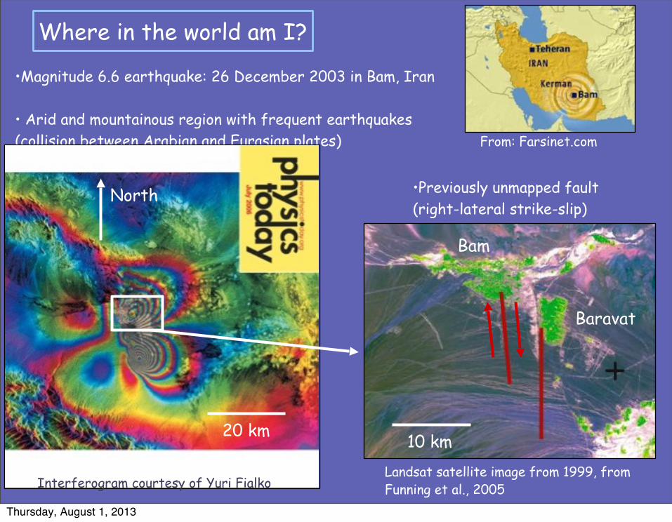
•Previously unmapped fault (right-lateral strike-slip)
Where in the world am I?
•Magnitude 6.6 earthquake: 26 December 2003 in Bam, Iran
• Arid and mountainous region with frequent earthquakes(collision between Arabian and Eurasian plates)
North
Bam
Baravat
10 km20 km
Interferogram courtesy of Yuri FialkoLandsat satellite image from 1999, from Funning et al., 2005
From: Farsinet.com
Thursday, August 1, 2013
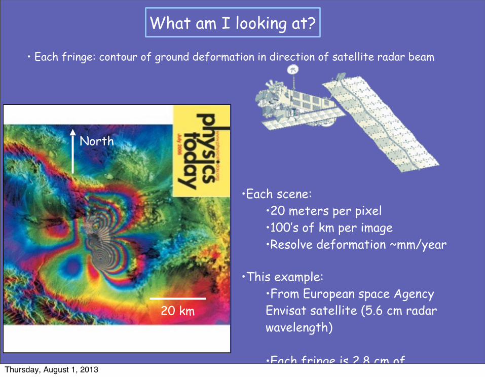
What am I looking at?
North
20 km
• Each fringe: contour of ground deformation in direction of satellite radar beam
•Each scene:•20 meters per pixel•100’s of km per image•Resolve deformation ~mm/year
•This example: •From European space Agency Envisat satellite (5.6 cm radar wavelength)
•Each fringe is 2.8 cm of deformation
Thursday, August 1, 2013
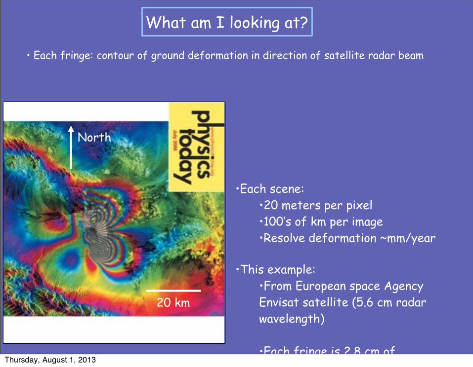
What am I looking at?
North
20 km
• Each fringe: contour of ground deformation in direction of satellite radar beam
•Each scene:•20 meters per pixel•100’s of km per image•Resolve deformation ~mm/year
•This example: •From European space Agency Envisat satellite (5.6 cm radar wavelength)
•Each fringe is 2.8 cm of deformation
Thursday, August 1, 2013
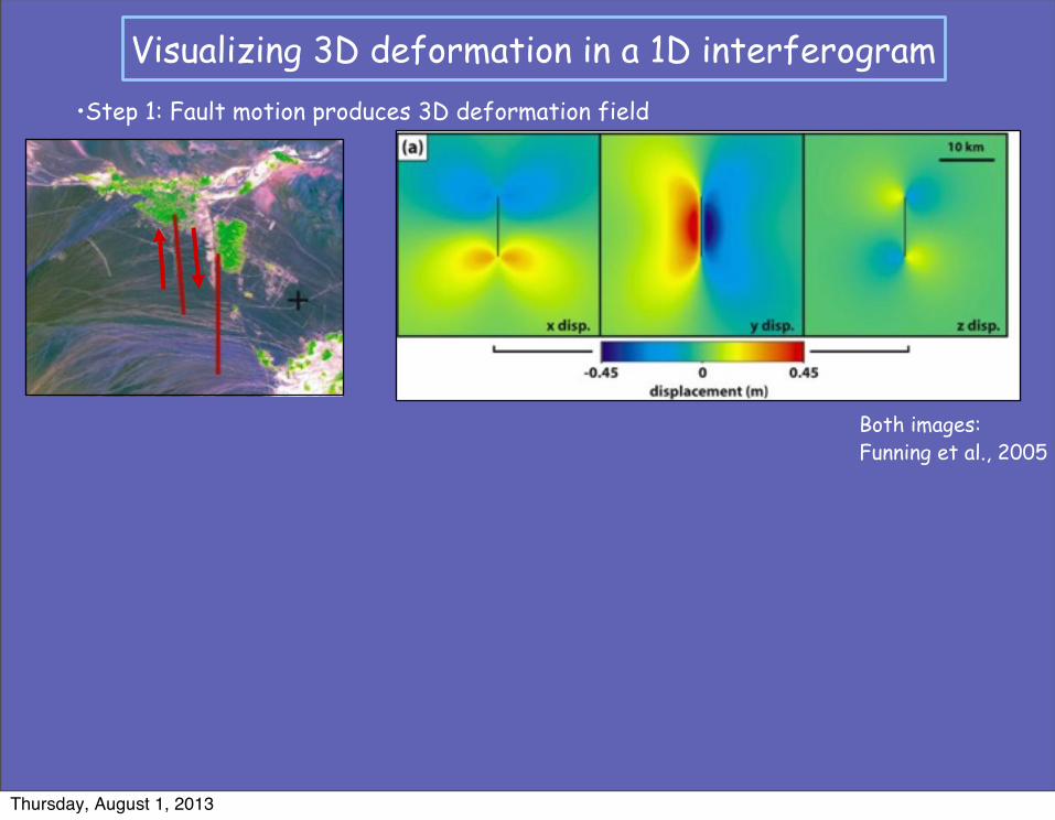
Visualizing 3D deformation in a 1D interferogram•Step 1: Fault motion produces 3D deformation field
Both images:Funning et al., 2005
Thursday, August 1, 2013
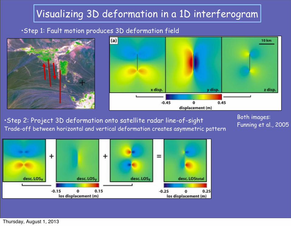
Visualizing 3D deformation in a 1D interferogram•Step 1: Fault motion produces 3D deformation field
•Step 2: Project 3D deformation onto satellite radar line-of-sightTrade-off between horizontal and vertical deformation creates asymmetric pattern
Both images:Funning et al., 2005
Thursday, August 1, 2013
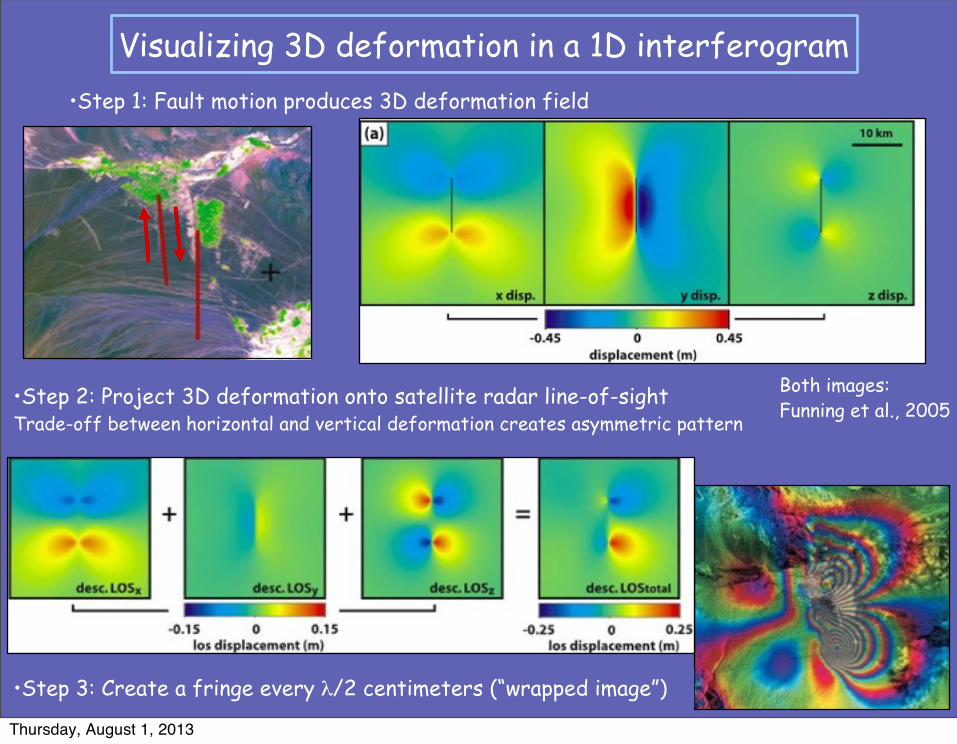
Visualizing 3D deformation in a 1D interferogram•Step 1: Fault motion produces 3D deformation field
•Step 2: Project 3D deformation onto satellite radar line-of-sightTrade-off between horizontal and vertical deformation creates asymmetric pattern
•Step 3: Create a fringe every λ/2 centimeters (“wrapped image”)
Both images:Funning et al., 2005
Thursday, August 1, 2013
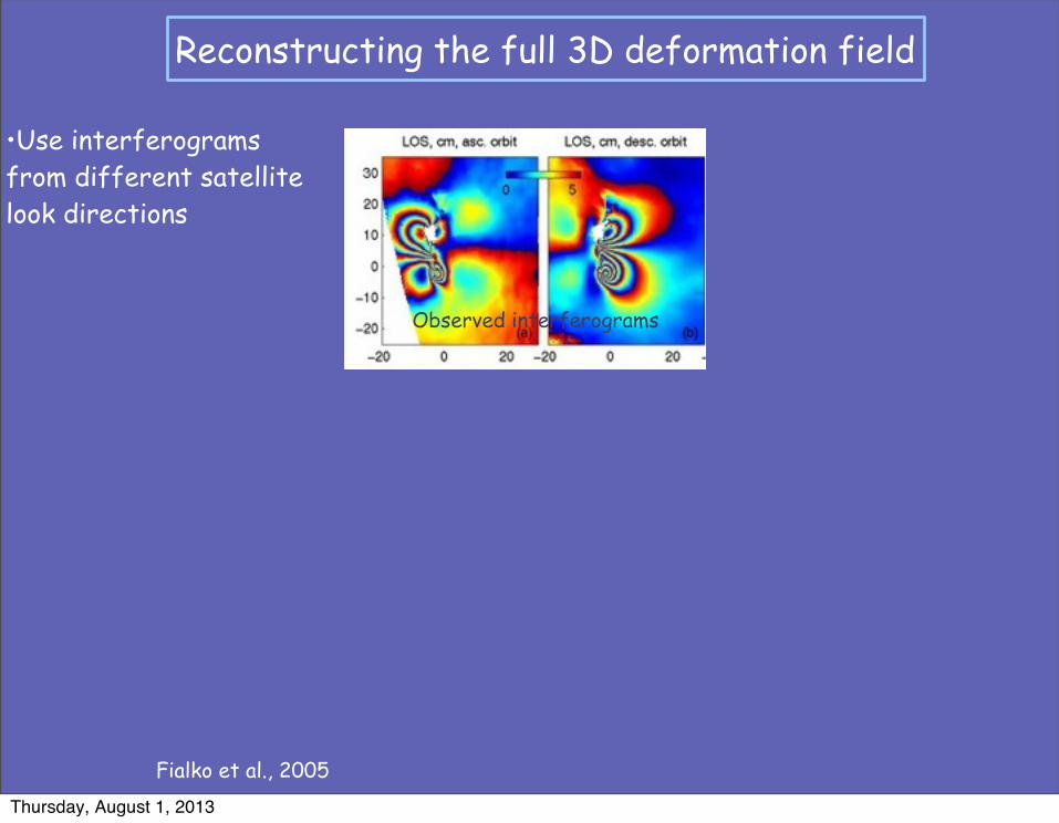
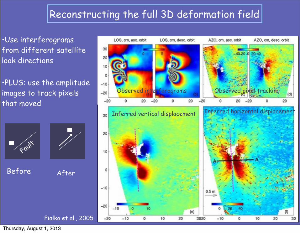
Reconstructing the full 3D deformation field
•Use interferograms from different satellite look directions
Fialko et al., 2005
Observed interferograms
Thursday, August 1, 2013
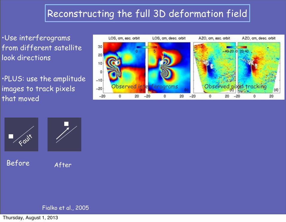
Reconstructing the full 3D deformation field
•Use interferograms from different satellite look directions
Fialko et al., 2005
Observed interferograms Observed pixel tracking
Before After
Fault
•PLUS: use the amplitude images to track pixels that moved
Thursday, August 1, 2013
Reconstructing the full 3D deformation field
•Use interferograms from different satellite look directions
Fialko et al., 2005
Inferred vertical displacement Inferred horizontal displacement
Observed interferograms Observed pixel tracking
Before After
Fault
•PLUS: use the amplitude images to track pixels that moved
Thursday, August 1, 2013
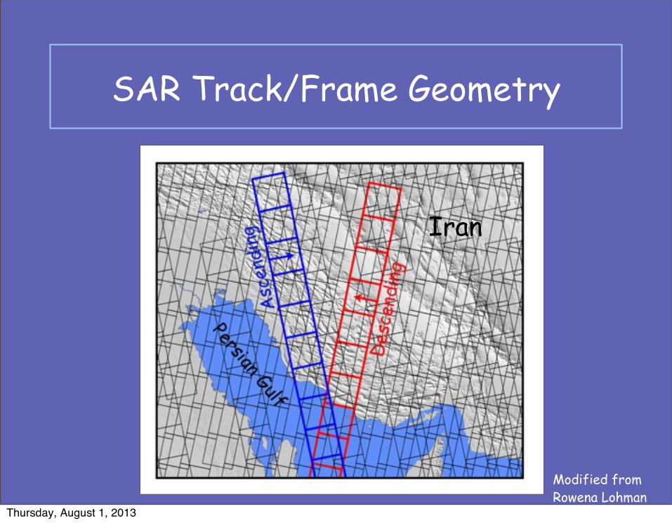
SAR Track/Frame Geometry
Iran
Modified from Rowena Lohman
Thursday, August 1, 2013
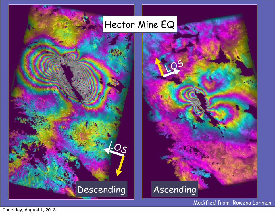
Descending Ascending
LOS
LOS
Hector Mine EQ
Modified from Rowena LohmanThursday, August 1, 2013
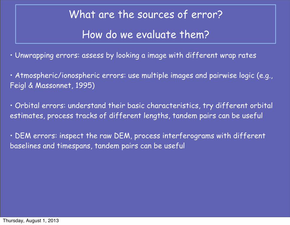
What are the sources of error?
How do we evaluate them?
• Unwrapping errors: assess by looking a image with different wrap rates
• Atmospheric/ionospheric errors: use multiple images and pairwise logic (e.g., Feigl & Massonnet, 1995)
• Orbital errors: understand their basic characteristics, try different orbital estimates, process tracks of different lengths, tandem pairs can be useful
• DEM errors: inspect the raw DEM, process interferograms with different baselines and timespans, tandem pairs can be useful
Thursday, August 1, 2013
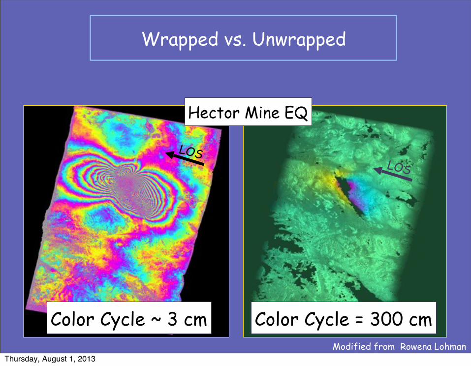
Wrapped vs. Unwrapped
Color Cycle = 300 cm
LOS
Color Cycle ~ 3 cm
LOS
Modified from Rowena Lohman
Hector Mine EQ
Thursday, August 1, 2013
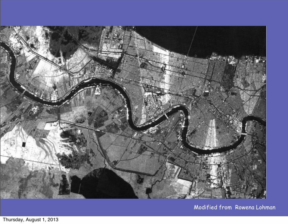
Modified from Rowena Lohman
Thursday, August 1, 2013
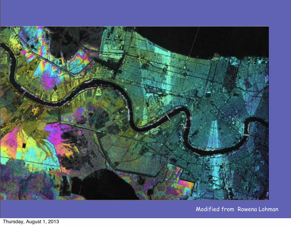
Modified from Rowena Lohman
Thursday, August 1, 2013
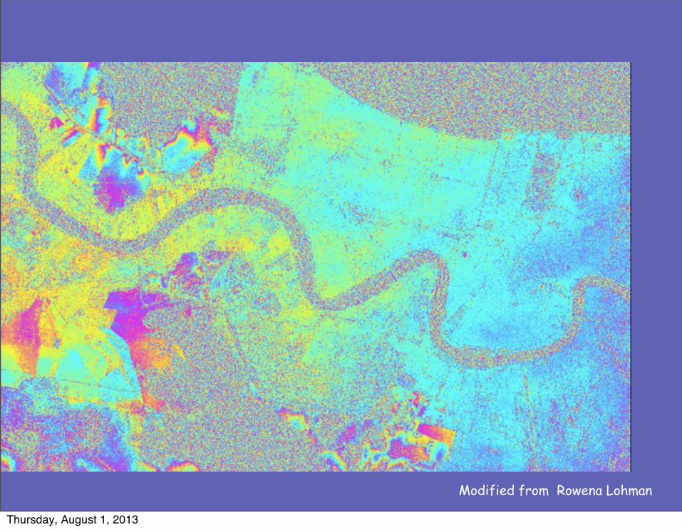
Modified from Rowena Lohman
Thursday, August 1, 2013
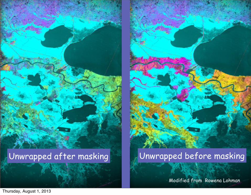
Unwrapped after masking Unwrapped before masking
Modified from Rowena Lohman
Thursday, August 1, 2013
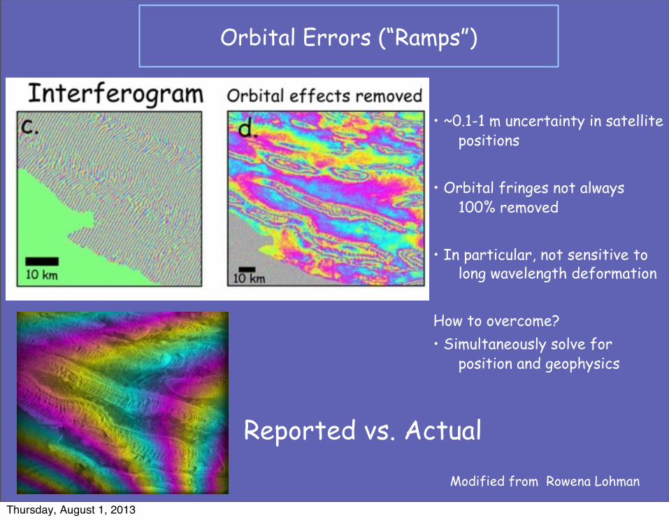
Orbital Errors (“Ramps”)
• ~0.1-1 m uncertainty in satellite positions
• Orbital fringes not always 100% removed
• In particular, not sensitive to long wavelength deformation
How to overcome?• Simultaneously solve for
position and geophysics
Reported vs. Actual
Modified from Rowena Lohman
Thursday, August 1, 2013
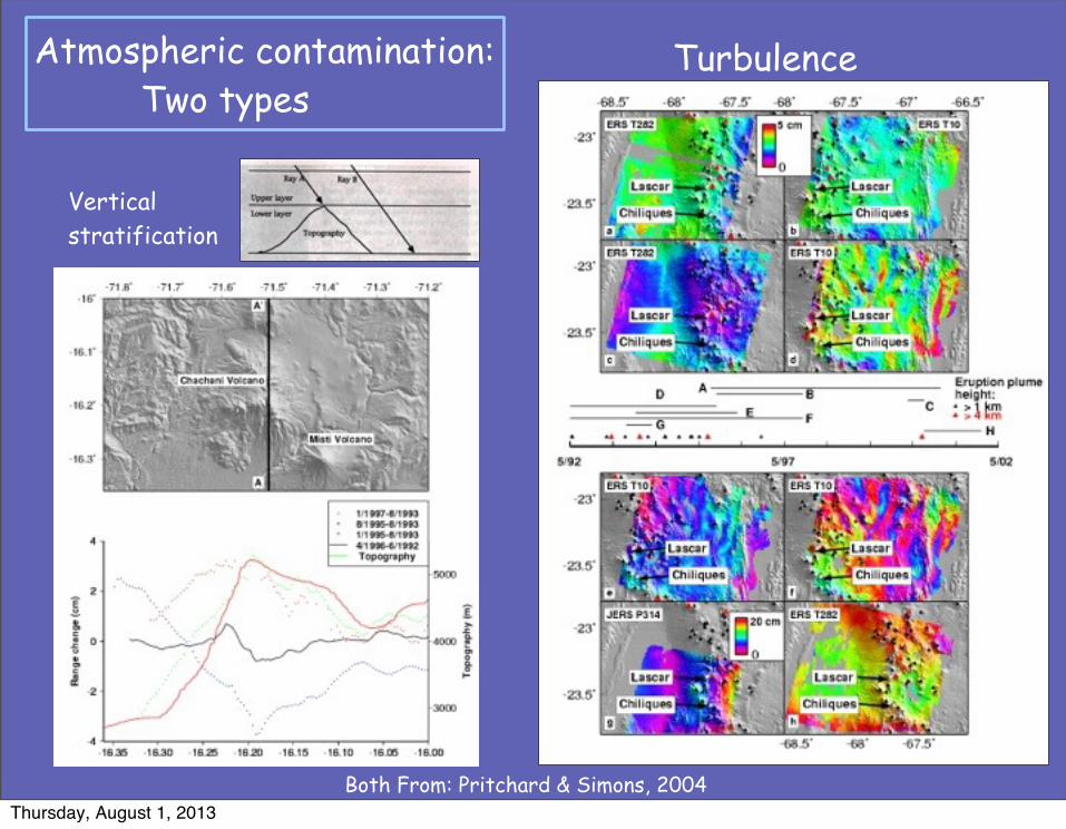
Atmospheric contamination: Two types
Turbulence
Vertical stratification
Both From: Pritchard & Simons, 2004Thursday, August 1, 2013
Can we remove the atmospheric signal from interferograms?
0) Use interferograms themselves to estimate linear or exponential phase with elevation: constant for image or spatially variable
1) Direct water vapor and “dry delay” observations: From satellite (e.g., Li et al., 2005) and OSCAR.jpl.nasa.gov From GPS & other ground sensors (e.g., Webley et al., 2002)
2) Data stacks or APS: Assume atmosphere random in time or low-pass time domain filtering (e.g., Ferretti et al., 2001; Simons and Rosen, 2007)
3) Global and Regional Models computed by data center (~100 km horizontal resolution by ECMWF, NCEP; North American RR ~ 32 km) (e.g., Doin et al., 2007; Elliott et al., 2007)
4) Regional or Local Model computed by user (<3 km horizontal resolution) (e.g., Foster et al., 2006)
Thursday, August 1, 2013
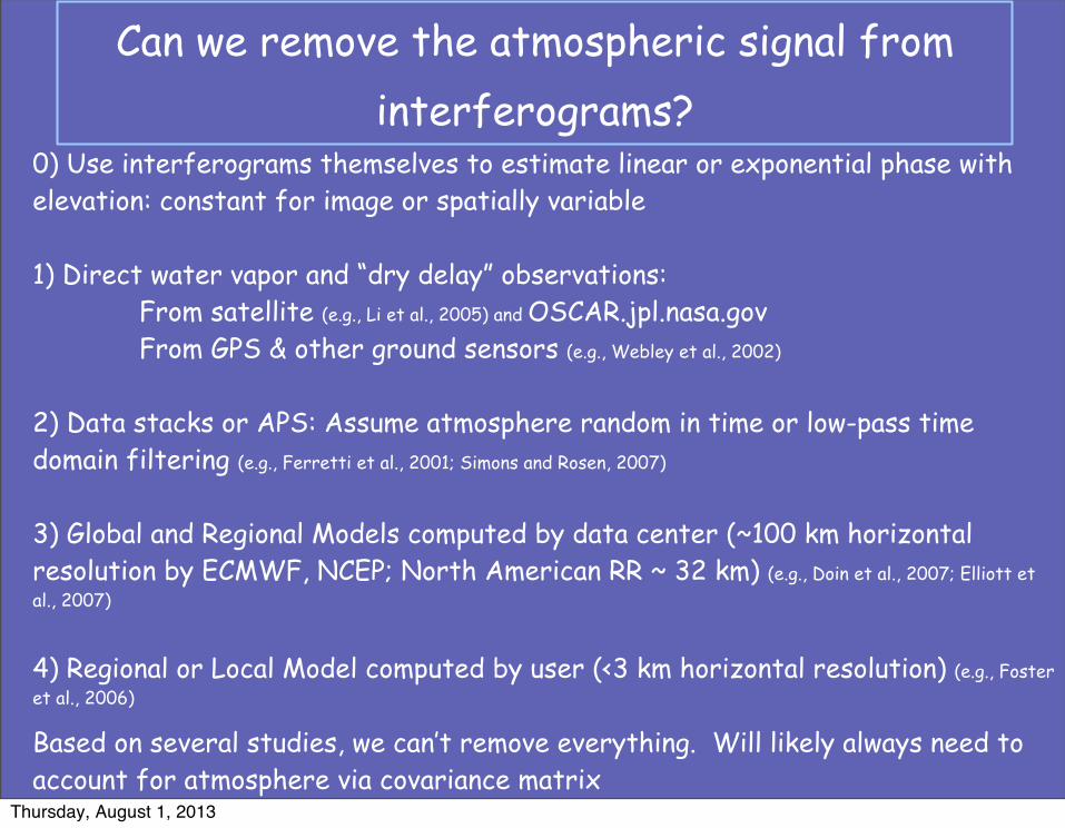
Can we remove the atmospheric signal from interferograms?
0) Use interferograms themselves to estimate linear or exponential phase with elevation: constant for image or spatially variable
1) Direct water vapor and “dry delay” observations: From satellite (e.g., Li et al., 2005) and OSCAR.jpl.nasa.gov From GPS & other ground sensors (e.g., Webley et al., 2002)
2) Data stacks or APS: Assume atmosphere random in time or low-pass time domain filtering (e.g., Ferretti et al., 2001; Simons and Rosen, 2007)
3) Global and Regional Models computed by data center (~100 km horizontal resolution by ECMWF, NCEP; North American RR ~ 32 km) (e.g., Doin et al., 2007; Elliott et al., 2007)
4) Regional or Local Model computed by user (<3 km horizontal resolution) (e.g., Foster et al., 2006)
Based on several studies, we can’t remove everything. Will likely always need to account for atmosphere via covariance matrix
Thursday, August 1, 2013
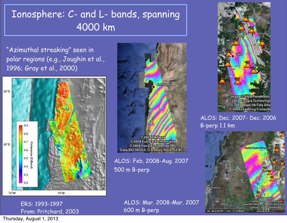
Ionosphere: C- and L- bands, spanning 4000 km
“Azimuthal streaking” seen in polar regions (e.g., Joughin et al., 1996; Gray et al., 2000)
ERS: 1993-1997From: Pritchard, 2003
ALOS: Feb. 2008-Aug. 2007500 m B-perp
ALOS: Dec. 2007- Dec. 2006B-perp 1.1 km
ALOS: Mar. 2008-Mar. 2007600 m B-perp
Thursday, August 1, 2013
Ionosphere
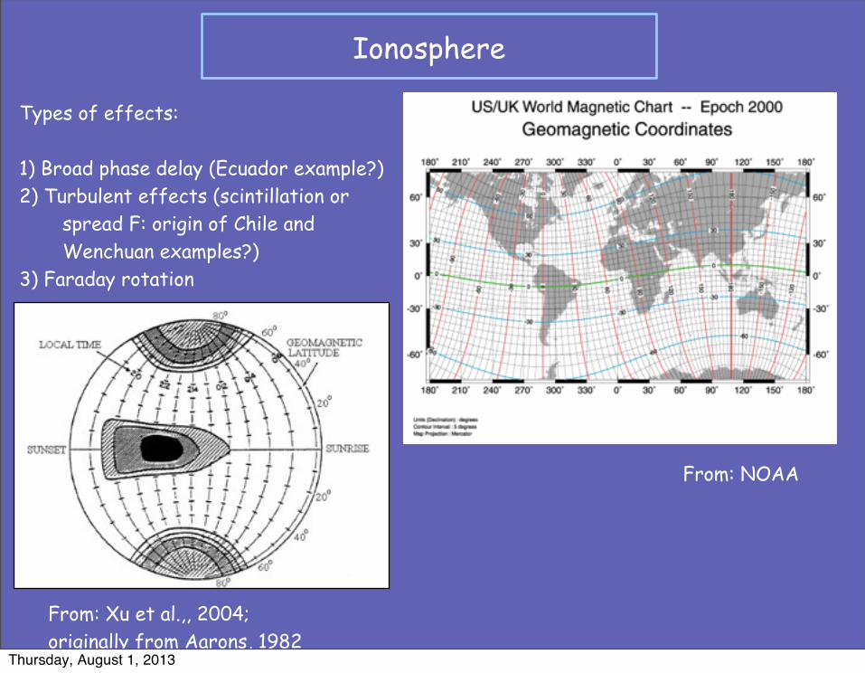
From: NOAA
From: Xu et al.,, 2004; originally from Aarons, 1982
Types of effects:
1) Broad phase delay (Ecuador example?)2) Turbulent effects (scintillation or
spread F: origin of Chile and Wenchuan examples?)
3) Faraday rotation
Thursday, August 1, 2013
Ionosphere
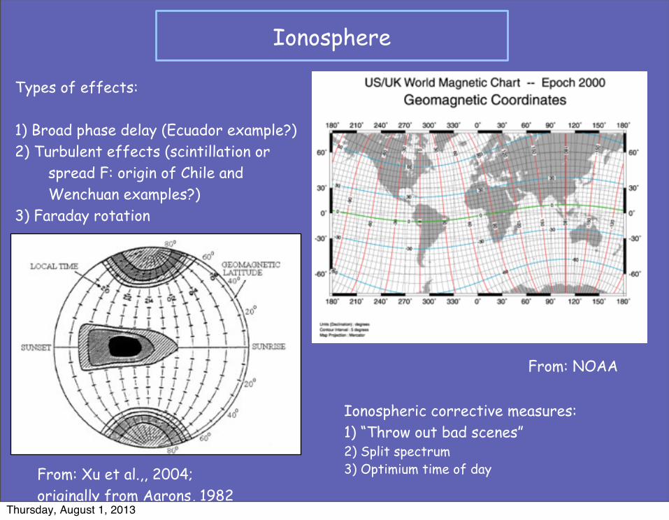
From: NOAA
From: Xu et al.,, 2004; originally from Aarons, 1982
Types of effects:
1) Broad phase delay (Ecuador example?)2) Turbulent effects (scintillation or
spread F: origin of Chile and Wenchuan examples?)
3) Faraday rotation
Ionospheric corrective measures:1) “Throw out bad scenes”2) Split spectrum3) Optimium time of day
Thursday, August 1, 2013
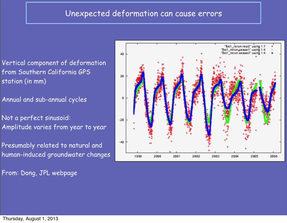
Unexpected deformation can cause errors
Vertical component of deformation from Southern California GPS station (in mm)
Annual and sub-annual cycles
Not a perfect sinusoid:Amplitude varies from year to year
Presumably related to natural and human-induced groundwater changes
From: Dong, JPL webpage
Thursday, August 1, 2013
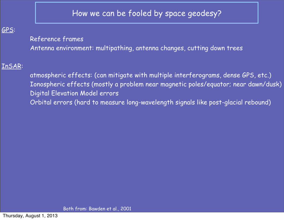
GPS: Reference frames Antenna environment: multipathing, antenna changes, cutting down trees
InSAR: atmospheric effects: (can mitigate with multiple interferograms, dense GPS, etc.) Ionospheric effects (mostly a problem near magnetic poles/equator; near dawn/dusk) Digital Elevation Model errors Orbital errors (hard to measure long-wavelength signals like post-glacial rebound)
How we can be fooled by space geodesy?
Both from: Bawden et al., 2001Thursday, August 1, 2013
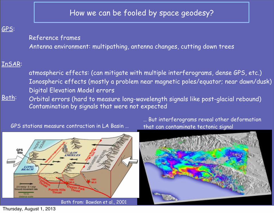
GPS: Reference frames Antenna environment: multipathing, antenna changes, cutting down trees
InSAR: atmospheric effects: (can mitigate with multiple interferograms, dense GPS, etc.) Ionospheric effects (mostly a problem near magnetic poles/equator; near dawn/dusk) Digital Elevation Model errors Orbital errors (hard to measure long-wavelength signals like post-glacial rebound)
How we can be fooled by space geodesy?
GPS stations measure contraction in LA Basin …
Both from: Bawden et al., 2001
… But interferograms reveal other deformation that can contaminate tectonic signal
Both: Contamination by signals that were not expected
Thursday, August 1, 2013
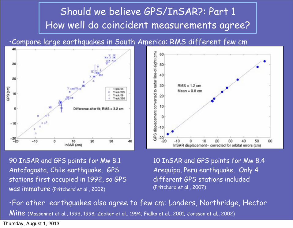
Should we believe GPS/InSAR?: Part 1How well do coincident measurements agree?
•Compare large earthquakes in South America: RMS different few cm
90 InSAR and GPS points for Mw 8.1 Antofagasta, Chile earthquake. GPS stations first occupied in 1992, so GPS was immature (Pritchard et al., 2002)
10 InSAR and GPS points for Mw 8.4 Arequipa, Peru earthquake. Only 4 different GPS stations included(Pritchard et al., 2007)
•For other earthquakes also agree to few cm: Landers, Northridge, Hector Mine (Massonnet et al., 1993, 1998; Zebker et al., 1994; Fialko et al., 2001; Jonsson et al., 2002)
Thursday, August 1, 2013
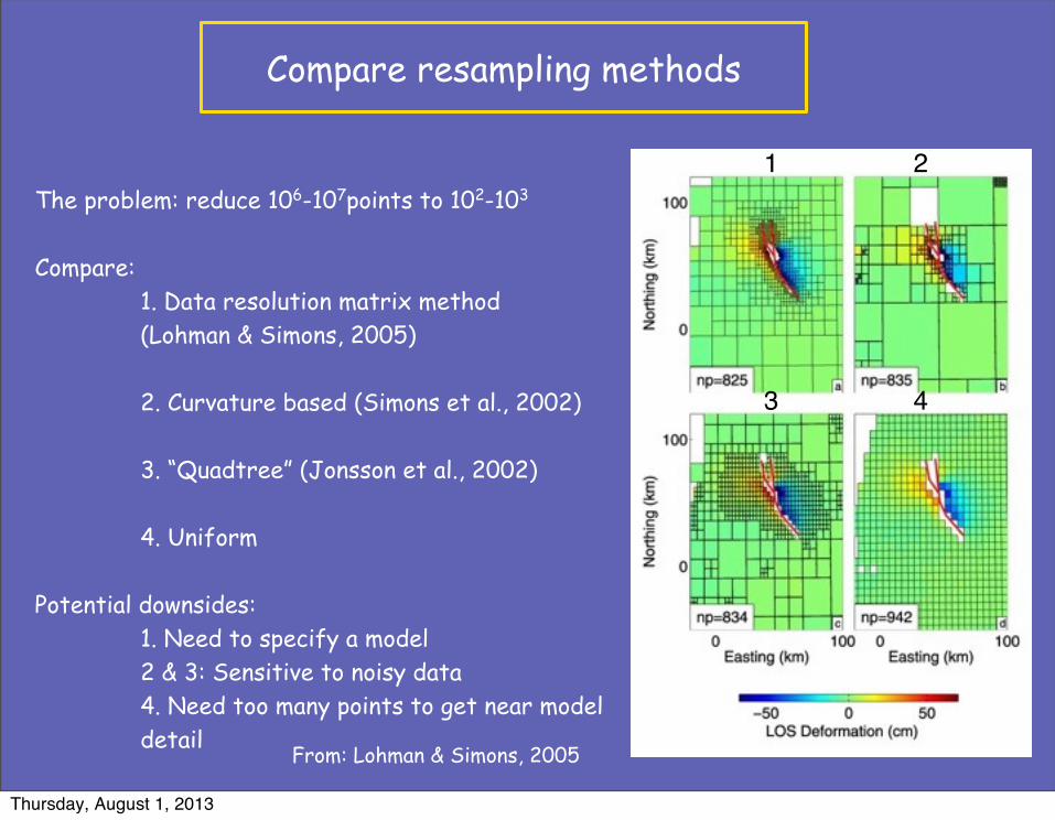
Compare resampling methods
The problem: reduce 106-107points to 102-103
Compare: 1. Data resolution matrix method (Lohman & Simons, 2005)
2. Curvature based (Simons et al., 2002)
3. “Quadtree” (Jonsson et al., 2002)
4. Uniform
Potential downsides: 1. Need to specify a model 2 & 3: Sensitive to noisy data 4. Need too many points to get near model detail
From: Lohman & Simons, 2005
1 2
3 4
Thursday, August 1, 2013
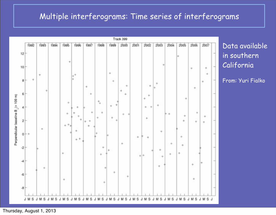
Data available in southern California
From: Yuri Fialko
Multiple interferograms: Time series of interferograms
Thursday, August 1, 2013
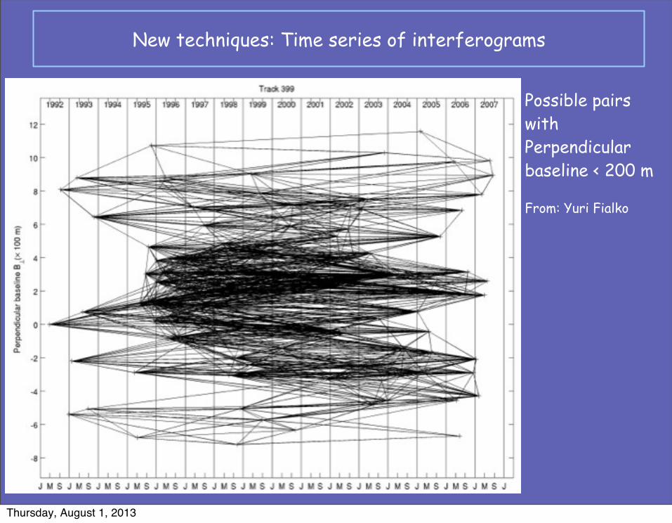
Possible pairs with Perpendicular baseline < 200 m
From: Yuri Fialko
New techniques: Time series of interferograms
Thursday, August 1, 2013
Strategies for combining multiple interferograms
Prerequisite: Need to co-register interferograms either in radar or geographic coordinate. You can do this in ROI_PAC 3.0.1 using process_2pass_master.pl by setting the Do_sim flag in the *.proc file--time-invariant view is stacking: Just take co-registered interferograms and add them together -- divide by the total time interval to get a rate
--time-variable view is called time-series: including methods called SBAS, PSInSAR, etc. More in lectures on GIAnT.Advantages: Deformation is time-dependent separate signal & error (atmosphere, unwrapping, DEM)Thursday, August 1, 2013
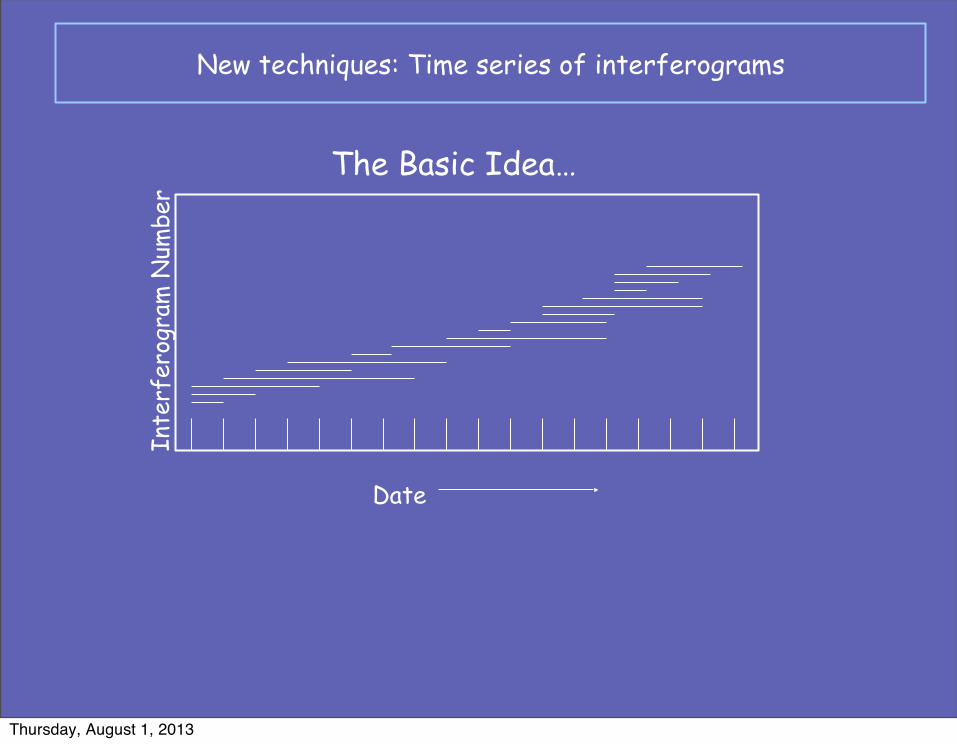
The Basic Idea…
Date
Inte
rfer
ogra
m N
umbe
r
New techniques: Time series of interferograms
Thursday, August 1, 2013
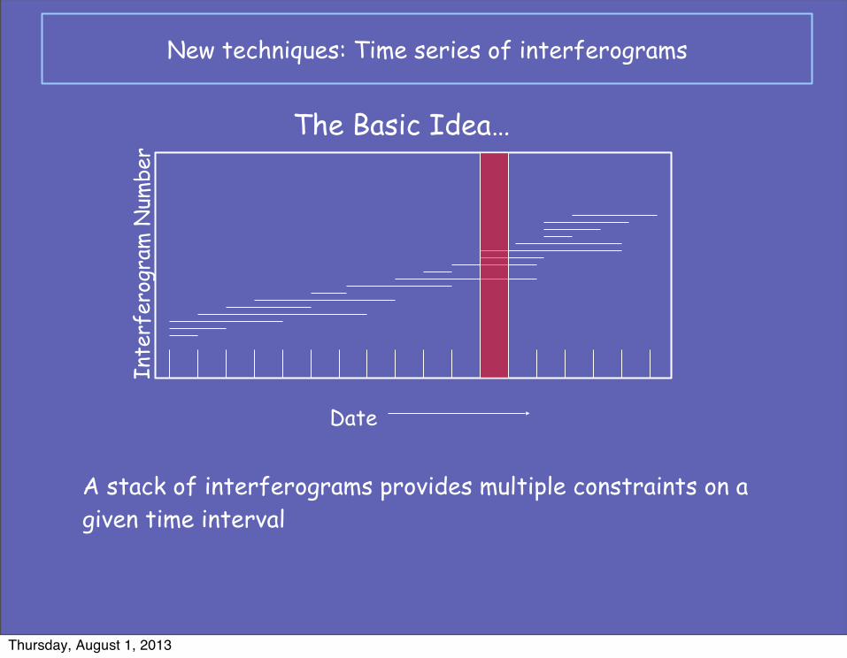
The Basic Idea…
Date
Inte
rfer
ogra
m N
umbe
r
A stack of interferograms provides multiple constraints on a given time interval
New techniques: Time series of interferograms
Thursday, August 1, 2013
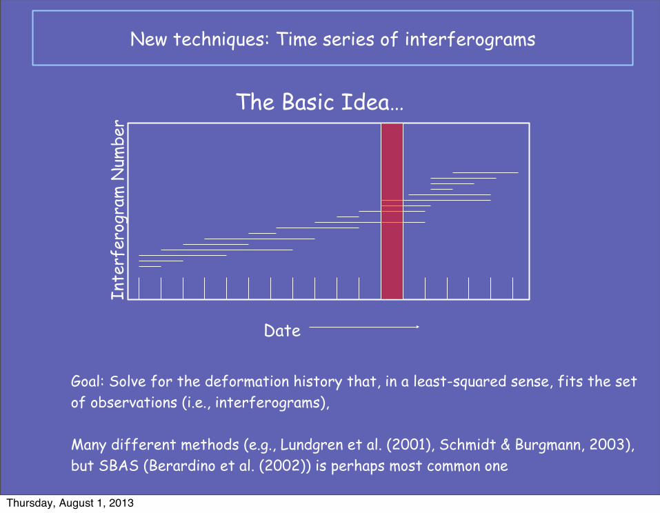
The Basic Idea…
Date
Inte
rfer
ogra
m N
umbe
r
Goal: Solve for the deformation history that, in a least-squared sense, fits the set of observations (i.e., interferograms),
Many different methods (e.g., Lundgren et al. (2001), Schmidt & Burgmann, 2003), but SBAS (Berardino et al. (2002)) is perhaps most common one
New techniques: Time series of interferograms
Thursday, August 1, 2013
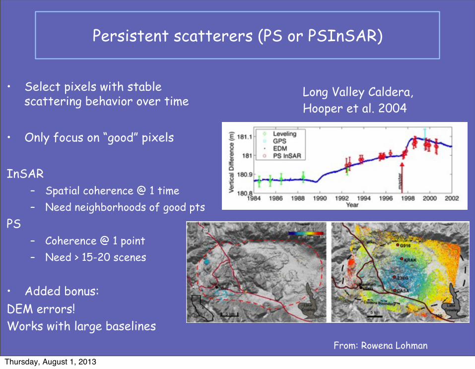
Persistent scatterers (PS or PSInSAR)
Long Valley Caldera,Hooper et al. 2004
• Select pixels with stable scattering behavior over time
• Only focus on “good” pixels
InSAR– Spatial coherence @ 1 time– Need neighborhoods of good pts
PS– Coherence @ 1 point– Need > 15-20 scenes
• Added bonus:DEM errors!Works with large baselines
From: Rowena LohmanThursday, August 1, 2013
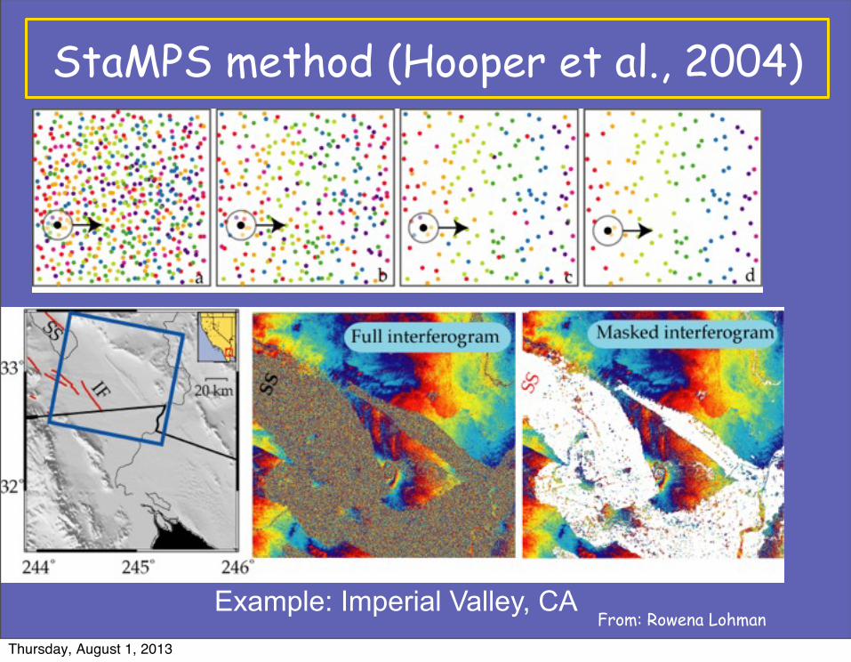
StaMPS method (Hooper et al., 2004)
Example: Imperial Valley, CAFrom: Rowena Lohman
Thursday, August 1, 2013
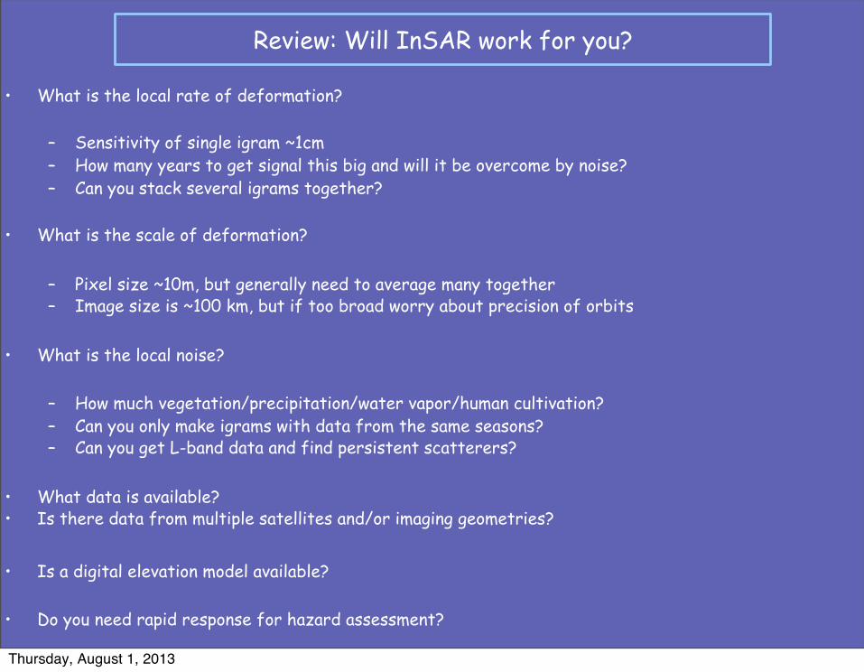
Review: Will InSAR work for you?
• What is the local rate of deformation?
– Sensitivity of single igram ~1cm – How many years to get signal this big and will it be overcome by noise?– Can you stack several igrams together?
• What is the scale of deformation?
– Pixel size ~10m, but generally need to average many together– Image size is ~100 km, but if too broad worry about precision of orbits
• What is the local noise?
– How much vegetation/precipitation/water vapor/human cultivation?– Can you only make igrams with data from the same seasons?– Can you get L-band data and find persistent scatterers?
• What data is available? • Is there data from multiple satellites and/or imaging geometries?
• Is a digital elevation model available?
• Do you need rapid response for hazard assessment?
Thursday, August 1, 2013
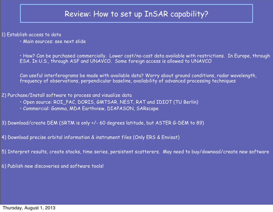
Review: How to set up InSAR capability?
1) Establish access to data • Main sources: see next slide
• How? Can be purchased commercially. Lower cost/no-cost data available with restrictions. In Europe, through ESA. In U.S., through ASF and UNAVCO. Some foreign access is allowed to UNAVCO
Can useful interferograms be made with available data? Worry about ground conditions, radar wavelength, frequency of observations, perpendicular baseline, availability of advanced processing techniques
2) Purchase/Install software to process and visualize data • Open source: ROI_PAC, DORIS, GMTSAR, NEST, RAT and IDIOT (TU Berlin) • Commercial: Gamma, MDA Earthview, DIAPASON, SARscape
3) Download/create DEM (SRTM is only +/- 60 degrees latitude, but ASTER G-DEM to 89)
4) Download precise orbital information & instrument files (Only ERS & Envisat)
5) Interpret results, create stacks, time series, persistent scatterers. May need to buy/downoad/create new software
6) Publish new discoveries and software tools!
Thursday, August 1, 2013
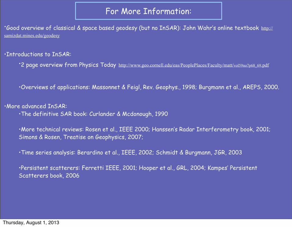
•Good overview of classical & space based geodesy (but no InSAR): John Wahr’s online textbook http://samizdat.mines.edu/geodesy
•Introductions to InSAR:•2 page overview from Physics Today http://www.geo.cornell.edu/eas/PeoplePlaces/Faculty/matt/vol59no7p68_69.pdf
•Overviews of applications: Massonnet & Feigl, Rev. Geophys., 1998; Burgmann et al., AREPS, 2000.
•More advanced InSAR:•The definitive SAR book: Curlander & Mcdonough, 1990
•More technical reviews: Rosen et al., IEEE 2000; Hanssen’s Radar Interferometry book, 2001; Simons & Rosen, Treatise on Geophysics, 2007;
•Time series analysis: Berardino et al., IEEE, 2002; Schmidt & Burgmann, JGR, 2003
•Persistent scatterers: Ferretti IEEE, 2001; Hooper et al., GRL, 2004; Kampes’ Persistent Scatterers book, 2006
For More Information:
Thursday, August 1, 2013


![practical considerations in paediatric arthritis.pptMicrosoft PowerPoint - practical considerations in paediatric arthritis.ppt [Compatibility Mode] Author: p4238583 Created Date:](https://img.pdfslide.net/doc/110x75/607dee492431fb326b3f50ef/practical-considerations-in-paediatric-microsoft-powerpoint-practical-considerations.jpg)


![PRACTICAL CONSIDERATIONS - Aalborg Universitethomes.nano.aau.dk/lg/Biosensors2009_files/Wang_Ch4.pdf · 118 PRACTICAL CONSIDERATIONS (DMF), dimethylsulfoxide (DMSO), or methanol]](https://img.pdfslide.net/doc/110x75/5a8645f77f8b9a882e8cc8c2/practical-considerations-aalborg-practical-considerations-dmf-dimethylsulfoxide.jpg)