Insider-Outsider Labor Markets,Hysteresis and Monetary Policy�

Jordi GalíCREI, UPF and Barcelona GSE

April 2016(�rst draft: September 2015)

Abstract

I develop a version of the New Keynesian model with insider-outsider labor markets and hysteresis that can account for the highpersistence of European unemployment. I study the implications ofthat environment for the design of monetary policy. The optimal pol-icy calls for strong emphasis on unemployment stabilization which astandard interest rate rule fails to deliver, with the gap between thetwo increasing in the degree of hysteresis. A simple interest rule thatincludes the unemployment rate is shown to approximate well the op-timal policy.

Keywords: wage stickiness, New Keynesian model, unemployment�uctuations, Phillips curve, monetary policy tradeo¤s.JEL Classi�cation No.: E24, E31, E32.

�Correspondence: CREI, Ramon Trias Fargas 25, 08005 Barcelona (Spain). I amgrateful for comments and suggestions to Juanjo Dolado, Nils Gottfries, Andy Levin,Silvana Tenreyro, Antonella Trigari and conference participants at the NBER Summer In-stitute and Oxford-NY Fed workshop, Banque de France, IAE-MacFinRobods Workshop,ECB-Fed International Research Forum on MonetaryPolicy, EABCN-University of ZurichConference, and seminars at Colegio Carlo Alberto, Riksbank, Norges Bank, and EinaudiInstitute. Christian Höynck, Cristina Manea, and Alain Schlaepfer provided excellentresearch assistance. E-mail: jgali@crei.cat

Much discussion on the European unemployment problem has tended tofocus on its high level, relative to the U.S. and other advanced economies.But a look at the path of the European unemployment rate over the pastfour decades points to another de�ning characteristic of that variable: itshigh persistence. The latter property has been emphasized by many authors,going back to Blanchard and Summer�s in�uential hysteresis paper.1

Can the standard New Keynesian model, the workhorse framework ofmodern macroeconomics, account for the high persistence of European un-employment? My analysis below suggests that the answer is a negative one.In particular, I show that simulations of a (realistically calibrated) version ofthat model tend to generate �uctuations in the unemployment rate that aretoo little persistent relative to the data.Motivated by the previous �ndings, I develop a variant of the New Keyne-

sian model whose equilibrium properties can be more easily reconciled withthe evidence on unemployment persistence. The modi�ed model, inspiredby the seminal work of Blanchard and Summers (1986), Gottfries and Horn(1987) and Lindbeck and Snower (1988), has two key distinctive features:(i) insider-outsider labor markets, and (ii) hysteresis. The �rst feature leadsunions to give a disproportionate weight to a subset of the labor force�theinsiders�when setting wages. The second feature implies that the measureof insiders evolves endogenously over time as a function of employment. Ishow how a calibrated version of the modi�ed model can generate a degreeof unemployment persistence comparable to that observed in the data, inresponse to a variety of shocks, and under a "realistic" monetary policy rule.Having made a case for insider-outsider labor markets and hysteresis as

a potential explanation for the high persistence of European unemployment,I turn to the implications of that environment for the design of monetarypolicy. Firstly, I derive and characterize the equilibrium under the optimalpolicy with commitment and compare it to that associated with the simpleinterest rate rule. Then I study how the simple interest rate rule can bemodi�ed in order to approximate the optimal policy. In particular, I showhow a rule that responds to the unemployment rate, in addition to in�ationand output growth, does a good job at approximating the outcomes of thefully optimal policy. In particular, I show that the welfare gains generated bythe adoption of the optimal policy (or the modi�ed rule that approximates it)

1Blanchard and Summers (1986). See Ball (2008) for an analysis of unemploymentpersistence across a number of OECD countries.

1

are substantial, and increasing in the degree of hysteresis in labor markets.

The paper is organized as follows. Section 2 presents the evidence. Sec-tion 3 develops the NewKeynesian model with insider-outsider labor markets.Section 4 analyzes the ability of that model to generate unemployment per-sistence, and contrasts it with the standard New Keynesian model. Section 5derives the optimal monetary policy in the presence of insider-outsider labormarkets, and characterizes the implied equilibrium. Section 6 analyzes thewelfare consequences of the di¤erent rules considered. Section 7 concludes.

1 Evidence

The high persistence of European unemployment is apparent in Figure 1,which displays the unemployment rate for the euro area over the sampleperiod 1970Q1-2014Q4, together with CEPR-dated recessions (as shaded ar-eas).2 The unemployment rate can be seen to wander about a (seemingly)upward trend, showing variations that are smooth and highly persistent.Each recession episode seems to pull the unemployment rate towards a newplateau, around which it appears to stabilize. The unemployment rate even-tually declines as the economy recovers, or increases further if a new recessionhits (as in 1980 or 2012). In any event, the unemployment rate shows no cleartendency to gravitate towards some constant long-run equilibrium value.3

The previous visual assessment is con�rmed by the estimated autocor-relogram for the euro area unemployment rate, which is displayed in Figure2.a (line with circles). The estimated autocorrelations decay very slowly, atrademark of highly persistent time series. As a benchmark for comparison,the �gure also shows the median and mean estimates (as well as 95 per centcon�dence bands) of the distribution of the estimated autocorrelogram for arandom walk, based on 200 simulated time series with the same number ofobservations as our sample (180). Note that the estimated autocorrelogramfor the euro area unemployment rate lies outside the con�dence interval, andwell above the median and mean autocorrelations associated with the random

2Source: ECB�s Area Wide Model quarterly data set, originally constructed Fagan,Henry and Mestre (2001) and subsequently updated by ECB. I am using update 14, whichcorresponds to 18 countries.

3The latter observation is in stark contrast to the U.S. unemployment rate, which�uctuates around a value not far from 5 percent.

2

walk, pointing to greater persistence than the latter process.4

When I drop from the sample the �rst �fteen years, during which the un-employment rate shows a (nearly) continuous increase, and start the sampleperiod at 1985Q1, the estimated autocorrelogram comes down uniformly, asshown in Figure 2.b. Note, however, that it remains close to the estimatedautocorrelogram for a simulated random walk (with 120 observations), andwell within the corresponding con�dence interval.The outcome of unit root tests applied to the euro area unemployment

rate tends to accord with the previous evidence. In particular, and as re-ported in Table 1, an Augmented Dickey-Fuller (ADF) test (with 1 and 4lags) does not reject the null of unit root in the unemployment rate at a 5percent signi�cance level. When I start the sample period in 1985Q1, thenull of a unit root is (marginally) rejected when only one lag of the �rst-di¤erenced unemployment rate is used in the ADF regression, but cannot berejected again when four lags are used. Finally, when I restrict myself to thesingle currency period proper (1999Q1-2015Q4) I cannot reject the null of aunit root again.

The evidence above makes it clear that the unemployment rate in theeuro area displays very high persistence. Here I do not take a stance as towhether it has or does not have a unit root. Yet, it is clear that given thesize of the sample periods considered, the observed persistence is comparableto that of a random walk.

2 ANewKeynesianModel with Insider-OutsiderLabor Markets

In the present section I modify an otherwise standard New Keynesian frame-work by embedding in it a model of wage setting along the lines of insider-outsider models of the labor market. With the exception of the assumptionson wage setting, the environment is similar to that described in Galí (2015,chapter 7), in which the household block of the New Keynesian model isreformulated in order to bring a meaningful concept of unemployment into

4A similar �nding is obtained when I use 1985Q1-2014Q4 and 1999Q1-2014Q4 as al-ternative sample periods (adjusting the number of observations in the simulated randomwalks accordingly), though in those cases the estimated autocorrelogram lies inside thecon�dence interval associated with the random walk.

3

the model.

2.1 Households

I assume a large number of identical households. Each household has a con-tinuum of members represented by the unit square. Each member is indexedby a pair (j; s) 2 [0; 1]� [0; 1]. The �rst index, j 2 [0; 1], represents the typeof labor service ("occupation") that she is specialized in. The second index,s 2 [0; 1], determines her disutility from work. The latter is given by �s'

if she is employed and zero otherwise, where � > 0 and ' > 0 are exoge-nous parameters. Employed individuals work a constant number of hours.Employment for each occupation, Nt(j) 2 [0; 1], is demand determined andtaken as given by the household, which allocates it to the members with thelowest work disutility among those specialized in the given occupation, i.e.s 2 [0;Nt(j)]. Full risk sharing within the household is assumed. Given theseparability of preferences, this implies the same level of consumption forall household members, independently of their occupation or employmentstatus.The household�s period utility is given by the integral of its members�

utilities:

U(Ct; fNt(j)g;Zt) � logCt � �

Z 1

0

Z Nt(j)

0

s'dsdj

!Zt

=

�logCt � �

Z 1

0

Nt(j)1+'

1 + 'dj

�Zt

where Ct ��R 1

0Ct(i)

1� 1�p;t di

� �p;t�p;t�1 is a consumption index, with Ct(i) being

the quantity consumed of good i, for all i 2 [0; 1]. Parameter �p;t denotes theelasticity of substitution, which is (possibly) time-varying. The exogenouspreference shifter zt � logZt is assumed to follow an AR(1) process:

zt = �zzt�1 + "zt

where �z 2 [0; 1] and "zt is a white noise process with zero mean and variance�2z.Each household seeks to maximize

E0

1Xt=0

�tU(Ct; fNt(j)g;Zt)

4

subject to a sequence of �ow budget constraints given byZ 1

0

Pt(i)Ct(i)di+QtBt � Bt�1 +Z 1

0

Wt(j)Nt(j)dj +Dt (1)

where Pt(i) is the price of good i, Wt(j) is the nominal wage for occupationj, Bt represents purchases of a nominally riskless one-period discount bondpaying one unit of account ("money"), Qt is the price of that bond, andDt is a lump-sum component of income (which may include, among otheritems, dividends from the ownership of �rms).5 � 2 [0; 1] is the household�sdiscount factor.Independently of the nature of wage setting, the household�s problem

above gives rise to two types of optimality conditions: a set of optimal de-mand schedules for each consumption good and a standard intertemporaloptimality condition (or Euler equation). Those take the familiar form (us-ing lower case letters to denote logs):

ct(i) = ��p;t(pt(i)� pt) + ct

for all i 2 [0; 1], and

ct = Etfct+1g � (it � Etf�pt+1g � �) + (1� �z)zt

where �pt � pt � pt�1 denotes price in�ation, and � � � log � is the discountrate.6

Following Galí (2011), I de�ne Lt(j) as the marginal participant for oc-cupation j, determined by condition:

1

Ct

Wt(j)

Pt= �Lt(j)

'

Taking logs and aggregating over all occupations one can derive the fol-lowing aggregate participation equation:

!t � wt � pt = ct + 'lt + � (2)

5The above sequence of period budget constraints is supplemented with a solvencycondition that prevents the household from engaging in Ponzi schemes.

6See Woodford (2003) or Galí (2015b) for a derivation of these and other equilibriumconditions unrelated to the labor market.

5

where wt �R 10wt(j)dj is the average (log) nominal wage, lt �

R 10lt(j)dj can

be interpreted as the (log) labor force (or participation), and � � log�.Thus, the unemployment rate can be (naturally) de�ned as:

ut � lt � nt (3)

where nt �R 10nt(j)dj is (log) aggregate employment, which is demand de-

termined.

2.2 Firms

I assume the existence of a continuum of di¤erentiated goods i 2 [0; 1], eachproduced by a monopolistic competitor, with a production function:

Yt(i) = AtNt(i)1�� (4)

where Yt(i) denotes the output of good i, At is an exogenous technologyparameter common to all �rms, and Nt(i) is a CES function of the quantitiesof the di¤erent types of labor services employed by �rm i, whose elasticity ofsubstitution is given by �w. Cost minimization by �rms gives rise to the labordemand schedule (10) introduced above. Technology is assumed to follow arandom walk in logs, i.e.

at = at�1 + "at

Price-setting is staggered à la Calvo, with a constant fraction �p of �rmsthat keep prices unchanged in any given period. Aggregation of price-settingdecisions, gives rise to an in�ation equation of the form (around a zero in�a-tion steady state)

�pt = �Etf�pt+1g � �p(�pt � xt) (5)

where�pt � at � �nt + log(1� �)� !t (6)

is the average price markup, �p � (1��p)(1���p)�p

1��1��+��p and xt � log

�p;t�p;t�1

is the desired or natural price markup.7 The latter is assumed to follow anAR(1) process with mean log �p

�p�1 autoregressive coe¢ cient �x and innovationvariance �2x.

7See chapter 3 in Galí (2015) for a derivation.

6

Note that we can rewrite the markup gap in terms of employment andwages as follows:

�pt � xt = at � �bnt � �n+ log(1� �)� xt � !t= ��bnt � e!t (7)

where e!t � !t � (at � �n + log(1� �)� xt) is the wage gap, de�ned as thelog deviation between the actual wage and the wage that would obtain under�exible prices conditional on employment being at its steady state level.Goods market equilibrium requires that ct = yt for all t, which combined

with the household�s Euler equation implies:

yt = Etfyt+1g � (it � Etf�pt+1g � �) + (1� �z)zt (8)

Given equilibrium output, employment is given by

(1� �)nt = yt � at (9)

2.3 Wage Setting

Next I turn to a description of wage setting. First I describe wage settingin the standard New Keynesian model, and then turn to wage setting in theinsider-outsider model. In both cases, I adopt the Calvo model of staggerednominal wage setting, which assumes that a constant fraction 1 � �w ofoccupations (or the unions representing them), drawn randomly from the setof existing occupations, are allowed to reset their nominal wage in any givenperiod.When setting the new wage w�t (j), a union representing occupation j takes

into account current and (expected) future demand for its work services, asgiven by:

nt+kjt(j) = ��w(w�t (j)� wt+k) + nt+k (10)

for k = 1; 2; 3; :::where nt+kjt(j) denotes period t + k (log) employment foroccupation j whose wage has been reset for the last time in period t, andnt+k is (log) aggregate employment in period t+ k. Note that �w > 1 is thewage elasticity of labor demand.As a result the evolution of the average (log) nominal wage is described

by the di¤erence equation:

wt = �wwt�1 + (1� �w)w�t (11)

7

where w�t � (1� �w)�1Rj2�t w

�t (j)dj, where �t � [0; 1] represents the subset

of occupations resetting their wage in period t: Thus, w�t is the average newlyset wage in period t, expressed in logs.8

The previous features are common to the two models of wage settingconsidered below.

2.3.1 Wage Setting in the Standard New Keynesian Model

In the standard New Keynesian model (e.g. Erceg, Henderson and Levin(2001)) it is assumed that, when resetting the wage, each union seeks to max-imize the utility of the representative household, to which all union members(employed or unemployed) belong.9 This gives rise to a (log-linearized) wagesetting rule of the form:

w�t = �w + (1� ��w)

1Xk=0

(��w)kEt

�wt+kjt

(12)

where wt+kjt � pt+k + ct+k + 'nt+kjt + � is the relevant reservation wage int + k for a union that has reset its wage for the last time in period t, and�w � log �w

�w�1 is the desired or natural wage markup (over the reservationwage), which is assumed to be constant. It is easy to show that the latteris the wage markup that any union (acting independently) would choose ifwages were fully �exible, given a labor demand schedule with a constant wageelasticity �w.Combining (11) and (12) allows one to derive the wage in�ation equation:

�wt = �Etf�wt+1g � �w(�wt � �w) (13)

where �wt � wt � wt�1 denotes wage in�ation and

�wt � !t � (ct + 'nt + �) (14)

is the average wage markup in period t, where !t � wt � pt is the average(log) real wage, and �w � (1��w)(1���w)

�w(1+�w').

8The previous equation, like others used in the present analysis, are log-linear ap-proximations in a neighborhood of a zero in�ation steady state to the exact equilibriumcondition. See Galí (2015) for detailed derivations.

9See, e.g., Galí (2015, chapter 6) for a discussion of the union�s problem and a derivationof the optimal wage setting rule.

8

Note that equations (2) and (14) can be combined with the de�nition ofthe unemployment rate in (3) to yield a simple relation linking the averagewage markup and unemployment:

�wt = 'ut (15)

Finally, one can combine the latter condition with (13) to derive thefollowing New Keynesian wage Phillips curve, linking wage in�ation andunemployment:

�wt = �Etf�wt+1g � �w'(ut � u) (16)

where u � �w

'is the natural rate of unemployment, i.e. the unemployment

rate that would obtain under �exible wages (and, hence, a constant wagemarkup �w).10

It is easy to see that the previous model of wage setting guarantees thetendency of the unemployment rate to gravitate towards its natural rate, evenin the presence of permanent shocks. Thus, (16) makes clear that in the faceof a high (low) unemployment rate (relative to the natural rate u), wages willtend to decrease (increase), thus lowering (raising) marginal cost, in�ation,and the interest rate (through a policy rule like (23)) and, as a result, boosting(dampening) output and reducing (increasing) the unemployment rate.The implied stationarity of the unemployment rate becomes apparent by

noting that (12) can be equivalently rewritten as

(1� ��w)1Xk=0

(��w)kEt

��wt+kjt

= �w

where �wt+kjt � w�t � wt+kjt is the markup k periods after the wage is setand conditional on the latter remeining in place. Thus, when reoptimizing,unions choose a wage such that, in expectation, a speci�c weighted averageof the wage markups that will prevail over the life of the newly set wageequals the desired or frictionless wage markup �w. Since all wage-settingunions behave in a similar way, the economy�s average wage markup �wt will�uctuate about �w. Accordingly, and given (15), the unemployment rate willdisplay mean-reverting �uctuations about the constant natural rate u.11

10Galí (2011) provides evidence in support of that wage equation based on postwar U.S.data.11In Galí (2015a) I discuss possible sources of unemployment rate nonstationarity in

9

2.3.2 An Insider-Outsider Model of Wage Setting

Insider-outsider models of the labor market, as originally developed in Blan-chard and Summers (1986), Gottfries and Horn (1987) and Lindbeck andSnower (1988), emphasize the segmentation of the labor force between insid-ers and outsiders and the dominant role of the former in wage determination.In the words of Blanchard and Summers:

"...there is a fundamental asymmetry in the wage-setting processbetween insiders who are employed and outsiders who want jobs.Outsiders are disenfranchised and wages are set with a view toensuring the jobs of insiders. Shocks that lead to reduced em-ployment change the number of insiders and thereby change thesubsequent equilibrium wage rate, given rise to hysteresis..."

Here I use a version of the insider-outsider model consistent with theCalvo wage setting formalism, and hence one that can be readily embeddedin the standard New Keynesian model.In the insider-outsider model proposed here a union resetting the wage

for occupation j in period t is assumed to choose a wage, w�t (j), such thatthe following condition is satis�ed

(1� ��w)1Xk=0

(��w)kEt

�nt+kjt(j)

= n�t (j) (17)

with nt+kjt(j) given by (10), for k = 0; 1; 2:::In words, the wage is set so that,in expectation, a weighted average of employment in occupation j over theperiod the wage remains e¤ective equals some employment target n�t (j). Thelatter can interpreted as representing the measure of insiders in occupationj.12

the New Keynesian model. In addition to the hysteresis model proposed below, I pointto nonstationarity in the desired wage markup and/or in the in�ation target as possibleaddition sources of a unit root in the unemployment rate. As argued in that paper,however, some of the implications of those alternative hypothesis are hard to reconcilewith the observed joint behavior of wage in�ation and the unemployment rate.12A possible justi�cation for this type of behavior may involve some deviation from

perfect consumption risk sharing within households, with each individual�s consumptionbeing related to her individual wage income. A formal treatment is beyond the scope ofthe present model.

10

Substituting (10) into (17) yields the wage setting rule:

w�t (j) = �1

�wn�t (j) + (1� ��w)

1Xk=0

(��w)kEt

�wt+k +

1

�wnt+k

�(18)

I follow Blanchard and Summers (1986) and assume that the measureof insiders (and, hence, the employment target) in any given occupation jevolves over time according to the di¤erence equation:

n�t (j) = nt�1(j) + (1� )n� (19)

where n� is the union�s long run target for (log) employment, which is as-sumed to be common across occupations. Note that (17) implies that n� alsocorresponds to equilibrium employment in the perfect foresight steady state,i.e. n = n�. Parameter 2 [0; 1] determines the extent to which changes inemployment a¤ect the economy�s state, by changing the measure of insiders.This is the phenomenon referred to in the literature as hysteresis.Beyond the particular speci�cation chosen, the motivation behind that

assumption is the notion that the concerns of employed workers are given adisproportionate weight in the bargaining of wages. This may be the case fora variety of reasons: they are more likely to participate or remain close to thebargaining process, they are the ones with the ability to strike and hence arean important source of the union�s bargaining power, they are more likely topay their union fees, etc. On the other hand, those who are unemployed areto some extent disenfranchised in the wage setting process.Plugging (19) into (18) and averaging over j 2 �t we obtain:

w�t = �

�wbn�t�1 + (1� ��w) 1X

k=0

(��w)kEt

�wt+k +

1

�wbnt+k� (20)

where bnt � nt � n, bn�t � n�t � n, and n�t � (1 � �w)�1Rj2�t n

�t (j)dj is the

average (log) employment target for unions resetting their wage in period t.Combining (20) with (11) yields (after some algebra) the following wage

in�ation equation for the insider-outsider economy:

�wt = �Etf�wt+1g+ (1� )�n(1� ��w)bnt + �n�nt] (21)

where �n � 1��w�w�w

, which is decreasing in the degree of wage rigidities. Notethat both the (log) employment change and its deviation from steady state,

11

bnt, are the drivers of �uctuations in wage in�ation, with the weights on eachbeing a function of , the degree of hysteresis.A special case of interest is given by = 1. In that case, already singled

out in Blanchard and Summers (1986), the set of insiders corresponds to theworkers employed at the end of the previous period, with no weight attachedto the unemployed in the wage setting decision. In that case equation (21)collapses to

�wt = �Etf�wt+1g+ �n�ntwith the employment change being the only driving force. As shown below,under that extreme assumption the model displays full hysteresis: employ-ment is permanently a¤ected by any shock that has a short run e¤ect onthat variable. That unit root property is inherited by many other macrovariables, including the unemployment rate. There is no well de�ned steadystate in that case.At the other extreme, when = 0, then we have

�wt = �Etf�wt+1g+ �n(1� ��w)bntwith only the current employment gap bnt emerging now as the driving vari-able.

2.4 E¢ cient Allocation, Steady State and EquilibriumDynamics

2.4.1 E¢ cient Allocation

The e¢ cient allocation, i.e. the one that maximizes households�utility giventhe economy�s resource constraints, is easy to characterize. Employmentis identical across �rms and occupations, and all goods are consumed inidentical quantities. The e¢ ciency condition equating the marginal rate ofsubstitution and the marginal product of labor implies a constant optimallevel of employment, given by:

net �log(1� �)� �

1 + '� ne

The e¢ cient level of output is thus given by

yet � at + (1� �)ne

That allocation provides a useful benchmark in some of the analyses be-low.

12

2.4.2 Steady State

The steady state of the decentralized economy is not invariant to the assumedwage setting environment.Thus in the standard model steady state employment is given by

n � log(1� �)� (� + �w + �p)� log(1� �)1 + '

where � denotes a (constant) wage subsidy which can be easily introducedin the framework without a¤ecting any equation describing the equilibriumdynamics. Note that steady state e¢ ciency can be attained by setting � =1� expf�(�w + �p)g.By contrast, steady state employment in the model with insider-outsider

labor markets is given by the long run employment target n�, which is as-sumed to be common across unions. Thus, n = n� in the modi�ed version ofthe New Keynesian model proposed above.In the welfare analysis below it is assumed that the steady state corre-

sponds to the e¢ cient steady state in all cases considered.

2.4.3 Equilibrium Dynamics

Equations (2), (3), (5), (7), (8), (9), (14), (15), and (23), together with theidentity

!t � !t�1 + �wt � �pt (22)

and wage in�ation equation (16) (standard model) or (21) (insider outsidermodel) de�ne the non-policy block of the model. In order to close the modelone must supplement the previous equilibrium conditions with a descriptionof a monetary policy rule that (directly or indirectly) determines the nominalinterest rate it.For the baseline simulations below I assume an interest rate rule of the

form:it = �iit�1 + (1� �i)[�+ ���

pt + �y�yt] (23)

For values of �i close to unity (as assumed in the simulations below) theprevious rule is similar to the one proposed in Orphanides (2006) and Smets(2010) as a good approximation to ECB policy.

13

3 Unemployment Persistence in the NewKey-nesian Model

Can the New Keynesian model account for the observed persistence of Eu-ropean unemployment? In the present section I try to provide an answrto that question by simulating a calibrated version of the New Keynesianmodel under the two wage setting regimes considered (standard and insider-outsider), and use the generated time series to determine the persistence (andother properties) of unemployment, which are then compared to analogousproperties in the data.

3.1 Calibration

Table 2 lists the baseline settings for the model parameters used in the sim-ulations. Parameters �p is set to 3:8. That value is associated with a steadystate price markup of 35 percent, and is consistent with the evidence used inthe calibration of the ECB�s New Area Wide Model (NAWM) of Christo¤elet al. (2008). Given that setting, a value of 1=4 for parameter � is roughlyconsistent with the observed average labor income share in the euro area.13

Parameter �w is set to 4:3, again following Christo¤el et al. (2008). Giventhat setting for �w, and using the approach developed in Galí (2011a), a valueof ' equal to 3:4 can be shown to be consistent with a steady state unem-ployment rate of 7:6 percent, the average unemployment rate in the euroarea over the 1970-2014 period.14 As to the discount factor, I set � = 0:99,as is common practice in the business cycle literature. I set the Calvo wageand price stickiness parameters, �p and �w, to 0:75, which implies an aver-age duration of individual wages and prices of four quarters. That setting

13Note that in the steady state the following relation holds:

WN

PY= (1� �)

�1� 1

�p

�14Galí (2011) shows that the ', �w and the steady state unemployment rate u are related

according to equation:'u = log

�w�w � 1

Interestingly, the resulting setting for ' is nearly identical to the calibrated value in theNAWM of Christo¤el et al. (2008).

14

is roughly consistent with the bulk of the micro evidence for the euro area(see, e.g. Álvarez et al. (2006) and ECB (2009)). As to the interest rate rulecoe¢ cients, I assume �� = 1:5; �y = 0:5, and �i = 0:9. That calibration isclose to the one proposed in Orphanides (2006) and Smets (2010) as a goodapproximation to ECB policy.

3.2 Unemployment Persistence in the Standard NewKeynesian Model

I simulate the standard New Keynesian model under the above baseline cal-ibration to evaluate its ability to generate the degree of unemployment per-sistence observed in the European data. More speci�cally, I generate 200draws of 180 observations each, and conditional on each of the three exoge-nous shocks separately. For each draw I estimate the autocorrelation of theunemployment rate at 1, 4 and 8 lags, as well as its standard deviation rela-tive to output, and its correlation with (price) in�ation. The middle panel ofTable 3 reports the median and a 95 percent con�dence interval for each ofthose statistics, conditional on each shock. The top row reports their empir-ical counterparts. For the purposes of the present exercise, and in order tomaximize the model�s chances to match the high unemployment persistenceobserved in the European data, I assume that the driving forces themselvesare extremely persistent. Speci�cally, I set �a = �x = �z = 0:99.

15

The simulations� outcome, as summarized in middle panel of Table 3,suggests that the standard New Keynesian model has clear di¢ culties tomatch the persistence of European unemployment, independently of the na-ture of the shock driving those �uctuations. Firstly, while unemploymentis positively autocorrelated in response to each of the shocks, the estimatedautocorrelations appear to decline much faster than in the data. The gap isparticularly large in the case of demand shocks. Furthermore, the empiricalautocorrelations (for any of the three sample considered) lie outside the 95percent con�dence interval generated by the model.Not surprisingly, the degree of unemployment persistence is not indepen-

dent of the degree of wage rigidities. This is illustrated by the estimatedautocorrelations obtained under the assumption of much stronger stickiness.

15Note that the statistics considered here (autocorrelations, relative standard deviationsand cross-correlations) are independent of the variance of the shocks, given the model�slinearity.

15

In particular I assume �w = 0:95, which implies an average duration of anindividual wage of 5 years (!). The implied autocorrelogram of unemploy-ment increases uniformly at all lags, and for all shocks, thus getting closerto its empirical counterpart. It is worth noting however that the impliedpersistence falls short of the observed one despite the assumption of a de-gree of wage stickiness unrealistically high, thus pointing to the limitationsof that channel by itself as a source of very high unemployment persistence.In particular, it 16

From the previous exercise I conclude that a calibrated version of the stan-dard New Keynesian model, under a "realistic" policy rule, cannot accountfor the high persistence of European unemployment, at least under plausi-ble calibrations of the degree of wage stickiness. A reasonable conjecture isthat the model�s failure may lie in its treatment of the labor market itself,which may be at odds with the European reality. Next I analyze how theprevious conclusion is a¤ected when the insider-outsider labor market struc-ture described above is embedded in an otherwise standard New Keynesianmodel.

3.3 Unemployment Persistence in the New KeynesianModel with Insider-Outsider Labor Markets andHysteresis

I repeat the exercise described in the previous subsection using a version ofthe New Keynesian model with insider-outsider labor markets, as describedabove. Again, I simulate the model 200 times, conditional on each shock andobtain a set of arti�cial time series with 180 observation for each draw. Irepeat this procedure for three alternative values of the hysteresis parameter : 0, 0:9 and 1. In Table 4 I report several statistics pertaining to the behaviorof unemployment for those simulated histories, conditional on each shock andcalibration of . For comparison purposes I also report the correspondingstatistics generated by the standard New Keynesian model. In each case,the median and a 95 per cent con�dence interval (across simulations) arereported. In contrast with the previous exercise I now assume high (but notextreme) values for the autoregressive coe¢ cient of the two remaining shocks,namely, �a = �x = �z = 0:92, implying a half-life of (roughly) two years for

16See Galí (2011b) for a discussion of the dependence of unemployment volatility andpersistence on the degree of wage stickiness, in an identical model.

16

the exogenous shocks themselves.A number of �ndings are worth stressing. First, note that under = 0,

i.e. in the absence of hysteresis (and, hence, a constant employment target),the behavior of unemployment is very similar (though not identical) to that inthe New Keynesian model, even though their wage setting rules are di¤erent(one targets employment, the other targets the wage markup). Secondly,and irrespective of the shock considered, the estimated autocorrelation ofunemployment increases substantially as goes up. For both = 0:9 and =1, the implied values are not too di¤erent from those observed in the data,with the latter generally falling within the 95 percent con�dence interval.It is also worth noting that under = 1, and under the assumed monetary

policy rule, the unemployment rate (as well as employment and output)displays a unit root. Accordingly, any shock will generally have a permanente¤ect on the level of those variables, even when the shock itself is transitory.Figure 3 illustrates graphically the role of the size of the hysteresis pa-

rameter as a source of unemployment persistence, by showing the impulseresponses of the unemployment rate under the three values of considered,as well as under the standard New Keynesian model, and conditional on eachof the shocks. Two results emphasized above are clearly illustrated here: (i)the similarity of the response with the standard model when = 0 and (ii)the positive relation between the size of and the observed persistence ofthe unemployment response.In addition to its ability to account for the high persistence of European

unemployment, and as analyzed in Galí (2015a), the assumption of insider-outsider labor markets combined with (strong) hysteresis also provides apotential explanation for the relative stability of wage in�ation in the euroarea since the mid-90s, despite the large and persistent �uctuations in theunemployment rate. The reason is that, for high values of , even largedeviations of employment from steady state have a small (or zero) weight inthe determination of wage in�ation, with more weight given to the change inemployment (which can be small even when the economy is far from steadystate).Having shown that a variation of the New Keynesian model that incorpo-

rates insider-outsider labor markets and hysteresis helps improve the model�sability to account for the high persistence of European unemployment I turnto the analysis of the implications of such an assumption for the design ofmonetary policy.

17

4 Optimal Monetary Policy with Insider-OutsiderLabor Markets

Next I analyze the optimal monetary policy in the context of the New Key-nesian model with insider-outsider labor markets developed above. In doingso, I examine the role played by the degree of hysteresis (as measured byparameter ) in shaping the response of unemployment to di¤erent shocks,with a focus on the di¤erential response under the optimal policy relative tothe simple policy rule.

4.1 The Optimal Monetary Policy Problem

In the analysis below I assume that unions�long term employment goal cor-responds to the e¢ cient level of employment. Formally,

n� = ne =log(1� �)� �

1 + '

Note that the previous assumption implies that the steady state allocationis e¢ cient since, as discussed above, n = n� (at least in the case of 2 [0; 1),for which a steady state is well de�ned). The previous assumption simpli�esthe analysis while allowing me to focus on the role of hysteresis without the(well understood) complications arising from an ine¢ cient steady state.17

In particular, and under the previous assumption, one can approximate(up to second order) the representative household�s welfare losses in a neigh-borhood of the steady state by the function:

1

2E0

1Xt=0

�t�(1 + ')(1� �)bn2t + �p

�p(�pt )

2 +�w(1� �)�w

(�wt )2

�(24)

where bnt � nt � n. Loss function (24) is equivalent to that used in thestandard New Keynesian model. The reason is that the wage setting equation(12) is not used in the derivation of the loss function for the New Keynesianmodel, so its replacement by (18) has no bearing in the form of that function.

17That assumption plays a role similar to the presence of an "optimal" employmentsubsidy in standard analyses of the optimal monetary policy in the New Keynesian model.

18

The monetary authority will seek to minimize (24) subject to:

�pt = �Etf�pt+1g+ �p�bnt + �pe!t (25)

�wt = �Etf�wt+1g+ �n(1� )(1� ��w)bnt + �n �nt] (26)e!t�1 � e!t � �wt + �pt +�at ��xt (27)

for t = 0; 1; 2; ::together with some initial conditions for e!�1 and bn�1.Let f�1;tg, f�2;tg, and f�3;tg denote the sequence of Lagrange multipli-

ers associated with the previous constraints, respectively. The optimalityconditions for the optimal policy problem are thus given by

(1+')(1��)bnt+�p��1;t+�n(1�(1� )��w)�2;t��n �Etf�2;t+1g = 0 (28)�p�p�pt ���1;t + �3;t = 0 (29)

�w(1� �)�w

�wt ���2;t � �3;t = 0 (30)

�p�1;t + �3;t � �Etf�3;t+1g = 0 (31)

for t = 0; 1; 2; :::which, together with the constraints (25), (26), and (27)given �1;�1 = �2;�1 = 0 and an initial condition for e!�1 and bn�1, characterizethe solution to the optimal policy problem.

4.2 Dynamic Responses to Shocks and Welfare: Opti-mal Policy vs. Simple Rule

Figures 4 displays the response of the unemployment rate to di¤erent shocksin the New Keynesian model with insider-outsider labor markets. For eachshock I show four responses, corresponding to the possible combinations of (i)monetary policy (optimal or simple rule) and (ii) degree of hysteresis ( = 0and = 1). The remaining parameters (including the coe¢ cients in thesimple policy rule) are kept at their baseline settings, as in the simulationsof the previous section. The size of the shock is normalized to 1 percent inall cases.Two �ndings are worth stressing. Firstly, the high stability of the unem-

ployment rate under the optimal policy, in comparison to the responses underthe simple rule. This is true independently of the degree of hysteresis andthe shock impinging on the economy; it takes an extreme form in the case of

19

demand shocks, in response to which the optimal policy fully stabilizes theunemployment rate. It is worth noting that in the same of full hysteresis,and with the exception of demand shocks, the unemployment rate preservesa unit root component, though the latter is tiny (and hardly visible in theFigure).Secondly, and as the Figure makes clear, in the absence of hysteresis (or

when the latter is low, more generally), the discrepancy between the unem-ployment responses under the simple rule and under the optimal policy is farfrom negligible, but very short-lived, with the unemployment reverting backrapidly towards its initial level (despite the high persistence of the shocks).On the other hand, under full hysteresis the discrepancy is quantitativelylarge and, most importantly, permanent.The nontrivial gap between the responses under the two policies suggests

that the adoption of the optimal policy may bring about considerable welfaregains relative to the simple rule, especially in the presence of strong hystere-sis. In TabIe 5 I report the welfare losses under the two policies, as measuredby (24), conditional on each of the three shocks considered, and for threealternative values of the hysteresis parameter (0, 0:9 and 1). I also reportthe welfare loss relative the simple rule (23) (i.e. with the latter normalizedto unity), for each value of considered.Two results are worth stressing. Firstly, and independently of the shock,

we see that under the simple rule the size of welfare losses is increasing withthe degree of hysteresis. More speci�cally, welfare losses under full hysteresis( = 1) are about seven times larger than in the absence of hysteresis ( = 0).That gradient largely disappears under the optimal policy, however.Secondly, the extent to which the adoption of the optimal policy implies a

reduction of welfare losses relative to the simple rule depends strongly on thedegree of hysteresis. Thus, the adoption of the optimal policy implies a sub-stantial reduction in welfare losses of more than 50 percent in all cases (100percent in the case of demand shocks, since welfare losses are zero under theoptimal policy). Most interestingly, the decline in welfare losses is increasingin the degree of hysteresis. To put it di¤erently, the costs of following thesimple rule as opposed to the optimal policy are larger in economies thatfeature strong hysteresis.

20

4.3 Dynamic Responses to Shocks and Welfare: AnAugmented Rule

The comparison of the model�s impulse responses under the simple rule (23)and under the optimal policy suggests that the former may be lacking is a realanchor that eliminates or, at least, reduces the persistence of the deviations ofactivity from its e¢ cient level in response to shocks. The option of increasingthe size of the coe¢ cient on output growth in the rule, or to replace it withthe output level may overstabilize activity in the face of shocks that changeits e¢ cient level, possibly permanently (e.g. technology shocks).18 Instead Ipropose an augmented rule that incorporates the unemployment rate as anadditional argument. In particular, I consider the rule:

it = �iit�1 + (1� �i)[�+ ���pt + �y�yt + �uut] (32)

with a baseline setting �u = �0:5. The choice of the latter is partly motivatedby the analysis in Galí (2011a) in the context of the standard New Keynesianmodel.Figure 5 displays the response of the unemployment rate to the three

shocks under the augmented rule, as well as under the optimal and simplerules. To convey the main idea more starkly, I restrict myself to the caseof full hysteresis ( = 1). The Figure makes clear that the response ofunemployment under the augmented rule is much closer to that under theoptimal policy than it is the case for the simple rule. In particular, thelarge highly persistent component in the response of the unemployment ratevanishes under the augmented rule.Figures 6a-6c illustrates the same point with regard to other variables and,

in particular, those that in�uence the level of welfare losses (employment,price in�ation and wage in�ation). Given the stationarity of the two in�ationvariables independently of the rule, the gap between the response of thosevariables under the optimal and augmented rules, on the one hand, and thesimple rule on the other is restricted to the short run, and if often small.The largest discrepancies involve, instead, the response of employment andoutput, as the Figure makes clear.

18Of course, adding the level of the output gap as an argument would help attainthe desired objective, but I take that variable to be unobservable in practice (since thee¢ cient level of output is not observable) and hence not to qualify as an argument in any"implementable" simple rule.

21

Most importantly, note that under strong hysteresis, the large deviationsof emploment or output from their e¢ cient levels do not generate in�ationarypressures (of either sign) and hence may not elicit a suitable response fromthe central bank, unless the latter seeks to prevent those deviations to beginwith (as in the optimal policy) or systematically responds to them (as in theaugmented rule).The previous �ndings are also re�ected in the analysis of welfare, as shown

in Table 5. Note that the welfare losses implied by the augmented ruleare of the same order of magnitude and quantitatively similar to (thoughobviously larger than) those associated with the optimal policy and, hence,much smaller than under the simple rule. Interestingly, welfare losses underthe augmented rule are hardly a¤ected by the size of the hysteresis parameter , a property that also characterizes the optimal policy, as discussed above.Accordingly, the welfare gains from switching from the simple rule to theaugmented rule also increase with the importance of hysteresis e¤ects.

5 Concluding Remarks

The high persistence of European unemployment constitutes a challenge forconventional macro models, including the standard New Keynesian model. Inthe present paper I have developed a modi�ed version of that model that cangenerate highly persistent unemployment. The main modi�cation consists ofcombining insider-outsider labor markets and hysteresis, as in Blanchard andSummers (1986), with the Calvo-type wage setting structure characteristicof the New Keynesian model. In the modi�ed model the degree of hysteresisneeds to be substantial in order to generate European levels of persistence.Under "full" hysteresis, unemployment and other real variables may expe-rience permanent deviations from their e¢ cient levels, even in response toshocks that are transitory. Such deviations, even if large, do not necessarilygenerate in�ationary pressures (of either sign) and hence may not elicit asuitable response from an in�ation-focused central bank.The presence of hysteresis e¤ects has important implications for the con-

duct of monetary policy. Speci�cally, the optimal monetary policy calls for amore aggressive stabilization of unemployment (and the output gap) than abaseline simple rule, in response to any shock. The welfare gains from shiftingto the optimal policy have been shown to be considerable, and increasing inthe degree of hysteresis. Furthermore, I have shown that the outcome of the

22

optimal policy can be approximated well by augmenting the simple rule sothat the central bank also responds to the level of unemployment, which thusacts as an anchor. The latter �nding may call for a reassessment of monetarypolicy strategies that put too much weight on in�ation stabilization.

23

References

Álvarez Luis J., Emmanuel Dhyne, MarcoM. Hoeberichts, Claudia Kwapil,Hervé Le Bihan, Patrick Lünnemann, Fernando Martins, Roberto Sabbatini,Harald Stahl, Philip Vermeulen and Jouko Vilmunen (2006): "Sticky Pricesin the Euro Area: A Summary of New Micro Evidence", Journal of theEuropean Economic Association 4(2-3), 575-584.Ball, Laurence (2009): "Hysteresis in Unemployment," in J. Fuhrer et

al. (eds.) Understanding In�ation and the Implications for Monetary Policy,MIT Press (Cambridge, MA).Blanchard, Olivier and Lawrence Summers (1986): "Hysteresis and the

European Unemployment Problem," NBER Macroeconomics Annual,Erceg, Christopher J., Dale W. Henderson, and Andrew T. Levin (2000):

�Optimal Monetary Policy with Staggered Wage and Price Contracts,�Jour-nal of Monetary Economics vol. 46, no. 2, 281-314.European Central Bank (2009): "Wage Dynamics in Europe: Final Re-

port of the Wage Dynamics Network (WDN)"Farmer, Roger E.A. (2015): "The Stock Market Crash Really Did Cause

the Great Recession," Oxford Bulletin of Economics and Statistics, forth-coming.Galí, Jordi (2011a): Unemployment Fluctuations and Stabilization Poli-

cies: A New Keynesian Perspective, MIT Press (Cambridge, MA).Galí, Jordi (2011b): "The Return of the Wage Phillips Curve," Journal

of the European Economic Association, vol. 9, issue 3, 436-461.Galí, Jordi (2015a): "Hysteresis and the European Unemployment Prob-

lem Revisited," in In�ation and Unemployment in Europe, Proceedings ofthe ECB Forum on Central Banking, European Central Bank, Frankfurt amMain, 2015, 53-79.Galí, Jordi (2015b): Monetary Policy, In�ation and the Business Cycle.

An Introduction to the New Keynesian Framework, Second Edition, Prince-ton University Press.Galí, Jordi, Frank Smets and Raf Wouters (2012): "Unemployment in

an Estimated New Keynesian Model," NBER Macroeconomics Annual 2011,329-360.Gordon, Robert J. (1997): "The Time-Varying NAIRU and Its Implica-

tions for Economic Policy," Journal of Economic Perspectives 11(1), 11-32.Gottfries, Nils and Henrik Horn (1987): "Wage Formation and the Per-

sistence of Unemployment," Economic Journal 97(388), 877-884.

24

Lindbeck, Assar and Dennis J. Snower (1988): The Insider-Outsider The-ory of Employment and Unemployment, MIT Press (Cambridge, MA).Nakamura, Emi and Jón Steinsson (2008): "Five Facts about Prices: A

Reevaluation of Menu Cost Models," Quarterly Journal of Economics, vol.CXXIII, issue 4, 1415-1464.Orphanides, Athanasios (2006): "Review of the ECB�s Strategy and Al-

ternative Approaches," contribution to The ECB and its Watchers, Centerfor Financial Studies, Frankfurt.Phillips, A.W. (1958): "The Relation between Unemployment and the

Rate of Change of Money Wage Rates in the United Kingdom, 1861-1957,"Economica 25, 283-299.Smets, Frank, and Rafael Wouters (2003): �An Estimated Dynamic Sto-

chastic General Equilibrium Model of the Euro Area,�Journal of the Euro-pean Economic Association, vol 1, no. 5, 1123-1175.Smets, Frank, and Rafael Wouters (2007): �Shocks and Frictions in US

Business Cycles: A Bayesian DSGE Approach,�American Economic Review,vol 97, no. 3, 586-606.Smets, Frank (2010): "Comment on chapters 6 and 7," in M. Buti et al.

(eds.) The Euro: The First Decade, Cambridge University Press.Staiger, Douglas, James H. Stock, and Mark W. Watson (1997): "The

NAIRU, Unemployment and Monetary Policy," Journal of Economic Per-spectives 11(1), 33-49.Woodford, Michael (2003): Interest and Prices. Foundations of a Theory

of Monetary Policy, Princeton University Press (Princeton, NJ).

25

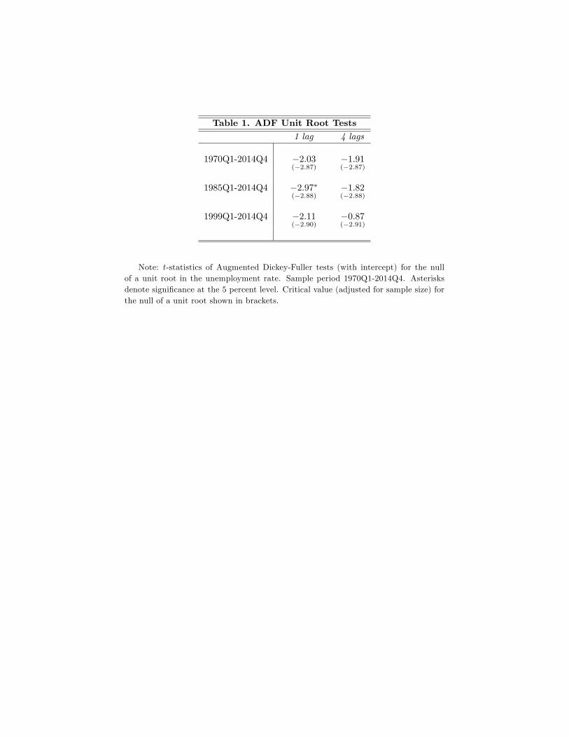
Table 1. ADF Unit Root Tests1 lag 4 lags

1970Q1-2014Q4 �2:03(�2:87)

�1:91(�2:87)

1985Q1-2014Q4 �2:97�(�2:88)

�1:82(�2:88)

1999Q1-2014Q4 �2:11(�2:90)

�0:87(�2:91)

Note: t -statistics of Augmented Dickey-Fuller tests (with intercept) for the nullof a unit root in the unemployment rate. Sample period 1970Q1-2014Q4. Asterisksdenote signi�cance at the 5 percent level. Critical value (adjusted for sample size) forthe null of a unit root shown in brackets.

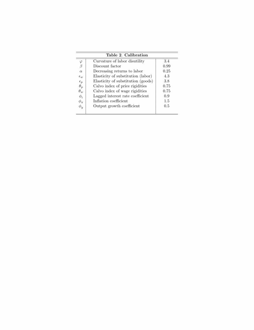
Table 2. Calibration' Curvature of labor disutility 3:4� Discount factor 0:99� Decreasing returns to labor 0:25�w Elasticity of substitution (labor) 4:3�p Elasticity of substitution (goods) 3:8�p Calvo index of price rigidities 0:75�w Calvo index of wage rigidities 0:75�i Lagged interest rate coe¢ cient 0:9�� In�ation coe¢ cient 1:5�y Output growth coe¢ cient 0:5

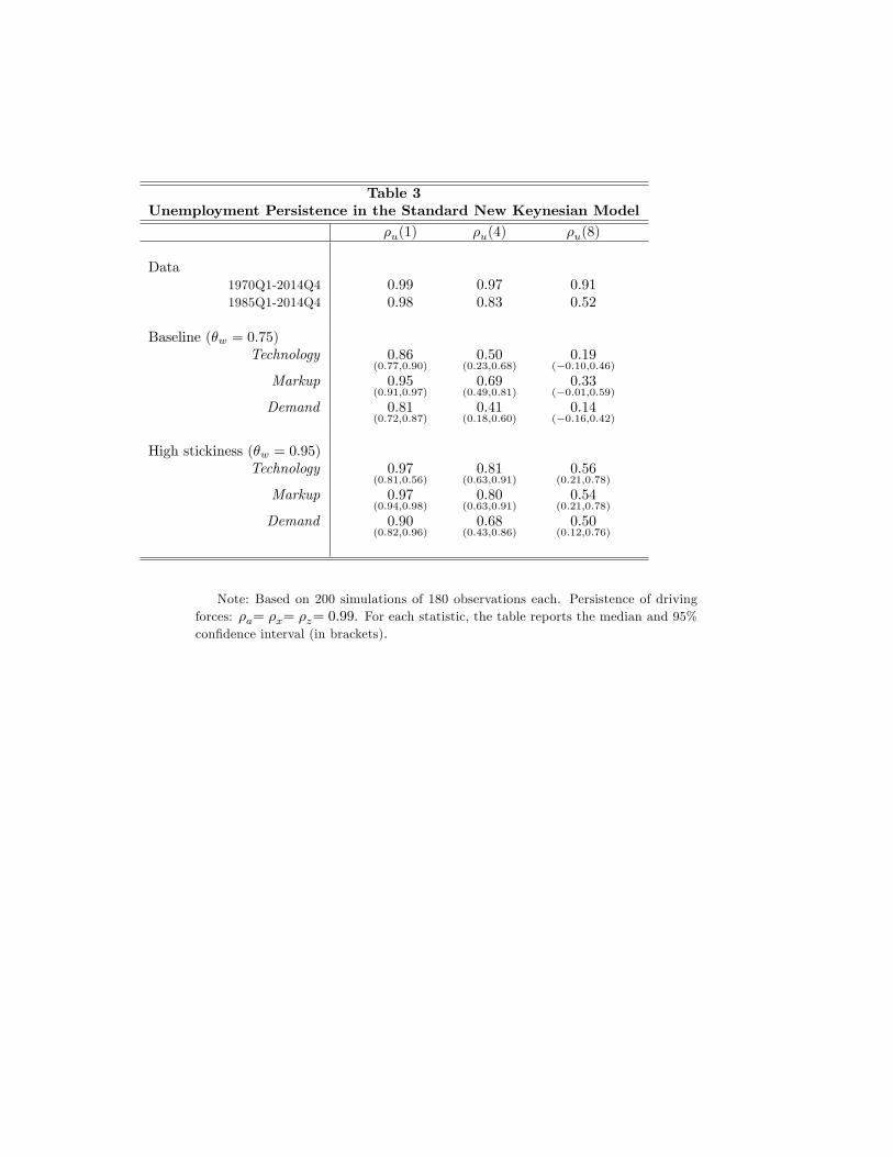
Table 3Unemployment Persistence in the Standard New Keynesian Model

�u(1) �u(4) �u(8)

Data1970Q1-2014Q4 0:99 0:97 0:911985Q1-2014Q4 0:98 0:83 0:52

Baseline (�w = 0:75)Technology 0:86

(0:77;0:90)0:50

(0:23;0:68)0:19

(�0:10;0:46)Markup 0:95

(0:91;0:97)0:69

(0:49;0:81)0:33

(�0:01;0:59)Demand 0:81

(0:72;0:87)0:41

(0:18;0:60)0:14

(�0:16;0:42)

High stickiness (�w = 0:95)Technology 0:97

(0:81;0:56)0:81

(0:63;0:91)0:56

(0:21;0:78)

Markup 0:97(0:94;0:98)

0:80(0:63;0:91)

0:54(0:21;0:78)

Demand 0:90(0:82;0:96)

0:68(0:43;0:86)

0:50(0:12;0:76)

Note: Based on 200 simulations of 180 observations each. Persistence of drivingforces: �a= �x= �z= 0:99. For each statistic, the table reports the median and 95%con�dence interval (in brackets).

Table 4Unemployment Persistence with Insider-Outsider Labor Markets

�u(1) �u(4) �u(8)

Data1970Q1-2014Q4 0:99 0:97 0:911985Q1-2014Q4 0:98 0:83 0:52

TechnologyStandard 0:62

(0:50;0:72)0:06

(�0:16;0:26)�0:09

(�0:25;0:12) = 0:0 0:61

(0:51;0:71)0:03

(�0:16;0:22)�0:10

(�0:32;0:08) = 0:9 0:83

(0:67;0:93)0:57

(0:16;0:83)0:45

(�0:06;0:78) = 1:0 0:93

(0:74;0:98)0:82

(0:34;0:94)0:73

(0:18;0:90)

MarkupStandard 0:95

(0:91;0:97)0:63

(0:46;0:76)0:21

(�0:09;0:46) = 0:0 0:95

(0:91;0:97)0:62

(0:40;0:76)0:15

(�0:20;0:45) = 0:9 0:97

(0:93;0:99)0:83

(0:59;0:92)0:58

(0:20;0:81)

= 1:0 0:97(0:94;0:99)

0:87(0:69;0:96)

0:70(0:36;0:92)

DemandStandard 0:80

(0:71;0:87)0:41

(0:18;0:57)0:12

(�0:18;0:37) = 0:0 0:81

(0:69;0:88)0:42

(0:14;0:62)0:15

(�0:16;0:40) = 0:9 0:93

(0:82;0:97)0:77

(0:45;0:92)0:60

(0:17;0:85)

= 1:0 0:96(0:87;0:99)

0:86(0:58;0:96)

0:73(0:33;0:91)

Note: Based on 200 simulations of 180 observations each. Persistence of drivingforces: �a= �x= �z= 0:92. For each statistic, the table reports the median and 95%con�dence interval (in brackets).

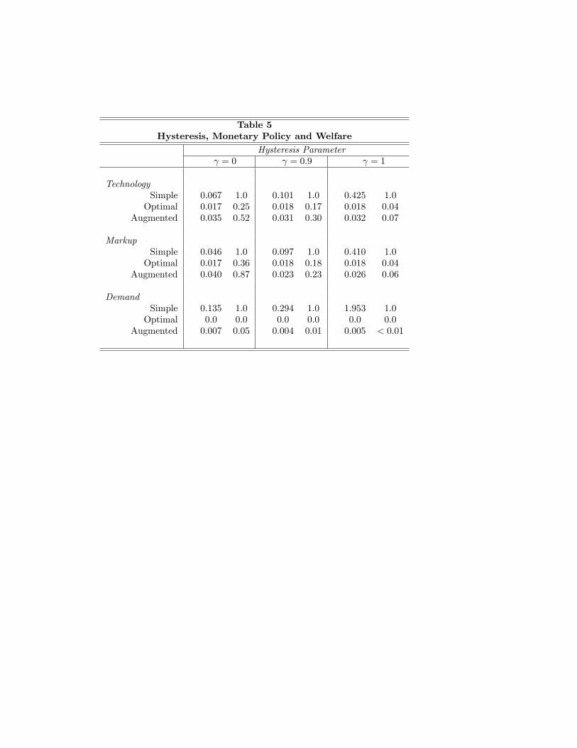
Table 5Hysteresis, Monetary Policy and Welfare

Hysteresis Parameter = 0 = 0:9 = 1

TechnologySimple 0:067 1:0 0:101 1:0 0:425 1:0Optimal 0:017 0:25 0:018 0:17 0:018 0:04

Augmented 0:035 0:52 0:031 0:30 0:032 0:07

MarkupSimple 0:046 1:0 0:097 1:0 0:410 1:0Optimal 0:017 0:36 0:018 0:18 0:018 0:04

Augmented 0:040 0:87 0:023 0:23 0:026 0:06

DemandSimple 0:135 1:0 0:294 1:0 1:953 1:0Optimal 0:0 0:0 0:0 0:0 0:0 0:0

Augmented 0:007 0:05 0:004 0:01 0:005 < 0:01

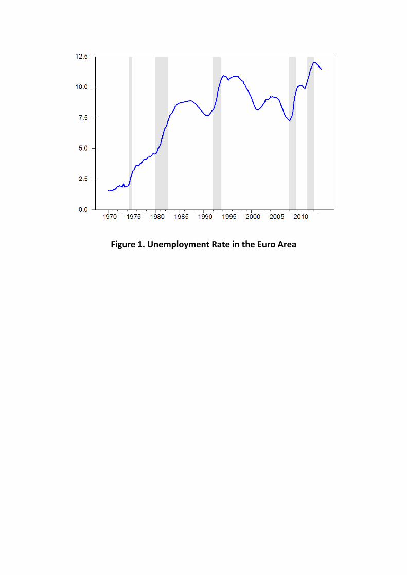
Figure 1. Unemployment Rate in the Euro Area

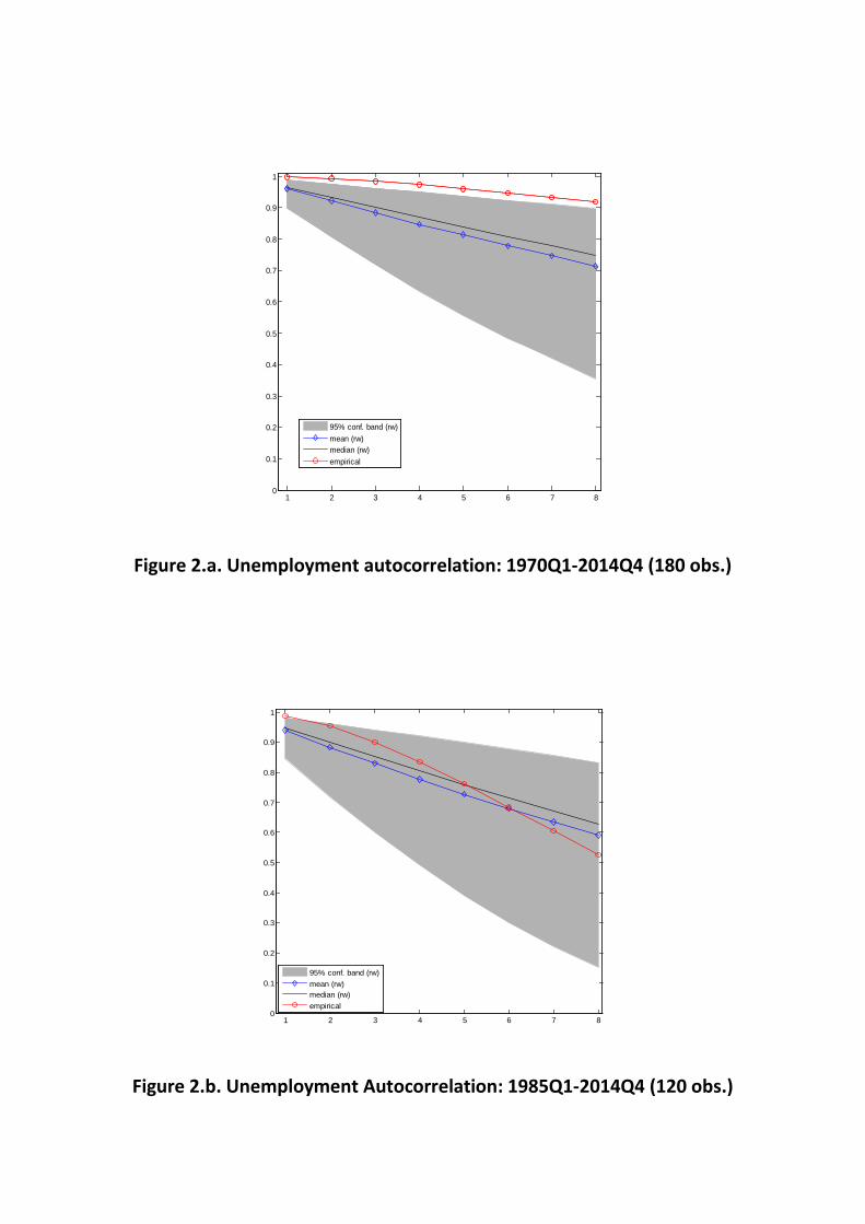
Figure 2.a. Unemployment autocorrelation: 1970Q1-2014Q4 (180 obs.)

Figure 2.b. Unemployment Autocorrelation: 1985Q1-2014Q4 (120 obs.)

1 2 3 4 5 6 7 80

0.1

0.2

0.3

0.4

0.5

0.6

0.7

0.8

0.9

1

95% conf. band (rw)mean (rw)median (rw)empirical

1 2 3 4 5 6 7 80

0.1

0.2

0.3

0.4

0.5

0.6

0.7

0.8

0.9

1

95% conf. band (rw)mean (rw)median (rw)empirical

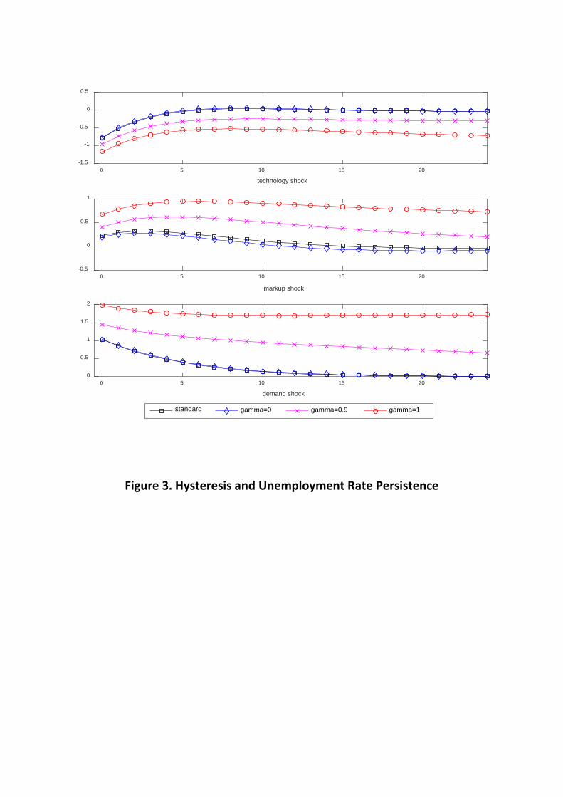
Figure 3. Hysteresis and Unemployment Rate Persistence

0 5 10 15 20

technology shock

-1.5

-1

-0.5

0

0.5

standard gamma=0 gamma=0.9 gamma=1

0 5 10 15 20

markup shock

-0.5

0

0.5

1

0 5 10 15 20

demand shock

0

0.5

1

1.5

2

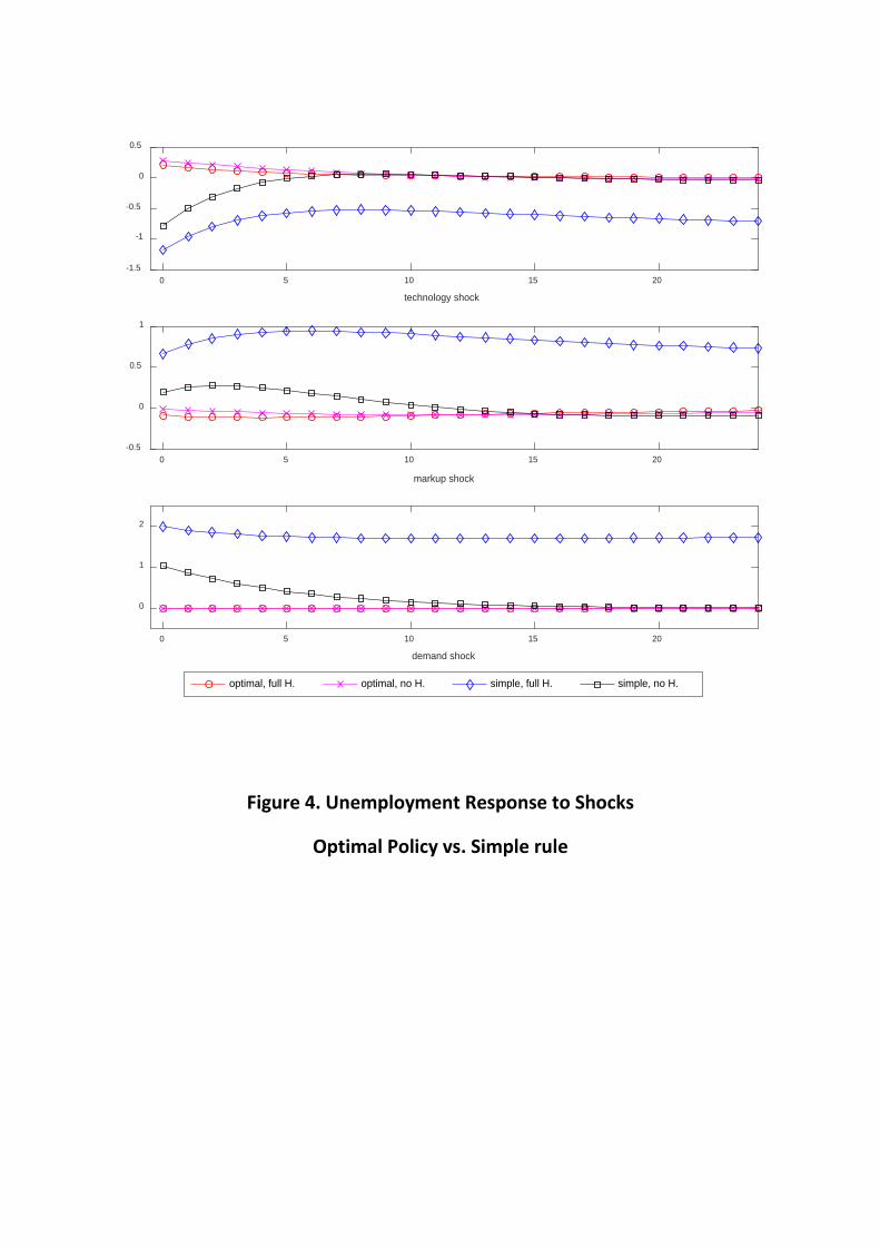
Figure 4. Unemployment Response to Shocks

Optimal Policy vs. Simple rule

0 5 10 15 20

technology shock

-1.5

-1

-0.5

0

0.5

optimal, full H. optimal, no H. simple, full H. simple, no H.

0 5 10 15 20

markup shock

-0.5

0

0.5

1

0 5 10 15 20

demand shock

0

1

2

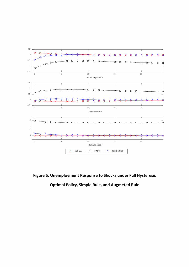
Figure 5. Unemployment Response to Shocks under Full Hysteresis

Optimal Policy, Simple Rule, and Augmeted Rule

0 5 10 15 20

technology shock

-1.5

-1

-0.5

0

0.5

optimal simple augmented

0 5 10 15 20

markup shock

-0.5

0

0.5

1

1.5

0 5 10 15 20

demand shock

0

1

2

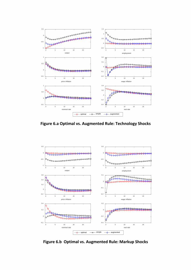
Figure 6.a Optimal vs. Augmented Rule: Technology Shocks

Figure 6.b Optimal vs. Augmented Rule: Markup Shocks

0 5 10 15 20

output

-1

-0.5

0

0.5

optimal simple augmented

0 5 10 15 20

employment

-0.5

0

0.5

1

1.5

0 5 10 15 20

price inflation

-0.5

0

0.5

1

0 5 10 15 20

wage inflation

-0.2

-0.1

0

0.1

0.2

0 5 10 15 20

nominal rate

-0.5

0

0.5

1

0 5 10 15 20

real rate

-0.4

-0.2

0

0.2

0.4

0 5 10 15 20

output

-1

-0.5

0

0.5

optimal simple augmented

0 5 10 15 20

employment

-1

-0.5

0

0.5

0 5 10 15 20

price inflation

-0.2

0

0.2

0.4

0.6

0 5 10 15 20

wage inflation

-0.2

-0.1

0

0.1

0 5 10 15 20

nominal rate

-0.2

0

0.2

0.4

0 5 10 15 20

real rate

-0.4

-0.2

0

0.2

Figure 6.c Optimal vs. Augmented Rule: Demand Shocks

0 5 10 15 20

output

-1

-0.5

0

0 5 10 15 20

employment

-2

-1

0

1

optimal simple augmented

0 5 10 15 20

price inflation

-0.3

-0.2

-0.1

0

0.1

0 5 10 15 20

wage inflation

-0.6

-0.4

-0.2

0

0.2

0 5 10 15 20

nominal rate

-0.4

-0.3

-0.2

-0.1

0

0 5 10 15 20

real rate

-0.4

-0.3

-0.2

-0.1

0