Embed Size (px)
Citation preview
Insole modeling using Kinect 3Dsensors
Daniell Algar and Anton Guldberg
Department of Signals & Systems
Division of Signal processing and Biomedical engineering
Chalmers University of Technology
Gothenburg, Sweden 2013
Master’s thesis 2013:EX017


MASTER THESIS IN BIOMEDICAL ENGINEERING
Insole modeling using Kinect 3D sensors
DANIELL ALGARANTON GULDBERG
Department of Signals & SystemsDivision of Signal processing and Biomedical engineering
CHALMERS UNIVERSITY OF TECHNOLOGY
Goteborg, Sweden 2013

Insole modeling using Kinect 3D sensorsDANIELL ALGARANTON GULDBERG
c©DANIELL ALGAR, ANTON GULDBERG, 2013
Master’s thesis 2013:EX017Department of Signals & SystemsDivision of Signal processing and Biomedical engineeringChalmers University of TechnologySE-412 58 Goteborg
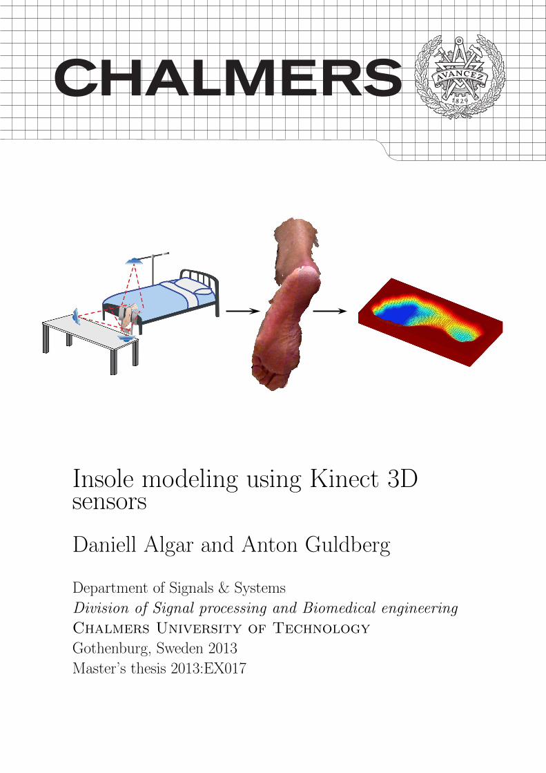
Cover: The proposed system for insole modeling
Chalmers ReproserviceGoteborg, Sweden 2013
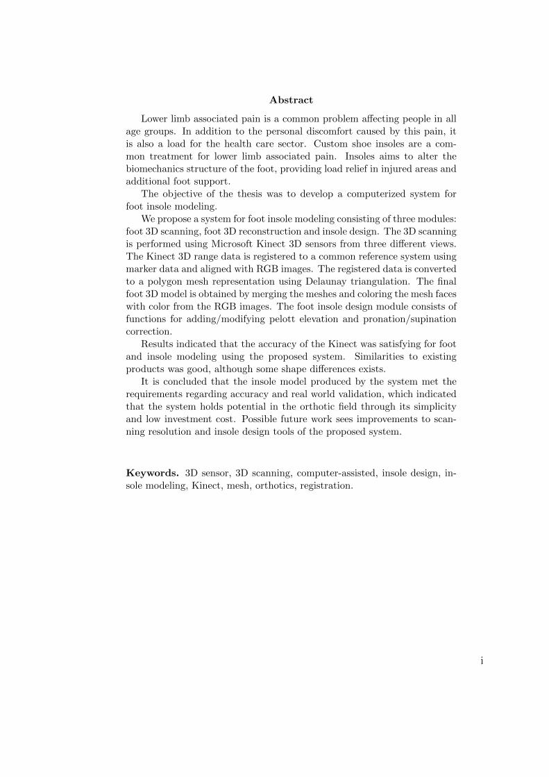
Abstract
Lower limb associated pain is a common problem affecting people in allage groups. In addition to the personal discomfort caused by this pain, itis also a load for the health care sector. Custom shoe insoles are a com-mon treatment for lower limb associated pain. Insoles aims to alter thebiomechanics structure of the foot, providing load relief in injured areas andadditional foot support.
The objective of the thesis was to develop a computerized system forfoot insole modeling.
We propose a system for foot insole modeling consisting of three modules:foot 3D scanning, foot 3D reconstruction and insole design. The 3D scanningis performed using Microsoft Kinect 3D sensors from three different views.The Kinect 3D range data is registered to a common reference system usingmarker data and aligned with RGB images. The registered data is convertedto a polygon mesh representation using Delaunay triangulation. The finalfoot 3D model is obtained by merging the meshes and coloring the mesh faceswith color from the RGB images. The foot insole design module consists offunctions for adding/modifying pelott elevation and pronation/supinationcorrection.
Results indicated that the accuracy of the Kinect was satisfying for footand insole modeling using the proposed system. Similarities to existingproducts was good, although some shape differences exists.
It is concluded that the insole model produced by the system met therequirements regarding accuracy and real world validation, which indicatedthat the system holds potential in the orthotic field through its simplicityand low investment cost. Possible future work sees improvements to scan-ning resolution and insole design tools of the proposed system.
Keywords. 3D sensor, 3D scanning, computer-assisted, insole design, in-sole modeling, Kinect, mesh, orthotics, registration.
i

Preface
This study was performed as a master thesis project at Chalmers University ofTechnology, carried out at MedTech West at Sahlgrenska University Hospital. Thecompany FotAnatomi, Gothenburg, came up with the original problem description.
A special thanks to Mikael Persson for steering the project on the right course,Arthur Chodorowski for continuous support and technical supervision, FernandoManuel da Silva Oliviera for his orthotic expertise, Hakan Toren for helping withthe fabrication, Ramin Moshavegh, Yazdan Shirvany and Lisa Snall.
The authors, Gothenburg June 25, 2013
ii

Contents
1 Introduction 11.1 The orthotic insole . . . . . . . . . . . . . . . . . . . . . . . . . . . 1
1.1.1 Prefabricated insoles . . . . . . . . . . . . . . . . . . . . . . 21.1.2 Custom insoles - traditional plaster cast method . . . . . . . 21.1.3 Custom insoles - computer assisted method . . . . . . . . . . 3
1.2 Aim and objective . . . . . . . . . . . . . . . . . . . . . . . . . . . 31.3 Scope of thesis . . . . . . . . . . . . . . . . . . . . . . . . . . . . . 41.4 Structure of thesis . . . . . . . . . . . . . . . . . . . . . . . . . . . 5
2 Existing products and research in computer assisted insole pro-duction 72.1 Ortolab . . . . . . . . . . . . . . . . . . . . . . . . . . . . . . . . . 72.2 Delcam . . . . . . . . . . . . . . . . . . . . . . . . . . . . . . . . . . 72.3 Related research in insole production . . . . . . . . . . . . . . . . . 82.4 Requirements of a novel system . . . . . . . . . . . . . . . . . . . . 9
3 Theory 113.1 Surface representation of point cloud . . . . . . . . . . . . . . . . . 113.2 Absolute orientation of 3D data sets . . . . . . . . . . . . . . . . . 12
3.2.1 Registering multi-view captures . . . . . . . . . . . . . . . . 133.3 Point cloud approximation using rectangular mesh grid . . . . . . . 14
4 The Kinect sensor and tools 174.1 Remarks on the Kinect as 3D sensor . . . . . . . . . . . . . . . . . 174.2 Real world depth map calculations . . . . . . . . . . . . . . . . . . 18
4.2.1 Depth formula correction . . . . . . . . . . . . . . . . . . . . 204.3 RGB-Depth frame alignment . . . . . . . . . . . . . . . . . . . . . . 204.4 Libfreenect framework . . . . . . . . . . . . . . . . . . . . . . . . . 21
4.4.1 Matlab Kinect wrapper . . . . . . . . . . . . . . . . . . . . 21
5 Evaluation of the Kinect as 3D sensor 235.1 RGB camera calibration . . . . . . . . . . . . . . . . . . . . . . . . 23
5.1.1 Calibration results . . . . . . . . . . . . . . . . . . . . . . . 245.1.2 Calibration discussion . . . . . . . . . . . . . . . . . . . . . 24
5.2 Depth map distortion correction . . . . . . . . . . . . . . . . . . . . 245.2.1 Distortion correction results . . . . . . . . . . . . . . . . . . 275.2.2 Distortion correction discussion . . . . . . . . . . . . . . . . 27
5.3 Depth resolution . . . . . . . . . . . . . . . . . . . . . . . . . . . . 295.3.1 Resolution results . . . . . . . . . . . . . . . . . . . . . . . . 30
iii
5.3.2 Resolution discussion . . . . . . . . . . . . . . . . . . . . . . 305.4 RGB-Depth alignment validation . . . . . . . . . . . . . . . . . . . 31
5.4.1 Alignment results . . . . . . . . . . . . . . . . . . . . . . . . 325.4.2 Alignment discussion . . . . . . . . . . . . . . . . . . . . . . 32
5.5 Depth measurement validation using known object . . . . . . . . . 335.5.1 Depth measurement results . . . . . . . . . . . . . . . . . . 345.5.2 Depth measurement discussion . . . . . . . . . . . . . . . . . 35
6 Proposed system for insole modeling 376.1 Foot scanning . . . . . . . . . . . . . . . . . . . . . . . . . . . . . . 376.2 Foot modeling . . . . . . . . . . . . . . . . . . . . . . . . . . . . . . 38
6.2.1 Reference system . . . . . . . . . . . . . . . . . . . . . . . . 386.2.2 Detection of reference markers . . . . . . . . . . . . . . . . . 396.2.3 Multi-view registration . . . . . . . . . . . . . . . . . . . . . 426.2.4 Removal of overlapping data in the foot bed . . . . . . . . . 42
6.3 Insole design . . . . . . . . . . . . . . . . . . . . . . . . . . . . . . . 436.3.1 Pronation/supination correction tool . . . . . . . . . . . . . 436.3.2 Pelott tool . . . . . . . . . . . . . . . . . . . . . . . . . . . . 456.3.3 Graphical user interface layout . . . . . . . . . . . . . . . . . 456.3.4 Insole model . . . . . . . . . . . . . . . . . . . . . . . . . . . 46
6.4 Block diagram system overview . . . . . . . . . . . . . . . . . . . . 47
7 Proposed system remarks 497.1 Foot scanning remarks . . . . . . . . . . . . . . . . . . . . . . . . . 497.2 Foot modeling remarks . . . . . . . . . . . . . . . . . . . . . . . . . 507.3 Insole design remarks . . . . . . . . . . . . . . . . . . . . . . . . . . 50
8 System evaluation through case study 518.1 Subject description . . . . . . . . . . . . . . . . . . . . . . . . . . . 518.2 Scanning patient and molds . . . . . . . . . . . . . . . . . . . . . . 518.3 Comparison method . . . . . . . . . . . . . . . . . . . . . . . . . . 528.4 Case study results . . . . . . . . . . . . . . . . . . . . . . . . . . . . 538.5 Case study discussion . . . . . . . . . . . . . . . . . . . . . . . . . . 54
8.5.1 Local differences . . . . . . . . . . . . . . . . . . . . . . . . 548.5.2 Shape differences . . . . . . . . . . . . . . . . . . . . . . . . 55
9 Direct insole fabrication 57
10 Summary and conclusion 5910.1 Thesis summary . . . . . . . . . . . . . . . . . . . . . . . . . . . . . 5910.2 Key results . . . . . . . . . . . . . . . . . . . . . . . . . . . . . . . 59
iv

10.3 Limitations . . . . . . . . . . . . . . . . . . . . . . . . . . . . . . . 6010.4 Future work . . . . . . . . . . . . . . . . . . . . . . . . . . . . . . . 60
10.4.1 Future design tools . . . . . . . . . . . . . . . . . . . . . . . 61
Appendix A Absolute orientation using closed-form quaternions 67
Appendix B Kinect RGB camera model and calibration 70
Appendix C RGB camera calibration results 71
v
List of Figures
1 Pronation example . . . . . . . . . . . . . . . . . . . . . . . . . . . 22 Plaster foot mold with pelott imprint, FotAnatomi . . . . . . . . . 33 Insole production methods . . . . . . . . . . . . . . . . . . . . . . . 44 Delaunay triangulation . . . . . . . . . . . . . . . . . . . . . . . . . 115 Absolute orientation of point sets . . . . . . . . . . . . . . . . . . . 126 Multi-view registration . . . . . . . . . . . . . . . . . . . . . . . . . 147 Approximating point cloud to mesh . . . . . . . . . . . . . . . . . . 158 The Kinect . . . . . . . . . . . . . . . . . . . . . . . . . . . . . . . 179 Triangulation setup . . . . . . . . . . . . . . . . . . . . . . . . . . . 1910 Depth map of flat wall . . . . . . . . . . . . . . . . . . . . . . . . . 2511 Distortion correction algorithm 1 and 2 . . . . . . . . . . . . . . . . 2812 Applied distortion correction, algorithm 1 . . . . . . . . . . . . . . 2813 Spatial resolution . . . . . . . . . . . . . . . . . . . . . . . . . . . . 3014 Depth resolution . . . . . . . . . . . . . . . . . . . . . . . . . . . . 3115 RGB-Depth alignment validation . . . . . . . . . . . . . . . . . . . 3216 Known object built out of Lego . . . . . . . . . . . . . . . . . . . . 3317 Distance measurements of known object . . . . . . . . . . . . . . . 3418 Lego distance errors at 640− 800 mm . . . . . . . . . . . . . . . . . 3519 Lego distance errors at 800− 1000 mm . . . . . . . . . . . . . . . . 3620 Proposed system outline . . . . . . . . . . . . . . . . . . . . . . . . 3721 Measurement setup . . . . . . . . . . . . . . . . . . . . . . . . . . . 3822 Capture interface . . . . . . . . . . . . . . . . . . . . . . . . . . . . 3923 Reference system . . . . . . . . . . . . . . . . . . . . . . . . . . . . 4024 Marker detection . . . . . . . . . . . . . . . . . . . . . . . . . . . . 4125 Marker registration . . . . . . . . . . . . . . . . . . . . . . . . . . . 4326 Foot mesh model . . . . . . . . . . . . . . . . . . . . . . . . . . . . 4427 Insole design GUI . . . . . . . . . . . . . . . . . . . . . . . . . . . . 4628 Digital insole model . . . . . . . . . . . . . . . . . . . . . . . . . . . 4729 Flowchart overview of the proposed system . . . . . . . . . . . . . . 4830 Foam foot model, Ortolab . . . . . . . . . . . . . . . . . . . . . . . 5231 Comparing the proposed system to existing products . . . . . . . . 5332 Absolute difference map between foot models . . . . . . . . . . . . . 5433 Insole prototype through CNC cutting . . . . . . . . . . . . . . . . 5734 Insole prototype through 3D printing . . . . . . . . . . . . . . . . . 58A.1 Absolute orientation of point sets . . . . . . . . . . . . . . . . . . . 67C.2 Image capture sets for the RGB camera calibration . . . . . . . . . 71C.3 Radial and tangential distortion components for Kinect 1 and 2 . . 72C.4 Complete distortion model for Kinect 1 and 2 . . . . . . . . . . . . 72C.5 Reprojection errors in pixel for Kinect 1 and 2 . . . . . . . . . . . . 73
vi

List of Tables
1 Calibration results . . . . . . . . . . . . . . . . . . . . . . . . . . . 242 RGD-Depth alignment test . . . . . . . . . . . . . . . . . . . . . . . 323 Geometric comparison between foot models . . . . . . . . . . . . . 53
Glossary
.stl STereoLithography is a file format commonly used for rapid prototyping andcomputer-aided manufacturing.
Achilles tendon The tendon connecting the heel to the calf.
CAD Computer aided design.
CAM Computer aided manufacturing.
CNC Computer numerical control.
Coronal plane The plane dividing the body into front and back.
FOV Field of view, describing the angular view from a monocular camera.
FPS Frames per second.
GUI Graphical user interface.
Orthosis An external device applied to modify the functional or structural char-acteristics of the musculo-skeletal system.
Pelott A locally modified area of an insole aimed to increased support at localareas of the foot.
Plantar aponeurosis The tendons connecting the forefoot and the heel in thebottom of the foot.
Plantar fasciitis An inflammatory process in the Plantar aponeurosis.
Pronation Indication that the Achilles tendon is not straight during standingand gait, which rotates the foot towards the center of the body.
PU-foam Polymer, crisp foam which can be shaped into various forms.
vii

RGB-D RGB data with depth processing, e.g. RGB image with range informa-tion for each pixel.
SDK Software development kit.
Supination Indication that the Achilles tendon is not straight during standingand gait, which rotates the foot away from the center of the body.
Transverse plane The plane dividing the body into upper and lower parts.
viii
1 Introduction
1 Introduction
Pain or discomfort in the lower limbs (e.g. foot, knee, pelvis, hip joint) is acommon complaint with many possible causes. In Europe among adults, everythird male and every second female experience pain in the lower limbs each year [1].Among people in the age group of 65 years of age or more, one third reportsfoot problems [2, 3]. The pain might originate from injuries, wear of ligaments,joints etc., which results in a degraded physical function. Other than the obviousindividual discomfort, injuries of these types leads to a high workload for the healthcare system as well as for employers [1].
1.1 The orthotic insole
One approach to ease the described pain, or to augment the healing process ofan injury, is by using an orthosis [4]. An orthosis is an ”external device appliedto modify the functional or structural characteristics of the musculoskeletal sys-tem” [5]. An example of an orthosis is the foot orthosis or the shoe insole whichmodifies the foot by adding support by e.g. applying a pelott or local elevationin the insole. There exists general, prefabricated insoles as well as custom moldedinsoles, designed for individual feet.
Insoles has been proven to improve foot function as well as relieving pain causedby foot problems. A study by Kogler (1995) [6] investigated the effectiveness of thelongitudinal arch support mechanism of custom foot insoles and concluded thatfoot insoles were effective in resisting the ”arch flattening moment” occurring inthe foot during gait. This was achieved by decreasing the strain in the plantaraponeurosis, increasing the load area. The result was a damping effect in the foot.
Another study by Kato (1995) [7] showed an increased mean contact area of62.7 % after applying a custom insole. This in turn reduced the mean pressure by56.3 % during standing, relieving areas normally under high load and spreadingthe pressure more even.
As mentioned above, strain relief in the plantar aponeurosis is achieved byspreading the force applied on the foot onto a greater area across the sole of thefoot [8]. This is important since the natural healing process of plantar fasciitisrequires the damaged area to be in rest for optimal healing effect [7].
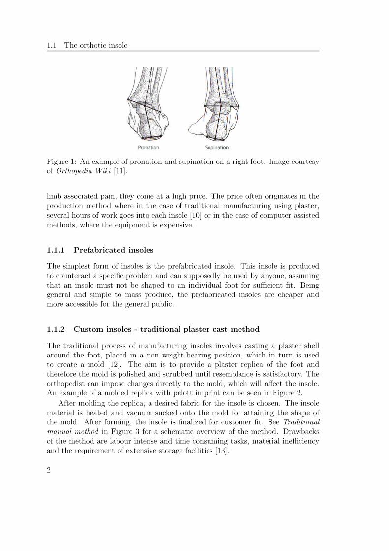
Another application of custom insoles is counteracting pronation and supina-tion [9]. This is the case when the Achilles tendon rotates during gait and stance,as seen in Figure 1. This will cause the foot to pronate or supinate to the side,imposing an unnatural rotation of the foot that could effect both the feet, kneesand the back of the patient. To remedy this, the insole must support the foot inorder to straighten the Achilles tendon [10].
Even though custom insoles are effective treatments for foot ache and lower
1
1.1 The orthotic insole
Figure 1: An example of pronation and supination on a right foot. Image courtesyof Orthopedia Wiki [11].
limb associated pain, they come at a high price. The price often originates in theproduction method where in the case of traditional manufacturing using plaster,several hours of work goes into each insole [10] or in the case of computer assistedmethods, where the equipment is expensive.
1.1.1 Prefabricated insoles
The simplest form of insoles is the prefabricated insole. This insole is producedto counteract a specific problem and can supposedly be used by anyone, assumingthat an insole must not be shaped to an individual foot for sufficient fit. Beinggeneral and simple to mass produce, the prefabricated insoles are cheaper andmore accessible for the general public.
1.1.2 Custom insoles - traditional plaster cast method
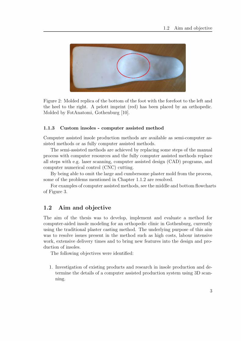
The traditional process of manufacturing insoles involves casting a plaster shellaround the foot, placed in a non weight-bearing position, which in turn is usedto create a mold [12]. The aim is to provide a plaster replica of the foot andtherefore the mold is polished and scrubbed until resemblance is satisfactory. Theorthopedist can impose changes directly to the mold, which will affect the insole.An example of a molded replica with pelott imprint can be seen in Figure 2.
After molding the replica, a desired fabric for the insole is chosen. The insolematerial is heated and vacuum sucked onto the mold for attaining the shape ofthe mold. After forming, the insole is finalized for customer fit. See Traditionalmanual method in Figure 3 for a schematic overview of the method. Drawbacksof the method are labour intense and time consuming tasks, material inefficiencyand the requirement of extensive storage facilities [13].
2
1.2 Aim and objective
Figure 2: Molded replica of the bottom of the foot with the forefoot to the left andthe heel to the right. A pelott imprint (red) has been placed by an orthopedic.Molded by FotAnatomi, Gothenburg [10].
1.1.3 Custom insoles - computer assisted method
Computer assisted insole production methods are available as semi-computer as-sisted methods or as fully computer assisted methods.
The semi-assisted methods are achieved by replacing some steps of the manualprocess with computer resources and the fully computer assisted methods replaceall steps with e.g. laser scanning, computer assisted design (CAD) programs, andcomputer numerical control (CNC) cutting.
By being able to omit the large and cumbersome plaster mold from the process,some of the problems mentioned in Chapter 1.1.2 are resolved.
For examples of computer assisted methods, see the middle and bottom flowchartsof Figure 3.
1.2 Aim and objective
The aim of the thesis was to develop, implement and evaluate a method forcomputer-aided insole modeling for an orthopedic clinic in Gothenburg, currentlyusing the traditional plaster casting method. The underlying purpose of this aimwas to resolve issues present in the method such as high costs, labour intensivework, extensive delivery times and to bring new features into the design and pro-duction of insoles.
The following objectives were identified:
1. Investigation of existing products and research in insole production and de-termine the details of a computer assisted production system using 3D scan-ning.
3
1.3 Scope of thesis
Foot model from 3D Scanning
Insole design
CNC cutter fabrication
Plaster casting of
foot
Vacuum forming insole
onto moldFoot mold
Computer assisted method
Traditional manual method
Foot model from 3Dscanning
CNC cutting of foot model
Semi-computer assisted method
mold modification
model modification
Modifications
Vacuum forming insole
onto model
Foot modeling Insole fabrication
ManualComputer assisted
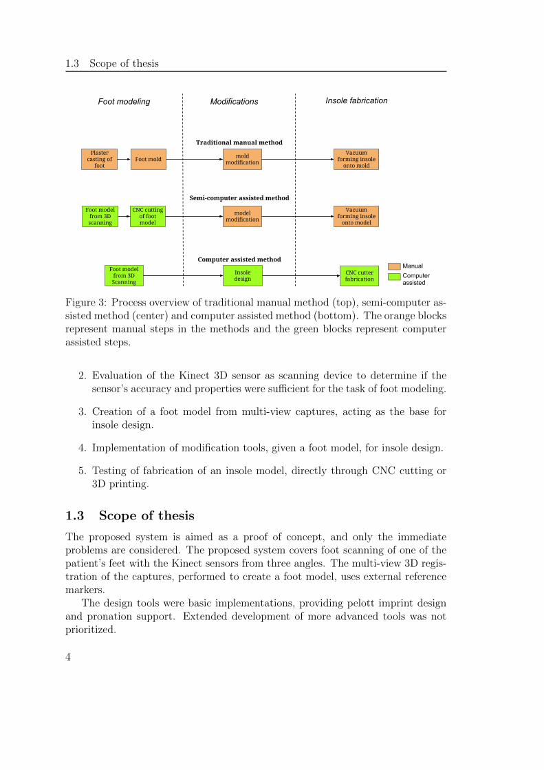
Figure 3: Process overview of traditional manual method (top), semi-computer as-sisted method (center) and computer assisted method (bottom). The orange blocksrepresent manual steps in the methods and the green blocks represent computerassisted steps.
2. Evaluation of the Kinect 3D sensor as scanning device to determine if thesensor’s accuracy and properties were sufficient for the task of foot modeling.
3. Creation of a foot model from multi-view captures, acting as the base forinsole design.
4. Implementation of modification tools, given a foot model, for insole design.
5. Testing of fabrication of an insole model, directly through CNC cutting or3D printing.
1.3 Scope of thesis
The proposed system is aimed as a proof of concept, and only the immediateproblems are considered. The proposed system covers foot scanning of one of thepatient’s feet with the Kinect sensors from three angles. The multi-view 3D regis-tration of the captures, performed to create a foot model, uses external referencemarkers.
The design tools were basic implementations, providing pelott imprint designand pronation support. Extended development of more advanced tools was notprioritized.
4

1.4 Structure of thesis
The proposed system for insole modeling does not include fabrication, eventhough some fabrication methods have been tested.
To relate the proposed system to existing methods, a study between the insolebase and existing insoles has been quantitatively compared with respect to localand shape differences.
1.4 Structure of thesis
The thesis is organized as follows
Chapter 2: Discusses existing products from Ortolab and Delcam, using com-puter assisted methods of insole production. Some research in insole production isdescribed and finally, some requirements of the proposed system are listed.
Chapter 3: Describes some theory regarding surface construction, 3D registra-tion and point cloud approximation.
Chapter 4: Discusses the Kinect sensor and its properties.
Chapter 5: Evaluates the Kinect sensor as a scanning device at 600–1000 mm.
Chapter 6: Proposes a system for foot scanning, foot modeling and insole design.
Chapter 7: Discusses remarks of the proposed system from Chapter 6.
Chapter 8: Discusses a case study which provides a quantitative comparisonbetween foot models from existing companies and the proposed system.
Chapter 9: Discusses methods for fabrication of an insole from the model de-scribed in Chapter 6. CNC cutting and 3D printing were tested.
Chapter 10 Summarizes the work of the thesis, states the key findings and thelimitations. This chapter also provides suggestions for future work.
5

6
2 Existing products and research in computer assisted insole production
2 Existing products and research in computer
assisted insole production
This chapter includes a sample overview of the market situation of computer as-sisted insole production. Two companies are selected; Ortolab and Delcam. Also,some research is presented for the purpose of broadening the readers scope regard-ing alternative approaches to the digitization of insole production. Finally, somerequirements of the desired system are pointed out.
2.1 Ortolab
Ortolab [14] is a Swedish custom foot insole manufacturer which is a large actoron the Swedish market [15].
Ortolab uses a sweeping flatbed laser scanner of brand Envisic Veriscan [16] fordata acquisition [17]. The patients foot is placed with the heel cap on a stand withthe toes pointing upwards. A full foot scan takes about 3.3 s with a resolution ofabout 1.6 mm [17, 18]. The price of a scanner with software is relatively high [17].
After capture, the scan is forwarded to another facility over Internet connectionfor analyze on a computer. After this step, the data is sent to a cutter that cutsthe foot mold out of a Poly Urethane (PU) foam block. This block is then usedby the orthopedist in a traditional fashion, using the model for pelott placementand vacuum sucking the final insole fabric onto the foot model [14].
In some settings, the Ortolab system acquire the foot scan when the patient isstanding, i.e. in a weight bearing position, which is unwanted [10, 19]. The stepsof the method can be seen in the middle of Figure 3.
2.2 Delcam
Delcam [20] is a worldwide company, delivering a complete computer aided design/-computer aided manufacturing (CAD/CAM) system from foot data acquisition tofabricated custom insole [21, 22].
Delcam provides the laser scanner iQube, which is able to scan the foot froma full, semi and non weight bearing position. The scan of one foot takes about 3 swith an accuracy of 0.4 mm [23]. It is stated that the foot model is represented infull color [21].
The company offers their own CAD software, called OrthoModel. The softwareis extensive, providing several features for insole design [22, 24] such as
• Possibility to work with one or two foot models at the same time.
7
2.3 Related research in insole production
• Place key points such as for marking the heel, the foot pads and/or metatarsalsfor measurements.
• Alter the orientation of the insole for extended support e.g. when pronating.
• Comparison of insole and scanned foot model to validate the fit.
• Free hand modification and thickness control of the insole is possible, withfree design of the pelott.
Delcam also supplies fabrication products [22, 25] for cutting the insoles froma digital design. Cast Medical is the Delcam partner in Sweden [22, 26].
The Delcam system is expensive being one of the most extensive on the market,providing a complete solution from scanning to manufacturing [22]. The steps ofthe method can be seen at the bottom of Figure 3.
2.3 Related research in insole production
As described in Chapter 2.1 and 2.2, both semi-computer assisted and fully com-puter assisted methods are available on the market. Research in the field of insoleproduction has several focuses; Sathish [27] (2012) proposed a system for rapidprototyping of custom orthotics for plantar ulcer. Using Computed Tomography(CT) scans to acquire the bone structure of the limb, the structure was exportedto a CAD software for modeling purpose. The modeled foot was then used for fab-rication of the insole using Plaster of Paris Powder (POP). Sathish concluded thatthe given method makes the acquisition of the foot imprint easier than traditionalmethods and in a more cost effective way.
Huppin (2009) [13] concluded that among existing imaging options, only theones giving a true 3D image has the potential of fulfilling necessary criteria toact as an alternative to traditional casting methods. This would exclude solutionsusing for example flatbed scanners from one angle.
Mavroidis (2011) [28] has used a 3D laser scanner with a novel approach forinsole design. The foot was scanned and the digitized foot surface was edited to anoptimal form using CAD software. The output from the software was forwardedto a rapid prototyping machine for fabrication. A gait analysis of patients wearingthe rapid prototyped orthoses showed a comparable performance to prefabricatedpolypropylene design.
As stated, research deals both with imaging and fabricating challenges of insoleproduction. Another challenge is lowering costs of custom insoles at the same timeas introducing better technology.
8

2.4 Requirements of a novel system
2.4 Requirements of a novel system
Described above are several techniques for insole production, both by existingcompanies and research based. Considering a new system, some requirements areestablished
1. The system described in Chapter 2.1 and 2.2 are high cost systems. A novelsystem should be of lower cost. This can be achieved by the use of low costscanners, such as the Kinect sensor.
2. Most systems today do not provide color/texture information of the patient’sfoot in their scans. A novel system with color/texture information associatedwith the scans could indicate e.g. sole condition and areas of interest.
3. Most systems today as described in Chapter 2, image the bottom of the foot.A system providing information regarding the Achilles tendon would yieldmore information in the case of pronation and supination.
9

10
3 Theory
3 Theory
This chapter presents the theory used in the reminder of the thesis. This includestheory used for creating surfaces from point clouds, the registration of different 3Ddata sets to a shared coordinate system and finally how an arbitrary point cloudcan be represented on a systematic mesh grid.
3.1 Surface representation of point cloud
A point cloud V is a collection of points in a coordinate system, in this case, theCartesian (x,y,z) coordinate system. Let a point cloud represent a view of anobject. To create a surface representation, a polygonal mesh is used. A polygonalmesh O is defined as
O = {P,V } (1)
where V = {v1,...,vNv} is a set of Nv vertices where vi = (xi,yi,zi) and P ={p1,...,pNp} is a list of Np polygons where pi = {vi,1,...,vi,nvi}. The vertices in piforms a polygon with nvi vertices. If nvi = 3 for all polygons, there will be onlytriangles in the mesh [29].
The point cloud V , holds all the vertices. Connecting the vertices to triangles,a triangular mesh can be defined. One method for creating the triangular mesh isby Delaunay triangulation [30].
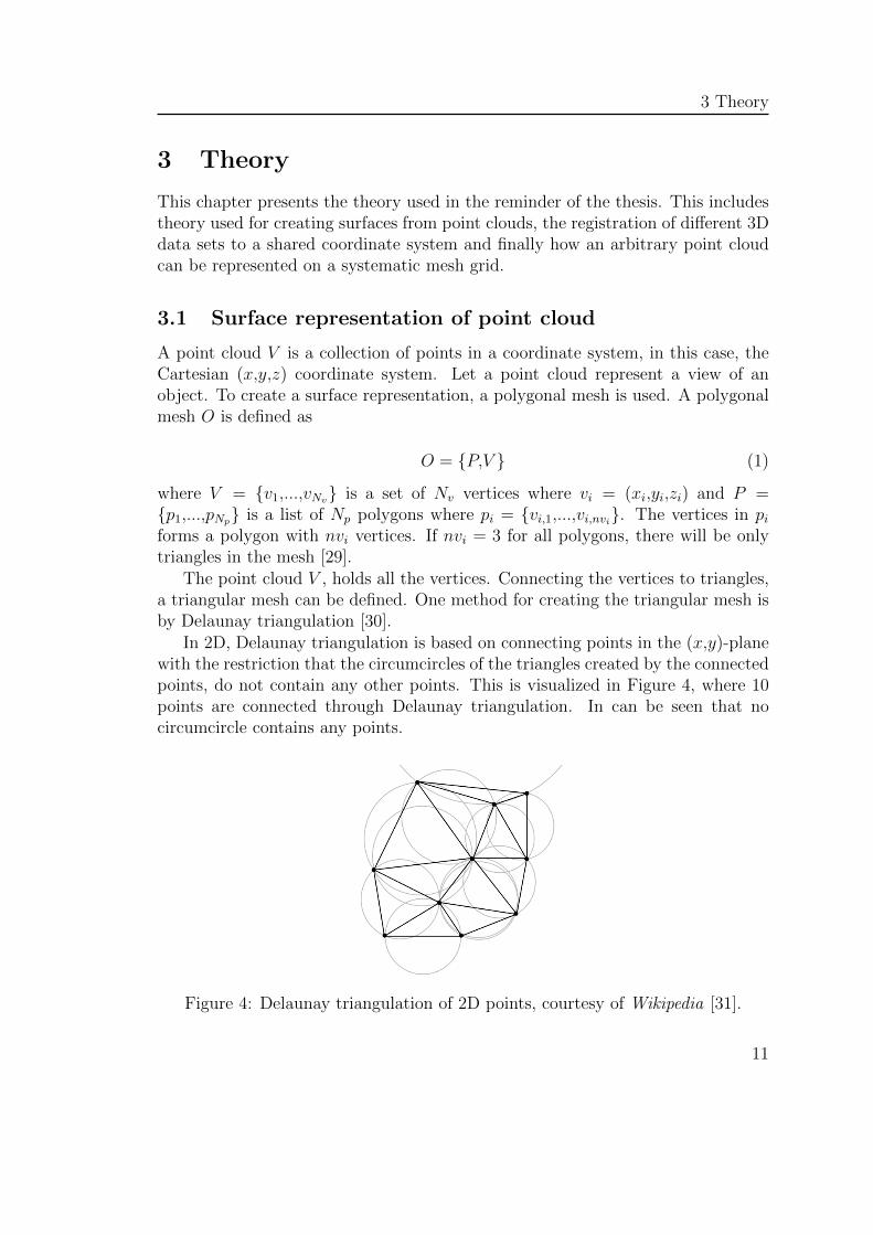
In 2D, Delaunay triangulation is based on connecting points in the (x,y)-planewith the restriction that the circumcircles of the triangles created by the connectedpoints, do not contain any other points. This is visualized in Figure 4, where 10points are connected through Delaunay triangulation. In can be seen that nocircumcircle contains any points.
Figure 4: Delaunay triangulation of 2D points, courtesy of Wikipedia [31].
11
3.2 Absolute orientation of 3D data sets
Figure 4 shows the 2D case of Delaunay triangulation, which can be applied for3D data as well to create a 3D surface. To create the surface from a point cloud,the 3D coordinates are projected into 2D space where the Delaunay triangulationis applied, connecting the points. Finally the coordinates are mapped back to 3D.An example case of this, is applying the Delaunay triangulation in the (x,y)-planeof point cloud to connect the points and create the surface. Then, adding thez-component, takes the surface to 3D.
3.2 Absolute orientation of 3D data sets
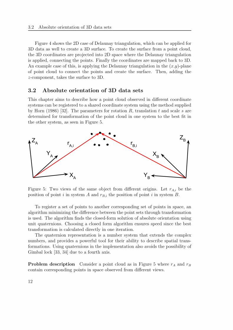
This chapter aims to describe how a point cloud observed in different coordinatesystems can be registered to a shared coordinate system using the method suppliedby Horn (1986) [32]. The parameters for rotation R, translation t and scale s aredetermined for transformation of the point cloud in one system to the best fit inthe other system, as seen in Figure 5.
XB
YB
ZA
YA
XA
ZBrA,i rB,i
Figure 5: Two views of the same object from different origins. Let rA,i be theposition of point i in system A and rB,i the position of point i in system B.
To register a set of points to another corresponding set of points in space, analgorithm minimizing the difference between the point sets through transformationis used. The algorithm finds the closed-form solution of absolute orientation usingunit quaternions. Choosing a closed form algorithm ensures speed since the besttransformation is calculated directly in one iteration.
The quaternion representation is a number system that extends the complexnumbers, and provides a powerful tool for their ability to describe spatial trans-formations. Using quaternions in the implementation also avoids the possibility ofGimbal lock [33, 34] due to a fourth axis.
Problem description Consider a point cloud as in Figure 5 where rA and rBcontain corresponding points in space observed from different views.
12
3.2 Absolute orientation of 3D data sets
Calculating the best fit between the point clouds through transformation isdone by minimizing
e =n∑
i=1
||rB,i − sR(rA,i)− t||2 (2)
where and rB,i and rA,i are corresponding points, s, R and t are transformationparameters and n are the number of corresponding points observed.
The quaternion based method finds the best transformation with respect toequation (2) and explicit expressions for s, R and t are
t = rB − sR(rA) (3)
where rA and rB are the centroids of the observed points,
s =
n∑i=1
r′B,iR(r′A,i)
n∑i=1
||r′A,i||2(4)
where r′A,i and r′B,i are the observed points, relative to the centroids rA and rB. Inthe case of s = 1, the transformation is a rigid body transformation.
R is found by retrieving the lower right 3× 3 sub matrix of the 4× 4 rotationmatrix qT q, where q is the quaternion that maximizes
n∑i=1
(qr′A,i) · (r′B,iq) (5)
For a more detailed description of the method, see Appendix A.
3.2.1 Registering multi-view captures
The method described in Chapter 3.2 registers one view of an object to anotherview of the same object. In the process of multi-view registration, the aim is toregister several views of an object to a shared coordinate system, placed arbitrary.
Let rA and rB be corresponding subsets of points observed in point cloud PA
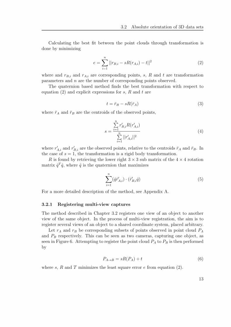
and PB respectively. This can be seen as two cameras, capturing one object, asseen in Figure 6. Attempting to register the point cloud PA to PB is then performedby
PA→B = sR(PA) + t (6)
where s, R and T minimizes the least square error e from equation (2).
13
3.3 Point cloud approximation using rectangular mesh grid
XB
YB
ZA
YA
XA
ZBrA,i rB,i
ZYXri
Camera 1 Camera 2
Figure 6: Two camera views of one object. Let rA,i be the position of point i insystem A and rB,i the position of point i in system B. Furthermore, let ri be theposition of point i in the new coordinate system (X,Y,Z).
Furthermore, Figure 6 shows the point cloud observed from a third angle,situated in coordinate system (X,Y,Z). Let this point cloud be denoted P and letr be the subset of P corresponding to the points in rA and rB. Using the methodin Chapter 3.2, the PA and PB can be sequentially registered to system (X,Y,Z)using rA, rB and r. After transformation, the two views of the point cloud PA andPB will be observed from the same coordinate system, (X,Y,Z).
The setup can be extended to any number of different capture angles and anyobjects, given at least 3 corresponding points observed from all captures to beregistered [32].
3.3 Point cloud approximation using rectangular mesh grid
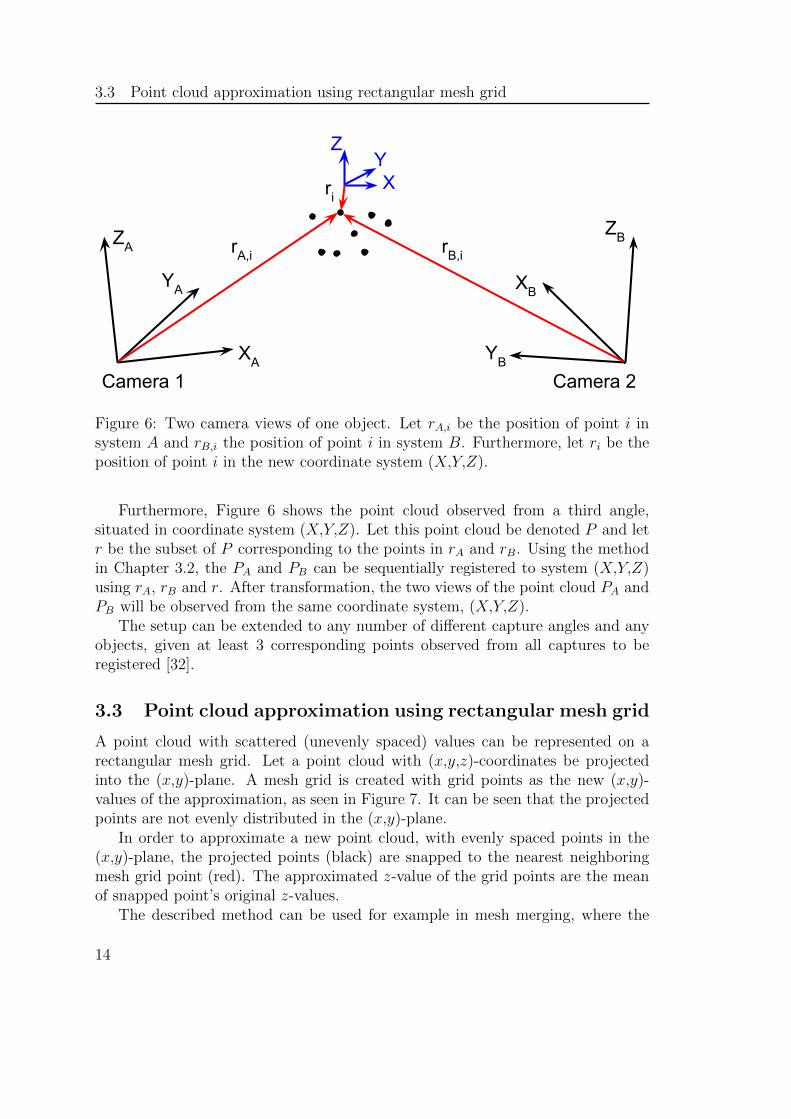
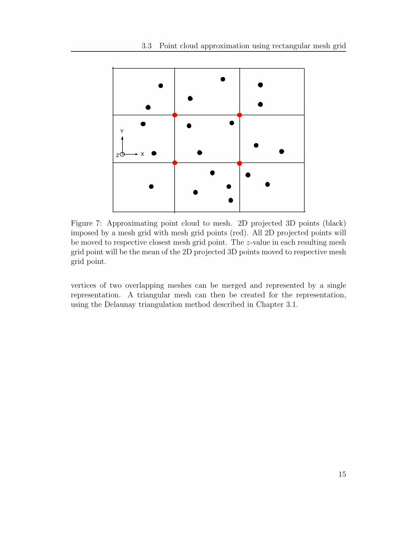
A point cloud with scattered (unevenly spaced) values can be represented on arectangular mesh grid. Let a point cloud with (x,y,z)-coordinates be projectedinto the (x,y)-plane. A mesh grid is created with grid points as the new (x,y)-values of the approximation, as seen in Figure 7. It can be seen that the projectedpoints are not evenly distributed in the (x,y)-plane.
In order to approximate a new point cloud, with evenly spaced points in the(x,y)-plane, the projected points (black) are snapped to the nearest neighboringmesh grid point (red). The approximated z-value of the grid points are the meanof snapped point’s original z-values.
The described method can be used for example in mesh merging, where the
14
3.3 Point cloud approximation using rectangular mesh grid
X
Y
Z
Figure 7: Approximating point cloud to mesh. 2D projected 3D points (black)imposed by a mesh grid with mesh grid points (red). All 2D projected points willbe moved to respective closest mesh grid point. The z-value in each resulting meshgrid point will be the mean of the 2D projected 3D points moved to respective meshgrid point.
vertices of two overlapping meshes can be merged and represented by a singlerepresentation. A triangular mesh can then be created for the representation,using the Delaunay triangulation method described in Chapter 3.1.
15

16
4 The Kinect sensor and tools
4 The Kinect sensor and tools
This chapter covers Kinect specifications such as depth map resolution and hard-ware. The chapter also reviews imaging techniques of the Kinect such as datacapture and alignment of the RGB and depth data. An overview of tools used tocommunicate with the Kinect will also be presented.
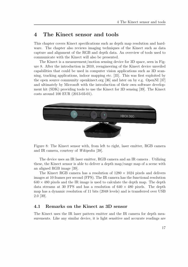
The Kinect is a measurement/motion sensing device for 3D space, seen in Fig-ure 8. After the introduction in 2010, reengineering of the Kinect device unveiledcapabilities that could be used in computer vision applications such as 3D scan-ning, tracking applications, indoor mapping etc. [35]. This was first exploited bythe open source community openkinect.org [36] and later on by e.g. OpenNI [37]and ultimately by Microsoft with the introduction of their own software develop-ment kit (SDK) providing tools to use the Kinect for 3D sensing [39]. The Kinectcosts around 100 EUR (2013-03-01).
Figure 8: The Kinect sensor with, from left to right, laser emitter, RGB cameraand IR camera, courtesy of Wikipedia [38].
The device uses an IR laser emitter, RGB camera and an IR camera . Utilizingthese, the Kinect sensor is able to deliver a depth map/range map of a scene withan aligned RGB image [39].
The Kinect RGB camera has a resolution of 1280 × 1024 pixels and deliversimages at 10 frames per second (FPS). The IR camera has the functional resolution640× 480 pixels and the IR image is used to calculate the depth map. The depthdata streams at 30 FPS and has a resolution of 640 × 480 pixels. The depthmap has a dynamic resolution of 11 bits (2048 levels) and is transferred over USB2.0 [39].
4.1 Remarks on the Kinect as 3D sensor
The Kinect uses the IR laser pattern emitter and the IR camera for depth mea-surements. Like any similar device, it is light sensitive and accurate readings are
17
4.2 Real world depth map calculations
impossible in direct sunlight, which contains IR wavelengths. Furthermore thedepth map delivered, provides inaccurate reading around sharp edges. This wasalso observed by Anderssen (2012) [40] and is due to the spatial precision of theKinect IR camera.
The sensor readings regarding the depth data is somewhat noisy and experi-ments have been done by Andersen (2012) that concludes that the noise on thedepth values provided, are normally distributed over time [40].
The minimum scanning distance of the Kinect is 800 mm according to themanufacturer [39]. It is possible to acquire images at nearer distances, but theimages will be distorted.
4.2 Real world depth map calculations
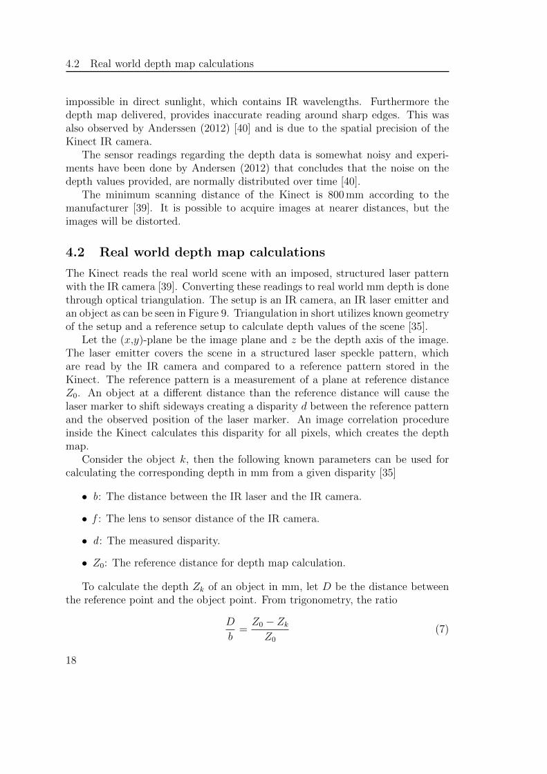
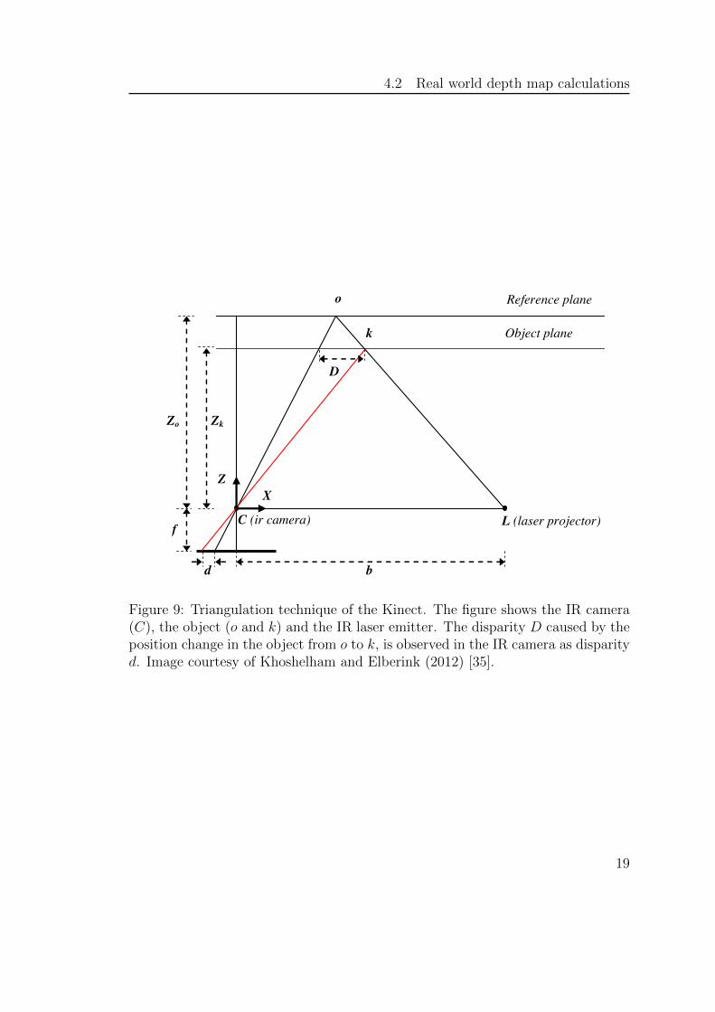
The Kinect reads the real world scene with an imposed, structured laser patternwith the IR camera [39]. Converting these readings to real world mm depth is donethrough optical triangulation. The setup is an IR camera, an IR laser emitter andan object as can be seen in Figure 9. Triangulation in short utilizes known geometryof the setup and a reference setup to calculate depth values of the scene [35].
Let the (x,y)-plane be the image plane and z be the depth axis of the image.The laser emitter covers the scene in a structured laser speckle pattern, whichare read by the IR camera and compared to a reference pattern stored in theKinect. The reference pattern is a measurement of a plane at reference distanceZ0. An object at a different distance than the reference distance will cause thelaser marker to shift sideways creating a disparity d between the reference patternand the observed position of the laser marker. An image correlation procedureinside the Kinect calculates this disparity for all pixels, which creates the depthmap.
Consider the object k, then the following known parameters can be used forcalculating the corresponding depth in mm from a given disparity [35]
• b: The distance between the IR laser and the IR camera.
• f : The lens to sensor distance of the IR camera.
• d : The measured disparity.
• Z0: The reference distance for depth map calculation.
To calculate the depth Zk of an object in mm, let D be the distance betweenthe reference point and the object point. From trigonometry, the ratio
D
b=Z0 − Zk
Z0
(7)
18
4.2 Real world depth map calculations
Sensors 2012, 12 1439
Figure 1. (a) Infrared image of the pattern of speckles projected on a sample scene. (b) The resulting depth image.
2.1. Mathematical Model
Figure 2 illustrates the relation between the distance of an object point k to the sensor relative to a reference plane and the measured disparity d. To express the 3D coordinates of the object points we consider a depth coordinate system with its origin at the perspective center of the infrared camera. The Z axis is orthogonal to the image plane towards the object, the X axis perpendicular to the Z axis in the direction of the baseline b between the infrared camera center and the laser projector, and the Y axis orthogonal to X and Z making a right handed coordinate system.
Figure 2. Relation between relative depth and measured disparity.
Assume that an object is on the reference plane at a distance Zo to the sensor, and a speckle on the object is captured on the image plane of the infrared camera. If the object is shifted closer to (or further away from) the sensor the location of the speckle on the image plane will be displaced in the X
(a)
(b)
L (laser projector) C (ir camera)
Reference plane
Object plane
f
Zo Zk
d
X Z
o
k
D
b
Figure 9: Triangulation technique of the Kinect. The figure shows the IR camera(C), the object (o and k) and the IR laser emitter. The disparity D caused by theposition change in the object from o to k, is observed in the IR camera as disparityd. Image courtesy of Khoshelham and Elberink (2012) [35].
19
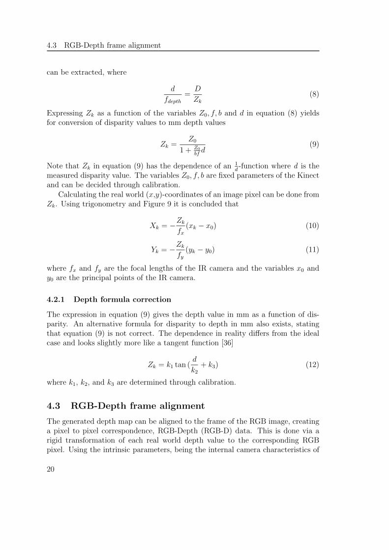
4.3 RGB-Depth frame alignment
can be extracted, where
d
fdepth=D
Zk
(8)
Expressing Zk as a function of the variables Z0, f, b and d in equation (8) yieldsfor conversion of disparity values to mm depth values
Zk =Z0
1 + Z0
bfd
(9)
Note that Zk in equation (9) has the dependence of an 1d-function where d is the
measured disparity value. The variables Z0, f, b are fixed parameters of the Kinectand can be decided through calibration.
Calculating the real world (x,y)-coordinates of an image pixel can be done fromZk. Using trigonometry and Figure 9 it is concluded that
Xk = −Zk
fx(xk − x0) (10)
Yk = −Zk
fy(yk − y0) (11)
where fx and fy are the focal lengths of the IR camera and the variables x0 andy0 are the principal points of the IR camera.
4.2.1 Depth formula correction
The expression in equation (9) gives the depth value in mm as a function of dis-parity. An alternative formula for disparity to depth in mm also exists, statingthat equation (9) is not correct. The dependence in reality differs from the idealcase and looks slightly more like a tangent function [36]
Zk = k1 tan (d
k2+ k3) (12)
where k1, k2, and k3 are determined through calibration.
4.3 RGB-Depth frame alignment
The generated depth map can be aligned to the frame of the RGB image, creatinga pixel to pixel correspondence, RGB-Depth (RGB-D) data. This is done via arigid transformation of each real world depth value to the corresponding RGBpixel. Using the intrinsic parameters, being the internal camera characteristics of
20
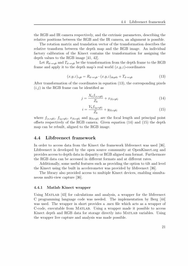
4.4 Libfreenect framework
the RGB and IR camera respectively, and the extrinsic parameters, describing therelative positions between the RGB and the IR camera, an alignment is possible.
The rotation matrix and translation vector of the transformation describes therelative transform between the depth map and the RGB image. An individualfactory calibration of the Kinect contains the transformation for assigning thedepth values to the RGB image [41, 42].
Let Rd→rgb and Td→rgb be the transformation from the depth frame to the RGBframe and apply it to the depth map’s real world (x,y,z)-coordinates
(x,y,z)rgb = Rd→rgb · (x,y,z)depth + Td→rgb (13)
After transformation of the coordinates in equation (13), the corresponding pixels(i,j) in the RGB frame can be identified as
j =Xkf(x,rgb)
Zk
+ x(0,rgb) (14)
i =Ykf(y,rgb)
Zk
+ y(0,rgb) (15)
where f(x,rgb), f(y,rgb), x(0,rgb) and y(0,rgb) are the focal length and principal pointoffsets respectively of the RGB camera. Given equation (14) and (15) the depthmap can be rebuilt, aligned to the RGB image.
4.4 Libfreenect framework
In order to access data from the Kinect the framework libfreenect was used [36].Libfreenect is developed by the open source community at OpenKinect.org andprovides access to depth data in disparity or RGB aligned mm format. Furthermorethe RGB data can be accessed in different formats and at different rates.
Additionally, some useful features such as providing the option to tilt and levelthe Kinect using the built in accelerometer was provided by libfreenect [36].
The library also provided access to multiple Kinect devices, enabling simulta-neous multi-view capture [36].
4.4.1 Matlab Kinect wrapper
Using Matlab [43] for calculations and analysis, a wrapper for the libfreenectC programming language code was needed. The implementation by Berg [44]was used. The wrapper in short provides a .mex file which acts as a wrapper ofC-code, executable from Matlab. Using a wrapper made it possible to accessKinect depth and RGB data for storage directly into Matlab variables. Usingthe wrapper live capture and analysis was made possible.
21

4.4 Libfreenect framework
The wrapper was partially modified to work with more than one device and todeliver data in the desired format; registered mm values.
22
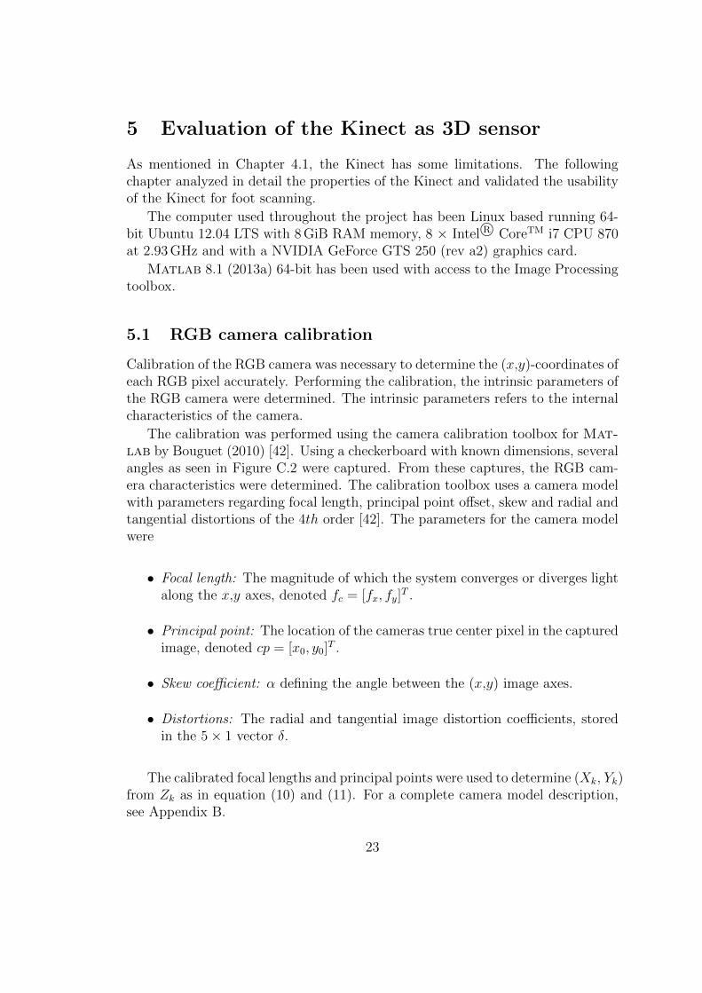
5 Evaluation of the Kinect as 3D sensor
As mentioned in Chapter 4.1, the Kinect has some limitations. The followingchapter analyzed in detail the properties of the Kinect and validated the usabilityof the Kinect for foot scanning.
The computer used throughout the project has been Linux based running 64-bit Ubuntu 12.04 LTS with 8 GiB RAM memory, 8 × Intel R© CoreTM i7 CPU 870at 2.93 GHz and with a NVIDIA GeForce GTS 250 (rev a2) graphics card.
Matlab 8.1 (2013a) 64-bit has been used with access to the Image Processingtoolbox.
5.1 RGB camera calibration
Calibration of the RGB camera was necessary to determine the (x,y)-coordinates ofeach RGB pixel accurately. Performing the calibration, the intrinsic parameters ofthe RGB camera were determined. The intrinsic parameters refers to the internalcharacteristics of the camera.
The calibration was performed using the camera calibration toolbox for Mat-lab by Bouguet (2010) [42]. Using a checkerboard with known dimensions, severalangles as seen in Figure C.2 were captured. From these captures, the RGB cam-era characteristics were determined. The calibration toolbox uses a camera modelwith parameters regarding focal length, principal point offset, skew and radial andtangential distortions of the 4th order [42]. The parameters for the camera modelwere
• Focal length: The magnitude of which the system converges or diverges lightalong the x,y axes, denoted fc = [fx, fy]
T .
• Principal point: The location of the cameras true center pixel in the capturedimage, denoted cp = [x0, y0]
T .
• Skew coefficient: α defining the angle between the (x,y) image axes.
• Distortions: The radial and tangential image distortion coefficients, storedin the 5× 1 vector δ.
The calibrated focal lengths and principal points were used to determine (Xk, Yk)from Zk as in equation (10) and (11). For a complete camera model description,see Appendix B.
23
5.2 Depth map distortion correction
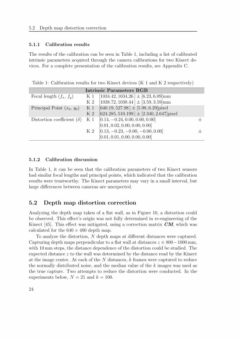
5.1.1 Calibration results
The results of the calibration can be seen in Table 1, including a list of calibratedintrinsic parameters acquired through the camera calibrations for two Kinect de-vices. For a complete presentation of the calibration results, see Appendix C.
Table 1: Calibration results for two Kinect devices (K 1 and K 2 respectively)
Intrinsic Parameters RGBFocal length (fx, fy) K 1 [1034.42, 1034.26 ]± [6.23, 6.09]mm
K 2 [1038.72, 1038.44 ]± [3.59, 3.59]mmPrincipal Point (x0, y0) K 1 [640.19, 527.98 ]± [5.98, 6.29]pixel
K 2 [624.285, 510.199 ]± [2.340, 2.647]pixelDistortion coefficient (δ) K 1 [0.14,−0.24, 0.00, 0.00, 0.00] ±
[0.01, 0.02, 0.00, 0.00, 0.00]K 2 [0.13,−0.23,−0.00,−0.00, 0.00] ±
[0.01, 0.01, 0.00, 0.00, 0.00]
5.1.2 Calibration discussion
In Table 1, it can be seen that the calibration parameters of two Kinect sensorshad similar focal lengths and principal points, which indicated that the calibrationresults were trustworthy. The Kinect parameters may vary in a small interval, butlarge differences between cameras are unexpected.
5.2 Depth map distortion correction
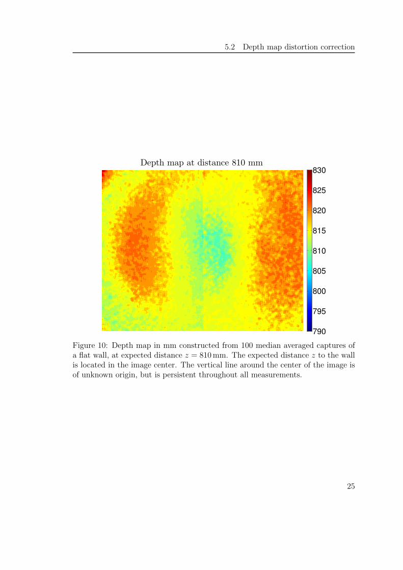
Analyzing the depth map taken of a flat wall, as in Figure 10, a distortion couldbe observed. This effect’s origin was not fully determined in re-engineering of theKinect [45]. This effect was mitigated, using a correction matrix CM, which wascalculated for the 640× 480 depth map.
To analyze the distortion, N depth maps at different distances were captured.Capturing depth maps perpendicular to a flat wall at distances z ∈ 800−1000 mm,with 10 mm steps, the distance dependence of the distortion could be studied. Theexpected distance z to the wall was determined by the distance read by the Kinectat the image center. At each of the N distances, k frames were captured to reducethe normally distributed noise, and the median value of the k images was used asthe true capture. Two attempts to reduce the distortion were conducted. In theexperiments below, N = 21 and k = 100.
24
5.2 Depth map distortion correction
Depth map at distance 810 mm
790
795
800
805
810
815
820
825
830
Figure 10: Depth map in mm constructed from 100 median averaged captures ofa flat wall, at expected distance z = 810 mm. The expected distance z to the wallis located in the image center. The vertical line around the center of the image isof unknown origin, but is persistent throughout all measurements.
25
5.2 Depth map distortion correction
Method 1 The first method, described in algorithm 1, is a method describedby Smisek (2011) [46]. This distortion correction is based on the mean distortionpattern in disparity over distance,
CM =N∑i=1
Di − diN
(16)
where di is the expected disparity value, Di is the measured disparity map of ameasurement and N is the number of depth map sets measured. Converting acaptured depth map mm values Zi to disparity Di was done through
Di =−1
0.00307(Zi − 3.33)(17)
The values in equation (17) were obtained by Burrus (2011) [41].
Algorithm 1 Calculation of the disparity correction matrix CM
1: for i=1:N do2: Convert measured depth Zi to disparity Di
3: Convert expected depth zi to disparity di4: Calculate difference map dMi = Di − di5: end for
6: Calculate correction matrix as the mean, i.e. CM = 1N
N∑i=1
dMi
The expected depth was taken as the mean of a neighborhood around the imagecenter using a kernel of 5× 5 pixels.
Given a distorted depth map, distortion correction was performed by
1. Converting depth to disparity.
2. Correcting distortion in disparity space D = D−CM.
3. Converting back to mm.
Applying CM on a captured flat surface with expected depth z, yielded themean absolute error per pixel and distance in disparity
er,i =|Di − d|
P(18)
and in mm
ed,i =
∣∣∣Zi − z∣∣∣
P(19)
respectively where P was the total number of pixels in the image (640× 480).
26
5.2 Depth map distortion correction
Method 2 The first method used the mean error in disparity space to correctthe depth map. The second method attempted to fit polynomials to the error overdistance, according to algorithm 2.
Algorithm 2 Calculation of the disparity correction matrix CM
1: for p=1:P do2: for i=1:N do3: Calculate difference dMi,p = zi,p − zi4: end for5: Fit 3rd order polynomial CMp to dMp
6: end for
Line 5 of algorithm 2 fitted the errors to a polynomial on the form
CMp(x) = ax3 + bx2 + cx+ d (20)
where a, b, c and d were the polynomial constant outputs at line 5 in algorithm 2.The correction was applied by evaluating the polynomial at given expected distancez according to
Z = Z−CMp(z) (21)
where Z is the corrected depth map.The mean absolute errors in mm for different distances was calculated using
equation (19).
5.2.1 Distortion correction results
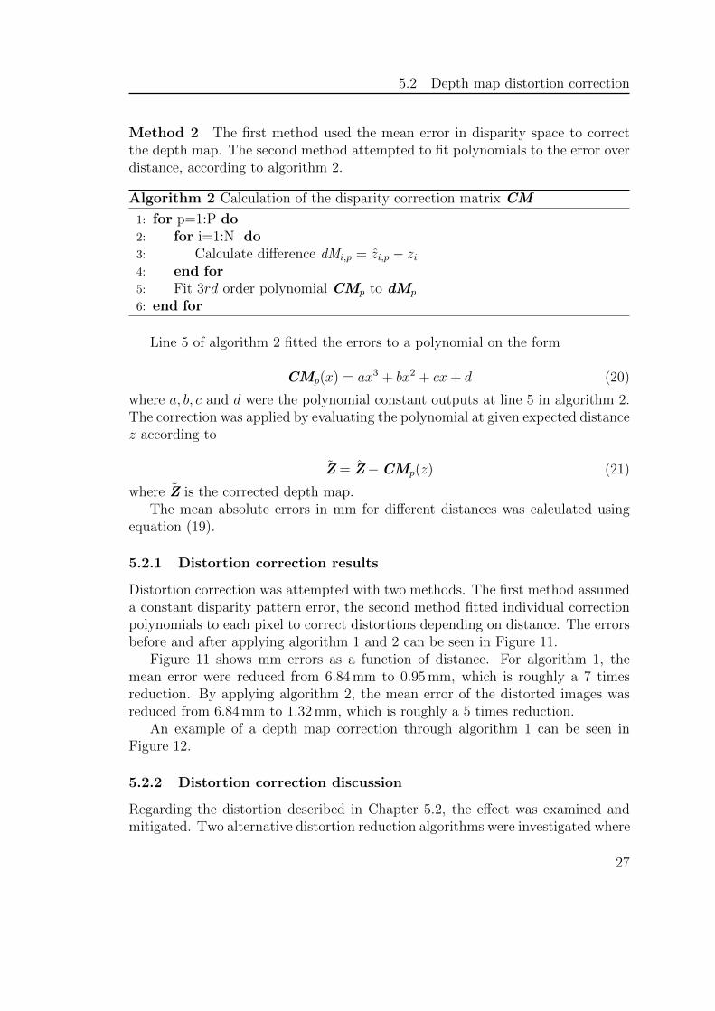
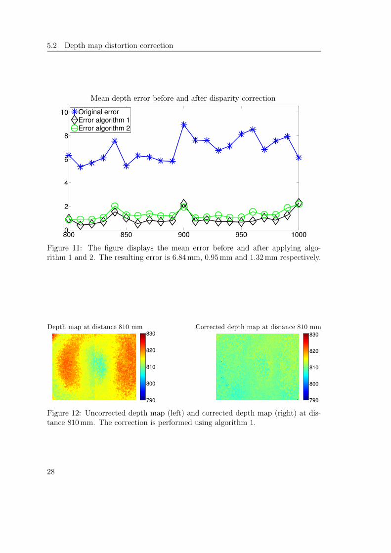
Distortion correction was attempted with two methods. The first method assumeda constant disparity pattern error, the second method fitted individual correctionpolynomials to each pixel to correct distortions depending on distance. The errorsbefore and after applying algorithm 1 and 2 can be seen in Figure 11.
Figure 11 shows mm errors as a function of distance. For algorithm 1, themean error were reduced from 6.84 mm to 0.95 mm, which is roughly a 7 timesreduction. By applying algorithm 2, the mean error of the distorted images wasreduced from 6.84 mm to 1.32 mm, which is roughly a 5 times reduction.
An example of a depth map correction through algorithm 1 can be seen inFigure 12.
5.2.2 Distortion correction discussion
Regarding the distortion described in Chapter 5.2, the effect was examined andmitigated. Two alternative distortion reduction algorithms were investigated where
27
5.2 Depth map distortion correction
800 850 900 950 10000
2
4
6
8
10
Mean depth error before and after disparity correction
Original errorError algorithm 1Error algorithm 2
Figure 11: The figure displays the mean error before and after applying algo-rithm 1 and 2. The resulting error is 6.84 mm, 0.95 mm and 1.32 mm respectively.
Depth map at distance 810 mm
790
800
810
820
830
Corrected depth map at distance 810 mm
790
800
810
820
830
Figure 12: Uncorrected depth map (left) and corrected depth map (right) at dis-tance 810 mm. The correction is performed using algorithm 1.
28
5.3 Depth resolution
the first used disparity value correction and the second used polynomial correction.The results, seen in Figure 11, indicated that algorithm 1 was the most effective,providing a lower mean error after correction than algorithm 2. The second methodof fitted polynomial would probably be more effective if the correction model wasto be used in a larger span of distances and fitted to the disparity values insteadof the mm values.
An alternative method is suggested by Herrera (2012) [45], that proposes ex-ponential weighting of the disparity correction matrix CM. Herrera’s results werepromising, measured over a larger distance span (0.8–4 m) than in this project.The project was only concerned with distances in a small interval, below 1000 mm.In this interval, the distortion was found to be relatively constant, yielding goodresults for algorithm 1.
5.3 Depth resolution
The Kinect depth map has a resolution of 640× 480 pixels which provides a fixedspatial resolution given the distance to the object. This spatial resolution wasdetermined by placing the sensor at different distances from an object and notingthe metric spacing between the x and y points in the mesh grid spanned. The realworld coordinates were calculated as described in Chapter 4.2. The object chosenfor scanning was a flat book. The measurement distances d were 600–1000 mmwith 10 mm steps.
Theoretically, the IR camera has an approximate horizontal field of view (FOV)of 58 ◦ and a vertical FOV of 45 ◦ [39]. Considering the area spanned by the FOVat a given distance d and the fixed pixel resolution of 640×480 pixels, a theoreticalspatial resolution was obtained through
Resx,y =2d tan (α/2)
S(22)
where α is the FOV in the x and y-direction (horizontal and vertical) and S is thepixel span in the x and y-direction.
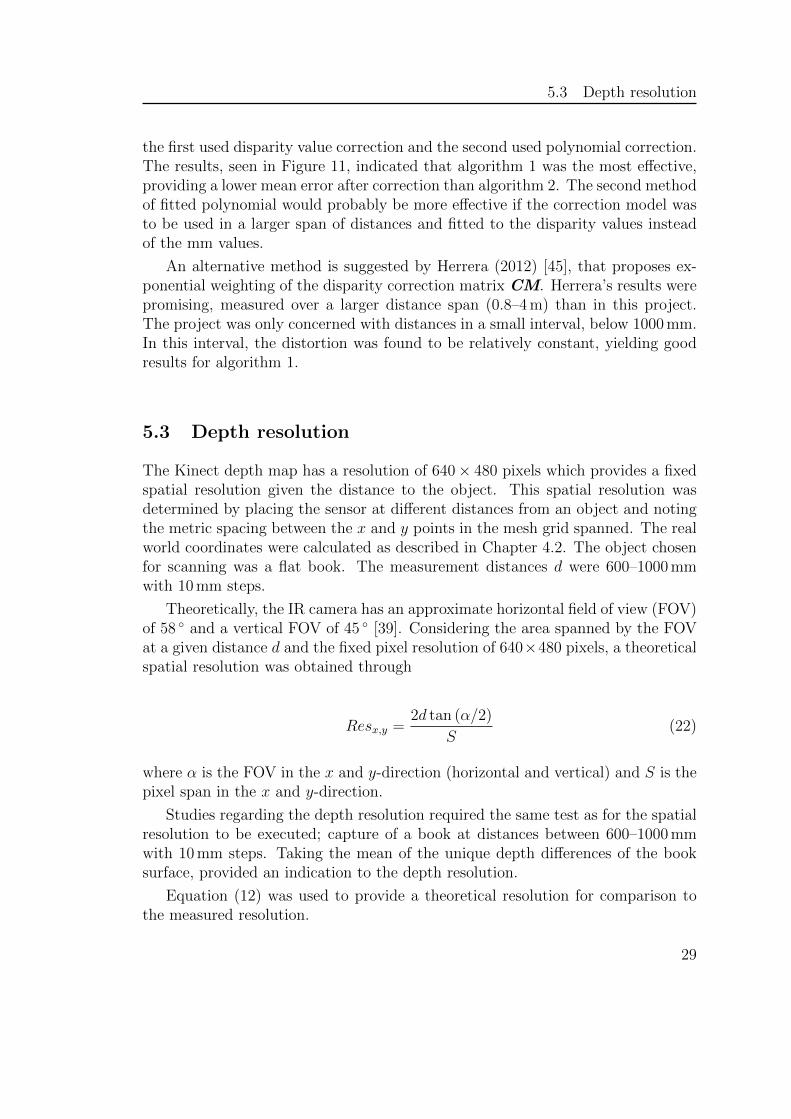
Studies regarding the depth resolution required the same test as for the spatialresolution to be executed; capture of a book at distances between 600–1000 mmwith 10 mm steps. Taking the mean of the unique depth differences of the booksurface, provided an indication to the depth resolution.
Equation (12) was used to provide a theoretical resolution for comparison tothe measured resolution.
29

5.3 Depth resolution
600 800 10001
1.2
1.4
1.6
1.8
2
2.2
Resolution[m
m/pix]
Distance [mm]
Spatial horizontal resolution
Measured resolutionTheoretical resolution
600 800 10001
1.2
1.4
1.6
1.8
2
2.2
Resolution[m
m/pix]
Distance [mm]
Spatial vertical resolution
Measured resolutiontheoretical Resolution
Figure 13: Spatial (x,y)-resolution of the Kinect depth map.
5.3.1 Resolution results
The results of the spatial resolution can be seen in Figure 13. From this figure thespatial resolution at distances between 600 and 1000 mm were determined to bebelow 2 mm both in x and y-direction [39].
The depth resolution measured can be seen in Figure 14. From this figure itcan be concluded that the depth resolution at distances around 600–1000 mm isaround 1–3 mm/pixel.
5.3.2 Resolution discussion
In Chapter 5.3, the resolution of the Kinect was established and validated. Theresults were in good agreement with the theoretical values both in spatial anddepth resolution. As seen in the right plot of Figure 13, the y-resolution comparedto the theoretical resolution of a 45 ◦ FOV camera was compared. There existedsome minor error of 0.1 mm which might originate from the FOV of the IR cameranot being exactly 45 ◦, degrading the theoretical resolution.
As observed by Andersen (2012) [40] the depth resolution varies with the dis-tance from the sensor. These results are in agreement with the findings of thisreport.
In the current setup, depth values in rounded mm units were delivered by
30
5.4 RGB-Depth alignment validation
600 650 700 750 800 850 900 950 10001
1.5
2
2.5
3
3.5Resolution
[mm/pix]
Distance [mm]
Depth resolution
Measured resolutionTheoretical resolution
Figure 14: Depth resolution (i.e. z-resolution) of the Kinect depth map.
the libfreenect library [36], degrading the measured resolution. A more accurateresolution would have been achieved using the disparity values and performing theconversion to mm by equation (9).
The observed resolution was deemed sufficient by the orthopedist specialistat FotAnatomi [10]. However, several products exists on the market today withbetter resolution scanners.
5.4 RGB-Depth alignment validation
The RGB image supplied by the Kinect of 1280 × 1024 pixels was cropped to1280 × 960 pixels by removing the bottom band of 1280 × 64 pixels. The RGBimage is observed to be a scaled version of the depth image. In order to have pixel-to-pixel correspondence the depth map was enlarged by a factor of 2, replicatingthe rows and columns, to a size of 1280× 960 pixels.
To determine how well the RGB-D alignment performs, an experiment thatvalidated the alignment of the frames was conducted.
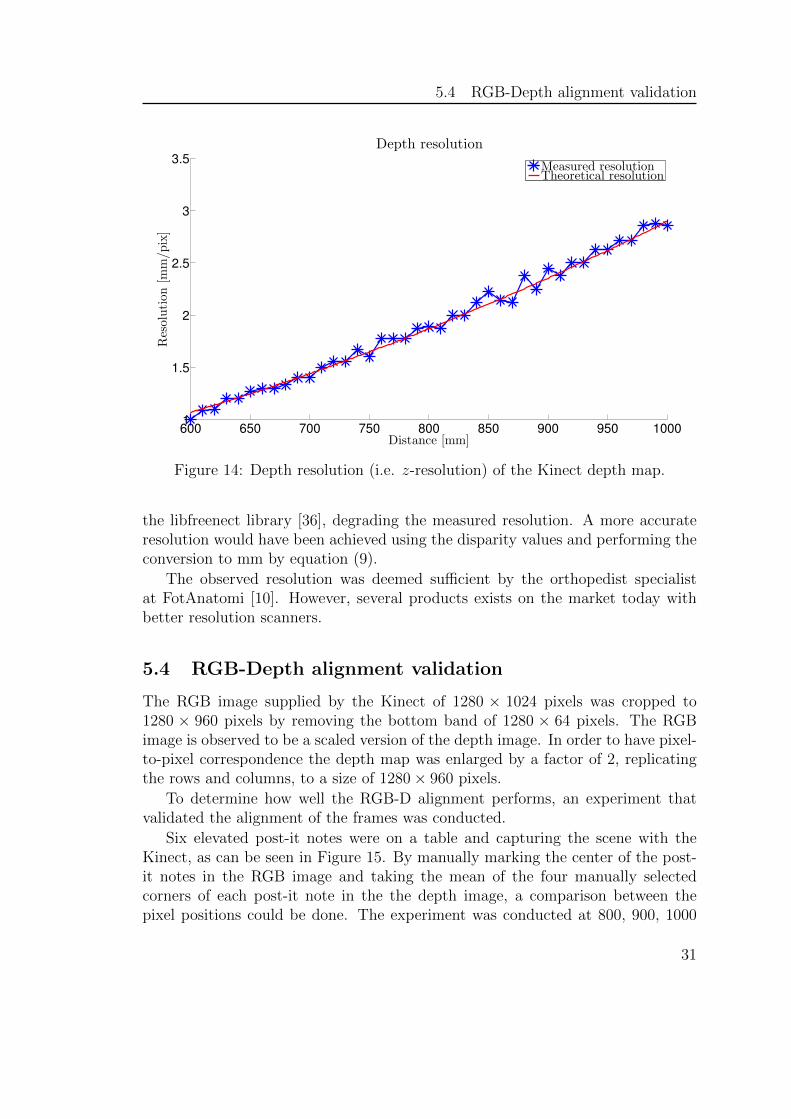
Six elevated post-it notes were on a table and capturing the scene with theKinect, as can be seen in Figure 15. By manually marking the center of the post-it notes in the RGB image and taking the mean of the four manually selectedcorners of each post-it note in the the depth image, a comparison between thepixel positions could be done. The experiment was conducted at 800, 900, 1000
31
5.4 RGB-Depth alignment validation
Figure 15: RGB-Depth alignment validation. The figure shows a capture of sixpost it notes where the alignment between depth map and RGB image was tested.To the left, the four corners of the first post-it in the depth map is marked in red.To the right, in the RGB image, the center of the post-it note is marked in red.
and 1100 mm from the post-it notes for two Kinect devices.
5.4.1 Alignment results
The results of the alignment validation can be seen in Table 2. Here, the offsetsbetween the depth and the RGB image for four different distances are shown.
Table 2: Alignment offset between depth and RGB images from two Kinect devices.The offsets listed are mean values of six measurement points.
Distance Kinect 1 offset (pixels) Kinect 2 offset (pixels)mm x y x y800 -0.17 4.91 -0.05 6.25900 0.58 5.33 -2.08 5.251000 0.58 5.83 0.17 4.081100 0.50 5.17 -1.92 4.17
5.4.2 Alignment discussion
The results presented in Table 2 shows that the RGB frame is shifted 5 pixels iny, compared to the the depth image. This result is consistent between the devicesand over the four distances measured.
32
5.5 Depth measurement validation using known object
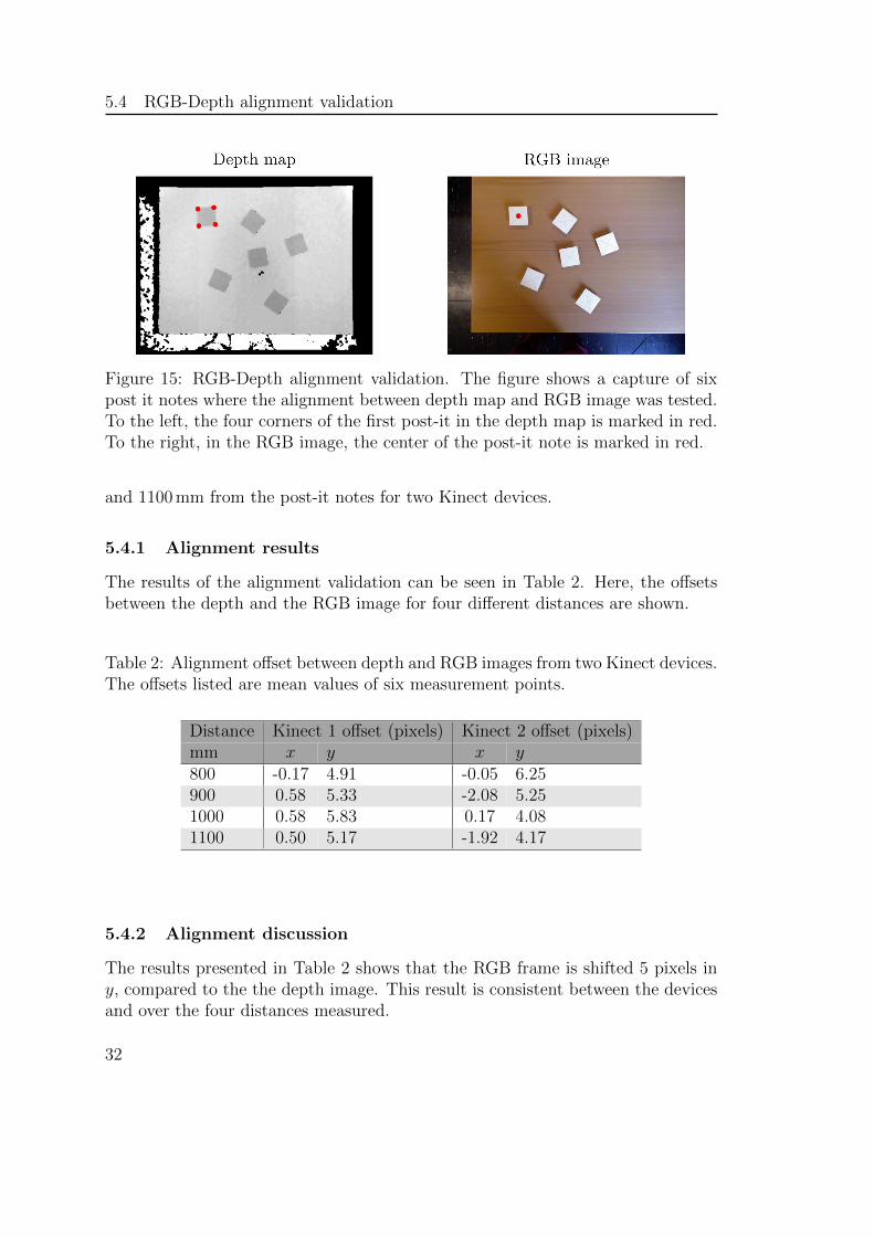
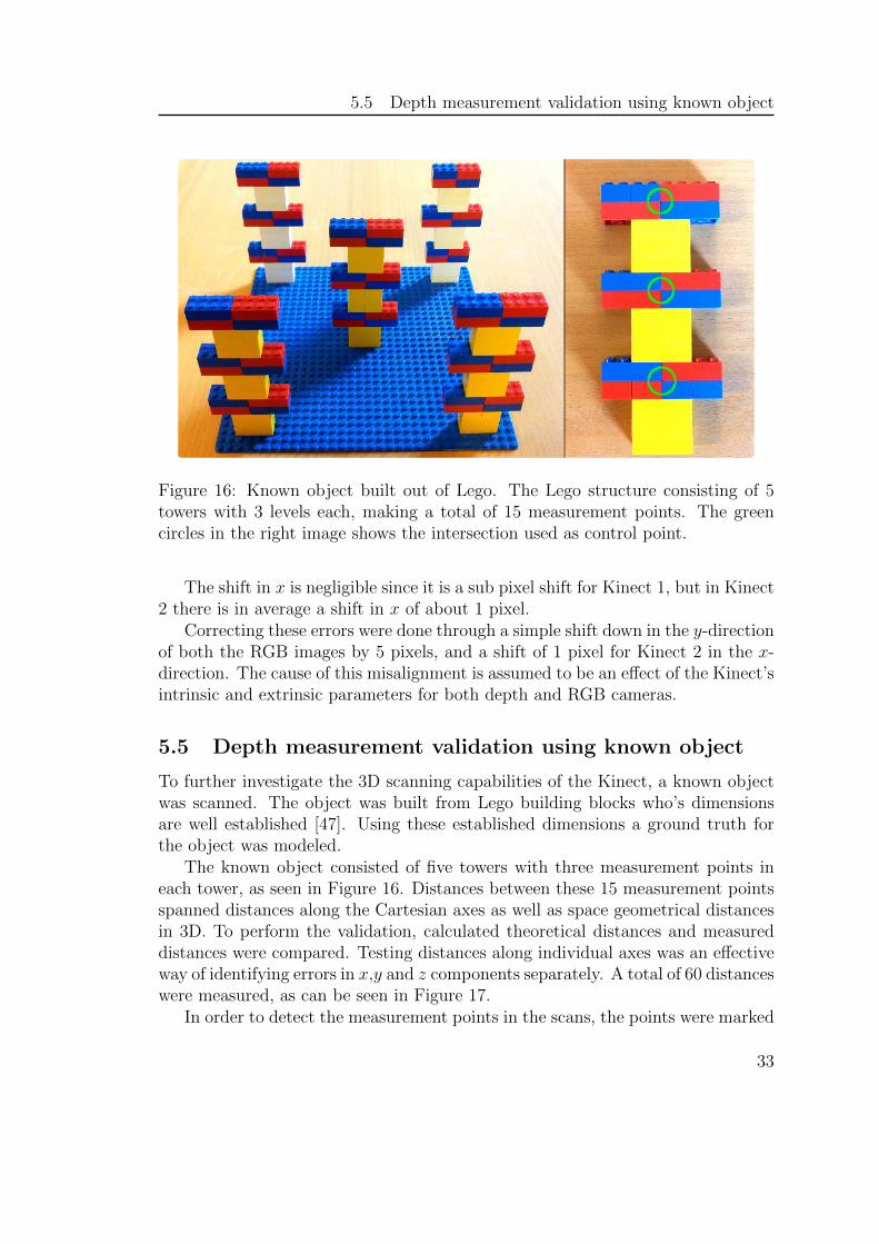
Figure 16: Known object built out of Lego. The Lego structure consisting of 5towers with 3 levels each, making a total of 15 measurement points. The greencircles in the right image shows the intersection used as control point.
The shift in x is negligible since it is a sub pixel shift for Kinect 1, but in Kinect2 there is in average a shift in x of about 1 pixel.
Correcting these errors were done through a simple shift down in the y-directionof both the RGB images by 5 pixels, and a shift of 1 pixel for Kinect 2 in the x-direction. The cause of this misalignment is assumed to be an effect of the Kinect’sintrinsic and extrinsic parameters for both depth and RGB cameras.
5.5 Depth measurement validation using known object
To further investigate the 3D scanning capabilities of the Kinect, a known objectwas scanned. The object was built from Lego building blocks who’s dimensionsare well established [47]. Using these established dimensions a ground truth forthe object was modeled.
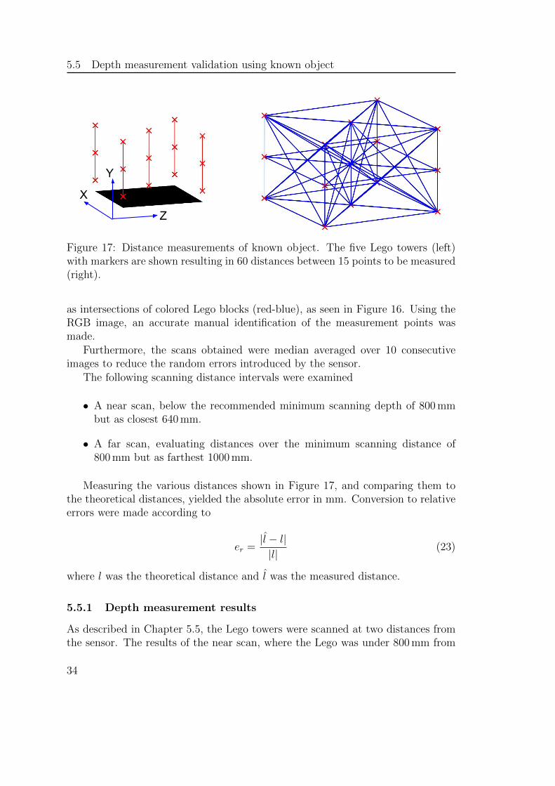
The known object consisted of five towers with three measurement points ineach tower, as seen in Figure 16. Distances between these 15 measurement pointsspanned distances along the Cartesian axes as well as space geometrical distancesin 3D. To perform the validation, calculated theoretical distances and measureddistances were compared. Testing distances along individual axes was an effectiveway of identifying errors in x,y and z components separately. A total of 60 distanceswere measured, as can be seen in Figure 17.
In order to detect the measurement points in the scans, the points were marked
33
5.5 Depth measurement validation using known object
Z
Y
X
Figure 17: Distance measurements of known object. The five Lego towers (left)with markers are shown resulting in 60 distances between 15 points to be measured(right).
as intersections of colored Lego blocks (red-blue), as seen in Figure 16. Using theRGB image, an accurate manual identification of the measurement points wasmade.
Furthermore, the scans obtained were median averaged over 10 consecutiveimages to reduce the random errors introduced by the sensor.
The following scanning distance intervals were examined
• A near scan, below the recommended minimum scanning depth of 800 mmbut as closest 640 mm.
• A far scan, evaluating distances over the minimum scanning distance of800 mm but as farthest 1000 mm.
Measuring the various distances shown in Figure 17, and comparing them tothe theoretical distances, yielded the absolute error in mm. Conversion to relativeerrors were made according to
er =|l − l||l|
(23)
where l was the theoretical distance and l was the measured distance.
5.5.1 Depth measurement results
As described in Chapter 5.5, the Lego towers were scanned at two distances fromthe sensor. The results of the near scan, where the Lego was under 800 mm from
34
5.5 Depth measurement validation using known object
0
2
4
6
Measurement distanceAbsolute
error[m
m]
Geometric distances, absolute error, 640-800 mm
x,z consty,z constx,y constz consty constx constDiagonals
−6 −4 −2 0 2 4 60
5
10
15
Histogram of errors
Distance error [mm]
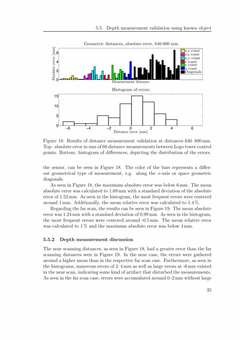
Figure 18: Results of distance measurement validation at distances 640–800 mm.Top: absolute error in mm of 60 distance measurements between Lego tower controlpoints. Bottom: histogram of differences, depicting the distribution of the errors.
the sensor, can be seen in Figure 18. The color of the bars represents a differ-ent geometrical type of measurement, e.g. along the x-axis or space geometricdiagonals.
As seen in Figure 18, the maximum absolute error was below 6 mm. The meanabsolute error was calculated to 1.69 mm with a standard deviation of the absoluteerror of 1.52 mm. As seen in the histogram, the most frequent errors were centeredaround 1 mm. Additionally, the mean relative error was calculated to 1.4 %.
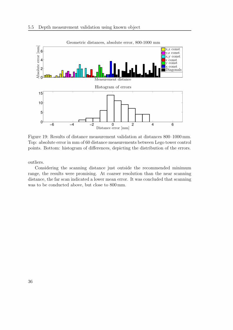
Regarding the far scan, the results can be seen in Figure 19. The mean absoluteerror was 1.24 mm with a standard deviation of 0.99 mm. As seen in the histogram,the most frequent errors were centered around -0.5 mm. The mean relative errorwas calculated to 1 % and the maximum absolute error was below 4 mm.
5.5.2 Depth measurement discussion
The near scanning distances, as seen in Figure 18, had a greater error than the farscanning distances seen in Figure 19. In the near case, the errors were gatheredaround a higher mean than in the respective far scan case. Furthermore, as seen inthe histograms, numerous errors of 2–4 mm as well as large errors at -6 mm existedin the near scan, indicating some kind of artifact that disturbed the measurements.As seen in the far scan case, errors were accumulated around 0–2 mm without large
35
5.5 Depth measurement validation using known object
0
2
4
6
Measurement distanceAbsolute
error[m
m]
Geometric distances, absolute error, 800-1000 mm
x,z consty,z constx,y constz consty constx constDiagonals
−6 −4 −2 0 2 4 60
5
10
15
Histogram of errors
Distance error [mm]
Figure 19: Results of distance measurement validation at distances 800–1000 mm.Top: absolute error in mm of 60 distance measurements between Lego tower controlpoints. Bottom: histogram of differences, depicting the distribution of the errors.
outliers.Considering the scanning distance just outside the recommended minimum
range, the results were promising. At coarser resolution than the near scanningdistance, the far scan indicated a lower mean error. It was concluded that scanningwas to be conducted above, but close to 800 mm.
36
6 Proposed system for insole modeling
6 Proposed system for insole modeling
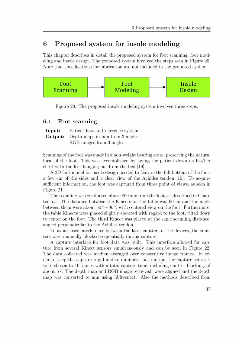
This chapter describes in detail the proposed system for foot scanning, foot mod-eling and insole design. The proposed system involved the steps seen in Figure 20.Note that specifications for fabrication are not included in the proposed system.
Foot Scanning
Insole Design
Foot Modeling
Figure 20: The proposed insole modeling system involves three steps.
6.1 Foot scanning
Input: Patient foot and reference systemOutput: Depth maps in mm from 3 angles
RGB images from 3 angles
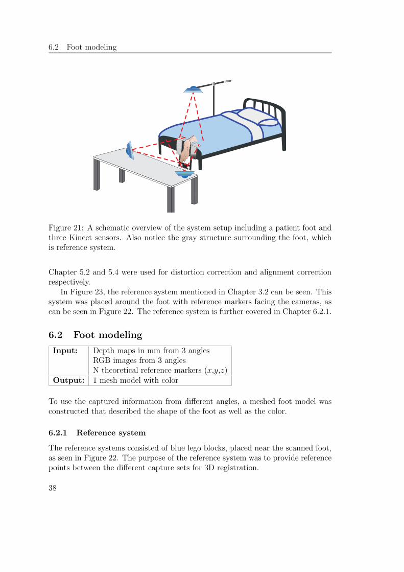
Scanning of the foot was made in a non-weight bearing state, preserving the naturalform of the foot. This was accomplished by laying the patient down on his/herchest with the feet hanging out from the bed [19].
A 3D foot model for insole design needed to feature the full bottom of the foot,a few cm of the sides and a clear view of the Achilles tendon [10]. To acquiresufficient information, the foot was captured from three point of views, as seen inFigure 21.
The scanning was conducted above 800 mm from the foot, as described in Chap-ter 5.5. The distance between the Kinects on the table was 60 cm and the anglebetween them were about 50 ◦−90 ◦, with centered view on the foot. Furthermore,the table Kinects were placed slightly elevated with regard to the foot, tilted downto center on the foot. The third Kinect was placed at the same scanning distance,angled perpendicular to the Achilles tendon.
To avoid laser interference between the laser emitters of the devices, the emit-ters were manually blocked sequentially during capture.
A capture interface for foot data was built. This interface allowed for cap-ture from several Kinect sensors simultaneously and can be seen in Figure 22.The data collected was median averaged over consecutive image frames. In or-der to keep the capture rapid and to minimize foot motion, the capture set sizeswere chosen to 10 frames with a total capture time, including emitter blocking, ofabout 5 s. The depth map and RGB image retrieved, were aligned and the depthmap was converted to mm using libfreenect. Also the methods described from
37
6.2 Foot modeling
Figure 21: A schematic overview of the system setup including a patient foot andthree Kinect sensors. Also notice the gray structure surrounding the foot, whichis reference system.
Chapter 5.2 and 5.4 were used for distortion correction and alignment correctionrespectively.
In Figure 23, the reference system mentioned in Chapter 3.2 can be seen. Thissystem was placed around the foot with reference markers facing the cameras, ascan be seen in Figure 22. The reference system is further covered in Chapter 6.2.1.
6.2 Foot modeling
Input: Depth maps in mm from 3 anglesRGB images from 3 anglesN theoretical reference markers (x,y,z)
Output: 1 mesh model with color
To use the captured information from different angles, a meshed foot model wasconstructed that described the shape of the foot as well as the color.
6.2.1 Reference system
The reference systems consisted of blue lego blocks, placed near the scanned foot,as seen in Figure 22. The purpose of the reference system was to provide referencepoints between the different capture sets for 3D registration.
38

6.2 Foot modeling
LEFTCenter Depth = 798 mm
LEFT
RIGHTCenter Depth = 799 mm
RIGHT
Figure 22: A capture interface example including buttons for tilt, re-capture anddata export of two Kinect sensors. The top images show depth maps color codedin mm where the center depth is indicated in the title. The bottom images showthe corresponding RGB images.
Various systems were experimented with, including reference markers paintedon the foot, different shapes of markers, different colors and systems varying insize and orientation, relative to the foot. Placing reference markers on the footyielded good results, but from a practical point of view, painting on the patient’sfeet was unwanted.
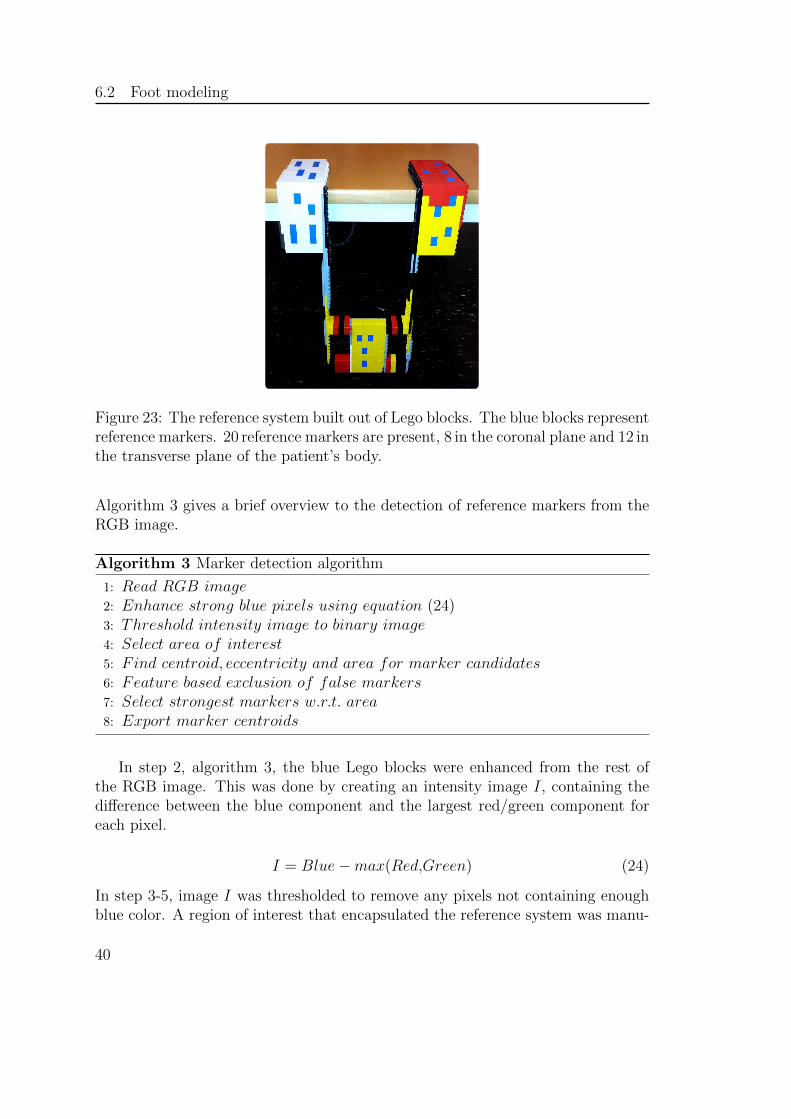
The final reference system used can be seen in Figure 23 and was chosen asa set of 20 blue reference markers, where 12 markers lay in the plane of the footand 8 markers lay in the plane parallel to the Achilles tendon. The system wasconstructed using Lego blocks, which enabled simple translation to a theoreticalmodel with known distances. The theoretical measurements of the the Lego blockswere provided by Caillau [47].
6.2.2 Detection of reference markers
Input: Depth maps in mm from 3 anglesRGB images from 3 angles
Output: N captured reference markers (x,y,z)Aligned depth maps in mm from 3 anglesRGB images from 3 angles
39
6.2 Foot modeling
Figure 23: The reference system built out of Lego blocks. The blue blocks representreference markers. 20 reference markers are present, 8 in the coronal plane and 12 inthe transverse plane of the patient’s body.
Algorithm 3 gives a brief overview to the detection of reference markers from theRGB image.
Algorithm 3 Marker detection algorithm
1: Read RGB image2: Enhance strong blue pixels using equation (24)3: Threshold intensity image to binary image4: Select area of interest5: Find centroid, eccentricity and area for marker candidates6: Feature based exclusion of false markers7: Select strongest markers w.r.t. area8: Export marker centroids
In step 2, algorithm 3, the blue Lego blocks were enhanced from the rest ofthe RGB image. This was done by creating an intensity image I, containing thedifference between the blue component and the largest red/green component foreach pixel.
I = Blue−max(Red,Green) (24)
In step 3-5, image I was thresholded to remove any pixels not containing enoughblue color. A region of interest that encapsulated the reference system was manu-
40
6.2 Foot modeling
ally selected. Furthermore, connected components of pixels were identified, result-ing in marker candidates.
In step 6-8, exclusion of false markers from the marker candidates was done,using eccentricity, removing segments resembling pixel lines more than blocks.Finally, the markers were identified as the largest area components in the image.
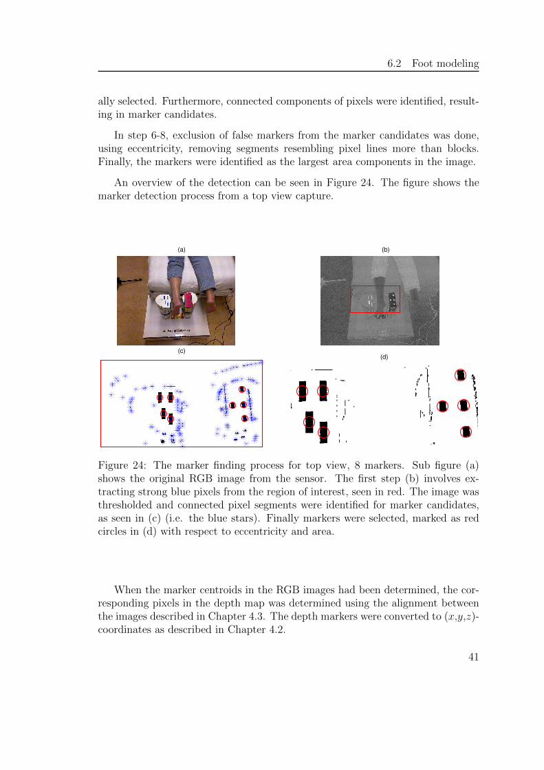
An overview of the detection can be seen in Figure 24. The figure shows themarker detection process from a top view capture.
(a) (b)
(c)(d)
Figure 24: The marker finding process for top view, 8 markers. Sub figure (a)shows the original RGB image from the sensor. The first step (b) involves ex-tracting strong blue pixels from the region of interest, seen in red. The image wasthresholded and connected pixel segments were identified for marker candidates,as seen in (c) (i.e. the blue stars). Finally markers were selected, marked as redcircles in (d) with respect to eccentricity and area.
When the marker centroids in the RGB images had been determined, the cor-responding pixels in the depth map was determined using the alignment betweenthe images described in Chapter 4.3. The depth markers were converted to (x,y,z)-coordinates as described in Chapter 4.2.
41

6.2 Foot modeling
6.2.3 Multi-view registration
Input: N captured reference markers (x,y,z)N theoretical reference system markers (x,y,z)Aligned depth maps in mm from 3 anglesRGB images from 3 angles
Output: 3 registered mesh models with color
Proceeding from multi-view scanned data to a mesh model of the foot with colorrequired some data processing. The depth map and RGB images of the captureswere processed as described in Chapter 4.2 and 4.3. This converted the depth mapsinto point clouds with color information for each point. Furthermore, surfaces tothe RGB-D data was constructed using 2D Delaunay Triangulation in the imageplane of the capture, described in Chapter 3.1. The color of the triangular faceswere determined by interpolation between the colors from the triangle vertices.Concluding, a mesh model with color was determined for each capture.
The captures contained data for the whole FOV, foot and room. Segmentationof the foot was done by selecting a volume of interest in space, were the (x,y,z)-coordinates of the foot resided.
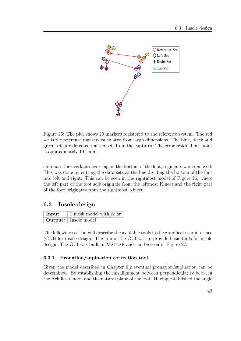
To bring the three foot data sets sequentially to one shared coordinate system,they were rotated and translated as a rigid body to the origin of the referencesystem (Figure 23), located in the centroid of the scanned foot. This was doneusing the detected marker coordinates and the Matlab implementation of theabsolute orientation quaternions by Wengert and Bianchi (2010) [48], based onHorn’s method [32] described in Chapter 3.2. An example of such a registrationcan be seen in Figure 25.
As seen in Figure 25 a fit of the captured reference markers to the theoreticalreference markers was accurate with error residuals per point of:
• Left set (blue): 2.03 mm
• Right set (black): 1.59 mm
• Top set (green): 1.29 mm
6.2.4 Removal of overlapping data in the foot bed
Input: 3 registered mesh models with colorOutput: 1 mesh model with color
Having registered the foot captures to one shared coordinate system, overlappingsegments existed due to the overlapping field of views of the cameras. In order to
42
6.3 Insole design
Reference Set
Left Set
Right Set
Top Set
Figure 25: The plot shows 20 markers registered to the reference system. The redset is the reference markers calculated from Lego dimensions. The blue, black andgreen sets are detected marker sets from the captures. The error residual per pointis approximately 1.64 mm.
eliminate the overlaps occurring on the bottom of the foot, segments were removed.This was done by cutting the data sets at the line dividing the bottom of the footinto left and right. This can be seen in the rightmost model of Figure 26, wherethe left part of the foot sole originate from the leftmost Kinect and the right partof the foot originates from the rightmost Kinect.
6.3 Insole design
Input: 1 mesh model with colorOutput: Insole model
The following section will describe the available tools in the graphical user interface(GUI) for insole design. The aim of the GUI was to provide basic tools for insoledesign. The GUI was built in Matlab and can be seen in Figure 27.
6.3.1 Pronation/supination correction tool
Given the model described in Chapter 6.2 eventual pronation/supination can bedetermined. By establishing the misalignment between perpendicularity betweenthe Achilles tendon and the natural plane of the foot. Having established the angle
43
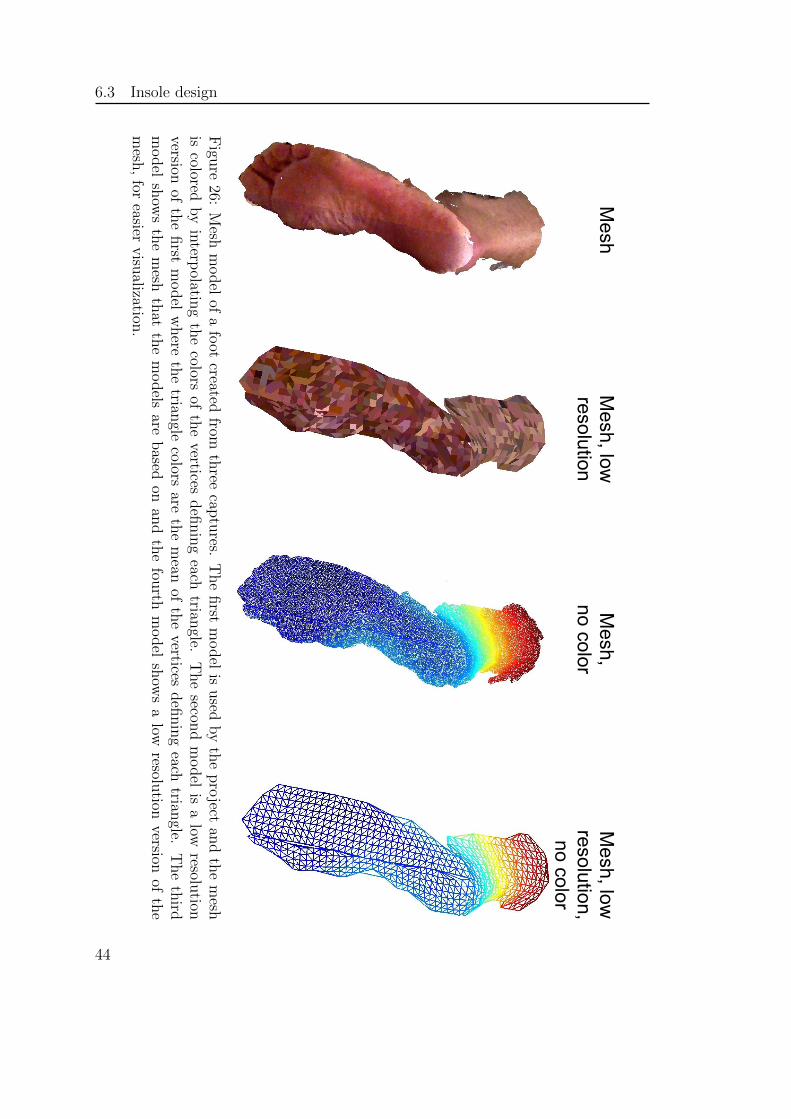
6.3 Insole design
Mesh
Mesh, low
resolution
Mesh,
no colorM
esh, low
resolution, no color
Figu
re26:
Mesh
model
ofa
foot
createdfrom
three
captu
res.T
he
first
model
isused
by
the
pro
jectan
dth
em
eshis
coloredby
interp
olating
the
colorsof
the
verticesdefi
nin
geach
triangle.
The
second
model
isa
lowresolu
tionversion
ofth
efirst
model
where
the
triangle
colorsare
the
mean
ofth
evertices
defi
nin
geach
triangle.
The
third
model
show
sth
em
eshth
atth
em
odels
arebased
onan
dth
efou
rthm
odel
show
sa
lowresolu
tionversion
ofth
em
esh,
foreasier
visu
alization.
44
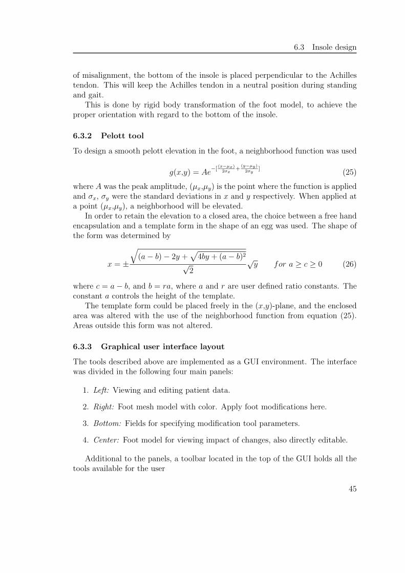
6.3 Insole design
of misalignment, the bottom of the insole is placed perpendicular to the Achillestendon. This will keep the Achilles tendon in a neutral position during standingand gait.
This is done by rigid body transformation of the foot model, to achieve theproper orientation with regard to the bottom of the insole.
6.3.2 Pelott tool
To design a smooth pelott elevation in the foot, a neighborhood function was used
g(x,y) = Ae−[ (x−µx)
2σx+
(y−µy)2σy
](25)
where A was the peak amplitude, (µx,µy) is the point where the function is appliedand σx, σy were the standard deviations in x and y respectively. When applied ata point (µx,µy), a neighborhood will be elevated.
In order to retain the elevation to a closed area, the choice between a free handencapsulation and a template form in the shape of an egg was used. The shape ofthe form was determined by
x = ±
√(a− b)− 2y +
√4by + (a− b)2
√2
√y for a ≥ c ≥ 0 (26)
where c = a− b, and b = ra, where a and r are user defined ratio constants. Theconstant a controls the height of the template.
The template form could be placed freely in the (x,y)-plane, and the enclosedarea was altered with the use of the neighborhood function from equation (25).Areas outside this form was not altered.
6.3.3 Graphical user interface layout
The tools described above are implemented as a GUI environment. The interfacewas divided in the following four main panels:
1. Left: Viewing and editing patient data.
2. Right: Foot mesh model with color. Apply foot modifications here.
3. Bottom: Fields for specifying modification tool parameters.
4. Center: Foot model for viewing impact of changes, also directly editable.
Additional to the panels, a toolbar located in the top of the GUI holds all thetools available for the user
45
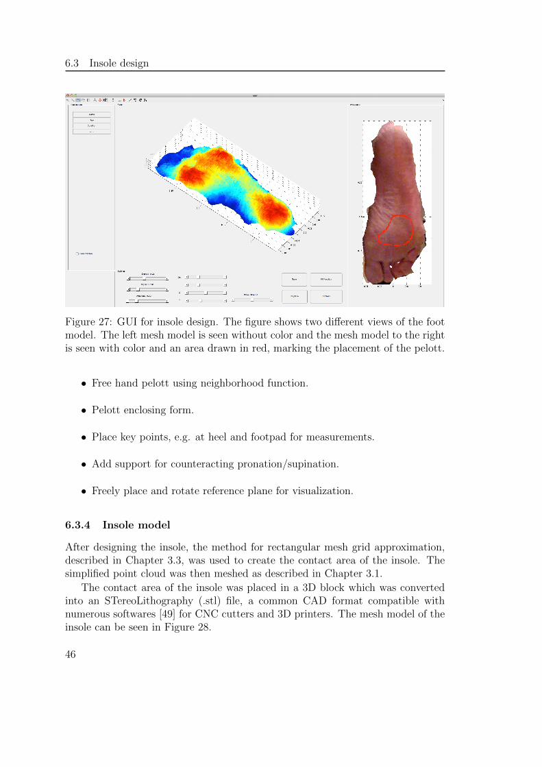
6.3 Insole design
Figure 27: GUI for insole design. The figure shows two different views of the footmodel. The left mesh model is seen without color and the mesh model to the rightis seen with color and an area drawn in red, marking the placement of the pelott.
• Free hand pelott using neighborhood function.
• Pelott enclosing form.
• Place key points, e.g. at heel and footpad for measurements.
• Add support for counteracting pronation/supination.
• Freely place and rotate reference plane for visualization.
6.3.4 Insole model
After designing the insole, the method for rectangular mesh grid approximation,described in Chapter 3.3, was used to create the contact area of the insole. Thesimplified point cloud was then meshed as described in Chapter 3.1.
The contact area of the insole was placed in a 3D block which was convertedinto an STereoLithography (.stl) file, a common CAD format compatible withnumerous softwares [49] for CNC cutters and 3D printers. The mesh model of theinsole can be seen in Figure 28.
46

6.4 Block diagram system overview
Figure 28: The insole model after design. Notice that only the part of the insolethat faces the foot has been designed, i.e. the side and bottom of the insole isuntouched. Also notice that no pelott is included in this model.
6.4 Block diagram system overview
The proposed system described in Chapter 6 can be summarized in a block dia-gram, as shown in Figure 29.
47
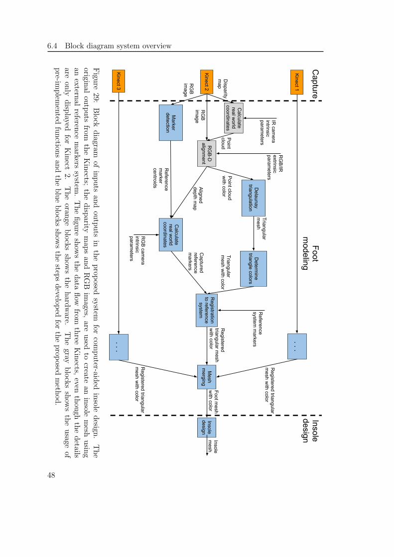
6.4 Block diagram system overview
Kinect 2
RG
B-D
alignm
entR
GB
im
age
Disparity
map
Calculate
real world
coordinatesP
oint cloud w
ith color
IR cam
era intrinsic param
eters
RG
B/IR
extrinsic param
eters
RG
B
image
Marker
detection
Aligned
depth map
Calculate
real world
coordinatesR
eference m
arker centroids
RG
B cam
era intrinsicparam
eters
Point
cloud
Delaunay
triangulation
Triangularm
eshD
etermine
triangle colors
Triangular m
esh with color
Registration
to reference system
Mesh
merging
Registered
triangular mesh
with color
Reference
system m
arkers
Captured
reference m
arkers
Insole design
Registered triangular
mesh w
ith color
Registered triangular
mesh w
ith color
Kinect 1
Kinect 3
. . .
. . .
Foot mesh
with color
Insole m
esh
Capture
Foot m
odelingInsoledesign
Figu
re29:
Blo
ckdiagram
ofin
puts
and
outp
uts
inth
eprop
osedsy
stemfor
computer-aid
edin
soledesign
.T
he
original
outp
uts
fromth
eK
inects;
the
disp
aritym
aps
and
RG
Bim
ages,are
used
tocreate
anin
solem
eshusin
gan
extern
alreferen
cem
arkerssy
stem.
The
figu
resh
ows
the
data
flow
fromth
reeK
inects,
eventh
ough
the
details
areon
lydisp
layedfor
Kin
ect2.
The
orange
blo
cks
show
sth
ehard
ware.
The
grayblo
cks
show
sth
eusage
ofpre-im
plem
ented
function
san
dth
eblu
eblo
cks
show
sth
estep
sdevelop
edfor
the
prop
osedm
ethod.
48
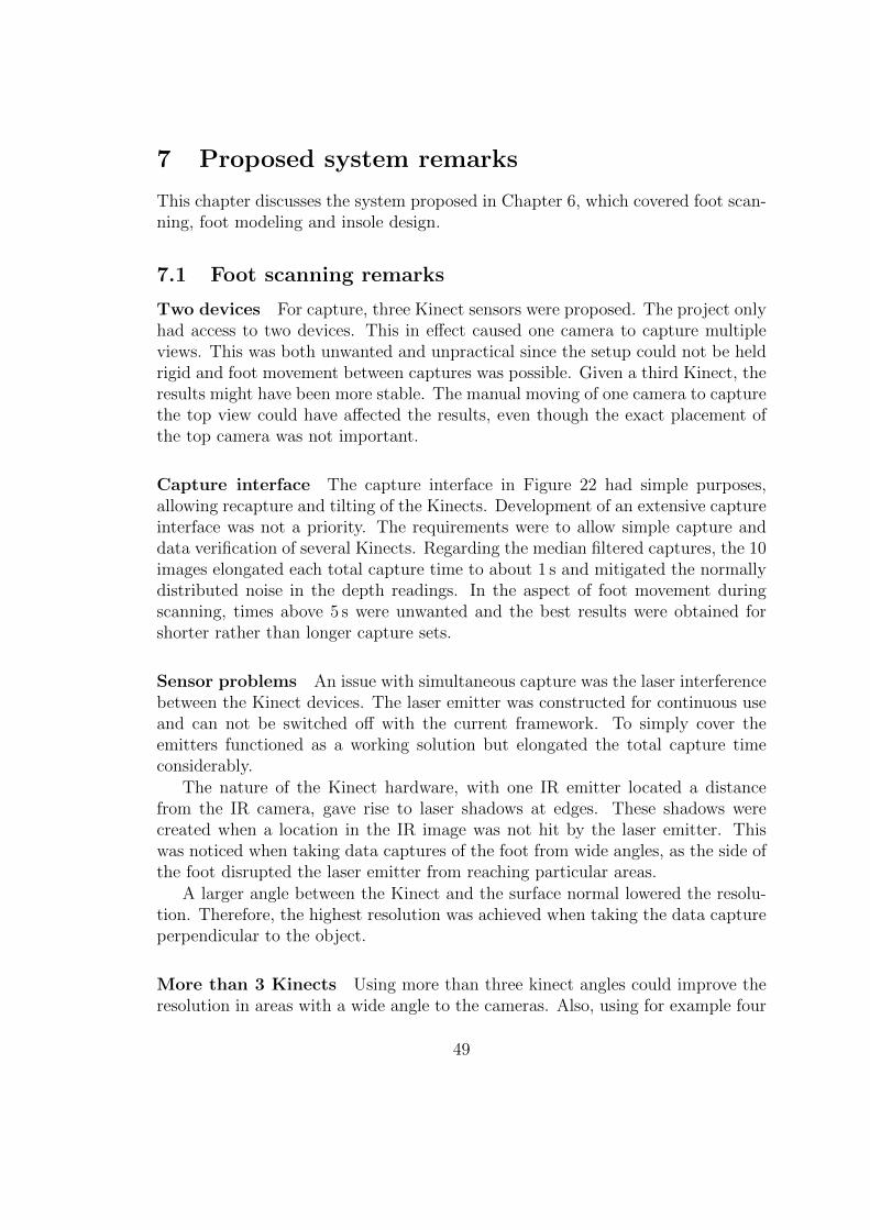
7 Proposed system remarks
This chapter discusses the system proposed in Chapter 6, which covered foot scan-ning, foot modeling and insole design.
7.1 Foot scanning remarks
Two devices For capture, three Kinect sensors were proposed. The project onlyhad access to two devices. This in effect caused one camera to capture multipleviews. This was both unwanted and unpractical since the setup could not be heldrigid and foot movement between captures was possible. Given a third Kinect, theresults might have been more stable. The manual moving of one camera to capturethe top view could have affected the results, even though the exact placement ofthe top camera was not important.
Capture interface The capture interface in Figure 22 had simple purposes,allowing recapture and tilting of the Kinects. Development of an extensive captureinterface was not a priority. The requirements were to allow simple capture anddata verification of several Kinects. Regarding the median filtered captures, the 10images elongated each total capture time to about 1 s and mitigated the normallydistributed noise in the depth readings. In the aspect of foot movement duringscanning, times above 5 s were unwanted and the best results were obtained forshorter rather than longer capture sets.
Sensor problems An issue with simultaneous capture was the laser interferencebetween the Kinect devices. The laser emitter was constructed for continuous useand can not be switched off with the current framework. To simply cover theemitters functioned as a working solution but elongated the total capture timeconsiderably.
The nature of the Kinect hardware, with one IR emitter located a distancefrom the IR camera, gave rise to laser shadows at edges. These shadows werecreated when a location in the IR image was not hit by the laser emitter. Thiswas noticed when taking data captures of the foot from wide angles, as the side ofthe foot disrupted the laser emitter from reaching particular areas.
A larger angle between the Kinect and the surface normal lowered the resolu-tion. Therefore, the highest resolution was achieved when taking the data captureperpendicular to the object.
More than 3 Kinects Using more than three kinect angles could improve theresolution in areas with a wide angle to the cameras. Also, using for example four
49
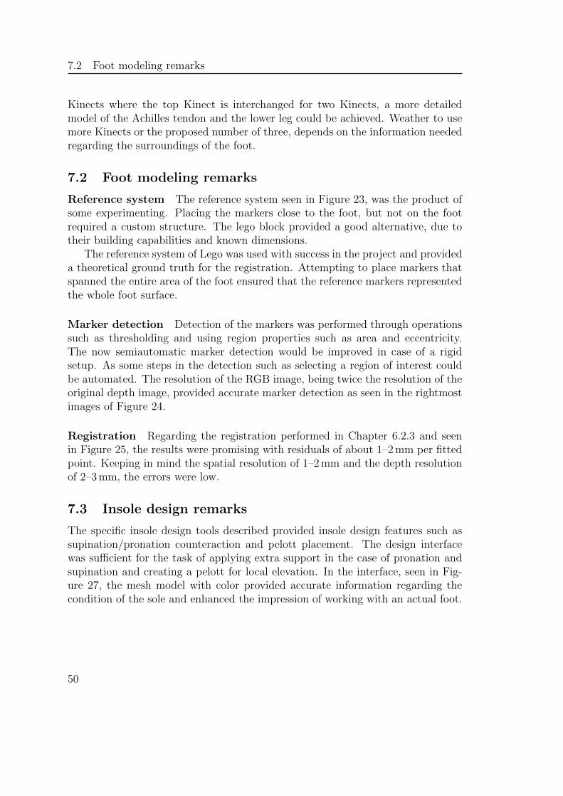
7.2 Foot modeling remarks
Kinects where the top Kinect is interchanged for two Kinects, a more detailedmodel of the Achilles tendon and the lower leg could be achieved. Weather to usemore Kinects or the proposed number of three, depends on the information neededregarding the surroundings of the foot.
7.2 Foot modeling remarks
Reference system The reference system seen in Figure 23, was the product ofsome experimenting. Placing the markers close to the foot, but not on the footrequired a custom structure. The lego block provided a good alternative, due totheir building capabilities and known dimensions.
The reference system of Lego was used with success in the project and provideda theoretical ground truth for the registration. Attempting to place markers thatspanned the entire area of the foot ensured that the reference markers representedthe whole foot surface.
Marker detection Detection of the markers was performed through operationssuch as thresholding and using region properties such as area and eccentricity.The now semiautomatic marker detection would be improved in case of a rigidsetup. As some steps in the detection such as selecting a region of interest couldbe automated. The resolution of the RGB image, being twice the resolution of theoriginal depth image, provided accurate marker detection as seen in the rightmostimages of Figure 24.
Registration Regarding the registration performed in Chapter 6.2.3 and seenin Figure 25, the results were promising with residuals of about 1–2 mm per fittedpoint. Keeping in mind the spatial resolution of 1–2 mm and the depth resolutionof 2–3 mm, the errors were low.
7.3 Insole design remarks
The specific insole design tools described provided insole design features such assupination/pronation counteraction and pelott placement. The design interfacewas sufficient for the task of applying extra support in the case of pronation andsupination and creating a pelott for local elevation. In the interface, seen in Fig-ure 27, the mesh model with color provided accurate information regarding thecondition of the sole and enhanced the impression of working with an actual foot.
50

8 System evaluation through case study
8 System evaluation through case study
Comparison of the proposed system from Chapter 6 to existing products was madeby a quantitative case evaluation. The foot mesh model from the proposed systemwas compared to two external company insoles, all modeled from the same foot.The products compared were
1. Proposed digital system.
2. FotAnatomi [10], traditional plaster cast production method.
3. Ortolab, semi-digital method.
To perform the comparison, a patient experienced with both the traditionalplaster cast method and a semi-computer assisted method was chosen as casesubject. The patient was scanned with the Kinect sensors and foot modeling andinsole design were performed.
The traditionally casted replica was created 2013-02-20 by FotAnatomi. Theplaster cast mold is also modified with a pelott imprint, done while casting theplaster shell. The resulting mold can be seen in Figure 2 with a pelott imprintmarked in red [10].
The computer assisted insole was made by Ortolab. The replica was cut out ofPU-foam from a digital model of the patient’s foot, in autumn 2012. Furthermore,the foam model was modified with a pelott imprint by an orthopedist from Ortolab.The foam model can be seen in Figure 30 with a pelott imprint marked in red. Acomparison between the results of the three systems could then be conducted.
8.1 Subject description
The patient had a forefoot valgus deformation emerging on the outer side of herleft foot due to forefoot insufficiency [10]. This caused the patient pain duringseveral years. To remedy the pain, the Ortolab insole alternative was tried. Thepatient then tried the services of FotAnatomi.
8.2 Scanning patient and molds
The patient was scanned from three angles. The left and right Kinect were placedon a table as depicted in Figure 21, the top Kinect in the figure was hold manuallyfor the last data capture set. A foot model was constructed as described in Chap-ter 6.2 and an insole proposition was created with a pelott imprint, mimicking thedesign of the mold from FotAnatomi, which was considered as the reference.
The two replicas from FotAnatomi and Ortolab respectively were scanned withthe Kinect sensor.
51
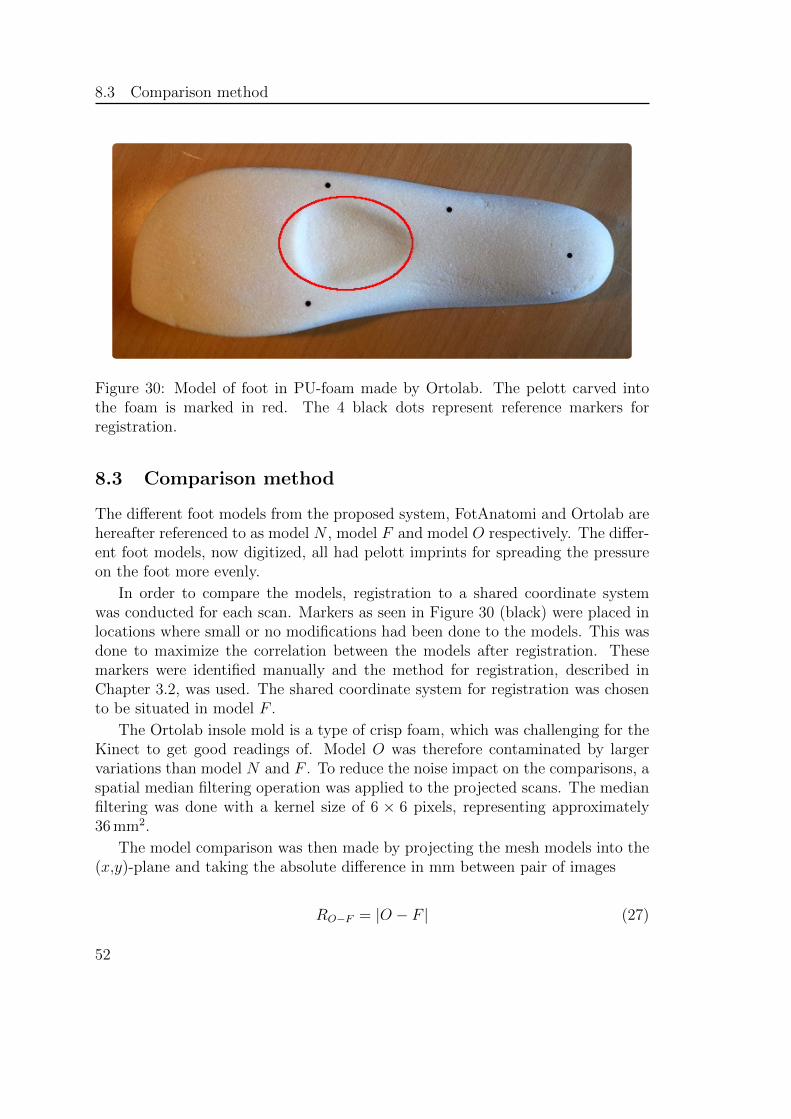
8.3 Comparison method
Figure 30: Model of foot in PU-foam made by Ortolab. The pelott carved intothe foam is marked in red. The 4 black dots represent reference markers forregistration.
8.3 Comparison method
The different foot models from the proposed system, FotAnatomi and Ortolab arehereafter referenced to as model N , model F and model O respectively. The differ-ent foot models, now digitized, all had pelott imprints for spreading the pressureon the foot more evenly.
In order to compare the models, registration to a shared coordinate systemwas conducted for each scan. Markers as seen in Figure 30 (black) were placed inlocations where small or no modifications had been done to the models. This wasdone to maximize the correlation between the models after registration. Thesemarkers were identified manually and the method for registration, described inChapter 3.2, was used. The shared coordinate system for registration was chosento be situated in model F .
The Ortolab insole mold is a type of crisp foam, which was challenging for theKinect to get good readings of. Model O was therefore contaminated by largervariations than model N and F . To reduce the noise impact on the comparisons, aspatial median filtering operation was applied to the projected scans. The medianfiltering was done with a kernel size of 6 × 6 pixels, representing approximately36 mm2.
The model comparison was then made by projecting the mesh models into the(x,y)-plane and taking the absolute difference in mm between pair of images
RO−F = |O − F | (27)
52
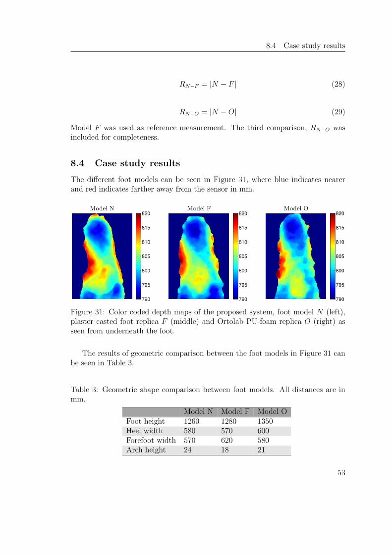
8.4 Case study results
RN−F = |N − F | (28)
RN−O = |N −O| (29)
Model F was used as reference measurement. The third comparison, RN−O wasincluded for completeness.
8.4 Case study results
The different foot models can be seen in Figure 31, where blue indicates nearerand red indicates farther away from the sensor in mm.
Model N Model F Model O
790
795
800
805
810
815
820
790
795
800
805
810
815
820
790
795
800
805
810
815
820
Figure 31: Color coded depth maps of the proposed system, foot model N (left),plaster casted foot replica F (middle) and Ortolab PU-foam replica O (right) asseen from underneath the foot.
The results of geometric comparison between the foot models in Figure 31 canbe seen in Table 3.
Table 3: Geometric shape comparison between foot models. All distances are inmm.
Model N Model F Model OFoot height 1260 1280 1350Heel width 580 570 600Forefoot width 570 620 580Arch height 24 18 21
53
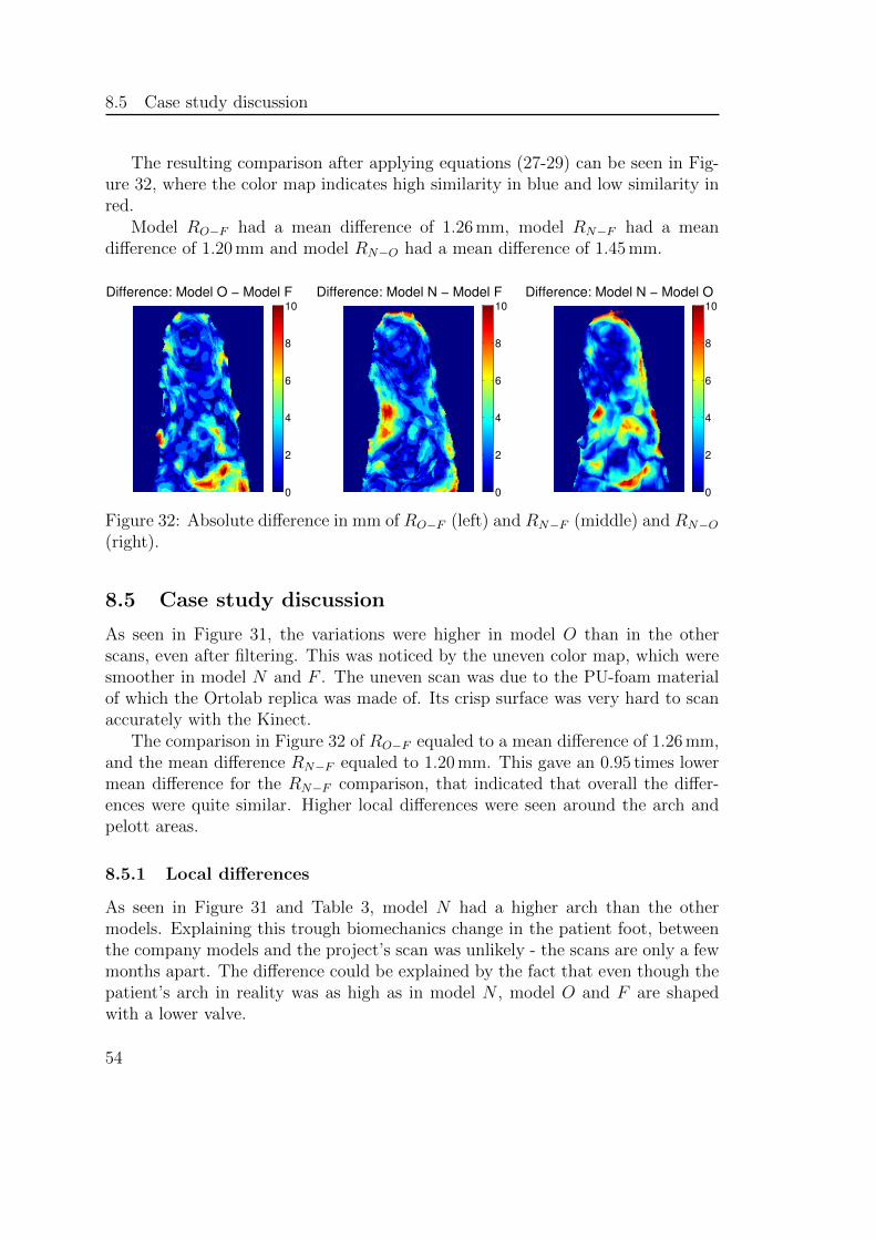
8.5 Case study discussion
The resulting comparison after applying equations (27-29) can be seen in Fig-ure 32, where the color map indicates high similarity in blue and low similarity inred.
Model RO−F had a mean difference of 1.26 mm, model RN−F had a meandifference of 1.20 mm and model RN−O had a mean difference of 1.45 mm.
Difference: Model O − Model F
0
2
4
6
8
10
Difference: Model N − Model F
0
2
4
6
8
10
Difference: Model N − Model O
0
2
4
6
8
10
Figure 32: Absolute difference in mm of RO−F (left) and RN−F (middle) and RN−O(right).
8.5 Case study discussion
As seen in Figure 31, the variations were higher in model O than in the otherscans, even after filtering. This was noticed by the uneven color map, which weresmoother in model N and F . The uneven scan was due to the PU-foam materialof which the Ortolab replica was made of. Its crisp surface was very hard to scanaccurately with the Kinect.
The comparison in Figure 32 of RO−F equaled to a mean difference of 1.26 mm,and the mean difference RN−F equaled to 1.20 mm. This gave an 0.95 times lowermean difference for the RN−F comparison, that indicated that overall the differ-ences were quite similar. Higher local differences were seen around the arch andpelott areas.
8.5.1 Local differences
As seen in Figure 31 and Table 3, model N had a higher arch than the othermodels. Explaining this trough biomechanics change in the patient foot, betweenthe company models and the project’s scan was unlikely - the scans are only a fewmonths apart. The difference could be explained by the fact that even though thepatient’s arch in reality was as high as in model N , model O and F are shapedwith a lower valve.
54
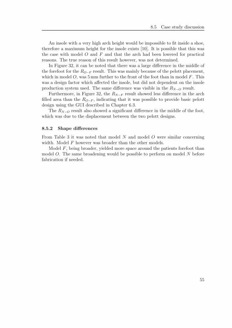
8.5 Case study discussion
An insole with a very high arch height would be impossible to fit inside a shoe,therefore a maximum height for the insole exists [10]. It is possible that this wasthe case with model O and F and that the arch had been lowered for practicalreasons. The true reason of this result however, was not determined.
In Figure 32, it can be noted that there was a large difference in the middle ofthe forefoot for the RO−F result. This was mainly because of the pelott placement,which in model O, was 5 mm further to the front of the foot than in model F . Thiswas a design factor which affected the insole, but did not dependent on the insoleproduction system used. The same difference was visible in the RN−O result.
Furthermore, in Figure 32, the RN−F result showed less difference in the archfilled area than the RO−F , indicating that it was possible to provide basic pelottdesign using the GUI described in Chapter 6.3.
The RN−O result also showed a significant difference in the middle of the foot,which was due to the displacement between the two pelott designs.
8.5.2 Shape differences
From Table 3 it was noted that model N and model O were similar concerningwidth. Model F however was broader than the other models.
Model F , being broader, yielded more space around the patients forefoot thanmodel O. The same broadening would be possible to perform on model N beforefabrication if needed.
55

56
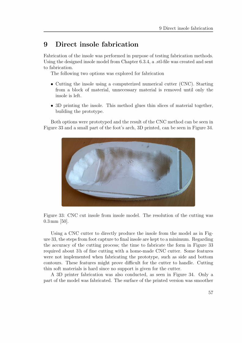
9 Direct insole fabrication
9 Direct insole fabrication
Fabrication of the insole was performed in purpose of testing fabrication methods.Using the designed insole model from Chapter 6.3.4, a .stl-file was created and sentto fabrication.
The following two options was explored for fabrication
• Cutting the insole using a computerized numerical cutter (CNC). Startingfrom a block of material, unnecessary material is removed until only theinsole is left.
• 3D printing the insole. This method glues thin slices of material together,building the prototype.
Both options were prototyped and the result of the CNC method can be seen inFigure 33 and a small part of the foot’s arch, 3D printed, can be seen in Figure 34.
Figure 33: CNC cut insole from insole model. The resolution of the cutting was0.3 mm [50].
Using a CNC cutter to directly produce the insole from the model as in Fig-ure 33, the steps from foot capture to final insole are kept to a minimum. Regardingthe accuracy of the cutting process; the time to fabricate the form in Figure 33required about 3 h of fine cutting with a home-made CNC cutter. Some featureswere not implemented when fabricating the prototype, such as side and bottomcontours. These features might prove difficult for the cutter to handle. Cuttingthin soft materials is hard since no support is given for the cutter.
A 3D printer fabrication was also conducted, as seen in Figure 34. Only apart of the model was fabricated. The surface of the printed version was smoother
57
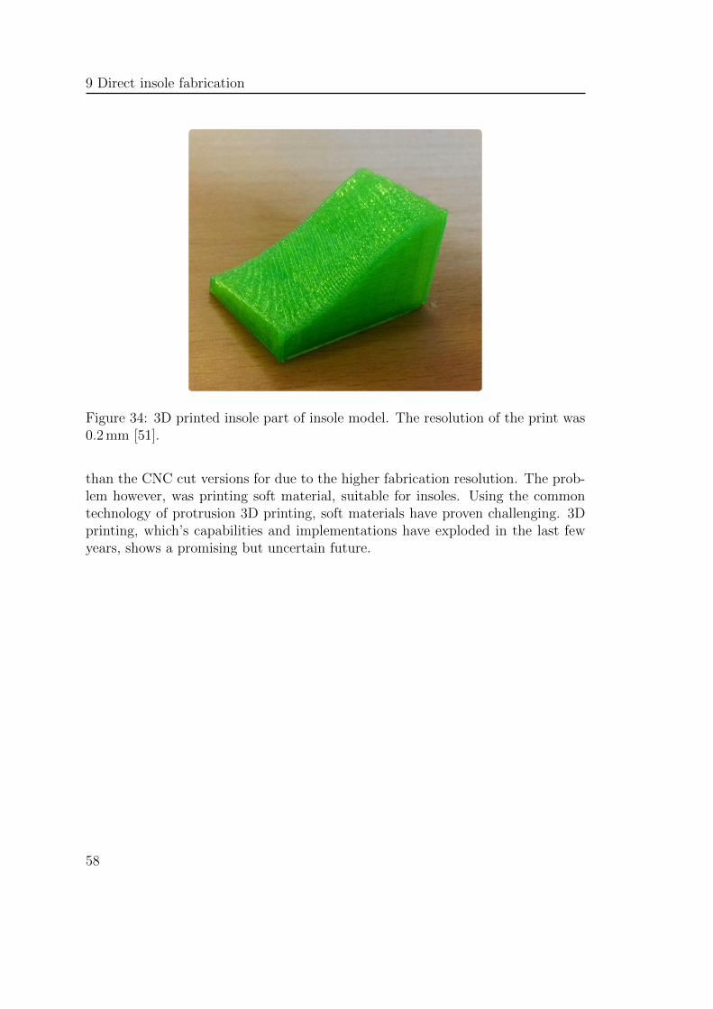
9 Direct insole fabrication
Figure 34: 3D printed insole part of insole model. The resolution of the print was0.2 mm [51].
than the CNC cut versions for due to the higher fabrication resolution. The prob-lem however, was printing soft material, suitable for insoles. Using the commontechnology of protrusion 3D printing, soft materials have proven challenging. 3Dprinting, which’s capabilities and implementations have exploded in the last fewyears, shows a promising but uncertain future.
58
10 Summary and conclusion
10 Summary and conclusion
This chapter reviews the work conducted throughout the project. It also discussesthe key results and findings, and propose suggestions for future work.
10.1 Thesis summary
Chapter 1: The chapter gave an introduction to limb associated pain andcustom insoles as a treatment. The primary aim of this thesis was to:
”Develop, implement and evaluate a system for insole modeling usinglow cost 3D scanners, foot mesh modeling and computer assisted insoledesign”
Chapter 2: The chapter discussed the current market situation and relative workof other research related to insole modeling and fabrication.Chapter 3: The chapter discussed some theory used in the project for creat-ing surfaces from point clouds, registration of 3D data sets and approximatingscattered data to a rectangular mesh grid.Chapter 4: The chapter introduced the Kinect sensor with imaging techniques,limitations and associated software.Chapter 5: The chapter evaluated the Kinect with regard to distortions, resolu-tion, accuracy, and RGB-D alignment.Chapter 6: The chapter discussed the proposed system for insole modeling. Scan-ning of the foot with three Kinect sensors was used for foot modeling. Design ofthe insole model was done through implemented software.Chapter 7: The chapter discussed remarks of the proposed system from Chap-ter 6.Chapter 8: The chapter evaluated the proposed system by conducted a casestudy. A quantitative comparison was made using existing products available onthe market.Chapter 9: The chapter described insole fabrication testing, using a CNC cutterand 3D printer.
10.2 Key results
The Kinect evaluation have in summary concluded that the sensor is sufficientfor the task of foot scanning with appropriate data processing. Using this device,available at a low cost, accurate foot modeling using multi-view captures was done.
Furthermore the design interface enabled simple design of a basic insole froma foot model, with the use of tools for orientation and modification.
59
10.3 Limitations
The case study provided a quantitative comparison between the proposed sys-tem and existing methods which indicated that the proposed system could achievesimilar results as existing methods on the market today.
The proposed system, being low priced, provided a comparable foot modelingsystem compared to other systems on the market.
10.3 Limitations
Using the factory calibration for the RGB-D alignment, even though it was man-ually verified and corrected, degraded the results. If a proper stereo calibrationwould have been made between the Kinect RGB and IR camera, it could haveimproved the results. This would also solve the limitation of whole mm valuesdelivered from libfreenect’s alignment.
Regarding the case study, the project were not able to compare the proposedsystem to a fully computer assisted system.
Not having a higher precision scanner regarding the comparison in Chapter 8degraded the results as the scan regarding the Ortolab mold was very coarse. Also,any artifacts produced by the Kinect affected the existing company models.
10.4 Future work
Considering the system proposed, there are improvements to be made as well asnew suggestions. There are other low cost 3D sensors today that has a minimumscanning distance of about 350–400 mm such as the Kinect for Windows withSDK [39] and Primesense 1.09 sensor [52]. By scanning at nearer distances, higherresolution can be achieved.
An evaluation of the system with two feet at the same time should be per-formed. It might be necessary with a more extensive reference system. However,capturing two feet at once is something that is not available on the market andcould provide correlated information between the feet and increase the efficiencyof patient scanning.
Interfering laser emitters were a problem with multiple Kinect captures. Usingsoftware to control the emitters or other solutions, is crucial if true simultaneousdata capture is to be made, which would yield the best results with foot capturein a sub second interval.
The fabrication process today is likely to be done by a CNC cutter. In the futurehowever, 3D printing could be an alternative. Given soft, functional 3D printingmaterial, it would be possible to print the insole model with high accuracy.
60

10.4 Future work
10.4.1 Future design tools
The design interface described in Chapter 6.3 could be further developed. Extend-ing the design interface with additional tools, required by an orthopedist, the insoledesign could be greatly improved. Personal communication with FotAnatomi [10]has suggested some future improvements to the developed insole design software:
• A more intuitive tool for pelott design; While the mouse and neighborhoodfunction provides functional local modification, it is at this moment some-what non-intuitive. Controlling the modification with reliable accuracy iscrucial for proper and efficient design. Attempts should be made with e.gtouch screen modification, an improved mouse interface or something radi-cally new.
• The ability to mark areas of interest while scanning, giving the orthopedistthe ability to mark a location for pelott or a location where other compensa-tion is needed. These markings should then be visible in the computer modelof the foot.
61

62
REFERENCES
References
[1] Dreinhofer, K.E., Reichel, H., Kafer, W. (2007) Lower limb pain. Best Practice& Research, vol. 21, no 1, pp. 135-152.
[2] Dunn, J.E., Link, C.L., Felson, D.T., Grincoli, M.G., Keysor, J.J., McKinlay,J.B. (2004) Prevalence of Foot and Ankle Conditions in a Multiethnic Com-munity Sample of Older Adults. American Journal of Epidemiology, vol. 159,issue 5, pp. 491-498.
[3] Hill, C.L., Gill, T., Menz, H.B., Taylor, A.W. (2008) Prevalence and correlatesof foot pain in a population-based study: the North West Adelaide HealthStudy. Journal of Foot and Ankle Research, vol. 1, pp. 2.
[4] Landorf, K.B., Keenan, A.M., Herbert, R.D. (2006) Effectiveness of FootOrthoses to Treat Plantar Fasciitis. American Medical Association, vol. 166,no 2006, pp. 1305-1310.
[5] International Standards Organization Document ISO 8549-1:1989.
[6] Kogler, G.F., Solomonidis, S.E., Paul, J.P. (1995) In vitro method for quan-tifying the effectiveness of the longitudinal arch support mechanism of a footorthosis. Clinical Biomechanics, vol. 10, no 5, pp. 245-252, ISSN 0268-0033,10.1016/0268-0033(95)99802-9.
[7] Kato, H., Takada, T., Kawamura, T., Hotta, N., Torii, S. (1996) The reductionand redistribution of plantar pressures using foot orthoses in diabetic patients.Diabetes Research and Clinical Practice, vol. 31, no 1-3, pp. 115-118, ISSN0168-8227, 10.1016/0168-8227(96)01214-4.
[8] Kogler, GF., et al. (1995) Biomechanics of longitudinal arch support mecha-nisms in foot orthoses and their effect on plantar aponeurisis strain. ClinicalBiomechanics, vol. 11, no 5, pp. 243-252.
[9] Stell, J.F., Buckley, J.G. Controlling excessive pronation: a comparison ofcasted and non-casted orthoses (1998), The Foot, vol. 8, no 4, pp. 210-214,ISSN 0958-2592, 10.1016/S0958-2592(98)90031-1.
[10] Silva Oliviera, F.M.d., personal communication.
[11] Image: Pronation. Orthopedia Wiki. http://orthopedia.wikia.com/wiki/Pronation. (2013-05-09).
[12] Pratt, D.J., Sanner, W.H., (1996) Paediatric foot orthoses. The Foot, vol. 6,pp. 99-111.
63

REFERENCES
[13] Huppin, L. (2009) Technology: Choosing a digital foot scanner. Lower Ex-tremity Review. http://lowerextremityreview.com/article/technology-choosing-a-digital-foot-scanner. (2013-03-06).
[14] Ortolab. http://ortolab.se. (2013-03-05).
[15] Personligt utformade fotbaddar. Lifecenter. http://www.lifecenter.nu/forforetag/personligt-utformade-fotbaddar. (2013-05-09).
[16] VeriScan, Podiatric Scanner. (2008) EnvisicVPS. http://www.envisicvps.com. (2013-03-06).
[17] Jorgen Wiklander (VD, Ortolab AB) interviewed by the authors the 26 Febru-ary 2013.
[18] Prockl, E. (2006) Pa god fot med lasern. NyTeknik. http://www.nyteknik.se/nyheter/bioteknik_lakemedel/medicin_teknik/article40220.ece.(2013-05-09).
[19] Pratt, D. J. (1995) Functional foot orthoses. The Foot, vol. 5, pp. 101-110.
[20] Delcam. http://delcam.com/. (2013-05-28).
[21] Custom Orthotic Insoles. DelCam Healthcare Solutions. http://www.orthotics-cadcam.com/orthotics-solution/index.asp. (2013-03-04).
[22] Anders Brask (Sales, CAD/CAM Protech) interviewed by the authors 2013-02-15.
[23] iQube. Custom Orthotic Insoles. http://lz.orthotics-cadcam.com/en/iqube.html. (2013-03-04).
[24] Design with OrthoModel. Custom Orthotic Insoles. http://lz.orthotics-cadcam.com/en/orthomodel.html. (2013-03-04).
[25] Make with OrthoMill. Custom Orthotic Insoles. http://lz.orthotics-cadcam.com/en/orthomill.html. (2013-03-0).
[26] Cast Medical, Health for life. Cast Medical. http://www.castmedical.se/Hem/tabid/71/Default.aspx. (2013-03-04).
[27] Sathish K.P., Sudesh, S., Lazar, M. (2012) Customized Foot Orthosis Devel-opment by 3D Reconstruction of the CT Images. Scientific Research, no 4,pp. 692-695.
64
REFERENCES
[28] Mavroidis, C., Ranky, R.G, Sivak, M.L., et al. (2011) Patient specific ankle-foot orthoses using rapid prototyping. Journal of NeuroEngineering and Re-habilitation, vol 8, no 1.
[29] Campbell R.J., Flynn P.J. (2001) A survey of free-form object representationand recognition techniques- Computer Vision and Image Understanding, vol81, pp 166-210.
[30] de Berg, M., Cheong, O., van Kreveld, M., Overmars, M. (2008) DelaunayTriangulations | Computational Geometry , pp 191-218. Berlin:Springer BerlinHeidelberg.
[31] Image: Delaunay triangulation. Wikipeida. http://en.wikipedia.org/wiki/Delaunay_triangulation (2013-06-15)
[32] Horn, B. K. P. (1986) Closed-form solution of absolute orientation using unitquaternions. Journal of the Optical Society of America A, vol. 4, pp. 629.
[33] Mukundan, R. (2012) Quaternions | Advanced Methods in Computer Graphicspp:77 -112. Springer.
[34] Lepetit, V., Fua, P. (2005) Mathematical Tools. | Monocular Model-Based3D Tracking of Rigid Objects: A Survey. Now Publishers Inc, 2005. pp. 12.(Foundations and Trends in Computer Graphics and Vision Series).
[35] Khoshelham, K., Elberink, S.O. (2012) Accuracy and resolution of Kinectdepth data for indoor mapping applications, Sensors (2012).
[36] OpenKinect. (2012) OpenKinect. http://openkinect.org. (2013-03-06).
[37] OpenNI, The standard framework for 3D sensing. OpenNI. http://openni.org. (2013-03-05).
[38] Image: Kinect. Wikipedia. http://en.wikipedia.org/wiki/Kinect. (2013-05-13).
[39] Kinect for Windows Sensor Components and Specifications. Microsoft De-veloper Network. http://msdn.microsoft.com/en-us/library/jj131033.aspx. (2013-03-06).
[40] Andersen, M.R., Jensen, T., Lisouski, P., Mortensen, A.K., Hansen, M.K.,Gregersen, T., Ahrendt, P. (2012). Kinect Depth Sensor Evaluation for Com-puter Vision Applications. Department of Engineering, Aarhus University.Denmark. Technical report ECE-TR-6.
65

REFERENCES
[41] Nicholas Burrus (2011), Kinect Calibration, http://burrus.name/index.php/Research/KinectCalibration. (2013-05-14).
[42] Bouguet, JY. (2010) Camera Calibration Toolbox for Matlab. http://www.vision.caltech.edu/bouguetj/calib_doc/index.html. (2013-04-18).
[43] MathWorks. http://www.mathworks.se/. (2013-06-16)
[44] Kinect to Matlab on OSX and linux via mex, Adam berg, http://acberg.com/kinect/. (2013-05-13).
[45] Herrera, D.C., Kannala, J., Heikkila, J. (2012) Joint Depth and Color Cam-era Calibration with Distortion Correction. IEEE Transactions on patternanalysis and machine intelligence, vol. 34, nr 10, pp. 2058-2064.
[46] Smisek, J., Jancosek, M., Pajdla, T. (2011) ”3D with Kinect”. Proc. IEEEInt’l Conf. Computer Vision Workshops.
[47] Cailliau, R. Lego dimensions, the measurements. RobertCailliau. http://www.robertcailliau.eu/Lego/Dimensions/zMeasurements-en.xhtml. (2013-04-03).
[48] Wengert, C., Bianchi, G. (2010) Absolute Orientation. Matlab Central,File Exchange. http://www.mathworks.com/matlabcentral/fileexchange/22422-absolute-orientation. (2013-02-02).
[49] Stroud, I, Xirouchakis, P.C. (2000) STL and extensions | Advances in Engi-neering Software Volume 31, Issue 2, February 2000, Pages 83–95. (2013-05-30).
[50] 3D cutter, Portal type, built by Hakan Thoren.
[51] 3D printer: Makerboot 2. https://store.makerbot.com/replicator2.html.(2013-05-14).
[52] Primesense. http://www.primesense.com/. (2013-05-17).
[53] Heikkila, J., Silven, O., (1997) A four-step camera calibration procedure withimplicit image correction. | Computer Vision and Pattern Recognition; 17-19Jun 1997, San Juan, pp. 1106 - 1112.
66
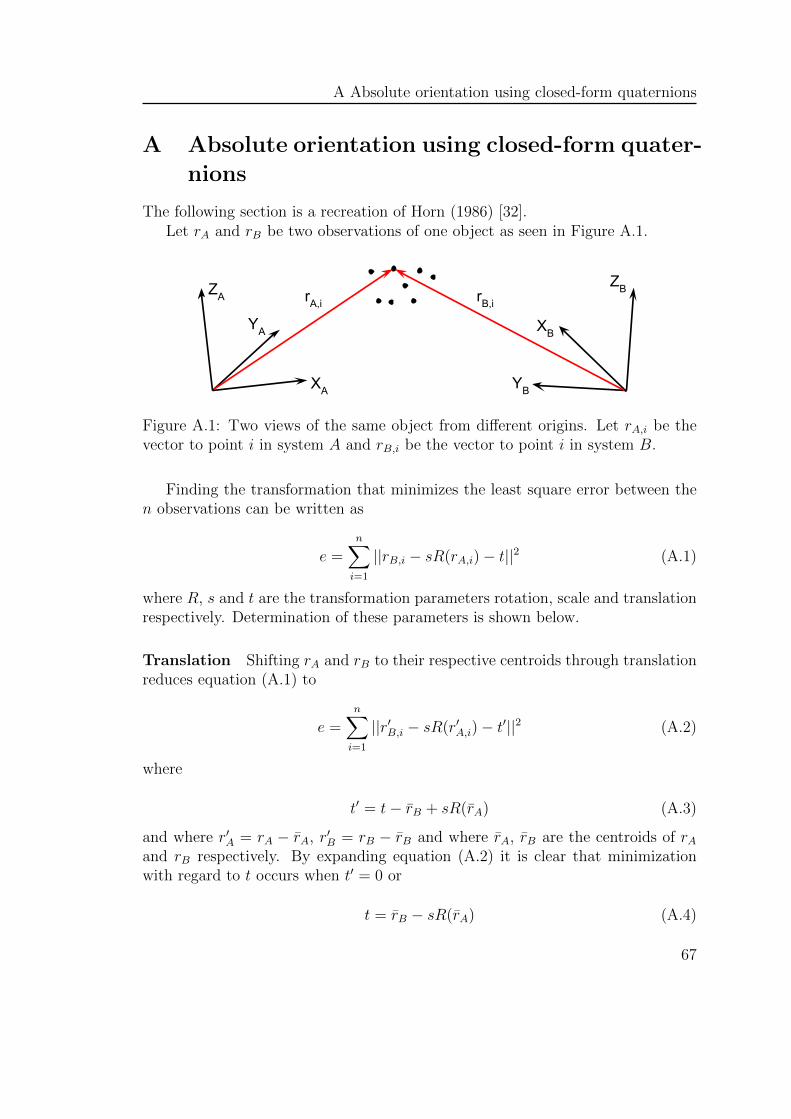
A Absolute orientation using closed-form quaternions
A Absolute orientation using closed-form quater-
nions
The following section is a recreation of Horn (1986) [32].Let rA and rB be two observations of one object as seen in Figure A.1.
XB
YB
ZA
YA
XA
ZBrA,i rB,i
Figure A.1: Two views of the same object from different origins. Let rA,i be thevector to point i in system A and rB,i be the vector to point i in system B.
Finding the transformation that minimizes the least square error between then observations can be written as
e =n∑
i=1
||rB,i − sR(rA,i)− t||2 (A.1)
where R, s and t are the transformation parameters rotation, scale and translationrespectively. Determination of these parameters is shown below.
Translation Shifting rA and rB to their respective centroids through translationreduces equation (A.1) to
e =n∑
i=1
||r′B,i − sR(r′A,i)− t′||2 (A.2)
where
t′ = t− rB + sR(rA) (A.3)
and where r′A = rA − rA, r′B = rB − rB and where rA, rB are the centroids of rAand rB respectively. By expanding equation (A.2) it is clear that minimizationwith regard to t occurs when t′ = 0 or
t = rB − sR(rA) (A.4)
67
A Absolute orientation using closed-form quaternions
determining the optimal translation as the vector between rB and the scaled androtated rA.
Scale Expanding equation (A.2) and using the orthonormality of matrix R theexpression can be rewritten as
SB − 2sD + s2SA (A.5)
where Sa and Sb are the sums of squares of the respective sets and D is the sumof the dot product between set rB and the rotated set rA. Completing the squarein s and writing the expression for the error, it can be found that the scale factorthat minimizes the error in equation (A.5) is determined by
s =
n∑i=1
r′B,iR(r′A,i)
n∑i=1
||r′A,i||2(A.6)
Rotation Translation and scale are determined by the rotation. It can be foundthat further minimization of equation (A.5) with regard to R is achieved by max-imizing
D =n∑
i=1
r′B,iR(r′A,i) (A.7)
Equation (A.7) can be written with quaternion notation as
D =n∑
i=1
(qr′A,i) · (r′B,iq) (A.8)
where q is a unit quaternion representing rotation and r′A,i, r′B,i are quaternion
representations of the sets r′A,i, r′B,i respectively.
Equation (A.8) can then be written as
D = qT
(n∑
i=1
Ni
)q (A.9)
It is shown in Horn (1986) [32] that the quaternion q maximizing
qTNq (A.10)
is the the eigenvector corresponding to the largest eigenvalue of N .
68

A Absolute orientation using closed-form quaternions
The final rotation is then found by retrieving the lower right 3× 3 sub matrixof the 4× 4 rotation matrix
qT q (A.11)
69
B Kinect RGB camera model and calibration
B Kinect RGB camera model and calibration
The following camera model description is a recreation from Bouquet (2010) [42],which in turn is based on the report by Heikkila (1997) [53].
Given a point P in space with coordinates (Xc, Yc, Zc), let the normalized imageprojection xn equal
xn =
[Xc/Zc
Yc/Zc
]=
[xy
](B.1)
Let
r2 = x2 + y2 (B.2)
By including lens distortion δ, the normalized point coordinate xd is defined by
xd =
[xd(1)xd(2)
]= (1 + δ(1)r2 + δ(2)r4 + δ(5)r6)xn + dx (B.3)
where dx is the tangential distortion vector, defined as
dx =
[2δ(3)xy + δ(4)(r2 + 2x2)δ(3)(r2 + 2y2) + 2δ(4)xy
](B.4)
where fc is the focal length, α is the skew coefficient and cp is the principal pointoffset. The complete camera model is thereforexpyp
1
=
fc(1) αfc(1) cp(1)0 fc(2) cp(2)0 0 1
xd(1)xd(2)
1
(B.5)
where xp, yp is the projection of point P on the image plane.
70
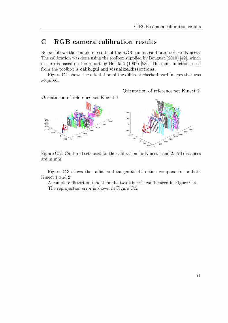
C RGB camera calibration results
C RGB camera calibration results
Below follows the complete results of the RGB camera calibration of two Kinects.The calibration was done using the toolbox supplied by Bouguet (2010) [42], whichin turn is based on the report by Heikkila (1997) [53]. The main functions usedfrom the toolbox is calib gui and visualize distortions.
Figure C.2 shows the orientation of the different checkerboard images that wasacquired.
−2000
−1000
0
10000
1000
2000
3000
4000
5000
6000
−600
−400
−200
0
200
2726
31
2319
30
18
32
422
21
14
3
516
Orientation of reference set Kinect 1
6
13
21
10
25
1112
7
33
9
351734
−1000
−500
0
500
1000 0
500
1000
1500
2000
2500
3000
3500−500
0
500
1000
17
71
12
141615
13
218
6
11
5
9
27
Orientation of reference set Kinect 2
18
204
1019
28
3
23
2
25
26
2224
Figure C.2: Captured sets used for the calibration for Kinect 1 and 2. All distancesare in mm.
Figure C.3 shows the radial and tangential distortion components for bothKinect 1 and 2.
A complete distortion model for the two Kinect’s can be seen in Figure C.4.The reprojection error is shown in Figure C.5.
71
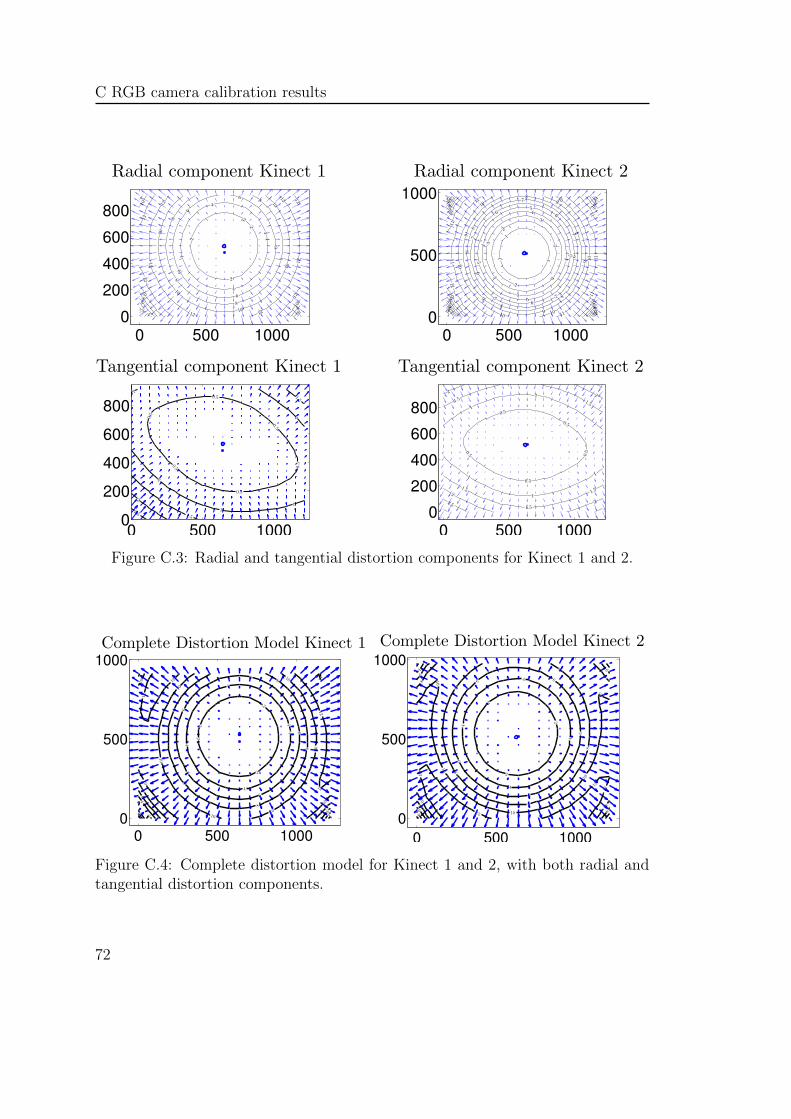
C RGB camera calibration results
0 500 1000
0
200
400
600
8002
2
2
2
44
4
4
4
4
4
6
6
6
6
6
6
6
8
8
8
8
8
8
8
10
10
10
10
10
10
10
10
12
12
12
12
12
12
12
12
12
12
Radial component Kinect 1
0 500 1000
0
500
1000
1
1
1
2
22
3
3
3
3
3
4
4
4
4
4
4
5
5
55
5
5
5
5
6
6
6
66
6
6
6
7
7
7
7
7 7
7
7
7
8
8
8
8
8
8
8
8
8
8
9
9
9
9
9
9
9
9
9
10
10
10
10
10 10
10
10
10
10
11
11
11
11
11
11
11
11
Radial component Kinect 2
0 500 10000
200
400
600
800
0.5
0.5
0.5
0.5
0.5
0.5
1
1
1
11
1.5
1.5
2
2.5
Tangential component Kinect 1
0 500 1000
0
200
400
600
8000.5
0.5
0.5
0.5
0.5
1
1
1
1
1
1
1.5 1.5
1.5
1.5
1.5
2
2
2
2
2.5
Tangential component Kinect 2
Figure C.3: Radial and tangential distortion components for Kinect 1 and 2.
0 500 1000
0
500
1000
Complete Distortion Model Kinect 1
2
2
2
2
2
44
4
4
4
4
4
4
66
6
6
6
6
6
6
8
8
8
8
8
8
8
10
10
10
10
1010
10
10
10
12
12
12
12
14
0 500 1000
0
500
1000
Complete Distortion Model Kinect 2
2
2
2
4
4
4
4
4
4
6
6
6
66
6
6
6
8
8
8
8
8
8
8
8
8
10
10
10
10
10
10
10
12
12
12
12
Figure C.4: Complete distortion model for Kinect 1 and 2, with both radial andtangential distortion components.
72
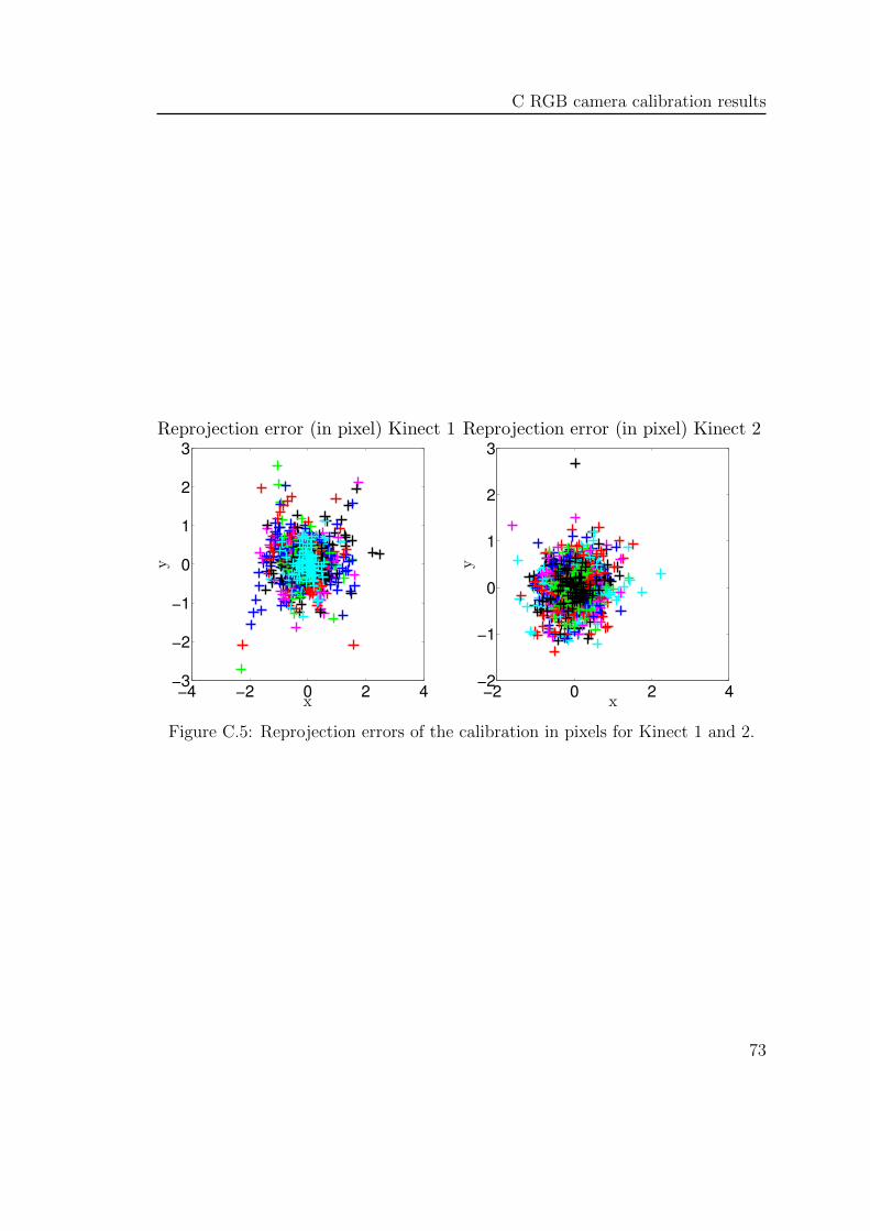
C RGB camera calibration results
−4 −2 0 2 4−3
−2
−1
0
1
2
3
Reprojection error (in pixel) Kinect 1
x
y
−2 0 2 4−2
−1
0
1
2
3
Reprojection error (in pixel) Kinect 2
x
y
Figure C.5: Reprojection errors of the calibration in pixels for Kinect 1 and 2.
73