Embed Size (px)
Citation preview
Inspection of Metals—Understanding the Basics Copyright © 2013 ASM International®
F.C. Campbell, editor All rights reservedwww.asminternational.org
INSPECTION OF METALS
UNDERSTANDINGTHE
BASICS
Editedby
F.C. Campbell
ASM International®Materials Park, Ohio 44073-0002
www.asminternational.org

Copyright © 2013 by
ASM International® All rights reserved
No part of this book may be reproduced, stored in a retrieval system, or transmitted, in any form or by any means, electronic, mechanical, photocopying, recording, or otherwise, without the written permission of the copyright owner.
First printing, April 2013
Great care is taken in the compilation and production of this book, but it should be made clear that NO WARRANTIES, EXPRESS OR IMPLIED, INCLUDING, WITHOUT LIMITATION, WARRANTIES OF MERCHANTABILITY OR FITNESS FOR A PARTICULAR PURPOSE, ARE GIVEN IN CONNECTION WITH THIS PUBLICATION. Although this information is believed to be accurate by ASM, ASM cannot guarantee that favorable results will be obtained from the use of this publication alone. This publication is intended for use by persons having technical skill, at their sole discretion and risk. Since the conditions of product or material use are outside of ASM’s control, ASM assumes no liability or obligation in connection with any use of this information. No claim of any kind, whether as to products or information in this publication, and whether or not based on negligence, shall be greater in amount than the purchase price of this product or publication in respect of which damages are claimed. THE REMEDY HEREBY PROVIDED SHALL BE THE EXCLUSIVE AND SOLE REMEDY OF BUYER, AND IN NO EVENT SHALL EITHER PARTY BE LIABLE FOR SPECIAL, INDIRECT OR CONSEQUENTIAL DAMAGES WHETHER OR NOT CAUSED BY OR RESULTING FROM THE NEGLIGENCE OF SUCH PARTY. As with any material, evaluation of the material under end-use conditions prior to specification is essential. Therefore, specific testing under actual conditions is recommended.
Nothing contained in this book shall be construed as a grant of any right of manufacture, sale, use, or reproduction, in connection with any method, process, apparatus, product, composition, or system, whether or not covered by letters patent, copyright, or trademark, and nothing contained in this book shall be construed as a defense against any alleged infringement of letters patent, copyright, or trademark, or as a defense against liability for such infringement.
Comments, criticisms, and suggestions are invited, and should be forwarded to ASM International.
Prepared under the direction of the ASM International Technical Book Committee (2012–2013), Bradley J. Diak, Chair.
ASM International staff who worked on this project include Scott Henry, Senior Manager, Content Development and Publishing; Karen Marken, Senior Managing Editor; Victoria Burt, Content Developer; Steve Lampman, Content Developer; Sue Sellers, Editorial Assistant; Bonnie Sanders, Manager of Production; Madrid Tramble, Senior Production Coordinator; and Diane Whitelaw, Production Coordinator.
Library of Congress Control Number: 2012955193ISBN-13: 978-1-62708-000-2
ISBN-10: 0-62708-000-7SAN: 204-7586
ASM International® Materials Park, OH 44073-0002
www.asminternational.org
Printed in the United States of America
vii
Inspection of Metals—Understanding the Basics Copyright © 2013 ASM International®
F.C. Campbell, editor All rights reservedwww.asminternational.org
Preface
Inspection of metals is used to ensure that the quality of the part or prod-uct meets minimum quality and safety requirements. There are hundreds of methods used to inspect metals during its fabrication (in-process in-spection), when the part is completed and ready for delivery (final inspec-tion), and during its service life (in-service inspection). While the three stages of inspection are addressed to some extent in this book, the empha-sis is on final part inspection. Because it is not possible to address all the different inspection methods used in the industry, only the most widely used inspection methods are covered.
The first half of this book attempts to answer three questions for each of these inspection methods:
• How is the inspection method performed?• When is it used?• How does it compare with other inspection methods?
The inspection methods covered are:
• Visual inspection• Coordinate measuring machines• Machine vision • Hardness testing• Tensile testing• Chemical composition• Metallography• Liquid penetrant, magnetic particle, and eddy current inspection• Radiographic inspection• Ultrasonic inspection
The second half of the book covers how these inspection methods are used in different metal fabrication industries:

viii / Preface
• Castings• Steel bar and wire• Tubular products• Forgings• Powder metallurgy parts• Weldments and brazed assemblies
The emphasis in the second half of the book shows why certain inspec-tion methods are selected for different product forms.
Since the purpose of this book is to cover the basics of inspection of metals, the reader is referred to more advanced texts for detailed informa-tion. In particular, for nondestructive test methods, Nondestructive Evalu-ation and Quality Control, Volume 17, ASM Handbook, for mechanical property test methods, Mechanical Testing and Evaluation, Volume 8, ASM Handbook, and for metallography, Metallography and Microstruc-tures, Volume 9, ASM Handbook.
I would like to acknowledge the help and guidance of Karen Marken, ASM International, and the staff at ASM for their valuable contributions.
F.C. Campbell
Inspection of Metals—Understanding the Basics Copyright © 2013 ASM International®
F.C. Campbell, editor All rights reservedwww.asminternational.org
Contents
Preface � � � � � � � � � � � � � � � � � � � � � � � � � � � � � � � � � � � � � � � � � � � � �vii
CHAPTER 1Inspection Methods—Overview and Comparison� � � � � � � � � � � � � 1
Visual Inspection . . . . . . . . . . . . . . . . . . . . . . . . . . . . . . . . . . . . . . . . . 1Coordinate Measuring Machines . . . . . . . . . . . . . . . . . . . . . . . . . . . . . 2Machine Vision . . . . . . . . . . . . . . . . . . . . . . . . . . . . . . . . . . . . . . . . . . 3Hardness Testing . . . . . . . . . . . . . . . . . . . . . . . . . . . . . . . . . . . . . . . . . 5Tensile Testing . . . . . . . . . . . . . . . . . . . . . . . . . . . . . . . . . . . . . . . . . . . 7Chemical Analysis . . . . . . . . . . . . . . . . . . . . . . . . . . . . . . . . . . . . . . . . 9Metallography . . . . . . . . . . . . . . . . . . . . . . . . . . . . . . . . . . . . . . . . . . . 9Nondestructive Testing . . . . . . . . . . . . . . . . . . . . . . . . . . . . . . . . . . . .11
CHAPTER 2Visual Inspection� � � � � � � � � � � � � � � � � � � � � � � � � � � � � � � � � � � � � 21
Visual Inspection Procedure . . . . . . . . . . . . . . . . . . . . . . . . . . . . . . . 21Visual Inspection Tools . . . . . . . . . . . . . . . . . . . . . . . . . . . . . . . . . . . 27
CHAPTER 3Coordinate Measuring Machines� � � � � � � � � � � � � � � � � � � � � � � � � 49
CMM Operating Principles . . . . . . . . . . . . . . . . . . . . . . . . . . . . . . . . 50Types of CMMs . . . . . . . . . . . . . . . . . . . . . . . . . . . . . . . . . . . . . . . . . 54
CHAPTER 4Machine Vision � � � � � � � � � � � � � � � � � � � � � � � � � � � � � � � � � � � � � � 63
Machine Vision Process . . . . . . . . . . . . . . . . . . . . . . . . . . . . . . . . . . . 66Machine Vision Applications . . . . . . . . . . . . . . . . . . . . . . . . . . . . . . . 82

iv / Contents
CHAPTER 5Hardness Testing � � � � � � � � � � � � � � � � � � � � � � � � � � � � � � � � � � � � � 85
Brinell Hardness Testing . . . . . . . . . . . . . . . . . . . . . . . . . . . . . . . . . . 85Rockwell Hardness Testing . . . . . . . . . . . . . . . . . . . . . . . . . . . . . . . . 91Vickers Hardness Testing (ASTM E384). . . . . . . . . . . . . . . . . . . . . 100Scleroscope Hardness Testing . . . . . . . . . . . . . . . . . . . . . . . . . . . . . 102Microhardness Testing . . . . . . . . . . . . . . . . . . . . . . . . . . . . . . . . . . . 106
CHAPTER 6Tensile Testing � � � � � � � � � � � � � � � � � � � � � � � � � � � � � � � � � � � � � � 117
Stress-Strain Behavior . . . . . . . . . . . . . . . . . . . . . . . . . . . . . . . . . . . .117Properties from Test Results . . . . . . . . . . . . . . . . . . . . . . . . . . . . . . .118Testing Machines . . . . . . . . . . . . . . . . . . . . . . . . . . . . . . . . . . . . . . . 124General Procedures . . . . . . . . . . . . . . . . . . . . . . . . . . . . . . . . . . . . . 129
CHAPTER 7Chemical Composition � � � � � � � � � � � � � � � � � � � � � � � � � � � � � � � 139
X-Ray Fluorescence Spectroscopy (XRF). . . . . . . . . . . . . . . . . . . . 139Optical Emission Spectroscopy (OES) . . . . . . . . . . . . . . . . . . . . . . 146Combustion and Inert Gas Fusion Analysis. . . . . . . . . . . . . . . . . . . 150Surface Analysis. . . . . . . . . . . . . . . . . . . . . . . . . . . . . . . . . . . . . . . . 152Scanning Auger Microprobe (SAM) . . . . . . . . . . . . . . . . . . . . . . . . 152Related Surface Analysis Techniques . . . . . . . . . . . . . . . . . . . . . . . 158
CHAPTER 8Metallography� � � � � � � � � � � � � � � � � � � � � � � � � � � � � � � � � � � � � � 161
Sectioning . . . . . . . . . . . . . . . . . . . . . . . . . . . . . . . . . . . . . . . . . . . . 162Mounting of Specimens . . . . . . . . . . . . . . . . . . . . . . . . . . . . . . . . . . 162Grinding . . . . . . . . . . . . . . . . . . . . . . . . . . . . . . . . . . . . . . . . . . . . . . 164Polishing . . . . . . . . . . . . . . . . . . . . . . . . . . . . . . . . . . . . . . . . . . . . . 166Etching . . . . . . . . . . . . . . . . . . . . . . . . . . . . . . . . . . . . . . . . . . . . . . . 170Microscopic Examination . . . . . . . . . . . . . . . . . . . . . . . . . . . . . . . . 171Microphotography . . . . . . . . . . . . . . . . . . . . . . . . . . . . . . . . . . . . . . 180Grain Size. . . . . . . . . . . . . . . . . . . . . . . . . . . . . . . . . . . . . . . . . . . . . 181
CHAPTER 9Liquid Penetrant, Magnetic Particle, and Eddy-Current
Inspection � � � � � � � � � � � � � � � � � � � � � � � � � � � � � � � � � � � � � 183
Liquid Penetrant Inspection . . . . . . . . . . . . . . . . . . . . . . . . . . . . . . . 183Magnetic Particle Inspection . . . . . . . . . . . . . . . . . . . . . . . . . . . . . . 197Eddy Current Inspection . . . . . . . . . . . . . . . . . . . . . . . . . . . . . . . . . 215

Contents / v
CHAPTER 10Radiographic Inspection � � � � � � � � � � � � � � � � � � � � � � � � � � � � � � 233
Uses of Radiography . . . . . . . . . . . . . . . . . . . . . . . . . . . . . . . . . . . . 234Principles of Radiography . . . . . . . . . . . . . . . . . . . . . . . . . . . . . . . . 236Sources of Radiation . . . . . . . . . . . . . . . . . . . . . . . . . . . . . . . . . . . . 237X-Ray Tubes . . . . . . . . . . . . . . . . . . . . . . . . . . . . . . . . . . . . . . . . . . 239Attenuation of Electromagnetic Radiation. . . . . . . . . . . . . . . . . . . . 243Principles of Shadow Formation . . . . . . . . . . . . . . . . . . . . . . . . . . . 246Image Conversion . . . . . . . . . . . . . . . . . . . . . . . . . . . . . . . . . . . . . . 248Characteristics of X-Ray Film . . . . . . . . . . . . . . . . . . . . . . . . . . . . . 254Exposure Factors . . . . . . . . . . . . . . . . . . . . . . . . . . . . . . . . . . . . . . . 257Neutron Radiography. . . . . . . . . . . . . . . . . . . . . . . . . . . . . . . . . . . . 262
CHAPTER 11Ultrasonic Inspection � � � � � � � � � � � � � � � � � � � � � � � � � � � � � � � � 267
Ultrasonic Flaw Detectors . . . . . . . . . . . . . . . . . . . . . . . . . . . . . . . . 268Ultrasonic Transducers and Search Units . . . . . . . . . . . . . . . . . . . . 269Couplants . . . . . . . . . . . . . . . . . . . . . . . . . . . . . . . . . . . . . . . . . . . . . 271Basic Inspection Methods . . . . . . . . . . . . . . . . . . . . . . . . . . . . . . . . 272Pulse Echo Method . . . . . . . . . . . . . . . . . . . . . . . . . . . . . . . . . . . . . 273Transmission Methods . . . . . . . . . . . . . . . . . . . . . . . . . . . . . . . . . . . 280General Characteristics of Ultrasonic Waves. . . . . . . . . . . . . . . . . . 282Factors Influencing Ultrasonic Inspection . . . . . . . . . . . . . . . . . . . . 285Advantages, Disadvantages, and Applications . . . . . . . . . . . . . . . . 291
CHAPTER 12Inspection of Castings � � � � � � � � � � � � � � � � � � � � � � � � � � � � � � � � 293
Inspection Categories. . . . . . . . . . . . . . . . . . . . . . . . . . . . . . . . . . . . 293Casting Defects . . . . . . . . . . . . . . . . . . . . . . . . . . . . . . . . . . . . . . . . 294Common Inspection Procedures . . . . . . . . . . . . . . . . . . . . . . . . . . . 299Computer-Aided Dimensional Inspection . . . . . . . . . . . . . . . . . . . . 302Liquid Penetrant Inspection . . . . . . . . . . . . . . . . . . . . . . . . . . . . . . . 308Magnetic Particle Inspection . . . . . . . . . . . . . . . . . . . . . . . . . . . . . . 309Eddy Current Inspection . . . . . . . . . . . . . . . . . . . . . . . . . . . . . . . . . 310Radiographic Inspection . . . . . . . . . . . . . . . . . . . . . . . . . . . . . . . . . 310Ultrasonic Inspection . . . . . . . . . . . . . . . . . . . . . . . . . . . . . . . . . . . . 314Leak Testing. . . . . . . . . . . . . . . . . . . . . . . . . . . . . . . . . . . . . . . . . . . 318
CHAPTER 13Inspection of Steel Bar and Wire� � � � � � � � � � � � � � � � � � � � � � � � 321
Types of Flaws Encountered . . . . . . . . . . . . . . . . . . . . . . . . . . . . . . 321Methods Used for Inspection of Steel Bars . . . . . . . . . . . . . . . . . . . 324
vi / Contents
CHAPTER 14Inspection of Tubular Products � � � � � � � � � � � � � � � � � � � � � � � � � 345
Selection of Inspection Method . . . . . . . . . . . . . . . . . . . . . . . . . . . . 346Inspection of Resistance Welded Steel Tubing . . . . . . . . . . . . . . . . 347Seamless Steel Tubular Products . . . . . . . . . . . . . . . . . . . . . . . . . . . 356Nonferrous Tubing . . . . . . . . . . . . . . . . . . . . . . . . . . . . . . . . . . . . . . 362
CHAPTER 15Inspection of Forgings � � � � � � � � � � � � � � � � � � � � � � � � � � � � � � � � 365
Flaws Originating in the Ingot . . . . . . . . . . . . . . . . . . . . . . . . . . . . . 365Flaws Caused by the Forging Operation . . . . . . . . . . . . . . . . . . . . . 370Selection of Inspection Method . . . . . . . . . . . . . . . . . . . . . . . . . . . . 371Visual Inspection . . . . . . . . . . . . . . . . . . . . . . . . . . . . . . . . . . . . . . . 383Magnetic Particle Inspection . . . . . . . . . . . . . . . . . . . . . . . . . . . . . . 383Liquid Penetrant Inspection . . . . . . . . . . . . . . . . . . . . . . . . . . . . . . . 387Ultrasonic Inspection . . . . . . . . . . . . . . . . . . . . . . . . . . . . . . . . . . . . 389Radiographic Inspection . . . . . . . . . . . . . . . . . . . . . . . . . . . . . . . . . 391
CHAPTER 16Inspection of Powder Metallurgy Parts � � � � � � � � � � � � � � � � � � � 393
Dimensional Evaluation. . . . . . . . . . . . . . . . . . . . . . . . . . . . . . . . . . 393Density Measurement . . . . . . . . . . . . . . . . . . . . . . . . . . . . . . . . . . . 394Apparent Hardness and Microhardness . . . . . . . . . . . . . . . . . . . . . . 396Mechanical Testing/Tensile Testing . . . . . . . . . . . . . . . . . . . . . . . . . 397Powder Metallurgy Part Defects . . . . . . . . . . . . . . . . . . . . . . . . . . . 398Flaw Detection . . . . . . . . . . . . . . . . . . . . . . . . . . . . . . . . . . . . . . . . . 400
CHAPTER 17Inspection of Weldments and Brazed Assemblies � � � � � � � � � � � 411
Weldments . . . . . . . . . . . . . . . . . . . . . . . . . . . . . . . . . . . . . . . . . . . . .411Methods of Nondestructive Inspection . . . . . . . . . . . . . . . . . . . . . . 421Brazed Assemblies . . . . . . . . . . . . . . . . . . . . . . . . . . . . . . . . . . . . . . 437Methods of Inspection . . . . . . . . . . . . . . . . . . . . . . . . . . . . . . . . . . . 442
Index� � � � � � � � � � � � � � � � � � � � � � � � � � � � � � � � � � � � � � � � � � � � � 447
Inspection of Metals—Understanding the Basics Copyright © 2013 ASM International®
F.C. Campbell, editor All rights reservedwww.asminternational.org
CHAPTER 1
Inspection Methods—Overview and Comparison
INSPECTION is an organized examination or formal evaluation exer-cise. In engineering, inspection involves the measurements, tests, and gages applied to certain characteristics in regard to an object or activity. The results are usually compared to specified requirements and standards for determining whether the item or activity is in line with these targets. Some inspection methods are destructive; however, inspections are usu-ally nondestructive.
Nondestructive examination (NDE), or nondestructive testing (NDT), are a number of technologies used to analyze materials for either inherent flaws (such as fractures or cracks), or damage from use. Some common methods are visual, microscopy, liquid or dye penetrant inspection, mag-netic particle inspection, eddy current testing, x-ray or radiographic test-ing, and ultrasonic testing. This chapter provides an overview of the in-spection methods that will be covered in the remainder of this book.
Visual Inspection
Visual inspection provides a means of detecting and examining a vari-ety of surface flaws, such as corrosion, contamination, surface finish, and surface discontinuities on joints (for example, welds, seals, and solder connections). Visual inspection is also the most widely used method for detecting and examining surface cracks that are particularly important be-cause of their relationship to structural failure mechanisms. Even when other inspection techniques are used to detect surface cracks, visual in-spection often provides a useful supplement. For example, when the eddy
2 / Inspection of Metals—Understanding the Basics
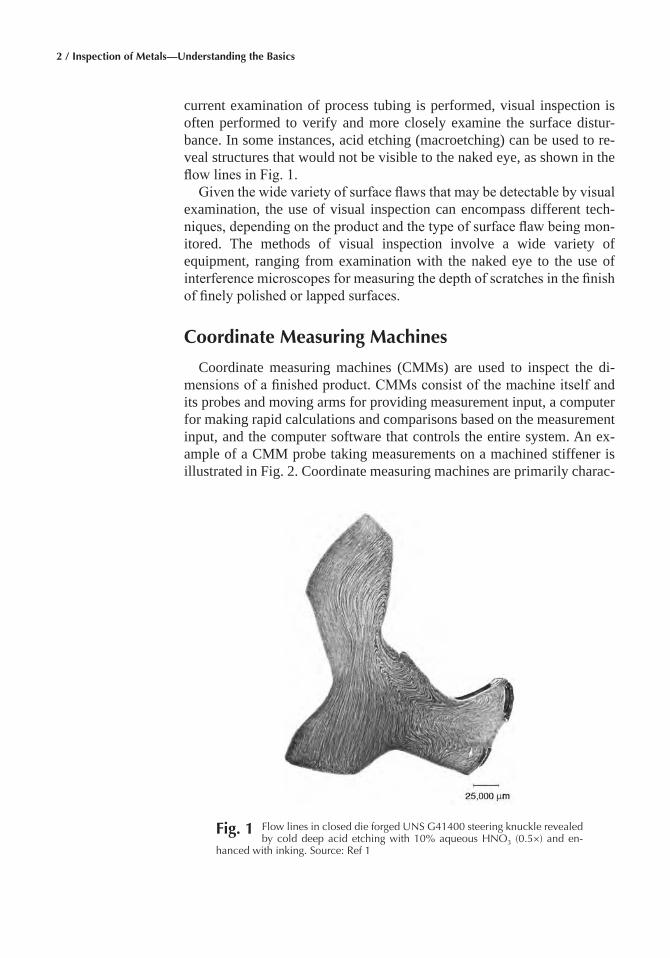
current examination of process tubing is performed, visual inspection is often performed to verify and more closely examine the surface distur-bance. In some instances, acid etching (macroetching) can be used to re-veal structures that would not be visible to the naked eye, as shown in the flow lines in Fig. 1.
Given the wide variety of surface flaws that may be detectable by visual examination, the use of visual inspection can encompass different tech-niques, depending on the product and the type of surface flaw being mon-itored. The methods of visual inspection involve a wide variety of equipment, ranging from examination with the naked eye to the use of interference microscopes for measuring the depth of scratches in the finish of finely polished or lapped surfaces.
Coordinate Measuring Machines
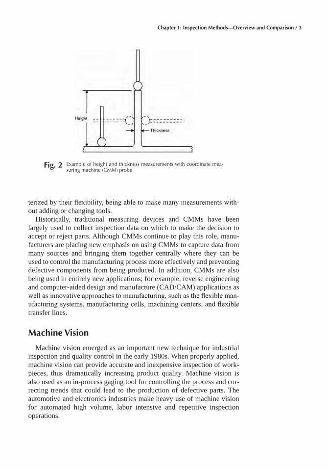
Coordinate measuring machines (CMMs) are used to inspect the di-mensions of a finished product. CMMs consist of the machine itself and its probes and moving arms for providing measurement input, a computer for making rapid calculations and comparisons based on the measurement input, and the computer software that controls the entire system. An ex-ample of a CMM probe taking measurements on a machined stiffener is illustrated in Fig. 2. Coordinate measuring machines are primarily charac-
Fig� 1 Flow lines in closed die forged UNS G41400 steering knuckle revealed by cold deep acid etching with 10% aqueous HNO3 (0.5×) and en-
hanced with inking. Source: Ref 1
Chapter 1: Inspection Methods—Overview and Comparison / 3
terized by their flexibility, being able to make many measurements with-out adding or changing tools.
Historically, traditional measuring devices and CMMs have been largely used to collect inspection data on which to make the decision to accept or reject parts. Although CMMs continue to play this role, manu-facturers are placing new emphasis on using CMMs to capture data from many sources and bringing them together centrally where they can be used to control the manufacturing process more effectively and preventing defective components from being produced. In addition, CMMs are also being used in entirely new applications; for example, reverse engineering and computer-aided design and manufacture (CAD/CAM) applications as well as innovative approaches to manufacturing, such as the flexible man-ufacturing systems, manufacturing cells, machining centers, and flexible transfer lines.
Machine Vision
Machine vision emerged as an important new technique for industrial inspection and quality control in the early 1980s. When properly applied, machine vision can provide accurate and inexpensive inspection of work-pieces, thus dramatically increasing product quality. Machine vision is also used as an in-process gaging tool for controlling the process and cor-recting trends that could lead to the production of defective parts. The auto motive and electronics industries make heavy use of machine vision for automated high volume, labor intensive and repetitive inspection operations.
Fig� 2 Example of height and thickness measurements with coordinate mea-suring machine (CMM) probe
4 / Inspection of Metals—Understanding the Basics
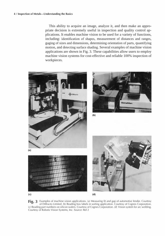
This ability to acquire an image, analyze it, and then make an appro-priate decision is extremely useful in inspection and quality control ap-plications. It enables machine vision to be used for a variety of functions, including: identification of shapes, measurement of distances and ranges, gaging of sizes and dimensions, determining orientation of parts, quantifying motion, and detecting surface shading. Several examples of machine vision applications are shown in Fig. 3. These capabilities allow users to employ machine vision systems for cost-effective and reliable 100% inspection of workpieces.
Fig� 3 Examples of machine vision applications. (a) Measuring fit and gap of automotive fender. Courtesy of Diffracto Limited. (b) Reading box labels in sorting application. Courtesy of Cognex Corporation.
(c) Reading part numbers on silicon wafers. Courtesy of Cognex Corporation. (d) Vision system for arc welding. Courtesy of Robotic Vision Systems, Inc. Source: Ref 2
Chapter 1: Inspection Methods—Overview and Comparison / 5
Hardness Testing
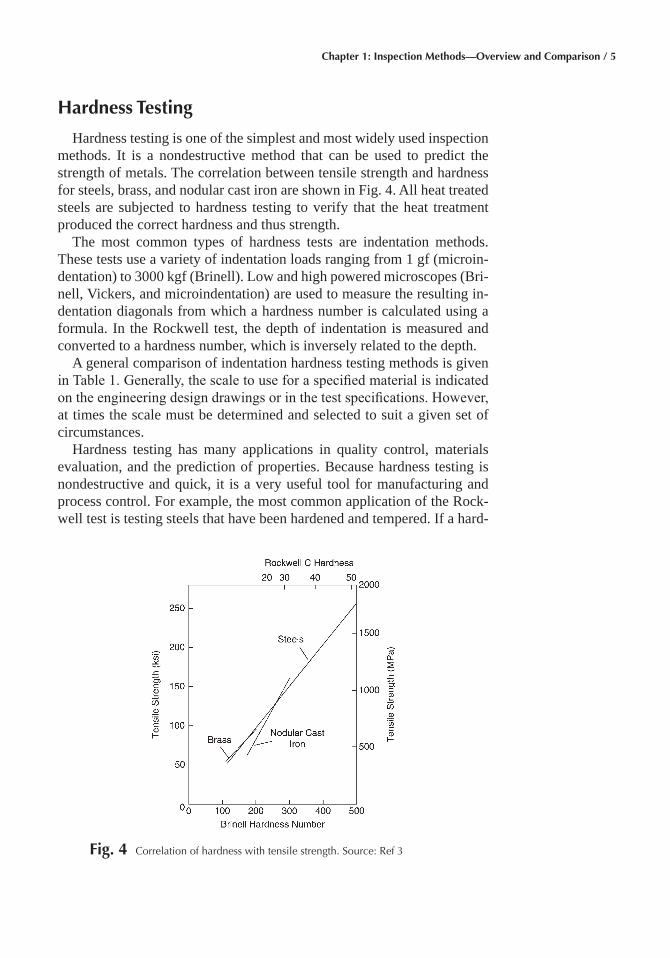
Hardness testing is one of the simplest and most widely used inspection methods. It is a nondestructive method that can be used to predict the strength of metals. The correlation between tensile strength and hardness for steels, brass, and nodular cast iron are shown in Fig. 4. All heat treated steels are subjected to hardness testing to verify that the heat treatment produced the correct hardness and thus strength.
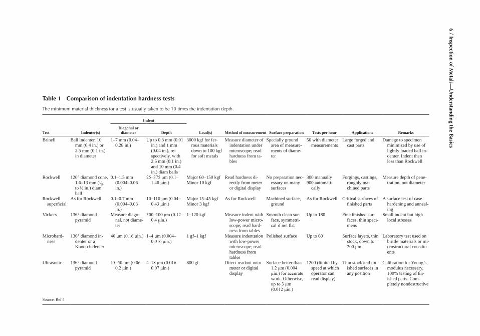
The most common types of hardness tests are indentation methods. These tests use a variety of indentation loads ranging from 1 gf (microin-dentation) to 3000 kgf (Brinell). Low and high powered microscopes (Bri-nell, Vickers, and microindentation) are used to measure the resulting in-dentation diagonals from which a hardness number is calculated using a formula. In the Rockwell test, the depth of indentation is measured and converted to a hardness number, which is inversely related to the depth.
A general comparison of indentation hardness testing methods is given in Table 1. Generally, the scale to use for a specified material is indicated on the engineering design drawings or in the test specifications. However, at times the scale must be determined and selected to suit a given set of circumstances.
Hardness testing has many applications in quality control, materials evaluation, and the prediction of properties. Because hardness testing is nondestructive and quick, it is a very useful tool for manufacturing and process control. For example, the most common application of the Rock-well test is testing steels that have been hardened and tempered. If a hard-
Fig� 4 Correlation of hardness with tensile strength. Source: Ref 3
6 / Inspection of Metals—
Understanding the B
asics
Table 1 Comparison of indentation hardness tests
The minimum material thickness for a test is usually taken to be 10 times the indentation depth.
Test Indenter(s)
Indent
Load(s) Method of measurement Surface preparation Tests per hour Applications RemarksDiagonal or
diameter Depth
Brinell Ball indenter, 10 mm (0.4 in.) or 2.5 mm (0.1 in.) in diameter
1–7 mm (0.04–0.28 in.)
Up to 0.3 mm (0.01 in.) and 1 mm (0.04 in.), re-spectively, with 2.5 mm (0.1 in.) and 10 mm (0.4 in.) diam balls
3000 kgf for fer-rous materials down to 100 kgf for soft metals
Measure diameter of indentation under microscope; read hardness from ta-bles
Specially ground area of measure-ments of diame-ter
50 with diameter measurements
Large forged and cast parts
Damage to specimen minimized by use of lightly loaded ball in-denter. Indent then less than Rockwell
Rockwell 120° diamond cone, 1.6–13 mm (1⁄16 to ½ in.) diam ball
0.1–1.5 mm (0.004–0.06 in.)
25–375 μm (0.1–1.48 μin.)
Major 60–150 kgfMinor 10 kgf
Read hardness di-rectly from meter or digital display
No preparation nec-essary on many surfaces
300 manually900 automati-
cally
Forgings, castings, roughly ma-chined parts
Measure depth of pene-tration, not diameter
Rockwell superficial
As for Rockwell 0.1–0.7 mm (0.004–0.03 in.)
10–110 μm (0.04–0.43 μin.)
Major 15–45 kgfMinor 3 kgf
As for Rockwell Machined surface, ground
As for Rockwell Critical surfaces of finished parts
A surface test of case hardening and anneal-ing
Vickers 136° diamond pyramid
Measure diago-nal, not diame-ter
300–100 μm (0.12–0.4 μin.)
1–120 kgf Measure indent with low-power micro-scope; read hard-ness from tables
Smooth clean sur-face, symmetri-cal if not flat
Up to 180 Fine finished sur-faces, thin speci-mens
Small indent but high local stresses
Microhard- ness
136° diamond in-denter or a Knoop indenter
40 μm (0.16 μin.) 1–4 μm (0.004–0.016 μin.)
1 gf–1 kgf Measure indentation with low-power microscope; read hardness from tables
Polished surface Up to 60 Surface layers, thin stock, down to 200 μm
Laboratory test used on brittle materials or mi-crostructural constitu-ents
Ultrasonic 136° diamond pyramid
15–50 μm (0.06–0.2 μin.)
4–18 μm (0.016–0.07 μin.)
800 gf Direct readout onto meter or digital display
Surface better than 1.2 μm (0.004 μin.) for accurate work. Otherwise, up to 3 μm (0.012 μin.)
1200 (limited by speed at which operator can read display)
Thin stock and fin-ished surfaces in any position
Calibration for Young’s modulus necessary, 100% testing of fin-ished parts. Com-pletely nondestructive
Source: Ref 4
Chapter 1: Inspection Methods—Overview and Comparison / 7
ened and quenched steel piece is tempered by reheating at a controlled and relatively low temperature and then cooled at a control rate and time, it is possible to produce a wide range of desired hardness levels. By using a hardness test to monitor the end results, the operator is able to determine and control the ideal temperatures and times so that a specified hardness may be obtained.
When large populations of materials make testing each workpiece im-practical and a tighter control is demanded for a product, statistical pro-cess control (SPC) is usually incorporated. This means of statistical con-trol can enable continual product manufacturing with minimum testing and a high level of quality. Because many hardness tests are done rapidly, they are well suited for use with SPC techniques. Users are cautioned that the proper testing procedures must be followed to ensure the high degree of accuracy necessary when using SPC.
Tensile Testing
The tensile test is the most common test used to evaluate the mechani-cal properties of materials. Tensile testing is normally conducted by the material producer and the results are supplied to the user as part of the material certification sheet. Since the tensile test is a destructive test, it is not performed directly on the supplied material. For wrought materials, the test specimens are taken from the same heat or lot of material that is supplied. In the case of castings, separate test bars are cast at the same time as the part casting and from the same material used to pour the part casting. Although the tensile test is not normally conducted by the user of the metal product, it is important for the user to understand the test and its results.
Unless the material specification requires an elevated temperature test, the tensile test is normally conducted at room temperature. Typical values reported on the material certification include the yield strength, the ulti-mate tensile strength, and the percent elongation. Since the modulus of elasticity is a structure insensitive property and not affected by process-ing, it is generally not required. The main advantages of the tensile test are, the stress state is well established, the test has been carefully stan-dardized, and the test is relatively easy and inexpensive to perform.
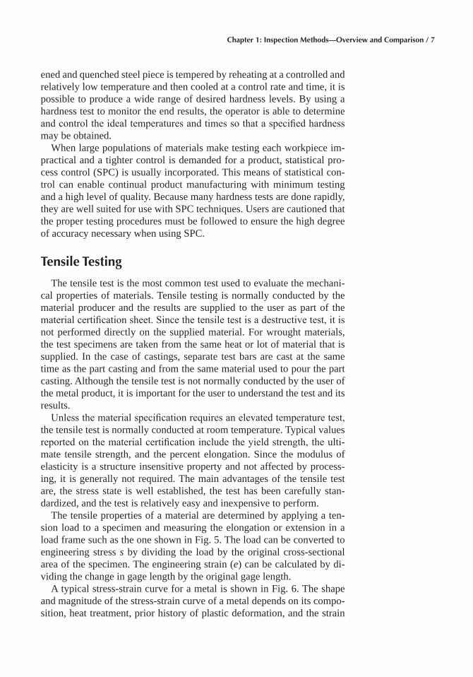
The tensile properties of a material are determined by applying a ten-sion load to a specimen and measuring the elongation or extension in a load frame such as the one shown in Fig. 5. The load can be converted to engineering stress s by dividing the load by the original cross-sectional area of the specimen. The engineering strain (e) can be calculated by di-viding the change in gage length by the original gage length.
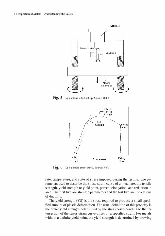
A typical stress-strain curve for a metal is shown in Fig. 6. The shape and magnitude of the stress-strain curve of a metal depends on its compo-sition, heat treatment, prior history of plastic deformation, and the strain
8 / Inspection of Metals—Understanding the Basics
rate, temperature, and state of stress imposed during the testing. The pa-rameters used to describe the stress-strain curve of a metal are, the tensile strength, yield strength or yield point, percent elongation, and reduction in area. The first two are strength parameters and the last two are indications of ductility.
The yield strength (YS) is the stress required to produce a small speci-fied amount of plastic deformation. The usual definition of this property is the offset yield strength determined by the stress corresponding to the in-tersection of the stress-strain curve offset by a specified strain. For metals without a definite yield point, the yield strength is determined by drawing
Fig� 5 Typical tensile test set-up. Source: Ref 3
Fig� 6 Typical stress-strain curve. Source: Ref 3
Chapter 1: Inspection Methods—Overview and Comparison / 9
a straight line parallel to the initial straight line portion of the stress-strain curve. The line is normally offset by a strain of 0.2% (0.002).
As shown in Fig. 6, the ultimate tensile strength (UTS) is the maximum stress that occurs during the test. Although the tensile strength is the value most often listed from the results of tensile testing, it is not generally the value that is used in design. Static design of ductile metals is usually based on the yield strength, since most designs do not allow any plastic defor-mation. However, for brittle metals that do not display any appreciable plastic deformation, tensile strength is a valid design criterion.
Measures of ductility that are obtained from the tension test are the en-gineering strain at fracture (ef) and the reduction of area at fracture (q). Both are usually expressed as percentages, with the engineering strain at failure often reported as the percent elongation.
Chemical Analysis
The overall chemical composition of metals and alloys is most com-monly determined by x-ray fluorescence (XRF) and optical emission spectroscopy (OES). While these methods work well for most elements, they are not useful for dissolved gases and some nonmetallic elements that can be present in metals as alloying or impurity elements. High tempera-ture combustion and inert gas fusion methods are typically used to analyze for dissolved gases (oxygen, nitrogen, hydrogen) and, in some cases, car-bon and sulfur in metals.
A number of methods can be used to obtain information about the chemistry of the first one to several atomic layers of samples of metals, as well as of other materials, such as semiconductors and various types of thin films. Of these methods, the scanning Auger microprobe (SAM) is the most widely used.
Metallography
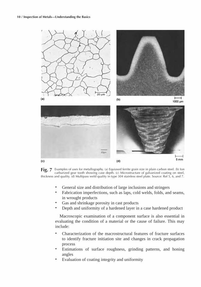
Metallography is the scientific discipline of examining and determining the constitution and the underlying structure of the constituents in metals and alloys. The objective of metallography is to accurately reveal material structure at the surface of a sample and/or from a cross-section specimen. For example, cross-sections cut from a component or sample may be mac-roscopically examined by light illumination in order to reveal various im-portant macrostructural features (on the order of 1 mm to 1 m or 0.04 in. to 3 ft), such as the ones shown in Fig. 7 and listed here:
• Flow lines in wrought products• Solidification structures in cast products• Weld characteristics, including depth of penetration, fusion zone size
and number of passes, size of heat affected zone, and type and density of weld imperfections
10 / Inspection of Metals—Understanding the Basics
• General size and distribution of large inclusions and stringers• Fabrication imperfections, such as laps, cold welds, folds, and seams,
in wrought products• Gas and shrinkage porosity in cast products• Depth and uniformity of a hardened layer in a case hardened product
Macroscopic examination of a component surface is also essential in evaluating the condition of a material or the cause of failure. This may include:• Characterization of the macrostructural features of fracture surfaces
to identify fracture initiation site and changes in crack propagation process
• Estimations of surface roughness, grinding patterns, and honing angles
• Evaluation of coating integrity and uniformity
Fig� 7 Examples of uses for metallography. (a) Equiaxed ferrite grain size in plain carbon steel. (b) Ion carburized gear tooth showing case depth. (c) Microstructure of galvanized coating on steel,
thickness and quality. (d) Multipass weld quality in type 304 stainless steel plate. Source: Ref 5, 6, and 7.

Chapter 1: Inspection Methods—Overview and Comparison / 11
• Determination of extent and location of wear• Estimation of plastic deformation associated with various mechanical
processes• Determination of the extent and form of corrosive attack; readily dis-
tinguishable types of attack include pitting, uniform, crevice, and ero-sion corrosion
• Evaluation of tendency for oxidation• Association of failure with welds, solders, and other processing
operations
This listing of macrostructural features in the characterization of met-als, though incomplete, represents the wide variety of features that can be evaluated by light macroscopy.
Nondestructive Testing
Nondestructive testing (NDT) and inspection techniques are commonly used to detect and evaluate flaws (irregularities or discontinuities) or leaks in engineering systems. Of the many different NDT techniques used in industry, liquid penetrant and magnetic particle testing account for about one-half of all NDT, ultrasonics and x-ray methods about another third, eddy current testing about 10%, and all other methods for only about 2%. It should be noted that the techniques reviewed in this book are by no means all of the NDT techniques utilized. However, they do represent the most commonly employed methods. A simplified breakdown of the com-plexity and relative requirements of the five most frequently used NDT techniques is shown in Table 2, and the common NDT methods are com-
Table 2 The relative uses and merits of various nondestructive testing methods
Test method
Ultrasonics X-ray Eddy current Magnetic particle Liquid penetrant
Capital cost Medium to high High Low to medium Medium Low Consumable cost Very low High Low Medium Medium Time of results Immediate Delayed Immediate Short delay Short delay Effect of geometry Important Important Important Not too impor-
tant Not too impor-
tant Access problems Important Important Important Important Important Type of defect Internal Most External External Surface breaking Relative sensitivity High Medium High Low Low Formal record Expensive Standard Expensive Unusual Unusual Operator skill High High Medium Low Low Operator training Important Important Important Important Training needs High High Medium Low Low Portability of equipment High Low High to medium High to medium High Dependent on material composition
Very Quite Very Magnetic only Little
Ability to automate Good Fair Good Fair Fair Capabilities Thickness gaging:
some composi-tion testing
Thickness gaging
Thickness gaging; grade sorting
Defects only Defects only
Source: Ref 8
12 / Inspection of Metals—Understanding the Basics
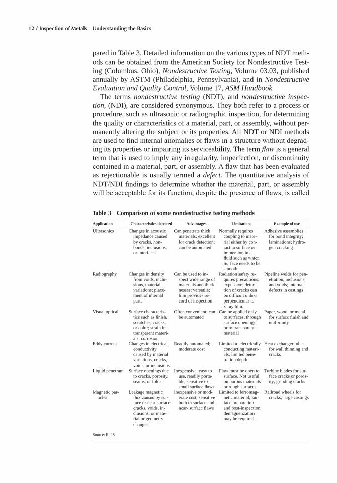
pared in Table 3. Detailed information on the various types of NDT meth-ods can be obtained from the American Society for Nondestructive Test-ing (Columbus, Ohio), Nondestructive Testing, Volume 03.03, published annually by ASTM (Philadelphia, Pennsylvania), and in Nondestructive Evaluation and Quality Control, Volume 17, ASM Handbook.
The terms nondestructive testing (NDT), and nondestructive inspec-tion, (NDI), are considered synonymous. They both refer to a process or procedure, such as ultrasonic or radiographic inspection, for determining the quality or characteristics of a material, part, or assembly, without per-manently altering the subject or its properties. All NDT or NDI methods are used to find internal anomalies or flaws in a structure without degrad-ing its properties or impairing its serviceability. The term flaw is a general term that is used to imply any irregularity, imperfection, or discontinuity contained in a material, part, or assembly. A flaw that has been evaluated as rejectionable is usually termed a defect. The quantitative analysis of NDT/NDI findings to determine whether the material, part, or assembly will be acceptable for its function, despite the presence of flaws, is called
Table 3 Comparison of some nondestructive testing methods
Application Characteristics detected Advantages Limitations Example of use
Ultrasonics Changes in acoustic impedance caused by cracks, non-bonds, inclusions, or interfaces
Can penetrate thick materials; excellent for crack detection; can be automated
Normally requires coupling to mate-rial either by con-tact to surface or immersion in a fluid such as water. Surface needs to be smooth.
Adhesive assemblies for bond integrity; laminations; hydro-gen cracking
Radiography Changes in density from voids, inclu-sions, material variations; place-ment of internal parts
Can be used to in-spect wide range of materials and thick-nesses; versatile; film provides re-cord of inspection
Radiation safety re-quires precautions; expensive; detec-tion of cracks can be difficult unless perpendicular to x-ray film.
Pipeline welds for pen-etration, inclusions, and voids; internal defects in castings
Visual optical Surface characteris-tics such as finish, scratches, cracks, or color; strain in transparent materi-als; corrosion
Often convenient; can be automated
Can be applied only to surfaces, through surface openings, or to transparent material
Paper, wood, or metal for surface finish and uniformity
Eddy current Changes in electrical conductivity caused by material variations, cracks, voids, or inclusions
Readily automated; moderate cost
Limited to electrically conducting materi-als; limited pene-tration depth
Heat exchanger tubes for wall thinning and cracks
Liquid penetrant Surface openings due to cracks, porosity, seams, or folds
Inexpensive, easy to use, readily porta-ble, sensitive to small surface flaws
Flaw must be open to surface. Not useful on porous materials or rough surfaces
Turbine blades for sur-face cracks or poros-ity; grinding cracks
Magnetic par- ticles
Leakage magnetic flux caused by sur-face or near-surface cracks, voids, in-clusions, or mate-rial or geometry changes
Inexpensive or mod-erate cost, sensitive both to surface and near- surface flaws
Limited to ferromag-netic material; sur-face preparation and post-inspection demagnetization may be required
Railroad wheels for cracks; large castings
Source: Ref 8
Chapter 1: Inspection Methods—Overview and Comparison / 13
nondestructive evaluation (NDE). With NDE, a flaw can be classified by its size, shape, type, and location, allowing the investigator to determine whether or not the flaw(s) is acceptable. Damage tolerant design ap-proaches are based on the philosophy of ensuring safe operation in the presence of flaws.
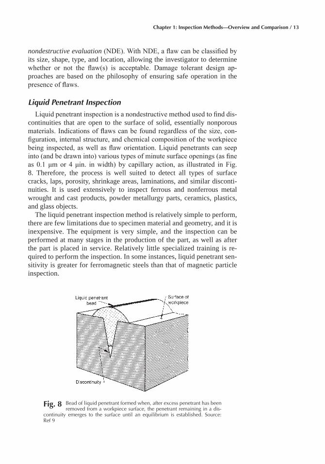
Liquid Penetrant Inspection
Liquid penetrant inspection is a nondestructive method used to find dis-continuities that are open to the surface of solid, essentially nonporous materials. Indications of flaws can be found regardless of the size, con-figuration, internal structure, and chemical composition of the workpiece being inspected, as well as flaw orientation. Liquid penetrants can seep into (and be drawn into) various types of minute surface openings (as fine as 0.1 μm or 4 μin. in width) by capillary action, as illustrated in Fig. 8. Therefore, the process is well suited to detect all types of surface cracks, laps, porosity, shrinkage areas, laminations, and similar disconti-nuities. It is used extensively to inspect ferrous and nonferrous metal wrought and cast products, powder metallurgy parts, ceramics, plastics, and glass objects.
The liquid penetrant inspection method is relatively simple to perform, there are few limitations due to specimen material and geometry, and it is inexpensive. The equipment is very simple, and the inspection can be performed at many stages in the production of the part, as well as after the part is placed in service. Relatively little specialized training is re-quired to perform the inspection. In some instances, liquid penetrant sen-sitivity is greater for ferromagnetic steels than that of magnetic particle inspection.
Fig� 8 Bead of liquid penetrant formed when, after excess penetrant has been removed from a workpiece surface, the penetrant remaining in a dis-
continuity emerges to the surface until an equilibrium is established. Source: Ref 9
14 / Inspection of Metals—Understanding the Basics
The major limitation of liquid penetrant inspection is that it can detect only imperfections that are open to the surface; some other method must be used to detect subsurface defects and discontinuities. Another factor that can inhibit the effectiveness of liquid penetrant inspection is the sur-face roughness of the object. Extremely rough and porous surfaces are likely to produce false indications.
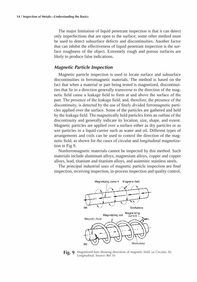
Magnetic Particle Inspection
Magnetic particle inspection is used to locate surface and subsurface discontinuities in ferromagnetic materials. The method is based on the fact that when a material or part being tested is magnetized, discontinui-ties that lie in a direction generally transverse to the direction of the mag-netic field cause a leakage field to form at and above the surface of the part. The presence of the leakage field; and, therefore, the presence of the discontinuity, is detected by the use of finely divided ferromagnetic parti-cles applied over the surface. Some of the particles are gathered and held by the leakage field. The magnetically held particles form an outline of the discontinuity and generally indicate its location, size, shape, and extent. Magnetic particles are applied over a surface either as dry particles or as wet particles in a liquid carrier such as water and oil. Different types of arrangements and coils can be used to control the direction of the mag-netic field, as shown for the cases of circular and longitudinal magnetiza-tion in Fig 9.
Nonferromagnetic materials cannot be inspected by this method. Such materials include aluminum alloys, magnesium alloys, copper and copper alloys, lead, titanium and titanium alloys, and austenitic stainless steels.
The principal industrial uses of magnetic particle inspection are final inspection, receiving inspection, in-process inspection and quality control,
Fig� 9 Magnetized bars showing directions of magnetic field. (a) Circular. (b) Longitudinal. Source: Ref 10
Chapter 1: Inspection Methods—Overview and Comparison / 15
maintenance and overhaul in the transportation industries, plant and ma-chinery maintenance, and, inspection of large components.
Although in-process magnetic particle inspection is used to detect dis-continuities and imperfections in material and parts as early as possible in the sequence of operations, final inspection is required to ensure that re-jectable discontinuities and imperfections detrimental to part use and function have not developed during processing.
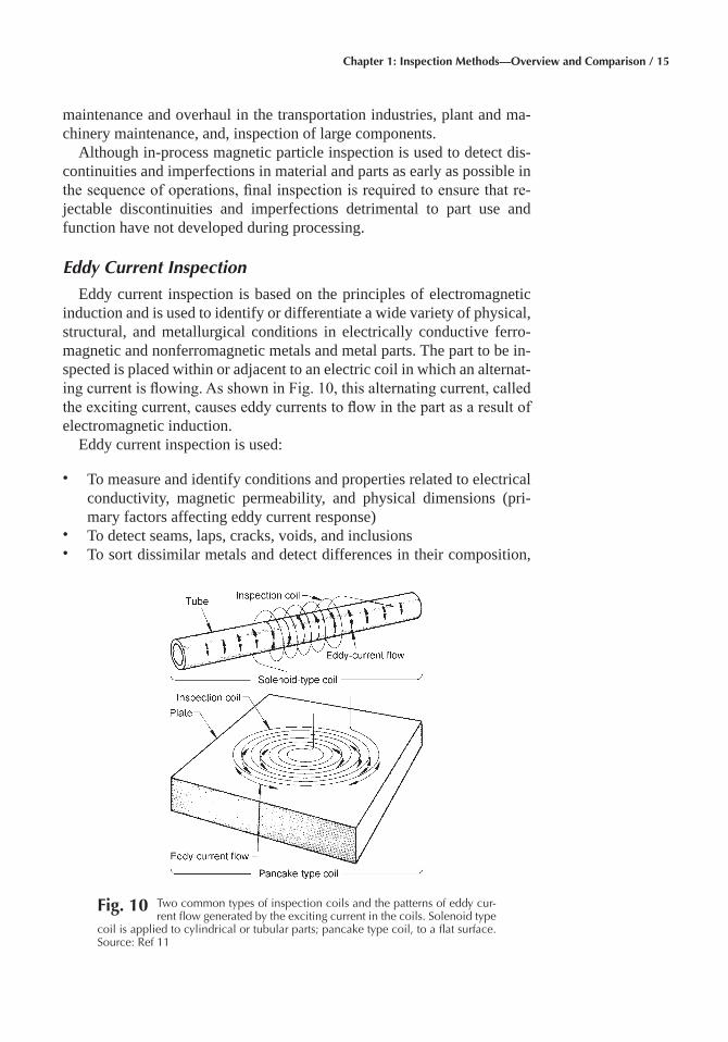
Eddy Current Inspection
Eddy current inspection is based on the principles of electromagnetic induction and is used to identify or differentiate a wide variety of physical, structural, and metallurgical conditions in electrically conductive ferro-magnetic and nonferromagnetic metals and metal parts. The part to be in-spected is placed within or adjacent to an electric coil in which an alternat-ing current is flowing. As shown in Fig. 10, this alternating current, called the exciting current, causes eddy currents to flow in the part as a result of electromagnetic induction.
Eddy current inspection is used:
• To measure and identify conditions and properties related to electrical conductivity, magnetic permeability, and physical dimensions (pri-mary factors affecting eddy current response)
• To detect seams, laps, cracks, voids, and inclusions • To sort dissimilar metals and detect differences in their composition,
Fig� 10 Two common types of inspection coils and the patterns of eddy cur-rent flow generated by the exciting current in the coils. Solenoid type
coil is applied to cylindrical or tubular parts; pancake type coil, to a flat surface. Source: Ref 11
16 / Inspection of Metals—Understanding the Basics
microstructure, and other properties, such as grain size, heat treatment, and hardness
• To measure the thickness of a nonconductive coating on a conductive metal, or the thickness of a nonmagnetic metal coating on a magnetic metal
Because eddy current inspection is an electromagnetic induction tech-nique, it does not require direct electrical contact with the part being in-spected. Eddy current is adaptable to high speed inspection, and because it is nondestructive, it can be used to inspect an entire production output if desired. The method is based on indirect measurement, and the correlation between instrument readings and the structural characteristics and ser-viceability of parts being inspected must be carefully and repeatedly established.
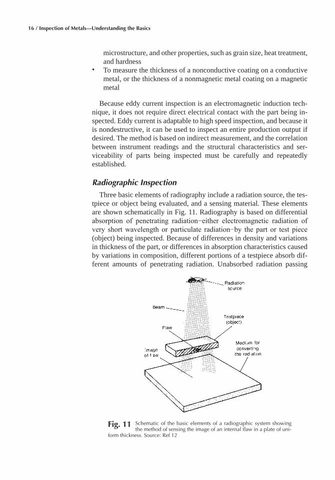
Radiographic Inspection
Three basic elements of radiography include a radiation source, the tes-tpiece or object being evaluated, and a sensing material. These elements are shown schematically in Fig. 11. Radiography is based on differential absorption of penetrating radiation−either electromagnetic radiation of very short wavelength or particulate radiation−by the part or test piece (object) being inspected. Because of differences in density and variations in thickness of the part, or differences in absorption characteristics caused by variations in composition, different portions of a testpiece absorb dif-ferent amounts of penetrating radiation. Unabsorbed radiation passing
Fig� 11 Schematic of the basic elements of a radiographic system showing the method of sensing the image of an internal flaw in a plate of uni-
form thickness. Source: Ref 12
Chapter 1: Inspection Methods—Overview and Comparison / 17
through the part can be recorded on film or photosensitive paper, viewed on a fluorescent screen, or monitored by various types of radiation detec-tors. The term radiography usually implies a radiographic process that produces a permanent image on film (conventional radiography) or paper (paper radiography or xeroradiography), although, in a broad sense, it re-fers to all forms of radiographic inspection. When inspection involves viewing of a real-time image on a fluorescent screen or image intensifier, the radiographic process is termed real-time inspection. When electronic, nonimaging instruments are used to measure the intensity of radiation, the process is termed radiation gaging. Tomography, a radiation inspection method adapted from the medical computerized axial tomography CAT scanner, provides a cross-sectional view of an inspection object. All the previous terms are mainly used in connection with inspection that in-volves penetrating electromagnetic radiation in the form of x-rays or gamma rays. Neutron radiography refers to radiographic inspection using neutrons rather than electromagnetic radiation.
In conventional radiography, an object is placed in a beam of x-rays and the portion of the radiation that is not absorbed by the object impinges on a detector such as film. The unabsorbed radiation exposes the film emul-sion, similar to the way that light exposes film in photography. Develop-ment of the film produces an image that is a twodimensional shadow pic-ture of the object. Variations in density, thickness, and composition of the object being inspected cause variations in the intensity of the unabsorbed radiation and appear as variations in photographic density (shades of gray) in the developed film. Evaluation of the radiograph is based on a compari-son of the differences in photographic density with known characteristics of the object itself or with standards derived from radiographs of similar objects of acceptable quality.
Radiography is used to detect features of a component or assembly that exhibit differences in thickness or physical density compared with sur-rounding material. Large differences are more easily detected than small ones. In general, radiography can detect only those features that have a reasonable thickness or radiation path length in a direction parallel to the radiation beam. This means that the ability of the process to detect planar discontinuities such as cracks depends on proper orientation of the test-piece during inspection. Discontinuities such as voids and inclusions, which have measurable thickness in all directions, can be detected as long as they are not too small in relation to section thickness. In general, fea-tures that exhibit differences in absorption of a few percent compared with the surrounding material can be detected.
Ultrasonic Inspection
Ultrasonic inspection is a nondestructive method in which beams of high frequency acoustic energy are introduced into a material to detect
18 / Inspection of Metals—Understanding the Basics
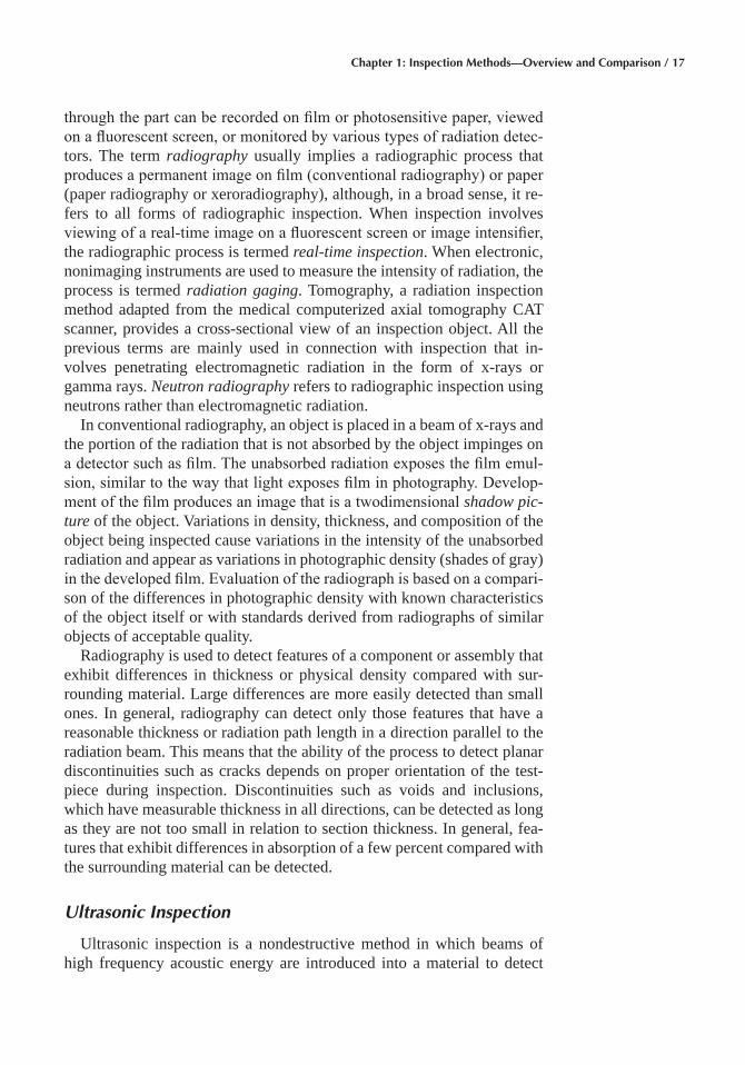
surface and subsurface flaws, to measure the thickness of the material, and to measure the distance to a flaw. An ultrasonic beam travels through a material until it strikes an interface or discontinuity such as a flaw. Inter-faces and flaws interrupt the beam and reflect a portion of the incident acoustic energy. The amount of energy reflected is a function of (a) the nature and orientation of the interface or flaw; and, (b) the acoustic imped-ance of such a reflector. Energy reflected from various interfaces and flaws can be used to define the presence and locations of flaws, the thickness of the material, and the depth of a flaw beneath a surface. Pulse echo and through transmission, two types of ultrasonic inspection, are illustrated in Fig. 12.
Fig� 12 Two types of ultrasonic inspection. (a) Pulse echo. (b) Through trans- mission
Chapter 1: Inspection Methods—Overview and Comparison / 19
Most ultrasonic inspections are performed using a frequency between 1 and 25 MHz. Short shock bursts of ultrasonic energy are aimed into the material from the ultrasonic search unit of the ultrasonic flaw detector in-strument. The electrical pulse from the flaw detector is converted into ul-trasonic energy by a piezoelectric transducer element in the search unit. The beam pattern from the search unit is determined by the operating frequency and size of the transducer element. Ultrasonic energy travels through the material at a specific velocity that is dependent on the physical properties of the material and on the mode of propagation of the ultrasonic wave. The amount of energy reflected from or transmitted through an in-terface, other type of discontinuity, or reflector depends on the properties of the reflector. These phenomena provide the basis for establishing two of the most common measurement parameters used in ultrasonic inspection: the amplitude of the energy reflected from an interface or flaw; and, the time required (from pulse initiation) for the ultrasonic beam to reach the interface or flaw.
REFERENCES
1. S.M. Purdy, Macroetching, Metallography and Microstructures, Vol 9, ASM Handbook, ASM International, 2004, p 313–324
2. J.D. Meyer, Machine Vision and Robotic Inspection Systems, Nonde-structive Evaluation and Quality Control, Vol 17, ASM Handbook, ASM International, 1992, p 29–45
3. F.C. Campbell, Elements of Metallurgy and Engineering Alloys, ASM International, 2008
4. A. Fee, Selection and Industrial Applications of Hardness Tests, Me-chanical Testing and Evaluation, Vol 8, ASM Handbook, ASM Inter-national, 2000, p 260–277
5. A. O. Benscoter and B.L. Bramfitt, Metallography and Microstruc-tures of Low-Carbon and Coated Steels, Metallography and Micro-structures, Vol 9, ASM Handbook, ASM International, 2004, p 588– 607
6. Metallography and Microstructures of Case-Hardening Steel, Metal-lography and Microstructures, Vol 9, ASM Handbook, ASM Interna-tional, 2004, p 627–643
7. Metallography and Microstructures of Weldments, Metallography and Microstructures, Vol 9, ASM Handbook, ASM International, 2004, p 1047–1056
8. L. Cartz, Quality Control and NDT, Nondestructive Testing, ASM In-ternational, 1995, p 1–13
9. J.S. Borucki and G. Jordan, Liquid Penetrant Inspection, Nondestruc-tive Evaluation and Quality Control, Vol 17, ASM Handbook, 1989, p 491–511
10. A. Lindgren, Magnetic Particle Inspection, Nondestructive Eval-

20 / Inspection of Metals—Understanding the Basics
uation and Quality Control, Vol 17, ASM Handbook, 1989, p 89– 128
11. Eddy Current Inspection, Nondestructive Evaluation and Quality Control, Vol 17, ASM Handbook, 1989, p 164–194
12. Radiographic Inspection, Nondestructive Evaluation and Quality Control, Vol 17, ASM Handbook, 1989, p 295–357
Inspection of Metals—Understanding the Basics Copyright © 2013 ASM International®
F.C. Campbell, editor All rights reservedwww.asminternational.org
CHAPTER 2
Visual Inspection
VISUAL INSPECTION is perhaps the most important method of in-spection of materials. Visual inspection is defined as the examination using the naked eye, alone or in conjunction with various magnifying de-vices, without changing, altering, or destroying the material involved.
To do a good job of visual inspection requires some knowledge of what you are looking at. It is good to have as much knowledge as possible of the product being examined. You must not only discover defects, but also be able to evaluate them from the point of usefulness or rejection. Knowl-edge of the cause of defective materials helps in future prevention. You should know how it may be abused. You should also be familiar with the types of defects that normally might be encountered in such a part, e.g., scabs, seams, and laminations in steel mill products; and corrosion, ero-sion, and physical abuse on parts that have been in service.
Visual Inspection Procedure
The part should first be carefully examined with the naked eye. Then, magnifying devices may be used to further examine suspect areas revealed by the naked eye examination.
Try to account for all unusual surface markings and conditions. Think in terms of depth effect and sharpness of penetration (stress concentra-tion). Note any discoloration and determine the cause (heat? corrosion?).
Markings� Observe any identification markings. Such markings may identify the manufacturer, date of manufacture, original size of material, material specification, and number of the original heat of steel traceable to analysis and physical properties. If you are unfamiliar with identification marking procedures, do not assume a part is unmarked. Find out by asking manufacturers how they identify such products.
22 / Inspection of Metals—Understanding the Basics
These are obvious markings. But there are also many hidden markings used by manufacturers, which they often do not readily reveal. One ex-ample is the wire rope industry. Some hemp center wire ropes have a sin-gle fiber wrapped with the group that reveals the name of the manufac-turer and also the type of wire rope. It is difficult to distinguish this fiber and requires some care to separate and flatten it; sometimes soaking in hot water helps. Nearly all wire ropes have an identifying strand. It may be colored plastic, or the diameter of a single wire, or part of the construction configuration. Bolt heads are another good example of markings which give information. In addition to the radial markings on the heads which tell the strength level, the manufacturer’s markings are often present.
Abuse� Look for evidence of abuse. In the case of failure, try to decide if the abuse occurred before or after the failure. Failures often involve se-vere trauma. Parts flying about after the fact can suffer severe abuse that may be misinterpreted as being related to the cause of the failure. If a part is distorted, try to ascertain the type, direction, and intensity of the load necessary to produce this distortion.
Heat Effects� Defects are often caused by heating problems. These heating problems generally leave telltale indications. The indications are the result of the complex oxide systems of iron and other alloying ele-ments. At lower temperatures, steel parts with a relatively bright surface may display characteristic temper colors. These colors vary somewhat with the composition and heat treatment. A variety of colors are produced within the temperature range of 195 to 370 °C (380 to 700 °F). Charts can be consulted for the approximate temperature reached (Ref 1).
As the temperature rises, a heavier scale of a different type forms. The formation temperature varies with the type of alloy. It should be noted that a scale layer may be quite thick. This does not necessarily indicate a great metal loss. Generally, the ratio of lost metal to oxygen in a scale layer is 8:1. This means a 3 mm (⅛ in.) thick scale layer represents only about 0.4 mm (0.015 in.) of lost metal. Since scaling can occur at such a low tem-perature, the microstructure may not have been altered appreciably (as-suming the lower critical temperature to be 723 °C, or 1333 °F).
The color of heat scale should also be observed. The brown- to red-colored scale layers on steel indicate the more completely oxidized iron oxide (Fe2O3). The black, mill-scale type of oxides are composed of the incompletely oxidized form of iron, black iron oxide (Fe3O4). This indi-cates an oxygen deficiency at the time of heating and may mean much higher temperatures of formation. There are other temperature indications associated with the observation of materials while being exposed to heat. Such materials just begin to glow dull red (in a dark area) at 620 to 650 °C (1150 to 1200 °F). The colors change as the temperature increases.
Corrosion Scaling� Scaling of materials is not necessarily associated with just heat. Corrosion also may create scale-type deposits. In some cases, these may be indistinguishable from heat scale. Often, valuable
Chapter 2: Visual Inspection / 23
data can be gained from scale analysis. It may be a good idea to remove scrapings and label for future tests. Try not to mix grease, paint, coating material, and mill scale with the corrosion product. If parts have internal and external surfaces, do not mix outside scrapings with inside scrapings. If corrosion is suspected, determine if it is localized or general. Is it uni-form or selective (pitting)? Is it in an area of contact with other mate- rials? Does it have special characteristics indicative of high velocity flow (e.g., erosion, cavitation)? Does it leave an unusual appearing corrosion product?
Cracking� If cracking is noted during visual examination, it is impor-tant to characterize the cracking. Is the crack straight or does it follow an irregular path? Is there one crack or a series of cracks? Are the cracks open or tightly closed? Are the cracks associated with markings of any kind? Are the cracks located in areas of natural stress concentration? Are the cracks associated with welding, for either fabrication or repair? Are the cracks associated in any way with evidence of corrosion, e.g., corro-sion product, corrosion pitting?
If cracking is observed during the inspection of raw materials or in ma-terials in process of manufacture or finished products, it should be ex-plored for the purpose of determining acceptance or rejection. This is usu-ally done by grinding to determine depth and extent. In such grinding, care must be exercised so that heat and stress do not cause extension of cracking. Grinding, if not done with care, can also close tight cracks by causing the adjacent metal to flow over the crack. It is often necessary to use methods such as magnetic particle testing or dye penetrant inspection to be assured that cracking is completely removed.
Once the crack has been completely removed, judgment must be exer-cised as to whether the part (a) can be used as is, (b) can be repaired, or (c) must be rejected and scrapped. Some specifications prescribe how much cracking is acceptable. The American Petroleum Institute, in many of its specifications, allows surface defects if the depth is no greater than 12½ percent of the wall thickness. Where no such specification exists, the ulti-mate usage must be considered.
Of primary consideration is dynamic loading versus static loading. Other helpful considerations in making an acceptance or rejection are drawing tolerances for the part and design information such as safety factors.
Once a decision is made, it is necessary to determine if welding repair is necessary or if the part can be used as is, with the defects ground out. Welds may cause a new set of problems. If the weld can be avoided, feather the ground-out area to a generous radius to avoid stress concentra-tions. The smoother this surface is, the less likely it is to crack again.
Straight, sharp, open, single cracks (Fig. 1a) are usually associated with very high stresses and/or material of lowered ductility. They may be as-sociated with suddenly applied (impact) loads. Open cracks may also be
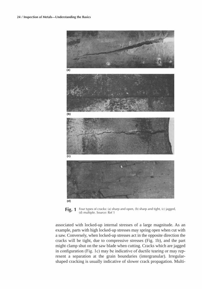
24 / Inspection of Metals—Understanding the Basics
associated with locked-up internal stresses of a large magnitude. As an example, parts with high locked-up stresses may spring open when cut with a saw. Conversely, when locked-up stresses act in the opposite direction the cracks will be tight, due to compressive stresses (Fig. 1b), and the part might clamp shut on the saw blade when cutting. Cracks which are jagged in configuration (Fig. 1c) may be indicative of ductile tearing or may rep-resent a separation at the grain boundaries (intergranular). Irregular-shaped cracking is usually indicative of slower crack propagation. Multi-
Fig� 1 Four types of cracks: (a) sharp and open, (b) sharp and tight, (c) jagged, (d) multiple. Source: Ref 1
Chapter 2: Visual Inspection / 25
ple cracks (Fig. 1d) are often associated with corrosion, stress corrosion, corrosion fatigue, thermal fatigue, or localized trauma.
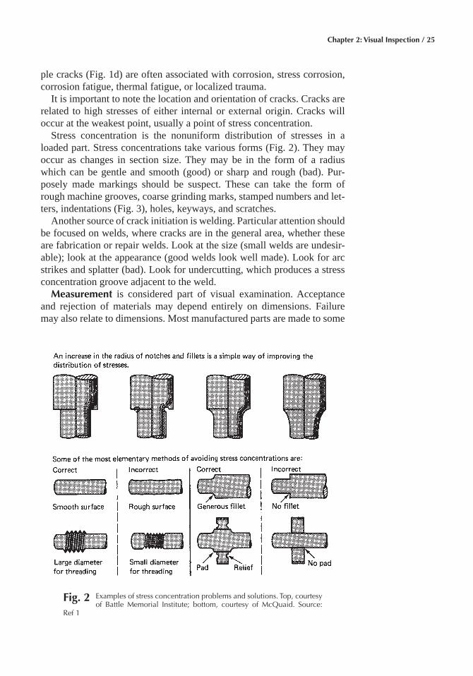
It is important to note the location and orientation of cracks. Cracks are related to high stresses of either internal or external origin. Cracks will occur at the weakest point, usually a point of stress concentration.
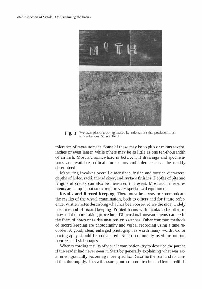
Stress concentration is the nonuniform distribution of stresses in a loaded part. Stress concentrations take various forms (Fig. 2). They may occur as changes in section size. They may be in the form of a radius which can be gentle and smooth (good) or sharp and rough (bad). Pur-posely made markings should be suspect. These can take the form of rough machine grooves, coarse grinding marks, stamped numbers and let-ters, indentations (Fig. 3), holes, keyways, and scratches.
Another source of crack initiation is welding. Particular attention should be focused on welds, where cracks are in the general area, whether these are fabrication or repair welds. Look at the size (small welds are undesir-able); look at the appearance (good welds look well made). Look for arc strikes and splatter (bad). Look for undercutting, which produces a stress concentration groove adjacent to the weld.
Measurement is considered part of visual examination. Acceptance and rejection of materials may depend entirely on dimensions. Failure may also relate to dimensions. Most manufactured parts are made to some
Fig� 2 Examples of stress concentration problems and solutions. Top, courtesy of Battle Memorial Institute; bottom, courtesy of McQuaid. Source:
Ref 1
26 / Inspection of Metals—Understanding the Basics
tolerance of measurement. Some of these may be to plus or minus several inches or even larger, while others may be as little as one ten-thousandth of an inch. Most are somewhere in between. If drawings and specifica-tions are available, critical dimensions and tolerances can be readily determined.
Measuring involves overall dimensions, inside and outside diameters, depths of holes, radii, thread sizes, and surface finishes. Depths of pits and lengths of cracks can also be measured if present. Most such measure-ments are simple, but some require very specialized equipment.
Results and Record Keeping� There must be a way to communicate the results of the visual examination, both to others and for future refer-ence. Written notes describing what has been observed are the most widely used method of record keeping. Printed forms with blanks to be filled in may aid the note-taking procedure. Dimensional measurements can be in the form of notes or as designations on sketches. Other common methods of record keeping are photography and verbal recording using a tape re-corder. A good, clear, enlarged photograph is worth many words. Color photography should be considered. Not so commonly used are motion pictures and video tapes.
When recording results of visual examination, try to describe the part as if the reader had never seen it. Start by generally explaining what was ex-amined, gradually becoming more specific. Describe the part and its con-dition thoroughly. This will assure good communication and lend credibil-
Fig� 3 Two examples of cracking caused by indentations that produced stress concentrations. Source: Ref 1

Chapter 2: Visual Inspection / 27
ity to your account. It will also serve as a good refresher if you are asked to explain your findings at a later date.
Visual Inspection Tools
Tools for visual inspection can be grouped into six categories:
• Magnifying devices • Lighting for visual inspection• Measuring devices• Miscellaneous measuring devices• Record-keeping devices• Macroetching
Magnifying Devices
Magnifiers can be characterized by magnifying power, focal length, and lens type.
Magnifying Power� An object appears to increase in size as it is brought closer to the eye. In determining magnifying power, the true size of the object is what the image appears to the eye at 10 in. (25 cm). The 10-inch value is used as a standard because this is the distance from the eye one usually holds a small object when examining it. Linear magnification is expressed in diameters. The letter × is normally used to designate the magnifying power of a lens, e.g., 10×.
If one could focus on an object at one inch (2.5 cm), it would appear 10 times larger. Since one cannot effectively focus the eye at one inch, a lens may be used to do so. Thus, magnification can be defined as the ratio of the apparent size of an object seen through a magnifier (known as a virtual image) to the size of the object as it appears to the unaided eye at 10 inches.
Focal Length� The focal length is the distance from the lens to the point at which parallel rays of light striking one side of a positive lens will be brought into focus on the opposite side. For lenses of short focal length, such as discussed here, light 30 to 40 feet, or 9 to 10 meters away can be considered parallel. The focal length can be determined by holding a lens such that light coming through a window, for example, will allow the image of the window or other object to focus sharply on a sheet of paper held behind the lens. The distance from lens to paper will then be the focal length. Once the focal length is known, the magnification of the lens can be determined, and vice versa. The shorter the focal length, the greater the magnifying power. The distance of the eye from the lens must be the same as the focal length. A lens with a one-inch focal length, for example, will have a magnifying power of 10 (10×). This is true if the lens is held one inch from an object and the eye is placed one inch from the lens.
28 / Inspection of Metals—Understanding the Basics
In summary, the following formula determines magnifying power:
Magnifying power (any positive lens)10
focal lengthin inch= ees( )
With a simple method of determining focal length, it becomes easy to determine magnification.
Lens Types
All lenses are either convex (bulged out), concave (sunken in), or flat. More often they are a combination of these. The most common type found in the laboratory is the double convex lens. Lenses with one side convex and the other flat (plano-convex) are used in projectors and microscopes. All other magnifiers are lenses used in combination.
The degree of correction dictates the quality of the lens. Three inherent faults in lenses–all of which are correctable—are:
• Distortion. The image appears unnatural. The quality of the lens mate-rial and the grinding and polishing are both the causes of and the means for correcting this problem.
• Spherical Aberration. Light rays passing through the center of the lens and at the outer edges come to a focus at different points. (The distor-tion is worse on large diameter lenses than small.) Spherical aberration can be corrected by slight modification of the curved surfaces.
• Chromatic Aberration. This is a prism effect: when broken down into colors, the light rays do not focus at the same place. This may occur both as a lateral and as a longitudinal effect. It is correctable by use of compound lenses of different types of glass.
Below about five magnifications, one double convex lens is satisfac-tory. Two combined lenses will have a shorter focal length than either lens used alone. Higher magnification in simple magnifiers usually employs two or three lenses in combination. Twenty magnifications is about the maximum for these simple devices. A 20× magnifier will have a focal length and a field of view of about 6 mm (¼ in.).
When choosing a simple magnifier, consider the following corrected lenses for quality (Fig. 4):
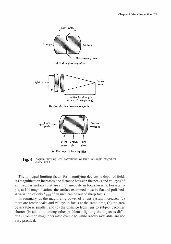
• Coddington Magnifier (Fig. 4a). This device uses a double convex lens with a groove ground in the middle. This diaphragm-like groove im-proves image quality by eliminating marginal rays of light.
• Double Plano-Convex Magnifier (Fig. 4b). This two-lens magnifier gives partial chromatic correction and flatter field of view.
• Hastings Triplet Magnifier (Fig. 4c). This is a multiglass lens corrected for both spherical and chromatic aberration. This is the best of all hand-held magnifiers.
Chapter 2: Visual Inspection / 29
The principal limiting factor for magnifying devices is depth of field. As magnification increases, the distance between the peaks and valleys (of an irregular surface) that are simultaneously in focus lessens. For exam-ple, at 100 magnifications the surface examined must be flat and polished. A variation of only 1⁄1000 of an inch can be out of sharp focus.
In summary, as the magnifying power of a lens system increases: (a) there are fewer peaks and valleys in focus at the same time, (b) the area observable is smaller, and (c) the distance from lens to subject becomes shorter (in addition, among other problems, lighting the object is diffi-cult). Common magnifiers rated over 20×, while readily available, are not very practical.
Fig� 4 Diagram showing lens corrections available in simple magnifiers. Source: Ref 1
30 / Inspection of Metals—Understanding the Basics
One other limiting factor in magnifying devices is light loss due to re-flection. Lens surfaces can be coated with special antireflection coatings to reduce light loss, which may be particularly useful when the level of light is low.
Simple Magnifiers
Simple magnifiers come in many varieties, and new devices are regu-larly being developed. The following is an effort to group the various de-vices into categories:
• Hand-held lenses, single and multiple• Pocket microscopes • Self-supporting magnifiers • Magnifying devices which can be worn attached to the head or in some
manner be used like eyeglasses or in conjunction with eyeglasses • Magnifying devices with built-in light sources
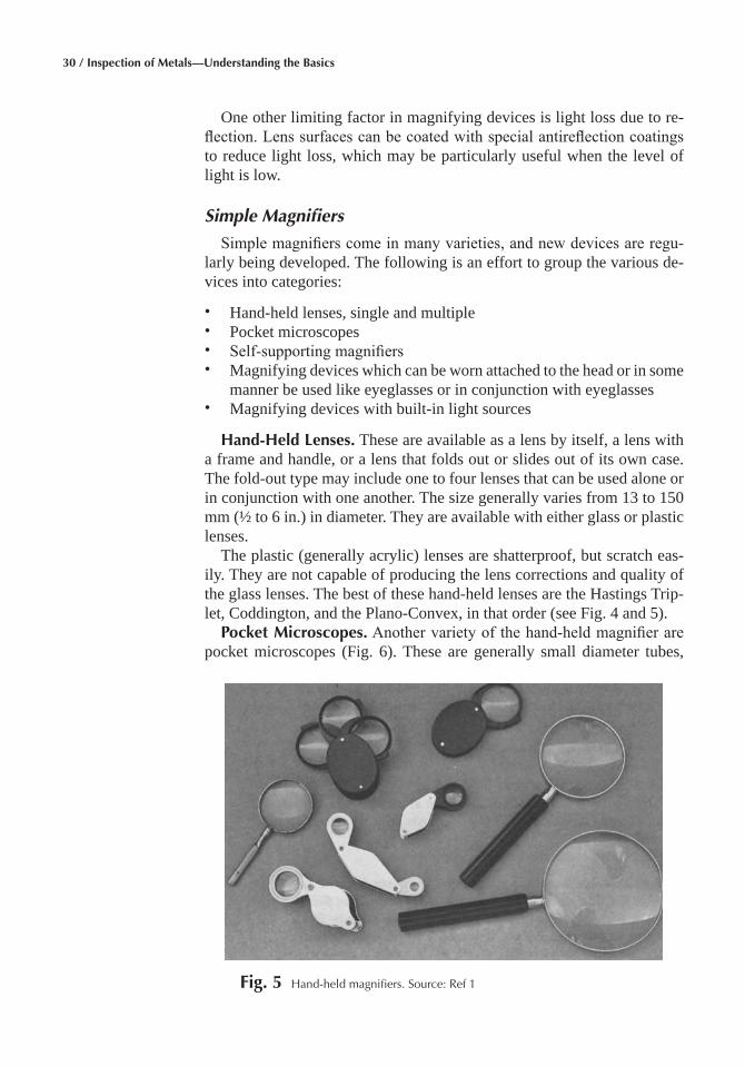
Hand-Held Lenses� These are available as a lens by itself, a lens with a frame and handle, or a lens that folds out or slides out of its own case. The fold-out type may include one to four lenses that can be used alone or in conjunction with one another. The size generally varies from 13 to 150 mm (½ to 6 in.) in diameter. They are available with either glass or plastic lenses.
The plastic (generally acrylic) lenses are shatterproof, but scratch eas-ily. They are not capable of producing the lens corrections and quality of the glass lenses. The best of these hand-held lenses are the Hastings Trip-let, Coddington, and the Plano-Convex, in that order (see Fig. 4 and 5).
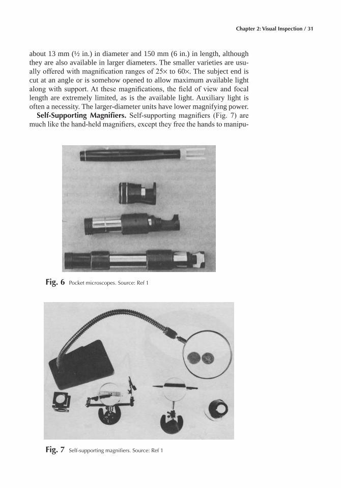
Pocket Microscopes� Another variety of the hand-held magnifier are pocket microscopes (Fig. 6). These are generally small diameter tubes,
Fig� 5 Hand-held magnifiers. Source: Ref 1
Chapter 2: Visual Inspection / 31
about 13 mm (½ in.) in diameter and 150 mm (6 in.) in length, although they are also available in larger diameters. The smaller varieties are usu-ally offered with magnification ranges of 25× to 60×. The subject end is cut at an angle or is somehow opened to allow maximum available light along with support. At these magnifications, the field of view and focal length are extremely limited, as is the available light. Auxiliary light is often a necessity. The larger-diameter units have lower magnifying power.
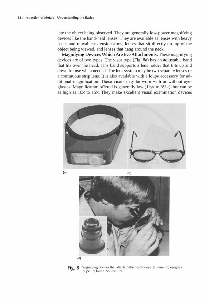
Self-Supporting Magnifiers� Self-supporting magnifiers (Fig. 7) are much like the hand-held magnifiers, except they free the hands to manipu-
Fig� 6 Pocket microscopes. Source: Ref 1
Fig� 7 Self-supporting magnifiers. Source: Ref 1
32 / Inspection of Metals—Understanding the Basics
late the object being observed. They are generally low-power magnifying devices like the hand-held lenses. They are available as lenses with heavy bases and movable extension arms, lenses that sit directly on top of the object being viewed, and lenses that hang around the neck.
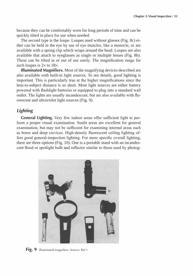
Magnifying Devices Which Are Eye Attachments� These magnifying devices are of two types. The visor type (Fig. 8a) has an adjustable band that fits over the head. This band supports a lens holder that tilts up and down for use when needed. The lens system may be two separate lenses or a continuous strip lens. It is also available with a loupe accessory for ad-ditional magnification. These visors may be worn with or without eye-glasses. Magnification offered is generally low (1½× to 3½×), but can be as high as 10× to 15×. They make excellent visual examination devices
Fig� 8 Magnifying devices that attach to the head or eye: (a) visor, (b) eyeglass loupe, (c) loupe. Source: Ref 1
Chapter 2: Visual Inspection / 33
because they can be comfortably worn for long periods of time and can be quickly tilted in place for use when needed.
The second type is the loupe. Loupes used without glasses (Fig. 8c) ei-ther can be held in the eye by use of eye muscles, like a monocle, or are available with a spring clip which wraps around the head. Loupes are also available that attach to eyeglasses as single or multiple lenses (Fig. 8b). These can be tilted in or out of use easily. The magnification range for such loupes is 2× to 18×.
Illuminated Magnifiers� Most of the magnifying devices described are also available with built-in light sources. To see details, good lighting is important. This is particularly true at the higher magnifications since the lens-to-subject distance is so short. Most light sources are either battery powered with flashlight batteries or equipped to plug into a standard wall outlet. The lights are usually incandescent, but are also available with flu-orescent and ultraviolet light sources (Fig. 9).
Lighting
General Lighting� Very few indoor areas offer sufficient light to per-form a proper visual examination. Sunlit areas are excellent for general examination, but may not be sufficient for examining internal areas such as bores and deep crevices. High-density fluorescent ceiling lighting of-fers good general-inspection lighting. For more specific overall lighting, there are three options (Fig. 10). One is a portable stand with an incandes-cent flood or spotlight bulb and reflector similar to those used by photog-
Fig� 9 Illuminated magnifiers. Source: Ref 1
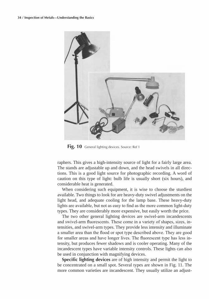
34 / Inspection of Metals—Understanding the Basics
raphers. This gives a high-intensity source of light for a fairly large area. The stands are adjustable up and down, and the head swivels in all direc-tions. This is a good light source for photographic recording. A word of caution on this type of light: bulb life is usually short (six hours), and considerable heat is generated.
When considering such equipment, it is wise to choose the sturdiest available. Two things to look for are heavy-duty swivel adjustments on the light head, and adequate cooling for the lamp base. These heavy-duty lights are available, but not as easy to find as the more common light-duty types. They are considerably more expensive, but easily worth the price.
The two other general lighting devices are swivel-arm incandescents and swivel-arm fluorescents. These come in a variety of shapes, sizes, in-tensities, and swivel-arm types. They provide less intensity and illuminate a smaller area than the flood or spot type described above. They are good for smaller areas and have longer lives. The fluorescent type has less in-tensity, but produces fewer shadows and is cooler operating. Many of the incandescent types have variable intensity controls. These lights can also be used in conjunction with magnifying devices.
Specific lighting devices are of high intensity and permit the light to be concentrated on a small spot. Several types are shown in Fig. 11. The more common varieties are incandescent. They usually utilize an adjust-
Fig� 10 General lighting devices. Source: Ref 1
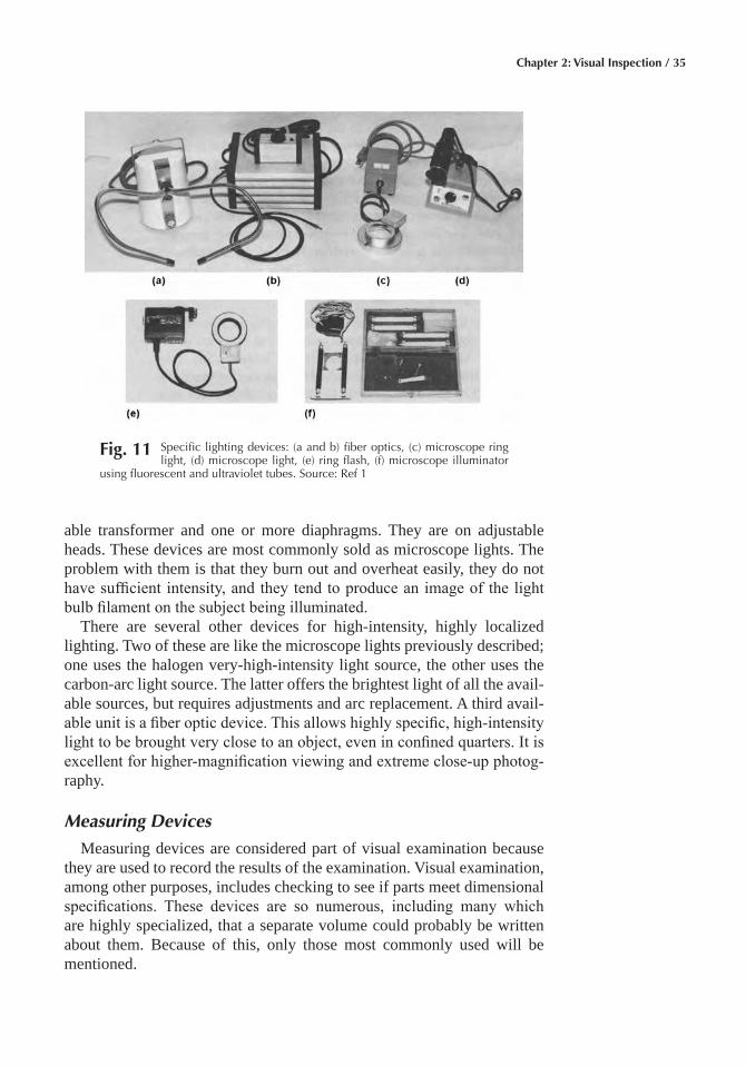
Chapter 2: Visual Inspection / 35
able transformer and one or more diaphragms. They are on adjustable heads. These devices are most commonly sold as microscope lights. The problem with them is that they burn out and overheat easily, they do not have sufficient intensity, and they tend to produce an image of the light bulb filament on the subject being illuminated.
There are several other devices for high-intensity, highly localized lighting. Two of these are like the microscope lights previously described; one uses the halogen very-high-intensity light source, the other uses the carbon-arc light source. The latter offers the brightest light of all the avail-able sources, but requires adjustments and arc replacement. A third avail-able unit is a fiber optic device. This allows highly specific, high-intensity light to be brought very close to an object, even in confined quarters. It is excellent for higher-magnification viewing and extreme close-up photog- raphy.
Measuring Devices
Measuring devices are considered part of visual examination because they are used to record the results of the examination. Visual examination, among other purposes, includes checking to see if parts meet dimensional specifications. These devices are so numerous, including many which are highly specialized, that a separate volume could probably be written about them. Because of this, only those most commonly used will be mentioned.
Fig� 11 Specific lighting devices: (a and b) fiber optics, (c) microscope ring light, (d) microscope light, (e) ring flash, (f) microscope illuminator
using fluorescent and ultraviolet tubes. Source: Ref 1
36 / Inspection of Metals—Understanding the Basics
Linear Measuring Devices� The most common measuring unit is the ruled straightedge. These come in many forms, such as the 12-inch rule and 36-inch yardstick, both of which are being replaced by meter sticks. Until the transition to the metric system is universal, both English and metric devices must be utilized. In addition, tape measures, which are available from 150 mm (6 in.) in length to over 30 mm (100 ft), are essen-tial for visual examination.
Of the rules, the 150 and 300 mm (6 and 12 in.) steel rules are desirable. The 150 mm (6 in.) scales, some of which can be clipped to a shirt pocket, are available with several scales on each rule. Scales can be both English and metric on the same rule and may be subdivided to as small as 1⁄100-inch divisions. These devices are also available with an adjustable 90° squaring edge to check for straightness.
Reticles�There are many magnifying devices available with built-in reticles (Fig. 12). Reticles made to measure nearly anything imaginable are available. If the desired reticle is not available, it can be custom-made.
Micrometers are extremely accurate mechanical devices. They are commonly used to measure to 1⁄1000 of an inch and can be used to 1⁄10,000 of an inch. Both inside and outside micrometers are available. Some incorpo-rate both in the same unit. They are available with various measuring tips (these are normally hardened to prevent wear). Tips can be flat, rounded, pointed, or blade. Others may also be available or custom-made. Very lit-tle training is required to use these devices, but experience produces more consistently accurate results.
Optical comparators (Fig. 13) are excellent devices for both visual examination and measurement. A comparator produces a two-dimensional enlarged image of an object on a large ground-glass screen. It can be used with reflected light or background lighting (or a combination of both). Magnification is available from actual size to 50×. Comparison templates can be placed on the screen to check dimensional accuracy. Results can be readily photographed.
Miscellaneous Measuring Devices (Fig� 14)� The dial indicator con-sists of a plunger-actuated dial, usually calibrated in 1⁄1000 of an inch. It comes with a series of mechanical arms and clamping devices such that it can be attached to a fixed (rigid) object and reference measurements can be made. A common usage is attachment to a lathe bed to check both hori-zontal and circumferential dimensional variations.
There are many specialty measuring gages. Some of these are inside micrometers, tubing wall measuring micrometers (one rounded anvil and one flat anvil), depth gages, thread-measuring gages, protractors and bevel protractors (to measure angles), levels (to measure variation from hori-zontal), inside and outside calipers, hole and plug gages (to measure diam-eter and uniformity of holes), radius gages, screw-pitch gages, thickness gages (a series of leaves of various known thicknesses to check clearance).
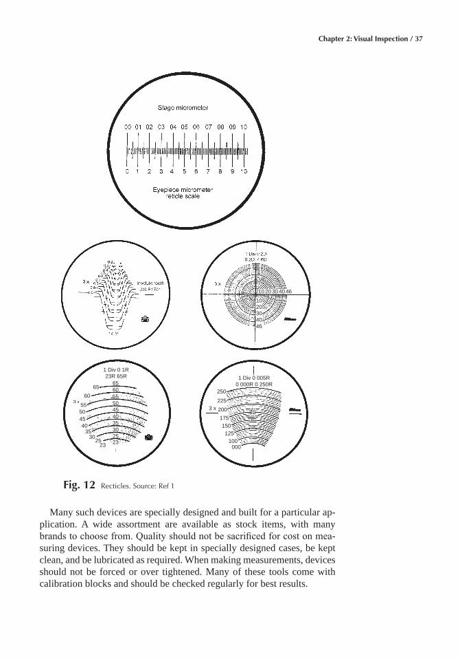
Chapter 2: Visual Inspection / 37
Many such devices are specially designed and built for a particular ap-plication. A wide assortment are available as stock items, with many brands to choose from. Quality should not be sacrificed for cost on mea-suring devices. They should be kept in specially designed cases, be kept clean, and be lubricated as required. When making measurements, devices should not be forced or over tightened. Many of these tools come with calibration blocks and should be checked regularly for best results.
10 20 30 40 46
1020304046
65
60
55504540
3530
2523
65605550454035302523
1 Div 0 1R23R 65R 1 Div 0 005R
0 000R 0 250R250
225
175150125
100000
3 x 200
Fig� 12 Recticles. Source: Ref 1
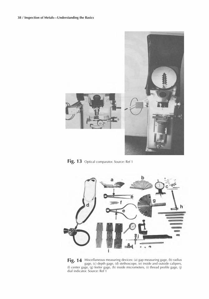
38 / Inspection of Metals—Understanding the Basics
Fig� 13 Optical comparator. Source: Ref 1
Fig� 14 Miscellaneous measuring devices: (a) gap measuring gage, (b) radius gage, (c) depth gage, (d) stethoscope, (e) inside and outside calipers,
(f) center gage, (g) feeler gage, (h) inside micrometers, (i) thread profile gage, (j) dial indicator. Source: Ref 1
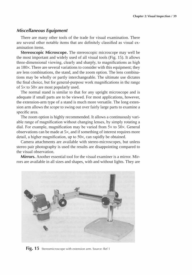
Chapter 2: Visual Inspection / 39
Miscellaneous Equipment
There are many other tools of the trade for visual examination. There are several other notable items that are definitely classified as visual ex-amination items.
Stereoscopic Microscope� The stereoscopic microscope may well be the most important and widely used of all visual tools (Fig. 15). It allows three-dimensional viewing, clearly and sharply, to magnifications as high as 180×. There are several variations to consider with this equipment; they are lens combinations, the stand, and the zoom option. The lens combina-tions may be wholly or partly interchangeable. The ultimate use dictates the final choice, but for general-purpose work magnifications in the range of 5× to 50× are most popularly used.
The normal stand is similar to that for any upright microscope and is adequate if small parts are to be viewed. For most applications, however, the extension-arm type of a stand is much more versatile. The long exten-sion arm allows the scope to swing out over fairly large parts to examine a specific area.
The zoom option is highly recommended. It allows a continuously vari-able range of magnification without changing lenses, by simply rotating a dial. For example, magnification may be varied from 5× to 50×. General observations can be made at 5×, and if something of interest requires more detail, a higher magnification, up to 50×, can rapidly be obtained.
Camera attachments are available with stereo-microscopes, but unless stereo pair photography is used the results are disappointing compared to the visual observation.
Mirrors� Another essential tool for the visual examiner is a mirror. Mir-rors are available in all sizes and shapes, with and without lights. They are
Fig� 15 Stereomicroscope with extension arm. Source: Ref 1
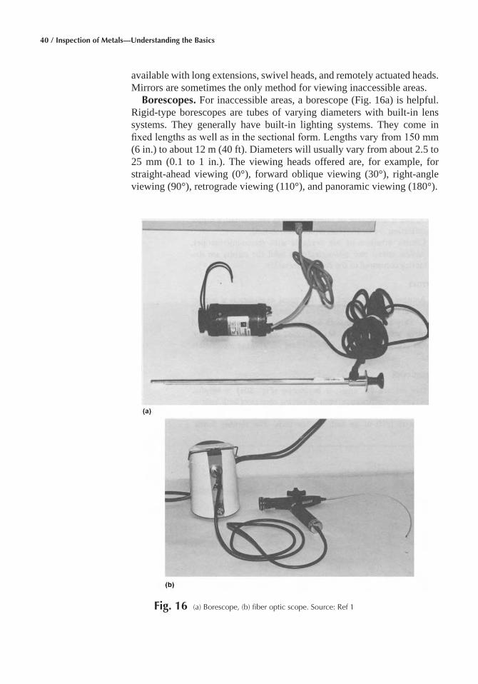
40 / Inspection of Metals—Understanding the Basics
available with long extensions, swivel heads, and remotely actuated heads. Mirrors are sometimes the only method for viewing inaccessible areas.
Borescopes� For inaccessible areas, a borescope (Fig. 16a) is helpful. Rigid-type borescopes are tubes of varying diameters with built-in lens systems. They generally have built-in lighting systems. They come in fixed lengths as well as in the sectional form. Lengths vary from 150 mm (6 in.) to about 12 m (40 ft). Diameters will usually vary from about 2.5 to 25 mm (0.1 to 1 in.). The viewing heads offered are, for example, for straight-ahead viewing (0°), forward oblique viewing (30°), right-angle viewing (90°), retrograde viewing (110°), and panoramic viewing (180°).
Fig� 16 (a) Borescope, (b) fiber optic scope. Source: Ref 1
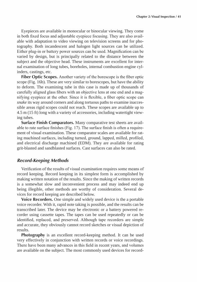
Chapter 2: Visual Inspection / 41
Eyepieces are available in monocular or binocular viewing. They come in both fixed focus and adjustable eyepiece focusing. They are also avail-able with adaptation to video viewing on television screens and for pho-tography. Both incandescent and halogen light sources can be utilized. Either plug-in or battery power sources can be used. Magnification can be varied by design, but is principally related to the distance between the subject and the objective head. These instruments are excellent for inter-nal examination of long tubes, boreholes, internal combustion engine cyl-inders, castings, etc.
Fiber Optic Scopes� Another variety of the borescope is the fiber optic scope (Fig. 16b). These are very similar to borescopes, but have the ability to deform. The examining tube in this case is made up of thousands of carefully aligned glass fibers with an objective lens at one end and a mag-nifying eyepiece at the other. Since it is flexible, a fiber optic scope can snake its way around corners and along tortuous paths to examine inacces-sible areas rigid scopes could not reach. These scopes are available up to 4.5 m (15 ft) long with a variety of accessories, including watertight view-ing tubes.
Surface Finish Comparators� Many comparative test sheets are avail-able to rate surface finishes (Fig. 17). The surface finish is often a require-ment of visual examination. These comparator scales are available for rat-ing machined surfaces, including turned, ground, lapped, milled, profiled, and electrical discharge machined (EDM). They are available for rating grit-blasted and sandblasted surfaces. Cast surfaces can also be rated.
Record-Keeping Methods
Verification of the results of visual examination requires some means of record keeping. Record keeping in its simplest form is accomplished by making written notation of the results. Since the making of written records is a somewhat slow and inconvenient process and may indeed end up being illegible, other methods are worthy of consideration. Several de-vices for record keeping are described below.
Voice Recorders� One simple and widely used device is the a portable voice recorder. With it, rapid note taking is possible, and the results can be transcribed later. The device may be electronic or a battery powered re-corder using cassette tapes. The tapes can be used repeatedly or can be identified, replaced, and preserved. Although tape recorders are simple and accurate, they obviously cannot record sketches or visual depiction of results.
Photography is an excellent record-keeping method. It can be used very effectively in conjunction with written records or voice recordings. There have been many advances in this field in recent years, and volumes are available on the subject. The most commonly used devices for record-
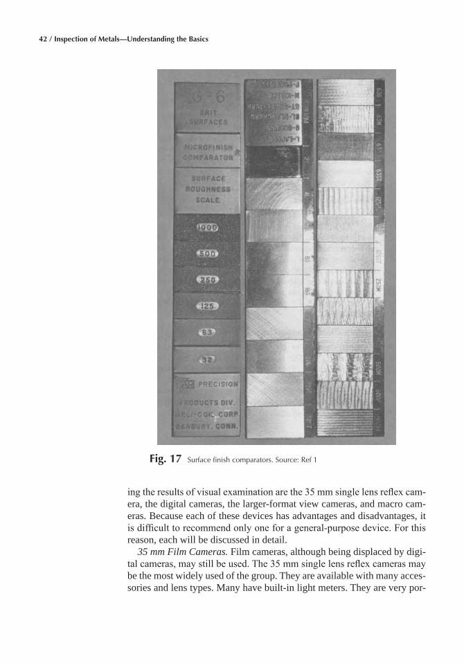
42 / Inspection of Metals—Understanding the Basics
ing the results of visual examination are the 35 mm single lens reflex cam-era, the digital cameras, the larger-format view cameras, and macro cam-eras. Because each of these devices has advantages and disadvantages, it is difficult to recommend only one for a general-purpose device. For this reason, each will be discussed in detail.
35 mm Film Cameras. Film cameras, although being displaced by digi-tal cameras, may still be used. The 35 mm single lens reflex cameras may be the most widely used of the group. They are available with many acces-sories and lens types. Many have built-in light meters. They are very por-
Fig� 17 Surface finish comparators. Source: Ref 1
Chapter 2: Visual Inspection / 43
table and produce excellent results. The operator looks directly through the lens in composing the picture, which prevents forgetting to remove the lens cap or having a thumb in the photo. At the time of exposure, a mirror device pivots out of the way, the exposure is made, and the viewing mirror returns to position. Lenses are interchangeable. Exposure times are vari-able and can be as little as 1⁄1000 of a second. Apertures vary, allowing light-entrance control and variation in the depth of focus. Lighting can be sunlight, artificial, flash, or strobe-type high-intensity lighting. These cameras usually take 20- or 36- exposure films. Film is available in many types and speeds, in either black-and-white or color. Film is also available for prints or slide projection. Cost per picture is low due to the small size of the film. The principal disadvantage of this camera is the small size of the film, which requires enlarging. If enlarged too much, loss of detail and graininess can occur. Another disadvantage is that 20 or 36 exposures must be made before developing, to avoid wasting film. After all of the exposures, delay may be experienced while the film is developed and each frame separately enlarged and printed. But the speed, versatility, portabil-ity, and variety of high-quality equipment and film generally outweigh any disadvantages, making 35 mm cameras an excellent choice for a wide range of record-keeping chores.
Digital Cameras. Digital cameras have the advantage of producing rapid records. This ensures that the results are what is expected without the delay of shooting, developing, and printing a roll of film. The resolu-tion in a digital image is determined by the number of pixels in the imag-ing sensor; the higher the number of pixels, the greater the image resolu-tion. High resolution photographs are attainable with multiple megapixel sensor arrays. Image file sizes in the multiple megabyte range produce excellent photographs with enlargement capability.
View Cameras. View cameras are simply cameras with a larger format. Common sizes are 4 by 5 inches, 5 by 7 inches, and 8 by 10 inches. These cameras produce probably the best quality, most detailed photos. They are somewhat bulky and often require tripod support. Film is available in black and white and in color. Prints can be greatly enlarged with little loss of detail.
Macro cameras. are another form of the view camera. They are particu-larly adapted to produce magnified photos. This is accomplished by use of special lenses in conjunction with focusing bellows. These cameras are best used with smaller parts. Lighting for this equipment is important. At higher magnifications, the lens-to-subject distance is short and lighting is even more difficult. A variety of films are available for use with this equip-ment, including black-and-white cut film, color film, and all of the rapid film types.
Photography Lighting. Lighting for all types of photography is very important. The choices are many, such as daylight, artificial light, flood-
44 / Inspection of Metals—Understanding the Basics
lights, photoflash, and all of the highly specific lights described earlier under the section “Lighting.” The type of lighting required is a function of the film type and, to a lesser degree, of the camera.
Motion Picture Photography. An advance in record-keeping photogra-phy is the motion picture or movie camera, which allows the taking of a sequence of thousands of photos. It records motion and when played back can slow or stop motion at any point. It can be used in conjunction with sound recording which becomes an integral part of the film. Sound can be the actual sound occurring during filming, or sound added later while viewing the film, as commentary. Both black-and-white and color film are available.
Video Recorders� A record-keeping device that promises to be widely used in the future is the video tape recorder. The equipment has been used for many years by the television industry, but has only recently become available in more portable and inexpensive forms. The video tape recorder produces records similar to the movie camera. The principal difference is that the results can be viewed instantly without processing. They can be shown on any standard television or video screen, and the recording tapes can either be stored or erased and used again.
Macroetching
Various imperfections or defects invisible to the naked eye can often be detected by hot or cold acid etching. Since the cross-section usually pro-vides more information than the longitudinal section, the general practice is to cut discs transversely; i.e., perpendicular to the hot working axis. To facilitate handling, disc thickness should generally be 25 mm (1 in.) or less. Longitudinal sectioning is used to study fibering, segregation, and inclusions. Common uses of macroetching are given below.
Solidification Structures� The structure resulting from solidification can be clearly revealed by macroetching. The macrostructure of a trans-verse disc cut from a small laboratory size steel ingot that was etched with 10% HNO3 in water is shown in Fig. 18. At the mold surface, there is a small layer of very fine equiaxed grains. From this outer shell, large co-lumnar grains grow inward toward the central, equiaxed region.
Billet and Bloom Macrostructures� The steelmaker uses hot acid etching on discs cut, with respect to the ingot location, from the top and bottom or the top, middle, and bottom of billets or blooms rolled from the first, middle, and last ingots teemed from the heat. If a disc reveals a re-jectable condition, the billet material is rejected until the condition is removed.
Continuously Cast Steel Macrostructures� Continuous casting has become an important process for producing metals. Macroetching has been widely employed in the development of macroetching to evaluate the
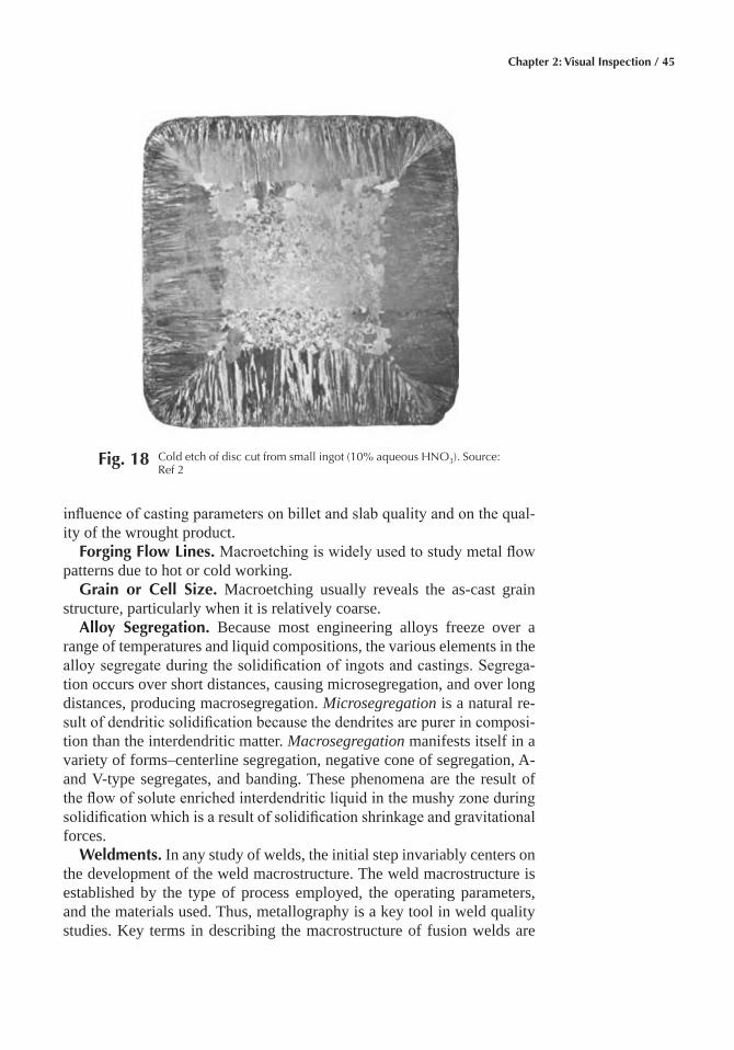
Chapter 2: Visual Inspection / 45
influence of casting parameters on billet and slab quality and on the qual-ity of the wrought product.
Forging Flow Lines� Macroetching is widely used to study metal flow patterns due to hot or cold working.
Grain or Cell Size� Macroetching usually reveals the as-cast grain structure, particularly when it is relatively coarse.
Alloy Segregation� Because most engineering alloys freeze over a range of temperatures and liquid compositions, the various elements in the alloy segregate during the solidification of ingots and castings. Segrega-tion occurs over short distances, causing microsegregation, and over long distances, producing macrosegregation. Microsegregation is a natural re-sult of dendritic solidification because the dendrites are purer in composi-tion than the interdendritic matter. Macrosegregation manifests itself in a variety of forms–centerline segregation, negative cone of segregation, A- and V-type segregates, and banding. These phenomena are the result of the flow of solute enriched interdendritic liquid in the mushy zone during solidification which is a result of solidification shrinkage and gravitational forces.
Weldments� In any study of welds, the initial step invariably centers on the development of the weld macrostructure. The weld macrostructure is established by the type of process employed, the operating parameters, and the materials used. Thus, metallography is a key tool in weld quality studies. Key terms in describing the macrostructure of fusion welds are
Fig� 18 Cold etch of disc cut from small ingot (10% aqueous HNO3). Source: Ref 2
46 / Inspection of Metals—Understanding the Basics
the basic three components—the weld metal or nugget, the heat affected zone (HAZ), and the base metal.
Within the weld metal and the heat affected zone, there are changes in composition, grain size and orientation, microstructure, and hardness. Thus one observes significant variations in microstructure as the weld-ment is scanned.
Macroetching is frequently employed to determine the influence of var-ious changes in weld parameters on the size and shape of the weld metal, on depth of penetration, on weld structure, and on hardness.
Response to Heat Treatment� Macroetching can also be used to de-termine the hardenability of various steel bars subjected to known heat treatment conditions. This procedure, coupled with hardness testing, was widely used prior to the adoption of hardenability analysis. As an illustration, Fig. 19 shows discs cut from round bars of AISI 1060 car-bon steel ranging in size from a diameter of 20 to 65 mm (¾ to 2½ in.). The two smallest sizes were through hardened, that is, the center region contains more than 50% martensite, and the etch pattern was uniform. The other three sizes exhibit a case and core pattern, since the central region was unhardened. For this test, all bars were austenitized at 829 °C (1525°F), brine quenched, and then tempered at 149 °C (300°F). The bar length was twice the diameter, and the etched section was taken from the center.
Cold etching is also useful in studying the results of surface hardening treatments. Figure 20 shows the results of induction hardening of gear teeth made from AISI 1055 carbon steel. The areas hardened and the depth of the hardened zone are quite apparent.
Fig� 19 Macroetching (10% aqueous HN03) was used to reveal the extent of hardening in these AISI 1060 carbon steel round bars. Source: Ref 2
Chapter 2: Visual Inspection / 47
ACKNOWLEDGMENT
This chapter was adapted from Inspection of Metals, Volume 1, Visual Inspection by R.C. Anderson, 1983, and Metallography–Principles and Practice, by G.F. Vander Voort, 1999.
REFERENCES
1. R.C. Anderson, Inspection of Metals, Volume 1, Visual Inspection, American Society for Metals, 1983
2. G.F. Vander Voort, Metallography–Principles and Practice, ASM In-ternational, 1999
Fig� 20 The depth and extent of hardening in these induction hardened gear teeth made of AISI 1055 carbon steel was determined by macroetching with 10% aqueous HNO3. Sur-
face hardness was 53 to 54 HRC while the unhardened area was about 23 HRC. Source: Ref 2

Inspection of Metals—Understanding the Basics Copyright © 2013 ASM International®
F.C. Campbell, editor All rights reservedwww.asminternational.org
CHAPTER 3
Coordinate Measuring Machines
THE COORDINATE MEASURING MACHINE (CMM) is used for three-dimensional inspection of both in-process and finished parts. His-torically, CMMs have been largely used to measure and collect dimen-sional inspection data used to make acceptance or rejection decisions. Al-though CMMs continue to play this role, manufacturers are placing new emphasis on using CMMs to capture data from many sources and bring them together centrally where they can be used to control the manufactur-ing process more effectively and to prevent defective components from being produced. In addition, CMMs are also being used in entirely new applications; for example, reverse engineering and computer-aided design and manufacture (CAD/CAM) applications as well as innovative ap-proaches to manufacturing, such as the flexible manufacturing systems, manufacturing cells, machining centers, and flexible transfer lines.
Important terminology for CMMs includes:
• Ball bar: A gage consisting of two highly spherical tooling balls of the same diameter connected by a rigid bar
• Gage: A mechanical artifact of high precision used either for checking a part or for checking the accuracy of a machine; a measuring device with a proportional range and some form of indicator, either analog or digital
• Pitch: The angular motion of a carriage, designed for linear motion, about an axis that is perpendicular to the motion direction and perpen-dicular to the yaw axis
• Pixel: The smallest element into which an image is divided, such as the dots on a television screen
• Plane: A surface of a part that is defined by three points
50 / Inspection of Metals—Understanding the Basics
• Repeatability: A measure of the ability of an instrument to produce the same indication (or measured value) when sequentially sensing the same quantity under similar conditions
• Roll: The angular motion of a carriage, designed for linear motion, about the linear motion axis
• Yaw: The angular motion of a carriage, designed for linear motion, about a specified axis perpendicular to the motion direction. In the case of a carriage with horizontal motion, the specified axis should be vertical unless explicitly specified. For a carriage that does not have horizontal motion, the axis must be explicitly specified
CMM Operating Principles
A CMM is a multiaxial device with two to six axes of travel or refer-ence axes, each of which provides a measurement output of position or displacement. Coordinate measuring machines are primarily character-ized by their flexibility, being able to make many measurements without adding or changing tools. As products evolve, the same CMM can gener-ally be used, depending on size and accuracy limitations, simply by alter-ing software instead of altering equipment mechanics or electronics.
CMMs consist of the machine itself and its probes and moving arms for providing measurement input, a computer for making rapid calculations and comparisons (to blueprint specifications, for example) based on the measurement input, and the computer software that controls the entire system. In addition, the CMM has some means of providing output to the user (printer, plotter CRT) and/or to other machines in a complete manu-facturing system. Coordinate measuring machines linked together in an overall inspection or manufacturing system are referred to as coordinate measuring systems.
The most important feature of the CMM is that it can rapidly and ac-curately measure objects of widely varying size and geometric configura-tion; for example, a particular part and the tooling for that part. Coordinate measuring machines can also readily measure the many different fea-tures of a part, such as holes, slots, studs, and weld-nuts, without needing other tools. Therefore, CMMs can replace the numerous hand tools used for measurement as well as the open plate and surface plate inspection tools and hard gages traditionally used for part measurement and in- spection.
Coordinate measuring machines do not always achieve the rates of throughput or levels of accuracy possible with fixed automation type mea-suring systems. However, if any changes must be made in a fixed system for any reason; for example, a different measurement of the same part or measurement of a different part, making the change will be costly and time consuming. This is not the case with a CMM. Changes in the mea-surement or inspection routine of a CMM are made quickly and easily
Chapter 3: Coordinate Measuring Machines / 51
by simply editing the computer program that controls the machine. The greater or more frequent the changes required, the greater the advantage of the CMM over traditional measuring devices. This flexibility, as well as the resulting versatility, is the principal advantage of the CMM.
CMM Measurement Techniques
A CMM takes measurements of an object within its work envelope by moving a sensing device called a probe along the various axes of travel until the probe contacts the object. The precise position of the contact is recorded and recorded as a measurement output of position or displace-ment (Fig. 1). The CMM is used to make numerous contacts, or hits, with the probe; using all axes of travel, until an adequate data base of the sur-faces of the object has been constructed. Various features of an object re-quire different quantities of hits to be accurately recorded. For example, a plane, surface, or circular hole can be recorded with a minimum of three hits.
Once repeated hits or readings have been made and stored, they can be used in a variety of ways through the computer and geometric measure-ment software. The data can be used to create a master program; for ex-ample, of the precise specifications for a part. They can also be compared (via the software) to stored part specification data or used to inspect pro-duction parts for compliance with specifications. A variety of other so-phisticated applications are also possible using the same captured mea-surement data; for example, the reverse engineering of broken parts or the development of part specifications from handmade models.
x
y
Fig� 1 Elements of a CMM showing typical digital position readout. The probe is positioned by brackets slid along two arms. Coordinate distances
from one point to another are measured in effect by counting electronically the lines in gratings ruled along each arm. Any point in each direction can be set to zero, and the count is made in a plus or minus direction from there. Source: Ref 1
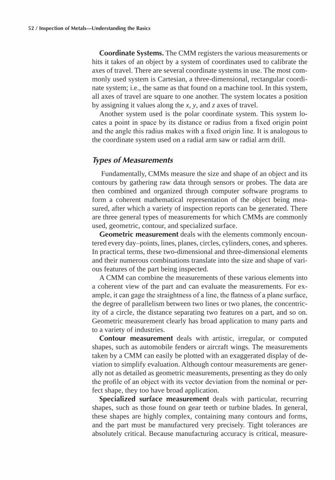
52 / Inspection of Metals—Understanding the Basics
Coordinate Systems� The CMM registers the various measurements or hits it takes of an object by a system of coordinates used to calibrate the axes of travel. There are several coordinate systems in use. The most com-monly used system is Cartesian, a three-dimensional, rectangular coordi-nate system; i.e., the same as that found on a machine tool. In this system, all axes of travel are square to one another. The system locates a position by assigning it values along the x, y, and z axes of travel.
Another system used is the polar coordinate system. This system lo-cates a point in space by its distance or radius from a fixed origin point and the angle this radius makes with a fixed origin line. It is analogous to the coordinate system used on a radial arm saw or radial arm drill.
Types of Measurements
Fundamentally, CMMs measure the size and shape of an object and its contours by gathering raw data through sensors or probes. The data are then combined and organized through computer software programs to form a coherent mathematical representation of the object being mea-sured, after which a variety of inspection reports can be generated. There are three general types of measurements for which CMMs are commonly used, geometric, contour, and specialized surface.
Geometric measurement deals with the elements commonly encoun-tered every day–points, lines, planes, circles, cylinders, cones, and spheres. In practical terms, these two-dimensional and three-dimensional elements and their numerous combinations translate into the size and shape of vari-ous features of the part being inspected.
A CMM can combine the measurements of these various elements into a coherent view of the part and can evaluate the measurements. For ex-ample, it can gage the straightness of a line, the flatness of a plane surface, the degree of parallelism between two lines or two planes, the concentric-ity of a circle, the distance separating two features on a part, and so on. Geometric measurement clearly has broad application to many parts and to a variety of industries.
Contour measurement deals with artistic, irregular, or computed shapes, such as automobile fenders or aircraft wings. The measurements taken by a CMM can easily be plotted with an exaggerated display of de-viation to simplify evaluation. Although contour measurements are gener-ally not as detailed as geometric measurements, presenting as they do only the profile of an object with its vector deviation from the nominal or per-fect shape, they too have broad application.
Specialized surface measurement deals with particular, recurring shapes, such as those found on gear teeth or turbine blades. In general, these shapes are highly complex, containing many contours and forms, and the part must be manufactured very precisely. Tight tolerances are absolutely critical. Because manufacturing accuracy is critical, measure-
Chapter 3: Coordinate Measuring Machines / 53
ment is also highly critical, and a specialty in measuring these forms has evolved. By its nature, specialized surface measurement is applied to far fewer applications than the other two types.
CMM Capabilities
Coordinate measuring machines have the fundamental ability to collect a variety of different types of very precise measurements and to do so quickly, with high levels of repeatability and great flexibility. In addition, they offer other important capabilities based on computational functions.
Automatic Calculation of Measurement Data� The inclusion of a computer in the CMM allows the automatic calculation of such workpiece features as hole size, boss size, the distance between points, incremental distances, feature angles, and intersections. Prior to this stage of CMM development, an inspector had to write down the measurements he ob-tained and manually compare them to the blueprint. Not only is such a process subject to error, but it is relatively time consuming. While waiting for the results of the inspection, production decisions are delayed and parts (possibly not being produced to specifications) are being manufactured.
Compensation for Misaligned Parts� Coordinate measuring machines no longer require that the parts being measured be manually aligned to the coordinate system of the machine. The operator cannot casually place the part within the CMM work envelope. Once the location of the appropriate reference surface or line has been determined through a series of hits on the datum features of the part, the machine automatically references that position as its zero-zero starting point, creates an x, y, z part coordinate system, and makes all subsequent measurements relative to that point. In addition, the part does not have to be leveled within the work envelope. Just as the CMM will mathematically compensate if the part is rotation-ally misaligned, it will also compensate for any tilt in the part.
Multiple Frames of Reference� The CMM can also create and store multiple frames of reference or coordinate systems that allows features to be measured on all surfaces of an object quickly and efficiently. The CMM automatically switches to the appropriate new alignment system and zero point (origin) for each plane (face) of the part. The CMM can also provide axis and plane rotation automatically.
Probe Calibration�The CMM automatically calibrates for the size and location of the probe tip (contact element) being used. It also automati-cally calibrates each tip of a multiple-tip probe.
Part Program and Data Storage� The CMM stores the program for a given part so that the program and the machine are ready to perform when-ever this part comes up for inspection. The CMM can also store the results of all prior inspections of a given part or parts so that a complete history of its production can be reconstructed. This same capability also provides the groundwork for statistical process control applications.
54 / Inspection of Metals—Understanding the Basics
Part programs can also be easily edited, rather than completely rewrit-ten, to account for design changes. When a dimension or a feature of a part is changed, only that portion of the program involving the workpiece revi-sion must be edited to conform to part geometry.
Interface and Output� CMMs can be linked together in an overall system or can be integrated with other devices in a complete manufactur-ing system. The CMM can provide the operator with a series of prompts that explain what to do next and guide the operator through the complete measurement routine. Output is equally flexible. The user can choose the type and format of the report to be generated. Data can be displayed in a wide variety of charts and graphs. Inspection comments can be included in the hard copy report and/or stored in memory for analysis of production runs.
CMM Applications
Coordinate measuring machines are most frequently used in two major roles: quality control and process control. In the area of quality control, CMMs can generally perform traditional final part inspection more accu-rately, more rapidly, and with greater repeatability than traditional surface plate methods.
In process control, CMMs are providing new capabilities. Because of the on-line, real-time analytical capability of many CMM software pack-ages, CMMs are increasingly used to monitor and identify evolving trends in production before scrap or out-of-spec parts are fabricated in the first place. Thus, the emphasis has shifted from inspecting parts and subse-quently rejecting scrap parts at selected points along the production line to eliminating the manufacture of scrap parts altogether and producing in-tolerance parts 100% of the time.
In addition to these uses, there is a trend toward integrating CMMs into systems for more complete and precise control of production. Some shop hardened CMMs, also known as process control robots, are being increas-ingly used in sophisticated flexible manufacturing systems in the role of flexible gages.
Coordinate measuring machines can also be used as part of a CAD/CAM system. A CMM can measure a part, for example, and feed that in-formation to the CAD/CAM program, which can then create an electronic model of the part. Going in the other direction, the model of the desired part in the CAD/CAM system can be used to create the part program automatically.
Types of CMMs
The ANSI/ASME B89 standard formally classifies CMMs into ten dif-ferent types based on design. All ten types employ three axes of measure-
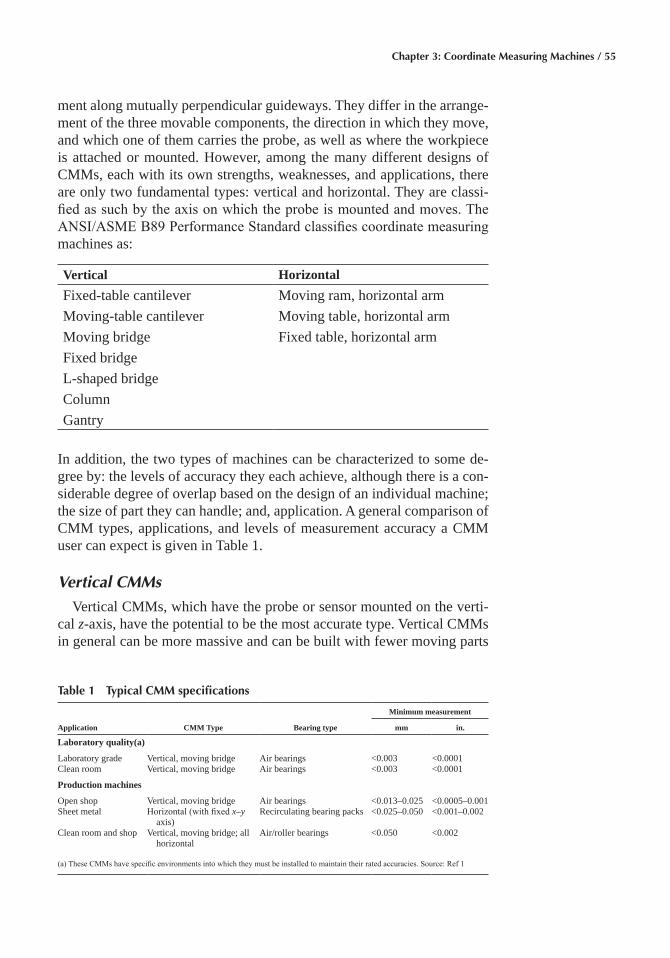
Chapter 3: Coordinate Measuring Machines / 55
ment along mutually perpendicular guideways. They differ in the arrange-ment of the three movable components, the direction in which they move, and which one of them carries the probe, as well as where the workpiece is attached or mounted. However, among the many different designs of CMMs, each with its own strengths, weaknesses, and applications, there are only two fundamental types: vertical and horizontal. They are classi-fied as such by the axis on which the probe is mounted and moves. The ANSI/ASME B89 Performance Standard classifies coordinate measuring machines as:
Vertical HorizontalFixed-table cantilever Moving ram, horizontal armMoving-table cantilever Moving table, horizontal armMoving bridge Fixed table, horizontal armFixed bridgeL-shaped bridgeColumnGantry
In addition, the two types of machines can be characterized to some de-gree by: the levels of accuracy they each achieve, although there is a con-siderable degree of overlap based on the design of an individual machine; the size of part they can handle; and, application. A general comparison of CMM types, applications, and levels of measurement accuracy a CMM user can expect is given in Table 1.
Vertical CMMs
Vertical CMMs, which have the probe or sensor mounted on the verti-cal z-axis, have the potential to be the most accurate type. Vertical CMMs in general can be more massive and can be built with fewer moving parts
Table 1 Typical CMM specifications
Application CMM Type Bearing type
Minimum measurement
mm in.
Laboratory quality(a)
Laboratory grade Vertical, moving bridge Air bearings <0.003 <0.0001Clean room Vertical, moving bridge Air bearings <0.003 <0.0001
Production machines
Open shop Vertical, moving bridge Air bearings <0.013–0.025 <0.0005–0.001Sheet metal Horizontal (with fixed x–y
axis)Recirculating bearing packs <0.025–0.050 <0.001–0.002
Clean room and shop Vertical, moving bridge; all horizontal
Air/roller bearings <0.050 <0.002
(a) These CMMs have specific environments into which they must be installed to maintain their rated accuracies. Source: Ref 1
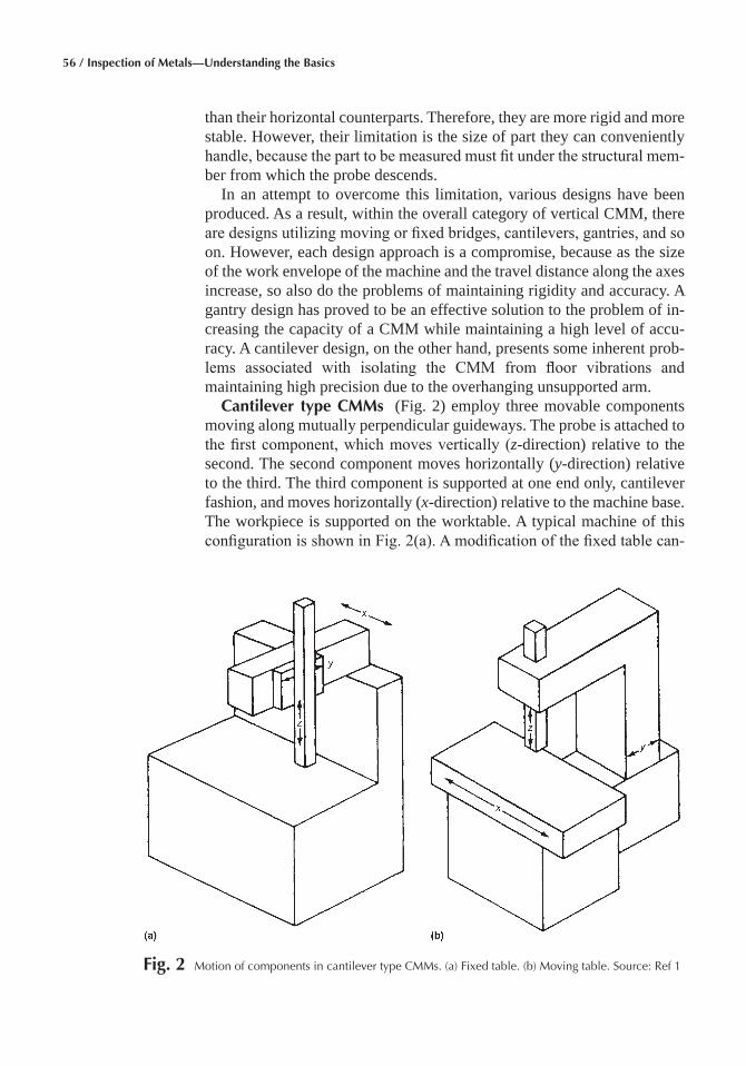
56 / Inspection of Metals—Understanding the Basics
than their horizontal counterparts. Therefore, they are more rigid and more stable. However, their limitation is the size of part they can conveniently handle, because the part to be measured must fit under the structural mem-ber from which the probe descends.
In an attempt to overcome this limitation, various designs have been produced. As a result, within the overall category of vertical CMM, there are designs utilizing moving or fixed bridges, cantilevers, gantries, and so on. However, each design approach is a compromise, because as the size of the work envelope of the machine and the travel distance along the axes increase, so also do the problems of maintaining rigidity and accuracy. A gantry design has proved to be an effective solution to the problem of in-creasing the capacity of a CMM while maintaining a high level of accu-racy. A cantilever design, on the other hand, presents some inherent prob-lems associated with isolating the CMM from floor vibrations and maintaining high precision due to the overhanging unsupported arm.
Cantilever type CMMs (Fig. 2) employ three movable components moving along mutually perpendicular guideways. The probe is attached to the first component, which moves vertically (z-direction) relative to the second. The second component moves horizontally (y-direction) relative to the third. The third component is supported at one end only, cantilever fashion, and moves horizontally (x-direction) relative to the machine base. The workpiece is supported on the worktable. A typical machine of this configuration is shown in Fig. 2(a). A modification of the fixed table can-
Fig� 2 Motion of components in cantilever type CMMs. (a) Fixed table. (b) Moving table. Source: Ref 1
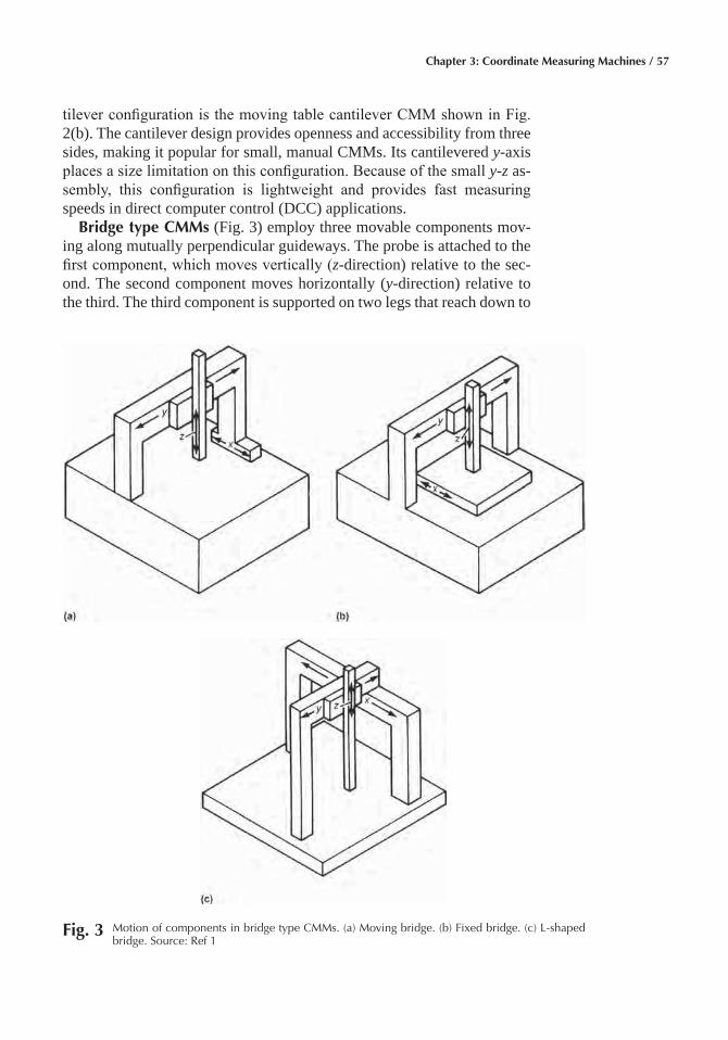
Chapter 3: Coordinate Measuring Machines / 57
tilever configuration is the moving table cantilever CMM shown in Fig. 2(b). The cantilever design provides openness and accessibility from three sides, making it popular for small, manual CMMs. Its cantilevered y-axis places a size limitation on this configuration. Because of the small y-z as-sembly, this configuration is lightweight and provides fast measuring speeds in direct computer control (DCC) applications.
Bridge type CMMs (Fig. 3) employ three movable components mov-ing along mutually perpendicular guideways. The probe is attached to the first component, which moves vertically (z-direction) relative to the sec-ond. The second component moves horizontally (y-direction) relative to the third. The third component is supported on two legs that reach down to
Fig� 3 Motion of components in bridge type CMMs. (a) Moving bridge. (b) Fixed bridge. (c) L-shaped bridge. Source: Ref 1
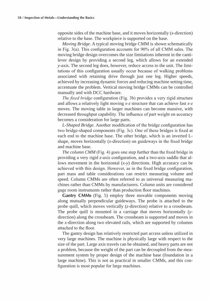
58 / Inspection of Metals—Understanding the Basics
opposite sides of the machine base, and it moves horizontally (x-direction) relative to the base. The workpiece is supported on the base.
Moving Bridge. A typical moving bridge CMM is shown schematically in Fig. 3(a). This configuration accounts for 90% of all CMM sales. The moving bridge design overcomes the size limitations inherent in the canti-lever design by providing a second leg, which allows for an extended y-axis. The second leg does, however, reduce access to the unit. The limi-tations of this configuration usually occur because of walking problems associated with retaining drive through just one leg. Higher speeds, achieved by increasing dynamic forces and reducing machine setting time, accentuate the problem. Vertical moving bridge CMMs can be controlled manually and with DCC hardware.
The fixed bridge configuration (Fig. 3b) provides a very rigid structure and allows a relatively light moving x-z structure that can achieve fast x-z moves. The moving table in larger machines can become massive, with decreased throughput capability. The influence of part weight on accuracy becomes a consideration for large parts.
L-Shaped Bridge. Another modification of the bridge configuration has two bridge-shaped components (Fig. 3c). One of these bridges is fixed at each end to the machine base. The other bridge, which is an inverted L-shape, moves horizontally (x-direction) on guideways in the fixed bridge and machine base.
The column CMM (Fig. 4) goes one step further than the fixed bridge in providing a very rigid z-axis configuration, and a two-axis saddle that al-lows movement in the horizontal (x-y) directions. High accuracy can be achieved with this design. However, as in the fixed bridge configuration, part mass and table considerations can restrict measuring volume and speed. Column CMMs are often referred to as universal measuring ma-chines rather than CMMs by manufacturers. Column units are considered gage room instruments rather than production floor machines.
Gantry CMMs (Fig. 5) employ three movable components moving along mutually perpendicular guideways. The probe is attached to the probe quill, which moves vertically (z-direction) relative to a crossbeam. The probe quill is mounted in a carriage that moves horizontally (y- direction) along the crossbeam. The crossbeam is supported and moves in the x-direction along two elevated rails, which are supported by columns attached to the floor.
The gantry design has relatively restricted part access unless utilized in very large machines. The machine is physically large with respect to the size of the part. Large axis travels can be obtained, and heavy parts are not a problem, because the weight of the part can be decoupled from the mea-surement system by proper design of the machine base (foundation in a large machine). This is not as practical in smaller CMMs, and this con-figuration is most popular for large machines.
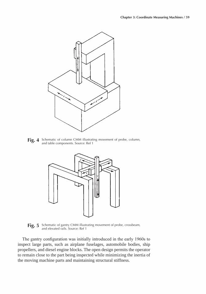
Chapter 3: Coordinate Measuring Machines / 59
The gantry configuration was initially introduced in the early 1960s to inspect large parts, such as airplane fuselages, automobile bodies, ship propellers, and diesel engine blocks. The open design permits the operator to remain close to the part being inspected while minimizing the inertia of the moving machine parts and maintaining structural stiffness.
Fig� 4 Schematic of column CMM illustrating movement of probe, column, and table components. Source: Ref 1
Fig� 5 Schematic of gantry CMM illustrating movement of probe, crossbeam, and elevated rails. Source: Ref 1
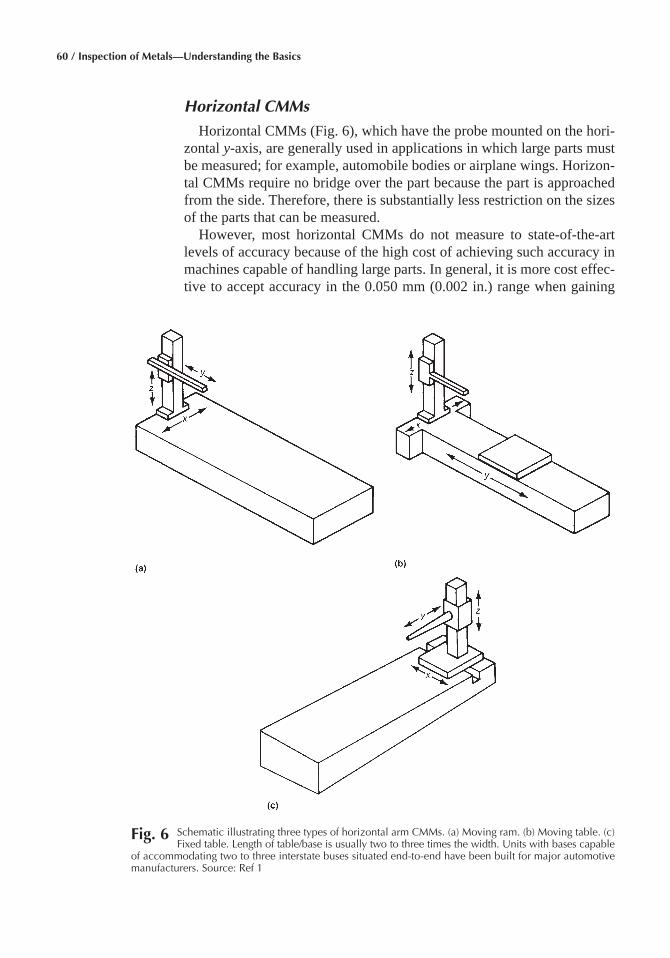
60 / Inspection of Metals—Understanding the Basics
Horizontal CMMs
Horizontal CMMs (Fig. 6), which have the probe mounted on the hori-zontal y-axis, are generally used in applications in which large parts must be measured; for example, automobile bodies or airplane wings. Horizon-tal CMMs require no bridge over the part because the part is approached from the side. Therefore, there is substantially less restriction on the sizes of the parts that can be measured.
However, most horizontal CMMs do not measure to state-of-the-art levels of accuracy because of the high cost of achieving such accuracy in machines capable of handling large parts. In general, it is more cost effec-tive to accept accuracy in the 0.050 mm (0.002 in.) range when gaining
Fig� 6 Schematic illustrating three types of horizontal arm CMMs. (a) Moving ram. (b) Moving table. (c) Fixed table. Length of table/base is usually two to three times the width. Units with bases capable
of accommodating two to three interstate buses situated end-to-end have been built for major automotive manufacturers. Source: Ref 1
Chapter 3: Coordinate Measuring Machines / 61
the part handling capabilities of large horizontal machines and to use ver-tical designs when finer measurement is demanded.
In any CMM design, fewer moving parts and joints will result in higher potential levels of accuracy. This principle has been applied to a class of horizontal CMM called process control robots. In these units, fixed mem-bers that move together provide the flexibility and capacity of a horizontal CMM, along with the higher accuracy of a vertical design. The horizontal direction of attack makes these CMMs the logical design for production applications in which horizontal machine tools are used.
In choosing a CMM, the buyer must take into consideration not only the degree of accuracy required but also the location of the unit and the measurements to be taken. In general, when dealing with smaller parts where measurements of very high accuracy are required, the potential user is likely to be best served by a machine located in a clean room environ-ment. When on-line process control is desired, the appropriate shop hard-ened CMM that can be located in the shop itself is the best solution.
Horizontal Arm CMMs� Several different types of horizontal arm CMMs are available. As with all CMMs, the horizontal arm configuration employs three movable components moving along mutually perpendicu-lar guideways.
Horizontal arm CMMs are used to inspect the dimensional and geomet-ric accuracy of a broad spectrum of machined or fabricated workpieces. Utilizing an electronic probe, these machines check parts in a mode simi-lar to the way they are machined on horizontal machine tools. They are especially suited for measuring large gear cases and engine blocks, for which high precision bore alignment and geometry measurements are re-quired. Four-axis capability can be obtained by incorporating a rotary table.
Horizontal arms for large machines have a lower profile than vertical arms. For some applications, horizontal access is desirable. For others, it is restrictive and a rotary table is usually required, thus increasing the cost.
Moving Ram Type. In this design, the probe is attached to the horizontal arm, which moves in a horizontal y-direction (Fig. 6a). The ram is encased in a carriage that moves in a vertical (z) direction and is supported on a column that moves horizontally (x-direction) relative to the base.
Moving Table Type. In this configuration, the probe is attached to the horizontal arm, which is permanently attached at one end only to a car-riage that moves in a vertical (z) direction (Fig. 6b) on the column. The arm support and table move horizontally (x- and y-directions) relative to the machine base. The moving table horizontal arm CMM unit is even more versatile because of the introduction of a rotary moving table.
Fixed Table Type. In the fixed table version, the probe is attached to the horizontal arm, which is supported cantilever style at the arm support and moves in a vertical (z) direction (Fig. 6c). The arm support moves hori-

62 / Inspection of Metals—Understanding the Basics
zontally (x- and y-directions) relative to the machine base. Parts to be in-spected are mounted on the machine base.
ACKNOWLEDGMENT
This chapter was adapted from Coordinate Measuring Machines by D.H. Genest in Nondestructive Evaluation and Quality Control, Volume 17, ASM Handbook 1992.
REFERENCES
1. D.H. Genest, Coordinate Measuring Machines, Nondestructive Evalu-ation and Quality Control, Vol 17, ASM Handbook, ASM Interna-tional, 1992, p 20
Inspection of Metals—Understanding the Basics Copyright © 2013 ASM International®
F.C. Campbell, editor All rights reservedwww.asminternational.org
CHAPTER 4
Machine Vision
MACHINE VISION emerged as an important new technique for indus-trial inspection and quality control in the early 1980s. When properly ap-plied, machine vision can provide accurate and inexpensive 100% in-spection of workpieces, dramatically increasing product quality. Machine vision is also used as an in-process gaging tool for controlling the process and correcting trends that could lead to the production of defective parts. Consequently, manufacturers in a variety of industries have investigated this important technology, regardless of the products being manufactured. The automotive and electronics industries are the largest users of machine vision systems.
Machine vision, sometimes referred to as computer vision or intelligent vision, is a means of simulating the image recognition and analysis capa-bilities of the human eye/brain system with electronic and electromechan-ical techniques. A machine vision system senses information about an image and analyzes the information to make a useful decision about its content; in much the same way, the eye acts as the body’s image sensor, with the brain analyzing this information and taking action based on the analysis.
Therefore, a machine vision system includes both visual sensing and interpretive capabilities. An image sensing device, such as a vidicon cam-era or a charge-coupled device (CCD) image sensor, is nothing more than a visual sensor that receives light through its lens and converts this light into electrical signals. When a data processing device, such as a micro-computer, is used, these electrical signals can be refined and analyzed to provide an interpretation of the scene that generated the signals. This in-formation can then be used as a basis for taking an appropriate course of action. The entire process of image formation, analysis, and decision mak-ing is referred to as machine vision.
This ability to acquire an image, analyze it, and then make an appropri-ate decision is extremely useful in inspection and quality control applica-

64 / Inspection of Metals—Understanding the Basics
tions. It enables machine vision to be used for a variety of functions, including:
• Identification of shapes• Measurement of distances and ranges• Gaging of sizes and dimensions• Determining orientation of parts• Quantifying motion• Detecting surface shading
These functional capabilities allow users to employ machine vision sys-tems for cost-effective and reliable 100% inspection of workpieces.
The analogy of human eye/brain system is helpful in understanding ma-chine vision, but the human eye/brain system is extremely complex and operates in ways and at data rates much different from those of commer-cial machine vision systems. Humans are more flexible and often faster than machine vision systems. On the other hand, machine vision systems provide capabilities not achievable by humans, particularly with respect to consistency and reliability. Table 1 compares human and machine vision capabilities, and Table 2 evaluates the performance of each. In addition,
Table 1 Comparison of machine and human vision capabilities
Capabilities Machine vision Human vision
Distance Limited capabilities Good qualitative capabilitiesOrientation Good for two dimensions Good qualitative capabilitiesMotion Limited; sensitive to image blurring Good qualitative capabilitiesEdges/regions High-contrast image required Highly developedImage shapes Good quantitative measurements Qualitative onlyImage organization Special software needed; limited capa-
bilityHighly developed
Surface shading Limited capability with gray scale Highly developedTwo-dimensional interpretation Excellent for well-defined features Highly developedThree-dimensional interpretation Very limited capabilities Highly developedOverall Best for qualitative measurement of
structured sceneBest for qualitative interpretation
of complex, unstructured scene
Source: Ref 1
Table 2 Evaluation of machine and human vision capabilities
Performance criteria Machine vision Human vision
Resolution Limited by pixel array size High resolution capabilityProcessing speed Fraction of a second per image Real-time processingDiscrimination Limited to high-contrast images Very sensitive discriminationAccuracy Accurate for part discrimination based on
quantitative differences; accuracy remains consistent at high production volume.
Accurate at distinguishing qualitative differ-ences; may decrease at high volume
Operating cost High for low volume; lower than human vision at high volume
Lower than machine at low volume
Overall Best at high production volume Best at low or moderate production volume
Source: Ref 1
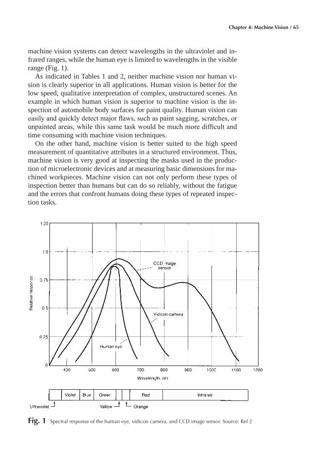
Chapter 4: Machine Vision / 65
machine vision systems can detect wavelengths in the ultraviolet and in-frared ranges, while the human eye is limited to wavelengths in the visible range (Fig. 1).
As indicated in Tables 1 and 2, neither machine vision nor human vi-sion is clearly superior in all applications. Human vision is better for the low speed, qualitative interpretation of complex, unstructured scenes. An example in which human vision is superior to machine vision is the in-spection of automobile body surfaces for paint quality. Human vision can easily and quickly detect major flaws, such as paint sagging, scratches, or unpainted areas, while this same task would be much more difficult and time consuming with machine vision techniques.
On the other hand, machine vision is better suited to the high speed measurement of quantitative attributes in a structured environment. Thus, machine vision is very good at inspecting the masks used in the produc-tion of microelectronic devices and at measuring basic dimensions for ma-chined workpieces. Machine vision can not only perform these types of inspection better than humans but can do so reliably, without the fatigue and the errors that confront humans doing these types of repeated inspec-tion tasks.
Fig� 1 Spectral response of the human eye, vidicon camera, and CCD image sensor. Source: Ref 2
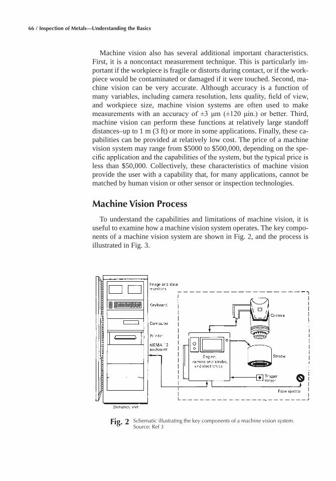
66 / Inspection of Metals—Understanding the Basics
Machine vision also has several additional important characteristics. First, it is a noncontact measurement technique. This is particularly im-portant if the workpiece is fragile or distorts during contact, or if the work-piece would be contaminated or damaged if it were touched. Second, ma-chine vision can be very accurate. Although accuracy is a function of many variables, including camera resolution, lens quality, field of view, and workpiece size, machine vision systems are often used to make measurements with an accuracy of ±3 μm (±120 μin.) or better. Third, machine vision can perform these functions at relatively large standoff distances–up to 1 m (3 ft) or more in some applications. Finally, these ca-pabilities can be provided at relatively low cost. The price of a machine vision system may range from $5000 to $500,000, depending on the spe-cific application and the capabilities of the system, but the typical price is less than $50,000. Collectively, these characteristics of machine vision provide the user with a capability that, for many applications, cannot be matched by human vision or other sensor or inspection technologies.
Machine Vision Process
To understand the capabilities and limitations of machine vision, it is useful to examine how a machine vision system operates. The key compo-nents of a machine vision system are shown in Fig. 2, and the process is illustrated in Fig. 3.
Fig� 2 Schematic illustrating the key components of a machine vision system. Source: Ref 3
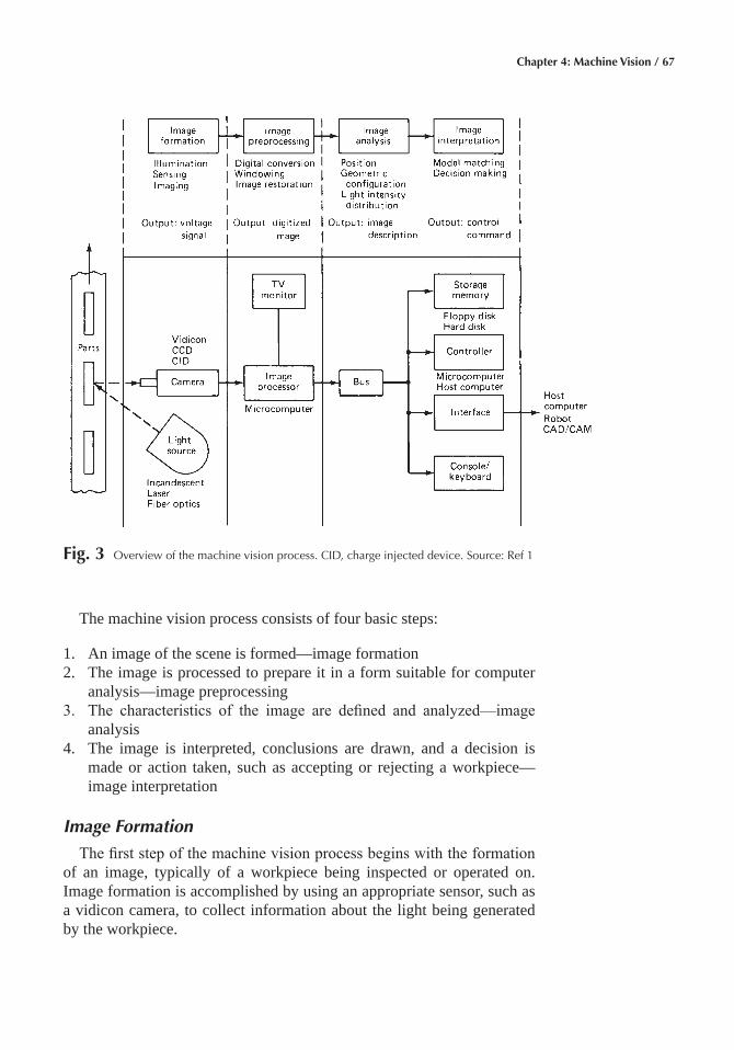
Chapter 4: Machine Vision / 67
The machine vision process consists of four basic steps:
1. An image of the scene is formed—image formation2. The image is processed to prepare it in a form suitable for computer
analysis—image preprocessing3. The characteristics of the image are defined and analyzed—image
analysis4. The image is interpreted, conclusions are drawn, and a decision is
made or action taken, such as accepting or rejecting a workpiece—image interpretation
Image Formation
The first step of the machine vision process begins with the formation of an image, typically of a workpiece being inspected or operated on. Image formation is accomplished by using an appropriate sensor, such as a vidicon camera, to collect information about the light being generated by the workpiece.
Fig� 3 Overview of the machine vision process. CID, charge injected device. Source: Ref 1
68 / Inspection of Metals—Understanding the Basics
The light being generated by the surface of a workpiece is determined by a number of factors, including the orientation of the workpiece, its sur-face finish, and the type and location of lighting being employed. Typical light sources include incandescent lights, fluorescent tubes, fiber optic bundles, arc lamps, and strobe lights. Laser beams are also used in some special applications, such as triangulation systems for measuring dis-tances. Polarized or ultraviolet light can also be used to reduce glare or to increase contrast.
Proper Illumination� Correct placement of the light source is ex-tremely important because it has a major effect on the contrast of the image. Several commonly used illumination techniques are illustrated in Fig. 4. When a simple silhouette image is all that is required, backlighting of the workpiece can be used for maximum image contrast. If certain key features on the surface of the workpiece must be inspected, front lighting would be used. If a three-dimensional feature is inspected, side lighting or structured lighting may be required. In addition to proper illumination, fixturing of the workpiece may also be required to orient the part properly and to simplify the rest of the machine vision process.
Once the workpiece or scene has been properly arranged and illumi-nated, an image sensor is used to generate the electronic signal represent-ing the image. The image sensor collects light from the scene (typically through a lens) and then converts the light into electrical energy by using a photosensitive target. The output is an electrical signal corresponding to the input light.
Most image sensors used in industrial machine vision systems produce signals representing two-dimensional arrays or scans of the entire image, such as those formed by conventional television cameras. Some image sensors, however, generate signals using one-dimensional or linear arrays that must be scanned numerous times in order to view the entire scene.
Vidicon Camera� The most common image sensor in the early ma-chine vision systems was the vidicon camera, which was extensively used in closed circuit television systems and consumer video recorders. An image is formed by focusing the incoming light through a series of lenses onto the photoconductive faceplate of the vidicon tube. An electron beam within the tube scans the photoconductive surface and produces an analog output voltage proportional to the variations in light intensity for each scan line of the original scene. Normally, the output signal conforms to commercial television standards–525 scan lines interlaced into 2 fields of 262.5 lines and repeated 30 times per second.
The vidicon camera has the advantage of providing a great deal of in-formation about a scene at very fast speeds and at relatively low cost. However, vidicon cameras do have several disadvantages. They tend to distort the image due to their construction and are subject to image burn-in on the photoconductive surface. Vidicon cameras also have limited ser-vice lives and are susceptible to damage from shock and vibration.
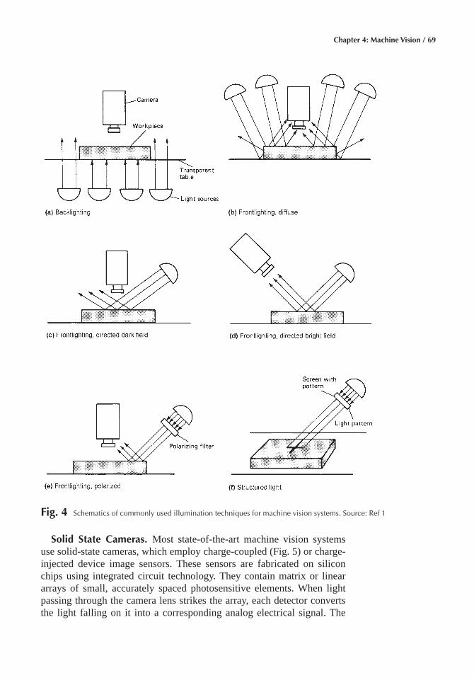
Chapter 4: Machine Vision / 69
Solid State Cameras� Most state-of-the-art machine vision systems use solid-state cameras, which employ charge-coupled (Fig. 5) or charge- injected device image sensors. These sensors are fabricated on silicon chips using integrated circuit technology. They contain matrix or linear arrays of small, accurately spaced photosensitive elements. When light passing through the camera lens strikes the array, each detector converts the light falling on it into a corresponding analog electrical signal. The
Fig� 4 Schematics of commonly used illumination techniques for machine vision systems. Source: Ref 1
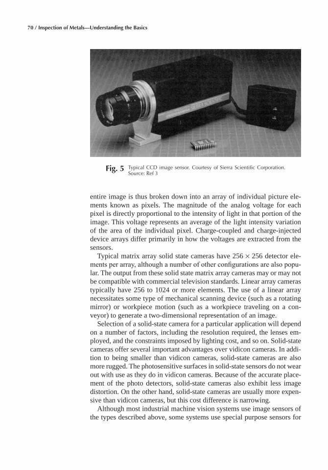
70 / Inspection of Metals—Understanding the Basics
entire image is thus broken down into an array of individual picture ele-ments known as pixels. The magnitude of the analog voltage for each pixel is directly proportional to the intensity of light in that portion of the image. This voltage represents an average of the light intensity variation of the area of the individual pixel. Charge-coupled and charge-injected device arrays differ primarily in how the voltages are extracted from the sensors.
Typical matrix array solid state cameras have 256 × 256 detector ele-ments per array, although a number of other configurations are also popu-lar. The output from these solid state matrix array cameras may or may not be compatible with commercial television standards. Linear array cameras typically have 256 to 1024 or more elements. The use of a linear array necessitates some type of mechanical scanning device (such as a rotating mirror) or workpiece motion (such as a workpiece traveling on a con-veyor) to generate a two-dimensional representation of an image.
Selection of a solid-state camera for a particular application will depend on a number of factors, including the resolution required, the lenses em-ployed, and the constraints imposed by lighting cost, and so on. Solid-state cameras offer several important advantages over vidicon cameras. In addi-tion to being smaller than vidicon cameras, solid-state cameras are also more rugged. The photosensitive surfaces in solid-state sensors do not wear out with use as they do in vidicon cameras. Because of the accurate place-ment of the photo detectors, solid-state cameras also exhibit less image distortion. On the other hand, solid-state cameras are usually more expen-sive than vidicon cameras, but this cost difference is narrowing.
Although most industrial machine vision systems use image sensors of the types described above, some systems use special purpose sensors for
Fig� 5 Typical CCD image sensor. Courtesy of Sierra Scientific Corporation. Source: Ref 3
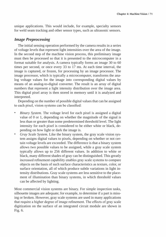
Chapter 4: Machine Vision / 71
unique applications. This would include, for example, specialty sensors for weld seam tracking and other sensor types, such as ultrasonic sensors.
Image Preprocessing
The initial sensing operation performed by the camera results in a series of voltage levels that represent light intensities over the area of the image. In the second step of the machine vision process, this preliminary image must then be processed so that it is presented to the microcomputer in a format suitable for analysis. A camera typically forms an image 30 to 60 times per second, or once every 33 to 17 ms. At each time interval, the image is captured, or frozen, for processing by an image processor. The image processor, which is typically a microcomputer, transforms the ana-log voltage values for the image into corresponding digital values by means of an analog-to-digital converter. The result is an array of digital numbers that represent a light intensity distribution over the image area. This digital pixel array is then stored in memory until it is analyzed and interpreted.
Depending on the number of possible digital values that can be assigned to each pixel, vision systems can be classified:
• Binary System. The voltage level for each pixel is assigned a digital value of 0 or 1, depending on whether the magnitude of the signal is less than or greater than some predetermined threshold level. The light intensity for each pixel is considered to be either white or black, de-pending on how light or dark the image is.
• Gray Scale System. Like the binary system, the gray scale vision sys-tem assigns digital values to pixels, depending on whether or not cer-tain voltage levels are exceeded. The difference is that a binary system allows two possible values to be assigned, while a gray scale system typically allows up to 256 different values. In addition to white or black, many different shades of gray can be distinguished. This greatly increased refinement capability enables gray scale systems to compare objects on the basis of such surface characteristics as texture, color, or surface orientation, all of which produce subtle variations in light in-tensity distributions. Gray scale systems are less sensitive to the place-ment of illumination than binary systems, in which threshold values can be affected by lighting.
Most commercial vision systems are binary. For simple inspection tasks, silhouette images are adequate; for example, to determine if a part is miss-ing or broken. However, gray scale systems are used in many applications that require a higher degree of image refinement. The effects of gray scale digitization on the surface of an integrated circuit module are shown in Fig. 6.
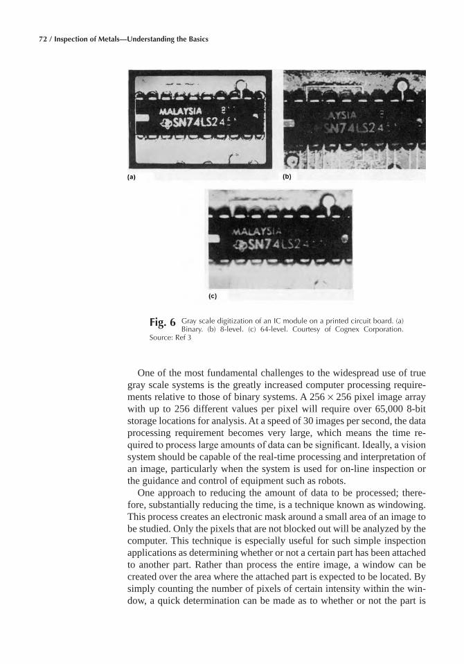
72 / Inspection of Metals—Understanding the Basics
One of the most fundamental challenges to the widespread use of true gray scale systems is the greatly increased computer processing require-ments relative to those of binary systems. A 256 × 256 pixel image array with up to 256 different values per pixel will require over 65,000 8-bit storage locations for analysis. At a speed of 30 images per second, the data processing requirement becomes very large, which means the time re-quired to process large amounts of data can be significant. Ideally, a vision system should be capable of the real-time processing and interpretation of an image, particularly when the system is used for on-line inspection or the guidance and control of equipment such as robots.
One approach to reducing the amount of data to be processed; there-fore, substantially reducing the time, is a technique known as windowing. This process creates an electronic mask around a small area of an image to be studied. Only the pixels that are not blocked out will be analyzed by the computer. This technique is especially useful for such simple inspection applications as determining whether or not a certain part has been attached to another part. Rather than process the entire image, a window can be created over the area where the attached part is expected to be located. By simply counting the number of pixels of certain intensity within the win-dow, a quick determination can be made as to whether or not the part is
Fig� 6 Gray scale digitization of an IC module on a printed circuit board. (a) Binary. (b) 8-level. (c) 64-level. Courtesy of Cognex Corporation.
Source: Ref 3

Chapter 4: Machine Vision / 73
present. A window can be virtually any size, from one pixel up to a major portion of the image.
Another way in which the image can be prepared in a more suitable form during the preprocessing step is through the techniques of image restoration. Very often an image suffers various forms of degradation, such as blurring of lines or boundaries, poor contrast between image re-gions, or the presence of background noise. There are several possible causes of image degradation, including:
• Motion of the camera or object during image formation• Poor illumination or improper placement of illumination• Variations in sensor response• Defects or poor contrast on the surface of the subject, such as deformed
letters on labels or overlapping parts with similar light intensities
Techniques for improving the quality of an image include:
• Constant brightness addition involves simply adding a constant amount of brightness to each pixel. This improves the contrast in the image.
• Contrast stretching increases the relative contrast between high and low intensity elements by making light pixels lighter and dark pixels darker.
• Fourier-domain processing is a powerful technique based on the prin-ciple that changes in brightness in an image can be represented as a series of sine and cosine waves. These waves can be described by specifying amplitudes and frequencies in a series of equations. By breaking the image down into its sinusoidal components, each compo-nent image wave can be acted upon separately. Changing the magni-tude of certain component waves will produce a sharper image that results in a less blurred image, better defined edges or lines, greater contrast between regions, or reduced background noise.
Some machine vision systems perform additional operations as part of the preprocessing function to facilitate image analysis or to reduce memory storage requirements. These operations, which significantly affect the de-sign, performance, and cost of vision systems, differ according to the spe-cific system and are largely dependent on the analysis technique employed in later stages of the process. Two commonly used preprocessing opera-tions are:
• Edge Detection. An edge is a boundary within an image where there is a dramatic change in light intensity between adjacent pixels. These boundaries usually correspond to the real edges on the workpiece being examined by the vision system and are very important for ap-plications such as the inspection of part dimensions. Edges are usually
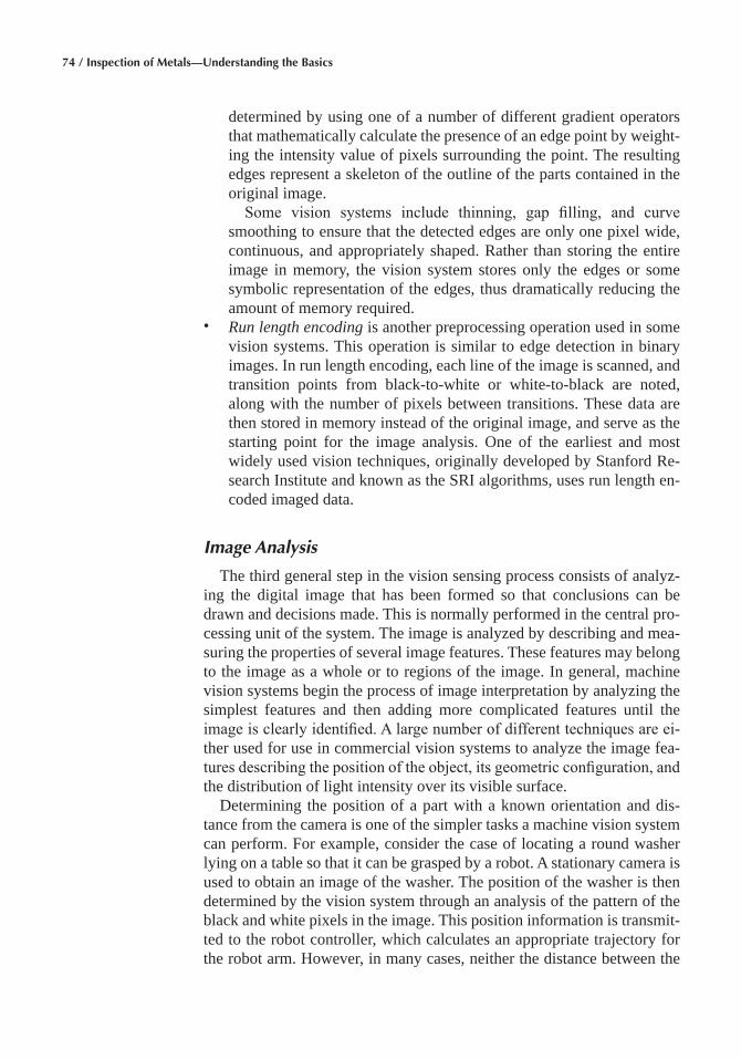
74 / Inspection of Metals—Understanding the Basics
determined by using one of a number of different gradient operators that mathematically calculate the presence of an edge point by weight-ing the intensity value of pixels surrounding the point. The resulting edges represent a skeleton of the outline of the parts contained in the original image.
• Some vision systems include thinning, gap filling, and curve smoothing to ensure that the detected edges are only one pixel wide, continuous, and appropriately shaped. Rather than storing the entire image in memory, the vision system stores only the edges or some symbolic representation of the edges, thus dramatically reducing the amount of memory required.
• Run length encoding is another preprocessing operation used in some vision systems. This operation is similar to edge detection in binary images. In run length encoding, each line of the image is scanned, and transition points from black-to-white or white-to-black are noted, along with the number of pixels between transitions. These data are then stored in memory instead of the original image, and serve as the starting point for the image analysis. One of the earliest and most widely used vision techniques, originally developed by Stanford Re-search Institute and known as the SRI algorithms, uses run length en-coded imaged data.
Image Analysis
The third general step in the vision sensing process consists of analyz-ing the digital image that has been formed so that conclusions can be drawn and decisions made. This is normally performed in the central pro-cessing unit of the system. The image is analyzed by describing and mea-suring the properties of several image features. These features may belong to the image as a whole or to regions of the image. In general, machine vision systems begin the process of image interpretation by analyzing the simplest features and then adding more complicated features until the image is clearly identified. A large number of different techniques are ei-ther used for use in commercial vision systems to analyze the image fea-tures describing the position of the object, its geometric configuration, and the distribution of light intensity over its visible surface.
Determining the position of a part with a known orientation and dis-tance from the camera is one of the simpler tasks a machine vision system can perform. For example, consider the case of locating a round washer lying on a table so that it can be grasped by a robot. A stationary camera is used to obtain an image of the washer. The position of the washer is then determined by the vision system through an analysis of the pattern of the black and white pixels in the image. This position information is transmit-ted to the robot controller, which calculates an appropriate trajectory for the robot arm. However, in many cases, neither the distance between the
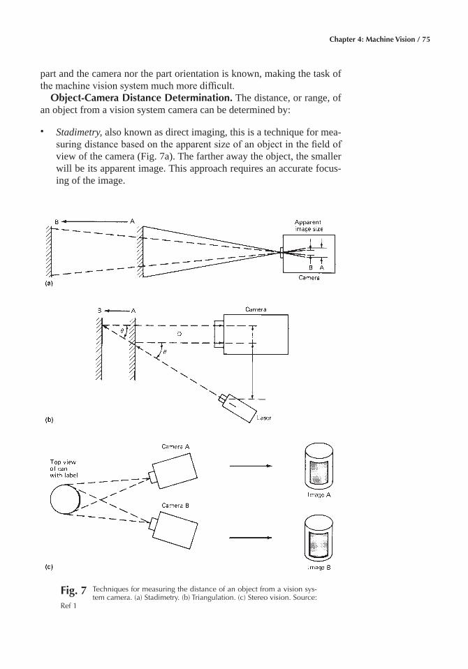
Chapter 4: Machine Vision / 75
part and the camera nor the part orientation is known, making the task of the machine vision system much more difficult.
Object-Camera Distance Determination� The distance, or range, of an object from a vision system camera can be determined by:
• Stadimetry, also known as direct imaging, this is a technique for mea-suring distance based on the apparent size of an object in the field of view of the camera (Fig. 7a). The farther away the object, the smaller will be its apparent image. This approach requires an accurate focus-ing of the image.
Fig� 7 Techniques for measuring the distance of an object from a vision sys-tem camera. (a) Stadimetry. (b) Triangulation. (c) Stereo vision. Source:
Ref 1
76 / Inspection of Metals—Understanding the Basics
• Triangulation is based on the measurement of the baseline of a right triangle formed by the light path to the object, the reflected light path to the camera, and a line from the camera to the light source (Fig. 7b). A typical light source for this technique is an LED or a laser, both of which form a well defined spot of light. Because the angle between the two light paths is preset, the standoff distance is readily calculated. Typical accuracies of 1 μm (40 μin.) can be achieved.
• Stereo vision, also known as binocular vision, is a method that uses the principle of parallax to measure distance (Fig. 7c). Parallax is the change in the relative perspective of a scene as the observer (or cam-era) moves. Human eyesight provides the best example of stereo vi-sion. The right eye views an object as if the object were rotated slightly from the position observed by the left eye. Also, an object in front of another object seems to move relative to the other object when seen from one eye and then from the other. The closer the objects, the greater the parallax.
Object orientation is important in manufacturing operations such as material handling or assembly to determine where a robot may need to position itself relative to a part to grasp the part and then transfer it to an-other location. Among the methods used for determining object orienta-tion are:
• Equivalent Ellipse. For an image of an object in a two-dimensional plane, an ellipse can be calculated that has the same area as the image. The major axis of the ellipse will define the orientation of the object. Another similar measure is the axis that yields the minimum moment of inertia of the object.
• Connecting of Three Points. If the relative positions of three noncolin-ear points in a surface are known, the orientation of the surface in space can be determined by measuring the apparent relative position of the points in the image.
• Light Intensity Distribution. A surface will appear darker if it is ori-ented at an angle other than normal to the light source. Determining orientation based on relative light intensity requires knowledge of the source of illumination as well as the surface characteristics of the object.
• Structured light involves the use of a light pattern rather than a dif-fused light source. The workpiece is illuminated by the structured light, and the way in which the pattern is distorted by the part can be used to determine both the three-dimensional shape and the orientation of the part.
Object Position Defined by Relative Motion� Certain operations, such as tracking or part insertion, may require the vision system to follow
Chapter 4: Machine Vision / 77
the motion of an object. This is a difficult task that requires a series of image frames to be compared for relative changes in position during specified time intervals. Motion in one-dimension, as in the case of a moving conveyor of parts, is the least complicated motion to detect. In two-dimensions, mo-tion may consist of both a rotational and a translational component. In three-dimensions, a total of six motion components (three rotational axes and three translational axes) may need to be defined.
Feature Extraction� One of the useful approaches to image inter-pretation is analysis of the fundamental geometric properties of two- dimensional images. Parts tend to have distinct shapes that can be recog-nized on the basis of elementary features. These distinguishing features are often simple enough to allow identification independent of the orienta-tion of the part. For example, if surface area (number of pixels) is the only feature needed for differentiating the parts, then orientation of the part is not important. For more complex three-dimensional objects, additional geometric properties may need to be determined, including descriptions of various image segments. The process of defining these elementary proper-ties of the image is often referred to as feature extraction. The first step is to determine boundary locations and to segment the image into distinct regions. Next, certain geometric properties of these regions are deter-mined. Finally, these image regions are organized in a structure describing their relationship.
Light Intensity Variations� One of the most sophisticated and po-tentially useful approaches to machine vision is the interpretation of an image based on the different intensity of light in different regions. Many of the features described above are used in vision systems to create two-dimensional interpretations of images. However, analysis of subtle changes in shadings over the image can add a great deal of information about the three-dimensional nature of the object.
The problem is that most machine vision techniques are not capable of dealing with the complex patterns formed by varying conditions of illumi-nations, surface texture and color, and surface orientation. Another, more fundamental difficulty is that image intensities can change drastically with relatively modest variations in illumination or surface condition. Systems that attempt to match the gray level values of each pixel to a stored model can easily suffer deterioration in performance in real world manufacturing environments. The use of such geometric features such as edges or bound-aries is likely to remain the preferred approach. Even better approaches are likely to result from research being performed on various techniques for determining surface shapes from relative intensity levels. For example, one approach assumes that the light intensity at a given point on the sur-face of an object can be precisely determined by an equation describing the nature and location of the light source, the orientation of the surface at the point, and the reflectivity of the surface.
78 / Inspection of Metals—Understanding the Basics
Image Interpretation
When the system has completed the process of analyzing image fea-tures, the fourth step is performed. Some conclusions must be drawn with regard to the findings, such as the verification that a part is or is not pres-ent; the identification of an object based on recognition of its image; or the determination that certain parameters of the object fall within acceptable limits. Based on these conclusions, certain decisions can then be made regarding the object or the production process. These conclusions are formed by comparing the results of the analysis with a prestored set of standard criteria. These standard criteria describe the expected character-istics of the image and are developed either through a programmed model of the image or by building an average profile of previously examined objects.
Statistical Approach� In the simplest case of a binary system, the pro-cess of comparing an image with standard criteria, may simply require that all white and black pixels within a certain area be counted. Once the image is segmented or windowed, all groups of black pixels within each segment that are connected (called blobs) are identified and counted. The same process is followed for groups of white pixels (called holes).
The blobs, holes, and pixels are counted and the total quantity is com-pared with expected numbers to determine how closely the real image matches the standard image. If the numbers are within a certain percent-age of each other, it can be assumed that there is a match.
An example of the statistical approach to image interpretation is the identification of a part on the basis of a known outline, such as the center hole of a washer. As illustrated in Fig. 8, a sample 3 × 3 pixel window can be used to locate the hole of the washer and to distinguish the washer from other distinctly different washers. The dark pixels shown in Fig. 8(a) rep-resents the rough shape of the washer. When the window is centered on the shape, all nine white pixels are assigned a value of 0. In Fig. 8(b), a defective washer appears, with the hole skewed to the right. Because the window counts only six white pixels, it can be assumed that the hole is incorrectly formed. In Fig. 8(c), a second washer category is introduced, one with a smaller hole. In this case, only five white pixels are counted, providing enough information to identify the washer as a different type. In Fig. 8(d), a third washer is inspected, one that is larger than the first. The window counts nine white pixels, as in Fig. 8(a). In this case, some ambi-guity remains, and so additional information would be required, such as the use of a 5 × 5 window. Another approach is to count all the black pix-els rather than the white ones.
Such simple methods are finding useful applications in manufacturing because of the controlled, structured nature of most manufacturing envi-ronments. The extent of the analysis required for part recognition depends on both the complexity of the image and the goal of the analysis. In a
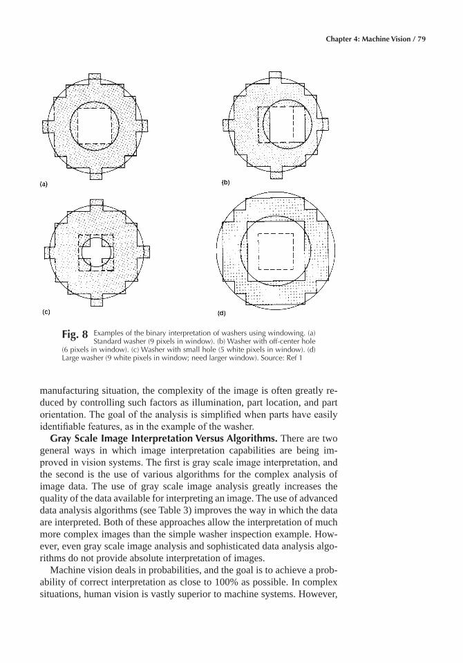
Chapter 4: Machine Vision / 79
manufacturing situation, the complexity of the image is often greatly re-duced by controlling such factors as illumination, part location, and part orientation. The goal of the analysis is simplified when parts have easily identifiable features, as in the example of the washer.
Gray Scale Image Interpretation Versus Algorithms� There are two general ways in which image interpretation capabilities are being im-proved in vision systems. The first is gray scale image interpretation, and the second is the use of various algorithms for the complex analysis of image data. The use of gray scale image analysis greatly increases the quality of the data available for interpreting an image. The use of advanced data analysis algorithms (see Table 3) improves the way in which the data are interpreted. Both of these approaches allow the interpretation of much more complex images than the simple washer inspection example. How-ever, even gray scale image analysis and sophisticated data analysis algo-rithms do not provide absolute interpretation of images.
Machine vision deals in probabilities, and the goal is to achieve a prob-ability of correct interpretation as close to 100% as possible. In complex situations, human vision is vastly superior to machine systems. However,
Fig� 8 Examples of the binary interpretation of washers using windowing. (a) Standard washer (9 pixels in window). (b) Washer with off-center hole
(6 pixels in window). (c) Washer with small hole (5 white pixels in window). (d) Large washer (9 white pixels in window; need larger window). Source: Ref 1
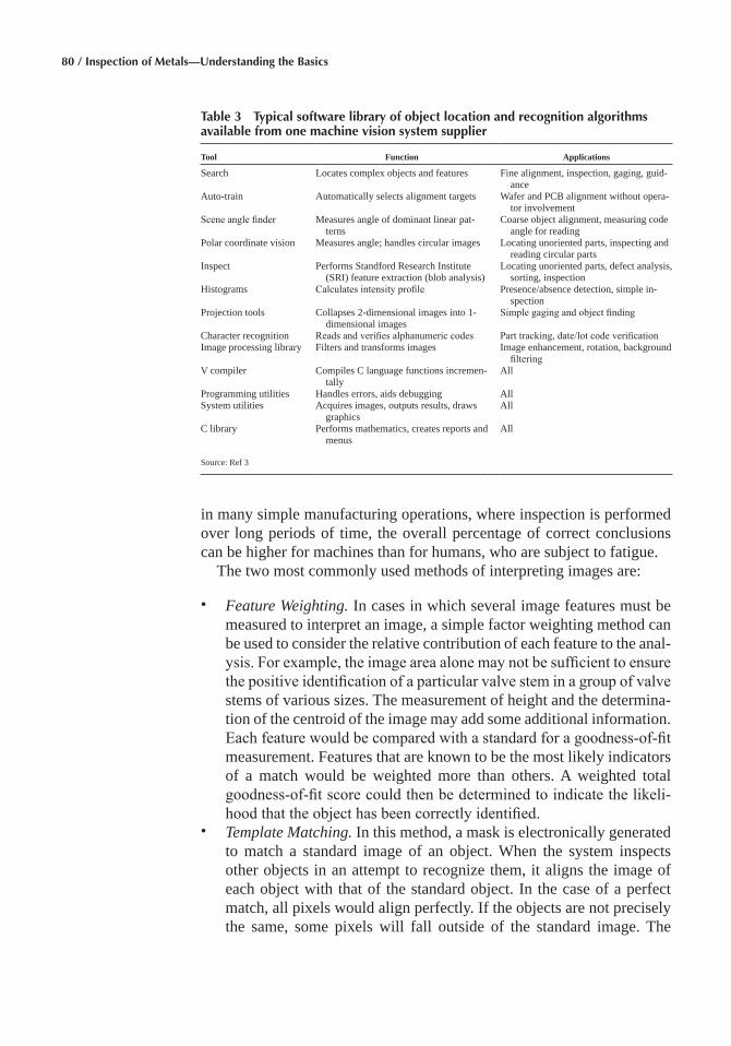
80 / Inspection of Metals—Understanding the Basics
in many simple manufacturing operations, where inspection is performed over long periods of time, the overall percentage of correct conclusions can be higher for machines than for humans, who are subject to fatigue.
The two most commonly used methods of interpreting images are:
• Feature Weighting. In cases in which several image features must be measured to interpret an image, a simple factor weighting method can be used to consider the relative contribution of each feature to the anal-ysis. For example, the image area alone may not be sufficient to ensure the positive identification of a particular valve stem in a group of valve stems of various sizes. The measurement of height and the determina-tion of the centroid of the image may add some additional information. Each feature would be compared with a standard for a goodness-of-fit measurement. Features that are known to be the most likely indicators of a match would be weighted more than others. A weighted total goodness-of-fit score could then be determined to indicate the likeli-hood that the object has been correctly identified.
• Template Matching. In this method, a mask is electronically generated to match a standard image of an object. When the system inspects other objects in an attempt to recognize them, it aligns the image of each object with that of the standard object. In the case of a perfect match, all pixels would align perfectly. If the objects are not precisely the same, some pixels will fall outside of the standard image. The
Table 3 Typical software library of object location and recognition algorithms available from one machine vision system supplier
Tool Function Applications
Search Locates complex objects and features Fine alignment, inspection, gaging, guid-ance
Auto-train Automatically selects alignment targets Wafer and PCB alignment without opera-tor involvement
Scene angle finder Measures angle of dominant linear pat-terns
Coarse object alignment, measuring code angle for reading
Polar coordinate vision Measures angle; handles circular images Locating unoriented parts, inspecting and reading circular parts
Inspect Performs Standford Research Institute (SRI) feature extraction (blob analysis)
Locating unoriented parts, defect analysis, sorting, inspection
Histograms Calculates intensity profile Presence/absence detection, simple in-spection
Projection tools Collapses 2-dimensional images into 1- dimensional images
Simple gaging and object finding
Character recognition Reads and verifies alphanumeric codes Part tracking, date/lot code verificationImage processing library Filters and transforms images Image enhancement, rotation, background
filteringV compiler Compiles C language functions incremen-
tallyAll
Programming utilities Handles errors, aids debugging AllSystem utilities Acquires images, outputs results, draws
graphicsAll
C library Performs mathematics, creates reports and menus
All
Source: Ref 3

Chapter 4: Machine Vision / 81
percentage of pixels in two images that match is a measure of the goodness-of-fit. A threshold value can then be assigned to test for pass (positive match) or reject (no match) mode. A probability factor, which presents the degree of confidence with which a correct interpretation has been made, is normally calculated, along with the go/no-go con- clusions.
Variations on these two approaches are used in most commercially avail-able vision systems. Although conceptually simple, they can yield power-ful results in a variety of manufacturing applications requiring the identi-fication of two-dimensional parts with well defined silhouettes. With either method, a preliminary session is usually held before the machine is put into use. During this session, several sample known parts are pre-sented to the machine for analysis. The part features are stored and up-dated as each part is presented, until the machine is familiar with the part. Then, the actual production parts are studied by comparison with this stored model of a standard part.
Mathematical Modeling� Although model building, or programming, is generally accomplished by presenting a known sample object to the machine for analysis, it is also possible to create a mathematical model describing the expected image. This is generally applicable for objects that have well defined shapes, such as rectangles or circles, especially if the descriptive data already exist in an off-line data base for computer-aided design and manufacture (CAD/CAM). For example, the geometry of a rectangular machined part with several circular holes of known diam-eters and locations can be readily programmed. Because more complex shapes may be difficult to describe mathematically, it may be easier to teach the machine by allowing it to analyze a sample part. Most commer-cial systems include standard image processing software for calculating basic image features and comparing with models. However, custom pro-gramming for model generation can be designed either by the purchaser or by the vision system supplier. Off-line programming is likely to become increasingly popular as CAD/CAM interface methods improve.
Although the image interpretation techniques described apply to many, if not most, of the machine vision systems that are commercially avail-able, there are still other approaches being used by some suppliers, particu-larly for special purpose systems for such applications as printed circuit board (PCB) inspection, weld seam tracking, robot guidance and control, and inspection of microelectronic devices and tooling. These special pur-pose systems often incorporate unique image analysis and interpretation techniques that exploit the constraints inherent in the applications. For ex-ample, some PCB inspection systems employ image analysis algorithms based on design rules rather than feature weighting or template matching. In the design rule approach, the inspection process is based on known
82 / Inspection of Metals—Understanding the Basics
characteristics of a good product. For PCBs, this would include minimum conductor width and spacing between conductors. Also, each conductor should end with a solder pad if the board is correct. If these rules are not complied with, then the product is rejected.
Interfacing� A machine vision system will rarely be used without some form of interaction with other factory equipment, such as CAD/CAM de-vices, robots, or host computers. This interaction is the final element of the machine vision process, in which conclusions about the image are trans-lated into actions. In some cases, the final action may take the form of cumulative storage of information in a host computer, such as counting the number of parts in various categories for inventory control. In other situations, a final action may be a specific motion, such as the transfer of parts into different conveyors, depending on their characteristics. Vision systems are being increasingly used for control purposes through the com-bination of vision systems and robots. In this case, the vision system greatly expands the flexibility of the robot.
For most applications, interfacing a machine vision system with other equipment is a straightforward task. Most systems are equipped with a number of input and output ports, including a standard RS232C interface. However, connecting a vision system to a robot is much more complicated because of timing constraints, data formats, and the inability of most robot controllers to handle vision system inputs. To overcome this problem, sev-eral robot and vision system manufacturers have developed integrated system capabilities.
Machine Vision Applications
Machine vision systems can be considered for use in most manufactur-ing applications in which human vision is currently required. Human vi-sion is required for applications in which noncontact feedback is used to provide information about a production process or a part. For example, a human welder or machinist uses visual feedback to ensure that the correct relationship is maintained between the tool and the workpiece. Human as-semblers visually analyze the position of parts so that other parts can be correctly aligned for insertion or some other form of mating. Quality con-trol inspectors visually check products or parts to ensure that there are no defects, such as missing parts, damage, or incorrect location of various features.
As discussed previously, the primary strength of human vision is the ability to analyze qualitative aspects of an object or a scene. However, humans are not particularly adept at measuring quantitative data. For ex-ample, although human vision uses a sophisticated approach for depth perception that allows it to correctly determine the relative distance of an object, it is not able to measure a specific distance to an object other than

Chapter 4: Machine Vision / 83
as a very rough estimate. In addition, human vision can measure dimen-sions only approximately. Humans must rely on some standard frame of reference for judging an object. A standard retained in the memory does not provide a very good frame of reference from which to make quantita-tive measurements. It is not absolute, and it will vary from individual to individual. Because humans are also subject to fatigue, the interpretation of a standard may change over time.
Machine vision systems are ideally suited to a number of applications in which their ability to interpret images consistently over long periods of time makes them perform better than humans. Machine vision systems are also beginning to be used in many new and unique applications that sim-ply did not exist previously. This includes, for example, on-line inspec-tions that were not economically feasible before and the use of machine vision to increase manufacturing flexibility and reduce dependence on ex-pensive hard tooling. The net result is both improved product quality and lower production costs.
In deciding whether or not machine vision will be effective in a particu-lar application, the user must consider the capabilities of machine vision versus the requirements of the application. Although many applications are suitable for automated vision sensing, there are several complex ap-plications in which the sophisticated recognition capability of human vi-sion is better, such as the inspection of certain complex three-dimensional objects. In general, machine vision systems are suitable for use in three categories of manufacturing applications:
• Visual inspection of a variety of parts, subassemblies, and finished products to ensure that certain standards are met
• Identification of parts by sorting them into groups• Guidance and control applications, such as controlling the motion of a
robot manipulator
Examples of each of these three areas are listed in Table 4.
Table 4 Typical applications of machine vision systems
Area Applications Area Applications Area Applications
Visual inspection Measurement of length, width, and area
Measurement of hole diameter and position
Inspection of part profile and con-tour
Crack detectionOn-line inspection of assembliesVerification of part featuresInspection of surface finish
Part identification Optical character rec-ognition
Identification of parts for spray painting
Conveyor belt part sorting
Bin pickingKeyboard and display
verification
Guidance and control
Vision-assisted robot assemblyVision-assisted robot material
handlingWeld seam trackingPart orientation and alignment
systemsDetermining part position and
orientationMonitoring high-speed packag-
ing equipment
Source: Ref 1

84 / Inspection of Metals—Understanding the Basics
ACKNOWLEDGMENT
This chapter was adapted from Machine Vision and Robotic Inspection Systems by J.D. Meyer, Nondestructive Evaluation and Quality Control, Volume 17, ASM Handbook, 1992, p 29–45.
REFERENCES
1. “Machine Vision Systems: A Summary and Forecast,” 2nd ed., Tech Tran Consultants, Inc., 1985
2. P. Dunbar, Machine Vision, Byte, Jan 19863. J.D. Meyer, Machine Vision and Robotic Inspection Systems, Nonde-
structive Evaluation and Quality Control, Vol 17, ASM Handbook, ASM International, 1992, p 29–45

Inspection of Metals—Understanding the Basics Copyright © 2013 ASM International®
F.C. Campbell, editor All rights reservedwww.asminternational.org
CHAPTER 5
Hardness Testing
THE TERM HARDNESS, as it is used in industry, may be defined as the ability of a material to resist permanent indentation or deformation when in contact with an indenter under load. Generally, a hardness test consists of pressing an indenter of known geometry and mechanical prop-erties into the test material. The hardness of the material is quantified using one of a variety of scales that directly or indirectly indicate the con-tact pressure involved in deforming the test surface. Because the indenter is pressed into the material during testing, hardness is also viewed as the ability of a material to resist compressive loads. The indenter may be spherical as in the Brinell test, pyramidal as in the Vickers and Knoop tests, or conical as in the Rockwell test. In the Brinell, Vickers, and Knoop tests, hardness value is the load supported by unit area of the indentation, expressed in kilograms per square millimeter (kgf/mm2). In the Rockwell test, the depth of indentation at a prescribed load is determined and con-verted to a hardness number (without measurement units), which is in-versely related to the depth.
Hardness testers can either be portable instruments or laboratory de-vices. Static indentation and rebound testing are discussed in this chapter. These two methods account for virtually all routine hardness testing in the metalworking industry. Static indentation hardness testing is the more widely used of the two methods, although rebound testing is extensively employed, particularly for hardness measurements on large workpieces or for applications in which visible or sharp impressions in the test surface cannot be tolerated.
Brinell Hardness Testing
The Brinell hardness test is simple and consists of applying a constant load, usually 500 to 3000 kg (1100 to 6600 lb), on a hardened steel ball
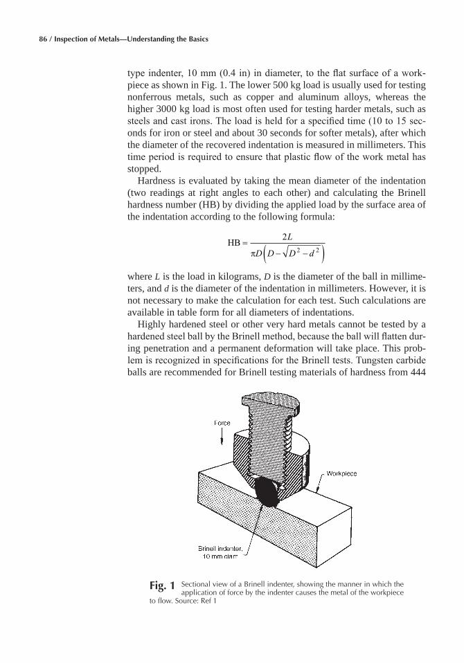
86 / Inspection of Metals—Understanding the Basics
type indenter, 10 mm (0.4 in) in diameter, to the flat surface of a work-piece as shown in Fig. 1. The lower 500 kg load is usually used for testing nonferrous metals, such as copper and aluminum alloys, whereas the higher 3000 kg load is most often used for testing harder metals, such as steels and cast irons. The load is held for a specified time (10 to 15 sec-onds for iron or steel and about 30 seconds for softer metals), after which the diameter of the recovered indentation is measured in millimeters. This time period is required to ensure that plastic flow of the work metal has stopped.
Hardness is evaluated by taking the mean diameter of the indentation (two readings at right angles to each other) and calculating the Brinell hardness number (HB) by dividing the applied load by the surface area of the indentation according to the following formula:
HB =− −( )
22 2
L
D D D dπ
where L is the load in kilograms, D is the diameter of the ball in millime-ters, and d is the diameter of the indentation in millimeters. However, it is not necessary to make the calculation for each test. Such calculations are available in table form for all diameters of indentations.
Highly hardened steel or other very hard metals cannot be tested by a hardened steel ball by the Brinell method, because the ball will flatten dur-ing penetration and a permanent deformation will take place. This prob-lem is recognized in specifications for the Brinell tests. Tungsten carbide balls are recommended for Brinell testing materials of hardness from 444
Fig� 1 Sectional view of a Brinell indenter, showing the manner in which the application of force by the indenter causes the metal of the workpiece
to flow. Source: Ref 1
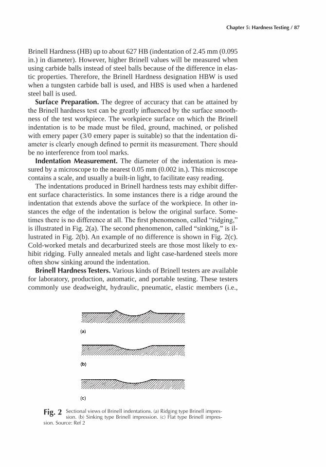
Chapter 5: Hardness Testing / 87
Brinell Hardness (HB) up to about 627 HB (indentation of 2.45 mm (0.095 in.) in diameter). However, higher Brinell values will be measured when using carbide balls instead of steel balls because of the difference in elas-tic properties. Therefore, the Brinell Hardness designation HBW is used when a tungsten carbide ball is used, and HBS is used when a hardened steel ball is used.
Surface Preparation� The degree of accuracy that can be attained by the Brinell hardness test can be greatly influenced by the surface smooth-ness of the test workpiece. The workpiece surface on which the Brinell indentation is to be made must be filed, ground, machined, or polished with emery paper (3/0 emery paper is suitable) so that the indentation di-ameter is clearly enough defined to permit its measurement. There should be no interference from tool marks.
Indentation Measurement� The diameter of the indentation is mea-sured by a microscope to the nearest 0.05 mm (0.002 in.). This microscope contains a scale, and usually a built-in light, to facilitate easy reading.
The indentations produced in Brinell hardness tests may exhibit differ-ent surface characteristics. In some instances there is a ridge around the indentation that extends above the surface of the workpiece. In other in-stances the edge of the indentation is below the original surface. Some-times there is no difference at all. The first phenomenon, called “ridging,” is illustrated in Fig. 2(a). The second phenomenon, called “sinking,” is il-lustrated in Fig. 2(b). An example of no difference is shown in Fig. 2(c). Cold-worked metals and decarburized steels are those most likely to ex-hibit ridging. Fully annealed metals and light case-hardened steels more often show sinking around the indentation.
Brinell Hardness Testers� Various kinds of Brinell testers are available for laboratory, production, automatic, and portable testing. These testers commonly use deadweight, hydraulic, pneumatic, elastic members (i.e.,
Fig� 2 Sectional views of Brinell indentations. (a) Ridging type Brinell impres-sion. (b) Sinking type Brinell impression. (c) Flat type Brinell impres-
sion. Source: Ref 2
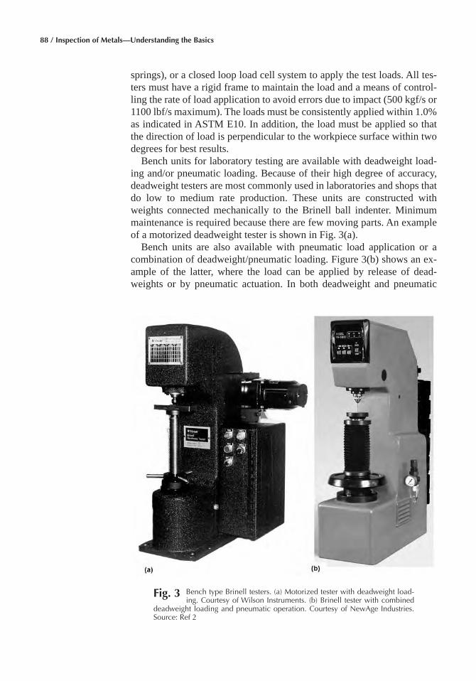
88 / Inspection of Metals—Understanding the Basics
springs), or a closed loop load cell system to apply the test loads. All tes-ters must have a rigid frame to maintain the load and a means of control-ling the rate of load application to avoid errors due to impact (500 kgf/s or 1100 lbf/s maximum). The loads must be consistently applied within 1.0% as indicated in ASTM E10. In addition, the load must be applied so that the direction of load is perpendicular to the workpiece surface within two degrees for best results.
Bench units for laboratory testing are available with deadweight load-ing and/or pneumatic loading. Because of their high degree of accuracy, deadweight testers are most commonly used in laboratories and shops that do low to medium rate production. These units are constructed with weights connected mechanically to the Brinell ball indenter. Minimum maintenance is required because there are few moving parts. An example of a motorized deadweight tester is shown in Fig. 3(a).
Bench units are also available with pneumatic load application or a combination of deadweight/pneumatic loading. Figure 3(b) shows an ex-ample of the latter, where the load can be applied by release of dead-weights or by pneumatic actuation. In both deadweight and pneumatic
Fig� 3 Bench type Brinell testers. (a) Motorized tester with deadweight load-ing. Courtesy of Wilson Instruments. (b) Brinell tester with combined
deadweight loading and pneumatic operation. Courtesy of NewAge Industries. Source: Ref 2
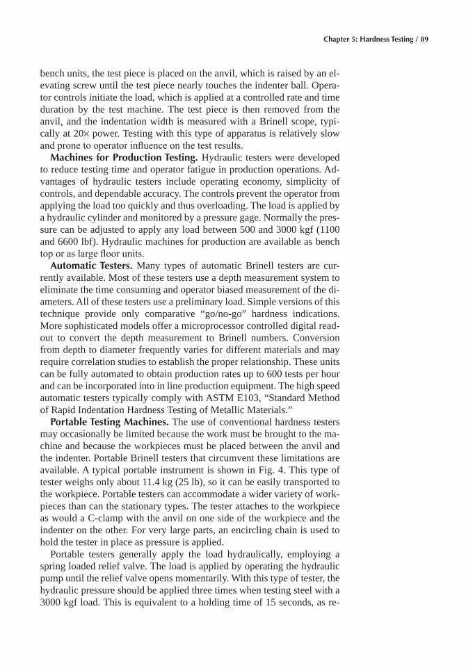
Chapter 5: Hardness Testing / 89
bench units, the test piece is placed on the anvil, which is raised by an el-evating screw until the test piece nearly touches the indenter ball. Opera-tor controls initiate the load, which is applied at a controlled rate and time duration by the test machine. The test piece is then removed from the anvil, and the indentation width is measured with a Brinell scope, typi-cally at 20× power. Testing with this type of apparatus is relatively slow and prone to operator influence on the test results.
Machines for Production Testing� Hydraulic testers were developed to reduce testing time and operator fatigue in production operations. Ad-vantages of hydraulic testers include operating economy, simplicity of controls, and dependable accuracy. The controls prevent the operator from applying the load too quickly and thus overloading. The load is applied by a hydraulic cylinder and monitored by a pressure gage. Normally the pres-sure can be adjusted to apply any load between 500 and 3000 kgf (1100 and 6600 lbf). Hydraulic machines for production are available as bench top or as large floor units.
Automatic Testers� Many types of automatic Brinell testers are cur-rently available. Most of these testers use a depth measurement system to eliminate the time consuming and operator biased measurement of the di-ameters. All of these testers use a preliminary load. Simple versions of this technique provide only comparative “go/no-go” hardness indications. More sophisticated models offer a microprocessor controlled digital read-out to convert the depth measurement to Brinell numbers. Conversion from depth to diameter frequently varies for different materials and may require correlation studies to establish the proper relationship. These units can be fully automated to obtain production rates up to 600 tests per hour and can be incorporated into in line production equipment. The high speed automatic testers typically comply with ASTM E103, “Standard Method of Rapid Indentation Hardness Testing of Metallic Materials.”
Portable Testing Machines� The use of conventional hardness testers may occasionally be limited because the work must be brought to the ma-chine and because the workpieces must be placed between the anvil and the indenter. Portable Brinell testers that circumvent these limitations are available. A typical portable instrument is shown in Fig. 4. This type of tester weighs only about 11.4 kg (25 lb), so it can be easily transported to the workpiece. Portable testers can accommodate a wider variety of work-pieces than can the stationary types. The tester attaches to the workpiece as would a C-clamp with the anvil on one side of the workpiece and the indenter on the other. For very large parts, an encircling chain is used to hold the tester in place as pressure is applied.
Portable testers generally apply the load hydraulically, employing a spring loaded relief valve. The load is applied by operating the hydraulic pump until the relief valve opens momentarily. With this type of tester, the hydraulic pressure should be applied three times when testing steel with a 3000 kgf load. This is equivalent to a holding time of 15 seconds, as re-
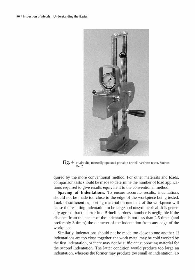
90 / Inspection of Metals—Understanding the Basics
quired by the more conventional method. For other materials and loads, comparison tests should be made to determine the number of load applica-tions required to give results equivalent to the conventional method.
Spacing of Indentations� To ensure accurate results, indentations should not be made too close to the edge of the workpiece being tested. Lack of sufficient supporting material on one side of the workpiece will cause the resulting indentation to be large and unsymmetrical. It is gener-ally agreed that the error in a Brinell hardness number is negligible if the distance from the center of the indentation is not less than 2.5 times (and preferably 3 times) the diameter of the indentation from any edge of the workpiece.
Similarly, indentations should not be made too close to one another. If indentations are too close together, the work metal may be cold worked by the first indentation, or there may not be sufficient supporting material for the second indentation. The latter condition would produce too large an indentation, whereas the former may produce too small an indentation. To
Fig� 4 Hydraulic, manually operated portable Brinell hardness tester. Source: Ref 2
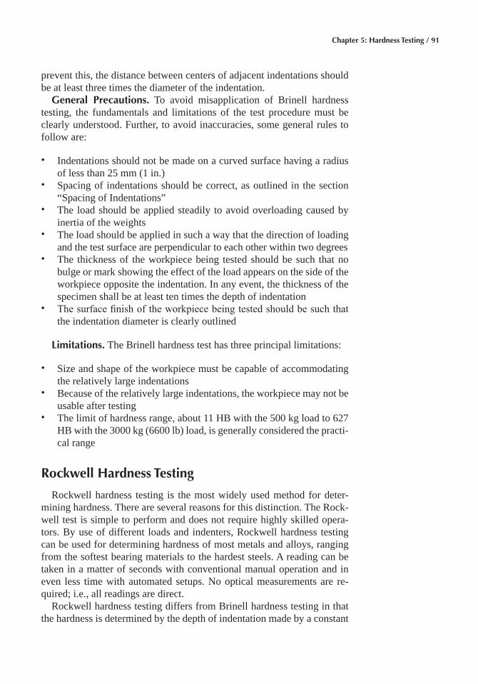
Chapter 5: Hardness Testing / 91
prevent this, the distance between centers of adjacent indentations should be at least three times the diameter of the indentation.
General Precautions� To avoid misapplication of Brinell hardness testing, the fundamentals and limitations of the test procedure must be clearly understood. Further, to avoid inaccuracies, some general rules to follow are:
• Indentations should not be made on a curved surface having a radius of less than 25 mm (1 in.)
• Spacing of indentations should be correct, as outlined in the section “Spacing of Indentations”
• The load should be applied steadily to avoid overloading caused by inertia of the weights
• The load should be applied in such a way that the direction of loading and the test surface are perpendicular to each other within two degrees
• The thickness of the workpiece being tested should be such that no bulge or mark showing the effect of the load appears on the side of the workpiece opposite the indentation. In any event, the thickness of the specimen shall be at least ten times the depth of indentation
• The surface finish of the workpiece being tested should be such that the indentation diameter is clearly outlined
Limitations� The Brinell hardness test has three principal limitations:
• Size and shape of the workpiece must be capable of accommodating the relatively large indentations
• Because of the relatively large indentations, the workpiece may not be usable after testing
• The limit of hardness range, about 11 HB with the 500 kg load to 627 HB with the 3000 kg (6600 lb) load, is generally considered the practi-cal range
Rockwell Hardness Testing
Rockwell hardness testing is the most widely used method for deter-mining hardness. There are several reasons for this distinction. The Rock-well test is simple to perform and does not require highly skilled opera-tors. By use of different loads and indenters, Rockwell hardness testing can be used for determining hardness of most metals and alloys, ranging from the softest bearing materials to the hardest steels. A reading can be taken in a matter of seconds with conventional manual operation and in even less time with automated setups. No optical measurements are re-quired; i.e., all readings are direct.
Rockwell hardness testing differs from Brinell hardness testing in that the hardness is determined by the depth of indentation made by a constant
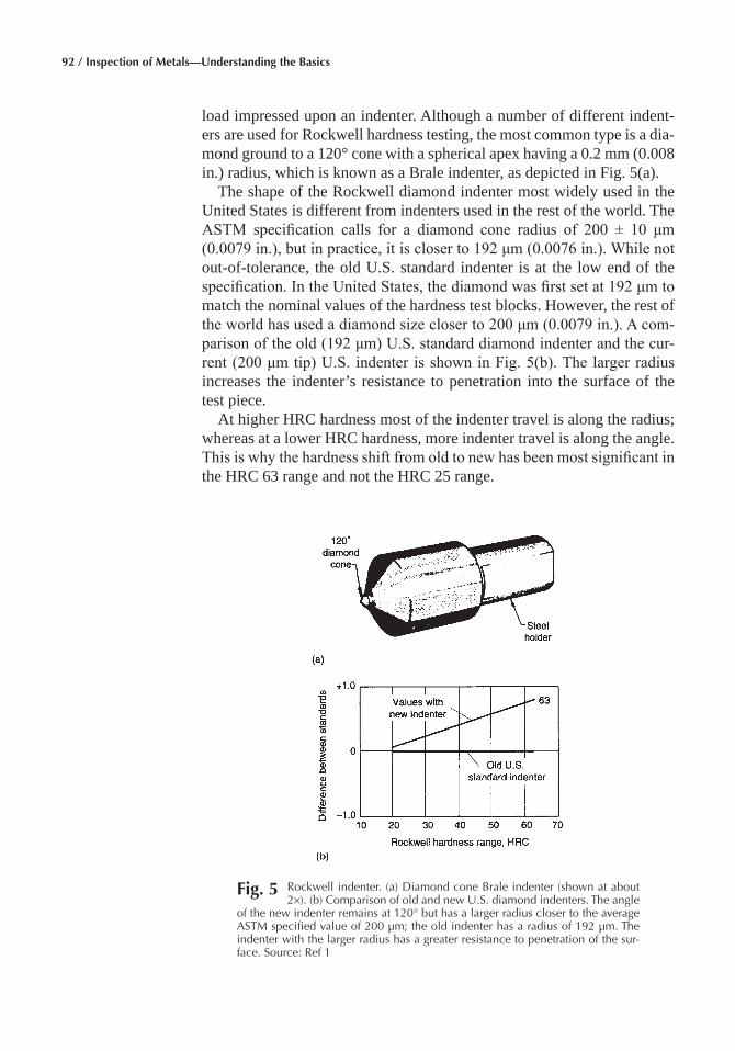
92 / Inspection of Metals—Understanding the Basics
load impressed upon an indenter. Although a number of different indent-ers are used for Rockwell hardness testing, the most common type is a dia-mond ground to a 120° cone with a spherical apex having a 0.2 mm (0.008 in.) radius, which is known as a Brale indenter, as depicted in Fig. 5(a).
The shape of the Rockwell diamond indenter most widely used in the United States is different from indenters used in the rest of the world. The ASTM specification calls for a diamond cone radius of 200 ± 10 μm (0.0079 in.), but in practice, it is closer to 192 μm (0.0076 in.). While not out-of-tolerance, the old U.S. standard indenter is at the low end of the specification. In the United States, the diamond was first set at 192 μm to match the nominal values of the hardness test blocks. However, the rest of the world has used a diamond size closer to 200 μm (0.0079 in.). A com-parison of the old (192 μm) U.S. standard diamond indenter and the cur-rent (200 μm tip) U.S. indenter is shown in Fig. 5(b). The larger radius increases the indenter’s resistance to penetration into the surface of the test piece.
At higher HRC hardness most of the indenter travel is along the radius; whereas at a lower HRC hardness, more indenter travel is along the angle. This is why the hardness shift from old to new has been most significant in the HRC 63 range and not the HRC 25 range.
Fig� 5 Rockwell indenter. (a) Diamond cone Brale indenter (shown at about 2×). (b) Comparison of old and new U.S. diamond indenters. The angle
of the new indenter remains at 120° but has a larger radius closer to the average ASTM specified value of 200 μm; the old indenter has a radius of 192 μm. The indenter with the larger radius has a greater resistance to penetration of the sur-face. Source: Ref 1
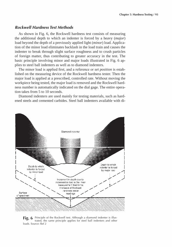
Chapter 5: Hardness Testing / 93
Rockwell Hardness Test Methods
As shown in Fig. 6, the Rockwell hardness test consists of measuring the additional depth to which an indenter is forced by a heavy (major) load beyond the depth of a previously applied light (minor) load. Applica-tion of the minor load eliminates backlash in the load train and causes the indenter to break through slight surface roughness and to crush particles of foreign matter, thus contributing to greater accuracy in the test. The basic principle involving minor and major loads illustrated in Fig. 6 ap-plies to steel ball indenters as well as to diamond indenters.
The minor load is applied first, and a reference or set position is estab-lished on the measuring device of the Rockwell hardness tester. Then the major load is applied at a prescribed, controlled rate. Without moving the workpiece being tested, the major load is removed and the Rockwell hard-ness number is automatically indicated on the dial gage. The entire opera-tion takes from 5 to 10 seconds.
Diamond indenters are used mainly for testing materials, such as hard-ened steels and cemented carbides. Steel ball indenters available with di-
Fig� 6 Principle of the Rockwell test. Although a diamond indenter is illus-trated, the same principle applies for steel ball indenters and other
loads. Source: Ref 2
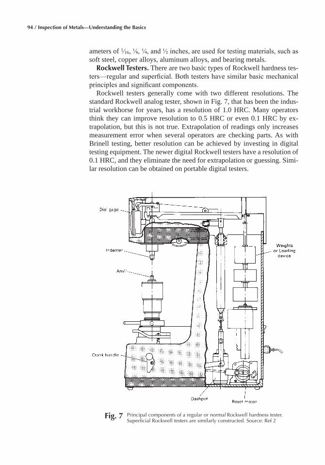
94 / Inspection of Metals—Understanding the Basics
ameters of 1⁄16, ⅛, ¼, and ½ inches, are used for testing materials, such as soft steel, copper alloys, aluminum alloys, and bearing metals.
Rockwell Testers� There are two basic types of Rockwell hardness tes-ters—regular and superficial. Both testers have similar basic mechanical principles and significant components.
Rockwell testers generally come with two different resolutions. The standard Rockwell analog tester, shown in Fig. 7, that has been the indus-trial workhorse for years, has a resolution of 1.0 HRC. Many operators think they can improve resolution to 0.5 HRC or even 0.1 HRC by ex-trapolation, but this is not true. Extrapolation of readings only increases measurement error when several operators are checking parts. As with Brinell testing, better resolution can be achieved by investing in digital testing equipment. The newer digital Rockwell testers have a resolution of 0.1 HRC, and they eliminate the need for extrapolation or guessing. Simi-lar resolution can be obtained on portable digital testers.
Fig� 7 Principal components of a regular or normal Rockwell hardness tester. Superficial Rockwell testers are similarly constructed. Source: Ref 2
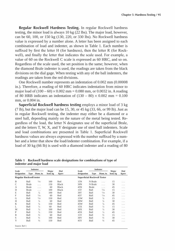
Chapter 5: Hardness Testing / 95
Regular Rockwell Hardness Testing� In regular Rockwell hardness testing, the minor load is always 10 kg (22 lbs). The major load, however, can be 60, 100, or 150 kg (130, 220, or 330 lbs). No Rockwell hardness value is expressed by a number alone. A letter has been assigned to each combination of load and indenter, as shown in Table 1. Each number is suffixed by first the letter H (for hardness), then the letter R (for Rock-well), and finally the letter that indicates the scale used. For example, a value of 60 on the Rockwell C scale is expressed as 60 HRC, and so on. Regardless of the scale used, the set position is the same; however, when the diamond Brale indenter is used, the readings are taken from the black divisions on the dial gage. When testing with any of the ball indenters, the readings are taken from the red divisions.
One Rockwell number represents an indentation of 0.002 mm (0.00008 in.). Therefore, a reading of 60 HRC indicates indentation from minor to major load of (100 – 60) × 0.002 mm = 0.080 mm, or 0.0032 in. A reading of 80 HRB indicates an indentation of (130 – 80) × 0.002 mm = 0.100 mm, or 0.004 in.
Superficial Rockwell hardness testing employs a minor load of 3 kg (7 lb), but the major load can be 15, 30, or 45 kg (33, 66, or 99 lb). Just as in regular Rockwell testing, the indenter may either be a diamond or a steel ball, depending mainly on the nature of the metal being tested. Re-gardless of the load, the letter N designates use of the superficial Brale, and the letters T, W, X, and Y designate use of steel ball indenters. Scale and load combinations are presented in Table 1. Superficial Rockwell hardness values are always expressed with the number suffixed by a num-ber and a letter that show the load/indenter combination. For example, if a load of 30 kg (66 lb) is used with a diamond indenter and a reading of 80
Table 1 Rockwell hardness scale designations for combinations of type of indenter and major load
Scale designation
IndenterMajor
load, kgDial
figureScale designation
IndenterMajor
load, kgDial
figureType Diam, in. Type Diam, in.
Regular Rockwell tester Superficial Rockwell Tester
B Ball 1⁄16 100 Red 15N N Brale . . . 15 . . . C Brale . . . 150 Black 30N N Brale . . . 30 . . . A Brale . . . 60 Black 45N Brale . . . 45 . . . D Brale . . . 100 Black 15T Ball 1⁄16 15 . . . E Ball ⅛ 100 Red 30T Ball 1⁄16 30 . . . F Ball 1⁄16 60 Red 45T Ball 1⁄16 45 . . . G Ball 1⁄16 150 Red 15W Ball ⅛ 15 . . . H Ball ⅛ 60 Red 30W Ball ⅛ 30 . . . K Ball ⅛ 150 Red 45W Ball ⅛ 45 . . . L Ball ¼ 60 Red 15X Ball ¼ 15 . . . M Ball ¼ 100 Red 30X Ball ¼ 30 . . . P Ball ¼ 150 Red 45X Ball ¼ 45 . . . R Ball ½ 60 Red 15Y Ball ½ 15 . . . S Ball ½ 100 Red 30Y Ball ½ 30 . . . V Ball ½ 150 Red 45Y Ball ½ 45 . . .
Source: Ref 1
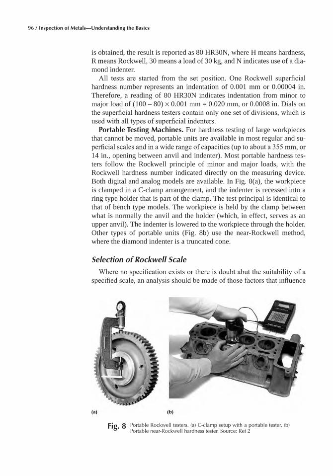
96 / Inspection of Metals—Understanding the Basics
is obtained, the result is reported as 80 HR30N, where H means hardness, R means Rockwell, 30 means a load of 30 kg, and N indicates use of a dia-mond indenter.
All tests are started from the set position. One Rockwell superficial hardness number represents an indentation of 0.001 mm or 0.00004 in. Therefore, a reading of 80 HR30N indicates indentation from minor to major load of (100 – 80) × 0.001 mm = 0.020 mm, or 0.0008 in. Dials on the superficial hardness testers contain only one set of divisions, which is used with all types of superficial indenters.
Portable Testing Machines� For hardness testing of large workpieces that cannot be moved, portable units are available in most regular and su-perficial scales and in a wide range of capacities (up to about a 355 mm, or 14 in., opening between anvil and indenter). Most portable hardness tes-ters follow the Rockwell principle of minor and major loads, with the Rockwell hardness number indicated directly on the measuring device. Both digital and analog models are available. In Fig. 8(a), the workpiece is clamped in a C-clamp arrangement, and the indenter is recessed into a ring type holder that is part of the clamp. The test principal is identical to that of bench type models. The workpiece is held by the clamp between what is normally the anvil and the holder (which, in effect, serves as an upper anvil). The indenter is lowered to the workpiece through the holder. Other types of portable units (Fig. 8b) use the near-Rockwell method, where the diamond indenter is a truncated cone.
Selection of Rockwell Scale
Where no specification exists or there is doubt abut the suitability of a specified scale, an analysis should be made of those factors that influence
Fig� 8 Portable Rockwell testers. (a) C-clamp setup with a portable tester. (b) Portable near-Rockwell hardness tester. Source: Ref 2
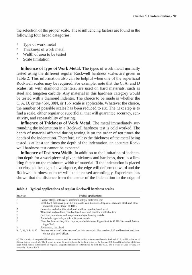
Chapter 5: Hardness Testing / 97
the selection of the proper scale. These influencing factors are found in the following four broad categories:
• Type of work metal • Thickness of work metal • Width of area to be tested • Scale limitation
Influence of Type of Work Metal� The types of work metal normally tested using the different regular Rockwell hardness scales are given in Table 2. This information also can be helpful when one of the superficial Rockwell scales may be required. For example, note that the C, A, and D scales, all with diamond indenters, are used on hard materials, such as steel and tungsten carbide. Any material in this hardness category would be tested with a diamond indenter. The choice to be made is whether the C, A, D, or the 45N, 30N, or 15N scale is applicable. Whatever the choice, the number of possible scales has been reduced to six. The next step is to find a scale, either regular or superficial, that will guarantee accuracy, sen-sitivity, and repeatability of testing.
Influence of Thickness of Work Metal� The metal immediately sur-rounding the indentation in a Rockwell hardness test is cold worked. The depth of material affected during testing is on the order of ten times the depth of the indentation. Therefore, unless the thickness of the metal being tested is at least ten times the depth of the indentation, an accurate Rock-well hardness test cannot be expected.
Influence of Test Area Width� In addition to the limitation of indenta-tion depth for a workpiece of given thickness and hardness, there is a lim-iting factor on the minimum width of material. If the indentation is placed too close to the edge of a workpiece, the edge will deform outward and the Rockwell hardness number will be decreased accordingly. Experience has shown that the distance from the center of the indentation to the edge of
Table 2 Typical applications of regular Rockwell hardness scales
Scale(a) Typical applications B Copper alloys, soft steels, aluminum alloys, malleable iron C Steel, hard cast irons, pearlitic malleable iron, titanium, deep case-hardened steel, and other
materials harder than 100 HRB A Cemented carbides, thin steel, and shallow case-hardened steel D Thin steel and medium case-hardened steel and pearlitic malleable iron E Cast iron, aluminum and magnesium alloys, bearing metals F Annealed copper alloys, thin soft sheet metals G Phosphor bronze, beryllium copper, malleable irons. Upper limit is 92 HRG to avoid flatten-
ing of ball. H Aluminum, zinc, lead K, L, M, P, R, S, V Bearing metals and other very soft or thin materials. Use smallest ball and heaviest load that
do not give anvil effect.
(a) The N scales of a superficial hardness tester are used for materials similar to those tested on the Rockwell C, A, and D scales but of thinner gage or case depth. The T scales are used for materials similar to those tested on the Rockwell B, F, and G scales but of thinner gage. When minute indentations are required, a superficial hardness tester should be used. The W, X, and Y scales are used for very soft materials . Source: Ref 1
98 / Inspection of Metals—Understanding the Basics
the workpiece must be at least 2.5 times the diameter of the indentation to ensure an accurate test. Therefore, the width of a narrow test area must be at least 5 indentation diameters when the indentation is placed in the center.
Limitations of Rockwell Scales� The potential range of each Rockwell scale can be determined readily from the dial gage divisions on the tester: the black scale (for diamond indenter) on all regular hardness tester dial gages is numbered from 0 to 100, with 100 corresponding to the set posi-tion; the red scale (for ball indenters) is numbered from 0 to 130, with 130 being the set position. On the superficial hardness tester, the dial gage has only one set of divisions, numbered from 0 to 100.
Use of the diamond indenter when readings fall below 20 is not recom-mended, because there is loss of sensitivity when indenting this far down the conical section of the indenter. Brale indenters are not calibrated below values of 20, and if used on soft materials, there is no assurance that there will be the usual degree of agreement in results when replacing the indenters.
Support for Workpiece� A fundamental requirement of the Rockwell hardness test is that the surface of the workpiece being tested be approxi-mately normal to the indenter and that the workpiece must not move or slip in the slightest degree as the major load is applied. The depth of in-dentation is measured by the movement of the plunger rod holding the indenter; therefore, any slipping or moving of the workpiece will be fol-lowed by the plunger rod and the motion transferred to the dial gage, caus-ing an error to be introduced into the hardness test. As one point of hard-ness represents a depth of only 0.002 mm (0.00008 in.), a movement of only 0.025 mm (0.001 in.), could cause an error of over 10 Rockwell num-bers. The support must be of sufficient rigidity to prevent its permanent deformation in use.
Anvils should be selected to minimize contact area of the workpiece while maintaining stability. Figure 9 illustrates several common types of anvils that can accommodate a broad range of workpiece shapes. An anvil with a large flat surface (Fig. 9b) should be used to support flat bottom workpieces of thick section. Anvils with a surface diameter greater than about 75 mm (3 in.) should be attached to the elevating screw by a threaded section, rather than inserted in the anvil hole in the elevating screw. Sheet metal and small workpieces that have flat undersurfaces are best tested on a spot anvil with a small, elevated, flat bearing surface (Fig. 9a). Work-pieces that are not flat should have the convex side down on the bearing surface. Round workpieces should be supported in a V-slot anvil (Fig. 9a and c). Diamond spot anvils (Fig. 9d) are used only for testing very thin sheet metal samples in the HR15T and HR30T scales. Other anvil designs are available for a wide range of odd shaped parts, such as the eyeball anvil (Fig. 9e) that is used for tapered parts. Special anvils to accommo-date specific workpiece configurations can be fabricated. Regardless of
Chapter 5: Hardness Testing / 99
anvil design, rigidity of the part to prevent movement during the test is absolutely essential for accurate results, as is cleanliness of the mating faces of the anvil and its supporting surface.
Work supports are available for long workpieces that cannot be firmly held on an anvil by the minor load. Because manual support is not practi-cal, a jack rest should be provided at the overhang end to prevent pressure between the specimen and the penetrator. Figure 10 illustrates methods for testing long, heavy workpieces. When testing cylindrical pieces such as rods, the shallow-V or standard-V anvil should be used, and the indenter should be applied over the axis of the rod. Care should be taken that the specimen lies flat, supported by the sides of the V-slot anvil.
Fig� 9 Typical anvils for Rockwell hardness testing. (a) Standard spot, flat, and V anvils. (b) Testing table for large workpieces. (c) Cylinder anvil. (d)
Diamond spot anvil. (e) Eyeball anvil. Source: Ref 2
Fig� 10 Rockwell test setups for long test pieces. (a) Jack setup. (b) Variable rest setup. Source: Ref 2
100 / Inspection of Metals—Understanding the Basics
Vickers Hardness Testing (ASTM E384)
In 1925, Smith and Sandland of the United Kingdom developed a new indentation test for metals that were too hard to evaluate by the Brinell test, whose hardened steel ball was limited to steels with a hardness below ~450 HBS (~48 HRC). In designing the new indenter, they chose a square based diamond pyramid (Fig. 11) geometry that would produce hardness numbers nearly identical to Brinell numbers within the range of both. This decision was very wise, as it made the Vickers test very easy to adopt.
The ideal d/D ratio (d = impression diameter, D = ball diameter) for a spherical indenter is 0.375. If tangents are drawn to the ball at the impres-sion edges for d/D = 0.375, they meet below the center of the impression at an angle of 136°, the angle chosen for the Vickers indenter.
The use of a diamond indenter allows the Vickers test to evaluate any material and, furthermore, has the very important advantage of placing the hardness of all materials on one continuous scale. The lack of a continu-ous scale is a major disadvantage of Rockwell type tests, for which 15 standard and 15 superficial scales were developed. Not one of these scales can cover the full hardness range. The HRA scale covers the broadest hardness range, but it is not commonly used.
In the Vickers test, the load is applied smoothly, without impact, and held in place for 10 or 15 seconds. The physical quality of the indenter and the accuracy of the applied load (defined in ASTM E384) must be con-trolled to get the correct results. After the load is removed, the two impres-sion diagonals are measured, usually with a filar micrometer, to the near-est 0.1 μm, and then averaged. The Vickers hardness (HV) is calculated by:
HV =1854 4
2
. L
d
where the load L is in grams-force, and the average diagonal d is in μm (although the hardness numbers are expressed in units of kgf/mm2 rather than the equivalent gf/μm2).
The original Vickers testers were developed for test loads of 1 to 120 kgf, which produce rather large indents. Recognizing the need for lower test loads, the National Physical Laboratory (U.K.) experimented with lower test loads in 1932. The first low load Vickers tester was described by Lips and Sack in 1936.
Because the shape of the Vickers indentation is geometrically similar at all test loads, the HV value is constant, within statistical precision, over a very wide test load range, as long as the test specimen is reasonably ho-mogeneous. However, studies of microindentation hardness test results conducted over the past several years on a wide range of loads have shown that results are not constant at very low loads. This problem, called the indentation size effect (ISE), has been attributed to fundamental character-
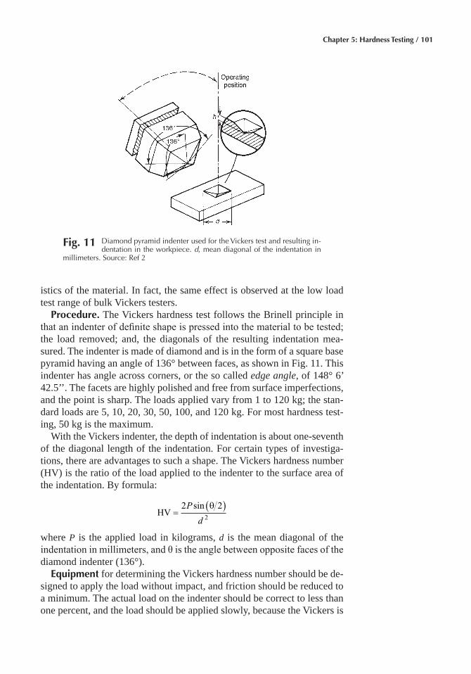
Chapter 5: Hardness Testing / 101
istics of the material. In fact, the same effect is observed at the low load test range of bulk Vickers testers.
Procedure� The Vickers hardness test follows the Brinell principle in that an indenter of definite shape is pressed into the material to be tested; the load removed; and, the diagonals of the resulting indentation mea-sured. The indenter is made of diamond and is in the form of a square base pyramid having an angle of 136° between faces, as shown in Fig. 11. This indenter has angle across corners, or the so called edge angle, of 148° 6’ 42.5’’. The facets are highly polished and free from surface imperfections, and the point is sharp. The loads applied vary from 1 to 120 kg; the stan-dard loads are 5, 10, 20, 30, 50, 100, and 120 kg. For most hardness test-ing, 50 kg is the maximum.
With the Vickers indenter, the depth of indentation is about one-seventh of the diagonal length of the indentation. For certain types of investiga-tions, there are advantages to such a shape. The Vickers hardness number (HV) is the ratio of the load applied to the indenter to the surface area of the indentation. By formula:
HV =( )2 22
P
d
sin θ
where P is the applied load in kilograms, d is the mean diagonal of the indentation in millimeters, and θ is the angle between opposite faces of the diamond indenter (136°).
Equipment for determining the Vickers hardness number should be de-signed to apply the load without impact, and friction should be reduced to a minimum. The actual load on the indenter should be correct to less than one percent, and the load should be applied slowly, because the Vickers is
Fig� 11 Diamond pyramid indenter used for the Vickers test and resulting in-dentation in the workpiece. d, mean diagonal of the indentation in
millimeters. Source: Ref 2
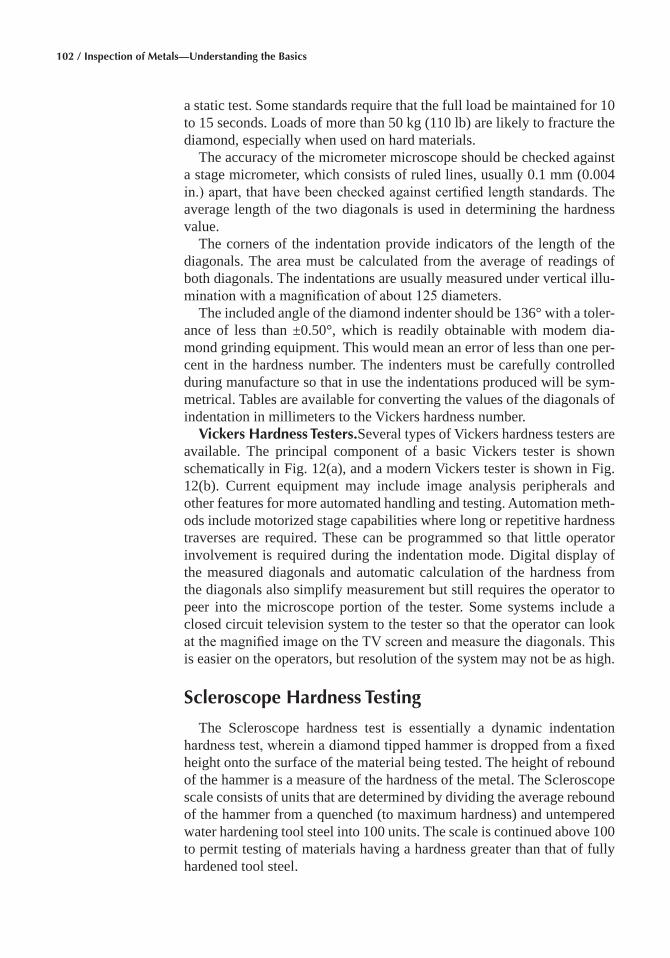
102 / Inspection of Metals—Understanding the Basics
a static test. Some standards require that the full load be maintained for 10 to 15 seconds. Loads of more than 50 kg (110 lb) are likely to fracture the diamond, especially when used on hard materials.
The accuracy of the micrometer microscope should be checked against a stage micrometer, which consists of ruled lines, usually 0.1 mm (0.004 in.) apart, that have been checked against certified length standards. The average length of the two diagonals is used in determining the hardness value.
The corners of the indentation provide indicators of the length of the diagonals. The area must be calculated from the average of readings of both diagonals. The indentations are usually measured under vertical illu-mination with a magnification of about 125 diameters.
The included angle of the diamond indenter should be 136° with a toler-ance of less than ±0.50°, which is readily obtainable with modem dia-mond grinding equipment. This would mean an error of less than one per-cent in the hardness number. The indenters must be carefully controlled during manufacture so that in use the indentations produced will be sym-metrical. Tables are available for converting the values of the diagonals of indentation in millimeters to the Vickers hardness number.
Vickers Hardness Testers�Several types of Vickers hardness testers are available. The principal component of a basic Vickers tester is shown schematically in Fig. 12(a), and a modern Vickers tester is shown in Fig. 12(b). Current equipment may include image analysis peripherals and other features for more automated handling and testing. Automation meth-ods include motorized stage capabilities where long or repetitive hardness traverses are required. These can be programmed so that little operator involvement is required during the indentation mode. Digital display of the measured diagonals and automatic calculation of the hardness from the diagonals also simplify measurement but still requires the operator to peer into the microscope portion of the tester. Some systems include a closed circuit television system to the tester so that the operator can look at the magnified image on the TV screen and measure the diagonals. This is easier on the operators, but resolution of the system may not be as high.
Scleroscope Hardness Testing
The Scleroscope hardness test is essentially a dynamic indentation hardness test, wherein a diamond tipped hammer is dropped from a fixed height onto the surface of the material being tested. The height of rebound of the hammer is a measure of the hardness of the metal. The Scleroscope scale consists of units that are determined by dividing the average rebound of the hammer from a quenched (to maximum hardness) and untempered water hardening tool steel into 100 units. The scale is continued above 100 to permit testing of materials having a hardness greater than that of fully hardened tool steel.
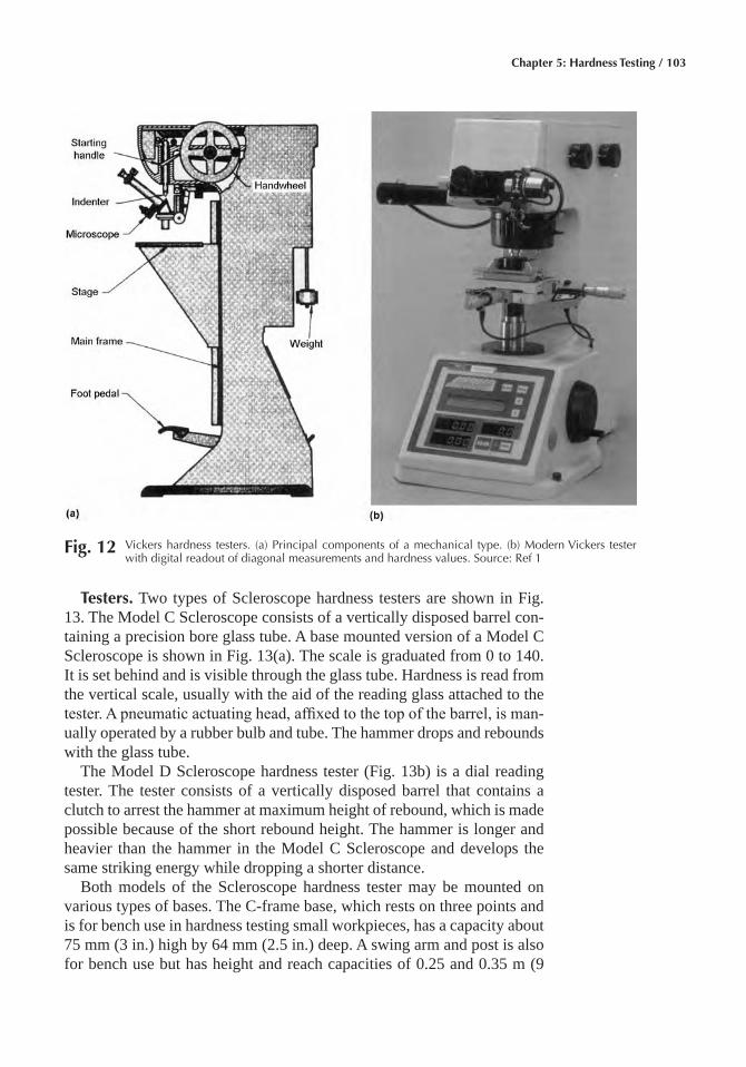
Chapter 5: Hardness Testing / 103
Testers� Two types of Scleroscope hardness testers are shown in Fig. 13. The Model C Scleroscope consists of a vertically disposed barrel con-taining a precision bore glass tube. A base mounted version of a Model C Scleroscope is shown in Fig. 13(a). The scale is graduated from 0 to 140. It is set behind and is visible through the glass tube. Hardness is read from the vertical scale, usually with the aid of the reading glass attached to the tester. A pneumatic actuating head, affixed to the top of the barrel, is man-ually operated by a rubber bulb and tube. The hammer drops and rebounds with the glass tube.
The Model D Scleroscope hardness tester (Fig. 13b) is a dial reading tester. The tester consists of a vertically disposed barrel that contains a clutch to arrest the hammer at maximum height of rebound, which is made possible because of the short rebound height. The hammer is longer and heavier than the hammer in the Model C Scleroscope and develops the same striking energy while dropping a shorter distance.
Both models of the Scleroscope hardness tester may be mounted on various types of bases. The C-frame base, which rests on three points and is for bench use in hardness testing small workpieces, has a capacity about 75 mm (3 in.) high by 64 mm (2.5 in.) deep. A swing arm and post is also for bench use but has height and reach capacities of 0.25 and 0.35 m (9
Fig� 12 Vickers hardness testers. (a) Principal components of a mechanical type. (b) Modern Vickers tester with digital readout of diagonal measurements and hardness values. Source: Ref 1
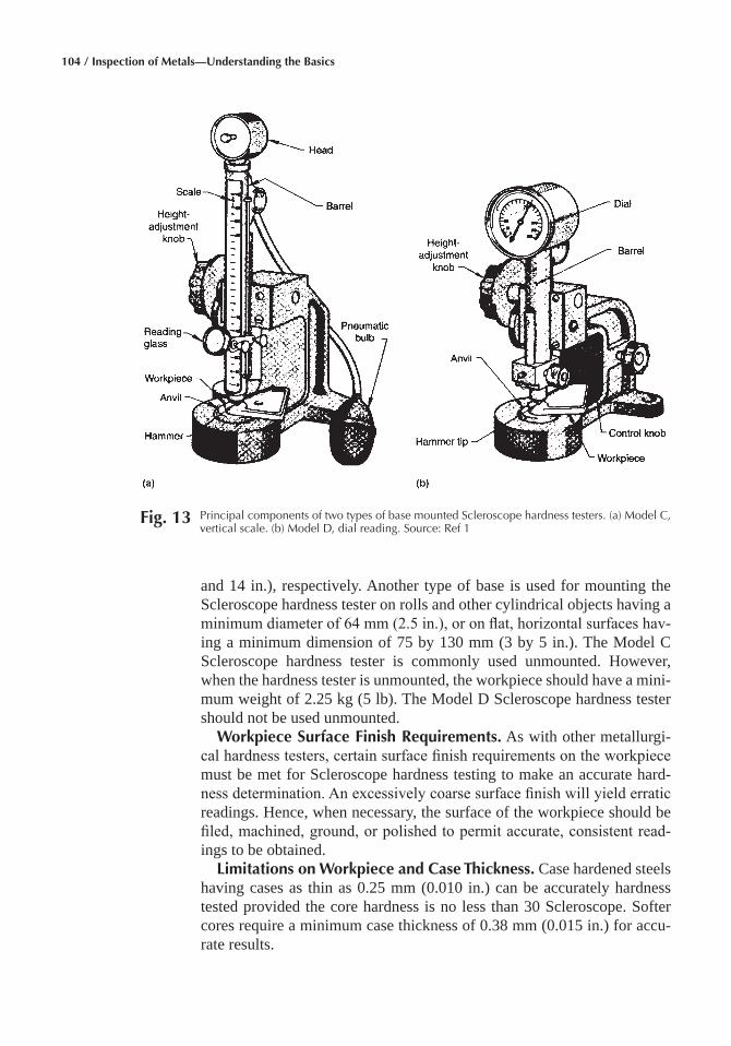
104 / Inspection of Metals—Understanding the Basics
and 14 in.), respectively. Another type of base is used for mounting the Scleroscope hardness tester on rolls and other cylindrical objects having a minimum diameter of 64 mm (2.5 in.), or on flat, horizontal surfaces hav-ing a minimum dimension of 75 by 130 mm (3 by 5 in.). The Model C Scleroscope hardness tester is commonly used unmounted. However, when the hardness tester is unmounted, the workpiece should have a mini-mum weight of 2.25 kg (5 lb). The Model D Scleroscope hardness tester should not be used unmounted.
Workpiece Surface Finish Requirements� As with other metallurgi-cal hardness testers, certain surface finish requirements on the workpiece must be met for Scleroscope hardness testing to make an accurate hard-ness determination. An excessively coarse surface finish will yield erratic readings. Hence, when necessary, the surface of the workpiece should be filed, machined, ground, or polished to permit accurate, consistent read-ings to be obtained.
Limitations on Workpiece and Case Thickness� Case hardened steels having cases as thin as 0.25 mm (0.010 in.) can be accurately hardness tested provided the core hardness is no less than 30 Scleroscope. Softer cores require a minimum case thickness of 0.38 mm (0.015 in.) for accu-rate results.
Fig� 13 Principal components of two types of base mounted Scleroscope hardness testers. (a) Model C, vertical scale. (b) Model D, dial reading. Source: Ref 1
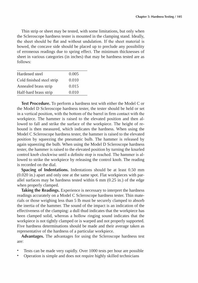
Chapter 5: Hardness Testing / 105
Thin strip or sheet may be tested, with some limitations, but only when the Scleroscope hardness tester is mounted in the clamping stand. Ideally, the sheet should be flat and without undulation. If the sheet material is bowed, the concave side should be placed up to preclude any possibility of erroneous readings due to spring effect. The minimum thicknesses of sheet in various categories (in inches) that may be hardness tested are as follows:
Hardened steel 0.005 Cold finished steel strip 0.010 Annealed brass strip 0.015 Half-hard brass strip 0.010
Test Procedure� To perform a hardness test with either the Model C or the Model D Scleroscope hardness tester, the tester should be held or set in a vertical position, with the bottom of the barrel in firm contact with the workpiece. The hammer is raised to the elevated position and then al-lowed to fall and strike the surface of the workpiece. The height of re-bound is then measured, which indicates the hardness. When using the Model C Scleroscope hardness tester, the hammer is raised to the elevated position by squeezing the pneumatic bulb. The hammer is released by again squeezing the bulb. When using the Model D Scleroscope hardness tester, the hammer is raised to the elevated position by turning the knurled control knob clockwise until a definite stop is reached. The hammer is al-lowed to strike the workpiece by releasing the control knob. The reading is recorded on the dial.
Spacing of Indentations� Indentations should be at least 0.50 mm (0.020 in.) apart and only one at the same spot. Flat workpieces with par-allel surfaces may be hardness tested within 6 mm (0.25 in.) of the edge when properly clamped.
Taking the Readings� Experience is necessary to interpret the hardness readings accurately on a Model C Scleroscope hardness tester. Thin mate-rials or those weighing less than 5 lb must be securely clamped to absorb the inertia of the hammer. The sound of the impact is an indication of the effectiveness of the clamping: a dull thud indicates that the workpiece has been clamped solid, whereas a hollow ringing sound indicates that the workpiece is not tightly clamped or is warped and not properly supported. Five hardness determinations should be made and their average taken as representative of the hardness of a particular workpiece.
Advantages� The advantages for using the Scleroscope hardness test are:
• Tests can be made very rapidly. Over 1000 tests per hour are possible • Operation is simple and does not require highly skilled technicians

106 / Inspection of Metals—Understanding the Basics
• The Model C Scleroscope tester is portable and may be used un-mounted for hardness testing workpieces of unlimited size: rolls, large dies, and machine tool ways
• The Scleroscope hardness test is a nonmarring test; no crater is left, and only in the most unusual instances would the tiny hammer mark be objectionable on a finished workpiece
• A single scale accommodates the entire hardness range from the soft-est to the hardest metals
Limitations� The limitations when using the Scleroscope hardness test are:
• The hardness tester must be in a vertical position, or the free fall of the hammer will be impeded and result in erratic readings
• Scleroscope hardness tests are more sensitive to variations in surface conditions than some other hardness tests
• Because readings taken with the Model C Scleroscope hardness tester are those observed from the maximum rebound of the hammer on the first bounce, even the most experienced operators may disagree among themselves by one or two points in the reading
Microhardness Testing
The term microhardness usually refers to indentation hardness tests made with loads not exceeding 1 kg (2 lbs). Such hardness tests have been made with a load as light as 1 g (0.002 lbs), although the majority of mi-crohardness tests are made with loads of 100 to 500 g (0.2 to 1 lb). In general, the term is related to the size of the indentation rather than the load applied. Microhardness testing is capable of providing information regarding the hardness characteristics of materials that cannot be obtained with hardness tests, such as the Brinell, Rockwell, or Scleroscope.
Because of the required degree of precision for both equipment and operation, microhardness testing is usually, although not necessarily, per-formed in a laboratory. However, such a laboratory is often a process con-trol laboratory and may be located close to production operations. Micro-hardness testing is recognized as a valuable method for controlling numerous production operations in addition to its use in research applica-tions. Specific fields of application of microhardness testing include:
• Measuring hardness of precision workpieces that are too small to be measured by the more common hardness testing methods
• Measuring hardness of product forms, such as foil or wire, that are too thin or too small in diameter to be measured by the more convenient methods
Chapter 5: Hardness Testing / 107
• Monitoring of carburizing or nitriding operations, which is usually ac-complished by hardness surveys taken on cross sections of test pieces that accompanied the workpieces through production operations
• Measuring hardness of individual microconstituents • Measuring hardness close to edges, thus detecting undesirable surface
conditions, such as grinding bum and decarburization • Measuring hardness of surface layers, such as plated or bonded layers
Indenters� Microhardness testing is performed with either the Knoop or the Vickers indenter. The Knoop indenter is more widely used in the United States, while the Vickers indenter is more widely used in Europe.
As previously discussed, the Vickers test is an indentation test that em-ploys a square based pyramidal shaped indenter made from diamond (Fig. 14a). Figure 14(b) shows examples of Vickers indents to illustrate the in-fluence of test force on indent size.
In this test, the force is applied smoothly, without impact, and held in contact for 10 to 15 seconds. The force must be known precisely (refer to ASTM E384 for tolerances). After the force is removed, both diagonals are measured and the average is used to calculate the HV according to:
HV =( )
=2000 2 1854 4
2 2
P
d
P
d
sin .α
where d is the mean diagonal in μm, P is the applied load in gf, and α is the face angle (136°).
The hardness can be computed with the formula and a calculator, or using a spreadsheet program. Most modern microhardness test units have the calculation capability built in and display the hardness value along with the measured diagonals. A book of tables of HV as a function of d and P also accompanies most testers, and ASTM E384 includes such tables.
In 1939, Frederick Knoop and his associates at the former National Bu-reau of Standards developed an alternate indenter based on a rhombohe-dral shaped diamond with the long diagonal approximately seven times as long as the short diagonal (Fig. 15a). Figure 15(b) shows examples of Knoop indents to illustrate the influence of applied load on indent size. The Knoop indenter is used in the same machine as the Vickers indenter, and the test is conducted in exactly the same manner, except that the Knoop hardness (HK) is calculated based on the measurement of the long diagonal only and calculation of the projected area of the indent rather than the surface area of the indent:
HKp
= =1000 14229
2 2
P
C d
P
d
where Cp is the indenter constant, which permits calculation of the pro-jected area of the indent from the long diagonal squared.
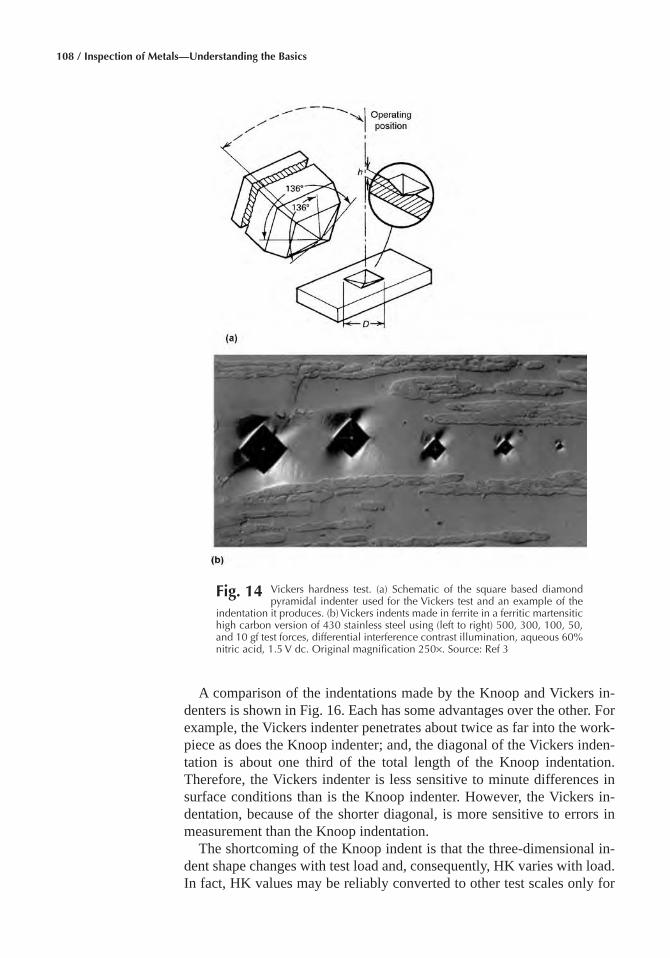
108 / Inspection of Metals—Understanding the Basics
A comparison of the indentations made by the Knoop and Vickers in-denters is shown in Fig. 16. Each has some advantages over the other. For example, the Vickers indenter penetrates about twice as far into the work-piece as does the Knoop indenter; and, the diagonal of the Vickers inden-tation is about one third of the total length of the Knoop indentation. Therefore, the Vickers indenter is less sensitive to minute differences in surface conditions than is the Knoop indenter. However, the Vickers in-dentation, because of the shorter diagonal, is more sensitive to errors in measurement than the Knoop indentation.
The shortcoming of the Knoop indent is that the three-dimensional in-dent shape changes with test load and, consequently, HK varies with load. In fact, HK values may be reliably converted to other test scales only for
Fig� 14 Vickers hardness test. (a) Schematic of the square based diamond pyramidal indenter used for the Vickers test and an example of the
indentation it produces. (b) Vickers indents made in ferrite in a ferritic martensitic high carbon version of 430 stainless steel using (left to right) 500, 300, 100, 50, and 10 gf test forces, differential interference contrast illumination, aqueous 60% nitric acid, 1.5 V dc. Original magnification 250×. Source: Ref 3
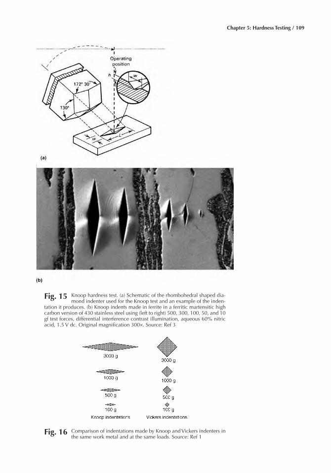
Chapter 5: Hardness Testing / 109
Fig� 15 Knoop hardness test. (a) Schematic of the rhombohedral shaped dia-mond indenter used for the Knoop test and an example of the inden-
tation it produces. (b) Knoop indents made in ferrite in a ferritic martensitic high carbon version of 430 stainless steel using (left to right) 500, 300, 100, 50, and 10 gf test forces, differential interference contrast illumination, aqueous 60% nitric acid, 1.5 V dc. Original magnification 300×. Source: Ref 3
Fig� 16 Comparison of indentations made by Knoop and Vickers indenters in the same work metal and at the same loads. Source: Ref 1
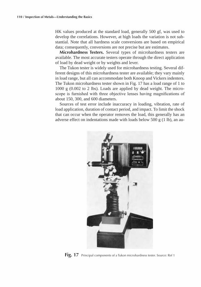
110 / Inspection of Metals—Understanding the Basics
HK values produced at the standard load, generally 500 gf, was used to develop the correlations. However, at high loads the variation is not sub-stantial. Note that all hardness scale conversions are based on empirical data; consequently, conversions are not precise but are estimates.
Microhardness Testers� Several types of microhardness testers are available. The most accurate testers operate through the direct application of load by dead weight or by weights and lever.
The Tukon tester is widely used for microhardness testing. Several dif-ferent designs of this microhardness tester are available; they vary mainly in load range, but all can accommodate both Knoop and Vickers indenters. The Tukon microhardness tester shown in Fig. 17 has a load range of 1 to 1000 g (0.002 to 2 lbs). Loads are applied by dead weight. The micro-scope is furnished with three objective lenses having magnifications of about 150, 300, and 600 diameters.
Sources of test error include inaccuracy in loading, vibration, rate of load application, duration of contact period, and impact. To limit the shock that can occur when the operator removes the load, this generally has an adverse effect on indentations made with loads below 500 g (1 lb), an au-
Fig� 17 Principal components of a Tukon microhardness tester. Source: Ref 1
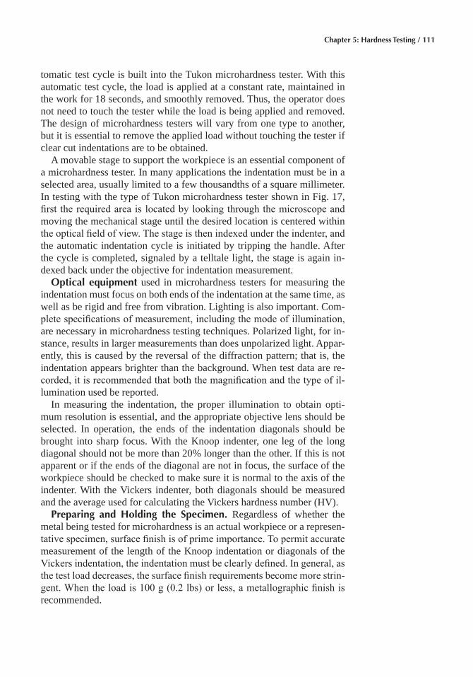
Chapter 5: Hardness Testing / 111
tomatic test cycle is built into the Tukon microhardness tester. With this automatic test cycle, the load is applied at a constant rate, maintained in the work for 18 seconds, and smoothly removed. Thus, the operator does not need to touch the tester while the load is being applied and removed. The design of microhardness testers will vary from one type to another, but it is essential to remove the applied load without touching the tester if clear cut indentations are to be obtained.
A movable stage to support the workpiece is an essential component of a microhardness tester. In many applications the indentation must be in a selected area, usually limited to a few thousandths of a square millimeter. In testing with the type of Tukon microhardness tester shown in Fig. 17, first the required area is located by looking through the microscope and moving the mechanical stage until the desired location is centered within the optical field of view. The stage is then indexed under the indenter, and the automatic indentation cycle is initiated by tripping the handle. After the cycle is completed, signaled by a telltale light, the stage is again in-dexed back under the objective for indentation measurement.
Optical equipment used in microhardness testers for measuring the indentation must focus on both ends of the indentation at the same time, as well as be rigid and free from vibration. Lighting is also important. Com-plete specifications of measurement, including the mode of illumination, are necessary in microhardness testing techniques. Polarized light, for in-stance, results in larger measurements than does unpolarized light. Appar-ently, this is caused by the reversal of the diffraction pattern; that is, the indentation appears brighter than the background. When test data are re-corded, it is recommended that both the magnification and the type of il-lumination used be reported.
In measuring the indentation, the proper illumination to obtain opti-mum resolution is essential, and the appropriate objective lens should be selected. In operation, the ends of the indentation diagonals should be brought into sharp focus. With the Knoop indenter, one leg of the long diagonal should not be more than 20% longer than the other. If this is not apparent or if the ends of the diagonal are not in focus, the surface of the workpiece should be checked to make sure it is normal to the axis of the indenter. With the Vickers indenter, both diagonals should be measured and the average used for calculating the Vickers hardness number (HV).
Preparing and Holding the Specimen� Regardless of whether the metal being tested for microhardness is an actual workpiece or a represen-tative specimen, surface finish is of prime importance. To permit accurate measurement of the length of the Knoop indentation or diagonals of the Vickers indentation, the indentation must be clearly defined. In general, as the test load decreases, the surface finish requirements become more strin-gent. When the load is 100 g (0.2 lbs) or less, a metallographic finish is recommended.
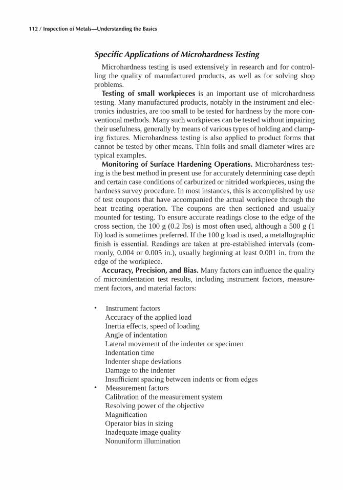
112 / Inspection of Metals—Understanding the Basics
Specific Applications of Microhardness Testing
Microhardness testing is used extensively in research and for control-ling the quality of manufactured products, as well as for solving shop problems.
Testing of small workpieces is an important use of microhardness testing. Many manufactured products, notably in the instrument and elec-tronics industries, are too small to be tested for hardness by the more con-ventional methods. Many such workpieces can be tested without impairing their usefulness, generally by means of various types of holding and clamp-ing fixtures. Microhardness testing is also applied to product forms that cannot be tested by other means. Thin foils and small diameter wires are typical examples.
Monitoring of Surface Hardening Operations� Microhardness test-ing is the best method in present use for accurately determining case depth and certain case conditions of carburized or nitrided workpieces, using the hardness survey procedure. In most instances, this is accomplished by use of test coupons that have accompanied the actual workpiece through the heat treating operation. The coupons are then sectioned and usually mounted for testing. To ensure accurate readings close to the edge of the cross section, the 100 g (0.2 lbs) is most often used, although a 500 g (1 lb) load is sometimes preferred. If the 100 g load is used, a metallographic finish is essential. Readings are taken at pre-established intervals (com-monly, 0.004 or 0.005 in.), usually beginning at least 0.001 in. from the edge of the workpiece.
Accuracy, Precision, and Bias� Many factors can influence the quality of microindentation test results, including instrument factors, measure-ment factors, and material factors:
• Instrument factors Accuracy of the applied load Inertia effects, speed of loading Angle of indentationLateral movement of the indenter or specimen Indentation time Indenter shape deviations Damage to the indenter Insufficient spacing between indents or from edges
• Measurement factors Calibration of the measurement system Resolving power of the objective Magnification Operator bias in sizing Inadequate image quality Nonuniform illumination
Chapter 5: Hardness Testing / 113
• Material factors Heterogeneity in composition or microstructure Crystallographic texture Quality of the specimen preparation Low reflectivity or transparency
In the early days of low load (<100 gf or < 0.2 lbf) hardness testing, it was quickly recognized that improper specimen preparation can influence hardness test results. Most texts state that improper preparation yields higher test results because the surface contains excessive preparation in-duced deformation. While this is certainly true, improper preparation may also create excessive heat, which reduces the hardness and strength of many metals and alloys. Either problem may be encountered due to faulty preparation.
For many years, it was considered necessary to electrolytically polish specimens so that the preparation induced damage could be removed, thus permitting bias free low load testing. However, the science behind me-chanical specimen preparation, chiefly due to the work of L. Samuels, has led to development of excellent mechanical specimen preparation proce-dures, and electropolishing is no longer required.
In addition, several operational factors must be controlled for optimum test results. First, it is good practice to inspect the indenter periodically for damage, for example, cracking or chipping of the diamond. If you have metrology equipment, you can measure the face angles and the sharpness of the tip. Specifications for Vickers and Knoop indenter geometries are given in ASTM E384.
A prime source of error is the alignment of the specimen surface rela-tive to the indenter. The indenter itself must be properly aligned perpen-dicular (±1°) to the stage plate. Next, the specimen surface must be per-pendicular to the indenter. Most testers provide holders that align the polished face perpendicular to the indenter or parallel to the stage. If a specimen is simply placed on the stage surface, its back surface must be parallel to its polished surface. Tilting the surface more than one degree perpendicular to the indenter results in nonsymmetrical impressions and can produce lateral movement between specimen and indenter. How-ever, in most cases, indenting procedures are not the major source of error.
It is important to regularly check the performance of the tester with a certified test block. The safest choice is a test block manufactured for mi-croindentation testing and certified for the test (Vickers or Knoop) as well as the specified load. Strictly speaking, a block certified for Vickers test-ing at 300 or 500 gf (0.7 or 1 lbf), commonly chosen loads, should yield essentially the same hardness with loads from about 50 to 1000 gf (0.1 to 2 lbf). That is, if you take the average of about five indents and compare the average at test load to the average at the calibrated load, knowing the
114 / Inspection of Metals—Understanding the Basics
standard deviation of the test results, statistical tests can tell at any desired confidence level, if the difference between the mean values of the tests at the two loads is statistically significant or not.
When considering a new tester, it is prudent to perform a series of in-dents, five is adequate, at each test load (L) available. Then, plot the mean and 95% confidence limits of each test as a function of load. Because of the method of defining HV and HK, which involves dividing by d2, mea-surement errors become more critical as d gets smaller; that is, as L de-creases and the material’s hardness increases. Therefore, departure from a constant hardness for the Vickers or Knoop tests as a function of load be-comes a greater problem as the hardness increases. For the Knoop test, HK increases as L decreases because the indent geometry changes with indent depth and width. But the change in HK varies with the test load. At a higher test load the change is greater as L decreases.
The greatest source of error is measuring the indent. The indent should be placed in the center of the measuring field, because lens image quality is best in the center. The light source should provide adequate, even illu-mination to provide maximum contrast and resolution. The accuracy of the filar micrometer or other measuring device should be verified by a stage micrometer.
Specimen preparation quality becomes more important as the load de-creases, and it must be at an acceptable level. Specimen thickness must be at least 2.5 times the Vickers diagonal length. Because the Knoop indent is shallower than the Vickers at the same load, somewhat thinner specimens can be tested. Spacing of indents is important because indenting produces plastic deformation and a strain field around the indent. If the spacing is too small, the new indent will be affected by the strain field around the last indent. ASTM recommends a minimum spacing (center to edge of adja-cent indent) of 2.5 times the Vickers diagonal. For the Knoop test, in which the long diagonals are parallel, the spacing is 2.5 times the short diagonal. The minimum recommended spacing between the edge of the specimen and the center of the indent should be 2.5 times. Again, Knoop indents can be placed closer to the surface than Vickers indents.
ACKNOWLEDGMENT
This chapter was adapted from Hardness Testing, Metals Handbook Desk Edition, Second Edition, 1998, and Macroindentation Hardness Testing by E.L. Tobolski and A. Fee in Mechanical Testing and Evalua-tion, Volume 8, ASM Handbook, 2000.
REFERENCES
1. Hardness Testing, Metals Handbook Desk Edition, 2nd ed., ASM In-ternational, 1998, p 1308–1317
Chapter 5: Hardness Testing / 115
2. E.L. Tobolski and A. Fee, Macroindentation Hardness Testing, Me-chanical Testing and Evaluation, Vol 8, ASM Handbook, ASM Inter-national, 2000, p 203–220
3. G.F. Vander Voort, Microindentation Hardness Testing, Mechanical Testing and Evaluation, Vol 8, ASM Handbook, ASM International, 2000, p 221–231
SELECTED REFERENCES
• Mechanical Testing and Evaluation, Vol 8, ASM Handbook, ASM In-ternational, 2000
Brinell Hardness Standards for Metals• ASTM E10, Standard Test Method for Brinell Hardness of Metallic
Materials• BS EN ISO 6506-1, Metallic Materials—Brinell Hardness Test—Test
Method • BS EN ISO 6506-2, Metallic Materials—Brinell Hardness Test—Veri-
fication and Calibration of Brinell Hardness Testing Machines • BS EN ISO 6506-3, Metallic Materials—Brinell Hardness Test—Cali-
bration of Reference Blocks• DIN EN, Brinell Hardness Test—Test Method 10003-1 • DIN EN 10003-2, Metallic Materials—Brinell Hardness Test—Verifi-
cation of Brinell Hardness Testing Machines• DIN EN 10003-3, Metallic Materials—Brinell Hardness Test—Cali-
bration of Standardized Blocks to be Used for Brinell Hardness Test-ing Machines
• JIS B 7724, Brinell Hardness Testing Machines• JIS B 7736, Standardized Blocks of Brinell Hardness• JIS Z 2243, Method of Brinell Hardness Test
Rockwell Hardness Standards for Metals• ASTM B294, Standard Test Method for Hardness Testing of Cemented
Carbides• ASTM E18, Test Methods for Hardness and Rockwell Superficial
Hardness of Metallic Materials• ASTM E1842, Test Method for Macro-Rockwell Hardness Testing of
Metallic Materials• BS 5600-4.5, Powder Metallurgical Materials and Products—Methods
of Testing and Chemical Analysis of Hardmetals—Rockwell Hardness Test (Scale A)
• BS EN ISO 6508-1, Metallic Materials—Rockwell Hardness Test—Part 1: Test Method (Scales A, B, C, D, E, F, G, H, K, N, T)
• BS EN ISO 6508-2, Metallic Materials—Rockwell Hardness Test—Part 2: Verification and Calibration of Testing Machines (Scales A, B, C, D, E, F, G, H, K, N, T)

116 / Inspection of Metals—Understanding the Basics
• BS EN ISO 6508-3, Metallic Materials—Rockwell Hardness Test—Part 3: Calibration of Reference Blocks (Scales A, B, C, D, E, F, G, H, K, N, T)
• ISO 3738-1, Hardmetals—Rockwell Hardness Test (Scale A)—Part 1: Test Method ISO 3738-2 Hardmetals—Rockwell Hardness Test (Scale A)—Part 2: Preparation and Calibration of Standard Test Blocks
• JIS B 7726, Rockwell Hardness Test—Verification of Testing Machines• JIS B 7730, Rockwell Hardness Test—Calibration of Reference Blocks
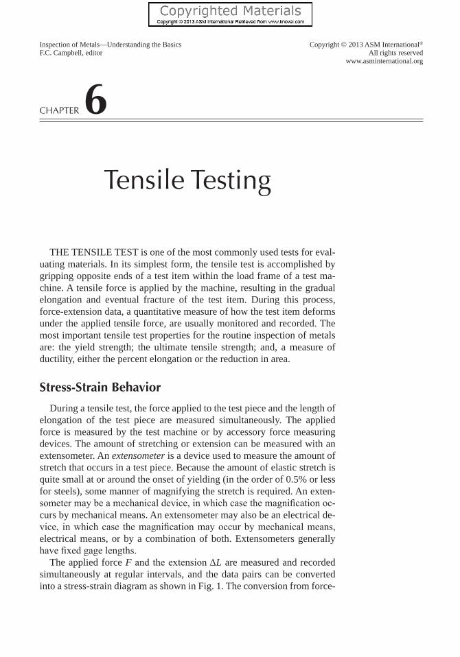
Inspection of Metals—Understanding the Basics Copyright © 2013 ASM International®
F.C. Campbell, editor All rights reservedwww.asminternational.org
CHAPTER 6
Tensile Testing
THE TENSILE TEST is one of the most commonly used tests for eval-uating materials. In its simplest form, the tensile test is accomplished by gripping opposite ends of a test item within the load frame of a test ma-chine. A tensile force is applied by the machine, resulting in the gradual elongation and eventual fracture of the test item. During this process, force-extension data, a quantitative measure of how the test item deforms under the applied tensile force, are usually monitored and recorded. The most important tensile test properties for the routine inspection of metals are: the yield strength; the ultimate tensile strength; and, a measure of ductility, either the percent elongation or the reduction in area.
Stress-Strain Behavior
During a tensile test, the force applied to the test piece and the length of elongation of the test piece are measured simultaneously. The applied force is measured by the test machine or by accessory force measuring devices. The amount of stretching or extension can be measured with an extensometer. An extensometer is a device used to measure the amount of stretch that occurs in a test piece. Because the amount of elastic stretch is quite small at or around the onset of yielding (in the order of 0.5% or less for steels), some manner of magnifying the stretch is required. An exten-someter may be a mechanical device, in which case the magnification oc-curs by mechanical means. An extensometer may also be an electrical de-vice, in which case the magnification may occur by mechanical means, electrical means, or by a combination of both. Extensometers generally have fixed gage lengths.
The applied force F and the extension ΔL are measured and recorded simultaneously at regular intervals, and the data pairs can be converted into a stress-strain diagram as shown in Fig. 1. The conversion from force-
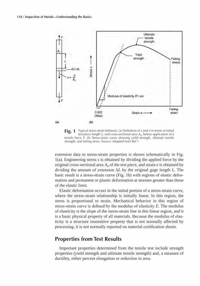
118 / Inspection of Metals—Understanding the Basics
extension data to stress-strain properties is shown schematically in Fig. 1(a). Engineering stress s is obtained by dividing the applied force by the original cross-sectional area A0 of the test piece, and strain e is obtained by dividing the amount of extension ΔL by the original gage length L. The basic result is a stress-strain curve (Fig. 1b) with regions of elastic defor-mation and permanent or plastic deformation at stresses greater than those of the elastic limit.
Elastic deformation occurs in the initial portion of a stress-strain curve, where the stress-strain relationship is initially linear. In this region, the stress is proportional to strain. Mechanical behavior in this region of stress-strain curve is defined by the modulus of elasticity E. The modulus of elasticity is the slope of the stress-strain line in this linear region, and it is a basic physical property of all materials. Because the modulus of elas-ticity is a structure insensitive property that is not normally affected by processing, it is not normally reported on material certification sheets.
Properties from Test Results
Important properties determined from the tensile test include strength properties (yield strength and ultimate tensile strength) and, a measure of ductility, either percent elongation or reduction in area.
Fig� 1 Typical stress-strain behavior. (a) Definition of s and e in terms of initial test piece length L, and cross-sectional area A0, before application of a
tensile force F. (b) Stress-strain curve showing yield strength, ultimate tensile strength, and failing stress. Source: Adapted from Ref 1
Chapter 6: Tensile Testing / 119
Strength Properties
Yield strength and tensile strength are the most common strength prop-erties determined in a tensile test. According to ASTM E6, tensile strength is calculated from the maximum force during a tensile test that is carried to rupture divided by the original cross-sectional area of the test piece. The yield strength refers to the stress at which a small, but measurable, amount of inelastic or plastic deformation occurs. Yield strength is usually defined as:
• Upper yield strength or upper yield point• Offset yield strength
An upper yield strength or upper yield point (Fig. 2a) usually oc-curs with low carbon steels and some other metal systems to a limited
Fig� 2 Examples of stress-strain curves exhibiting pronounced yield point be-havior. Pronounced yielding, of the type shown, is usually called yield
point elongation (YPE). (a) Classic example of upper yield strength (UYS) behavior typically observed in low carbon steels with a very pronounced upper yield strength. (b) General example of pronounced yielding without an upper yield strength. LYS, lower yield strength. Source: Ref 2
120 / Inspection of Metals—Understanding the Basics
degree. Often, the pronounced peak of the upper yield is suppressed due to slow testing speed or nonaxial loading (i.e., bending of the test piece), metallurgical factors, or a combination of these; in this case, a curve of the type shown in Fig. 2(b) is obtained. The offset definition of yield strength was developed for materials that do not exhibit the yield point behavior shown in Fig. 2. To determine the offset yield strength, the stress-strain curve must be determined during the test.
Upper yield strength or upper yield point can be defined as the stress at which measurable strain occurs without an increase in the stress; that is, there is a horizontal region of the stress-strain curve (Fig. 2) where dis-continuous yielding occurs. Before the onset of discontinuous yielding, a peak of maximum stress for yielding is typically observed (Fig. 2a). This pronounced yielding, of the type shown, is usually called yield point elon-gation (YPE). This elongation is a diffusion related phenomenon, where under certain combinations of strain rate and temperature as the material deforms, interstitial atoms are dragged along with dislocations, or disloca-tions can alternately break away and be repinned, with little or no increase in stress. Either or both of these actions cause serrations or discontinuous changes in a stress-strain curve, which are usually limited to the onset of yielding. This type of yield point is sometimes referred to as the upper yield strength or upper yield point and is usually associated with low car-bon steels, although other metal systems may exhibit yield points to some degree.
The yield point is easy to measure because the increase in strain that occurs without an increase in stress is visually apparent during the con-duct of the test by observing the force indicating system. As shown in Fig. 2, the yield point is usually quite obvious and thus can easily be deter-mined by observation during a tensile test. It can be determined from a stress-strain curve or by the halt of the dial when the test is performed on machines that use a dial to indicate the applied force. However, when watching the movement of the dial, sometimes a minimum value, recorded during discontinuous yielding, is noted. This value is sometimes referred to as the lower yield point. When the value is ascertained without instru-mentation readouts, it is often referred to as the halt-of-dial or the drop-of-beam yield point (as an average usually results from eye readings). It is almost always the upper yield point that is determined from instrument readouts.
Offset yield strength is the stress that causes a specified amount of set to occur; that is, at this stress, the test piece exhibits plastic deformation or set equal to a specific amount. To determine the offset yield strength, it is necessary to secure data (autographic or numerical) from which a stress-strain diagram may be constructed graphically or in computer memory. Figure 3 shows how to use these data; the amount of the specified offset 0-m is laid out on the strain axis. A line, m-n, parallel to the modulus of elasticity line, 0-A, is drawn to intersect the stress-strain curve. The point
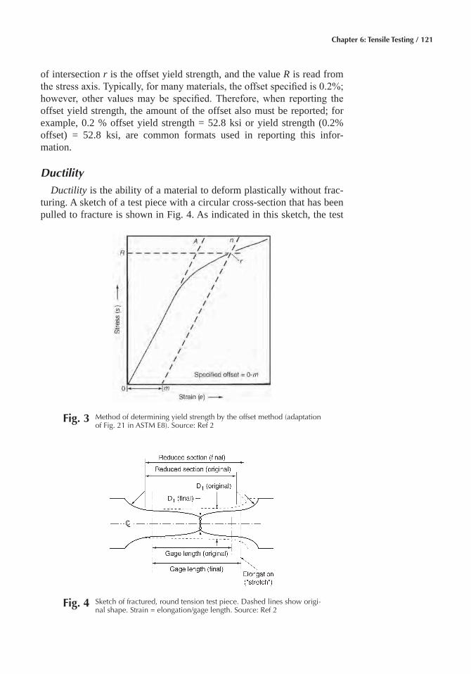
Chapter 6: Tensile Testing / 121
of intersection r is the offset yield strength, and the value R is read from the stress axis. Typically, for many materials, the offset specified is 0.2%; however, other values may be specified. Therefore, when reporting the offset yield strength, the amount of the offset also must be reported; for example, 0.2 % offset yield strength = 52.8 ksi or yield strength (0.2% offset) = 52.8 ksi, are common formats used in reporting this infor- mation.
Ductility
Ductility is the ability of a material to deform plastically without frac-turing. A sketch of a test piece with a circular cross-section that has been pulled to fracture is shown in Fig. 4. As indicated in this sketch, the test
Fig� 4 Sketch of fractured, round tension test piece. Dashed lines show origi-nal shape. Strain = elongation/gage length. Source: Ref 2
Fig� 3 Method of determining yield strength by the offset method (adaptation of Fig. 21 in ASTM E8). Source: Ref 2
s
e
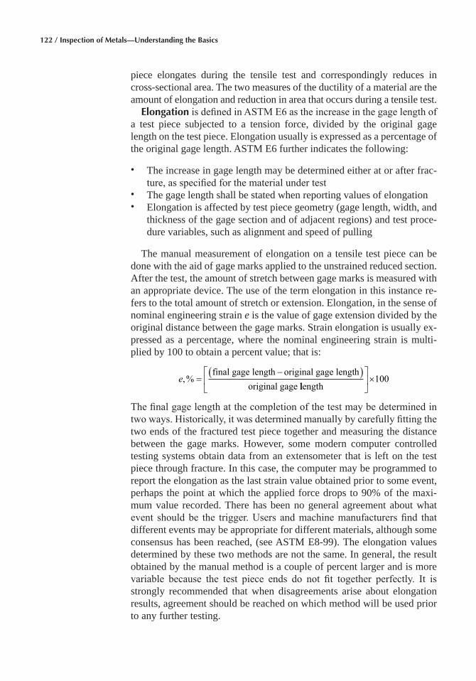
122 / Inspection of Metals—Understanding the Basics
piece elongates during the tensile test and correspondingly reduces in cross-sectional area. The two measures of the ductility of a material are the amount of elongation and reduction in area that occurs during a tensile test.
Elongation is defined in ASTM E6 as the increase in the gage length of a test piece subjected to a tension force, divided by the original gage length on the test piece. Elongation usually is expressed as a percentage of the original gage length. ASTM E6 further indicates the following:
• The increase in gage length may be determined either at or after frac-ture, as specified for the material under test
• The gage length shall be stated when reporting values of elongation• Elongation is affected by test piece geometry (gage length, width, and
thickness of the gage section and of adjacent regions) and test proce-dure variables, such as alignment and speed of pulling
The manual measurement of elongation on a tensile test piece can be done with the aid of gage marks applied to the unstrained reduced section. After the test, the amount of stretch between gage marks is measured with an appropriate device. The use of the term elongation in this instance re-fers to the total amount of stretch or extension. Elongation, in the sense of nominal engineering strain e is the value of gage extension divided by the original distance between the gage marks. Strain elongation is usually ex-pressed as a percentage, where the nominal engineering strain is multi-plied by 100 to obtain a percent value; that is:
e,% =−( )final gage length original gage length
original gage llength
×100
The final gage length at the completion of the test may be determined in two ways. Historically, it was determined manually by carefully fitting the two ends of the fractured test piece together and measuring the distance between the gage marks. However, some modern computer controlled testing systems obtain data from an extensometer that is left on the test piece through fracture. In this case, the computer may be programmed to report the elongation as the last strain value obtained prior to some event, perhaps the point at which the applied force drops to 90% of the maxi-mum value recorded. There has been no general agreement about what event should be the trigger. Users and machine manufacturers find that different events may be appropriate for different materials, although some consensus has been reached, (see ASTM E8-99). The elongation values determined by these two methods are not the same. In general, the result obtained by the manual method is a couple of percent larger and is more variable because the test piece ends do not fit together perfectly. It is strongly recommended that when disagreements arise about elongation results, agreement should be reached on which method will be used prior to any further testing.
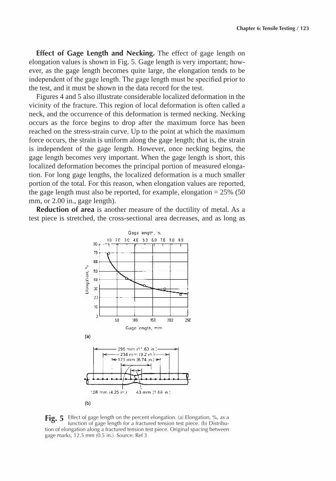
Chapter 6: Tensile Testing / 123
Effect of Gage Length and Necking� The effect of gage length on elongation values is shown in Fig. 5. Gage length is very important; how-ever, as the gage length becomes quite large, the elongation tends to be independent of the gage length. The gage length must be specified prior to the test, and it must be shown in the data record for the test.
Figures 4 and 5 also illustrate considerable localized deformation in the vicinity of the fracture. This region of local deformation is often called a neck, and the occurrence of this deformation is termed necking. Necking occurs as the force begins to drop after the maximum force has been reached on the stress-strain curve. Up to the point at which the maximum force occurs, the strain is uniform along the gage length; that is, the strain is independent of the gage length. However, once necking begins, the gage length becomes very important. When the gage length is short, this localized deformation becomes the principal portion of measured elonga-tion. For long gage lengths, the localized deformation is a much smaller portion of the total. For this reason, when elongation values are reported, the gage length must also be reported, for example, elongation = 25% (50 mm, or 2.00 in., gage length).
Reduction of area is another measure of the ductility of metal. As a test piece is stretched, the cross-sectional area decreases, and as long as
Fig� 5 Effect of gage length on the percent elongation. (a) Elongation, %, as a function of gage length for a fractured tension test piece. (b) Distribu-
tion of elongation along a fractured tension test piece. Original spacing between gage marks, 12.5 mm (0.5 in.). Source: Ref 3
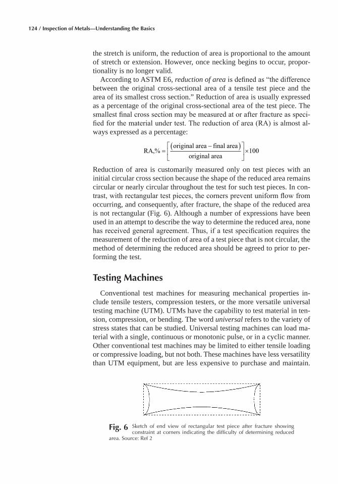
124 / Inspection of Metals—Understanding the Basics
the stretch is uniform, the reduction of area is proportional to the amount of stretch or extension. However, once necking begins to occur, propor-tionality is no longer valid.
According to ASTM E6, reduction of area is defined as “the difference between the original cross-sectional area of a tensile test piece and the area of its smallest cross section.” Reduction of area is usually expressed as a percentage of the original cross-sectional area of the test piece. The smallest final cross section may be measured at or after fracture as speci-fied for the material under test. The reduction of area (RA) is almost al-ways expressed as a percentage:
RA,%original area final area
original area=
−( )
×100
Reduction of area is customarily measured only on test pieces with an initial circular cross section because the shape of the reduced area remains circular or nearly circular throughout the test for such test pieces. In con-trast, with rectangular test pieces, the corners prevent uniform flow from occurring, and consequently, after fracture, the shape of the reduced area is not rectangular (Fig. 6). Although a number of expressions have been used in an attempt to describe the way to determine the reduced area, none has received general agreement. Thus, if a test specification requires the measurement of the reduction of area of a test piece that is not circular, the method of determining the reduced area should be agreed to prior to per-forming the test.
Testing Machines
Conventional test machines for measuring mechanical properties in-clude tensile testers, compression testers, or the more versatile universal testing machine (UTM). UTMs have the capability to test material in ten-sion, compression, or bending. The word universal refers to the variety of stress states that can be studied. Universal testing machines can load ma-terial with a single, continuous or monotonic pulse, or in a cyclic manner. Other conventional test machines may be limited to either tensile loading or compressive loading, but not both. These machines have less versatility than UTM equipment, but are less expensive to purchase and maintain.
Fig� 6 Sketch of end view of rectangular test piece after fracture showing constraint at corners indicating the difficulty of determining reduced
area. Source: Ref 2
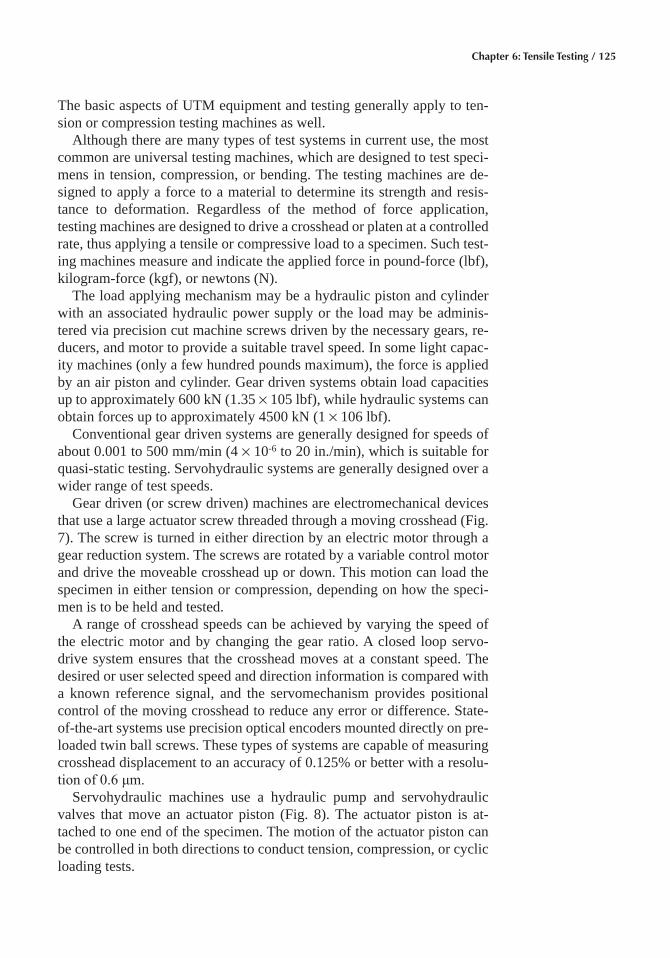
Chapter 6: Tensile Testing / 125
The basic aspects of UTM equipment and testing generally apply to ten-sion or compression testing machines as well.
Although there are many types of test systems in current use, the most common are universal testing machines, which are designed to test speci-mens in tension, compression, or bending. The testing machines are de-signed to apply a force to a material to determine its strength and resis-tance to deformation. Regardless of the method of force application, testing machines are designed to drive a crosshead or platen at a controlled rate, thus applying a tensile or compressive load to a specimen. Such test-ing machines measure and indicate the applied force in pound-force (lbf), kilogram-force (kgf), or newtons (N).
The load applying mechanism may be a hydraulic piston and cylinder with an associated hydraulic power supply or the load may be adminis-tered via precision cut machine screws driven by the necessary gears, re-ducers, and motor to provide a suitable travel speed. In some light capac-ity machines (only a few hundred pounds maximum), the force is applied by an air piston and cylinder. Gear driven systems obtain load capacities up to approximately 600 kN (1.35 × 10⁵ lbf), while hydraulic systems can obtain forces up to approximately 4500 kN (1 × 10⁶ lbf).
Conventional gear driven systems are generally designed for speeds of about 0.001 to 500 mm/min (4 × 10⁻⁶ to 20 in./min), which is suitable for quasi-static testing. Servohydraulic systems are generally designed over a wider range of test speeds.
Gear driven (or screw driven) machines are electromechanical devices that use a large actuator screw threaded through a moving crosshead (Fig. 7). The screw is turned in either direction by an electric motor through a gear reduction system. The screws are rotated by a variable control motor and drive the moveable crosshead up or down. This motion can load the specimen in either tension or compression, depending on how the speci-men is to be held and tested.
A range of crosshead speeds can be achieved by varying the speed of the electric motor and by changing the gear ratio. A closed loop servo-drive system ensures that the crosshead moves at a constant speed. The desired or user selected speed and direction information is compared with a known reference signal, and the servomechanism provides positional control of the moving crosshead to reduce any error or difference. State-of-the-art systems use precision optical encoders mounted directly on pre-loaded twin ball screws. These types of systems are capable of measuring crosshead displacement to an accuracy of 0.125% or better with a resolu-tion of 0.6 μm.
Servohydraulic machines use a hydraulic pump and servohydraulic valves that move an actuator piston (Fig. 8). The actuator piston is at-tached to one end of the specimen. The motion of the actuator piston can be controlled in both directions to conduct tension, compression, or cyclic loading tests.
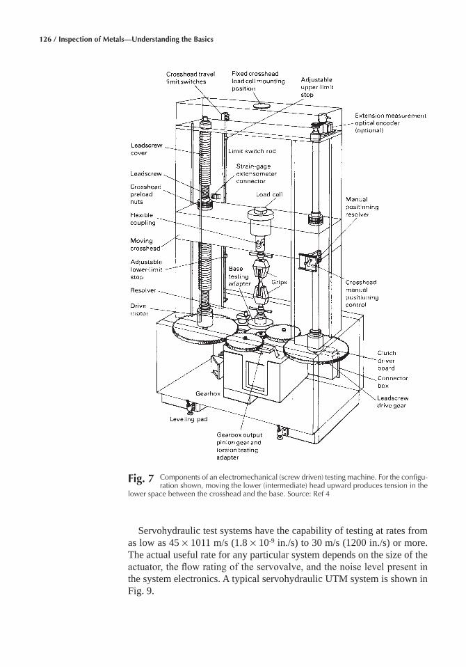
126 / Inspection of Metals—Understanding the Basics
Servohydraulic test systems have the capability of testing at rates from as low as 45 × 1011 m/s (1.8 × 10⁻⁹ in./s) to 30 m/s (1200 in./s) or more. The actual useful rate for any particular system depends on the size of the actuator, the flow rating of the servovalve, and the noise level present in the system electronics. A typical servohydraulic UTM system is shown in Fig. 9.
Fig� 7 Components of an electromechanical (screw driven) testing machine. For the configu-ration shown, moving the lower (intermediate) head upward produces tension in the
lower space between the crosshead and the base. Source: Ref 4
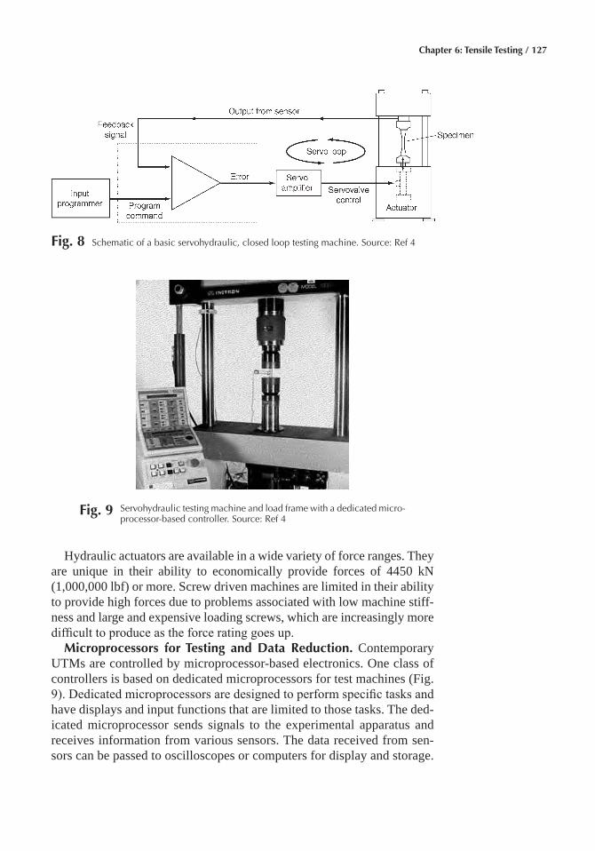
Chapter 6: Tensile Testing / 127
Hydraulic actuators are available in a wide variety of force ranges. They are unique in their ability to economically provide forces of 4450 kN (1,000,000 lbf) or more. Screw driven machines are limited in their ability to provide high forces due to problems associated with low machine stiff-ness and large and expensive loading screws, which are increasingly more difficult to produce as the force rating goes up.
Microprocessors for Testing and Data Reduction� Contemporary UTMs are controlled by microprocessor-based electronics. One class of controllers is based on dedicated microprocessors for test machines (Fig. 9). Dedicated microprocessors are designed to perform specific tasks and have displays and input functions that are limited to those tasks. The ded-icated microprocessor sends signals to the experimental apparatus and receives information from various sensors. The data received from sen-sors can be passed to oscilloscopes or computers for display and storage.
Fig� 8 Schematic of a basic servohydraulic, closed loop testing machine. Source: Ref 4
Fig� 9 Servohydraulic testing machine and load frame with a dedicated micro-processor-based controller. Source: Ref 4
128 / Inspection of Metals—Understanding the Basics
The experimental results consist of time and voltage information that must be further reduced to analyze material behavior. Analysis of the data requires the conversion of test results, such as voltage, to specific quantities, such as displacement and load, based on known conversion factors.
The second class of controllers is the personal computer (PC) designed with an electronic interface to the experimental apparatus, and the appro-priate application software. The software takes the description of the test to be performed, including specimen geometry data, and establishes the requisite electronic signals. Once the test is underway, the computer con-trols the tests and collects, reduces, displays, and stores the data. The ob-vious advantage of the PC-based controller is reduced time to generate graphic results, or reports. The other advantage is the elimination of some procedural errors, or the reduction of the interfacing details between the operator and the experimental apparatus. Some systems are designed with both types of controllers. Having both types of controllers provides maxi-mum flexibility in data gathering with a minimal amount of time required for reducing data when conducting standard experiments.
Measuring Load� Current testing machines use strain gaged load cells and pressure transducers. In a load cell, strain gages are mounted on preci-sion machined alloy steel elements, hermetically sealed in a case with the necessary electrical outlets, and arranged for tensile and/or compressive loading. The load cell can be mounted so that the specimen is in direct contact, or the cell can be indirectly loaded through the machine cross-head, table, or columns of the load frame. The load cell and the load cell circuit are calibrated to provide a specific voltage as an output signal when a certain force is detected. In pressure transducers, which are variations of strain gage load cells, the strain gaged member is activated by the hydrau-lic pressure of the system.
Strain Measurement� Deformation of the specimen can be measured in several ways, depending on the size of specimen, environmental condi-tions, and measurement requirements for accuracy and precision of antici-pated strain levels. A simple method is to use the velocity of the crosshead while tracking the load as a function of time. For the load and time data pair, the stress in the specimen and the amount of deformation, or strain, can be calculated. When the displacement of the platen is assumed to be equal to the specimen displacement, an error is introduced by the fact that the entire load frame has been deflected under the stress state. This effect is related to the machine stiffness.
The elongation of a specimen during load application can be measured directly with various types of devices, such as clip-on extensometers, di-rectly mounted strain gages, and various optical devices. These devices are used extensively and can provide a high degree of deformation (strain) measurement accuracy. Other more advanced instrumentations, such as laser interferometry and video extensometers, are also available.
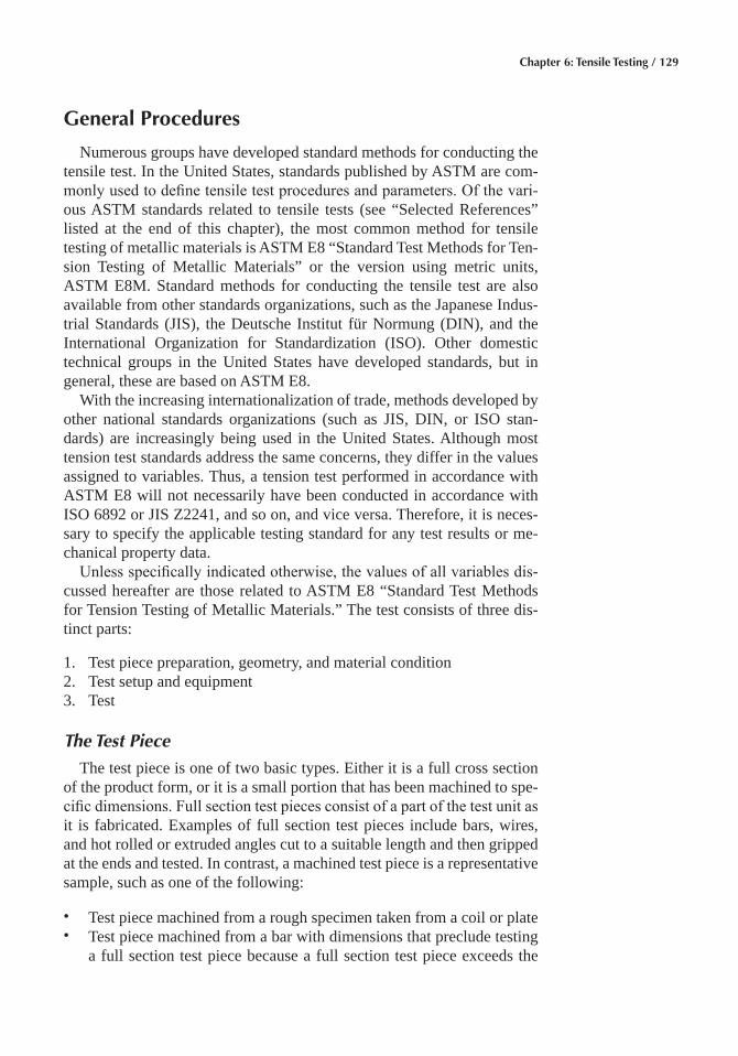
Chapter 6: Tensile Testing / 129
General Procedures
Numerous groups have developed standard methods for conducting the tensile test. In the United States, standards published by ASTM are com-monly used to define tensile test procedures and parameters. Of the vari-ous ASTM standards related to tensile tests (see “Selected References” listed at the end of this chapter), the most common method for tensile testing of metallic materials is ASTM E8 “Standard Test Methods for Ten-sion Testing of Metallic Materials” or the version using metric units, ASTM E8M. Standard methods for conducting the tensile test are also available from other standards organizations, such as the Japanese Indus-trial Standards (JIS), the Deutsche Institut für Normung (DIN), and the International Organization for Standardization (ISO). Other domestic technical groups in the United States have developed standards, but in general, these are based on ASTM E8.
With the increasing internationalization of trade, methods developed by other national standards organizations (such as JIS, DIN, or ISO stan-dards) are increasingly being used in the United States. Although most tension test standards address the same concerns, they differ in the values assigned to variables. Thus, a tension test performed in accordance with ASTM E8 will not necessarily have been conducted in accordance with ISO 6892 or JIS Z2241, and so on, and vice versa. Therefore, it is neces-sary to specify the applicable testing standard for any test results or me-chanical property data.
Unless specifically indicated otherwise, the values of all variables dis-cussed hereafter are those related to ASTM E8 “Standard Test Methods for Tension Testing of Metallic Materials.” The test consists of three dis-tinct parts:
1. Test piece preparation, geometry, and material condition2. Test setup and equipment3. Test
The Test Piece
The test piece is one of two basic types. Either it is a full cross section of the product form, or it is a small portion that has been machined to spe-cific dimensions. Full section test pieces consist of a part of the test unit as it is fabricated. Examples of full section test pieces include bars, wires, and hot rolled or extruded angles cut to a suitable length and then gripped at the ends and tested. In contrast, a machined test piece is a representative sample, such as one of the following:
• Test piece machined from a rough specimen taken from a coil or plate• Test piece machined from a bar with dimensions that preclude testing
a full section test piece because a full section test piece exceeds the
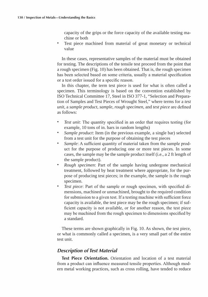
130 / Inspection of Metals—Understanding the Basics
capacity of the grips or the force capacity of the available testing ma-chine or both
• Test piece machined from material of great monetary or technical value
In these cases, representative samples of the material must be obtained for testing. The descriptions of the tensile test proceed from the point that a rough specimen (Fig. 10) has been obtained. That is, the rough specimen has been selected based on some criteria, usually a material specification or a test order issued for a specific reason.
In this chapter, the term test piece is used for what is often called a specimen. This terminology is based on the convention established by ISO Technical Committee 17, Steel in ISO 377-1, “Selection and Prepara-tion of Samples and Test Pieces of Wrought Steel,” where terms for a test unit, a sample product, sample, rough specimen, and test piece are defined as follows:
• Test unit: The quantity specified in an order that requires testing (for example, 10 tons of in. bars in random lengths)
• Sample product: Item (in the previous example, a single bar) selected from a test unit for the purpose of obtaining the test pieces
• Sample: A sufficient quantity of material taken from the sample prod-uct for the purpose of producing one or more test pieces. In some cases, the sample may be the sample product itself (i.e., a 2 ft length of the sample product).
• Rough specimen: Part of the sample having undergone mechanical treatment, followed by heat treatment where appropriate, for the pur-pose of producing test pieces; in the example, the sample is the rough specimen.
• Test piece: Part of the sample or rough specimen, with specified di-mensions, machined or unmachined, brought to the required condition for submission to a given test. If a testing machine with sufficient force capacity is available, the test piece may be the rough specimen; if suf-ficient capacity is not available, or for another reason, the test piece may be machined from the rough specimen to dimensions specified by a standard.
These terms are shown graphically in Fig. 10. As shown, the test piece, or what is commonly called a specimen, is a very small part of the entire test unit.
Description of Test Material
Test Piece Orientation� Orientation and location of a test material from a product can influence measured tensile properties. Although mod-ern metal working practices, such as cross rolling, have tended to reduce
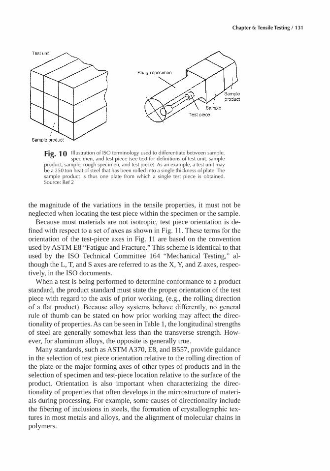
Chapter 6: Tensile Testing / 131
the magnitude of the variations in the tensile properties, it must not be neglected when locating the test piece within the specimen or the sample.
Because most materials are not isotropic, test piece orientation is de-fined with respect to a set of axes as shown in Fig. 11. These terms for the orientation of the test-piece axes in Fig. 11 are based on the convention used by ASTM E8 “Fatigue and Fracture.” This scheme is identical to that used by the ISO Technical Committee 164 “Mechanical Testing,” al-though the L, T, and S axes are referred to as the X, Y, and Z axes, respec-tively, in the ISO documents.
When a test is being performed to determine conformance to a product standard, the product standard must state the proper orientation of the test piece with regard to the axis of prior working, (e.g., the rolling direction of a flat product). Because alloy systems behave differently, no general rule of thumb can be stated on how prior working may affect the direc-tionality of properties. As can be seen in Table 1, the longitudinal strengths of steel are generally somewhat less than the transverse strength. How-ever, for aluminum alloys, the opposite is generally true.
Many standards, such as ASTM A370, E8, and B557, provide guidance in the selection of test piece orientation relative to the rolling direction of the plate or the major forming axes of other types of products and in the selection of specimen and test-piece location relative to the surface of the product. Orientation is also important when characterizing the direc-tionality of properties that often develops in the microstructure of materi-als during processing. For example, some causes of directionality include the fibering of inclusions in steels, the formation of crystallographic tex-tures in most metals and alloys, and the alignment of molecular chains in polymers.
Fig� 10 Illustration of ISO terminology used to differentiate between sample, specimen, and test piece (see text for definitions of test unit, sample
product, sample, rough specimen, and test piece). As an example, a test unit may be a 250 ton heat of steel that has been rolled into a single thickness of plate. The sample product is thus one plate from which a single test piece is obtained. Source: Ref 2
132 / Inspection of Metals—Understanding the Basics
The location from which a test material is taken from the initial product form is important because the manner in which a material is processed influences the uniformity of microstructure along the length of the product as well as through its thickness properties. For example, the properties of metal cut from castings are influenced by the rate of cooling and by shrink-
Fig� 11 System for identifying the axes of test-piece orientation in various product forms. (a) Flat rolled products. (b) Cylindrical sections. (c)
Tubular products. Source: Ref 2
Table 1 Effect of test piece orientation on tensile properties
OrientationYield strength,
ksiTensile strength,
ksi
Elongation in 50 mm (2 in.), %
Reduction of area, %
ASTM A 572, Grade 50 (¾ in. thick plate, low sulfur level)
Longitudinal 58.8 84.0 27.0 70.2Transverse 59.8 85.2 28.0 69.0
ASTM A 656, Grade 80 (¾ in. thick plate, low sulfur level + controlled rolled)
Longitudinal 81.0 102.3 25.8 71.2Transverse 86.9 107.9 24.5 67.1
ASTM A 5414 (¾ in. thick plate, low sulfur level)
Longitudinal 114.6 121.1 19.8 70.6Transverse 116.3 122.2 19.5 69.9
Source: Courtesy of Francis J. Marsh. Source: Ref 2
Chapter 6: Tensile Testing / 133
age stresses at changes in the section. Generally, test pieces taken from near the surface of iron castings are stronger. To standardize test results relative to location, ASTM A370 recommends that tensile test pieces be taken from midway between the surface and the center of round, square, hexagon, or octagonal bars. ASTM E8 recommends that test pieces be taken from the thickest part of a forging from which a test coupon can be obtained, from a prolongation of the forging, or in some cases, from sepa-rately forged coupons representative of the forging.
Test Piece Geometry
As previously noted, the item being tested may be either the full cross section of the item or a portion of the item that has been machined to spe-cific dimensions. Test piece geometry is often influenced by product form. For example, only test pieces with rectangular cross sections can be ob-tained from sheet products. Test pieces taken from thick plate may have either flat (plate type) or round cross sections. Most tensile test specifi-cations show machined test pieces with either circular cross sections or rectangular cross sections. Nomenclature for the various sections of a ma-chined test piece is shown in Fig. 12. Most tensile test specifications pres-ent a set of dimensions, for each cross-section type, that are standard, as well as additional sets of dimensions for alternative test pieces. In general, the standard dimensions published by ASTM, ISO, JIS, and DIN are simi-lar, but they are not identical.
Measurement of Initial Test Piece Dimensions� Machined test pieces are expected to meet size specifications, but to ensure dimensional accu-racy, each test piece should be measured prior to testing. Gage length, fil-let radius, and cross-sectional dimensions are measured easily. Cylindrical test pieces should be measured for concentricity. Maintaining acceptable concentricity is extremely important in minimizing unintended bending stresses on materials in a brittle state.
Fig� 12 Nomenclature for a typical tension test piece. Source: Ref 2
134 / Inspection of Metals—Understanding the Basics
Measurement of Cross-Sectional Dimensions� The test pieces must be measured to determine whether they meet the requirements of the test method. Test piece measurements must also determine the initial cross-sectional area when it is compared against the final cross section after testing as a measure of ductility. The precision with which these measure-ments are made is based on the requirements of the test method, or if none are given, on good engineering judgment.
Measurement of the Initial Gage Length� ASTM E8 assumes that the initial gage length is within specified tolerance; therefore, it is neces-sary only to verify that the gage length of the test piece is within the tolerance.
Marking Gage Length� Measurement of elongation requires marking the gage length of the test piece. The gage marks should be placed on the test piece in a manner so that when fracture occurs, the fracture will be located within the center one-third of the gage length (or within the center one-third of one of several sets of gage length marks). For a test piece machined with a reduced section length that is the minimum specified by ASTM E8 and with a gage length equal to the maximum allowed for that geometry, a single set of marks is usually sufficient.
Surface Finish and Condition� Test pieces from materials that are not high strength or that are ductile are usually insensitive to surface finish effects. However, if surface finish in the gage length of a tensile test piece is extremely poor (with machine tool marks deep enough to act as stress-concentrating notches, for example), test results may exhibit a tendency toward decreased and variable strength and ductility.
It is good practice to examine the test piece surface for deep scratches, gouges, edge tears, or shear burrs. These discontinuities may sometimes be minimized or removed by polishing or, if necessary, by further machin-ing; however, dimensional requirements may often no longer be met after additional machining or polishing. In all cases, the reduced sections of machined test pieces must be free of detrimental characteristics, such as cold work, chatter marks, grooves, gouges, burrs, and so on.
Test Setup
The setup of a tensile test involves the installation of a test piece in the load frame of suitable factors; for example, calibration and load frame ri-gidity must be considered. The other aspects of the test setup include proper gripping and alignment of the test piece as well as the installation of extensometers or strain sensors when plastic deformation or yield be-havior of the piece is being measured.
Gripping Devices� The grips must furnish an axial connection between the test piece and the testing machine; that is, the grips must not cause bending in the test piece during loading. The choice of grip is primarily
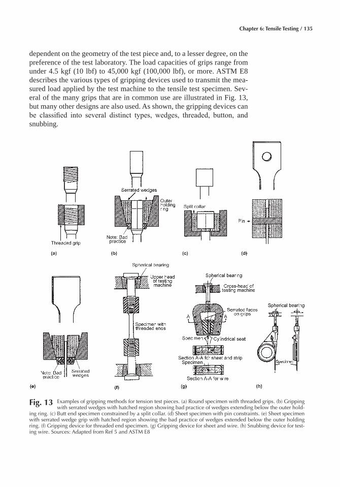
Chapter 6: Tensile Testing / 135
dependent on the geometry of the test piece and, to a lesser degree, on the preference of the test laboratory. The load capacities of grips range from under 4.5 kgf (10 lbf) to 45,000 kgf (100,000 lbf), or more. ASTM E8 describes the various types of gripping devices used to transmit the mea-sured load applied by the test machine to the tensile test specimen. Sev-eral of the many grips that are in common use are illustrated in Fig. 13, but many other designs are also used. As shown, the gripping devices can be classified into several distinct types, wedges, threaded, button, and snubbing.
Fig� 13 Examples of gripping methods for tension test pieces. (a) Round specimen with threaded grips. (b) Gripping with serrated wedges with hatched region showing bad practice of wedges extending below the outer hold-
ing ring. (c) Butt end specimen constrained by a split collar. (d) Sheet specimen with pin constraints. (e) Sheet specimen with serrated wedge grip with hatched region showing the bad practice of wedges extended below the outer holding ring. (f) Gripping device for threaded end specimen. (g) Gripping device for sheet and wire. (h) Snubbing device for test-ing wire. Sources: Adapted from Ref 5 and ASTM E8
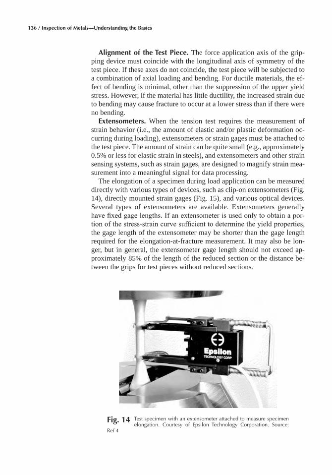
136 / Inspection of Metals—Understanding the Basics
Alignment of the Test Piece� The force application axis of the grip-ping device must coincide with the longitudinal axis of symmetry of the test piece. If these axes do not coincide, the test piece will be subjected to a combination of axial loading and bending. For ductile materials, the ef-fect of bending is minimal, other than the suppression of the upper yield stress. However, if the material has little ductility, the increased strain due to bending may cause fracture to occur at a lower stress than if there were no bending.
Extensometers� When the tension test requires the measurement of strain behavior (i.e., the amount of elastic and/or plastic deformation oc-curring during loading), extensometers or strain gages must be attached to the test piece. The amount of strain can be quite small (e.g., approximately 0.5% or less for elastic strain in steels), and extensometers and other strain sensing systems, such as strain gages, are designed to magnify strain mea-surement into a meaningful signal for data processing.
The elongation of a specimen during load application can be measured directly with various types of devices, such as clip-on extensometers (Fig. 14), directly mounted strain gages (Fig. 15), and various optical devices. Several types of extensometers are available. Extensometers generally have fixed gage lengths. If an extensometer is used only to obtain a por-tion of the stress-strain curve sufficient to determine the yield properties, the gage length of the extensometer may be shorter than the gage length required for the elongation-at-fracture measurement. It may also be lon-ger, but in general, the extensometer gage length should not exceed ap-proximately 85% of the length of the reduced section or the distance be-tween the grips for test pieces without reduced sections.
Fig� 14 Test specimen with an extensometer attached to measure specimen elongation. Courtesy of Epsilon Technology Corporation. Source:
Ref 4
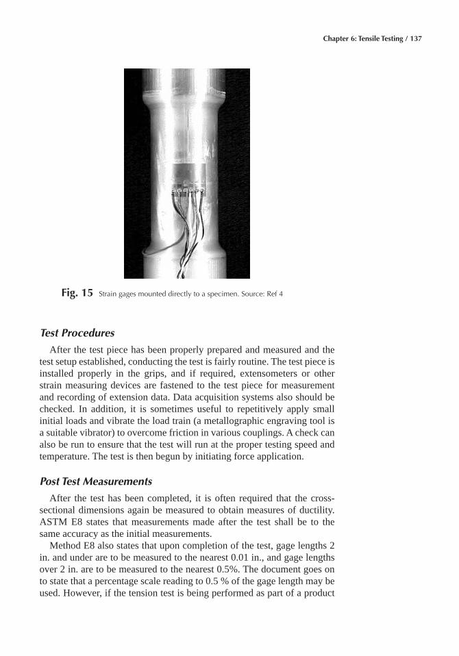
Chapter 6: Tensile Testing / 137
Test Procedures
After the test piece has been properly prepared and measured and the test setup established, conducting the test is fairly routine. The test piece is installed properly in the grips, and if required, extensometers or other strain measuring devices are fastened to the test piece for measurement and recording of extension data. Data acquisition systems also should be checked. In addition, it is sometimes useful to repetitively apply small initial loads and vibrate the load train (a metallographic engraving tool is a suitable vibrator) to overcome friction in various couplings. A check can also be run to ensure that the test will run at the proper testing speed and temperature. The test is then begun by initiating force application.
Post Test Measurements
After the test has been completed, it is often required that the cross-sectional dimensions again be measured to obtain measures of ductility. ASTM E8 states that measurements made after the test shall be to the same accuracy as the initial measurements.
Method E8 also states that upon completion of the test, gage lengths 2 in. and under are to be measured to the nearest 0.01 in., and gage lengths over 2 in. are to be measured to the nearest 0.5%. The document goes on to state that a percentage scale reading to 0.5 % of the gage length may be used. However, if the tension test is being performed as part of a product
Fig� 15 Strain gages mounted directly to a specimen. Source: Ref 4
138 / Inspection of Metals—Understanding the Basics
specification, and the elongation is specified to meet a value of 3% or less, special techniques, which are described, are to be used to measure the final gage length.
ACKNOWLEDGMENT
This chapter was adapted from Uniaxial Tension Testing by J.M. Holt in Mechanical Testing and Evaluation, Volume 8, ASM Handbook, 2000.
REFERENCES
1. F.C. Campbell, Elements of Metallurgy and Engineering Alloys, ASM International, 2008
2. J. M. Holt, Uniaxial Tension Testing, Mechanical Testing and Evalua-tion, Vol 8, ASM Handbook, ASM International, 2000
3. Making, Shaping, and Treating of Steel, 10th ed., U.S. Steel, 1985, Fig. 50-12 and 50-13
4. J.W. House and P.P. Gillis, Testing Machines and Strain Sensors, Me-chanical Testing and Evaluation, Vol 8, ASM Handbook, ASM Inter-national, 2000
5. D. Lewis, Tensile Testing of Ceramics and Ceramic-Matrix Compos-ites, Tensile Testing, P. Han, Ed., ASM International, 1992, p 147– 182
SELECTED REFERENCES
• “Standard Test Methods for Tension Testing of Metallic Materials.” E8, ASTM
• “Standard Methods and Definitions for Mechanical Testing of Steel Products,” A370, ASTM
• “Standard Test Methods for Poisson’s Ratio at Room Temperature,” E132, ASTM
• “Standard Test Methods for Young’s Modulus, Tangent Modulus, and Chord Modulus,” E111, ASTM
• “Standard Methods of Tension Testing of Metallic Materials,” E8, ASTM
• “Standard Methods of Tension Testing Wrought and Cast Aluminum- and Magnesium-Alloy Products,” B557, ASTM
• “Standard Recommended Practice for Verification of Specimen Align-ment Under Tensile Loading,” E1012, ASTM

Inspection of Metals—Understanding the Basics Copyright © 2013 ASM International®
F.C. Campbell, editor All rights reservedwww.asminternational.org
CHAPTER 7
Chemical Composition
THE OVERALL CHEMICAL COMPOSITION of metals and alloys is most commonly determined by x-ray fluorescence (XRF) and optical emission spectroscopy (OES). While these methods work well for most elements, they are not useful for dissolved gases and some nonmetallic elements that can be present in metals as alloying or impurity elements. High-temperature combustion and inert gas fusion methods are typically used to analyze dissolved gases (oxygen, nitrogen, hydrogen) and in some cases, carbon and sulfur in metals.
X-Ray Fluorescence Spectroscopy (XRF)
X-ray fluorescence is capable of the detection and quantification of ele-ments with atomic number 5 or higher. Older energy dispersive units with beryllium window detectors are limited to atomic number 11 or higher.
Typical uses are:
• Qualitative and quantitative chemical analysis for major and minor elements in metals and alloys
• Determination of composition and thickness of thin film deposits
X-ray fluorescence with energy dispersive detectors have a threshold sensitivity of ~0.02% and a precision for quantitative analysis of ~1% relative, or 0.02% absolute, depending on count time. The detection threshold and precision for wavelength dispersive detectors is a threshold sensitivity of ~0.005% and a precision for quantitative analysis of ~0.2% relative, or 0.005% absolute, whichever is greater.
For powders, the sample size is several grams pressed into a pellet. Powder samples are typically attached to substrates not produced by x-ray or are pressed into pellets. For bulk solids, the sample size is typically ~1 cm (~0.4 in.) diameter spot on the surface with a depth of 10 to 100 μm,
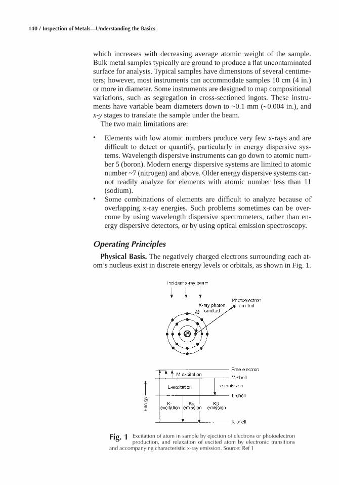
140 / Inspection of Metals—Understanding the Basics
which increases with decreasing average atomic weight of the sample. Bulk metal samples typically are ground to produce a flat uncontaminated surface for analysis. Typical samples have dimensions of several centime-ters; however, most instruments can accommodate samples 10 cm (4 in.) or more in diameter. Some instruments are designed to map compositional variations, such as segregation in cross-sectioned ingots. These instru-ments have variable beam diameters down to ~0.1 mm (~0.004 in.), and x-y stages to translate the sample under the beam.
The two main limitations are:
• Elements with low atomic numbers produce very few x-rays and are difficult to detect or quantify, particularly in energy dispersive sys-tems. Wavelength dispersive instruments can go down to atomic num-ber 5 (boron). Modern energy dispersive systems are limited to atomic number ~7 (nitrogen) and above. Older energy dispersive systems can-not readily analyze for elements with atomic number less than 11 (sodium).
• Some combinations of elements are difficult to analyze because of overlapping x-ray energies. Such problems sometimes can be over-come by using wavelength dispersive spectrometers, rather than en-ergy dispersive detectors, or by using optical emission spectroscopy.
Operating Principles
Physical Basis� The negatively charged electrons surrounding each at-om’s nucleus exist in discrete energy levels or orbitals, as shown in Fig. 1.
Fig� 1 Excitation of atom in sample by ejection of electrons or photoelectron production, and relaxation of excited atom by electronic transitions
and accompanying characteristic x-ray emission. Source: Ref 1
Chapter 7: Chemical Composition / 141
Each electron’s energy depends on its quantum state or the orbital it in-habits, and the number of positively charged protons in the atom’s nu-cleus. Electrons with low principal quantum numbers (those close to the nucleus) are tightly bound; they require large amounts of energy to re-move them (i.e., to cause ionization). Electrons with higher principal quantum numbers (those farther from the nucleus) are less tightly bound; less energy is required to remove them. Atoms with many positive protons in the nucleus (elements of high atomic number) tend to bind their inner shell electrons more tightly. Atoms with few protons in the nucleus (ele-ments of lower atomic number) are more easily stripped of their inner shell electrons.
The net result is that each element has a unique set of known electron energy levels. Similarly, the set of energy differences between these elec-tron energy levels are also unique for each element and constitutes a char-acteristic fingerprint by which each element can be identified. In XRF spectroscopy, as well as many other analytical methods, the combined electron energy level fingerprints of the elements present in the sample are experimentally obtained and are then compared to the fingerprints of known elements. From these comparisons, it is possible to identify the elements and their compositions present in a sample.
When sufficient energy is externally supplied to a sample of unknown composition, some of the electrons are excited to higher quantum states or energy levels, or removed from the atom or ionization. These excited atoms quickly relax by electrons from higher energy levels filling the va-cated levels. When this happens, photons are emitted whose energies are equal to the differences between the two energy levels involved; this pro-cess is called fluorescence. If the energies of these emitted photons are measured, they provide the fingerprint of the unknown sample. This mea-surement can then be compared to the known fingerprints of the elements, enabling determination of which elements are present in the sample and the concentration of each element present. Which elements are present can be deduced from the energies of the photons emitted by the sample. How much of each element is present can be deduced from the numbers of pho-tons with energies characteristic of the various elements. The characteris-tic energies emitted as excited atoms relax span a range of the electro-magnetic spectrum. Electronic transitions between inner shells typically produce x-rays (photons with energies in the 200 to 20,000 eV range, characterized by wavelengths of 6 to 0.06 nm).
Instrumentation� A simplified schematic of an XRF spectrometer is shown in Fig. 2. A beam of x-rays is produced by electronic excitation of a metal target in the instrument’s x-ray source. The beam’s only function is to excite atoms in the sample. As the incident x-ray beam is directed onto the sample surface, it penetrates some small distance into the sample, typically 10 to 100 μm, depending on the atomic numbers of the elements in the sample. Penetration depths are greater for low atomic number ele-ments. The incident x-rays excite atoms in the sample, transitioning some
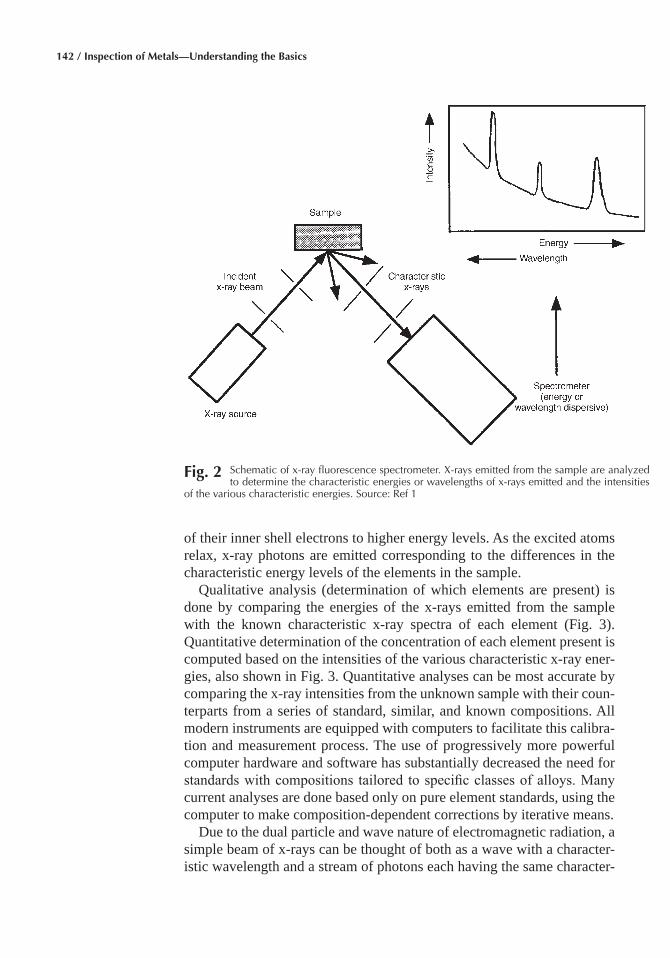
142 / Inspection of Metals—Understanding the Basics
of their inner shell electrons to higher energy levels. As the excited atoms relax, x-ray photons are emitted corresponding to the differences in the characteristic energy levels of the elements in the sample.
Qualitative analysis (determination of which elements are present) is done by comparing the energies of the x-rays emitted from the sample with the known characteristic x-ray spectra of each element (Fig. 3). Quantitative determination of the concentration of each element present is computed based on the intensities of the various characteristic x-ray ener-gies, also shown in Fig. 3. Quantitative analyses can be most accurate by comparing the x-ray intensities from the unknown sample with their coun-terparts from a series of standard, similar, and known compositions. All modern instruments are equipped with computers to facilitate this calibra-tion and measurement process. The use of progressively more powerful computer hardware and software has substantially decreased the need for standards with compositions tailored to specific classes of alloys. Many current analyses are done based only on pure element standards, using the computer to make composition-dependent corrections by iterative means.
Due to the dual particle and wave nature of electromagnetic radiation, a simple beam of x-rays can be thought of both as a wave with a character-istic wavelength and a stream of photons each having the same character-
Fig� 2 Schematic of x-ray fluorescence spectrometer. X-rays emitted from the sample are analyzed to determine the characteristic energies or wavelengths of x-rays emitted and the intensities
of the various characteristic energies. Source: Ref 1
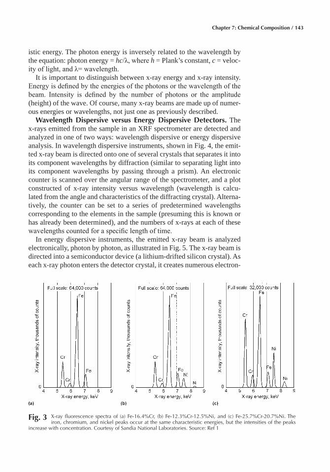
Chapter 7: Chemical Composition / 143
istic energy. The photon energy is inversely related to the wavelength by the equation: photon energy = hc/λ, where h = Plank’s constant, c = veloc-ity of light, and λ= wavelength.
It is important to distinguish between x-ray energy and x-ray intensity. Energy is defined by the energies of the photons or the wavelength of the beam. Intensity is defined by the number of photons or the amplitude (height) of the wave. Of course, many x-ray beams are made up of numer-ous energies or wavelengths, not just one as previously described.
Wavelength Dispersive versus Energy Dispersive Detectors� The x-rays emitted from the sample in an XRF spectrometer are detected and analyzed in one of two ways: wavelength dispersive or energy dispersive analysis. In wavelength dispersive instruments, shown in Fig. 4, the emit-ted x-ray beam is directed onto one of several crystals that separates it into its component wavelengths by diffraction (similar to separating light into its component wavelengths by passing through a prism). An electronic counter is scanned over the angular range of the spectrometer, and a plot constructed of x-ray intensity versus wavelength (wavelength is calcu-lated from the angle and characteristics of the diffracting crystal). Alterna-tively, the counter can be set to a series of predetermined wavelengths corresponding to the elements in the sample (presuming this is known or has already been determined), and the numbers of x-rays at each of these wavelengths counted for a specific length of time.
In energy dispersive instruments, the emitted x-ray beam is analyzed electronically, photon by photon, as illustrated in Fig. 5. The x-ray beam is directed into a semiconductor device (a lithium-drifted silicon crystal). As each x-ray photon enters the detector crystal, it creates numerous electron-
Fig� 3 X-ray fluorescence spectra of (a) Fe-16.4%Cr, (b) Fe-12.3%Cr-12.5%Ni, and (c) Fe-25.7%Cr-20.7%Ni. The iron, chromium, and nickel peaks occur at the same characteristic energies, but the intensities of the peaks
increase with concentration. Courtesy of Sandia National Laboratories. Source: Ref 1
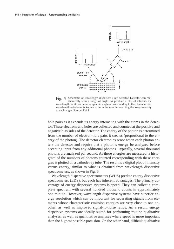
144 / Inspection of Metals—Understanding the Basics
hole pairs as it expends its energy interacting with the atoms in the detec-tor. These electrons and holes are collected and counted at the positive and negative bias sides of the detector. The energy of the photon is determined from the number of electron-hole pairs it creates (proportional to the en-ergy of the photon). The detector electronics sense when each photon en-ters the detector and require that a photon’s energy be analyzed before accepting input from any additional photons. Typically, several thousand photons are analyzed per second. As these energies are measured, a histo-gram of the numbers of photons counted corresponding with these ener-gies is plotted on a cathode ray tube. The result is a digital plot of intensity versus energy, similar to what is obtained from wavelength dispersive spectrometers, as shown in Fig. 6.
Wavelength dispersive spectrometers (WDS) predate energy dispersive spectrometers (EDS), but each has inherent advantages. The primary ad-vantage of energy dispersive systems is speed. They can collect a com-plete spectrum with several hundred thousand counts in approximately one minute. However, wavelength dispersive systems have superior en-ergy resolution which can be important for separating signals from ele-ments whose characteristic emission energies are very close to one an-other, as well as improved signal-to-noise ratios. As a result, energy dispersive systems are ideally suited for performing routine qualitative analyses, as well as quantitative analyses where speed is more important than the highest possible precision. On the other hand, difficult qualitative
Fig� 4 Schematic of wavelength dispersive x-ray detector. Detector can me-chanically scan a range of angles to produce a plot of intensity vs.
wavelength, or it can be set at specific angles corresponding to the characteristic wavelengths of elements known to be in the sample, counting the x-ray intensity at each angle. Source: Ref 1
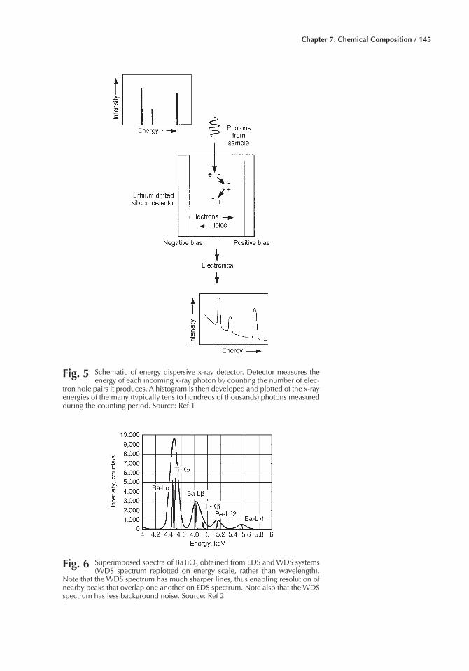
Chapter 7: Chemical Composition / 145
Fig� 5 Schematic of energy dispersive x-ray detector. Detector measures the energy of each incoming x-ray photon by counting the number of elec-
tron hole pairs it produces. A histogram is then developed and plotted of the x-ray energies of the many (typically tens to hundreds of thousands) photons measured during the counting period. Source: Ref 1
Fig� 6 Superimposed spectra of BaTiO3 obtained from EDS and WDS systems (WDS spectrum replotted on energy scale, rather than wavelength).
Note that the WDS spectrum has much sharper lines, thus enabling resolution of nearby peaks that overlap one another on EDS spectrum. Note also that the WDS spectrum has less background noise. Source: Ref 2
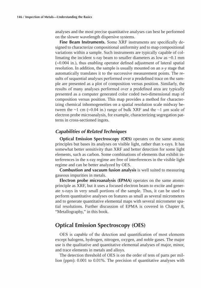
146 / Inspection of Metals—Understanding the Basics
analyses and the most precise quantitative analyses can best be performed on the slower wavelength dispersive systems.
Fine Beam Instruments� Some XRF instruments are specifically de-signed to characterize compositional uniformity and to map compositional variations within a sample. Such instruments are typically capable of col-limating the incident x-ray beam to smaller diameters as low as ~0.1 mm (~0.004 in.), thus enabling operator defined adjustment of lateral spatial resolution. In addition, the sample is usually mounted on an x-y stage that automatically translates it to the successive measurement points. The re-sults of sequential analyses performed over a predefined trace on the sam-ple are presented as a plot of composition versus position. Similarly, the results of many analyses performed over a predefined area are typically presented as a computer generated color coded two-dimensional map of composition versus position. This map provides a method for character-izing chemical inhomogeneities on a spatial resolution scale midway be-tween the ~1 cm (~0.04 in.) range of bulk XRF and the ~1 μm scale of electron probe microanalysis, for example, characterizing segregation pat-terns in cross-sectioned ingots.
Capabilities of Related Techniques
Optical Emission Spectroscopy (OES) operates on the same atomic principles but bases its analyses on visible light, rather than x-rays. It has somewhat better sensitivity than XRF and better detection for some light elements, such as carbon. Some combinations of elements that exhibit in-terferences in the x-ray regime are free of interferences in the visible light regime and can be better analyzed by OES.
Combustion and vacuum fusion analysis is well suited to measuring gaseous impurities in metals.
Electron probe microanalysis (EPMA) operates on the same atomic principle as XRF, but it uses a focused electron beam to excite and gener-ate x-rays in very small portions of the sample. Thus, it can be used to perform quantitative analyses on features as small as several micrometers and to generate quantitative elemental maps with several micrometer spa-tial resolutions. Further discussion of EPMA is covered in Chapter 8, “Metallography,” in this book.
Optical Emission Spectroscopy (OES)
OES is capable of the detection and quantification of most elements except halogens, hydrogen, nitrogen, oxygen, and noble gases. The major use is the qualitative and quantitative elemental analyses of major, minor, and trace elements in metals and alloys.
The detection threshold of OES is on the order of tens of parts per mil-lion (ppm): 0.001 to 0.01%. The precision of quantitative analyses with
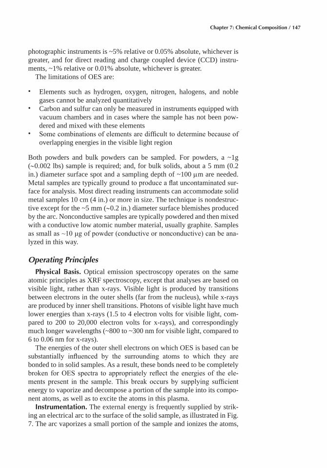
Chapter 7: Chemical Composition / 147
photographic instruments is ~5% relative or 0.05% absolute, whichever is greater, and for direct reading and charge coupled device (CCD) instru-ments, ~1% relative or 0.01% absolute, whichever is greater.
The limitations of OES are:
• Elements such as hydrogen, oxygen, nitrogen, halogens, and noble gases cannot be analyzed quantitatively
• Carbon and sulfur can only be measured in instruments equipped with vacuum chambers and in cases where the sample has not been pow-dered and mixed with these elements
• Some combinations of elements are difficult to determine because of overlapping energies in the visible light region
Both powders and bulk powders can be sampled. For powders, a ~1g (~0.002 lbs) sample is required; and, for bulk solids, about a 5 mm (0.2 in.) diameter surface spot and a sampling depth of ~100 mm are needed. Metal samples are typically ground to produce a flat uncontaminated sur-face for analysis. Most direct reading instruments can accommodate solid metal samples 10 cm (4 in.) or more in size. The technique is nondestruc-tive except for the ~5 mm (~0.2 in.) diameter surface blemishes produced by the arc. Nonconductive samples are typically powdered and then mixed with a conductive low atomic number material, usually graphite. Samples as small as ~10 μg of powder (conductive or nonconductive) can be ana-lyzed in this way.
Operating Principles
Physical Basis� Optical emission spectroscopy operates on the same atomic principles as XRF spectroscopy, except that analyses are based on visible light, rather than x-rays. Visible light is produced by transitions between electrons in the outer shells (far from the nucleus), while x-rays are produced by inner shell transitions. Photons of visible light have much lower energies than x-rays (1.5 to 4 electron volts for visible light, com-pared to 200 to 20,000 electron volts for x-rays), and correspondingly much longer wavelengths (~800 to ~300 nm for visible light, compared to 6 to 0.06 nm for x-rays).
The energies of the outer shell electrons on which OES is based can be substantially influenced by the surrounding atoms to which they are bonded to in solid samples. As a result, these bonds need to be completely broken for OES spectra to appropriately reflect the energies of the ele-ments present in the sample. This break occurs by supplying sufficient energy to vaporize and decompose a portion of the sample into its compo-nent atoms, as well as to excite the atoms in this plasma.
Instrumentation� The external energy is frequently supplied by strik-ing an electrical arc to the surface of the solid sample, as illustrated in Fig. 7. The arc vaporizes a small portion of the sample and ionizes the atoms,
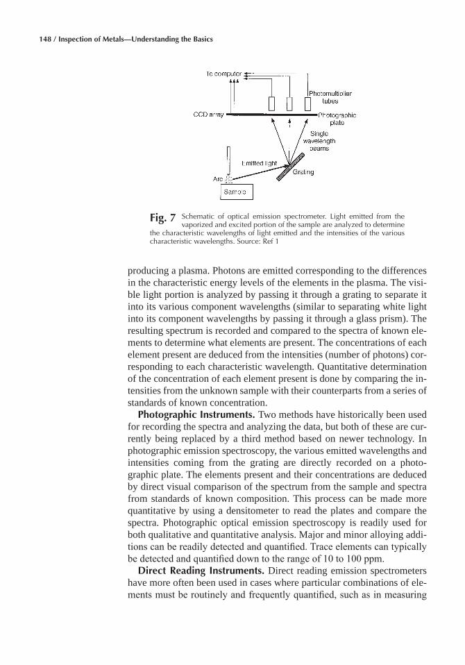
148 / Inspection of Metals—Understanding the Basics
producing a plasma. Photons are emitted corresponding to the differences in the characteristic energy levels of the elements in the plasma. The visi-ble light portion is analyzed by passing it through a grating to separate it into its various component wavelengths (similar to separating white light into its component wavelengths by passing it through a glass prism). The resulting spectrum is recorded and compared to the spectra of known ele-ments to determine what elements are present. The concentrations of each element present are deduced from the intensities (number of photons) cor-responding to each characteristic wavelength. Quantitative determination of the concentration of each element present is done by comparing the in-tensities from the unknown sample with their counterparts from a series of standards of known concentration.
Photographic Instruments� Two methods have historically been used for recording the spectra and analyzing the data, but both of these are cur-rently being replaced by a third method based on newer technology. In photographic emission spectroscopy, the various emitted wavelengths and intensities coming from the grating are directly recorded on a photo-graphic plate. The elements present and their concentrations are deduced by direct visual comparison of the spectrum from the sample and spectra from standards of known composition. This process can be made more quantitative by using a densitometer to read the plates and compare the spectra. Photographic optical emission spectroscopy is readily used for both qualitative and quantitative analysis. Major and minor alloying addi-tions can be readily detected and quantified. Trace elements can typically be detected and quantified down to the range of 10 to 100 ppm.
Direct Reading Instruments� Direct reading emission spectrometers have more often been used in cases where particular combinations of ele-ments must be routinely and frequently quantified, such as in measuring
Fig� 7 Schematic of optical emission spectrometer. Light emitted from the vaporized and excited portion of the sample are analyzed to determine
the characteristic wavelengths of light emitted and the intensities of the various characteristic wavelengths. Source: Ref 1
Chapter 7: Chemical Composition / 149
the compositions of heats being produced by an aluminum ingot produc-tion facility. In these instruments, photomultiplier tubes are set up at the wavelength positions corresponding to each element of interest. These tubes measure the intensities of light obtained from the sample at each predetermined characteristic wavelength and input the results to a com-puter. The computer then compares these intensities to the corresponding intensities from various standards of known composition (which are al-ready stored in its memory) and calculates the composition of the sample in a matter of seconds. This facilitates rapid quantitative analysis of sam-ples of unknown but similar composition. Because they are only set up to analyze for specific preselected elements and over commonly encountered composition ranges, direct reading emission spectrometers are not useful for qualitative or quantitative analysis of broader ranges of samples.
Instruments with Charge Coupled Device (CCD) Detectors� Both of the previously described methods of detection are now being supplant-ed by CCD detectors (a high-resolution array of solid state light detec-tors). These detectors take the place of photographic plates and electroni-cally record both the location or wavelength and intensity or brightness of the light emitted from the sample. The output of the CCD detector is in-putted to a computer, which constructs a histogram of intensity versus wavelength. The computer also facilitates comparison of the observed wavelengths with the known characteristic wavelengths of each element, thus providing for qualitative determination of which elements are present in the sample. In addition, the computer can make quantitative determina-tions of the concentrations of each element present from the intensities of the emitted light at various characteristic energies. These determinations can be made based on comparison with calibrated standards (measured by the instrument and stored in the computer memory) or based on pure ele-ment standards. Analyses based on calibrated standards are typically used in cases where greater accuracy and precision are required. In essence, then, an instrument equipped with a CCD detector is like a direct reading instrument with a semi-infinite number of detectors positioned at every wavelength of possible interest, which provides a rapid and powerful ca-pability for both qualitative and quantitative analysis.
Capabilities of Related Techniques
Inductively coupled plasma atomic emission spectroscopy (ICP/AES) operates on the same atomic principle. However, solid samples are dissolved into liquid solutions that are then aspirated into an argon plasma. This process provides greater flexibility, as liquid standards can be made of essentially any combination of elements, including combinations that cannot be obtained in solid form. Inductively coupled plasma can be used for both qualitative and quantitative elemental analysis. However, its de-tection limits are lower than those of other OES methods. Because the
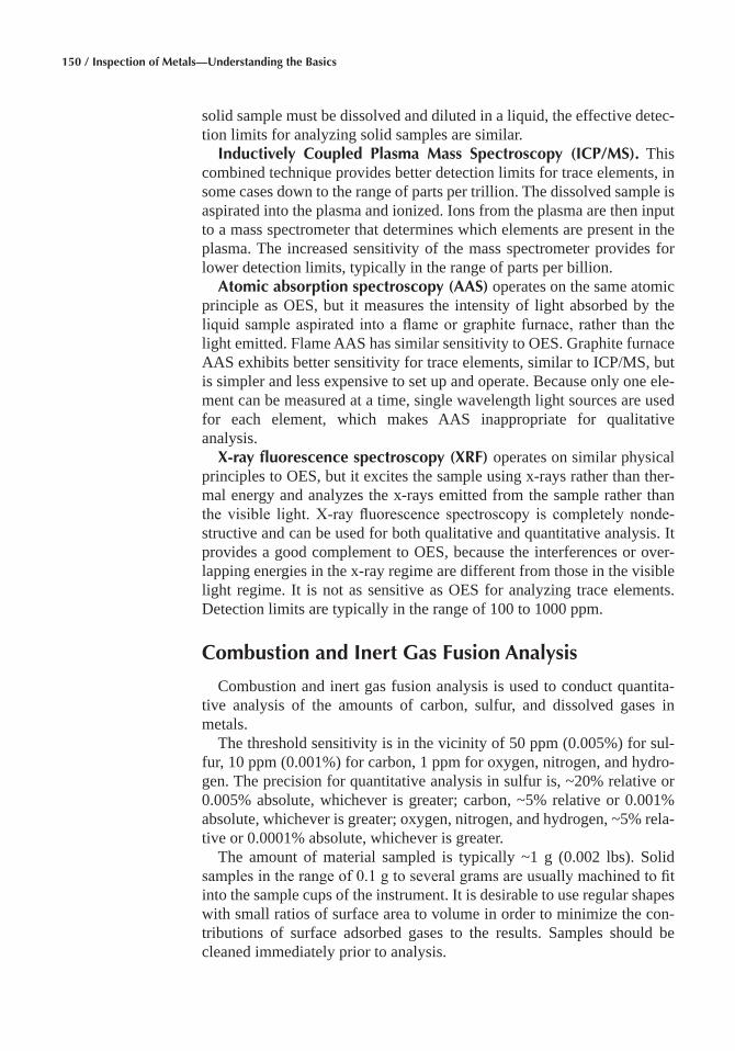
150 / Inspection of Metals—Understanding the Basics
solid sample must be dissolved and diluted in a liquid, the effective detec-tion limits for analyzing solid samples are similar.
Inductively Coupled Plasma Mass Spectroscopy (ICP/MS)� This combined technique provides better detection limits for trace elements, in some cases down to the range of parts per trillion. The dissolved sample is aspirated into the plasma and ionized. Ions from the plasma are then input to a mass spectrometer that determines which elements are present in the plasma. The increased sensitivity of the mass spectrometer provides for lower detection limits, typically in the range of parts per billion.
Atomic absorption spectroscopy (AAS) operates on the same atomic principle as OES, but it measures the intensity of light absorbed by the liquid sample aspirated into a flame or graphite furnace, rather than the light emitted. Flame AAS has similar sensitivity to OES. Graphite furnace AAS exhibits better sensitivity for trace elements, similar to ICP/MS, but is simpler and less expensive to set up and operate. Because only one ele-ment can be measured at a time, single wavelength light sources are used for each element, which makes AAS inappropriate for qualitative analysis.
X-ray fluorescence spectroscopy (XRF) operates on similar physical principles to OES, but it excites the sample using x-rays rather than ther-mal energy and analyzes the x-rays emitted from the sample rather than the visible light. X-ray fluorescence spectroscopy is completely nonde-structive and can be used for both qualitative and quantitative analysis. It provides a good complement to OES, because the interferences or over-lapping energies in the x-ray regime are different from those in the visible light regime. It is not as sensitive as OES for analyzing trace elements. Detection limits are typically in the range of 100 to 1000 ppm.
Combustion and Inert Gas Fusion Analysis
Combustion and inert gas fusion analysis is used to conduct quantita-tive analysis of the amounts of carbon, sulfur, and dissolved gases in metals.
The threshold sensitivity is in the vicinity of 50 ppm (0.005%) for sul-fur, 10 ppm (0.001%) for carbon, 1 ppm for oxygen, nitrogen, and hydro-gen. The precision for quantitative analysis in sulfur is, ~20% relative or 0.005% absolute, whichever is greater; carbon, ~5% relative or 0.001% absolute, whichever is greater; oxygen, nitrogen, and hydrogen, ~5% rela-tive or 0.0001% absolute, whichever is greater.
The amount of material sampled is typically ~1 g (0.002 lbs). Solid samples in the range of 0.1 g to several grams are usually machined to fit into the sample cups of the instrument. It is desirable to use regular shapes with small ratios of surface area to volume in order to minimize the con-tributions of surface adsorbed gases to the results. Samples should be cleaned immediately prior to analysis.
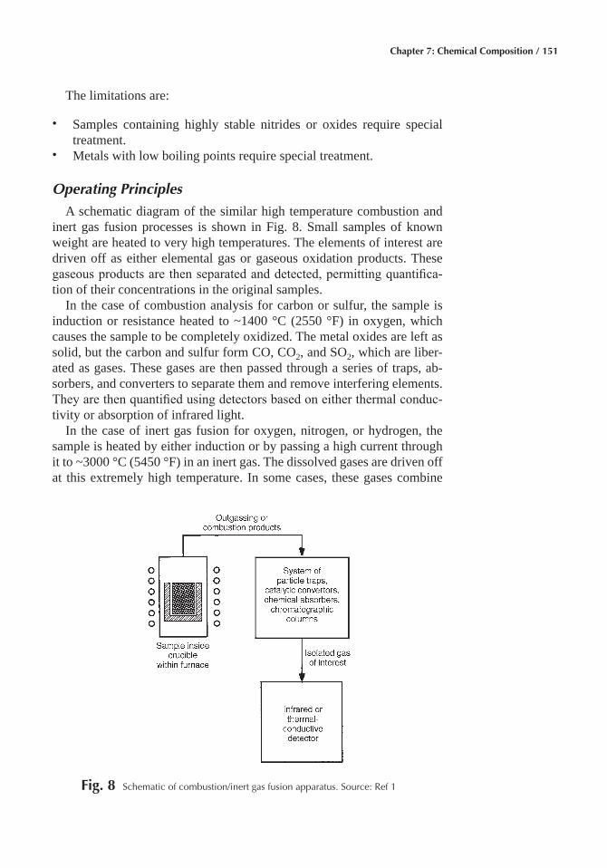
Chapter 7: Chemical Composition / 151
The limitations are:
• Samples containing highly stable nitrides or oxides require special treatment.
• Metals with low boiling points require special treatment.
Operating Principles
A schematic diagram of the similar high temperature combustion and inert gas fusion processes is shown in Fig. 8. Small samples of known weight are heated to very high temperatures. The elements of interest are driven off as either elemental gas or gaseous oxidation products. These gaseous products are then separated and detected, permitting quantifica-tion of their concentrations in the original samples.
In the case of combustion analysis for carbon or sulfur, the sample is induction or resistance heated to ~1400 °C (2550 °F) in oxygen, which causes the sample to be completely oxidized. The metal oxides are left as solid, but the carbon and sulfur form CO, CO2, and SO2, which are liber-ated as gases. These gases are then passed through a series of traps, ab-sorbers, and converters to separate them and remove interfering elements. They are then quantified using detectors based on either thermal conduc-tivity or absorption of infrared light.
In the case of inert gas fusion for oxygen, nitrogen, or hydrogen, the sample is heated by either induction or by passing a high current through it to ~3000 °C (5450 °F) in an inert gas. The dissolved gases are driven off at this extremely high temperature. In some cases, these gases combine
Fig� 8 Schematic of combustion/inert gas fusion apparatus. Source: Ref 1
152 / Inspection of Metals—Understanding the Basics
with other elements in the system; for example, oxygen reacts with carbon to form CO or CO2. The liberated gases and/or reaction products are then passed through a series of particle traps, catalytic converters, gas chemical absorbers, and chromatographic columns to separate and purify them. They are then quantified using detectors based on either thermal conduc-tivity or absorption of infrared light, as in combustion analysis.
Capabilities of Related Techniques
X-ray fluorescence spectroscopy (XRF) can analyze nondestructively for carbon and sulfur but with higher detection limits and reduced precision.
Optical emission spectroscopy (OES) can analyze less destructively for carbon and sulfur, but with higher detection limits and reduced precision.
Hot extraction high vacuum analysis is similar to inert gas fusion, but gases are liberated at lower temperatures (without destroying sample). Gas evolution can be monitored as a function of time or temperature, thus permitting separation of internally dissolved and surface adsorbed gases.
Surface Analysis
A number of methods can be used to obtain information about the chemistry of the several atomic layers of samples of metals, as well as of other materials, such as semiconductors and various types of thin films. Of these methods, the scanning Auger microprobe is the most widely used. This instrument and method will be described in some detail, and the op-eration and capabilities of several other surface analysis methods will be more briefly described in comparison to it.
Scanning Auger Microprobe (SAM)
The scanning Auger microprobe is basically a scanning electron micro-scope (SEM) with two additional features:
• An Auger electron detector replaces an x-ray detector. The Auger de-tector is used to measure the energies of Auger electrons emitted from the sample. These characteristic energies enable identification of the elements present in the first few atomic layers of the surface. The con-centrations of each element present can also be determined by the number of electrons detected at each of the characteristic energies. All elements except hydrogen and helium can be identified and analyzed in this way.
• An in situ ion milling capability provides for gradual removal of sur-face layers, thereby permitting depth profiling of elemental composi-tions within about 1 μm of the surface.
Chapter 7: Chemical Composition / 153
These capabilities make the SAM well suited for the following types of applications:
• Identification and mapping of light elements (atomic numbers 3 to ~9) that are difficult to detect using SEM or electron probe microanalysis (EPMA)
• Elemental characterization of surface contaminants • Depth profiling of elemental compositions within ~1 μm of the surface
(this is particularly widely used in microelectronics applications)
The spatial resolution of secondary electron imaging of surface topog-raphy is ~10 nm (same as SEM), and the resolution of Auger electron characterization of elemental chemistry is 10 to 20 nm at a sampling depth of ~1 nm. The threshold sensitivity is ~0.5%, and the precision for quanti-tative analysis is ~10% relative or 0.5% absolute, whichever is greater.
Samples up to ~2.5 cm (~0.10 in.) diameter and 0.5 cm (0.20 in.) thick can be accommodated by most SAMs; larger samples can be accommo-dated in instruments designed for this purpose. Provisions must be made for charge to bleed off. Ideal samples are electrically conductive and must be free of fingerprints, oils, and other high vapor pressure materials. Flat samples are preferred, but rough samples can also be accommodated.
Limitations of SAM are:
• Cannot detect hydrogen or helium • Quantitative analyses are typically lower in quality than those of
EPMA
Operating Principles
Instrumentation� As noted above, the scanning Auger microprobe is essentially a SEM to which an Auger electron detector and an ion miller have been added as shown in Fig. 9 An electron beam is produced and focused to a small spot on the sample surface. This spot can be rastered across an operator defined area of the surface or stopped and moved to a particular location of interest. The beam penetrates the sample and inter-acts with the atoms in the first ~1 μm, exciting atoms and producing sec-ondary electrons, exactly like a SEM. A secondary electron detector pro-vides the capability to image the surface and locate areas of particular interest, as in a scanning electron microscope. However, the primary tool for chemical analysis is the Auger electron detector.
Physical Basis� Auger electrons are emitted as the excited atoms relax. In a sense, they are the complements of the characteristic x-rays that are used for chemical characterization in x-ray fluorescence (XRF), SEM, EPMA, and transmission electron microscopy (TEM). When atoms be-come excited by electrons being ejected from their inner shells, electrons from higher energy shells fill these vacated sites. This process always re-sults in the release of energy equal to the energy difference between the
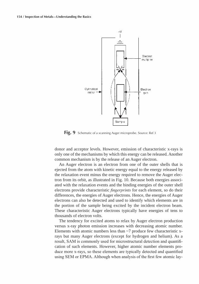
154 / Inspection of Metals—Understanding the Basics
donor and acceptor levels. However, emission of characteristic x-rays is only one of the mechanisms by which this energy can be released. Another common mechanism is by the release of an Auger electron.
An Auger electron is an electron from one of the outer shells that is ejected from the atom with kinetic energy equal to the energy released by the relaxation event minus the energy required to remove the Auger elec-tron from its orbit, as illustrated in Fig. 10. Because both energies associ-ated with the relaxation events and the binding energies of the outer shell electrons provide characteristic fingerprints for each element, so do their differences, the energies of Auger electrons. Hence, the energies of Auger electrons can also be detected and used to identify which elements are in the portion of the sample being excited by the incident electron beam. These characteristic Auger electrons typically have energies of tens to thousands of electron volts.
The tendency for excited atoms to relax by Auger electron production versus x-ray photon emission increases with decreasing atomic number. Elements with atomic numbers less than ~7 produce few characteristic x-rays but many Auger electrons (except for hydrogen and helium). As a result, SAM is commonly used for microstructural detection and quantifi-cation of such elements. However, higher atomic number elements pro-duce more x-rays, so these elements are typically detected and quantified using SEM or EPMA. Although when analysis of the first few atomic lay-
Fig� 9 Schematic of a scanning Auger microprobe. Source: Ref 3
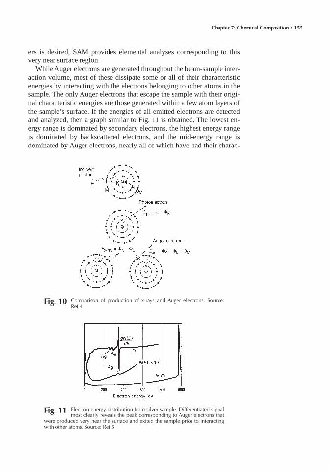
Chapter 7: Chemical Composition / 155
Fig� 10 Comparison of production of x-rays and Auger electrons. Source: Ref 4
ers is desired, SAM provides elemental analyses corresponding to this very near surface region.
While Auger electrons are generated throughout the beam-sample inter-action volume, most of these dissipate some or all of their characteristic energies by interacting with the electrons belonging to other atoms in the sample. The only Auger electrons that escape the sample with their origi-nal characteristic energies are those generated within a few atom layers of the sample’s surface. If the energies of all emitted electrons are detected and analyzed, then a graph similar to Fig. 11 is obtained. The lowest en-ergy range is dominated by secondary electrons, the highest energy range is dominated by backscattered electrons, and the mid-energy range is dominated by Auger electrons, nearly all of which have had their charac-
Fig� 11 Electron energy distribution from silver sample. Differentiated signal most clearly reveals the peak corresponding to Auger electrons that
were produced very near the surface and exited the sample prior to interacting with other atoms. Source: Ref 5
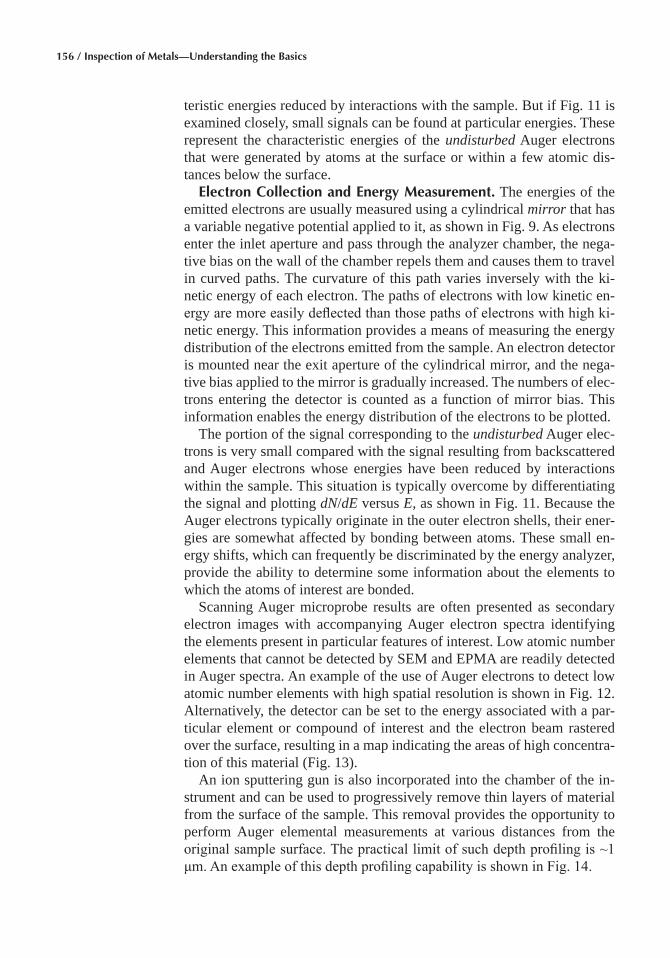
156 / Inspection of Metals—Understanding the Basics
teristic energies reduced by interactions with the sample. But if Fig. 11 is examined closely, small signals can be found at particular energies. These represent the characteristic energies of the undisturbed Auger electrons that were generated by atoms at the surface or within a few atomic dis-tances below the surface.
Electron Collection and Energy Measurement� The energies of the emitted electrons are usually measured using a cylindrical mirror that has a variable negative potential applied to it, as shown in Fig. 9. As electrons enter the inlet aperture and pass through the analyzer chamber, the nega-tive bias on the wall of the chamber repels them and causes them to travel in curved paths. The curvature of this path varies inversely with the ki-netic energy of each electron. The paths of electrons with low kinetic en-ergy are more easily deflected than those paths of electrons with high ki-netic energy. This information provides a means of measuring the energy distribution of the electrons emitted from the sample. An electron detector is mounted near the exit aperture of the cylindrical mirror, and the nega-tive bias applied to the mirror is gradually increased. The numbers of elec-trons entering the detector is counted as a function of mirror bias. This information enables the energy distribution of the electrons to be plotted.
The portion of the signal corresponding to the undisturbed Auger elec-trons is very small compared with the signal resulting from backscattered and Auger electrons whose energies have been reduced by interactions within the sample. This situation is typically overcome by differentiating the signal and plotting dN/dE versus E, as shown in Fig. 11. Because the Auger electrons typically originate in the outer electron shells, their ener-gies are somewhat affected by bonding between atoms. These small en-ergy shifts, which can frequently be discriminated by the energy analyzer, provide the ability to determine some information about the elements to which the atoms of interest are bonded.
Scanning Auger microprobe results are often presented as secondary electron images with accompanying Auger electron spectra identifying the elements present in particular features of interest. Low atomic number elements that cannot be detected by SEM and EPMA are readily detected in Auger spectra. An example of the use of Auger electrons to detect low atomic number elements with high spatial resolution is shown in Fig. 12. Alternatively, the detector can be set to the energy associated with a par-ticular element or compound of interest and the electron beam rastered over the surface, resulting in a map indicating the areas of high concentra-tion of this material (Fig. 13).
An ion sputtering gun is also incorporated into the chamber of the in-strument and can be used to progressively remove thin layers of material from the surface of the sample. This removal provides the opportunity to perform Auger elemental measurements at various distances from the original sample surface. The practical limit of such depth profiling is ~1 μm. An example of this depth profiling capability is shown in Fig. 14.
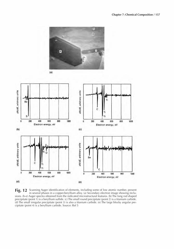
Chapter 7: Chemical Composition / 157
Fig� 12 Scanning Auger identification of elements, including some of low atomic number, present in several phases in a copper-beryllium alloy. (a) Secondary electron image showing inclu-
sions. (b-e) Auger spectra obtained from the indicated microstructural features. (b) The long rod shaped precipitate (point 1) is a beryllium sulfide. (c) The small round precipitate (point 2) is a titanium carbide. (d) The small irregular precipitate (point 3) is also a titanium carbide. (e) The large blocky angular pre-cipitate (point 4) is a beryllium carbide. Source: Ref 5
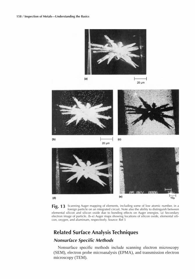
158 / Inspection of Metals—Understanding the Basics
Related Surface Analysis TechniquesNonsurface Specific Methods
Nonsurface specific methods include scanning electron microscopy (SEM), electron probe microanalysis (EPMA), and transmission electron microscopy (TEM).
Fig� 13 Scanning Auger mapping of elements, including some of low atomic number, in a foreign particle on an integrated circuit. Note also the ability to distinguish between
elemental silicon and silicon oxide due to bonding effects on Auger energies. (a) Secondary electron image of particle. (b–e) Auger maps showing locations of silicon oxide, elemental sili-con, oxygen, and aluminum, respectively. Source: Ref 5
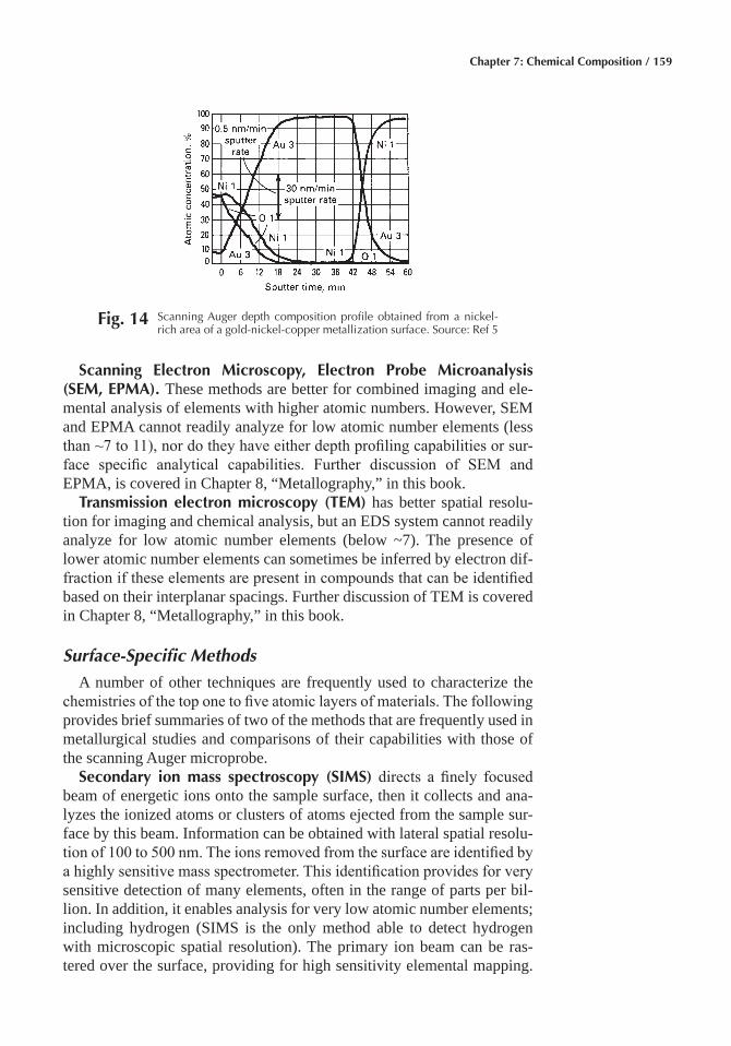
Chapter 7: Chemical Composition / 159
Scanning Electron Microscopy, Electron Probe Microanalysis (SEM, EPMA)� These methods are better for combined imaging and ele-mental analysis of elements with higher atomic numbers. However, SEM and EPMA cannot readily analyze for low atomic number elements (less than ~7 to 11), nor do they have either depth profiling capabilities or sur-face specific analytical capabilities. Further discussion of SEM and EPMA, is covered in Chapter 8, “Metallography,” in this book.
Transmission electron microscopy (TEM) has better spatial resolu-tion for imaging and chemical analysis, but an EDS system cannot readily analyze for low atomic number elements (below ~7). The presence of lower atomic number elements can sometimes be inferred by electron dif-fraction if these elements are present in compounds that can be identified based on their interplanar spacings. Further discussion of TEM is covered in Chapter 8, “Metallography,” in this book.
Surface-Specific Methods
A number of other techniques are frequently used to characterize the chemistries of the top one to five atomic layers of materials. The following provides brief summaries of two of the methods that are frequently used in metallurgical studies and comparisons of their capabilities with those of the scanning Auger microprobe.
Secondary ion mass spectroscopy (SIMS) directs a finely focused beam of energetic ions onto the sample surface, then it collects and ana-lyzes the ionized atoms or clusters of atoms ejected from the sample sur-face by this beam. Information can be obtained with lateral spatial resolu-tion of 100 to 500 nm. The ions removed from the surface are identified by a highly sensitive mass spectrometer. This identification provides for very sensitive detection of many elements, often in the range of parts per bil-lion. In addition, it enables analysis for very low atomic number elements; including hydrogen (SIMS is the only method able to detect hydrogen with microscopic spatial resolution). The primary ion beam can be ras-tered over the surface, providing for high sensitivity elemental mapping.
Fig� 14 Scanning Auger depth composition profile obtained from a nickel-rich area of a gold-nickel-copper metallization surface. Source: Ref 5
160 / Inspection of Metals—Understanding the Basics
Because it removes material from the surface, it also provides for depth profiling.
X-ray photoelectron spectroscopy (XPS) directs a single energy x-ray beam onto the surface. This beam penetrates 10 to 100 μm into the sam-ple, interacting with atoms and ejecting photoelectrons from their inner shells. The energies of these photoelectrons are equal to the energy of the x-ray photons minus the characteristic electron binding energies. Many of the photoelectrons lose some or all of their energy in interactions with other atoms, but a few that are generated very close to the surface exit the sample undisturbed. The photoelectrons are collected and their energies analyzed using a device similar to the cylindrical mirror in a scanning Auger microprobe (SAM). Analysis of the energies of the photoelectrons permits identification of the elements in the top few atomic layers. The excellent energy resolution of the analyzer enables it to discriminate the very small shifts in energy that result from bonding of the atoms of inter-est to other surrounding atoms. Hence, XPS is capable of providing infor-mation on surrounding atoms and chemical bonding. X-ray photoelectron spectroscopy does not utilize a fine incident beam; therefore, it does not provide images or chemical information with high lateral spatial resolu-tion. It is generally not as sensitive as SIMS, but it is very useful for de-tecting some elements for which SIMS is not very sensitive. An ion sput-tering capability is generally available to facilitate depth profiling. In general, XPS is most extensively used to obtain surface analyses with chemical bonding sensitivity.
ACKNOWLEDGMENT
This chapter was adapted from Bulk Elemental Analysis and Surface Analysis, both by K.H. Eckelmeyer in Metals Handbook Desk Edition, Second Edition, ASM International, 1998.
REFERENCES
1. K.H. Eckelmeyer, Bulk Elemental Analysis, Metals Handbook Desk Edition, 2nd ed., ASM International, 1998, p 1410–1411
2. C. Brundle, C. Evans, and S. Wilson, Encyclopedia of Materials Char-acterization, Butterworth-Heinemann, 1992, p 128
3. K.H. Eckelmeyer, Surface Analysis, Metals Handbook Desk Edition, 2nd ed., ASM International, 1998, p 1433–1436
4. R. Jenkins, R. Gould, and D. Gedcke, Quantitative X-Ray Spectrome-try, Dekker, 1981, p 16
5. Materials Characterization, Vol 10, ASM Handbook, ASM Interna-tional, 1986
Inspection of Metals—Understanding the Basics Copyright © 2013 ASM International®
F.C. Campbell, editor All rights reservedwww.asminternational.org
CHAPTER 8
Metallography
THE METHODS AND EQUIPMENT described in this chapter cover the preparation of specimens for examination by light optical microscopy (LOM). It is assumed that the specimen or specimens being prepared are representative of the material to be examined. However, random sam-pling, as advocated by statisticians, can rarely be performed by metallog-raphers. Instead, metallographers are usually restricted to inspecting areas of interest or systematically chosen test locations based on sampling con-venience. In failure analysis, specimens are usually removed to study the origin of the failure, to examine highly stressed areas, and to examine secondary cracks.
All sectioning processes produce damage; some methods, such as flame cutting, produce extreme amounts of damage. Traditional laboratory sec-tioning procedures using abrasive cut-off saws introduce minor damage that varies with the material being cut and its thermal and mechanical his-tory. This damage must be removed if the true structure is to be examined. However, because abrasive grinding and polishing steps also produce damage, where the depth of damage decreases with decreasing abrasive size, the preparation sequence must be carefully planned and performed. Otherwise, preparation induced artifacts will be interpreted as structural elements. The characteristics of a properly prepared specimen are:
• Deformation induced by sectioning, grinding, and polishing is re-moved or shallow enough to be removed by the etchant
• Coarse grinding scratches are removed; fine polishing scratches are tolerated in routine metallographic studies
• Pullout, pitting, cracking of hard particles, and smear are avoided • Relief (i.e., excessive surface height variations between structural fea-
tures of different hardness) is minimized• The surface is flat particularly at edges, if they are to be examined, and
at coated surfaces to permit examination at high magnifications
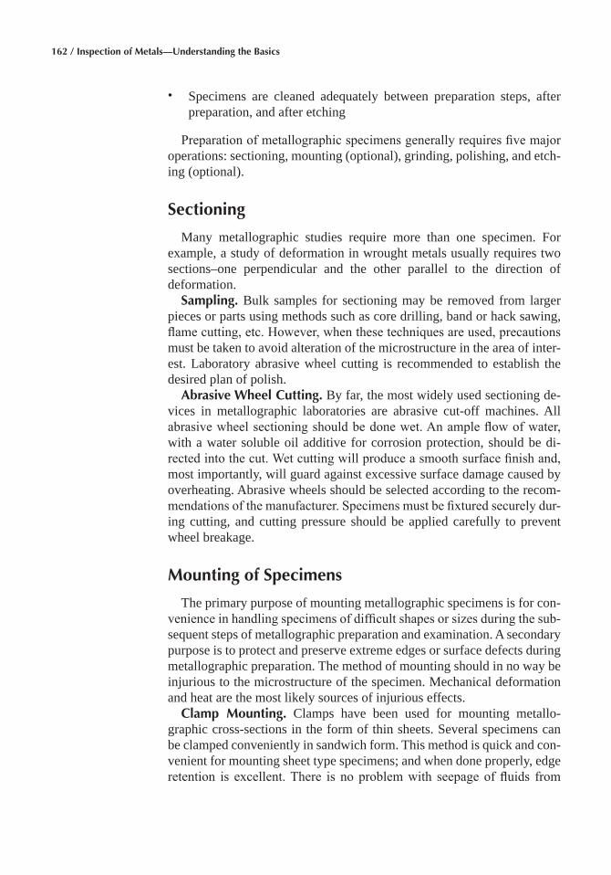
162 / Inspection of Metals—Understanding the Basics
• Specimens are cleaned adequately between preparation steps, after preparation, and after etching
Preparation of metallographic specimens generally requires five major operations: sectioning, mounting (optional), grinding, polishing, and etch-ing (optional).
Sectioning
Many metallographic studies require more than one specimen. For example, a study of deformation in wrought metals usually requires two sections–one perpendicular and the other parallel to the direction of deformation.
Sampling� Bulk samples for sectioning may be removed from larger pieces or parts using methods such as core drilling, band or hack sawing, flame cutting, etc. However, when these techniques are used, precautions must be taken to avoid alteration of the microstructure in the area of inter-est. Laboratory abrasive wheel cutting is recommended to establish the desired plan of polish.
Abrasive Wheel Cutting� By far, the most widely used sectioning de-vices in metallographic laboratories are abrasive cut-off machines. All abrasive wheel sectioning should be done wet. An ample flow of water, with a water soluble oil additive for corrosion protection, should be di-rected into the cut. Wet cutting will produce a smooth surface finish and, most importantly, will guard against excessive surface damage caused by overheating. Abrasive wheels should be selected according to the recom-mendations of the manufacturer. Specimens must be fixtured securely dur-ing cutting, and cutting pressure should be applied carefully to prevent wheel breakage.
Mounting of Specimens
The primary purpose of mounting metallographic specimens is for con-venience in handling specimens of difficult shapes or sizes during the sub-sequent steps of metallographic preparation and examination. A secondary purpose is to protect and preserve extreme edges or surface defects during metallographic preparation. The method of mounting should in no way be injurious to the microstructure of the specimen. Mechanical deformation and heat are the most likely sources of injurious effects.
Clamp Mounting� Clamps have been used for mounting metallo-graphic cross-sections in the form of thin sheets. Several specimens can be clamped conveniently in sandwich form. This method is quick and con-venient for mounting sheet type specimens; and when done properly, edge retention is excellent. There is no problem with seepage of fluids from
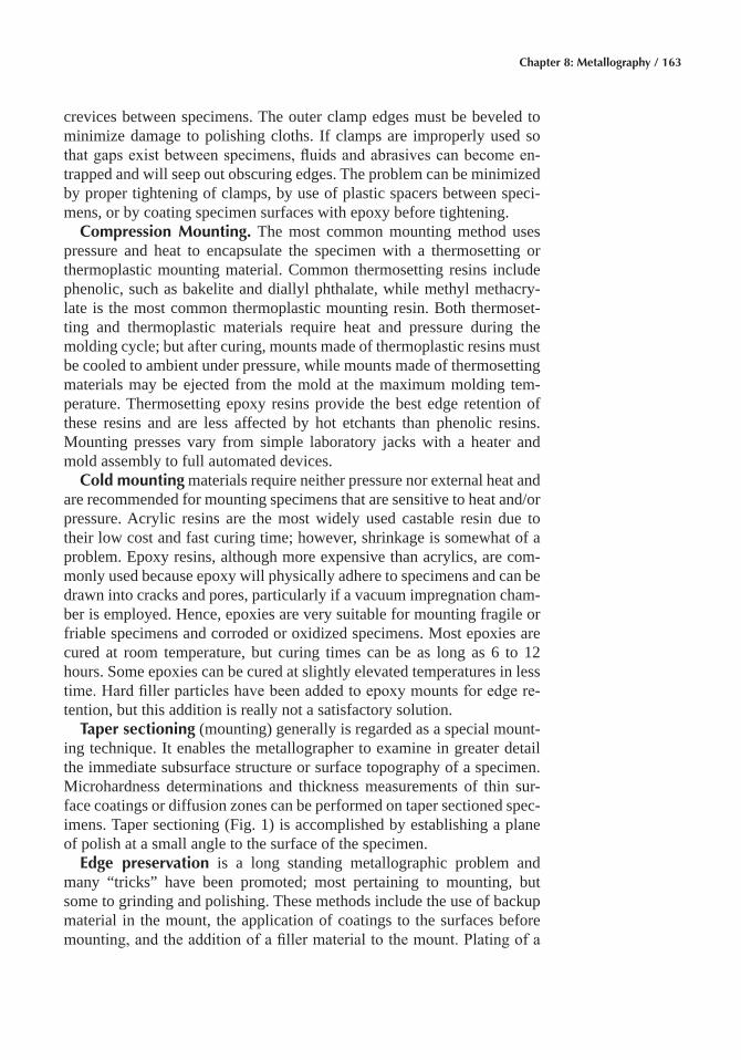
Chapter 8: Metallography / 163
crevices between specimens. The outer clamp edges must be beveled to minimize damage to polishing cloths. If clamps are improperly used so that gaps exist between specimens, fluids and abrasives can become en-trapped and will seep out obscuring edges. The problem can be minimized by proper tightening of clamps, by use of plastic spacers between speci-mens, or by coating specimen surfaces with epoxy before tightening.
Compression Mounting� The most common mounting method uses pressure and heat to encapsulate the specimen with a thermosetting or thermoplastic mounting material. Common thermosetting resins include phenolic, such as bakelite and diallyl phthalate, while methyl methacry-late is the most common thermoplastic mounting resin. Both thermoset-ting and thermoplastic materials require heat and pressure during the molding cycle; but after curing, mounts made of thermoplastic resins must be cooled to ambient under pressure, while mounts made of thermosetting materials may be ejected from the mold at the maximum molding tem-perature. Thermosetting epoxy resins provide the best edge retention of these resins and are less affected by hot etchants than phenolic resins. Mounting presses vary from simple laboratory jacks with a heater and mold assembly to full automated devices.
Cold mounting materials require neither pressure nor external heat and are recommended for mounting specimens that are sensitive to heat and/or pressure. Acrylic resins are the most widely used castable resin due to their low cost and fast curing time; however, shrinkage is somewhat of a problem. Epoxy resins, although more expensive than acrylics, are com-monly used because epoxy will physically adhere to specimens and can be drawn into cracks and pores, particularly if a vacuum impregnation cham-ber is employed. Hence, epoxies are very suitable for mounting fragile or friable specimens and corroded or oxidized specimens. Most epoxies are cured at room temperature, but curing times can be as long as 6 to 12 hours. Some epoxies can be cured at slightly elevated temperatures in less time. Hard filler particles have been added to epoxy mounts for edge re-tention, but this addition is really not a satisfactory solution.
Taper sectioning (mounting) generally is regarded as a special mount-ing technique. It enables the metallographer to examine in greater detail the immediate subsurface structure or surface topography of a specimen. Microhardness determinations and thickness measurements of thin sur-face coatings or diffusion zones can be performed on taper sectioned spec-imens. Taper sectioning (Fig. 1) is accomplished by establishing a plane of polish at a small angle to the surface of the specimen.
Edge preservation is a long standing metallographic problem and many “tricks” have been promoted; most pertaining to mounting, but some to grinding and polishing. These methods include the use of backup material in the mount, the application of coatings to the surfaces before mounting, and the addition of a filler material to the mount. Plating of a
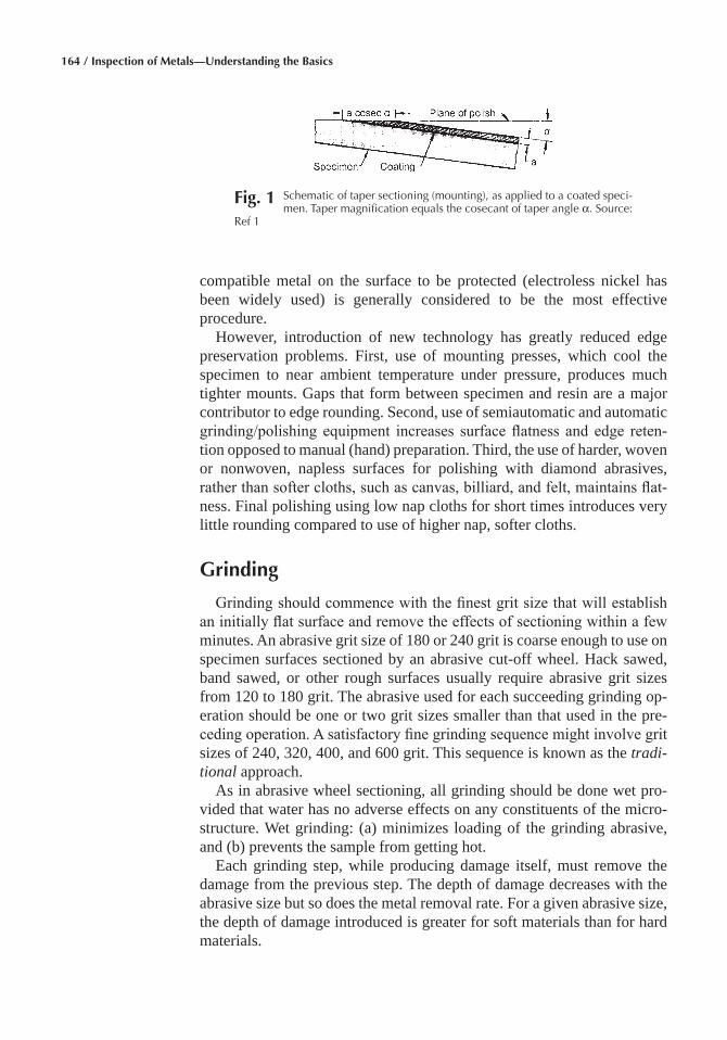
164 / Inspection of Metals—Understanding the Basics
compatible metal on the surface to be protected (electroless nickel has been widely used) is generally considered to be the most effective procedure.
However, introduction of new technology has greatly reduced edge preservation problems. First, use of mounting presses, which cool the specimen to near ambient temperature under pressure, produces much tighter mounts. Gaps that form between specimen and resin are a major contributor to edge rounding. Second, use of semiautomatic and automatic grinding/polishing equipment increases surface flatness and edge reten-tion opposed to manual (hand) preparation. Third, the use of harder, woven or nonwoven, napless surfaces for polishing with diamond abrasives, rather than softer cloths, such as canvas, billiard, and felt, maintains flat-ness. Final polishing using low nap cloths for short times introduces very little rounding compared to use of higher nap, softer cloths.
Grinding
Grinding should commence with the finest grit size that will establish an initially flat surface and remove the effects of sectioning within a few minutes. An abrasive grit size of 180 or 240 grit is coarse enough to use on specimen surfaces sectioned by an abrasive cut-off wheel. Hack sawed, band sawed, or other rough surfaces usually require abrasive grit sizes from 120 to 180 grit. The abrasive used for each succeeding grinding op-eration should be one or two grit sizes smaller than that used in the pre-ceding operation. A satisfactory fine grinding sequence might involve grit sizes of 240, 320, 400, and 600 grit. This sequence is known as the tradi-tional approach.
As in abrasive wheel sectioning, all grinding should be done wet pro-vided that water has no adverse effects on any constituents of the micro-structure. Wet grinding: (a) minimizes loading of the grinding abrasive, and (b) prevents the sample from getting hot.
Each grinding step, while producing damage itself, must remove the damage from the previous step. The depth of damage decreases with the abrasive size but so does the metal removal rate. For a given abrasive size, the depth of damage introduced is greater for soft materials than for hard materials.
Fig� 1 Schematic of taper sectioning (mounting), as applied to a coated speci-men. Taper magnification equals the cosecant of taper angle α. Source:
Ref 1
Chapter 8: Metallography / 165
Besides SiC paper, a number of other options are available to circum-vent their use. One option, used chiefly with semiautomatic and automatic systems, is to grind a number of specimens placed in a holder simultane-ously using a conventional grinding stone generally made of coarse grit alumina. This step, often called planar grinding, has the second goal of making all of the specimen surfaces coplanar. This process requires a spe-cial purpose machine because the stone must rotate at a high speed, ≥1500 rpm, to cut effectively. The stone must be dressed regularly with a dia-mond tool to maintain flatness.
Other materials have also been used both for the planar grinding stage or, afterwards, to replace SiC paper. For very hard materials such as ce-ramics and sintered carbides, two or more metal bonded or resin bonded diamond disks with grit sizes from about 70 to 9 μm can be used. An alter-nate type of disk has diamond particles suspended in a resin applied in small blobs, or spots, to a disk surface. These disks are available with dia-mond sizes from 120 to 6 μm. Another type of disk available in several diamond sizes uses diamond attached to the edges of a perforated, screen like metal disk. Another approach uses a stainless steel woven mesh cloth on a platen charged with coarse diamond, usually in slurry form, for pla-nar grinding. Once planar surfaces have been obtained, there are several single step procedures available for avoiding the finer SiC papers. These processes include the use of platens, woven polyester thick cloths, or rigid grinding disks. With each of these, a coarse diamond size, most commonly 9 μm, is used.
Grinding Media� The grinding abrasives commonly used in the prepa-ration of metallographic specimens are silicon carbide (SiC), aluminum oxide (Al2O3), emery (Al2O3-Fe3O4), composite ceramics, and diamond. All except diamond are generally bonded to paper or cloth backing mate-rials of various weights in the form of sheets, disks, and belts of various sizes. Limited use is made of grinding wheels consisting of abrasives em-bedded in a bonding material. The abrasives may be used also in powder form by charging the grinding surfaces with loose abrasive particles or with abrasive in a premixed slurry or suspension.
Grinding Equipment� Although it is rarely used in industry, students still use stationary grinding paper that is supplied in strips or rolls. The specimen is slid against the paper from top to bottom. Grinding in one di-rection is usually safer than grinding in both directions. While this can be done dry for certain delicate materials, water is usually added to keep the specimen surface cool and to carry the swarf away.
Belt grinders are usually present in most laboratories. They are mainly used to remove burrs from sectioning; to round edges that need not be pre-served for examination; to flatten cut surfaces to be macroetched; or to re-move sectioning damage. Generally, only very coarse abrasive papers with 60 to 240 grits are used. Most grinding work is done on rotating wheels; that is, a motor driven platen upon which the SiC paper is attached (Fig. 2).
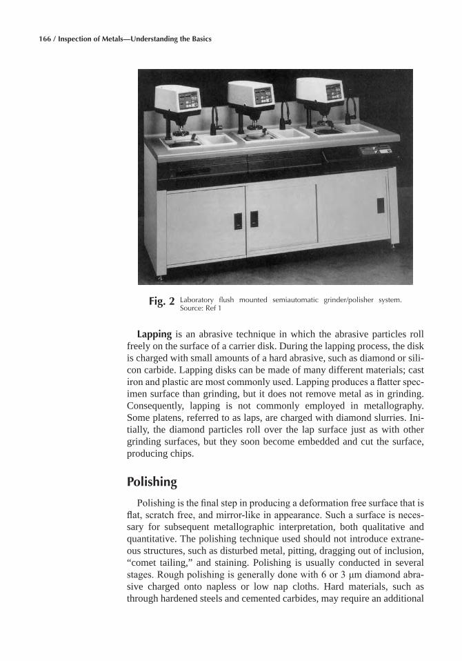
166 / Inspection of Metals—Understanding the Basics
Lapping is an abrasive technique in which the abrasive particles roll freely on the surface of a carrier disk. During the lapping process, the disk is charged with small amounts of a hard abrasive, such as diamond or sili-con carbide. Lapping disks can be made of many different materials; cast iron and plastic are most commonly used. Lapping produces a flatter spec-imen surface than grinding, but it does not remove metal as in grinding. Consequently, lapping is not commonly employed in metallography. Some platens, referred to as laps, are charged with diamond slurries. Ini-tially, the diamond particles roll over the lap surface just as with other grinding surfaces, but they soon become embedded and cut the surface, producing chips.
Polishing
Polishing is the final step in producing a deformation free surface that is flat, scratch free, and mirror-like in appearance. Such a surface is neces-sary for subsequent metallographic interpretation, both qualitative and quantitative. The polishing technique used should not introduce extrane-ous structures, such as disturbed metal, pitting, dragging out of inclusion, “comet tailing,” and staining. Polishing is usually conducted in several stages. Rough polishing is generally done with 6 or 3 μm diamond abra-sive charged onto napless or low nap cloths. Hard materials, such as through hardened steels and cemented carbides, may require an additional
Fig� 2 Laboratory flush mounted semiautomatic grinder/polisher system. Source: Ref 1
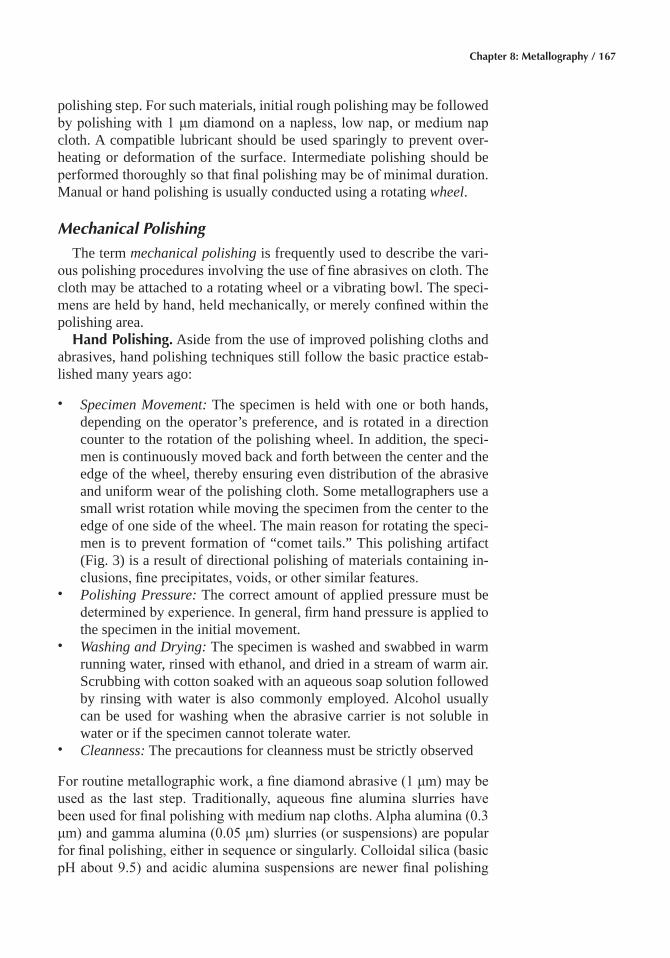
Chapter 8: Metallography / 167
polishing step. For such materials, initial rough polishing may be followed by polishing with 1 μm diamond on a napless, low nap, or medium nap cloth. A compatible lubricant should be used sparingly to prevent over-heating or deformation of the surface. Intermediate polishing should be performed thoroughly so that final polishing may be of minimal duration. Manual or hand polishing is usually conducted using a rotating wheel.
Mechanical Polishing
The term mechanical polishing is frequently used to describe the vari-ous polishing procedures involving the use of fine abrasives on cloth. The cloth may be attached to a rotating wheel or a vibrating bowl. The speci-mens are held by hand, held mechanically, or merely confined within the polishing area.
Hand Polishing� Aside from the use of improved polishing cloths and abrasives, hand polishing techniques still follow the basic practice estab-lished many years ago:
• Specimen Movement: The specimen is held with one or both hands, depending on the operator’s preference, and is rotated in a direction counter to the rotation of the polishing wheel. In addition, the speci-men is continuously moved back and forth between the center and the edge of the wheel, thereby ensuring even distribution of the abrasive and uniform wear of the polishing cloth. Some metallographers use a small wrist rotation while moving the specimen from the center to the edge of one side of the wheel. The main reason for rotating the speci-men is to prevent formation of “comet tails.” This polishing artifact (Fig. 3) is a result of directional polishing of materials containing in-clusions, fine precipitates, voids, or other similar features.
• Polishing Pressure: The correct amount of applied pressure must be determined by experience. In general, firm hand pressure is applied to the specimen in the initial movement.
• Washing and Drying: The specimen is washed and swabbed in warm running water, rinsed with ethanol, and dried in a stream of warm air. Scrubbing with cotton soaked with an aqueous soap solution followed by rinsing with water is also commonly employed. Alcohol usually can be used for washing when the abrasive carrier is not soluble in water or if the specimen cannot tolerate water.
• Cleanness: The precautions for cleanness must be strictly observed
For routine metallographic work, a fine diamond abrasive (1 μm) may be used as the last step. Traditionally, aqueous fine alumina slurries have been used for final polishing with medium nap cloths. Alpha alumina (0.3 μm) and gamma alumina (0.05 μm) slurries (or suspensions) are popular for final polishing, either in sequence or singularly. Colloidal silica (basic pH about 9.5) and acidic alumina suspensions are newer final polishing
168 / Inspection of Metals—Understanding the Basics
abrasives being used for difficult to prepare materials. Vibratory polishers are often used for final polishing, particularly with more difficult to pre-pare materials, for image analysis studies, or for publication quality work.
Automatic Polishing� Mechanical polishing can be automated to a high degree using a wide variety of devices ranging from relatively simple systems to rather sophisticated minicomputer or microprocessor con-trolled devices. Units also vary in capacity from a single specimen to a half dozen or more at a time. Most units can be used for all grinding and polishing steps. These devices enable the operator to prepare a large num-ber of specimens per day, often with a higher degree of quality than that of hand polishing and at reduced consumable costs. Automatic polishing de-vices also are desirable for preparing radioactive specimens by remote control or for using corrosive attack polishing procedures safely without hand contact.
Polishing Cloths� The requirements of a good polishing cloth include the ability to hold an abrasive; long life; absence of any foreign material that may cause scratches; and absence of any processing chemical such as dye or sizing that may react with the specimen. More than a hundred cloths of different fabrics (woven or nonwoven) with a wide variety of naps (or napless) are available for metallographic polishing. Napless or low nap cloths are recommended for rough polishing using diamond abra-sive compounds. Low, medium, and occasionally high nap cloths are used for final polishing, but this step should be as brief as possible to minimize relief.
Fig� 3 Comet tails due to directional polishing and pull out of hard particles. Original magnification 200×.Source: Ref 1
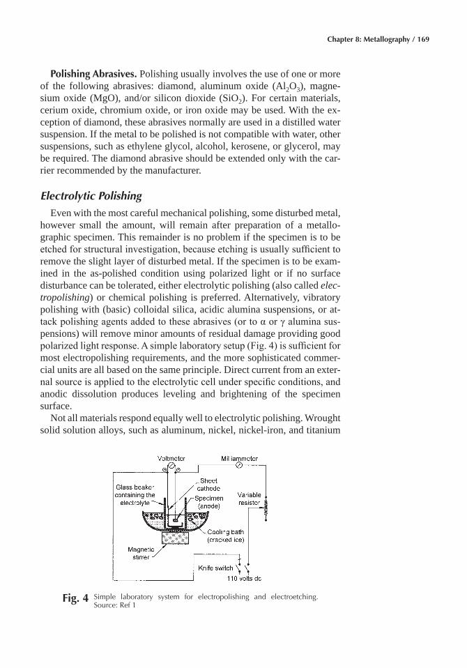
Chapter 8: Metallography / 169
Polishing Abrasives� Polishing usually involves the use of one or more of the following abrasives: diamond, aluminum oxide (Al2O3), magne-sium oxide (MgO), and/or silicon dioxide (SiO2). For certain materials, cerium oxide, chromium oxide, or iron oxide may be used. With the ex-ception of diamond, these abrasives normally are used in a distilled water suspension. If the metal to be polished is not compatible with water, other suspensions, such as ethylene glycol, alcohol, kerosene, or glycerol, may be required. The diamond abrasive should be extended only with the car-rier recommended by the manufacturer.
Electrolytic Polishing
Even with the most careful mechanical polishing, some disturbed metal, however small the amount, will remain after preparation of a metallo-graphic specimen. This remainder is no problem if the specimen is to be etched for structural investigation, because etching is usually sufficient to remove the slight layer of disturbed metal. If the specimen is to be exam-ined in the as-polished condition using polarized light or if no surface disturbance can be tolerated, either electrolytic polishing (also called elec-tropolishing) or chemical polishing is preferred. Alternatively, vibratory polishing with (basic) colloidal silica, acidic alumina suspensions, or at-tack polishing agents added to these abrasives (or to α or γ alumina sus-pensions) will remove minor amounts of residual damage providing good polarized light response. A simple laboratory setup (Fig. 4) is sufficient for most electropolishing requirements, and the more sophisticated commer-cial units are all based on the same principle. Direct current from an exter-nal source is applied to the electrolytic cell under specific conditions, and anodic dissolution produces leveling and brightening of the specimen surface.
Not all materials respond equally well to electrolytic polishing. Wrought solid solution alloys, such as aluminum, nickel, nickel-iron, and titanium
Fig� 4 Simple laboratory system for electropolishing and electroetching. Source: Ref 1
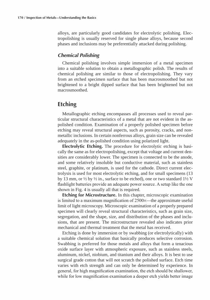
170 / Inspection of Metals—Understanding the Basics
alloys, are particularly good candidates for electrolytic polishing. Elec-tropolishing is usually reserved for single phase alloys, because second phases and inclusions may be preferentially attacked during polishing.
Chemical Polishing
Chemical polishing involves simple immersion of a metal specimen into a suitable solution to obtain a metallographic polish. The results of chemical polishing are similar to those of electropolishing. They vary from an etched specimen surface that has been macrosmoothed but not brightened to a bright dipped surface that has been brightened but not macrosmoothed.
Etching
Metallographic etching encompasses all processes used to reveal par-ticular structural characteristics of a metal that are not evident in the as-polished condition. Examination of a properly polished specimen before etching may reveal structural aspects, such as porosity, cracks, and non-metallic inclusions. In certain nonferrous alloys, grain size can be revealed adequately in the as-polished condition using polarized light.
Electrolytic Etching� The procedure for electrolytic etching is basi-cally the same as for electropolishing, except that voltage and current den-sities are considerably lower. The specimen is connected to be the anode, and some relatively insoluble but conductive material, such as stainless steel, graphite, or platinum, is used for the cathode. Direct current elec-trolysis is used for most electrolytic etching, and for small specimens (13 by 13 mm, or ½ by ½ in., surface to be etched), one or two standard 1½ V flashlight batteries provide an adequate power source. A setup like the one shown in Fig. 4 is usually all that is required.
Etching for Microstructure� In this chapter, microscopic examination is limited to a maximum magnification of 2500×—the approximate useful limit of light microscopy. Microscopic examination of a properly prepared specimen will clearly reveal structural characteristics, such as grain size, segregation, and the shape, size, and distribution of the phases and inclu-sions, that are present. The microstructure revealed also indicates prior mechanical and thermal treatment that the metal has received.
Etching is done by immersion or by swabbing (or electrolytically) with a suitable chemical solution that basically produces selective corrosion. Swabbing is preferred for those metals and alloys that form a tenacious oxide surface layer with atmospheric exposure, such as stainless steels, aluminum, nickel, niobium, and titanium and their alloys. It is best to use surgical grade cotton that will not scratch the polished surface. Etch time varies with etch strength and can only be determined by experience. In general, for high magnification examination, the etch should be shallower, while for low magnification examination a deeper etch yields better image
Chapter 8: Metallography / 171
contrast. Some etchants produce selective results in that only one phase will be attacked or colored. A vast number of etchants have been devel-oped; the more commonly used etchants are given in Tables 1 to 6.
Microscopic Examination
Metallurgical microscopes differ from biological microscopes primar-ily in the manner by which the specimen is illuminated. Unlike biological
Table 1 Typical etchants used for microscopic examinationGeneral reagents for irons and steels (carbon, low, and medium-alloy steels)
Etching reagent Composition Remarks Uses
Nital 2 mL HNO3, 90 mL ethyl or methyl al-cohol (95% or abso-lute; also amyl alco-hol)
Not as good as picral for high-resolution work with heat-treated structures; ex-cellent for outlining ferrite grain boundaries; etching time, a few sec-onds to 1 min
For carbon steels, gives maximum contrast be-tween pearlite and a fer-rite or cementite net-work; reveals ferrite boundaries; differenti-ates ferrite from mar-tensite
Picral 4 g picric acid, 100 mL ethyl or methyl alcohol (95% or ab-solute; use absolute alcohol only when acid contains 10% or more moisture), 4 or 5 drops zephi-ran chloride (17%)—wetting agent
Not as good as nital for revealing ferrite grain boundaries; gives superior reso-lution with fine pearlite, martensite, tempered martensite, and bainitic structures; detects carbides; etching time, a few seconds to 1 min or more
For all grades of carbon steels, annealed, normal-ized, quenched, quenched and tempered, spheroidized, austem-pered
Sodium metabisulfite
A 8 g Na2S2O5, 100 mL distilled water
General reagent for steel; results similar to picral; etching time, a few seconds to 1 min
Darkens as-quenched mar-tensite
B 1 g Na2S2O5, dilute to 100 mL with dis-tilled water
Immerse specimen in the solution for 2 min or until the polished surface turns a bluish-red; do not mount specimen in a steel clamp
Tint etches lath-type or plate-type martensite in Fe-C alloys
Vilella’s reagent
5 mL HCl, 1 g picric acid, 100 mL ethyl or methyl alcohol (95% or absolute)
Best results obtained when martensite is tempered
For revealing austenitic grain size in quenched and quenched and tem-pered steels
Heat tinting Heat only Heat by placing specimen face up on a hot plate that has been preheated to 205–370 ºC (400–700 ºF); time and temperature both have decided effects; bath of sand or molten metal may be used
Pearlite first to pass through a given color, followed by ferrite; ce-mentite less affected, iron phosphide still less
Heat etching Heat only Specimen is heated 10–60 min at 815–1205 ºC (1500–2200 ºF) in carefully purified hydrogen, and must have no contact with scale or reducible oxides; after etching, specimen is cooled in mercury to avoid oxidation
For revealing austenitic grain size of polished specimens
Klemm’s reagent
50 mL saturated (in H2O) Na2S2O3 solu-tion, 1 g K2S2O5
Etching time, 40–120s, ferrite appears black-brown, while carbides, nitrides, and phosphides remain white; also, phosphorus distribution can be de-tected more sensitively than with usual phosphorus reagents based on copper salts
Tint etches pearlite, hard-ened structures of unal-loyed steel, and cast iron
Source: Ref 2
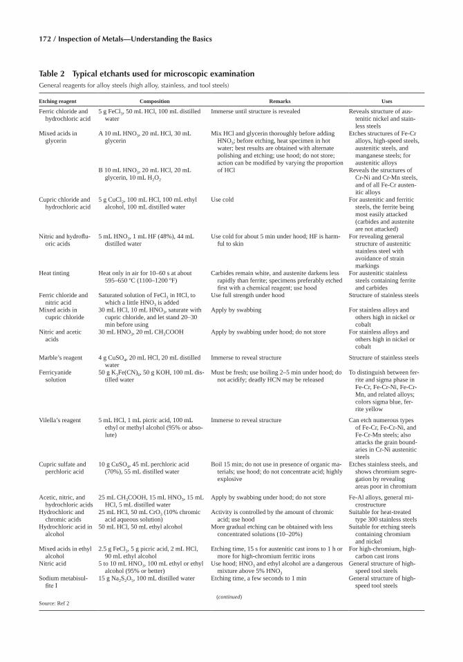
172 / Inspection of Metals—Understanding the Basics
Table 2 Typical etchants used for microscopic examinationGeneral reagents for alloy steels (high alloy, stainless, and tool steels)
Etching reagent Composition Remarks Uses
Ferric chloride and hydrochloric acid
5 g FeCl3, 50 mL HCl, 100 mL distilled water
Immerse until structure is revealed Reveals structure of aus-tenitic nickel and stain-less steels
Mixed acids in glycerin
A 10 mL HNO3, 20 mL HCl, 30 mL glycerin
B 10 mL HNO3, 20 mL HCl, 20 mL glycerin, 10 mL H2O2
Mix HCl and glycerin thoroughly before adding HNO3; before etching, heat specimen in hot water; best results are obtained with alternate polishing and etching; use hood; do not store; action can be modified by varying the proportion of HCl
Etches structures of Fe-Cr alloys, high-speed steels, austenitic steels, and manganese steels; for austenitic alloys
Reveals the structures of Cr-Ni and Cr-Mn steels, and of all Fe-Cr austen-itic alloys
Cupric chloride and hydrochloric acid
5 g CuCl2, 100 mL HCl, 100 mL ethyl alcohol, 100 mL distilled water
Use cold For austenitic and ferritic steels, the ferrite being most easily attacked (carbides and austenite are not attacked)
Nitric and hydroflu-oric acids
5 mL HNO3, 1 mL HF (48%), 44 mL distilled water
Use cold for about 5 min under hood; HF is harm-ful to skin
For revealing general structure of austenitic stainless steel with avoidance of strain markings
Heat tinting Heat only in air for 10–60 s at about 595–650 ºC (1100–1200 ºF)
Carbides remain white, and austenite darkens less rapidly than ferrite; specimens preferably etched first with a chemical reagent; use hood
For austenitic stainless steels containing ferrite and carbides
Ferric chloride and nitric acid
Saturated solution of FeCl3 in HCl, to which a little HNO3 is added
Use full strength under hood Structure of stainless steels
Mixed acids in cupric chloride
30 mL HCl, 10 mL HNO3, saturate with cupric chloride, and let stand 20–30 min before using
Apply by swabbing For stainless alloys and others high in nickel or cobalt
Nitric and acetic acids
30 mL HNO3, 20 mL CH3COOH Apply by swabbing under hood; do not store For stainless alloys and others high in nickel or cobalt
Marble’s reagent 4 g CuSO4, 20 mL HCl, 20 mL distilled water
Immerse to reveal structure Structure of stainless steels
Ferricyanide solution
50 g K3Fe(CN)6, 50 g KOH, 100 mL dis-tilled water
Must be fresh; use boiling 2–5 min under hood; do not acidify; deadly HCN may be released
To distinguish between fer-rite and sigma phase in Fe-Cr, Fe-Cr-Ni, Fe-Cr-Mn, and related alloys; colors sigma blue, fer-rite yellow
Vilella’s reagent 5 mL HCl, 1 mL picric acid, 100 mL ethyl or methyl alcohol (95% or abso-lute)
Immerse to reveal structure Can etch numerous types of Fe-Cr, Fe-Cr-Ni, and Fe-Cr-Mn steels; also attacks the grain bound-aries in Cr-Ni austenitic steels
Cupric sulfate and perchloric acid
10 g CuSO4, 45 mL perchloric acid (70%), 55 mL distilled water
Boil 15 min; do not use in presence of organic ma-terials; use hood; do not concentrate acid; highly explosive
Etches stainless steels, and shows chromium segre-gation by revealing areas poor in chromium
Acetic, nitric, and hydrochloric acids
25 mL CH3COOH, 15 mL HNO3, 15 mL HCl, 5 mL distilled water
Apply by swabbing under hood; do not store Fe-Al alloys, general mi-crostructure
Hydrochloric and chromic acids
25 mL HCl, 50 mL CrO3 (10% chromic acid aqueous solution)
Activity is controlled by the amount of chromic acid; use hood
Suitable for heat-treated type 300 stainless steels
Hydrochloric acid in alcohol
50 mL HCl, 50 mL ethyl alcohol More gradual etching can be obtained with less concentrated solutions (10–20%)
Suitable for etching steels containing chromium and nickel
Mixed acids in ethyl alcohol
2.5 g FeCl3, 5 g picric acid, 2 mL HCl, 90 mL ethyl alcohol
Etching time, 15 s for austenitic cast irons to 1 h or more for high-chromium ferritic irons
For high-chromium, high-carbon cast irons
Nitric acid 5 to 10 mL HNO3, 100 mL ethyl or ethyl alcohol (95% or better)
Use hood; HNO3 and ethyl alcohol are a dangerous mixture above 5% HNO3
General structure of high-speed tool steels
Sodium metabisul-fite I
15 g Na2S2O5, 100 mL distilled water Etching time, a few seconds to 1 min General structure of high-speed tool steels
(continued)Source: Ref 2
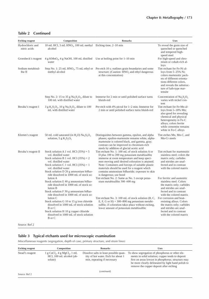
Chapter 8: Metallography / 173
Table 2 Continued
Etching reagent Composition Remarks Uses
Hydrochloric and nitric acids
10 mL HCl, 3 mL HNO3, 100 mL methyl alcohol
Etching time, 2–10 min To reveal the grain size of quenched or quenched and tempered high-speed steel
Groesbeck’s reagent 4 g KMnO4, 4 g NaOH, 100 mL distilled water
Use at boiling point for 1–10 min For high-speed and chro-mium or cobalt-rich al-loys
Sodium metabisul-fite II
Step No. 1: 25 mL HNO3, 75 mL ethyl or methyl alcohol
Pre-etch 10 s; outlines grain boundaries and some structure; (Caution: HNO3 and ethyl dangerous at this concentration)
Tint etchant for Fe-Ni al-loys from 5–25% Ni; colors martensitic pack-ets of different orienta-tions different colors, and reveals the substruc-ture of lath-type mar-tensite
Step No. 2: 15 to 35 g Na2S2O5, dilute to 100 mL with distilled water
Immerse for 2 min or until polished surface turns bluish-red
Concentration of Na2S2O5 varies with nickel con-tent
Beraha’s reagent I 3 g K2S2O5, 10 g Na2S2O3, dilute to 100 mL with distilled water
Pre-etch with 4% picral for 1–2 min; Immerse for 2 min or until polished surface turns bluish-red
Tint etchant for Fe-Mn al-loys from 5–18% Mn; also good for revealing chemical and physical heterogeneity in Fe-C alloys; colors ferrite while cementite remains white in Fe-C alloys
Klemm’s reagent 50 mL cold saturated (in H2O) Na2S2O3 solution, 5 g K2S2O5
Distinguishes between gamma, epsilon, and alpha phases; epsilon-martensite remains white, alpha-martensite is colored black, and gamma, gray; contrast can be improved in chromium-rich steels by addition of glacial acetic acid
Tint etches Mn, Mn-C, and Mn-Cr steels
Beraha’s reagent II Stock solution A 1 vol. HCl (35%) + 5 vol. distilled water
Stock solution B 1 vol. HCl (35%) + 2 vol. distilled water
Stock solution C 1 vol. HCl (35%) + 1 vol. distilled water
Stock solution D 20 g ammonium bifluo-ride dissolved in 1000 mL of stock so-lution A
Stock solution E 40 g ammonium bifluo-ride dissolved in 1000 mL of stock so-lution B
Stock solution F 50 g ammonium bifluo-ride dissolved in 1000 mL of stock so-lution C
Stock solution G 10 to 15 g iron chloride dissolved in 1000 mL of stock solution B or C
Stock solution H 10 g copper chloride dissolved in 1000 mL of stock solution B or C
Tint etchant No. 1: 100 mL of stock solution A or D plus 100 to 200 mg potassium metabisulfite immerse at room temperature and keep speci-men moving until desired coloration is attained. Note: Containers and forceps of suitable plastic materials should be used for a reagent which contains ammonium bifluoride; exposure to skin is dangerous; use hood
Tint etchant No. 2: Same as No. 1 except potas-sium metabisulfite 300–600 mg
Tint etchant No. 3: 100 mL of stock solution (B, C, E, F, G or H) + 300–800 mg potassium metabi-sulfite; if coloration takes place without etching, lower amount of potassium metabisulfite
Tint etchant for martensitic stainless steel; colors the matrix only; carbides and nitrides are unaf-fected and in contrast with the colored matrix
For ferritic and austenitic stainless steel. Colors the matrix only; carbides and nitrides are unaf-fected and in contrast with the colored matrix
For corrosion and heat- resisting alloys. Colors the matrix only; carbides and nitrides are unaf-fected and in contrast with the colored matrix
Source: Ref 2
Table 3 Typical etchants used for microscopic examinationMiscellaneous reagents (segregation, depth of case, primary structure, and strain lines)
Etching reagent Composition Remarks Uses
Stead’s reagent 1 g CuCl2, 4 g MgCl2, 1 mL HCl, 100 mL alcohol (ab-solute)
Dissolve salts in least possible quan-tity of hot water. Etch for about 1 min, repeating if necessary
To show segregation of phosphorus or other ele-ments in solid solution; copper tends to deposit first on areas lowest in phosphorus; structure may be more clearly delineated by light hand polish to remove the copper deposit after etching
(continued)Source: Ref 2
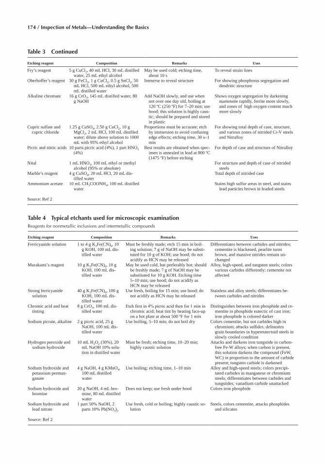
174 / Inspection of Metals—Understanding the Basics
Table 3 Continued
Etching reagent Composition Remarks Uses
Fry’s reagent 5 g CuCl2, 40 mL HCl, 30 mL distilled water, 25 mL ethyl alcohol
May be used cold; etching time, about 10 s
To reveal strain lines
Oberhoffer’s reagent 30 g FeCl3, 1 g CuCl2, 0.5 g SnCl2, 50 mL HCl, 500 mL ethyl alcohol, 500 mL distilled water
Immerse to reveal structure For showing phosphorus segregation and dendritic structure
Alkaline chromate 16 g CrO3, 145 mL distilled water, 80 g NaOH
Add NaOH slowly, and use when not over one day old, boiling at 120 ºC (250 ºF) for 7–20 min; use hood; this solution is highly caus-tic; should be prepared and stored in plastic
Shows oxygen segregation by darkening martensite rapidly, ferrite more slowly, and zones of high oxygen content much more slowly
Cupric sulfate and cupric chloride
1.25 g CuSO4, 2.50 g CuCl2, 10 g MgCl2, 2 mL HCl, 100 mL distilled water; dilute above solution to 1000 mL with 95% ethyl alcohol
Proportions must be accurate; etch by immersion to avoid confusing edge effects; etching time, 30 s–1 min
For showing total depth of case, structure, and various zones of nitrided Cr-V steels and Nitralloy
Picric and nitric acids 10 parts picric acid (4%), 1 part HNO3 (4%)
Best results are obtained when spec-imen is annealed in lead at 800 ºC (1475 ºF) before etching
For depth of case and structure of Nitralloy
Nital 1 mL HNO3, 100 mL ethyl or methyl alcohol (95% or absolute)
For structure and depth of case of nitrided steels
Marble’s reagent 4 g CuSO4, 20 mL HCl, 20 mL dis-tilled water
Total depth of nitrided case
Ammonium acetate 10 mL CH3COONH4, 100 mL distilled water
Stains high sulfur areas in steel, and stains lead particles brown in leaded steels
Source: Ref 2
Table 4 Typical etchants used for microscopic examinationReagents for nonmetallic inclusions and intermetallic compounds
Etching reagent Composition Remarks Uses
Ferricyanide solution 1 to 4 g K3Fe(CN)6, 10 g KOH, 100 mL dis-tilled water
Must be freshly made; etch 15 min in boil-ing solution; 7 g of NaOH may be substi-tuted for 10 g of KOH; use hood; do not acidify as HCN may be released
Differentiates between carbides and nitrides; cementite is blackened, pearlite turns brown, and massive nitrides remain un-changed
Murakami’s reagent 10 g K3Fe(CN)6, 10 g KOH, 100 mL dis-tilled water
May be used cold, but preferably hot; should be freshly made; 7 g of NaOH may be substituted for 10 g KOH. Etching time 5–10 min; use hood; do not acidify as HCN may be released
Alloy, high-speed, and tungsten steels; colors various carbides differently; cementite not affected
Strong ferricyanide solution
40 g K3Fe(CN)6, 100 g KOH, 100 mL dis-tilled water
Use fresh, boiling for 15 min; use hood; do not acidify as HCN may be released
Stainless and alloy steels; differentiates be-tween carbides and nitrides
Chromic acid and heat tinting
8 g CrO3, 100 mL dis-tilled water
Etch first in 4% picric acid then for 1 min in chromic acid; heat tint by heating face-up on a hot plate at about 500 ºF for 1 min
Distinguishes between iron phosphide and ce-mentite in phosphide eutectic of cast iron; iron phosphide is colored darker
Sodium picrate, alkaline 2 g picric acid, 25 g NaOH, 100 mL dis-tilled water
Use boiling, 5–10 min; do not boil dry Colors cementite, but not carbides high in chromium; attacks sulfides; delineates grain boundaries in hypereutectoid steels in slowly cooled condition
Hydrogen peroxide and sodium hydroxide
10 mL H2O2 (30%), 20 mL NaOH 10% solu-tion in distilled water
Must be fresh; etching time, 10–20 min; highly caustic solution
Attacks and darkens iron tungstide in carbon-free Fe-W alloys; when carbon is present, this solution darkens the compound (FeW, WC) in proportion to the amount of carbide present; tungsten carbide is darkened
Sodium hydroxide and potassium perman- ganate
4 g NaOH, 4 g KMnO4, 100 mL distilled water
Use boiling; etching time, 1–10 min Alloy and high-speed steels; colors precipi-tated carbides in manganese or chromium steels; differentiates between carbides and tungstides; vanadium carbide unattacked
Sodium hydroxide and bromine
20 g NaOH, 4 mL bro-mine, 80 mL distilled water
Does not keep; use fresh under hood Colors iron phosphide
Sodium hydroxide and lead nitrate
1 part 50% NaOH, 2 parts 10% Pb(NO3)2
Use fresh, cold or boiling; highly caustic so-lution
Steels, colors cementite, attacks phosphides and silicates
Source: Ref 2
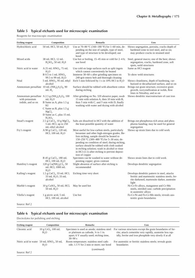
Chapter 8: Metallography / 175
Table 5 Typical etchants used for microscopic examinationReagents for macroscopic examination
Etching reagent Composition Remarks Uses
Hydrochloric acid 50 mL HCl, 50 mL H2O Use at 70–80 ºC (160–180 ºF) for 1–60 min, de-pending on the size of sample, type of steel, and type of structure to be developed; use hood
Shows segregation, porosity, cracks depth of hardened zone in tool steel, and so on; may produce cracks in strained steel
Mixed acids 38 mL HCl, 12 mL H2SO4, 50 mL H20
Use hot or boiling, 15–45 min or cold for 2–4 h; use hood
Steel, general macro; one of the best; shows segregation, cracks, hardened zone, soft spots, weld structures
Nitric acid in water A 25 mL HNO3, 75 mL H2O
Use cold on large surfaces such as split ingots which cannot conveniently be heated
Same as HCl reagent
B 0.5 to 1 mL HNO3, 99.5 to 99 mL H2O
Immerse 30–60 s after grinding specimen on 240-grit emery belt and thorough cleaning
To show weld structures
Nital 5 mL HNO3, 95 mL ethyl alcohol
Etch 5 min followed by 1 s in 10% HCl in H2O Shows cleanliness, depth of hardening, car-burized or decarburized surface, and so on
Ammonium persulfate 10 mL (NH4)2S2O8, 90 mL H2
Surface should be rubbed with absorbent cotton during etching
Brings out grain structure, excessive grain growth, recrystallization at welds, flow lines in Nitralloy, and so on
Ammonium persulfate with potassium iodide, and so on
A 2.5 g (NH4)2S2O8, 100 mL H2O
B Same as A, plus 1.5 g KI
C Same as B, plus 1.5 g HgCl2
D Same as C, plus 15 mL H2SO4
After grinding on No. 320 abrasive paper, swab 15 min with solution A, then 10 min with B, then 5 min with C, and 5 min with D, finally washing with water and drying with alcohol
Shows dendritic macrostructure of cast iron
Stead’s reagent 2.5 g CuCl2, 10 g MgCl2, 5 mL HCl, up to 250 mL ethyl alcohol
Salts are dissolved in HCl with the addition of the least possible quantity of water
Brings out phosphorus-rich areas and phos-phorus banding; may be used for general segregation
Fry’s reagent A 90 g CuCl2, 120 mL HCl, 100 mL H2O
Most useful for low-carbon steels, particularly bessemer and other high-nitrogen grades. Be-fore etching, sample should be heated to 150–250 ºC (300–480 ºF) for 5–30 min; de-pending on condition of steel; during etching, surface should be rubbed with cloth soaked in etching solution; wash in alcohol or rinse in HCl (1:1) after etching to prevent deposi-tion of copper
Shows up strain lines due to cold work
B 45 g CuCl2, 180 mL HCl, 100 mL H2O
Specimen can be washed in water without de-positing copper; gives contrast
Shows strain lines due to cold work
Humfrey’s reagent 120 g Cu(NH3)4Cl2, 50 mL HCl, 1000 mL H2O
Slight abrasion of surface after etching is recommended
Develops dendritic segregation
Kalling’s reagent 1.5 g CuCl2, 33 mL HCl, 33 mL H2O, 33 mL alcohol
Etching time very short Develops dendritic pattern in steel, attacks ferritic and martensitic stainless steels; fer-rite darkened, martensite darker, austenite light
Marble’s reagent 10 g CuSO4, 50 mL HCl, 50 mL H2O
May be used hot Ni-Cr-Fe alloys, manganese and Cr-Mn steels, nitrided case; carbide precipitation in austenitic alloys
Vilella’s reagent 1 g picric acid, 5 mL HCl, 100 mL alcohol
Use hot Fe-Cr-Ni and Fe-Cr-Mn steels; reveals aus-tenitic grain boundaries
Source: Ref 2
Table 6 Typical etchants used for microscopic examinationElectrolytes for polishing and etching
Etching reagent Composition Remarks Uses
Chromic acid 10 g CrO3, 100 mL H2O
Specimen is used as anode; stainless steel or platinum as cathode, ¾ to 1 in. apart; 6 V usually used; etching time, 30–90 s
For various structures except the grain boundaries of fer-rite; attack cementite very rapidly, austenite less rap-idly, ferrite and iron phosphide very slowly if at all
Nitric acid in water 50 mL HNO3, 50 mL H2O
Room temperature; stainless steel cath-ode; 1.5 V for 2 min or more; use hood
For austenitic or ferritic stainless steels; reveals grain boundaries
(continued)Source: Ref 2
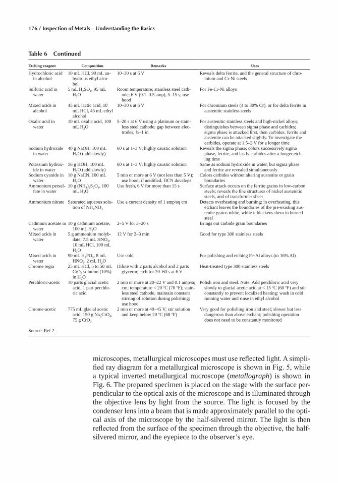
176 / Inspection of Metals—Understanding the Basics
microscopes, metallurgical microscopes must use reflected light. A simpli-fied ray diagram for a metallurgical microscope is shown in Fig. 5, while a typical inverted metallurgical microscope (metallograph) is shown in Fig. 6. The prepared specimen is placed on the stage with the surface per-pendicular to the optical axis of the microscope and is illuminated through the objective lens by light from the source. The light is focused by the condenser lens into a beam that is made approximately parallel to the opti-cal axis of the microscope by the half-silvered mirror. The light is then reflected from the surface of the specimen through the objective, the half-silvered mirror, and the eyepiece to the observer’s eye.
Table 6 Continued
Etching reagent Composition Remarks Uses
Hydrochloric acid in alcohol
10 mL HCl, 90 mL an-hydrous ethyl alco-hol
10–30 s at 6 V Reveals delta ferrite, and the general structure of chro-mium and Cr-Ni steels
Sulfuric acid in water
5 mL H2SO4, 95 mL H2O
Room temperature; stainless steel cath-ode; 6 V (0.1–0.5 amp), 5–15 s; use hood
For Fe-Cr-Ni alloys
Mixed acids in alcohol
45 mL lactic acid, 10 mL HCl, 45 mL ethyl alcohol
10–30 s at 6 V For chromium steels (4 to 30% Cr), or for delta ferrite in austenitic stainless steels
Oxalic acid in water
10 mL oxalic acid, 100 mL H2O
5–20 s at 6 V using a platinum or stain-less steel cathode; gap between elec-trodes, ¾–1 in.
For austenitic stainless steels and high-nickel alloys; distinguishes between sigma phase and carbides; sigma phase is attacked first, then carbides; ferrite and austenite can be attacked slightly. To investigate the carbides, operate at 1.5–3 V for a longer time
Sodium hydroxide in water
40 g NaOH, 100 mL H2O (add slowly)
60 s at 1–3 V; highly caustic solution Reveals the sigma phase; colors successively sigma phase, ferrite, and lastly carbides after a longer etch-ing time
Potassium hydrox-ide in water
56 g KOH, 100 mL H2O (add slowly)
60 s at 1–3 V; highly caustic solution Same as sodium hydroxide in water, but sigma phase and ferrite are revealed simultaneously
Sodium cyanide in water
10 g NaCN, 100 mL H2O
5 min or more at 6 V (not less than 5 V); use hood; if acidified, HCN develops
Colors carbides without altering austenite or grain boundaries
Ammonium persul-fate in water
10 g (NH4)2S2O8, 100 mL H2O
Use fresh, 6 V for more than 15 s Surface attack occurs on the ferrite grains in low-carbon steels; reveals the fine structures of nickel austenitic steels, and of transformer sheet
Ammonium nitrate Saturated aqueous solu-tion of NH4NO3
Use a current density of 1 amp/sq cm Detects overheating and burning; in overheating, this etchant leaves the boundaries of the pre-existing aus-tenite grains white, while it blackens them in burned steel
Cadmium acetate in water
10 g cadmium acetate, 100 mL H2O
2–5 V for 3–20 s Brings out carbide grain boundaries
Mixed acids in water
5 g ammonium molyb-date, 7.5 mL HNO3, 10 mL HCl, 100 mL H2O
12 V for 2–3 min Good for type 300 stainless steels
Mixed acids in water
90 mL H2PO3, 8 mL HNO3, 2 mL H2O
Use cold For polishing and etching Fe-Al alloys (to 16% Al)
Chrome regia 25 mL HCl, 5 to 50 mL CrO3 solution (10%) in H2O
Dilute with 2 parts alcohol and 2 parts glycerin; etch for 20–60 s at 6 V
Heat-treated type 300 stainless steels
Perchloric-acetic 10 parts glacial acetic acid, 1 part perchlo-ric acid
2 min or more at 20–22 V and 0.1 amp/sq cm; temperature < 20 ºC (70 ºF); stain-less steel cathode, maintain constant stirring of solution during polishing; use hood
Polish iron and steel. Note: Add perchloric acid very slowly to glacial acetic acid at < 15 ºC (60 ºF) and stir constantly to prevent localized heating; wash in cold running water and rinse in ethyl alcohol
Chrome-acetic 775 mL glacial acetic acid, 150 g Na2CrO4, 75 g CrO3
2 min or more at 40–45 V; stir solution and keep below 20 ºC (68 ºF)
Very good for polishing iron and steel; slower but less dangerous than above etchant; polishing operation does not need to be constantly monitored
Source: Ref 2
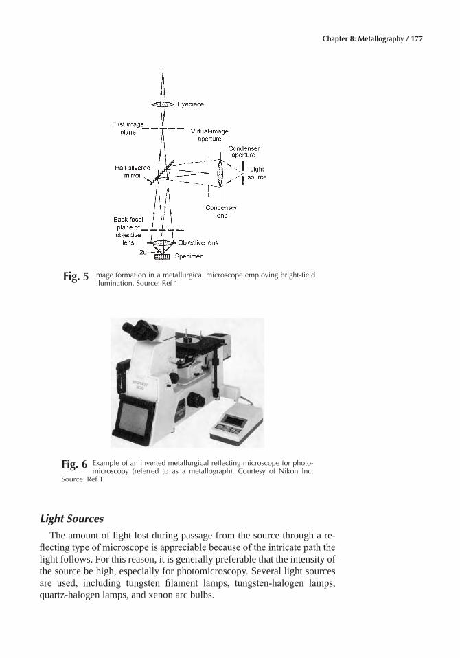
Chapter 8: Metallography / 177
Light Sources
The amount of light lost during passage from the source through a re-flecting type of microscope is appreciable because of the intricate path the light follows. For this reason, it is generally preferable that the intensity of the source be high, especially for photomicroscopy. Several light sources are used, including tungsten filament lamps, tungsten-halogen lamps, quartz-halogen lamps, and xenon arc bulbs.
Fig� 5 Image formation in a metallurgical microscope employing bright-field illumination. Source: Ref 1
Fig� 6 Example of an inverted metallurgical reflecting microscope for photo-microscopy (referred to as a metallograph). Courtesy of Nikon Inc.
Source: Ref 1

178 / Inspection of Metals—Understanding the Basics
Tungsten filament lamps generally operate at low voltage and high cur-rent. They are widely used for visual examination because of their low cost and ease of operation.
Tungsten-halogen lamps are the most popular light source due to their high light intensity. They produce good color micrographs when tungsten-corrected films are employed.
Xenon arc lamps produce extremely high intensity, and their uniform spectra and daylight color temperature makes them suitable for color pho-tomicrography. The first xenon lamps produced ozone, but modern units have overcome this problem. Light output is constant and can only be re-duced using neutral density filters.
Microscopic Techniques
Most microscopic studies of metals are made using bright-field illumi-nation. In addition to this type of illumination, several special techniques (oblique illumination, dark-field illumination, opaque stop microscopy, phase contrast microscopy, and polarized light microscopy) have particu-lar applications for metallographic studies.
Köhler Illumination� Most microscopes using reflected or transmitted light use Köhler illumination, because it provides the most intense, even illumination possible with standard light sources. The reflected light mi-croscope has two adjustable diaphragms, the aperture diaphragm and the field diaphragm, located between the lamp housing and the objective. Both diaphragms are adjusted to improve illumination and the image. To obtain Köhler illumination, the image of the field diaphragm must be brought into focus on the specimen plane. This situation normally occurs automatically when the microstructural image is brought into focus. The filament image must also be focused on the aperture diaphragm plane. This focus produces uniform illumination of the specimen imaged at the intermediate image plane and magnified by the eyepiece.
In bright-field illumination, the surface of the specimen is normal to the optical axis of the microscope, and white light is used. Figure 5 shows the ray diagram for this type of illumination in a standard type of bench microscope. Light that passes through the objective and strikes a region of the specimen surface perpendicular to the beam will be reflected back up the objective through the eyepieces to the eyes, where it will appear to be bright or white. Light that strikes grain boundaries, phase boundaries, and other features not perpendicular to the optical axis will be scattered at an angle and will not be collected by the objective. These regions will appear to be dark or black in the image. Bright-field is the most common mode of illumination used by metallographers.
Oblique illumination reveals the surface relief of a metallographic specimen. This process involves offsetting the condenser lens system or, as is more usually done, moving the condenser aperture to a position
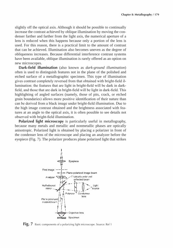
Chapter 8: Metallography / 179
slightly off the optical axis. Although it should be possible to continually increase the contrast achieved by oblique illumination by moving the con-denser farther and farther from the light axis, the numerical aperture of a lens is reduced when this happens because only a portion of the lens is used. For this reason, there is a practical limit to the amount of contrast that can be achieved. Illumination also becomes uneven as the degree of obliqueness increases. Because differential interference contrast systems have been available, oblique illumination is rarely offered as an option on new microscopes.
Dark-field illumination (also known as dark-ground illumination) often is used to distinguish features not in the plane of the polished and etched surface of a metallographic specimen. This type of illumination gives contrast completely reversed from that obtained with bright-field il-lumination: the features that are light in bright-field will be dark in dark-field, and those that are dark in bright-field will be light in dark-field. This highlighting of angled surfaces (namely, those of pits, crack, or etched grain boundaries) allows more positive identification of their nature than can be derived from a black image under bright-field illumination. Due to the high image contrast obtained and the brightness associated with fea-tures at an angle to the optical axis, it is often possible to see details not observed with bright-field illumination.
Polarized light microscopy is particularly useful in metallography, because many metals and metallic and nonmetallic phases are optically anisotropic. Polarized light is obtained by placing a polarizer in front of the condenser lens of the microscope and placing an analyzer before the eyepiece (Fig. 7). The polarizer produces plane polarized light that strikes
Fig� 7 Basic components of a polarizing light microscope. Source: Ref 1
180 / Inspection of Metals—Understanding the Basics
the surface and is reflected through the analyzer to the eyepieces. If an anisotropic metal is examined with the analyzer set 90° to the polarizer, the grain structure will be visible. However, viewing of an isotropic metal (cubic metals) under such conditions will produce a dark, extinguished condition. Polarized light is particularly useful in metallography for re-vealing grain structure and twinning in anisotropic metals and alloys and for identifying anisotropic phases and inclusions.
Differential Interference Contrast Microscopy� When crossed polar-ized light is used along with a double quartz prism (Wollaston prism) placed between the objective and the vertical illuminator, two light beams are produced that exhibit coherent interference in the image plane. This occurrence leads to two slightly displaced (laterally) images differing in phase (λ/2) that produces height contrast. The image produced reveals topographic detail somewhat similar to that produced by oblique illumina-tion but without the loss of resolution. Images can be viewed with natural colors similar to those observed in bright-field, or artificial coloring can be introduced by adding a sensitive tint plate.
Microphotography
All metallographs come equipped with one or more camera ports, as well as provisions for attaching charge-coupled device (CCD) cameras (or other types, although the CCD is by far the most common type used). While biologists frequently use 35 mm cameras to record microstructures, they are less popular with metallographers. A small percentage of metal-lographers still prefer to use wet processed sheet film, usually 4 by 5 in. (10 by 12.5 cm) in size. Orthochromatic film is no longer available in this size, and panchromatic films must be employed. These are less convenient to use because loading, unloading, and developing must be done in total darkness. Otherwise, results are the same. Contact printing is most com-monly performed.
The majority of metallographers switched to instant films (Polaroid), which were introduced in the 1960s. At that time, few (if any) metallo-graphs had exposure meters, and wastage was significant because instant films have no latitude (exposures must be exactly controlled to get good images, unlike wet processed films). Instant films are convenient because dark room work is avoided. However, except for the P/N type, there is no negative so extra prints cannot be made in the same way as by traditional photography. Instead, multiple photographs must be made anticipating fu-ture needs.
Electronic photography is now the dominant mode as it features all the convenience of instant photography with none of the disadvantages. In addition, digital images can be stored on a disk, eliminating the need for storing negatives. With the advent of high quality, high resolution printers,
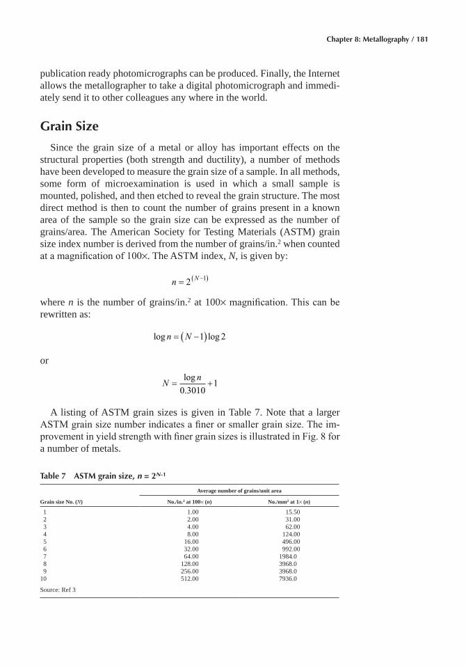
Chapter 8: Metallography / 181
publication ready photomicrographs can be produced. Finally, the Internet allows the metallographer to take a digital photomicrograph and immedi-ately send it to other colleagues any where in the world.
Grain Size
Since the grain size of a metal or alloy has important effects on the structural properties (both strength and ductility), a number of methods have been developed to measure the grain size of a sample. In all methods, some form of microexamination is used in which a small sample is mounted, polished, and then etched to reveal the grain structure. The most direct method is then to count the number of grains present in a known area of the sample so the grain size can be expressed as the number of grains/area. The American Society for Testing Materials (ASTM) grain size index number is derived from the number of grains/in.2 when counted at a magnification of 100×. The ASTM index, N, is given by:
n N= −( )2 1
where n is the number of grains/in.2 at 100× magnification. This can be rewritten as:
log logn N= −( )1 2
or
Nn
= +log
.0 30101
A listing of ASTM grain sizes is given in Table 7. Note that a larger ASTM grain size number indicates a finer or smaller grain size. The im-provement in yield strength with finer grain sizes is illustrated in Fig. 8 for a number of metals.
Table 7 ASTM grain size, n = 2N–1
Grain size No. (N)
Average number of grains/unit area
No./in.2 at 100× (n) No./mm2 at 1× (n)
1 1.00 15.50 2 2.00 31.00 3 4.00 62.00 4 8.00 124.00 5 16.00 496.00 6 32.00 992.00 7 64.00 1984.0 8 128.00 3968.0 9 256.00 3968.010 512.00 7936.0
Source: Ref 3
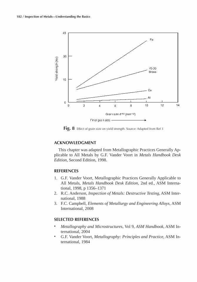
182 / Inspection of Metals—Understanding the Basics
ACKNOWLEDGMENT
This chapter was adapted from Metallographic Practices Generally Ap-plicable to All Metals by G.F. Vander Voort in Metals Handbook Desk Edition, Second Edition, 1998.
REFERENCES
1. G.F. Vander Voort, Metallographic Practices Generally Applicable to All Metals, Metals Handbook Desk Edition, 2nd ed., ASM Interna-tional, 1998, p 1356–1371
2. R.C. Anderson, Inspection of Metals: Destructive Testing, ASM Inter-national, 1988
3. F.C. Campbell, Elements of Metallurgy and Engineering Alloys, ASM International, 2008
SELECTED REFERENCES
• Metallography and Microstructures, Vol 9, ASM Handbook, ASM In-ternational, 2004
• G.F. Vander Voort, Metallography: Principles and Practice, ASM In-ternational, 1984
Fig� 8 Effect of grain size on yield strength. Source: Adapted from Ref 3
Inspection of Metals—Understanding the Basics Copyright © 2013 ASM International®
F.C. Campbell, editor All rights reservedwww.asminternational.org
CHAPTER 9
Liquid Penetrant, Magnetic Particle, and
Eddy-Current Inspection
LIQUID PENETRANT, magnetic particle, and eddy current inspection are used to detect surface flaws. Magnetic particle and eddy current in-spection can also detect subsurface flaws. Liquid penetrant and eddy cur-rent inspection can be used to inspect ferrous and nonferrous metals, while magnetic particle inspection is restricted to materials that can be magne-tized. Both magnetic particle and eddy current inspection can be auto-mated. In the case of automated eddy current inspection, quite high rates of production can be attained. While liquid penetrant inspection is primar-ily a manual operation, the equipment requirements are less than for mag-netic particle or eddy current inspection.
Liquid Penetrant Inspection
Liquid penetrant inspection is a nondestructive method used to find dis-continuities that are open to the surface of solid, essentially nonporous materials. Indications of flaws can be found regardless of the size, con-figuration, internal structure, and chemical composition of the workpiece being inspected, as well as flaw orientation. Liquid penetrants can seep into (and be drawn into) various types of minute surface openings (as fine as 0.1 μm, or 4 μin., in width) by capillary action. Therefore, the process is well suited to detect all types of surface cracks, laps, porosity, shrinkage areas, laminations, and similar discontinuities. It is used extensively to inspect ferrous and nonferrous metal wrought and cast products, powder metallurgy parts, ceramics, plastics, and glass objects.
The liquid penetrant inspection method is relatively simple to perform; there are few limitations due to specimen material and geometry, and it is
184 / Inspection of Metals—Understanding the Basics
inexpensive. The equipment is very simple, and the inspection can be per-formed at many stages during part production, as well as after the part is placed in service. Relatively little specialized training is required. In some instances, liquid penetrant sensitivity is greater for ferromagnetic steels than that of magnetic particle inspection.
The major limitation of liquid penetrant inspection is that it can detect only imperfections that are open to the surface; some other method must be used to detect subsurface defects and discontinuities. Another factor that can inhibit the effectiveness of liquid penetrant inspection is the sur-face roughness of the object. Extremely rough and porous surfaces are likely to produce false indications.
Although liquid penetrant is often used to inspect some types of powder metallurgy parts, the process is generally not well suited to inspect low density powder metallurgy parts and other porous materials, because the penetrant enters the pores and registers each pore as a defect.
Physical Principles
Liquid penetrant inspection depends mainly on the ability of liquid pen-etrant to effectively wet the surface of a solid workpiece; flow over the surface to form a continuous, reasonably uniform coating; and migrate into cavities that are open to the surface. The cavities of interest usually are very small, often invisible to the unaided eye. The ability of a given liquid to flow over a surface and enter surface cavities depends principally on:
• Cleanness of the surface • Configuration of the cavity • Size of the cavity • Surface tension of the liquid • Ability of the liquid to wet the surface
The cohesive forces between molecules of a liquid cause surface ten-sion. An example of the influence of surface tension is the tendency of a free liquid, such as a droplet of water, to contract into a sphere. In such a droplet, surface tension is counterbalanced by the internal hydrostatic pressure of the liquid. When the liquid comes into contact with a solid surface, the cohesive force responsible for surface tension competes with the adhesive force between the molecules of the liquid and the solid sur-face. These forces jointly determine the contact angle between the liquid and the surface. If the angle is less than 90°, the liquid is regarded as hav-ing good wetting ability.
Description of the Process
Regardless of the type of penetrant used and other variations in the basic process, liquid penetrant inspection requires at least five essential steps:
Chapter 9: Liquid Penetrant, Magnetic Particle, and Eddy-Current Inspection / 185
1� Surface Preparation� All surfaces of a workpiece must be thor-oughly cleaned and completely dried before inspection. Discontinuities exposed to the surface must be free from oil, water, and other contami-nants for at least 25 mm (1 in.) beyond the area being inspected to increase the probability of detection.
2� Penetrant Application� Liquid penetrant is applied in a suitable manner to form a film of the penetrant over the surface for at least 13 mm (0.5 in.) beyond the area being inspected. The penetrant is left on the sur-face for a sufficient time to allow penetration into flaws. Times are based on experience but generally range from 2 to 20 minutes.
3� Removal of Excess Penetrant� Uniform removal of excess pene-trant is necessary for effective inspection, but over cleaning must be avoided. Penetrants can be washed off directly using water, treated first with an emulsifier and then rinsed with water, or removed using a solvent.
4� Developer Application� Developer can be applied by dusting (dry powdered) and immersion and spray (water developers) applications. Nonaqueous wet developers can only be applied by spraying. The devel-oper should be allowed to dwell on the surface for a sufficient time (usu-ally 10 minutes minimum) to permit it to draw penetrant out of any sur-face flaws to form visible indications of such flaws. Longer times could be necessary for tight cracks. The developer also provides a uniform back-ground to assist visual inspection.
5� Inspection� After being sufficiently developed, the surface is visu-ally examined for indications of penetrant bleed back from surface open-ings. This examination must be performed in a suitable inspection envi-ronment. Visible penetrant inspection is performed in good white light. When fluorescent penetrant is used, inspection is performed in a suitably darkened area using black (ultraviolet) light, which causes the penetrant to emit visible light. The actions of penetrant and developer are illustrated in Fig. 1.
Penetrant Systems
Liquid penetrant inspection applications have been developed to handle the wide variations in three basic penetrant systems. They are broadly classified as (a) the water-washable system, (b) the postemulsifiable sys-tem, and (c) the solvent-removable system.
The water-washable penetrant system is designed so that the pene-trant is directly washable from the surface of the workpiece using water. It can be used to process workpieces quickly and efficiently. However, it is important that washing is carefully controlled, because water-washable penetrants are susceptible to over washing. The degree and speed of re-moval depend on processing conditions such as spray nozzle characteris-tics, water pressure and temperature, duration of rinse cycle, surface con-
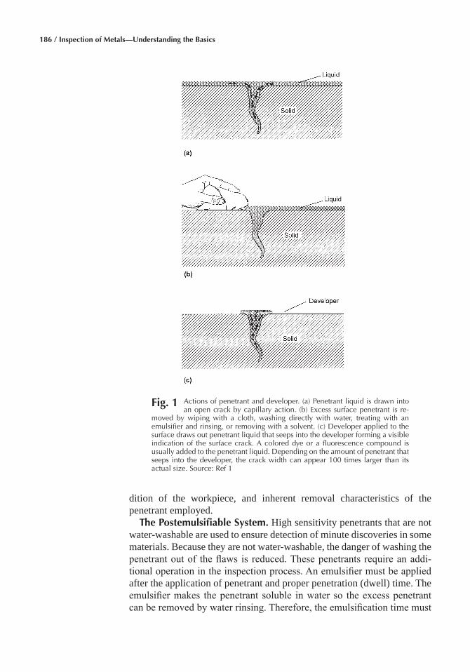
186 / Inspection of Metals—Understanding the Basics
dition of the workpiece, and inherent removal characteristics of the penetrant employed.
The Postemulsifiable System� High sensitivity penetrants that are not water-washable are used to ensure detection of minute discoveries in some materials. Because they are not water-washable, the danger of washing the penetrant out of the flaws is reduced. These penetrants require an addi-tional operation in the inspection process. An emulsifier must be applied after the application of penetrant and proper penetration (dwell) time. The emulsifier makes the penetrant soluble in water so the excess penetrant can be removed by water rinsing. Therefore, the emulsification time must
Fig� 1 Actions of penetrant and developer. (a) Penetrant liquid is drawn into an open crack by capillary action. (b) Excess surface penetrant is re-
moved by wiping with a cloth, washing directly with water, treating with an emulsifier and rinsing, or removing with a solvent. (c) Developer applied to the surface draws out penetrant liquid that seeps into the developer forming a visible indication of the surface crack. A colored dye or a fluorescence compound is usually added to the penetrant liquid. Depending on the amount of penetrant that seeps into the developer, the crack width can appear 100 times larger than its actual size. Source: Ref 1
Chapter 9: Liquid Penetrant, Magnetic Particle, and Eddy-Current Inspection / 187
be carefully controlled so the surface penetrant becomes water soluble but penetrant in the flaws does not. Postemulsifiable penetrants include lipo-philic (oil base) and hydrophilic (water base).
The Solvent-Removable System� Occasionally, it is necessary to in-spect only a small area of a workpiece or to inspect a workpiece on site rather than at a regular inspection station. In such situations, solvent-re-movable penetrants are used. Normally, the same type of solvent is used both for precleaning and for removal of excess penetrant. This penetrant process is convenient and broadens the range of applications of penetrant inspection.
The solvent-removable penetrants have an oil base. Optimum solvent removal is accomplished by wiping off as much of the excess penetrant as possible with a paper towel or a lint free cloth, then slightly dampening a clean cloth with solvent and wiping off the remaining penetrant. Final wiping with a dry paper towel or clean cloth is required. The penetrant also can be removed by flooding the surface with solvent, in the same manner as for water-washable penetrants. The flooding technique is par-ticularly useful for large workpieces, but it must be very carefully used to prevent removal of the penetrant from the flaws. The solvent-removable system is used mainly in special applications; it is not practical for pro-duction applications because it is labor intensive.
Liquid Penetrant Materials
Two basic types of liquid penetrants are fluorescent and visible. Each type is available for any one of the three systems (water-washable, poste-mulsifiable, or solvent-removable).
Fluorescent penetrant inspection uses penetrants that fluoresce bril-liantly under ultraviolet light. The sensitivity of a fluorescent penetrant depends on its ability to form indications that appear as small sources of light in an otherwise dark area. Sensitivity levels of fluorescent penetrants are: ultra-low (Level ½), low (Level 1), medium (Level 3), high (Level 4), and ultrahigh (Level 5).
Visible penetrant inspection uses a penetrant that is usually red in color and produces vivid red indications in contrast to the light background of the applied developer under visible light. The visible penetrant indications must be viewed under adequate white light. The sensitivity of visible pen-etrants is regarded as Level 1 and adequate for many applications.
Penetrant selection and use depend on the criticality of the inspection, the condition of the workpiece surface, the type of processing, and the desired sensitivity.
Physical and Chemical Characteristics� Both fluorescent and visible penetrants, whether water-washable, postemulsifiable, or solvent-remov-able, must have certain chemical and physical characteristics to perform their intended functions. Principal requirements of penetrants are:

188 / Inspection of Metals—Understanding the Basics
• Chemical stability and uniform physical consistency • A flash point not lower than 95 °C (200 °F); penetrants that have lower
flash points constitute a potential fire hazard • A high degree of wettability • Low viscosity to permit better coverage and minimum dragout • Ability to penetrate discontinuities quickly and completely • Sufficient brightness and permanence of color • Chemical inertness with materials being inspected and with con-
tainers • Low toxicity to protect personnel • Slow drying characteristics • Ease of removal • Inoffensive odor • Low cost • Resistance to ultraviolet light and heat fade
Emulsifiers
Emulsifiers are liquids used to render excess oily penetrant on the work-piece surface water washable. Emulsifiers are oil base and water base.
Oil base emulsifiers function by diffusion. The emulsifier diffuses into the penetrant film and renders it spontaneously emulsifiable in water. The rate at which it diffuses into the penetrant establishes its emulsification time. Because the emulsifier is fast acting, the rinse operation should be done quickly to avoid over emulsification.
Water base emulsifiers usually are supplied as liquid concentrates that are diluted in water to concentrations of 5 to 30% for dip tank applications and of 0.05 to 5% for spray applications. Water base emulsifiers function by displacing excess surface penetrant from the surface of the part by de-tergent action. The force of the water spray or air agitation of open dip tanks provides the scrubbing action while the detergent displaces the ex-cess surface penetrant.
Solvent Cleaners
Solvent cleaners differ from emulsifiers in that they remove excess sur-face penetrant through direct solvent action. The penetrant is dissolved by the solvent. Solvent cleaners are flammable and nonflammable. Flamma-ble cleaners are free of halogens, but are potential fire hazards. Nonflam-mable cleaners usually contain halogenated solvents, which render them unsuitable for some applications, usually because of their high toxicity or because they have undesirable effects on some materials.
Developers
Because the amount of penetrant that emerges from a small surface opening is minute, the visible evidence of its presence must be enhanced. Developers are used to spread the penetrant available at the defect, thus

Chapter 9: Liquid Penetrant, Magnetic Particle, and Eddy-Current Inspection / 189
increasing the amount of light emitted, or the amount of contrast, that makes the defect visible to the unaided eye.
The properties/characteristics developers must have for optimal perfor-mance are:
• It must be adsorptive to maximize blotting• It must have fine grain size and a particle shape that will disperse and
expose the penetrant at a flaw to produce strong and sharply defined indications of flaws
• It must be capable of providing a contrast background for indications when color contrast penetrants are used
• It must be easy to apply • It must form a thin, uniform coating over a surface• It must be easily wetted by the penetrant at the flaw (the liquid must be
allowed to spread over the particle surfaces) • It must be nonfluorescent if used with fluorescent penetrants• It must be easy to remove after inspection • It must not contain ingredients harmful to parts being inspected or to
equipment used in the inspection operation • It must not contain ingredients harmful or toxic to the operator
Four forms of developers commonly used are dry powder (Form A), water soluble (Form B), water suspendible (Form C), and nonaqueous solvent suspendible (Form D).
Dry Developers� Dry powder developers are widely used with fluores-cent penetrants, but should not be used with visible dye penetrants be-cause they do not produce a satisfactory contrast coating on the surface of the workpiece. Ideally, dry powder developers should be light and fluffy to allow easy application and should cling to dry surfaces in a fine film. Powder adherence should not be excessive, because the amount of pene-trant at fine flaws is insufficient to seep back into a thick coating.
Hand processing equipment usually includes a developer station, which usually is an open tank for dry developers. Workpieces are dipped into the powder, or powder is picked up with a scoop or with the hands, and dropped onto the workpiece. Excess powder is removed by shaking and tapping the workpiece. Some powders are so light and fluffy that parts are dipped into them as easily as into a liquid.
Other effective methods of application are rubber spray bulbs and air operated spray guns. An electrostatic charged powder gun that can apply an extremely even and adherent coating of dry powder on metal parts is also used. For simple application, especially when only a portion of the surface of a large part is being inspected, a very soft bristle brush is often adequate.
Powder can dry the skin and irritate the lining of air passages. Opera-tors should use rubber gloves and respirators. Modern equipment often includes an exhaust system on the developer spray booth or on the devel-

190 / Inspection of Metals—Understanding the Basics
oper dust chamber, which prevents dust from escaping. Powder recovery filters often are included in such installations.
Wet Developers� Three types of wet developers are: suspensions of developer powder in water (the most widely used), aqueous solutions of suitable salts, and suspensions of powder in volatile solvents.
Water suspendible developers can be used with both visible and fluores-cent penetrants. With a fluorescent penetrant, the dried developer coating must not fluoresce or absorb or filter out black light used for inspection. Water suspendible developers permit high speed application of developer in mass inspection of small to medium size workpieces using the fluores-cent method. A basket of small, irregularly shaped workpieces that has gone through the steps of penetrant application, penetrant dwell, and washing can be coated with developer in one quick dip in a water suspen-sion. This method not only is quick, but also, it provides thorough, com-plete coverage of all surfaces of the pieces being inspected. No dry pow-der application method has all these advantages to the same degree.
Wet developer is applied just after excess penetrant is washed away and immediately before drying. After drying, surfaces are uniformly coated with a thin film of developer. Developing time is decreased because heat from the drier helps to bring penetrant back out of surface openings, and the developing action occurs immediately with the developer film already in place. Workpieces are ready for inspection in a shorter period of time, before excessive bleed out from large openings occurs, so better definition of flaw indications often is obtained.
Water suspendible developers are supplied as a dry powder concentrate, which is then dispersed in water in recommended proportions, usually from 0.04 to 0.12 kg/L (1/3 to 1 lb/gal). The amount of powder in suspen-sion must be carefully maintained. Too much or too little developer on the surface of a workpiece can seriously affect sensitivity.
Water soluble developers can be used for both fluorescent and visible postemulsifiable and solvent-removable penetrants. Water soluble devel-opers are not recommended for use with water-washable penetrants, be-cause of the potential to wash the penetrant from within the flaw if the developer is not very carefully controlled. Water soluble developers are supplied as a dry powder concentrate, which is then dispersed in water in recommended proportions, usually from 0.12 to 0.24 kg/L (1 to 2 lb/gal). Advantages of this form of developer are:
• The prepared bath is completely soluble and does not require any agitation
• The developer is applied prior to drying, thus decreasing the develop-ing time
• The dried developer film on the workpiece is completely water soluble and is easily and completely removed following inspection by simple water rinsing

Chapter 9: Liquid Penetrant, Magnetic Particle, and Eddy-Current Inspection / 191
Nonaqueous solvent suspendible developers are commonly used for both the fluorescent and the visible penetrant process. This form of devel-oper produces a white coating on the surface of the part, which yields the maximum white color contrast with the red visible penetrant indication and extremely brilliant fluorescent indication.
Nonaqueous solvent suspendible developers are supplied in the ready to use condition and contain particles of developer suspended in a mixture of volatile solvents. The solvents are carefully selected for their compati-bility with the penetrants. Nonaqueous solvent suspendible developers also contain surfactants in a dispersant that coat the particles and reduce their tendency to clump or agglomerate.
Nonaqueous solvent suspendible developers are the most sensitive form of developer used with fluorescent penetrants because the solvent action contributes to the absorption and adsorption mechanisms. In many cases where tight, small flaws occur, dry powder, water soluble, and water sus-pendible developers do not contact the entrapped penetrant. This results in the failure of the developer to create the necessary capillary action and surface tension that serve to pull the penetrant from the flaw. The non-aqueous solvent suspendible developer enters the flaw and dissolves into the penetrant. This action increases the volume and reduces the viscosity of the penetrant.
The manufacturer must carefully select and compound the solvent mix-ture. There are two types of solvent based developers: nonflammable (chlorinated solvents) and flammable (nonchlorinated solvents). Both types are widely used. Selection is based on the nature of the application and the type of alloy being inspected.
Solvent developers are sometimes applied with a paintbrush, but this is likely to result in smeared indications; application by a pressure spray can is a preferred method.
Selection of Developer� Because developers play such an important role in penetrant inspection, it is very important to select the appropriate developer for a given job. For example, on very smooth or polished sur-faces, dry powder does not adhere satisfactorily, and wet developers do a better job. Conversely, on very rough surfaces dry powder is far more effective.
Some general rules regarding developer selection are:
• Use a wet developer instead of a dry developer on very smooth surfaces
• Use a dry developer versus a wet developer on very rough surfaces• Wet developers are better suited for high production inspection of
small workpieces because of their greater ease and speed of appli- cation
• Wet developers cannot be used reliably where sharp fillets unavoid-ably accumulate developer, which can mask flaw indications
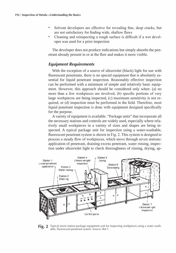
192 / Inspection of Metals—Understanding the Basics
• Solvent developers are effective for revealing fine, deep cracks, but are not satisfactory for finding wide, shallow flaws
• Cleaning and reinspecting a rough surface is difficult if a wet devel-oper was used for a prior inspection
The developer does not produce indications but simply absorbs the pen-etrant already present in or at the flaw and makes it more visible.
Equipment Requirements
With the exception of a source of ultraviolet (black) light for use with fluorescent penetrants, there is no special equipment that is absolutely es-sential for liquid penetrant inspection. Reasonably effective inspection can be performed with a minimum of simple and relatively basic equip-ment. However, this approach should be considered only when: (a) no more than a few workpieces are involved, (b) specific portions of very large workpieces are being inspected, (c) maximum sensitivity is not re-quired, or (d) inspection must be performed in the field. Therefore, most liquid penetrant inspection is done with equipment designed specifically for the purpose.
A variety of equipment is available. “Package units” that incorporate all the necessary stations and controls are widely used, especially where rela-tively small workpieces in a variety of sizes and shapes are being in-spected. A typical package unit for inspection using a water-washable, fluorescent penetrant system is shown in Fig. 2. This system is designed to process a steady flow of workpieces, which move through seven stations: application of penetrant, draining excess penetrant, water rinsing, inspec-tion under ultraviolet light to check thoroughness of rinsing, drying, ap-
Fig� 2 Typical seven station package equipment unit for inspecting workpieces using a water wash-able, fluorescent penetrant system. Source: Ref 1
Chapter 9: Liquid Penetrant, Magnetic Particle, and Eddy-Current Inspection / 193
plication of developer, and final ultraviolet-light inspection for flaws. The unit does not include stations for preliminary cleaning and post cleaning; these operations often are performed in another area. The equipment shown in Fig. 2 is available in a wide range of sizes and can be modified in many ways to fit specific needs. For example, if a postemulsifiable sys-tem is used, workpieces are coated with emulsifier after the penetrant has been allowed to drain and prior to rinsing.
Precleaning� Regardless of the penetrant chosen, adequate precleaning of workpieces prior to penetrant inspection is absolutely necessary for ac-curate results. Inadequate removal of surface contamination can result in missed relevant indications because:
• The penetrant does not enter the flaw • The penetrant loses its ability to reveal the flaw because it reacts with
a substance contained in the flaw • The surface immediately surrounding the flaw retains too much pene-
trant, which masks the true appearance of the flaw
Also, nonrelevant (false) indications can be caused by residual materials holding penetrants.
Cleaning methods generally are classified as chemical, mechanical, solvent, and combinations of these.
Chemical cleaning methods include alkaline or acid cleaning, pickling or chemical etching, and molten salt bath cleaning.
Mechanical cleaning methods include tumbling, wet blasting, dry abra-sive blasting, wire brushing, and high pressure water or steam cleaning. Mechanical cleaning can mask flaws by smearing adjacent metal over them and by filling them with abrasive material.
Solvent cleaning methods include vapor degreasing, solvent spraying, solvent wiping, and ultrasonic immersion using solvents. Ultrasonic im-mersion is by far the most effective means of ensuring clean parts, but it can be a very expensive capital equipment investment.
Cleaning methods and their common uses are listed in Table 1. Major factors in the selection of a cleaning method are the type of contaminant to be removed, the type of alloy being cleaned, and the chemical composi-tion of the workpiece being cleaned. It is good practice to test the method on known flaws to ensure that it will not mask the flaws.
The surface finish of the workpiece must always be considered. When further processing is scheduled, such as machining or final polishing, or when a surface finish of 3.20 μm (125 μin.) or coarser is allowed, an abra-sive cleaning method is frequently a good choice. Generally, chemical cleaning methods have fewer degrading effects on surface finish than me-chanical methods (unless the chemical used is strongly corrosive to the material being cleaned). Steam cleaning and solvent cleaning rarely have any effect on surface finish.
194 / Inspection of Metals—Understanding the Basics
The choice of a cleaning method can be dictated by Occupational Safety and Health Administration and Environmental Protection Agency health and safety regulations. Factors to consider include quantities of materials that will be used, toxicity, filtering, neutralization and disposal techniques, and worker safety.
Penetrant Station� The principal requirement of a penetrant station is to provide a means to coat workpieces with penetrant–the entire surface for small workpieces, or over small areas of large workpieces when only local inspection is required. The station also should provide a means to drain excess penetrant back into the penetrant reservoir, unless the ex-pendable technique is being used. Draining racks usually serve the addi-tional purpose of providing a storage place for parts during the time re-quired for penetration (dwell time).
Emulsifier Station� Emulsifier liquid is contained in a tank large enough to permit immersion of the workpieces, either individually or in batches. Accessory equipment includes covers to reduce evaporation and drain valves for cleanout when the bath has to be renewed. Suitable drain racks are also a part of this station, to permit excess emulsifier to drain back into the tank.
Table 1 Applications of various methods of precleaning for liquid penetrant inspection
Method Use
MechanicalAbrasive tumbling Removing light scale, burrs, welding flux, braze stopoff, rust, casting mold,
and core material; should not be used on soft metals such as aluminum, magnesium, and titanium
Dry abrasive grit blasting Removing light and heavy scale, flux, stopoff, rust, casting mold and core material, sprayed coatings, and carbon deposits—in general, any friable deposit. Can be fixed or portable
Wet abrasive grit blasting Same as dry except, where deposits are light, better surface and better con-trol of dimensions are required
Wire brushing Removing light deposits of scale, flux, and stopoffHigh-pressure water and steam Typically used with an alkaline cleaner or detergent; removing typical ma-
chine-shop soils such as cutting oils, polishing compounds, grease, chips, and deposits from electrical discharge machining; used when surface fin-ish must be maintained; inexpensive
Ultrasonic cleaning Typically used with detergent and water or with a solvent; removing adher-ent shop soil from large quantities of small parts
Chemical
Alkaline cleaning Removing braze stopoff, rust, scale, oils, greases, polishing material, and carbon deposits; typically used on large articles where hand methods are too labor intensive; also used on aluminum for gross metal removal
Acid cleaning Strong solutions for removing heavy scale; solutions for light scale; weak (etching) solutions for removing lightly smeared metal
Molten salt bath cleaning Conditioning and removing heavy scale
Solvent
Vapor degreasing Removing typical shop soil, oil, and grease; usually uses chlorinated sol-vents; not suitable for titanium
Solvent wiping Same as for vapor degreasing except a hand operation; can use nonchlori-nated solvents; used for localized low-volume cleaning
Source: Ref 1
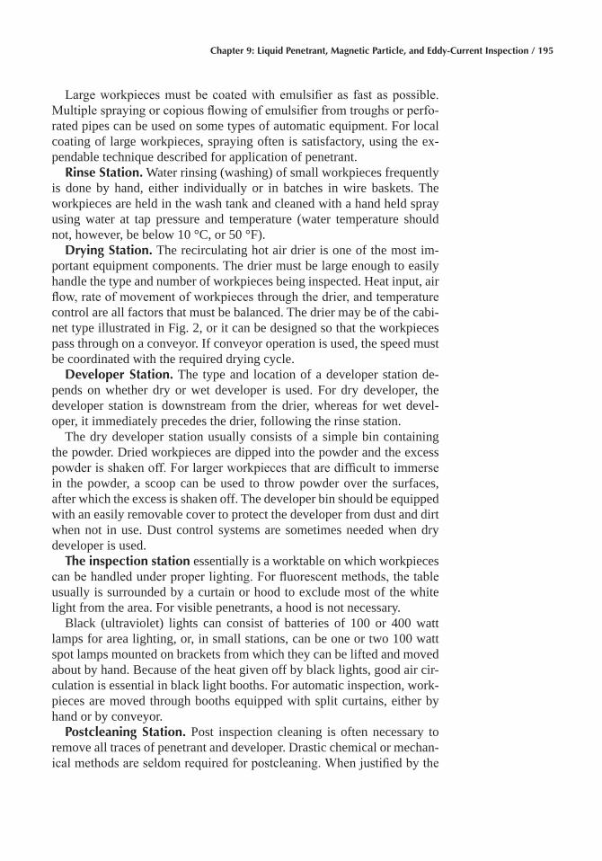
Chapter 9: Liquid Penetrant, Magnetic Particle, and Eddy-Current Inspection / 195
Large workpieces must be coated with emulsifier as fast as possible. Multiple spraying or copious flowing of emulsifier from troughs or perfo-rated pipes can be used on some types of automatic equipment. For local coating of large workpieces, spraying often is satisfactory, using the ex-pendable technique described for application of penetrant.
Rinse Station� Water rinsing (washing) of small workpieces frequently is done by hand, either individually or in batches in wire baskets. The workpieces are held in the wash tank and cleaned with a hand held spray using water at tap pressure and temperature (water temperature should not, however, be below 10 °C, or 50 °F).
Drying Station� The recirculating hot air drier is one of the most im-portant equipment components. The drier must be large enough to easily handle the type and number of workpieces being inspected. Heat input, air flow, rate of movement of workpieces through the drier, and temperature control are all factors that must be balanced. The drier may be of the cabi-net type illustrated in Fig. 2, or it can be designed so that the workpieces pass through on a conveyor. If conveyor operation is used, the speed must be coordinated with the required drying cycle.
Developer Station� The type and location of a developer station de-pends on whether dry or wet developer is used. For dry developer, the developer station is downstream from the drier, whereas for wet devel-oper, it immediately precedes the drier, following the rinse station.
The dry developer station usually consists of a simple bin containing the powder. Dried workpieces are dipped into the powder and the excess powder is shaken off. For larger workpieces that are difficult to immerse in the powder, a scoop can be used to throw powder over the surfaces, after which the excess is shaken off. The developer bin should be equipped with an easily removable cover to protect the developer from dust and dirt when not in use. Dust control systems are sometimes needed when dry developer is used.
The inspection station essentially is a worktable on which workpieces can be handled under proper lighting. For fluorescent methods, the table usually is surrounded by a curtain or hood to exclude most of the white light from the area. For visible penetrants, a hood is not necessary.
Black (ultraviolet) lights can consist of batteries of 100 or 400 watt lamps for area lighting, or, in small stations, can be one or two 100 watt spot lamps mounted on brackets from which they can be lifted and moved about by hand. Because of the heat given off by black lights, good air cir-culation is essential in black light booths. For automatic inspection, work-pieces are moved through booths equipped with split curtains, either by hand or by conveyor.
Postcleaning Station� Post inspection cleaning is often necessary to remove all traces of penetrant and developer. Drastic chemical or mechan-ical methods are seldom required for postcleaning. When justified by the

196 / Inspection of Metals—Understanding the Basics
volume of work, an emulsion cleaning line is effective and reasonable in cost. In special circumstances, ultrasonic cleaning may be the only satis-factory way of cleaning deep crevices or small holes. However, solvents or detergent aided steam or water is almost always sufficient. The use of steam with detergent is probably the most effective of all methods.
Selection of Penetrant System
Size, shape, and weight of workpieces, as well as number of similar workpieces to be inspected, can influence the selection of a penetrant system.
Sensitivity and Cost� The required level of sensitivity and cost usually are the most important factors in selecting a system. The methods capable of the greatest sensitivity are also the most costly. There are many inspec-tion operations that require the ultimate in sensitivity, but there are also many where extreme sensitivity is not required, but where extreme sensi-tivity can also produce misleading results.
On a practical basis, the three major penetrant systems are broken down into six systems or variations of systems. The six systems, in order of de-creasing sensitivity and decreasing cost are:
• Postemulsifiable fluorescent • Solvent-removable fluorescent • Water-washable fluorescent • Postemulsifiable visible • Solvent-removable visible • Water-washable visible
Table 2 compares the sensitivities and uses of the six systems.
Table 2 Comparison of penetrant systems
Water washable Postemulsifiable Solvent removable
Visible dye penetrants
Lowest in sensitivity Higher sensitivity than water washables Where water rinse is not feasible, or desirable
Suited for large surface areas
Suited for large surface areasSuited for large quantities of similar
objects
For spot inspectionsRecommended for small areas and
simple geometries
Fluorescent penetrants
Lowest in sensitivity of fluorescent penetrants
Higher sensitivity than water washable fluorescent penetrants
Higher sensitivity than solvent- removable visible penetrant
Suited for large surface areas
Suited for large quantities of similar articles
Where water rinse is not feasible or desirable
Suited for large quantities of similar objects
Suited for wide, shallow discontinuities and tight cracks
For spot inspections
Suited for deep, narrow discontinuities
Contaminants must be removed prior to in-spection
Recommended for small areas and simple geometries
Recommended for rough sur-faces (i.e., sand castings)
Suited for stress, intergranular, and grinding cracks
Note: For environmental reasons, water washable penetrant systems are used even though the solvent system would be preferable. Source: Ref 1

Chapter 9: Liquid Penetrant, Magnetic Particle, and Eddy-Current Inspection / 197
Magnetic Particle Inspection
Magnetic particle inspection is used to locate surface and subsurface discontinuities in ferromagnetic materials. The method is based on the fact that when a material or part being tested is magnetized, discontinui-ties that lie in a direction generally transverse to the direction of the mag-netic field cause a leakage field to form at and above the part surface. The presence of the leakage field, and, therefore, the presence of the disconti-nuity, is detected by the use of finely divided ferromagnetic particles ap-plied over the surface. Some of the particles are gathered and held by the leakage field. The magnetically held particles form an outline of the dis-continuity and generally indicate its location, size, shape, and extent. Magnetic particles are applied over a surface either as dry particles or as wet particles in a liquid carrier such as water and oil. Nonferromagnetic materials cannot be inspected by this method. Such materials include alu-minum alloys, magnesium alloys, copper and copper alloys, lead, titanium and titanium alloys, and austenitic stainless steels.
The principal industrial uses of magnetic particle inspection are final inspection; receiving inspection; in-process inspection and quality con-trol; maintenance and overhaul in the transportation industries; plant and machinery maintenance; and inspection of large components. Although in-process magnetic particle inspection is used to detect discontinuities and imperfections in material and parts as early as possible in the sequence of operations, final inspection is required to ensure that rejectable discon-tinuities and imperfections detrimental to part use and function have not developed during processing.
Advantages� The magnetic particle method is a sensitive means to lo-cate small, shallow surface cracks in ferromagnetic materials. Cracks large enough to be seen by the naked eye can produce an indication, but very wide cracks will not produce a particle pattern if the surface opening is too wide for the particles to bridge.
Discontinuities that do not actually break through the surface also are indicated in many instances using magnetic particle inspection within cer-tain limitations. Fine, sharp discontinuities close to the surface (a long stringer of nonmetallic inclusions, for example) can produce an indica-tion. Indications of deeper discontinuities are less distinct.
Limitations� The operator must be aware of certain limitations of mag-netic particle inspection. For example, thin coatings of paint and nonmag-netic coverings, such as plating, adversely affect sensitivity. Other limita-tions are:
• Workpiece material must be ferromagnetic • The direction of the magnetic field must intercept the principal plane
of the discontinuity at right angles for best results. This could require two or more sequential inspections with different magnetizations
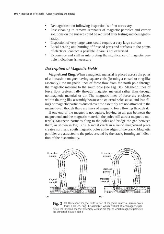
198 / Inspection of Metals—Understanding the Basics
• Demagnetization following inspection is often necessary • Post cleaning to remove remnants of magnetic particles and carrier
solutions on the surface could be required after testing and demagneti - zation
• Inspection of very large parts could require a very large current • Local heating and burning of finished parts and surfaces at the points
of electrical contact is possible if care is not exercised • Experience and skill in interpreting the significance of magnetic par-
ticle indications is necessary
Description of Magnetic Fields
Magnetized Ring� When a magnetic material is placed across the poles of a horseshoe magnet having square ends (forming a closed or ring like assembly), the magnetic lines of force flow from the north pole through the magnetic material to the south pole (see Fig. 3a). Magnetic lines of force flow preferentially through magnetic material rather than through nonmagnetic material or air. The magnetic lines of force are enclosed within the ring like assembly because no external poles exist, and iron fil-ings or magnetic particles dusted over the assembly are not attracted to the magnet even though there are lines of magnetic force flowing through it.
If one end of the magnet is not square, leaving an air gap between the magnet end and the magnetic material, the poles still attract magnetic ma-terials. Magnetic particles cling to the poles and bridge the gap between them, as shown in Fig. 3(b). A radial crack in a round magnetized piece creates north and south magnetic poles at the edges of the crack. Magnetic particles are attracted to the poles created by the crack, forming an indica-tion of the discontinuity.
Fig� 3 (a) Horseshoe magnet with a bar of magnetic material across poles forms a closed, ring like assembly, which will not attract magnetic par-
ticles. (b) Ring like magnet assembly with an air gap, to which magnetic particles are attracted. Source: Ref 2
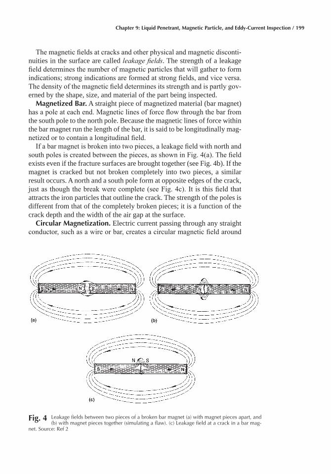
Chapter 9: Liquid Penetrant, Magnetic Particle, and Eddy-Current Inspection / 199
The magnetic fields at cracks and other physical and magnetic disconti-nuities in the surface are called leakage fields. The strength of a leakage field determines the number of magnetic particles that will gather to form indications; strong indications are formed at strong fields, and vice versa. The density of the magnetic field determines its strength and is partly gov-erned by the shape, size, and material of the part being inspected.
Magnetized Bar� A straight piece of magnetized material (bar magnet) has a pole at each end. Magnetic lines of force flow through the bar from the south pole to the north pole. Because the magnetic lines of force within the bar magnet run the length of the bar, it is said to be longitudinally mag-netized or to contain a longitudinal field.
If a bar magnet is broken into two pieces, a leakage field with north and south poles is created between the pieces, as shown in Fig. 4(a). The field exists even if the fracture surfaces are brought together (see Fig. 4b). If the magnet is cracked but not broken completely into two pieces, a similar result occurs. A north and a south pole form at opposite edges of the crack, just as though the break were complete (see Fig. 4c). It is this field that attracts the iron particles that outline the crack. The strength of the poles is different from that of the completely broken pieces; it is a function of the crack depth and the width of the air gap at the surface.
Circular Magnetization� Electric current passing through any straight conductor, such as a wire or bar, creates a circular magnetic field around
Fig� 4 Leakage fields between two pieces of a broken bar magnet (a) with magnet pieces apart, and (b) with magnet pieces together (simulating a flaw). (c) Leakage field at a crack in a bar mag-
net. Source: Ref 2
200 / Inspection of Metals—Understanding the Basics
the conductor. The passage of current through a ferromagnetic conductor induces a magnetic field in both the conductor and surrounding space. A part magnetized in this manner is said to have a circular field or to be cir-cularly magnetized, as shown in Fig. 5(a).
Longitudinal Magnetization� Electric current also can be used to cre-ate a longitudinal magnetic field in magnetic materials. When current is passed through a coil of one or more turns, a magnetic field is established lengthwise, or longitudinally, within the coil, as shown in Fig. 5(b). The nature and direction of the field around the conductor that forms the turns of the coil produces longitudinal magnetization.
Effect of Flux Direction� To form an indication, the magnetic field must approach a discontinuity at a sufficiently large angle to cause the magnetic lines of force to leave the part and return after bridging the dis-continuity. An intersection approaching 90° produces the best results. For this reason, discontinuity direction, size, and shape are important. The di-rection of the magnetic field and the strength of the field in the area of the discontinuity also are important for optimum results.
Figure 6a illustrates a condition where the current is passed through the part, causing formation of a circular field around the part. Under normal circumstances, there would be no indication of the presence of a disconti-nuity such as one designated A in Fig. 6(a) because it is regular in shape and lies in a direction parallel to that of the magnetic field. A discontinuity having an irregular shape and predominantly parallel to the magnetic field, B, has a good chance to form a weak indication. Where the predominant direction of the discontinuity is at a 45° angle to the magnetic field, such
Fig� 5 Magnetized bars showing directions of magnetic field: (a) Circular. (b) Longitudinal. Source: Ref 2
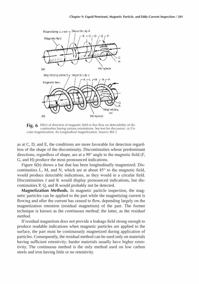
Chapter 9: Liquid Penetrant, Magnetic Particle, and Eddy-Current Inspection / 201
as at C, D, and E, the conditions are more favorable for detection regard-less of the shape of the discontinuity. Discontinuities whose predominant directions, regardless of shape, are at a 90° angle to the magnetic field (F, G, and H) produce the most pronounced indications.
Figure 6(b) shows a bar that has been longitudinally magnetized. Dis-continuities L, M, and N, which are at about 45° to the magnetic field, would produce detectable indications, as they would in a circular field. Discontinuities J and K would display pronounced indications, but dis-continuities P, Q, and R would probably not be detected.
Magnetization Methods� In magnetic particle inspection, the mag-netic particles can be applied to the part while the magnetizing current is flowing and after the current has ceased to flow, depending largely on the magnetization retention (residual magnetism) of the part. The former technique is known as the continuous method; the latter, as the residual method.
If residual magnetism does not provide a leakage field strong enough to produce readable indications when magnetic particles are applied to the surface, the part must be continuously magnetized during application of particles. Consequently, the residual method can be used only on materials having sufficient retentivity; harder materials usually have higher reten-tivity. The continuous method is the only method used on low carbon steels and iron having little or no retentivity.
Fig� 6 Effect of direction of magnetic field or flux flow on detectability of dis-continuities having various orientations. See text for discussion. (a) Cir-
cular magnetization. (b) Longitudinal magnetization. Source: Ref 2
202 / Inspection of Metals—Understanding the Basics
Magnetizing Current
Both direct and alternating currents are suitable to magnetize parts for magnetic particle inspection. Magnetic field strength, direction, and distri-bution are greatly affected by the current type used for magnetization.
The fields produced by direct and alternating current have different characteristics. The important difference in magnetic particle inspection is that fields produced by direct current generally penetrate the cross-section of the part, whereas fields produced by alternating current are confined to the metal at or near the surface of the part, which commonly is known as the skin effect. Therefore, alternating current should not be used to search for subsurface discontinuities.
Direct Current� The best source of direct current is rectified alternat-ing current. Both single-phase and three-phase alternating currents are furnished commercially. Rectifiers convert reversing alternating current to unidirectional current. Rectified three-phase alternating current is nearly equivalent to straight direct current for purposes of magnetic particle in-spection. The only difference between rectified three-phase alternating current and straight direct current is a slight ripple in the value of the recti-fied current, amounting for only about five percent of the maximum cur-rent value.
Alternating current, which must be single-phase when used directly to magnetize a part, is used directly from commercial power lines at a frequency of 50 or 60 Hz. When used for magnetizing, line voltage is stepped down by means of a transformer to the lower voltages required. Magnetizing currents of several thousand amperes often are used at the low voltages.
One problem in using alternating current is that residual magnetism in the part might be lower than that of the magnetism generated by the peak current of the alternating current cycle. This is because the level of resid-ual magnetism depends on where in the cycle the current is discontinued.
Power Sources
Portable equipment is available in lightweight (16 to 41 kg, or 35 to 90 lb) power source units that are easily transported to the inspection site. Generally, portable units are designed to use 115, 230, and 460 V alternat-ing current, and supply 750 to 1500 A magnetizing current outputs in half-wave or alternating current. Small, lightweight pulsed dc units that can produce up to 7000 A of magnetizing current also are available.
Mobile units generally are mounted on wheels to facilitate transport to an inspection site. Mobile equipment usually supplies full-wave, half-wave, and alternating magnetizing current outputs. Part inspection is ac-complished by use of flexible cables, yokes, prod contacts, contact clamps, and coils. Instruments and controls are mounted on the front of the unit. Magnetizing current is usually controlled using a remote control switch
Chapter 9: Liquid Penetrant, Magnetic Particle, and Eddy-Current Inspection / 203
connected to the unit by an electrical cord. Quick coupling connectors for connecting magnetizing cables are on the front of the unit. Mobile equip-ment is usually powered by single phase or three phase, 60 Hz alternating current (230 and 460 V), and has an output range of 1500 to 10,000 A.
Stationary equipment is available in both general purpose and special purpose units. The general purpose unit is primarily used in the wet method, and has a built-in tank containing a bath pump, which continu-ously agitates the bath and forces the fluid through hoses onto the part being inspected. Pneumatically operated contact heads, together with a rigid type coil, provide capabilities for both circular and longitudinal mag-netization. Self-contained ac and dc power supplies are available in am-perage ratings from 1000 to 10,000 A.
Stationary power packs function as high-amperage, magnetizing cur-rent sources used in conjunction with special fixtures, and with cable wrap and clamp and contact techniques. Rated output varies from a customary 4000 to 6000 A to as high as 30,000 A. Higher amperage units are used for overall magnetization of large forgings and castings, which otherwise would require systematic prod inspection at much lower current levels. Some units feature three output circuits, which are systematically ener-gized in rapid sequence, either electrically or mechanically, to effectively magnetize a part in several directions at virtually the same time. This al-lows exposure of discontinuities lying in any direction after only a single processing step.
Special purpose stationary units are designed to handle and inspect large quantities of similar items. Generally, conveyors, automatic mark-ers, and alarm systems are included in such units to expedite part handling and disposition.
Methods of Generating Magnetic Fields
A basic requirement of magnetic particle inspection is to properly mag-netize the part so leakage fields created by discontinuities attract magnetic particles. While permanent magnets can accomplish this to some degree, magnetization generally is produced using electromagnets and the mag-netic field associated with the flow of electric current. Basically, magneti-zation is derived from the circular magnetic field generated when an elec-tric current flows through a conductor. The direction of the field is dependent on the direction of current flow.
Yokes� Two basic types of yokes commonly used for magnetizing pur-poses are permanent magnets and electromagnetic yokes. Both are hand held and mobile.
Electromagnetic yokes (Fig. 7) consist of a coil wound around a U-shape core of soft iron. The legs of the yoke are either fixed or adjustable. Adjustable legs permit changing the contact spacing and the relative angle of contact to accommodate irregular shape parts. Unlike a permanent
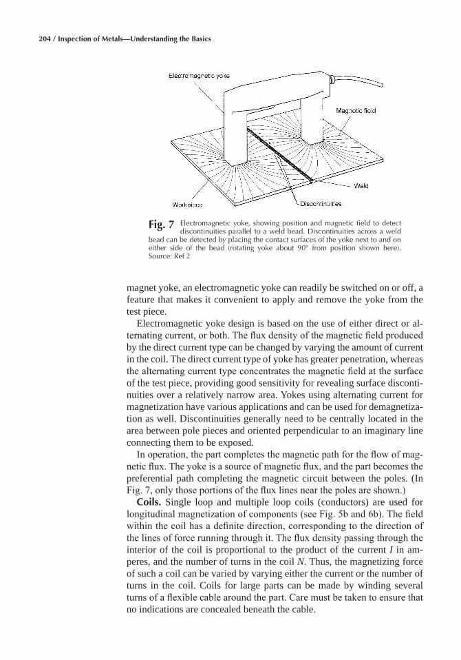
204 / Inspection of Metals—Understanding the Basics
magnet yoke, an electromagnetic yoke can readily be switched on or off, a feature that makes it convenient to apply and remove the yoke from the test piece.
Electromagnetic yoke design is based on the use of either direct or al-ternating current, or both. The flux density of the magnetic field produced by the direct current type can be changed by varying the amount of current in the coil. The direct current type of yoke has greater penetration, whereas the alternating current type concentrates the magnetic field at the surface of the test piece, providing good sensitivity for revealing surface disconti-nuities over a relatively narrow area. Yokes using alternating current for magnetization have various applications and can be used for demagnetiza-tion as well. Discontinuities generally need to be centrally located in the area between pole pieces and oriented perpendicular to an imaginary line connecting them to be exposed.
In operation, the part completes the magnetic path for the flow of mag-netic flux. The yoke is a source of magnetic flux, and the part becomes the preferential path completing the magnetic circuit between the poles. (In Fig. 7, only those portions of the flux lines near the poles are shown.)
Coils� Single loop and multiple loop coils (conductors) are used for longitudinal magnetization of components (see Fig. 5b and 6b). The field within the coil has a definite direction, corresponding to the direction of the lines of force running through it. The flux density passing through the interior of the coil is proportional to the product of the current I in am-peres, and the number of turns in the coil N. Thus, the magnetizing force of such a coil can be varied by varying either the current or the number of turns in the coil. Coils for large parts can be made by winding several turns of a flexible cable around the part. Care must be taken to ensure that no indications are concealed beneath the cable.
Fig� 7 Electromagnetic yoke, showing position and magnetic field to detect discontinuities parallel to a weld bead. Discontinuities across a weld
bead can be detected by placing the contact surfaces of the yoke next to and on either side of the bead (rotating yoke about 90° from position shown here). Source: Ref 2
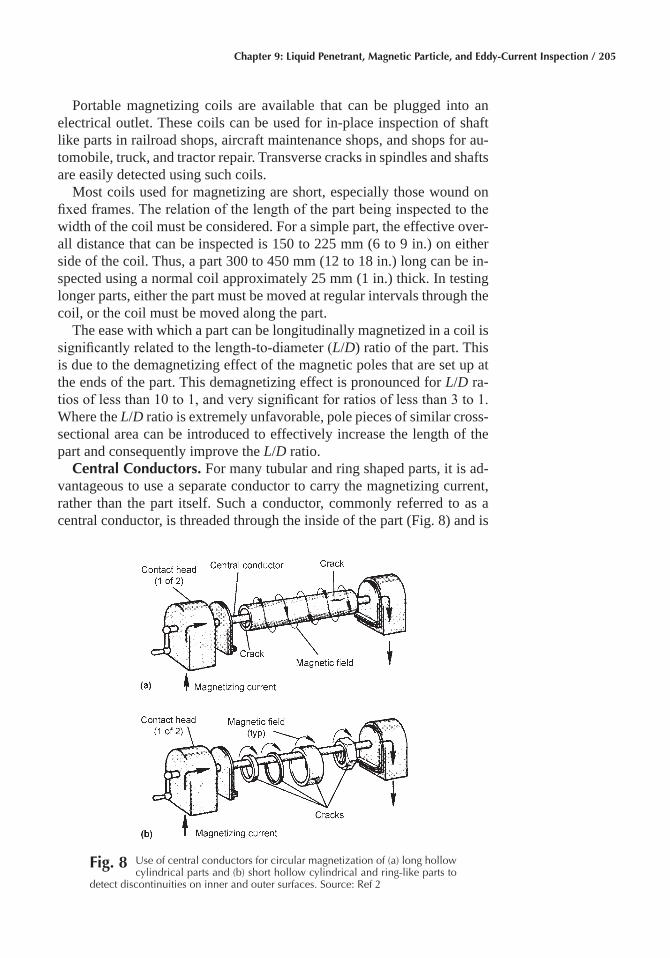
Chapter 9: Liquid Penetrant, Magnetic Particle, and Eddy-Current Inspection / 205
Portable magnetizing coils are available that can be plugged into an electrical outlet. These coils can be used for in-place inspection of shaft like parts in railroad shops, aircraft maintenance shops, and shops for au-tomobile, truck, and tractor repair. Transverse cracks in spindles and shafts are easily detected using such coils.
Most coils used for magnetizing are short, especially those wound on fixed frames. The relation of the length of the part being inspected to the width of the coil must be considered. For a simple part, the effective over-all distance that can be inspected is 150 to 225 mm (6 to 9 in.) on either side of the coil. Thus, a part 300 to 450 mm (12 to 18 in.) long can be in-spected using a normal coil approximately 25 mm (1 in.) thick. In testing longer parts, either the part must be moved at regular intervals through the coil, or the coil must be moved along the part.
The ease with which a part can be longitudinally magnetized in a coil is significantly related to the length-to-diameter (L/D) ratio of the part. This is due to the demagnetizing effect of the magnetic poles that are set up at the ends of the part. This demagnetizing effect is pronounced for L/D ra-tios of less than 10 to 1, and very significant for ratios of less than 3 to 1. Where the L/D ratio is extremely unfavorable, pole pieces of similar cross-sectional area can be introduced to effectively increase the length of the part and consequently improve the L/D ratio.
Central Conductors� For many tubular and ring shaped parts, it is ad-vantageous to use a separate conductor to carry the magnetizing current, rather than the part itself. Such a conductor, commonly referred to as a central conductor, is threaded through the inside of the part (Fig. 8) and is
Fig� 8 Use of central conductors for circular magnetization of (a) long hollow cylindrical parts and (b) short hollow cylindrical and ring-like parts to
detect discontinuities on inner and outer surfaces. Source: Ref 2
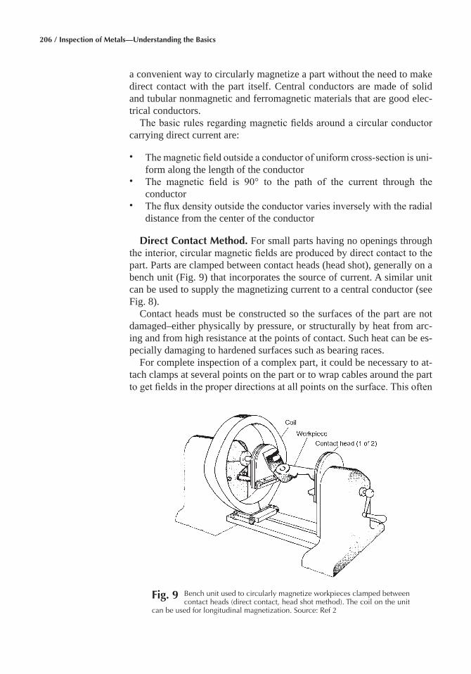
206 / Inspection of Metals—Understanding the Basics
a convenient way to circularly magnetize a part without the need to make direct contact with the part itself. Central conductors are made of solid and tubular nonmagnetic and ferromagnetic materials that are good elec-trical conductors.
The basic rules regarding magnetic fields around a circular conductor carrying direct current are:
• The magnetic field outside a conductor of uniform cross-section is uni-form along the length of the conductor
• The magnetic field is 90° to the path of the current through the conductor
• The flux density outside the conductor varies inversely with the radial distance from the center of the conductor
Direct Contact Method� For small parts having no openings through the interior, circular magnetic fields are produced by direct contact to the part. Parts are clamped between contact heads (head shot), generally on a bench unit (Fig. 9) that incorporates the source of current. A similar unit can be used to supply the magnetizing current to a central conductor (see Fig. 8).
Contact heads must be constructed so the surfaces of the part are not damaged–either physically by pressure, or structurally by heat from arc-ing and from high resistance at the points of contact. Such heat can be es-pecially damaging to hardened surfaces such as bearing races.
For complete inspection of a complex part, it could be necessary to at-tach clamps at several points on the part or to wrap cables around the part to get fields in the proper directions at all points on the surface. This often
Fig� 9 Bench unit used to circularly magnetize workpieces clamped between contact heads (direct contact, head shot method). The coil on the unit
can be used for longitudinal magnetization. Source: Ref 2
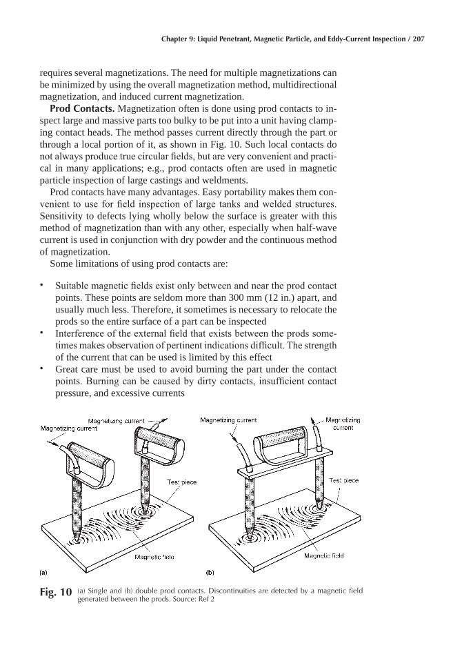
Chapter 9: Liquid Penetrant, Magnetic Particle, and Eddy-Current Inspection / 207
requires several magnetizations. The need for multiple magnetizations can be minimized by using the overall magnetization method, multidirectional magnetization, and induced current magnetization.
Prod Contacts� Magnetization often is done using prod contacts to in-spect large and massive parts too bulky to be put into a unit having clamp-ing contact heads. The method passes current directly through the part or through a local portion of it, as shown in Fig. 10. Such local contacts do not always produce true circular fields, but are very convenient and practi-cal in many applications; e.g., prod contacts often are used in magnetic particle inspection of large castings and weldments.
Prod contacts have many advantages. Easy portability makes them con-venient to use for field inspection of large tanks and welded structures. Sensitivity to defects lying wholly below the surface is greater with this method of magnetization than with any other, especially when half-wave current is used in conjunction with dry powder and the continuous method of magnetization.
Some limitations of using prod contacts are:
• Suitable magnetic fields exist only between and near the prod contact points. These points are seldom more than 300 mm (12 in.) apart, and usually much less. Therefore, it sometimes is necessary to relocate the prods so the entire surface of a part can be inspected
• Interference of the external field that exists between the prods some-times makes observation of pertinent indications difficult. The strength of the current that can be used is limited by this effect
• Great care must be used to avoid burning the part under the contact points. Burning can be caused by dirty contacts, insufficient contact pressure, and excessive currents
Fig� 10 (a) Single and (b) double prod contacts. Discontinuities are detected by a magnetic field generated between the prods. Source: Ref 2
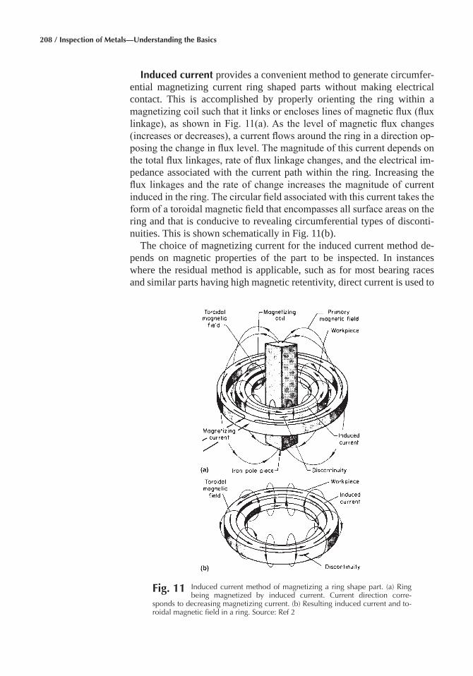
208 / Inspection of Metals—Understanding the Basics
Induced current provides a convenient method to generate circumfer-ential magnetizing current ring shaped parts without making electrical contact. This is accomplished by properly orienting the ring within a magnetizing coil such that it links or encloses lines of magnetic flux (flux linkage), as shown in Fig. 11(a). As the level of magnetic flux changes (increases or decreases), a current flows around the ring in a direction op-posing the change in flux level. The magnitude of this current depends on the total flux linkages, rate of flux linkage changes, and the electrical im-pedance associated with the current path within the ring. Increasing the flux linkages and the rate of change increases the magnitude of current induced in the ring. The circular field associated with this current takes the form of a toroidal magnetic field that encompasses all surface areas on the ring and that is conducive to revealing circumferential types of disconti-nuities. This is shown schematically in Fig. 11(b).
The choice of magnetizing current for the induced current method de-pends on magnetic properties of the part to be inspected. In instances where the residual method is applicable, such as for most bearing races and similar parts having high magnetic retentivity, direct current is used to
Fig� 11 Induced current method of magnetizing a ring shape part. (a) Ring being magnetized by induced current. Current direction corre-
sponds to decreasing magnetizing current. (b) Resulting induced current and to-roidal magnetic field in a ring. Source: Ref 2
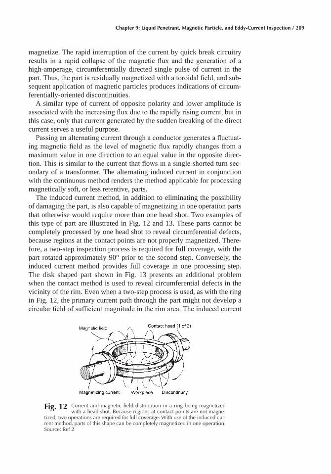
Chapter 9: Liquid Penetrant, Magnetic Particle, and Eddy-Current Inspection / 209
magnetize. The rapid interruption of the current by quick break circuitry results in a rapid collapse of the magnetic flux and the generation of a high-amperage, circumferentially directed single pulse of current in the part. Thus, the part is residually magnetized with a toroidal field, and sub-sequent application of magnetic particles produces indications of circum-ferentially-oriented discontinuities.
A similar type of current of opposite polarity and lower amplitude is associated with the increasing flux due to the rapidly rising current, but in this case, only that current generated by the sudden breaking of the direct current serves a useful purpose.
Passing an alternating current through a conductor generates a fluctuat-ing magnetic field as the level of magnetic flux rapidly changes from a maximum value in one direction to an equal value in the opposite direc-tion. This is similar to the current that flows in a single shorted turn sec-ondary of a transformer. The alternating induced current in conjunction with the continuous method renders the method applicable for processing magnetically soft, or less retentive, parts.
The induced current method, in addition to eliminating the possibility of damaging the part, is also capable of magnetizing in one operation parts that otherwise would require more than one head shot. Two examples of this type of part are illustrated in Fig. 12 and 13. These parts cannot be completely processed by one head shot to reveal circumferential defects, because regions at the contact points are not properly magnetized. There-fore, a two-step inspection process is required for full coverage, with the part rotated approximately 90° prior to the second step. Conversely, the induced current method provides full coverage in one processing step. The disk shaped part shown in Fig. 13 presents an additional problem when the contact method is used to reveal circumferential defects in the vicinity of the rim. Even when a two-step process is used, as with the ring in Fig. 12, the primary current path through the part might not develop a circular field of sufficient magnitude in the rim area. The induced current
Fig� 12 Current and magnetic field distribution in a ring being magnetized with a head shot. Because regions at contact points are not magne-
tized, two operations are required for full coverage. With use of the induced cur-rent method, parts of this shape can be completely magnetized in one operation. Source: Ref 2
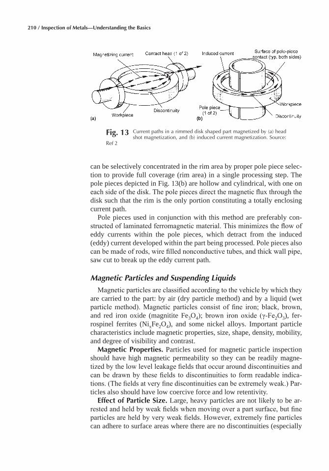
210 / Inspection of Metals—Understanding the Basics
can be selectively concentrated in the rim area by proper pole piece selec-tion to provide full coverage (rim area) in a single processing step. The pole pieces depicted in Fig. 13(b) are hollow and cylindrical, with one on each side of the disk. The pole pieces direct the magnetic flux through the disk such that the rim is the only portion constituting a totally enclosing current path.
Pole pieces used in conjunction with this method are preferably con-structed of laminated ferromagnetic material. This minimizes the flow of eddy currents within the pole pieces, which detract from the induced (eddy) current developed within the part being processed. Pole pieces also can be made of rods, wire filled nonconductive tubes, and thick wall pipe, saw cut to break up the eddy current path.
Magnetic Particles and Suspending Liquids
Magnetic particles are classified according to the vehicle by which they are carried to the part: by air (dry particle method) and by a liquid (wet particle method). Magnetic particles consist of fine iron; black, brown, and red iron oxide (magnitite Fe3O4); brown iron oxide (γ-Fe2O3), fer-rospinel ferrites (NixFe2O4), and some nickel alloys. Important particle characteristics include magnetic properties, size, shape, density, mobility, and degree of visibility and contrast.
Magnetic Properties� Particles used for magnetic particle inspection should have high magnetic permeability so they can be readily magne-tized by the low level leakage fields that occur around discontinuities and can be drawn by these fields to discontinuities to form readable indica-tions. (The fields at very fine discontinuities can be extremely weak.) Par-ticles also should have low coercive force and low retentivity.
Effect of Particle Size� Large, heavy particles are not likely to be ar-rested and held by weak fields when moving over a part surface, but fine particles are held by very weak fields. However, extremely fine particles can adhere to surface areas where there are no discontinuities (especially
Fig� 13 Current paths in a rimmed disk shaped part magnetized by (a) head shot magnetization, and (b) induced current magnetization. Source:
Ref 2
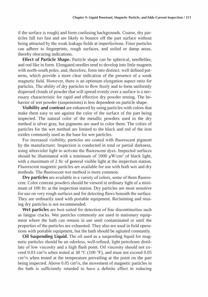
Chapter 9: Liquid Penetrant, Magnetic Particle, and Eddy-Current Inspection / 211
if the surface is rough) and form confusing backgrounds. Coarse, dry par-ticles fall too fast and are likely to bounce off the part surface without being attracted by the weak leakage fields at imperfections. Finer particles can adhere to fingerprints, rough surfaces, and soiled or damp areas, thereby obscuring indications.
Effect of Particle Shape� Particle shape can be spherical, needlelike, and rod like in form. Elongated needles tend to develop into little magnets with north-south poles, and, therefore, form into distinct, well defined pat-terns, which provide a more clear indication of the presence of a weak magnetic field. However, there is an optimum elongation aspect ratio for particles. The ability of dry particles to flow freely and to form uniformly dispersed clouds of powder that will spread evenly over a surface is a nec-essary characteristic for rapid and effective dry powder testing. The be-havior of wet powder (suspensions) is less dependent on particle shape.
Visibility and contrast are enhanced by using particles with colors that make them easy to see against the color of the surface of the part being inspected. The natural color of the metallic powders used in the dry method is silver gray, but pigments are used to color them. The colors of particles for the wet method are limited to the black and red of the iron oxides commonly used as the base for wet particles.
For increased visibility, particles are coated with fluorescent pigment by the manufacturer. Inspection is conducted in total or partial darkness, using ultraviolet light to activate the fluorescent dyes. Inspected surfaces should be illuminated with a minimum of 1000 μW/cm2 of black light, with a maximum of 2 ftc of general visible light at the inspection station. Fluorescent magnetic particles are available for use with both wet and dry methods. The fluorescent wet method is more common.
Dry particles are available in a variety of colors, some of them fluores-cent. Color contrast powders should be viewed in ordinary light of a mini-mum of 100 ftc at the inspection station. Dry particles are most sensitive for use on very rough surfaces and for detecting flaws beneath the surface. They are ordinarily used with portable equipment. Reclaiming and reus-ing dry particles is not recommended.
Wet particles are best suited for detection of fine discontinuities such as fatigue cracks. Wet particles commonly are used in stationary equip-ment where the bath can remain in use until contaminated or until the properties of the particles are exhausted. They also are used in field opera-tions with portable equipment, but the bath should be agitated constantly.
Oil Suspending Liquid� The oil used as a suspending liquid for mag-netic particles should be an odorless, well-refined, light petroleum distil-late of low viscosity and a high flash point. Oil viscosity should not ex-ceed 0.03 cm2/s when tested at 38 °C (100 °F), and must not exceed 0.05 cm2/s when tested at the temperature prevailing at the point on the part being inspected. Above 0.05 cm2/s, the movement of magnetic particles in the bath is sufficiently retarded to have a definite effect in reducing

212 / Inspection of Metals—Understanding the Basics
buildup; therefore, reducing visibility of an indication of a small disconti-nuity. Parts should be precleaned to remove oil and grease because oil from the surface builds up in the bath and increases its viscosity.
Water Suspending Liquid� The use of water instead of oil for mag-netic particle, wet method baths reduces costs and eliminates bath flam-mability. Water suspendible particle concentrates include the necessary wetting agents, dispersing agents, rust inhibitors, and antifoam agents.
Strength of the bath is a major factor in determining the quality of the indications obtained. The proportion of magnetic particles in the bath must be maintained at a uniform level. The strength of indications varies with varying concentration, which could cause misinterpretation of indi-cations. Fine indications can be missed entirely with a weak bath. High concentrations produce a confusing background and excessive adherence of particles at external poles, which interferes with distinct indications of extremely fine discontinuities.
The best method to ensure optimum bath concentration for any given combination of equipment, bath application, and type of part and disconti-nuities involved, is to test the bath using parts with known discontinuities. Bath strength can be adjusted until satisfactory indications are obtained. This bath concentration can then be adopted as standard for similar conditions.
Bath concentration can be measured reasonably accurately using the settling test. In the test, 100 mL (0.03 gal) of well agitated bath is placed in a pear shape centrifuge tube. The volume of solid material that settles out after a predetermined interval (usually 30 minutes) is measured on the graduated cylindrical part of the tube. Dirt in the bath also will settle and usually shows as a separate layer on top of the oxide. The layer of dirt usu-ally is easily distinguishable because it is different in color from the mag-netic particles.
Ultraviolet Light
A mercury vapor lamp is a convenient source of ultraviolet light, emit-ting a light spectrum that has several intensity peaks within a wide band of wavelengths. When used for a specific purpose, emitted light is passed through a suitable filter so only a relatively narrow band of ultraviolet wavelength is available. For example, a band in the long wave ultraviolet spectrum is used for fluorescent liquid penetrant or magnetic particle inspection.
Fluorescence is the quality of an element or combination of elements to absorb the energy of light at one frequency and emit light of a different frequency. Fluorescent materials used in liquid penetrant and magnetic particle inspection are combinations of elements selected to absorb light in the peak energy band of the mercury vapor lamp fitted with a Kopp glass filter. This peak occurs at about 365 nm (14.4 μin.). The ability of fluorescent materials to emit light in the greenish-yellow wavelengths of
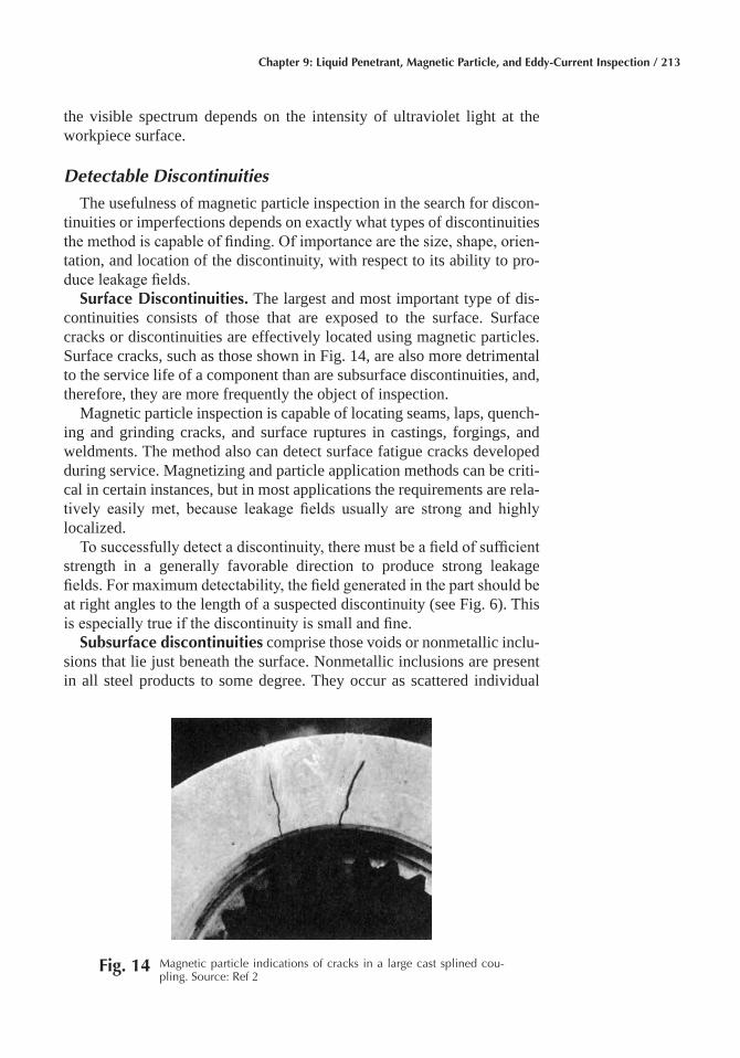
Chapter 9: Liquid Penetrant, Magnetic Particle, and Eddy-Current Inspection / 213
the visible spectrum depends on the intensity of ultraviolet light at the workpiece surface.
Detectable Discontinuities
The usefulness of magnetic particle inspection in the search for discon-tinuities or imperfections depends on exactly what types of discontinuities the method is capable of finding. Of importance are the size, shape, orien-tation, and location of the discontinuity, with respect to its ability to pro-duce leakage fields.
Surface Discontinuities� The largest and most important type of dis-continuities consists of those that are exposed to the surface. Surface cracks or discontinuities are effectively located using magnetic particles. Surface cracks, such as those shown in Fig. 14, are also more detrimental to the service life of a component than are subsurface discontinuities, and, therefore, they are more frequently the object of inspection.
Magnetic particle inspection is capable of locating seams, laps, quench-ing and grinding cracks, and surface ruptures in castings, forgings, and weldments. The method also can detect surface fatigue cracks developed during service. Magnetizing and particle application methods can be criti-cal in certain instances, but in most applications the requirements are rela-tively easily met, because leakage fields usually are strong and highly localized.
To successfully detect a discontinuity, there must be a field of sufficient strength in a generally favorable direction to produce strong leakage fields. For maximum detectability, the field generated in the part should be at right angles to the length of a suspected discontinuity (see Fig. 6). This is especially true if the discontinuity is small and fine.
Subsurface discontinuities comprise those voids or nonmetallic inclu-sions that lie just beneath the surface. Nonmetallic inclusions are present in all steel products to some degree. They occur as scattered individual
Fig� 14 Magnetic particle indications of cracks in a large cast splined cou-pling. Source: Ref 2
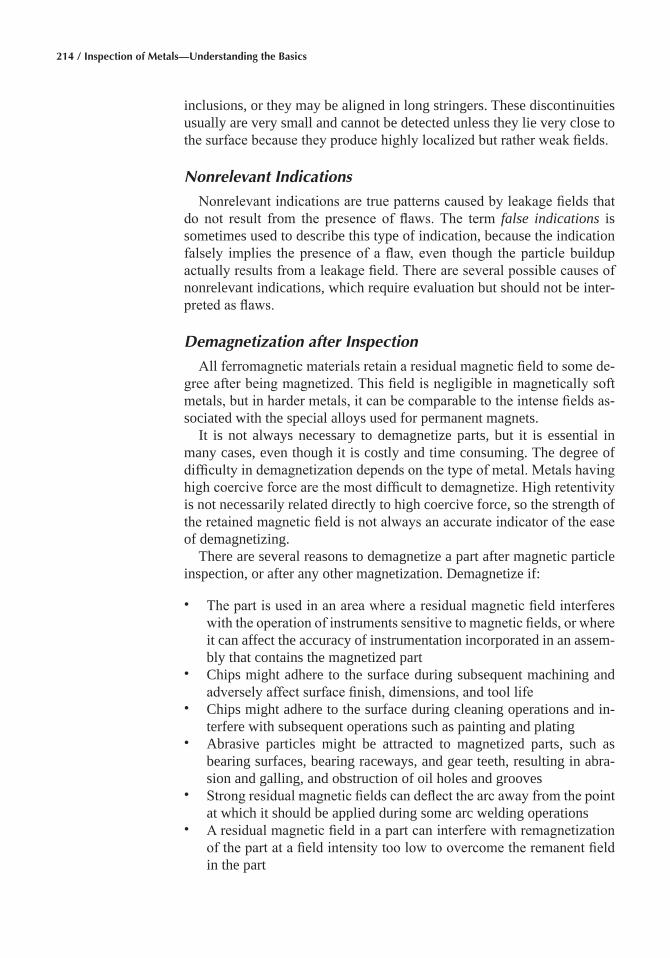
214 / Inspection of Metals—Understanding the Basics
inclusions, or they may be aligned in long stringers. These discontinuities usually are very small and cannot be detected unless they lie very close to the surface because they produce highly localized but rather weak fields.
Nonrelevant Indications
Nonrelevant indications are true patterns caused by leakage fields that do not result from the presence of flaws. The term false indications is sometimes used to describe this type of indication, because the indication falsely implies the presence of a flaw, even though the particle buildup actually results from a leakage field. There are several possible causes of nonrelevant indications, which require evaluation but should not be inter-preted as flaws.
Demagnetization after Inspection
All ferromagnetic materials retain a residual magnetic field to some de-gree after being magnetized. This field is negligible in magnetically soft metals, but in harder metals, it can be comparable to the intense fields as-sociated with the special alloys used for permanent magnets.
It is not always necessary to demagnetize parts, but it is essential in many cases, even though it is costly and time consuming. The degree of difficulty in demagnetization depends on the type of metal. Metals having high coercive force are the most difficult to demagnetize. High retentivity is not necessarily related directly to high coercive force, so the strength of the retained magnetic field is not always an accurate indicator of the ease of demagnetizing.
There are several reasons to demagnetize a part after magnetic particle inspection, or after any other magnetization. Demagnetize if:
• The part is used in an area where a residual magnetic field interferes with the operation of instruments sensitive to magnetic fields, or where it can affect the accuracy of instrumentation incorporated in an assem-bly that contains the magnetized part
• Chips might adhere to the surface during subsequent machining and adversely affect surface finish, dimensions, and tool life
• Chips might adhere to the surface during cleaning operations and in-terfere with subsequent operations such as painting and plating
• Abrasive particles might be attracted to magnetized parts, such as bearing surfaces, bearing raceways, and gear teeth, resulting in abra-sion and galling, and obstruction of oil holes and grooves
• Strong residual magnetic fields can deflect the arc away from the point at which it should be applied during some arc welding operations
• A residual magnetic field in a part can interfere with remagnetization of the part at a field intensity too low to overcome the remanent field in the part
Chapter 9: Liquid Penetrant, Magnetic Particle, and Eddy-Current Inspection / 215
Demagnetization might not be necessary if:
• Parts are made of magnetically soft steel having low retentivity; such parts usually will become demagnetized as soon as they are removed from the magnetizing source
• The parts are subsequently heated above their Curie point and conse-quently lose their magnetic properties
• The magnetic field is such that it will not affect the function of the part in service
• The part is to be remagnetized for further magnetic particle inspection or for some secondary operation in which a magnetic plate or chuck may be used to hold the part.
The last reasons for demagnetizing and not demagnetizing seem to be contradictory. The establishment of a longitudinal field after circular mag-netization negates the circular field because two fields in different direc-tions cannot exist in the same part at the same time. If the magnetizing force is not of sufficient strength to establish the longitudinal field it should be increased, or other steps taken to ensure that the longitudinal field actually has been established. The same is true in changing from longitudinal to circular magnetization. If the two fields (longitudinal and circular) are applied simultaneously, a field is established that is a vector combination of the two in both strength and direction. However, if the fields are impressed successively, the last field applied, if strong enough to establish itself in the part, destroys the remanent field from the previous magnetization.
Eddy Current Inspection
Eddy current inspection is based on the principles of electromagnetic induction and is used to identify or differentiate a wide variety of physical, structural, and metallurgical conditions in electrically conductive ferro-magnetic and nonferromagnetic metals and metal parts. Eddy current in-spection is used:
• To measure and identify conditions and properties related to electrical conductivity, magnetic permeability, and physical dimensions (pri-mary factors affecting eddy current response)
• To detect seams, laps, cracks, voids, and inclusions • To sort dissimilar metals and detect differences in their composition,
microstructure, and other properties (such as grain size, heat treat-ment, and hardness)
• To measure the thickness of a nonconductive coating on a conductive metal, or the thickness of a nonmagnetic metal coating on a magnetic metal
216 / Inspection of Metals—Understanding the Basics
Because eddy current inspection is an electromagnetic induction tech-nique, it does not require direct electrical contact with the part being in-spected. The eddy current method is adaptable to high speed inspection, and because it is nondestructive, it can be used to inspect an entire produc-tion output if desired. The method is based on indirect measurement, and the correlation between instrument readings and the structural characteris-tics and serviceability of parts being inspected must be carefully and re-peatedly established.
Eddy current inspection is extremely versatile, which is both an advan-tage and a disadvantage. The advantage is that the method can be applied to many inspection problems provided that the physical requirements of the material are compatible with the inspection method. However, in many applications, the sensitivity of the method to many inherent material prop-erties and characteristics can be a disadvantage. Some variables in a mate-rial that are not important in terms of material or part serviceability can cause instrument signals that mask critical variables or are mistakenly in-terpreted to be caused by critical variables.
Eddy Current Versus Magnetic Inspection Methods� In eddy current inspection, eddy currents create their own electromagnetic field, which is sensed either through the effects of the field on the primary exciting coil or by means of an independent sensor. In nonferromagnetic materials, the secondary electromagnetic field is derived exclusively from eddy cur-rents. However, with ferromagnetic materials, additional magnetic effects occur that usually are of sufficient magnitude to overshadow the basic eddy current effects from electrical conductivity only. These magnetic ef-fects result from the magnetic permeability of the material being in-spected, and can be virtually eliminated by magnetizing the material to saturation in a static (direct current) magnetic field. When the permeabil-ity effect is not eliminated, the inspection method is more correctly cate-gorized as electromagnetic or magnetoinductive inspection.
Principles of Operation
Functions of a Basic System� The part to be inspected is placed within or adjacent to an electrical coil in which an alternating current is flowing. As shown in Fig. 15, the alternating current, called the exciting current, causes eddy currents to flow in the part as a result of electromagnetic in-duction. These currents flow within closed loops in the part, and their magnitude and timing (or phase) depend on (a) the original or primary field established by the exciting currents, (b) the electrical properties of the part, and (c) the electromagnetic fields established by currents flowing within the part.
The electromagnetic field in the region in the part and surrounding the part depends on both the exciting current from the coil and the eddy cur-rents flowing in the part. The flow of eddy currents depends on the electri-
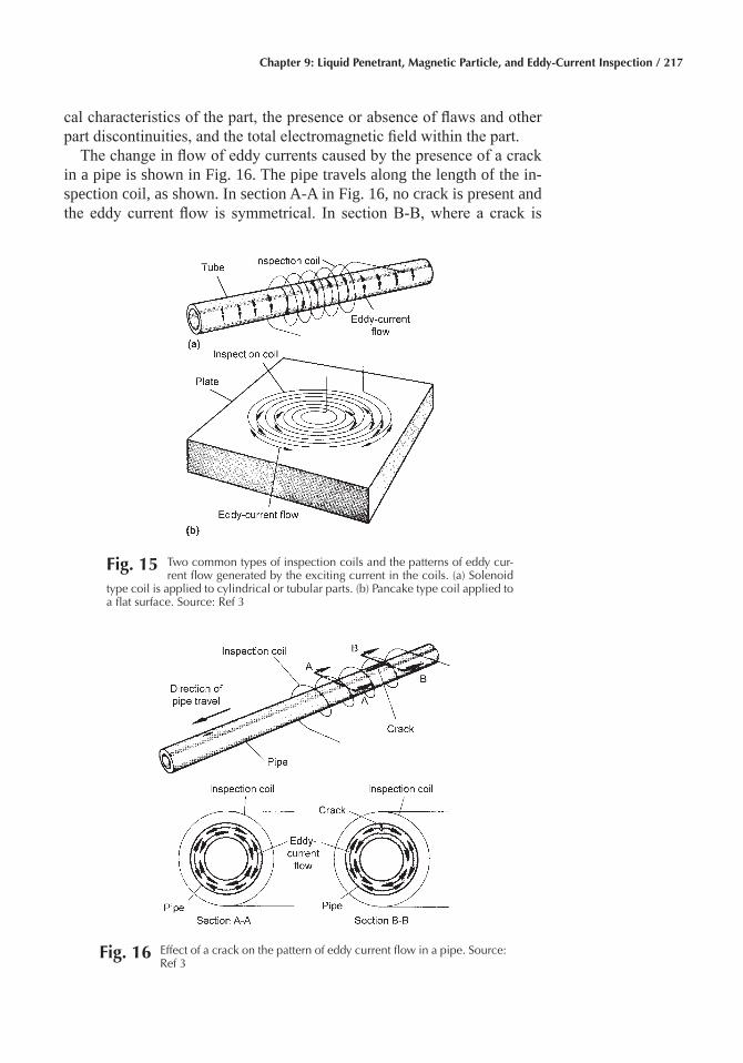
Chapter 9: Liquid Penetrant, Magnetic Particle, and Eddy-Current Inspection / 217
cal characteristics of the part, the presence or absence of flaws and other part discontinuities, and the total electromagnetic field within the part.
The change in flow of eddy currents caused by the presence of a crack in a pipe is shown in Fig. 16. The pipe travels along the length of the in-spection coil, as shown. In section A-A in Fig. 16, no crack is present and the eddy current flow is symmetrical. In section B-B, where a crack is
Fig� 15 Two common types of inspection coils and the patterns of eddy cur-rent flow generated by the exciting current in the coils. (a) Solenoid
type coil is applied to cylindrical or tubular parts. (b) Pancake type coil applied to a flat surface. Source: Ref 3
Fig� 16 Effect of a crack on the pattern of eddy current flow in a pipe. Source: Ref 3

218 / Inspection of Metals—Understanding the Basics
present, the eddy current flow is impeded and changed in direction, caus-ing significant changes in the associated electromagnetic field. The condi-tion of the part can be monitored by observing the effect of the resulting field on the electrical characteristics of the exciting coil, such as its electri-cal impedance, induced voltage, and induced currents. Alternatively, the effect of the electromagnetic field can be monitored by observing the in-duced voltage in one or more other coils placed within the field near the part being monitored.
Each and all of these changes can have an effect on the exciting coil and other coil or coils used to sense the electromagnetic field adjacent to a part. The effects most often used to monitor the condition of the part being inspected are the electrical impedance of the coil and the induced voltage of either the exciting coil or other adjacent coil or coils.
Eddy current systems vary in complexity depending on individual in-spection requirements. However, most systems must provide for the fol-lowing functions:
• Excitation of the inspection coil with one or more frequencies • Modulation of the inspection coil output signal by the part being
inspected • Processing of the inspection coil signal prior to amplification • Amplification of the inspection coil signals • Detection or demodulation of the inspection coil signal, usually ac-
companied by some analysis or discrimination of signals, which can be performed by a computer
• Display of signals on an instrument such as a meter, an oscilloscope, an oscillograph, and a strip chart recorder; or recording of signals on paper punch tape and magnetic tape
• Handling of the part being inspected and support of inspection coil assembly
Elements of a typical inspection system are shown schematically in Fig. 17. The particular elements in Fig. 17 are for a system developed to inspect bar or tubing. The generator supplies excitation current to the in-spection coil and a synchronizing signal to the phase shifter, which pro-vides switching signals for the detector. The loading of the inspection coil by the part being inspected modulates the electromagnetic field of the coil. This causes changes in the amplitude and phase of the inspection coil volt-age output.
The output of the inspection coil is fed to the amplifier and detected or demodulated by the detector. The demodulated output signal, after some further filtering and analyzing, is then displayed on an oscilloscope or a chart recorder. The displayed signals, having been detected or demodu-lated, vary at a much slower rate, depending on (a) the rate of changing the inspection probe from one part being inspected to another; (b) the
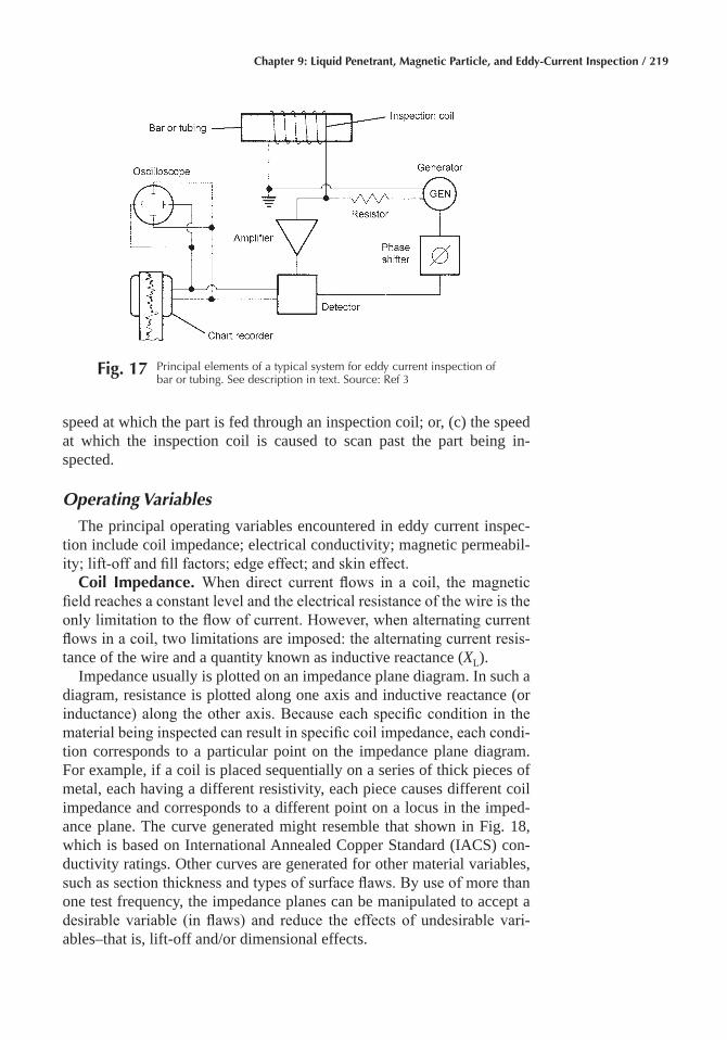
Chapter 9: Liquid Penetrant, Magnetic Particle, and Eddy-Current Inspection / 219
speed at which the part is fed through an inspection coil; or, (c) the speed at which the inspection coil is caused to scan past the part being in- spected.
Operating Variables
The principal operating variables encountered in eddy current inspec-tion include coil impedance; electrical conductivity; magnetic permeabil-ity; lift-off and fill factors; edge effect; and skin effect.
Coil Impedance� When direct current flows in a coil, the magnetic field reaches a constant level and the electrical resistance of the wire is the only limitation to the flow of current. However, when alternating current flows in a coil, two limitations are imposed: the alternating current resis-tance of the wire and a quantity known as inductive reactance (XL).
Impedance usually is plotted on an impedance plane diagram. In such a diagram, resistance is plotted along one axis and inductive reactance (or inductance) along the other axis. Because each specific condition in the material being inspected can result in specific coil impedance, each condi-tion corresponds to a particular point on the impedance plane diagram. For example, if a coil is placed sequentially on a series of thick pieces of metal, each having a different resistivity, each piece causes different coil impedance and corresponds to a different point on a locus in the imped-ance plane. The curve generated might resemble that shown in Fig. 18, which is based on International Annealed Copper Standard (IACS) con-ductivity ratings. Other curves are generated for other material variables, such as section thickness and types of surface flaws. By use of more than one test frequency, the impedance planes can be manipulated to accept a desirable variable (in flaws) and reduce the effects of undesirable vari-ables–that is, lift-off and/or dimensional effects.
Fig� 17 Principal elements of a typical system for eddy current inspection of bar or tubing. See description in text. Source: Ref 3
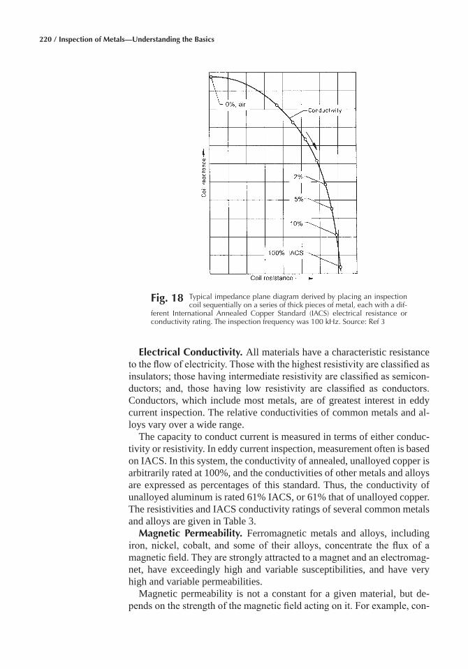
220 / Inspection of Metals—Understanding the Basics
Electrical Conductivity� All materials have a characteristic resistance to the flow of electricity. Those with the highest resistivity are classified as insulators; those having intermediate resistivity are classified as semicon-ductors; and, those having low resistivity are classified as conductors. Conductors, which include most metals, are of greatest interest in eddy current inspection. The relative conductivities of common metals and al-loys vary over a wide range.
The capacity to conduct current is measured in terms of either conduc-tivity or resistivity. In eddy current inspection, measurement often is based on IACS. In this system, the conductivity of annealed, unalloyed copper is arbitrarily rated at 100%, and the conductivities of other metals and alloys are expressed as percentages of this standard. Thus, the conductivity of unalloyed aluminum is rated 61% IACS, or 61% that of unalloyed copper. The resistivities and IACS conductivity ratings of several common metals and alloys are given in Table 3.
Magnetic Permeability� Ferromagnetic metals and alloys, including iron, nickel, cobalt, and some of their alloys, concentrate the flux of a magnetic field. They are strongly attracted to a magnet and an electromag-net, have exceedingly high and variable susceptibilities, and have very high and variable permeabilities.
Magnetic permeability is not a constant for a given material, but de-pends on the strength of the magnetic field acting on it. For example, con-
Fig� 18 Typical impedance plane diagram derived by placing an inspection coil sequentially on a series of thick pieces of metal, each with a dif-
ferent International Annealed Copper Standard (IACS) electrical resistance or conductivity rating. The inspection frequency was 100 kHz. Source: Ref 3
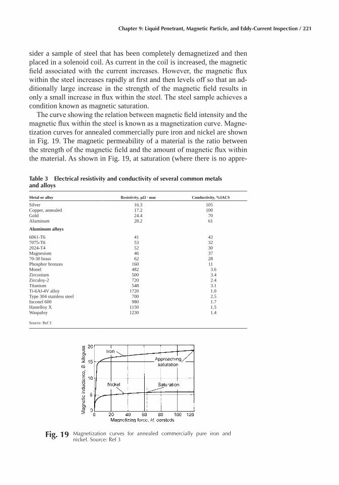
Chapter 9: Liquid Penetrant, Magnetic Particle, and Eddy-Current Inspection / 221
sider a sample of steel that has been completely demagnetized and then placed in a solenoid coil. As current in the coil is increased, the magnetic field associated with the current increases. However, the magnetic flux within the steel increases rapidly at first and then levels off so that an ad-ditionally large increase in the strength of the magnetic field results in only a small increase in flux within the steel. The steel sample achieves a condition known as magnetic saturation.
The curve showing the relation between magnetic field intensity and the magnetic flux within the steel is known as a magnetization curve. Magne-tization curves for annealed commercially pure iron and nickel are shown in Fig. 19. The magnetic permeability of a material is the ratio between the strength of the magnetic field and the amount of magnetic flux within the material. As shown in Fig. 19, at saturation (where there is no appre-
Table 3 Electrical resistivity and conductivity of several common metals and alloys
Metal or alloy Resistivity, μΩ · mm Conductivity, %IACS
Silver 16.3 105Copper, annealed 17.2 100Gold 24.4 70Aluminum 28.2 61
Aluminum alloys
6061-T6 41 427075-T6 53 322024-T4 52 30Magnesium 46 3770-30 brass 62 28Phosphor bronzes 160 11Monel 482 3.6Zirconium 500 3.4Zircaloy-2 720 2.4Titanium 548 3.1Ti-6Al-4V alloy 1720 1.0Type 304 stainless steel 700 2.5Inconel 600 980 1.7Hastelloy X 1150 1.5Waspaloy 1230 1.4
Source: Ref 3
Fig� 19 Magnetization curves for annealed commercially pure iron and nickel. Source: Ref 3
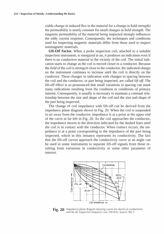
222 / Inspection of Metals—Understanding the Basics
ciable change in induced flux in the material for a change in field strength) the permeability is nearly constant for small changes in field strength. The magnetic permeability of the material being inspected strongly influences the eddy current response. Consequently, the techniques and conditions used for inspecting magnetic materials differ from those used to inspect nonmagnetic materials.
Lift-Off Factor� When a probe inspection coil, attached to a suitable inspection instrument, is energized in air, it produces an indication even if there is no conductive material in the vicinity of the coil. The initial indi-cation starts to change as the coil is moved closer to a conductor. Because the field of the coil is strongest close to the conductor, the indicated change on the instrument continues to increase until the coil is directly on the conductor. These changes in indication with changes in spacing between the coil and the conductor, or part being inspected, are called lift off. The lift-off effect is so pronounced that small variations in spacing can mask many indications resulting from the condition or conditions of primary interest. Consequently, it usually is necessary to maintain a constant rela-tionship between the size and shape of the coil and the size and shape of the part being inspected.
The change of coil impedance with lift-off can be derived from the impedance plane diagram shown in Fig. 20. When the coil is suspended in air away from the conductor, impedance is at a point at the upper end of the curve at far left in Fig. 20. As the coil approaches the conductor, the impedance moves in the direction indicated by the dashed lines until the coil is in contact with the conductor. When contact occurs, the im-pedance is at a point corresponding to the impedance of the part being inspected, which in this instance represents its conductivity. The fact that the lift-off curves approach the conductivity curve at an angle can be used in some instruments to separate lift-off signals from those re-sulting from variations in conductivity or some other parameter of interest.
Fig� 20 Impedance plane diagram showing curves for electrical conductivity and lift off. Inspection frequency was 100 kHz. Source: Ref 3
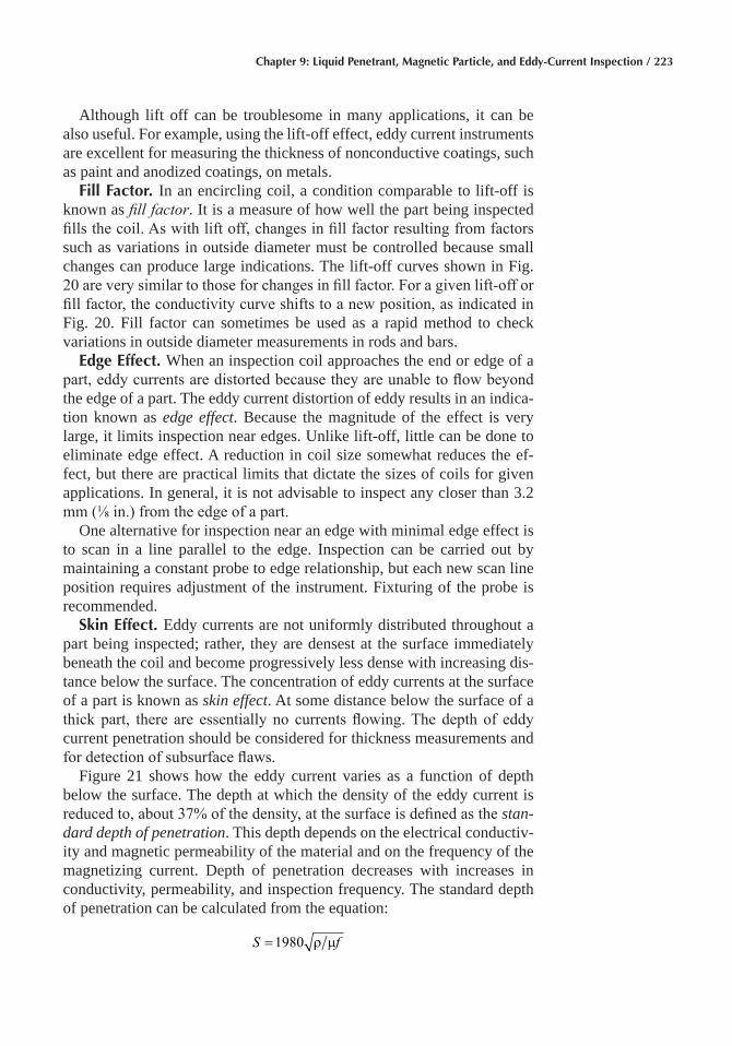
Chapter 9: Liquid Penetrant, Magnetic Particle, and Eddy-Current Inspection / 223
Although lift off can be troublesome in many applications, it can be also useful. For example, using the lift-off effect, eddy current instruments are excellent for measuring the thickness of nonconductive coatings, such as paint and anodized coatings, on metals.
Fill Factor� In an encircling coil, a condition comparable to lift-off is known as fill factor. It is a measure of how well the part being inspected fills the coil. As with lift off, changes in fill factor resulting from factors such as variations in outside diameter must be controlled because small changes can produce large indications. The lift-off curves shown in Fig. 20 are very similar to those for changes in fill factor. For a given lift-off or fill factor, the conductivity curve shifts to a new position, as indicated in Fig. 20. Fill factor can sometimes be used as a rapid method to check variations in outside diameter measurements in rods and bars.
Edge Effect� When an inspection coil approaches the end or edge of a part, eddy currents are distorted because they are unable to flow beyond the edge of a part. The eddy current distortion of eddy results in an indica-tion known as edge effect. Because the magnitude of the effect is very large, it limits inspection near edges. Unlike lift-off, little can be done to eliminate edge effect. A reduction in coil size somewhat reduces the ef-fect, but there are practical limits that dictate the sizes of coils for given applications. In general, it is not advisable to inspect any closer than 3.2 mm (⅛ in.) from the edge of a part.
One alternative for inspection near an edge with minimal edge effect is to scan in a line parallel to the edge. Inspection can be carried out by maintaining a constant probe to edge relationship, but each new scan line position requires adjustment of the instrument. Fixturing of the probe is recommended.
Skin Effect� Eddy currents are not uniformly distributed throughout a part being inspected; rather, they are densest at the surface immediately beneath the coil and become progressively less dense with increasing dis-tance below the surface. The concentration of eddy currents at the surface of a part is known as skin effect. At some distance below the surface of a thick part, there are essentially no currents flowing. The depth of eddy current penetration should be considered for thickness measurements and for detection of subsurface flaws.
Figure 21 shows how the eddy current varies as a function of depth below the surface. The depth at which the density of the eddy current is reduced to, about 37% of the density, at the surface is defined as the stan-dard depth of penetration. This depth depends on the electrical conductiv-ity and magnetic permeability of the material and on the frequency of the magnetizing current. Depth of penetration decreases with increases in conductivity, permeability, and inspection frequency. The standard depth of penetration can be calculated from the equation:
S f=1980 ρ µ
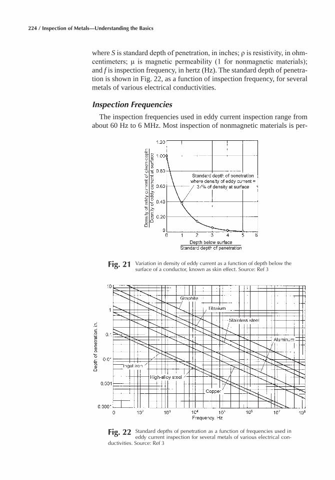
224 / Inspection of Metals—Understanding the Basics
where S is standard depth of penetration, in inches; ρ is resistivity, in ohm-centimeters; μ is magnetic permeability (1 for nonmagnetic materials); and f is inspection frequency, in hertz (Hz). The standard depth of penetra-tion is shown in Fig. 22, as a function of inspection frequency, for several metals of various electrical conductivities.
Inspection Frequencies
The inspection frequencies used in eddy current inspection range from about 60 Hz to 6 MHz. Most inspection of nonmagnetic materials is per-
Fig� 21 Variation in density of eddy current as a function of depth below the surface of a conductor, known as skin effect. Source: Ref 3
Fig� 22 Standard depths of penetration as a function of frequencies used in eddy current inspection for several metals of various electrical con-
ductivities. Source: Ref 3
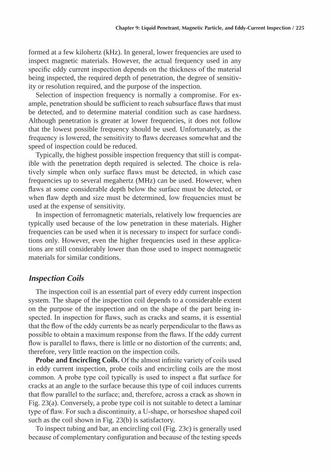
Chapter 9: Liquid Penetrant, Magnetic Particle, and Eddy-Current Inspection / 225
formed at a few kilohertz (kHz). In general, lower frequencies are used to inspect magnetic materials. However, the actual frequency used in any specific eddy current inspection depends on the thickness of the material being inspected, the required depth of penetration, the degree of sensitiv-ity or resolution required, and the purpose of the inspection.
Selection of inspection frequency is normally a compromise. For ex-ample, penetration should be sufficient to reach subsurface flaws that must be detected, and to determine material condition such as case hardness. Although penetration is greater at lower frequencies, it does not follow that the lowest possible frequency should be used. Unfortunately, as the frequency is lowered, the sensitivity to flaws decreases somewhat and the speed of inspection could be reduced.
Typically, the highest possible inspection frequency that still is compat-ible with the penetration depth required is selected. The choice is rela-tively simple when only surface flaws must be detected, in which case frequencies up to several megahertz (MHz) can be used. However, when flaws at some considerable depth below the surface must be detected, or when flaw depth and size must be determined, low frequencies must be used at the expense of sensitivity.
In inspection of ferromagnetic materials, relatively low frequencies are typically used because of the low penetration in these materials. Higher frequencies can be used when it is necessary to inspect for surface condi-tions only. However, even the higher frequencies used in these applica-tions are still considerably lower than those used to inspect nonmagnetic materials for similar conditions.
Inspection Coils
The inspection coil is an essential part of every eddy current inspection system. The shape of the inspection coil depends to a considerable extent on the purpose of the inspection and on the shape of the part being in-spected. In inspection for flaws, such as cracks and seams, it is essential that the flow of the eddy currents be as nearly perpendicular to the flaws as possible to obtain a maximum response from the flaws. If the eddy current flow is parallel to flaws, there is little or no distortion of the currents; and, therefore, very little reaction on the inspection coils.
Probe and Encircling Coils� Of the almost infinite variety of coils used in eddy current inspection, probe coils and encircling coils are the most common. A probe type coil typically is used to inspect a flat surface for cracks at an angle to the surface because this type of coil induces currents that flow parallel to the surface; and, therefore, across a crack as shown in Fig. 23(a). Conversely, a probe type coil is not suitable to detect a laminar type of flaw. For such a discontinuity, a U-shape, or horseshoe shaped coil such as the coil shown in Fig. 23(b) is satisfactory.
To inspect tubing and bar, an encircling coil (Fig. 23c) is generally used because of complementary configuration and because of the testing speeds
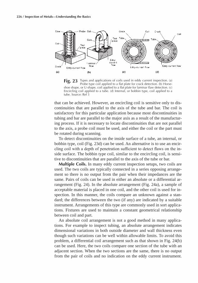
226 / Inspection of Metals—Understanding the Basics
that can be achieved. However, an encircling coil is sensitive only to dis-continuities that are parallel to the axis of the tube and bar. The coil is satisfactory for this particular application because most discontinuities in tubing and bar are parallel to the major axis as a result of the manufactur-ing process. If it is necessary to locate discontinuities that are not parallel to the axis, a probe coil must be used, and either the coil or the part must be rotated during scanning.
To detect discontinuities on the inside surface of a tube, an internal, or bobbin type, coil (Fig. 23d) can be used. An alternative is to use an encir-cling coil with a depth of penetration sufficient to detect flaws on the in-side surface. The bobbin type coil, similar to the encircling coil, is sensi-tive to discontinuities that are parallel to the axis of the tube or bar.
Multiple Coils� In many eddy current inspection setups, two coils are used. The two coils are typically connected in a series opposing arrange-ment so there is no output from the pair when their impedances are the same. Pairs of coils can be used in either an absolute or a differential ar-rangement (Fig. 24). In the absolute arrangement (Fig. 24a), a sample of acceptable material is placed in one coil, and the other coil is used for in-spection. In this manner, the coils compare an unknown against a stan-dard; the differences between the two (if any) are indicated by a suitable instrument. Arrangements of this type are commonly used in sort applica-tions. Fixtures are used to maintain a constant geometrical relationship between coil and part.
An absolute coil arrangement is not a good method in many applica-tions. For example to inspect tubing, an absolute arrangement indicates dimensional variations in both outside diameter and wall thickness even though such variations can be well within allowable limits. To avoid this problem, a differential coil arrangement such as that shown in Fig. 24(b) can be used. Here, the two coils compare one section of the tube with an adjacent section. When the two sections are the same, there is no output from the pair of coils and no indication on the eddy current instrument.
Fig� 23 Types and applications of coils used in eddy current inspection. (a) Probe type coil applied to a flat plate for crack detection. (b) Horse-
shoe shape, or U-shape, coil applied to a flat plate for laminar flaw detection. (c) Encircling coil applied to a tube. (d) Internal, or bobbin type, coil applied to a tube. Source: Ref 3
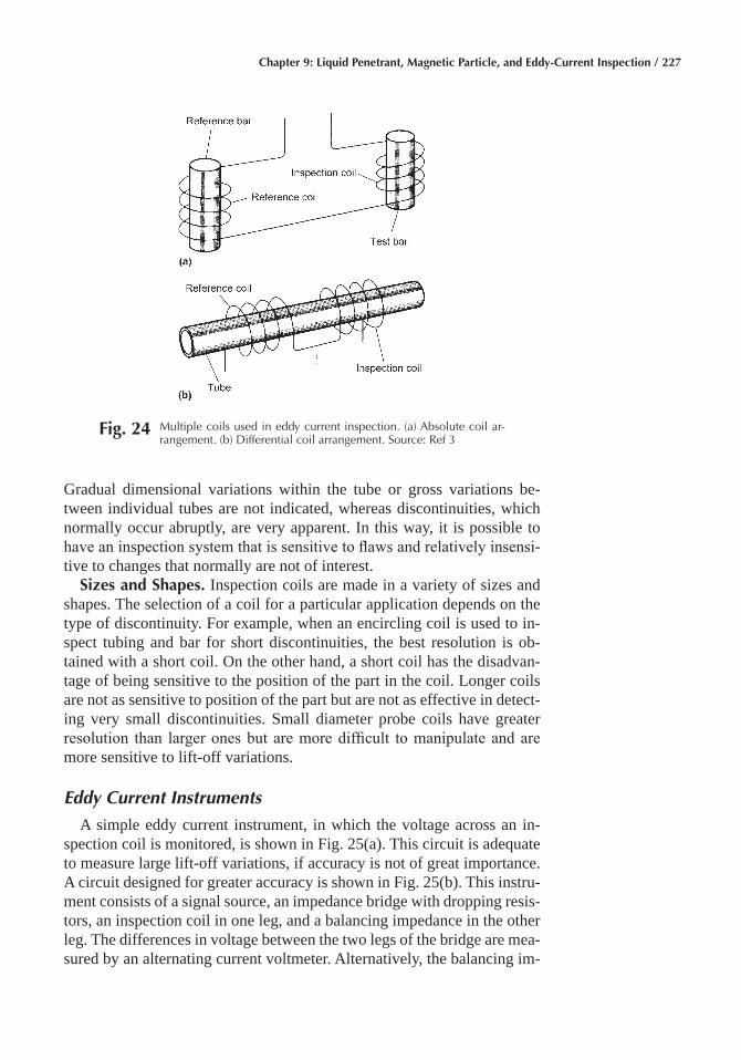
Chapter 9: Liquid Penetrant, Magnetic Particle, and Eddy-Current Inspection / 227
Gradual dimensional variations within the tube or gross variations be-tween individual tubes are not indicated, whereas discontinuities, which normally occur abruptly, are very apparent. In this way, it is possible to have an inspection system that is sensitive to flaws and relatively insensi-tive to changes that normally are not of interest.
Sizes and Shapes� Inspection coils are made in a variety of sizes and shapes. The selection of a coil for a particular application depends on the type of discontinuity. For example, when an encircling coil is used to in-spect tubing and bar for short discontinuities, the best resolution is ob-tained with a short coil. On the other hand, a short coil has the disadvan-tage of being sensitive to the position of the part in the coil. Longer coils are not as sensitive to position of the part but are not as effective in detect-ing very small discontinuities. Small diameter probe coils have greater resolution than larger ones but are more difficult to manipulate and are more sensitive to lift-off variations.
Eddy Current Instruments
A simple eddy current instrument, in which the voltage across an in-spection coil is monitored, is shown in Fig. 25(a). This circuit is adequate to measure large lift-off variations, if accuracy is not of great importance. A circuit designed for greater accuracy is shown in Fig. 25(b). This instru-ment consists of a signal source, an impedance bridge with dropping resis-tors, an inspection coil in one leg, and a balancing impedance in the other leg. The differences in voltage between the two legs of the bridge are mea-sured by an alternating current voltmeter. Alternatively, the balancing im-
Fig� 24 Multiple coils used in eddy current inspection. (a) Absolute coil ar-rangement. (b) Differential coil arrangement. Source: Ref 3
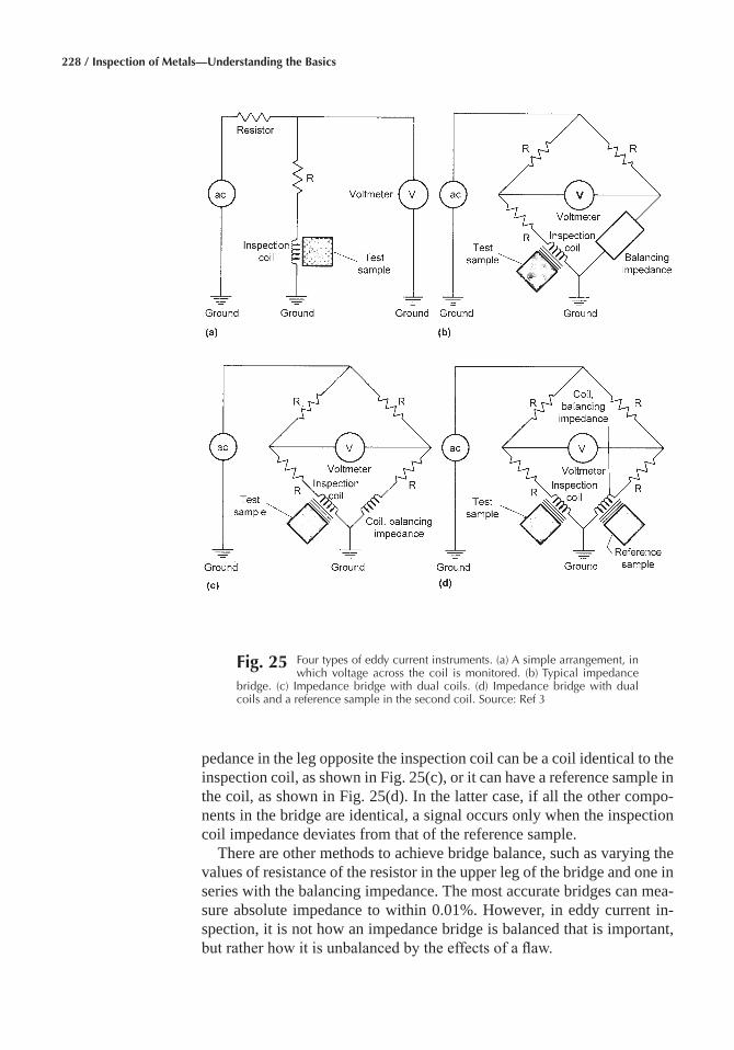
228 / Inspection of Metals—Understanding the Basics
pedance in the leg opposite the inspection coil can be a coil identical to the inspection coil, as shown in Fig. 25(c), or it can have a reference sample in the coil, as shown in Fig. 25(d). In the latter case, if all the other compo-nents in the bridge are identical, a signal occurs only when the inspection coil impedance deviates from that of the reference sample.
There are other methods to achieve bridge balance, such as varying the values of resistance of the resistor in the upper leg of the bridge and one in series with the balancing impedance. The most accurate bridges can mea-sure absolute impedance to within 0.01%. However, in eddy current in-spection, it is not how an impedance bridge is balanced that is important, but rather how it is unbalanced by the effects of a flaw.
Fig� 25 Four types of eddy current instruments. (a) A simple arrangement, in which voltage across the coil is monitored. (b) Typical impedance
bridge. (c) Impedance bridge with dual coils. (d) Impedance bridge with dual coils and a reference sample in the second coil. Source: Ref 3
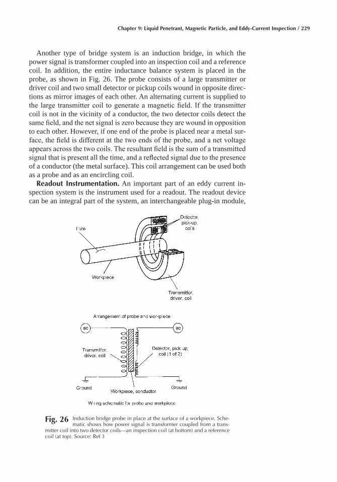
Chapter 9: Liquid Penetrant, Magnetic Particle, and Eddy-Current Inspection / 229
Another type of bridge system is an induction bridge, in which the power signal is transformer coupled into an inspection coil and a reference coil. In addition, the entire inductance balance system is placed in the probe, as shown in Fig. 26. The probe consists of a large transmitter or driver coil and two small detector or pickup coils wound in opposite direc-tions as mirror images of each other. An alternating current is supplied to the large transmitter coil to generate a magnetic field. If the transmitter coil is not in the vicinity of a conductor, the two detector coils detect the same field, and the net signal is zero because they are wound in opposition to each other. However, if one end of the probe is placed near a metal sur-face, the field is different at the two ends of the probe, and a net voltage appears across the two coils. The resultant field is the sum of a transmitted signal that is present all the time, and a reflected signal due to the presence of a conductor (the metal surface). This coil arrangement can be used both as a probe and as an encircling coil.
Readout Instrumentation� An important part of an eddy current in-spection system is the instrument used for a readout. The readout device can be an integral part of the system, an interchangeable plug-in module,
Fig� 26 Induction bridge probe in place at the surface of a workpiece. Sche-matic shows how power signal is transformer coupled from a trans-
mitter coil into two detector coils—an inspection coil (at bottom) and a reference coil (at top). Source: Ref 3
230 / Inspection of Metals—Understanding the Basics
and a solitary unit connected by cable. The readout instrument should be of adequate speed, accuracy, and range to meet the inspection require-ments of the system. Frequently, several readout devices are used in a single inspection system. More common types of readout, in order of in-creasing cost and complexity, are:
• Alarm lights alert the operator that a test parameter limit has been exceeded
• Sound alarms serve the same purpose as alarm lights but free the atten-tion of the operator to allow manipulating the probe in manual scan- ning.
• Kick-out relays activate a mechanism that automatically rejects and marks a part when a test parameter is exceeded
• Analog meters give a continuous reading over an extended range. They are fairly rapid (with a frequency of about 1 Hz), and the scales can be calibrated to read parameters directly. The accuracy of these devices is limited to about 1% of full scale. They can be used to set the limits on alarm lights, sound alarms, and kick-out relays
• Digital meters are easier to read and can have greater ranges than ana-log meters. Numerical values are easily read without extrapolation, but fast trends of changing readings are more difficult to interpret. Al-though many digital meters have binary coded decimal (bcd) output, they are relatively slow
• X-Y plotters can be used to display impedance plane plots of the eddy current response. They are very helpful in the design and set up of eddy current, bridge unbalance inspections and in discriminating against undesirable variables. They also are useful to sort out inspec-tion results. They are fairly accurate and provide a permanent copy
• X-Y storage oscilloscopes are very similar to X-Y plotters but can ac-quire signals at high speed. However, the signals have to be processed manually, and the screen can quickly become cluttered with signals. In some instruments, high-speed X-Y gates can be displayed and set on the screen
• Strip chart recorders furnish a fairly accurate (about 1% of full scale) recording at reasonably high speed (about 200 Hz). However, once on the chart, the data must be read by an operator. Several channels can be recorded simultaneously, and the record is permanent
• Magnetic tape recorders are fairly accurate and capable of recording at very high speed (10 MHz). Moreover, the data can be processed by automated techniques
• Computers. The data from several channels can be fed directly to a high speed computer, either analog or digital, for on-line processing. The computer can separate parameters and calculate the variable of interest and significance, catalog the data, print summaries of the re-sult, and store all data on tape for reference in future scans
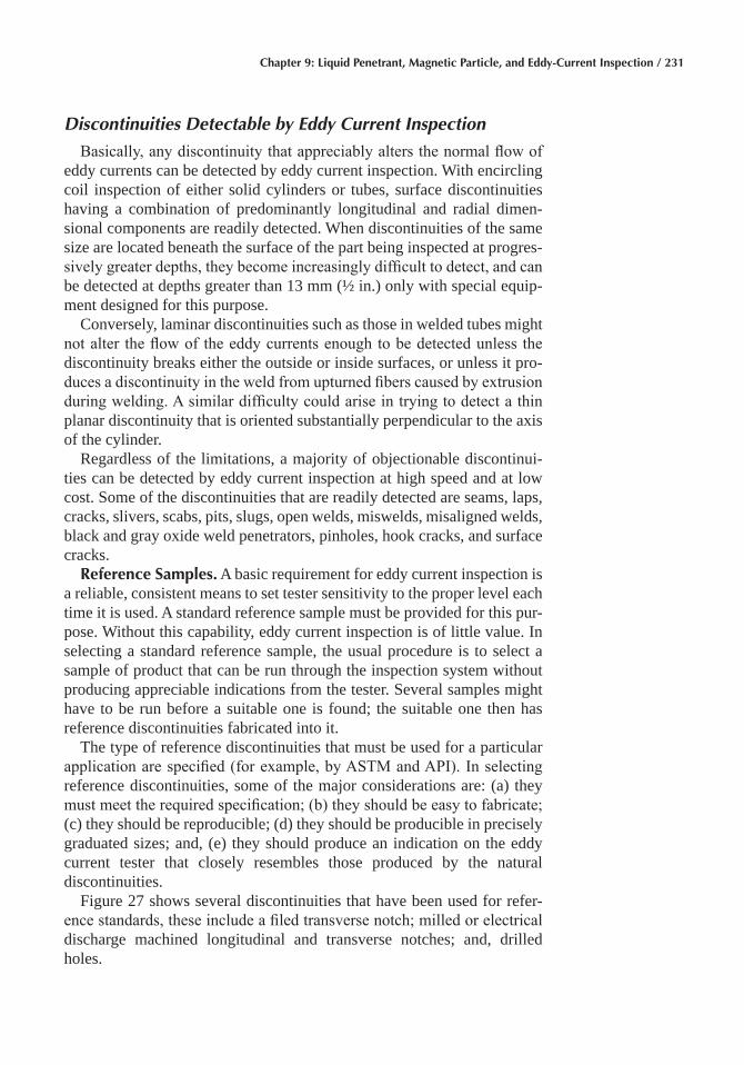
Chapter 9: Liquid Penetrant, Magnetic Particle, and Eddy-Current Inspection / 231
Discontinuities Detectable by Eddy Current Inspection
Basically, any discontinuity that appreciably alters the normal flow of eddy currents can be detected by eddy current inspection. With encircling coil inspection of either solid cylinders or tubes, surface discontinuities having a combination of predominantly longitudinal and radial dimen-sional components are readily detected. When discontinuities of the same size are located beneath the surface of the part being inspected at progres-sively greater depths, they become increasingly difficult to detect, and can be detected at depths greater than 13 mm (½ in.) only with special equip-ment designed for this purpose.
Conversely, laminar discontinuities such as those in welded tubes might not alter the flow of the eddy currents enough to be detected unless the discontinuity breaks either the outside or inside surfaces, or unless it pro-duces a discontinuity in the weld from upturned fibers caused by extrusion during welding. A similar difficulty could arise in trying to detect a thin planar discontinuity that is oriented substantially perpendicular to the axis of the cylinder.
Regardless of the limitations, a majority of objectionable discontinui-ties can be detected by eddy current inspection at high speed and at low cost. Some of the discontinuities that are readily detected are seams, laps, cracks, slivers, scabs, pits, slugs, open welds, miswelds, misaligned welds, black and gray oxide weld penetrators, pinholes, hook cracks, and surface cracks.
Reference Samples� A basic requirement for eddy current inspection is a reliable, consistent means to set tester sensitivity to the proper level each time it is used. A standard reference sample must be provided for this pur-pose. Without this capability, eddy current inspection is of little value. In selecting a standard reference sample, the usual procedure is to select a sample of product that can be run through the inspection system without producing appreciable indications from the tester. Several samples might have to be run before a suitable one is found; the suitable one then has reference discontinuities fabricated into it.
The type of reference discontinuities that must be used for a particular application are specified (for example, by ASTM and API). In selecting reference discontinuities, some of the major considerations are: (a) they must meet the required specification; (b) they should be easy to fabricate; (c) they should be reproducible; (d) they should be producible in precisely graduated sizes; and, (e) they should produce an indication on the eddy current tester that closely resembles those produced by the natural discontinuities.
Figure 27 shows several discontinuities that have been used for refer-ence standards, these include a filed transverse notch; milled or electrical discharge machined longitudinal and transverse notches; and, drilled holes.
232 / Inspection of Metals—Understanding the Basics
ACKNOWLEDGMENT
This chapter was adapted from Liquid-Penetrant Inspection, Magnetic-Particle Inspection, and Eddy-Current Inspection all in Metals Handbook Desk Edition, Second Edition, 1998.
REFERENCES
1. Liquid-Penetrant Inspection, Metals Handbook Desk Edition, 2nd ed., ASM International, 1998, p 1260–1267
2. Magnetic-Particle Inspection, Metals Handbook Desk Edition, 2nd ed., ASM International, 1998, p 1267–1273
3. Eddy-Current Inspection, Metals Handbook Desk Edition, 2nd ed., ASM International, 1998, p 1275–1281
SELECTED REFERENCES
• C. Hellier, Handbook of Nondestructive Evaluation, McGraw-Hill, 2000
• Nondestructive Testing and Quality Control, Vol 17, ASM Handbook, ASM International, 1989
Fig� 27 Several fabricated discontinuities used as reference standards in eddy current inspection. ASTM standards for eddy current testing include E
215 (aluminum alloy tube), E 376 (measurement of coating thickness), E 243 (copper and copper alloy tube), E 566 (ferrous metal sorting), E 571 (nickel and nickel alloy tube), E 690 (nonmagnetic heat-exchanger tubes), E 426 (stainless steel tube), and E 309 (steel tube). Source: Ref 3

Inspection of Metals—Understanding the Basics Copyright © 2013 ASM International®
F.C. Campbell, editor All rights reservedwww.asminternational.org
CHAPTER 10
Radiographic Inspection
RADIOGRAPHY is a nondestructive inspection method that is based on differential absorption of penetrating radiation−either electromagnetic radiation of very short wavelength or particulate radiation−by the part or test piece (object) being inspected. Because of differences in density and variations in thickness of the part, or differences in absorption characteris-tics caused by variations in composition, different portions of a test piece absorb different amounts of penetrating radiation. Unabsorbed radiation passing through the part can be recorded on film or photosensitive paper, viewed on a fluorescent screen, or monitored by various types of radiation detectors. The term radiography usually implies a radiographic process that produces a permanent image on film (conventional radiography) or paper (paper radiography or xeroradiography), although in a broad sense it refers to all forms of radiographic inspection. When inspection involves viewing of a real-time image on a fluorescent screen or image intensifier, the radiographic process is termed real-time inspection. When electronic, nonimaging instruments are used to measure the intensity of radiation, the process is termed radiation gaging. Tomography, a radiation inspection method adapted from the medical computerized axial tomography CAT scanner, provides a cross-sectional view of an inspection object. All the previous terms are used mainly in connection with inspection that in-volves penetrating electromagnetic radiation in the form of x-rays or gamma rays (also known as γ-rays). Neutron radiography refers to radio-graphic inspection using neutrons rather than electromagnetic radiation. This chapter discusses radiography methods using x-rays, gamma rays, and neutrons.
In conventional radiography, an object is placed in a beam of x-rays and the portion of the radiation that is not absorbed by the object impinges on a detector such as film. The unabsorbed radiation exposes the film emul-sion, similar to the way that light exposes film in photography. Develop-ment of the film produces an image that is a two-dimensional shadow pic-
234 / Inspection of Metals—Understanding the Basics
ture of the object. Variations in density, thickness, and composition of the object being inspected cause variations in the intensity of the unabsorbed radiation and appear as variations in photographic density (shades of gray) in the developed film. Evaluation of the radiograph is based on a compari-son of the differences in photographic density with known characteristics of the object itself or with standards derived from radiographs of similar objects of acceptable quality.
Uses of Radiography
Radiography is used to detect features of a component or assembly that exhibit differences in thickness or physical density compared with sur-rounding material. Large differences are more easily detected than small ones. In general, radiography can detect only those features that have a reasonable thickness or radiation path length in a direction parallel to the radiation beam. This means that the ability of the process to detect planar discontinuities such as cracks depends on proper orientation of the test piece during inspection. Discontinuities such as voids and inclusions, which have measurable thickness in all directions, can be detected as long as they are not too small in relation to section thickness. In general, fea-tures that exhibit differences in absorption of a few percent compared with the surrounding material can be detected.
Applicability� Radiographic inspection is used extensively on castings and weldments, particularly where there is a critical need to ensure free-dom from internal flaws. For instance, radiography often is specified for inspection of thick wall castings and weldments for steam power equip-ment, boiler and turbine components and assemblies, and other high pres-sure systems. Radiography also can be used on forgings and mechanical assemblies. When used with mechanical assemblies, radiography provides a unique nondestructive testing (NDT) capability of inspecting for condi-tion and proper placement of components. Certain special devices are more satisfactorily inspected by radiography than by other methods. For instance, radiography is well suited to the inspection of semiconductor devices for cracks, broken wires, unsoldered connections, foreign mate-rial, and misplaced components, whereas other methods are limited in ability to inspect semiconductor devices.
Sensitivity of x-ray radiography, real-time x-ray methods, and gamma ray radiography to various types of flaws depends on many factors, in-cluding type of material, type of flaw, and product form. (Type of material in this context is usually expressed in terms of atomic number, for in-stance, metals having low atomic numbers are classified as light metals and those having high atomic numbers as heavy metals.) Table 1 indicates the general degrees of suitability of the three main radiographic methods for detection of discontinuities in various product forms and applications. In some instances, radiography cannot be used even though it appears

Chapter 10: Radiographic Inspection / 235
suitable from Table 1, because the part is accessible from one side only. Both sides must be accessible for radiography.
Radiography can be used to inspect most types of solid material, with the possible exception of assemblies containing materials of very high or very low density. Neutron radiography, however, often can be used in
Table 1 Comparison of suitabilities of three radiographic methods for inspection of light and heavy metals
Inspection application
Suitability for light metals(a) Suitability for heavy metals(a)
X-rayReal-time
radiography(b) Gamma ray X-rayReal-time
radiography(b) Gamma ray
General
Surface cracks(c) F(d) F(d) F(d) F(d) F(d) F(d)Internal cracks F(d) F(d) F(d) F(d) F(d) F(d)Voids G G G G G GThickness F F F F F FMetallurgical variations F F F F F F
Sheet and plate
Thickness G(e) G(e) G(e) G(e) U G(e)Laminations U U U U U UVoids G G G G G G
Bar and tube
Seams P P P P P PPipe G G G G F FCupping G G G G F FInclusions F F F F F F
Castings
Cold shuts G G G G G GSurface cracks F(d) F(d) F(d) F(d) F(d) F(d)Internal shrinkage G G G G G GVoids, pores G G G G G GCore shift G G G G G G
Forgings
Laps P(d) P(d) P(d) P(d) U UInclusions F F F F F UInternal bursts G G G F F GInternal flakes P(d) P(d) U P(d) P(d) UCracks and tears F(d) F(d) F(d) F(d) F(d) F(d)
Welds
Shrinkage cracks G(d) G(d) G(d) G(d) G(d) G(d)Slag inclusions G G G G G GIncomplete fusion G G G G G GPores G G G G F GIncomplete penetration G G G G G G
Processing
Heat treating cracks U F U P P UGrinding cracks U F U U U U
Service
Fatigue and heat cracks F(d) F(d) P(d) P P PStress corrosion F F P F F PBlistering P P P P P PThinning F F F F F FCorrosion pits F F P G G P
(a) G, good; F, fair: P, poor; U, unsatisfactory. (b) Real-time radiography offers the advantage that the part can be manipulated to present the best view—for example, align a crack. Also, when microfocus, magnification methods are used, real-time radiography presents ex-cellent resolution and contrast. (c) Includes only visible cracks. Minute surface cracks normally are undetectable by radiographic inspec-tion methods. (d) Radiation beam must be parallel to the cracks, laps, or flakes. (e) When calibrated using special thickness gages. Source: Ref 1
236 / Inspection of Metals—Understanding the Basics
such instances. Both ferrous and nonferrous alloys can be radiographed, as can nonmetallic materials and composites.
Limitations� Compared with other nondestructive methods of inspec-tion, radiography is expensive. Relatively large capital costs and space allocations are required for a radiographic laboratory or a real time inspec-tion station. Conversely, when portable x-ray or gamma ray sources are used, capital costs can be relatively low. Operating costs can be high; a large percentage of the total inspection time is spent in setting up for radi-ography. With real-time radiography, operating costs usually are much lower, because setup times are shorter and there are no extra costs for x-ray film and processing.
Field inspection of thick sections is a time-consuming process. Portable x-ray sources generally emit relatively low energy radiation, up to approx-imately 400 keV, and also are limited as to the intensity of radiation output. These characteristics of portable sources combine to limit x-radiography in the field to sections having absorption equivalent to that of approxi-mately 75 mm (3 in.) of steel. Radioactive sources also are limited in the thickness that can be inspected, primarily because high activity sources require heavy shielding for protection of personnel. This limits field usage to sources of lower activity that can be transported in relatively light-weight containers. Because portable x-ray and gamma ray sources are limited in effective radiation output, exposure times usually are long for thick sections. Recent developments, such as a portable linear accelerator, can speed up and increase the penetrating power of field radiographic methods.
Certain types of flaws are difficult to detect by radiography. Laminar defects such as cracks present problems unless they are essentially parallel to the radiation beam. Tight, meandering cracks in thick sections usually cannot be detected even when properly oriented. Minute discontinuities such as inclusions in wrought material, flakes, microporosity, and micro-fissures cannot be detected unless they are sufficiently segregated to yield a detectable gross effect. Laminations normally are not detectable by radi-ography because of their unfavorable orientation, usually parallel to the surface. Laminations seldom yield differences in absorption that enable laminated areas to be distinguished from lamination-free areas.
Principles of Radiography
There are three basic elements that combine to produce a radiograph: a radiation source or probing medium; the test piece or object being evalu-ated; and, a recording medium (usually film), as shown schematically in Fig. 1. The test piece is a plate of uniform thickness containing an internal flaw that has absorption characteristics different from those of the sur-rounding material. Radiation from the source is absorbed by the test piece as the radiation passes through it; the flaw and surrounding material ab-
Chapter 10: Radiographic Inspection / 237
sorb different amounts of radiation. Thus, the amount of radiation that reaches the film in the area beneath the flaw is different from the amount that impinges on adjacent areas. This produces on the film a latent image of the flaw that, when the film is developed, can be seen as a shadow of different photographic density from that of the image of the surrounding material.
Geometric Factors In Radiography� Because a radiograph is a two-dimensional representation of a three-dimensional object, the radiographic images of most test pieces are somewhat distorted in size and shape.
In conventional radiography, the position of a flaw within the volume of a test piece cannot be determined exactly with a single radiograph; depth in the direction of the radiation beam cannot be determined exactly. Con-clusions regarding depth sometimes can be drawn from the sharpness of the flaw image. Images of flaws close to the detector tend to appear sharper than images of flaws near the source side of the object. However, tech-niques such as stereoradiography, tomography, triangulation, or simply making two or more exposures, with the radiation beam being directed at the test piece from a different angle for each exposure, can be used to lo-cate flaws more exactly within the test-piece volume.
Sources of Radiation
Two types of electromagnetic radiation are used in radiographic inspec-tion: x-rays and γ-rays. X-rays and γ-rays differ in their wavelengths from other types of electromagnetic radiation such as visible light, microwaves,
Fig� 1 Diagram of the basic elements of a radiographic system, showing method of detecting and recording an internal flaw in a plate of uni-
form thickness. Source: Ref 1

238 / Inspection of Metals—Understanding the Basics
and radio waves; although there is not always a distinct transition from one type of electromagnetic radiation to another (Fig. 2). Only x-rays and γ-rays, because of their relatively short wavelengths (high energies), have the capability of penetrating opaque materials to reveal internal flaws.
X-rays and γ-rays are physically indistinguishable; they differ only in the manner in which they are produced. X-rays result from the interaction between a rapidly moving stream of electrons and atoms in a solid target material, while γ-rays are emitted during the radioactive decay of unstable atomic nuclei.
The amount of exposure from x-rays or γ-rays is measured in roentgens (R), where 1 R is the amount of radiation exposure that produces one elec-trostatic unit (3.33564 × 10⁻¹⁰ C) of charge from 1.293 mg (45.61 × 10⁻⁶ oz) of air. The intensity of an x-ray or γ-ray radiation is measured in roent-gens per unit time.
Although the intensity of x-ray or γ-ray radiation is measured in the same units, the strengths of x-ray and γ-ray sources are usually given in different units. The strength of an x-ray source is typically given in roent-gens per minute at one meter (RMM) from the source or in some other suitable combination of time or distance units (such as roentgens per hour at one meter, or RHM). The strength of a γ-ray source is usually given in terms of the radioactive decay rate, which has the traditional unit of a Curie (1 Ci = 37 × 109 disintegrations per second). The corresponding unit in the Système International d’Unités (SI) system is a gigabecquerel (1 GBq = 1 × 10⁹ disintegrations per second).
The spectrum of radiation is often expressed in terms of photon energy rather than as a wavelength. Photon energy is measured in electron volts (eV), with 1 eV being the energy imparted to an electron by an accelerat-ing potential of 1 V. The radiation spectrum in terms of both wavelength and photon energy is shown in Fig. 2.
Fig� 2 Schematic representation of the portion of the electromagnetic spec-trum that includes x-rays, gamma rays, ultraviolet and visible light, and
infrared radiation, showing their relationship with wave length and photon en-ergy. Source: Ref 1
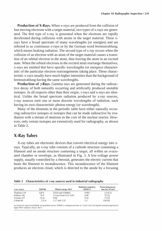
Chapter 10: Radiographic Inspection / 239
Production of X-Rays� When x-rays are produced from the collision of fast moving electrons with a target material, two types of x-rays are gener-ated. The first type of x-ray is generated when the electrons are rapidly decelerated during collisions with atoms in the target material. These x-rays have a broad spectrum of many wavelengths (or energies) and are referred to as continuous x-rays or by the German word bremsstrahlung, which means braking radiation. The second type of x-ray occurs when the collision of an electron with an atom of the target material causes a transi-tion of an orbital electron in the atom, thus leaving the atom in an excited state. When the orbital electrons in the excited atom rearrange themselves, x-rays are emitted that have specific wavelengths (or energies) character-istic of the particular electron rearrangements taking place. These charac-teristic x-rays usually have much higher intensities than the background of bremsstrahlung having the same wavelengths.
Production of γ-Rays� Gamma rays are generated during the radioac-tive decay of both naturally occurring and artificially produced unstable isotopes. In all respects other than their origin, γ-rays and x-rays are iden-tical. Unlike the broad spectrum radiation produced by x-ray sources, γ-ray sources emit one or more discrete wavelengths of radiation, each having its own characteristic photon energy (or wavelength).
Many of the elements in the periodic table have either naturally occur-ring radioactive isotopes or isotopes that can be made radioactive by irra-diation with a stream of neutrons in the core of the nuclear reactor. How-ever, only certain isotopes are extensively used for radiography, as shown in Table 2.
X-Ray Tubes
X-ray tubes are electronic devices that convert electrical energy into x-rays. Typically, an x-ray tube consists of a cathode structure containing a filament and an anode structure containing a target, all within an evacu-ated chamber or envelope, as illustrated in Fig. 3. A low-voltage power supply, usually controlled by a rheostat, generates the electric current that heats the filament to incandescence. This incandescence of the filament produces an electron cloud, which is directed to the anode by a focusing
Table 2 Characteristics of γ-ray sources used in industrial radiography
γ-ray source Half-life Photon energy, MeVRadiation output(a),
RHM/CiPenetrating power,
mm (in.) of steel
Thulium-170 128 d 0.054 and 0.084(b) 0.003 13 (0.5)Iridium-192 74 d 12 rays from 0.21–0.61 0.48 75 (3)Cesium-137 33 yr 0.66 0.32 75 (3)Cobalt-60 5.3 yr 1.17 and 1.33 1.3 230 (9)
(a) Output for typical unshielded, encapsulated sources: RHM/Ci, roentgens per hour at 1 m per Curie. (b) Against strong background of higher MeV radiation. Source: Ref 1
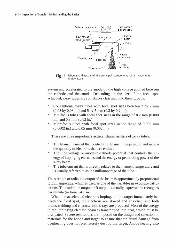
240 / Inspection of Metals—Understanding the Basics
system and accelerated to the anode by the high voltage applied between the cathode and the anode. Depending on the size of the focal spot achieved, x-ray tubes are sometimes classified into three groups:
• Conventional x-ray tubes with focal spot sizes between 2 by 2 mm (0.08 by 0.08 in.) and 5 by 5 mm (0.2 by 0.2 in.)
• Minifocus tubes with focal spot sizes in the range of 0.2 mm (0.008 in.) and 0.8 mm (0.03 in.)
• Microfocus tubes with focal spot sizes in the range of 0.005 mm (0.0002 in.) and 0.05 mm (0.002 in.)
There are three important electrical characteristics of x-ray tubes:
• The filament current that controls the filament temperature and in turn the quantity of electrons that are emitted
• The tube voltage or anode-to-cathode potential that controls the en-ergy of impinging electrons and the energy or penetrating power of the x-ray beam
• The tube current that is directly related to the filament temperature and is usually referred to as the milliamperage of the tube
The strength or radiation output of the beam is approximately proportional to milliamperage, which is used as one of the variables in exposure calcu-lations. This radiation output or R output is usually expressed in roentgens per minute (or hour) at 1 m.
When the accelerated electrons impinge on the target immediately be-neath the focal spot, the electrons are slowed and absorbed, and both bremsstrahlung and characteristic x-rays are produced. Most of the energy in the impinging electron beam is transformed into heat, which must be dissipated. Severe restrictions are imposed on the design and selection of materials for the anode and target to ensure that structural damage from overheating does not prematurely destroy the target. Anode heating also
Fig� 3 Schematic diagram of the principal components of an x-ray unit. Source: Ref 1
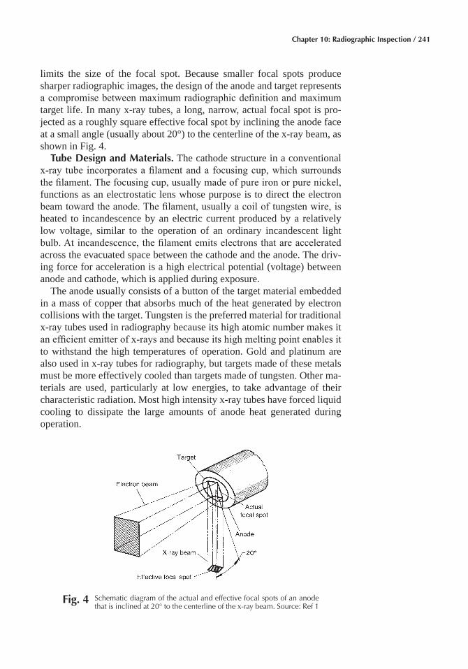
Chapter 10: Radiographic Inspection / 241
limits the size of the focal spot. Because smaller focal spots produce sharper radiographic images, the design of the anode and target represents a compromise between maximum radiographic definition and maximum target life. In many x-ray tubes, a long, narrow, actual focal spot is pro-jected as a roughly square effective focal spot by inclining the anode face at a small angle (usually about 20°) to the centerline of the x-ray beam, as shown in Fig. 4.
Tube Design and Materials� The cathode structure in a conventional x-ray tube incorporates a filament and a focusing cup, which surrounds the filament. The focusing cup, usually made of pure iron or pure nickel, functions as an electrostatic lens whose purpose is to direct the electron beam toward the anode. The filament, usually a coil of tungsten wire, is heated to incandescence by an electric current produced by a relatively low voltage, similar to the operation of an ordinary incandescent light bulb. At incandescence, the filament emits electrons that are accelerated across the evacuated space between the cathode and the anode. The driv-ing force for acceleration is a high electrical potential (voltage) between anode and cathode, which is applied during exposure.
The anode usually consists of a button of the target material embedded in a mass of copper that absorbs much of the heat generated by electron collisions with the target. Tungsten is the preferred material for traditional x-ray tubes used in radiography because its high atomic number makes it an efficient emitter of x-rays and because its high melting point enables it to withstand the high temperatures of operation. Gold and platinum are also used in x-ray tubes for radiography, but targets made of these metals must be more effectively cooled than targets made of tungsten. Other ma-terials are used, particularly at low energies, to take advantage of their characteristic radiation. Most high intensity x-ray tubes have forced liquid cooling to dissipate the large amounts of anode heat generated during operation.
Fig� 4 Schematic diagram of the actual and effective focal spots of an anode that is inclined at 20° to the centerline of the x-ray beam. Source: Ref 1
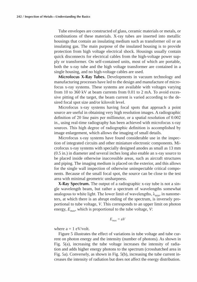
242 / Inspection of Metals—Understanding the Basics
Tube envelopes are constructed of glass, ceramic materials or metals, or combinations of these materials. X-ray tubes are inserted into metallic housings that contain an insulating medium such as transformer oil or an insulating gas. The main purpose of the insulated housing is to provide protection from high voltage electrical shock. Housings usually contain quick disconnects for electrical cables from the high-voltage power sup-ply or transformer. On self-contained units, most of which are portable, both the x-ray tube and the high voltage transformer are contained in a single housing, and no high-voltage cables are used.
Microfocus X-Ray Tubes� Developments in vacuum technology and manufacturing processes have led to the design and manufacture of micro-focus x-ray systems. These systems are available with voltages varying from 10 to 360 kV at beam currents from 0.01 to 2 mA. To avoid exces-sive pitting of the target, the beam current is varied according to the de-sired focal spot size and/or kilovolt level.
Microfocus x-ray systems having focal spots that approach a point source are useful in obtaining very high resolution images. A radiographic definition of 20 line pairs per millimeter, or a spatial resolution of 0.002 in., using real-time radiography has been achieved with microfocus x-ray sources. This high degree of radiographic definition is accomplished by image enlargement, which allows the imaging of small details.
Microfocus x-ray systems have found considerable use in the inspec-tion of integrated circuits and other miniature electronic components. Mi-crofocus x-ray systems with specially designed anodes as small as 13 mm (0.5 in.) in diameter and several inches long also enable an x-ray source to be placed inside otherwise inaccessible areas, such as aircraft structures and piping. The imaging medium is placed on the exterior, and this allows for the single wall inspection of otherwise uninspectable critical compo-nents. Because of the small focal spot, the source can be close to the test area with minimal geometric unsharpness.
X-Ray Spectrum� The output of a radiographic x-ray tube is not a sin-gle wavelength beam, but rather a spectrum of wavelengths somewhat analogous to white light. The lower limit of wavelengths, λmin, in nanome-ters, at which there is an abrupt ending of the spectrum, is inversely pro-portional to tube voltage, V. This corresponds to an upper limit on photon energy, Emax, which is proportional to the tube voltage, V:
Emax = aV
where a = 1 eV/volt.Figure 5 illustrates the effect of variations in tube voltage and tube cur-
rent on photon energy and the intensity (number of photons). As shown in Fig. 5(a), increasing the tube voltage increases the intensity of radia- tion and adds higher energy photons to the spectrum (crosshatched area in Fig. 5a). Conversely, as shown in Fig. 5(b), increasing the tube current in-creases the intensity of radiation but does not affect the energy distribution.
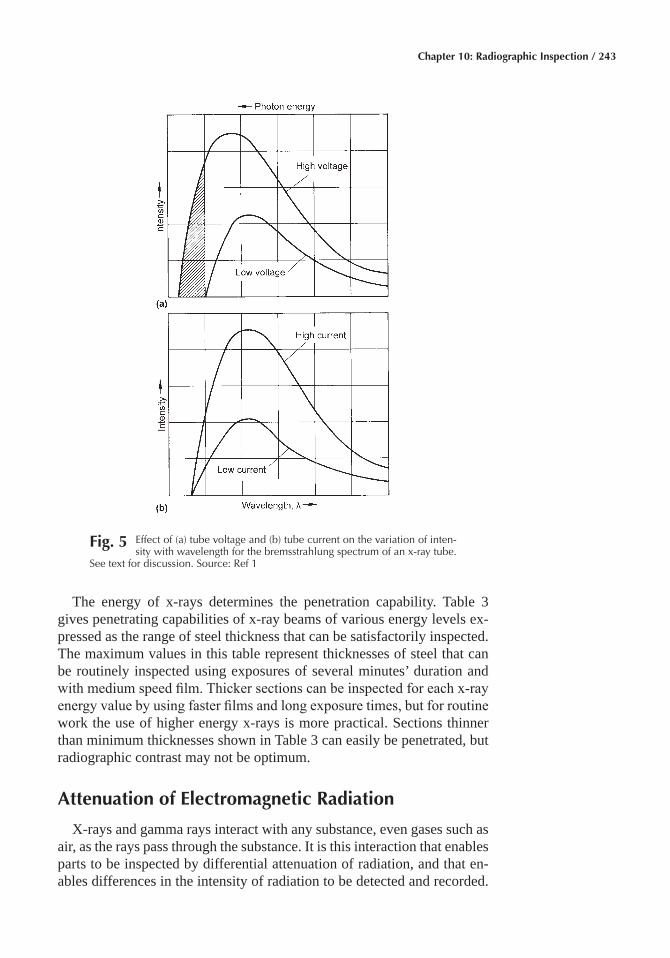
Chapter 10: Radiographic Inspection / 243
The energy of x-rays determines the penetration capability. Table 3 gives penetrating capabilities of x-ray beams of various energy levels ex-pressed as the range of steel thickness that can be satisfactorily inspected. The maximum values in this table represent thicknesses of steel that can be routinely inspected using exposures of several minutes’ duration and with medium speed film. Thicker sections can be inspected for each x-ray energy value by using faster films and long exposure times, but for routine work the use of higher energy x-rays is more practical. Sections thinner than minimum thicknesses shown in Table 3 can easily be penetrated, but radiographic contrast may not be optimum.
Attenuation of Electromagnetic Radiation
X-rays and gamma rays interact with any substance, even gases such as air, as the rays pass through the substance. It is this interaction that enables parts to be inspected by differential attenuation of radiation, and that en-ables differences in the intensity of radiation to be detected and recorded.
Fig� 5 Effect of (a) tube voltage and (b) tube current on the variation of inten-sity with wavelength for the bremsstrahlung spectrum of an x-ray tube.
See text for discussion. Source: Ref 1
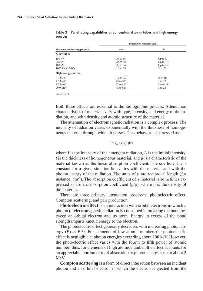
244 / Inspection of Metals—Understanding the Basics
Both these effects are essential to the radiographic process. Attenuation characteristics of materials vary with type, intensity, and energy of the ra-diation, and with density and atomic structure of the material.
The attenuation of electromagnetic radiation is a complex process. The intensity of radiation varies exponentially with the thickness of homoge-neous material through which it passes. This behavior is expressed as:
I = Io exp(–μt)
where I is the intensity of the emergent radiation, I0 is the initial intensity, t is the thickness of homogeneous material, and μ is a characteristic of the material known as the linear absorption coefficient. The coefficient μ is constant for a given situation but varies with the material and with the photon energy of the radiation. The units of μ are reciprocal length (for instance, cm-1). The absorption coefficient of a material is sometimes ex-pressed as a mass-absorption coefficient (μ/ρ), where ρ is the density of the material.
There are three primary attenuation processes: photoelectric effect, Compton scattering, and pair production.
Photoelectric effect is an interaction with orbital electrons in which a photon of electromagnetic radiation is consumed in breaking the bond be-tween an orbital electron and its atom. Energy in excess of the bond strength imparts kinetic energy to the electron.
The photoelectric effect generally decreases with increasing photon en-ergy (E) as E-3.5. For elements of low atomic number, the photoelectric effect is negligible at photon energies exceeding about 100 keV. However, the photoelectric effect varies with the fourth to fifth power of atomic number; thus, for elements of high atomic number, the effect accounts for an appreciable portion of total absorption at photon energies up to about 2 MeV.
Compton scattering is a form of direct interaction between an incident photon and an orbital electron in which the electron is ejected from the
Table 3 Penetrating capabilities of conventional x-ray tubes and high energy sources
Maximum accelerating potential
Penetration range for steel
mm in.
X-ray tubes
150 kV Up to 16 Up to ⅝250 kV Up to 38 Up to 1½400 kV Up to 64 Up to 2½1000 kV (1 MV) 6.4 to 89 ¼ to 3½
High-energy sources
2.0 MeV 6.4 to 250 ¼ to 104.5 MeV 25 to 305 1 to 127.5 MeV 57 to 460 2¼ to 1820.0 MeV 75 to 610 3 to 24
Source: Ref 1
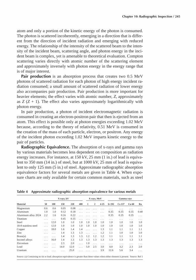
Chapter 10: Radiographic Inspection / 245
atom and only a portion of the kinetic energy of the photon is consumed. The photon is scattered incoherently, emerging in a direction that is differ-ent from the direction of incident radiation and emerging with reduced energy. The relationship of the intensity of the scattered beam to the inten-sity of the incident beam, scattering angle, and photon energy in the inci-dent beam is complex, yet is amenable to theoretical evaluation. Compton scattering varies directly with atomic number of the scattering element and approximately inversely with photon energy in the energy range that is of major interest.
Pair production is an absorption process that creates two 0.5 MeV photons of scattered radiation for each photon of high energy incident ra-diation consumed; a small amount of scattered radiation of lower energy also accompanies pair production. Pair production is more important for heavier elements; the effect varies with atomic number, Z, approximately as Z (Z + 1). The effect also varies approximately logarithmically with photon energy.
In pair production, a photon of incident electromagnetic radiation is consumed in creating an electron-positron pair that then is ejected from an atom. This effect is possible only at photon energies exceeding 1.02 MeV because, according to the theory of relativity, 0.51 MeV is consumed in the creation of the mass of each particle, electron, or positron. Any energy of the incident photon exceeding 1.02 MeV imparts kinetic energy to the pair of particles.
Radiographic Equivalence� The absorption of x-rays and gamma rays by various materials becomes less dependent on composition as radiation energy increases. For instance, at 150 kV, 25 mm (1 in.) of lead is equiva-lent to 350 mm (14 in.) of steel, but at 1000 kV, 25 mm of lead is equiva-lent to only 125 mm (5 in.) of steel. Approximate radiographic absorption equivalence factors for several metals are given in Table 4. When expo-sure charts are only available for certain common materials, such as steel
Table 4 Approximate radiographic absorption equivalence for various metals
Material
X-rays, kV X-rays, MeV Gamma rays
50 100 150 220 400 1 2 4-25 Ir-192 Cs-137 Co-60 Ra
Magnesium 0.6 0.6 0.05 0.08 . . . . . . . . . . . . . . . . . . . . . . . .Aluminum 1.0 1.0 0.12 0.18 . . . . . . . . . . . . 0.35 0.35 0.35 0.40Aluminum alloy 2024 2.2 1.6 0.16 0.22 . . . . . . . . . . . . 0.35 0.35 0.35 . . .Titanium . . . . . . 0.45 0.35 . . . . . . . . . . . . . . . . . . . . . . . .Steel . . . 12.0 1.0 1.0 1.0 1.0 1.0 1.0 1.0 1.0 1.0 1.018-8 stainless steel . . . 12.0 1.0 1.0 1.0 1.0 1.0 1.0 1.0 1.0 1.0 1.0Copper . . . 18.0 1.6 1.4 1.4 . . . . . . 1.3 1.1 1.1 1.1 1.1Zinc . . . . . . 1.4 1.3 1.3 . . . . . . 1.2 1.1 1.0 1.0 1.0Brass(a) . . . . . . 1.4 1.3 1.3 1.2 1.2 1.2 1.1 1.1 1.1 1.1Inconel alloys . . . 16.0 1.4 1.3 1.3 1.3 1.3 1.3 1.3 1.3 1.3 1.3Zirconium . . . . . . 2.3 2.0 . . . 1.0 . . . . . . . . . . . . . . . . . .Lead . . . . . . 14.0 12.0 . . . 5.0 2.5 3.0 4.0 3.2 2.3 2.0Uranium . . . . . . . . . 25.0 . . . . . . . . . 3.9 12.6 5.6 3.4 . . .
Source: (a) Containing no tin or lead; absorption equivalence is greater than these values when either element is present. Source: Ref 1

246 / Inspection of Metals—Understanding the Basics
or aluminum, exposure times for other materials can be estimated by de-termining the exposure time for an equal thickness of a common material from the chart, then multiplying by the radiographic equivalence factor.
Principles of Shadow Formation
The image formed on a radiograph is similar to the shadow cast on a screen by an opaque object placed in a beam of light. Although radiation used in radiography penetrates an opaque object whereas light does not, the geometric laws of shadow formation are basically the same. X-rays, gamma rays, and light all travel in straight lines. Straight line propagation is the chief characteristic of radiation that permits formation of a sharply discern-ible shadow. The geometric relationships of source, object, and screen to each other determine the three main characteristics of the shadow: the de-grees of enlargement, distortion, and unsharpness (see Fig. 6).
Enlargement� The shadow of the object (test piece) is always farther from the source than the object itself. Thus, as illustrated for a point source in Fig. 6(a), dimensions of the shadow are always greater than correspond-ing dimensions of the object. Mathematically, the size of the image or de-gree of enlargement may be calculated from the relationship:
M = Si/So = Li/Lo
where M is the degree of enlargement (magnification), Si is the size of the image, So is the size of the object, Li is the source-to-image distance, and Lo is the source-to-object distance.
With very small focal spots, large values of geometric magnification can be used effectively. Values of 6 to 20 are common; magnification val-ues as high as 100 can be used. Focal spots in microfocal x-ray equipment range from 5 to 20 μm (0.0002 to 0.0008 in.). In addition to increased image size, magnification systems also offer improved contrast because radiation scattered in the object does not reach the detector.
Distortion� As long as the plane of a two-dimensional object and the plane of the recording surface are parallel to each other, the image of that object plane will be undistorted regardless of the angle at which the beam of radiation impinges on the object. Also, the degree of enlargement for different points in a given object plane is constant because the ratio Li/Lo is invariant. However, as shown in Fig. 6(b), if the plane of the object and the plane of the recording surface are not parallel, the image will be dis-torted. For objects of appreciable thickness, the magnification for different object planes will vary because Lo varies.
Geometric Unsharpness� In reality, most radiation sources are too large to be approximated by a point. Most conventional x-ray tubes have focal spots several millimeters in size. Even high energy sources have focal spots of appreciable size, although seldom exceeding 2 mm (0.08
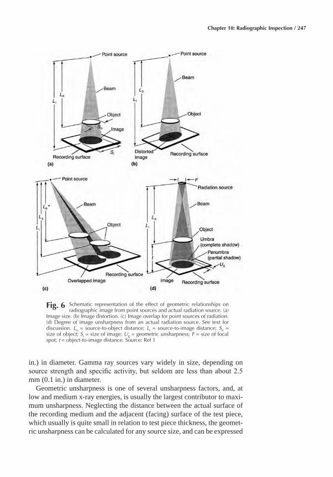
Chapter 10: Radiographic Inspection / 247
in.) in diameter. Gamma ray sources vary widely in size, depending on source strength and specific activity, but seldom are less than about 2.5 mm (0.1 in.) in diameter.
Geometric unsharpness is one of several unsharpness factors, and, at low and medium x-ray energies, is usually the largest contributor to maxi-mum unsharpness. Neglecting the distance between the actual surface of the recording medium and the adjacent (facing) surface of the test piece, which usually is quite small in relation to test piece thickness, the geomet-ric unsharpness can be calculated for any source size, and can be expressed
Fig� 6 Schematic representation of the effect of geometric relationships on radiographic image from point sources and actual radiation source. (a)
Image size. (b) Image distortion. (c) Image overlap for point sources of radiation. (d) Degree of image unsharpness from an actual radiation source. See text for discussion. Lo = source-to-object distance; Li = source-to-image distance; So = size of object; Si = size of image; Ug = geometric unsharpness; F = size of focal spot; t = object-to-image distance. Source: Ref 1
248 / Inspection of Metals—Understanding the Basics
as a series of straight-line plots relating geometric unsharpness, Ug, to test-piece thickness, t, for various values of source-to-object distance, Lo. A typical series is shown in Fig. 7 for a 5 mm (0.2 in.) diameter source. It is helpful to prepare graphs like the one in Fig. 7 for each source size used.
Image Conversion
The most important process in radiography is the conversion of radia-tion into a form suitable for observation or further signals processing. After penetrating the test piece, the x-rays or γ-rays pass through a me-dium on the imaging surface. This medium may be a recording medium such as film, or a medium that responds to the intensity of the radiation, such as fluorescent screen or a scintillation crystal in a discrete detector. These two types of media provide the images for subsequent observation.
Radiography can also utilize radiographic screens, which are pressed into intimate contact with the imaging medium. Radiographic screens include:
• Metallic screens placed over film, paper, or the screens used in real-time systems
• Fluorescent screens placed over film or photographic paper • Fluorometallic screens placed over film
These screens are used to improve radiographic contrast by intensifying the conversion of radiation and by filtering the lower energy radiation produced by scattering.
Permanent images are recorded on x-ray film, radiographic paper, or electrostatically sensitive paper such as is used in the xeroradiographic process and are called radiographs. Real-time images, such as those pre-sented on a fluorescent screen, image amplifier, or television monitor, dif-
Fig� 7 Relation of geometric unsharpness to testpiece thickness for various source-to-object distances when the source is 5 mm in diameter.
Source: Ref 1
Chapter 10: Radiographic Inspection / 249
fer in appearance from those on radiographs; records of these images may be made by photography or video recording. If the information is sensed or recorded using radiation measuring instruments and does not appear as an image, the recording process is termed radiation gaging. X-ray film is used more extensively than all other recording media combined.
X-ray film is constructed of a thin, transparent plastic support called a film base, which usually is coated on both sides (but occasionally on one side only) with an emulsion consisting mainly of grains of silver salts that are embedded in gelatin (see Fig. 8). These salts are very sensitive to elec-tromagnetic radiation, especially x-rays, gamma rays, and visible light. The film base, usually tinted blue, is approximately 0.18 mm (0.007 in.) thick. An adhesive undercoat fastens the emulsion to the film base. A very thin but tough coating of gelatin called a protective overcoat covers the emulsion to protect it against minor abrasion. The total thickness of the x-ray film is approximately 0.23 mm (0.009 in.), including film base, two emulsions, two adhesive undercoats, and two protective overcoats.
Radiographic Paper� Ordinary photographic paper can be used to re-cord x-ray images, although its characteristics are not always satisfactory. Photographic paper has a low speed and the resulting image is low in con-trast. However, photographic paper in various forms can be used effec-tively for some applications.
Radiographic paper can exhibit excellent sensitivity, which in many re-spects matches or exceeds that of fast direct exposure x-ray films. Radio-graphic paper does not match the sensitivities of slow x-ray films, but be-cause of their speed, convenience, and low cost, radiographic papers are being used both for radiography of materials that do not require critical examination and for “in-process” control.
Xeroradiography (dry radiography) is a form of imaging that uses electrostatic principles for formation of a radiographic image. In film radi-ography, a latent image is formed in the emulsion of a film. In xeroradiog-raphy, the latent image is formed on a plate coated with a photoconductive layer of selenium. Before use, the plate is given an even charge of static electricity over the entire surface. As soon as the plate is charged, it be-
Fig� 8 Schematic cross-section of a typical x-ray film. Source: Ref 1
250 / Inspection of Metals—Understanding the Basics
comes sensitive to light as well as to x-radiation and must be protected from light by a rigid holder similar to a film cassette. In practice, the holder is used for radiography as though it contained film. X-radiation will differentially discharge the plate according to the amount of radiation received by different areas. This forms an electrostatic latent image of the test piece on the plate.
Development of the exposed plate is done by subjecting the plate, in the absence of light, to a cloud of fine powder charged opposite to the electro-static charges remaining on the plate. The charged powder is attracted to the residual charges on the plate. The visible radiographic image can be made permanent by placing a piece of specially treated paper over the plate and transferring the powder to the paper, which then is heated to fix the powder in place.
Selenium coated plates can be easily damaged by fingerprints, dirt, and abrasion. For this reason, automated equipment is used for charging and for development and image transfer to paper.
Fluorescent screens consist of crystals that emit light in proportion to the intensity of the impinging radiation. The real-time image can then be viewed directly with appropriate measures to protect the viewer from ra-diation or can be monitored by low level television camera tubes.
Direct viewing of fluoroscopic images is known as fluoroscopy. This method is the predecessor of the modern methods of real-time radiogra-phy but fluoroscopy is now largely obsolete. The main problem with fluo-roscopy is the low level of light output from the fluorescent screen. This requires the suppression of background light and about 30 minutes for the viewer’s eyes to become acclimated. Moreover, radiation safety dictates viewing through leaded glass or indirectly by mirrors. Because of these limitations, image intensities have been developed to improve safety and to amplify the images from fluorescent screens.
The modern development of low-level television camera tubes and low noise video circuitry also allows video monitoring of the dim images on fluorescent screens. The contrast sensitivity and the spatial resolution of fluorescent screen systems are comparable to those of image intensifiers, but the use of fluorescent screens is limited to lower radiation energies, below about 320 keV without intensifying screens and about 1 MeV with intensifying screens. Nevertheless, fluorescent screens can provide an un-limited field of view, while image intensifiers have a field of view limited to approximately 300 mm (12 in.). The dynamic range of systems with fluorescent screens can vary from 20 to 1 for raw images to 1000 to 1 with digital processing and a large number of frames averaged.
Image intensifier tubes are glass enclosed vacuum devices that con-vert a low-intensity x-ray image or a low-brightness, fluorescent screen image into a high-brightness, visible light image. Image intensification is achieved by a combination of electronic amplification and image minifi-cation. The image brightness at the output window of an image intensifier
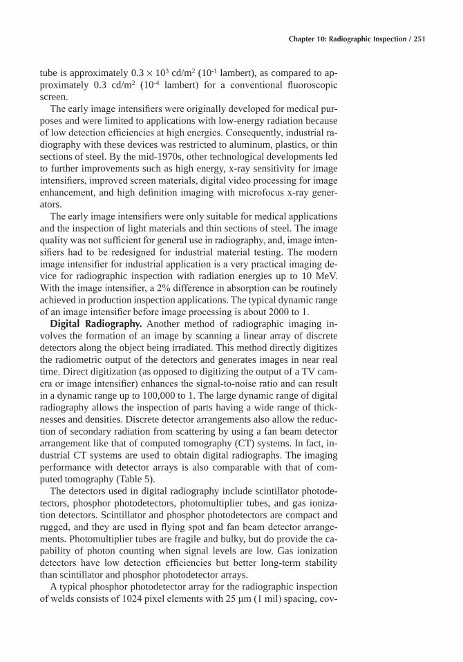
Chapter 10: Radiographic Inspection / 251
tube is approximately 0.3 × 10³ cd/m2 (10-1 lambert), as compared to ap-proximately 0.3 cd/m2 (10-4 lambert) for a conventional fluoroscopic screen.
The early image intensifiers were originally developed for medical pur-poses and were limited to applications with low-energy radiation because of low detection efficiencies at high energies. Consequently, industrial ra-diography with these devices was restricted to aluminum, plastics, or thin sections of steel. By the mid-1970s, other technological developments led to further improvements such as high energy, x-ray sensitivity for image intensifiers, improved screen materials, digital video processing for image enhancement, and high definition imaging with microfocus x-ray gener- ators.
The early image intensifiers were only suitable for medical applications and the inspection of light materials and thin sections of steel. The image quality was not sufficient for general use in radiography, and, image inten-sifiers had to be redesigned for industrial material testing. The modern image intensifier for industrial application is a very practical imaging de-vice for radiographic inspection with radiation energies up to 10 MeV. With the image intensifier, a 2% difference in absorption can be routinely achieved in production inspection applications. The typical dynamic range of an image intensifier before image processing is about 2000 to 1.
Digital Radiography� Another method of radiographic imaging in-volves the formation of an image by scanning a linear array of discrete detectors along the object being irradiated. This method directly digitizes the radiometric output of the detectors and generates images in near real time. Direct digitization (as opposed to digitizing the output of a TV cam-era or image intensifier) enhances the signal-to-noise ratio and can result in a dynamic range up to 100,000 to 1. The large dynamic range of digital radiography allows the inspection of parts having a wide range of thick-nesses and densities. Discrete detector arrangements also allow the reduc-tion of secondary radiation from scattering by using a fan beam detector arrangement like that of computed tomography (CT) systems. In fact, in-dustrial CT systems are used to obtain digital radiographs. The imaging performance with detector arrays is also comparable with that of com-puted tomography (Table 5).
The detectors used in digital radiography include scintillator photode-tectors, phosphor photodetectors, photomultiplier tubes, and gas ioniza-tion detectors. Scintillator and phosphor photodetectors are compact and rugged, and they are used in flying spot and fan beam detector arrange-ments. Photomultiplier tubes are fragile and bulky, but do provide the ca-pability of photon counting when signal levels are low. Gas ionization detectors have low detection efficiencies but better long-term stability than scintillator and phosphor photodetector arrays.
A typical phosphor photodetector array for the radiographic inspection of welds consists of 1024 pixel elements with 25 μm (1 mil) spacing, cov-
252 / Inspection of Metals—Understanding the Basics
ering 25 mm (1 in.) in length perpendicular weld seam. The linear photo-diode array is covered with a fiberoptic faceplate and can be cooled in order to reduce noise. For the conversion of the x-rays to visible light, fluorescent screens are coupled to the array by means of the fiber optics. A linear collimator parallel to the array is arranged in front of the screen. The resolution perpendicular to the array is defined by the width of this slit and the speed of the manipulator. A second, single element detector is provided to detect instabilities of the x-ray beam. Using 100 kV radiation, a spatial resolution of 0.1 mm (0.004 in.) can be achieved with a scanning speed of 1 to 10 mm/s (0.04 to 0.4 in./s).
The data from the detector system are digitized and then stored in a fast dual ported memory. This permits quasi simultaneous access to the data during acquisition. Before the image is stored in the frame buffer and dis-played on the monitor, simple preprocessing can be done, such as inten-sity correction of the x-ray tube by the data of the second detector and correction of the sensitivity for different array elements. If further image processing or automatic defect evaluation is required, the system can be equipped with fast image processing hardware. All standard devices for digital storage can be utilized.
Image Processing� Because real-time systems generally do not provide the same level of image quality and contrast as radiographic film, image processing is often used to enhance the images from image intensifiers, fluorescent screens, and detector arrays. With image processing, the video images from real-time systems can compete with the image quality of film radiography. Moreover, image processing also increases the dynamic
Table 5 Comparison of performance characteristics for film radiography, real-time radiography, and x-ray computed tomography
Performance characteristic Film radiography Real-time radiography(a) Computed tomography or
digital radiography(b)
Spatial resolution(c) >5 line pairs/mm ~2.5 line pairs/mm 0.2–4.5 line pairs/mmAbsorption efficiencies, %Absorption efficiency
(80 keV)5 20 99
Absorption efficiency (420 keV)
2 8 95
Absorption efficiency (2 MeV)
0.5 2 80
Sources of noise Scatter, poor photon statistics
Scatter, poor photon statistics
Minimal scatter
Dynamic range 200–1000 500–2000 Up to 1 × 10⁶
Digital image processing Poor, requires film scanner
Moderate to good; typi-cally 8-bit data
Excellent; typically 16-bit data
Dimensioning capability Moderate; affected by structure visibility and variable radiographic magnification
Moderate to poor; affected by structure visibility, resolution, variable ra-diographic magnifica-tion, and optical distor-tions
Excellent; affected by reso-lution, enhanced by low contrast detectability
Source: (a) General characteristics of real-time radiography with fluorescent screen-TV camera system or an image intensifier. (b) Digi-tal radiographic imaging performance with discrete element detector arrays is comparable to computed tomography performance values. (c) Can be improved with microfocus x-ray source and geometric magnification. Source: Ref 1
Chapter 10: Radiographic Inspection / 253
range of real-time systems beyond that of film, which typically has a dy-namic range of about 1000 to 1.
Images can be processed in two ways: as an analog video signal and as a digitized signal. An example of analog processing is to shade the image after the signal leaves the camera. Shading compensates for irregularities in brightness across the video image due to thickness or density variations in the test piece. This increases the dynamic range (or latitude) of the sys-tem, which allows the inspection of parts having larger variations in thick-ness and density.
After analog image processing, the images can be digitized for further image enhancement. This digitization of the signal may involve some de-tector requirements. In all real-time radiological applications, the images have to be obtained at low dose rates (around 20 μR/s). However, in digital x-ray imaging, the most often used dose is around 1 mR, in order to reduce the signal fluctuations that would result from a weak x-ray flux. This means that only a short exposure time (of the order of a few milliseconds) and a frequency of several images can be used if kinetic (motion) blurring is to be avoided. The resulting requirements for the x-ray detector are:
• The capability of operating properly in a pulsed mode, which calls for a fast temporal response
• An excellent linearity, to allow the use of the simplest and most effi-cient form of signal processing
• A wide operating dynamic range in terms of dose output (around 2000 to 1)
Once the image from the video camera has been digitized in the image processor, a variety of processing techniques can be implemented. The image processing techniques may range from the relatively simple opera-tion of frame integration to more complex operations such as automatic defect evaluation.
Radiation Gaging� Radiation measuring instruments do not produce images. The output from these instruments is a meter reading or a strip chart, which records the radiation transmitted through a test piece in terms of roentgens. Many of these instruments are routinely used to check areas surrounding a radiographic inspection site for excessive radiation.
Radiation gaging can be applied to certain automated processes, such as thickness gaging of materials or determination of liquid levels in sealed containers. In these applications, it may not be necessary to actually mea-sure the amount of radiation passing through the material, but only to de-tect changes in the level of radiation, in other words, for a “go, no-go” type of inspection.
When a highly absorbing material such as thick lead or concrete must be inspected for voids and when usual radiographic techniques are im-practical, radiation gaging can be used effectively. Voids can be located in
254 / Inspection of Metals—Understanding the Basics
these materials by noting increases in the readings of radiation detecting instruments.
Computed Tomography (CT)� Cross-sectional images of an inspection object can be obtained by a series of radiation attenuation measurements all around the object. Typically, a fan beam of radiation about 1 or 2 mm in height is used along with a bank of detectors on the opposite side of the object. The attenuation data permit a computer reconstruction showing density differences in the cross section of the object (Fig. 9a).
X-ray computed tomography has many of the same benefits and limi-tations as film and real-time radiography. The primary difference is the nature of the radiological image. Radiography (Fig. 9b) compresses the structural information from a three-dimensional volume into a two- dimensional image. This is useful in that it allows a relatively large vol-ume to be interrogated and represented in a single image. However, this compression limits the information and reduces the sensitivity to small variations. Radiographic images also can be difficult to interpret because of shadows from overlying and underlying structures superimposed on the features of interest. In contrast, the CT method provides sufficient infor-mation to localize a feature (Fig. 9a).
Some of the performance characteristics of radiography and computed tomography are compared in Table 5.
One of the limitations of CT inspection is that the CT image provides detailed information only over the limited volume of the cross-sectional slice. Full inspection of the entire volume of a component with computed tomography requires many slices, limiting the inspection throughput of the system. Therefore, CT equipment is often used in a digital radiography (DR) mode during production operations, with the CT imaging mode used for specific critical areas or to obtain more detailed information on indica-tions found in the DR image. Digital radiography capabilities and through-put can be significant operational considerations for the overall system usage. Computed tomography systems generally provide a DR imaging mode, producing a two-dimensional radiographic image of the overall test piece.
Characteristics of X-Ray Film
Three general characteristics of film (speed, gradient, and graininess) are primarily responsible for the performance of the film during exposure and processing and for the quality of the resulting image. Film speed, gra-dient, and graininess are interrelated; that is, the faster the film, the larger the graininess and the lower the gradient, and vice versa. Film speed and gradient are derived from the characteristic curve for a film emulsion, which is a plot of film density versus the exposure required for producing that density in the processed film. Graininess is an inherent property of the
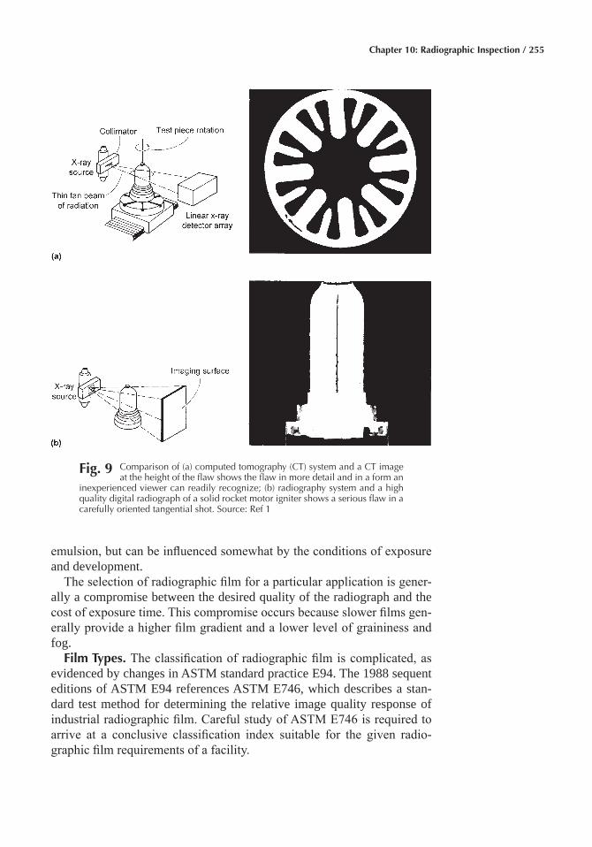
Chapter 10: Radiographic Inspection / 255
emulsion, but can be influenced somewhat by the conditions of exposure and development.
The selection of radiographic film for a particular application is gener-ally a compromise between the desired quality of the radiograph and the cost of exposure time. This compromise occurs because slower films gen-erally provide a higher film gradient and a lower level of graininess and fog.
Film Types� The classification of radiographic film is complicated, as evidenced by changes in ASTM standard practice E94. The 1988 sequent editions of ASTM E94 references ASTM E746, which describes a stan-dard test method for determining the relative image quality response of industrial radiographic film. Careful study of ASTM E746 is required to arrive at a conclusive classification index suitable for the given radio-graphic film requirements of a facility.
Fig� 9 Comparison of (a) computed tomography (CT) system and a CT image at the height of the flaw shows the flaw in more detail and in a form an
inexperienced viewer can readily recognize; (b) radiography system and a high quality digital radiograph of a solid rocket motor igniter shows a serious flaw in a carefully oriented tangential shot. Source: Ref 1
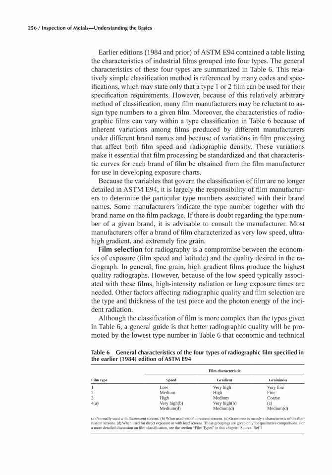
256 / Inspection of Metals—Understanding the Basics
Earlier editions (1984 and prior) of ASTM E94 contained a table listing the characteristics of industrial films grouped into four types. The general characteristics of these four types are summarized in Table 6. This rela-tively simple classification method is referenced by many codes and spec-ifications, which may state only that a type 1 or 2 film can be used for their specification requirements. However, because of this relatively arbitrary method of classification, many film manufacturers may be reluctant to as-sign type numbers to a given film. Moreover, the characteristics of radio-graphic films can vary within a type classification in Table 6 because of inherent variations among films produced by different manufacturers under different brand names and because of variations in film processing that affect both film speed and radiographic density. These variations make it essential that film processing be standardized and that characteris-tic curves for each brand of film be obtained from the film manufacturer for use in developing exposure charts.
Because the variables that govern the classification of film are no longer detailed in ASTM E94, it is largely the responsibility of film manufactur-ers to determine the particular type numbers associated with their brand names. Some manufacturers indicate the type number together with the brand name on the film package. If there is doubt regarding the type num-ber of a given brand, it is advisable to consult the manufacturer. Most manufacturers offer a brand of film characterized as very low speed, ultra-high gradient, and extremely fine grain.
Film selection for radiography is a compromise between the econom-ics of exposure (film speed and latitude) and the quality desired in the ra-diograph. In general, fine grain, high gradient films produce the highest quality radiographs. However, because of the low speed typically associ-ated with these films, high-intensity radiation or long exposure times are needed. Other factors affecting radiographic quality and film selection are the type and thickness of the test piece and the photon energy of the inci-dent radiation.
Although the classification of film is more complex than the types given in Table 6, a general guide is that better radiographic quality will be pro-moted by the lowest type number in Table 6 that economic and technical
Table 6 General characteristics of the four types of radiographic film specified in the earlier (1984) edition of ASTM E94
Film type
Film characteristic
Speed Gradient Graininess
1 Low Very high Very fine 2 Medium High Fine 3 High Medium Coarse 4(a) Very high(b) Very high(b) (c)
Medium(d) Medium(d) Medium(d)
(a) Normally used with fluorescent screens. (b) When used with fluorescent screens. (c) Graininess is mainly a characteristic of the fluo-rescent screens. (d) When used for direct exposure or with lead screens. These groupings are given only for qualitative comparisons. For a more detailed discussion on film classification, see the section “Film Types” in this chapter. Source: Ref 1
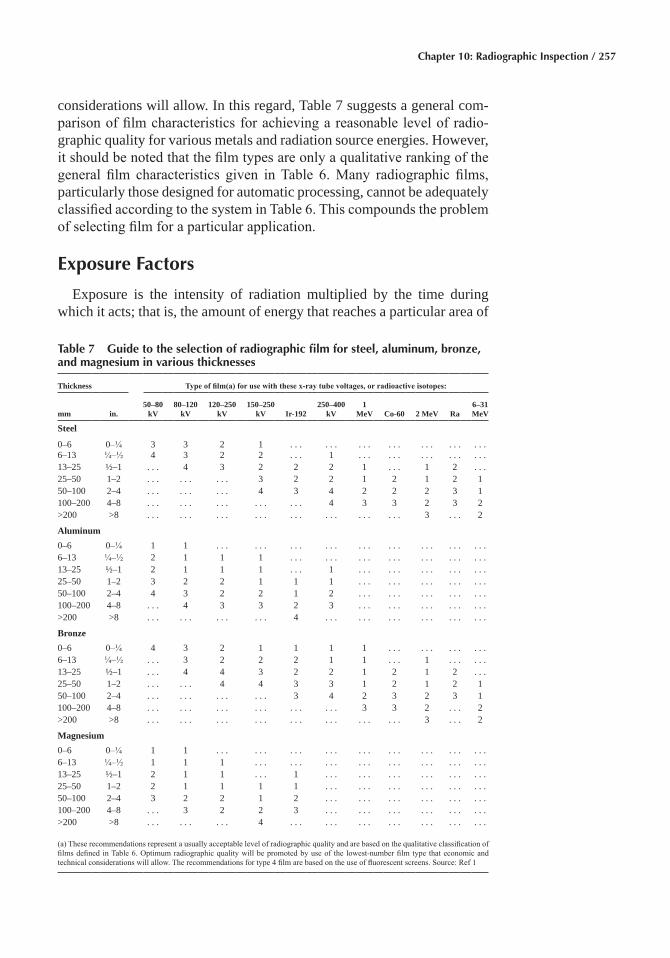
Chapter 10: Radiographic Inspection / 257
considerations will allow. In this regard, Table 7 suggests a general com-parison of film characteristics for achieving a reasonable level of radio-graphic quality for various metals and radiation source energies. However, it should be noted that the film types are only a qualitative ranking of the general film characteristics given in Table 6. Many radiographic films, particularly those designed for automatic processing, cannot be adequately classified according to the system in Table 6. This compounds the problem of selecting film for a particular application.
Exposure Factors
Exposure is the intensity of radiation multiplied by the time during which it acts; that is, the amount of energy that reaches a particular area of
Table 7 Guide to the selection of radiographic film for steel, aluminum, bronze, and magnesium in various thicknesses
Thickness Type of film(a) for use with these x-ray tube voltages, or radioactive isotopes:
mm in.50–80
kV80–120
kV120–250
kV150–250
kV Ir-192250–400
kV1
MeV Co-60 2 MeV Ra6–31 MeV
Steel
0–6 0–¼ 3 3 2 1 . . . . . . . . . . . . . . . . . . . . .6–13 ¼–½ 4 3 2 2 . . . 1 . . . . . . . . . . . . . . .13–25 ½–1 . . . 4 3 2 2 2 1 . . . 1 2 . . .25–50 1–2 . . . . . . . . . 3 2 2 1 2 1 2 150–100 2–4 . . . . . . . . . 4 3 4 2 2 2 3 1100–200 4–8 . . . . . . . . . . . . . . . 4 3 3 2 3 2>200 >8 . . . . . . . . . . . . . . . . . . . . . . . . 3 . . . 2
Aluminum0–6 0–¼ 1 1 . . . . . . . . . . . . . . . . . . . . . . . . . . .6–13 ¼–½ 2 1 1 1 . . . . . . . . . . . . . . . . . . . . .13–25 ½–1 2 1 1 1 . . . 1 . . . . . . . . . . . . . . .25–50 1–2 3 2 2 1 1 1 . . . . . . . . . . . . . . .50–100 2–4 4 3 2 2 1 2 . . . . . . . . . . . . . . .100–200 4–8 . . . 4 3 3 2 3 . . . . . . . . . . . . . . .>200 >8 . . . . . . . . . . . . 4 . . . . . . . . . . . . . . . . . .
Bronze0–6 0–¼ 4 3 2 1 1 1 1 . . . . . . . . . . . .6–13 ¼–½ . . . 3 2 2 2 1 1 . . . 1 . . . . . .13–25 ½–1 . . . 4 4 3 2 2 1 2 1 2 . . .25–50 1–2 . . . . . . 4 4 3 3 1 2 1 2 150–100 2–4 . . . . . . . . . . . . 3 4 2 3 2 3 1100–200 4–8 . . . . . . . . . . . . . . . . . . 3 3 2 . . . 2>200 >8 . . . . . . . . . . . . . . . . . . . . . . . . 3 . . . 2
Magnesium0–6 0–¼ 1 1 . . . . . . . . . . . . . . . . . . . . . . . . . . .6–13 ¼–½ 1 1 1 . . . . . . . . . . . . . . . . . . . . . . . .13–25 ½–1 2 1 1 . . . 1 . . . . . . . . . . . . . . . . . .25–50 1–2 2 1 1 1 1 . . . . . . . . . . . . . . . . . .50–100 2–4 3 2 2 1 2 . . . . . . . . . . . . . . . . . .100–200 4–8 . . . 3 2 2 3 . . . . . . . . . . . . . . . . . .>200 >8 . . . . . . . . . 4 . . . . . . . . . . . . . . . . . . . . .
(a) These recommendations represent a usually acceptable level of radiographic quality and are based on the qualitative classification of films defined in Table 6. Optimum radiographic quality will be promoted by use of the lowest-number film type that economic and technical considerations will allow. The recommendations for type 4 film are based on the use of fluorescent screens. Source: Ref 1
258 / Inspection of Metals—Understanding the Basics
the film and that is responsible for producing a particular density on the developed film. Density is the quantitative measure of blackening of a photographic emulsion. Density, measured directly with an instrument called a densitometer, is the logarithm of the ratio of the light intensity incident on the film to that transmitted by the film. Therefore, a film with a density of 1.0 will transmit only 10% of the light, a film with a density of 2.0 will transmit only 1/100 of the light, and so on.
There are two kinds of density: (a) the density associated with transpar-ent base radiographic film, called transmission density, and (b) the density associated with opaque base imaging material such as radiographic paper, called reflection density.
The exposure time in film radiography depends mainly on film speed, the intensity of radiation at the film surface, the characteristics of any screens used, and the desired level of photographic density. In practice, the energy of the radiation is first chosen to be sufficiently penetrating for the type of material and thickness to be inspected. The film type and the desired photographic density are then selected according to requirements for contrast sensitivity. Once these factors are fixed, then the source strength, the source-to-film distance, and the characteristics of any screens used determine the exposure time.
With a given type of film and screen, the exposure time to produce the desired photographic density can be determined. Because intensity is in-versely proportional to the square of distance from the source, the reci-procity law for equivalent exposures with an x-ray tube can be written as:
i t
L
i t
L1 1
12
2 2
22
=
where i is the tube current, t is the exposure time, L is the source-to-film distance, and the subscripts refer to two different combinations that pro-duce images with the desired photographic density. The parallel expres-sion that applies to exposures made with a γ-ray source is:
a t
L
a t
L1 1
12
2 2
22
=
where a is the source strength in gigabecquerel (Curies).Contrast sensitivity refers to the ability of responding to and display-
ing small variations in subject contrast. Contrast sensitivity depends on the characteristics of the image detector and on the level of radiation being detected or on the amount of exposure for films. The relationship between the contrast sensitivity and the level of radiation intensity, or film expo-sure, can be illustrated by considering two extremes. At low levels of ra-diation intensity, the contrast sensitivity of the detectors is reduced by a smaller signal-to-noise ratio, while at high levels, the detectors become
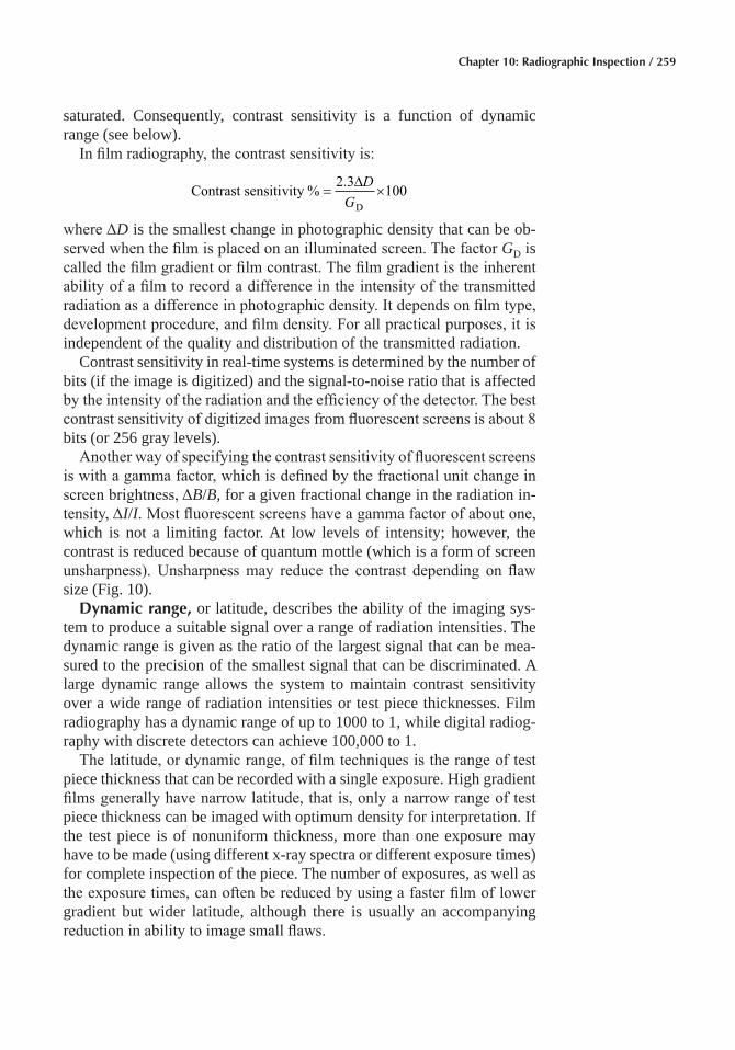
Chapter 10: Radiographic Inspection / 259
saturated. Consequently, contrast sensitivity is a function of dynamic range (see below).
In film radiography, the contrast sensitivity is:
Contrast sensitivity %D
= ×2 3
100. ∆DG
where ΔD is the smallest change in photographic density that can be ob-served when the film is placed on an illuminated screen. The factor GD is called the film gradient or film contrast. The film gradient is the inherent ability of a film to record a difference in the intensity of the transmitted radiation as a difference in photographic density. It depends on film type, development procedure, and film density. For all practical purposes, it is independent of the quality and distribution of the transmitted radiation.
Contrast sensitivity in real-time systems is determined by the number of bits (if the image is digitized) and the signal-to-noise ratio that is affected by the intensity of the radiation and the efficiency of the detector. The best contrast sensitivity of digitized images from fluorescent screens is about 8 bits (or 256 gray levels).
Another way of specifying the contrast sensitivity of fluorescent screens is with a gamma factor, which is defined by the fractional unit change in screen brightness, ΔB/B, for a given fractional change in the radiation in-tensity, ΔI/I. Most fluorescent screens have a gamma factor of about one, which is not a limiting factor. At low levels of intensity; however, the contrast is reduced because of quantum mottle (which is a form of screen unsharpness). Unsharpness may reduce the contrast depending on flaw size (Fig. 10).
Dynamic range, or latitude, describes the ability of the imaging sys-tem to produce a suitable signal over a range of radiation intensities. The dynamic range is given as the ratio of the largest signal that can be mea-sured to the precision of the smallest signal that can be discriminated. A large dynamic range allows the system to maintain contrast sensitivity over a wide range of radiation intensities or test piece thicknesses. Film radiography has a dynamic range of up to 1000 to 1, while digital radiog-raphy with discrete detectors can achieve 100,000 to 1.
The latitude, or dynamic range, of film techniques is the range of test piece thickness that can be recorded with a single exposure. High gradient films generally have narrow latitude, that is, only a narrow range of test piece thickness can be imaged with optimum density for interpretation. If the test piece is of nonuniform thickness, more than one exposure may have to be made (using different x-ray spectra or different exposure times) for complete inspection of the piece. The number of exposures, as well as the exposure times, can often be reduced by using a faster film of lower gradient but wider latitude, although there is usually an accompanying reduction in ability to image small flaws.
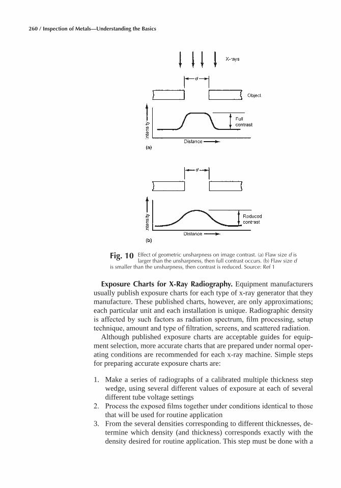
260 / Inspection of Metals—Understanding the Basics
Exposure Charts for X-Ray Radiography� Equipment manufacturers usually publish exposure charts for each type of x-ray generator that they manufacture. These published charts, however, are only approximations; each particular unit and each installation is unique. Radiographic density is affected by such factors as radiation spectrum, film processing, setup technique, amount and type of filtration, screens, and scattered radiation.
Although published exposure charts are acceptable guides for equip-ment selection, more accurate charts that are prepared under normal oper-ating conditions are recommended for each x-ray machine. Simple steps for preparing accurate exposure charts are:
1. Make a series of radiographs of a calibrated multiple thickness step wedge, using several different values of exposure at each of several different tube voltage settings
2. Process the exposed films together under conditions identical to those that will be used for routine application
3. From the several densities corresponding to different thicknesses, de-termine which density (and thickness) corresponds exactly with the density desired for routine application. This step must be done with a
Fig� 10 Effect of geometric unsharpness on image contrast. (a) Flaw size d is larger than the unsharpness, then full contrast occurs. (b) Flaw size d
is smaller than the unsharpness, then contrast is reduced. Source: Ref 1
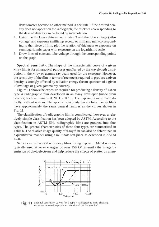
Chapter 10: Radiographic Inspection / 261
densitometer because no other method is accurate. If the desired den-sity does not appear on the radiograph, the thickness corresponding to the desired density can be found by interpolation
4. Using the thickness determined in step 3 and the tube voltage (kilo-voltage) and exposure (milliamp second or milliamp min) correspond-ing to that piece of film, plot the relation of thickness to exposure on semilogarithmic paper with exposure on the logarithmic scale
5. Draw lines of constant tube voltage through the corresponding points on the graph
Spectral Sensitivity� The shape of the characteristic curve of a given x-ray film is for all practical purposes unaffected by the wavelength distri-bution in the x-ray or gamma ray beam used for the exposure. However, the sensitivity of the film in terms of roentgens required to produce a given density is strongly affected by radiation energy (beam spectrum of a given kilovoltage or given gamma ray source).
Figure 11 shows the exposure required for producing a density of 1.0 on type 4 radiographic film developed in an x-ray developer (made from powder) for five minutes at 20 °C (68 °F). The exposures were made di-rectly, without screens. The spectral sensitivity curves for all x-ray films have approximately the same general features as the curves shown in Fig. 11.
The classification of radiographic film is complicated; however, a rela-tively simple classification has been adopted by ASTM. According to the classification in ASTM E94, radiographic films are grouped into four types. The general characteristics of these four types are summarized in Table 6. The relative image quality of x-ray film can also be determined in a quantitative manner using a multihole test piece as described in ASTM E746.
Screens are often used with x-ray films during exposure. Metal screens, typically used at x-ray energies of over 150 kV, intensify the image by emission of photoelectrons and help reduce the effects of scatter by atten-
Fig� 11 Spectral sensitivity curves for a type 4 radiographic film, showing exposure required to produce a density of 1.0. Source: Ref 1
262 / Inspection of Metals—Understanding the Basics
uating the lower-energy scattered radiation. Lead is typically used. Fluo-rescent screens are used in some situations to help reduce exposure times.
Image Quality� The quality level of an industrial radiograph is gov-erned by the radiographic sensitivity exhibited on the radiograph itself. Radiographic sensitivity is determined through the use of penetrameters or image-quality indicators (IQI).
Penetrameters, or IQIs, are of a known size and shape, and have the same attenuation characteristics as the material in the test piece. They are placed on the test piece or on a block of identical material during setup and are radiographed at the same time as the test piece. Penetrameters are preferably located in regions of maximum test piece thickness and great-est test piece-to-film distance, and near the outer edge of the central beam of radiation. The degree to which features of the penetrameter are visible in the developed image is a measure of the quality of that image. The image of the penetrameter that appears on the finished radiograph is eval-uated during interpretation to ensure that the desired sensitivity, definition, and contrast have been achieved in the developed image.
Penetrameters of different designs have been developed by various standards making organizations. Common types are plaques containing holes and a second type containing a series of wires. Plaque type pene-trameters consist of strips of material of uniform thickness with holes drilled through them specified by ASTM E142. Wire type penetrameters are widely used in Europe (German standard DIN 54109). They are also used in the United States and are described in ASTM standard E747. The sensitivity of a wire type penetrameter is expressed in terms of wire diam-eter divided by object thickness.
Neutron Radiography
Neutron radiography is a form of nondestructive inspection that uses a specific type of particulate radiation, called neutrons, to form a radio-graphic image of a test piece. The geometric principles of shadow forma-tion, variation of attenuation with test piece thickness, and many other factors that govern the exposure and processing of a neutron radiograph are similar to those for radiography using x-rays or gamma rays.
The section deals mainly with the characteristics that differentiate neu-tron radiography from x-ray or gamma ray radiography. The application of neutron radiography is described in terms of its advantages for im-proved contrast on low atomic number materials, discrimination between isotopes, or inspection of radioactive specimens.
Neutrons are subatomic particles that are characterized by relatively large mass and a neutral electric charge. The attenuation of neutrons dif-fers from the attenuation of x-rays in that the processes of attenuation are nuclear rather than processes that depend on interaction with electron shells surrounding the nucleus.

Chapter 10: Radiographic Inspection / 263
Neutrons are produced by nuclear reactors, accelerators, or certain ra-dioactive isotopes, all of which emit neutrons of relatively high energy (fast neutrons). Because most neutron radiography is performed with neu-trons of lower energy (thermal neutrons), the sources are usually sur-rounded by a moderator, which is a material that reduces the kinetic en-ergy of the neutrons by scattering.
Neutron radiography differs from conventional radiography in that the attenuation of neutrons as they pass through the test piece is more related to the specific isotope present than to density or atomic number. X-rays are attenuated more by elements of high atomic number than by elements of low atomic number, and this effect varies relatively smoothly with atomic number. Also, x-rays are generally attenuated more by materials of high density than they are by materials of low density. For thermal neu-trons, the attenuation tends to decrease with increasing atomic number, although the trend is by no means a smooth relationship. In addition to the high attenuation of several light elements (hydrogen, lithium, and boron), certain medium to heavy elements (especially cadmium, samarium, euro-pium, gadolinium, and dysprosium) and certain specific isotopes have ex-ceptionally high capabilities for absorbing thermal neutrons. This means that neutron radiography is capable of detecting these highly attenuating elements or isotopes when present in a structure of lower absorption capability.
Using neutrons, it is possible to radiographically detect certain isotopes, for instance, certain isotopes of hydrogen, cadmium, or uranium. Some neutron image detection methods are insensitive to gamma rays or x-rays and can be used to inspect radioactive materials such as reactor fuel ele-ments. The high attenuation of hydrogen, in particular, opens many appli-cation possibilities, including inspection of assemblies for detection of adhesives, explosives, lubricants, water, hydrides, corrosion, plastics, or rubber.
Neutron Sources
The excellent discrimination capabilities of neutrons generally refer to neutrons of low energy, that is, thermal neutrons. Characteristics of neu-tron radiography corresponding to various ranges of neutron energy are summarized in Table 8. Although any of these energy ranges can be used for radiography, this section emphasizes the thermal neutron range, which is the most widely used for inspection.
In thermal-neutron radiography, an object or test piece is placed in a thermal-neutron beam in front of an image detector. The neutron beam may be obtained from a nuclear reactor, a radioactive source, or an accel-erator. Several characteristics of these sources are summarized in Table 9. For thermal neutron radiography, fast neutrons emitted by these sources must first be moderated and then collimated. The radiographic intensities
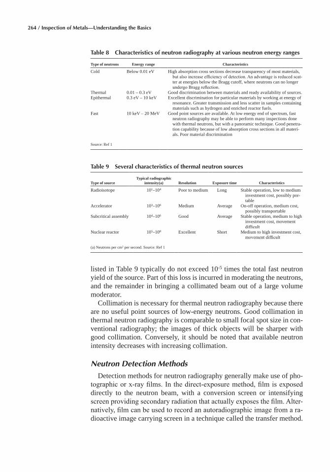
264 / Inspection of Metals—Understanding the Basics
listed in Table 9 typically do not exceed 10-5 times the total fast neutron yield of the source. Part of this loss is incurred in moderating the neutrons, and the remainder in bringing a collimated beam out of a large volume moderator.
Collimation is necessary for thermal neutron radiography because there are no useful point sources of low-energy neutrons. Good collimation in thermal neutron radiography is comparable to small focal spot size in con-ventional radiography; the images of thick objects will be sharper with good collimation. Conversely, it should be noted that available neutron intensity decreases with increasing collimation.
Neutron Detection Methods
Detection methods for neutron radiography generally make use of pho-tographic or x-ray films. In the direct-exposure method, film is exposed directly to the neutron beam, with a conversion screen or intensifying screen providing secondary radiation that actually exposes the film. Alter-natively, film can be used to record an autoradiographic image from a ra-dioactive image carrying screen in a technique called the transfer method.
Table 8 Characteristics of neutron radiography at various neutron energy ranges
Type of neutrons Energy range Characteristics
Cold Below 0.01 eV High absorption cross sections decrease transparency of most materials, but also increase efficiency of detection. An advantage is reduced scat-ter at energies below the Bragg cutoff, where neutrons can no longer undergo Bragg reflection.
Thermal 0.01 – 0.3 eV Good discrimination between materials and ready availability of sources.Epithermal 0.3 eV – 10 keV Excellent discrimination for particular materials by working at energy of
resonance. Greater transmission and less scatter in samples containing materials such as hydrogen and enriched reactor fuels.
Fast 10 keV – 20 MeV Good point sources are available. At low energy end of spectrum, fast neutron radiography may be able to perform many inspections done with thermal neutrons, but with a panoramic technique. Good penetra-tion capability because of low absorption cross sections in all materi-als. Poor material discrimination
Source: Ref 1
Table 9 Several characteristics of thermal neutron sources
Type of sourceTypical radiographic
intensity(a) Resolution Exposure time Characteristics
Radioisotope 101–104 Poor to medium Long Stable operation, low to medium investment cost, possibly por-table
Accelerator 103–106 Medium Average On-off operation, medium cost, possibly transportable
Subcritical assembly 104–106 Good Average Stable operation, medium to high investment cost, movement difficult
Nuclear reactor 105–108 Excellent Short Medium to high investment cost, movement difficult
(a) Neutrons per cm2 per second. Source: Ref 1
Chapter 10: Radiographic Inspection / 265
Direct Exposure Method� Conversion screens of thin gadolinium foil or a scintillator have been most widely used in the direct exposure method. When bombarded with a beam of neutrons, some of the gadolinium atoms absorb neutrons and promptly emit gamma rays and internal conversion electrons. Scintillators are fluorescent screens, often made of zinc sulfide crystals that also contain a specific isotope such as 3Li6 or 5B10. Gadolin-ium oxysulfide, a scintillator originally developed for x-ray radiography, has been widely used for neutron radiography.
Scintillators provide useful images with total exposures as low as 5 × 10⁵ neutrons per cm2. The high speed and favorable relative response make scintillators attractive for use with nonreactor neutron sources. Gad-olinium screens provide greater uniformity and image sharpness (high-contrast resolution of 10 mm has been reported), but an exposure about 30 or more times that of a scintillator is required, even with fast films.
Transfer Method� In the transfer method, a thin sheet of metal, typi-cally of indium or dysprosium, is exposed to the neutron beam transmitted through the specimen. Neutron capture induces radioactivity−indium hav-ing a half-life of 54 minutes and dysprosium a half-life of 2.35 hours. The radiograph to be interpreted is made by placing the radioactive transfer screen in contact with a sheet of film. Beta-particles and gamma rays from the transfer screen expose the film.
The transfer method is especially valuable for inspection of a radioac-tive specimen. Although radiation emitted by the specimen (especially gamma rays) causes heavy film fogging during x-ray radiography or direct exposure neutron radiography, the same radiation will not induce radioac-tivity in a transfer screen. Thus, a clear image of the specimen can be ob-tained even when there is a high level of background radiation.
In comparing the two primary detection methods, the direct exposure method offers high speed, indefinite image integration time and the best spatial resolution. The transfer method offers insensitivity to gamma rays emitted by the specimen and greater contrast because of lower amounts of scattered and secondary radiation.
Real time imaging, in which light from a scintillator is observed by a television camera, also can be used for neutron radiography. Because of low brightness, most real-time neutron radiographic images are enhanced by an image intensifier tube, which may be separate or integral with a television camera. This method can be used for applications such as the study of fluid flow in a closed system such as a heat pipe or engine or the study of metal flow in a mold during casting.
Applications
Various applications that are discussed in ASTM STP 586 emphasize the value of neutron radiography for inspection of ordnance, explosive,
266 / Inspection of Metals—Understanding the Basics
aerospace, and nuclear components. The presence, absence, or correct placement of explosives, adhesives, O-rings, plastic components, and similar materials can be verified. The presence of fluids or corrosion can be detected. Nuclear fuel and control materials can be inspected to deter-mine distribution of isotopes and to detect foreign or imperfect material. Hydride deposition in metals and diffusion of boron in heat-treated, bo-ron-fiber composites can be observed.
The characteristics of neutron radiography complement those of con-ventional x-radiography; one radiation provides a capability lacking or difficult for the other.
ACKNOWLEDGMENT
This chapter was adapted from Radiography in Metals Handbook Desk Edition, Second Edition, 1998.
REFERENCES
1. Radiography, Metals Handbook Desk Edition, 2nd ed., ASM Interna-tional, 1998, p 1292–1302
SELECTED REFERENCES
• L. Cartz, Nondestructive Testing, ASM International, 1995• D.E. Bray and R.K. Stanley, Nondestructive Evaluation: A Tool in De-
sign, Manufacturing, and Service, Taylor & Francis, 1996• Nondestructive Testing and Quality Control, Vol 17, ASM Handbook,
ASM International, 1989• P.J. Shull, Nondestructive Evaluation: Theory, Techniques, and Ap-
plications, Marcel Dekker, 2001
Inspection of Metals—Understanding the Basics Copyright © 2013 ASM International®
F.C. Campbell, editor All rights reservedwww.asminternational.org
CHAPTER 11
Ultrasonic Inspection
ULTRASONIC INSPECTION is a nondestructive method in which beams of high frequency acoustic energy are introduced into a material to detect surface and subsurface flaws, to measure the thickness of the material, and to measure the distance to a flaw. An ultrasonic beam trav-els through a material until it strikes an interface or discontinuity such as a flaw. Interfaces and flaws interrupt the beam and reflect a portion of the incident acoustic energy. The amount of energy reflected is a func-tion of (a) the nature and orientation of the interface or flaw and (b) the acoustic impedance of such a reflector. Energy reflected from various interfaces and flaws can be used to define the presence and locations of flaws; the thickness of the material; and, the depth of a flaw beneath a surface.
Most ultrasonic inspections are performed using a frequency between 1 and 25 MHz. Short shock bursts of ultrasonic energy are aimed into the material from the ultrasonic search unit of the ultrasonic flaw detector in-strument. The electrical pulse from the flaw detector is converted into ul-trasonic energy by a piezoelectric transducer element in the search unit. The beam pattern from the search unit is determined by the operating fre-quency and size of the transducer element. Ultrasonic energy travels through the material at a specific velocity that is dependent on the physical properties of the material and on the mode of propagation of the ultrasonic wave. The amount of energy reflected from or transmitted through an in-terface, other type of discontinuity, or reflector depends on the properties of the reflector. These phenomena provide the basis for establishing two of the most common measurement parameters used in ultrasonic inspection: the amplitude of the energy reflected from an interface or flaw and the time required from pulse initiation for the ultrasonic beam to reach the interface or flaw.
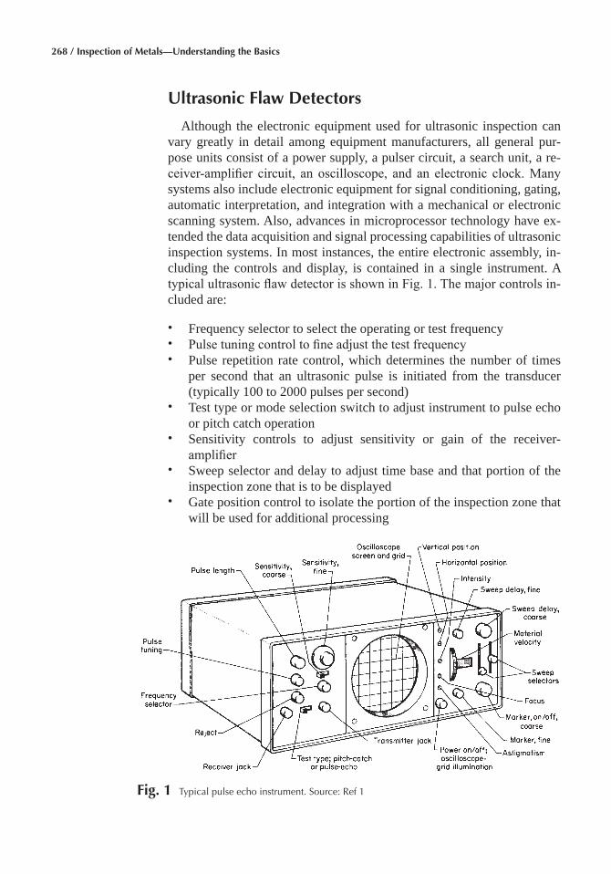
268 / Inspection of Metals—Understanding the Basics
Ultrasonic Flaw Detectors
Although the electronic equipment used for ultrasonic inspection can vary greatly in detail among equipment manufacturers, all general pur-pose units consist of a power supply, a pulser circuit, a search unit, a re-ceiver-amplifier circuit, an oscilloscope, and an electronic clock. Many systems also include electronic equipment for signal conditioning, gating, automatic interpretation, and integration with a mechanical or electronic scanning system. Also, advances in microprocessor technology have ex-tended the data acquisition and signal processing capabilities of ultrasonic inspection systems. In most instances, the entire electronic assembly, in-cluding the controls and display, is contained in a single instrument. A typical ultrasonic flaw detector is shown in Fig. 1. The major controls in-cluded are:
• Frequency selector to select the operating or test frequency • Pulse tuning control to fine adjust the test frequency • Pulse repetition rate control, which determines the number of times
per second that an ultrasonic pulse is initiated from the transducer (typically 100 to 2000 pulses per second)
• Test type or mode selection switch to adjust instrument to pulse echo or pitch catch operation
• Sensitivity controls to adjust sensitivity or gain of the receiver- amplifier
• Sweep selector and delay to adjust time base and that portion of the inspection zone that is to be displayed
• Gate position control to isolate the portion of the inspection zone that will be used for additional processing
Fig� 1 Typical pulse echo instrument. Source: Ref 1
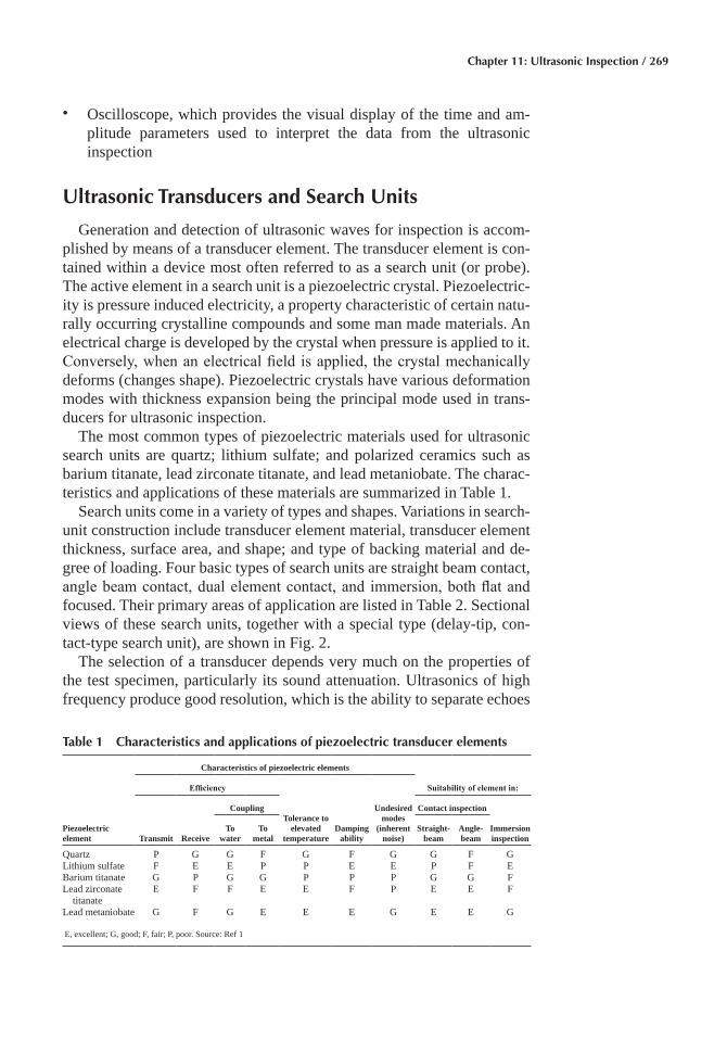
Chapter 11: Ultrasonic Inspection / 269
• Oscilloscope, which provides the visual display of the time and am-plitude parameters used to interpret the data from the ultrasonic inspection
Ultrasonic Transducers and Search Units
Generation and detection of ultrasonic waves for inspection is accom-plished by means of a transducer element. The transducer element is con-tained within a device most often referred to as a search unit (or probe). The active element in a search unit is a piezoelectric crystal. Piezoelectric-ity is pressure induced electricity, a property characteristic of certain natu-rally occurring crystalline compounds and some man made materials. An electrical charge is developed by the crystal when pressure is applied to it. Conversely, when an electrical field is applied, the crystal mechanically deforms (changes shape). Piezoelectric crystals have various deformation modes with thickness expansion being the principal mode used in trans-ducers for ultrasonic inspection.
The most common types of piezoelectric materials used for ultrasonic search units are quartz; lithium sulfate; and polarized ceramics such as barium titanate, lead zirconate titanate, and lead metaniobate. The charac-teristics and applications of these materials are summarized in Table 1.
Search units come in a variety of types and shapes. Variations in search-unit construction include transducer element material, transducer element thickness, surface area, and shape; and type of backing material and de-gree of loading. Four basic types of search units are straight beam contact, angle beam contact, dual element contact, and immersion, both flat and focused. Their primary areas of application are listed in Table 2. Sectional views of these search units, together with a special type (delay-tip, con-tact-type search unit), are shown in Fig. 2.
The selection of a transducer depends very much on the properties of the test specimen, particularly its sound attenuation. Ultrasonics of high frequency produce good resolution, which is the ability to separate echoes
Table 1 Characteristics and applications of piezoelectric transducer elements
Piezoelectric element
Characteristics of piezoelectric elements
Suitability of element in: Efficiency
Tolerance to elevated
temperature Damping
ability
Undesired modes
(inherent noise) Transmit Receive
Coupling Contact inspection
Immersion inspection
To water
To metal
Straight-beam
Angle-beam
Quartz P G G F G F G G F G Lithium sulfate F E E P P E E P F E Barium titanate G P G G P P P G G F Lead zirconate titanate
E F F E E F P E E F
Lead metaniobate G F G E E E G E E G
E, excellent; G, good; F, fair; P, poor. Source: Ref 1
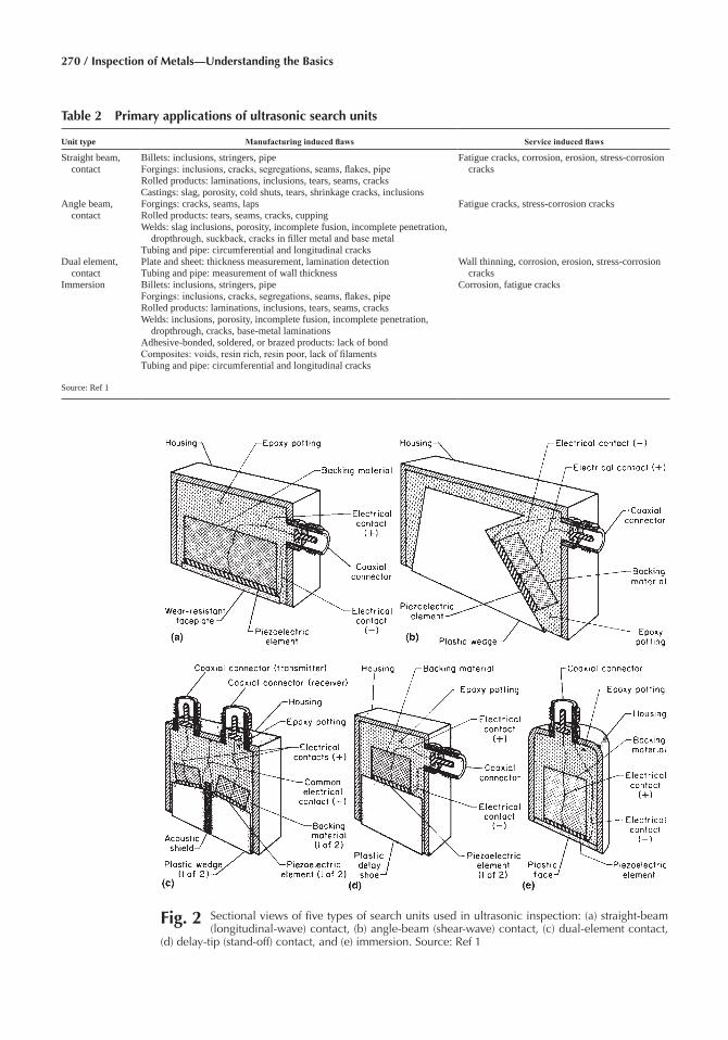
270 / Inspection of Metals—Understanding the Basics
Table 2 Primary applications of ultrasonic search units
Unit type Manufacturing induced flaws Service induced flaws
Straight beam, contact
Billets: inclusions, stringers, pipeForgings: inclusions, cracks, segregations, seams, flakes, pipeRolled products: laminations, inclusions, tears, seams, cracks Castings: slag, porosity, cold shuts, tears, shrinkage cracks, inclusions
Fatigue cracks, corrosion, erosion, stress-corrosion cracks
Angle beam, contact
Forgings: cracks, seams, laps Rolled products: tears, seams, cracks, cupping Welds: slag inclusions, porosity, incomplete fusion, incomplete penetration,
dropthrough, suckback, cracks in filler metal and base metal Tubing and pipe: circumferential and longitudinal cracks
Fatigue cracks, stress-corrosion cracks
Dual element, contact
Plate and sheet: thickness measurement, lamination detection Tubing and pipe: measurement of wall thickness
Wall thinning, corrosion, erosion, stress-corrosion cracks
Immersion Billets: inclusions, stringers, pipe Forgings: inclusions, cracks, segregations, seams, flakes, pipe Rolled products: laminations, inclusions, tears, seams, cracks Welds: inclusions, porosity, incomplete fusion, incomplete penetration,
dropthrough, cracks, base-metal laminations Adhesive-bonded, soldered, or brazed products: lack of bond Composites: voids, resin rich, resin poor, lack of filaments Tubing and pipe: circumferential and longitudinal cracks
Corrosion, fatigue cracks
Source: Ref 1
Fig� 2 Sectional views of five types of search units used in ultrasonic inspection: (a) straight-beam (longitudinal-wave) contact, (b) angle-beam (shear-wave) contact, (c) dual-element contact,
(d) delay-tip (stand-off) contact, and (e) immersion. Source: Ref 1

Chapter 11: Ultrasonic Inspection / 271
from closely spaced defects. Ultrasonics of low frequency penetrate deeper into materials because attenuation is generally lower. However, backscattering “noise” from grain boundaries is usually more important than attenuation, although the net result is the same because the signal-to-noise ratio also usually decreases with frequency, as shown in Fig. 3. This means that the two requirements of high penetration and high resolution are mutually exclusive. For example, a specimen having high attenuation, such as steel, should be examined by a low frequency beam of about 0.5 MHz and a large transducer diameter about 50 mm (2 in.), which provides a high penetration, but a relatively low lateral resolution of about 6 mm (1/4 in.). Improved resolution can be obtained by using shear waves, be-cause these have shorter wavelengths than compression waves of the same frequency in the solid. The velocity of a longitudinal wave in a solid is greater than that of the shear wave of the same frequency. Large diameter transducers are chosen to produce a narrow focused beam, which en-hances the lateral resolution.
Couplants
Air is a poor transmitter of sound waves at megahertz frequencies. Also, because the acoustic impedance mismatch between air and most solids is significant, even a very thin layer of air severely retards the transmission of sound waves from the transducer to the test piece. Therefore, it is nec-essary to use a couplant to eliminate air between the transducer and the test piece for satisfactory contact inspection.
Couplants normally used for contact inspection include water, oils, glycerin, petroleum greases, silicone grease, cellulose gum, and various commercial pastelike substances. Certain soft rubbers that transmit sound
Fig� 3 Oscilloscope displays using ultrasonic transducers of (a) high and low penetration (ability to detect defects at distances within the solid), and
(b) high and low resolution (ability to separate echoes from closely spaced de-fects). Source: Ref 1
272 / Inspection of Metals—Understanding the Basics
waves can be used where adequate coupling can be achieved by applying pressure to the search unit.
Factors that should be considered in selecting a couplant are:
• Surface finish of test piece • Temperature of test surface • Possibility of chemical reactions between test surface and couplant • Cleaning requirements (some couplants are difficult to remove)
Water is a suitable couplant for use on a relatively smooth surface, but a wetting agent should be added. The addition of glycerin sometimes is nec-essary to increase viscosity.
Heavy oil or grease should be used on hot and vertical surfaces and on rough surfaces where irregularities need to be filled.
Cellulose gum is especially useful on rough surfaces when good cou-pling is needed to minimize background noise and yield an adequate signal-to-noise ratio.
Basic Inspection Methods
Ultrasound can be used to measure material thickness by (a) determin-ing resonant frequencies of a test piece and (b) measuring time required for an ultrasonic wave packet (pulse) to traverse the test piece. The former uses reflected ultrasound to create standing waves in the test piece; the frequencies at which standing waves occur are used to compute thickness. In the latter method, the time it takes for a pulse of ultrasonic energy to be transmitted through the test piece is measured; this time period can be 100 nanoseconds or less. Thickness is calculated as the product of the mea-sured time of flight and the known acoustic wave velocity.
Ultrasound can be used to detect flaws by measuring (a) the amplitude of the acoustic pressure wave and time of flight of reflected acoustic waves and (b) the amplitude of the acoustic pressure wave of either transmitted or reflected acoustic waves. The pulse echo technique is the most widely used ultrasonic technique. Flaws are detected and their sizes estimated by comparing the amplitude of a reflected echo from an interface (either within the test piece or at the back surface) with the amplitude of an echo reflected from a reference interface of known size or from the back sur-face of a test piece that has no flaws. The echo from the back surface (back reflection) serves as a reference point for time-of-flight measurements that enable measuring the depth of some internal flaws. It is necessary that an internal flaw reflect at least part of the sound energy onto the receiving transducer to measure depth. However, echoes from flaws are not essen-tial to their detection. Just because the amplitude of an echo from back reflection of a test piece is lower than that of an echo from an identical flaw-free workpiece implies that the test piece contains one or more flaws.
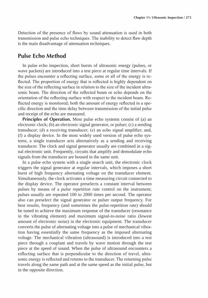
Chapter 11: Ultrasonic Inspection / 273
Detection of the presence of flaws by sound attenuation is used in both transmission and pulse echo techniques. The inability to detect flaw depth is the main disadvantage of attenuation techniques.
Pulse Echo Method
In pulse echo inspection, short bursts of ultrasonic energy (pulses, or wave packets) are introduced into a test piece at regular time intervals. If the pulses encounter a reflecting surface, some or all of the energy is re-flected. The proportion of energy that is reflected is highly dependent on the size of the reflecting surface in relation to the size of the incident ultra-sonic beam. The direction of the reflected beam or echo depends on the orientation of the reflecting surface with respect to the incident beam. Re-flected energy is monitored; both the amount of energy reflected in a spe-cific direction and the time delay between transmission of the initial pulse and receipt of the echo are measured.
Principles of Operation� Most pulse echo systems consist of (a) an electronic clock; (b) an electronic signal generator, or pulser; (c) a sending transducer; (d) a receiving transducer; (e) an echo signal amplifier; and, (f) a display device. In the most widely used version of pulse echo sys-tems, a single transducer acts alternatively as a sending and receiving transducer. The clock and signal generator usually are combined in a sig-nal electronic unit. Frequently, circuits that amplify and demodulate echo signals from the transducer are housed in the same unit.
In a pulse echo system with a single search unit, the electronic clock triggers the signal generator at regular intervals, which imposes a short burst of high frequency alternating voltage on the transducer element. Simultaneously, the clock activates a time measuring circuit connected to the display device. The operator preselects a constant interval between pulses by means of a pulse repetition rate control on the instrument; pulses usually are repeated 100 to 2000 times per second. The operator also can preselect the signal generator or pulser output frequency. For best results, frequency (and sometimes the pulse-repetition rate) should be tuned to achieve the maximum response of the transducer (resonance in the vibrating element) and maximum signal-to-noise ratio (lowest amount of electronic noise) in the electronic equipment. The transducer converts the pulse of alternating voltage into a pulse of mechanical vibra-tion having essentially the same frequency as the imposed alternating voltage. The mechanical vibration (ultrasound) is introduced into a test piece through a couplant and travels by wave motion through the test piece at the speed of sound. When the pulse of ultrasound encounters a reflecting surface that is perpendicular to the direction of travel, ultra-sonic energy is reflected and returns to the transducer. The returning pulse travels along the same path and at the same speed as the initial pulse, but in the opposite direction.
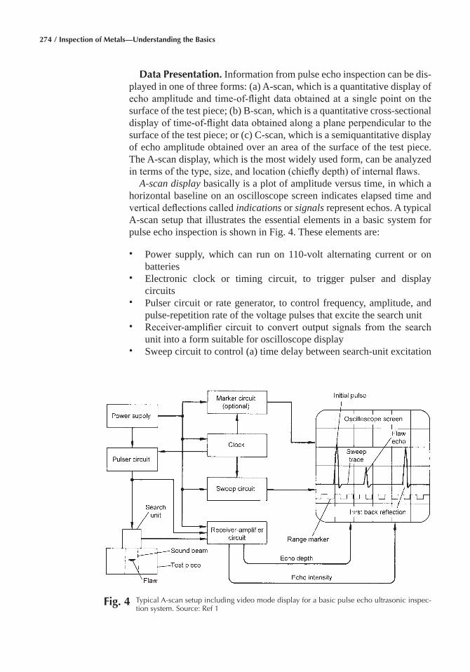
274 / Inspection of Metals—Understanding the Basics
Data Presentation� Information from pulse echo inspection can be dis-played in one of three forms: (a) A-scan, which is a quantitative display of echo amplitude and time-of-flight data obtained at a single point on the surface of the test piece; (b) B-scan, which is a quantitative cross-sectional display of time-of-flight data obtained along a plane perpendicular to the surface of the test piece; or (c) C-scan, which is a semiquantitative display of echo amplitude obtained over an area of the surface of the test piece. The A-scan display, which is the most widely used form, can be analyzed in terms of the type, size, and location (chiefly depth) of internal flaws.
A-scan display basically is a plot of amplitude versus time, in which a horizontal baseline on an oscilloscope screen indicates elapsed time and vertical deflections called indications or signals represent echos. A typical A-scan setup that illustrates the essential elements in a basic system for pulse echo inspection is shown in Fig. 4. These elements are:
• Power supply, which can run on 110-volt alternating current or on batteries
• Electronic clock or timing circuit, to trigger pulser and display circuits
• Pulser circuit or rate generator, to control frequency, amplitude, and pulse-repetition rate of the voltage pulses that excite the search unit
• Receiver-amplifier circuit to convert output signals from the search unit into a form suitable for oscilloscope display
• Sweep circuit to control (a) time delay between search-unit excitation
Fig� 4 Typical A-scan setup including video mode display for a basic pulse echo ultrasonic inspec-tion system. Source: Ref 1
Chapter 11: Ultrasonic Inspection / 275
and start of oscilloscope trace and (b) rate at which oscilloscope trace travels horizontally across the screen
• Marker circuit (optional) to produce a secondary trace, on or below the main trace, usually in the form of a square wave, which is used for precise depth measurements
• Oscilloscope screen, including separate controls for trace brightness, trace focus, and illuminated measuring grid
• Flaw gate (not shown) to isolate the echo of interest for further processing
The search unit and the coaxial cable connecting the unit to the instru-ment, although not strictly part of the electronic circuitry, must be matched to the electronics.
B-scan display is a plot of time versus distance, in which one orthogo-nal axis on the display corresponds to elapsed time, while the other axis represents the position of the search unit along a line on the surface of the test piece relative to the position of the search unit at the start of the in-spection. Echo amplitude is not measured directly as in A-scan inspection, but often it is indicated semiquantitatively by the relative brightness of echo indications on an oscilloscope screen.
A typical B-scan system is shown in Fig. 5. System functions are identi-cal to those of the A-scan system except for the following differences:
• The display is generated on an oscilloscope screen consisting of a long-persistence phosphor; that is, a phosphor that continues to fluo-resce long after the means of excitation ceases to fall on the fluoresc-
Fig� 5 Typical B-scan setup including video mode display for a basic pulse echo ultrasonic inspec-tion system. Source: Ref 1
276 / Inspection of Metals—Understanding the Basics
ing area of the screen. This allows the imaginary cross section to be viewed as a whole without having to resort to permanent imaging methods such as photographs. (Photographic equipment, facsimile re-corders, or x-y plotters can be used to record B-scan data for later reference.)
• Oscilloscope input for one axis of the display is provided by an elec-tromechanical device, which generates an electrical voltage propor-tional to the position of the search unit relative to a reference point on the surface of the test piece. Most B-scans are generated by scanning the search unit in a straight line across the surface of the test piece at a uniform rate. One axis of the display (usually the horizontal axis) rep-resents the distance traveled along this line.
• Echoes are indicated by bright spots on the screen rather than by de-flections of the time trace. The position of a bright spot along the axis orthogonal to the search-unit position axis (usually measured top to bottom on the screen) indicates the depth of the echo within the test piece.
• The echo-intensity signal from the receiver-amplifier is connected to the trace-brightness control on the oscilloscope to ensure that echoes are recorded as bright spots. In some systems, the brightnesses corre-sponding to different values of echo amplitude has sufficient contrast to permit semiquantitative appraisal of echo amplitude, which is re-lated to flaw size and shape.
The oscilloscope screen in Fig. 5 illustrates the type of video-mode dis-play that is generated by B-scan equipment. The internal flaw in the test piece shown at left in Fig. 5 is shown only as a profile view of its top re-flecting surface. Portions of the test piece that are behind this large reflect-ing surface are in shadow.
C-scan display records echoes from internal portions of test pieces as a function of the position of each reflecting interface within an area. Flaws are shown on a readout superimposed on a plan view of the test piece, and both flaw size (flaw area) and position within the plan view are recorded. Flaw depth typically is not recorded, although it can be measured semi-quantitatively by restricting the range of depths within the test piece that is covered in a given scan.
In a basic C-scan system, shown schematically in Fig. 6, the search unit is moved over the surface of the test piece in a search pattern. The search pattern can take many forms, such as a series of closely spaced parallel lines, a fine zigzag pattern, and a spiral pattern (polar scan). Mechanical linkage connects the search unit to x-axis and y-axis position indicators, which in turn, feed position data to the x-y plotter or facsimile device. Echo-recording systems vary; some produce a shaded-line scan with echo amplitude recorded as a variation in line shading, while others indicate
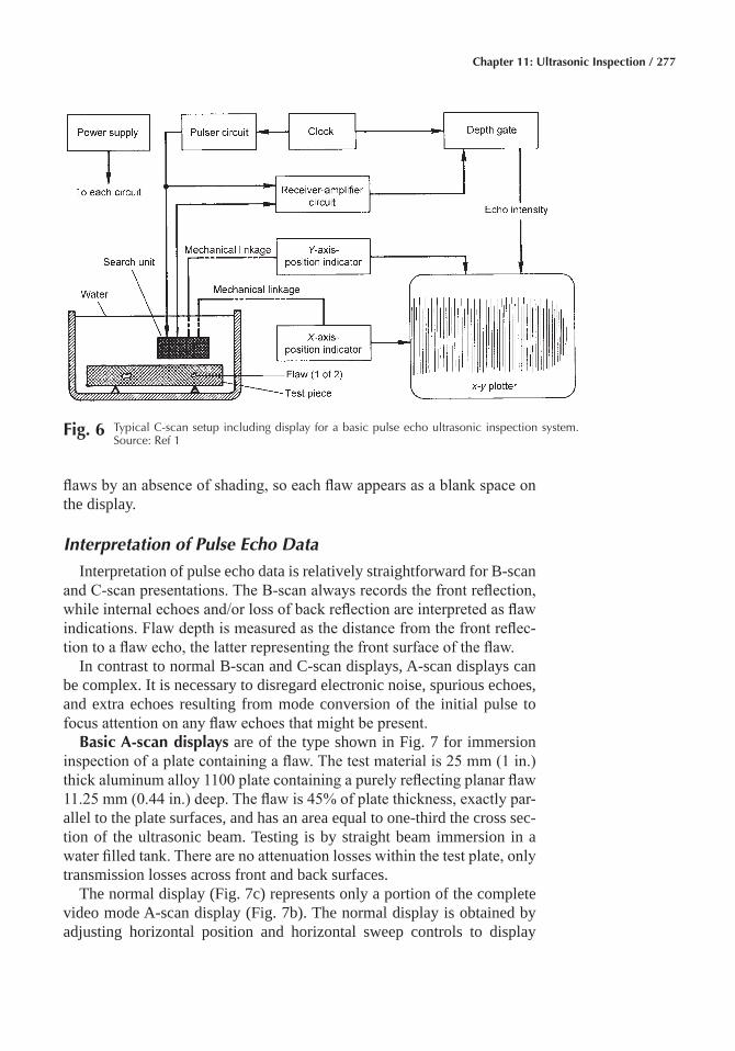
Chapter 11: Ultrasonic Inspection / 277
flaws by an absence of shading, so each flaw appears as a blank space on the display.
Interpretation of Pulse Echo Data
Interpretation of pulse echo data is relatively straightforward for B-scan and C-scan presentations. The B-scan always records the front reflection, while internal echoes and/or loss of back reflection are interpreted as flaw indications. Flaw depth is measured as the distance from the front reflec-tion to a flaw echo, the latter representing the front surface of the flaw.
In contrast to normal B-scan and C-scan displays, A-scan displays can be complex. It is necessary to disregard electronic noise, spurious echoes, and extra echoes resulting from mode conversion of the initial pulse to focus attention on any flaw echoes that might be present.
Basic A-scan displays are of the type shown in Fig. 7 for immersion inspection of a plate containing a flaw. The test material is 25 mm (1 in.) thick aluminum alloy 1100 plate containing a purely reflecting planar flaw 11.25 mm (0.44 in.) deep. The flaw is 45% of plate thickness, exactly par-allel to the plate surfaces, and has an area equal to one-third the cross sec-tion of the ultrasonic beam. Testing is by straight beam immersion in a water filled tank. There are no attenuation losses within the test plate, only transmission losses across front and back surfaces.
The normal display (Fig. 7c) represents only a portion of the complete video mode A-scan display (Fig. 7b). The normal display is obtained by adjusting horizontal position and horizontal sweep controls to display
Fig� 6 Typical C-scan setup including display for a basic pulse echo ultrasonic inspection system. Source: Ref 1
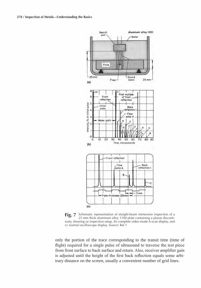
278 / Inspection of Metals—Understanding the Basics
only the portion of the trace corresponding to the transit time (time of flight) required for a single pulse of ultrasound to traverse the test piece from front surface to back surface and return. Also, receiver amplifier gain is adjusted until the height of the first back reflection equals some arbi-trary distance on the screen, usually a convenient number of grid lines.
Fig� 7 Schematic representation of straight-beam immersion inspection of a 25 mm thick aluminum alloy 1100 plate containing a planar disconti-
nuity, showing (a) inspection setup, (b) complete video mode A-scan display, and (c) normal oscilloscope display. Source: Ref 1
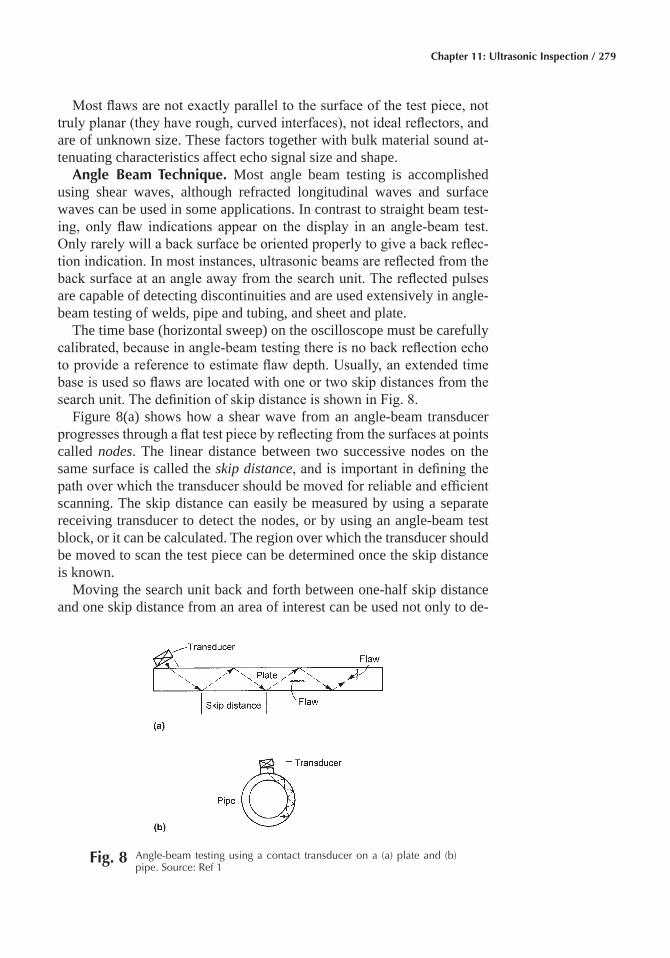
Chapter 11: Ultrasonic Inspection / 279
Most flaws are not exactly parallel to the surface of the test piece, not truly planar (they have rough, curved interfaces), not ideal reflectors, and are of unknown size. These factors together with bulk material sound at-tenuating characteristics affect echo signal size and shape.
Angle Beam Technique� Most angle beam testing is accomplished using shear waves, although refracted longitudinal waves and surface waves can be used in some applications. In contrast to straight beam test-ing, only flaw indications appear on the display in an angle-beam test. Only rarely will a back surface be oriented properly to give a back reflec-tion indication. In most instances, ultrasonic beams are reflected from the back surface at an angle away from the search unit. The reflected pulses are capable of detecting discontinuities and are used extensively in angle-beam testing of welds, pipe and tubing, and sheet and plate.
The time base (horizontal sweep) on the oscilloscope must be carefully calibrated, because in angle-beam testing there is no back reflection echo to provide a reference to estimate flaw depth. Usually, an extended time base is used so flaws are located with one or two skip distances from the search unit. The definition of skip distance is shown in Fig. 8.
Figure 8(a) shows how a shear wave from an angle-beam transducer progresses through a flat test piece by reflecting from the surfaces at points called nodes. The linear distance between two successive nodes on the same surface is called the skip distance, and is important in defining the path over which the transducer should be moved for reliable and efficient scanning. The skip distance can easily be measured by using a separate receiving transducer to detect the nodes, or by using an angle-beam test block, or it can be calculated. The region over which the transducer should be moved to scan the test piece can be determined once the skip distance is known.
Moving the search unit back and forth between one-half skip distance and one skip distance from an area of interest can be used not only to de-
Fig� 8 Angle-beam testing using a contact transducer on a (a) plate and (b) pipe. Source: Ref 1
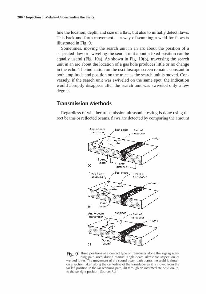
280 / Inspection of Metals—Understanding the Basics
fine the location, depth, and size of a flaw, but also to initially detect flaws. This back-and-forth movement as a way of scanning a weld for flaws is illustrated in Fig. 9.
Sometimes, moving the search unit in an arc about the position of a suspected flaw or swiveling the search unit about a fixed position can be equally useful (Fig. 10a). As shown in Fig. 10(b), traversing the search unit in an arc about the location of a gas hole produces little or no change in the echo. The indication on the oscilloscope screen remains constant in both amplitude and position on the trace as the search unit is moved. Con-versely, if the search unit was swiveled on the same spot, the indication would abruptly disappear after the search unit was swiveled only a few degrees.
Transmission Methods
Regardless of whether transmission ultrasonic testing is done using di-rect beams or reflected beams, flaws are detected by comparing the amount
Fig� 9 Three positions of a contact type of transducer along the zigzag scan-ning path used during manual angle-beam ultrasonic inspection of
welded joints. The movement of the sound beam path across the weld is shown on a section taken along the centerline of the transducer as it is moved from the far left position in the (a) scanning path, (b) through an intermediate position, (c) to the far right position. Source: Ref 1
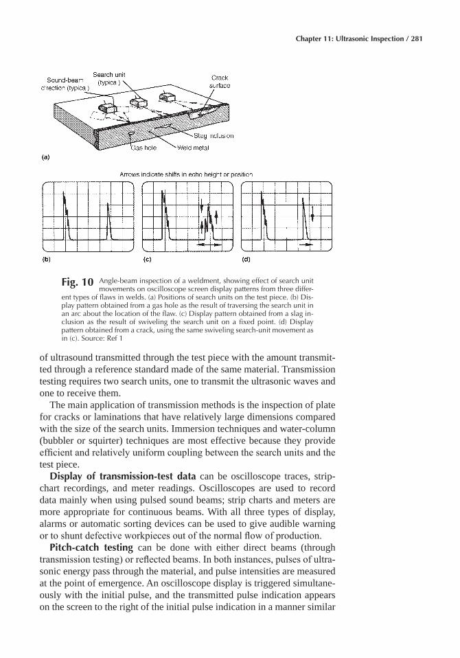
Chapter 11: Ultrasonic Inspection / 281
of ultrasound transmitted through the test piece with the amount transmit-ted through a reference standard made of the same material. Transmission testing requires two search units, one to transmit the ultrasonic waves and one to receive them.
The main application of transmission methods is the inspection of plate for cracks or laminations that have relatively large dimensions compared with the size of the search units. Immersion techniques and water-column (bubbler or squirter) techniques are most effective because they provide efficient and relatively uniform coupling between the search units and the test piece.
Display of transmission-test data can be oscilloscope traces, strip-chart recordings, and meter readings. Oscilloscopes are used to record data mainly when using pulsed sound beams; strip charts and meters are more appropriate for continuous beams. With all three types of display, alarms or automatic sorting devices can be used to give audible warning or to shunt defective workpieces out of the normal flow of production.
Pitch-catch testing can be done with either direct beams (through transmission testing) or reflected beams. In both instances, pulses of ultra-sonic energy pass through the material, and pulse intensities are measured at the point of emergence. An oscilloscope display is triggered simultane-ously with the initial pulse, and the transmitted pulse indication appears on the screen to the right of the initial pulse indication in a manner similar
Fig� 10 Angle-beam inspection of a weldment, showing effect of search unit movements on oscilloscope screen display patterns from three differ-
ent types of flaws in welds. (a) Positions of search units on the test piece. (b) Dis-play pattern obtained from a gas hole as the result of traversing the search unit in an arc about the location of the flaw. (c) Display pattern obtained from a slag in-clusion as the result of swiveling the search unit on a fixed point. (d) Display pattern obtained from a crack, using the same swiveling search-unit movement as in (c). Source: Ref 1
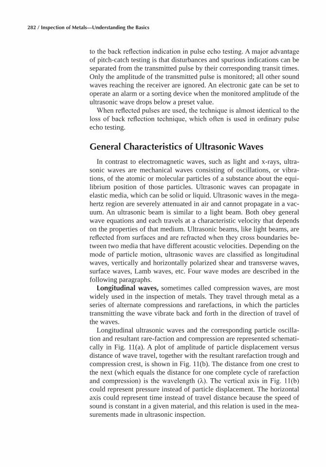
282 / Inspection of Metals—Understanding the Basics
to the back reflection indication in pulse echo testing. A major advantage of pitch-catch testing is that disturbances and spurious indications can be separated from the transmitted pulse by their corresponding transit times. Only the amplitude of the transmitted pulse is monitored; all other sound waves reaching the receiver are ignored. An electronic gate can be set to operate an alarm or a sorting device when the monitored amplitude of the ultrasonic wave drops below a preset value.
When reflected pulses are used, the technique is almost identical to the loss of back reflection technique, which often is used in ordinary pulse echo testing.
General Characteristics of Ultrasonic Waves
In contrast to electromagnetic waves, such as light and x-rays, ultra-sonic waves are mechanical waves consisting of oscillations, or vibra-tions, of the atomic or molecular particles of a substance about the equi-librium position of those particles. Ultrasonic waves can propagate in elastic media, which can be solid or liquid. Ultrasonic waves in the mega-hertz region are severely attenuated in air and cannot propagate in a vac-uum. An ultrasonic beam is similar to a light beam. Both obey general wave equations and each travels at a characteristic velocity that depends on the properties of that medium. Ultrasonic beams, like light beams, are reflected from surfaces and are refracted when they cross boundaries be-tween two media that have different acoustic velocities. Depending on the mode of particle motion, ultrasonic waves are classified as longitudinal waves, vertically and horizontally polarized shear and transverse waves, surface waves, Lamb waves, etc. Four wave modes are described in the following paragraphs.
Longitudinal waves, sometimes called compression waves, are most widely used in the inspection of metals. They travel through metal as a series of alternate compressions and rarefactions, in which the particles transmitting the wave vibrate back and forth in the direction of travel of the waves.
Longitudinal ultrasonic waves and the corresponding particle oscilla-tion and resultant rare-faction and compression are represented schemati-cally in Fig. 11(a). A plot of amplitude of particle displacement versus distance of wave travel, together with the resultant rarefaction trough and compression crest, is shown in Fig. 11(b). The distance from one crest to the next (which equals the distance for one complete cycle of rarefaction and compression) is the wavelength (λ). The vertical axis in Fig. 11(b) could represent pressure instead of particle displacement. The horizontal axis could represent time instead of travel distance because the speed of sound is constant in a given material, and this relation is used in the mea-surements made in ultrasonic inspection.
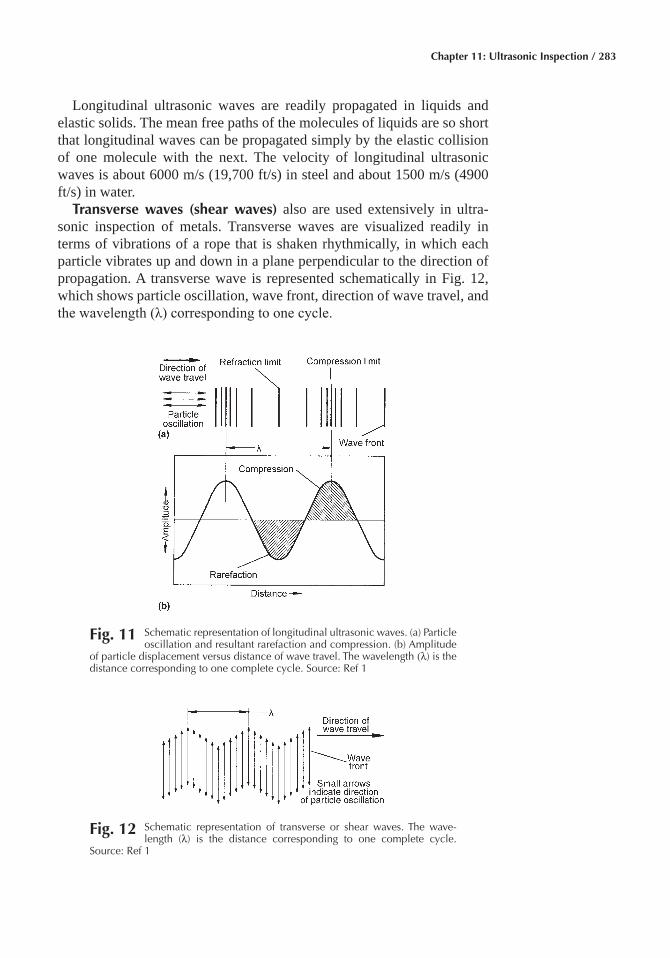
Chapter 11: Ultrasonic Inspection / 283
Longitudinal ultrasonic waves are readily propagated in liquids and elastic solids. The mean free paths of the molecules of liquids are so short that longitudinal waves can be propagated simply by the elastic collision of one molecule with the next. The velocity of longitudinal ultrasonic waves is about 6000 m/s (19,700 ft/s) in steel and about 1500 m/s (4900 ft/s) in water.
Transverse waves (shear waves) also are used extensively in ultra-sonic inspection of metals. Transverse waves are visualized readily in terms of vibrations of a rope that is shaken rhythmically, in which each particle vibrates up and down in a plane perpendicular to the direction of propagation. A transverse wave is represented schematically in Fig. 12, which shows particle oscillation, wave front, direction of wave travel, and the wavelength (λ) corresponding to one cycle.
Fig� 11 Schematic representation of longitudinal ultrasonic waves. (a) Particle oscillation and resultant rarefaction and compression. (b) Amplitude
of particle displacement versus distance of wave travel. The wavelength (λ) is the distance corresponding to one complete cycle. Source: Ref 1
Fig� 12 Schematic representation of transverse or shear waves. The wave-length (λ) is the distance corresponding to one complete cycle.
Source: Ref 1
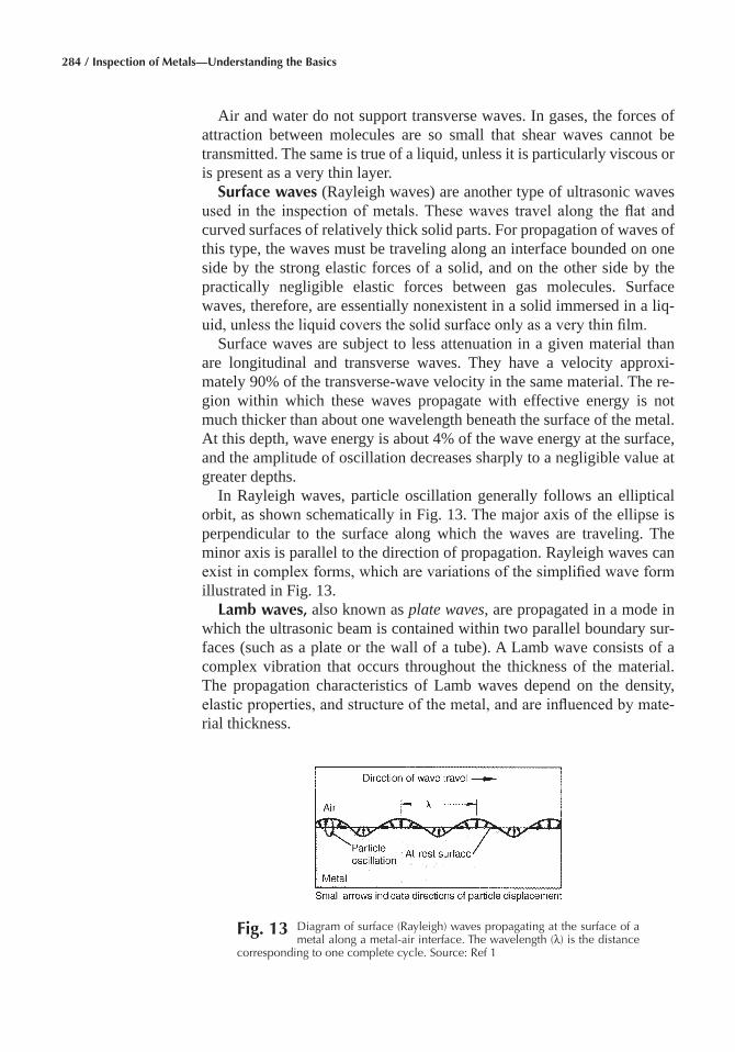
284 / Inspection of Metals—Understanding the Basics
Air and water do not support transverse waves. In gases, the forces of attraction between molecules are so small that shear waves cannot be transmitted. The same is true of a liquid, unless it is particularly viscous or is present as a very thin layer.
Surface waves (Rayleigh waves) are another type of ultrasonic waves used in the inspection of metals. These waves travel along the flat and curved surfaces of relatively thick solid parts. For propagation of waves of this type, the waves must be traveling along an interface bounded on one side by the strong elastic forces of a solid, and on the other side by the practically negligible elastic forces between gas molecules. Surface waves, therefore, are essentially nonexistent in a solid immersed in a liq-uid, unless the liquid covers the solid surface only as a very thin film.
Surface waves are subject to less attenuation in a given material than are longitudinal and transverse waves. They have a velocity approxi-mately 90% of the transverse-wave velocity in the same material. The re-gion within which these waves propagate with effective energy is not much thicker than about one wavelength beneath the surface of the metal. At this depth, wave energy is about 4% of the wave energy at the surface, and the amplitude of oscillation decreases sharply to a negligible value at greater depths.
In Rayleigh waves, particle oscillation generally follows an elliptical orbit, as shown schematically in Fig. 13. The major axis of the ellipse is perpendicular to the surface along which the waves are traveling. The minor axis is parallel to the direction of propagation. Rayleigh waves can exist in complex forms, which are variations of the simplified wave form illustrated in Fig. 13.
Lamb waves, also known as plate waves, are propagated in a mode in which the ultrasonic beam is contained within two parallel boundary sur-faces (such as a plate or the wall of a tube). A Lamb wave consists of a complex vibration that occurs throughout the thickness of the material. The propagation characteristics of Lamb waves depend on the density, elastic properties, and structure of the metal, and are influenced by mate-rial thickness.
Fig� 13 Diagram of surface (Rayleigh) waves propagating at the surface of a metal along a metal-air interface. The wavelength (λ) is the distance
corresponding to one complete cycle. Source: Ref 1
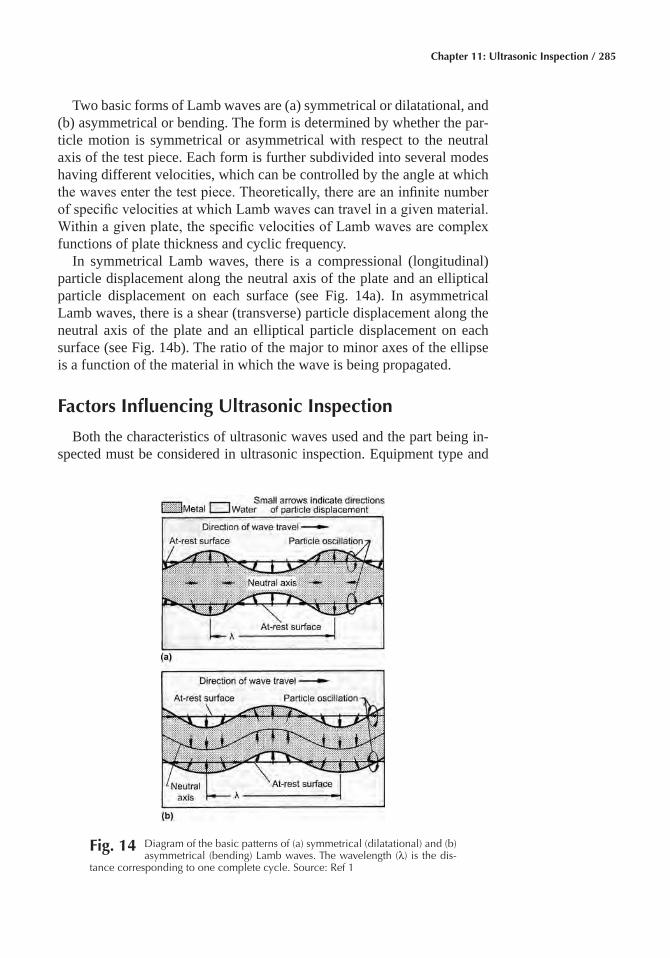
Chapter 11: Ultrasonic Inspection / 285
Two basic forms of Lamb waves are (a) symmetrical or dilatational, and (b) asymmetrical or bending. The form is determined by whether the par-ticle motion is symmetrical or asymmetrical with respect to the neutral axis of the test piece. Each form is further subdivided into several modes having different velocities, which can be controlled by the angle at which the waves enter the test piece. Theoretically, there are an infinite number of specific velocities at which Lamb waves can travel in a given material. Within a given plate, the specific velocities of Lamb waves are complex functions of plate thickness and cyclic frequency.
In symmetrical Lamb waves, there is a compressional (longitudinal) particle displacement along the neutral axis of the plate and an elliptical particle displacement on each surface (see Fig. 14a). In asymmetrical Lamb waves, there is a shear (transverse) particle displacement along the neutral axis of the plate and an elliptical particle displacement on each surface (see Fig. 14b). The ratio of the major to minor axes of the ellipse is a function of the material in which the wave is being propagated.
Factors Influencing Ultrasonic Inspection
Both the characteristics of ultrasonic waves used and the part being in-spected must be considered in ultrasonic inspection. Equipment type and
Fig� 14 Diagram of the basic patterns of (a) symmetrical (dilatational) and (b) asymmetrical (bending) Lamb waves. The wavelength (λ) is the dis-
tance corresponding to one complete cycle. Source: Ref 1
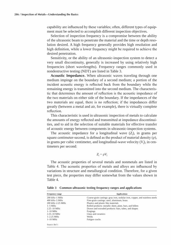
286 / Inspection of Metals—Understanding the Basics
capability are influenced by these variables; often, different types of equip-ment must be selected to accomplish different inspection objectives.
Selection of inspection frequency is a compromise between the ability of the ultrasonic beam to penetrate the material and the time or depth reso-lution desired. A high frequency generally provides high resolution and high definition, while a lower frequency might be required to achieve the desired penetration.
Sensitivity, or the ability of an ultrasonic-inspection system to detect a very small discontinuity, generally is increased by using relatively high frequencies (short wavelengths). Frequency ranges commonly used in nondestructive testing (NDT) are listed in Table 3.
Acoustic Impedance� When ultrasonic waves traveling through one medium impinge on the boundary of a second medium; a portion of the incident acoustic energy is reflected back from the boundary while the remaining energy is transmitted into the second medium. The characteris-tic that determines the amount of reflection is the acoustic impedance of the two materials on either side of the boundary. If the impedances of the two materials are equal, there is no reflection; if the impedances differ greatly (between a metal and air, for example), there is virtually complete reflection.
This characteristic is used in ultrasonic inspection of metals to calculate the amounts of energy reflected and transmitted at impedance discontinui-ties, and to aid in the selection of suitable materials for effective transfer of acoustic energy between components in ultrasonic-inspection systems.
The acoustic impedance for a longitudinal wave (Zl), in grams per square centimeter-second, is defined as the product of material density (ρ), in grams per cubic centimeter, and longitudinal-wave velocity (Vl), in cen-timeters per second:
Zl = ρVl
The acoustic properties of several metals and nonmetals are listed in Table 4. The acoustic properties of metals and alloys are influenced by variations in structure and metallurgical condition. Therefore, for a given test piece, the properties may differ somewhat from the values shown in Table 4.
Table 3 Common ultrasonic testing frequency ranges and applications
Frequency range Applications
200 kHz–1 MHz Coarse-grain castings: gray iron, nodular iron, copper, and stainless steels 400 kHz–5 MHz Fine-grain castings: steel, aluminum, brass 200 kHz–2.25 MHz Plastics and plastic like materials 1–5 MHz Rolled products: metallic sheet, plate, bars, and billets 2.25–10 MHz Drawn and extruded products: bars, tubes, and shapes 1–10 MHz Forgings 2.25–10 MHz Glass and ceramics 1–2.25 MHz Welds 1–10 MHz Fatigue cracks
Source: Ref 1
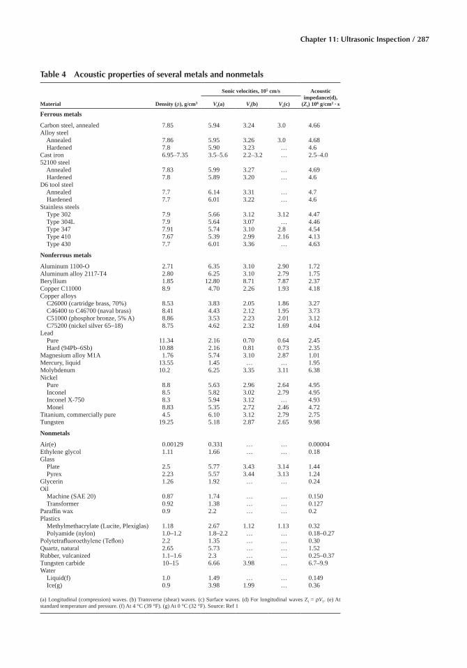
Chapter 11: Ultrasonic Inspection / 287
Table 4 Acoustic properties of several metals and nonmetals
Material Density (ρ), g/cm3
Sonic velocities, 105 cm/s Acoustic impedance(d),
(Zt) 106 g/cm2 · sVt(a) Vt(b) Vs(c)
Ferrous metals
Carbon steel, annealed 7.85 5.94 3.24 3.0 4.66Alloy steel Annealed 7.86 5.95 3.26 3.0 4.68 Hardened 7.8 5.90 3.23 … 4.6Cast iron 6.95–7.35 3.5–5.6 2.2–3.2 … 2.5–4.052100 steel Annealed 7.83 5.99 3.27 … 4.69 Hardened 7.8 5.89 3.20 … 4.6D6 tool steel Annealed 7.7 6.14 3.31 … 4.7 Hardened 7.7 6.01 3.22 … 4.6Stainless steels Type 302 7.9 5.66 3.12 3.12 4.47 Type 304L 7.9 5.64 3.07 … 4.46 Type 347 7.91 5.74 3.10 2.8 4.54 Type 410 7.67 5.39 2.99 2.16 4.13 Type 430 7.7 6.01 3.36 … 4.63
Nonferrous metals
Aluminum 1100-O 2.71 6.35 3.10 2.90 1.72Aluminum alloy 2117-T4 2.80 6.25 3.10 2.79 1.75Beryllium 1.85 12.80 8.71 7.87 2.37Copper C11000 8.9 4.70 2.26 1.93 4.18Copper alloys C26000 (cartridge brass, 70%) 8.53 3.83 2.05 1.86 3.27 C46400 to C46700 (naval brass) 8.41 4.43 2.12 1.95 3.73 C51000 (phosphor bronze, 5% A) 8.86 3.53 2.23 2.01 3.12 C75200 (nickel silver 65–18) 8.75 4.62 2.32 1.69 4.04Lead Pure 11.34 2.16 0.70 0.64 2.45 Hard (94Pb–6Sb) 10.88 2.16 0.81 0.73 2.35Magnesium alloy M1A 1.76 5.74 3.10 2.87 1.01Mercury, liquid 13.55 1.45 … … 1.95Molybdenum 10.2 6.25 3.35 3.11 6.38Nickel Pure 8.8 5.63 2.96 2.64 4.95 Inconel 8.5 5.82 3.02 2.79 4.95 Inconel X-750 8.3 5.94 3.12 … 4.93 Monel 8.83 5.35 2.72 2.46 4.72Titanium, commercially pure 4.5 6.10 3.12 2.79 2.75Tungsten 19.25 5.18 2.87 2.65 9.98
Nonmetals
Air(e) 0.00129 0.331 … … 0.00004Ethylene glycol 1.11 1.66 … … 0.18Glass Plate 2.5 5.77 3.43 3.14 1.44 Pyrex 2.23 5.57 3.44 3.13 1.24Glycerin 1.26 1.92 … … 0.24Oil Machine (SAE 20) 0.87 1.74 … … 0.150 Transformer 0.92 1.38 … … 0.127Paraffin wax 0.9 2.2 … … 0.2Plastics Methylmethacrylate (Lucite, Plexiglas) 1.18 2.67 1.12 1.13 0.32 Polyamide (nylon) 1.0–1.2 1.8–2.2 … … 0.18–0.27Polytetrafluoroethylene (Teflon) 2.2 1.35 … … 0.30Quartz, natural 2.65 5.73 … … 1.52Rubber, vulcanized 1.1–1.6 2.3 … … 0.25–0.37Tungsten carbide 10–15 6.66 3.98 … 6.7–9.9Water Liquid(f) 1.0 1.49 … … 0.149 Ice(g) 0.9 3.98 1.99 … 0.36
(a) Longitudinal (compression) waves. (b) Transverse (shear) waves. (c) Surface waves. (d) For longitudinal waves Zt = ρV1. (e) At standard temperature and pressure. (f) At 4 °C (39 °F). (g) At 0 °C (32 °F). Source: Ref 1
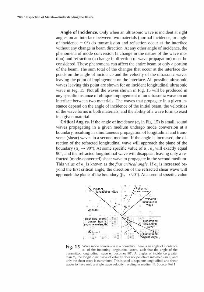
288 / Inspection of Metals—Understanding the Basics
Angle of Incidence� Only when an ultrasonic wave is incident at right angles on an interface between two materials (normal incidence, or angle of incidence = 0°) do transmission and reflection occur at the interface without any change in beam direction. At any other angle of incidence, the phenomena of mode conversion (a change in the nature of the wave mo-tion) and refraction (a change in direction of wave propagation) must be considered. These phenomena can affect the entire beam or only a portion of the beam. The sum total of the changes that occur at the interface de-pends on the angle of incidence and the velocity of the ultrasonic waves leaving the point of impingement on the interface. All possible ultrasonic waves leaving this point are shown for an incident longitudinal ultrasonic wave in Fig. 15. Not all the waves shown in Fig. 15 will be produced in any specific instance of oblique impingement of an ultrasonic wave on an interface between two materials. The waves that propagate in a given in-stance depend on the angle of incidence of the initial beam, the velocities of the wave forms in both materials, and the ability of a wave form to exist in a given material.
Critical Angles� If the angle of incidence (α1 in Fig. 15) is small, sound waves propagating in a given medium undergo mode conversion at a boundary, resulting in simultaneous propagation of longitudinal and trans-verse (shear) waves in a second medium. If the angle is increased, the di-rection of the refracted longitudinal wave will approach the plane of the boundary (α2 → 90°). At some specific value of α1, α2 will exactly equal 90°, and the refracted longitudinal wave will disappear, leaving only a re-fracted (mode-converted) shear wave to propagate in the second medium. This value of α1 is known as the first critical angle. If α1 is increased be-yond the first critical angle, the direction of the refracted shear wave will approach the plane of the boundary (β2 → 90°). At a second specific value
Fig� 15 Wave mode conversion at a boundary. There is an angle of incidence α1 of the incoming longitudinal wave, such that the angle of the
transmitted longitudinal wave α2 becomes 90°. At angles of incidence greater than α1, the longitudinal wave of velocity does not penetrate into medium II, and only the shear wave is transmitted. This is used to separate longitudinal and shear waves to have only a single wave velocity traveling in medium II. Source: Ref 1
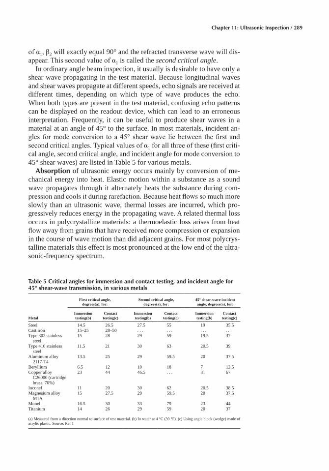
Chapter 11: Ultrasonic Inspection / 289
of α1, β2 will exactly equal 90° and the refracted transverse wave will dis-appear. This second value of α1 is called the second critical angle.
In ordinary angle beam inspection, it usually is desirable to have only a shear wave propagating in the test material. Because longitudinal waves and shear waves propagate at different speeds, echo signals are received at different times, depending on which type of wave produces the echo. When both types are present in the test material, confusing echo patterns can be displayed on the readout device, which can lead to an erroneous interpretation. Frequently, it can be useful to produce shear waves in a material at an angle of 45° to the surface. In most materials, incident an-gles for mode conversion to a 45° shear wave lie between the first and second critical angles. Typical values of α1 for all three of these (first criti-cal angle, second critical angle, and incident angle for mode conversion to 45° shear waves) are listed in Table 5 for various metals.
Absorption of ultrasonic energy occurs mainly by conversion of me-chanical energy into heat. Elastic motion within a substance as a sound wave propagates through it alternately heats the substance during com-pression and cools it during rarefaction. Because heat flows so much more slowly than an ultrasonic wave, thermal losses are incurred, which pro-gressively reduces energy in the propagating wave. A related thermal loss occurs in polycrystalline materials: a thermoelastic loss arises from heat flow away from grains that have received more compression or expansion in the course of wave motion than did adjacent grains. For most polycrys-talline materials this effect is most pronounced at the low end of the ultra-sonic-frequency spectrum.
Table 5 Critical angles for immersion and contact testing, and incident angle for 45° shear-wave transmission, in various metals
Metal
First critical angle, degrees(a), for:
Second critical angle, degrees(a), for:
45° shear-wave incident angle, degrees(a), for:
Immersion testing(b)
Contact testing(c)
Immersion testing(b)
Contact testing(c)
Immersion testing(b)
Contact testing(c)
Steel 14.5 26.5 27.5 55 19 35.5 Cast iron 15–25 28–50 . . . . . . . . . . . . Type 302 stainless
steel 15 28 29 59 19.5 37
Type 410 stainless steel
11.5 21 30 63 20.5 39
Aluminum alloy 2117-T4
13.5 25 29 59.5 20 37.5
Beryllium 6.5 12 10 18 7 12.5 Copper alloy
C26000 (cartridge brass, 70%)
23 44 46.5 . . . 31 67
Inconel 11 20 30 62 20.5 38.5 Magnesium alloy
M1A 15 27.5 29 59.5 20 37.5
Monel 16.5 30 33 79 23 44 Titanium 14 26 29 59 20 37
(a) Measured from a direction normal to surface of test material. (b) In water at 4 °C (39 °F). (c) Using angle block (wedge) made of acrylic plastic. Source: Ref 1
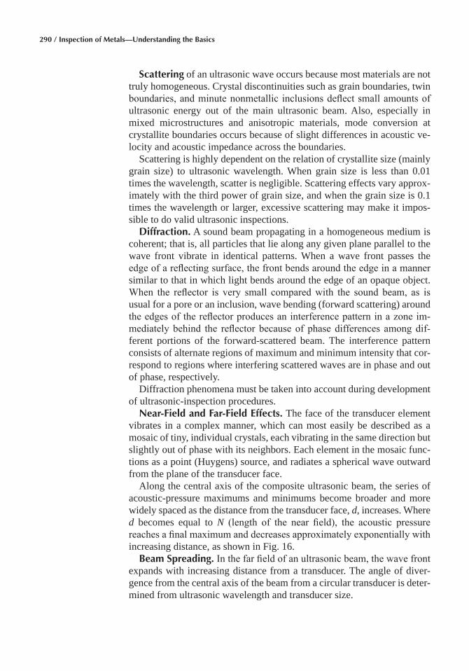
290 / Inspection of Metals—Understanding the Basics
Scattering of an ultrasonic wave occurs because most materials are not truly homogeneous. Crystal discontinuities such as grain boundaries, twin boundaries, and minute nonmetallic inclusions deflect small amounts of ultrasonic energy out of the main ultrasonic beam. Also, especially in mixed microstructures and anisotropic materials, mode conversion at crystallite boundaries occurs because of slight differences in acoustic ve-locity and acoustic impedance across the boundaries.
Scattering is highly dependent on the relation of crystallite size (mainly grain size) to ultrasonic wavelength. When grain size is less than 0.01 times the wavelength, scatter is negligible. Scattering effects vary approx-imately with the third power of grain size, and when the grain size is 0.1 times the wavelength or larger, excessive scattering may make it impos-sible to do valid ultrasonic inspections.
Diffraction� A sound beam propagating in a homogeneous medium is coherent; that is, all particles that lie along any given plane parallel to the wave front vibrate in identical patterns. When a wave front passes the edge of a reflecting surface, the front bends around the edge in a manner similar to that in which light bends around the edge of an opaque object. When the reflector is very small compared with the sound beam, as is usual for a pore or an inclusion, wave bending (forward scattering) around the edges of the reflector produces an interference pattern in a zone im-mediately behind the reflector because of phase differences among dif-ferent portions of the forward-scattered beam. The interference pattern consists of alternate regions of maximum and minimum intensity that cor-respond to regions where interfering scattered waves are in phase and out of phase, respectively.
Diffraction phenomena must be taken into account during development of ultrasonic-inspection procedures.
Near-Field and Far-Field Effects� The face of the transducer element vibrates in a complex manner, which can most easily be described as a mosaic of tiny, individual crystals, each vibrating in the same direction but slightly out of phase with its neighbors. Each element in the mosaic func-tions as a point (Huygens) source, and radiates a spherical wave outward from the plane of the transducer face.
Along the central axis of the composite ultrasonic beam, the series of acoustic-pressure maximums and minimums become broader and more widely spaced as the distance from the transducer face, d, increases. Where d becomes equal to N (length of the near field), the acoustic pressure reaches a final maximum and decreases approximately exponentially with increasing distance, as shown in Fig. 16.
Beam Spreading� In the far field of an ultrasonic beam, the wave front expands with increasing distance from a transducer. The angle of diver-gence from the central axis of the beam from a circular transducer is deter-mined from ultrasonic wavelength and transducer size.
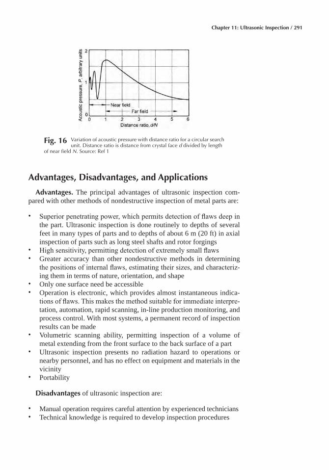
Chapter 11: Ultrasonic Inspection / 291
Advantages, Disadvantages, and Applications
Advantages� The principal advantages of ultrasonic inspection com-pared with other methods of nondestructive inspection of metal parts are:
• Superior penetrating power, which permits detection of flaws deep in the part. Ultrasonic inspection is done routinely to depths of several feet in many types of parts and to depths of about 6 m (20 ft) in axial inspection of parts such as long steel shafts and rotor forgings
• High sensitivity, permitting detection of extremely small flaws • Greater accuracy than other nondestructive methods in determining
the positions of internal flaws, estimating their sizes, and characteriz-ing them in terms of nature, orientation, and shape
• Only one surface need be accessible • Operation is electronic, which provides almost instantaneous indica-
tions of flaws. This makes the method suitable for immediate interpre-tation, automation, rapid scanning, in-line production monitoring, and process control. With most systems, a permanent record of inspection results can be made
• Volumetric scanning ability, permitting inspection of a volume of metal extending from the front surface to the back surface of a part
• Ultrasonic inspection presents no radiation hazard to operations or nearby personnel, and has no effect on equipment and materials in the vicinity
• Portability
Disadvantages of ultrasonic inspection are:
• Manual operation requires careful attention by experienced technicians • Technical knowledge is required to develop inspection procedures
Fig� 16 Variation of acoustic pressure with distance ratio for a circular search unit. Distance ratio is distance from crystal face d divided by length
of near field N. Source: Ref 1

292 / Inspection of Metals—Understanding the Basics
• Parts that are rough, irregular in shape, very small and thin, and not homogeneous are difficult to inspect
• Discontinuities that are present in a shallow layer immediately beneath the surface might not be detectable
• Couplants are needed to provide effective transfer of the ultrasonic beam between search units and parts being inspected
• Reference standards are required, both to calibrate equipment and to characterize flaws
Applications� Some of the major types of components that are ultra-sonically inspected for the presence of flaws are:
• Mill components: rolls, shafts, drives, and press columns • Power equipment: turbine forgings, generator rotors, pressure piping,
weldments, pressure vessels, nuclear fuel elements, and other reactor components
• Jet-engine parts: turbine and compressor forgings, and gear blanks • Aircraft components: forging stock, frame sections, and honeycomb
sandwich assemblies • Machinery materials: die blocks, tool steels, and drill pipe • Railroad parts: axles, wheels, and bolted and welded rail • Automotive parts: forgings, ductile castings, brazed and/or welded
components
Ultrasonic inspection is an effective and inexpensive method for volu-metric examination of structures and components of both regular and complex shapes.
ACKNOWLEDGMENT
This chapter was adapted from Ultrasonic Inspection in Metals Hand-book Desk Edition, Second Edition, 1998.
REFERENCES
1. Ultrasonic Inspection, Metals Handbook Desk Edition, 2nd ed., ASM International, 1998, p 1282–1290
SELECTED REFERENCES
• L. Cartz, Nondestructive Testing, ASM International, 1995• K.-J. Langenberg, R. Marklein, and K. Mayer, Ultrasonic Nondestruc-
tive Testing of Materials: Theoretical Foundations, CRC Press, 2012• Nondestructive Testing and Quality Control, Vol 17, ASM Handbook,
ASM International, 1989• C.H. Shen, Ultrasonic and Advanced Methods for Nondestructive
Testing and Materials Characterization, World Scientific, 2007

Inspection of Metals—Understanding the Basics Copyright © 2013 ASM International®
F.C. Campbell, editor All rights reservedwww.asminternational.org
CHAPTER 12
Inspection of Castings
INSPECTION PROCEDURES FOR CASTINGS are established at the foundry to ensure conformance with customer drawings and documents, which are frequently based on various government, technical society, or commercial specifications. For a foundry to ensure casting quality, inspec-tion procedures must be efficiently directed toward the prevention of im-perfections, the detection of unsatisfactory trends, and the conservation of material, all of which ultimately lead to reduction in costs. Inspectors should be able to assess on sight the probable strong and weak points of a casting and know where weaknesses and faults would most likely be found.
The inspection of castings normally involves checking for shape and dimensions, coupled with aided and unaided visual inspection for external discontinuities and surface quality. Chemical analyses and tests for me-chanical properties are supplemented by various forms of nondestructive inspection, including leak testing and proof loading, all of which are used to evaluate the soundness of the casting. These inspections add to the cost of the product; therefore, the initial consideration must be to determine the amount of inspection needed to maintain adequate control over quality. In some cases, this may require full inspection of each individual casting, but in other cases sampling procedures may be sufficient.
Inspection Categories
Methods for Determining Surface Quality� Cracks and other imper-fections at the surface of a casting can be detected by a number of in-spection techniques, including visual inspection, chemical etching, liquid penetrant inspection, eddy current inspection, and magnetic particle in-spection, which can also reveal discontinuities situated immediately below the surface. All these inspection methods require clean and relatively smooth surfaces for effective results.
294 / Inspection of Metals—Understanding the Basics
Methods for Detecting Internal Discontinuities� The principal non-destructive methods used for detecting internal discontinuities in castings are radiography, ultrasonic inspection, and eddy current inspection. Of these methods, radiography is the most highly developed technique for detailed inspection; it can provide a pictorial representation of the form and extent of many types of internal discontinuities. Ultrasonic inspec-tion, which is less universally applicable, can give qualitative indications of many discontinuities. It is especially useful in the inspection of castings of fairly simple design, for which the signal pattern can be most reliably interpreted. Ultrasonic inspection can also be used to determine the shape of graphite particles in cast iron.
Eddy current and other closely related electromagnetic methods are used to sort castings for variations in composition, surface hardness, and structure. Infrared thermography (thermal inspection) has also occasion-ally been proposed as a method for detecting subsurface defects. How-ever, its successful uses have generally been restricted to the detection of larger defects because of the relatively slow rates at which heat can be put into a component and because of the relatively low sensitivity of infrared detectors. Increased use of thermal inspection may occur with the intro-duction of pulsed video thermography, in which a very short burst of in-tense heat is directed at the component. The presence of near-surface de-fects influences the rate at which heat is dissipated from the surface, and temperature variations are detected with a high resolution infrared camera recorded onto videotape and presented as an image on a TV monitor. The method was developed for the detection of small defects in composites and in aerospace turbine engine blades, but some initial results obtained with cast iron test plates have proved promising.
Methods for Dimensional Inspection� A number of techniques are used to determine the dimensional accuracy of castings. These include manual checks with micrometers, manual and automatic gages, coordi-nate measuring machines, and three-dimensional automatic inspection stations (machine vision systems).
Casting Defects
Poor casting design can interfere with the ability of the foundry to use the best techniques to produce reliable castings. The designer also speci-fies the quality requirements that ensure that the cast component will per-form as desired. Over specification causes needless expense and can be avoided by understanding the effect of discontinuities on casting perfor-mance, and the effect of casting design on the tendency for discontinuities to form during the casting process. Important types of casting discontinui-ties include porosity, inclusions, oxide films, second phases, hot tears, metal penetration, and surface defects. A number of typical casting defects are shown in Fig. 1.
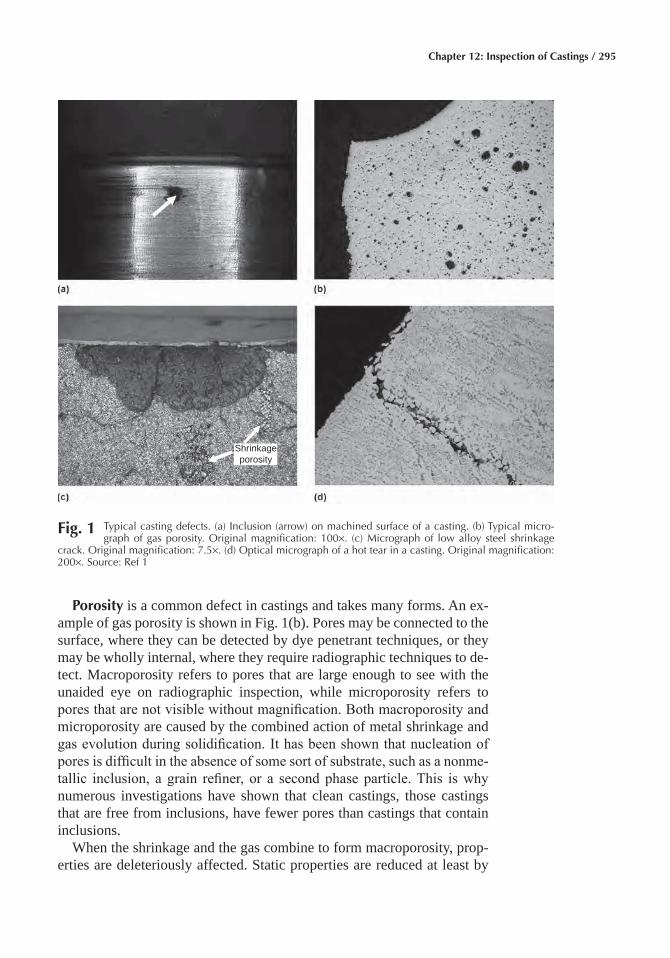
Chapter 12: Inspection of Castings / 295
Porosity is a common defect in castings and takes many forms. An ex-ample of gas porosity is shown in Fig. 1(b). Pores may be connected to the surface, where they can be detected by dye penetrant techniques, or they may be wholly internal, where they require radiographic techniques to de-tect. Macroporosity refers to pores that are large enough to see with the unaided eye on radiographic inspection, while microporosity refers to pores that are not visible without magnification. Both macroporosity and microporosity are caused by the combined action of metal shrinkage and gas evolution during solidification. It has been shown that nucleation of pores is difficult in the absence of some sort of substrate, such as a nonme-tallic inclusion, a grain refiner, or a second phase particle. This is why numerous investigations have shown that clean castings, those castings that are free from inclusions, have fewer pores than castings that contain inclusions.
When the shrinkage and the gas combine to form macroporosity, prop-erties are deleteriously affected. Static properties are reduced at least by
Shrinkageporosity
Fig� 1 Typical casting defects. (a) Inclusion (arrow) on machined surface of a casting. (b) Typical micro-graph of gas porosity. Original magnification: 100×. (c) Micrograph of low alloy steel shrinkage
crack. Original magnification: 7.5×. (d) Optical micrograph of a hot tear in a casting. Original magnification: 200×. Source: Ref 1
296 / Inspection of Metals—Understanding the Basics
the portion of the cross-sectional area that is taken up with the pores; be-cause there is no metal in the pores, there is no metal to support the load there, and the section acts as though its area was reduced. Because the pores may also cause a stress concentration in the remaining material, static properties may be reduced by more than the percentage of cross-sectional area that is caused by the macroporosity. Dynamic properties are also affected by porosity. A study of aluminum alloys showed that fatigue properties in some were reduced 11% when specimens having x-ray qual-ity equivalent to ASTM E155 level 4 were tested, and that they were re-duced 17% when specimens having quality of ASTM E155 level 8 were tested.
Static properties are mostly unaffected by microporosity. Microporosity is found between dendrites, and like macroporosity, is caused by the in-ability of feed metal to reach the interdendritic areas of the casting where shrinkage is occurring and where gas is being evolved. However, because this type of porosity occurs late in solidification, particularly in long range freezing (mushy freezing) alloys, it is particularly difficult to eliminate. The most effective method is to increase the thermal gradient, often ac-complished by increasing the solidification rate, which decreases the length of the mushy zone. However, this technique may be limited by alloy and mold thermal properties, and by casting geometry, that is, the design of the casting.
As long as the micropores are less than 0.2 mm (0.008 in.) in length, there is no effect on dynamic properties; fatigue properties of castings with pores that size or smaller are in the same range as those of castings where no micropores were found. The shape of the micropore is as impor-tant as its size, with elongated pores having a greater effect than round pores. Microporosity can be healed by hot isostatic pressing (HIP). In one study comparing HIP and non-HIP samples, no difference was found in fatigue lives of HIP and non-HIP samples. However, the HIP samples showed a lower crack growth rate than non-HIP samples. In another study, HIP improved fatigue crack growth resistance only close to threshold lev-els. The design of the casting directly affects its tendency to solidify in a progressive manner, thereby affecting both the quality and the price of the cast component. Porosity and casting costs are minimized in casting de-signs that emphasize progressive solidification toward a gate or riser, ta-pered walls, and the avoidance of hot spots.
Inclusions are nonmetallic particles that are found in the casting. They may form during solidification as some elements (notably manganese and sulfur in steel) precipitate from solution in the liquid. More frequently, they are formed before solidification begins. The former are sometimes called indigenous inclusions, and the latter are called exogenous inclu-sions. Inclusions are ceramic phases that have little ductility. A crack may form in the inclusion and propagate from the inclusion into the metal, or a crack may form at the interface between the metal and the inclusion. In
Chapter 12: Inspection of Castings / 297
addition, because inclusions and the metal have different coefficients of thermal expansion, thermally induced stresses may appear in the metal surrounding the inclusions during solidification. As a result, the inclusions act as a stress concentration and reduce dynamic properties. As in the case of microporosity, the size of the inclusion and its location determines its effect. Small inclusions that are located well within the center of the cross section of the casting have little effect, whereas larger inclusions and those located near the surface of the casting may be particularly detrimental to properties. Inclusions may also be a problem when machining surfaces (Fig. 1a), causing excessive tool wear and tool breakage.
Exogenous inclusions are mostly oxides or mixtures of oxides and are primarily slag or dross particles, which are the oxides that result when the metal reacts with oxygen in the air during melting. These are removed from the melt before pouring by filtration. Most inclusions found in steel castings arise from the oxidation of metal during the pouring operation. This is known as reoxidation, and takes place when the turbulent flow of the metal in the gating system causes the metal to break up into small droplets, which then react with the oxygen in the air in the gating system or casting cavity to form oxides. Metal casters use computer analysis of gating systems to indicate when reoxidation can be expected in a gating system and to eliminate it. However, casting designs that require molten metal to “jet” through a section of the casting to fill other sections will recreate the inclusions and should be avoided.
Oxide films are similar to inclusions and have been found to reduce casting properties. These form on the surface of the molten metal as it fills the mold. If the surface film is trapped within the casting instead of being carried into a riser, it forms a linear discontinuity and an obvious site for crack initiation. It has been shown that elimination of oxide films, in addi-tion to substantially improving static properties, results in up to a five-fold improvement of fatigue life in axial tension-tension tests.
Oxide films are of particular concern in nonferrous castings, although they also must be controlled in steel and stainless steel castings. If the film folds over on itself as a result of turbulent flow or waterfalling when mol-ten metal falls to a lower level in the casting during mold filling, the ef-fects are particularly damaging. Casting design influences how the metal fills the mold, and features of the design that require the metal to fall from one level to another while the mold is filling should be avoided so that waterfalls are eliminated. Oxide films are avoided by filling the casting from the bottom, in a controlled manner, by pumping the metal into the mold using pneumatic or electromagnetic pumps.
Second phases, which form during solidification, can also nucleate cracks if they have the proper size and morphology. An example is alumi-num-silicon alloys, where the silicon eutectic is present as large platelets, which can nucleate cracks, and along which cracks propagate. The size of these platelets may be significantly reduced by modifying the alloy with
298 / Inspection of Metals—Understanding the Basics
additions of sodium or strontium. However, such additions increase the size of micropores, and for this reason, many foundrymen rely on acceler-ated solidification of the casting to refine the silicon. As the solidification rates increase, the structure is refined in thin sections. Heavy sections are to be avoided if a fine structure is desired.
Hot tears form when casting sections are constrained by the mold from shrinking as they cool near the end of solidification. These discontinuities are fairly large and are most often weld repaired. If not repaired, their ef-fect is not readily predictable. While generally they are detrimental to casting properties, under some circumstances they do not affect them. Hot tears (Fig. 1d) are caused by a combination of factors, including alloy type, metal cleanliness, and mold and core hardness. However, poor cast-ing design is the primary cause. Castings should be designed so that so-lidifying sections are not subjected to tensile forces caused by shrinkage during solidification, as the solidifying alloy has little strength before it solidifies.
Metal Penetration� Molten metal may penetrate the surface of the mold, forming a rough surface or, in extreme cases, actually becoming intimately mixed with the sand in the mold. In iron castings, this is nor-mally the result of the combination of metallostatic head (the pressure exerted on the molten iron at the bottom of the mold by the weight of the metal on top of it) and the surface tension relationship between the liquid iron and molding materials. In cast iron, it is also frequently the result of the expansion of graphite at the end of solidification, forcing liquid metal into the mold if the casting is not properly designed with a tapered wall to promote directional solidification and avoid hot spots.
Surface Defects� Surface finish is also an important property. Surface discontinuities affect fatigue life, and obviously smoother surfaces are su-perior to rough surfaces. Designers should be certain that fatigue data used in design calculations has been taken from as-cast surfaces rather than machined surfaces, as most surfaces on castings where stress concen-trations might be expected are not machined. Surface finish in castings is controlled by the application of coatings to the mold as well as proper se-lection of mold materials. Metal mold casting processes generally produce better surface finishes than sand casting processes.
Design and Service Considerations� The existence of casting discon-tinuities does not, in and of itself, indicate that casting performance in service will be affected. Equally important are the size, location, and dis-tribution of these discontinuities. Those discontinuities that are small and located near the center of the casting have little effect, while those located at or near the surface of the casting are usually damaging. Clustered dis-continuities and those that occur in a regular array have a greater effect on properties than those that are isolated and randomly distributed. In speci-fying acceptable levels of discontinuities, such as microporosity and in-clusion sizes and distribution, the designer should determine the critical
Chapter 12: Inspection of Castings / 299
flaw size that will deleteriously affect performance in service. This per-mits the foundry to design a casting practice that will eliminate such dis-continuities at minimum cost.
Common Inspection Procedures
The inspection of castings is most often limited to visual and dimen-sional inspections, weight testing, and hardness testing. However, for castings that are to be used in critical applications, such as automotive or aerospace components, additional methods of nondestructive inspection are used to determine and to control casting quality.
Visual inspection of each casting ensures that none of its features has been omitted or malformed by molding errors, short running, or mistakes in cleaning. Most surface defects and roughness can be observed at this stage.
Initial sample castings from new pattern equipment should be carefully inspected for obvious defects. Liquid penetrant inspection can be used to detect surface defects. Such casting imperfections as shrinks, cracks, blows, or dross usually indicate the need for adjustment in the gating or foundry techniques. If the casting appears to be satisfactory based on vi-sual inspection, internal quality can be checked by radiographic and ultra-sonic inspection.
The first visual inspection operation on the production casting is usually performed immediately after shakeout or knockout of the casting, ensur-ing that major visible imperfections are detected as quickly as possible. This information, promptly relayed to the foundry, permits early correc-tive action to be taken with a minimum of scrap loss. The size and com-plexity of some sand castings requires that the gates and risers be removed to permit proper inspection of the casting.
Many castings that contain numerous internal cores or have close di-mensional tolerances require a rapid, but fairly accurate check of critical wall dimensions. In some cases, an indicating type caliper gage is suitable for this work, and special types are available for casting shapes that do not lend themselves to the standard types. Ultrasonic inspection is also used to determine wall thickness in such components as cored turbine blades made by investment casting. New developments in visual inspection pro-cedures for examining component appearance are mainly based on vision systems that use electronic cameras coupled to computer-assisted image processing systems.
With the development of high sensitivity cameras having exposure times of 1/1000 s, components can be inspected on moving belts. Flexibil-ity for examining three-dimensional components can be achieved with an array of cameras multiplexed to a common image processor or with a computer controlled camera scanning system. Such systems have been successfully applied to the inspection of printed circuit boards in the elec-
300 / Inspection of Metals—Understanding the Basics
tronics industry and subassemblies in automobile manufacture. These tests usually operate on a go/no-go basis; either the assembly is complete with connections correctly made or it is not correct. This is a far easier task than evaluating casting quality.
Studies that have been carried out to assess the possibility of extending such methods to iron castings have not given encouraging results. Con-trast between defective and nondefective areas is low, illumination is criti-cal, and consistent standards of inspection are difficult to maintain be-cause of differences in reflectivity of the casting surfaces depending on whether or not they have been recently shot blasted. Even the simple task of identifying castings to determine their type is best carried out by exam-ining their back lighted silhouette, and this provides no advantage in ex-amining their quality.
Dimensional Inspection� Consistency of dimensions is an inescapable requirement of premium quality castings supplied as near net shape com-ponents on which subsequent high speed machining operations are to be carried out. Customers will not accept increased machining costs due to inconsistencies in dimensions nor will they tolerate damage to flexible machining systems or transfer times resulting from poor control and in-spection in foundries.
Variations in dimensions represent one of the most common complaints with regard to the machinability of iron castings. Prevention is within the control of foundries. Differences in pattern size when using multipattern plates can be virtually eliminated by the use of computer aided design and manufacturing methods and computer numerical control machines in pat-ternmaking. Better process control and pouring methods can eliminate variations in dimensions due to changes in metal composition or feeding methods. Variations in mold rigidity, caused by inadequate compaction with green sand, or the use of cold sand or insufficient curing times with cold setting systems, which cause casting dimensions to fall outside the preset tolerance limits, can be greatly reduced by good molding and core-making practices.
Because the dimensions and weight of iron castings are directly related to their soundness and are dependent on mold rigidity, the measurement of size or weight provides a simple test for checking casting integrity and for monitoring the consistency of the moldmaking process.
Casting dimensions are usually checked with dial gages, vernier cali-pers, micrometers, or vertical height gages, which may be hand held or incorporated into acceptance fixtures. Wall thickness measurements can be made with small handheld ultrasonic thickness gages. Under ideal con-ditions, the accuracy of these instruments is claimed to be ±0.01 mm (±0.004 in.), but this is rarely achieved in practice because the surfaces are not parallel and are not machined. Instruments are available that display variations in thickness from some preset standard and provide a digital readout and a permanent record of results for statistical analysis.
Chapter 12: Inspection of Castings / 301
The use of measuring systems employing capacitance, electrical con-tact, or linear displacement transducers are capable of high accuracy and the output can be linked directly to microcomputers for data recording and statistical analysis to meet the requirements of statistical process control.
Laser methods of measurement using beam displacement or time-lapse techniques are available for use in machine shops where accurate mea-surement is required for control of automatic machining processes. At present, they are generally not well suited for measuring castings, because of their high cost and because it is difficult to make precise measurements on components having a complex shape with curved or as-cast surfaces. As these laser methods become more widely used in other industries, lower cost systems will become available.
Weight Testing� Many intricately cored castings are extremely difficult to measure accurately, particularly the internal sections. It is important to ensure that these sections are correct in thickness for three main reasons:
• There should be no additional weight that would make the finished product heavier than permissible
• Sections must not be thinner than designed so as not to decrease the strength of the casting
• If hollow cavities have been reduced in area by increasing the metal thickness of the sections, any flow of liquid or gases is reduced
A ready means of testing for these discrepancies is by accurately weigh-ing each casting or by measuring the displacement caused by immersing the casting in a liquid filled measuring vessel. In certain cases in which extreme accuracy is demanded, a tolerance of only ±1% of a given weight may be allowed.
Hardness testing is often used to verify the effectiveness of the heat treatment applied to actual castings. Its general correlation with the tensile strength of many ferrous alloys allows a rough prediction of tensile strength to be made.
The Brinell hardness test is most frequently used for casting alloys. Combination of a large diameter ball (5 or 10 mm or 0.2 or 0.4 in.) and heavy load (500 to 3000 kgf or 1100 to 6600 lb) is preferred for the most effective representation because a deep impression minimizes the influ-ence of the immediate surface layer and of the relatively coarse micro-structure. The Brinell hardness test is unsuitable for use at high hardness levels (above 600 HB), because distortion of the ball indenter can affect the shape of the indentation.
Either the Rockwell or the Vickers (136° diamond pyramid) hardness test is used for alloys of extreme hardness or for high quality and precision castings in which the large Brinell indentation cannot be tolerated. Be-cause of the very small indentations produced in Rockwell and Vickers tests, which use loads of 150 kg (330 lb) or less, results must be based on
302 / Inspection of Metals—Understanding the Basics
the average of a number of determinations. Portable hardness testers or ultrasonic microhardness testers can be used on large castings that cannot be placed on the platform of a bench type machine.
The hardness of ferrous castings can be determined from the sonic ve-locity of the metal if all other test conditions remain constant. This has been demonstrated on chilled rolls in determining the average hardness of the core.
Computer-Aided Dimensional Inspection
The use of computer equipment in foundry inspection operations is finding more acceptance as the power and utility of available hardware and software increase. The computerization of operations can reduce the manhours required for inspection tasks, can increase accuracy, and can allow the analysis of data in ways that are not possible or practical with manual operations. Perhaps the best example of this, given the currently available equipment, is the application of computer technology to the di-mensional inspection of castings.
Importance of Dimensional Inspection� One of the most critical de-terminants of casting quality in the eyes of the casting buyer is dimen-sional accuracy. Parts that are within dimensional tolerances, given the absence of other casting defects, can be machined, assembled, and used for their intended functions with minimal testing and inspection costs. Major casting buyers are therefore demanding statistical evidence that dimen-sional tolerances are being maintained. In addition, the statistical analysis of in-house processes has been demonstrated to be effective in keeping those processes under control, thus reducing scrap and rework costs.
The application of computer equipment to the collection and analysis of dimensional inspection data can increase the amount of inspection that can be performed and decrease the time required to record and analyze the results. This furnishes control information for making adjustments to tool-ing on the foundry floor and statistical information for reporting to cus-tomers on the dimensional accuracy of parts.
Typical Equipment� A typical installation for the dimensional inspec-tion of castings consists of an electronic coordinate measuring machine, a microcomputer interfaced to the coordinate measuring machine controller with a data transfer cable, and a software system for the microcomputer (Fig. 2). The software system should be capable of controlling the func-tions and memory storage of the coordinate measuring machine, as well as recalling and analyzing the data it collects. The software serves as the main control element for the dimensional inspection and statistical report-ing of results. Such software can be purchased or, if the expertise is avail-able, developed in-house for highly specialized requirements.
Coordinate measuring machines typically record dimensions along three-axes from data points specified by the user. Depending on the so-
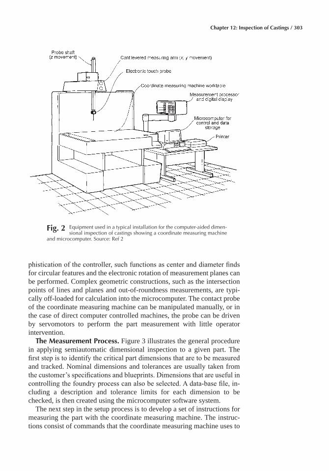
Chapter 12: Inspection of Castings / 303
phistication of the controller, such functions as center and diameter finds for circular features and the electronic rotation of measurement planes can be performed. Complex geometric constructions, such as the intersection points of lines and planes and out-of-roundness measurements, are typi-cally off-loaded for calculation into the microcomputer. The contact probe of the coordinate measuring machine can be manipulated manually, or in the case of direct computer controlled machines, the probe can be driven by servomotors to perform the part measurement with little operator intervention.
The Measurement Process� Figure 3 illustrates the general procedure in applying semiautomatic dimensional inspection to a given part. The first step is to identify the critical part dimensions that are to be measured and tracked. Nominal dimensions and tolerances are usually taken from the customer’s specifications and blueprints. Dimensions that are useful in controlling the foundry process can also be selected. A data-base file, in-cluding a description and tolerance limits for each dimension to be checked, is then created using the microcomputer software system.
The next step in the setup process is to develop a set of instructions for measuring the part with the coordinate measuring machine. The instruc-tions consist of commands that the coordinate measuring machine uses to
Fig� 2 Equipment used in a typical installation for the computer-aided dimen-sional inspection of castings showing a coordinate measuring machine
and microcomputer. Source: Ref 2
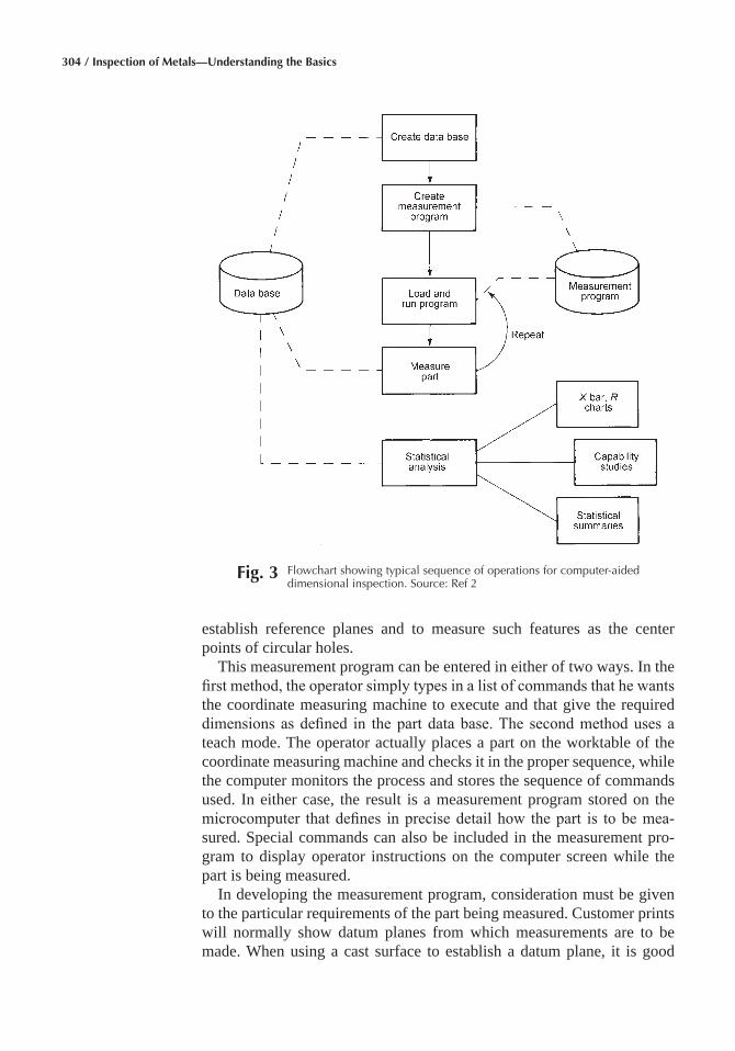
304 / Inspection of Metals—Understanding the Basics
establish reference planes and to measure such features as the center points of circular holes.
This measurement program can be entered in either of two ways. In the first method, the operator simply types in a list of commands that he wants the coordinate measuring machine to execute and that give the required dimensions as defined in the part data base. The second method uses a teach mode. The operator actually places a part on the worktable of the coordinate measuring machine and checks it in the proper sequence, while the computer monitors the process and stores the sequence of commands used. In either case, the result is a measurement program stored on the microcomputer that defines in precise detail how the part is to be mea-sured. Special commands can also be included in the measurement pro-gram to display operator instructions on the computer screen while the part is being measured.
In developing the measurement program, consideration must be given to the particular requirements of the part being measured. Customer prints will normally show datum planes from which measurements are to be made. When using a cast surface to establish a datum plane, it is good
Fig� 3 Flowchart showing typical sequence of operations for computer-aided dimensional inspection. Source: Ref 2
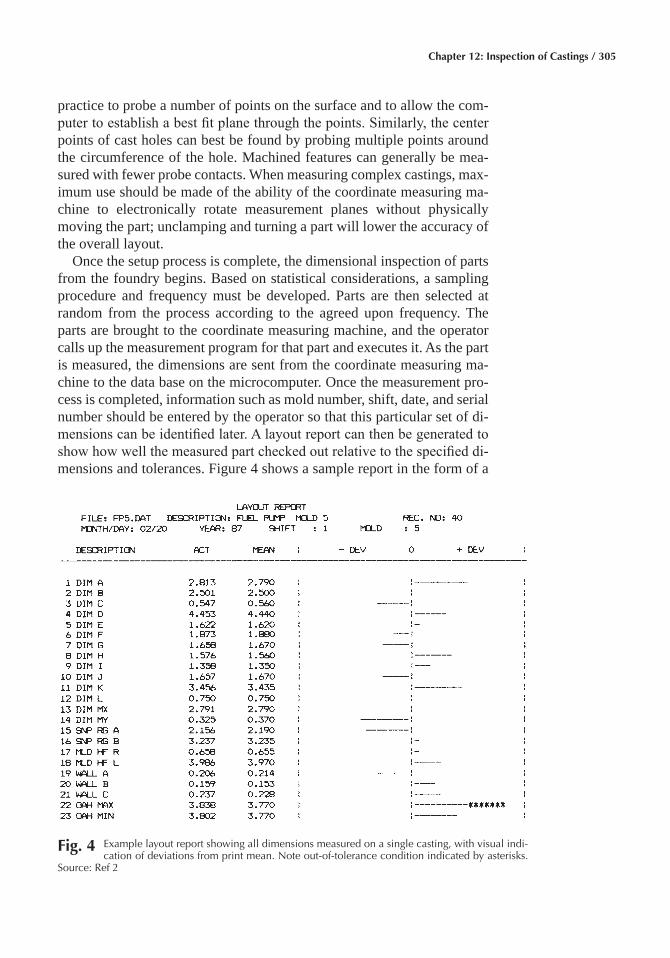
Chapter 12: Inspection of Castings / 305
practice to probe a number of points on the surface and to allow the com-puter to establish a best fit plane through the points. Similarly, the center points of cast holes can best be found by probing multiple points around the circumference of the hole. Machined features can generally be mea-sured with fewer probe contacts. When measuring complex castings, max-imum use should be made of the ability of the coordinate measuring ma-chine to electronically rotate measurement planes without physically moving the part; unclamping and turning a part will lower the accuracy of the overall layout.
Once the setup process is complete, the dimensional inspection of parts from the foundry begins. Based on statistical considerations, a sampling procedure and frequency must be developed. Parts are then selected at random from the process according to the agreed upon frequency. The parts are brought to the coordinate measuring machine, and the operator calls up the measurement program for that part and executes it. As the part is measured, the dimensions are sent from the coordinate measuring ma-chine to the data base on the microcomputer. Once the measurement pro-cess is completed, information such as mold number, shift, date, and serial number should be entered by the operator so that this particular set of di-mensions can be identified later. A layout report can then be generated to show how well the measured part checked out relative to the specified di-mensions and tolerances. Figure 4 shows a sample report in the form of a
Fig� 4 Example layout report showing all dimensions measured on a single casting, with visual indi-cation of deviations from print mean. Note out-of-tolerance condition indicated by asterisks.
Source: Ref 2
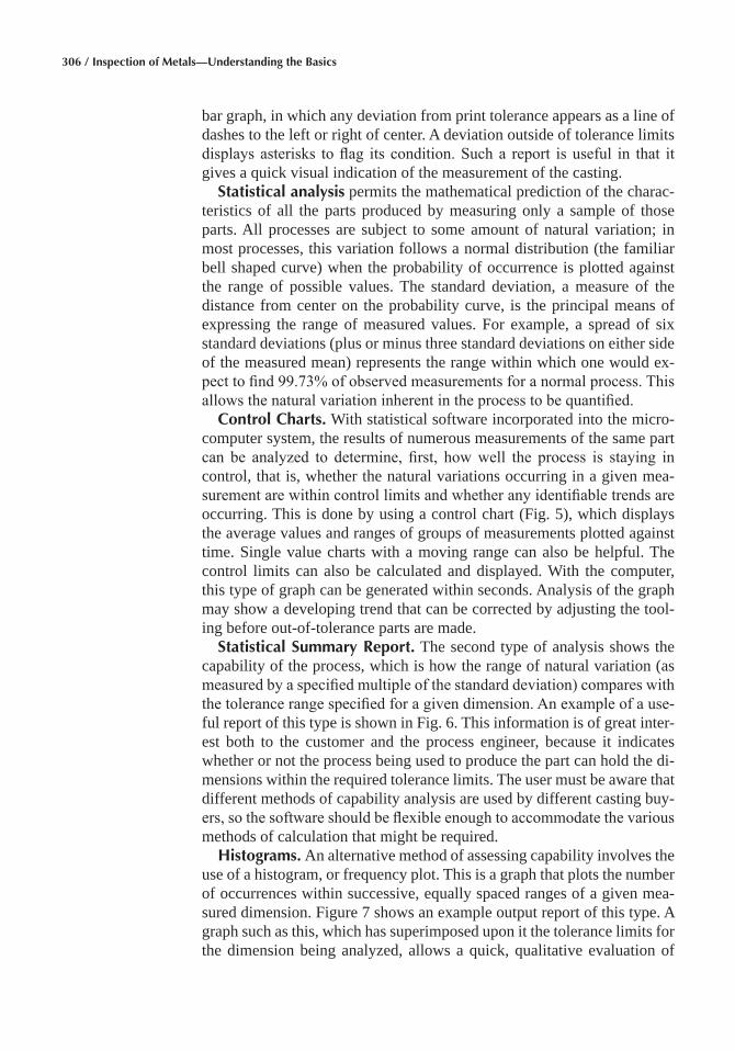
306 / Inspection of Metals—Understanding the Basics
bar graph, in which any deviation from print tolerance appears as a line of dashes to the left or right of center. A deviation outside of tolerance limits displays asterisks to flag its condition. Such a report is useful in that it gives a quick visual indication of the measurement of the casting.
Statistical analysis permits the mathematical prediction of the charac-teristics of all the parts produced by measuring only a sample of those parts. All processes are subject to some amount of natural variation; in most processes, this variation follows a normal distribution (the familiar bell shaped curve) when the probability of occurrence is plotted against the range of possible values. The standard deviation, a measure of the distance from center on the probability curve, is the principal means of expressing the range of measured values. For example, a spread of six standard deviations (plus or minus three standard deviations on either side of the measured mean) represents the range within which one would ex-pect to find 99.73% of observed measurements for a normal process. This allows the natural variation inherent in the process to be quantified.
Control Charts� With statistical software incorporated into the micro-computer system, the results of numerous measurements of the same part can be analyzed to determine, first, how well the process is staying in control, that is, whether the natural variations occurring in a given mea-surement are within control limits and whether any identifiable trends are occurring. This is done by using a control chart (Fig. 5), which displays the average values and ranges of groups of measurements plotted against time. Single value charts with a moving range can also be helpful. The control limits can also be calculated and displayed. With the computer, this type of graph can be generated within seconds. Analysis of the graph may show a developing trend that can be corrected by adjusting the tool-ing before out-of-tolerance parts are made.
Statistical Summary Report� The second type of analysis shows the capability of the process, which is how the range of natural variation (as measured by a specified multiple of the standard deviation) compares with the tolerance range specified for a given dimension. An example of a use-ful report of this type is shown in Fig. 6. This information is of great inter-est both to the customer and the process engineer, because it indicates whether or not the process being used to produce the part can hold the di-mensions within the required tolerance limits. The user must be aware that different methods of capability analysis are used by different casting buy-ers, so the software should be flexible enough to accommodate the various methods of calculation that might be required.
Histograms� An alternative method of assessing capability involves the use of a histogram, or frequency plot. This is a graph that plots the number of occurrences within successive, equally spaced ranges of a given mea-sured dimension. Figure 7 shows an example output report of this type. A graph such as this, which has superimposed upon it the tolerance limits for the dimension being analyzed, allows a quick, qualitative evaluation of
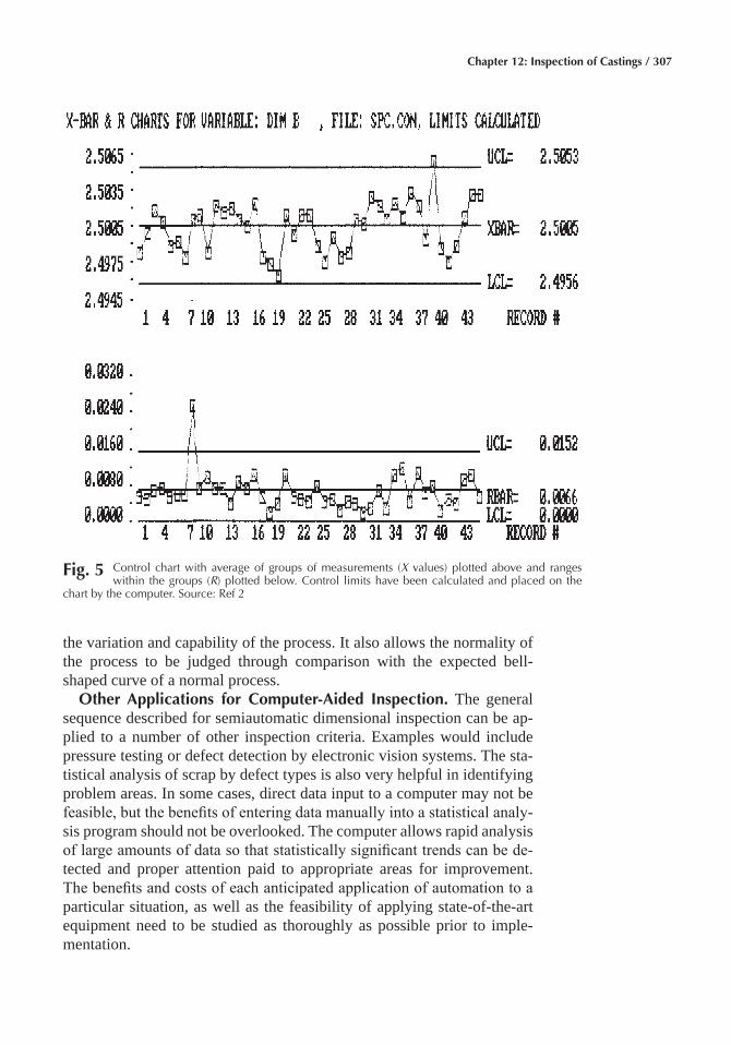
Chapter 12: Inspection of Castings / 307
the variation and capability of the process. It also allows the normality of the process to be judged through comparison with the expected bell-shaped curve of a normal process.
Other Applications for Computer-Aided Inspection� The general sequence described for semiautomatic dimensional inspection can be ap-plied to a number of other inspection criteria. Examples would include pressure testing or defect detection by electronic vision systems. The sta-tistical analysis of scrap by defect types is also very helpful in identifying problem areas. In some cases, direct data input to a computer may not be feasible, but the benefits of entering data manually into a statistical analy-sis program should not be overlooked. The computer allows rapid analysis of large amounts of data so that statistically significant trends can be de-tected and proper attention paid to appropriate areas for improvement. The benefits and costs of each anticipated application of automation to a particular situation, as well as the feasibility of applying state-of-the-art equipment need to be studied as thoroughly as possible prior to imple- mentation.
Fig� 5 Control chart with average of groups of measurements (X values) plotted above and ranges within the groups (R) plotted below. Control limits have been calculated and placed on the
chart by the computer. Source: Ref 2
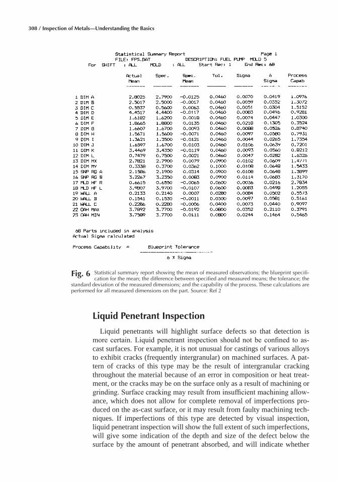
308 / Inspection of Metals—Understanding the Basics
Liquid Penetrant Inspection
Liquid penetrants will highlight surface defects so that detection is more certain. Liquid penetrant inspection should not be confined to as-cast surfaces. For example, it is not unusual for castings of various alloys to exhibit cracks (frequently intergranular) on machined surfaces. A pat-tern of cracks of this type may be the result of intergranular cracking throughout the material because of an error in composition or heat treat-ment, or the cracks may be on the surface only as a result of machining or grinding. Surface cracking may result from insufficient machining allow-ance, which does not allow for complete removal of imperfections pro-duced on the as-cast surface, or it may result from faulty machining tech-niques. If imperfections of this type are detected by visual inspection, liquid penetrant inspection will show the full extent of such imperfections, will give some indication of the depth and size of the defect below the surface by the amount of penetrant absorbed, and will indicate whether
Fig� 6 Statistical summary report showing the mean of measured observations; the blueprint specifi-cation for the mean; the difference between specified and measured means; the tolerance; the
standard deviation of the measured dimensions; and the capability of the process. These calculations are performed for all measured dimensions on the part. Source: Ref 2
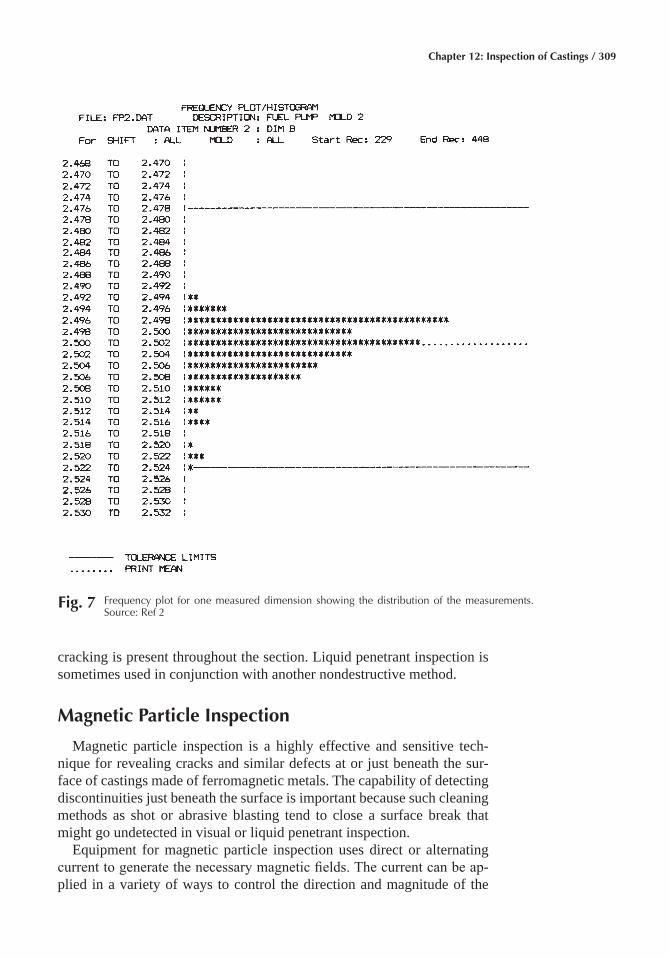
Chapter 12: Inspection of Castings / 309
cracking is present throughout the section. Liquid penetrant inspection is sometimes used in conjunction with another nondestructive method.
Magnetic Particle Inspection
Magnetic particle inspection is a highly effective and sensitive tech-nique for revealing cracks and similar defects at or just beneath the sur-face of castings made of ferromagnetic metals. The capability of detecting discontinuities just beneath the surface is important because such cleaning methods as shot or abrasive blasting tend to close a surface break that might go undetected in visual or liquid penetrant inspection.
Equipment for magnetic particle inspection uses direct or alternating current to generate the necessary magnetic fields. The current can be ap-plied in a variety of ways to control the direction and magnitude of the
Fig� 7 Frequency plot for one measured dimension showing the distribution of the measurements. Source: Ref 2
310 / Inspection of Metals—Understanding the Basics
magnetic field. In one method of magnetization, a heavy current is passed directly through the casting placed between two solid contacts. The in-duced magnetic field then runs in the transverse or circumferential direc-tion, producing conditions favorable to the detection of longitudinally ori-ented defects. A coil encircling the casting will induce a magnetic field that runs in the longitudinal direction, producing conditions favorable to the detection of circumferentially (or transversely) oriented defects. Alter-natively, a longitudinal magnetic field can be conveniently generated by passing current through a flexible cable conductor, which can be coiled around any metal section. This method is particularly adaptable to cast-ings of irregular shape. Circumferential magnetic fields can be induced in hollow cylindrical castings by using an axially disposed central conductor threaded through the casting.
Small castings can be magnetic particle inspected directly on bench type equipment that incorporates both coils and solid contacts. Critical regions of larger castings can be inspected by the use of yokes, coils, or contact probes carried on flexible cables connected to the source of cur-rent; this setup enables most regions of castings to be inspected.
Eddy Current Inspection
Eddy current methods of inspection are effective with both ferromag-netic and nonferromagnetic castings. Eddy current methods are not as sen-sitive to small, open defects as liquid penetrant or magnetic particle meth-ods are. Because of the skin effect, eddy current inspection is generally restricted to depths less than 6 mm (¼ in.). The results of inspecting fer-romagnetic materials can be obscured by changes in the magnetic perme-ability of the workpiece. Changes in temperature must be avoided to pre-vent erroneous results if electrical conductivity or other properties, including metallurgical properties, are being determined.
Applications of eddy current and electromagnetic methods of inspec-tion to castings can be divided into the following three categories:
• Detecting near-surface flaws such as cracks, voids, inclusions, blow-holes, and pinholes (eddy current inspection)
• Sorting according to alloy, temper, electrical conductivity, hardness, and other metallurgical factors (primarily electromagnetic inspection)
• Gaging according to size, shape, plating thickness, or insulation thick-ness (eddy current or electromagnetic inspection)
Radiographic Inspection
Internal flaws, such as gas entrapment or nonmetallic inclusions, have a direct effect on radiation attenuation. These flaws create variations in ma-terial thickness, resulting in localized dark or light spots on the image.
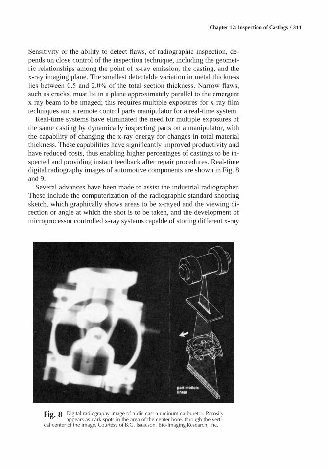
Chapter 12: Inspection of Castings / 311
Sensitivity or the ability to detect flaws, of radiographic inspection, de-pends on close control of the inspection technique, including the geomet-ric relationships among the point of x-ray emission, the casting, and the x-ray imaging plane. The smallest detectable variation in metal thickness lies between 0.5 and 2.0% of the total section thickness. Narrow flaws, such as cracks, must lie in a plane approximately parallel to the emergent x-ray beam to be imaged; this requires multiple exposures for x-ray film techniques and a remote control parts manipulator for a real-time system.
Real-time systems have eliminated the need for multiple exposures of the same casting by dynamically inspecting parts on a manipulator, with the capability of changing the x-ray energy for changes in total material thickness. These capabilities have significantly improved productivity and have reduced costs, thus enabling higher percentages of castings to be in-spected and providing instant feedback after repair procedures. Real-time digital radiography images of automotive components are shown in Fig. 8 and 9.
Several advances have been made to assist the industrial radiographer. These include the computerization of the radiographic standard shooting sketch, which graphically shows areas to be x-rayed and the viewing di-rection or angle at which the shot is to be taken, and the development of microprocessor controlled x-ray systems capable of storing different x-ray
Fig� 8 Digital radiography image of a die cast aluminum carburetor. Porosity appears as dark spots in the area of the center bore, through the verti-
cal center of the image. Courtesy of B.G. Isaacson, Bio-Imaging Research, Inc.
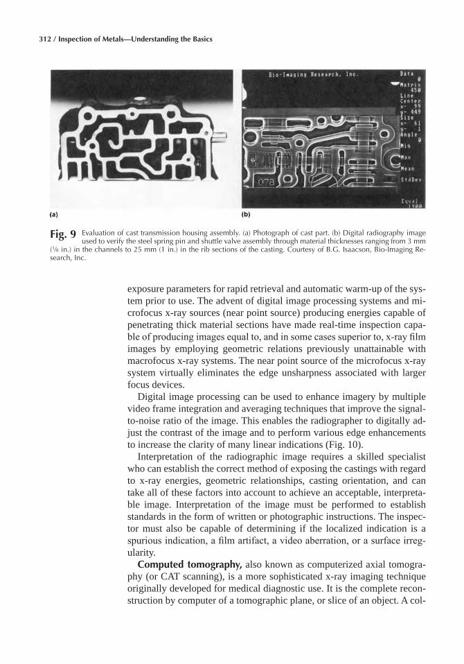
312 / Inspection of Metals—Understanding the Basics
exposure parameters for rapid retrieval and automatic warm-up of the sys-tem prior to use. The advent of digital image processing systems and mi-crofocus x-ray sources (near point source) producing energies capable of penetrating thick material sections have made real-time inspection capa-ble of producing images equal to, and in some cases superior to, x-ray film images by employing geometric relations previously unattainable with macrofocus x-ray systems. The near point source of the microfocus x-ray system virtually eliminates the edge unsharpness associated with larger focus devices.
Digital image processing can be used to enhance imagery by multiple video frame integration and averaging techniques that improve the signal-to-noise ratio of the image. This enables the radiographer to digitally ad-just the contrast of the image and to perform various edge enhancements to increase the clarity of many linear indications (Fig. 10).
Interpretation of the radiographic image requires a skilled specialist who can establish the correct method of exposing the castings with regard to x-ray energies, geometric relationships, casting orientation, and can take all of these factors into account to achieve an acceptable, interpreta-ble image. Interpretation of the image must be performed to establish standards in the form of written or photographic instructions. The inspec-tor must also be capable of determining if the localized indication is a spurious indication, a film artifact, a video aberration, or a surface irreg- ularity.
Computed tomography, also known as computerized axial tomogra-phy (or CAT scanning), is a more sophisticated x-ray imaging technique originally developed for medical diagnostic use. It is the complete recon-struction by computer of a tomographic plane, or slice of an object. A col-
Fig� 9 Evaluation of cast transmission housing assembly. (a) Photograph of cast part. (b) Digital radiography image used to verify the steel spring pin and shuttle valve assembly through material thicknesses ranging from 3 mm
(1⁄8 in.) in the channels to 25 mm (1 in.) in the rib sections of the casting. Courtesy of B.G. Isaacson, Bio-Imaging Re-search, Inc.
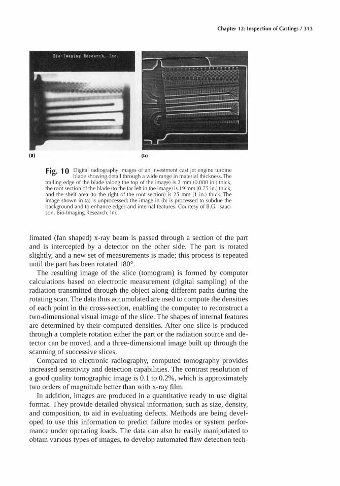
Chapter 12: Inspection of Castings / 313
limated (fan shaped) x-ray beam is passed through a section of the part and is intercepted by a detector on the other side. The part is rotated slightly, and a new set of measurements is made; this process is repeated until the part has been rotated 180°.
The resulting image of the slice (tomogram) is formed by computer calculations based on electronic measurement (digital sampling) of the radiation transmitted through the object along different paths during the rotating scan. The data thus accumulated are used to compute the densities of each point in the cross-section, enabling the computer to reconstruct a two-dimensional visual image of the slice. The shapes of internal features are determined by their computed densities. After one slice is produced through a complete rotation either the part or the radiation source and de-tector can be moved, and a three-dimensional image built up through the scanning of successive slices.
Compared to electronic radiography, computed tomography provides increased sensitivity and detection capabilities. The contrast resolution of a good quality tomographic image is 0.1 to 0.2%, which is approximately two orders of magnitude better than with x-ray film.
In addition, images are produced in a quantitative ready to use digital format. They provide detailed physical information, such as size, density, and composition, to aid in evaluating defects. Methods are being devel-oped to use this information to predict failure modes or system perfor-mance under operating loads. The data can also be easily manipulated to obtain various types of images, to develop automated flaw detection tech-
Fig� 10 Digital radiography images of an investment cast jet engine turbine blade showing detail through a wide range in material thickness. The
trailing edge of the blade (along the top of the image) is 2 mm (0.080 in.) thick, the root section of the blade (to the far left in the image) is 19 mm (0.75 in.) thick, and the shelf area (to the right of the root section) is 25 mm (1 in.) thick. The image shown in (a) is unprocessed; the image in (b) is processed to subdue the background and to enhance edges and internal features. Courtesy of B.G. Isaac-son, Bio-Imaging Research, Inc.
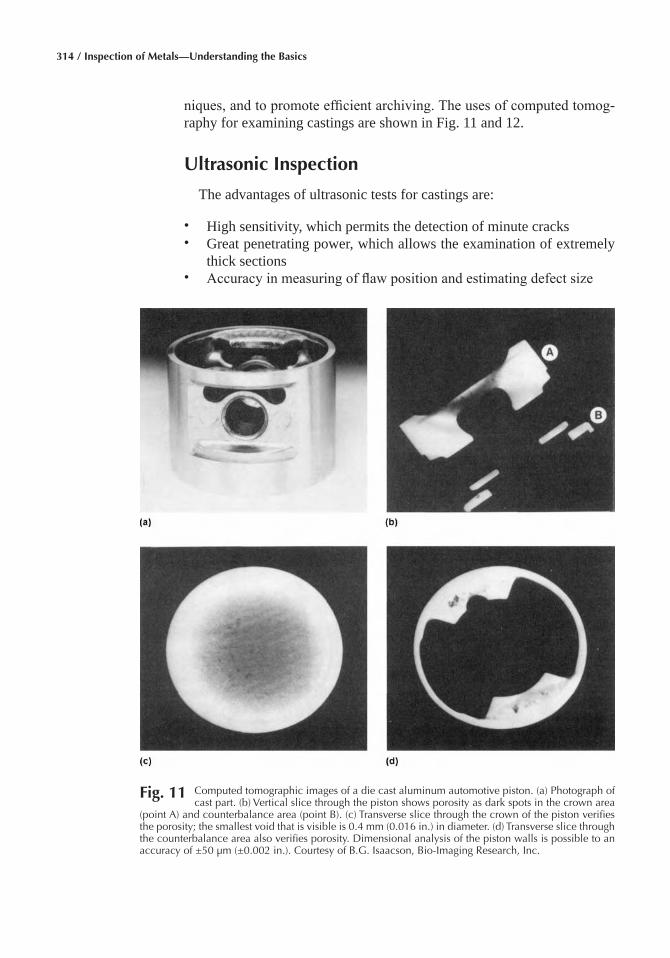
314 / Inspection of Metals—Understanding the Basics
niques, and to promote efficient archiving. The uses of computed tomog-raphy for examining castings are shown in Fig. 11 and 12.
Ultrasonic Inspection
The advantages of ultrasonic tests for castings are:
• High sensitivity, which permits the detection of minute cracks• Great penetrating power, which allows the examination of extremely
thick sections• Accuracy in measuring of flaw position and estimating defect size
Fig� 11 Computed tomographic images of a die cast aluminum automotive piston. (a) Photograph of cast part. (b) Vertical slice through the piston shows porosity as dark spots in the crown area
(point A) and counterbalance area (point B). (c) Transverse slice through the crown of the piston verifies the porosity; the smallest void that is visible is 0.4 mm (0.016 in.) in diameter. (d) Transverse slice through the counterbalance area also verifies porosity. Dimensional analysis of the piston walls is possible to an accuracy of ±50 μm (±0.002 in.). Courtesy of B.G. Isaacson, Bio-Imaging Research, Inc.
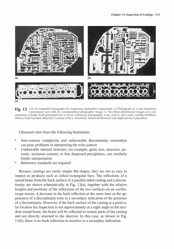
Chapter 12: Inspection of Castings / 315
Ultrasonic tests have the following limitations:
• Size-contour complexity and unfavorable discontinuity orientation can pose problems in interpreting the echo pattern
• Undesirable internal structure, for example, grain size, structure, po-rosity, inclusion content, or fine dispersed precipitates, can similarly hinder interpretation
• Reference standards are required
Because castings are rarely simple flat shapes, they are not as easy to inspect as products such as rolled rectangular bars. The reflections of a sound beam from the back surface of a parallel sided casting and a discon-tinuity are shown schematically in Fig. 13(a), together with the relative heights and positions of the reflections of the two surfaces on an oscillo-scope screen. A decrease in the back reflection at the same time as the ap-pearance of a discontinuity echo is a secondary indication of the presence of a discontinuity. However, if the back surface of the casting at a particu-lar location for inspection is not approximately at a right angle to the inci-dent sound beam, the beam will be reflected to remote parts of the casting and not directly returned to the detector. In this case, as shown in Fig. 13(b), there is no back reflection to monitor as a secondary indication.
Fig� 12 Use of computed tomography for examining automotive components. (a) Photograph of a cast aluminum transmission case with (b) corresponding tomographic image. (c) Two three-dimensional images of a cast
aluminum cylinder head generated from a set of continuous tomographic scans used to view water cooling chambers where a leak had been detected. Courtesy of R.A. Armistead, Advanced Research and Applications Corporation.
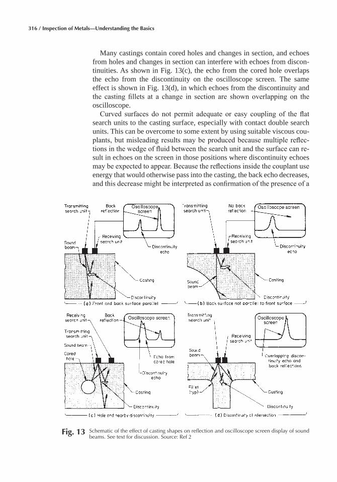
316 / Inspection of Metals—Understanding the Basics
Many castings contain cored holes and changes in section, and echoes from holes and changes in section can interfere with echoes from discon-tinuities. As shown in Fig. 13(c), the echo from the cored hole overlaps the echo from the discontinuity on the oscilloscope screen. The same effect is shown in Fig. 13(d), in which echoes from the discontinuity and the casting fillets at a change in section are shown overlapping on the oscilloscope.
Curved surfaces do not permit adequate or easy coupling of the flat search units to the casting surface, especially with contact double search units. This can be overcome to some extent by using suitable viscous cou-plants, but misleading results may be produced because multiple reflec-tions in the wedge of fluid between the search unit and the surface can re-sult in echoes on the screen in those positions where discontinuity echoes may be expected to appear. Because the reflections inside the couplant use energy that would otherwise pass into the casting, the back echo decreases, and this decrease might be interpreted as confirmation of the presence of a
Fig� 13 Schematic of the effect of casting shapes on reflection and oscilloscope screen display of sound beams. See text for discussion. Source: Ref 2
Chapter 12: Inspection of Castings / 317
discontinuity. On cylindrical surfaces, the indication will change as a dou-ble search unit is rotated. The wedge effect is least when the division be-tween the transmitting and receiving transducers is parallel to the axis of the cylinder. Wedge effects in the couplant are a particular problem on castings curved in two directions. One solution in this case is to use a small search unit so that the wedge is short, although the resolution and sensitivity may be reduced.
If the surface of the casting to be inspected is of regular shape, such as the bore of a cylinder in an engine block, the front of the search unit can be shaped to fit the curvature of the surface. These curved shapes form an acoustic lens that will alter the shape of the sound beam, but unless the curvature is severe, this will not prevent adequate accuracy in the in-spection. Cast-on flat metal pads for application of the ultrasonic search unit are very effective and allow particular areas of the casting to be inspected.
Subsurface Defects� Defects, such as small blowholes, pinholes, or inclusions that occur within depths of 3 or 4 mm (0.1 or 0.15 in.) of a cast surface, are among the most difficult to detect. They are beyond the limits of sensitivity of conventional magnetic particle methods and are not easily identified by eddy current techniques. They usually fall within the dead zone (the surface layer that cannot be inspected) of conventional single-crystal ultrasonic probes applied directly to a cast surface, although some improvement can be obtained by using twin crystal probes focused to depths not too far below the surface. The other alternative using contact methods of ultrasonic testing is to employ angle probes, but this compli-cates the procedures and interpretation methods to the point at which they can only be applied satisfactorily under the close control of skilled oper- ators.
However, freedom from such surface defects is a very important aspect of the casting quality. Apart from their effect in reducing bending fatigue properties, such defects are frequently revealed at late stages in the ma-chining of a component, leading to its rejection. Ultrasonic methods for detecting subsurface defects are much more successful when the dead zone beneath the as-cast surface is virtually eliminated by using immer-sion methods in which the probe is held away from the cast surface at a known controlled distance, with coupling being obtained through a liquid bath. To make such methods consistent and reliable, the test itself must be automated.
Semiautomatic equipment has been developed for examining castings such as cylinder heads by this method. With this equipment, the casting is loaded into a cradle from a roller track and is then transferred using a hoist into the immersion tank until the surface of the casting to be inspected is just submerged in the liquid. Depth of immersion is closely controlled because the customer will not permit liquid to be left in the internal pas-sageways of the cylinder head. The immersed surface of the casting is
318 / Inspection of Metals—Understanding the Basics
then scanned manually using an ultrasonic probe held at a fixed distance from the casting surface. This equipment is suitable for testing any casting requiring examination over a flat surface.
Internal Defects� Ultrasonic inspection is a well established method for the detection of internal defects in castings. Test equipment develop-ments, automated testing procedures, and improvements in determining the size and position of defects, which is essential to assessing whether or not their presence will likely affect the service performance of the casting, have contributed to the increasing use of ultrasonic test equipment.
For determining the position and size of defects, the usual method of presentation of ultrasonic data is an A-scan, in which the amplitude of the echoes from defects is shown on a time base and has well known limita-tions. Sizing relies on measuring the drop in amplitude of the echo as the probe is passed over the boundary of a defect or measuring the reduction in the amplitude of the back wall echo due to the scattering of sound by the defect. In most cases, sizing is approximate and is restricted to one or two dimensions. Improvements in data presentation in the form of B-scans and C-scans that present a plane view through the section of the compo-nent provide a marked improvement in defining defect positions and size in two or three dimensions. Such displays have been used for automated defect characterization systems in which porosity, cracks, and dross have been distinguished. Because of the requirement to scan the probe over the surface, the application of B-scan and C-scan methods has generally been limited to simple geometric shapes having good surface finish, such as welded plate structures. Application to castings is currently restricted, but greater use of B-scan and C-scan methods is likely with either improved scanning systems or arrays of ultrasonic probes.
Structure evaluation is an area of growing importance for foundry engineers. Ultrasonic velocity measurements are widely used as a means of guaranteeing the nodularity of the graphite structure, and if the matrix structure is known to be consistent, guaranteeing the principal material properties of ductile irons. Velocity measurements have been used to eval-uate compacted graphite iron structures to ensure that the desired proper-ties have been consistently obtained.
Leak Testing
Castings that are intended to withstand pressures can be leak tested at the foundry. Various methods are used, according to the type of metal being tested. One method consists of pumping air at a specific pressure into the inside of the casting in water at a given temperature. Any leaks through the casting become apparent by the release of bubbles of air through the faulty portions. An alternative method is to fill the cavities of a casting with paraffin at a specified pressure. Paraffin, which penetrates the smallest of crevices, will rapidly find any defect, such as porosity, and

Chapter 12: Inspection of Castings / 319
will show quickly as an oily or moist patch at the position of the fault. Liquid penetrants can be poured into areas of apparent porosity and time allowed for the liquid to seep through the casting wall. However, the intro-duction of contaminants into the defect may make repair welding more difficult.
The pressure testing of rough (unmachined) castings at the foundry may not reveal any leaks, but it must be recognized that subsequent machining operations on the casting may cut into porous areas and cause the casting to leak after machining. Minor seepage leaks can be sealed by impregna-tion of the casting with liquid or by filling with sodium silicate, a synthetic resin, or other suitable substance. As-cast parts can be impregnated at the foundry to seal leaks if there is little machining or if experience has shown that machining does not affect the pressure tightness. However, it is usu-ally preferable to impregnate the casting after final machining.
ACKNOWLEDGMENT
This chapter was adapted from Inspection of Castings, Nondestructive Evaluation and Quality Control, Volume 17, ASM Handbook, 1992.
REFERENCES
1. R. DasGupta, Common Defects in Various Casting Processes, ASM Handbook, Vol 15, Casting, ASM International, 2008, p 1192–1202
2. Inspection of Castings, Nondestructive Evaluation and Quality Con-trol, Vol 17, ASM Handbook, ASM International, 1989, p 231–277
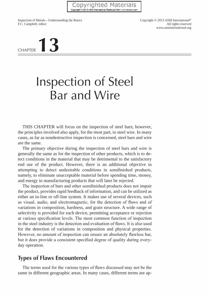
Inspection of Metals—Understanding the Basics Copyright © 2013 ASM International®
F.C. Campbell, editor All rights reservedwww.asminternational.org
CHAPTER 13
Inspection of Steel Bar and Wire
THIS CHAPTER will focus on the inspection of steel bars; however, the principles involved also apply, for the most part, to steel wire. In many cases, as far as nondestructive inspection is concerned, steel bars and wire are the same.
The primary objective during the inspection of steel bars and wire is generally the same as for the inspection of other products, which is to de-tect conditions in the material that may be detrimental to the satisfactory end use of the product. However, there is an additional objective in attempting to detect undesirable conditions in semifinished products, namely, to eliminate unacceptable material before spending time, money, and energy in manufacturing products that will later be rejected.
The inspection of bars and other semifinished products does not impair the product, provides rapid feedback of information, and can be utilized as either an in-line or off-line system. It makes use of several devices, such as visual, audio, and electromagnetic, for the detection of flaws and of variations in composition, hardness, and grain structure. A wide range of selectivity is provided for each device, permitting acceptance or rejection at various specification levels. The most common function of inspection in the steel industry is the detection and evaluation of flaws. It is also used for the detection of variations in composition and physical properties. However, no amount of inspection can ensure an absolutely flawless bar, but it does provide a consistent specified degree of quality during every-day operation.
Types of Flaws Encountered
The terms used for the various types of flaws discussed may not be the same in different geographic areas. In many cases, different terms are ap-
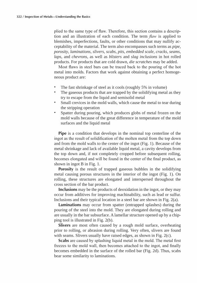
322 / Inspection of Metals—Understanding the Basics
plied to the same type of flaw. Therefore, this section contains a descrip-tion and an illustration of each condition. The term flaw is applied to blemishes, imperfections, faults, or other conditions that may nullify ac-ceptability of the material. The term also encompasses such terms as pipe, porosity, laminations, slivers, scabs, pits, embedded scale, cracks, seams, laps, and chevrons, as well as blisters and slag inclusions in hot rolled products. For products that are cold drawn, die scratches may be added.
Most flaws in steel bars can be traced back to the pouring of the hot metal into molds. Factors that work against obtaining a perfect homoge-neous product are:
• The fast shrinkage of steel as it cools (roughly 5% in volume)• The gaseous products that are trapped by the solidifying metal as they
try to escape from the liquid and semisolid metal• Small crevices in the mold walls, which cause the metal to tear during
the stripping operation• Spatter during pouring, which produces globs of metal frozen on the
mold walls because of the great difference in temperature of the mold surfaces and the liquid metal
Pipe is a condition that develops in the nominal top centerline of the ingot as the result of solidification of the molten metal from the top down and from the mold walls to the center of the ingot (Fig. 1). Because of the metal shrinkage and lack of available liquid metal, a cavity develops from the top down and, if not completely cropped before subsequent rolling, becomes elongated and will be found in the center of the final product, as shown in ingot B in Fig. 1.
Porosity is the result of trapped gaseous bubbles in the solidifying metal causing porous structures in the interior of the ingot (Fig. 1). On rolling, these structures are elongated and interspersed throughout the cross section of the bar product.
Inclusions may be the products of deoxidation in the ingot, or they may occur from additives for improving machinability, such as lead or sulfur. Inclusions and their typical location in a steel bar are shown in Fig. 2(a).
Laminations may occur from spatter (entrapped splashes) during the pouring of the steel into the mold. They are elongated during rolling and are usually in the bar subsurface. A lamellar structure opened up by a chip-ping tool is illustrated in Fig. 2(b).
Slivers are most often caused by a rough mold surface, overheating prior to rolling, or abrasion during rolling. Very often, slivers are found with seams. Slivers usually have raised edges, as shown in Fig. 2(c).
Scabs are caused by splashing liquid metal in the mold. The metal first freezes to the mold wall, then becomes attached to the ingot, and finally becomes embedded in the surface of the rolled bar (Fig. 2d). Thus, scabs bear some similarity to laminations.
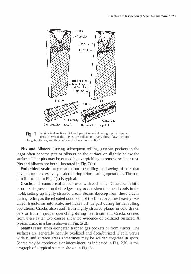
Chapter 13: Inspection of Steel Bar and Wire / 323
Pits and Blisters� During subsequent rolling, gaseous pockets in the ingot often become pits or blisters on the surface or slightly below the surface. Other pits may be caused by overpickling to remove scale or rust. Pits and blisters are both illustrated in Fig. 2(e).
Embedded scale may result from the rolling or drawing of bars that have become excessively scaled during prior heating operations. The pat-tern illustrated in Fig. 2(f) is typical.
Cracks and seams are often confused with each other. Cracks with little or no oxide present on their edges may occur when the metal cools in the mold, setting up highly stressed areas. Seams develop from these cracks during rolling as the reheated outer skin of the billet becomes heavily oxi-dized, transforms into scale, and flakes off the part during further rolling operations. Cracks also result from highly stressed planes in cold drawn bars or from improper quenching during heat treatment. Cracks created from these latter two causes show no evidence of oxidized surfaces. A typical crack in a bar is shown in Fig. 2(g).
Seams result from elongated trapped gas pockets or from cracks. The surfaces are generally heavily oxidized and decarburized. Depth varies widely, and surface areas sometimes may be welded together in spots. Seams may be continuous or intermittent, as indicated in Fig. 2(h). A mi-crograph of a typical seam is shown in Fig. 3.
Fig� 1 Longitudinal sections of two types of ingots showing typical pipe and porosity. When the ingots are rolled into bars, these flaws become
elongated throughout the center of the bars. Source: Ref 1
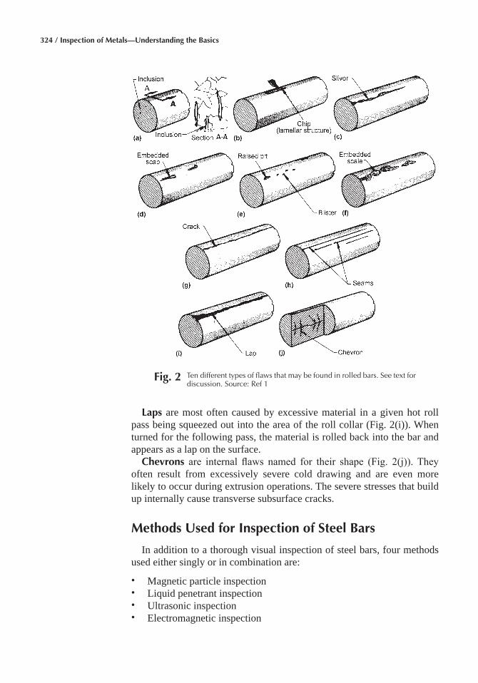
324 / Inspection of Metals—Understanding the Basics
Laps are most often caused by excessive material in a given hot roll pass being squeezed out into the area of the roll collar (Fig. 2(i)). When turned for the following pass, the material is rolled back into the bar and appears as a lap on the surface.
Chevrons are internal flaws named for their shape (Fig. 2(j)). They often result from excessively severe cold drawing and are even more likely to occur during extrusion operations. The severe stresses that build up internally cause transverse subsurface cracks.
Methods Used for Inspection of Steel Bars
In addition to a thorough visual inspection of steel bars, four methods used either singly or in combination are:
• Magnetic particle inspection• Liquid penetrant inspection• Ultrasonic inspection• Electromagnetic inspection
Fig� 2 Ten different types of flaws that may be found in rolled bars. See text for discussion. Source: Ref 1
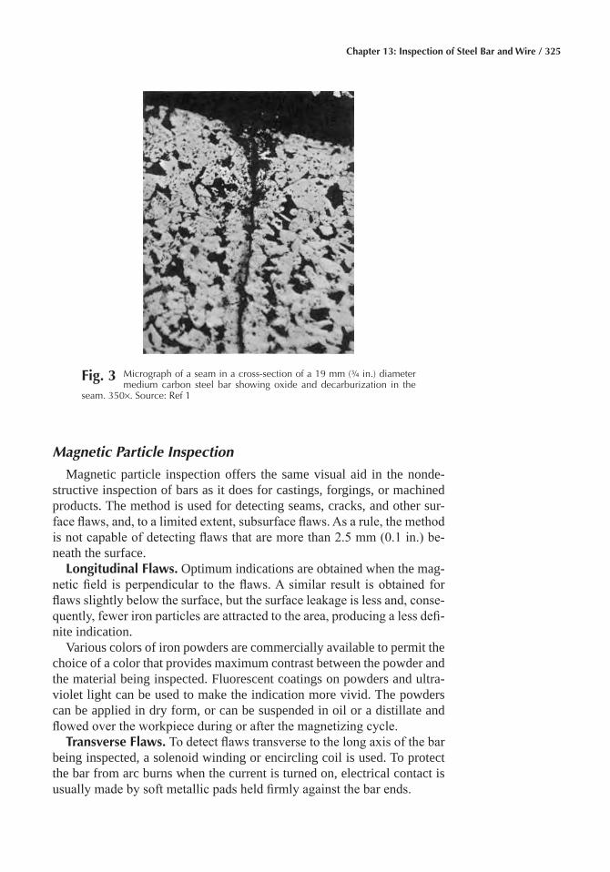
Chapter 13: Inspection of Steel Bar and Wire / 325
Magnetic Particle Inspection
Magnetic particle inspection offers the same visual aid in the nonde-structive inspection of bars as it does for castings, forgings, or machined products. The method is used for detecting seams, cracks, and other sur-face flaws, and, to a limited extent, subsurface flaws. As a rule, the method is not capable of detecting flaws that are more than 2.5 mm (0.1 in.) be-neath the surface.
Longitudinal Flaws� Optimum indications are obtained when the mag-netic field is perpendicular to the flaws. A similar result is obtained for flaws slightly below the surface, but the surface leakage is less and, conse-quently, fewer iron particles are attracted to the area, producing a less defi-nite indication.
Various colors of iron powders are commercially available to permit the choice of a color that provides maximum contrast between the powder and the material being inspected. Fluorescent coatings on powders and ultra-violet light can be used to make the indication more vivid. The powders can be applied in dry form, or can be suspended in oil or a distillate and flowed over the workpiece during or after the magnetizing cycle.
Transverse Flaws� To detect flaws transverse to the long axis of the bar being inspected, a solenoid winding or encircling coil is used. To protect the bar from arc burns when the current is turned on, electrical contact is usually made by soft metallic pads held firmly against the bar ends.
Fig� 3 Micrograph of a seam in a cross-section of a 19 mm (¾ in.) diameter medium carbon steel bar showing oxide and decarburization in the
seam. 350×. Source: Ref 1
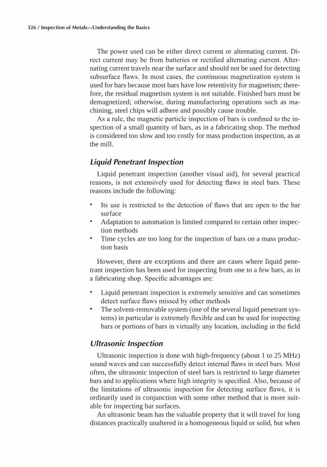
326 / Inspection of Metals—Understanding the Basics
The power used can be either direct current or alternating current. Di-rect current may be from batteries or rectified alternating current. Alter-nating current travels near the surface and should not be used for detecting subsurface flaws. In most cases, the continuous magnetization system is used for bars because most bars have low retentivity for magnetism; there-fore, the residual magnetism system is not suitable. Finished bars must be demagnetized; otherwise, during manufacturing operations such as ma-chining, steel chips will adhere and possibly cause trouble.
As a rule, the magnetic particle inspection of bars is confined to the in-spection of a small quantity of bars, as in a fabricating shop. The method is considered too slow and too costly for mass production inspection, as at the mill.
Liquid Penetrant Inspection
Liquid penetrant inspection (another visual aid), for several practical reasons, is not extensively used for detecting flaws in steel bars. These reasons include the following:
• Its use is restricted to the detection of flaws that are open to the bar surface
• Adaptation to automation is limited compared to certain other inspec-tion methods
• Time cycles are too long for the inspection of bars on a mass produc-tion basis
However, there are exceptions and there are cases where liquid pene-trant inspection has been used for inspecting from one to a few bars, as in a fabricating shop. Specific advantages are:
• Liquid penetrant inspection is extremely sensitive and can sometimes detect surface flaws missed by other methods
• The solvent-removable system (one of the several liquid penetrant sys-tems) in particular is extremely flexible and can be used for inspecting bars or portions of bars in virtually any location, including in the field
Ultrasonic Inspection
Ultrasonic inspection is done with high-frequency (about 1 to 25 MHz) sound waves and can successfully detect internal flaws in steel bars. Most often, the ultrasonic inspection of steel bars is restricted to large diameter bars and to applications where high integrity is specified. Also, because of the limitations of ultrasonic inspection for detecting surface flaws, it is ordinarily used in conjunction with some other method that is more suit-able for inspecting bar surfaces.
An ultrasonic beam has the valuable property that it will travel for long distances practically unaltered in a homogeneous liquid or solid, but when
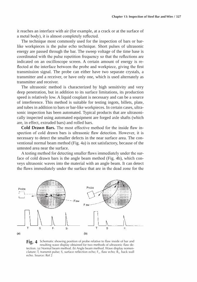
Chapter 13: Inspection of Steel Bar and Wire / 327
it reaches an interface with air (for example, at a crack or at the surface of a metal body), it is almost completely reflected.
The technique most commonly used for the inspection of bars or bar-like workpieces is the pulse echo technique. Short pulses of ultrasonic energy are passed through the bar. The sweep voltage of the time base is coordinated with the pulse repetition frequency so that the reflections are indicated on an oscilloscope screen. A certain amount of energy is re-flected at the interface between the probe and workpiece, giving the first transmission signal. The probe can either have two separate crystals, a transmitter and a receiver, or have only one, which is used alternately as transmitter and receiver.
The ultrasonic method is characterized by high sensitivity and very deep penetration, but in addition to its surface limitations, its production speed is relatively low. A liquid couplant is necessary and can be a source of interference. This method is suitable for testing ingots, billets, plate, and tubes in addition to bars or bar-like workpieces. In certain cases, ultra-sonic inspection has been automated. Typical products that are ultrasoni-cally inspected using automated equipment are forged axle shafts (which are, in effect, extruded bars) and rolled bars.
Cold Drawn Bars� The most effective method for the inside flaw in-spection of cold drawn bars is ultrasonic flaw detection. However, it is necessary to detect the smaller defects in the near surface area. The con-ventional normal beam method (Fig. 4a) is not satisfactory, because of the untested area near the surface.
A testing method for detecting smaller flaws immediately under the sur-face of cold drawn bars is the angle beam method (Fig. 4b), which con-veys ultrasonic waves into the material with an angle beam. It can detect the flaws immediately under the surface that are in the dead zone for the
Fig� 4 Schematic showing position of probe relative to flaw inside of bar and resulting wave display obtained for two methods of ultrasonic flaw de-
tection. (a) Normal beam method. (b) Angle beam method. Wave display nomen-clature: T, transmit pulse; S, surface reflection echo; F1, flaw echo; B1, back wall echo. Source: Ref 2
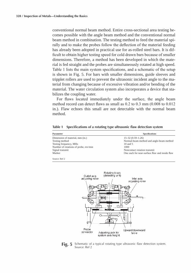
328 / Inspection of Metals—Understanding the Basics
conventional normal beam method. Entire cross-sectional area testing be-comes possible with the angle beam method and the conventional normal beam method in combination. The testing method to feed the material spi-rally and to make the probes follow the deflection of the material feeding has already been adopted in practical use for as-rolled steel bars. It is dif-ficult to obtain higher testing speed for cold drawn bars because of smaller dimensions. Therefore, a method has been developed in which the mate-rial is fed straight and the probes are simultaneously rotated at high speed. Table 1 lists the main system specifications, and a schematic of the setup is shown in Fig. 5. For bars with smaller dimensions, guide sleeves and tripplet rollers are used to prevent the ultrasonic incident angle to the ma-terial from changing because of excessive vibration and/or bending of the material. The water circulation system also incorporates a device that sta-bilizes the coupling water.
For flaws located immediately under the surface, the angle beam method record can detect flaws as small as 0.2 to 0.3 mm (0.008 to 0.012 in.). Flaw echoes this small are not detectable with the normal beam method.
Table 1 Specifications of a rotating type ultrasonic flaw detection system
Parameter Specifications
Dimension of material, mm (in.) 15–32 (0.59–1.26)Testing method Normal-beam method and angle-beam methodTesting frequency, MHz 10 and 5Number of rotations of probe, rev/min 1000Signal transmit Noncontact rotation transmitMarker One each for near-surface flaw and inside flaw
Source: Ref 2
Fig� 5 Schematic of a typical rotating type ultrasonic flaw detection system. Source: Ref 2
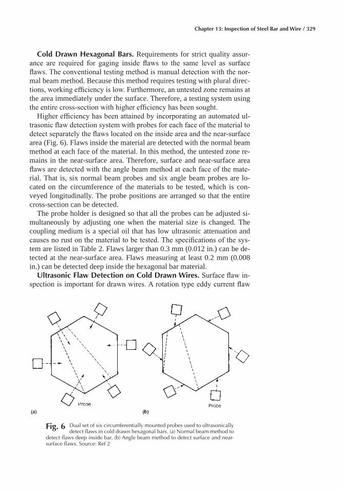
Chapter 13: Inspection of Steel Bar and Wire / 329
Cold Drawn Hexagonal Bars� Requirements for strict quality assur-ance are required for gaging inside flaws to the same level as surface flaws. The conventional testing method is manual detection with the nor-mal beam method. Because this method requires testing with plural direc-tions, working efficiency is low. Furthermore, an untested zone remains at the area immediately under the surface. Therefore, a testing system using the entire cross-section with higher efficiency has been sought.
Higher efficiency has been attained by incorporating an automated ul-trasonic flaw detection system with probes for each face of the material to detect separately the flaws located on the inside area and the near-surface area (Fig. 6). Flaws inside the material are detected with the normal beam method at each face of the material. In this method, the untested zone re-mains in the near-surface area. Therefore, surface and near-surface area flaws are detected with the angle beam method at each face of the mate-rial. That is, six normal beam probes and six angle beam probes are lo-cated on the circumference of the materials to be tested, which is con-veyed longitudinally. The probe positions are arranged so that the entire cross-section can be detected.
The probe holder is designed so that all the probes can be adjusted si-multaneously by adjusting one when the material size is changed. The coupling medium is a special oil that has low ultrasonic attenuation and causes no rust on the material to be tested. The specifications of the sys-tem are listed in Table 2. Flaws larger than 0.3 mm (0.012 in.) can be de-tected at the near-surface area. Flaws measuring at least 0.2 mm (0.008 in.) can be detected deep inside the hexagonal bar material.
Ultrasonic Flaw Detection on Cold Drawn Wires� Surface flaw in-spection is important for drawn wires. A rotation type eddy current flaw
Fig� 6 Dual set of six circumferentially mounted probes used to ultrasonically detect flaws in cold drawn hexagonal bars. (a) Normal beam method to
detect flaws deep inside bar. (b) Angle beam method to detect surface and near-surface flaws. Source: Ref 2
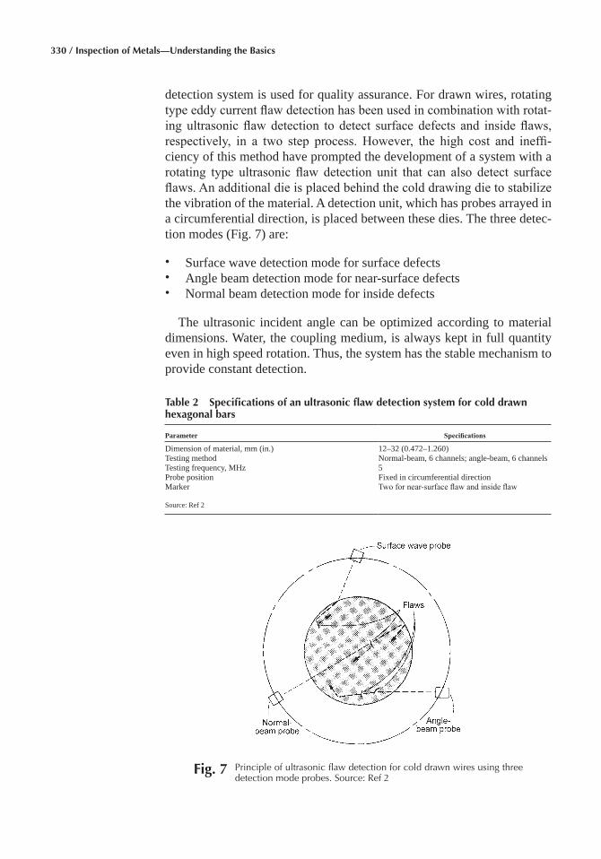
330 / Inspection of Metals—Understanding the Basics
detection system is used for quality assurance. For drawn wires, rotating type eddy current flaw detection has been used in combination with rotat-ing ultrasonic flaw detection to detect surface defects and inside flaws, respectively, in a two step process. However, the high cost and ineffi-ciency of this method have prompted the development of a system with a rotating type ultrasonic flaw detection unit that can also detect surface flaws. An additional die is placed behind the cold drawing die to stabilize the vibration of the material. A detection unit, which has probes arrayed in a circumferential direction, is placed between these dies. The three detec-tion modes (Fig. 7) are:
• Surface wave detection mode for surface defects• Angle beam detection mode for near-surface defects• Normal beam detection mode for inside defects
The ultrasonic incident angle can be optimized according to material dimensions. Water, the coupling medium, is always kept in full quantity even in high speed rotation. Thus, the system has the stable mechanism to provide constant detection.
Table 2 Specifications of an ultrasonic flaw detection system for cold drawn hexagonal bars
Parameter Specifications
Dimension of material, mm (in.) 12–32 (0.472–1.260)Testing method Normal-beam, 6 channels; angle-beam, 6 channelsTesting frequency, MHz 5Probe position Fixed in circumferential directionMarker Two for near-surface flaw and inside flaw
Source: Ref 2
Fig� 7 Principle of ultrasonic flaw detection for cold drawn wires using three detection mode probes. Source: Ref 2
Chapter 13: Inspection of Steel Bar and Wire / 331
One advantage of this system is that linear defects can be detected by surface wave detection at the same level as an eddy current method. An-other is that the entire cross section can be covered by means of a combi-nation angle beam/normal beam method. The specifications of this setup are summarized in Table 3. Results with this system showed detectability of 0.1 mm (0.004 in.) minimum flaw depth on surface defects and 0.2 mm (0.008 in.) minimum inside defect size. This system enables the user to inspect the entire cross section of cold drawn wires to a high degree of accuracy.
Electromagnetic Inspection Methods
Electromagnetic methods of inspection are used far more extensively for nondestructive inspection of steel bars than any of the methods dis-cussed. Electromagnetic methods are readily adaptable to automation and can be set up to detect flaws, as well as a number of different composi-tional and structural variations, in bars on a mass production basis.
Equipment can be relatively simple, but for mass production inspec-tion, the equipment may be highly sophisticated and costly. Such equip-ment can not only detect flaws and indicate them on an oscilloscope or other form of readout, but can also mark the location of the flaw on the bar before it emerges from the inspection equipment and can automatically sort the bars on the basis of seam depth.
Electromagnetic systems include the systems that use magnetic fields generated by alternating current flowing in a solenoid. A wide range of frequencies is used. As the alternating current flows through the solenoid, the magnetic field generated induces eddy currents within the metal work-piece. These currents are affected by the electrical resistivity (more com-monly expressed as electrical conductivity, the reciprocal of resistivity), magnetic permeability, configuration, homogeneity, surface irregularities, and flaws in the metal. The resistivity of the workpiece can vary because of the chemical composition, crystal orientation, structure, and history of me-chanical working. Permeability will vary over a broad range, depending on the amount of stresses present in the workpiece. It increases slightly in the vicinity of a flaw when the bar is subjected to a stress producing operation.
Table 3 Specifications of an ultrasonic flaw detection system for cold drawn wires
Parameter Specifications
Dimension of material, mm (in.) 15–30 (0.590–1.181)Testing frequency Normal beam: 10 MHz, 1 channel
Angle beam: 5 MHz, 2 channelsSurface wave: 5 MHz, 2 channels
Number of rotations of probe, rev/min 1000Signal transmit Noncontact rotation transmitMarker One each for near-surface flaw and inside flaw
Source: Ref 2
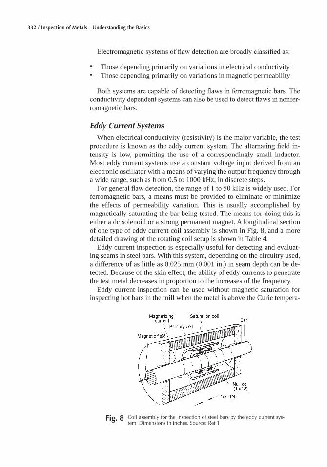
332 / Inspection of Metals—Understanding the Basics
Electromagnetic systems of flaw detection are broadly classified as:
• Those depending primarily on variations in electrical conductivity• Those depending primarily on variations in magnetic permeability
Both systems are capable of detecting flaws in ferromagnetic bars. The conductivity dependent systems can also be used to detect flaws in nonfer-romagnetic bars.
Eddy Current Systems
When electrical conductivity (resistivity) is the major variable, the test procedure is known as the eddy current system. The alternating field in-tensity is low, permitting the use of a correspondingly small inductor. Most eddy current systems use a constant voltage input derived from an electronic oscillator with a means of varying the output frequency through a wide range, such as from 0.5 to 1000 kHz, in discrete steps.
For general flaw detection, the range of 1 to 50 kHz is widely used. For ferromagnetic bars, a means must be provided to eliminate or minimize the effects of permeability variation. This is usually accomplished by magnetically saturating the bar being tested. The means for doing this is either a dc solenoid or a strong permanent magnet. A longitudinal section of one type of eddy current coil assembly is shown in Fig. 8, and a more detailed drawing of the rotating coil setup is shown in Table 4.
Eddy current inspection is especially useful for detecting and evaluat-ing seams in steel bars. With this system, depending on the circuitry used, a difference of as little as 0.025 mm (0.001 in.) in seam depth can be de-tected. Because of the skin effect, the ability of eddy currents to penetrate the test metal decreases in proportion to the increases of the frequency.
Eddy current inspection can be used without magnetic saturation for inspecting hot bars in the mill when the metal is above the Curie tempera-
Fig� 8 Coil assembly for the inspection of steel bars by the eddy current sys-tem. Dimensions in inches. Source: Ref 1
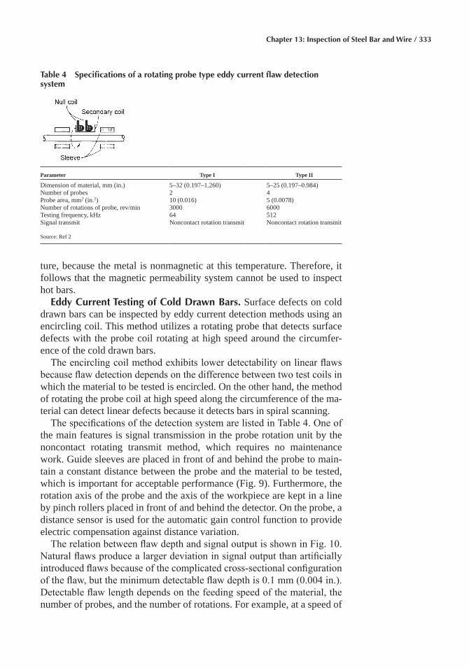
Chapter 13: Inspection of Steel Bar and Wire / 333
ture, because the metal is nonmagnetic at this temperature. Therefore, it follows that the magnetic permeability system cannot be used to inspect hot bars.
Eddy Current Testing of Cold Drawn Bars� Surface defects on cold drawn bars can be inspected by eddy current detection methods using an encircling coil. This method utilizes a rotating probe that detects surface defects with the probe coil rotating at high speed around the circumfer-ence of the cold drawn bars.
The encircling coil method exhibits lower detectability on linear flaws because flaw detection depends on the difference between two test coils in which the material to be tested is encircled. On the other hand, the method of rotating the probe coil at high speed along the circumference of the ma-terial can detect linear defects because it detects bars in spiral scanning.
The specifications of the detection system are listed in Table 4. One of the main features is signal transmission in the probe rotation unit by the noncontact rotating transmit method, which requires no maintenance work. Guide sleeves are placed in front of and behind the probe to main-tain a constant distance between the probe and the material to be tested, which is important for acceptable performance (Fig. 9). Furthermore, the rotation axis of the probe and the axis of the workpiece are kept in a line by pinch rollers placed in front of and behind the detector. On the probe, a distance sensor is used for the automatic gain control function to provide electric compensation against distance variation.
The relation between flaw depth and signal output is shown in Fig. 10. Natural flaws produce a larger deviation in signal output than artificially introduced flaws because of the complicated cross-sectional configuration of the flaw, but the minimum detectable flaw depth is 0.1 mm (0.004 in.). Detectable flaw length depends on the feeding speed of the material, the number of probes, and the number of rotations. For example, at a speed of
Table 4 Specifications of a rotating probe type eddy current flaw detection system
Parameter Type I Type II
Dimension of material, mm (in.) 5–32 (0.197–1.260) 5–25 (0.197–0.984)Number of probes 2 4Probe area, mm2 (in.2) 10 (0.016) 5 (0.0078)Number of rotations of probe, rev/min 3000 6000Testing frequency, kHz 64 512Signal transmit Noncontact rotation transmit Noncontact rotation transmit
Source: Ref 2
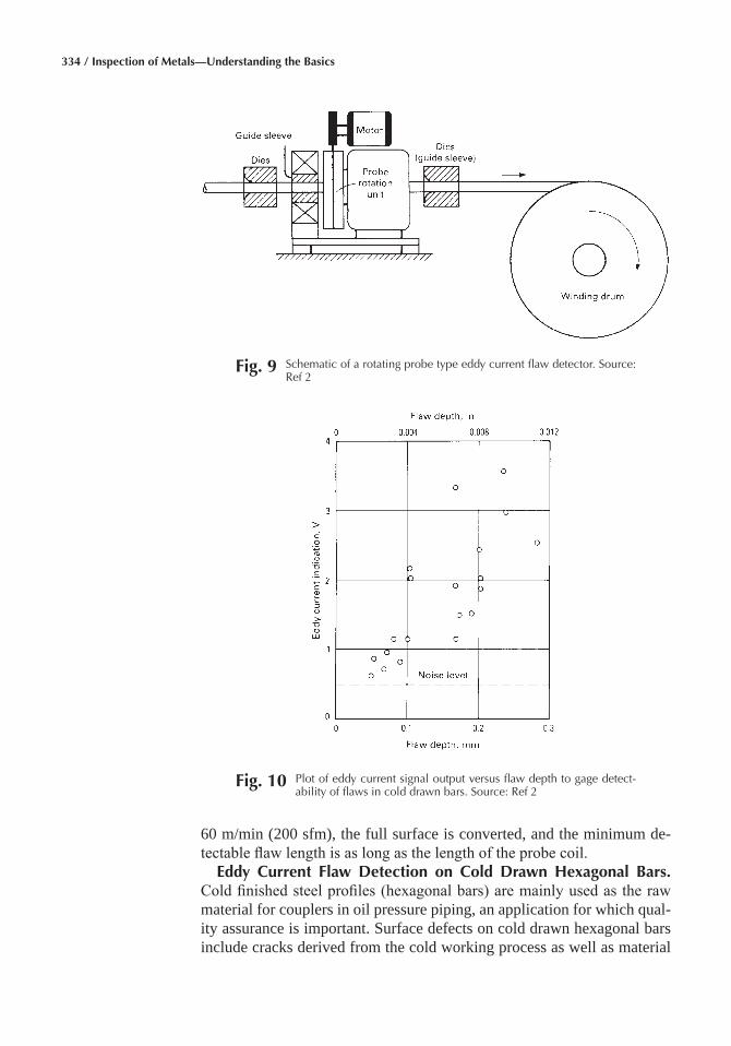
334 / Inspection of Metals—Understanding the Basics
60 m/min (200 sfm), the full surface is converted, and the minimum de-tectable flaw length is as long as the length of the probe coil.
Eddy Current Flaw Detection on Cold Drawn Hexagonal Bars� Cold finished steel profiles (hexagonal bars) are mainly used as the raw material for couplers in oil pressure piping, an application for which qual-ity assurance is important. Surface defects on cold drawn hexagonal bars include cracks derived from the cold working process as well as material
Fig� 9 Schematic of a rotating probe type eddy current flaw detector. Source: Ref 2
Fig� 10 Plot of eddy current signal output versus flaw depth to gage detect-ability of flaws in cold drawn bars. Source: Ref 2
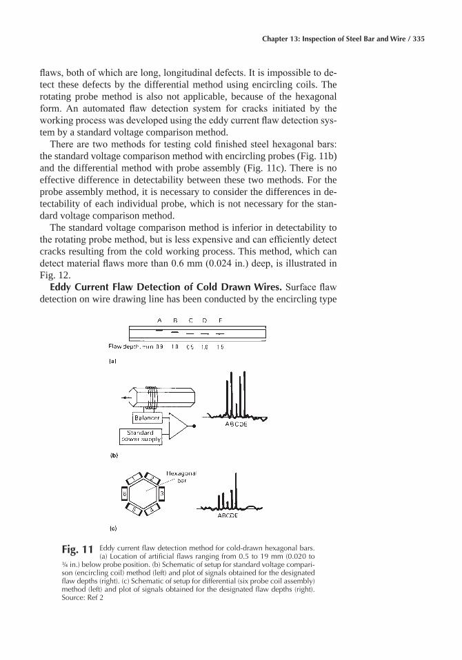
Chapter 13: Inspection of Steel Bar and Wire / 335
flaws, both of which are long, longitudinal defects. It is impossible to de-tect these defects by the differential method using encircling coils. The rotating probe method is also not applicable, because of the hexagonal form. An automated flaw detection system for cracks initiated by the working process was developed using the eddy current flaw detection sys-tem by a standard voltage comparison method.
There are two methods for testing cold finished steel hexagonal bars: the standard voltage comparison method with encircling probes (Fig. 11b) and the differential method with probe assembly (Fig. 11c). There is no effective difference in detectability between these two methods. For the probe assembly method, it is necessary to consider the differences in de-tectability of each individual probe, which is not necessary for the stan-dard voltage comparison method.
The standard voltage comparison method is inferior in detectability to the rotating probe method, but is less expensive and can efficiently detect cracks resulting from the cold working process. This method, which can detect material flaws more than 0.6 mm (0.024 in.) deep, is illustrated in Fig. 12.
Eddy Current Flaw Detection of Cold Drawn Wires� Surface flaw detection on wire drawing line has been conducted by the encircling type
Fig� 11 Eddy current flaw detection method for cold-drawn hexagonal bars. (a) Location of artificial flaws ranging from 0.5 to 19 mm (0.020 to
¾ in.) below probe position. (b) Schematic of setup for standard voltage compari-son (encircling coil) method (left) and plot of signals obtained for the designated flaw depths (right). (c) Schematic of setup for differential (six probe coil assembly) method (left) and plot of signals obtained for the designated flaw depths (right). Source: Ref 2
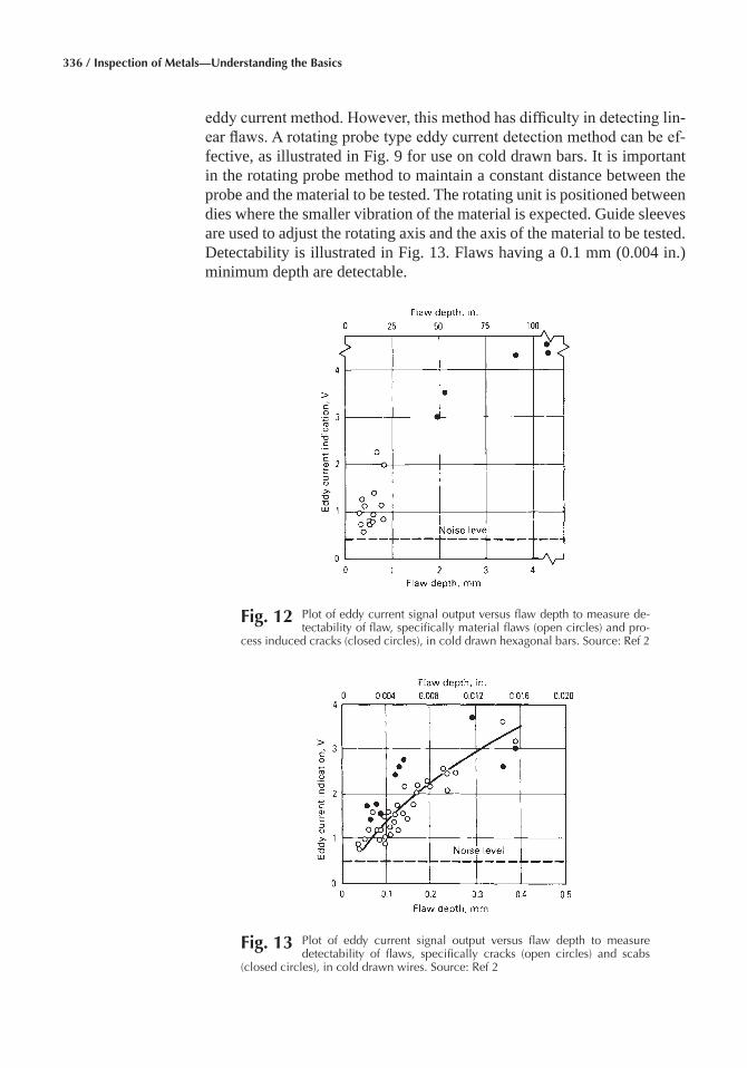
336 / Inspection of Metals—Understanding the Basics
eddy current method. However, this method has difficulty in detecting lin-ear flaws. A rotating probe type eddy current detection method can be ef-fective, as illustrated in Fig. 9 for use on cold drawn bars. It is important in the rotating probe method to maintain a constant distance between the probe and the material to be tested. The rotating unit is positioned between dies where the smaller vibration of the material is expected. Guide sleeves are used to adjust the rotating axis and the axis of the material to be tested. Detectability is illustrated in Fig. 13. Flaws having a 0.1 mm (0.004 in.) minimum depth are detectable.
Fig� 12 Plot of eddy current signal output versus flaw depth to measure de-tectability of flaw, specifically material flaws (open circles) and pro-
cess induced cracks (closed circles), in cold drawn hexagonal bars. Source: Ref 2
Fig� 13 Plot of eddy current signal output versus flaw depth to measure detectability of flaws, specifically cracks (open circles) and scabs
(closed circles), in cold drawn wires. Source: Ref 2
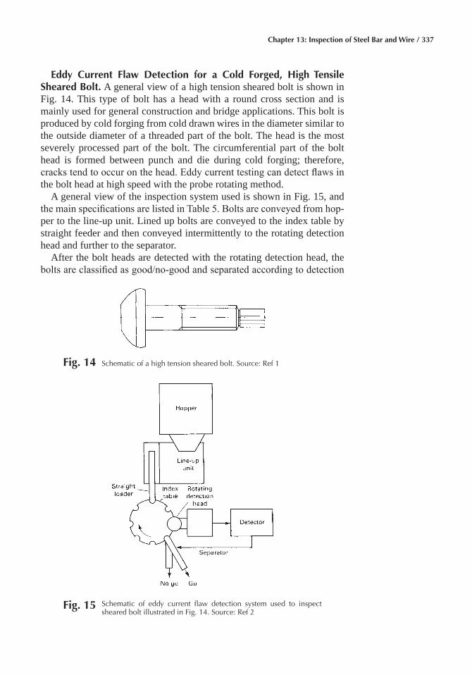
Chapter 13: Inspection of Steel Bar and Wire / 337
Eddy Current Flaw Detection for a Cold Forged, High Tensile Sheared Bolt� A general view of a high tension sheared bolt is shown in Fig. 14. This type of bolt has a head with a round cross section and is mainly used for general construction and bridge applications. This bolt is produced by cold forging from cold drawn wires in the diameter similar to the outside diameter of a threaded part of the bolt. The head is the most severely processed part of the bolt. The circumferential part of the bolt head is formed between punch and die during cold forging; therefore, cracks tend to occur on the head. Eddy current testing can detect flaws in the bolt head at high speed with the probe rotating method.
A general view of the inspection system used is shown in Fig. 15, and the main specifications are listed in Table 5. Bolts are conveyed from hop-per to the line-up unit. Lined up bolts are conveyed to the index table by straight feeder and then conveyed intermittently to the rotating detection head and further to the separator.
After the bolt heads are detected with the rotating detection head, the bolts are classified as good/no-good and separated according to detection
Fig� 14 Schematic of a high tension sheared bolt. Source: Ref 1
Fig� 15 Schematic of eddy current flaw detection system used to inspect sheared bolt illustrated in Fig. 14. Source: Ref 2
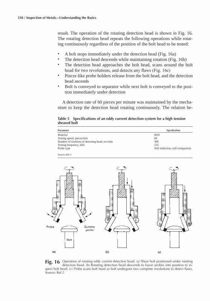
338 / Inspection of Metals—Understanding the Basics
result. The operation of the rotating detection head is shown in Fig. 16. The rotating detection head repeats the following operations while rotat-ing continuously regardless of the position of the bolt head to be tested:
• A bolt stops immediately under the detection head (Fig. 16a)• The detection head descends while maintaining rotation (Fig. 16b)• The detection head approaches the bolt head, scans around the bolt
head for two revolutions, and detects any flaws (Fig. 16c)• Pincer-like probe holders release from the bolt head, and the detection
head ascends• Bolt is conveyed to separator while next bolt is conveyed to the posi-
tion immediately under detection
A detection rate of 60 pieces per minute was maintained by the mecha-nism to keep the detection head rotating continuously. The relation be-
Table 5 Specifications of an eddy current detection system for a high tension sheared bolt
Parameter Specification
Material M20Testing speed, pieces/min 60Number of rotations of detecting head, rev/min 300Testing frequency, kHz 125Probe type Self-induction, self-comparison
Source: Ref 2
Fig� 16 Operation of rotating eddy current detection head. (a) Shear bolt positioned under rotating detection head. (b) Rotating detection head descends to lower probes into position to in-
spect bolt head. (c) Probe scans bolt head as bolt undergoes two complete revolutions to detect flaws. Source: Ref 2
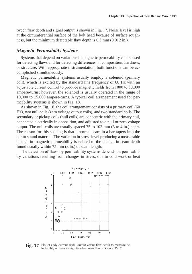
Chapter 13: Inspection of Steel Bar and Wire / 339
tween flaw depth and signal output is shown in Fig. 17. Noise level is high at the circumferential surface of the bolt head because of surface rough-ness, but the minimum detectable flaw depth is 0.3 mm (0.012 in.).
Magnetic Permeability Systems
Systems that depend on variations in magnetic permeability can be used for detecting flaws and for detecting differences in composition, hardness, or structure. With appropriate instrumentation, both functions can be ac-complished simultaneously.
Magnetic permeability systems usually employ a solenoid (primary coil), which is excited by the standard line frequency of 60 Hz with an adjustable current control to produce magnetic fields from 1000 to 30,000 ampere-turns; however, the solenoid is usually operated in the range of 10,000 to 15,000 ampere-turns. A typical coil arrangement used for per-meability systems is shown in Fig. 18.
As shown in Fig. 18, the coil arrangement consists of a primary coil (60 Hz), two null coils (zero voltage output coils), and two standard coils. The secondary or pickup coils (null coils) are concentric with the primary coil, connected electrically in opposition, and adjusted to a null or zero voltage output. The null coils are usually spaced 75 to 102 mm (3 to 4 in.) apart. The reason for this spacing is that a normal seam in a bar tapers into the bar to sound material. The variation in stress level producing a measurable change in magnetic permeability is related to the change in seam depth found usually within 75 mm (3 in.) of seam length.
The detection of flaws by permeability systems depends on permeabil-ity variations resulting from changes in stress, due to cold work or heat
Fig� 17 Plot of eddy current signal output versus flaw depth to measure de-tectability of flaws in high tensile sheared bolts. Source: Ref 2
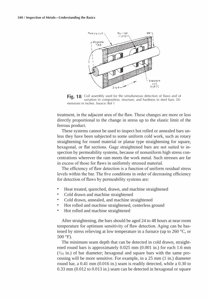
340 / Inspection of Metals—Understanding the Basics
treatment, in the adjacent area of the flaw. These changes are more or less directly proportional to the change in stress up to the elastic limit of the ferrous product.
These systems cannot be used to inspect hot rolled or annealed bars un-less they have been subjected to some uniform cold work, such as rotary straightening for round material or planar type straightening for square, hexagonal, or flat sections. Gage straightened bars are not suited to in-spection by permeability systems, because of nonuniform high stress con-centrations wherever the ram meets the work metal. Such stresses are far in excess of those for flaws in uniformly stressed material.
The efficiency of flaw detection is a function of uniform residual stress levels within the bar. The five conditions in order of decreasing efficiency for detection of flaws by permeability systems are:
• Heat treated, quenched, drawn, and machine straightened• Cold drawn and machine straightened• Cold drawn, annealed, and machine straightened• Hot rolled and machine straightened, centerless ground• Hot rolled and machine straightened
After straightening, the bars should be aged 24 to 48 hours at near room temperature for optimum sensitivity of flaw detection. Aging can be has-tened by stress relieving at low temperature in a furnace (up to 260 °C, or 500 °F).
The minimum seam depth that can be detected in cold drawn, straight-ened round bars is approximately 0.025 mm (0.001 in.) for each 1.6 mm (1⁄16 in.) of bar diameter; hexagonal and square bars with the same pro-cessing will be more sensitive. For example, in a 25 mm (1 in.) diameter round bar, a 0.41 mm (0.016 in.) seam is readily detected, while a 0.30 to 0.33 mm (0.012 to 0.013 in.) seam can be detected in hexagonal or square
Fig� 18 Coil assembly used for the simultaneous detection of flaws and of variation in composition, structure, and hardness in steel bars. Di-
mensions in inches. Source: Ref 1
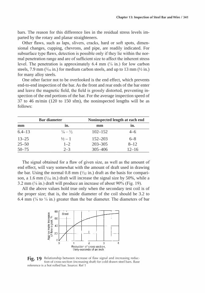
Chapter 13: Inspection of Steel Bar and Wire / 341
bars. The reason for this difference lies in the residual stress levels im-parted by the rotary and planar straighteners.
Other flaws, such as laps, slivers, cracks, hard or soft spots, dimen-sional changes, cupping, chevrons, and pipe, are readily indicated. For subsurface type flaws, detection is possible only if they lie within the nor-mal penetration range and are of sufficient size to affect the inherent stress level. The penetration is approximately 6.4 mm (¼ in.) for low carbon steels, 7.9 mm (5⁄16 in.) for medium carbon steels, and up to 13 mm (½ in.) for many alloy steels.
One other factor not to be overlooked is the end effect, which prevents end-to-end inspection of the bar. As the front and rear ends of the bar enter and leave the magnetic field, the field is grossly distorted, preventing in-spection of the end portions of the bar. For the average inspection speed of 37 to 46 m/min (120 to 150 sfm), the noninspected lengths will be as follows:
Bar diameter Noninspected length at each endmm in. mm in.6.4–13 ¼ – ½ 102–152 4–613–25 ½ – 1 152–203 6–825–50 1–2 203–305 8–1250–75 2–3 305–406 12–16
The signal obtained for a flaw of given size, as well as the amount of end effect, will vary somewhat with the amount of draft used in drawing the bar. Using the normal 0.8 mm (1⁄32 in.) draft as the basis for compari-son, a 1.6 mm (1⁄16 in.) draft will increase the signal size by 50%, while a 3.2 mm (⅛ in.) draft will produce an increase of about 90% (Fig. 19).
All the above values hold true only when the secondary test coil is of the proper size; that is, the inside diameter of the coil should be 3.2 to 6.4 mm (⅛ to ¼ in.) greater than the bar diameter. The diameters of bar
Fig� 19 Relationship between increase of flaw signal and increasing reduc-tion of cross-section (increasing draft) for cold drawn steel bars. Base
reference is a hot rolled bar. Source: Ref 1
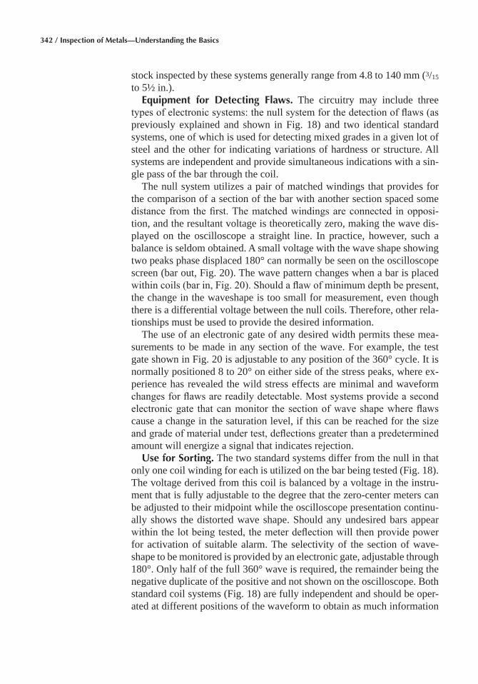
342 / Inspection of Metals—Understanding the Basics
stock inspected by these systems generally range from 4.8 to 140 mm (3/15 to 5½ in.).
Equipment for Detecting Flaws� The circuitry may include three types of electronic systems: the null system for the detection of flaws (as previously explained and shown in Fig. 18) and two identical standard systems, one of which is used for detecting mixed grades in a given lot of steel and the other for indicating variations of hardness or structure. All systems are independent and provide simultaneous indications with a sin-gle pass of the bar through the coil.
The null system utilizes a pair of matched windings that provides for the comparison of a section of the bar with another section spaced some distance from the first. The matched windings are connected in opposi-tion, and the resultant voltage is theoretically zero, making the wave dis-played on the oscilloscope a straight line. In practice, however, such a balance is seldom obtained. A small voltage with the wave shape showing two peaks phase displaced 180° can normally be seen on the oscilloscope screen (bar out, Fig. 20). The wave pattern changes when a bar is placed within coils (bar in, Fig. 20). Should a flaw of minimum depth be present, the change in the waveshape is too small for measurement, even though there is a differential voltage between the null coils. Therefore, other rela-tionships must be used to provide the desired information.
The use of an electronic gate of any desired width permits these mea-surements to be made in any section of the wave. For example, the test gate shown in Fig. 20 is adjustable to any position of the 360° cycle. It is normally positioned 8 to 20° on either side of the stress peaks, where ex-perience has revealed the wild stress effects are minimal and waveform changes for flaws are readily detectable. Most systems provide a second electronic gate that can monitor the section of wave shape where flaws cause a change in the saturation level, if this can be reached for the size and grade of material under test, deflections greater than a predetermined amount will energize a signal that indicates rejection.
Use for Sorting� The two standard systems differ from the null in that only one coil winding for each is utilized on the bar being tested (Fig. 18). The voltage derived from this coil is balanced by a voltage in the instru-ment that is fully adjustable to the degree that the zero-center meters can be adjusted to their midpoint while the oscilloscope presentation continu-ally shows the distorted wave shape. Should any undesired bars appear within the lot being tested, the meter deflection will then provide power for activation of suitable alarm. The selectivity of the section of wave-shape to be monitored is provided by an electronic gate, adjustable through 180°. Only half of the full 360° wave is required, the remainder being the negative duplicate of the positive and not shown on the oscilloscope. Both standard coil systems (Fig. 18) are fully independent and should be oper-ated at different positions of the waveform to obtain as much information
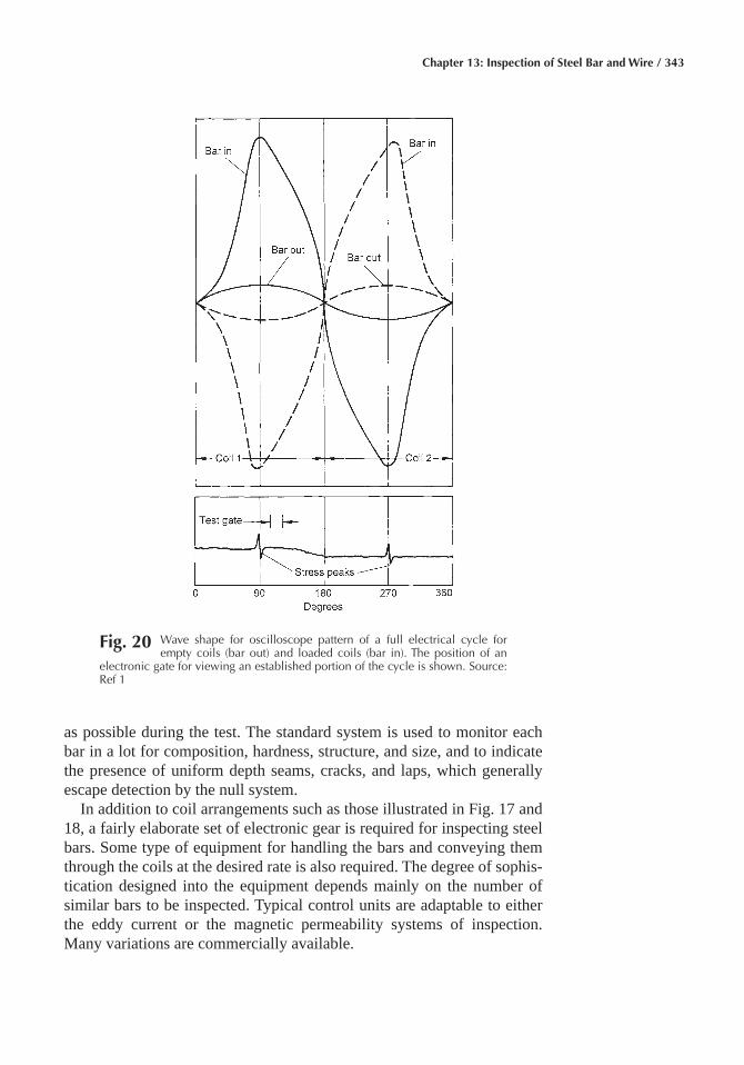
Chapter 13: Inspection of Steel Bar and Wire / 343
as possible during the test. The standard system is used to monitor each bar in a lot for composition, hardness, structure, and size, and to indicate the presence of uniform depth seams, cracks, and laps, which generally escape detection by the null system.
In addition to coil arrangements such as those illustrated in Fig. 17 and 18, a fairly elaborate set of electronic gear is required for inspecting steel bars. Some type of equipment for handling the bars and conveying them through the coils at the desired rate is also required. The degree of sophis-tication designed into the equipment depends mainly on the number of similar bars to be inspected. Typical control units are adaptable to either the eddy current or the magnetic permeability systems of inspection. Many variations are commercially available.
Fig� 20 Wave shape for oscilloscope pattern of a full electrical cycle for empty coils (bar out) and loaded coils (bar in). The position of an
electronic gate for viewing an established portion of the cycle is shown. Source: Ref 1

344 / Inspection of Metals—Understanding the Basics
ACKNOWLEDGMENT
This chapter was adapted from Nondestructive Inspection of Steel Bar, Wire, and Billets, Nondestructive Evaluation and Quality Control, Vol-ume 17, ASM Handbook, 1989.
REFERENCES
1. Nondestructive Inspection of Steel Bar, Wire, and Billets, Nondestruc-tive Evaluation and Quality Control, Vol 17, ASM Handbook, ASM International, 1989, p 549–560
2. N. Matsubara, H. Yamaguchi, T. Hiroshima, T. Sakamoto, and S. Mat-sumoto, Nondestructive Testing of Cold Drawn Wires and Cold Forged Products, Wire J. Int., March 1986

Inspection of Metals—Understanding the Basics Copyright © 2013 ASM International®
F.C. Campbell, editor All rights reservedwww.asminternational.org
CHAPTER 14
Inspection of Tubular Products
WROUGHT TUBULAR PRODUCTS are nondestructively inspected chiefly by eddy current techniques (including the magnetic flux leakage technique) and by ultrasonic techniques. In general, the eddy current and magnetic flux leakage techniques are applied to products not exceeding 1020 mm (40 in.) in diameter or 19 mm (¾ in.) in wall thickness. On the other hand, ultrasonic inspection is used on tubes ranging from 3.2 to 2030 mm (⅛ to 80 in.) in diameter and from 0.25 to 64 mm (0.01 to 2½ in.) in wall thickness. However, there are many exceptions, and the range of spe-cial techniques and applications associated with each inspection method is large. Most welded and seamless tubular products are nondestructively inspected by the manufacturer at the mill.
The many uses to which steel tubular products have been applied form a basis for classifying steel tubular products; for example, the terms used for the first classification casing, tube, and pipe are assigned on the basis of usage, as in water well casing, oil well tubing, and drill pipe. A second classification is based on methods of manufacture. Accordingly, all steel tubular products can be classified as either welded or seamless. A third classification applicable to special shapes can be considered subordinate to both of the general classifications above.
The major applications of the nondestructive inspection of tubular products are:
• Detection and evaluation of flaws• Sorting of mixed stock• Measurement of dimensions• Comparative measurement of specific physical and mechanical
properties
346 / Inspection of Metals—Understanding the Basics
Of these, the primary application is the detection and evaluation of flaws. Sorting is often an auxiliary application employed for grade or size verifi-cation and can be based on chemical composition, dimensions, physical and mechanical properties, or other significant variables. A difficulty en-countered in sorting arises when variables of little or no interest affect in-strument indications to a greater degree than do the variables of interest.
Selection of Inspection Method
The fundamental factors that should be considered in selecting a nonde-structive inspection method and in selecting from among the commer-cially available inspection equipment, are the product characteristics, na-ture of the flaws, extraneous variables, rate of inspection, end effect, mill versus laboratory inspection, specification requirements, equipment costs, and operating costs.
Product Characteristics� Among the product characteristics that may affect the choice of inspection method and equipment are tube or pipe di-ameter, wall thickness, surface condition, method of fabrication, electrical conductivity, metallurgical condition, magnetic properties (notably per-meability), and degree of magnetization.
Nature of Flaws� Both the nature of flaws and of potential but unallow-able deviations from certain specified dimensions or properties have a bearing on the selection of inspection methods and equipment. The nature of flaws is often markedly influenced by the method of manufacture. For example, flaws in welded pipe are usually confined to the vicinity of the weld; therefore, an inspection procedure that is confined to the weld area may be adequate. If the welds are resistance welds, the most usual flaws are located in the weld plane and are in effect two-dimensional, having length and width but negligible thickness. On the other hand, if the welds are arc welds, porosity is the most usual flaw. In all welded tubular prod-ucts, cracks are the most damaging flaws. In seamless tube, the location of flaws is not restricted, but may occur anywhere in or on the tube section.
Extraneous Variables� Many of the measurable variables in tubing and pipe are normal to the product and are not cause for rejection. These extra-neous or harmless factors sometimes exert a greater effect on the inspec-tion instrument than do the flaws that must be detected. For example, variations in magnetic permeability are common in steel and generate large signals in instruments that are permeability sensitive. However, the signals often are not pertinent to the test, nor are they cause for rejection. Surface scratches may be cause for rejection in some products and yet may be acceptable in others. Consequently, the inspection method and in-strument selected must ignore or minimize variables that will not affect the utility of the part in its intended application.
The rate of inspection required is a major factor in the selection of an inspection procedure. When the value of the part or the hazard associated
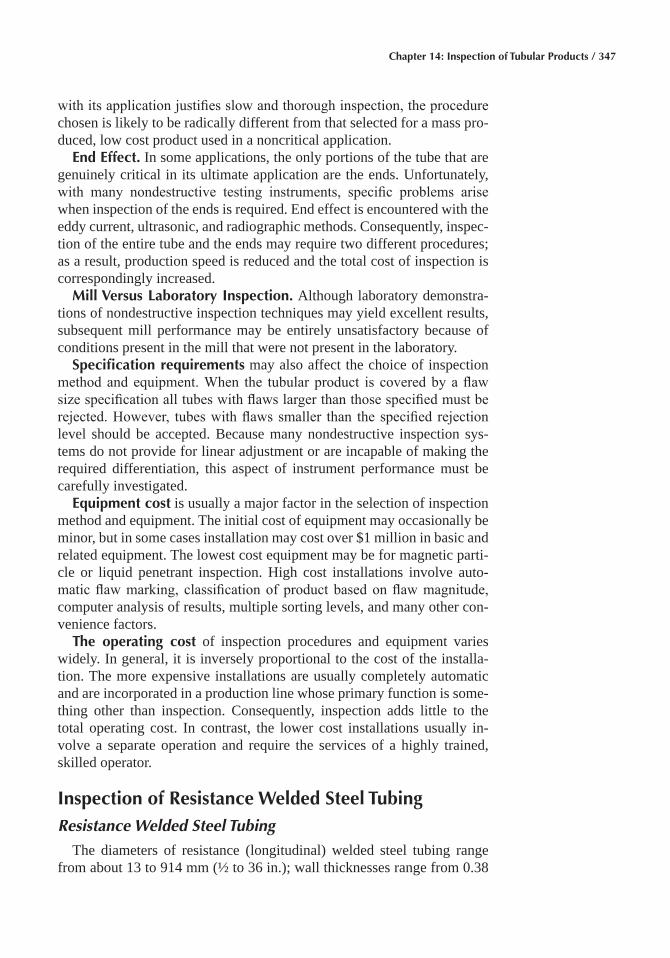
Chapter 14: Inspection of Tubular Products / 347
with its application justifies slow and thorough inspection, the procedure chosen is likely to be radically different from that selected for a mass pro-duced, low cost product used in a noncritical application.
End Effect� In some applications, the only portions of the tube that are genuinely critical in its ultimate application are the ends. Unfortunately, with many nondestructive testing instruments, specific problems arise when inspection of the ends is required. End effect is encountered with the eddy current, ultrasonic, and radiographic methods. Consequently, inspec-tion of the entire tube and the ends may require two different procedures; as a result, production speed is reduced and the total cost of inspection is correspondingly increased.
Mill Versus Laboratory Inspection� Although laboratory demonstra-tions of nondestructive inspection techniques may yield excellent results, subsequent mill performance may be entirely unsatisfactory because of conditions present in the mill that were not present in the laboratory.
Specification requirements may also affect the choice of inspection method and equipment. When the tubular product is covered by a flaw size specification all tubes with flaws larger than those specified must be rejected. However, tubes with flaws smaller than the specified rejection level should be accepted. Because many nondestructive inspection sys-tems do not provide for linear adjustment or are incapable of making the required differentiation, this aspect of instrument performance must be carefully investigated.
Equipment cost is usually a major factor in the selection of inspection method and equipment. The initial cost of equipment may occasionally be minor, but in some cases installation may cost over $1 million in basic and related equipment. The lowest cost equipment may be for magnetic parti-cle or liquid penetrant inspection. High cost installations involve auto-matic flaw marking, classification of product based on flaw magnitude, computer analysis of results, multiple sorting levels, and many other con-venience factors.
The operating cost of inspection procedures and equipment varies widely. In general, it is inversely proportional to the cost of the installa-tion. The more expensive installations are usually completely automatic and are incorporated in a production line whose primary function is some-thing other than inspection. Consequently, inspection adds little to the total operating cost. In contrast, the lower cost installations usually in-volve a separate operation and require the services of a highly trained, skilled operator.
Inspection of Resistance Welded Steel TubingResistance Welded Steel Tubing
The diameters of resistance (longitudinal) welded steel tubing range from about 13 to 914 mm (½ to 36 in.); wall thicknesses range from 0.38
348 / Inspection of Metals—Understanding the Basics
to 13 mm (0.015 to 0.5 in.). Tubing of intermediate and smaller diameters is produced on a draw bench.
Flaws that occur in resistance welded steel tubing include cold welds, contact marks, cracks, pinholes, and stitching. The terminology used to designate such flaws varies; the terms used in this chapter are those ad-opted by the American Petroleum Institute (API).
Cold weld is the term widely used to indicate inadequate or brittle bonding with no apparent discontinuity in the fracture. Cold weld cannot be detected reliably by any nondestructive inspection method currently available.
Contact marks (electrode burns) (Fig. 1a) are intermittent imperfec-tions near the weld line that result from miniature arcs between the weld-ing electrode and the surface of the tube.
Hook cracks (upturned fiber flaws) (Fig. 1b) are separations within the base metal due to imperfections in the strip edge, which are parallel to
Fig� 1 Typical flaws in resistance welded steel tubing, (a) contact marks (elec-trode burns), (b) hook cracks (upturned fiber flaws), (c) weld area crack,
(d) pinhole, (e) stitching. Views (c), (d), and (e) are mating fracture surfaces of welds. Source: Ref 1

Chapter 14: Inspection of Tubular Products / 349
the surface and turn toward the outside or inside surface when the edges are upset during welding.
Weld area cracks (Fig. 1c) are any cracks in the weld area not due to upturned fibers.
Pinholes (Fig. 1d) are minute holes located in the weld line.Stitching (Fig. 1e) comprises a regular pattern of light and dark areas
that are visible when the weld is broken in the weld line. The frequency of variation usually corresponds to weld-current variation. Increased use of ultrahigh frequency current for welding has minimized the occurrence of stitching.
The nondestructive inspection of resistance welded tube can be per-formed continuously on a welding machine or on individual lengths at any stage of processing. When performed on a welding machine, test indica-tions can be used to guide the welding machine operator in making ma-chine adjustments.
Eddy Current Inspection
Eddy current methods are probably the most widely used for the inspec-tion of welded steel tubing in diameters up to 75 mm (3 in.), although these methods are not limited to the smaller diameters. Typical weld im-perfections detectable by eddy current inspection are shown in Fig. 2. In welded tubing, most flaws occur in or near the longitudinal welded seam, and in most cases a test of a narrow band including the seam is adequate. This makes possible the use of small eddy current probe coils tangent to the seam area, eliminating the diameter limitation. Tubes with diameters up to 406 mm (16 in.) are currently being inspected by this method.
Eddy current inspection is usually performed on tubing having wall thicknesses less than 3.2 mm (⅛ in.), but successful production testing has been reported on tubing having wall thicknesses to 13 mm (½ in.). Most eddy current tests use differential systems and are most sensitive to flaws that involve a marked change in normal electrical characteristics. If the flaw is of considerable length and of uniform characteristics, it is some-times necessary to use special arrangements for its detection. Small probe coils continuously compare the weld zone with the base metal, thus re-vealing the existence of the elongated or long flaw.
When inspecting for shallow crack-like surface flaws 3.2 mm (⅛ in.) or less in depth, relatively close correlation between crack depth and signal magnitude has been obtained with a single coil arrangement without mag-netic saturation. However, the limited penetration of this arrangement and its need for a surface opening for depth evaluation limit its usefulness.
The speed of inspection by eddy current methods depends in part on many factors, including the size of the flaw that must be detected, the dis-criminating ability of the circuit used, end inspection requirements, and the speed of response of the signal circuit. The mathematical relationship
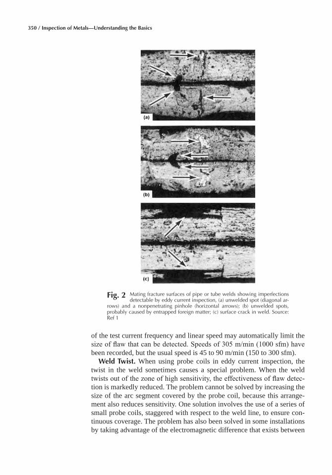
350 / Inspection of Metals—Understanding the Basics
of the test current frequency and linear speed may automatically limit the size of flaw that can be detected. Speeds of 305 m/min (1000 sfm) have been recorded, but the usual speed is 45 to 90 m/min (150 to 300 sfm).
Weld Twist� When using probe coils in eddy current inspection, the twist in the weld sometimes causes a special problem. When the weld twists out of the zone of high sensitivity, the effectiveness of flaw detec-tion is markedly reduced. The problem cannot be solved by increasing the size of the arc segment covered by the probe coil, because this arrange-ment also reduces sensitivity. One solution involves the use of a series of small probe coils, staggered with respect to the weld line, to ensure con-tinuous coverage. The problem has also been solved in some installations by taking advantage of the electromagnetic difference that exists between
Fig� 2 Mating fracture surfaces of pipe or tube welds showing imperfections detectable by eddy current inspection, (a) unwelded spot (diagonal ar-
rows) and a nonpenetrating pinhole (horizontal arrows); (b) unwelded spots, probably caused by entrapped foreign matter; (c) surface crack in weld. Source: Ref 1
Chapter 14: Inspection of Tubular Products / 351
the weld zone and the base metal. Special probe coils respond to this dif-ference and automatically rotate the test head or the tube until the weld zone is properly located with respect to the probe coil.
End effect, caused by abrupt changes in the magnetic field, becomes a problem whenever cut lengths are inspected. Various auxiliary circuits, ranging widely in effectiveness, have been developed for suppressing end effect to permit satisfactory inspection closer to the end of the tube. End effect can be minimized by keeping the tube ends in contact as they move through the test coils.
Mechanical variables that may affect inspection results include trans-verse movement of the tube in the test coil and changes in temperature or linear speed. The contribution of these factors to test results is sometimes difficult to determine in the laboratory, but they may create serious prob-lems in production testing.
Equipment costs for eddy current inspection can vary widely, depend-ing on the extent of refined circuitry, automatic handling and sorting equipment, computer analyzers, or special auxiliary equipment that may be needed.
The operating costs of a well designed eddy current system are among the lowest of any nondestructive inspection method. After the system has been properly adjusted, it can be operated by unskilled workers. When automatic marking is provided, the inspection can frequently be combined with another operation without appreciably increasing the cost of the latter operation.
Advantages and Limitations� All flaws in resistance welds except cold weld are readily detected by eddy current methods. Cold weld is by far the most difficult of all flaws to detect by any of the nondestructive inspection methods.
Although the other types of flaws discussed can be detected by eddy current methods, it should not be inferred that all eddy current instruments will detect all of these flaws. The range of capabilities of commercial eddy current instruments is extensive, and conclusions regarding their capabili-ties often require actual tests. Because eddy current test coils may either surround or be adjacent to the tube being tested, the variety of coil de-signs, arrangements, and combinations constitutes another major group of variables affecting equipment capabilities. In general, eddy current instru-ments have the advantages of speed in testing and convenience in operat-ing, marking, and sorting. Perhaps their most universal disadvantage is their inability to inspect completely to the ends of tubes.
Flux Leakage Inspection
Flux leakage (or magnetic field perturbation) inspection is similar to eddy current inspection but requires magnetization of the tube and is lim-ited to the inspection of ferromagnetic materials. When the tube is magne-
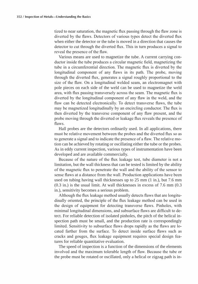
352 / Inspection of Metals—Understanding the Basics
tized to near saturation, the magnetic flux passing through the flaw zone is diverted by the flaws. Detectors of various types detect the diverted flux when either the detector or the tube is moved in a direction that causes the detector to cut through the diverted flux. This in turn produces a signal to reveal the presence of the flaw.
Various means are used to magnetize the tube. A current carrying con-ductor inside the tube produces a circular magnetic field, magnetizing the tube in a circumferential direction. The magnetic flux is diverted by the longitudinal component of any flaws in its path. The probe, moving through the diverted flux, generates a signal roughly proportional to the size of the flaw. On a longitudinal welded seam, an electromagnet with pole pieces on each side of the weld can be used to magnetize the weld area, with flux passing transversely across the seam. The magnetic flux is diverted by the longitudinal component of any flaw in the weld, and the flaw can be detected electronically. To detect transverse flaws, the tube may be magnetized longitudinally by an encircling conductor. The flux is then diverted by the transverse component of any flaw present, and the probe moving through the diverted or leakage flux reveals the presence of flaws.
Hall probes are the detectors ordinarily used. In all applications, there must be relative movement between the probes and the diverted flux so as to generate a signal and to indicate the presence of a flaw. The relative mo-tion can be achieved by rotating or oscillating either the tube or the probes. As in eddy current inspection, various types of instrumentation have been developed and are available commercially.
Because of the nature of the flux leakage test, tube diameter is not a limitation, but the wall thickness that can be tested is limited by the ability of the magnetic flux to penetrate the wall and the ability of the sensor to sense flaws at a distance from the wall. Production applications have been used on tubing having wall thicknesses up to 25 mm (1 in.), but 7.6 mm (0.3 in.) is the usual limit. At wall thicknesses in excess of 7.6 mm (0.3 in.), sensitivity becomes a serious problem.
Although the flux leakage method usually detects flaws that are longitu-dinally oriented, the principle of the flux leakage method can be used in the design of equipment for detecting transverse flaws. Pinholes, with minimal longitudinal dimensions, and subsurface flaws are difficult to de-tect. For reliable detection of isolated pinholes, the pitch of the helical in-spection path must be small, and the production rate is correspondingly limited. Sensitivity to subsurface flaws drops rapidly as the flaws are lo-cated farther from the surface. To detect inside surface flaws such as cracks and gouges, flux leakage equipment requires special design fea-tures for reliable quantitative evaluation.
The speed of inspection is a function of the dimensions of the elements involved and the maximum tolerable length of flaw. Because the tube or the probe must be rotated or oscillated, only a helical or zigzag path is in-
Chapter 14: Inspection of Tubular Products / 353
spected, and the pitch of the helix or the distance between reversals must be less than the maximum tolerable length of flaw. When the tube must be fed over a central conductor for magnetization and then removed for in-spection, high speed production is hindered. The use of multiple probes reduces the actual testing time in proportion to the number of probes, but the time required feeding the tube over the conductor remains constant. Such installations are operated in production at speeds as high as 15 m/min (50 sfm). Installations using external magnetization are reported to operate at speeds to 60 m/min (200 sfm).
Weld twist presents a problem in any installation in which only the weld is inspected. In flux leakage inspection, the problem is solved by increas-ing the magnitude of the arc covered by the oscillating probe. As in eddy current inspection, the error caused by end effect can be minimized by butting the ends of the tubes together during the test. Mechanical condi-tions, such as tube ovality, variations in linear speed, and transverse move-ment of the tube, have adverse effects on the test results and must be controlled.
As with eddy current equipment, the cost of equipment for flux leakage inspection varies. An elementary unit costs slightly more than a compara-ble eddy current unit because of the need for rotating devices. The addi-tion of auxiliary equipment, such as automatic markers, recorders, com-puter analyzers, and special handling devices, markedly increases cost.
Operating costs, which are relatively low, depend on the degree of auto-mation and the degree to which the inspection can be combined with other operations. Flux leakage tests can sometimes be combined with another operation, for example, welding. As the tube emerges from the welding operation, it enters the field of the electromagnetic yoke (Fig. 3), which generates a flux in the weld area. The oscillating probe detects any flux diverted by a flaw in the weld. However, in most cases, the need for move-
Fig� 3 Setup for the flux leakage inspection of welded steel tubing. Source: Ref 1
354 / Inspection of Metals—Understanding the Basics
ment of the probe through the diverted flux makes the combination less desirable than systems with no moving parts.
Ultrasonic Inspection
Ultrasonic inspection is one of the most widely used methods for in-specting tubular products. Widespread use of ultrasonics on tubular prod-ucts was made practical by the development of angle beam shear wave testing, immersion testing, and focused transducers. As with the eddy cur-rent and flux leakage methods, ultrasonic inspection can be applied either to the entire tube or to the weld only.
Ultrasonic inspection of the entire welded tube is usually limited to small diameter, drawn products, in which the weld cannot easily be distin-guished from the remainder of the tube. The tubing may have a diameter as small as 3.2 mm (⅛ in.) and a wall thickness of only 0.25 mm (0.01 in.). These small products are usually inspected while immersed in water (im-mersion inspection). They are rotated as they pass longitudinally through a glanded immersion tank. The immersed transducers must be carefully selected for tube diameter, wall thickness, and type of imperfection to be located. The transducer, focal length, response to outside diameter and inside diameter calibration notches, instrumentation pulse rate, gate ad-justment for flaw alarm, and speed of tube travel are all variables to be taken into consideration. Inspection is usually performed slowly (0.9 m/min or 3 sfm). Tubes must be clean, straight, round, and of uniform di-mensions. All types of flaws that commonly occur in resistance welds, except cold weld, can be detected by ultrasonic inspection.
Most ultrasonic inspection of resistance welded tubing is restricted to the weld zone and is performed immediately after the welding operation. Components and adjustments for inspecting the weld must be carefully selected and accurately controlled. The transducer must be appropriate for the size and type of flaws to be detected. Focused transducers are gener-ally preferred. The shear wave angle must be selected for the best evalua-tion of imperfections. The angle often used is 45°, but tests have revealed that angles between 50 and 70° yield signals more directly proportional to the area of flaws in the weld plane.
In the inspection of pipe, provision must be made to maintain the spac-ing between the transducer and the pipe constant within close tolerances as the pipe moves past the transducer. The couplant should preferably be continuously delivered to the surface of the pipe through openings in the transducer mounting. Coupling through a water jet is also used. Particular attention should be given to the detection of short flaws. Some ultrasonic pipe inspection equipment will not detect flaws shorter than 6.4 mm (¼ in.), which will not satisfy the inspection requirements for most resistance welded pipe.
Chapter 14: Inspection of Tubular Products / 355
A disadvantage of the ultrasonic method in tube inspection is its high sensitivity to minor scratches and to elongated dimensional changes, such as the ridge left when the weld flash is not completely removed or rolled down. However, proper selection of inspection equipment can minimize this problem. An important development is the wheel type search unit. The transducer of the wheel type search unit is mounted on the axle of a liquid filled wheel and is held in a fixed position as the wheel rotates. The surface of the wheel is flexible and adapts itself to the surface condition of the tube as it rolls over it. A small amount of liquid couplant, usually water, is required between the surface of the wheel tire and the surface of the tube. This arrangement provides most of the advantages of immersion testing without the necessity of immersing the tube.
The speed of inspection is limited by the pulse rate of the ultrasonic equipment and by the maximum length of a tolerable imperfection. Speeds as high as 69 m/min (225 sfm) have been reported, but unless multiple inspection heads are used speed is ultimately dependent on the rejectable flaw size.
Weld twist can present a problem; as the weld twists away from the critical location, transducer sensitivity drops sharply. To maintain the weld and the transducer in the correct mechanical relationship, the weld can be positioned automatically by the use of an electromagnetic control.
End effect, although less of a problem than in eddy current inspection, is a factor in ultrasonic inspection; and supplementary testing may be nec-essary if inspection of the tube ends is critical. The supplementary test can be made with ultrasonic equipment of special design. Mechanical vari-ables are critical in contact ultrasonic testing. Spacing between the trans-ducer and the surface of the tube, angle of transducer, and sidewise move-ment of tube must be accurately controlled. These variables can sometimes be better controlled in immersion testing.
The equipment costs of ultrasonic inspection equipment are highly de-pendent on the amount of auxiliary equipment included. Accessories such as automatic marking devices, computer analyzers, and material handling equipment can markedly increase equipment costs, especially for the in-spection of heavy pipe.
The operating costs of ultrasonic inspection, in accord with other in-spection methods, depend on whether inspection is operated separately or combined with another operation. For example, if inspection is incorpo-rated into the welding line, an inspector usually is not required, and the operating costs are minimal.
Magnetic Particle Inspection
The principal use of the magnetic particle method in the inspection of resistance welded pipe is largely limited to the inspection of pipe ends. In
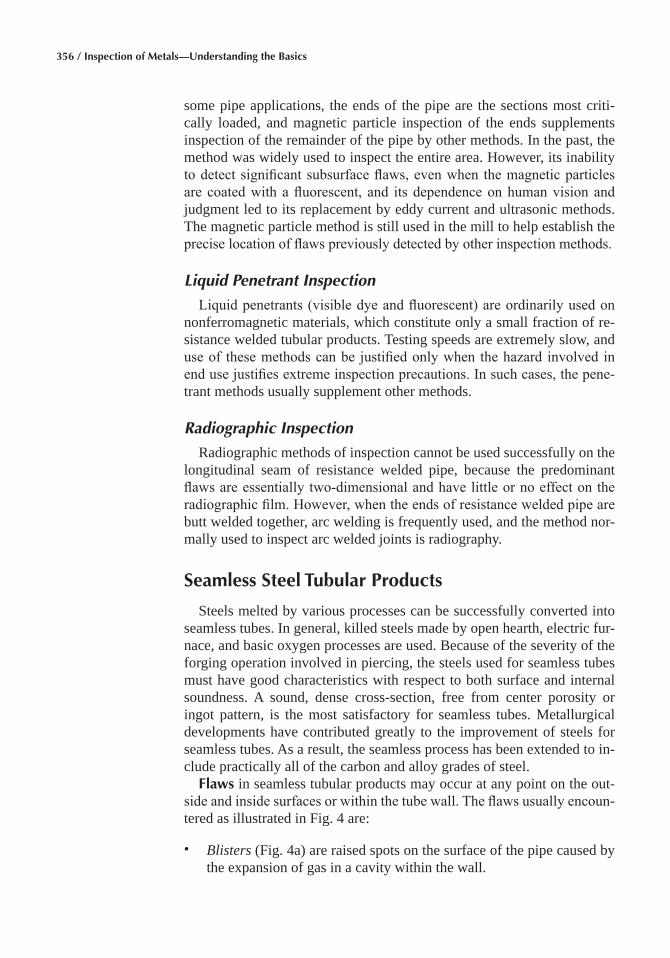
356 / Inspection of Metals—Understanding the Basics
some pipe applications, the ends of the pipe are the sections most criti-cally loaded, and magnetic particle inspection of the ends supplements inspection of the remainder of the pipe by other methods. In the past, the method was widely used to inspect the entire area. However, its inability to detect significant subsurface flaws, even when the magnetic particles are coated with a fluorescent, and its dependence on human vision and judgment led to its replacement by eddy current and ultrasonic methods. The magnetic particle method is still used in the mill to help establish the precise location of flaws previously detected by other inspection methods.
Liquid Penetrant Inspection
Liquid penetrants (visible dye and fluorescent) are ordinarily used on nonferromagnetic materials, which constitute only a small fraction of re-sistance welded tubular products. Testing speeds are extremely slow, and use of these methods can be justified only when the hazard involved in end use justifies extreme inspection precautions. In such cases, the pene-trant methods usually supplement other methods.
Radiographic Inspection
Radiographic methods of inspection cannot be used successfully on the longitudinal seam of resistance welded pipe, because the predominant flaws are essentially two-dimensional and have little or no effect on the radiographic film. However, when the ends of resistance welded pipe are butt welded together, arc welding is frequently used, and the method nor-mally used to inspect arc welded joints is radiography.
Seamless Steel Tubular Products
Steels melted by various processes can be successfully converted into seamless tubes. In general, killed steels made by open hearth, electric fur-nace, and basic oxygen processes are used. Because of the severity of the forging operation involved in piercing, the steels used for seamless tubes must have good characteristics with respect to both surface and internal soundness. A sound, dense cross-section, free from center porosity or ingot pattern, is the most satisfactory for seamless tubes. Metallurgical developments have contributed greatly to the improvement of steels for seamless tubes. As a result, the seamless process has been extended to in-clude practically all of the carbon and alloy grades of steel.
Flaws in seamless tubular products may occur at any point on the out-side and inside surfaces or within the tube wall. The flaws usually encoun-tered as illustrated in Fig. 4 are:
• Blisters (Fig. 4a) are raised spots on the surface of the pipe caused by the expansion of gas in a cavity within the wall.
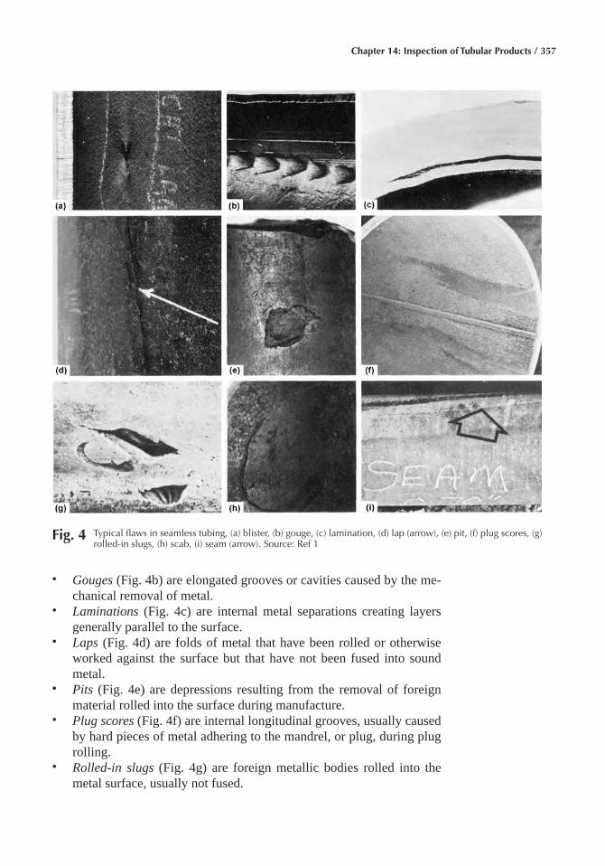
Chapter 14: Inspection of Tubular Products / 357
• Gouges (Fig. 4b) are elongated grooves or cavities caused by the me-chanical removal of metal.
• Laminations (Fig. 4c) are internal metal separations creating layers generally parallel to the surface.
• Laps (Fig. 4d) are folds of metal that have been rolled or otherwise worked against the surface but that have not been fused into sound metal.
• Pits (Fig. 4e) are depressions resulting from the removal of foreign material rolled into the surface during manufacture.
• Plug scores (Fig. 4f) are internal longitudinal grooves, usually caused by hard pieces of metal adhering to the mandrel, or plug, during plug rolling.
• Rolled-in slugs (Fig. 4g) are foreign metallic bodies rolled into the metal surface, usually not fused.
Fig� 4 Typical flaws in seamless tubing, (a) blister, (b) gouge, (c) lamination, (d) lap (arrow), (e) pit, (f) plug scores, (g) rolled-in slugs, (h) scab, (i) seam (arrow). Source: Ref 1
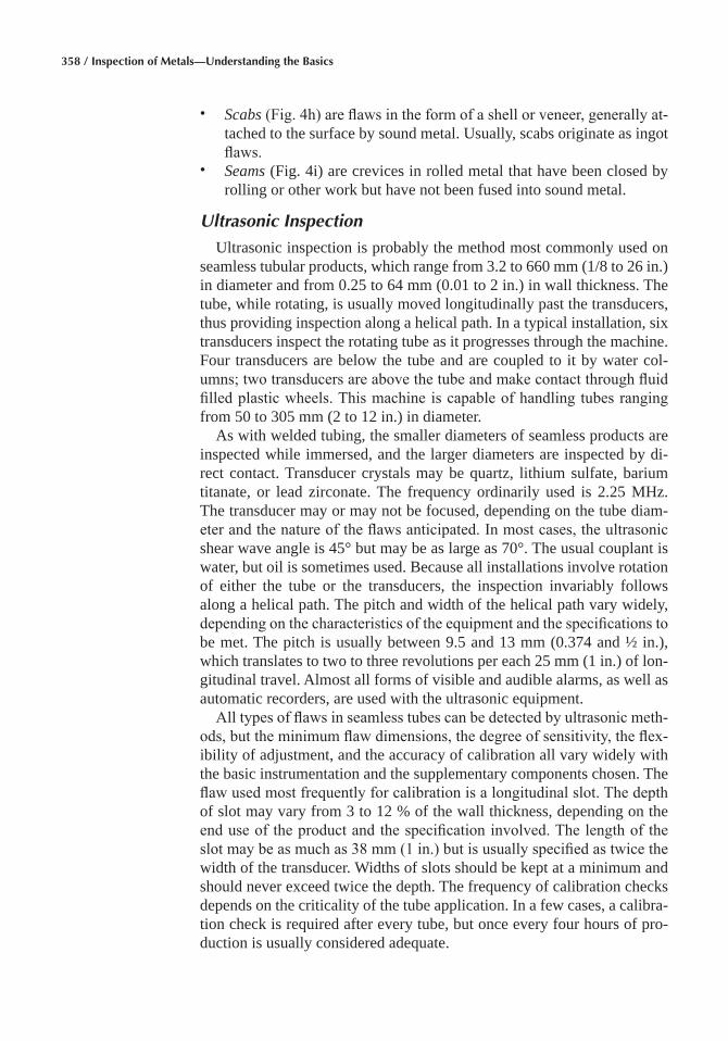
358 / Inspection of Metals—Understanding the Basics
• Scabs (Fig. 4h) are flaws in the form of a shell or veneer, generally at-tached to the surface by sound metal. Usually, scabs originate as ingot flaws.
• Seams (Fig. 4i) are crevices in rolled metal that have been closed by rolling or other work but have not been fused into sound metal.
Ultrasonic Inspection
Ultrasonic inspection is probably the method most commonly used on seamless tubular products, which range from 3.2 to 660 mm (1/8 to 26 in.) in diameter and from 0.25 to 64 mm (0.01 to 2 in.) in wall thickness. The tube, while rotating, is usually moved longitudinally past the transducers, thus providing inspection along a helical path. In a typical installation, six transducers inspect the rotating tube as it progresses through the machine. Four transducers are below the tube and are coupled to it by water col-umns; two transducers are above the tube and make contact through fluid filled plastic wheels. This machine is capable of handling tubes ranging from 50 to 305 mm (2 to 12 in.) in diameter.
As with welded tubing, the smaller diameters of seamless products are inspected while immersed, and the larger diameters are inspected by di-rect contact. Transducer crystals may be quartz, lithium sulfate, barium titanate, or lead zirconate. The frequency ordinarily used is 2.25 MHz. The transducer may or may not be focused, depending on the tube diam-eter and the nature of the flaws anticipated. In most cases, the ultrasonic shear wave angle is 45° but may be as large as 70°. The usual couplant is water, but oil is sometimes used. Because all installations involve rotation of either the tube or the transducers, the inspection invariably follows along a helical path. The pitch and width of the helical path vary widely, depending on the characteristics of the equipment and the specifications to be met. The pitch is usually between 9.5 and 13 mm (0.374 and ½ in.), which translates to two to three revolutions per each 25 mm (1 in.) of lon-gitudinal travel. Almost all forms of visible and audible alarms, as well as automatic recorders, are used with the ultrasonic equipment.
All types of flaws in seamless tubes can be detected by ultrasonic meth-ods, but the minimum flaw dimensions, the degree of sensitivity, the flex-ibility of adjustment, and the accuracy of calibration all vary widely with the basic instrumentation and the supplementary components chosen. The flaw used most frequently for calibration is a longitudinal slot. The depth of slot may vary from 3 to 12 % of the wall thickness, depending on the end use of the product and the specification involved. The length of the slot may be as much as 38 mm (1 in.) but is usually specified as twice the width of the transducer. Widths of slots should be kept at a minimum and should never exceed twice the depth. The frequency of calibration checks depends on the criticality of the tube application. In a few cases, a calibra-tion check is required after every tube, but once every four hours of pro-duction is usually considered adequate.
Chapter 14: Inspection of Tubular Products / 359
Speed of inspection also varies widely, depending on many variables, especially the maximum tolerable length of flaw and the number of trans-ducers used. The current range of inspection speed is 0.6 to 46 m/min (2 to 150 sfm); the upper limit can be increased by increasing the number of transducers.
Multiple search units can be used in the immersion tank to provide sev-eral simultaneous inspections during one pass of the pipe or tube through the unit. Specifications may call for circumferential inspection from two directions because the reflection from a flaw may vary, depending on the direction in which the ultrasonic beam strikes it. In addition to the circum-ferential inspection to detect longitudinal flaws, a longitudinal (axial) in-spection may be required to detect transverse flaws. Also, it may be desir-able to ultrasonically measure wall thickness, eccentricity, or both. All these tests can be performed at the same time by utilizing search units that are designed for the tests and that are properly positioned in the tank. Nor-mally, rejection is based on the presence of flaw indications exceeding those from the reference notch. Reworking and reinspection are generally permitted if other requirements, such as minimum wall thickness, are sat-isfied. Other refinements are included in, or can be added to, the inspec-tion system. For example, the feeding of tubes to the unit and their with-drawal can be automated. Various audible and visible alarm systems and marking devices can be added.
Normally, the water couplant used in the system is filtered and deaer-ated. Air entrapped in the water can produce false indications. Similarly, water on the inside surfaces of tubes will produce false signals, and these surfaces must be kept dry. Tubes are connected to each other by stoppers or by taping the ends together. The glands at each end of the water tank must be cut in a manner that will allow passage of the tubes without undue loss of water couplant. Finally, air must be prevented from being drawn into the entry gland along with the tube. This is accomplished by directing a stream of water over the outside of the tube just before it enters the gland.
Eddy Current Inspection
In eddy current inspection, use of an encircling detector coil is limited to a maximum tube diameter of about 75 mm (3 in.). As tube diameter in-creases, the ratio of flaw size to tube diameter decreases; consequently, the flaw is increasingly more difficult to detect. This problem is overcome by using several small probe coils and with spinning probes. When probe coils are used, the flaw becomes a significantly high percentage of the zone surveyed.
Because independently mounted probes ride over the tube surface, good magnetic coupling is ensured. Magnetic saturation is used to obtain maxi-mum sensitivity to flaws close to, or on, the inside surface of the tube, and
360 / Inspection of Metals—Understanding the Basics
the frequency of the test current is kept relatively low, sometimes as low as 1 kHz. Internal spinning probes can also be used if a lower production rate can be tolerated.
In some installations, the eddy current test with magnetic saturation is supplemented by a probe type eddy current test, which in effect provides high sensitivity inspection of the surface. Each of the four probe coils shown in Fig. 5, serves as both inductor and detector, and rotates about the tube as it moves longitudinally through the rotating assembly. Magnetic saturation is not required. The segment of the tube where the flaw occurs is identified by markers. In Fig. 6, the test head is shown ready for use, with eight paint spray guns in position for marking the proper zone.
Eddy current inspection is used on seamless tubular products ranging from 3.2 to 244 mm (⅛ to 9⅝ in.) in diameter and from 0.25 to 14.0 mm (0.01 to 0.55 in.) in wall thickness. In most cases, magnetic saturation is used, but when the primary concern is the detection of surface imperfec-tions, small probe coils without magnetic saturation are used. If the steel is entirely nonmagnetic, no saturation is required in any system. The fre-quency used ranges from 1 to 400 kHz and depends on such variables as the wall thickness of the pipe or tube, the coil design and arrangement, and the use of saturation. The spacing between the pipe or tube and the test coil(s) varies widely. However, for high sensitivity and accuracy, it should be kept to a minimum and is occasionally kept to as little as 0.25
Fig� 5 Unit used for the probe type eddy current inspection of seamless steel tubing; A, outer cover, containing test head, in open position; B, one of four rotating eddy current probe coils; C, reference standard test piece in
position for calibration; D, one of eight paint spray guns for marking. Source: Ref 1
Chapter 14: Inspection of Tubular Products / 361
mm (0.01 in.). This clearance is insufficient for practical use, and the usual clearance for production testing ranges from 1.6 to 19 mm (1/16 to ¾ in.).
Although all flaws that usually occur in seamless pipe or tube can be detected by eddy current methods, external flaws are more easily detected than internal flaws. Laminations are the most difficult flaws to detect. Some installations are intended to detect surface flaws only.
Flux leakage techniques are used for the inspection of seamless tubular products ranging from 32 to 914 mm (1¼ to 36 in.) in diameter and from 3.2 to 19 mm (⅛ to ¾ in.) in wall thickness. Because the flaws usually have a significant longitudinal dimension, transverse magnetic fields are usually used. Longitudinal fields can be used but are rarely considered necessary. As a rule, the transverse magnetic field is produced by a current passing through a conductor located in the center of the pipe or tube. In some cases, the field is produced between the poles of an electromagnet or a permanent magnet whose pole pieces are shaped to fit the pipe or tube diameters. The signal generating movement of either the tube or the probe with respect to the other is accomplished by rotating either tube or probe.
Sensitivity to inside surface flaws is a problem when using these meth-ods; the problem becomes more serious as the wall thickness increases. In
Fig� 6 Test head of the eddy current inspection unit shown in Fig. 5; A, orifice for test pipe or tube; B, one of eight paint spray guns for marking; C, reference standard test piece. Source: Ref 1
362 / Inspection of Metals—Understanding the Basics
some cases, the solution to the problem is a rotating internal probe moving through the tube or kept stationary while the tube moves. Other installa-tions depend on electronic filters and the difference in frequency between the signals for internal and surface flaws.
The production rate of flux leakage inspection depends on many fac-tors. The maximum permissible speed of probe or tube movement with respect to the other is about 90 m/min (300 sfm). The circuits will respond almost instantaneously when inspection speeds are kept below this speed limit. The principal limiting factor in production output speed then be-comes the maximum tolerable length of the flaw, which in turn governs the pitch of the helix inspected. However, the production rate can be in-creased to any desired level by the simultaneous inspection of several seg-ments of the same pipe or tube. Actual inspection speeds range from 0.9 to 60 m/min (3 to 200 sfm), depending on the diameter, the system used, sensitivity required, and other variables. The methods that use external magnets can inspect at a much higher overall rate than those that depend on an internal conductor for magnetization.
Magnetic particle and liquid penetrant inspection methods are sim-ple and economical and are most useful for surface inspection in special-ized, small scale applications. When applied to welded tubing, their use can be restricted to the weld zone. However, when applied to seamless tubing, there are no surface restrictions. The inability of these methods to locate small flaws beneath the surface and their dependence on the vision, alertness, and judgment of the inspector limit their usefulness in meeting modern specifications for seamless steel tubing.
Radiographic Inspection� The principal application of radiography to seamless tubing, as with welded tubing, is the inspection of girth welds joining the ends of tubes. Even in this application, it should be supple-mented by magnetic particle inspection.
Nonferrous Tubing
A wide variety of nonferrous alloy tubing, such as tubing made of brass, copper, aluminum, nickel, titanium, and zirconium, can be inspected for cracks, seams, splits, and other flaws. Eddy current inspection is the method most widely used, followed by the ultrasonic and liquid penetrant methods.
Eddy Current Inspection
When eddy current inspection is employed for nonferrous tubing, the range of tube diameters normally permits the use of an encircling coil. The typical flaws respond well to differential type coils. The frequencies em-ployed usually range from 1 to 25 kHz. The choice of frequency is gener-ally dependent on the electrical conductivity and wall thickness of the tub-

Chapter 14: Inspection of Tubular Products / 363
ing. Because magnetic saturation is not required, the inspection equipment is simpler and more compact than that used on ferromagnetic tubing. Tubes range from 3.2 to 89 mm (⅛ to 3½ in.) in diameter, with wall thick-nesses from 0.25 to 14.2 mm (0.01 to 0.56 in.). Testing speeds to 370 m/min (1200 sfm) have been reported. On a limited basis, eddy current in-spection is also being applied to finned copper tubing.
Immersion ultrasonic inspection is used on tubes ranging in diameter from 6.4 to 254 mm (¼ to 10 in.), with wall thicknesses as small as 0.25 mm (0.01 in.). In some installations, four channels are used, two for the detection of transverse flaws and two for longitudinal flaws. Because these tests are usually critical, they are performed at low speeds, usually less than 3 m/min (10 sfm).
The liquid penetrant inspection of nonferrous tubular products is performed in the conventional manner.
ACKNOWLEDGMENT
This chapter was adapted from Nondestructive Inspection of Tubular Products, Nondestructive Evaluation and Quality Control, Volume 17, ASM Handbook, 1992.
REFERENCES
1. Nondestructive Inspection of Tubular Products, Nondestructive Evalu-ation and Quality Control, Vol 17, ASM Handbook, ASM Interna-tional, 1992, p 561–581

Inspection of Metals—Understanding the Basics Copyright © 2013 ASM International®
F.C. Campbell, editor All rights reservedwww.asminternational.org
CHAPTER 15
Inspection of Forgings
IN FORGINGS of both ferrous and nonferrous metals, the flaws that most often occur are caused by conditions that exist in the ingot, by subse-quent hot working of the ingot or the billet, and by hot or cold working during forging. The inspection methods most commonly used to detect these flaws include visual, magnetic particle, liquid penetrant, ultrasonic, eddy current, and radiographic inspection.
Flaws Originating in the Ingot
Many large open-die forgings are forged directly from ingots. Most closed-die forgings and upset forgings are produced from billets, rolled bar stock, or preforms. Many, though by no means all, of the imperfec-tions found in forgings can be attributed to conditions that existed in the ingot, sometimes even when the ingot has undergone primary reduction prior to the forging operation. Some, but again by no means all, of the service problems that occur with forgings can be traced to imperfections originating in the ingot.
Chemical Segregation� The elements in a cast alloy are seldom dis-tributed uniformly. Even unalloyed metals contain random amounts of various types of impurities in the form of tramp elements or dissolved gases that are seldom distributed uniformly. Therefore, the composition of the metal or alloy will vary from location to location.
Deviation from the mean composition at a particular location in a forg-ing is termed segregation. In general, segregation is the result of solute rejection at the solidification interface during casting. For example, the gradation of composition with respect to the individual alloying elements exists from the cores of dendrites to interdendritic regions. Therefore, seg-regation produces a material having a range of compositions that do not have identical properties. Forging can partially correct the results of seg-
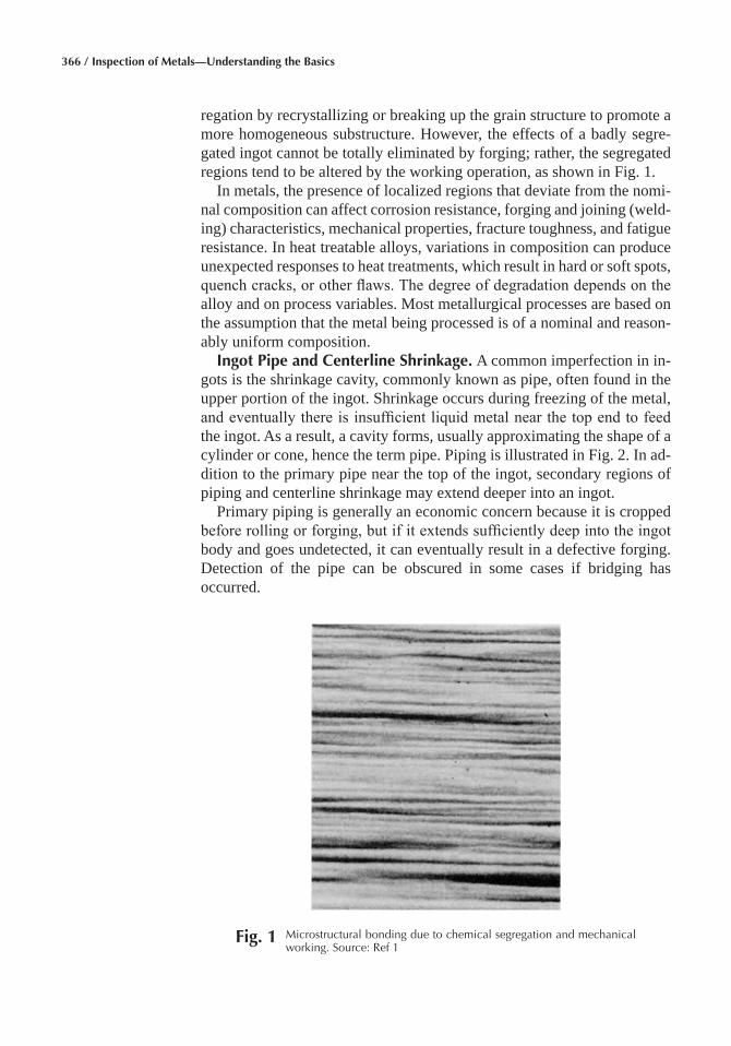
366 / Inspection of Metals—Understanding the Basics
regation by recrystallizing or breaking up the grain structure to promote a more homogeneous substructure. However, the effects of a badly segre-gated ingot cannot be totally eliminated by forging; rather, the segregated regions tend to be altered by the working operation, as shown in Fig. 1.
In metals, the presence of localized regions that deviate from the nomi-nal composition can affect corrosion resistance, forging and joining (weld-ing) characteristics, mechanical properties, fracture toughness, and fatigue resistance. In heat treatable alloys, variations in composition can produce unexpected responses to heat treatments, which result in hard or soft spots, quench cracks, or other flaws. The degree of degradation depends on the alloy and on process variables. Most metallurgical processes are based on the assumption that the metal being processed is of a nominal and reason-ably uniform composition.
Ingot Pipe and Centerline Shrinkage� A common imperfection in in-gots is the shrinkage cavity, commonly known as pipe, often found in the upper portion of the ingot. Shrinkage occurs during freezing of the metal, and eventually there is insufficient liquid metal near the top end to feed the ingot. As a result, a cavity forms, usually approximating the shape of a cylinder or cone, hence the term pipe. Piping is illustrated in Fig. 2. In ad-dition to the primary pipe near the top of the ingot, secondary regions of piping and centerline shrinkage may extend deeper into an ingot.
Primary piping is generally an economic concern because it is cropped before rolling or forging, but if it extends sufficiently deep into the ingot body and goes undetected, it can eventually result in a defective forging. Detection of the pipe can be obscured in some cases if bridging has occurred.
Fig� 1 Microstructural bonding due to chemical segregation and mechanical working. Source: Ref 1
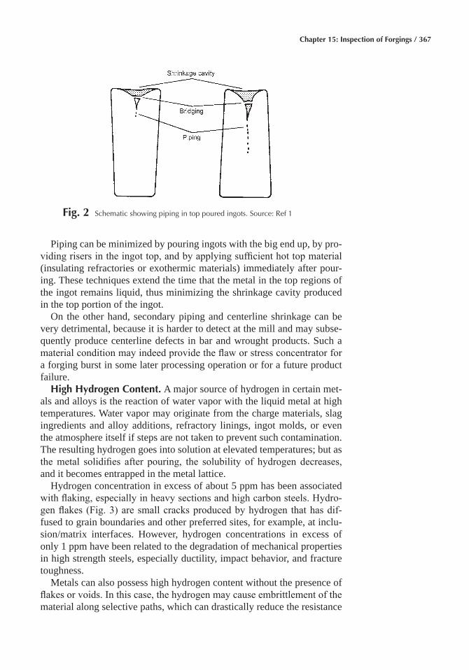
Chapter 15: Inspection of Forgings / 367
Piping can be minimized by pouring ingots with the big end up, by pro-viding risers in the ingot top, and by applying sufficient hot top material (insulating refractories or exothermic materials) immediately after pour-ing. These techniques extend the time that the metal in the top regions of the ingot remains liquid, thus minimizing the shrinkage cavity produced in the top portion of the ingot.
On the other hand, secondary piping and centerline shrinkage can be very detrimental, because it is harder to detect at the mill and may subse-quently produce centerline defects in bar and wrought products. Such a material condition may indeed provide the flaw or stress concentrator for a forging burst in some later processing operation or for a future product failure.
High Hydrogen Content� A major source of hydrogen in certain met-als and alloys is the reaction of water vapor with the liquid metal at high temperatures. Water vapor may originate from the charge materials, slag ingredients and alloy additions, refractory linings, ingot molds, or even the atmosphere itself if steps are not taken to prevent such contamination. The resulting hydrogen goes into solution at elevated temperatures; but as the metal solidifies after pouring, the solubility of hydrogen decreases, and it becomes entrapped in the metal lattice.
Hydrogen concentration in excess of about 5 ppm has been associated with flaking, especially in heavy sections and high carbon steels. Hydro-gen flakes (Fig. 3) are small cracks produced by hydrogen that has dif-fused to grain boundaries and other preferred sites, for example, at inclu-sion/matrix interfaces. However, hydrogen concentrations in excess of only 1 ppm have been related to the degradation of mechanical properties in high strength steels, especially ductility, impact behavior, and fracture toughness.
Metals can also possess high hydrogen content without the presence of flakes or voids. In this case, the hydrogen may cause embrittlement of the material along selective paths, which can drastically reduce the resistance
Fig� 2 Schematic showing piping in top poured ingots. Source: Ref 1
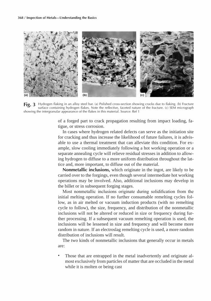
368 / Inspection of Metals—Understanding the Basics
of a forged part to crack propagation resulting from impact loading, fa-tigue, or stress corrosion.
In cases where hydrogen related defects can serve as the initiation site for cracking and thus increase the likelihood of future failures, it is advis-able to use a thermal treatment that can alleviate this condition. For ex-ample, slow cooling immediately following a hot working operation or a separate annealing cycle will relieve residual stresses in addition to allow-ing hydrogen to diffuse to a more uniform distribution throughout the lat-tice and, more important, to diffuse out of the material.
Nonmetallic inclusions, which originate in the ingot, are likely to be carried over to the forgings, even though several intermediate hot working operations may be involved. Also, additional inclusions may develop in the billet or in subsequent forging stages.
Most nonmetallic inclusions originate during solidification from the initial melting operation. If no further consumable remelting cycles fol-low, as in air melted or vacuum induction products (with no remelting cycle to follow), the size, frequency, and distribution of the nonmetallic inclusions will not be altered or reduced in size or frequency during fur-ther processing. If a subsequent vacuum remelting operation is used, the inclusions will be lessened in size and frequency and will become more random in nature. If an electroslag remelting cycle is used, a more random distribution of inclusions will result.
The two kinds of nonmetallic inclusions that generally occur in metals are:
• Those that are entrapped in the metal inadvertently and originate al-most exclusively from particles of matter that are occluded in the metal while it is molten or being cast
Fig� 3 Hydrogen flaking in an alloy steel bar. (a) Polished cross-section showing cracks due to flaking. (b) Fracture surface containing hydrogen flakes. Note the reflective, faceted nature of the fracture. (c) SEM micrograph
showing the intergranular appearance of the flakes in this material. Source: Ref 1
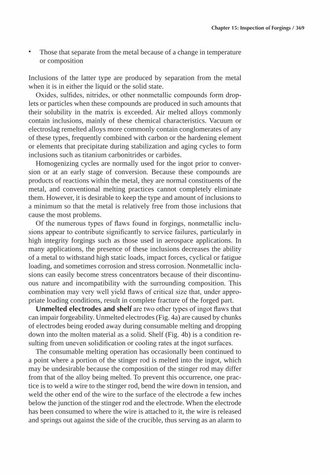
Chapter 15: Inspection of Forgings / 369
• Those that separate from the metal because of a change in temperature or composition
Inclusions of the latter type are produced by separation from the metal when it is in either the liquid or the solid state.
Oxides, sulfides, nitrides, or other nonmetallic compounds form drop-lets or particles when these compounds are produced in such amounts that their solubility in the matrix is exceeded. Air melted alloys commonly contain inclusions, mainly of these chemical characteristics. Vacuum or electroslag remelted alloys more commonly contain conglomerates of any of these types, frequently combined with carbon or the hardening element or elements that precipitate during stabilization and aging cycles to form inclusions such as titanium carbonitrides or carbides.
Homogenizing cycles are normally used for the ingot prior to conver-sion or at an early stage of conversion. Because these compounds are products of reactions within the metal, they are normal constituents of the metal, and conventional melting practices cannot completely eliminate them. However, it is desirable to keep the type and amount of inclusions to a minimum so that the metal is relatively free from those inclusions that cause the most problems.
Of the numerous types of flaws found in forgings, nonmetallic inclu-sions appear to contribute significantly to service failures, particularly in high integrity forgings such as those used in aerospace applications. In many applications, the presence of these inclusions decreases the ability of a metal to withstand high static loads, impact forces, cyclical or fatigue loading, and sometimes corrosion and stress corrosion. Nonmetallic inclu-sions can easily become stress concentrators because of their discontinu-ous nature and incompatibility with the surrounding composition. This combination may very well yield flaws of critical size that, under appro-priate loading conditions, result in complete fracture of the forged part.
Unmelted electrodes and shelf are two other types of ingot flaws that can impair forgeability. Unmelted electrodes (Fig. 4a) are caused by chunks of electrodes being eroded away during consumable melting and dropping down into the molten material as a solid. Shelf (Fig. 4b) is a condition re-sulting from uneven solidification or cooling rates at the ingot surfaces.
The consumable melting operation has occasionally been continued to a point where a portion of the stinger rod is melted into the ingot, which may be undesirable because the composition of the stinger rod may differ from that of the alloy being melted. To prevent this occurrence, one prac-tice is to weld a wire to the stinger rod, bend the wire down in tension, and weld the other end of the wire to the surface of the electrode a few inches below the junction of the stinger rod and the electrode. When the electrode has been consumed to where the wire is attached to it, the wire is released and springs out against the side of the crucible, thus serving as an alarm to
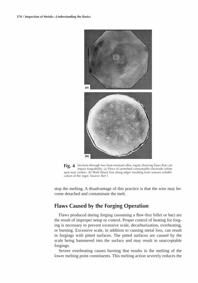
370 / Inspection of Metals—Understanding the Basics
stop the melting. A disadvantage of this practice is that the wire may be-come detached and contaminate the melt.
Flaws Caused by the Forging Operation
Flaws produced during forging (assuming a flaw-free billet or bar) are the result of improper setup or control. Proper control of heating for forg-ing is necessary to prevent excessive scale, decarburization, overheating, or burning. Excessive scale, in addition to causing metal loss, can result in forgings with pitted surfaces. The pitted surfaces are caused by the scale being hammered into the surface and may result in unacceptable forgings.
Severe overheating causes burning that results in the melting of the lower melting point constituents. This melting action severely reduces the
Fig� 4 Sections through two heat-resistant alloy ingots showing flaws that can impair forgeability. (a) Piece of unmelted consumable electrode (white
spot near center). (b) Shelf (black line along edge) resulting from uneven solidifi-cation of the ingot. Source: Ref 1
Chapter 15: Inspection of Forgings / 371
mechanical properties of the metal, and the damage is irreparable. Detec-tion and sorting of forgings that have been burned during heating can be extremely difficult.
In many cases, the flaws that occur during forging are the same as, or at least similar to, those that may occur during hot working of the ingots or billets; these are described in the previous section.
Internal flaws often appear as cracks or tears, and they can result either from forging with too light a hammer or from continuing forging after the metal has cooled down below a safe forging temperature. Bursts can also occur during the forging operation.
A number of surface flaws can be produced by the forging operation. These flaws are often caused by the movement of metal over or upon an-other surface without actual welding or fusing of the surfaces; such flaws may be laps or folds.
Cold shuts often occur in closed-die forgings. They are junctures of two adjoining surfaces caused by incomplete metal fill and incomplete fusion of the surfaces.
Surface flaws weaken forgings and can usually be eliminated by correct die design; proper heating; and, correct sequencing and positioning of the workpieces in the dies.
Shear cracks often occur in steel forgings; they are diagonal cracks oc-curring on the trimmed edges and are caused by shear stresses. Proper design and condition of trimming dies to remove forging flash are required for the prevention of shear cracks.
Other flaws in steel forgings that can be produced by improper die de-sign or maintenance are internal cracks and splits. If the material is moved abnormally during forging, these flaws may be formed without any evi-dence on the surface of the forging.
Selection of Inspection Method
The principal factors that influence the selection of a nondestructive inspection (NDI) method for forgings include degree of required integrity of the forging, metal composition, size and shape of the forging, and cost. There are sometimes other influential factors, such as the type of forging method used.
For high integrity forgings, it is often required that more than one in-spection method be employed because some inspection methods are ca-pable of locating only surface flaws; therefore, one or more additional methods are required for locating internal flaws. For example, many forg-ings for aerospace applications are inspected with liquid penetrants (or with magnetic particles, depending on the metal composition) for locating surface flaws, then by ultrasonics for detecting internal flaws.
Certain conditions unique to forgings can create service problems, yet they are not easily detected by nondestructive inspection. Exposed end
372 / Inspection of Metals—Understanding the Basics
grain, which can lead to poor corrosion resistance or to susceptibility to stress corrosion cracking, is the most prevalent of the undesirable condi-tions. The strength of the forging can be adversely affected if the grains flow in an undesirable direction (as in grain reversal) or if grain flow is confined to only a portion of the section being forged, rather than being well distributed. Both exposed end grain and poor grain flow can be most effectively corrected by redesigning the forging or forging blank, particu-larly with regard to flash. It is virtually impossible to detect exposed end grain nondestructively; only rarely can poor grain flow be detected nonde-structively. Both conditions are much more readily analyzed by sectioning and macroetching sample forgings in the preproduction stage of product development.
When certain steels or nonferrous alloys are forged at too high a tem-perature, or sometimes when a part cools too slowly after forging, there is the potential for excessive grain growth. Such a condition is difficult to detect nondestructively, except with ultrasonics, and then only when the grains are very large. Even with very large grains, ultrasonic inspection cannot determine grain size quantitatively, nor can it detect large grains reliably. The possibility that large grains are present can only be inferred from excessive attenuation of the ultrasonic beam.
Effect of Type of Forging
Many of the types of flaws that can occur in forgings do so without par-ticular regard to the type of forging; that is, open die, closed-die, upset, or rolled. However, there are many cases in which a specific type of flaw is more likely to occur in one type of forging than in another.
Open-Die Forgings� Most forgings produced in open dies are rela-tively large; therefore, their size is likely to impose some restrictions not only on the inspection method used but also on the system within a given inspection method. For large open-die forgings, NDI methods (other than visual) are generally limited to magnetic particle or liquid penetrant in-spection (for surface discontinuities) or to ultrasonic inspection (for inter-nal flaws). In general, the flaws likely to be found in open-die forgings are similar to those that may occur in other hot-worked shapes, with the ex-ception of forging laps and cold shuts, which usually occur only in closed-die forgings.
Closed-Die and Upset Forgings� The discontinuities in closed-die forgings that can be detected by liquid penetrant inspection or magnetic particle inspection (if the forging is ferromagnetic) are:
• Forging laps, which can be caused by incorrect die design, use of in-correct size of forging stock, excessive local conditioning of forging stock for removal of surface flaws, and excessively sharp corners in the forging stock
Chapter 15: Inspection of Forgings / 373
• Seams, due to incomplete removal of seams from the forging stock• Surface cracks, caused by incorrect forging temperature, nonductile
metallic or nonmetallic segregates in the forging stock, or surface con-tamination from the furnace atmosphere or other contaminants in the furnace or on the forging (such as high sulfur fuels for heating nickel alloys or leaded crayons used for marking parts before heating)
• Quench cracks• Cold straightening cracks
The likelihood that any of the listed discontinuities will appear in a closed-die forging produced in a press or by upsetting is more prevalent than for hammer forgings, because press and upset forgings permit no opportunity to monitor the workpiece being forged during the forging operation. Dur-ing hammer forging, the top surface of the forging is visible between ham-mer blows. The bottom surface may also be visible at times–particularly for large forgings that are raised intermittently during forging for descal-ing and lubricating the bottom surface or for forgings of temperature sen-sitive alloys that are raised off the bottom die to permit heat recovery to the bottom surface.
Any seam in the forging stock or incipient laps or cracks will probably develop into significant forging laps or cracks if not detected during for-mation. Consequently, in hammer forging, a large percentage of such po-tentially scrap forgings can be removed from the production run and can either be salvaged by removing the discontinuity prior to finishing or scrapped at that point to avoid wasted forging time. Also, multiple cavity hammer forgings permit inspection of the parts and blending out of minor laps or superficial cracks before finish forging.
Most discontinuities detected by ultrasonic inspection and not detect-able by either magnetic particle or liquid penetrant inspection are:
• Flakes, due to the absorption of hydrogen• Pipe, due to center shrinkage in the ingot and subsequent insufficient
reduction of forging stock• Subsurface nonmetallic segregation• Subsurface cracking, which may occur in certain alloys, particularly
during the forging of irregular sections• Weak centers in forging stock, caused by insufficient reduction from
the ingot• Subsurface cracks caused by forging material having comparatively
cold centers, and generally occurring in large forging billets heated for insufficient time
• Rewelded forging laps, formed and rewelded during forging. With subsequent hammer blows, the lap forms, the scale is knocked or blown off, and the lapped metal rewelds, forming a healed lap with transverse grain flow and possibly entrapped scale
374 / Inspection of Metals—Understanding the Basics
The presence of a rewelded forging lap in a suspected area can be checked by removing the surface metal below the decarburized layer and polishing this surface and swabbing with cold ammonium persulfate, thus revealing the decarburization at both sides of the lap (if present). The con-dition can be eliminated with corrections in blocker die design.
Ring-Rolled Forgings� Discontinuities in forgings produced by ring-rolling can either be inherited from the ingot or mechanically induced dur-ing forging, much the same as for forgings produced by hammers or presses.
Inherited discontinuities are common to all products produced from bar or billet and can usually be traced back to the composition, cleanliness, or condition of the ingot. Although these discontinuities are not found only in ring-rolled forgings, they probably account for the vast majority of known discontinuities in ring-rolled forgings. Typical discontinuities are inclusions, porosity, hot-top remnants, and segregation.
Ultrasonic inspection is a reliable method of detecting the presence of inherited discontinuities. It is always advisable to inspect the material be-fore it is ring-rolled. Extremely large billets (120 cm or 48 in. in diameter and larger) may have surface conditions that cause problems relative to sound entry. Large billets may exhibit structural conditions, depending on the amount of reduction from the ingot, that are too large for a complete ultrasonic inspection. Smaller, well worked billets can be examined at 2.25 MHz. The larger billets require the use of 1.0 MHz crystals, and even then ultrasonic penetration is not always possible.
Final proof that the forging is free of inherited discontinuities is accom-plished through ultrasonic inspection of the completed forging. Depend-ing on the final machined shape, certain ring-rolled forgings may require a preliminary ultrasonic inspection before final machining. When an ex-treme change in contour prevents a complete ultrasonic inspection of the final shape, inspection can be performed on portions of the forged ring.
Externally induced mechanical discontinuities that have been found in ring-rolled forgings include surface related laps, cracks, and exfoliations. Normally, these discontinuities can be detected visually either during the manufacturing process or in the machined condition after rolling. How-ever, ultrasonic inspection can be valuable for determining the depth of surface related discontinuities and for detecting them even when they have been obscured by subsequent working or metal movement. Magnetic particle inspection is also used to detect surface related, externally in-duced mechanical discontinuities in ferromagnetic ring-rolled forgings. Liquid penetrant inspection has often been successfully used to detect sur-face flaws in nonferromagnetic rings.
Mechanically induced internal discontinuities also known as strain in-duced porosity can occur in certain materials. Some nickel or titanium al-loys have an inherent susceptibility to these types of discontinuities in portions of the ring stretched at critical temperatures. This can result from
Chapter 15: Inspection of Forgings / 375
improper stock distribution, improper rolling techniques, or improper tooling. In extreme cases, in which the induced porosity is excessive, the rupturing can progress to one or more external surfaces. Either form of internal mechanically induced discontinuity can initiate in an area where inherited discontinuities are present.
Effect of Forging Material
Some types of forging flaws are unique to specific work metals, and may influence the choice of inspection method.
Steel Forgings� The most common surface flaws in steel forgings are seams, laps, and slivers. Other surface flaws include rolled-in scale, ferrite fingers, fins, overfills, and underfills. The most common internal flaws found in steel forgings are pipe, segregation, nonmetallic inclusions, and stringers.
Either magnetic particle or liquid penetrant inspection can be used for steel forgings, although magnetic particle inspection is usually preferred. Only liquid penetrant inspection can be used for some stainless steel or nonferrous forgings. The selection of an inspection method depends on the size and shape of the forging and on whether the forging can be moved to the inspection station or the inspection equipment can be moved to the forging. For either inspection method, systems are available for in-specting forgings of almost unlimited size and weight. In most cases, magnetic particle inspection is less expensive and faster than liquid pene-trant inspection.
Heat-Resistant Alloy Forgings� Most of the flaws found in heat- resistant forgings are those related to scrap selection, melting, or primary conversion to bar or billet, or those that occur during forging or heat treat-ment. Tramp elements, such as lead or zinc, have been present in scrap charges at levels that have caused hot shortness and a degradation of hot tensile ductility occurring near 370 °C (700 °F) of air melted alloys. No NDI method can reliably evaluate the presence or absence of possible tramp element contamination, and composition checks or hot tensile checks are too random for complete assurance of the presence or absence of contamination. The positive corrective action is to use a vacuum re-melted product.
Melt related discontinuities, such as inclusions, pipe, unhealed center conditions, flakes, or voids, are the types of discontinuities that most fre-quently exist in heat-resistant alloy forgings. Ultrasonic inspection can detect and isolate these conditions. Segregated structures, unmelted elec-trodes, or portions of stringer rods are types of discontinuities that may sometimes be found in heat-resistant alloys.
Flakes (internal cracks) can be produced each time the material is heated and cooled to room temperature. The random orientation does not always present a properly oriented reflector for ultrasonic inspection, but
376 / Inspection of Metals—Understanding the Basics
in most cases flaking can be detected ultrasonically with a high degree of reliability.
Unmelted pieces of electrode or shelf conditions appear infrequently in vacuum melted alloys. Either of these conditions can seriously degrade forgeability. Macroetching or another appropriate type of surface inspec-tion of the machined forging or the billet is the most effective method of detecting unmelted electrodes or shelf conditions.
Seams are common and are readily detected by visual, magnetic parti-cle, or liquid penetrant inspection. Grinding cracks are caused by severe grinding, which promotes network-type cracking on the surface of the ma-terial being conditioned. The network-type cracking may be present im-mediately after grinding or may not occur until subsequent heating for further forging. Seams and grinding cracks will cause severe surface rup-turing during forging.
Center bursts occur during conversion to bar or billet if reduction rates are too severe or temperatures are incorrect; they are readily detected by ultrasonic inspection.
Ingot pipe, unhealed center conditions, or voids are melt-related dis-continuities, but their occurrence in forgings is often a function of reduc-tion ratio. The conversion practice must impart sufficient homogenization or healing to produce a product with sound center conditions. An example of an unsound condition that did not heal is shown in Fig. 5. Macroetching and ultrasonic inspection methods are the most widely used for identify-ing regions of unsoundness.
The nickel-base heat-resistant alloys are highly susceptible to surface contamination during heating for forging. Fuel oils containing sulfur will induce a grain boundary attack, which will cause subsequent rupturing during forging. Paint or marking crayons with high levels of similar con-taminants will cause similar areas of grain boundary contamination.
Surface contamination is not normally detected by NDI methods prior to heating and processing, but if present at a level high enough to cause contamination, rupturing during forging will occur that can be detected by visual inspection. If the contamination occurs after final forging, with no subsequent metal deformation, the contaminated areas will be apparent as areas of intergranular attack. Macroetching, followed by liquid penetrant inspection, should be used.
Advanced forging processes, such as isothermal and hot-die forging, and the increasing use of computer modeling have greatly reduced prob-lems associated with heat-resistant alloy forgings.
Nickel Alloy Forgings� The discontinuities that occur in nickel alloy forgings are generally of the same type as those found in heat-resistant alloy forgings; namely, cracks (external and internal), tears, seams, laps, coarse grain wrinkles, inclusions, and pipe. Although all metals may be subject to thermal cracking during forging, the age hardenable nickel al-
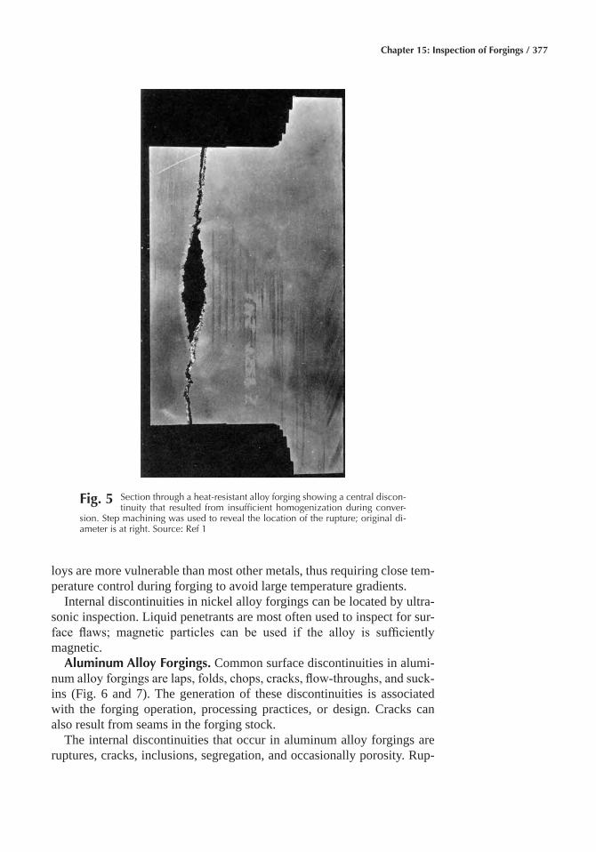
Chapter 15: Inspection of Forgings / 377
loys are more vulnerable than most other metals, thus requiring close tem-perature control during forging to avoid large temperature gradients.
Internal discontinuities in nickel alloy forgings can be located by ultra-sonic inspection. Liquid penetrants are most often used to inspect for sur-face flaws; magnetic particles can be used if the alloy is sufficiently magnetic.
Aluminum Alloy Forgings� Common surface discontinuities in alumi-num alloy forgings are laps, folds, chops, cracks, flow-throughs, and suck-ins (Fig. 6 and 7). The generation of these discontinuities is associated with the forging operation, processing practices, or design. Cracks can also result from seams in the forging stock.
The internal discontinuities that occur in aluminum alloy forgings are ruptures, cracks, inclusions, segregation, and occasionally porosity. Rup-
Fig� 5 Section through a heat-resistant alloy forging showing a central discon-tinuity that resulted from insufficient homogenization during conver-
sion. Step machining was used to reveal the location of the rupture; original di-ameter is at right. Source: Ref 1
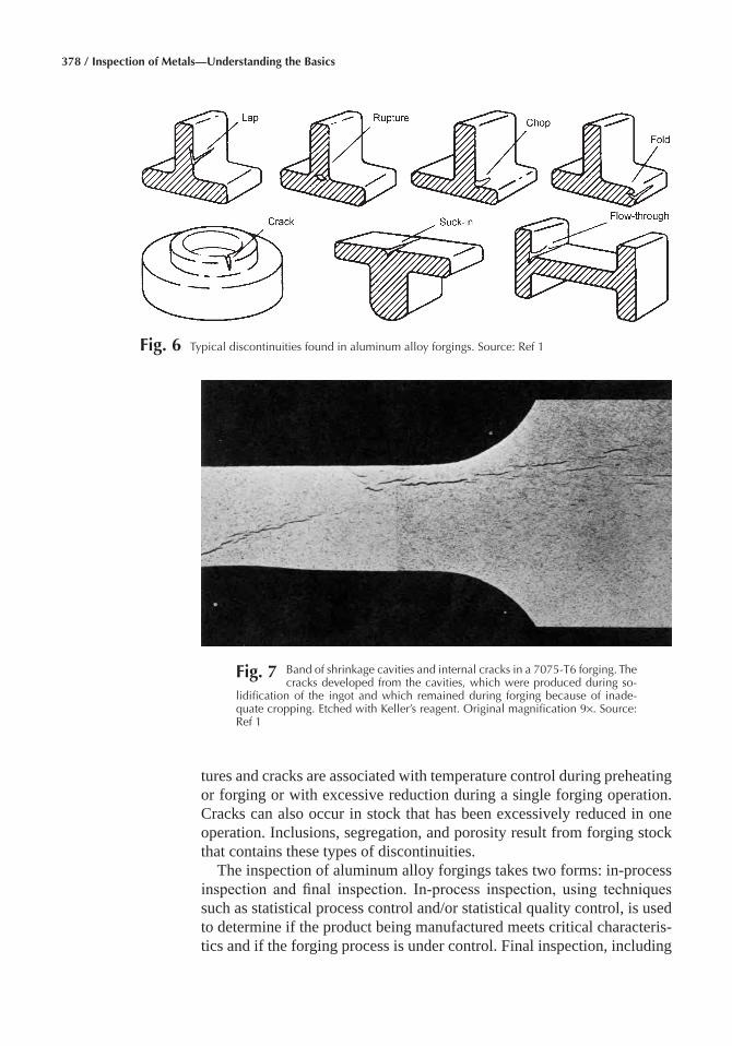
378 / Inspection of Metals—Understanding the Basics
tures and cracks are associated with temperature control during preheating or forging or with excessive reduction during a single forging operation. Cracks can also occur in stock that has been excessively reduced in one operation. Inclusions, segregation, and porosity result from forging stock that contains these types of discontinuities.
The inspection of aluminum alloy forgings takes two forms: in-process inspection and final inspection. In-process inspection, using techniques such as statistical process control and/or statistical quality control, is used to determine if the product being manufactured meets critical characteris-tics and if the forging process is under control. Final inspection, including
Fig� 6 Typical discontinuities found in aluminum alloy forgings. Source: Ref 1
Fig� 7 Band of shrinkage cavities and internal cracks in a 7075-T6 forging. The cracks developed from the cavities, which were produced during so-
lidification of the ingot and which remained during forging because of inade-quate cropping. Etched with Keller’s reagent. Original magnification 9×. Source: Ref 1
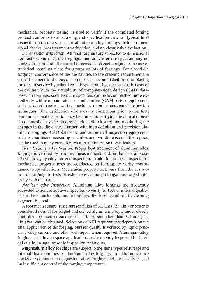
Chapter 15: Inspection of Forgings / 379
mechanical property testing, is used to verify if the completed forging product conforms to all drawing and specification criteria. Typical final inspection procedures used for aluminum alloy forgings include dimen-sional checks, heat treatment verification, and nondestructive evaluation.
Dimensional Inspection. All final forgings are subjected to dimensional verification. For open-die forgings, final dimensional inspection may in-clude verification of all required dimensions on each forging or the use of statistical sampling plans for groups or lots of forgings. For closed-die forgings, conformance of the die cavities to the drawing requirements, a critical element in dimensional control, is accomplished prior to placing the dies in service by using layout inspection of plaster or plastic casts of the cavities. With the availability of computer-aided design (CAD) data-bases on forgings, such layout inspections can be accomplished more ex-pediently with computer-aided manufacturing (CAM) driven equipment, such as coordinate measuring machines or other automated inspection techniques. With verification of die cavity dimensions prior to use, final part dimensional inspection may be limited to verifying the critical dimen-sion controlled by the process (such as die closure) and monitoring the changes in the die cavity. Further, with high definition and precision alu-minum forgings, CAD databases and automated inspection equipment, such as coordinate measuring machines and two-dimensional fiber optics, can be used in many cases for actual part dimensional verification.
Heat Treatment Verification. Proper heat treatment of aluminum alloy forgings is verified by hardness measurements and, in the case of 7xxx-T7xxx alloys, by eddy current inspection. In addition to these inspections, mechanical property tests are conducted on forgings to verify confor-mance to specifications. Mechanical property tests vary from the destruc-tion of forgings to tests of extensions and/or prolongations forged inte-grally with the parts.
Nondestructive Inspection. Aluminum alloy forgings are frequently subjected to nondestructive inspection to verify surface or internal quality. The surface finish of aluminum forgings after forging and caustic cleaning is generally good.
A root mean square (rms) surface finish of 3.2 μm (125 μin.) or better is considered normal for forged and etched aluminum alloys; under closely controlled production conditions, surfaces smoother than 3.2 μm (125 μin.) rms can be obtained. Selection of NDI requirements depends on the final application of the forging. Surface quality is verified by liquid pene-trant, eddy current, and other techniques when required. Aluminum alloy forgings used in aerospace applications are frequently inspected for inter-nal quality using ultrasonic inspection techniques.
Magnesium alloy forgings are subject to the same types of surface and internal discontinuities as aluminum alloy forgings. In addition, surface cracks are common in magnesium alloy forgings and are usually caused by insufficient control of the forging temperature.
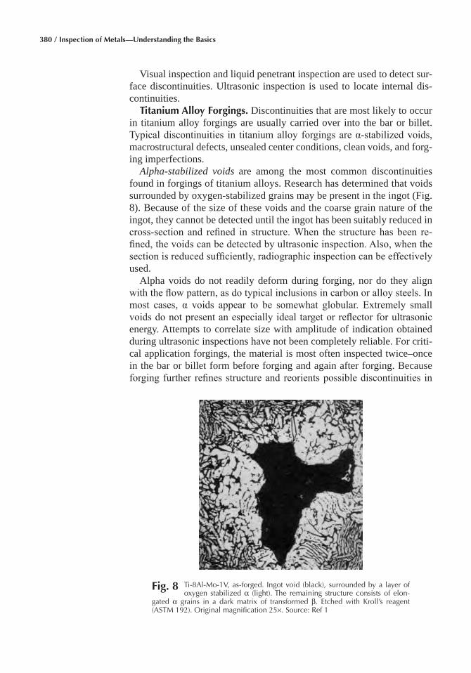
380 / Inspection of Metals—Understanding the Basics
Visual inspection and liquid penetrant inspection are used to detect sur-face discontinuities. Ultrasonic inspection is used to locate internal dis- continuities.
Titanium Alloy Forgings� Discontinuities that are most likely to occur in titanium alloy forgings are usually carried over into the bar or billet. Typical discontinuities in titanium alloy forgings are α-stabilized voids, macrostructural defects, unsealed center conditions, clean voids, and forg-ing imperfections.
Alpha-stabilized voids are among the most common discontinuities found in forgings of titanium alloys. Research has determined that voids surrounded by oxygen-stabilized grains may be present in the ingot (Fig. 8). Because of the size of these voids and the coarse grain nature of the ingot, they cannot be detected until the ingot has been suitably reduced in cross-section and refined in structure. When the structure has been re-fined, the voids can be detected by ultrasonic inspection. Also, when the section is reduced sufficiently, radiographic inspection can be effectively used.
Alpha voids do not readily deform during forging, nor do they align with the flow pattern, as do typical inclusions in carbon or alloy steels. In most cases, α voids appear to be somewhat globular. Extremely small voids do not present an especially ideal target or reflector for ultrasonic energy. Attempts to correlate size with amplitude of indication obtained during ultrasonic inspections have not been completely reliable. For criti-cal application forgings, the material is most often inspected twice–once in the bar or billet form before forging and again after forging. Because forging further refines structure and reorients possible discontinuities in
Fig� 8 Ti-8Al-Mo-1V, as-forged. Ingot void (black), surrounded by a layer of oxygen stabilized α (light). The remaining structure consists of elon-
gated α grains in a dark matrix of transformed β. Etched with Kroll’s reagent (ASTM 192). Original magnification 25×. Source: Ref 1
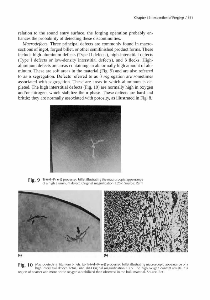
Chapter 15: Inspection of Forgings / 381
relation to the sound entry surface, the forging operation probably en-hances the probability of detecting these discontinuities.
Macrodefects. Three principal defects are commonly found in macro-sections of ingot, forged billet, or other semifinished product forms. These include high-aluminum defects (Type II defects), high-interstitial defects (Type I defects or low-density interstitial defects), and β flecks. High- aluminum defects are areas containing an abnormally high amount of alu-minum. These are soft areas in the material (Fig. 9) and are also referred to as α segregation. Defects referred to as β segregation are sometimes associated with segregation. These are areas in which aluminum is de-pleted. The high interstitial defects (Fig. 10) are normally high in oxygen and/or nitrogen, which stabilize the α phase. These defects are hard and brittle; they are normally associated with porosity, as illustrated in Fig. 8.
Fig� 9 Ti-6Al-4V α-β processed billet illustrating the macroscopic appearance of a high aluminum defect. Original magnification 1.25×. Source: Ref 1
Fig� 10 Macrodefects in titanium billets. (a) Ti-6Al-4V α-β processed billet illustrating macroscopic appearance of a high interstitial defect, actual size. (b) Original maginification 100×. The high oxygen content results in a
region of coarser and more brittle oxygen α stabilized than observed in the bulk material. Source: Ref 1
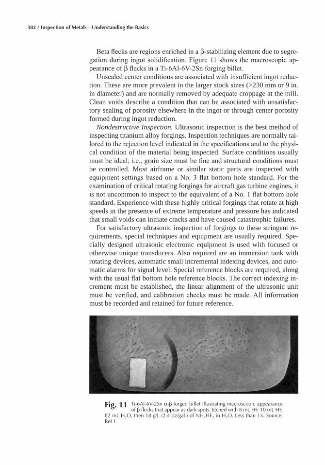
382 / Inspection of Metals—Understanding the Basics
Beta flecks are regions enriched in a β-stabilizing element due to segre-gation during ingot solidification. Figure 11 shows the macroscopic ap-pearance of β flecks in a Ti-6Al-6V-2Sn forging billet.
Unsealed center conditions are associated with insufficient ingot reduc-tion. These are more prevalent in the larger stock sizes (>230 mm or 9 in. in diameter) and are normally removed by adequate croppage at the mill. Clean voids describe a condition that can be associated with unsatisfac-tory sealing of porosity elsewhere in the ingot or through center porosity formed during ingot reduction.
Nondestructive Inspection. Ultrasonic inspection is the best method of inspecting titanium alloy forgings. Inspection techniques are normally tai-lored to the rejection level indicated in the specifications and to the physi-cal condition of the material being inspected. Surface conditions usually must be ideal; i.e., grain size must be fine and structural conditions must be controlled. Most airframe or similar static parts are inspected with equipment settings based on a No. 3 flat bottom hole standard. For the examination of critical rotating forgings for aircraft gas turbine engines, it is not uncommon to inspect to the equivalent of a No. 1 flat bottom hole standard. Experience with these highly critical forgings that rotate at high speeds in the presence of extreme temperature and pressure has indicated that small voids can initiate cracks and have caused catastrophic failures.
For satisfactory ultrasonic inspection of forgings to these stringent re-quirements, special techniques and equipment are usually required. Spe-cially designed ultrasonic electronic equipment is used with focused or otherwise unique transducers. Also required are an immersion tank with rotating devices, automatic small incremental indexing devices, and auto-matic alarms for signal level. Special reference blocks are required, along with the usual flat bottom hole reference blocks. The correct indexing in-crement must be established, the linear alignment of the ultrasonic unit must be verified, and calibration checks must be made. All information must be recorded and retained for future reference.
Fig� 11 Ti-6Al-6V-2Sn α-β forged billet illustrating macroscopic appearance of β flecks that appear as dark spots. Etched with 8 mL HF, 10 mL HF,
82 mL H2O, then 18 g/L (2.4 oz/gal.) of NH4HF2 in H2O. Less than 1×. Source: Ref 1
Chapter 15: Inspection of Forgings / 383
Visual Inspection
Despite the many sophisticated inspection methods available, unaided visual inspection is still important and is often the sole method of in-specting forgings used for common hardware items. Under proper lighting conditions, the trained eye can detect several types of surface imperfec-tions, including certain laps, folds, and seams. Visual inspection is often used first then questionable forgings are further examined by macroetch-ing and inspection with macrophotography or some type of nondestruc-tive method.
The only equipment necessary for visual inspection is a bench on which to place the forging and suitable cranes or hoists for forgings that are too heavy to lift by hand. Good and well controlled lighting conditions are es-sential. Optical aids such as magnifying glasses that can magnify up to about ten diameters are often used to increase the effectiveness of visual inspection.
Magnetic Particle Inspection
Magnetic particle inspection is useful for detecting surface imperfec-tions as well as certain subsurface imperfections that are within approxi-mately 3 mm (⅛ in.) of the surfaces in forgings of steel, some grades of stainless steel, and other ferromagnetic metals. Magnetic particle inspec-tion can be used with fluorescent particles and ultraviolet light.
The advantages of magnetic particle inspection are:
• Almost instant results can be obtained in locating surface and certain subsurface imperfections
• Equipment can be transported to the forging, or the forging can be transported to the inspection station, as dictated by the size and shape of forging
• Preparation of the forging is minimal, mainly involving the removal of surface contaminants that would prevent magnetization or inhibit par-ticle mobility
• Routine inspection work can be effectively done by relatively un-skilled labor properly trained in interpretation
• For forgings that are simple in configuration, and when justified by the quantity, magnetic particle inspection can be automated
• For some forgings, electronic sensing can be used, thus reducing the chances of human error and increasing inspection reliability
• Many forgings have sufficient retentivity to permit the use of multi-directional magnetization, thus permitting the inspection of indica-tions in all orientations with a single preparation. Retentivity must be checked for the particular forging before a decision is made to use multidirectional magnetization
384 / Inspection of Metals—Understanding the Basics
• The cost of magnetic particle inspection is generally lower than that for several other inspection methods in terms of investment in equip-ment, inspection materials, and inspection time
The limitations, generally the same as for inspecting other workpieces, of the magnetic particle inspection of forgings are:
• The method is applicable only to forgings made from ferromagnetic metals
• Because magnetic particle inspection is basically an aided visual in-spection, under most circumstances, its effectiveness is subject to the visual acuity and judgment of the inspector
• Magnetic particle inspection is generally limited to detecting imper-fections that are within about 3 mm (⅛ in.) of the surface of the forging
• Because the forging must be thoroughly magnetized, magnetic particle inspection is likely to be ineffective unless scale, grease, or other con-taminants are removed from the forging. Such surface contaminants inhibit the mobility of the particles necessary to delineate the indi- cations
• Following inspection, the forging usually must be demagnetized, de-pending mainly on the retentivity of the particular metal, subsequent shop operations, and end use
Detection of Surface Discontinuities� Magnetic particle inspection and liquid penetrant inspection are both widely used for detecting discon-tinuities in steel forgings, although the former is more widely used. As described previously, one advantage of using the magnetic particle tech-nique is its ability to detect certain subsurface discontinuities that are not open to the surface. Subsurface discontinuities cannot be located with liq-uid penetrants. Also, some surface discontinuities may be so packed with scale that liquid penetrant techniques are marginal or infeasible. There-fore, in most cases, magnetic particle inspection is preferred to liquid pen-etrant inspection. Continuous magnetization is usually prescribed for in-specting steel forgings, because at the stage in which the forgings are inspected they are in an annealed or semiannealed condition and conse-quently have poor retentivity of magnetism.
Two inspection methods are available: dry powder and wet. Selection between the dry and the wet methods may sometimes be purely arbitrary, although it is usually based on the available equipment and the size of the forgings being inspected. The dry powder method is used to a greater ex-tent for large forgings. Similarly, selection between fluorescent and non-fluorescent particles may often be arbitrary, although the size of the forg-ing can be a major factor, because if the fluorescent method is used the forging must usually be of such size and shape that it can be inspected under ultraviolet light, with white light substantially eliminated.
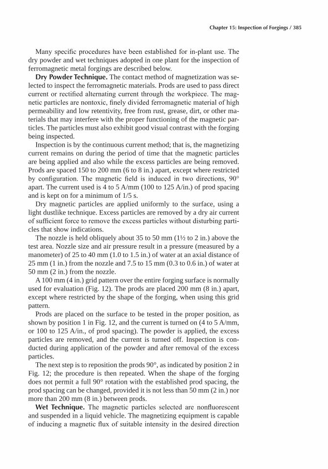
Chapter 15: Inspection of Forgings / 385
Many specific procedures have been established for in-plant use. The dry powder and wet techniques adopted in one plant for the inspection of ferromagnetic metal forgings are described below.
Dry Powder Technique� The contact method of magnetization was se-lected to inspect the ferromagnetic materials. Prods are used to pass direct current or rectified alternating current through the workpiece. The mag-netic particles are nontoxic, finely divided ferromagnetic material of high permeability and low retentivity, free from rust, grease, dirt, or other ma-terials that may interfere with the proper functioning of the magnetic par-ticles. The particles must also exhibit good visual contrast with the forging being inspected.
Inspection is by the continuous current method; that is, the magnetizing current remains on during the period of time that the magnetic particles are being applied and also while the excess particles are being removed. Prods are spaced 150 to 200 mm (6 to 8 in.) apart, except where restricted by configuration. The magnetic field is induced in two directions, 90° apart. The current used is 4 to 5 A/mm (100 to 125 A/in.) of prod spacing and is kept on for a minimum of 1/5 s.
Dry magnetic particles are applied uniformly to the surface, using a light dustlike technique. Excess particles are removed by a dry air current of sufficient force to remove the excess particles without disturbing parti-cles that show indications.
The nozzle is held obliquely about 35 to 50 mm (1½ to 2 in.) above the test area. Nozzle size and air pressure result in a pressure (measured by a manometer) of 25 to 40 mm (1.0 to 1.5 in.) of water at an axial distance of 25 mm (1 in.) from the nozzle and 7.5 to 15 mm (0.3 to 0.6 in.) of water at 50 mm (2 in.) from the nozzle.
A 100 mm (4 in.) grid pattern over the entire forging surface is normally used for evaluation (Fig. 12). The prods are placed 200 mm (8 in.) apart, except where restricted by the shape of the forging, when using this grid pattern.
Prods are placed on the surface to be tested in the proper position, as shown by position 1 in Fig. 12, and the current is turned on (4 to 5 A/mm, or 100 to 125 A/in., of prod spacing). The powder is applied, the excess particles are removed, and the current is turned off. Inspection is con-ducted during application of the powder and after removal of the excess particles.
The next step is to reposition the prods 90°, as indicated by position 2 in Fig. 12; the procedure is then repeated. When the shape of the forging does not permit a full 90° rotation with the established prod spacing, the prod spacing can be changed, provided it is not less than 50 mm (2 in.) nor more than 200 mm (8 in.) between prods.
Wet Technique� The magnetic particles selected are nonfluorescent and suspended in a liquid vehicle. The magnetizing equipment is capable of inducing a magnetic flux of suitable intensity in the desired direction
386 / Inspection of Metals—Understanding the Basics
by both the circular and the longitudinal methods. Direct current from generators, storage batteries, or rectifiers is used to induce the magnetic flux.
Circular magnetization is obtained by passing the current through the forging being examined or through a central conductor to induce the mag-netic flux. Longitudinal magnetization is obtained by using a solenoid, coil, or magnet to induce the magnetic flux. The magnetic particles are nontoxic and exhibit good visual contrast. The viscosity of the suspension vehicle for the particles must be a maximum of 5 × 10⁻⁶ m2/s (5.0 centi-stokes) at any bath temperature used. The magnetic particles are limited to 28 to 40 g (1.0 to 1.4 oz) of solid per gallon of liquid vehicle. The liquid used as a vehicle for the magnetic particles may be a petroleum distillate such as kerosene. Tap water with suitable rust inhibitors and wetting and antifoaming agents can be substituted for the petroleum distillate. The water should contain about 0.3% antifoam agent, 3.9% rust inhibitor, and 12.8% wetting agent.
Inspection is carried out by the continuous method. For this method, the magnetizing circuit is closed just before applying the suspension or just before removing the forging from the suspension. The circuit remains closed for approximately a half second.
For circular magnetization, an ammeter is used to verify the presence of adequate field strength. For verifying adequate field strength in longitudi-nal magnetization, a field indicator is useful. Typical current levels uti-lized to provide an adequate field strength are 4 to 12 A/mm (100 to 300
Fig� 12 Grid pattern and prod positions used in one plant for the magnetic particle inspection of forgings using prods and the dry powder tech-
nique. Dimensions are in inches. Source: Ref 1
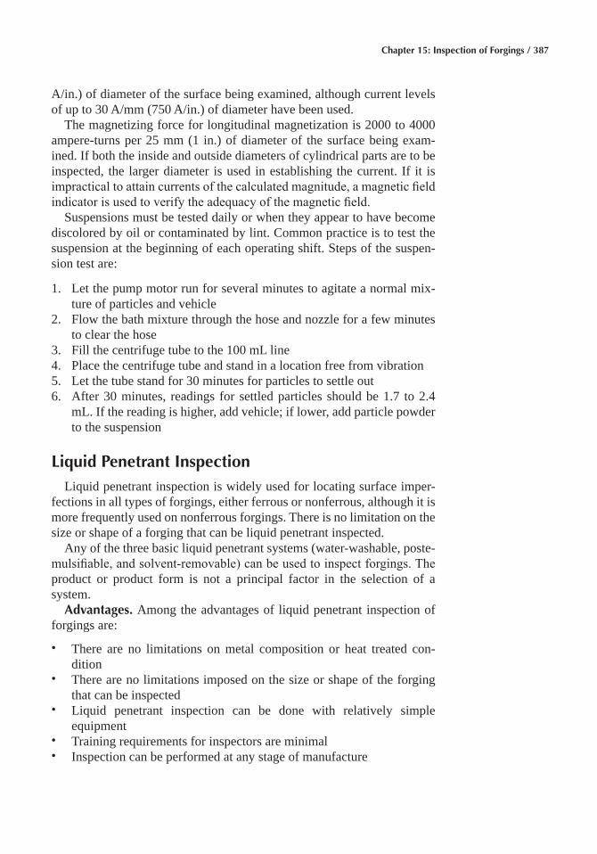
Chapter 15: Inspection of Forgings / 387
A/in.) of diameter of the surface being examined, although current levels of up to 30 A/mm (750 A/in.) of diameter have been used.
The magnetizing force for longitudinal magnetization is 2000 to 4000 ampere-turns per 25 mm (1 in.) of diameter of the surface being exam-ined. If both the inside and outside diameters of cylindrical parts are to be inspected, the larger diameter is used in establishing the current. If it is impractical to attain currents of the calculated magnitude, a magnetic field indicator is used to verify the adequacy of the magnetic field.
Suspensions must be tested daily or when they appear to have become discolored by oil or contaminated by lint. Common practice is to test the suspension at the beginning of each operating shift. Steps of the suspen-sion test are:
1. Let the pump motor run for several minutes to agitate a normal mix-ture of particles and vehicle
2. Flow the bath mixture through the hose and nozzle for a few minutes to clear the hose
3. Fill the centrifuge tube to the 100 mL line4. Place the centrifuge tube and stand in a location free from vibration5. Let the tube stand for 30 minutes for particles to settle out6. After 30 minutes, readings for settled particles should be 1.7 to 2.4
mL. If the reading is higher, add vehicle; if lower, add particle powder to the suspension
Liquid Penetrant InspectionLiquid penetrant inspection is widely used for locating surface imper-
fections in all types of forgings, either ferrous or nonferrous, although it is more frequently used on nonferrous forgings. There is no limitation on the size or shape of a forging that can be liquid penetrant inspected.
Any of the three basic liquid penetrant systems (water-washable, poste-mulsifiable, and solvent-removable) can be used to inspect forgings. The product or product form is not a principal factor in the selection of a system.
Advantages� Among the advantages of liquid penetrant inspection of forgings are:
• There are no limitations on metal composition or heat treated con- dition
• There are no limitations imposed on the size or shape of the forging that can be inspected
• Liquid penetrant inspection can be done with relatively simple equipment
• Training requirements for inspectors are minimal• Inspection can be performed at any stage of manufacture
388 / Inspection of Metals—Understanding the Basics
• Liquid penetrant materials can be taken to the forgings or the forgings taken to the inspection station, depending on the size and shape of the forgings
The limitations of the liquid penetrant inspection of forgings are basi-cally the same as those for the inspection of other workpieces. The charac-teristics of the surface of a forging sometimes impose specific limitations. The most important general limitations are:
• Liquid penetrant inspection is restricted to detecting discontinuities that are open to the surface
• Liquid penetrant inspection is basically a visual aid; therefore, results depend greatly on the visual acuity and judgment of the inspector
• Satisfactory inspection results require that the surface of the forging be thoroughly cleaned before inspection. The presence of surface scale can cause inaccurate readouts. If the surface of the forging is exces-sively scaled, it should be pickled or grit blasted, preferably pickled. The forgings should also be cleaned to remove surface contaminants, such as grease and oil
• Liquid penetrant inspection is slower than magnetic particle inspec- tion
Liquid Penetrant Detection of Flaws in Steel Forgings
Factors affecting the selection of a special penetrant system for inspect-ing steel forgings include available equipment; size, shape, and surface conditions of the forgings; degree of sensitivity required; whether or not the entire forging requires inspection; and cost. Regardless of which sys-tem is used, the degree of success achieved depends greatly on the surface conditions of the forging. Rough, scaly surfaces are likely to result in ei-ther false indications or obscuring of meaningful flaws. Pickled surfaces are preferred. Abrasive blasting is usually satisfactory for cleaning forging surfaces, although overblasting must be avoided or some flaws may be tightly closed preventing the penetrant from entering. The postemulsifi-able and solvent-removable liquid penetrant systems are most often used to inspect steel forgings.
The postemulsifiable system is generally preferred to the water- washable system for forgings because of its greater sensitivity. Either the fluorescent-penetrant or the visible-dye technique can be used. Selection depends largely on whether ultraviolet light inspection can be used. For forgings of a size and shape that can be immersed in tanks and inspected in a booth, the fluorescent technique is usually preferred.
The solvent-removable system is especially well adapted to applica-tions in which only a portion of the forging requires inspection. Equip-ment for this system can be minimal and completely portable or may in-
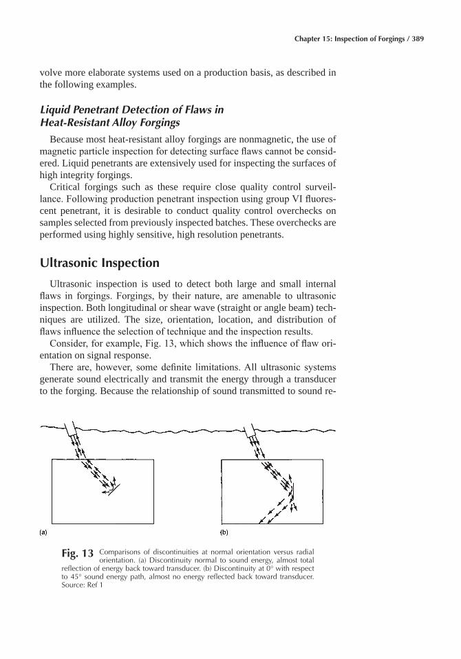
Chapter 15: Inspection of Forgings / 389
volve more elaborate systems used on a production basis, as described in the following examples.
Liquid Penetrant Detection of Flaws in Heat-Resistant Alloy Forgings
Because most heat-resistant alloy forgings are nonmagnetic, the use of magnetic particle inspection for detecting surface flaws cannot be consid-ered. Liquid penetrants are extensively used for inspecting the surfaces of high integrity forgings.
Critical forgings such as these require close quality control surveil-lance. Following production penetrant inspection using group VI fluores-cent penetrant, it is desirable to conduct quality control overchecks on samples selected from previously inspected batches. These overchecks are performed using highly sensitive, high resolution penetrants.
Ultrasonic Inspection
Ultrasonic inspection is used to detect both large and small internal flaws in forgings. Forgings, by their nature, are amenable to ultrasonic inspection. Both longitudinal or shear wave (straight or angle beam) tech-niques are utilized. The size, orientation, location, and distribution of flaws influence the selection of technique and the inspection results.
Consider, for example, Fig. 13, which shows the influence of flaw ori-entation on signal response.
There are, however, some definite limitations. All ultrasonic systems generate sound electrically and transmit the energy through a transducer to the forging. Because the relationship of sound transmitted to sound re-
Fig� 13 Comparisons of discontinuities at normal orientation versus radial orientation. (a) Discontinuity normal to sound energy, almost total
reflection of energy back toward transducer. (b) Discontinuity at 0° with respect to 45° sound energy path, almost no energy reflected back toward transducer. Source: Ref 1
390 / Inspection of Metals—Understanding the Basics
ceived is a factor in the inspectability of a forging, particular attention must be given to the surface condition of the forging.
Although techniques and couplants can enhance the energy transmis-sion from the transducer to the forging, as-forged surfaces impair the ef-fectiveness of ultrasonic inspection. Near-surface flaws are most difficult to detect, and a dead zone at the entry surface often interferes. Because of the difficulty involved in detecting surface flaws by ultrasonic inspection, another method, such as magnetic particle or liquid penetrant inspection, is often used in conjunction with ultrasonic inspection to inspect high in-tegrity forgings thoroughly.
Complex shapes are difficult to inspect ultrasonically because of the problems associated with sound entry angle. Most ultrasonic inspection of forgings uses techniques that send waves into the forging perpendicu-lar to the surface. Radii, fillets, and similar configurations must receive special treatment if all areas of the forging must be inspected. The special treatment involves the use of a standoff that has an end contoured to fit the inspection surface or the use of a small diameter or focused trans- ducer.
In certain cases, where the end use of a forging is considered critical, ultrasonic inspection is used to inspect the wrought material before it is worked. Surface or internal flaws that are not detected before a billet is forged may not be detected in the final forging and will be present in the finished part. Ultrasonic inspection is often used as part of a completely diagnostic inspection of a forging from newly designed dies, where use of the finished part does not warrant inspection of every part. Quality control measures often include the ultrasonic inspection of random samples from a particular forging. This provides the necessary assurance that the pro-cess is under control and that variables affecting internal quality have not been inadvertently introduced. Ultrasonic inspection is often used in the further evaluation of flaws detected by other nondestructive methods. This reduces the possibility that a particular forging will be unsuitable for its intended service.
Ultrasonic inspection can be used on every forging to validate its in-tegrity for extremely rigorous requirements. This applies in particular to forgings for nuclear and aerospace applications, where rigid standards of acceptance have been established. Standards and criteria have been set up to detect material inclusions, internal voids, laminations, and other con-ditions. In addition, the inspection of every forging by ultrasonics has been effective in detecting excessive grain size and other structural con- ditions.
Ultrasonic inspection is often used to qualify a particular lot of forgings that has been subjected to certain variations in approved processing proce-dures. A notable instance is the use of ultrasonics to determine the pres-ence of thermal flakes or in locating quench cracks.
Chapter 15: Inspection of Forgings / 391
Radiographic Inspection
Radiography (γ-ray or x-ray) is not extensively used for the inspection of forgings for two reasons. First, the types of discontinuities most com-monly located by radiography (gas porosity, shrinkage porosity, and shrinkage cavities) are not usually found in forgings. Second, for the types of internal discontinuities that are commonly found in forgings (inclu-sions, pipe, bursts, or flakes), ultrasonic inspection is more effective, more adaptable, and more economical.
Radiographic techniques can sometimes be helpful in the further inves-tigation of known internal discontinuities in forgings when the presence of these discontinuities has been determined earlier by ultrasonic inspection. In sections that are not too thick to penetrate with available radiographic equipment, the size, orientation, and possibly the type of discontinuities can be evaluated by radiography.
ACKNOWLEDGMENT
This chapter was adapted from Nondestructive Inspection of Forgings, Nondestructive Evaluation and Quality Control, Volume 17, ASM Hand-book, 1992.
REFERENCES
1. Nondestructive Inspection of Forgings, Nondestructive Evaluation and Quality Control, Vol 17, ASM Handbook, ASM International, 1992, p 491–511
Inspection of Metals—Understanding the Basics Copyright © 2013 ASM International®
F.C. Campbell, editor All rights reservedwww.asminternational.org
CHAPTER 16
Inspection of Powder Metallurgy Parts
FABRICATED POWDER METALLURGY (P/M) parts are evaluated and tested at several stages during manufacturing for part acceptance and process control. The various types of tests included are:
• Dimensional evaluation• Density measurements• Hardness testing• Mechanical testing• NDT
Dimensional Evaluation
Dimensional accuracy of P/M sintered parts is determined with the same measurement techniques that are used for wrought materials. How-ever, other testing methods for P/M materials are specialized, such as de-termination of surface finish. For sintered parts, a chisel pointed stylus is used to deemphasize the effects of porosity. A conical stylus tends to en-gage porosity, thus giving an exaggerated measurement of roughness.
During the manufacture of sintered parts, dimensional change must be accommodated for during each processing step. Causes of dimensional changes include:
• Elastic springback during ejection from the tooling used for cold pressing
• Growth or shrinkage during delubrication, presintering, and sintering• Elastic springback from tooling during cold repressing or sizing
394 / Inspection of Metals—Understanding the Basics
• Thermal contraction from the tools used in hot forging or hot repressing
• Tool wear in cold or hot compacting• Machining tolerances at secondary machining and associated tool
wear• Distortion during annealing• Growth or shrinkage during carburizing, nitriding, or neutral hard-
ening• Shrinkage during tempering• Growth during steam blackening
Parts manufacturers must be familiar with the amount of dimensional changes to expect for the materials and equipment in use so that tooling can be produced that accommodates these changes and produces accurate parts. Understanding and controlling these factors is essential to commer-cial P/M parts manufacturing.
Density Measurement
Density is the ratio of mass to volume. For a given material, degree of sintering, and heat treatment, density determines mechanical and physical properties. For example, higher density in sintered steels results in higher tensile strength, elongation, and impact resistance. As-pressed or green density also influences growth or shrinkage that occurs during sintering. With nonuniform green density, parts grow or shrink nonuniformly, as in a thin walled bronze bearing with a low density region equidistant from the ends. This results in a significantly smaller diameter at mid-length than at the ends and necessitates repressing or sizing for close dimensional control.
If cubes or right cylinders can be extracted from actual parts, linear di-mensions can be measured and volume can be easily calculated. From the weight of a part, density can be calculated. This yields a value that, under ideal conditions, differs by 0.04 g/cm3 (0.5%) from a reference. Unless the sintered part is directly molded to an easily measured shape such as a transverse rupture bar (31.8 by 12.7 by 6.4 mm or 1.25 by 0.50 by 0.25 in.), this method of measuring linear dimensions is infrequently used.
Methods Based on Archimedes’ Principle� Typical methods of mea-suring density depend on Archimedes’ principle, in which hydrostatic forces in a liquid exerts buoyant forces proportional to the part volume. This measurement is standardized in ASTM B328, MPIF test method 42, and International Standards Organization test method ISO 2738.
When an object is immersed in a liquid, the liquid exerts an upward buoyant force that is equal to the product of the object volume and the density of the liquid. The difference in weight between an object weighed
Chapter 16: Inspection of Powder Metallurgy Parts / 395
in air and its weight when suspended in water is equal to the object vol-ume in cubic centimeters times the density of water. Approximating the density of water as unity:
V = Wair – Wwater
where V is the volume in cm3, Wair is the weight in air in g, and Wwater is the weight of object suspended in water less the weight of the suspending wire in water (tare) in g. Density in g/cm3 is then:
Density = Wair/(Wair – Wwater)
For unsintered materials molded with 0.75% lubricant, the pores are well sealed, and water cannot penetrate. For such parts, the above calculation is suitable. It is also suitable for materials with pores that are sealed off from the surface (materials close to theoretical density).
However, for most sintered materials that are 70 to 95% dense, water tends to infiltrate the pores during weighing in water. This minimizes the buoyancy effect of the water (that is, the liquid is acting on a smaller vol-ume) and results in an erroneous calculation of low volume. This low vol-ume then causes an erroneously high density value. Infiltration of water into pores usually is accompanied by air bubbles escaping from the part. If the part is blotted to remove surface water and reweighed in air after weighing in water, any weight gain indicates that water has entered the pores. Although not a standard procedure, volume can be approximated as the weight in air after removing the part from the water, minus the weight in water.
To prevent infiltration of water, all three standard test methods require that the pores of the part be filled with oil. Oil impregnation is done after the part is weighed in air. This is carried out under vacuum or by immer-sion in hot oil. Oil prevents the water from entering the pores. The volume of the part is then determined as the part weight in air with oil in the pores, minus the weight of the oiled part suspended in water. Care should be taken to select an oil that is not soluble in water or not soluble in water plus wetting agent. Such oils also must exhibit superior demulsibility.
The precision of the ISO method is ±0.25%, regardless of sample den-sity, and assumes a water density of 0.997 g/cm3. To determine density variation from one point to another in a complex part, the available sam-ples must be considerably <17 g. According to ASTM B328, a minimum sample of 2 g is recommended, because a relatively high error rate results from measuring small samples.
Metallographic estimates can also be made of the area fraction of porosity, which is numerically equal to the volume porosity, and thus the density of sintered materials. The method is not standardized, and accu-
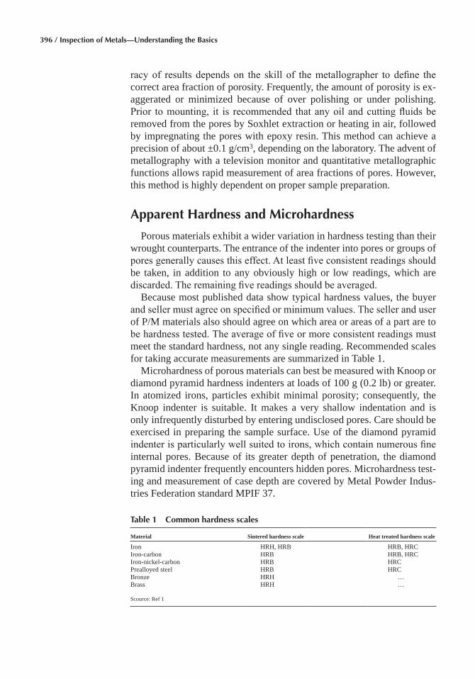
396 / Inspection of Metals—Understanding the Basics
racy of results depends on the skill of the metallographer to define the correct area fraction of porosity. Frequently, the amount of porosity is ex-aggerated or minimized because of over polishing or under polishing. Prior to mounting, it is recommended that any oil and cutting fluids be removed from the pores by Soxhlet extraction or heating in air, followed by impregnating the pores with epoxy resin. This method can achieve a precision of about ±0.1 g/cm3, depending on the laboratory. The advent of metallography with a television monitor and quantitative metallographic functions allows rapid measurement of area fractions of pores. However, this method is highly dependent on proper sample preparation.
Apparent Hardness and Microhardness
Porous materials exhibit a wider variation in hardness testing than their wrought counterparts. The entrance of the indenter into pores or groups of pores generally causes this effect. At least five consistent readings should be taken, in addition to any obviously high or low readings, which are discarded. The remaining five readings should be averaged.
Because most published data show typical hardness values, the buyer and seller must agree on specified or minimum values. The seller and user of P/M materials also should agree on which area or areas of a part are to be hardness tested. The average of five or more consistent readings must meet the standard hardness, not any single reading. Recommended scales for taking accurate measurements are summarized in Table 1.
Microhardness of porous materials can best be measured with Knoop or diamond pyramid hardness indenters at loads of 100 g (0.2 lb) or greater. In atomized irons, particles exhibit minimal porosity; consequently, the Knoop indenter is suitable. It makes a very shallow indentation and is only infrequently disturbed by entering undisclosed pores. Care should be exercised in preparing the sample surface. Use of the diamond pyramid indenter is particularly well suited to irons, which contain numerous fine internal pores. Because of its greater depth of penetration, the diamond pyramid indenter frequently encounters hidden pores. Microhardness test-ing and measurement of case depth are covered by Metal Powder Indus-tries Federation standard MPIF 37.
Table 1 Common hardness scales
Material Sintered hardness scale Heat treated hardness scale
Iron HRH, HRB HRB, HRCIron-carbon HRB HRB, HRCIron-nickel-carbon HRB HRCPrealloyed steel HRB HRCBronze HRH …Brass HRH …
Scource: Ref 1
Chapter 16: Inspection of Powder Metallurgy Parts / 397
Mechanical Testing/Tensile Testing
Metal Powder Industries Federation standard 10 describes specimens for tensile testing. Specimens include flat unmachined test bars or ma-chined rounds. Unmachined flats are more prone to slippage of grips or breakage in the gauge region. For testing to be meaningful, it is important to verify that such bars are free of microlaminations, which requires care-ful metallographic evaluation. Highest quality bars are molded in well bolstered die sets (890 kN or 100 ton rating), with generous exit taper, high green strength powder, and top punch hold down, if possible.
With all steel test bars, it is necessary to determine that substantial car-burization or decarburization resulting from sintering or hardening does not exist. If the bars are heat treated, the microstructure at the surface and in the interior should be described in the test report, because many P/M steels have low hardenability.
For heat treated materials, unmachined flat specimens tend to slip in the grips. A machined bar provides more accurate data. The machined bar shows an increase in apparent tensile strength of 50% compared to molded bars. Even with machined bars, some heat treated materials exhibit such low elongation that failure occurs prior to reaching 0.2% permanent deformation.
Transverse Rupture Strength� The transverse rupture test breaks a 31.8 by 12.7 by 6.4 mm (1.25 by 0.5 by 0.25 in.) test bar as a simple beam. The test is theoretically valid only for perfectly brittle materials and measures the stress in the outer fiber at fracture. For many sintered steels, transverse rupture stress is considered to be equal to twice the ul-timate tensile strength. This is only an approximation. Metal Powder In-dustries Federation standard 35 presents transverse rupture stress values that correspond with ultimate tensile stress values for common P/M materials.
The transverse rupture test is useful for comparing and evaluating ma-terials for strength, even if the bar bends before fracture. These bars are preferred, because they can be molded and sintered conveniently. Testing is faster than when using a tensile bar. When heat treated, the test bar does not experience distortion. This testing procedure is used mainly as a qual-ity control tool to ensure the maintenance of minimum mechanical proper-ties. During P/M part production, this method is used to evaluate proper-ties of incoming powder, such as compressibility, sintered strength, and dimensional change.
Unnotched Charpy Impact Strength� A 10 by 10 by 76 mm (0.35 by 0.35 by 3.00 in.) molded bar is used for impact testing. The unnotched bar provides a more sensitive test, suitable for use on materials with an impact strength below 14 J (10 ft · lbf). The bar is conventionally struck on the sur-face that contacted the die at molding.
398 / Inspection of Metals—Understanding the Basics
Proof Testing� The most common method of demonstrating the strength of sintered parts is through mechanical tests that stress parts to failure. Qualification samples or first production lots are used to establish desired strength values; these data are incorporated in the part design speci- fication.
For testing gears, several teeth are removed. The remaining teeth are loaded in a predetermined arrangement on a fixture. The load to fracture is recorded. To be meaningful, the destructive test must imitate service load-ing on the part.
Impact or drop weight tests also are used to evaluate materials. A drop weight test does not only use an acceptance or rejection evaluation. This testing procedure investigates the impacts above the acceptance level and below the rejection value. When a part does not break, each succeeding load is increased until breakage occurs. Thus, if load P does not break a part, 1.05 P is used on the succeeding impact.
Powder Metallurgy Part Defects
The problem of forming defects in green parts during compaction and ejection has become more prevalent as parts producers have begun to use higher compaction pressures in an effort to achieve high density, high per-formance powder metallurgy (P/M) steels. Proper press setup for molding P/M parts is also critical to prevent cracking. In a flanged part that experi-ences a change in diameter, density in the hub and flange should be nearly equal. Unequal density leads to powder displacement from one part level to the next and to the formation of shear cracks. Such cracks often occur at 45° to the pressing direction and at surfaces at the junction (radius) be-tween the hub and flange. At press setup, equal density should be obtained in the hub and flange. A high green strength powder and a press that main-tains a small counter pressure on the top of the part during ejection from the tools (top punch hold-down) should be used.
The four most common types of defects in P/M parts are ejection cracks, density variations, microlaminations, and poor sintering.
Ejection Cracks� When a part has been pressed, there are large residual stresses in the part due to the constraint of the die and punches, which are relieved as the part is ejected from the die. The strains associated with this stress relief depend on the compacting pressure, the green expansion of the material being compacted, and the rigidity of the die. Green expan-sion, also known as spring out, is the difference between the ejected part size and the die size. A typical value of green expansion for a powder mix based on atomized iron powder pressed at relatively high pressure (600 to 700 MPa or 45 to 50 tsi) is 0.20%. For example, in a partially ejected com-pact, the portion that is out of the die expands to relieve the residual stresses, while the constrained portion remains die size and a shear stress is imposed on the compact. When the ability of the powder compact to
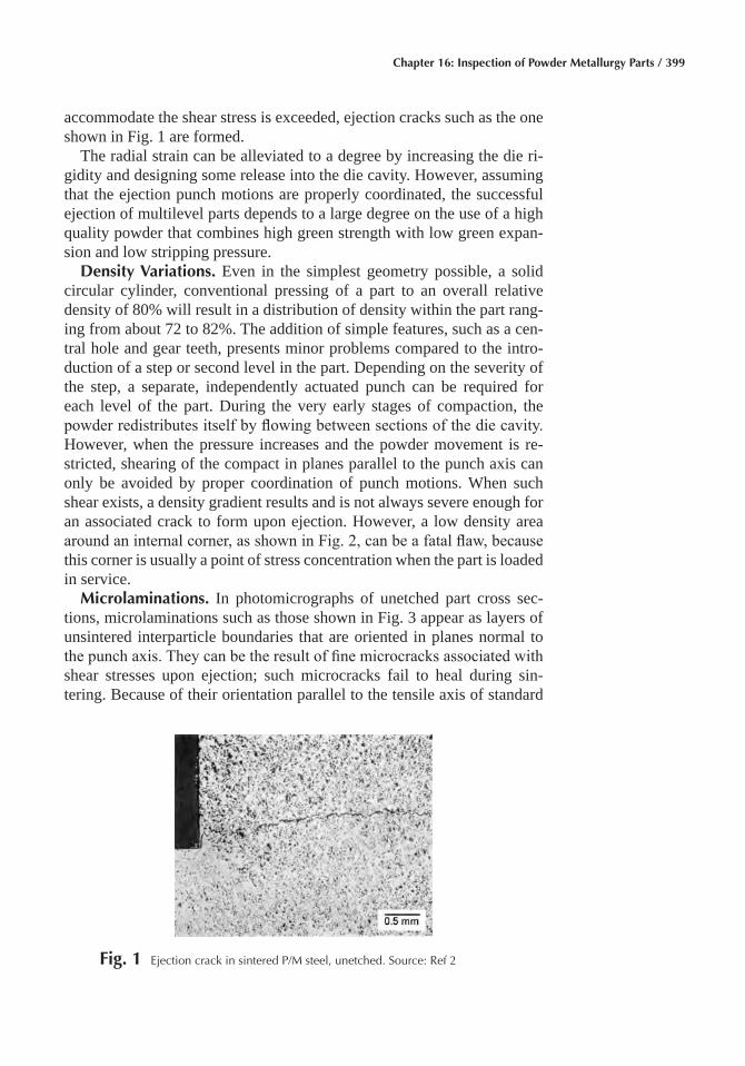
Chapter 16: Inspection of Powder Metallurgy Parts / 399
accommodate the shear stress is exceeded, ejection cracks such as the one shown in Fig. 1 are formed.
The radial strain can be alleviated to a degree by increasing the die ri-gidity and designing some release into the die cavity. However, assuming that the ejection punch motions are properly coordinated, the successful ejection of multilevel parts depends to a large degree on the use of a high quality powder that combines high green strength with low green expan-sion and low stripping pressure.
Density Variations� Even in the simplest geometry possible, a solid circular cylinder, conventional pressing of a part to an overall relative density of 80% will result in a distribution of density within the part rang-ing from about 72 to 82%. The addition of simple features, such as a cen-tral hole and gear teeth, presents minor problems compared to the intro-duction of a step or second level in the part. Depending on the severity of the step, a separate, independently actuated punch can be required for each level of the part. During the very early stages of compaction, the powder redistributes itself by flowing between sections of the die cavity. However, when the pressure increases and the powder movement is re-stricted, shearing of the compact in planes parallel to the punch axis can only be avoided by proper coordination of punch motions. When such shear exists, a density gradient results and is not always severe enough for an associated crack to form upon ejection. However, a low density area around an internal corner, as shown in Fig. 2, can be a fatal flaw, because this corner is usually a point of stress concentration when the part is loaded in service.
Microlaminations� In photomicrographs of unetched part cross sec-tions, microlaminations such as those shown in Fig. 3 appear as layers of unsintered interparticle boundaries that are oriented in planes normal to the punch axis. They can be the result of fine microcracks associated with shear stresses upon ejection; such microcracks fail to heal during sin-tering. Because of their orientation parallel to the tensile axis of standard
Fig� 1 Ejection crack in sintered P/M steel, unetched. Source: Ref 2
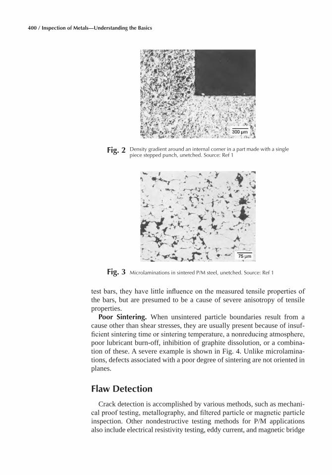
400 / Inspection of Metals—Understanding the Basics
test bars, they have little influence on the measured tensile properties of the bars, but are presumed to be a cause of severe anisotropy of tensile properties.
Poor Sintering� When unsintered particle boundaries result from a cause other than shear stresses, they are usually present because of insuf-ficient sintering time or sintering temperature, a nonreducing atmosphere, poor lubricant burn-off, inhibition of graphite dissolution, or a combina-tion of these. A severe example is shown in Fig. 4. Unlike microlamina-tions, defects associated with a poor degree of sintering are not oriented in planes.
Flaw Detection
Crack detection is accomplished by various methods, such as mechani-cal proof testing, metallography, and filtered particle or magnetic particle inspection. Other nondestructive testing methods for P/M applications also include electrical resistivity testing, eddy current, and magnetic bridge
Fig� 2 Density gradient around an internal corner in a part made with a single piece stepped punch, unetched. Source: Ref 1
Fig� 3 Microlaminations in sintered P/M steel, unetched. Source: Ref 1
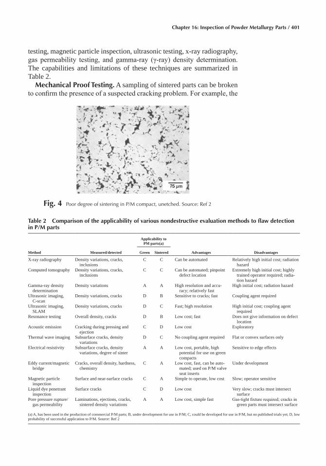
Chapter 16: Inspection of Powder Metallurgy Parts / 401
testing, magnetic particle inspection, ultrasonic testing, x-ray radiography, gas permeability testing, and gamma-ray (γ-ray) density determination. The capabilities and limitations of these techniques are summarized in Table 2.
Mechanical Proof Testing� A sampling of sintered parts can be broken to confirm the presence of a suspected cracking problem. For example, the
Fig� 4 Poor degree of sintering in P/M compact, unetched. Source: Ref 2
Table 2 Comparison of the applicability of various nondestructive evaluation methods to flaw detection in P/M parts
Method Measured/detected
Applicability to PM parts(a)
Advantages DisadvantagesGreen Sintered
X-ray radiography Density variations, cracks, inclusions
C C Can be automated Relatively high initial cost; radiation hazard
Computed tomography Density variations, cracks, inclusions
C C Can be automated; pinpoint defect location
Extremely high initial cost; highly trained operator required; radia-tion hazard
Gamma-ray density determination
Density variations A A High resolution and accu-racy; relatively fast
High initial cost; radiation hazard
Ultrasonic imaging, C-scan
Density variations, cracks D B Sensitive to cracks; fast Coupling agent required
Ultrasonic imaging, SLAM
Density variations, cracks D C Fast; high resolution High initial cost; coupling agent required
Resonance testing Overall density, cracks D B Low cost; fast Does not give information on defect location
Acoustic emission Cracking during pressing and ejection
C D Low cost Exploratory
Thermal wave imaging Subsurface cracks, density variations
D C No coupling agent required Flat or convex surfaces only
Electrical resistivity Subsurface cracks, density variations, degree of sinter
A A Low cost, portable, high potential for use on green compacts
Sensitive to edge effects
Eddy current/magnetic bridge
Cracks, overall density, hardness, chemistry
C A Low cost, fast, can be auto-mated; used on P/M valve seat inserts
Under development
Magnetic particle inspection
Surface and near-surface cracks C A Simple to operate, low cost Slow; operator sensitive
Liquid dye penetrant inspection
Surface cracks C D Low cost Very slow; cracks must intersect surface
Pore pressure rupture/ gas permeability
Laminations, ejections, cracks, sintered density variations
A A Low cost, simple fast Gas-tight fixture required; cracks in green parts must intersect surface
(a) A, has been used in the production of commercial P/M parts; B, under development for use in P/M; C, could be developed for use in P/M, but no published trials yet; D, low probability of successful application to P/M. Source: Ref 2
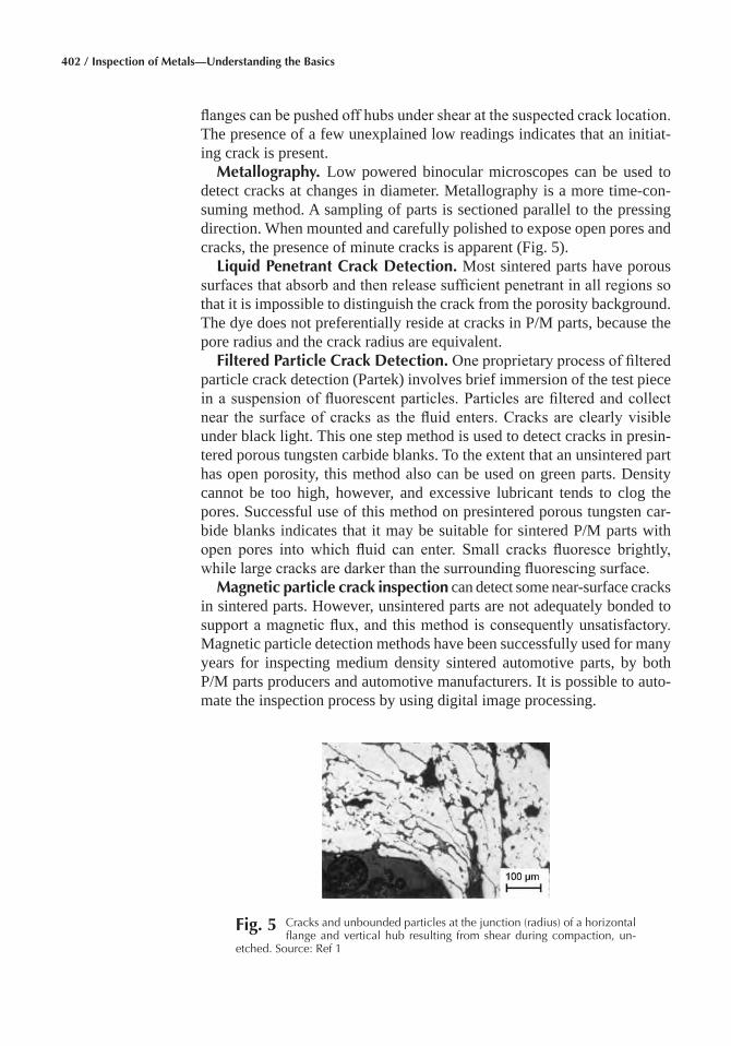
402 / Inspection of Metals—Understanding the Basics
flanges can be pushed off hubs under shear at the suspected crack location. The presence of a few unexplained low readings indicates that an initiat-ing crack is present.
Metallography� Low powered binocular microscopes can be used to detect cracks at changes in diameter. Metallography is a more time-con-suming method. A sampling of parts is sectioned parallel to the pressing direction. When mounted and carefully polished to expose open pores and cracks, the presence of minute cracks is apparent (Fig. 5).
Liquid Penetrant Crack Detection� Most sintered parts have porous surfaces that absorb and then release sufficient penetrant in all regions so that it is impossible to distinguish the crack from the porosity background. The dye does not preferentially reside at cracks in P/M parts, because the pore radius and the crack radius are equivalent.
Filtered Particle Crack Detection� One proprietary process of filtered particle crack detection (Partek) involves brief immersion of the test piece in a suspension of fluorescent particles. Particles are filtered and collect near the surface of cracks as the fluid enters. Cracks are clearly visible under black light. This one step method is used to detect cracks in presin-tered porous tungsten carbide blanks. To the extent that an unsintered part has open porosity, this method also can be used on green parts. Density cannot be too high, however, and excessive lubricant tends to clog the pores. Successful use of this method on presintered porous tungsten car-bide blanks indicates that it may be suitable for sintered P/M parts with open pores into which fluid can enter. Small cracks fluoresce brightly, while large cracks are darker than the surrounding fluorescing surface.
Magnetic particle crack inspection can detect some near-surface cracks in sintered parts. However, unsintered parts are not adequately bonded to support a magnetic flux, and this method is consequently unsatisfactory. Magnetic particle detection methods have been successfully used for many years for inspecting medium density sintered automotive parts, by both P/M parts producers and automotive manufacturers. It is possible to auto-mate the inspection process by using digital image processing.
Fig� 5 Cracks and unbounded particles at the junction (radius) of a horizontal flange and vertical hub resulting from shear during compaction, un-
etched. Source: Ref 1
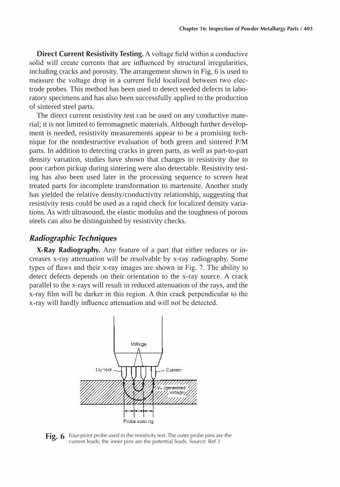
Chapter 16: Inspection of Powder Metallurgy Parts / 403
Direct Current Resistivity Testing� A voltage field within a conductive solid will create currents that are influenced by structural irregularities, including cracks and porosity. The arrangement shown in Fig. 6 is used to measure the voltage drop in a current field localized between two elec-trode probes. This method has been used to detect seeded defects in labo-ratory specimens and has also been successfully applied to the production of sintered steel parts.
The direct current resistivity test can be used on any conductive mate-rial; it is not limited to ferromagnetic materials. Although further develop-ment is needed, resistivity measurements appear to be a promising tech-nique for the nondestructive evaluation of both green and sintered P/M parts. In addition to detecting cracks in green parts, as well as part-to-part density variation, studies have shown that changes in resistivity due to poor carbon pickup during sintering were also detectable. Resistivity test-ing has also been used later in the processing sequence to screen heat treated parts for incomplete transformation to martensite. Another study has yielded the relative density/conductivity relationship, suggesting that resistivity tests could be used as a rapid check for localized density varia-tions. As with ultrasound, the elastic modulus and the toughness of porous steels can also be distinguished by resistivity checks.
Radiographic TechniquesX-Ray Radiography� Any feature of a part that either reduces or in-
creases x-ray attenuation will be resolvable by x-ray radiography. Some types of flaws and their x-ray images are shown in Fig. 7. The ability to detect defects depends on their orientation to the x-ray source. A crack parallel to the x-rays will result in reduced attenuation of the rays, and the x-ray film will be darker in this region. A thin crack perpendicular to the x-ray will hardly influence attenuation and will not be detected.
Fig� 6 Four-point probe used in the resistivity test. The outer probe pins are the current leads; the inner pins are the potential leads. Source: Ref 3
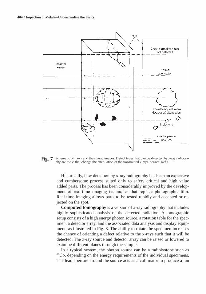
404 / Inspection of Metals—Understanding the Basics
Historically, flaw detection by x-ray radiography has been an expensive and cumbersome process suited only to safety critical and high value added parts. The process has been considerably improved by the develop-ment of real-time imaging techniques that replace photographic film. Real-time imaging allows parts to be tested rapidly and accepted or re-jected on the spot.
Computed tomography is a version of x-ray radiography that includes highly sophisticated analysis of the detected radiation. A tomographic setup consists of a high energy photon source, a rotation table for the spec-imen, a detector array, and the associated data analysis and display equip-ment, as illustrated in Fig. 8. The ability to rotate the specimen increases the chance of orienting a defect relative to the x-rays such that it will be detected. The x-ray source and detector array can be raised or lowered to examine different planes through the sample.
In a typical system, the photon source can be a radioisotope such as 60Co, depending on the energy requirements of the individual specimens. The lead aperture around the source acts as a collimator to produce a fan
Fig� 7 Schematic of flaws and their x-ray images. Defect types that can be detected by x-ray radiogra-phy are those that change the attenuation of the transmitted x-rays. Source: Ref 4
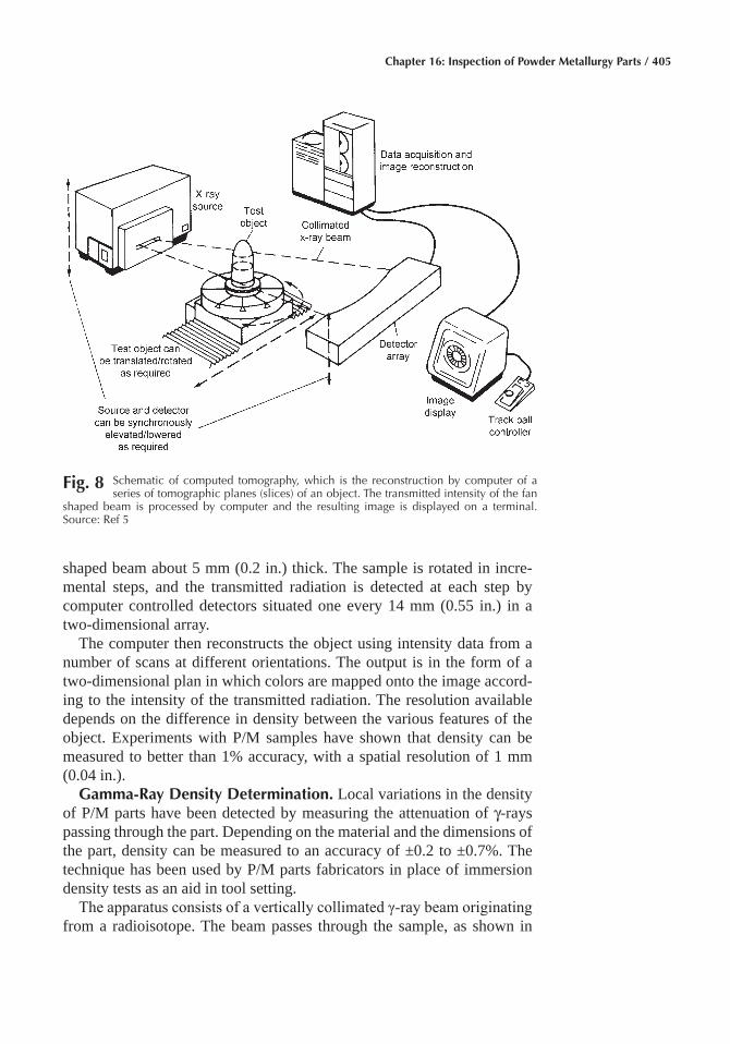
Chapter 16: Inspection of Powder Metallurgy Parts / 405
shaped beam about 5 mm (0.2 in.) thick. The sample is rotated in incre-mental steps, and the transmitted radiation is detected at each step by computer controlled detectors situated one every 14 mm (0.55 in.) in a two-dimensional array.
The computer then reconstructs the object using intensity data from a number of scans at different orientations. The output is in the form of a two-dimensional plan in which colors are mapped onto the image accord-ing to the intensity of the transmitted radiation. The resolution available depends on the difference in density between the various features of the object. Experiments with P/M samples have shown that density can be measured to better than 1% accuracy, with a spatial resolution of 1 mm (0.04 in.).
Gamma-Ray Density Determination� Local variations in the density of P/M parts have been detected by measuring the attenuation of γ-rays passing through the part. Depending on the material and the dimensions of the part, density can be measured to an accuracy of ±0.2 to ±0.7%. The technique has been used by P/M parts fabricators in place of immersion density tests as an aid in tool setting.
The apparatus consists of a vertically collimated γ-ray beam originating from a radioisotope. The beam passes through the sample, as shown in
Fig� 8 Schematic of computed tomography, which is the reconstruction by computer of a series of tomographic planes (slices) of an object. The transmitted intensity of the fan
shaped beam is processed by computer and the resulting image is displayed on a terminal. Source: Ref 5
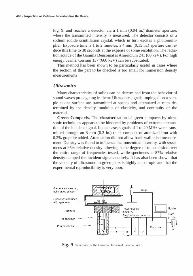
406 / Inspection of Metals—Understanding the Basics
Fig. 9, and reaches a detector via a 1 mm (0.04 in.) diameter aperture, where the transmitted intensity is measured. The detector consists of a sodium iodide scintillation crystal, which in turn excites a photomulti-plier. Exposure time is 1 to 2 minutes; a 4 mm (0.15 in.) aperture can re-duce this time to 30 seconds at the expense of some resolution. The radia-tion source of the Gamma Densomat is Americium 241 (60 keV). For high energy beams, Cesium 137 (660 keV) can be substituted.
This method has been shown to be particularly useful in cases where the section of the part to be checked is too small for immersion density measurements
Ultrasonics
Many characteristics of solids can be determined from the behavior of sound waves propagating in them. Ultrasonic signals impinged on a sam-ple at one surface are transmitted at speeds and attenuated at rates de-termined by the density, modulus of elasticity, and continuity of the material.
Green Compacts� The characterization of green compacts by ultra-sonic techniques appears to be hindered by problems of extreme attenua-tion of the incident signal. In one case, signals of 1 to 20 MHz were trans-mitted through an 8 mm (0.3 in.) thick compact of atomized iron with 0.2% graphite added. Attenuation did not allow back-wall echo measure-ment. Density was found to influence the transmitted intensity, with speci-mens at 95% relative density allowing some degree of transmission over the entire range of frequencies tested, while specimens at 87% relative density damped the incident signals entirely. It has also been shown that the velocity of ultrasound in green parts is highly anisotropic and that the experimental reproducibility is very poor.
Fig� 9 Schematic of the Gamma Densomat. Source: Ref 6
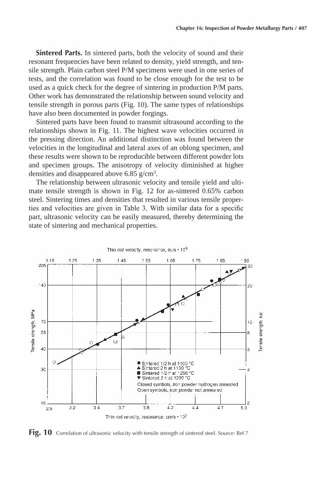
Chapter 16: Inspection of Powder Metallurgy Parts / 407
Sintered Parts� In sintered parts, both the velocity of sound and their resonant frequencies have been related to density, yield strength, and ten-sile strength. Plain carbon steel P/M specimens were used in one series of tests, and the correlation was found to be close enough for the test to be used as a quick check for the degree of sintering in production P/M parts. Other work has demonstrated the relationship between sound velocity and tensile strength in porous parts (Fig. 10). The same types of relationships have also been documented in powder forgings.
Sintered parts have been found to transmit ultrasound according to the relationships shown in Fig. 11. The highest wave velocities occurred in the pressing direction. An additional distinction was found between the velocities in the longitudinal and lateral axes of an oblong specimen, and these results were shown to be reproducible between different powder lots and specimen groups. The anisotropy of velocity diminished at higher densities and disappeared above 6.85 g/cm3.
The relationship between ultrasonic velocity and tensile yield and ulti-mate tensile strength is shown in Fig. 12 for as-sintered 0.65% carbon steel. Sintering times and densities that resulted in various tensile proper-ties and velocities are given in Table 3. With similar data for a specific part, ultrasonic velocity can be easily measured, thereby determining the state of sintering and mechanical properties.
Fig� 10 Correlation of ultrasonic velocity with tensile strength of sintered steel. Source: Ref 7
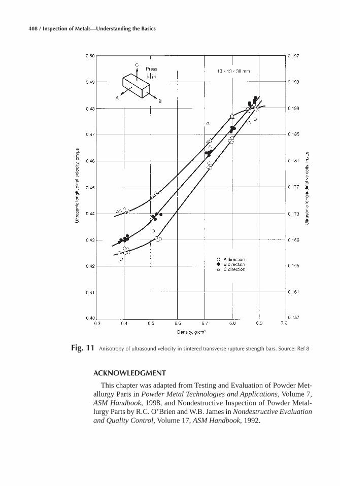
408 / Inspection of Metals—Understanding the Basics
ACKNOWLEDGMENT
This chapter was adapted from Testing and Evaluation of Powder Met-allurgy Parts in Powder Metal Technologies and Applications, Volume 7, ASM Handbook, 1998, and Nondestructive Inspection of Powder Metal-lurgy Parts by R.C. O’Brien and W.B. James in Nondestructive Evaluation and Quality Control, Volume 17, ASM Handbook, 1992.
Fig� 11 Anisotropy of ultrasound velocity in sintered transverse rupture strength bars. Source: Ref 8
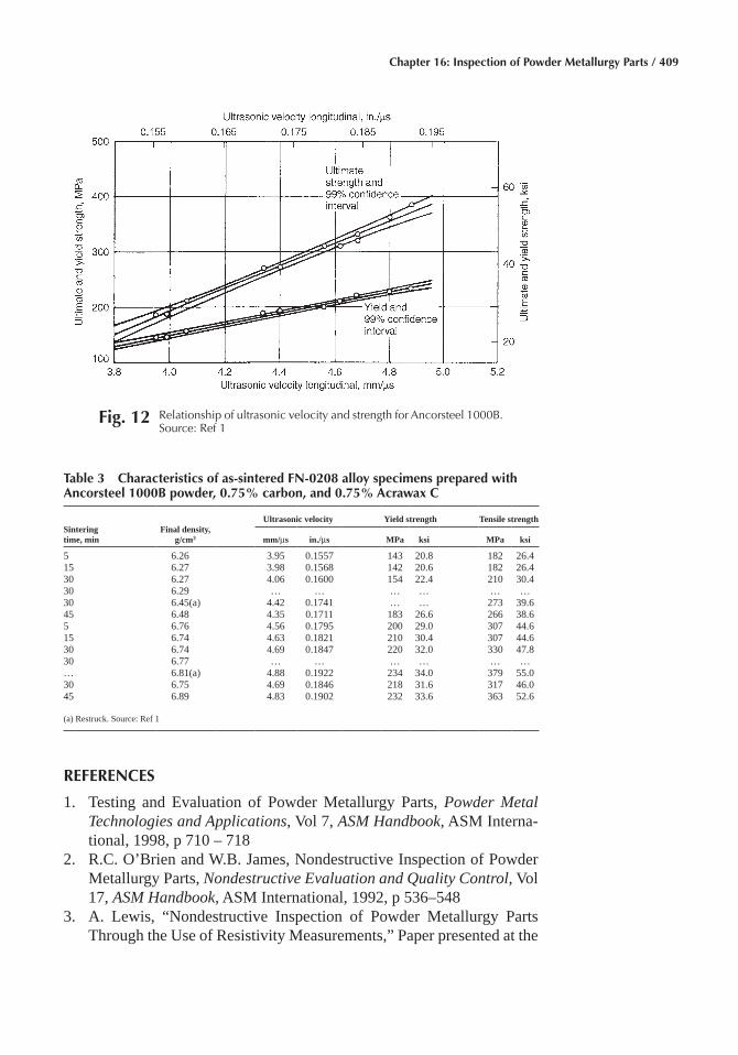
Chapter 16: Inspection of Powder Metallurgy Parts / 409
REFERENCES
1. Testing and Evaluation of Powder Metallurgy Parts, Powder Metal Technologies and Applications, Vol 7, ASM Handbook, ASM Interna-tional, 1998, p 710 – 718
2. R.C. O’Brien and W.B. James, Nondestructive Inspection of Powder Metallurgy Parts, Nondestructive Evaluation and Quality Control, Vol 17, ASM Handbook, ASM International, 1992, p 536–548
3. A. Lewis, “Nondestructive Inspection of Powder Metallurgy Parts Through the Use of Resistivity Measurements,” Paper presented at the
Fig� 12 Relationship of ultrasonic velocity and strength for Ancorsteel 1000B. Source: Ref 1
Table 3 Characteristics of as-sintered FN-0208 alloy specimens prepared with Ancorsteel 1000B powder, 0�75% carbon, and 0�75% Acrawax C
Sintering time, min
Final density, g/cm3
Ultrasonic velocity Yield strength Tensile strength
mm/μs in./μs MPa ksi MPa ksi
5 6.26 3.95 0.1557 143 20.8 182 26.415 6.27 3.98 0.1568 142 20.6 182 26.430 6.27 4.06 0.1600 154 22.4 210 30.430 6.29 … … … … … …30 6.45(a) 4.42 0.1741 … … 273 39.645 6.48 4.35 0.1711 183 26.6 266 38.65 6.76 4.56 0.1795 200 29.0 307 44.615 6.74 4.63 0.1821 210 30.4 307 44.630 6.74 4.69 0.1847 220 32.0 330 47.830 6.77 … … … … … …… 6.81(a) 4.88 0.1922 234 34.0 379 55.030 6.75 4.69 0.1846 218 31.6 317 46.045 6.89 4.83 0.1902 232 33.6 363 52.6
(a) Restruck. Source: Ref 1

410 / Inspection of Metals—Understanding the Basics
Prevention and Detection of Cracks in Ferrous P/M Parts Seminar, Metal Powder Industries Federation, 1988
4. C. Rain, Uncovering Hidden Flaws, High Technol., Feb 1984 5. B. Chang et al., Spatial Resolution in Industrial Tomography, IEEE
Trans. Nuclear Sci., NS30 (No. 2), April 1983 6. G. Schlieper, W.J. Huppmann, and A. Kozuch, Nondestructive Deter-
mination of Sectional Densities by the Gamma Densomat, Prog. Pow-der Metall., Vol 43, 1987, p 351
7. R.H. Brockelman, Dynamic Elastic Determination of the Properties of Sintered Powder Metals, Perspect. Powder Metall., Vol 5, 1970, p 201
8. E.P. Papadakis and B.W. Petersen, Ultrasonic Velocity as a Predictor of Density in Sintered Powder Metal Parts, Mater. Eval., April 1979, p 76

Inspection of Metals—Understanding the Basics Copyright © 2013 ASM International®
F.C. Campbell, editor All rights reservedwww.asminternational.org
CHAPTER 17
Inspection of Weldments and Brazed Assemblies
THE SELECTION of a method for inspecting weldments and brazed assemblies for flaws (referred to as discontinuities in welding terminol-ogy) depends on a number of variables, including the nature of the discon-tinuity, the accessibility of the joint, the types of materials joined, the number of joints to be inspected, the detection capabilities of the inspec-tion method, the level of joint quality required, and economic consider-ations. Regardless of the method selected, established standards must be followed to obtain valid inspection results.
In general, nondestructive inspection (NDI) methods are preferred over destructive inspection methods. Sections can be trepanned from a joint to determine its integrity; however, the joint must be refilled, and there is no certainty that discontinuities would not be introduced during repair. De-structive inspection is usually impractical, because of the high cost and the inability of such methods to accurately predict the quality of those joints that were not inspected.
Weldments
Weldments made by the various welding processes may contain discon-tinuities that are characteristic of that process. Therefore, each process, as well as the discontinuities typical of that process, are discussed in this section.
Discontinuities in Arc Welds
Discontinuities may be divided into three broad classifications: design related, welding process related, and metallurgical. Design related discon-tinuities include problems with design or structural details, choice of the

412 / Inspection of Metals—Understanding the Basics
wrong type of weld joint for a given application, or undesirable changes in cross section.
Discontinuities resulting from the welding process include:
• Undercut: A groove melted into the base metal adjacent to the toe of a weld and left unfilled by weld metal
• Slag inclusions: Nonmetallic solid materials entrapped in the weld metal or between the weld metal and the base metal
• Porosity: Cavity type discontinuities formed by gas entrapment during solidification
• Overlap: The protrusion of weld metal beyond the toe or root of the weld
• Tungsten inclusions: Particles from tungsten electrodes embedded in the weld metal that result from improper gas tungsten arc welding procedures
• Backing piece left on: Failure to remove material placed at the root of a weld joint to support molten weld metal
• Shrinkage voids: Cavity-type discontinuities normally formed by shrinkage during solidification
• Oxide inclusions: Particles of surface oxides that have not melted and are mixed into the weld metal
• Incomplete fusion (also known as lack of fusion): A condition in which fusion of the weld metal to the base metal is less than complete
• Incomplete penetration (also known as lack of penetration): A condi-tion in which joint penetration is less than that specified
• Craters: Depressions at the termination of a weld bead or in the mol-ten weld pool
• Melt-through: A condition resulting when the arc melts through the bottom of a joint welded from one side
• Spatter: Metal particles expelled during welding and deposited on the base metal surface
• Arc strikes (arc burns): Discontinuities consisting of any localized re-melted metal, heat affected metal, or change in the surface profile of any part of a weld or base metal resulting from an arc
• Underfill: A depression on the face of the weld or root surface extend-ing below the surface of the adjacent base metal
Metallurgical discontinuities include:
• Cracks: Fracture type discontinuities characterized by a sharp tip and high ratio of length and width to opening displacement
• Fissures: Small cracklike discontinuities with only a slight separation (opening displacement) of the fracture surfaces
• Fisheye: A discontinuity found on the fracture surface of a weld in steel that consists of a small pore or inclusion surrounded by a bright, round area
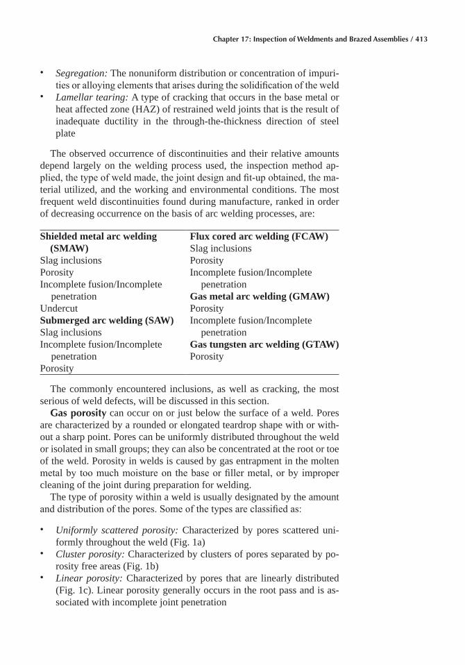
Chapter 17: Inspection of Weldments and Brazed Assemblies / 413
• Segregation: The nonuniform distribution or concentration of impuri-ties or alloying elements that arises during the solidification of the weld
• Lamellar tearing: A type of cracking that occurs in the base metal or heat affected zone (HAZ) of restrained weld joints that is the result of inadequate ductility in the through-the-thickness direction of steel plate
The observed occurrence of discontinuities and their relative amounts depend largely on the welding process used, the inspection method ap-plied, the type of weld made, the joint design and fit-up obtained, the ma-terial utilized, and the working and environmental conditions. The most frequent weld discontinuities found during manufacture, ranked in order of decreasing occurrence on the basis of arc welding processes, are:
Shielded metal arc welding (SMAW)Slag inclusionsPorosityIncomplete fusion/Incomplete
penetrationUndercutSubmerged arc welding (SAW)Slag inclusionsIncomplete fusion/Incomplete
penetrationPorosity
Flux cored arc welding (FCAW)Slag inclusionsPorosityIncomplete fusion/Incomplete
penetrationGas metal arc welding (GMAW)PorosityIncomplete fusion/Incomplete
penetrationGas tungsten arc welding (GTAW)Porosity
The commonly encountered inclusions, as well as cracking, the most serious of weld defects, will be discussed in this section.
Gas porosity can occur on or just below the surface of a weld. Pores are characterized by a rounded or elongated teardrop shape with or with-out a sharp point. Pores can be uniformly distributed throughout the weld or isolated in small groups; they can also be concentrated at the root or toe of the weld. Porosity in welds is caused by gas entrapment in the molten metal by too much moisture on the base or filler metal, or by improper cleaning of the joint during preparation for welding.
The type of porosity within a weld is usually designated by the amount and distribution of the pores. Some of the types are classified as:
• Uniformly scattered porosity: Characterized by pores scattered uni-formly throughout the weld (Fig. 1a)
• Cluster porosity: Characterized by clusters of pores separated by po-rosity free areas (Fig. 1b)
• Linear porosity: Characterized by pores that are linearly distributed (Fig. 1c). Linear porosity generally occurs in the root pass and is as-sociated with incomplete joint penetration
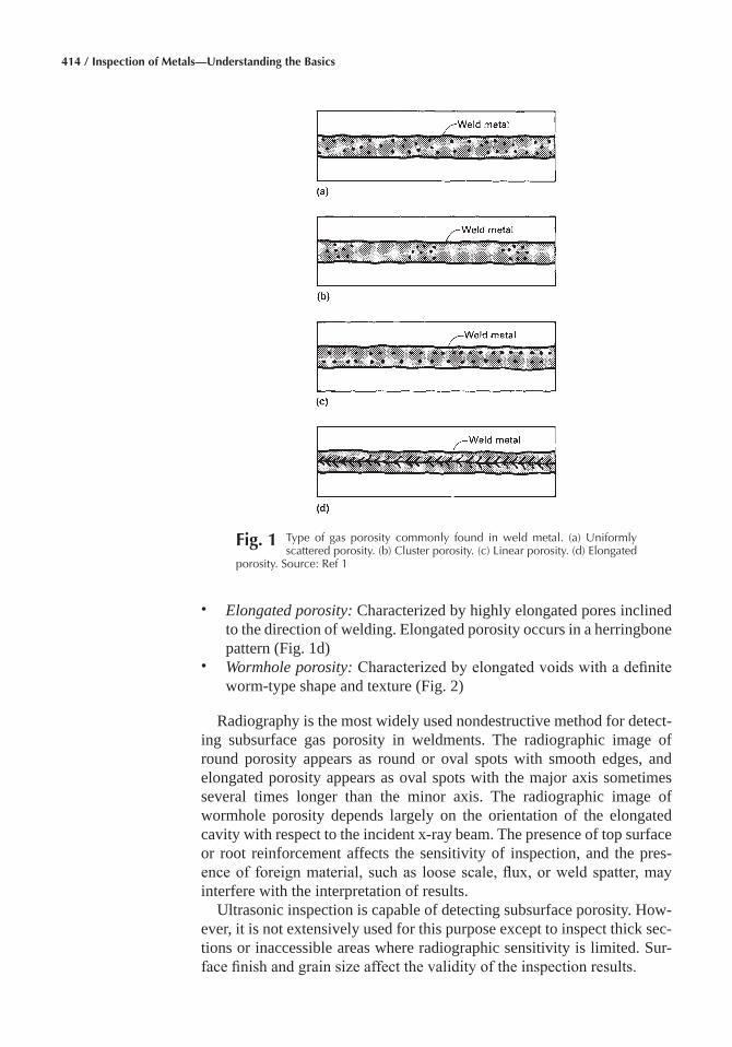
414 / Inspection of Metals—Understanding the Basics
• Elongated porosity: Characterized by highly elongated pores inclined to the direction of welding. Elongated porosity occurs in a herringbone pattern (Fig. 1d)
• Wormhole porosity: Characterized by elongated voids with a definite worm-type shape and texture (Fig. 2)
Radiography is the most widely used nondestructive method for detect-ing subsurface gas porosity in weldments. The radiographic image of round porosity appears as round or oval spots with smooth edges, and elongated porosity appears as oval spots with the major axis sometimes several times longer than the minor axis. The radiographic image of wormhole porosity depends largely on the orientation of the elongated cavity with respect to the incident x-ray beam. The presence of top surface or root reinforcement affects the sensitivity of inspection, and the pres-ence of foreign material, such as loose scale, flux, or weld spatter, may interfere with the interpretation of results.
Ultrasonic inspection is capable of detecting subsurface porosity. How-ever, it is not extensively used for this purpose except to inspect thick sec-tions or inaccessible areas where radiographic sensitivity is limited. Sur-face finish and grain size affect the validity of the inspection results.
Fig� 1 Type of gas porosity commonly found in weld metal. (a) Uniformly scattered porosity. (b) Cluster porosity. (c) Linear porosity. (d) Elongated
porosity. Source: Ref 1
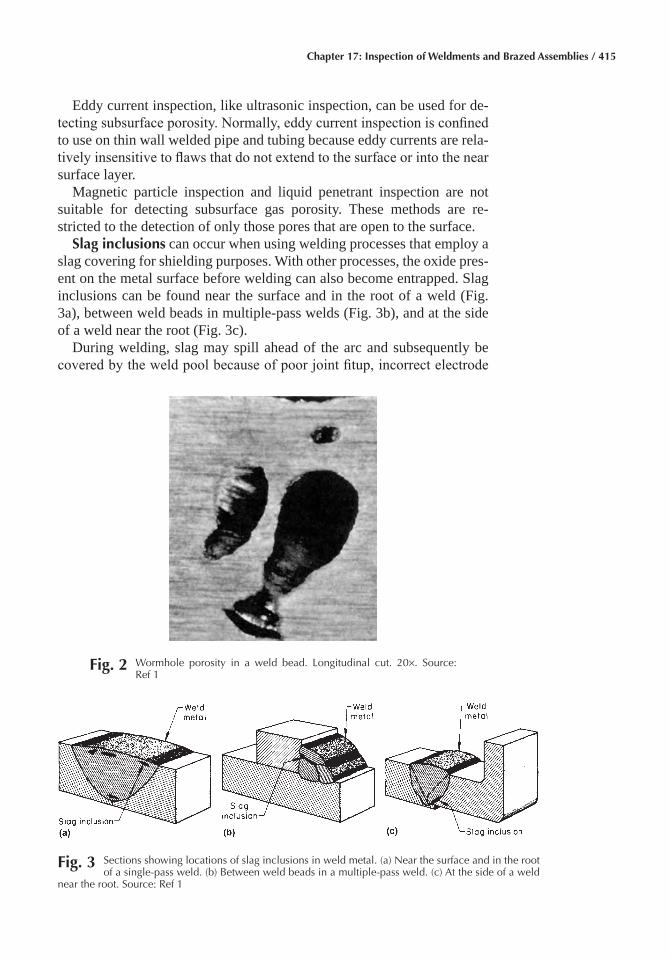
Chapter 17: Inspection of Weldments and Brazed Assemblies / 415
Eddy current inspection, like ultrasonic inspection, can be used for de-tecting subsurface porosity. Normally, eddy current inspection is confined to use on thin wall welded pipe and tubing because eddy currents are rela-tively insensitive to flaws that do not extend to the surface or into the near surface layer.
Magnetic particle inspection and liquid penetrant inspection are not suitable for detecting subsurface gas porosity. These methods are re-stricted to the detection of only those pores that are open to the surface.
Slag inclusions can occur when using welding processes that employ a slag covering for shielding purposes. With other processes, the oxide pres-ent on the metal surface before welding can also become entrapped. Slag inclusions can be found near the surface and in the root of a weld (Fig. 3a), between weld beads in multiple-pass welds (Fig. 3b), and at the side of a weld near the root (Fig. 3c).
During welding, slag may spill ahead of the arc and subsequently be covered by the weld pool because of poor joint fitup, incorrect electrode
Fig� 2 Wormhole porosity in a weld bead. Longitudinal cut. 20×. Source: Ref 1
Fig� 3 Sections showing locations of slag inclusions in weld metal. (a) Near the surface and in the root of a single-pass weld. (b) Between weld beads in a multiple-pass weld. (c) At the side of a weld
near the root. Source: Ref 1
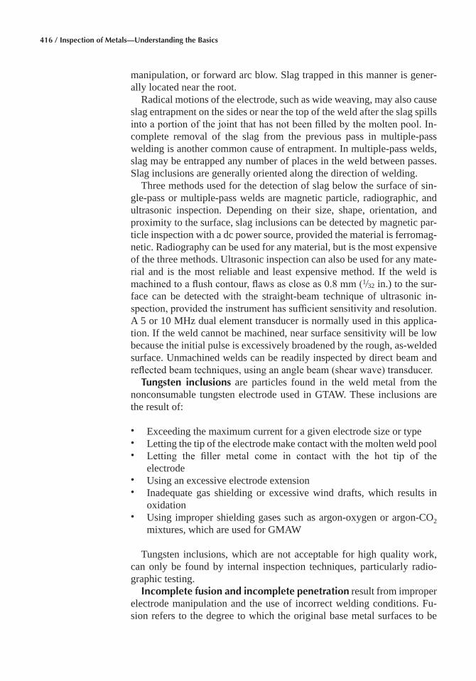
416 / Inspection of Metals—Understanding the Basics
manipulation, or forward arc blow. Slag trapped in this manner is gener-ally located near the root.
Radical motions of the electrode, such as wide weaving, may also cause slag entrapment on the sides or near the top of the weld after the slag spills into a portion of the joint that has not been filled by the molten pool. In-complete removal of the slag from the previous pass in multiple-pass welding is another common cause of entrapment. In multiple-pass welds, slag may be entrapped any number of places in the weld between passes. Slag inclusions are generally oriented along the direction of welding.
Three methods used for the detection of slag below the surface of sin-gle-pass or multiple-pass welds are magnetic particle, radiographic, and ultrasonic inspection. Depending on their size, shape, orientation, and proximity to the surface, slag inclusions can be detected by magnetic par-ticle inspection with a dc power source, provided the material is ferromag-netic. Radiography can be used for any material, but is the most expensive of the three methods. Ultrasonic inspection can also be used for any mate-rial and is the most reliable and least expensive method. If the weld is machined to a flush contour, flaws as close as 0.8 mm (1⁄32 in.) to the sur-face can be detected with the straight-beam technique of ultrasonic in-spection, provided the instrument has sufficient sensitivity and resolution. A 5 or 10 MHz dual element transducer is normally used in this applica-tion. If the weld cannot be machined, near surface sensitivity will be low because the initial pulse is excessively broadened by the rough, as-welded surface. Unmachined welds can be readily inspected by direct beam and reflected beam techniques, using an angle beam (shear wave) transducer.
Tungsten inclusions are particles found in the weld metal from the nonconsumable tungsten electrode used in GTAW. These inclusions are the result of:
• Exceeding the maximum current for a given electrode size or type• Letting the tip of the electrode make contact with the molten weld pool• Letting the filler metal come in contact with the hot tip of the
electrode• Using an excessive electrode extension• Inadequate gas shielding or excessive wind drafts, which results in
oxidation• Using improper shielding gases such as argon-oxygen or argon-CO2
mixtures, which are used for GMAW
Tungsten inclusions, which are not acceptable for high quality work, can only be found by internal inspection techniques, particularly radio-graphic testing.
Incomplete fusion and incomplete penetration result from improper electrode manipulation and the use of incorrect welding conditions. Fu-sion refers to the degree to which the original base metal surfaces to be
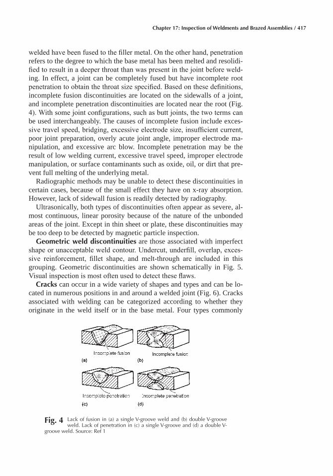
Chapter 17: Inspection of Weldments and Brazed Assemblies / 417
welded have been fused to the filler metal. On the other hand, penetration refers to the degree to which the base metal has been melted and resolidi-fied to result in a deeper throat than was present in the joint before weld-ing. In effect, a joint can be completely fused but have incomplete root penetration to obtain the throat size specified. Based on these definitions, incomplete fusion discontinuities are located on the sidewalls of a joint, and incomplete penetration discontinuities are located near the root (Fig. 4). With some joint configurations, such as butt joints, the two terms can be used interchangeably. The causes of incomplete fusion include exces-sive travel speed, bridging, excessive electrode size, insufficient current, poor joint preparation, overly acute joint angle, improper electrode ma-nipulation, and excessive arc blow. Incomplete penetration may be the result of low welding current, excessive travel speed, improper electrode manipulation, or surface contaminants such as oxide, oil, or dirt that pre-vent full melting of the underlying metal.
Radiographic methods may be unable to detect these discontinuities in certain cases, because of the small effect they have on x-ray absorption. However, lack of sidewall fusion is readily detected by radiography.
Ultrasonically, both types of discontinuities often appear as severe, al-most continuous, linear porosity because of the nature of the unbonded areas of the joint. Except in thin sheet or plate, these discontinuities may be too deep to be detected by magnetic particle inspection.
Geometric weld discontinuities are those associated with imperfect shape or unacceptable weld contour. Undercut, underfill, overlap, exces-sive reinforcement, fillet shape, and melt-through are included in this grouping. Geometric discontinuities are shown schematically in Fig. 5. Visual inspection is most often used to detect these flaws.
Cracks can occur in a wide variety of shapes and types and can be lo-cated in numerous positions in and around a welded joint (Fig. 6). Cracks associated with welding can be categorized according to whether they originate in the weld itself or in the base metal. Four types commonly
Fig� 4 Lack of fusion in (a) a single V-groove weld and (b) double V-groove weld. Lack of penetration in (c) a single V-groove and (d) a double V-
groove weld. Source: Ref 1
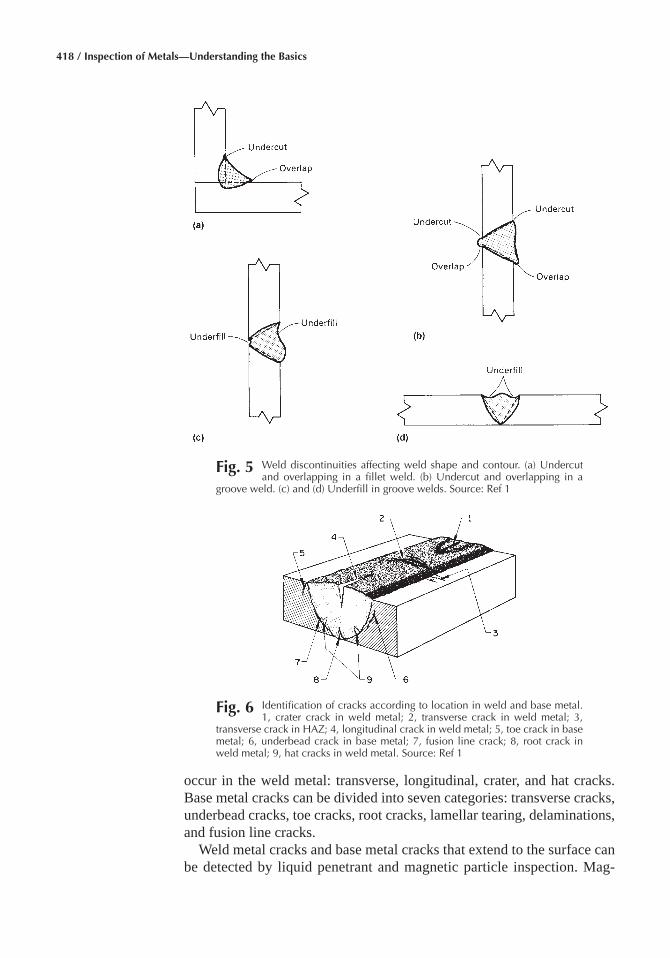
418 / Inspection of Metals—Understanding the Basics
occur in the weld metal: transverse, longitudinal, crater, and hat cracks. Base metal cracks can be divided into seven categories: transverse cracks, underbead cracks, toe cracks, root cracks, lamellar tearing, delaminations, and fusion line cracks.
Weld metal cracks and base metal cracks that extend to the surface can be detected by liquid penetrant and magnetic particle inspection. Mag-
Fig� 5 Weld discontinuities affecting weld shape and contour. (a) Undercut and overlapping in a fillet weld. (b) Undercut and overlapping in a
groove weld. (c) and (d) Underfill in groove welds. Source: Ref 1
Fig� 6 Identification of cracks according to location in weld and base metal. 1, crater crack in weld metal; 2, transverse crack in weld metal; 3,
transverse crack in HAZ; 4, longitudinal crack in weld metal; 5, toe crack in base metal; 6, underbead crack in base metal; 7, fusion line crack; 8, root crack in weld metal; 9, hat cracks in weld metal. Source: Ref 1
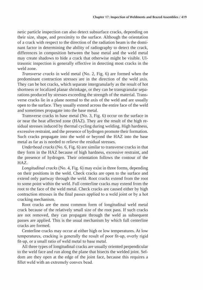
Chapter 17: Inspection of Weldments and Brazed Assemblies / 419
netic particle inspection can also detect subsurface cracks, depending on their size, shape, and proximity to the surface. Although the orientation of a crack with respect to the direction of the radiation beam is the domi-nant factor in determining the ability of radiography to detect the crack, differences in composition between the base metal and the weld metal may create shadows to hide a crack that otherwise might be visible. Ul-trasonic inspection is generally effective in detecting most cracks in the weld zone.
Transverse cracks in weld metal (No. 2, Fig. 6) are formed when the predominant contraction stresses are in the direction of the weld axis. They can be hot cracks, which separate intergranularly as the result of hot shortness or localized planar shrinkage, or they can be transgranular sepa-rations produced by stresses exceeding the strength of the material. Trans-verse cracks lie in a plane normal to the axis of the weld and are usually open to the surface. They usually extend across the entire face of the weld and sometimes propagate into the base metal.
Transverse cracks in base metal (No. 3, Fig. 6) occur on the surface in or near the heat affected zone (HAZ). They are the result of the high re-sidual stresses induced by thermal cycling during welding. High hardness, excessive restraint, and the presence of hydrogen promote their formation. Such cracks propagate into the weld or beyond the HAZ into the base metal as far as is needed to relieve the residual stresses.
Underbead cracks (No. 6, Fig. 6) are similar to transverse cracks in that they form in the HAZ because of high hardness, excessive restraint, and the presence of hydrogen. Their orientation follows the contour of the HAZ.
Longitudinal cracks (No. 4, Fig. 6) may exist in three forms, depending on their positions in the weld. Check cracks are open to the surface and extend only partway through the weld. Root cracks extend from the root to some point within the weld. Full centerline cracks may extend from the root to the face of the weld metal. Check cracks are caused either by high contraction stresses in the final passes applied to a weld joint or by a hot cracking mechanism.
Root cracks are the most common form of longitudinal weld metal crack because of the relatively small size of the root pass. If such cracks are not removed, they can propagate through the weld as subsequent passes are applied. This is the usual mechanism by which full centerline cracks are formed.
Centerline cracks may occur at either high or low temperatures. At low temperatures, cracking is generally the result of poor fit-up, overly rigid fit-up, or a small ratio of weld metal to base metal.
All three types of longitudinal cracks are usually oriented perpendicular to the weld face and run along the plane that bisects the welded joint. Sel-dom are they open at the edge of the joint face, because this requires a fillet weld with an extremely convex bead.
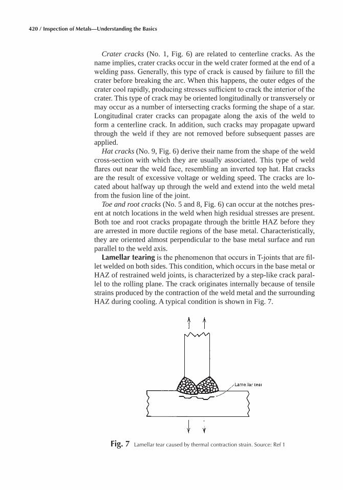
420 / Inspection of Metals—Understanding the Basics
Crater cracks (No. 1, Fig. 6) are related to centerline cracks. As the name implies, crater cracks occur in the weld crater formed at the end of a welding pass. Generally, this type of crack is caused by failure to fill the crater before breaking the arc. When this happens, the outer edges of the crater cool rapidly, producing stresses sufficient to crack the interior of the crater. This type of crack may be oriented longitudinally or transversely or may occur as a number of intersecting cracks forming the shape of a star. Longitudinal crater cracks can propagate along the axis of the weld to form a centerline crack. In addition, such cracks may propagate upward through the weld if they are not removed before subsequent passes are applied.
Hat cracks (No. 9, Fig. 6) derive their name from the shape of the weld cross-section with which they are usually associated. This type of weld flares out near the weld face, resembling an inverted top hat. Hat cracks are the result of excessive voltage or welding speed. The cracks are lo-cated about halfway up through the weld and extend into the weld metal from the fusion line of the joint.
Toe and root cracks (No. 5 and 8, Fig. 6) can occur at the notches pres-ent at notch locations in the weld when high residual stresses are present. Both toe and root cracks propagate through the brittle HAZ before they are arrested in more ductile regions of the base metal. Characteristically, they are oriented almost perpendicular to the base metal surface and run parallel to the weld axis.
Lamellar tearing is the phenomenon that occurs in T-joints that are fil-let welded on both sides. This condition, which occurs in the base metal or HAZ of restrained weld joints, is characterized by a step-like crack paral-lel to the rolling plane. The crack originates internally because of tensile strains produced by the contraction of the weld metal and the surrounding HAZ during cooling. A typical condition is shown in Fig. 7.
Fig� 7 Lamellar tear caused by thermal contraction strain. Source: Ref 1
Chapter 17: Inspection of Weldments and Brazed Assemblies / 421
Methods of Nondestructive Inspection
The nondestructive inspection of weldments has two functions:
• Quality control, which is the monitoring of welder and equipment per-formance and of the quality of the consumables and the base materials used
• Acceptance or rejection of a weld on the basis of its fitness for purpose under the service conditions imposed on the structure
The appropriate method of inspection is different for each function. If evaluating for discontinuities is a viable option they must be detected, identified, located exactly, sized, and their orientation established.
Weld discontinuities constitute the center of activity with the inspection of welded constructions. The most widely used inspection techniques used in the welding industry are visual, liquid penetrant, magnetic particle, ra-diographic, ultrasonic, acoustic emission, eddy current, and electric cur-rent perturbation methods. Each of these techniques has specific advan-tages and limitations. Existing codes and standards that provide guidelines for these various techniques are based on the capabilities and/or limita-tions of these nondestructive methods.
Selection of Technique� A number of factors influence selection of the appropriate nondestructive test technique for inspecting a welded struc-ture, including discontinuity characteristics, fracture mechanics require-ments, part size, portability of equipment, and other application con-straints. These categories, although perhaps unique to a specific inspection problem, may not clearly point the way to the most appropriate technique. It is generally necessary to exercise engineering judgment in ranking the importance of these criteria and thus determining the optimum inspection technique.
Characteristics of the Discontinuity� Because nondestructive tech-niques are based on physical phenomena, it is useful to describe the prop-erties of the discontinuity of interest, such as composition and electrical, magnetic, mechanical, and thermal properties. Most significant are those properties that are most different from those of the weld or base metal. It is also necessary to identify a means of discriminating between disconti-nuities with similar properties.
Fracture mechanics requirements, solely from a discontinuity view-point, typically include detection, identification, location, sizing, and ori-entation. In addition, complicated configurations may necessitate a nonde-structive assessment of the state of the stress of the region containing the discontinuity. In the selection process, it is important to establish these requirements correctly. This may involve consultation with stress ana-lysts, materials engineers, and statisticians. Often, the criteria may strongly suggest a particular technique. Under ideal conditions, such as in a labora-
422 / Inspection of Metals—Understanding the Basics
tory, the application of such a technique might be routine. In the field, however, other factors may force a different choice of technique.
Constraints tend to be unique to a given application and may be com-pletely different even when the welding process and metals are the same. Some of these constraints include:
• Access to the region under inspection• Geometry of the structure (flat, curved, thick, thin)• Condition of the surface (smooth, irregular)• Mode of inspection (pre-service, in-service, continuous, periodic, spot)• Environment (hostile, underwater)• Time available for inspection (high speed, time intensive)• Reliability• Application of multiple techniques• Cost
Failure to consider adequately the constraints imposed by a specific ap-plication can render the most sophisticated equipment and theory useless. Moreover, for the simple or less important cases of failure, it may be un-necessary. Once criteria have been established, an optimum inspection technique can be selected, or designed and constructed.
Visual Inspection
For many noncritical welds, integrity is verified principally by visual inspection. Even when other nondestructive methods are used, visual in-spection still constitutes an important part of practical quality control. Widely used to detect discontinuities, visual inspection is simple, quick, and relatively inexpensive. The only aids that might be used to determine the conformity of a weld are a low power magnifier, a borescope, a dental mirror, or a gage. Visual inspection can and should be done before, during, and after welding. Although visual inspection is the simplest inspection method to use, a definite procedure should be established to ensure that it is carried out accurately and uniformly.
Visual inspection is useful for checking the following:
• Dimensional accuracy of weldments• Conformity of welds to size and contour requirements• Acceptability of weld appearance with regard to surface roughness,
weld spatter, and cleanness• Presence of surface flaws such as unfilled craters, pockmarks, under-
cuts, overlaps, and cracks
Although visual inspection is an invaluable method, it is unreliable for detecting subsurface flaws. Therefore, judgment of weld quality must be based on information in addition to that afforded by surface indications.
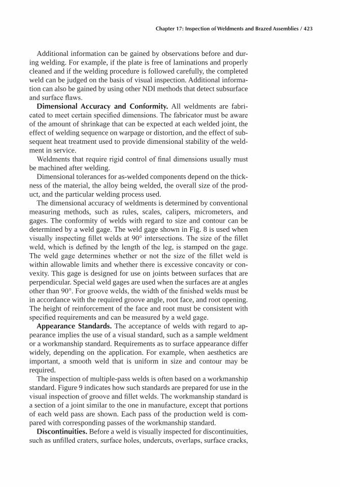
Chapter 17: Inspection of Weldments and Brazed Assemblies / 423
Additional information can be gained by observations before and dur-ing welding. For example, if the plate is free of laminations and properly cleaned and if the welding procedure is followed carefully, the completed weld can be judged on the basis of visual inspection. Additional informa-tion can also be gained by using other NDI methods that detect subsurface and surface flaws.
Dimensional Accuracy and Conformity� All weldments are fabri-cated to meet certain specified dimensions. The fabricator must be aware of the amount of shrinkage that can be expected at each welded joint, the effect of welding sequence on warpage or distortion, and the effect of sub-sequent heat treatment used to provide dimensional stability of the weld-ment in service.
Weldments that require rigid control of final dimensions usually must be machined after welding.
Dimensional tolerances for as-welded components depend on the thick-ness of the material, the alloy being welded, the overall size of the prod-uct, and the particular welding process used.
The dimensional accuracy of weldments is determined by conventional measuring methods, such as rules, scales, calipers, micrometers, and gages. The conformity of welds with regard to size and contour can be determined by a weld gage. The weld gage shown in Fig. 8 is used when visually inspecting fillet welds at 90° intersections. The size of the fillet weld, which is defined by the length of the leg, is stamped on the gage. The weld gage determines whether or not the size of the fillet weld is within allowable limits and whether there is excessive concavity or con-vexity. This gage is designed for use on joints between surfaces that are perpendicular. Special weld gages are used when the surfaces are at angles other than 90°. For groove welds, the width of the finished welds must be in accordance with the required groove angle, root face, and root opening. The height of reinforcement of the face and root must be consistent with specified requirements and can be measured by a weld gage.
Appearance Standards� The acceptance of welds with regard to ap-pearance implies the use of a visual standard, such as a sample weldment or a workmanship standard. Requirements as to surface appearance differ widely, depending on the application. For example, when aesthetics are important, a smooth weld that is uniform in size and contour may be required.
The inspection of multiple-pass welds is often based on a workmanship standard. Figure 9 indicates how such standards are prepared for use in the visual inspection of groove and fillet welds. The workmanship standard is a section of a joint similar to the one in manufacture, except that portions of each weld pass are shown. Each pass of the production weld is com-pared with corresponding passes of the workmanship standard.
Discontinuities� Before a weld is visually inspected for discontinuities, such as unfilled craters, surface holes, undercuts, overlaps, surface cracks,
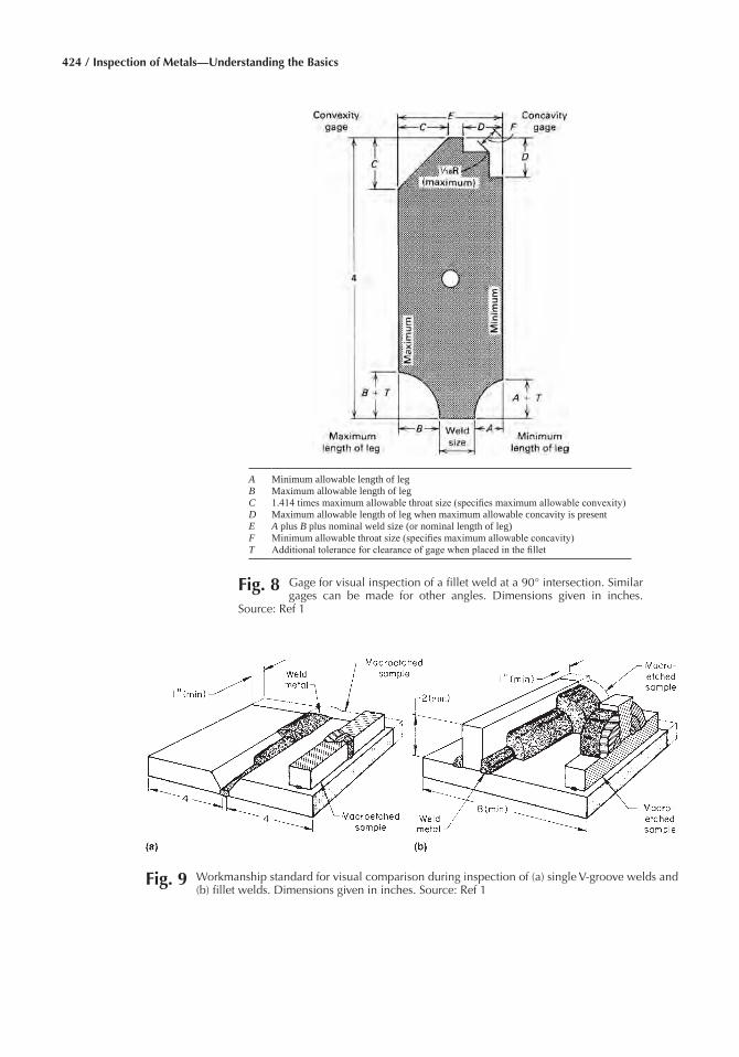
424 / Inspection of Metals—Understanding the Basics
Fig� 9 Workmanship standard for visual comparison during inspection of (a) single V-groove welds and (b) fillet welds. Dimensions given in inches. Source: Ref 1
Fig� 8 Gage for visual inspection of a fillet weld at a 90° intersection. Similar gages can be made for other angles. Dimensions given in inches.
Source: Ref 1
A Minimum allowable length of legB Maximum allowable length of legC 1.414 times maximum allowable throat size (specifies maximum allowable convexity)D Maximum allowable length of leg when maximum allowable concavity is presentE A plus B plus nominal weld size (or nominal length of leg)F Minimum allowable throat size (specifies maximum allowable concavity)T Additional tolerance for clearance of gage when placed in the fillet
Chapter 17: Inspection of Weldments and Brazed Assemblies / 425
and incomplete joint penetration, the surface of the weld should be cleaned of oxides and slag. Cleaning must be done carefully. For example, a chip-ping hammer used to remove slag could leave hammer marks that can hide fine cracks. Shot blasting can peen the surface of relatively soft metals and hide flaws. A stiff wire brush and sandblasting have been found to be satis-factory for cleaning surfaces of slag and oxides without marring.
Magnetic Particle Inspection
Magnetic particle inspection is particularly suitable for the detection of surface flaws in highly ferromagnetic metals. Under favorable conditions, those discontinuities that lie immediately under the surface are also de-tectable. Nonferromagnetic and weakly ferromagnetic metals, which can-not be strongly magnetized, cannot be inspected by this method. With suitable ferromagnetic metals, magnetic particle inspection is highly sen-sitive and produces readily discernible indications at flaws in the surface of the material being inspected.
The types of weld discontinuities normally detected by magnetic parti-cle inspection include cracks, incomplete penetration, incomplete fusion, and porosity open to the surface. Linear porosity, slag inclusions, and gas pockets can be detected if large or extensive or if smaller and near the surface. The recognition of patterns that indicate deep-lying flaws requires more experience than that required to detect surface flaws.
Nonrelevant indications that have no bearing on the quality of the weldment may be produced. These indications are magnetic particle pat-terns held by conditions caused by leakage fields. Some of these condi-tions are:
• Particles held mechanically or by gravity in surface irregularities• Adherent scale or slag• Indications at a sharp change in material direction, such as sharp fillets
and threads• Grain boundaries. Large grain sizes in the weld metal or the base metal
may produce indications• Boundary zones in welds, such as indications produced at the junction
of the weld metal and the base metal. This condition occurs in fillet welds at T-joints, or in double V-groove joints, where 100% penetra-tion is not required
• Flow lines in forgings and formed parts• Brazed joints. Two parts made of a ferromagnetic material joined by a
nonferromagnetic material will produce an indication• Different degrees of hardness in a material, which will usually have
different permeabilities that may create a leakage field, forming indi- cations
426 / Inspection of Metals—Understanding the Basics
Operational Requirements� The magnetic particle inspection of weld-ments requires that the weld bead be free of scale, slag, and moisture. For maximum sensitivity, the weld bead should be machined flush with the surface; however, wire brushing, sandblasting, or grit blasting usually pro-duces a satisfactory bead surface. If the weld bead is rough, grinding will remove the high spots.
Weldments are often inspected using the dry particle method. A powder or paste of a color that gives the best possible contrast to the surface being inspected should be used. The type of magnetizing current used depends on whether there are surface or subsurface discontinuities. Alternating current is satisfactory for surface cracks, but if the deepest possible pene-tration is essential, direct current, direct current with surge, or half-wave rectified alternating current is used.
The voltage should be as low as practical to reduce the possibility of damage to the surface of the part from overheating or arcing at contacts. Another advantage of low voltage is freedom from arc flashes if a prod slips or is withdrawn before the current is turned off.
The field strength and flux density used must be determined for each type of weldment. An overly strong field will cause the magnetic particles to adhere too tightly to the surface and hinder their mobility, preventing them from moving to the sites of the flaws. Low field strengths result in nondiscernible patterns and failure to detect indications.
Inspections can be made using the continuous-field and residual-field methods. In the continuous-field method, magnetic particles are placed on the weldment while the current is flowing. In the residual-field method, the particles are placed on the weldment after the magnetizing current is turned off. Residual magnetic fields are weaker than continuous fields. Conse-quently, inspections using the residual-field method are less sensitive.
The need for the demagnetization of weldments after magnetic particle inspection must be given serious consideration. Where subsequent weld-ing or machining operations are required, it is good practice to demagne-tize. Residual magnetism may also hinder cleaning operations and inter-fere with the performance of instruments used near the weldment.
Liquid Penetrant Inspection
Liquid penetrant inspection is capable of detecting discontinuities open to the surface in weldments made of either ferromagnetic or nonferromag-netic alloys, even when the flaws are generally not visible to the unaided eye. For the correct usage of liquid penetrant inspection, it is essential that the surface of the part be thoroughly clean, leaving the openings free to receive the penetrant. Operating temperatures of 20 to 30 °C (70 to 90 °F) produce optimum results. If the part is cold, the penetrant may become chilled and thickened so that it cannot enter very fine openings. If the part
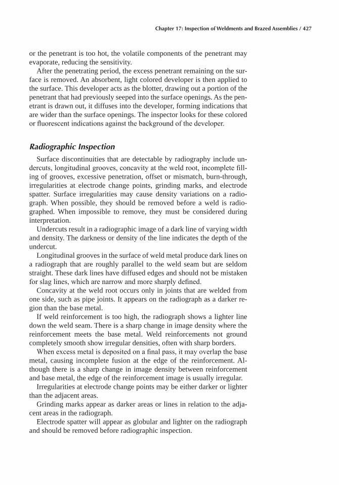
Chapter 17: Inspection of Weldments and Brazed Assemblies / 427
or the penetrant is too hot, the volatile components of the penetrant may evaporate, reducing the sensitivity.
After the penetrating period, the excess penetrant remaining on the sur-face is removed. An absorbent, light colored developer is then applied to the surface. This developer acts as the blotter, drawing out a portion of the penetrant that had previously seeped into the surface openings. As the pen-etrant is drawn out, it diffuses into the developer, forming indications that are wider than the surface openings. The inspector looks for these colored or fluorescent indications against the background of the developer.
Radiographic Inspection
Surface discontinuities that are detectable by radiography include un-dercuts, longitudinal grooves, concavity at the weld root, incomplete fill-ing of grooves, excessive penetration, offset or mismatch, burn-through, irregularities at electrode change points, grinding marks, and electrode spatter. Surface irregularities may cause density variations on a radio-graph. When possible, they should be removed before a weld is radio-graphed. When impossible to remove, they must be considered during interpretation.
Undercuts result in a radiographic image of a dark line of varying width and density. The darkness or density of the line indicates the depth of the undercut.
Longitudinal grooves in the surface of weld metal produce dark lines on a radiograph that are roughly parallel to the weld seam but are seldom straight. These dark lines have diffused edges and should not be mistaken for slag lines, which are narrow and more sharply defined.
Concavity at the weld root occurs only in joints that are welded from one side, such as pipe joints. It appears on the radiograph as a darker re-gion than the base metal.
If weld reinforcement is too high, the radiograph shows a lighter line down the weld seam. There is a sharp change in image density where the reinforcement meets the base metal. Weld reinforcements not ground completely smooth show irregular densities, often with sharp borders.
When excess metal is deposited on a final pass, it may overlap the base metal, causing incomplete fusion at the edge of the reinforcement. Al-though there is a sharp change in image density between reinforcement and base metal, the edge of the reinforcement image is usually irregular.
Irregularities at electrode change points may be either darker or lighter than the adjacent areas.
Grinding marks appear as darker areas or lines in relation to the adja-cent areas in the radiograph.
Electrode spatter will appear as globular and lighter on the radiograph and should be removed before radiographic inspection.
428 / Inspection of Metals—Understanding the Basics
As material thickness increases, radiography becomes less sensitive as an inspection method. Thus, for thick material, other NDI methods are used before, during, and after welding on both the base metal and weld metal.
Subsurface discontinuities detectable by radiography include gas po-rosity, slag inclusions, cracks, incomplete penetration, incomplete fusion, and tungsten inclusions. On a radiograph, a pore appears as a round or oval dark spot with or without a rather sharp tail. The spots caused by po-rosity are often of varying size and distribution. A wormhole appears as a dark rectangle if its long axis is perpendicular to the radiation beam, and it appears as two concentric circles, one darker than the other, if the long axis is parallel to the beam. Linear porosity is recorded on radiographs as a series of round dark spots along a line parallel to the direction of welding.
Slag inclusions appear along the edge of a weld as irregular or continu-ous dark lines on the radiograph. Voids are sometimes present between weld beads because of irregular deposition of metal during multiple-pass welding. These voids have a radiographic appearance that resembles slag lines.
The radiographic image of a crack is a dark narrow line that is generally irregular. If the plane of the crack is in line with the radiation beam, its image is a fairly distinct line. If the plane is not exactly in line with the radiation beam, a faint dark linear shadow results. In this case, additional radiographs should be taken at other angles.
Incomplete penetration shows on a radiograph as a very narrow dark line near the center of the weld. The narrowness can be caused by drawing together of the plates being welded, and the incomplete penetration may be very severe. Slag inclusions and gas holes are sometimes found in con-nection with incomplete penetration and cause the line to appear broad and irregular.
The radiographic image of incomplete fusion shows a very thin, straight dark line parallel to and on one side of the weld image. Where there is doubt, additional radiographs should be made with the radiation beam parallel to the bevel face. This will increase the possibility of the incom-plete fusion appearing on the radiograph.
Tungsten inclusions appear either as single light spots or as clusters of small light spots. The spots are usually irregular in shape, but sometimes a rectangular light spot will appear.
Real-time radiography, which involves the display of radiographic images on television monitors through the use of an image converter and a television camera, is a rapidly developing method for weld inspection. One of the main advantages of real-time radiography for weld inspection is the cost savings that results from reducing the use of x-ray films. How-ever, the possibility of expanding such an inspection system to include automatic defect evaluation by the image processing system can yield sig-
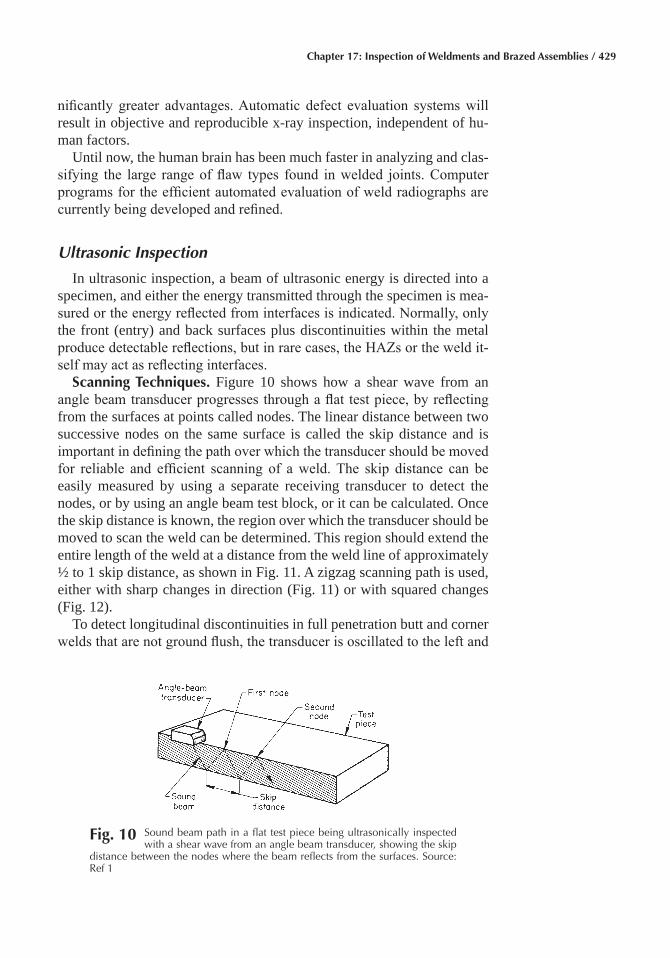
Chapter 17: Inspection of Weldments and Brazed Assemblies / 429
nificantly greater advantages. Automatic defect evaluation systems will result in objective and reproducible x-ray inspection, independent of hu- man factors.
Until now, the human brain has been much faster in analyzing and clas-sifying the large range of flaw types found in welded joints. Computer programs for the efficient automated evaluation of weld radiographs are currently being developed and refined.
Ultrasonic Inspection
In ultrasonic inspection, a beam of ultrasonic energy is directed into a specimen, and either the energy transmitted through the specimen is mea-sured or the energy reflected from interfaces is indicated. Normally, only the front (entry) and back surfaces plus discontinuities within the metal produce detectable reflections, but in rare cases, the HAZs or the weld it-self may act as reflecting interfaces.
Scanning Techniques� Figure 10 shows how a shear wave from an angle beam transducer progresses through a flat test piece, by reflecting from the surfaces at points called nodes. The linear distance between two successive nodes on the same surface is called the skip distance and is important in defining the path over which the transducer should be moved for reliable and efficient scanning of a weld. The skip distance can be easily measured by using a separate receiving transducer to detect the nodes, or by using an angle beam test block, or it can be calculated. Once the skip distance is known, the region over which the transducer should be moved to scan the weld can be determined. This region should extend the entire length of the weld at a distance from the weld line of approximately ½ to 1 skip distance, as shown in Fig. 11. A zigzag scanning path is used, either with sharp changes in direction (Fig. 11) or with squared changes (Fig. 12).
To detect longitudinal discontinuities in full penetration butt and corner welds that are not ground flush, the transducer is oscillated to the left and
Fig� 10 Sound beam path in a flat test piece being ultrasonically inspected with a shear wave from an angle beam transducer, showing the skip
distance between the nodes where the beam reflects from the surfaces. Source: Ref 1
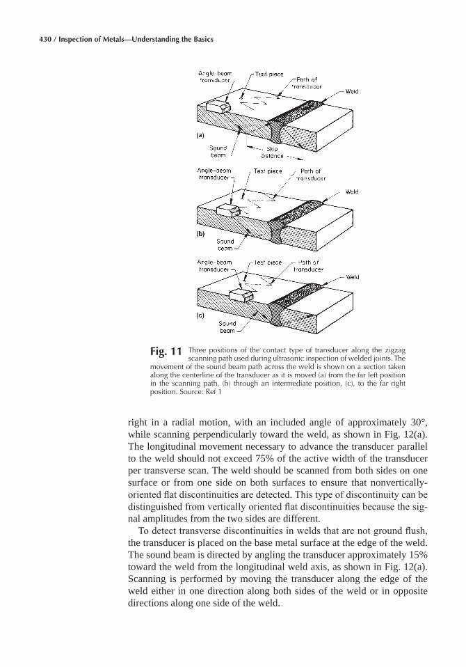
430 / Inspection of Metals—Understanding the Basics
right in a radial motion, with an included angle of approximately 30°, while scanning perpendicularly toward the weld, as shown in Fig. 12(a). The longitudinal movement necessary to advance the transducer parallel to the weld should not exceed 75% of the active width of the transducer per transverse scan. The weld should be scanned from both sides on one surface or from one side on both surfaces to ensure that nonvertically-oriented flat discontinuities are detected. This type of discontinuity can be distinguished from vertically oriented flat discontinuities because the sig-nal amplitudes from the two sides are different.
To detect transverse discontinuities in welds that are not ground flush, the transducer is placed on the base metal surface at the edge of the weld. The sound beam is directed by angling the transducer approximately 15% toward the weld from the longitudinal weld axis, as shown in Fig. 12(a). Scanning is performed by moving the transducer along the edge of the weld either in one direction along both sides of the weld or in opposite directions along one side of the weld.
Fig� 11 Three positions of the contact type of transducer along the zigzag scanning path used during ultrasonic inspection of welded joints. The
movement of the sound beam path across the weld is shown on a section taken along the centerline of the transducer as it is moved (a) from the far left position in the scanning path, (b) through an intermediate position, (c), to the far right position. Source: Ref 1
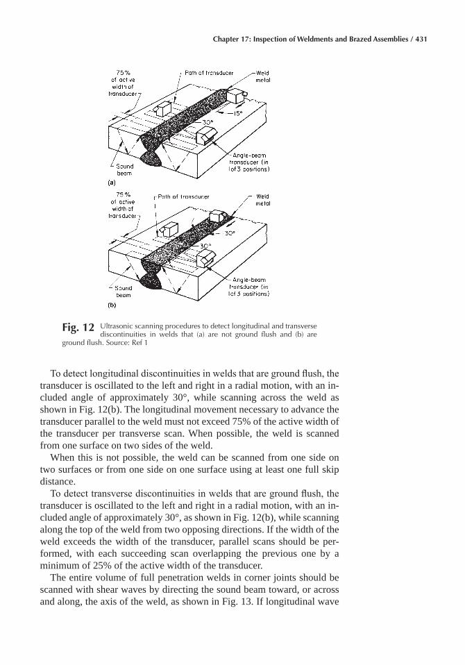
Chapter 17: Inspection of Weldments and Brazed Assemblies / 431
To detect longitudinal discontinuities in welds that are ground flush, the transducer is oscillated to the left and right in a radial motion, with an in-cluded angle of approximately 30°, while scanning across the weld as shown in Fig. 12(b). The longitudinal movement necessary to advance the transducer parallel to the weld must not exceed 75% of the active width of the transducer per transverse scan. When possible, the weld is scanned from one surface on two sides of the weld.
When this is not possible, the weld can be scanned from one side on two surfaces or from one side on one surface using at least one full skip distance.
To detect transverse discontinuities in welds that are ground flush, the transducer is oscillated to the left and right in a radial motion, with an in-cluded angle of approximately 30°, as shown in Fig. 12(b), while scanning along the top of the weld from two opposing directions. If the width of the weld exceeds the width of the transducer, parallel scans should be per-formed, with each succeeding scan overlapping the previous one by a minimum of 25% of the active width of the transducer.
The entire volume of full penetration welds in corner joints should be scanned with shear waves by directing the sound beam toward, or across and along, the axis of the weld, as shown in Fig. 13. If longitudinal wave
Fig� 12 Ultrasonic scanning procedures to detect longitudinal and transverse discontinuities in welds that (a) are not ground flush and (b) are
ground flush. Source: Ref 1
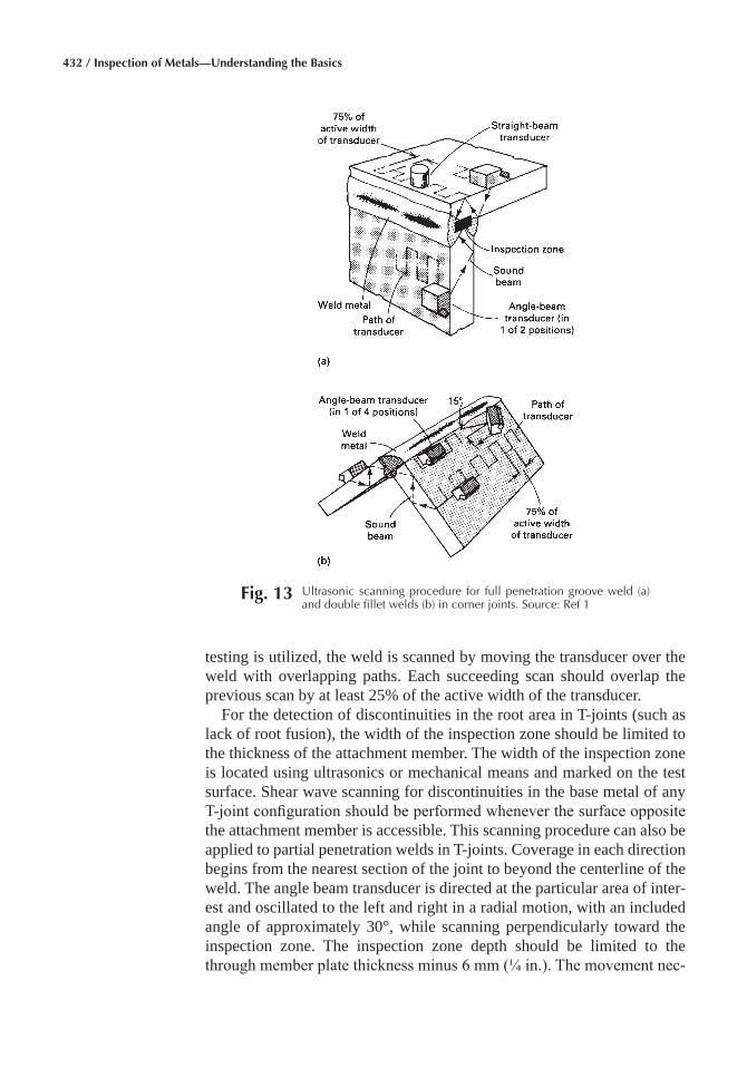
432 / Inspection of Metals—Understanding the Basics
testing is utilized, the weld is scanned by moving the transducer over the weld with overlapping paths. Each succeeding scan should overlap the previous scan by at least 25% of the active width of the transducer.
For the detection of discontinuities in the root area in T-joints (such as lack of root fusion), the width of the inspection zone should be limited to the thickness of the attachment member. The width of the inspection zone is located using ultrasonics or mechanical means and marked on the test surface. Shear wave scanning for discontinuities in the base metal of any T-joint configuration should be performed whenever the surface opposite the attachment member is accessible. This scanning procedure can also be applied to partial penetration welds in T-joints. Coverage in each direction begins from the nearest section of the joint to beyond the centerline of the weld. The angle beam transducer is directed at the particular area of inter-est and oscillated to the left and right in a radial motion, with an included angle of approximately 30°, while scanning perpendicularly toward the inspection zone. The inspection zone depth should be limited to the through member plate thickness minus 6 mm (¼ in.). The movement nec-
Fig� 13 Ultrasonic scanning procedure for full penetration groove weld (a) and double fillet welds (b) in corner joints. Source: Ref 1
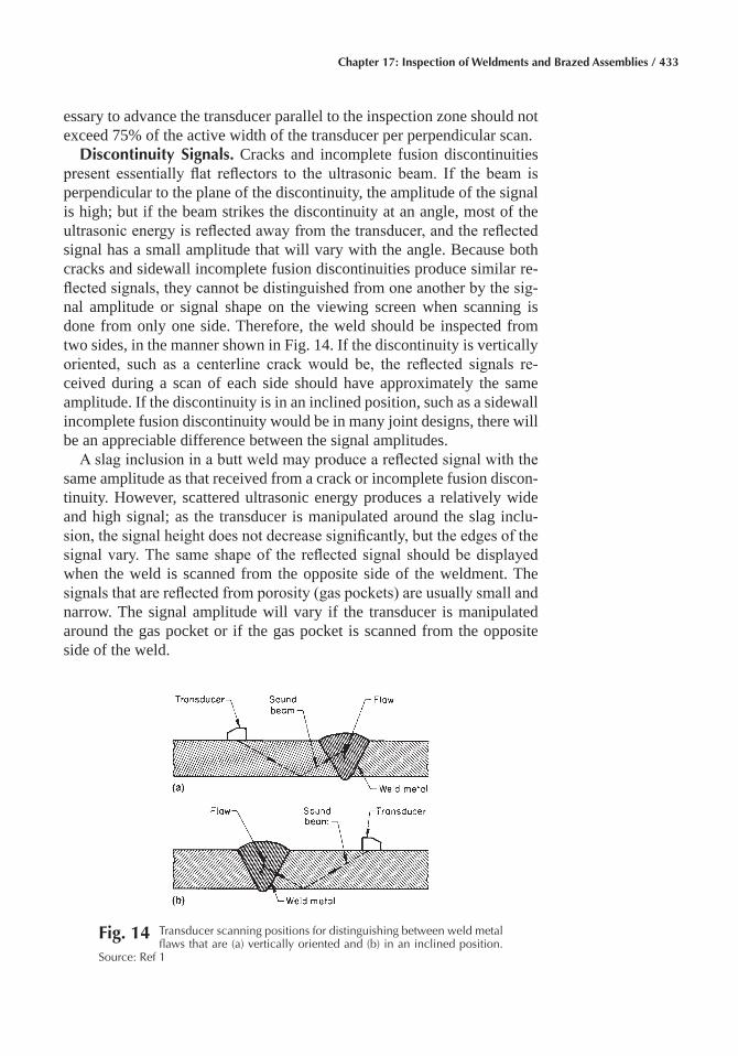
Chapter 17: Inspection of Weldments and Brazed Assemblies / 433
essary to advance the transducer parallel to the inspection zone should not exceed 75% of the active width of the transducer per perpendicular scan.
Discontinuity Signals� Cracks and incomplete fusion discontinuities present essentially flat reflectors to the ultrasonic beam. If the beam is perpendicular to the plane of the discontinuity, the amplitude of the signal is high; but if the beam strikes the discontinuity at an angle, most of the ultrasonic energy is reflected away from the transducer, and the reflected signal has a small amplitude that will vary with the angle. Because both cracks and sidewall incomplete fusion discontinuities produce similar re-flected signals, they cannot be distinguished from one another by the sig-nal amplitude or signal shape on the viewing screen when scanning is done from only one side. Therefore, the weld should be inspected from two sides, in the manner shown in Fig. 14. If the discontinuity is vertically oriented, such as a centerline crack would be, the reflected signals re-ceived during a scan of each side should have approximately the same amplitude. If the discontinuity is in an inclined position, such as a sidewall incomplete fusion discontinuity would be in many joint designs, there will be an appreciable difference between the signal amplitudes.
A slag inclusion in a butt weld may produce a reflected signal with the same amplitude as that received from a crack or incomplete fusion discon-tinuity. However, scattered ultrasonic energy produces a relatively wide and high signal; as the transducer is manipulated around the slag inclu-sion, the signal height does not decrease significantly, but the edges of the signal vary. The same shape of the reflected signal should be displayed when the weld is scanned from the opposite side of the weldment. The signals that are reflected from porosity (gas pockets) are usually small and narrow. The signal amplitude will vary if the transducer is manipulated around the gas pocket or if the gas pocket is scanned from the opposite side of the weld.
Fig� 14 Transducer scanning positions for distinguishing between weld metal flaws that are (a) vertically oriented and (b) in an inclined position.
Source: Ref 1
434 / Inspection of Metals—Understanding the Basics
Cluster porosity (groups of gas pockets) usually produces displays with a number of small signals. Depending on the number of gas pockets and their orientation to the ultrasonic beam, the displayed signals will be sta-tionary or will be connected with one another.
Lack of fusion, weld root cracks, and incomplete penetration give es-sentially the same type of signal on an oscilloscope screen; the reflected signals are narrow and appear at the same location. The best way to dif-ferentiate among these flaws is to determine the extent of the flaw in the transverse direction.
Weld undercutting is distinguishable from sidewall incomplete fusion. The signals reflected from undercutting are approximately equal in ampli-tude when scanned from both sides. The signals produced by a sidewall incomplete fusion discontinuity vary considerably in amplitude when scanned from both sides.
In many cases, a weld is made when two misaligned parts must be joined; this condition is termed weld mismatch. The inspector must not confuse a signal reflected from a root crack with one reflected from the misaligned edge. A narrow signal is usually produced when the ultrasonic beam strikes the misaligned edge. In most cases, no reflected signal will be received if the misaligned edge is scanned from the opposite side.
Ultrasonic Inspection of Spot Welds in Thin Gage Steel� With the development of high frequency transducers (12 to 20 MHz), the pulse echo ultrasonic inspection of spot welds in very thin gage sheet metal (0.58 mm, or 0.023 in.) is now possible. The ultrasonic test for spot weld nugget integrity relies on an ultrasonic wave to measure the size of the nugget. The size is in three dimensions, including thickness as well as length and breadth (or diameter for a circular spot). The successful mea-surement of nugget size places several requirements on the ultrasonic wave path, wave velocity, and wave attenuation.
Wave Path� The first requirement is that the ultrasonic wave be in the form of a beam directed perpendicular to the faces of the metal sheets and through the center of the nugget (Fig. 15). Two diameters of nuggets are shown: larger than the beam and smaller than the beam.
In general, an ultrasonic wave will be reflected when it impinges on an interface where the density and/or the ultrasonic velocity change. Exam-ples are water-to-metal and metal-to-air. In Fig. 15, reflections will occur at the outer surfaces of the two sheets and at the interface (air) between the two sheets if the nugget is small, as in Fig. 15(c). The nugget-to-parent metal boundary will not produce perceptible reflections, refraction, or scattering, because the changes in density and velocity are a tenth of a percent or less, while the air-to-steel difference is more than 99.9%. Typi-cal oscilloscope displays showing the pulse echo patterns for these two nugget-to-beam diameter ratios are shown in Fig. 15(b) and 15(d). The difference in the echo patterns permits the distinction to be made between adequate and undersize welds.
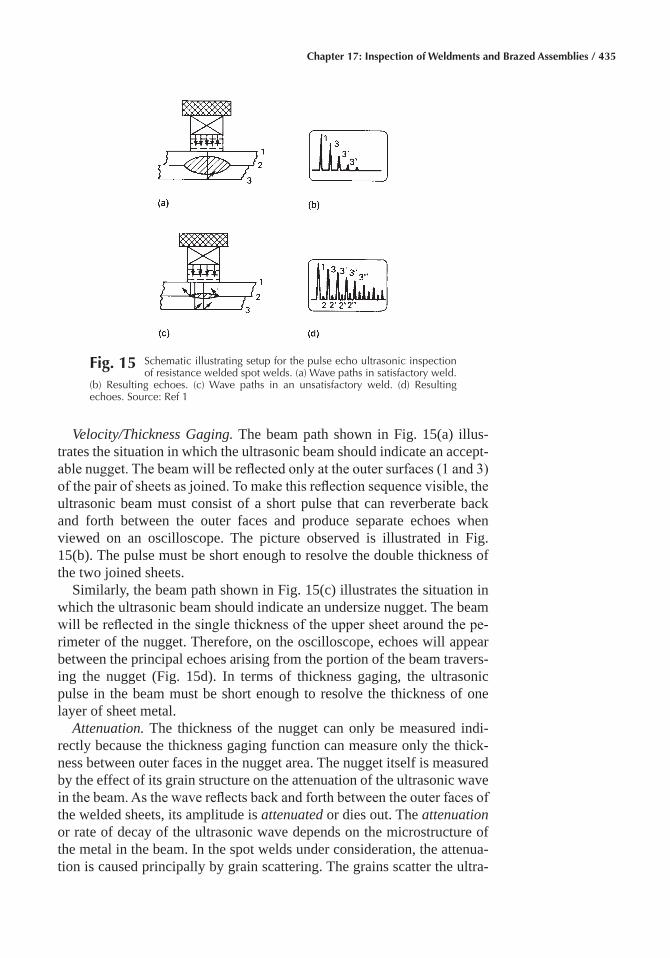
Chapter 17: Inspection of Weldments and Brazed Assemblies / 435
Velocity/Thickness Gaging. The beam path shown in Fig. 15(a) illus-trates the situation in which the ultrasonic beam should indicate an accept-able nugget. The beam will be reflected only at the outer surfaces (1 and 3) of the pair of sheets as joined. To make this reflection sequence visible, the ultrasonic beam must consist of a short pulse that can reverberate back and forth between the outer faces and produce separate echoes when viewed on an oscilloscope. The picture observed is illustrated in Fig. 15(b). The pulse must be short enough to resolve the double thickness of the two joined sheets.
Similarly, the beam path shown in Fig. 15(c) illustrates the situation in which the ultrasonic beam should indicate an undersize nugget. The beam will be reflected in the single thickness of the upper sheet around the pe-rimeter of the nugget. Therefore, on the oscilloscope, echoes will appear between the principal echoes arising from the portion of the beam travers-ing the nugget (Fig. 15d). In terms of thickness gaging, the ultrasonic pulse in the beam must be short enough to resolve the thickness of one layer of sheet metal.
Attenuation. The thickness of the nugget can only be measured indi-rectly because the thickness gaging function can measure only the thick-ness between outer faces in the nugget area. The nugget itself is measured by the effect of its grain structure on the attenuation of the ultrasonic wave in the beam. As the wave reflects back and forth between the outer faces of the welded sheets, its amplitude is attenuated or dies out. The attenuation or rate of decay of the ultrasonic wave depends on the microstructure of the metal in the beam. In the spot welds under consideration, the attenua-tion is caused principally by grain scattering. The grains scatter the ultra-
Fig� 15 Schematic illustrating setup for the pulse echo ultrasonic inspection of resistance welded spot welds. (a) Wave paths in satisfactory weld.
(b) Resulting echoes. (c) Wave paths in an unsatisfactory weld. (d) Resulting echoes. Source: Ref 1
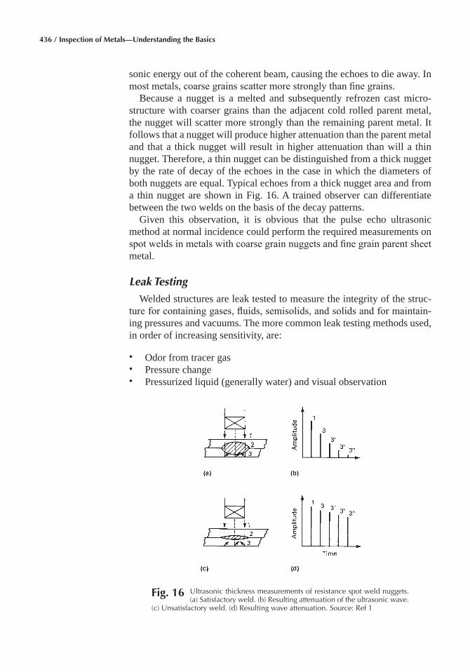
436 / Inspection of Metals—Understanding the Basics
sonic energy out of the coherent beam, causing the echoes to die away. In most metals, coarse grains scatter more strongly than fine grains.
Because a nugget is a melted and subsequently refrozen cast micro-structure with coarser grains than the adjacent cold rolled parent metal, the nugget will scatter more strongly than the remaining parent metal. It follows that a nugget will produce higher attenuation than the parent metal and that a thick nugget will result in higher attenuation than will a thin nugget. Therefore, a thin nugget can be distinguished from a thick nugget by the rate of decay of the echoes in the case in which the diameters of both nuggets are equal. Typical echoes from a thick nugget area and from a thin nugget are shown in Fig. 16. A trained observer can differentiate between the two welds on the basis of the decay patterns.
Given this observation, it is obvious that the pulse echo ultrasonic method at normal incidence could perform the required measurements on spot welds in metals with coarse grain nuggets and fine grain parent sheet metal.
Leak Testing
Welded structures are leak tested to measure the integrity of the struc-ture for containing gases, fluids, semisolids, and solids and for maintain-ing pressures and vacuums. The more common leak testing methods used, in order of increasing sensitivity, are:
• Odor from tracer gas• Pressure change• Pressurized liquid (generally water) and visual observation
Fig� 16 Ultrasonic thickness measurements of resistance spot weld nuggets. (a) Satisfactory weld. (b) Resulting attenuation of the ultrasonic wave.
(c) Unsatisfactory weld. (d) Resulting wave attenuation. Source: Ref 1
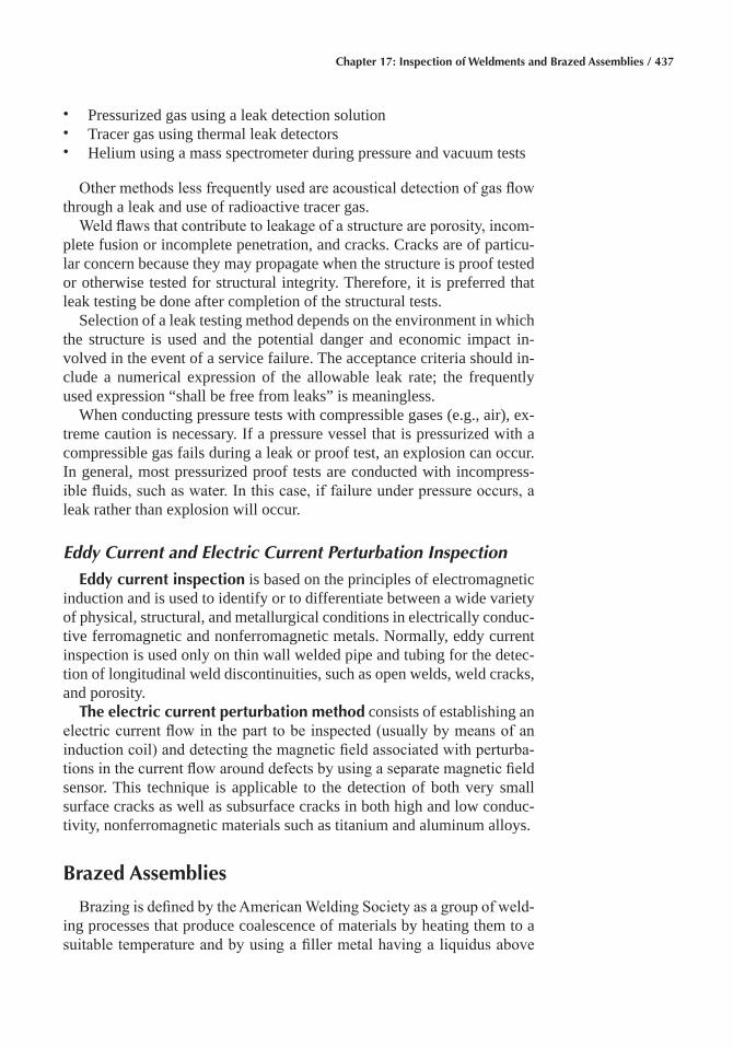
Chapter 17: Inspection of Weldments and Brazed Assemblies / 437
• Pressurized gas using a leak detection solution• Tracer gas using thermal leak detectors• Helium using a mass spectrometer during pressure and vacuum tests
Other methods less frequently used are acoustical detection of gas flow through a leak and use of radioactive tracer gas.
Weld flaws that contribute to leakage of a structure are porosity, incom-plete fusion or incomplete penetration, and cracks. Cracks are of particu-lar concern because they may propagate when the structure is proof tested or otherwise tested for structural integrity. Therefore, it is preferred that leak testing be done after completion of the structural tests.
Selection of a leak testing method depends on the environment in which the structure is used and the potential danger and economic impact in-volved in the event of a service failure. The acceptance criteria should in-clude a numerical expression of the allowable leak rate; the frequently used expression “shall be free from leaks” is meaningless.
When conducting pressure tests with compressible gases (e.g., air), ex-treme caution is necessary. If a pressure vessel that is pressurized with a compressible gas fails during a leak or proof test, an explosion can occur. In general, most pressurized proof tests are conducted with incompress-ible fluids, such as water. In this case, if failure under pressure occurs, a leak rather than explosion will occur.
Eddy Current and Electric Current Perturbation Inspection
Eddy current inspection is based on the principles of electromagnetic induction and is used to identify or to differentiate between a wide variety of physical, structural, and metallurgical conditions in electrically conduc-tive ferromagnetic and nonferromagnetic metals. Normally, eddy current inspection is used only on thin wall welded pipe and tubing for the detec-tion of longitudinal weld discontinuities, such as open welds, weld cracks, and porosity.
The electric current perturbation method consists of establishing an electric current flow in the part to be inspected (usually by means of an induction coil) and detecting the magnetic field associated with perturba-tions in the current flow around defects by using a separate magnetic field sensor. This technique is applicable to the detection of both very small surface cracks as well as subsurface cracks in both high and low conduc-tivity, nonferromagnetic materials such as titanium and aluminum alloys.
Brazed Assemblies
Brazing is defined by the American Welding Society as a group of weld-ing processes that produce coalescence of materials by heating them to a suitable temperature and by using a filler metal having a liquidus above

438 / Inspection of Metals—Understanding the Basics
450 °C (840 °F) and below the solidus of the base metal. The filler metal is distributed between the closely fitted faying surfaces of the joint by capillary action.
The temperature limitation of 450 °C (840 °F) differentiates brazing from soft soldering, which involves the use of filler metals having a liqui-dus below 450 °C (840 °F). To clarify the difference between brazing and conventional welding, it should be pointed out that in brazing the base materials being joined are never melted, while in most welding processes the base metals are melted (exceptions are those welding processes that utilize pressure in conjunction with heat).
There are six brazing processes included under the group heading of brazing. These processes are torch brazing, furnace brazing, induction brazing, dip brazing, resistance brazing, and infrared brazing.
Brazing can also be classified according to the major constituents of the more common types of filler metals used:
• Aluminum brazing• Silver brazing• Copper brazing• Nickel brazing• Precious metal brazing
The five essential properties for brazing filler metal are:
• Ability to wet and make a strong, sound bond on the base metal• Suitable melting temperature and flow properties to permit distribu-
tion by capillary attraction in properly prepared joints• A composition of sufficient homogeneity and stability to minimize
separation by liquation under the brazing conditions to be encoun-tered. Excessively volatile constituents in filler metals may be objec- tionable
• Capability of producing a brazed joint that will meet service require-ments, such as required strength and corrosion resistance
• Depending on the requirements, ability to produce or avoid interac-tions between the base metal and filler metal
Flaws Commonly Found in Brazed Joints
The usual types of flaws exhibited by brazed joints are:
• Lack of fill• Flux entrapment• Noncontinuous fillet• Base metal erosion
Lack of Fill� Voids resulting from lack of fill can be the result of im-proper cleaning of the faying surfaces, improper clearances, insufficient brazing temperatures, or insufficient brazing filler metal (Fig. 17).
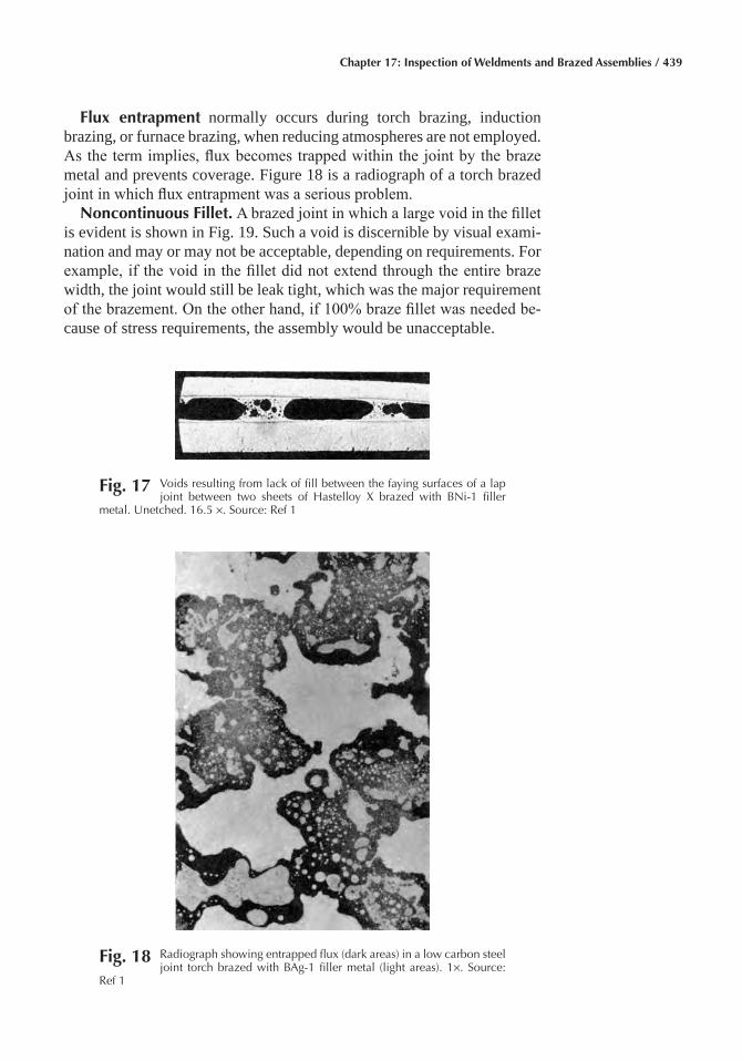
Chapter 17: Inspection of Weldments and Brazed Assemblies / 439
Flux entrapment normally occurs during torch brazing, induction brazing, or furnace brazing, when reducing atmospheres are not employed. As the term implies, flux becomes trapped within the joint by the braze metal and prevents coverage. Figure 18 is a radiograph of a torch brazed joint in which flux entrapment was a serious problem.
Noncontinuous Fillet� A brazed joint in which a large void in the fillet is evident is shown in Fig. 19. Such a void is discernible by visual exami-nation and may or may not be acceptable, depending on requirements. For example, if the void in the fillet did not extend through the entire braze width, the joint would still be leak tight, which was the major requirement of the brazement. On the other hand, if 100% braze fillet was needed be-cause of stress requirements, the assembly would be unacceptable.
Fig� 17 Voids resulting from lack of fill between the faying surfaces of a lap joint between two sheets of Hastelloy X brazed with BNi-1 filler
metal. Unetched. 16.5 ×. Source: Ref 1
Fig� 18 Radiograph showing entrapped flux (dark areas) in a low carbon steel joint torch brazed with BAg-1 filler metal (light areas). 1×. Source:
Ref 1
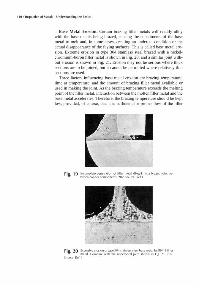
440 / Inspection of Metals—Understanding the Basics
Base Metal Erosion� Certain brazing filler metals will readily alloy with the base metals being brazed, causing the constituents of the base metal to melt and, in some cases, creating an undercut condition or the actual disappearance of the faying surfaces. This is called base metal ero-sion. Extreme erosion in type 304 stainless steel brazed with a nickel-chromium-boron filler metal is shown in Fig. 20, and a similar joint with-out erosion is shown in Fig. 21. Erosion may not be serious where thick sections are to be joined, but it cannot be permitted where relatively thin sections are used.
Three factors influencing base metal erosion are brazing temperature, time at temperature, and the amount of brazing filler metal available or used in making the joint. As the brazing temperature exceeds the melting point of the filler metal, interaction between the molten filler metal and the base metal accelerates. Therefore, the brazing temperature should be kept low, provided, of course, that it is sufficient for proper flow of the filler
Fig� 20 Excessive erosion of type 304 stainless steel base metal by BNi-1 filler metal. Compare with the noneroded joint shown in Fig. 21. 20×.
Source: Ref 1
Fig� 19 Incomplete penetration of filler metal (BAg-1) in a brazed joint be-tween copper components. 20×. Source: Ref 1
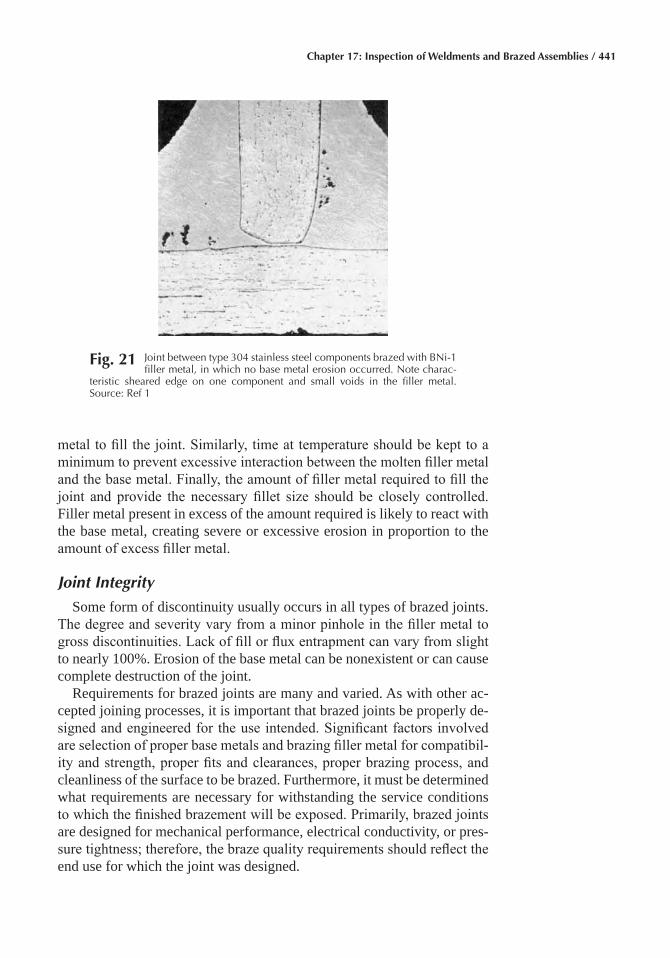
Chapter 17: Inspection of Weldments and Brazed Assemblies / 441
metal to fill the joint. Similarly, time at temperature should be kept to a minimum to prevent excessive interaction between the molten filler metal and the base metal. Finally, the amount of filler metal required to fill the joint and provide the necessary fillet size should be closely controlled. Filler metal present in excess of the amount required is likely to react with the base metal, creating severe or excessive erosion in proportion to the amount of excess filler metal.
Joint Integrity
Some form of discontinuity usually occurs in all types of brazed joints. The degree and severity vary from a minor pinhole in the filler metal to gross discontinuities. Lack of fill or flux entrapment can vary from slight to nearly 100%. Erosion of the base metal can be nonexistent or can cause complete destruction of the joint.
Requirements for brazed joints are many and varied. As with other ac-cepted joining processes, it is important that brazed joints be properly de-signed and engineered for the use intended. Significant factors involved are selection of proper base metals and brazing filler metal for compatibil-ity and strength, proper fits and clearances, proper brazing process, and cleanliness of the surface to be brazed. Furthermore, it must be determined what requirements are necessary for withstanding the service conditions to which the finished brazement will be exposed. Primarily, brazed joints are designed for mechanical performance, electrical conductivity, or pres-sure tightness; therefore, the braze quality requirements should reflect the end use for which the joint was designed.
Fig� 21 Joint between type 304 stainless steel components brazed with BNi-1 filler metal, in which no base metal erosion occurred. Note charac-
teristic sheared edge on one component and small voids in the filler metal. Source: Ref 1
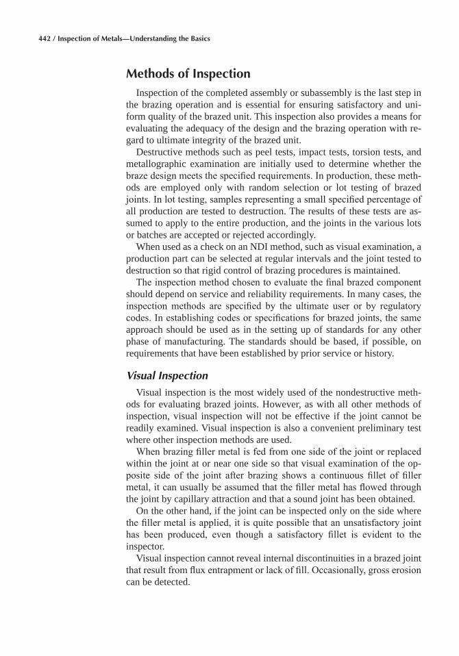
442 / Inspection of Metals—Understanding the Basics
Methods of InspectionInspection of the completed assembly or subassembly is the last step in
the brazing operation and is essential for ensuring satisfactory and uni-form quality of the brazed unit. This inspection also provides a means for evaluating the adequacy of the design and the brazing operation with re-gard to ultimate integrity of the brazed unit.
Destructive methods such as peel tests, impact tests, torsion tests, and metallographic examination are initially used to determine whether the braze design meets the specified requirements. In production, these meth-ods are employed only with random selection or lot testing of brazed joints. In lot testing, samples representing a small specified percentage of all production are tested to destruction. The results of these tests are as-sumed to apply to the entire production, and the joints in the various lots or batches are accepted or rejected accordingly.
When used as a check on an NDI method, such as visual examination, a production part can be selected at regular intervals and the joint tested to destruction so that rigid control of brazing procedures is maintained.
The inspection method chosen to evaluate the final brazed component should depend on service and reliability requirements. In many cases, the inspection methods are specified by the ultimate user or by regulatory codes. In establishing codes or specifications for brazed joints, the same approach should be used as in the setting up of standards for any other phase of manufacturing. The standards should be based, if possible, on requirements that have been established by prior service or history.
Visual Inspection
Visual inspection is the most widely used of the nondestructive meth-ods for evaluating brazed joints. However, as with all other methods of inspection, visual inspection will not be effective if the joint cannot be readily examined. Visual inspection is also a convenient preliminary test where other inspection methods are used.
When brazing filler metal is fed from one side of the joint or replaced within the joint at or near one side so that visual examination of the op-posite side of the joint after brazing shows a continuous fillet of filler metal, it can usually be assumed that the filler metal has flowed through the joint by capillary attraction and that a sound joint has been obtained.
On the other hand, if the joint can be inspected only on the side where the filler metal is applied, it is quite possible that an unsatisfactory joint has been produced, even though a satisfactory fillet is evident to the inspector.
Visual inspection cannot reveal internal discontinuities in a brazed joint that result from flux entrapment or lack of fill. Occasionally, gross erosion can be detected.
Chapter 17: Inspection of Weldments and Brazed Assemblies / 443
Proof Testing
Proof testing is a method of inspection that subjects the completed joints to loads slightly in excess of the loads to be applied during their subsequent service life. These loads can be applied by hydrostatic meth-ods, tensile loading, spin testing, or numerous other methods. Occasion-ally, it is not possible to ensure a serviceable part by any of the other nondestructive methods of inspection, and proof testing then becomes the most satisfactory method.
Pressure Testing
Pressure testing of brazed assemblies is a method of leak testing and is usually confined to vessels and heat exchangers where liquid, gas, or air tightness is required. Several methods of pressure testing can be em-ployed. Most use either air or gas, depending on the application of the vessel or heat exchanger. In most cases, the test pressures are greater than those to which the assembly will be subjected in service and are specified by the user.
One or more of the following three procedures are generally employed for pressure testing:
• All openings are closed. Air or gas is injected into the assembly until the specified pressure is reached. The inlet sources are closed off, the assembly is allowed to sit for a period of time, and pressure decreases are then measured on a gage
• All openings in the assembly are closed except one, which is fitted with an inlet pressure line. With the assembly submerged in a tank of water, air or gas is admitted through the inlet line until a specified pres-sure is reached. The inspector then looks for bubbles rising through the water
• All openings are closed, and the assembly is pressurized to the speci-fied pressure. Then a leak detecting solution, of which there are several commercially available, is brushed on the joints to be inspected. If any of the joints leak, bubbling will occur
Vacuum and helium testing is generally used in inspecting assem-blies where it is imperative that the most minute leak be detected. This method of inspection is often employed on nuclear reactor hardware. It is also extensively used in the inspection of refrigeration equipment. The as-sembly to be inspected is connected to a vacuum system, and the vacuum is monitored by a mass spectrometer.
Helium gas is flushed around the brazed joint; if any minute leak is present, the helium, because of its small molecule, will be pulled in by vacuum and register on the mass spectrometer, thus indicating the leak.
444 / Inspection of Metals—Understanding the Basics
A more sensitive technique is pressurizing the assembly with helium while the assembly is contained in a sealed plastic bag. After pressurizing for a period of time (for example, 24 hours), the atmosphere in the bag is analyzed for the presence of helium.
Ultrasonic Inspection
Ultrasonic inspection, although not extensively used in the evaluation of brazed joints, can be the only method applicable in certain cases. The use of ultrasonic inspection depends largely on the design of the joint and the configuration of the adjacent areas of the brazed assembly. Advance-ments in ultrasonic inspection may increase the utility of this process so that brazed joints can be evaluated with reliability.
Radiographic Inspection
Radiographic inspection is commonly used for the nondestructive eval-uation of brazed joints following visual examination. In almost all cases, the radiation beam is directed at about 90° to the plane of the joint, and the radiograph is taken through the thickness of the braze metal.
X-rays readily discern the differences in density between the brazing filler metal and the base metal. Care must be exercised because joints be-tween sections of varying thicknesses can produce radiographs that are misleading and difficult to interpret. Also, it is often difficult to determine whether a joint has been penetrated fully or not at all; both situations yield radiographs in which there is a full fillet visible around the joint, and the gap in the joint itself has uniform radiographic density. By contrast, partly filled joints, voids in the braze metal, and inclusions are relatively easy to find with radiography.
The filler metal in brazed joints is very thin, from 0.013 to 0.25 mm (0.0005 to 0.010 in.) in thickness. When radiographs are made of brazed joints between thick components, the process may be unable to record the braze metal as a difference in density; at least 2% difference is usually needed for good sensitivity.
Liquid Penetrant Inspection
Liquid penetrant inspection is another nondestructive method for deter-mining the reliability of brazed joints and assemblies. This inspection method produces a visual image of a discontinuity in the surface of the braze and reveals the nature of a discontinuity without impairing the par-ent metal. Acceptable and unacceptable components or assemblies can be separated in accordance with predetermined standards.
There are certain advantages obtained from the liquid penetrant inspec-tion of brazed assemblies. However, a brazed joint or component should be visually inspected first, and then inspected by a liquid penetrant method
Chapter 17: Inspection of Weldments and Brazed Assemblies / 445
to resolve any doubt concerning joint integrity. Visual examination is re-stricted to those discontinuities that can be detected by the unaided eye. Liquid penetrant carries visual inspection a step further by increasing the detectability of fine cracks or openings.
Discontinuities such as incomplete fusion, cracks that x-rays cannot show because of orientation, and porosity and laps become visible with this technique. Liquid penetrants do not disclose subsurface discontinui-ties such as voids, cracks, or flux entrapment; radiography is best used to discover such discontinuities.
Selection of the specific liquid penetrant system for the inspection of brazed assemblies depends on the same factors as those that affect system selection for other workpieces. The water-washable, post-emulsifiable, and solvent-removable systems have been successfully used for inspect-ing brazed assemblies.
Inspection using liquid penetrants should not be performed prior to brazing unless adequate cleaning steps, such as vapor degreasing, are taken to remove entrapped penetrant fluid. If permitted to remain during the brazing cycle, this fluid can contaminate the furnace atmosphere and braze metal, producing flaws.
ACKNOWLEDGMENT
This chapter was adapted from Nondestructive Inspection of Weld-ments, Brazed Assemblies, and Soldered Joints, Nondestructive Evalua-tion and Quality Control, Volume 17, ASM Handbook, 1992.
REFERENCES
1. Nondestructive Inspection of Weldments, Brazed Assemblies, and Soldered Joints, Nondestructive Evaluation and Quality Control, Vol 17, ASM Handbook, ASM International, 1992, p 582–609
SELECTED REFERENCES
• R. Halmshaw, Introduction to Non-Destructive Testing of Welded Joints, 2nd ed., Woodhead Publishing Ltd., 1996

This page has been reformatted by Knovel to provide easier navigation.
INDEX
Index Terms Links
A
AAS. See atomic absorption spectroscopy (AAS)
abrasive blasting 388
abrasive wheel cutting 162
acid etching 2 2(F)
See also macroetching
acidic alumina suspensions 169
acrylic resins 163
aerospace industry
aluminum alloy forgings 379
forging inspection methods 371
inspection procedures 299–302
penetrants 371
thermal inspection 294
titanium alloy forgings 382
ultrasonic inspection 379 390
age hardenable nickel alloys 376–377
air melted alloys 369
AISI 1055 carbon steel 46 47(F)
AISI 1060 carbon steel 46 46(F)
alcohol 167 169 171(T)
173(T) 175(T) 176(T)
alloy segregation 45
alternating current
eddy current inspection 15 15(F) 216
219 229
magnetic particle inspection 202 309–310 326
magnetizing current 202
Index Terms Links
This page has been reformatted by Knovel to provide easier navigation.
aluminum
electrolytic polishing 169–170
etching 170
macrodefects 380(F) 381 381(F)
radioactive equivalence 245–246
radiographic film, selection 257(T)
aluminum alloy forgings
aerospace industry 379
CAD databases 379
CAM driven equipment 379
closed-die forgings 379
cracks 378 378(F)
die cavity dimensions 379
dimensional inspection 379
discontinuities 377–378 378(F)
eddy current inspection 379
final inspection 378–379
hardness measurements 379
heat treatment 379
heat treatment verification 379
in-process inspection 378
liquid penetrant inspection 379
mechanical property tests 379
nondestructive inspection 379
open-die forgings 379
root mean surface (rms) 379
ultrasonic inspection 379
aluminum alloys
electric current perturbation method 437
fatigue properties 296
forging material 377–379 378(F)
surface cracks 437
aluminum oxide (Al2O3) 165 169
aluminum-silicon alloys 297–298

Index Terms Links
This page has been reformatted by Knovel to provide easier navigation.
American Petroleum Institute (API)
cracking 23
flaws (terminology) 348
reference discontinuities 231
American Society for Nondestructive Testing 12
ammeter 386
analog video signal 253
angle beam testing 279–280 279(F) 280(F)
281(F) 289 327–328
annealing 6(T) 368 394
anodes
etchants 175(T)
etching 170
x-ray tubes 239–241 241(F) 242
ANSI/ASME B89 Performance Standard 54–55
anvils
diamond spot anvils 98 99(F)
eyeball anvil 98 99(F)
Rockwell hardness testing 98–99 99(F)
V-slot anvil 98 99 99(F)
API. See American Petroleum Institute (API)
arc strikes 412
arc welding
demagnetization 214
gas tungsten arc welding 412
machine vision applications 4(F)
processes 413(F) 423
radiographic inspection 356
tubular products 346
arc welds. See also arc welding
discontinuities 411–420(F)
incomplete penetration 416–417 417(F)
tubular products 346
Archimedes’ principle 394–395
Index Terms Links
This page has been reformatted by Knovel to provide easier navigation.
ASTM (American Society for Testing and Materials) 12
tensile test pieces 133
ASTM grain size 181(T)
ASTM standards
ASTM A370 131 133
ASTM B328 394 395
ASTM B557 131
ASTM E6 122 124
ASTM E8 122 131 133
137–138
ASTM E10 88
ASTM E94 255–256 256(T) 261
ASTM E103 89
ASTM E142 (Withdrawn 2000) 262
ASTM E155 level 4 296
ASTM E384 7
ASTM E746 255 261
ASTM E747 262
ASTM STP 586 265–266
eddy current inspection 231 232(F)
tensile testing 129
atomic absorption spectroscopy (AAS)
light sources 150
OES 150
atomized iron powder 398–399
atoms 140(F) 141
attenuation
basic A-scan displays 277
cold drawn hexagonal bars 329
CT 254
electromagnetic radiation 243–246(T)
forgings 372
gamma-ray density determination 405
green compacts 406
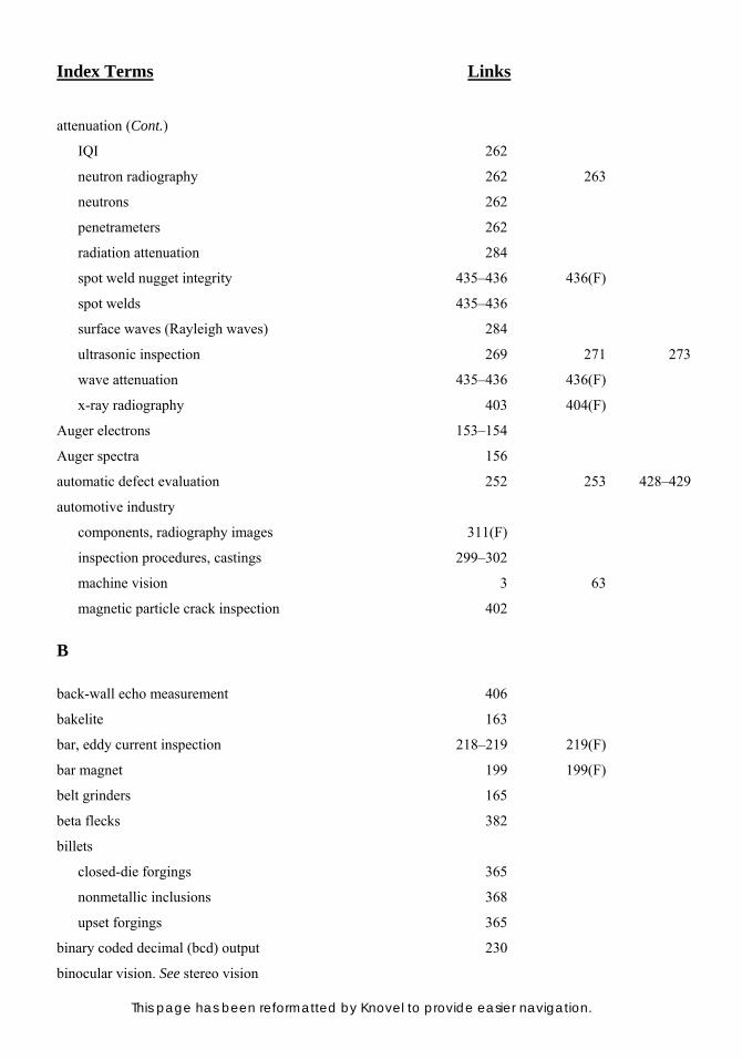
Index Terms Links
This page has been reformatted by Knovel to provide easier navigation.
attenuation (Cont.)
IQI 262
neutron radiography 262 263
neutrons 262
penetrameters 262
radiation attenuation 284
spot weld nugget integrity 435–436 436(F)
spot welds 435–436
surface waves (Rayleigh waves) 284
ultrasonic inspection 269 271 273
wave attenuation 435–436 436(F)
x-ray radiography 403 404(F)
Auger electrons 153–154
Auger spectra 156
automatic defect evaluation 252 253 428–429
automotive industry
components, radiography images 311(F)
inspection procedures, castings 299–302
machine vision 3 63
magnetic particle crack inspection 402
B
back-wall echo measurement 406
bakelite 163
bar, eddy current inspection 218–219 219(F)
bar magnet 199 199(F)
belt grinders 165
beta flecks 382
billets
closed-die forgings 365
nonmetallic inclusions 368
upset forgings 365
binary coded decimal (bcd) output 230
binocular vision. See stereo vision

Index Terms Links
This page has been reformatted by Knovel to provide easier navigation.
biological microscopes 171 176
black (ultraviolet) light
filtered particle crack detection 402
liquid penetrant inspection 185 192 195
magnetic particle inspection 211 212–213 383
blisters 323 324(F) 356
357(F)
blobs 78
blowholes 317
bolt heads 22
boron 263 266
boron-fiber composites 266
boroscopes 40–41 40(F)
Brale indenter 92 92(F)
brazed assemblies. See also brazed joints; brazing
brazed joints, flaws in (see brazed joints)
brazing, defined 437–438
cracks 445
inspection methods
helium testing 443–444
liquid penetrant inspection 444–445
overview 442
pressure testing 443
proof testing 443
radiographic inspection 444
ultrasonic inspection 444
vacuum testing 443
visual inspection 442 444
overview 437–438
penetrants 445
pressure testing 443–444
processes 438
soft soldering, differentiation between 438
welding, differentiation between 438

Index Terms Links
This page has been reformatted by Knovel to provide easier navigation.
brazed joints
base metal erosion 440–441 440(F) 441(F)
flux entrapment 439 439(F)
incomplete penetration 440(F)
inspection methods
codes and specifications, establishing 442
destructive tests 442
liquid penetrant inspection 444–445
NDI 442
pressure testing 443
proof testing 443
radiographic inspection 444
ultrasonic inspection 444
vacuum and helium testing 443–444
visual inspection 442 445
joint integrity 441
lack of fill 438 439(F)
lot testing 442
noncontinuous fillet 439 440(F)
penetrants 445
brazing
classifications 438
corrosion 438
definition of 437–438
filler metal 438
processes 438
brazing filler metals
base metal erosion 440 440(F)
essential properties for 438
joint integrity 441
lack of fill 438 439(F)
radiographic inspection 444
visual inspection 442
bremsstrahlung 239
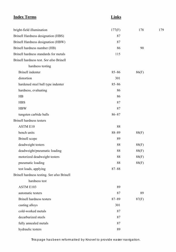
Index Terms Links
This page has been reformatted by Knovel to provide easier navigation.
bright-field illumination 177(F) 178 179
Brinell Hardness designation (HBS) 87
Brinell Hardness designation (HBW) 87
Brinell hardness number (HB) 86 90
Brinell hardness standards for metals 115
Brinell hardness test. See also Brinell
hardness testing
Brinell indenter 85–86 86(F)
distortion 301
hardened steel ball type indenter 85–86
hardness, evaluating 86
HB 86
HBS 87
HBW 87
tungsten carbide balls 86–87
Brinell hardness testers
ASTM E10 88
bench units 88–89 88(F)
Brinell scope 89
deadweight testers 88 88(F)
deadweight/pneumatic loading 88 88(F)
motorized deadweight testers 88 88(F)
pneumatic loading 88 88(F)
test loads, applying 87–88
Brinell hardness testing. See also Brinell
hardness test
ASTM E103 89
automatic testers 87 89
Brinell hardness testers 87–89 87(F)
casting alloys 301
cold-worked metals 87
decarburized steels 87
fully annealed metals 87
hydraulic testers 89
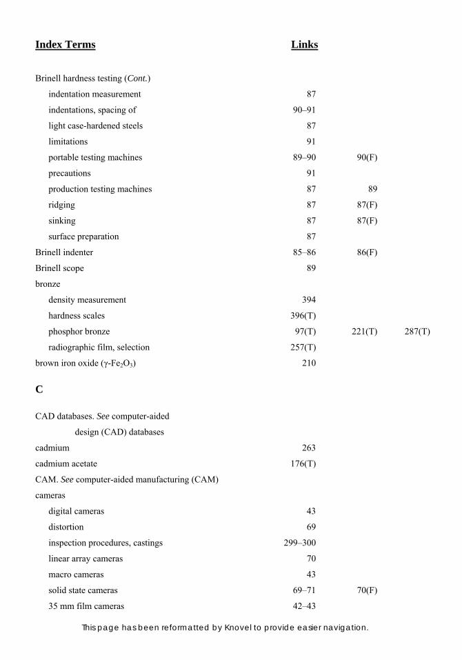
Index Terms Links
This page has been reformatted by Knovel to provide easier navigation.
Brinell hardness testing (Cont.)
indentation measurement 87
indentations, spacing of 90–91
light case-hardened steels 87
limitations 91
portable testing machines 89–90 90(F)
precautions 91
production testing machines 87 89
ridging 87 87(F)
sinking 87 87(F)
surface preparation 87
Brinell indenter 85–86 86(F)
Brinell scope 89
bronze
density measurement 394
hardness scales 396(T)
phosphor bronze 97(T) 221(T) 287(T)
radiographic film, selection 257(T)
brown iron oxide (γ-Fe2O3) 210
C
CAD databases. See computer-aided
design (CAD) databases
cadmium 263
cadmium acetate 176(T)
CAM. See computer-aided manufacturing (CAM)
cameras
digital cameras 43
distortion 69
inspection procedures, castings 299–300
linear array cameras 70
macro cameras 43
solid state cameras 69–71 70(F)
35 mm film cameras 42–43
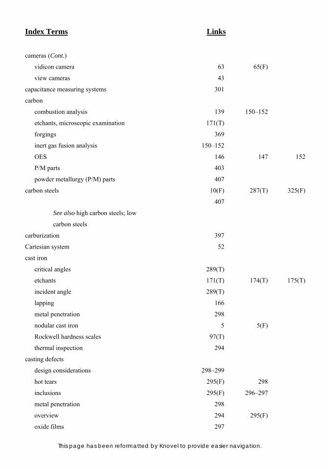
Index Terms Links
This page has been reformatted by Knovel to provide easier navigation.
cameras (Cont.)
vidicon camera 63 65(F)
view cameras 43
capacitance measuring systems 301
carbon
combustion analysis 139 150–152
etchants, microscopic examination 171(T)
forgings 369
inert gas fusion analysis 150–152
OES 146 147 152
P/M parts 403
powder metallurgy (P/M) parts 407
carbon steels 10(F) 287(T) 325(F)
407
See also high carbon steels; low
carbon steels
carburization 397
Cartesian system 52
cast iron
critical angles 289(T)
etchants 171(T) 174(T) 175(T)
incident angle 289(T)
lapping 166
metal penetration 298
nodular cast iron 5 5(F)
Rockwell hardness scales 97(T)
thermal inspection 294
casting defects
design considerations 298–299
hot tears 295(F) 298
inclusions 295(F) 296–297
metal penetration 298
overview 294 295(F)
oxide films 297
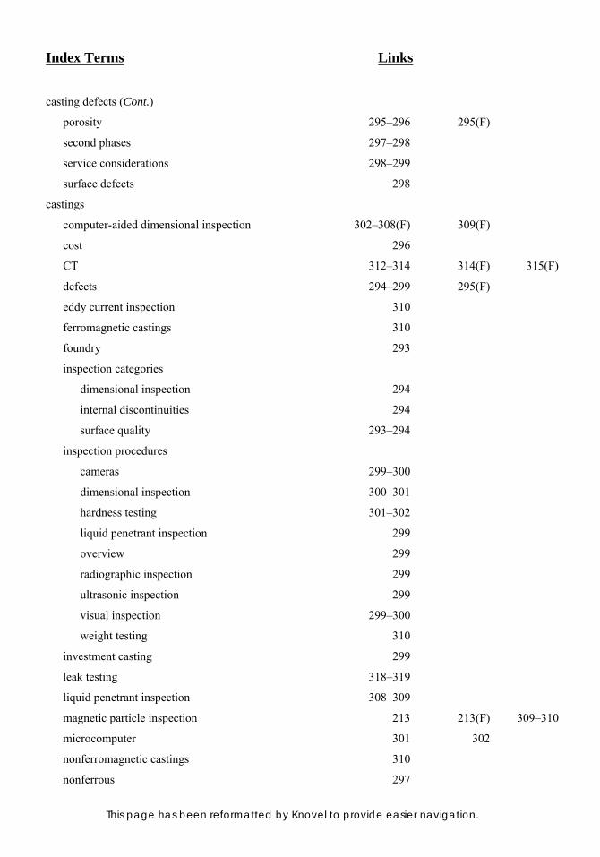
Index Terms Links
This page has been reformatted by Knovel to provide easier navigation.
casting defects (Cont.)
porosity 295–296 295(F)
second phases 297–298
service considerations 298–299
surface defects 298
castings
computer-aided dimensional inspection 302–308(F) 309(F)
cost 296
CT 312–314 314(F) 315(F)
defects 294–299 295(F)
eddy current inspection 310
ferromagnetic castings 310
foundry 293
inspection categories
dimensional inspection 294
internal discontinuities 294
surface quality 293–294
inspection procedures
cameras 299–300
dimensional inspection 300–301
hardness testing 301–302
liquid penetrant inspection 299
overview 299
radiographic inspection 299
ultrasonic inspection 299
visual inspection 299–300
weight testing 310
investment casting 299
leak testing 318–319
liquid penetrant inspection 308–309
magnetic particle inspection 213 213(F) 309–310
microcomputer 301 302
nonferromagnetic castings 310
nonferrous 297
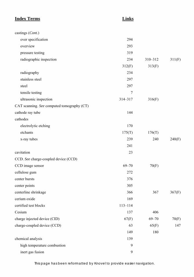
Index Terms Links
This page has been reformatted by Knovel to provide easier navigation.
castings (Cont.)
over specification 294
overview 293
pressure testing 319
radiographic inspection 234 310–312 311(F)
312(F) 313(F)
radiography 234
stainless steel 297
steel 297
tensile testing 7
ultrasonic inspection 314–317 316(F)
CAT scanning. See computed tomography (CT)
cathode ray tube 144
cathodes
electrolytic etching 170
etchants 175(T) 176(T)
x-ray tubes 239 240 240(F)
241
cavitation 23
CCD. See charge-coupled device (CCD)
CCD image sensor 69–70 70(F)
cellulose gum 272
center bursts 376
center points 305
centerline shrinkage 366 367 367(F)
cerium oxide 169
certified test blocks 113–114
Cesium 137 406
charge injected device (CID) 67(F) 69–70 70(F)
charge-coupled device (CCD) 63 65(F) 147
149 180
chemical analysis 139
high temperature combustion 9
inert gas fusion 9
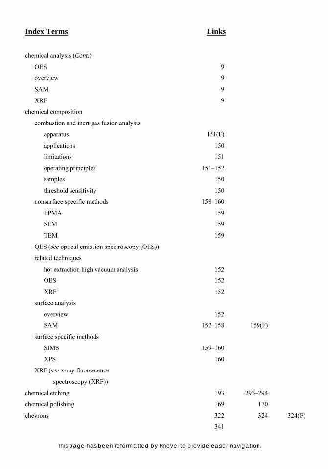
Index Terms Links
This page has been reformatted by Knovel to provide easier navigation.
chemical analysis (Cont.)
OES 9
overview 9
SAM 9
XRF 9
chemical composition
combustion and inert gas fusion analysis
apparatus 151(F)
applications 150
limitations 151
operating principles 151–152
samples 150
threshold sensitivity 150
nonsurface specific methods 158–160
EPMA 159
SEM 159
TEM 159
OES (see optical emission spectroscopy (OES))
related techniques
hot extraction high vacuum analysis 152
OES 152
XRF 152
surface analysis
overview 152
SAM 152–158 159(F)
surface specific methods
SIMS 159–160
XPS 160
XRF (see x-ray fluorescence
spectroscopy (XRF))
chemical etching 193 293–294
chemical polishing 169 170
chevrons 322 324 324(F)
341

Index Terms Links
This page has been reformatted by Knovel to provide easier navigation.
chisel pointed stylus 393
chromatic aberration 28
chromium oxide 169
circular magnetization 199–200 200(F)
circumferential magnetic fields 310
clip-on extensometers 128
closed-die forgings 365 371 372–373
379
coarse grip alumina 165
Coddington magnifier 28 29(F)
coefficients of thermal expansion 297
coil impedance 219 220(F)
coils
absolute coil arrangement 226 227(F)
bobbin type coil 226 226(F)
differential coil arrangement 226 227(F)
eddy current inspection 15(F) 204–205 222
229 229(F)
encircling coils 225–226 226(F) 325
encircling detector coil 359
horseshoe shaped coils 225 226(F)
internal coil 226 226(F)
magnetic permeability systems 339–340 339(F) 340(F)
342–343
null coils 339 340(F)
probe, type 225 226(F)
probe coils 359 360
U-shape coils 225 226(F)
zero voltage output coils 339 340(F)
cold drawn bars
coupling 324 327–328 327(F)
eddy current testing 333–334 334(F)

Index Terms Links
This page has been reformatted by Knovel to provide easier navigation.
cold drawn hexagonal bars
attenuation 329
coupling 329
cracks 334 335
cold drawn wires. See also steel bar, flaws;
steel bars
coupling 330
cracks 336(F)
rotating type ultrasonic flaw detection unit 330–331 330(F)
rotation type eddy current flaw detection system 229–330
ultrasonic flaw detection 329–331
advantages 331
system 331 331(T)
cold etching 46 47(F)
cold forged, high tensile sheared bolt
cracks 337
detection rate 338
eddy current flaw detection system 337 337(F) 338(T)
flaw depth and signal output, relation between 339 339(F)
general view 337 337(F)
rotating eddy current detection head 338 338(F)
cold shuts 371
cold working process 335
collimation 264
collimator 252 404–405
colloidal silica 169
column units 58
combustion analysis 146 150–152
composite ceramics 165
composites 236 266 270(T)
294
compression waves 282–283 283(F)
See also longitudinal waves
Compton scattering 244–245
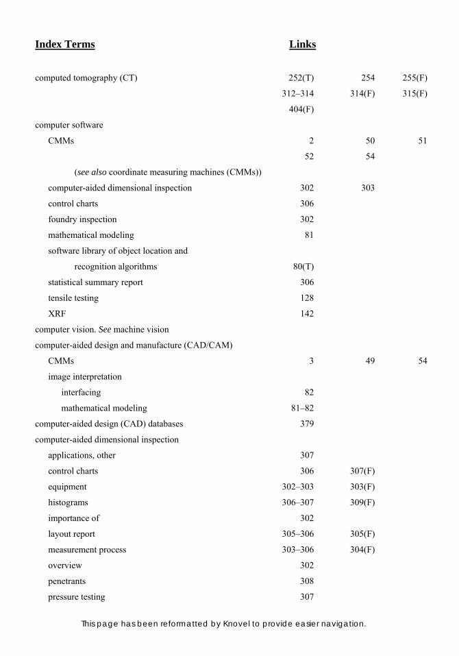
Index Terms Links
This page has been reformatted by Knovel to provide easier navigation.
computed tomography (CT) 252(T) 254 255(F)
312–314 314(F) 315(F)
404(F)
computer software
CMMs 2 50 51
52 54
(see also coordinate measuring machines (CMMs))
computer-aided dimensional inspection 302 303
control charts 306
foundry inspection 302
mathematical modeling 81
software library of object location and
recognition algorithms 80(T)
statistical summary report 306
tensile testing 128
XRF 142
computer vision. See machine vision
computer-aided design and manufacture (CAD/CAM)
CMMs 3 49 54
image interpretation
interfacing 82
mathematical modeling 81–82
computer-aided design (CAD) databases 379
computer-aided dimensional inspection
applications, other 307
control charts 306 307(F)
equipment 302–303 303(F)
histograms 306–307 309(F)
importance of 302
layout report 305–306 305(F)
measurement process 303–306 304(F)
overview 302
penetrants 308
pressure testing 307
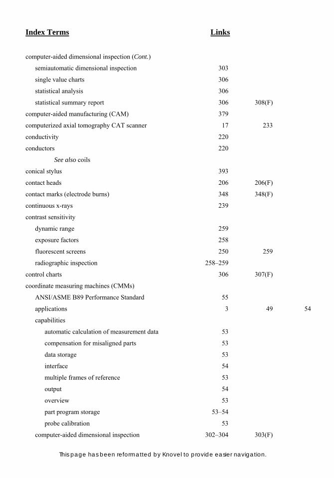
Index Terms Links
This page has been reformatted by Knovel to provide easier navigation.
computer-aided dimensional inspection (Cont.)
semiautomatic dimensional inspection 303
single value charts 306
statistical analysis 306
statistical summary report 306 308(F)
computer-aided manufacturing (CAM) 379
computerized axial tomography CAT scanner 17 233
conductivity 220
conductors 220
See also coils
conical stylus 393
contact heads 206 206(F)
contact marks (electrode burns) 348 348(F)
continuous x-rays 239
contrast sensitivity
dynamic range 259
exposure factors 258
fluorescent screens 250 259
radiographic inspection 258–259
control charts 306 307(F)
coordinate measuring machines (CMMs)
ANSI/ASME B89 Performance Standard 55
applications 3 49 54
capabilities
automatic calculation of measurement data 53
compensation for misaligned parts 53
data storage 53
interface 54
multiple frames of reference 53
output 54
overview 53
part program storage 53–54
probe calibration 53
computer-aided dimensional inspection 302–304 303(F)

Index Terms Links
This page has been reformatted by Knovel to provide easier navigation.
coordinate measuring machines (CMMs) (Cont.)
contact probe 303 303(F)
coordinate systems 52
Cartesian system 52
polar coordinate system 52
measurements, types of
contour measurement 52
geometric measurement 52
overview 52
specialized surface measurement 52–53
measuring techniques 51 51(F)
operating principles 50–51
overview 2–3(F)
position or displacement, measurement output 51 51(F)
probe 51
process control robots 54
specifications 55(T)
terminology 49–50
coordinate measuring machines (CMMs) types
ANSI/ASME B89 Performance
Standard 54–55
bridge type
column CMM 58 59(F)
column units 58
fixed bridge configuration 57(F) 58
L-shaped bridge 57(F) 58
moving bridge 57(F) 58
process 57–58
universal measuring machines 58
cantilever type 56–57 56(F)
gantry CMMs 58–59 59(F)
horizontal arm CMMs
applications 61
fixed table type 60(F) 61–62

Index Terms Links
This page has been reformatted by Knovel to provide easier navigation.
coordinate measuring machines (CMMs) types
horizontal arm CMMs (Cont.)
moving ram type 60(F) 61
moving table type 60(F) 61
overview 61
horizontal CMMs
accuracy range 60–61
applications 60
process control robots 61
schematic 60(F)
overview 54–55
specifications 55(T)
vertical CMMs 55–59(F)
corrosion
abrasive wheel cutting 162
brazing 438
etching 170
forgings 368 369
macroscopic examination 10
neutron detection methods 264
neutron radiography 263
ultrasonic search units 270
visual inspection 1 21 22–23
25
corrosion resistance 366 372 438
corrosion scaling 22–23
cosine waves 73
couplants
overview 271–272
resistance welded steel tubing 354 355
seamless steel tubular products 358 359
coupling
castings 316 317
cellulose gum 272

Index Terms Links
This page has been reformatted by Knovel to provide easier navigation.
coupling (Cont.)
cold drawn bars 328
cold drawn hexagonal bars 329
cold drawn wires 330
eddy current inspection 359
magnetic particle inspection 213(F)
piezoelectric transducer elements 269(T)
P/M parts 401(T)
soft rubbers 271–272
tensile testing 127
tubular products 354 359
ultrasonic inspection 281 330
coupling medium 329 330
cracking
stress corrosion cracking 372
visual inspection 23–25 24(F)
cracks. See also inspection methods: cracks
castings 308
cold straightening cracks 373
detection (see powder metallurgy (P/M)
parts, flaw detection)
direct current resistivity testing 403
eddy current flow 216–217 217(F)
ejection cracks 398–399 399(F)
electric current perturbation method 437
fatigue cracks 211 286(T)
fusion cracks 445
heat treatment 323
hook cracks (upturned fiber flaws) 231 348–349 348(F)
internal defects, castings 318
magnetic particle crack inspection 402
measuring 26
microcracks 399–400 400(F)
multiple 23–24 24(F)

Index Terms Links
This page has been reformatted by Knovel to provide easier navigation.
cracks (Cont.)
near surface cracks 12(T) 401(T) 402
quench cracks 366 373 390
shear cracks 371 398
single 23–24 24(F)
steel bar 323 324(F)
stress concentrations 25 25(F)
subsurface cracks 6 373 401(T)
419 437
surface type (see surface cracks; surface defects)
transverse cracks 205
tubular products 346
weld area cracks 348(F) 349
weld root cracks 434
welding process 412
weldments (see weldments, cracks)
craters 412
critical angles 288–289 288(F) 289(T)
cross rolling 130–131
crystallite boundaries 290
CT. See computed tomography (CT)
cubes 394
cubic metals 180
Curie 238
D
damage tolerant design approaches 13
dark-field illumination 179
dark-ground illumination 179
datum planes 304–305
decarburization 397
defects, use of term 12

Index Terms Links
This page has been reformatted by Knovel to provide easier navigation.
deformation
hardness testing 85 86
heat-resistant alloy forgings 376
neck (see necking)
piezoelectric crystals 269
P/M parts 397
polishing 166–167
preparation induced deformation 113
sectioning 162
specimens 161
specimens, mounting of 162
strain measurement 128
tensile testing 128
UTM 124
workpiece support 98
demagnetization
electromagnetic yokes 204
ferromagnetic materials 214
following inspection 198 214–215
forgings 384
magnetic particle inspection 198 426
overview 214
reasons not to 215
reasons to 214
residual magnetic field 214
retentivity 214
steel bar 326
weldments 426
dendrites 296
dendritic solidification 45
densitometer 148 258
density
as-pressed 394
definition of 394

Index Terms Links
This page has been reformatted by Knovel to provide easier navigation.
density (Cont.)
exposure factors 258
green 394
sintered steels 394
density measurement 394–396
destructive tests
brazed joints 442
tensile testing 7–9
weldments 411
Deutsche Institut für Normung (DIN)
DIN 54109 — Image Quality of X-ray
and Gamma-ray Radiographs of
Metallic Materials 262
tensile test pieces 133
developer station 195
developers
application 185
dry developers
application methods 189
developer station 195
hand processing equipment 189
overview 189
safety equipment 189–190
forms of (A-D) 189
overview 188–189
penetrant and developer 186(F)
properties/characteristics 189
purpose of 188–189
selection process 191–192
wet developers
developer station 195
nonaqueous solvent suspendible
developers 191
types 190

Index Terms Links
This page has been reformatted by Knovel to provide easier navigation.
developers
wet developers (Cont.)
water soluble developers 190
water suspendible developers 190
dial gages 300
diallyl phthalate 163
diamond
grinding 169
grinding media 165
diamond disks 165
diamond size, grinding 165
die scratches 322
differential interference contrast
microscopy 180
diffraction 143
digital image processing 312 313(F) 402
digital radiography (DR)
CT 254
fluorescent screens 252 256(T) 257(T)
scattering 251
tubes 251
digitized signal 253
dimensional evaluation, powder metallurgy parts
ASTM B 328 394 395
cubes 394
density measurement
Archimedes’ principle 394–395
metallographic estimates 395–396
overview 394
dimensional changes, causes of 393–394
distortion 394
hardness testing 396
ISO 2738 394 395
linear dimensions 394
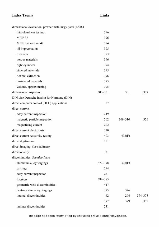
Index Terms Links
This page has been reformatted by Knovel to provide easier navigation.
dimensional evaluation, powder metallurgy parts (Cont.)
microhardness testing 396
MPIF 37 396
MPIF test method 42 394
oil impregnation 395
overview 393
porous materials 396
right cylinders 394
sintered materials 395
Soxhlet extraction 396
unsintered materials 395
volume, approximating 395
dimensional inspection 300–301 301 379
DIN. See Deutsche Institut für Normung (DIN)
direct computer control (DCC) applications 57
direct current
eddy current inspection 219
magnetic particle inspection 202 309–310 326
magnetizing current 202
direct current electrolysis 170
direct current resistivity testing 403 403(F)
direct digitization 251
direct imaging. See stadimetry
directionality 131
discontinuities. See also flaws
aluminum alloy forgings 377–378 378(F)
castings 294
eddy current inspection 231
forgings 384–385
geometric weld discontinuities 417
heat-resistant alloy forgings 375 376
internal discontinuities 42 294 374–375
377 379 391
laminar discontinuities 231

Index Terms Links
This page has been reformatted by Knovel to provide easier navigation.
discontinuities (Cont.)
magnesium alloy forgings 379
magnetic particle inspection 201(F) 213–214 213(F)
425
melt-related discontinuities 375 376
nickel alloy forgings 376
radiographic inspection 428
reference discontinuities 231
surface discontinuities 384–385
titanium alloy forgings 380
visual inspection 417 423 425
welded tubes 231
weldments (see weldments:
discontinuities)
discontinuity signals 433–434 433(F)
distilled water suspension 169
distortion
annealing 394
Brinell hardness test 301
dimensional evaluation 394
edge effect 223
inspection coils 225
lenses 28
magnifying devices 27
shadow formation 246 247(F)
solid state cameras 69
transverse rupture strength 397
visual inspection 21
weldments 423
DR. See digital radiography (DR)
drop weight tests 398
drop-of-beam yield point 120
dross 297 299 318
dry radiography. See xeroradiography

Index Terms Links
This page has been reformatted by Knovel to provide easier navigation.
ductility
defined 121
fractured, round tension test piece 121(F)
inclusions 296
tensile testing
elongation 122
fractured, round tension test piece 121(F)
gage length, effect on elongation values 123 123(F)
necking, effect of 121(F) 123 123(F)
overview 121–122
reduction of area 123–124 124(F)
dwell time 186 194
dye penetrant inspection 1 23
See also liquid penetrant inspection
dynamic range
contrast sensitivity 259
direct digitization 251
exposure factors, radiographic
inspection 259
fluorescent screens 250
image intensifer 251
image processing 253
radiographic inspection 259
dysprosium 263 265
E
eddy current inspection
advantages 216
alternating current 15 15(F)
aluminum alloy forgings 379
applications 15–16 215
bar 218–219 219(F)
basic system 216–218 217(F)
castings 293–294 310

Index Terms Links
This page has been reformatted by Knovel to provide easier navigation.
eddy current inspection (Cont.)
coil assembly 332 332(F)
coils 15(F) 204–205 222
229 229(F)
cold drawn bars
encircling coil method 333
flaw depth and signal output, relation
between 333–334 334(F)
noncontact rotating transmission method 333
rotating probe type detection system 333(T)
rotating probe type eddy current flaw detector 333 334(F)
cold drawn hexagonal bars
differential method with probe assembly 335 335(F)
longitudinal defects 335
standard voltage method 335 335(F) 336(F)
surface defects 334–335
cold drawn wires
detectability of flaws 336(F)
encircling type method 335–336
guide sleeves 336
rotating probe type eddy current flaw
detector 334(F)
cold forged, high tensile sheared bolt 337–339 337(F) 338(F,T)
339(F)
cold working process 335
coupling 359
crack, in a pipe 217–218 217(F)
cracks 15 225 231
310
disadvantages 216
discontinuities detectable 231
eddy current flow 217(F)
eddy current flow patterns 15 15(F)
electromagnetic induction 15
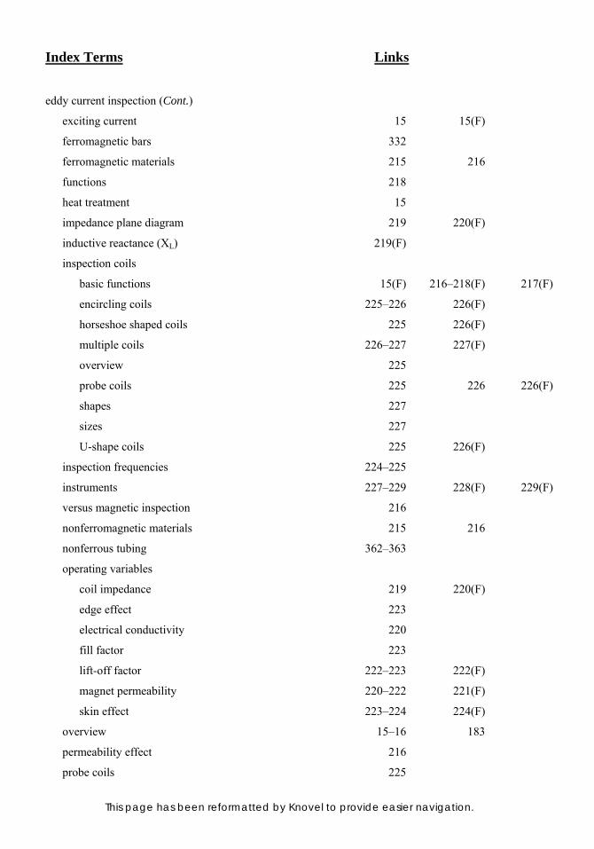
Index Terms Links
This page has been reformatted by Knovel to provide easier navigation.
eddy current inspection (Cont.)
exciting current 15 15(F)
ferromagnetic bars 332
ferromagnetic materials 215 216
functions 218
heat treatment 15
impedance plane diagram 219 220(F)
inductive reactance (XL) 219(F)
inspection coils
basic functions 15(F) 216–218(F) 217(F)
encircling coils 225–226 226(F)
horseshoe shaped coils 225 226(F)
multiple coils 226–227 227(F)
overview 225
probe coils 225 226 226(F)
shapes 227
sizes 227
U-shape coils 225 226(F)
inspection frequencies 224–225
instruments 227–229 228(F) 229(F)
versus magnetic inspection 216
nonferromagnetic materials 215 216
nonferrous tubing 362–363
operating variables
coil impedance 219 220(F)
edge effect 223
electrical conductivity 220
fill factor 223
lift-off factor 222–223 222(F)
magnet permeability 220–222 221(F)
skin effect 223–224 224(F)
overview 15–16 183
permeability effect 216
probe coils 225

Index Terms Links
This page has been reformatted by Knovel to provide easier navigation.
eddy current inspection (Cont.)
readout instrumentation 229–230
reference samples 231–232 232(F)
resistance welded steel tubing 349–351 350(F)
rotating coil setup 332 333(T)
seamless steel tubular products 359–361 360(F) 361(F)
skin effect 310 332
standard depth of penetration 223–224 224(F)
steel bars
coil assembly 332 332(F)
electrical conductivity 332
electrical resistivity 332
ferromagnetic bars 332
magnetic permeability systems 333
overview 332–333
rotating coil setup 332 333(T)
skin effect 332
surface cracks 231
system elements 218–219 219(F)
tubes 231
tubing 218–219 219(F)
weldments 415 437
eddy current testing 1 11 232(F)
333–334 334(F)
See also eddy current inspection
edge angle 101
edge detection 73–74
edge effect 219 223
edge preservation 163–164
EDS. See energy dispersive spectrometers (EDS)
elastic deformation 118 118(F)
elastic springback 393–394
electric current perturbation method 421 437
electrical conductivity 331 332

Index Terms Links
This page has been reformatted by Knovel to provide easier navigation.
electrical contact measuring systems 301
electrical discharge machined (EDM) 41
electrical resistivity 331 332
electroless nickel 164
electrolytic polishing 169–170 169(F)
electromagnetic field 216–217
electromagnetic induction 15 215
See also eddy current inspection
electromagnetic induction techniques 16 216
electromagnetic inspection
castings 310
steel bars 324 331–332
electromagnetic pumps 297
electromagnetic radiation
radiographic inspection 16 17 233
types 237–238 238(F)
XRF 139
electromagnetic radiation, attenuation of
exposure times 245–246
overview 243–244
processes
Compton scattering 244–245
pair production 245
photoelectric effect 244
radioactive equivalence 245–246
radiographic absorption equivalence, metals 245(T)
electromagnetic yokes 203–204 353 353(F)
electron energy levels 141
electron probe microanalysis (EPMA) 146 159
electronic coordinate measuring machine 302 303(F)
electronic gates 282 342 343(F)
electronics industry
applications 4(F)
inspection procedures, castings 299–300

Index Terms Links
This page has been reformatted by Knovel to provide easier navigation.
electronics industry (Cont.)
machine vision 3 63
electrons 140–141 140(F)
electropolishing 113 169
electroslag remelting cycle 368
electrostatic charged powder gun 189
elongation
definition of 122
measurement of 122
strain elongation 122
tensile testing 128
embedded scale 322 323 324(F)
emery (Al2O3-Fe3O4) 165
emulsification time 186–187
emulsifier station 194–195
emulsifiers
definition of 188
oil base 188
postemulsifable system 186
water base 188
encircling coil inspection
solid cylinders 231
tubes 231
encircling coils 325
end effect
resistance welded steel tubing 351 355
steel bar 341
tubular products 347
energy, defined 143
energy dispersive spectrometers (EDS) 144 145(F)
Environmental Protection Agency 194
EPMA. See electron probe microanalysis (EPMA)
epoxy resins 163 396
equivalent ellipse 76

Index Terms Links
This page has been reformatted by Knovel to provide easier navigation.
erosion 23
etching
corrosion 170
cracks 170
direct current electrolysis 170
electrolytic etching 169(F) 170
etch strength 170–171
etch time 170
etchants 171–176(T)
grain size 170
for microstructure 170–171
nonmetallic inclusions 170 174(T)
overview 170
polarized light 170
process 170–171
ethylene glycol 169
europium 263
excited atoms 141
exciting current 15 15(F) 216
exogenous inclusions 296 297
exposure, defined 257–258
exposure charts, x-ray radiography 260–261
exposure factors, radiographic inspection
contrast sensitivity 258–259 260(F)
densitometer 258
density 258
dynamic range 259
exposure charts 260–261
exposure time 258
image quality 262
IQI 262
overview 257–258
penetrameters 262

Index Terms Links
This page has been reformatted by Knovel to provide easier navigation.
exposure factors, radiographic inspection (Cont.)
spectral sensitivity 261–262
fluorescent screens 262
radiation energy 261
radiographic film, classification 256(T)
roentgens 261
screens 261–262
spectral sensitivity curves 261(F)
exposure time 258
extensometers
description of 117
tensile testing 136 136(F) 137(F)
eyepieces (boroscopes) 41
F
false indications 14 184 193
214 359 388
See also nonrelevant indications
FCAW. See flux cored arc welding (FCAW)
feature weighting 80
ferromagnetic castings 310
ferromagnetic conductor 200
ferromagnetic materials
cracks 197
demagnetization 214
eddy current inspection 215 216 225
flux leakage inspection 351
magnetic particle inspection 197 309
residual magnetic field 214
ferromagnetic metals 220 309 383
384 425
ferromagnetic steels 13 184
ferrospinel ferrites (NixFe2O4) 210
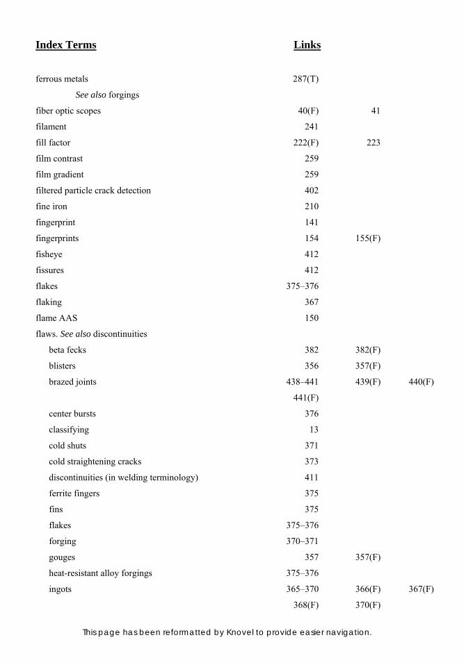
Index Terms Links
This page has been reformatted by Knovel to provide easier navigation.
ferrous metals 287(T)
See also forgings
fiber optic scopes 40(F) 41
filament 241
fill factor 222(F) 223
film contrast 259
film gradient 259
filtered particle crack detection 402
fine iron 210
fingerprint 141
fingerprints 154 155(F)
fisheye 412
fissures 412
flakes 375–376
flaking 367
flame AAS 150
flaws. See also discontinuities
beta fecks 382 382(F)
blisters 356 357(F)
brazed joints 438–441 439(F) 440(F)
441(F)
center bursts 376
classifying 13
cold shuts 371
cold straightening cracks 373
discontinuities (in welding terminology) 411
ferrite fingers 375
fins 375
flakes 375–376
forging 370–371
gouges 357 357(F)
heat-resistant alloy forgings 375–376
ingots 365–370 366(F) 367(F)
368(F) 370(F)
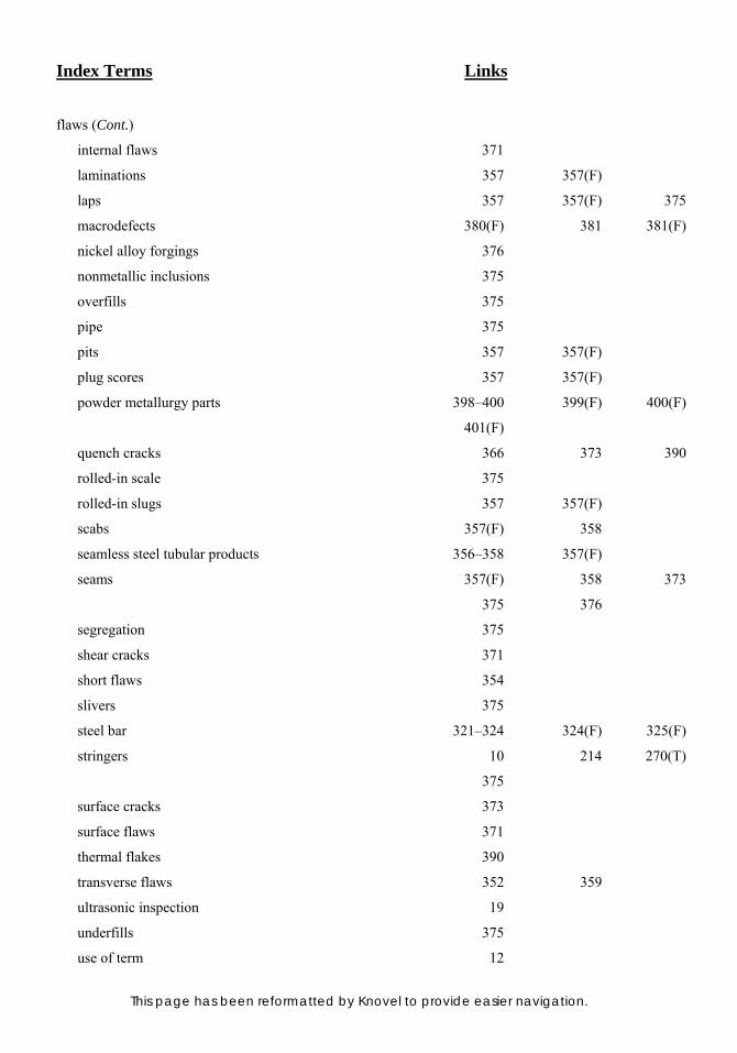
Index Terms Links
This page has been reformatted by Knovel to provide easier navigation.
flaws (Cont.)
internal flaws 371
laminations 357 357(F)
laps 357 357(F) 375
macrodefects 380(F) 381 381(F)
nickel alloy forgings 376
nonmetallic inclusions 375
overfills 375
pipe 375
pits 357 357(F)
plug scores 357 357(F)
powder metallurgy parts 398–400 399(F) 400(F)
401(F)
quench cracks 366 373 390
rolled-in scale 375
rolled-in slugs 357 357(F)
scabs 357(F) 358
seamless steel tubular products 356–358 357(F)
seams 357(F) 358 373
375 376
segregation 375
shear cracks 371
short flaws 354
slivers 375
steel bar 321–324 324(F) 325(F)
stringers 10 214 270(T)
375
surface cracks 373
surface flaws 371
thermal flakes 390
transverse flaws 352 359
ultrasonic inspection 19
underfills 375
use of term 12
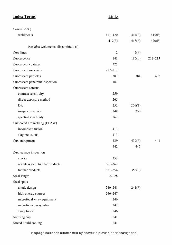
Index Terms Links
This page has been reformatted by Knovel to provide easier navigation.
flaws (Cont.)
weldments 411–420 414(F) 415(F)
417(F) 418(F) 420(F)
(see also weldments: discontinuities)
flow lines 2 2(F)
fluorescence 141 186(F) 212–213
fluorescent coatings 325
fluorescent materials 212–213
fluorescent particles 383 384 402
fluorescent penetrant inspection 187
fluorescent screens
contrast sensitivity 259
direct exposure method 265
DR 252 256(T)
image conversion 248 250
spectral sensitivity 262
flux cored arc welding (FCAW)
incomplete fusion 413
slag inclusions 413
flux entrapment 439 439(F) 441
442 445
flux leakage inspection
cracks 352
seamless steel tubular products 361–362
tubular products 351–354 353(F)
focal length 27–28
focal spots
anode design 240–241 241(F)
high energy sources 246–247
microfocal x-ray equipment 246
microfocus x-ray tubes 242
x-ray tubes 246
focusing cap 241
forced liquid cooling 241
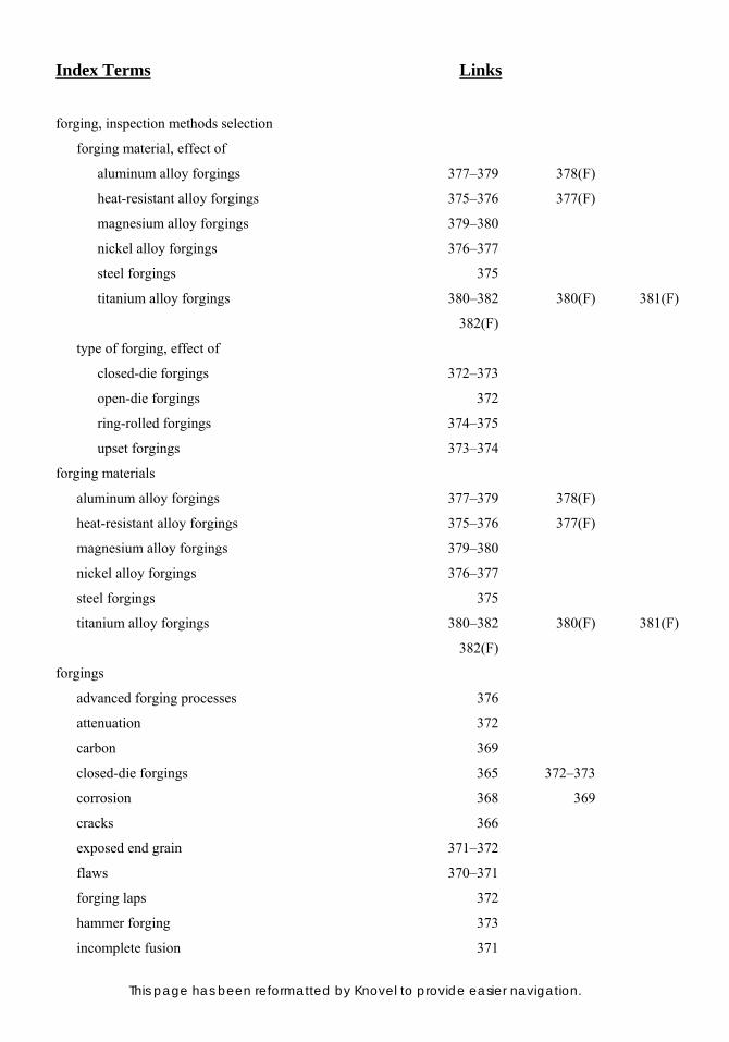
Index Terms Links
This page has been reformatted by Knovel to provide easier navigation.
forging, inspection methods selection
forging material, effect of
aluminum alloy forgings 377–379 378(F)
heat-resistant alloy forgings 375–376 377(F)
magnesium alloy forgings 379–380
nickel alloy forgings 376–377
steel forgings 375
titanium alloy forgings 380–382 380(F) 381(F)
382(F)
type of forging, effect of
closed-die forgings 372–373
open-die forgings 372
ring-rolled forgings 374–375
upset forgings 373–374
forging materials
aluminum alloy forgings 377–379 378(F)
heat-resistant alloy forgings 375–376 377(F)
magnesium alloy forgings 379–380
nickel alloy forgings 376–377
steel forgings 375
titanium alloy forgings 380–382 380(F) 381(F)
382(F)
forgings
advanced forging processes 376
attenuation 372
carbon 369
closed-die forgings 365 372–373
corrosion 368 369
cracks 366
exposed end grain 371–372
flaws 370–371
forging laps 372
hammer forging 373
incomplete fusion 371
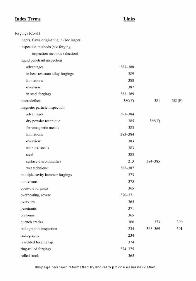
Index Terms Links
This page has been reformatted by Knovel to provide easier navigation.
forgings (Cont.)
ingots, flaws originating in (see ingots)
inspection methods (see forging,
inspection methods selection)
liquid penetrant inspection
advantages 387–388
in heat-resistant alloy forgings 389
limitations 388
overview 387
in steel forgings 388–389
macrodefects 380(F) 381 381(F)
magnetic particle inspection
advantages 383–384
dry powder technique 385 386(F)
ferromagnetic metals 383
limitations 383–384
overview 383
stainless steels 383
steel 383
surface discontinuities 213 384–385
wet technique 385–387
multiple cavity hammer forgings 373
nonferrous 375
open-die forgings 365
overheating, severe 370–371
overview 365
penetrants 371
preforms 365
quench cracks 366 373 390
radiographic inspection 234 368–369 391
radiography 234
rewelded forging lap 374
ring-rolled forgings 374–375
rolled stock 365
Index Terms Links
This page has been reformatted by Knovel to provide easier navigation.
forgings (Cont.)
shear cracks 371
steel (see steel forgings)
subsurface cracks 373 375
surface cracks 373
ultrasonic inspection 373 389–390 389(F)
ultrasonics 390
upset forgings 365 373–374
vacuum remelting operation 368
visual inspection 383
forward scattering 290
foundries 293 300 318
319
foundry inspection 302
Fourier-domain processing 73
frequency plot 306–307 309(F)
fuel oils 376
fusion
incomplete fusion 412
lack of fusion 412
G
gadolinium 263 265
gadolinium foil 265
gadolinium oxysulfide 265
gadolinium screens 265
gage 49
gage marks 122
Gamma Densomat 406 406(F)
gamma ray sources 236 247
gamma rays 233 236
See also γ-rays
γ-rays 237–238 238(F) 239
239(T)
Index Terms Links
This page has been reformatted by Knovel to provide easier navigation.
gamma-ray density determination 405–406 406(F)
gas entrapment 310
gas evolution 152 295
gas ionization detectors 251
gas metal arc welding (GMAW) 413
gas porosity
castings 295 295(F) 391
radiography 391
types 413–414 414(F) 415(F)
weldments 413–415 414(F) 415(F)
428
gas tungsten arc welding (GTAW) 413
gating system 297
geometric unsharpness 246–248 248(F)
glycerol 169
GMAW. See gas metal arc welding (GMAW)
gold 159(F) 221(T) 241
gouges 357 357(F)
grain boundaries
bright-field illumination 178
dark-field illumination 179
hydrogen flakes 367
intergranular 24 24(F)
microscopic examination 171–176(T)
scattering 290
ultrasonic inspection 271
weldments 425
grain boundary attack 376
grain size
ASTM grain size 181(T)
etching 170
measuring 181 182(F)
ultrasonic inspection 390
yield strength, effect on 182(F)
Index Terms Links
This page has been reformatted by Knovel to provide easier navigation.
graphite 298
graphite furnace AAS 150
graphite iron structures 318
graphite particles 294
green compacts 406
attenuation 406
green expansion 398–399
grinding
damage 164
depth of damage 164
diamond size 165
equipment 165 166(F)
flush mounted semiautomatic grinder/
polisher system 166(F)
grit size 164
lapping 166
materials 165
media 165
overview 164–165
planar grinding 165
platens 165
SiC paper 165
traditional approach 164
visual inspection 23
wet grinding 164
gripping devices 134–135(F)
guide sleeves 336
H
Hall probes 352
halogenated solvents 188
halt-of-dial yield point 120
hardness, defined 85
Index Terms Links
This page has been reformatted by Knovel to provide easier navigation.
hardness testing
applications 5 7
Brinell hardness testing 85–91(F)
castings 299 301–302
hardness 85
hardness scales 396(T)
hardness value 85
heat treatment 301
indentation hardness tests comparison 6(T)
indentation methods 5
indenter 85
light sources 114
macroetching 46
microhardness testing 106–114(F)
overview 5–7 85
P/M parts 393 396
powder metallurgy parts 396
rebound testing 85
Rockwell hardness testing 91–99(F,T)
Scleroscope hardness testing 102–106(F)
SPC 7
static indentation 85
tensile strength, correlation of hardness with 5–7
Vickers hardness testing 100–102(F) 103(F)
hardness value 85
Hastings triplet magnifier 28 29(F)
HAZ. See heat affected zone (HAZ)
HB. See Brinell hardness number (HB)
HBS. See Brinell Hardness designation (HBS)
HBW. See Brinell Hardness designation (HBW)
head shot 206 206(F) 209
209(F) 210(F)
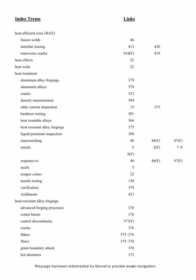
Index Terms Links
This page has been reformatted by Knovel to provide easier navigation.
heat affected zone (HAZ)
fusion welds 46
lamellar tearing 413 420
transverse cracks 418(F) 419
heat effects 22
heat scale 22
heat treatment
aluminum alloy forgings 379
aluminum alloys 379
cracks 323
density measurement 394
eddy current inspection 15 215
hardness testing 301
heat treatable alloys 366
heat-resistant alloy forgings 375
liquid penetrant inspection 308
macroetching 46 46(F) 47(F)
metals 5 5(F) 7–8
8(F)
response to 46 46(F) 47(F)
steels 5
temper colors 22
tensile testing 130
verification 379
weldments 423
heat-resistant alloy forgings
advanced forging processes 376
center bursts 376
central discontinuity 377(F)
cracks 376
flakes 375–376
flaws 375–376
grain boundary attack 376
hot shortness 375
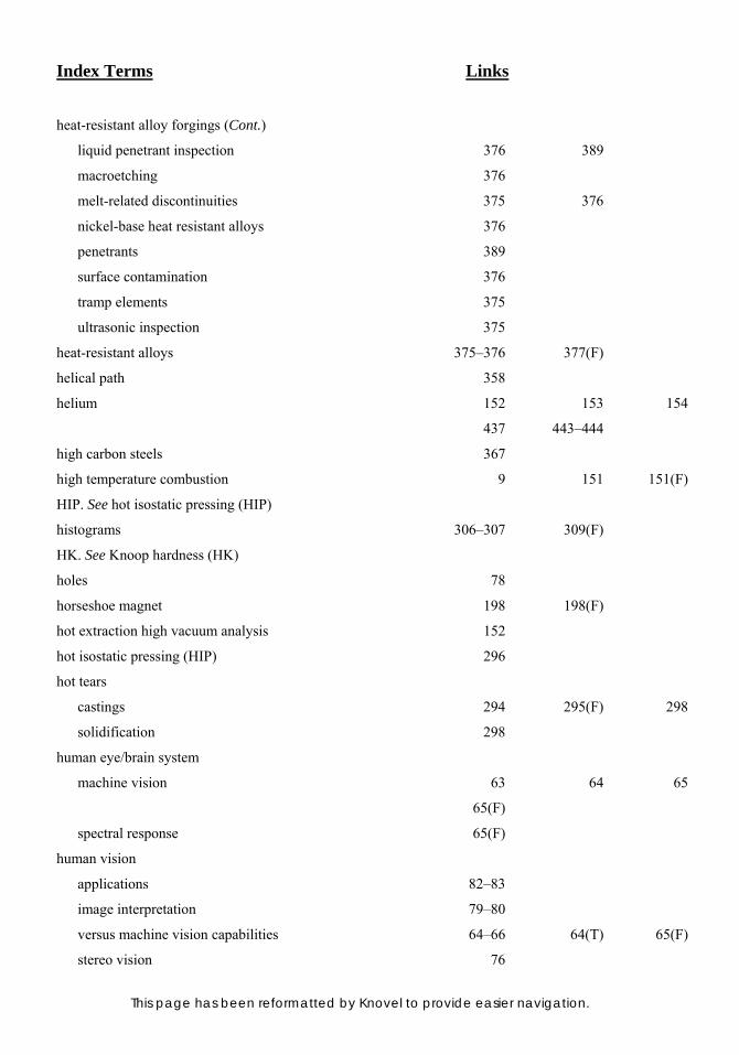
Index Terms Links
This page has been reformatted by Knovel to provide easier navigation.
heat-resistant alloy forgings (Cont.)
liquid penetrant inspection 376 389
macroetching 376
melt-related discontinuities 375 376
nickel-base heat resistant alloys 376
penetrants 389
surface contamination 376
tramp elements 375
ultrasonic inspection 375
heat-resistant alloys 375–376 377(F)
helical path 358
helium 152 153 154
437 443–444
high carbon steels 367
high temperature combustion 9 151 151(F)
HIP. See hot isostatic pressing (HIP)
histograms 306–307 309(F)
HK. See Knoop hardness (HK)
holes 78
horseshoe magnet 198 198(F)
hot extraction high vacuum analysis 152
hot isostatic pressing (HIP) 296
hot tears
castings 294 295(F) 298
solidification 298
human eye/brain system
machine vision 63 64 65
65(F)
spectral response 65(F)
human vision
applications 82–83
image interpretation 79–80
versus machine vision capabilities 64–66 64(T) 65(F)
stereo vision 76
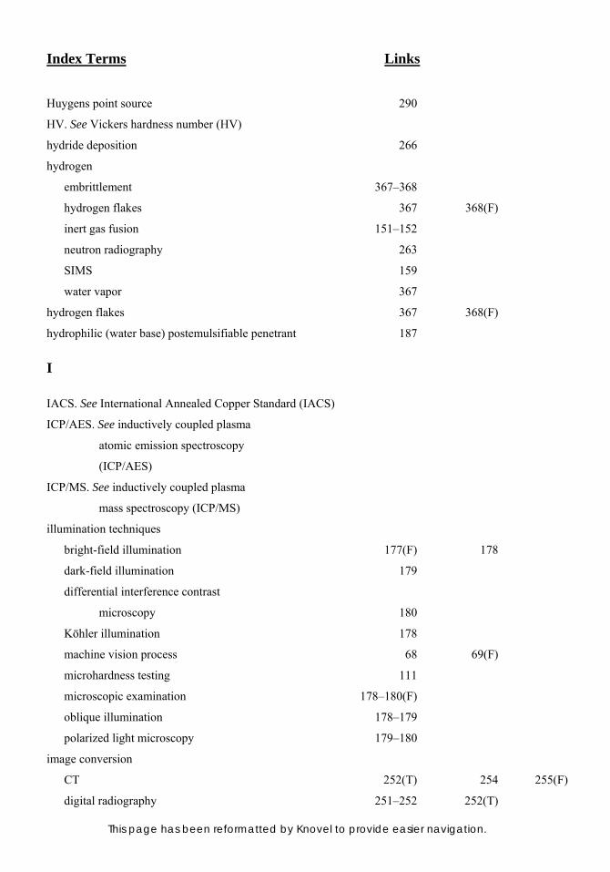
Index Terms Links
This page has been reformatted by Knovel to provide easier navigation.
Huygens point source 290
HV. See Vickers hardness number (HV)
hydride deposition 266
hydrogen
embrittlement 367–368
hydrogen flakes 367 368(F)
inert gas fusion 151–152
neutron radiography 263
SIMS 159
water vapor 367
hydrogen flakes 367 368(F)
hydrophilic (water base) postemulsifiable penetrant 187
I
IACS. See International Annealed Copper Standard (IACS)
ICP/AES. See inductively coupled plasma
atomic emission spectroscopy
(ICP/AES)
ICP/MS. See inductively coupled plasma
mass spectroscopy (ICP/MS)
illumination techniques
bright-field illumination 177(F) 178
dark-field illumination 179
differential interference contrast
microscopy 180
Köhler illumination 178
machine vision process 68 69(F)
microhardness testing 111
microscopic examination 178–180(F)
oblique illumination 178–179
polarized light microscopy 179–180
image conversion
CT 252(T) 254 255(F)
digital radiography 251–252 252(T)
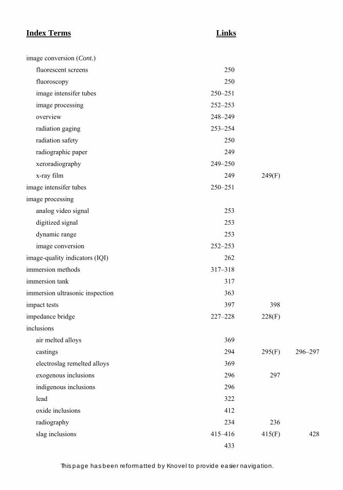
Index Terms Links
This page has been reformatted by Knovel to provide easier navigation.
image conversion (Cont.)
fluorescent screens 250
fluoroscopy 250
image intensifer tubes 250–251
image processing 252–253
overview 248–249
radiation gaging 253–254
radiation safety 250
radiographic paper 249
xeroradiography 249–250
x-ray film 249 249(F)
image intensifer tubes 250–251
image processing
analog video signal 253
digitized signal 253
dynamic range 253
image conversion 252–253
image-quality indicators (IQI) 262
immersion methods 317–318
immersion tank 317
immersion ultrasonic inspection 363
impact tests 397 398
impedance bridge 227–228 228(F)
inclusions
air melted alloys 369
castings 294 295(F) 296–297
electroslag remelted alloys 369
exogenous inclusions 296 297
indigenous inclusions 296
lead 322
oxide inclusions 412
radiography 234 236
slag inclusions 415–416 415(F) 428
433
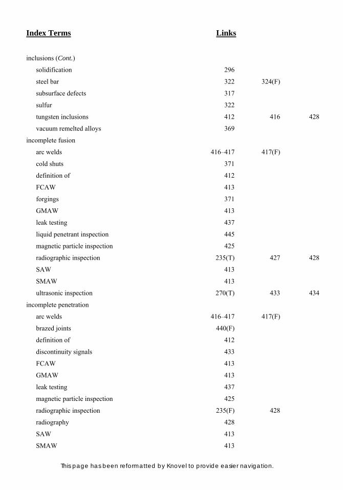
Index Terms Links
This page has been reformatted by Knovel to provide easier navigation.
inclusions (Cont.)
solidification 296
steel bar 322 324(F)
subsurface defects 317
sulfur 322
tungsten inclusions 412 416 428
vacuum remelted alloys 369
incomplete fusion
arc welds 416–417 417(F)
cold shuts 371
definition of 412
FCAW 413
forgings 371
GMAW 413
leak testing 437
liquid penetrant inspection 445
magnetic particle inspection 425
radiographic inspection 235(T) 427 428
SAW 413
SMAW 413
ultrasonic inspection 270(T) 433 434
incomplete penetration
arc welds 416–417 417(F)
brazed joints 440(F)
definition of 412
discontinuity signals 433
FCAW 413
GMAW 413
leak testing 437
magnetic particle inspection 425
radiographic inspection 235(F) 428
radiography 428
SAW 413
SMAW 413
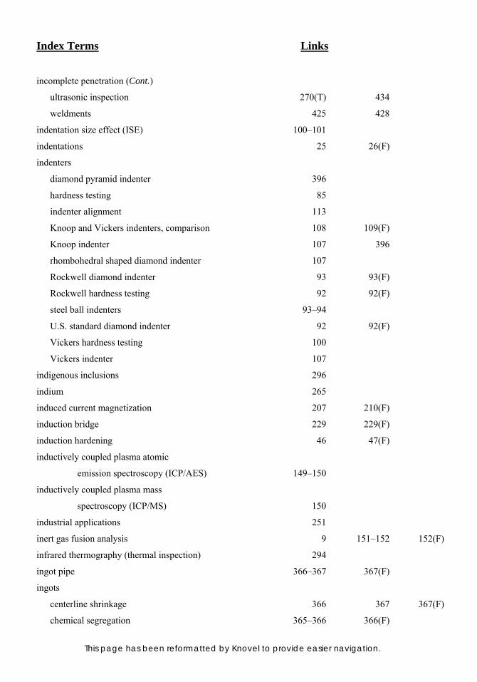
Index Terms Links
This page has been reformatted by Knovel to provide easier navigation.
incomplete penetration (Cont.)
ultrasonic inspection 270(T) 434
weldments 425 428
indentation size effect (ISE) 100–101
indentations 25 26(F)
indenters
diamond pyramid indenter 396
hardness testing 85
indenter alignment 113
Knoop and Vickers indenters, comparison 108 109(F)
Knoop indenter 107 396
rhombohedral shaped diamond indenter 107
Rockwell diamond indenter 93 93(F)
Rockwell hardness testing 92 92(F)
steel ball indenters 93–94
U.S. standard diamond indenter 92 92(F)
Vickers hardness testing 100
Vickers indenter 107
indigenous inclusions 296
indium 265
induced current magnetization 207 210(F)
induction bridge 229 229(F)
induction hardening 46 47(F)
inductively coupled plasma atomic
emission spectroscopy (ICP/AES) 149–150
inductively coupled plasma mass
spectroscopy (ICP/MS) 150
industrial applications 251
inert gas fusion analysis 9 151–152 152(F)
infrared thermography (thermal inspection) 294
ingot pipe 366–367 367(F)
ingots
centerline shrinkage 366 367 367(F)
chemical segregation 365–366 366(F)
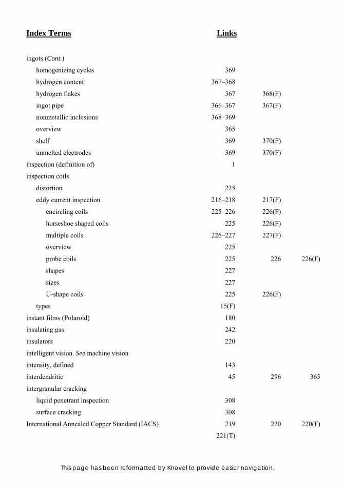
Index Terms Links
This page has been reformatted by Knovel to provide easier navigation.
ingots (Cont.)
homogenizing cycles 369
hydrogen content 367–368
hydrogen flakes 367 368(F)
ingot pipe 366–367 367(F)
nonmetallic inclusions 368–369
overview 365
shelf 369 370(F)
unmelted electrodes 369 370(F)
inspection (definition of) 1
inspection coils
distortion 225
eddy current inspection 216–218 217(F)
encircling coils 225–226 226(F)
horseshoe shaped coils 225 226(F)
multiple coils 226–227 227(F)
overview 225
probe coils 225 226 226(F)
shapes 227
sizes 227
U-shape coils 225 226(F)
types 15(F)
instant films (Polaroid) 180
insulating gas 242
insulators 220
intelligent vision. See machine vision
intensity, defined 143
interdendritic 45 296 365
intergranular cracking
liquid penetrant inspection 308
surface cracking 308
International Annealed Copper Standard (IACS) 219 220 220(F)
221(T)
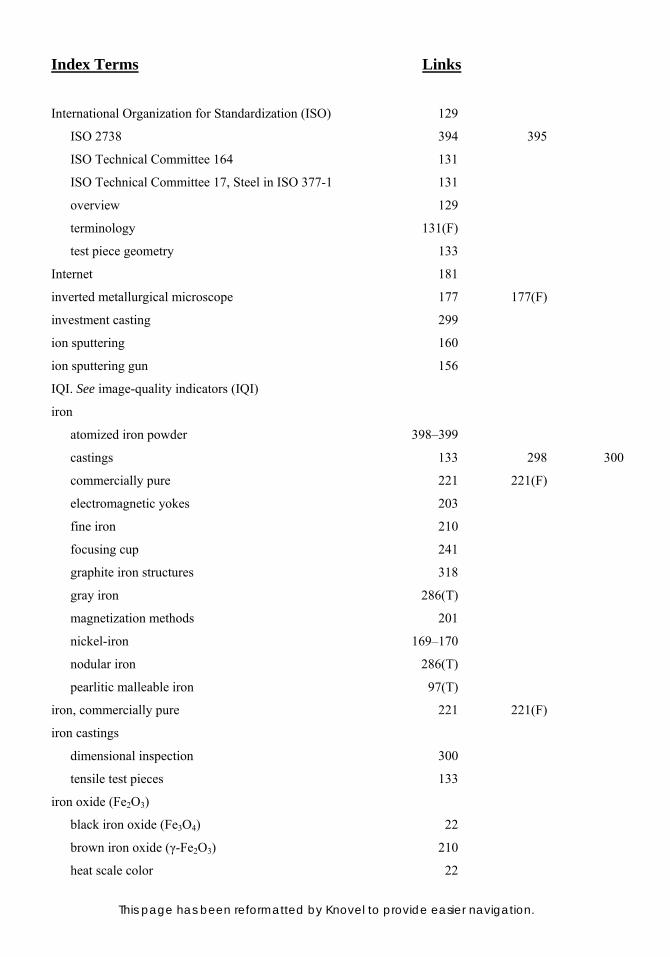
Index Terms Links
This page has been reformatted by Knovel to provide easier navigation.
International Organization for Standardization (ISO) 129
ISO 2738 394 395
ISO Technical Committee 164 131
ISO Technical Committee 17, Steel in ISO 377-1 131
overview 129
terminology 131(F)
test piece geometry 133
Internet 181
inverted metallurgical microscope 177 177(F)
investment casting 299
ion sputtering 160
ion sputtering gun 156
IQI. See image-quality indicators (IQI)
iron
atomized iron powder 398–399
castings 133 298 300
commercially pure 221 221(F)
electromagnetic yokes 203
fine iron 210
focusing cup 241
graphite iron structures 318
gray iron 286(T)
magnetization methods 201
nickel-iron 169–170
nodular iron 286(T)
pearlitic malleable iron 97(T)
iron, commercially pure 221 221(F)
iron castings
dimensional inspection 300
tensile test pieces 133
iron oxide (Fe2O3)
black iron oxide (Fe3O4) 22
brown iron oxide (γ-Fe2O3) 210
heat scale color 22

Index Terms Links
This page has been reformatted by Knovel to provide easier navigation.
iron oxide (Fe2O3) (Cont.)
polishing abrasives 169
red iron oxide (magnitite Fe3O4) 210
irradiation 239
ISO. See International Organization for
Standardization (ISO) 129
isotopes
-rays, production of 239
neutron radiography 262 263 265
isotropic metal 180
J
jack rest 99 99(F)
Japanese Industrial Standards (JIS) 129 133
JIS. See Japanese Industrial Standards (JIS)
K
kerosene 169
kilogram-force (kgf) 125
Knoop, Frederick 107
Knoop hardness (HK) 107
Knoop indenter 107 108–110 109(F)
111 396
Knoop indents 107 109(F) 114
Knoop test 109(F) 113 114
Köhler illumination 178
Kopp glass filter 212
L
lack of fill 438 439(F) 441
442
lack of fusion 412 417(F) 434
See also incomplete fusion
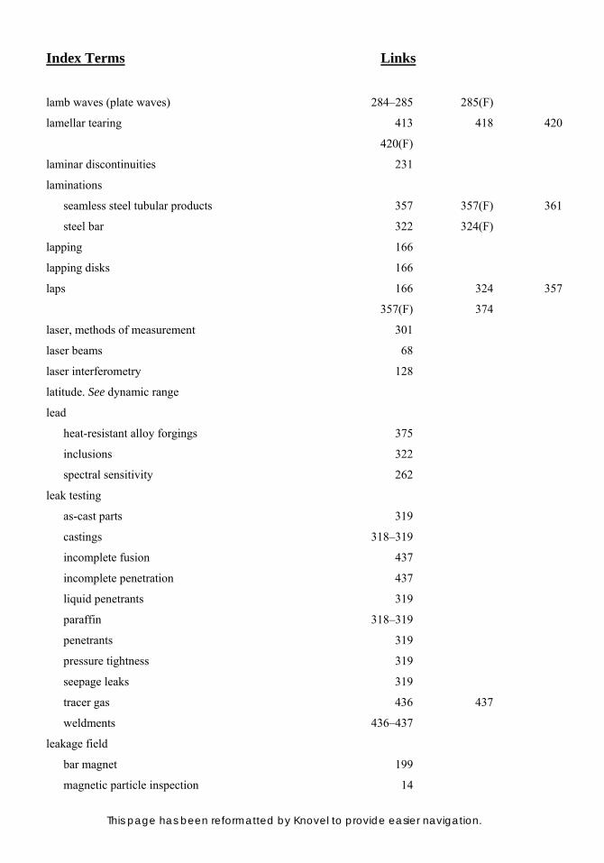
Index Terms Links
This page has been reformatted by Knovel to provide easier navigation.
lamb waves (plate waves) 284–285 285(F)
lamellar tearing 413 418 420
420(F)
laminar discontinuities 231
laminations
seamless steel tubular products 357 357(F) 361
steel bar 322 324(F)
lapping 166
lapping disks 166
laps 166 324 357
357(F) 374
laser, methods of measurement 301
laser beams 68
laser interferometry 128
latitude. See dynamic range
lead
heat-resistant alloy forgings 375
inclusions 322
spectral sensitivity 262
leak testing
as-cast parts 319
castings 318–319
incomplete fusion 437
incomplete penetration 437
liquid penetrants 319
paraffin 318–319
penetrants 319
pressure tightness 319
seepage leaks 319
tracer gas 436 437
weldments 436–437
leakage field
bar magnet 199
magnetic particle inspection 14
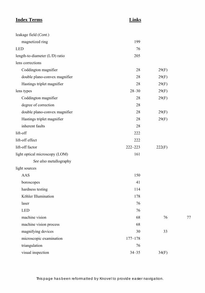
Index Terms Links
This page has been reformatted by Knovel to provide easier navigation.
leakage field (Cont.)
magnetized ring 199
LED 76
length-to-diameter (L/D) ratio 205
lens corrections
Coddington magnifier 28 29(F)
double plano-convex magnifier 28 29(F)
Hastings triplet magnifier 28 29(F)
lens types 28–30 29(F)
Coddington magnifier 28 29(F)
degree of correction 28
double plano-convex magnifier 28 29(F)
Hastings triplet magnifier 28 29(F)
inherent faults 28
lift-off 222
lift-off effect 222
lift-off factor 222–223 222(F)
light optical microscopy (LOM) 161
See also metallography
light sources
AAS 150
boroscopes 41
hardness testing 114
Köhler Illumination 178
laser 76
LED 76
machine vision 68 76 77
machine vision process 68
magnifying devices 30 33
microscopic examination 177–178
triangulation 76
visual inspection 34–35 34(F)

Index Terms Links
This page has been reformatted by Knovel to provide easier navigation.
lighting
illuminated magnifiers 33 33(F)
machine vision process 68
microhardness testing 111
photography 43–44
visual inspection 33–35 34(F) 35(F)
linear absorption coefficient 244
linear arrays 68
linear dimensions 394
linear displacement transducers 301
lipophilic postemulsifable penetrant 187
liquid penetrant inspection
aluminum alloy forgings 379
applications 13
brazed joints 444–445
castings 293–294 299 308–309
cleaning methods 193 194(T)
crack detection 402
cracks 183 185 192
196(T) 308 402
detectable flaws 183
developers 185 186(F) 188–192
emulsifiers 188
equipment 184
equipment requirements
developer station 195
drying station 192(F) 195
emulsifier station 194–195
inspection station 195
overview 192–193 192(F)
package units 192–193 192(F)
penetrant station 194
postcleaning station 195–196
precleaning 193 194(T)

Index Terms Links
This page has been reformatted by Knovel to provide easier navigation.
liquid penetrant inspection
equipment requirements (Cont.)
recirculating hot air drier 192(F) 195
rinse station 195
ultraviolet (black) light 192
ferromagnetic steels 13
ferrous metals 183
fluorescent penetrant inspection 187
forgings 387–388
heat-resistant alloy forgings 389
incomplete fusion 445
limitations 14 183–184
materials 183–184
nickel alloy forgings 377
nonferrous metals 183
nonferrous tubing 363
overview 13–14 13(F)
penetrant materials 187
penetrant requirements 187–188
physical principles 184
physical/chemical characteristics 187–188
PM parts 184
postemulsifable system 186–187 193 388
process 184–185 186(F)
resistance welded steel tubing 356
seamless steel tubular products 362
sensitivity 184
solvent cleaners 188
solvent-removable system 187 326 388–389
445
steel bar 326
steel forgings
forging material, effect of 375
postemulsifable system 388
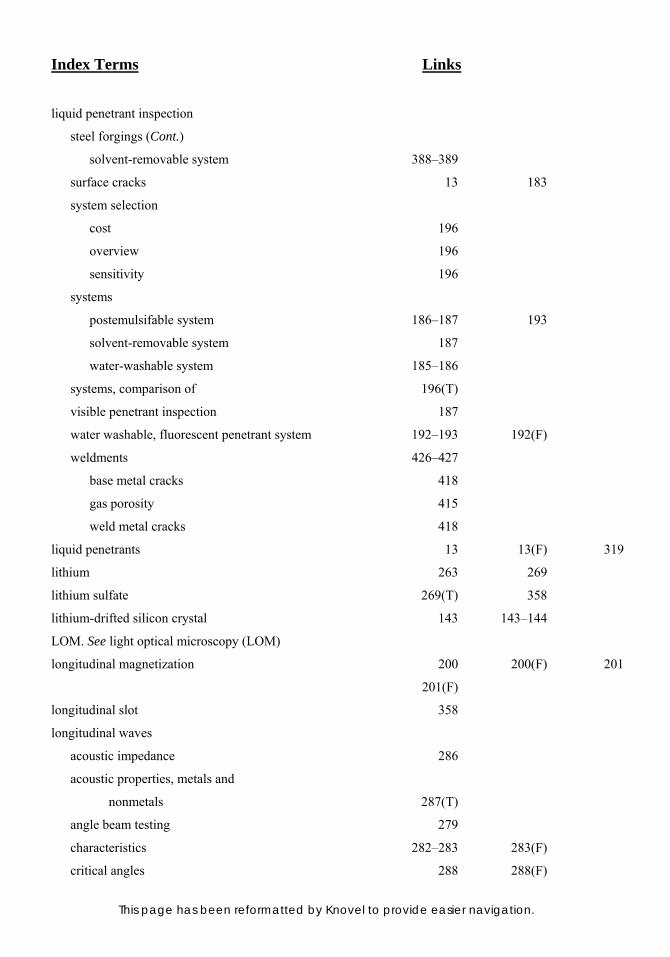
Index Terms Links
This page has been reformatted by Knovel to provide easier navigation.
liquid penetrant inspection
steel forgings (Cont.)
solvent-removable system 388–389
surface cracks 13 183
system selection
cost 196
overview 196
sensitivity 196
systems
postemulsifable system 186–187 193
solvent-removable system 187
water-washable system 185–186
systems, comparison of 196(T)
visible penetrant inspection 187
water washable, fluorescent penetrant system 192–193 192(F)
weldments 426–427
base metal cracks 418
gas porosity 415
weld metal cracks 418
liquid penetrants 13 13(F) 319
lithium 263 269
lithium sulfate 269(T) 358
lithium-drifted silicon crystal 143 143–144
LOM. See light optical microscopy (LOM)
longitudinal magnetization 200 200(F) 201
201(F)
longitudinal slot 358
longitudinal waves
acoustic impedance 286
acoustic properties, metals and
nonmetals 287(T)
angle beam testing 279
characteristics 282–283 283(F)
critical angles 288 288(F)
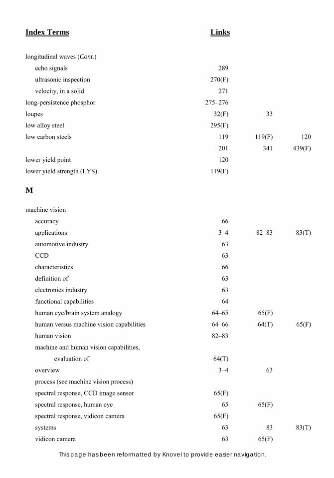
Index Terms Links
This page has been reformatted by Knovel to provide easier navigation.
longitudinal waves (Cont.)
echo signals 289
ultrasonic inspection 270(F)
velocity, in a solid 271
long-persistence phosphor 275–276
loupes 32(F) 33
low alloy steel 295(F)
low carbon steels 119 119(F) 120
201 341 439(F)
lower yield point 120
lower yield strength (LYS) 119(F)
M
machine vision
accuracy 66
applications 3–4 82–83 83(T)
automotive industry 63
CCD 63
characteristics 66
definition of 63
electronics industry 63
functional capabilities 64
human eye/brain system analogy 64–65 65(F)
human versus machine vision capabilities 64–66 64(T) 65(F)
human vision 82–83
machine and human vision capabilities,
evaluation of 64(T)
overview 3–4 63
process (see machine vision process)
spectral response, CCD image sensor 65(F)
spectral response, human eye 65 65(F)
spectral response, vidicon camera 65(F)
systems 63 83 83(T)
vidicon camera 63 65(F)
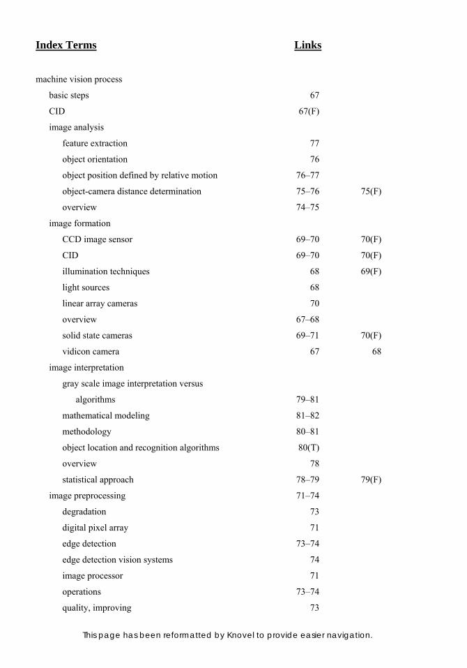
Index Terms Links
This page has been reformatted by Knovel to provide easier navigation.
machine vision process
basic steps 67
CID 67(F)
image analysis
feature extraction 77
object orientation 76
object position defined by relative motion 76–77
object-camera distance determination 75–76 75(F)
overview 74–75
image formation
CCD image sensor 69–70 70(F)
CID 69–70 70(F)
illumination techniques 68 69(F)
light sources 68
linear array cameras 70
overview 67–68
solid state cameras 69–71 70(F)
vidicon camera 67 68
image interpretation
gray scale image interpretation versus
algorithms 79–81
mathematical modeling 81–82
methodology 80–81
object location and recognition algorithms 80(T)
overview 78
statistical approach 78–79 79(F)
image preprocessing 71–74
degradation 73
digital pixel array 71
edge detection 73–74
edge detection vision systems 74
image processor 71
operations 73–74
quality, improving 73
Index Terms Links
This page has been reformatted by Knovel to provide easier navigation.
machine vision process
image preprocessing (Cont.)
restoration 73
run length encoding 73–74
windowing 72–73
image sensors 70–71
light sources 68 76 77
machine vision system 66 66(F)
process 67(F)
vision systems
binary 71
gray scale system 71–72 72(F)
weld seam tracking 71
machine vision systems. See also machine vision
accuracy 66
applications 82–83 83(T)
components 66(F)
costs 66
dimensional inspection 294
illumination techniques 69(F)
image analysis 74–75
image preprocessing 73–74
image sensors 68 70–71
interfacing 82
microcomputers 63 71
overview 4 4(F) 63–65
software library of object location and
recognition algorithms 80(T)
solid state cameras 69
special purpose systems 81–82
users 63
vidicon camera 68
macrodefects 381–382 381(F)
Index Terms Links
This page has been reformatted by Knovel to provide easier navigation.
macroetching
heat-resistant alloy forgings 376
solidification 44
visual inspection 44–46 45(F) 46(F)
47(F)
macroporosity 295–296
macrosegregation 45
magnesium
acoustic properties 287
critical angles 289(T)
electrical resistivity/conductivity 221(T)
incident angle 289(T)
magnetic particle inspection 14 197
polishing abrasives 169
radiographic absorption equivalence 245(T)
radiographic film, selection 257(T)
radiographic film, selection of 257(T)
Rockwell hardness scales 97
magnesium alloy forgings
cracks 379
discontinuities 379
forging materials 379–380
liquid penetrant inspection 379
surface cracks 379
ultrasonic inspection 379
visual inspection 380
magnesium oxide (MgO) 169
magnetic field perturbation. See flux
leakage inspection
magnetic fields
circular field 200
circular magnetization 199–200 200(F)
circularly magnetized 200
circumferential magnetic fields 310
Index Terms Links
This page has been reformatted by Knovel to provide easier navigation.
magnetic fields (Cont.)
controlling direction of 14 14(F)
demagnetization 214
eddy current inspection 216 361
electromagnetic inspection 331
ferromagnetic conductor 200
flux direction, effect of 200–201 201(F)
generation of (see magnetic fields,
generating)
horseshoe magnet 198 198(F)
longitudinal field 199
longitudinal magnetization 200 200(F) 201
201(F)
longitudinally magnetized 199
magnetic particle inspection 309 426
magnetic particles 198 198(F)
magnetic permeability systems 339
magnetization methods 201
magnetized bar 199 199(F) 201
201(F)
magnetized ring 198–199 198(F)
magnetizing current
alternating current 202
direct current 202
overview 202
power sources
mobile units 202–203
portable equipment 202
stationary equipment 203
transverse magnetic fields 361
tubular products 361
magnetic fields, generating
bench unit 206 206(F)
central conductors 205–206 205(F)
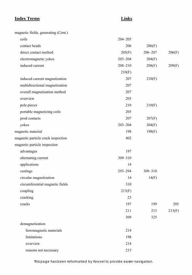
Index Terms Links
This page has been reformatted by Knovel to provide easier navigation.
magnetic fields, generating (Cont.)
coils 204–205
contact heads 206 206(F)
direct contact method 205(F) 206–207 206(F)
electromagnetic yokes 203–204 204(F)
induced current 208–210 208(F) 209(F)
210(F)
induced current magnetization 207 210(F)
multidirectional magnetization 207
overall magnetization method 207
overview 203
pole pieces 210 210(F)
portable magnetizing coils 205
prod contacts 207 207(F)
yokes 203–204 204(F)
magnetic material 198 198(F)
magnetic particle crack inspection 402
magnetic particle inspection
advantages 197
alternating current 309–310
applications 14
castings 293–294 309–310
circular magnetization 14 14(F)
circumferential magnetic fields 310
coupling 213(F)
cracking 23
cracks 197 199 205
211 213 213(F)
309 325
demagnetization
ferromagnetic materials 214
limitations 198
overview 214
reasons not necessary 215

Index Terms Links
This page has been reformatted by Knovel to provide easier navigation.
magnetic particle inspection
demagnetization (Cont.)
reasons to 214
residual magnetic field 214
retentivity 214
weldments 426
direct current 309–310
discontinuities
overview 213
subsurface discontinuities 213–214
surface discontinuities 201(F) 213 213(F)
ferromagnetic materials 197
forgings 383–387 386(F)
incomplete fusion 425
incomplete penetration 425
industrial uses 14–15 197
in-process magnetic particle inspection 15 197
leakage field 14
limitations 197–198
longitudinal magnetization 14 14(F)
magnesium 14 197
magnetic fields
controlling direction of 14 14(F)
description of 198–201(F)
generating 203–210(F)
magnetic particles 197 210–211
magnetizing current
alternating current 202
direct current 202
overview 202
near surface cracks 402
nonferromagnetic materials 14 197
nonmetallic inclusions 197 213–214
nonrelevant indications 214

Index Terms Links
This page has been reformatted by Knovel to provide easier navigation.
magnetic particle inspection (Cont.)
overview 14–15 183 197
penetrants 356 384
power sources
mobile units 202–203
portable equipment 202
stationary equipment 203
resistance welded steel tubing 355–356
seamless steel tubular products 362
slag inclusions 425
steel bar 325–326
steel forgings 375
surface cracks 197 313 402
ultraviolet light 212–213
weldments
gas porosity 415
incomplete fusion 417
incomplete penetration 417
nonrelevant indications 425
operational requirements 426
overview 425
slag inclusions 416
subsurface cracks 419
weld metal cracks 418
magnetic particles
application 197
bath strength 212
brown iron oxide (γ-Fe2O3) 210
characteristics 210
classification of 210
contrast 211
dry particle method 210
dry particles 211
dry powder testing 211

Index Terms Links
This page has been reformatted by Knovel to provide easier navigation.
magnetic particles (Cont.)
ferrospinel ferrites (NixFe2O4) 210
fine iron 210
fluorescent magnetic particles 211
magnetic particle inspection 197
magnetic properties 210
magnetized ring 198 198(F)
nickel alloys 210
oil suspending liquid 211–212
overview 210
particle shape, effect of 211
particle size, effect of 210–211
red iron oxide (magnitite Fe3O4) 210
suspensions 211
visibility 211
water suspending liquid 212
wet particle method 210
wet particles 211
magnetic permeability 221–222 221(F)
magnetic permeability systems (steel bars)
aging 340
bar stock 341–342
coil arrangement 339
coil assembly 340(F)
control units 343
cracks 341 343
detectable flaws 341
draft 341 341(F)
efficiency of 340
end effect 341
equipment 342 343(F)
limitations 340
null system 342 343(F)
oscilloscope screens 342 343(F)
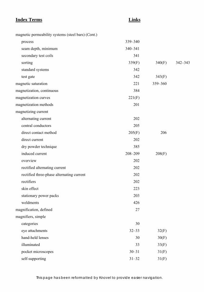
Index Terms Links
This page has been reformatted by Knovel to provide easier navigation.
magnetic permeability systems (steel bars) (Cont.)
process 339–340
seam depth, minimum 340–341
secondary test coils 341
sorting 339(F) 340(F) 342–343
standard systems 342
test gate 342 343(F)
magnetic saturation 221 359–360
magnetization, continuous 384
magnetization curves 221(F)
magnetization methods 201
magnetizing current
alternating current 202
central conductors 205
direct contact method 205(F) 206
direct current 202
dry powder technique 385
induced current 208–209 208(F)
overview 202
rectified alternating current 202
rectified three-phase alternating current 202
rectifiers 202
skin effect 223
stationary power packs 203
weldments 426
magnification, defined 27
magnifiers, simple
categories 30
eye attachments 32–33 32(F)
hand-held lenses 30 30(F)
illuminated 33 33(F)
pocket microscopes 30–31 31(F)
self-supporting 31–32 31(F)

Index Terms Links
This page has been reformatted by Knovel to provide easier navigation.
magnifying devices
depth of field 29
distortion 27
focal length 27–28
limiting factors 29–30
magnifying power 27
manganese 172(T) 174(T) 175(T)
296
manufacturing applications
machine vision applications 82
machine vision systems 81 83 83(T)
marking crayons 376
markings
bolt heads 22
hidden markings 22
stress concentrations 25 26(F)
visual inspection 21–22
wire rope industry 22
mass spectrometer 150 159 437
443
mass-absorption coefficient 244
mathematical modeling 81–82
measuring devices
specialty 36–38 38(F)
visual inspection 35–38 37(F) 38(F)
mechanical assemblies 234
mechanical proof testing 400 401–402
medical applications 251
megahertz (MHz) 225
melt-through 412
mercury vapor lamp 212
metal penetration
castings 294 298
solidification 298
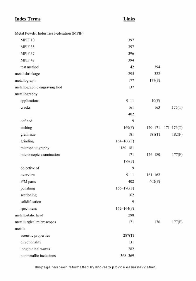
Index Terms Links
This page has been reformatted by Knovel to provide easier navigation.
Metal Powder Industries Federation (MPIF)
MPIF 10 397
MPIF 35 397
MPIF 37 396
MPIF 42 394
test method 42 394
metal shrinkage 295 322
metallograph 177 177(F)
metallographic engraving tool 137
metallography
applications 9–11 10(F)
cracks 161 163 175(T)
402
defined 9
etching 169(F) 170–171 171–176(T)
grain size 181 181(T) 182(F)
grinding 164–166(F)
microphotography 180–181
microscopic examination 171 176–180 177(F)
179(F)
objective of 9
overview 9–11 161–162
P/M parts 402 402(F)
polishing 166–170(F)
sectioning 162
solidification 9
specimens 162–164(F)
metallostatic head 298
metallurgical microscopes 171 176 177(F)
metals
acoustic properties 287(T)
directionality 131
longitudinal waves 282
nonmetallic inclusions 368–369

Index Terms Links
This page has been reformatted by Knovel to provide easier navigation.
metals (Cont.)
surface waves (Rayleigh waves) 284 284(F)
transverse waves (shear waves) 283
methyl methacrylate 163
microcomputer
castings 301 302
CMMs 304
computer-aided dimensional inspection 302 303 303(F)
305
control charts 306
dimensional inspection 301
machine vision systems 63 71
microfissures 412
microfocal x-ray equipment 246
microfocus x-ray systems 242
microfocus x-ray tubes 242
microhardness 106
See also microhardness testing
microhardness testers 110–111 110(F)
microhardness testing
applications 106–107
accuracy, precision, bias 112–114
small workpieces 112
surface hardening operations, monitoring 112
certified test blocks 113–114
hardness scales 396
HK 107
HV 111
illumination techniques 111
indenter alignment 113
indenters 107–110 108(F) 109(F)
Knoop and Vickers indenters, comparison 108 109(F)
Knoop indent, shortcomings 108–110
Knoop indenter 107 109(F) 111
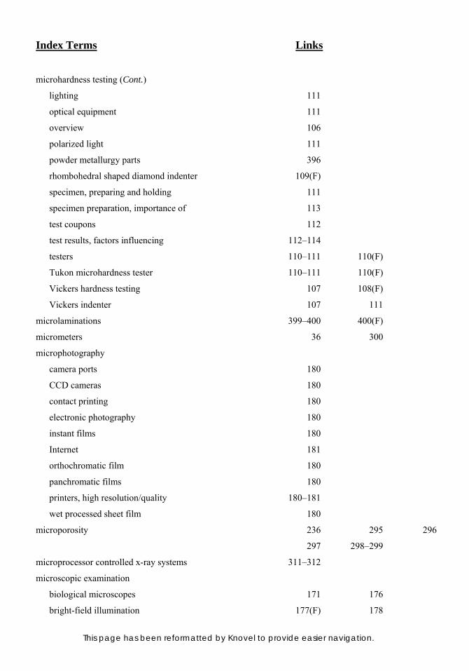
Index Terms Links
This page has been reformatted by Knovel to provide easier navigation.
microhardness testing (Cont.)
lighting 111
optical equipment 111
overview 106
polarized light 111
powder metallurgy parts 396
rhombohedral shaped diamond indenter 109(F)
specimen, preparing and holding 111
specimen preparation, importance of 113
test coupons 112
test results, factors influencing 112–114
testers 110–111 110(F)
Tukon microhardness tester 110–111 110(F)
Vickers hardness testing 107 108(F)
Vickers indenter 107 111
microlaminations 399–400 400(F)
micrometers 36 300
microphotography
camera ports 180
CCD cameras 180
contact printing 180
electronic photography 180
instant films 180
Internet 181
orthochromatic film 180
panchromatic films 180
printers, high resolution/quality 180–181
wet processed sheet film 180
microporosity 236 295 296
297 298–299
microprocessor controlled x-ray systems 311–312
microscopic examination
biological microscopes 171 176
bright-field illumination 177(F) 178

Index Terms Links
This page has been reformatted by Knovel to provide easier navigation.
microscopic examination (Cont.)
dark-field illumination 179
differential interference contrast microscopy 180
inverted metallurgical microscope 177(F)
isotropic metal 180
Köhler illumination 178
light sources 177–178
metallurgical microscopes 171 176 177(F)
oblique illumination 178–179
polarized light 178
polarized light microscopy 179–180 179(F)
polarizing light microscope 179(F)
techniques 178–180(F)
microsegregation 45
mirrors 39–40 154(F) 156
modulus of elasticity 118 118(F) 120
406
MPIF. See Metal Powder Industries
Federation (MPIF)
MPIF test method 42 394
multidirectional magnetization 207 383
mushy freezing 296
N
National Bureau of Standards 107
National Physical Laboratory (U.K.) 100
NDT. See nondestructive testing (NDT)
neck 123
necking 121(F) 123 123(F)
neutron detection methods 264
neutron radiography
applications 263 265–266
characteristics 263 264(T)
collimation 264

Index Terms Links
This page has been reformatted by Knovel to provide easier navigation.
neutron radiography (Cont.)
composites 236
conventional radiography, differs from 263
corrosion 263
ferrous alloys 236
neutron detection methods
direct exposure method 265
overview 264
real time imaging 265
transfer method 265
neutron sources 263–264
nonferrous alloys 236
nonmetallic materials 236
overview 17 233 262–263
scattering 263
thermal neutron radiography 263–264
thermal neutron sources 264(T)
thermal neutrons 263
neutrons. See also neutron radiography
attenuation of 262
moderators 263
production of 263
newtons (N) 125
nickel
electrolytic polishing 169–170
etching 170
nickel, commercially pure 221(F)
nickel alloy forgings
age hardenable nickel alloys 376–377
cracks 377
discontinuities 376
liquid penetrant inspection 377
penetrants 377
thermal cracking 376–377
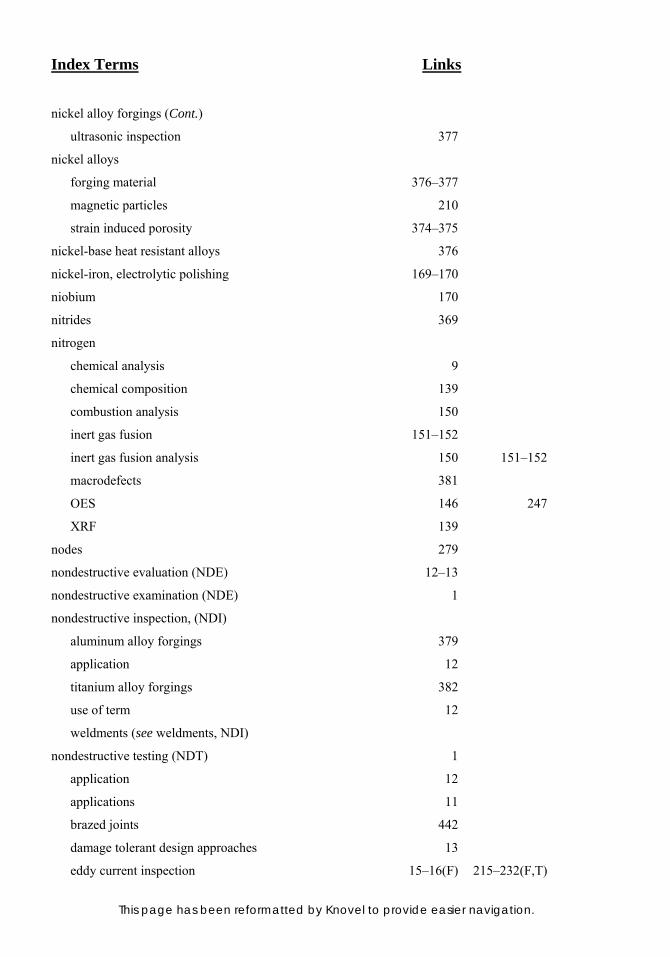
Index Terms Links
This page has been reformatted by Knovel to provide easier navigation.
nickel alloy forgings (Cont.)
ultrasonic inspection 377
nickel alloys
forging material 376–377
magnetic particles 210
strain induced porosity 374–375
nickel-base heat resistant alloys 376
nickel-iron, electrolytic polishing 169–170
niobium 170
nitrides 369
nitrogen
chemical analysis 9
chemical composition 139
combustion analysis 150
inert gas fusion 151–152
inert gas fusion analysis 150 151–152
macrodefects 381
OES 146 247
XRF 139
nodes 279
nondestructive evaluation (NDE) 12–13
nondestructive examination (NDE) 1
nondestructive inspection, (NDI)
aluminum alloy forgings 379
application 12
titanium alloy forgings 382
use of term 12
weldments (see weldments, NDI)
nondestructive testing (NDT) 1
application 12
applications 11
brazed joints 442
damage tolerant design approaches 13
eddy current inspection 15–16(F) 215–232(F,T)
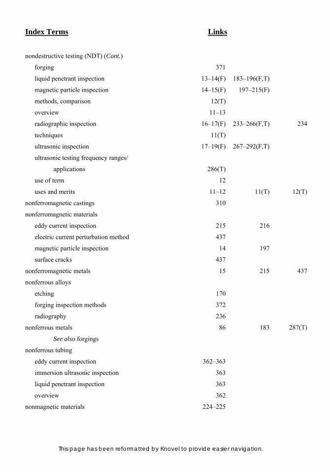
Index Terms Links
This page has been reformatted by Knovel to provide easier navigation.
nondestructive testing (NDT) (Cont.)
forging 371
liquid penetrant inspection 13–14(F) 183–196(F,T)
magnetic particle inspection 14–15(F) 197–215(F)
methods, comparison 12(T)
overview 11–13
radiographic inspection 16–17(F) 233–266(F,T) 234
techniques 11(T)
ultrasonic inspection 17–19(F) 267–292(F,T)
ultrasonic testing frequency ranges/
applications 286(T)
use of term 12
uses and merits 11–12 11(T) 12(T)
nonferromagnetic castings 310
nonferromagnetic materials
eddy current inspection 215 216
electric current perturbation method 437
magnetic particle inspection 14 197
surface cracks 437
nonferromagnetic metals 15 215 437
nonferrous alloys
etching 170
forging inspection methods 372
radiography 236
nonferrous metals 86 183 287(T)
See also forgings
nonferrous tubing
eddy current inspection 362–363
immersion ultrasonic inspection 363
liquid penetrant inspection 363
overview 362
nonmagnetic materials 224–225

Index Terms Links
This page has been reformatted by Knovel to provide easier navigation.
nonmetallic inclusions
castings 310
etching 170 174(T)
forgings 368–369
magnetic particle inspection 197 213–214
radiographic inspection 310
scattering 290
solidification 368
steel forgings 375
steel products 213–214
ultrasonic inspection 290
nonmetals 286–287 287(T)
nonrelevant indications 193 214 425
nuclear applications
ultrasonic inspection 390
vacuum and helium testing 443–444
nuggets
fusion welds 46
ultrasonic testing 434–436 435(F) 436(F)
null system 342 343(F)
O
Occupational Safety and Health
Administration (OSHA) 194
offline programming 81
offset yield strength 120–121 121(F)
oil impregnation 395
oil viscosity 211
one-dimensional array 68
open-die forgings 365 372 379
optical comparators 36 38(F)
optical emission spectroscopy (OES)
applications 146
carbon 146 147 152

Index Terms Links
This page has been reformatted by Knovel to provide easier navigation.
optical emission spectroscopy (OES) (Cont.)
CCD instruments 147
chemical analysis 9
chemical composition 152
detection threshold 146
limitations 147
nitrogen 146 147
operating principles
CCD detectors, instruments with 149
direct reading instruments 148–149
instrumentation 147–148 148(F)
photographic instruments 148
physical basis 147
optical emission spectrometer 148(F)
overview 146–147
oxygen 146 147
quantitative analyses, precision of 146–147
related techniques
AAS 150
flame AAS 150
graphite furnace AAS 150
ICP/AES 149–150
ICP/MS 150
XRF 150
samples
bulk solids 147
metallographic engraving tool 147
powders 147
size 147
XRF 146
orthochromatic film 180
oscilloscope displays 269 271(F) 434
435 435(F)

Index Terms Links
This page has been reformatted by Knovel to provide easier navigation.
oscilloscope screens
angle beam testing 279 280
magnetic permeability systems 342 343(F)
pulse echo inspection 275–276 275(F)
ultrasonic inspection, steel bar 327
oscilloscopes 127 230 281–282
overall magnetization method 207
overlap
definition of 412
geometric weld discontinuities 417
radiographic inspection 427
overpickling 323
oxidation 297
oxide films 294 297
oxides 369
oxygen
alpha-stabilized voids 380 380(F)
combustion analysis 150 151
exogenous inclusions 297
high temperature combustion 9
inert gas fusion 9 151–152
inert gas fusion analysis 150 151–152
interstitial defects 381 381(F)
OES 146 147
SAM 158
scale 22
seamless steel tubular products 356
tungsten inclusions 416
ozone 178
P
paint 376
panchromatic films 180
paraffin 318–319
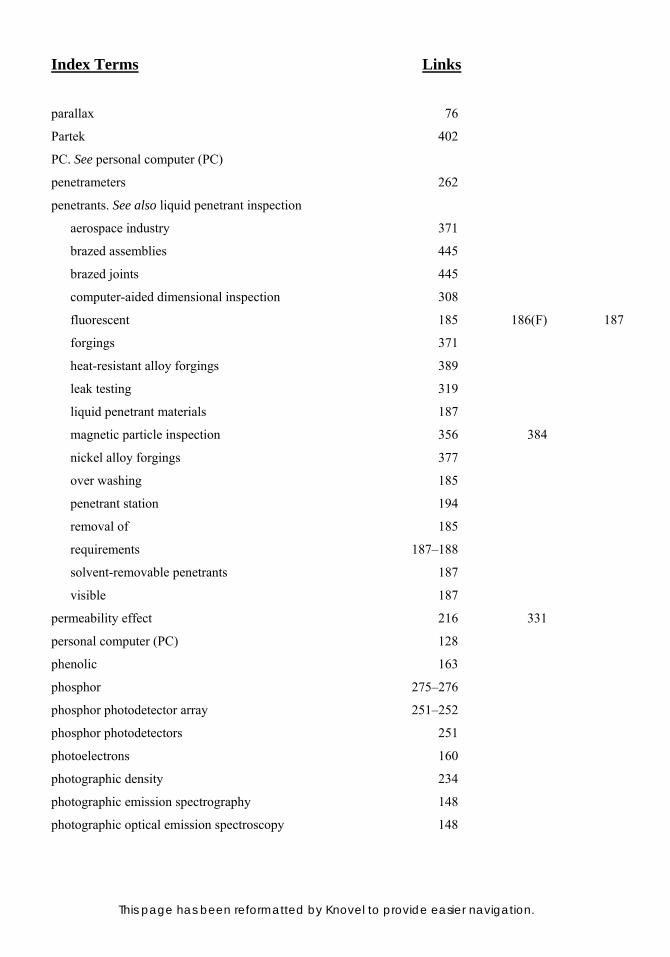
Index Terms Links
This page has been reformatted by Knovel to provide easier navigation.
parallax 76
Partek 402
PC. See personal computer (PC)
penetrameters 262
penetrants. See also liquid penetrant inspection
aerospace industry 371
brazed assemblies 445
brazed joints 445
computer-aided dimensional inspection 308
fluorescent 185 186(F) 187
forgings 371
heat-resistant alloy forgings 389
leak testing 319
liquid penetrant materials 187
magnetic particle inspection 356 384
nickel alloy forgings 377
over washing 185
penetrant station 194
removal of 185
requirements 187–188
solvent-removable penetrants 187
visible 187
permeability effect 216 331
personal computer (PC) 128
phenolic 163
phosphor 275–276
phosphor photodetector array 251–252
phosphor photodetectors 251
photoelectrons 160
photographic density 234
photographic emission spectrography 148
photographic optical emission spectroscopy 148
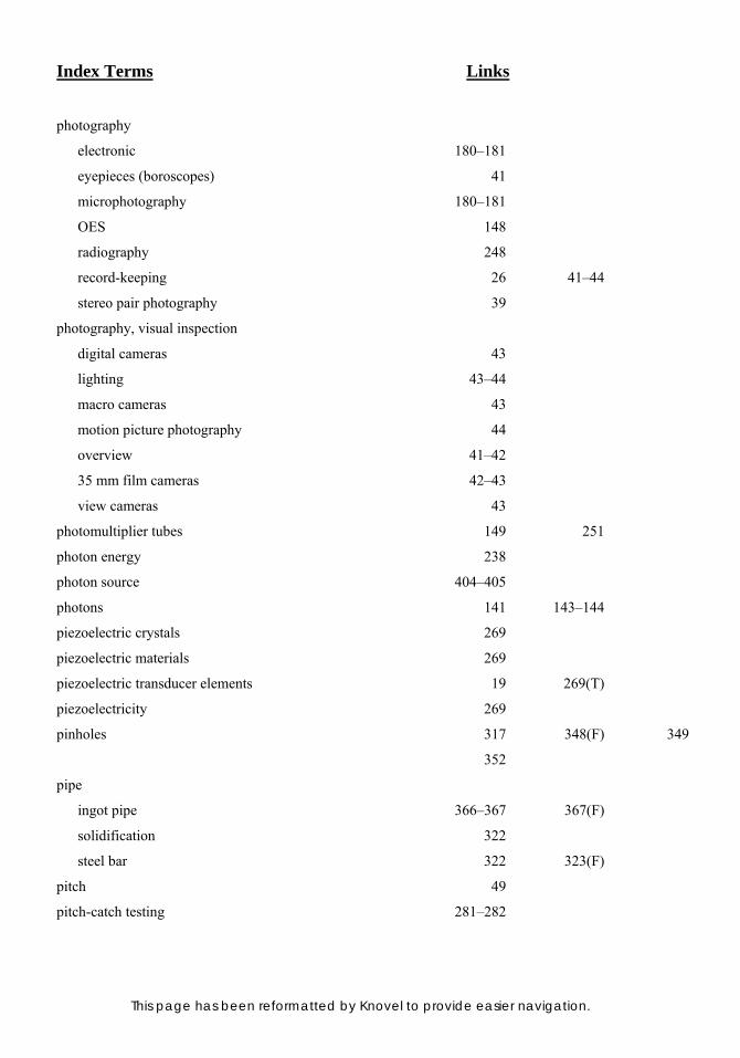
Index Terms Links
This page has been reformatted by Knovel to provide easier navigation.
photography
electronic 180–181
eyepieces (boroscopes) 41
microphotography 180–181
OES 148
radiography 248
record-keeping 26 41–44
stereo pair photography 39
photography, visual inspection
digital cameras 43
lighting 43–44
macro cameras 43
motion picture photography 44
overview 41–42
35 mm film cameras 42–43
view cameras 43
photomultiplier tubes 149 251
photon energy 238
photon source 404–405
photons 141 143–144
piezoelectric crystals 269
piezoelectric materials 269
piezoelectric transducer elements 19 269(T)
piezoelectricity 269
pinholes 317 348(F) 349
352
pipe
ingot pipe 366–367 367(F)
solidification 322
steel bar 322 323(F)
pitch 49
pitch-catch testing 281–282

Index Terms Links
This page has been reformatted by Knovel to provide easier navigation.
pits
definition of 357 357(F)
measuring 26
steel bar 323 324(F)
pitting 23
pixels
definition of 49
image interpretation 78 79(F)
planar grinding 165
plane 49–50
plastic deformation
extensometers 136
indenting 114
macroscopic examination 11
offset yield strength 120
stress-strain behavior 118 118(F)
stress-strain curve, for metal 7–8 8(F)
tensile testing setup 134
YS 8 9 119
platens 165 166
plating 163–164
platinum
electrolytic etching 170 175(T) 176(T)
x-ray tubes 241
plug scores 357 357(F)
P/M parts. See powder metallurgy (P/M) parts
pneumatic pumps 297
pocket microscopes 30–31 31(F)
polar coordinate system 52
polarized light
differential interference contrast
microscopy 180
electrolytic polishing 169
etching 170

Index Terms Links
This page has been reformatted by Knovel to provide easier navigation.
polarized light (Cont.)
microhardness testing 111
microscopic examination 178
optical equipment 111
polarized light microscopy 179–180 179(F)
polarizer 179–180 179(F)
polarizing light microscope 179(F)
Polaroid instant films 180
pole pieces 210 210(F)
polishing
abrasives 169
automatic polishing 168
chemical polishing 170
deformation 166–167
electrolytic polishing 169–170 169(F)
hand polishing
abrasives 167–168
polishing cloths 168
techniques 167
vibratory polishers 168
mechanical polishing
overview 167
use of term 167
overview 166–167
polishing abrasives 169
polishing cloths 168
polycrystalline materials 289
polymers 131
pores
castings 295
radiographs 428
porosity
castings 295–296 295(F) 318
cluster porosity 434
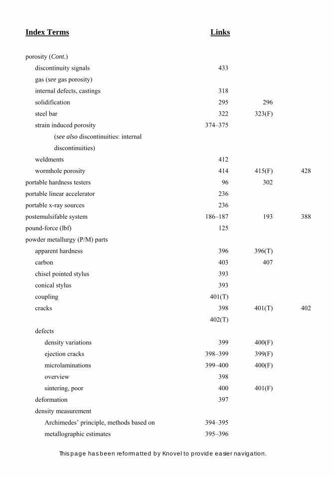
Index Terms Links
This page has been reformatted by Knovel to provide easier navigation.
porosity (Cont.)
discontinuity signals 433
gas (see gas porosity)
internal defects, castings 318
solidification 295 296
steel bar 322 323(F)
strain induced porosity 374–375
(see also discontinuities: internal
discontinuities)
weldments 412
wormhole porosity 414 415(F) 428
portable hardness testers 96 302
portable linear accelerator 236
portable x-ray sources 236
postemulsifable system 186–187 193 388
pound-force (lbf) 125
powder metallurgy (P/M) parts
apparent hardness 396 396(T)
carbon 403 407
chisel pointed stylus 393
conical stylus 393
coupling 401(T)
cracks 398 401(T) 402
402(T)
defects
density variations 399 400(F)
ejection cracks 398–399 399(F)
microlaminations 399–400 400(F)
overview 398
sintering, poor 400 401(F)
deformation 397
density measurement
Archimedes’ principle, methods based on 394–395
metallographic estimates 395–396
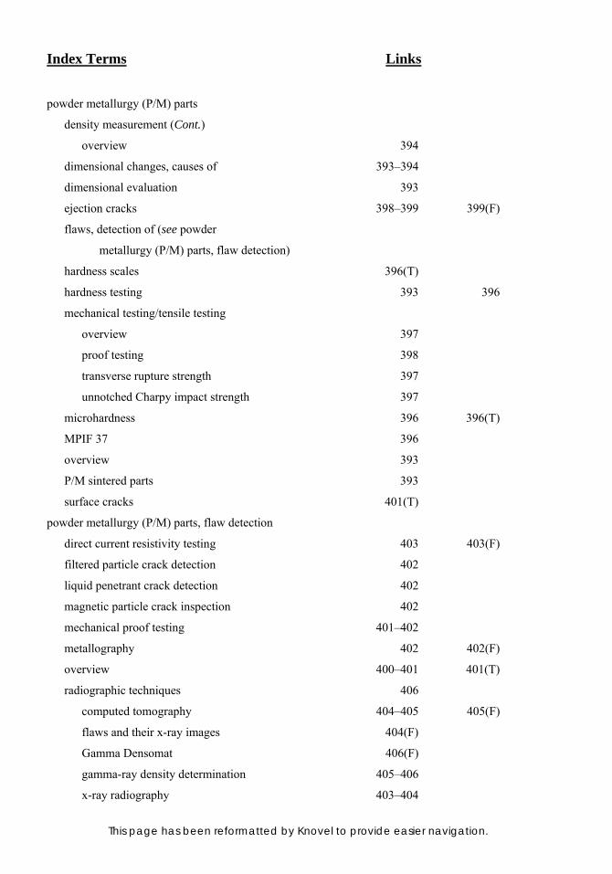
Index Terms Links
This page has been reformatted by Knovel to provide easier navigation.
powder metallurgy (P/M) parts
density measurement (Cont.)
overview 394
dimensional changes, causes of 393–394
dimensional evaluation 393
ejection cracks 398–399 399(F)
flaws, detection of (see powder
metallurgy (P/M) parts, flaw detection)
hardness scales 396(T)
hardness testing 393 396
mechanical testing/tensile testing
overview 397
proof testing 398
transverse rupture strength 397
unnotched Charpy impact strength 397
microhardness 396 396(T)
MPIF 37 396
overview 393
P/M sintered parts 393
surface cracks 401(T)
powder metallurgy (P/M) parts, flaw detection
direct current resistivity testing 403 403(F)
filtered particle crack detection 402
liquid penetrant crack detection 402
magnetic particle crack inspection 402
mechanical proof testing 401–402
metallography 402 402(F)
overview 400–401 401(T)
radiographic techniques 406
computed tomography 404–405 405(F)
flaws and their x-ray images 404(F)
Gamma Densomat 406(F)
gamma-ray density determination 405–406
x-ray radiography 403–404
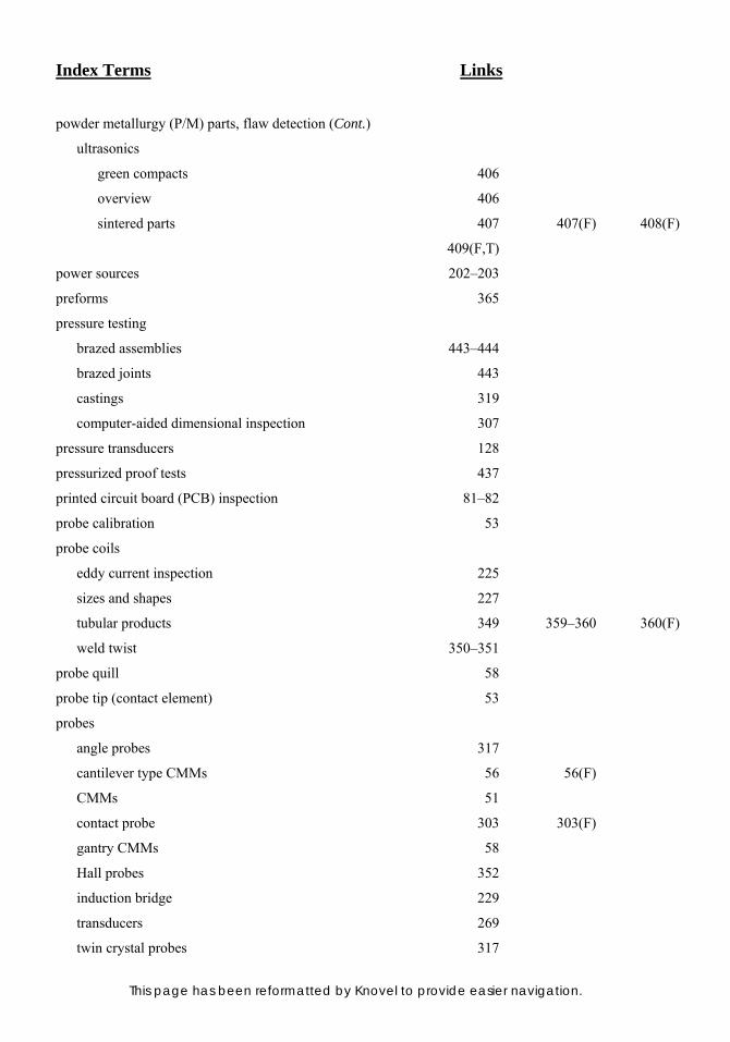
Index Terms Links
This page has been reformatted by Knovel to provide easier navigation.
powder metallurgy (P/M) parts, flaw detection (Cont.)
ultrasonics
green compacts 406
overview 406
sintered parts 407 407(F) 408(F)
409(F,T)
power sources 202–203
preforms 365
pressure testing
brazed assemblies 443–444
brazed joints 443
castings 319
computer-aided dimensional inspection 307
pressure transducers 128
pressurized proof tests 437
printed circuit board (PCB) inspection 81–82
probe calibration 53
probe coils
eddy current inspection 225
sizes and shapes 227
tubular products 349 359–360 360(F)
weld twist 350–351
probe quill 58
probe tip (contact element) 53
probes
angle probes 317
cantilever type CMMs 56 56(F)
CMMs 51
contact probe 303 303(F)
gantry CMMs 58
Hall probes 352
induction bridge 229
transducers 269
twin crystal probes 317
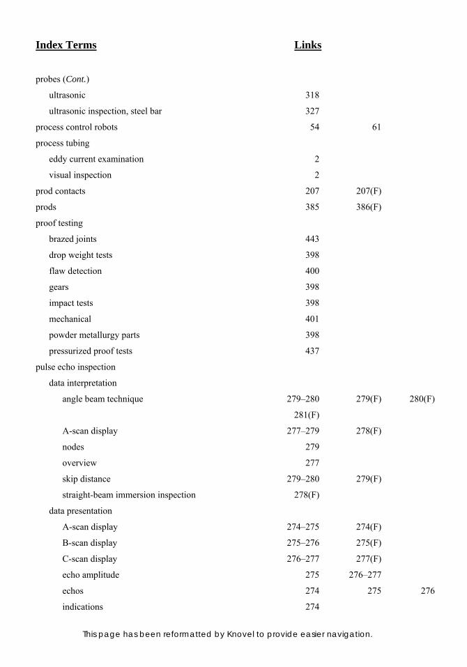
Index Terms Links
This page has been reformatted by Knovel to provide easier navigation.
probes (Cont.)
ultrasonic 318
ultrasonic inspection, steel bar 327
process control robots 54 61
process tubing
eddy current examination 2
visual inspection 2
prod contacts 207 207(F)
prods 385 386(F)
proof testing
brazed joints 443
drop weight tests 398
flaw detection 400
gears 398
impact tests 398
mechanical 401
powder metallurgy parts 398
pressurized proof tests 437
pulse echo inspection
data interpretation
angle beam technique 279–280 279(F) 280(F)
281(F)
A-scan display 277–279 278(F)
nodes 279
overview 277
skip distance 279–280 279(F)
straight-beam immersion inspection 278(F)
data presentation
A-scan display 274–275 274(F)
B-scan display 275–276 275(F)
C-scan display 276–277 277(F)
echo amplitude 275 276–277
echos 274 275 276
indications 274
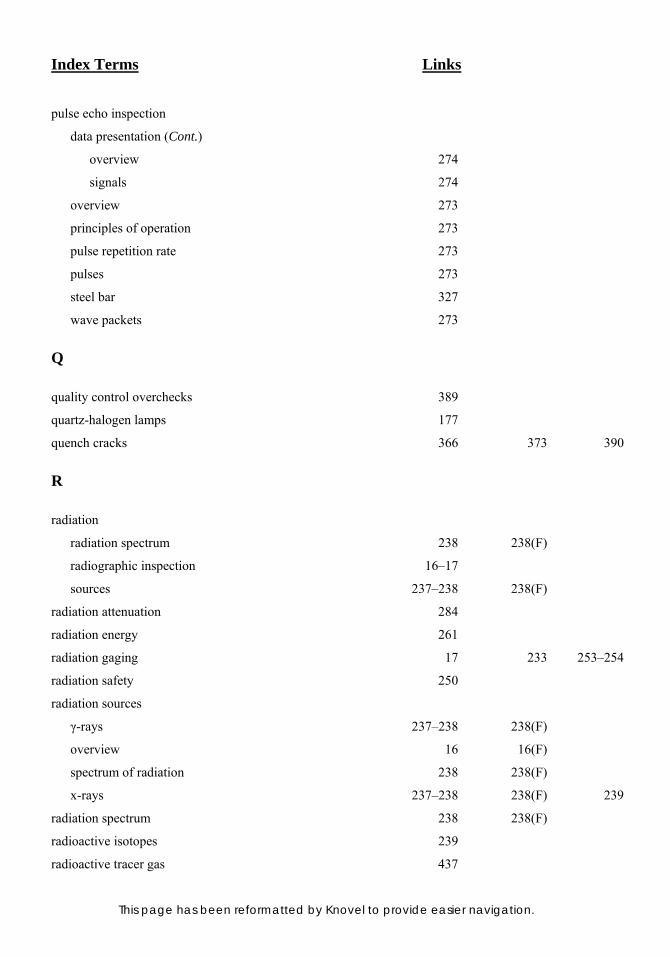
Index Terms Links
This page has been reformatted by Knovel to provide easier navigation.
pulse echo inspection
data presentation (Cont.)
overview 274
signals 274
overview 273
principles of operation 273
pulse repetition rate 273
pulses 273
steel bar 327
wave packets 273
Q
quality control overchecks 389
quartz-halogen lamps 177
quench cracks 366 373 390
R
radiation
radiation spectrum 238 238(F)
radiographic inspection 16–17
sources 237–238 238(F)
radiation attenuation 284
radiation energy 261
radiation gaging 17 233 253–254
radiation safety 250
radiation sources
γ-rays 237–238 238(F)
overview 16 16(F)
spectrum of radiation 238 238(F)
x-rays 237–238 238(F) 239
radiation spectrum 238 238(F)
radioactive isotopes 239
radioactive tracer gas 437
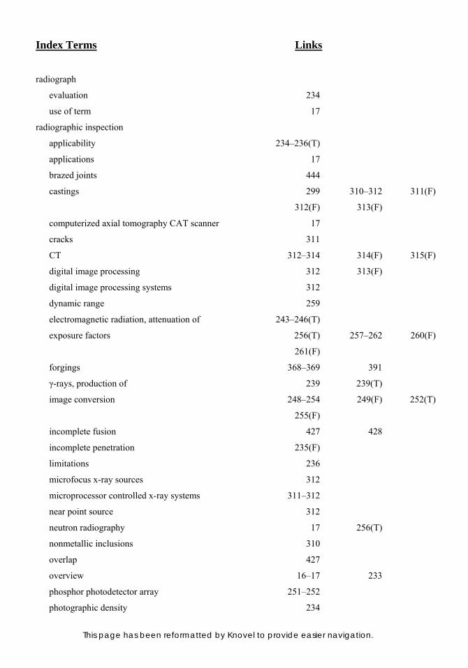
Index Terms Links
This page has been reformatted by Knovel to provide easier navigation.
radiograph
evaluation 234
use of term 17
radiographic inspection
applicability 234–236(T)
applications 17
brazed joints 444
castings 299 310–312 311(F)
312(F) 313(F)
computerized axial tomography CAT scanner 17
cracks 311
CT 312–314 314(F) 315(F)
digital image processing 312 313(F)
digital image processing systems 312
dynamic range 259
electromagnetic radiation, attenuation of 243–246(T)
exposure factors 256(T) 257–262 260(F)
261(F)
forgings 368–369 391
γ-rays, production of 239 239(T)
image conversion 248–254 249(F) 252(T)
255(F)
incomplete fusion 427 428
incomplete penetration 235(F)
limitations 236
microfocus x-ray sources 312
microprocessor controlled x-ray systems 311–312
near point source 312
neutron radiography 17 256(T)
nonmetallic inclusions 310
overlap 427
overview 16–17 233
phosphor photodetector array 251–252
photographic density 234

Index Terms Links
This page has been reformatted by Knovel to provide easier navigation.
radiographic inspection (Cont.)
principles 236–237
process 17 233–234
radiation 16–17
radiation gaging 17
radiation safety 250
radiation sources 16 16(F) 237–238
238(F)
radiation spectrum 238 238(F)
radiographic system 16 16(F) 236–237
237(F)
radiography 234–237 235(T) 237(F)
real-time inspection 17
resistance welded steel tubing 356
shadow formation 246–248 247(F) 248(F)
shadow picture 17 233–234
steel forgings 375
suitabilities of three radiographic
methods, comparison of 235(T)
surface cracks 235(T)
terminology 133
tomography 17
uses of 234
weldments
applicability 234
incomplete fusion 417
incomplete penetration 417
overview 427–428
real-time radiography 428–429
slag inclusions 416
subsurface discontinuities 428
tungsten inclusions 416
x-ray film 254–257 256(T) 257(T)
x-ray tubes 239–241 240(F)

Index Terms Links
This page has been reformatted by Knovel to provide easier navigation.
radiographic inspection (Cont.)
x-rays, production of 239
radiographic system 16(F)
radiography. See also radiographic inspection
applicability 234–236
castings 294
conventional 233
cracks 17 234 235(T)
236
discontinuities detectable 234
gamma ray sources 236
geometric factors 237
image conversion 248–254 249(F) 252(T)
255(F)
incomplete penetration 428
limitations 236
NDT capability 234
paper radiography 233
portable linear accelerator 236
portable x-ray sources 236
principles of 236–237
radiation gaging 233
radiographic system, elements of 237(F)
real-time inspection 233
slag inclusions 428
suitabilities of three radiographic
methods, comparison of 235(T)
tomography 233
use of term 233
weldments 234 414
cracks 419
xeroradiography 233
radioisotope 264(T) 404 405
Rayleigh waves 284 284(F)

Index Terms Links
This page has been reformatted by Knovel to provide easier navigation.
real-time inspection 17
rebound testing 85
recirculating hot air drier 192(F) 195
record-keeping 26–27 41–44
rectifiers 202
red iron oxide (magnitite Fe3O4) 210
reduction of area
defined 124
expressed as a percentage 124
rectangular test piece 124(F)
tensile testing 123–124 124(F)
test pieces 124
reduction ratio 376
relative motion
machine vision process 76–77
tubular products 352
relax (excited atoms) 141
relief 161
reoxidation 297
repeatability 50
residual magnetic field 214 426
resistance welded steel tubing
cold weld 348
contact marks (electrode burns) 348 348(F)
cracks 348 349(F)
diameters 347–348
eddy current inspection
advantages 351
detectable flaws 349 350(F)
end effect 351
equipment cost 351
inspection, speed 349–350
limitations 351
operating costs 351

Index Terms Links
This page has been reformatted by Knovel to provide easier navigation.
resistance welded steel tubing
eddy current inspection (Cont.)
overview 349–350
weld twist 350–351
flaws 348
flux leakage inspection
equipment cost 353
ferromagnetic materials 351
Hall probes 352
inspection, speed 352–353
magnetizing the tube 352
operating costs 353
overview 351–352
pinholes 352
setup 353(F)
subsurface defects 352
transverse flaws 352
tube diameter 352
wall thickness 352
weld twist 353
hook cracks (upturned fiber flaws) 348–349 348(F)
liquid penetrant inspection 356
magnetic particle inspection
applications 355–356
pipe ends 355–356
pinholes 348(F) 349
radiographic inspection 356
stitching 348(F) 349
terminology 348
ultrasonic inspection
couplants 354 355
coupling 354
disadvantages 355
end effect 355

Index Terms Links
This page has been reformatted by Knovel to provide easier navigation.
resistance welded steel tubing
ultrasonic inspection (Cont.)
equipment cost 355
inspection, speed 354 355
operating costs 355
overview 354–355
shear wave angle 354
short flaws 354
transducer and pipe, spacing 354
tube diameter 354
weld twist 355
weld zone 354
wheel type search unit 355
weld area cracks 348(F) 349
welding machines, performing on 349
resistivity
coil impedance 219
conductors 220
depth of penetration 224
direct current resistivity testing 403 403(F)
eddy current systems 332
electrical conductivity 220 221(T)
electrical resistivity 221(T)
electrical resistivity testing 400 401(T)
electromagnetic inspection methods 331
insulators 220
P/M parts 400
semiconductors 220
retentivity 214
reticles 36 37(F)
reverse engineering 3 49 51
ridging 87 87(F)
risers 299 367
rms. See root mean surface (rms)

Index Terms Links
This page has been reformatted by Knovel to provide easier navigation.
Rockwell diamond indenter 92 92(F)
Rockwell hardness scales
applications 97(T)
limitations 98
Rockwell hardness standards for metals 115–116
Rockwell hardness test 91
See also Rockwell hardness testing
Rockwell hardness testing
anvil selection 98–99 99(F)
Brale indenter 92 92(F)
Brinell hardness testing, difference between 91–92
casting alloys 301–302
cylindrical pieces 99
indenters 92
jack rest 99 99(F)
long test pieces 99 99(F)
near-Rockwell method 96 96(F)
overview 91–92
portable testing machines 96 96(F)
regular Rockwell hardness testing 94(F) 95 95(T)
Rockwell diamond indenter 92 92(F) 93
93(F)
Rockwell hardness scales, applications of 97(T)
Rockwell scales, limitations of 98
Rockwell scales, selection of
overview 96–97
test area width, influence of 97–98
work metal, influence of thickness of 97
work metal, influence of type of 97 97(T)
workpiece, support for 98–99 99(F)
scale designations 95 95(T)
set position 93
steel ball indenters 93–94
superficial Rockwell hardness testing 94(F) 95–96 95(T)

Index Terms Links
This page has been reformatted by Knovel to provide easier navigation.
Rockwell hardness testing (Cont.)
test methods
major load 93 93(F)
minor load 93 93(F)
overview 93–94 93(F)
testers 94 94(F)
Rockwell testers 94 94(F) 96(F)
roentgens (R) 238
roentgens per hour at one meter (RHM) 238
roentgens per minute at one meter (RMM) 238
roll 50
roll bar 49
rolled stock 365
rolled-in slugs 357 357(F)
root mean surface (rms) 379
run length encoding 74
S
SAM. See scanning Auger microprobe (SAM)
samarium 263
Samuels, L. 113
SAW. See submerged arc welding (SAW)
scabs 322 324(F) 357(F)
358
scale 22
scale analysis 23
scaling 22
scanning Auger microprobe (SAM)
applications 153
Auger electrons 153–154
Auger spectra 156
chemical analysis 9
depth composition profile 159(F)
depth profiling 156

Index Terms Links
This page has been reformatted by Knovel to provide easier navigation.
scanning Auger microprobe (SAM) (Cont.)
electron collection and energy
measurement 154(F) 156–158 157(F)
158(F) 159(F)
EPMA 154
features 152
identification of elements 157(F)
ion sputtering gun 156
limitations 153
mapping of elements 158(F)
operating principles
instrumentation 153
physical basis 153–156
overview 152–153
oxygen 158
resolutions 153
results 156
samples 153
scanning Auger microprobe 154(F)
SEM 154
silver sample, electron energy
distribution from 155(F)
undisturbed Auger electrons 156
XPS 160
x-rays and Auger electrons, comparison 154(F)
scanning electron microscopy (SEM) 159
scatter 252(T) 261–262 264(T)
290 435–436
scattering
backscattering noise 271
Compton scattering 244–245
DR 251
forward scattering 290
image conversion 248

Index Terms Links
This page has been reformatted by Knovel to provide easier navigation.
scattering (Cont.)
neutron radiography 263
nonmetallic inclusions 290
spot welds 434
ultrasonic inspection 290
wave bending 290
wave path 434
scintillator 265
See also fluorescent screens
scintillator photodetectors 251
Scleroscope hardness testers 103–104(F)
C-frame base 103–104
Model C Scleroscope 103–104 104(F) 105
106
Model D Scleroscope 103–104 104(F) 105
Scleroscope hardness testing
advantages 105–106
indentations, spacing of 105
limitations 106
overview 102
procedure 105
readings, taking 105
Scleroscope scale 102
sheet, minimum thickness 105
testers 103–104 104(F) 105
106
workpiece and case thickness, limitations on 104–105
workpiece surface finish requirements 104
Scleroscope scale 102
seamless steel tubular products
eddy current inspection
detectable flaws 361
encircling detector coil 359
flaw detection 359

Index Terms Links
This page has been reformatted by Knovel to provide easier navigation.
seamless steel tubular products
eddy current inspection (Cont.)
laminations 361
magnetic coupling 359
magnetic saturation 359–360
pipe and tube, spacing 360–361
probe coils 359 360
probe type test 360 360(F)
test current frequency 360
test head 360 361(F)
flaws
blisters 356 357(F)
gouges 357 357(F)
laminations 357 357(F)
laps 357 357(F)
location 356 357(F)
pits 357 357(F)
plug scores 357 357(F)
rolled-in slugs 357 357(F)
scabs 357(F) 358
seams 357(F) 358
flux leakage techniques 361–362
liquid penetrant inspection 362
magnetic particle inspection 362
overview 356
oxygen 356
ultrasonic inspection
alarms 358
calibration checks 358
circumferential inspection 359
couplant 358
couplant, water 359
detectable flaws 358
diameters 358
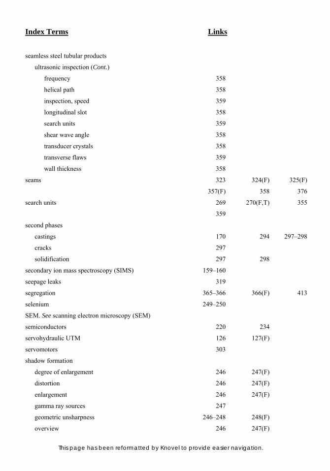
Index Terms Links
This page has been reformatted by Knovel to provide easier navigation.
seamless steel tubular products
ultrasonic inspection (Cont.)
frequency 358
helical path 358
inspection, speed 359
longitudinal slot 358
search units 359
shear wave angle 358
transducer crystals 358
transverse flaws 359
wall thickness 358
seams 323 324(F) 325(F)
357(F) 358 376
search units 269 270(F,T) 355
359
second phases
castings 170 294 297–298
cracks 297
solidification 297 298
secondary ion mass spectroscopy (SIMS) 159–160
seepage leaks 319
segregation 365–366 366(F) 413
selenium 249–250
SEM. See scanning electron microscopy (SEM)
semiconductors 220 234
servohydraulic UTM 126 127(F)
servomotors 303
shadow formation
degree of enlargement 246 247(F)
distortion 246 247(F)
enlargement 246 247(F)
gamma ray sources 247
geometric unsharpness 246–248 248(F)
overview 246 247(F)
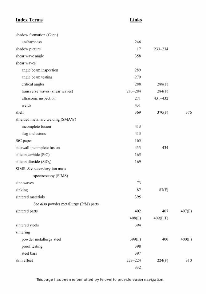
Index Terms Links
This page has been reformatted by Knovel to provide easier navigation.
shadow formation (Cont.)
unsharpness 246
shadow picture 17 233–234
shear wave angle 358
shear waves
angle beam inspection 289
angle beam testing 279
critical angles 288 288(F)
transverse waves (shear waves) 283–284 284(F)
ultrasonic inspection 271 431–432
welds 431
shelf 369 370(F) 376
shielded metal arc welding (SMAW)
incomplete fusion 413
slag inclusions 413
SiC paper 165
sidewall incomplete fusion 433 434
silicon carbide (SiC) 165
silicon dioxide (SiO2) 169
SIMS. See secondary ion mass
spectroscopy (SIMS)
sine waves 73
sinking 87 87(F)
sintered materials 395
See also powder metallurgy (P/M) parts
sintered parts 402 407 407(F)
408(F) 409(F,T)
sintered steels 394
sintering
powder metallurgy steel 399(F) 400 400(F)
proof testing 398
steel bars 397
skin effect 223–224 224(F) 310
332
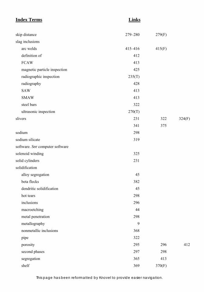
Index Terms Links
This page has been reformatted by Knovel to provide easier navigation.
skip distance 279–280 279(F)
slag inclusions
arc welds 415–416 415(F)
definition of 412
FCAW 413
magnetic particle inspection 425
radiographic inspection 235(T)
radiography 428
SAW 413
SMAW 413
steel bars 322
ultrasonic inspection 270(T)
slivers 231 322 324(F)
341 375
sodium 298
sodium silicate 319
software. See computer software
solenoid winding 325
solid cylinders 231
solidification
alloy segregation 45
beta flecks 382
dendritic solidification 45
hot tears 298
inclusions 296
macroetching 44
metal penetration 298
metallography 9
nonmetallic inclusions 368
pipe 322
porosity 295 296 412
second phases 297 298
segregation 365 413
shelf 369 370(F)
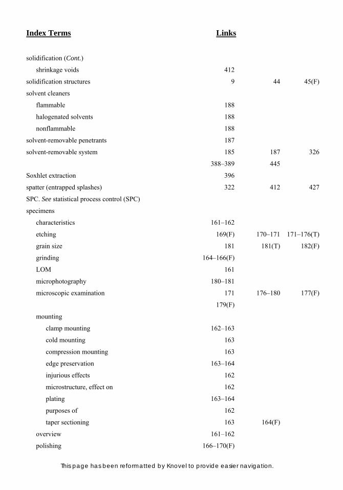
Index Terms Links
This page has been reformatted by Knovel to provide easier navigation.
solidification (Cont.)
shrinkage voids 412
solidification structures 9 44 45(F)
solvent cleaners
flammable 188
halogenated solvents 188
nonflammable 188
solvent-removable penetrants 187
solvent-removable system 185 187 326
388–389 445
Soxhlet extraction 396
spatter (entrapped splashes) 322 412 427
SPC. See statistical process control (SPC)
specimens
characteristics 161–162
etching 169(F) 170–171 171–176(T)
grain size 181 181(T) 182(F)
grinding 164–166(F)
LOM 161
microphotography 180–181
microscopic examination 171 176–180 177(F)
179(F)
mounting
clamp mounting 162–163
cold mounting 163
compression mounting 163
edge preservation 163–164
injurious effects 162
microstructure, effect on 162
plating 163–164
purposes of 162
taper sectioning 163 164(F)
overview 161–162
polishing 166–170(F)
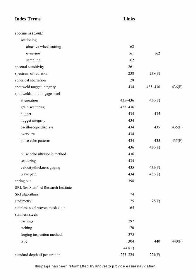
Index Terms Links
This page has been reformatted by Knovel to provide easier navigation.
specimens (Cont.)
sectioning
abrasive wheel cutting 162
overview 161 162
sampling 162
spectral sensitivity 261
spectrum of radiation 238 238(F)
spherical aberration 28
spot weld nugget integrity 434 435–436 436(F)
spot welds, in thin gage steel
attenuation 435–436 436(F)
grain scattering 435–436
nugget 434 435
nugget integrity 434
oscilloscope displays 434 435 435(F)
overview 434
pulse echo patterns 434 435 435(F)
436 436(F)
pulse echo ultrasonic method 436
scattering 434
velocity/thickness gaging 435 435(F)
wave path 434 435(F)
spring out 398
SRI. See Stanford Research Institute
SRI algorithms 74
stadimetry 75 75(F)
stainless steel woven mesh cloth 165
stainless steels
castings 297
etching 170
forging inspection methods 375
type 304 440 440(F)
441(F)
standard depth of penetration 223–224 224(F)

Index Terms Links
This page has been reformatted by Knovel to provide easier navigation.
standard deviation 306
Stanford Research Institute 74
static indentation 85
stationary grinding paper 165
statistical process control (SPC)
caution 7
hardness testing 7
statistical summary report 306 308(F)
steel
castings 297
inclusions 296 297
magnetic saturation 221
radioactive equivalence 245–246
radiographic film, selection 257(T)
steel bar, flaws
blisters 323 324(F)
chevrons 324 324(F)
cracks 323 324(F)
embedded scale 323 324(F)
inclusions 322 324(F)
laminations 322 324(F)
laps 324 324(F)
pipe 322 323(F)
pits 323 324(F)
porosity 322 323(F)
scabs 322 324(F)
seams 323 324(F) 325(F)
slivers 322 324(F)
steel bar 324(F)
steel bars
eddy current systems
cold drawn bars 333–334 333(T) 334(F)
cold drawn hexagonal bars 334–335 335(F) 336(F)
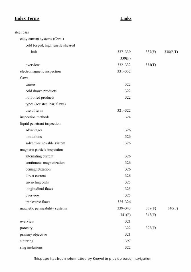
Index Terms Links
This page has been reformatted by Knovel to provide easier navigation.
steel bars
eddy current systems (Cont.)
cold forged, high tensile sheared
bolt 337–339 337(F) 338(F,T)
339(F)
overview 332–332 333(T)
electromagnetic inspection 331–332
flaws
causes 322
cold drawn products 322
hot rolled products 322
types (see steel bar, flaws)
use of term 321–322
inspection methods 324
liquid penetrant inspection
advantages 326
limitations 326
solvent-removable system 326
magnetic particle inspection
alternating current 326
continuous magnetization 326
demagnetization 326
direct current 326
encircling coils 325
longitudinal flaws 325
overview 325
transverse flaws 325–326
magnetic permeability systems 339–343 339(F) 340(F)
341(F) 343(F)
overview 321
porosity 322 323(F)
primary objective 321
sintering 397
slag inclusions 322
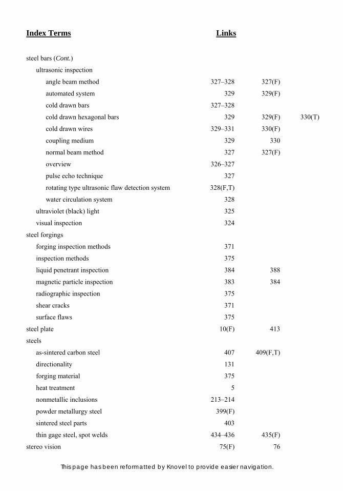
Index Terms Links
This page has been reformatted by Knovel to provide easier navigation.
steel bars (Cont.)
ultrasonic inspection
angle beam method 327–328 327(F)
automated system 329 329(F)
cold drawn bars 327–328
cold drawn hexagonal bars 329 329(F) 330(T)
cold drawn wires 329–331 330(F)
coupling medium 329 330
normal beam method 327 327(F)
overview 326–327
pulse echo technique 327
rotating type ultrasonic flaw detection system 328(F,T)
water circulation system 328
ultraviolet (black) light 325
visual inspection 324
steel forgings
forging inspection methods 371
inspection methods 375
liquid penetrant inspection 384 388
magnetic particle inspection 383 384
radiographic inspection 375
shear cracks 371
surface flaws 375
steel plate 10(F) 413
steels
as-sintered carbon steel 407 409(F,T)
directionality 131
forging material 375
heat treatment 5
nonmetallic inclusions 213–214
powder metallurgy steel 399(F)
sintered steel parts 403
thin gage steel, spot welds 434–436 435(F)
stereo vision 75(F) 76

Index Terms Links
This page has been reformatted by Knovel to provide easier navigation.
stereoradiography 237
stereoscopic microscope 39 39(F)
stinger rod 369–370
stitching 348(F) 349
strain elongation 122
strain gaged load cells 128
strain gages 128 136 137(F)
stress concentrations 25 25(F)
stress corrosion cracking 372
stringer rods 375
stringers 10 214 270(T)
375
strontium 298
submerged arc welding (SAW) 413
subsurface defects 14 184 294
317–318 352
sulfides 369
sulfur
combustion analysis 151
inclusions 296 322
surface cracks. See also surface defects
aluminum alloys 437
eddy current inspection 231
forgings 373
liquid penetrant inspection 13 183
magnesium alloy forgings 379
magnetic particle inspection 197 213 213(F)
313 402
nonferromagnetic materials 437
P/M parts 401(T)
radiographic inspection 235(T)
titanium alloys 437
visual inspection 1–2
welds 423

Index Terms Links
This page has been reformatted by Knovel to provide easier navigation.
surface defects
castings 294 298 308–309
cold drawn hexagonal bars 334–335
forgings 317
seamless steel tubular products 361–362
tubular products 346
surface finish comparators 41 42(F)
surface tension 184
surface waves (Rayleigh waves) 284 284(F)
surgical grade cotton 170
suspending liquids
oil suspending liquid 211–212
oil viscosity 211
water suspending liquid 212
suspension test 387
suspensions
acidic alumina suspensions 169
magnetic particle inspection 387
magnetic particles 211
polishing abrasives 169
Système International d’Unités (SI) 238
T
taper sectioning 163 164(F)
TEM. See transmission electron microscopy (TEM)
temper colors 22
template matching 80–81
tensile strength 119
tensile testing
advantages 7
ASTM standards 129
castings 7
coupling 127
ductility 9 121–124 121(F)

Index Terms Links
This page has been reformatted by Knovel to provide easier navigation.
tensile testing (Cont.)
engineering strain 7
extensometers 117
gage lengths 137–138
heat treated materials 397
load frame 7 8(F)
LYS 119(F)
mechanical testing 397–398
modulus of elasticity 118 118(F)
MPIF 10 397–398
overview 7–9 117
post test measurements 137–138
procedures 129–138(F,T) 137(F)
setup
extensometers 136 136(F) 137(F)
gripping devices 134–135(F)
gripping methods 135 135(F)
overview 134
strain gages 136 137(F)
test piece alignment 136
strength properties
offset yield strength 120–121 121(F)
upper yield strength or upper yield point 119–120 119(F)
stress-strain behavior 117–118 118(F)
stress-strain curve (for metal) 7–8 8(F)
stress-strain curves 118 119(F)
tensile properties, determining 7 8(F)
test piece (see tensile testing test piece)
testing machines (see tensile testing machines)
UTS 8(F) 9
UYS 119(F)
wrought materials 7
YPE 119(F)
YS 8–9 8(F)

Index Terms Links
This page has been reformatted by Knovel to provide easier navigation.
tensile testing machines
closed loop servo-drive system 125
controllers 127–128 127(F)
conventional gear driven systems 125
crosshead speeds 125
data analysis 128
dedicated microprocessors 127–128 127(F)
force ranges, hydraulic actuators 127
gear driven (or screw driven) 125 126(F)
load, measuring 128
load applying mechanism 125
microprocessors, for testing and data reduction 127–128 127(F)
overview 124–125
PC 128
pressure transducers 128
servohydraulic machines 125 127(F)
servohydraulic UTM 126 127(F)
strain gaged load cells 128
strain measurement 128
testing rates, servohydraulic test systems 126
UTM 124–125
tensile testing test piece
geometry
cross-sectional dimensions,
measurement of 134
dimensions 133
gage length, marking 134
initial gage length, measurement of 134
initial test piece dimensions,
measurement of 133
nomenclature 133 133(F)
overview 133
surface condition 134
surface finish 134

Index Terms Links
This page has been reformatted by Knovel to provide easier navigation.
tensile testing test piece (Cont.)
rough specimen 130 131(F)
terminology
rough specimen 130 131(F)
sample 130 131(F)
sample product 130 131(F)
specimen 130 131(F)
test piece 130 131(F)
test unit 130 131(F)
test piece orientation
ASTM E8 131
defined 131 132(F)
directionality 131
ISO Technical Committee 164 131
location from initial product 132–133
overview 130–131
standards 131
tensile properties, effect on 132(T)
types
full cross section 129
machined test piece 129–130
test coupons 112
thermal cracking 376–377
thermal fakes 390
thermal inspection 294
thermal loss 289
thermal neutron radiography 263–264
thermal neutrons 263
thermoelastic loss 289
thermoplastic mounting resin 163
thermosetting resins 163
three-dimensional array 68
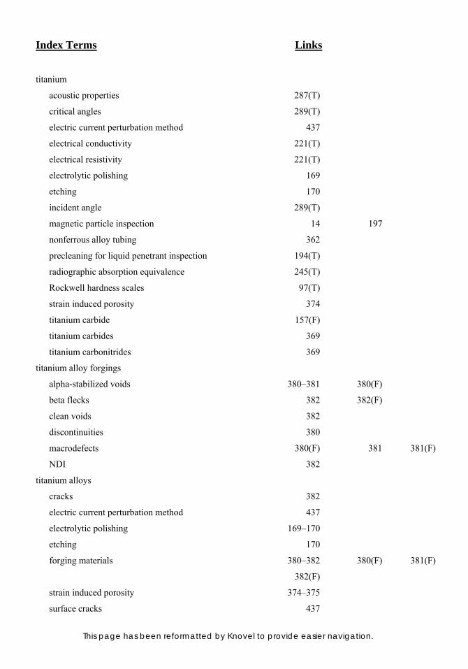
Index Terms Links
This page has been reformatted by Knovel to provide easier navigation.
titanium
acoustic properties 287(T)
critical angles 289(T)
electric current perturbation method 437
electrical conductivity 221(T)
electrical resistivity 221(T)
electrolytic polishing 169
etching 170
incident angle 289(T)
magnetic particle inspection 14 197
nonferrous alloy tubing 362
precleaning for liquid penetrant inspection 194(T)
radiographic absorption equivalence 245(T)
Rockwell hardness scales 97(T)
strain induced porosity 374
titanium carbide 157(F)
titanium carbides 369
titanium carbonitrides 369
titanium alloy forgings
alpha-stabilized voids 380–381 380(F)
beta flecks 382 382(F)
clean voids 382
discontinuities 380
macrodefects 380(F) 381 381(F)
NDI 382
titanium alloys
cracks 382
electric current perturbation method 437
electrolytic polishing 169–170
etching 170
forging materials 380–382 380(F) 381(F)
382(F)
strain induced porosity 374–375
surface cracks 437

Index Terms Links
This page has been reformatted by Knovel to provide easier navigation.
T-joints 420 420(F) 425
432
tomogram 313
tomography
overview 17
radiographic inspection 233
radiography 237
top punch hold-down 398
tracer gas 436 437
transformer oil 242
transmission electron microscopy (TEM) 159
transverse flaws 359
transverse rupture strength 397
trepanned 411
triangulation 75(F) 76 237
tube envelopes 242
tubes
boroscopes 40–41
direct reading instruments 149
DR 251
eddy current inspection 231
encircling coil inspection 231
fiber optic scopes 41
fluorescent tubes 35(F) 68
heat exchanger tubes 12(T)
image intensifer tubes 250–251
low level television camera tubes 250
multiple coils 227
nonmagnetic heat-exchanger tubes 232(F)
photomultiplier tubes 149 251
pocket microscopes 30
pole pieces 210
ultrasonic inspection (see also tubular products)
ultrasonic testing application 286(T)

Index Terms Links
This page has been reformatted by Knovel to provide easier navigation.
tubes (Cont.)
ultrasonic testing frequency ranges 286(T)
ultraviolet tubes 35(F)
welded tubes 231
wire filled nonconductive tubes 210
xeroradiography 250
x-ray (see x-ray tubes)
tubing. See also resistance welded steel
tubing; seamless steel tubular
products
absolute coil arrangement 226
angle beam testing 279
applications 345
eddy current inspection 218–219 219(F) 415
encircling coils 225–226 226(F) 227
extraneous variables 346
nonferrous tubing 362–363
tubing wall measuring micrometers 36
ultrasonic search units 270(T)
visual inspection 2
weldments 415
tubular products
applications 345–346
classifications 345
coupling 354 359
cracks 346 352
inspection method selection
end effect 347
equipment cost 347
extraneous variables 346
flaws, nature of 346
inspection rate 346–347
mill versus laboratory inspection 347
operating cost 347

Index Terms Links
This page has been reformatted by Knovel to provide easier navigation.
tubular products
inspection method selection (Cont.)
overview 346
product characteristics 346
specification requirements 347
magnetic flux leakage technique 345
magnetic permeability, variations in 346
nonferrous tubing 362–363
overview 345–346
resistance welded steel tubing (see
resistance welded steel tubing)
seamless steel tubular products (see
seamless steel tubular products)
seamless tube 346
sorting 346
surface scratches 346
ultrasonics 354
wrought tubular products 345
Tukon microhardness tester 110–111 110(F)
tungsten
carbide balls 86–87
filament lamps 177 178
inclusions 412 416 428
x-ray tubes 241
tungsten-halogen lamps 177 178
twin boundaries 290
two-dimensional arrays/scans 68
U
ultimate tensile strength (UTS) 8(F) 9
ultrasonic beam 282
ultrasonic inspection
advantages 291
aluminum alloy forgings 379
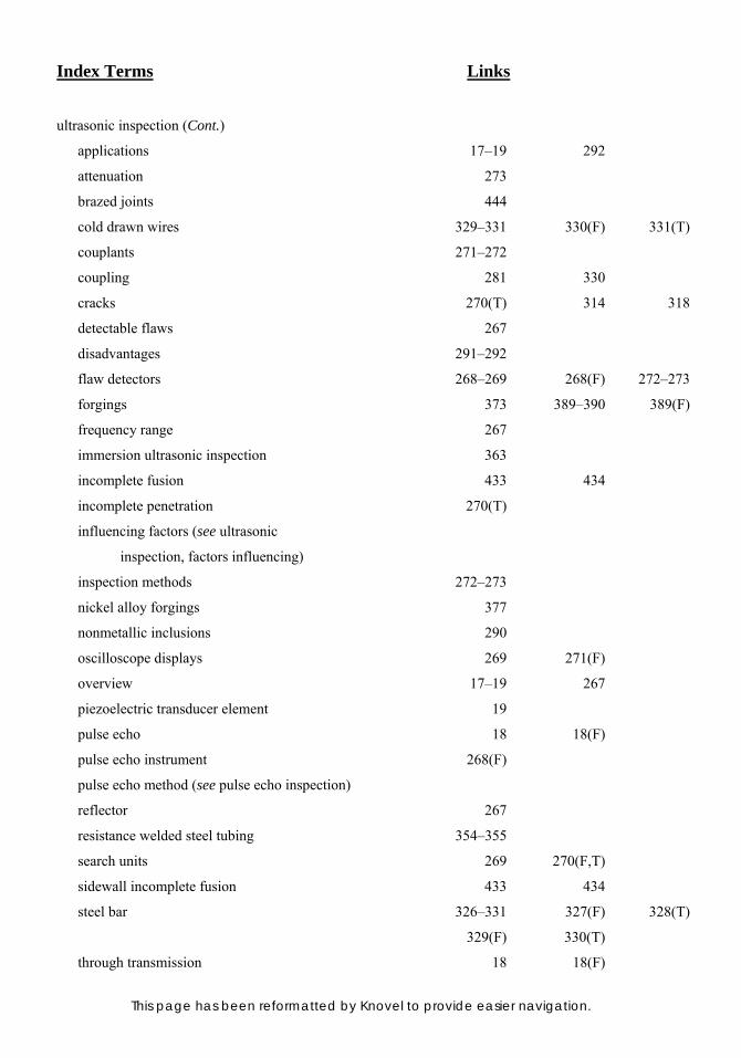
Index Terms Links
This page has been reformatted by Knovel to provide easier navigation.
ultrasonic inspection (Cont.)
applications 17–19 292
attenuation 273
brazed joints 444
cold drawn wires 329–331 330(F) 331(T)
couplants 271–272
coupling 281 330
cracks 270(T) 314 318
detectable flaws 267
disadvantages 291–292
flaw detectors 268–269 268(F) 272–273
forgings 373 389–390 389(F)
frequency range 267
immersion ultrasonic inspection 363
incomplete fusion 433 434
incomplete penetration 270(T)
influencing factors (see ultrasonic
inspection, factors influencing)
inspection methods 272–273
nickel alloy forgings 377
nonmetallic inclusions 290
oscilloscope displays 269 271(F)
overview 17–19 267
piezoelectric transducer element 19
pulse echo 18 18(F)
pulse echo instrument 268(F)
pulse echo method (see pulse echo inspection)
reflector 267
resistance welded steel tubing 354–355
search units 269 270(F,T)
sidewall incomplete fusion 433 434
steel bar 326–331 327(F) 328(T)
329(F) 330(T)
through transmission 18 18(F)
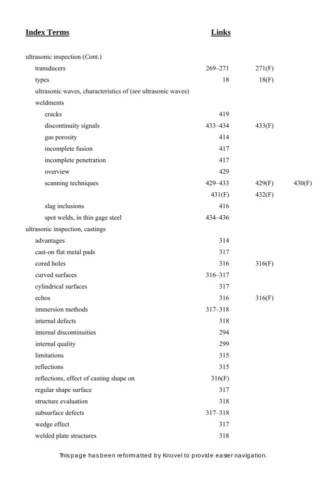
Index Terms Links
This page has been reformatted by Knovel to provide easier navigation.
ultrasonic inspection (Cont.)
transducers 269–271 271(F)
types 18 18(F)
ultrasonic waves, characteristics of (see ultrasonic waves)
weldments
cracks 419
discontinuity signals 433–434 433(F)
gas porosity 414
incomplete fusion 417
incomplete penetration 417
overview 429
scanning techniques 429–433 429(F) 430(F)
431(F) 432(F)
slag inclusions 416
spot welds, in thin gage steel 434–436
ultrasonic inspection, castings
advantages 314
cast-on flat metal pads 317
cored holes 316 316(F)
curved surfaces 316–317
cylindrical surfaces 317
echos 316 316(F)
immersion methods 317–318
internal defects 318
internal discontinuities 294
internal quality 299
limitations 315
reflections 315
reflections, effect of casting shape on 316(F)
regular shape surface 317
structure evaluation 318
subsurface defects 317–318
wedge effect 317
welded plate structures 318

Index Terms Links
This page has been reformatted by Knovel to provide easier navigation.
ultrasonic inspection, factors influencing
absorption 289
acoustic impedance 286–287
acoustic properties, metals and
nonmetals 287(T)
angle of incidence 288 288(F)
beam spreading 290
critical angles
first critical angle 288 289(T)
45° shear-wave incident angle 289 289(T)
second critical angle 289 289(T)
diffraction 290
far-filed effects 290 291(F)
frequency ranges/applications 286 286(T)
Huygens point source 290
inspection frequency 286
near-filed effects 290 291(F)
overview 285–286
scattering 290
ultrasonic inspection, transmission methods
applications 281
cracks 281
immersion techniques 281
overview 280–281
pitch-catch testing 281–282
transmission-test data 281
water-column (bubbler or squirter) techniques 281
ultrasonic microhardness testers 302
ultrasonic search units 269 270(T)
ultrasonic sensors 71
ultrasonic thickness gages 300
ultrasonic velocity measurements 318
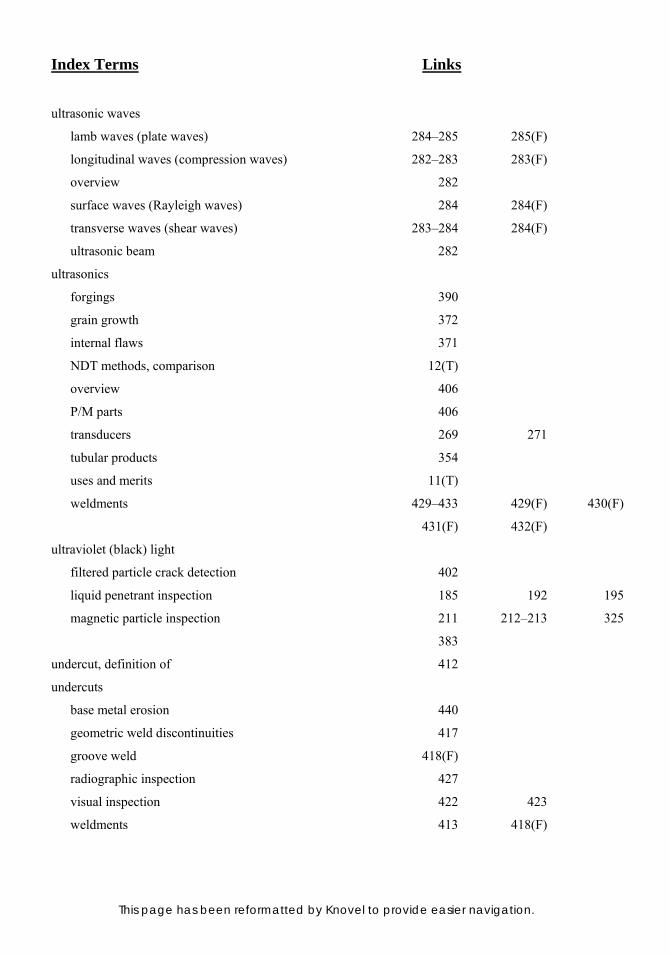
Index Terms Links
This page has been reformatted by Knovel to provide easier navigation.
ultrasonic waves
lamb waves (plate waves) 284–285 285(F)
longitudinal waves (compression waves) 282–283 283(F)
overview 282
surface waves (Rayleigh waves) 284 284(F)
transverse waves (shear waves) 283–284 284(F)
ultrasonic beam 282
ultrasonics
forgings 390
grain growth 372
internal flaws 371
NDT methods, comparison 12(T)
overview 406
P/M parts 406
transducers 269 271
tubular products 354
uses and merits 11(T)
weldments 429–433 429(F) 430(F)
431(F) 432(F)
ultraviolet (black) light
filtered particle crack detection 402
liquid penetrant inspection 185 192 195
magnetic particle inspection 211 212–213 325
383
undercut, definition of 412
undercuts
base metal erosion 440
geometric weld discontinuities 417
groove weld 418(F)
radiographic inspection 427
visual inspection 422 423
weldments 413 418(F)
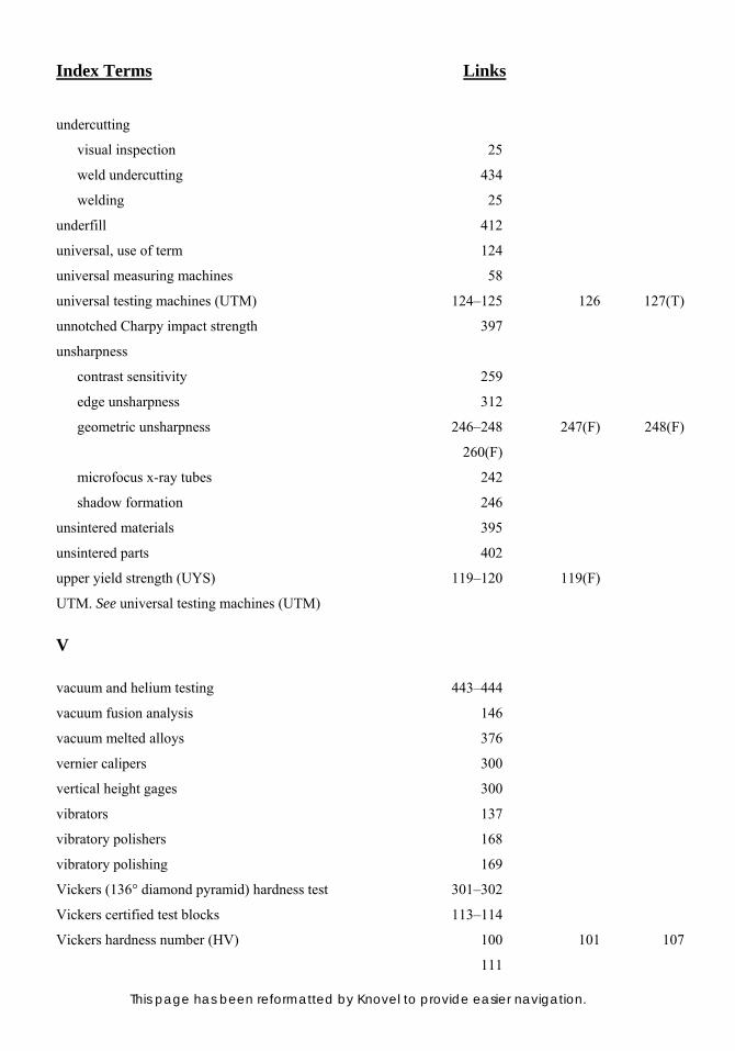
Index Terms Links
This page has been reformatted by Knovel to provide easier navigation.
undercutting
visual inspection 25
weld undercutting 434
welding 25
underfill 412
universal, use of term 124
universal measuring machines 58
universal testing machines (UTM) 124–125 126 127(T)
unnotched Charpy impact strength 397
unsharpness
contrast sensitivity 259
edge unsharpness 312
geometric unsharpness 246–248 247(F) 248(F)
260(F)
microfocus x-ray tubes 242
shadow formation 246
unsintered materials 395
unsintered parts 402
upper yield strength (UYS) 119–120 119(F)
UTM. See universal testing machines (UTM)
V
vacuum and helium testing 443–444
vacuum fusion analysis 146
vacuum melted alloys 376
vernier calipers 300
vertical height gages 300
vibrators 137
vibratory polishers 168
vibratory polishing 169
Vickers (136° diamond pyramid) hardness test 301–302
Vickers certified test blocks 113–114
Vickers hardness number (HV) 100 101 107
111
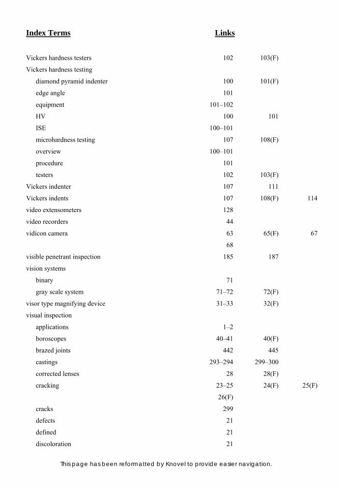
Index Terms Links
This page has been reformatted by Knovel to provide easier navigation.
Vickers hardness testers 102 103(F)
Vickers hardness testing
diamond pyramid indenter 100 101(F)
edge angle 101
equipment 101–102
HV 100 101
ISE 100–101
microhardness testing 107 108(F)
overview 100–101
procedure 101
testers 102 103(F)
Vickers indenter 107 111
Vickers indents 107 108(F) 114
video extensometers 128
video recorders 44
vidicon camera 63 65(F) 67
68
visible penetrant inspection 185 187
vision systems
binary 71
gray scale system 71–72 72(F)
visor type magnifying device 31–33 32(F)
visual inspection
applications 1–2
boroscopes 40–41 40(F)
brazed joints 442 445
castings 293–294 299–300
corrected lenses 28 28(F)
cracking 23–25 24(F) 25(F)
26(F)
cracks 299
defects 21
defined 21
discoloration 21

Index Terms Links
This page has been reformatted by Knovel to provide easier navigation.
visual inspection (Cont.)
distortion 21
equipment 2 2(F)
fiber optic scopes 40(F) 41
flow lines 2 2(F)
forgings 383
geometric weld discontinuities 417
heat-resistant alloy forgings 376
lens types 28–30
degree of correction 28
faults 28
lighting
general 33–35 34(F)
specific devices 34–35 35(F)
macroetching
alloy segregation 45
billet macrostructure 44
bloom macrostructure 44
cell size 45
continuously cast steel
macrostructures 44–45
forging flow lines 45
grain size 45
heat treatment, response to 46 46(F) 47(F)
overview 44
solidification structures 44 45(F)
weldments 45–46
magnesium alloy forgings 380
magnifiers
eye attachments 32–33 32(F)
focal length 27–28
hand-held lenses 30 30(F)
illuminated magnifiers 33 33(F)
magnifying power 27

Index Terms Links
This page has been reformatted by Knovel to provide easier navigation.
visual inspection
magnifiers (Cont.)
pocket microscopes 30–31 31(F)
self-supporting 31–32 31(F)
measurement 25–26
measuring devices
linear 36
micrometers 36
miscellaneous devices 36–38 38(F)
optical comparators 36 38(F)
overview 35
reticles 36 37(F)
mirrors 39–40
overview 1–2 21
procedure
abuse 22
corrosion scaling 22–23
cracking 23–25 24(F)
heat effects 22
markings 21–22
measurement 25–26
overview 21
record keeping 26–27
results 26–27
record-keeping methods
overview 41
photography (see photography, visual inspection)
video recorders 44
voice recorders 41
steel bars 324
stereoscopic microscope 39 39(F)
surface cracks 1
surface finish comparators 41 42(F)
tools 27

Index Terms Links
This page has been reformatted by Knovel to provide easier navigation.
visual inspection (Cont.)
undercutting 25
weldments
appearance standards 423 424(F)
conformity 423 424(F)
dimensional accuracy 423 424(F)
discontinuities 423 425
geometric weld discontinuities 417
overview 422–423
voice recorders 41
voids
alpha-stabilized voids 380–381 380(F)
clean voids 382
radiation gaging 253–254
radiography 234
shrinkage voids 412
W
water vapor 367
waterfalling 297
wave bending 290
wave packets 273
wave path 434 435(F)
wavelength dispersive spectrometers (WDS) 144 145(F)
wedge effect 317
weld gage 423 424(F)
weld macrostructure 46
weld mismatch 434
weld seam tracking 71 81
weld twist 350–351 353 355
weld zone 354 362 419
welded pipe 346
welded tubes 231

Index Terms Links
This page has been reformatted by Knovel to provide easier navigation.
welding
arc strikes 25
arc welding 356
base metal 46
crack initiation 25
crack repair 23
flux leakage inspection, combining with 353
fusion welds 45–46
heat affected zone (HAZ) 46
hot tears 298
nugget 46
repair, castings 319
resistance welded steel tubing,
inspecting (see resistance welded steel tubing)
splatter 25
undercutting 25
weld root cracks 434
weld undercutting 434
welding machines 349
weldments
discontinuities
cracks 417–420 418(F)
design related 411–412
FCAW 413
gas porosity 413–415
gas porosity, types 413–414 414(F) 415(F)
geometric weld discontinuities 417 418(F)
GMAW 413
GTAW 413
incomplete fusion 416–417 417(F)
incomplete penetration 416–417 417(F)
lamellar tearing 420 420(F)
metallurgical discontinuities 412–413
SAW 413
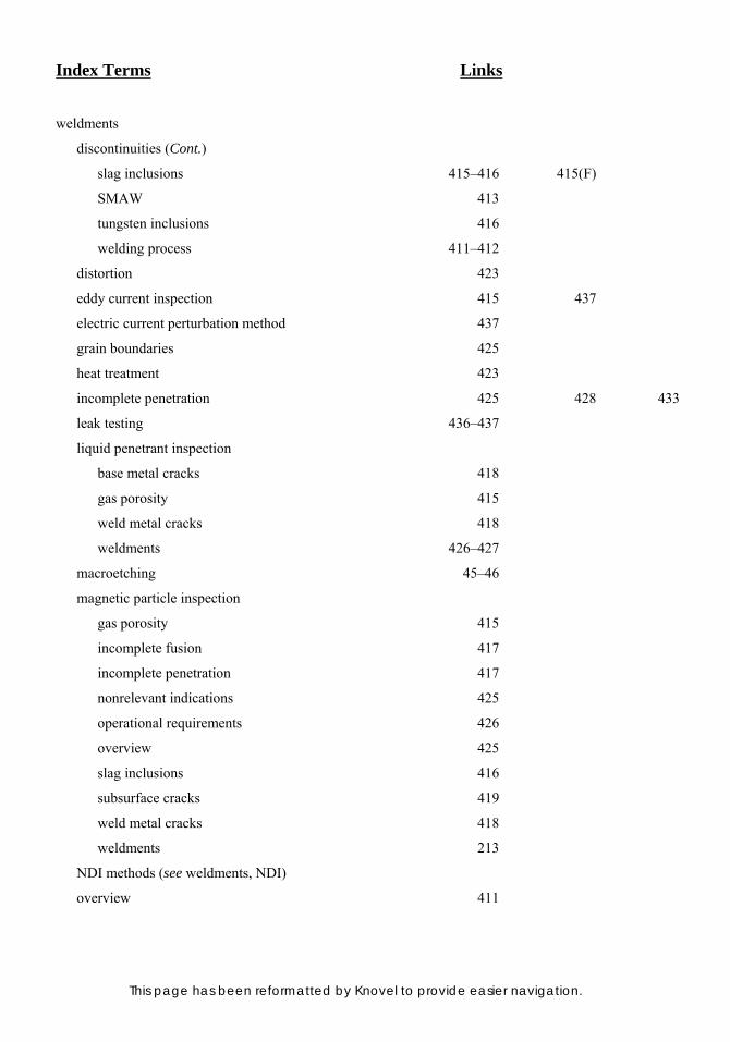
Index Terms Links
This page has been reformatted by Knovel to provide easier navigation.
weldments
discontinuities (Cont.)
slag inclusions 415–416 415(F)
SMAW 413
tungsten inclusions 416
welding process 411–412
distortion 423
eddy current inspection 415 437
electric current perturbation method 437
grain boundaries 425
heat treatment 423
incomplete penetration 425 428 433
leak testing 436–437
liquid penetrant inspection
base metal cracks 418
gas porosity 415
weld metal cracks 418
weldments 426–427
macroetching 45–46
magnetic particle inspection
gas porosity 415
incomplete fusion 417
incomplete penetration 417
nonrelevant indications 425
operational requirements 426
overview 425
slag inclusions 416
subsurface cracks 419
weld metal cracks 418
weldments 213
NDI methods (see weldments, NDI)
overview 411
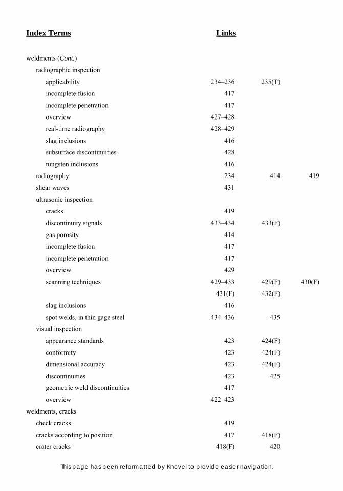
Index Terms Links
This page has been reformatted by Knovel to provide easier navigation.
weldments (Cont.)
radiographic inspection
applicability 234–236 235(T)
incomplete fusion 417
incomplete penetration 417
overview 427–428
real-time radiography 428–429
slag inclusions 416
subsurface discontinuities 428
tungsten inclusions 416
radiography 234 414 419
shear waves 431
ultrasonic inspection
cracks 419
discontinuity signals 433–434 433(F)
gas porosity 414
incomplete fusion 417
incomplete penetration 417
overview 429
scanning techniques 429–433 429(F) 430(F)
431(F) 432(F)
slag inclusions 416
spot welds, in thin gage steel 434–436 435
visual inspection
appearance standards 423 424(F)
conformity 423 424(F)
dimensional accuracy 423 424(F)
discontinuities 423 425
geometric weld discontinuities 417
overview 422–423
weldments, cracks
check cracks 419
cracks according to position 417 418(F)
crater cracks 418(F) 420
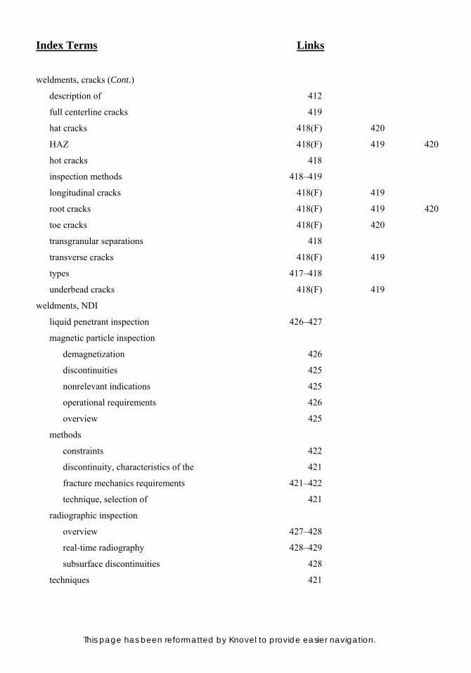
Index Terms Links
This page has been reformatted by Knovel to provide easier navigation.
weldments, cracks (Cont.)
description of 412
full centerline cracks 419
hat cracks 418(F) 420
HAZ 418(F) 419 420
hot cracks 418
inspection methods 418–419
longitudinal cracks 418(F) 419
root cracks 418(F) 419 420
toe cracks 418(F) 420
transgranular separations 418
transverse cracks 418(F) 419
types 417–418
underbead cracks 418(F) 419
weldments, NDI
liquid penetrant inspection 426–427
magnetic particle inspection
demagnetization 426
discontinuities 425
nonrelevant indications 425
operational requirements 426
overview 425
methods
constraints 422
discontinuity, characteristics of the 421
fracture mechanics requirements 421–422
technique, selection of 421
radiographic inspection
overview 427–428
real-time radiography 428–429
subsurface discontinuities 428
techniques 421
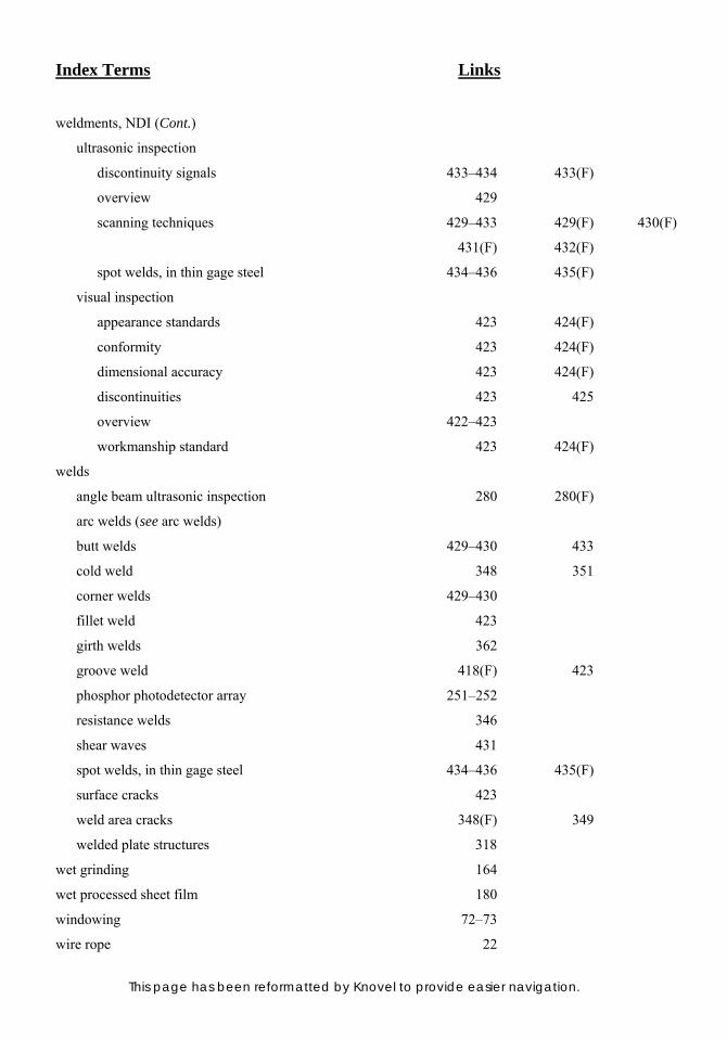
Index Terms Links
This page has been reformatted by Knovel to provide easier navigation.
weldments, NDI (Cont.)
ultrasonic inspection
discontinuity signals 433–434 433(F)
overview 429
scanning techniques 429–433 429(F) 430(F)
431(F) 432(F)
spot welds, in thin gage steel 434–436 435(F)
visual inspection
appearance standards 423 424(F)
conformity 423 424(F)
dimensional accuracy 423 424(F)
discontinuities 423 425
overview 422–423
workmanship standard 423 424(F)
welds
angle beam ultrasonic inspection 280 280(F)
arc welds (see arc welds)
butt welds 429–430 433
cold weld 348 351
corner welds 429–430
fillet weld 423
girth welds 362
groove weld 418(F) 423
phosphor photodetector array 251–252
resistance welds 346
shear waves 431
spot welds, in thin gage steel 434–436 435(F)
surface cracks 423
weld area cracks 348(F) 349
welded plate structures 318
wet grinding 164
wet processed sheet film 180
windowing 72–73
wire rope 22

Index Terms Links
This page has been reformatted by Knovel to provide easier navigation.
Wollaston prism 180
wormhole 428
wormhole porosity 414 415(F)
wrought materials
radiography 236
tensile testing 7
ultrasonic inspection 390
wrought tubular products 345
X
xenon arc bulbs 177
xenon arc lamps 178
xeroradiography 233 249–250
XPS. See X-ray photoelectron spectroscopy (XPS)
x-ray film
film emulsion 254
film gradient 254
film speed 254
graininess 254–255
overview 254–255
selection 256–257 256(T) 257(T)
types 255–256 256(T)
x-ray fluorescence spectroscopy (XRF)
applications 139
chemical analysis 9
chemical composition 152
computer software 142
electromagnetic radiation 139
energy dispersive x-ray detector 145(F)
limitations 140
nitrogen 139
OES 150
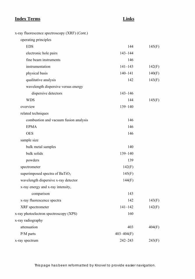
Index Terms Links
This page has been reformatted by Knovel to provide easier navigation.
x-ray fluorescence spectroscopy (XRF) (Cont.)
operating principles
EDS 144 145(F)
electronic hole pairs 143–144
fine beam instruments 146
instrumentation 141–143 142(F)
physical basis 140–141 140(F)
qualitative analysis 142 143(F)
wavelength dispersive versus energy
dispersive detectors 143–146
WDS 144 145(F)
overview 139–140
related techniques
combustion and vacuum fusion analysis 146
EPMA 146
OES 146
sample size
bulk metal samples 140
bulk solids 139–140
powders 139
spectrometer 142(F)
superimposed spectra of BaTiO3 145(F)
wavelength dispersive x-ray detector 144(F)
x-ray energy and x-ray intensity,
comparison 143
x-ray fluorescence spectra 142 143(F)
XRF spectrometer 141–142 142(F)
x-ray photoelectron spectroscopy (XPS) 160
x-ray radiography
attenuation 403 404(F)
P/M parts 403–404(F)
x-ray spectrum 242–243 243(F)
Index Terms Links
This page has been reformatted by Knovel to provide easier navigation.
x-ray tubes
anode design 240 240(F) 241(F)
anode heating 240–241
cathode structure 241
characteristics 240
classification of 240
components 240(F)
definition of 239
design 241–242 241(F)
focal spot 240 241 241(F)
forced liquid cooling 241
insulating gas 242
materials 241–242 241(F)
microfocus x-ray tubes 242
overview 239–240
penetration capability 243 244(T)
strength/radiation output 240
structure 239–240
target design 240
transformer oil 242
tube envelopes 242
x-ray spectrum 242–243 243(F)
x-ray unit 240(F)
x-rays 237–238 238(F) 239
XRF. See x-ray fluorescence spectroscopy (XRF)
Y
yaw 50
yield point elongation (YPE) 119(F) 120
yield strength (YS)
defined 119
offset yield strength 120
tensile testing 8–9 8(F) 119–120
119(F)

Index Terms Links
This page has been reformatted by Knovel to provide easier navigation.
yokes 203–204 204(F)
Z
zinc
heat-resistant alloy forgings 375
radiographic absorption equivalence 245(T)
Rockwell hardness scales 97(T)
zinc sulfide crystals 265