Inspiral of Generic Black Hole Binaries:

Spin, Precession, and Eccentricity

Janna Levin1,2, Sean T. McWilliams1,2,3, and Hugo Contreras4

1Department of Physics and Astronomy,

Barnard College of Columbia University,

3009 Broadway, New York, NY 10027

2Institute for Strings, Cosmology and Astroparticle Physics (ISCAP),

Columbia University, New York, NY 10027

3Department of Physics, Princeton University, Princeton, NJ 08544 and

4Department of Physics, Columbia University, New York, NY 10027∗

Given the absence of observations of black hole binaries, it is critical that the full

range of accessible parameter space be explored in anticipation of future observation

with gravitational wave detectors. To this end, we compile the Hamiltonian equa-

tions of motion describing the conservative dynamics of the most general black hole

binaries and incorporate an effective treatment of dissipation through gravitational

radiation, as computed by Will and collaborators. We evolve these equations for

systems with orbital eccentricity and precessing spins. We find that, while spin-

spin coupling corrections can destroy constant radius orbits in principle, the effect

is so small that orbits will reliably tend to quasi-spherical orbits as angular momen-

tum and energy are lost to gravitational radiation. Still, binaries that are initially

highly eccentric may retain eccentricity as they pass into the detectable bandwidth

of ground-based gravitational wave detectors. We also show that a useful set of

natural frequencies for an orbit demonstrating both spin precession and periastron

precession is comprised of (1) the frequency of angular motion in the orbital plane,

(2) the frequency of the plane precession, and (3) the frequency of radial oscillations.

These three natural harmonics shape the observed waveform.

∗Electronic address: janna@astro.columbia.edu

arX

iv:1

009.

2533

v3 [

gr-q

c] 2

8 Ju

l 201

1

2

I. INTRODUCTION

Motivated by future gravitational-wave observatories, a campaign to track the inspiral

of the most generic black hole binaries has long been underway [1–11]. The promise of

gravitational-wave astronomy lies in our ability to observe and test the full range of astro-

physical phenomena, including spinning, precessing, eccentric pairs of unequal mass. To

this end, Will and collaborators have published a series of computations of the equations

governing black hole binary motion in the Post-Newtonian (PN) expansion to 3.5PN order,

including spin corrections [8–11]. We compile those results in an appendix to provide a re-

source for probing and testing the PN dynamics. We then convert the dissipative terms into

Hamiltonian variables and suggest a modification of the Hamiltonian equations of motion

that incorporates the effects of radiation reaction. The modified Hamiltonian formulation

and the Lagrangian formulation admit equivalent descriptions, though for the purposes of

investigating the natural harmonics of these systems we will exploit the ease of interpretation

offered by the Hamiltonian formulation.

Binary stars that evolve to a pair of black holes can show evidence of eccentricity and spin

precession in waveforms detectable by LISA [12]. Although long-lived pairs will likely shed

eccentricity by the time they enter the LIGO bandwidth, the entire orbital plane continues

to precess along with the spins. Also, black hole pairs formed by tidal capture in globular

clusters or galactic nuclei may retain significant eccentricity as their signals pass through

the band of current and future ground-based gravitational-wave observatories [13, 14]. The

equations of motion of Refs. [8–11] allow flexibility in handling the gravitational radiation

emitted by any realistic black hole pair, prior to entering the strong-field.

There are four questions we can address immediately with this compilation of the inspiral

equations: (1) Do spinning pairs tend to quasi-spherical orbits? (2) What features are

generically introduced into waveforms through periastron precession and spin precession?

(3) How much energy is lost during each burst near periastron passage? (4) How much

of the orbit and the waveform for eccentric, precessing orbits is well-described by the PN

expansion?

The first question (Do spinning pairs tend to quasi-spherical orbits?) must be asked since

the purely circular orbits are destroyed by spin-spin (SS) couplings. When spin-orbit (SO)

coupling is incorporated, the entire orbital-plane precesses and the quasi-circular orbits are

3

replaced by quasi-spherical orbits – trajectories that lie on the surface of a sphere whose

radius shrinks only due to dissipation. However, spin-spin couplings actually destroy even

these so that there are no constant radius orbits, even if we were to artificially turn off

dissipation by turning off the half-order terms in the expansion. In other words, if black

holes spin, there may not be any quasi-spherical orbits and all orbits could retain eccentricity

at all stages of their inspiral. We can ask how significant the effect is. Since spin-spin is a

subdominant effect, we find that the eccentric behavior is small and that orbits can appear

to be very nearly quasi-spherical.

The second question (What features are generically introduced into waveforms through

periastron precession and spin precession?) is significant for designing optimal detection

algorithms and estimating source parameters. For systems possessing spin, modulation due

to orbital plane precession will leave an imprint on the observed waveform. In the case of

significant eccentricity, the waveforms are modulated by the radial oscillation of the orbit.

Characteristically the amplitude is modulated by eccentricity, as is the polarization due

to the precession of the periastron and the orbital plane. The Fourier transform of the

waveform will reflect these precessions by reflecting the natural frequencies of the orbit,

which modulate the frequency evolution from loss of orbital energy that is present in all

black hole binaries. We demonstrate these features for an example black hole binary that

possesses all three characteristic frequencies, for which we also address the third question

posed (How much energy is lost during each burst near periastron passage?).

The fourth question (How much of the orbit and waveform for eccentric, precessing orbits

is well described by the PN expansion?) has not been addressed for generic orbits. In the

limit of quasi-spherical orbits, the dynamics and waveform are usually taken to be accurate

until the system reaches the innermost stable circular orbit (ISCO), beyond which even the

conservative dynamics cannot be treated adiabatically. However, the ISCO is formally a

characteristic of a test-particle orbit in Schwarzschild or Kerr spacetime, and is not well

defined for binary spacetimes. As we will show, the PN sequence actually diverges well

outside the ISCO not only for eccentric precessing systems, but for quasi-spherical systems

as well. We find that the breakdown happens at radial separations r ∼ 10M , which is well

outside the Schwarzschild ISCO (6M), in contrast to the conventional wisdom of using 6M

as a reference point for truncating PN approximations.

Due to this limitation of the approximation, the PN equations of motion cannot be used

4

to probe the most extreme form of precession manifest as zoom-whirl behavior – elliptical

zooms out to apastron followed by multiple nearly circular whirls around periastron [15].

Zoom-whirl orbits are most prevalent when periastron drops into the strong-field regime. As

shown in Ref. [16], complete whirls occur when periastron falls between the IBCO (innermost

bound circular orbit) and the ISCO. To be clear, zoom-whirl orbits exist and have been

observed in numerical relativity simulations [17, 18]; they are simply beyond the trusted

regime for the PN approximation.

To lay the foundation, we begin with a discussion of conservative black hole dynamics in

§II. In §III, we discuss the utility of a Hamiltonian formulation of the equations of motion

for simplifying interpretation of the dynamics of the full inspiral trajectories and resulting

gravitational waveforms for spinning black hole pairs on eccentric, precessing orbits. In

§IV, we explore the limits of our, and indeed any, PN formulation, due to the intrinsic

non-perturbative nature of the dynamics at the end of the inspiral. In §V, we summarize

the results and the answers to the four questions we posed. For completeness and ease of

reference, in §A the PN corrections to the equations of motion including the dissipation due

to gravitational radiation are compiled from Refs. [8–11] as derived by Will and collaborators

to 3.5PN order with SO and SS coupling. Finally, in §B, we convert the PN corrections

originally computed in the Lagrangian formulation into Hamiltonian coordinates, which is

the approach we apply throughout the text.

II. DYNAMICS WITHOUT DISSIPATION

For this section, radiation reaction has artificially been turned off so the pair shows no

evidence of dissipation. The advantage of doing so is that we can clearly see intrinsic features

of the dynamics that dissipation can obscure. In the following section, dissipation is included

while the insights of this section will continue to guide our perspective.

If either of the black holes spin, orbital motion famously no longer lies in a plane in the

absence of special symmetries. The black holes engage in an intricate three-dimensional

motion tangled by precession. An example of the three-dimensional range of a spinning pair

is shown in center-of-mass coordinates on the far left of Fig. 1. We want to highlight the

two different precession effects: periastron precession and precession of the orbital plane.

The two effects can be cleanly separated with a natural choice of coordinates [19, 20].

5

FIG. 1: A black hole pair with m2/m1 = 1/4. The heavier of the two black holes is spinning at

0.9 maximal. The lighter is not spinning. Left: The orbit. Middle: The orbit in the orbital plane

showing the constancy of the periastron and apastron as well as isolating the periastron precession.

In the orbital plane, the pair precesses around a four-leaf clover. Right: A projection of the orbit

onto the equatorial plane, showing that the innate symmetry of the orbit is obscured.

First, consider precession of the orbital plane. If the spins of the black hole and the orbital

angular momentum are aligned or anti-aligned, motion will lie in the equatorial plane, defined

as the plane perpendicular to the total angular momentum, J = L + S, where L is the

orbital angular momentum and S is the sum of the spins. However, when the spins are not

aligned with the orbital angular momentum, the spins will precess around the total angular

momentum, and by conservation of the total momentum (i. e. J = 0), the orbital angular

momentum will precess to compensate (i. e. L = −S). Since the orbital plane is spanned by

(r,p) and is orthogonal to the orbital angular momentum, L = r × p, as shown in Fig. 2,

the entire orbital plane precesses. Plane precession is a purely relativistic reflection of black

hole spins and so isolating the effect draws out distinct signatures for parameter estimation.

Periastron precession can be isolated, in turn, by following the motion confined to the

orbital plane. In Ref. [19, 20], it was shown that when there is one effective spin – defined by

one black hole spinning or two equal-mass black holes with arbitrary spins – that periastron

and apastron are constants and the periastron precesses at a fixed rate, as shown in the

middle panel of 1. By contrast, these precise features are obscured in the equatorial plane,

as shown by the projection in the far right panel of 1. So, to separate periastron precession

from the precession of the orbital plane, we select a coordinate system that cleaves the two

effects.

6

The coordinate system that affects this separation is given by (r,Φ,Ψ) where r is the

radial coordinate, Φ is the angle swept out in the orbital plane, and Ψ is the angle swept

out as L swings around J [19, 20]. The polar coordinates in the orbital plane that precess

through space as the plane precesses are (n, Φ) with

Φ = L× n . (1)

where n = r/r. The entire orbital plane then precesses around the total momentum in the

direction Ψ given by

Ψ = J× (J× L)

|J× L|. (2)

In the set of coordinates (r,Φ,Ψ) and their conjugate momenta (Pr, PΦ, PΨ), the angular

conjugate momenta are simply PΦ = L and PΨ = Lz = L · J. The magnitude of the orbital

angular momentum L is conserved and so, therefore, is PΦ.

In the restricted case of one effective spin – again, defined by one black hole spinning

or two equal mass black holes with arbitrary spins – the component of the orbital angular

momentum along J, and therefore PΨ, is also conserved. The Hamiltonian equations of

motion then have a remarkably simple form:

r =∂H

∂Pr

, Pr = −∂H∂r

Φ =∂H

∂PΦ

, PΦ = 0

Ψ =∂H

∂PΨ

, PΨ = 0 (3)

The natural frequencies given by radial oscillations, fr = 1/Tr where Tr is the radial period,

periastron precession, fΦ = Φ/2π, and orbital plane precession fΨ = Ψ/2π, are functions of

r only.

The more general equations, when both black holes spin and have unequal masses, and

dissipation is included, are collected in the Appendices. In the coordinate system introduced

above, adding a second spin (for unequal mass) renders PΨ = Lz no longer conserved,

although PΦ = L continues to be conserved. Consequently, the precessional frequencies will

not depend solely on r, but will be modulated by angular position. Adding dissipation drains

both PΦ and PΨ, although (r,Φ,Ψ) remains the natural coordinate system for disentangling

the two kinds of precession.

7

FIG. 2: The orbital plane coordinates as defined in Ref. [19] Fig. 1. Left: The orbital plane spanned

by r×p precesses around the total angular momentum with frequency Ψ. Right: The coordinates

as defined within the orbital plane.

We then convert the radiation-reaction terms derived in the Lagrangian formulation (§A)

into Hamiltonian variables (§B). We are motivated to show our results in the following

section in Hamiltonian variables by the simplicity of Eqs. (3) and the simplicity of the

analytic expressions for the frequencies, as we discuss in the following section (see Eqs.

(7)). Of course, practitioners are free to choose either the Lagrangian or the Hamiltonian

formulation, since both admit equivalent descriptions, so that an orbital-plane decomposition

can be found with corresponding frequencies. The Hamiltonian formulation offers a cleaner

framework in which to examine the explicit equations, so we favor it slightly for the purposes

of the paper. 1

III. GALLERY OF INSPIRALS

Using the equations of motion of §B, we can investigate a completely generic orbit. The

most general scenario allows for both black holes to spin and for those spins to be misaligned.

These three-dimensional orbits should have three natural frequencies. As described in §II,

the natural frequencies are the radial oscillations of an eccentric orbit

fr =1

Tr, (4)

1 For example, the simplicity of ~L = ~r × ~p in the Hamiltonian formulation renders our geometric interpre-

tation more transparent than the lengthy 3PN corrected definition of ~L in the Lagrangian variables.

8

where Tr is the time between successive periastra, the frequency of periastron precession in

the orbital plane,

fΦ =Φ

2π, (5)

and the frequency of plane precession,

fΨ =Ψ

2π. (6)

In the conservative Hamiltonian system, it was found that if spin-spin contributions were

omitted, then [19]

2πfΦ = Φ = AL

r2+

Seff · Lr3

− Ψ(J · L)

2πfΨ = Ψ =

(J× (Seff × L)

|J× L|r3

)· Ψ (7)

where A = 2 ∂H/∂p2 (Eq. (B17), and Seff is defined in Eq. (B6). Although we add spin-spin

coupling, we continue to use Eqs. (7) as adiabatic estimates for the frequencies.

The full waveform will be composed of the frequencies (4)-(6). The waveform is computed

to leading quadrupole order, although the orbital variables that go into this expression are

computed in the full 3.5PN system,

hij =2µ

D2

(vivj −

1

rrirj

), (8)

with D the distance to the sources. This is referred to as the restricted PN waveform

approximation. For simplicity, we place the Earth along z = J . For greater precision,

higher-order corrections to the amplitude (including spins) have been computed [21, 22],

but for our purposes, the leading-order amplitude is sufficient.

A. Quasi-spherical

We now consider quasi-spherical, low eccentricity orbits (see also [23]). Low eccentricity

orbits look quasi-circular in the orbital plane. As the orbital plane precesses, these orbits lie

on the surface of a sphere whose radius decreases monotonically as gravitational radiation

is emitted. We work in the Hamiltonian formulation, since the Hamiltonian better lends

itself to finding constant radius orbits and facilitates the geometric breakdown in terms

of the orbital plane. Of course, this procedure can readily be repeated in the Lagrangian

9

o o oooooooooooooooooooooooooooooo

oooooooooooooooo

@@@@@@@@@@@@@@@@@@@@@@@@@@@@@@@@@@@@@@@@

@

@@@@@@@

0 10 20 30 40 50 60

0.1

0.5

1

5

10

30

0 10 20 30 40 50 60

0.1

0.5

1

5

10

30

tHsL

fHH

zL

o

fF

@

fW

FIG. 3: The initial conditions are set to those of the constant radius orbit at ri = 50 in the

absence of spin-spin coupling for an equal mass binary with maximal spins, and spin angles θ1 =

θ2 = 45o. Left: The first 10 sec of the orbit is shown (length measured in units of GM/c2 '

26.5 (M/20M�)km). Right: The frequency in the orbital plane as defined in Eq. (7) marked with

open circles, and the frequency of plane precession, as defined in Eq. (7), marked with crosses.

Both are shown versus time over the entire inspiral. We plot frequencies in units of (20M�/M)Hz

and time in units of (M/20M�)sec.

formulation. We find the constant radius orbit according to the prescription in [19] (see also

[23]). We sketch the argument here. The Hamiltonian of Eqs. (B3) and (B4) does not admit

a simple effective potential formulation since it is a complicated function of p2. Nonetheless,

we can still use the Hamiltonian as an effective potential at the turning points if we exclude

spin-spin coupling:

Veff = H(Pr = 0) , (9)

With this condition, we can find the L of an orbit at a given constant radius. Fixing the initial

conditions this way and including spin-spin couplings, we can estimate the deviation away

from quasi-sphericity. We find that the oscillations in the radius due to spin-spin coupling

are negligible (less than a few percent) and that the radius quickly begins a monotonic

decrease as gravitational waves are radiated. Therefore, the spin-spin effect seems to be

too small to induce measurable eccentricity during the inspiral if no eccentricity is present

initially.

10

FIG. 4: The pair has m2/m1 = 1/4, maximal spins, a1 = a2 = 1, and initial spin angles θ1 =

45o, θ2 = 45o and initial values ri = 3000 and Li = 0.003ri. Left: The first 1150s of the inspiral.

Right: The final 5s before cutoff.

As an example, consider an equal mass pair with maximal spins a1 = a2 = 1, and spin

angles initially misaligned so that θ1 ≡ arccos(L · S1) = 45o and θ2 ≡ arccos(L · S2) = 45o.

This is shown in Fig. 3, where the first ten seconds of the total orbit is shown. The full

orbit takes ∼ 60 seconds to merge for M = 20M�. We take the initial condition to be

ri = 50 and set L initially at the quasi-spherical value determined by Eq. (9). The natural

frequencies fΦ and fΨ are shown in the right panel. Since the orbit is quasi-spherical, the

frequency of radial oscillations fr is not informative. Periastron precession dominates over

plane precession, fΦ > fΨ, which is expected since plane precession is a higher-order effect.

Using physical units, with the initial separation of ri ∼ 50, the gravitational radiation

has an initial frequency

2× fΦ ∼ 9.5Hz

(20M�M

)(10)

which is already nearing the Advanced LIGO/VIRGO band for two 10M� black holes, and

is sweeping through the bandwidth as the orbital separation decreases. The much slower

frequency of precession, fΨ, does not have a significant effect on the waveform for the quasi-

spherical case.

11

0 1 2 3 4−4

−2

0

2x 10

−22

t [sec]

h

2944 2946 2948 2950 2952−1

−0.5

0

0.5

1x 10

−21

t [sec]0 1000 2000 3000

−1

−0.5

0

0.5

1x 10

−21

t [sec]

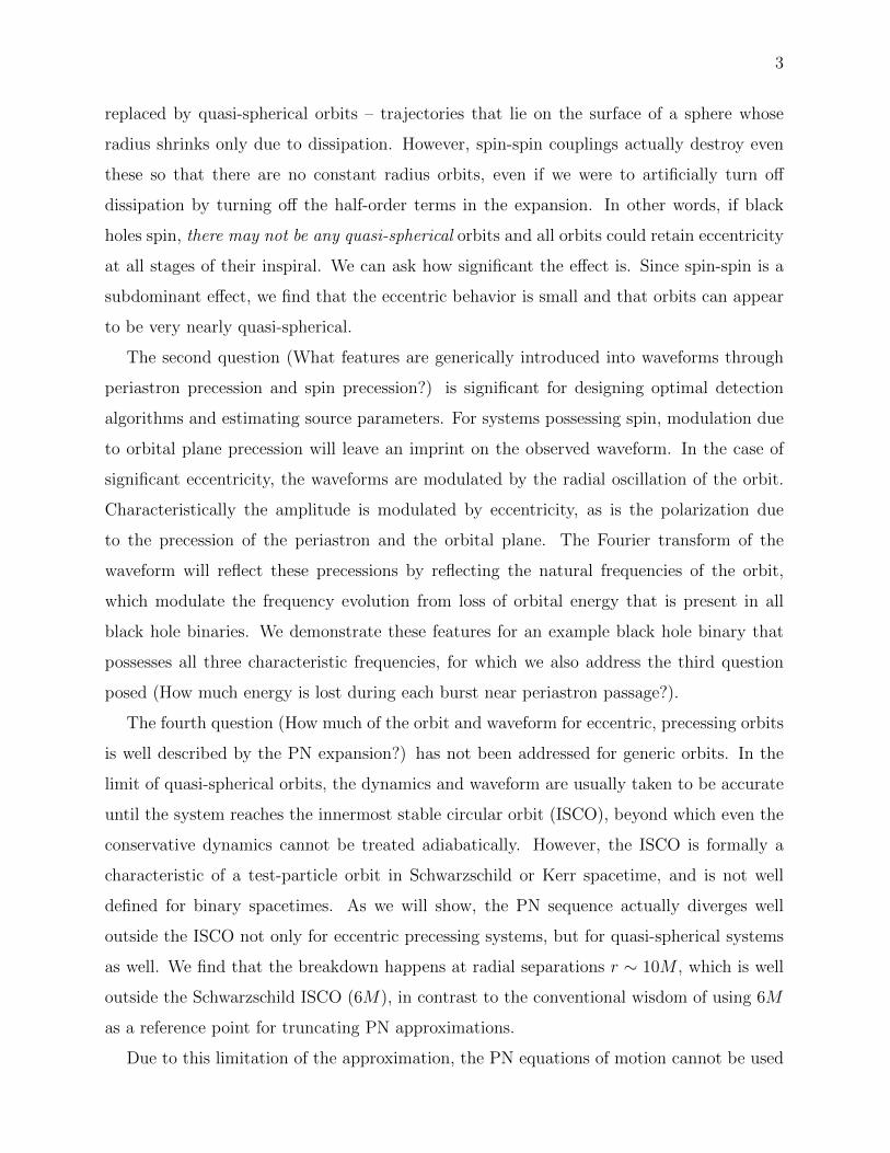
FIG. 5: Strain for an optimally-oriented binary with M = 20M� at D = 100 Mpc. From left to

right, we show three periastron passes occurring ∼ 3000 sec prior to waveform truncation (shifted

in time by ∼ 34 sec each to increase their overlap), the final 10 seconds, and the final ∼ 3000

seconds of the waveform.

FIG. 6: ∆H is the absolute value of the difference between the energy as a function of time and

the initial energy. Left: The burst of energy emitted during one periastron passage (rp ∼ 38). As

the pair separate to apastron ra ∼ 3000, negligible energy is lost as confirmed by the flatness of

∆H. Each burst is small although a few percent of the total energy in µ is lost cumulatively prior

to cutoff as shown on the right.

B. Eccentric, unequal masses

We next consider an eccentric pair with mass ratio m1/m2 = 1/4. Each black hole is

spinning maximally. Both spins are misaligned with the orbital plane with θ1 ≡ arccos(L ·S1) = 45o and θ2 ≡ arccos(L · S2) = 45o. The pair begins at large separation, ri = 3000,

and with angular momentum L = 0.003ri. The first periastron passage is rp ∼ 38, so the

12

100

101

102

103

10−24

10−23

10−22

10−21

freq [Hz]

hc,S

1/2

n

−3000s < tc − t < 0s

−10s < tc − t < 0s

1st 3 periastra

LIGO ASDAdv. LIGO ASD

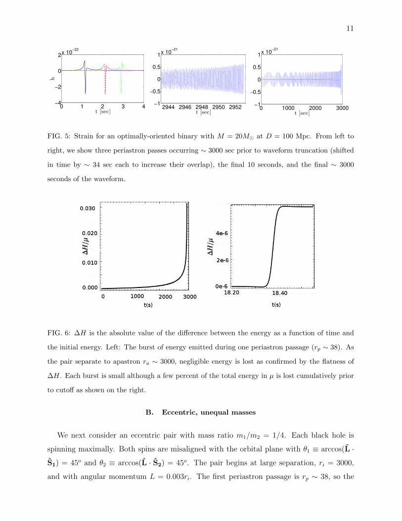
FIG. 7: Left: The three natural frequencies versus time for the eccentric configuration. There are

two lines for fΦ, one marking the value at periastron (top line) and the other marking the value

at apastron (bottom line). Same for fΨ. All frequencies are plotted in units of (20M�/M)Hz and

all times in units of (M/20M�)sec. Right: The characteristic strain, hc, of an optimally-oriented

realization of the eccentric configuration, at a distance of 100 Mpc, again scaled for M = 20M�.

We show hc for each of the first three periastron passages, the final 100 sec, and the entire 3000

sec intervals shown in Fig. 5. We show the LIGO and Advanced LIGO sensitivity curves [24] for

comparison.

pair is set on a highly eccentric orbit. The eccentricity can be defined loosely as

e =ra − rpra + rp

(11)

where ra is the apastron and rp is the periastron. The eccentricity begins large, e = 0.97,

and drifts down to e = 0.17 by the time the simulation is ended. Cutoff is set when the

3.5PN terms become larger than the 2.5PN terms, or, equivalently, when E > 0, as we

discuss in the next section. At cutoff, the periastron is rp ∼ 12 and the apastron is ra ∼ 17.

Our choice of the initial pericenter distance and eccentricity is consistent with the capture

formation scenario of stellar mass black hole binaries in globular clusters [14]. Therefore,

an initially highly eccentric orbit could retain significant eccentricity by the time it evolves

into the bandwidth of a terrestrial network of gravitational-wave interferometers.

The pair experiences both periastron precession and orbital-plane precession during a

total of 1384 orbits, some of which are shown in Fig. 4. On the left of Fig. 4 the first

1150s of the orbit are shown and on the right the final 5s of the orbit is shown before the

13

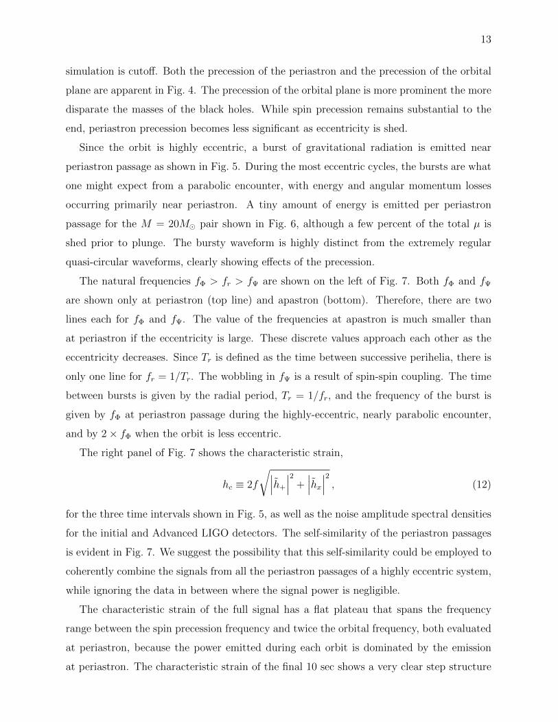
simulation is cutoff. Both the precession of the periastron and the precession of the orbital

plane are apparent in Fig. 4. The precession of the orbital plane is more prominent the more

disparate the masses of the black holes. While spin precession remains substantial to the

end, periastron precession becomes less significant as eccentricity is shed.

Since the orbit is highly eccentric, a burst of gravitational radiation is emitted near

periastron passage as shown in Fig. 5. During the most eccentric cycles, the bursts are what

one might expect from a parabolic encounter, with energy and angular momentum losses

occurring primarily near periastron. A tiny amount of energy is emitted per periastron

passage for the M = 20M� pair shown in Fig. 6, although a few percent of the total µ is

shed prior to plunge. The bursty waveform is highly distinct from the extremely regular

quasi-circular waveforms, clearly showing effects of the precession.

The natural frequencies fΦ > fr > fΨ are shown on the left of Fig. 7. Both fΦ and fΨ

are shown only at periastron (top line) and apastron (bottom). Therefore, there are two

lines each for fΦ and fΨ. The value of the frequencies at apastron is much smaller than

at periastron if the eccentricity is large. These discrete values approach each other as the

eccentricity decreases. Since Tr is defined as the time between successive perihelia, there is

only one line for fr = 1/Tr. The wobbling in fΨ is a result of spin-spin coupling. The time

between bursts is given by the radial period, Tr = 1/fr, and the frequency of the burst is

given by fΦ at periastron passage during the highly-eccentric, nearly parabolic encounter,

and by 2× fΦ when the orbit is less eccentric.

The right panel of Fig. 7 shows the characteristic strain,

hc ≡ 2f

√∣∣∣h+

∣∣∣2 +∣∣∣hx∣∣∣2 , (12)

for the three time intervals shown in Fig. 5, as well as the noise amplitude spectral densities

for the initial and Advanced LIGO detectors. The self-similarity of the periastron passages

is evident in Fig. 7. We suggest the possibility that this self-similarity could be employed to

coherently combine the signals from all the periastron passages of a highly eccentric system,

while ignoring the data in between where the signal power is negligible.

The characteristic strain of the full signal has a flat plateau that spans the frequency

range between the spin precession frequency and twice the orbital frequency, both evaluated

at periastron, because the power emitted during each orbit is dominated by the emission

at periastron. The characteristic strain of the final 10 sec shows a very clear step structure

14

due to the large set of harmonics excited by the eccentric motion. We emphasize that

these harmonics are not the instantaneous harmonics from PN corrections, as we have not

included higher-harmonic PN corrections. Rather, the harmonics apparent in Fig. 7 are the

result of the large change in instantaneous frequency over the course of each orbit, which

is represented in Fourier space as higher (and lower) harmonics of twice the mean orbital

frequency. Again, the highest plateau spans between the spin precession frequency and twice

the orbital frequency, with the step at lower frequency occurring at the orbital frequency,

and the many steps at higher frequencies occurring at larger integer multiples of the orbital

frequency.

IV. DOMAIN OF VALIDITY FOR THE PN APPROXIMATION

The PN equations of motion are a series expansion of corrections to the acceleration

of the binary components, with whole order terms representing conservative, relativistic

corrections, and half order terms representing dissipative corrections. As such, the expansion

should not be trusted when higher-order terms become comparable in magnitude to lower-

order terms. In this regard, it is noteworthy that the sign of the acceleration term along

the radial direction is negative at 2.5PN order, as expected, and the black holes are drawn

together. However, the sign of the acceleration term along the radial direction is positive

at 3.5PN order. In other words, the 2.5PN terms over estimate the effects of dissipation,

and the 3.5PN terms temper this over estimate. A consequence of the breakdown of the

PN expansion in the strong-field regime is that the 3.5PN term comes to dominate, and

spuriously drives the system to a larger separation, with the 3.5PN term acting as a source,

rather than a sink, of energy and angular momentum. Implementation of the equations of

motion must be cut off before this happens, as the PN approximation has already broken

down at this point. We find that the break down tends to happen at radial separations

r ∼ 10 in units of the total mass, which is well outside the Schwarzschild ISCO at 6M that

is frequently used to represent the boundary for a valid application of the PN expansion.

All of the simulations in the preceding section are therefore cut off when the PN approx-

imation begins to break down. Specifically, we use the criterion that the simulation ends

when the rate of energy loss drops below some threshold, indicating that the 3.5PN correc-

tion is approaching the same magnitude as the 2.5PN term. In Fig. 8, we show the relative

15

magnitude of different PN-order contributions to the (Lagrangian) equations of motion. We

focus on two cases: an equal mass, nonspinning binary undergoing quasi-circular inspiral,

and our eccentric configuration from the previous section. The first case is likely to be a

best-case scenario for the convergence of the PN expansion, while the latter is likely to over

extend the PN expansion at larger orbital separations. We find that, for the conservative

terms, the ratio of adjacent whole-order terms in the PN sequence remains less than unity

over the full domain, and indeed would remain so down to the aforementioned ISCO radius.

However, the ratio of the two half order, dissipative terms exceeds unity at r = 9.125M in

the circular case, and at r = 10M in the eccentric spinning case. Since the approximation is

certainly unreliable prior to the point where this ratio equals unity, we suggest that generally

the PN expansion cannot be reliably applied for separations r <∼ 10M for any configuration

when dissipation is included.

Another possibility is that the optimal asymptotic expansion for the PN sequence should

be truncated at 3 PN order. This is an interesting possibility, and would in fact be consistent

with findings in the Schwarzschild test-mass limit, where much higher PN terms are available

to demonstrate this behavior [25]. Since for comparable masses we lack higher PN-order

terms, it is not yet possible to distinguish between these two possibilities.

V. SUMMARY

We have compiled the equations of motion of Refs. [8–11], and have transformed them into

Hamiltonian coordinates for ready-to-use equations governing general black hole binaries.

With these in hand, we can study any black hole pair, including the effects of spin, eccen-

tricity, and their accompanying precessions. Given this flexible system, we have answered

four basic questions:

• ‘Do spinning pairs tend to quasi-spherical orbits?’

We find that the deviation for a constant radius orbit due to spin-spin coupling is

insignificantly small, so quasi-spherical orbits are accessible. Consequently spinning

pairs do tend to quasi-spherical orbits.

• ‘What features are generically introduced into waveforms through periastron and spin

precession?’

16

6 8 10 12 14 16 18 20 22 240

0.2

0.4

0.6

0.8

1

r [M]

|~an+1|/

|~an|

1 PN/0 PN, circular

2 PN/1 PN, circular

3 PN/2 PN, circular

3.5 PN/2.5 PN, circular

1 PN/0 PN, prec/ecc

2 PN/1 PN, prec/ecc

3 PN/2 PN, prec/ecc

3.5 PN/2.5 PN, prec/ecc

FIG. 8: The ratio of different PN-order contributions to the Lagrangian equations of motion for

a circular, equal mass, nonspinning inspiral, and separately for our eccentric configuration. Even

for the circular case, the 3.5 PN dissipation term grows larger than the 2.5 PN dissipation term

for radial separations less than ∼ 9M . Less ideal cases, not surprisingly, appear to make the PN

sequence diverge at larger radii.

As was shown in [19], an orbit can be projected onto an orbital plane. The char-

acteristic frequency within the plane supplants the usual coordinate frequency. The

frequency of plane precession and the frequency of radial oscillations provide the other

crucial frequencies for analysis. We have shown that these three frequencies leave a

characteristic imprint on the waveforms in Fourier space. Furthermore, the frequency

of bursts for highly eccentric orbits and the quiescent time between bursts directly

reflect these natural harmonics and could encourage novel data analysis techniques.

• ‘How much energy is lost during each burst near periastron passage?’

Given the caveat that most of the energy will be lost during the merger, which is

beyond the reach of the PN approximation, for highly eccentric binaries we show that

less than 10−3 of a percent of the reduced mass µ is lost to gravitational radiation per

periastron passage. Some pairs may execute thousands of orbits before plunge so that

a few percent of µ is lost during inspiral up to r ∼ 10M .

• ‘How much of the orbit and waveform for eccentric, precessing orbits is well described

by the PN expansion?’

17

The PN expansion has broken down whenever higher-order corrections become larger

than lower-order corrections. We find this tends to happen at r ∼ 10M , which is well

outside of the Schwarzschild ISCO that is often used to demarcate the breaking point

of the PN approximation. Possibly the PN sequence diverges inside ∼ 10M , or it may

be that the optimal PN expansion inside this radius should be truncated at no higher

than 3 PN order.

The orbits shown give a sample of the complete range that can be probed in detail for

generic, spinning, precessing, eccentric black hole pairs. We intend to build a data set

of black hole pairs to be made available as a testing ground for developing data analysis

techniques.

*Acknowledgements*

We are grateful to Clifford Will for his invaluable insights and to Jameson Rollins for

important conversations. This work was supported by an NSF grant AST-0908365. JL

gratefully acknowledges support of a KITP Scholarship, under Grant no. NSF PHY05-

51164.

Appendix A: Lagrangian Equations of Motion

In this section we compile the equations of motion including spin couplings and dissipation

as computed by Will and collaborators over the series of papers [8–11]. We measure length

in units of total mass M = m1 + m2 and write the equations in terms of the dimensionless

center-of-mass coordinate x and center-of-mass velocity v. The reduced mass is defined as

η = µ/M = m1m2/M2. The Lagrangian equations of motion in x,v with spins added are

(with x =√

x · x the harmonic radial coordinate and x = n · v) as compiled from Refs.

[8, 9, 21, 22]

x = v (A1)

x = aN + a1PN + a2PN + a2.5PN + a3PN + a3.5PN + aPN−SO + a3.5PN−SO + aPN−SS + a3.5PN−SS

18

and

aN = − n

x2

a1PN = − n

x2

{(1 + 3η)v2 − 2(2 + η)

1

x− 3

2ηx2

}+

v

x22(2− η)x

a2PN = − n

x2

{3

4(12 + 29η)

1

x2+ η(3− 4η)(v2)2 +

15

8η(1− 3η)x4

− 3

2η(3− 4η)v2x2 − 1

2η(13− 4η)

v2

x− (2 + 25η + 2η2)

x2

x

}+

v

x2

{x

2

[η(15 + 4η)v2 − (4 + 41η + 8η2)

1

x− 3η(3 + 2η)x2

]}.

a2.5PN =n

x2

{8

5η

(1

x

)x

(17

3

1

x+ 3v2

)}− v

x2

{8

5η

(1

x

)(3

1

x+ v2

)}.

a3PN = − n

x2

{−[16 +

(1399

12− 41

16π2

)η +

71

2η2

](1

x

)3

− η[

20827

840+

123

64π2 − η2

](1

x

)2

v2

+

[1 +

(22717

168+

615

64π2

)η +

11

8η2 − 7η3

](1

x

)2

x2

+η

4

(11− 49η + 52η2

)v6 − 35

16η(1− 5η + 5η2)x6 +

η

4

(75 + 32η − 40η2

)(1

x

)v4

+η

2

(158− 69η − 60η2

)(1

x

)x4 − η

(121− 16η − 20η2

)(1

x

)v2x2

−3

8η(20− 79η + 60η2

)v4x2 +

15

8η(4− 18η + 17η2

)v2x4

}+

v

x2x

{[4 +

(5849

840+

123

32π2

)η − 25η2 − 8η3

](1

x

)2

+η

8

(65− 152η − 48η2

)v4

+15

8η(3− 8η − 2η2

)x4 + η

(15 + 27η + 10η2

)(1

x

)v2

−η6

(329 + 177η + 108η2

)(1

x

)x2 − 3

4η(16− 37η − 16η2

)v2x2

}

19

a3.5PN = − n

x2

{8

5η

(1

x

)x

[23

14(43 + 14η)

(1

x

)2

+3

28(61 + 70η)v4 + 70x4

+1

42(519− 1267η)

(1

x

)v2 +

1

4(147 + 188η)

(1

x

)x2 − 15

4(19 + 2η) v2x2

]}+

v

x2

{8

5η

(1

x

)[1

42(1325 + 546η)

(1

x

)2

+1

28(313 + 42η) v4 + 75x4

− 1

42(205 + 777η)

(1

x

)v2 +

1

12(205 + 424η)

(1

x

)x2 − 3

4(113 + 2η) v2x2

]}.

(A2)

using the 3PN and half-order terms from Ref. [9].

We also absorb an M2 into the spins so the physical spin in the Lagrangian system is

denoted Si = a i(m2i /M

2) where ai is the dimensionless amplitude 0 ≤ |ai| ≤ 1. As we will

see in §B, this is a different normalization from that for spins in the Hamiltonian case, where

spins are expressed as Si = ai(m2i /µM). The spin-orbit contribution to the acceleration is

aPN−SO =1

x3

{6n

xLN · (S + ξ)− v × (4S + 3ξ) + 3xn× (2S + ξ)

}with ξ ≡ (m2/m1)S1+(m1/m2)S2 [10]. It is customary to define a reduced Newtonian orbital

angular momentum,

LN = x× v . (A3)

The spin-orbit dissipation term with the covariant spin supplementary condition is (see the

appendix of Ref. [10]),

a3.5PN−SO = − η

5x4

{xn

x

[(120v2 + 280x2 + 453

1

x

)LN · S

+

(120v2 + 280x2 + 458

1

x

)LN · ξ

]+

v

x

[(87v2 − 675x2 − 901

3

1

x

)LN · S + 4

(18v2 − 150x2 − 66

1

x

)LN · ξ

]−2

3xv × S

(48v2 + 15x2 + 364

1

x

)+

1

3xv × ξ

(291v2 − 705x2 − 772

1

x

)+

1

2n× S

(31v4 − 260v2x2 + 245x4 − 689

3v2 1

x+ 537x2 1

x+

4

3

1

x2

)+

1

2n× ξ

(115v4 − 1130v2x2 + 1295x4 − 869

3v2 1

x+ 849x2 1

x+

44

3

1

x2

)}.

(A4)

20

And the spin-spin contribution is

aPN−SS = − 3

µx4[n(S1 · S2) + S1(n · S2) + S2(n · S1)− 5n(n · S1)(n · S2)] (A5)

See also [22]. The 3.5PN order effects of Spin-Spin coupling from Ref. [11] are

a3.5PN−SS =1

x5

{n

[(287x2 − 99v2 +

541

5

1

x

)x(S1 · S2)−

(2646x2 − 714v2 +

1961

5

1

x

)x(n · S1)(n · S2)

+

(1029x2 − 123v2 +

629

10

1

x

)((n · S1)(v · S2) + (n · S2)(v · S1))− 336x(v · S1)(v · S2)

]+v

[(171

5v2 − 195x2 − 67

1

x

)(S1 · S2)−

(174v2 − 1386x2 − 1038

5

1

x

)(n · S1)(n · S2)

−438x ((n · S1)(v · S2) + (n · S2)(v · S1)) + 96(v · S1)(v · S2)]

+

(27

10v2 − 75

2x2 − 509

30

1

x

)((v · S2)S1 + (v · S1)S2)

+

(15

2v2 +

77

2x2 +

199

10

1

x

)x ((n · S2)S1 + (n · S1)S2)

}. (A6)

The spin supplementary condition has no effect on spin-spin terms up to this order. We have

not yet included the quadrupole-monopole contribution. Finally, the spins precess according

to

S1 = η(x× v)× S1

x3

(2 +

3m2

2m1

)S2 = η

(x× v)× S2

x3

(2 +

3m1

2m2

). (A7)

We could also add to the right hand side of (A7) the spin-spin terms:

(S1)PN−SS = − 1

x3(S2 − 3(n · S2)n)× S1 (A8)

[22] and

(S1)3.5PN−SS =η

x5

(2

3(v · S2) + 30x(n · S2)

)(n× S1) (A9)

[11]. Equations (A1)-(A9) constitute the Lagrangian dynamical system. These equations

are complete through 3.5PN order except for the spin contributions, for which additional

terms have been calculated (see for instance Ref. [26, 27]). Since spin effects are already

small at the order we include here, we have not pursued inclusion of the higher- order spin

terms.

Notice these spins are not reduced by µ and a definition of dimensionful angular momen-

tum will have a µ in it: J = µLN + ...+ S1 + S2.

Next we re-express the dissipation terms in the language of the Hamiltonian system.

21

Appendix B: Hamiltonian Equations of Motion: Including Dissipation

The Hamiltonian PN-formulation is by definition conservative and therefore does not

incorporate dissipation [1–6]. We can, however, take the half-order acceleration terms from

the Lagrangian coordinates and simply convert them to the coordinates appropriate for the

Hamiltonian. We begin by first laying out the whole-order terms in the usual Hamiltonian

system [1–6].

In a Hamiltonian formulation, the equations of motion are derived from

r =∂H

∂p, p = −∂H

∂r. (B1)

As is standard convention, we work in dimensionless coordinates: the dimensionless coor-

dinate vector, r, is measured in units of total mass, M = m1 + m2, for a pair with black

hole masses m1 and m2. The canonical momentum, p, is measured in units of the reduced

mass, µ = m1m2/M . The dimensionless combination η = µ/M will again prove useful. We

write vector quantities in bold. The coordinate r is to be understood as the magnitude

r =√

r · r. Unit vectors such as n = r/r will additionally carry a hat. Finally, we have

used the dimensionless reduced Hamiltonian H = H/µ in Eqs. (B1), where H is the physical

Hamiltonian, to 3PN order plus spin-orbit terms [1–6]. H can be expanded as

H = HN +H1PN +H2PN +H3PN +HSO +HSS , (B2)

where

22

HN =p2

2− 1

r(B3)

H1PN =1

8(3η − 1)

(p2)2 − 1

2

[(3 + η) p2 + η(n · p)2

] 1

r+

1

2r2

H2PN =1

16

(1− 5η + 5η2

) (p2)3

+1

8

[(5− 20η − 3η2

) (p2)2

−2η2(n · p)2p2 − 3η2(n · p)4] 1

r

+1

2

[(5 + 8η) p2 + 3η(n · p)2

] 1

r2− 1

4(1 + 3η)

1

r3

H3PN =1

128

(−5 + 35η − 70η2 + 35η3

) (p2)4

+1

16

[(−7 + 42η − 53η2 − 5η3

) (p2)3

+(2− 3η)η2(n · p)2(p2)2 + 3(1− η)η2(n · p)4p2 − 5η3(n · p)6] 1

r

+

[1

16(−27 + 136η + 109η2)(p2)2 +

1

16(17 + 30η)η(n · p)2p2 +

1

12(5 + 43η)η(n · p)4

]1

r2

+

{1

192

[−600 +

(3π2 − 1340

)η − 552η2

]p2 − 1

64

(340 + 3π2 + 112η

)η(n · p)2

}1

r3

+1

96

[12 +

(872− 63π2

)η] 1

r4,

HSO =L · Seff

r3. (B4)

and adding spin-spin,

HSS =µ

r3[ 3(S1 · n)(S2 · n)− S1 · S2+ (B5)

m2

2m1

(3(S1 · n)(S1 · n)− S1 · S1) +m1

2m2

(3(S2 · n)(S2 · n)− S2 · S2)

].

Notice that HSS includes S21 and S2

2 terms. For two spinning black holes Seff is2

Seff = δ1S1 + δ2S2 (B6)

where the dimensionless reduced spins are defined as

S1 = a1(m21/µM) , S2 = a2(m2

2/µM) . (B7)

and

δ1 ≡(

2 +3m2

2m1

)η , δ2 ≡

(2 +

3m1

2m2

)η . (B8)

2 The definitions for Seff can vary in the literature up to an overall constant although the reduced HSO

must be the same for all prescriptions.

23

The dimensionless spin amplitudes are confined to the range 0 ≤ a1,2 ≤ 1. The spins precess

according todS1

dt=∂H

∂S1

× S1 (B9)

or

S1 = δ1L× S1

r3+µ

r3

[3n

((S2 +

m2

m1

S1

)· n)− S2

]× S1

S2 = δ2L× S2

r3+µ

r3

[3n

((S1 +

m1

m2

S2

)· n)− S1

]× S2 . (B10)

The orbital angular momentum precesses according to

L = r× p + r× p (B11)

= −L× Seff

r3− µ

r3

[3n

((S2 +

m2

m1

S1

)· n)]× S1 −

µ

r3

[3n

((S1 +

m1

m2

S2

)· n)]× S2

Adding these together, it follows that the total angular momentum J = L + S1 + S2 is

conserved in the absence of dissipation so that the orbital angular momentum precesses

according to

L = −S1 − S2 . (B12)

Now, we are ready to convert the radiation-reaction terms of appendix A into Hamiltonian

variables. To do so, we need to relate the Hamiltonian variables (r,p) to the Lagrangian

variables (x,v). To convert the 2.5PN radiation-reaction term, we only need the 1PN-order

coordinate conversion to catch all corrections up to 3.5PN. To convert the 3.5PN radiation-

reaction term, we only need the zeroth-order PN coordinate conversion. It has been shown

that to 1PN order [? ]

r = x , (B13)

so that

r = x = v . (B14)

What we really want are the harmonic variables of the Lagrangian formulation (x,v) in

terms of canonical Hamiltonian variables (r,p) to 1PN order. We have x(r,p) above. To

find v(r,p), we use Hamilton’s equations:

r = Ap +Bn +Seff × r

r3

p = Cp +Dn +Seff × p

r3+

3n

rHSO −

∂HSS

∂r, (B15)

24

where A,B,C,D are

A ≡ 2∂HPN

∂p2

∣∣∣∣r,(n·p)

(B16)

B ≡ ∂HPN

∂(n · p)

∣∣∣∣r,p

C ≡ −1

r

∂HPN

∂(n · p)

∣∣∣∣r,p

= −Br

D ≡ − ∂HPN

∂r

∣∣∣∣p,(n·p)

+∂HPN

∂(n · p)

∣∣∣∣r,p

(n · p)

r

= − ∂HPN

∂r

∣∣∣∣p,(n·p)

− (n · p)C . (B17)

and HPN = HN +H1PN +H2PN +H3PN . Explicit expressions can be found in [20], but we

will only need A and B here to 1PN order to calculate v(r,p) to 1PN order and ultimately

find the radiative contributions to the accelerations. Taking the appropriate derivatives of

the Hamiltonian to 1PN order, we have

A≤1PN = 1 +1

2(3η − 1) p2 − (3 + η)

1

r

B≤1PN = −η (n · p)1

r. (B18)

This gives us v in terms of (r,p):

v =

(1 +

1

2(3η − 1) p2 − (3 + η)

1

r

)p− η (n · p)

1

rn +

Seff × r

r3(B19)

and

v2 =

(1 + (3η − 1) p2 − 2 (3 + η)

1

r

)p2 − 2η (n · p)2 1

r+ 2

p · (Seff × r)

r3

=

(1 + (3η − 1) p2 − 2 (3 + η)

1

r

)p2 − 2η (n · p)2 1

r+ 2

Seff · Lr3

. (B20)

We can now re-write a2.5PN of Eq. (A2) in terms of ADM variables as

a2.5PN→ADM =8

5

(ηr

)× { (B21)

n

r2

[r

(17

3r+ 3p2 + 3 (3η − 1) p4 − 6 (3 + η)

p2

r− 6η

(n · p)2

r+ 6

Seff · Lr3

)+ η (n · p)

(3

r2+

p2

r

)]

− p

r2

[3

r+ p2 +

3

2(3η − 1) p4 +

1

2(3η − 21)

p2

r− 3(3 + η)

1

r2− 2η

(n · p)2

r+ 2

Seff · Lr3

]

−Seff × r

r5

(3

r+ p2

)}.

25

We can also replace r with

r = n · v =

(1 +

1

2(3η − 1) p2 − (3 + η)

1

r

)n · p− η (n · p)

1

r

=

(1 +

1

2(3η − 1) p2 − (3 + 2η)

1

r

)n · p (B22)

To get

a2.5PN→ADM =8

5

(ηr

)× { (B23)

n

r2

[(n · p)

(17

3r+ 3p2 +

9

2(3η − 1) p4 − 1

2

(5η +

179

3

)p2

r− 1

3(25η + 51)

1

r2− 6η

(n · p)2

r+ 6

Seff · Lr3

)]

− p

r2

[3

r+ p2 +

3

2(3η − 1) p4 +

1

2(3η − 21)

p2

r− 3(3 + η)

1

r2− 2η

(n · p)2

r+ 2

Seff · Lr3

]

−Seff × r

r5

(3

r+ p2

)}.

Since we used a coordinate change valid to 1PN order, Eqs. (B23 and B21) includes 3.5PN

corrections as well as 2.5PN corrections.

To rewrite a3.5PN→ADM we simply take the harmonic expressions and replace x = r and

v = p, noting that LN = L to lowest order, and that the spins of Refs. [10, 11] are η times

those of this section: Si = ηSi.

Now, to incorporate the effects of dissipation, we can add the appropriately converted

accelerations. Taking the time derivative of Eq. (B19) and rearranging to solve for p, there

are additional corrections of the form

p = v

(1− 1

2(3η − 1) p2 + (3 + η)

1

r

)− (3η − 1)(p · p)p + η(n · p)

1

rn + ... (B24)

We then use v = a2.5PN→ADM + a3.5PN→ADM and drop all terms higher than 3.5PN to get

p = ...+ a2.5PN→ADM

(1− 1

2(3η − 1) p2 + (3 + η)

1

r

)+ a3.5PN→ADM+

− (3η − 1)(p · a2.5PN)p + η(n · a2.5PN)1

rn (B25)

where we have only isolated the relevant half-order terms so “...” represents all the whole-

order PN terms. Here a2.5PN→ADM is defined in Eq. (B23), and we replace p where it

occurs on the right hand side of (B25) with a2.5PN evaluated at x = r, v = p. The term

a3.5PN→ADM is also evaluated at x = r, v = p, and, again, the spins of the previous section

26

are related to these spins through Si = ηSi, yielding

a2.5PN→ADM ≡ a2.5PN→ADM

(1− 1

2(3η − 1) p2 + (3 + η)

1

r

)=

8

5

(ηr

)×{

n

r2

[n · p

(17

3r+ 3p2 + 3 (3η − 1) p4 − 2 (4η + 9)

p2

r− 8

3

η

r2− 6η

(n · p)2

r+ 6

Seff · Lr3

)]

− p

r2

[3

r+ p2 + (3η − 1) p4 − 2 (η + 3)

p2

r− 2η

(n · p)2

r+ 2

Seff · Lr3

]

−Seff × r

r5

(3

r+ p2

)}, (B26)

Finally, our equations of motion become

r = Ap +Bn +Seff × r

r3

p = Cp +Dn +Seff × p

r3+

3n

rHSO −

∂HSS

∂r+ a2.5PN→ADM + a3.5PN→ADM

+ η(n · a2.5PN)1

rn− (3η − 1)(p · a2.5PN)p (B27)

We can regroup the accelerations to 2.5 order and 3.5 orders in ADM variables:

r = Ap +Bn +Seff × r

r3

p = Cp +Dn +Seff × p

r3+

3n

rHSO −

∂HSS

∂r+ a

(2.5)ADM + a

(3.5)ADM (B28)

with

a(2.5)ADM =

8

5

(ηr

)×{

n

r2

[n · p

(17

3r+ 3p2

)]− p

r2

[3

r+ p2

]}, (B29)

and using

η(n · a2.5PN)1

rn =

(8η

5r

)n

r2(n · p)

(8η

3r2+ 2η

p2

r

)−(3η − 1)(p · a2.5PN)p =

(8η

5r

)(− p

r2

)(3η − 1)

[(n · p)2

(17

3r+ 3p2

)− p2

(3

r+ p2

)](B30)

and the 3.5PN piece in a2.5PN→ADM

...8

5

(ηr

)×{

n

r2

[n · p

(3 (3η − 1) p4 − 2 (4η + 9)

p2

r− 8

3

η

r2− 6η

(n · p)2

r+ 6

Seff · Lr3

)]

− p

r2

[(3η − 1) p4 − 2 (η + 3)

p2

r− 2η

(n · p)2

r+ 2

Seff · Lr3

]

−Seff × r

r5

(3

r+ p2

)}, (B31)

27

and adding all of these 3.5PN pieces to

a3.5PN→ADM =8

5η

(1

r

)× {

− n

r2(n · p)

[23

14(43 + 14η)

(1

r

)2

+3

28(61 + 70η)p4 + 70(n · p)4

+1

42(519− 1267η)

(1

r

)p2 +

1

4(147 + 188η)

(1

r

)(n · p)2 − 15

4(19 + 2η) p2(n · p)2

]+

p

r2

[1

42(1325 + 546η)

(1

r

)2

+1

28(313 + 42η) p4 + 75(n · p)4

− 1

42(205 + 777η)

(1

r

)p2 +

1

12(205 + 424η)

(1

r

)r2 − 3

4(113 + 2η) p2(n · p)2

]}.

gives

a(3.5)ADM =

8

5η

(1

r

)× {

− n

r2(n · p)

[1

14(989 + 322η)

(1

r

)2

+3

28(89− 14η) p4 + 70(n · p)4

+1

42(1275− 1015η)

(1

r

)p2 +

1

4(147 + 212η)

(1

r

)(n · p)2 − 15

4(19 + 2η) p2(n · p)2 − 6

Seff · Lr3

]+

p

r2

[1

42(1325 + 546η)

(1

r

)2

+1

28(313 + 42η) p4 + 75(n · p)4 +

1

12(273 + 244η)

(n · p)2

r

− 1

42(79 + 315η)

(1

r

)p2 − 1

4(327 + 42η) p2(n · p)2 − 2

Seff · Lr3

]−Seff × r

r5

(3

r+ p2

)}.

Then there are the spin pieces:

a(3.5PN−SO)ADM = − η2

5r4

{(n · p)n

r

[(120p2 + 280(n · p)2 + 453

1

r

)L · S

+

(120p2 + 280(n · p)2 + 458

1

r

)L · ξADM

]+

p

r

[(87p2 − 675(n · p)2 − 901

3

1

r

)L · S + 4

(18p2 − 150(n · p)2 − 66

1

r

)L · ξADM

]−2

3(n · p)p× S

(48p2 + 15(n · p)2 + 364

1

r

)+

1

3(n · p)p× ξADM

(291p2 − 705(n · p)2 − 772

1

r

)+

1

2n× S

(31p4 − 260p2(n · p)2 + 245(n · p)4 − 689

3p2 1

r+ 537(n · p)2 1

r+

4

3

1

r2

)+

1

2n× ξADM

(115p4 − 1130p2(n · p)2 + 1295(n · p)4 − 869

3p2 1

r+ 849(n · p)2 1

r+

44

3

1

r2

)}.

(B32)

28

and

a(3.5PN−SS)ADM =

η2

r5

{n

[(287(n · p)2 − 99p2 +

541

5

1

r

)(n · p)(S1 · S2)

−(

2646(n · p)2 − 714p2 +1961

5

1

r

)(n · p)(n · S1)(n · S2)

+

(1029(n · p)2 − 123p2 +

629

10

1

r

)((n · S1)(p · S2) + (n · S2)(p · S1))− 336(n · p)(p · S1)(p · S2)

]+p

[(171

5p2 − 195(n · p)2 − 67

1

r

)(S1 · S2)−

(174p2 − 1386(n · p)2 − 1038

5

1

r

)(n · S1)(n · S2)

−438(n · p) ((n · S1)(p · S2) + (n · S2)(p · S1)) + 96(p · S1)(p · S2)]

+

(27

10p2 − 75

2(n · p)2 − 509

30

1

r

)((p · S2)S1 + (p · S1)S2)

+

(15

2p2 +

77

2(n · p)2 +

199

10

1

r

)(n · p) ((n · S2)S1 + (n · S1)S2)

}. (B33)

with ξADM ≡ (m2/m1)S1 + (m1/m2)S2.

Given the equations of this section and the previous section, the equations of motion can

be evolved in either set of variables.

In §II we introduced the (r,Φ,Ψ) coordinates. The equations of motion (B28) can be

projected onto this basis as was done in Refs. [19, 20].

[1] G. Schaefer, Annals Phys. 161, 81 (1985).

[2] T. Damour and N. Deruelle, C. R. Acad. Sci. Paris 293, 537 (1981).

[3] T. Damour and G. Schaefer, Nuovo Cim. B101, 127 (1988).

[4] P. Jaranowski and G. Schaefer, erratum-ibib.d 63, 029902 (2001).

[5] T. Damour, P. Jaranowski, and G. Schafer, Phys. Lett. B 513, 147 (2001).

[6] T. Damour, P. Jaranowski, and G. Schaefer, Phys. Rev. D 62, 084011 (2000).

[7] B. R. Iyer and C. M. Will, Phys. Rev. D 52, 6882 (1995).

[8] T. Mora and C. M. Will, Phys. Rev. D69, 104021 (2004).

[9] M. E. Pati and C. M. Will, Phys. Rev. D65, 104008 (2002).

[10] C. M. Will, Phys. Rev. D71, 084027 (2005).

[11] H. Wang and C. M. Will, Phys. Rev. D75, 064017 (2007).

[12] A. Sesana, Astrophys. J. 719, 851 (2010).

[13] L. Wen, Ap. J. 598, 419 (2003).

29

[14] R. M. O’Leary, B. Kocsis, and A. Loeb, (2008).

[15] K. Glampedakis, Class. Quant. Grav. 22, S605 (2005).

[16] J. Levin and G. Perez-Giz, Phys. Rev. D77, 103005 (2008).

[17] F. Pretorius and D. Khurana, Class. Quant. Grav. 24, S83 (2007).

[18] J. Healy, J. Levin, and D. Shoemaker, Phys. Rev. Lett. 103, 131101 (2009).

[19] J. Levin and B. Grossman, Phys. Rev. D79, 043016 (2009).

[20] R. Grossman and J. Levin, Phys. Rev. D79, 043017 (2009).

[21] L. E. Kidder, C. M. Will, and A. G. Wiseman, Phys. Rev. D 47, 4183 (1993).

[22] L. E. Kidder, Phys. Rev. D 52, 821 (1995).

[23] A. Buonanno, Y. Chen, and T. Damour, Phys. Rev. D74, 104005 (2006).

[24] 2011, private communication.

[25] N. Yunes and E. Berti, Phys. Rev. D 77, 124006 (2008).

[26] K. G. Arun, A. Buonanno, G. Faye, and E. Ochsner, Phys. Rev. D 79, 104023 (2009).

[27] G. Faye, L. Blanchet, and A. Buonanno, Phys. Rev. D 74, 104033 (2006).