Embed Size (px)
Citation preview
AD-AI1932 STANFORD UNIV CA INST FOR PLASMA RESEARCH F/6 3/2STRUCTURE OF THE HELIOSPHERIC CURRENT SHEET IN THE EARLY PORTIO -ETC U)
A PR 82 J T HOEKSEMA, J M WILCOX, P H SCHERRER N0O0iR 76-C 0207
UNCLASSIFIED U PR 924 NL
00001MFm llllIllllllllhlllllmh/I/Ihhmhhmhml
STRUCTURE OF THE HELIOSPHERIC CURRENT SHEET IN THEEARLY PORTION OF SUNSPOT CYCLE 21
.J. Todd Hoekse.na, John.M. Wilcox and Philip H. Scherrer
Institute for Plasma ResearchStanford University,
Stanford, California 94305, U.S.A.
Stanford University, Institute for Plasma ResearchSUIPR Report #924
April 1982
Submitted to: Journal of Geophysical Research
This manuscript is not yet refereed. It is mailed out whenthe paper is submitted for publication. The published ver-sion is often improved by the refereeing process. ThisSUIPR report should not be cited after the published versionhas appeared. We would appreciate receiving any commentsthat might improve the published version.
Tls docurnq'r has biRen PmT)for public xvemee and sole; its
idiutibutic-1 is ur.i mitodJ
Structure of the Heliospheric Current Sheet in theEarly Portion of Sunspot Cycle 21
J. Todd Hoeksema, John 4. Wilcox and Philip H. Scherrer
Institute for Plasma ResearchStanford University
Via CrespiStanford, California 94305
kBSTRACT
The structure of the heliospheric currentsheet on a spherical source surface of radius 2.35R. has been computed using a potential field modelduring the first year and a half after the lastsunspot minimum. The solar polar magnetic fieldthat is not fully observed in conventional magne-tograph scans was included in the computation.The computed heliospheric current sheet had ajuasi-stationary structure consisting of twonorthward and two southward maxima in latitude persolar rotation. The extent in latitude slowlyincreased from about 15 degrees near the start ofthe interval to about 45 degrees near the end ofthe interval. The magnetic field polarity (awayfrom ths Sun or toward the Sun) at the sub-terrestrial latitude on the source surface agreedwith the interplanetary magnetic field polarityobserved or inferred at Earth on 82% of the days.The interplanetary field structure observed atEarth at this time is finely tuned to the struc-turs of low-latitude fields on the source surface./
S " .a, r ! ,:
i ,A -,r " . f.'
A .... .L. zini/or,..
1. Introduction
Almost daily obserqations of the large-scale photos-
pheric magnetic field structure were started at the Stanford
Solar Observatory in May 1976 and have continued to the
present time. We compute the large-scale structure of the
magnetic field in the heliosphere using Zeeman observations
of the line-of-sight component of the photospheric magnetic
field together with a potential field model. It is also
possible to infer the structure of the heliospheric current
sheet from the maximum brightness contours in the K coronam-
eter observations at Mauna Loa Observatory (Burlaga et al.
1981 and references therein).
During the time interval considered here there was an
electric current sheet that was warped northward and south-
ward of the plane of the solar equator (Schulz, 1973).
North of the current sheet the interplanetary magnetic field
(14P) was directed away from the Sun and south of the
current sheet the IMF was directed toward the Sun
The minimum between sunspot cycles 20 and 21 occurred
in June 1975. During the 18 Carrington Solar Rotations
beginning in May 1976 the computed current sheet was quasi-
stationary, having in each solar rotation two northward
extensions and two southward extensions. This usually
I____________________ _______________...._____ ..........__________________________......... .____________
I-
-3-
produced the characteristic four sector structure in the
interplanetary magnetic field observed at Earth (Svalgaard
and Wilcox, 1975). Occasionally during a rotation one or
even both of the northward extensions of the current sheet
Omissed" the Earth resulting in a two sector or even a
*zero" sector structure being observed at Earth. Around
sunspot minimum the maximum extent in latitude of the com-
puted current sheet was about 15 degrees, while by the end
of the 18 solar rotations discussed here the maximum lati-
tude had increased to about 45 degrees. Just after the time
interval discussed here the maximum latitude of the current
sheet increasel further and the quasi-stationary structure
of the current sheet began to change, so that September 1977
seems a natural point to end the present investigation. The
strurture of the computed heliospheric current sh~et in
later portions of sunspot cycle 21 will be discussed in
future papers.
We also investigate here the effect of varying the
source surface radius, the strength of the polar field
correction and the latitude on the source surface used to
predict the IIF polarity seen at Earth.
2. Computation of the Source Surface
Schatten at al. (1969) and Altschuler and Newkirk
-4-
(1969) introduced the concept of a potential field model
with a spherical source surface surrounding and concentric
with the Sun (see also Levine and Altschuler, 1974; Poletto
et al., 1975; hltschuler et al., 1976; Adams and Pneuman,
1976; Svalgaard and Wilcox, 1978 and Riesebieter and Neu-
bauer, 1979). Outside the source surface it is assumed that
the radial flow of the solar wind carries the magnetic field
outward into the heliosphere. Between the photosphere and
the source surface it is assumed that the magnetic field can
be described in terms of a potential which satisfies
Laplace's equation. For the work described here the inner
boundary condition at the photosphere is the line-of-sight
magnetic field observed at the Stanford Solar Observatory.
The outer boundary condition is that the field is normal to
the source surface, consistent with the assumption that it
is then carried outward by the solar wind. The assumption
in the source surface calculation that there are no currents
would aot be vary good for the strong localized fields of an
active region, but for the large-scale, quasi-stationary
fields that dominate the present analysis the source surface
gives a reasonably good prediction of the polarity of the
interplanetary magnetic field observed at Earth.
A non-spherical source surface computation (Schulz et
al-., 1978; Levine et al., 1982) should give an improved
-5-
prediction of the coronal structure and of the I14 observed
at Earth, but as we shall see the spherical source surface
already does quite well at predicting the I4F polarity. The
amount of improvement to be obtained from a non-spherical
source surface using our observations will be investigated
in a later paper. The magnitude of the interplanetary mag-
netic field may be better cor7uted with non-spherical source
surface.
In most previous work the magnetic field on the source
surface has been computed only once for each Carrington
Rotation, i.e. ii steps of 360 degrees in longitude. This
forces the beginning (360 degrees) and the end (0 degrees)
of the rotation to have the same structure, even thougA they
are separated in tine by 27 days. To avoid this difficulty
we have computed the field on the source surface in steps of
10 degrees in th- 3tarting longitude, and retained only the
central interval of width 30 degrees in longitude from each
such computation. As the last step a 1:2:1 averaging of the
three calculations for each longitude strip is applied to
slightly smooth the structure. In the (rare) case of data
gaps we interpolate between the previous and the subsequent
rotation.
Stenflo (1971), Howard (1977), Svalgaard et al. (1978),
k |j .
-6
Pneuman et al. (1978), and Burlaga et al. (1981) have
pointed out that conventional solar magnetograph observa-
tions do not adequately represent the solar polar magnetic
field strength. Wilcox et al. (1980) computed the helios-
pheric current sheet configuration early in 1976 using solar
magnetograph observations from Nt. Wilson Observatory that
were not corrected for the solar polar magnetic field not
observed in daily solar magnetograph observations. As a
result the computed extent in latitude of the heliospheric
current sheet was probably too large, as was pointed out by
Burlaga et al. (1981).
In the present computation of the heliospheric current
sheet we use the magnetic field observed at a resolution of
three arc minutes in daily scans with the solar magnetograph
at the Stanford Solar Observatory, plus the solar polar
field strength determined by Svalgaard et al. (1978) for the
same solar rotations analyzed in the present paper. In the
interval analyzed by Svalgaard et al. (1978) the magnitude
of the solar polar field did not change appreciably. We
note that near the mini'uum of the sunspot cycle the solar
polar fields will have the maximum influence. As the sun-
spot cycle progresses after minimum the strength of the
solar polar field decreases while the strength of the low
latitude fields increases. Near sunspot maximum, when the
__ no
-7-
polarity of the solar polar fields is changing, most of the
heliosphere may be dominated by the lower latitude magnetic
fields.
3. The Computed Heliospheric Current Sheet
The radial magnetic field computed on a spherical
source surface at 2.35 Re for Carrington Rotation 1648
beginning 7 November 1976 is shown in Figure 1. The current
sheet is represented by the zero contour shown as a thick
solid line near the equator. The solid contours above it
represent field directed away from the Sun with relative
magnitudes 1, 5, and 10, while the dashed contours represent
field directed toward the sun with the same contour levels.
The predominance of away polarity magnetic field in most of
the northern region of the heliosphere and of toward field
in most of the southern heliosphere is apparent in Figure 1.
lhe + (away from the Sun) and - (toward the Sun) sym-
bols in Figure 1 represent daily polarities of the inter-
planetary magnetic field at Earth as observed by spacecraft
(King, 1979) or, when spacecraft observations were not
available, inferred from polar geomagnetic observations
(Svalgaard, 1973). The I4F polarities at Earth plotted in
Figure 1 have been displaced by five days corresponding to
the average transit time of solar wind from Sun to Earth
near the times when the large-scale magnetic polarity
changes (sector boundaries) . The average magnitude of this
transit time during the solar rotations studied here has
been determined by a c-ross correlation analysis to be
described later. We note that near the sector boundaries
the velocity of the solar wind is almost always near a
minionum (Wilcox and Ness, 1965), so that this transit time
is longer than the average solar wind transit time.
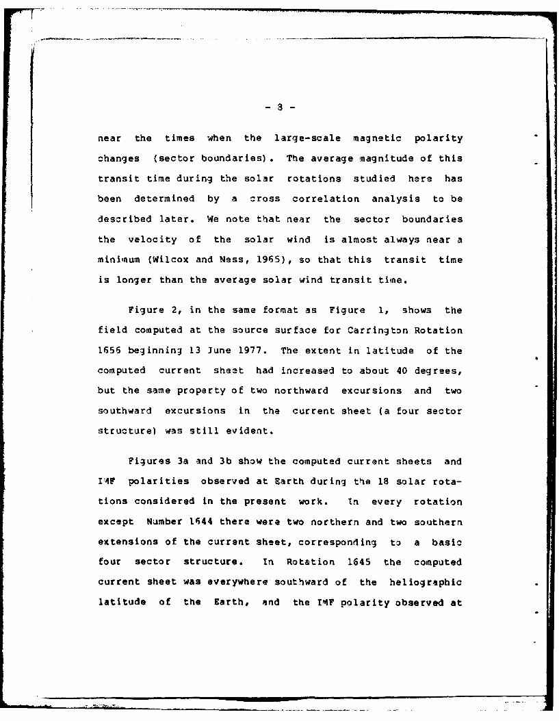
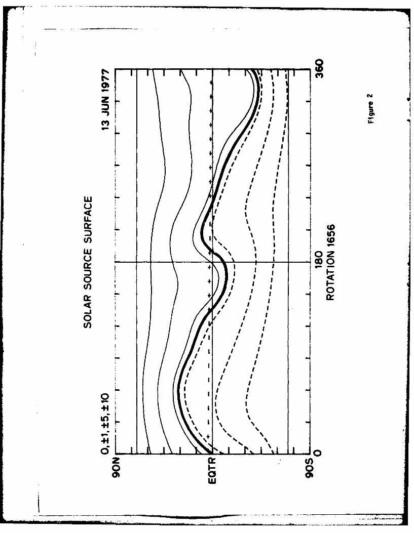
Figure 2, in the same format as Figure 1, shows the
field computed at the source surface for Carrington Rotation
1656 beginning 13 June 1977. The extent in latitude of the
computed current sheat had increased to about 40 degrees,
but the same property of two northward excursions and two
southward excursions in the current sheet (a four sector
structure) was still evident.
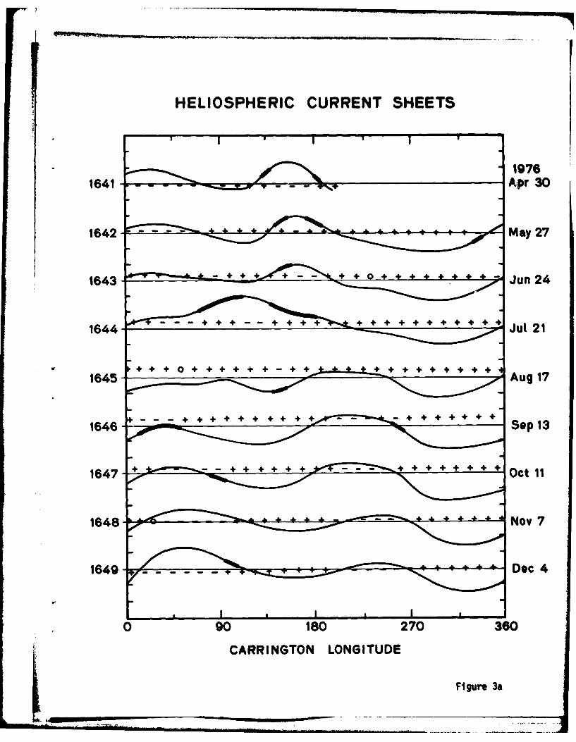
Figjures 3a and 3b show the computed current sheets and
IlAP polarities observed at Earth during the 18 solar rota-
tions considered in the present work. tn every rotation
except Number 1644 there were two northern and two southern
extensions of the current sheet, corresponding to a basic
four sector structure. In Rotation 1645 the computed
current sheet was everywhere southward of the heliographic
latitude of the Earth, and the I1*' polarity observed at
9
Earth was almost entirely away from the Sun. This presum-
ably is an example of the situation discussed by Wilcox
(1972) in which near the last five (now six) sunspot minima
the observed or inferred IM4F polarity has been largely away
from the Sun during a few consecutive rotations. If the
current sheet "misses" the Earth near the time of a sunspot
minimum the resulting predominant polarity of the I4F could
oe either away from or toward the Sun according to the con-
siderations discussed in this papar. 4 predominance in away
polarity in the observed photospheric field also discussed
by Wilcox (1972) would not necessarily be directly related
to the situation shown here in Rotation 1645.
Hundhausen (1977) noted that a "monopolar" sector
structure as seen in Rotation 1645 of Figure 3a might appear
at the beginning of a new solar cycle. However, the sugges-
tions that at this time "The prominent recurrent sectors,
streams and geomagnetic activity sequences should end
abruptly* and the "Recurrence with the 27-day solar rotation
period should become rare" are not consistent with the com-
puted current sheets in Figures 3a and 3b.
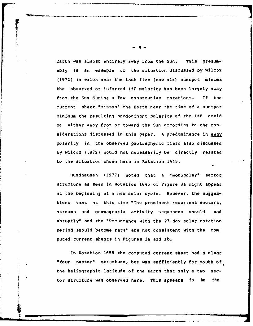
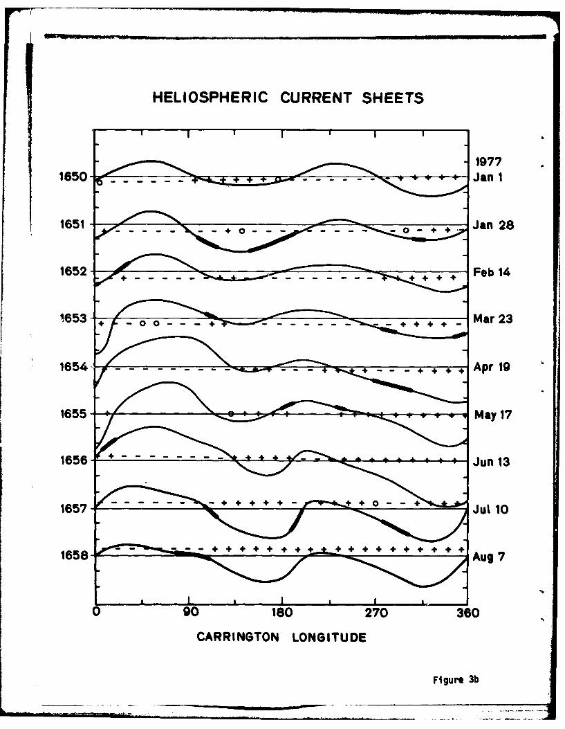
In Rotation 1658 the computed current sheet had a clear
"four sector" structure, but was sufficiently far south of'
the heliographic latitude of the Earth that only a two sec-
tor structure was observed here. This appears to be the
4
I
- 10 -
same geometry but the opposite sense from the situation in
early 1976 described by Scherrer et al. (1977).
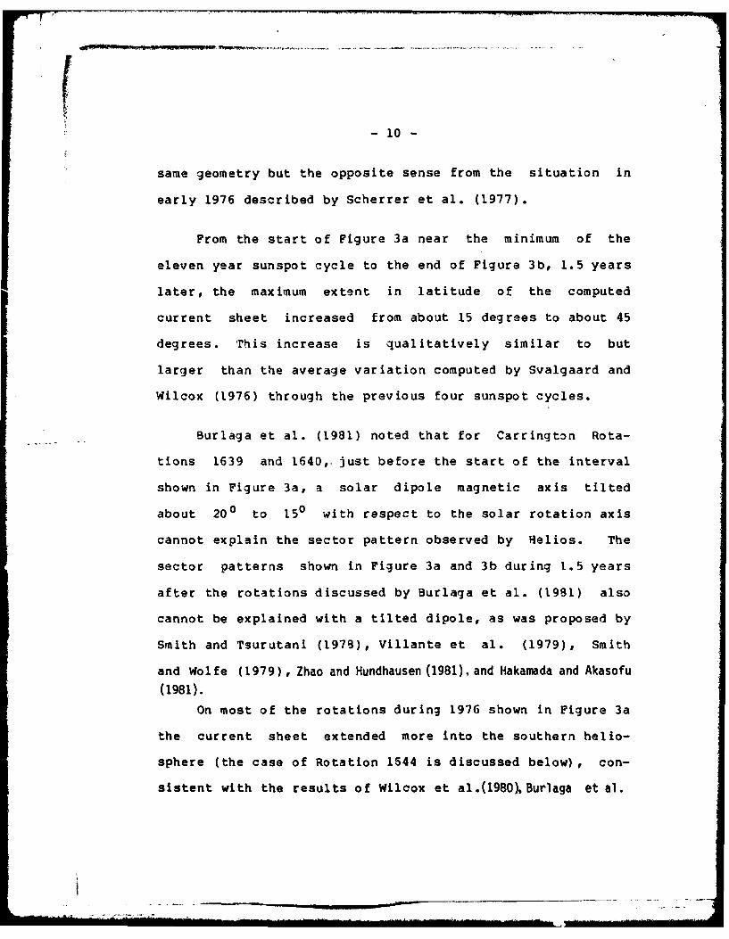
From the start of Figure 3a near the minimum of the
eleven year sunspot cycle to the end of Figure 3b, 1.5 years
later, the maximum extent in latitude of the computed
current sheet increased from about 15 degrees to about 45
degrees. This increase is qualitatively similar to but
larger than the average variation computed by Svalgaard and
Wilcox (1976) through the previous four sunspot cycles.
Burlaga et al. (1981) noted that for Carrington Rota-
tions 1639 and 1640,. just before the start of the interval
shown in Figure 3a, a solar dipole magnetic axis tilted
about 200 to 150 with respect to the solar rotation axis
cannot explain the sector pattern observed by Helios. The
sector patterns shown in Figure 3a and 3b during 1.5 years
after the rotations discussed by Burlaga et al. (1981) also
cannot be explained with a tilted dipole, as was proposed by
Smith and Tsurutani (1979), Villante et al. (1979), Smith
and Wolfe (1979), Zhao and Hundhausen (1981), and Hakamada and Akasofu
(1981).
On most of the rotations during 1976 shown in Figure 3a
the current sheet extended more into the southern hello-
sphere (the case of Rotation 1644 is discussed below), con-
sistent with the results of Wilcox et al.(1980),Burlaga et al.
P., Raw-
(1981) and Villante et al. (1982). The conjecture of Vil-
lante et al. (1982) that the current sheet during the first
half of 1977 was confined in a narrower latitude region is
not consistent with the current sheets shown in Figure 3b.
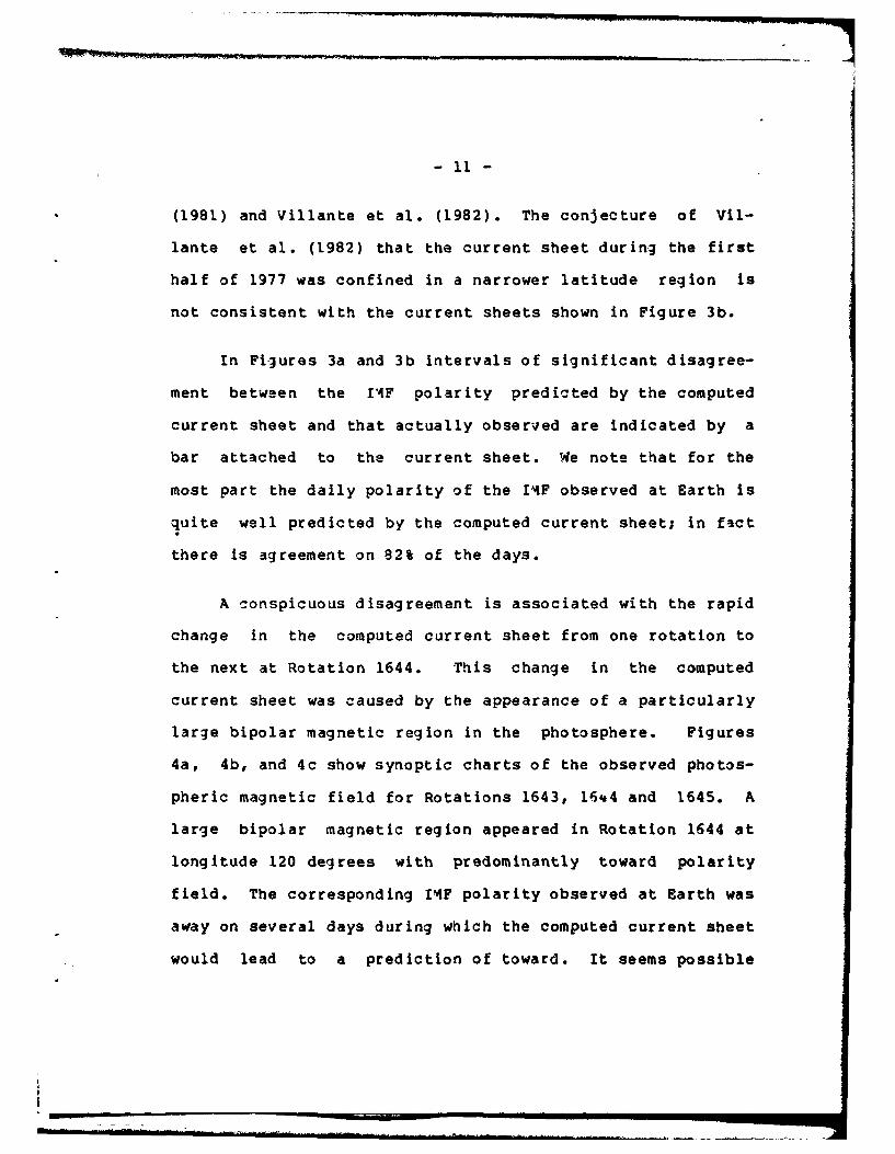
In Figures 3a and 3b intervals of significant disagree-
ment between the t'4F polarity predicted by the computed
current sheet and that actually observed are indicated by a
bar attached to the current sheet. We note that for the
most part the daily polarity of the IflF observed at Earth is
quite well predicted by the computed current sheet; in fact
there is agreement on 82% of the days.
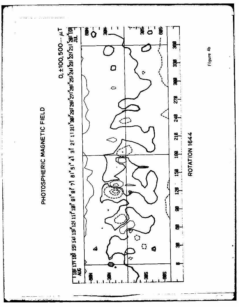
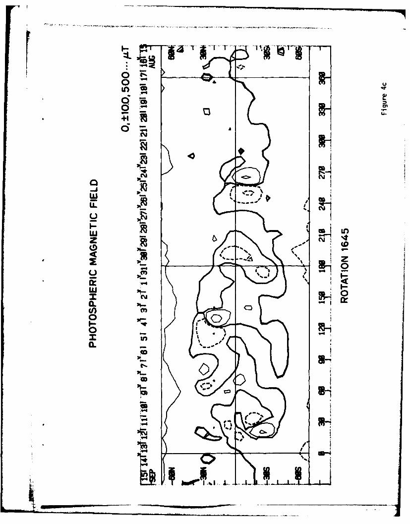
A conspicuous disagreement is associated with the rapid
change in the computed current sheet from one rotation to
the next at Rotation 1644. This change in the computed
current sheet was caused by the appearance of a particularly
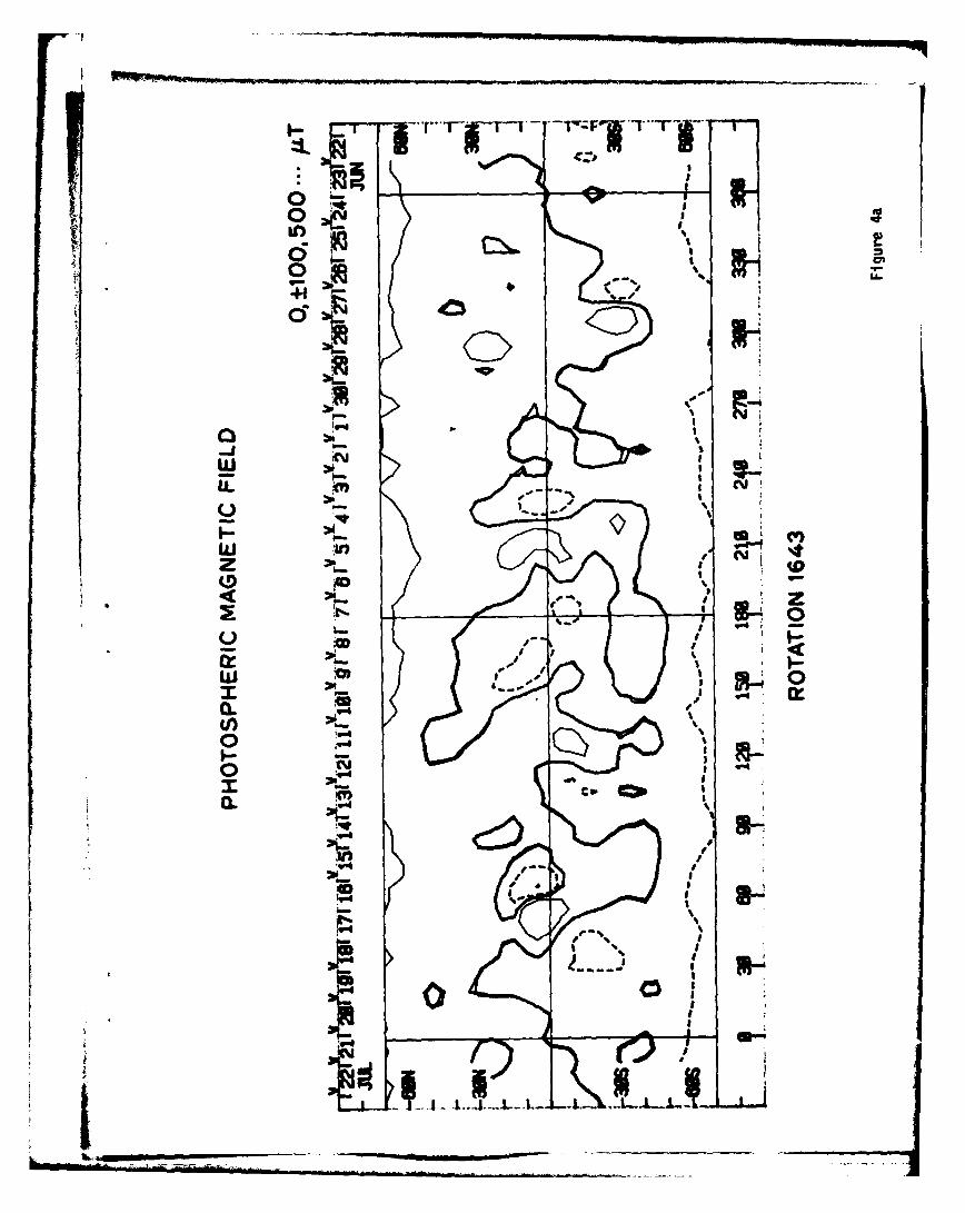
large bipolar magnetic region in the photosphere. Figures
4a, 4b, and 4c show synoptic charts of the observed photos-
pheric magnetic field for Rotations 1643, 16'.4 and 1645. A
large bipolar magnetic region appeared in Rotation 1644 at
longitude 120 degrees with predominantly toward polarity
field. The corresponding 11'1F polarity observed at Earth was
away on several days during which the computed current sheet
would lead to a prediction of toward. It seems possible
J- 12 -
that there may have been a region of toward magnetic field
polarity in the hellosphere corresponding to this bipolar
magnetic region, but at a latitude sufficiently far north so
as not to intersect the Barth. A similar event occurred
near 1.40 degrees longitude in the southern hemisphere in
Carrington Rotation 1651.
The rather rapid change in the computed current sheet
near longitude zero from Rotations 1652 to 1653 was also
caused by the appearance of a large bipolar magnetic region
in the photosphere, but in this case the region remained in
the photosphere for several rotations, and the corresponding
effects on the computed current sheet also continued for
several rotations.
In many of the rotations shown in Figures 3a and 3b,
the latitude of the current sheet at the end of the rotation
is significantly different from the latitude at the start of
the rotation. This illustrates the advantage gained from
computing the field structure on the source surface at steps
of 10 degrees in the starting longitude, since if only one
computation were made for each rotation the latitude of the
current sheet at the start and the end of the rotation would
be forced to be the same.
-13 -
4. Influence on t1,9 Solar Polar Field Strength and the
Radius of the Source Surface
The source surface current sheet was computed in the
above discussions using the solar polar field strength of
the form 11.5 cos 86 gauss derived by Svalgaard et al.
(1978), where 6 is the colatitude. We will now investigate
the effect of changing the magnitude of the derived solar
polar field and of changing the radius of the source sur-
face. For this purpose we will compute a cross correlation
between the I-IF polarity predicted from the computed current
sheet and that actually observed or inferred at Earth.
In order to determine the predicted IF polarity a line
is drawn on the source surface at the heliographic latitude
of the Earth, i.e. varying from 7 degrees north to 7 degrees
south through the year. This line is divided into daily
increments, and on a given day if the current sheet is
southward of the line the predicted polarity is away, and If
the current sheet is northward of the line the predicted
polarity is toward the Sun. At least 5/8 of a day must have
the same polarity in order for a polarity to be assigned.
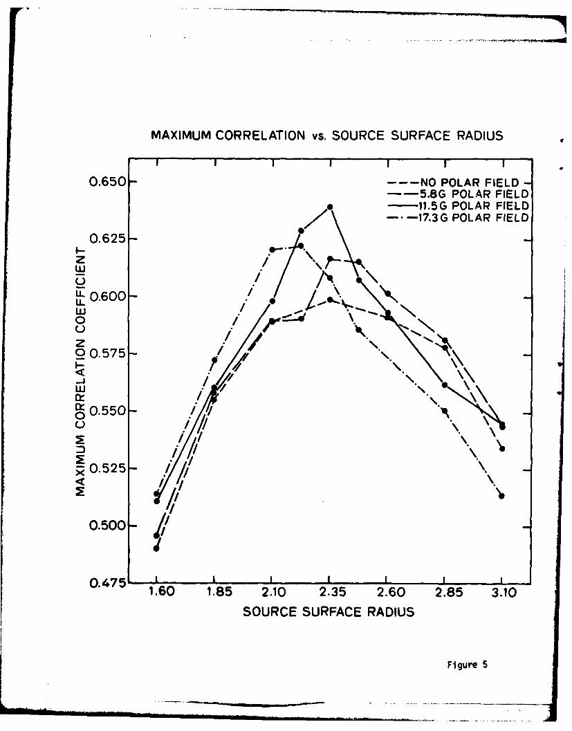
The solid curve in Figure 5 shows the maximum cross correla-
* tion between the predicted IMP polarity described above and
the polarity observed at Earth as a function of the radius
-14 -
of the source surface on which the current sheet is comn- -
puted, using the polar field strength computed by Svalgaard
et al. (1978). The largest correlation occurs for a source
surface of radius 2.35 R., and this radius has therefore
been chosen for most of the discussion in this paper. For.
comparison Figure 5 also shows similar maximum cross corre-
lations for source surfaces computed with no polar field
added, and for 5.8 gauss and 17.3 gauss added polar field.
We note that the solar polar field of 11.5 gauss computed by
Svalgaard et al. (1978) does give the best agreement,
although the differences are not large.
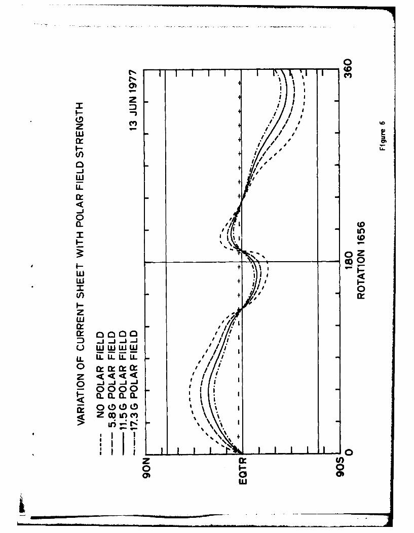
Figure 6 shows aomputed current sheets on a typical
Carrington rotation (i.e. Rotation 1656) for the four values
of added solar polar magnetic field. The current sheet for
the selected value of 11.5 gauss is shown with a solid line.
The current sheet shown with short dashes was computed with
no added solar polar field, and it has the largest extent in
latitude in Figure 6. The dash dot line is a current sheet
computed with 17.3 gauss added solar polar field (i.e. one
and one half times the preferred value), and it has the
smallest extent in heliographic latitude.
Pneuman et al. (1978) computed the field on a source
surface at 2.5 Re during the Skylab period in 1973 and found
- 15 -
that their computed neutral lines were systematically pole-
ward of the brightness maxima observed at 1.8 R9 with the
K-coronameter at Mauna Loa Hawaii. If the fields above 700
latitude measured with the full disk magnetograph at Kitt
Peak National Observatory were increased to about 30 gauss
this effect was removed. This is a much larger correction
for the solar polar field than we have used. The reason for
the difference from our work is not clear. Pneuman et al.
(1978) suggested other possible causes for their sys-
tematic polaward displacement of the neutral line; to the
extent that these operated the solar polar field correction
would be reduced. A difference in solar magnetograph cali-
brations between Kitt Peak and Stanford may have contributed
to the different corrections, and the solar polar field
strength may have been different in 1973 and 1976.
411 the computed current sheets in Figure 6 cross the
solar equator at the same longitudes, and the cross correla-
tions shown in Figure 5 are nearly the same for all the
values of added solar polar magnetic field. Near 340
degrees longitude the maximum latitude of the current sheet
decreases from 58 degrees for no added solar polar field to
37 degrees for 17.3 gauss added field. All of the computed
current sheets in Figure 6 agree almost equally well with
the ZqF polarity observed at Earth.
I
-16-
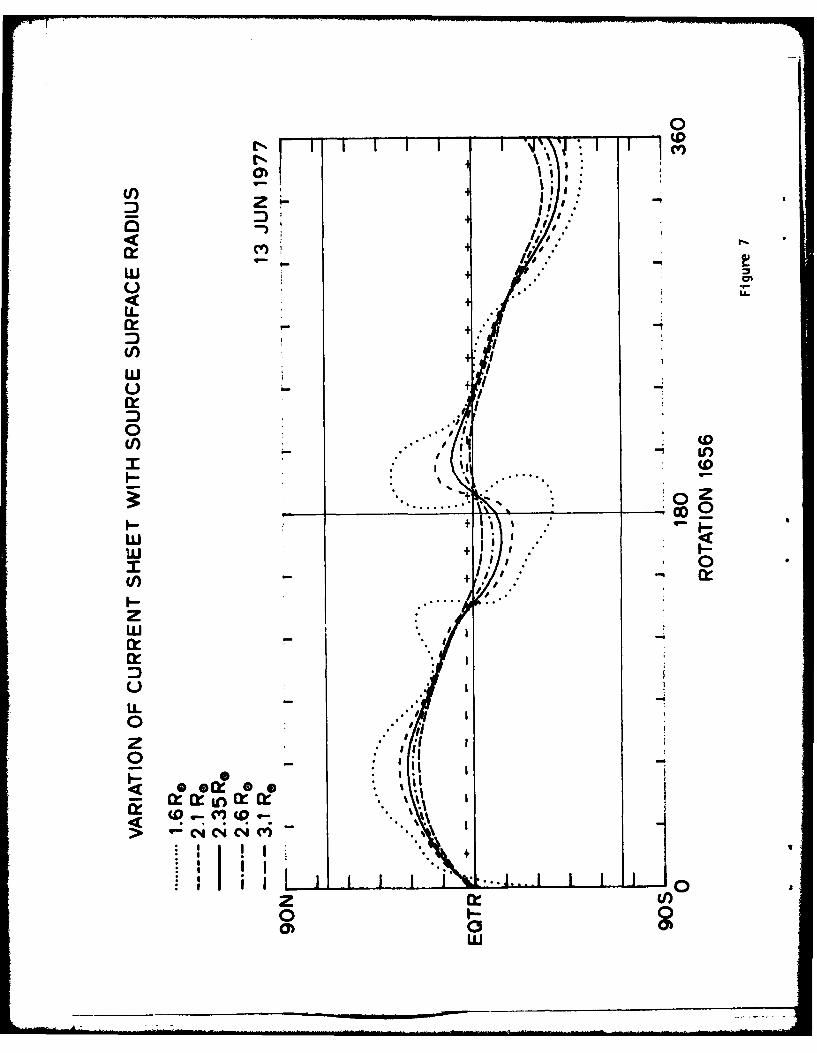
The computed current sheet in Carrington Rotation 1656
for several values of the radius of a spherical source sur-
face is shown In Figure 7. As the radius of the source sur-
face is increased the extent in latitude of the computed
current sheet decreases since the relative weight of the
dipole component of the solar magnetic field increases. All
of the computed current sheets in this Rotation agree almost
equally well with the observed I14F polarity.
Thus a comparison of the IF polarity predicted from a
computed current sheet with the IMP polarity observed at
Earth is a weak test of the extent in latitude of the com-
puted current sheet. A spacecraft observing at large helio-
graphic latitudes would give the definitive answer to the
problem of the extent in latitude of the heliographic
current sheet.
5. Purther Comparson of Predicted and observed IMF Polar-
In the discussion so far the IFP polarity observed at
Earth has been compared with the source surface field polar-
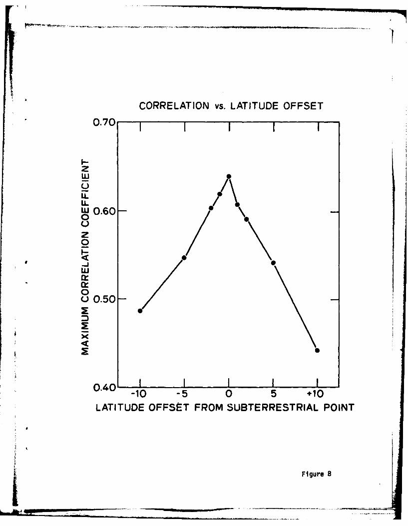
ity at the heliographic latitude of the Earth. Wihat happens
if instead we compare the observed I4F polarity at Earthwith the polarity on the source surface 5 degrees north of
the sub-terrestrial latitude? Figure 8 shows that the
IL_______________________________________________________
-17 -
maximum cross correlation decreases from 0.64 to 0.54. we
see in Figure 8 that the sub-terrestrial latitude on the
source surface has the most similar magnetic polarity struc-
ture to that observed at Earth, and that even a few degrees
north or south of the sub-terrestrial latitude the correlation
with the observed field is smaller.
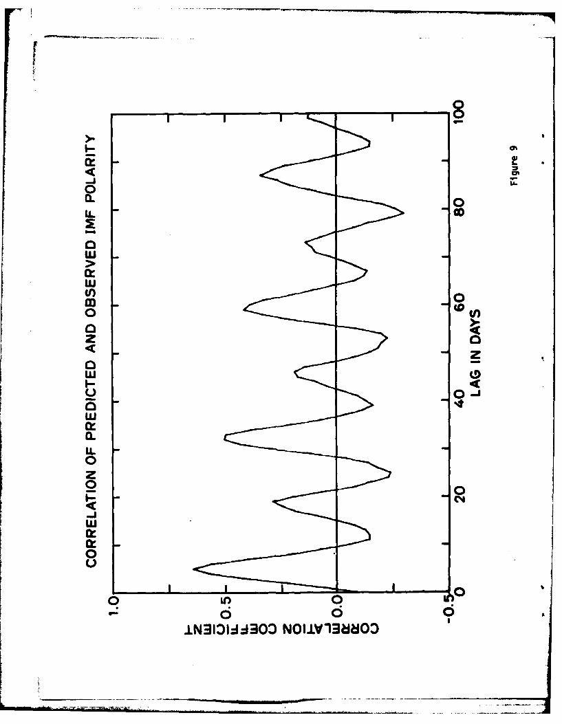
For the adopted conditions of source surface radius
equal to 2.35 Re and added solar polar field of 11.5 gauss,
Figure 9 shows a cross correlation between the predicted
field polarity at the sub-terrestrial point on the source
surface and the IMF polarity observed at Earth. The first
peak at 5.0 + 0.3 days represents the transit time for the
solar wind plasma to transport the magnetic field from Sun
to Earth. The five day lag corresponds to a solar wind
velocity of 350 km/s. This represents the average solar
wind velocity at sector boundary crossings, which are usu-
ally near minima in solar wind velocity (Wilcox and Ness,
1965). The relatively slow decline in amplitude of the
peaks near 32 days, 69 days and 36 days shows that the
large-scale IM4F structure Is quasi-stationary. The inter-
mediate peaks are caused by the four-sector nature of the
114F structure at this time. The difference in time between
the peak at 32 days and at 5 days shows that the recurrence
time of the IMF Is close to 27 days.
- 18 -
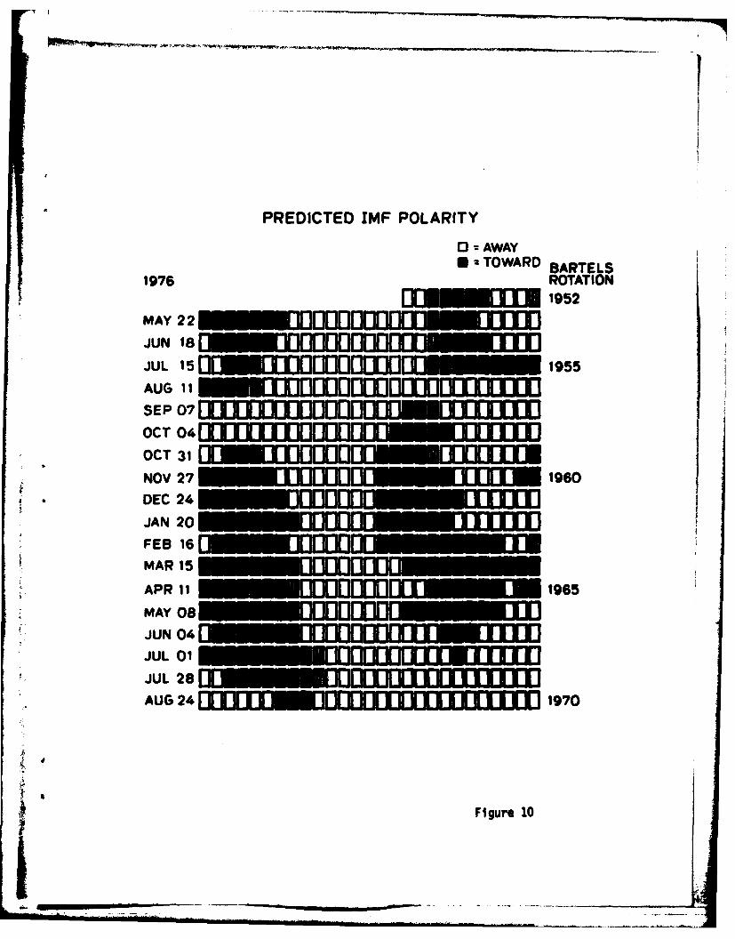
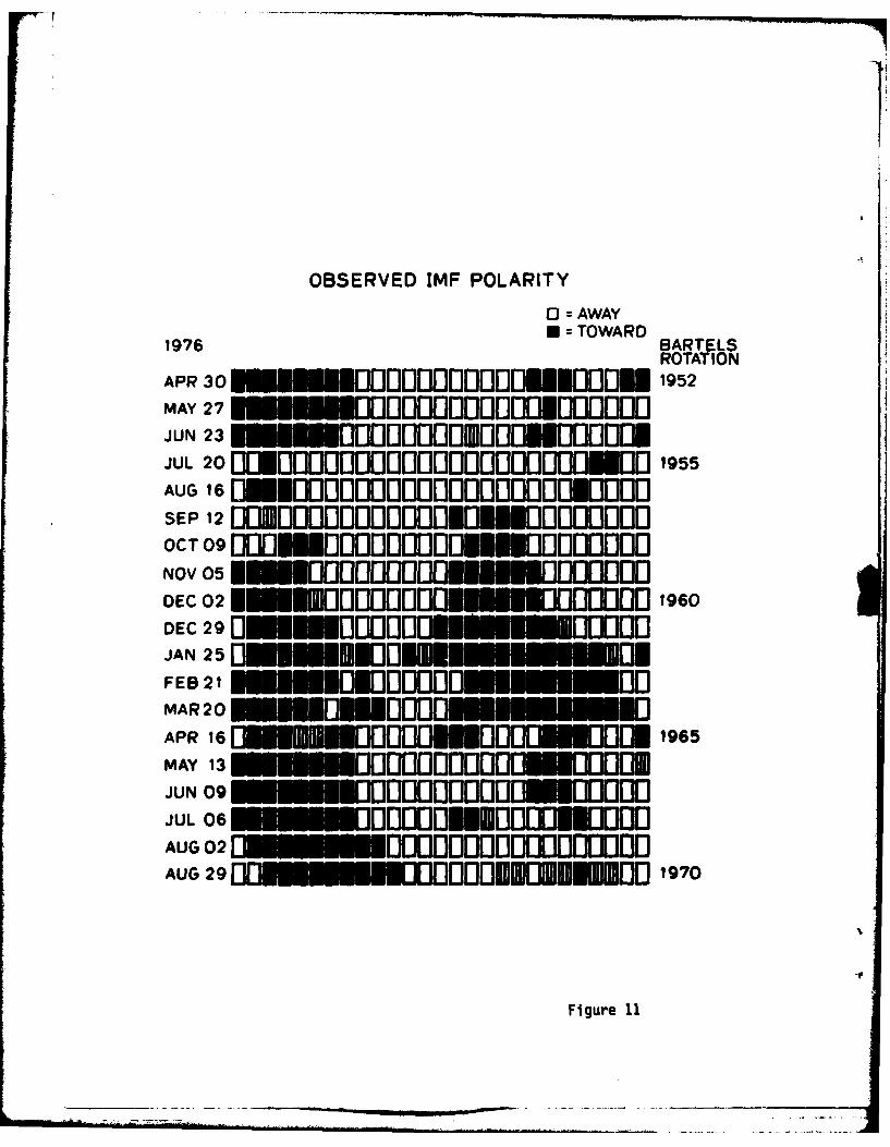
Our final comparison of the structure predicted from
the source surface and observed at Earth is shown in Figures
10 and 11. These figures are now in a Bartels rotation plot
as is customary for geomagnetic observations. Comparison of
the figures shows that the large-scale structure is quite
well predicted, and most of the disagreements come near sec-
tor boundary crossings or on occasional rotations. A por-
tion of the disagreement near boundary crossings is caused
by our use of a constant five day solar wind transit time
from Sun to Earth, while in fact there are some variations
among the actual transit times. On the one day scale used
in plotting Figures 10 and II these variations in transit
time would not be a large effect.
6. Summary
The heliospheric current sheet configuration has been
computed on a source surface at 2.35 Re during an interval
of 1.5 years after the last sunspot minimum. The magnetic
field observed on almost-daily scans with the solar magneto-
graph at the Stanford Solar Observatory has been corrected
for the solar polar fields that are not fully observed.
This correction significantly reduces the extent in latitude
of the computed current sheet.
The field on the source surface at the sub-terrestrial
-19-
latitude agrees best with the interplanetary magnetic field
observed at Earth. A deviation from this latitude of more
than a few degrees produces a significant decrease in the
accuracy of the predicted M~1.
During these 18 rotations the computed current sheet
had a quasi-stationary structure with two northward and two
southward excursions per rotation, corresponding to a four
sector structure. Occasionally an excursion *missed' the
Earth. Near sunspot minimum the maximum extent in latitude
of the current sheet was about 15 deg~rees, but 1.5 years
later the maximum latitude had increased to about 45
degrees.
Comparisons with the I4P polarity observed at Erth
give only a weak test of the extent in latitude of the
current sheet. The most definitive answer to this question
will come from observations with spazacraft at larger helio-
graphic latitudes. Although a large part of the heliosphere
is filled with magnetic flux from the solar polar regions#
the structure of the 114F observed at Earth is still closely
related to the structure of low-latitude fields on the
source surface.
- 20 -
Acknowledgements
This work was supported in part by the Office of Naval
Research under Contract N00014-76-C-0207, by the National
Aeronautics and Space Administration under Grant NGR05-020-
559 and Contract NAS5-24420, by the Atmospheric Sciences
Section of the National Science Foundation under Grant
XT477-20580 and by the 14ax C. Fleischmann Foundation.
Li
!I- 21-
References
Adams, 3., and G.W. Pneuman, A new technique for the determination
of coronal magnetic fields: a fixed mesh solution to Laplace's
equation using line-of-sight boundary crossings, Solar Phys., 46,
185-204, 1976.
Altschuler, M.D. and G. Newkirk Jr., Magnetic fields and the
structure of the solar corona, Solar Phys., 9, 131-149, 1969.
Altschuler, M.D., R.H. Levine, 4. Stix, and J.W. Harvey, High
resolution mapping of the magnetic field of the solar corona,
Solar Phys., 51, 345-376, 1976.
Burlaga, L.P., k.l. Hundhausen and Xue-pu Zhao, The coronal and
interplanetary current sheet in early 1976, 3. Geophys. Res.,
86, 8893-8898, 1981.
Rakamada, K. and S.-I. Akasofu, A cause of solar wind speed
variations observed at 1 N.U., 3. Geophyo. Res., 86,
1290-1298, 1981.
Howard, R., Studies of solar magnetic fields, Solar Phys., 52,
243-248, 1977.
Iundhausen, N.J., An interplanetary view of coronal holes, in
3.8. Zirker (ed.), Coronal holes and high speed wind streams,
- 22 -
Colo. Assoc. Univ. Press, Boulder, pp. 225-329, 1977.
King, J.H., Interplanetary N1editza Data Book (Supplement 1), Rep.
qSSDC 7908, NkSh Goddard Space Plight Center, Greenbelt, 4d.,
1979.
Levine, R.H. and 4.D. hltschuler, Representations of coronal
magnetic fields including currents, Solar Phys., 36, 345-350,
1974.
Levine, R.H., K. Schulz and E.N. Frazier, Simulation of the
magnetic structure of the inner heliosphere by means of a
non-spherical source surface, Solar Phys., 77, 363-392, 1982.
Pneuman, G.W., S.F. Hansen and R.T. Hansen, On the reality of
potential magnetic fields in the solar corona, Solar Phys., 59,
313-330, 1978.
Poletto, G., G.S. Vaiana, 4.V. Zombeck, A.S. Krieger, and h.F.
Timothy, A comparison of coronal X-ray structures of active
regions with magnetic fields computed from photospheric
observations, Solar Phys., 44, 83-100, 1975.
Riesebieter, W. and P.M. Neubauer, Direct solution of Laplace's
equation for coronal magnetic fields using line-of-sight
boundary conditions, Solar Phys., 63, 127-134, 1979.
Schatten, K.., J.. Wilcox and N.F. Ness, A model of inter-
- 23 -
planetary and coronal magnetic fields, Solar Phys., 6,
442-455, 1969.
Scherrer, Philip H., John M. Wilcox, L. Svalgaard, T.L. Duvall, Jr.,
P.H. Dittmer and E.K. Gustafson, The mean magnetic field of the
sun: observations at Stanford, Solar Phys., 54, 353-361, 1977.
Schulz, C., Interplanetary sector structure and the heliomagnetic
equator, Nstrophys. and Space Sci., 24, 371, 1973.
Schulz, A., E.N. Frazier, ind D.J. Boucher, Jr., Coronal magnetic
field model with non-spherical source surface, Solar Phys.,
50, 83-104, 1978.
Smith, E.J. and B.T. Tsurutani, Observations of the interplanetary
sector structure up to heliographic latitudes of 16 : Pioneer 11,
J. Geophys. Res., 83, 717-724, 1978.
Smith, E.J. and J.H. Wolfe, Fields and plasmas in the outer solar
system, Space Sci. Rev., 23, 217-252, 1979.
Stenflo, J.O., Observations of the polar magnetic fields, I.A.U.
Symposium No.43, Solar Magnetic Fields, 714-724, 1971.
Svalgaard, L., Polar cap magnetic variations and their relationship
with the interplanetary magnetic sector structure, J. Geophys.
Res., 78, 2064-2078, 1973.
- 24 -
Svalgaard, L. and J.M. Wilcox, Long term evolution of solar sector
structure, Solar Phys., 41, 461-475, 1975.
Svalgaard, L. and J.M. Wilcox, Structure of the extended solar
magnetic field and the sunspot cycle variation in cosmic ray
intensity, Nature, 262, 766-768, 1976.
Svalgaard, L., T.L. Duvall, Jr., and P.H. Scherrer, The strength
of the Sun's polar fields, Solar Physics, 58, 225-240, 1978.
Svalgaard, L. and 7.4. Wilcox, A view of solar magnetlc fields,
the solar corona, and the solar wind in three dimensions,
Nnn. Rav. kstron. Astrophys., 16, 429-443, 1978.
Villante, U., R. Bruno, F. Nariani, L.F. Burlaga, and N.F. Ness,
The shape and location of the sector boundary surface in the
inner solar system, J. Geophys. Res., 84, 6641-6648, 1979.
Villante, U., F. Mariani, and P. Francia, The I14F sector pattern
through the solar minimum: two spacecraft observations
during 1974-1978, J. Geophys. Res., 87, 249-253, 1982.
Wilcox, John M. and N.F. Ness, Quasi-stationary corotating
structure in the interplanetary medium, J. Geophys. Res.,
70, 5793, 1965.
Wilcox, John 4., Why does the Sun sometimes look like a magnetic
monopole?, Comments on Astrophys. and Space Phys., 4, 141-147,
- 25 -
1972.
Wilcox, John M., J.T. Hoeksema, and P.H. Scherrer, Origin of the
warped heliospheric current sheet, Science, 209, 603-605, 1980.
Zhao, Xue-pu and A..J. [undhausen, Organization of solar wind
plasma properties in a tilted, neliomagnetic coordinate system,
3. Geophys. Res., 86, 5423-5430, 1981.
- 26 -
Figure Captions
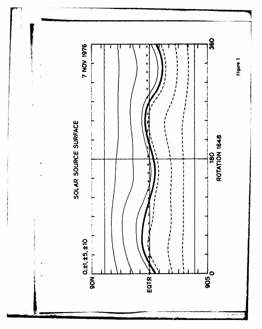
Figure 1 Computed magnetic field contours on a spherical
source surface concentric with the Sun at a radius
of 2.35 R. for Carrington Rotation 1648, beginning
7 November 1976. The solid contour lines represent
field directed away from the Sun with relative
strengths 1, 5 and 10; the dashed contours represent
field directed toward the Sun. The heavier line
near the solar equator is where the direction of
the computed field changes from away to towards,
and is assumed to be the source of the hellospheric
current sheet. The + and - symbols represent daily
values of the polarity of the interplanetary magnetic
field observed at Earth, adjusted for the five Jay
transit time of solar wind from Sun to Earth.
Figure 2 The same format as Figure 1, but for a later Carrington
Rotation 1656 beginning 13 3une 1977. Note that
the extent in latitude of the computed heliospheric
current sheet extends to higher latitudes than in
Figure 1.
Figure 3a The heliospheric current sheet computed on a source
surface at 2.35 R. on nine successive Carrington
Rotations, 1641-1649, beginning on 30 kpril 1976 to
L Ogo-
- 27-
4 December 1977. Compare for example the current
sheet shown here for Carrington Rotation 1648 with
that shown in Figure 1. Each succeeding base line
(solar equator) is displaced by 45 degrees heliographic
latitude. The + and - symbols represent daily values of
the 14F polarity observed at Earth allowing for the five
day transit time of solar wind from Sun to Earth.
Significant disagreements between the predicted and
observed I"4F polarities are indicated with a thicker
neutral line. (The first rotation shown in Figure 3a
is near sunspot minimum.)
Figure 3b The same as Figure 3a, but for the next nine Carrington
Rotations, 1650-1658, beginning 1 January 1977 to
7 Nugust 1977. Note that the extent in latitude of
the computed current sheet increases in the later
rotations.
Figure 4a A synoptic map of the line of sight photospheric
magnetic field measurements observed at the Stanford
Solar Observatory for Carrington Rotation 1643. The
dates indicate the central meridian passage time for
corresponding longitude. The inverted carets show the
dates of magnetograph scans which contribute to the
chart.
1t
- 28 -
Figure 4b The same format as figure 4a for Carrington Rotation
1644. Notice the large active region that has appeared
in the northern hemisphere near longitude 120.
Figure 4c Synoptic chart for Carrington Rotation 1645. The size
and strength of the active region is greatly reduced.
Figure 5 -Aaximum correlation between the 1VV polarity predicted
from the computed heliospheric current sheet and the
IAF polarity observed at Earth as a function of the
source surface radius on which the current sheet was
computed. Source surfaces were computed with an added
solar polar field strength of 11.5 gauss as computed by
Svalgaard et al. (1978), and for other values of the
added solar polar field as shown.
Figure 6 Computed heliospheric current sheets on Carrington
Rotation 1656 beginning 13 June 1977 for several
values of added solar polar magnetic field. As the
strength of the polar field 13 increased the
computed current sheet approaches the plane of the
solar equator.
Figure 7 Computed current sheets for Carrington Rotation 1656
beginning 13 June 1977 for source surfaces at several
different radii, as indicated. As the radius of the
-29-
source surface is increased the computed current sheet
approaches the solar equator.
Figure 8 The maximum cross correlation between the IMF? polarity
predicted from a computed current sheet on a source
surface at 2.*35 %with 11.5 gauss added polar field
and the 114F observed at Earth as a function of the
latitude on the source surface at which the field
polarity was predicted. in the abscissa zero represents
the heliographic latitude of the earth.
Figure 9 Cross correlation between the IIF polarity predicted
from the adopted computation of the heliospheric current
sheet and the polarity observed at earth. The lag of
the first peak is five days, which represents the transit
time from Sun to Earth of the solar wind near the sector
boundaries.
Figure 10 The 1'4F polarity computed at the source surface by the
model is presented in the Bartels chart format. Each
row has 27 boxes with the polarity for each
day indicated in a box. 4 filled box indicates toward
polarity; a hatched box indicates indeterminate polarityl
an empty box indicates away polarity. The plot is displac
by five days to account for the solar wind transit time
from Sun to Earth. This format emphasizes the 27-day
- 30 -
recurrence pattern in the polarity and the large-scale
structure over many rotations.
Figure 11 Same format as Figure 10, but for the IP4F polarity
observed at Earth.
I|
40 1 * I + I I
II
U.0 z
(OD0
u
0 +
( i)
1k .40
Ob'
U I-
414dI
HELIOSPHERIC CURRENT SHEETS
'19761641- Apr 30
1642 - - May 27
1644. . . .. . . . Jul 21
1645 Aug 17
+ + +- + Sep 13
1647- + . .. . . .Oct 11
'1648 - bNov 7
0 90 '180 270 360
CARRINGTON LONGITUDE
Lm _ Figure 3a
HELIOSPHERIC CURRENT SHEETS
19771650-Jan 1
1651- 0Jan 28
1652- - - -- - -Feb 14
1653 0 0Mar 23
1655 May 17
1656-Jun 13
Ju 1
1658 -Aug 7
p+ +
090 180 270 360
CARRINGTON LONGITUDE
Figure 3b
IH94 .-
T d - La0
07
C-C>
I-'---
7.17
CL
0~ .
0CIP Clo
0.
ILM
+1Y0-
w
o )
0
(I)
oAmok.
wo--
0o
CC
CL
I-0
MAXIMUM CORRELATION vs. SOURCE SURFACE RADIUS
0.650. --- NO POLAR FIELD --- 5.8G POLAR FIELD
-11.56 POLAR FIELD-- 17.3 G POLAR FIELD
0.625-
zw
U_0.6 0 0/
0/o//////=\"
00.550 -l/
0(.525
0.500
0.475 i .1.60 1.85 2.10 2.35 2.60 2.85 3.10
SOURCE SURFACE RADIUS
Figure 5
wI E
w + .II
+
w +4
I
a..0/ (0
z OZ
0 ---/ 000
z -w 0
00
0 Zii,:2
Cl) I,: 0
Li-
011
0 .1' CCi)- ... 0
CORRELATION vs. LATITUDE OFFSET
0.70
I-zw •5L-
0.60U
z0
* °w
0O 0.50
xS
0.40 I I I I-10 -5 0 5 +10
LATITUDE OFFSET FROM SUBTERRESTRIAL POINT
j Figure 8
(n 0
0
wu
0:0
0z0J
C4
w0.
IN1U-:30NII180
PREDICTED IMF POLARITY
O - AWAY•= TOWARD BARTELS
1976 ROTATION
[] hh11N 1952MAY 2 2 IIEEIIEUOOOOOOOlOEEIOOOOJUN I18 UEUO 0000OINMOOOEIJUL 151hu000hOOOO]UIfI 1955AUG1I1 0000LJUIIIIU 115
OCT 0o111 l mooo I]011--1---]--OCT 31 0011 I I 11 1]001111NOV 27 IUll] , Ivi o6DEC 24 111110JAN 20 Iml mFEB 16011EfOO(EEETMAR15
APR 11 [ Jono0m:U~i 1965MAY 08IEEEEOOOOMIM i )JUN 04(NEEEO00000UOOIJUL 01u ]O000000IIJUL 28 E 1JOOOOOOOOOOOAUG241 1111J 1]][11970
i
OBSERVED IMF POLARITY
0O=AWAY0 TOWARD
1976 BARTELSROTATION
APR 301111111 N IIJOOO OOOQOOIIODI 1952MAY 27 111111111000 0IOOOOOOOIOI0OJUN 23 1MUMUIHUO OOOOOIDOOOEOOOOOJUL 20 001=00000000000000000OEUO 1955AUG 16 [OOOOOOOOOOOOOOOOOOITOOSEP 12 OIJIDOO0iOOOO1J01OEIOOOOOOOOCT 09 OOIJIEOOOOO IJOOIIEOOOOOIJINOV 05 0000OOOOOOUUUIJEOOflDEC 02 UIUE000000EUOOOOI 1960DEC 29 OUUUUU[]0000EI EmnhuooJAN 25 EO101I RDONFEB 21 EUEJOOOLUoU 101noMAR 20 EIE JOOOOIE lii EUUUAPR 16 OEEEEOOOOJO~OOU O 1ro965
MAY 13 EUUUUJOOOOOOD OUOOOOIJUN 09 EUU00IJOOOOOOOOUUOO0O0JUL 06 EIITOOO 10OOOAUOOAUG 02 [1UUEUE0I)OOO0OIJOOOOOIJOAUG 29 [JUUEI IElOOOOOIOUE00 1970
Figure 11