Institut für Numerische und Angewandte Mathematik

Locating a median line with partial coverage distance

J. Brimberg, R. Schieweck, A. Schöbel

Nr. 32

Preprint-Serie desInstituts für Numerische und Angewandte Mathematik

Lotzestr. 16-18D - 37083 Göttingen

Locating a median line with partialcoverage distance

Jack Brimberg∗† Robert Schieweck‡§¶ Anita Schobel‡¶

December 2013

We generalize the classical median line location problem, where the sumof distances from a line to some given demand points is to be minimized,to a setting with partial coverage distance. In this setting, a demand pointwithin a certain specified threshold distance r of the line is considered coveredand its partial coverage distance is considered to be zero, while non-covereddemand points are penalized an amount proportional to their distance to thecovered region. The sum of partial coverage distances is to be minimized. Weconsider general norm distances as well as the vertical distance and extendclassical properties of the median line location problem to the partial coveragecase. We are finally able to derived a finite dominating set. While a simpleenumeration of the finite dominating set takes O(m3) time, m being thenumber of demand points, we show that this can be reduced to O(m2 logm)in the general case by plane sweeping techniques and even to O(m) for thevertical distance and block norm distances by linear programming.

Keywords median line location, partial coverage, finite dominating set, plane sweeping,block norm

1 Introduction

Locating a straight line in continuous space in order to represent (or to fit) a given setof fixed points is a well-studied problem in facilities location theory. The problem was

∗Royal Military College of Canada, 13 General Crerar Crescent Kingston, ON, K7K 7B4 Canada†This author was supported by the Natural Sciences and Engineering Research Council of CanadaDiscovery Grant (NSERC #205041-2008)

‡Institute for Numerical and Applied Mathematics, University of Gottingen, Lotzestr. 16–18, 37083Gottingen, Germany

§This author was supported by the DFG through the Research Training Group 1023¶This author was supported by the European Union Seventh Framework Programme (FP7-PEOPLE-

2009-IRSES) under grant agreement no. 246647 within the OptALI project.

1

originally posed in terms of a minimization of the sum of weighted Euclidean distancesfrom a set of fixed points (demand points or customers) to a line in the plane R2 [MT83,LC85]. The minmax criterion, i.e., minimizing the maximum distance to the line, has alsobeen investigated [HT88]. In facility location, the linear facility, or line, can representa new road or railway track through a given region, a dense series of communicationtowers, a main connector in an electrical circuit board, and so on. For an introductionto the linear facility location problem, see for example [LMW88]. Extensions of the basicmodel include the use of arbitrary norms in place of Euclidean distances [Sch99] and thelocation of a line in R3 [BJS02, BJS03, BCSS11]. A related problem to line location inthe plane is the location of a hyperplane in Rn, [MS98, MS01] and references therein.Locating a linear facility on a sphere translates to the location of a great circle on thesphere [BJS07].

In this paper we investigate a new extension of the median line problem in the planewhere ’partial coverage distance’ is used as the distance measure. The concept of partialcoverage was recently introduced by [BJKS13] for the location of a point facility. Theidea is that the distance function between a customer and the new facility is zero if thecustomer is within a threshold value r of the facility, and otherwise, becomes the closestdistance from the customer to the boundary of a disc of diameter 2r centered at thefacility. Thus, the partial coverage model attempts to combine the notion of coveragewith the median objective. For further details and motivation see [BJKS13].

We extend the partial coverage concept to a linear facility in a straightforward manner.If a customer is within a specified threshold distance of r to the line, we consider that thecustomer is happy (i.e., covered) and associate a zero cost to that customer. Otherwise,a penalty is assessed which is proportional to the distance to the line in excess of r. Theobjective is then to minimize the sum of these penalty costs.

The location of a line with partial coverage is equivalent in effect to the location of a’thick’ linear facility which is a strip of width 2r (as measured by the given distancefunction). Thus, we obtain a new type of problem, which may also be referred to asmedian strip location problem, and which may have interesting applications in areas otherthan facility location such as regression analysis. Another interpretation of the problemis as follows: replace each fixed point by a disc of diameter 2r centered at the point;then locate a median line with respect to the discs. This problem has been studied forthe Euclidean distance in [RT94].

It is well-known that an optimal solution of the median line problem always exists wheretwo of the fixed points are coincident with the line when distance is measured by anarbitrary norm. Furthermore, if the norm is a smooth one, this incidence propertyeven becomes a necessary condition [Sch99, MS99]. This important result reduces theproblem to a search through a finite number of candidate solutions. One of the mainfindings of this paper is that the incidence property may be generalized to line locationwith partial coverage. Based on this, a finite dominating set can be developed also forthe more general problem, although the candidate solutions are different than before.

2

The paper is organized as follows: Section 2 summarizes the notation and presentsthe mathematical model; Section 3 analyzes the model and establishes the incidenceproperty and the finite dominating set. Section 4 presents different approaches derivedfrom the properties obtained in the previous sections. These are an enumeration of thefinite candidate set, an efficient sweep algorithm, and a linear programming formulationfor the case of block norm distances. Finally, Section 5 gives our conclusions and somethoughts on further research.

2 The line location problem with partial coverage distance

The given information consists of a set of m fixed points (also demand points or cus-tomers) with known locations pi = (pi1, pi2)

T ∈ R2, i = 1, . . . ,m, and given weightswi > 0, i = 1, . . . ,m, which may, for example, represent a demand for service or a flowin the location model. A threshold value r is also specified. If the distance to the linearfacility exceeds r, a penalty cost proportional to the excess distance is charged; other-wise, the point is covered and the cost is zero. The distance to the line refers either tothe closest distance measured by some given (arbitrary) norm, or to the vertical distanceto the line. The latter is added because of its importance in regression analysis.

Let L denote the line (i.e., linear facility) to be located. We may define this line in termsof an unknown normal vector n = (n1, n2)

T ∈ R2 \ {0} and some number c ∈ R:

L = {x ∈ R2 : nTx = c}. (1)

If L is not a vertical line (n2 6= 0), we may set n2 = 1 and obtain an equivalentrepresentation:

L = {x ∈ R2 : x2 = sx1 + b} (2)

where s and b are, respectively, the slope and intercept of the line. We write Ln,c fora line in the normal vector parametrization or, if possible without ambiguity, Ls,b for aline in the slope-intercept parametrization.

Let k : R2 → R be a norm in the plane. Then the distance from any point p ∈ R2 toline L with respect to norm k is defined as

d(p, L) = min{k(p− x) : x ∈ L}, (3)

that is, the distance is the shortest one between p and L measured by the norm k. In[Man99] and [PC01] it is shown that for a line L = Ln,c this distance can be computedas

d(p, Ln,c) =|nT p− c|k◦(n)

(4)

where k◦ : R2 → R2 denotes the dual norm of k. For the case of the vertical distancebetween a point p and a non-vertical line L (i.e., n2 6= 0) we obtain

d(p, Ln,c) =|nT p− c||n2|

(5)

3

or equivalently d(p, Ls,b) = |p2−sp1− b| in the (s, b)-representation. Hence, the distancebetween a point and a (non-vertical) line with respect to a norm k is given as the verticaldistance divided by the dual norm k◦((s,−1)T ) of the normal vector. Notice that point-line distance, no matter if vertical or measured with a norm, can be written in the form(4) where k◦ is a convex function of n, namely the dual norm in the norm distance caseand k◦(n) := |n2| in the vertical distance case. We will make use of this in the nextsections to unify some of the proofs.The partial coverage distance between p and L is defined as follows for either case:

D(p, L) = max{d(p, L)− r, 0} = [d(p, L)− r]+, (6)

where [a]+ = max{a, 0} for all a ∈ R. The new problem which we study here replacesthe standard distance from point to line by the partial coverage distance:

(MLPC) minline L

m∑i=1

wiD(pi, L). (7)

We refer to the problem above as the median line problem with partial coverage (MLPC)and denote its objective by f(L) or also

f(n, c) =m∑i=1

wi

[|nT pi − c|k◦(n)

− r]+

(8)

if L is parametrized by normal n and a real number c.

Since (MLPC) is a generalization of a well-known line location problem, we will first ofall explore connections to previously treated problems from the literature.

Lemma 1 (Connections to other line location problems). Let rmax be the optimal ob-jective value of the unweighted center line location problem for points p1, . . . , pn. Let aradius r be given and denote by z∗ the optimal objective value of (MLPC) for the samepoints, but possibly with weights. Then the following hold.

1. If r = 0, then (MLPC) is the median line location problem.

2. r < rmax if and only if z∗ > 0 and r ≥ rmax if and only if z∗ = 0.

3. If r ≥ rmax then any optimal solution to the unweighted center line location problemis optimal for (MLPC). In case of r = rmax a line L is optimal for (MLPC) ifand only if L is optimal for the unweighted center line problem.

Proof. 1. This is obvious since D(p, L) = d(p, L) for r = 0.

2.

z∗ = 0 ⇔ ∃L : D(pi, L) = 0 ∀ i = 1, . . . ,m

⇔ ∃L : d(pi, L) ≤ r ∀ i = 1, . . . ,m

⇔ ∃L : maxi=1,...,m

d(pi, L) ≤ r

⇔ rmax = minL

maxi=1,...,m

d(pi, L) ≤ r

4

which proves both assertions because f ≥ 0.

3. This can be seen easily from a calculation similar to that of the second case.

This allows us to calculate an optimal solution to (MLPC) in O(m logm) time as centerline if r ≥ rmax [Sch99]. If the threshold r is even larger, namely

r ≥ r := maxi,j=1,...,n

d(pi, pj)

the problem becomes trivial and can be solved in constant time: every line L passingthrough one of the fixed points, say pk, is optimal because d(pi, L) ≤ d(pi, pk) ≤ rfor all i = 1, . . . ,m. The interesting cases are those with some intermediate r, namelyr ∈ (0, rmax).

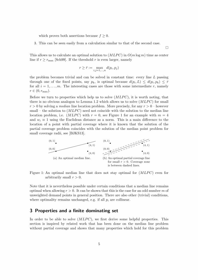
Before we turn to properties which help us to solve (MLPC), it is worth noting, thatthere is no obvious analogon to Lemma 1.2 which allows us to solve (MLPC) for smallr > 0 by solving a median line location problem. More precisely, for any r > 0 – howeversmall – the solution to (MLPC) need not coincide with the solution to the median linelocation problem, i.e. (MLPC) with r = 0, see Figure 1 for an example with m = 4and wi ≡ 1 using the Euclidean distance as a norm. This is a main difference to thelocation of a point with partial coverage where it is known that the solution of thepartial coverage problem coincides with the solution of the median point problem forsmall coverage radii, see [BJKS13].

(0, 0)

(0, 1)

(4, 0)

(4, 1)

(a) An optimal median line.

(0, 0)

(0, 1)

(4, 0)

(4, 1)

(b) An optimal partial coverage linefor small r > 0. Coverage zoneis between dashed lines.

Figure 1: An optimal median line that does not stay optimal for (MLPC) even forarbitrarily small r > 0.

Note that it is nevertheless possible under certain conditions that a median line remainsoptimal when allowing r > 0. It can be shown that this is the case for an odd numberm ofunweighted demand points in general position. There are also other (trivial) conditions,where optimality remains unchanged, e.g. if all pi are collinear.

3 Properties and a finite dominating set

In order to be able to solve (MLPC), we first derive some helpful properties. Thissection is inspired by related work that has been done on the median line problemwithout partial coverage and shows that many properties which hold for this problem

5

can be generalized to our case. We start by showing an analogon to the well-knownpseudo-halving property which states that every median line cuts the set of demandpoints approximately in half. To this end, denote for a fixed line L by

I+L = {i : d(pi, L) > r and pi lies above L}

the index sets of demand points above L and having a strictly greater distance to Lthan the threshold value r. Furthermore, let analogously I

+L be the index set of demand

points above L with distance greater or equal than the threshold distance r, and let I−Land I

−L be the corresponding index sets for demand points below L. Note that above

should be replaced by to the right to deal with vertical lines. For each of these index setsthe sum of corresponding weights is denoted by W+

L , W+L , W−L , and W

−L , respectively,

e.g.

W+L =

∑i∈I+L

wi.

Recall that in the case r = 0, i.e. the median line location problem without partialcoverage, every optimal line L satisfies W+

L ≤ W−L and W−L ≤ W

+L , see e.g. [Sch99].

The following theorem extends this to the case r > 0, i.e. the partial coverage setting.

Theorem 2 (Pseudo-halving property). Let L be optimal for (MLPC). Then W+L ≤

W−L and W−L ≤W

+L .

Proof. To show this, we prove the stronger statement, that a line L is optimal for(MLPC) restricted to some normal n if and only if W+

L ≤ W−L and W−L ≤ W

+L . Then

the assertion follows since an optimal line L (which has some normal, say n) for (MLPC)must be optimal for (MLPC) restricted to that normal n.

Clearly, for each partial coverage distance discussed here, induced by a norm or vertical,the objective f(n, c) is convex in the right hand side c for each normal n, see (4) and(5). Hence every locally optimal solution is globally optimal for fixed n. We show nowthat the assertion of the theorem is equivalent to a local optimality condition.Take some line L = Ln,c, w.l.o.g. n pointing upwards. Then there is an δ > 0 such thatfor every upward translation Lε = Ln,c+ε, 0 < ε < δ of L the sets I+L and I+Lε as well as

I−L and I

−Lε coincide. Then it holds

f(n, c+ ε) =∑i∈I+Lε

wi

(nT pi − c− ε

k◦(n)− r)−∑i∈I−Lε

wi

(nT pi − c− ε

k◦(n)− r)

=∑i∈I+L

wi

(nT pi − ck◦(n)

− r)−∑i∈I−L

wi

(nT pi − ck◦(n)

− r)−ε(W+

L −W−L )

k◦(n)

= f(n, c)−ε(W+

L −W−L )

k◦(n).

6

We hence obtain that f(n, c) ≤ f(n, c + ε) if and only if W+L − W

−L ≤ 0. A similar

calculation for downward translations yields f(n, c− ε) = f(n, c)− ε(W−L −W+L )/k◦(n)

and hence f(n, c) ≤ f(n, c− ε) if and only if W−L ≤W+L . Together, L is optimal for the

normal-restricted (MLPC) if and only if W+L ≤W

−L and W−L ≤W

+L .

We will now come to one of the most important results from an algorithmically point ofview, the incidence property. It is an extension of the incidence property for the medianline location problem which states that there always is an optimal line which passesthrough two of the demand points [MN80, Sch99], thus giving rise to a finite dominatingset and a simple enumeration algorithm. In our case with partial coverage we obtain theexistence of an optimal line which has two of the given points at threshold distance r tothe line.

Theorem 3 (Incidence property). If r < rmax there is an optimal line L for (MLPC)such that d(pj , L) = d(pk, L) = r for at least two j, k ∈ {1, . . . ,m} such that pj 6= pk. Ifd is induced by a smooth norm, then every optimal line satisfies this criterion.

Proof. Without loss of generality, suppose that all pi, i = 1, . . . ,m, are distinct. Other-wise duplicate points may be replaced by a single point with adjusted weight.

Similarly to the proof of the pseudo-halving property (Theorem 2), any line L maybe shifted upwards or downwards without deteriorating the objective until there is onedemand point, say pj , at threshold distance from L, i.e. d(pj , L) = r. We now perturb anoptimal line L = Ln,c while keeping pj at distance r from L – and still not increasing theobjective – until we reach another point, say pk, also at threshold distance. The argumentis based on the observation that this perturbation is a locally quasi-concave process sincethe objective function is locally the ratio of a non-negative linear function and a positiveconvex function, see [ADSZ88]. This is now justified formally. Let L = Ln,c be fixedand consider any (n, c) in the region

R := {(n′, c′) : I+Ln′,c′= I+

Land I−Ln′,c′

= I−L}.

For every (n, c) ∈ R we obtain

f(n, c) =∑i∈I+

L

wi

(nT pi − ck◦(n)

− r)

+∑i∈I−

L

wi

(c− nT pik◦(n)

− r)

(9)

=1

k◦(n)

( ∑i∈I+

L

winT pi −

∑i∈I−

L

winT pi + c(W−

L−W+

L)− rk◦(n)(W+

L+W−

L))

.

We are interested in the behavior of f(n, c) under the constraint that pj is at thresholddistance from Ln,c, i.e. under the constraint nT pj − c = rk◦(n) if we assume w.l.o.g.

7

that pj lies above L. Plugging this into (9) yields

f(n, c) =1

k◦(n)

( ∑i∈I+

L

winT pi −

∑i∈I−

L

winT pi (10)

+ (nT pj − rk◦(n))(W−L−W+

L))− r(W+

L+W−

L)

=1

k◦(n)

( ∑i∈I+

L

winT (pi − pj)−

∑i∈I−

L

winT (pi − pj)− 2rk◦(n)W−

L

)

which is quasi-concave on any region for n on which the index sets do not change. Thusa minimum is attained on the boundary of this region. Note that these regions arefull-dimensional. Such a boundary corresponds to another point pk being at distance rfrom the minimizing line.To obtain the stronger result for smooth norms k, note that k◦ is strictly convex in thiscase and thus (10) is strictly quasi-concave in n, see [ADSZ88]. Hence a minimum isonly attained on the boundary.

A direct consequence of the incidence properties is an extension of the so-called halvingproperty for smooth norms [Sch99]. This property states that every optimal line in the

model without partial coverage satisfies W+L < W

−L and W−L < W

+L . This holds also in

the partial coverage setting.

Corollary 4 (Halving property). If d is induced by a smooth norm, then every optimal

line L for (MLPC) satisfies W+L < W

−L and W−L < W

+L .

Proof. Suppose there is an optimal line L with W+L = W

−L . Similar to the proof of

Theorem 2, this line stays optimal if shifted by some small ε > 0 upwards where ε canbe chosen so that there is no point at threshold distance r from L anymore. This is acontradiction to Theorem 3 and the case W−L = W

+L is settled analogously.

While Theorem 3 yields a finite dominating set in the median line location model withoutpartial coverage, this is unfortunately not true in the partial coverage case, i.e. r > 0.More precisely, a line is not necessarily determined by two points which are at fixeddistance r of the line.

For d = dver this is the case if two demand points, p = (xp, yp)T and q = (xq, yq)

T , arevertically aligned, i. e. xp = xq and |yp − yq| = 2r. Then any line L passing through(xp,

yp+yq2 )T will satisfy dver(p, L) = dver(q, L) = r. Fortunately, this is the only case in

which infinitely many lines have the same distance r from both p and q. If |yp−yq| 6= 2rthere is in fact no line with this property since if there was such a line L it would have topass the midpoint of the segment joining p and q, otherwise d(p, L) 6= d(q, L). But then2r = d(p, L) + d(q, L) = |yp − yq| 6= 2r, a contradiction. If on the other hand xp 6= xq,then a line with d(p, L) = d(q, L) = r has to have p and q either above or below it,respectively. If e. g. p is below L then L has to pass through (xp, yp + r). Thus there

8

are 4 lines in total with p and q at distance r of it: each such line must pass through(xp, yp + r) or (xp, yp − r) and also through (xq, yq + r) or (xq, yq − r).Theorem 6 settles the question for norm distances d. In order to proof it, we need ageneralized version of the Cauchy-Schwarz inequality which can be found for example in[Mic93].

Lemma 5 (Generalized Cauchy-Schwarz). Let k be a norm on R2 and k◦ its dual. ThenvTw ≤ k(v)k◦(w) for any v, w ∈ R and if v, w 6= 0 equality holds if and only if w = λzfor some λ ∈ R and a subgradient z ∈ ∂k(v).

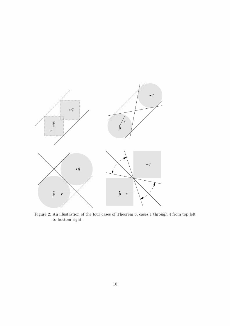
Theorem 6 (Solution count). Let p and q be two distinct points in R2 and r > 0. Letk be a norm on R2.

1. If 2r > k(p− q), there are exactly two lines with p and q at distance r.

2. If 2r < k(p− q), there are exactly four lines with p and q at distance r.

3. If 2r = k(p− q) and k is smooth at p− q, there are exactly three lines with p andq at distance r.

4. If 2r = k(p− q) and k is non-smooth at p− q, there are infinitely many lines withp and q at distance r.

For an illustration of Theorem 6, see Figure 2.

Proof. Given two points p and q, there always exist two lines with p and q at distancer, regardless of k(p− q): both are parallel to the line joining p and q, since

d(p, L) =nT p− ck◦(n)

= r and d(q, L) =nT q − ck◦(n)

= r ⇒ nT (p− q) = 0,

and one is translated such that both p and q lie below it, the other is translated suchthat both p and q lie above it. The amount of translation must be chosen such thatd(p, L) = d(q, L) = r.It is more interesting to analyze if there exist lines L such that p and q lie on differentsides of L. The number of such lines has to be added to each of the four cases stated inthe theorem, namely 0, 2, 1, or infinitely many, as proved below. Together with the twolines with p and q on the same side of L this gives the stated number of lines.If p and q are on different sides of L it holds

d(p, L) =nT p− ck◦(n)

and d(q, L) =c− nT qk◦(n)

after appropriately selecting n. This means that d(p, L) = d(q, L) = r if and only ifnT (p− q)/k◦(n) = 2r. We are hence interested in the solutions of

g(n) :=nT (p− q)k◦(n)

= 2r (11)

and distinguish the following three cases.

9

p

q

rp

q

r

p

q

r p

q

r

Figure 2: An illustration of the four cases of Theorem 6, cases 1 through 4 from top leftto bottom right.

10

1. If k(p − q) < 2r then (11) does not have a solution. Assume it had a solution.Then we get nT (p− q) = 2rk◦(n) > k(p− q)k◦(n) which is a contradiction to theCauchy-Schwarz inequality, Lemma 5.

2. In the case k(p − q) > 2r we construct two solutions each of which determinesa different line. To this end, choose some subgradient v ∈ ∂k(p − q) and choosew ⊥ v as well as u ⊥ (p− q) to define the cones

A :={z ∈ R2 : zT (p− q) ≥ 0, zTw ≥ 0} \ {0} and

B :={z ∈ R2 : zT (p− q) ≥ 0, zTw ≤ 0} \ {0}.

Now u, v ∈ A and −u, v ∈ B (if not, substitute v by −v or w by −w) and itis g(u) = g(−u) = 0. Furthermore, v ∈ ∂k(p − q) (or −v ∈ ∂k(p − q)), hencethe generalized Cauchy-Schwarz inequality vT (p − q) ≤ k◦(v)k(p − q) holds with

equality. This yields g(v) = vT (p−q)k◦(v) = k(p−q). Since A and B are both connected,

for any r satisfying 0 < 2r < k(p − q) there are nA ∈ A and nB ∈ B withg(nA) = g(nB) = 2r by the intermediate value theorem (see e.g. [Fle77, Thm.2.8]). To show that nA and nB determine distinct lines, we have to show thatthere is no λ ∈ R \ {0}, so that nA = λnB. Assume on the contrary that sucha λ exists. If λ > 0, then nA ∈ B and hence in A ∩ B. Since A ∩ B containsonly multiples of v ∈ ∂k(p − q), this leads to g(nA) = k(p − q), again by theequality part of the Cauchy-Schwarz inequality, and thus to a contradiction tog(nA) = 2r < k(p− q). If λ < 0, then nA = λnB /∈ A gives another contradictionand thus we have found two distinct lines with normals nA and nB, respectively.

Now we show that there are not more than two lines having p and q on differentsides and distance r to both of them. Suppose there are three lines L1, L2 and L3.Since they all have the same distance from p and q and also p and q lie on differentsides of each Li, they all intersect in the midpoint x = 1

2(p+ q) of the line segmentjoining p and q. This holds since, w.l.o.g.,

nT p− c = k◦(n)r and c− nT = k◦(n)r ⇒ nT (p− q) = 2rk◦(n).

It follows that

nT(p+ q

2

)= nT

(p+

q − p2

)= nT p− 1

2nT (p− q) = nT p− k◦(n)r = c.

Observe that x cannot be the closest point of any Li to p since otherwise p wouldhave distance k(p− x) > r from each line.

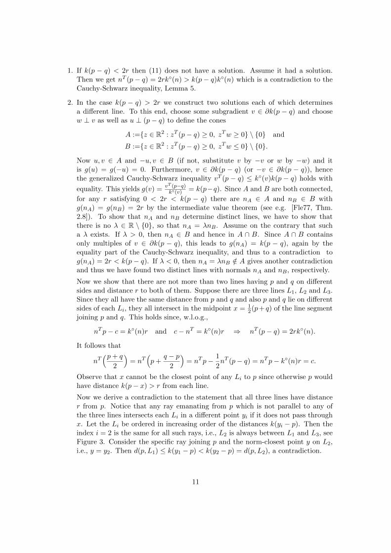
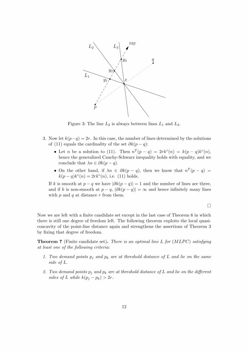
Now we derive a contradiction to the statement that all three lines have distancer from p. Notice that any ray emanating from p which is not parallel to any ofthe three lines intersects each Li in a different point yi if it does not pass throughx. Let the Li be ordered in increasing order of the distances k(yi − p). Then theindex i = 2 is the same for all such rays, i.e., L2 is always between L1 and L3, seeFigure 3. Consider the specific ray joining p and the norm-closest point y on L2,i.e., y = y2. Then d(p, L1) ≤ k(y1 − p) < k(y2 − p) = d(p, L2), a contradiction.

11

L1

L2 L3ray

p

q

xy1

y2

y3

Figure 3: The line L2 is always between lines L1 and L3.

3. Now let k(p−q) = 2r. In this case, the number of lines determined by the solutionsof (11) equals the cardinality of the set ∂k(p− q):• Let n be a solution to (11). Then nT (p − q) = 2rk◦(n) = k(p − q)k◦(n),

hence the generalized Cauchy-Schwarz inequality holds with equality, and weconclude that λn ∈ ∂k(p− q).• On the other hand, if λn ∈ ∂k(p − q), then we know that nT (p − q) =k(p− q)k◦(n) = 2rk◦(n), i.e. (11) holds.

If k is smooth at p− q we have |∂k(p− q)| = 1 and the number of lines are three,and if k is non-smooth at p − q, |∂k(p − q)| = ∞ and hence infinitely many lineswith p and q at distance r from them.

Now we are left with a finite candidate set except in the last case of Theorem 6 in whichthere is still one degree of freedom left. The following theorem exploits the local quasi-concavity of the point-line distance again and strengthens the assertions of Theorem 3by fixing that degree of freedom.

Theorem 7 (Finite candidate set). There is an optimal line L for (MLPC) satisfyingat least one of the following criteria:

1. Two demand points pj and pk are at threshold distance of L and lie on the sameside of L.

2. Two demand points pj and pk are at threshold distance of L and lie on the differentsides of L while k(pj − pk) > 2r.

12

3. Two demand points pj and pk are at threshold distance of L and lie on the differentsides of L while k(pj−pk) = 2r and the normal vector of L is an extremal directionof the cone {λx : x ∈ ∂k(pj − pk), λ ≥ 0}.

This determines a finite candidate set for (MLPC).

Proof. We know from Theorem 3 that there is an optimal solution L that has at leasttwo points, say pj and pk, both at distance r from the line L. If pj and pk are on thesame side of L then the first criterion is fulfilled. If not, then we know k(pj − pk) ≥ 2r,compare the proof of Theorem 6. If in fact k(pj − pk) > 2r holds, the second criterionis fulfilled. Consider now the case k(pj − pk) = 2r.The idea is to construct a solution L′ with an objective not worse than that of L whichfulfills one of the three criteria. To this end perturb L while keeping pj and pk at distancer and on different sides of L as long as the subdifferential ∂k(pj − pk) permits. By ananalogous argument as in the proof of Theorem 3 this is a quasi-concave process (for thedetails see below) as long as no point enters or leaves the coverage zone. This means thatthere are two possibilities to finally fix the line while not deteriorating the objective:

1. a line L′ with at least three demand points at threshold distance, two of thembeing pj and pk

2. a line L′ with pj and pk at threshold distance and an extremal direction of {λx :x ∈ ∂k(pj − pk), λ ≥ 0} as a normal vector.

In the second case obviously L′ satisfies the third criterion. Moreover, there are onlyfinitely many possibilities for L′ since a cone in R2 cannot have more than two extremaldirections.In the first case, it is clear that fixing three points at threshold distance of L′

forces two of them, say pj and pk, to lie on the same side of L′. Since both of them havethe same distance from L′, the first criterion of the theorem is satisfied.

We finally give the details of the quasi-concave process: Consider the objective func-tion of (MLPC) according to (9), but restricted to a feasible region that guarantees

d(pj , Ln,c) = d(pk, Ln,c) = r as well as I+L = I

+Ln,c

and I−L = I

−Ln,c

minn,c

1

k◦(n)

( ∑i∈I+

L

winT pi −

∑i∈I−

L

winT pi + c(W−

L−W+

L)− rk◦(n)(W+

L+W−

L))

(12)

s. t. nT pj = nT pk + 2rk◦(n)

|nT pi − c| ≥ rk◦(n) i ∈ I+L ∪ I

−L

|nT pi − c| ≤ rk◦(n) i ∈ I \ (I+L ∪ I−L ).

Observe that the second constraint is equivalent to two linear constraints, since we haveby the generalized Cauchy-Schwarz inequality [Mic93]

nT pj = nT pk + 2rk◦(n) ⇔ nT (pj − pk) = k(pj − pk)k◦(n)

which is fulfilled if and only if n ∈ {λx : x ∈ ∂k(pj − pk), λ ≥ 0}. Since this is acone in R2 this condition is again equivalent to n ∈ {x : xT v1 ≥ 0 and xT v2 ≥ 0} for

13

some v1, v2 ∈ R2 which are orthogonal to the two extremal directions of that cone. Nowsubstitute these two linear inequalities for the first constraint in (12) and assume that wehave an optimal solution where none of the constraints is fulfilled with equality. Then, bycontinuity, there is a small environment around that solution in the feasible region and,by quasi-concavity, a minimum is also attained at the boundary, where one constraint issatisfied with equality. This corresponds to another point at threshold distance (if oneof the relative position preserving constraints is fulfilled with equality in the minimum)– and thus to an optimal L′ fulfilling the first criterion – or a minimizing n which is anextremal direction of the subdifferential cone (if nT v1 = 0 or nT v2 = 0) – and thus thethird criterion.

Summarizing, we have that there is an optimal solution to (MLPC) which satisfies atleast one of the three stated criteria. From Theorem 6 and this proof we also see thateach criterion is fulfilled by only finitely many lines and thus we have a finite dominatingset.

4 Solution approaches

4.1 Enumeration

Theorem 7 enables us to solve (MLPC) in a straightforward way: for each pair (pj , pk)of demand points, determine the finitely many candidate lines as stated in the threecases of Theorem 7. Their number is two (if k(pj − pk) < 2r), three (if k(pj − pk) = 2rand k is smooth at pj − pk) or four (if k(pj − pk) > 2r or k(pj − pk) = 2r and k isnon-smooth at pj − pk). Then calculate the objective for each candidate line and keepthe one with the smallest value.

Lemma 8. The enumeration approach takes O(n3) time.

Proof. For O(m2) pairs of fixed points, we determine the finitely many candidate linesas stated in the three cases of Theorem 7. This can be done by solving equation (11)(at least numerically) in constant time, i.e., it does not depend on the number of fixedpoints. We then evaluate each candidate line in O(m) time, giving us a total of O(m3)time for the approach.

Since the Euclidean and the Manhattan norm are among the most common norms inlocation problems we exemplarily show in the following how to calculate all candidatepartial coverage lines for two points p and q at distance r from the line. Note that thecalculation of all candidates determined by two points p and q in the case of d = dvercan be easily derived from the argumentation on page 3 preceding Theorem 6.

The Euclidean case We start with the Euclidean norm k2 and p and q on the sameside of the line L = Ln,c which is to be determined. Since L has distance r from both,p and q, it is clear that the normal n of L is perpendicular to p− q. Then the first line

14

with p and q on the same side is determined by c = nT p + rk◦2(n) and the second oneby c = nT p− rk◦2(n). Then d(p, L) = d(q, L) = r. Note that k◦2 = k2.

The case of p and q on different sides of L = Ln,c is slightly more complicated. As in theproof of Theorem 6, n is determined by the equation |nT (p−q)| = 2rk◦2(n) or equivalentlynT (p− q) = 2rk◦2(n) or nT (p− q) = −2rk◦2(n). Letting n = (n1, n2)

T , assuming w.l.o.g.n21 + n22 = 1 and substituting n2 =

√1− n21 this becomes, for σ ∈ {−1, 1},

n1(p1 − q1) +√

1− n21(p2 − q2) = 2rσ

=⇒ n21 · [(p1 − q1)2 + (p2 − q2)2]− n1 · 4rσ(p1 − q1) + 4r2 − (p2 − q2)2 = 0

and the solutions of this quadratic equation are given by

n1 =2rσ(p1 − q1)± (p2 − q2)

√k2(p− q)2 − 4r2

k2(p− q)2. (13)

Note that this has no real root if k2(p− q) < 2r (which corresponds to the first case ofTheorem 6), a double root if k2(p − q) = 2r (third case), and two distinct real roots ifk2(p − q) > 2r (second case). Note that the Euclidean norm is a smooth norm, henceall possible cases are covered. Among the candidate solutions for (13) we pick the onesthat actually satisfy |nT (p− q)| = 2r. Finally, c is determined by the fact that the pointp+q2 is contained in L = Ln,c with d(p, L) = d(q, L) = r and p and q on different sides ofL.

The Manhattan case For the Manhattan norm k1, the case of p and q on the same sideof L = Ln,c is completely analogous to the Euclidean norm. n is again perpendicular top− q and c = nT p± rk◦1(n). Note that k◦1 is the Chebyshev norm.

This means we have to solve

|nT (p− q)| = 2rk◦1(n) = 2rmax{|n1|, |n2|} (14)

in the case of p and q on different sides of L = Ln,c. From (14) we get by assumingk◦1(n) = 1 and p2 − q2 6= 0 w.l.o.g. and with the triangle inequality

|n1(p1 − q1) + n2(p2 − q2)| = 2r =⇒ |p1 − q1|+ |p2 − q2| ≥ 2r

=⇒ |p2 − q2| ≥ 2r − |p1 − q1|.

Thus one can choose n1 ∈ [−1, 1] and n2 ∈ {−1, 1} such that

n2(p2 − q2) = 2r − |p1 − q1| and n2(p2 − q2) = 2r − n1(p1 − q1)

and we have that

|nT (p− q)| = n1(p1 − q1) + n2(p2 − q2) = 2rmax{|n1|, |n2|}

15

i.e., (n1, n2)T is a normal vector of one candidate line. If p1 = q1, the second line is

determined by inverting the sign of n1, if p1 6= q1 the second line is obtained by reversingthe roles of p1 − q1 and p2 − q2. Notice that, in the case p1 = q1 and |p2 − q2| = 2r,which corresponds to the third case in Theorem 6, it holds in fact n2 ∈ {−1, 1} and n1can be chosen arbitrarily in [−1, 1]. As in the Euclidean case, c is obtained readily sincep+q2 ∈ L.

4.2 Sweeping

In order to explore the possibilities of solving (MLPC) faster for arbitrary norms k wepropose an alternative approach based on a plane-sweeping technique for arrangementsof lines by [EW86]. This allows us to efficiently update the objective function, namelyin constant time per candidate line, instead of linear time as in the brute force approachused for enumeration in Section4.1.For the sweeping algorithm we restrict ourselves to non-vertical lines. This is not a severerestriction, since one can, for any norm k, treat the vertical line problem separately asspecial case. This results in a one-dimensional problem. Using that also this problemsatisfies an incidence property, namely, that there is one point at distance r to the verticalline, it can be solved by sorting the fixed points p1, . . . , pn by their x-coordinate and thenevaluate O(m) candidate lines which have at least one of the fixed points at distance r.This can be done in a straight-forward way in O(m2) time or by linear programming inO(m) time.Neglecting the case of a vertical line we can apply a well-known duality transform ∗,mapping non-vertical lines to points in R2 and vice versa, which can be found e. g. in[Mat02]:

L = Ls,b 7→ L∗ = (s,−b), p = (x, y) 7→ p∗ = Lx,−y.

This transform preserves the vertical distance dver(p, L) = dver(L∗, p∗) and above-below

relationships, i. e. p lies above L if and only if L∗ lies above p∗. Hence also the partialcoverage distance D(p, L) = D(L∗, p∗) is preserved in the vertical distance case. Wecall the original space the primal space and the transformed space the dual space. Thehorizontal coordinate of a dual point hence is the slope of the corresponding line inprimal space.By the above considerations of the duality transform, (MLPC) is now to find a dualpoint L∗ which has at least two dual lines p∗i at distance r, a consequence of Theorem 3.We can enumerate all these dual points L∗ satisfying this property by sweeping thearrangement of dual lines p∗1, . . . , p

∗n starting at an arbitrary horizontal coordinate and

sweeping first to the right from that point and then to the left from the same point.During the sweep we calculate the objective values of all candidates and return the bestone in the end.Say we start the sweeping at horizontal coordinate a and sweep to the right. Thesweeping to the left is completely analogous. We determine the best dual point L∗a forthis particular horizontal coordinate a. This means, finding the best intercept for aline with given slope. Since we know that the objective function w.r.t the intercept is

16

piecewise linear and convex (see the proof of Theorem 2) this can be done, e.g. by linearprogramming in O(m) time. If the solution is not unique, we choose it such, that it has atleast one of the dual lines p∗i at distance r. Moreover, we determine the top-down order(1)a, . . . , (m)a of the p∗i at the current horizontal coordinate in the dual space and the

indices i+,ua and i+,la as well as i−,ua and i−,la such that p∗(i+,u

a )ais the first dual line above

L∗ with d(L∗, p∗(i+,u

a )a) ≥ r and p∗

(i+,la )a

the last dual line above L∗ with d(L∗, p∗(i+,l

a )a) ≤ r

The other two indices store the position of the corresponding dual lines below L∗. Thesewill be needed during the sweep to allow for efficient updates of the objective function.Now we have to find the next candidate along the horizontal axis. There are onlythe following possibilities for an event that asks for an action to be performed, whenincreasing the horizontal coordinate from a to A > a. We calculate the horizontalcoordinate A of each possibly next event, but in fact only the one with least A actuallyoccurs.

1. Two lines p∗(i)A and p∗(i+1)Aintersect at A.

2. L∗a has only one of the p∗i , say p∗i0 , at distance r. W.l.o.g. let p∗i0 be below L∗a.Then pi0 is also below L∗A and either

a) L∗A has at least two of the p∗i at distance r, both above L∗A or

b) L∗A has at least two of the p∗i at distance r, one above and one L∗A

3. L∗a has more than one of the p∗i at distance r and either (a) or (b) as above occurat A.

The first case is simple. In order to keep the top-down order updated, we exchange(i+ 1)A := (i)a and (i)A := (i+ 1)a and also adjust i+,uA , i+,lA , i−,uA , and i−,lA if necessary.Consider now the second case. Since L∗a with one dual line p∗i at distance r is optimalfor horizontal coordinate a, L∗A, A > a with the same p∗i at distance r remains optimalas long as none of the above events occur due to Theorem 2, since there is no changein the weights above and below when passing from L∗a to L∗A. Thus we keep increasinga until an event of type 2(a) or 2(b) occurs. A type 2(a) event implies that two of thedual lines p∗i intersect and can be found as a type 1 event. In addition to the actionsperformed, when the event is only of type 1, we also evaluate the objective since theseevents yield candidate solutions for optimality according to Theorem 3. The horizontalcoordinates of possible type 2(b) events can be found in constant time as solutions of

|nT (pj − pi0)| = 2rk◦(n), (15)

for each j ∈ {i+,uA , i+,lA , i−,uA , i−,lA } where n = (A,−1).The third case can be reduced to the second one: if L∗a has more than one dual line atdistance r, one can always tell by the weights of dual lines above and below, respectively,which one of those lines should be kept at distance r when moving on to horizontalcoordinate A and is going to play the role of p∗i0 in the distinction of the possible eventswhen continuing the sweep, compare also Theorem 2. The other dual lines at distancer can be ignored and we are in the second case.

17

Lemma 9. (MLPC) can be solved in O(m2 logm) time with the sweeping approach.

Proof. We first calculate the O(m2) intersection points of the dual lines p∗1, . . . , p∗n and

sort them by their horizontal coordinates in O(m2 logm) time. We then sweep to theright and to the left from an arbitralily chosen horizontal coordinate in the dual space.Each direction of the sweep ends if no further events in the direction of sweeping arefound. It takes only constant time to find the next event and the objective can also beevaluated in constant time, if we keep track of the quantities

X+a :=

i+,ua∑j=1

w(j)a(d(p(j)a , L∗a)− r) and X−a :=

n∑j=i−,l

a

w(j)a(d(p(j)a , L∗a)− r)

which can be viewed as aggregate distances. The objective is then X+a + X−a . If we

can now assure an amount of O(m2) events during the sweep to the left and to theright, this approach has a running time of O(m2 log n), the sorting of the intersectionpoints being the bottleneck. Clearly each pair of points p and q with k(p − q) 6= 2rgives rise to a constant number of events by the first two assertions of Theorem 6. Ifk(p − q) = 2r, it suffices to examine a constant number of solutions in (15) (if there ismore than one at all) by Theorem 7, namely the two solutions (Amin,−1) and (Amax,−1)with minimal and maximal A, respectively. Thus we have O(m2) events in total for bothdirections of the sweep. The correctness of the sweeping algorithm follows directly fromTheorem 7.

4.3 A linear programming formulation

We start by considereing the vertical distance. As used before (see page 3) we mayparametrize L by its slope s and intercept b in this case, since a vertical line can onlybe optimal if all demand points lie on that line.We obtain d(pi, Ls,b) = |pi2 − spi1 − b| for a point pi = (pi1, pi2) ∈ R2 and (MLPC) canbe written as the following linear program

min

m∑i=1

wiDi

s. t. Di ≥ pi2 − spi1 − b− r i = 1, . . . ,m (16)

Di ≥ −pi2 + spi1 + b− r i = 1, . . . ,m (17)

s, b ∈ R, d1, . . . , dm ≥ 0. (18)

In an optimal solution to this program, the variables Di contain the partial coveragedistance of the line Ls,b to point pi. This holds, since (16) and (17) together are equivalentto Di + r ≥ |pi2 − spi1 − b|, and the minimization of the Di ≥ 0 forces them to become

Di = max{0, |pi2 − spi1 − b| − r}.

This linear program is of the form considered in [Zem84] and hence a linear time algo-rithm is available.

18

The case of a block norm distances can be reduced to vertical distance case in thefollowing way. For the point-line distance for a block norm k with fundamental directione1, . . . , eF it holds that

d(p, L) = mink=1,...,F

min{|λ| : p+ λek ∈ L, λ ∈ R

}︸ ︷︷ ︸=:dk(p,L)

,

where the optimal index k∗ in the outer minimization depends only on the slope of L,see [Sch99]. Thus, the objective function becomes

f(s, b) = mink=1,...,F

m∑i=1

[dk(pi, L)− r]+. (19)

Moreover, it holds

dk(p, L) =1

lkdver(Tαk

(p), L) ∀ k = 1, . . . , F

where lk is the Euclidean length of ek and Tαkthe rotation about the origin by αk, the

angle subtended by the positive x-axis and ek. Hence we can solve (MLPC) in the blocknorm case by solving F linear programs of the form

minm∑i=1

wiDi (20)

s. t. Di ≥1

lk(p

(αk)i2 − p(αk)

i1 s− b)− r i = 1, . . . ,m

Di ≥ −1

lk(p

(αk)i2 − p(αk)

i1 s− b)− r i = 1, . . . ,m

s, b ∈ R, d1, . . . , dm ≥ 0

for k = 1, . . . , F , where (p(αk)i1 , p

(αk)i2 ) = Tαk

(pi). According to (19), the linear pro-gram with the minimal objective value among them determines the optimal solution to(MLPC) with block norm k. These considerations hence yield the following result.

Lemma 10. (MLPC) with a block norm k having F fundamental directions can besolved in O(mF ) time by solving F linear programs of the form (20).

The linear porgramming approach is therefore substantially faster then the sweeping inO(m2 logm) time if the number F of fundamental directions is small, e.g. in the case ofManhattan or Chebyshev distances.

5 Conclusion

In this paper we have generalize the classical median line model to a setting with partialcoverage where a demand point sufficiently close to a line, i.e. closer than some fixed

19

threshold distance r, is considered covered. A covered point contributes no cost to theobjective function. Demand points which are not within the threshold distance incur apenalty cost proportional to the distance to the zone covered by the line. The (MLPC)model represents a compromise between the classical median objective and the centerobjective, see Lemma 1: for r = 0 the median model is reproduced and for a certainrmax our problem is equivalent to the center line problem.

To solve the (MLPC) for arbitrary distances induced by a norm we generalized classicalresults for the median model, in particular, we could establish an incidence property inTheorem 3 which led to a finite candidate set (Theorem 7) and allowing to solve theproblem by pure enumeration in O(m3) time. We were able to reduce the enumerationtime by applying plane sweeping techniques in Section 4.2 to O(m2 logm). For thespecial case of block norms and vertical distances, a linear programming formulationwhich has the structure required for the linear time algorithm proposed in [Zem84] canbe found in Section 4.3.

Since another interpretation of the median line problem with partial coverage is thelocation of a median line to approximate norm disks of radius r, an interesting general-ization would be the approximation of norms disks of different radii (or even arbitrarysets). First results can be found in [Sch13].Another obvious extension is the location of a line or hyperplane with partial coverage inhigher dimensions. In the case of block norms an experimental comparison of the sweep-ing approach in Section 4.2 and of the linear programming formulation in Section 4.3would be interesting.

References

[ADSZ88] Mordecai Avriel, Walter E. Diewert, Siegfried Schaible, and Israel Zang. Gen-eralized Concavity, volume 36 of Mathematical Concepts and Methods in Sci-ence and Engineering. Plenum Press, New York, 1988.

[BCSS11] R. Blanquero, E. Carrizosa, A. Schobel, and D. Scholz. Location of a line inthe three-dimensional space. EJOR, pages 14–20, 2011.

[BJKS13] J. Brimberg, H. Juel, M.-C. Korner, and A. Schobel. On models for continuousfacility location with partial coverage. JORS, 2013. to appear.

[BJS02] J. Brimberg, H. Juel, and A. Schobel. Linear facility location in three dimen-sions - models and solution methods. Operations Research, 50(6):1050–1057,2002.

[BJS03] J. Brimberg, H. Juel, and A. Schobel. Properties of 3-dimensional line locationmodels. Annals of Operations Research, 122:71–85, 2003.

[BJS07] J. Brimberg, H. Juel, and A. Schobel. Locating a circle on a sphere. OperationsReserach, 55(4):782–791, 2007.

20

[EW86] H. Edelsbrunner and E. Welzl. Constructing belts in two-dimensional ar-rangements with applications. SIAM J. Comput., 15(1):271–284, 1986.

[Fle77] Wendell Fleming. Functions of Several Variables. Undergraduate Texts inMathematics. Springer, New York, 1977.

[HT88] M.E. Houle and G.T. Toussaint. Computing the width of a set. PatternAnalysis and Machine Intelligence, IEEE Transactions on, 10(5):761–765,1988.

[LC85] D. T. Lee and Y. T. Ching. The power of geometric duality revisited. Infor-mation Processing Letters, 21(3):117 – 122, 1985.

[LMW88] Robert F. Love, James G. Morris, and George O. Wesolowsky. FacilitiesLocation: Models and Methods. North-Holland, 1988.

[Man99] Olvi L. Mangasarian. Arbitrary-norm separating plane. Operations ResearchLetters, 24(1-2):15 – 23, 1999.

[Mat02] Jirı Matousek. Lectures on Discrete Geometry, volume 212 of Graduate Textsin Mathematics. Springer, New York, 2002.

[Mic93] Christian Michelot. The mathematics of continuous location. Studies inLocational Analysis, 5:58–83, 1993.

[MN80] James G. Morris and John P. Norback. A simple approach to linear facilitylocation. Transportation Science, 14(1):1–8, 1980.

[MS98] H. Martini and A. Schobel. Median hyperplanes in normed spaces — a survey.Discrete Applied Mathematics, 89:181–195, 1998.

[MS99] H. Martini and A. Schobel. A characterization of smooth norms. GeometriaeDedicata, 77:173–183, 1999.

[MS01] H. Martini and A. Schobel. Median and center hyperplanes in Minkowskispaces — a unifying approach. Discrete Mathematics, 241:407–426, 2001.

[MT83] Nimrod Megiddo and Arie Tamir. Finding least-distances lines. SIAM J.Algebraic Discrete Methods, 4(2):207–211, 1983.

[PC01] F. Plastria and E. Carrizosa. Gauge distances and median hyperplanes. J.Optim. Theory Appl., 110(1):173–182, 2001.

[RT94] Jean-Marc Robert and Godfried T. Toussaint. Linear approximation of simpleobjects. Computational Geometry, 4(1):27–52, 1994.

[Sch99] A. Schobel. Locating Lines and Hyperplanes — Theory and Algorithms. Num-ber 25 in Applied Optimization Series. Kluwer, 1999.

21

[Sch13] R. Schieweck. Lower bounds for line location problems via demand regions.Preprint 28, Institute for Numerical and Applied Mathematics, University ofGottingen, 2013.

[Zem84] Eitan Zemel. An O(n) algorithm for the linear multiple choice knapsackproblem and related problems. Inform. Process. Lett., 18(3):123–128, 1984.

22

Institut für Numerische und Angewandte MathematikUniversität GöttingenLotzestr. 16-18D - 37083 Göttingen

Telefon: 0551/394512Telefax: 0551/393944

Email: trapp@math.uni-goettingen.de URL: http://www.num.math.uni-goettingen.de

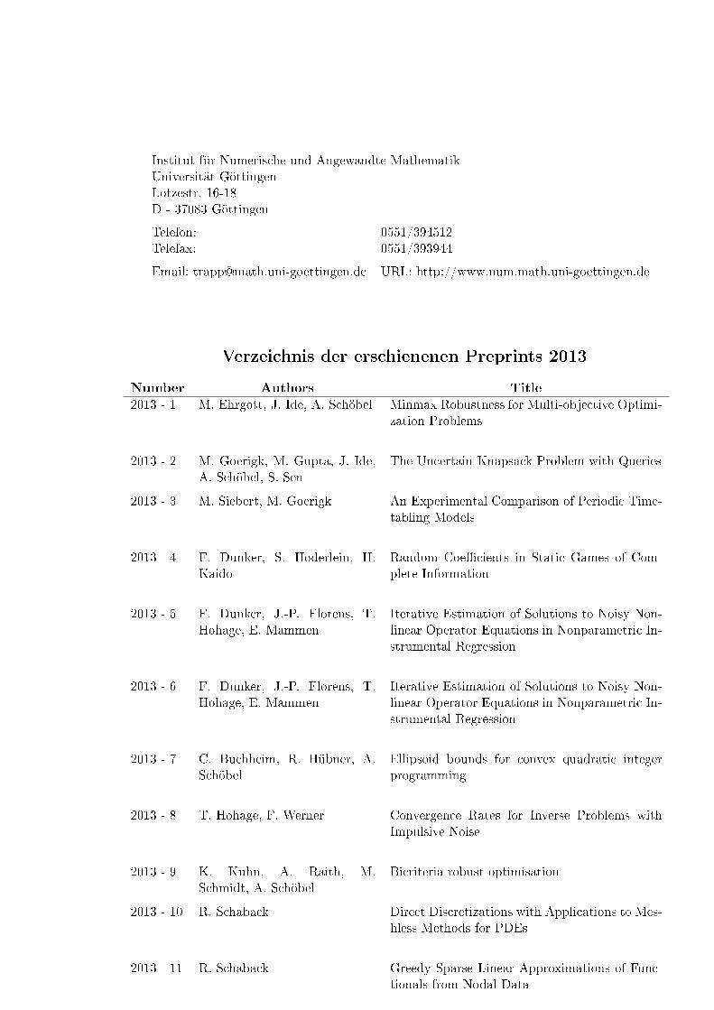
Verzeichnis der erschienenen Preprints 2013

Number Authors Title

2013 - 1 M. Ehrgott, J. Ide, A. Schöbel Minmax Robustness for Multi-objective Optimi-zation Problems

2013 - 2 M. Goerigk, M. Gupta, J. Ide,A. Schöbel, S. Sen

The Uncertain Knapsack Problem with Queries

2013 - 3 M. Siebert, M. Goerigk An Experimental Comparison of Periodic Time-tabling Models

2013 - 4 F. Dunker, S. Hoderlein, H.Kaido

Random Coe�cients in Static Games of Com-plete Information

2013 - 5 F. Dunker, J.-P. Florens, T.Hohage, E. Mammen

Iterative Estimation of Solutions to Noisy Non-linear Operator Equations in Nonparametric In-strumental Regression

2013 - 6 F. Dunker, J.-P. Florens, T.Hohage, E. Mammen

Iterative Estimation of Solutions to Noisy Non-linear Operator Equations in Nonparametric In-strumental Regression

2013 - 7 C. Buchheim, R. Hübner, A.Schöbel

Ellipsoid bounds for convex quadratic integerprogramming

2013 - 8 T. Hohage, F. Werner Convergence Rates for Inverse Problems withImpulsive Noise

2013 - 9 K. Kuhn, A. Raith, M.Schmidt, A. Schöbel

Bicriteria robust optimisation

2013 - 10 R. Schaback Direct Discretizations with Applications to Mes-hless Methods for PDEs

2013 - 11 R. Schaback Greedy Sparse Linear Approximations of Func-tionals from Nodal Data

Number Authors Title

2013 - 12 M. Bozzini, M. Rossini, R.Schaback, E. Volonte

Kernels via Scale Derivatives

2013 - 13 O. Davydov, R. Schaback Error Bounds for Kernel-Based NumericalDi�erentiation

2013 - 14 R. Schaback A computational tool for comparing all linearPDE solvers ( - Error-optimal methods are mes-hless - )

2013 - 15 M. Mohammadi, R. Mokhtari,R. Schaback

Simulating the 2D Brusselator system in repro-ducing kernel Hilbert space

2013 - 16 Y.C. Hon, R. Schaback Direct Meshless Kernel Techniques for Time�Dependent Equations

2013 - 17 Y.C. Hon, M. Zhong, R. Scha-back

The Meshless Kernel-Based Method of Lines forthe Heat Equation

2013 - 18 M. Bozzini. L. Lenarduzzi. M.Rossini, R. Schaback

Interpolation with variably scaled kernels

2013 - 19 T. Hohage, F. Le Louer A spectrally accurate method for the dielectricobstacle scattering problem and applications tothe inverse problem

2013 - 20 T. Hohage, F. Le Louer A spectrally accurate method for the dielectricobstacle scattering problem and applications tothe inverse problem

2013 - 23 M. Schmidt, A. Schöbel Timetabling with Passenger Routing

2013 - 24 J. Ide, E. Köbis Concepts of Robustness for Multi-ObjectiveOptimization Problems based on Set OrderRelations

Number Authors Title

2013 - 25 J. Ide, E. Köbis, D. Kuroiwa, A.Schöbel, C. Tammer

The relation between multicriteria robustnessconcepts and set valued optimization

2013 - 26 J. Ide, M. Tiedemann, S. West-phal, F. Haiduk

An Application of Deterministic and Robust Op-timization in the Wood Cutting Industry

2013 - 27 J. Ide, A. Schöbel Robustness for uncertain multi-objectiveoptimization

2013 - 28 R. Schieweck Lower bounds for line location problems via de-mand regions

2013 - 29 A. Schöbel, S. Schwarze Finding Delay-Resistant Line Concepts using aGame-Theoretic Approach

2013 - 30 M. Goerigk, A. Schöbel Recovery-to-Optimality: A New Two-Stage Ap-proach to Robustness with an Application toAperiodic Timetabling

2013 - 31 M. Goerigk, A. Schöbel Algorithm Engineering in Robust Optimization

2013 - 32 J. Brimberg, R. Schieweck, A.Schöbel

Locating a median line with partial coveragedistance