INSTITUT NATIONAL POLYTECHNIQUE DE TOULOUSE Ecole ... · INSTITUT NATIONAL POLYTECHNIQUE DE TOULOUSE Ecole Nationale Sup erieure d’Electrotechnique, d’Electronique, d’Informatique,

INSTITUT NATIONAL POLYTECHNIQUE DETOULOUSE

Ecole Nationale Superieure d’Electrotechnique,d’Electronique, d’Informatique, d’Hydraulique et de

Telecommunications

TfMin: Short Reference Manual

J. B. Caillau, J. Gergaud and J. Noailles

ENSEEIHT–IRIT, UMR CNRS 5505Parallel Algorithms and Optimization group (APO)

2 rue Camichel, F-31071 Toulousewww.enseeiht.fr/apo

Technical Report RT/APO/01/3

TFMIN – SHORT REFERENCE MANUAL∗

J. B. CAILLAU† , J. GERGAUD† AND J. NOAILLES†

Abstract. This is a short guide to use the Fortran 77 and Matlab package TfMin designed forthe numerical solution of continuous 3D minimum-time orbit transfer around the Earth (with freefinal longitude), especially for low thrust engines. The underlying method is single shooting. TheMatlab interface with the solver allows the user to define the problem and to draw the min-timeorbits computed.

Key words. continuous minimum-time orbit transfer, low-thrust transfer, single shooting,continuation

AMS subject classifications. 49-04, 70Q05

1. Introduction. The 3D minimum time transfer of a satellite around the Earthis considered. The optimal control model given by the French Space Agency is thefollowing (we refer to [3] for details1):

tf → min(x,m) ∈W1,∞

7 ([0, tf ]), u ∈ L∞3 ([0, tf ])x = f0(x) + 1/m

∑3i=1 uifi(x), t ∈ [0, tf ]

m = −β|u|x(0) = x0, m(0) = m0, h(x(tf )) = 0|u| ≤ Tmax

The norms |.| above are Euclidean so that, for instance, the control constraint can berewritten

|u1|2 + |u2|2 + |u3|2 ≤ T 2max

where Tmax is the maximum modulus of the thrust. The state of the satellite isdescribed by the geometry of the ellipse osculating to the trajectory and its positionon it, x = (P, ex, ey, hx, hy, L), and by its mass m. The four vector fields that definethe dynamics are:

f0 =√µ0/P

00000

W 2/P

∗This work was supported in part by the French Ministry for Education, Higher Education and

Research (grant 20INP96) and by the French Space Agency (contracts 871/94/CNES/1454 and86/776/98/CNES/7462).†ENSEEIHT–IRIT, UMR CNRS 5505, 2 rue Camichel, F-31071 Toulouse ([email protected],

[email protected], [email protected]).1The paper is available at the following Web address: www.enseeiht.fr/apo/tfmin

1

2 J. B. CAILLAU, J. GERGAUD AND J. NOAILLES

f1 =√P/µ0

0

sinL− cosL

000

f2 =√P/µ0

2P/W

cosL+ (ex + cosL)/WsinL+ (ey + sinL)/W

000

f3 = 1/W√P/µ0

0−ZeyZex

C/2 cosLC/2 sinL

Z

with

W = 1 + ex cosL+ ey sinLZ = hx sinL− hy cosLC = 1 + h2

x + h2y.

The boundary conditions are given by:

x0 = (P 0, e0x, e

0y, h

0x, h

0y, L

0) ∈ R6

h(x) = (P − P f , ex − efx, ey − efy , hx − hfx, hy − hfy) ∈ R5

and

P 0 = 11625 km P f = 42165 kme0x = 0.75 efx = 0e0y = 0 efy = 0h0x = 0.0612 hfx = 0h0y = 0 hfy = 0L0 = π Lf freem0 = 1500 kg mf free

The two constants β (related to the specific impulsion of the engine) and µ0 (gravi-tation constant of the Earth) are respectively taken equal to:

β = 1.42.10−5 km−1.hµ0 = 398600.47 km3.s−2

The Fortran 77 kernel (see §4) of the software uses two public libraries:• Minpack: the ODE solver RKF45 by H. A. Watts and L. F. Shampine, and

the NLE solver HYBRD by B. S. Garbow, K. E. Hillstrom and J. J. More.

TFMIN: SHORT REFERENCE MANUAL 3

• Adifor [1]: automatic differentiation is called to generate the right hand sideof the boundary value problem.

We are grateful to the authors for making their software available.The document is organised in the following way: the installation procedure of the

package is described in §2; the usage of the Matlab package TfMin and of the underly-ing Fortran 77 solver shoot are detailed in §3 and §4, respectively. Several examplesare provided. The synopses of the Fortran 77 files is finally given in appendix A.

2. Installation. The installation procedure is performed in five steps:1. Retrieve the compressed archive tfmin-v1.zip at the following Web address:

www.enseeiht.fr/apo/tfmin2. Uncompress and unarchive it (unzip tfmin.zip). Check with the readme

file that the contents is correct.3. From the parent directory tfmin-v1, go into the subdirectory src, edit the

appropriate makefile (e.g.: makefile.sol if you are working on a Solarisworkstation), and set the variable LADI properly (for instance by setting theenvironment variables AD LIB and AD OS). If you do not have Adifor (version2.0 or higher), install it first. The package can be downloaded at:

www-unix.mcs.anl.gov/autodiff/ADIFOR4. Go back to the parent directory, and do a make, precising the architecture

(e.g.: make sol if you are on a Solaris workstation; make alone will indicatethe architectures currently supported).

5. Go into the matlab subdirectory, launch Matlab (version 4.0 or higher) andtry the command tfmin. A menu should prompt as below.

>> tfmin

tfmin - Minimum time orbit transfer

1. Create initial data2. Call the solver3. Make graphs and prints4. Demo5. Help

0. Quit

Choice ?

3. Usage of the Matlab package TfMin. The Matlab package TfMin is aninterface for the Fortran 77 code shoot. Though shoot is designed to handle generalboundary value problems by single shooting (see §4), the interface is aimed at solvingthe specific minimum time transfer problem of §1. Roughly, it allows the user to preand postprocess the data for the Fortran 77 code.

Here is a brief review of TfMin’s entries:1. Create initial data. Generates input files for the solver. The user can

specify:• the main physical values, Tmax to hyf.• the initial guesses for the shooting unknowns, zi1 to zi7:

– zi1 is tf (the unknown transfer time)


– zi2 is p0P (value at t = 0 of the costate adjoint to P )

– zi3 is p0ex (value at t = 0 of the costate adjoint to ex)

– zi4 is p0ey (value at t = 0 of the costate adjoint to ey)

– zi5 is p0hx

(value at t = 0 of the costate adjoint to hx)– zi6 is p0

hy(value at t = 0 of the costate adjoint to hy)

– zi7 is p0L (value at t = 0 of the costate adjoint to L)

• the scalings for each component of the state-costate vector y = (x, p)(scalei is the scaling for yi).• the number nint of integration steps for the solution.• the name of the generated input file.

The values in brackets are default values. They correspond to values suitedfor the resolution of the transfer problem with a maximum thrust Tmax of60 Newtons and boundary conditions exactly as in §1. The default name forthe generated file is in.dat.

2. Call the solver. Calls the solver using the indicated files as input/outputfiles.

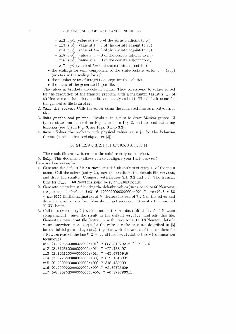
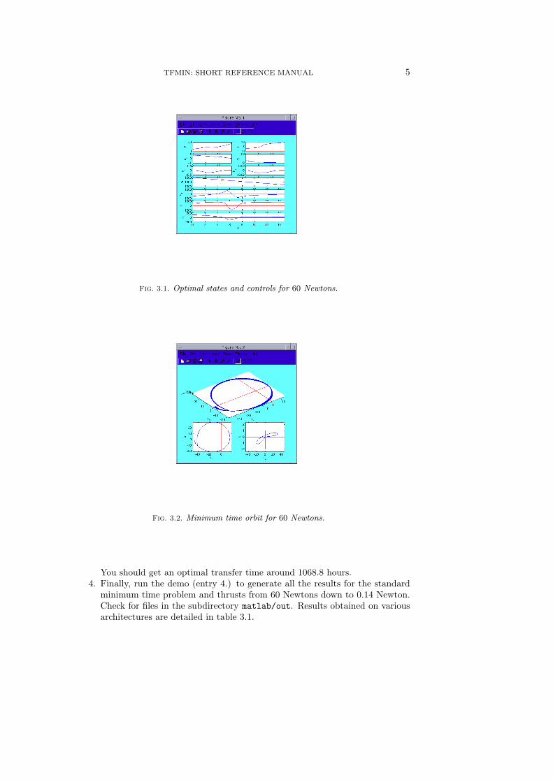
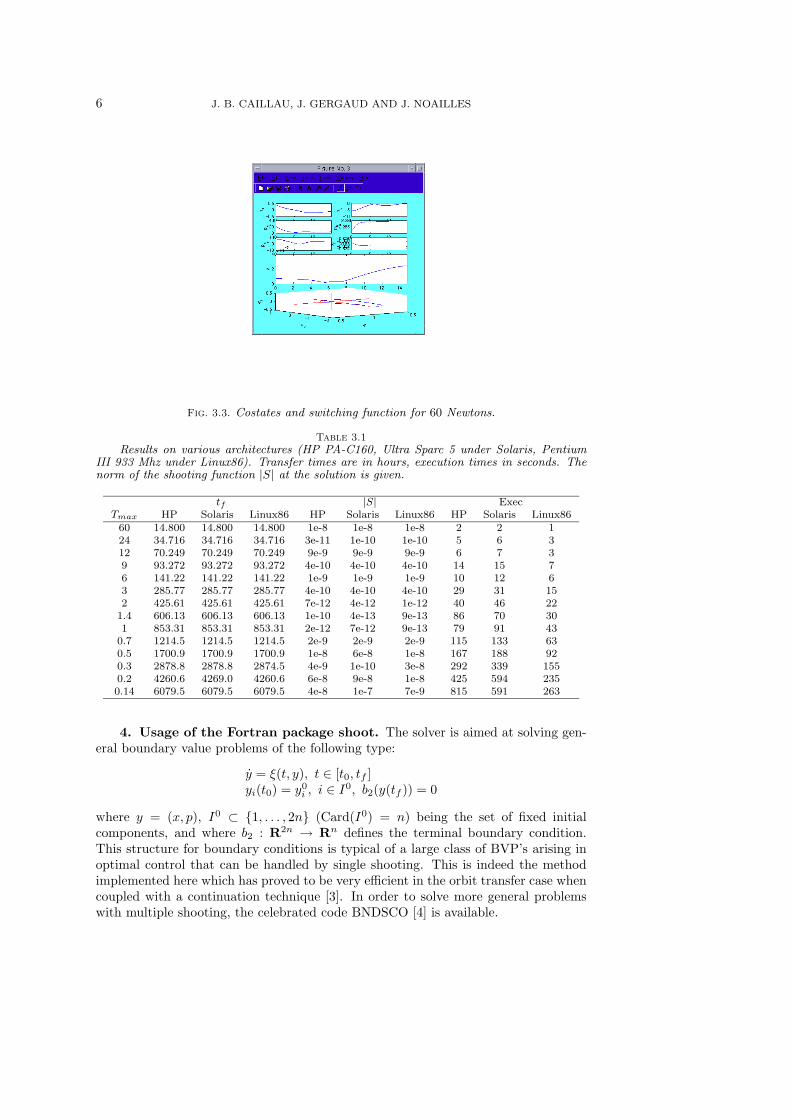
3. Make graphs and prints. Reads output files to draw Matlab graphs (3types: states and controls in Fig. 1, orbit in Fig. 2, costates and switchingfunction (see [3]) in Fig. 3; see Figs. 3.1 to 3.3).

4. Demo. Solves the problem with physical values as in §1 for the followingthrusts (continuation technique, see [3]):

60, 24, 12, 9, 6, 3, 2, 1.4, 1, 0.7, 0.5, 0.3, 0.2, 0.14

The result files are written into the subdirectory matlab/out.5. Help. This document (allows you to configure your PDF browser).

Here are four examples:1. Generate the default file in.dat using defaults values of entry 1. of the main

menu. Call the solver (entry 2.), save the results in the default file out.dat,and draw the results. Compare with figures 3.1, 3.2 and 3.3. The transfertime for Tmax = 60 Newtons sould be tf ' 14.800 hours.

2. Generate a new input file using the defaults values (Tmax equal to 60 Newtons,etc.), except for hx0: do hx0 (6.120000000000000e-02) ? tan(0.5 * 50* pi/180) (initial inclination of 50 degrees instead of 7). Call the solver anddraw the graphs as before. You should get an optimal transfer time around21.331 hours.

3. Call the solver (entry 2.) with input file in/in1.dat (initial data for 1 Newtoncomputation). Save the result in the default out.dat, and edit this file.Generate a new input file (entry 1.) with Tmax equal to 0.8 Newton, defaultvalues anywhere else except for the zi’s: use the heuristic described in [3]for the initial guess of tf (zi1), together with the values of the solutions for1 Newton read on the line # Z =... of the file out.dat as below (continuationtechnique).zi1 (1.520550000000000e+01) ? 853.310792 * (1 / 0.8)zi2 (3.612660000000000e-01) ? -22.153197zi3 (2.224120000000000e+01) ? -43.4710948zi4 (7.877360000000000e+00) ? 0.961318881zi5 (0.000000000000000e+00) ? 318.180099zi6 (0.000000000000000e+00) ? -2.30723609zi7 (-5.908020000000000e+00) ? -0.579786311


Fig. 3.1. Optimal states and controls for 60 Newtons.

Fig. 3.2. Minimum time orbit for 60 Newtons.

You should get an optimal transfer time around 1068.8 hours.4. Finally, run the demo (entry 4.) to generate all the results for the standard

minimum time problem and thrusts from 60 Newtons down to 0.14 Newton.Check for files in the subdirectory matlab/out. Results obtained on variousarchitectures are detailed in table 3.1.


Fig. 3.3. Costates and switching function for 60 Newtons.

Table 3.1

Results on various architectures (HP PA-C160, Ultra Sparc 5 under Solaris, PentiumIII 933 Mhz under Linux86). Transfer times are in hours, execution times in seconds. Thenorm of the shooting function |S| at the solution is given.

tf |S| ExecTmax HP Solaris Linux86 HP Solaris Linux86 HP Solaris Linux86

60 14.800 14.800 14.800 1e-8 1e-8 1e-8 2 2 124 34.716 34.716 34.716 3e-11 1e-10 1e-10 5 6 312 70.249 70.249 70.249 9e-9 9e-9 9e-9 6 7 39 93.272 93.272 93.272 4e-10 4e-10 4e-10 14 15 76 141.22 141.22 141.22 1e-9 1e-9 1e-9 10 12 63 285.77 285.77 285.77 4e-10 4e-10 4e-10 29 31 152 425.61 425.61 425.61 7e-12 4e-12 1e-12 40 46 22

1.4 606.13 606.13 606.13 1e-10 4e-13 9e-13 86 70 301 853.31 853.31 853.31 2e-12 7e-12 9e-13 79 91 43

0.7 1214.5 1214.5 1214.5 2e-9 2e-9 2e-9 115 133 630.5 1700.9 1700.9 1700.9 1e-8 6e-8 1e-8 167 188 920.3 2878.8 2878.8 2874.5 4e-9 1e-10 3e-8 292 339 1550.2 4260.6 4269.0 4260.6 6e-8 9e-8 1e-8 425 594 2350.14 6079.5 6079.5 6079.5 4e-8 1e-7 7e-9 815 591 263

4. Usage of the Fortran package shoot. The solver is aimed at solving gen-eral boundary value problems of the following type:

y = ξ(t, y), t ∈ [t0, tf ]yi(t0) = y0

i , i ∈ I0, b2(y(tf )) = 0

where y = (x, p), I0 ⊂ {1, . . . , 2n} (Card(I0) = n) being the set of fixed initialcomponents, and where b2 : R2n → Rn defines the terminal boundary condition.This structure for boundary conditions is typical of a large class of BVP’s arising inoptimal control that can be handled by single shooting. This is indeed the methodimplemented here which has proved to be very efficient in the orbit transfer case whencoupled with a continuation technique [3]. In order to solve more general problemswith multiple shooting, the celebrated code BNDSCO [4] is available.


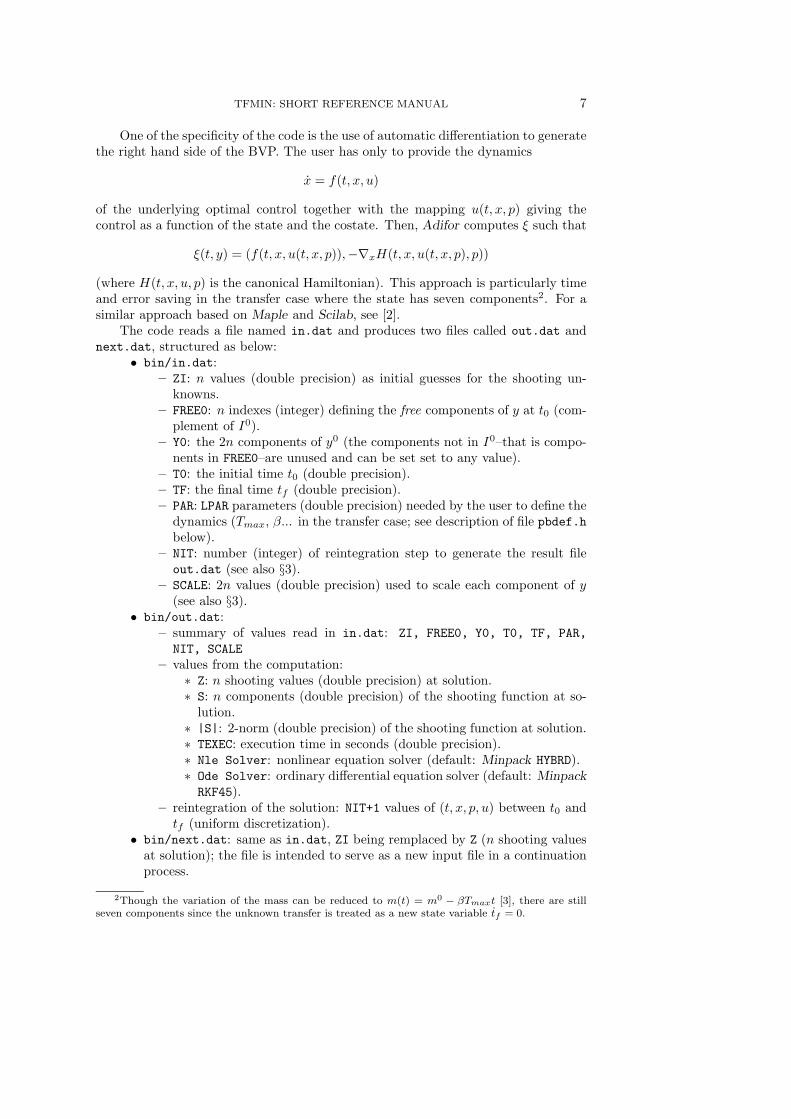
One of the specificity of the code is the use of automatic differentiation to generatethe right hand side of the BVP. The user has only to provide the dynamics

x = f(t, x, u)

of the underlying optimal control together with the mapping u(t, x, p) giving thecontrol as a function of the state and the costate. Then, Adifor computes ξ such that

ξ(t, y) = (f(t, x, u(t, x, p)),−∇xH(t, x, u(t, x, p), p))

(where H(t, x, u, p) is the canonical Hamiltonian). This approach is particularly timeand error saving in the transfer case where the state has seven components2. For asimilar approach based on Maple and Scilab, see [2].

The code reads a file named in.dat and produces two files called out.dat andnext.dat, structured as below:

• bin/in.dat:– ZI: n values (double precision) as initial guesses for the shooting un-

knowns.– FREE0: n indexes (integer) defining the free components of y at t0 (com-

plement of I0).– Y0: the 2n components of y0 (the components not in I0–that is compo-

nents in FREE0–are unused and can be set set to any value).– T0: the initial time t0 (double precision).– TF: the final time tf (double precision).– PAR: LPAR parameters (double precision) needed by the user to define the

dynamics (Tmax, β... in the transfer case; see description of file pbdef.hbelow).

– NIT: number (integer) of reintegration step to generate the result fileout.dat (see also §3).

– SCALE: 2n values (double precision) used to scale each component of y(see also §3).

• bin/out.dat:– summary of values read in in.dat: ZI, FREE0, Y0, T0, TF, PAR,

NIT, SCALE– values from the computation:∗ Z: n shooting values (double precision) at solution.∗ S: n components (double precision) of the shooting function at so-

lution.∗ |S|: 2-norm (double precision) of the shooting function at solution.∗ TEXEC: execution time in seconds (double precision).∗ Nle Solver: nonlinear equation solver (default: Minpack HYBRD).∗ Ode Solver: ordinary differential equation solver (default: MinpackRKF45).

– reintegration of the solution: NIT+1 values of (t, x, p, u) between t0 andtf (uniform discretization).

• bin/next.dat: same as in.dat, ZI being remplaced by Z (n shooting valuesat solution); the file is intended to serve as a new input file in a continuationprocess.

2Though the variation of the mass can be reduced to m(t) = m0 − βTmaxt [3], there are stillseven components since the unknown transfer is treated as a new state variable tf = 0.


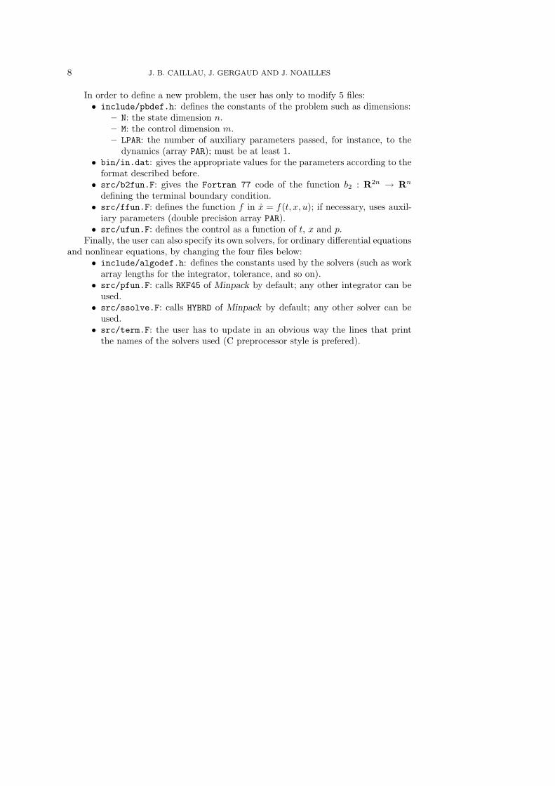
In order to define a new problem, the user has only to modify 5 files:• include/pbdef.h: defines the constants of the problem such as dimensions:

– N: the state dimension n.– M: the control dimension m.– LPAR: the number of auxiliary parameters passed, for instance, to the

dynamics (array PAR); must be at least 1.• bin/in.dat: gives the appropriate values for the parameters according to the

format described before.• src/b2fun.F: gives the Fortran 77 code of the function b2 : R2n → Rn

defining the terminal boundary condition.• src/ffun.F: defines the function f in x = f(t, x, u); if necessary, uses auxil-

iary parameters (double precision array PAR).• src/ufun.F: defines the control as a function of t, x and p.

Finally, the user can also specify its own solvers, for ordinary differential equationsand nonlinear equations, by changing the four files below:

• include/algodef.h: defines the constants used by the solvers (such as workarray lengths for the integrator, tolerance, and so on).• src/pfun.F: calls RKF45 of Minpack by default; any other integrator can be

used.• src/ssolve.F: calls HYBRD of Minpack by default; any other solver can be

used.• src/term.F: the user has to update in an obvious way the lines that print

the names of the solvers used (C preprocessor style is prefered).


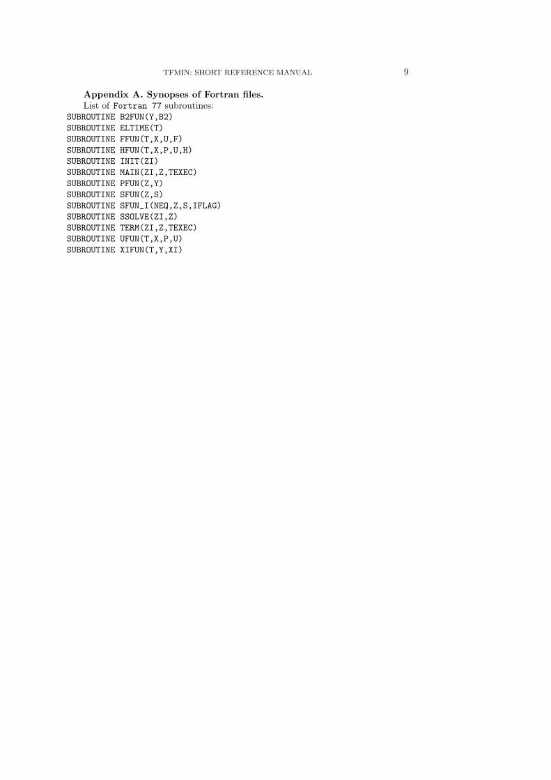
Appendix A. Synopses of Fortran files.List of Fortran 77 subroutines:

SUBROUTINE B2FUN(Y,B2)SUBROUTINE ELTIME(T)SUBROUTINE FFUN(T,X,U,F)SUBROUTINE HFUN(T,X,P,U,H)SUBROUTINE INIT(ZI)SUBROUTINE MAIN(ZI,Z,TEXEC)SUBROUTINE PFUN(Z,Y)SUBROUTINE SFUN(Z,S)SUBROUTINE SFUN_I(NEQ,Z,S,IFLAG)SUBROUTINE SSOLVE(ZI,Z)SUBROUTINE TERM(ZI,Z,TEXEC)SUBROUTINE UFUN(T,X,P,U)SUBROUTINE XIFUN(T,Y,XI)


b2funSUBROUTINE B2FUN(Y,B2)IMPLICIT NONE

C Written on Fri Apr 6 17:30:30 MET DST 2001C by Jean-Baptiste Caillau - ENSEEIHT-IRIT, UMR CNRS 5505CC Function b2 = b2fun(y). Computes the boundary condition (atC final instant) of the BVP. **** Must be set by the user****.C See also FFUN and UFUN.

C .. Global ..#include "pbdef.h"

C .. Arguments ..C Y (input) DOUBLE PRECISION array, dimension 2*NC Flow of BVP at final instantC B2 (output) DOUBLE PRECISION array, dimension NC Boundary condition


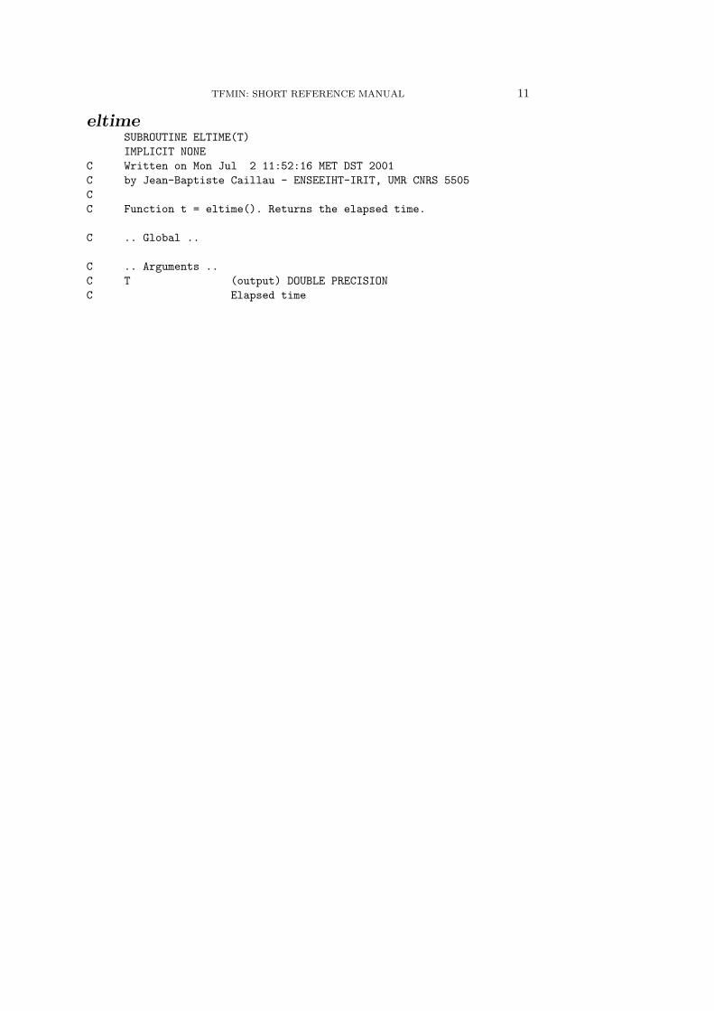
eltimeSUBROUTINE ELTIME(T)IMPLICIT NONE

C Written on Mon Jul 2 11:52:16 MET DST 2001C by Jean-Baptiste Caillau - ENSEEIHT-IRIT, UMR CNRS 5505CC Function t = eltime(). Returns the elapsed time.

C .. Global ..

C .. Arguments ..C T (output) DOUBLE PRECISIONC Elapsed time


ffunSUBROUTINE FFUN(T,X,U,F)IMPLICIT NONE

C Written on Fri Apr 6 17:30:30 MET DST 2001C by Jean-Baptiste Caillau - ENSEEIHT-IRIT, UMR CNRS 5505CC Function y = ffun(t,x,u). Computes the dynamics. **** Must besetC by the user ****. See also UFUN and B2FUN.


C .. Arguments ..C T (input) DOUBLE PRECISIONC TimeC X (input) DOUBLE PRECISION array, dimension NC StateC U (input) DOUBLE PRECISION array, dimension MC ControlC F (output) DOUBLE PRECISION array, dimension NC Second member of the dynamics


hfunSUBROUTINE HFUN(T,X,P,U,H)IMPLICIT NONE

C Written on Fri Apr 6 17:30:30 MET DST 2001C by Jean-Baptiste Caillau - ENSEEIHT-IRIT, UMR CNRS 5505CC Function h = hfun(t,x,p,u). Hamiltonian of the problem.


C .. Arguments ..C T (input) DOUBLE PRECISIONC TimeC X (input) DOUBLE PRECISION array, dimension NC StateC P (input) DOUBLE PRECISION array, dimension NC Adjoint stateC U (input) DOUBLE PRECISION array, dimension MC ControlC H (output) DOUBLE PRECISIONC Hamiltonian


initSUBROUTINE INIT(ZI)IMPLICIT NONE

C Written on Fri Apr 6 17:30:30 MET DST 2001C by Jean-Baptiste Caillau - ENSEEIHT-IRIT, UMR CNRS 5505CC Function zi = init(). Initializes zi and the global variablesC (see pbdef.h and algodef.h). Reads file ./in.dat with theC following format:C ZI FREE0 Y0 T0 TF PAR NIT SCALE


mainSUBROUTINE MAIN(ZI,Z,TEXEC)IMPLICIT NONE

C Written on Fri Apr 6 17:30:30 MET DST 2001C by Jean-Baptiste Caillau - ENSEEIHT-IRIT, UMR CNRS 5505CC Function [z texec] = main(zi). Returns the solution of theC shooting problem together with the elapsed time for itsC computation.


C .. Arguments ..C ZI (input) DOUBLE PRECISION array, dimension NC Initial guess for the shooting unknownC Z (output) DOUBLE PRECISION array, dimension NC Shooting solutionC TEXEC (output) DOUBLE PRECISIONC Execution time


pfunSUBROUTINE PFUN(Z,Y)IMPLICIT NONE

C Written on Fri Apr 6 17:30:30 MET DST 2001C by Jean-Baptiste Caillau - ENSEEIHT-IRIT, UMR CNRS 5505CC Function y = pfun(z). Computes the evaluation at the finalC instant of the maximal flow associated with the BVP for theC initial condition defined by z. See also XIFUN.

C .. Global ..#include "pbdef.h"#include "algodef.h"

C .. Arguments ..C Z (input) DOUBLE PRECISION array, dimension NC Shooting unknownC Y (output) DOUBLE PRECISION array, dimension 2*NC Flow at final instant


sfunSUBROUTINE SFUN(Z,S)IMPLICIT NONE

C Written on Fri Apr 6 17:30:30 MET DST 2001C by Jean-Baptiste Caillau - ENSEEIHT-IRIT, UMR CNRS 5505CC Function s = sfun(z). Computes the shooting function for theC initial condition defined by z. See also PFUN, B2FUN.


C .. Arguments ..C Z (input) DOUBLE PRECISION array, dimension NC Shooting unknownC S (output) DOUBLE PRECISION array, dimension NC Shooting value


sfun iSUBROUTINE SFUN_I(NEQ,Z,S,IFLAG)IMPLICIT NONE

C Written on Fri Apr 6 17:30:30 MET DST 2001C by Jean-Baptiste Caillau - ENSEEIHT-IRIT, UMR CNRS 5505CC Function [s iflag] = sfun_i(neq,z,iflag). Interface for SFUNC used by the NLE solver. See also SFUN.


C .. Arguments ..C NEQ (input) INTEGERC Number of equationsC Z (input) DOUBLE PRECISION array, dimension NC Shooting unknownC S (output) DOUBLE PRECISION array, dimension NC Shooting valueC IFLAG (input/output) INTEGERC Flag from the NLE solver


ssolveSUBROUTINE SSOLVE(ZI,Z)IMPLICIT NONE

C Written on Fri Apr 6 17:30:30 MET DST 2001C by Jean-Baptiste Caillau - ENSEEIHT-IRIT, UMR CNRS 5505CC Function z = ssolve(z_i). Solves the shooting equationC S(z) = 0 with initial guess z_i.


C .. Arguments ..C ZI (input) DOUBLE PRECISION array, dimension NC Initial guess for zC Z (output) DOUBLE PRECISION array, dimension NC Shooting solution


termSUBROUTINE TERM(ZI,Z,TEXEC)IMPLICIT NONE

C Written on Fri Apr 6 17:30:30 MET DST 2001C by Jean-Baptiste Caillau - ENSEEIHT-IRIT, UMR CNRS 5505CC Function term(zi,z,texec). Writes the result into the filesC ./out.dat and ./next.dat (same format as in.dat). ./out.datC contains all the information required to reproduce theC computation plus an evaluation of T, Y, U (solution) at NITC steps.


C .. Arguments ..C ZI (input) DOUBLE PRECISION array, dimension NC Initial guess for the shooting unknownC Z (input) DOUBLE PRECISION array, dimension NC Shooting solutionC TEXEC (input) DOUBLE PRECISIONC Execution time


ufunSUBROUTINE UFUN(T,X,P,U)IMPLICIT NONE

C Written on Fri Apr 6 17:30:30 MET DST 2001C by Jean-Baptiste Caillau - ENSEEIHT-IRIT, UMR CNRS 5505CC Function u = u(t,x,p). Computes the control as a function of t,xC and p (maximum principle). **** Must be set by the user ****.C See also FFUN, B2FUN.


C .. Arguments ..C T (input) DOUBLE PRECISIONC TimeC X (input) DOUBLE PRECISION array, dimension NC StateC P (input) DOUBLE PRECISION array, dimension NC Adjoint stateC U (output) DOUBLE PRECISION array, dimension MC Control


xifunSUBROUTINE XIFUN(T,Y,XI)IMPLICIT NONE

C Written on Fri Apr 6 17:30:30 MET DST 2001C by Jean-Baptiste Caillau - ENSEEIHT-IRIT, UMR CNRS 5505CC Function xi = xifun(t,y). Defines the second member \xi(t,y) ofC the BVP by automatic differentiation. See also FFUN, UFUN andC HFUN.


C .. Arguments ..C T (input) DOUBLE PRECISIONC TimeC Y (input) DOUBLE PRECISION array, dimension 2*NC State and adjoint stateC XI (output) DOUBLE PRECISION array, dimension 2*NC Second member of the BVP


REFERENCES

[1] C. Bischof, A. Carle, P. Kladem, and A. Mauer, Adifor 2.0: Automatic Differentiation ofFortran 77 Programs, IEEE Computational Science and Engineering, 3 (1996), pp. 18–32.

[2] F. Bonnans and S. Maurin, An implementation of the shooting algorithm for solving optimalcontrol problems, report 0240, INRIA, Rocquencourt, France, May 2000.

[3] J. B. Caillau, J. Gergaud, and J. Noailles, 3D Geosynchronous Transfer of a Satellite:Continuation on the Thrust, Submitted to Journal of Optimization Theory and Applications,(2001).

[4] H. J. Oberle and W. Grimm, BNDSCO: A Program for the Numerical Solution of OptimalControl Problems, report 515, Institute for Flight Systems Dynamics, German AerospaceResearch Establishment DLR, Oberpfaffenhofen, Germany, 1989.

Documents

INSTITUT NATIONAL POLYTECHNIQUE DE TOULOUSE Ecole ... · INSTITUT NATIONAL POLYTECHNIQUE DE TOULOUSE Ecole Nationale Sup erieure d’Electrotechnique, d’Electronique, d’Informatique,